Annex to EQ3 rev 23-4-08 - European...

Agrosynergie Groupement Européen d’Intérêt Economique

Framework contract no 30-CE-0035027/00-37

Evaluations fruit and vegetables

Evaluation of the system of entry prices and export refunds in the fruit and vegetables sector

Annexes to EQ3

April 2008

1

LE GEIE AGROSYNERGIE EST CONSTITUE PAR LES SOCIETES

COGEA S.p.A

Via Po 9 - 00198 Roma ITALIE

Tél. : + 39 6 853 73 51 Fax : + 39 6 855 78 65

Mail : [email protected]

Représenté par Massimo Ciarrocca

OREADE–BRECHE Sarl 64 chemin del prat - 31320 Auzeville FRANCE

Tél. : + 33 5 61 73 62 62 Fax : + 33 5 61 73 62 90

Mail : [email protected]

Représentée par Thierry Clément

2

Table of contents

1. ANNEXES TO THE EVALUATION QUESTION 3 ............................................................................... 3

1.1 Annex to EQ 3 – Import growth ........................................................................................................... 3

1.2 Annex to EQ 3 – Monthly imports 1995-2001 ..................................................................................... 6

1.3 Annex to EQ 3 – Monthly imports 2002-2006 ................................................................................... 12

1.4 Annex to EQ 3 – Methodology of Gravity Model .............................................................................. 18

1.5 Annex to EQ 3 – Gravity Flows ........................................................................................................ 20

1.6 Annex to EQ 3 – Value and volume of imports growth..................................................................... 23

1.6.1 Tables based on COMTRADE database .................................................................................... 23

1.6.2 Tables based on COMEXT database ......................................................................................... 26

1.7 Annex to EQ 3 – Analysis of Preferences ......................................................................................... 28

1.8 Annex to EQ 3 – Seasonal value of Preferences................................................................................ 35

1.9 Annex to EQ 3 – The Trade Model ................................................................................................... 39

1.9.1 The Export Model ...................................................................................................................... 43

1.9.2 The Import Model ...................................................................................................................... 49

1.10 Annex to EQ 3 – Export growth ........................................................................................................ 61

1.11 Annex to EQ 3 – Export Refunds ...................................................................................................... 64

3

1. ANNEXES TO THE EVALUATION QUESTION 3

1.1 Annex to EQ 3 – Import growth

Tab. 1 - Percentage changes between average import volumes 1992/94 and 1995/97

Tomato Turkey Morocco Israel Extra EU

1 November to 14 May 7020010 26 -3 46 -1

15 May to 31 October 7020090 -73 2 161 -22

Onion Chile Australia New Zealand Extra EU

7031019 93 -19 41 18

Cucumber Turkey Hungary Romania Extra EU

7070005 -31 -43 1 -28

Beans Morocco Egypt Kenya Extra EU

1 October to 30 June 7082010 42 8 18 39

1 July to 30 September 7082090 42 46

Artichoke Egypt Extra EU

70910 -8 -18

Asparagus South Africa USA Chile Extra EU

7092000 76 -21 -18 39

Sweet peppers Turkey Hungary Israel Extra EU

7096010 26 -14 201 19

Courgettes Morocco Kenya USA Extra EU

70990 13 42 21 43

Oranges Brazil Morocco South Africa Extra EU

80510 0 -9 23 7

Grapefruit South Africa USA Israel Extra EU

80540 11 32 17 12

Table grapes South Africa Chile Turkey Extra EU

1 November to 14 July 8061015 23 -1 15

15 July to 31 October 8061019 165 61

Melons Brazil Israel Extra EU

8071090 -10 12 20

Apple (*) South Africa USA Chile Extra EU

Golden 1 January to 31 March 8081051 -49 -27

Granny 1 January to 31 March 8081053 -35 -29

Other Apples 1 January to 31 March 8081059 101 27

Golden 1 April to 31 July 8081081 19 156

Granny 1 April to 31 July 8081083 -10 35 5

New Zealand Chile Extra EU

Other Apples 1 April to 31 July 8081089 130 82 97

Golden 1 August to 31 December 8081031 -11 -13

Granny 1 August to 31 December 8081033 -9 -48

Other Apples 1 August to 31 December 8081039 -1 41

Pears South Africa Chile Argentina Extra EU

1 January to 31 March 8082031 -26 9 3 -3

1 April to 15 July 8082033 3 12 27 2

16 July to 31 July 8082035 122 159

1 Aug - 31 Dec 8082039 -75 50

Strawberries Morocco USA Extra EU

1 May to 31 July 8101010 -56 40 14

1 August to 30 April 8101090 37 -30 -7

Kiwifruit Chile New Zealand Extra EU

8105000 13 16 15

Clementines 80520 Morocco Extra EU

-18 -28

Source: COMEXT. Processed by Agrosynergie

Note: (*) Values for the initial period correspond to 1993 and 1994 for which COMEXT data (for 1992 no distinction between

varieties is offered in COMEXT)

6

1.2 Annex to EQ 3 – Monthly imports 1995-2001

Index of EU imports of selected F&V from major partners.

Remarks:

The following tables show “Indices” of EU imports from selected partners.

The index is given by the vertical axis values and they are indicated by the ratio Xt/X1995

expressed in %, where Xt is the import volume in month “t” and X1995 is the average of monthly

imports in 1995, counting just the months when imports are not zero.

Consequently, Index 100 = Average of monthly imports for 1995.

The horizontal axis show the monthly period from January 1995 to December 2001.

We also include in the graphs the MFN levels of entry prices in Euro/T

(see legends at the bottom of each graph).

Sources: TARIC and COMEXT data base. Processed by Agrosynergie.

7

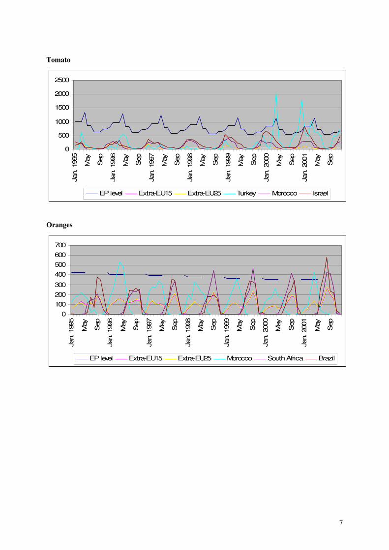
Tomato

0

500

1000

1500

2000

2500Jan. 1995

May

Sep

Jan. 1996

May

Sep

Jan. 1997

May

Sep

Jan. 1998

May

Sep

Jan. 1999

May

Sep

Jan. 2000

May

Sep

Jan. 2001

May

Sep

EP level Extra-EU15 Extra-EU25 Turkey Morocco Israel

Oranges

0

100

200

300

400

500

600

700

Jan. 1995

May

Sep

Jan. 1996

May

Sep

Jan. 1997

May

Sep

Jan. 1998

May

Sep

Jan. 1999

May

Sep

Jan. 2000

May

Sep

Jan. 2001

May

Sep

EP level Extra-EU15 Extra-EU25 Morocco South Africa Brazil

8

Courgettes

0

200400

600

8001000

1200

14001600

1800

Jan. 1995

May

Sep

Jan. 1996

May

Sep

Jan. 1997

May

Sep

Jan. 1998

May

Sep

Jan. 1999

May

Sep

Jan. 2000

May

Sep

Jan. 2001

May

Sep

EP level Extra-EU15 Extra-EU25 Morocco

Clementines

0

100200

300

400500

600

700800

900

Jan. 1995

May

Sep

Jan. 1996

May

Sep

Jan. 1997

May

Sep

Jan. 1998

May

Sep

Jan. 1999

May

Sep

Jan. 2000

May

Sep

Jan. 2001

May

Sep


Pears

0

100200

300

400500

600

700800

900

Jan. 1995

May

Sep

Jan. 1996

May

Sep

Jan. 1997

May

Sep

Jan. 1998

May

Sep

Jan. 1999

May

Sep

Jan. 2000

May

Sep

Jan. 2001

May

Sep

EP level Extra-EU15 Extra-EU25 South Africa Chile Argentina

9

Apples

0100200300400500600700800

Jan. 1995

May

Sep

Jan. 1996

May

Sep

Jan. 1997

May

Sep

Jan. 1998

May

Sep

Jan. 1999

May

Sep

Jan. 2000

May

Sep

Jan. 2001

May

Sep

EP level Extra-EU15 Extra-EU25 South Africa

USA Chile New Zealand

Cucumbers

0

200

400

600

800

1000

1200

1400

Jan. 1995

May

Sep

Jan. 1996

May

Sep

Jan. 1997

May

Sep

Jan. 1998

May

Sep

Jan. 1999

May

Sep

Jan. 2000

May

Sep

Jan. 2001

May

Sep

EP level Extra-EU15 Extra-EU25 Turkey Hungary Romania Bulgaria

Table grapes

0

200

400

600

800

1000

1200

Jan. 1995

Jun

Nov

Apr

Sep

Feb

Jul

Dec

May

Oct

:Mar

Aug

Jan. 2000

Jun

Nov

Apr

Sep

EP level

Extra-EU15

Extra-EU25

Turkey

South Africa

Chile

10

Artichokes

0

200

400

600

800

1000

1200

Jan. 1995

May

Sep

Jan. 1996

May

Sep

Jan. 1997

May

Sep

Jan. 1998

May

Sep

Jan. 1999

May

Sep

Jan. 2000

May

Sep

Jan. 2001

May

Sep

EP level Extra-EU15 Extra-EU25 Egypt

Onions

050

100150200250300350400450500

Jan. 1995

May

Sep

Jan. 1996

May

Sep

Jan. 1997

May

Sep

Jan. 1998

May

Sep

Jan. 1999

May

Sep

Jan. 2000

May

Sep

Jan. 2001

May

Sep

AUSTRALIA CHILE Extra-EU15 Extra-EU25 New Zealand

Asparagus

050

100150200250300350400450500

Jan. 1995

May

Sep

Jan. 1996

May

Sep

Jan. 1997

May

Sep

Jan. 1998

May

Sep

Jan. 1999

May

Sep

Jan. 2000

May

Sep

Jan. 2001

May

Sep

CHILE Extra-EU15 Extra-EU25 UNITED STATES South Africa

11

Sweet Peppers

0

100

200

300

400

500

600

Jan. 1995

May

Sep

Jan. 1996

May

Sep

Jan. 1997

May

Sep

Jan. 1998

May

Sep

Jan. 1999

May

Sep

Jan. 2000

May

Sep

Jan. 2001

May

Sep

Extra-EU15 Extra-EU25 HUNGARY TURKEY

Melons

0

100

200

300

400

500

600

Jan. 1995

May

Sep

Jan. 1996

May

Sep

Jan. 1997

May

Sep

Jan. 1998

May

Sep

Jan. 1999

May

Sep

Jan. 2000

May

Sep

Jan. 2001

May

Sep

BRAZIL Extra-EU15 Extra-EU25 Israel

Kiwifruit

0

100

200

300

400

500

600

700

800

Jan. 199

5

:Mar

May Ju

lSep N

ov

Jan. 199

6

:Mar

May Ju

lSep N

ov

CHILE

Extra-EU15

Extra-EU25

New Zealand

12

1.3 Annex to EQ 3 – Monthly imports 2002-2006

Index of EU imports of selected F&V from major partners.

Remarks:

The following tables show “Indices” of EU imports from given partners.

The index is given by the vertical axis values and they are indicated by the ratio Xt/X2001

expressed in %, where Xt is the import volume in month “t” and X2001 is the average of monthly

imports in 2001, counting just the months when imports are not zero.

Consequently, Index 100 = Average of monthly imports for 2001.

We also include in the graphs the MFN levels of entry prices in Euro/T (see legends at the

bottom of each graph).

Sources: TARIC and COMEXT. Processed by Agrosynergie.

Tomato

0

200

400

600

800

1000

1200

Jan. 2002

Apr

Jul

Oct

Jan. 2003

Apr

Jul

Oct

Jan. 2004

Apr

Jul

Oct

Jan. 2005

Apr

Jul

Oct

Jan. 2006

Apr

Jul

Oct

EP MFN Extra-EU15 Extra-EU25 Turkey Morocco Israel

13

Oranges

0

50

100

150

200

250

300

350

400

Jan. 2002

Apr

Jul

Oct

Jan. 2003

Apr

Jul

Oct

Jan. 2004

Apr

Jul

Oct

Jan. 2005

Apr

Jul

Oct

Jan. 2006

Apr

Jul

Oct

EP level Extra-EU15 Extra-EU25 Morocco South Africa Brazil

Courgettes

0

100200

300400

500600

700800

900

Jan. 2002

Apr

Jul

Oct

Jan. 2003

Apr

Jul

Oct

Jan. 2004

Apr

Jul

Oct

Jan. 2005

Apr

Jul

Oct

Jan. 2006

Apr

Jul

Oct


Clementines

0

100

200

300

400

500

600

700

Jan. 2002

Apr

Jul

Oct

Jan. 2003

Apr

Jul

Oct

Jan. 2004

Apr

Jul

Oct

Jan. 2005

Apr

Jul

Oct

Jan. 2006

Apr

Jul

Oct


14

Pears

0

100

200

300

400

500

600

700

800

Jan. 2002

Apr

Jul

Oct

Jan. 2003

Apr

Jul

Oct

Jan. 2004

Apr

Jul

Oct

Jan. 2005

Apr

Jul

Oct

Jan. 2006

Apr

Jul

Oct

EP level Extra-EU15 Extra-EU25 South Africa Chile Argentina

Apples

0

100

200

300

400

500

600

Jan. 2002

Apr

Jul

Oct

Jan. 2003

Apr

Jul

Oct

Jan. 2004

Apr

Jul

Oct

Jan. 2005

Apr

Jul

Oct

Jan. 2006

Apr

Jul

Oct

EP level Extra-EU15 Extra-EU25 South Africa

USA Chile New Zealand

Cucumbers

0

200

400

600

800

1000

1200

Jan. 2002

Apr

Jul

Oct

Jan. 2003

Apr

Jul

Oct

Jan. 2004

Apr

Jul

Oct

Jan. 2005

Apr

Jul

Oct

Jan. 2006

Apr

Jul

Oct

EP level Extra-EU15 Extra-EU25 Turkey Romania Bulgaria

15

Table grapes

0

100

200

300

400

500

600

700

800

Jan. 2002

Apr

Jul

Oct

Jan. 2003

Apr

Jul

Oct

Jan. 2004

Apr

Jul

Oct

Jan. 2005

Apr

Jul

Oct

Jan. 2006

Apr

Jul

Oct

EP level Extra-EU15 Extra-EU25 Turkey South Africa Chile

Artichokes

0100020003000400050006000700080009000

10000

Jan. 2002

Apr

Jul

Oct

Jan. 2003

Apr

Jul

Oct

Jan. 2004

Apr

Jul

Oct

Jan. 2005

Apr

Jul

Oct

Jan. 2006

Apr

Jul

Oct

EP level Extra-EU15 Extra-EU25 Egypt

Onions

0

100200

300400

500600

700800

900

Jan. 2002

Apr

Jul

Oct

Jan. 2003

Apr

Jul

Oct

Jan. 2004

Apr

Jul

Oct

Jan. 2005

Apr

Jul

Oct

Jan. 2006

Apr

Jul

Oct

AUSTRALIA CHILE Extra-EU15 Extra-EU25 New Zealand

16

Asparagus

0

100

200

300

400

500

600

700

Jan. 2002

May

Sep

Jan. 2003

May

Sep

Jan. 2004

May

Sep

Jan. 2005

May

Sep

Jan. 2006

May

Sep

CHILE

Extra-EU15

Extra-EU25

UNITED STATES

South Africa

Sweet Peppers

0

100

200

300

400

500

600

Jan. 2002

Apr

Jul

Oct

Jan. 2003

Apr

Jul

Oct

Jan. 2004

Apr

Jul

Oct

Jan. 2005

Apr

Jul

Oct

Jan. 2006

Apr

Jul

Oct

Extra-EU15 Extra-EU25 HUNGARY TURKEY

Melons

0

50100

150200

250300

350400

450

Jan. 2002

Apr

Jul

Oct

Jan. 2003

Apr

Jul

Oct

Jan. 2004

Apr

Jul

Oct

Jan. 2005

Apr

Jul

Oct

Jan. 2006

Apr

Jul

Oct

BRAZIL Extra-EU15 Extra-EU25 Israel

17

Strawberries

0

1000

2000

3000

4000

5000

6000Jan. 2002

Apr

Jul

Oct

Jan. 2003

Apr

Jul

Oct

Jan. 2004

Apr

Jul

Oct

Jan. 2005

Apr

Jul

Oct

Jan. 2006

Apr

Jul

Oct

Extra-EU15 Extra-EU25 Israel MOROCCO UNITED STATES

Kiwifruit

0

100200

300400

500600

700800

900

Jan. 2002

Apr

Jul

Oct

Jan. 2003

Apr

Jul

Oct

Jan. 2004

Apr

Jul

Oct

Jan. 2005

Apr

Jul

Oct

Jan. 2006

Apr

Jul

Oct

CHILE Extra-EU15 Extra-EU25 New Zealand

18

1.4 Annex to EQ 3 – Methodology of Gravity Model

The econometric modeling

In its most basic application, the gravity model of international trade posits that the level of

imports to one country from another is a function of each country’s gross domestic product

(GDP) and its population, as well as the distance between the two countries. Additional

explanatory variables can indicate a country’s membership in a specific trade agreement or

trade bloc. The model proponed is a modified version of the Standard gravity that will include

two sets of fixed effects (variables with the value of one or zero) that respectively identify

specific importing countries and specific seasons (peak season and off-season periods). A

fixed effect for the entry price will control the effect of the system. The trade-agreement

variables are country-specific in order to address the possibility that the impact of an

agreement varies among its participants.

The products chosen for the analysis are:…. - the 8 products listed in Tab. 1 (Chapter 4 in the report) with EP (tomatoes, artichokes,

cucumbers, courgettes, oranges, , apples, pears, table grapes ). We also considered clementines

because of their relevance as a fruit imported from preferential partners.

- the 8 products listed in Errore. L'origine riferimento non è stata trovata. (Chapter 4 in the

report) without EP (onion, beans, asparagus, sweet peppers, grapefruits, melons, strawberries,

kiwifruit).

Import changes will be assessed in relative terms by calculating the average values for 1993-94, 1995-

96, 2001-02 and 2005-2006. The model proposed is simpler than most gravity equations used to

capture the forces that either attract or inhibit bilateral trade. The equations proposed take the

following form:

∆ Ln Xijkt= β0+ β1 ln (D1) + β2 ln(Di) +β3 ln(Dj) + β4 ln(Dk) + β5 ln(D2) + β6 ln(D1 Di) + β7 ∆ ln(Yj) +β8 ∆

ln(Y) + uijt

[1]

Where,

Xij: is the bilateral exports from country i to country j in period t.

Yjt: is the GDP of the main exporting countries (j) in time t.

Y is the EU’s GDP in time t

D1: is a dummy variable for capturing the existence of entry prices.

D2: is a dummy variable for capturing the existence of “reduced” entry prices (preferential

imports).

Di: is a vector of dummy variables for each product “i” including those not subjected to the

entry price system.

Di: is a vector of dummy variables for each origin “j” including those not subjected to the

entry price system.

Dk: is a vector of dummy variables for each month, grouping the products in four or five

categories according to their pattern of intra-EU monthly supply.

19

D1 Di is a vector of multiplicative dummy variables for taking into account the impact of the

entry price system applied to specific products.

For treating specific sectors, such as F&V, and bilateral agreements, the interpretation of models like

the presented above needs some note of caution. The model approach ignores the explicit assessment

of specific policy instruments unless applied tariffs in the EU are included in the RHS of the equation.

However, the model must provide for an ex post test of statistical significance of a simple question.

The effect of the entry prices on imports can be studied from the significance of the coefficients of the

binary variables.

The model assesses the import change between a couple of years (for example between 1993/94 and

1995/96) by specifying regression equations as follows:

Gravity model specification

∆ Denotes changes between period "x" and period "y"

Dependent variable: ∆ Log of imports from country “i” to EU15 (in tons)

Explanatory variables:

Intercept

∆ Log of GDP of country i

∆ Log of GDP per capita of country i

∆ Log of domestic production of commodity j for country i (in tons)

∆ Log of EU production of commodity j (in tons)

Trade-agreement variables – dummy variables that identify

country i’s participation in a particular trade agreement in year t

Egypt: Equals one for imports from Egypt for comparisons 2000-2001 to 2005-2006 and zero otherwise

Israel: Equals one for imports from Israel for comparisons 1995-96 to 2000-01, 2000-01 to 2005-06 and zero otherwise

Chile: Equals one for imports from Chile for comparisons 2000-2001 to 2005-2006 and zero otherwise

Morocco: Equals to one for imports from Morocco for comparisons 1995-96 to 2000-01, 2000-01 to 2005-06 and zero

otherwise

South Africa: Equals one for imports from South Africa for comparisons 2000-2001 to 2005-2006 and zero otherwise

Fixed effects denoting entry price

The fixed effect for EP equals one if the commodity has entry price and zero otherwise

Fixed effects denoting neighbouring countries

The fixed effect for neighbouring country equals one if the partner country is neighbour to EU15, and zero otherwise

For example, the dummy variables equal one for Bulgaria, Egypt, Hungary, Israel, Morocco, Romania and Turkey.

20

1.5

Annex to EQ 3 – Gravity Flows

Tab

. 1 E

xis

ten

ce o

f n

on

-zer

o i

mp

ort

flo

ws

of

fres

h F

&V

in

th

e E

U15 (

*)

Pro

du

cts

AR

AU

BG

BR

CL

CN

CR

EG

HU

ILK

EM

ON

ZP

AR

OS

NT

RU

SU

YZ

AN

º fl

ow

s

Tom

ato

+-

++

+-

++

++

-+

--

++

++

-+

14

On

ion

++

+-

++

-+

++

++

+-

--

++

-+

14

Cu

cum

ber

--

+-

--

-+

++

++

--

+-

+-

--

8

Bea

ns

--

--

-+

-+

++

++

--

-+

++

-+

10

S.

Pep

per

s-

-+

+-

+-

++

++

+-

--

-+

--

+1

0

Cou

rget

tes

--

--

--

-+

++

++

--

--

++

++

9

Art

ich

ok

es-

--

--

--

+-

++

+-

--

-+

++

+8

Asp

ara

gu

s+

-+

++

--

-+

-+

+-

--

--

+-

+9

Ora

ng

es+

+-

++

+-

++

+-

+-

--

-+

++

+1

3

Cle

men

tin

es+

--

++

--

++

+-

+-

--

-+

-+

+1

0

Gra

pef

ruit

++

-+

++

-+

++

-+

--

--

++

++

13

Tab

le g

rap

es+

+-

++

+-

++

+-

++

+-

-+

+-

+1

4

Mel

on

s+

--

++

++

++

++

+-

+-

++

--

+1

4

Ap

ple

s+

+-

++

+-

-+

+-

-+

++

-+

++

+1

4

Pea

rs+

+-

++

+-

-+

--

-+

--

-+

++

+1

1

Str

aw

ber

ries

++

-+

++

-+

++

-+

-+

--

++

++

14

Kiw

ifru

it+

+-

-+

+-

-+

--

-+

--

--

+-

-6

Co

un

try

of

ori

gin

of

imp

ort

s:

Note

: (*

) “+

” den

ote

s ex

iste

nce

of

non-z

ero i

mport

s/ “

-“ d

enote

s no e

xis

tence

of

non-z

ero i

mport

s

Sourc

e: C

OM

EX

T d

ata

pro

cess

ed b

y A

gro

syner

gie

.

Leg

en

d:

Ab

b.

Co

un

try

AR

Arg

en

tin

a

BR

Bra

zil

AU

Au

stra

lia

BG

Bu

lga

ria

CL

Ch

ile

CN

Ch

ina

CR

Co

sta

Ric

a

EG

Eg

ypt

HU

Hu

ng

ary

ILIs

rae

l

KE

Ke

ny

a

MO

Mo

rocc

o

NZ

Ne

w Z

ea

lan

d

PA

Pa

na

ma

RO

Ro

ma

nia

SN

Se

ne

ga

l

TR

Tu

rke

y

US

Un

ite

d S

tate

s o

f A

me

rica

UY

Uru

gu

ay

ZA

So

uth

Afr

ica

21

Tab. 2 - Overview of model results

22

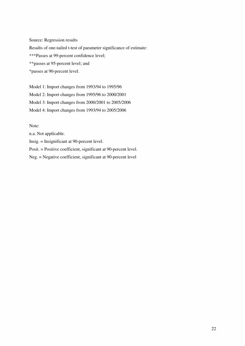
Source: Regression results

Results of one-tailed t-test of parameter significance of estimate:

***Passes at 99-percent confidence level;

**passes at 95-percent level; and

*passes at 90-percent level.

Model 1: Import changes from 1993/94 to 1995/96




Note:

n.a. Not applicable.

Insig. = Insignificant at 90-percent level.

Posit. = Positive coefficient, significant at 90-percent level.

Neg. = Negative coefficient, significant at 90-percent level

23

1.6

Annex to EQ 3 – Value and volume of im

ports growth

1.6.1

Tables based on COMTRADE database

So

urc

e: C

OM

TR

AD

E d

ata

pro

cess

ed b

y A

GR

OS

YN

ER

GIE

24

So

urc

e: C

OM

TR

AD

E d

ata

pro

cess

ed b

y A

GR

OS

YN

ER

GIE

25

So

urc

e: C

OM

TR

AD

E d

ata

pro

cess

ed b

y A

GR

OS

YN

ER

GIE

26

1.6.2 Tables based on COMEXT database

28

1.7 Annex to EQ 3 – Analysis of Preferences

Tab. 1 - Products to which a reduced entry price applies

Source: Commission Regulation (EC) No 1789/2003 and Euro-Mediterranean Agreements

Note: Notice that quotas indicated for Jordanian citrus and cucumbers correspond to the ad valorem tariff quotas.

29

Tab. 2. - Periods for separate analysis. Tomatoes

Tab. 3. - Periods for separate analysis. Cucumbers

Tab. 4 - Periods for separate analysis. Artichokes

November

December

Tab. 5 - Periods for separate analysis. Courgettes

January

1-20April

October

November

December

Tab. 6 - Periods for separate analysis. Oranges

December

January

February

March

April

1-15 May

16-31 may

30

Fig. 1 - Comparison between value of preferential trade and specific gain. Moroccan tomatoes.

0

20

40

60

80

100

120

140

160

Campaign

2003/2004

Campaign

2004/2005

Campaign

2005/2006

Campaign

2006/2007

Million €

Preferential trade

Specific gain

Source: own calculations based on Comext and Taric data. Caveat: calculations for the marketing year 2006/2007 correspond

only to the period October to December 2006.

Fig. 2 - Comparison between value of preferential trade and specific gain. Moroccan cucumbers.

0

500

1000

1500

2000

2500

3000

3500

4000

Campaign

2003/2004

Campaign

2004/2005

Campaign

2005/2006

Thousand €

Preferential trade

Specific gain

Source: own calculations based on Comext and Taric data.

31

Fig. 3 - Total trade value, VPM and specific gain. Moroccan artichokes

- 5.000 10.000 15.000

Euro

20.000 25.000 30.000 35.000

Campaign 2004

Campaign 2005

Campaign 2006

Trade value

VPM

M Specific gain


Fig. 4- Total trade value, VPM and specific gain. Moroccan clementines

0 20 40 60

Campaign

2003/2004

Campaign

2004/2005

Campaign

2005/2006

Million €

Total trade

VPM

Specific gain

Source: own calculations based on Taric data.

32

Fig. 5 - Values of trade, VPM and specific gain. Jordanian tomatoes.


Fig. 6 - Values of trade, VPM and specific gain. Jordanian cucumbers.


33

Fig. 7 - Average SIVs (€/100Kg) and EPs since January 2004. Israel oranges.

0

10

20

30

40

50

60

70

Dece

mbe

rApril

Marketing year 2003/2004 Marketing year 2004/2005 Marketing year 2005/2006

MFN EP Preferential EP


Fig. 8 - Average SIVs (€/100Kg) and EPs since June 2004. Egypt oranges.

0

10

20

30

40

50

60

Dec

ember

Januar

y

Febru

ary

Mar

chApr

il

1-15 M

ay

16-31

May

Marketing year

2004/2005Marketing year

2005/2006MFN EP

Preferential EP


34

Fig. 9- Evolution of Moroccan courgette imports and quota in force (tonnes).

0

5000

10000

15000

20000

25000

30000

35000

40000

45000

50000

Quota

Marketing year 2003/2004




Source: Agrosynergie calculations based on Taric data and EU-Morocco Agreement

35

1.8 Annex to EQ 3 – Seasonal value of Preferences

The VPM has been split into two different addends. The first addend assesses the gain due to the

specific tariff cut, which in turn is caused by the EP reduction. The second addend of the expression

corresponds mostly to the gain due to the cutting of the ad valorem part of the tariff. We call the first

addend “specific gain” and the second is the “ad valorem gain”. It is worth emphasising that the

specific gain is equivalent to an entry price quota rent, as discussed above.

Tomatoes

The next table shows the periods analysis for the tomatoes.

Tab. 1 - Periods for in-marketing year analysis. Tomatoes

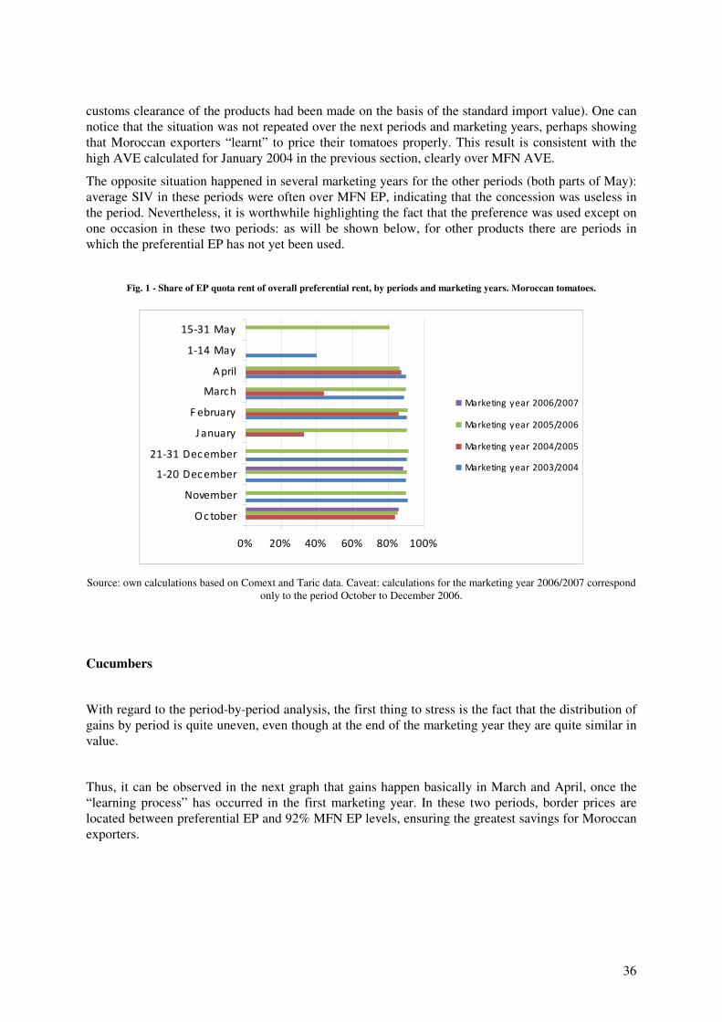
This breakdown makes it possible to identify patterns of seasonal variations in the use of the reduced

EP. As the next graph shows, there are a number of periods in which the relevance of the EP quota is

very large in all the marketing years considered: over 80% of the total tariff revenue foregone.

Namely, these periods are February and April. Practically, it means than in these periods Moroccan

tomatoes are priced at the EU border between 92% of MFN EP and its preferential EP. Thus Morocco

takes the highest advantage from this preference, since it is “saving” the MTE if it was treated as

MFN and simultaneously not paying any specific tariff, being considered as preferential.

In a second category, October, November and the two periods in December and March are months in

which Morocco did not take advantage of the preferential EP in all the marketing years, mainly

because of the high SIVs in the marketing year 2004/2005. Therefore, it indicates that in these periods

Morocco is able to benefit from the reduced EP, but the margin of manoeuvre for Morocco is less than

in previous months - if it wants to take full advantage of the preferential EP.

Finally, January and the two periods in May indicate that in some cases Morocco has not taken any

advantage of the reduced EP, but the reasons are different. In January 2004, it exported so cheaply

that average SIV was below 92% of preferential EP, therefore it would have paid the MTE (if the

36

customs clearance of the products had been made on the basis of the standard import value). One can

notice that the situation was not repeated over the next periods and marketing years, perhaps showing

that Moroccan exporters “learnt” to price their tomatoes properly. This result is consistent with the

high AVE calculated for January 2004 in the previous section, clearly over MFN AVE.

The opposite situation happened in several marketing years for the other periods (both parts of May):

average SIV in these periods were often over MFN EP, indicating that the concession was useless in

the period. Nevertheless, it is worthwhile highlighting the fact that the preference was used except on

one occasion in these two periods: as will be shown below, for other products there are periods in

which the preferential EP has not yet been used.

Fig. 1 - Share of EP quota rent of overall preferential rent, by periods and marketing years. Moroccan tomatoes.

0% 20% 40% 60% 80% 100%

Oc tober

November

1-20 Dec ember

21-31 Dec ember

J anuary

F ebruary

Marc h

A pril

1-14 May

15-31 May





Source: own calculations based on Comext and Taric data. Caveat: calculations for the marketing year 2006/2007 correspond

only to the period October to December 2006.

Cucumbers

With regard to the period-by-period analysis, the first thing to stress is the fact that the distribution of

gains by period is quite uneven, even though at the end of the marketing year they are quite similar in

value.

Thus, it can be observed in the next graph that gains happen basically in March and April, once the

“learning process” has occurred in the first marketing year. In these two periods, border prices are

located between preferential EP and 92% MFN EP levels, ensuring the greatest savings for Moroccan

exporters.

37

Fig. 2- Share of EP quota rent of overall preferential rent, by period and marketing year. Moroccan cucumbers.

0% 20% 40% 60% 80% 100%

1-10 November

11-30 November

December

J anuary

F ebruary

Marc h

April

1-15 May

16-31 May





At any rate, these conclusions should be viewed with caution, since only two marketing years with

specific gains have been analysed and also, great changes in border prices are reported, and their

relationship with different Entry Prices determines the amount of the specific gain. The next graph

compares these series.

Fig. 3- Average SIVs (€/100Kg) in two consecutive marketing years and EPs. Moroccan cucumbers.

0,00

20,00

40,00

60,00

80,00

100,00

120,00

140,00

160,00

180,00

1-10 N

ovem

ber

11-30

Nov

ember

Dec

ember

Januar

y

Febru

ary

Mar

chApr

il

1-15 M

ay

16-31

May

Marketing year

2004/2005

Marketing year

2005/2006

Reduced EP

MFN EP


38

Courgettes

The period-by-period analysis clearly shows that Morocco is taking advantage of the reduced EP only

in the period 1-20 April. In all other periods, border prices are above MFN EP, and thus the

concession is irrelevant. This circumstance apparently happens because in this period the difference

between preferential EP and MFN EP widens compared with other periods, when the gap between

both is quite narrow. The situation is shown in the next graph.

Fig. 4 - Average SIVs (€/100Kg) in two consecutive marketing years and EPs. Moroccan courgettes.

0,00

20,00

40,00

60,00

80,00

100,00

120,00

140,00

160,00

Oct

ober

Novem

ber

Decem

ber

Januar

y

1-20April

Marketing year

2004/2005Marketing year

2005/2006Preferential EP

MFN EP


39

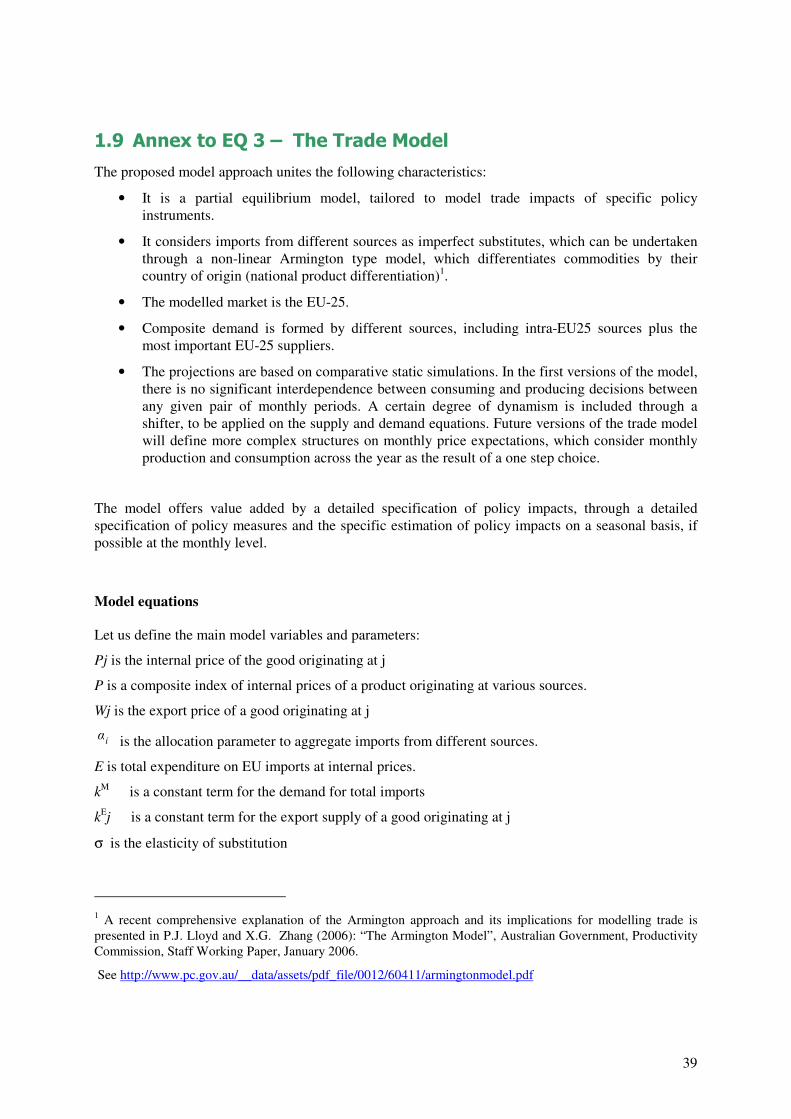
1.9 Annex to EQ 3 – The Trade Model

The proposed model approach unites the following characteristics:

• It is a partial equilibrium model, tailored to model trade impacts of specific policy

instruments.

• It considers imports from different sources as imperfect substitutes, which can be undertaken

through a non-linear Armington type model, which differentiates commodities by their

country of origin (national product differentiation)1.

• The modelled market is the EU-25.

• Composite demand is formed by different sources, including intra-EU25 sources plus the

most important EU-25 suppliers.

• The projections are based on comparative static simulations. In the first versions of the model,

there is no significant interdependence between consuming and producing decisions between

any given pair of monthly periods. A certain degree of dynamism is included through a

shifter, to be applied on the supply and demand equations. Future versions of the trade model

will define more complex structures on monthly price expectations, which consider monthly

production and consumption across the year as the result of a one step choice.

The model offers value added by a detailed specification of policy impacts, through a detailed

specification of policy measures and the specific estimation of policy impacts on a seasonal basis, if

possible at the monthly level.

Model equations

Let us define the main model variables and parameters:

Pj is the internal price of the good originating at j

P is a composite index of internal prices of a product originating at various sources.

Wj is the export price of a good originating at j

αi is the allocation parameter to aggregate imports from different sources.

E is total expenditure on EU imports at internal prices.

kM

is a constant term for the demand for total imports

kEj

is a constant term for the export supply of a good originating at j

σ is the elasticity of substitution

1 A recent comprehensive explanation of the Armington approach and its implications for modelling trade is

presented in P.J. Lloyd and X.G. Zhang (2006): “The Armington Model”, Australian Government, Productivity

Commission, Staff Working Paper, January 2006.

See http://www.pc.gov.au/__data/assets/pdf_file/0012/60411/armingtonmodel.pdf

40

t jo

is the extra-quota total duty (or the only duty when TRQ is not defined)..

t jw

is the price wedge on country j imports.

η is the demand for total imports, including intra-EU and extra-EU partners’ goods.

µj is the export supply of a good originating at j to the EU market.

Mqj is the total quota volume for a product originating at j

Mj = import flow originating at j

q = total composite demand.

Xj = export flow originating at j

Model description

For the sake of simplifying the model description, we assume in the equations below that preferential

suppliers are not constrained by tariffs (though they could be restricted by TRQs). However, the

model extension to the case where tariffs also apply to preferential suppliers is straightforward.

Moreover, the actual empirical exercises are based on the assumption that preferential suppliers are

actually facing tariffs.

Demand side:

We first define the composite good, q, as a Constant Elasticity of Substitution (CES) composite of

intra-EU goods and imports from different regions. Total composite goods demand can be described

by a demand standard equation:

q= kM

Pη

[1]

The price P is an index of prices of the imports originated at various regions:

Import price index:

ρ

σσα

/11

1

1

−

=

−

= ∑

n

i

ii PP , where ρ = (σ-1)/σ

While equation [1] represents the total EU import demand, i.e., for tomato, we need to describe the

specific demand for imports from the considered regions. Thus, the import demand of good

originating at region j is:

EPP

Mjj

j 1−

= σ

σα

[2]

Consequently, the demand side is defined by a composite import demand plus specific demands for

imports from different exporting regions.

Supply side:

Supply functions are specified as a function with constant supply elasticity. Again, imports

originating at various regions are separately modelled. Thus, supply of imports originating at j:

41

Xj = k j

E [Wj ]µ

j

[3]

The relation between internal prices and export prices being this:

)1( w

j

j

t

PWj

+=

where w

jt ≤ o

jt .

Note that a price wedge is defined when imports face TRQs. In the basic formulation a preferential

supplier not constrained by TRQs, when these are not binding, t jw

= 0. When TRQs are binding, then

a price wedge is defined and has to be calculated endogenously. When exports are over the TRQ

limits, then the maximum price wedge is applied, which is, for this case, equal to the maximum tariff

t jo

.

Actually, in the first applications of the model, a differentiation is made, for each supplier, between

the actual tariff applied, on the one hand, and the price wedge resulting from the implementation of

TRQs, on the other.

System equations:

The model is finally constructed through a system of non-linear equation, which can be written and

solved through the use of GAMS programming2..

The equations to be solved are:

Excess of demand good originating at j must be zero:

Mj - jX = 0

Replacing import demand (equation [2]) and import supply (equation [3]) the excess demand

condition is:

[ ] njWjkEPP

jE

j

j

j......101 ==−

− µσ

σα

Replacing Wj by its value in terms of Pj:

njt

PkEP

P

j

w

j

jE

j

j

j......10

)1(

1 ==

+−

−

µ

σ

σα

[4]

Total import demand. This can be expressed as follows:

01 =−+ EPk M η

2 The General Algebraic Modelling System (GAMS) is a high-level modelling system for mathematical

programming and optimization. It consists of a language compiler and a stable of integrated high-performance

solvers. In the case of the import model, GAMS 20.7 142 version with CONOPT-3 solver were used.

42

Note that the equation above is specified just by multiplying the composite demand for the composite

price and rearranging.

Total price index: 0

/11

1

1 =

−

−

=

−∑ρ

σσαn

i

ii PP [5]

Then the system to solve is formed by n + 2 equations and n + 2 unknown variables (n prices, total

expenditure E and composite price P).

TRQs:

As indicated above the price wedge for preferential suppliers can get three kinds of value, depending

on the size of imports compared to the applied TRQs. For cases where preferential tariffs are nil:

a) M j < Mqj then t j

w

= 0

b) M j = Mqj then 0 < t j

w

< t jo

, and t jw

is estimated endogenously.

c) M j > Mqj then t j

w

= t jo

Calibration

Calibration is based on unit price normalisation, so that all constants are equal to benchmark

expenditures. If a TRQ is binding we have to propose a value for the reference price wedge. However,

if Mj >Mqj then the price wedge is taken as the initial out-of-quota tariff t j

o

.

Adjustment to study export refunds

Equation 3 can be adjusted to consider shifts in the total EU supply in the non-EU market related to

export refunds. To study the effect of export refund changes we will take the same modelling

approach and the supply function including constant supply elasticity. Again, imports originating

from various regions are separately modelled. Thus, supply of imports originating from the EU in the

world market being:

X [ ]µEUk= [3]

Where U is the EU internal price (including the export refund per physical unit), and the relation

between world and EU export prices being this:

PSU )1( +=

where S is the export refund per ton.

Trade policy scenarios

The preliminary version of the F&V trade model is applied to study the trade impacts of several

scenarios of trade liberalisation. These scenarios are the following:

43

• Eliminating Entry Prices. If entry prices are phased out, this has an impact on both

preferential suppliers as well as MFN imports.

• Eliminating export subsidies. What has been the impact of the export refund reduction and

what would be the impact of its complete elimination?

1.9.1 The Export Model

Basic data and assumptions

44

EX

PO

RT

MO

DE

L -

AP

PL

ES

RE

SU

LT

S

45

EX

PO

RT

MO

DE

L -

OR

AN

GE

S R

ES

UL

TS

46

EX

PO

RT

MO

DE

L -

T

AB

LE

GR

AP

ES

RE

SU

LT

S

47

EX

PO

RT

MO

DE

L -

TO

MA

TO

RE

SU

LT

S

48

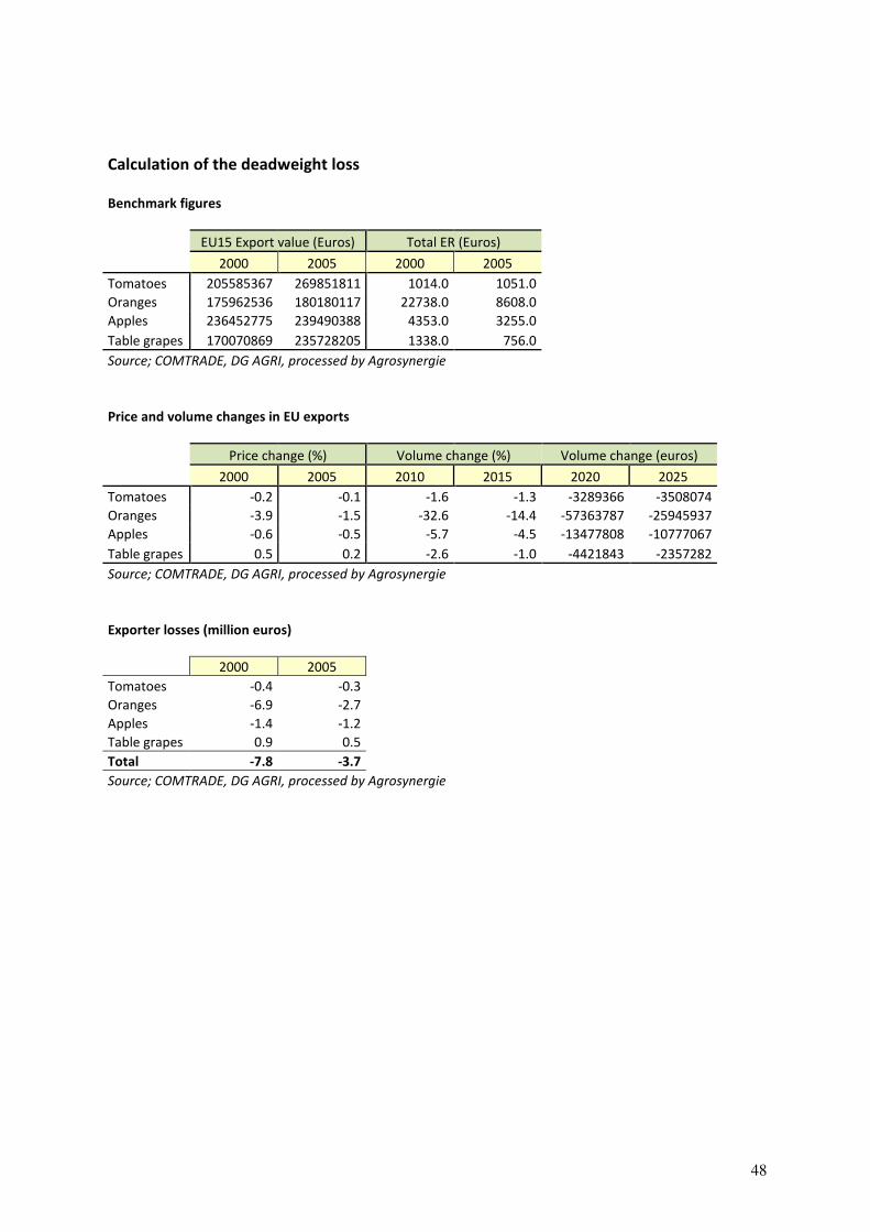
Calculation of the deadweight loss

Benchmark figures

EU15 Export value (Euros) Total ER (Euros)

2000 2005 2000 2005

Tomatoes 205585367 269851811 1014.0 1051.0

Oranges 175962536 180180117 22738.0 8608.0

Apples 236452775 239490388 4353.0 3255.0

Table grapes 170070869 235728205 1338.0 756.0

Source; COMTRADE, DG AGRI, processed by Agrosynergie

Price and volume changes in EU exports

Price change (%) Volume change (%) Volume change (euros)

2000 2005 2010 2015 2020 2025

Tomatoes -0.2 -0.1 -1.6 -1.3 -3289366 -3508074

Oranges -3.9 -1.5 -32.6 -14.4 -57363787 -25945937

Apples -0.6 -0.5 -5.7 -4.5 -13477808 -10777067

Table grapes 0.5 0.2 -2.6 -1.0 -4421843 -2357282


Exporter losses (million euros)

2000 2005

Tomatoes -0.4 -0.3

Oranges -6.9 -2.7

Apples -1.4 -1.2

Table grapes 0.9 0.5

Total -7.8 -3.7


49

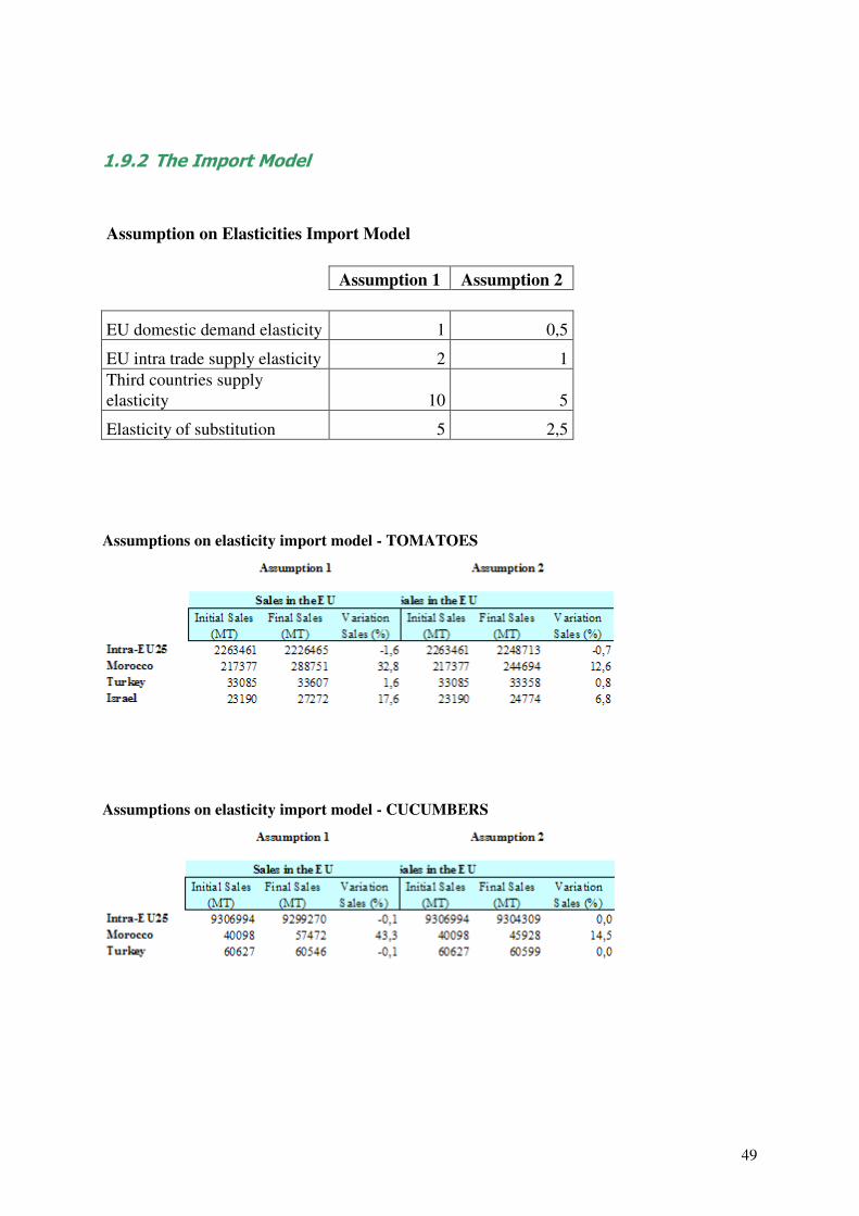
1.9.2 The Import Model

Assumption on Elasticities Import Model

Assumption 1 Assumption 2

EU domestic demand elasticity 1 0,5

EU intra trade supply elasticity 2 1

Third countries supply

elasticity 10 5

Elasticity of substitution 5 2,5

Assumptions on elasticity import model - TOMATOES

Assumptions on elasticity import model - CUCUMBERS

50

The next tables show the raw data used to run the import model. All of them come from official EU

data (trade values, EP levels, average SIV by periods, TRQs and duties).

The figure under “in-quota tariff reduction” indicates the reduction -from the MFN level- of the ad

valorem tariff if trade is within the TRQ for the preferential supplier. Hence, “1” means total

elimination of the tariff. Similarly, the “out-of-quota” tariff reduction is the reduction of the MFN ad

valorem tariff that applies for the preferential partner for quantities traded over the TRQ. Hence, the

figure “0,6” indicates a 60% tariff reduction.

61

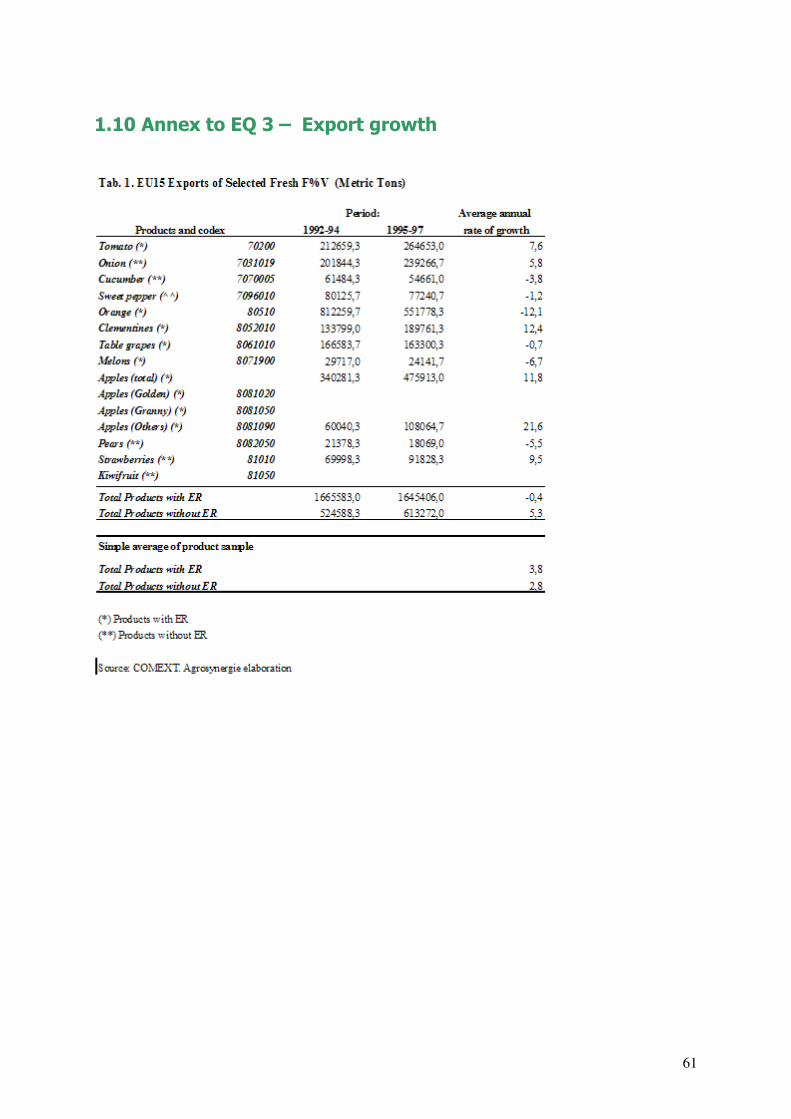
1.10 Annex to EQ 3 – Export growth

64

1.11

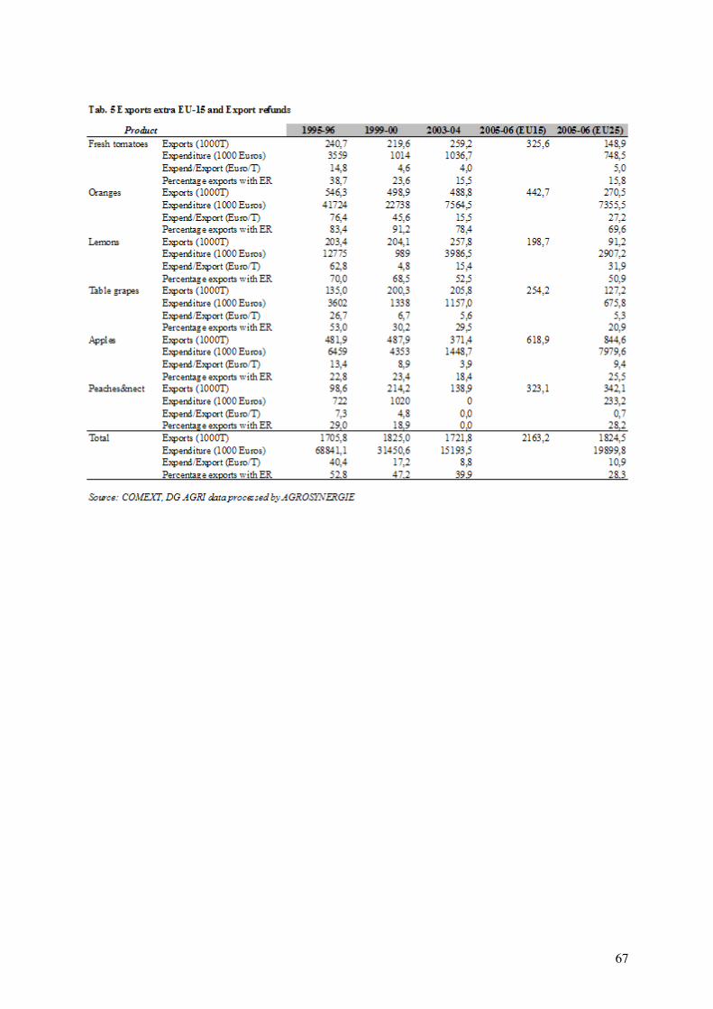
Annex to EQ 3 – Export Refunds

Annex to EQ3 rev 23-4-08 - European...

Documents

Transcript of Annex to EQ3 rev 23-4-08 - European...