Annals of Mathematics Studies Number 197
829
Shock December 8, 2017 6x9 Annals of Mathematics Studies Number 197
Transcript of Annals of Mathematics Studies Number 197

Shock December 8, 2017 6x9
Annals of Mathematics StudiesNumber 197

Shock December 8, 2017 6x9

Shock December 8, 2017 6x9
The Mathematics ofShock Reflection-Diffractionandvon Neumann’s Conjectures
Gui-Qiang G. ChenMikhail Feldman
PRINCETON UNIVERSITY PRESS
PRINCETON AND OXFORD
2 0 1 8

Shock December 8, 2017 6x9
Copyright c© 2018 by Princeton University Press
Published by Princeton University Press, 41 William Street,Princeton, New Jersey 08540
In the United Kingdom: Princeton University Press, 6 Oxford Street,Woodstock, Oxfordshire OX20 1TR
press.princeton.edu
All Rights Reserved
Library of Congress Cataloging-in-Publication Data
Names: Chen, Gui-Qiang, 1963– | Feldman, Mikhail, 1960–Title: The mathematics of shock reflection-diffraction and von Neumann’s
conjectures / Gui-Qiang G. Chen and Mikhail Feldman.Description: Princeton : Princeton University Press, 2017. | Series: Annals
of mathematics studies ; number 197 | Includes bibliographical referencesand index.
Identifiers: LCCN 2017008667| ISBN 9780691160542 (hardcover : alk. paper) |ISBN 9780691160559 (pbk. : alk. paper)
Subjects: LCSH: Shock waves–Diffraction. | Shock waves–Free boundaries. |Shock waves–Mathematics. | von Neumann conjectures. | Analysis of PDEs.
Classification: LCC QC168.85.S45 C44 2017 | DDC 531/.1133–dc23 LC recordavailable at https://lccn.loc.gov/2017008667
British Library Cataloging-in-Publication Data is available
This book has been composed in LATEX. [sjp]
The publisher would like to acknowledge the authors of this volume for providingthe camera-ready copy from which this book was printed.
Printed on acid-free paper ∞
10 9 8 7 6 5 4 3 2 1

Shock December 8, 2017 6x9
Contents
Preface xi
I Shock Reflection-Diffraction, Nonlinear Conservation Lawsof Mixed Type, and von Neumann’s Conjectures 1
1 Shock Reflection-Diffraction, Nonlinear Partial DifferentialEquations of Mixed Type, and Free Boundary Problems 3
2 Mathematical Formulations and Main Theorems 162.1 The potential flow equation . . . . . . . . . . . . . . . . . . . . . 162.2 Mathematical problems for shock reflection-diffraction . . . . . . 192.3 Weak solutions of Problem 2.2.1 and Problem 2.2.3 . . . . . . . 232.4 Structure of solutions: Regular reflection-diffraction
configurations . . . . . . . . . . . . . . . . . . . . . . . . . . . . 242.5 Existence of state (2) and continuous dependence on
the parameters . . . . . . . . . . . . . . . . . . . . . . . . . . . . 272.6 Von Neumann’s conjectures, Problem 2.6.1 (free boundary
problem), and main theorems . . . . . . . . . . . . . . . . . . . . 28
3 Main Steps and Related Analysis in the Proofs of the MainTheorems 373.1 Normal reflection . . . . . . . . . . . . . . . . . . . . . . . . . . 373.2 Main steps and related analysis in the proof of the sonic conjecture 373.3 Main steps and related analysis in the proof of the detachment
conjecture . . . . . . . . . . . . . . . . . . . . . . . . . . . . . . 553.4 Appendix: The method of continuity and fixed point theorems . 65
II Elliptic Theory and Related Analysis for ShockReflection-Diffraction 67
4 Relevant Results for Nonlinear Elliptic Equations of SecondOrder 694.1 Notations: Hölder norms and ellipticity . . . . . . . . . . . . . . 694.2 Quasilinear uniformly elliptic equations . . . . . . . . . . . . . . 72

vi
Shock December 8, 2017 6x9
CONTENTS
4.3 Estimates for Lipschitz solutions of elliptic boundary valueproblems . . . . . . . . . . . . . . . . . . . . . . . . . . . . . . . 105
4.4 Comparison principle for a mixed boundary value problem in adomain with corners . . . . . . . . . . . . . . . . . . . . . . . . . 142
4.5 Mixed boundary value problems in a domain with corners foruniformly elliptic equations . . . . . . . . . . . . . . . . . . . . . 145
4.6 Hölder spaces with parabolic scaling . . . . . . . . . . . . . . . . 1924.7 Degenerate elliptic equations . . . . . . . . . . . . . . . . . . . . 1974.8 Uniformly elliptic equations in a curved triangle-shaped domain
with one-point Dirichlet condition . . . . . . . . . . . . . . . . . 207
5 Basic Properties of the Self-Similar Potential Flow Equation 2165.1 Some basic facts and formulas for the potential flow equation . . 2165.2 Interior ellipticity principle for self-similar potential flow . . . . 2225.3 Ellipticity principle for self-similar potential flow with slip
condition on the flat boundary . . . . . . . . . . . . . . . . . . . 227
III Proofs of the Main Theorems for the Sonic Conjectureand Related Analysis 229
6 Uniform States and Normal Reflection 2316.1 Uniform states for self-similar potential flow . . . . . . . . . . . 2316.2 Normal reflection and its uniqueness . . . . . . . . . . . . . . . . 2386.3 The self-similar potential flow equation in the coordinates
flattening the sonic circle of a uniform state . . . . . . . . . . . . 239
7 Local Theory and von Neumann’s Conjectures 2427.1 Local regular reflection and state (2) . . . . . . . . . . . . . . . . 2427.2 Local theory of shock reflection for large-angle wedges . . . . . . 2457.3 The shock polar for steady potential flow and its properties . . . 2487.4 Local theory for shock reflection: Existence of the weak and
strong state (2) up to the detachment angle . . . . . . . . . . . . 2637.5 Basic properties of the weak state (2) and the definition of
supersonic and subsonic wedge angles . . . . . . . . . . . . . . . 2737.6 Von Neumann’s sonic and detachment conjectures . . . . . . . . 279
8 Admissible Solutions and Features of Problem 2.6.1 2818.1 Definition of admissible solutions . . . . . . . . . . . . . . . . . . 2818.2 Strict directional monotonicity for admissible solutions . . . . . 2868.3 Appendix: Properties of solutions of Problem 2.6.1 for large-
angle wedges . . . . . . . . . . . . . . . . . . . . . . . . . . . . . 305

CONTENTS
Shock December 8, 2017 6x9
vii
9 Uniform Estimates for Admissible Solutions 3199.1 Bounds of the elliptic domain Ω and admissible solution ϕ in Ω 3199.2 Regularity of admissible solutions away from Γshock∪Γsonic∪P3 3229.3 Separation of Γshock from Γsym . . . . . . . . . . . . . . . . . . . 3399.4 Lower bound for the distance between Γshock and Γwedge . . . . 3419.5 Uniform positive lower bound for the distance between Γshock
and the sonic circle of state (1) . . . . . . . . . . . . . . . . . . . 3549.6 Uniform estimates of the ellipticity constant in Ω \ Γsonic . . . . 369
10 Regularity of Admissible Solutions away from the Sonic Arc 38210.1 Γshock as a graph in the radial directions with respect to state (1) 38210.2 Boundary conditions on Γshock for admissible solutions . . . . . 38510.3 Local estimates near Γshock . . . . . . . . . . . . . . . . . . . . . 38710.4 The critical angle and the distance between Γshock and Γwedge . 38910.5 Regularity of admissible solutions away from Γsonic . . . . . . . . 39010.6 Regularity of the limit of admissible solutions away from Γsonic . 392
11 Regularity of Admissible Solutions near the Sonic Arc 39611.1 The equation near the sonic arc and structure of elliptic degeneracy 39611.2 Structure of the neighborhood of Γsonic in Ω and estimates of
(ψ,Dψ) . . . . . . . . . . . . . . . . . . . . . . . . . . . . . . . . 39811.3 Properties of the Rankine-Hugoniot condition on Γshock near Γsonic 41311.4 C2,α–estimates in the scaled Hölder norms near Γsonic . . . . . . 42111.5 The reflected-diffracted shock is C2,α near P1 . . . . . . . . . . . 43111.6 Compactness of the set of admissible solutions . . . . . . . . . . 434
12 Iteration Set and Solvability of the Iteration Problem 44012.1 Statement of the existence results . . . . . . . . . . . . . . . . . 44012.2 Mapping to the iteration region . . . . . . . . . . . . . . . . . . 44012.3 Definition of the iteration set . . . . . . . . . . . . . . . . . . . . 46112.4 The equation for the iteration . . . . . . . . . . . . . . . . . . . 46912.5 Assigning a boundary condition on the shock for the iteration . 48512.6 Normal reflection, iteration set, and admissible solutions . . . . 50412.7 Solvability of the iteration problem and estimates of solutions . 50512.8 Openness of the iteration set . . . . . . . . . . . . . . . . . . . . 520
13 Iteration Map, Fixed Points, and Existence of AdmissibleSolutions up to the Sonic Angle 52413.1 Iteration map . . . . . . . . . . . . . . . . . . . . . . . . . . . . 52413.2 Continuity and compactness of the iteration map . . . . . . . . . 52813.3 Normal reflection and the iteration map for θw = π
2 . . . . . . . 53013.4 Fixed points of the iteration map for θw < π
2 are admissiblesolutions . . . . . . . . . . . . . . . . . . . . . . . . . . . . . . . 531
13.5 Fixed points cannot lie on the boundary of the iteration set . . . 557

viii
Shock December 8, 2017 6x9
CONTENTS
13.6 Proof of the existence of solutions up to the sonic angle or thecritical angle . . . . . . . . . . . . . . . . . . . . . . . . . . . . . 559
13.7 Proof of Theorem 2.6.2: Existence of global solutions up to thesonic angle when u1 ≤ c1 . . . . . . . . . . . . . . . . . . . . . . 559
13.8 Proof of Theorem 2.6.4: Existence of global solutions when u1 > c1 56213.9 Appendix: Extension of the functions in weighted spaces . . . . 564
14 Optimal Regularity of Solutions near the Sonic Circle 58614.1 Regularity of solutions near the degenerate boundary for
nonlinear degenerate elliptic equations of second order . . . . . . 58614.2 Optimal regularity of solutions across Γsonic . . . . . . . . . . . . 599
IV Subsonic Regular Reflection-Diffraction and GlobalExistence of Solutions up to the Detachment Angle 613
15 Admissible Solutions and Uniform Estimates up to theDetachment Angle 61515.1 Definition of admissible solutions for the supersonic and subsonic
reflections . . . . . . . . . . . . . . . . . . . . . . . . . . . . . . . 61515.2 Basic estimates for admissible solutions up to the detachment
angle . . . . . . . . . . . . . . . . . . . . . . . . . . . . . . . . . 61715.3 Separation of Γshock from Γsym . . . . . . . . . . . . . . . . . . . 61815.4 Lower bound for the distance between Γshock and Γwedge away
from P0 . . . . . . . . . . . . . . . . . . . . . . . . . . . . . . . . 61815.5 Uniform positive lower bound for the distance between Γshock
and the sonic circle of state (1) . . . . . . . . . . . . . . . . . . . 62115.6 Uniform estimates of the ellipticity constant . . . . . . . . . . . 62215.7 Regularity of admissible solutions away from Γsonic . . . . . . . . 625
16 Regularity of Admissible Solutions near the Sonic Arcand the Reflection Point 62916.1 Pointwise and gradient estimates near Γsonic and the reflection
point . . . . . . . . . . . . . . . . . . . . . . . . . . . . . . . . . 62916.2 The Rankine-Hugoniot condition on Γshock near Γsonic and the
reflection point . . . . . . . . . . . . . . . . . . . . . . . . . . . . 63316.3 A priori estimates near Γsonic in the supersonic-away-from-sonic
case . . . . . . . . . . . . . . . . . . . . . . . . . . . . . . . . . . 63516.4 A priori estimates near Γsonic in the supersonic-near-sonic case . 63616.5 A priori estimates near the reflection point in the subsonic-near-
sonic case . . . . . . . . . . . . . . . . . . . . . . . . . . . . . . . 65616.6 A priori estimates near the reflection point in the subsonic-away-
from-sonic case . . . . . . . . . . . . . . . . . . . . . . . . . . . . 665
CONTENTS
Shock December 8, 2017 6x9
ix
17 Existence of Global Regular Reflection-Diffraction Solutionsup to the Detachment Angle 69017.1 Statement of the existence results . . . . . . . . . . . . . . . . . 69017.2 Mapping to the iteration region . . . . . . . . . . . . . . . . . . 69017.3 Iteration set . . . . . . . . . . . . . . . . . . . . . . . . . . . . . 70717.4 Existence and estimates of solutions of the iteration problem . . 72517.5 Openness of the iteration set . . . . . . . . . . . . . . . . . . . . 73717.6 Iteration map and its properties . . . . . . . . . . . . . . . . . . 74117.7 Compactness of the iteration map . . . . . . . . . . . . . . . . . 74517.8 Normal reflection and the iteration map for θw = π
2 . . . . . . . 74717.9 Fixed points of the iteration map for θw < π
2 are admissiblesolutions . . . . . . . . . . . . . . . . . . . . . . . . . . . . . . . 747
17.10 Fixed points cannot lie on the boundary of the iteration set . . . 75217.11 Proof of the existence of solutions up to the critical angle . . . . 75317.12 Proof of Theorem 2.6.6: Existence of global solutions up to the
detachment angle when u1 ≤ c1 . . . . . . . . . . . . . . . . . . 75317.13 Proof of Theorem 2.6.8: Existence of global solutions when
u1 > c1 . . . . . . . . . . . . . . . . . . . . . . . . . . . . . . . . 753
V Connections and Open Problems 755
18 The Full Euler Equations and the Potential Flow Equation 75718.1 The full Euler equations . . . . . . . . . . . . . . . . . . . . . . . 75718.2 Mathematical formulation I: Initial-boundary value problem . . 76118.3 Mathematical formulation II: Boundary value problem . . . . . . 76218.4 Normal reflection . . . . . . . . . . . . . . . . . . . . . . . . . . 76818.5 Local theory for regular reflection near the reflection point . . . 76918.6 Von Neumann’s conjectures . . . . . . . . . . . . . . . . . . . . . 77718.7 Connections with the potential flow equation . . . . . . . . . . . 781
19 Shock Reflection-Diffraction and New MathematicalChallenges 78519.1 Mathematical theory for multidimensional conservation laws . . 78519.2 Nonlinear partial differential equations of mixed elliptic-hyperbolic
type . . . . . . . . . . . . . . . . . . . . . . . . . . . . . . . . . . 78819.3 Free boundary problems and techniques . . . . . . . . . . . . . . 79019.4 Numerical methods for multidimensional conservation laws . . . 791
Bibliography 794
Index 815

Shock December 8, 2017 6x9

Shock December 8, 2017 6x9
Preface
The purpose of this research monograph is to survey some recent developments inthe analysis of shock reflection-diffraction, to present our original mathematicalproofs of von Neumann’s conjectures for potential flow, to collect most of therelated results and new techniques in the analysis of partial differential equations(PDEs) achieved in the last decades, and to discuss a set of fundamental openproblems relevant to the directions of future research in this and related areas.
Shock waves are fundamental in nature, especially in high-speed fluid flows.Shocks are generated by supersonic or near-sonic aircraft, explosions, solar wind,and other natural processes. They are governed by the Euler equations for com-pressible fluids or their variants, generally in the form of nonlinear conservationlaws – nonlinear PDEs of divergence form. The Euler equations describing themotion of a perfect fluid were first formulated by Euler [112, 113, 114] in 1752(based in part on the earlier work of Bernoulli [15]), and were among the firstPDEs for describing physical processes to be written down.
When a shock hits an obstacle (steady or flying), shock reflection-diffractionconfigurations take shape. One of the most fundamental research directions inmathematical fluid dynamics is the analysis of shock reflection-diffraction bywedges, with focus on the wave patterns of the reflection-diffraction configura-tions formed around the wedge. The complexity of such configurations wasfirst reported by Ernst Mach [206] in 1878, who observed two patterns of shockreflection-diffraction configurations that are now named the Regular Reflection(RR) and the Mach Reflection (MR). The subject remained dormant until the1940s when von Neumann [267, 268, 269], as well as other mathematical andexperimental scientists, began extensive research on shock reflection-diffractionphenomena, owing to their fundamental importance in applications. It has sincebeen found that the phenomena are much more complicated than what Machoriginally observed, and various other patterns of shock reflection-diffractionconfigurations may occur. On the other hand, the shock reflection-diffractionconfigurations are core configurations in the structure of global entropy solu-tions of the two-dimensional Riemann problem, while the Riemann solutionsthemselves are local building blocks and determine local structures, global at-tractors, and large-time asymptotic states of general entropy solutions of mul-tidimensional hyperbolic systems of conservation laws. In this sense, we haveto understand the shock reflection-diffraction configurations, in order to under-stand fully the global entropy solutions of multidimensional hyperbolic systemsof conservation laws.

xii
Shock December 8, 2017 6x9
PREFACE
Diverse patterns of shock reflection-diffraction configurations have attractedmany asymptotic/numerical analysts since the middle of the 20th century. How-ever, most of the fundamental issues involved, such as the structure and transi-tion criteria of the different patterns, have not been understood. This is partiallybecause physical and numerical experiments are hampered by various difficultiesand have not yielded clear transition criteria between the different patterns. Inlight of this, a natural approach for understanding fully the shock reflection-diffraction configurations, especially with regard to the transition criteria, is viarigorous mathematical analysis. To achieve this, it is essential to establish theglobal existence, regularity, and structural stability of shock reflection-diffractionconfigurations: That is the main topic of this book.
Mathematical analysis of shock reflection-diffraction configurations involvesdealing with several core difficulties in the analysis of nonlinear PDEs. Theseinclude nonlinear PDEs of mixed hyperbolic-elliptic type, nonlinear degener-ate elliptic PDEs, nonlinear degenerate hyperbolic PDEs, free boundary prob-lems for nonlinear degenerate PDEs, and corner singularities (especially whenfree boundaries meet the fixed boundaries), among others. These difficultiesalso arise in many further fundamental problems in continuum mechanics, dif-ferential geometry, mathematical physics, materials science, and other areas,including transonic flow problems, isometric embedding problems, and phasetransition problems. Therefore, any progress in solving these problems requiresnew mathematical ideas, approaches, and techniques, all of which will both bevery helpful for solving other problems with similar difficulties and open up newresearch directions.
Our efforts in the analysis of shock reflection-diffraction configurations forpotential flow started 18 years ago when both of us were at Northwestern Uni-versity, USA. We soon realized that the first step to achieving our goal should beto develop new free boundary techniques for multidimensional transonic shocks,along with other analytical techniques for nonlinear degenerate elliptic PDEs.After about two years of struggle, we developed such techniques, and thesewere published in [49] in 2003 and subsequent papers [42, 50, 51, 53]. Withthis groundwork, we first succeeded in developing a rigorous mathematical ap-proach to establish the global existence and stability of regular shock reflection-diffraction solutions for large-angle wedges in [52] in 2005, the complete versionof which was published electronically in 2006 and in print form in [54] in 2010.Since 2005, we have continued our efforts to solve von Neumann’s sonic con-jecture (i.e., the existence of global regular reflection-diffraction solutions up tothe sonic wedge angle with the supersonic reflection-diffraction configuration,containing a transonic reflected-diffracted shock), as well as von Neumann’s de-tachment conjecture (i.e., the necessary and sufficient condition for the existenceof global regular reflection-diffraction solutions, even beyond the sonic angle, upto the detachment angle with the subsonic reflection-diffraction configuration,containing a transonic reflected-diffracted shock) (cf. [55, 57]). The results ofthese efforts were announced in [56, 58], and their detailed proofs constitute themain part of this book.

PREFACE
Shock December 8, 2017 6x9
xiii
Some efforts have also been made by several groups of researchers on relatedmodels, including the unsteady small disturbance equation (USD), the pressuregradient equations, and the nonlinear wave system, as well as for some partialresults for the potential flow equation and the full Euler equations. For the sakeof completeness, we have made remarks and notes about these contributionsthroughout the book, and have tried to collect a detailed list of appropriatereferences in the bibliography.
Based on these results, along with our recent results on von Neumann’sconjectures for potential flow, mathematical understanding of shock reflection-diffraction, especially for the global regular reflection-diffraction configurations,has reached a new height, and several new mathematical approaches and tech-niques have been developed. Moreover, new research opportunities and manynew, challenging, and important problems have arisen during this exploration.Given these developments, we feel that it is the right time to publish this re-search monograph.
During the process of assembling this work, we have received persistentencouragement and invaluable suggestions from many leading mathematiciansand scientists, especially John Ball, Luis Caffarelli, Alexander Chorin, DemetriosChristodoulou, Peter Constantin, Constantine Dafermos, Emmanuele Di-Benedetto, Xiaxi Ding, Weinan E, Björn Engquist, Lawrence Craig Evans,Charles Fefferman, Edward Fraenkel, James Glimm, Helge Holden, JiaxingHong, Carlos Kenig, Sergiu Klainerman, Peter D. Lax, Tatsien Li, Fanhua Lin,Andrew Majda, Cathleen Morawetz, Luis Nirenberg, Benoît Perthame, RichardSchoen, Henrik Shahgholian, Yakov Sinai, Joel Smoller, John Toland, NeilTrudinger, and Juan Luis Vázquez. The materials presented herein contain di-rect and indirect contributions from many leading experts – teachers, colleagues,collaborators, and students alike, including Myoungjean Bae, Sunčica Canić, YiChao, Jun Chen, Shuxing Chen, Volker Elling, Beixiang Fang, Jingchen Hu,Feimin Huang, John Hunter, Katarina Jegdić, Siran Li, Tianhong Li, YachunLi, Gary Lieberman, Tai-Ping Liu, Barbara Keyfitz, Eun Heui Kim, Jie Kuang,Stefano Marchesani, Ho Cheung Pang, Matthew Rigby, Matthew Schrecker,Denis Serre, Wancheng Sheng, Marshall Slemrod, Eitan Tadmor, Dehua Wang,Tian-Yi Wang, Yaguang Wang, Wei Xiang, Zhouping Xin, Hairong Yuan, TongZhang, Yongqian Zhang, Yuxi Zheng, and Dianwen Zhu, among others. We aregrateful to all of them.
A significant portion of this work was done while the authors attended theSpring 2011 Program “Free Boundary Problems: Theory and Applications” atthe Mathematical Sciences Research Institute in Berkeley, California, USA, andthe 2014 Program “Free Boundary Problems and Related Topics” at the IsaacNewton Institute for Mathematical Sciences in Cambridge, UK. A part of thework was also supported by Keble College, University of Oxford, and a UKEPSRC Science and Innovation Award to the Oxford Centre for Nonlinear PDE(EP/E035027/1) when Mikhail Feldman visited Oxford in 2010.
The work of Gui-Qiang G. Chen was supported in part by the NationalScience Foundation under Grants DMS-0935967 and DMS-0807551, a UK EP-

xiv
Shock December 8, 2017 6x9
PREFACE
SRC Science and Innovation Award to the Oxford Centre for Nonlinear PDE(EP/E035027/1), a UK EPSRC Award to the EPSRC Centre for Doctoral Train-ing in PDEs (EP/L015811/1), the National Natural Science Foundation of China(under joint project Grant 10728101), and the Royal Society–Wolfson ResearchMerit Award (UK). The work of Mikhail Feldman was supported in part bythe National Science Foundation under Grants DMS-0800245, DMS-1101260,and DMS-1401490, the Vilas Award from the University of Wisconsin-Madison,and the Simons Foundation via the Simons Fellows Program. Kurt Ballstadt de-serves our special thanks for his effective assistance during the preparation of themanuscript. We are indebted to Princeton University Press, especially VickieKearn (Executive Editor) and Betsy Blumenthal and Lauren Bucca (EditorialAssistants), for their professional assistance.
Finally, we remark in passing that further supplementary materials to thisresearch monograph will be posted at:http://people.maths.ox.ac.uk/chengq/books/Monograph-CF-17/index.htmlhttps://www.math.wisc.edu/˜feldman/Monograph-CF-17/monograph.html

Shock December 8, 2017 6x9
Part I
Shock Reflection-Diffraction,Nonlinear Conservation Laws ofMixed Type, and von Neumann’s
Conjectures

Shock December 8, 2017 6x9

Shock December 8, 2017 6x9
Chapter One
Shock Reflection-Diffraction, Nonlinear Partial
Differential Equations of Mixed Type, and Free
Boundary Problems
Shock waves are steep fronts that propagate in compressible fluids when con-vection dominates diffusion. They are fundamental in nature, especially inhigh-speed fluid flows. Examples include transonic shocks around supersonic ornear-sonic flying bodies (such as aircraft), transonic and/or supersonic shocksformed by supersonic flows impinging onto solid wedges, bow shocks created bysolar wind in space, blast waves caused by explosions, and other shocks gener-ated by natural processes. Such shocks are governed by the Euler equations forcompressible fluids or their variants, generally in the form of nonlinear conserva-tion laws – nonlinear partial differential equations (PDEs) of divergence form.When a shock hits an obstacle (steady or flying), shock reflection-diffractionphenomena occur. One of the most fundamental research directions in mathe-matical fluid mechanics is the analysis of shock reflection-diffraction by wedges;see Ben-Dor [12], Courant-Friedrichs [99], von Neumann [267, 268, 269], and thereferences cited therein. When a plane shock hits a two-dimensional wedge head-on (cf. Fig. 1.1), it experiences a reflection-diffraction process; a fundamentalquestion arisen is then what types of wave patterns of shock reflection-diffractionconfigurations may be formed around the wedge.
An archetypal system of PDEs describing shock waves in fluid mechanics,widely used in aerodynamics, is that of the Euler equations for potential flow(cf. [16, 95, 99, 139, 146, 221]). The Euler equations for describing the motionof a perfect fluid were first formulated by Euler [112, 113, 114] in 1752, basedin part on the earlier work of D. Bernoulli [15], and were among the first PDEsfor describing physical processes to be written down. The n-dimensional Eulerequations for potential flow consist of the conservation law of mass and theBernoulli law for the density and velocity potential (ρ,Φ):
∂tρ+ divx(ρ∇xΦ) = 0,
∂tΦ +1
2|∇xΦ|2 + h(ρ) = B0,
(1.1)
where x ∈ Rn, B0 is the Bernoulli constant determined by the incoming flow

4
Shock December 8, 2017 6x9
CHAPTER 1
x1
x2
Figure 1.1: A plane shock hits a two-dimensional wedge in R2 head-on
and/or boundary conditions,
h′(ρ) =p′(ρ)
ρ=c2(ρ)
ρ,
and c(ρ) =√p′(ρ) is the sonic speed (i.e., the speed of sound).
The first equation in (1.1) is a transport-type equation for density ρ for agiven ∇xΦ, while the second equation is the Hamilton-Jacobi equation for thevelocity potential Φ coupling with density ρ through function h(ρ).
For polytropic gases,
p(ρ) = κργ , c2(ρ) = κγργ−1, γ > 1, κ > 0.
Without loss of generality, we may choose κ = 1γ so that
h(ρ) =ργ−1 − 1
γ − 1, c2(ρ) = ργ−1. (1.2)
This can be achieved by noting that (1.1) is invariant under scaling:
(t,x, B0) 7→ (α2t, αx, α−2B0)
with α2 = κγ. In particular, Case γ = 1 can be considered as the limit ofγ → 1+ in (1.2):
h(ρ) = ln ρ, c(ρ) = 1. (1.3)

SHOCK REFLECTION-DIFFRACTION
Shock December 8, 2017 6x9
5
Henceforth, we will focus only on Case γ > 1, since Case γ = 1 can be handledsimilarly by making appropriate changes in the formulas so that the results ofthe main theorems for γ > 1 (below) also hold for γ = 1.
From the Bernoulli law, the second equation in (1.1), we have
ρ(∂tΦ, |∇xΦ|2) = h−1(B0 − (∂tΦ +1
2|∇xΦ|2)). (1.4)
Then system (1.1) can be rewritten as the following time-dependent potentialflow equation of second order:
∂tρ(∂tΦ, |∇xΦ|2) +∇x ·(ρ(∂tΦ, |∇xΦ|2)∇xΦ
)= 0 (1.5)
with ρ(∂tΦ, |∇xΦ|2) determined by (1.4). Equation (1.5) is a nonlinear waveequation of second order. Notice that equation (1.5) is invariant under a sym-metry group formed of space-time dilations.
For a steady solution Φ = ϕ(x), i.e., ∂tΦ = 0, we obtain the celebratedsteady potential flow equation, especially in aerodynamics (cf. [16, 95, 99]):
∇x ·(ρ(|∇xϕ|2)∇xϕ
)= 0, (1.6)
which is a second-order nonlinear PDE of mixed elliptic-hyperbolic type. Thisis a simpler case of the nonlinear PDE of mixed type for self-similar solutions,as shown in (1.12)–(1.13) later.
When the effects of vortex sheets and the deviation of vorticity becomesignificant, the full Euler equations are required. The full Euler equations forcompressible fluids in Rn+1
+ = R+ × Rn, t ∈ R+ := (0,∞) and x ∈ Rn, are ofthe following form:
∂t ρ+∇x · (ρv) = 0,
∂t(ρv) +∇x · (ρv ⊗ v) +∇xp = 0,
∂t(ρ(
1
2|v|2 + e)
)+∇x ·
(ρv(
1
2|v|2 + e+
p
ρ))
= 0,
(1.7)
where ρ is the density, v ∈ Rn the fluid velocity, p the pressure, and e the internalenergy. Two other important thermodynamic variables are temperature θ andentropy S. Here, a⊗ b denotes the tensor product of vectors a and b.
Choose (ρ, S) as the independent thermodynamical variables. Then the con-stitutive relations can be written as (e, p, θ) = (e(ρ, S), p(ρ, S), θ(ρ, S)), governedby
θdS = de+ pdτ = de− p
ρ2dρ,
as introduced by Gibbs [129].For a polytropic gas,
p = (γ − 1)ρe, e = cvθ, γ = 1 +R
cv, (1.8)

6
Shock December 8, 2017 6x9
CHAPTER 1
or equivalently,
p = p(ρ, S) = κργeS/cv , e = e(ρ, S) =κ
γ − 1ργ−1eS/cv , (1.9)
where R > 0 may be taken to be the universal gas constant divided by theeffective molecular weight of the particular gas, cv > 0 is the specific heat atconstant volume, γ > 1 is the adiabatic exponent, and κ > 0 may be chosen asany constant through scaling.
The full Euler equations in the general form presented here were originallyderived by Euler [112, 113, 114] for mass, Cauchy [29, 30] for linear and angularmomentum, and Kirchhoff [165] for energy.
The nonlinear equations (1.5) and (1.7) fit into the general form of hyperbolicconservation laws:
∂tA(∂tu,∇xu,u) +∇x ·B(∂tu,∇xu,u) = 0, (1.10)
or∂tu +∇x · f(u) = 0, u ∈ Rm, x ∈ Rn, (1.11)
where A : Rm × Rn×m × Rm 7→ Rm, B : Rm × Rn×m × Rm 7→ (Rm)n, andf : Rm 7→ (Rm)n are nonlinear mappings. Besides (1.5) and (1.7), most ofthe nonlinear PDEs arising from physical or engineering science can also beformulated in accordance with form (1.10) or (1.11), or their variants. Moreover,the second-order form (1.10) of hyperbolic conservation laws can be reformulatedas a first-order system (1.11). The hyperbolicity of system (1.11) requires that,for all ξ ∈ Sn−1, matrix [ξ · ∇uf(u)]m×m have m real eigenvalues λj(u, ξ), j =1, 2, · · · ,m, and be diagonalizable. See Lax [171], Glimm-Majda [139], andMajda [210].
The complexity of shock reflection-diffraction configurations was first re-ported in 1878 by Ernst Mach [206], who observed two patterns of shock re-flection-diffraction configurations that are now named the Regular Reflection(RR: two-shock configuration; see Fig. 1.2) and the Simple Mach Reflection(SMR: three-shock and one-vortex-sheet configuration; see Fig. 1.3); see also[12, 167, 228]. The problem remained dormant until the 1940s when von Neu-mann [267, 268, 269], as well as other mathematical/experimental scientists, be-gan extensive research on shock reflection-diffraction phenomena, owing to theirfundamental importance in various applications (see von Neumann [267, 268]and Ben-Dor [12]; see also [11, 132, 152, 160, 166, 205, 248, 249] and the refer-ences cited therein).
It has since been found that there are more complexity and variety of shockreflection-diffraction configurations than what Mach originally observed: TheMach reflection can be further divided into more specific sub-patterns, and manyother patterns of shock reflection-diffraction configurations may occur, for ex-ample, the Double Mach Reflection (see Fig. 1.4), the von Neumann Reflection,and the Guderley Reflection; see also [12, 99, 139, 143, 159, 243, 257, 258, 259,263, 267, 268] and the references cited therein.

SHOCK REFLECTION-DIFFRACTION
Shock December 8, 2017 6x9
7
Figure 1.2: Regular Reflection for large-angle wedges. From Van Dyke [263, pp.142].
The fundamental scientific issues arising from all of this are
(i) The structure of shock reflection-diffraction configurations;
(ii) The transition criteria between the different patterns of shock reflection-diffraction configurations;
(iii) The dependence of the patterns upon the physical parameters such as thewedge angle θw, the incident-shock Mach number MI (a measure of thestrength of the shock), and the adiabatic exponent γ ≥ 1.
Careful asymptotic analysis has been made for various reflection-diffractionconfigurations in Lighthill [199, 200], Keller-Blank [162], Hunter-Keller [158],and Morawetz [221], as well as in [128, 148, 155, 255, 267, 268] and the refer-ences cited therein; see also Glimm-Majda [139]. Large or small scale numericalsimulations have also been made; e.g., [12, 139], [104, 105, 149, 170, 232, 240],and [133, 134, 135, 160, 273] (see also the references cited therein).
On the other hand, most of the fundamental issues for shock reflection-diffraction phenomena have not been understood, especially the global structure

8
Shock December 8, 2017 6x9
CHAPTER 1
Figure 1.3: Simple Mach Reflection when the wedge angle becomes small. FromVan Dyke [263, pp. 143].
and transition between the different patterns of shock reflection-diffraction con-figurations. This is partially because physical and numerical experiments arehampered by various difficulties and have not thusfar yielded clear transitioncriteria between the different patterns. In particular, numerical dissipation orphysical viscosity smears the shocks and causes the boundary layers that inter-act with the reflection-diffraction configurations and may cause spurious Machsteams; cf. Woodward-Colella [273]. Furthermore, some different patterns occurin which the wedge angles are only fractions of a degree apart; a resolution haschallenged even sophisticated modern numerical and laboratory experiments.For this reason, it is almost impossible to distinguish experimentally betweenthe sonic and detachment criteria, as was pointed out by Ben-Dor in [12] (also cf.Chapter 7 below). On account of this, a natural approach to understand fullythe shock reflection-diffraction configurations, especially the transition criteria,is via rigorous mathematical analysis. To carry out this analysis, it is essentialto establish first the global existence, regularity, and structural stability of shockreflection-diffraction configurations: That is the main topic of this book.
Furthermore, the shock reflection-diffraction configurations are core config-urations in the structure of global entropy solutions of the two-dimensional Rie-

SHOCK REFLECTION-DIFFRACTION
Shock December 8, 2017 6x9
9
Figure 1.4: Double Mach Reflection when the wedge angle becomes even smaller.From Ben-Dor [12, pp. 67].

10
Shock December 8, 2017 6x9
CHAPTER 1
Density contour curves Self-Mach number contour curves
Figure 1.5: Riemann solutions: Simple Mach Reflection; see [33]
mann problem for hyperbolic conservation laws (see Figs. 1.5–1.6), while theRiemann solutions are building blocks and determine local structures, globalattractors, and large-time asymptotic states of general entropy solutions of mul-tidimensional hyperbolic systems of conservation laws (see [31]–[35], [138, 139,169, 175, 181, 233, 235, 236, 286], and the references cited therein). Conse-quently, we have to understand the shock reflection-diffraction configurationsin order to fully understand global entropy solutions of the multidimensionalhyperbolic systems of conservation laws.
Mathematically, the analysis of shock reflection-diffraction configurations in-volves several core difficulties that we have to face for the mathematical theoryof nonlinear PDEs:
(i) Nonlinear PDEs of Mixed Elliptic-Hyperbolic Type: The first isthat the underlying nonlinear PDEs change type from hyperbolic to elliptic inthe shock reflection-diffraction configurations, so that the nonlinear PDEs areof mixed hyperbolic-elliptic type.
This can be seen as follows: Since both the system and the initial-boundaryconditions admit a symmetry group formed of space-time dilations, we seekself-similar solutions of the problem:
ρ(t,x) = ρ(ξ), Φ(t,x) = tφ(ξ),
depending only upon ξ = xt ∈ R2. For the Euler equation (1.5) for potential
flow, the corresponding pseudo-potential function ϕ(ξ) = φ(ξ) − |ξ|2
2 satisfiesthe following potential flow equation of second order:
div(ρ(|Dϕ|2, ϕ)Dϕ
)+ 2ρ(|Dϕ|2, ϕ) = 0 (1.12)
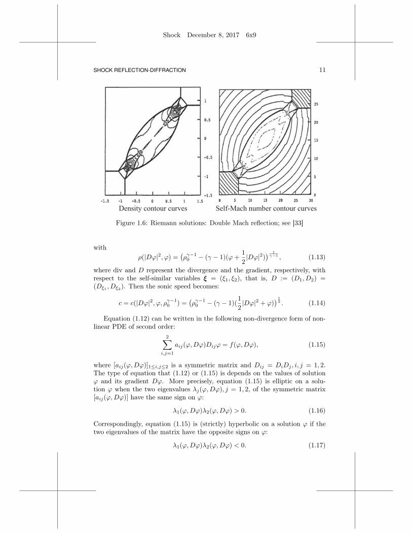
SHOCK REFLECTION-DIFFRACTION
Shock December 8, 2017 6x9
11
Density contour curves Self-Mach number contour curves
Figure 1.6: Riemann solutions: Double Mach reflection; see [33]
withρ(|Dϕ|2, ϕ) =
(ργ−1
0 − (γ − 1)(ϕ+1
2|Dϕ|2)
) 1γ−1 , (1.13)
where div and D represent the divergence and the gradient, respectively, withrespect to the self-similar variables ξ = (ξ1, ξ2), that is, D := (D1, D2) =(Dξ1 , Dξ2). Then the sonic speed becomes:
c = c(|Dϕ|2, ϕ, ργ−10 ) =
(ργ−1
0 − (γ − 1)(1
2|Dϕ|2 + ϕ)
) 12 . (1.14)
Equation (1.12) can be written in the following non-divergence form of non-linear PDE of second order:
2∑
i,j=1
aij(ϕ,Dϕ)Dijϕ = f(ϕ,Dϕ), (1.15)
where [aij(ϕ,Dϕ)]1≤i,j≤2 is a symmetric matrix and Dij = DiDj , i, j = 1, 2.The type of equation that (1.12) or (1.15) is depends on the values of solutionϕ and its gradient Dϕ. More precisely, equation (1.15) is elliptic on a solu-tion ϕ when the two eigenvalues λj(ϕ,Dϕ), j = 1, 2, of the symmetric matrix[aij(ϕ,Dϕ)] have the same sign on ϕ:
λ1(ϕ,Dϕ)λ2(ϕ,Dϕ) > 0. (1.16)
Correspondingly, equation (1.15) is (strictly) hyperbolic on a solution ϕ if thetwo eigenvalues of the matrix have the opposite signs on ϕ:
λ1(ϕ,Dϕ)λ2(ϕ,Dϕ) < 0. (1.17)

12
Shock December 8, 2017 6x9
CHAPTER 1
The more complicated case is that of the mixed elliptic-hyperbolic type for whichλ1(ϕ,Dϕ)λ2(ϕ,Dϕ) changes its sign when the values of ϕ and Dϕ change inthe physical domain under consideration.
In particular, equation (1.12) is a nonlinear second-order conservation lawof mixed elliptic-hyperbolic type. It is elliptic if
|Dϕ| < c(|Dϕ|2, ϕ, ργ−10 ), (1.18)
and hyperbolic if|Dϕ| > c(|Dϕ|2, ϕ, ργ−1
0 ). (1.19)
The types normally change with ξ from hyperbolic in the far field to ellipticaround the wedge vertex, which is the case that the corresponding physicalvelocity ∇xΦ is bounded.
Similarly, for the full Euler equations, the corresponding self-similar solutionsare governed by a nonlinear system of conservation laws of composite-mixedhyperbolic-elliptic type, as shown in (18.3.1) in Chapter 18.
Such nonlinear PDEs of mixed type also arise naturally in many other fun-damental problems in continuum physics, differential geometry, elasticity, rela-tivity, calculus of variations, and related areas.
Classical fundamental linear PDEs of mixed elliptic-hyperbolic type includethe following:
The Lavrentyev-Bitsadze equation for an unknown function u(x, y):
uxx + sign(x)uyy = 0. (1.20)
This becomes the wave equation (hyperbolic) in half-plane x < 0 and the Laplaceequation (elliptic) in half-plane x > 0, and changes the type from elliptic tohyperbolic via a jump discontinuous coefficient sign(x).
The Keldysh equation for an unknown function u(x, y):
xuxx + uyy = 0. (1.21)
This is hyperbolic in half-plane x < 0, elliptic in half-plane x > 0, and de-generates on line x = 0. This equation is of parabolic degeneracy in domainx ≤ 0, for which the two characteristic families are quadratic parabolas lyingin half-plane x < 0 and tangential at contact points to the degenerate linex = 0. Its degeneracy is also determined by the classical elliptic or hyperbolicEuler-Poisson-Darboux equation:
uττ ± uyy +β
τuτ = 0 (1.22)
with β = − 14 , where τ = 1
2 |x|12 , and signs “± ” in (1.22) are determined by the
corresponding half-planes ±x > 0.The Tricomi equation for an unknown function u(x, y):
uxx + xuyy = 0. (1.23)

SHOCK REFLECTION-DIFFRACTION
Shock December 8, 2017 6x9
13
This is hyperbolic when x < 0, elliptic when x > 0, and degenerates on linex = 0. This equation is of hyperbolic degeneracy in domain x ≤ 0, for which thetwo characteristic families coincide perpendicularly to line x = 0. Its degeneracyis also determined by the classical elliptic or hyperbolic Euler-Poisson-Darbouxequation (1.22) with β = 1
3 , where τ = 23 |x|
32 .
For linear PDEs of mixed elliptic-hyperbolic type such as (1.20)–(1.23), thetransition boundary between the elliptic and hyperbolic phases is known a pri-ori. One of the classical approaches to the study of such mixed-type linearequations is the fundamental solution approach, since the optimal regularityand/or singularities of solutions near the transition boundary are determinedby the fundamental solution (see [17, 37, 39, 41, 275, 278]).
For nonlinear PDEs of mixed elliptic-hyperbolic type such as (1.12), the tran-sition boundary between the elliptic and hyperbolic phases is a priori unknown,so that most of the classical approaches, especially the fundamental solutionapproach, no longer work. New ideas, approaches, and techniques are in greatdemand for both theoretical and numerical analysis.
(ii) Free Boundary Problems: Following the discussion in (i), above,the analysis of shock reflection-diffraction configurations can be reduced to theanalysis of a free boundary problem, as we will show in §2.4, in which thereflected-diffracted shock, defined as the transition boundary from the hyper-bolic to elliptic phase, is a free boundary that cannot be determined prior tothe determination of the solution.
The subject of free boundary problems has its origin in the study of theStefan problem, which models the melting of ice (cf. Stefan [250]). In thatproblem, the moving-in-time boundary between water and ice is not known apriori, but is determined by the solution of the problem. More generally, freeboundary problems are concerned with sharp transitions in the variables in-volved in the problems, such as the change in the temperature between waterand ice in the Stefan problem, and the changes in the velocity and densityacross the shock wave in the shock reflection-diffraction configurations. Mathe-matically, this rapid transition is simplified to be seen as occurring infinitely fastacross a curve or surface of discontinuity or constraint in the PDEs governingthe physical or other processes under consideration. The location of these curvesand surfaces, called free boundaries, is required to be determined in the processof solving the free boundary problem. Free boundaries subdivide the domaininto subdomains in which the governing equations (usually PDEs) are satisfied.On the free boundaries, the free boundary conditions, derived from the models,are prescribed. The number of conditions on the free boundary is such thatthe PDE governing the problem, combined with the free boundary conditions,allows us to determine both the location of the free boundary and the solution inthe whole domain. That is, more conditions are required on the free boundarythan in the case of the fixed boundary value problem for the same PDEs in afixed domain. Great progress has been made on free boundary problems for lin-ear PDEs. Further developments, especially in terms of solving such problems

14
Shock December 8, 2017 6x9
CHAPTER 1
for nonlinear PDEs of mixed type, ask for new mathematical approaches andtechniques. For a better sense of these, see Chen-Shahgholian-Vázquez [67] andthe references cited therein.
(iii) Estimates of Solutions to Nonlinear Degenerate PDEs: Thethird difficulty concerns the degeneracies that are along the sonic arc, since thesonic arc is another transition boundary from the hyperbolic to elliptic phase inthe shock reflection-diffraction configurations, for which the corresponding non-linear PDE becomes a nonlinear degenerate hyperbolic equation on its one sideand a nonlinear degenerate elliptic equation on the other side; both of these de-generate on the sonic arc. Also, unlike the reflected-diffracted shock, the sonicarc is not a free boundary; its location is explicitly known. In order to con-struct a global regular reflection-diffraction configuration, we need to determinethe unknown velocity potential in the subsonic (elliptic) domain such that thereflected-diffracted shock and the sonic arc are parts of its boundary. Thus, wecan view our problem as a free boundary problem for an elliptic equation ofsecond order with ellipticity degenerating along a part of the fixed boundary.Moreover, the solution should satisfy two Rankine-Hugoniot conditions on thetransition boundary of the elliptic region, which includes both the shock and thesonic arc. While this over-determinacy gives the correct number of free bound-ary conditions on the shock, the situation is different on the sonic arc that is afixed boundary. Normally, only one condition may be prescribed for the ellipticproblem. Therefore, we have to prove that the other condition is also satisfied onthe sonic arc by the solution. To achieve this, we exploit the detailed structureof the elliptic degeneracy of the nonlinear PDE to make careful estimates of thesolution near the sonic arc in the properly weighted and scaled C2,α–spaces, forwhich the nonlinearity plays a crucial role.
(iv) Corner Singularities: Further difficulties include the singularities ofsolutions at the corner formed by the reflected-diffracted shock (free boundary)and the sonic arc (degenerate elliptic curve), at the wedge vertex, as well asat the corner between the reflected shock and the wedge at the reflection pointfor the transition from the supersonic to subsonic regular reflection-diffractionconfigurations when the wedge angle decreases. For the latter, it requires uni-form a priori estimates for the solutions as the sonic arc shrinks to a point; thedegenerate ellipticity then changes to the uniform ellipticity when the wedgeangle decreases across the sonic angle up to the detachment angle, as describedin §2.4–§2.6.
These difficulties also arise in many further fundamental problems in continu-um physics (fluid/solid), differential geometry, mathematical physics, materialsscience, and other areas, such as transonic flow problems, isometric embeddingproblems, and phase transition problems; see [9, 10, 16, 93, 68, 69, 95, 99,139, 147, 168, 181, 220, 270, 286] and the references cited therein. Therefore,any progress in shock reflection-diffraction analysis requires new mathematicalideas, approaches, and techniques, all of which will be very useful for solvingother problems with similar difficulties and open up new research opportunities.

SHOCK REFLECTION-DIFFRACTION
Shock December 8, 2017 6x9
15
We focus mainly on the mathematics of shock reflection-diffraction and vonNeumann’s conjectures for potential flow, as well as offering (in Parts I–IV) newanalysis to overcome the associated difficulties. The mathematical approachesand techniques developed here will be useful in tackling other nonlinear prob-lems involving similar difficulties. One of the recent examples of this is thePrandtl-Meyer problem for supersonic flow impinging onto solid wedges, an-other longstanding open problem in mathematical fluid mechanics, which hasbeen treated in Bae-Chen-Feldman [5, 6].
In Part I, we state our main results and give an overview of the main stepsof their proofs.
In Part II, we present some relevant results for nonlinear elliptic equationsof second order (for which the structural conditions and some regularity of co-efficients are not required), convenient for applications in the rest of the book,and study the existence and regularity of solutions of certain boundary valueproblems in the domains of appropriate structure for an equation with elliptic-ity degenerating on a part of the boundary, which include the boundary valueproblems used in the construction of the iteration map in the later chapters.We also present basic properties of the self-similar potential flow equation, withfocus on the two-dimensional case.
In Part III, we first focus on von Neumann’s sonic conjecture – that is, theconjecture concerning the existence of regular reflection-diffraction solutions upto the sonic angle, with a supersonic shock reflection-diffraction configurationcontaining a transonic reflected-diffracted shock, and then provide its wholedetailed proof and related analysis. We treat this first on account of the factthat the presentation in this case is both foundational and relatively simplerthan that in the case beyond the sonic angle.
Once the analysis for the sonic conjecture is done, we present, in Part IV,our proof of von Neumann’s detachment conjecture – that is, the conjectureconcerning the existence of regular reflection-diffraction solutions, even beyondthe sonic angle up to the detachment angle, with a subsonic shock reflection-diffraction configuration containing a transonic reflected-diffracted shock. Thisis more technically involved. To achieve it, we make the whole iteration again,starting from the normal reflection when the wedge angle is π
2 , and prove theresults for both the supersonic and subsonic regular reflection-diffraction con-figurations by going over the previous arguments with the necessary additions(instead of writing all the details of the proof up to the detachment angle fromthe beginning). We present the proof in this way to make it more readable.
In Part V, we present the mathematical formulation of the shock reflection-diffraction problem for the full Euler equations and uncover the role of thepotential flow equation for the shock reflection-diffraction even in the realm ofthe full Euler equations. We also discuss further connections and their rolesin developing new mathematical ideas, techniques, and approaches for solvingfurther open problems in related scientific areas.

Shock December 8, 2017 6x9
Chapter Two
Mathematical Formulations and Main Theorems
In this chapter, we first analyze the potential flow equation (1.5) and its pla-nar shock-front solutions, and then formulate the shock reflection-diffractionproblem into an initial-boundary value problem. Next we employ the self-similarity of the problem to reformulate the initial-boundary value problem intoa boundary value problem in the self-similar coordinates. To solve von Neu-mann’s conjectures, we further reformulate the boundary value problem into afree boundary problem for a nonlinear second-order conservation law of mixedhyperbolic-elliptic type. Finally, we present the main theorems for the exis-tence, regularity, and stability of regular reflection-diffraction solutions of thefree boundary problem.
2.1 THE POTENTIAL FLOW EQUATION
The time-dependent potential flow equation of second order for the velocitypotential Φ takes the form of (1.5) with ρ(∂tΦ,∇xΦ) determined by (1.4), whichis a nonlinear wave equation.
Definition 2.1.1. A function Φ ∈ W 1,1loc (R+ × R2) is called a weak solution of
equation (1.5) in a domain D ⊂ R+ ×R2 if Φ satisfies the following properties:
(i) B0 −(∂tΦ + 1
2 |∇xΦ|2)≥ h(0+) a.e. in D;
(ii) (ρ(∂tΦ, |∇xΦ|2), ρ(∂tΦ, |∇xΦ|2)|∇xΦ|) ∈ (L1loc(D))2;
(iii) For every ζ ∈ C∞c (D),∫
D
(ρ(∂tΦ, |∇xΦ|2)∂tζ + ρ(∂tΦ, |∇xΦ|2)∇xΦ · ∇xζ
)dxdt = 0.
In the study of a piecewise smooth weak solution of (1.5) with jump for(∂tΦ,∇xΦ) across an oriented surface S with unit normal n = (nt,nx),nx =(n1, n2), in the (t,x)–coordinates, the requirement of the weak solution of (1.5)in the sense of Definition 2.1.1 yields the Rankine-Hugoniot jump conditionacross S:
[ρ(∂tΦ, |∇xΦ|2)]nt + [ρ(∂tΦ, |∇xΦ|2)∇xΦ] · nx = 0, (2.1.1)
where the square bracket, [w], denotes the jump of quantity w across the orientedsurface S; that is, assuming that S subdivides D into subregions D+ and D−

MATHEMATICAL FORMULATIONS AND MAIN THEOREMS
Shock December 8, 2017 6x9
17
so that, for every (t,x) ∈ S, there exists ε > 0 such that (t,x) ± sn ∈ D± ifs ∈ (0, ε), define
[w](t,x) := lim(τ,y) → (t,x)
(τ,y) ∈ D+
w(τ,y)− lim(τ,y) → (t,x)
(τ,y) ∈ D−
w(τ,y).
Notice that Φ ∈W 1,1 is required in Definition 2.1.1, which implies the continuityof Φ across a shock-front S for piecewise smooth solutions:
[Φ]S = 0. (2.1.2)
In fact, the continuity of Φ in (2.1.2) can also be derived for the piecewisesmooth solution Φ (without assumption Φ ∈W 1,1) by requiring that Φ keep thevalidity of the equations:
∇x × v = 0, ∂tv = ∇x(∂tΦ) (2.1.3)
in the sense of distributions. This is tantamount to requiring that
(∂tΦ,v) = (∂tΦ,∇xΦ). (2.1.4)
The condition on v is that
(∂t,∇x)× (∂tΦ,v) = 0,
which is equivalent to (2.1.3). By definition, the equations in (2.1.4) for piecewisesmooth solutions are understood as
∫∫Φ∂xiψ dtdx = −
∫∫viψ dtdx, i = 1, 2,
for any test function ψ ∈ C∞0 ((0,∞) × R2). Using the Gauss-Green formulain the two regions of continuity of (∂tΦ,∇xΦ) separated by S in the standardfashion, we obtain ∫
S[Φ]ψ dσ = 0,
where dσ is the surface measure on S. This implies the continuity of Φ across ashock-front S in (2.1.2).
The discontinuity S of (∂tΦ,∇xΦ) is called a shock if Φ further satisfies thephysical entropy condition: The corresponding density function ρ(∂tΦ,∇xΦ)increases across S in the relative flow direction with respect to S (cf. [94, 99]).
Definition 2.1.2. Let Φ be a piecewise smooth weak solution of (1.5) with jumpfor (∂tΦ,∇xΦ) across an oriented surface S. The discontinuity S of (∂tΦ,∇xΦ)is called a shock if Φ further satisfies the physical entropy condition: The cor-responding density function ρ(∂tΦ,∇xΦ) increases across S in the relative flowdirection with respect to S (cf. [94, 99]).
18
Shock December 8, 2017 6x9
CHAPTER 2
The jump condition in (2.1.1) from the conservation of mass and the continu-ity of Φ in (2.1.2) are the conditions that are actually used in practice, especiallyin aerodynamics, resulting from the Rankine-Hugoniot conditions for the time-dependent potential flow equation (1.5). The empirical evidence for this is thatentropy solutions of (1.1) or (1.5) are fairly close to the corresponding entropysolutions of the full Euler equations, provided that the strengths of shock-frontsare small, the curvatures of shock-fronts are not too large, and the amount ofvorticity is small in the region of interest. In fact, for the solutions containing aweak shock, especially in aerodynamic applications, the potential flow equation(1.5) and the full Euler flow model (1.7) match each other well up to the thirdorder of the shock strength. Furthermore, we will show in Chapter 18 that, forthe shock reflection-diffraction problem, the Euler equations (1.1) for potentialflow are actually an exact match in an important region of the shock reflection-diffraction configurations to the full Euler equations (1.7). See also Bers [16],Glimm-Majda [139], and Morawetz [220, 221, 222].
Planar shock-front solutions are special piecewise smooth solutions given bythe explicit formulae:
Φ =
Φ+, x1 > st,
Φ−, x1 < st(2.1.5)
withΦ± = a±0 t+ u±x1 + v±x2. (2.1.6)
Then the continuity condition (2.1.2) of Φ across the shock-front implies
[v] = 0, [a0] + s[u] = 0. (2.1.7)
The jump condition (2.1.1) yields
s[ρ] = [ρu], (2.1.8)
since n = 1√s2+1
(−s, 1, 0).The relation between ρ and Φ via the Bernoulli law is
[a0 +1
2u2] +
1
γ − 1[ργ−1] = 0, (2.1.9)
where we have used (1.2) for polytropic gases. From now on, we focus on γ > 1.Combining (2.1.7)–(2.1.9), we conclude
[u] = −√
2[ρ][ργ−1]
(γ − 1)(ρ+ + ρ−),
[a0] = − [ρu][u]
[ρ],
s =[ρu]
[ρ].
(2.1.10)

MATHEMATICAL FORMULATIONS AND MAIN THEOREMS
Shock December 8, 2017 6x9
19
This implies that the shock speed s is
s = u+ + ρ−
√2[ργ−1]
(γ − 1)[ρ2]. (2.1.11)
The entropy condition is
ρ+ < ρ− if u± > 0. (2.1.12)
2.2 MATHEMATICAL PROBLEMS FOR SHOCKREFLECTION-DIFFRACTION
When a plane shock in the (t,x)–coordinates, t ∈ R+ := [0,∞),x = (x1, x2) ∈R2, with left state (ρ,∇xΦ) = (ρ1, u1, 0) and right state (ρ0, 0, 0), u1 > 0, ρ0 <ρ1, hits a symmetric wedge
W := x : |x2| < x1 tan θw, x1 > 0head-on (see Fig. 1.1), it experiences a reflection-diffraction process. Thensystem (1.1) in R+ × (R2 \W ) becomes
∂tρ+ divx(ρ∇xΦ) = 0,
∂tΦ +1
2|∇xΦ|2 +
ργ−1 − ργ−10
γ − 1= 0,
(2.2.1)
where we have used the Bernoulli constant B0 =ργ−1
0 −1γ−1 determined by the right
state (ρ0, 0, 0). From (2.1.10), we find that u1 > 0 is uniquely determined by(ρ0, ρ1) and γ > 1:
u1 =
√2(ρ1 − ρ0)(ργ−1
1 − ργ−10 )
(γ − 1)(ρ1 + ρ0)> 0, (2.2.2)
where we have used that ρ0 < ρ1.Then the shock reflection-diffraction problem can be formulated as the fol-
lowing problem:
Problem 2.2.1 (Initial-Boundary Value Problem). Seek a solution of system(2.2.1) for B0 =
ργ−10 −1γ−1 with the initial condition at t = 0:
(ρ,Φ)|t=0 =
(ρ0, 0) for |x2| > x1 tan θw, x1 > 0,
(ρ1, u1x1) for x1 < 0,(2.2.3)
and the slip boundary condition along the wedge boundary ∂W :
∇xΦ · ν|R+×∂W = 0, (2.2.4)
where ν is the exterior unit normal to ∂W (see Fig. 2.1).

20
Shock December 8, 2017 6x9
CHAPTER 2
· =0
x1wθ
(1) (0)
ν
Incident shock
Φ∇
ν
x2
Figure 2.1: Initial-boundary value problem
Notice that the initial-boundary value problem (Problem 2.2.1) is invariantunder the self-similar scaling:
(t,x) 7→ (αt, αx), (ρ,Φ) 7→ (ρ,Φ
α) for α 6= 0. (2.2.5)
That is, if (ρ,Φ)(t,x) satisfy (2.2.1)–(2.2.4), so do (ρ, Φα )(αt, αx) for any constant
α 6= 0.Therefore, we seek self-similar solutions with the following form:
ρ(t,x) = ρ(ξ), Φ(t,x) = t φ(ξ) for ξ = (ξ1, ξ2) =x
t. (2.2.6)
We then see that the pseudo-potential function ϕ = φ− |ξ|2
2 satisfies the followingEuler equations for self-similar solutions:
div (ρDϕ) + 2ρ = 0,
(γ − 1)(1
2|Dϕ|2 + ϕ) + ργ−1 = ργ−1
0 ,(2.2.7)
where div and D represent the divergence and the gradient, respectively, withrespect to the self-similar variables ξ.
This implies that the pseudo-potential function ϕ(ξ) is governed by the fol-lowing potential flow equation of second order:
div(ρ(|Dϕ|2, ϕ)Dϕ
)+ 2ρ(|Dϕ|2, ϕ) = 0 (2.2.8)
withρ(|Dϕ|2, ϕ) =
(ργ−1
0 − (γ − 1)(ϕ+1
2|Dϕ|2)
) 1γ−1 . (2.2.9)
We consider (2.2.8) with (2.2.9) for functions ϕ satisfying
ργ−10 − (γ − 1)
(ϕ+
1
2|Dϕ|2
)≥ 0. (2.2.10)

MATHEMATICAL FORMULATIONS AND MAIN THEOREMS
Shock December 8, 2017 6x9
21
Definition 2.2.2. A function ϕ ∈W 1,1loc (Ω) is called a weak solution of equation
(2.2.8) in domain Ω if ϕ satisfies (2.2.10) and the following properties:
(i) For ρ(|Dϕ|2, ϕ) determined by (2.2.9),
(ρ(|Dϕ|2, ϕ), ρ(|Dϕ|2, ϕ)|Dϕ|) ∈ (L1loc(Ω))2;
(ii) For every ζ ∈ C∞c (Ω),∫
Ω
(ρ(|Dϕ|2, ϕ)Dϕ ·Dζ − 2ρ(|Dϕ|2, ϕ)ζ
)dξ = 0.
We will also use the non-divergence form of equation (2.2.8) for φ = ϕ+ |ξ|2
2 :
(c2 − ϕ2ξ1)φξ1ξ1 − 2ϕξ1ϕξ2φξ1ξ2 + (c2 − ϕ2
ξ2)φξ2ξ2 = 0, (2.2.11)
where the sonic speed c = c(|Dϕ|2, ϕ, ργ−10 ) is determined by (1.14).
Equation (2.2.8) or (2.2.11) is a nonlinear second-order PDE of mixed elliptic-hyperbolic type. It is elliptic if and only if (1.18) holds, which is equivalent tothe following condition:
|Dϕ| < c∗(ϕ, ρ0, γ) :=
√2
γ + 1
(ργ−1
0 − (γ − 1)ϕ). (2.2.12)
Throughout the rest of this book, for simplicity, we drop term “pseudo” andsimply call ϕ as a potential function and Dϕ as a velocity, respectively, whenno confusion arises.
Shocks are discontinuities in the velocity functions Dϕ. That is, if Ω+ andΩ− := Ω \Ω+ are two non-empty open subsets of Ω ⊂ R2, and S := ∂Ω+ ∩Ω isa C1–curve where Dϕ has a jump, then ϕ ∈ W 1,1
loc (Ω) ∩ C1(Ω±) ∩ C2(Ω±) is aglobal weak solution of (2.2.8) in Ω in the sense of Definition 2.2.2 if and only ifϕ is in W 1,∞
loc (Ω) and satisfies equation (2.2.8) in Ω± and the Rankine-Hugoniotcondition on S: [
ρ(|Dϕ|2, ϕ)Dϕ · ν]S = 0. (2.2.13)
Note that the condition that ϕ ∈ W 1,∞loc (Ω) implies the continuity of ϕ across
shock S:[ϕ]S = 0. (2.2.14)
The plane incident shock solution in the (t,x)–coordinates with the left andright states:
(ρ,∇xΦ) = (ρ0, 0, 0), (ρ1, u1, 0)
corresponds to a continuous weak solution ϕ of (2.2.8) in the self-similar coor-dinates ξ with the following form:
ϕ =
ϕ0 for ξ1 > ξ0
1 ,
ϕ1 for ξ1 < ξ01 ,
(2.2.15)

22
Shock December 8, 2017 6x9
CHAPTER 2
where
ϕ0(ξ) = −|ξ|2
2, (2.2.16)
ϕ1(ξ) = −|ξ|2
2+ u1(ξ1 − ξ0
1), (2.2.17)
and
ξ01 = ρ1
√2(ργ−1
1 − ργ−10 )
(γ − 1)(ρ21 − ρ2
0)=
ρ1u1
ρ1 − ρ0> 0 (2.2.18)
is the location of the incident shock in the ξ–coordinates, uniquely determinedby (ρ0, ρ1, γ) through (2.2.13), which is obtained from (2.1.11) and (2.2.2) owingto the fact that ξ0
1 = s here. Since the problem is symmetric with respect tothe ξ1–axis, it suffices to consider the problem in half-plane ξ2 > 0 outside thehalf-wedge:
Λ := ξ : ξ1 ∈ R, ξ2 > max(ξ1 tan θw, 0). (2.2.19)
Then the initial-boundary value problem (2.2.1)–(2.2.4) in the (t,x)–coordinatescan be formulated as a boundary value problem in the self-similar coordinatesξ.
·ϕ∇
=0
wθ
ν
2ξ
1ξ
θtan1ξ=2ξ
10ξ
=0
ν
2ξϕ
1ϕ
ϕ
ϕ
0ϕIncident shock
Figure 2.2: Boundary value problem
Problem 2.2.3 (Boundary Value Problem; see Fig. 2.2). Seek a solution ϕ ofequation (2.2.8) in the self-similar domain Λ with the slip boundary condition:
Dϕ · ν|∂Λ = 0 (2.2.20)
and the asymptotic boundary condition at infinity:
ϕ→ ϕ =
ϕ0 for ξ ∈ Λ, ξ1 > ξ0
1 ,
ϕ1 for ξ ∈ Λ, ξ1 < ξ01 ,
when |ξ| → ∞, (2.2.21)

MATHEMATICAL FORMULATIONS AND MAIN THEOREMS
Shock December 8, 2017 6x9
23
where (2.2.21) holds in the sense that limR→∞
‖ϕ− ϕ‖C0,1(Λ\BR(0)) = 0.
This is a boundary value problem for the second-order nonlinear conservationlaw (2.2.8) of mixed elliptic-hyperbolic type in an unbounded domain. Themain feature of this boundary value problem is that Dϕ has a jump at ξ1 = ξ0
1
at infinity, which is not conventional, coupling with the wedge corner for thedomain. The solutions with complicated patterns of wave configurations asobserved experimentally should be the global solutions of this boundary valueproblem: Problem 2.2.3.
2.3 WEAK SOLUTIONS OF PROBLEM 2.2.1 ANDPROBLEM 2.2.3
Note that the boundary condition (2.2.20) for Problem 2.2.3 implies
ρDϕ · ν|∂Λ = 0. (2.3.1)
Conditions (2.2.20) and (2.3.1) are equivalent if ρ 6= 0. Since ρ 6= 0 for thesolutions under consideration, we use condition (2.3.1) instead of (2.2.20) in thedefinition of weak solutions of Problem 2.2.3.
Similarly, we write the boundary condition (2.2.4) for Problem 2.2.1 as
ρ∇xΦ · ν|R+×∂W = 0. (2.3.2)
Condition (2.3.1) is the conormal condition for equation (2.2.8). Also, (2.3.2)is the spatial conormal condition for equation (1.5). This yields the followingdefinitions:
Definition 2.3.1 (Weak Solutions of Problem 2.2.1). A function
Φ ∈W 1,1loc (R+ × (R2 \W ))
is called a weak solution of Problem 2.2.1 if Φ satisfies the following properties:
(i) B0 −(∂tΦ + 1
2 |∇xΦ|2)≥ h(0+) a.e. in R+ × (R2 \W );
(ii) For ρ(∂tΦ,∇xΦ) determined by (1.4),
(ρ(∂tΦ, |∇xΦ|2), ρ(∂tΦ, |∇xΦ|2)|∇xΦ|) ∈ (L1loc(R+ × R2 \W ))2;
(iii) For every ζ ∈ C∞c (R+ × R2),∫ ∞
0
∫
R2\W
(ρ(∂tΦ, |∇xΦ|2)∂tζ + ρ(∂tΦ, |∇xΦ|2)∇Φ · ∇ζ
)dxdt
+
∫
R2\Wρ|t=0ζ(0,x)dx = 0,

24
Shock December 8, 2017 6x9
CHAPTER 2
where
ρ|t=0 =
ρ0 for |x2| > x1 tan θw, x1 > 0,
ρ1 for x1 < 0.
Remark 2.3.2. Since ζ does not need to be zero on ∂W , the integral identityin Definition 2.3.1 is a weak form of equation (1.5) and the boundary condition(2.3.2).
Definition 2.3.3 (Weak solutions of Problem 2.2.3). A function ϕ ∈W 1,1loc (Λ)
is called a weak solution of Problem 2.2.3 if ϕ satisfies (2.2.21) and the fol-lowing properties:
(i) ργ−10 − (γ − 1)
(ϕ+ 1
2 |Dϕ|2)≥ 0 a.e. in Λ;
(ii) For ρ(|Dϕ|2, ϕ) determined by (2.2.9),
(ρ(|Dϕ|2, ϕ), ρ(|Dϕ|2, ϕ)|Dϕ|) ∈ (L1loc(Λ))2;
(iii) For every ζ ∈ C∞c (R2),∫
Λ
(ρ(|Dϕ|2, ϕ)Dϕ ·Dζ − 2ρ(|Dϕ|2, ϕ)ζ
)dξ = 0.
Remark 2.3.4. Since ζ does not need to be zero on ∂Λ, the integral identity inDefinition 2.3.3 is a weak form of equation (2.2.8) and the boundary condition(2.3.1).
Remark 2.3.5. From Definition 2.3.3, we observe the following fact: If B ⊂ R2
is an open set, and ϕ is a weak solution of Problem 2.2.3 satisfying ϕ ∈C2(B ∩ Λ) ∩ C1(B ∩ Λ), then ϕ satisfies equation (2.2.8) in the classical sensein B ∩ Λ, the boundary condition (2.3.1) on B ∩ ∂Λ \ 0, and Dϕ(0) = 0.
2.4 STRUCTURE OF SOLUTIONS: REGULARREFLECTION-DIFFRACTION CONFIGURATIONS
We now discuss the structure of solutions ϕ of Problem 2.2.3 correspondingto shock reflection-diffraction.
Since ϕ1 does not satisfy the slip boundary condition (2.2.20), the solutionmust differ from ϕ1 in ξ1 < ξ0
1 ∩ Λ so that a shock diffraction by the wedgeoccurs. We now describe two of the most important configurations: the su-personic and subsonic regular reflection-diffraction configurations, as shown inFig. 2.3 and Fig. 2.4, respectively. From now on, we will refer to these twoconfigurations as a supersonic reflection configuration and a subsonic reflectionconfiguration respectively, whose corresponding solutions are called the super-sonic reflection solution and the subsonic reflection solution respectively, whenno confusion arises.

MATHEMATICAL FORMULATIONS AND MAIN THEOREMS
Shock December 8, 2017 6x9
25
(2)
wθ
(0)(1)
Ω
Sonic circle of (2)
Incident shock
Reflect
ed-diffr
acted
shock
1ξ2P
3P
0P1P
4P
Figure 2.3: Supersonic regu-lar reflection-diffraction config-uration
Incident shock
Ω
Reflected-diffracted
shock
(0)(1)
wθ
1ξ2P
0P
3P
Figure 2.4: Subsonic regularreflection-diffraction configura-tion
In Figs. 2.3 and 2.4, the vertical line is the incident shock S0 = ξ1 = ξ01
that hits the wedge at point P0 = (ξ01 , ξ
01 tan θw), and state (0) and state (1),
ahead of and behind S0, are given by ϕ0 and ϕ1 defined in (2.2.16) and (2.2.17),respectively. Thus, we only need to describe the solution in subregion P0P2P3
between the wedge and the reflected-diffracted shock. The solution is expectedto be C1 in P0P2P3. Now we describe its structure. Below, ϕ denotes thepotential of the solution in P0P2P3, while we use the uniform states ϕ0 and ϕ1
to describe the solution outside P0P2P3, ahead of and behind the incident shockS1, respectively. In particular, Dϕ(P0) denotes the limit at P0 of the gradientof the solution in P0P2P3.
2.4.1 Definition of state (2)
Since ϕ is C1 in region P0P2P3, it should satisfy the boundary conditionDϕ·ν =0 on the wedge boundary P0P3 including the endpoints, as well as the Rankine-Hugoniot conditions (2.2.13)–(2.2.14) at P0 across the reflected shock separatingϕ from ϕ1. Let
(u2, v2) := Dϕ(P0) + ξP0.
Then v2 = u2 tan θw by Dϕ ·ν = 0. Moreover, using (2.2.17), in addition to theprevious properties, we see by a direct calculation that the uniform state withthe pseudo-potential:
ϕ2(ξ) = −|ξ|2
2+ u2(ξ1 − ξ0
1) + u2 tan θw(ξ2 − ξ01 tan θw), (2.4.1)
called state (2), satisfies the boundary condition on the wedge boundary:
Dϕ2 · ν = 0 on ∂Λ ∩ ξ1 = ξ2 cot θw, (2.4.2)
and the Rankine-Hugoniot conditions (2.2.13) on the flat shock S1 determinedby (2.2.14):
S1 := ϕ1 = ϕ2 (2.4.3)

26
Shock December 8, 2017 6x9
CHAPTER 2
which passes through P0 between states (1) and (2).We note that the constant velocity u2 > 0 is determined by (ρ0, ρ1, γ, θw)
from the algebraic equation expressing (2.2.13) for ϕ1 and ϕ2 across S1, wherewe have used (2.2.2) to eliminate u1 from the list of parameters and have notedthat νS1
= (u1−u2,−u2 tan θw)|(u1−u2,−u2 tan θw)| .
Thus, state (2) is defined by the following requirements: It is a uniform statewith pseudo-potential ϕ2(ξ) such that Dϕ2 · ν = 0 on the wedge boundary, andthe Rankine-Hugoniot conditions (2.2.13)–(2.2.14) for ϕ1 and ϕ2 hold at P0. Aswe will discuss in §2.5, such a state (2) exists for any wedge angle θw ∈ [θd
w,π2 ],
for some θdw = θd
w(ρ0, ρ1, γ) > 0. From the discussion above, it is apparent thatthe existence of state (2) is a necessary condition for the existence of regularreflection-diffraction configurations as shown in Figs. 2.3–2.4.
From now on, we fix the data, i.e., parameters (ρ0, ρ1, γ). Thus, the param-eters of state (2) depend only on θw.
State (2) can be either pseudo-subsonic or pseudo-supersonic at P0. Thisdetermines the subsonic or supersonic type of regular reflection-diffraction con-figurations, as shown in Figs. 2.3–2.4.
We note that the uniform state (2) is pseudo-subsonic within its sonic circlewith center O2 = (u2, u2 tan θw) and radius c2 = ρ
(γ−1)/22 > 0, the sonic speed
of state (2), and that ϕ2 is pseudo-supersonic outside this circle.Thus, if state (2) is pseudo-supersonic at P0, P0 lies outside the sonic cir-
cle Bc2(O2) of state (2). It can be shown (see §7.5) that line S1 intersects∂Bc2(O2) at two points and, denoting by P1 the point that is closer to P0, wefind that P1 lies in Λ and segment P0P1 lies in Λ and outside of Bc2(u2, v2); seeFig. 2.3. Denote by P4 the point of intersection of ∂Bc2(O2) with the wedgeboundary ξ2 = ξ1 tan θw, ξ1 > 0 such that arc P1P4 lies between S1 andξ2 = ξ1 tan θw, ξ1 > 0.
2.4.2 Supersonic regular reflection-diffraction configurations
This is the case when state (2) is supersonic at P0.The supersonic reflection configuration as shown in Fig. 2.3 consists of three
uniform states: (0), (1), (2), plus a non-uniform state in domain Ω = P1P2P3P4.As described above, the solution is equal to state (0) and state (1) ahead of andbehind the incident shock S0, away from subregion P0P2P3. The solution isequal to state (2) in subregion P0P1P4. Note that state (2) is supersonic inP0P1P4.
The non-uniform state in Ω is subsonic, i.e., the potential flow equation(2.2.8) for ϕ is elliptic in Ω.
We denote the boundary parts of Ω by
Γshock := P1P2, Γsym := P2P3, Γwedge := P3P4, Γsonic := P1P4, (2.4.4)
where Γshock is the curved part of the reflected shock, Γsonic is the sonic arc, andΓwedge (the wedge boundary) and Γsym are the straight segments, respectively.

MATHEMATICAL FORMULATIONS AND MAIN THEOREMS
Shock December 8, 2017 6x9
27
Note that the curved part of the reflected shock Γshock separates the su-personic flow outside Ω from the subsonic flow in Ω, i.e., Γshock is a transonicshock.
2.4.3 Subsonic regular reflection-diffraction configurations
This is the case when state (2) is subsonic or sonic at P0.The subsonic reflection configuration as shown in Fig. 2.4 consists of two
uniform states – (0) and (1) – in the regions described above, and a non-uniformstate in domain Ω = P0P2P3. The non-uniform state in Ω is subsonic, i.e., thepotential flow equation (2.2.8) for ϕ is elliptic in Ω. Moreover, solution ϕ in Ωmatches with ϕ2 at P0 as follows:
ϕ(P0) = ϕ2(P0), Dϕ(P0) = Dϕ2(P0).
The boundary parts of Ω in this case are
Γshock := P0P2, Γsym := P2P3, Γwedge := P0P3. (2.4.5)
Similar to the previous case, Γshock is a transonic shock. We unify the notationswith supersonic reflection configurations by introducing points P1 and P4 forsubsonic reflection configurations via setting
P1 := P0, P4 := P0, Γsonic := P0. (2.4.6)
Note that, with this convention, (2.4.5) coincides with (2.4.4).In Part III, we develop approaches, techniques, and related analysis to es-
tablish the global existence of a supersonic reflection configuration up to thesonic angle, or the critical angle in the attached case (defined in §2.6).
In Part IV, we develop the theory further to establish the global existence ofregular reflection-diffraction configurations up to the detachment angle, or thecritical angle in the attached case. In particular, this will imply the existence ofboth supersonic and subsonic reflection configurations.
2.5 EXISTENCE OF STATE (2) AND CONTINUOUSDEPENDENCE ON THE PARAMETERS
We note that state (2), the uniform state (2.4.1), satisfies (2.4.2) and theRankine-Hugoniot condition with state (1) on S1 = ϕ1 = ϕ2 as defined in(2.4.3):
ρ2Dϕ2 · ν = ρ1Dϕ1 · ν on S1, (2.5.1)
where ν is the unit normal on S1.From the regular reflection-diffraction configurations as described in §2.4.2–
§2.4.3, the existence of state (2) is a necessary condition for the existence ofsuch a solution. We note that S1, defined in (2.4.3), is a straight line, which

28
Shock December 8, 2017 6x9
CHAPTER 2
is concluded from the explicit expressions of ϕj , j = 1, 2, and the fact that(u1, 0) 6= (u2, v2). The last statement holds since ϕ1 does not satisfy (2.4.2).
State (2), (u2, v2) in (2.4.1), is obtained as a solution of the algebraic systeminvolving the slope of S1 (i.e., the direction of ν) and the equality in (2.5.1); see§7.4 below.
This algebraic system has solutions for some but not all θw ∈ (0, π2 ). Moreprecisely, there exist the sonic angle θs
w and the detachment angle θdw satisfying
0 < θdw < θs
w <π
2
such that there are two states (2), weak and strong with ρwk2 < ρsg
2 , for allθw ∈ (θd
w,π2 ), but ρwk
2 = ρsg2 at θw = θd
w. Moreover, the strong state (2) isalways subsonic at the reflection point P0(θw), while the weak state (2) is:
(i) supersonic at the reflection point P0(θw) for θw ∈ (θsw,
π2 );
(ii) sonic at P0(θw) for θw = θsw;
(iii) subsonic at P0(θw) for θw ∈ (θdw, θ
sw), for some θs
w ∈ (θdw, θ
sw].
Moreover, the weak state (2)= (u2, v2) depends continuously on θw in [θdw,
π2 ].
For details of this, see Theorem 7.1.1 in Chapter 7.As for the weak and strong states for each θw ∈ (θd
w,π2 ), there has been a
long debate to determine which one is physical for the local theory; see Courant-Friedrichs [99], Ben-Dor [12], and the references cited therein. It has beenconjectured that the strong reflection-diffraction configuration is non-physical.Indeed, when the wedge angle θw tends to π
2 , the weak reflection-diffraction con-figuration tends to the unique normal reflection as proved in Chen-Feldman [54];however, the strong reflection-diffraction configuration does not (see Chapter 7below).
In the existence results of regular reflection-diffraction solutions below, wealways use the weak state (2).
2.6 VON NEUMANN’S CONJECTURES, PROBLEM 2.6.1(FREE BOUNDARY PROBLEM), AND MAIN THEOREMS
If the weak state (2) is supersonic, on which equation (2.2.8) is hyperbolic,the propagation speeds of the solution are finite, and state (2) is completelydetermined by the local information: state (1), state (0), and the location ofpoint P0. That is, any information from the region of shock reflection-diffraction,such as the disturbance at corner P3, cannot travel towards the reflection pointP0. However, if the weak state (2) is subsonic, on which equation (2.2.8) iselliptic, the information can reach P0 and interact with it, potentially creating anew type of shock reflection-diffraction configurations. This argument motivatedthe conjecture by von Neumann in [267, 268], which can be formulated as follows:

MATHEMATICAL FORMULATIONS AND MAIN THEOREMS
Shock December 8, 2017 6x9
29
von Neumann’s Sonic Conjecture: There exists a supersonic regularreflection-diffraction configuration when θw ∈ (θs
w,π2 ), i.e., the supersonicity
of the weak state (2) at P0(θw) implies the existence of a supersonic regularreflection-diffraction configuration to Problem 2.2.3 as shown in Fig. 2.3.
Another conjecture states that the global regular reflection-diffraction con-figuration is possible whenever the local regular reflection at the reflection pointP0 is possible, even beyond the sonic angle θs
w up to the detachment angle θdw:
von Neumann’s Detachment Conjecture: There exists a global regu-lar reflection-diffraction configuration for any wedge angle θw ∈ (θd
w,π2 ), i.e.,
the existence of state (2) implies the existence of a regular reflection-diffractionconfiguration to Problem 2.2.3. Moreover, the type (subsonic or supersonic)of the reflection-diffraction configuration is determined by the type of the weakstate (2) at P0(θw), as shown in Figs. 2.3–2.4.
It is clear that the supersonic and subsonic reflection configurations are notpossible without a local two-shock configuration at the reflection point on thewedge, so that it is the necessary criterion for the existence of supersonic andsubsonic reflection configurations.
There has been a long debate in the literature whether there still exists aglobal regular reflection-diffraction solution beyond the sonic angle θs
w up tothe detachment angle θd
w; see Ben-Dor [12] and the references cited therein. Asshown in Fig. 18.7 for the full Euler case, the difference on the physical pa-rameters between the sonic conjecture and the detachment conjecture is onlyfractions of a degree apart in terms of the wedge angles; a resolution has chal-lenged even sophisticated modern numerical and laboratory experiments. InPart IV (Chapters 15–17), we rigorously prove the global existence of regularreflection-diffraction configurations, beyond the sonic angle up to the detach-ment angle. This indicates that the necessary criterion is also sufficient forthe existence of supersonic and subsonic reflection configurations, at least forpotential flow.
To solve von Neumann’s conjectures, we reformulate Problem 2.2.3 intothe following free boundary problem:
Problem 2.6.1 (Free Boundary Problem). For θw ∈ (θdw,
π2 ), find a free bound-
ary (curved reflected-diffracted shock) Γshock in region Λ ∩ ξ1 < ξ1P1 (where
we use (2.4.6) for subsonic reflections) and a function ϕ defined in region Ω asshown in Figs. 2.3–2.4 such that ϕ satisfies:
(i) Equation (2.2.8) in Ω;
(ii) ϕ = ϕ1 and ρDϕ · ν = ρ1Dϕ1 · ν on the free boundary Γshock separatingthe elliptic phase from the hyperbolic phase;
(iii) ϕ = ϕ2 and Dϕ = Dϕ2 on Γsonic for the supersonic reflection configurationas shown in Fig. 2.3 and at P0 for the subsonic reflection configuration asshown in Fig. 2.4;
30
Shock December 8, 2017 6x9
CHAPTER 2
(iv) Dϕ · ν = 0 on Γwedge ∪ Γsym,
where ν is the interior unit normal to Ω on Γshock ∪ Γwedge ∪ Γsym.
We remark that condition (iii) is equivalent to the Rankine-Hugoniot condi-tions for ϕ across Γsonic. The sonic arc Γsonic is a weak discontinuity of ϕ (whichis different from a strong discontinuity such as Γshock); that is, if the state fromone side is sonic, the Rankine-Hugoniot conditions require the gradient of ϕ tobe continuous across Γsonic.
Furthermore, since condition (ii) is the Rankine-Hugoniot conditions for ϕacross Γshock, we can extend solution ϕ of Problem 2.6.1 from Ω to Λ so thatthe extended function (still denoted) ϕ is a weak solution of Problem 2.2.3(at least when Γshock and ϕ are sufficiently regular). More specifically,
Definition 2.6.2. Let ϕ be a solution of Problem 2.6.1 in region Ω. Definethe extension of ϕ from Ω to Λ by setting:
ϕ =
ϕ0 for ξ1 > ξ01 and ξ2 > ξ1 tan θw,
ϕ1 for ξ1 < ξ01 and above curve P0P1P2,
ϕ2 in region P0P1P4,
(2.6.1)
where we have used the notational convention (2.4.6) for subsonic reflections.In particular, for subsonic reflections, region P0P1P4 is one point, and curveP0P1P2 is P0P2. See Figs. 2.3 and 2.4.
We note that ξ01 used in (2.6.1) is the location of the incident shock; cf.
(2.2.15) and (2.2.18). Also, the extension by (2.6.1) is well-defined because ofthe requirement Γshock ⊂ Λ ∩ ξ1 < ξ1P1
in Problem 2.6.1.From now on, using Definition 2.6.2, we consider solutions ϕ of Problem
2.6.1 to be defined in Λ.It turns out that another key obstacle for establishing the existence of regular
reflection-diffraction configurations is the additional possibility that, for somewedge angle θc
w ∈ (θdw,
π2 ), the reflected-diffracted shock P0P2 may strike the
wedge vertex P3, an additional sub-type of regular reflection-diffraction config-urations in which the reflected-diffracted shock is attached to the wedge vertexP3, i.e., P2 = P3. Indeed, in such a case, we establish the existence of such aglobal solution of regular reflection-diffraction configurations as shown in Figs.2.5–2.6 for any wedge angle θw ∈ (θc
w,π2 ).
Observe that some experimental results (cf. [263, Fig. 238, Page 144])suggest that solutions with an attached shock to the wedge vertex may existfor the Mach reflection case. We are not aware of experimental or numericalevidence of the existence of regular reflection-diffraction configurations with anattached shock to the wedge vertex. However, it is possible that such solutionsmay exist, as shown in Figs. 2.5–2.6. Thus, it is not surprising that two differentcases on the parameters of the initial data in Problem 2.2.1 are consideredseparately in our study.

MATHEMATICAL FORMULATIONS AND MAIN THEOREMS
Shock December 8, 2017 6x9
31
Ω
(2)
wθ
1O=
1> c1u
Sonic circle of (1)
Sonic circle of (2)
Incident shock
(0)(1)
Reflec
ted-d
iffra
cted
sh
ock
1ξ2P 3P
0P1P
Figure 2.5: Attached supersonic reg-ular reflection-diffraction configura-tion
Reflec
ted-diff
racted
shock
1> c1u
Ω
1O=
Sonic circle of (1)
Incident shock
(0)(1)
1ξ2P 3P
0P
wθ
Figure 2.6: Attached subsonic reg-ular reflection-diffraction configura-tion
We show that the solutions with an attached shock do not exist when theinitial data of Problem 2.2.1, equivalently parameters (ρ0, ρ1, γ) in Problem2.6.1 which also define u1 by (2.2.2), satisfy u1 ≤ c1. Moreover, in this case,the regular reflection-diffraction solution of Problem 2.6.1 exists for each θw ∈(θd
w,π2 ), as von Neumann conjectured [267, 268]. In the other case, u1 > c1, we
assert the existence of a regular reflection-diffraction configuration for Problem2.6.1 for any θw ∈ (θc
w,π2 ), where either θc
w = θdw or θc
w ∈ (θdw,
π2 ) is the hitting
wedge angle in the sense that a solution with P2 = P3 exists for θw = θcw.
We also note that both cases u1 ≤ c1 and u1 > c1 exist, for the correspondingparameters (ρ0, ρ1, γ), where ρ1 > ρ0 by the entropy condition on S1. Indeed,
since c1 = ργ−1
21 , and u1 is a function of (ρ0, ρ1) for fixed γ > 1, determined by
(2.2.2), then, for each ρ0 > 0, there exists ρ∗1 > ρ0 such that
(i) u1 < c1 for any ρ1 ∈ (ρ0, ρ∗1);
(ii) u1 = c1 for ρ1 = ρ∗1;
(iii) u1 > c1 for any ρ1 ∈ (ρ∗1,∞).
This is verified via a straightforward but lengthy calculation by both noting that(2.2.2) implies that u1 = 0 < c1 for ρ1 = ρ0 and showing that ∂ρ1
(u1 − c1) ≥C(ρ0) > 0 for ρ1 > ρ0.
Therefore, Case u1 ≤ c1 (resp. Case u1 > c1) corresponds to the weaker(resp. stronger) incident shocks.
In Parts II–III, we focus on von Neumann’s sonic conjecture, that is, theexistence of supersonic reflection configurations up to the sonic angle θs
w forθw ∈ (θs
w,π2 ), or the critical angle θc
w ∈ (θsw,
π2 ) for θw ∈ (θc
w,π2 ). We estab-
lish two existence theorems: Theorem 2.6.3, which corresponds to the case ofa relatively weaker incident shock, and Theorem 2.6.5, which corresponds tothe case of a relatively stronger incident shock. We also establish a regularity

32
Shock December 8, 2017 6x9
CHAPTER 2
theorem, Theorem 2.6.6, for supersonic reflection solutions. We stress that, inwhat follows, ϕ2 always denotes the weak state (2). Furthermore, in all of thetheorems below, we always assume that ρ1 > ρ0 > 0 and γ > 1.
Theorem 2.6.3 (Existence of Supersonic Reflection Configurations for u1 ≤ c1).Consider all (ρ0, ρ1, γ) such that u1 ≤ c1. Then there is α = α(ρ0, ρ1, γ) ∈ (0, 1
2 )so that, when θw ∈ (θs
w,π2 ), there exists a solution ϕ of Problem 2.6.1 such
that
Φ(t,x) = t ϕ(x
t) +|x|22t
forx
t∈ Λ, t > 0
with
ρ(t,x) =(ργ−1
0 − (γ − 1)(Φt +
1
2|∇xΦ|2
)) 1γ−1
is a global weak solution of Problem 2.2.1 in the sense of Definition 2.3.3,which satisfies the entropy condition (cf. Definition 2.1.2). Furthermore,
(a) ϕ ∈ C∞(Ω) ∩ C1,α(Ω);
(b) ϕ has structure (2.6.1) in Λ \ Ω;
(c) ϕ is C1,1 across part Γsonic of the sonic circle including endpoints P1 andP4;
(d) The reflected-diffracted shock P0P1P2 is C2,β up to its endpoints for anyβ ∈ [0, 1
2 ) and C∞ except P1;
(e) The relative interior of the reflected-diffracted shock P0P1P2 lies in ξ2 >ξ1 tan θw, ξ2 > 0, i.e., the domain bounded by the wedge and the symmetryline ξ2 = 0.
Moreover, ϕ satisfies the following properties:
(i) Equation (2.2.8) is strictly elliptic in Ω \ Γsonic:
|Dϕ| < c(|Dϕ|2, ϕ) in Ω \ Γsonic; (2.6.2)
(ii) In Ω,ϕ2 ≤ ϕ ≤ ϕ1. (2.6.3)
See Fig. 2.3.
Remark 2.6.4. In fact, ϕ in Theorem 2.6.3 is an admissible solution in thesense of Definition 8.1.1 below so that ϕ satisfies the further conditions listed inDefinition 8.1.1.
Now we address Case u1 > c1. In this case, the results of Theorem 2.6.3hold for any wedge angle θw from π
2 until either θsw or θc
w ∈ (θsw,
π2 ) when the
shock hits the wedge vertex P3.

MATHEMATICAL FORMULATIONS AND MAIN THEOREMS
Shock December 8, 2017 6x9
33
Theorem 2.6.5 (Existence of Supersonic Reflection Configurations when u1 > c1).Consider all (ρ0, ρ1, γ) such that u1 > c1. There are θc
w ∈ [θsw,
π2 ) and α ∈ (0, 1
2 )depending only on (ρ0, ρ1, γ) so that the results of Theorem 2.6.3 hold for eachwedge angle θw ∈ (θc
w,π2 ). If θc
w > θsw, then, for the wedge angle θw = θc
w, thereexists an attached solution as shown in Fig. 2.5 (i.e., a solution ϕ of Problem2.6.1 with the properties as those in Theorem 2.6.3 except that P3 = P2) withthe regularity:
ϕ ∈ C∞(Ω) ∩ C2,α(Ω \ (Γsonic ∪ P2)) ∩ C1,1(Ω \ P2) ∩ C0,1(Ω),
and the reflected-diffracted shock P0P1P2 is Lipschitz up to its endpoints, C2,β
for any β ∈ [0, 12 ) except point P2, and C∞ except points P1 and P2.
Since solution ϕ of Problem 2.6.1 constructed in Theorems 2.6.3 and2.6.5 satisfies the C1,1–continuity across P1P4, (2.6.2)–(2.6.3), and further es-timates including (11.2.23)–(11.2.24), (11.2.38)–(11.2.40), (11.4.38)–(11.4.39),and (11.5.2), as well as Propositions 11.2.8 and 11.4.6, then the regularity re-sults of Theorem 14.2.8 and Corollary 14.2.11 apply. More precisely, we have
Theorem 2.6.6 (Regularity of Solutions up to Γsonic). Any solution ϕ in The-orems 2.6.3 and 2.6.5 satisfies the following:
(i) ϕ is C2,α up to the sonic arc Γsonic away from point P1 for any α ∈ (0, 1).That is, for any α ∈ (0, 1) and any given ξ0 ∈ Γsonic \ P1, there existC < ∞ depending only on (ρ0, ρ1, γ, α) and dist(ξ0, Γshock), and d > 0depending only on (ρ0, ρ1, γ) and dist(ξ0, Γshock) such that
‖ϕ‖2,α;Bd(ξ0)∩Ω
≤ C.
(ii) For any ξ0 ∈ Γsonic \ P1,
limξ→ξ0
ξ∈Ω
(Drrϕ−Drrϕ2) =1
γ + 1,
where (r, θ) are the polar coordinates with the center at (u2, v2).
(iii) D2ϕ has a jump across Γsonic: For any ξ0 ∈ Γsonic \ P1,
limξ→ξ0
ξ∈Ω
Drrϕ − limξ→ξ0
ξ∈Λ\Ω
Drrϕ =1
γ + 1.
(iv) lim ξ→P1ξ∈Ω
D2ϕ does not exist.
From Chapter 4 to Chapter 14, we develop approaches, techniques, andrelated analysis to complete the proofs of these theorems in detail, which providea solution to von Neumann’s Sonic Conjecture. We give an overview ofthese techniques in Chapter 3.

34
Shock December 8, 2017 6x9
CHAPTER 2
In Part IV, we extend Theorems 2.6.3 and 2.6.5 beyond the sonic angleto include the wedge angles θw ∈ (θd
w, θsw]. Therefore, we establish the global
existence of regular reflection-diffraction configurations for any wedge angle be-tween π
2 and the detachment angle θdw, or the critical angle θc
w in the attachedcase. As in Theorems 2.6.3 and 2.6.5, we need to analyze two separate cases:Case u1 ≤ c1 and Case u1 > c1, since the reflected-diffracted shock may hitthe wedge vertex in the latter case. Below, we use the notations introduced in§2.4.2–§2.4.3, and ϕ2 denotes the weak state (2).
The theorems that follow assert the global existence of regular reflection-diffraction configurations for any wedge angle between π
2 and the detachmentangle θd
w, or the critical angle θcw in the attached case. The type of regular
reflection-diffraction configuration for θw ∈ (θdw,
π2 ) is supersonic if |Dϕ2(P0)| >
c2 and subsonic if |Dϕ2(P0)| ≤ c2. In particular, the regular reflection-diffractionconfiguration is supersonic for all θw ∈ (θs
w,π2 ), as we have presented in Theo-
rems 2.6.3 and 2.6.5. Also, as we have discussed in (iii) of §2.5 and will provein Theorem 7.1.1(vi) later, there exists θs
w ∈ (θdw, θ
sw] such that |Dϕ2(P0)| < c2
for all θw ∈ (θdw, θ
sw), and then the regular reflection-diffraction configuration is
subsonic for these wedge angles.
Theorem 2.6.7 (Global Solutions up to the Detachment Angle when u1 ≤ c1).Consider all (ρ0, ρ1, γ) such that u1 ≤ c1. Then there is α = α(ρ0, ρ1, γ) ∈ (0, 1
2 )so that, when θw ∈ (θd
w,π2 ), there exists a solution ϕ of Problem 2.6.1 such
that
Φ(t,x) = t ϕ(x
t) +|x|22t
forx
t∈ Λ, t > 0
with
ρ(t,x) =(ργ−1
0 − (γ − 1)(Φt +
1
2|∇xΦ|2
)) 1γ−1
is a global weak solution of Problem 2.2.1 in the sense of Definition 2.3.3,which satisfies the entropy condition (cf. Definition 2.1.2), and the type of re-flection configurations (supersonic or subsonic) is determined by θw:
• If |Dϕ2(P0)| > c2, then ϕ has the supersonic reflection configuration andsatisfies all the properties in Theorem 2.6.3, which is the case for anywedge angle θw ∈ (θs
w,π2 );
• If |Dϕ2(P0)| ≤ c2, then ϕ has the subsonic reflection configuration andsatisfies
ϕ ∈ C∞(Ω) ∩ C2,α(Ω \ P0, P3) ∩ C1,α(Ω),
ϕ =
ϕ0 for ξ1 > ξ01 and ξ2 > ξ1 tan θw,
ϕ1 for ξ1 < ξ01 and above curve P0P2,
ϕ2(P0) at P0,
(2.6.4)
Dϕ(P0) = Dϕ2(P0), and the reflected-diffracted shock Γshock is C1,α up toits endpoints and C∞ except P0. Also, the relative interior of shock Γshock

MATHEMATICAL FORMULATIONS AND MAIN THEOREMS
Shock December 8, 2017 6x9
35
lies in ξ2 > ξ1 tan θw, ξ2 > 0, i.e., a domain bounded by the wedge andthe symmetry line ξ2 = 0.Furthermore, ϕ satisfies the following properties:
(i) Equation (2.2.8) is strictly elliptic:
|Dϕ| < c(|Dϕ|2, ϕ) (2.6.5)
in Ω \ P0 if |Dϕ2(P0)| = c2 and in Ω if |Dϕ2(P0)| < c2;
(ii) In Ω,ϕ2 ≤ ϕ ≤ ϕ1. (2.6.6)
Note that the regular reflection-diffraction solution has a subsonic reflec-tion configuration for any θw ∈ (θd
w, θsw), where θs
w is from (iii) in §2.5.
Moreover, the optimal regularity theorem, Theorem 2.6.6, applies to any globalregular reflection solutions of supersonic reflection configuration.
Remark 2.6.8. Solution ϕ in Theorem 2.6.7 is also an admissible solution inthe sense of Definition 15.1.1 in the supersonic case and of Definition 15.1.2 inthe subsonic case, so that ϕ satisfies the further conditions listed in Definitions15.1.1–15.1.2, respectively, in Chapter 15.
Now we address Case u1 > c1. In this case, the results of Theorem 2.6.7hold from the wedge angle π
2 until either θdw or the critical angle θc
w ∈ (θdw,
π2 )
when the shock hits the wedge vertex P3.
Theorem 2.6.9 (Global Solutions up to the Detachment Angle when u1 > c1).Consider all (ρ0, ρ1, γ) such that u1 > c1. Then there are θc
w ∈ [θdw,
π2 ) and
α ∈ (0, 12 ) depending only on (ρ0, ρ1, γ) so that the results of Theorem 2.6.7 hold
for each wedge angle θw ∈ (θcw,
π2 ).
If θcw > θd
w, then, for the wedge angle θw = θcw, there exists an attached
solution ϕ as shown in Fig. 2.5–2.6, i.e., a solution ϕ of Problem 2.6.1 withthe properties as in Theorem 2.6.7 except that P2 = P3. Moreover, the attachedsolution ϕ has the following two cases:
• If |Dϕ2(P0)| > c2 for θw = θcw (the supersonic case), the reflected-
diffracted shock of the attached solution satisfies all of the properties listedin Theorem 2.6.5;
• If |Dϕ2(P0)| ≤ c2 for θw = θcw (the subsonic case),
ϕ ∈ C∞(Ω) ∩ C2,α(Ω \ P0, P3) ∩ C1,α(Ω \ P3) ∩ C0,1(Ω).
The reflected-diffracted shock is Lipschitz up to its endpoints, C1,α exceptpoint P2, and C∞ except its endpoints P0 and P2.

36
Shock December 8, 2017 6x9
CHAPTER 2
Remark 2.6.10. We emphasize that all the results in the main theorems –Theorem 2.6.3, Theorems 2.6.5–2.6.7, and Theorem 2.6.9 – hold when γ = 1,which can be handled similarly with appropriate changes in the formulas in theirrespective proofs.
Remark 2.6.11. In Chen-Feldman-Xiang [60], the strict convexity of self-similar transonic shocks has also been proved in the regular shock reflection-diffraction configurations in Theorem 2.6.3, Theorems 2.6.5–2.6.7, and Theorem2.6.9.
In Part IV, we further develop analytical techniques to complete the proofsof these theorems and further results, which provides a solution to von Neu-mann’s Detachment Conjecture. The main challenge is the analysis of thetransition from the supersonic to subsonic reflection configurations, which re-quires uniform a priori estimates for the solutions at the corner between thereflected-diffracted shock and the wedge when the wedge angle θw decreasesacross the sonic angle θs
w up to the detachment angle θdw, or the critical angle
θcw in the attached case.

Shock December 8, 2017 6x9
Chapter Three
Main Steps and Related Analysis in the Proofs of the
Main Theorems
In this chapter, we give an overview of the main steps and related analysis inthe proofs of the main theorems for the existence of global regular reflection-diffraction solutions. We first discuss the proof of the existence and propertiesof supersonic regular reflection-diffraction configurations up to the sonic anglein Theorems 2.6.3 and 2.6.5. Then we discuss the proofs of the existence andproperties of regular reflection-diffraction configurations beyond the sonic angle,up to the detachment angle, in Theorems 2.6.7 and 2.6.9. The detailed proofsand analysis developed for the main theorems will be given in Parts III–IV.
3.1 NORMAL REFLECTION
When the wedge angle θw = π2 , the incident shock reflects normally (see Fig.
3.1). The reflected shock is also a plane at ξ1 = ξ1 < 0. Then the velocity ofstate (2) is zero, u2 = v2 = 0, state (1) is of form (2.2.17), and state (2) is ofthe form:
ϕ2(ξ) = −|ξ|2
2+ u1(ξ1 − ξ0
1), (3.1.1)
where ξ01 = ρ1u1
ρ1−ρ0> 0, which is the position of the incident shock in the self-
similar coordinates ξ.The position: ξ1 = ξ1 < 0 of the reflected shock and density ρ2 of state (2)
can be determined uniquely from the Rankine-Hugoniot condition (2.2.13) atthe reflected shock and the Bernoulli law (2.2.7).
3.2 MAIN STEPS AND RELATED ANALYSIS IN THE PROOFOF THE SONIC CONJECTURE
In this section, we always discuss the global solutions of Problem 2.6.1 in§2.6 for the wedge angles θw ∈ (θs
w,π2 ), where θs
w is the sonic angle. Then theexpected solutions are of the supersonic reflection configuration as described in§2.4.2.
To solve the free boundary problem (Problem 2.6.1) for the wedge anglesθw ∈ (θs
w,π2 ), we first define a class of admissible solutions that are of the

38
Shock December 8, 2017 6x9
CHAPTER 3
Location ofincident shock
Reflected shock
Sonic circle
2ξ
1ξ10ξ
(1)
(2)
1ξ 0
Figure 3.1: Normal reflection
structure of §2.4.2 and satisfy some additional properties as discussed below.Then we make a priori estimates of admissible solutions. Finally, based on thea priori estimates, we obtain the existence of admissible solutions as fixed pointsof the iteration procedure by employing the Leray-Schauder degree theory. Wenow discuss these steps in more detail.
3.2.1 Admissible solutions
To solve the free boundary problem (Problem 2.6.1), we first define a classof admissible solutions ϕ that are the solutions with supersonic reflection con-figuration as described in §2.4.2, which is the case when the wedge angle θw isbetween θs
w and π2 .
Let γ > 1 and ρ1 > ρ0 > 0 be given constants, and let ξ01 > 0 and u1 > 0 be
defined by (2.2.18). Let the incident shock be defined by S0 := ξ1 = ξ01, and
let state (0) and state (1) ahead of and behind S0 be given by (2.2.16)–(2.2.17),respectively, so that the Rankine-Hugoniot condition (2.2.13) holds on S0. Aswe will show in Theorem 7.1.1 (see also the discussion in §2.5), there existsθs
w ∈ (0, π2 ) such that, when the wedge angle θw ∈ (θsw,
π2 ), there is a unique
weak state (2) of form (2.4.1) so that
(i) u2 > 0. Then v2 = u2 tan θw > 0, and S1 := ϕ1 = ϕ2 is a line. Lines S0
and S1 meet the wedge boundary ξ2 = ξ1 tan θw at point P0 ≡ P0(θw) =(ξ0
1 , ξ01 tan θw).
(ii) The entropy condition, ρ2 > ρ1, holds.
(iii) The Rankine-Hugoniot condition (2.2.13) holds for ϕ1 and ϕ2 along lineS1.
(iv) ϕ2 is supersonic at the reflection point P0, i.e., |Dϕ2(P0)| > c2.
(v) u2 and ρ2 depend continuously on θw ∈ (θsw,
π2 ).

MAIN STEPS AND RELATED ANALYSIS IN THE PROOFS OF THE MAIN THEOREMS
Shock December 8, 2017 6x9
39
(vi) limθw→π2−(u2(θw), ρ2(θw)) = (0, ρ2), where ρ2 is the unique density of state
(2) for the normal reflection solution.
Using the properties of the uniform state solutions of (2.2.8), we show that,for each θw ∈ (θs
w,π2 ), line S1 = ϕ1 = ϕ2 necessarily intersects with boundary
∂Bc2(u2, v2) of the sonic circle of state (2) in two points. Let P1 be the nearestpoint of intersection of S1 with ∂Bc2(u2, v2) to P0 = (ξ0
1 , ξ01 tan θw); see Fig. 2.3.
Then P1 necessarily lies within Λ, so does the whole segment P0P1.With this, for any θw ∈ (θs
w,π2 ), we define the points, segments, and curves
shown in Fig. 2.3 as follows:
• Line S1 := ϕ1 = ϕ2.• Point P0 := (ξ0
1 , ξ01 tan θw).
• Point P1 is the unique point of intersection of S1 with ∂Bc2(u2, v2) suchthat state (2) is supersonic at any ξ = (ξ1, ξ2) ∈ S1 satisfying ξ2 > ξ2P1
.
• Point P3 := 0 := (0, 0).
• Point P4 := (q2 + c2)(cos θw, sin θw), where q2 :=√u2
2 + v22 ; that is, P4
is the upper point of intersection of the sonic circle of state (2) with thewedge boundary ξ2 = ξ1 tan θw. From the definition,
ξ1P1< ξ1P4
.
• Line segment Γwedge := P3P4 ⊂ ξ2 = ξ1 tan θw.• Γsonic is the upper arc P1P4 of the sonic circle of state (2), that is,
Γsonic := (ξ1, v2 +√c22 − (ξ1 − u2)2) : ξ1P1
≤ ξ1 ≤ ξ1P4.
Now we define the admissible solutions of Problem 2.6.1 for the wedgeangles θw ∈ (θs
w,π2 ). The admissible solutions are of the structure of supersonic
reflection configuration described in §2.4.2. These conditions are listed in con-ditions (i)–(iii) of Definition 3.2.1. We also add conditions (iv)–(v) of Definition3.2.1. This is motivated by the fact that, for the wedge angles sufficiently closeto π
2 , the solutions of Problem 2.6.1 which satisfy conditions (i)–(iii) of Defi-nition 3.2.1 also satisfy conditions (iv)–(v) of Definition 3.2.1, as we will provein Appendix 8.3.
Definition 3.2.1. Fix a wedge angle θw ∈ (θsw,
π2 ). A function ϕ ∈ C0,1(Λ) is
called an admissible solution of the regular shock reflection-diffraction problemif ϕ is a solution of Problem 2.6.1 and satisfies the following:
(i) There exists a relatively open curve segment Γshock (without self-intersection)whose endpoints are P1 = (ξ1P1
, ξ2P1) and P2 = (ξ1P2
, 0) with
ξ1P2< min0, u1 − c1, ξ1P2
≤ ξ1P1,
such that Γshock satisfies that:

40
Shock December 8, 2017 6x9
CHAPTER 3
• For the sonic circle ∂Bc1(u1, 0) of state (1),
Γshock ⊂(Λ \Bc1(u1, 0)
)∩ ξ1P2
≤ ξ1 ≤ ξ1P1; (3.2.1)
• Γshock is C2 in its relative interior, and curve Γextshock := Γshock ∪
Γ−shock∪P2 is C1 at its relative interior (including P2), where Γ−shock
is the reflection of Γshock with respect to the ξ1–axis.
Let Γsym := P2P3 be the line segment. Then Γsonic, Γsym, and Γwedge
do not have common points except their common endpoints P3, P4. Werequire that there be no common points between Γshock and curve Γsym ∪Γwedge ∪ Γsonic except their common endpoints P1, P2. Thus, Γshock ∪Γsym ∪ Γwedge ∪ Γsonic is a closed curve without self-intersection. Denoteby Ω the open bounded domain restricted by this curve. Note that Ω ⊂ Λand ∂Ω ∩ ∂Λ = Γsym ∪ Γwedge.
(ii) ϕ satisfies
ϕ ∈ C0,1(Λ) ∩ C1(Λ \ P0P1P2),
ϕ ∈ C3(Ω \ (Γsonic ∪ P2, P3)) ∩ C1(Ω),
ϕ =
ϕ0 for ξ1 > ξ01 and ξ2 > ξ1 tan θw,
ϕ1 for ξ1 < ξ01 and above curve P0P1P2,
ϕ2 in P0P1P4.
(3.2.2)
(iii) Equation (2.2.8) is strictly elliptic in Ω \ Γsonic:
|Dϕ| < c(|Dϕ|2, ϕ) in Ω \ Γsonic. (3.2.3)
(iv) In Ω,ϕ2 ≤ ϕ ≤ ϕ1. (3.2.4)
(v) Let eS1 be the unit vector parallel to S1 oriented so that eS1 ·Dϕ2(P0) > 0;that is,
eS1 =P1 − P0
|P1 − P0|= − (v2, u1 − u2)√
(u1 − u2)2 + v22
. (3.2.5)
Then
∂eS1(ϕ1 − ϕ) ≤ 0 in Ω, (3.2.6)
∂ξ2(ϕ1 − ϕ) ≤ 0 in Ω. (3.2.7)
Remark 3.2.2. Condition (3.2.4) of Definition 3.2.1 implies that Ω ⊂ ϕ2 <ϕ1, i.e., that Ω lies between line S1 and the wedge boundary; see Fig. 3.2.

MAIN STEPS AND RELATED ANALYSIS IN THE PROOFS OF THE MAIN THEOREMS
Shock December 8, 2017 6x9
41
(0)(1)
Sonic circle of (2)
2
3P
2P
0P
1P
O
1ξ
Figure 3.2: Location of domain Ω
Remark 3.2.3 (Cone of monotonicity directions). Conditions (3.2.6) and (3.2.7)imply that, if ϕ is an admissible solution of Problem 2.6.1 in the sense of Def-inition 3.2.1, then
∂e(ϕ1 − ϕ) ≤ 0 in Ω, for all e ∈ Cone(eS1, eξ2), e 6= 0, (3.2.8)
where, for e,g ∈ R2 \ 0 with e,g 6= 0 and e 6= cg,
Cone(e,g) := ae + bg : a, b ≥ 0. (3.2.9)
We denote by Cone0(e,g) the interior of Cone(e,g).
Remark 3.2.4 (Γshock does not intersect with Γwedge and the sonic circle ofstate (1)). The property that Γshock ⊂ Λ \ Bc1(u1, 0) of (3.2.1) implies thatΓshock intersects with neither Γwedge nor the sonic circle ∂Bc1(u1, 0) of state (1)with
Bc1(u1, 0) ∩ Λ ⊂ Ω. (3.2.10)
Remark 3.2.5 (ϕ matches with ϕ2 on Γsonic). From Definition 3.2.1(ii), itfollows that
ϕ = ϕ2, Dϕ = Dϕ2 on Γsonic.
Note that the Rankine-Hugoniot conditions (2.2.13)–(2.2.14) imply the fol-lowing equalities on Γshock:
ρ(|Dϕ|2, ϕ)∂νϕ = ρ1∂νϕ1, (3.2.11)∂τϕ = ∂τϕ1, (3.2.12)ϕ = ϕ1, (3.2.13)
where, on the left-hand sides of (3.2.11)–(3.2.12), Dϕ is evaluated on the Ω–sideof Γshock.
Throughout the rest of this section, we always assume that ϕ is an admissiblesolution of Problem 2.6.1.

42
Shock December 8, 2017 6x9
CHAPTER 3
3.2.2 Strict monotonicity cone for ϕ1 − ϕ and its geometricconsequences
First, we prove that, for any e ∈ Cone0(eS1 , eξ2),
∂e(ϕ1 − ϕ) < 0 in Ω, (3.2.14)
where Cone0(e,g) is the interior of Cone(e,g) defined by (3.2.9) for e,g ∈R2 \ 0. For the proof, we derive an equation for w = ∂e(ϕ1 − ϕ) in Ω, andemploy the maximum principle and boundary conditions on ∂Ω, including theconditions on Γsonic in Remark 3.2.5.
This implies that Γshock is a graph in the directions of the cone. That is,for e ∈ Cone0(eS1
, eξ2) with e⊥ being orthogonal to e and oriented so thate⊥ · eS1 < 0 and |e| = |e⊥| = 1, coordinates (S, T ) with basis e, e⊥, andPk = (SPk , TPk), k = 1, . . . , 4, with TP2 < TP1 < TP4 , there exists fe,sh ∈ C1(R)such that
(i) Γshock = S = fe,sh(T ) : TP2< T < TP1
andΩ ⊂ S < fe,sh(T ) : T ∈ R.
(ii) In the (S, T )–coordinates, Pk = (fe,sh(TPk), TPk), k = 1, 2.
(iii) The tangent directions to Γshock are between the directions of line S1 andteξ2 : t ∈ R, which are the tangent lines to Γshock at points P1 and P2,respectively. That is, for any T ∈ (TP2
, TP1),
−∞ <eS1· e
eS1· e⊥ = f ′e,sh(TP1
)
≤ f ′e,sh(T ) ≤ f ′e,sh(TP2) =
eξ2 · eeξ2 · e⊥
<∞.
Note that the last property gives an estimate of the Lipschitz constant of Γshock
for an admissible solution in terms of the parameters of states (0), (1), and (2).
3.2.3 Monotonicity cone for ϕ− ϕ2 and its consequences
We prove that, for any e ∈ Cone0(eS1 ,−νw),
∂e(ϕ− ϕ2) ≥ 0 in Ω, (3.2.15)
where Cone0(eS1 ,−νw) is defined by (3.2.9), and νw is the unit normal onΓwedge, interior to Ω.
As a consequence of this, we conclude that, in the local coordinates (x, y)with x the normal directional coordinate into Ω with respect to the sonic arcΓsonic,
∂x(ϕ− ϕ2) ≥ 0
in a uniform neighborhood of Γsonic. This is important for the regularity esti-mates near Γsonic; see §3.2.5.2.

MAIN STEPS AND RELATED ANALYSIS IN THE PROOFS OF THE MAIN THEOREMS
Shock December 8, 2017 6x9
43
3.2.4 Uniform estimates for admissible solutions
We next discuss several uniform estimates for admissible solutions. Some ofthese estimates hold for any wedge angle θw ∈ (θs
w,π2 ). The universal constant
C in these estimates depends only on the data: (ρ0, ρ1, γ).In the other estimates, we have to restrict the range of wedge angles as
follows: Fix any θ∗w ∈ (θsw,
π2 ), and consider admissible solutions with θw ∈
[θ∗w,π2 ). In the case of Theorem 2.6.5, for some estimates, we need to restrict
the wedge angles further by considering only θ∗w ∈ (θcw,
π2 ), where θc
w ∈ [θsw,
π2 )
is defined in §2.6 (also see §3.2.4.3). Then we obtain the uniform estimates foradmissible solutions with the wedge angles θw ∈ [θ∗w,
π2 ]. The universal constant
C in these estimates depends only on the data and θ∗w.The proofs are achieved by employing the conditions of admissible solutions
in Definition 3.2.1 and the monotonicity properties discussed in §3.2.2–§3.2.3.The arguments are based on the maximum principle via the strict ellipticity ofthe equation in Ω.
3.2.4.1 Uniform estimate of the size of Ω, the Lipschitz norm of thepotential, and the density from above and below
In estimating diam(Ω), a difficulty is that we cannot exclude the possibility thatthe ray:
S+1 = P0 + t(P1 − P0) : t > 0
does not intersect with the ξ1–axis for θw ∈ [θsw,
π2 ). Then diam(Ω) would not
be estimated by the coordinates of the points of intersection of S+1 with the
ξ1–axis.By using the potential flow equation (2.2.8) and the conditions of admissible
solutions in Definition 3.2.1, including the strict ellipticity in Ω, we show thatthere exists C > 0 such that, if ϕ is an admissible solution of Problem 2.6.1with θw ∈ (θs
w,π2 ), then
Ω ⊂ BC(0), (3.2.16)‖ϕ‖0,1,Ω ≤ C, (3.2.17)
aρ1 ≤ ρ ≤ C in Ω with a =(
2γ+1
) 1γ−1 > 0, (3.2.18)
ρ1 < ρ ≤ C on Γshock ∪ P3. (3.2.19)
These properties allow us to obtain the uniform C2,α–estimates of ϕ in Ω awayfrom Γshock ∪ Γsonic ∪ P3. With this, we obtain certain (preliminary) com-pactness properties of admissible solutions. In particular, we show that theadmissible solutions tend to the normal reflection as the wedge angles tend toπ2 , where the convergence is understood in the appropriate sense that impliesthe convergence of Γshock to the normal reflected shock Γnorm
shock.

44
Shock December 8, 2017 6x9
CHAPTER 3
(2)
wθ
1 c1u ≤(0)(1)
Reflected-diffracted shock
Ω
Sonic circle of (1)
Incident shock
1ξ
0P
1P
Sonic circle of (2)
2P
3P
4P
Figure 3.3: Supersonic regularreflection-diffraction configurationwhen u1 ≤ c1
wθ
1 c1u ≤(0)(1)
Reflected-diffracted shock
Ω
Sonic circle of (1)
Incident shock
1ξ
0P
2P
3P
Figure 3.4: Subsonic regularreflection-diffraction configurationwhen u1 ≤ c1
3.2.4.2 Separation of Γshock and Γsym
There exists µ > 0 depending only on the data such that, for any admissiblesolution ϕ of Problem 2.6.1 with θw ∈ (θs
w,π2 ),
fsh(ξ1) ≥ min(c12, µ(ξ1 − ξP2
1 )) for all ξ1 ∈ [ξP21 ,minξP1
1 , 0],
where ξ2 = fsh(ξ1) represents Γshock when ξ1 ∈ [ξP21 ,minξP1
1 , 0].
3.2.4.3 Uniform positive lower bound for the distance betweenΓshock and Γwedge
We now extend the set of admissible solutions by including the normal reflectionas the unique admissible solution for θw = π
2 . This is justified by the fact thatall the admissible solutions converge to the normal reflection solution as thewedge angles tend to π
2 ; see §3.2.4.1. Fix θ∗w ∈ (θsw,
π2 ).
If u1 ≤ c1, which is determined by (ρ0, ρ1, γ), then there exists C > 0 suchthat
dist(Γshock,Γwedge) >1
C(3.2.20)
for any admissible solution of Problem 2.6.1 with θw ∈ [θ∗w,π2 ]. In this case,
the reflected-diffracted shock does not hit the wedge vertex P3, since point P2
should be away from the sonic circle of state (1), as shown in Figs. 3.3–3.4.Without assuming the condition that u1 ≤ c1, we show the uniform lower
bound of the distance between Γshock and Γwedge away from P3 for any θw ∈[θ∗w,
π2 ]: For any small r > 0, there exists Cr > 0 such that
dist(Γshock,Γwedge \Br(P3)) >1
Cr(3.2.21)
for every admissible solution with θw ∈ [θ∗w,π2 ].

MAIN STEPS AND RELATED ANALYSIS IN THE PROOFS OF THE MAIN THEOREMS
Shock December 8, 2017 6x9
45
Recall that estimates (3.2.20)–(3.2.21) hold for the wedge angles θw ∈ [θ∗w,π2 ],
and the constants in these estimates depend on θ∗w. However, for the applicationin §3.2.4.4, we need an estimate of the distance between Γshock and Γwedge whichholds for all the wedge angles θw ∈ [θs
w,π2 ]. We do not assume that u1 ≤ c1,
which implies that our estimate has to be made away from P3, as we discussedearlier. Moreover, for θw = θs
w, Γshock and Γwedge meet at P0, which impliesthat our estimate has to be made away from P0. Then we obtain the followingestimate: For every small r > 0, there exists Cr > 0 depending on (ρ0, ρ1, γ, r)such that
dist (Γshock, Γwedge \ (Br(P0) ∪Br(P3))) ≥ 1
Cr(3.2.22)
for any admissible solution of Problem 2.6.1 with the wedge angle θw ∈(θs
w,π2 ).
If u1 > c1, the critical angle θcw in Theorem 2.6.5 is defined as follows:
θcw = inf A,
where
A :=
θ∗w ∈ (θs
w,π
2] :∃ ε > 0 so that dist(Γshock,Γwedge) ≥ ε for
any admissible solution with θw ∈ [θ∗w,π
2]
.
Since the normal reflection solution is the unique admissible solution for θw = π2 ,
the set of admissible solutions with angles θw ∈ [θ∗w,π2 ] is non-empty for any
θ∗w ∈ (θsw,
π2 ]. Moreover, since dist(Γshock,Γwedge) > 0 for the normal reflection
solution, we conclude that π2 ∈ A, i.e., A 6= ∅. Furthermore, we show that
θcw < π
2 by using that Γshock → Γnormshock as θw → π
2 ; see §3.2.4.1. Then it followsdirectly from the definition of θc
w that, for each θ∗w ∈ (θcw,
π2 ), there exists C > 0
such thatdist(Γshock,Γwedge) ≥ 1
C(3.2.23)
for any admissible solution with θw ∈ [θ∗w,π2 ].
We note that property (3.2.21) is employed in the proof of Theorem 2.6.5 toshow the existence of the attached solution for θw = θc
w when θcw > θs
w.
3.2.4.4 Uniform positive lower bound for the distance betweenΓshock and the sonic circle of state (1)
Employing the detail structure of the potential flow equation (2.2.8) for a solu-tion ϕ that is close to a uniform state near its sonic circle, and the property ofadmissible solutions that ϕ ≤ ϕ1 holds in Ω by (3.2.4), we use estimate (3.2.22)to prove that there exists C > 0 such that
dist(Γshock, Bc1(O1)) >1
C(3.2.24)
46
Shock December 8, 2017 6x9
CHAPTER 3
for any admissible solution ϕ of Problem 2.6.1 with θw ∈ (θsw,
π2 ), where
O1 = (u1, 0) is the center of the sonic circle of state (1).Estimate (3.2.24) is crucial, especially since it is employed for the ellipticity
estimate in §3.2.4.5 below and the uniform estimate of the lower bound of thegradient jump across Γshock in the radial direction with respect to the soniccircle of state (1); see (3.2.29).
3.2.4.5 Uniform estimate of the ellipticity of equation (2.2.8) in Ω upto Γshock
Set the Mach number
M2 =|Dϕ|2c2
=|Dϕ|2
ργ−10 − (γ − 1)(ϕ+ 1
2 |Dϕ|2), (3.2.25)
where we have used (2.2.9) for the second equality. Note that, for an admissiblesolution of Problem 2.6.1, by (3.2.2),
M ∈ C(Ω) ∩ C2(Ω \ (Γsonic ∪ P2, P3)).
We conclude that there exists µ > 0 depending only on (ρ0, ρ1, γ) such that, ifϕ is an admissible solution of Problem 2.6.1 with θw ∈ (θs
w,π2 ), then
M2(ξ) ≤ 1− µdist(ξ,Γsonic) for all ξ ∈ Ω(ϕ). (3.2.26)
To achieve this, we show that a maximum of M2 +µd, which is close to one,cannot be attained on Ω \Γsonic, where µ > 0 is a small constant and d(ξ) is anappropriate function comparable with dist(ξ,Γsonic).
First, the maximum of M2 + µd cannot be attained on Ω ∪ Γwedge ∪ Γsym if1 −M2 ≥ 0 is sufficiently small; see §5.2–§5.3 below. Also, we explicitly checkthat M = 0 at P3 so that, by choosing µ small, we conclude that M2 + µd issmall at P3.
Thus, it remains to show that the maximum of M2 + µd cannot be attainedon Γshock∪P2. Crucially, the result of §3.2.4.4 on the positive lower bound onthe distance between Γshock and the sonic circle of state (1) is employed, since itallows us to estimate that state (1) is sufficiently hyperbolic on the other side ofΓshock. Then, assuming that the maximum ofM2 +µd is attained at P ∈ Γshock,we use the first-order conditions at the maximum point, ∂τ (M2 + µd)(P ) = 0and ∂ν(M2 + µd)(P ) ≤ 0 (where ν is the interior normal to Γshock), the factthat the equation holds at P , and the Rankine-Hugoniot condition:
∂τ
((ρDϕ− ρ1Dϕ1) · Dϕ−Dϕ1
|Dϕ−Dϕ1|)
= 0 on Γshock,
to obtain the four relations at P for the three components of D2ϕ, which leadsto a contradiction. Thus, the maximum of M2 + µd cannot be attained onΓshock. The maximum at P2 is handled similarly, since P2 can be regarded as

MAIN STEPS AND RELATED ANALYSIS IN THE PROOFS OF THE MAIN THEOREMS
Shock December 8, 2017 6x9
47
an interior point of Γshock after extending the solution by even reflection withrespect to the ξ1–axis. This completes the proof of (3.2.26).
Write equation (2.2.8) in the form:
divA(Dϕ,ϕ, ξ) + B(Dϕ,ϕ, ξ) = 0 (3.2.27)
with p = (p1, p2) ∈ R2 and z ∈ R, where
A(p, z, ξ) ≡ A(p, z) := ρ(|p|2, z)p, B(p, z, ξ) ≡ B(p, z) := 2ρ(|p|2, z)
with function ρ(|p|2, z) defined by (2.2.9). We restrict (p, z) in a set such that(2.2.9) is defined, i.e., satisfying ργ−1
0 − (γ − 1)(z + 12 |p|2) ≥ 0.
As a corollary of (3.2.26), we employ (3.2.18) to conclude that, for anyθ∗w ∈ (θs
w,π2 ), there exists C > 0 depending only on (ρ0, ρ1, γ) such that, if ϕ is
an admissible solution of Problem 2.6.1 with θw ∈ [θ∗w,π2 ), equation (3.2.27)
satisfies the strict ellipticity condition:
dist(ξ,Γsonic)
C|κ|2 ≤
2∑
i,j=1
Aipj (Dϕ(ξ), ϕ(ξ), ξ)κiκj ≤ C|κ|2 (3.2.28)
for any ξ ∈ Ω and κ = (κ1, κ2) ∈ R2. Note that the ellipticity degenerates onΓsonic.
3.2.5 Regularity and related uniform estimates
We consider θ∗w ∈ (θsw,
π2 ) for Case u1 ≤ c1 and θ∗w ∈ (θc
w,π2 ) for Case u1 > c1.
Then, from §3.2.4.3, we obtain the uniform estimate:
dist(Γshock,Γwedge) ≥ 1
C
for any admissible solution with θw ∈ [θ∗w,π2 ). This fixes the geometry of Ω for
such a solution.With the geometry of Ω and the strict ellipticity controlled, we can conclude
the estimates in the properly scaled and weighted Ck,α–spaces. We perform theestimates separately away from Γsonic where the equation is uniformly elliptic,and near Γsonic where the ellipticity degenerates.
3.2.5.1 Weighted Ck,α–estimates away from Γsonic
Away from the ε-neighborhood of Γsonic, we use the uniform ellipticity to es-timate admissible solutions with the bounds independent of the solution andthe wedge angle θw ∈ [θ∗w,
π2 ). Also, in order to avoid the difficulty related to
the corner at point P2 of intersection of Γshock and Γsym, we extend the ellipticdomain Ω by reflection over the symmetry line and use the even extension ofthe solution. From the structure of the potential flow equation (2.2.8), it follows

48
Shock December 8, 2017 6x9
CHAPTER 3
that (2.2.8) is satisfied in the extended domain, and the Rankine-Hugoniot con-ditions (2.2.13)–(2.2.14) are satisfied on the extended shock. Now the boundarypart Γsym lies in the interior of the extended domain Ωext, and P2 is the interiorpoint of the extended shock Γext
shock.In the argument below, we consider the points of Ωext which are on the
distance, d > 0, from the original and reflected sonic arcs, and for which theconstants in the estimates depend on d.
We use the estimates obtained in §3.2.4.2–§3.2.4.3 to control the geometryof domain Ω. Then, for any α ∈ (0, 1), the C2,α–estimates in the interior of Ωext
and near Γwedge and the reflected Γ−wedge (away from corner P3) follow from thestandard elliptic theory, where we use the homogeneous Neumann boundarycondition on Γwedge, the uniform estimate of the distance between Γshock andΓwedge, and the Lipschitz estimates of the solution.
For the estimates of the shock curve Γshock and the solution near Γshock
(away from the ε–neighborhood of Γsonic), we first show that the function:
φ := ϕ1 − ϕ
is uniformly monotone in a uniform neighborhood of Γshock in the radial directionwith respect to the center of the sonic circle O1 of state (1), i.e., there existδ, σ > 0 such that
∂rφ ≤ −δ in Nσ(Γextshock) ∩ Ωext. (3.2.29)
Note that φ = 0 on Γshock, by the Rankine-Hugoniot condition (2.2.14), andthat φ > 0 in Ωext. Using that ϕ is an admissible solution of Problem 2.6.1,we show that the extended shock Γext
shock is a graph in the radial direction inthe polar coordinates (r, θ) with center O1. With this, working in the (r, θ)–coordinates, we inductively make the Ck,α–estimates of Γext
shock and ϕ near Γextshock,
for k = 1, 2, . . . , as follows: ϕ satisfies the uniformly elliptic equation in Ωext
(away from the original and reflected sonic arcs) and an oblique boundary con-dition on Γext
shock from the Rankine-Hugoniot conditions. The nonlinear equationand boundary condition are given by smooth functions. Now we use the esti-mates due to Lieberman [192] (stated in §4.3 below) for two-dimensional ellipticequations with nonlinear boundary conditions, which show that the regular-ity of the solution is higher than that of the boundary. More precisely, from(3.2.17) and (3.2.29), we obtain the Lipschitz estimates of Γext
shock and of ϕ inΩext. Then, from Theorem 4.3.2, we obtain the C1,α–estimates of ϕ near Γext
shock
for some α ∈ (0, 1). Moreover, by (3.2.29) and the fact that ϕ = ϕ1 on Γextshock,
we obtain the C1,α–estimates of Γextshock. Now, using Corollary 4.3.5, we obtain
the C2,α–estimates of ϕ near Γextshock, which in turn implies the C2,α–estimates
of Γextshock. We repeat this argument inductively for k = 2, 3, . . . .Finally, we obtain the C1,α–estimates near corner P3 for sufficiently small
α > 0 by using the results of Lieberman [189], stated in Theorem 4.3.13 below.For that, we work on the original domain Ω instead of the extended domainΩext, and use the homogeneous Neumann conditions on Γwedge ∪ Γsym. This is
MAIN STEPS AND RELATED ANALYSIS IN THE PROOFS OF THE MAIN THEOREMS
Shock December 8, 2017 6x9
49
crucial, because the angle at the corner point P3 of ∂Ω is less than π in thisway, which allows us to obtain the C1,α–estimates.
Combining all the above estimates, we obtain
ϕ ∈ Ck(Ω \ (Nd(Γsonic) ∪ P3)) ∩ C1,α(Ω \ Nd(Γsonic))
andΓshock \ Nd(Γsonic) ∈ Ck for k = 1, 2, . . . ,
with uniform estimates.
3.2.5.2 Weighted and scaled C2,α–estimates near Γsonic
Near Γsonic, i.e., in Nε1(Γsonic)∩Ω for sufficiently small ε1 > 0, it is convenientto work in the coordinates flattening Γsonic. We consider the polar coordinates(r, θ) with respect to O2 = (u2, v2), note that Γsonic is an arc of the circle withradius r = c2 and center O2, and define
(x, y) = (c2 − r, θ).
Then there exists ε0 ∈ (0, ε1) such that, for any ε ∈ (0, ε0],
Ωε := Ω ∩Nε1(Γsonic) ∩ x < ε = 0 < x < ε, θw < y < f(x),Γsonic = ∂Ωε ∩ x = 0,Γwedge ∩ ∂Ωε = 0 < x < ε, y = θw,
Γshock ∩ ∂Ωε = 0 < x < ε, y = f(x)
(3.2.30)
for some f(x) defined on (0, ε0). We perform the estimates in terms of thefunction:
ψ = ϕ− ϕ2.
Note that ψ(0, y) ≡ 0, since ϕ = ϕ2 on Γsonic by Definition 3.2.1(ii).We write the potential flow equation (2.2.8) in terms of ψ in the (x, y)–
coordinates. Then (3.2.28) implies that there exists δ > 0 so that, for eachadmissible solution,
ψx ≤2− δ1 + γ
x in Ωε.
Combining this with the estimate that ψx ≥ 0 shown in §3.2.3, we obtain
|ψx| ≤ Cx in Nε(Γsonic) ∩ Ω.
From this, using the monotonicity cone of ψ discussed in §3.2.3, we obtain
|ψy| ≤ Cx.

50
Shock December 8, 2017 6x9
CHAPTER 3
Now, since |Dψ| ≤ Cx, we can modify equation (2.2.8) to obtain that anyadmissible solution ψ satisfies an equation in Nε(Γsonic):
2∑
i,j=1
Aij(Dψ,ψ, x)Dijψ +
2∑
i=1
Ai(Dψ,ψ, x)Diψ = 0 (3.2.31)
with smooth (Aij , Ai)(p, z, x) (independent of y), which is of the degenerateellipticity structure:
λ|ξ|2 ≤ A11(p, z, x)ξ21
x+ 2A12(p, z, x)
ξ1ξ2√x
+A22(p, z, x)ξ22 ≤
1
λ|ξ|2 (3.2.32)
for (p, z) = (Dψ,ψ)(x, y) and for any (x, y) ∈ Ωε, where we recall (3.2.30).We use (3.2.31)–(3.2.32) for the estimates in the weighted and scaled C2,α–
norms with the weights depending on x, which reflect the ellipticity structure.One way to define these norms is as follows: For any (x0, y0) ∈ Ωε and ρ ∈ (0, 1),let
R(x0,y0)ρ :=
(s, t) : |s− x0| <
ρ
4x0, |t− y0| <
ρ
4
√x0
,
R(x0,y0)ρ := R(x0,y0)
ρ ∩ Ω.(3.2.33)
Rescale ψ from R(x0,y0)ρ to the portion of the square with side-length 2ρ, i.e.,
define the rescaled function:
ψ(x0,y0)(S, T ) =1
x20
ψ(x0 +x0
4S, y0 +
√x0
4T ) inQ(x0,y0)
ρ , (3.2.34)
where
Q(x0,y0)ρ :=
(S, T ) ∈ (−ρ, ρ)2 : (x0 +
x0
4S, y0 +
√x0
4T ) ∈ Ω
.
The parabolic norm of ‖ψ‖(par)2,α,Ωε
is the supremum over (x0, y0) ∈ Ωε of norms
‖ψ(x0,y0)‖2,α,Q
(x0,y0)1
. Note that the estimate in norm ‖ · ‖(par)2,α,Ωε
implies the
C1,1–estimate in Ωε.In order to estimate ‖ψ‖(par)
2,α,Ωε, we need to obtain the C2,α–estimates of the
rescaled functions ψ(x0,y0). By the standard covering argument, it suffices toconsider three cases:
(i) The interior rectangle: R(x0,y0)1/10 ⊂ Ω for (x0, y0) ∈ Ωε;
(ii) Rectangle R(x0,y0)1/2 centered at (x0, y0) ∈ Γwedge ∩ ∂Ωε (on the wedge);
(iii) Rectangle R(x0,y0)1/2 centered at (x0, y0) ∈ Γshock ∩ ∂Ωε (on the shock).

MAIN STEPS AND RELATED ANALYSIS IN THE PROOFS OF THE MAIN THEOREMS
Shock December 8, 2017 6x9
51
y
1Py
shockΓ
d√
0y
Ω
d
0x
x
y
1Py
shockΓ
d√
0y
Ω
d
0x
x
Figure 3.5: Rectangles in Cases (i) and (iii)
See Fig. 3.5 for d = x0
4 .The gradient estimate |Dψ| ≤ Cx and the property that ψ(0, y) ≡ 0 imply
|ψ| ≤ Cx2,
so that‖ψ(x0,y0)‖
L∞(Q(x0,y0)1 )
≤ C for any (x0, y0) ∈ Ωε.
Also, writing equation (3.2.31) in terms of the rescaled function ψ(x0,y0)
and using the ellipticity structure (3.2.32), we see that ψ(x0,y0) satisfies a uni-formly elliptic homogeneous equation in Q
(x0,y0)1 , with the ellipticity constants
and certain Hölder norms of the coefficients independent of (x0, y0). Then theC2,α–estimates of ψ(x0,y0) in the smaller square Q(x0,y0)
1/20 in Case (i) follow fromthe interior elliptic estimates. In Case (ii), in addition to the equation, we usethe boundary condition ∂νψ = 0 on Γwedge, which holds under rescaling.
In Case (iii), we need to make the estimates up to Γshock, i.e., the freeboundary, for which only the Lipschitz estimates are a priori available. Thus,we rescale the region as in Cases (i)–(ii) to obtain the uniformly elliptic equation,and then follow the argument in §3.2.5.1 for the estimates near Γshock.
Owing to the non-isotropic rescaling (3.2.34), some difference from the esti-mates in §3.2.5.1 appears because:
(a) The Lipschitz estimate for ψ, combined with (3.2.34), does not imply theuniform Lipschitz estimate of ψ(x0,y0) with respect to (x0, y0) ∈ Γshock∩∂Ωε.The estimate blows up as d = x0
4 → 0, i.e., for the rectangles close to Γsonic.Thus we have, a priori, only the L∞ bound of ψ(x0,y0) uniform with respectto (x0, y0) ∈ Γshock ∩ ∂Ωε.
(b) The boundary condition for ψ on Γshock is uniformly oblique up to P1 (i.e.,up to x = 0). However, the obliqueness of the rescaled condition for ψ(x0,y0)
on Γshock degenerates as d → 0. On the other hand, we can show that therescaled boundary condition has an almost tangential structure with theconstants uniform with respect to (x0, y0) ∈ Γshock ∩ ∂Ωε.

52
Shock December 8, 2017 6x9
CHAPTER 3
For these reasons, we cannot use the estimates of [192] (stated in §4.3 below) forthe oblique derivative problem, with the bounds depending on the C0,1–normof the solution. Instead, we employ the estimates for the problem with almosttangential structure, when only the L∞ bound of the solution is a priori known;see Theorems 4.2.4 and 4.2.8. These results give the gain-in-regularity similar tothe estimates in [192], i.e., we obtain the C1,α–estimate of the solution for theC1–boundary with the Lipschitz estimate and the C2,α–estimate of the solutionfor the C1,α–boundary. This allows us to obtain the C2,α–estimates of Γshock
and ψ(x0,y0) in Case (iii).
3.2.6 Existence of the supersonic regular reflection-diffractionconfigurations up to the sonic angle
Once the a priori estimates are established, we obtain a solution to Problem2.6.1 as a fixed point of an iteration map. The existence of a fixed point followsfrom the Leray-Schauder degree theory (cf. §3.4).
In order to apply the degree theory, the iteration set should be boundedand open in an appropriate function space (actually, in its product with theparameter space, i.e., interval [θ∗w,
π2 ] of the wedge angles), the iteration map
should be defined and continuous on the closure of the iteration set, and any fixedpoint of the iteration map should not occur on the boundary of the iteration set.We choose this function space according to the norms and the other quantitiesin the a priori estimates. Then the a priori estimates allow us to conclude thatthe fixed point cannot occur on the boundary of the iteration set, if the boundsdefining the iteration set are chosen appropriately large or small, depending onthe context and the a priori estimates. This can be done for any θ∗w ∈ (θs
w,π2 )
if u1 ≤ c1 and for any θ∗w ∈ (θcw,
π2 ) if u1 > c1.
In our case, there is an extra issue of connecting the admissible solutionswith the normal reflection solution in the setup convenient for the application ofthe degree theory. We use the strict monotonicity properties of the admissiblesolutions (proved as a part of the a priori estimates) in our definition of theiteration set. These strict monotonicity properties can be made uniform for anywedge angle θw away from π
2 and any point away from the appropriate partsof the boundary of the elliptic region by using the compactness of the set ofadmissible solutions, which is a corollary of the a priori estimates. However,the monotonicities become nonstrict when the wedge angle θw is π
2 , i.e., at thenormal reflection solution. Then, for the wedge angles near π
2 , we use the factthat the admissible solutions converge to the normal reflection solution as θw
tends to π2 .
From this fact, we can derive the estimates similar to Chen-Feldman [54] forthe admissible solutions and the approximate solutions for θw near π
2 . Then, forthe wedge angle θw near π
2 , the iteration set Kθw is a small neighborhood of thenormal reflection solution, where the norms used and the size of neighborhoodare related to the estimates of Chapters 9–11. For the wedge angle θw awayfrom π
2 , the iteration set Kθw is defined by the bounds in the appropriate norms

MAIN STEPS AND RELATED ANALYSIS IN THE PROOFS OF THE MAIN THEOREMS
Shock December 8, 2017 6x9
53
related to the a priori estimates and by the lower bounds of certain directionalderivatives, corresponding to the strict monotonicity properties so that the ac-tual solution cannot be on the boundary of the iteration set according to the apriori estimates. These two definitions are combined into one setup, with thebounds depending continuously on the wedge angle θw.
Also, since the elliptic domain Ω depends on the solution, we define theiteration set in terms of the functions on the unit square Qiter = (0, 1)2 :=(0, 1)× (0, 1) and, for each such function and wedge angle θw, define the ellipticdomain Ω of the approximate solution and a smooth invertible map from Qiter toΩ, where Ω is of the same structure as the elliptic region of supersonic reflectionconfigurations; see §2.4.2 and Fig. 2.3. This defines the iteration set:
K = ∪θw∈[θ∗w,π2 ]Kθw × θw
with Kθw ⊂ C, where C is a weighted and scaled C2,α–type space on Qiter sothat C ⊂ C2,α(Qiter) ∩C1,α(Qiter). For each (u, θw) ∈ K, the map from Qiter toΩ(u, θw) can be extended to the smooth and smoothly invertible map Qiter 7→ Ω,where the sides of square Qiter are mapped to the boundary parts Γsonic, Γshock,Γsym, and Γwedge of Ω.
The iteration map I is defined as follows: Given (u, θw) ∈ K, define thecorresponding elliptic domain Ω = Ω(u, θw) by both mapping from the unitsquareQiter to the physical plane and determining the iteration Γshock dependingon (u, θw), and set up a boundary value problem in Ω for an elliptic equationthat is degenerate near Γsonic. Let ϕ be the solution of the boundary valueproblem in Ω. Then we define u on Qiter by mapping ϕ back in such a waythat the gain-in-regularity of the solution is preserved. This requires some care,since the original mapping between Qiter and the physical domain is defined byu and hence has a lower regularity. Then the iteration map is defined by
I(u, θw) = u.
The boundary value problem in the definition of I is defined so that, at thefixed point u = u, its solution satisfies the potential flow equation (2.2.8) withthe ellipticity cutoff in a small neighborhood of Γsonic, and both the Rankine-Hugoniot conditions (2.2.13)–(2.2.14) on Γshock and Dϕ ·ν = 0 on Γwedge∪Γsym.On the sonic arc Γsonic that is a fixed boundary, we can prescribe only onecondition, the Dirichlet condition ϕ = ϕ2. However, it is not sufficient to havethe potential flow equation (2.2.8) satisfied across Γsonic. Indeed, the Rankine-Hugoniot conditions (2.2.13)–(2.2.14) need to be satisfied for ϕ and ϕ2 on Γsonic,and condition (2.2.13) implies that Dϕ = Dϕ2 on Γsonic, since ϕ2 is sonic onΓsonic. Thus, we need to prove that the last property holds for the solution ofthe iteration problem (at least for the fixed point). In this proof, we use theelliptic degeneracy of the iteration equation in Ω near Γsonic by obtaining theestimates of ψ = ϕ−ϕ2 in the norms of ‖·‖(par)
2,α,Nε(Γsonic)∩Ω introduced in §3.2.5.2.
These estimates imply that Dψ = 0 on Γsonic, i.e., Dϕ = Dϕ2 on Γsonic.

54
Shock December 8, 2017 6x9
CHAPTER 3
Furthermore, the other conditions required in the definition of an admissiblesolution ϕ (including the inequalities, ϕ2 ≤ ϕ ≤ ϕ1, and the monotonicityproperties) are satisfied for ϕ for any wedge angle θw away from π
2 and for anypoint away from the appropriate parts of the boundary of the elliptic domain.
Then we prove the following facts:(i) Any fixed point u = I(u, θw), mapped to the physical plane, is an ad-
missible solution ϕ. For that, we remove the ellipticity cutoff and prove theinequalities and monotonicity properties mentioned above for the regions andthe wedge angles where they are not readily known from the definition of theiteration set. The fact that these estimates need to be proved only in the local-ized regions is crucial. This localization is achieved by using the uniform boundsand monotonicity properties which are a part of the a priori estimates.
(ii) The iteration set is open. We prove this by showing the existence of asolution for the iteration boundary value problem determined by any (v, θ) in asufficiently small neighborhood of any (u, θw) ∈ K.
(iii) The iteration map is compact. We prove this by using the gain-in-regularity of the solution of the iteration boundary value problem.
(iv) Any fixed point of the iteration map cannot occur on the boundary ofthe iteration set. This is shown by using the a priori estimates, which can beapplied since the fixed point is, by (i) above, an admissible solution.
(v) The normal reflection solution u(norm), expressed on the unit square, isin the iteration set, which shows that the iteration set is non-empty for θw = π
2 .Now the Leray-Schauder degree theory (see §3.4) guarantees that the fixed
point index:Ind(I(θw),K(θw))
of the iteration map on the iteration set (for given θw) is independent of thewedge angle θw ∈ [θ∗w,
π2 ].
It remains to show that Ind(I(θw),K(θw)) is nonzero. In fact, at θw = π2 , we
show that Iπ2
(v) = u(norm) for any v ∈ Kπ2. This implies that Ind(I(π2 ),K(π2 )) =
1.Then, for any θw ∈ [θ∗w,
π2 ], Ind(I(θw),K(θw)) = 1, which implies that a fixed
point exists. Moreover, the fixed point is an admissible solution of Problem2.6.1.
Since θ∗w is arbitrary in interval (θsw,
π2 ) if u1 ≤ c1 and in (θc
w,π2 ) if u1 > c1,
we obtain the existence of admissible solutions in the intervals of the wedgeangles θw indicated in Theorems 2.6.3 and 2.6.5.
Moreover, for Case u1 > c1, if θcw > θs
w, then, from the definition of θcw
in §3.2.4.3, there exists a sequence θ(i)w ∈ [θc
w,π2 ) with limi→∞ θ
(i)w = θc
w and acorresponding admissible solution ϕ(i) with the wedge angle θ(i)
w such that
limi→∞
dist(Γ(i)shock,Γ
(i)wedge) = 0.
Taking the uniform limit in a subsequence of ϕ(i) and employing the geometricproperties of the free boundary (shock) proved in §3.2.4.3, including (3.2.21),

MAIN STEPS AND RELATED ANALYSIS IN THE PROOFS OF THE MAIN THEOREMS
Shock December 8, 2017 6x9
55
and the regularity of admissible solutions and involved shocks, we obtain anattached solution for the wedge angle θw = θc
w as asserted in Theorem 2.6.5.In Part III, we give the detailed proofs of the steps described above for the
main theorems for von Neumann’s sonic conjecture, as well as related furtherfiner estimates and analysis of the solutions.
3.3 MAIN STEPS AND RELATED ANALYSIS IN THE PROOFOF THE DETACHMENT CONJECTURE
In this section we discuss the solutions of Problem 2.6.1 in §2.6 for the fullrange of wedge angles for which state (2) exists, i.e., for any θw ∈ (θd
w,π2 ),
where θdw is the detachment angle. We make the whole iteration again, starting
from the normal reflection, and prove the results for both the supersonic andsubsonic reflection configurations. We follow the procedure discussed in §3.2with the changes described below.
The difference with §3.2 is from the fact that, depending on θw ∈ (θdw,
π2 ), the
expected solutions have the structure of either supersonic or subsonic reflectionconfigurations described in §2.4.2 and §2.4.3, respectively; it is of supersonic(resp. subsonic) structure if state (2) is supersonic (resp. subsonic or sonic) atP0, i.e., |Dϕ2(P0)| > c2 (resp. |Dϕ2(P0)| ≤ c2), where we recall that P0 and(u2, v2, c2) depend only on θw.
Then we will use the following terminology: θw ∈ (θdw,
π2 ) is a supersonic
(resp. subsonic, or sonic) wedge angle if |Dϕ2(P0)| > c2 (resp. |Dϕ2(P0)| < c2,or |Dϕ2(P0)| = c2) for θw. Note that the sonic angle θs
w, introduced above, is asonic wedge angle according to this terminology; moreover, θs
w is the supremumof the set of sonic wedge angles (even though it is not clear if more sonic wedgeangles other than θs
w exist).Note that, if θ(i)
w ∈ (θdw,
π2 ) is a sequence of supersonic wedge angles, and
θ(i)w → θ
(∞)w for a sonic wedge angle θ(∞)
w , then P0(i) → P0
(∞), P1(i) → P0
(∞),P4
(i) → P0(∞), and Γsonic
(i)shrinks to point P0
(∞). Thus, we define that, forthe subsonic/sonic wedge angles, P1 = P4 := P0 and Γsonic := P0. That is,P0 = P1 = P4 for the subsonic/sonic wedge angles.
Now we comment on the steps in §3.2 with the changes necessary in thepresent case.
3.3.1 Admissible solutions of Problem 2.6.1
The definition of admissible solutions of Problem 2.6.1 in §3.2.1 has included onlythe supersonic reflection solutions. Now we need to define admissible solutionsof both supersonic and subsonic reflection configurations.
For the supersonic wedge angles θw ∈ (θdw,
π2 ), we define the admissible so-
lutions by Definition 3.2.1.For the subsonic/sonic wedge angles θw ∈ (θd
w,π2 ), we define the admissible
solutions which correspond to the subsonic configuration described in §2.4.3 and

56
Shock December 8, 2017 6x9
CHAPTER 3
shown on Fig. 2.4, which are elliptic in Ω as in Definition 3.2.1(iii), and satisfyconditions (iv)–(v) of Definition 3.2.1. Moreover, we require the property similarto that in Remark 3.2.5 to be held for the subsonic reflection configurations.Since Γsonic = P0 in this case, Definition 3.2.1(ii) for the subsonic reflectionsolutions is changed into the following:
(ii) ϕ satisfies (2.6.4) and
ϕ ∈ C0,1(Λ) ∩ C1(Λ \ Γshock),
ϕ ∈ C3(Ω \ P0, P2, P3) ∩ C1(Ω),(3.3.1)
together with
ϕ(P0) = ϕ2(P0), Dϕ(P0) = Dϕ2(P0). (3.3.2)
3.3.2 Strict monotonicity cones for ϕ1 − ϕ and ϕ− ϕ2
All of the results discussed in §3.2.2–§3.2.3 hold without change. In the proofs,the only difference is that, for subsonic reflection solutions, Γshock is only onepoint, P0. However, we use (3.3.2) instead of Remark 3.2.5 in this case, andthen the argument works without change.
3.3.3 Uniform estimates for admissible solutions
We discuss the extensions of the estimates stated in §3.2.4 to the present case.Some of the estimates hold for any θw ∈ (θd
w,π2 ), in which the universal
constant C depends only on (ρ0, ρ1, γ).In the other estimates, we have to restrict the range of angles by fixing any
θ∗w ∈ (θdw,
π2 ) and considering the admissible solutions with θw ∈ [θ∗w,
π2 ). The
universal constant C in these estimates depends only on (ρ0, ρ1, γ, θ∗w). Note that
both the supersonic and subsonic reflection configurations occur if θ∗w ∈ (θdw, θ
sw].
We need to consider such θ∗w, since we will prove the existence of solutions upto θd
w.
3.3.3.1 Basic estimates of (ϕ, ρ,Ω), the distance between Γshock andthe sonic circle of state (1), and separation of Γshock and Γsym
The estimates in §3.2.4.1–§3.2.4.2 and §3.2.4.4 hold without change in the presentcase.
Specifically, the estimates of (ϕ, ρ,Ω) in §3.2.4.1 hold for admissible solutions(supersonic and subsonic) with θ∗w ∈ (θd
w, θsw] for some C > 0. The proofs are
the same as those in the previous case; indeed, the only difference is that, in thesubsonic reflection case, we use (3.3.2) instead of Remark 3.2.5.
Then we obtain (3.2.24) with uniform C for any admissible solution forθw ∈ (θd
w,π2 ).
The estimate in §3.2.4.2 is extended to all θw ∈ (θdw,
π2 ) without change in
its proof, since the supersonic and subsonic admissible solutions are of similarstructures near Γsym.

MAIN STEPS AND RELATED ANALYSIS IN THE PROOFS OF THE MAIN THEOREMS
Shock December 8, 2017 6x9
57
3.3.3.2 The distance between Γshock and Γwedge
We note that estimates (3.2.20)–(3.2.21) of the distance between Γshock andΓwedge discussed in §3.2.4.3 cannot hold for the subsonic reflection configura-tions. Indeed, in this case, Γshock ∩Γwedge = P0, i.e., dist(Γshock,Γwedge) = 0,even if u1 ≤ c1. Thus, we need to consider the distance between Γshock andΓwedge away from P0, as we have done in estimate (3.2.22). Then the estimatesin §3.2.4.3 in the present case have the following two forms:
If u1 ≤ c1, then, for every small r > 0, there exists Cr > 0 such that
dist(Γshock,Γwedge \Br(P0)) >1
Cr(3.3.3)
for any admissible solution (supersonic and subsonic) of Problem 2.6.1 withθw ∈ (θd
w,π2 ). Note that, if θw is supersonic, P0 /∈ Γwedge. Thus, choosing r
sufficiently small, we see that Γwedge \Br(P0) = Γwedge so that, for such θw andr, estimate (3.3.3) coincides with (3.2.20). Moreover, in this case, the reflected-diffracted shock does not hit the wedge vertex P3 as shown in Figs. 3.3–3.4.
Without assuming the condition that u1 ≤ c1, we show the uniform lowerbound of the distance between Γshock and Γwedge away from P0 and P3, i.e.,extending estimate (3.2.22) to the present case. That is, for any small r > 0,there exists Cr > 0 such that
dist (Γshock, Γwedge \ (Br(P0) ∪Br(P3))) ≥ 1
Cr(3.3.4)
for every admissible solution with θw ∈ (θdw,
π2 ).
If u1 > c1, the wedge angle θcw in Theorem 2.6.9 is defined as follows: As in
§3.2.4.3, we extend the set of admissible solutions by including the normal reflec-tion as the unique admissible solution for θw = π
2 . Let r1 := infθw∈(θdw,π2 ) |Γ(θw)
wedge|,which can be shown that r1 > 0. Then we replace the definition of set A in§3.2.4.3 by
A :=
θ∗w ∈ (θd
w,π
2] :
For each r ∈ (0, r1), there exists ε > 0 such thatdist(Γshock,Γwedge \Br(P0)) ≥ ε for all admissible
solutions with the wedge angles θw ∈ [θ∗w,π
2]
.
Since the normal reflection solution is the unique admissible solution for θw = π2 ,
the set of admissible solutions with angles θw ∈ [θ∗w,π2 ] is non-empty for any
θ∗w ∈ (θdw,
π2 ]. Moreover, since dist(Γshock,Γwedge) > 0 for the normal reflection
solution, then π2 ∈ A, i.e., A 6= ∅. Thus, we have
θcw = inf A.
Similarly to §3.2.4.3, we find that θcw < π
2 . Therefore, for any θ∗w ∈ (θc
w,π2 ) and
r ∈ (0, r1), there exists Cr > 0 such that, for any admissible solution ϕ withθw ∈ [θ∗w,
π2 ),
dist(Γshock,Γwedge \Br(P0)) ≥ 1
Cr. (3.3.5)

58
Shock December 8, 2017 6x9
CHAPTER 3
We note that, while the estimates of this section are weaker than the es-timates in §3.2.4.3, since Γwedge is replaced by Γwedge \ Br(P0), the presentestimates are used in the same way as the estimates in §3.2.4.3. Specifically,(3.2.20) and (3.2.23) are used in §3.2.5.1 to obtain the weighted Ck,α–estimatesaway from Γsonic. Clearly, (3.3.3) and (3.3.5) can be used for that purpose aswell. Similarly, one can replace (3.2.21) by (3.3.4) in the proof that, for theattached solution for θw = θc
w, the relative interior of Γwedge is disjoint fromΓshock.
3.3.3.3 Uniform estimate of the ellipticity of equation (2.2.8) in Ω upto Γshock
We estimate the Mach number defined by (3.2.25).First, we prove that (3.2.26) holds for all the supersonic admissible solutions
with any supersonic wedge angle θw ∈ (θdw,
π2 ), with uniform µ > 0.
For the subsonic admissible solutions, we obtain the following estimate ofthe Mach number:
M2(ξ) ≤ max(1− ζ, |Dϕ2(P0)|2c22
− µ|ξ − P0|) for all ξ ∈ Ω(ϕ),
where the positive constants ζ and µ depend only on (ρ0, ρ1, γ).From these estimates, we obtain the following ellipticity properties of the
potential flow equation (2.2.8), written in the form of (3.2.27): There existζ > 0 and C > 0 depending only on (ρ0, ρ1, γ) such that, if ϕ is an admissiblesolution of Problem 2.6.1 with θw ∈ (θd
w,π2 ), then
(i) For any supersonic wedge angle θw, (3.2.28) holds;
(ii) For any subsonic/sonic wedge angle θw,
1
Cmin(c2 − |Dϕ2(P0)|+ |ξ − P0|, ζ)|κ|2
≤2∑
i,j=1
Aipj (Dϕ(ξ), ϕ(ξ))κiκj ≤ C|κ|2(3.3.6)
for any ξ ∈ Ω and κ = (κ1,κ2) ∈ R2.
Note that, if θw is a subsonic wedge angle, then |Dϕ2(P0)| < c2 so that (3.3.6)shows the uniform ellipticity of (2.2.8) for ϕ in Ω. However, this ellipticitydegenerates near P0 as the subsonic wedge angles tend to a sonic angle. If θw isa sonic angle, |Dϕ2(P0)| = c2 and Γsonic = P0 so that (3.3.6) coincides with(3.2.28) in this case.

MAIN STEPS AND RELATED ANALYSIS IN THE PROOFS OF THE MAIN THEOREMS
Shock December 8, 2017 6x9
59
3.3.4 Regularity and related uniform estimates
3.3.4.1 Weighted Ck,α–estimates away from Γsonic or the reflectionpoint
Now all the preliminary results used for the estimates in §3.2.5.1 are extendedto all the admissible solutions (supersonic and subsonic) with θw ∈ (θd
w,π2 ),
where there is some difference in the estimates of the distance between Γshock
and Γwedge. However, the estimates obtained there are sufficient, as discussedin §3.3.3.2. Then we obtain the weighted Ck,α–estimates away from Γsonic orthe reflection point for any admissible solutions (supersonic and subsonic) withθw ∈ (θd
w,π2 ) by the same argument as that in §3.2.5.1.
3.3.4.2 Weighted and scaled Ck,α–estimates near Γsonic or thereflection point
The main difference between the structure of supersonic and subsonic admissiblesolutions is near Γsonic, since Γsonic is an arc for the supersonic wedge angles,and Γsonic = P0 is one point for the subsonic and sonic wedge angles. Thus,the main difference from the argument in §3.2 is in the estimates near Γsonic orthe reflection point, i.e., near Γsonic.
Similarly to (3.2.30), we define and characterize Ωε, which now works forboth supersonic and subsonic reflection solutions. We work in the (x, y)–coordi-nates introduced in §3.2.5.2, and note that Γsonic ⊂ (x, y) : x = xP1
for anywedge angle, where xP1
= 0 for supersonic and sonic wedge angles, and xP1> 0
for subsonic wedge angles. Then, for appropriately small ε1 > ε0 > 0, we findthat, for any ε ∈ (0, ε0],
Ωε := Ω ∩Nε1(Γsonic) ∩ x < xP1 + ε= xP1
< x < xP1+ ε, θw < y < f(x),
Γsonic = ∂Ωε ∩ x = xP1,
Γwedge ∩ ∂Ωε = xP1< x < xP1
+ ε, y = θw,
Γshock ∩ ∂Ωε = xP1< x < xP1
+ ε, y = f(x)
(3.3.7)
for some f(x) defined on (xP1, xP1
+ ε0) and satisfyingf(xP1
) = yP1> yP4
= θw for supersonic reflection solutions,
f(xP1) = yP0
= yP1= yP4
= θw otherwise,(3.3.8)
and
0 < ω ≤ df
dx< C for any x ∈ (xP1
, xP1+ ε0). (3.3.9)
To obtain the estimates near Γsonic, we consider four separate cases depend-
ing on the Mach number|Dϕ2|c2
at P0:

60
Shock December 8, 2017 6x9
CHAPTER 3
(a) Supersonic: |Dϕ2(P0)|c2
≥ 1 + δ;
(b) Supersonic-almost-sonic: 1 + δ > |Dϕ2(P0)|c2
> 1;
(c) Subsonic-almost-sonic: 1 ≥ |Dϕ2(P0)|c2
≥ 1− δ;
(d) Subsonic: |Dϕ2(P0)|c2
≤ 1− δ.We derive the uniform estimates in Ωε for any θw ∈ [θ∗w,
π2 ), where ε is indepen-
dent of θw. Recall that P1 = P0 in the subsonic case. The choice of constants(ε, δ) will be described below with the following properties: δ is chosen small,depending on (ρ0, ρ1, γ), so that the estimates in Cases (b)–(c) work in Ωε forsome ε > 0; then ε is further reduced so that all the estimates in Cases (a)–(d)work in Ωε.
We first present a general overview of the estimates. In Cases (a)–(b), equa-tion (2.2.8) is degenerate elliptic in Ω near Γsonic = P1P4; see Fig. 2.3. In Case(c), the equation is uniformly elliptic in Ω, but the ellipticity constant is smallnear P0 in Fig. 2.4. Thus, in Cases (a)–(c), we use the local elliptic degeneracy,which allows us to find a comparison function in each case, to show the appro-priately fast decay of ϕ−ϕ2 near P1P4 in Cases (a)–(b) and near P0 in Case (c).Similarly to the argument of §3.2.5.2, we perform the local non-isotropic rescal-ing (different in each of Cases (a)–(c)) near each point of Ωε so that the rescaledfunctions satisfy a uniformly elliptic equation and the uniform L∞–estimates,which follow from the decay of ϕ − ϕ2 obtained above. Then we obtain thea priori estimates in the weighted and scaled C2,α–norms, which are differentin each of Cases (a)–(c), but they imply the standard C1,1–estimates. This isan extension of the methods in §3.2.5.2. In the uniformly elliptic case, Case(iv), the solution is of subsonic reflection configuration (cf. Fig. 2.4) and theestimates are more technically challenging than those in Cases (a)–(c), owingto the fact that the lower a priori regularity (Lipschitz) of the free boundarypresents a new difficulty in Case (d) and the uniform ellipticity does not allowa comparison function that shows the sufficiently fast decay of ϕ− ϕ2 near P0.Thus, we prove the Cα–estimates of D(ϕ − ϕ2) near P0 by deriving the corre-sponding elliptic equations and oblique boundary conditions for appropriatelychosen directional derivatives of ϕ− ϕ2.
Now we discuss the estimates in Cases (a)–(c) in more detail.The techniques described in §3.2.5.2, for θw ∈ [θ∗w,
π2 ) with θ∗w ∈ (θs
w,π2 ),
cannot be extended to all the supersonic reflection solutions. The reason forthis is that, if the length of Γsonic is very small, rectangles R(x0,y0)
ρ specified inCases (i)–(iii) in §3.2.5.2 do not fit into Ω in the following sense: The argumentin §3.2.5.2 uses the property that the rectangles in Cases (i)–(ii) do not inter-sect with Γshock and the rectangles in Cases (i) and (iii) do not intersect withΓwedge (cf. Fig. 3.5) so that rectangles R(x0,y0)
ρ fit into Ω. From (3.3.7)–(3.3.9),rectangles R(x0,y0)
1/2 in Cases (ii)–(iii) fit into Ω if√x0 . yP1 −yP4 , and do not fit
into Ω in the opposite case; see Fig. 3.6. Thus, all the rectangles R(x0,y0)1/2 with

MAIN STEPS AND RELATED ANALYSIS IN THE PROOFS OF THE MAIN THEOREMS
Shock December 8, 2017 6x9
61
y
1Py
d√
0y
Ω
d
0x
x
x
y0
0
Figure 3.6: Rectangles when the sonic arc is short
y
1Py
d√
0y
Ω
0x
x
y0
1Py2 0x∼d
0x∼dˆ ˆ
d021
x d 23
=ˆ ˆˆ0x
Figure 3.7: Estimates in the supersonic-almost-sonic case
(x0, y0) ∈ Γwedge ∪ Γshock fit into Ω only if yP1− yP4
&√ε, i.e., when Γsonic is
sufficiently long, depending only on ε. Note that making the rectangles smallerby choosing ρ < 1
2 in (3.2.33) does not change the argument. The condition that|Dϕ2(P0)|
c2≥ 1 + δ implies a positive lower bound b > 0 on the length of Γsonic,
depending on δ > 0. We fix δ > 0 below. Then the estimates in §3.2.5.2 apply to
any θw ∈ (θdw,
π2 ) satisfying
|Dϕ2(P0)|c2
≥ 1+δ, and these estimates are obtained
in Ωε with ε ∼ b2. This describes the estimates in Case (a) (supersonic).In Case (b) (supersonic-almost-sonic), when yP1 − yP4 is very small, we use
(3.3.7)–(3.3.9) to note that there exists k > 1 so that the rectangles:
R(x0,y0) :=|x− x0| <
x3/20
10k, |y − y0| <
x0
10k
∩ Ω (3.3.10)
for (x0, y0) ∈ (Γwedge∪Γshock)∩∂Ωε fit into Ω in the sense described above. Note

62
Shock December 8, 2017 6x9
CHAPTER 3
that the ratio of the lengths in the x– and y–directions of R(x0,y0) is√x0, i.e.,
the same as for the rectangles in (3.2.33). This implies that, rescaling R(x0,y0)
to the portion of square (−1, 1)2 := (−1, 1)× (−1, 1):
Q(x0,y0) :=
(S, T ) ∈ (−1, 1)2 : (x0 + x320 S, y0 +
x0
10kT ) ∈ Ω
,
we obtain a uniformly elliptic equation for the function:
ψ(x0,y0)(S, T ) :=1
xm0ψ(x0 + x
320 S, y0 +
x0
10kT ) in Q(x0,y0) (3.3.11)
with any positive integer m. Thus, if the uniform L∞ bound is obtained forfunctions ψ(x0,y0), we can follow the argument in §3.2.5.2 by using the rectanglesin (3.3.10). However, ifm = 2 is used, the resulting estimates, rescaled back intothe (x, y)–variables, are weaker than the estimates obtained in §3.2.5.2, where wehave used the rectangles in (3.2.33), and such estimates are not sufficient for therest of the argument. In fact, we need to use m = 4. This requires the estimate:ψ(x, y) ≤ Cx4, in order to obtain the uniform L∞ bound of ψ(x0,y0). However,Theorem 2.6.6 implies that ψ ∈ C2,α(Ωε \ P1) with ψxx = 1
γ+1 > 0 on Γsonic
so that, recalling that ψ = ψx = 0 on Γsonic, we conclude that the estimate,ψ(x, y) ≤ Cx4, does not hold near Γsonic. For this reason, we decompose Ωεinto two subdomains; see Fig. 3.7. For θw ∈ (θd
w,π2 ) satisfying the condition of
Case (b), definebso := yP1
− yP4.
As we have discussed above, in Ωb2so , we can use the argument in §3.2.5.2 toobtain the estimates described there. Furthermore, for each m = 2, 3, . . . , if δis small in the condition of Case (b) depending only on (ρ0, ρ1, γ,m), we obtain
0 ≤ ψ(x, y) ≤ Cxm in Ωε ∩ x >b2so10, (3.3.12)
where C > 0 and ε ∈ (0, ε0] depend only on (ρ0, ρ1, γ,m). The main pointhere is that C > 0 and ε are independent of bso. Estimate (3.3.12) is proved byshowing that
0 ≤ ψ(x, y) ≤ C(x+Mb2so)m in Ωε
with C,M , and ε depending only on (ρ0, ρ1, γ,m). We use m = 4 in (3.3.12).This fixes δ for Cases (a)–(b). Then, as we have discussed above, we obtain theestimates in Ωε ∩ x > b2so
2 by using the rectangles in (3.3.10) and the rescaledfunctions (3.3.11) with m = 4. Combining this with the estimates in Ωb2so , wecomplete the uniform estimates in Ωε for Case (b).
If θw ∈ (θdw,
π2 ) satisfies the condition of Case (c), we argue similar to Case
(b), by changing the size of the rectangles (i.e., the scaling) according to thegeometry of the domain; see Fig. 3.8. Specifically, for each m = 2, 3, . . . , if δ issmall depending only on (ρ0, ρ1, γ,m) in the condition of Case (c), we obtain
0 ≤ ψ(x, y) ≤ C(x− xP0)m in Ωε (3.3.13)

MAIN STEPS AND RELATED ANALYSIS IN THE PROOFS OF THE MAIN THEOREMS
Shock December 8, 2017 6x9
63
Figure 3.8: Estimates in the subsonic-almost-sonic case
with C,M , and ε depending only on (ρ0, ρ1, γ,m). Recall that xP0= xP1
> 0in the subsonic case. Also, for sufficiently large k > 1, the rectangles:
R(x0,y0) :=|x− x0| <
√x0
10k(x− xP0
), |y − y0| <1
10k(x− xP0
)∩ Ω
for (x0, y0) ∈ (Γwedge ∪ Γshock) ∩ ∂Ωε fit into Ω in the sense described above.The ratio of the side lengths in the x– and y–directions of R(x0,y0) is
√x0, as in
the previous cases. Thus, rescaling R(x0,y0) to the portion of square (−1, 1)2:
Q(x0,y0) :=
(S, T ) ∈ (−1, 1)2 : (x0 +
√x0
10k(x−xP0
)S, y0 +1
10k(x−xP0
)T ) ∈ Ω,
we obtain a uniformly elliptic equation in Q(x0,y0) for the function:
ψ(z0)(S, T ) :=1
(x− xP0)mψ(x0+
√x0
10k(x−xP0
)S, y0+1
10k(x−xP0
)T ). (3.3.14)
We use m = 5 in (3.3.13), which fixes δ for Cases (c)–(d). Then, repeating theargument of the previous cases for the rescaled functions (3.3.14) with m = 5,we obtain the uniform estimates of ψ in C2,α(Ωε) with ε(ρ0, ρ1, γ).
Next we consider Case (d). If θ∗w ∈ (θdw,
π2 ) is fixed, and θw ∈ (θd
w,π2 ) satisfies
the condition of Case (d) with δ fixed above, we use the uniform ellipticity(independent of θw) in the estimates. The main steps of these estimates aredescribed in §16.6.1. We note the following points of this argument:
• We use the fact that ϕ2 in (3.3.2) is the weak state (2);
• We use the monotonicity cone of ϕ1 −ϕ (cf. §3.3.2), and the convexity ofthe shock polar;
• We obtain the estimates in C1,α up to P0, which is a weaker regularitythan that in Cases (a)–(c);
64
Shock December 8, 2017 6x9
CHAPTER 3
• The constants in the estimates depend on θ∗w, in addition to (ρ0, ρ1, γ),and blow up as θ∗w → θd
w+.
3.3.5 Existence of the regular reflection-diffraction configurationup to the detachment angle
Let θ∗w ∈ (θdw,
π2 ). We show that there exists an admissible solution for any
wedge angle θw ∈ (θ∗w,π2 ].
We follow the argument described in §3.2.6 with the changes necessary tohandle both cases of supersonic and subsonic reflection solutions in the argu-ment. This includes the following three steps:
1. As in §3.2.6, the iteration set K consists of pairs (u, θw), for a function uon the unit square Qiter and θw ∈ [θ∗w,
π2 ]:
K = ∪θw∈[θ∗w,π2 ]Kθw × θw
with Kθw ⊂ C, where C is a weighted and scaled C2,α–type space on Qiter forsome α = α(ρ0, ρ1, γ) ∈ (0, 1), which satisfies
C ⊂ C2,α(Qiter) ∩ C1,α(Qiter).
For each (u, θw) ∈ K, the elliptic domain Ω of the approximate solution anda smooth invertible map Gu,θw : Qiter 7→ Ω are defined. As in §3.2.6, for anysupersonic wedge angle θw ∈ (θ∗w,
π2 ], region Ω is of the same structure as an
elliptic region of supersonic reflection solutions; see §2.4.2 and Fig. 2.3. MapGu,θw : Qiter 7→ Ω(u, θw) can be extended to the smooth and smoothly invertiblemap Qiter 7→ Ω, where the sides of square Qiter are mapped to the boundaryparts Γsonic,Γshock,Γsym, and Γwedge of Ω. However, for any subsonic/sonicwedge angle θw, Ω(u, θw) is of the structure described in §2.4.3 and Fig. 2.4,i.e., has a triangular shape P0P2P3. Thus, map Gu,θw : Qiter 7→ Ω is smooth butnot invertible; one of the sides of Qiter is now mapped into point Γsonic = P0.
2. The singularity of mapping Gu,θw : Qiter 7→ Ω, described above, affects thechoice of the function space C introduced above. The norm in C is a weightedand scaled C2,α–type norm on Qiter such that
• If (u, θw) ∈ K and v ∈ C, then, expressing v as a function w on Ω(u, θw)by w = v G−1
u,θw, we obtain that w ∈ C1,α(Ω) ∩ C2,α(Ω) and some more
detailed properties.
• If ϕ is an admissible solution for the wedge angle θw, there exists u ∈ Kθw ,which is related to ϕ through map Gu,θw . The a priori estimates of theadmissible solutions for all the cases described in §3.3.4.1–§3.3.4.2 implythe estimates for u in a norm which is stronger than the norm of C. Thisallows us to define an iteration map which is compact in the norm of C andto show that there is no fixed point of the iteration map on the boundaryof the iteration set.

MAIN STEPS AND RELATED ANALYSIS IN THE PROOFS OF THE MAIN THEOREMS
Shock December 8, 2017 6x9
65
3. The properties of the potential flow equation (2.2.8) for admissible solu-tions, near Γsonic or the reflection point, are different for θw belonging to thedifferent cases (a)–(d) in §3.3.4.2. This affects the definition of the equation inthe boundary value problem used in the definition of the iteration map for thecorresponding angle θw. Also, in solving this problem and deriving the estimatesof its solutions, we employ techniques similar to the estimates of admissible solu-tions in §3.3.4.1–§3.3.4.2 for Cases (a)–(d). This allows us to define the iterationmap and obtain its compactness.
3.4 APPENDIX: THE METHOD OF CONTINUITY ANDFIXED POINT THEOREMS
For completeness, we now present several fundamental theorems regarding themethod of continuity and fixed point theorems that are used in this book.
Theorem 3.4.1 (Method of Continuity). Let B be a Banach space and V anormed linear space, and let L0 and L1 be bounded linear operators from B intoV. Suppose that there is a constant C such that, for any τ ∈ [0, 1],
‖x‖B ≤ C‖((1− τ)L0 + τL1
)x‖V for any x ∈ B. (3.4.1)
Then L1 maps B onto V if and only if L0 maps B onto V.
Definition 3.4.2. Let X and Y be metric spaces. A map h : X 7→ Y is compactprovided that
(i) h is continuous;
(ii) f(A) is compact whenever A ⊂ X is bounded.
Theorem 3.4.3 (Leray-Schauder Fixed Point Theorem). Let T be a compactmapping of a Banach space B into itself. Suppose that there exists a constantM such that, for all x ∈ B and τ ∈ [0, 1] satisfying x = τTx,
‖x‖B ≤M. (3.4.2)
Then T has a fixed point.
Theorems 3.4.1 to 3.4.3 can be found as Theorem 5.2 and 11.3 in [131].
Theorem 3.4.4 (Schauder Fixed Point Theorem). Let K be a closed and convexsubset of a Banach space, and let J : K 7→ K be a continuous map such thatJ(K) is precompact. Then J has a fixed point.
More details can be found in [131], including Corollary 11.2.Next we present some further basic definitions and facts in the Leray-Schauder
degree theory.

66
Shock December 8, 2017 6x9
CHAPTER 3
Definition 3.4.5. Let G be an open bounded set in a Banach space X. Denoteby V (G,X) the set of all the maps f : G 7→ X satisfying the following:
(i) f is compact;
(ii) f has no fixed points on boundary ∂G.
Definition 3.4.6. Two maps f ,g ∈ V (G,X) are called compactly homotopicon ∂G if there exists a map H with the following properties:
(i) H : G× [0, 1] 7→ X is compact;
(ii) H(x, τ) 6= x for any (x, τ) ∈ ∂G× [0, 1];
(iii) H(x, 0) = f(x) and H(x, 1) = g(x) on G.
We write ∂G : f=g. This map H is called a compact homotopy.
Then we have the following Leray-Schauder degree theory.
Theorem 3.4.7. Let G be an open bounded set in a Banach space X. Then, toeach map f ∈ V (G,X), an integer number Ind(f , G) can be uniquely assignedsuch that
(i) If f(x) ≡ x0 for any x ∈ G and some fixed x0 ∈ G, then Ind(f , G) = 1;
(ii) If Ind(f , G) 6= 0, there exists x ∈ G such that f(x) = x;
(iii) Ind(f , G) =∑nj=1 Ind(f , Gj), whenever f ∈ V (G,X) ∩
(∪nj=1 V (Gj , X)
),
where Gj is a regular partition of G, i.e., Gj are pairwise disjoint andG = ∪nj=1Gj ;
(iv) If ∂G : f=g, then Ind(f , G) = Ind(g, G).
The integer number Ind(f , G) is called the fixed point index of f on G.
We also need to consider the case in which set G varies with the homotopyparameter t; see §13.6(A4∗) in [283].
Theorem 3.4.8 (Generalized Homotopy Invariance of the Fixed Point Index).Let X be a Banach space, t2 > t1. Let U ⊂ X × [t1, t2], and let Ut := x :(x, t) ∈ U. Then
Ind(h(·, t), Ut) = const. for all t ∈ [t1, t2],
provided that U is bounded and open in X × [t1, t2], and operator h : U 7→ X iscompact with h(x, t) 6= x on ∂U .
Note that set U is open with respect to the subspace topology on X× [t1, t2].That is, U is an intersection of an open set in X × R with X × [t1, t2].
More details about the degree theory can be found in Chapters 12–13 in[283].

Shock December 8, 2017 6x9
Part II
Elliptic Theory and RelatedAnalysis for Shock
Reflection-Diffraction

Shock December 8, 2017 6x9

Shock December 8, 2017 6x9
Chapter Four
Relevant Results for Nonlinear Elliptic Equations of
Second Order
In this chapter, we present some relevant results for nonlinear elliptic equationsof second order (for which the structural conditions and some regularity of thecoefficients are not required) with focus on the two-dimensional case, and studythe existence and regularity of solutions of certain boundary value problems indomains of appropriate structure for an equation with ellipticity degenerating ona part of the boundary. These results will be applied in solving von Neumann’sconjectures in Parts III–IV.
Through this chapter, we use the following notations: x = (x1, x2) or X =(X1, X2) for the coordinates in R2, R2
+ := x2 > 0, and Br := Br(0) andB+r := B+
r (0) ∩ R2+ for r > 0.
4.1 NOTATIONS: HÖLDER NORMS AND ELLIPTICITY
In this section we first introduce some notations, including the Hölder normsand notions of ellipticity, which will be used in subsequent developments.
4.1.1 Hölder norms
Let Ω ⊂ R2 be an open bounded set. We now introduce the Hölder norms in Ω.For α ∈ (0, 1) and m ∈ 0, 1, . . . , define
‖u‖m,0,Ω :=∑
0≤|β|≤m
supx∈Ω|Dβu(x)|,
[u]m,α,Ω :=∑
|β|=m
supx,y∈Ω,x 6=y
|Dβu(x)−Dβu(y)||x− y|α ,
‖u‖m,α,Ω := ‖u‖m,0,Ω + [u]m,α,Ω,
(4.1.1)
where Dβ = Dβ1
1 Dβ2
2 , Di = ∂xi , and β = (β1, β2) is a multi-index with βj ∈N∪0 and |β| = β1 +β2 (note that D(0,0)u = u), where N is the set of naturalnumbers, i.e., all positive integers.
We denote by Cm,α,Ω := Cm,α(Ω) the space of functions on Ω with finitenorm ‖ · ‖m,α,Ω. We also write ‖u‖m,Ω for ‖u‖m,0,Ω, m = 0, 1, . . . .

70
Shock December 8, 2017 6x9
CHAPTER 4
Let Σ ⊂ ∂Ω. We define partially interior norms in Ω ∪ Σ: For x,y ∈ Ω, let
dx = dist(x, ∂Ω \ Σ), dx,y = min(dx, dy).
For α ∈ (0, 1), m ∈ 0, 1, . . . , and σ ∈ R, define
‖u‖(σ)m,0,Ω∪Σ :=
∑
|β|=m
supx∈Ω
(dm+σx |Dβu(x)|
),
[u](σ)m,α,Ω∪Σ :=
∑
|β|=m
supx,y∈Ω,x 6=y
(dm+α+σx,y
|Dβu(x)−Dβu(y)||x− y|α
),
‖u‖(σ)m,α,Ω∪Σ :=
m∑
k=0
‖u‖(σ)k,0,Ω∪Σ,
‖u‖(σ)m,α,Ω∪Σ := ‖u‖(σ)
m,0,Ω∪Σ + [u](σ)m,α,Ω∪Σ.
(4.1.2)
Furthermore, we use the notations:
[u]∗m,0,Ω∪Σ = [u](0)m,0,Ω∪Σ, ‖u‖∗m,0,Ω∪Σ = ‖u‖(0)
m,0,Ω∪Σ,
[u]∗m,α,Ω∪Σ = [u](0)m,α,Ω∪Σ, ‖u‖∗m,α,Ω∪Σ = ‖u‖(0)
m,α,Ω∪Σ,(4.1.3)
where the right-hand sides are the norms in (4.1.2). We denote by Cm,α,Ω∪Σ :=Cm,α(Ω ∪ Σ) the space of functions with finite norm ‖ · ‖∗m,α,Ω∪Σ.
We also define the interior norms in Ω: For m ∈ N ∪ 0, α ∈ (0, 1), andσ ∈ R,
‖u‖(σ)m,α,Ω, ‖u‖∗m,α,Ω are norms (4.1.2)–(4.1.3) with Σ = ∅. (4.1.4)
Next, we introduce the Hölder norms in Ω weighted by the distance to Σ ⊂∂Ω. Set
δx := dist(x,Σ), δx,y := min(δx, δy) for x,y ∈ Ω.
Then, for k ∈ R, α ∈ (0, 1), and l,m ∈ N ∪ 0, define
[u](k),Σl,0,Ω :=
∑
|β|=l
supx∈Ω
(δmaxl+k,0x |Dβu(x)|
),
[u](k),Σm,α,Ω :=
∑
|β|=m
supx,y∈Ω,x6=y
(δmaxm+α+k,0x,y
|Dβu(x)−Dβu(y)||x− y|α
),
‖u‖(k),Σm,0,Ω :=
m∑
l=0
[u](k),Σl,0,Ω ,
‖u‖(k),Σm,α,Ω := ‖u‖(k),Σ
m,0,Ω + [u](k),Σm,α,Ω.
(4.1.5)
We denote by C(k),Σm,α,Ω the closure of space C∞(Ω) under norm ‖ · ‖(k),Σ
m,α,Ω.

RELEVANT RESULTS FOR NONLINEAR ELLIPTIC EQUATIONS OF SECOND ORDER
Shock December 8, 2017 6x9
71
Remark 4.1.1. If m ≥ −k ≥ 1 and k is an integer, any function u ∈ C(k),Σm,α,Ω
is C |k|−1,1 up to Σ, but not necessarily C |k| up to Σ.
We also note
Lemma 4.1.2. Let 0 ≤ α1 < α2 < 1, and let m be a nonnegative integer. Then
‖u‖(−m+1−α1),Σm,α1,Ω
≤ max(diamΩ)α2−α1 , 1‖u‖(−m+1−α2),Σm,α2,Ω
.
This follows directly from the expressions of norms in (4.1.5) by a straight-forward estimate.
4.1.2 Notions of ellipticity
We adopt the following notions of strict ellipticity and uniform ellipticity. LetΩ ⊂ R2 be open, u ∈ C2(Ω), and
N (u) =
2∑
i,j=1
Aij(Du, u,x)Diju+A(Du, u,x), (4.1.6)
where Aij(p, z,x) and B(p, z,x) are continuous on R2 × R × Ω, Dij = DiDj ,p = (p1, p2) ∈ R2, and z ∈ R. Operator N is elliptic with respect to u in Ωif the matrix of coefficients of the second-order terms, [Aij(Du(x), u(x),x)], isnonnegative for every x ∈ Ω, i.e.,
2∑
i,j=1
Aij(Du(x), u(x),x)µiµj ≥ 0 for any x ∈ Ω and µ = (µ1, µ2) ∈ R2.
(4.1.7)The ellipticity is strict when inequality (4.1.7) becomes strict for any x ∈ Ωand µ = (µ1, µ2) ∈ R2 \ 0, which means that matrix [Aij(Du(x), u(x),x)] ispositive for every x ∈ Ω; otherwise, the ellipticity is degenerate. Furthermore,N is uniformly elliptic with respect to u in Ω if there exists a positive constantλ > 0 such that, for any x ∈ Ω and µ = (µ1, µ2) ∈ R2,
λ|µ|2 ≤2∑
i,j=1
Aij(Du(x), u(x),x)µiµj ≤ λ−1|µ|2.
The following standard comparison principle for operator N follows from[131, Theorem 10.1]:
Lemma 4.1.3. Let Ω ⊂ R2 be an open bounded set. Let u, v ∈ C(Ω)∩C2(Ω) besuch that operator N is elliptic in Ω with respect to either u or v, and coefficientsAij(p, z,x) and A(p, z,x) are independent of z. Let Nu ≤ N v in Ω and u ≥ von ∂Ω. Then u ≥ v in Ω.

72
Shock December 8, 2017 6x9
CHAPTER 4
4.2 QUASILINEAR UNIFORMLY ELLIPTIC EQUATIONS
In this section, we present some estimates of solutions of the boundary valueproblems for quasilinear elliptic equations in dimension two, which are appliedin later chapters. The main features of these estimates are that the structuralconditions (other than the ellipticity) and some regularity of the coefficients arenot required, and the Ck,α–estimates of the solution, k = 1, 2, depend only onits C0–norm, independent of the C0,1–norm of the solution. These features arenecessary for our applications to the shock reflection-diffraction problems.
Consider a quasilinear elliptic equation of the form:
N (u) = f(x) (4.2.1)
with
N (u) :=
2∑
i,j=1
Aij(Du, u,x)Diju+A(Du, u,x), (4.2.2)
where Aij = Aij(p, z,x) with Aij = Aji, and A = A(p, z,x) with A(0, 0,x) = 0,for (p, z,x) ∈ R2 × R× Ω, Ω ⊂ R2, and i, j = 1, 2.
We study boundary value problems with the following three types of bound-ary conditions:
(i) the Dirichlet condition;(ii) the oblique derivative condition;(iii) the almost tangential derivative condition.We restrict to the two-dimensional case that allows for equations of a general
structure. For equation (4.2.1), we require only the strict ellipticity and certainregularity of the coefficients. In particular, we do not require equation (4.2.1) tosatisfy any structural conditions. This is important for our applications, becauseour iteration equation does not satisfy the structural conditions used in higherdimensions; cf. [131, Chapter 15] and [197].
The main point at which the structural conditions are needed in higherdimensions is for the gradient estimates; cf. [131, Chapter 15] for the interiorestimates for the Dirichlet problem and [197] for the oblique derivative problem.The interior gradient estimates and global gradient estimates for the Dirichletproblem, without requiring the structural conditions, were obtained in the earlierwork in the two-dimensional case; see Trudinger [262] and the references therein.However, it is not clear how this approach can be extended to the oblique andalmost tangential derivative problems. We also note some related results byLieberman [191, 192] for fully nonlinear equations with the boundary conditionsin the two-dimensional case, in which the Hölder estimates for the gradientof a solution depend on both the bounds of the solution and its gradient. Inthis section, we present the C2,α–estimates of the solution only in terms of itsC0–norm.
For simplicity, we restrict to the case of the quasilinear equation (4.2.1) withboundary conditions which either are linear or are nonlinear but are of a certain

RELEVANT RESULTS FOR NONLINEAR ELLIPTIC EQUATIONS OF SECOND ORDER
Shock December 8, 2017 6x9
73
linear structure, which is the case for later applications in this book. We firstpresent the interior estimate in the form that will be used in later parts of thisbook. Then we give a proof of the C2,α–estimates for the almost tangentialderivative problem. Since the proofs for the Dirichlet and oblique derivativeproblems are similar to that for the almost tangential derivative problem, wewill only sketch these proofs.
Let Ω ⊂ R2 be an open bounded set. Let Aij(p, z,x), Ai(p, z,x), and f(x)satisfy the following conditions: There exist constants λ > 0 and α ∈ (0, 1) suchthat
λ|µ|2 ≤2∑
i,j=1
Aij(Du(x), u(x),x)µiµj ≤ λ−1|µ|2 (4.2.3)
for any x ∈ Ω,µ = (µ1, µ2) ∈ R2, and
‖(Aij , D(p,z)A)(p, z, ·)‖0,α,Ω ≤ λ−1 for all (p, z) ∈ R2 × R, (4.2.4)
‖D(p,z)Aij‖0,0,R2×R×Ω ≤ λ−1, (4.2.5)
A(0, 0,x) ≡ 0 for all x ∈ Ω. (4.2.6)
Theorem 4.2.1. Let Aij(p, z,x), Ai(p, z,x), and f(x) satisfy (4.2.3)–(4.2.6)in Ω = B2r for r ∈ (0, 1]. Then, for any solution u ∈ C2,α(B2r) of (4.2.1) inB2r satisfying
‖u‖0,B2r+ ‖f‖0,α,B2r
≤M, (4.2.7)
there exists C > 0 depending only on (λ,M,α) such that
‖u‖2,α,Br ≤C
r2+α
(‖u‖0,B2r
+ r2‖f‖0,α,B2r
). (4.2.8)
Proof. We start by considering Case r = 1.We first show the following estimate for A(Du(x), u(x),x) (to be used later
in the proof). For any β ∈ [0, α] and D ⊂ B2,
‖A(Du(·), u(·), ·)‖0,β,D ≤ C‖u‖1,β,D. (4.2.9)
Indeed, |A(Du, u,x)| ≤ C(|Du| + |u|) by (4.2.4) and (4.2.6). Furthermore,denoting H(x) := A(Du(x), u(x),x), we have
|H(x)−H(x)| ≤ |A(Du(x), u(x),x)−A(Du(x), u(x),x)|+ |A(Du(x), u(x),x)−A(Du(x), u(x), x)|
= : I1 + I2.
Then
I1 ≤(‖DpA‖L∞(R2×R×B2)[Du]0,β,D + ‖DzA‖0,R2×R×B2
[u]0,β,D)|x− x|β
≤C ([Du]0,β,D + [u]0,β,D) |x− x|β ,

74
Shock December 8, 2017 6x9
CHAPTER 4
since ‖D(p,z)A‖L∞(R2×R×B2) ≤ λ−1 by (4.2.4). Moreover, using (4.2.6), we have
A(p, z,x) = a1p1 + a2p2 + a0z,
where
(a1, a2, a0)(x) =
∫ 1
0
(Dp1 , Dp2 , Dz)A(tp, tz,x)dt.
Thus, setting p = Du(x) and z = u(x), we have
I2 ≤ supt∈[0,1]
([DpA(tp, tz, ·)]0,β,B2 |Du(x)|+ [DzA(tp, tz, ·)]0,β,B2 |u(x)|
)|x− x|β
≤ C([Du]0,0,D + [u]0,0,D
)|x− x|β ,
by (4.2.4). Now (4.2.9) is proved.We consider (4.2.1) as a linear elliptic equation:
2∑
i,j=1
aij(x)Diju = f(x)−A(Du(x), u(x),x) in B3/2
with coefficients aij(x) = Aij(Du(x), u(x),x). The strict ellipticity and L∞
bounds of aij follow from (4.2.3)–(4.2.4). We use the interior norms (4.1.4). By[131, Theorem 12.4], there exists β ∈ (0, 1) depending only on λ such that
[u]∗1,β,B2≤ C(λ)
(‖u‖0,B2
+ ‖f −A‖(2)0,B2
)
≤ C(λ)(‖u‖0,B2
+ ‖Du‖(2)0,B2
+ ‖f‖(2)0,B2
),
where A = A(Du(x), u(x),x), and we have used (4.2.4) and (4.2.6) to obtain thelast inequality. Then, applying the interpolation inequality (cf. [131, (6.82)]):
[u]∗1,0,B2≤ ε[u]∗1,β,B2
+ C(ε, β)‖u‖0,B2,
using the fact that ‖Du‖(2)0,B2
= [u](1)1,0,B2
≤ 2[u]∗1,0,B2and β = β(λ), and choosing
small ε = ε(λ), we obtain
‖u‖∗1,β,B2≤ C(λ)
(‖u‖0,B2
+ ‖f‖(2)0,B2
). (4.2.10)
We can assume that β ≤ α. We obtain aij ∈ Cβ(B3/2) with
‖aij‖0,αβ,B3/2≤ C,
by (4.2.4)–(4.2.5), (4.2.7), and (4.2.10).Then the local estimates for linear elliptic equations yield
‖u‖2,β,B5/4≤ C
(‖u‖0,B3/2
+ ‖f‖0,β,B3/2+ ‖A(Du, u,x)‖0,β,B3/2
).

RELEVANT RESULTS FOR NONLINEAR ELLIPTIC EQUATIONS OF SECOND ORDER
Shock December 8, 2017 6x9
75
From this, using (4.2.9) with D = B3/2 and (4.2.10) to estimate ‖u‖1,β,B3/2, we
have‖u‖2,β,B5/4
≤ C(‖u‖0,B3/2
+ ‖f‖0,β,B3/2
).
With this estimate, we obtain that ‖aij‖0,α,B5/4≤ C(λ,M). Then the local
estimates for linear elliptic equations in B5/4 yield (4.2.8) for r = 1.In the general case r ∈ (0, 1), we rescale by defining
v(x) =1
ru(rx).
Then v is a solution of the equation of form (4.2.1) in B2 with the modifiedingredients (Aij , A, B) and f defined by
Aij(p, z,x) = Aij(p, rz, rx), A(p, z,x) = rA(p, rz, rx), f(x) = rf(rx).
It follows that (Aij , A) satisfy (4.2.3)–(4.2.6) in B2 with the unchanged constants(λ,M,α). Therefore, estimate (4.2.8) with r = 1 holds for (v, f). Writing it interms of (u, f, h) and using that r ≤ 1, we conclude (4.2.8).
Remark 4.2.2. Note that ellipticity (4.2.3) of equation (4.2.1) in Theorem 4.2.1and the following theorems are assumed only on solution u. We will use this forapplication to the potential flow equation (2.2.8) with (2.2.9), which is of mixedtype.
Remark 4.2.3. From the proof, we also obtain the following estimate under theconditions of Theorem 4.2.1: There exist β ∈ (0, 1) and C > 0 depending onlyon λ such that
‖u‖1,β,Br ≤C
r1+β
(‖u‖0,B2r
+ r2‖f‖0,α,B2r
). (4.2.11)
Indeed, estimate (4.2.10) implies (4.2.11) for r = 1. Then the scaling performedat the end of the proof of Theorem 4.2.1 yields (4.2.11) for any r ∈ (0, 1].
Now we consider the boundary value problems. We start with the almosttangential derivative problem. The first result is the C1,α–estimates up to theboundary. For these estimates, the C1–boundary suffices.
For Φ ∈ C(R) and R > 0, we set
ΩR := BR ∩ x2 > εΦ(x1), ΓR := BR ∩ x2 = εΦ(x1). (4.2.12)
Theorem 4.2.4. Let λ ∈ (0, 1) and r ∈ (0, 1]. Let Φ ∈ C1(R) satisfy
‖Φ‖1,R ≤ λ−1, Φ(0) = 0. (4.2.13)
Let Ω = Ω2r be of structure (4.2.12). Let Aij(p, z,x) and A(p, z,x) satisfy(4.2.3), (4.2.6), and
‖(Aij , D(p,z)A)‖0,0,R2×R×Ω ≤ λ−1. (4.2.14)

76
Shock December 8, 2017 6x9
CHAPTER 4
Let B(p2, z,x), f(x), and h(x) satisfy
B(0, 0,x) ≡ 0 for all x ∈ Γ2r, (4.2.15)
|∂p2B(p2, z,x)| ≤ ε for all (p2, z) ∈ R2, x ∈ Γ2r, (4.2.16)
‖D(p2,z)B(p2, z, ·)‖1,Γ2r≤ λ−1 for all (p2, z) ∈ R× R, (4.2.17)
f ∈ L∞(Ω2r), h ∈ C1(Γ2r). (4.2.18)
Then there exist ε, β ∈ (0, 1) and C > 0 depending only on λ such that, foru ∈ C2(Ω2r) ∩ C1,β(Ω2r ∪ Γ2r) satisfying (4.2.1) in Ω2r and
ux1= B(ux2
, u,x) + h(x) on Γ2r, (4.2.19)
we have
‖u‖1,β,Ω9r/5≤ C
r1+β
(‖u‖0,Ω2r
+ r2‖f‖0,Ω2r+ r‖h‖1,0,Γ2r
). (4.2.20)
Proof. From (4.2.13), if ε is small, depending only on λ, then
BR(x0) ∩ x2 > εΦ(x1) is connected for any x0 = (x01,Φ(x0
1)). (4.2.21)
We assume that (4.2.21) holds from now on. In particular, ΩR is connected forany R. We divide the proof into six steps.
1. We first prove Theorem 4.2.4 for Case r = 1.We extend B(p2, z,x) from R×R×Γ2 to R×R×Ω2, and h from Γ2 to Ω2, so
that (4.2.15)–(4.2.18) are satisfied for the extended functions in their domains,where the bound in (4.2.17) may change, but still depends on λ. Specifically,if x = (x1, x2) ∈ Ω2 ∩ B2−2ε, and ελ−2 is small, then (x1, εΦ(x1)) ∈ B2, whichimplies that (x1, εΦ(x1)) ∈ Γ2. It follows that, by setting
B(p2, z,x) := B(p2, z, x1, 0), h(x) := h(x1, 0) (4.2.22)
for any (p2, z) ∈ R × R and x = (x1, x2) ∈ Ω2 ∩ B2−2ε, we obtain B and hextended to Ω2 ∩ B2−2ε so that they satisfy all the required properties. Then,for simplicity of notation, we assume without loss of generality that B(p2, z,x)and h(x) are defined in R× R× Ω2 and Ω2, respectively, and satisfy
B(0, 0,x) ≡ 0 for all x ∈ Ω2, (4.2.23)
|∂p2B(p2, z,x)| ≤ ε for all (p2, z) ∈ R2, x ∈ Ω2, (4.2.24)
‖D(p2,z)B(p2, z, ·)‖1,Ω2 ≤ λ−1 for all (p2, z) ∈ R× R, (4.2.25)
h ∈ C1(Ω2). (4.2.26)
The universal constant C in the argument below depends only on λ, unlessotherwise specified.

RELEVANT RESULTS FOR NONLINEAR ELLIPTIC EQUATIONS OF SECOND ORDER
Shock December 8, 2017 6x9
77
2. As in [131, §13.2], we define wi := Diu for i = 1, 2. Then we conclude fromequation (4.2.1) that w1 and w2 are weak solutions of the following equationsof divergence form:
D1
(A11
A22D1w1 +
A12 +A21
A22D2w1
)+D22w1 = D1
( f
A22− A
A22
), (4.2.27)
and
D11w2 +D2
(A12 +A21
A11D1w2 +
A22
A11D2w2
)= D2
( f
A11− A
A11
), (4.2.28)
where (Aij , A) = (Aij , A)(Du, u,x).Condition (4.2.3) implies that equations (4.2.27)–(4.2.28), considered as lin-
ear equations for w1 and w2 respectively, are elliptic with ellipticity constant λ.Also, (4.2.3), (4.2.6), and (4.2.14) imply that, in Ω2,
A22(Du, u,x) ≥ λ, |Aij(Du, u,x)| ≤ C, (4.2.29)∣∣∣(f −A
Aii
)(Du, u,x)
∣∣∣ ≤ C(|f |+ |u|+ |Du|
). (4.2.30)
From (4.2.19), we have
w1 = g on Γ2, (4.2.31)
whereg(x) := B(D2u(x), u(x),x) + h(x) in Ω2. (4.2.32)
We first obtain the following Hölder estimates of D1u, for which dx :=dist(x, ∂Ω2 \ Γ2):
Lemma 4.2.5. There exist β ∈ (0, α] and C > 0 depending only on λ suchthat, for any x0 ∈ Ω2 ∪ Γ2,
dβx0[w1]0,β,B dx0
16
(x0)∩Ω2
≤ C(‖(Du, f)‖0,0,B dx0
2
(x0)∩Ω2+ dβx0
[g]0,β,B dx02
(x0)∩Ω2
), (4.2.33)
where g is defined in (4.2.32).
Proof. For x0 ∈ x2 = εΦ(x1) and R > 0, denote
ΩR(x0) = BR(x0) ∩ x2 > εΦ(x1). (4.2.34)
We first prove that, for x ∈ Γ2 such that Ω2R(x) ⊂ Ω2,
Rβ [w1]0,β,ΩR(x) ≤ C(‖(Du,Rf)‖0,0,Ω2R(x) +Rβ [g]0,β,Ω2R(x)
). (4.2.35)

78
Shock December 8, 2017 6x9
CHAPTER 4
We rescale u, w1, and f from Ω2R(x) into Ω1, where
Ωρ = Bρ ∩ X2 > εΦ(X1), Γρ = Bρ ∩ X2 = εΦ(X1)
with Φ(X1) = 12R
(Φ(x1 + 2RX1)− Φ(x1)
).
Note that
‖Φ′‖L∞(R) = ‖Φ′‖L∞(R) ≤ λ−1, Φ(0) = 0.
For X ∈ Ω1, define
u(X) =1
2Ru(x + 2RX), f(X) = 2Rf(x + 2RX),
(Aij , A)(X) = (Aij , 2RA)(Du(X), 2Ru(X), x + 2RX),
wi = DXi u.
(4.2.36)
Then w1 satisfies an equation of form (4.2.27) in Ω1 with (Aij , A, f) replacedby (Aij(X), A(X), f). Note that Aij(X), i, j = 1, 2, satisfy (4.2.3) in Ω1, and(4.2.29)–(4.2.30) imply
∣∣∣ f − AA22
∣∣∣ ≤ C(|f |+ 2R|u|+ |Du|
)in Ω1
with unchanged constants λ and C. By the elliptic version of [196, Theorem 6.33]stated in the parabolic setting (it can also be obtained by using [196, Lemma4.6] instead of [131, Lemma 8.23] in the proofs of [131, Theorems 8.27 and 8.29]to achieve α = α0 in [131, Theorem 8.29]), we find β ∈ (0, 1) depending only onλ, and C = C(λ,Lip[εΦ]) such that, for β = minβ, α,
[w1]0,β,Ω1/2≤ C
(‖(Ru,Du, f)‖0,0,Ω1
+ [w1]0,β,Γ1
).
Since Lip[εΦ] ≤ ελ−1 and ε < 1, it follows that C = C(λ).Rescaling back and using (4.2.31), we obtain (4.2.35).If x ∈ Ω2 and B2R(x) ⊂ Ω2, an argument similar to the proof of (4.2.35) by
using the interior estimates [131, Theorem 8.24] yields
Rβ [w1]0,β,BR(x) ≤ C‖(u,Du,Rf)‖0,0,B2R(x). (4.2.37)
Now let x0 ∈ Ω2. If B dx08
(x0) ⊂ Ω2, we apply (4.2.37) with x = x0 and
R =dx0
16 ≤ 1 to obtain (4.2.33). Otherwise, there exists x′0 ∈ B dx08
(x0) ∩ Γ2
such that
B dx016
(x0) ∩ Ω2 ⊂ Ω dx02
(x′0) ⊂ Ω2.
Then, applying (4.2.35) with x = x′0 and R =dx0
2 ≤ 1 and using the inclusionsstated above, we obtain (4.2.33).

RELEVANT RESULTS FOR NONLINEAR ELLIPTIC EQUATIONS OF SECOND ORDER
Shock December 8, 2017 6x9
79
3. Next, we make the Hölder estimates for Du. We first note that g definedby (4.2.32) satisfies
|g| ≤ C(ε|Du|+ |u|
)+ |h| in Ω2, (4.2.38)
|Dg| ≤ C(ε|D2u|+ |Du|+ |u|
)+ |Dh| in Ω2, (4.2.39)
[g]0,β,D ≤ C(ε[Du]0,β,D + ‖u‖1,0,D
)+ [h]0,β,D for any D ⊂ Ω2. (4.2.40)
Indeed, (4.2.38) follows directly from (4.2.23)–(4.2.25).To show (4.2.39), we differentiate (4.2.32) with respect to xi to obtain
Dxig = Bp2Di2u+BzDiu+Bxi + hxi , i = 1, 2, (4.2.41)
where (B,DB) = (B,DB)(Du, u,x). From (4.2.24) and the bound:
‖Bz‖0,R2×R×Ω2≤ λ−1,
which follows from (4.2.25), we see that the first two terms on the right-hand sideof (4.2.41) are estimated by the right-hand side of (4.2.39). Thus, it only remainsto estimate Bxi(Du, u,x). We first note that Bxi(0, 0,x) ≡ 0 by (4.2.23). Also,(4.2.25) implies that ‖Dx(Bp2 , Bz)‖0,R2×R×Ω2
≤ λ−1. Then |DxB(Du, u,x)| ≤C(|Du|+ |u|
), which completes the proof of (4.2.39).
To show (4.2.40), we denote
g1(x) := B(D2u, u,x),
and estimate [g1]0,β,D. For x, x ∈ D, we have
|g1(x)− g1(x)| ≤ |B(D2u(x), u(x),x)−B(D2u(x), u(x),x)|+ |B(D2u(x), u(x),x)−B(D2u(x), u(x), x)|
= : I1 + I2.
Then
I1 ≤(‖Bp2
‖0,R2×R×Ω2[Du]0,β,D + ‖Bz‖0,R2×R×Ω2
[u]0,β,D)|x− x|β
≤(ε[Du]0,β,D + C[u]0,β,D
)|x− x|β ,
by (4.2.24)–(4.2.25). Furthermore, using (4.2.23), we have
B(p2, z,x) = a1p2 + a2z,
where (a1, a2) =∫ 1
0D(p2,z)B(tp2, tz,x)dt. Thus, setting p2 = D2u(x) and z =
u(x), we have
I2 ≤ supt∈[0,1]
([Bp2(tp2, tz, ·)]0,β,Ω2 |D2u(x)|+ [Bz(tp2, tz, ·)]0,β,Ω2 |u(x)|
)|x− x|β
≤ C([Du]0,0,D + [u]0,0,D
)|x− x|β ,
by (4.2.25). Now (4.2.40) is proved.

80
Shock December 8, 2017 6x9
CHAPTER 4
Lemma 4.2.6. Let β be as in Lemma 4.2.5. Then there exist ε0(λ) > 0 andC(λ) > 0 such that, if 0 ≤ ε ≤ ε0,
dβx0[Du]0,β,B dx0
32
(x0)∩Ω2≤ C
(‖u‖1,0,B dx0
2
(x0)∩Ω2+ εdβx0
[Du]0,β,B dx02
(x0)∩Ω2
+ ‖f‖0,0,Ω2+ ‖h‖1,0,Ω2
)(4.2.42)
for any x0 ∈ Ω2 ∪ Γ2.
Proof. The Hölder norm of D1u has been estimated in Lemma 4.2.5. It remainsto estimate the Hölder norm of D2u. We follow the proof of [131, Theorem13.1].
Fix x0 ∈ Ω2 ∪ Γ2. In order to prove (4.2.42), it suffices to show that, forevery x ∈ B dx0
32
(x0) ∩ Ω2 and every R > 0 such that BR(x) ⊂ B dx016
(x0), wehave ∫
BR(x)∩Ω2
|D2u|2dx ≤ L2
d2βx0
R2β , (4.2.43)
where L is the right-hand side of (4.2.42) (cf. [131, Theorem 7.19] and [196,Lemma 4.11]).
In order to prove (4.2.43), we consider two separate cases: (i) B2R(x)∩Γ2 6= ∅and (ii) B2R(x) ∩ Γ2 = ∅.
We first consider Case (i). Let B2R(x) ∩ Γ2 6= ∅. Since BR(x) ⊂ B dx016
(x0),then
R ≤ dx0
16. (4.2.44)
Let η ∈ C10 (B2R(x)) and ζ = (w1 − g)η2. Note that ζ ∈ W 1,2
0 (B2R(x) ∩ Ω2) by(4.2.31). We use ζ as a test function in the weak form of (4.2.27):
∫
Ω2
( 2∑
i,j=1
aijDiw1Djζ)dx =
∫
Ω2
1
A22
(f −A
)D1ζ dx, (4.2.45)
whereaii =
AiiA22
, a12 = 0, a21 =A12 +A21
A22,
and (Aij , A) = (Aij , A)(Du(x), u(x),x). We apply (4.2.3), (4.2.29)–(4.2.30),and (4.2.39) to obtain
∫
Ω2
|Dw1|2η2 dx
≤ C∫
Ω2
( ((δ + ε)|Dw1|2 + ε|D2u|2
)η2
+(1
δ+ 1)
((|Dη|2 + |f |η2)(w1 − g)2 + |(Du, u, f,Dh)|2η2
) )dx,
(4.2.46)
RELEVANT RESULTS FOR NONLINEAR ELLIPTIC EQUATIONS OF SECOND ORDER
Shock December 8, 2017 6x9
81
where C depends only on λ, and the sufficiently small constant δ > 0 will bechosen below. Since
|Dw1|2 = (D11u)2 + (D12u)2, (4.2.47)
it remains to estimate |D22u|2. Using the ellipticity property (4.2.3) and (4.2.29),we can express D22u from equation (4.2.1) and use (4.2.30) to obtain
|D22u|2 ≤ C(λ)|(D11u,D12u,Du, u, f)|2.
Combining this with (4.2.46)–(4.2.47), we have
∫
Ω2
|D2u|2η2 dx
≤ C∫
Ω2
((ε+ δ)|D2u|2η2
+ (1
δ+ 1)
(|(Dη, η)|2(w1 − g)2 + |(Du, u, f,Dh)|2η2
) )dx.
Choose ε0 = δ = 14C , where C is from the last inequality. Then, when ε ∈ (0, ε0),
we have∫
Ω2
|D2u|2η2 dx ≤ C∫
Ω2
(|(Dη, η2)|2(w1 − g)2 + |(Du, u, f,Dh)|2η2
)dx.
(4.2.48)Now we make a more specific choice of η: In addition to η ∈ C1
0 (B2R(x)),we assume that η ≡ 1 on BR(x), 0 ≤ η ≤ 1 on R2, and |Dη| ≤ 10
R . Also, sinceB2R(x) ∩ Γ2 6= ∅, we fix some x∗ ∈ B2R(x) ∩ Γ2. Then |x − x∗| ≤ 4R for anyx ∈ B2R(x). Moreover, (w1−g)(x∗) = 0 by (4.2.31). Since B2R(x) ⊂ B dx0
16
(x0),we find from (4.2.33), (4.2.44), and (4.2.40) with D = B dx0
2
(x0) ∩ Ω2 that, forany x ∈ B2R(x) ∩ Ω2,
|(w1 − g)(x)| = |(w1 − g)(x)− (w1 − g)(x∗)|≤ |w1(x)− w1(x∗)|+ |g(x)− g(x∗)|
≤ C
dβx0
(‖(Du, f)‖0,0,B dx0
2
(x0)∩Ω2+ dβx0
[g]0,β,B dx02
(x0)∩Ω2
)|x− x∗|β
+ [g]0,β,B dx02
(x0)∩Ω2|x− x∗|β
≤ C( 1
dβx0
‖(Du, f)‖0,0,B dx02
(x0)∩Ω2+ ε[Du]0,β,B dx0
2
(x0)∩Ω2
+ ‖u‖0,0,B dx02
(x0)∩Ω2+ [h]0,β,B dx0
2
(x0)∩Ω2
)Rβ .

82
Shock December 8, 2017 6x9
CHAPTER 4
Using this estimate and our choice of η, we obtain from (4.2.48) that
∫
BR(x)∩Ω2
|D2u|2dx
≤ C( 1
d2βx0
‖(Du, f)‖20,0,B dx02
(x0)∩Ω2+ ‖h‖20,β,Ω2
+ ε2[Du]20,β,B dx02
(x0)∩Ω2
)R2β
+C‖u‖21,0,B dx02
(x0)∩Ω2(R2β +R2) + C‖Dh‖20,0,B dx0
2
∩Ω2R2,
which implies (4.2.43) for Case (i).Now we consider Case (ii): x ∈ Ω2 and R > 0 satisfy BR(x) ⊂ B dx0
32
(x0)
and B2R(x)∩Γ2 = ∅. Then B2R(x) ⊂ B dx016
(x0)∩Ω2. Let η ∈ C10 (B2R(x)) and
ζ = η2(w1−w1(x)). Note that ζ ∈W 1,20 (Ω2), since B2R(x) ⊂ Ω2. Thus, we can
use ζ as a test function in (4.2.45). Performing estimates similar to those thatwe have made for obtaining (4.2.48), we have
∫
Ω2
|D2u|2η2dx ≤ C(λ)
∫
Ω2
(|(Dη, η)|2(w1 − w1(x))2 + |(Du, u, f)|2η2
)dx.
(4.2.49)Choose η ∈ C1
0 (B2R(x)) so that η ≡ 1 on BR(x), 0 ≤ η ≤ 1 on R2, and|Dη| ≤ 10
R . Note that, for any x ∈ B2R(x),
|w1(x)− w1(x)| ≤ C( 1
dβx0
‖(Du, f)‖0,0,B dx02
(x0)∩Ω2+ ε[Du]0,β,B dx0
2
(x0)∩Ω2
)Rβ
by (4.2.33), since B2R(x) ⊂ B dx016
(x0)∩Ω2. Now we obtain (4.2.43) from (4.2.49)in a way similar to that for Case (i). Then Lemma 4.2.6 is proved.
4. Now we make the C1,β–estimate of u. In the next lemma, we use thepartially interior norms (4.1.3) in Ω2 ∪ Γ2. Note that the distance functionrelated to the norms is dx = dist(x, ∂Ω2 \Γ2), i.e., the function used in Lemmas4.2.5–4.2.6.
Lemma 4.2.7. Let β and ε0 be as in Lemma 4.2.6. Then, for ε ∈ (0, ε0), thereexists C(λ) such that
[u]∗1,β,Ω2∪Γ2≤ C
(‖u‖∗1,0,Ω2∪Γ2
+ ε[u]∗1,β,Ω2∪Γ2+ ‖f‖0,0,Ω2
+ ‖h‖1,0,Ω2
).
(4.2.50)
This can be seen as follows: Estimate (4.2.50) follows directly from Lemma4.2.6 and an argument similar to the proof of [131, Theorem 4.8]. Let x, x ∈ Ω2
with dx ≤ dx (so that dx,x = dx) and let |x− x| ≤ dx64 . Then x ∈ B dx0
32
(x0)∩Ω2
RELEVANT RESULTS FOR NONLINEAR ELLIPTIC EQUATIONS OF SECOND ORDER
Shock December 8, 2017 6x9
83
and, by Lemma 4.2.6 applied to x0 = x, we have
d1+βx,x
|Du(x)−Du(x)||x− x|β
≤ C(dx‖u‖1,0,B dx
2
(x)∩Ω2+ εd1+β
x [Du]0,β,B dx2
(x)∩Ω2
+‖f‖0,0,Ω2+ ‖h‖1,0,Ω2
)
≤ C(‖u‖∗1,0,Ω2∪Γ2
+ ε[u]∗1,β,Ω2∪Γ2+ ‖f‖0,0,Ω2 + ‖h‖1,0,Ω2
),
where the last inequality holds since 2dx ≥ dx for any x ∈ B dx2
(x) ∩ Ω2. If
x, x ∈ Ω2 with dx ≤ dx and |x− x| ≥ dx64 , then
d1+βx,x
|Du(x)−Du(x)||x− x|β ≤ 64
(dx|Du(x)|+ dx|Du(x)|
)
≤ 64 ‖u‖∗1,0,Ω2∪Γ2.
5. Now we can complete the proof of Theorem 4.2.4. For sufficiently smallε0 > 0 depending only on λ, when ε ∈ (0, ε0), we use Lemma 4.2.7 to obtain
[u]∗1,β,Ω2∪Γ2≤ C(λ)
(‖u‖∗1,0,Ω2∪Γ2
+ ‖f‖0,0,Ω2+ ‖h‖1,0,Ω2
). (4.2.51)
We use the interpolation inequality [131, Eq. (6.89)] to estimate
‖u‖∗1,0,Ω2∪Γ2≤ C(β, δ)‖u‖0,Ω2 + δ[u]∗1,β,Ω2∪Γ2
for δ > 0.
Since β = β(λ), we choose sufficiently small δ(λ) > 0 to find
‖u‖∗1,β,Ω2∪Γ2≤ C(λ)
(‖u‖0,0,Ω2
+ ‖f‖0,0,Ω2+ ‖h‖1,0,Ω2
)(4.2.52)
from (4.2.51). Since h has been obtained by extension from the boundary sothat ‖h‖1,0,Ω2
= ‖h‖1,0,Γ2, estimate (4.2.20) is proved for r = 1.
6. Now let r ∈ (0, 1). We rescale into the case when r = 1, by defining
v(x) =1
ru(rx).
Then v is a solution of the equation of form (4.2.1) in Ω2, defined by the modifiedboundary function Φ(t) = 1
rΦ(rt), and the boundary condition of form (4.2.19)on the corresponding boundary Γ2, with the modified ingredients (Aij , A, B)
and the right-hand sides (f , h), defined by
Aij(p, z,x) = Aij(p, rz, rx), A(p, z,x) = rA(p, rz, rx),
B(p2, z,x) = B(p2, rz, rx), f(x) = rf(rx), h(x) = h(rx).
It follows that (Φ, Aij , A, B) satisfy (4.2.3), (4.2.6), and (4.2.14)–(4.2.17) withr = 1 and the unchanged constant λ. Thus, if ε is small, depending only on λ,estimate (4.2.20) with r = 1 holds for (v, f , h). Writing this in terms of (u, f, h),we obtain (4.2.20).

84
Shock December 8, 2017 6x9
CHAPTER 4
Now we assume the C1,α–regularity of the boundary, and more regularity inthe ingredients of the equation and the boundary condition than those in Theo-rem 4.2.4, to prove the C2,α–estimates for the solutions of the almost tangentialderivative problem.
Theorem 4.2.8. Let λ > 0, α ∈ (0, 1), M > 0, and r ∈ (0, 1]. Let Φ ∈ C1(R)satisfy
‖Φ‖C1,α(R) ≤ λ−1, Φ(0) = 0. (4.2.53)
Assume that Aij(p, z,x), A(p, z,x), and B(p2, z,x) satisfy (4.2.3)–(4.2.6) inΩ = Ω2r, and (4.2.15)–(4.2.17), and
‖D(p2,z)B(p2, z, ·)‖1,α,Γ2r≤ λ−1 for all (p2, z) ∈ R× R, (4.2.54)
‖D2(p2,z)
B‖1,0,R×R×Γ2r≤ λ−1. (4.2.55)
Then there exist ε ∈ (0, 1) and C > 0 depending only on (λ, α,M) such that,for u ∈ C2,α(Ω2r ∪ Γ2r) satisfying (4.2.1), (4.2.19), and
‖u‖0,Ω2r+ ‖f‖0,α,Ω2r
+ ‖h‖1,α,Γ2r≤M, (4.2.56)
we have
‖u‖2,α,Ωr ≤C
r2+α
(‖u‖0,Ω2r + r2‖f‖0,α,Ω2r + r‖h‖1,α,Γ2r
). (4.2.57)
Proof. We first prove the theorem for Case r = 1 and then extend the results tothe general case r ∈ (0, 1] by scaling. The universal constant C in the argumentbelow depends only on (λ, α,M), unless otherwise specified. We divide the proofinto five steps.
1. For r = 1, we extend B(p2, z,x) from R×R×Γ2 to R×R×Ω2, and h fromΓ2 to Ω2, so that the conditions of the theorem still hold for the extension. Theextension can be done in the same way as that at the beginning of the proof ofTheorem 4.2.4: Extend to x ∈ Ω2∩B2−2ε by (4.2.22) and then, for simplicity ofnotation, assume without loss of generality that B(p2, z,x) and h(x) are definedin R × R × Ω2 and Ω2 respectively, and satisfy (4.2.15)–(4.2.16) and (4.2.54)–(4.2.55) with Ω2 instead of Γ2. That is, B(p2, z,x) satisfies (4.2.23)–(4.2.25)and
‖D(p2,z)B(p2, z, ·)‖1,α,Ω2 ≤ Cλ−1 for all (p2, z) ∈ R× R, (4.2.58)
‖D2(p2,z)
B‖1,R×R×Ω2≤ λ−1, (4.2.59)
‖h‖1,α,Ω2≤ C‖h‖1,α,Γ2
, (4.2.60)
where C depends only on α and the C1,α–norm of Γ2, i.e., only on (α,M).Note that the conditions of Theorem 4.2.8 imply the conditions of Theorem
4.2.4 with the same constant λ. Thus, u satisfies (4.2.20). Then, using (4.2.56)with r = 1, i.e.,
‖u‖0,Ω2 + ‖f‖0,α,Ω2 + ‖h‖1,α,Γ2 ≤M,

RELEVANT RESULTS FOR NONLINEAR ELLIPTIC EQUATIONS OF SECOND ORDER
Shock December 8, 2017 6x9
85
we obtain‖u‖1,β,Ω9/5
≤ C. (4.2.61)
2. We may assume that β ≤ α. Now we consider (4.2.27) as a linear ellipticequation:
2∑
i,j=1
Di(aij(x)Djw1) = D1F in Ω9/5, (4.2.62)
where aij(x) =AijA22
, a12(x) = 0, a21(x) = A12+A21
A22, and F (x) = −A−fA22
with(Aij , A) = (Aij , A)(Du(x), u(x),x). Then aij , i, j = 1, 2, satisfy the ellipticityin Ω9/5 with the same constant λ as in (4.2.3). Also, combining (4.2.61) with(4.2.3)–(4.2.5) implies that
‖aij‖0,β,Ω9/5≤ C(λ,M). (4.2.63)
From now on, dx denotes the distance related to the partially interior norms inΩ9/5 ∪ Γ9/5, i.e., for x ∈ Ω9/5, dx := dist(x, ∂Ω9/5 \ Γ9/5) ≡ dist(x, ∂Ω9/5 ∩∂B9/5). Now, similarly to the proof of Lemma 4.2.5, we rescale equation(4.2.62) and the Dirichlet condition (4.2.31) from subdomains ΩR(x′1) ⊂ Ω9/5
and ΩR(x) ⊂ Ω9/5 with R ≤ 1 to B = B+1 or B = B1, respectively, by defining
(w1, g, aij)(X) = (w1, g, aij)(x +RX), F (X) = RF (x +RX) for X ∈ B.
Then2∑
i,j=1
Di(aij(x)Djw1) = D1F in B,
the strict ellipticity of this rescaled equation is the same as that for (4.2.62),and ‖aij‖0,β,B ≤ C for C = C(λ,M) in (4.2.63), where we have used R ≤ 1.This allows us to apply the local C1,β interior and boundary estimates for theDirichlet problem [131, Theorem 8.32, Corollary 8.36] to the rescaled problemsin balls B+
3dx08
(x′0) and B dx08
(x0) as in Lemma 4.2.5. Then scaling back, multi-
plying by dx0, and applying the covering argument as in Lemma 4.2.5, we see
that, for any x0 ∈ Ω9/5 ∪ Γ9/5,
d2+βx0
[w1]1,β,D1+ d2
x0‖w1‖1,0,D1
≤ C(dx0‖w1‖0,0,D2 + dx0‖F‖0,0,D2 + d1+β
x0[F ]0,β,D2 + dx0‖w1‖0,0,Γ2
+ d2x0‖Dw1‖0,0,Γ2 + d2+β
x0[Dw1]0,β,Γ2
)
≤ C(dx0‖u‖1,0,D2 + ‖f‖0,β,D2 + d1+β
x0‖u‖1,β,D2 + dx0‖g‖0,0,D2
+ d2x0‖Dg‖0,0,D2 + d2+β
x0[Dg]0,β,D2
),
(4.2.64)
86
Shock December 8, 2017 6x9
CHAPTER 4
where
D1 = B dx016
(x0) ∩ Ω 95, D2 = B dx0
2
(x0) ∩ Ω 95, Γ2 = ∂D2 ∩ x2 = 0,
and we have also used dx0< 2, w1 = D1u, the boundary condition (4.2.19) with
(4.2.32), and the definition of F to obtain the last inequality. In addition, wehave also used that A(Du, u,x) satisfies estimate (4.2.9) for any β ∈ [0, α] andD ⊂ Ω2, which follows from the present assumptions, by repeating the proof of(4.2.9).
Now we prove that, for any D ⊂ Ω9/5,
[g]1,β,D ≤ C(ε[D2u]0,β,D + ‖u‖2,0,D + [h]1,β,D
). (4.2.65)
To obtain this estimate, we use expression (4.2.41). From (4.2.55) and (4.2.61),we obtain that functions x 7→ D(p2,z)B(D2u(x), u(x),x) satisfy
‖D(p2,z)B(D2u(·), u(·), ·)‖0,β,Ω9/5≤ C.
From this and (4.2.24), we obtain that [Bp2Di2u+BzDiu+hxi ]0,β,D is estimatedby the right-hand side of (4.2.65).
Thus, it remains to estimate [Bxi(D2u(·), u(·), ·)]0,β,D. Using thatBxi(0, 0,x)≡ 0 by (4.2.23), we have
Bxi(p2, z,x) = a1p2 + a2z,
where (a1, a2) =∫ 1
0D(p2,z)Bxi(tp2, tz,x)dt. Therefore, we employ (4.2.58)–
(4.2.59) and (4.2.61) to obtain
[Bxi(D2u(·), u(·), ·)]0,β,D ≤ C‖Du‖2,0,D, i = 1, 2.
Now (4.2.65) is proved.Recall thatDw1 = (D11u,D12u). ExpressingD22u from equation (4.2.1) and
then using (4.2.3)–(4.2.6), (4.2.9), and (4.2.52) to estimate the Hölder norms ofD22u, in terms of the norms of (D11u,D12u,Du, u, f), as follows:
d2+βx0
[D22u]0,β,D1 + d2x0‖D22u‖0,0,D1
≤ C(d2+βx0
[(D11, D12u, f)]0,β,D1+ d2
x0‖(D11, D12u, f)‖0,0,D1
+ d2x0‖u‖1,β,D1
),
and using (4.2.38)–(4.2.39) and (4.2.65) to estimate the terms involving g in(4.2.64), we obtain from (4.2.64) that, for every x0 ∈ Ω9/5 ∪ Γ2,
d2+βx0
[D2u]0,β,D1+ d2
x0‖D2u‖0,0,D1
≤ C(dx0‖u‖1,0,D2 + d1+β
x0[u]1,β,D2 + dx0‖u‖1,0,D2 + ‖f‖0,β,D2
+d2+βx0
(ε[D2u]0,β,D2 + ‖D2u‖0,0,D2 + [h]1,β,D2
)+ εd2
x0‖D2u‖0,0,D2
).

RELEVANT RESULTS FOR NONLINEAR ELLIPTIC EQUATIONS OF SECOND ORDER
Shock December 8, 2017 6x9
87
Then the argument in the proof of Lemma 4.2.7, combined with dx0≤ 2, implies
‖u‖∗2,β,Ω9/5∪Γ9/5
≤ C(‖u‖∗2,0,Ω9/5∪Γ9/5
+ ε‖u‖∗2,β,Ω9/5∪Γ9/5+ ‖f‖0,β,Ω9/5
+ ‖h‖1,β,Ω9/5
).
(4.2.66)
Using the interpolation inequality – For any ε > 0, there exists Cε > 0 suchthat
‖u‖∗2,0,Ω9/5∪Γ9/5≤ ε‖u‖∗2,β,Ω9/5∪Γ9/5
+ Cε‖u‖0,Ω9/5,
reducing ε0 if necessary, and using (4.2.60), we conclude
‖u‖∗2,β,Ω9/5∪Γ9/5≤ C(λ,M)
(‖u‖0,Ω2
+ ‖f‖0,β,Ω2+ ‖h‖1,β,Γ2
). (4.2.67)
This implies
‖u‖1,α,Ω8/5≤ C(λ,M)
(‖u‖0,Ω2
+ ‖f‖0,β,Ω2
)≤ C(λ,M),
that is, we obtain (4.2.61) with α in place of β. Now we can repeat the argument,which leads from (4.2.61) to (4.2.67) with β replaced by α in Ω8/5, to obtain
‖u‖∗2,α,Ω8/5∪Γ8/5≤ C(λ,M,α)
(‖u‖0,Ω2
+ ‖f‖0,α,Ω2+ ‖h‖1,α,Γ2
), (4.2.68)
where we have used norm (4.1.3). This implies (4.2.57). Theorem 4.2.8 is provedfor r = 1.
3. Now let r ∈ (0, 1). By Theorem 4.2.4, estimate (4.2.20) holds. Then,using (4.2.56), we have
‖u‖1,β,Ω9r/5≤ C(λ,M).
We rescale by defining
v(x) =1
ρu(ρx) with ρ =
9r
10.
Then v is a solution of the equation of form (4.2.1) in Ω2, defined by the modifiedboundary function Φ(t) = 1
rΦ(rt), and the boundary condition of form (4.2.19)on the corresponding boundary Γ2 with the modified ingredients (Aij , A, B) andthe right-hand sides (f , h), defined by
Aij(p, z,x) = Aij(p, ρz, ρx), A(p, z,x) = ρA(p, ρz, ρx),
B(p2, z,x) = B(p2, ρz, ρx), f(x) = ρf(ρx), h(x) = h(ρx).
It follows that (Φ, Aij , A, B) satisfy the conditions of Theorem 4.2.8 with r = 1and the unchanged constants (λ,M,α). Therefore, if ε is small, depending onlyon (λ,M,α), estimate (4.2.57) with r = 1 holds for (v, f , h). Writing this interms of (u, f, h) and using that r ≤ 1, we conclude (4.2.57).

88
Shock December 8, 2017 6x9
CHAPTER 4
Next we show the a priori estimates for the Dirichlet problem. Below, weuse the notations:
B+R := BR(0) ∩ x2 > 0, ΣR := BR(0) ∩ x2 = 0 for R > 0.
Theorem 4.2.9. Let λ > 0 and α ∈ (0, 1). Let Φ ∈ C2,α(R) satisfy
‖Φ‖2,α,R ≤ λ−1, Φ(0) = 0, (4.2.69)
and let ΩR := BR ∩ x2 > Φ(x1) for R ∈ (0, 2]. Let u ∈ C2(ΩR) ∩ C(ΩR)satisfy (4.2.1) in ΩR and
u = g on ΓR := ∂ΩR ∩ x2 = Φ(x1), (4.2.70)
where Aij = Aij(Du,x), A = A(Du, u,x), and f = f(x) satisfy the assumptionsof Theorem 4.2.8, and g = g(x) satisfies
‖g‖2,α,ΩR ≤M. (4.2.71)
Assume that ‖u‖0,ΩR ≤M . Then
‖u‖2,α,ΩR/2 ≤ C(λ,M,α,R)(‖u‖0,ΩR + ‖f‖0,α,ΩR + ‖g‖2,α,ΩR
). (4.2.72)
Proof. We flatten the boundary by the change of variables:
A(x1, x2) = (x1, x2 − Φ(x1)).
Assumption (4.2.69) implies that A : R2 7→ R2 is a C2,α–diffeomorphism with‖(A,A−1)‖2,α,R2 ≤ C(λ,R), and that B+
R/K ⊂ A(ΩR) with K = K(λ,R) > 1.Then, changing further the variables to rescale B+
R/K to B+2 , and noticing that
the ingredients and the right-hand sides of the equation and the boundary con-dition in the new variables satisfy the same conditions as those for the originalequation with the constants depending only on (λ,M,R, α), we reduce the prob-lem to Case R = 2 with ΩR = B+
2 .Furthermore, replacing u by u− g, we can assume without loss of generality
that g ≡ 0. Thus, D1u = 0 on Γ2. Then estimate (4.2.72) in our case ΩR =B+
2 and g ≡ 0 follows from Theorem 4.2.8. Changing the variables back, weobtain (4.2.72) with the norm of the left-hand side in domain ΩµR for someµ ∈ (0, 1
2 ) depending only on (λ,M,R). Then, from a covering argument andusing the interior estimates (4.2.8) in Theorem 4.2.1, we obtain the full estimate(4.2.72).
We now derive the estimates for a class of oblique derivative problems.
Theorem 4.2.10. Let λ > 0, α ∈ (0, 1), and M > 0. Let Φ ∈ C2,α(R) satisfy(4.2.69), and let
ΩR := BR ∩ x2 > Φ(x1), ΓR := ∂ΩR ∩ x2 = Φ(x1) for R ∈ (0, 2).

RELEVANT RESULTS FOR NONLINEAR ELLIPTIC EQUATIONS OF SECOND ORDER
Shock December 8, 2017 6x9
89
Let u ∈ C2,α(ΩR ∪ ΓR) satisfy
2∑
i,j=1
Aij(Du, u,x)Diju+A(Du, u,x) = f in ΩR, (4.2.73)
b ·Du+ b0u = h on ΓR. (4.2.74)
Assume that Aij = Aij(Du, u,x) and A = A(Du, u,x) satisfy (4.2.3)–(4.2.6),and that b = (b1, b2)(x) and b0 = b0(x) satisfy the following obliqueness condi-tion and C1,α–bounds:
b · ν ≥ λ on ΓR, (4.2.75)
‖(b, b0)‖1,α,ΓR ≤ λ−1. (4.2.76)
Assume that (4.2.56) holds in ΩR∪ΓR. Then there exists C > 0 depending onlyon (λ, α,M) such that
‖u‖2,α,ΩR/2 ≤C
R2+α
(‖u‖0,ΩR +R2‖f‖0,α,ΩR +R‖h‖1,α,ΓR
). (4.2.77)
In addition, there exist β ∈ (0, 1) and C > 0 depending only on λ such that
‖u‖1,β,ΩR/2 ≤C
R1+β
(‖u‖0,ΩR +R2‖f‖0,ΩR +R‖h‖0,1,ΓR
). (4.2.78)
Proof. We divide the proof into five steps.
1. We first consider Case R = 2. Then, by flattening boundary ΓR = Γ2 asat the beginning of the proof of Theorem 4.2.9, we can assume without loss ofgenerality that
R = 2, ΩR = B+2 , ΓR = Σ2,
that u ∈ C2,α(B+2 ∪ Σ2) satisfies (4.2.73)–(4.2.74) with ΩR = B+
2 and ΓR =Σ2, and (4.2.56) holds, and that the ingredients of the equation, the boundarycondition, and the right-hand sides satisfy the same assumptions as those forthe original problem. We also note that (4.2.75) now is of the form:
b2(x) ≥ λ for all x ∈ Σ2. (4.2.79)
We need to prove that
‖u‖2,α,B+1≤ C
(‖u‖0,B+
2+ ‖f‖0,α,B+
2+ ‖h‖1,α,Σ2
), (4.2.80)
‖u‖1,β,B+1≤ C
(‖u‖0,B+
2+ ‖f‖1,B+
2+ ‖h‖1,0,Σ2
), (4.2.81)
where C depends only on (λ,M,α) in (4.2.80), and C and β ∈ (0, 1) dependonly on λ in (4.2.81).

90
Shock December 8, 2017 6x9
CHAPTER 4
Using (4.2.76)–(4.2.79), we can extend (b, b0) to B+2 so that
b2(x) ≥ λ
2for all x ∈ B+
2 , (4.2.82)
‖(b, b0)‖1,α,B+2≤ λ−1. (4.2.83)
Note that, in order to prove (4.2.80), it suffices to prove that there exist Kand C depending only on (λ,M,α) such that
‖u‖2,α,B+1/K≤ C
(‖u‖0,B+
2+ ‖f‖0,α,B+
2+ ‖h‖1,α,Σ2
). (4.2.84)
Indeed, if (4.2.84) is proved, (4.2.80) is obtained by the standard covering tech-nique, the scaled estimates (4.2.84), and the interior estimates (4.2.8) in Theo-rem 4.2.1.
2. To obtain (4.2.84), we first make a linear change of variables to normalizethe problem so that
b1(0) = 0, b2(0) = 1 (4.2.85)
for the modified problem.This can be done as follows: Let
X = Ψ(x) :=1
b2(0)(b2(0)x1 − b1(0)x2, x2).
Then
x = Ψ−1(X) = (X1 + b1(0)X2, b2(0)X2), |DΨ|+ |DΨ−1| ≤ C(λ),
where the estimate follows from (4.2.82)–(4.2.83). Then
v(X) := u(x) ≡ u(X1 + b1(0)X2, b2(0)X2)
is a solution of the equation of form (4.2.73) in domain Ψ(B+2 ) and the boundary
condition of form (4.2.74) on the boundary part Ψ(Σ1) such that (4.2.3)–(4.2.6),(4.2.56), and (4.2.82)–(4.2.83) are satisfied with constant λ > 0 depending onlyon λ, (4.2.85) holds, and ‖v‖0,Ψ(B+
2 ) ≤ M , which can be verified by a straight-forward calculation.
Moreover, Ψ(B+2 ) ⊂ R2
+ := X2 > 0 and Ψ(Σ1) = ∂Ψ(B+2 ) ∩ X2 = 0.
Since |DΨ| + |DΨ−1| ≤ C(λ), there exists K1 = K1(λ) > 0 such that, for anyr > 0, Br/K1
⊂ Ψ(Br) ⊂ BK1r. Therefore, it suffices to prove
‖v‖2,α,B+r/2≤ C
(‖v‖0,B+
r+ ‖f‖0,α,B+
r+ ‖h‖1,α,Σr
)
for some r ∈ (0, 1K1
), where f and h are the right-hand sides in the equation andthe boundary condition for v. This estimate implies (4.2.84) with K = 2K1
r .3. As a result of the reduction performed in Step 2, it suffices to prove that
there exist ε ∈ (0, 1) and C depending only on (λ, α,M) such that, if u satisfies

RELEVANT RESULTS FOR NONLINEAR ELLIPTIC EQUATIONS OF SECOND ORDER
Shock December 8, 2017 6x9
91
(4.2.73)–(4.2.74) in B+2ε and on Σ2ε respectively, if (4.2.3)–(4.2.6), (4.2.56),
(4.2.82)–(4.2.83) in B+2ε, ‖u‖0,B+
2ε≤M , and (4.2.85) hold, then
‖u‖2,α,B+ε≤ C
(‖u‖0,B+
2ε+ ‖f‖0,α,B+
2ε+ ‖h‖1,α,Σ2ε
). (4.2.86)
This implies (4.2.80), and the corresponding C1,β–estimate leads to (4.2.81).We now prove (4.2.86). For ε > 0 to be chosen later, we rescale from B+
2ε
into B+2 by defining
v(x) =1
ε
(u(εx)− u(0)
)for x ∈ B+
2 . (4.2.87)
Then v satisfies
2∑
i,j=1
Aij(Dv, v,x)Dijv + A(Dv, v,x) = f in B+2 , (4.2.88)
D2v = b ·Dv + b0v + b0(εx)u(0) + h on Σ2, (4.2.89)
where
(Aij , Ai)(p, z,x) = (Aij , εAi)(p, εz + u(0), εx) for i = 1, 2,
b(x) = (−b1(εx),−b2(εx) + 1), b0(x) = −εb0(εx),
f(x) = εf(εx), h(x) = h(εx),
so that (Aij , Ai) satisfy (4.2.3)–(4.2.6) in B+2 . Using (4.2.76), (4.2.85), and
ε ≤ 1, and extending (b, b0) from Σ2 by (b, b0)(x) := (b, b0)(x1, 0), we have
‖(b, b0)‖1,α,B+2≤ Cε for some C = C(λ). (4.2.90)
Similarly, (v, f , h) satisfy (4.2.56) in B+2 .
Now we follow the proofs of Theorems 4.2.4 and 4.2.8 with the only differencethat we now work with w2 = D2v and equation (4.2.28), instead of w1 and(4.2.27).
More specifically, the sketch of argument is as follows: We first find from(4.2.88) that w2 is a weak solution of the equation:
D11w2 +D2
(2A12
A11
D1w2 +A22
A11
D2w2
)= D2
( f − AA11
)in B+
2 . (4.2.91)
From (4.2.89), we havew2 = g on Σ2, (4.2.92)
whereg := b ·Dv + b0v + b0(εx)u(0) + h in B+
2 .

92
Shock December 8, 2017 6x9
CHAPTER 4
Using equation (4.2.91) and the Dirichlet boundary condition (4.2.92) for w2
and following the proof of Lemma 4.2.5, we can show the existence of β ∈ (0, α]and C depending only on λ such that, for any x0 ∈ B+
2 ∪ Σ2,
dβx0[w2]0,β,B dx0
16
(x0)∩B+2
≤ C(‖(Dv, f)‖0,B dx0
2
(x0)∩B+2
+ dβx0[g]0,β,B dx0
2
(x0)∩B+2
). (4.2.93)
Next, we obtain the Hölder estimates of Dv if ε is sufficiently small. We firstnote that, by (4.2.90), g satisfies
|Dg| ≤ Cε(|D2v|+ |Dv|+ |v|+ ‖u‖0,B+
2ε
)+ |Dh| in B+
2 , (4.2.94)
[g]0,β,B dx02
(x0)∩B+2≤ Cε
(‖v‖1,β,B dx0
2
(x0)∩B+2
+ ‖u‖0,B+2ε
)+ [h]0,β,B+
2
(4.2.95)
for some C = C(λ). The term, ε‖u‖0,B+2ε, in (4.2.94)–(4.2.95) comes from term
b0(εx)u(0) in the definition of g. We follow the proof of Lemma 4.2.6, but we nowemploy the integral form of equation (4.2.91) with a test function ζ = η2(w2− g)and ζ = η2(w2 −w2(x)) to obtain an integral estimate of |Dw2|, i.e., |Dijv| fori+ j > 2, and then use the elliptic equation (4.2.88) to estimate the remainingderivative D11v. In these estimates, we use (4.2.93)–(4.2.95). We obtain that,for sufficiently small ε depending only on λ,
dβx0[Dv]0,β,B dx0
32
(x0)∩B+2
≤ C(‖v‖1,B dx0
2
(x0)∩B+2
+ εdβx0[Dv]0,β,B dx0
2
(x0)∩B+2
+εdβx0‖u‖0,B+
2ε+ ‖f‖0,0,B+
2ε+ ‖h‖1,0,B+
2ε
)(4.2.96)
for any x0 ∈ B+2 ∪ Σ2, with C = C(λ). Using (4.2.96), we follow the proof of
Lemma 4.2.7 to obtain
[v]∗1,β,B+
2 ∪Σ2≤ C
(‖v‖∗
1,0,B+2 ∪Σ2
+ ε[v]∗1,β,B+
2 ∪Σ2+ ε‖u‖0,B+
2ε
+ ‖f‖0,0,B+2ε
+ ‖h‖1,0,B+2ε
), (4.2.97)
where we have used norms (4.1.3). Now we choose sufficiently small ε > 0depending only on λ such that Cε ≤ 1
2 in (4.2.97). Then we obtain
[v]∗1,β,B+
2 ∪Σ2≤ C(λ)
(‖v‖∗
1,0,B+2 ∪Σ2
+ ‖u‖0,B+2ε
+ ‖f‖0,0,B+2ε
+ ‖h‖1,0,B+2ε
).
We employ the interpolation inequality, similar to the proof of (4.2.52), to obtain
‖v‖∗1,β,B+
2 ∪Σ2≤ C(λ)
(‖v‖0,B+
2+ ‖u‖0,B+
2ε+ ‖f‖0,0,B+
2ε+ ‖h‖1,0,B+
2ε
). (4.2.98)

RELEVANT RESULTS FOR NONLINEAR ELLIPTIC EQUATIONS OF SECOND ORDER
Shock December 8, 2017 6x9
93
4. We can assume that β ≤ α for the rest of the argument. Problem(4.2.91)–(4.2.92) can be regarded as a Dirichlet problem for the linear ellipticequation:
2∑
i,j=1
Di(aij(x)Djw2) = D2F in B+9/5,
where aij(x) =AijA22
, a12(x) = 0, a21(x) = A12+A21
A22, and F (x) = f−A
A22with
(Aij , A) = (Aij , A)(Dv(x), v(x),x). Then ‖(aij , F )‖0,β,B+9/5≤ C(λ,M), from
(4.2.4)–(4.2.6), (4.2.56), and (4.2.98). Note that the equation and the estimatesof its coefficients are similar to (4.2.62)–(4.2.63). Thus, we employ (4.2.90) andargue as in Step 2 of the proof of Theorem 4.2.8 to obtain estimate (4.2.65) forg. Then we obtain the following estimate similar to (4.2.68):
‖v‖∗2,α,B+
8/5∪Σ8/5
≤ C(λ,M,α)(‖v‖0,B+
2+ ‖f‖0,α,B+
2+ ‖h‖1,α,Σ2
),
where we have used norm (4.1.3). By (4.2.87) with ε = ε(λ) as chosen above,the last estimate implies (4.2.86) with C = C(λ,M,α).
As we have discussed in Steps 1–2, this implies (4.2.84), so that (4.2.80) holds.Moreover, by the same change of variables, estimate (4.2.81) with C = C(λ) isobtained directly from (4.2.98) by using ε = ε(λ).
As we have shown in Step 1, this implies (4.2.77)–(4.2.78) for R = 2.5. To obtain (4.2.77)–(4.2.78) for any R ∈ (0, 2], we perform the scaling as
in Step 3 of Theorem 4.2.8; see also Step 6 of Theorem 4.2.4.
Corollary 4.2.11. Under the assumptions of Theorem 4.2.10, solution u satis-fies the following estimates:
‖u‖∗2,α,ΩR∪ΓR ≤ C(λ,M,α)(‖u‖0,ΩR + ‖f‖(2)
0,α,ΩR∪ΓR+ ‖h‖(1)
1,α,ΓR
), (4.2.99)
‖u‖∗1,β,ΩR∪ΓR ≤ C(λ)(‖u‖0,ΩR + ‖f‖(2)
0,0,ΩR∪ΓR+ ‖h‖(1)
0,1,ΓR
)(4.2.100)
for β = β(λ) ∈ (0, 1), where we have used norms (4.1.2)–(4.1.3).
Proof. To obtain (4.2.99), we use estimate (4.2.77) in Bdx/4(x) ∩ ΩR for eachx ∈ ΓR, and the interior estimate (4.2.8) in Bdx/4(x) ⊂ ΩR, where dx :=
dist(x, ∂ΩR \ΓR) and we have used radius dx4 in the estimates; finally we argue
as in the proof of [131, Theorem 4.8] (cf. the proof of Lemma 4.2.7 above).By a similar argument, using the boundary estimate (4.2.78) and the interior
estimate (4.2.11), we obtain (4.2.100).
Next we consider a version of Theorem 4.2.10 where some nonlinearity inthe boundary conditions is included.
Theorem 4.2.12. Let λ > 0, α ∈ (0, 1), and M > 0. Let Φ ∈ C2,α(R) satisfy(4.2.69), and let
ΩR := BR ∩ x2 > Φ(x1), ΓR := ∂ΩR ∩ x2 = Φ(x1) for R > 0.

94
Shock December 8, 2017 6x9
CHAPTER 4
Let u ∈ C2,α(ΩR ∪ΓR) satisfy equation (4.2.73) in ΩR and the boundary condi-tion:
B(Du, u,x) = 0 on ΓR. (4.2.101)
Assume that equation (4.2.73) satisfies (4.2.3)–(4.2.6) in ΩR. Assume that thereexist δ ∈ (0, 1), a nonhomogeneous linear operator:
L(p, z,x) := b(x) · p + b0(x)z − h(x) for (p, z,x) ∈ R2 × R× ΓR,
and a function v ∈ C2,α(ΓR) such that
|B(p, z,x)− L(p, z,x)| ≤ δ(|p−Dv(x)|+ |z − v(x)|
),∣∣D(p,z)(B − L)(p, z,x)
∣∣ ≤ δ(4.2.102)
for any (p, z,x) ∈ R2 × R× ΓR. Assume that B satisfies
‖D(p,z)B(p, z, ·)‖C1,α(ΓR) ≤ λ−1 for all (p, z) ∈ R2 × R, (4.2.103)
‖D2(p,z)B‖C1(R2×R×ΓR) ≤ λ−1, (4.2.104)
that b satisfies (4.2.75)–(4.2.76) with c = b0, that
‖v‖2,α,ΓR ≤M,
and that (4.2.56) holds in ΩR. Then there exist δ0 > 0 and C < ∞ dependingonly on (λ, α,M,R) such that, if δ ∈ (0, δ0), u satisfies
‖u‖2,α,ΩR/2 ≤ C. (4.2.105)
Proof. Repeating the argument in the first part of the proof of Theorem 4.2.9,we flatten the boundary and reduce Problem (4.2.73) with (4.2.101) to the case:
R = 2, ΩR = B+2 , ΓR = Σ2.
We work in this setting for the rest of proof, which is divided into three steps.The universal constant C below depends only on (λ, α,M), unless otherwisespecified.
1. First we may assume that v ≡ 0. Indeed, introducing u := u − v, andsubstituting u = u+v and its derivatives into (4.2.73) and (4.2.101), we find thatu satisfies the problem of form (4.2.73) and (4.2.101) with (Aij , A,B) satisfyingthe same properties as the problem for u, except that (4.2.102) holds with v = 0and the new function h in operator L is hold−b ·Dv− b0v, which has a similarestimate. Also, from the regularity of v, estimate (4.2.105) for u implies a similarestimate for u.
Then it suffices to prove (4.2.105) for u. That is, keeping the original notationfor u and the ingredients of the problem, we can assume that v ≡ 0 so that(4.2.102) is of the form:
|(B − L)(p, z,x)| ≤ δ (|p|+ |z|) ,∣∣D(p,z)(B − L)(p, z,x)
∣∣ ≤ δ (4.2.106)

RELEVANT RESULTS FOR NONLINEAR ELLIPTIC EQUATIONS OF SECOND ORDER
Shock December 8, 2017 6x9
95
for any (p, z,x) ∈ R2 ×R×Σ2. Furthermore, we extend (B,L) from Σ2 to B+2
by (B,L)(p, z,x) := (B,L)(p, z, (x1, 0)) for x = (x1, x2). Then it follows thatthese extensions satisfy (4.2.106) for any (p, z,x) ∈ R2 × R×B+
2 .We can rewrite the boundary condition (4.2.101) as
b(x) ·Du+ b0(x)u = h(x) +H(x), (4.2.107)
where H(x) = L(Du(x), u(x),x) − B(Du(x), u(x),x). Let β = β(λ) ∈ (0, 1)be the constant from (4.2.78) for the present constants λ and R = 2. Com-bining (4.2.106) with the other assumptions on (B,L), i.e., (4.2.76), (4.2.103)–(4.2.104), and arguing as in the proof of (4.2.38)–(4.2.39), we conclude that Hsatisfies (4.2.38)–(4.2.39) inB+
2 , without term involving h. Let dx := dist(x, ∂B+2 \
Σ2). Then, for each x ∈ B+2 , multiplying (4.2.38) and (4.2.39) for H at x by dx
and d2x, respectively, we obtain
‖H‖(1)
0,1,B+2 ∪Σ2
≤ δ[u]∗1,β,B+
2 ∪Σ2+ C‖u‖∗
1,0,B+2 ∪Σ2
(4.2.108)
for C depending only on (λ,M, β). Here and hereafter, we use norms (4.1.2)–(4.1.3). Since u satisfies equation (4.2.73) and the boundary condition (4.2.107),our assumptions allow us to apply Corollary 4.2.11. From (4.2.100), we have
‖u‖∗1,β,B+
2 ∪Σ2≤ C
(‖u‖0,B+
2+ ‖f‖(2)
0,0,B+2 ∪Σ2
+ ‖(h,H)‖(1)0,1,Σ2
),
where β ∈ (0, 1) depends only on λ. Now we apply (4.2.108) to obtain
‖u‖∗1,β,B+
2 ∪Σ2≤ C
(δ‖u‖∗
1,β,B+2 ∪Σ2
+ ‖u‖∗1,0,B+
2 ∪Σ2
)
+ C(‖u‖0,B+
2+ ‖f‖(2)
0,0,B+2 ∪Σ2
+ ‖h‖(1)0,1,Σ2
). (4.2.109)
Using the interpolation inequality [131, Eq. (6.89)]:
‖u‖∗1,0,B+
2 ∪Σ2≤ δ[u]∗
1,β,B+2 ∪Σ2
+ C(β, δ)‖u‖0,B+2
on the right-hand side of estimate (4.2.109), choosing small δ depending onlyon (λ,M) (which also fixes constant C), and using (4.2.56), we have
‖u‖∗1,β,B+
2 ∪Σ2≤ C
(‖u‖0,B+
2+ ‖f‖(2)
0,0,B+2 ∪Σ2
+ ‖h‖(1)0,1,Σ2
)≤ C. (4.2.110)
Now we consider two separate cases: α ≤ β and α > β.2. If α ≤ β, we argue as in the proof of (4.2.65) by using estimate (4.2.110)
and the assumptions with (4.2.76), (4.2.103)–(4.2.104), and (4.2.106) to obtain(4.2.65) for H in B+
2 , without term involving h. Then, for each x ∈ B+2 ,
multiplying (4.2.65) for H with D = Bdx/4(x) by d1+αx and combining these
estimates as in the proof of Lemma 4.2.7, we have
[H](1)
1,α,B+2 ∪Σ2
≤ δ[u]∗2,α,B+
2 ∪Σ2+ C‖u‖∗
2,0,B+2 ∪Σ2
. (4.2.111)

96
Shock December 8, 2017 6x9
CHAPTER 4
Since u satisfies equation (4.2.73) and the boundary condition (4.2.107), weapply estimate (4.2.99) in Corollary 4.2.11 to obtain
‖u‖∗2,α,B+
2 ∪Σ2≤ C
(‖u‖0,B+
2+ ‖f‖(2)
0,α,B+2 ∪Σ2
+ ‖(h,H)‖(1)1,α,Σ2
).
From this, using (4.2.108) and (4.2.111), we have
‖u‖∗2,α,B+
2 ∪Σ2
≤ C(δ[u]∗
2,α,B+2 ∪Σ2
+ ‖u‖∗2,0,B+
2 ∪Σ2+ ‖u‖0,B+
2+ ‖f‖(2)
0,α,B+2 ∪Σ2
+ ‖h‖(1)1,α,Σ2
).
Using the interpolation inequality [131, Eq.(6.89)]:
‖u‖∗2,0,B+
2 ∪Σ2≤ δ[u]∗
2,α,B+2 ∪Σ2
+ C(α, δ)‖u‖0,B+2
on the right-hand side of the last estimate, choosing δ small, and using (4.2.56),we obtain (4.2.105).
3. If α > β, we obtain (4.2.111) and the subsequent estimates with β insteadof α, so that ‖u‖∗
2,β,B+2 ∪Σ2
≤ C holds. Now we can obtain (4.2.111) with α, andthen the subsequent estimates imply (4.2.105).
Remark 4.2.13. The conditions for A(p, z,x) in (4.2.4)–(4.2.6) in Theorems4.2.1, 4.2.8–4.2.10, and 4.2.12 can be replaced by the following conditions:
A(p, z,x) = A1(p, z,x)p1 +A2(p, z,x)p2 +A0(p, z,x)z,
‖Ai(p, z, ·)‖0,α,Ω ≤ λ−1 for all (p, z) ∈ R2 × R,‖D(p,z)Ai‖0,R2×R×Ω ≤ λ−1,
(4.2.112)
where Ω is the respective domain considered in the conditions of the respectivetheorems. Then the conclusions of these theorems remain unchanged. This canbe seen from the proofs of these theorems, which may be briefly summarized asfollows: Condition (4.2.6) follows from (4.2.112) and, furthermore, conditions(4.2.4)–(4.2.6) for A(·) are used in the proofs in the following way:
(i) To obtain that |A(p, z,x)| ≤ C(λ)(|p|+ |z|). Clearly, (4.2.112) also impliesthis estimate.
(ii) To obtain (4.2.9) with constant C depending only on (λ,M). Under as-sumptions (4.2.112), we can obtain (4.2.9) with constant C depending onlyon (λ,M, ‖u‖1,D). However, in the proof, we obtain the estimate that‖u‖1,β,D ≤ C(λ,M), before we apply (4.2.9). With this estimate, condi-tions (4.2.112) imply (4.2.9) with C depending only on (λ,M). This allowsus to complete the proof of the corresponding theorem without change.

RELEVANT RESULTS FOR NONLINEAR ELLIPTIC EQUATIONS OF SECOND ORDER
Shock December 8, 2017 6x9
97
Remark 4.2.14. Conditions (4.2.6) and (4.2.14) in Theorem 4.2.4 can be re-placed by
A(p, z,x) = A1(p, z,x)p1 +A2(p, z,x)p2 +A0(p, z,x)z,
‖Ai‖0,R2×R×Ω ≤ λ−1.(4.2.113)
Then the conclusion of Theorem 4.2.4 remains unchanged.This can be seen from the proof of Theorem 4.2.4. Indeed, (4.2.6) and (4.2.14)
are used only to obtain (4.2.30). Clearly, (4.2.113), combined with the strictellipticity, also implies (4.2.30).
Next we discuss an estimate of a solution of an oblique derivative problemnear a corner, in the case that the equation in the domain is linear, but theboundary condition is nonlinear. In this case, we can allow a lower regularity ofthe coefficients for the lower-order terms of the equation.
Let λ > 0, α ∈ (0, 1), M > 0, and
Φ(0) = 0, |Φ′(0)| ≤ λ−1, ‖Φ‖(−1−α),02,α,(0,∞) ≤M. (4.2.114)
Denote
R+,Φr = Br(0) ∩ x1 > 0, x2 > Φ(x1) for r > 0. (4.2.115)
We denote the boundary parts of R+,Φr by
Γ(l)r =
(∂R+,Φ
r ∩ x1 = 0)0, Γ(n)
r =(∂R+,Φ
r ∩ x2 = Φ(x1))0, x0 = 0,
(4.2.116)where (·)0 denotes the relative interior of a segment of a curve or line. From(4.2.114), it follows that there exists R0 depending only on (λ,M,α) such that
Γ(n)r is connected for all 0 < r ≤ R0. (4.2.117)
For R ∈ (0, R0), we consider the following problem:
2∑
i,j=1
aij(x)Diju+
2∑
i=1
ai(x)Diu+ a0(x)u = f in R+,ΦR , (4.2.118)
B(Du, u,x) = 0 on Γ(n)R , (4.2.119)
b(l)(x) ·Du+ b(l)0 (x)u = h(l)(x) on Γ
(l)R . (4.2.120)
Theorem 4.2.15. Let λ ∈ (0, 1), κ > 0, and M > 0. Let Φ satisfy (4.2.114).Let R+,Φ
R be defined by (4.2.115) for some R ∈ (0, R0), where R0 is such that(4.2.117) holds. Then there exists α1 ∈ (0, 1) depending only on (λ, κ) so that,for each α, β ∈ (0, α1) with β ≤ α, there exist δ ∈ (0, 1) and C > 0 dependingonly on (κ, λ,M,R, α, β) with the following property: Let u ∈ C2,α(R+,Φ
R ∪

98
Shock December 8, 2017 6x9
CHAPTER 4
Γ(n)R ) ∩ C1,α(R+,Φ
R ∪ Γ(l)R ∪ Γ
(n)R ) satisfy (4.2.118)–(4.2.120). Assume that the
coefficients of (4.2.118) satisfy the ellipticity:
2∑
i,j=1
aij(x)µiµj ≥ λ|µ|2 for all x ∈ R+,ΦR , µ = (µ1, µ2) ∈ R2, (4.2.121)
and
‖aij‖(−β), Γ(l)R
0,α,R+,ΦR
+ ‖(ai, a0)‖(1−α), Γ(l)R
0,α,R+,ΦR
≤M. (4.2.122)
Assume that the boundary condition (4.2.119) satisfies
‖D(p,z)B(p, z, ·)‖(−α),x0
1,α,Γ(n)R
≤M for all (p, z) ∈ R2 × R, (4.2.123)
‖D2(p,z)B‖C1(R2×R×Γ
(n)R )≤M. (4.2.124)
Let there be a nonhomogeneous linear operator:
L(n)(p, z,x) = b(n)(x) · p + b(n)0 (x)z − h(n)(x),
defined for (p, z,x) ∈ R2 × R× Γ(n)R , and a function v satisfying
‖v‖(−1−α), Γ(l)R
2,α,R+,ΦR
≤M,
such that (4.2.102) holds for any (p, z,x) ∈ R2 × R× Γ(n)R . Assume that
λ ≤ b(l) · ν ≤ λ−1 on Γ(l)R , λ ≤ b(n) · ν ≤ λ−1 on Γ
(n)R , (4.2.125)
‖(b(l), b(l)0 )‖
0,α,Γ(l)R
+ ‖(b(n), b(n)0 )‖(−α),x0
1,α,Γ(n)R
≤M, (4.2.126)∣∣∣∣b(l)
|b(l)| −b(n)
|b(n)|
∣∣∣∣ ≥ κ at x0 = 0. (4.2.127)
Furthermore, assume that
‖u‖0,R+,ΦR
+ ‖f‖(1−α), Γ(l)R
0,α,R+,ΦR
+ ‖h(l)‖0,α,Γ
(l)R
+ ‖h(n)‖(−α),x01,α,Γ
(n)R
≤M. (4.2.128)
Then u satisfies
‖u‖(−1−α), Γ(l)
R/2
2,α,R+,ΦR/2
≤ C. (4.2.129)
Before establishing Theorem 4.2.15, we prove the local versions in some casesof intermediate Schauder estimates for linear equations.
Lemma 4.2.16. Let α, β, σ, λ ∈ (0, 1) with β ≤ α.

RELEVANT RESULTS FOR NONLINEAR ELLIPTIC EQUATIONS OF SECOND ORDER
Shock December 8, 2017 6x9
99
(i) Let u ∈ C(−1−σ), Σ1
2,α,B+1
satisfy equation (4.2.118) in half-ball B+2 = B2∩x1 >
0 and the boundary condition:
b(x) ·Du+ b0(x)u = h(x) on Σ2 := B2 ∩ x1 = 0, (4.2.130)
where the equation and boundary conditions satisfy ellipticity (4.2.121) inB+
2 , obliqueness (4.2.75) on Σ2, and
‖aij‖(−β), Σ2
0,α,B+2
+ ‖(ai, a)‖(1−σ), Σ2
0,α,B+2
+ ‖b‖0,σ,Σ2≤ λ−1.
Then u satisfies
‖u‖(−1−σ), Σ1
2,α,B+1
≤ C(‖u‖0,B+
2+ ‖f‖(1−σ),Σ2
0,α,B+2
+ ‖h‖0,σ,Σ2
), (4.2.131)
where C depends only on (λ, α, β, σ).
(ii) Let k ∈ 0, 1. Let u ∈ C(−k−σ), Σ1
2,α,B+1
satisfy equation (4.2.118) in half-ball
B+2 = B2 ∩ x1 > 0 and the boundary condition:
u = h(x) on Σ2 := B2 ∩ x1 = 0. (4.2.132)
We assume that the coefficients of equation (4.2.118) satisfy the same prop-erties as in part (i) above. Then u satisfies
‖u‖(−k−σ), Σ1
2,α,B+1
≤ C(‖u‖0,B+
2+ ‖f‖(2−k−σ),Σ2
0,α,B+2
+ ‖h‖k,σ,Σ2
), (4.2.133)
where C depends only on (λ, k, α, β, σ).
Proof. We first prove part (i). The universal constant C below depends only on(λ, α, β, σ), unless otherwise specified.
In the proof, we will use the following partially interior Hölder norms, relatedto norms (4.1.5): For open Ω ⊂ R2 and E ⊂ ∂Ω, let
δx := dist(x,Σ), δx,y := min(δx, δy),
dx := dist(x, ∂Ω \ Σ), dx,y := min(dx, dy)
for x,y ∈ Ω. Then, for nonnegative integers l and m, and for k ∈ R andα ∈ (0, 1), define the weights:
d(k; l)x := min
(dlx, d
minl,−kx δmaxl+k,0
x
),
d(k;m;α)x,y := min
(dm+αx,y , dminm+α,−k
x,y δmaxm+α+k,0x,y
)

100
Shock December 8, 2017 6x9
CHAPTER 4
and the norms:
[u]∗,(k),Σl,0,Ω :=
∑
|β|=l
supx∈Ω
(d(k; l)x |Dβu(x)|
),
[u]∗,(k),Σm,α,Ω :=
∑
|β|=m
supx,y∈Ω,x 6=y
(d(k;m;α)x,y
|Dβu(x)−Dβu(y)||x− y|α
),
‖u‖∗,(k),Σm,0,Ω :=
m∑
l=0
[u]∗,(k),Σl,0,Ω ,
‖u‖∗,(k),Σm,α,Ω := ‖u‖∗,(k),Σ
m,0,Ω + [u]∗,(k),Σm,α,Ω .
(4.2.134)
We first discuss the motivation for the choice of weights in norms (4.2.134). Inthe following discussion, we use the fact that minl,−k + maxl + k, 0 = land minm+ α,−k+ maxm+ α+ k, 0 = m+ α.
To fix the notations, we consider the case that Ω = B+2 and Σ = Σ2. First,
the homogeneity of weights in norms ‖ · ‖∗,(k),Σm,α,Ω and its seminorms is the same
as for norms ‖ · ‖∗m,α,Ω∪Σ in (4.1.3). Also, away from Σ for which dx < δx
and dx,y < δx,y, the weights in norms ‖ · ‖∗,(k),Σm,α,Ω in (4.2.134) coincide with the
weights in norms ‖ · ‖∗m,α,Ω∪Σ in (4.1.3). On the other hand, for x,y ∈ B+1 , i.e.,
away from Γ := ∂Ω \ Σ, we see that δx, δx,y < 1 and dx, dx,y > 1, and then
[u](−1−σ), Σ1
2,α,B+1
≤ [u]∗,(−1−σ), Σ2
2,α,B+2
.
Thus, to obtain (4.2.131), it suffices to show
‖u‖∗,(−1−σ), Σ2
2,α,B+2
≤ C(‖u‖0,B+
2+ ‖f‖(1−σ),Σ2
0,α,B+2
+ ‖h‖0,σ,Σ2
). (4.2.135)
Now we prove (4.2.135).Fix an open region D with ∂D ∈ C2,α such that
B+8/5 ⊂ D ⊂ B+
9/5.
Such D clearly exists. Let η ∈ C∞(R2) be such that η ≡ 1 in B1(0), and η ≡ 0in R2 \B6/5(0).
Denote by L the operator on the left-hand side of (4.2.118). Then v = ηusatisfies
Lv = f in D, (4.2.136)
where f := ηf − uLη −∑2i,j=1 aij(DiηDju+DjηDiu).
In order to determine the boundary condition for v on ∂D, we note that∂D∩ (supp η) ⊂ Σ6/5, so that functions ηb, ηb0, and ηh are well-defined on ∂D,and the boundary condition for v is
b ·Dv + b0v = h on ∂D,

RELEVANT RESULTS FOR NONLINEAR ELLIPTIC EQUATIONS OF SECOND ORDER
Shock December 8, 2017 6x9
101
where b = ζb+ (1− ζ)ν, h = ηh−ub ·Dη, ν is the interior normal to ∂D, andζ ∈ C∞(R2) is such that ζ ≡ 1 in B7/5(0) and ζ ≡ 0 in R2 \B8/5(0). Note thatthis boundary condition has the same obliqueness and regularity properties ofthe coefficients with the modified constants which depend only on λ, since D isfixed. Now, from [186, Corollary] with parameters a = 2 + α and b = 1 + σ, weobtain
‖v‖(−1−σ), ∂D2,α,D ≤ C
(‖v‖0,D + ‖f‖(1−σ),∂D
0,α,D + ‖h‖0,σ,∂D), (4.2.137)
which implies
‖u‖(−1−σ), Σ1
2,α,B+1
≤ C(‖u‖1,B+
2+ ‖f‖(1−σ),Σ2
0,α,B+2
+ ‖h‖0,σ,Σ2
)
≤ C(C(δ)‖u‖0,B+
2+ δ[u]
(−1−σ), Σ2
2,α,B+2
+ ‖f‖(1−σ),Σ2
0,α,B+2
+ ‖h‖0,σ,Σ2
),
where we have used the interpolation inequality to obtain the last expression.Note that δ > 0 will be chosen below.
Furthermore, by the scaling argument as in Step 6 of the proof of Theorem4.2.4, we see that, for any r ∈ (0, 1],
‖u‖(−1−σ), Σr
2,α,B+r
≤ C
r1+σ
(C(δ)‖u‖0,B+
2r+ r1+σδ[u]
(−1−σ), Σ2r
2,α,B+2r
+ r‖f‖(1−σ),Σ2r
0,α,B+2r
+ r‖h‖0,σ,Σ2r
).
(4.2.138)
Similarly, for any B2r(x0) ⊂ B+2 , we apply Theorem 4.2.1 to equation (4.2.136),
rewrite the resulting estimate (4.2.8) in terms of (u, f), and use the interpolationinequality on the right-hand side to obtain
‖u‖2,α,B+r (x0)
≤ C
r2+α
(C(δ)‖u‖0,B+
2r(x0) + σr2+α[u]2,α,B+2r(x0) + r2‖f‖0,α,B+
2r(x0)
).(4.2.139)
Next, we note that
(i) For any x and y in the boundary half-balls B+dx0/10(x0) with x0 ∈ Σ2,
δx ≤ dx so that d(−1−σ; 2+α)x,y = d1+σ
x,y δ1+α−σx,y .
(ii) For any x and y in the interior balls Bdx0/50(x0) ⊂ B+
2 with dx0
20 ≤ δx0,
d(−1−σ; 2+α)x,y
d2+αx,y
∈ [(
120
)1+α−σ, 1].
Also, dxdx0∈ ( 1
2 , 2) for any x in the half-balls and balls in (i) and (ii), while thesehalf-balls and balls cover all B+
2 .Thus, for the half-balls described in (i), we use (4.2.138) in B+
dx0/10(x0) with
r =dx0
10 , and multiply this by d1+σx0
. For the balls described in (ii), we use

102
Shock December 8, 2017 6x9
CHAPTER 4
(4.2.139) in Bdx0/50(x0) with r =
dx0
50 , and multiply this by d2+αx0
. Combiningthese estimates with the argument as in the proof of [131, Theorem 4.8] (cf. alsothe proof of Lemma 4.2.7 above), we have
‖u‖∗,(−1−σ), Σ2
2,α,B+2
≤ C(C(δ)‖u‖0,B+
2+ δ[u]
∗,(−1−σ), Σ2
2,α,B+2
+ ‖f‖(1−σ),Σ2
0,α,B+2
+ ‖h‖0,σ,Σ2
).
Choosing δ small, we obtain (4.2.135) so that (4.2.131) holds.Now we prove part (ii). We follow the proof of part (i) and use domain D
and function η defined above. Then v = ηu satisfies equation (4.2.136) in D,and the Dirichlet boundary condition:
v = h on ∂D,
where h := ηh. We use that ∂D∩ (supp η) ⊂ Σ6/5 to verify these boundary con-ditions. Now we apply the estimate for the Dirichlet problem in [130, Theorem5.1], with parameters γ = a = 2 + α and b = k + σ, to obtain
‖v‖(−k−σ), ∂D2,α,D ≤ C
(‖v‖0,D + ‖f‖(2−k−σ),∂D
0,α,D + ‖h‖k,σ,∂D). (4.2.140)
Now we follow the argument in the proof of part (i) starting after (4.2.137), anduse (4.2.140) instead of (4.2.137) to conclude (4.2.133).
Proof of Theorem 4.2.15. From (4.2.114), there exists R ∈ (0, R] depend-ing only on (λ, α,M) such that
‖Φ′‖L∞((0,R)) ≤ 2λ−1. (4.2.141)
DenoteR+r := R+,Φ
r for Φ ≡ 0.
By flattening boundary Γ(n)R via the map: A(x1, x2) = (x1, x2 − Φ(x1)), it
follows from (4.2.114)–(4.2.115) that A is a diffeomorphism on R2, and thereexists R′ ∈ (0, R] depending only on (λ, α,M) such that A(R+,Φ
R ) ∩ BR′(0) =R+R′ . Moreover, the equations and boundary conditions, written in the new
coordinates, have the same properties as in the original coordinates, with themodified constants. More precisely, it follows from (4.2.141) that the constantsin (4.2.121) and (4.2.125) in the new coordinates depend only on λ, and theconstant in (4.2.127) depends only on (λ, κ), while the constants in the otherconditions depend only on (λ, α,M) by (4.2.114).
Then it suffices to prove the results in R+R′ with α1 depending only on the
constants in conditions (4.2.121), (4.2.125), and (4.2.127), i.e., on (λ, κ), andwith C depending on the constants in all the conditions, i.e., on (λ, κ, α,M),where we have used thatR′ depends also on these constants. Indeed, by (4.2.114)and (4.2.141), we obtain the estimate:
‖u‖(−1−α), Γ(l)ρ
2,α,R+,Φρ
≤ C
RELEVANT RESULTS FOR NONLINEAR ELLIPTIC EQUATIONS OF SECOND ORDER
Shock December 8, 2017 6x9
103
in the original coordinates for some ρ := ρ(R, λ) = ρ(λ, α,M) with unchanged α,and for C depending only on (λ, κ, α,M). Then, performing a covering argumentby employing the interior estimates in Theorem 4.2.1, and using Theorem 4.2.12in the balls of radius r(λ,R) centered at boundaries Γ
(l)R ∪ Γ
(n)R , we recover the
full estimate (4.2.129).Thus, it remains to prove the results in R+
R′ . Assuming without loss ofgenerality that R′ ≤ 2, we can rescale to R+
2 so that, in the new coordinates,the constants in the assumptions for the equation and boundary conditionsare unchanged. Since R′ depends only on (λ, α,M), we rescale the resultingestimate back from R+
2 into R+R′ to obtain the unchanged Hölder exponent, and
the modified constant C depending only on (λ, κ, α,M). Then we reduce thecase to the following:
R = 2, Φ ≡ 0, R+,ΦR = R+
2 .
For the rest of the proof, we work in this setting. We divide the proof into foursteps.
1. Similarly to the proof of Theorem 4.2.12, introducing u := u−v, rewritingthe problem in terms of u, and noting that the problem is of the same structurewith similar estimates for its ingredients, we reduce the problem to the case thatv ≡ 0. Thus, we assume without loss of generality that (4.2.106) holds, insteadof (4.2.102).
For 0 < ρ < r ≤ 2, denote
R+[ρ,r] = R+
2 ∩ ρ < |x| < r,
Γ(l)[ρ,r] = Γ
(l)2 ∩ ρ < |x| < r, Γ
(n)[ρ,r] = Γ
(n)2 ∩ ρ < |x| < r,
and
Γr = Γ(l)r ∪ Γ(n)
r ∪ x0, Γ[ρ,r] = Γ2 ∩ ρ < |x| < r. (4.2.142)
2. We first show that u satisfies the following estimate in R+[1/5,9/5]:
‖u‖(−1−α), Γ[1/2,5/4]
2,α,R+[1/2,5/4]
≤ C. (4.2.143)
Indeed, in D = R+[1/3,3/2] \ N1/20(Γ
(l)[1/3,3/2]), we see from (4.2.122) that
‖(aij , ai, a)‖0,α,D ≤ C,
where Nr(·) denotes the r–neighborhood of a set. Thus, applying the properlyscaled Theorem 4.2.12 in B1/100(x)∩D for each x ∈ Γ
(n)[1/2,5/4] and the standard
interior Schauder estimates for linear elliptic equations in each B1/200(x) ⊂ D,we have
‖u‖2,α,R+
[1/2,5/4]\N1/10(Γ
(l)
[1/2,5/4])≤ C.

104
Shock December 8, 2017 6x9
CHAPTER 4
Applying (4.2.131), scaled from B+2 into half-balls B1/4(x) ∩ R+
2 for each x ∈Γ
(l)[1/2,5/4], we complete the proof of (4.2.143).3. Now we make the estimates near the corner. Similarly to the proof of
Theorem 4.2.12, we rewrite the boundary conditions (4.2.119) as
b(n)(x) ·Du+ b(n)0 (x)u = h(n)(x) +H(n)(x) on Γ
(n)2 , (4.2.144)
where H(n)(x) := L(n)(Du, u,x) − B(n)(Du, u,x). Using the assumptions on(B(n), L(n)), i.e., (4.2.106), (4.2.123)–(4.2.124), and (4.2.126), and arguing as inthe proof of (4.2.38) and (4.2.40), we obtain that, for each ρ ∈ (0, 2],
‖H(n)‖0,α,Γ
(n)ρ≤ ‖H(n)‖0,α,R+
ρ≤ δ‖u‖1,α,R+
ρ+ C‖u‖1,0,R+
ρ.
Now, u satisfies the linear elliptic equation (4.2.118) and the linear obliqueboundary conditions (4.2.120) and (4.2.144). Also, (4.2.143) implies that usatisfies the condition:
∂νu = h(Σ) on Σ6/5 := ∂R+6/5 \ Γ6/5, (4.2.145)
where Γ6/5 is defined by (4.2.142) with
‖h(Σ)‖0,α,Σ6/5≤ C.
Furthermore, we can modify the coefficients of the conditions on Γ(n) ∪ Γ(l)
within Γ6/5 \ B1, without changing notations, so that, at corners x(n),x(l)where Σ6/5 meets Γ
(n)6/5 and Γ
(l)6/5, respectively, the resulting coefficients satisfy
b(l)(x(l)) = νΓ(l) and b(n)(x(n)) = νΓ(n) , obliqueness (4.2.125) is satisfied onΓ6/5 with the same constant, and (4.2.126) is satisfied with an updated constantdepending only on (λ, α). We note that all the properties are achieved bydefining the modified function b(l) at xr = Γ(l)∩∂Br by η(r)b(l)+(1−η(r))νΓ(l)
for r ∈ [1, 65 ], where η(·) is smooth and monotone on R with η ≡ 1 on (−∞, 1]
and η ≡ 0 on [ 65 ,∞). On Γ(n), the definition is similar.
Then, from (4.2.128), (4.2.143), and the estimates of the modified coeffi-cients discussed above, u satisfies these modified conditions on Γ6/5 with themodified right-hand sides (h(l), h(n)) satisfying (4.2.128) on Γ6/5 with the con-stant depending only on (λ, α). Now, at corners x(n),x(l), all the boundaryconditions are in the normal direction to the respective boundary curves, sothat a condition similar to (4.2.127) is satisfied at the corner points x(n) andx(l) with uniform constant
√2, from the definition of domain R+
6/5.Lemma 1.3 in [193] implies the existence of α1 ∈ (0, 1) depending only on
(κ, λ) such that, if α ∈ (0, α1), then
‖u‖(−1−α), ∂R+6/5
2,α,R+6/5
≤ C(‖u‖0,R+
6/5+ ‖f‖(1−α), Γ
(l)
3/2
α,R+6/5
+ ‖h(l)‖0,α,Γ
(l)
6/5
+ ‖h(n) +H(n)‖0,α,Γ
(n)
6/5
+ ‖h(Σ)‖0,α,Σ6/5
),

RELEVANT RESULTS FOR NONLINEAR ELLIPTIC EQUATIONS OF SECOND ORDER
Shock December 8, 2017 6x9
105
where C = C(κ, λ,M,α, β).Using the estimates of H(n) and h(Σ) obtained above, we have
‖u‖(−1−α), ∂R+6/5
2,α,R+6/5
≤ C(δ[u]1,α,R+
6/5+ ‖u‖1,0,R+
6/5+ ‖u‖0,R+
2+ ‖f‖0,α,R+
2
+ ‖h(l)‖0,α,Γ
(l)2
+ ‖h(n)‖0,α,Γ
(n)2
+ 1).
Using the interpolation inequality:
‖u‖1,0,R+6/5≤ δ[u]1,α,R+
6/5+ C(α, δ)‖u‖0,R+
6/5
on the right-hand side of the last estimate, choosing δ small, and then using
(4.2.128), we obtain that ‖u‖(−1−α), ∂R+6/5
2,α,R+6/5
≤ C, which implies
‖u‖(−1−α), ∂R+7/6
2,α,R+7/6
≤ C. (4.2.146)
4. In order to complete the proof of (4.2.105), we need to prove the higherregularity near Γ
(n)1 . Let x ∈ Γ
(n)1 . Denote dx := dist(x,Γ(n)
2 ). Then dx =dist(x,x0) = |x|. Rescale u from half-ball B dx
2
(x) ∩ R+2 to half-ball B+
2 bydefining
v(x)(X) =1
d1+αx
(u(x +
dx4R(X))− u(x0)− dx
4Du(x0) ·R(X)
),
where R(X) = X1ν + X2τ . Then ‖v(x)‖1,α,B+2≤ ‖u‖1,α,Bdx/2(x)∩R+
2≤ C by
(4.2.143) and (4.2.146). The equation in B+2 and the boundary condition on Σ2
for v(x), obtained from (4.2.118)–(4.2.119), satisfy the conditions of Theorem4.2.12. Thus, v(x) satisfies (4.2.105). Then, writing this estimate in terms ofu(x) and following an argument similar to the proof of Lemma 4.2.7, we concludethe proof of (4.2.129). 2
4.3 ESTIMATES FOR LIPSCHITZ SOLUTIONS OF ELLIPTICBOUNDARY VALUE PROBLEMS
In this section we state and prove some results by Lieberman [192], as wellas some related results, which are used in the later sections. The results in[192] are obtained for fully nonlinear elliptic equations with nonlinear first-orderboundary conditions. We state these results for quasilinear equations with lessgeneral assumptions than those in [192] (for convenience in later applications inthis book). The difference from the results in §4.2 is that the Ck,α–estimatesof solutions in this section, k = 1, 2, are obtained for more general nonlinearboundary conditions, without assumptions on the linear structure as in §4.2.However, now the estimates depend on the C0,1–norm of the solution, while, in§4.2, the estimates depend only on the L∞–norm of solutions.

106
Shock December 8, 2017 6x9
CHAPTER 4
Remark 4.3.1. In later chapters, the estimates of this section are used forthe a priori estimates of the regular reflection-diffraction solutions, where theboundary conditions, derived from the Rankine-Hugoniot conditions, are not ofa linear structure as required in §4.2, but the Lipschitz estimates of the solutionsare available. The estimates in §4.2 are used for solving the iteration problem,where the boundary condition is defined so that it is of a linear structure, butthe Lipschitz estimate of the solution is not available a priori.
Some calculations and notations below are from the proof of [192, Theorem2.1], given in [111, Appendix 5.1].
4.3.1 Estimates near the Lipschitz boundary
Theorem 4.3.2. Let R > 0, λ ∈ (0, 1), γ ∈ [0, 1), and K > 0. Let Φ ∈ C1(R)satisfy
‖Φ‖0,1,R ≤ λ−1, Φ(0) = 0, (4.3.1)
let Ωr := Br ∩ x2 > Φ(x1) and Γr := Br ∩ x2 = Φ(x1) for r > 0, andlet d(x) := dist(x,ΓR) for x ∈ ΩR. Assume that u ∈ C3(ΩR) ∩ C1(ΩR) is asolution of
2∑
i,j=1
Aij(Du, u,x)Diju+A(Du, u,x) = 0 in ΩR, (4.3.2)
B(Du, u,x) = 0 on ΓR. (4.3.3)
Let Aij(p, z,x), A(p, z,x), and z ∈ R satisfy that, for any x ∈ ΩR and |p|+|z| ≤2K,
λ|µ|2 ≤2∑
i,j=1
Aij(Du(x), u(x),x)µiµj
≤ λ−1|µ|2 for all µ = (µ1, µ2) ∈ R2,
(4.3.4)
|(Aij , A)(p, z,x)| ≤ λ−1, (4.3.5)
|D(p,z)(Aij , A)(p, z,x)|+ [d(x)]γ |Dx(Aij , A)(p, z,x)| ≤ λ−1, (4.3.6)
and let B(p, z,x) satisfy
|DpB(Du(x), u(x),x)| ≥ λ for all x ∈ ΩR, (4.3.7)
‖B‖2,|p|+|z|≤2K, x∈ΩR ≤ λ−1. (4.3.8)
Assume that u satisfies
|u|+ |Du| ≤ K on ΩR ∪ ΓR. (4.3.9)
Then there exist β ∈ (0, 1] depending only on (λ,K, γ), and C > 0 dependingonly on (R, λ,K, γ), such that
‖u‖1,β,ΩR/2 ≤ C (4.3.10)

RELEVANT RESULTS FOR NONLINEAR ELLIPTIC EQUATIONS OF SECOND ORDER
Shock December 8, 2017 6x9
107
and‖u‖(−1−β),ΓR/2
2,β,ΩR/2≤ C. (4.3.11)
Proof. We may assume without loss of generality that
A12(p, z,x) = A21(p, z,x), (4.3.12)
which can be achieved by replacing A12 and A21 by 12 (A12 + A21). We divide
the proof into six steps.1. First we show that the proof may be reduced to Case R = 1.Indeed, if R ≤ 1, we reduce to R = 1 by scaling, i.e., rewriting the problem
in terms of u(x) := u(Rx)−u(0)R on Ω1. Then the rescaled domain Ω1 has the
boundary part Γ1 = ∂Ω1 ∩ B1 with the same Lipschitz constant as for ΓR,u(x) satisfies (4.3.9) in Ω1 with the same K, and the equation and boundaryconditions written in terms of u(x) satisfy the assumptions in the theorem withthe same constants (λ, γ,M), since R ≤ 1. When estimates (4.3.10)–(4.3.11),proved for u in Ω1/2, rewritten in terms of u and β remain unchanged, constantC depends on R.
If R > 1, we cover ΩR/2 by the balls of radius 12 centered on ΓR/2 and
by the interior balls B1/4(x) ⊂ ΩR. Combining estimates (4.3.11)–(4.3.12) forthe boundary balls with the interior estimates in Theorem 4.2.1 for the interiorballs, we obtain (4.3.10)–(4.3.11) with β independent of R.
Thus, for the rest of the proof, we fix R = 1. Then d(x) = dist(x,Γ1) forx ∈ Ω1. All the constants in this proof depend only on (λ,K, γ). We also usethe notations:
(aij , a, g)(x) := (Aij , A,B)(Du(x), u(x),x).
2. By [214], there exist δ > 0 and L0 > 1 (depending only on λ) and afunction w ∈ C2(Ω1) ∩ C0(Ω1) such that
2∑
i,j=1
aijDijw(x) ≤ −[d(x)]δ−2,
1
L0[d(x)]δ ≤ w(x) ≤ L0[d(x)]δ, |∇w(x)| ≤ L0[d(x)]δ−1,
(4.3.13)
where the upper and lower bounds of w(x) follow from [214, Eq. (53)] andLemma 3.6 with k = 0. With these bounds, the other estimates follow from[214, Theorem 3.7] and [215, Definition 3.1].
Then it follows that there exists L1 = L1(λ) > 1 such that, for any ε ∈ (0, 1],x ∈ Ω1,
2∑
i,j=1
aijDijwε(x) ≤ − ε
L1[d(x)]εδ−2,
[d(x)]εδ
L1≤ wε(x) ≤ L1[d(x)]εδ, |∇wε(x)| ≤ εL1[d(x)]εδ−1.
(4.3.14)

108
Shock December 8, 2017 6x9
CHAPTER 4
Denotev(x) = g(x) + Swε(x) + S|x|2, (4.3.15)
whereS = d−εδε−
12 , (4.3.16)
and ε, d ∈ (0, 1] will be determined below. The assumptions in the theoremimply v ∈ C2(Ω) ∩ C(Ω).
It suffices to prove the estimates in Ω(d) := Ω1 ∩ d(x) ≤ d, where d =
d(λ, γ,K) ∈ (0, 1) will be determined below. Then, combining this with theinterior estimates of Theorem 4.2.1 in balls Bd/4(x) for x ∈ Ω1 ∩ d(x) ≥ d
2,we obtain (4.3.10)–(4.3.11) with R = 1.
3. We now derive the boundary conditions for v in Ω(d) = Ω1 ∩ d(x) ≤ d.Since
∂Ω(d) = Γ1 ∪(∂Ω(d) ∩ ∂B1
)∪(Ω1 ∩ d(x) = d
),
we employ (4.3.3) and (4.3.14)–(4.3.16), use the fact that g(x) ≥ −λ−1 in Ω1 by(4.3.8)–(4.3.9), and choose small ε > 0 depending only on (λ,K) to compute:
v = S(wε + x2) ≥ 0 on Γ1,
v(x) ≥ g(x) + S ≥ −λ−1 + ε−12 ≥ 0 on ∂Ω1 ∩ ∂B1,
v ≥ g + Swε ≥ g + ε−12 d−εδ
dεδ
L1≥ −λ−1 +
ε−12
L1≥ 0 on Ω1 ∩ d(x) = d.
Thus, for ε > 0 chosen small as above,
v ≥ 0 on ∂Ω(d). (4.3.17)
4. We now derive the differential inequality for v in Ω(d) = Ω1 ∩d(x) ≤ d.Notice that
Dig = Di(B(Du, u,x)) = Bp ·D(Diu) +BzDiu+Bxi for i = 1, 2. (4.3.18)
We write these expressions and equation (4.3.2) as a linear algebraic system for(D11u,D12u,D22u):a11 2a12 a22
Bp1Bp2
00 Bp1 Bp2
D11uD12uD22u
=
0D1gD2g
−
aBzD1u+Bx1
BzD2u+Bx2
. (4.3.19)
The determinant of the matrix in this system is
a11(Bp2)2 − 2a12Bp1Bp2 + a22(Bp1)2 ≥ λ|DpB|2 ≥ λ3, (4.3.20)
where we have used (4.3.7), and (4.3.4) with µ = (−Bp2, Bp1
). Then we haveD11uD12uD22u
= Q(x)Dg +R(x), (4.3.21)

RELEVANT RESULTS FOR NONLINEAR ELLIPTIC EQUATIONS OF SECOND ORDER
Shock December 8, 2017 6x9
109
where Q is a 3× 2 matrix, and
|(Q,R)(x)| ≤ C, (4.3.22)
by (4.3.8)–(4.3.9) and (4.3.20).Now we compute
2∑
i,j=1
aijDijg =∑
i,j,k
BpkaijDkiju
+∑
i,j,k
aij(BpkplDikuDjlu+BpkzDikuDju+BpkzDjkuDiu
+BpkxjDiku+BpkxiDjku)
+∑
i,j
aij(BzDiju+ 2BzxiDju+Bxixj
).
(4.3.23)
Taking the partial derivative with respect to xk on both sides of equation(4.3.2), we have
2∑
i,j=1
(aijDkiju+ ∂plAij DijuDklu+ ∂zAij DijuDku+ ∂xAij Diju
)
+
2∑
l=1
AplDklu+AzDku+Axk = 0.
(4.3.24)
We replace the term of BpkaijDkiju in (4.3.23) by its expression from (4.3.24).In the resulting equation (which does not contain the third derivatives of u), wereplace Diju by their expression from (4.3.21) to obtain the equation for g:
∑
i,j=1
(aijDijg+mijDigDjg
)+[d(x)]−γ
( 2∑
i=1
miDig+m)
= 0 in Ω(d), (4.3.25)
where|(mij ,mi,m)(x)| ≤ C in Ω(d), (4.3.26)
by (4.3.5)–(4.3.6), (4.3.8)–(4.3.9), (4.3.12), and (4.3.22) so that C depends onlyon (λ, γ,K).
Now we derive the differential inequality for v given by (4.3.15). Denote
qi =
2∑
j=1
(mijvj − S(mij +mji)((w
ε)xj + 2xj))
+ [d(x)]−γmi,

110
Shock December 8, 2017 6x9
CHAPTER 4
where S is defined by (4.3.16). Then, substituting Dkg = Dkv − S(Dk(wε) +
Dk(x2))into (4.3.25) and using (4.3.14), we obtain that, in Ω(d) = Ω1∩d(x) ≤
d,
2∑
i,j=1
aijDijv +
2∑
i=1
qiDiv
=
2∑
i,j=1
(Saij(w
ε + |x|2)xixj − S2mij((wε)xi + 2xi)((w
ε)xj + 2xj))
+ [d(x)]−γ( 2∑
i=1
Smi((wε)xi + 2xi)−m
)
≤ − ε
L1S[d(x)]εδ−2 + CS + C
(ε2S2[d(x)]2εδ−2 + S2[d(x)]2
)
+ C(εS[d(x)]εδ−γ−1 + [d(x)]−γ
)
= I1 + I2,
(4.3.27)
where
I1 = − ε
L1S[d(x)]εδ−2 + Cε2S2[d(x)]2εδ−2 + CεS[d(x)]εδ−γ−1,
I2 = CS + CS2[d(x)]2 + C[d(x)]−γ .
We first estimate I1. Using (4.3.16), 0 < d(x) < d < 1 in Ω(d), and γ < 1,we have
I1 =S
L1ε[d(x)]εδ−2
(− 1 + C
√ε[d(x)
d
]εδ+ C[d(x)]1−γ
)
≤ S
L1ε[d(x)]εδ−2
(−1 + C
√ε+ Cd1−γ
).
To estimate the last expression, we choose (ε, d) so that ε ∈ (0, 1) is smallenough with C
√ε ≤ 1
4 and all the previous requirements are satisfied. Nowε > 0 is fixed for the rest of proof. Then we choose d = d(λ,K, γ) small so thatCd1−γ ≤ 1
4 . We obtain
I1 ≤ −S
2L1ε[d(x)]εδ−2.
Now we estimate I1 + I2. We compare I13 with each of the three terms in I2.
For the first term, we use 2 − εδ > 1 and recall that C is a universal constant

RELEVANT RESULTS FOR NONLINEAR ELLIPTIC EQUATIONS OF SECOND ORDER
Shock December 8, 2017 6x9
111
independent of ε and L1 to obtain that, if d is small,
I13
+ CS ≤ − S
6L1ε[d(x)]εδ−2 + CS
=S
6L1ε[d(x)]εδ−2
(− 1 + Cε−1[d(x)]2−εδ
)
≤ S
6L1ε[d(x)]εδ−2
(− 1 + Cε−1d
)< 0.
For the next term, we employ (4.3.16), εδ < 1, and 0 < d(x) < d to obtain that,if d is small,
I13
+ C[d(x)]2S2 ≤ − S
6L1ε[d(x)]εδ−2 + CS2[d(x)]2
=S
6L1ε[d(x)]εδ−2
(− 1 + Cε−
32 [d(x)]4−2εδ
(d(x)
d
)εδ)
≤ S
6L1ε[d(x)]εδ−2
(−1 + Cε−
32 d2)< 0.
For the last term, we use 2− εδ − γ > 0 and choose d small to find
I13
+ C[d(x)]−γ ≤ − Sε
6L1[d(x)]εδ−2 + C[d(x)]−γ
=Sε
6L1[d(x)]εδ−2
(−1 + Cε−
12 [d(x)]2−εδ−γ
)< 0.
Therefore, we have
2∑
i,j=1
aijDijv +
2∑
i=1
qiDiv < 0 in Ω(d).
Combining this with (4.3.17) and recalling that v ∈ C2(Ω) ∩ C(Ω), we see thatv(x) = g(x) + Lwε(x) + Lx2 ≥ 0 in Ω(d). A similar argument shows thatv(x) = −g(x) + Lwε(x) + Lx2 ≥ 0 in Ω(d). This implies
|g(x)| ≤ C[d(x)]β + C|x|2 in Ω(d)
with β = minεδ, 1. Shifting the origin to the other points in Γ7/8 and takingthe infimum of the right-hand sides of the resulting estimates, we have
|g(x)| ≤ C[d(x)]β + [d(x)]2 ≤ 2C[d(x)]β in Ω(d) ∩B5/6(0).
Also, the interior estimates in Theorem 4.2.1 yield
‖u‖2,α,Ω3/4∩d(x)≥d/2 ≤ C.

112
Shock December 8, 2017 6x9
CHAPTER 4
Combining the last two estimates, we have
|g(x)| ≤ C[d(x)]β in Ω3/4. (4.3.28)
5. We now estimate Dg and D2u. Let x0 ∈ Ω3/4. Denote r := d(x0).Denote V (x) = r1−βg(x). We note that d(x) ≥ 9r
10 for any x ∈ Br/10(x0) andthat β + γ < 2. Then, from (4.3.25) and (4.3.28),
|aijDijV | ≤C
r
(DV |2 + 1
), |V | ≤ Cr in Br/10(x0).
By [262, Part (i) on Page 75], we obtain that |DV (x0)| ≤ C, which implies
|Dg(x)| ≤ C[d(x)]β−1 in Ω3/4.
By (4.3.21), we have
|D2u(x)| ≤ C[d(x)]β−1 in Ω3/4. (4.3.29)
Let η ∈ C∞(R2) satisfy η ≡ 1 on B1/2(0) and η ≡ 0 on R2 \ B5/8(0). Then,using (4.3.29) and (4.3.9) with R = 1, we have
|D2(ηu)(x)| ≤ C[dist(x, ∂Ω3/4)]β−1 in Ω3/4.
Combining this with (4.3.9), we obtain that ‖ηu‖(−1−β),∂Ω3/4
2,0,Ω3/4≤ C. Now (4.3.10)
with R = 1 follows from
‖ηu‖1,β,Ω3/4= ‖ηu‖(−1−β),∂Ω3/4
1,β,Ω3/4≤ ‖ηu‖(−1−β),∂Ω3/4
2,0,Ω3/4,
where the last inequality holds by [130, Lemma 2.1].6. Estimate (4.3.11) follows from (4.3.10) by the standard argument, which
we now sketch below. By the covering argument, we obtain (4.3.10) in Ω3R/4,instead of ΩR/2. We continue to consider Case R = 1, without loss of generality.
For each x0 ∈ Ω1/2, denote ρ := d(x0)10 and
U(X) =u(x0 + ρX)− u(x0)− ρDu(x0) ·X
ρβ+1for all X ∈ B1(0).
By (4.3.10) in Ω3/4, we find that ‖U‖1,β,B1(0) ≤ C, independent of x0. Since usatisfies equation (4.3.2), U satisfies the equation of similar form with ingredients(Aij , A)(p, z,X) in B1(0), where
(Aij , A)(p, z,X)
= (Aij , ρ1−βA)(Du(x0) + ρβp, u(x0) + ρ1+βz + ρDu(x0) ·X, x0 + ρX).
In particular, by (4.3.6), γ ≤ 1, and 12d(x0) ≤ d(x) ≤ 2d(x0) for any x ∈ Bρ(x0),
we note that, for any X, X ∈ B1(0) and (p, z) ∈ R2 ×R with |Du(x0) + ρβp|+|u(x0) + ρDu(x0) ·X + ρβ+1z| ≤ 2K, we have
|Aij(p, z,X)− Aij(p, z, X)| ≤ Cρ−γ |ρX− ρX| ≤ C|X− X|,

RELEVANT RESULTS FOR NONLINEAR ELLIPTIC EQUATIONS OF SECOND ORDER
Shock December 8, 2017 6x9
113
and the same holds for A(·). Combining this with the estimate of D(p,z)(Aij , A)in (4.3.6), estimate (4.3.9), and ‖U‖1,β,B1(0) ≤ C, we have
‖(aij , a)‖0,β,B1(0) ≤ C,
where (aij , a)(X) := (Aij , A)(DU(X), U(X),X).Since U satisfies the linear equation:
2∑
i,j=1
aij(X)DijU + a(X) = 0 in B1(0),
which is elliptic by (4.3.4), and ‖U‖1,β,B1(0) ≤ C, we conclude
‖U‖2,β,B1/2(0) ≤ C.
Since this holds for each x0 ∈ Ω1/2 with the same constant C, and (4.3.10) alsoholds, then (4.3.11) follows.
We obtain the C2,α–regularity of the solution under stronger assumptions,including the C1,α–boundary. We start by noting that the localized intermediateSchauder estimates for linear boundary value problems shown in Lemma 4.2.16,in the case that the boundary conditions are prescribed on the flat boundaryparts, can be extended to the case of C1,α–boundaries. We state this only forthe linear Dirichlet problem which will be used below, since the estimates forthe oblique derivative problem are extended similarly.
Lemma 4.3.3. Let α, β, σ, λ ∈ (0, 1) with β ≤ α. Let
‖Φ‖C1,σ(R) ≤ λ−1, Φ(0) = 0,
and let Ωr := Br ∩ x2 > Φ(x1) and Γr := Br ∩ x2 = Φ(x1) for r > 0. LetR > 0, and let u ∈ C(−1−σ), ΓR
2,α,ΩRsatisfy equation (4.2.118) in ΩR with
u = h(x) on ΓR, (4.3.30)
where equation (4.2.118) satisfies ellipticity (4.2.121) in ΩR, and
‖aij‖(−β), ΓR0,α,ΩR
+ ‖(ai, a)‖(1−σ), ΓR0,α,ΩR
≤ λ−1. (4.3.31)
Then u satisfies
‖u‖(−1−σ), ΓR/22,α,ΩR/2
≤ C(‖u‖0,ΩR + ‖f‖(1−σ),ΓR
0,α,ΩR+ ‖h‖1,σ,ΓR
), (4.3.32)
where C depends only on (λ, α, β, σ,R).

114
Shock December 8, 2017 6x9
CHAPTER 4
Proof. The proof consists of two steps.
1. First consider Case α ≤ σ. We flatten the boundary by the change ofvariables: A(x1, x2) = (x1, x2 − Φ(x1)) and reduce the problem to Case R = 2,as in the proof of Theorem 4.2.9. Using the C1,σ–regularity of Φ with σ ≥ α,we note that, under this change of variables, the ellipticity and regularity of thecoefficients remain unchanged, with the modified constants depending only on(λ, σ, α, β,R). Now the assertion follows from Lemma 4.2.16(ii) with k = 1.
2. Next we consider Case α > σ. First, we note that, reducing α by settingα := σ, then the conditions of the lemma are satisfied for this reduced α. Thus,by the result of Step 1, we obtain (4.3.32) with σ instead of α. Also, by a coveringargument, we obtain a similar estimate with region Ω3R/4 on the left-hand side.In particular,
‖u‖1,σ, Ω3R/4≤ CM. (4.3.33)
Here and hereafter, M denotes the sum of norms on the right-hand side of(4.3.32), and C = C(λ, α, β, σ,R).
It remains to prove the higher interior regularity of the solution by using thehigher interior regularity of the coefficients in (4.3.31), determined by α > σ.This is done by following the argument in Step 6 of the proof of Theorem 4.3.2.Specifically, for each x0 ∈ ΩR/2, denote ρ := d(x0)
10 and
U(X) :=u(x0 + ρX)− u(x0)− ρDu(x0) ·X
ρσ+1for all X ∈ B1(0).
From (4.3.33), we find that ‖U‖1,σ,B1(0) ≤ CM . Also, U satisfies an equationof form (4.2.118) in B1(0), with coefficients (aij , ai, a) and the right-hand sidef defined by
(aij , ai, a)(X) = (aij , ρai, ρ2a)(x),
f(X) = ρ1−σ(f(x)−2∑
i=1
ai(x)ui(x0)− a(x0)(u(x0) + ρDu(x0) ·X)),
where x = x0 + ρX and X ∈ B1(0). Recalling that ρ = d(x0)10 , we have
‖(aij , ai, a)‖0,α,B1≤ ‖aij‖(−β), ΓR
0,α,ΩR+ ‖(ai, a)‖(1−σ), ΓR
0,α,ΩR≤ λ−1,
‖f‖0,α,B1≤ C
(‖f‖(1−σ),ΓR
0,α,ΩR+ ‖(ai, a)‖(1−σ), ΓR
0,α,ΩR‖u‖1,0,Ω3R/4
)≤ CM.
Thus, the interior Schauder estimates imply that ‖U‖2,σ,B1/2(0) ≤ CM . Com-bining with (4.3.33) and arguing as in the proof of [131, Theorem 4.8] (cf. theproof of Lemma 4.2.7 above), we obtain (4.3.32).
The next theorem is a version of [192, Corollary 1.4].

RELEVANT RESULTS FOR NONLINEAR ELLIPTIC EQUATIONS OF SECOND ORDER
Shock December 8, 2017 6x9
115
Theorem 4.3.4. Let the assumptions of Theorem 4.3.2 be satisfied with γ = 0.In addition, assume that α, σ ∈ (0, 1),
‖Φ‖C1,σ(R) ≤ λ−1, Φ(0) = 0, (4.3.34)
and
‖(Aij , A)‖C1,α(|p|+|z|≤2K, x∈ΩR) + ‖B‖C2,α(|p|+|z|≤2K, x∈ΩR) ≤ λ−1.
(4.3.35)
Then‖u‖C2,σ(ΩR/4) ≤ C, (4.3.36)
where C depends only on (λ,K, α, σ,R).
Proof. As in the proof of Theorem 4.3.2, we may assume R = 1, without lossof generality. All the constants in this proof depend only on (λ,K, α, σ). Fur-thermore, we may also assume without loss of generality that σ ≥ α. Indeed, ifα > σ, (4.3.35) holds with σ instead of α, i.e., we can set α := σ.
From (4.3.11) in Theorem 4.3.2 with R = 1 and by a covering argument, wehave
‖u‖(−1−β),Γ3/4
2,β,Ω3/4≤ C. (4.3.37)
We write equation (4.3.25) with γ = 0 as
2∑
i,j=1
aijDijg +
2∑
i=1
miDig +m = 0, (4.3.38)
with mi =∑2j=1mijDjg + mi, i = 1, 2. Note that this equation is satisfied in
the whole region Ω1 and is also uniformly elliptic. Using (4.3.35) and (4.3.37),we see that coefficients (Q,R) in (4.3.21) and (aij ,m) in (4.3.38), i, j = 1, 2,have Cαβ(Ω3/4)–bounds, and mi, i = 1, 2, have a C1−β,Γ3/4
0,αβ,Ω3/4–bound depending
only on (λ, α, β). Since β depends only on (λ,K), it follows that these estimatesof the coefficients depend only on (λ,K, α).
Moreover, g(x) := B(Du(x), u(x),x) satisfies the linear elliptic equation(4.3.38) in Ω3/4 with the coefficients discussed above, and the boundary condi-tion: g = 0 on Γ3/4. Also, |g| ≤ C in Ω1 by (4.3.35) and (4.3.37). Then weemploy Lemma 4.3.3 to obtain
‖g‖(−1−αβ),Γ1/2
2,αβ,Ω1/2≤ C.
In particular, from (4.3.21) with Cαβ(Ω3/4)–coefficients (Q,R), we have
‖u‖C2,αβ(Ω1/2) ≤ C.
From this, we obtain the estimates of coefficients (Q,R) in (4.3.21) in theC1,αβ(Ω1/2)–norm, and hence in the Cσ(Ω1/2)–norm, and the estimates of mi

116
Shock December 8, 2017 6x9
CHAPTER 4
in (4.3.38) in the Cαβ(Ω1/2)–norm. We also recall that the estimates of (aij ,m)
in (4.3.38) in the Cαβ(Ω3/4)–norm have been obtained earlier. Then we useLemma 4.3.3 to obtain
‖g‖(−1−σ),Γ1/2
2,αβ,Ω1/4≤ C,
that is, ‖g‖1,σ,Ω1/4≤ C. Now, from (4.3.21) with Cσ(Ω1/2)–coefficients (Q,R),
we conclude (4.3.36).
Corollary 4.3.5. Let the assumptions of Theorem 4.3.2 be satisfied with γ = 0.In addition, we assume that α ∈ (0, 1), k ≥ 1 integer,
‖Φ‖k,α,R ≤ λ−1, Φ(0) = 0, (4.3.39)
and
‖(Aij , A)‖Ck,α(|p|+|z|≤2K, x∈ΩR) + ‖B‖Ck+1,α(|p|+|z|≤2K, x∈ΩR) ≤ λ−1.
(4.3.40)Then
‖u‖k+1,α,ΩR/2≤ C, (4.3.41)
where C depends only on (λ,K, k, α,R).
Proof. As in the proof of Theorem 4.3.2, we may assume that R = 1, withoutloss of generality. We do induction over k.
If k = 1, this is Theorem 4.3.4.Assume that k ≥ 2, and estimate (4.3.41) with R = 1 holds for k−1 instead of
k. Then, by a covering argument, we obtain that ‖u‖k,α,Ω3/4≤ C, which yields
the estimates of coefficients (Q,R) in (4.3.21) and (aij , mi,m) in (4.3.38) in theCk−1+α(Ω3/4)–norm. Arguing as in the proof of Theorem 4.3.4, we note that gsatisfies the elliptic equation (4.3.38) in Ω3/4, g = 0 on Γ3/4, and |g| ≤ C in Ω1.The ellipticity of [aij ], the estimates of coefficients (aij , mi,m) in Ck−1+α(Ω3/4),and the boundary regularity (4.3.39) with k ≥ 2 allow us to use the standardlocal Schauder estimates for the Dirichlet problem (see e.g. [131, the argumentafter Theorem 6.19]) to obtain
‖g‖k,α,Ω1/2≤ C.
Now, from (4.3.21) with Ck−1+α(Ω1/2)–coefficients (Q,B), we obtain (4.3.41)for k.
Theorem 4.3.6. The assertions of Theorems 4.3.2 and 4.3.4 and Corollary4.3.5 remain true when condition (4.3.7) is replaced by
|DpB(p, z,x)| ≥ λ (4.3.42)
for any (p, z,x) ∈ (R2 × R× ΓR) ∩ |p|+ |z| ≤ 3K.

RELEVANT RESULTS FOR NONLINEAR ELLIPTIC EQUATIONS OF SECOND ORDER
Shock December 8, 2017 6x9
117
Proof. From (4.3.8), there exists R ∈ (0, R) depending only on (λ,M) such that
|DpB(p, z,x)| ≥ λ
2
for any (p, z,x) ∈(R2 × R× x ∈ ΩR : dist(x,Γ1) ≤ R
)∩ |p|+ |z| ≤ 2K.
Now we can apply Theorems 4.3.2 and 4.3.4 and Corollary 4.3.5 in ΩR.
4.3.2 Estimates of solutions at a corner for the oblique derivativeproblem
Next we present the results in Lieberman [192, Theorem 2.1] on the C1,α–regularity of solutions of the oblique derivative problem at a corner. Someof the argument and notations below follow the presentation of the results in[111, Appendix 5.1]. In addition, we prove some related estimates under weakerassumptions than those in [192, Theorem 2.1] and [111, Appendix 5.1]. We needto do this in order to apply these results in the situation when one side of thecorner is a free boundary with a priori unknown regularity, and the functionalindependence of the boundary conditions is known only for the solution on thefree boundary, i.e., not for all (p, z,x).
We first consider the case that the solution is a priori known to be C1 upto the corner.
Proposition 4.3.7. Let R > 0, β ∈ (0, 1), γ ∈ [0, 1), λ ∈ (0, 1], and K,M ≥ 1.Let Ω ⊂ R2 be an open domain contained within x0 + x : x2 > τ |x1| forsome x0 ∈ ∂Ω and τ > 0, and let
∂Ω ∩BR(x0) = Γ1 ∪ Γ2,
where Γk, k = 1, 2, are two Lipschitz curves intersecting only at x0. Let
Ω ≡ ΩR := Ω ∩BR(x0).
Assume that Γ2 is C1,σ up to the endpoints for some σ ∈ (0, 1) with the bound:
‖Γ2‖1,σ ≤M. (4.3.43)
Let u ∈ C1(Ω) ∩ C2(Ω ∪ Γ2) ∩ C3(Ω) satisfy
‖u‖0,1,Ω ≤ K. (4.3.44)
Assume that u is a solution of the boundary value problem:
2∑
i,j=1
Aij(Du, u,x)Diju+A(Du, u,x) = 0 in Ω, (4.3.45)
B(1)(Du, u,x) = h(x) on Γ1, (4.3.46)
B(2)(Du, u,x) = 0 on Γ2, (4.3.47)

118
Shock December 8, 2017 6x9
CHAPTER 4
where functions (Aij , A,B(k)) are defined in the set:
V = (p, z,x) ∈ R2 × R× Ω : |p|+ |z| ≤ 2K. (4.3.48)
Assume that (Aij , A) ∈ C(V ) ∩ C1(V \ x0), B(1) ∈ C2(V ), B(2) ∈ C1(V ),and h ∈ C(Γ1) with
‖(Aij , A)‖0,V + ‖D(p,z)(Aij , A)‖0,V ≤M, (4.3.49)
|Dx(Aij , A)(p, z,x)| ≤M |x− x0|−γ for all (p, z,x) ∈ V, (4.3.50)
‖B(1)‖2,V + ‖B(2)‖1,V ≤M, (4.3.51)
|h(x)− h(x0)| ≤ λ−1
Rβ|x− x0|β for all x ∈ Γ1. (4.3.52)
Assume that equation (4.3.45) is uniformly elliptic on solution u in Ω:
λ|µ|2 ≤2∑
i,j=1
Aij(Du(x), u(x),x)µiµj ≤1
λ|µ|2 (4.3.53)
for any x ∈ Ω and µ = (µ1, µ2) ∈ R2, and that the boundary condition B(2) isoblique for u on Γ2:
DpB(2)(Du(x), u(x),x) · ν ≥ λ for any x ∈ Γ2, (4.3.54)
where ν is the interior unit normal to Γ2. Moreover, assume
|DpB(1)(Du(x), u(x),x)| ≥ λ for any x ∈ Ω2. (4.3.55)
Furthermore, assume the functional independence of B(1) and B(2) for u on Γ2:
|detG(Du(x), u(x),x)| ≥ λ for any x ∈ Γ2, (4.3.56)
where G(p, z,x) is the matrix with columns DpB(k)(p, z,x), k = 1, 2.
Then there exist α ∈ (0, β] and C depending only on (λ,K,M), and R′ ∈(0, R] depending on (λ, γ,K,M, σ), such that, for any x ∈ Ω ∩BR′(x0),
|B(1)(Du(x), u(x),x)−B(1)(Du(x0), u(x0),x0)| ≤ C|x− x0|α. (4.3.57)
Proof. We use the notations and some calculations from the proof of Theorem4.3.2. In particular, we define
(aij , a, g(k))(x) := (Aij , A,B
(k))(Du(x), u(x),x). (4.3.58)
Constants α, µ, and C, below, depend only on (λ,K,M), and constant R′depends only on (λ, γ,K,M, σ), unless otherwise specified. We may also assumeas before, without loss of generality, that (4.3.12) holds. We divide our proofinto four steps.

RELEVANT RESULTS FOR NONLINEAR ELLIPTIC EQUATIONS OF SECOND ORDER
Shock December 8, 2017 6x9
119
1. We use the polar coordinates (r, θ) centered at x0. Under the assumptionson Ω given in Proposition 4.3.7 and (4.3.43), reducing R depending only on M ,there exists θ1 ∈ (0, π) so that, choosing the direction of θ and ray θ = 0appropriately, we have
Γk ∩BR(x0) = (r, φk(r)) : 0 < r < R for k = 1, 2,
‖φ2‖C1,σ([0,R]) ≤ CM, −θ1
2≤ φ1(·) < φ2(·) ≤ θ1
2,
(4.3.59)
Ω = 0 < r < R, φ1(r) < θ < φ2(r). (4.3.60)
Denotew(r, θ) = rαh(θ), h(θ) = 1− µe−Lθ, (4.3.61)
where α ∈ (0, 12 ] and L, µ > 0 to be chosen. Take µ so small that h(θ) ≥ 1
2 forany θ ∈ [−π2 , π2 ]. Then the explicit calculation in [111, Page 97] shows, by using(4.3.43) and (4.3.53), that, for x ∈ Ω, rotating the coordinates to be along theangular and radial directions, and denoting (arr, arθ, aθθ) as the correspondingcomponents of aij , we have
2∑
i,j=1
aijDijw ≤(e−LθµL
(2|arθ| − Laθθ
)+ αaθθ
)rα−2 at x.
Note that 2 sup |arθ+1|inf arr
≤ 3λ2 . If L = 3
λ2 , then, for every µ > 0 small, thereexist α0 ∈ (0, µ] depending only on (λ, µ), and R′ ∈ (0, R) depending only on(λ,M, µ), so that, for every α ∈ (0, α0),
2∑
i,j=1
aij(x)Dijw(x) ≤ −µL2e−Lθrα−2,
|Dw(x)| ≤ C(α+ µ)rα−1,1
2rα ≤ w(x) ≤ rα in Ω.
(4.3.62)
The further calculation in [111, Page 97] shows that, for any T : Γ2 ∩BR′ 7→ R,
wν + Twτ ≤ −(µLe−Lθ − C(R′)σ − T (α+ C(R′)σLµ)
)rα−1 on Γ2 ∩BR′ ,
(4.3.63)where ν is the inner normal to Ω on Γ2.
Definev(x) = g(1)(x)− g(1)(x0) + Lw(x), (4.3.64)
whereL =
1√µ(R′)α
. (4.3.65)
Then our assumptions imply that v ∈ C(Ω) ∩ C1(Ω ∪ Γ2) ∩ C2(Ω).2. We first derive the boundary conditions for v on ∂(Ω∩BR′(x0))\Γ2, i.e.,
on Γ1 ∩BR′(x0) and ∂BR′(x0) ∩ Ω.

120
Shock December 8, 2017 6x9
CHAPTER 4
Notice that |B(1)(Du(x), u(x),x)| ≤ ‖B(1)‖L∞(V ) ≤ C for any x ∈ Ω, by(4.3.44) and (4.3.51). Also, w(x) ≥ 1
2 (R′)α on ∂BR′(x0)∩Ω, by (4.3.62). Thus,using (4.3.65) and choosing µ sufficiently small,
v ≥ −2‖B(1)‖L∞(V ) +(R′)α
2√µ(R′)α
≥ 0 on ∂BR′(x0) ∩ Ω. (4.3.66)
For x ∈ Γ1 ∩ BR′(x0), we choose α ≤ β and employ (4.3.46) and (4.3.52) toobtain that, on Γ1 ∩BR′(x0),
v(x) = h(x)− h(x0) +w(x)√µ(R′)α
≥ −λ−1( rR
)β+
1õ
( rR′
)α≥ 0,
(4.3.67)
by using that r < R′ < R and choosing µ so small that µ−1/2 ≥ λ−1.3. Next, using (4.3.55) and following the calculations in Step 4 of the proof
of Theorem 4.3.2, we find that D2u and g(1) satisfy (4.3.21) with (Q(x), R(x))satisfying (4.3.22) in Ω and that, similar to (4.3.25), g(1) satisfies
2∑
i,j=1
(aijDijg
(1) +mijDig(1)Djg
(1))
+ r−γ( 2∑
i=1
miDig(1) +m
)= 0 in Ω,
(4.3.68)where, similar to (4.3.26),
|(mij ,mi,m)(x)| ≤ C for x ∈ Ω.
Now, setting
qi :=
2∑
j=1
(mijvj − L(mij +mji)wj
)+ r−γmi, (4.3.69)
we perform a calculation similar to (4.3.27): Substituting Dkg(1) = Dkv −LDkw, k = 1, 2, into (4.3.68) and using (4.3.62) and (4.3.65), we find that, inΩ ∩BR′(x0),
2∑
i,j=1
aijDijv +
2∑
i=1
qiDiv
= L
2∑
i,j=1
(aijDijw − LmijDiwDjw
)+ r−γ
(L
2∑
i=1
miDiw −m)
≤ −LµCrα−2 + CL2(α2 + µ2)r2α−2 + CL(α+ µ)rα−γ−1 + Cr−γ
=(−√µ
C+ C
α2 + µ2
µ
( rR′)α
+ Cα+ µ√
µr1−γ
)( rR′)αr−2 + Cr−γ .

RELEVANT RESULTS FOR NONLINEAR ELLIPTIC EQUATIONS OF SECOND ORDER
Shock December 8, 2017 6x9
121
Using that α ≤ µ (where α will further be chosen below), γ ∈ [0, 1), andrR′ ∈ (0, 1), we have
2∑
i,j=1
aijDijv +
2∑
i=1
qiDiv ≤(−√µ
C+ Cµ+ C
√µ(R′)1−γ
)( rR′)αr−2 + Cr−γ
≤ −√µ
2C
( rR′)αr−2 + Cr−γ ,
where the last inequality has been obtained by choosing µ so small that −√µ
4C +
Cµ < 0 and then taking R′ = R′(λ,M,K, γ) small so that−√µ
4C +C√µ(R′)1−γ <
0. Now µ ∈ (0, 1) is fixed for the rest of the proof.Next, noting that α, γ ∈ (0, 1) so that α+γ < 2, we find that, in Ω∩BR′(x0),
2∑
i,j=1
aijDijv +
2∑
i=1
qiDiv ≤ r−γ(−√µ
2C(R′)−αr−2+γ+α + C
)
≤ r−γ(−√µ
2C(R′)−α(R′)−2+γ+α + C
)
= r−γ(−√µ
2C(R′)−2+γ + C
).
Since µ > 0 is fixed and γ < 1, we choose R′ small to conclude
2∑
i,j=1
aijDijv +
2∑
i=1
qiDiv < 0 in Ω ∩BR′(x0). (4.3.70)
4. We now derive a differential inequality for v on the C1,σ–curve Γ2. First,we seek T = T (x) on Γ2 so that
|g(1)ν + Tg(1)
τ | ≤ C on Γ2. (4.3.71)
Since g(2)τ = 0 on Γ2 and equation (4.3.45) holds, it suffices to find (T, y1, y2)
at every point x ∈ Γ2 so that, after substituting (4.3.18) for (g(1), g(2)) into theexpression:
g(1)ν + Tg(1)
τ + y1N (u) + y2g(2)τ ,
all the coefficients of Diju vanish, where N (u) is the left-hand side of (4.3.45).By explicit calculation, this happens if
[y1 y2 1]
aττ 2aτν aνν
B(2)pτ B
(2)pν 0
TB(1)pτ TB
(1)pν +B
(1)pτ B
(1)pν
= 0,
where we have used (4.3.12). Then the determinant must vanish, which gives
aνν(B(1)pνB(2)
pτ−B(1)
pτB(2)
pν)T = m, (4.3.72)

122
Shock December 8, 2017 6x9
CHAPTER 4
where m = −aννB(1)pτ B
(2)pτ + B
(1)pν (aττB
(2)pν − 2aντB
(2)pτ ). From (4.3.49) and
(4.3.51), we see that |m(x)| ≤ C on Γ2. The assumptions in (4.3.53) and(4.3.56) allow us to solve for T to obtain |T (x)| ≤ C on Γ2. From (4.3.54),B
(2)pν ≥ λ so that
y1 = −B(1)pν
aνν, y2 = −aννB
(1)pτ − 2aτνB
(1)pν + TaννB
(1)pν
aνν B(2)pν
, (4.3.73)
which implies that |(y1, y2)| ≤ C on Γ2. It follows that (4.3.71) holds. Withthis, using (4.3.63) with L + |T (x)| ≤ C and θ ∈ [−π2 , π2 ] by (4.3.59)–(4.3.60),and using (4.3.65), we obtain that, on Γ2 ∩BR′(x0),
vν + Tvτ = L(wν + Twτ ) + g(1)ν + Tg(1)
τ
≤ − 1√µ
µC− C(R′)σ − C(α+ C(R′)σµ)
rα−1
(R′)α+ C.
Now we choose α and R′ small so that the first term of the expression in thebraces dominates the other terms. For this, we recall that µ ∈ (0, 1) has beenfixed. First choose α ≤ µ
10C2 . Combining this with the previous requirements onα, we fix α ∈ (0, β] such that it depends only on (λ,M,K) and is independentof (γ, σ). Now, choosing R′ small so that
C(1 + µC
)(R′)σ ≤ µ
10C,
we obtain that, for r ∈ (0, R′),
vν + Tvτ ≤ −√µrα−1
2C(R′)α+ C ≤ −
õ
2C
(R′)α−1
(R′)α+ C = −
õ
2C(R′)−1 + C.
Since µ > 0 is fixed, we choose R′ = R′(λ,M, γ, σ,K) small to obtain
vν + Tvτ < 0 on Γ2 ∩BR′(x0). (4.3.74)
Therefore, v ∈ C(Ω)∩C1(Ω∪Γ2)∩C2(Ω) satisfies the differential inequality(4.3.70) in Ω ∩ BR′(x0) and the boundary conditions (4.3.74) and (4.3.66)–(4.3.67) on ∂(Ω∩BR′(x0)). Note that matrix [aij ] satisfies the uniform ellipticity.Then, by the maximum principle, v ≥ 0 in Ω ∩BR′(x0), i.e.,
B(1)(Du(x), u(x),x)−B(1)(Du(x0), u(x0),x0) + Lw(x) ≥ 0 in Ω ∩BR′(x0).
By a similar argument,
−(B(1)(Du(x), u(x),x)−B(1)(Du(x0), u(x0),x0)
)+Lw(x) ≥ 0 in Ω∩BR′(x0).
Combining these estimates and using (4.3.62), we obtain (4.3.57).

RELEVANT RESULTS FOR NONLINEAR ELLIPTIC EQUATIONS OF SECOND ORDER
Shock December 8, 2017 6x9
123
Remark 4.3.8. Note that, in Proposition 4.3.7, we assume the functional in-dependence (4.3.56) only on (p, z,x) = (Du(x), u(x),x) : x ∈ Γ2. Also, theC1,σ–regularity of Γ1 is not required in Proposition 4.3.7.
Next we note the following fact for the functional independence.
Proposition 4.3.9. Suppose that Ω = ΩR is as in Proposition 4.3.7 and thatu ∈ C1(Ω) satisfies (4.3.44). Assume that functions B(k), k = 1, 2, are definedin V given by (4.3.48) and satisfy
|B(k)(Y)−B(k)(Y)| ≤M |Y − Y| for all Y, Y ∈ V. (4.3.75)
Moreover, denoting
h(k)(p) = B(k)(p, u(x0),x0) for k = 1, 2,
and noting that functions h(k) are defined on BK(Du(x0)), we assume thath(k) ∈ C1,α(BK(Du(x0))) with
‖h(k)‖1,α,BK(Du(x0))
≤M (4.3.76)
and|detH(Du(x0))| ≥M−1, (4.3.77)
where α ∈ (0, 1), and H(p) is the matrix with columns Dph(k)(p), k = 1, 2.
Let W ⊂ Ω satisfy
W ∩∂Br(x0) 6= ∅, W ∩∂Br(x0) ⊂W ∩Br(x0) for all r ∈ (0, R), (4.3.78)
where Br(x0) is the open ball of radius r centered at x0. For k = 1, 2, let
|B(k)(Du(x), u(x),x)−B(k)(Du(x0), u(x0),x0)|≤M |x− x0|α for all x ∈W.
(4.3.79)
Then there exists C depending only on (K,M,R, α) such that
|Du(x)−Du(x0)| ≤ C|x− x0|α for all x ∈W. (4.3.80)
Proof. In this proof, constants C and Ck depend only on (K,M,R, α).From (4.3.79), using (4.3.44) and (4.3.75), we obtain that, for k = 1, 2,
|B(k)(Du(x), u(x0),x0)−B(k)(Du(x0), u(x0),x0)| ≤ C|x− x0|α,
which is
|h(k)(Du(x))− h(k)(Du(x0))| ≤ C|x− x0|α for any x ∈W. (4.3.81)
From (4.3.76)–(4.3.77), by the inverse function theorem, there exists ρ ∈(0,K) depending only on (K,M,α) such that the map:
h(p) := (h(1), h(2))(p)

124
Shock December 8, 2017 6x9
CHAPTER 4
is one-to-one on Bρ(Du(x0)) onto an open set U , and
|h−1(q1)− h−1(q2)| ≤ C|q1 − q2| for all q1,q2 ∈ U. (4.3.82)
Since u ∈ C1(Ω), there exists r > 0 such that
|Du(x)−Du(x0)| ≤ ρ for all x ∈W ∩Br(x0). (4.3.83)
ThenDu(x) = h−1(h(Du(x))) for all x ∈W ∩Br(x0),
so that, from (4.3.81)–(4.3.82) and u ∈ C1(Ω),
|Du(x)−Du(x0)| ≤ C|h(Du(x))− h(Du(x0))| ≤ C1|x− x0|α (4.3.84)
for any x ∈W ∩Br(x0).Let R′ be the supremum of all r ∈ (0, R) such that (4.3.83) holds. Since
ρ ∈ (0,K), the regularity that u ∈ C1(Ω) and h(k) ∈ C1,α(BK(Du(x0))) andproperties (4.3.78) of W imply that (4.3.83)–(4.3.84) hold in W ∩BR′(x0).
If R′ = R, (4.3.84) in W ∩BR′(x0) implies (4.3.80).If R′ < R, we obtain from (4.3.76) and (4.3.84), with r = R′, that
|Du(x)−Du(x0)| ≤MC1(R′)α for all x ∈W ∩BR′(x0).
If MC1(R′)α < ρ, we use (4.3.78) and u ∈ C1(Ω) to conclude that (4.3.83)holds with some r > R′. This contradicts the definition of R′. Therefore,(4.3.84) holds in W ∩Br(x0) with r = R′ ≥
(ρ
MC1
)1/α, where we recall that ρdepends only on (K,M,α). From this, using (4.3.44), we obtain (4.3.80).
Remark 4.3.10. Examples for such sets W ⊂ Ω satisfying (4.3.78) include:
(i) W = Ω;
(ii) W = (r, θ) : 0 ≤ r ≤ R, θ = f(r) ⊂ Ω, where f(·) is continuous. Inparticular, if Ω = ΩR is as in Proposition 4.3.7 and (4.3.43) holds, then,from (4.3.59), W = Γ2 ∩BR(x0) satisfies (4.3.78).
To obtain the C1,α–regularity at the corner, we now prove
Proposition 4.3.11. Let R, λ > 0, α ∈ (0, 1], γ ∈ [0, 1), and M ≥ 1.
(i) Let Ω = ΩR be the domain between two Lipschitz curves as in Proposition4.3.7. Assume that
Γk ∈ C1 with ‖Γk‖C0,1 ≤M, k = 1, 2, (4.3.85)
in the sense that, for k = 1, 2, there exist c(k) > 0 and f (k) ∈ C1((0, c(k)))with ‖f (k)‖C0,1([0,c(k)]) ≤M such that, in the appropriate basis in R2,
Ω ⊂ x2 > f (k)(x1), Γk = x2 = f (k)(x1) : 0 ≤ x1 ≤ c(k).

RELEVANT RESULTS FOR NONLINEAR ELLIPTIC EQUATIONS OF SECOND ORDER
Shock December 8, 2017 6x9
125
Moreover, curves Γ1 and Γ2 are separated in the sense that, for k = 1, 2,
B d(x)M
(x) ∩ ∂Ω = B d(x)M
(x) ∩ Γk for all x ∈ Γk ∩B 3R4
(x0), (4.3.86)
where d(x) := |x− x0|. Assume that u ∈ C1(Ω) ∩ C3(Ω) satisfies (4.3.44)and is a solution of (4.3.45)–(4.3.47) with h ≡ 0. Let (Aij , A)(p, z,x)satisfy (4.3.49)–(4.3.50) and ellipticity (4.3.53). For k = 1, 2, let
‖B(k)‖2,|p|+|z|≤2K, x∈Ω ≤M, (4.3.87)
|DpB(k)(Du(x), u(x),x)| ≥ λ for all x ∈ Ω. (4.3.88)
Moreover, assume that
|Du(x)−Du(x0)| ≤M |x− x0|α for all x ∈ Ω. (4.3.89)
Then there exist β ∈ (0, α] depending only on (λ,K,M,α), and C > 0depending only on (λ,K,M,R, α), such that u ∈ C1,β(Ω ∩BR/2(x0)) with
‖u‖1,β,Ω∩BR/2(x0) ≤ C. (4.3.90)
(ii) If, in addition to the previous assumptions,
‖Γk‖1,σ ≤M, k = 1, 2, (4.3.91)
for some σ ∈ (0, 1) in the sense that, for k = 1, 2, functions fk introducedabove satisfy ‖f (k)‖1,σ,[0,c(k)] ≤ M , and if assumptions (4.3.49)–(4.3.50)and (4.3.87) for (Aij , A) and B(k) are replaced by
‖((Aij , A)(0, 0, ·), Dm(p,z)(Aij , A)(p, z, ·))‖(−δ),x0
1,δ,Ω ≤M (4.3.92)
for any |p|+ |z| ≤ 2K and m = 1, 2, and
‖B(k)‖2,δ,|p|+|z|≤2K, x∈Ω ≤M for k = 1, 2, (4.3.93)
with some δ ∈ (0, 1), then
‖u‖(−1−α),x02,σ,Ω∩BR/2(x0) ≤ C, (4.3.94)
where C depends only on (λ,K,M,R, α, σ, δ).
Proof. In the proof, constants R′, C, and Ck depend only on (λ,K,M,R, α).We first note that it suffices to prove the estimates in Ω ∩ BR′/2(x0) for
some R′ ∈ (0, R) depending only on (λ,K,M,R, α). Indeed, estimate (4.3.90)in Ω∩
(BR/2(x0) \BR′/2(x0)
)is obtained by a covering argument and by using:
(a) estimates (4.3.10) from Theorem 4.3.2 in Ω ∩ BR′/(10M)(x) for each x ∈Γk∩(BR/2(x0)\BR′/2(x0)), k = 1, 2, where we have used condition (4.3.86);

126
Shock December 8, 2017 6x9
CHAPTER 4
(b) the interior estimates (as in Theorem 4.2.1) applied in the interior ballsBR′/(50M)(x) ⊂ Ω.
These estimates imply
‖u‖1,β,Ω∩(BR/2(x0)\BR′/2(x0)) ≤ C. (4.3.95)
In the conditions of assertion (ii), for the balls described in (b), we useTheorem 4.3.4 to obtain
‖u‖2,σ,Ω∩(BR/2(x0)\BR′/2(x0)) ≤ C. (4.3.96)
Thus, it remains to prove the estimates in Ω∩BR′(x0), for sufficiently smallR′ ∈ (0, R2 ) which will be chosen. We divide the proof into two steps.
1. We first prove (4.3.90) in Ω ∩BR′(x0). There are two cases.Case 1: k ∈ 1, 2 and x = (x1, x2) ∈ Γk ∩ BR′(x0). Then x2 = f (k)(x1) in
the appropriate basis. Let rx := min(d(x)4M , 1), where d(x) = |x−x0|. Define the
function:v(X) =
u(x + rxX)− u(x)− rxDu(x) ·Xr1+αx
(4.3.97)
for X ∈ Ωx = X ∈ B1(0) : x + rxX ∈ Ω. Then (4.3.86) implies that,in the appropriate basis in R2, Ωx = B1(0) ∩ X2 > Φ(X1) with Φ(X1) =1rx
(f (k)(x1 + rxX1) − f (k)(x1)
). Thus, Φ(0) = 0 and ‖Φ‖C0,1(R) ≤ M , by
(4.3.85). Furthermore, using (4.3.89), we have
‖v‖1,0,Ωx≤ C1, (v,Dv)(0) = (0,0). (4.3.98)
Also, v satisfies an equation of form (4.3.45) in Ωx, and a condition that comesfrom rescaling (4.3.46) (with h ≡ 0) or (4.3.47) on Γx = B1(0)∩X2 = Φ(X1).The condition is of a form similar to the original conditions; specifically, the cor-responding functions (Aij , A, B
(k)) in the equation and the boundary conditionfor v are
(Aij , A, Bk)(p, z,X) = (Aij , r
1−αx A, r−αx Bk)(Y), (4.3.99)
where Y = (Du(x) + rαxp, u(x) + rxDu(x) ·X + rα+1x z, x + rxX). Denote
V = (p, z,X) : |p|+ |z| ≤ 2C1, X ∈ Ωx,
where C1 is from (4.3.98). Since |Du(x)|+ |u(x)| ≤ K and rx ≤ d(x)4 ≤ R′
4 , wechoose R′ small to conclude
Y(p, z,x) ∈ (q, w,y) ∈ R2 × R× Ω : |q|+ |w| ≤ 2K if (p, z,X) ∈ V .
Noting that
B(k)(Du(x0), u(x0),x0) = 0, |x− x0| = 10rx, rx ≤ 1, |X| ≤ 1 in Ωx,

RELEVANT RESULTS FOR NONLINEAR ELLIPTIC EQUATIONS OF SECOND ORDER
Shock December 8, 2017 6x9
127
we see that (Aij , A) satisfy condition (4.3.53) on Ωx, B(k) satisfies (4.3.88) onΩx with unchanged constants, and
‖(Aij , A)‖0,V + ‖D(p,z)(Aij , A)‖0,V ≤M for i, j = 1, 2,
‖B(k)‖2,V ≤M for k = 1, 2,(4.3.100)
from (4.3.49)–(4.3.50) and (4.3.87). Then, from Theorem 4.3.2, there exist β ∈(0, 1) and C > 0 depending only on (λ,K,M,α) such that
‖v‖1,β,Ωx∩B1/2(0) ≤ C. (4.3.101)
Case 2: x ∈ Ω and dist(x, ∂Ω) ≥ d(x)10M . Let rx := d(x)
10M . Defining v(X) by(4.3.97) as in Case 1, v is now defined on B1(0) and satisfies the same rescaledelliptic equation in B1(0) as in Case 1, with (Aij , A) satisfying (4.3.100) forΩx = B1(0). The interior estimates (e.g., Theorem 4.2.1) imply that, for anyκ ∈ (0, 1),
‖v‖2,κ,B1/2(0) ≤ C(κ), (4.3.102)
where C(κ) depends only on (λ,K,M,R, α, κ).Now, defining β = minβ, α, we note that estimates (4.3.89) and (4.3.101)–
(4.3.102) hold with exponent β, which also fixes constant C in (4.3.102), de-pending on (λ,K,M,R, α). These estimates imply (4.3.90) on Ω∩BR′(x0) by astandard argument; cf. the proof of Lemma 4.2.7 or the proof of [131, Theorem4.8]. Combining this with (4.3.95), we obtain the full estimate (4.3.90).
2. Now we prove (4.3.94) on Ω ∩ BR′(x0) under the assumptions of part(ii). We consider Cases 1–2 as in Step 1 above. In Case 1, by using the nota-tions introduced there, assumption (4.3.91) implies that ‖Φ‖C1,σ(R) ≤ M , andassumptions (4.3.92)–(4.3.93) imply that
‖(Aij , A)‖1,δ,V ≤ C(M,K,α, δ) for i, j = 1, 2,
‖B(k)‖2,δ,V ≤M for k = 1, 2.(4.3.103)
Thus, for the boundary value problem introduced in Case 1, we can use Theorem4.3.4 to obtain the stronger estimate:
‖v‖2,σ,Ωx∩B1/2(0) ≤ C, (4.3.104)
instead of (4.3.101).In Case 2, we employ estimate (4.3.102) with κ = σ. These estimates and
(4.3.89) imply (4.3.94).Finally, we extend estimate (4.3.94) from Ω ∩ BR′(x0) to Ω ∩ BR/2(x0) by
using (4.3.96).
Remark 4.3.12. Condition (4.3.92) implies (4.3.49)–(4.3.50) with γ = 1 − δand an updated constant M , depending only on M in (4.3.92) and K.

128
Shock December 8, 2017 6x9
CHAPTER 4
Combining Proposition 4.3.7 with Proposition 4.3.11, we obtain the followingC1,α–regularity:
Theorem 4.3.13. Let R > 0, γ ∈ [0, 1), λ ∈ (0, 1], σ ∈ (0, 1), and K,M ≥ 1.
(i) Let Ω ≡ ΩR be as in Proposition 4.3.7 with
‖Γk‖1,σ ≤M for k = 1, 2. (4.3.105)
We also assume that curves Γ1 and Γ2 satisfy (4.3.86). Let u ∈ C1(Ω) ∩C2(Ω ∪ Γ1 ∪ Γ2) ∩ C3(Ω) be a solution of (4.3.45)–(4.3.47) with h ≡ 0 in(4.3.46), satisfying (4.3.44). Let (Aij , A)(p, z,x) satisfy (4.3.49)–(4.3.50)and ellipticity (4.3.53). Assume that B(k)(p, z,x) satisfy (4.3.87)–(4.3.88)for k = 1, 2, and
DpB(k)(Du(x), u(x),x) · ν ≥ λ for all x ∈ Γk, (4.3.106)
|detG(Du(x), u(x),x)| ≥ λ for all x ∈ Γ1 ∪ Γ2, (4.3.107)
where G(p, z,x) is the matrix with columns DpB(k)(p, z,x), k = 1, 2.
Then there exist β ∈ (0, 1) depending only on (λ,K,M), and C > 0 de-pending only on (λ,K,M, γ,R, σ), such that u ∈ C1,β(Ω ∩BR/2), and(4.3.90) holds.
(ii) Replace conditions (4.3.49)–(4.3.50) and (4.3.87) on (Aij , A,B(k))(p, z,x)
by conditions (4.3.92)–(4.3.93) for some δ ∈ (0, 1) with all the other as-sumptions unchanged. Then u satisfies (4.3.94) with α ∈ (0, 1) dependingonly on (λ,K,M) and C > 0 depending only on (λ,K,M,R, δ, σ).
Proof. By Proposition 4.3.7 with h ≡ 0, we have
|B(k)(Du(x), u(x),x)−B(k)(Du(x0), u(x0),x0)| ≤ C|x− x0|α (4.3.108)
for any x ∈ Ω ∩ BR′(x0), k = 1, 2, where α and C depend only on (λ,K,M),and R′ depends only on (λ,K,M, γ, σ). Now, we apply Proposition 4.3.9 withW = Ω ∩ BR′(x0), and note that (4.3.75)–(4.3.76) hold, by (4.3.87), and that(4.3.77) holds, by (4.3.107). Then we have
|Du(x)−Du(x0)| ≤ C|x− x0|α for all x ∈ Ω ∩BR′(x0), (4.3.109)
where C = C(λ,K,M, γ, σ).Now estimate (4.3.90) for some β ∈ (0, α] depending only on (λ,K,M, γ) and
the fact that C also depends on (R, σ) directly follow from Proposition 4.3.11(i)applied in Ω ∩ BR′(x0). Then we use Theorems 4.2.1 and 4.3.2 to extend thisestimate from Ω ∩ BR′/2(x0) to Ω ∩ BR/2(x0) by arguing as in the proof of(4.3.95).
If (Aij , A,B(k))(p, z,x) satisfy (4.3.92)–(4.3.93) for some δ ∈ (0, 1), we use
Remark 4.3.12 and apply Proposition 4.3.7 with h ≡ 0 to obtain (4.3.108) with

RELEVANT RESULTS FOR NONLINEAR ELLIPTIC EQUATIONS OF SECOND ORDER
Shock December 8, 2017 6x9
129
α and C depending only on (λ,K,M), and R′ depending only on (λ,K,M, δ, σ).Note that α is independent of δ. From this, arguing as above, we obtain (4.3.109)with C = C(λ,K,M, δ, σ). Using (4.3.109), we can apply Proposition 4.3.11(ii)to obtain (4.3.94) in Ω ∩ BR′(x0). Then we apply Theorems 4.2.1 and 4.3.4 toextend this estimate from Ω ∩ BR′/2(x0) to Ω ∩ BR/2(x0) by arguing as in theproof of (4.3.96).
Next we obtain a refined version of estimate (4.3.94) in Theorem 4.3.13(ii):Under the conditions of Theorem 4.3.13(ii), the Hölder exponent α in (4.3.94)can be chosen independently of ‖u‖C0,1(Ω), constant γ, and some higher regular-ity norms of the ingredients of the equation and the oblique boundary conditions(even though these norms still affect estimate (4.3.94) through constant C). Thisform of (4.3.94) will be used in §12.7.2 and §17.4 via Lemma 4.5.12.
Remark 4.3.14. In what follows, constant λ is used in the conditions thataffect the Hölder exponent of the resulting estimates, and the other constants(M,K, . . . ) are used for the conditions that do not affect the Hölder expo-nent, so that the Hölder exponent in the resulting estimates depends only onλ. This sometimes leads to a redundancy in the conditions (e.g., in (4.3.92)and (4.3.110) of Theorem 4.3.15; we include both, since the weaker condition(4.3.110) has bound λ, and the stronger condition (4.3.92) does not).
Theorem 4.3.15. Assume that all the conditions of Theorem 4.3.13(ii) hold:Ω ≡ ΩR is as in Proposition 4.3.7, and curves Γ1 and Γ2 satisfy (4.3.86)and (4.3.105). Furthermore, u ∈ C1(Ω) ∩ C2(Ω ∪ Γ1 ∪ Γ2) ∩ C3(Ω) is a so-lution of (4.3.45)–(4.3.47) with h ≡ 0 and satisfies (4.3.44), where functions(Aij , A,B
(k))(p, z,x) satisfy (4.3.53), (4.3.88), (4.3.92)–(4.3.93), and (4.3.106)–(4.3.107). Moreover, assume
‖Aij‖0,|p|+|z|≤2K, x∈Ω ≤ λ−1 for i, j = 1, 2, (4.3.110)
‖DpB(k)‖0,|p|+|z|≤2K, x∈Ω ≤ λ−1 for k = 1, 2; (4.3.111)
see Remark 4.3.14. Then there exist α ∈ (0, 1) depending only on λ, and C > 0depending only on (λ,K,M,R, δ, σ) such that
‖u‖(−1−α),x02,σ,Ω∩BR/2 ≤ C. (4.3.112)
Proof. The assumptions above allow us to apply Theorem 4.3.13(ii) to obtain(4.3.94) with α ∈ (0, 1) depending only on (λ,K,M), and C > 0 depending onlyon (λ,K,M,R, δ, σ). We denote this α by α1.
Then the main part of proof is to use estimate (4.3.94) and the additionalassumptions (4.3.110)–(4.3.111) to refine the argument for Proposition 4.3.7(with h ≡ 0) to obtain (4.3.57) with α depending only on λ, which is α in(4.3.112). We do that in Step 1 now.
1. Note that B(k) are the same as in Proposition 4.3.7. We set h ≡ 0. Thenthe assumptions of Proposition 4.3.7 are satisfied with γ = 1− δ; we use this γand follow the proof of Proposition 4.3.7 with the changes specified below.

130
Shock December 8, 2017 6x9
CHAPTER 4
In the remaining part of Step 1, constants α, µ, L, and Cλ depend only onλ, the universal constant C depends only on (λ, γ,K,M), and R′ depends on(λ, γ,K,M, σ), unless otherwise specified. We use the notations introduced inthe proof of Proposition 4.3.7, especially the notations in (4.3.58).
Then, using (4.3.55) and following the calculations in Step 3 of the proofof Theorem 4.3.2, we find that D2u and B(1) satisfy (4.3.19) and (4.3.21) with(Q,R)(x) satisfying (4.3.22) in Ω. Using (4.3.19), (4.3.94), and assumptions(4.3.92)–(4.3.93), we have
|Dg(1)(x)| ≤ C|Du(x)|+ C ≤ Crα1−1 for any x ∈ ΩR/2, (4.3.113)
where r = |x|.Furthermore, g(1) satisfies equation (4.3.68) in Ω with
|(mij ,mi,m)(x)| ≤ C in Ω.
Denote
qi =
2∑
j=1
mijDjg(1) + r−γmi. (4.3.114)
Then equation (4.3.68) takes the form:
2∑
i,j=1
aijDijg(1) +
2∑
i=1
qiDig(1) + r−γm = 0. (4.3.115)
Moreover, from (4.3.113)–(4.3.114), we have
|qi(x)| ≤ Cr−γ1 in ΩR/2, (4.3.116)
where γ1 = max1− α1, γ ∈ (0, 1). Note that this is the main point where wehave used (4.3.94) to improve the estimates in the proof of Proposition 4.3.7: Wehave rewritten equation (4.3.68) as a linear elliptic equation with |(aij ,m)| ≤ Cand the coefficients of the first-order terms satisfying (4.3.116).
Now we define w(x) by (4.3.61) with µ = 12 and L = 3
λ2 . Then there existα0 ∈ (0, 1
2 ] depending only on λ, and R′ ∈ (0, R2 ) depending only on (λ,M) sothat, for every α ∈ (0, α0) and T : Γ2 ∩ BR′ 7→ R, we obtain (4.3.62)–(4.3.63)with µ = 1
2 . We will fix α later, depending only on λ, and further reduce R′ inthe following calculations.
Definev(x) = g(1)(x) +
4M
(R′)αw(x) in ΩR′ . (4.3.117)
Then, by (4.3.58), (4.3.62), and (4.3.93), we have
v ≥ −‖g(1)‖L∞(V ) +1
2
4M
(R′)α(R′)α
= −‖g(1)‖L∞(V ) + 2M ≥ 0 on Ω ∩ ∂BR′(x0).
(4.3.118)

RELEVANT RESULTS FOR NONLINEAR ELLIPTIC EQUATIONS OF SECOND ORDER
Shock December 8, 2017 6x9
131
Also, since h ≡ 0 so that B(1)|Γ1≡ 0, we have
v(x) =4M
(R′)αw(x) ≥ 0 on Γ1 ∩BR′(x0). (4.3.119)
Now, using (4.3.115)–(4.3.116) and (4.3.62) with µ = 12 , we calculate in Ω ∩
BR′(x0):
2∑
i,j=1
aijDijv +
2∑
i=1
qiDiv =4M
(R′)α
( 2∑
i,j=1
aijwij +
2∑
i=1
qiwi
)− r−γm
≤ 4M
(R′)α
(− 1
Crα−2 + Cr−γ1+α−1 + Cr−γ(R′)α
)
=4M
(R′)αrα−2
(− 1
C+ Cr1−γ1 + Cr2−α−γ(R′)α
).
Using that α, γ, γ1 ∈ (0, 1) (so that 2− α− γ > 1− γ > 0) and r ∈ (0, R′), andchoosing R′ small depending only on (C, γ, γ1), i.e., on (λ,K,M, γ, δ), we have
2∑
i,j=1
aijDijv +
2∑
i=1
qiDiv < 0 in Ω ∩BR′(x0). (4.3.120)
It remains to derive a differential inequality for v on Γ2. Repeating theargument starting from (4.3.71), we obtain (4.3.72), where
m = −aννB(1)pτB(2)
pτ+B(1)
pν
(aττB
(2)pν− 2aντB
(2)pτ
).
Using (4.3.110)–(4.3.111), we obtain
|m| ≤ Cλ on Γ2,
where we recall that constant Cλ depends only on λ. Then assumptions (4.3.53)and (4.3.56) allow us to solve for T with |T (x)| ≤ Cλ on Γ2. From (4.3.54),B
(2)pν ≥ λ. Using this, we obtain (4.3.73), which yields |(y1, y2)| ≤ Cλ on Γ2
by using (4.3.110)–(4.3.111) and (4.3.53) again. It follows that (4.3.71) holds.With this, using (4.3.63) with µ = 1
2 and L = 3λ2 , |T (x)| ≤ Cλ, and recalling
that θ ∈ [−π2 , π2 ] by (4.3.59)–(4.3.60), we obtain that, on Γ2 ∩ BR′(x0), v(x) in(4.3.117) satisfies
vν + Tvτ =4M
(R′)α(wν + Twτ
)+ g(1)
ν + Tg(1)τ
≤ −4M
(1
Cλ− C(R′)σ − Cλ
(α+ C(R′)σ
) rα−1
(R′)α+ C.
Now we choose α and R′ small so that the first term of the expression in thebraces dominates the other terms. For that, we first choose α = 1
10C2λ(which

132
Shock December 8, 2017 6x9
CHAPTER 4
fixes α ∈ (0, 1) depending only on λ) and then choose R′ so small that C(1 +Cλ)(R′)σ ≤ 1
10Cλto deduce that, for r ∈ (0, R′),
vν + Tvτ ≤ −M
Cλ
rα−1
(R′)α+ C ≤ −M
Cλ
(R′)α−1
(R′)α+ C = −M
Cλ(R′)−1 + C.
Now, choosing R′ = R′(λ,M, γ, σ,K) small, we obtain (4.3.74). Then, followingthe rest of the argument in the proof of Proposition 4.3.7, we conclude the proofof (4.3.57) with B(1)(Du(x0), u(x0),x0) = 0, since h ≡ 0, and with α chosenabove so that α = α(λ), C = C(λ, δ,K,M), and R′ = R′(λ, δ,K,M, σ), wherewe recall that γ = 1− δ.
We also obtain a similar estimate for B(2)(Du(x), u(x),x). Denote by α theexponent α chosen above so that α = α(λ).
2. With both B(k), k = 1, 2, satisfying (4.3.57) with α = α, we applyProposition 4.3.9 with W = Ω ∩ BR′(x0) and note that (4.3.75)–(4.3.76) holdby (4.3.93), and that (4.3.77) holds by (4.3.107). Then we have
|Du(x)−Du(x0)| ≤ C|x− x0|α for any x ∈ Ω ∩BR′(x0),
where C and R′ depend only on (λ,K,M, ε0, δ, σ). Using (4.3.44), we have
|Du(x)−Du(x0)| ≤ C|x− x0|α for any x ∈ Ω ∩BR(x0)
with an updated constant C, depending only on R, in addition to the previousparameters. Now we conclude the proof by applying Proposition 4.3.11(ii).
Next, we consider the case that the solution is a priori assumed to be onlyLipschitz up to the corner. Then, following [192, Theorem 2.1], we show theC1,α–regularity up to the corner under stronger assumptions on the functionalindependence of the boundary conditions.
Theorem 4.3.16. Let R > 0, λ ∈ (0, 1], σ, δ ∈ (0, 1), and K,M ≥ 1. LetΩ := ΩR be as in Proposition 4.3.7, and let curves Γ1 and Γ2 satisfy (4.3.86)and (4.3.105). Let u ∈ C0,1(Ω)∩C2(Ω \ x0)∩C3(Ω) satisfy (4.3.44) and be asolution of (4.3.45)–(4.3.47) with h ≡ 0 in (4.3.46). Let (Aij , A,B
(k))(p, z,x)satisfy (4.3.53), (4.3.88), (4.3.92)–(4.3.93), (4.3.106), (4.3.110)–(4.3.111), andthe following functional independence condition: Map H : R2 7→ R2 defined byH(p) := (B(1), B(2))(p, u(x0),x0) satisfies
H : R2 7→ R2 is one-to-one and onto, (4.3.121)
H ∈ C1(R2; R2), ‖DH‖L∞(R2) ≤ λ−1, (4.3.122)
|detDH(p)| ≥ λ for all p ∈ R2. (4.3.123)
Then there exist α ∈ (0, 1) depending only on λ, and C > 0 depending only on(λ,K,M, δ, σ,R), such that (4.3.112) holds.

RELEVANT RESULTS FOR NONLINEAR ELLIPTIC EQUATIONS OF SECOND ORDER
Shock December 8, 2017 6x9
133
Proof. In the argument below, constants α and R depend only on λ, whereasconstants C, R′, and R′′ depend only on (λ,K,M, δ,R, σ). We also set γ = 1−δbased on Remark 4.3.12. Then the proof consists of five steps.
1. We combine (4.3.123) with (4.3.44) and (4.3.111) to obtain (4.3.107) on(Γ1 ∪ Γ2) ∩ BR(x0) for some small R ∈ (0, R) depending only on (K,λ,R).In order to prove (4.3.112) with R instead of R, it suffices to show that u ∈C1(Ω ∩BR(x0)): Indeed, we can then apply Theorem 4.3.15 in Ω ∩ BR(x0)and extend (4.3.112) in Ω ∩ BR/2(x0) to the similar estimate in Ω ∩ BR/2(x0)
by applying the interior estimates (Theorem 4.2.1) and the estimates near theC1,σ–boundaries (Theorem 4.3.4), as in the proof of (4.3.96).
Therefore, it remains to show that u ∈ C1(Ω ∩BR(x0)).
2. As a preliminary step, we show that, for sufficiently small R,
|D2u(x)| ≤ C
|x− x0|for any x ∈ Ω ∩BR(x0). (4.3.124)
Now the argument repeats the proof of Proposition 4.3.11: For x ∈ Ω ∩BR(x0), we denote rx := |x−x0|
M and define
v(X) :=u(x + rxX)− u(x)
rx(4.3.125)
for X ∈ Ωx = X ∈ B1(0) : x + rxX ∈ Ω. Then (4.3.44) implies that v(X)satisfies (4.3.98) with C1 = K. We argue as in the proof of Proposition 4.3.11by considering Cases 1–2 and deriving the equation and boundary condition forv, which have the same properties in the present case as in Proposition 4.3.11.Indeed, Ω and Γk now have the same properties as in Proposition 4.3.11(ii).Thus, as in Step 2 of the proof of Proposition 4.3.11, we find that, in Case 1,i.e., when x ∈ Γk ∩BR(x0), in the appropriate basis in R2, Ωx = B1(0)∩X2 >Φ(X1) with Φ(0) = 0 and ‖Φ‖C1,σ(R) ≤ M . Also, v satisfies an equation ofform (4.3.45) in Ωx, a condition of form (4.3.47) on Γx = B1(0)∩X2 = Φ(X1),and the corresponding functions (Aij , A, B
(k)) in the equation and the boundarycondition for v are
(Aij , A, B(k))(p, z,X) = (Aij , rxA,B
(k))(p, u(x) + rxz, x + rxX). (4.3.126)
Then Aij and B(k) satisfy (4.3.53) and (4.3.88) on Ωx with the unchangedconstants, respectively. Moreover, since |u(x)| ≤ K by (4.3.44), then (4.3.92)–(4.3.93) imply
‖(Aij , A)‖C1,δ(|p|+|z|≤2K, X∈Ωx)
≤M,
‖B(k)‖2,δ,|p|+|z|≤2K, x∈Ωx
≤M for k = 1, 2,(4.3.127)
by using rx ≤ R and further reducing R if necessary.

134
Shock December 8, 2017 6x9
CHAPTER 4
Thus, following the argument in Proposition 4.3.11, we obtain estimate(4.3.104) in Case 1 and (4.3.102) in Case 2. This implies (4.3.124).
3. We now show that, for k = 1, 2,
|B(k)(Du(x), u(x),x)| ≤ C|x− x0|α for all x ∈ Ω ∩BR′(x0). (4.3.128)
We first show (4.3.128) with k = 1. We follow the proof of Proposition4.3.7, with R replaced by R, and h ≡ 0. Let w be defined by (4.3.61), with theparameters chosen so that (4.3.62)–(4.3.63) are satisfied. We use the notationsin (4.3.58) and define
v(x) = g(1)(x) + Lw(x), (4.3.129)
where L is defined by (4.3.65). Then v ∈ L∞(Ω)∩C1(Ω \ x0)∩C2(Ω), wherewe have used (4.3.44) to conclude that v ∈ L∞(Ω). By (4.3.46) with h ≡ 0, and(4.3.62), we have
v(x) = Lw(x) > 0 on Γ1 ∩BR′(x0). (4.3.130)
Furthermore, using that (4.3.107) holds on (Γ1 ∪ Γ2) ∩ BR(x0), as we havediscussed in Step 1, we can repeat the calculations in the proof of Proposition4.3.7. Then we obtain that v satisfies (4.3.66), and (4.3.70) with qi defined by(4.3.69), as well as (4.3.74) if parameters (µ, α,R′) are chosen appropriately.However, since v is not known to be continuous up to x0 ∈ ∂Ω ∩ BR′(x0), wecannot apply the maximum principle in Ω ∩BR′(x0).
Then we construct a comparison function which becomes infinite at x0.Specifically, we show that, for some R′′ ∈ (0, R], there exist both a functionW ∈ C∞(Ω \ x0) and a constant β > 0 such that
2∑
i,j=1
aijDijW +
2∑
i=1
qiDiW < 0 in Ω ∩BR′′(x0), (4.3.131)
Wν + TWτ < 0 on Γ2 ∩BR′′(x0), (4.3.132)
W ≥ 1
2|x− x0|−β in Ω ∩BR′′(x0), (4.3.133)
where (aij , qi)(x) are the same as in (4.3.70), and T (x) is the same as in (4.3.74).The proof largely repeats the existence proof of w satisfying (4.3.62)–(4.3.63),given in [111, Page 97]. We only sketch the proof here.
We again use the polar coordinates (r, θ), centered at x0, chosen so that(4.3.59)–(4.3.60) hold. Then we set
W (r, θ) = r−βh(θ), h(θ) = 1− µe−Lθ, (4.3.134)
where the positive constants β, µ, L, and R′′ will be fixed below. More specifi-cally, we will choose (β, µ, R′′) depending on (λ,K,M,R, γ, σ) and L, and even-tually choose a large L depending only on (λ,K,M,R, γ, σ).

RELEVANT RESULTS FOR NONLINEAR ELLIPTIC EQUATIONS OF SECOND ORDER
Shock December 8, 2017 6x9
135
For each L ≥ 1, we choose µ = 12e−π2 L so that h(θ) ≥ 1
2 for all θ ∈ [−π2 , π2 ].Then (4.3.133) holds. We fix such a constant µ from now on.
Now we show (4.3.131). Fix a point x ∈ Ω ∩ BR′′(x0), and rotate theCartesian coordinates in R2 so that (x1, x2) become the radial and tangentialcoordinates at x. We denote by arr, arθ, etc. the coefficients of equation(4.3.131) in these rotated coordinates. As usual, C is a universal constant thatmay be different at each occurrence, depending only on (λ,K,M,R, γ, σ). Weuse that β ∈ (0, 1) and 1
2 ≤ h(θ) ≤ 1 to compute at x:
2∑
i,j=1
aijDijW
= arrWrr + 2arθ(r−1Wrθ − r−2Wθ) + aθθ(r
−2Wθθ + r−1Wr)
=(µLe−Lθ
(− aθθL− 2arθ(β + 1)
)+ β
((β + 1)arr − aθθ
)h(θ)
)r−β−2
≤(µLe−Lθ
(− L
C+ C
)+ Cβ
)r−β−2.
Then, for any L ≥ 10C2, using that µ = 12e−π2 L > 0, we can choose β(L) so
small that
2∑
i,j=1
aijDijW ≤ −µL2
2Ce−Lθr−β−2.
Next, we estimate qi by using expression (4.3.69) with L given by (4.3.65) and|(mij ,mi)| ≤ C. First we note that |Dv| ≤ C
r by (4.3.129), since u satisfies(4.3.44), (4.3.124), and L|Dw| ≤ C
r by (4.3.62) and (4.3.65). Using the lastestimate in the second term of (4.3.69) as well, and noting that γ < 1, weconclude that
|qi| ≤C
r.
Then we have
2∑
i,j=1
aijDijW +
2∑
i=1
qiDiW ≤ −µL2
2Ce−Lθr−β−2 +
C
r|DW |
≤(− µ L
2
2Ce−Lθ + C(β + µLe−Lθ)
)r−β−2
=(µLe−Lθ(− L
2C+ C) + Cβ
)r−β−2.
We first choose L large so that − L2C +C ≤ − L
4C , i.e., L ≥ 4C2. Then, for suchL, using that µ = 1
2e−π2 L > 0 and θ ∈ [−π2 , π2 ], we can choose β(L) small so
that the last expression is negative, i.e., that (4.3.131) holds.
136
Shock December 8, 2017 6x9
CHAPTER 4
To show (4.3.132), we use (4.3.59)–(4.3.60) to see that, at x ∈ Γ2, choosingν to be the interior unit normal to Γ2 and τ the unit tangent vector pointingaway from the corner,
Wν = −1 +O(rσ)
rWθ +O(rσ)Wr, Wτ =
(1 +O(rσ)
)Wr +
O(rσ)
rWθ,
where O(rσ) denotes any quantity satisfying that |O(rσ)| ≤ Crσ. Then, differ-entiating (4.3.134) and using that |T (x)| ≤ C, we have
Wν + TWτ ≤(− µLe−Lθ + Cβ + Crσ
)r−β−1
≤(− µLe−Lθ + Cβ + C(R′′)σ
)r−β−1.
Therefore, for any L ≥ 1, using that µ = 12e−π2 L > 0, we can choose both β and
R′′ small such that the last expression is negative for each θ ∈ [−π2 , π2 ] so that(4.3.132) holds. Thus, we fix L sufficiently large to satisfy all the conditionsstated above, which fixes (µ, β, R′′). This determines W satisfying (4.3.131)–(4.3.133).
Now we note that, from the proof of Proposition 4.3.7 applied above tofunction v defined by (4.3.129), it follows that R′ can be replaced by any R ∈(0, R′] without change of (µ, α), and the resulting function v (which changesbecause we now use R in (4.3.65)) satisfies (4.3.70) in Ω ∩ BR(x0), as well as(4.3.66), (4.3.74), and (4.3.130) on the corresponding boundary parts of Ω ∩BR(x0). Thus, replacing R′ by minR′, R′′, we can assume without loss ofgenerality that R′′ ≥ R′.
Now, for any ε ∈ (0, 1), we can define
vε = v + εW in Ω ∩BR′(x0).
Then vε ∈ C1(Ω \ x0) ∩ C2(Ω) satisfies (4.3.70) and (4.3.74), and vε ≥ 0 on(Ω∩∂BR′(x0)
)∪(Γ1∩BR′(x0)
). Also, since v ∈ L∞(Ω) andW satisfies (4.3.133),
it follows that there exists rε > 0 such that vε > 0 in Brε(x0). Therefore, forany ρ ∈ (0, rε), applying the maximum principle in Ω ∩ (BR′(x0) \ Bρ(x0)),we see that vε ≥ 0 in that domain. Sending ρ → 0+, we find that vε ≥ 0 inΩ ∩BR′(x0). Sending ε→ 0+, we conclude that v ≥ 0 in Ω ∩BR′(x0), i.e.,
B(1)(Du(x), u(x),x) + Lw(x) ≥ 0 in Ω ∩BR′(x0).
By a similar argument,
−B(1)(Du(x), u(x),x) + Lw(x) ≥ 0 in Ω ∩BR′(x0).
Combining these estimates together, we conclude (4.3.128) for k = 1. By asimilar argument, we also conclude (4.3.128) for k = 2.
4. Using (4.3.121), we can define
p0 := H−1(0).

RELEVANT RESULTS FOR NONLINEAR ELLIPTIC EQUATIONS OF SECOND ORDER
Shock December 8, 2017 6x9
137
In this step, we now show that
|Du(x)− p0| ≤ C|x− x0|α for all x ∈ Ω ∩BR′(x0) (4.3.135)
with α > 0 depending only on (λ,K,M, γ), and C > 0 depending also on (σ,R).Denote B(p, z,x) := (B(1), B(2))(p, z,x). Let x ∈ Ω ∩BR′(x0). Then
H(Du(x)) = B(Du(x), u(x),x) +(B(Du(x), u(x0),x0)−B(Du(x), u(x),x)
).
From (4.3.128), |B(Du(x), u(x),x)| ≤ C|x− x0|α. From (4.3.44) and (4.3.87),
|B(Du(x), u(x0),x0)−B(Du(x), u(x),x)| ≤ C|x− x0|,
which implies|H(Du(x))| ≤ C|x− x0|α.
Also, from (4.3.121)–(4.3.123) and the inverse function theorem, map H−1 is inC1(R2; R2) with ‖DH−1‖L∞(R2) ≤ C. Then
|Du(x)− p0| = |H−1(H(Du(x))
)−H−1(0)| ≤ C|H(Du(x))− 0| ≤ C|x− x0|α.
Thus, (4.3.135) is proved.5. Now we show that u is differentiable at x0 with Du(x0) = p0.We recall that Ω is as in Proposition 4.3.7. In particular, Ω is contained in
x0 + x : x2 > τ |x1| for x0 ∈ ∂Ω and τ > 0, and is between curves Γ1 and Γ2
passing through x0, and (4.3.86) holds. Then, using (4.3.105), we can choose acoordinate system such that x0 = 0 and, for small R′ = R′(M,σ),
Ω ∩ x1 < R′ = x : 0 < x1 < R′, f1(x1) < x2 < f2(x1)
with ‖fk‖C1,σ([0,R′]) ≤ C and fk(0) = 0, k = 1, 2. Let x ∈ Ω ∩ BR′ . Thenx = (x1, x2) in our coordinate system with x1 ∈ (0, R′) and x2 = κf1(x1) +(1 − κ)f2(x1) for some κ ∈ (0, 1), and f(s) := κf1(s) + (1 − κ)f2(s) satisfies‖f‖C1,σ([0,R′]) ≤ C, f(0) = 0, and (s, f(s)) ∈ Ω for each s ∈ [0, x1].
With this, using that x0 = 0 in our coordinates and applying (4.3.135), wehave
|u(x)− u(0)− p0 · x| =∣∣∣∫ x1
0
(Du(s, f(s))− p0) · (1, f ′(s))ds∣∣∣ ≤ C|x1|1+α
≤C|x|1+α.
Therefore, Du(0) = p0, i.e., Du(x0) = p0.Combining this with (4.3.135), we conclude that Du is continuous at x0.
Thus, u ∈ C1(Ω ∩BR(x0)). Now the argument in Step 1 implies (4.3.112).
We note one case (important for our applications in later chapters) in whichconditions (4.3.121)–(4.3.123) are satisfied:
138
Shock December 8, 2017 6x9
CHAPTER 4
Lemma 4.3.17. Let λ, κ ∈ (0, 1). Let Ω, x0, and Γk, k = 1, 2, be as inTheorem 4.3.16. Let B(k) ∈ C1(R2 × R × Γk), k = 1, 2, satisfy (4.2.102) withsome δ ≥ 0 and functions L(k)(p, z,x) = b(k)(x) · p + b
(k)0 (x)z − h(k)(x) and
v(k)(x), where b(k) = (b(k)1 , b
(k)2 ), b
(k)0 , h(k), v(k) ∈ C(Γk),
|b(k)(x0)| ≤ λ−1 for k = 1, 2, (4.3.136)
and ∣∣∣∣b(1)
|b(1)| −b(2)
|b(2)|
∣∣∣∣ ≥ κ at x0. (4.3.137)
If δ in (4.2.102) is small, depending only on (λ, κ), then, for any z0 ∈ R, mapH : R2 7→ R2 defined by H(p) := (B(1), B(2))(p, z0,x0) satisfies (4.3.121)–(4.3.123) with some λ(λ, κ) ∈ (0, 1).
Proof. Fix z0 ∈ R. Denote L(p) = (L(1), L(2))(p, z0,x0). Let L : R2 7→ R2
be defined by L(p) := L(p) − L(0) for p ∈ R2. Then L is a linear map,namely, L(p) = Bp, where B is the 2 × 2 matrix with rows b(k)(x0). Thus,(4.3.136)–(4.3.137) imply that L satisfies (4.3.121)–(4.3.123) with λ ∈ (0, 1)depending only on (λ, κ). In particular, the constant matrix B is invertible,with ‖B−1‖ ≤ C(κ, λ).
Using the second inequality in (4.2.102) forBk(p, z0,x0), k = 1, 2, and notingthat DpL(p, z,x0) = B for any (p, z), it follows that, if δ is small dependingonly on (λ, κ), H satisfies (4.3.122)–(4.3.123) with λ = λ
2 .Therefore, it remains to prove (4.3.121) for H. In the following calculations,
we use that L satisfies (4.3.121)–(4.3.123). Then, for any p, p ∈ R2, we have
p− p = L−1(H(p)−H(p)− q(p, p)
),
whereq(p, p) = H(p)−H(p)− L(p− p). (4.3.138)
Since L(p) = Bp for any p ∈ R2, where B is a constant matrix,
|q(p, p)| =∣∣∣∣∫ 1
0
(DH(tp + (1− t)p)− B
)(p− p)dt
∣∣∣∣
≤2∑
k=1
∣∣∣∣∫ 1
0
(DpB
(k)(tp + (1− t)p, z0,x0)− b(k)(x0))· (p− p)dt
∣∣∣∣
≤ δ|p− p|,
where we have used the second inequality in (4.2.102) and the fact that
DpL(k)(p, z,x0) = b(k)(x0) for any (p, z).
If δ is small, depending only on (λ, κ), then
|L−1(q(p, p)
)| ≤ C|q(p, p)| ≤ 1
2|p− p| for all p, p ∈ R2, (4.3.139)

RELEVANT RESULTS FOR NONLINEAR ELLIPTIC EQUATIONS OF SECOND ORDER
Shock December 8, 2017 6x9
139
so ∣∣L−1(H(p)−H(p)
)∣∣ ≥ 1
2|p− p|,
which implies that H is one-to-one on R2.Now we show that H(R2) = R2. Let v ∈ R2. Then H(p) = v if and only if
p = Gv(p) is a fixed point of map Gv(p) = L−1(v + (L(p)−H(p))
). We show
that Gv : R2 7→ R2 is a contraction map if δ is small, depending only on (λ, κ),so that (4.3.139) holds. Indeed, we then see that
|Gv(p)−Gv(p)| = |L−1(q(p, p)
)| ≤ 1
2|p− p|.
Therefore, a fixed point of Gv exists for any v ∈ R2, which implies that H(R2) =R2.
Next, we prove the regularity of the solution at a corner without assuming itsLipschitz bound a priori. Instead, we assume the linear growth of the solutionfrom the corner.
Theorem 4.3.18. Let R > 0, κ > 0, λ ∈ (0, 1], σ, δ ∈ (0, 1), and L,M ≥ 1.Let Ω ≡ ΩR be as in Theorem 4.3.16, satisfying (4.3.86) and (4.3.105). Letu ∈ C(Ω) ∩ C2(Ω \ x0) ∩ C3(Ω) be a solution of (4.3.45)–(4.3.47) with h ≡ 0in (4.3.46) and satisfy
|u(x0)| ≤ L, (4.3.140)|u(x)− u(x0)| ≤ L|x− x0| for all x ∈ Ω. (4.3.141)
Let (Aij , A,B(k))(p, z,x) satisfy (4.3.53), (4.3.88), (4.3.92)–(4.3.93), (4.3.106),
and (4.3.110)–(4.3.111) with K =∞, and δ instead of δ.Furthermore, assume that B(k)(p, z,x), for k = 1, 2, satisfy (4.2.102) with
some δ ≥ 0 and functions L(k)(p, z,x) = b(k)(x) · p + b(k)0 (x)z − h(k)(x) and
v(k)(x) for b(k), b(k)0 , h(k), v(k) ∈ C(Γk) satisfying (4.3.136) and
‖v(k)‖(−1−α),x02,α,Ω + ‖(b(k), h(k))‖(−α),x0
1,α,Γ(k) ≤M (4.3.142)
for k = 1, 2. Moreover, let (4.3.137) hold.Then there exists δ0 > 0 depending only on (κ, λ, L,M, δ, σ,R) such that, if
δ ∈ (0, δ0), u satisfies (4.3.112) with α ∈ (0, 1) depending only on (κ, λ), andC > 0 depending only on (κ, λ, L,M, δ, σ,R).
Proof. We divide the proof into three steps. In the first two steps, we proveestimate (4.3.112) in a smaller region Ω ∩ BR/4(x0) for R ∈ (0, R), dependingonly on (λ, L,M, δ, R, σ). In the last step, we extend this estimate to Ω ∩BR/2(x0).
1. In this step, we show that u ∈ C0,1(Ω) and satisfies
‖Du‖L∞(Ω∩BR/2(x0)) ≤ K, (4.3.143)

140
Shock December 8, 2017 6x9
CHAPTER 4
where R ∈ (0, R), and K depends only on (λ, L,M, δ, R, σ).For the proof of (4.3.143), we follow the argument in Step 2 of the proof of
Theorem 4.3.16. We use R, rx, and Ωx introduced there, and denote d(x) :=|x− x0|. Then v(X), defined by (4.3.125), satisfies
‖v‖L∞(Ωx) ≤ 3ML, (4.3.144)
under the present assumptions. Indeed, for each x ∈ Ω ∩ BR(x0) and X ∈ Ωx,rx ≤ d(x) and |X| ≤ 1 so that |x + rxX − x0| ≤ |x − x0| + rx ≤ 2d(x), whichimplies
|v(X)| ≤ |u(x + rxX)− u(x0)|d(x)/M
+|u(x)− u(x0)|
d(x)/M≤M(2L+ L) = 3ML.
Thus, (4.3.144) is proved.Now we show estimates (4.3.104) and (4.3.102) in Cases 1 and 2, respectively,
considered in the proof of Proposition 4.3.11.First, as in Step 2 of the proof of Theorem 4.3.16, we note that, in Case 1, the
following properties of the rescaled domain, equation, and boundary conditionshold: Domain Ωx := X ∈ B1(0) : x + rxX ∈ Ω is of the form:
Ωx = B1(0) ∩ X2 > Φ(X1) with Φ(0) = 0 and ‖Φ‖C1,σ(R) ≤M ;
v satisfies an equation of form (4.3.45) in Ωx and a condition of form (4.3.47) onΓx = B1(0) ∩ X2 = Φ(X1), where the corresponding functions (Aij , A, B
(k))in the equation and the boundary condition for v are defined by (4.3.126) andsatisfy (4.3.53) and (4.3.88) on Ωx with the same λ, and (4.3.127) (with δ insteadof δ) with the unchanged constants, M and K as in (4.3.92)–(4.3.93), so thatK =∞ in the present case.
However, since the Lipschitz continuity of v has not been proved yet, wecannot use Theorem 4.3.4 to obtain (4.3.104) in Case 1. Instead, we use The-orem 4.2.12. Then we need to check that the conditions of Theorem 4.2.12 aresatisfied.
The properties of (Aij , A, B(k)) discussed above imply that it suffices to
check that (4.2.102) is satisfied for B(k), k = 1, 2. Since condition (4.2.102) issatisfied for B(k)(p, z,x) with L(k)(p, z,x) = b(k)(x) · p + b
(k)0 (x)z − h(k)(x)
and v(k)(x), using (4.3.126) and rx ≤ 1, we obtain that, in the X-coordinates,condition (4.2.102) is satisfied with the same constant δ for B(k)(p, z,X), wherethe corresponding L(k)(p, z,X) and v(k) are defined by
L(k)(p, z,X) = L(k)(p, u(x)+rxz, x+rxX), v(k)(X) =1
rx(v(k)−u)(x+rxX).
ThenL(k)(p, z,X) = b(k)(X) · p + b
(k)0 (X)z − h(k)(X),

RELEVANT RESULTS FOR NONLINEAR ELLIPTIC EQUATIONS OF SECOND ORDER
Shock December 8, 2017 6x9
141
where
(b(k), b(k)0 )(X) = (b(k), rxb
(k)0 )(x + rxX),
h(k)(X) = h(k)(x + rxX)− u(x)b(k)0 (x + rxX).
From (4.3.142), (4.3.144), and rx ≤ 1,
‖v(k)‖2,α,Ωx+ ‖(b(k), h(k))‖1,α,Γx
≤ C(M,L) for k = 1, 2.
It follows that the conditions of Theorem 4.2.12 for the rescaled problem aresatisfied with the constants depending only on (λ, L,M, δ, σ,R), independent ofx ∈ Γk. Then there exist δ0 and C depending only on these constants such that,when δ ∈ (0, δ0), (4.3.104) holds.
The argument for the interior estimate (4.3.102) in Case 2 works withoutchange, because the estimate of Theorem 4.2.1 depends only on its L∞–norm ofthe solution, which is estimated in (4.3.144). Thus, in the present case, for anyκ ∈ (0, 1), we obtain (4.3.102) with C(κ) depending only on (λ, L,M,R, α, κ).
Estimates (4.3.102) and (4.3.104), with C depending only on (λ, L,M, δ, σ,R),obtained for each v(·) = v(x)(·) for every x considered in Cases 1–2 for Propo-sition 4.3.11, imply (4.3.143).
2. Combining (4.3.143) with (4.3.140), we obtain
‖u‖C0,1(Ω∩BR/2(x0)) ≤ C(λ, L,M, δ, R, σ).
With this estimate, we note that all the conditions of Theorem 4.3.16 are sat-isfied in Ω ∩ BR/2(x0), where (4.3.121)–(4.3.123) hold in the present case withsome λ(λ, κ) > 0 by Lemma 4.3.17. Now we can apply Theorem 4.3.16 inΩ∩BR/2(x0), with λ replaced by minλ, λ, to obtain (4.3.112) in Ω∩BR/4(x0).Note that α depends on (κ, α), since λ depends on these constants.
3. Finally, we extend this estimate from Ω ∩ BR/4(x0) to Ω ∩ BR/2(x0),arguing as in the proof of (4.3.96) with the following difference: From (4.3.140)–(4.3.141), ‖u‖L∞(Ω∩(BR(x0)\BR/2(x0))) ≤ L(R + 1). With this, we can applyTheorem 4.2.1 in the interior balls BR/50M (x) ⊂ Ω. However, in the boundaryhalf-balls Ω∩BR/10M (x) for x ∈ Γk ∩ (BR/2(x0) \BR′/2(x0)), we cannot applyTheorem 4.3.4 (since the Lipschitz bound of u is not available). Instead, we ap-ply Theorem 4.2.12 by noting that its conditions are satisfied by the assumptionsof this theorem.
Corollary 4.3.19. The assertion of Theorem 4.3.18 also holds if assumption(4.3.92) is replaced by the following:
(i) A(p, z,x) = (A1(p, z,x), A2(p, z,x)) · p +A0(p, z,x)z;
(ii) For any (p, z) ∈ R2 × R and m = 1, 2,
‖((Aij , Ai)(p, z, ·), Dm
(p,z)(Aij , Ai)(p, z, ·))‖(−δ),x0
1,δ,Ω ≤M. (4.3.145)

142
Shock December 8, 2017 6x9
CHAPTER 4
Proof. We follow the proof of Theorem 4.3.18, except that we now apply The-orem 4.2.12 with the conditions modified in Remark 4.2.13. Thus, we obtain(4.3.143) with R ∈ (0, R) and K depending only on (κ, λ, L,M, δ, R, σ). Thenwe notice that conditions (i)–(ii) imply (4.3.92) for K = 4K, with the constanton the right-hand side depending only on (M, K), hence on (κ, λ, L,M, δ, R, σ).With this, we can complete the proof as in Theorem 4.3.18.
4.4 COMPARISON PRINCIPLE FOR A MIXED BOUNDARYVALUE PROBLEM IN A DOMAIN WITH CORNERS
We present a comparison principle for elliptic equations with degenerate ellip-ticity near a part of the boundary of the domain with corners and with mixedboundary conditions.
4.4.1 Linear case
We first define the obliqueness of the boundary conditions at a corner.
Definition 4.4.1. Let Ω ⊂ R2 be open, P ∈ ∂Ω, and R > 0, and let ∂Ω∩BR(P )be a union of two C1–curves Γ1 and Γ2 with common endpoint P . Assume that,for each i = 1, 2, a vector field b(i) = (b
(i)1 , b
(i)2 ) is defined on Γi, is continuous
up to P , and points into Ω, i.e., b(i) · ν(i) ≥ 0 on Γi, where ν(i) is the interiorunit normal on Γi to Ω. We say that the boundary conditions:
b(i) ·Du+ b(i)0 u = gi on Γi, for i = 1, 2,
are oblique at P if vectors b(i)(P ), i = 1, 2, lie on the same side of a supportingC1,α–curve Σ at P as Ω, i.e., there exist a C1,α–curve Σ and a constant λ > 0such that
Σ ∩ Ω = ∅, P ∈ Σ0,
b(i) · νΣ ≥ λ, at P for i = 1, 2,(4.4.1)
where νΣ is a normal to Σ at P , oriented so that νΣ ·ν(i) ≥ 0 at P for i = 1, 2,and Σ0 is the relative interior of Σ. We also say that the λ-obliqueness holds atP for a particular choice of λ in (4.4.1).
Lemma 4.4.2 (Comparison Principle). Let Ω ⊂ R2 be a bounded domain whoseboundary ∂Ω is a union of curves Γk, k = 0, . . . , 3, such that curve Γk hasendpoints Pk and Pk+1 for each k = 1, 2, 3, and Γ0 has endpoints P1 and P4,where Γk refers to the corresponding curve segment that includes the endpoints.Assume that curves Γk, k = 1, 2, 3, are C2 at their relative interiors and C1,α
up to their endpoints for some α ∈ (0, 1). Furthermore, assume that curves Γkdo not intersect each other at the points of their relative interiors Γ0
k. Moreover,assume that the angles (from the Ω–side) between the curves meeting at points

RELEVANT RESULTS FOR NONLINEAR ELLIPTIC EQUATIONS OF SECOND ORDER
Shock December 8, 2017 6x9
143
P2 and P3 are less than π. Let u ∈ C(Ω) ∩ C1(Ω \ Γ0) ∩ C2(Ω) satisfy
L(u) ≤ 0 in Ω,u ≥ 0 on Γ0,
b(k) ·Du+ b(k)0 u ≤ 0 on Γk for k = 1, 2, 3,
(4.4.2)
where
L(u) :=
2∑
i,j=1
aijDiju+
2∑
i=1
aiDiu+ a0u. (4.4.3)
Assume that coefficients (aij , ai) are continuous in Ω and that operator L in(4.4.3) is strictly elliptic in Ω \ Γ0 in the sense that
∑2i,j=1 aij(x)ξiξj > 0 for
every ξ ∈ R2 \ 0 and x ∈ Ω \ Γ0. Assume that
(b(1), b(1)0 ) ∈ C(Γ1 \ P1), (b(2), b
(2)0 ) ∈ C(Γ2), (b(3), b
(3)0 ) ∈ C(Γ3 \ P4),
and the strict obliqueness of the boundary conditions hold on Γk, k = 1, 2, 3, inthe following sense:
b(1) · ν(1) > 0 on Γ1 \ P1,
b(2) · ν(2) > 0 on Γ2,
b(3) · ν(3) > 0 on Γ3 \ P4,
where ν(k) is the interior unit normal on Γk to Ω. Moreover, assume that theboundary conditions are oblique at corners P2, P3 in the sense of Definition4.4.1. Furthermore, assume
a0 ≤ 0 in Ω, b(k)0 ≤ 0 on Γk for k = 1, 2, 3.
Then u ≥ 0 in Ω.
Proof. If u is not a constant in Ω, then a negative minimum of u over Ω cannotbe attained:
(i) In the interior of Ω, by the strong maximum principle for linear ellipticequations;
(ii) In the relative interiors of Γk for k = 1, 2, 3, by Hopf’s lemma, using theC2–regularity of Γ0
k, the obliqueness of the boundary conditions on Γk,and the non-positivity of the zero-order term on Γk for k = 1, 2, 3;
(iii) At corners P2 and P3, by the result in Lieberman [189, Lemma 2.2], viathe standard argument as in [131, Theorem 8.19], where we have used theobliqueness of the boundary conditions at P2 and P3. Note that curves Γkhave to be flattened in order to apply [189, Lemma 2.2] near P2 and P3,which can be done by using the C1,α–regularity of Γk.
Since u ≥ 0 on Γ0, we conclude the proof.

144
Shock December 8, 2017 6x9
CHAPTER 4
4.4.2 Nonlinear case
Next, we consider the corresponding nonlinear problems and related comparisonprinciple.
Definition 4.4.3. Let Ω ⊂ R2 be open, P ∈ ∂Ω, and R > 0. Assume that∂Ω ∩BR(P ) is a union of two C1–curves Γ1 and Γ2 with common endpoint P .Assume that, for i = 1, 2, a function B(i)(p, z,x) is defined on R2 × R × Γi,and B(i) and D(p,z)B
(i) are continuous on R2 ×R× (Γi ∪ P), and the vectorfield DpB
(i) points into Ω, i.e., DpB(i)(p, z,x) · ν(i)(x) ≥ 0 on Γi, for each
(p, z,x) ∈ R2 × R × Γi, where ν(i) is the interior unit normal on Γi to Ω. Wesay that the boundary conditions:
B(i)(Du, u,x) = 0 on Γi, for i = 1, 2,
are oblique at P if, for each (p, z) ∈ R2 × R, vectors DpB(i)(p, z, P ), i = 1, 2,
lie on the same side of a supporting C1,α–curve Σ at P ; that is, there exist aC1–curve Σ and a constant λ > 0 such that Σ ∩ Ω = ∅, P ∈ Σ0, and, for(p, z) ∈ R2 × R,
λ ≤ DpB(i)(p, z, P ) · νΣ ≤
1
λfor i = 1, 2, (4.4.4)
where νΣ is the unit normal to Σ at P , oriented so that νΣ · ν(i) ≥ 0 at P fori = 1, 2, and Σ0 is the relative interior of Σ. We also say that the λ-obliquenessholds at P for a particular choice of λ in (4.4.4).
Lemma 4.4.4 (Comparison Principle). Let Ω ⊂ R2, Γk, and Pk be as in Lemma4.4.2. Let u, v ∈ C(Ω) ∩ C1(Ω \ Γ0) ∩ C2(Ω) satisfy
N (u) ≤ N (v) in Ω,
u ≥ v on Γ0,
B(k)(Du, u,x) ≤ B(k)(Dv, v,x) on Γk for k = 1, 2, 3,
where N (u) is defined in (4.2.2) in which (Aij , A) are functions of (p, z,x) ∈R2 × R × Ω. Assume that (Aij , A) and D(p,z)(Aij , A) are continuous on R2 ×R×Ω, and that the equation is strictly elliptic in Ω\Γ0 in the sense that matrix[Aij ](p, z,x) is strictly positive definite for each (p, z,x) ∈ R2 × R × (Ω \ Γ0).Assume that
(B(1), D(p,z)B(1)) ∈ C(R2 × R× (Γ1 \ P1)),
(B(2), D(p,z)B(2)) ∈ C(R2 × R× Γ2),
(B(3), D(p,z)B(3)) ∈ C(R2 × R× (Γ3 \ P4)),
and that the boundary conditions on Γk, k = 1, 2, 3, are oblique in the followingsense:
DpB(1)(p, z,x) · ν(1)(x) > 0 for (p, z,x) ∈ R2 × R× (Γ1 \ P1),
DpB(2)(p, z,x) · ν(2)(x) > 0 for (p, z,x) ∈ R2 × R× Γ2,
DpB(3)(p, z,x) · ν(3)(x) > 0 for (p, z,x) ∈ R2 × R× (Γ3 \ P4),

RELEVANT RESULTS FOR NONLINEAR ELLIPTIC EQUATIONS OF SECOND ORDER
Shock December 8, 2017 6x9
145
where ν(k) is the interior unit normal on Γk to Ω. Moreover, assume that theboundary conditions are oblique at corners P2, P3 in the sense of Definition4.4.3. Furthermore, assume that
DzA ≤ 0 in R2 × R× Ω,
DzB(k) ≤ 0 on R2 × R× Γk for k = 1, 2, 3.
Then u ≥ v in Ω.
Proof. From the conditions, u−v solves a linear problem of form (4.4.2) with thecoefficients satisfying the conditions of Lemma 4.4.2. Now the assertion followsdirectly from Lemma 4.4.2.
Remark 4.4.5. In most of our applications of Lemma 4.4.4, Γ0 = Γsonic, Γ1 =Γshock, Γ2 = Γsym, and Γ3 = Γwedge.
Remark 4.4.6. Assume that P1 = P4, i.e., Γ0 is one point. In this case, inLemmas 4.4.2 and 4.4.4, the condition that u ≥ v on Γ0 is replaced by the one-point condition that u ≥ v at P1 = P4. Then Lemmas 4.4.2 and 4.4.4 still holdwithout change of the proofs.
Note that, in this case, sides Γ1 and Γ3 meet at corner P1 = P4. We do notassume that the boundary conditions on Γ1 ∪ Γ3 satisfy the obliqueness at P1 inthe sense of Definitions 4.4.1 and 4.4.3 for Lemmas 4.4.2 and 4.4.4, respectively.Indeed, we use the one-point Dirichlet condition: u ≥ v at P1 = P4 for the proofsof the comparison principles.
4.5 MIXED BOUNDARY VALUE PROBLEMS IN A DOMAINWITH CORNERS FOR UNIFORMLY ELLIPTICEQUATIONS
4.5.1 Linear problem
In this section, we consider a domain
Ω = x ∈ R2 : 0 < x1 < h, 0 < x2 < fbd(x1), (4.5.1)
where
fbd ∈ C1([0, h]), fbd(0) = t0, ‖f ′bd‖L∞([0,h]) ≤Mbd,
fbd(x1) ≥ min(t0 + t1x1, t2) for all x1 ∈ (0, h),(4.5.2)
for some h, t0, t1, t2,Mbd > 0. We denote the boundary vertices and segmentsas follows:
P1 = (0, fbd(0)), P2 = (h, fbd(h)), P3 = (h, 0), P4 = 0,
Γ0 = ∂Ω ∩ x1 = 0, Γ1 = ∂Ω ∩ x2 = fbd(x1),Γ2 = ∂Ω ∩ x1 = h, Γ3 = ∂Ω ∩ x2 = 0,
(4.5.3)

146
Shock December 8, 2017 6x9
CHAPTER 4
and Γk, k = 0, . . . , 3, are the relative interiors of the segments defined above.Then ∂Ω = ∪3
k=0(Γk ∪ Pk+1).Consider the following mixed boundary value problem for the linear elliptic
equation:2∑
i,j=1
aijDiju+
2∑
i=1
aiDiu+ a0u = f in Ω, (4.5.4)
b(k) ·Du+ b(k)0 u = gk on Γk for k = 1, 2, 3, (4.5.5)
u = 0 on Γ0. (4.5.6)
Assume that there exist constants λ > 0, κ > 0, and M <∞ such that
λ|µ|2 ≤2∑
i,j=1
aij(x)µiµj ≤ λ−1|µ|2 (4.5.7)
for any x ∈ Ω, µ = (µ1, µ2) ∈ R2, and
a0 ≤ 0 in Ω, (4.5.8)
‖aij‖0,α,Ω + ‖(ai, a0)‖(1−α),Γ0
0,α,Ω ≤M, i, j = 1, 2. (4.5.9)
Assume that the boundary conditions satisfy
Obliqueness: λ ≤ b(k) · ν(k) ≤ λ−1 on Γk for k = 1, 2, 3, (4.5.10)λ− obliqueness at corners P2, P3 in the sense of Definition 4.4.1, (4.5.11)
b(k)0 ≤ 0 on Γk for k = 1, 2, 3, (4.5.12)∣∣∣∣b(k)
|b(k)| (Pk)± b(k−1)
|b(k−1)| (Pk)
∣∣∣∣ ≥ κ for k = 2, 3, (4.5.13)
maxk∈1,3
‖(b(k), b(k)0 )‖
C(−α),∂Γk1,α,Γk
+ ‖(b(2), b(2)0 )‖0,α,Γ2
≤M, (4.5.14)
where ν(k) is the interior unit normal on Γk to Ω, and ∂Γk denotes the endpointsof Γk.
We consider the following norm in Ω: Let ε > 0 be such that Nε(Γ0) ∩Nε(Γ2) = ∅. Also, denote by Ω(−ε/2) := Ω \ (Nε/2(Γ0) ∪ Nε/2(Γ2)). Then, form = 0, 1, . . . , and α ∈ (0, 1),
‖u‖∗,m,α,Ω := ‖u‖(−m+2−α),Γ0
m,α,Nε(Γ0)∩Ω + ‖u‖(−m+1−α),Γ2
m,α,Nε(Γ2)∩Ω + ‖u‖m,α,Ω(−ε/2).
Denote C∗,m,α(Ω) := u ∈ Cm(Ω) : ‖u‖∗,m,α,Ω < ∞. Then C∗,m,α(Ω) withnorm ‖·‖∗,m,α,Ω is a Banach space. Also, the choice of different ε > 0, satisfyingthe properties described above, determines an equivalent norm on C∗,m,α(Ω).
Similarly, define
‖g‖∗,1,α,Γ1:= ‖g‖(1−α),P1
1,α,Nε(Γ0)∩Γ1+ ‖g‖(−α),P2
1,α,Nε(Γ2)∩Γ1+ ‖g‖1,α,Ω(−ε/2)∩Γ1
,
‖g‖∗,1,α,Γ3 := ‖g‖(1−α),P41,α,Nε(Γ0)∩Γ3
+ ‖g‖(−α),P31,α,Nε(Γ2)∩Γ3
+ ‖g‖1,α,Ω(−ε/2)∩Γ3 ,

RELEVANT RESULTS FOR NONLINEAR ELLIPTIC EQUATIONS OF SECOND ORDER
Shock December 8, 2017 6x9
147
and C∗,1,α(Γk) := g ∈ C1(Γk) : ‖g‖∗,1,α,Γk <∞ for k = 1, 3.
Lemma 4.5.1. Let h, t0, t1, t2,Mbd > 0, and let Ω be a domain of structure(4.5.1)–(4.5.3). Let κ, λ ∈ (0, 1] and M < ∞ be constants. Then there existsα1(κ, λ,Mbd) ∈ (0, 1) such that, for every α ∈ (0, α1], there is C(Ω, λ, κ,M,α)so that the following holds: Let
‖fbd‖(−1−α), 0,h2,α,(0,h) ≤M. (4.5.15)
Let (4.5.7)–(4.5.14) be satisfied. Then any solution u ∈ Cα(Ω)∩C1,α(Ω \ Γ0)∩C2,α(Ω) of Problem (4.5.4)–(4.5.6) satisfies
‖u‖∗,2,α,Ω ≤ C(‖f‖∗,0,α,Ω +
∑
j=1,3
‖gj‖∗,1,α,Γj + ‖g2‖0,α,Γ2
). (4.5.16)
Proof. In this proof, constants α1 and C depend only on the parameters listedin the statement, unless otherwise specified.
From (4.5.1), we obtain the existence of θ0 ∈ (0, π2 ) depending only on Mbd
such that angles θk at vertices Pk, k = 1, . . . , 4, satisfy
θ0 ≤ θk ≤π
2− θ0.
From (4.5.2), there exists r > 0 depending only on (t0, t1, t2,Mbd,M) suchthat, for i = 1, . . . , 4,
(i) ∂Ω ∩B10r(Pi) ⊂ Γi−1 ∪ Γi, where Γ4 denotes Γ0;
(ii) ∂Ω∩B10r(P ) ⊂ Γi for any P ∈ Γi such that dist(P, ∂Γi) > 10r, where ∂Γidenotes the endpoints of Γi.
Fix r in such a way.We first estimate the solution near corners Pi4i=1.We now estimate the solution in B2r(Pi) ∩ Ω for i = 1, 4. Consider i = 1
to fix the notations. We show that there exists α1 ∈ (0, 1) such that, for anyα ∈ (0, α1),
‖u‖(−α),Γ0
1,α,Ω∩B3r/4(P1) ≤ C(‖u‖0,Ω∩B2r(P1) + ‖f‖(2−α),Γ0
0,Ω∩B2r(P1)
+ ‖g1‖(1−α),P10,α,Γ1∩B2r(P1)
).
(4.5.17)
This is a localized version of the estimates of [194, Theorem 1] for the mixedderivative problem.
Estimate (4.5.17) is obtained from the global estimate of [194, Theorem1] by an argument similar to the proof of Lemma 4.2.16. The dependence ofthe constants in (4.5.17) is as follows: α1 depends only on the ellipticity, theobliqueness, and angle θ1, and hence on (λ,Mbd). Constant C depends on theseparameters, as well as (α, r) and the right-hand sides of estimates (4.5.9) and

148
Shock December 8, 2017 6x9
CHAPTER 4
(4.5.14) for (b(1), b(1)0 ). Thus, C in (4.5.17) depends only on (λ,M,α) and r
(where Mbd is not included since M ≥ Mbd). Since r depends only on theparameters of domain Ω in (4.5.2), we see that C = C(Ω, λ,M,α). That is, thedependence of constants α1 and C is as asserted in this lemma.
Furthermore, we improve (4.5.17) by showing a higher regularity away fromΓ0, with the use of the corresponding higher regularity of the coefficients in(4.5.9). Specifically, following Step 4 of the proof of Theorem 4.2.15, we obtain
‖u‖(−α),Γ0
2,α,Ω∩Br(P1) ≤ C(‖u‖0,Ω∩B2r(P1) + ‖f‖(2−α),Γ0
α,Ω∩B2r(P1)
+ ‖g1‖(1−α),P11,α,Γ1∩B2r(P1)
).
(4.5.18)
Near P4, we obtain a similar estimate, namely (4.5.18), with (P1,Γ1, g1) replacedby (P4,Γ3, g3).
The estimates near P2 and P3 are obtained via a similar argument by usingthe localized version of [193, Lemma 1.3] and then improving the regularity awayfrom Γ2. The resulting estimate near P2 is
‖u‖(−1−α),Γ2
2,α,Ω∩Br(P2) ≤ C(‖u‖0,Ω∩B2r(P2) + ‖f‖(1−α),Γ2
α,Ω∩B2r(P2)
+ ‖g1‖(−α),P21,α,Γ1∩B2r(P2) + ‖g2‖0,α,Γ2
).
(4.5.19)
Near P3, we obtain a similar estimate, with (P2,Γ1, g1) replaced by (P3,Γ3, g3).Next we make the estimates near Γm, m = 0, . . . , 3, away from the corners. If
P ∈ Γm and Br/2(P )∩∂Γm = ∅, we obtain the following estimates in Br(P )∩Ω.For m = 0, we have (4.2.133) with k = 0 and σ = α, rescaled from B+
2 toBr/4(P ) ∩ Ω. For m = 2, we have (4.2.131) with σ = α, rescaled from B+
2 toBr/4(P ) ∩ Ω. For m = 1, 3, we use the standard local Schauder estimates forthe oblique derivative problem near the C2,α–boundaries in Br/4(P )∩Ω, wherewe note that
‖(aij , ai, a0)‖0,α,Br/4(P )∩Ω ≤ C, ‖(b(m), b(m)0 )‖1,α,Br/4(P )∩Ω ≤ C.
Similarly, in the interior, i.e., in Br/2(P ) ⊂ Ω, ‖(aij , ai, a0)‖0,α,Br/4(P ) ≤ C,so that the standard interior local Schauder estimates for the elliptic equationcan be used.
Combining all the estimates discussed above with a scaling technique similarto that of Step 4 of the proof of Theorem 4.2.15, and noticing the regularityof ∂Ω, we obtain that there exists α1 depending only on (κ, λ, θ0), hence on(κ, λ,Mbd), such that, for each α ∈ (0, α1), there is C > 0 depending onlyon (Ω, λ, κ,M,α) so that any solution u ∈ Cα(Ω) ∩ C1,α(Ω \ Γ0) ∩ C2,α(Ω) ofProblem (4.5.4)–(4.5.6) satisfies
‖u‖∗,2,α,Ω ≤ C(‖u‖0,Ω + ‖f‖∗,0,α,Ω +
∑
j=1,3
‖gj‖∗,1,α,Γj + ‖g2‖0,α,Γ2
). (4.5.20)
Thus, in order to show (4.5.16), we need to estimate ‖u‖0,Ω by the right-handside of (4.5.16).

RELEVANT RESULTS FOR NONLINEAR ELLIPTIC EQUATIONS OF SECOND ORDER
Shock December 8, 2017 6x9
149
Suppose that such an estimate is false. Then, for m = 1, 2, . . . , there existsa sequence of problems of form (4.5.4)–(4.5.6) with coefficients (amij , a
mi ,b
(k),m),the right-hand sides (fm, gmk ), and solutions um ∈ C∗,2,α(Ω), where the assump-tions on (amij ,b
(k),m) stated above are satisfied with the uniform constants κ, λ,α, and M so that
‖fm‖∗,0,α,Ω +∑
j=1,3
‖gmj ‖∗,1,α,Γj + ‖gm2 ‖Cα(Γ2) → 0 as m→∞,
but ‖um‖0,Ω = 1 for m = 1, 2, . . . . Then, from (4.5.20), we obtain that‖um‖∗,2,α ≤ C with C independent of m. Passing to a subsequence (withoutchange of notation), we find that um → u∞ in C∗,2,
α2 , amij → a∞ij in C
α2 (Ω),
(ami , am0 ) → (a∞i , a
∞0 ) in C
(1−α2 ),Γ0
0,α/2,Ω , and b(k),m → b(k),∞ in C(−α2 ),∂Γk1,α/2,Γk
fork = 1, 3, and in Cα(Γ2) for k = 2. Moreover, a∞ij and b(k),∞ satisfy (4.5.4)–(4.5.14). Then ‖u∞‖0,Ω = 1, and u∞ is a solution of the homogeneous problem(4.5.4)–(4.5.6) with coefficients (a∞ij ,b
(k),∞). Obviously, v = 0 is another solu-tion of the same problem. This is in contradiction to the uniqueness of a solutionin C(Ω) ∩C1(Ω \ Γ0) ∩C2(Ω) of Problem (4.5.4)–(4.5.6), where the uniquenessfollows from Lemma 4.4.2. Therefore, (4.5.16) is proved.
We first prove the existence of solutions in the case that Ω is a unit square.
Proposition 4.5.2. Let Ω be a square Q = (0, 1)× (0, 1), which corresponds toh = 1 and fbd ≡ 1 in (4.5.1). We use the notations in (4.5.3). Let κ, λ ∈ (0, 1],M <∞, and α ∈ (0, α1] be constants, where α1(κ, λ, 0) ∈ (0, 1) is determined inLemma 4.5.1. Let (4.5.7)–(4.5.14) be satisfied. Then, for every (f, g1, g2, g3) ∈C∗,0,α(Q) × C∗,1,α(Γ1) × Cα(Γ2) × C∗,1,α(Γ3), there exists a unique solutionu ∈ C∗,2,α(Q) of Problem (4.5.4)–(4.5.6). Moreover, u satisfies (4.5.16), whereC depends only on (κ, λ,M,α).
Proof. We first consider Problem P0 defined as follows:
∆u = f in Q; ∂νu|Γk = gk, k = 1, 2, 3; u|Γ0= 0.
By [53, Theorem 3.2], for any f ∈ Cα(Q) and gk ∈ Cα(Γk) with k = 1, 2, 3,there exists a unique weak solution u ∈ H1(Q) of Problem P0. Moreover,u ∈ Cα(Q) ∩ C1,α(Q \ Γ0).
Next, it is easy to see that each
(f, g1, g2, g3) ∈ Yα := C∗,0,α(Q)× C∗,1,α(Γ1)× Cα(Γ2)× C∗,1,α(Γ3)
can be approximated by a sequence of Cα–functions (f (m), g(m)1 , g
(m)2 , g
(m)3 ),
which are uniformly bounded in the Yα–norm, such that f (m) → f uniformlyon every K b Q, and g
(m)i → gi uniformly on every K b Γk as m → ∞ for

150
Shock December 8, 2017 6x9
CHAPTER 4
i = 0, . . . , 3. Indeed, for m = 1, 2, . . . , we define that, for each (x1, x2) ∈ Q,
f (m)(x1, x2) =
f(x1, x2) if x1 ∈ [ 110m , 1− 1
10m ],
f( 110m , x2) if x1 ∈ (0, 1
10m ),
f(1− 110m , x2) if x1 ∈ (1− 1
10m , 1),
and g(m)j (x1), j = 1, 3, are defined similarly, while g(m)
2 := g2 ∈ Cα(Γ2). It iseasy to see that (f (m), g
(m)1 , g
(m)2 , g
(m)3 ) satisfy the properties asserted above.
From the existence of a unique solution u(m) of Problem P0 with the right-hand side (f (m), g
(m)1 , g
(m)2 , g
(m)3 ), and using estimate (4.5.16), we find that there
exists C such that ‖u(m)‖∗,2,α,Q ≤ C for all m. Then a subsequence u(mj)
converges to u ∈ C∗,2,α(Q) in C∗,2,α2 (Q) which is a solution of Problem P0
for the right-hand sides (f, g1, g2, g3). This leads to the existence of a solutionu ∈ C∗,2,α for any (f, g1, g2, g3) ∈ Yα. By Lemma 4.5.1, u satisfies (4.5.16),which also implies the uniqueness of the solution in C∗,2,α for Problem P0.
Now the existence of a unique solution u ∈ C∗,2,α(Q) of Problem (4.5.4)–(4.5.6), denoted by Problem P, for any (f, g1, g2, g3) ∈ Yα, follows by themethod of continuity (cf. Theorem 3.4.1), applied to the family of ProblemstP+(1−t)P0 for t ∈ [0, 1], where we have used that all of these problems satisfyestimate (4.5.16) with uniform C by Lemma 4.5.1.
Now we consider the case of general domain Ω.
Proposition 4.5.3. Let h, t0, t1, t2,Mbd > 0, and let Ω be a domain of structure(4.5.1)–(4.5.3). Let κ, λ ∈ (0, 1), M < ∞, and α ∈ (0, α1] be constants, whereα1(κ, λ,Mbd) ∈ (0, 1) is determined in Lemma 4.5.1. Let fbd satisfy (4.5.15).Let (4.5.7)–(4.5.14) be satisfied. Then, for every (f, g1, g2, g3) ∈ C∗,0,α(Ω) ×C∗,1,α(Γ1) × Cα(Γ2) × C∗,1,α(Γ3), there exists a unique solution u ∈ C∗,2,α(Ω)of Problem (4.5.4)–(4.5.6). Moreover, u satisfies (4.5.16), where C depends onlyon (Ω, κ, λ,M,α).
Proof. LetQ be the unit square as in Proposition 4.5.2. We denote by Pk(Q) andΓk(Q) its boundary parts in (4.5.3). Define mapping F : Ω 7→ Q by F (x1, x2) =
(x1
h,
x2
fbd(x1)). Then (4.5.1) and (4.5.15) imply that F is a diffeomorphism
Ω 7→ Q, with F (Γk) = Γk(Q) and F (Pk+1) = Pk+1(Q) for k = 0, . . . , 3, and
‖F‖(−1−α),Γ0∪Γ2
2,α,Ω + ‖F−1‖(−1−α),Γ0(Q)∪Γ2(Q)2,α,Q ≤ C,
where C = C(M, t0, t2). It is easy to check that, if u ∈ C∗,2,α(Ω) is a solutionof (4.5.4)–(4.5.6) (which is called Problem P1), then the function on Q definedby v(x) := u(F−1(x)) satisfies v ∈ C∗,2,α(Q). Moreover, v is a solution of aproblem on Q with structure (4.5.4)–(4.5.6), which is called Problem P2. It iseasy to see that, for Problem P2, the equation and boundary conditions satisfy

RELEVANT RESULTS FOR NONLINEAR ELLIPTIC EQUATIONS OF SECOND ORDER
Shock December 8, 2017 6x9
151
the assumptions of Proposition 4.5.2. If (f, g1, g2, g3) ∈ C∗,0,α(Ω)×C∗,1,α(Γ1)×Cα(Γ2)× C∗,1,α(Γ3) and (f , gk)(x) := (f, gk)(F−1(x)), then
(f , g1, g2, g3) ∈ C∗,0,α(Q)× C∗,1,α(Γ1(Q))× Cα(Γ2(Q))× C∗,1,α(Γ3(Q)).
Moreover, if v ∈ C∗,2,α(Q) is a solution of Problem P2 with the right-handsides (f , g1, g2, g3), then u(x) = v(F (x)) on Ω satisfies u ∈ C∗,2,α(Ω) and isa solution of Problem P1 with the right-hand sides (f, g1, g2, g3). Then theexistence and uniqueness assertion in Proposition 4.5.2 implies the existenceand uniqueness assertion we want here. The estimate of the solution followsfrom Lemma 4.5.1.
Next we discuss some cases in which the regularity at corners P1, P4 can beimproved from Cα to C1,α. We prove the local estimates in the corner-shapeddomains in two cases.
Consider the corner domain:
R+s = Bs(0) ∩ x1 > 0, x2 > fob(x1), s > 0, fob(0) = 0, (4.5.21)
where fob ∈ C1([0,∞)). Denote the boundary parts of R+s :
Γ(d)s := ∂R+
s ∩ x1 = 0, Γ(ob)s := ∂R+
s ∩ x2 = fob(x1), P = 0. (4.5.22)
We now consider equation (4.5.4) in R+s with the boundary conditions:
b ·Du+ b0u = g on Γ(ob)s , (4.5.23)
u = 0 on Γ(d)s . (4.5.24)
The first case corresponds with the conditions near point P4, for which Γ(ob)s
is flat.
Lemma 4.5.4. Let s > 0, and let R+s be the domain in (4.5.21) with
fob ≡ 0 on [0,∞).
Let α ∈ (0, 1), λ ∈ (0, 1], and M < ∞ be constants. Let (4.5.4) satisfy (4.5.7)and (4.5.9) with Ω = R+
s , and
‖(aij , ai, a0)‖Cα(R+
s )≤M, i, j = 1, 2, (4.5.25)
a12(0) = a21(0) = 0. (4.5.26)
Let the coefficients of (4.5.23) satisfy b ≡ (0, 1) and b0 ≡ 0, and let g ≡ 0, i.e.,condition (4.5.23) is
uν = 0 on Γ(ob)s .
Furthermore, let f ∈ Cα(R+s ). Then any solution u ∈ C(R+
s )∩C1(R+s \Γ
(d)s )∩
C2(R+s ) of (4.5.4) and (4.5.23)–(4.5.24) is in C2,α(R+
s/2) with the estimate:
‖u‖C2,α(R+
s/2)≤ C
(‖u‖L∞(R+
s ) + ‖f‖Cα(R+s )
), (4.5.27)
where C depends only on (λ,M,α).

152
Shock December 8, 2017 6x9
CHAPTER 4
Proof. It suffices to prove (4.5.27) in R+%/2 for some % > 0 depending only on
(λ,M). Indeed, in order to complete the proof of (4.5.27), it then suffices toderive the C2,α–estimate in domain R+
s/2 \ R+%/4. These estimates are obtained
by combining the standard interior estimates for elliptic equations and the localestimates near the boundary for the Dirichlet and oblique derivative problems.The small constant % ∈ (0, s2 ) will be chosen below. The proof is divided intofour steps.
1. Rescale u byv(x) = u(%x) for x ∈ R+
2 .
Then v ∈ C(R+2 ) ∩ C1(R+
2 \ x1 = 0) ∩ C2(R+2 ) satisfies
‖v‖L∞(R+2 ) = ‖u‖L∞(R+
2%), (4.5.28)
and is a solution of2∑
i,j=1
a(%)ij Dijv + a
(%)i Div + a
(%)0 v = f (%) in R+
2 , (4.5.29)
v = 0 on ∂R+2 ∩ x1 = 0, (4.5.30)
vν ≡ D2v = 0 on ∂R+2 ∩ x2 = 0, (4.5.31)
where
a(%)ij (x) = aij(%x), a
(%)i (x) = % ai(%x) for i, j = 1, 2,
a(%)0 (x) = %2a0(%x), f (%)(x) = %2f(%x) for x ∈ R+
2 .(4.5.32)
Thus, a(%)ij , i, j = 1, 2, satisfy (4.5.8), (4.5.26), and (4.5.7) with the unchanged
constant λ > 0. Moreover, since % ≤ 1,
‖(a(%)ij , a
(%)i , a
(%)0 )‖
Cα(R+2 )≤ ‖(aij , ai, a0)‖
Cα(R+s )≤M,
‖f (%)‖Cα(R+
2 )≤ ‖f‖
Cα(R+s ).
(4.5.33)
Denote Q := x ∈ R+2 : dist(x, ∂R+
2 ) > 150. The interior estimates for the
elliptic equation (4.5.29) imply
‖v‖C2,α(Q) ≤ C(‖v‖L∞(R+
2 ) + ‖f (%)‖Cα(R+
2 )
).
The local estimates for the Dirichlet problem (4.5.29)–(4.5.30) imply
‖v‖C2,α(B1/10(x)∩R+
2 )≤ C
(‖v‖L∞(R+
2 ) + ‖f (%)‖Cα(R+
2 )
)(4.5.34)
for every x ∈ x1 = 0, 12 ≤ x2 ≤ 3
2. The local estimates for the obliquederivative problem (4.5.29) and (4.5.31) imply (4.5.34) for every x ∈ 1
2 ≤ x1 ≤32 , x2 = 0. Combining these estimates, we have
‖v‖C2,α(R+
3/2\R+
1/2)≤ C
(‖v‖L∞(R+
2 ) + ‖f (%)‖Cα(R+
2 )
). (4.5.35)

RELEVANT RESULTS FOR NONLINEAR ELLIPTIC EQUATIONS OF SECOND ORDER
Shock December 8, 2017 6x9
153
2. We modify domain R+1 by mollifying the corner at (0, 1) and denote the
resulting domain by D. That is, D denotes an open domain such that
D ⊂ R+1 , D \B1/10((0, 1)) = R+
1 \B1/10((0, 1)),
and ∂D ∩ B1/5((0, 1)) is a C2,α–curve. Then we prove the fact that, for anyf ∈ Cα(D), there exists a unique solution w ∈ C2,α(D) of the problem:
∑2i=1 a
(%)ii Diiw + a
(%)1 D1w = f in D,
w = 0 on ∂D ∩ x1 = 0, x2 > 0,wν ≡ D2w = 0 on ∂D ∩ x1 > 0, x2 = 0,w = v on ∂D ∩ x1 > 0, x2 > 0
(4.5.36)
with‖w‖C2,α(D) ≤ C
(‖v‖L∞(R+
2 ) + ‖f‖Cα(D)
). (4.5.37)
This can be seen as follows: Denote B+s := Bs(0) ∩ x1 > 0 for any s > 0.
Denote by D+ the even extension of D from x1 > 0, x2 > 0 into x1 > 0,i.e.,
D+ := D ∪ (x1, 0) : 0 < x1 < 1 ∪ x : (x1,−x2) ∈ D.Then B+
7/8 ⊂ D+ ⊂ B+1 , and ∂D+ is a C2,α–curve.
Extend F = (v, g, a(%)11 , a
(%)22 , a
(%)1 , a
(%)0 ) from R+
2 to B+2 by setting
F (x1,−x2) = F (x1, x2) for (x1, x2) ∈ R+2 .
Then it follows from (4.5.30)–(4.5.31) and (4.5.35) that, denoting by v the re-striction of the extended function v to ∂D+, we obtain that v ∈ C2,α(∂D+)with
‖v‖C2,α(∂D+) ≤ C(‖v‖L∞(R+
2 ) + ‖f‖Cα(D)
). (4.5.38)
Also, the extended function f satisfies that f ∈ Cα(D+) with ‖f‖Cα(D+)
=
‖f‖Cα(D). For % ≤ 1, the extended functions (a(%)11 , a
(%)22 , a
(%)1 ) satisfy (4.5.7) and
‖(a(%)11 , a
(%)22 , a
(%)1 )‖
Cα(B+2 )
= ‖(a(%)11 , a
(%)22 , a
(%)1 )‖
Cα(R+2 )
≤2∑
i,j=1
‖(aij , ai)‖Cα(R+s ).
Then, by [131, Theorem 6.8], there exists a unique solution w ∈ C2,α2 (D+) ofthe Dirichlet problem:
2∑
i=1
a(%)ii Diiw + a
(%)1 D1w = f in D+, (4.5.39)
w = v on ∂D+, (4.5.40)

154
Shock December 8, 2017 6x9
CHAPTER 4
and w satisfies
‖w‖C2,α(D+)
≤ C(‖v‖C2,α(∂D+) + ‖f‖
Cα(D+)
). (4.5.41)
From the structure of equation (4.5.39) and the symmetry of the domain, itfollows that w, defined by w(x1, x2) = w(x1,−x2) in D+, is also a solution of(4.5.39)–(4.5.40), since the coefficients and right-hand sides are obtained by evenextension. By uniqueness for Problem (4.5.39)–(4.5.40), we have
w(x1, x2) = w(x1,−x2) in D+.
It follows that D2w(x1, 0) = 0 for all x1 ∈ (0, 1). Thus, w restricted to D is asolution of (4.5.36), where we have used (4.5.30) to see that w = 0 on ∂D∩x1 =0, x2 > 0. Moreover, (4.5.38) and (4.5.41) imply (4.5.37). The uniqueness ofsolution w ∈ C2,α(D) of (4.5.36) follows from the maximum principle and Hopf’slemma, as in Steps (i) and (ii) of the proof of Lemma 4.4.2.
3. Now we prove the existence of a solution w ∈ C2,α(D) of the problem:∑2i,j=1 a
(%)ij Dijw +
∑2j=1 a
(%)j Djw + a
(%)0 w = f (%) in D,
w = 0 on ∂D ∩ x1 = 0,wν ≡ D2w = 0 on ∂D ∩ x2 = 0,w = v on ∂D ∩ x1 > 0, x2 > 0.
(4.5.42)
Moreover, we prove that w satisfies
‖w‖C2,α(D) ≤ C(‖v‖L∞(R+
2 ) + ‖f (%)‖Cα(D)
). (4.5.43)
We obtain such a function w as a fixed point of map K : C2,α(D) 7→ C2,α(D)defined as follows: Let W ∈ C2,α(D). Define
f = −2a(%)12 D12W − a(%)
2 D2W − a(%)0 W + f (%). (4.5.44)
By (4.5.25)–(4.5.26) and (4.5.32), we have
‖(a(%)12 , a
(%)2 , a
(%)0 )‖Cα(D) ≤M%α, (4.5.45)
which impliesf ∈ Cα(D).
Then, by the results of Step 2, there exists a unique solution w ∈ C2,α(D) of(4.5.36) with f defined by (4.5.44). We set K[W ] = w.
Now we prove that, if % > 0 is sufficiently small, K is a contraction map.Let W (i) ∈ C2,α(D) and w(i) := K[W (i)] for i = 1, 2. Then w := w(1) − w(2) isa solution of (4.5.36) with
f = −2a(%)12 D12(W (1) −W (2))− a(%)
2 D2(W (1) −W (2))− a(%)0 (W (1) −W (2)),
v ≡ 0.

RELEVANT RESULTS FOR NONLINEAR ELLIPTIC EQUATIONS OF SECOND ORDER
Shock December 8, 2017 6x9
155
By (4.5.45), we have
‖f‖α,D ≤ C%α‖W (1) −W (2)‖2,α,D.Thus, we apply (4.5.37) to obtain
‖w(1) − w(2)‖2,α,D ≤ C%α‖W (1) −W (2)‖2,α,D≤ 1
2‖W (1) −W (2)‖2,α,D,
where the last inequality holds if % > 0 is sufficiently small, depending only on(M,α). We fix such %. Then map K has a fixed point w ∈ C2,α(D), which is asolution of (4.5.42).
4. Since v satisfies (4.5.29)–(4.5.31), v satisfies (4.5.42). Now it follows fromthe uniqueness of solutions in C(D) ∩ C1(D \ x1 = 0) ∩ C2(D) of Problem(4.5.42) that w = v in D. Therefore, v ∈ C2,α(D), which implies that u ∈C2,α(R+
%/2).
The next case we consider is modeled by the conditions near P1: Considerdomain R+
s , defined by (4.5.21), with curved boundary segment Γ(ob)s :
‖fob‖(−1−α),02,α,(0,s) ≤Mob for α ∈ (0, 1). (4.5.46)
For equation (4.5.4), the uniform ellipticity (4.5.7) is replaced by the ellip-ticity that is uniform, but with a certain degeneracy near Γ
(d)s : There exist
λ ∈ (0, 1] and δ > 0 such that
λ|µ|2 ≤2∑
i,j=1
aij(x)µiµj
(maxx1, δ
)2− i+j2
≤ λ−1|µ|2 (4.5.47)
for any x ∈ R+s and µ ∈ R2, and that the conditions for x ∈ R+
s :
|aii(x)− aii(P )|+ |a12(x)| ≤ λ−1|x|α, (4.5.48)
|ai(x)| ≤ λ−1|x|α−1, (4.5.49)a0(x) ≤ 0, (4.5.50)‖aij‖Cα(R+
s )+ ‖(ai, a0)‖
C(1−α),P0,α,R+
s
≤M, (4.5.51)
and (4.5.8)–(4.5.9) hold with Ω = R+s . The boundary condition (4.5.23) with
b = (b1, b2) satisfies that, on Γ(ob)s ,
Obliqueness: λ ≤ b · ν ≤ λ−1, (4.5.52)
|(b(x), b0(x))| ≤ λ−1, (4.5.53)
b0 ≤ 0, (4.5.54)
b1 ≤ −λ, (4.5.55)
‖(b, b0)‖C
(−α),P
1,α,Γ(ob)s
≤M. (4.5.56)

156
Shock December 8, 2017 6x9
CHAPTER 4
Lemma 4.5.5. Let s > 0 and Mob ≥ 1, and let R+s be the domain in (4.5.21)
such that (4.5.46) holds. Let α ∈ (0, 1) and λ ∈ (0, 1]. Then there existsδ0 ∈ (0, 1) depending only on (Mob, α, λ) such that, for every δ ∈ (0, δ0), if(4.5.47)–(4.5.50) and (4.5.52)–(4.5.55) hold, and f ∈ C(1−α),P
α,R+s
, g ∈ C(−α),P1,α,Γ
(ob)s
,and one of the following assumptions hold:
(i) g(P ) = 0,
(ii) (4.5.51) and (4.5.56) hold for some M,
then any solution u ∈ C(R+s )∩C1(R+
s \Γ(d)s )∩C2(R+
s ) of (4.5.4) and (4.5.23)–(4.5.24) satisfies
∣∣∣u(x)− g(P )
b1(P )x1
∣∣∣
≤ C(‖u‖L∞(R+
s ) + ‖f‖(1−α),P0,α,R+
s+ ‖g‖(−α),P
1,α,Γ(ob)s
)|x|1+α in R+
s ,
(4.5.57)
where constant C depends only on (s,Mob, α, λ, δ) for Case (i), and depends onM in addition to the previous parameters for Case (ii).
In particular, for Case (ii), u is in C1,α(R+s/2)∩C2,α(R+
s/2\P) and satisfies
‖u‖(−1−α),P2,α,R+
s/2
≤ C(‖u‖L∞(R+
s ) + ‖f‖(1−α),P0,α,R+
s+ ‖g‖(−α),P
1,α,Γ(ob)s
)(4.5.58)
with C depending only on (s,Mob, α, λ, δ,M).
Proof. We divide the proof into five steps.1. In Steps 1–4, we prove (4.5.57). To achieve this, it suffices to prove (4.5.57)
in R+% for some % > 0 and C depending only on (Mob, α, λ, δ) for Case (i), and
on (Mob, α, λ, δ,M) for Case (ii). Indeed, in order to extend (4.5.57) from R+%
to R+s , we need only the L∞–bound of u in R+
s . Then, since term ‖u‖L∞(R+s ) is
present on the right-hand side of (4.5.57), we readily extend (4.5.57) from R+%
to R+s , where C now depends on s, in addition to the previous parameters.2. We may assume without loss of generality that g(P ) = 0. Otherwise,
(4.5.51) and (4.5.56) hold by assumption (ii), and then umay be replaced by u =
u− g(P )
b1(P )x1 so that u satisfies (4.5.4) and (4.5.23)–(4.5.24) with the right-hand
sides f = f− g(P )
b1(P )
(a1(x)+a0(x)x1
)in (4.5.4) and g = g− g(P )
b1(P )(b1(x)+b0(x)x1)
in (4.5.23). Since P = 0, we obtain that g(P ) = 0. Moreover, using (4.5.51)and (4.5.55)–(4.5.56), we find that estimate (4.5.57) for (u, f , g) implies (4.5.57)for (u, f, g), with C depending on M , in addition to (Mob, α, λ, δ).
To summarize, it suffices to prove (4.5.57) in R+% for some % > 0 and C,
depending only on (Mob, α, λ, δ), under the assumption that g(P ) = 0.

RELEVANT RESULTS FOR NONLINEAR ELLIPTIC EQUATIONS OF SECOND ORDER
Shock December 8, 2017 6x9
157
In Steps 3–4 below, the positive constants C, N , and % depend only on(Mob, λ, δ, α), and constant δ0 > 0 depends only on (Mob, α, λ).
3. Since g(P ) = 0, we use (4.5.46) to obtain
|g(x)| ≤ C‖g‖(−α),P1,α,Γ
(ob)s
|x1|α on Γ(ob)s . (4.5.59)
Fix δ ∈ (0, δ0). We work in R+% for % to be defined. We change the variables
in such a way that the second-order part of equation (4.5.4) at P becomes theLaplacian. Denote
µ =
√a11(P )/a22(P ). (4.5.60)
Then, using (4.5.47) and P = 0, we have
λ√δ ≤ µ ≤
√δ
λ. (4.5.61)
In particular, µ < 1, by choosing δ0 small.Now we introduce the variables:
X = (X1, X2) := (x1
µ, x2).
Expressing domain R+s in (4.5.21) and its boundary Γ
(ob)s in (4.5.22) in the X-
coordinates, and restricting them to Br(0) for r ∈ (0, s), we obtain the followingregions: For r ∈ (0,∞),
R+r = X1 > 0, X2 > F (X1) ∩Br(0),
Γ(ob)r := X1 > 0, X2 = F (X1) ∩Br(0),
whereF (X1) = fob(µX1). (4.5.62)
From (4.5.21), (4.5.46), and (4.5.61)–(4.5.62),
F (0) = 0, |F ′(X1)| ≤ Mob
λ
√δ for X1 ∈ [0,
s
µ]. (4.5.63)
We now consider our problem in domain R+% in the X–coordinates.
We first write u in the X–coordinates. Introduce the function:
v(X) := u(x) = u(µX1, X2).
Since µ < 1, and u is defined in R+% , then v is defined in R+
% . Since u satisfiesequation (4.5.4) and the boundary conditions (4.5.23)–(4.5.24), v satisfies
Av :=1
µ2a11vX1X1
+2
µa12vX1X2
+ a22vX2X2+
1
µa1vX1
+ a2vX2+ a0v = f
(4.5.64)

158
Shock December 8, 2017 6x9
CHAPTER 4
in R+% ,
Bv :=1
µb1vX1
+ b2vX2+ b0v = g on Γ(ob)
% , (4.5.65)
andv = 0 on X1 = 0, X2 > F (0) ∩B%, (4.5.66)
where (aij , ai, bi, f , g)(X) = (aij , ai, bi, f, g)(µX1, X2). In particular, from (4.5.48)–(4.5.50) and (4.5.60), we have
a22(0) =1
µ2a11(0), a12(0) = a2(0) = 0, a0 ≤ 0, (4.5.67)
|aii(X)− aii(0)| ≤ C|X|α for i = 1, 2, (4.5.68)|a12(X)|+ µ1−α|X||(a1, a2)(X)| ≤ C|X|α. (4.5.69)
From (4.5.53) and (4.5.55), we have
b1 ≤ −λ, |b| ≤ λ−1 on Γ(ob)% . (4.5.70)
Also, (4.5.52) and the expression of F in (4.5.62) imply
(1
µb1, b2) · νF > 0 on Γ(ob)
% ,
where νF is the normal to Γ(ob)% . Therefore, condition (4.5.65) is oblique.
4. We use the polar coordinates (r, θ) on the X–plane, i.e.,
X = (r cos θ, r sin θ).
From (4.5.63), it follows that, if δ0 > 0 is small, |θ| ≤ C√δ on Γ
(ob)% so that, on
Γ(ob)% ,
∂θ(X2 − F (X1)
)= ∂θ
(r sin θ − F (r cos θ)
)≥ r(
cos θ − C√δ| sin θ|
)≥ r
2,
∣∣∂r(X2 − F (X1)
)∣∣ =∣∣∂r(r sin θ − F (r cos θ)
)∣∣ ≤ | sin θ + |F ′(r cos θ)| ≤ C√δ.
Thus, there exists a function θF ∈ C1([0, %]) such that
R+% = 0 < r < %, θF (r) < θ <
π
2,
Γ(ob)% = 0 < r < %, θ = θF (r).
(4.5.71)
Also, by (4.5.63),|θF (r)| ≤ C
√δ. (4.5.72)
Choosing sufficiently small δ0 > 0 and % > 0, and large N = N(α, λ) ≥ 1,we show that, for any δ ∈ (0, δ0), the function:
w(r, θ) = Lr1+α cos(G(θ)) (4.5.73)

RELEVANT RESULTS FOR NONLINEAR ELLIPTIC EQUATIONS OF SECOND ORDER
Shock December 8, 2017 6x9
159
is a positive supersolution of (4.5.64)–(4.5.66) in R+% , where
G(θ) =3 + α
2(θ − π
4),
L = N(‖u‖L∞(R+
s ) + ‖f‖(1−α),P0,α,R+
s+ ‖g‖(−α),P
1,α,Γ(ob)s
).
(4.5.74)
From (4.5.71)–(4.5.72), we find that, for sufficiently small δ0 depending onlyon (α, λ,M) and any δ ∈ (0, δ0),
−π2
+(1− α)π
16≤ G(θ) ≤ π
2− (1− α)π
16for any (r, θ) ∈ R+
% .
In particular, we have
cos(G(θ)) ≥ sin(1− α
16π)> 0 for any (r, θ) ∈ R+
% \ X = 0, (4.5.75)
which impliesw > 0 in R+
% .
By (4.5.71)–(4.5.72), we find that, if δ ∈ (0, δ0) with small δ0 > 0,
cos(θF (r)) ≥ 1− Cδ0 > 0, | sin(θF (r))| ≤ C√δ0 for all r ∈ (0, %).
Now, possibly reducing δ0 further, we show that w is a supersolution of(4.5.65). Using (4.5.61), (4.5.65), and (4.5.70), the estimates of (θF , G(θF ))
derived above, and the fact that θ = θF on Γ(ob)% , we have
Bw ≤ Lb1µrα(
(α+ 1) cos(θF ) cos(G(θF )) +3 + α
2sin(θF ) sin(G(θF ))
)
+ CLrα|b2|+ CLrα+1|b3|
≤ − Lrα( λ2
√δ0
((1− Cδ0) sin(
1− α16
π)− C√δ0
)− C
)
≤− Lrα,
if δ0 is sufficiently small. We now fix δ0 such that it satisfies all the smallnessassumptions above. Then we have
Bw ≤ −Lrα ≤ −N‖g‖(−α),P1,α,Γ
(ob)r
rα ≤ g,
where we have used (4.5.59) and chosen N sufficiently large to achieve the lastinequality.
Finally, we show that w is a supersolution of equation (4.5.64) in X ∈ X1 >0, X2 > F (X1)∩B% if % is small. Denote by A0 the operator obtained by fixingthe coefficients of A in (4.5.64) at X = 0. Then A0 = a22(0)∆ by (4.5.67). By(4.5.47), we obtain that a22(0) ≥ λ. Now, by explicit calculation and using

160
Shock December 8, 2017 6x9
CHAPTER 4
(4.5.61), (4.5.67)–(4.5.69), and (4.5.75), we find that, for any δ ∈ (0, δ0) andX ∈ X1 > 0, X2 > F (X1) ∩B%,
Aw(r, θ) = a2(0)∆w(r, θ) + (A−A0)w(r, θ)
≤La22(0)rα−1((α+ 1)2 − (
3 + α
2)2)
cos(G(θ))
+ CLrα−1
(1
µ2|a11(X)− a11(0)|+ |a22(X)− a22(0)|
)
+CL
µ
(rα−1|a12(X)|+ rα|a1(X)|
)+ CLrα
(|a2(X)|+ r|a0(X)|
)
≤− Lrα−1
((1− α)(5 + 3α)
4λ sin
(1− α16
π)− C %
α
δ
)
≤− (1− α)(5 + 3α)
8Lrα−1λ sin
(1− α16
π),
where we have chosen sufficiently small % > 0 to obtain the last inequality. Notethat such a small constant % depends on (δ, α, λ, C), and hence on (Mob, α, λ, δ)as stated in Step 2. We now fix %. Choosing N in (4.5.74) sufficiently large, wehave
Aw ≤ −‖f‖(1−α),P0,α,R+
%rα−1 ≤ f.
Now the maximum principle and Hopf’s lemma imply that
v ≤ w ≤ Crα+1 in R+% ,
by the argument that repeats Steps (i)–(ii) of the proof of Lemma 4.4.2. Asimilar estimate can be obtained for −v. Thus, |v| ≤ w in R+
% . Then, from(4.5.73)–(4.5.74) and v(X) = u(µX1, X2), we obtain (4.5.57) in R+
% in the casethat g(P ) = 0. This implies the full estimate (4.5.57) in the general case,according to Steps 1–2.
5. We now prove (4.5.58) under the assumption that (4.5.51) and (4.5.56)hold. Similar to Step 2, it suffices to consider the case that g(P ) = 0. In the fol-lowing argument, the positive constants C and L depend only on(s,Mob, λ, δ, α,M).
Estimate (4.5.58) can be obtained from (4.5.57), combined with rescalingfrom balls Bd x
10(x)∩R+
s for x ∈ R+s/2 \ P into the unit ball and the standard
interior estimates for the linear elliptic equations and the local estimates for thelinear Dirichlet and oblique derivative problems in smooth domains. Specifically,from (4.5.21) and (4.5.46), it follows that there exists L > 1, depending only onMob, such that
B dxL
(x) ∩ (∂R+s \ Γ(ob)
s ) = ∅ for any x ∈ Γ(ob)s/2 ,
B dxL
(x) ∩ (∂R+s \ Γ(d)
s ) = ∅ for any x ∈ Γ(d)s/2,

RELEVANT RESULTS FOR NONLINEAR ELLIPTIC EQUATIONS OF SECOND ORDER
Shock December 8, 2017 6x9
161
where dx := dist(x, P ). Also, for any x ∈ R+s/2, we have at least one of the
following three cases:
(a) B dx10L
(x) ⊂ R+s ;
(b) x ∈ B dx2L
(x) for some x ∈ Γ(d)s ;
(c) x ∈ B dx2L
(x) for some x ∈ Γ(ob)s .
Thus, it suffices to make the C2,α–estimates of u in the following subdomains:
(i) B dx20L
(x) when B dx10L
(x) ⊂ R+s ;
(ii) B dx2L
(x) ∩R+s for x ∈ Γ
(d)s/2;
(iii) B dx2L
(x) ∩R+s for x ∈ Γ
(ob)s/2 .
We discuss only Case (iii), since the other cases are simpler and can behandled similarly.
Let x ∈ Γ(ob)s/2 . Denote d := dx
2L > 0. Without loss of generality, we can
assume that d ≤ 1.We rescale near x = (x1, x2), i.e., define the coordinates:
X :=x− x
d.
Since Bd(x) ∩ (∂R+s \ Γ
(ob)s ) = ∅, then, for ρ ∈ (0, 1), the domain obtained by
rescaling R+s ∩Bρd(x) is
Ωxρ := Bρ ∩
X2 > F (X1)
,
where F (X1) = fob(x1+dX1)−fob(x1)
d. Then ‖F‖2,α,(−1,1) ≤ ‖f‖(−1−α),0
2,α,(0,s) ≤Mob.Define
v(X) =u(x + dX)
d1+αfor X ∈ Ωx
1 . (4.5.76)
Then, by (4.5.57),
‖v‖0,Ωx1≤ C
(‖u‖0,R+
s+ ‖f‖(1−α),P
0,α,R+s
+ ‖g‖(−α),P1,α,Γ
(ob)s
), (4.5.77)
since g(P ) = 0 in the case under consideration.Since u satisfies equation (4.5.4) in R+
s and the oblique derivative condition(4.5.23) on Γ
(ob)s , v satisfies an equation and an oblique derivative condition of
a similar form in Ωx1 and on Γ
(ob)x := ∂Ωx
1 ∩ X2 = F (X1), respectively, whose

162
Shock December 8, 2017 6x9
CHAPTER 4
coefficients satisfy properties (4.5.47) and (4.5.51) with the same constants asfor the original equations, since d ≤ 1. Moreover, (4.5.51) and (4.5.56) implythat the coefficients of the rescaled equation and the boundary condition are inCα(Ωx
1 ) and C1,α(Γ(ob)x ), respectively, with the norms bounded by M . Further-
more, the right-hand sides (f , g) of these equations and the oblique conditionfor v are determined by
f(X) = d1−αf(x + dX), g(X) = d−αg(x + dX).
Since g(P ) = 0, we have
g(x) ≤ ‖g‖(−α),P1,α,Γ
(ob)s
|x|α ≤ C‖g‖(−α),P1,α,Γ
(ob)s
dα.
Using this estimate and d ≤ 1, we have
‖f‖0,α,Ωx1≤ C‖f‖(1−α),P
0,α,R+s
, ‖g‖1,α,Γ
(ob)x
≤ C‖g‖(−α),P1,α,Γ
(ob)s
.
We also note the C2,α–regularity of the boundary Γ(ob)x := ∂Ωx
1∩X2 = F (X1):‖F‖2,α,(−1,1) ≤Mob. Then, from the standard local estimates for linear obliquederivative problems, we have
‖v‖2,α,Ωx1/2≤ C
(‖v‖0,Ωx
1+ ‖f‖
0,α,Ωx1
+ ‖g‖1,α,Γ
(ob)x
)
≤ C(‖u‖0,R+
s+ ‖f‖(1−α),P
0,α,R+s
+ ‖g‖(−α),P1,α,Γ
(ob)s
)
with C depending only on (λ,M, δ).We obtain similar estimates for Cases (i)–(ii) by using the interior estimates
for elliptic equations for Case (i) and the local estimates for the Dirichlet problemfor linear elliptic equations for Case (ii).
Writing the above estimates in terms of u and using the fact that the wholedomain R+
s/2 is covered by the subdomains in (i)–(iii), we obtain (4.5.58) by anargument similar to that for the proof of [131, Theorem 4.8]; see also the proofof Lemma 4.2.7.
Now we obtain the following existence result for solutions of Problem (4.5.4)–(4.5.6) with global C1,α–regularity:
Proposition 4.5.6. Let h, t0, t1, t2,Mbd > 0, and let Ω be a domain of structure(4.5.1)–(4.5.3). Let ε ∈ (0, 1
2 minh, t0), κ, λ ∈ (0, 1], M < ∞, and α ∈ (0, α1]be constants, where α1(κ, λ,Mbd) ∈ (0, 1) is determined in Lemma 4.5.1. Letfbd satisfy (4.5.15). Let δ ∈ (0, δ0) for δ0(λ, α) determined in Lemma 4.5.5.Assume that the coefficients of equation (4.5.4) satisfy the ellipticity condition(4.5.47) for all x ∈ Ω and µ ∈ R2 and the properties:
‖aij‖0,α,Ω + ‖(ai, a0)‖(1−α),P10,α,Ω ≤M, (4.5.78)
a12(Pj) = a21(Pj) = 0, j = 1, 4, (4.5.79)

RELEVANT RESULTS FOR NONLINEAR ELLIPTIC EQUATIONS OF SECOND ORDER
Shock December 8, 2017 6x9
163
and (4.5.8). Assume that the coefficients of the boundary conditions (4.5.5)satisfy (4.5.10)–(4.5.14) and the following additional properties:
b(1)1 (P1) ≤ −λ, (4.5.80)
b(3)1 ≡ 0, b
(3)2 ≡ 1, b
(3)0 ≡ 0 on Γ3 ∩ x1 < ε. (4.5.81)
Let f ∈ C(1−α),P1∪Γ2
0,α,Ω , g2 ∈ Cα(Γ2), and gi ∈ C(−α),∂Γi1,α,Γi
for i = 1, 3, where ∂Γidenotes the endpoints of Γi. Moreover, let
g3 ≡ 0 on Γ3 ∩ x1 < ε. (4.5.82)
Then there exists a unique solution u ∈ C(−1−α),P1∪Γ2
2,α,Ω of Problem (4.5.4)–(4.5.6) with
‖u‖(−1−α),P1∪Γ2
2,α,Ω ≤ C(‖f‖(1−α),P1∪Γ2
0,α,Ω +∑
i=1,3
‖gi‖(−α),∂Γi1,α,Γi
+ ‖g2‖0,α,Γ2
),
(4.5.83)where C depends only on (Ω, κ, λ,M, ε, α).
Proof. Fix α and δ satisfying the conditions above. Since λ and δ determinethe ellipticity in the present case, then, from Proposition 4.5.2, there existsβ1(κ, λ, δ) such that, for each β ∈ (0, β1), there is a solution u ∈ C∗,2,α,β(Ω)of Problem (4.5.4)–(4.5.6) satisfying (4.5.16). Fix β = β1
2 . Then C in (4.5.16)depends only on (κ, λ,M,α). Applying Lemma 4.5.4 in Bε(P4)∩Ω and Lemma4.5.5 in Bε(P1)∩Ω, we obtain the higher regularity of u near P1, P4. Note thatour assumptions allow us to apply Lemmas 4.5.4–4.5.5, that assumption (4.5.82)especially determines the size of region where we apply Lemma 4.5.4, and thatrestriction ε ∈ (0, 1
2 minh, t0) implies that regions Bε(Pj) ∩ Ω, j = 1, 4, areof structure (4.5.21) in the appropriate coordinate system. Also, we applythe standard local Schauder estimates for the Dirichlet problem in Ωε/4(x) :=Bε/4(x)∩Ω for any x ∈ Γ0 with dist(x, P1, P4) > ε
2 , where we have used that
‖f‖0,α,Ωε/4(x) ≤ C(ε, α)‖f‖(1−α),P1∪Γ2
0,α,Ω and
‖(a1, a0)‖0,α,Ωε/4(x) ≤ C(ε, α)M
by (4.5.78) to obtain
‖u‖2,α,Ωε/8(x) ≤ C(λ,M, ε, α)(‖u‖0,Ω + ‖f‖(1−α),P1∪Γ2
0,α,Ω
).
Combining these estimates allows us to improve (4.5.16) to (4.5.83). The unique-ness of the solution follows from (4.5.83).
4.5.2 Nonlinear problem
In this section, we consider a nonlinear problem in the domain of structure(4.5.1)–(4.5.2), which will be used later. We use the notations introduced in(4.5.3) for its sides and vertices.

164
Shock December 8, 2017 6x9
CHAPTER 4
The nonlinear problem under consideration is
2∑
i,j=1
Aij(Du,x)Diju+
2∑
i=1
Ai(Du,x)Diu = 0 in Ω, (4.5.84)
B(Du, u,x) = 0 on Γ1, (4.5.85)
b(2)(x) ·Du = g2 on Γ2, (4.5.86)
b(3)(x) ·Du = 0 on Γ3, (4.5.87)u = 0 on Γ0. (4.5.88)
Now we list the assumptions for Problem (4.5.84)–(4.5.88). Let α ∈ (0, 12 ),
β ∈ ( 12 , 1), λ ∈ (0, 1], δ > 0, κ > 0, ε ∈ (0, h10 ), σ ∈ (0, 1), and M <∞.
Assumptions on the equation:
(i) Ellipticity degenerating on Γ0: For any x ∈ Ω and p,µ ∈ R2,
λ dist(x,Γ0)|µ|2 ≤2∑
i,j=1
Aij(p,x)µiµj ≤ λ−1|µ|2; (4.5.89)
Anisotropic uniform ellipticity near Γ0: For any x ∈ Ω ∩ x1 <ε2 and
p,µ = (µ1, µ2) ∈ R2,
λ|µ|2 ≤2∑
i,j=1
Aij(p,x)µiµj
(max(x1, δ)
)2− i+j2
≤ λ−1|µ|2; (4.5.90)
(ii) Functions (Aij , Ai)(p,x) are independent of p on Ω ∩ x1 ≥ ε, i.e.,(Aij , Ai)(p,x) = (Aij , Ai)(x) for any x ∈ Ω ∩ x1 ≥ ε and p ∈ R2,with
‖Aij‖L∞(Ω∩x1≥ε) ≤ λ−1, ‖(Aij , Ai)‖C(−α),Γ21,α,Ω∩x1≥ε
≤M ; (4.5.91)
(iii) There exists β ∈ ( 12 , 1) such that, for any p ∈ R2,
‖(Aij , Ai)(p, ·)‖Cβ(Ω∩x1<2ε)
+ ‖(DpAij , DpAi)(p, ·)‖L∞(Ω∩x1<2ε) ≤M ; (4.5.92)
(iv) (Aij , Ai) ∈ C1,α(R2 × (Ω \ (Γ0 ∪ Γ2))) and, for any s ∈ (0, h4 ),
‖(Aij , Ai)‖C1,α(R2×(Ω∩s≤x1≤h−s)) ≤M(hs
)M; (4.5.93)

RELEVANT RESULTS FOR NONLINEAR ELLIPTIC EQUATIONS OF SECOND ORDER
Shock December 8, 2017 6x9
165
(v) For any (p, (x1, 0)) ∈ R2 × (Γ3 ∩ x1 < ε),
(A11, A22, A1)((p1,−p2), (x1, 0))
= (A11, A22, A1)((p1, p2), (x1, 0))(4.5.94)
and, for any (p, (x1, x2)) ∈ R2 × (Ω ∩ x1 < ε),
|Aii(p, (x1, x2))−Aii(0, (0, x2))| ≤M |x1|β , i = 1, 2; (4.5.95)
(vi) For any p ∈ R2 and (0, x2) ∈ Γ0,
(A12, A21)(p, (0, x2)) = 0; (4.5.96)
(vii) For any p ∈ R2 and x ∈ Ω ∩ x1 <ε2,
A1(p,x) ≤ −λ. (4.5.97)
Assumptions on the nonlinear boundary condition (4.5.85):
(a) Uniform obliqueness: For any (p, z,x) ∈ R2 × R× Γ1,
DpB(p, z,x) · ν(1)(x) ≥ λ, (4.5.98)
where ν(1) is the interior unit normal on Γ1 to Ω;
(b) Regularity of the coefficients: For any (p, z) ∈ R2 × R,
‖(B(0, 0, ·), Dk(p,z)B(p, z, ·))‖C3(Ω) ≤M, k = 1, 2, 3, (4.5.99)
‖DpB(p, z, ·)‖C0(Ω) ≤ λ−1, (4.5.100)
DzB(p, z,x) ≤ −λ for all x ∈ Γ1, (4.5.101)Dp1
B(p, z,x) ≤ −λ for all Γ1 ∩ x1 < ε; (4.5.102)
(c) Almost-linear structure: There exist v ∈ C3(Γ1) and a nonhomogeneouslinear operator:
L(p, z,x) = b(1)(x) · p + b(1)0 (x)z + g1(x),
defined for x ∈ Γ1 and (p, z) ∈ R2 × R, satisfying
‖v‖C3(Ω) + ‖(b(1), b(1)0 , g1)‖C3(Γ1) ≤M, (4.5.103)
such that, for any (p, z,x) ∈ R2 × R× Γ1,
|B(p, z,x)− L(p, z,x)| ≤ σ(|p−Dv(x)|+ |z − v(x)|
),
∣∣DpB(p, z,x)− b(1)(x)∣∣+∣∣DzB(p, z,x)− b(1)
0 (x)∣∣ ≤ σ.
(4.5.104)

166
Shock December 8, 2017 6x9
CHAPTER 4
Assumptions on the linear boundary conditions (4.5.86)–(4.5.87): The coeffi-cients b(k) of the boundary conditions on Γk, k = 2, 3, satisfy
Obliqueness: b(k) · ν(k) ≥ λ on Γk, (4.5.105)
b(3)1 ≤ 0 on Γ3, b(3) = (0, 1) on Γ3 ∩ 0 < x1 < ε, (4.5.106)
‖b(k)‖C3(Ω) ≤ λ−1 for k = 2, 3, (4.5.107)
where ν(k) is the interior unit normal on Γk to Ω, and ∂Γk denotes the endpointsof Γk.Assumptions at corners Pk, k = 2, 3:
The boundary conditions on Γk−1 and Γk satisfy theλ-obliqueness at corner Pk in the sense of Definition 4.4.3,
(4.5.108)
∣∣∣∣b(k−1)
|b(k−1)| −b(k)
|b(k)|
∣∣∣∣ ≥ κ at Pk. (4.5.109)
Assumptions on the right-hand sides:
‖g2‖C3(Γ2) ≤M, (4.5.110)
B(0, 0, ·) ≡ 0 on Γ1 ∩ x1 < ε. (4.5.111)
We first establish the a priori estimates for solutions of (4.5.84)–(4.5.88).
Remark 4.5.7. Some of the estimates below are proved under the assumptionsof possibly nonstrictly positive t0 in (4.5.1). In the case that fbd(0) = t0 = 0,P1 = P4 so that the boundary part Γ0 becomes one point. Then condition (4.5.6)becomes the one-point Dirichlet condition. We will consider such problems in§4.8.
We start with the L∞–estimates. One important point for our applicationsto the degenerate elliptic equations is that these estimates are independent ofparameter δ in (4.5.90). Another important point is that these estimates areindependent of t0 ≥ 0 in (4.5.1).
Lemma 4.5.8. Let λ ∈ (0, 1) and M < ∞. Let Ω be a domain of structure(4.5.1)–(4.5.3) with h, t1, t2,Mbd > 0 and t0 ≥ 0. Assume that h ∈ (λ, 1
λ ). Letε ∈ (0, h2 ). Let equation (4.5.84) be strictly elliptic in Ω \ Γ0, and let
(Aij , Ai) ∈ C1(R2 × Ω) with sup(p,x)∈R2×Ω
|(A11, A1)(p,x)| ≤M, (4.5.112)
A11(p,x)
x1≥ λ for all x = (x1, x2) ∈ Ω, p ∈ R2, (4.5.113)
and (4.5.97) hold.Let the boundary condition (4.5.85) satisfy B ∈ C1(R2 × (Γ1 \ P1)) with
‖B(0, 0, ·)‖0,Γ1+ ‖B(p1,z)‖0,R2×R×Γ1
≤M, (4.5.114)

RELEVANT RESULTS FOR NONLINEAR ELLIPTIC EQUATIONS OF SECOND ORDER
Shock December 8, 2017 6x9
167
the strict obliqueness:
DpB(p, z,x) · ν(1) > 0 for all (p, z,x) ∈ R2 × R× (Γ1 \ P1), (4.5.115)
and (4.5.101)–(4.5.102). Let coefficients b(k) of the boundary conditions onΓ2 ∪ Γ3 satisfy
b(2) ∈ C(Γ2), b(3) ∈ C(Γ3 \ P4), ‖b(2)‖0,Γ2 ≤M, (4.5.116)
the obliqueness properties:
b(2) · ν(2) ≥ λ on Γ2, b(3) · ν(3) > 0 on Γ3 \ P4, (4.5.117)
and (4.5.106). Also, we assume that λ-obliqueness (4.5.108) holds at P2 ∪ P3.Let f ∈ C(Ω) and gk ∈ C(Γk), k = 2, 3, with
‖f‖0,Ω + ‖g2‖0,Γ2 + ‖g3‖0,Γ3 ≤M. (4.5.118)
Let u ∈ C2(Ω) ∩C1(Ω \ Γ0) ∩C(Ω) be a solution of (4.5.84)–(4.5.88), in whichequation (4.5.84) and the boundary condition (4.5.87) are now nonhomogeneouswith the right-hand sides f and g3, respectively. Then there exists C dependingonly on (λ,M, ε) so that
‖u‖0,Ω ≤ C, (4.5.119)
|u(x)| ≤ Cx1 in Ω. (4.5.120)
Proof. It suffices to prove (4.5.120), since it implies (4.5.119). Constants C andC1 in this proof are positive and depend only on (λ,M, ε).
Consider equation (4.5.84) and the boundary condition (4.5.85) as a linearequation and boundary condition:
Lu =
2∑
i,j=1
aij(x)Diju+
2∑
i=1
ai(x)Diu = f in Ω, (4.5.121)
B(1)u := b(1)(x) ·Du+ b(1)0 (x)u = g1 on Γ1, (4.5.122)
where
(aij , ai)(x) = (Aij , Ai)(Du(x),x) for i, j = 1, 2,
(b(1), b(1)0 )(x) =
∫ 1
0
D(p,z)B(tDu(x), tu(x),x)dt,
g1(x) = B(0, 0,x).
(4.5.123)
Then our assumptions imply that aij satisfy the strict ellipticity condition andthe bounds:
λx1 ≤ a11(x) ≤M for all x ∈ Ω,|a1(x)| ≤M for all x ∈ Ω,a1(x) ≤ −λ for all x ∈ Ω ∩ 0 < x1 <
ε2,
(4.5.124)

168
Shock December 8, 2017 6x9
CHAPTER 4
where the last property follows from (4.5.97). Also, from (4.5.101)–(4.5.102)and (4.5.114)–(4.5.115), (b(1), b
(1)0 , g1) satisfy the strict obliqueness:
b(1) · ν(1) > 0 on Γ1
and
‖(b(1), g1)‖L∞(Γ1) ≤M, b(1)1 ≤ −λ, b
(1)0 ≤ −λ on Γ1. (4.5.125)
We use the comparison function:
v(x) = w(x1),
where w(x1) withw′ > 0, w′′ < 0 on (0, h) (4.5.126)
will be determined below in such a way that v(x) is a supersolution of equation(4.5.121) with the boundary conditions (4.5.86)–(4.5.88) and (4.5.122).
First we consider equation (4.5.121). We employ (4.5.124) and (4.5.126) tocompute that
Lv − f = a11w′′ + a1w
′ − f ≤ λx1w′′ +Mw′ +M. (4.5.127)
Now we work in Ω ∩ x1 ≥ ε2 and Ω ∩ x1 <
ε2, separately.
We first consider Ω ∩ x1 ≥ ε2. From (4.5.126)–(4.5.127), we obtain that
Lv ≤ f in Ω ∩ x1 ≥ ε2 if
λεw′′ +Mw′ +M = 0.
Solving this equation with condition: w(0) = 0, we have
w(x1) = −x1 + C1(1− e−Mx1), w′(x1) = −1 + MC1e−Mx1 , (4.5.128)
where M = Mλε > 0, and C1 is an arbitrary constant, which will be chosen
below. We define w(x1) by (4.5.128) on the whole interval (0, h). Then, fromthe expression of w′(·) and its derivative, it follows that (4.5.126) holds if C1 =C1(λ,M, ε) is sufficiently large, where we recall that h ∈ (λ, 1
λ ). This justifiesthe estimates above.
We now show that Lv − f ≤ 0 on Ω ∩ x1 < ε2, when C1 is large. On
Ω∩x1 <ε2, a1 ≤ −λ by (4.5.124). Thus, using that a11 > 0 by (4.5.124), and
employing (4.5.126) and the fact that x1 ∈ (0, ε2 ) in the present case, we findfrom (4.5.124) and (4.5.127)–(4.5.128) that
Lv − f ≤ a1w′ − f ≤ −λw′ +M < 0 on Ω ∩ 0 < x1 <
ε
2,
if C1 > 0 is sufficiently large. Therefore, Lv − f < 0 in Ω.

RELEVANT RESULTS FOR NONLINEAR ELLIPTIC EQUATIONS OF SECOND ORDER
Shock December 8, 2017 6x9
169
Next consider (4.5.86). Note that ν(2) = −(1, 0) so that (4.5.117) impliesthat b(2)
1 ≤ −λ. Then, using (4.5.126), we have
B(2)v := b(2) ·Dv = b(2)1 w′(x1) ≤ −λw′(h).
Thus, B(2)v ≤ g2 on Γ2 if
w′(h) ≥ λ−1‖g2‖L∞ .By (4.5.128), the last inequality holds if C1 is sufficiently large.
Furthermore, from (4.5.126) and (4.5.128), w(0) = 0 and w′ > 0 on (0, h) sothat
v(x) = w(x1) ≥ 0 in Ω.
Next we show that v is a supersolution of (4.5.87). We use (4.5.106) and(4.5.126) to compute:
B(3)v := b(3) ·Dv = b(3)1 w′(x1) ≤ 0 on Γ3.
Finally, consider the boundary condition (4.5.122) on Γ1: From (4.5.122),
B(1)v(x) = b(1)1 (x)w′(x1) + b
(1)0 (x)w(x1) ≤ b(1)
1 (x)w′(x1) for x ∈ Γ1,
where we have used (4.5.125) and w ≥ 0. Then, using (4.5.114), (4.5.123), and(4.5.128), and choosing C1 large, we have
B(1)v(x) ≤ b(1)1 (x)w′(x1) ≤ −M ≤ g1(x) on Γ1.
Thus, Lv ≤ f in Ω, B(1)v ≤ g1 on Γ1, B(i)v ≤ gi on Γi for i = 2, 3, andv ≥ 0 on Γ0. Also, u satisfies the same equation and boundary conditionswith equalities. Now we can apply the comparison principle in Lemma 4.4.2to this problem. Indeed, we use the assumptions regarding the strict ellipticityof the equation and the strict obliqueness of the boundary conditions on Γi,i = 1, . . . , 3. Therefore, we only need to check the obliqueness at the cornerpoints P2 and P3. The obliqueness at P3 follows directly from assumption(4.5.108). Also, by (4.5.108), the λ-obliqueness at corner P2 is satisfied for thenonlinear boundary condition (4.5.85) on Γ1 and (4.5.86) on Γ2. From Definition4.4.3 and (4.5.123), the λ-obliqueness at P2 is still satisfied when the nonlinearcondition (4.5.85) is replaced by the linear condition (4.5.122). Then, by Lemma4.4.2 applied to v − u, we conclude that u ≤ v in Ω. A similar argument showsthat −u ≤ v in Ω. Therefore, we have
|u(x)| ≤ v(x) = w(x1) in Ω.
From (4.5.126) and (4.5.128),
0 = w(0) ≤ w(x1) ≤ ‖w′‖L∞([0,h])x1 = (MC1 − 1)x1 for x1 ∈ [0, h).
Then|u(x)| ≤ (MC1 − 1)x1 in Ω.
Now (4.5.120) is proved.

170
Shock December 8, 2017 6x9
CHAPTER 4
We will also need the following version of Lemma 4.5.8.
Lemma 4.5.9. In the conditions of Lemma 4.5.8, assumptions (4.5.97) and(4.5.113) are replaced by the following assumption:
A11(p,x) ≥ λ for all x ∈ Ω, p ∈ R2. (4.5.129)
Then the assertion of Lemma 4.5.8 still holds.
Proof. We argue similar to the proof of Lemma 4.5.8, with the changes outlinedbelow. We prove only (4.5.120), since that implies (4.5.119).
We rewrite equation (4.5.84) and the boundary condition (4.5.85) as a linearequation (4.5.121) and boundary condition (4.5.122). Then (4.5.124) is nowreplaced by
λ ≤ a11(x) ≤M, |a1(x)| ≤M for all x ∈ Ω. (4.5.130)
The properties of coefficients b(1) of (4.5.122) are the same as in the proof ofLemma 4.5.8.
We use the comparison function v(x) = w(x1). In order to find w(·) so thatv(x) is a supersolution of equation (4.5.121), we require w to satisfy (4.5.126)and follow the calculation in (4.5.127). In the present case, using (4.5.130), wehave
Lv − f = a11w′′ + a1w
′ − f ≤ λw′′ +Mw′ +M in Ω.
Then it suffices to determine w by solving the equation:
λw′′ +Mw′ +M = 0 on (0, h)
with condition w(0) = 0. It has a solution w(x1) as in (4.5.128) with ε = 1for an arbitrary constant C1. Thus, (4.5.126) holds if C1 > 0 is sufficientlylarge. This justifies our estimates above, which implies that v(x) = w(x1) is asupersolution of equation (4.5.121) in Ω.
Then, repeating the argument for Lemma 4.5.8, we show that v(·) is a su-persolution of the boundary conditions if constant C1 is chosen appropriatelylarge, which leads to (4.5.120).
Now we prove the a priori estimates of solutions of (4.5.84)–(4.5.88). Wefirst estimate a solution away from Γ0.
Lemma 4.5.10. Let κ > 0, λ > 0, M < ∞, α ∈ (0, 1), β ∈ [ 12 , 1), and
s ∈ (0, λ10 ). Then there exist α1 ∈ (0, 12 ) depending only on (κ, λ) and σ > 0
depending only on (κ, λ,M,α, β, s) such that the following holds:Let Ω be a domain of structure (4.5.1)–(4.5.3) with h, t1, t2 ∈ [λ, 1
λ ], Mbd ≤1λ , and t0 ≥ 0. Let fbd satisfy (4.5.15), and let ε ∈ (0, h10 ). Let (4.5.89),(4.5.91)–(4.5.93), (4.5.98)–(4.5.100), (4.5.103)–(4.5.105), and (4.5.107)–(4.5.110)hold with the constants fixed above, including σ = σ(s).

RELEVANT RESULTS FOR NONLINEAR ELLIPTIC EQUATIONS OF SECOND ORDER
Shock December 8, 2017 6x9
171
Let u ∈ C2(Ω) ∩ C1(Ω \ Γ0) ∩ C(Ω) satisfy (4.5.84)–(4.5.87) and
‖u‖L∞(Ω) ≤ K.
Then‖u‖(−1−α1), Γ2
2,α1,Ω(s) ≤ Cs, (4.5.131)
where Ω(s): = Ω ∩ x1 > s, and Cs depends only on (κ, λ,M,K, α, β, s).
Proof. In the proof below, all the following constants C, Ck, and Cs dependonly on (κ, λ,M,K, α, β, s). The proof is divided into two steps.
1. Fix s ∈ (0, λ10 ). Since dist(x,Γ0) ≥ s4 for any x ∈ Ω(s/4), then, from
(4.5.89), equation (4.5.84) is uniformly elliptic in Ω(s/4). That is, for any x ∈Ω(s/4) and p,µ ∈ R2,
s
4λ|µ|2 ≤
2∑
i,j=1
Aij(p,x)µiµj ≤ λ−1|µ|2. (4.5.132)
To do further estimates, we note that, from (4.5.1) with t0 ≥ 0 and t1, t2 ∈[λ, 1
λ ],
fbd ≥ ls := mint1s, t2 ≥ λmins, 1 > 0 on [s, h]. (4.5.133)
We note that ls is independent of t0.From (4.5.133), for ρ := 1
4 minλ, s ≤ 14 mint1s, t2, s and k = 1, 3, we
haveBρ(x) ∩ ∂Ω = Bρ(x) ∩ (Γk ∪ Γ2) for all x ∈ Γk ∩ ∂Ω(s).
From h ∈ [λ, 1λ ], we find that ρ ≤ h
4 . Also, from (4.5.1), we see that, for anyR < ρ, Ω ∩BR(P2) is of structure (4.2.115)–(4.2.116) with Γ
(n)r = Γ1 ∩BR(P2)
and Γ(l)r = Γ2 ∩ BR(P2). Then, by (4.5.15), there exists R0 ∈ (0, ρ] depending
only on (λ,M,α, s) such that (4.2.117) holds. Using (4.5.15), we find that, forR1 = R0
8√
1+M2and k = 1, 2, 3,
BR1(x) ∩ ∂Ω = BR1
(x) ∩ Γk (4.5.134)
for x ∈ (Γk ∩ x1 ≥ s4) \ (BR0/8(P2) ∪ BR0/8(P3)), where we have used that
R1 ≤ ρ8 ≤ s
32 .Also, combining (4.5.91) with (4.5.92), we have
‖(Aij , Ai)(p, ·)‖(−α),Γ2
0,β,Ω + ‖Dp(Aij , Ai)(p, ·)‖L∞(Ω) ≤ C, (4.5.135)
and β ∈ [ 12 , 1).
We now make the estimates of u in Ωs, in which equation (4.5.84) is uniformlyelliptic by (4.5.132). We use R0 and R1 defined above and, in the argumentbelow, we further reduce R0 depending only on (λ,M, κ), keeping R1 = R0
8√
1+M2,
so that (4.5.134) holds.

172
Shock December 8, 2017 6x9
CHAPTER 4
(a) We apply the interior estimates in Theorem 4.2.1, rescaled into the balls:
BR1/100(x) ⊂ Ω with x ∈ Ω(s).
We then obtain that ‖u‖C2,β(BR1/200(x))
≤ C, where we have used (4.5.135).
Thus, we estimate u in the interior of Ω(s) and near ∂Ω(s) ∩ x1 = s, awayfrom Γ1 and Γ3.
(b) We employ estimate (4.2.131) in Lemma 4.2.16, rescaled into half-ballsBR1/10(x) ∩ Ω with x ∈ Γ2 \ (BR0(P2) ∪ BR0(P3)) for the estimates nearΓ2 away from P2 ∪ P3, where we have used the fact that the equationnear Γ2 and the boundary condition on Γ2 are linear, with the regular-ity of the coefficients given in (4.5.91) and (4.5.107). Then we obtain that‖u‖(−1−γ), Γ2
2,γ,BR1/20(x)∩Ω ≤ Cγ for any γ ∈ (0, 1).
(c) We apply estimate (4.2.77) in Theorem 4.2.10, rescaled into the half-balls:
BR1/10(x) ∩ Ω with x ∈ Γ3 ∩ s < x1 < 1− s,
with the regularity of coefficients in (4.5.135), to obtain
‖u‖C2,β(BR1/20(x)∩Ω)
≤ C(M,λ, β, s).
Thus, we obtain the estimates on Γ3 ∩ ∂Ω(s) away from P3.
(d) Now we obtain the estimates near corners P2, P3, i.e., in BR0(P2)∩Ω andBR0
(P3)∩Ω, by reducing R0 depending only on (λ,M, κ), since h ∈ (λ, 1λ ).
We recall that regions BR0(P2) ∩ Ω and BR0
(P3) ∩ Ω are of the structureof R+,Φ
R0in (4.2.115) with Φ(x1) = fbd(h − x1) for P2, and Φ ≡ 0 for P3.
Therefore, in both cases,
‖Φ‖(−1−α),02,α,(0,R0) ≤M,
where we have used (4.5.15) near P2.
We also note that, since R0 < ρ ≤ h4 , BR0
(Pk) ⊂ x1 ≥ h2 for k = 2, 3,
so that, by (4.5.89), equation (4.5.84) is uniformly elliptic in BR0(P2) ∩ Ω
and BR0(P3) ∩ Ω with constant λ := λ
2 minh, 1. The assumption thath ∈ (λ, 1
λ ) implies that λ depends only on λ.
With this, we will perform the estimates in two steps. First, since we do nothave the Lipschitz bound of u near the corners, we apply Theorem 4.2.15.Then we obtain the C1,α2–estimate near the corners, with α2 depending onlyon (κ, λ, α), where the dependence on α is from the requirement α2 ∈ (0, α).However, we show that the Hölder exponent in the corner can be estimatedin terms of (κ, λ) only, but independent of α. Thus, we refine the previousestimate as follows: Using the Lipschitz bound provided by that estimate,

RELEVANT RESULTS FOR NONLINEAR ELLIPTIC EQUATIONS OF SECOND ORDER
Shock December 8, 2017 6x9
173
we can apply Theorem 4.3.15 to obtain the C1,α1–estimate of u near thecorners with α1 depending only on (κ, λ). Now we prove these estimates:
(i) In this sub-step, we obtain the Lipschitz estimate of u in BR0(Pk)∩Ω, k =
2, 3. We apply Theorem 4.2.15, with Γ2 corresponding to Γ(l) in Theorem4.2.15 for both corners P2, P3.Our assumptions now imply that all the conditions of Theorem 4.2.15 aresatisfied, where we only need to note that (4.5.98) and the second esti-mate in (4.5.104) with σ ≤ λ
2 imply that b(1) satisfies (4.2.125) with con-stant λ. Indeed, λ
2 ≤ b(1) · νΓ2≤ (λ2 )−1 on Γ2, and λ ≤ λ
2 . Let α1 :=
α1(λ, κ) determined in Theorem 4.2.15 with κ from (4.5.109), and let α2 :=12 minα1, α. Then, further reducing σ depending only on (κ, λ,M,α),
we obtain from Theorem 4.2.15 that ‖u‖(−1−α2), Γ2
2,α2,BR0/2(Pk)∩Ω ≤ C for k =
2, 3, where C = C(κ, λ,M,K, α,R0) = C(κ, λ,M,K, α, s). In particular,‖u‖1,0,BR0/2(Pk)∩Ω ≤ C.(ii) We now apply Theorem 4.3.15 in BR0/2(Pk) ∩ Ω. As we have dis-cussed above, domains BR0
(Pk) ∩ Ω, for k = 2, 3, are of the structure ofR+,ΦR0
in (4.2.115) with ‖Φ‖1,α,(0,R0) ≤ M . The estimate of the solution inC1(BR0/2(Pk) ∩ Ω) is obtained in (a). The assumptions of Theorem 4.3.15on the equations and boundary conditions are satisfied as described below.
For equation (4.5.84) in BR0/2(Pk) ∩ Ω, k = 2, 3, the ellipticity with con-stant λ > 0 depending only on λ is shown above. The regularity estimate(4.3.92) holds by (4.5.91), where we also note that the equation is linear inBR0/2(Pk) ∩ Ω so that D2
(p,z)(Aij , A) = 0.
For the boundary conditions, the obliqueness condition (4.3.106) holds withconstant λ by (4.5.98) and (4.5.105). Regularity (4.3.93) holds by (4.5.99)and (4.5.107). Condition (4.3.88) is satisfied in BR0/2(Pk)∩Ω, k = 2, 3, withconstant λ
2 after further reducing R0 depending only on (λ, α,M). Indeed,for B(Du, u,x), this follows from (4.5.98)–(4.5.99), while, for Gk(Du,x) :=b(k)(x) ·Du, k = 2, 3, this follows from (4.5.105) and (4.5.107).
Furthermore, the functional independence (4.3.107) holds in BR0/2(P2) ∩Ω with constant κ
2 by (4.5.109) with k = 2, combined with (4.5.104) forsufficiently small σ depending only on (κ, λ), and by reducing R0 dependingonly on (λ,M, κ), where we have used (4.5.99) and (4.5.107). Similarly,(4.3.107) holds in BR0/2(P3)∩Ω with constant κ
2 by (4.5.109) for k = 3, byusing (4.5.107) for small R0.
Finally, (4.3.110) holds with constant λ by the first estimate in (4.5.91), and(4.3.111) holds with constant λ for B(·) by (4.5.100) and the conditions:b(k)(x) ·Du, k = 2, 3, by (4.5.107).
We note that, from the discussion above, the conditions of Theorem 4.3.15with the bounds depending only on λ are now satisfied with the constants
174
Shock December 8, 2017 6x9
CHAPTER 4
depending only on parameters (λ, κ). Thus, applying Theorem 4.3.15 andrecalling that Γ1 is a C1,α–curve by (4.5.15), and Γ2 and Γ3 are flat, thereexists α ∈ (0, 1) depending only on (λ, κ) such that
‖u‖(−1−α), Γ2
2,α,BR0/4(Pk)∩Ω ≤ C for k = 2, 3,
where C = C(λ, κ,M,K, α,R0) = C(λ, κ,M,K, α, s). Then, using thehigher regularity of Γ1 in (4.5.15), recalling that Γ2 and Γ3 are flat, andemploying the argument in Step 4 of the proof of Theorem 4.2.15 by usingTheorem 4.3.4 instead of Theorem 4.2.12, we find that, for any γ ∈ (0, 1),
‖u‖(−1−α), Γ2
2,γ,BR0/4(Pk)∩Ω ≤ C for k = 2, 3, with C = C(λ, κ,M,K, α, s, γ).
We now fix α1 in the lemma to be α from the last estimate.
Therefore, combining the estimates obtained above and noting that α1 ≤12 ≤ β, we see that there exists α1 depending only on (λ, κ) such that
‖u‖(−1−α1), Γ2
2,α1,Ω(s)\NR1/100(Γ1\BR0/4(P2))≤ Cs, (4.5.136)
where Nr(·) denotes the r–neighborhood.
Remark 4.5.11. Note that, in the proof of (4.5.136), we have introduced asmallness requirement for σ in the argument of the estimate near P2, but at thispoint, σ depends only on (κ, λ), i.e., is independent of s.
It remains to obtain the estimates near Γ1 ∩ ∂Ω(s) away from P2, i.e., near(Γ1 ∩ x1 ≥ s) \ BR0/4(P2), where we recall (4.5.134). To do this, we willintroduce a further smallness requirement for σ, which will depend on s, amongthe other parameters.
2. We now estimate u in NR1/10((Γ1∩x1 ≥ s)\BR0/4(P2))∩Ω. Since theboundary condition on Γ1 is oblique and is of structure (4.5.104), we intend toapply Theorem 4.2.12 with Remark 4.2.13, followed by Theorem 4.3.4, similarto the estimates near corners P2, P3 in Step 1(d). For the application of The-orem 4.2.12, we then need to choose σ in (4.5.104) sufficiently small, dependingespecially on the ellipticity of the equation, which degenerates near Γ0, i.e., forsmall x1. This will introduce the dependence of σ on s.
We use R0 and R1 chosen above so that (4.5.134) holds. Fix
x = (x1, fbd(x1)) ∈ (Γ1 ∩ x1 ≥ s) \BR0/4(P2).
Note that, by (4.5.15) and R1 = R0
8√
1+M2, it follows that
(Γ1 ∩ x1 ≥ s) \BR0/4(P2) ⊂ Γ1 ∩ h− 2R1 ≥ x1 ≥ s.

RELEVANT RESULTS FOR NONLINEAR ELLIPTIC EQUATIONS OF SECOND ORDER
Shock December 8, 2017 6x9
175
Also, by (4.5.15), h ∈ (λ, 1λ ), and Mbd ≤ 1
λ ,
‖fbd‖2,α,(s/2,h−R1) ≤Ms, (4.5.137)
where Ms depends only on (M,λ, α, s,R1), and hence on (M,λ, κ, α, s). Wealso recall that R1 ≤ ρ
8 ≤ s32 . Then domain BR1(x) ∩ Ω satisfies the condi-
tions of Theorem 4.2.12 in the appropriately rotated coordinate system. Usingthe uniform ellipticity (4.5.132) with the constant depending on s, oblique-ness (4.5.98), regularity (4.5.91)–(4.5.92) and (4.5.99), and structure (4.5.103)–(4.5.104), we can choose σ in (4.5.104) depending only on (κ, λ,M,K, α, s) suchthat Theorem 4.2.12 with Remark 4.2.13 can be applied in BR1
(x) for anyx = (x1, fbd(x1)) ∈ (Γ1 ∩ x1 ≥ s) \BR0/4(P2). Thus, we have
‖u‖C2,α(BR1/2(x)∩Ω) ≤ C for all x ∈ (Γ1 ∩ x1 ≥ s) \BR0/4(P2)
with C = C(κ, λ,M,K, α, s). This implies that ‖u‖C1,0(BR1/2(x)∩Ω)
≤ C. There-fore, we can apply Theorem 4.3.4 in BR1/2(x)∩Ω. Its conditions are satisfied inBR1/2(x)∩Ω by (4.5.89) and (4.5.93) (since x ∈ (Γ1∩x1 ≥ s)\BR0/4(P2)) and(4.5.98)–(4.5.99), where the last two properties also imply that (4.3.7) holds inBR1/2(x) ∩Ω after reducing R1 depending only on (λ,M). Moreover, (4.5.137)implies that ‖fbd‖1,γ,(s/2,h−R1) ≤ Ms for any γ ∈ (0, 1), which means that(4.3.34) is satisfied for any Hölder exponent in (0, 1). Therefore, Theorem 4.3.4implies that, for any γ ∈ (0, 1),
‖u‖C2,γ(BR1/4
(x)∩Ω)≤ C for all x ∈ (Γ1 ∩ x1 ≥ s) \BR0/4(P2)
with C = C(κ, λ,M,K, α, s). Combining this with (4.5.136), we obtain (4.5.131).
Now we show the a priori estimates for Problem (4.5.84)–(4.5.88). We usethe structural conditions near Γ0 in order to remove the dependence of σ on s,which we have in Lemma 4.5.10.
Lemma 4.5.12. Let κ > 0, λ > 0, M < ∞, α ∈ (0, 1), β ∈ [ 12 , 1), and
ε ∈ (0, λ10 ). Then there exist α1 ∈ (0, 12 ) depending only on (κ, λ), and σ, δ0 > 0
depending only on (κ, λ,M,α, β, ε), such that the following holds:Let Ω be a domain of structure (4.5.1)–(4.5.3) with h, t1, t2 ∈ (λ, 1
λ ), Mbd ≤1λ , and t0 ≥ 0. Let fbd satisfy (4.5.15), and δ ∈ (0, δ0). Let (4.5.89)–(4.5.111)hold. Let u ∈ C2(Ω)∩C1(Ω\Γ0)∩C(Ω) be a solution of (4.5.84)–(4.5.88). Thenu satisfies (4.5.119)–(4.5.120) with constant C depending only on (λ,M, ε) and,for each s ∈ (0, h10 ), there exists Cs depending only on (κ, λ,M,α, β, ε, s), butindependent of δ, so that
‖u‖(−1−α1), Γ2
2,α1,Ω(s) ≤ Cs, (4.5.138)
where Ω(s) := Ω ∩ x1 > s. Moreover, if t0 > 0 in addition to the previousassumptions, then
‖u‖(−1−α1), P1∪Γ2
2,α1,Ω≤ Cδ, (4.5.139)

176
Shock December 8, 2017 6x9
CHAPTER 4
where Cδ depends only on (κ, λ,M,α, β, ε, δ, t0).
Proof. We first note that our assumptions allow us to apply Lemma 4.5.8, sothat u satisfies the L∞–estimates (4.5.119)–(4.5.120) with constant C dependingonly on (λ,M, ε). Then it remains to show the regularity. We divide the proofinto four steps.
In the proof, we assume without loss of generality that A12 = A21. Other-wise, we replace A12 and A21 by 1
2 (A12 + A21) so that the modified Aij satisfythe same assumptions and u is a solution of the modified equation.
1. We first prove (4.5.138). In this step, constants C,Ck, and Cs dependonly on (κ, λ,M,α, β, s), but are independent of δ. Also, from the conditions,ε < λ
10 ≤ 110 minh, 1.
We note that an estimate similar to (4.5.138) is obtained in Lemma 4.5.10,but now we need σ to be independent of s and constant δ in (4.5.90). As wehave discussed in Step 2 of the proof of Lemma 4.5.10, this dependence comesfrom the application of Theorem 4.2.12 with Remark 4.2.13, since we need thento choose σ in (4.5.104) sufficiently small, depending on the ellipticity of theequation among the other parameters. In the present lemma, the ellipticity isuniform up to Γ0, but depends on δ, or we can consider the uniform ellipticity inΩ(s) independent of δ but depending on s. In both cases, we do not obtain therequired estimate by employing Theorem 4.2.12. Instead, for small ε∗ ∈ (0, ε)to be chosen depending only on the parameters in the assumptions, we use thenon-isotropy of the ellipticity condition (4.5.90) and property (4.5.102) to applyTheorem 4.2.8 for the estimates near Γ1 ∩ x1 < ε∗, after the rescaling thatmakes the equation locally uniformly elliptic, and then the boundary conditionbecomes almost tangential. On Γ1 ∩ x1 ≥ ε∗
2 , we obtain the estimate fromLemma 4.5.10 with σ = σ( ε
∗
2 ), hence independent of (δ, s). Combining theseestimates, we obtain (4.5.138).
More precisely, let ε∗ ∈ (0, ε) be chosen depending only on (κ, λ,M,α, β, ε)below. Let α1 and σ be determined in Lemma 4.5.10 for s = ε∗
2 , where Lemma4.5.10 is applied with parameters (κ, λ,M,α, β) in this lemma, and withK equalto the right-hand side of the L∞–estimate (4.5.119) for u, which depends onlyon (λ,M, ε). Thus, α1 = α1(κ, λ) and σ = σ(κ, λ,M,α, β, ε).
If s ≥ ε∗
2 , then (4.5.138) with Cs depending only on (κ, λ,M,α, β, ε) followsfrom Lemma 4.5.10 applied with s = ε∗
2 and the parameters described in theprevious paragraph. Therefore, we assume that s < ε∗ from now on.
We follow the argument in Step 1 of the proof of Lemma 4.5.10 by usingL∞–estimate (4.5.119) for u obtained above and noting Remark 4.5.11. Then,for fixed σ above, we obtain estimate (4.5.136) with R0 ≤ 1
4 minλ, s depend-ing only on (λ,M, κ, s) and satisfying R0 ≤ 1
4 mint1s, t2, s such that R1 =R0
8√
1+M2satisfies (4.5.134), and with Cs depending only on (κ, λ,M,α, β, ε, s).
Now it remains to estimate u near Γ1 ∩ s < x1 < ε∗, i.e., in NR1/10(Γ1 ∩s < x1 < ε∗). Specifically, we show that
‖u‖C2,β(BR1/10(x)∩Ω)
≤ C(λ,M, β, s) (4.5.140)

RELEVANT RESULTS FOR NONLINEAR ELLIPTIC EQUATIONS OF SECOND ORDER
Shock December 8, 2017 6x9
177
for all x ∈ Γ1 ∩ s < x1 ≤ ε∗.We first note that, using (4.5.102), we can rewrite the boundary condition
(4.5.85) on Γ1 ∩ s2 < x1 < ε in the form:
ux1 = B(ux2, u,x) on Γ1 ∩ 0 < x1 < ε, (4.5.141)
where
B(0, 0,x) = 0 for all x ∈ Γ1 ∩ 0 < x1 < ε, (4.5.142)
by (4.5.111). Using (4.5.99) and (4.5.102), we have
‖Dk(p2,z)
B(p2, z, ·)‖C3(Γ1∩0≤x1≤ε) ≤ C(λ)M (4.5.143)
for any (p2, z) ∈ R× R, k = 1, 2, 3.From (4.5.133), in which we can assume without loss of generality that ls ≤ 1
2 ,we conclude that, if ε∗ ∈ (0, 1) is small, depending on M in (4.5.15), then, foreach x = (x1, fbd(x1)) ∈ Γ1 ∩ s < x1 < ε∗,
(x +Qxs ) ∩ Ω = x ∈ x +Qx
s : x2 < fbd(x1),
(x +Qxs ) ∩ Γ1 = (x1, fbd(x1)) : x2 = fbd(x1),
(4.5.144)
where Qxs := (−lsx1, lsx1)×(−ls
√x1, ls
√x1). We rescale u in x+Qx
s as follows:Let
d(δ)x = max(δ, x1) for x = (x1, x2) ∈ Ω. (4.5.145)
Define the change of variables:
x = (x1 + d(δ)x X1, fbd(x1)−
√d
(δ)x X2) for X = (X1, X2) ∈ R2,
so that
x ∈ (x +Qxs ) ∩ Ω if and only if X = (X1, X2) ∈ Ω(x) ,
where
Ω(x) :=
X :
X1 ∈(− lsx1
d(δ)x
, lsx1
d(δ)x
), X2 ∈
(− ls
√x1
d(δ)x
, ls√
x1
d(δ)x
)
X2 ≥√d
(δ)x f
(x)bd (X1)
(4.5.146)with f (x)
bd (X1) = 1
d(δ)x
(fbd(x1)− fbd(x1 + d
(δ)x X1)
).
Denote Γ(x)1 := ∂Ω(x) ∩ X2 = f
(x)bd (X1). From (4.5.144),
Γ(x)1 =
(X1,
√d
(δ)x f
(x)bd (X1)) : X1 ∈ (− lsx1
d(δ)x
,lsx1
d(δ)x
), (4.5.147)
178
Shock December 8, 2017 6x9
CHAPTER 4
and
x ∈ (x +Qxs ) ∩ Γ1 if and only if X = (X1, X2) ∈ Γ
(x)1 .
From the definition of f (x)bd and (4.5.15), we have
‖fbd‖(−1−α), h1,β,(s/2,h) ≤Ms,
where Ms depends only on (M,β, s). Then
f(x)bd (0) = 0, ‖f (x)
bd ‖C1,β(− x1
10d(δ)x
,x1
10d(δ)x
)≤ CMs, (4.5.148)
where C depends only on β. From the first equality in (4.5.148),
0 ∈ Γ(x)1 . (4.5.149)
From (4.5.148), noting that
d(δ)x = max(δ, x1) ≤ maxε∗, δ0 for x ∈ Ω ∩ x1 < ε∗,
and choosing δ0 and ε∗ small, depending on (β,M), we have
√d
(δ)x |f
(x)bd (X1)| ≤ lsx1
d(δ)x
≤ ls√
x1
d(δ)x
for X1 ∈ (− lsx1
d(δ)x
,lsx1
d(δ)x
),
where we have used that x1 ≤ d(δ)x in the last inequality. With this, restricting
v to the region:
Ω(x) :=(
(− lsx1
d(δ)x
,lsx1
d(δ)x
)× (− lsx1
d(δ)x
,lsx1
d(δ)x
))∩ Ω(x),
we have
Ω(x) =
X :
X1 ∈(− lsx1
d(δ)x
, lsx1
d(δ)x
),
X2 ∈(− lsx1
d(δ)x
,
√d
(δ)x f
(x)bd (X1)
)
(4.5.150)
and Γ(x)1 = Ω(x) ∩ X2 = f
(x)bd (X1).
Now define
v(X) =1
d(δ)x
u(x1 + d(δ)x X1, fbd(x1)−
√d
(δ)x X2) in Ω(x). (4.5.151)
Estimate (4.5.120) for u(·) implies that
‖v‖L∞(Ω(x)) ≤ C,

RELEVANT RESULTS FOR NONLINEAR ELLIPTIC EQUATIONS OF SECOND ORDER
Shock December 8, 2017 6x9
179
where C is independent of x1.Furthermore, v satisfies an equation of form (4.5.84) in Ω(x), and the bound-
ary condition of form (4.5.141) on Γ(x)1 with modified ingredients (Aij , Ai, B)
defined as follows:
Aij(p,X)
= (−1)i+j(d(δ)x )
i+j2 −2 Aij(p1, −
√d
(δ)x p2, x1 + d
(δ)x X1, fbd(x1)−
√d
(δ)x X2),
Ai(p,X)
= (−1)i+1(d(δ)x )
i−12 Ai(p1, −
√d
(δ)x p2, x1 + d
(δ)x X1, fbd(x1)−
√d
(δ)x X2),
B(p2, z,X) = B(−√d
(δ)x p2, d
(δ)x z, x1 + d
(δ)x X1, fbd(x1)−
√d
(δ)x X2).
From (4.5.142), choosing ε∗ ≤ ε2 , we have
B(0, 0,X) = 0 on Γ(x)1 .
Also, since ls ≤ 12 , it follows from (4.5.90) that Aij , i, j = 1, 2, satisfy (4.2.3)
with constant λ2 in Ω(x), independent of the rescaling base point x. Further-
more, from (4.5.135), it follows that (4.2.113) holds for Ai in Ω(x). Also, fromthe properties of B, it follows that B satisfies (4.5.143) on Γ
(x)1 with constant
C(λ,M). Furthermore,
Bp2(p2, z,X)
= −√d
(δ)x Bp2(−
√d
(δ)x p2, d
(δ)x z, x1 + d
(δ)x X1, fbd(x1)−
√d
(δ)x X2).
Thus, using (4.5.143), we have
|Bp2(p2, z,X)| ≤ C
√d
(δ)x ≤ C
√maxε∗, δ0 for all (p2, z,X) ∈ R× R× Γ
(x)1 .
(4.5.152)
That is, B satisfies (4.2.16) with√d
(δ)x on the right-hand side and, from (4.5.145),
this quantity can be made small for all x ∈ Γ1 ∩ 0 < x1 ≤ ε∗ by making ε∗and δ0 sufficiently small and recalling that δ ∈ (0, δ0). Furthermore, if x1 ≥ sand δ0 ∈ (0, 1), then
s ≤ x1
δ≤ x1
d(δ)x
≤ 1, (4.5.153)
from (4.5.145). Also, we use the boundary structure (4.5.147) and (4.5.150) with(4.5.148). Then Theorem 4.2.4 and Remark 4.2.14 imply that, if ε∗ ∈ (0, h10 )and δ0 ∈ (0, 1) are small in (4.5.152), depending only on (λ,M), there existsγ = γ(λ,M) ∈ (0, 1) such that, for any x ∈ Γ1 ∩ s < x1 ≤ ε∗,
‖v‖C1,γ(Ω
(x)
1/2)≤ C
( x1
10d(δ)x
)−(γ+1)
‖v‖C(Ω(x))
≤ C(λ,M, s), (4.5.154)

180
Shock December 8, 2017 6x9
CHAPTER 4
where Ω(x)ρ :=
((−ρ lsx1
d(δ)x
, ρ lsx1
d(δ)x
)× (−ρ lsx1
d(δ)x
, ρ lsx1
d(δ)x
))∩ Ω(x) for ρ ∈ (0, 1].
However, we cannot apply Theorem 4.2.8 with Remark 4.2.13 to obtaina C2,β–estimate, since (A11, A12) do not satisfy (4.2.4)–(4.2.5) for the Hölderexponent β with the constant independent of δ, s > 0. Instead, we use (4.5.154)and perform further rescaling:
For x ∈ Γ1∩s < x1 ≤ ε∗, let v(X) be the corresponding function (4.5.151).Define
v(%)(X) =1
%1+γ
(v(%X)− v(0)− %Dv(0) ·X
)in 1
ρΩ(x)ρ . (4.5.155)
From (4.5.147) and (4.5.150),
1
ρΩ(x)ρ =
(− lsx1
d(δ)x
,lsx1
d(δ)x
)× (− lsx1
d(δ)x
,lsx1
d(δ)x
) : X2 ≥√d
(δ)x f
(x,ρ)bd (X1)
,
where f (x,ρ)bd (X1) = 1
ρf(x)bd (ρX1). It follows that f (x,ρ)
bd satisfies (4.5.148) with
unchanged constants for any ρ ∈ (0, 1). Also, Γ(x,ρ)1 := ∂( 1
ρΩ(x)ρ ) ∩ X2 =
f(x,ρ)bd (X1) is of form (4.5.147) with function f (x,ρ)
bd .From (4.5.154),
‖v(%)‖L∞( 1
ρΩ(x)ρ )≤ C(λ,M, s).
Furthermore, v(%) satisfies an equation of form (4.5.84) with the right-hand sidef (%)(X) in domain 1
ρΩ(x)ρ , and the boundary condition of form (4.5.141) on Γ
(x,ρ)1
with the modified ingredients (A(%)ij , A
(%)i , f (%), B(%)) defined as follows:
A(%)ij (p,X) = Aij(%
γp +Dv(0), %X),
A(%)i (p,X) = %Ai(%
γp +Dv(0), %X),
f (%)(X) = −%1−γ2∑
i=1
Ai(%γp +Dv(0), %X)Div(0),
B(%)(p2, z,X) =1
%γ
(B(%γp2 + vX2
(0), Z, %X)− vX1(0)),
(4.5.156)
where Z = %1+γz + %Dv(0) ·X + v(0).Since Aij , i, j = 1, 2, satisfy (4.2.3) with constant λ2 in Ω(x), then A(%)
ij satisfythe same property in 1
ρΩ(x)ρ . This and A(%)
12 = A(%)21 imply
‖A(%)ij ‖L∞(R2×( 1
ρΩ(x)ρ ))≤ C.
Also, from the definition of A(%)ij and using (4.5.135), it follows that, for every
p ∈ R2,
[A(%)ij (p, ·)]
Cβ( 1ρΩ
(x)ρ )
+ ‖DpA(%)ij (p, ·)‖
L∞( 1ρΩ
(x)ρ )≤ C%β(d
(δ)x )
i+j2 −2 ≤ C(λ,M, β)

RELEVANT RESULTS FOR NONLINEAR ELLIPTIC EQUATIONS OF SECOND ORDER
Shock December 8, 2017 6x9
181
when % ≤ s 1β . Then we fix % = 1
2 mins 1β , 1. Moreover, from (4.5.135),
[A(%)i (p, ·)]
Cβ( 1ρΩ
(x)ρ )
+ ‖DpA(%)i (p, ·)‖
L∞( 1ρΩ
(x)ρ )≤ C(λ,M, β).
Next we discuss the properties of B(%)(·). Note that
vX1(0) = B(vX2
(0), v(0), 0)
by (4.5.149) and the boundary condition for v on Γ(x)1 . Also, recall that B
satisfies (4.5.143) on Γ(x)1 with C(λ,M). Then there exists C(λ,M) such that,
for k = 1, 2, 3,
‖Dk(p2,z)
B(%)(p2, z, ·)‖C3(Γ
(x)1 )≤ C for any (p2, z) ∈ R× R. (4.5.157)
Also, (4.5.152) holds for B(%) with the same constant as for B. Furthermore,B(%)(0, 0,X) = 0 for any X ∈ Γ
(x,ρ)1 , since B has the property on Γ
(x)1 . Also,
(4.5.135), (4.5.154), and the expression of f (%) in (4.5.156) imply
‖f (%)‖Cβ( 1
ρΩ(x)ρ )≤ C(λ,M, β).
Therefore, we have shown that (A(%)ij , A
(%)i , B(%)) satisfy all the conditions in
Theorem 4.2.8 and Remark 4.2.13 in 1ρΩ
(x)ρ , for β in place of α and ‖h‖C1,β ≡ 0,
with the constants depending only on (λ,M, β). Recall that (4.5.152) holdsfor B(%) with the same constant as for B. Thus, further reducing ε∗ and δ0depending only on (λ,M, β), we have
‖v(%)‖C2,β( 1
ρΩ(x)
ρ/2)≤ C
( x1
10d(δ)x
)−(β+2)(‖v(%)‖
C( 1ρΩ
(x)ρ )
+ ‖B(%)(0, ·)‖C1,β(Γ
(x)1 )
)
≤ C(λ,M, β, s),
where we have used (4.5.153) in the second inequality. Combining this estimatewith (4.5.154) and expressing them in terms of u, we find that r > 0 dependsonly on (t1, t2,M, s), hence on (λ,M, s), such that
‖u‖C2,β(Br(x)∩Ω)
≤ C(λ,M, β, s) for all x ∈ Γ1 ∩ s < x1 ≤ ε∗.
Since R1 satisfies (4.5.134), we combine the last estimate with the standardinterior estimates to obtain (4.5.140).
Now combine (4.5.140) with estimate (4.5.131) for s = ε∗
2 , where K =K(λ,M, ε) is from (4.5.119) in the application of Lemma 4.5.10, as we havediscussed at the beginning of Step 1. Then we obtain (4.5.138) for any s ∈(0,min h10 , 1).
2. It remains to prove (4.5.139) under the assumption that t0 > 0. Themain part is to estimate u(·) near corners P1, P4, which we do from now on.

182
Shock December 8, 2017 6x9
CHAPTER 4
Furthermore, the universal constant C ≥ 1 depends only on (λ,M,α, β, ε, δ),unless otherwise specified; constants Ct0 ≥ 1 and % ∈ (0, 1) depend only on(λ,M,α, β, ε, δ, t0); the small constant δ0 > 0 depends only on (λ,M,α, β, ε).We always assume that δ ∈ (0, δ0) in the proof.
In this step, we first prove that u ∈ C2,β(B%(P4) ∩ Ω) for sufficiently small% > 0, so that
‖u‖C2,β(B%(P4)∩Ω)
≤ Ct0 , (4.5.158)
where exponent β is from (4.5.135).We follow the proof of Lemma 4.5.4. We use R+
% defined by (4.5.21). SinceΓ3 ⊂ x2 = 0, then Ω ∩ B4%(P4) is R+
4% with fob ≡ 0 on [0,∞), if we choose% ≤ 1
8 minλ, t0 which implies % ≤ 18 mint0, t2, h. Also, we define B+
% :=B%(0) ∩ x1 > 0 as in Step 2 of the proof of Lemma 4.5.4, and consider thefunction:
v(x) =1
%u(%x) for x ∈ R+
2 .
Then, by (4.5.120), v satisfies
‖v‖L∞(R+2 ) ≤ C. (4.5.159)
Moreover, v is a solution of
2∑
i,j=1
A(%)ij Dijv + (A
(%)1 , A
(%)2 ) ·Dv = 0 in R+
2 , (4.5.160)
v = 0 on ∂R+2 ∩ x1 = 0, (4.5.161)
vν ≡ D2v = 0 on ∂R+2 ∩ x2 = 0, (4.5.162)
with (A(%)ij , A
(%)i ) = (A
(%)ij , A
(%)i )(Dv,x) defined by
A(%)ij (p,x) = Aij(p, %x), A
(%)i (p,x) = %Ai(p, %x),
where we have used (4.5.111) and assumed that % < ε to have the homogeneousequation and boundary condition (4.5.160)–(4.5.162).
Then, by (4.5.90), (A(%)ij , A
(%)i ) satisfy that, for any x ∈ R+
2 and p ∈ R2,
δλ|µ|2 ≤2∑
i,j=1
A(%)ij (p,x)µiµj ≤ λ−1|µ|2 for any µ ∈ R2, (4.5.163)
and, by (4.5.92),
‖(A(%)ij , DpA
(%)ij )‖
L∞(R2×R+2 )≤M, (4.5.164)
‖(A(%)i , DpA
(%)i )‖
L∞(R2×R+2 )≤ %M, (4.5.165)
[(A(%)ij , A
(%)i )(p, ·)]
Cβ(R+2 )≤M%β , (4.5.166)

RELEVANT RESULTS FOR NONLINEAR ELLIPTIC EQUATIONS OF SECOND ORDER
Shock December 8, 2017 6x9
183
since 0 < % ≤ 1. Moreover, by (4.5.94), we find that, for any (p, (x1, 0)) ∈R2 × (∂R+
2 ∩ x2 = 0),
(A(%)11 , A
(%)22 , A
(%)1 )((p1,−p2), (x1, 0)) = (A
(%)11 , A
(%)22 , A
(%)1 )((p1, p2), (x1, 0)).
(4.5.167)Furthermore, (4.5.92) and (4.5.96) imply that
|(A12, A21)(p,x)| ≤Mxβ1 (4.5.168)
for any (p,x) ∈ R2 × Ω ∩ x1 < ε, so that
|(A(%)12 , A
(%)21 )(p,x)| ≤M%βxβ1 for any (p,x) ∈ R2 ×R+
2 . (4.5.169)
Using (4.5.159) and (4.5.163)–(4.5.166), and combining the estimates in The-orems 4.2.1 and 4.2.9–4.2.10 with Remark 4.2.13 and the argument that has ledto (4.5.35), we have
‖v‖C2,β(R+
3/2\R+
1/2)≤ C, (4.5.170)
where C is independent of %.We now use domain D introduced in Step 2 of the proof of Lemma 4.5.4.
Recall that D ⊂ R+1 . We prove that, for any g ∈ Cβ(D) with ‖g‖Cβ(D) ≤ 1,
there exists a unique solution w ∈ C2,β(D) of the following problem:
2∑
i=1
A(%)ii Diiw + A
(%)1 D1w = g in D, (4.5.171)
w = 0 on ∂D ∩ x1 = 0, x2 > 0, (4.5.172)
wν ≡ D2w = 0 on ∂D ∩ x1 > 0, x2 = 0, (4.5.173)
w = v on ∂D ∩ x1 > 0, x2 > 0, (4.5.174)
with (A(%)ii , A
(%)1 ) = (A
(%)ii , A
(%)1 )(Dw,x). Moreover, we show
‖w‖C2,β(D) ≤ C. (4.5.175)
For that, in a way similar to Step 2 of the proof of Lemma 4.5.4, we consider theeven reflection D+ of D and the even reflection of (v, g, A
(%)11 , A
(%)22 , A
(%)1 ) fromR+
2
to B+2 , without change of notation, where the even reflection of (A
(%)11 , A
(%)22 , A
(%)1 ),
which depends on (p,x), is defined by
A(%)ii ((p1, p2), x1,−x2) = A
(%)ii ((p1,−p2), x1, x2),
A(%)1 ((p1, p2), x1,−x2) = A
(%)1 ((p1,−p2), x1, x2)
(4.5.176)
for any x = (x1, x2) ∈ R+2 and p = (p1, p2) ∈ R2.

184
Shock December 8, 2017 6x9
CHAPTER 4
Also, denote by v the restriction of the extended function v to ∂D+. Itfollows from (4.5.161)–(4.5.162) and (4.5.170) that v ∈ C2,β(∂D+) with
‖v‖C2,β(∂D+) ≤ C. (4.5.177)
Moreover, the extended function g satisfies that g ∈ Cβ(D+) with ‖g‖Cβ(D+)
=
‖g‖Cβ(D) ≤ 1. The extended functions (A(%)11 , A
(%)22 , A
(%)1 ) satisfy (4.5.163) and
(4.5.166) in D+ with the same constants as in R+2 . Also, using (4.5.164)–
(4.5.165) and (4.5.167) inR+2 , we see that the extended functions (A
(%)11 , A
(%)22 , A
(%)1 )
are Lipschitz with respect to p in D+ and satisfy
‖(A(%)ij , A
(%)i , DpA
(%)ij , DpA
(%)i )(p, ·)‖
L∞(D+)≤M.
We consider the Dirichlet problem:
2∑
i=1
A(%)ii Diiw + A
(%)1 D1w = g in D+, (4.5.178)
w = v on ∂D+, (4.5.179)
with (A(%)ii , A
(%)1 ) := (A
(%)ii , A
(%)1 )(Dw,x). By the maximum principle,
‖w‖L∞(D+) ≤ ‖v‖L∞(∂D+) + C‖g‖L∞(D+) ≤ ‖v‖L∞(∂D+) + C.
Using (4.5.177), we obtain an estimate of ‖w‖L∞(D+). Now, using Theorems4.2.1 and 4.2.9 and the estimates of ‖g‖
Cβ(D+)and ‖v‖C2,β(∂D+) discussed above,
we obtain the a priori estimate for the C2,β–solution w of (4.5.178)–(4.5.179):
‖w‖C2,β(D+)
≤ C. (4.5.180)
Moreover, for every w ∈ C1,β(D+), the existence of a unique solution w ∈C2,β(D+) of the linear Dirichlet problem, obtained by substituting w into thecoefficients of (4.5.178), follows from [131, Theorem 6.8]. Now, by a standard ap-plication of the Leray-Schauder theorem, there exists a solution w ∈ C2,β(D+) ofthe Dirichlet problem (4.5.178)–(4.5.179), which satisfies (4.5.180). The unique-ness of this solution follows from the comparison principle.
From the structure of equation (4.5.178) in D+, specifically from (4.5.167),(4.5.176), and the symmetry of the right-hand sides obtained by even exten-sion, it follows that w, defined by w(x1, x2) = w(x1,−x2), is also a solutionof (4.5.178)–(4.5.179). By uniqueness for Problem (4.5.178)–(4.5.179), we findthat w(x1, x2) = w(x1,−x2) in D+. Thus, w restricted to D is a solution of(4.5.171)–(4.5.174), where (4.5.172) follows from (4.5.161) and (4.5.179). More-over, (4.5.180) implies (4.5.175).
The uniqueness of a solution w ∈ C2,β(D) of (4.5.171)–(4.5.174) follows fromthe standard comparison principle.

RELEVANT RESULTS FOR NONLINEAR ELLIPTIC EQUATIONS OF SECOND ORDER
Shock December 8, 2017 6x9
185
Now we prove the existence of a solution w ∈ C2,β(D) of the problem:∑2i,j=1 A
(%)ij Dijw +
∑2i=1 A
(%)i Diw = 0 in D,
w = 0 on ∂D ∩ x1 = 0, x2 > 0,wν ≡ D2w = 0 on ∂D ∩ x1 > 0, x2 = 0,w = v on ∂D ∩ x1 > 0, x2 > 0,
(4.5.181)where (A
(%)ij , A
(%)i ) := (A
(%)ij , A
(%)i )(Dw,x). Moreover, we prove that w satisfies
‖w‖C2,β(D) ≤ C. (4.5.182)
Define
R(N) :=W ∈ C2,β(D) : ‖W‖C2,β(D) ≤ N
, (4.5.183)
where N will be determined later. We obtain such w as a fixed point of mapK : R(N) 7→ R(N) (if % is small and N is large) defined as follows:
For W ∈ R(N), define
g = −2A(%)12 (DW,x)Wx1x2
− A(%)2 (DW,x)Wx2
. (4.5.184)
By (4.5.164)–(4.5.166) and (4.5.169), we can estimate ‖g‖Cβ(D). First, G(x) :=
A(%)12 (DW (x),x) satisfies
‖G‖C(D) ≤ C%β , ‖DG‖C(D) ≤ CN,
where constant C depends only on the parameters described at the beginning ofStep 2, which are fixed for this argument, so we do not specify the dependenceon them below. Then, by the interpolation inequality, for any ε > 0,
‖G‖Cβ(D) ≤ ε‖DG‖C(D) + C(ε, β)‖G‖C(D) ≤ CNε+ C(ε, β)C%β ,
where C(ε, β) depends only on ε and β. Thus, choosing ε small depending onN so that CNε ≤ 1
4N2 , and then choosing % small depending on (ε, β,N), weobtain that ‖G‖Cβ(D) ≤ 1
2N2 . With this, we have
‖g‖Cβ(D) ≤1
2N2N + CN(1 +N)%β ≤ 1,
if % ≤ %0 with %0(N, β, δ) small. Then, as we have proved above, there exists aunique solution w ∈ C2,β(D) of (4.5.171)–(4.5.174) with g defined by (4.5.184).Moreover, w satisfies (4.5.175). Choosing N to be constant C in (4.5.175), weconclude that w ∈ R(N). Thus, N is chosen depending only on (λ,M,α, β, ε, δ).Now our choice of % ≤ %0 and the other smallness conditions stated abovedetermines % in terms of (δ, λ,M,α, β, ε, δ, t0). We define K[W ] := w so thatK : R(N) 7→ R(N).

186
Shock December 8, 2017 6x9
CHAPTER 4
Now the existence of a fixed point of K follows from the Schauder fixedpoint theorem in the following setting: From its definition, R(N) is a compactand convex subset in C2,β/2(D). Map K : R(N) 7→ R(N) is continuous inC2,β/2(D). Indeed, if Wk ∈ R(N) for k = 1, . . . , and Wk →W in C2,β/2(D), itis easy to see thatW ∈ R(N). Define gk and g∞ by (4.5.184) forWk andW , re-spectively. Then gk → g∞ in Cβ/2(D) by (4.5.164)–(4.5.166). Let wk = K[Wk].Then wk ∈ R(N), and R(N) is bounded in C2,β(D). Thus, for any subsequencewkl , there exists a further subsequence wklm converging in C2,β/2(D). The limitfunction w is a solution of (4.5.171)–(4.5.174) with g∞ on the right-hand sideof (4.5.171). By the uniqueness of solutions in R(N) to (4.5.171)–(4.5.174), wefind that w = K[W ]. Then it follows that the whole sequence K[Wk] convergesto K[W ], so that K : R(N) 7→ R(N) is continuous in C2,β/2(D). Therefore,there exists w ∈ R(N), which is a fixed point of K. This function w is a solutionof (4.5.181).
Since v satisfies (4.5.160)–(4.5.162) and D ⊂ R+1 , it follows from the unique-
ness of solutions in C(D)∩C1(D \ x1 = 0)∩C2(D) of Problem (4.5.181) thatw = v in D. Thus, v ∈ C2,β(D) and satisfies (4.5.175). This implies that usatisfies (4.5.158).
3. In this step, we show the following estimate near corner P1: There exist(δ0, C, %) such that, if δ ∈ (0, δ0),
‖u‖(−1−β),P12,β,Ω∩B%(P1) ≤ Ct0 . (4.5.185)
The dependence of constants (δ0, C, Ct0 , %) on the parameters in the problemhas been discussed at the beginning of Step 2.
We assume that % < 110 mint0, λ, ε so that % < 1
10 mint0, t2, h, ε. Then,by shifting the origin into P1 and inverting the direction of the x2–axis, Ω ∩B4%(P1) becomes R+
4% defined by (4.5.21) with
fob(x1) = fbd(0)− fbd(x1) on [0,∞),
and parts Γ0 and Γ1 within ∂Ω ∩ B4%(P1) are mapped into Γ(d)4% and Γ
(ob)4% ,
respectively. We now work in these coordinates.As in Step 1 of the proof of Lemma 4.5.8, we consider equation (4.5.84) and
the boundary condition (4.5.85) as a linear equation and boundary condition(4.5.121)–(4.5.122), in which we now have that f = 0 by (4.5.84), and g1 = 0
within Γ(ob)4% by (4.5.111) for % ≤ ε. Also, since u ∈ C1(Ω) satisfies (4.5.88),
(4.5.85) with (4.5.102), and (4.5.111), Du(P1) = 0 in the original coordinates,which is Du(P ) = 0 in the new coordinates, where we recall that P = 0. Then(4.5.90), (4.5.92), and (4.5.95)–(4.5.102) imply that conditions (4.5.47)–(4.5.50)and (4.5.52)–(4.5.55) are satisfied for Problem (4.5.121)–(4.5.122) in the presentcase with β in place of α, where we have used that Du(P ) = 0 to derive (4.5.48)from (4.5.95). Using that f = 0 and g1 = 0, we obtain estimate (4.5.57) for uwith α replaced by β and with f = g = 0, if δ is sufficiently small, depending

RELEVANT RESULTS FOR NONLINEAR ELLIPTIC EQUATIONS OF SECOND ORDER
Shock December 8, 2017 6x9
187
only on (λ,M,α, ε):
|u(x)| ≤ C‖u‖L∞(R+% )|x|1+β ≤ C|x|1+β in R+
% , (4.5.186)
where we have used the L∞–bound (4.5.119) of u.We note that d(δ)
x defined by (4.5.145) satisfies
d(δ)x ≡ δ for all x ∈ Ω ∩ x1 < δ.
We assume that δ0 ≤ ε and rescale u in R+% by combining (4.5.151) with
(4.5.155), which now takes the form:
w(x) :=1
%1+βu(√δ %x1, %x2) for x = (x1, x2) ∈ R+
1 , (4.5.187)
where
R+r := Br(0) ∩ x1 > 0, x2 >
√δF (x1) for r > 0 (4.5.188)
withF (x1) =
1√δ %fob(√δ %x1) =
1√δ %
(fbd(0)− fbd(
√δ %x1)
).
From (4.5.15),
F (0) = 0, ‖F‖(−1−α),02,α,(0,2) ≤ 2M. (4.5.189)
Hence, R+r is of structure (4.5.21), where Γ
(d)r and Γ
(ob)r are denoted as its
boundary parts from (4.5.22). We note that (4.5.187) is well-defined if δ0 < 1,since, in this case, (%
√δx1, %x2) ∈ R+
% if (x1, x2) ∈ R+1 . Thus, defining β
′ := 1+β2
so that 12 < β′ < β (since β ∈ ( 1
2 , 1)), and choosing % > 0 small, depending onlyon (β, δ), we use (4.5.186) to obtain
|w(x)| ≤ Cδ− 12 %β−β
′ |x|1+β′ ≤ |x|1+β′ in R+% . (4.5.190)
Furthermore, w satisfies an equation of form (4.5.84) in R+% , and a boundary
condition of form (4.5.141) on Γ(ob)1 = ∂R+
1 ∩x2 = 0 with modified ingredients(Aij , Ai, f , B) defined as follows:
Aij(p,x) = δi+j2 −2 Aij(
%β√δp1, %
βp2,√δ %x1, %x2),
Ai(p,x) = δi−2
2 % Ai(%β√δp1, %
βp2,√δ %x1, %x2),
B(p2, z,x) =√δ %−βB(%βp2, %
1+βz,√δ %x1, %x2).
Choosing δ0 < ε, we obtain from (4.5.142) that
B(0, 0,x) = 0.

188
Shock December 8, 2017 6x9
CHAPTER 4
Also, w = 0 on Γ(d)% = ∂R+
1 ∩ x1 = 0.From (4.5.90), it follows that Aij , i, j = 1, 2, satisfy (4.2.3) with constant λ
in R+1 . This also implies that ‖Aij‖L∞(R2×R+
1 ) ≤ C(λ), where we have usedthe symmetry: A12 = A21. Using this estimate, (4.5.92), and the definitionsof (Aij , Ai), and choosing % small depending only on (δ, β), we obtain that, foreach p ∈ R2,
‖(Aij , Ai)(p, ·)‖Cβ(R+1 )
+ ‖Dp(Aij , Ai)(p, ·)‖L∞(R+1 ) ≤ 1. (4.5.191)
Since %, δ0 < 1, then |Dk(p,z,x)B| ≤ |Dk
(p,z,x)B|, k = 1, 2, . . . . Combining thiswith (4.5.143), and again choosing % small depending only on (δ, β), we have
‖Dk(p2,z)
B(p2, z, ·)‖C3(Γ
(ob)1 )≤ C(λ, β,M) (4.5.192)
for any (p2, z) ∈ R×R and k = 0, 1, 2, 3, where we have used (4.5.142) to obtainthe estimate for k = 0.
Also, Bp2(p2, z, x1) =√δBp2(
√δp2, δz, δx1). Thus, using (4.5.143), we
have
|Bp2(p2, z, x1)| ≤ C(λ, β,M)
√δ for all (p2,x) ∈ R× Γ(ob)
% . (4.5.193)
That is, B satisfies (4.2.16) with√δ on the right-hand side.
Then, for small %(δ, β), (Aij , Ai, B) satisfy all the conditions of Theorem 4.2.8and Remark 4.2.13 in R+
1 , with the constants depending only on (λ,M, β). Atthis point, recalling also our previous requirements on the smallness of %, we fix% for the rest of Step 3.
Now we follow the argument in Step 5 of the proof of Lemma 4.5.5. ConsiderCases (i)–(iii) in R+
1/2, which are defined by the same conditions. We discussonly Case (iii), since the other cases are simpler and can be handled similarly.On the other hand, in Case (iii), we use that the boundary condition is almosttangential, instead of using its obliqueness as in Step 5 of the proof of Lemma4.5.5. The details are as follows:
We define L > 0 and dx as in Step 5 of the proof of Lemma 4.5.5 with respectto R+
1/2. Then, in this case, dx := dist(x, P1) = |x|, since we have shifted P1 tothe origin. Also, using (4.5.189), we have L = L(M).
In Case (iii), we fix x ∈ Γ(ob)1/2 and define v(x), similar to (4.5.76), by
v(x) =1
d1+β′w(x + dx) for x ∈ Ωx
1 ,
where d = dx2L and, for r ∈ (0, 1],
Ωxr := Br(0) ∩
x2 >
√δ F (x)(x1)
,

RELEVANT RESULTS FOR NONLINEAR ELLIPTIC EQUATIONS OF SECOND ORDER
Shock December 8, 2017 6x9
189
where F (x)(x1) := F (x1+dx1)−F (x1)
dand F (x1) is from (4.5.188). By (4.5.189),
F (x)(0) = 0, ‖F (x)‖2,0,(−2,2) ≤ C(L)M, (4.5.194)
so that ‖F (x)‖1,β,(−2,2) ≤ C(M), where we have used that L = L(M). By(4.5.190), we have
‖v‖L∞(Ωx1 ) ≤ C
with C independent of x. Also, v satisfies an equation of form (4.5.84) in Ωx1
and the boundary condition of form (4.5.141) on
Γx1 = ∂Ωx
1 ∩ x2 =√δ F (x)(x1),
with ingredients:
(A(x)ij , A
(x)i )(p,x) = (Aij , dAi)(d
β′p, x + dx),
B(x)(p2, z,x) =1
dβ′B(dβ
′p2, d
1+β′z, x + dx).
From the properties of (Aij , Ai, B), it follows that (A(x)ij , A
(x)i , B(x)) satisfy
the uniform ellipticity, the almost tangentiality property (4.5.193), and theregularity estimates (4.5.191)–(4.5.192) with the unchanged constants, sinceB(0, 0,x) ≡ 0 and d < 1. Also, for boundary Γx
1 , we note (4.5.194). Then wecan choose δ0 small, depending only on these constants, i.e., (h, t1, t2, λ,M, β),such that, for any δ ∈ (0, δ0), we can employ Theorem 4.2.8 and Remark 4.2.13in Ωx
1 to obtain
‖v‖C2,β(Ωx1/2
) ≤ C(‖v‖L∞(Ωx
1 ) + ‖B(%)(0, 0, ·)‖C1,β(Γ
(x)1 )
)≤ C(λ,M, β, δ).
Cases (i)–(ii) in Step 5 of the proof of Lemma 4.5.5 are handled similarly, byusing Theorem 4.2.1 for Case (i) and Theorem 4.2.9 for Case (ii).
Combining these estimates as in Step 5 of the proof of Lemma 4.5.5, we findthat, for w in (4.5.187),
‖w‖(−1−β),02,β,R+
1/2
≤ C.
This implies (4.5.185) with % fixed above.4. In this step, we prove (4.5.139). Let σ be fixed as in Step 1. Let δ0 be
small, depending only on (λ,M,α, β, ε), to satisfy the conditions in Steps 1–3.Let % be small, depending on (λ,M,α, ε, δ, t0), to satisfy the conditions of Steps2–3. Then we combine estimate (4.5.138) with s = %
100 so that constant Csdepends only on (κ, λ,M,α, ε, δ, t0), estimates (4.5.158) and (4.5.185), and theestimates of Theorem 4.2.9 with Remark 4.2.13 applied in half-balls B%/10(x)∩x1 > 0 for any x = (0, x2) with x2 ∈ (%4 , t0 −
%4 ), where the constants in
(4.2.72) with f = g = 0 depend only on (λ,M,α, β, ε), since % depends on theseparameters, and the ellipticity constant is δ. Finally, we conclude (4.5.139).
190
Shock December 8, 2017 6x9
CHAPTER 4
Next we prove the existence of solutions.
Proposition 4.5.13. Let κ > 0, λ > 0, M < ∞, α ∈ (0, 1), β ∈ [ 12 , 1), and
ε ∈ (0, λ10 ). Then there exist α1 ∈ (0, 12 ) depending only on (κ, λ), and σ, δ0 > 0
depending only on (κ, λ,M,α, β, ε), such that the following holds: Let Ω be adomain of structure (4.5.1)–(4.5.3) with h, t1, t2,Mbd ∈ (λ, 1
λ ) and t0 > 0. Letfbd satisfy (4.5.15), and let ε ∈ (0, h10 ) and δ ∈ (0, δ0). Let (4.5.89)–(4.5.111)hold.
Then there exists a unique solution u ∈ C(Ω)∩C1(Ω\Γ0)∩C2(Ω) of (4.5.84)–(4.5.88). Moreover, u ∈ C(Ω)∩C1,α1(Ω\Γ0)∩C2,α1(Ω\ (Γ0∪Γ2)) and satisfies(4.5.119)–(4.5.120), (4.5.139), as well as (4.5.138) for each s ∈ (0, h10 ). Theconstants in these estimates depend only on the parameters described in Lemma4.5.12. In particular, both constant C in (4.5.119)–(4.5.120) and Cs in (4.5.138)are independent of δ and t0.
Proof. We employ a nonlinear method of continuity for this proof.Let α1 be sufficiently small in order to satisfy the conditions of Lemma 4.5.1,
Proposition 4.5.6, and Lemma 4.5.12 with κ2 ,
λ2 , and Mbd = 2
λ , where κ and λare given in the assumptions. Then α1 = α1(κ, λ). Fix α ∈ (0, 1). Let δ0 bechosen to satisfy the conditions of Proposition 4.5.6 and Lemma 4.5.12, and let σbe as in Lemma 4.5.12 so that these constants depend only on (κ, λ,M,α, β, ε).
For t ∈ [0, 1], denote by Pt the operator defined for u ∈ C1(Ω) ∩ C2(Ω) by
Pt(u) =
∑2i,j=1Aij(Du,x)uxixj +
∑2i=1Ai(Du,x)uxi(
B(Du, u,x)− (1− t)B(0, 0,x))|Γ1(
b(2)(x) ·Du− tg2
)|Γ2
b(3)(x) ·Du|Γ3
,
where (Aij , Ai, B, b(k)i , g2) are from (4.5.84)–(4.5.87). Note that we do not in-
clude condition (4.5.88) in the operator, since it will be included in the definitionof spaces below. With that, the existence of a solution of (4.5.84)–(4.5.88) isequivalent to the existence of u such that P1(u) = 0.
Now we define the spaces:
CD =u ∈ C(−1−α1),P1∪Γ2
2,α1,Ω: uν |Γ3∩0<x1<ε = 0, u|Γ0
= 0,
CT =
(f, g1, g2, g3) ∈ C(1−α1),P1∪Γ2
0,α1,Ω× C(−α1),∂Γ1
1,α1,Γ1× Cα1(Γ2)× C(−α1),∂Γ3
1,α1,Γ3
with g3|Γ3∩0<x1<ε = 0
.
Sets CD and CT are closed subspaces of the Banach spaces C(−1−α1),P1∪Γ2
2,α1,Ωand
C(1−α1),P1∪Γ2
0,α1,Ω× C(−α1),∂Γ1
1,α1,Γ1× Cα1(Γ2) × C(−α1),∂Γ3
1,α1,Γ3, respectively. Therefore,
CD and CT are the Banach spaces with respect to these norms. Also, u ∈ CDimplies that u satisfies (4.5.88).
RELEVANT RESULTS FOR NONLINEAR ELLIPTIC EQUATIONS OF SECOND ORDER
Shock December 8, 2017 6x9
191
Our assumptions in this proposition imply that (t, u) 7→ Pt(u) is a Fréchet-differentiable mapping from [0, 1] × CD to CT . In particular, (4.5.106) impliesthat, if u ∈ CD and Pt(u) = (f, g1, g2, g3), then g3 = 0 on Γ3 ∩ 0 < x1 < ε.
DenoteT = t ∈ [0, 1] : Pt(ut) = 0 for some ut ∈ CD.
We need to show that 1 ∈ T . For that, we show that T = [0, 1].From the explicit definition of Pt(·), we see that P0(0) = 0 so that 0 ∈ T ;
that is, T is non-empty.Next, we show that T is relatively open in [0, 1]. Let t0 ∈ T . Then there
exists a corresponding ut0 ∈ CD such that Pt0(ut0) = 0. From assumptions(4.5.89)–(4.5.111), it follows that the linearization on u = ut0 of the boundaryvalue problem:
Pt0(u) = 0, u = 0 on Γ0
is a boundary value problem of form (4.5.4)–(4.5.6), satisfying the conditions ofProposition 4.5.6 with α = α1. In addition to the ellipticity, obliqueness, non-positive zero-order terms, and properties of the boundary conditions at cornersP1 ∪ P4, we note the following properties of the linearization:
(i) (4.5.78) with α = α1, which follows from the fact that the equation islinear on Ω ∩ x1 ≥ ε with the coefficients satisfying (4.5.91), as well asfrom (4.5.92) with u ∈ C(−1−α1),P1∪Γ2
2,α1,Ω;
(ii) (4.5.14) with α = α1, which follows from u ∈ C(−1−α1),P1∪Γ2
2,α1,Ωand (4.5.99);
(iii) (4.5.79) which follows from (4.5.96);
(iv) (4.5.80) from (4.5.102);
(v) (4.5.81) from (4.5.106) and b(3)0 = 0 in (4.5.87).
Also, (4.5.82) holds for the linearized problem from the definition of space CT .Then Proposition 4.5.6 with α = α1 implies that the partial Fréchet derivativeDuPt0(ut0) : CD 7→ CT is an isomorphism. Thus, by the implicit functiontheorem, for each t ∈ [0, 1] sufficiently close to t0, Problem Pt(u) = 0 has asolution ut ∈ CD; that is, T is open.
Finally, for each t ∈ [0, 1], Problem Ptu = 0 with u|Γ0 = 0 has the form of(4.5.84)–(4.5.88) and satisfies (4.5.90)–(4.5.111) with the constants independentof t. In fact, this applies with the same constants as for the original problemfor all the conditions with one exception that, for Bt(p, z, x1) := B(p, z,x) −(1− t)B(0, 0,x), estimate (4.5.99) holds with constant 2M instead of M . Thenestimate (4.5.139) of Lemma 4.5.12 implies that T is closed. Indeed, let T 3 ti →t∞. Then t∞ ∈ [0, 1]. Also, for each i, there exists ui ∈ CD such that Pti(ui) = 0.Estimate (4.5.139) holds for each i with the uniform constant. Thus, there existsa subsequence uij converging in the norm of C(−1−α1/2),P1∪Γ2
2,α1/2,Ω, and its limit
u∞ satisfies u∞ ∈ CD and Pt∞(u∞) = 0, so that t∞ ∈ T .
192
Shock December 8, 2017 6x9
CHAPTER 4
Thus, T = [0, 1], which implies the existence of a solution u ∈ C(−1−α1),P1∪Γ2
2,α1,Ω
for the original problem (4.5.84)–(4.5.88). Furthermore, Lemmas 4.5.8 and4.5.12 imply that this solution satisfies the estimates asserted.
The uniqueness of the solution follows directly from Lemma 4.4.4.
4.6 HÖLDER SPACES WITH PARABOLIC SCALING
We now define a family of norms convenient for the analysis of degenerate ellipticequations in the open domain D ⊂ (x1, x2) : x1 > 0 ⊂ R2, with ellipticitydegenerating at x1 = 0.
For α ∈ (0, 1), denote
δ(par)α (x, x) :=
(|x1 − x1|2 + max(x1, x1)|x2 − x2|2
)α2 . (4.6.1)
For a nonnegative integer m, and real constants σ > 0 and α ∈ (0, 1), define theparabolic Hölder norms, weighted and scaled by the distance to x1 = 0:
‖u‖(σ),(par)m,0,D :=
∑
0≤k+l≤m
supz∈D
(xk+ l
2−σ1 |∂kx1
∂lx2u(x)|
),
[u](σ),(par)m,α,D :=
∑
k+l=m
supx,x∈D,x 6=x
(min
(xα+k+ l
2−σ1 , x
α+k+ l2−σ
1
)
× |∂kx1∂lx2
u(x)− ∂kx1∂lx2
u(x)|δ
(par)α (x, x)
),
‖u‖(σ),(par)m,α,D := ‖u‖(σ),(par)
m,0,D + [u](σ),(par)m,α,D ,
(4.6.2)
where k and l are nonnegative integers.For integer m ≥ 0 and constant α ∈ [0, 1), denote by Cm,ασ,(par)(D) the com-
pletion of space u ∈ C∞(D) : ‖u‖(σ),(par)m,α,D <∞ under norm ‖ · ‖(σ),(par)
m,α,D .Related to the estimates of the degenerate elliptic equations in later sections,
we characterize spaces Cm,ασ,(par)(D) in terms of the Cm,α–norms of the rescaledfunctions in the parabolic rectangles.
Fix ε > 0. Denote Dε := D ∩ 0 < x1 < ε. We define a scaled version offunction u(x) in the parabolic rectangles: For x ∈ Dε and ρ ∈ (0, 1],
Rx,ρ :=
(s, t) : |s− x1| <ρ
4x1, |t− x2| <
ρ
4
√x1
∩ Dε. (4.6.3)
Note that, for ρ ∈ (0, 1],
Rx,ρ ⊂ Dε ∩ (s, t) :3x1
4< s <
5x1
4. (4.6.4)
For ρ ∈ (0, 1], denote Qρ := (−ρ, ρ)× (−ρ, ρ). Then, rescaling Rx,ρ, we obtain
Q(x)ρ :=
(S, T ) ∈ Qρ : (x1 +
x1
4S, x2 +
√x1
4T ) ∈ Dε
. (4.6.5)

RELEVANT RESULTS FOR NONLINEAR ELLIPTIC EQUATIONS OF SECOND ORDER
Shock December 8, 2017 6x9
193
Denote by u(x)(S, T ) the following function in Q(x)ρ :
u(x)(S, T ) :=1
xσ1u(x1 +
x1
4S, x2 +
√x1
4T ) for (S, T ) ∈ Q(x)
ρ . (4.6.6)
Lemma 4.6.1. For any ε ∈ (0, 1) and ρ ∈ (0, 1], we have
C−1 supx∈D3ε/4
‖u(x)‖m,α,Q
(x)ρ≤ ‖u‖(σ),(par)
m,α,Dε ≤ C supx∈Dε
‖u(x)‖m,α,Q
(x)ρ, (4.6.7)
where C depends only on (m,α, σ, ρ) and is independent of D and ε > 0.
Proof. Most of the asserted estimates follow directly from the definitions. Weprove only the estimate of [u]
(σ),(par)m,α,D in terms of the right-hand side of (4.6.7).
For simplicity of notation, we consider only Case ρ = 1, since Case ρ ∈ (0, 1)can be handled similarly. We also use the notation for the rectangles in (4.6.3):
Rx := Rx,1.
The universal constant C below depends only on (m,α, σ) and ρ = 1.For integers k, l ≥ 0, differentiating (4.6.6), we obtain
1
4k+lxk+ l
2−σ1 ∂kx1
∂lx2u(x) = ∂kS∂
lTu
(x)(0),
which implies‖u‖(σ),(par)
m,0,Dε ≤ C supx∈Dε
‖u(x)‖m,α,Q
(x)1
=: M. (4.6.8)
Let k + l = m and α ∈ (0, 1). Let x = (x1, x2), x = (x1, x2) ∈ D , and let
x1 ≥ x1.
If x ∈ Rx, then, from (4.6.5)–(4.6.6), there exist (Sj , Tj) ∈ Q(x)1 , j = 1, 2,
such that x = x+(x1
4 S1,√x1
4 T1) and x = x+(x1
4 S2,√x1
4 T2), where (S1, T1) = 0.With this, we have
xα+k+ l
2−σ1 |∂kx1
∂lx2u(x)− ∂kx1
∂lx2u(x)|
4k+l+α (|x1 − x1|2 + x1|x2 − x2|2)α2
=|∂kS∂lTu(x)(0)− ∂kS∂lTu(x)(S2, T2)|
|(S2, T2)|α .
Also, x ∈ Rx implies x1 ∈ ( 34x1,
54x1). It follows that
min(xα+k+ l
2−σ1 , x
α+k+ 12−σ
1 )|∂kx1
∂lx2u(x)− ∂kx1
∂lx2u(x)|
δ(par)α (x, x)
≤ C‖u(x)‖m,α,Q
(x)1.
If x /∈ Rx, there are two cases:
(i) x1 − x1 ≥ x1
4 ;

194
Shock December 8, 2017 6x9
CHAPTER 4
(ii) 0 < x1 − x1 <x1
4 , but√x1|x2 − x2| ≥ x1
4 .
Thus, in both Cases (i) and (ii),
δ(par)α (x, x) ≥
(x1
4
)α≥(x1
4
)α. (4.6.9)
Also, 0 < x1 ≤ x1 ≤ ε < 1. Then, using (4.6.8),
|∂kx1∂lx2
u(x)− ∂kx1∂lx2
u(x)|δ
(par)α (x, x)
≤ C(|∂kx1
∂lx2u(x)|
xα1+|∂kx1
∂lx2u(x)|
xα1
)
≤ C max(x−α−k− l
2 +σ1 , x
−α−k− l2 +σ
1 )M,
(4.6.10)
where M is from (4.6.8). This implies
min(xα+k+ l
2−σ1 , x
α+k+ l2−σ
1 )|∂kx1
∂lx2u(x)− ∂kx1
∂lx2u(x)|
δ(par)α (x, x)
≤ CM.
The proof is completed.
We also note the following properties:
Lemma 4.6.2. Let D be an open bounded subset of R2. Let m be a nonnegativeinteger, α ∈ (0, 1), and σ > 0. Then there exists C such that, for any ε > 0,
‖u‖(σ),(par)m,α,D ≤ C
(‖u‖(σ),(par)
m,α,D∩x1>ε + ‖u‖(σ),(par)m,α,D∩x1<2ε
)(4.6.11)
for any u ∈ Cm,ασ,(par)(D).
Proof. The assertion obviously holds for norms ‖ · ‖(σ),(par)m,0,D . Then we only need
to estimate [u](σ),(par)m,α,D in terms of the right-hand side of (4.6.11). More precisely,
it suffices to consider points x and x with x1 > 2ε and x1 < ε, since the othercases are included in the norms on the right-hand side of (4.6.11). Therefore,x1− x1 >
12x1 so that we can follow the argument in Case (i) in the last part of
the proof of Lemma 4.6.1. We first see that (4.6.9) holds, and then we obtainthe first inequality in (4.6.10) and, from that,
min(xα+k+ 1
2−σ1 , x
α+k+ 12−σ
1 )|∂kx1
∂lx2u(x)− ∂kx1
∂lx2u(x)|
δ(par)α (x, x)
≤ ‖u‖(σ),(par)m,0,D ≤ ‖u‖(σ),(par)
m,0,D∩x1>ε + ‖u‖(σ),(par)m,0,D∩x1<2ε.
Lemma 4.6.3. Let D be an open bounded subset of R2 with a Lipschitz bound-ary. Let m1 and m2 be nonnegative integers, α1, α2 ∈ [0, 1), and m1 + α1 >m2 + α2. Let σ1 > σ2 > 0. Then Cm1,α1
σ1,(par)(D) is compactly imbedded intoCm2,α2
σ2,(par)(D).

RELEVANT RESULTS FOR NONLINEAR ELLIPTIC EQUATIONS OF SECOND ORDER
Shock December 8, 2017 6x9
195
Proof. We note first that, for every ε > 0, norm ‖ · ‖(σ),(par)m,α,D∩x1>ε is equivalent
to the standard Hölder norm ‖ · ‖m,α,D∩x>ε. This follows directly from thedefinitions (though the constants in the equivalence of the norms would blowup as ε→ 0).
Let ‖ui‖(σ1),(par)m1,α1,D ≤ C for i = 1, 2, . . . . Let j = 1. From the equivalence
of the norms mentioned above and the standard compactness results on theHölder spaces, there exists a subsequence of ui, denoted as u1k∞k=1, whichis a Cauchy sequence in Cm2,α2
σ2,(par)(D∩x1 >12j ). Then, for j = 2, we can select
a further subsequence, denoted as u2k∞k=1, with the properties stated above(for j = 2), and continue the process for j = 3, 4, . . . .
Now, using the properties of the selected subsequences, for each j, thereexists N(j) > 0 so that, for any k, l ≥ N(j),
‖ujk − ujl‖(σ2),(par)
m2,α2,D∩x1>12j ≤ jσ2−σ1 .
Moreover, we can choose these N(j) so that N(j + 1) > N(j) for each j. Thenit follows that ujN(j)∞j=1 is a subsequence of the original sequence ui.
Also, for any j, k, l = 1, 2, . . . ,
‖ujk − ujl‖(σ2),(par)
m2,α2,D∩x1<1j ≤ ‖ujk‖(σ2),(par)
m2,α2,D∩x1<1j
+ ‖ujl‖(σ2),(par)
m2,α2,D∩x1<1j
≤ jσ2−σ1
(‖ujk‖(σ1),(par)
m1,α1,D + ‖ujl‖(σ1),(par)m1,α1,D
)
≤ Cjσ2−σ1 .
From the estimates above and Lemma 4.6.2, there exists C so that, for eachj1 > j2 ≥ 1,
‖uj1N(j1) − uj2N(j2)‖(σ2),(par)m2,α2,D ≤ Cj
σ2−σ12 .
That is, ujN(j)∞j=1 is a Cauchy sequence in Cm2,α2
σ2,(par)(D) for σ2 < σ1.
We also note the following fact:
Lemma 4.6.4. Let 0 ≤ α1 < α2 < 1, σ > 0, and let m be a nonnegative integer.Then
‖u‖(σ),(par)m,α1,D ≤ 9‖u‖(σ),(par)
m,α2,D .
Proof. It suffices to show that
[u](σ),(par)m,α1,D ≤ 8‖u‖(σ),(par)
m,0,D + [u](σ),(par)m,α2,D . (4.6.12)
For all nonnegative integers k and l with k + l = m, and α ∈ (0, 1), and forany x, x ∈ D with x 6= x, define
A(α)kl (x, x) := min(x
α+k+ l2−σ
1 , xα+k+ l
2−σ1 )
|∂kx1∂lx2
u(x)− ∂kx1∂lx2
u(x)|δ
(par)α (x, x)
.

196
Shock December 8, 2017 6x9
CHAPTER 4
To prove (4.6.12), we need to estimate A(α1)kl (x, x) for all k, l,x, and x as above.
We use rectangles (4.6.3), with the simplified notation Rx := Rx,1. We canassume without loss of generality that
x1 ≥ x1.
If x ∈ Rx, it follows that δ(par)1 (x, x) ≤
√2
4 x1. Also, x ∈ Rx with x1 ≥ x1
implies x1 ≥ x1 ≥ 34x1. Then we have
δ(par)1 (x, x) ≤
√2
3x1 =
√2
3min(x1, x1).
Now we note that 0 ≤ α1 < α2 < 1 implies
A(α2)kl (x, x) ≥
( (x1, x1)
δ(par)1 (x, x)
)α2−α1
A(α1)kl (x, x).
Therefore, when x ∈ Rx, we have
A(α1)kl (x, x) ≤
(√2
3
)α2−α1
A(α2)kl (x, x) ≤ [u]
(σ),(par)m,α2,D ,
where we have used that α2 − α1 ∈ (0, 1).If x /∈ Rx, we have shown that inequalities (4.6.9) hold. Then we have
A(α1)kl (x, x) ≤ (max(x1, x1))α1
δ(par)α (x, x)
(|x1|k+ l
2−σ|∂kx1∂lx2
u(x)|+ |x1|k+ l2−σ|∂kx1
∂lx2u(x)|
)
≤ 4α1(2‖u‖(σ),(par)
m,0,D)≤ 8‖u‖(σ),(par)
m,0,D ,
since α1 ∈ (0, 1).Combining the two cases considered above, we conclude (4.6.12).
Next we consider the functions on a unit square: Ω ≡ (0, 1)× (0, 1). We usethe notations for the sides and vertices of Ω, introduced in Proposition 4.5.2.We introduce the following spaces: For a set S ∈ Ω,Γ1,Γ3, and for integerk ≥ 0 and constants σ > 0 and α ∈ (0, 1), we choose ε ∈ (0, 1] and denote
‖u‖∗,σk,α,S := ‖u‖(−k+1−α),Γ2
k,α,S∩x1>ε/10 + ‖u‖(σ),(par)k,α,S∩x1<ε/5. (4.6.13)
Of course, for a different choice of ε ∈ (0, 1], we obtain an equivalent norm(4.6.13).
Define
Ck,α∗,σ (S) :=u ∈ Ck−1(S) ∩ Ck(S) : ‖u‖∗,σk,α,S <∞
. (4.6.14)
Lemma 4.6.5. Let α1, α2 ∈ (0, 1), and α1 > α2. Let σ ≥ 0. Then C2,α1∗,σ (Ω) is
dense in C2,α2∗,σ (Ω).

RELEVANT RESULTS FOR NONLINEAR ELLIPTIC EQUATIONS OF SECOND ORDER
Shock December 8, 2017 6x9
197
Proof. Let u ∈ C2,α2∗,σ2 (Ω). We approximate u by the following functions uε ∈
C∞(Ω \ Γ0) for ε > 0:We first extend u to a larger region. Using Theorem 13.9.5, we extend
u through the boundary parts Γ1 = x2 = 1 ∩ ∂Ω and Γ3 = x2 = 0 ∩∂Ω so that u ∈ C2,α2
∗,σ ((0, 1) × (−1, 2)). In particular, we obtain that u ∈W 2, 1
1−α2 ((0, 1) × (−1, 2)) ∩ C1,α2([ 12 , 1] × [−1, 2]). Then the standard exten-
sion of order 2 of u through the boundary part x1 = 1 yields the extendedfunction u that is in W 2, 1
1−α2 ((0, 2) × (−1, 2)) ∩ C1,α2([ 12 , 2] × [−1, 2]); more-
over, u ∈ C(−1−α2),x1=12,α2
((0, 1) × (−1, 2)) ∩ C(−1−α2),x1=12,α2
((1, 2) × (−1, 2)).In particular, |D2u(x)| ≤ C|x1 − 1|α2−1 for x ∈ (( 1
2 , 2)× (−1, 2)) \ x1 = 1.Let ζ ∈ C∞c (R2) with ζ ≥ 0 and
∫R2 ζ dx = 1. We introduce the following
elliptic and parabolic rescaling on ζ: For r > 0, let
ζ(ell)r (x) =
1
r2ζ(
x
r), ζ(par)
r (x) =1
r3/2ζ(x1
r,x2√r
).
Let η ∈ C∞(R) with η ≡ 1 on ( 34 ,∞), η ≡ 0 on (−∞, 1
4 ), and η ≥ 0 on R. Then,for u extended as described above, we define that, for ε ∈ (0, 1
10 ),
uε(x) = η(x1)
∫
R2
u(x)ζ(ell)ε (x− x)dx +
(1− η(x1)
) ∫
R2
u(x)ζ(par)2εx1
(x− x)dx
for x ∈ Ω. This can also be written as
uε(x) = η(x1)
∫
R2
u(x− εX)ζ(X)dX
+(1− η(x1)
) ∫
R2
u(x1 − εx1X1, x2 −√εx1X2)ζ(X) dX.
Now a standard calculation by using the properties of the extended function uyields that uε ∈ C2,α1
∗,σ (Ω) and ‖uε − u‖∗,σ2,α2,Ω→ 0 as ε→ 0+.
4.7 DEGENERATE ELLIPTIC EQUATIONS
4.7.1 Mixed boundary value problem in a domain with corners fordegenerate elliptic equations: The nonlinear case
In this section, we establish the existence of solutions for Problem (4.5.84)–(4.5.88) under the conditions that include the case that the equation is degen-erate elliptic with ellipticity degenerating near Γ0. That is, we require δ to besmall in (4.5.90), including Case δ = 0. Then we consider either degenerateelliptic or close to degenerate elliptic equations.
Furthermore, we consider the domain of structure (4.5.1)–(4.5.3) with t0 ≥ 0.In Case t0 = 0, i.e., fbd(0) = 0, the boundary part Γ0 becomes a single point,i.e., P1 = P4 = 0 and
Γ0 = P1 = P4 if t0 = 0.

198
Shock December 8, 2017 6x9
CHAPTER 4
In this case, we interpret (4.5.88) as a one-point Dirichlet condition. To simplifythe notation, we denote point P1 = P4 by P0:
P0 := P1 = P4 = 0 when t0 = 0 in (4.5.1)–(4.5.3). (4.7.1)
Remark 4.7.1. Let t0 = 0. Then the oblique derivative conditions are pre-scribed on sides Γ1 and Γ3 that meet at P0, where we have used the notationin (4.7.1). If the obliqueness holds at P0 in the sense of Definition 4.4.3, andthe equation is uniformly elliptic at and near P0, Lieberman’s Harnack estimateat the corner [189, Lemma 2.2], combined with (4.5.101), would not allow usto prescribe a one-point Dirichlet condition at P0. Thus, it is important that(4.5.102), (4.5.106), and the structure of Ω imply that conditions (4.5.85) and(4.5.88) do not satisfy the obliqueness at P0. In Proposition 4.7.2 below, weshow that, under these conditions and for the small ellipticity constant of theequation at and near P0, we can prescribe the one-point Dirichlet condition atP0. The case of similar boundary conditions, but with the uniform ellipticity ofthe equation near P0 (without smallness assumption on the ellipticity constant),will be considered in §4.8.
Now we show the existence of solutions.
Proposition 4.7.2. Let κ > 0, λ ∈ (0, 12 ), M < ∞, α ∈ (0, 1), β ∈ [ 1
2 , 1), andε ∈ (0, λ10 ). Then there exist α1 ∈ (0, 1
2 ) depending only on (κ, λ), and σ, δ0 > 0depending only on (κ, λ,M,α, β, ε) such that the following hold: Let Ω be adomain of structure (4.5.1)–(4.5.3) with h, t1, t2,Mbd ∈ (λ, 1
λ ) and t0 ≥ 0. Letfbd satisfy (4.5.15), and let ε ∈ (0, h10 ). Let δ ∈ [0, δ0). Let (4.5.89)–(4.5.111)be satisfied. Then there exists a unique solution u ∈ C(Ω)∩C1(Ω \Γ0)∩C2(Ω)of (4.5.84)–(4.5.88). Moreover, u satisfies (4.5.119)–(4.5.120) with constant Cdepending only on (λ,M, ε). Furthermore, u ∈ C(Ω)∩C1,α1(Ω\Γ0)∩C2,α1(Ω\(Γ0∪Γ2)) and satisfies (4.5.138) for each s ∈ (0, h10 ), with constant Cs dependingonly on (κ, λ,M,α, β, ε, s).
Proof. Let α1, σ, and δ0 be the constants defined in Proposition 4.5.13 for(κ,M,α, β), and (λ2
√λ2 + 1, ε2 ) instead of (λ, ε). Note that α1 depends only
on (κ, λ) given in this proposition.Let δ ∈ (0, δ0). We assume that (4.5.89)–(4.5.111) are satisfied with σ fixed
above, and with (κ, λ,M,α, β, ε) given in this proposition.We approximate (4.5.84)–(4.5.88) in Ω by the problems in domains Ω(γ) of
structure (4.5.1) and (4.5.3) with t(γ)0 > 0. More precisely, for each γ ∈
(0,minε2, δ0 − δ), denote
Ω(γ) := Ω ∩ x1 > γ, Γ(γ)0 := ∂Ω(γ) ∩ x1 = γ,
Γ(γ)k := Γk ∩ x1 > γ for k = 1, 2, 3.

RELEVANT RESULTS FOR NONLINEAR ELLIPTIC EQUATIONS OF SECOND ORDER
Shock December 8, 2017 6x9
199
Denoting the left-hand side of equation (4.5.84) by N (Du,x), we consider thefollowing boundary value problem in Ω(γ) for uγ ∈ C1(Ω(γ)) ∩ C2(Ω(γ)):
N (Du,x) = 0 in Ω(γ),
B(Du, u,x) = 0 on Γ(γ)1 , (4.7.2)
b(k) ·Du+ b(k)0 u = gk on Γ
(γ)k , k = 2, 3,
u = 0 on Γ(γ)0 ,
where g3 ≡ 0.We shift the coordinates replacing x1 by x1 − γ, so that x1 = γ becomes
x1 = 0. In the new coordinates, domain Ω(γ) is of structure (4.5.1) withconstants (t
(γ)k , h(γ)) and function f (γ)
bd , where
t(γ)0 = fbd(γ) ≥ mint1γ + t0, t2, (t
(γ)1 , t
(γ)2 ) = (t1, t2),
h(γ) = h− γ, fbd(x1)(γ) = fbd(x1 + γ).
Thus, t(γ)0 ≥ mint1γ, t2 ≥ λγ > 0. Also, h(γ) ≥ 9
10h, M(γ)bd = Mbd, and f
(γ)bd
satisfies (4.5.15) on (0, h(γ)).Moreover, in the shifted coordinates, the boundary value problem (4.7.2) for
uγ satisfies conditions (4.5.89)–(4.5.111) in Ω(γ) for each γ ∈ (0,min ε2 , δ0−δ),with constants (κ,M,α) given in the proposition, and with (λ, δ, ε) replaced by(λ2√λ2 + 1, δ + γ, ε2 ). Indeed, condition (4.5.90) in the shifted coordinates is
satisfied with δ + γ instead of δ, where we note that δ + γ ∈ (0, δ0). The lowerbound in condition (4.5.89) with a modified constant follows from (4.5.90), sincedist(x,Γ0) ≤ 1
λ√λ2+1
x1 by (4.5.2) with Mbd ∈ [λ, 1λ ], and the upper bound in
(4.5.89) is unchanged. Furthermore, since γ < ε2 , conditions (4.5.91)–(4.5.111)
are satisfied with ε2 instead of ε, and the other constants are unchanged, for
Problem (4.7.2) in the shifted coordinates. We note that the modified constantλ depends only on the original constant λ.
Finally, since λ ∈ (0, 12 ), λ := λ2
√λ2 + 1 > λ
2 . Also, since ε ∈ (0, λ10 ), h ≥ λ,and γ ≤ ε
2 , then h(γ) = h− γ > h
2 . Thus, (h(γ), t(γ)1 , t
(γ)2 ,M
(γ)bd ) ∈ [λ, 1
λ].
Therefore, by Proposition 4.5.13, there exists a solution uγ ∈ C(Ω(γ)) ∩C1(Ω(γ)\Γ(γ)
0 )∩C2(Ω(γ)) of (4.7.2) and, for each s ∈ (0, h10 ), solution uγ satisfies(4.5.138) in Ω(γ) ∩ x1 > s in the shifted coordinates.
Then, for each γ ∈ (0,min ε2 , δ0 − δ), we can apply Lemma 4.5.8 (withε2 instead of ε) to Problem (4.8.8) to obtain that uγ satisfies (4.5.120) in Ω(γ).Writing this estimate in the original coordinates, we obtain that, for each γ ∈(0,min ε2 , δ0 − δ),
|uγ(x)| ≤ C(x1 − γ) ≤ Cx1 in Ω ∩ x1 > γ, (4.7.3)
where constant C depends only on (λ,M, ε).

200
Shock December 8, 2017 6x9
CHAPTER 4
Since each uγ satisfies (4.5.138) in (Ω(γ))(s) ≡ Ω(γ+s) for each s ∈ (0, h10 ), wehave
‖uγ‖(−1−α1), Γ2
2,α1,Ω(γ+s) ≤ Cs, (4.7.4)
where Cs depends only on (κ, λ, α,M, s).Define
h1 = minε2,h
10.
From (4.7.4) with s = h1
2 , there exists a sequence γj → 0+ such that uγjconverges in C
(−1−α12 ), Γ2
2,α1/2,Ω(h1) . Similarly, from (4.7.4) with s = h1
4 ,h1
8 , . . . , there
exists a subsequence of uγj, converging in C(−1−α12 ), Γ2
2,α1/2,Ω(h1/2) , then a further sub-
sequence converging in C(−1−α12 ), Γ2
2,α1/2,Ω(h1/4) , etc. By the diagonal procedure, there ex-
ists a sequence γk → 0 such that uγk converges to a function u in C(−1−α12 ), Γ2
2,α1/2,K
for each compact K ⊂ Ω \ Γ0. Since each uγk is a solution of (4.7.2) sat-isfying the uniform estimates (4.7.3)–(4.7.4), it follows that u satisfies u ∈C1,α1(Ω\Γ0)∩C2,α1(Ω\(Γ0∪Γ2)) and is a solution of (4.5.84)–(4.5.87) satisfying
|u(x)| ≤ Cx1 in Ω, (4.7.5)
where C = C(λ,M, ε) is from (4.7.3). Then (4.7.5), combined with the propertythat u ∈ C1,α1(Ω \ Γ0), implies that u ∈ C(Ω), and (4.5.88) holds. Therefore,u ∈ C(Ω)∩C1,α1(Ω\Γ0)∩C3(Ω) and is a solution of (4.5.84)–(4.5.88) satisfying(4.5.138) for each s ∈ (0, h10 ), where we have used the interior regularity ofsolutions of (4.5.84).
Remark 4.7.3. Note that the existence result in Proposition 4.7.2 applies tothe case that the ellipticity of the equation either degenerates on Γ0 or is closeto degenerate near Γ0. In §4.8, we consider Case t0 = 0, when the equation isuniformly elliptic at Ω.
4.7.2 Regularity in the Hölder spaces with parabolic scaling for aclass of degenerate elliptic equations
In this section, we make the estimates in the norms defined in (4.6.2) withσ = 2 for a nonlinear mixed problem for an elliptic equation with ellipticitydegenerating near the boundary part Γ0, under the condition that the solutionhas a quadratic growth from Γ0. In Chapter 12, we will have this case for theiteration problem.
We consider domain Ω ⊂ R2 of the form:
Ω = x : x1 > 0, 0 < x2 < f(x1), (4.7.6)

RELEVANT RESULTS FOR NONLINEAR ELLIPTIC EQUATIONS OF SECOND ORDER
Shock December 8, 2017 6x9
201
where f ∈ C1,α(R+) and f > 0 on R+. We denote the boundary parts of Ω asfollows:
Γ0 = ∂Ω ∩ x1 = 0, Γn = ∂Ω ∩ x2 = 0, Γf = ∂Ω ∩ x1 > 0, x2 = f(x1).
For r > 0, denote
Ωr = Ω ∩ x1 < r, Γn,r = Γn ∩ x1 < r, Γf,r = Γf ∩ x1 < r.
For r > 0, we consider a boundary value problem of the form:
2∑
i,j=1
Aij(Du, u,x)Diju+
2∑
i=1
Ai(Du, u,x)Diu = 0 in Ωr, (4.7.7)
B(Du, u,x) = 0 on Γf,r, (4.7.8)D2u = 0 on Γn,r, (4.7.9)u = 0 on Γ0. (4.7.10)
We assume that (4.7.7) satisfies the following degenerate ellipticity condition:For any p ∈ R2, z ∈ R, x ∈ Ωr, and κ = (κ1, κ2) ∈ R2,
λ|κ|2 ≤2∑
i,j=1
Aij(p, z,x)κiκj
x2− i+j21
≤ 1
λ|κ|2. (4.7.11)
Note that the ellipticity degenerates near x1 = 0. We show the following regu-larity result for solutions with quadratic growth from Γsonic:
Theorem 4.7.4. Let Ω be of form (4.7.6). Let r > 0, M ≥ 1, and l, λ ∈ (0, 1).Let β ∈ (0, 1), and let f ∈ C1,β([0, r]) satisfy
‖f‖C
(−1−β),02,β,(0,r)
≤M, f ≥ l on R+, (4.7.12)
and let Problem (4.7.7)–(4.7.10) be given in Ωr. Let functions (Aij , Ai), j = 1, 2,satisfy ellipticity (4.7.11) and the following regularity properties:
‖(A11, A12)‖0,1,R2×R×Ωr≤M, (4.7.13)
|Dx2A11(p, z,x)| ≤M√x1 on R2 × R× Ωr, (4.7.14)‖(A22, A1, A2)‖0,R2×R×Ωr
+ ‖D(p,z)(A22, A1, A2)‖0,R2×R×Ωr≤M, (4.7.15)
sup(p,z)∈R2×R,x∈Ωr
∣∣(x1Dx1,√x1Dx2
)(A22, A1, A2)(p, z,x)∣∣ ≤M. (4.7.16)
Let B satisfy
‖B‖3,R2×R×Γf,r ≤M, (4.7.17)
∂p1B(p, z,x) ≤ −M−1 for all (p, z) ∈ R2 × R, x ∈ Γf,r, (4.7.18)B(0, 0,x) = 0 for all x ∈ Γf,r. (4.7.19)

202
Shock December 8, 2017 6x9
CHAPTER 4
Let u ∈ C(Ωr) ∩ C2(Ωr \ Γ0) be a solution of (4.7.7)–(4.7.10) satisfying
|u(x)| ≤Mx21 in Ωr. (4.7.20)
Then, for any α ∈ (0, 1), there exist r0 ∈ (0, 1] and C > 0 depending only on(M,λ, α) such that
‖u‖(2),(par)2,α,Ωε
≤ C, (4.7.21)
whereε = minr
2, r0, l
2. (4.7.22)
Proof. In this proof, the universal constant C depends only on (M,λ, β), andconstants C(α) and r0 depend only on (M,λ, β, α). We divide the proof intofive steps.
1. Let r0 > 0 to be chosen below. Denote r′ = min r2 , r0 so that ε =minr′, l2 for ε defined by (4.7.22).
For x ∈ Ωr′ and ρ ∈ (0, 1), define
Rx,ρ :=
(s, t) : |s− x1| <ρ
4x1, |t− x2| <
ρ
4
√x1
, Rx,ρ := Rx,ρ ∩ Ωr.
(4.7.23)Then, for any x ∈ Ωr′ and ρ ∈ (0, 1),
Rx,ρ ⊂ Ωr ∩ (s, t) :3
4x1 < s <
5
4x1 ⊂ Ωr. (4.7.24)
Let ε be defined by (4.7.22). For any x ∈ Ωε, we have at least one of thefollowing three cases:
(i) Rx,1/10 = Rx,1/10;
(ii) x ∈ Rxn,1/2 for xn = (x1, 0) ∈ Γn,ε;
(iii) x ∈ Rxf ,1/2 for xf = (x1, f(x1)) ∈ Γf,ε.
Then it suffices to make the local estimates of Du and D2u in the followingrectangles:
(i) Rx,1/20 for x ∈ Ωε such that Rx,1/10 = Rx,1/10;
(ii) Rx,1/4 for x ∈ Γn,ε;
(iii) Rx,1/4 for x ∈ Γf,ε.
Since ε ≤ l2 by (4.7.22), we obtain from (4.7.23) with ρ = 1 and f ≥ l in(4.7.12) that
Rx,1 ∩ Γf,r = ∅ for all x = (x1, 0) ∈ Γn,ε,
Rx,1 ∩ Γn,r = ∅ for all x = (x1, f(x1)) ∈ Γf,ε.(4.7.25)

RELEVANT RESULTS FOR NONLINEAR ELLIPTIC EQUATIONS OF SECOND ORDER
Shock December 8, 2017 6x9
203
Furthermore, denotingQρ := (−ρ, ρ)2,
and introducing variables (S, T ) by the invertible change of variables:
x = x +1
4(x1S,
√x1T ), (4.7.26)
we find that there exists Qxρ ⊂ Qρ such that rectangle Rx,ρ in (4.7.12) is ex-
pressed as:
Rx,ρ =
(x1 +x1
4S, x2 +
√x1
4T ) : (S, T ) ∈ Qx
ρ
. (4.7.27)
Rescale u in Rx,ρ by defining
u(x)(S, T ) :=1
x21
u(x1 +x1
4S, x2 +
√x1
4T ) for (S, T ) ∈ Qx
ρ . (4.7.28)
Then, by (4.7.20) and (4.7.24),
‖u(x)‖0,Q
(x)ρ≤ 4M. (4.7.29)
Moreover, since u satisfies equation (4.7.7) in Rx,ρ, then u(x) satisfies
2∑
i,j=1
A(x)ij Diju
(x) +
2∑
i
A(x)i Diu
(x) = 0 in Qxρ , (4.7.30)
where (Axij , A
xi ) are defined by
A(x)ij (p, z, S, T ) = x
i+j2 −2
1 Aij(4x1p1, 4x321 p2, x
21z,x),
A(x)i (p, z, S, T ) =
1
4xi−1
21 Ai(4x1p1, 4x
321 p2, x
21z,x),
(4.7.31)
withx = x +
1
4(x1S,
√x1T ). (4.7.32)
From (4.7.11) and (4.7.24), it follows that (4.7.30) is uniformly elliptic, i.e., itsatisfies that, for p ∈ R2, z ∈ R, (S, T ) ∈ Q(x)
ρ , and κ = (κ1, κ2) ∈ R2,
λ
2|κ|2 ≤
2∑
i,j=1
A(x)ij (p, z, S, T )κiκj ≤
2
λ|κ|2. (4.7.33)
Also, from (4.7.33) with A(x)12 = A
(x)21 , we obtain
|A(x)ij (p, z, S, T )| ≤ C.

204
Shock December 8, 2017 6x9
CHAPTER 4
Combining this with (4.7.15) and using the fact that, in (4.7.31) for A(x)i , the
corresponding function Ai is multiplied by x in a nonnegative power, we obtain
‖(A(x)ij , A
(x)i )‖
0,R2×R×Q(x)ρ≤ C for i, j = 1, 2. (4.7.34)
Next we show that
‖D(p,z,S,T )(A(x)ij , A
(x)i )‖
0,R2×R×Q(x)ρ≤ C for i, j = 1, 2. (4.7.35)
Indeed, let (p, z) ∈ R2 × R and (S, T ) ∈ Q(x)ρ . Then, using that x in (4.7.31) is
given by (4.7.32), we obtain from (4.7.13)–(4.7.14) that
|Dp1A(x)11 (p, z, S, T )| = 4x−1
1 x1|(Dp1A11)(4x1p1, 4x
321 p2, x
21z,x)| ≤ C,
|DTA(x)11 (p, z, S, T )| = 1
4x−1
1
√x1|(Dx2
A11)(4x1p1, 4x321 p2, x
21z,x)|
≤ Cx−11 x1 = C.
The estimates of D(p2,z,S)A(x)11 are obtained similarly. This confirms (4.7.35) for
A(x)11 . Also, (4.7.35) for A(x)
12 is obtained similarly.Next we show (4.7.35) for A(x)
22 . Using (4.7.15)–(4.7.16) and (4.7.31)–(4.7.32),we estimate
|Dp1A
(x)22 (p, z, S, T )| = 4x1|(Dp1
A22)(4x1p1, 4x321 p2, x
21z,x)| ≤ C,
|DSA(x)22 (p, z, S, T )| = 1
4x1|(Dx1A22)(4x1p1, 4x
321 p2, x
21z,x)| ≤ Cx1x
−11 = C,
|DTA(x)22 (p, z, S, T )| = 1
4
√x1|(Dx2
A22)(4x1p1, 4x321 p2, x
21z,x)| ≤ C.
The estimates of D(p2,z)A(x)22 are obtained similarly. This confirms (4.7.35) for
A(x)22 . Also, (4.7.35) for A(x)
i , i = 1, 2, is obtained similarly.2. We first consider Case (i) in Step 1. Let x ∈ Ωε be such that Rx,1/10 =
Rx,1/10. Then Q(x)1/10 = Q1/10 in (4.7.27), i.e., for any ρ ∈ (0, 1
10 ],
Rx,ρ =x +
1
4(x1S,
√x1T ) : (S, T ) ∈ Qρ
.
Using the bounds in (4.7.29) and (4.7.33)–(4.7.35) in Q1/10, and employingTheorem 4.2.1 with Remark 4.2.13, where conditions (4.2.4)–(4.2.5) for A(x)
ij
and (4.2.112) for A(x)i in Q1/10 are satisfied in our case with any α ∈ (0, 1) by
(4.7.34)–(4.7.35), we obtain that, for each α ∈ (0, 1), ‖u(x)‖2,α,Q1/20≤ C(α),
that is,‖u(x)‖
2,α,Q(x)
1/20
≤ C(α). (4.7.36)

RELEVANT RESULTS FOR NONLINEAR ELLIPTIC EQUATIONS OF SECOND ORDER
Shock December 8, 2017 6x9
205
3. We then consider Case (ii) in Step 1. Let x ∈ Γn,ε. By (4.7.25), for anyρ ∈ (0, 1],
Rx,ρ =x +
1
4(x1S,
√x1T ) : (S, T ) ∈ Qρ ∩ T > 0
,
so thatQ(x)ρ = Qρ ∩ T > 0.
Define u(x)(S, T ) by (4.7.28) for (S, T ) ∈ Q1 ∩ T > 0. Then, by (4.7.20)and (4.7.24), we have
‖u(x)‖C(Q1∩T≥0) ≤ 4M. (4.7.37)
Moreover, u(x) satisfies equation (4.7.30) in Q1 ∩ T > 0. As in Step 2, weconclude that (4.7.30) satisfies ellipticity (4.7.33) in Q1∩T > 0 and properties(4.2.4)–(4.2.5) and (4.2.112) for any α ∈ (0, 1) in Q1∩T > 0. Moreover, sinceu satisfies (4.7.9), it follows that
∂Tu(x) = 0 on T = 0 ∩Q1.
Then, from Theorem 4.2.10 and Remark 4.2.13, we obtain that, for each α ∈(0, 1), ‖u(x)‖2,α,Q1/2∩T≥0 ≤ C; that is,
‖u(x)‖2,α,Q
(x)
1/2
≤ C. (4.7.38)
4. We now consider Case (iii) in Step 1. Let x ∈ Γf,ε. By (4.7.23) and(4.7.25), for any ρ ∈ (0, 1],
Rx,ρ =x +
1
4(x1S,
√x1T ) : (S, T ) ∈ Qρ ∩ T < Fx(S)
(4.7.39)
with Fx(S) = 4f(x1+
x14 S)−f(x1)√x1
. That is, for any ρ ∈ (0, 1],
Q(x)ρ = Qρ ∩ T < Fx(S).
Since ε ≤ r′ by (4.7.22), x1 ∈ (0, r′). Then we obtain
Fx(0) = 0,
‖Fx‖1,[−1,1] ≤2‖f ′‖0,[0,r]x1√
x1
≤ 2M√r′,
‖F ′′x ‖0,[−1,1] = supx1∈( 3
4 x1,54 x1)
x21|f ′′(x1)|16√x1
≤ ‖f‖(−1−β),02,β,(0,r)
√x1 ≤M
√r′.
Since r0 ≤ 1 so that r′ ≤ 1, we have
‖Fx‖1,α,[−1,1] ≤ C(M,α). (4.7.40)

206
Shock December 8, 2017 6x9
CHAPTER 4
By (4.7.20) and (4.7.24), u(x)(S, T ) defined by (4.7.28) in Q(x)1 = Q1 ∩ T <
Fx(S) satisfies‖u(x)‖0,Q1∩T≤Fx(S) ≤ 4M. (4.7.41)
Similar to Steps 2–3, u(x) satisfies equation (4.7.30), which satisfies ellipticity(4.7.33) and properties (4.2.4)–(4.2.5) and (4.2.112) in Q1 ∩ T < Fx(S).
Moreover, u satisfies (4.7.8) on Γf,r, which implies that u(x) satisfies
Bx(Du(x), u(x), S, T ) = 0 on T = Fx(S) ∩Q1, (4.7.42)
whereB(x)(p, z, S, T ) = B(4x1p1, 4x
321 p2, x
20z, x)
with x = x + 14 (x1S,
√x1T ). Using (4.7.18)–(4.7.19), this condition can be
written in the form:
∂Su(x) = Bx(∂Tu
(x), u(x), S, T ) on T = Fx(S) ∩Q1,
where Bx(p2, z, S, T ) satisfies
∂p2Bx(p, z, S, T ) = −
√x1Bp2
Bp1
(4x1p1, 4x321 p2, x
21z, x1(1 +
S
4), x2 +
√x1
4T ).
Thus, from (4.7.17)–(4.7.18), using that x1 ∈ (0, ε) and 0 < ε ≤ r0, we have
|∂p2Bx| ≤ √r0M for all (p2, z) ∈ R2, (S, T ) ∈ T = Fx(S) ∩Q1. (4.7.43)
Also, computing Dk(p2,z,S,T )B
x, k = 1, 2, 3, in a similar way and using (4.7.17)–(4.7.18), we have
‖Bx‖3,Γx1≤ CM.
Now, for any α ∈ (0, 1), if r0 in (4.7.43) is sufficiently small, depending only on(M,λ, α), we can employ Theorem 4.2.8 to obtain
‖u(x)‖2,α,Q1/2∩T≤Fz0 (S) ≤ C,
which is‖u(x)‖2,α,Qx
1/2≤ C. (4.7.44)
5. Combining (4.7.36), (4.7.38), and (4.7.44), we have
‖u(x)‖2,α,Qx1/100
≤ C for all x ∈ Ωε \ Γsonic,
where we have used (4.6.5). Then Lemma 4.6.1 implies (4.7.21).

RELEVANT RESULTS FOR NONLINEAR ELLIPTIC EQUATIONS OF SECOND ORDER
Shock December 8, 2017 6x9
207
4.8 UNIFORMLY ELLIPTIC EQUATIONS IN A CURVEDTRIANGLE-SHAPED DOMAIN WITH ONE-POINTDIRICHLET CONDITION
In order to analyze the subsonic reflection configurations, we need to considerProblem (4.5.84)–(4.5.88) in the domain of structure (4.5.1)–(4.5.3) with t0 = 0,i.e., fbd(0) = 0. In this case, P1 = P4 = 0, so that Ω has the triangular shapewith one curved side P1P2. Also, Γ0 is now one point P1 = P4 which is origin 0,so (4.5.1) becomes the one-point Dirichlet condition. To simplify the notations,we denote point P1 = P4 by P0:
P0 := P1 = P4 = 0 when t0 = 0 in (4.5.1)–(4.5.3). (4.8.1)
Moreover, we need to consider the case that equation (4.5.84) is uniformly ellipticin Ω. Note that the oblique derivative conditions are prescribed on sides Γ1 andΓ3 that meet at P0. Then, if the obliqueness holds at P0 in the sense of Definition4.4.3, Lieberman’s Harnack estimate [189, Lemma 2.2] at the corner, combinedwith (4.5.101), would not allow us to prescribe a one-point Dirichlet condition atP0. Therefore, it is important that (4.5.102), (4.5.106), and the structure of Ωimply that conditions (4.5.85) and (4.5.88) do not satisfy the obliqueness at P0.We will show that these conditions in fact allow us to prescribe the one-pointDirichlet condition at P0.
Another important point is that, in the view of applications to the case forsubsonic reflection configurations, we will not require condition (4.5.97). For thisreason, we cannot use Lemma 4.5.8 for the L∞–estimates, but can use Lemma4.5.9, since the equation is uniformly elliptic in Ω.
Now we state and prove the results. We follow the procedure of §4.5, andconsider first the corresponding linear problem.
4.8.1 Linear problems with one-point Dirichlet condition
We consider Problem (4.5.4)–(4.5.6) in the domain of structure (4.5.1)–(4.5.3)with t0 = 0. Then, using (4.8.1), we can write (4.5.6) in the form:
u(P0) = 0. (4.8.2)
Throughout this section, we assume that equation (4.5.4) and the boundaryconditions (4.5.5) satisfy properties (4.5.7)–(4.5.15), (4.5.80) (P0 = P1 = P4 inthis case), (4.5.106), and
‖b(k)‖L∞(Γk) ≤ λ−1 for k = 1, 2, 3, (4.8.3)
where we introduce condition (4.8.3), in addition to (4.5.14), for the reasonsdescribed in Remark 4.3.14.
We note that the conditions listed above imply that the following conditionsimilar to (4.5.13) holds at P0, where Γ1 and Γ3 meet:
∣∣∣∣b(1)
|b(1)| (P0)± b(3)
|b(3)| (P0)
∣∣∣∣ ≥ λ2. (4.8.4)

208
Shock December 8, 2017 6x9
CHAPTER 4
Indeed, using (4.5.80), (4.5.106), and (4.8.3), and denoting by L the left-handside of (4.8.4), we have
L =
∣∣∣∣b(1)
|b(1)| (P0)± (0, 1)
∣∣∣∣ ≥|b(1)
1 ||b(1)| (P0) ≥ λ2.
Then (4.8.4) is proved.
Lemma 4.8.1. Let t0 = 0, let h, t1, t2,Mbd > 0, and let Ω be a domain ofstructure (4.5.1)–(4.5.3) and (4.8.1). Let κ > 0, λ > 0, M <∞, and ε ∈ (0, h10 )be constants. Then there exists α1(κ, λ,Mbd) ∈ (0, 1) such that, for every α ∈(0, α1], there is C(Ω, λ, κ,M,α) so that the following holds: Let (4.5.7)–(4.5.15)and (4.5.80) with P0 = P1 = P4, (4.5.106), and (4.8.3) be satisfied. Then anysolution u ∈ C1,α(Ω) ∩ C2,α(Ω) of Problem (4.5.4)–(4.5.5) and (4.8.2) satisfies
‖u‖(−1−α),P0∪Γ2
2,α,Ω ≤ C(‖f‖(1−α),P0∪Γ2
0,α,Ω +∑
j=1,3
‖gj‖(−α),∂Γj1,α,Γ1
+ ‖g2‖Cα(Γ2)
),
(4.8.5)where ∂Γk denotes the endpoints of Γk.
Proof. From (4.5.1) with t0 = 0 and (4.5.15), there exists θ0 ∈ [π2 , π) dependingon Mbd such that angles θ1 at P0, and θk at Pk for k = 2, 3, satisfy
0 < θj ≤ θ0, j = 1, 2, 3.
Now we follow the proof of Lemma 4.5.1, with the only difference that thelocalized version of the estimates of [193, Lemma 1.3] is used near all the threecorner points, i.e., in B2r(Pi) ∩ Ω for i = 0, 2, 3, where we use (4.8.4) for theestimate near P0. We also use a scaling technique similar to Step 2 of the proofof Proposition 4.3.11 to obtain the estimates in the weighted norms near P0.Note that, for the estimate near P0, we use the oblique conditions on Γ1 ∪ Γ3
(but do not use the Dirichlet condition at P0). Then we have
‖u‖(−1−α),P0∪Γ2
2,α,Ω
≤ C(‖u‖0,Ω + ‖f‖(1−α),P0∪Γ2
0,α,Ω +∑
j=1,3
‖gj‖(−α),∂Γj1,α,Γ1
+ ‖g2‖Cα(Γ2)
),
(4.8.6)
where C = C(Ω, λ, κ,M,α). Thus, it remains to estimate ‖u‖0,Ω by the right-hand side of (4.8.5) multiplied by C(Ω, λ, κ,M,α). For that, we employ anargument similar to the one after (4.5.20) in the proof of Lemma 4.5.1, by using(4.8.6) and the uniqueness for Problem (4.5.4)–(4.5.5) and (4.8.2), which followsfrom Lemma 4.4.2 and Remark 4.4.6.
Remark 4.8.2. In the proof of Lemma 4.8.1, the Dirichlet condition (4.8.2)at P0 has been used only through the application of the comparison principle inLemma 4.4.2 with Remark 4.4.6.

RELEVANT RESULTS FOR NONLINEAR ELLIPTIC EQUATIONS OF SECOND ORDER
Shock December 8, 2017 6x9
209
Next we note that any solution of Problem (4.5.4)–(4.5.6) in the domain ofstructure (4.5.1)–(4.5.3) with t0 ≥ 0 satisfies the estimates similar to (4.5.131)in Lemma 4.5.10.
Lemma 4.8.3. Let κ > 0, λ > 0, and M <∞ be constants. Let Ω be a domainof structure (4.5.1)–(4.5.3) with h, t1, t2 ∈ (λ, 1
λ ), Mbd ≤ 1λ , and t0 ≥ 0. Let
fbd satisfy (4.5.15). Then there exists α1(κ, λ) ∈ (0, 1) such that the followingholds: Let α ∈ (0, α1]. Let (4.5.7)–(4.5.15) and (4.8.3) be satisfied. Let u ∈C2(Ω) ∩ C1(Ω \ P0) satisfy (4.5.4)–(4.5.5). Then
‖u‖(−1−α), Γ2
2,α,Ω(s) ≤ Cs(‖u‖0,Ω(s/2) +‖f‖(1−α),Γ2
0,α,Ω(s/2) +∑
j=1,3
‖gj‖(−α),P21,α,Γ
(s/2)j
+‖g2‖Cα(Γ2)
),
(4.8.7)where Ω(s) = Ω ∩ x1 > s, Γ
(s)j = Γj ∩ x1 > s for j = 1, 3, and Cs depends
only on (κ, λ,M,K, α, s).
Proof. The proof follows that for Lemma 4.5.10, in which we replace the esti-mates for the nonlinear equations and boundary conditions by the correspondinglinear estimates used in the proof of Lemma 4.8.1.
Next we prove the existence of solutions of Problem (4.5.4)–(4.5.5) and(4.8.2) in the domain of structure (4.5.1)–(4.5.3) with t0 = 0.
Proposition 4.8.4. Let κ > 0, λ > 0, and M < ∞ be constants. Let t0 = 0,h, t1, t2 ∈ (λ, 1
λ ), and Mbd ≤ 1λ , and let Ω be a domain of structure (4.5.1)–
(4.5.3) and (4.8.1). Then there exists α1 = α1(κ, λ) ∈ (0, 1) such that thefollowing holds: Let ε ∈ (0, h10 ), and let α ∈ (0, α1]. Let fbd satisfy (4.5.15). Let(aij , ai,b
(k)) satisfy (4.5.7)–(4.5.15) and (4.5.80) with P0 = P1 = P4, (4.5.106),and (4.8.3). Then, for every (f, g1, g2, g3) ∈ C
(1−α),P0∪Γ2
0,α,Ω × C(−α),∂Γ1
1,α,Γ1×
Cα(Γ2)×C(−α),∂Γ3
1,α,Γ3, there exists a unique solution u ∈ C(−1−α),P0∪Γ2
2,α,Ω of Prob-lem (4.5.4)–(4.5.5) and (4.8.2). Moreover, u satisfies (4.8.5), where C dependsonly on (Ω, κ, λ,M,α).
Proof. We assume that α ∈ (0, α1), where α1 := α1(κ, λ) will be fixed below.We divide the proof into two steps.
1. We first replace equation (4.5.4) by the corresponding Poisson equation,and consider Problem P0 defined as follows:
∆u = f in Ω; b(k) ·Du+ b(k)0 u = gk on Γk, k = 1, 2, 3; u(P0) = 0.
Clearly, Problem P0 satisfies all the conditions in the proposition. We firstprove that, for every (f, g1, g2, g3) ∈ C
(1−α),P0∪Γ2
0,α,Ω × C(−α),∂Γ1
1,α,Γ1× Cα(Γ2) ×
C(−α),∂Γ3
1,α,Γ3, there exists a unique solution u ∈ C(−1−α),P0∪Γ2
2,α,Ω of Problem P0.
Note that, while f ∈ C(1−α),P0∪Γ2
0,α,Ω may be unbounded, the assumptionson gk imply that gk ∈ L∞(Γk). We first prove the existence of a solution

210
Shock December 8, 2017 6x9
CHAPTER 4
of Problem P0 for the right-hand sides (f, g1, g2, g3) satisfying the additionalcondition that f ∈ L∞(Ω).
We approximate Problem P0 by the problems of structure (4.5.4)–(4.5.6)in domains Ω(δ) of structure (4.5.1)–(4.5.3) with t(δ)0 > 0. Specifically, for eachδ ∈ (0, h10 ), denote
Ω(δ) := Ω ∩ x1 > δ, Γ(δ)0 := ∂Ω(δ) ∩ x1 = δ,
Γ(δ)k := Γk ∩ x1 > δ for k = 1, 2, 3.
We consider the following boundary value problem P(δ)0 for uδ ∈ C1(Ω(δ)) ∩
C2(Ω(δ)):
∆u = f in Ω(δ); u = 0 on Γ(δ)0 ; b(k) ·Du+ b
(k)0 u = gk on Γ
(δ)k , k = 1, 2, 3.
(4.8.8)We shift the coordinates, replacing x1 by x1 + δ, so that x1 = δ becomesx1 = 0. In the new coordinates, domain Ω(δ) is of structure (4.5.1), withconstants t(δ)k and h(δ), and function f (δ)
bd , where
t(δ)0 = fbd(δ) ≥ mint1δ + t0, t2, (t
(δ)1 , t
(δ)2 ) = (t1, t2),
h(δ) = h− δ, fbd(x1)(δ) = fbd(x1 + δ).
Then t(δ)0 ≥ mint1δ, t2 > 0. Also, h(δ) ≥ 9
10h, M(δ)bd = Mbd, and f
(δ)bd sat-
isfies (4.5.15) on (0, h(δ)). Thus, Ω(δ) for δ ∈ (0, h10 ) satisfies the conditions ofProposition 4.5.3 with λ
2 instead of λ.Moreover, in the shifted coordinates, the boundary value problem (4.8.8)
for uδ is of the structure of Problem (4.5.4)–(4.5.6) in Ω(δ). It is also easy tosee that conditions (4.5.7)–(4.5.14) are satisfied for Problem (4.8.8) in Ω(δ) foreach δ, with constants (κ, λ,M,α) given in the proposition. Furthermore, theright-hand sides (f, g1, g2, g3) restricted to x1 > δ satisfy the conditions ofProposition 4.5.3 for each δ ∈ (0, h10 ].
Thus, by Proposition 4.5.3 applied with λ2 instead of λ, and the other con-
stants from this proposition unchanged, there exists α1 = α1(κ, λ) ∈ (0, 1) suchthat, if α ∈ (0, α1], for each δ ∈ (0, h10 ], there is a solution uδ ∈ C(Ω(δ)) ∩C1(Ω(δ) \ Γ
(δ)
0 ) ∩ C2(Ω(δ)) of (4.8.8), which satisfies (4.5.16) in domain Ω(δ) inthe shifted coordinates.
Furthermore, from (4.5.80), using (4.5.14)–(4.5.15), we obtain the existenceof ε ∈ (0, ε] depending only on (λ, α,M, ε) such that
b(1)1 ≤ −λ
2on Γ1 ∩ x1 < ε.
Then, using the uniform ellipticity (4.5.7), for each δ ∈ (0, ε2 ), we can ap-ply Lemma 4.5.9 (with ε instead of ε) to Problem (4.8.8), so that uδ satisfies

RELEVANT RESULTS FOR NONLINEAR ELLIPTIC EQUATIONS OF SECOND ORDER
Shock December 8, 2017 6x9
211
(4.5.120) in Ω(δ). Writing this estimate in the original coordinates, we obtainthat, for each δ ∈ (0, ε2 ),
|uδ(x)| ≤ C(x1 − δ) ≤ Cx1 in Ω ∩ x1 > δ, (4.8.9)
where C depends only on (λ,M, ε), while we keep (f, g1, g2, g3) ∈ L∞ fixed.Thus, C = C(λ, α,M, ε), since ε = ε(λ, α,M, ε).
Applying Lemma 4.8.3 with λ2 instead of λ, and (κ,M,α) given in this propo-
sition, which possibly requires the reduction of α1 depending only on (κ, λ), andusing that ‖uδ‖0,Ωδ ≤ Ch for C from (4.8.9), we obtain that uδ satisfies (4.8.7)in (Ω(δ))(s) ≡ Ω(δ+s) for each s ∈ (0, h10 ), which implies
‖uδ‖(−1−α), Γ2
2,α,Ω(δ+s)
≤ Cs(Ch+ ‖f‖(1−α),Γ2
0,α,Ω(s/2) +∑
j=1,3
‖gj‖(−α),P21,α,Γ
(s/2)j
+ ‖g2‖Cα(Γ2)
)=: Cs, (4.8.10)
where Cs depends only on (κ, λ, α,M, s), and Cs depends on the same parame-ters if we keep (f, g1, g2, g3) fixed.
Define h1 = min ε2 , h10. From (4.8.10), we have
‖uδ‖(−1−α), Γ2
2,α,Ω(2s) ≤ Cs for all s ∈ (0,h1
2], δ ∈ (0, s]. (4.8.11)
Thus, from (4.8.11) with s = h1
2 , there exists a sequence δj → 0+ such that
uδj converges in C(−1−α2 ), Γ2
2,α/2,Ω(h1) . Similarly, from (4.8.11) with s = h1
4 ,h1
8 , . . . ,
there exists a subsequence of uδj, converging in C(−1−α2 ), Γ2
2,α/2,Ω(h1/2) , then a further
subsequence converging in C(−1−α2 ), Γ2
2,α/2,Ω(h1/4) , etc. By the diagonal procedure, there
exists a sequence δk → 0 such that uδk converges in C(−1−α2 ), Γ2
2, α/2, K for each compactK ⊂ Ω\Γ0. Since each uδk is a solution of (4.8.8) satisfying the uniform estimates(4.8.9)–(4.8.11), it follows that the limit function u is a solution of
∆u = f in Ω, b(k) ·Du+ b(k)0 u = gk on Γk, k = 1, 2, 3,
and satisfies u ∈ C1,α(Ω \ Γ0) ∩ C2,α(Ω \ (Γ0 ∪ Γ2)) and
|u(x)| ≤ Cx1 in Ω, (4.8.12)
where C = C(λ, α,M) is from (4.8.9). Then (4.8.12), combined with the factthat u ∈ C1,α(Ω \ P0), implies that u ∈ C(Ω) with u(P0) = 0. Therefore,u ∈ C(Ω)∩C1,α(Ω \ P0)∩C3(Ω) and is a solution of Problem P0, where wehave used (4.8.12) (that is satisfied by u) and the interior regularity of harmonicfunctions.
Now we note that Theorem 4.3.18 (with the conditions as in Corollary4.3.19) applies to Problem P0 near corner P0. Indeed, (4.5.1)–(4.5.3) with

212
Shock December 8, 2017 6x9
CHAPTER 4
t0 = 0, (4.8.1), and (4.5.15) imply that region Ω ∩ Br(P0) for sufficiently smallr = r(M,α, λ) > 0 is of the structure described in Proposition 4.3.7, (4.3.86)
holds for M =
√t21+1
t1≤√λ2+1λ2 , and (4.3.105) holds with σ = α and M as in
this proposition. The ellipticity of the equation, obliqueness of the boundaryconditions, and regularity of the ingredients and the right-hand sides requiredin Theorem 4.3.18 (with the conditions as in Corollary 4.3.19) follow from theassumptions. Condition (4.2.102) for the boundary conditions on both Γ1 andΓ3 is satisfied with δ = 0, v ≡ 0, and the nonhomogeneous linear operatorL(·, ·, ·) equal to the original linear boundary condition minus the right-handside, so that (4.3.142) is satisfied. Also, (4.3.137) holds by (4.8.4) with κ = λ2
√2.
Furthermore, u satisfies (4.8.12) so that constant L in Theorem 4.3.18 is nowconstant C in (4.8.12). Thus, reducing α1 if necessary depending only on λ sothat the resulting constant α1 depends only on (κ, λ), we obtain from Theorem4.3.18 (with the conditions as in Corollary 4.3.19) that u ∈ C1,α(Ω) ∩ C2,α(Ω).Then estimate (4.8.5) for u follows from Lemma 4.8.1. This estimate also impliesthe uniqueness of the solution.
Therefore, we have proved the existence of α1 = α1(κ, λ) ∈ (0, 1) such that,for each α ∈ (0, α1], there exists a solution u ∈ C1,α(Ω) ∩ C2,α(Ω) of ProblemP0 for the general functions:
(f, g1, g2, g3) ∈ Y := C(1−α),P0∪Γ2
0,α,Ω × C(−α),∂Γ1
1,α,Γ1× Cα(Γ2)× C(−α),∂Γ3
1,α,Γ3
with the additional assumption of the boundedness of f .The existence of solution u ∈ C1,α(Ω)∩C2,α(Ω) of Problem P0, for general
(f, g1, g2, g3) ∈ Y, follows by the approximation procedure via repeating the onein Proposition 4.5.2 and employing estimate (4.8.5). Here, in the present case,the bounded approximations of f are defined as follows: For (x1, x2) ∈ Ω andm = 1, 2, . . . ,
f (m)(x1, x2) =
f(x1, x2) if x1 ∈ [ h10m , h− h
10m ],
f( h10m , x2) if x1 ∈ (0, h
10m ),
f(h− h10m , x2) if x1 ∈ (h− h
10m , h),
and g(m)k = gk for k = 1, 2, 3, sequence (f (m), g
(m)1 , g
(m)2 , g
(m)3 ) is uniformly
bounded in Y. Estimate (4.8.5) for u follows from Lemma 4.8.1, which alsoimplies the uniqueness of the solution.
Therefore, the proposition is proved for Problem P0.
2. Now the existence and uniqueness of solutions for Problem (4.5.4)–(4.5.5)and (4.8.2) satisfying the assumptions of the proposition (denoted this problemas Problem P) follow by the method of continuity, applied to the family ofProblems tP + (1 − t)P0 for t ∈ [0, 1], where we have used that all of theseproblems satisfy estimate (4.8.5) with uniform C by Lemma 4.8.1.

RELEVANT RESULTS FOR NONLINEAR ELLIPTIC EQUATIONS OF SECOND ORDER
Shock December 8, 2017 6x9
213
Remark 4.8.5. The proof of Proposition 4.8.4 is based crucially on assumptions(4.5.15), (4.5.80) (with P0 = P1 = P4), and (4.5.106); they allow us to employLemma 4.5.9 to obtain (4.8.9) and (4.8.12), which leads to the C1,α–regularity atP0 by Theorem 4.3.18 with Corollary 4.3.19. It is also easy to see from (4.5.15)and (4.5.80) that the obliqueness at the corner point P0 in the sense of Definition4.4.1 is not satisfied.
4.8.2 Nonlinear problems with one-point Dirichlet condition
We consider Problem (4.5.84)–(4.5.88) in the domain of structure (4.5.1)–(4.5.3)with t0 = 0. We continue to use notation (4.8.1). Then the Dirichlet condition(4.5.88) becomes the one-point Dirichlet condition (4.8.2).
Our assumptions on the ingredients of the problem are the following: Fixconstants α ∈ (0, 1
2 ), β ∈ (0, 1), λ ∈ (0, 1], δ > 0, κ > 0, ε ∈ (0, h10 ), σ ∈ (0, 1),and M <∞. Then we assume that
(λ dist(x,Γ0) + δ
)|µ|2 ≤
2∑
i,j=1
Aij(p,x)µiµj ≤ λ−1|µ|2 (4.8.13)
for all x ∈ Ω and p,µ ∈ R2,
‖((Aij , A)(0, ·), Dmp (Aij , A)(p, ·))‖(−α),P0
1,α,Ω∩x1<2ε ≤M (4.8.14)
for all p ∈ R2 and m = 1, 2, as well as (4.5.91), (4.5.93), and (4.5.98)–(4.5.110).We note that the conditions listed above imply that, if σ is small, depending
on λ, the following condition similar to (4.5.109) holds at P0 where Γ1 and Γ3
meet: ∣∣∣∣b(1)
|b(1)| (P0)± b(3)
|b(3)| (P0)
∣∣∣∣ ≥3λ2
8(4.8.15)
with b(1) from (4.5.103)–(4.5.104). Indeed, using (4.5.100), (4.5.102), and (4.5.104)with small σ = σ(λ), we have
‖b(1)‖L∞(Γk) ≤2
λ, b
(1)1 (P0) ≤ −3λ
4.
Also, b(3)(P0) = (0, 1) by (4.5.106). With this, we prove (4.8.15) by repeatingthe corresponding calculation in the proof of (4.8.4). Now (4.8.15) is proved.
We first show an a priori estimate. Note that, unlike Lemma 4.5.12, hereσ depends on δ, i.e., we only consider the uniformly elliptic case, but do notconsider the limit for these estimates as δ → 0+.
Lemma 4.8.6. Let κ > 0, λ > 0, δ > 0, M < ∞, α ∈ (0, 1), and ε ∈(0, λ10 ). Then there exists σ > 0 depending only on (κ, λ, δ,M,α, ε) such thatthe following hold: Let Ω be a domain of structure (4.5.1)–(4.5.3) with h, t1, t2 ∈(λ, 1
λ ), Mbd ≤ 1λ , and t0 = 0. Let fbd satisfy (4.5.15). Let (4.8.13)–(4.8.14),

214
Shock December 8, 2017 6x9
CHAPTER 4
(4.5.91), (4.5.93), and (4.5.98)–(4.5.110) hold. Let u ∈ C2(Ω) ∩C1(Ω \ P0) ∩C(Ω) be a solution of Problem (4.5.84)–(4.5.87) and (4.8.2). Then u satisfies(4.5.119)–(4.5.120) with C depending only on (λ,M, δ, ε). Moreover,
‖u‖(−1−α1), P0∪Γ2
2,α1,Ω≤ C (4.8.16)
with α1 = α1(κ, λ, δ) ∈ (0, 12 ), where C depends on (κ, λ, δ,M,α, ε).
Proof. We divide the proof into two steps.1. Condition (4.8.13) (which implies the uniform ellipticity with constant δ)
and condition (4.5.102), together with the obliqueness of the boundary condi-tions and the regularity of the ingredients of the equation and boundary con-ditions, imply that Lemma 4.5.9 can be employed to obtain (4.5.119)–(4.5.120)with constant C depending only on (λ,M, δ, ε).
2. We now prove (4.8.16). First, using (4.8.15) and the uniform ellipticity(4.8.13) (with the ellipticity constant δ > 0), together with the obliqueness ofthe boundary conditions on Γ1∪Γ3, then the almost-linear structure (4.5.104) ofthe boundary condition on Γ1, the regularity of the ingredients of the equationand boundary conditions, and the structure of Ω allow us to apply Theorem4.3.18 (with the conditions as in Corollary 4.3.19) near P0. More precisely,we have shown in Step 1 of the proof of Proposition 4.8.4 that there existsR(M,α, λ) > 0 such that Ω ∩ BR(P0) satisfies the requirements of Theorem4.3.18. Reducing R if necessary, then R ∈ (0, ε] so that R = R(M,α, λ, ε). Weuse estimate (4.5.120) of u obtained in Step 1 to satisfy assumption (4.3.141)with L depending only on (λ,M, δ, ε). Also, (4.3.140) is satisfied by (4.8.2).Furthermore, assumption (4.3.137) of Theorem 4.3.18 with κ = 3λ2
8 followsfrom (4.8.15). The other assumptions of Theorem 4.3.18 (with the conditions asin Corollary 4.3.19) follow directly from the assumptions of this lemma, wherewe recall that the ellipticity constant is δ, by (4.8.13). Then we find that thereexist α2 = α2(λ, δ) ∈ (0, 1
2 ) and positive constants (σ1, C1) depending only on(λ, δ,M, α, ε) such that, if (4.5.104) is satisfied with σ ∈ (0, σ1],
‖u‖(−1−α2), P02,α2,BR(P0)∩Ω ≤ C1.
Next, using the structure of Ω, we note that Ω ∩ x1 < s∗ ⊂ BR(P0) ∩ Ω fors∗ = R√
1+λ−2. Then we have
‖u‖(−1−α2), P02,α2,Ω∩x1<s∗ ≤ C1. (4.8.17)
Also, from its definition, s∗ = s∗(λ,M,α, ε).Now we note that (4.8.13) with δ > 0 implies (4.5.89). With this, it follows
that our conditions and the L∞–bound of u obtained in Step 1 allow us to applyLemma 4.5.10 with K = K(λ,M, δ, ε). We use s = 1
2s∗(λ, δ,M, α, ε) in Lemma
4.5.10 to obtain α3 = α3(κ, λ) ∈ (0, 12 ) and σ2 = σ2(κ, λ, δ,M,α, ε) > 0 such

RELEVANT RESULTS FOR NONLINEAR ELLIPTIC EQUATIONS OF SECOND ORDER
Shock December 8, 2017 6x9
215
that, if (4.5.104) is satisfied with σ ∈ (0, σ2], then
‖u‖(−1−α3), Γ2
2,α3,Ω∩x1>s∗/2 ≤ C2,
where C2 depends only on (κ, λ, δ,M,α, ε). Combining this estimate with(4.8.17), choosing α1 = minα2, α3, and assuming that (4.5.104) is satisfiedwith σ = minσ1, σ2, we obtain (4.8.16).
Now we prove the existence of solutions.
Proposition 4.8.7. Let κ > 0, λ > 0, δ > 0, M < ∞, α ∈ (0, 1), andε ∈ (0, λ10 ). Then there exist α1 ∈ (0, 1
2 ) depending only on (κ, λ, δ), and σ >0 depending only on (κ, λ, δ,M,α, ε), such that the following holds: Let Ω bea domain of structure (4.5.1)–(4.5.3) with h, t1, t2 ∈ (λ, 1
λ ), Mbd ≤ 1λ , and
t0 = 0. Let fbd satisfy (4.5.15). Let (4.8.13)–(4.8.14), (4.5.91), (4.5.93), and(4.5.98)–(4.5.110) hold. Then there exists a unique solution u ∈ C(Ω) ∩ C1(Ω \P0)∩C2(Ω) of (4.5.84)–(4.5.87) and (4.8.2). Moreover, u ∈ C(Ω)∩C1,α1(Ω\P0) ∩C2,α1(Ω \ (P0 ∪ Γ2)) satisfies (4.5.119)–(4.5.120) and (4.8.16), wherethe constants in these estimates depend only on the parameters described inLemma 4.8.6.
Proof. We use a nonlinear method of continuity by following the proof of Propo-sition 4.5.13. We only comment on the proof and highlight the differences.
Let α1 be sufficiently small to satisfy the conditions of Proposition 4.8.4 withλ replaced by 1
2 minλ, δ, and with (κ2 ,δ2 ) and Mbd = 2
λ ; and the conditionsof Lemma 4.8.6 with (κ2 ,
λ2 ,
δ2 ) and Mbd = 2
λ , where (κ, λ, δ) are given in thisproposition. Hence, α1 = α1(κ, λ, δ). Fix α ∈ (0, 1). Let σ be as in Lemma4.5.12, which depends only on (κ, λ, δ,M,α, ε).
In the proof, we define Problems Pt(u), spaces CD and CT , and set T in thesame way as in Proposition 4.5.13, with only notational change: Both Γ0 andP1 are replaced by P0, in both the definitions and the argument. We employProposition 4.8.4 to show that T is open, and Lemma 4.8.6 to show that T isclose.
Further details of the proof of Proposition 4.5.13 are easily adjusted to thepresent case.

Shock December 8, 2017 6x9
Chapter Five
Basic Properties of the Self-Similar Potential Flow
Equation
5.1 SOME BASIC FACTS AND FORMULAS FOR THEPOTENTIAL FLOW EQUATION
We first show some facts that hold for sufficiently regular solutions of Problem2.6.1, as well as for approximate solutions which will be considered in Chapter12. Therefore, we do not assume that ϕ is an admissible solution; that is, ϕ is notrequired to satisfy any equation in Ω or any boundary conditions on ∂Ω, unlessotherwise specified. Instead, we use the following notations through this section:Ω denotes a domain in R2 which is of the structure as described in §2.4.2, wherewe assume that curve Γshock is C2 in its relative interior; furthermore, ϕ denotesa function in Ω satisfying ϕ ∈ C3(Ω \ (Γsonic ∪ P2, P3)) ∩ C1(Ω).
For a smooth function G on Ω and vectors a,b ∈ R2, we denote
D2G[a,b] ≡ D2G[a,b](ξ) :=
2∑
i,j=1
DijG(ξ)aibj for ξ ∈ Ω.
Note that the right-hand side in the above equality is invariant under the orthog-onal transform so that we can use the partial derivatives of G and components(a,b) with respect to any orthonormal basis in R2. In particular, we often usethe basis, ν, τ, at ξ = (ξ1, ξ2) ∈ Γshock.
Denote
φ(ξ) := (ϕ− ϕ0)(ξ) = ϕ(ξ) +|ξ|22, φ(ξ) := (ϕ1 − ϕ)(ξ), ψ(ξ) := (ϕ− ϕ2)(ξ),
(5.1.1)where ϕ0, ϕ1, and ϕ2 are the potentials of states (0), (1), and (2) defined by(2.2.16), (2.2.17), and (2.4.1), respectively. Since ϕ0, ϕ1, and ϕ2 are uniformstates, we have
D2φ = −D2φ = D2ψ.
Denoteρ(s) =
(ργ−1
0 + (γ − 1)s) 1γ−1 .
Then, by (2.2.9),
ρ(|Dϕ|2, ϕ) = ρ(−(ϕ+1
2|Dϕ|2)). (5.1.2)

BASIC PROPERTIES OF THE SELF-SIMILAR POTENTIAL FLOW EQUATION
Shock December 8, 2017 6x9
217
In the calculations below, ρ and ρ′ are always evaluated at −(ϕ+ 12 |Dϕ|2), and
we often drop the argument. From (1.14),
c2(|Dϕ|2, ϕ) =ρ
ρ′. (5.1.3)
5.1.1 Partial derivatives of the density and sonic speed
By explicit calculation from (5.1.2), we have
∂ξiρ(|Dϕ|2, ϕ) = −(ϕξi +Dϕ ·Dϕξi)ρ′ = −(ϕξi +Dϕ ·D2ϕ ei)ρ′
= −(ϕξi +D2ϕ[ei, Dϕ]
)ρ′,
(5.1.4)
where e1 = (1, 0)>, e2 = (0, 1)>, and D2ϕ[e,v] := e>D2ϕv for any vectors eand v.
Using that D2ϕ = D2φ− I, we can write (5.1.4) as
∂ξiρ(|Dϕ|2, ϕ) = −ρ′D2φ[ei, Dϕ]. (5.1.5)
Similarly, from (1.14), we have
∂ξic2(|Dϕ|2, ϕ) =− (γ − 1)
(ϕξi +D2ϕ[ei, Dϕ]
)
=− (γ − 1)ρ′D2φ[ei, Dϕ]. (5.1.6)
In particular, on Γshock,
ρτ = −(ϕτ +D2ϕ[τ , Dϕ]
)ρ′ = −D2φ[τ , Dϕ]ρ′, (5.1.7)
ρν = −(ϕν +D2ϕ[ν, Dϕ]
)ρ′ = −D2φ[ν, Dϕ]ρ′. (5.1.8)
Also, since D2φ = −D2φ = D2ψ, we can replace D2φ by either −D2φ or D2ψon the right-hand sides of (5.1.5)–(5.1.6).
5.1.2 An elliptic equation for ∂eφ in Ω, provided that ϕ is asubsonic potential
In this subsection, we assume that ϕ satisfies equation (2.2.8) (hence its non-divergence form (2.2.11)) in Ω and that equation (2.2.8) is strictly elliptic on ϕin Ω \ Γsonic.
Let e ∈ R2 be a unit vector and e⊥ the unit vector orthogonal to e. Denoteby (S, T ) the coordinates with basis e, e⊥. Then ∂eφ = ∂Sφ. Since equation(2.2.11) is invariant with respect to the orthogonal coordinate transforms, it isof the same form in the (S, T )–coordinates as in the ξ–coordinates, that is,
(c2 − ϕ2S)φSS − 2ϕSϕTφST + (c2 − ϕ2
T )φTT = 0. (5.1.9)
We differentiate equation (5.1.9) with respect to S and use (5.1.6) to obtain
∂Sc2 = −(γ − 1)D2φ[e, Dϕ] = −(γ − 1)(ϕSφSS + ϕTφST ).

218
Shock December 8, 2017 6x9
CHAPTER 5
Also, we use that ϕST = φST . Then we have the following equation forw := ∂eφ = ∂Sφ:
(c2 − ϕ2S)wSS − 2ϕSϕTwST + (c2 − ϕ2
T )wTT
−((γ − 1)ϕS(φSS + φTT ) + (γ − 1)ϕTφST + 2ϕS(φSS − 1)
)wS
−(2ϕT (φSS − 1) + 2φSTϕS + (γ + 1)ϕTφTT
)wT = 0.
(5.1.10)
Now we assume that (2.2.11) is strictly elliptic in a region D ⊂ Ω. Equation(5.1.10) has the same coefficients of the second derivative terms as in (5.1.9),i.e., in (2.2.11). Thus, (5.1.10) is strictly elliptic in D.
Furthermore, in some cases, we want to avoid the dependence of the coef-ficients on the second derivatives of ϕ. Since (2.2.11) is strictly elliptic in D,then, using its form (5.1.9), we obtain that c2 − ϕ2
T > 0 in D. Using (5.1.9)to express φTT through (φSS , φST ) that are substituted by (wS , wT ) below, weobtain the following nonlinear equation for w:
(c2 − ϕ2S)wSS − 2ϕSϕTwST + (c2 − ϕ2
T )wTT
−((
(γ − 1)ϕ2S − ϕ2
T
c2 − ϕ2T
+ 2)ϕSwS
+ (γ − 1)( 2ϕ2
S
c2 − ϕ2T
+ 1)ϕTwT − 2ϕS
)wS
−((
(γ + 1)c2 − ϕ2
S
c2 − ϕ2T
+ 2)ϕTwS
+ 2(2(γ + 1)ϕ2
S
c2 − ϕ2T
+ 1)ϕSwT − (γ + 1)ϕT
)wT = 0.
(5.1.11)
Equation (5.1.11) has the same coefficients of the second derivative terms as(2.2.11). Thus, (5.1.11) is strictly elliptic in D.
5.1.3 Tangential derivative of ϕ on Γshock through theRankine-Hugoniot conditions
In this subsection, we assume that Ω ⊂ R2 is an open region, Γshock ⊂ ∂Ω,and Γshock is a relatively open segment of curve, which is locally C2. Let ϕ ∈C2(Ω ∪ Γshock) satisfy the Rankine-Hugoniot conditions (2.2.13)–(2.2.14) withthe uniform state ϕ1 across Γshock. Then, on Γshock,
ρ(|Dϕ|2, ϕ)∂νϕ = ρ1∂νϕ1, (5.1.12)ϕ = ϕ1, (5.1.13)
where ρ1 > 0 is the density of state ϕ1. Moreover, we assume that
∂νϕ1 > ∂νϕ > 0 on Γshock. (5.1.14)

BASIC PROPERTIES OF THE SELF-SIMILAR POTENTIAL FLOW EQUATION
Shock December 8, 2017 6x9
219
Thus, by (5.1.12),
ρ(|Dϕ|2, ϕ) > ρ1 on Γshock. (5.1.15)
Then, assuming that ϕ satisfies (5.1.12)–(5.1.15) on Γshock and using thenotations in (5.1.1), we have the following:
• From (5.1.13)–(5.1.14) and (2.2.17), the normal to Γshock is in the direc-tion:
ν = Dϕ1 −Dϕ = (u1 − φξ1 ,−φξ2)>, (5.1.16)
and the tangent vector to Γshock is in the direction:
τ = (φξ2 , u1 − φξ1)>. (5.1.17)
Then the unit normal and tangent vectors to Γshock are
ν =ν
|ν| , τ =τ
|τ | ,
respectively. We can also express vectors ν and τ at P ∈ Γshock as
ν =D(ϕ1 − ϕ)
|D(ϕ1 − ϕ)| =Dφ
|Dφ| , τ = (τ1, τ2) =(−∂ξ2 φ, ∂ξ1 φ)
|Dφ| , (5.1.18)
where φ is defined by (5.1.1). Using the Rankine-Hugoniot conditions(5.1.12)–(5.1.13) along Γshock, we have
|ν| = |Dϕ1 −Dϕ| = |Dϕ1 · ν −Dϕ · ν| =ρ− ρ1
ρ1ϕν > 0. (5.1.19)
• Since νξi = (Dϕ1)ξi −Dϕξi = D2ϕ1 ei−D2ϕ ei = −ei−D2ϕ ei, we have
ντ = −τ −D2ϕ τ . (5.1.20)
Taking the tangential derivative to both sides of (5.1.12) with ν replacedby ν for convenience:
(ρDϕ− ρ1Dϕ1) · ν = 0,
we have
(ρD2ϕ τ + ρτDϕ− ρ1τ ) · ν + (ρDϕ− ρ1Dϕ1) · (−D2ϕ τ − τ ) = 0.
Noting that τ · ν = 0 and using (5.1.3), (5.1.7), and (5.1.19), we have
D2ϕ[τ , ρν + ρ1Dϕ1 − ρ(1 +
ρ− ρ1
ρ1
ϕ2ν
c2)Dϕ
]
=ρ(ρ− ρ1)
ρ1c2ϕτϕ
2ν + (ρ− ρ1)ϕτ
=ρ− ρ1
ρ1ϕτ
(ρ1 + ρ
ϕ2ν
c2
).

220
Shock December 8, 2017 6x9
CHAPTER 5
That is, for g = ρν + ρ1Dϕ1,
D2ϕ[τ ,g] = ρ(
1 +ρ− ρ1
ρ1
ϕ2ν
c2
)D2ϕ[τ , Dϕ] +
ρ− ρ1
ρ1ϕτ
(ρ1 + ρ
ϕ2ν
c2
).
(5.1.21)
Using that D2φ = D2ϕ+ I, we can rewrite (5.1.21) in terms of φ to obtainthe following lemma:
Lemma 5.1.1. Let Ω ⊂ R2 be an open set, and let Γshock be a relatively opensegment of curve, which is C2 locally. Let ϕ satisfy (5.1.12)–(5.1.14), where ϕ1
is a uniform state with density ρ1. Then
D2φ[τ ,h] = 0 on Γshock, (5.1.22)
where
h =ρ− ρ1
ρ1c2(−ρ(c2 − ϕ2
ν)ϕνν + (ρϕ2ν + ρ1c
2)ϕττ). (5.1.23)
Remark 5.1.2. Note that (5.1.22)–(5.1.23) still hold if ν is replaced by −ν, orτ by −τ .
We also use the expression of function h in basis e1, e2 corresponding tothe ξ–coordinates:
h =ρ− ρ1
ρ1c2
( (−ρ(c2 − ϕ2
ν)ϕνν1 + (ρϕ2ν + ρ1c
2)ϕτ τ1)e1
+(−ρ(c2 − ϕ2
ν)ϕνν2 + (ρϕ2ν + ρ1c
2)ϕτ τ2)e2
),
(5.1.24)
where τ = (τ1, τ2) and ν = (ν1, ν2) are the unit tangent and normal vectors toΓshock, respectively.
5.1.4 Oblique derivative condition for the directional derivatives ofφ on Γsym ∪ Γwedge.
Lemma 5.1.3. Let ϕ be a solution of Problem 2.6.1 with the structure ofsupersonic reflection configuration as in §2.4.2, or subsonic reflection configura-tion as in §2.4.3. Moreover, assume that equation (2.2.11) is strictly elliptic forϕ in Ω ∪ Γwedge ∪ Γsym. Let φ = ϕ+ |ξ|2
2 , and w := ∂eφ for e ∈ R2 \ 0. Then
(i) Let e be non-orthogonal to Γwedge, i.e., e = a1ν + a2τ , where ν and τ arethe unit normal and tangent vectors to Γwedge, and a1 and a2 are constantswith a2 6= 0. Then w := ∂eφ satisfies the following oblique derivativecondition on Γwedge:
∂νw +a1(c2 − ϕ2
ν)
a2(c2 − ϕ2τ )∂τw = 0. (5.1.25)

BASIC PROPERTIES OF THE SELF-SIMILAR POTENTIAL FLOW EQUATION
Shock December 8, 2017 6x9
221
(ii) Let e be non-orthogonal to Γsym, i.e., e = a1ν + a2τ , where ν and τ arethe unit normal and tangent vectors to Γsym, and a1 and a2 are constantswith a2 6= 0. Then (5.1.25) holds on Γsym.
Proof. Using that ϕν = 0 on Γwedge, we have
∂νφ = 0 on Γwedge. (5.1.26)
Now we work in the (S, T )–coordinates with basis ν, τ so that Γwedge ⊂ S =0. Then (5.1.26) becomes
∂Sφ = 0 on Γwedge ⊂ S = 0. (5.1.27)
Differentiating condition (5.1.27) in the T -direction (tangential to Γwedge), wehave
∂STφ = 0 on Γwedge. (5.1.28)
Recall that equation (2.2.11) in the (S, T )–variables is of form (5.1.9). Moreover,since the equation is strictly elliptic in Ω ∪ ΓwedgeΓsym, then
c2 − ϕ2S > 0
in that region. Also recall that ϕS = ϕν and ϕT = ϕτ on Γwedge. Thus equation(5.1.9), combined with (5.1.28), implies
∂SSφ = −c2 − ϕ2
τ
c2 − ϕ2ν
∂TTφ on Γwedge.
Now we use (5.1.28) to compute on Γwedge that
∂Sw = a1∂SSφ+ a2∂STφ = a1∂SSφ = −a1c2 − ϕ2
τ
c2 − ϕ2ν
∂TTφ
= −a1(c2 − ϕ2τ )
a2(c2 − ϕ2ν)
(a1∂STφ+ a2∂TTφ
)= −a1(c2 − ϕ2
τ )
a2(c2 − ϕ2ν)∂Tw.
This implies (5.1.25). Part (i) is proved.Part (ii) is proved similarly, using that
∂νφ = ∂νϕ = 0 on Γsym.
More generally, we have
Lemma 5.1.4. Let Ω be an open region, and let L be a line in R2 passing throughthe origin so that Γ = L ∩ ∂Ω is a non-empty segment. Let ϕ ∈ C2(Ω ∪ Γ0),where Γ0 denotes the relative interior of Γ, with
∂νϕ = 0 on Γ0,

222
Shock December 8, 2017 6x9
CHAPTER 5
and let φ = ϕ+ |ξ|22 satisfy the equation:
2∑
i,j=1
aijDijφ = 0 in Ω, (5.1.29)
where aij ∈ C(Ω) satisfy2∑
i,j=1
aijνiνj ≥ κ on Γ0 (5.1.30)
for some constant κ > 0, and ν = (ν1, ν2) is the unit normal to Γ0. Lete ∈ R2 \ 0 be non-orthogonal to L. Then w := ∂eφ satisfies the followingoblique derivative condition on Γ0:
∂νw + b∂τw = 0 on Γ0, (5.1.31)
where b ∈ C(Γ0).
Proof. Note that equation (5.1.29) remains the same form with some new coef-ficients aij under a rotation of the coordinates, and these coefficients aij satisfy(5.1.30). Then the rest of the proof follows the proof of Lemma 5.1.3. Indeed,in the (S, T )–coordinates defined in that proof, ν = (1, 0) so that condition(5.1.30) becomes a11 ≥ κ > 0. Also, (5.1.28) holds on Γ0. Therefore, equation(5.1.29) implies
∂SSφ = − a22
a11∂TTφ on Γ0.
Then we obtain (5.1.31) with
b =a1a22
a2a11on Γ0,
where a1 = e · ν and a2 = e · τ so that e = a1ν + a2τ , and a2 6= 0 since e is notorthogonal to Γ.
5.2 INTERIOR ELLIPTICITY PRINCIPLE FORSELF-SIMILAR POTENTIAL FLOW
For γ ≥ 1, the coefficients of the self-similar potential flow equation for ϕ, writtenin either the divergence form (2.2.8) or the non-divergence form (2.2.11), dependon the potential function ϕ itself, besides Dϕ, which is a significant differencefrom the steady case.
We now discuss an extension of the interior ellipticity principle of Elling-Liu[110] in R2, as well as the corresponding ellipticity principle for flat boundariesin §5.3. We let γ ≥ 1 and use the notation:
M :=|Dϕ|
c(Dϕ,ϕ)
as the pseudo-Mach number.

BASIC PROPERTIES OF THE SELF-SIMILAR POTENTIAL FLOW EQUATION
Shock December 8, 2017 6x9
223
Theorem 5.2.1. Let Ω ⊂ R2 be an open bounded domain.
(i) Let ϕ ∈ C3(Ω) satisfy (2.2.11) with M ≤ 1 and ρ > 0 in Ω. Then eitherM ≡ 0 in Ω or M does not attain its maximum in Ω.
(ii) More generally, for any d > 0, there exists C0 > 0 depending only on(γ, d) such that, if diam(Ω) ≤ d, for any δ ≥ 0, c ≥ 1, and b ∈ C2(Ω) with|Db| + c|D2b| ≤ δ
c , and for any solution ϕ ∈ C3(Ω) of (2.2.11) satisfyingM ≤ 1, ρ(|Dϕ|2, ϕ) > 0, and c(|Dϕ|2, ϕ) ≤ c in Ω, then either
M2 ≤ C0δ in Ω
or M2 + b does not attain its maximum in Ω.
Proof. In the proof below, for σ ∈ R, O(σ) denotes any expression that canbe estimated as |O(σ)| ≤ C|σ|, where C depends only on γ. We follow thecalculation in the proof of [110, Theorem 2.1], keeping more terms in its exactform.
Note that assertion (i) is essentially assertion (ii) with δ = 0, except that (ii)has the assumption of boundedness of c(|Dϕ|2, ϕ) in Ω, which is not present in(i). Thus, we first prove (ii) for δ > 0, and then give the proof of (i).
1. Let δ > 0. Let b satisfy the conditions in (ii). Let the maximum ofM2 +b
be attained at P = ξ ∈ Ω, and let
M2 > C1δ at P
for a constant C1 ≥ 1 to be chosen. We will arrive at a contradiction if C1 islarge, depending only on γ.
Our assumptions imply that |Dϕ| = Mc > 0 at P since M(P ) > 0. Also,since C1 ≥ 1, our assumptions imply that δ
M2 ≤ 1 at P .In the calculation below, all the equations and inequalities hold only at P ,
unless otherwise specified. Also, we use expression (1.14) and the notations:ϕi = ϕξi , ϕij = ϕξiξj , and ϕijk = ϕξiξjξk in the calculation for simplicity.
2. Since equation (2.2.11) is rotationally invariant, we can assume withoutloss of generality that ϕξ1 = |Dϕ| and ϕξ2 = 0 at P . Then the first-ordercondition at the maximum point implies that, at P ,
0 = ∂ξ1
( |Dϕ|2c2(|Dϕ|2, ϕ)
+ b)
=2c2ϕ1ϕ11 + (γ − 1)(ϕ1 + ϕ1ϕ11)ϕ2
1
c4+ ∂ξ1b
=M(2ϕ11 + (γ − 1)(1 + ϕ11)M2
)
c+ ∂ξ1b.
Using that M ≤ 1, we have
ϕ11 =(1− γ)M2
2 + (γ − 1)M2+O(
δ
M2). (5.2.1)

224
Shock December 8, 2017 6x9
CHAPTER 5
Remark 5.2.2. Equality (5.2.1) holds with O( δM ) instead of O( δ
M2 ), sinceO( δ
M ) is a stronger estimate of the error term than O( δM2 ) owing to the fact
that M ≤ 1. We have adapted the weaker error term O( δM2 ) here and below,
since the weak error form is good enough to carry through our analysis later onand some estimates below hold only with O( δ
M2 ).
Similarly,
0 = ∂ξ2
( |Dϕ|2c2(|Dϕ|2, ϕ)
+ b)
=2c2ϕ1ϕ12 + (γ − 1)ϕ1ϕ12ϕ
21
c4+ ∂ξ2b
=M(2 + (γ − 1)M2
)ϕ12
c+ ∂ξ2b.
Thus, we have
ϕ12 = O(δ
M2). (5.2.2)
Now we note that equation (2.2.11) in Ω can be written in the followingform:
c2∆ϕ−2∑
i,j=1
ϕiϕjϕij = |Dϕ|2 − 2c2. (5.2.3)
Then, at P , we have
(1−M2)ϕ11 + ϕ22 = M2 − 2,
and, using (5.2.1),
ϕ22 =(3− γ)M2 − 4
2 + (γ − 1)M2+O(
δ
M2). (5.2.4)
In particular, we have|ϕ11|+ |ϕ22| ≤ C(γ), (5.2.5)
where we have used that δM2 ≤ 1.
3. We now use the second-order conditions at the maximum point. First wecompute at a generic point for k = 1, 2:
∂ξkξk
( |Dϕ|2c2
)
= ∂ξk
( 2
c2
∑
i
ϕiϕki +γ − 1
c4(ϕk +
∑
i
ϕiϕki)|Dϕ|2
)
=2
c4
((∑
i
ϕiϕkki +∑
i
ϕ2ki
)c2 + (γ − 1)
(ϕk +
∑
j
ϕjϕkj)∑
i
ϕiϕki
)
+γ − 1
c4
((ϕkk +
∑
i
ϕ2ki +
∑
i
ϕiϕkki)|Dϕ|2 + 2
(ϕk +
∑
i
ϕiϕki)∑
j
ϕjϕkj
)
+2(γ − 1)2
c6(ϕk +
∑
i
ϕiϕki)2|Dϕ|2.
BASIC PROPERTIES OF THE SELF-SIMILAR POTENTIAL FLOW EQUATION
Shock December 8, 2017 6x9
225
Then, at P , using that ϕ1 = |Dϕ| = Mc and ϕ2 = 0, and employing (5.2.2) and(5.2.5), we obtain
0 ≥ ∂ξ1ξ1( |Dϕ|2
c2+ b)
=1
c2
(Mc(2 + (γ − 1)M2
)ϕ111 +O(
δ
M2)
+(ϕ11 + 2(γ − 1)M2(1 + ϕ11)
)(2ϕ11 + (γ − 1)M2(1 + ϕ11)
)),
where we have used that δM2 ≤ 1 so that O( δ
M2 ) can be used instead of O(δ2
M4
).
Now, from (5.2.1), we have
2ϕ11 + (γ − 1)M2(1 + ϕ11) = O(δ
M2).
Thus, using (5.2.5), we have
1
c2
(Mc(2 + (γ − 1)M2)ϕ111 +O(
δ
M2))≤ 0,
which implies
Mcϕ111 ≤ O(δ
M2). (5.2.6)
Similarly,
0 ≥ ∂ξ2ξ2( |Dϕ|2
c2+ b)
=1
c2
(Mc(2 + (γ − 1)M2)ϕ122
+(2 + (γ − 1)M2
)ϕ2
22 + (γ − 1)M2ϕ22 +O(δ
M2)),
which implies
cMϕ122 ≤ −ϕ222 −
(γ − 1)M2
2 + (γ − 1)M2ϕ22 +O(
δ
M2).
Now, from (5.2.4), we obtain
cMϕ122 ≤ −((γ − 3)M2 + 4
)(4− 2M2
)(2 + (γ − 1)M2
)2 +O(δ
M2) ≤ − 4
(γ + 1)2+O(
δ
M2),
where we have used that γ ≥ 1 and 0 ≤ M ≤ 1 to derive the last inequality.Therefore, we have
cMϕ122 ≤ −4
(γ + 1)2+O(
δ
M2). (5.2.7)

226
Shock December 8, 2017 6x9
CHAPTER 5
4. We differentiate equation (5.2.3) with respect to ξ1 and use ϕ1 = |Dϕ| =Mc and ϕ2 = 0 at P to obtain
c2(ϕ111 + ϕ122)− (γ − 1)ϕ1(1 + ϕ11)∆ϕ− ϕ21ϕ111 − 2ϕ1
(ϕ2
11 + ϕ212
)
= 2ϕ1ϕ11 + 2(γ − 1)ϕ1(1 + ϕ11),
which, using also (5.2.2), implies
(c2 − ϕ21)ϕ111 + c2ϕ122
= (γ − 1)Mc(1 + ϕ11)∆ϕ+ 2Mcϕ211 + 2γMcϕ11
+ 2(γ − 1)Mc+ cMO(δ
M2).
Since M ≤ 1, we obtain from (5.2.6) that (c2 − ϕ21)ϕ111 ≤ c
MO( δM2 ). Then we
have
cMϕ122 ≥M2(
(γ − 1)(1 + ϕ11)∆ϕ+ 2ϕ211 + 2γϕ11 + 2(γ − 1)
)+O(
δ
M2).
Substituting expressions (5.2.1) and (5.2.4) into the right-hand side of the in-equality above, we conclude after a tedious but direct calculation that
cMϕ122 ≥ O(δ
M2). (5.2.8)
This contradicts (5.2.7) if δM2 ≤ 1
C1for sufficiently large C1 ≥ 1, depending only
on γ.Therefore, we have shown that the maximum of M2 + b cannot be attained
in Ω unlessδ
M2≥ 1
C1at P , that is, M2(P ) ≤ C1δ. Since oscΩb ≤
δ
cdiam(Ω) ≤
δ diam(Ω), and P is a maximum point of M2 + b, it follows that, at any pointin Ω,
M2 ≤M2(P ) + oscΩb ≤ C0δ,
where C0 = C1 + diam(Ω). Assertion (ii) is proved for δ > 0.5. Now we prove assertion (i). Let the maximum of M2 be attained at
P = ξ ∈ Ω, and let M2 be not identically zero in Ω. Then
M2 > 0 at P .
It also follows that |Dϕ| = Mc > 0 at P , since c = ργ−1
2 > 0 in Ω.Now we follow the proof of (ii) for δ > 0. The only difference is that, in all of
the expressions, the O(·)–terms are now replaced by zero. In particular, insteadof (5.2.7), we have
cMϕ122 ≤ −4
(γ + 1)2,
and, instead of (5.2.8), we obtain
cMϕ122 ≥ 0.
These two inequalities clearly contradict each other, thus assertion (i) is proved.

BASIC PROPERTIES OF THE SELF-SIMILAR POTENTIAL FLOW EQUATION
Shock December 8, 2017 6x9
227
5.3 ELLIPTICITY PRINCIPLE FOR SELF-SIMILARPOTENTIAL FLOW WITH SLIP CONDITION ON THEFLAT BOUNDARY
We consider a domain Ω ⊂ R2 with a flat boundary part Γ ⊂ ∂Ω, and a solutionϕ ∈ C3(Ω ∪ Γ) of (2.2.11) satisfying
∂νϕ = 0 on Γ. (5.3.1)
Theorem 5.3.1. Let Ω ⊂ R2 be an open bounded domain and Γ ⊂ ∂Ω arelatively open flat segment.
(i) Let ϕ ∈ C3(Ω ∪ Γ) satisfy (2.2.11) in Ω, and (5.3.1) on Γ, with M ≤ 1and ρ > 0 in Ω∪ Γ. Then either M ≡ 0 in Ω∪ Γ or M does not attain itsmaximum in Ω ∪ Γ.
(ii) More generally, for any d > 0, there exists C0 > 0 depending only on(γ, d) such that, if diam(Ω) ≤ d, for any δ ≥ 0, c ≥ 1, and b ∈ C2(Ω) with∂νb = 0 on Γ and |Db| + c|D2b| ≤ δ
c in Ω, and for any ϕ ∈ C3(Ω ∪ Γ)satisfying (2.2.11) in Ω and (5.3.1) on Γ with M ≤ 1, ρ(|Dϕ|2, ϕ) > 0,and c(|Dϕ|2, ϕ) ≤ c in Ω ∪ Γ, then either
M2 ≤ C0δ in Ω ∩ Γ
or M2 + b does not attain its maximum in Ω ∩ Γ.
Proof. The proof consists of two steps. We continue to use ϕk := ϕξk and form(5.2.3) of equation (2.2.11) in the proof.
1. First consider the case that Ω = Bd/2(0) ∩ ξ1 > 0 with Γ = Bd/2(0) ∩ξ1 = 0, for some d > 0. Then (5.3.1) is of the form:
ϕ1 = 0 on Γ.
Taking the tangential derivative along Γ, we have
ϕ12 = 0, ϕ122 = 0 on Γ.
From this, using (5.1.6),
∂ξ1(c2(|Dϕ|2, ϕ)) = −(γ − 1)(ϕ1 + ϕ11ϕ1 + ϕ12ϕ2
)= 0 on Γ.
Using all of the vanishing properties obtained above and taking ∂ξ1 to both sidesof equation (5.2.3), we obtain that c2ϕ111 = 0 on Γ, since all the other termsvanish on Γ. Then, using that c = ρ
γ−12 > 0 in Ω ∪ Γ, we obtain
ϕ111 = 0 on Γ.
From all of the properties on Γ obtained above, we see that the even extensionϕ(ξ1, ξ2) = ϕ(−ξ1, ξ2) of ϕ into Bd/2(0) satisfies ϕ ∈ C3(Bd/2(0)). Moreover,

228
Shock December 8, 2017 6x9
CHAPTER 5
using the explicit form (5.2.3), it follows that the extended function ϕ is asolution of (5.2.3) in Bd/2(0). Now, the conditions of Theorem 5.2.1 are satisfied.Thus, we obtain Theorem 5.3.1 in the present special case of Ω and Γ, with thesame constant C0(γ, d) as in Theorem 5.2.1.
2. Now we consider the general case of Ω and Γ. We only give the argumentfor the proof of (ii), since the proof of (i) is similar.
By an orthogonal coordinate transformation and a shift of the origin, wereduce to the case that Γ ⊂ ξ1 = 0 and ν = e1 on Γ, where the invarianceof equation (2.2.11) with respect to the rotation and translation of coordinateshas been used. Let d > 0 be such that diam(Ω) ≤ d. Let C0 = C0(γ, d) be fromTheorem 5.2.1. Assume that there exists P ∈ Ω ∩ Γ such that
M2(P ) = maxξ∈Ω∩Γ
M2(ξ), M2(P ) > C0δ.
If P ∈ Ω, we arrive at a contradiction with Theorem 5.2.1. Thus, P ∈ Γ. SinceΓ is a relatively open segment, there exists r ∈ (0, d2 ) such that Br(P ) ∩ Ω =Br(P ) ∩ ξ1 > 0. Also, since Γ ⊂ ξ1 = 0, then, shifting the origin into P ,we obtain that P = 0 and Br(P ) ∩ Ω = Br(0) ∩ ξ1 > 0, and the maximumof ϕ over Br(0) ∩ ξ1 > 0 is attained at 0. Using that r < d
2 , we arrive at acontradiction to the result of Step 1. This proves (ii).

Shock December 8, 2017 6x9
Part III
Proofs of the Main Theorems forthe Sonic Conjectureand Related Analysis

Shock December 8, 2017 6x9

Shock December 8, 2017 6x9
Chapter Six
Uniform States and Normal Reflection
In this chapter, we analyze the uniform states and normal reflection in the self-similar coordinates for potential flow.
6.1 UNIFORM STATES FOR SELF-SIMILAR POTENTIALFLOW
Let ρ0 > 0 and O± = (u±, v±) be fixed constants. Let ϕ+ and ϕ− represent theuniform (physical) states, i.e.,
ϕ±(ξ) = −|ξ|2
2+ (u±, v±) · (ξ − ξ±), (6.1.1)
where ξ± are constant vectors. Set
ργ−1± := ργ−1
0 − (γ − 1)(− (u±, v±) · ξ± +
1
2|(u±, v±)|2
)> 0, (6.1.2)
where we assume that ρ0 is chosen so that the right-hand side is positive. Thenϕ± are the solutions of equation (2.2.8) with constant densities ρ± defined by(2.2.9) and corresponding constant sonic speeds c2± = ργ−1
± , respectively.
Lemma 6.1.1. Let P, τ ∈ R2 with |τ | = 1, and let L := P + sτ : s ∈ R bea line. Let ν be a unit vector orthogonal to τ . Then Dϕ± · ν is constant alongline L. Moreover, |Dϕ± · ν|(ξ) = dist(O±, L) for any ξ ∈ L; see Fig. 6.1.
)u, v(
)P(ϕD
P
L
ν·ϕ|D) =
O,L(dist
|
=
ν
O
Figure 6.1: |Dϕ± · ν| = dist(O±, L)

232
Shock December 8, 2017 6x9
CHAPTER 6
Proof. Let Q ∈ L. Then L = Q+ sτ : s ∈ R. Moreover,
Dϕ±(ξ) = (u± − ξ1, v± − ξ2) = O± − ξ.
If ξ ∈ L, then ξ = Q+ sτ for some s ∈ R. Since ν · τ = 0, then
Dϕ±(ξ) · ν = (O± −Q) · ν,
independent of s, i.e., ξ ∈ L. Furthermore, since Q ∈ L, and ν is the unit vectororthogonal to L, then |(O± −Q) · ν| = dist(O±, L).
Note that, if (u+, v+) 6= (u−, v−), set ϕ+ = ϕ− is a line. Also, if ρ+ 6= ρ−,(u+, v+) 6= (u−, v−) by (1.13).
Lemma 6.1.2. Assume that ρ+ > ρ− so that (u+, v+) 6= (u−, v−). Denote
S := ξ : ϕ+(ξ) = ϕ−(ξ).
Assume that ϕ± satisfy the Rankine-Hugoniot condition on S:
ρ+Dϕ+ · ν = ρ−Dϕ
− · ν on S.
Then the following holds:
(i) Dϕ± · ν 6= 0 on S.
(ii) ϕ := min(ϕ+, ϕ−) is a weak solution of (2.2.8)–(2.2.9) satisfying the en-tropy condition on shock S. That is, choosing the unit normal ν on S sothat Dϕ+ · ν > 0, we have
Dϕ− · ν > Dϕ+ · ν > 0 on S.
Thus, ϕ = ϕ− in the upstream half-plane ξ ∈ R2 : (ξ−ξS)·ν < 0, whereξS ∈ S is arbitrary and fixed, and ϕ = ϕ+ in the downstream half-planeξ ∈ R2 : (ξ − ξS) · ν > 0.
(iii) In addition, we have
Bc−(O−) ⊂ ϕ− > ϕ+, (6.1.3)Bc+(O+) ∩ S 6= ∅, (6.1.4)O+ ∈ ϕ− > ϕ+, (6.1.5)O+O− ⊥ S, (6.1.6)
where Ba(P ) is the ball with center at P and radius a > 0; see also Fig.6.2.

UNIFORM STATES AND NORMAL REFLECTION
Shock December 8, 2017 6x9
233
Figure 6.2: Line S = ϕ+ = ϕ− and O+O− ⊥ S
Proof. We divide the proof into four steps.1. The Rankine-Hugoniot conditions (2.2.13)–(2.2.14) imply that, at any
P ∈ S,
ρ+ϕ+ν = ρ−ϕ
−ν , (6.1.7)
ϕ+ = ϕ−, (6.1.8)
ϕ+τ = ϕ−τ . (6.1.9)
Also, ρ± 6= 0 and, by Lemma 6.1.1,
ϕ±ν = const. on S.
Thus, if ϕ+ν = 0 on S, ϕ−ν = 0 by (6.1.7). This, combined with (6.1.9), yields
Dϕ+ = Dϕ− on S, which implies
Dφ+ = Dφ− on S
for φ = ϕ+ |ξ|22 . Since φ± are linear functions, then
Dφ+ = Dφ− in R2.
Using φ+ = φ− on S by (6.1.8), it follows that φ+ = φ− in R2, which is incontradiction to the fact that ρ+ > ρ−. Thus, ϕ±ν 6= 0 on S. Assertion (i) isproved.
2. By (6.1.7), ϕ+ν and ϕ−ν on S have the same sign. Choose the direction
of ν so that ϕ±ν > 0 on S. Then (6.1.7) and ρ+ > ρ− imply that Dϕ− · ν >Dϕ+ · ν > 0 on S. Assertion (ii) is proved.
3. It remains to prove (6.1.3)–(6.1.6). Note that assertion (i) and Lemma6.1.1 imply that O± /∈ S. Let P ∈ S be such that PO− ⊥ S. Since Dϕ±(P ) =O± − P by (6.1.1), ϕ−τ (P ) = Dϕ−(P ) · τ = 0. By (6.1.9), ϕ+
τ (P ) = 0 so thatPO+ ⊥ S. That is,
PO± ⊥ S. (6.1.10)

234
Shock December 8, 2017 6x9
CHAPTER 6
Moreover, since (O±−P )·ν = ϕ±ν (P ) > 0, (6.1.10) implies that ϕ±ν (P ) = |PO±|.Thus, from the entropy condition shown above, |PO−| > |PO+|. Note that wehave shown that
Dϕ±(P ) = O± − P = |PO±|ν.Also, recall that φ± are linear functions, and ϕ−(P ) = ϕ+(P ) since P ∈ S.Then we compute:
ϕ−(O−)− ϕ+(O−) = φ−(O−)− φ+(O−)
= (φ− − φ+)(O−)− (φ− − φ+)(P )
= D(φ− − φ+)(P ) · (O− − P )
= D(ϕ− − ϕ+)(P ) · (O− − P )
=(|PO−|ν − |PO+|ν
)·(|PO−|ν
)
=(|PO−| − |PO+|
)|PO−| > 0.
Hence, O− ∈ ϕ− > ϕ+. Then (O± − P ) · ν = ϕ±ν (P ) > 0 with P ∈ S =ϕ+ = ϕ− implies that O+ ∈ ϕ− > ϕ+, which yields (6.1.5). Also, (6.1.10)leads to (6.1.6).
Furthermore, since O− ∈ ϕ− > ϕ+, and P is the nearest point to O− onS = ∂ϕ− > ϕ+, then, in order to prove (6.1.3), it suffices to show that ϕ− issupersonic at P . Also, (6.1.4) follows if ϕ+ is shown to be subsonic at P .
4. It remains to show that |Dϕ−(P )| > c− and |Dϕ+(P )| < c+. TheBernoulli law in (2.2.7), or equivalently, (2.2.9), implies that, at P ,
ργ−1+ + (γ − 1)
(1
2|Dϕ+|2 + ϕ+
)= ργ−1− + (γ − 1)
(1
2|Dϕ−|2 + ϕ−
).
Using (6.1.8)–(6.1.9), this can be reduced to
ργ−1+ +
γ − 1
2|ϕ+ν |2 = ργ−1
− +γ − 1
2|ϕ−ν |2 =: B0 at P. (6.1.11)
Consider the functions:
ρ(s) =(B0 −
γ − 1
2s2) 1γ−1 and Φ(s) = sρ(s) on [0,
√2B0
γ − 1]. (6.1.12)
Then ρ± = ρ(ϕ±ν (P )), and condition (6.1.7) at P is equivalent to
Φ(ϕ−ν (P )) = Φ(ϕ+ν (P )). (6.1.13)
By explicit differentiation, we have
ρ′(s) < 0 on (0, qmax) ,
Φ′(s)
> 0 if s ∈ (0, q∗) ,
< 0 if s ∈ (q∗, qmax) ,
(6.1.14)

UNIFORM STATES AND NORMAL REFLECTION
Shock December 8, 2017 6x9
235
where qmax =√
2B0
γ−1 and q∗ =√
2B0
γ+1 .Therefore, if (6.1.13) holds and ϕ−ν (P ) > ϕ+
ν (P ) > 0, then
ϕ−ν (P ) > q∗ > ϕ+ν (P ) > 0. (6.1.15)
Also, by an explicit calculation,
ρ(q∗)γ−1 = q2
∗. (6.1.16)
Then, using ρ′(s) < 0, we have
|ϕ−ν (P )|2 > q2∗ = ρ(q∗)
γ−1 > ρ(ϕ−ν (P ))γ−1 = ργ−1− = c2−,
|ϕ+ν (P )|2 < q2
∗ = ρ(q∗)γ−1 < ρ(ϕ+
ν (P ))γ−1 = ργ−1+ = c2+.
Since ϕ±τ (P ) = 0, this implies that |Dϕ−(P )| > c− and |Dϕ+(P )| < c+.
In the next lemma, we show that, for any point P of the shock curve sepa-rating the upstream uniform state ϕ− with density ρ− from a downstream stateϕ+ (possibly non-uniform) such that the entropy condition holds at P , the gra-dient jump across the shock at P depends only on ρ− and ∂νϕ−(P ), and strictlyincreases with respect to ∂νϕ−(P ) when ρ− is fixed. Also, by Lemma 6.1.1 andthe entropy condition, ∂νϕ−(P ) = dist(LP ,O−), where LP is the tangent lineto the shock at P , so we can express the gradient jump at P through ρ− anddist(LP ,O−).
Lemma 6.1.3. Let Ω ⊂ R2 be open. Let a smooth curve S subdivide Ω into twoopen subdomains Ω+ and Ω−. Let ϕ ∈ C0,1(Ω) be a weak solution of equation(2.2.8) in Ω such that ϕ ∈ C2(Ω±)∩C1(Ω±∪S). Denote by ϕ± := ϕ|Ω± . Supposethat ϕ is a constant state in Ω− with density ρ− and sonic speed c− = ρ
γ−12− ,
i.e.,
ϕ−(ξ) = −ξ2
2+ (u−, v−) · ξ +A,
where (u−, v−) is a constant vector and A is the constant such that ρ− =ρ(|(u−, v−)|2, A) for ρ(·, ·) from (2.2.9). Let P ∈ S be such that
(i) ϕ− is supersonic at P , i.e., |Dϕ−| > c− at P ;
(ii) Dϕ− · ν > Dϕ+ · ν > 0 at P , where ν is the unit normal vector to Soriented from Ω− to Ω+.
Let LP be the tangent line to S at P . Let d(P ) be the distance between line LPand center O− = (u−, v−) of the sonic circle of state ϕ−, where d(P ) > c− by(6.1.3); see Fig. 6.3. Then (ϕ−ν − ϕ+
ν )(P ) depends only on ρ− and d(P ).More precisely, for each ρ− > 0, there exists a unique function
H ∈ C([c−,∞)) ∩ C∞((c−,∞))

236
Shock December 8, 2017 6x9
CHAPTER 6
Figure 6.3: Distance d(P ) between LP and O− = (u−, v−)
such that, for any Ω, S, ϕ±, and P , as above,
(ϕ−ν − ϕ+ν )(P ) = H(d(P )).
Moreover, H satisfies
H(c−) = 0, H ′(d) > 0 for all d ∈ (c−,∞). (6.1.17)
Proof. We divide the proof into four steps.1. The Rankine-Hugoniot conditions (2.2.13)–(2.2.14) imply that equations
(6.1.7)–(6.1.9) hold at P , where ρ− is the constant density of ϕ− and ρ+ =ρ(|Dϕ+(P )|2, ϕ+(P )). Moreover, the Bernoulli law in (2.2.7), or equivalently,(2.2.9), combined with (6.1.8)–(6.1.9), implies that (6.1.11) holds at P .
Since ν is orthogonal to LP , and Dϕ− · ν > 0 at P for Dϕ− = O1 − P , wehave
d(P ) = (O1 − P ) · ν(P ) = ∂νϕ−(P ).
Denote d := d(P ). Then, at P , we have
ϕ+ν = (ϕ+
ν − ϕ−ν ) + ϕ−ν = (φ+ν − φ−ν ) + d = d− w,
wherew := φ−ν − φ+
ν = (u−, v−) · ν − φ+ν at P. (6.1.18)
By conditions (i)–(ii),d ∈ (c−,∞), w ∈ (0, d). (6.1.19)
With these notations, (6.1.7) and (6.1.11) imply
G(w, d) := ργ−1−
( dγ−1
(d− w)γ−1− 1)
+γ − 1
2
((d− w)2 − d2
)= 0. (6.1.20)
We show that, for each d ∈ (c−,∞), this equation has a unique solution w ∈(0, d) and, defining H(·) by H(d) = w, H ∈ C∞((c−,∞)).

UNIFORM STATES AND NORMAL REFLECTION
Shock December 8, 2017 6x9
237
2. We now prove that, for any d ∈ (c−,∞), equation (6.1.20) has a uniquesolution w ∈ (0, d). Moreover, ∂G∂w (w, d) > 0.
In order to show this, we note from the explicit definition of G(w, d) andrelation ργ−1
− = c2− that
G ∈ C∞(c− ≤ d <∞, 0 ≤ w < d),G(0, d) = 0 for all d ∈ (c−,∞),
∂G
∂w(0, d) =
γ − 1
d(c2− − d2) < 0 for all d ∈ (c−,∞),
limw→d−
G(w, d) =∞ for all d ∈ (c−,∞),
∂2G
∂w2= (γ − 1)
( γργ−1− dγ−1
(d− w)γ+1+ 1)> 0 for all d ∈ (c−,∞) and w ∈ [0, d).
Combining these facts implies the assertion.3. From Step 2 and the implicit function theorem, there exists H∈C∞((c−,∞))
such that, for any d ∈ (c−,∞), the unique solution w ∈ (0, d) of (6.1.20) isw = H(d).
We also note that
∂G
∂w=
γ − 1
(d− w)γ(dγ−1ργ−1
− − (d− w)γ+1).
Since, by Step 2, ∂G∂w (d,H(d)) > 0, we have
dγ−1ργ−1− − (d− w)γ+1 > 0 for all d ∈ (c−,∞), w = H(d). (6.1.21)
4. Now we show that H ′(d) > 0 for any d ∈ (c−,∞).Differentiating the equality, G(H(d), d) = 0, with respect to d, we have
γ − 1
(d− w)γ
(−w(dγ−2ργ−2
− + (d− w)γ)
+ H ′(d)(dγ−1ργ−1
− − (d− w)γ+1))
= 0 for all d ∈ (c−,∞) and w = H(d).
That is,
H ′(d) =w(dγ−2ργ−2
− + (d− w)γ)
dγ−1ργ−1− − (d− w)γ+1
for all d ∈ (c−,∞) and w = H(d).
Then (6.1.21) and 0 < H(d) < d imply the assertion.Finally, the assertions of Steps 2–4 yield the result stated in Lemma 6.1.3.
Lemma 6.1.4. Let Ω ⊂ R2, S, ϕ, and ϕ± be as in Lemma 6.1.3. Let Pk ∈ S,k = 1, 2, be such that

238
Shock December 8, 2017 6x9
CHAPTER 6
(i) ϕ− is supersonic at Pk, i.e., |Dϕ−| > c− := c(|Dϕ−|2, ϕ−) at Pk;
(ii) Dϕ− · ν > Dϕ+ · ν > 0 at Pk for the unit normal vector ν to S orientedfrom Ω− to Ω+;
(iii) ν(P1) = ν(P2);
(iv) d(P1) > d(P2) for d(Pk) := dist(LPk ,O−), where O− = (u−, v−), and LPkis the tangent line to S at Pk.
Let φ±(ξ) = 12 |ξ|2 + ϕ±(ξ). Then
φ+ν (P1) < φ+
ν (P2).
Proof. By assumptions (i)–(ii), we can apply Lemma 6.1.3 to obtain
φ+ν (Pk) = (u−, v−) · ν(Pk)− H(d(Pk)) for k = 1, 2,
where we note by assumption (i) that d(Pk) > c−. Now, using (6.1.17) andassumptions (iii)–(iv), we have
φ+ν (P2)− φ+
ν (P1) = H(d(P1))− H(d(P2)) > 0.
6.2 NORMAL REFLECTION AND ITS UNIQUENESS
We consider the shock reflection when the wedge angle θw is π2 . Then the
incident shock reflects normally (see Fig. 3.1), and the reflected shock is also aplane at ξ1 = ξ1 < 0, which will be defined below. Thus, we seek ξ1 < 0 and auniform state (2) with potential:
ϕ2(ξ) = −|ξ|2
2+ (u2, v2) · ξ + C,
which satisfies ∂νϕ2 = 0 on Γwedge = ξ1 = 0 and the Rankine-Hugoniotconditions (2.2.13)–(2.2.14) for (ϕ1, ϕ2) on S1 = ξ1 = ξ1, where ϕ1 for state(1) is of form (2.2.17). Then, from (2.2.14) on ξ1 = ξ1, we obtain that∂ξ2ϕ2 = ∂ξ2ϕ1 on that line, so that v2 = v1 = 0 by (2.2.17). Also, from thecondition on Γwedge, u2 = 0. Again using (2.2.14) on ξ1 = ξ1 and (2.2.17), weobtain that state (2) is of the form:
ϕ2(ξ) = −|ξ|2
2+ u1(ξ1 − ξ0
1), (6.2.1)
where ξ01 = ρ1u1
ρ1−ρ0> 0 by (2.2.18).
Now the Rankine-Hugoniot condition (2.2.13) on ξ1 = ξ1 implies
ξ1 = − ρ1u1
ρ2 − ρ1, (6.2.2)

UNIFORM STATES AND NORMAL REFLECTION
Shock December 8, 2017 6x9
239
where ρ2 is the density of state (2). In particular, we see that ξ1 < 0 if and onlyif ρ2 > ρ1.
We use the Bernoulli law in (2.2.7) and expressions (2.2.17) and (6.2.1) tosee that
ργ−10 = ργ−1
1 + (γ − 1)(1
2u2
1 − u1ξ01
)= ργ−1
2 + (γ − 1)u1(ξ1 − ξ01),
so that we obtain the equation for ρ2:
ργ−12 = ργ−1
1 + (γ − 1)(1
2u2
1 +ρ1u
21
ρ2 − ρ1
). (6.2.3)
Now we show that there is a unique solution ρ2 of (6.2.3) such that
ρ2 > ρ1.
Indeed, for fixed γ > 1 and ρ1, u1 > 0, and for F (ρ2) that is the right-hand sideof (6.2.3), we have
lims→∞
F (s) = ργ−11 +
γ − 1
2u2
1 > ργ−11 , lim
s→ρ1+F (s) =∞,
F ′(s) = − (γ − 1)ρ1u21
(s− ρ1)2< 0 for s > ρ1.
Thus, there exists a unique ρ2 ∈ (ρ1,∞) satisfying ργ−12 = F (ρ2), i.e., (6.2.3).
Then the position of the reflected shock ξ1 < 0 is uniquely determined by (6.2.2).Note that, on S1 = ξ1 = ξ1, choosing the orientation of the normal as
ν = (1, 0), we find that ∂νϕ1 = u1 − ξ1 and ∂νϕ2 = −ξ1 > 0, so that ∂νϕ1 >∂νϕ2 > 0. This allows us to apply Lemma 6.1.2 with ϕ− = ϕ1 and ϕ+ = ϕ2.
Then O+ = 0. From (6.1.4), we conclude that, for the sonic speed c2 =√ργ−1
2
of state (2),|ξ1| < c2. (6.2.4)
This leads to the following theorem:
Theorem 6.2.1. There exists a unique solution to the normal reflection withthe unique state (2) whose velocity (u2, v2) = 0 and density ρ2 ∈ (ρ1,∞), andthe unique location of the reflected shock:
ξ1 = − ρ1u1
ρ2 − ρ1∈ (−c2, 0).
6.3 THE SELF-SIMILAR POTENTIAL FLOW EQUATION INTHE COORDINATES FLATTENING THE SONIC CIRCLEOF A UNIFORM STATE
Let ρ0 > 0 be a fixed constant. Let ϕ be a C2–solution of equation (2.2.8) with(2.2.9) in a domain D ⊂ R2.

240
Shock December 8, 2017 6x9
CHAPTER 6
Let (u, v) be a constant vector, P = ξ ∈ R2, and
ϕun(ξ) = −|ξ|2
2+ (u, v) · (ξ − ξ).
Assume that the above constants satisfy condition (6.1.2). Then ϕun is thepseudo-potential of the uniform state, which is a solution of (2.2.8)–(2.2.9) withthe constant velocity (u, v) and density ρun defined by
ργ−1un + (γ − 1)
(− (u, v) · ξ +
u2 + v2
2
)= ργ−1
0 .
Introduce the function:
ψ = ϕ− ϕun in D. (6.3.1)
Since both ϕ and ϕun satisfy (2.2.9),
ργ−1(|Dϕ|2, ϕ) + (γ − 1)(ϕ+1
2|Dϕ|2) = ργ−1
un + (γ − 1)(ϕun +1
2|Dϕun|2).
Then we obtain the following expression for the sonic speed in terms of ψ:
c2(Dψ,ψ, ξ) = c2un − (γ − 1)(Dϕun ·Dψ +
1
2|Dψ|2 + ψ
). (6.3.2)
Denote Oun := (u, v), so that Oun is the center of the sonic circle of stateϕun. Introduce the polar coordinates (r, θ) with respect to Oun:
(ξ1 − u, ξ2 − v) = r(cos θ, sin θ). (6.3.3)
Then
ϕun(r, θ) = −r2
2+ C0 (6.3.4)
with C0 = u2+v2
2 − (u, v) · ξ.In D \ Oun, we introduce the coordinates:
(x, y) = (cun − r, θ). (6.3.5)
Note that, in the (x, y)–coordinates, the sonic circle of state ϕun is x = 0, andϕun is subsonic on 0 < x < cun and supersonic on x < 0.
Substituting ϕ = ψ + ϕun into the non-divergence form (2.2.11) of equation(2.2.8), writing the resulting equation in the (x, y)–coordinates (6.3.5), and using(6.3.2) and (6.3.4), we obtain that ψ satisfies the following equation in D\Oun:(2x− (γ + 1)ψx +O1
)ψxx +O2ψxy +
( 1
cun+O3
)ψyy − (1 +O4)ψx +O5ψy = 0,
(6.3.6)

UNIFORM STATES AND NORMAL REFLECTION
Shock December 8, 2017 6x9
241
where
O1(Dψ,ψ, x) = − x2
cun+γ + 1
2cun(2x− ψx)ψx −
γ − 1
cun
(ψ +
1
2(cun − x)2ψ2y
),
O2(Dψ,ψ, x) = − 2
cun(cun − x)2(ψx + cun − x)ψy,
O3(Dψ,ψ, x) =1
cun(cun − x)2
(x(2cun − x)− (γ − 1)
(ψ + (cun − x)ψx +
1
2ψ2x
)
− γ + 1
2(cun − x)2ψ2y
),
O4(Dψ,ψ, x) =1
cun − x(x− γ − 1
cun
(ψ + (cun − x)ψx +
1
2ψ2x
+γ + 1
2(γ − 1)(cun − x)2ψ2y
)),
O5(Dψ,ψ, x) = − 2
cun(cun − x)3
(ψx + cun − 2x
)ψy.
(6.3.7)
We also write equation (6.3.6)–(6.3.7) as
2∑
i,j=1
Aij(Dψ,ψ, x, y)Dijψ +
2∑
i=1
Ai(Dψ,ψ, x, y)Diψ = 0, (6.3.8)
where D1 = Dx, D2 = Dy, Dij = DiDj , and A12 = A21.

Shock December 8, 2017 6x9
Chapter Seven
Local Theory and von Neumann’s Conjectures
In this chapter, we describe the local theory of shock reflection and von Neu-mann’s conjectures for shock reflection-diffraction configurations.
7.1 LOCAL REGULAR REFLECTION AND STATE (2)
In this section, we follow von Neumann’s detachment criterion to derive the nec-essary condition for the existence of regular reflection-diffraction configurations,as described in §2.6.
The incident shock S0 = ξ1 = ξ01 separates the upstream uniform state
(0) determined by pseudo-potential ϕ0 from the downstream uniform state (1)determined by pseudo-potential ϕ1. Here the potential functions (ϕ0, ϕ1) andpositive constants (ξ0
1 , u1) are determined by (2.2.16)–(2.2.18), where ρ1 > ρ0 >0 are the densities of states (0) and (1) determined by (2.2.9). For each wedgeangle θw ∈ (0, π2 ), the wedge in the upper half-plane is defined by
W := ξ : 0 < ξ2 < ξ1 tan θw, ξ1 > 0. (7.1.1)
The incident shock S0 intersects with the wedge boundary ξ2 = ξ1 tan θw atthe point:
P0 := (ξ01 , ξ
01 tan θw). (7.1.2)
We study the local reflection at point P0; that is, we seek a straight shock S1
passing through P0 and a uniform state ϕ2, so that S1 separates the upstreamstate ϕ1 from the downstream state ϕ2 with the velocity parallel to the wedgeboundary, thus satisfying the boundary condition:
∂νwϕ2 = 0 on Γwedge := ξ2 = ξ1 tan θw (7.1.3)
for the unit normal νw to Γwedge:
νw = (− sin θw, cos θw). (7.1.4)
Then the Rankine-Hugoniot conditions (2.2.13)–(2.2.14) and the entropy con-dition are satisfied on S1. From (2.2.14), it follows that S1 = ϕ1 = ϕ2,so that the unit normal to S1 in the direction of the downstream region isν = D(ϕ1−ϕ2)
|D(ϕ1−ϕ2)| . It also follows that Dϕ2 · τ = Dϕ1 · τ on S1.In order to find such a two-shock configuration, it suffices to find the uniform
state (2) with pseudo-potential ϕ2, which satisfies all the conditions described

LOCAL THEORY AND VON NEUMANN’S CONJECTURES
Shock December 8, 2017 6x9
243
above only at point P0 – then it satisfies these conditions at any P ∈ S1, a factthat is easily checked by a direct calculation.
Thus, we seek a uniform state ϕ2 that satisfies the Rankine-Hugoniot con-ditions with state (1):
ϕ2(P0) = ϕ1(P0),
ρ2Dϕ2 · ν = ρ1Dϕ1 · ν, Dϕ2 · τ = Dϕ1 · τ at P0,(7.1.5)
the entropy condition:
Dϕ1 · ν > Dϕ2 · ν > 0 at P0 (7.1.6)
for ν = D(ϕ1−ϕ2)|D(ϕ1−ϕ2)| , τ ⊥ ν, |τ | = 1, and ρk = ρ(|Dϕk|2, ϕk), with ρ(·) given by
(2.2.9) and k = 1, 2, and the boundary condition:
Dϕ2 · νw = 0 at P0, (7.1.7)
where νw is given by (7.1.4).In particular, substituting the expression of νw into (7.1.5), we have
gsh(Dϕ2(ξ), ϕ2(ξ), ξ) = 0 at ξ = P0, (7.1.8)
where
gsh(p, z, ξ) :=(ρ(|p|2, z)p− ρ1Dϕ1(ξ)
)· Dϕ1(ξ)− p
|Dϕ1(ξ)− p| (7.1.9)
for ρ(|p|2, z) defined by (2.2.9).
Theorem 7.1.1 (Local Theory). Let ρ1 > ρ0 > 0. Then there exists θdw =
θdw(ρ0, ρ1, γ) ∈ (0, π2 ), called the detachment angle, such that
(a) For each θw ∈ (θdw,
π2 ), there are exactly two states (2) satisfying (7.1.5)–
(7.1.7): the weak reflection state ϕwk2 := ϕwk,θw
2 and the strong reflectionstate ϕsg
2 := ϕsg,θw2 , such that
ρ1 < ρwk,θw2 < ρsg,θw
2 .
Moreover,
limθw→θd
w+(ρwk,θw
2 , Dφwk,θw2 ) = lim
θw→θdw+
(ρsg,θw2 , Dφsg,θw
2 ); (7.1.10)
(b) For the detachment angle θw = θdw, there exists the unique state (2), φθ
dw
2 (ξ),satisfying (7.1.5)–(7.1.7) so that (ρ
θdw
2 , Dφθdw
2 ) is equal to the limit in (7.1.10),which can be interpreted as the coincidence of the weak and strong states (2)when θw = θd
w.

244
Shock December 8, 2017 6x9
CHAPTER 7
Here ρwk,θw2 and ρsg,θw
2 are the constant densities for the weak and strong states(2), φwk,θw
2 (ξ) = ϕwk,θw2 (ξ)+ |ξ|
2
2 and φsg,θw2 (ξ) = ϕsg,θw
2 (ξ)+ |ξ|2
2 with the pseudo-potentials ϕwk,θw
2 (ξ) and ϕsg,θw2 (ξ) of the weak and strong states (2), respectively.
Note that Dφwk,θw2 and Dφsg,θw
2 are constant vectors.Furthermore, denoting by cwk,θw
2 and csg,θw2 the sonic speeds of the weak andstrong states (2) respectively, we have
(i) ρwk,θw2 , ρsg,θw
2 , Dφwk,θw2 , and Dφsg,θw
2 depend continuously on θw ∈ [θdw,
π2 )
and C∞-smoothly on θw ∈ (θdw,
π2 ). Moreover, ρwk,θw
2 and Dφwk,θw2 depend
continuously on θw ∈ [θdw,
π2 ] and C∞-smoothly on θw ∈ (θd
w,π2 ];
(ii) limθw→π2−(ρwk,θw
2 , Dφwk,θw2 ) = (ρ2,0), where ρ2 is the density of state (2)
for the normal reflection in Theorem 6.2.1, so that the normal state (2)may be considered as the weak state (2) for θw = π
2 ;
(iii) For any θw ∈ [θdw,
π2 ),
|Dϕ1(P0(θw))| > c1; (7.1.11)
(iv) For any θw ∈ (θdw,
π2 ),
|Dϕsg,θw2 (P0)| < csg,θw2 ; (7.1.12)
(v) There exists θsw ∈ (θd
w,π2 ), called the sonic wedge angle, such that
|Dϕwk,θw2 (P0)| > cwk,θw
2 for all θw ∈ (θsw,π
2),
|Dϕwk,θw2 (P0)| = cwk
2 for θw = θsw;
(vi) There exists θsw ∈ (θd
w, θsw] such that |Dϕwk,θw
2 (P0)| < cwk,θw2 for any θw ∈
[θdw, θ
sw);
(vii) For any θw ∈ (θdw,
π2 ), the weak reflection satisfies
Dpgsh(Dϕwk,θw
2 (P0), ϕwk,θw2 (P0), P0) ·Dϕwk,θw
2 (P0) < 0,
and the strong reflection satisfies
Dpgsh(Dϕsg,θw
2 (P0), ϕsg,θw2 (P0), P0) ·Dϕsg,θw
2 (P0) > 0;
(viii) Let ϕ2 be a pseudo-potential of either the weak or strong state (2). Then,for any ξ ∈ S1 = ϕ1 = ϕ2,
Dpgsh(Dϕ2(ξ), ϕ2(ξ), ξ) ·D⊥ϕ2(ξ) < 0,
where D⊥ϕ2(ξ) is the π2 –rotation of Dϕ2(ξ) in the direction chosen so that
Dϕ1(ξ) ·D⊥ϕ2(ξ) < 0, that is, D⊥ϕ2(ξ) is either (−∂ξ2ϕ2(ξ), ∂ξ1ϕ2(ξ)) or(∂ξ2ϕ2(ξ),−∂ξ1ϕ2(ξ)), for the sign chosen so that Dϕ1(ξ) ·D⊥ϕ2(ξ) < 0.

LOCAL THEORY AND VON NEUMANN’S CONJECTURES
Shock December 8, 2017 6x9
245
For a possible two-shock configuration satisfying the corresponding bound-ary condition on the wedge boundary ξ2 = ξ1 tan θw, the three state pseudo-potentials ϕj , j = 0, 1, 2, must be of form (2.2.16)–(2.2.17) and (2.4.1).
We prove this theorem in the next subsections. We first consider the caseof large-angle wedges in §7.2. After that, we discuss the shock polar for steadypotential flow in §7.3. Then, in §7.4, we use the shock polar to prove theexistence of the weak and strong state (2) for any wedge angle θw ∈ (θd
w,π2 ),
and to identify the sonic angle θsw.
7.2 LOCAL THEORY OF SHOCK REFLECTION FORLARGE-ANGLE WEDGES
In this section, we assume that θw ∈ (π2 − σ1,π2 ), where σ1 > 0 is small, as
determined below, depending only on (ρ0, ρ1, γ). We construct the weak state(2) satisfying (7.1.5)–(7.1.7) close to state (2) of the normal reflection in §6.2and show that (7.1.10) holds.
Let P0 = (ξ01 , ξ
01 tan θw) be the reflection point (i.e., the intersection point
of the incident shock with Γwedge). We show below that, if σ1 is small, then S1
intersects with the ξ1–axis, and the point of intersection (ξ1, 0) is close to point(ξ1, 0) from Theorem 6.2.1. Denote by θsh the angle between line S1 and theξ1-axis.
We look for ϕ2(·) in the form:
ϕ2(ξ) = −|ξ|2
2+ (u2, v2) · ξ + C,
where (u2, v2, C) are constants to be determined. Note that ϕ1(ξ) is defined by(2.2.17). Using that ϕ1 = ϕ2 on S1, we find that (ϕ1 − ϕ2)(ξ1, 0) = 0. Thisimplies
ϕ2(ξ) = −|ξ|2
2+ (u2, v2) · ξ + u1(ξ1 − ξ0
1)− u2ξ1. (7.2.1)
Furthermore, (7.1.4) and (7.1.7) yield
v2 = u2 tan θw. (7.2.2)
Also, since S1 passes through points P0 = (ξ01 , ξ
01 tan θw) and (ξ1, 0), and has
angle θsh with the ξ1–axis, we have
ξ1 = ξ01 − ξ0
1
tan θw
tan θsh. (7.2.3)
The Bernoulli law (2.2.7) becomes
ργ−10 = ργ−1
2 + (γ − 1)(1
2(u2
2 + v22) + (u1 − u2)ξ1 − u1ξ
01
). (7.2.4)

246
Shock December 8, 2017 6x9
CHAPTER 7
We can express τ = (cos θsh, sin θsh). Since ν = D(ϕ1−ϕ2)|D(ϕ1−ϕ2)| = (u2−u1,v2)
|(u2−u1,v2)| , wehave
(u2 − u1, v2) · (cos θsh, sin θsh) = 0, (7.2.5)
so that, using (7.2.2),
u2 = u1cos θw cos θsh
cos(θw − θsh). (7.2.6)
From (7.2.5), the Rankine-Hugoniot condition (2.2.13) along the reflected shockis
[ρDϕ] · (sin θsh,− cos θsh) = 0,
that is,
ρ1(u1 − ξ1) sin θsh = ρ2
(u2
sin(θsh − θw)
cos θw− ξ1 sin θsh
). (7.2.7)
Combining (7.2.3)–(7.2.7), we obtain the following system for (ρ2, θsh, ξ1):
(ξ1 − ξ01) cos θw + ξ0
1 sin θw cot θsh = 0, (7.2.8)
ργ−12 − ργ−1
0
γ − 1+
u21 cos2 θsh
2 cos2(θw − θsh)+u1 sin θw sin θsh
cos(θw − θsh)ξ1 − u1ξ
01 = 0, (7.2.9)
(u1 cos θsh tan(θsh − θw)− ξ1 sin θsh
)ρ2 − ρ1(u1 − ξ1) sin θsh = 0. (7.2.10)
Lemma 7.2.1. There exist positive constants σ1, ε, and C depending only on(ρ0, ρ1, γ) such that, for any θw ∈ [π2 − σ1,
π2 ), system (7.2.8)–(7.2.10) has a
unique solution satisfying |(ρ2, θsh, ξ1)− (ρ2,π2 , ξ1)| < ε, where ρ2 and ξ1 are the
parameters of the normal reflection state (2) from Theorem 6.2.1. Moreover,(ρ2, θsh, ξ1), as functions of θw, are in C∞([π2 − σ1,
π2 ]) and
|ρ2 − ρ2|+ |π
2− θsh|+ |ξ1 − ξ1|+ |c2 − c2| ≤ C(
π
2− θw), (7.2.11)
where c2 is the sonic speed of state (2).
Proof. We compute the Jacobian J of the left-hand side of (7.2.8)–(7.2.10) interms of (ρ2, θsh, ξ1) at the normal reflection state (ρ2,
π2 , ξ1) in §3.1 for state (2)
when θw = π2 to obtain
J = −ξ01
(ργ−2
2 (ρ2 − ρ1)− u1ξ1)< 0,
since ρ2 > ρ1 and ξ1 < 0. Then, by the implicit function theorem, we concludethe proof.
Reducing σ1 > 0 if necessary, we find that, for any σ ∈ (0, σ1),
ξ1 < 0, (7.2.12)

LOCAL THEORY AND VON NEUMANN’S CONJECTURES
Shock December 8, 2017 6x9
247
from (6.2.2) and (7.2.11). Since θw ∈ (π2 − σ1,π2 ), θsh ∈ (π4 ,
3π4 ) if σ1 is small,
which implies sin θsh > 0. We conclude from (7.2.8), (7.2.12), and ξ01 > 0 that
tan θw > tan θsh > 0. Therefore, we have
π
4< θsh < θw <
π
2. (7.2.13)
Now, given θw, we define ϕ2 as follows: We have shown that there existsa unique solution (ρ2, θsh, ξ1) close to (ρ2,
π2 , ξ1) of system (7.2.8)–(7.2.10), and
define u2 by (7.2.6), v2 by (7.2.2), and ϕ2 by (7.2.1). Now (7.2.2) and (7.2.6)imply (7.2.5). This, combined with (2.2.17) and (7.2.1), implies that line S1 =ξ : ϕ1(ξ) = ϕ2(ξ) is given by the equation:
ξ1 = ξ2 cot θsh + ξ1.
Now (7.2.10) implies that the Rankine-Hugoniot condition (2.2.13) holds onS1. Furthermore, (7.2.8) implies (7.2.3). From (7.2.3), using that S1 = ξ1 =ξ2 cot θsh + ξ1, we find that point P0 = (ξ0
1 , ξ01 tan θw) lies on S1. Also, (7.2.9)
and (7.2.6) imply (7.2.4), i.e., (1.13), or equivalently (2.2.9), holds. This can bestated as the Bernoulli law:
ργ−12 + (γ − 1)
(1
2|Dϕ2|2 + ϕ2
)= ργ−1
0 . (7.2.14)
Thus, we have shown that ϕ2 defined above satisfies (7.1.5)–(7.1.7).We also notice from (7.2.2) and (7.2.6) that
|u2|+ |v2| ≤ C(π
2− θw), (7.2.15)
by using (7.2.11) and (7.2.13). Then, reducing σ1 if necessary, we obtain from(7.2.1) and (7.2.11) that, for θw ∈ [π2 − σ1,
π2 ) and P0 = (ξ0
1 , ξ01 tan θw),
|Dϕ2(P0)| > c2.
Furthermore, from (6.2.4) and the continuity of (ρ2, ξ1) with respect to θw on(π2 − σ1,
π2 ], it follows that, if σ > 0 is small,
|ξ1| < c2. (7.2.16)
Therefore, we have
Proposition 7.2.2. There exist positive constants σ1 and C depending only on(ρ0, ρ1, γ) such that, for any θw ∈ [π2 − σ1,
π2 ), there exists a state (2) of form
(7.2.1). Its parameters (u2, v2, ξ1), and the corresponding density and the sonicspeed (ρ2, c2), determined by (1.13) and (1.14), satisfy (7.2.11) and (7.2.15)–(7.2.16). Moreover, ϕ2 is supersonic at P0, i.e., |Dϕ2(P0)| > c2.

248
Shock December 8, 2017 6x9
CHAPTER 7
7.3 THE SHOCK POLAR FOR STEADY POTENTIAL FLOWAND ITS PROPERTIES
The steady potential flow is governed by the following equations for the velocitypotential ϕ:
div(ρDϕ) = 0,
(u, v) = Dϕ,12 (u2 + v2) + h(ρ) = K0 (Bernoulli’s law),
(7.3.1)
with the Bernoulli constant K0, where h(ρ) is given by (1.2).Suppose that a point P0 lies on a smooth shock curve S separating two
smooth states, and ν, τ are the unit normal and tangent vectors to S at P0.Furthermore, assume that the upstream velocity and density are v∞ = (u∞, 0)and ρ∞, and the downstream velocity and density are v = (uO, vO) and ρO.Then the condition that the equations in (7.3.1) hold in the weak sense acrossS implies the following Rankine-Hugoniot conditions at P0:
ρOv · ν = ρ∞v∞ · ν, (7.3.2)(v∞ − v) · τ = 0, (7.3.3)
ργ−1Oγ − 1
+1
2|v|2 =
ργ−1∞γ − 1
+1
2u2∞. (7.3.4)
If the upstream and downstream states are uniform, S is a straight line SO,and ν, τ are the unit normal and tangent vectors to SO, respectively. Thus,if (ρO, uO, vO) is a solution of (7.3.2)–(7.3.4) with some unit vectors ν, τsuch that ν · τ = 0, then ρO and (uO, vO) are the density and velocity of thedownstream uniform state, separated by the straight shock SO ⊥ ν from theupstream uniform state with density ρ∞ and velocity (u∞, 0), which will bedenoted as the incoming uniform state (ρ∞, u∞) below.
We also note that, if SO forms an angle β with the positive v–axis,
ν = (cosβ,− sinβ) and τ = (sinβ, cosβ) (7.3.5)
are a unit normal and a unit tangent vector to SO, respectively. Of course,replacing ν by −ν and/or τ by −τ does not change system (7.3.2)–(7.3.4).However, if u∞ > 0 is assumed, then the uniform flow (ρ∞, u∞) is the upstreamstate, and ν in (7.3.5) is the unit normal to SO toward downstream. In fact, thechoice of directions of the normal ν and the tangent vector τ to SO in (7.3.5)for v 6= v∞ is uniquely determined by the following requirements:
ν =v∞ − v
|v∞ − v| , τ · v∞ = τ · v ≥ 0. (7.3.6)
Therefore, we have

LOCAL THEORY AND VON NEUMANN’S CONJECTURES
Shock December 8, 2017 6x9
249
Definition 7.3.1. Let ρ∞ > 0 and u∞ > 0, and let (ρ∞, u∞) be the incominguniform state. Then ρO and (uO, vO) are the density and velocity of the down-stream uniform state behind a straight oblique shock SO of angle β ∈ [0, π2 ) withthe positive v–axis if (ρO, uO, vO) is a solution of (7.3.2)–(7.3.4) with vectorsν, τ defined by (7.3.5).
The shock polar is the collection of all the downstream velocities (uO, vO)for a fixed incoming uniform state (ρ∞, u∞).
7.3.1 Convexity and further properties of the steady shock polar
We now present some further properties of the steady shock polar.
Lemma 7.3.2. Fix γ ≥ 1 and the incoming constant state (ρ∞, u∞) with u∞ >
c∞ := ργ−1
2∞ . Then, for any β ∈ [0, cos−1( c∞u∞ )], there exists a unique state(uO, vO) ∈ R+ × R+ so that (uO, vO) becomes the downstream velocity behinda straight oblique shock SO of angle β with the positive v–axis in the senseof Definition 7.3.1, and satisfies the entropy condition |(uO, vO)| ≤ u∞. Inparticular,
• For β ∈ [0, cos−1( c∞u∞ )), the entropy inequality is strict: |(uO, vO)| < u∞;
• For β = cos−1( c∞u∞ ), the unique downstream state has velocity (u∞, 0);
• For β ∈ (cos−1( c∞u∞ ), π2 ), there is no solution (downstream state) satisfying|(uO, vO)| ≤ u∞.
Furthermore, the following properties hold:
(a) The collection of all (uO, vO) for β ∈ [0, cos−1( c∞u∞ )] forms a convex curve inthe upper half-plane v ≥ 0 of the (u, v)–plane. The curve: [0, cos−1( c∞u∞ )] 7→R2, defined by β 7→ (uO, vO), is called a shock polar for potential flow. Theshock polar is in C([0, cos−1( c∞u∞ )]; R2) ∩ C∞((0, cos−1( c∞u∞ )); R2).
(b) Function β 7→ uO satisfies u′O(β) > 0 on (0, cos−1( c∞u∞ )].
(c) The shock polar in the upper half-plane v ≥ 0 is the graph:
(u, fpolar(u)) : u0 ≤ u ≤ u∞,where u0 ∈ (0, u∞) is the unique solution of the equation on (0, u∞):
(ργ−1∞ +
γ − 1
2(u2∞ − u2
0)) 1γ−1 u0 = ρ∞u∞. (7.3.7)
Also fpolar satisfies fpolar ∈ C([u0, u∞]) ∩ C∞((u0, u∞)) and
fpolar(u0) = fpolar(u∞) = 0. (7.3.8)
Moreover, fpolar is strictly concave:
f ′′polar(u) < 0 for all u ∈ (u0, u∞). (7.3.9)

250
Shock December 8, 2017 6x9
CHAPTER 7
(d) For a downstream state (uO, vO), define the wedge angle:
θw = tan−1( vOuO
).
Since (uO, vO) is uniquely defined by angle β, the above equation defines afunction θw = Θw(β), where Θw ∈ C([0, cos−1( c∞u∞ )])∩C∞((0, cos−1( c∞u∞ ))).Then there exist the detachment wedge angle θd ∈ (0, π2 ) and the detachmentshock angle βd ∈ (0, cos−1( c∞u∞ )) such that
(i) Θw(βd) = θd, and βd is uniquely determined in (0, cos−1( c∞u∞ )) by thisequation;
(ii) For any θw ∈ [0, θd), there exist two values of β such that Θw(β) =θw: The strong reflection βsg ∈ [0, βd) and the weak reflection βwk ∈(βd, cos−1( c∞u∞ )];
(iii) Θw(·) is strictly increasing on (0, βd) and strictly decreasing on(βd, cos−1( c∞u∞ )) with
Θw(0) = Θw(cos−1(c∞u∞
)) = 0.
(e) There exists the sonic value βs ∈ (βd, cos−1( c∞u∞ )) such that
|(uO, vO)| < c(|(uO, vO)|2) if β ∈ (0, βs),
|(uO, vO)| > c(|(uO, vO)|2) if β ∈ (βs, cos−1(c∞u∞
)),(7.3.10)
where c∞ = c(u2∞), and the sonic speed c(q2) ≥ 0 and density ρ(q2) ≥ 0 are
defined by
c2(q2) = ργ−1(q2) := ργ−1∞ +
γ − 1
2(u2∞ − q2). (7.3.11)
We also denote by θs the wedge angle, introduced in (d) above, correspondingto βs, i.e., θs := Θ(βs).
(f) Denote ud := uO(βd) as the detachment value of u, and us := uO(βs) thesonic value of u. Then
u0 < ud < us < u∞. (7.3.12)
Furthermore,
v = (u, fpolar(u)) is
strong reflection if u ∈ [u0, ud),
weak reflection if u ∈ (ud, u∞].(7.3.13)
Also, for v = (u, fpolar(u)),
|v| < c(|v|2) if u ∈ [u0, us), |v| > c(|v|2) if u ∈ (us, u∞]. (7.3.14)
In particular, all the strong reflections are subsonic.

LOCAL THEORY AND VON NEUMANN’S CONJECTURES
Shock December 8, 2017 6x9
251
(g) The continuous dependence on the parameters of the incoming flow (ρ∞, u∞):
(i) u0 is a C∞–function of (ρ∞, u∞) on the domain:
(ρ∞, u∞) : ρ∞ > 0, u∞ > c∞;
(ii) Denote by fpolar(· ; ρ∞, u∞) the shock polar function fpolar(·) for theincoming flow (ρ∞, u∞). Then the function: (u, ρ∞, u∞) 7→fpolar(u; ρ∞, u∞) is C∞ on the domain:
(u, ρ∞, u∞) : ρ∞ > 0, u∞ > c∞, u0(ρ∞, u∞) < u < u∞;
(iii) (ud, us), defined in assertion (f), have the property that
(ud, us) depend continuously on (ρ∞, u∞). (7.3.15)
(h) Any v = (uO, vO) 6= v∞ on the shock polar satisfies
g(v) :=(ρ(|v|2)v − ρ∞v∞
)· v∞ − v
|v∞ − v| = 0, (7.3.16)
where ρ(|v|2) is defined by (7.3.11). Moreover, Dg 6= 0 on the shock polarand, for all u ∈ (u0, u∞),
Dg(u, fpolar(u)) =|Dg(u, fpolar(u))|√
1 + (f ′polar(u))2(f ′polar(u), −1). (7.3.17)
Furthermore, for any v = (uO, vO) on the shock polar,
Dg(v) · v < 0 if and only if v is a weak reflection,
Dg(v) · v > 0 if and only if v is a strong reflection,(7.3.18)
and
Dg(v) · v⊥ < 0 for all β ∈ (0, cos−1(c∞u∞
)], (7.3.19)
where v⊥ is uniquely determined by
v⊥ · v = 0, v⊥ · v∞ ≤ 0, |v⊥| = |v|.
Here we have used the definition of weak and strong reflections given inassertion (d)(ii) above.
Proof. The convexity of the shock polar curve will be shown by adjusting theproof of [108, Theorem 1] to the case of steady flow.
Fix γ > 1 and set v∞ := (u∞, 0). Let SO be a straight oblique shockwith angle π
2 − β from the horizontal ground that is the u-axis, and let ρO and

252
Shock December 8, 2017 6x9
CHAPTER 7
v = (uO, vO) be the density and velocity behind shock SO. In this case, theunit normal ν towards the downstream and the unit tangent τ obtained fromrotating ν by π
2 counterclockwise are given in (7.3.5). On SO, state (ρO,v)satisfies the Rankine-Hugoniot conditions (7.3.2)–(7.3.4). We divide the proofinto nine steps.
1. We first reduce the general case to Case ρ∞ = 1. From the explicitexpressions, if (ρO,v) satisfies (7.3.2)–(7.3.4) for the incoming constant state(ρ∞, u∞), then, defining u∞ and (ρO, v) by
u∞ = c∞u∞, v = c∞v, ρO = ρ∞ρO
with c∞ = ργ−1
2∞ , we see that (ρO, v) satisfies (7.3.2)–(7.3.4) for the incomingconstant state (ρ∞, u∞) = (1, u∞). Moreover, the direction of shock SO doesnot change. Indeed, from (7.3.6), we have
ν =v − v∞|v − v∞|
=v − v∞|v − v∞|
= ν.
Therefore, from now on, we assume without loss of generality that ρ∞ = 1.Then c∞ = 1, and condition u∞ > c∞ becomes
u∞ > 1,
and (7.3.2)–(7.3.4) can be written as
ρOv · ν = v∞ · ν, (7.3.20)
(v∞ − v) · τ = 0, (7.3.21)
ργ−1Oγ − 1
+1
2(v · ν)2 =
1
γ − 1+
1
2(v∞ · ν)2 =
1
γ − 1+
1
2(u∞ cosβ)2, (7.3.22)
where h(ρ) is given by (1.2). In particular, (7.3.22) is obtained from the Bernoullilaw in (7.3.1) and (7.3.21). By (7.3.21), the angle between vector v − v∞ andthe horizontal axis in Fig. 7.1 is β.
By the expression of ν, τ above, we have
v∞ · ν = u∞ cosβ, v∞ · τ = u∞ sinβ,
v · ν = uO cosβ − vO sinβ, v · τ = uO sinβ + vO cosβ.(7.3.23)
2. Fix β ∈ [0, π2 ). Seek a solution (v, ρO) of (7.3.20)–(7.3.22) satisfying theentropy condition:
|(uO, vO)| ≤ u∞and the conditions on β for the existence of such a solution.
Since (uO, vO) = (v · ν)ν + (v · τ )τ , and v · τ = u∞ sinβ by (7.3.21) and(7.3.23), it remains to express v · ν in terms of u∞ and β. From (7.3.20) and(7.3.22), qν := v · ν satisfies
ρ(q2ν)qν = u∞ cosβ, (7.3.24)
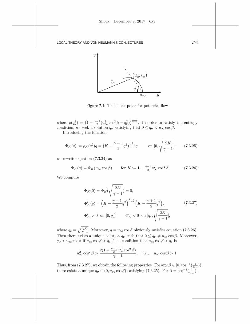
LOCAL THEORY AND VON NEUMANN’S CONJECTURES
Shock December 8, 2017 6x9
253
β
∞u
q
), vu(
u
v
O O
O
Figure 7.1: The shock polar for potential flow
where ρ(q2ν) =
(1 + γ−1
2 (u2∞ cos2 β − q2
ν)) 1γ−1 . In order to satisfy the entropy
condition, we seek a solution qν satisfying that 0 ≤ qν < u∞ cosβ.Introducing the function:
ΦK(q) := ρK(q2)q =(K − γ − 1
2q2) 1γ−1 q on [0,
√2K
γ − 1], (7.3.25)
we rewrite equation (7.3.24) as
ΦK(q) = ΦK(u∞ cosβ) for K := 1 + γ−12 u2
∞ cos2 β. (7.3.26)
We compute
ΦK(0) = ΦK(
√2K
γ − 1) = 0,
Φ′K(q) =(K − γ − 1
2q2) 2−γγ−1(K − γ + 1
2q2),
Φ′K > 0 on [0, qc], Φ′K < 0 on [qc,
√2K
γ − 1],
(7.3.27)
where qc =√
2Kγ+1 . Moreover, q = u∞ cosβ obviously satisfies equation (7.3.26).
Then there exists a unique solution qν such that 0 ≤ qν 6= u∞ cosβ. Moreover,qν < u∞ cosβ if u∞ cosβ > qc. The condition that u∞ cosβ > qc is
u2∞ cos2 β >
2(1 + γ−12 u2
∞ cos2 β)
γ + 1, i.e., u∞ cosβ > 1.
Thus, from (7.3.27), we obtain the following properties: For any β ∈ [0, cos−1( 1u∞
)),there exists a unique qν ∈ (0, u∞ cosβ) satisfying (7.3.25). For β = cos−1( 1
u∞),

254
Shock December 8, 2017 6x9
CHAPTER 7
we obtain that u∞ cosβ = qc = 1, and hence the only solution of equa-tion (7.3.25) is qν = u∞ cosβ. Also, qν is a continuous function of β on[0, cos−1( 1
u∞)].
Once qν is determined, we find (uO, vO) from the last two equations in(7.3.23) by setting that v · ν = qν and v · τ = u∞ sinβ, where the last equalityfollows from (7.3.21). Also, from the continuity of qν(β) on [0, cos−1( 1
u∞)], we
see that (uO, vO) depends continuously on β ∈ [0, cos−1( 1u∞
)].Therefore, we have shown that, for every β ∈ [0, cos−1( 1
u∞)], there ex-
ists (uO, vO) satisfying (7.3.20)–(7.3.22) and the entropy condition, and thatcurve β 7→ (uO, vO) has the regularity stated in assertion (a). Also, since qν <u∞ cosβ for all β ∈ [0, cos−1( 1
u∞)), (uO, vO) · ν = qν < u∞ cosβ = (u∞, 0) · ν
for these angles. Using (7.3.21), we show that, for β 7→ (uO, vO), the entropyinequality is strict: |(uO, vO)| < u∞. Moreover, since
(qν)|β=cos−1( 1u∞ ) = u∞ cosβ = 1,
it follows that(uO, vO)|β=cos−1( 1
u∞ ) = (u∞, 0).
Furthermore, by the implicit function theorem, we obtain from equation(7.3.25) that
function (ρ∞, u∞, β) 7→ (uO, vO) is C∞ on the set:
(ρ∞, u∞, β) : ρ∞ > 0, u∞ > c∞, 0 < β < cos−1(c∞u∞
). (7.3.28)
Now, plugging (7.3.23) into (7.3.20)–(7.3.21), we have
(uO, vO) = (u∞(1− (1− 1
ρO) cos2 β), u∞(1− 1
ρO) cosβ sinβ). (7.3.29)
Combining the entropy condition with (7.3.21)–(7.3.22) implies
ρO > ρ∞ = 1 (7.3.30)
for each β. Then, by (7.3.29), curve β 7→ (uO, vO) for β ∈ (0, cos−1( c∞u∞ )) lies inthe first quadrant of the (u, v)–plane and is bounded.
Thus, we have proved the existence of (uO, vO, ρO), satisfying the conditionsin Definition 7.3.1, the entropy condition for all β ∈ [0, cos−1( c∞u∞ )], and theproperties of the shock polar stated in assertion (a).
3. Next, we prove assertion (b). Set Mν := v·νcO
and M∞,ν = v∞ · ν for
cO = ργ−1
2
O . Also, since β ∈ [0, cos−1( 1u∞
)], we employ (7.3.23) to concludeM∞,ν > 1.
Furthermore, we note that (7.3.27) implies that the unique solution qν ∈(0, u∞ cosβ) of (7.3.26) satisfies qν < qc for every β ∈ [0, cos−1( 1
u∞)). Then,
from (7.3.25),ργ−1K (qν) > ργ−1
K (qc) = q2c > q2
ν ,

LOCAL THEORY AND VON NEUMANN’S CONJECTURES
Shock December 8, 2017 6x9
255
where the equality holds, since qc =√
2Kγ+1 . Note that, for a fixed β, v · ν = qν
for K defined in (7.3.26). Since c2O = ργ−1O = ργ−1
K (qν), we can rewrite the aboveinequality as
(v · ν)2 < c2O, (7.3.31)
which implies that Mν < 1. Thus, we have shown that
0 < Mν < 1 < M∞,ν .
Plugging these expressions into (7.3.20) and (7.3.22), and then combining theresulting expressions, we obtain the equation:
g(Mν) = g(M∞,ν), (7.3.32)
whereg(M) =
(M2 +
2
γ − 1
)M−
2(γ−1)γ+1 .
We note that g′(M) = 4γ+1 (M− 1
M )M−2(γ−1)γ+1 < 0 for 0 < M < 1, and g′(M) > 0
for M > 1. Thus, differentiating equation (7.3.32) with respect to β and using0 < Mν < 1 < M∞,ν = u∞ cosβ, we obtain that, on (0, cos−1
(1u∞
)],
dMν
dβ=
g′(M∞,ν)
g′(Mν)
dM∞,νdβ
= −g′(M∞,ν)
g′(Mν)u∞ sinβ > 0. (7.3.33)
Using the definition of Mν , we can write equation (7.3.24) as follows:
ργ+1
2
O Mν = u∞ cosβ.
Differentiating this equation with respect to β and using (7.3.33), we have
dρOdβ
< 0 for all β ∈ (0, cos−1( 1
u∞
)]. (7.3.34)
From (7.3.29), we have
duOdβ
= u∞
((1− 1
ρO
)sin(2β)− cos2 β
ρ2O
dρOdβ
).
Thus, using (7.3.30) and (7.3.34), we conclude assertion (b).This also implies assertion (c), except for the convexity part. In particular,
the definition of u0 in (c) is from the fact that u0 := (uO)|β=0 satisfies equation(7.3.24) for β = 0. Noting that, for β = 0, ν = (1, 0) such that uO = v · ν, weconclude that equation (7.3.24) for β = 0 is (7.3.7).
This also implies the smooth dependence of u0 on (ρ∞, u∞) as stated in part(i) of assertion (g). Since the problem has been reduced to Case ρ∞ = 1 by asmooth transformation, it suffices to consider the continuity of u0 with respectto u∞, while keeping ρ∞ = 1.

256
Shock December 8, 2017 6x9
CHAPTER 7
This continuity can be seen as follows: Note that qν = u0 is the uniquesolution of equation (7.3.24) for β = 0, satisfying qν ∈ (0, qc(u∞)|β=0). Thenthe C∞–smoothness of u∞ 7→ u0 follows from the implicit function theorem byusing form (7.3.26) of equation (7.3.24), considering ΦK(q) − ΦK(u∞) with Kdefined in (7.3.26) and β = 0 as a function of (u∞, q), and using that ∂ΦK
∂q > 0
for any q ∈ (0, qc(u∞)|β=0) by (7.3.27).
4. Now we prove the strict convexity of the shock polar, i.e., the convexityof curve (uO(β), vO(β)) for β ∈ [0, cos−1( c∞u∞ )].
Let v = (u, v) denote a point on the shock polar curve, corresponding toβ ∈ (0, cos−1( c∞u∞ )), i.e., v 6= v∞. By (7.3.21), the unit normal ν to SO isdefined by (7.3.6) up to the orientation. Plugging this expression into (7.3.20)and expressing ρO from (7.3.4), we obtain equation (7.3.16) with ρ∞ = 1. Onthe other hand, if ν and τ for v 6= v∞ are defined by (7.3.6), then (7.3.21)holds. Under this condition, (7.3.20) with ρ defined by (7.3.23) is equivalent to(7.3.16). This means that the shock polar curve is the zero level set of functiong on the first quadrant of the (u, v)–plane. Also, (7.3.21) holds on the shockpolar. Then, differentiating g and using (7.3.21), we obtain that, on the shockpolar,
gv · ν = ρ(
1−(v · ν
c
)2),
gv · τ = −(v∞ · τ )(ρv · ν
c2+
ρ− 1
|v∞ − v|).
(7.3.35)
As we have discussed earlier, Mν < 1, which implies
gv · ν > 0.
Then we can define a vector q by
q =gv
gv · ν= ν +
gv · τgv · ν
τ .
We claim that
q× qβ < 0 for β ∈ (0, cos−1(
1u∞
)).
Set A := − gv·τgv·ν . Noting that ν = (cosβ,− sinβ) and τ = (sinβ, cosβ), we findthat qβ = −(1 +Aβ)τ −Aν, which yields
q× qβ = −(1 +A2 +Aβ).
By (7.3.35), on the shock polar, A can be written as
A =u∞ sinβ
1−M2ν
(Mν
c+
1
u∞ cosβ
)for Mν :=
v · νc
,

LOCAL THEORY AND VON NEUMANN’S CONJECTURES
Shock December 8, 2017 6x9
257
where we have used that (7.3.20)–(7.3.21) hold on the shock polar so that |v∞−v| = (1− ρ∞
ρ )(v∞ · ν) = (1− ρ∞ρ )u∞ cosβ. From (7.3.34), we obtain
dcOdβ
< 0 on [0, cos−1 1u∞
).
Then, using (7.3.33), we obtain that Aβ ≥ 0, which yields
q× qβ ≤ −1 for β ∈ (0, cos−1(
1u∞
)].
From the definition of q, we see that q 6= 0. Then we finally obtain
q
|q| ×(
q
|q|
)
β
=q× qβ|q|2 ≤ − 1
|q|2 < 0 (7.3.36)
on the shock polar curve.Fix a point P0 = (uO, vO) on the curve that g(v) = 0, and let P0 correspond
to β0 for β0 ∈ (0, cos−1(
1u∞
)).
Connect (u∞, 0) to P0 by a line L. Let L∗ be the line perpendicular to Land passing through P0. Then vectors ν, τ, introduced above, are parallel tolines L and L∗, respectively. We introduce a coordinate system (s, t) with basisν, τ. Then gs = −gv · ν < 0 at P0. Thus, we can apply the implicit functiontheorem to see that there exists a function fP0 so that
g(v) = 0, |v − P0| < ε0 = (fP0(t), t) : |t− tP0
| < ε1
for some small positive constants ε0 and ε1. Note that q|q| is the unit normal to
the shock polar at P0 with q|q| · ν > 0. Then q
|q| can be expressed as
q
|q| =(−f ′P0
(t), 1)√1 + (f ′P0
)2(t)for |t− tP0
| < ε1,
from whichq
|q| ×(
q
|q|
)
t
=f ′′P0
(t)
1 + (f ′P0)2(t)
.
From the definition of the (s, t)–coordinates,(
q
|q|
)
t
(P0) =1
B
(q
|q|
)
β
(P0),
where B = |P0 − (u∞, 0)| > 0. Then (7.3.36) implies that
f ′′P0(tP0) < 0 for β0 ∈ (0, cos−1 1
u∞).
This implies the strict convexity (7.3.9). One can repeat this argument to leadto the same conclusion about the shock polar for Case γ = 1.

258
Shock December 8, 2017 6x9
CHAPTER 7
Now we prove assertion (d). We have shown in Step 2 that curve β 7→(uO, vO) for β ∈ (0, cos−1( c∞u∞ )) lies in the first quadrant of the (u, v)–plane andis bounded. This implies that we can find θd ∈ (0, π2 ) such that line v
u = tan θd
is tangential to the shock polar curve, and the whole curve lies between linevu = tan θd and the u–axis in the first quadrant of the (u, v)–plane. Combiningthe strict convexity of the shock polar with its structure of the graph as describedin assertion (c), property (7.3.8), we obtain that line v
u = tan θd has exactlyone contact point with the shock polar and, for any θw ∈ [0, θd), line v
u =tan θw intersects with the curve of (uO, vO) at exactly two different points.Applying the monotonicity shown in assertion (b) and using (7.3.8) again, weobtain the existence of Θ(·) and its properties (i)–(iii) in assertion (d). Nowthe regularity that Θw ∈ C([0, cos−1( c∞u∞ )]) ∩ C∞((0, cos−1( c∞u∞ ))) follows fromΘw(β) = tan−1
(vOuO
)(β), the regularity of (uO, vO)(·) in assertion (a), and the
fact that uO ∈ [u0, u∞] with u0 > 0.Now assertions (a)–(d) are proved.
5. Next we prove assertion (h). We first show (7.3.18). As shown in Step4, equation (7.3.16) holds and Dg 6= 0 on the shock polar. Then the strictconvexity of the shock polar and its structure described in assertion (c) implythat Dg(v) · v = 0 if and only if v is the detachment point that corresponds toangle βd introduced in (d) and the sign of Dg(v) · v as a continuous functionof β ∈ [0, cos−1( c∞u∞ )] changes across β = βd. Therefore, it remains to check thesign of Dg(v) · v for some β ∈ [0, βd).
At β = 0, as shown in Step 2, we have
ν = (1, 0), v = (u0, 0), 0 < u0 < c.
Then, from (7.3.35),
Dg(v) · v = ρ(1− u20
c2) > 0 at β = 0.
Thus,
Dg(v) · v> 0 for all β ∈ [0, βd),
< 0 for all β ∈ (βd, cos−1( c∞u∞ )].
This implies (7.3.18).Furthermore, since g(v) = 0 and Dg(v) 6= 0 on the shock polar:
(u, fpolar(u)) : u0 ≤ u ≤ u∞,
then either (7.3.17) holds on the whole shock polar or the right-hand side of(7.3.17) is equal to the minus left-hand side of (7.3.17) on the whole shockpolar. Thus, it suffices to check the sign at one point. Choose any θw ∈ (0, θd).As we have discussed at the end of Step 4, line v
u = tan θw intersects with thecurve of (uO, vO) at exactly two different points which lie in the first quadrant.

LOCAL THEORY AND VON NEUMANN’S CONJECTURES
Shock December 8, 2017 6x9
259
Let v = (uO, fpolar(uO)) be the nearest to the origin of intersection. It followsthat the segment connecting the origin to v lies outside of the open convex set:
A := (u, v) : u0 < u < u∞, 0 < v < fpolar(u);
the line containing that segment (i.e., line v = u tan θw) has a non-empty inter-section with A, and v ∈ ∂A. This implies that f ′polar(uO) >
fpolar(uO)uO
. Then
v · (f ′polar(uO),−1) = (uO, fpolar(uO)) · (f ′polar(uO),−1) > 0.
Since Dg(v) · v > 0, we conclude (7.3.17) at v, and hence also on the wholeshock polar.
6. We continue the proof of assertion (h). It remains to show (7.3.19). Wecan write (7.3.35) as
gv = ρOν −ρOc2O
(v · ν)v − ρO − 1
|v − v∞|(v · τ )τ .
Let β 6= 0, i.e., β ∈ (0, cos−1( c∞u∞ )]. Then v = (uO, vO) and v∞ = (u∞, 0) withuO, vO, u∞ > 0. Thus, from the definition of v⊥, it follows that
v⊥ = (−vO, uO),
that is, v⊥ is a counterclockwise rotation of v. Then, from (7.3.5),
τ = ν⊥,
so that v⊥ · ν = −v · τ and v⊥ · τ = v · ν. We calculate
gv · v⊥ = −(v · τ )(ρO +
ρO − 1
|v − v∞|(v · ν)
)< 0,
where we have used that ρO ≥ 1 by (7.3.22) and the entropy condition, and
v · ν > 0, v · τ > 0. (7.3.37)
The first inequality in (7.3.37) follows by (7.3.20), since ρOvν > 0 and v∞ ·ν =u∞ cosβ > 0, where we have used (7.3.5). The second inequality in (7.3.37)for β ∈ (0, cos−1( c∞u∞ )] follows by (7.3.5) and uO, vO > 0. Now assertion (h) isproved.
7. It remains to prove assertions (e)–(g). In this step, we first prove assertion(e).
Assertion (a) implies that the function:
β 7→ (qO, cO) is in C([0, cos−1( 1u∞
)]; R2) ∩ C∞((0, cos−1( 1u∞
)); R2).
Then we need to show that there exists a unique solution βs ∈ [0, cos−1(
1u∞
)]
of the equation:cO = qO (7.3.38)

260
Shock December 8, 2017 6x9
CHAPTER 7
for qO = |(uO, vO)|, where qO and cO are functions of β (for fixed u∞ andρ∞ = 1).
Differentiating the Bernoulli law in (7.3.1), we obtain that dρOdqO
= −ρOqOc2O
.Thus, (7.3.34) implies that
dqOdβ
> 0 for all β ∈ (0, cos−1( 1
u∞
)].
Moreover, (7.3.34) implies that dcOdβ < 0. Also, qO, cO > 0. Then
d( qOcO )
dβ> 0 for all β ∈ (0, cos−1
( 1
u∞
)]. (7.3.39)
Since v|β=0 = (u0, 0) by (7.3.29), and ν|β=0 = (1, 0), we conclude that u0 =(v · ν)|β=0. Then (7.3.31) implies that
qOcO
∣∣∣β=0
=u0
cO|β=0
< 1.
Since (uO, vO)|β=cos−1( 1u∞ ) = (u∞, 0), as discussed in Step 2, and u∞ > c∞ by
the assumption, we obtain
qOcO
∣∣∣β=cos−1( 1
u∞ )=u∞c∞
> 1.
This implies that there exists a unique βs ∈ (0, cos−1( c∞u∞ )) so that (7.3.10)holds.
It remains to show that βs > βd, i.e., that the strong reflections are subsonic.From (7.3.35), using the notations that vν = v · ν and vτ = v · τ , and recallingthat ρ∞ = 1, we have
gv · v = ρOvν
(1− |v|
2
c2O
)− v2
τ
ρO − 1
|v∞ − v| at βs.
We note that ρO > 1 by (7.3.22) and the entropy condition, where the inequalityis strict since βs ∈ (0, cos−1( c∞u∞ )). Then ρOvν > 0 by (7.3.37). Thus, gv ·v < 0
if |v|2 ≥ c2O. Then, using assertion (h), proved above, we see that |v|2 ≥ c2O canhold only for (strictly) weak reflections. This implies that βs > βd.
8. We now prove assertion (f) with the following steps:
• (7.3.12) follows from the inequality: 0 < βd < βs < cos−1( c∞u∞ ), proved inassertions (d) and (e), by using assertion (b) and recalling that uO(0) = u0
and uO(
cos−1( c∞u∞ ))
= u∞;
• (7.3.13) follows from assertions (b) and (d);
• (7.3.14) follows from assertions (b) and (e).

LOCAL THEORY AND VON NEUMANN’S CONJECTURES
Shock December 8, 2017 6x9
261
9. It remains to prove assertion (g). Since we have reduced the problemto Case ρ∞ = 1 by a smooth explicit transformation, it suffices to prove thecontinuity and regularity stated in (g) with respect to the other parametersstated there, while keeping ρ∞ = 1 fixed.
Part (i) of assertion (g) has been shown at the end of Step 3 above.Part (ii) of assertion (g) follows from part (i), property (7.3.28), assertion
(b), the regularity of β 7→ uO in assertion (a), and the regularity of fpolar inassertion (c).
Part (iii) of assertion (g) can be seen as follows: We first show the conti-nuity of ud(u∞). Recall that (ud, vd) are the coordinates of the unique con-tact point of the tangent line Ld = v = u tan θd from the origin to graphv = fpolar(u) : u0 ≤ u ≤ u∞ of the strictly concave and positive func-tion fpolar ∈ C∞((u0, u∞))∩C([u0, u∞]) satisfying fpolar(u0) = fpolar(u∞) = 0.These properties, combined with the continuity property of parts (i)–(ii) of as-sertion (g), imply the continuous dependence of ud on u∞. Indeed, if u(j)
∞ → u∗∞,then, from (i)–(ii) of assertion (g) and the concavity of f (j)
polar and f∗polar, it is
easy to see that lines L(j)d converge to the tangent line L∗d from the origin to
graph v = f∗polar(u) : u∗0 ≤ u ≤ u∗∞ and, for any subsequence of the contactpoints of L(j)
d with graphs v = f(j)polar(u) : u
(j)0 ≤ u ≤ u
(j)∞ , we can extract a
further subsequence converging to a contact point of the limiting line and graph.Such a contact point is unique, since f∗polar(·) is strictly concave and positive in(u∗0, u
∗∞) with f∗polar(u
∗0) = f∗polar(u
∗∞) = 0; we denote the unique contact point
by (u∗d, v∗d). Thus, u(j)
d → u∗d.Now we show the continuity of us(u∞). From (7.3.28) and assertion (b), it
suffices to show that βs depends continuously on u∞, where βs ∈ (βd, cos−1( c∞u∞ ))
is defined in assertion (e). Recall that βs ∈ (0, cos−1( 1u∞
)) is a solution ofequation (7.3.38). Considering qO and cO as functions of (u∞, β) (with ρ∞ = 1fixed) and using (7.3.28) and (7.3.39) (where the derivative is now understoodas the partial derivative), we apply the implicit function theorem to obtain thecontinuous dependence of u∞ 7→ βs, which yields the continuity of us(u∞).
7.3.2 The limit of the detachment angle as the upstream velocitytends to the sonic speed for steady flow
Denote by θdw(u∞) the detachment angle for the steady incoming uniform flow
(ρ∞, u∞).
Lemma 7.3.3. Fix ρ∞ > 0. Then, for u∞ > c∞,
limu∞→c∞+
θdw(u∞) = 0.
Proof. In this proof, we denote u0 defined in Lemma 7.3.2(c) for the steadyincoming uniform flow (ρ∞, u∞) by u(u∞)
0 , while ρ∞ is fixed through this proof.
262
Shock December 8, 2017 6x9
CHAPTER 7
1. We first show that
limu∞→c∞+
u(u∞)0 = c∞. (7.3.40)
Let u∞ > c∞. Then u(u∞)0 ∈ (0, u∞) satisfies (7.3.7), which can be written
asρ(u2∞, (u
(u∞)0 )2)u
(u∞)0 = ρ∞u∞, (7.3.41)
whereρ(s2, t2) =
(ργ−1∞ +
γ − 1
2(s2 − t2)
) 1γ−1 .
DenoteΦ(s, t) := ρ(s2, t2)t.
We calculate:
∂Φ
∂t(s, t) = ρ2−γ(s2, t2)
(ργ−1∞ +
γ − 1
2s2 − γ + 1
2t2).
Then, for each s ≥ c∞, Φ(s, ·) is:
(i) defined on (0,
√2
γ − 1ργ−1∞ + s2);
(ii) C∞ smooth on its domain;
(iii) ∂Φ∂t (s, ·) > 0 on (0,
√2
γ+1 (ργ−1∞ + γ−1
2 s2) ), and∂Φ∂t (s, ·) < 0 on (
√2
γ+1 (ργ−1∞ + γ−1
2 s2),√
2γ−1ρ
γ−1∞ + s2 ).
We also note that ρ∞ = ρ(u2∞, u
2∞). Thus, equation (7.3.41) can be written as
Φ(u∞, u(u∞)0 ) = Φ(u∞, u∞).
If u∞ > c∞ = ργ−1
2∞ , u∞ >√
2γ+1 (ργ−1
∞ + γ−12 u2
∞), i.e., ∂Φ∂t (u∞, u∞) < 0. From
properties (i)–(iii) above, and since Φ(u∞, 0) = 0 and Φ(u∞, u∞) = ρ∞u∞ > 0,we conclude that, for each u∞ > c∞, there exists a unique solution u
(u∞)0 ∈
(0, u∞) of (7.3.41).Let u(i)
∞ → c∞ as i → ∞. Then there exists a subsequence (still denoted)u
(u(i)∞ )
0 converging to some constant u∗0 ∈ [0, c∞]. Taking the limit in (7.3.41),using the smoothness of Φ(·, ·) in a neighborhood of c∞× [0, c∞], and recallingthat ρ∞ = ρ(u2
∞, u2∞), we have
Φ(c∞, u∗0) = Φ(c∞, c∞).
Note that c∞ = ργ−1
2∞ =√
2γ+1 (ργ−1
∞ + γ−12 c2∞). Then it follows from property
(iii) of Φ(s, ·) that u∗0 = c∞. Therefore, (7.3.40) is proved.

LOCAL THEORY AND VON NEUMANN’S CONJECTURES
Shock December 8, 2017 6x9
263
2. Let u(i)∞ → c∞ as i→∞. Assume that there exists δ > 0 such that
θdw(u(i)∞ ) ∈ (δ,
π
2) for all i. (7.3.42)
Then we denote by (u(i)d , v
(i)d ) the coordinates of the corresponding detachment
point on the shock polar f (u∞)polar (·), i.e., the unique u
(i)d ∈ [u
(u(i)∞ )
0 , u(i)∞ ] with
u(i)d tan(θd
w(u(i)∞ )) = f
(u∞)polar (u
(i)d ), and by βi the corresponding β–angle defined in
§7.3.1. From this, using u(i)∞ → c∞ > 0, (7.3.40), and (7.3.42), we have
tanβi =u
(i)d tan(θd
w(u(i)∞ ))
u(i)∞ − u(i)
d
→∞,
which impliesβi →
π
2−, (7.3.43)
since βi ∈ (0, π2 ).On the other hand, since (u
(i)∞ , 0) and (u
(i)d , v
(i)d ) satisfy the Rankine-Hugoniot
conditions (7.3.20)–(7.3.21) on the straight-line shock:
(u, v) : v = u cot(βdw(u(i)∞ )),
where βdw is angle β from Definition 7.3.1 for the detachment point of the shock
polar for the incoming flow (u∞, ρ∞) (where ρ∞ has been fixed at the beginningof the proof). Then the equality of the tangential to the shock components of(u
(i)∞ , 0) and (u
(i)d , v
(i)d ) implies
u(i)∞ sinβi = q
(i)O sin(βi + θd
w(u(i)∞ )),
where q(i)O =
∣∣(u(i)d , v
(i)d )∣∣. Moreover, from the Rankine-Hugoniot conditions
(7.3.20)–(7.3.21), we know that u(i)∞ ≥ q(i)
O for any i. From this and (7.3.43), wehave
lim infi→∞
sin(βi + θdw(u(i)∞ )) = lim inf
i→∞
(u(i)∞
q(i)O
sinβi
)≥ 1,
which implieslimi→∞
sin(βi + θdw(u(i)∞ )) = 1.
This is impossible, since both θdw(u
(i)∞ ) ∈ (δ, π2 ) and (7.3.43) hold. Thus, (7.3.42)
is impossible. This completes the proof.
7.4 LOCAL THEORY FOR SHOCK REFLECTION: EXISTENCEOF THE WEAK AND STRONG STATE (2) UP TO THEDETACHMENT ANGLE
Proof of Theorem 7.1.1. We divide the proof into five steps.

264
Shock December 8, 2017 6x9
CHAPTER 7
1. For any angle θw ∈ (0, π2 ), the existence of the weak and strong state (2)can be proved by employing the steady shock polar.
We start by fixing θw ∈ (0, π2 ). This determines the reflection point P0 =(ξ0
1 , ξ01 tan θw) that is the intersection point of the incident shock with the wedge
boundary Γwedge = ξ2 = ξ1 tan θw, and the incident shock is line ξ1 = ξ01
with ξ01 = ρ1u1
ρ1−ρ0> u1; see §6.2.
Note that we can rewrite (7.1.5) with ρ(·) given by (2.2.9) as
ρ2Dϕ2(P0) · ν = ρ1Dϕ1(P0) · ν,Dϕ2(P0) · τ = Dϕ1(P0) · τ ,
ργ−12
γ − 1+
1
2|Dϕ2(P0)|2 =
ργ−11
γ − 1+
1
2|Dϕ1(P0)|2,
(7.4.1)
where ν, τ , and ρk, k = 1, 2, are defined in (7.1.5). Note that the condition thatϕ2(P0) = ϕ1(P0) has been used to write the Bernoulli law (2.2.9), as the lastline in (7.4.1).
Also, with possibly changing τ to −τ , we may assume that
τ ·Dϕ1(P0) ≥ 0.
We consider (7.4.1) as an algebraic system for (ρ2, Dϕ2(P0)). Note that, if(ρ2, Dϕ2(P0)) satisfy (7.4.1), the pseudo-potential ϕ2 of the self-similar uniformstate uniquely determined by ϕ2(P0) := ϕ1(P0) and Dϕ2(P0), i.e.,
ϕ2(ξ) = ϕ2(P0) +Dϕ2(P0) · (ξ − P0)− 1
2(ξ − P0)2
satisfies (7.1.5), and its density, calculated by (2.2.9), is ρ2 = ρ(|Dϕ2|2, ϕ2).The last assertion follows from (7.4.1), since ρ1 = ρ(|Dϕ1|2, ϕ1) and ϕ2(P0) =ϕ1(P0). Therefore, we have proved the following claim:
Claim 7.4.1. Every state (2) for a self-similar wedge angle θw ∈ (0, π2 ) isdetermined by a solution (ρ2, Dϕ2(P0)) of algebraic system (7.4.1) with P0 =(ξ0
1 , ξ01 tan θw).
Therefore, from now on, we study the existence and multiplicity of solutionsof the algebraic system (7.4.1) with P0 = (ξ0
1 , ξ01 tan θw).
Fix a self-similar wedge angle θw ∈ (0, π2 ). Denote
τ (0)w := −(cos θw, sin θw). (7.4.2)
Then τ (0)w is a unit tangent vector to the wedge boundary Γwedge and
τ (0)w ·Dϕ1(P0) > 0 for all θw ∈ (0,
π
2). (7.4.3)

LOCAL THEORY AND VON NEUMANN’S CONJECTURES
Shock December 8, 2017 6x9
265
Fact (7.4.3) can be seen as follows: Since Dϕ1(P0) = (u1 − ξ01 ,−ξ0
1 tan θw) by(2.2.17), and ξ0
1 > u1 by (2.2.18), we have
τ (0)w ·Dϕ1(P0) = (cos θw, sin θw) · (ξ0
1 − u1, ξ01 tan θw)
=ξ01
cos θw− u1 sin θw > 0.
(7.4.4)
Thus, we can define the coordinate system with the origin at P0 and basise(P0), e⊥(P0) such that
e(P0) :=Dϕ1(P0)
|Dϕ1(P0)| ,
e⊥(P0) ⊥ e(P0), e⊥(P0) · νw > 0,
(7.4.5)
where e⊥(P0) · νw 6= 0 by (7.4.3). Then we see that conditions (7.4.1) co-incide with the Rankine-Hugoniot conditions (7.3.2)–(7.3.3) and the Bernoullilaw (7.3.4) for the steady shock with incoming steady flow:
(ρ∞, u∞) = (ρ1, |Dϕ1(P0)|). (7.4.6)
Definition 7.4.2. Fix the self-similar uniform state ϕ1(ξ) with density ρ1 andsonic speed c1. For ξ ∈ R2 \ Bc1(O1), we denote by f (ξ)
polar(·) the steady shockpolar considered in Lemma 7.3.2 for the steady incoming flow with density andvelocity (ρ∞, u∞) = (ρ1, |Dϕ1(ξ)|); see Fig. 7.2.
We use the notations introduced in Lemma 7.3.2 below. One difference isthat θw is denoted as the wedge angle for steady flow, introduced in Lemma7.3.2(d), which will not be the same as the wedge angle θw for self-similar flowin our application.
Note that, if state (2) exists for some θw ∈ (0, π2 ), the boundary condition(7.1.7) and property (7.4.3) imply that
Dϕ2(P0) = |Dϕ2(P0)|τ (0)w .
Thus, angle θw between Dϕ1(P0) and Dϕ2(P0) is
θw = θw(θw) := cos−1(Dϕ1(P0) · τ (0)
w
|Dϕ1(P0)| ) ∈ (0,π
2), (7.4.7)
where the last inclusion follows from both (7.4.3) and the fact that Dϕ1(P0) =
(u1− ξ01 ,−ξ0
1 tan θw) is not parallel to τ (0)w , since u1 6= 0. From Lemma 7.3.2(d),
it follows that (ρ2, Dϕ2(P0)) satisfying (7.4.1)–(7.4.5) (or its non-existence) isdetermined by the shock polar f (P0)
polar(·) and the steady wedge angle θw defined
above. More precisely, by Lemma 7.3.2(c)–(d) and Definition 7.4.2 of f (ξ)polar(·),
Dϕ2(P0) = u e(P0) + f(P0)polar(u)e⊥(P0), (7.4.8)

266
Shock December 8, 2017 6x9
CHAPTER 7
where u is determined by the intersection point (u, v) of the shock polar curve:
(u, v) : u(|Dϕ1(P0)|)0 ≤ u ≤ |Dϕ1(P0)|, v = f
(P0)polar(u), (7.4.9)
with line (u, v) : v = u tan θw. Note that, for the steady shock polar de-scribed above, θw in (7.4.7) is the angle introduced in Lemma 7.3.2(d) (denotedby θw there). Thus, we have
Definition 7.4.3. Angle θw = θw(θw), defined by (7.4.7) for (P0, τ(0)w )(θw), is
called a steady wedge angle corresponding to the self-similar wedge angle θw ∈(0, π2 ).
Furthermore, using Lemma 7.3.2(d), we see that the existence or non-existenceof solutions (ρ2, Dϕ2(P0)) of (7.4.1), when (7.1.11) holds, is determined as fol-lows:
(a) If θw < θdw(ρ1, |Dϕ1(P0)|), there are two solutions;
(b) If θw = θdw(ρ1, |Dϕ1(P0)|), there is one solution;
(c) If θw > θdw(ρ1, |Dϕ1(P0)|), there is no solution.
Here θdw(ρ∞, u∞) denotes the detachment angle for the steady incoming flow
(ρ∞, u∞) defined in Lemma 7.3.2(d) (denoted by θd there).2. By Proposition 7.2.2, there exists σ1 > 0 such that, for any self-similar
wedge angle θw ∈ (π2−σ1,π2 ), there exists a solution (ρ2, Dϕ2(P0)) of (7.4.1) such
that |Dϕ2(P0)| > c2, i.e., the steady uniform flow (ρ2, Dϕ2(P0)) is supersonic:|Dϕ2(P0)| > c2.
We note that, from Lemma 7.3.2(d)–(f), it follows that the unique solutionfor the steady detachment wedge angle θd
w is v = (ud, fpolar(ud)) which is sub-sonic by (7.3.12). Since, for any self-similar wedge angle θw ∈ (π2 − σ1,
π2 ), the
steady uniform flow (ρ2, Dϕ2(P0(θw))) is supersonic as we have shown above,
it follows from Lemma 7.3.2(d)–(f) that, in this case, there exist two solutions(ρwk
2 , Dϕwk2 (P0)) and (ρsg
2 , Dϕsg2 (P0)) of (7.4.1) with ρwk
2 < ρsg2 , and solution ϕsg
2
is subsonic at P0, i.e., |Dϕsg2 (P0)| < csg2 = (ρsg
2 )γ−1
2 . Note that (ρ2, Dϕ2(P0))obtained in §7.2 is the weak reflection solution (ρwk
2 , Dϕwk2 (P0)), since it is su-
personic.This implies that, for any self-similar wedge angle θw ∈ (π2 − σ1,
π2 ), there
exist two solutions ϕwk2 and ϕsg
2 for state (2).Moreover, since Dϕwk
2 (P0) > cwk2 for θw ∈ (π2 − σ1,
π2 ) as discussed above,
then, by Lemma 7.3.2(d)–(e), we obtain that, for any θw ∈ (π2 − σ1,π2 ),
θw(θw) < θsw(ρ1, |Dϕ1(P0
(θw))|) < θdw(ρ1, |Dϕ1(P0
(θw))|), (7.4.10)
where θsw(ρ∞, u∞) denotes the sonic angle for the steady incoming flow (ρ∞, u∞)
defined in Lemma 7.3.2(e).

LOCAL THEORY AND VON NEUMANN’S CONJECTURES
Shock December 8, 2017 6x9
267
3. We next prove the existence of the self-similar detachment angle θdw ∈
(0, π2 ) and assertions (i)–(iv) and (vi) of Theorem 7.1.1.We first note that the incident shock S0 = ξ1 = ξ0
1 is the shock betweenstates (0) and (1) with ρ0 < ρ1. Denoting by νS0 := (−1, 0) the normal to S0,we have
Dϕ0(ξ) · νS0= ξ0
1 > ξ01 − u1 = Dϕ1(ξ) · νS0
for all ξ ∈ S0.
Applying Lemma 6.1.2 with ϕ− = ϕ0 and ϕ+ = ϕ1, we obtain from (6.1.4) thatBc1(O1) ∩ S0 6= ∅, that is,
c1 > ξ01 − u1.
Thus, denoting
θ+w := tan−1(
√c21 − (ξ0
1 − u1)2
ξ01
) > 0,
we obtain that the steady uniform flow (ρ1, |Dϕ1(P0(θ+
w ))|) is sonic, and
|Dϕ1(P0(θw))| > c
(θw)1 for all θw ∈ (θ+
w ,π
2).
On the other hand,
θ+w := θw(θ+
w ) = ∠O1P0(θ+
w )P3 > 0.
Using Lemma 7.3.3 and the continuous dependence of θw on θw, we concludethat there exists δ > 0 such that
θw(θw) > θdw(ρ1, |Dϕ1(P0
(θw))|) for all θw ∈ (θ+w , θ
+w + δ).
Combining with (7.4.10), we obtain the existence of θ(d1)w ∈ (θ+
w +δ, π2 −σ1) suchthat
θw(θ(d1)w ) = θd
w(ρ1, |Dϕ1(P0(θ(d1)
w ))|). (7.4.11)
Defining θdw to be the supremum of all such angles θ(d1)
w , we find that θdw ∈
[θ+w +δ, π2 −σ1]. Then it follows from Lemma 7.3.2(d) that there exist two states
for state (2) for each θw ∈ (θdw,
π2 ), and there exists a unique state (2) when
θw = θdw.
We now show the continuous dependence of the weak and strong states (2)on θw, stated in (7.1.10) and Theorem 7.1.1(i).
We first note the C∞–dependence of θw on θw ∈ [θdw,
π2 ). Indeed, it follows
from the explicit formula of θw(θw) in (7.4.7), using that Dϕ1(P0) = −(ξ01 −
u1, ξ01 tan θw) by (2.2.17), and |Dϕ1(P0)| ≥ ξ0
1 − u1 > 0 by (7.4.4).Now the continuous dependence of the weak and strong states for (2) on θw
can be seen by letting θ(i)w ∈ (θd
w,π2 ) with θ(i)
w → θ(∞)w ∈ [θd
w,π2 ). Recall that, for
each θw ∈ (θdw,
π2 ), the strictly convex shock polar curve, defined by (7.4.9) and
denoted by Γ(θw), intersects with line L(θw) = v = u tan(θw(θw)) at exactly

268
Shock December 8, 2017 6x9
CHAPTER 7
two points, with coordinates (uwkO , vwk
O ) and (usgO , v
sgO ). Moreover, Dϕwk
2 (P0)and Dϕsg
2 (P0), written in coordinates (7.4.8), are Dϕwk2 (P0) = (uwk
O , vwkO ) and
Dϕsg2 (P0) = (usg
O , vsgO ), i.e.,
Dϕwk2 (P0) = uwk
O e(P0) + vwkO e⊥(P0), Dϕsg
2 (P0) = usgOe(P0) + vsg
O e⊥(P0).(7.4.12)
If θw = θdw, L(θw) touches Γ(θw) at exactly one point, with the coordinates given
by the components of Dϕwk(P0) = Dϕsg(P0) in coordinates (7.4.8). From thecontinuity of θw(·), it follows that lines L(θ
(i)w ) converge to L(θ
(∞)w ). Then the
continuity stated in assertions (ii)–(iii) of Lemma 7.3.2(g) implies that
(uwkO , vwk
O )(θ(i)w )→ (uwk
O , vwkO )(θ(∞)
w ), (usgO , v
sgO )(θ(i)
w )→ (usgO , v
sgO )(θ(∞)
w ),
where(uwkO , vwk
O )(θ(∞)w ) 6= (usg
O , vsgO )(θ(∞)
w ) if θ∞w ∈ (θdw,
π2 ),
and(uwkO , vwk
O )(θ(∞)w ) = (usg
O , vsgO )(θ(∞)
w ) if θ∞w = θdw.
Then, using (7.4.12) where vectors (e(P0(θw)), e⊥(P0
(θw))) depend C∞-smoothlyon θw, and using that Dφ2 = Dϕ2(P0) + P0 = (uO, vO) + (ξ0
1 , ξ01 tan θw) for
any θw and for both the weak and strong states (2), we obtain the continuousdependence of (ρwk
2 , ρsg2 , Dφ
wk2 , Dφsg
2 ) on θw ∈ [θdw,
π2 ). We have also shown
(7.1.10).To show the C∞–dependence on θw ∈ (θd
w,π2 ), we consider the function:
G(u, θw) := u tan(θw(θw))− f (P0(θw))
polar (u),
where f (ξ)polar(·) is from Definition 7.4.2. Then, for fixed θw ∈ (θd
w,π2 ),
G(u, θw) = 0 only for u = usgO (θw) and u = uwk
O (θw).
From the smoothness of θw(·) shown above and assertions (i)–(ii) of Lemma7.3.2(g), we have
G ∈ C∞((u, θw) : θdw ≤ θw <
π
2, u0(ρ1, |Dϕ1(P0
(θw))|) < u < |Dϕ1(P0(θw))|).
Since f (P0(θw))
polar (·) is strictly concave in the interior of its domain, we have
∂uG(uwkO (θw), θw) 6= 0, ∂uG(usg
O (θw), θw) 6= 0 for all θw ∈ (θdw,π
2),
since L(θw) = v = u tan(θw(θw)) intersects with the graph of f (P0(θw))
polar (·) attwo points, and hence intersects transversally at both points. Now, from theimplicit function theorem, we obtain the C∞–dependence of (uwk
O , usgO ) on θw ∈
(θdw,
π2 ). Since vO = f
(P0)polar(uO) for both the weak and strong reflections, with

LOCAL THEORY AND VON NEUMANN’S CONJECTURES
Shock December 8, 2017 6x9
269
P0 = (ξ01 , ξ
01 tan θw), we use Definition 7.4.2 and assertion (ii) of Lemma 7.3.2(g)
to obtain the C∞–dependence of (uwkO , vwk
O , usgO , v
sgO ) on θw ∈ (θd
w,π2 ). Finally,
using (7.4.12) with the argument as in the proof of continuity above, we concludethe proof of the C∞–dependence of (ρwk
2 , ρsg2 , Dφ
wk2 , Dφsg
2 ) on θw ∈ (θdw,
π2 ). This
completes the proof of assertion (i) of Theorem 7.1.1.Now we prove assertion (ii) of Theorem 7.1.1. First, we note that assertion
(iv) holds, since the existence of two states for (2) for a self-similar wedge angleθw, and equivalently for the steady wedge angle θw(θw), implies (7.1.12) asfollows: By (b) and (d) of Lemma 7.3.2, we conclude that usg
O ∈ [u0, ud), andthen (7.3.12)–(7.3.14) in Lemma 7.3.2(f) imply (7.1.12). Noting that state (2)constructed in Proposition 7.2.2 is supersonic at P0, we conclude that it is a weakstate (2). Now Proposition 7.2.2 implies the C∞–dependence of (ρwk
2 , Dφwk2 ) on
θw ∈ (π2 − σ1,π2 ]. Combining this with the C∞–dependence on θw ∈ (θd
w,π2 )
proved above, we conclude the C∞–dependence of (ρwk2 , Dφwk
2 ) on θw ∈ (θdw,
π2 ].
Therefore, assertions (i)–(ii) and (iv) of Theorem 7.1.1 hold. Also, assertion(iii) of Theorem 7.1.1 follows from the fact that θd
w > θ+w .
Furthermore, from the continuity of θw(·) and P0(·) on θw ∈ [θdw,
π2 ) and
assertion (iii) of Lemma 7.3.2(g), there exists δ > 0 such that, for any θw ∈[θd
w,π2 − σ1],
θdw(ρ1, |Dϕ1(P0
(θw))|)− θsw(ρ1, |Dϕ1(P0
(θw))|) ≥ δ > 0. (7.4.13)
This, combined with (7.4.11), Lemma 7.3.2(f), and the continuity on θw ∈[θd
w,π2 ) in assertion (i) of Theorem 7.1.1, implies assertion (vi) of Theorem 7.1.1.Therefore, we have shown assertions (i)–(iv) and (vi) of Theorem 7.1.1.4. Next, we show the existence of the self-similar sonic angle, i.e., assertion
(v) of Theorem 7.1.1. Denote by S the set of all angles θs1w ∈ [θd
w,π2 ) such that
|Dϕwk2 (P0)| > c2 for any θw ∈ (θs1
w ,π2 ). From Proposition 7.2.2 and Theorem
7.1.1(iv), we conclude that (π2 − σ1,π2 ) ⊂ S. Thus, S 6= ∅. Let θs
w := inf S. Weshow that θs
w satisfies all the properties given in assertion (v) of Theorem 7.1.1.First, we note that θs
w > θdw, since
• (7.4.11) holds for θdw;
• (7.4.10) holds for any θw ∈ (θsw,
π2 );
• (7.4.13) holds for any θw ∈ [θdw,
π2 − σ1].
Now, using assertion (i) of Theorem 7.1.1, we find that |Dϕwk2 (P0)| = cwk
2
for θw = θsw.
Now θsw satisfies all the properties asserted in Theorem 7.1.1(v).
5. We show assertions (vii)–(viii) of Theorem 7.1.1. Let ϕ2 be the pseudo-potential of either weak or strong state (2). Since ρ1 = ρ(|Dϕ1|2, ϕ1) for ρ(·)given by (2.2.9) and ϕ1(P0) = ϕ2(P0) by (7.1.5), then, for function (7.1.9), wehave
gsh(p, ϕ2(P0), P0) =(ρ(|p|2, P0)p− ρ1Dϕ1(P0)
)· Dϕ1(P0)− p
|Dϕ1(P0)− p| , (7.4.14)

270
Shock December 8, 2017 6x9
CHAPTER 7
3P
0P
Incident shock
Shock polar
2
ϕ=1
ϕ=1S
0),1u()
0P(
2ϕ∇
)0
P(1ϕ
∇Figure 7.2: Dϕ2(P0) lies on the shock polar of the steady incoming flow(ρ∞, u∞) = (ρ1, |Dϕ(P0)|)
where ρ(|p|2, P0) =(ργ−1
1 + γ−12 (|Dϕ1(P0)|2 − |p|2)
) 1γ−1 . Thus, function p 7→
gsh(p, ϕ2(P0), P0) coincides with function (7.3.16) for the steady incoming flow(ρ∞, u∞) = (ρ1, |Dϕ1(P0)|). Next, using that Dϕ1(P0) · Dϕ2(P0) > 0 by theRankine-Hugoniot conditions (7.4.1) at P0, by rotating the coordinates ξ so thatthe new ξ1–axis is in the direction of Dϕ1(P0), and reflecting ξ2 if necessary,we conclude that Dϕ1(P0) = (|Dϕ1(P0)|, 0), and v := Dϕ2(P0) has positivecomponents in the new coordinates. Then, using that Dϕ1(P0) ·τ = Dϕ2(P0) ·τby (7.1.5), we find that v := Dϕ2(P0) (expressed in the new coordinates) lieson the shock polar of the steady incoming flow (ρ∞, u∞) = (ρ1, |Dϕ1(P0)|); seeFig. 7.2.
Moreover, for any fixed self-similar wedge angle θw ∈ (θdw,
π2 ) and the corre-
sponding weak and strong reflection solutions ϕwk2 and ϕsg
2 , velocities Dϕw2 (P0)
and Dϕs2(P0), which lie on the shock polar described in the previous paragraph,
correspond to the weak and strong steady reflection solutions for the steadywedge angle θw(θw) introduced in Definition 7.4.3. Indeed, the correspondingsteady flows have both the same steady wedge angle θw(θw) with densities ρwk
2
and ρsg2 , respectively. Since ρwk
2 < ρsg2 , the assertion follows. Therefore, we have
proved the following lemma:
Lemma 7.4.4. For any θw ∈ (θdw,
π2 ) and the corresponding P0 = P0(θw),
denoting by ϕ2 the pseudo-potential of either weak or strong state (2), we have
(i) Function p 7→ gsh(p, ϕ2(P0), P0) coincides with function (7.3.16) for thesteady incoming flow (ρ∞, u∞) = (ρ1, |Dϕ1(P0)|);
LOCAL THEORY AND VON NEUMANN’S CONJECTURES
Shock December 8, 2017 6x9
271
(ii) Change the coordinates in R2 to the ones determined on the basis of (7.4.5),so that Dϕ1(P0) = (|Dϕ1(P0)|, 0), and Dϕ2(P0) has positive components.Then v := Dϕ2(P0) (expressed in the new coordinates) lies on the shockpolar of the steady incoming flow (ρ∞, u∞) = (ρ1, |Dϕ1(P0)|); see Fig. 7.2.
(iii) For weak and strong self-similar reflection solutions ϕwk2 and ϕsg
2 , veloc-ities Dϕwk
2 (P0) and Dϕsg2 (P0) correspond to the weak and strong steady
reflection solutions respectively on the steady shock polar described in (ii)above with the steady wedge angle θw(θw) introduced in Definition 7.4.3.
Now assertion (vii) of Theorem 7.1.1 directly follows from Lemma 7.4.4(ii)–(iii) and (7.3.18) in Lemma 7.3.2(h).
Moreover, it is easy to check that, if two self-similar uniform states withpseudo-potentials ϕ1 and ϕ2 satisfy (7.1.5)–(7.1.6) at some point P0 ∈ S1 :=ϕ1 = ϕ2, then (7.1.5)–(7.1.6) with P0 replaced by ξ hold at any ξ ∈ S1.Repeating the argument that leads to (7.4.14), we see that, for any ξ ∈ S1,
gsh(p, ϕ2(ξ), ξ) =(ρ(|p|2, ξ)p− ρ1Dϕ1(ξ)
)· Dϕ1(ξ)− p
|Dϕ1(ξ)− p| , (7.4.15)
where
ρ(|p|2, ξ) =(ργ−1
1 +γ − 1
2(|Dϕ1(ξ)|2 − |p|2)
) 1γ−1
. (7.4.16)
Then, arguing as in the proof of Lemma 7.4.4, we have
Lemma 7.4.5. Let ϕ1 and ϕ2 be the pseudo-potentials of two self-similar uni-form states, and let (7.1.5)–(7.1.6) hold at some point P0 ∈ S1 := ϕ1 = ϕ2.Then, for every ξ ∈ S1, we have
(i) (7.1.5)–(7.1.6) hold with P0 replaced by ξ ∈ S1;
(ii) Function p 7→ gsh(p, ϕ2(ξ), ξ) coincides with function (7.3.16) for thesteady incoming flow (ρ∞, u∞) = (ρ1, |Dϕ1(ξ)|);
(iii) There exists an orthogonal transformation of R2 such that, in the new coor-dinates (still denoted ξ), Dϕ1(ξ) = (|Dϕ1(ξ)|, 0), and Dϕ2(ξ) has positivecomponents. Then v := Dϕ2(ξ) (expressed in the new coordinates) lies onthe shock polar of the steady incoming flow (ρ∞, u∞) = (ρ1, |Dϕ1(ξ)|).
Now assertion (viii) of Theorem 7.1.1 directly follows from (7.3.19) in Lemma7.3.2(h).
Theorem 7.1.1 is proved.Next we show some corollaries from Theorem 7.1.1 and their proofs.
Corollary 7.4.6. Let ϕ1 be a uniform state. Let Ω ⊂ R2 be open, and let Ω besubdivided by a C1–smooth curve S into two open subdomains Ω1 and Ω2. Letϕ ∈ C0,1(Ω) be a weak solution of (2.2.8) in Ω such that ϕ ∈ C2(Ωk)∩C1(Ωk∪S)

272
Shock December 8, 2017 6x9
CHAPTER 7
for k = 1, 2. Assume that S ⊂ R2 \ Bc1(O1) and that ϕ = ϕ1 on Ω1. Assumethat the following entropy condition holds on S:
∂νϕ1 > ∂νϕ > 0 on S,
where ν is the unit normal to S pointing into Ω2. Let ξ ∈ S. Denote
e(ξ) :=Dϕ1(ξ)
|Dϕ1(ξ)| ,
e⊥(ξ) as the rotation of e(ξ) byπ
2such that Dϕ2(ξ) · e⊥(ξ) ≥ 0.
(7.4.17)
Then, for u = Dϕ2(ξ) · e(ξ) and v = Dϕ2(ξ) · e⊥(ξ),
v = f(ξ)polar(u), (7.4.18)
where f (ξ)polar(·) is introduced in Definition 7.4.2.
Proof. The argument is the same as that in the proof of (7.4.8) in Step 1 of theproof of Theorem 7.1.1 for point ξ (instead of P0).
Corollary 7.4.7. Let ϕ1 and ϕ2 be pseudo-potentials of two self-similar uniformstates with densities ρ1 and ρ2, respectively, and let (7.1.5)–(7.1.6) hold at somepoint P0 ∈ S1 := ϕ1 = ϕ2. Let gsh be defined by (7.1.9). Let ξ ∈ S1 satisfy|Dϕ2(ξ)| ≥ c2, where c2 is the sonic speed of the uniform state ϕ2. Then
Dpgsh(Dϕ2(ξ), ϕ2(ξ), ξ) ·Dϕ2(ξ) < 0. (7.4.19)
Proof. By Lemma 7.4.5, v = Dϕ2(ξ), expressed in the appropriately chosencoordinates, lies on the shock polar of the steady incoming flow (ρ∞, u∞) =(ρ1, |Dϕ1(ξ)|). Comparing (7.4.16) with (7.3.11), we see that the conditionthat |Dϕ2(ξ)| ≥ c2 implies that the steady flow with velocity v = Dϕ2(ξ)(expressed in the coordinates described in Lemma 7.4.5(iii)) is supersonic, i.e.,|v| ≥ c(|v|2), where c(·) is given by (7.3.11) with (ρ∞, u∞) = (ρ1, |Dϕ1(ξ)|).Now Lemma 7.3.2(f) implies that v is a weak reflection solution for the steadyshock polar of the incoming flow (ρ∞, u∞) = (ρ1, |Dϕ1(ξ)|).
Also, Dϕ1(ξ) 6= Dϕ2(ξ) by (7.1.6). Now (7.4.19) follows from Lemma7.4.5(ii) and (7.3.18) in Lemma 7.3.2(h).
We also note the following property of state (2):
Lemma 7.4.8. Let θw ∈ (θdw,
π2 ), and let ϕ2 be a state (2) (weak or strong)
written in the form of (2.4.1). Then center O2 = (u2, u2 tan θw) of the soniccircle of ϕ2 lies within the relative interior of segment P0P3 ⊂ ξ2 = ξ1 tan θw,where P3 = 0.

LOCAL THEORY AND VON NEUMANN’S CONJECTURES
Shock December 8, 2017 6x9
273
Proof. Recall that P0 = (ξ01 , ξ
01 tan θw).
Points P0, P3, and O2 lie on line ξ2 = ξ1 tan θw, which implies
O2 − P0 = t(P3 − P0) for t ∈ R.
Thus, it remains to show that t ∈ (0, 1).Denoting by O1 = (u1, 0) the center of state (1) and using (7.1.5) and the
fact that Dϕk(P0) = Ok − P0 for k = 1, 2, we can write (7.1.6) as
|P0O1| > |P0O2|.
Also, by (2.2.18),ξ01 > u1 > 0,
and hence |P0P3| = ξ01 sec θw >
√(ξ0
1)2 tan2 θw + (ξ01 − u1)2 = |P0O1|, which
implies|P0P3| > |P0O2|.
Furthermore, P0 ∈ S1, and hence O2 6= P0 = (ξ01 , ξ
01 tan θw), on account of
(6.1.5) applied with ϕ− = ϕ1, ϕ+ = ϕ2, and S = S1. Then we have
|P0P3| > |P0O2| 6= 0,
which implies that |t| ∈ (0, 1).It remains to show that t > 0. We first note that Dϕ1(P0) ·Dϕ2(P0) > 0 by
(7.1.5) so that(O1 − P0) · (O2 − P0) > 0.
Again using that ξ01 > u1 > 0 by (2.2.18), we calculate
(O1 − P0) · (P3 − P0) = ξ01(ξ0
1 − u1) + (ξ01)2 tan2 θw > 0.
The last two inequalities imply t > 0, which concludes the proof.
From Lemma 7.4.8, we conclude
Corollary 7.4.9. For any θw ∈ (θdw,
π2 ), writing state (2) in the form of (2.4.1),
we haveu2 > 0, v2 > 0.
7.5 BASIC PROPERTIES OF THE WEAK STATE (2) AND THEDEFINITION OF SUPERSONIC AND SUBSONIC WEDGEANGLES
In this section, for any wedge angle θw ∈ (θdw,
π2 ), we consider the weak state (2)
associated with the wedge angle (that is, state (2) means the weak state (2)),and denote ϕ2 and (u2, v2, ρ2, c2) as the pseudo-potential and the quantitiesrelated to the weak state (2) in the form of (2.4.1).

274
Shock December 8, 2017 6x9
CHAPTER 7
Definition 7.5.1. We call the wedge angle θw ∈ (θdw,
π2 ) supersonic if state (2)
is supersonic at P0, i.e., if |Dϕ2(P0)| > c2 for θw; sonic if state (2) is sonic atP0, i.e., if |Dϕ2(P0)| = c2 for θw; and subsonic if state (2) is subsonic at P0,i.e., if |Dϕ2(P0)| < c2 for θw.
We also define the wedge angle θw = π2 to be supersonic (since, as θw → π
2−,P0(θw) → ∞, while Bc2(θw)(O2(θw)) → Bc2(0) in the Hausdorff metric, whichimplies that |Dϕ2P0(θw)| = |P0(θw)−O2(θw)| → ∞ > c2).
Remark 7.5.2. By Theorem 7.1.1(v), any θw ∈ (θsw,
π2 ) is a supersonic wedge
angle.
Remark 7.5.3. The sonic angle θsw introduced in Theorem 7.1.1(v) is also a
sonic angle in the terms of Definition 7.5.1. The existence (or non-existence) ofother sonic angles is unclear; however, if they existed, θs
w from Theorem 7.1.1(v)would be the largest sonic angle, on account of Remark 7.5.2.
Remark 7.5.4. Let θsw be an angle introduced in assertion (vi) of Theorem
7.1.1. Then, by Theorem 7.1.1(vi), any θw ∈ (θdw, θ
sw) is a subsonic wedge angle.
Next we introduce some points and lines shown on Figs. 2.3 and 2.4. Weuse region Λ defined by (2.2.19) and note the following remarks.
Remark 7.5.5. Let θw ∈ (θdw,
π2 ) be a supersonic wedge angle. Then
(i) Line S1 = ϕ1 = ϕ2 necessarily intersects with the sonic circle ∂Bc2(u2, v2)of state (2) in two points.
This follows from (6.1.4) of Lemma 6.1.2, which can be applied with ϕ− =ϕ1 and ϕ+ = ϕ2 by properties (7.1.5)–(7.1.6) of state (2), where we notethat (7.1.5) at point P0 for the uniform states (1) and (2) implies that theequalities in (7.1.5) hold at every point of S1 = ϕ1 = ϕ2.
(ii) Let P1 be the nearest point of intersection of S1 with ∂Bc2(u2, v2) to P0 =(ξ0
1 , ξ01 tan θw). Then P1 necessarily lies within Λ.
Indeed, by (6.1.6) of Lemma 6.1.2 (applied again with ϕ− = ϕ1 and ϕ+ =ϕ2), it follows that O1O2 ⊥ S1. Denote by Q the point of intersectionof line LO through O1 and O2 with S1. Noting that Dϕi(P0) = Oi − P0
so that (6.1.6) implies that Dϕi(P0) · ν = |QOi| for i = 1, 2, we use(7.1.6) to obtain |QO1| > |QO2|. Then, since O1,O2 ∈ ϕ1 > ϕ2 by(6.1.3) and (6.1.5), and Q ∈ S1 = ϕ1 = ϕ2, we conclude that O2 lies onsegment QO1. From this and (2.2.19), using that O1 = (u1, 0) /∈ Λ andO2 = (u2, u2 tan θw) with u2 > 0 and θw ∈ (0, π2 ) so that O2 ∈ ∂Λ, we seethat Q ∈ Λ. Since θw is a supersonic wedge angle, i.e., P0 /∈ Bc2(u2, v2),it follows that P1 is on segment P0Q. Using (2.2.19), we conclude thatP1 ∈ Λ.
(iii) From the last argument, it also follows that the whole segment P0P1 (in-cluding endpoint P1, but excluding endpoint P0) lies within Λ.

LOCAL THEORY AND VON NEUMANN’S CONJECTURES
Shock December 8, 2017 6x9
275
Remark 7.5.6. Let θw ∈ (θsw,
π2 ). Then θw is supersonic by Remark 7.5.2.
Let P1(θw) be the point introduced in Remark 7.5.5 for θw. Let P1(π2 ) be thecorresponding point for the normal reflection, i.e., P1(π2 ) is the unique pointof intersection within Λ(π2 ) of the vertical shock (between states (1) and (2))and the sonic circle of state (2). That is, using the notations in §6.2, P1(π2 ) =
(ξ1,√c22 − ξ2
1). Then, by (7.2.11),
P1(θw)→ P1(π
2) as θw →
π
2− .
Definition 7.5.7. If θw ∈ (θdw,
π2 ], the following lines, points, and segments are
defined for the wedge angle θw in terms of the data and the parameters of state(2):
• Line S1 = ϕ1 = ϕ2. We note that, for θw ∈ (θdw,
π2 ), line S1 is not
parallel to the wedge boundary ξ1 = ξ2 cot θw; otherwise, ν = νw in(7.1.6), which contradicts (7.1.7). For θw = π
2 , S1(π2 ) = ξ1 = ξ1, by(2.2.16) and (6.2.1).
• Point P1 is defined as follows: If θw is a supersonic wedge angle, P1 ∈ Λis the point described in Remarks 7.5.5–7.5.6. If θw is a subsonic/sonicwedge angle, we set P1 := P0.
• Point P3 = 0.
• Point P4 for supersonic wedge angles is defined by
P4 = (q2 + c2)(cos θw, sin θw) for q2 =√u2
2 + v22 .
That is, P4 is the upper point of intersection of the sonic circle of state(2) with the wedge boundary ξ1 = ξ2 cot θw. Also, from the definitions,
ξ1P1< ξ1P4
.
For supersonic wedge angles θw ∈ (θdw,
π2 ), we note that, since O2 =
(u2, v2) ∈ P0P3 (by Lemma 7.4.8) and |Dϕ2(P0)| > c2, we have
P4 ∈ P0O2 ⊂ P0P3 ⊂ ξ1 = ξ2 cot θw. (7.5.1)
Furthermore, since O2 = (u2, v2) ∈ P0P3, we obtain from the definition ofP4 that
O2 ⊂ (P3P4)0 ⊂ ξ1 = ξ2 cot θw. (7.5.2)
• For subsonic/sonic wedge angles θw, we set P4 := P0.
• The relatively open line segment Γwedge := P3P4 ⊂ ξ1 = ξ2 cot θw. Notethat, for subsonic/sonic wedge angles, the previous definition implies thatΓwedge = P0P3.

276
Shock December 8, 2017 6x9
CHAPTER 7
• For supersonic wedge angles, denote by Γsonic the upper arc P1P4 of thesonic circle of state (2), that is,
Γsonic = (ξ1, fso(ξ1)) : ξ1P1≤ ξ1 ≤ ξ1P4
with fso(ξ1) = v2 +√c22 − (ξ1 − u2)2. For subsonic/sonic wedge angles,
Γsonic denotes point P0 = P1 = P4.
The property that ξ1P1< ξ1P4
for supersonic wedge angles, as claimed above,is from (2.2.19), since O2, P4 ∈ ξ1 = ξ2 cot θw ⊂ ∂Λ, P1 ∈ Λ, and |O2P1| =|O2P4| = c2, where O2 := (u2, v2) is the center of sonic circle of state (2).
Remark 7.5.8. If θw ∈ (θdw,
π2 ), then
ξ2P0> v2, ξ2P1
> v2,
where we recall that P0 = P1 for subsonic/sonic wedge angles.The first inequality follows from Lemma 7.4.8. This also implies the second
inequality for subsonic/sonic wedge angles. To show the second inequality forsupersonic wedge angles, we note that Lemma 7.4.8 and (7.5.1) imply that O2
lies in the relative interior of P3P4, which concludes the proof.
We now prove
Lemma 7.5.9. The points introduced in Definition 7.5.7 depend continuouslyon θw:
(i) P0 depends continuously on θw ∈ [θdw,
π2 );
(ii) P1 and P4 continuously depend on θw ∈ [θdw,
π2 ];
(iii) P1 6= P3 and P4 6= P3 for any θw ∈ [θdw,
π2 ].
Proof. The proof consists of four steps.1. Since P0 = (ξ0
1 , ξ01 tan θw), (i) follows.
2. Next, we show the continuity of P1(θw) on interval [θdw,
π2 ]. To do this,
we first show the continuity of P1 on set A of all supersonic angles θw ∈ [θdw,
π2 ).
Since S1 = ϕ1 = ϕ2, the unit vector νS1= (u1−u2,−v2)|(u1−u2,−v2)| is orthogonal to S1.
Moreover, note that the denominator in the last expression of νS1is nonzero for
any θw ∈ [θdw,
π2 ), by Corollary 7.4.9, and also for θw = π
2 , since (u2, v2)θw=π2
= 0by Theorem 7.1.1(ii) and u1 > 0. Now the continuity of the parameters of theweak state (2) in Theorem 7.1.1(i) and the fact that (u2, v2) = Dφwk
2 imply thatνS1 depends continuously on θw ∈ [θd
w,π2 ]. Notice that, for any supersonic angle
θw ∈ [θdw,
π2 ), point P1 is the nearest intersection point of S1 with ∂Bc2(O2) to
P0, and S1 = ϕ1 = ϕ2 is the line containing P0 and perpendicular to νS1.
Then, noting that (7.1.2) and Theorem 7.1.1(i) imply that all of P0, νS1, c2,
and O2 = (u2, v2) depend continuously on θw ∈ [θdw,
π2 ), and that A is open, we
obtain the continuous dependence of P1 on θw ∈ A.

LOCAL THEORY AND VON NEUMANN’S CONJECTURES
Shock December 8, 2017 6x9
277
Also, combining this with Remark 7.5.6, we obtain the continuity of P1(θw)on the set of all supersonic angles θw ∈ [θd
w,π2 ].
Since set B of all the subsonic and sonic angles θw satisfies B ⊂ [θdw, θ
sw] ⊂
(0, π2 ), and P1 = P0 on B, the continuity of P1(θw) on B follows from assertion(i).
It remains to show that, if θ(i)w are supersonic angles for i = 1, 2, . . . , such
that θ(i)w → θ
(∞)w for which θ(∞)
w is a sonic wedge angle, then
P1(θ(i)w )→ P0(θ(∞)
w ). (7.5.3)
Indeed, from the definition of P1 for supersonic angles in Remark 7.5.5, weestimate
|P0P1| ≤√(
c2 + dist(P0, ∂Bc2(O2)))2 − c22 for each θ(i)
w . (7.5.4)
Also, θ(∞)w is a sonic wedge angle so that
dist(P0, ∂Bc2(O2))(θ(i)w )→ dist(P0, ∂Bc2(O2))(θ(∞)
w ) = 0,
and c2(θw) is uniformly bounded on [θdw,
π2 ] for the weak states (2) by Theorem
7.1.1(i). Thus, from (7.5.4), we have
|P0P1|(θ(i)w )→ 0 as i→∞.
This, combined with the continuity of P0(θw) and νS1(θw) at θw = θ
(∞)w , implies
(7.5.3).Therefore, we have proved the continuous dependence of P1 on [θd
w,π2 ].
3. Next we show the continuity of P4(θw) on the angle interval [θdw,
π2 ].
On the set of supersonic angles θw ∈ [θdw,
π2 ], P4(θw) = q(cos θw, sin θw),
where q =√u2
2 + v22 + c2. This implies the continuity of P4(θw) on the set of
all the supersonic angles θw ∈ [θdw,
π2 ]. The remaining part of the proof follows
an argument similar to that in Step 2, with the obvious modifications, by usingthat |P0P4| = dist(P0, ∂Bc2(O2)) for any supersonic angle θw. Then assertion(ii) is proved.
4. Now we prove assertion (iii).We first show that P1 6= P3.Consider first Case θw ∈ [θd
w,π2 ). Recall that P3 = 0 lies on the wedge
boundary ξ2 = ξ1 tan θw. If P1 = P3, then, using that P0 ∈ S1 ∩ ξ2 =ξ1 tan θw and P1 ∈ S1, we obtain that S1 coincides with ξ2 = ξ1 tan θw.Then ν = νw in (7.1.6), which contradicts (7.1.7). Therefore, P1 6= P3.
If θw = π2 , O2 = 0, by Theorem 7.1.1(ii), so that P3 = O2. Then P1 ∈
∂Bc2(P3), so P1 6= P3, since c2 > c1 > 0.Moreover, |P4P3| ≥ c2 > 0 for any θw ∈ [θd
w,π2 ].
Furthermore, we note the following properties of state (2).

278
Shock December 8, 2017 6x9
CHAPTER 7
Lemma 7.5.10. For any θw ∈ (θdw,
π2 ),
Bc1(O1) ∩ Λ ⊂ ϕ1 > ϕ2 ∩ Λ, (7.5.5)
∠P3O2O1 <π
2. (7.5.6)
Moreover, if θw ∈ (θdw,
π2 ) is any supersonic wedge angle,
Bc1(O1) ∩ Γsonic = ∅. (7.5.7)
Proof. (7.5.5) follows from (6.1.3). Now we prove (7.5.6) and (7.5.7).From (6.1.6), it follows that O1O2 ⊥ S1. Denote by Q the point of intersec-
tion of line O1O2 with S1. Then, in triangle P0O2Q, angle ∠O2QP0 is π2 , so
that ∠QO2P0 <π2 . Thus, ∠P3O2O1 = ∠QO2P0 <
π2 , which shows (7.5.6).
Furthermore, let θw ∈ (θdw,
π2 ) be any supersonic wedge angle. Then, from
(7.5.1) and (7.5.6), ∠P4O2O1 = π−∠P3O2O1 >π2 . Since Γsonic and O1 are on
the opposite sides of line ξ2 = ξ1 tan θw, which contains points O2 and P4, itfollows that, for every P ∈ Γsonic, ∠PO2O1 ≥ ∠P4O2O1 >
π2 . From triangle
PO2O1, |O1P | > |O2P |. Since P ∈ Γsonic, then |O2P | = c2. Also, ρ1 < ρ2, sothat c1 < c2. Then |O1P | > |O2P | = c2 implies that P /∈ Bc1(O1). Therefore,(7.5.7) holds.
Lemma 7.5.11. There exists δ > 0 depending only on the data such that, forany θw ∈ [θd
w,π2 ],
|D(ϕ1 − ϕ(θw)2 )| ≥ δ.
Note that D(ϕ1 − ϕ(θw)2 ) is a constant vector (independent of ξ).
Proof. The parameters of the weak state (2) depend continuously on θw ∈ [θdw,
π2 ]
by Theorem 7.1.1(i)–(ii). Thus, it suffices to show that
|D(ϕ1 − ϕ(θw)2 )| > 0 for each θw ∈ [θd
w,π2 ].
If θdw ≤ θw < π
2 , then, by Corollary 7.4.9, v2 > 0. Thus, we have
|D(ϕ1 − ϕ(θw)2 )| =
√(u1 − u2)2 + v2
2 > 0.
If θw = π2 (which is the normal reflection case), then, by Theorem 6.2.1,
(u2, v2) = 0. Thus, using u1 > 0, we obtain
|D(ϕ1 − ϕ(θw)2 )| =
√(u1 − u2)2 + v2
2 = u1 > 0.
Let eS1be the unit vector parallel to S1, oriented so that eS1
·Dϕ2(P0) > 0,that is,
eS1 = − (v2, u1 − u2)√(u1 − u2)2 + v2
2
. (7.5.8)

LOCAL THEORY AND VON NEUMANN’S CONJECTURES
Shock December 8, 2017 6x9
279
Lemma 7.5.12. If θw ∈ (θdw,
π2 ), then eS1
is not orthogonal to Γwedge ∪ Γsym.
Proof. From its definition, eS1‖ S1. If S1 were orthogonal to Γwedge, then,
since Dϕ2(P0) is parallel to Γwedge and ϕ1 = ϕ2 on S1, it would follow thatDϕ1(P0) is parallel to Γwedge. However, Dϕ1(P0) = −(ξ1P0
, ξ2P0) + (u1, 0),
where (ξ1P0, ξ2P0
) is parallel to Γwedge and (u1, 0) is not parallel to Γwedge.Thus, eS1
is not orthogonal to Γwedge.Furthermore, by Corollary 7.4.9, v2 > 0. Then, by (7.5.8) with v2 > 0, we
see that eS1is not orthogonal to Γsym ⊂ ξ2 = 0.
Remark 7.5.13. For any supersonic wedge angle θw ∈ (θdw,
π2 ), we can express
eS1as
eS1=
P1 − P0
|P1 − P0|. (7.5.9)
Remark 7.5.14. For θw = π2 , we also define eS1 by (7.5.8) for (u2, v2) = 0.
TheneS1
= −(0, 1) = −eξ2 for θw =π
2.
7.6 VON NEUMANN’S SONIC AND DETACHMENTCONJECTURES
The local theory indicates that there are two possible states for state (2), andthere has been a long debate on the issue of which one is physical for the lo-cal theory; see Courant-Friedrichs [99], Ben-Dor [12], and the references citedtherein.
Notice that the shock reflection-diffraction is not a local problem. Therefore,we take a different point of view, namely that the selection of state (2) shouldbe determined by the global feature of the problem and, more precisely, by thestability of the configuration with respect to the wedge angle θw.
Stability/Continuity Criterion to Select the Correct State (2) (Chen-Feldman [52]): Since the normal reflection solution is unique when the wedgeangle θw = π
2 , the global regular reflection-diffraction configurations should berequired to converge to the unique normal reflection solution when θw → π
2 ,provided that such global configurations can be constructed.
Employing this stability/continuity criterion, we conclude that the choiceof state (2) should be ϕwk
2 , provided that such a global configuration can beconstructed, as is confirmed in the main theorems of this book.
As indicated in the previous sections, in general, ϕwk2 may be supersonic or
subsonic.As described in §2.6, von Neumann’s Sonic Conjecture asserts that there
exists a global supersonic reflection configuration when θw ∈ (θsw,
π2 ) for θs
w > θdw
such that |Dϕwk2 (P0)| > cwk
2 at the reflection point P0. In Chapters 8–13, we

280
Shock December 8, 2017 6x9
CHAPTER 7
present the detailed proof of this conjecture. Also, in Chapter 14, we study thefurther regularity properties of solutions.
Another conjecture, von Neumann’s Detachment Conjecture, statesthat global regular reflection is possible whenever the local regular reflectionat the reflection point is possible. That is, there exists a regular reflection-diffraction configuration for any wedge angle θw ∈ (θd
w,π2 ), i.e., the existence
of state (2) implies the existence of a regular reflection-diffraction solution toProblem 2.2.3, of the structure shown in Figs. 2.3–2.6. In particular, thereexists a global subsonic reflection configuration when θw is beyond the sonic angleup to the detachment angle as shown in Figs. 2.4 and 2.6.
It is clear that the regular reflection-diffraction configurations are not possi-ble without a local two-shock configuration at the reflection point on the wedge(i.e., the existence of state (2)), so this is the necessary criterion. In Chapters15–17, we prove this conjecture, which indicates that the detachment criterionis also sufficient to ensure a global regular reflection-diffraction configuration.
The local theory developed in this chapter indicates that, for any θw ∈(θd
w,π2 ), there are two possible solutions for state (2). In the case of subsonic
wedge angles, both states (2) are subsonic at the reflection point P0. In Chapters15–17, we show that the weak state (2) is physically admissible indeed, whilethe strong state (2) will not ensure the existence of a global regular reflection-diffraction in general. On the other hand, the regime between the wedge anglesθs
w and θdw is normally very narrow, and the two are only fractions of a degree
apart; see also Fig. 18.7, below.

Shock December 8, 2017 6x9
Chapter Eight
Admissible Solutions and Features of
Problem 2.6.1
8.1 DEFINITION OF ADMISSIBLE SOLUTIONS
Let γ > 1 and ρ1 > ρ0 > 0 be given constants. We use the terminology andnotations introduced in §7.5.
Starting from this chapter, right through to Chapter 14, we focus on thewedge angles in the angle interval (θs
w,π2 ), where θs
w is the sonic angle introducedin Theorem 7.1.1(v). From Definition 7.5.1 and Remark 7.5.2, any wedge angleθw ∈ (θs
w,π2 ) is supersonic.
Now we define the admissible solutions of Problem 2.6.1 for the wedge an-gles θw ∈ (θs
w,π2 ), for which we establish the existence of such solutions starting
in this chapter and carrying on to Chapter 13. The admissible solutions are ofthe structure of supersonic reflection configuration described in §2.4.2. Theseproperties are listed in (i)–(iii) of Definition 8.1.1. We also add conditions (iv)–(v) of Definition 8.1.1. This is motivated by the fact that, for any wedge anglesufficiently close to π
2 , the solution of Problem 2.6.1 which satisfies (i)–(iii)of Definition 8.1.1 also satisfies (iv)–(v) of Definition 8.1.1, as we will show inAppendix 8.3, below.
Definition 8.1.1. Fix a wedge angle θw ∈ (θsw,
π2 ). A function ϕ ∈ C0,1(Λ) is
called an admissible solution of the regular shock reflection-diffraction problemif ϕ is a solution of Problem 2.6.1 and satisfies the following:
(i) There exists a relatively open curve segment Γshock (without self-intersection)whose endpoints are P1 and P2 = (ξ1P2
, 0) with
ξ1P2< min0, u1 − c1, ξ1P2
≤ ξ1P1, (8.1.1)
so that
• For the sonic circle C1 = ∂Bc1(u1, 0) of state (1),
Γshock ⊂(Λ \Bc1(u1, 0)
)∩ ξ1P2
≤ ξ1 ≤ ξ1P1; (8.1.2)
• Γshock is C2 in its relative interior. Moreover, denote Γextshock :=
Γshock ∪ Γ−shock ∪ P2, where Γ−shock is the reflection of Γshock withrespect to the ξ1–axis. Then curve Γext
shock is C1 at its relative interior

282
Shock December 8, 2017 6x9
CHAPTER 8
including P2 in the sense that, for any P in the relative interior ofΓext
shock, there exist r > 0, f ∈ C1(R), and an orthonormal coordinatesystem (S, T ) ∈ R2 such that Γshock ∩Br(P ) = S = f(T ) ∩Br(P ).Furthermore, if P 6= P2, f ∈ C2(R) can be chosen for sufficientlysmall r.
Let Γsonic and Γwedge be the arc and line segment introduced in Defini-tion 7.5.7, respectively. Let Γsym := P2P3 be the line segment. Note thatΓsonic, Γsym, and Γwedge do not have common points except their commonendpoints P3, P4. We require that there be no common points betweenΓshock and curve Γsym ∪ Γwedge ∪ Γsonic except their common endpointsP1, P2. Thus, Γshock ∪ Γsym ∪ Γwedge ∪ Γsonic is a closed curve with-out self-intersection. Denote by Ω the open bounded domain restricted bythis curve. Note that Ω ⊂ Λ, ∂Ω = Γshock ∪ Γsym ∪ Γwedge ∪ Γsonic, and∂Ω ∩ ∂Λ = Γsym ∪ Γwedge.
(ii) ϕ satisfies
ϕ ∈ C0,1(Λ) ∩ C1(Λ \ P0P1P2),
ϕ ∈ C3(Ω \ (Γsonic ∪ P2, P3)) ∩ C1(Ω),
ϕ =
ϕ0 for ξ1 > ξ01 and ξ2 > ξ1 tan θw,
ϕ1 for ξ1 < ξ01 and above curve P0P1P2,
ϕ2 in P0P1P4.
(8.1.3)
(iii) Equation (2.2.8) is strictly elliptic in Ω \ Γsonic:
|Dϕ| < c(|Dϕ|2, ϕ) in Ω \ Γsonic. (8.1.4)
(iv) In Ω,ϕ2 ≤ ϕ ≤ ϕ1. (8.1.5)
(v) Let eS1 be defined by (7.5.8). Then, in Ω,
∂eS1(ϕ1 − ϕ) ≤ 0, (8.1.6)
∂ξ2(ϕ1 − ϕ) ≤ 0. (8.1.7)
Remark 8.1.2 (C1–smoothness across Γsonic). By Definition 8.1.1(ii), solutionϕ is C1 across Γsonic so that
ϕ = ϕ2, Dϕ = Dϕ2 on Γsonic.
Remark 8.1.3 (Γsym ∪ P2 are interior points). Let Ω− (resp. Γ−sonic) be thereflection of Ω (resp. Γsonic) with respect to the ξ1–axis, and
Ωext = Ω ∪ Ω− ∪ Γsym, Γextsonic = Γsonic ∪ Γ−sonic.

ADMISSIBLE SOLUTIONS AND FEATURES OF PROBLEM 2.6.1
Shock December 8, 2017 6x9
283
Then Γextshock ⊂ ∂Ωext, where Γext
shock is defined in Definition 8.1.1(i). Let ϕext
be the even extension of ϕ into Ωext, i.e., ϕext(ξ1,±ξ2) = ϕ(ξ1, ξ2) for ξ2 > 0.Using (8.1.3) and ∂νφ = 0 on Γsym, we have
ϕext ∈ C2(Ωext \ (Γextsonic ∪ P2, P3)) ∩ C1(Ωext). (8.1.8)
Then φext := ϕext + |ξ|22 ≡ ϕext − ϕext
0 is the even extension of φ into Ωext withφext ∈ C2(Ωext \ (Γext
sonic ∪P2, P3))∩C1(Ωext). It can be checked by an explicitcalculation that ϕext and φext satisfy equations (2.2.8) and the non-divergenceform (2.2.11) in Ωext and that the equations are strictly elliptic in Ωext \ Γext
sonic.Moreover, ϕ1(ξ1,−ξ2) = ϕ1(ξ1, ξ2) in R2 so that ϕext satisfies
ϕext = ϕ1, ρ(|Dϕext|2, ϕext)Dϕext · ν = ρ1Dϕ1 · ν on Γextshock.
Remark 8.1.4 (Velocity jump across Γshock). Condition (8.1.2) implies thatϕ1 is pseudo-supersonic on Γshock. Then Definition 8.1.1(iii) implies that Dϕ 6=Dϕ1 on Γshock. A similar argument, using ξ1P2
< u1 − c1 from (8.1.1), impliesthe gradient jump at P2. Also, using (8.1.3), Dϕ(P1) = Dϕ2(P1) 6= Dϕ1(P1).Thus, we have
Dϕ 6= Dϕ1 on Γshock. (8.1.9)
In the next remark, we use the following notation: For e,g ∈ R2 \ 0 withe 6= cg,
Cone(e,g) := ae + bg : a, b ≥ 0,Cone0(e,g) is the interior of Cone(e,g).
(8.1.10)
Remark 8.1.5 (Cone of monotonicity directions). Conditions (8.1.6)–(8.1.7)imply that, for any admissible solution ϕ of Problem 2.6.1 in the sense ofDefinition 8.1.1,
∂e(ϕ1 − ϕ) ≤ 0 in Ω, for all e ∈ Cone(eS1, eξ2) with e 6= 0. (8.1.11)
Remark 8.1.6 (Γshock does not intersect with Γwedge and the sonic circle ofstate (1)). Γshock ⊂ Λ \ Bc1(u1, 0) in condition (8.1.2) implies that Γshock doesnot intersect with Γwedge and the sonic circle of state (1). Furthermore, fromthis property and Lemma 7.5.10, we have
Bc1(u1, 0) ∩ Λ ⊂ Ω. (8.1.12)
Note that the Rankine-Hugoniot conditions (2.2.13)–(2.2.14) imply the fol-lowing equalities on Γshock:
ρ(|Dϕ|2, ϕ)∂νϕ = ρ1∂νϕ1, (8.1.13)∂τϕ = ∂τϕ1, (8.1.14)ϕ = ϕ1, (8.1.15)
where, on the left-hand sides of (8.1.13)–(8.1.14), Dϕ is evaluated on the Ω–sideof Γshock.
We also note the following property:

284
Shock December 8, 2017 6x9
CHAPTER 8
Lemma 8.1.7 (Directions of pseudo-velocities on Γshock: The entropy con-dition). If ϕ is a solution of Problem 2.6.1 satisfying conditions (i)–(iii) ofDefinition 8.1.1, then
∂νϕ1 > ∂νϕ > 0 on Γshock, (8.1.16)
where ν is the unit normal to Γshock, interior to Ω.
Proof. We first notice that Dϕ1(P2) = (u1 − ξ1P2, 0) = (u1 + |ξ1P2
|, 0), andνsh(P2) = (1, 0), since Γext
shock is C1 in part (i) of Definition 8.1.1. Then
∂νϕ1(P2) > 0.
Suppose that ∂νϕ1(P ) = 0 at some point P ∈ Γshock. Then the Rankine-Hugoniot condition (8.1.13) at P implies that either ∂νϕ = 0 or ρ(|Dϕ|2, ϕ) = 0
at P . In the latter case, c(|Dϕ|2, ϕ) = ργ−1
2 (|Dϕ|2, ϕ) = 0 at P , and then theellipticity condition (8.1.4) in Definition 8.1.1 implies that Dϕ(P ) = 0. Thus,in either case, ∂νϕ(P ) = 0 = ∂νϕ1 at P . This, combined with (8.1.14), implies
Dϕ(P ) = Dϕ1(P ).
Therefore, by (8.1.13), we have
ρ(|Dϕ|2, ϕ) = ρ1 at P ,
which implies that c(|Dϕ|2, ϕ) = c1 at P . Now the ellipticity condition (8.1.4)implies that |Dϕ1(P )| ≤ c1, that is, P ∈ Bc1(u1, 0). This contradicts (8.1.2).Thus, ∂νϕ1 6= 0 on Γshock. Also, ∂νϕ1 is continuous on Γshock ∪ P2 sinceΓext
shock ∈ C1. Since ∂νϕ1(P2) > 0, we conclude that ∂νϕ1 > 0 on Γshock. Also,ρ1 > 0 and ρ(|Dϕ|2, ϕ) ≥ 0 since ϕ ∈ C1(Ω) is a solution of (2.2.8) in Ω, i.e.,satisfies (2.2.10) in Ω. Now (8.1.13) implies
∂νϕ > 0, ρ(|Dϕ|2, ϕ) > 0 on Γshock.
Then expression (2.2.9) of the density, the Rankine-Hugoniot conditions (8.1.13)–(8.1.15), and the strict ellipticity of equation (8.1.4) in Ω imply the first inequal-ity in (8.1.16).
Corollary 8.1.8. Let ϕ be a solution of Problem 2.6.1 satisfying conditions(i)–(iii) of Definition 8.1.1. Let h be defined by (5.1.23) (or equivalently, by(5.1.24)) for ϕ on Γshock. Then
h · ν = −ρ− ρ1
ρ1c2ρ(c2 − ϕ2
ν)ϕν < 0 on Γshock, (8.1.17)
where ρ = ρ(|Dϕ|2, ϕ). Moreover, assertion (5.1.22) of Lemma 5.1.1 holds.

ADMISSIBLE SOLUTIONS AND FEATURES OF PROBLEM 2.6.1
Shock December 8, 2017 6x9
285
Proof. From Lemma 8.1.7, (5.1.14)–(5.1.15) hold.The first equality in (8.1.17) follows from (5.1.23). The inequality in (8.1.17)
follows from (5.1.15), (8.1.4), and (8.1.16).Also, since (5.1.14) holds, ϕ satisfies all the conditions of Lemma 5.1.1.
Next, we show that condition (iv) of Definition 8.1.1 in fact holds with strictinequalities. This follows from the more general fact below (which we will uselater). Let D ⊂ Λ be open. Denote
Γwedge(D) :=(∂D \ (∂D \ ξ2 = ξ1 tan θw)
)0,
Γsym(D) :=(∂D \ (∂D \ ξ2 = 0)
)0,
(8.1.18)
where these sets may be empty, and (·)0 denotes the relative interior of thesubset of a line. Note also that, by definition,
Γwedge(D) ⊂ ∂D ∩ ξ2 = ξ1 tan θw, Γsym(D) ⊂ ∂D ∩ ξ2 = 0.
Furthermore, it is easy to show that every point of Γwedge(D)∪ Γsym(D) has aninterior ball with respect to D.
Lemma 8.1.9. Let D ⊂ Λ be open. Let ϕ ∈ C1(D) ∩ C2(D) satisfy equation(2.2.8) in D and ∂νϕ = 0 on Γwedge(D) ∪ Γsym(D) if any of the boundary partsare non-empty. Let equation (2.2.8) be strictly elliptic on ϕ in D ∪ Γwedge(D)∪Γsym(D). Assume that (8.1.5) holds in D. Then
ϕ < ϕ1 in D ∪ Γwedge(D) ∪ Γsym(D) if Γwedge(D) 6= ∅; (8.1.19)ϕ > ϕ2 in D ∪ Γwedge(D) ∪ Γsym(D) if Γsym(D) 6= ∅. (8.1.20)
If, in addition to the previous assumptions, Λ ∩Br(0) ⊂ D for some r > 0 andequation (2.2.8) is strictly elliptic on ϕ at 0, then
ϕ2 < ϕ < ϕ1 in D ∪ Γwedge(D) ∪ Γsym(D) ∪ 0. (8.1.21)
Proof. We divide the proof into three steps.1. We first show (8.1.19). Note that equality ϕ ≡ ϕ1 in D is not possible if
Γwedge(D) 6= ∅, since ϕ1 does not satisfy that ∂νϕ = 0 on Γwedge(D).Note that ϕ satisfies the non-divergence form (2.2.11) of (2.2.8). φ := ϕ1 −
ϕ = φ1 − φ satisfies D2φ = −D2φ, since φ1 is a linear function. Thus equation(2.2.11), considered as a linear equation for D2φ, is satisfied with D2φ replacedby D2φ, and the equation is strictly elliptic in D ∪ Γwedge(D) ∪ Γsym(D). Also,since φ1 = u1ξ1 + const. and ∂νϕ = 0 on Γwedge(D) ∪ Γsym(D), we have
∂ν φ = 0 on Γsym(D), ∂ν φ = −u1 sin θw < 0 on Γwedge(D).
Moreover, φ ≥ 0 in D since ϕ1 ≥ ϕ in D. Then, by the strong maximumprinciple and Hopf’s lemma, the minimum value φ = 0 cannot be achieved in D∪

286
Shock December 8, 2017 6x9
CHAPTER 8
Γwedge(D)∪Γsym(D) unless φ ≡ 0 in D, since every point of Γwedge(D)∪Γsym(D)has an interior ball with respect to D. However, φ ≡ 0 in D is impossible, sinceϕ ≡ ϕ1 in D is not possible as we have shown above in that case. Therefore,φ > 0 on D ∪ Γwedge(D) ∪ Γsym(D), which is (8.1.19).
2. Assertion (8.1.20) is proved similarly by considering ψ = ϕ−ϕ2 = φ−φ2,and by noting that equality ϕ ≡ ϕ2 in D is impossible if Γsym(D) 6= ∅ (since ϕ2
does not satisfy that ∂νϕ = 0 on Γsym(D)) and that ∂νψ = −∂νψ2 = −v2 < 0on Γsym(D), where the last inequality holds by Corollary 7.4.9.
3. If, in addition to the previous assumptions, Λ ∩ Br(0) ⊂ D for somer > 0, then both Γwedge(D) and Γsym(D) are non-empty. Since ϕ ∈ C1(D) and∂νϕ = 0 on Γwedge(D) ∪ Γsym(D), we conclude
Dφ(0) = 0.
We perform the reflection about the ξ1–axis, as in Remark 8.1.3, to the extendeddomain Dext. Then equation (2.2.11) in Dext is strictly elliptic on ϕ in Dext∪0,and hence in a neighborhood of 0. Since φ1(ξ) = u1ξ1 + const. is independentof ξ2, the extended function φ1 is of the same form φ1(ξ) = u1ξ1 + const. indomain Dext.
We now consider the extended function φ = φ1 − φ. Note that domain Dext
satisfies the interior sphere condition at 0 ∈ ∂Dext with ν(0) = (−1, 0), since0 ∈ ∂Br(r, 0). Then, using (2.2.19), we have
Br(−r
2, 0) ∩ ξ2 > 0 ⊂ Br(0) ∩ Λ ⊂ D,
which implies that Br(− r2 , 0) ⊂ Dext. If the minimum value φ = 0 is attainedat 0, then, by Hopf’s lemma, ∂ν φ(0) > 0, i.e., ∂ξ1 φ(0) < 0. On the other hand,from Dφ(0) = 0 and φ1(ξ) = u1ξ1 + const., we find that ∂ξ1 φ(0) = u1 > 0.This contradiction shows that the minimum value φ = 0 cannot be attainedat 0; hence the first inequality in (8.1.21) is proved. The second inequality in(8.1.21) is proved similarly by considering ψ = ϕ− ϕ2.
Corollary 8.1.10. Let ϕ be an admissible solution of Problem 2.6.1. Then
ϕ2 < ϕ < ϕ1 in Ω ∪ Γwedge ∪ Γsym ∪ 0. (8.1.22)
8.2 STRICT DIRECTIONAL MONOTONICITY FORADMISSIBLE SOLUTIONS
We consider a solution ϕ of Problem 2.6.1 for the wedge angle θw ∈ [θsw,
π2 ).
For further applications, some results of this section are proved for the solutionsof Problem 2.6.1 only satisfying a priori some conditions stated in Definition8.1.1.
In this section, the universal positive constant C depends only on the data,which may be different at different occurrence. Throughout this section, we use
ADMISSIBLE SOLUTIONS AND FEATURES OF PROBLEM 2.6.1
Shock December 8, 2017 6x9
287
the notations introduced in Definition 7.5.7. We note that, from (7.1.6) andassertion (i) of Theorem 7.1.1 for the weak state (2), there exists C such that,for any θw ∈ [θs
w,π2 ],
|(u2, v2)| ≤ C, 0 < ρ1 < ρ2 ≤ C, 0 < c1 < c2 ≤ C,|ξ0
1 |+ |P1|+ |P3|+ |P4| ≤ C.(8.2.1)
8.2.1 Directions of strict monotonicity of ϕ1 − ϕWe first prove several properties of the directional derivatives of φ and φ =ϕ1 − ϕ.
Lemma 8.2.1. Let ϕ = φ − |ξ|2
2 be a solution of Problem 2.6.1 satisfyingconditions (i)–(iii) of Definition 8.1.1. Let e ∈ R2 \ 0. Then ∂eφ is not aconstant in Ω.
Proof. Denote by (S, T ) the coordinates with basis e, e⊥. Let a ∈ R, and let∂eφ ≡ a in Ω. Then φS ≡ a in Ω, which implies that φSS ≡ 0 and φST ≡ 0 in Ω.Since both equation (2.2.8) and equation (5.1.9) are strictly elliptic in Ω\ Γsonic,it follows that φTT ≡ 0 in Ω. Thus, there exist constants (u, v) and C such that
φ(ξ) = (u, v) · ξ + C in Ω.
Now, using that ϕ is C1 across Γsonic by Definition 8.1.1(ii), we see that (ϕ,Dϕ) =(ϕ2, Dϕ2) on Γsonic. This implies that (u, v) = (u2, v2) so that
ϕ = ϕ2 in Ω.
This is a contradiction, since ϕ2 does not satisfy (2.2.20) on Γsym. Therefore,∂eφ is not a constant in Ω.
Corollary 8.2.2. Let ϕ, φ, and e be as those in Lemma 8.2.1. Then, forφ = ϕ1 − ϕ, ∂eφ is not a constant in Ω. Furthermore, for ψ = ϕ − ϕ2, ∂eψ isnot a constant in Ω.
Proof. Since φ1 is a linear function, ∂eφ = ∂e(φ1 − φ) is not constant in Ω byLemma 8.2.1. The argument for ∂eψ is similar.
Lemma 8.2.3. Let ϕ = φ − |ξ|2
2 be a solution of Problem 2.6.1 satisfyingconditions (i)–(iii) of Definition 8.1.1. Let e ∈ R2 \ 0 and w = ∂eφ in Ω. Letm = minΩ w and M = maxΩ w, where M > m by Lemma 8.2.1. Then
(i) m < w < M in Ω;
(ii) If e is not orthogonal to Γwedge, m < w < M on Γwedge;
(iii) If e is not orthogonal to Γsym, m < w < M on Γsym,
where segments Γwedge and Γsym do not include their endpoints.

288
Shock December 8, 2017 6x9
CHAPTER 8
Proof. Let e = (a1, a2) in the ξ–coordinates. Then
w = e ·Dφ.
Now we prove each item.For (i), we know that w = ∂eφ satisfies equation (5.1.10) in Ω, and the
equation is strictly elliptic in Ω \ Γsonic and has continuous coefficients in Ω ∪Γwedge ∪ Γsym by Definition 8.1.1(ii)–(iii), where we recall that segments Γwedge
and Γsym do not include their endpoints. Also, w is not constant in Ω byLemma 8.2.1. Then the strong maximum principle implies that w cannot attainits minimum or maximum in Ω.
For (ii), Lemma 5.1.3(i) implies that w = ∂eφ satisfies the oblique derivativecondition (5.1.25) on Γwedge whose coefficients are continuous on Γwedge by Def-inition 8.1.1(ii)–(iii). Since w satisfies the elliptic equation (5.1.10) in Ω withcontinuous coefficients in Ω ∪ Γwedge ∪ Γsym, and w is not a constant in Ω, weconclude from (5.1.25) and Hopf’s lemma that w cannot attain its minimum ormaximum over Ω on Γwedge.
The proof of (iii) is similar to the proof of (ii), and is achieved by usingLemma 5.1.3(ii).
Lemma 8.2.4. Let ϕ be a solution of Problem 2.6.1 satisfying conditions (i)–(iv) of Definition 8.1.1. Let w = ∂eφ in Ω for e ∈ R2\0. Let h = hνν+hττ isdefined by (5.1.23). If the extremum of w over Ω is attained at P ∈ Γshock, thenh(P ) = ke for some k ∈ R, where curve Γshock does not include its endpoints.
Proof. Notice that, for e ∈ R2 \ 0,
w = ∂eφ = e ·Dφ.
Since w is not constant in Ω by Lemma 8.2.1, we may assume that the minimumof w over Ω is attained at P = ξ ∈ Γshock, since the maximum case can be arguedsimilarly. Then w(ξ) = minξ∈Ω w(ξ). Thus, we have the following equalities atξ = ξ:
• Since ∂τw = 0 at P , and ∂τw = τ ·D(e ·Dφ) = D2φ[e, τ ], we have
D2φ[e, τ ] = 0 at P . (8.2.2)
Writing (8.2.2) in basis ν(P ), τ (P ), we have
φντ bν + φττ bτ = 0 at P , (8.2.3)
where (bν , bτ ) are the coordinates of e with basis ν(P ), τ (P ), i.e.,e = bνν(P ) + bττ (P ).
• Writing (5.1.22) at P in basis ν(P ), τ (P ), we obtain
φντhν + φττhτ = 0 at P , (8.2.4)
where h = hνν + hττ is defined by (5.1.23).

ADMISSIBLE SOLUTIONS AND FEATURES OF PROBLEM 2.6.1
Shock December 8, 2017 6x9
289
Assume thath 6= ke for any k ∈ R. (8.2.5)
Then (8.2.3)–(8.2.4) imply that
φντ = φττ = 0 at P . (8.2.6)
Equation (2.2.11), written in the (S, T )–coordinates with basis ν(P ), τ (P ), isof form (5.1.9). Equality (8.2.6) becomes
φST (P ) = φTT (P ) = 0.
Since equation (5.1.9) is strictly elliptic in Ω∪Γshock, we obtain that φSS(P ) = 0.Thus, D2φ = 0 at P .
Then, at P ,∂νw = D2φ[e,ν] = 0. (8.2.7)
On the other hand, w satisfies equation (5.1.10), which is uniformly ellipticand has continuous coefficients in Ω ∩ Br(P ) for some small r > 0, P is aminimum point of w over Ω, and w is not constant in Ω by Lemma 8.2.1. ThenHopf’s lemma implies that ∂νw > 0 at P . Therefore, we have arrived at acontradiction with (8.2.7). This completes the proof.
Lemma 8.2.5. Let ϕ be a solution of Problem 2.6.1 satisfying conditions(i)–(iv) of Definition 8.1.1. Let ∂eφ ≥ 0 in Ω for some e ∈ R2 \ 0, whereφ = ϕ1 − ϕ. Then ∂eφ > 0 on Γshock, where curve Γshock does not include itsendpoints.
Proof. By Corollary 8.2.2, ∂eφ is not constant in Ω. We need to show that theminimum value ∂eφ = 0 over Ω cannot be attained on Γshock.
Since φ = ϕ1 − ϕ = φ1 − φ and Dφ1(ξ) = (u1, 0) for any ξ ∈ R2, we need toshow that the maximum of w := ∂eφ over Ω cannot be attained at ξ ∈ Γshock if∂eφ(ξ) = 0.
Suppose that there exists ξ ∈ Γshock such that
w(ξ) = maxξ∈Ω
w(ξ), ∂eφ(ξ) = 0.
Then, by Lemma 8.2.4,
h(ξ) = ke for some k ∈ R,
where h = hνν + hττ is defined by (5.1.23).Furthermore, ∂eφ(ξ) = 0, i.e., e ·Dφ(ξ) = 0. From this, we use (5.1.14) and
(5.1.18) to see thate = lτ (ξ) for some l ∈ R.
Thus, h(ξ) = klτ (ξ), that is,
h · ν = 0 at ξ = ξ.
This contradicts (8.1.17).

290
Shock December 8, 2017 6x9
CHAPTER 8
Now we can establish the strict monotonicity of φ in the appropriate direc-tions.
Proposition 8.2.6. Let ϕ be an admissible solution of Problem 2.6.1 in thesense of Definition 8.1.1. Then
∂eS1(ϕ1 − ϕ) < 0 in Ω \ Γsonic, (8.2.8)
where eS1is defined by (7.5.8).
Proof. Denotew := ∂−eS1
(ϕ1 − ϕ) = ∂−eS1φ.
We need to show that w > 0 in Ω \ Γsonic.Note that w is not constant in Ω by Corollary 8.2.2. From Definition 8.1.1(v),
w ≥ 0 in Ω. We need to show that the minimum value w = 0 cannot be attainedwithin Ω \ Γsonic.
From Lemma 7.5.12, eS1 is not orthogonal to Γwedge∪Γsym. Then combiningthe fact that w ≥ 0 in Ω with Lemmas 8.2.3 and 8.2.5 implies that w > 0 inΩ ∪ Γshock ∪ Γwedge ∪ Γsym. Thus, it remains to show that w > 0 at pointsP2, P3. We recall that ϕ is C1 up to P2 and P3.
The condition that ∂νϕ = 0 on Γsonic and (2.2.17) imply that ∂ξ2ϕ1 = ∂ξ2ϕ =0 at P2. Then
∂ξ2 φ(P2) = 0.
Also, ∂ξ1ϕ1(P2) = u1 − ξ1P2> 0 since ξ1P2
< 0 by (8.1.1). Furthermore,considering the reflection with respect to the ξ1–axis as in Remark 8.1.3, wefind that the shock normal νsh(P2) = (1, 0), and (8.1.13) is satisfied at P2 sothat
0 < ∂ξ1ϕ =ρ1
ρ(|Dϕ|2, ϕ)∂ξ1ϕ1 < ∂ξ1ϕ1 at P2,
where we have used (5.1.15) in the last inequality. Then ∂ξ1 φ(P2) > 0. Now,using (7.5.8), we compute at P2 that
w =v2∂ξ1 φ+ (u1 − u2)∂ξ2 φ√
(u1 − u2)2 + v22
=v2∂ξ1 φ√
(u1 − u2)2 + v22
> 0.
We estimate w(P3). The condition that ϕν = 0 on Γwedge ∪ Γsym impliesDϕ(P3) = 0. Thus, using (7.5.8), we compute at P3 = 0 to obtain
w = ∂−eS1(ϕ1 − ϕ) = ∂−eS1
ϕ1 =u1v2√
(u1 − u2)2 + v22
> 0.
Corollary 8.2.7. Let ϕ be an admissible solution of Problem 2.6.1 in thesense of Definition 8.1.1 for θw ∈ (θs
w,π2 ). Then
(i) Γshock \ P1 ⊂ ϕ2 < ϕ1;

ADMISSIBLE SOLUTIONS AND FEATURES OF PROBLEM 2.6.1
Shock December 8, 2017 6x9
291
(ii) ϕ > ϕ2 on Ω \ Γsonic.
Proof. Since Γshock ⊂ ϕ2 ≤ ϕ1 from Definition 8.1.1(iv), then, in order toprove assertion (i), we need to show that no point of Γshock \ P1 lies on lineS1 := ϕ1 = ϕ2. On the contrary, we suppose that Q ∈ (Γshock \ P1) ∩ S1.
We first consider the case that Q 6= P2, i.e., when Q ∈ Γshock ∩ S1. ThenΓshock ⊂ ϕ2 ≤ ϕ1 touches S1 = ϕ2 = ϕ1 at Q. That is, denoting byν the unit normal to Γshock at Q interior for Ω, and by τ the unit tangentvector to Γshock at Q, we see that τ = ±eS1 . Hence, we can choose τ = eS1 .Moreover, since ϕ1 − ϕ ≡ 0 on Γshock, then, by Proposition 8.2.6, Γshock ∩ S1
cannot include the segments of nonzero length. Thus, there exists δ > 0 suchthat Γshock ∩ Q + seS1
: |s| < δ = Q. From this, and since Γshock isa C1–curve, there exist small constants ε, σ > 0 so that Qε := Q + εν ∈ Ωand Qε − seS1 ∈ Ω for s ∈ [0, σ), but Qε − σeS1 ∈ Γshock. Then Proposition8.2.6 implies that (ϕ1 − ϕ)(Qε) < (ϕ1 − ϕ)(Qε − σeS1). On the other hand,Qε ∈ Ω ⊂ ϕ ≤ ϕ1 by Definition 8.1.1(iv), and Qε−σeS1
∈ Γshock ⊂ ϕ = ϕ1so that (ϕ1−ϕ)(Qε) ≥ 0 = (ϕ1−ϕ)(Qε−σeS1
), which contradicts the previousestimate. Therefore, Γshock ∩ S1 = ∅.
The remaining case is that P2 ∈ S1. Recall that P2 ⊂ ξ1 < 0, ξ2 = 0. SinceP0 ∈ S1 ∩ ξ1 > 0 ξ2 > 0, and eS1 is parallel to S1, (7.5.8) with u1, u2, v2 > 0implies that S1 intersects half-line ξ1 < 0, ξ2 = 0 only if u1 > u2. Also, wenote that the normal to S1 = ϕ1 = ϕ2 in the direction to region ϕ1 > ϕ2 isνS1
= (u1−u2,−v2)√(u1−u2)2+v2
2
. Finally, since Γshock ⊂ ϕ1 ≥ ϕ2 is C1 up to P2 (because
Γextshock is C1), it follows that the tangent line LP2
to Γshock at P2 is parallel tovector eS1
+ sνS1for some s ≤ 0. We calculate
(eS1+ sνS1
) · (1, 0) = − v2 − s(u1 − u2)√(u1 − u2)2 + v2
2
< 0,
since u1 > u2, v2 > 0, and s ≤ 0. Thus, line LP2is not vertical. However, LP2
is the tangent line to Γextshock at P2, which must be vertical. This contradiction
yields the proof of assertion (i).Now we prove assertion (ii). Using ψ = ϕ − ϕ2 and φ = ϕ − ϕ0, we have
D2ψ = D2(φ+ ϕ0 − ϕ2) = D2φ because ϕ0 − ϕ2 = φ0 − φ2 is a linear function.Thus, equation (2.2.11) is satisfied with D2φ replaced by D2ψ. This equation(considered as a linear equation for ψ) is uniformly elliptic on each compactsubset of Ω \Γsonic, by Definition 8.1.1(iii) and since ϕ ∈ C1(Ω). Also, ψ ≥ 0 inΩ by (8.1.5).
If the minimum value ψ(P ) = 0 is attained at some point P ∈ Ω, ψ = 0everywhere in Ω by the strong maximum principle. This contradicts Corollary8.2.2.
On Γwedge, ∂νψ = ∂νϕ − ∂νϕ2 = 0. Thus, if the minimum value ψ(P ) = 0is attained at some point P ∈ Γwedge, then ψ = 0 everywhere in Ω by Hopf’slemma and the strong maximum principle. This leads to a contradiction, as inthe previous case.

292
Shock December 8, 2017 6x9
CHAPTER 8
On Γsym, the interior unit normal to Ω is eξ2 . Thus, using the regularity:ϕ ∈ C1(Ω), and the boundary condition: ∂νϕ = 0 on Γsym ⊂ ξ2 = 0, we findthat ∂νφ = ∂νϕ+∂ξ2
( |ξ|22
)= 0 on Γsym so that ∂νψ = ∂νφ−∂ξ2(u2ξ1 +v2ξ2) =
−v2 < 0, where we have used that θw < π2 . This implies that the minimum of
ψ cannot be attained on Γsym.Also, from part (i) as we have proved above, and by the fact that ϕ = ϕ1 on
Γshock, we haveϕ = ϕ1 > ϕ2 on Γshock \ P1.
Now assertion (ii) is proved.
Proposition 8.2.8. Let ϕ be an admissible solution of Problem 2.6.1 in thesense of Definition 8.1.1. Then
∂ξ2(ϕ1 − ϕ) < 0 in Ω \ Γsym. (8.2.9)
Proof. Denotew := −∂ξ2 φ,
where φ = ϕ1 − ϕ. Then w is not constant in Ω by Corollary 8.2.2.From Definition 8.1.1(v), w ≥ 0 in Ω. We need to show that the minimum
value w = 0 cannot be attained within Ω \ Γsym.Note that e−ξ2 = (0,−1) is not orthogonal to Γwedge. Then, repeating
the argument in the proof of Proposition 8.2.6, we conclude that w > 0 inΩ ∪ Γshock ∪ Γwedge.
Thus, it remains to show that w > 0 on Γsonic. We recall that, by (8.1.3),(ϕ,Dϕ) = (ϕ2, Dϕ2) on Γsonic. Then
−∂ξ2(ϕ1 − ϕ) = −∂ξ2(ϕ1 − ϕ2) = v2 > 0 on Γsonic.
Since φ1 − φ = ϕ1 − ϕ = 0 on Γshock and ∂ξ2(φ1 − φ) = ∂ξ2(ϕ1 − ϕ) < 0 inΩ\Γsym by Proposition 8.2.8 with φ1 = u1ξ2 +const., we employ (8.1.2)–(8.1.3)to obtain
Corollary 8.2.9 (Γshock is a graph in the vertical direction). The strict inequal-ity ξ1P1
> ξ1P2holds in (8.1.1). Moreover, there exists
fsh ∈ C2((ξ1P2, ξ1P1
)) ∩ C1((ξ1P2, ξ1P1
])
such that
Γshock = (ξ1, fsh(ξ1)) : ξ1P2≤ ξ1 ≤ ξ1P1
(8.2.10)
and
Ω =
ξ ∈ Λ :
ξ1P2< ξ1 < ξ1P4
, ξ2 < fsh(ξ1) for ξ1 ∈ (ξ1P2, ξ1P1
]
ξ2 < fso(ξ1) for ξ1 ∈ [ξ1P1, ξ1P4
)
(8.2.11)

ADMISSIBLE SOLUTIONS AND FEATURES OF PROBLEM 2.6.1
Shock December 8, 2017 6x9
293
with fso(ξ1) = v2 +√c22 − (ξ1 − u2)2. Furthermore, for ξ1 ∈ (ξ1P2
, ξ1P1),
fsh(ξ1) > max(ξ1 tan θw,√
max(0, c21 − (ξ1 − u1)2) ). (8.2.12)
Next, Propositions 8.2.6 and 8.2.8, combined with Γsonic ∩ Γsym = ∅, imply
Corollary 8.2.10 (Cone of strict monotonicity directions for ϕ1 − ϕ). Let ϕbe an admissible solution of Problem 2.6.1 in the sense of Definition 8.1.1.Then, for all e ∈ Cone0(eS1
, eξ2),
∂e(ϕ1 − ϕ) < 0 in Ω, (8.2.13)
where Cone0(eS1, eξ2) is defined by (8.1.10).
In the next lemma, we show that, for any θw ∈ (θsw,
π2 ), the interior unit
normal to Γwedge with respect to Λ:
νw = (− sin θw, cos θw), (8.2.14)
is in Cone0(eS1 , eξ2). We use the terminology in §7.5. In particular, we re-call vector eS1 defined for θw ∈ (θd
w,π2 ] by (7.5.8) and Remark 7.5.14. From
this, Cone0(eS1 , eξ2) is a half-plane when θw = π2 , since Cone0(eS1 , eξ2) =
Cone0(−eξ2 , eξ2); see also (9.2.20). To be precise, we define this to be theleft half-plane:
Cone0(eS1 , eξ2)|θw=π2
:= ξ1 < 0. (8.2.15)
Then, by (7.5.8) and Remark 7.5.14, it follows that, for any R > 0,
BR(0) ∩ Cone0(eS1, eξ2)|θw=θ
(i)w→ BR(0) ∩ Cone0(eS1
, eξ2)|θw=π2
(8.2.16)
in the Hausdorff metric, as θ(i)w → π
2−.We also define τw to be the unit tangent vector to Γwedge in the direction of
Dϕ2(P3), i.e., from P3 to P4:
τw =P3P4
|P3P4|= (cos θw, sin θw). (8.2.17)
Note that νw and τw can be defined when θw = π2 by (8.2.14) and (8.2.17).
Then νw = −eξ1 and τw = eξ2 when θw = π2 .
Lemma 8.2.11. For any wedge angle θw ∈ (θdw,
π2 ],
τw · eS1< 0, (8.2.18)
νw ∈ Cone0(eS1, eξ2). (8.2.19)
Moreover, if (S, T ) are the coordinates in R2 with basis νw, τw and the originat P3, then
T (P2) < T (P3) < T (P1) < T (P4) < T (P0) for supersonic θw ∈ (θdw,
π2 ),
T (P2) < T (P3) < T (P0) for subsonic θw ∈ (θdw,
π2 ),
T (P2) = T (P3) < T (P1) < T (P4) for θw = π2 .
(8.2.20)

294
Shock December 8, 2017 6x9
CHAPTER 8
Proof. We divide the proof into three steps.1. Prove (8.2.18). If θw ∈ (θd
w,π2 ), we use v2 = u2 tan θw with u2 > 0 to find
from (8.2.17) that
τw = (cos θw, sin θw) =(u2, v2)
|(u2, v2)| .
Now, using (7.5.8),
τw · eS1 =−u1v2
|(u1 − u2,−v2)||(u2, v2)| < 0,
which is (8.2.18).If θw = π
2 , we have
τw · eS1 = eξ2 · (−eξ2) = −1.
Now (8.2.18) is proved.2. Prove (8.2.19). For θw = π
2 , νw = (0,−1) so that (8.2.19) follows directlyfrom definition (8.2.15) of Cone0(eS1
, eξ2)|θw=π2.
Now let θw ∈ (θdw,
π2 ). Then v2 6= 0. Thus, (7.5.8) shows that eS1 6= ceξ2 .
Also, |(u1 − u2, v2)| 6= 0. Therefore, there exist a and b such that
νw = a|(u1 − u2, v2)|eS1 + beξ2 .
We need to show that a, b > 0.From (7.5.8), (8.2.14), (8.2.17), and eξ2 = (0, 1), we have
a =sin θw
v2> 0,
b =v2 cos θw + (u1 − u2) sin θw
v2= −|(u1 − u2, v2)|τw · eS1
v2.
From (8.2.18), we see that b > 0. This implies (8.2.19).3. Prove (8.2.20). First let θw ∈ (θd
w,π2 ) be supersonic. Since P2 = (0, a)
with a < 0 in the ξ–coordinates, TP2 = a cos θw < 0 = TP3 . Also, we use thatP3, O2, P4, and P0 lie on line ξ1 = ξ2 cot θw (i.e., on the T–axis) to obtain
O2 = P3 + |(u2, v2)|τw, P4 = O2 + c2τw, P0 = O2 + |O2P0|τw (8.2.21)
with |O2P0| > c2. This implies
TO2 = |(u2, v2)| > 0 = TP3 , TP4 = TO2 + c2 > TO2 ,
TP0= TO2
+ |O2P0| > TO2+ c2 = TP4
.
Furthermore, |O2P1| = c2 and ∠P1O2P0 ∈ (0, π2 ), since segment P1P0 is outsidecircle Bc2(O2) and is not tangential to the circle by assertion (6.1.4) of Lemma6.1.2 applied with ϕ− = ϕ1 and ϕ+ = ϕ2. Thus, we have
TP1 = TO2 + |O2P1| cos(∠P1O2P0) = TO2 + c2 cos(∠P1O2P0) ∈ (TO2 , TP4),

ADMISSIBLE SOLUTIONS AND FEATURES OF PROBLEM 2.6.1
Shock December 8, 2017 6x9
295
since ∠P1O2P0 ∈ (0, π2 ). Now (8.2.20) is proved for supersonic wedge angles.For subsonic angles θw ∈ (θd
w,π2 ), the argument is similar, except now we
take into account that P0 = P1 = P4.If θw = π
2 , then TP2 = ξ2P2= 0 = TP3 . The rest of the argument is as
above.
Remark 8.2.12. Let (S, T ) be the coordinates in R2 with basis νw, τw andthe origin at P3. Using (8.2.20), we define the function:
fνw,so(T ) =√c22 − (T − |(u2, v2)|)2 on (TP1
, TP4),
and the linear functions:
Lνw,w(T ) = 0, Lνw,sym(T ) = −(T − TP3) tan θw,
and recall that TP3= 0, where we have used that |T−(u2, v2)| < c2 on (TP1
, TP4).
Then
Γsonic = S = fνw,so(T ) : TP1< T < TP4
,Γwedge = S = Lνw,w(T ) : TP3
< T < TP4,
Γsym = S = Lνw,sym(T ) : TP2< T < TP3
.
On Γshock, the assertion of Corollary 8.2.10 can be expressed as follows:
Corollary 8.2.13. Let ϕ be an admissible solution of Problem 2.6.1 in thesense of Definition 8.1.1. Then, for all e ∈ Cone0(eS1 , eξ2),
ν · e < 0 on Γshock, (8.2.22)
where Cone0(eS1 , eξ2) is defined by (8.1.10), and ν is the interior unit normalto Γshock with respect to Ω.
Proof. We first see that e · ν = e·D(ϕ1−ϕ)|D(ϕ1−ϕ)| on Γshock, by (5.1.18). Then (8.2.22)
follows from (8.2.13).
In the next property, we use the following fact: For g(1),g(2) ∈ R2 \0 withg(1) 6= cg(2), it follows from definition (8.1.10) of Cone(g(1),g(2)) that
e⊥ · g(k) 6= 0 for all e ∈ Cone0(g(1),g(2)), k = 1, 2,
(e⊥ · g(1))(e⊥ · g(2)) < 0.(8.2.23)
Corollary 8.2.14 (Γshock is a graph for a cone of directions). Let ϕ be anadmissible solution of Problem 2.6.1. Let e ∈ Cone0(eS1 , eξ2) with |e| = 1,and let e⊥ be orthogonal to e and oriented, so that |e⊥| = 1 and e⊥ · eS1
< 0,which is possible by (8.2.23). Let (S, T ) be the coordinates with basis e, e⊥.Denote (SPk , TPk) the (S, T )–coordinates of points Pk, k = 1, . . . , 4, and notethat TP2 < TP1 . Then there exists fe := fe,sh ∈ C1(R) such that

296
Shock December 8, 2017 6x9
CHAPTER 8
(i) Γshock = S = fe(T ) : TP2< T < TP1
and Ω ⊂ S < fe(T ) : T ∈ R;
(ii) In the (S, T )–coordinates, P1 = (fe(TP1), TP1
) and P2 = (fe(TP2), TP2
);
(iii) For any P ∈ Γshock, there exists r > 0 such that(P − Cone0(eS1
, eξ2))⊂ S < fe(T ) : T ∈ R,
(P − Cone0(eS1
, eξ2))∩Br(P ) ⊂ Ω,
(P + Cone0(eS1 , eξ2)
)⊂ S > fe(T ) : T ∈ R,
(P + Cone0(eS1
, eξ2))∩ Ω = ∅.
That is, at P , Cone0(eS1 , eξ2) is below the graph of fe, and −Cone0(eS1 , eξ2)is above the graph of fe.
Moreover, fe satisfies the following:
(a) The directions of tangent lines to Γshock are between the directions of lineS1 and teξ2 : t ∈ R, which are tangent lines to Γshock at points P1 andP2, respectively. That is, for any T ∈ (TP2
, TP1),
−∞ <eS1 · eeS1· e⊥ = f ′e(TP1) ≤ f ′e(T ) ≤ f ′e(TP2) =
eξ2 · eeξ2 · e⊥
<∞. (8.2.24)
(b) In particular, when e = νw (cf. (8.2.14)), region Ω in the (S, T )–coordinatesis of the following form:
fe,sh(T ) > max(Le,w(T ), Le,sym(T )) ≥ 0 for T ∈ [TP2, TP1
],
fe,so(T ) > max(Le,w(T ), Le,sym(T )) for T ∈ [TP1, TP4
),
Λ =
(S, T ) ∈ R2 : T ∈ R, S > max(Le,w(T ), Le,sym(T )),
Ω =
(S, T ) ∈ R2 :
TP2< T < TP4
,−(T − TP3
) tan θw < S < fe,sh(T )for T ∈ (TP2
, TP3],
0 < S < fe,sh(T ) for T ∈ (TP3, TP1
],0 < S < fe,so(T ) for T ∈ (TP1 , TP4)
,
(8.2.25)
where fe,sh = fe,so at TP1, and the notations introduced in Remark 8.2.12
have been used.
Proof. Since ϕ = ϕ1 on Γshock and ϕ < ϕ1 in Ω by Corollary 8.1.10, thenCorollary 8.2.10, regularity ϕ ∈ C1(Ω) given in (8.1.3), and the implicit functiontheorem imply the existence of fe ∈ C1([TP2
, TP1]) such that (i) holds. Thus,
(ii) follows from the definition of P1 and P2.

ADMISSIBLE SOLUTIONS AND FEATURES OF PROBLEM 2.6.1
Shock December 8, 2017 6x9
297
We extend fe from [TP2, TP1
] to R by the tangent lines to S = fe(T ) at theendpoints, i.e., we define
fe(T ) =
f ′e(TP2
)(T − TP2) + fe(TP2
) for T < TP2,
f ′e(TP1)(T − TP1
) + fe(TP1) for T > TP1
.
Note that the tangent lines to Γshock at P1 and P2 are in directions eS1 and eξ2 ,respectively. Also, the extended function fe is in C1(R).
From Corollary 8.2.10 (combined with the extension of fe beyond [TP2 , TP1 ]defined above), it follows that Γshock intersects only once with each line t 7→P + te, where P ∈ Γshock and e ∈ Cone0(eS1
, eξ2). Moreover, ∂e(ϕ1−ϕ) < 0 inΩ by Corollary 8.2.10 and Ω ⊂ ϕ1 > ϕ∩Λ with Γshock ⊂ ϕ1 = ϕ. Using thisand the fact that Γshock ⊂ ∂Ω is a C1–curve without self-intersection, which doesnot intersect with the other boundary parts in the points of its relative interioras assumed in Definition 8.1.1(i), we conclude (iii).
Now we prove (8.2.24). We work in the (S, T )–coordinates. For any P =(SP , TP ) ∈ R2 and g 6= ce, line P + tg : t ∈ R is the graph: (S, T ) : S =lg(T ), T ∈ R, where
lg(T ) = SP +g · eg · e⊥ (T − TP ).
Let T ∈ (TP2, TP1
). Then P = (fe(T ), T ) ∈ Γshock. Recall that e⊥ is chosen sothat e⊥ · eS1 < 0. Also, e ∈ Cone0(eS1 , eξ2) implies e = aeS1 + beξ2 for somea, b > 0. Then
beξ2 · e = |e|2 − aeS1 · e > −aeS1 · e,beξ2 · e⊥ = −aeS1
· e⊥ > 0,
so thateξ2 · eeξ2 · e⊥
>eS1· e
eS1 · e⊥.
It follows from (iii) that, for any small τ > 0,
leξ2 (T + τ) ≥ f(T + τ) ≥ leS1(T + τ),
that is,
f(T ) +eξ2 · eeξ2 · e⊥
τ ≥ f(T + τ) ≥ f(T ) +eS1 · eeS1· e⊥ τ.
This implies (8.2.24).Finally, combining assertions (i)–(iii) with the facts about state (2) stated
in Definition 7.5.7 and Lemma 8.2.11, we conclude (8.2.25).

298
Shock December 8, 2017 6x9
CHAPTER 8
8.2.2 Directional derivatives of φ in a cone of directions cannotattain the maximum on Γshock
In §8.2.1, we have shown that φ = ϕ1 − ϕ is strictly monotone in the cone ofdirections, Cone0(eS1
, eξ2). In order to prove this, we have demonstrated inLemma 8.2.3 that the maximum or minimum of ∂eφ (and hence of φ) for anye ∈ R2 \ 0 cannot be attained within Ω ∪ Γwedge ∪ Γsym. On the other hand,in order to prove the same property on Γshock, we used Lemma 8.2.5, which isspecific to φ because of the assumption of non-positivity of ∂eφ in the cone ofdirections e ∈ Cone0(eS1
, eξ2) and the fact that φ = 0 on Γshock.In this section, we partially extend the properties proved in Lemma 8.2.3 to
Γshock. We first refine the result of Lemma 8.2.4.
Lemma 8.2.15. Let ϕ be a solution of Problem 2.6.1 satisfying conditions(i)–(iv) of Definition 8.1.1. For a fixed e ∈ R2 \ 0, define w := ∂eφ in Ω.If the maximum of w over Ω is attained at P ∈ Γshock and ν(P ) · e < 0, thenφττ (P ) < 0, where ν denotes the interior unit normal to Γshock with respect toΩ, and curve Γshock does not include its endpoints.
Proof. Let e = (a1, a2) in the ξ–coordinates. Then w = e ·Dφ. By Lemma 8.2.4,
h(P ) = ke for some k ∈ R,
where h is defined by (5.1.23). From (8.1.17), h·ν < 0 at P . Thus, ke·ν(P ) < 0.Now the assumption that ν(P ) · e < 0 implies
k > 0.
Writing (5.1.22) at P in basis ν(P ), τ (P ), we obtain (8.2.4):
φντ = −hτhνφττ at P . (8.2.26)
Equation (2.2.11), written in the (S, T )–coordinates with basis ν(P ), τ (P ),combined with (8.2.26), implies
φνν =1
c2 − ϕ2ν
(− 2ϕνϕτ
hτhν− (c2 − ϕ2
τ ))φττ at P , (8.2.27)
where we have used that |Dϕ| < c in Ω \ Γsonic.We have
wν = (e · ν)φνν + (e · τ )φντ = D2φ[ν, e] =1
kD2φ[ν,h] at P ,
so thatwν =
1
k(hνφνν + hτφντ ) at P .

ADMISSIBLE SOLUTIONS AND FEATURES OF PROBLEM 2.6.1
Shock December 8, 2017 6x9
299
Then, substituting the expressions of hν and hτ given by (5.1.23), and the ex-pressions of ψνν and ψντ given by (8.2.26)–(8.2.27), we obtain (after a somewhattedious but straightforward calculation):
wν =c2
kρϕν(c2 − ϕ2ν)
(ρ2ϕ2
ν(c2 − |Dϕ|2) + ρ21c
2ϕ2τ
)φττ at P . (8.2.28)
Since w satisfies equation (5.1.10), which is uniformly elliptic and has continuouscoefficients in Ω∩Br(P ) for some small r > 0, and since P is a maximum pointof w over Ω and w is not constant in Ω by Lemma 8.2.1, then Hopf’s lemmaimplies
wν(P ) < 0.
Thus, the right-hand side of (8.2.28) is negative. We employ that ϕν > 0 onΓshock (by Lemma 8.1.7), |Dϕ| < c at P , and k > 0 to conclude
φττ < 0 at P .
Now we prove the main result of this subsection.
Proposition 8.2.16. Let ϕ = φ − |ξ|2
2 be an admissible solution of Problem2.6.1 in the sense of Definition 8.1.1. Let e ∈ Cone0(eS1 , eξ2). Then the maxi-mum of ∂eφ over Ω cannot be attained on Γshock.
Proof. We can assume without loss of generality that |e| = 1. Denote
w = ∂eφ.
We need to show that w cannot attain its maximum over Ω on Γshock. We dividethe proof into three steps.
1. Suppose that there exists P = ξ ∈ Γshock such that
w(P ) = maxξ∈Ω
w(ξ).
Let (S, T ) be the coordinates with basis e, e⊥, where e⊥ is as in Corollary8.2.14. Then, by Corollary 8.2.14, Γshock is a graph in the S–direction, i.e.,there exists fe ∈ C1(R) such that Γshock = S = fe(T ) : TP2 < T < TP1,Ω ⊂ S < fe(T ) : T ∈ R, and fe satisfies all the other properties in Corollary8.2.14.
Furthermore, by Lemma 8.2.15,
φττ (P ) < 0. (8.2.29)
Let P = (S, T ) in the (S, T )–coordinates. Then T ∈ (TP2, TP1
). Fromthe definition of fe, φ(fe(T ), T ) = 0 holds on T ∈ (TP2
, TP1) for φ = φ1 − φ.

300
Shock December 8, 2017 6x9
CHAPTER 8
Differentiating this equality twice and using ν = Dφ|Dφ| and τ = ν⊥, which imply
that ∂τ φ(P ) = 0, and ∂eφ(P ) > 0 by Corollary 8.2.10, we have
f′′
e (T ) = −D2φ[D⊥φ,D⊥φ]
(∂eφ)3(P ) = − (∂ν φ)2φττ
(∂eφ)3(P ),
where D⊥φ = (−DT φ,DSφ), and we have also used the fact that the expressionofD2φ[D⊥φ,D⊥φ] is invariant with respect to the orthogonal change of variablesthat can be expressed in basis ν, τ. Recall that φ1 is a linear function so thatD2φ = D2(φ1 − φ) = −D2φ. Then φττ (P ) > 0 by (8.2.29). Also, ∂eφ(P ) > 0by Corollary 8.2.10. Thus, we have
f′′
e (T ) > 0.
The tangent line to Γshock at P is S = l(T ), where
l(T ) = f ′e(T )(T − T ) + S.
DenoteF (T ) = fe(T )− l(T ).
Let T ∗ ∈ [TP2, TP1
] be a point at which the maximum of F (T ) over [TP2, TP1
] isattained. Let S∗ = fe(T ∗) and P ∗ = (S∗, T ∗). Then P ∗ ∈ Γshock.
Since l(T ) is a linear function, F′′(T ) = f
′′
e (T ) > 0. Using that T ∈(TP2
, TP1), we find that the maximum of F over [TP2
, TP1] cannot be attained
at T . Thus, T 6= T ∗ andF (T ) < F (T ∗). (8.2.30)
Note thatF ′(T ) = f ′e(T )− f ′e(T ) = 0.
If T ∗ ∈ (TP2, TP1
), then F ′(T ∗) = 0, since T ∗ is a maximum point. Supposethat T ∗ = TP2
or T ∗ = TP1. Since l(T ) is a linear function, we obtain from
(8.2.24) that
F ′(TP1) ≤ F ′(T ) ≤ F ′(TP2
) for all T ∈ [TP2, TP1
]. (8.2.31)
From this, since F ′(T ) = 0, TP2< TP1
, and T ∗ is a maximum point, we find thatF ′(T ∗) = 0 if T ∗ = TP2
or T ∗ = TP1. Indeed, if T ∗ = TP2
, then F ′(TP2) ≤ 0,
since the maximum over [TP2, TP1
] is attained at TP2. If F ′(TP2
) < 0, we use(8.2.31) to see that F ′(T ) ≤ F ′(TP2) < 0 for any T ∈ [TP2 , TP1 ], which is incontradiction to the fact that F ′(T ) = 0. Case T ∗ = TP1 is similar. Thus, in allcases, F ′(T ∗) = 0 = F ′(T ), which implies
f ′e(T ∗) = f ′e(T ).
Therefore, the tangent lines to Γshock at P and P ∗, denoted by LP and LP∗ ,are parallel to each other.

ADMISSIBLE SOLUTIONS AND FEATURES OF PROBLEM 2.6.1
Shock December 8, 2017 6x9
301
Moreover, using that Ω ⊂ S < fe(T ) : T ∈ R and denoting by B :=f ′e(T ∗) = f ′e(T ), we have
νsh(P ) = νsh(P ∗) =1√
1 +B2
(−e +Be⊥
). (8.2.32)
2. Denote by O1 the center of sonic circle of state (1). Then O1 = (0, u1) inthe ξ–coordinates. In this step, we show that dist(O1, LP∗) > dist(O1, LP ).
Since ν(P ) = ν(P ∗) and τ (P ) = τ (P ∗) from the results of Step 1, in thecalculations below, νsh denotes both ν(P ) and ν(P ∗), and τ sh denotes bothτ (P ) and τ (P ∗).
By Lemma 8.1.7, we see that (O1 − P ) · ν(P ) = Dϕ1(P ) · ν(P ) > 0 for anyP ∈ Γshock. Then, since P ∈ LP and P ∗ ∈ LP∗ , and νsh is the normal to bothLP and LP∗ , we obtain by Lemma 6.1.1 that
dist(O1, LP ) = νsh · (O1 − P ), dist(O1, LP∗) = νsh · (O1 − P ∗).
We now find the expression of O1 − P ∗ in terms of O1 − P .From the definition of (S, T )–coordinates and the shock function fe in Step
1, we haveP ∗ = P +
(fe(T ∗)− fe(T )
)e +
(T ∗ − T
)e⊥.
Using the definitions of functions F (T ) and l(T ) in Step 1, we rewrite thisexpression as
P ∗ = P +(F (T ∗)− F (T )
)e +
(T ∗ − T
)(f ′e(T )e + e⊥
).
Since Γshock = S = fe(T ) : TP2< T < TP1
, we have
τ sh = τ (P ) =1√
1 + (f ′e(T ))2
(f ′e(T )e + e⊥
).
Combining the last two equations, we obtain
P ∗ = P + (F (T ∗)− F (T ))e +Mτ sh,
where M = (T ∗ − T )
√1 + (f ′e(T ))2. This implies
O1 − P ∗ = (O1 − P )− (F (T ∗)− F (T ))e−Mτ sh.
Then
νsh · (O1 − P ∗) = νsh · (O1 − P )− (F (T ∗)− F (T ))e · νsh > νsh · (O1 − P ),
where the inequality holds since F (T ∗)− F (T ) > 0 by (8.2.30) and e · νsh < 0by Corollary 8.2.13. Thus, we have shown that
dist(O1, LP∗) > dist(O1, LP ). (8.2.33)

302
Shock December 8, 2017 6x9
CHAPTER 8
3. By (8.1.2), Lemma 8.1.7, and (8.2.32)–(8.2.33), we can apply Lemma6.1.4 to points P and P ∗ to obtain
∂νφ(P ∗) < ∂νφ(P ) for ν := νsh(P ) = νsh(P ∗).
Also, since τ sh(P ∗) = τ sh(P ) =: τ sh, and φ1 is a linear function, we use (8.1.14)to obtain
∂τφ(P ∗) = τ sh ·Dφ1(P ∗) = τ sh ·Dφ1(P ) = ∂τφ(P ).
Furthermore, e · νsh < 0, by Corollary 8.2.13. Then we have
e ·Dφ(P ∗) = ∂νφ(P ∗)νsh · e + ∂τφ(P ∗)τ sh · e
= ∂νφ(P ∗)νsh · e + ∂τφ(P )τ sh · e
>∂νφ(P )νsh · e + ∂τφ(P )τ sh · e
= e ·Dφ(P ),
which is to say that w(P ∗) > w(P ). This contradicts the assumption that themaximum of w over Ω is attained at P .
8.2.3 Directions of monotonicity of ϕ− ϕ2
Proposition 8.2.17. Let ϕ be an admissible solution of Problem 2.6.1 in thesense of Definition 8.1.1. Then
∂eS1(ϕ− ϕ2) > 0 in Ω \ Γsonic, (8.2.34)
where eS1is defined by (7.5.8).
Proof. Since eS1‖ S1 and S1 = ϕ1 = ϕ2 = φ1 = φ2, and φ1 and φ2 are
linear functions, we find that ∂eS1φ1 = ∂eS1
φ2 in R2. Thus, by Proposition8.2.6, we obtain
∂eS1(ϕ− ϕ2) = ∂eS1
(φ− φ2) = ∂eS1(φ− φ1) = ∂eS1
(ϕ− ϕ1) > 0
in Ω \ Γsonic.
Next, we show that ϕ−ϕ2 is monotone in the direction orthogonal to Γwedge.More precisely, ϕ− ϕ2 is non-decreasing in the nw–direction in Ω, where
nw = −νw = (sin θw,− cos θw). (8.2.35)
We first prove some preliminary facts. We will use vector τw defined by(8.2.17).

ADMISSIBLE SOLUTIONS AND FEATURES OF PROBLEM 2.6.1
Shock December 8, 2017 6x9
303
Lemma 8.2.18. Let ϕ be a solution of Problem 2.6.1 satisfying (8.1.7) andconditions (i)–(iv) of Definition 8.1.1. Then
φ(P2) ≤ φ(P ) for all P ∈ Ω, (8.2.36)
∂ξ1φ(P ) ≥ 0 for all P ∈ Γsym. (8.2.37)
Proof. We divide the proof into two steps.1. We first note that ∂ξ2(φ1 − φ) = ∂ξ2(ϕ1 − ϕ) ≤ 0 in Ω by (8.1.7), where
∂ξ2φ1 = 0 by (2.2.17). Then
∂ξ2φ ≥ 0 in Ω. (8.2.38)
Let R+ = t > 0. By (8.2.11), we have
Ω ⊂ ∪P∈Γsym∪Γwedge
(P + R+eξ2
).
Thus, by (8.2.38),minΩφ = minΓsym∪Γwedge
φ. (8.2.39)
On the other hand, we can express the unit tangent vector to Γwedge as
τw = A(
cot θwnw +1
sin θweξ2
)for A =
sin θw√cos2 θw + 1
> 0.
From that, using φν = 0 on Γwedge and (8.2.38), we have
∂τwφ = A
(cot θw∂nw
φ+1
sin θw∂eξ2φ
)=
A
sin θw∂eξ2φ ≥ 0 on Γwedge.
Thus, φ(P ) ≥ φ(P3) for any P ∈ Γwedge. Then (8.2.39) implies
minΩφ = minΓsymφ. (8.2.40)
Clearly, (8.2.40), combined with (8.2.37), implies (8.2.36). Therefore, itremains to prove (8.2.37).
2. To achieve this, it is convenient to consider the extension of φ by evenreflection into domain Ωext, as in Remark 8.1.3. Then the extended functionφ ∈ C1(Ωext). Also, Dφ(P3) = 0, since φνsym(P3) = 0 and φnw(P3) = 0, whereνsym = (0, 1). Furthermore, (8.2.38) and the extension of φ into ξ2 < 0 by evenreflection imply
ξ2 ∂ξ2φ(ξ) ≥ 0 for all ξ ∈ Ωext. (8.2.41)
Moreover, equation (2.2.8) (considered as a linear equation with respect to φ)is strictly elliptic near P3. Since φ ∈ C1(Ωext), the coefficients of (2.2.8) are inC(Ωext), which implies that (2.2.8) is uniformly elliptic in a neighborhood of P3
in Ωext.Now we prove (8.2.37). Recall that |Dφ(P3)| = 0. Suppose that there exists
P ∗ ∈ Γsym \ P3 satisfying that ∂ξ1φ(P ∗) < 0.

304
Shock December 8, 2017 6x9
CHAPTER 8
If ∂ξ1φ(P ) ≤ 0 for any P ∈ [P ∗, P3] (in this argument, [P ∗, P3] ⊂ Γsym
denotes the straight segment connecting P ∗ to P3), we then use (8.2.41) toconclude that there exists r > 0 such that Br(P3) := Br(P3)∩ξ1 < 0 ⊂ Ω andφ(P3) ≤ φ(ξ) for any ξ ∈ Br(P3). Since Dφ(P3) = 0 and P3 = 0 ∈ ∂Br(P3), weobtain a contradiction to Hopf’s lemma at P3 applied in domain Br(P3), wherewe note that this domain satisfies the interior sphere condition at P3.
Therefore, there exists P ∗∗ ∈ (P ∗, P3) satisfying that ∂ξ1φ(P ∗∗) > 0. Thenthe minimum of φ over [P ∗, P ∗∗] is attained at some point Q ∈ (P ∗, P ∗∗) withφ(Q) < φ(P ∗) and φ(Q) < φ(P ∗∗). Using (8.2.41), we conclude that Q is a pointof local minimum of φ in Ωext, and φ is not constant on Γsym. This contradictsthe strong maximum principle, since Q is an interior point of Ωext and equation(2.2.8) is uniformly elliptic near Γsym by Definition 8.1.1(iii). Therefore, (8.2.37)is proved, which implies (8.2.36).
Now we prove the monotonicity property:
Proposition 8.2.19. Let ϕ be a regular reflection-diffraction solution in thesense of Definition 8.1.1. Then
∂nw(ϕ− ϕ2) ≥ 0 in Ω. (8.2.42)
Proof. We divide the proof into three steps.1. By Definition 8.1.1(ii), Dϕ = Dϕ2 on Γsonic. Also, ∂nw
ϕ = ∂nwϕ2 = 0
on Γwedge by (2.2.20) and (7.1.3).At P2, ∂ξ1φ(P2) ≥ 0 by (8.2.37), and ∂ξ2φ(P2) = 0 by the boundary condition
(2.2.20). Thus, using (8.2.35), we have
nw ·Dφ(P2) = ∂ξ1φ(P2) sin θw − ∂ξ2φ(P2) cos θw = ∂ξ1φ(P2) sin θw ≥ 0.
Since Dφ2(P ) = (u2, v2) =√u2
2 + v22 τw for any P ∈ R2, nw · Dφ2(P2) = 0.
Hence, we have
∂nw(ϕ− ϕ2)(P2) = ∂nw
(φ− φ2)(P2) ≥ 0.
Then ∂nw(ϕ − ϕ2) ≥ 0 on Γsonic ∪ Γwedge ∪ P2. It remains to show that theminimum of ∂nw(ϕ−ϕ2) over Ω cannot be attained within Ω\ (Γsonic∪Γwedge∪P2).
2. Denotew := ∂nw
φ.
Since ∂nw(ϕ − ϕ2) = ∂nw(φ − φ2), and ∂nwφ2 is constant in R2, it suffices toshow that the minimum of w over Ω cannot be attained within Ω \ (Γsonic ∪Γwedge ∪ P2).
3. Since w satisfies equation (5.1.10), which is uniformly elliptic and hascontinuous coefficients on any compact subset of Ω, and w is non-constant in Ωby Lemma 8.2.1, it follows that the minimum of w over Ω cannot be attainedin the interior of Ω.

ADMISSIBLE SOLUTIONS AND FEATURES OF PROBLEM 2.6.1
Shock December 8, 2017 6x9
305
Since θw ∈ (0, π2 ), nw is not orthogonal to Γsym ⊂ ξ2 = 0. Then Lemma8.2.3(iii) implies that w cannot attain its minimum over Ω on Γsym.
Also, by assertion (8.2.19) in Lemma 8.2.11 and Proposition 8.2.16, the max-imum of ∂−nw
φ over Ω cannot be attained on Γshock. In other words, the mini-mum of w over Ω cannot be attained on Γshock.
Therefore, we have shown in Step 3 that w cannot attain its minimum overΩ on Ω ∪ Γsym ∪ Γshock. Note that
Ω ∪ Γsym ∪ Γshock = Ω \ (Γsonic ∪ Γwedge ∪ P2).
This, combining with the conclusion of Step 2, completes the proof.
Combining Proposition 8.2.17 with Proposition 8.2.19, we have
Corollary 8.2.20 (Cone of monotonicity directions for ϕ − ϕ2). Let ϕ be anadmissible solution of Problem 2.6.1 in the sense of Definition 8.1.1. Then,for all e ∈ Cone(eS1 ,nw),
∂e(ϕ− ϕ2) ≥ 0 in Ω, (8.2.43)
where Cone(eS1,nw) is defined by (8.1.10).
8.3 APPENDIX: PROPERTIES OF SOLUTIONS OF PROBLEM2.6.1 FOR LARGE-ANGLE WEDGES
In this section we show that, if θw is sufficiently close to π2 depending only on
(ρ0, ρ1, γ), and a solution ϕ of Problem 2.6.1 is of supersonic reflection config-uration as described in §2.4.2 and is sufficiently close to ϕ2 in Ω, then solution ϕsatisfies conditions (iv)–(v) of Definition 8.1.1. This motivates Definition 8.1.1for the class of admissible solutions.
The main result of this section is the following:
Proposition 8.3.1. There exists σ > 0 depending only on (ρ0, ρ1, γ) such that,if ϕ is a solution of Problem 2.6.1 for θw ∈ (π2 − σ, π2 ), which satisfies condi-tions (i)–(iii) of Definition 8.1.1 and
‖ϕ− ϕ(θw)2 ‖C1(Ω) ≤ C0σ (8.3.1)
for some constant C0 > 0 independent of σ, then ϕ satisfies conditions (iv)–(v)of Definition 8.1.1.
To prove Proposition 8.3.1, we first recall some facts proved earlier. Denoteby ϕ0
2 the pseudo-potential for state (2) for the normal reflection (i.e., θw = π2 )
corresponding to (ρ0, ρ1, γ). Then ϕ02 is defined by (6.2.1), and the Rankine-
Hugoniot conditions (2.2.13) hold between states (1) and (2) along the flatreflected shock S0
1 = ϕ1 = ϕ02 ≡ ξ1 = ξ1.
306
Shock December 8, 2017 6x9
CHAPTER 8
Denote by ρ2 and c2 the density and sonic speed of the normal reflectionsolution, and denote by P1 the point in half-plane ξ2 > 0 of intersection of thesonic circle ∂Bc2 of the normal reflection solution with the flat reflected shockξ1 = ξ1. Let P2 = (ξ1, 0), and denote by Γnorm
shock the line segment P1P2 that isthe transonic part of the flat reflected shock S0
1 in half-plane ξ2 > 0. For r > 0,denote by Nr(Γnorm
shock) the r–neighborhood of Γnormshock. Also, for θw ∈ (π2−σ, π2 ), let
ϕ2 be the pseudo-potential of state (2). Let Γflatshock be the transonic part of shock
S1 = ϕ1 = ϕ2, i.e., the line segment between P1 and point P2 := S1∩ξ2 = 0.Moreover, the normal to Γflat
shock in the direction to the region for state (2) isνS1
= (u1−u2,−v2)√(u1−u2)2+v2
2
. Then
−c2 < ξ1 < 0, ρ2 > ρ1, (8.3.2)
and there exists σ > 0 such that, for any θw ∈ (π2 − σ, π2 ),
state (2) exists and (u2, v2, ρ2) depends continuously on θw, (8.3.3)|(u2, v2)|+ |(ρ2, c2)− (ρ2, c2)| ≤ Cσ, (8.3.4)
|P1 − P1|+ |P2 − P2| ≤ Cσ, (8.3.5)
where the universal constant C may be different at different occurrence, butdepends only on (ρ0, ρ1, γ).
Property (8.3.2) follows from Theorem 6.2.1. Properties (8.3.3)–(8.3.4) fol-low from Theorem 7.1.1 (see also §3.1–§3.2 of [54]). Property (8.3.5) easilyfollows from (8.3.2) and (8.3.4). Furthermore, it holds that
∂νϕ1 > ∂νϕ2 > 0 on Γflatshock, (8.3.6)
which follows from (7.1.6).In the rest of this section, we prove Proposition 8.3.1.
8.3.1 ϕ ≤ ϕ1 if ϕ is a smooth solution in Ω
Lemma 8.3.2. Let ϕ be a solution of Problem 2.6.1 for the wedge angleθw ∈ (θs
w,π2 ), which satisfies conditions (i)–(iii) of Definition 8.1.1. Then
ϕ ≤ ϕ1 in Ω.
Proof. We use φ := ϕ1 − ϕ. Since νw = (− sin θw, cos θw),
∂νw(ϕ1 − ϕ) = ∂νwφ1 = −u1 sin θw < 0 on Γwedge.
Since ϕ ∈ C1(Ω), the same holds at P3 = 0, which is an endpoint of Γwedge.Also, at any point ξ ∈ Γwedge ∪ P3, νw = (− sin θw, cos θw) points into Ω, i.e.,there exists ε0 > 0 such that ξ+ ενw ∈ Ω for ε ∈ (0, ε0). Then the minimum ofφ over Ω cannot be achieved on Γwedge ∪ P3.
Furthermore, φ satisfies:

ADMISSIBLE SOLUTIONS AND FEATURES OF PROBLEM 2.6.1
Shock December 8, 2017 6x9
307
• The elliptic equation (2.2.11) in Ω (considered as a linear equation withrespect to D2φ) with D2φ replaced by D2φ, which can be done sinceD2φ = −D2φ;
• ∂ν φ = 0 on Γsym;
• ∂ν φ = −u1 sin θw < 0 on Γwedge;
• φ = 0 on Γshock;
• φ = ϕ1 − ϕ = ϕ1 − ϕ2 > 0 on Γsonic.
Then, by the strong maximum principle and Hopf’s lemma, if the minimum ofφ over Ω is achieved in Ω∪Γsym, φ is a constant in Ω; in this case, the conditionon Γwedge is not satisfied. Thus, the minimum of φ over Ω cannot be achieved inΩ ∪ Γsym. Also, the minimum of φ over Ω cannot be achieved on Γwedge ∪ P3as we have shown above. Therefore, we have
minΩφ = min
Γshock∪Γsonic
φ = 0.
8.3.2 ϕ ≥ ϕ2 if ϕ is a solution close to the normal reflection
Now we show that ϕ ≥ ϕ2 in Ω, if the conditions of Proposition 8.3.1 are satisfiedwith small σ. For this, it is convenient to rewrite the potential flow equation inΩ and the boundary conditions on ∂Ω in terms of ψ = ϕ− ϕ2.
8.3.2.1 Shifting coordinates
It is more convenient to change the coordinates in the self-similar plane byshifting the origin to the center of sonic circle of state (2). We define
ξnew := ξ − (u2, v2).
For simplicity of notation, throughout the rest of this section, we always workin the new coordinates without changing notation ξ.
Rewriting the background solutions (2.2.16)–(2.2.17) and (2.4.1) in the shiftedcoordinates, we have
ϕ0(ξ) = −1
2|ξ|2 − (u2, v2) · ξ − 1
2q22 , (8.3.7)
ϕ1(ξ) = −1
2|ξ|2 + (u1 − u2,−v2) · ξ − 1
2q22 + u1(u2 − ξ0
1), (8.3.8)
ϕ2(ξ) = −1
2|ξ|2 − 1
2q22 + (u1 − u2)ξ1 + u1(u2 − ξ0
1), (8.3.9)
where q22 = u2
2 + v22 .

308
Shock December 8, 2017 6x9
CHAPTER 8
We first note that, from (8.3.4),
u1 − u2 > 0 for θw ∈ (π
2− σ, π
2)
if σ is small, depending only on the data. Since eξ1 = (1, 0) and D(ϕ1 − ϕ2) =(u1−u2,−v2), it follows that ∂eξ1 (ϕ1−ϕ2) = u1−u2 > 0 in R2 for such θw. Then,after possibly further reducing σ, it follows from (8.3.1) that ∂eξ1 (ϕ1 − ϕ) > 0
in Ω. Since ϕ = ϕ1 on Γshock by the Rankine-Hugoniot condition (5.1.12), andϕ ≥ ϕ1 in Ω by Lemma 8.3.2, it follows that there exists a function f ∈ C1(R)such that
Γshock = ξ1 = f(ξ2) : 0 < ξ2 < ξ2P1, Ω ⊂ ξ1 > f(ξ2) : ξ2 ∈ R.
‖f − l‖C1([ξ2P2,ξ2P1
]) ≤ Cσ, (8.3.10)
where ξ1 = l(ξ2) is line S1 = ϕ1 = ϕ2. That is,
l(ξ2) = ξ2 cot θs + ξ1, (8.3.11)
andξ1 = ξ1 − u2 + v2 cot θsh < 0 (8.3.12)
if σ = π2 − θw > 0 is sufficiently small, since |(u2, v2)| is small and ξ1 < 0 by
(6.2.2) in this case. Since u2 = v2 cot θw > 0, it follows from (7.2.13) that
ξ1 > ξ1. (8.3.13)
Another condition on f comes from the fact that, since ϕ satisfies Definition8.1.1(i)–(ii), the curved part and straight part of the reflected-diffracted shockshould match at least up to the first-order at P1. From its definition, P1 = ξP1
is the intersection point of line ξ1 = l(ξ2) and the sonic circle |ξ|2 = c22 withξ2P1
> 0, i.e., ξP1is the unique point for small σ > 0 satisfying
l(ξ2P1)2 + ξ2
2P1= c22, ξ1P1
= l(ξ2P1), ξ2P1
> 0. (8.3.14)
The existence and uniqueness of such a point ξP1follows from −c2 < ξ1 < 0,
which holds from (7.2.13), (7.2.16), (8.3.12), and the smallness of |(u2, v2)|.Then f satisfies
f(ξ2P1) = l(ξ2P1
), f ′(ξ2P1) = l′(ξ2P1
) = cot θsh. (8.3.15)
Note also that, for small σ > 0, we obtain from (7.2.16), (8.3.12)–(8.3.13), andl′(ξ2) = cot θsh > 0 that
−c2 < ξ1 < ξ1 < ξ1P1< 0, c2 − |ξ1| ≥
c2 − |ξ1|2
> 0. (8.3.16)
Thus, in the new shifted coordinates, domain Ω is expressed as
Ω = Bc2(0) ∩ ξ2 > −v2 ∩ f(ξ2) < ξ1 < ξ2 cot θw. (8.3.17)

ADMISSIBLE SOLUTIONS AND FEATURES OF PROBLEM 2.6.1
Shock December 8, 2017 6x9
309
Furthermore, equations (2.2.8)–(2.2.9) and the Rankine-Hugoniot conditions(2.2.13)–(2.2.14) on Γshock do not change under the shift of coordinates. That is,ϕ satisfies both (2.2.8)–(2.2.9) in Ω (so that the equation is elliptic on ϕ) and thefollowing boundary conditions on Γshock: The continuity of the pseudo-potentialfunction across the shock
ϕ = ϕ1 on Γshock, (8.3.18)
and the gradient jump condition
ρ(|Dϕ|2, ϕ)Dϕ · νsh = ρ1Dϕ1 · νsh on Γshock, (8.3.19)
where νsh is the interior unit normal to Γshock ⊂ ∂Ω.The boundary conditions on the other parts of ∂Ω are:
ϕ = ϕ2 on Γsonic = ∂Ω ∩ ∂Bc2(0), (8.3.20)
ϕν = 0 on Γwedge = ∂Ω ∩ ξ2 = ξ1 tan θw, (8.3.21)
ϕν = 0 on Γsym = ∂Ω ∩ ξ2 = −v2. (8.3.22)
Moreover, substituting ξ1 in (8.3.12) into equation (7.2.8) and using (7.2.2)and (7.2.5), we have
ρ2ξ1 = ρ1
(ξ1 −
(u1 − u2)2 + v22
u1 − u2
), (8.3.23)
which expresses the Rankine-Hugoniot conditions on S1 in terms of ξ1. We usethis equality below.
1ξ
(2)
2ξ
Ωwθ
4P
)2v,2u(3P)2v,2ξ(2P
)1, η1ξ(1P
O
(1)(0)
Figure 8.1: Supersonic reflection configurations in the new coordinates

310
Shock December 8, 2017 6x9
CHAPTER 8
8.3.2.2 The equations and boundary conditions in terms ofψ = ϕ− ϕ2
We consider the function: ψ = ϕ− ϕ2. It follows from (2.2.8)–(2.2.9), (7.2.14),and (8.3.9), by explicit calculation, that ψ satisfies the following equation in Ω:
(c2(Dψ,ψ, ξ)− (ψξ1 − ξ1)2
)ψξ1ξ1 +
(c2(Dψ,ψ, ξ)− (ψξ2 − ξ2)2
)ψξ2ξ2
−2(ψξ1 − ξ1)(ψξ2 − ξ2)ψξ1ξ2 = 0, (8.3.24)
and the expressions of the density and sonic speed in Ω in terms of ψ are
ρ(Dψ,ψ, ξ) =(ργ−1
2 + (γ − 1)(ξ ·Dψ − 1
2|Dψ|2 − ψ
)) 1γ−1
, (8.3.25)
c2(Dψ,ψ, ξ) = c22 + (γ − 1)(ξ ·Dψ − 1
2|Dψ|2 − ψ
), (8.3.26)
where ρ2 is the density of state (2).From (8.3.9) and (8.3.20)–(8.3.21), we obtain
ψ = 0 on Γsonic = ∂Ω ∩ ∂Bc2(0), (8.3.27)
ψν = 0 on Γwedge = ∂Ω ∩ ξ2 = ξ1 tan θw, (8.3.28)
ψξ2 = −v2 on Γsym = ∂Ω ∩ ξ2 = −v2. (8.3.29)
From (8.3.8)–(8.3.9), the Rankine-Hugoniot conditions in terms of ψ take thefollowing form: The continuity of the pseudo-potential function across (8.3.18)is written as
ψ−1
2q22+ξ1(u1−u2)+u1(u2−ξ0
1) = ξ1(u1−u2)−ξ2v2−1
2q22+u1(u2−ξ0
1) (8.3.30)
on Γshock, that is,
ξ1 =ψ(ξ) + v2ξ2u1 − u2
+ ξ1 on Γshock, (8.3.31)
where ξ1 is defined by (8.3.12). The gradient jump condition (8.3.19) is
ρ(Dψ,ψ) (Dψ − ξ) · νsh = ρ1 (u1 − u2 − ξ1,−v2 − ξ2) · νsh (8.3.32)
on Γshock, where ρ(Dψ,ψ) is defined by (8.3.25) and νsh is the interior unitnormal to Ω on Γshock. If |(u2, v2, Dψ)| < u1
50 , the unit normal νsh can beexpressed as
νsh =D(ϕ1 − ϕ)
|D(ϕ1 − ϕ)| =(u1 − u2 − ψξ1 ,−v2 − ψξ2)√
(u1 − u2 − ψξ1)2 + (v2 + ψξ2)2, (8.3.33)
where we have used (8.3.8)–(8.3.9) and (6.3.1) to obtain the last expression.Now we rewrite the jump condition (8.3.32) in a more convenient form for
ψ satisfying (8.3.18) when σ > 0 and ‖ψ‖C1(Ω) are sufficiently small.

ADMISSIBLE SOLUTIONS AND FEATURES OF PROBLEM 2.6.1
Shock December 8, 2017 6x9
311
Lemma 8.3.3. There exists σ > 0 small, depending only on (ρ0, ρ1, γ), suchthat, if θw and ϕ satisfy the conditions of Proposition 8.3.1, ϕ satisfies thefollowing condition on Γshock:
ρ′2(c22 − |ξ1|2)ψξ1 +(ρ2 − ρ1
u1− ρ′2ξ1
)(ξ2ψξ2 − ψ)
+E1(Dψ,ψ, ξ2) ·Dψ + E2(Dψ,ψ, ξ2)ψ = 0, (8.3.34)
where functions E1 = (E11, E12)(p, z, ξ2) and E2(p, z, ξ2) are smooth on R2 ×R× R and satisfy
|Ei(p, z, ξ2)| ≤ C (|p|+ |z|+ σ) , (8.3.35)
|(D(p,z,ξ2)Ei, D2(p,z,ξ2)Ei)| ≤ C, (8.3.36)
for i = 1, 2.
Proof. We use the notations introduced in §6.2. In particular, ρ2 and c2 denotethe density and sonic speed of the normal reflection.
We first discuss the smallness assumptions for σ > 0 and ‖ψ‖C1(Ω). By(7.2.11) and (7.2.15), it follows that, if σ is small, depending only on the data,then
5c26≤ c2 ≤
6c25,
5ρ2
6≤ ρ2 ≤
6ρ2
5,√u2
2 + v22 ≤
u1
50. (8.3.37)
We also require that ‖ψ‖C1(Ω) be sufficiently small so that, if (8.3.37) holds,expressions (8.3.25) and (8.3.33) are well-defined in Ω, and ξ1 defined by theright-hand side of (8.3.31) satisfies |ξ1| ≤ 7c2
5 for ξ2 ∈ (−v2, c2), which is therange of ξ2 on Γshock. Since (8.3.37) holds and Ω ⊂ Bc2(0) by (8.3.17), it sufficesto assume
‖ψ‖C1(Ω) ≤ min ργ−1
2
50(1 + 4c2),min1, c2
u1
50
=: δ∗. (8.3.38)
For the rest of the proof, we assume that (8.3.37)–(8.3.38) hold. Under theseconditions, we can substitute the right-hand side of (8.3.33) for νsh into (8.3.32).Thus, we rewrite (8.3.32) as
F (Dψ,ψ, u2, v2, ξ) = 0 on Γshock, (8.3.39)
where, denoting p = (p1, p2) ∈ R2 and z ∈ R,
F (p, z, u2, v2, ξ) =(ρ (p− ξ)− ρ1 (u1 − u2 − ξ1,−v2 − ξ2)
)· ν, (8.3.40)
with ρ := ρ(p, z, ξ) and ν := ν(p, u2, v2) defined by
ρ(p, z, ξ) =(ργ−1
2 + (γ − 1)(p · ξ − |p|
2
2− z)) 1
γ−1
, (8.3.41)
ν(p, u2, v2) =(u1 − u2 − p1,−v2 − p2)√
(u1 − u2 − p1)2 + (v2 + p2)2. (8.3.42)

312
Shock December 8, 2017 6x9
CHAPTER 8
From the explicit definitions of ρ and ν, it follows from (8.3.37) that
ρ ∈ C∞(Bδ∗(0)× (−δ∗, δ∗)×B2c2(0)), ν ∈ C∞(Bδ∗(0)×Bu1/50(0)),
where BR(0) denotes the ball in R2 with center 0 and radius R and, for k ∈ N(the set of nonnegative integers), the Ck–norms of ρ and ν over the regionsspecified above are bounded by the constants depending only on (u1, ρ2, c2, γ, k),that is, the Ck–norms depend only on the data and k. Then
F ∈ C∞(Bδ∗(0)× (−δ∗, δ∗)×Bu1/50(0)×B2c2(0)) (8.3.43)
with its Ck–norm depending only on the data and k.Furthermore, since ψ satisfies (8.3.18) so that (8.3.31) holds, we can substi-
tute the right-hand side of (8.3.31) for ξ1 into (8.3.39). Thus, we rewrite (8.3.32)as
Ψ(Dψ,ψ, u2, v2, ξ2) = 0 on Γshock, (8.3.44)
where
Ψ(p, z, u2, v2, ξ2) = F (p, z, u2, v2,z + v2ξ2u1 − u2
+ ξ1, ξ2). (8.3.45)
If ξ2 ∈ (− 6c25 , 6c2
5 ) and |z| ≤ δ∗, it follows from (8.3.16) and (8.3.37)–(8.3.38)that
∣∣ z+v2ξ2u1−u2
+ ξ1∣∣ ≤ 7c2
5 . That is, ( z+v2ξ2u1−u2
+ ξ1, ξ2) ∈ B2c2(0) if ξ2 ∈ (− 6c25 , 6c2
5 )
and |z| ≤ δ∗. Thus, from (8.3.43) and (8.3.45), Ψ ∈ C∞(A) with ‖Ψ‖Ck(A) de-pending only on the data and k ∈ N, where A = Bδ∗(0)×(−δ∗, δ∗)×Bu1/50(0)×(− 6c2
5 , 6c25 ).
Using the explicit expression of Ψ given by (8.3.40)–(8.3.42) and (8.3.45), wecalculate
Ψ(0, 0, u2, v2, ξ2)
= − (u1 − u2)ρ2ξ1√(u1 − u2)2 + v2
2
− ρ1
(√(u1 − u2)2 + v2
2 −(u1 − u2)ξ1√
(u1 − u2)2 + v22
).
Now, using (8.3.23), we have
Ψ(0, 0, u2, v2, ξ2) = 0 for any (u2, v2, ξ2) ∈ Bu150
(0)× (−6c25,
6c25
).
Then, denoting p0 = z and X = (p, p0, u2, v2, ξ2) ∈ A, we have
Ψ(X ) =
2∑
i=0
piDpiΨ(0, 0, u2, v2, ξ2) +
2∑
i,j=0
pipjgij(X ), (8.3.46)
where gij(X ) =∫ 1
0(1 − t)DpipjΨ(tp, tp0, u2, v2, ξ2)dt for i, j = 0, 1, 2. Thus,
gij ∈ C∞(A) and ‖gij‖Ck(A) ≤ ‖Ψ‖Ck+2(A), depending only on the data andk ∈ N.

ADMISSIBLE SOLUTIONS AND FEATURES OF PROBLEM 2.6.1
Shock December 8, 2017 6x9
313
Next, denoting ρ′2 := ρ′(ργ−12 ) = ρ2
c22> 0, we compute from the explicit
expression of Ψ given by (8.3.40)–(8.3.42) and (8.3.45) that
D(p,z)Ψ(0, 0, 0, 0, ξ2) =(ρ′2(c22 − ξ2
1),(ρ2 − ρ1
u1− ρ′2ξ1
)ξ2, ρ
′2ξ1 −
ρ2 − ρ1
u1
).
Note that, for i = 0, 1, 2,
∂piΨ(0, 0, u2, v2, ξ2) = ∂piΨ(0, 0, 0, 0, ξ2) + hi(u2, v2, ξ2)
with
‖hi‖Ck(Bu1/50(0)×(−6c2/5,6c2/5))≤ ‖Ψ‖Ck+2(A) for k ∈ N,
|hi(u2, v2, ξ2)| ≤ ‖D2Ψ‖C(A)
(|u2|+ |v2|
).
Then we obtain from (8.3.46) that, for any X = (p, z, u2, v2, ξ2) ∈ A,
Ψ(X ) = ρ′2(c22−ξ21)p1+
(ρ2 − ρ1
u1−ρ′2ξ1
)(ξ2p2−z)+E1(X )·p+E2(X )z, (8.3.47)
where E1 ∈ C∞(A; R2) and E2 ∈ C∞(A) with
‖Ei‖Ck(A) ≤ ‖Ψ‖Ck+2(A), i = 1, 2, k ∈ N,
|Ei(p, z, u2, v2, ξ2)| ≤ C(|p|+ |z|+ |u2|+ |v2|) for any (p, z, u2, v2, ξ2) ∈ A,
for C, depending only on ‖D2Ψ‖C(A).From now on, we fix (u2, v2) to equal the velocity of state (2) and write
Ei(p, z, ξ2) for Ei(p, z, u2, v2, ξ2). We conclude that, if (8.3.37) holds and ψ ∈C1(Ω) satisfies (8.3.38), then ψ = ϕ− ϕ2 satisfies (8.3.18)–(8.3.19) on Γshock ifand only if ψ satisfies conditions (8.3.31) on Γshock:
ρ′2(c22 − ξ21)ψξ1 +
(ρ2 − ρ1
u1− ρ′2ξ1
)(ξ2ψξ2 − ψ)
+E1(Dψ,ψ, ξ2) ·Dψ + E2(Dψ,ψ, ξ2)ψ = 0, (8.3.48)
and Ei(p, z, ξ2), i = 1, 2, are smooth on Bδ∗(0)× (−δ∗, δ∗)× (− 6c25 , 6c2
5 ) andsatisfy that, for any (p, z, ξ2) ∈ Bδ∗(0)× (−δ∗, δ∗)× (− 6c2
5 , 6c25 ),
|Ei(p, z, ξ2)| ≤ C (|p|+ |z|+ σ) , (8.3.49)
|(D(p,z,ξ2), D2(p,z,ξ2))Ei)| ≤ C, (8.3.50)
where we have used (7.2.15) in the derivation of (8.3.49), and C depends onlyon the data.
Lemma 8.3.4. Let θw,Ω, and ϕ be as those in Lemma 8.3.3. Write (8.3.34) inthe form:
a1ψξ1 + a2ψξ2 + a3ψ = 0 on Γshock, (8.3.51)

314
Shock December 8, 2017 6x9
CHAPTER 8
where
a1 = ρ′2(c22 − ξ21) + E11, a2 =
(ρ2 − ρ1
u1− ρ′2ξ1
)ξ2 + E12,
a3 = −(ρ2 − ρ1
u1− ρ′2ξ1
)+ E2,
(8.3.52)
for (E1k, E2) = (E1k, E2)(Dψ(ξ), ψ(ξ), ξ2), where E1 = (E11, E12) and E2 arefrom Lemma 8.3.3. Then, if σ is sufficiently small, depending only on (ρ0, ρ1, γ),the linear homogeneous boundary condition (8.3.51) is oblique:
(a1, a2) · νsh ≥1
2ρ′2(c22 − ξ2
1) > 0, (8.3.53)
where νsh is the normal to Γshock, interior with respect to Ω. Moreover,
a1(P2) > 0, a2(P2) < 0, (8.3.54)
a3 ≤ −1
2
(ρ2 − ρ1
u1− ρ′2ξ1
)< 0 on Γshock, (8.3.55)
where we have used that ξ1 < 0.
Proof. Denote by νS1the unit normal to line S1 = ϕ1 = ϕ2 towards the
region of state (2). Then νS1= D(ϕ1−ϕ2)|D(ϕ1−ϕ2) = (u1−u2,−v2)√
(u1−u2)2+v22
. We employ (7.2.15)to compute
(ρ′2(c22 − ξ2
1), (ρ2 − ρ1
u1− ρ′2ξ1)ξ2
)· νS1
=1√
(u1 − u2)2 + v22
(ρ′2(c22 − ξ2
1)(u1 − u2) +(ρ2 − ρ1
u1− ρ′2ξ1
)ξ2v2
)
≥ 3
4ρ′2(c22 − ξ2
1) > 0,
if π2 − θw is small and ξ2 ∈ [ξ2P2, ξ2P1
]. From (8.3.33), we have
‖νsh − νS1‖L∞(Γshock) ≤ C‖Dψ‖C(Ω).
Using this and (8.3.52) with (8.3.35), we conclude that, if σ > 0, (8.3.53) holds.Similarly, using (8.3.52) with (8.3.35), noting that ξ1 < 0 and ξ2(P2) =
−v2 < 0, and choosing σ small, we obtain (8.3.54)–(8.3.55).
Lemma 8.3.5. Let ϕ be as that in Proposition 8.3.1. Then, if σ is sufficientlysmall,
ϕ ≥ ϕ2 in Ω.

ADMISSIBLE SOLUTIONS AND FEATURES OF PROBLEM 2.6.1
Shock December 8, 2017 6x9
315
Proof. We have shown that ψ = ϕ− ϕ2 satisfies equation (8.3.24) in Ω and theboundary conditions (8.3.27)–(8.3.29) and (8.3.51).
Equation (8.3.24) is strictly elliptic in Ω, since its ellipticity constants for ψare equal to the ellipticity constants for ϕ, and ϕ satisfies Definition 8.1.1(iii).
Also, by Lemma 8.3.4, ψ satisfies the linear homogeneous condition (8.3.51)on Γshock, and (8.3.53)–(8.3.55) hold.
Now we apply the comparison principle of Lemma 4.4.2 with Γ0 = Γsonic,Γ1 = Γshock, Γ2 = Γsym, and Γ3 = Γwedge. We note that the obliquenesscondition at corners P2 and P3 is satisfied. Indeed, for corner P3, the Neumanncondition is prescribed at both straight sides Γwedge and Γsym, which meet atangle π − θw ∈ (0, π), so that the obliqueness at P3 holds. At corner P2,the Neumann condition is prescribed on Γsym ⊂ ξ2 = −v2 with the interiornormal νsym = (0, 1), and condition (8.3.4) holds on Γshock, which is close to lineξ1 = ξ1(P2) by (7.2.11), (7.2.15), and (8.3.10)–(8.3.12). Coefficients a1 and a2
are continuous near P2 by (8.3.52), Lemma 8.3.3, and Definition 8.1.1(ii). Also,(8.3.53) implies that vector (a1, a2) on Γshock points into Ω. Then (8.3.54) andνsym = (0, 1) imply that, if σ is small, (4.4.1) is satisfied with Σ as a straight linethrough P2 parallel to vector (a1, 2a2)(P2). Now, by Lemma 4.4.2, we concludethat ψ ≥ 0 in Ω.
Corollary 8.3.6. ϕ satisfies condition (iv) of Definition 8.1.1.
8.3.3 Cone of monotonicity for solutions close to the normalreflection
In the next argument, we use vector h introduced in Lemma 5.1.1, specificallyform (5.1.24) of h. Denote by h = (h1, h2) and P1 = (ξ1,
√c22 − |ξ1|2) the
corresponding vector and point in the normal reflection case. Thus, Γnormshock =
(ξ1, ξ2) : 0 < ξ2 <√c22 − |ξ1|2, and ν = (1, 0) and τ = (0, 1) at any
P ∈ Γnormshock. Furthermore, ϕ = − |ξ|
2
2 +const. in Ω. Then, from (5.1.24), we have
h = − ρ2 − ρ1
ρ1(h1, h2) at P = (ξ1, ξ2) ∈ Γnorm
shock, (8.3.56)
where h1 = ρ2(c22 − |ξ1|2)ξ1 and h2 = −(ρ2|ξ1|2 + ρ1c22)ξ2.
Lemma 8.3.7. Let ϕ be as in Proposition 8.3.1. Let e = (a1, a2) ∈ R2 \ 0with |e| = 1 be uniformly separated from h = (h1, h2) on Γnorm
shock in the sense thatthere exists µ > 0 such that
d := det
[h1(P ) h2(P )a1 a2
]satisfies |d| ≥ µ for any P ∈ Γnorm
shock. (8.3.57)
Then there exists σ > 0 depending only on (ρ0, ρ1, γ, µ) such that w = ∂eφ forφ = ϕ − ϕ0 in Ω satisfies that m < w < M on Γshock, where m = minΩ w andM = maxΩ w.

316
Shock December 8, 2017 6x9
CHAPTER 8
Proof. By Lemma 8.2.1, ∂eφ is not a constant in Ω. Then we need to show thatthe extremum of w over Ω cannot be attained on Γshock. We divide the proofinto three steps.
1. Suppose that P ∗ = ξ∗ ∈ Γshock is a point of extremum of w over Ω. Then,at P ∗, we have three equalities involving D2φ:
(i) Equation (2.2.11),
(ii) The tangential derivative of the Rankine-Hugoniot condition (5.1.22),
(iii) ∂τw=0,
where the last equality is true since P ∗ is a point of extremum. Also, (ii) hasbeen obtained by Lemma 5.1.1, which can be applied since condition (5.1.14) issatisfied for small σ by (7.1.6) and (8.3.1).
Denoting e = (a1, a2), we then see that w = a1∂1φ + a2∂2φ. Also, denoteby τ (P ∗) = (τ1, τ2) the unit tangent vector to Γshock at P ∗. Thus, the threeequalities at P ∗ mentioned above are written as:
(c2 − ϕ2ξ1)φξ1ξ1 − 2ϕξ1ϕξ2φξ1ξ2 + (c2 − ϕ2
ξ2)φξ2ξ2 = 0,
τ1h1φ11 + (τ1h2 + τ2h1)φ12 + τ2h2φ22 = 0,
τ1a1φ11 + (τ1a2 + τ2a1)φ12 + τ2a2φ22 = 0.
(8.3.58)
Regarding (8.3.58) as a linear algebraic system for φij , 1 ≤ i ≤ j ≤ 2, weshow that the only solution is D2φ = 0 if σ > 0 is sufficiently small, i.e., thedeterminant of the linear system (8.3.58) is nonzero for small σ > 0.
2. For that, we compute first the determinant of the linear system (8.3.58)in the normal reflection case. Then τ = (0, 1), ϕ = − |ξ|
2
2 + const., P1 =
(ξ1,√c22 − |ξ1|2), and Γnorm
shock = (ξ1, ξ2) : 0 < ξ2 <√c22 − |ξ1|2. Now, using
(8.3.56), we compute the determinant of (8.3.58) at P = (ξ1, ξ2) ∈ Γnormshock in the
normal reflection case and obtain
D0 := det
c22 − |ξ1|2 −2ξ1ξ2 c22 − ξ2
2
0 h1 h2
0 a1 a2
=(c22 − |ξ1|2
)( ρ2 − ρ1
ρ1
)2
det
[h1 h2
a1 a2
].
From this, we employ (8.3.57) to obtain
|D0| ≥ (c22 − |ξ1|2)( ρ2 − ρ1
ρ1
)2
µ for any P ∈ Γnormshock,
where, by (8.3.2), the right-hand side is a positive constant.3. Now, if θw ∈ (π2 − σ), the coefficients of the linear algebraic system
(8.3.58) differ from the coefficients of the system for the normal reflection by

ADMISSIBLE SOLUTIONS AND FEATURES OF PROBLEM 2.6.1
Shock December 8, 2017 6x9
317
no more than Cσ, which follows from (1.14), (8.3.1), and (8.3.4). Then, if σ issufficiently small, the determinant of (8.3.58) is positive. Thus, at point P ofextremum of w, D2φ(P ) = 0. Then, at P ,
∂νw = D2φ[e,ν] = 0.
On the other hand, since w satisfies equation (5.1.10), which is uniformly ellipticin Ω ∩ Br(P ) for sufficiently small r > 0, and P is a point of extremum of wover Ω, Hopf’s lemma implies that ∂νw > 0 at P , where we have used that, byLemma 8.2.1, w is not a constant in Ω. Therefore, we arrive at a contradiction,which implies that a point of extremum of w cannot be on Γshock.
Lemma 8.3.8. Let ϕ be as that in Proposition 8.3.1. Then, if σ > 0 is suffi-ciently small, depending on (ρ0, ρ1, γ),
∂eS1(ϕ1 − ϕ) ≤ 0 in Ω, (8.3.59)
where eS1 is defined by (7.5.8).
Proof. Let w := ∂−eS1φ. We need to show that w ≥ 0 in Ω. We divide the proof
into three steps.1. We first show that condition (8.3.57) holds for (a1, a2) = eS1
. From(7.5.8) and (8.3.4), |eS1
− (0,−1)| ≤ Cσ. Then
det
[h1(P ) h2(P )a1 a2
]≥ −h1 − Cσ.
Note that, by (8.3.2) and (8.3.56), −h1 is a positive constant. Thus, if σ is small,depending only on (ρ0, ρ1, γ), condition (8.3.57) is satisfied with µ = − h1
2 > 0.Then, further reducing σ if necessary, depending only on (ρ0, ρ1, γ), since
now µ depends on these constants, we see that the conclusion of Lemma 8.3.7holds.
2. By Lemma 7.5.12, eS1is not orthogonal to Γwedge ∪ Γsym. Then, by
Lemmas 8.2.3 and 8.3.7, and using that w is not constant in Ω, we concludethat the extremum of w over Ω cannot be attained on Ω∪Γshock∪Γwedge∪Γsym.Since ∂eS1
φ1 = ∂eS1(u1ξ1) = const. and ϕ1 − ϕ = φ1 − φ, we conclude that the
extremum of ∂eS1(ϕ1 − ϕ) over Ω cannot be attained on Ω ∪ Γshock ∪ Γwedge ∪
Γsym. That is, the extremum of ∂eS1(ϕ1 − ϕ) over Ω can be attained only on
P2, P3 ∪ Γsonic.3. In the proof of Proposition 8.2.6, we have shown that ∂eS1
(ϕ1−ϕ) ≤ 0 atP2 and P3. This argument works in the present case. Thus, it remains to showthat ∂eS1
(ϕ1 − ϕ) ≤ 0 on Γsonic.Then Dϕ = Dϕ2 on Γsonic; see also Remark 8.1.2. Thus, on Γsonic,
∂eS1(ϕ1 − ϕ) = ∂eS1
(φ1 − φ2) = ∂eS1
((u1 − u2)ξ1 − v2ξ2
)= 0,
where we have used (7.5.8). This completes the proof.

318
Shock December 8, 2017 6x9
CHAPTER 8
Lemma 8.3.9. Let ϕ be as that in Proposition 8.3.1. Then, if σ > 0 is suffi-ciently small, depending on (ρ0, ρ1, γ),
∂ξ2(ϕ1 − ϕ) ≤ 0 in Ω. (8.3.60)
Proof. Note that ∂ξ2(ϕ1 − ϕ) = ∂eξ2 (ϕ1 − ϕ) for eξ2 = (0, 1). Then eξ2 is notorthogonal to Γwedge. Arguing as in the proof of Lemma 8.3.8, and using that∂ξ2(ϕ1 − ϕ) = −v2 < 0 on Γsonic as shown in the proof of Proposition 8.2.8, wesee that, for sufficiently small σ > 0, it suffices to check that ∂ξ2(ϕ1 − ϕ) ≤ 0on Γsym. To show this, we notice that, since ∂ξ2ϕ = 0 on Γsym by the boundaryconditions, and ∂ξ2ϕ1 = ∂ξ2(− |ξ|
2
2 +u1ξ1) = 0 on Γsym ⊂ ξ2 = 0, we find that∂ξ2(ϕ1 − ϕ) = 0 on Γsym.
Lemmas 8.3.8–8.3.9 imply that ϕ satisfies condition (v) of Definition 8.1.1.This and Corollary 8.3.6 imply Proposition 8.3.1.

Shock December 8, 2017 6x9
Chapter Nine
Uniform Estimates for Admissible Solutions
In this chapter, we always assume that ϕ is an admissible solution of Problem2.6.1 in the sense of Definition 8.1.1. We make several key uniform estimatesfor the admissible solution ϕ with respect to the wedge angle θw.
9.1 BOUNDS OF THE ELLIPTIC DOMAIN Ω ANDADMISSIBLE SOLUTION ϕ IN Ω
In this section, we first make some basic uniform estimates for any admissiblesolution ϕ for the wedge angle θw ∈ (θs
w,π2 ). The universal constant C in this
section depends only on the data, i.e., (ρ0, ρ1, γ), unless otherwise specified.
Lemma 9.1.1. For φ = ϕ+ 12 |ξ|2,
supΩ|φ| = sup
Γsonic∪Γshock∪P3|φ|.
Proof. Since ϕ is smooth in Ω, then ϕ satisfies equation (2.2.11) in Ω. Equation(2.2.11) is strictly elliptic in Ω\Γsonic by Definition 8.1.1(iii). Then we concludethat sup
Ω|φ| = sup
∂Ω|φ|, by writing (2.2.11) as a linear equation:
a11(ξ)φξ1ξ1 + a12(ξ)φξ1ξ2 + a22(ξ)φξ2ξ2 = 0 (9.1.1)
with strict ellipticity inside Ω, by considering the domains:
Ωε = P ∈ Ω : dist(P, ∂Ω) > ε for ε > 0,
in which (9.1.1) is uniformly elliptic, and then by sending ε → 0+ and usingthat φ ∈ C(Ω).
Moreover, the boundary condition (2.2.20) implies that φ satisfies ∂νφ = 0 onΓwedge∪Γsym. Also, for any P ∈ Γwedge∪Γsym (where the segments do not includethe endpoints), equation (9.1.1) is uniformly elliptic in some neighborhood of Pby Definition 8.1.1(iii). Thus, the extremum of φ over Ω cannot be attained onΓwedge ∪ Γsym, unless φ is constant in Ω. However, for an admissible solutionϕ for θw < π
2 , φ cannot be constant in Ω by Lemma 8.2.1. Therefore, theextremum of φ over Ω cannot be attained on Γwedge ∪ Γsym.

320
Shock December 8, 2017 6x9
CHAPTER 9
Now we prove the estimates on diam(Ω) and supΩ |ϕ|. The main difficultyis that, if θw is sufficiently small, we cannot exclude the possibility that rayS+
1 := P0 + t(P1 − P0) : t > 0 does not intersect with the ξ1–axis. Thus, wecannot obtain a uniform bound of diam(Ω) by the coordinates of the intersectionpoints of S+
1 with the ξ1–axis.
Proposition 9.1.2. There exists C > 0 such that
Ω ⊂ BC(0), (9.1.2)|ϕ|+ |φ| ≤ C in Ω. (9.1.3)
Proof. We divide the proof into three steps.1. In the first step, we show a lower bound for φ in Ω. By (8.2.36) in Lemma
8.2.18, it suffices to bound φ at P2. Moreover, we also obtain the bound of ξ1P2.
We note that P2 = (ξ1P2, 0) and ν(P2) = (1, 0). Then the Rankine-Hugoniot
condition (8.1.13) at P2 implies
ρ(∂ξ1φ− ξ1) = ρ1(u1 − ξ1) at ξ = (ξ1P2, 0).
Since φ(P2) = minP∈Ω φ(P ) by (8.2.36),
∂ξ1φ(P2) = ∂νφ(P2) ≥ 0.
We also note that ρ > ρ1 > 0 on Γshock ∪ P2 by (8.1.13) and (8.1.16). Com-bining this with the last two facts implies
ρ1u1 − (ρ− ρ1)(−ξ1P2) = ρ∂ξ1φ ≥ 0 at P2.
Since ξ1P2< 0, we have
(ρ− ρ1)|ξ1P2| ≤ ρ1u1. (9.1.4)
Now we recall that the sonic circle of state (1) is C1 = ∂Bc1(u1, 0). Since u1 > 0,we find that either 0 > ξ1P2
> −c1 or dist(P2, C1) > u1.In the first case, we have the bound that |ξ1P2
| ≤ c1.In the second case, dist(P2, C1) > u1, and then Lemma 6.1.3 implies that
∂νϕ1(P2) − ∂νϕ(P2) ≥ 1C . Combining this with the facts that ϕ(P2) = ϕ1(P2)
and ∂τϕ(P2) = ∂τϕ1(P2) = 0, and using the Bernoulli law (2.2.9), we concludethat ρ(P2)− ρ1 >
1C . Then (9.1.4) implies that |ξ1P2
| ≤ C.Therefore, we obtain that |ξ1P2
| ≤ C in both cases. Now φ(P2) = φ1(P2) =u1(ξ1P2
− ξ01) implies that |φ(P2)| ≤ C.
2. Prove (9.1.2). From Step 1, |φ| ≤ C at its minimum point. Thus, φ ≥ −Cin Ω. Then, on Γshock, u1(ξ1 − ξ0
1) = φ1(ξ) = φ(ξ) ≥ −C, which implies thatξ1 ≥ −C by using (8.2.1). From this, using that ξ1 ≤ ξ1P1
on Γshock, we obtainthat |ξ1| ≤ C on Γshock. Thus, by Definition 8.1.1(i), we conclude that |ξ1| ≤ Cin Ω.
It remains to bound ξ2 in Ω. By Definition 8.1.1(i), ξ2 > 0 in Ω. Thus, weonly need to estimate ξ2 from above.

UNIFORM ESTIMATES FOR ADMISSIBLE SOLUTIONS
Shock December 8, 2017 6x9
321
Since u2 is a continuous function of θw ∈ [θsw,
π2 ] with u2|θw=π
2= 0, we
conclude from (7.5.8) that there exists θ ∈ [θsw,
π2 ) such that eS1
·(0, 1) ≤ 0 for anyθw ∈ [θ, π2 ). For such θw, we obtain that supΩ ξ2 ≤ supΓsonic
ξ2 ≤ u2 + c2 ≤ C.Next, we estimate supΩ ξ2 for θw ∈ (θs
w, θ). By (8.1.22), Ω ⊂ ϕ2 < ϕ1.Thus, by (2.2.17) and (2.4.1),
ξ2 <(u1 − u2)(ξ1 − ξ0
1)
u2 tan θw+ ξ0
1 tan θw in Ω.
From this, using that θsw < θw < θ, with θs
w > 0 and θ < π2 , which depend only
on (ρ0, ρ1, γ), we conclude that |ξ2| ≤ C|ξ1|+ C in Ω so that (9.1.2) follows.3. Now, supΩ |φ| = supΓsonic∪Γshock∪P3 |φ| by Lemma 9.1.1. Since φ = φ1
on Γshock, φ = φ2 on Γsonic, and φ1 ≥ φ ≥ φ2 at P3, then (8.2.1) and (9.1.2)imply that |φ| ≤ C in Ω. Thus, using (9.1.2) again, we see that |ϕ| ≤ C in Ω.Now (9.1.3) is proved.
Corollary 9.1.3. There exists C > 0 such that
‖(ϕ, φ, ψ)‖C0,1(Ω) ≤ C. (9.1.5)
Proof. By Definition 8.1.1(iii), equation (2.2.8) is elliptic in Ω. Then (1.18)holds, which implies (2.2.12). From (2.2.12), we use (9.1.3) to obtain that|Dϕ| ≤ C in Ω. From this and (9.1.2), we find that |Dφ| = |Dϕ + ξ| ≤ Cin Ω. Combining these derivative estimates with (9.1.3), we obtain the estimateof ‖ϕ‖C0,1(Ω) in (9.1.5). Also, using this estimate, we have
‖ψ‖C0,1(Ω) ≤ ‖ϕ‖C0,1(Ω) + ‖ϕ2‖C0,1(Ω) ≤ C,
where we have used (9.1.2) and Theorem 7.1.9(i).
Lemma 9.1.4. There exists C > 0 such that, for any admissible solution ϕ ofProblem 2.6.1,
( 2
γ + 1
) 1γ−1
ρ1 ≤ ρ ≤ C in Ω,
ρ1 < ρ ≤ C on Γshock ∪ P3.(9.1.6)
Proof. The upper bound in (9.1.6) follows from (2.2.9) and (9.1.5).Now we prove the lower bounds. From the Bernoulli law in (2.2.7) applied
to ϕ in Ω and to ϕ1 in R2, and using ϕ ∈ C1(Ω) by (8.1.3), we have
ργ−1 +γ − 1
2
(|Dϕ|2 + ϕ
)= ργ−1
1 +γ − 1
2
(|Dϕ1|2 + ϕ1
)in Ω. (9.1.7)
Since ϕ ≤ ϕ1 in Ω by (8.1.5), we have
ργ−1 +γ − 1
2|Dϕ|2 ≥ ργ−1
1 +γ − 1
2|Dϕ1|2 in Ω. (9.1.8)

322
Shock December 8, 2017 6x9
CHAPTER 9
Using (9.1.8) and the fact that |Dϕ|2 ≤ c2 = ργ−1 in Ω by (8.1.4), we have
ργ−1 +γ − 1
2ργ−1 ≥ ργ−1
1 ,
that is, ρ ≥(
2γ+1
) 1γ−1 ρ1 in Ω.
On Γshock, |Dϕ|2 ≤ c2 = ργ−1 by (8.1.4) and |Dϕ1|2 > c21 = ργ−11 by (8.1.2).
Thus, (9.1.8) implies
ργ−1 +γ − 1
2ργ−1 > ργ−1
1 +γ − 1
2ργ−1
1 ,
that is, ρ > ρ1 on Γshock.At P3, |Dϕ| = 0, by combining (2.2.20) on Γwedge ∪ Γsym with ϕ ∈ C1(Ω).
Also, |Dϕ1(P3)| = u1 > 0. Therefore, (9.1.8) implies that ρ > ρ1 at P3.
9.2 REGULARITY OF ADMISSIBLE SOLUTIONS AWAYFROM Γshock ∪ Γsonic ∪ P3
9.2.1 An elliptic equation satisfied by the admissible solutions in Ω
Any admissible solution ϕ ofProblem 2.6.1 satisfies the potential flow equation(2.2.8) in Λ. The equation is of mixed type and, by Definition 8.1.1(ii)–(iii), itis uniformly elliptic for ϕ on any compact subset of Ω \ (Γshock ∪ Γsonic ∪ P3).It is more convenient to show that ϕ satisfies a uniformly elliptic equation withsmooth ingredients on these subsets by making an appropriate modification ofthe potential flow equation (2.2.8).
Write equation (2.2.8) in the form:
divA(Dϕ,ϕ) + B(Dϕ,ϕ) = 0, (9.2.1)
whereA(p, z) := ρ(|p|2, z)p, B(p, z) := 2ρ(|p|2, z) (9.2.2)
with function ρ(|p|2, z) defined by (2.2.9), for which we restrict to such (p, z)that (2.2.9) is defined, i.e., satisfying ργ−1
0 − (γ−1)(z+ 12 |p|2) ≥ 0, p ∈ R2, and
z ∈ R.
Lemma 9.2.1. Let M ≥ 2. Denote
KM :=
(p, z) ∈ R2 × R :
|p|+ |z| ≤M, ρ(|p|2, z) ≥ 1M
|p|2 ≤(1− 1
M
)c2(|p|2, z)
,
where ρ(|p|2, z) is defined by (2.2.9):
ρ(s, z) =(ργ−1
0 − (γ − 1)(1
2s+ z)
) 1γ−1 ,
and c2 = ργ−1. Then there exist A(p, z) and B(p, z) on R2 × R satisfying thefollowing properties:

UNIFORM ESTIMATES FOR ADMISSIBLE SOLUTIONS
Shock December 8, 2017 6x9
323
(i) If |(p, z)− (p, z)| < ε for some (p, z) ∈ KM ,
A(p, z) = A(p, z), B(p, z) = B(p, z); (9.2.3)
(ii) For any (p, z) ∈ R2 × R and κ = (κ1,κ2) ∈ R2,
2∑
i,j=1
Aipj (p, z)κiκj ≥ λ|κ|2; (9.2.4)
(iii) For k = 1, . . . ,
|B| ≤ C0, |Dk(p,z)(A, B)| ≤ Ck on R2 × R, (9.2.5)
where the positive constants ε, λ, and Ck with k = 0, 1, . . . depend only on(ρ0, γ,M). In particular, if D ⊂ R2 is open, and ϕ ∈ C2(D) is a solution of(2.2.8) in D such that
‖ϕ‖C0,1(D) ≤M, (9.2.6)
ρ(|Dϕ|2, ϕ) ≥ 1
M, (9.2.7)
|Dϕ|2c2(|Dϕ|2, ϕ)
≤ 1− 1
M(9.2.8)
for M ≥ 2, then ϕ satisfies the equation:
divA(Dϕ,ϕ) + B(Dϕ,ϕ) = 0 in D, (9.2.9)
with functions A and B introduced above.
Proof. In this proof, constants C, Ck, and δ are positive and depend only on(ρ0, γ,M).
Let ρ(s, z) be a nonnegative smooth function on (s, z) ∈ R×R with ∂sρ ≤ 0.Then, by a simple explicit calculation, we find that the equation:
div(ρ(|Dϕ|2, ϕ)Dϕ
)+ 2ρ(|Dϕ|2, ϕ) = 0, (9.2.10)
considered as (9.2.9), has
Aipj (p, z) = ρδij + 2pipj∂sρ = ρδij − 2pipj |∂sρ|
with (ρ, ∂sρ) = (ρ, ∂sρ)(|p|2, z). Thus, denoting Φ(s, z) = ρ(s2, z)s and notingthat
∂sΦ(s, z) = ρ(s2, z) + 2s2∂sρ(s2, z) = ρ(s2, z)− 2s2|∂sρ(s2, z)|,
324
Shock December 8, 2017 6x9
CHAPTER 9
we have
2∑
i,j=1
Aipj (p, z)κiκj =(ρ− 2
(p · κ)2
|κ|2 |∂sρ|)|κ|2
≥(ρ− 2|p|2|∂sρ|
)|κ|2 = ∂sΦ(|p|, z)|κ|2,
where the inequality becomes an equality if κ = ap with a ∈ R. Therefore,ellipticity (9.2.4) holds if there exists λ > 0 such that
∂sΦ(s, z) ≥ λ for all s ≥ 0, z ∈ R.
We note that (2.2.8) is of form (9.2.10) with
ρ∗(s, z) =(ργ−1
0 − (γ − 1)(z +s
2)) 1γ−1 .
We compute
∂sρ∗ = −1
2ρ2−γ∗ ,
∂sΦ∗(s, z) = ρ2−γ∗ (s2, z)
(ργ−1
0 − (γ − 1)z − γ + 1
2s2).
Denoting sso(z) :=√
2γ+1
(ργ−1
0 − (γ − 1)z)as the sonic speed, we can rewrite
the last expression as
∂sΦ∗(s, z) =γ + 1
2ρ2−γ∗ (s2, z)
(s2
so(z)− s2). (9.2.11)
Then ∂sΦ∗(s, z) > 0 for s ∈ [0, sso(z)). Denoting
KM := (|p|, z) : (p, z) ∈ KM ⊂ R2,
we find from the definition of KM and the fact that c2(s2, z) ≤ s2so(z) for γ > 1
that, for all (s, z) ∈ KM ,
s2 ≤(1− 1
M
)c2(s2, z) ≤
(1− 1
M
)s2
so(z),
1
M≤ ρ∗(s2, z) ≤ C,
1
C≤ c2(s2, z) ≤ s2
so(z) ≤ C.
The estimate of ρ∗ above and the explicit expression of ρ∗(s, z) imply that
−C1 ≤ z ≤1
γ − 1ργ−1
0 − δ if (s, z) ∈ KM .

UNIFORM ESTIMATES FOR ADMISSIBLE SOLUTIONS
Shock December 8, 2017 6x9
325
Therefore, we have proved that
KM ⊂
(s, z) : −C1 < z <1
γ − 1ργ−1
0 − δ, s2 ≤(1− 1
M
)s2
so(z)
=: SM .
Then we need to modify ρ∗(s, z) outside SM so that the corresponding functionρmod(s, z) is smooth and that Φmod(s, z) := ρmod(s2, z)s satisfies
∂sΦmod(s, z) ≥ 1
Cfor all s ≥ 0, z ∈ R.
We first define ρmod(s, z) for all s ≥ 0 and z ∈ [−2C1,1
γ−1ργ−10 − δ
2 ]. Infact, we first define ∂sρmod(s, z) on this set.
Choose η ∈ C∞(R) satisfying 0 ≤ η ≤ 1 on R, η ≡ 1 on (−∞, 0), and η ≡ 0on (1,∞).
Fix z ∈ [−2C1,1
γ−1ργ−10 − δ
2 ]. We define
∂sρmod(s, z) := ∂sρ∗(s, z)η(2M(s2 − (1− 1
M )s2so(z))
s2so(z)
),
ρmod(s, z) := ρ∗(0, z) +
∫ s
0
∂sρmod(t, z) dt,
Φmod(s, z) := ρmod(s2, z)s
for all s ≥ 0.Using that ∂sρ∗(s, z) < 0 for (s, z) ∈ SM , we obtain that, for each z ∈
[−2C1,1
γ−1ργ−10 − δ
2 ],
∂sρ∗(s, z) ≤ ∂sρmod(s, z) ≤ 0 for all s ∈ [0,∞),
∂sρmod(s, z) = ∂sρ∗(s, z) for all s2 ≤ (1− 1M )s2
so(z),
∂sρmod(s, z) = 0 for all s2 ≥ (1− 12M )s2
so(z).
(9.2.12)
From the definition of ρmod(·) above, we find that, for each z as above,
ρ∗(s, z) ≤ ρmod(s, z) ≤ ρ∗(0, z) for all s ∈ [0,∞),
ρmod(s, z) = ρ∗(s, z) for all s2 ≤ (1− 1M )s2
so(z),
ρmod(s, z) = C2 ≥ ρ∗((1− 12M )s2
so(z), z) for all s2 ≥ (1− 12M )s2
so(z).
We also note from the explicit expression that
s2so(z) ≥ δ
γ + 1for all z ∈ (−∞, 1
γ − 1ργ−1
0 − δ
2],
which implies that, for such z,
ρmod(s, z) ≥ ρ∗(s, z) ≥(γ + 1
2s2
so(z)) 1γ−1 ≥ 1
Cfor all s ≥ 0.

326
Shock December 8, 2017 6x9
CHAPTER 9
Now we show the ellipticity. Using the first estimate in (9.2.12), we see that,for all z ∈ (−2C1,
1γ−1ρ
γ−10 − δ
2 ] and s ∈ [0, (1− 12M )s2
so(z)],
∂sΦmod(s, z) = ρmod(s2, z) + 2s2∂sρmod(s2, z)
≥ ρ∗(s2, z) + 2s2∂sρ∗(s2, z)
= ∂sΦ∗(s, z)
≥ γ + 1
2ρ2−γ∗ (s2, z)
1
M
≥ 1
C,
where we have used (9.2.11). For z ∈ (−2C1,1
γ−1ργ−10 − δ
2 ] and s ≥ (1 −1
2M )s2so(z), ∂sρmod = 0 so that
∂sΦmod(s, z) = ρmod((1− 1
2M)s2
so(z), z) ≥ 1
C,
where we have used the positive lower bound of ρmod obtained above.Combining the last two estimates, we have
∂sΦmod ≥1
Con− 2C1 ≤ z ≤
1
γ − 1ργ−1
0 − δ
2, s ≥ 0
.
Note also that ρmod ∈ C∞([0,∞)× [−2C1,1
γ−1ργ−10 − δ
2 ]). Furthermore,
∂sΦmod = ρmod((1− 1
2M)s2
so(z), z)
for any (s2, z) ∈ ((1 − 12M )s2
so(z),∞) × [−2C1,1
γ−1ργ−10 − δ
2 ]. From this andthe estimates of ρmod obtained above, it is easy to see that |ρmod| ≤ C and|Dk(Φmod, ρmod)| ≤ Ck for any (s2, z) ∈ [0,∞) × [−2C1,
1γ−1ρ
γ−10 − δ
2 ] for k =1, 2, . . . .
Thus, it remains to extend ρmod to all z, without modifying ρmod for z ∈[−2C1,
1γ−1ρ
γ−10 − δ].
Let ζ ∈ C∞(R) satisfying −2C1 ≤ ζ ≤ 1γ−1ρ
γ−10 − δ
2 on R, and let η(z) = z
on (−C1,1
γ−1ργ−10 − δ). Then we define
ρnewmod(s, z) := ρmod(s, ζ(z)).
The resulting function ρnewmod is defined on s ∈ [0,∞) and z ∈ R, and equation
(9.2.10) with ρ = ρnewmod satisfies all of the asserted properties.
9.2.2 Regularity away from Γshock ∪ Γsonic ∪ P3 and compactness
Lemma 9.2.2. For any α ∈ (0, 1) and r > 0, there exists C > 0 depending onlyon (ρ0, ρ1, γ, α, r) such that, if ϕ is an admissible solution of Problem 2.6.1for the wedge angle θw ∈ (θs
w,π2 ), then

UNIFORM ESTIMATES FOR ADMISSIBLE SOLUTIONS
Shock December 8, 2017 6x9
327
(i) If P ∈ Ω such that B4r(P ) ⊂ Ω,
‖ϕ‖C2,α(Br(P ))
≤ C; (9.2.13)
(ii) If P ∈ Γsym such that B4r(P ) ∩ Ω is a half-ball B4r(P ) ∩ ξ2 > 0,
‖ϕ‖C2,α(B+
r (P ))≤ C, (9.2.14)
where B+r (P ) := Br(P ) ∩ ξ2 > 0;
(iii) If P ∈ Γwedge such that B4r(P ) ∩ Ω is a half-ball,
‖ϕ‖C2,α(Br(P )∩Ω)
≤ C. (9.2.15)
Proof. Let ϕ be an admissible solution. We divide the proof into two steps.1. Let B4r(P ) ⊂ Ω. Equation (2.2.8) on ϕ is elliptic in Ω. We use the
ellipticity principle in Theorem 5.2.1 with the function:
b(ξ) = δ b(ξ),
where δ > 0 is a small constant to be fixed later, and b ∈ C2(B4r(P )) such that
b(ξ) = 0 on ∂B4r(P ), b(ξ) ≥ r in B2r(P ), ‖b‖C2(B4r(P )) ≤C
r2
for some constant C. The existence of such b is easily obtained by first choosingb(ξ) = max(3r − |ξ − P |, 0) and then smoothing it as b = b ∗ ηε, where ηε isthe standard mollifier, and ε = r
100 . Using the uniform bounds in (9.1.6), weapply Theorem 5.2.1(ii) in ball B4r(P ) (i.e., d = 4r) with function b definedabove. Then, choosing δ small depending on (r, γ), the constants in (9.1.6), andconstant C0 in Theorem 5.2.1(ii) (hence δ = δ(ρ0, ρ1, γ)), we obtain the followingellipticity estimate for equation (2.2.8) on ϕ in the smaller ball B2r(P ): Thereexists M > 0 depending only on r and (ρ0, ρ1, γ) such that
|Dϕ|2c2(Dϕ,ϕ)
≤ 1− 1
Min B2r(P ). (9.2.16)
With this and (9.1.5)–(9.1.6), we use Lemma 9.2.1 to modify the coefficientsin (9.2.1), as (A, B)(p, z), so that they are defined for all (p, z) ∈ R2 × R andsatisfy (9.2.3)–(9.2.5) for D = B2r(P ), with constants λ and Ck, k = 0, 1, 2, . . . ,depending only on (ρ0, ρ1, γ), and ϕ still satisfies equation (9.2.9) in B2r(P ).
Now write equation (9.2.9) in the non-divergence form with separation ofthe nonhomogeneous part:
2∑
i,j=1
Aipj (Dϕ,ϕ)Dijϕ+(B(Dϕ,ϕ)− B(0, 0)
)= −B(0, 0), (9.2.17)

328
Shock December 8, 2017 6x9
CHAPTER 9
where B(Dϕ,ϕ) = B(Dϕ,ϕ)+Aϕ(Dϕ,ϕ) ·Dϕ. Then, using the properties of itscoefficients discussed above and estimate (9.1.5), we can apply Theorem 4.2.1(rescaled from B1 to Br) to obtain (i).
2. Let P ∈ Γsym so that B4r(P )∩Ω is half-ball B+4r(P ) = B4r(P )∩ξ2 > 0.
Then equation (2.2.8) on ϕ is elliptic in B+4r(P ), and the boundary condition
ϕν = 0 holds on B4r(P ) ∩ ∂Λ = B4r(P ) ∩ ξ2 = 0. We use the ellipticity prin-ciple with the slip boundary condition, Theorem 5.3.1. We note that functionb, constructed in Step 1, is radial, and has the structure: b(ξ) = f(|ξ−P |) withf ∈ C2(R+). Thus, for P ∈ Γsym ⊂ ξ2 = 0, we find that ∂νb = 0 on seg-ment B4r(P )∩ξ2 = 0. Applying Theorem 5.3.1(ii) in B+
4r(P ) with this b, andthe uniform bounds in (9.1.6), we obtain, as in Step 1, the uniform ellipticityestimates (9.2.16) in B+
2r(P ) with M > 0 depending only on r and the data.Then, arguing as in Step 1, we can modify coefficients (A,B) in equation (9.2.1)so that ϕ satisfies equation (9.2.9) in B+
2r(P ) with the coefficients satisfying(9.2.3)–(9.2.5) for D = B+
2r(P ) and the constants depending only on r and thedata for all (p, z, ξ) ∈ R2 × R×B+
2r(P ).Then, writing equation (9.2.9) in the form of (9.2.17), recalling the boundary
condition that ∂νϕ = 0 on B2r(P ) ∩ ξ2 = 0, and using the uniform boundsin (9.1.5), we can apply Theorem 4.2.10 to obtain (9.2.14) from (4.2.77) for anyα ∈ (0, 1). Now Case (ii) is proved.
The proof of Case (iii) is similar.
Now we need to define weak solutions of Problem 2.6.1.
Definition 9.2.3 (Weak solutions of Problem 2.6.1). Let θw ∈ [θsw,
π2 ], and let
P1, Γsonic, and Γwedge be from Definition 7.5.7 for θw. Let Γshock ⊂ Λ ∩ ξ1 ≤ξ1P1 be a Lipschitz curve with endpoints P1 and P2 ∈ ∂Λ ∩ ξ2 = 0. Let Ω be
the interior of the region bounded by Γshock, Γsym, Γwedge, and Γsonic.A function ϕ ∈ W 1,1
loc (Ω) is called a weak solution of Problem 2.6.1 if itsextension to Λ introduced in Definition 2.6.2 is a weak solution of Problem 2.2.3in the sense of Definition 2.3.3.
This definition is motivated by the following fact (which follows directly fromthe definitions): Let ϕ be an admissible solution of Problem 2.6.1, then ϕ isa weak solution of Problem 2.6.1 in the sense of Definition 9.2.3.
We note the following features of Definition 9.2.3:
(a) The relative interior of Γshock may have common points with Γwedge andΓsym;
(b) Set Ω is not necessarily connected;
(c) If θw = θsw, then region P0P1P4 in (2.6.1) is one point;
(d) If θw = π2 , then region P0P1P4 in (2.6.1) is the region between the vertical
lines ξ1 ∈ (ξ1P1(π2 ), 0) and above Γsonic, where we have used Lemma 7.5.9to define P1(π2 ). Note that ξ1P1(π2 ) = ξ1 for ξ1 defined in Theorem 6.2.1.

UNIFORM ESTIMATES FOR ADMISSIBLE SOLUTIONS
Shock December 8, 2017 6x9
329
Remark 9.2.4. In some arguments below, we consider the limit of a sequence ofadmissible solutions ϕ(i) of Problem 2.6.1 with the wedge angles θ(i)
w ∈ (θsw,
π2 ).
Then each solution ϕ(i) is defined in the corresponding domain Λ(i) as describedin Definition 2.6.2, which is different for each different i. We define the uniformlimit of such functions as follows:
First, we extend ϕ(i) to R2 in the following way: It suffices to extend φ(i) =
ϕ(i) + |ξ|22 . Note that φ(i) on Λ(i) \ Ω(i) is equal to one of the linear functions
φ(i)k , for k = 0, 1, 2, in the respective regions of the constant states (0), (1), and
(2) as in (8.1.3) and, by (9.1.3), φ(i) is Lipschitz in Ω(i) and continuous across∂Ω(i) \ ∂Λ(i) so that φ(i) is Lipschitz in Λ(i). Then, by the standard results, wecan extend φ(i) to R2 as a Lipschitz function with the same Lipschitz constantas in Λ(i). For each admissible solution, fix such an extension, which definesan extension of ϕ(i). Note that, using (8.1.3), Corollary 9.1.3, and estimate(9.1.2), and by the continuity (hence the boundedness) of the parameters of state(2) on [θs
w,π2 ], we conclude that there exist C < ∞ and C(K) < ∞ for every
compact K ⊂ R2 such that, for any admissible solution ϕ of Problem 2.6.1with θw ∈ (θs
w,π2 ), the extension of ϕ satisfies
‖Dφ‖L∞(R2) ≤ C, ‖ϕ‖C0,1(K) ≤ C(K). (9.2.18)
We will consider these extensions in the convergence statements below.The equi-Lipschitz property (9.2.18) implies that the limit assertions below
are independent of the particular choice of the Lipschitz extension of ϕ(i) withthe properties described above, in the light of the following fact: Let compact setsKi ⊂ Λ(i) for i = 1, 2, . . . , and K∞ ⊂ Λ(∞) satisfy Ki → K∞ in the Hausdorffmetric. Let ‖ϕ(i)‖C0,1(Ki) ≤ C for all i, and let extensions ϕ(i)
ext of ϕ(i) satisfy‖Dϕ(i)
ext‖L∞(BR) ≤ C, where R is such that ∪∞i=1Ki ⊂ BR (here we have used
that ∪∞i=1Ki is bounded since Ki → K∞). Then ϕ(i)ext → ϕ∞ uniformly on K∞
if and only if this convergence holds for any other such extensions ϕ(i)ext of ϕ(i).
In a similar way, we define the uniform convergence of the equi-Lipschitzfunctions fi defined on intervals [ai, bi] ⊂ R with ai → a and bi → b.
When taking the limits below, we allow the case that θ(i)w → π
2−. In order toinclude this case, we introduce the notion of weak solutions to Problem 2.6.1for θw = π
2 . The only exception is that, in Definition 2.3.3, condition (2.2.21)at infinity should be replaced by the condition of the convergence to the normalreflection at infinity, that is,
ϕ→ ϕnorm =
ϕ1 for ξ1 < ξ1, ξ2 > 0,
ϕnorm2 for 0 > ξ1 > ξ1, ξ2 > 0,
when |ξ| → ∞,
(9.2.19)in the same sense as in Problem 2.6.1. We also note that line S1, pointsP1, P3, P4, the boundary curves Γsonic ∪ Γwedge, and vector eS1 for θw = π
2
330
Shock December 8, 2017 6x9
CHAPTER 9
have been introduced in Definition 7.5.7 and Remark 7.5.14 with
S1(π
2) = ξ1 = ξ1, eS1
(π
2) = −eξ2 = (0,−1). (9.2.20)
Then eS1(θw) is continuous on [θs
w,π2 ]. Also, by (7.2.11) and (7.2.15), it follows
that, as θw → π2−,
S1(θw)→ S1(π
2) (9.2.21)
in the Hausdorff metric on compact subsets of R2. Finally, we recall thatCone0(eS1 , eξ2) for θw = π
2 is defined by (8.2.15), so that (8.2.16) holds.
Furthermore, in taking the limits below, we allow the case that θ(i)w → θs
w.Then, as in Definition 7.5.7, P1(θs
w) = P4(θsw) = P0(θs
w).
Corollary 9.2.5. Let ϕ(i) be a sequence of admissible solutions of Problem2.6.1 with the corresponding wedge angles θ(i)
w ∈ (θsw,
π2 ) such that
θ(i)w → θ(∞)
w ∈ [θsw,π
2].
Then there exists a subsequence ϕ(ij) converging uniformly to a functionϕ(∞) ∈ C0,1
loc (Λ(∞)) in any compact subset of Λ(∞), which is a weak solution ofProblem 2.6.1 for the wedge angle θ(∞)
w , where Λ(∞) := Λ(θ(∞)w ). Moreover,
under the notations in Definition 7.5.7 and Corollary 8.2.14, with superscriptsi and ∞ indicating which of solutions ϕ(i) and ϕ(∞) these objects are related,ϕ(∞) is of the following structure:
Let g ∈ Cone0(eS(∞)1
, eξ2), let g⊥ be orthogonal to g and oriented so thatg⊥ · eS(∞)
1< 0, let |g| = |g⊥| = 1, and let (S, T ) be the coordinates with basis
g,g⊥. Then
(i) Sequence P2(ij) converges to a limit P2
(∞), so that P2(∞) = (ξ1P2
(∞) , 0)with ξ1P2
(∞) < ξ1P1(∞) in the ξ–coordinates.
(ii) Let f (ij)g,sh be the functions in Corollary 8.2.14 for ϕ(ij). Then functions
f(ij)g,sh are uniformly bounded in C0,1([TP2
(∞) , TP1(∞) ]) and converge
uniformly on [TP2(∞) , TP1
(∞) ] to a limit f (∞)g,sh ∈ C0,1([TP2
(∞) , TP1(∞) ]).
(iii) Let e = ν(∞)w , and let (S, T ) be the coordinates with basis ν(∞)
w , τ(∞)w ,
where ν(∞)w and τ (∞)
w are defined by (8.2.14) and (8.2.17) with θ(∞)w , and
Lemma 8.2.11 has also been used. Then
f(∞)e,sh (T ) ≥ max(0,−T tan θ(∞)
w ) for T ∈ (TP2(∞) , TP1
(∞)).

UNIFORM ESTIMATES FOR ADMISSIBLE SOLUTIONS
Shock December 8, 2017 6x9
331
Denote
Ω(∞) =
(S, T ) :
TP2(∞) ≤ T ≤ TP4
(∞) ,
−(T − TP3) tan θ
(∞)w ≤ S ≤ f (∞)
e,sh (T )
for T ∈ [TP2(∞) , TP3
(∞) ],
0 ≤ S ≤ f (∞)e,sh (T ) for T ∈ (TP3
(∞) , TP1(∞) ],
0 ≤ S ≤ f (∞)e,so (T ) for T ∈ (TP1
(∞) , TP4(∞) ]
,
(9.2.22)where TP1
(∞) = TP4(∞) when θ(∞)
w = θsw, i.e., the corresponding interval is
not present in (9.2.22).
Denote by Ω(∞) the interior of Ω(∞). Denote
Γ(∞)shock := S = f (∞)
e (T ) : TP2(∞) < T < TP1
(∞). (9.2.23)
Let Γ(∞)wedge be as defined in Definition 7.5.7 for θw = θ
(∞)w , and let Γ
(∞)sym =
(ξ1, 0) : ξ1P2(∞) < ξ1 < ξ1P3
(∞) in the ξ–coordinates. Denote by Γ(∞),0wedge
(resp. Γ(∞),0sym ) the relative interior of Γ
(∞)wedge \ Γ
(∞)shock (resp. Γ
(∞)sym \ Γ
(∞)shock).
Then
ϕ(∞) ∈ C∞(Ω(∞) ∪ Γ(∞),0
sym ∪ Γ(∞),0wedge
), (9.2.24)
ϕ(∞) = ϕ1 on Γ(∞)shock, (9.2.25)
(2.2.8) is strictly elliptic for ϕ(∞) in Ω(∞) ∪ Γ(∞),0sym ∪ Γ
(∞),0wedge, (9.2.26)
ϕ(ij) → ϕ(∞) in C2 on compact subsets of Ω(∞), (9.2.27)
∂g(ϕ1 − ϕ(∞)) ≤ 0 in Ω(∞) for all g ∈ Cone0(eS(∞)1
, eξ2), (9.2.28)
Bc1(O1) ∩ Λ(∞) ⊂ Ω(∞), (9.2.29)
where O1 is the center of sonic circle of state (1), i.e., O1 = (u1, 0) in theξ–coordinates.
(iv) ϕ(∞) and Γ(∞)wedge satisfy that
ϕ1 > ϕ(∞) ∩ Γ(∞)wedge is dense in Γ
(∞)wedge. (9.2.30)
(v) If θ(∞)w > θ
(s)w , then ϕ(∞) is equal to the constant states ϕ0, ϕ1, and ϕ
(∞)2
in their respective subdomains of Λ(∞) \Ω(∞), as in (8.1.3). If θ(∞)w = θ
(s)w ,
then ϕ(∞) is equal to the constant states in their respective domains as in(2.6.4).
Proof. Let ϕ(i)∞i=1 be admissible solutions of Problem 2.6.1 with
θ(i)w → θ(∞)
w ∈ [θsw,π
2].

332
Shock December 8, 2017 6x9
CHAPTER 9
From (9.2.18), there exist a subsequence (still denoted) ϕ(i)∞i=1 and a functionϕ(∞) ∈ C0,1
loc (Λ(∞)) such that
ϕ(i) → ϕ(∞) uniformly in any compact subset of Λ(∞). (9.2.31)
We divide the remaining proof into four steps.1. Prove assertions (i)–(ii). Fix a unit vector g ∈ Cone0(eS(∞)
1, eξ2). Let
g⊥ be the orthogonal unit vector to g which is oriented so that
g⊥ · eS(∞)1
< 0, eξ2 · g⊥ > 0. (9.2.32)
Such a vector g⊥ exists by (8.2.23). Using the smooth dependence of the pa-rameters of state (2) from θw, we have
eS(i)1→ eS(∞)
1as i→∞.
Thus, from (9.2.32), there existsN > 0 such that, for all i > N , g ∈ Cone0(eS(i)1, eξ2)
andeS(i)
1· g⊥ ≤ 1
2eS(∞)
1· g⊥ < 0. (9.2.33)
Let (S, T ) be the coordinates with basis g,g⊥. Then, by Corollary 8.2.14,there exist TP2
(i) < TP1(i) and functions f (i)
g such that
Γ(i)shock = S = f (i)
g (T ) : TP2(i) < T < TP1
(i), Ω(i) ⊂ S < f (i)g (T ) : T ∈ R,
and all the other properties in Corollary 8.2.14 are satisfied. Extend f (i)g from
(TP2(i) , TP1
(i)) to R by setting f (i)g (T ) = f
(i)g (TP2
(i)) for T < TP2(i) , and f (i)
g (T ) =
f(i)g (TP1
(i)) for T > TP1(i) . Now (8.2.24), (9.2.32)–(9.2.33), and |eS(i)
1| = |eξ2 | =
|g| = 1 imply thatf (i)
g are equi-Lipschitz on R. (9.2.34)
Furthermore, using (9.1.2) applied to each ϕ(i) and the fact that f (i)g is constant
outside (TP2(i) , TP1
(i)), we obtain that
f (i)g are uniformly bounded on R. (9.2.35)
Using (9.1.2), there exist subsequences (still denoted) TP1(i) and TP2
(i) , andcorresponding limits TP1
(∞) and TP2(∞) , such that
(TP1(i) , TP2
(i))→ (TP1(∞) , TP2
(∞)) with TP2(∞) ≤ TP1
(∞) . (9.2.36)
Then, using (9.2.34)–(9.2.35) and passing to a further subsequence, we concludethat there exists f (∞) ∈ C0,1([TP2
(∞) − 1, TP1(∞) + 1]) such that
f (i)g → f (∞)
g uniformly on [TP2(∞) − 1, TP1
(∞) + 1]. (9.2.37)

UNIFORM ESTIMATES FOR ADMISSIBLE SOLUTIONS
Shock December 8, 2017 6x9
333
DenoteP2
(∞) := f (∞)g (TP2
(∞))g + TP2(∞)g⊥. (9.2.38)
Now we consider the case that θ∞w > θsw and show that, as i→∞,
P(i)k → P
(∞)k for k = 0, 1, 2, 3, 4,
Γ(i)sonic → Γ
(∞)sonic in the Hausdorff metric,
(9.2.39)
where all the limiting objects, except P2(∞), are from Definition 7.5.7 for θ(∞)
w ,and point P2
(∞) is defined by (9.2.38). We work in the ξ–coordinates. SinceP0
(i) = (ξ01 , ξ
01 tan θ
(i)w ) and P3
(i) = 0 for all i, the convergence of these pointsfollows. Furthermore, P1
(i) is a point of intersection of line
S1 = ξ : (u1 − u(i)2 )(ξ1 − ξ0
1)− v(i)2 (ξ2 − ξ0
1 tan θ(i)w ) = 0
and the sonic circle C(i)2 = ∂B
c(i)2
(u(i)2 , v
(i)2 ) of state (2). Similarly, P4
(i) is a
point of intersection of the wedge boundary ξ : ξ2 = ξ1 tan θ(i)w and C(i)
2 .Moreover, Γ
(i)sonic is the smaller arc of C(i)
2 between points P4(i) and P1
(i). Thus,the convergence of P4
(i), P1(i), and Γ
(i)sonic follows from the smooth dependence
of the parameters of state (2) from θw.If θ∞w = θs
w, a similar argument shows that P (i)k → P
(∞)k for k = 0, 2, 3. Also,
we now know that P (i)k → P0
(∞) for k = 1, 4, by arguing as in the previous caseand using the definition of the sonic angle.
Finally, P2(i) = f
(i)g (TP2
(i))g+TP2(i)g⊥, by Corollary 8.2.14(ii). Then (9.2.36)–
(9.2.38) imply that
P2(i) → f (∞)
g (TP2(∞))g + TP2
(∞)g⊥ = P2(∞).
Now (9.2.39) is proved.Next, we show that TP2
(∞) < TP1(∞) strictly, i.e., that the limit of Γ
(i)shock does
not degenerate to a point. We work in the ξ–coordinates. By Remark 7.5.8,ξ2P1
(i) > v(i)2 . Passing to the limit, ξ2P1
(∞) ≥ v(∞)2 > 0. Since ξ2P2
(∞) = 0,then P2
(∞) 6= P1(∞). On the other hand, from (9.2.39) and Corollary 8.2.14(ii)
(applied to f (i)g ), we find that P1
(∞) = f (∞)(TP1(∞))g + TP1
(∞)g⊥. Also, fromits definition, P2
(∞) = f (∞)(TP2(∞))g + TP2
(∞)g⊥. Thus, TP2(∞) 6= TP1
(∞) , thatis, TP2
(∞) < TP1(∞) .
Now assertions (i) and (ii) are proved.
2. Prove assertion (iii). In the following argument, when θ∞w = θsw, we set
Γ(∞)sonic = ∅ and Γ
(∞)sonic = P0
(∞).Let e and coordinates (S, T ) be as those defined in the statement of assertion
(iii). By Lemma 8.2.11, e = ν(∞)w ∈ Cone0(eS(∞)
1, eξ2) with τ (∞)
w · e(∞)S1
< 0.

334
Shock December 8, 2017 6x9
CHAPTER 9
Then, using assertions (i)–(ii) as proved in Step 1, we obtain a function f (∞)e,sh on
(TP2(∞) , TP1
(∞)).From (8.2.25) in Corollary 8.2.14 (under the notations introduced there and
in Remark 8.2.12), applied to ϕ(i) with e(i) = ν(i)w , using (9.2.37) and (9.2.39),
and noting that ν(i)w → ν
(∞)w as i→∞ by (8.2.14), we have
f(∞)e,sh (T ) ≥ max(0,−T tan θ(∞)
w ) for T ∈ (TP2 , TP1).
It follows that
∂Ω(∞) = Γ(∞)shock ∪ Γ
(∞)sonic ∪ Γ
(∞)wedge ∪ Γ
(∞)sym,
Ω(∞) \ Ω(∞) = (Γ(∞)wedge \ Γ
(∞),0wedge) ∪ (Γ(∞)
sym \ Γ(∞),0sym ), (9.2.40)
∂Ω(∞) ⊂ ∂Ω(∞), ∂Ω(∞) \ ∂Ω(∞) = Ω(∞) \ Ω(∞),
where sets ∂Ω(∞) and Ω(∞) are defined in (9.2.22). Since Γ(∞)shock is the graph
of a Lipschitz function, Γsonic(∞)
is an arc of circle (which becomes a point ifθ∞w = θs
w), and Γ(∞)wedge and Γ
(∞)sym are line segments, we have
|∂Ω(∞)| = |∂Ω(∞)| = 0. (9.2.41)
Let P be an interior point of Ω(∞). Then, from (9.2.37) and (9.2.39), thereexist r > 0 and N such that B4r(P ) ⊂ Ω(i) for all i > N . Fix some α ∈ (0, 1).Then, from Lemma 9.2.2(i), estimate (9.2.13) holds for each ϕ(i) with i > N .Combining these uniform C2,α(Br(P ))–estimates with (9.2.31), we have
ϕ(i) → ϕ(∞) in C2,α2 (Br(P )), (9.2.42)
and ϕ(∞) ∈ C2,α(Br(P )) is a solution of (2.2.8) in Br(P ). Also, since Theorem5.2.1 and the bounds in (9.1.5)–(9.1.6) provide the uniform ellipticity estimateswith respect to i for equation (2.2.8) on ϕ(i) in B2r(P ), we conclude that equa-tion (2.2.8) is uniformly elliptic on ϕ(∞) in Br(P ). Then the further regularity,ϕ(∞) ∈ C∞(Br(P )), follows from the linear elliptic theory.
If P ∈ Γ(∞),0wedge, then, using the (S, T )–coordinates with basis ν(∞)
w , τ(∞)w , we
find that P = (SP , TP ) with SP = L(∞)e,w (TP ) < f
(∞)e,sh (TP ). Using the continuity
of f (∞)e,sh , there exists r > 0 such that B3r(P ) ∩Λ(∞) is a half-ball and B4r(P ) ∩
Λ(∞) ⊂ Ω(∞). Then there exists N such that, for each i > N , there is P (i) ∈Γ
(i),0wedge so that Br/2(P ) ⊂ Br(P
(i)) and B4r(P(i)) ∩ Λ(i) ⊂ Ω(i) for all i > N ,
i.e., B4r(P(i)) ∩Ω(i) is a half-ball. Fix some α ∈ (0, 1). From Lemma 9.2.2(iii),
estimate (9.2.15) holds for each ϕ(i) with i > N . Then, for any compact K ⊂Br/2(P )∩Λ(∞), there exists NK such that K ⊂ Br(P (i)) for each i ≥ NK. Thus,the uniform convergence ϕ(i) → ϕ(∞) on K, combined with estimates (9.2.15)for ϕ(i) on Br(P (i)) ∩ Ω(i), implies
ϕ(i) → ϕ(∞) in C2,α2 (K),

UNIFORM ESTIMATES FOR ADMISSIBLE SOLUTIONS
Shock December 8, 2017 6x9
335
and‖ϕ(∞)‖C2,α(K) ≤ ‖ϕ(i)‖C2,α(K) ≤ ‖ϕ(i)‖
C2,α(Br(P (i))∩Ω(i))≤ C
with C independent of K, where we have used that B4r(P(i))∩Ω(i) is a half-ball.
This implies that‖ϕ(∞)‖
C2,α(Br/2(P )∩Ω(∞))≤ C,
and that ϕ(∞) is a smooth solution of (2.2.8) in Br(P ) ∩ Λ(∞) and satisfies∂νϕ
(∞) = 0 on Γ(∞)wedge ∩Br/2(P ).
Since Theorem 5.2.1 (also see [110, Theorem 3.1]) and the bounds in (9.1.5)–(9.1.6) provide the uniform ellipticity estimates with respect to i for equa-tion (2.2.8) on ϕ(i) in B2r(P
(i)) ∩ Ω(i), we conclude that equation (2.2.8) isuniformly elliptic on ϕ(∞) in Br/2(P ) ∩ Ω(∞). Then the further regularity,ϕ(∞) ∈ C∞(Br(P ) ∩ Λ), follows from the linear elliptic theory for the obliquederivative problem.
Case P ∈ Γ(∞),0sym is similar. Now (9.2.24) and (9.2.26)–(9.2.27) are proved.
Furthermore, (9.2.25) follows from the uniform convergence of both ϕ(i) →ϕ(∞) and f (i)
ν(∞)w ,sh
→ f(∞)
ν(∞)w ,sh
, and the fact that ϕ(i) = ϕ1 on Γ(i)shock.
Now we prove property (9.2.28). Fix g ∈ Cone0(eS(∞)1
, eξ2). First we note
that g ∈ Cone0(eS(ik)
1
, eξ2) for large k, since eS(ik)
1
→ eS(∞)1
. Thus, ϕ1−ϕ(ik) is
monotonically non-increasing in direction g in Ω(ik) for such k. Then we see thatϕ1−ϕ(∞) is monotonically non-increasing in direction g in Ω(∞), by employingthe uniform convergence of ϕ(ik) to ϕ(∞) on compact subsets of Λ(∞), the equi-Lipschitz estimate and uniform convergence of f (ik)
g,sh to f (∞)g,sh on [TP2
(∞) , TP1(∞) ],
and the definition of Ω(∞) in part (iii). Combining this with (9.2.24), we con-clude (9.2.28).
Property (9.2.29) follows from (8.1.12) of ϕ(i), (9.2.37), (9.2.39), and thedefinition of Ω(∞) in (9.2.22).
3. Prove assertion (v) and show that ϕ(∞) is a weak solution of Problem2.6.1. In this proof, in order to fix the notations, we focus on the case thatθ∞w > θs
w. The other case, θ∞w = θsw, is similar and simpler.
We first prove assertion (v) for ϕ(∞) in Λ \Ω(∞). For that, we consider twoseparate cases: θ(∞)
w < π2 and θ(∞)
w = π2 .
First consider Case θ(∞)w < π
2 . Denote by S(∞)P0P1
the segment between pointsP0
(∞) and P1(∞) on line S(∞)
1 = ϕ1 = ϕ(∞)2 . Let P ∈ Λ(∞) \ (Ω(∞) ∪ S(∞)
P0P1∪
ξ1 = ξ01). By (9.2.40), it follows that P ∈ Λ(∞) \ (Ω(∞) ∪ S(∞)
P0P1∪ ξ1 = ξ0
1).Then, using (9.2.36)–(9.2.38), we find that there exist k ∈ 0, 1, 2, large integerN , and small r > 0 such that, for all i > N , B2r(P ) ⊂ Λ(i) and ϕ(i) ≡ ϕ
(i)k in
B2r(P ), where we have used the convention that ϕk = ϕ(i)k = ϕ
(∞)k for k = 0, 1.
Sending i→∞ and using (9.2.31), we arrive at assertion (v).

336
Shock December 8, 2017 6x9
CHAPTER 9
Now we consider Case θ(∞)w = π
2 . In this case, we denote S(∞)P0P1
as half-lineξ ∈ S(∞)
1 : ξ2 > ξ2P1(∞). Let P ∈ Λ(∞) \ (Ω(∞) ∪ S(∞)
P0P1). Using (9.2.20)–
(9.2.21), we can follow the same argument as in the previous case (the onlydifference is now that k ∈ 1, 2).
Furthermore, in both cases with the choice of P and r as above, (9.2.42)holds and B2r(P ) ⊂ Λ(∞). Combining this with the fact that the convergence in(9.2.42) holds for a subsequence for any B4r(P ) ⊂ Ω(∞), considering a countablecollection of ballsB4r(P ) ⊂ Ω(∞) covering Ω(∞), and using a diagonal procedure,we conclude that, for a subsequence,
(ϕ(i), Dϕ(i))→ (ϕ(∞), Dϕ(∞))
everywhere in Λ(∞) \ (∂Ω(∞) ∪ S(∞)P0P1
∪ ξ1 = ξ01). Then, using (9.2.41),
(ϕ(i), Dϕ(i))→ (ϕ(∞), Dϕ(∞)) a.e. in Λ(∞). (9.2.43)
Each ϕ(i) is a weak solution of Problem 2.6.1 in the sense of Definition9.2.3. Using (9.1.5)–(9.1.6), (9.2.43), and the dominated convergence theorem,we can take the limit in the conditions of Definition 2.3.3 to conclude that ϕ(∞)
is a weak solution of Problem 2.6.1.4. It remains to prove assertion (iv). Note that, on Γ
(∞)sonic, ϕ
(∞) = ϕ(∞)2 <
ϕ1. Then, using (9.2.22) and (9.2.28) with g = ν(∞)w , we have
ϕ(∞) < ϕ1 on Γ(∞)wedge ∩ TP1
(∞) < T ≤ TP4(∞).
Thus, it remains to show (9.2.30) on Γ(∞)wedge ∩ TP3
(∞) < T ≤ TP1(∞).
On the contrary, if (9.2.30) is false on Γ(∞)wedge ∩ TP3
(∞) < T ≤ TP1(∞), then
there exist T1 and T2 satisfying
TP3(∞) < T1 < T2 ≤ TP1
(∞) ,
such that
ϕ(∞) = ϕ1 on Γ(∞)wedge ∩ (S, T ) : T1 < T < T2 ≡ (0, T ) : T1 < T < T2.
Using (9.2.22), (9.2.28) with g = ν(∞)w , and ϕ(∞) = ϕ1 on Γ
(∞)shock, we have
ϕ(∞) = ϕ1 in (S, T ) : T1 < T < T2, 0 < S < f(∞)
ν(∞)w ,sh
(T ).
Also, from part (v) as proved above,
ϕ(∞) = ϕ1 in (S, T ) : TP3(∞) < T < TP1
(∞) , S > f(∞)
ν(∞)w ,sh
(T ).
Since ϕ(∞) ∈ C0,1(Λ(∞)), it follows that
ϕ(∞) = ϕ1 in (S, T ) : T1 < T < T2, S > 0.

UNIFORM ESTIMATES FOR ADMISSIBLE SOLUTIONS
Shock December 8, 2017 6x9
337
This implies that ϕ(∞) is not a weak solution of Problem 2.6.1 in the senseof Definition 9.2.3, since it does not satisfy the boundary condition that ϕν = 0
on Γ(∞)wedge ∩ (S, T ) : T1 < T < T2, even in the weak sense. Indeed, if
ζ ∈ C∞c (R2) with supp(ζ) ⊂ (S, T ) : T1 < T < T2 in the (S, T )–coordinates,then ϕ(∞) = ϕ1 on supp(ζ) so that, calculating the left-hand side of the equalityin Definition 2.3.3(iii) in the ξ–coordinates, we have
∫
Λ(∞)
(ρ(|Dϕ(∞)|2, ϕ(∞))Dϕ(∞) ·Dζ − 2ρ(|Dϕ(∞)|2, ϕ(∞))ζ
)dξ
=
∫
Λ(∞)
(ρ(|Dϕ1|2, ϕ1)Dϕ1 ·Dζ − 2ρ(|Dϕ1|2, ϕ1)ζ
)dξ
=
∫
Λ(∞)
(ρ1Dϕ1 ·Dζ − 2ρ1ζ
)dξ
= ρ1u1 sin θ(∞)w
∫
Γ(∞)wedge
ζ dl > 0,
if ζ is chosen to be nonnegative in R2 and positive on some segment on Γ(∞)wedge∩
(0× (T1, T2)). This is a contradiction, since ϕ(∞) is a weak solution of Prob-lem 2.6.1 as we have proved in Step 3.
Lemma 9.2.6. Let ϕ(i) be a sequence of admissible solutions of Problem2.6.1 with the wedge angles θ(i)
w ∈ (θsw,
π2 ) such that θ(i)
w → π2 . Then
(i) ϕ(i) converges to the normal reflection solution, uniformly in compactsubsets of Λ(∞) ≡ Λ(π2 ) ≡ ξ : ξ2 ≤ 0, as θ(i)
w → π2 ;
(ii) For sufficiently large N ,
Γ(i)shock = (f (i)
−eξ1 ,sh(ξ2), ξ2) : 0 < ξ2 < ξ2(P1
(i)) for all i ≥ N,
where f (i)−eξ1 ,sh
are equi-Lipschitz on [0, ξ2(P1(π2 ))],
f(i)−eξ1 ,sh
→ f(∞)−eξ1 ,sh
uniformly on [0, ξ2(P1(π
2))],
and f (∞)−eξ1 ,sh
is the constant function f(∞)−eξ1 ,sh
(·) ≡ ξ1 with ξ1 < 0 definedby (6.2.2).
Proof. By Corollary 9.2.5, there exists a subsequence ϕ(ij) converging uni-formly in compact subsets of Λ(∞) to a function ϕ(∞) ∈ C0,1
loc (Λ(∞)), which isa weak solution of Problem 2.6.1 for the wedge angle θw = π
2 . Then, by
(8.2.15)–(8.2.16), it follows that −eξ1 ∈ Cone0(e(θ
(ij)w )S1
, eξ2) for all j > N forsufficiently large N . Expressing Γ
(ij)shock = (f
(ij)−eξ1 ,sh
(ξ2), ξ2) by Corollary 8.2.14,

338
Shock December 8, 2017 6x9
CHAPTER 9
we find from Corollary 9.2.5 that f (ij)−eξ1 ,sh
are equi-Lipschitz and converge uni-
formly on [0, ξ2(P1(π2 ))] to a function f (∞)−eξ1 ,sh
. Using (8.2.15)–(8.2.16) and the
properties in Corollary 8.2.14(iii) for each f(ij)−eξ1 ,sh
, we find that f (∞)−eξ1 ,sh
is a
constant function. Furthermore, since f (ij)−eξ1 ,sh
(ξ2(P1(θ(ij)w ))) = ξ1(P1(θ
(ij)w )),
we employ Remark 7.5.6 and the equi-Lipschitz property of f (ij)−eξ1 ,sh
to conclude
f(∞)−eξ1 ,sh
(ξ2(P1(π
2))) = ξ1(P1(
π
2)) = ξ1,
where ξ1 is defined by (6.2.2). Thus, f (∞)−eξ1 ,sh
(ξ2) = ξ1 for all ξ2, and ξ1 < 0 by(6.2.2). Then assertion (ii) is proved for a subsequence ϕ(ij).
Now we prove assertion (i) for a subsequence ϕ(ij). From Corollary 9.2.5(v),it suffices to prove that ϕ(∞) = ϕ
(π2 )2 in Ω(∞), below.
Since assertion (ii) has been proved, Corollary 9.2.5(iii), combined with(8.2.15), implies that
Ω(∞) =
ξ ∈ R2 :
ξ1 ≤ ξ1 ≤ 0 for ξ2 ∈ [0, ξ2(P1(π2 ))],
f(∞)−eξ1 ,so
(ξ2) < ξ1 < 0
for ξ2 ∈ (ξ2(P1(π2 )), ξ2(P4(π2 ))]
.
In particular, Ω(∞) coincides with the elliptic domain of the normal reflection,i.e., Ω(∞) is the domain between the vertical lines ξ1 = ξ1 < 0 and ξ1 =0, and is bounded by the horizontal line ξ2 = 0 from below and the sonicarc ∂Bc2(0) ∩ ξ2 > 0, ξ1 < ξ1 < 0 from above. Since each ϕ1 − ϕ(i) ismonotonically non-increasing in Ω(i) in the directions in Cone0(eS1
, eξ2)|θw=θ
(i)w,
then, using (8.2.15)–(8.2.16) and the uniform convergence of ϕ(i) to ϕ(∞), weobtain that ϕ1−ϕ(∞) is monotonically non-increasing in Ω(∞) in every directionin Cone0(−eξ2 , eξ2)|θw=π
2. Using (9.2.24), we conclude that ∂ξ2(ϕ1 − ϕ(∞)) ≡ 0
in Ω(∞), i.e., (ϕ1−ϕ(∞))(ξ) = g(ξ1) in Ω(∞) for some g ∈ C([ξ1, 0])∩C∞((ξ1, 0]),where we have used (9.2.24) and the structure of Ω(∞) as shown above. Also,by Corollary 9.2.5, ϕ(∞) is a solution of the potential flow equation (2.2.8) inΩ(∞).
Since D2(ϕ − ϕ0) = D2(ϕ − ϕ1), equation (2.2.11) with g(ξ1) instead ofφ(ξ) holds in Ω(∞), and this equation, considered as a linear equation for g, isstrictly elliptic in Ω(∞) by (9.2.26). It follows that g′′ = 0 on (ξ1, 0). Thus,ϕ1−ϕ(∞) in Ω is a linear function of form (ϕ1−ϕ(∞))(ξ) = aξ1 + b. Using thatϕ1 = − |ξ|
2
2 + u1ξ1 + const., it follows that ϕ(∞) = − |ξ|2
2 + aξ1 + b. Moreover,from Corollary 9.2.5(v), it follows that ϕ(∞) = ϕ
(π2 )2 on Γsonic. Since ϕ(π2 )
2 =
− |ξ|2
2 +const., ϕ(∞)−ϕ(π2 )2 is a linear function in Ω(∞), which vanishes on Γsonic.
Thus, ϕ(∞) − ϕ(π2 )2 is identically zero in Ω(∞). Therefore, ϕ(∞) is the normal
reflection solution.

UNIFORM ESTIMATES FOR ADMISSIBLE SOLUTIONS
Shock December 8, 2017 6x9
339
Repeating the argument above, from any subsequence of ϕ(i), one can ex-tract a further subsequence converging to the normal reflection solution in thesense of assertions (i)–(ii), as shown above. Then, from the uniqueness of thenormal reflection solution, it follows that the whole sequence ϕ(i) converges tothe normal reflection solution in the sense of assertions (i)–(ii).
More generally, from (8.2.15)–(8.2.16), it follows that there exist σ∗ > 0
and C, depending on (ρ0, ρ1, γ), such that −eξ1 ∈ Cone0(e(θw)S1
, eξ2) for anyθw ∈ (π2−σ∗, π2 ). By Corollary 8.2.14, for any admissible solution ϕ of Problem2.6.1 with the wedge angle θw ∈ (π2 − σ, π2 ),
Γshock = (f−eξ1 ,sh(ξ2), ξ2) : 0 < ξ2 < ξ2(P1(θw)),
where ‖f−eξ1 ,sh‖C0,1((0,ξ2(P1))) ≤ C. Then we have
Corollary 9.2.7. For any ε > 0, there exists σ > 0 such that, for any θw ∈(π2−σ, π2 ) and any admissible solution ϕ of Problem 2.6.1 with the wedge angleθw,
|f−eξ1 ,sh(ξ2)− ξ1| ≤ ε on (0, ξ2(P1(θw))),
where ξ1 < 0 is defined by (6.2.2).
Proof. Noting that P1(θw)→ P1(π2 ) as θw → π2 by Remark 7.5.5 and using the
equi-Lipschitz property of f−eξ1 ,sh for admissible solutions with θw ∈ (π2−σ∗, π2 ),it follows that, if the assertion is false, there exists a sequence ϕ(i) of admissiblesolutions of Problem 2.6.1 with the wedge angles θ(i)
w → π2 , which does not
satisfy the convergence property as stated in Lemma 9.2.6(ii). This contradictionyields Corollary 9.2.7.
9.3 SEPARATION OF Γshock FROM Γsym
In this section, we use the expression of Γshock as a graph in the vertical directiongiven in Corollary 8.2.9 with the corresponding function fsh from (8.2.10).
Proposition 9.3.1. There exists µ > 0 depending only on the data such that
f ′sh(ξ1) ≥ µ for any ξ1 ∈ (ξ1P2,minξ1P1
, 0) ∩ 0 < fsh(ξ1) <c12
for any admissible solution ϕ of Problem 2.6.1 with θw ∈ (θsw,
π2 ), where fsh
is defined in (8.2.10).
Proof. We use the C1–regularity of fsh shown in Corollary 8.2.9. Now we dividethe remaining proof into two steps.
1. Prove
f ′sh(ξ1) > 0 for any ξ1 ∈ (ξ1P2,minξ1P1
, 0) ∩ 0 < fsh(ξ1) <c12. (9.3.1)

340
Shock December 8, 2017 6x9
CHAPTER 9
For P = (ξ1P , ξ2P ) ∈ Γshock, denote by LP the tangent line to Γshock at P .By (8.2.10), LP = (ξ1P +s, fsh(ξ1P )+sf ′sh(ξ1P )) : s ∈ R. Denote by G(ξ1P )the ξ2–coordinate of the point of intersection of LP with line O1 + Reξ2 . Then
G(ξ1P ) = fsh(ξ1P ) + (u1 − ξ1P )f ′sh(ξ1P ). (9.3.2)
By Lemma 8.1.7 and (6.1.3) in Lemma 6.1.2 (applied with ϕ− = ϕ1), it followsthat LP does not intersect with Bc1(O1). This implies
|G(ξ1P )| > c1 for all ξ1P ∈ (ξ1P2, ξ1P1
). (9.3.3)
By Definition 8.1.1(i), fsh(ξ1P2) = ξ2P2
= 0 and fsh > 0 on (ξ1P2, ξ1P1
),where the last property follows from (8.1.2). Then there exists P = ξ ∈ Γshock
such that ξ1 ∈ (ξ1P2,minξ1P1
, 0) and f ′sh(ξ1) > 0. By (9.3.2), G(ξ1) > 0.Thus, by (9.3.3),
G(ξ1) > c1.
Let P = ξ ∈ Γshock be such that ξ1 ∈ (ξ1P2,minξ1P1
, 0), ξ2 = fsh(ξ1) ≤ c12 ,
and f ′sh(ξ1) < 0. Then G(ξ1) < c12 by (9.3.2). Thus, by (9.3.3),
G(ξ1) < −c1.
Since fsh ∈ C1((ξ1P2, ξ1P1
]), G(ξ1) depends continuously on ξ1 ∈ (ξ1P2, ξ1P1
].Therefore, there exists ξ∗1 ∈ (ξ1P2
, ξ1P1] between ξ1 and ξ1 such that G(ξ∗1) = 0.
This contradicts (9.3.3). Now (9.3.1) is proved.
2. From (9.3.1)–(9.3.2), it follows that
G(ξ1) > 0 for any ξ1 ∈ (ξ1P2,minξ1P1
, 0)
such that fsh(ξ1) ∈ (0, c12 ). By (9.3.3), G(ξ1) > c1 for all such ξ1. Also we recallthat, by (9.1.2), ξ1P2
≥ −C, depending only on the data. Then, from (9.3.2),
f ′sh(ξ1) =G(ξ1)− fsh(ξ1)
u1 − ξ1≥ c1 − c1
2
u1 + C= µ.
This completes the proof.
Corollary 9.3.2. For any admissible solution ϕ of Problem 2.6.1 with θw ∈(θs
w,π2 ),
fsh(ξ1) ≥ min(c12, µ(ξ1 − ξ1P2
)) for all ξ1 ∈ [ξ1P2,minξ1P1
, 0],
where µ > 0 is the constant in Proposition 9.3.1.

UNIFORM ESTIMATES FOR ADMISSIBLE SOLUTIONS
Shock December 8, 2017 6x9
341
9.4 LOWER BOUND FOR THE DISTANCE BETWEEN Γshock
AND Γwedge
In this section, we obtain the estimates of the lower bound for the distancebetween Γshock and Γwedge in several cases.
We start by proving some preliminary facts.
Lemma 9.4.1. For every a > 0, there exists C > 0 depending only on (a, ρ0, ρ1, γ)such that, if ϕ is an admissible solution of Problem 2.6.1 with the wedge angleθw ∈ (θs
w,π2 ), and there are Q1 and Q2 ∈ Γshock so that
dist(Q1, Q2) ≥ a,dist(Qj , LΓwedge
) ≥ a for j = 1, 2,
where LΓwedge= ξ : ξ1 = ξ2 cot θw, then
dist(Γshock[Q1, Q2], Γwedge) ≥ 1
C,
where Γshock[Q1, Q2] denotes the segment of curve Γshock between points Q1 andQ2.
Proof. The proof is achieved by employing the maximum principle in the casethat Γshock[Q1, Q2] is very close to Γwedge in order to lead to a contradiction.
In this proof, the universal constants C and R depend only on the data anda, i.e., on (ρ0, ρ1, γ, a). We divide the proof into three steps.
1. Choose a sequence of admissible solutions. If the claim in the propositionis false, then there exist a sequence θ(i)
w ⊂ (θsw,
π2 ) and corresponding se-
quences of admissible solutions ϕ(i) of Problem 2.6.1 and points Q(i)1 , Q
(i)2
⊂ Γ(i)shock and Q(i) ∈ Γ
(i)shock[Q
(i)1 , Q
(i)2 ] such that
dist(Q(i)1 , Q
(i)2 ) ≥ a, dist(Q(i)
j , LΓ
(i)wedge
) ≥ a for j = 1, 2,
dist(Q(i), Γ(i)wedge)→ 0.
(9.4.1)
Passing to a subsequence (without change of the index), we have
θ(i)w → θ(∞)
w ∈ [θsw,π
2].
Denote Γ(∞)wedge := Γwedge(θ
(∞)w ) and Λ(∞) := Λ(θ
(∞)w ). Let
ν(∞) = ν(∞)w
be the unit normal on Γ(∞)wedge, interior to Λ(∞). Thus, ν(∞)
w ∈ Cone0(eS(∞)1
, eξ2)
by Lemma 8.2.11. Then ν(∞)w ∈ Cone0(eS(i)
1, eξ2) for all i > N , where N is

342
Shock December 8, 2017 6x9
CHAPTER 9
large. From Corollary 8.2.14(i), it follows that, in the (S, T )–coordinates withbasis ν(∞)
w , τ(∞)w , we see that, for j = 1, 2,
Q(i)j = (f
(i)
ν(∞),sh(TQ
(i)j
), TQ
(i)j
) with TP2(i) ≤ T
Q(i)j≤ TP1
(i) ,
Q(i) = (f(i)
ν(∞),sh(TQ(i)), TQ(i)) with T
Q(i)1< TQ(i) < T
Q(i)2,
(9.4.2)
where TQ
(i)1< T
Q(i)2
by switching Q(i)1 and Q(i)
2 if necessary.By passing to a subsequence (without change of the index) and using (9.1.2),
we have(Q
(i)1 , Q
(i)2 , Q(i))→ (Q
(∞)1 , Q
(∞)2 , Q(∞)).
It follows from (9.4.1) that
dist(Q(∞)1 , Q
(∞)2 ) ≥ a, dist(Q(∞)
j , LΓ
(∞)wedge
) ≥ a for j = 1, 2,
dist(Q(∞), Γ(∞)wedge) = 0.
(9.4.3)
2. Choose a solution, a domain, and coordinates for employing the maximumprinciple. Using Corollary 9.2.5 and passing to a subsequence (without changeof the index), and employing the Lipschitz extensions of ϕ(i) as in Remark 9.2.4,we have
ϕ(i) → ϕ(∞) uniformly on each compact subset of Λ(θ∞w ),
f(i)
ν(∞),sh→ f
(∞)
ν(∞),shuniformly on [TP2
(∞) , TP1(∞) ],
where ϕ(∞) is a weak solution of Problem 2.6.1 in Λ(∞), and ϕ(∞) is of thestructure described in Corollary 9.2.5. In particular,
‖(f (i)
ν(∞),sh, f
(∞)
ν(∞),sh)‖C0,1([T
P2(∞) ,TP1
(∞) ]) ≤ C. (9.4.4)
Passing to the limit in (9.4.2), we obtain that, in the (S, T )–coordinates withbasis ν(∞)
w , τ(∞)w ,
Q(∞) = (f(∞)
ν(∞),sh(TQ(∞)), TQ(∞)),
Q(∞)j = (f
(∞)
ν(∞),sh(TQ
(∞)j
), TQ
(∞)j
) for j = 1, 2,
and, noting that Q(∞) 6= Q(∞)j for j = 1, 2, by (9.4.3),
TP2(∞) ≤ T
Q(∞)1
< TQ(∞) < TQ
(∞)2≤ TP1
(∞) . (9.4.5)
Now, by Corollary 9.2.5(iii),
Q(∞), Q(∞)j ∈ Γ
(∞)shock.

UNIFORM ESTIMATES FOR ADMISSIBLE SOLUTIONS
Shock December 8, 2017 6x9
343
Also, by (9.2.22) and (9.4.3),
f(∞)
ν(∞),sh(TQ
(∞)j
) = dist(Q(∞)j , L
Γ(θ
(∞)w )
wedge
) ≥ a for j = 1, 2,
f(∞)
ν(∞),sh(TQ(∞)) = dist(Q(∞), L
Γ(θ
(∞)w )
wedge
) = 0.(9.4.6)
From this, using (9.2.22) and (9.4.5), we have
TQ(∞) ∈ [TP3(∞) , TP1
(∞)). (9.4.7)
Next we show thatTQ(∞) ∈ (TP3
(∞) , TP1(∞)). (9.4.8)
Indeed, assume that (9.4.8) is false. Then (9.4.7) implies that TQ(∞) = TP3(∞) .
Thus, (9.4.4)–(9.4.6) imply
TP2(∞) +
1
C≤ T
Q(∞)1
+1
C≤ TP3
(∞) = TQ(∞) ≤ TQ
(∞)2− 1
C≤ TP1
(∞) − 1
C.
Then, for all i ≥ N for sufficiently large N , we have
TP2(i) +
1
2C≤ TP3
(i) ≤ TP1(i) − 1
2C. (9.4.9)
Thus, |P3(i) − P2
(i)| ≥ 12C . Since ξ2P3
(i) = ξ2P2(i) = 0 in the ξ–coordinates, we
haveξ1P3
(i) − ξ1P2(i) = |P3
(i) − P2(i)| ≥ 1
2C.
Now (8.2.10) and Corollary 9.3.2 imply that there exists R > 0 such that
Γishock ∩(BR(P3
(i)) ∩ ξ1 < 0)
= ∅ for all i ≥ N.
This and (8.2.25) imply that f (i)
ν(∞),sh(TP3
(i)) ≥ R. Sending this to the limit as
i→∞ and using the uniform convergence of f (i)
ν(∞),sh→ f
(∞)
ν(∞),sh, we obtain that
f(∞)
ν(∞),sh(TP3
(∞)) ≥ R. That is, f (∞)
ν(∞),sh(TQ(∞)) ≥ R. This contradicts (9.4.6).
Now (9.4.8) is proved.From (9.4.6) and (9.4.8),
Q(∞) ∈ Γ(∞)wedge.
Then, by (9.2.30), (9.4.6), and the continuity of f (∞)
ν(∞),sh(·), there exist T1 ∈
(TP3(∞) , TQ(∞)) and T2 ∈ (TQ(∞) , TP1
(∞)) such that the points:
Bj = (0, Tj) ∈ Γ∞wedge, Q(∞)j := (f
(∞)
ν(∞),sh(Tj), Tj), j = 1, 2, (9.4.10)
satisfy(ϕ1 − ϕ(∞))(Bj) > 0, f
(∞)
ν(∞),sh(Tj) > 0 for j = 1, 2.

344
Shock December 8, 2017 6x9
CHAPTER 9
Denote
a := minj=1,2
f(∞)
ν(∞),sh(Tj), (9.4.11)
b := minj=1,2
(ϕ1 − ϕ(∞))(Bj). (9.4.12)
Then a > 0 and b > 0.Also, note that
TP2(∞) ≤ T
Q(∞)1
< T1 < TQ(∞) < T2 < TQ
(∞)2≤ TP1
(∞) ,
dist(Q(∞)j , L
Γ(∞)wedge
) = f(∞)
ν(∞),sh(Tj) ≥ a for j = 1, 2.
(9.4.13)
DenoteQ
(i)j := (f
(i)
ν(∞),sh(Tj), Tj) for j = 1, 2.
Then TQ(∞) , Tj ∈ (TP3(i) , TP1
(i)) for all sufficiently large i, which implies
Q(i)j ∈ Γ
(i)shock.
Moreover, from the uniform convergence f (i)
ν(∞),sh→ f
(∞)
ν(∞),sh, it follows that
(Q(i)1 , Q
(i)2 )→ (Q
(∞)1 , Q
(∞)2 ) as i→∞.
This and (9.4.13) imply that
limi→∞
dist(Q(i)j , L
Γ(i)wedge
) = dist(Q(∞)j , L
Γ(∞)wedge
) ≥ a for j = 1, 2, (9.4.14)
where LΓ
(i)wedge
= ξ : ξ1 = ξ2 cot θ(i)w .
Now we write points Q(i) and Q(i)j in the (s, t)–coordinates with basis ν(i),
(ν(i))⊥ and the origin at P3, where
ν(i) = ν(i)w = (− sin θ(i)
w , cos θ(i)w ), (ν(i))⊥ = τ (i)
w = (cos θ(i)w , sin θ(i)
w ).
In the coordinates, Λ(i) ⊂ s > 0 and Γ(i)wedge ⊂ s = 0. Using (8.2.25), we
have
Ω(i) =
(s, t) ∈ R2 :
tP2(i) < t < tP4
(i) ,
−(t− tP3(i)) tan θ
(i)w < s < f
(i)
ν(i),sh(t)
for t ∈ (tP2(i) , tP3
(i) ],
0 < s < f(i)
ν(i),sh(t) for t ∈ (tP3
(i) , tP1(i) ],
0 < s < fν(i),so(t) for t ∈ (tP1(i) , tP4
(i))
(9.4.15)
andΓ
(i)shock =
(f
(i)
ν(i),sh(t), t) : tP2
(i) < t < tP1(i)
(9.4.16)

UNIFORM ESTIMATES FOR ADMISSIBLE SOLUTIONS
Shock December 8, 2017 6x9
345
with f (i)
ν(i),sh> 0 on (tP2
(i) , tP1(i)), since ϕi is an admissible solution of Problem
2.6.1. From the definition and properties of points Q(i) and Q(i)j expressed in
the (S, T )–coordinates with basis ν(∞)w , τ
(∞)w (cf. (9.4.2) and (9.4.13)), and
the convergence: ν(i)w → ν
(∞)w , it follows that
Q(i) = (f(i)
ν(i),sh(tQ(i)), tQ(i)), Q
(i)j = (f
(i)
ν(i),sh(t
(i)j ), t
(i)j ) for j = 1, 2,
where, restricting to i ≥ N for sufficiently large N , we have
tP2(i) < t
(i)1 < tQ(i) < t
(i)2 < tP1
(i) ,
limi→∞
t(i)j = Tj for j = 1, 2,
f(i)
ν(i),sh(tQ(i)) = dist(Q(i), L
Γ(i)wedge
)→ dist(Q(∞), LΓ
(∞)wedge
) = 0,
f(i)
ν(i),sh(t
(i)j ) = dist(Q(i)
j , LΓ
(i)wedge
) ≥ a
2for j = 1, 2.
(9.4.17)
Thus, for any sufficiently large i, there exists t(i) ∈ (t(i)1 , t
(i)2 ) such that
f(i)
ν(i),sh(t(i)) = min
t∈[t(i)1 ,t
(i)2 ]
f(i)
ν(i),sh(t) ≤ a
4< minj=1,2
f(i)
ν(i),sh(t
(i)j ). (9.4.18)
Denotes(i) := f
(i)
ν(i),sh(t(i)), R(i) = (s(i), t(i)).
Then R(i) ∈ Γ(i)shock. By (8.2.25), s(i) > 0. Also, by (9.4.17) and 0 < s(i) ≤
f(i)
ν(i),sh(tQ(i)), we have
s(i) → 0. (9.4.19)
In the (s, t)–coordinates with basis ν(i)w , τ
(i)w , denoteD(i) := (0, s(i))×(t
(i)1 , t
(i)2 ).
Then it follows from (8.2.25) for ϕ(i) by using (9.4.18) that, for sufficiently largei,
D(i) ⊂ Ω(i), R(i) ∈ ∂D(i) ∩ ∂Ω(i),
and ∂D(i) is smooth (flat) at and near R(i). Then, denoting by ν∂D(i) =ν∂D(i)(R(i)) the interior unit normal with respect to D(i) at R(i), we have
ν∂D(i) = νΓ
(i)shock
(R(i)) = −ν(i)w . (9.4.20)
3. Application of the maximum principle in D(i) for sufficiently large i.Consider the function:
φ(i) = ϕ1 − ϕ(i) in D(i).
Since D2φ(i) = −D2φ(i) for φ(i) = ϕ(i) + |ξ|22 , equation (2.2.11) (considered
as a linear equation for D2φ(i)) is satisfied with D2φ(i) replaced by D2φ(i),

346
Shock December 8, 2017 6x9
CHAPTER 9
and is strictly elliptic in Ω(i) \ Γ(i)sonic. Also, from (9.4.17)–(9.4.19), we see that
D(i) ⊂ Ω(i) for all large i, so that dist(D(i),Γ(i)sonic) > 0. Thus, φ satisfies the
linear equation:
a11Dssφ(i) + 2a12Dstφ
(i) + a22Dttφ(i) = 0 in D(i), (9.4.21)
with continuous coefficients in D(i), which is uniformly elliptic in D(i).Next, we show the following properties of φ(i) on ∂D(i) for sufficiently large
i:
φ(i) ≥ 0 on s(i) × (t(i)1 , t
(i)2 ), (9.4.22)
∂ν φ(i) = −u1 sin θ(i)
w on 0 × (t(i)1 , t
(i)2 ), (9.4.23)
φ(i) ≥ b
2on (0, s(i))× t(i)j for j = 1, 2, (9.4.24)
where b is from (9.4.12).Indeed, (9.4.22) holds because ϕ(i) is an admissible solution of Problem
2.6.1.To show (9.4.23), we note that 0×(t
(i)1 , t
(i)2 ) = Γ
(i)wedge∩∂D(i), which implies
that ∂νϕ(i) = 0 on 0 × (t(i)1 , t
(i)2 ). Then we calculate in the ξ–coordinates to
obtain that ∂ν φ(i) = ∂νϕ1 = −u1 sin θ(i)w on Γ
(i)wedge, which implies (9.4.23).
Next we show (9.4.24). Denoting B(i)j := (0, t
(i)j ) for j = 1, 2 in the (s, t)–
coordinates with basis ν(i)w , τ
(i)w , we have
B(i)j ∈ Γ
(i)wedge.
Using (9.4.17) and the convergence: ν(i)w → ν
(∞)w , we see that B(i)
j → Bj for Bjdefined in (9.4.10). From the uniform convergence that ϕ(i) → ϕ(∞), (9.4.4), and(9.4.12), it follows that φ(B
(i)j ) ≥ 2
3b for large i. Then, from the equi-Lipschitzproperty of ϕ(i) and (9.4.19), we conclude (9.4.24) for large i.
Now, define the function:
v(s, t) = −u1 sin θ(i)w (s− s(i)).
Note that v(R(i)) = v(s(i), t(i)) = 0. Also, for i sufficiently large, v satisfies
a11Dssv + 2a12Dstv + a22Dttv = 0 in D(i), (9.4.25)
v = 0 on s(i) × (t(i)1 , t
(i)2 ), (9.4.26)
∂νv = −u1 sin θ(i)w on 0 × (t
(i)1 , t
(i)2 ), (9.4.27)
0 < v <b
2on (0, s(i))× t(i)j for j = 1, 2, (9.4.28)
where we obtain (9.4.28) by noting that 0 < v(s, t) < u1s(i) sin θ
(i)w on (0, s(i))×
t(i)j and s(i) → 0.

UNIFORM ESTIMATES FOR ADMISSIBLE SOLUTIONS
Shock December 8, 2017 6x9
347
From (9.4.21)–(9.4.28), by the comparison principle,
φ(i) ≥ v in D(i). (9.4.29)
On the other hand, since R(i) ∈ Γ(i)shock, the Rankine-Hugoniot condition
(8.1.13), combined with (9.4.20), implies
ρDϕ(i) · ν∂D(i) = −ρ1Dϕ1 · ν(i)w at R(i).
Since ϕ1 = − |ξ|2
2 + u1ξ1 + const., we have
−(Dϕ1 · ν(i)w )(R(i)) = s(i) + u1 sin θ(i)
w > 0,
by using s(i) > 0 and θ(i)w ∈ (θs
w,π2 ). Combining this with the bound of the
density in Lemma 9.1.4, we have
Dϕ(i) · ν∂D(i) =ρ1
ρ(−Dϕ1 · ν(i)
w ) ≥ 1
Cu1 sin θ(i)
w at R(i).
Thus, using (9.4.20) again, we compute at R(i):
Dφ(i)(R(i)) · ν∂D(i) = −Dϕ1(R(i)) · ν(i)w −Dϕ(i)(R(i)) · ν∂D(i)
= s(i) + u1 sin θ(i)w −Dϕ(i)(R(i)) · ν∂D(i)
≤ s(i) + u1 sin θ(i)w −
1
Cu1 sin θ(i)
w .
Then, using (9.4.19), we obtain that Dφ(i)(R(i)) ·ν∂D(i) < u1 sin θ(i)w if i is large.
That is,Dφ(i)(R(i)) · ν∂D(i) < Dv(R(i)) · ν∂D(i) .
Since R(i) ∈ Γ(i)shock ∩ s = s(i), we see that φ(i)(R(i)) = v(R(i)) = 0. Then the
last inequality contradicts (9.4.29).
In order to state the next property, we note that, from the continuous de-pendence of P3 = 0 and P4 on θw ∈ [θd
w,π2 ] by Lemma 7.5.9(ii), it follows that
r0 := minθw∈[θs
w,π2 ]|P3P4
(θw)| > 0. (9.4.30)
Moreover, if ϕ is an admissible solution for θw ∈ [θsw,
π2 ), then Γ
(θw)wedge = P3P4
(θw).
Lemma 9.4.2. Let r ∈ (0, r0). There exists Cr > 0 depending only on (r, ρ0, ρ1, γ)such that, for any admissible solution of Problem 2.6.1 with the wedge angleθw ∈ (θs
w,π2 ),
supP∈Γshock∩Br(P3)
dist(P, LΓwedge) >
1
Crif |P2 − P3| ≤
r
10, (9.4.31)
and
supP∈Γshock∩Br(P4)
dist(P, LΓwedge) >
1
Crif |P1 − P4| ≤
r
10. (9.4.32)

348
Shock December 8, 2017 6x9
CHAPTER 9
Proof. We first prove (9.4.32).If the statement is false, then there exist a sequence θ(i)
w ⊂ (θsw,
π2 ) and a
corresponding admissible solution sequence ϕ(i) of Problem 2.6.1 such that
|P1(i) − P4
(i)| ≤ r
10, sup
P∈Γ(i)shock∩Br(P4
(i))
dist(P,LΓ
(i)wedge
) ≤ 1
i.
Using Corollary 9.2.5 and passing to a subsequence (without change of the in-dex), and employing the Lipschitz extensions of ϕ(i) as in Remark 9.2.4, weconclude that
ϕ(i) → ϕ(∞) uniformly on each compact subset of Λ(θ∞w ),
and
|P1(∞) − P4
(∞)| ≤ r
10, sup
P∈Γ(∞)shock∩Br(P4
(∞))
dist(P,LΓ
(∞)wedge
) = 0, (9.4.33)
where ϕ(∞) is a weak solution of Problem 2.6.1 in Λ(∞), with the structuredescribed in Corollary 9.2.5. In particular, we obtain from (9.2.23) and (9.4.33)that P1
(∞) ∈ LΓ
(∞)wedge
, which implies
P1(∞) = P4
(∞). (9.4.34)
By Remark 8.2.12,
Γ(∞)wedge = (0, T ) : TP3
(∞) < T < TP4(∞).
Then, using (9.2.23) with e = ν(∞)w , we obtain from (9.4.33)–(9.4.34) that
Γ(∞)wedge ∩ (0, T ) : TP4
(∞) − r < T < TP4(∞) ⊂ Γ
(∞)shock.
From this, since ϕ(∞) = ϕ1 on Γ(∞)shock, we find that ϕ(∞) = ϕ1 on Γ
(∞)wedge ∩
(0, T ) : TP4(∞) − r < T < TP4
(∞). This contradicts (9.2.30).The proof of (9.4.31) is similar.
Corollary 9.4.3. Let r ∈ (0, r0). There exists Cr > 0 depending only on(r, ρ0, ρ1, γ) such that, for any admissible solution of Problem 2.6.1 with thewedge angle θw ∈ (θs
w,π2 ), there is Q ∈ Γshock so that, in the (S, T )–coordinates
with basis νw, τw,
dist(Q, LΓwedge) ≥ 1
Cr, TQ ≤ TP3
+r
2, (9.4.35)
where C depends only on (ρ0, ρ1, γ, r).

UNIFORM ESTIMATES FOR ADMISSIBLE SOLUTIONS
Shock December 8, 2017 6x9
349
Proof. To prove (9.4.35), we first consider the case that |P3 − P2| ≥ r20 . Then,
using (8.2.25), we estimate
fνw(TP2
) ≥ r
20sin θw ≥
r
20sin θs
w > 0,
so thatdist(P2, LΓwedge
) = fνw(TP2) ≥ r
20sin θs
w.
Moreover, TP2≤ TP3
by Lemma 8.2.11. Then (9.4.35) is satisfied with Q = P2
in this case.Otherwise, |P3 − P2| < r
20 . From Lemma 9.4.2 applied with r2 instead
of r, there exists Q ∈ Γshock ∩Br/2(P3) with dist(Q, LΓwedge) ≥ 1
C . Clearly,Γshock ∩Br/2(P3) ⊂ Γshock ∩ T ≤ TP3 + r
2. Now (9.4.35) is proved.
9.4.1 Uniform positive lower bound for the distance between Γshock
and Γwedge when u1 < c1
We first prove the lower bound for the distance between Γshock and Γwedge
when (ρ0, ρ1, γ) satisfy u1 < c1. The bound is uniform for the wedge anglesθw ∈ [θ∗w,
π2 ) where θ∗w ∈ (θs
w,π2 ). Note that, for the sonic angle, P1 = P4 = P0 ∈
Γwedge. For this reason, in order to have a uniform bound with respect to thewedge angles up to the sonic angle, we would need to remove a neighborhood ofP0. We will do that in §9.4.4 and §15.4, in order to obtain the estimates for allthe wedge angles up to the sonic angle and the detachment angle, respectively.
Remark 9.4.4. When u1 = c1, the uniform positive lower bound will also beobtained in §9.5 (Corollary 9.5.7) below. On the other hand, when u1 > c1,experimental results suggest that Γshock may hit the wedge vertex P3 in cer-tain cases, and hence the general positive lower bound for the distance betweenΓshock and Γwedge does not seem to exist in this case. This is the reason forthe difference in the conclusions of Theorems 2.6.3 and 2.6.5. However, in thenext subsections, we will obtain the positive lower bound of the distance betweenΓshock and Γwedge away from P3 for any (ρ0, ρ1, γ), including for Case u1 ≥ c1.Proposition 9.4.5. Assume that u1 < c1. Let θ∗w ∈ (θs
w,π2 ). Then there exists
C > 0 depending only on (ρ0, ρ1, γ, θ∗w) such that, for any admissible solution of
Problem 2.6.1 with θw ∈ [θ∗w,π2 ),
dist(Γshock,Γwedge) >1
C.
Proof. Let ϕ be an admissible solution for a wedge angle θw ∈ [θ∗w,π2 ). Let
νw, τw be the unit normal and tangent vectors to Γwedge, defined by (8.2.14)and (8.2.17), respectively. Let (S, T ) be the coordinates with basis νw, τwand the origin at P3.
Let LΓwedge= ξ : ξ1 = ξ2 cot θw as that defined in Lemma 9.4.1. Let
fνw = fνw,sh be the function from (8.2.25).
350
Shock December 8, 2017 6x9
CHAPTER 9
Using (8.1.2) and the condition that u1 < c1, we obtain that ξ1P2≤ −(c1 −
u1). Then, using that |P2P3| = |ξ1P2|, changing ξ to the (S, T )–coordinates,
and using (8.2.25), we have
fνw(TP2
) = |P2P3| sin θw ≥ (c1 − u1) sin θw > 0.
Using that θw ∈ [θ∗w,π2 ) ⊂ (θs
w,π2 ), we obtain
dist(P2, LΓwedge) = fνw
(TP2) ≥ (c1 − u1) sin θs
w > 0, (9.4.36)
i.e., the positive lower bound depends only on the data, i.e., (ρ0, ρ1, γ).Next, by Lemma 7.5.9(ii), dist(P1, LΓwedge
) depends continuously on θw ∈[θd
w,π2 ]. Also dist(P1, LΓwedge
) > 0 for each θw ∈ [θ∗w,π2 ). Then
minθw∈[θ∗w,
π2 ]dist(P1, LΓwedge
)(θw) ≥ 1
C, (9.4.37)
where C depends only on (ρ0, ρ1, γ, θ∗w).
Finally, using Corollary 8.2.14(i) and (8.2.25) with e = νw, we find that, inthe (S, T )–coordinates, Pk = (fνw(TPk), TPk) for k = 1, 2, and
|P1 − P2| ≥ TP1− TP2
≥ TP1− TP3
. (9.4.38)
Also, TP1 − TP3 is strictly positive and depends continuously on θw ∈ [θdw,
π2 ] by
Lemma 7.5.9(ii) and Lemma 8.2.11. Then
|P1 − P2| ≥ minθw∈[θd
w,π2 ]
(TP1 − TP3) ≥ 1
C, (9.4.39)
where C > 0 depends only on (ρ0, ρ1, γ).Now we can apply Lemma 9.4.1 with Q1 = P1 and Q2 = P3, and with a > 0
being the smallest of the lower bounds in (9.4.36)–(9.4.37) and (9.4.39), so thata depends only on (ρ0, ρ1, γ, θ
∗w). Also, note that Γshock[P1, P2] = Γshock. Then,
applying Lemma 9.4.1, we conclude the proof.
Remark 9.4.6. In the proof of Proposition 9.4.5 (cf. equation (9.4.39)), wehave shown that
r0 := minθw∈[θd
w,π2 ]
(TP
(θw)1− TP3
) > 0,
where we use the coordinates (S, T ) with basis νw(θw), τw
(θw) for each θw.
9.4.2 Lower bound for the distance between Γshock and Γwedge forlarge-angle wedges
When the requirement that u1 < c1 is dropped, the lower bound for the distancebetween Γshock and Γwedge cannot be established in general. In this and the nextsubsections, we prove some partial results for this. We fix (ρ0, ρ1, γ) withoutthe condition on u1 < c1.

UNIFORM ESTIMATES FOR ADMISSIBLE SOLUTIONS
Shock December 8, 2017 6x9
351
Lemma 9.4.7. There exists σ1 > 0 such that, if ϕ is an admissible solution ofProblem 2.6.1 with the wedge angle θw,
Γshock ⊂ ξ2 ≤ξ12 if θw ∈ [
π
2− σ1,
π
2),
where ξ1 < 0 is defined by (6.2.2). In particular, we have
dist(Γshock, Γwedge) ≥ |ξ1|2
if θw ∈ [π
2− σ1,
π
2).
Proof. Indeed, this follows from Corollary 9.2.7 with ε = |ξ1|2 , and the fact that
Γwedge ⊂ ξ2 ≥ 0.
9.4.3 Lower bound for the distance between Γshock and Γwedge awayfrom P3.
In the next proposition, we use r0 defined by (9.4.30).
Proposition 9.4.8. Let θ∗w ∈ (θsw,
π2 ). For every r ∈ (0, r010 ), there exists Cr > 0
depending only on (ρ0, ρ1, γ, θ∗w, r) such that
dist(Γshock, Γwedge \Br(P3)) ≥ 1
Cr
for any admissible solution of Problem 2.6.1 with the wedge angle θw ∈ [θ∗w,π2 ).
Proof. In this proof, the universal constant C depends only on (ρ0, ρ1, γ, θ∗w, r),
unless otherwise specified. It suffices to consider r ∈ (0, r∗
10 ] for r∗ = minr0, r0,where r0 is defined in Remark 9.4.6. Fix such a constant r.
Let ϕ be an admissible solution for a wedge angle θw ∈ [θ∗w,π2 ). We use
coordinates (S, T ) with basis νw, τw and the origin at P3, as in the proof ofProposition 9.4.5.
First, we apply Corollary 9.4.3 to obtain Q ∈ Γshock such that (9.4.35) holds.Next, we note that (9.4.37) holds in the present case, which can be seen from
its proof. Also, since r < r∗
10 ≤ r010 , we use Remark 9.4.6 and (9.4.35) to estimate
|P1 −Q| ≥ TP1− TQ ≥ TP1
− TP3− r
2≥ r0
2. (9.4.40)
Thus, we can apply Lemma 9.4.1 with Q1 = P1 and Q2 = Q, and with a > 0being the smallest of the lower bounds in (9.4.35), (9.4.37), and (9.4.40), so thata depends only on (ρ0, ρ1, γ, θ
∗w, r). Then we obtain
dist(Γshock[Q,P1],Γwedge) ≥ 1
C. (9.4.41)
Using Corollary 8.2.14(i), (8.2.25), and TQ < TP1, we have
Γshock[Q,P1] = Γshock ∩ T > TQ.

352
Shock December 8, 2017 6x9
CHAPTER 9
From (9.4.35), we see that Γshock ∩T > TP3
+ r2
⊂ Γshock[Q,P1]. Then, by
(9.4.41), we have
dist(Γshock ∩T > TP3
+r
2
, Γwedge) ≥ 1
C. (9.4.42)
On the other hand,
Γwedge \Br(P3) = (0, T ) : TP3+ r ≤ T < TP4
.
Thusdist(Γshock ∩
T ≤ TP3
+r
2
, Γwedge \Br(P3)) ≥ r
2.
Combining this with (9.4.42), we conclude the proof.
9.4.4 Lower bound for the distance between Γshock and Γwedge awayfrom P0 and P3.
The lower bounds in Propositions 9.4.5 and 9.4.8 are obtained for admissiblesolutions with the wedge angles θw ∈ [θ∗w,
π2 ), and the bounds depend on θ∗w.
However, for some applications below, we need to obtain the lower bounds in-dependent of θ∗w, which hold for admissible solutions with θw ∈ (θs
w,π2 ).
We do not assume that u1 < c1, which implies that our estimate has to bemade away from P3, as we have discussed earlier. Moreover, for θw = θs
w, Γshock
and Γwedge meet at P0, which implies that our estimate has to be made awayfrom P0. Then we obtain the following estimate:
Proposition 9.4.9. Fix ρ1 > ρ0 > 0 and γ > 1. For every r ∈ (0, r010 ), thereexists Cr > 0 depending only on (ρ0, ρ1, γ, r) such that
dist (Γshock, Γwedge \ (Br(P0) ∪Br(P3))) ≥ 1
Cr(9.4.43)
for any admissible solution of Problem 2.6.1 with the wedge angle θw ∈ (θsw,
π2 ).
Proof. In this proof, the universal constants C and Ck are positive and dependonly on (ρ0, ρ1, γ, r). It suffices to consider r ∈ (0, r
∗
10 ] for r∗ = minr0, r0,where r0 is defined in Remark 9.4.6. Fix such a constant r.
Let ϕ be an admissible solution for a wedge angle θw ∈ (θsw,
π2 ). We use
coordinates (S, T ) with basis νw, τw and the origin at P3, as in the proof ofProposition 9.4.5. The proof consists of four steps.
1. We show that there exist C,C1 > 0 such that, if dist(P1, LΓwedge) ≤ 1
C1,
then
|P0 − P4| ≤r
20,
∃ Q ∈ Γshock with dist(Q, LΓwedge) ≥ 1
Cand TQ ≥ TP0
− 3r
4.
(9.4.44)

UNIFORM ESTIMATES FOR ADMISSIBLE SOLUTIONS
Shock December 8, 2017 6x9
353
To prove (9.4.44), we first define the set:
A = θw ∈ [θsw,π
2) : |P0 − P4| ≥
r
20 ∪ π
2.
Then, using the continuous dependence of points P0 and P4 on θw ∈ [θdw,
π2 ),
which holds by Lemma 7.5.9(i)–(ii), we conclude that A is closed. Also, Aincludes only the supersonic wedge angles (since P0 = P4 for the sonic angle),so that dist(P1, LΓwedge
) > 0 for all θw ∈ A. Using the continuous dependenceof dist(P1, LΓwedge
) on θw ∈ [θdw,
π2 ], we have
dist(P1, LΓwedge) ≥ 2
C1for all θw ∈ A.
Also, defineB := θw ∈ [θs
w,π
2] : |P1 − P4| ≥
r
20.
Using the continuous dependence of points P1 and P4 on θw ∈ [θdw,
π2 ], which
holds by Lemma 7.5.9(ii), we conclude that B is closed. Then, noting thatdist(P1, LΓwedge
) > 0 for any θw ∈ B and using the continuous dependence ofdist(P1, LΓwedge
) on θw ∈ [θdw,
π2 ], we obtain (possibly increasing C1):
dist(P1, LΓwedge) ≥ 2
C1for all θw ∈ B.
If θw /∈ A∪B, then |P1−P4| ≤ r20 . We can apply Lemma 9.4.2 with r
2 insteadof r to obtain the existence of Q ∈ Γshock ∩Br/2(P4) with dist(Q, LΓwedge
) ≥1C from (9.4.32). Moreover, using that |P0 − P4| ≤ r
20 , we see that Q ∈Γshock ∩B3r/4(P0), so that TQ ≥ TP0
− 3r4 . Thus, (9.4.44) holds in this case.
That is, we have shown that, if dist(P1, LΓwedge) ≤ 1
C1for some θw, then
θw /∈ A ∪ B so that (9.4.44) holds for such θw.2. Next we apply Corollary 9.4.3 to obtain Q ∈ Γshock such that (9.4.35)
holds with Cr depending only on (ρ0, ρ1, γ, r).3. If θw is such that
dist(P1, LΓwedge) ≥ 1
C1(9.4.45)
for C1 from (9.4.44), we argue as in the proof of Proposition 9.4.8 by using(9.4.45) instead of (9.4.37). Note that, in this argument, we use the lowerbounds in (9.4.35), (9.4.40), and (9.4.45), which depend only on (ρ0, ρ1, γ, r),where, for (9.4.39), 1
C = r0, from Remark 9.4.6 by (9.4.38). Thus, we obtainthe estimate of Proposition 9.4.8 with Cr depending only on (ρ0, ρ1, γ, r). Thisimplies (9.4.43).
4. If θw is such that
dist(P1, LΓwedge) ≤ 1
C1, (9.4.46)
354
Shock December 8, 2017 6x9
CHAPTER 9
then (9.4.44) holds. Now we can apply Lemma 9.4.1 with Q1 = Q from (9.4.44)and Q2 = Q from (9.4.35), which holds, as we have shown in Step 2. Moreover,since r < r∗
10 ≤ r010 , we use (9.4.35), (9.4.44), and Remark 9.4.6 to estimate
|Q−Q| ≥ TQ − TQ ≥ TP0− 3r
4− TP3
− r
2≥ r0 −
5r
4≥ r0
2. (9.4.47)
Thus, in the application of Lemma 9.4.1 with Q1 = Q and Q2 = Q, we usea > 0 that is the smallest of the lower bounds in (9.4.35), (9.4.44), and (9.4.47),so that a depends only on (ρ0, ρ1, γ, r). We then obtain
dist(Γshock[Q, Q],Γwedge) ≥ 1
C. (9.4.48)
Using Corollary 8.2.14(i) and noting that TQ < TQ by (9.4.47), we have
Γshock[Q, Q] = Γshock ∩ TQ < T < TQ.
Then, from (9.4.35) and (9.4.44),
Γshock ∩TP3 +
r
2≤ T ≤ TP0 −
3r
4
⊂ Γshock[Q, Q],
which, by (9.4.48), implies
dist(Γshock ∩TP3
+r
2≤ T ≤ TP0
− 3r
4
, Γwedge) ≥ 1
C. (9.4.49)
On the other hand,
Γwedge \ (Br(P3) ∪Br(P4)) = (0, T ) : TP3 + r ≤ T ≤ TP4 − r.
Thus, using that TP0 ≥ TP4 ,
dist(Γshock \
TP3 +
r
2≤ T ≤ TP0 −
3r
4
, Γwedge \ (Br(P3) ∪Br(P4))
)≥ r
4.
Combining this with (9.4.49), we conclude the proof.
9.5 UNIFORM POSITIVE LOWER BOUND FOR THEDISTANCE BETWEEN Γshock AND THE SONIC CIRCLE OFSTATE (1)
In this section, we keep the notation that O1 = (u1, 0) as the center of the soniccircle of state (1) and recall that P3 = 0. The universal constant C dependsonly on the data, i.e., on (ρ0, ρ1, γ), unless otherwise specified. We first prove apreliminary fact.

UNIFORM ESTIMATES FOR ADMISSIBLE SOLUTIONS
Shock December 8, 2017 6x9
355
Lemma 9.5.1. For every non-empty compact set K ⊂ Bc1(O1) \ P3, thereexists C = C(K) > 0 such that K ∩ Λ(θw) ⊂ Ω(ϕ) and
infK∩Λ(θw)
(ϕ1 − ϕ) ≥ 1
C(K), (9.5.1)
for any wedge angle θw ∈ (θsw,
π2 ) satisfying K ∩ Λ(θw) 6= ∅ and any admissible
solution ϕ of Problem 2.6.1 with the wedge angle θw.
Proof. Since K ⊂ Bc1(O1), the fact that K∩Λ(θw) ⊂ Ω(ϕ) follows directly from(8.1.2). Thus, it suffices to prove (9.5.1).
On the contrary, if (9.5.1) does not hold, then, since ϕ ≤ ϕ1 in Ω by (8.1.5)for any admissible solution, there exist a compact K ⊂ Bc1(u1, 0), a sequenceof admissible solutions ϕ(i) of Problem 2.6.1 for the wedge angles θ(i)
w ⊂(θs
w,π2 ) extended to Λ(θ(i)
w ) as in Definition 2.6.2, and a corresponding sequence
of points Q(i) ⊂ K ∩ Λ(θ(i)w ) such that
(ϕ1 − ϕ(i))(Q(i))→ 0. (9.5.2)
Passing to a subsequence (without change of the index), we have
θ(i)w → θ(∞)
w ∈ [θsw,π
2], Q(i) → Q(∞) ∈ K ∩ Λ(∞).
For each i, choose and fix a Lipschitz extension of ϕ(i) from Λ(θ(i)w ) to R2 as
in Remark 9.2.4, i.e., satisfying (9.2.18) for any compact set K in R2 with theconstants independent of i. Passing to a further subsequence and using Corollary9.2.5, we obtain that, for the extended functions ϕ(i),
ϕ(i) → ϕ(∞) uniformly on compact subsets of R2,
where ϕ(∞) is a weak solution of Problem 2.6.1 in Λ(∞). Moreover, ϕ(∞) inΛ(∞) is of the structure described in Corollary 9.2.5. Using the uniform con-vergence and equicontinuity of the extended function ϕ(i), we find from (9.5.2)that
ϕ(∞)(Q(∞)) = ϕ1(Q(∞)). (9.5.3)
Since the compact set K ⊂ Bc1(u1, 0)\0, then K ⊂ Bc1−2ε(u1, 0)\B2ε(0)for some ε > 0 satisfying c1 > 5ε. Denote
Dε :=(Bc1−ε(u1, 0) \Bε(0)
)∩ Λ(∞).
Since Q(∞) ∈ K ∩ Λ(∞) ⊂(Bc1−2ε(u1, 0) \ B2ε(0)
)∩ Λ(∞), it follows from the
form of Λ(∞) that(Bc1−2ε(u1, 0) \B2ε(0)
)∩ Λ(∞) 6= ∅,

356
Shock December 8, 2017 6x9
CHAPTER 9
which implies, after possibly reducing ε, that Dε 6= ∅. From this, we infer thatΓwedge(Dε) 6= ∅, where we have used and will hereafter use the notations in(8.1.18). Indeed, since θw ∈ (0, π2 ), it follows from (7.5.6) that the nearest pointR to O1 = (u1, 0) on line ξ2 = ξ1 tan θw lies in the relative interior of P3O2 ⊂Γwedge, where the last inclusion follows from Lemma 7.4.8 and the definition ofP4. Then, reducing ε, we conclude that R /∈ Bε(0) so that R ∈ Γwedge(Dε).
Note that (9.2.29) implies that Dε/4 ⊂ Ω(∞) ∪ Γ(∞),0sym ∪ Γ
(∞),0wedge. Then, from
(9.2.24) and (9.2.26), we infer that ϕ(∞) ∈ C3(Dε/2
)and that equation (2.2.8)
is strictly elliptic for ϕ(∞) in Dε/2. Since Γwedge(Dε) 6= ∅ (as shown above) andΓwedge(Dε) ⊂ Γwedge(Dε/2), then Γwedge(Dε/2) 6= ∅. Now (8.1.19) in Lemma8.1.9 implies that ϕ1 > ϕ(∞) on Dε/2∪Γwedge(Dε/2)∪Γsym(Dε/2). Since Q(∞) ∈Dε ⊂ Dε/2∪Γwedge(Dε/2)∪Γsym(Dε/2), we arrive at a contradiction to (9.5.3).
Now we prove the main technical result of this section. In order to clarify theconditions for this, we note that, if u1 < c1, then Bc1(O1) ∩ Λ(θw) 6= ∅ for anyθw ∈ (0, π2 ]. However, if u1 ≥ c1, Bc1(O1)∩Λ(θw) = ∅ for all θw ∈ [arcsin( c1u1
), π2 ],and Bc1(O1)∩Λ(θw) 6= ∅ for any θw ∈ (0, arcsin( c1u1
)). Now we consider the casethat Bc1−ε0(O1) ∩ Λ(θw) 6= ∅ for some small ε0 > 0. Then, when c1 − ε0 ≤ u1,we have
Bc1−ε0(O1) ∩ Λ(θw) 6= ∅ for all θw ∈ (0, arcsin(c1 − ε0
u1)),
Bc1−ε0(O1) ∩ Λ(θw) = ∅ for all θw ∈ [arcsin(c1 − ε0
u1),π
2].
We also recall that u1 and c1 are determined by (ρ0, ρ1, γ).
Lemma 9.5.2. For any ε0 ∈ (0, c12 ), there exists C > 0 such that, if θw ∈(θs
w,π2 ) satisfies Bc1−ε0∩Λ(θw) 6= ∅, and ϕ is a corresponding admissible solution
of Problem 2.6.1 with the wedge angle θw, then
dist(Γshock, Bc1(O1)) ≥ 1
C.
Proof. In this proof, C denotes a universal constant that depends only on(ρ0, ρ1, γ, ε0). Denote
d := dist(Γshock, Bc1(O1)). (9.5.4)
Then d > 0 by (8.1.2); see also Remark 8.1.6. We now show that d has a positivelower bound d ≥ 1
C for any admissible solution ϕ of Problem 2.6.1. We dividethe proof into five steps.
1. We first note that Bc1−ε0 ∩ Λ(θw) 6= ∅ implies
Bc1(O1) ∩ Γwedge 6= ∅. (9.5.5)
Indeed, from (7.5.6), we obtain that the nearest point to O1 on ξ2 = ξ1 tan θwlies within segment P3O2. This and Bc1−ε0 ∩ Λ(θw) 6= ∅ imply (9.5.5).

UNIFORM ESTIMATES FOR ADMISSIBLE SOLUTIONS
Shock December 8, 2017 6x9
357
For ε ∈ (0, ε0) and δ > −c1, denote
Dε,δ :=(Bc1+δ(O1) \Bc1−ε(O1)
)∩ Ω.
Using (8.1.12) and (9.5.5), we find that, if ε ∈ (0, ε0), and d is from (9.5.4),
Dε,d 6= ∅, ∂Dε,d ∩ Γwedge 6= ∅, ∂Dε,d ∩ Γshock 6= ∅. (9.5.6)
Furthermore, if ε ∈ (0, ε0) and δ ∈ (−ε, d), then
Dε,δ 6= ∅, ∂Dε,δ ∩ Γwedge 6= ∅, ∂Dε,δ ∩ Γshock = ∅, (9.5.7)
Dε,δ =(Bc1+δ(O1) \Bc1−ε(O1)
)∩ Λ, (9.5.8)
where we have used (8.1.2) and (9.5.4) to obtain (9.5.8). Thus, ϕ ∈ C3(Dε,d) ∩C1(Dε,d) by (8.1.3). Note also that O1 /∈ Λ implies that O1 /∈ Dε,d. Then wecan write equation (2.2.8) for ϕ in Dε,d as in §6.3, with respect to state (1).That is, for (u, v) = (u1, 0), ϕun = ϕ1, and cun = c1, we define function (6.3.1),coordinates (6.3.3) and (6.3.5), and rewrite equation (2.2.8) in Dε,d as (6.3.6)–(6.3.7). Also, in the (x, y)–coordinates with (u, v) = (u1, 0) and cun = c1, weuse (9.5.8) to obtain
Dε,δ = Λ ∩ −δ < x < ε for ε ∈ (0, ε0) and δ ∈ (−ε, d]. (9.5.9)
Note that, by Corollary 8.1.10, function ψ defined by (6.3.1) with ϕun = ϕ1
satisfies that ψ < 0 in Dε,d. Since it is more convenient to work with a positivefunction, define
w = −ψ = ϕ1 − ϕ.Then equation (6.3.6) in terms of w takes the form:
N (w) = 0, (9.5.10)
where
N (w) :=(2x+ (γ + 1)wx +O−1
)wxx +O−2 wxy
+ (1
c1+O−3 )wyy − (1 +O−4 )wx +O−5 wy
(9.5.11)
with O−k (Dw,w, x) := Ok(−Dw,−w, x) for k = 1, . . . , 5, where Ok are definedby (6.3.7). Note that the plus sign (+) of term (γ + 1)wx in the coefficient ofwxx makes equation (9.5.10) very different from equation (6.3.6), as we will seebelow. Furthermore, separating the zero-order terms, we have
O−1 (Dw,w, x) =γ − 1
c1w + O−1 (Dw, x),
O−4 (Dw,w, x) =γ − 1
c1(c1 − x)w + O−4 (Dw, x).
(9.5.12)

358
Shock December 8, 2017 6x9
CHAPTER 9
Denote
N1(V ) :=(2x+ (γ + 1)Vx + O−1 +
γ − 1
c1w)Vxx +O−2 Vxy
+ (1
c1+O−3 )Vyy − (1 +O−4 )Vx +O−5 Vy,
(9.5.13)
where O−1 = O−1 (DV, x) and O−k = O−k (DV, V, x) for k = 2, . . . , 5. The onlydifference between N1(V ) and N (V ) is term γ−1
c1w in the coefficient of Vxx in
N1(V ). By (9.5.12), the corresponding term in N (V ) is γ−1c1V .
2. Now we show the following fact:
Claim 9.5.3. Let ε ∈ (0, ε0) and δ ∈ [0, d], and let U ∈ C2(Dε,δ) be a subsolu-tion of N1(U) ≥ 0 in Dε,δ. Assume that U is independent of y, i.e., U = U(x),and that Ux > 0 and Uxx > 0 in Dε,δ. Then U − w cannot attain a positivemaximum in the interior of Dε,δ.
We first note that N (w) = N1(w) so that
N1(w) = 0 in Dε,δ.
For the sake of brevity, we write (9.5.13) as
N1(V ) =
2∑
i,j=1
aijDijV +
2∑
i=1
aiDiV,
where a12 = a21 and (D1, D2) = (∂x, ∂y). Note explicitly that
a11 = a11(DV, x, y) = 2x+ (γ + 1)Vx + O−1 (DV, x) +γ − 1
c1w(x, y),
a1 = a1(DV, V, x) = −1−O−1 (DV, V, x) = −1− γ − 1
c1(c1 − x)V − O−4 (DV, x).
(9.5.14)
We now write aij(V ), representing aij(DV, V, x, y), and do the same for ai. SinceDε,δ ⊂ Ω, equation (9.5.10) is elliptic on w in Dε,δ, which implies
[aij(w)]2i,j=1 is positive definite in Dε,δ.
Assume that U − w attains a positive maximum at Q ∈ Dε,δ. Then
Dw = DU, D2w ≥ D2U at Q.
Using the explicit form of a11 and a1 in (9.5.13), we have
a11(w) = a11(U), a1(w) = a1(U) +γ − 1
c1(c1 − x)(U − w) at Q,

UNIFORM ESTIMATES FOR ADMISSIBLE SOLUTIONS
Shock December 8, 2017 6x9
359
where we have used (9.5.14) to obtain the second equality. Also, since U = U(x),
Uy = Uxy = Uyy = 0.
Then we obtain that, at Q,
0 ≤ N1(U)−N1(w)
=
2∑
i,j=1
aij(w)Dij(U − w) +
2∑
i=1
ai(w)Di(U − w)− γ − 1
c1(c1 − x)(U − w)Ux
=
2∑
i,j=1
aij(w)Dij(U − w)− γ − 1
c1(c1 − x)(U − w)Ux
=: I1 − I2 < 0,
where the last inequality is proved as follows: I1 ≤ 0 because [aij(w)] > 0(positive definite) and D2(w−U)(Q) ≥ 0, and I2 > 0 because (U −w)(Q) > 0,Ux > 0, and x < ε < ε0 < c1 in Dε,δ. Therefore, we arrive at a contradiction,which implies Claim 9.5.3.
3. Now we show a lower bound of w := ϕ1 − ϕ.Claim 9.5.4. Fix α ∈ ( 1
2 , 1). There exist ε ∈ (0, ε0) and A > 0 depending onlyon (ρ0, ρ1, γ, α) such that
(ϕ1 − ϕ)(x, y) ≥ Ax1+α in Dε,0.First, we note that 0 < x < ε in Dε,0 by (9.5.9). Then the function:
U(x, y) = U(x) = Ax1+α
satisfies U ∈ C∞(Dε,0) ∩ C1,α(Dε,0). We divide the proof into four sub-steps.3.1. We first show that there exists ε ∈ (0, ε0) depending only on (ρ0, ρ1, γ, α)
such that, for any A ∈ (0, 1), U is a subsolution of (9.5.13) in Dε,0.Note that
Ux = (1 + α)Axα > 0, Uxx = α(1 + α)Axα−1 > 0 in Dε,0.Also, w := ϕ1 − ϕ > 0 in Dε,0. Furthermore, Uy = Uxy = Uyy = 0. Then
N1(U) =(
2x+ (γ + 1)Ux + O−1 (DU, x) +γ − 1
c1w)Uxx
−(1 +O−4 (DU,U, x)
)Ux
≥(2x+ (γ + 1)Ux + O−1 (DU, x)
)Uxx −
(1 +O−4 (DU,U, x)
)Ux
= (1 + α)Axα−1(x(2α− 1 +
O−1x−O−4 ) + (γ + 1)(1 + α)Axα
)
≥(1 + α)Axα
(2α− 1 +
O−1x−O−4
).

360
Shock December 8, 2017 6x9
CHAPTER 9
Using (6.3.7) and (9.5.12), and choosing ε < 1, we obtain that, in Dε,0,
|O−1 (DU, x)| ≤ C(|DU |2 + x2
), |O−4 (DU,U, x)| ≤ C
(|DU |+ |U |+ x
).
Here and hereafter, C denotes a universal constant that depends on (ρ0, ρ1, γ, α)only. Thus, from the explicit expressions of U and DU , and using α > 1
2 , weconclude that, for any A ∈ (0, 1) and ε > 0 sufficiently small, depending onlyon (ρ0, ρ1, γ, α), when x ∈ Dε,0,
|O−1 (DU, x)|x
≤ C(x+A2x2α−1
)≤ C
(ε+ ε2α−1
)≤ 2α− 1
4,
|O−4 (DU,U, x)| ≤ CAxα ≤ 2α− 1
4.
Thus, N1(U) > 0, i.e., U = Ax1+α is a subsolution of (9.5.13) in Dε,0.Therefore, by Claim 9.5.3, Ax1+α − w cannot attain a positive maximum inDε,0.
3.2. Since Dε,0 ⊂ Bc1(u1, 0), we use (9.5.9) to obtain
∂Dε,0 = ∂Dε,0 ∩ Ω ∪ ∂Dε,0 ∩ Γwedge ∪ (∂Dε,0 ∩ Γsym)0, (9.5.15)
where (Γ)0 denotes the relative interior of Γ which is a subset of a line or smoothcurve. In order to obtain (9.5.15), we have used (7.5.7) in Lemma 7.5.10 toobtain that ∂Dε,0 ∩ Γsonic = ∅.
Part (∂Dε,0 ∩ Γsym)0 of decomposition (9.5.15) may be empty: Specifically,it is empty if u1 ≥ c1. On the other hand, the first two parts in decomposition(9.5.15) are non-empty by (9.5.7).
We first consider ∂Dε,0 ∩ Γwedge in the ξ–coordinates. Since ∂νϕ1 = −u1 sin θw
and ∂νϕ = 0 on Γwedge for the interior unit normal ν on Γwedge to Ω, then
∂νw = −u1 sin θw on (∂Dε,0 ∩ Γwedge)0.
Writing U(x) = Ax1+α in the ξ–coordinates, we have
U(ξ) = A(c1 −
√(ξ1 − u1)2 + ξ2
2)1+α
.
Since θdw > 0, there exists C such that dist((u1, 0),Λ(θw)) > 1
C for any θw ∈[θd
w,π2 ]. Then there exists C1 depending only on the data and α such that
‖U‖C1(Bc1 (O1)∩Λ(θw))
≤ C1A for all θw ∈ [θ∗w,π
2].
Thus, choosing A such that it satisfies 0 < A <u1 sin θd
w
2C1, and using θw ∈ [θd
w,π2 ],
we find that, on ∂Dε,0 ∩ Γwedge,
∂ν(U−w) ≥ −‖U‖C1(Bc1 (O1))
+u1 sin θw ≥ u1
(−1
2sin θd
w+sin θw
)> 0. (9.5.16)
UNIFORM ESTIMATES FOR ADMISSIBLE SOLUTIONS
Shock December 8, 2017 6x9
361
The strict inequality implies that the maximum of U −w cannot be attained on∂Dε,0 ∩ Γwedge.
Next consider (∂Dε,0 ∩ Γsym)0 with the assumption that it is non-empty,since this step can be skipped if it is empty. Since ∂νϕ = ∂νϕ1 = 0 on Γsym ⊂ξ2 = 0, we can perform the reflection about the ξ1–axis as in Remark 8.1.3 toobtain C2–functions ϕ and ϕ1 in the extended domain Ωext. SinceO1 = (u1, 0) ∈ξ2 = 0, coordinates (6.3.3) and (6.3.5) with center (u, v) = (u1, 0) satisfy that,if P+ = (ξ1, ξ2) is (x, y) in coordinates (6.3.5), P− := (ξ1,−ξ2) is (x, 2π − y) incoordinates (6.3.5). Moreover, Ωext∩ξ2 = 0 ⊂ ξ1 < 0 ⊂ y = π. Thus, theextended function w = ϕ1−ϕ is in C2(Ωext) in the (x, y)–coordinates. Moreover,w(x, y) = w(x, 2π − y) in Ωext.
Now, from the explicit structure of equation (9.5.10) given by (6.3.6)–(6.3.7),it follows that the extended function w satisfies (9.5.10) in Ωext expressed in the(x, y)–coordinates. Furthermore, similar to (9.5.9), the extended domain Dε,δ isΛext∩−δ < x < ε. Then Claim 9.5.3 and the assertion in Step 3.1 hold in theextended domain Dε,δ. Now, the points of (∂Dε,0 ∩ Γsym)0 are interior pointsof the extended domain Dε,δ. Therefore, the positive maximum of Ax1+α − wcannot be attained on (∂Dε,0 ∩ Γsym)0.
Finally, we consider ∂Dε,0 ∩ Ω. From (9.5.9), we have
∂Dε,0 ∩ Ω = Ω ∩ x = 0 ∪ Ω ∩ x = ε.
Since w = ϕ1 − ϕ ≥ 0 on Ω by (8.1.5), and U(x) = Ax1+α = 0 on x = 0, wehave
w ≥ U(x) on Ω ∩ x = 0.Furthermore, Ω ∩ x = ε = Ω ∩ ∂Bc1−ε(u1, 0) ⊂ Bc1(u1, 0). Also, reducing εif necessary, depending only on (ρ0, ρ1, γ), we have 0 /∈ ∂Bc1−ε(u1, 0), wherewe note that point 0 may be either inside Bc1−ε(u1, 0) or outside Bc1−ε(u1, 0),depending on (ρ0, ρ1, γ). Thus, 0 /∈ x = ε. Then it follows from Lemma 9.5.1that
w ≥ 1
Con Ω ∩ x = ε,
where C depends only on (ρ0, ρ1, γ, ε). Moreover, since the choice of ε abovedepends only on (ρ0, ρ1, γ, α), then constant C depends only on (ρ0, ρ1, γ, α).Since U = Aε1+α on x = ε, then reducing A, depending only on (C, ε, α), i.e.,on (ρ0, ρ1, γ, α), we find that U ≤ 1
C on x = ε. That is,
w ≥ U(x) on Ω ∩ x = ε.
3.3. Therefore, we have discussed all the parts of decomposition (9.5.15).It follows that w ≥ U(x) on ∂Dε,0 ∩ Ω, and the maximum of U − w cannot beattained on (∂Dε,0 ∩ Γwedge)0 ∪ (∂Dε,0 ∩ Γsym)0. Also, by Step 3.1, the positivemaximum of U − w cannot be attained in Dε,0. Furthermore, ∂Dε,0 ∩ Ω 6= ∅.Thus, w ≥ U = Ax1+α on Dε,0. Claim 9.5.4 is proved.
4. Now we further improve the lower bound of w := ϕ1 − ϕ.

362
Shock December 8, 2017 6x9
CHAPTER 9
Claim 9.5.5. Let ε > 0 be the constant from Claim 9.5.4 for α = 34 (we choose
α = 34 from now on). Then there exist d0 ∈ (0, 1), σ ∈ (0, ε), and k ∈ (0, 1)
depending only on (ρ0, ρ1, γ, ε0) such that, if d defined by (9.5.4) satisfies d < d0,the corresponding function w = ϕ1 − ϕ satisfies
w(x, y) ≥ (x+ d)2 + k(x+ d) in Dσ,d.
We prove Claim 9.5.5 by following a procedure similar to that of the proofof Claim 9.5.4 and using the result of Claim 9.5.4. Since O1 /∈ Λ, Dσ,d ⊂ Λ, andthe (x, y)–coordinates are defined by (6.3.3) and (6.3.5) with (u, v) = O1, thenthe function:
U(x, y) = U(x) = (x+ d)2 + k(x+ d)
satisfies U ∈ C∞(Dσ,d). We divide the proof into two sub-steps.4.1. We show first that, for sufficiently small d0, k > 0 and σ ∈ (0, ε)
depending only on (ρ0, ρ1, γ, ε0), U is a subsolution of (9.5.13) in Dσ,d if d ≤ d0.Notice that, in Dσ,d,
Ux = 2(x+ d) + k > 0, Uxx = 2 > 0.
Also, w > 0 in Dσ,d. Furthermore, Uy = Uxy = Uyy = 0. Then
N1(U) =(
2x+ (γ + 1)Ux + O−1 (DU, x) +γ − 1
c1w)Uxx
−(1 +O−4 (DU, U , x)
)Ux
≥(
2x+ (γ + 1)Ux + O−1 (DU, x))Uxx −
(1 +O−4 (DU, U , x)
)Ux
= 2(1 + 2(γ + 1)
)(x+ d) + k
(2(γ + 1)− 1
)− 4d+ 2O−1
− (2(x+ d) + k)O−4 .
Using (6.3.7) and (9.5.12) and noting that k ∈ (0, 1) and |x| < 1 in Dσ,d, weobtain that, in Dσ,d,
|O−1 (DU, x)| ≤ C(|DU |2 + x2) ≤ C((x+ d)2 + k2
),
|(2(x+ d) + k)O−4 (DU, U , x)| ≤ C(2(x+ d) + k)(|DU |+ |U |+ x)
≤ C((x+ d)2 + k2
),
where C denotes a universal constant that depends only on the data and ε0.Then, using also γ ≥ 1, we have
N1(U) ≥ 10(x+ d) + 3k − 4d− C((x+ d)2 + k2
)in Dσ,d.
We choosek := 4d0, σ := d0. (9.5.17)

UNIFORM ESTIMATES FOR ADMISSIBLE SOLUTIONS
Shock December 8, 2017 6x9
363
Since −d < x < σ in Dσ,d and 0 ≤ x + d < 2d0, we have
N1(U) ≥ (10− Cd0)(x+ d) + 4(2− Cd0)d0 in Dσ,d.
Choosing d0 small, depending on C above, i.e., on (ρ0, ρ1, γ), we conclude thatN1(U) > 0, which implies that U is a subsolution of (9.5.13) in Dσ,d. Therefore,by Claim 9.5.3, U − w cannot attain a positive maximum in Dσ,d.
4.2. It remains to estimate U − w on ∂Dσ,d. Similar to (9.5.15), we have
∂Dσ,d = ∂Dσ,d ∩ Ω ∪ ∂Dσ,d ∩ Γwedge ∪ (∂Dσ,d ∩ Γsym)0, (9.5.18)
where we have used (7.5.7) in Lemma 7.5.10 and reduced σ if necessary depend-ing only on the data to obtain Bc1+σ(O1)∩Γsonic = ∅, so that ∂Dσ,d∩Γsonic = ∅.
Now all the parts of this decomposition, except ∂Dσ,d ∩ Ω, are consideredsimilarly to the corresponding parts of (9.5.15) in Step 3.2 of the proof of Claim9.5.4. We briefly comment on each part.
For (∂Dσ,d ∩ Γwedge)0, write U in the ξ–coordinates as follows:
U(ξ) =(c1 −
√(ξ1 − u1)2 + ξ2
2
)2
+ k(c1 −
√(ξ1 − u1)2 + ξ2
2
),
and use that dist((u1, 0),Λ(θw)) > 1C for any θw ∈ [θd
w,π2 ]. Then we have
‖U‖C1(Dσ,d∩Λ(θw))
≤ C1
((σ + d)2 + σ + d+ k
)for all θw ∈ [θd
w,π
2].
Thus, recalling (9.5.17) with d0 ∈ (0, 1), we have
‖U‖C1(Dσ,d∩Λ(θw))
≤ Cd0.
Choosing d0 small, we obtain that ∂ν(U − w) > 0 on (∂Dσ,d ∩ Γwedge)0, by anargument similar to (9.5.16). This implies that the maximum of U − w cannotbe attained on (∂Dσ,d ∩ Γwedge)0. Points (∂Dσ,d ∩ Γsym)0 can be considered asthe interior points by even reflection with respect to the ξ1–axis expressed in the(x, y)–coordinates. Thus, the positive maximum of U − w cannot be attainedon (∂Dσ,d ∩ Γsym)0 by Step 4.1.
Then it remains to consider ∂Dσ,d ∩ Ω. From (9.5.9), we have
∂Dσ,d ∩ Ω = Λ ∩ x = −d ∪ Λ ∩ x = σ.
Since w = ϕ1 − ϕ ≥ 0 on Ω by (8.1.5), and U(x) = 0 on x = −d, we have
w ≥ U(x) on Ω ∩ x = −d = Λ ∩ x = −d.
Next, using Claim 9.5.4 (with α = 34 ) and (9.5.17), in which we choose d0
small, depending only on the data and ε0, we conclude that, on Ω ∩ x = σ =Λ ∩ x = σ,
w ≥ Aσ1+ 34 ≥ 5σ2 = σ2 + kσ = U .

364
Shock December 8, 2017 6x9
CHAPTER 9
Thus, we have considered all the parts of decomposition (9.5.18). Now repeatingthe argument in Step 3.3 of the proof of Claim 9.5.4, we complete the proof ofClaim 9.5.5.
5. Now we conclude the proof of Lemma 9.5.2. By (9.5.4), Γshock ⊂ R2 \Bc1+d(O1), and there exists Q ∈ Γshock such that Q ∈ ∂Bc1+d(O1). Also,from (6.1.3) and the continuous dependence of the parameters of state (2) onθw ∈ [θd
w,π2 ], it follows that there exists a > 0 depending only on the data such
that dist(S1, Bc1(O1)) ≥ a for any θw ∈ [θdw,
π2 ]. Thus, dist(P1, Bc1(O1)) ≥ a,
i.e., either d ≥ a (in which case the lemma is proved) or Q 6= P1. Point P2
can be considered as a relative interior point of Γshock by reflection across theξ1–axis, i.e., Q ∈ Γext
shock, by using the notations in Remark 8.1.3. Moreover,since O1 ∈ ξ2 = 0, Γext
shock ⊂ R2 \Bc1+d(O1). Then
νΓshock(Q) = ν∂Bc1+d(O1)(Q) =
QO1
|QO1|.
Using the polar coordinates (6.3.3) with (u, v) = (u1, 0) = O1, we have
∂νw(Q) = − 1
c1 + d∂rw(Q) =
1
c1 + d∂xw(Q). (9.5.19)
Let k and d0 be the constants in Claim 9.5.5, and let d < d0 (otherwise,the lemma is proved). Since Q ∈ Bc1+d(O1) ∩ Γext
shock, then Q ∈ x = −d andw(Q) = ϕ1(Q) − ϕ(Q) = 0. Thus, w(Q) = U(Q), where U(x, y) = (x + d)2 +k(x + d) in the (x, y)–coordinates. Using Claim 9.5.5 and the fact that Q is inthe relative interior of Γext
shock, i.e., Br(Q) ∩ x > −d ⊂ Dσ,d for some smallr > 0, we see that w ≥ U in Br(Q) ∩ x > −d, so that
∂xw(Q) ≥ ∂xU(Q) = 2d+ k ≥ k,
which implies
∂ν(ϕ1 − ϕ)(Q) ≥ k
c1 + d0,
on account of (9.5.19) and by recalling that w = ϕ1 − ϕ. Lemma 6.1.3 appliedwith ϕ− = ϕ1 and ϕ+ = ϕ implies that
dist(Q,Bc1(O1)) ≥ d := H−1(k
c1 + d0)− c1, (9.5.20)
where H−1(·) : [0,∞) 7→ [c−,∞) is the inverse function of H(·). Then, by(6.1.17), d > 0, since k > 0. Note that H(·) in Lemma 6.1.3, applied withϕ− = ϕ1 and ϕ+ = ϕ, depends only on (ρ0, ρ1, γ). By the dependence of (k, d0)
in Claim 9.5.5, it follows that d depends only on (ρ0, ρ1, γ, ε0). Then (9.5.20)leads to the expected result.
Now we show a uniform positive lower bound for the distance between Γshock
and the sonic circle of state (1).

UNIFORM ESTIMATES FOR ADMISSIBLE SOLUTIONS
Shock December 8, 2017 6x9
365
Proposition 9.5.6. There exists C > 0 such that
dist(Γshock, Bc1(O1)) ≥ 1
C
for any admissible solution of Problem 2.6.1 with θw ∈ (θsw,
π2 ).
Proof. Recall that u1 and c1 are determined by (ρ0, ρ1, γ). We consider threeseparate cases: u1 < c1, u1 = c1, and u1 > c1.
Case 1: u1 < c1. Let ε0 = 12 (c1 − u1). Since O1 = (u1, 0), it follows that
Bc1−ε0(O1)∩Λ(θw) 6= ∅ for any θw ∈ (0, π2 ). Thus, the result in this case followsdirectly from Lemma 9.5.2 applied with ε0 = 1
2 (c1 − u1).Case 2: u1 = c1. Then Bc1(O1) ⊂ ξ1 > 0 and 0 ∈ ∂Bc1(O1). From Corol-
lary 9.2.7 applied with ε = |ξ1|2 , there exists σ > 0 depending only on (ρ0, ρ1, γ)
such that Γshock ⊂ ξ1 < − |ξ1|2 for any admissible solution for the wedge angleθw ∈ (π2 − σ, π2 ). Thus, dist(Γshock, Bc1(O1)) ≥ |ξ1|2 for any admissible solutionwith θw ∈ (π2 − σ, π2 ).
It remains to consider an admissible solution with the wedge angle θw ∈(θs
w,π2 − σ]. Since u1 = c1, there exists ε0, depending only on the data, such
that Bc1−ε0(O1) ∩ Λ(θw) 6= ∅ for any θw ∈ (0, π2 − σ]. Thus, applying Lemma9.5.2 with ε0 just determined, we conclude the proof in this case.
Case 3: u1 > c1. To motivate the ongoing argument, we note that
Bc1−σ(O1) ∩ Λ(θw) 6= ∅ for all θw ∈ (0, arcsin(c1 − σu1
)),
Bc1−σ(O1) ∩ Λ(θw) = ∅ for all θw ∈ [arcsin(c1 − σu1
),π
2]
for any small σ > 0. Thus, if θw ≥ arcsin( c1u1), then Bc1−σ(O1) ∩ Λ(θw) = ∅ for
any σ ≥ 0. That is, we cannot apply Lemma 9.5.2 in this case. Then, for anywedge angle θw ≥ arcsin( c1−σu1
) for σ > 0 determined below, we obtain the lowerbound of dist(Γshock, Bc1(O1)) by the argument which follows:
Let r(θw)2 := |O(θw)
2 P4(θw)|. Then r(θw)
2 > 0 for each θw ∈ [θsw,
π2 ] by Lemma
7.4.8 and the definition of P4(θw) in Definition 7.5.7. Then minθw∈[θs
w,π2 ] r
(θw)2 > 0
from the continuous dependence of points O2 = (u2, v2) and P4 on θw ∈ [θsw,
π2 ],
where we have used Theorem 7.1.1(i) and Lemma 7.5.9. Thus,
r :=1
10min
√u2
1 − c21, r0, minθw∈[θs
w,π2 ]r
(θw)2 > 0
for r0 in (9.4.30). From Proposition 9.4.9 applied with r = r, there existsδ > 0 depending only on the data such that, for any admissible solution withθw ∈ (θs
w,π2 ),
dist (Γshock, Γwedge \ (Br(P3) ∪Br(P4))) ≥ δ.

366
Shock December 8, 2017 6x9
CHAPTER 9
From this, working in the (S, T )–coordinates with basis νw, τw introduced inLemma 8.2.11, and using (8.2.25), we find that, for any admissible solution withthe wedge angle θw ∈ (θs
w,π2 ),
Γshock ⊂S ≥ F (θw)(T ) : TP2 < T < T
(θw)P1
, (9.5.21)
where F (θw)(·) is defined by noting that TP3 = 0 and r ≤ 110 |T
(θw)P4
− TP3| by
(9.4.30) as follows:
F (θw)(T ) =
−T tan θw, −∞ < T ≤ 0,
0, 0 < T ≤ r,δr (T − r), r < T ≤ 2r,
δ, 2r < T ≤ T (θw)P4− 2r,
δr (T
(θw)P4− r − T ), T
(θw)P4− 2r < T ≤ T (θw)
P4− r,
0, T ≤ T (θw)P4− r < T <∞.
The expression above defines F (θw)(T ) for all (T, θw) ∈ R× [θsw,
π2 ]. Note that,
using Lemma 7.5.9(ii) and the definition of the (S, T )–coordinates, we find thatT
(θw)P4
depends continuously on θw ∈ [θsw,
π2 ]. If θs
w > 12 arcsin( c1u1
), we extend
the function: θw 7→ T(θw)P4
to domain [ 12 arcsin( c1u1
), π2 ] by defining T (θw)P4
:= T(θs
w)P4
on θw ∈ [ 12 arcsin( c1u1
), θsw]. Then θw 7→ T
(θw)P4
is continuous on [ 12 arcsin( c1u1
), π2 ].Now F (θw)(T ) is defined on (T, θw) ∈ R× [ 1
2 arcsin( c1u1), π2 ].
Also, for each θw, O1 = (−u1 sin θw, u1 cos θw) in the (S, T )–coordinates,which implies
Bc1(O1) ⊂S < G(θw)(T ), |T − u1 cos θw| ≤ c1
, (9.5.22)
where
G(θw)(T ) =
−u1 sin θw +
√c21 − (T − u1 cos θw)2 if |T − u1 cos θw| ≤ c1,
−u1 sin θw otherwise.
Note that F (T, θw) := F (θw)(T ) and G(T, θw) := G(θw)(T ) are continuous func-tions of (T, θw) on R × [ 1
2 arcsin( c1u1), π2 ], where we have used the continuous
dependence of T (θw)P4
on θw ∈ [ 12 arcsin( c1u1
), π2 ], as discussed above.From the explicit expressions,
F (T, θw) ≥ 0 ≥ G(T, θw) on R× [arcsin(c1u1
),π
2], (9.5.23)
and also
G < 0 on(R× [arcsin(
c1u1
),π
2])\ (
√u2
1 − c21, arcsin(c1u1
)),
G(√u2
1 − c21, arcsin(c1u1
)) = 0.(9.5.24)

UNIFORM ESTIMATES FOR ADMISSIBLE SOLUTIONS
Shock December 8, 2017 6x9
367
Then we have
F > G on(R× [arcsin(
c1u1
),π
2])\ (
√u2
1 − c21, arcsin(c1u1
)).
Now we show that F > G at (T, θw) = (√u2
1 − c21, arcsin( c1u1)). For θw ∈ [θs
w,π2 ),
denote by Q = Q(θw) the nearest point on line ξ2 = ξ1 tan θw to center O1
of the sonic circle of state (1). From (7.5.1) and (7.5.6), we obtain that Q lieswithin segment P3O2. Using (7.5.1)–(7.5.2), we have
|QP4| > |O2P4| = r2 ≥ 10r. (9.5.25)
Since Q = (0, u1 cos θw) in the (S, T )–coordinates, we obtain from the previousinequality that
u1 cos θw = TQ(θw) < T(θw)P4− 10r. (9.5.26)
If θsw ≤ arcsin( c1u1
), we use (9.5.26) with θw = arcsin( c1u1) to obtain
√u2
1 − c21 = u1 cos(arcsin(c1u1
)) < T(arcsin(
c1u1
))
P4− 10r.
If θsw > arcsin( c1u1
), then, recalling that we have extended θw 7→ T(θw)P4
to θw ∈[arcsin( c1u1
), π2 ] so that T(arcsin(
c1u1
))
P4= T
(θsw)
P4in the definition of F , we obtain
similar estimates by using (9.5.26) with θw = θsw:
√u2
1 − c21 = u1 cos(arcsin(c1u1
)) < u1 cos θsw < T
(θsw)
P4− 10r = T
(arcsin(c1u1
))
P4− 10r.
Thus, in both cases,√u2
1 − c21 < T(arcsin(
c1u1
))
P4− 10r.
Using this and√u2
1 − c21 > 2r from the choice of r, we employ the explicitdefinition of F and (9.5.24) to obtain
F (√u2
1 − c21, arcsin(c1u1
)) = δ > 0 = G(√u2
1 − c21, arcsin(c1u1
)).
Combining this with (9.5.23)–(9.5.24), we have
F > G on R× [arcsin(c1u1
),π
2]. (9.5.27)
Also, using (9.1.2), there exists T > 1 such that, for every admissible solutionϕ with θw ∈ (θs
w,π2 ),
T(θw)P1
, T(θw)P2
, u1 cos θw ± c1 ∈ (−T , T )

368
Shock December 8, 2017 6x9
CHAPTER 9
in the corresponding (S, T )–coordinates. Then, recalling that F and G arecontinuous on R× [ 1
2 arcsin( c1u1), π2 ], we obtain from (9.5.27) that there exists a
constant σ > 0 such that
F (T, θw) ≥ G(T, θw) + σ for all (T, θw) ∈ [−2T , 2T ]× [arcsin(c1 − σu1
),π
2],
and σ depends only on F , G, and (u1, c1), i.e., on (ρ0, ρ1, γ). This, combinedwith (9.5.21)–(9.5.22), implies that, for any admissible solution with the wedgeangle θw,
dist(Γshock, Bc1(O1)) ≥ σ if θw ∈ [arcsin(c1 − σu1
),π
2].
If θsw ≥ arcsin( c1−σu1
), the proof for Case 3 is completed.If θs
w < arcsin( c1−σu1), we notice that
Bc1−σ(O1) ∩ Λ(θw) 6= ∅ for all θw ∈ (0, arcsin(c1 − σu1
)).
Therefore, for θw ∈ [θsw, arcsin( c1−σu1
)), we apply Lemma 9.5.2 with ε0 = σ tocomplete the proof for Case 3.
Now we extend the result of Proposition 9.4.5 to Case u1 = c1.
Corollary 9.5.7. Let γ > 1 and ρ1 > ρ0 > 0 be such that u1 = c1. Letθ∗w ∈ (θs
w,π2 ). Then there exists C > 0 such that
dist(Γshock,Γwedge) ≥ 1
C
for any admissible solution of Problem 2.6.1 with θw ∈ [θ∗w,π2 ).
Proof. In this proof, the universal constant C > 0 depends only on (ρ0, ρ1, γ).By Lemma 9.4.7, it suffices to consider only admissible solutions with the
wedge angles θw ∈ [θ∗w,π2 − σ1), where σ1 > 0 depends only on (ρ0, ρ1, γ).
Since u1 = c1, choosing r = 2c1 sinσ1, we obtain
Γwedge(θw) ∩Br(0) ⊂ Bc1(O1) ≡ Bc1(c1, 0) for all θw ∈ (0,π
2− σ1).
Then, using (8.1.2) and Proposition 9.5.6, we have
dist(Γshock,Γwedge ∩Br(0)) ≥ dist(Γshock, Bc1(O1)) ≥ 1
C.
On the other hand, from Proposition 9.4.8 applied with r, as defined above, weconclude
dist(Γshock,Γwedge \Br(0)) ≥ 1
C.
This completes the proof.

UNIFORM ESTIMATES FOR ADMISSIBLE SOLUTIONS
Shock December 8, 2017 6x9
369
9.6 UNIFORM ESTIMATES OF THE ELLIPTICITYCONSTANT IN Ω \ Γsonic
Set the Mach number
M2 =|Dϕ|2c2
= M21 +M2
2 with M21 =
ϕ2ν
c2and M2
2 =ϕ2τ
c2.
Notice that, for an admissible solution of Problem 2.6.1, M,M1,M2 ∈ C(Ω)∩C2(Ω \ (Γsonic ∪ P2, P3)), by (8.1.3). Also, by (8.1.4),
M2 < 1 in Ω \ Γsonic. (9.6.1)
In this section, we improve estimate (9.6.1).We now prove two preliminary lemmas. We first show that, for the hyperbolic-
elliptic shock, if the elliptic part is strictly elliptic, the gradient jump acrossΓshock can be estimated in terms of the ellipticity.
Lemma 9.6.1. Fix γ > 1 and ρ− > 0. Then, for any δ ∈ (0, 1) and R > 0,there exists κ > 0 such that the following holds: Let Ω ⊂ R2, S, ϕ, and ϕ± beas in Lemma 6.1.3 (note, in particular, that ϕ− is a uniform state, and ϕ+ isnot assumed to be uniform). Let P ∈ S be such that
(i) |PO−| ≤ R, where O− = v− is the center of sonic circle of state ϕ−;
(ii) Dϕ− ·ν > Dϕ+ ·ν > 0 at P , where ν is a unit normal to S oriented fromΩ− to Ω+;
(iii) M2+ ≤ 1− δ at P, where M2
+ is the Mach number of ϕ+.
ThenDϕ− · ν −Dϕ+ · ν ≥ κ at P. (9.6.2)
Proof. In the proof, constants C and C1 below are positive and depend only on(ρ−, γ, R). We use functions ρ and Φ, as defined in (6.1.12), and constants q∗and qmax, as defined in the line after (6.1.14).
First, assumption (ii), combined with (6.1.14), implies that (6.1.15).Note that constant B0 in definition (6.1.12) of ρ is determined by the second
equality in (6.1.11). Thus, using that |Dϕ−(P )|2 = |PO−|2 ≤ R2, we have
ργ−1− ≤ B0 ≤ ργ−1
− +R2.
Now, by an explicit calculation, we find that ρ′(s) ≤ − 1C for any s ∈ (0, q∗).
Also, B1
γ−1
0 = ρ(0) > ρ(s) > ρ(q∗) = q2
γ−1∗ > 0 for any s ∈ (0, q∗). Then
M2+ ≤ 1− δ and (6.1.16) yield
ϕ+ν (P ) ≤ q∗ −
δ
C1.
Combining this with (6.1.15) implies (9.6.2) with κ = δC1
.
370
Shock December 8, 2017 6x9
CHAPTER 9
Next we show that, for the hyperbolic-elliptic shock, if the upstream state isstrictly hyperbolic, and the shock direction is almost orthogonal to the flow, thedownstream state is strictly elliptic with a quantitative estimate of the ellipticity.
Lemma 9.6.2. For any γ > 1, ρ− > 0, and δ ∈ (0, 12 ), there exist α, ζ > 0
such that the following holds: Let Ω ⊂ R2, S, ϕ, and ϕ± be as in Lemma 6.1.3(again, ϕ− is a uniform state, and ϕ+ is not assumed to be uniform). Let P ∈ Sbe such that
(i) Dϕ− ·ν > Dϕ+ ·ν > 0 at P , where ν is a unit normal to S oriented fromΩ− to Ω+;
(ii) |Dϕ−(P )|2 ≥ (1 + δ)c2− at P ;
(iii) |ϕ+τ |2 ≤ α|ϕ+
ν |2 at P .
Let M2+ be the Mach number of ϕ+. Then
M2+ ≤ 1− ζ at P. (9.6.3)
Proof. In the proof, for simplicity, we write ϕ and ρ for ϕ+ and ρ+. Also, wewrite M2, M2
1 , and M22 for M2
+, (M+)21, and (M+)2
2, respectively.By assumption (i),
ρ ≥ ρ− at P.
Since ρϕν = ρ−ϕ−ν along Γshock, we have
|Dϕ−|2 − |ϕ−ν |2 ≤ αϕ2ν = α
(ρ−ρ
)2|ϕ−ν |2,
that is,|Dϕ−|2 ≤
(1 + α
(ρ−ρ
)2)|ϕ−ν |2.
Then we have
|ϕ−ν |2 ≥1
1 + α(ρ−ρ
)2 |Dϕ−|2 ≥1 + δ
1 + α(ρ−ρ
)2 ργ−1− . (9.6.4)
The Bernoulli law in (2.2.7) and the Rankine-Hugoniot conditions (6.1.8)–(6.1.9) imply
1
2
(1−
(ρ−ρ
)2)|ϕ−ν |2 =1
γ − 1(ργ−1 − ργ−1
− ) = ργ−2∗ (ρ− ρ−)
for some ρ∗ ∈ (ρ−, ρ). That is,
|ϕ−ν |2 =2ρ2ργ−2
∗
ρ+ ρ−. (9.6.5)

UNIFORM ESTIMATES FOR ADMISSIBLE SOLUTIONS
Shock December 8, 2017 6x9
371
Set t = ρ−ρ ∈ (0, 1). Combining (9.6.4) with (9.6.5), we have
(ρ−ρ∗
)γ−2(t2 + t) ≤ 2(1 + αt2)
1 + δ. (9.6.6)
We now consider two separate cases: 1 < γ ≤ 2 and γ > 2.When 1 < γ ≤ 2, (ρ−ρ∗ )γ−2 ≥ 1, since ρ− < ρ∗. Thus, (9.6.6) implies
(1− 2α
1 + δ)t2 + t− 2
1 + δ≤ 0.
Set s = t− 1 < 0. Thens2 + bs+ c ≤ 0,
where b = 3(1+δ)−4α1+δ−2α and c = 2(δ−α)
1+δ−2α . Thus, we have
s ≤ −2c√b2 − 4c+ b
≤ −cb≤ −1
3(δ − α)
when 0 < α < δ ≤ 12 , which implies
ρ−ρ≤ 1− 1
3(δ − α). (9.6.7)
By (6.1.7) and (9.6.5),
ϕ2ν =
(ρ−ρ
)2
|ϕ−ν |2 =2ρ2−ρ
γ−2∗
ρ+ ρ−= 2(ρ∗ρ
)γ−2
ργ−1 t2
t+ 1.
Also, since γ − 2 ≤ 0 and ρ− ≤ ρ∗, it follows that (ρ∗ρ )γ−2 ≤ (ρ−ρ )γ−2 = tγ−2.Then
M21 ≤
2tγ+1
t+ 1=: g(t),
which implies
M2 = M21 +M2
2 ≤ (1 + α)M21 ≤ (1 + α)g(t).
Since t ∈ (0, 1− 13 (δ − α)) with δ and α small, and g′(t) > 0 for t > 0 with
mint∈[ 12 ,1] g
′(t) = B(γ) > 0, we have
g(t) ≤ g(1)− 1
3(δ − α) min
t∈[ 12 ,1]
g′(t) = 1− B
3(δ − α).
Therefore, we obtain
M2 ≤ (1 + α)(1− B
3(δ − α)
)≤ 1− ζ, (9.6.8)

372
Shock December 8, 2017 6x9
CHAPTER 9
if ζ is chosen as
0 < ζ ≤ B
3(δ − α)(1 + α)− α,
where the right-hand side is positive if α is chosen as
0 < α ≤ δ
4minB
3, 1.
Thus, with the choice of parameters (α, ζ) specified above, (9.6.3) is provedwhen 1 < γ ≤ 2.
When γ > 2,
(ρ−ρ∗
)γ−2
≥(ρ−ρ
)γ−2
for ρ− < ρ∗ ≤ ρ,
which, by (9.6.6) and t ∈ (0, 1), implies the inequality:
tγ−2(t2 + t) ≤ 2(1 + αt2)
1 + δ≤ 2(1 + α)
1 + δ. (9.6.9)
Denote
h(t) = tγ−2(t2 + t).
Then
h(1) = 2, h′(t) = γtγ−1 + (γ − 1)tγ−2 > 0 on (0, 1],
maxt∈[0,1]
h′(t) = h′(1) = 2γ − 1 > 1.
Now (9.6.9) is that h(t) ≤ 2(1+α)1+δ < 2 if α < δ. Then 1 − K(δ − α) > 0 if
0 < α < δ ≤ 12 and K ∈ (0, 1). Thus, if t > 1−K(δ − α),
h(t) ≥ h(1)−K(δ − α) maxt∈[0,1]
h′(t) = 2−K(2γ − 1)(δ − α),
which contradicts (9.6.9) if K < 21+δ . Therefore, choosing K = 1
1+δ , we have
t ≤ 1−K(δ − α) ≤ 1− 1
2(δ − α). (9.6.10)
By (6.1.7) and (9.6.5),
M21 =
(ρ∗ρ
)γ−2 2t2
t+ 1≤ 2t2
t+ 1,

UNIFORM ESTIMATES FOR ADMISSIBLE SOLUTIONS
Shock December 8, 2017 6x9
373
where we have used γ > 2 and ρ∗ < ρ in the last inequality. Thus, assumingthat 0 < α ≤ δ
100 , we employ (9.6.10) and(
2t2
t+1
)′> 0 for t > 0 to obtain
M2 ≤ (1 + α)M21 ≤ (1 + α)
2t2
t+ 1
≤ 2(1 + α)(1− 12 (δ − α))2
2− 12 (δ − α)
≤ (1 + α)(1− (δ − α) + 12δ
2)
1− 14 (δ − α)
≤ 1− (δ − α) + 12δ
2(1 + α) + α
1− 14 (δ − α)
≤ 1− δ
2.
Choose 0 < ζ ≤ δ2 . Then
M2 ≤ 1− ζ.Thus, with the choice of parameters (α, ζ) specified above, (9.6.3) is provedwhen γ > 2.
Now we can prove the main technical result in this section.
Proposition 9.6.3. There exists µ > 0 depending only on (ρ0, ρ1, γ) such that,if ϕ is an admissible solution of Problem 2.6.1 with θw ∈ (θs
w,π2 ), and g ∈
C1(Ω) with g(P1) = 0 and |Dg| ≤ 1 in Ω, then the maximum of M2 + µg overΩ cannot be attained on Γshock ∪ P2.Proof. In this proof, constants C, µ, α, ζ, and δ depend only on (ρ0, ρ1, γ). Theproof consists of three steps.
1. By Proposition 9.5.6,
dist(Γshock, Bc1(O1)) ≥ 1
C
for any admissible solution ofProblem 2.6.1 with θw ∈ (θsw,
π2 ). SinceDϕ1(ξ) =
(u1, 0)− ξ, then there exists δ > 0 such that, for all such solutions,
|Dϕ1|2 ≥ (1 + δ)c21 on Γshock. (9.6.11)
Let ϕ be an admissible solution of Problem 2.6.1 with θw ∈ (θsw,
π2 ). Note
that, from Lemma 9.1.4,
ρ ≥ aρ1 > 0 in Ω.
Let g ∈ C1(Ω) with g(P1) = 0 and |Dg| ≤ 1 in Ω. Denote
d(ξ) = µg(ξ)

374
Shock December 8, 2017 6x9
CHAPTER 9
for µ > 0 to be chosen. Since diam(Ω) ≤ C by Proposition 9.1.2,
d(ξ) ≤ µ(g(P1) + ‖Dg‖L∞(Ω)diam(Ω)
)≤ Cµ for all ξ ∈ Ω. (9.6.12)
Assume that the maximum of M2 + d over Ω is attained at Pmax ∈ Γshock ∪P2. Note that M2 = 1 on Γsonic, since ϕ is C1 across Γsonic by (8.1.3). Thus,we have
(M2 + d)(Pmax) ≥ (M2 + d)(P1) = 1.
Then, using (9.6.12),
M2(Pmax) ≥ 1− d(Pmax) ≥ 1− Cµ. (9.6.13)
Let α, ζ > 0 be the constants in Lemma 9.6.2 for δ defined by (9.6.11). Withoutloss of generality, we may assume that α, ζ < 1
2 . From (9.6.13), choosing µsufficiently small, we have
M2(Pmax) ≥ 1− ζ
2. (9.6.14)
This impliesM2
2 ≥ αM21 at Pmax (9.6.15)
by (8.1.16), (9.6.11), and Lemma 9.6.2. Equivalently,
ϕ2τ ≥ αϕ2
ν at Pmax.
In particular, ϕτ 6= 0 by (8.1.16). This implies
Pmax 6= P2,
since τ sh(P2) = νsym(P2). Therefore, (Dϕ · τ sh)(P2) = (Dϕ · νsym)(P2) = 0 by(2.2.20), where we have used that ϕ ∈ C1(Ω).
It remains to consider the case that Pmax ∈ Γshock. Since the maximum ofM2 + d over Ω is achieved at Pmax, it follows that, at Pmax,
(M2 + d)τ = 0, i.e., (M2)τ = −dτ , (9.6.16)
∂ν(M2 + d) ≤ 0. (9.6.17)
Now we compute the derivatives of the Mach number along Γshock and thenapply these calculations at (9.6.16)–(9.6.17) to arrive at a contradiction.
2. Derivatives of the Mach number along Γshock. Since
(|Dϕ|2)ξi = 2Dϕ ·D2ϕ ei = 2D2ϕ[ei, Dϕ],
we have
(|Dϕ|2)τ = 2D2ϕ[τ , Dϕ], (|Dϕ|2)ν = 2D2ϕ[ν, Dϕ].

UNIFORM ESTIMATES FOR ADMISSIBLE SOLUTIONS
Shock December 8, 2017 6x9
375
From (5.1.6),
(c2)τ = −(γ − 1)(D2ϕ[τ , Dϕ] + ϕτ
), (c2)ν = −(γ − 1)
(D2ϕ[ν, Dϕ] + ϕν
).
Thus, we have
(M2)τ =2c2D2ϕ[τ , Dϕ] + (γ − 1)|Dϕ|2
(D2ϕ[τ , Dϕ] + ϕτ
)
c4,
that is,
(M2)τ =
(2 + (γ − 1)M2
)D2ϕ[τ , Dϕ] + (γ − 1)M2ϕτ
c2. (9.6.18)
Similarly, we have
(M2)ν =
(2 + (γ − 1)M2
)D2ϕ[ν, Dϕ] + (γ − 1)M2ϕν
c2. (9.6.19)
3. The maximum point Pmax. From now on, all the functions are estimatedat Pmax. Then, from (9.6.16) and (9.6.18), we have
D2ϕ[τ , Dϕ] = − (γ − 1)M2ϕτ + c2dτ2 + (γ − 1)M2
=: B1. (9.6.20)
Consider equation (5.1.21). Then the right-hand side of (5.1.21) is
ρ− ρ1
ρ1ϕτ(ρ1 + ρM2
1
)− ρ(
1 +ρ− ρ1
ρ1M2
1
) (γ − 1)M2ϕτ + c2dτ2 + (γ − 1)M2
= ϕτ
(ρ− ρ1
ρ1(ρ1 + ρM2
1 )− (γ − 1)ρM2
2 + (γ − 1)M2
(1 +
ρ− ρ1
ρ1M2
1
))
−c2ρ(1 + ρ−ρ1
ρ1M2
1 )dτ
2 + (γ − 1)M2
= ϕτ
(− (γ − 1)ρM2
2 + (γ − 1)M2+ρ− ρ1
ρ1
2ρM21
2 + (γ − 1)M2+ ρ− ρ1
)
−c2ρ(1 + ρ−ρ1
ρ1M2
1
)dτ
2 + (γ − 1)M2.
Thus, (5.1.21) yields
D2ϕ[τ ,g] =
(2(ρ− ρ1)(1 + ρ
ρ1M2
1 )− (γ − 1)ρ1M2)ϕτ − c2ρ
(1 + ρ−ρ1
ρ1M2
1
)dτ
2 + (γ − 1)M2
=: B2. (9.6.21)
Note that, under the orthogonal transformation:
O : (e1, e2) 7→ (ν, τ ),
376
Shock December 8, 2017 6x9
CHAPTER 9
the left-hand sides of equations (9.6.20)–(9.6.21) are invariant. Then (9.6.20)implies
ϕντϕν + ϕττϕτ = B1, (9.6.22)
and (9.6.21) impliesϕντ g1 + ϕττ g2 = B2, (9.6.23)
where
g1 := g · ν = ρ|ν|+ ρ1Dϕ1 · ν =ρ
ρ1(ρ− ρ1)ϕν + ρϕν =
ρ2
ρ1ϕν ,
g2 = ρ1Dϕ1 · τ = ρ1ϕτ .
Then the Jacobian of system (9.6.22)–(9.6.23) is
J := ϕνg2 − ϕτ g1 =ρ2
1 − ρ2
ρ1ϕτϕν = (ρ1 − ρ)
(1 +
ρ
ρ1
)ϕνϕτ .
Recall that ϕν , ϕτ 6= 0, by (8.1.16) and (9.6.15). Also, ρ > ρ1 on Γshock, byLemma 9.1.4. Thus, J 6= 0. Then
ϕντ =g2B1 − ϕτB2
J=ρ1(ρ1B1 −B2)
(ρ21 − ρ2)ϕν
,
ϕττ =−g1B1 + ϕνB2
J=
ρ1B2 − ρ2B1
(ρ1 − ρ)(ρ1 + ρ)ϕτ.
Since
ρ1B1 −B2 =−2(ρ− ρ1)(ρ1 + ρM2
1 )ϕτ + ρ1c2dτ(ρ1 − ρ(1 + ρ−ρ1
ρ1M2
1 ))
ρ1(2 + (γ − 1)M2)
=− (ρ− ρ1)(ρ1 + ρM21 )
ρ1(2 + (γ − 1)M2)(2ϕτ − c2dτ ),
we have
ϕντ =(ρ1 + ρM2
1 )(2ϕτ − c2dτ )
(ρ+ ρ1)(2 + (γ − 1)M2). (9.6.24)
Similarly, we have
ρ1B2 − ρ2B1
=(ρ− ρ1)
((2(ρ1 + ρM2
1 ) + (γ − 1)M2(ρ+ ρ1))ϕτ + c2ρ(1−M2
1 )dτ
)
2 + (γ − 1)M2
and
ϕττ = −((γ − 1)(ρ+ ρ1)M2 + 2(ρ1 + ρM2
1 ))ϕτ + c2ρ(1−M2
1 )dτ
ϕτ (ρ+ ρ1)(2 + (γ − 1)M2). (9.6.25)

UNIFORM ESTIMATES FOR ADMISSIBLE SOLUTIONS
Shock December 8, 2017 6x9
377
Equation (2.2.8) is also invariant under the orthogonal transformation O sothat
(c2 − ϕ2ν)ϕνν − 2ϕνϕτϕτν + (c2 − ϕ2
τ )ϕττ = |Dϕ|2 − 2c2. (9.6.26)
Then we have
ϕνν =1
c2 − ϕ2ν
(2ϕνϕτϕτν − (c2 − ϕ2
τ )ϕττ + |Dϕ|2 − 2c2)
=1
1−M21
(4M2
2 (ρ1 + ρM21 ) + (1−M2
2 )((γ − 1)(ρ+ ρ1)M2 + 2(ρ1 + ρM2
1 ))
(ρ+ ρ1)(2 + (γ − 1)M2
)
+M2 − 2− c2dτ2M2
2 (ρ1 + ρM21 )− ρ(1−M2
2 )(1−M21 )
ϕτ (ρ+ ρ1)(2 + (γ − 1)M2
)).
Therefore, we obtain
ϕνν =(ρ+ ρ1)
(2(M2 +M2
1 − 1) + (γ − 1)M2(M21 − 1)
)+ 2ρ(M2
1M22 − 1)
(ρ+ ρ1)(1−M21 )(2 + (γ − 1)M2
)
−c2dτ
(2M2
2 (ρ1 + ρM21 )− ρ(1−M2
2 )(1−M21 ))
ϕτ (ρ+ ρ1)(1−M21 )(2 + (γ − 1)M2
) . (9.6.27)
Furthermore, using (9.6.19), inequality (9.6.17) can be written as(2 + (γ − 1)M2
)D2ϕ[ν, Dϕ] + (γ − 1)M2ϕν ≤ −c2dν ,
or, equivalently,(2 + (γ − 1)M2
)(ϕννM
21 + ϕντM1M − 2) + (γ − 1)M2M2
1 + c2ϕνdν ≤ 0.
The substitution of ϕνν and ϕντ into the above inequality yields
(ρ+ ρ1)M21
(2(M2 +M2
1 − 1) + (γ − 1)M2(M21 − 1)
)+ 2ρM2
1 (M21M
22 − 1)
(ρ+ ρ1)(1−M21 )
+2M2
2 (ρ1 + ρM21 )
ρ+ ρ1+ (γ − 1)M2M2
1 + c2ϕνdν
−c2dτϕτ
(M21
((2ρ2
1 − ρ2)M22 + ρ2
)
(ρ21 − ρ2)(1−M2
1 )+
ρ21M
22
ρ21 − ρ2
)≤ 0,
that is,
2ρM21
(M2 +M2
1 +M21M
22 − 2
)+ 2ρ1M
21
(M2 +M2
2 − 1)
+2M22 (1−M2
1 )(ρ1 + ρM21 ) + c2ϕν(ρ+ ρ1)(1−M2
1 )dν
− c2dτϕτ (ρ1 + ρ)
(M2
1
((ρ2
1 − ρ2)M22 + ρ2
)+ ρ2
1M22
)≤ 0.

378
Shock December 8, 2017 6x9
CHAPTER 9
Therefore, we have
∆ := 2(2ρ+ ρ1)M21 (M2 − 1) + 2ρ1M
22 + c2ϕν(ρ+ ρ1)(1−M2
1 )dν
−c2((ρ2
1 − ρ2)M21M
22 + ρ2M2
1 + ρ21M
22
)
ϕτ (ρ1 + ρ)dτ ≤ 0. (9.6.28)
Property (9.6.15) implies that
M22 ≥ α(M2 −M2
2 ).
Thus, recalling that α ∈ (0, 12 ) and choosing µ > 0 small,
M22 ≥
α
2M2 ≥ α
2(1− Cµ) ≥ α
4,
where we have used (9.6.13). Equivalently,
ϕ2τ ≥
α
4c2.
Therefore, (9.6.13) and (9.6.15) imply
M2 − 1 ≥ −Cµ, M21 ≤M2 ≤ 1 at Pmax,
where we have used that M2 ≤ 1 in Ω by (8.1.4). Then we find from (9.6.28)that
∆ ≥ − 2(2ρ+ ρ1)Cµ+ 2ρ1α
4− Cµ− C µ√
α
≥ 1
2ρ1
(α− 4(2
ρ
ρ1+ 1)Cµ
)− C µ√
α
≥ 1
2ρ1α
(1− C µ
α
)− C µ√
α
≥ 1
2ρ1α
(1− C µ
α√α
)> 0,
if µ is chosen sufficiently small (recall that α > 0 has been chosen).This contradicts (9.6.28), which implies that the maximum of M2 + d for
such a choice of µ > 0 cannot be achieved on Γshock.
Noting that ξ 7→ dist(ξ,Γsonic) is Lipschitz, but not smooth in Ω, we nowconstruct a function g(ξ) that is smooth and comparable with dist(ξ,Γsonic) inΩ.
Lemma 9.6.4. There exist g ∈ C(R2× [θsw,
π2 ]) with g(·, θw) ∈ C∞(R2) for each
θw ∈ (θsw,
π2 ], and constants C0, C1 <∞ depending only on (ρ0, ρ1, γ) such that,
for any ξ ∈ Ω(ϕ),
1
C0dist(ξ,Γsonic(θw)) ≤ g(ξ, θw) ≤ C0 dist(ξ,Γsonic(θw)),
|Dξg(ξ, θw)| ≤ 1, |D2ξg(ξ, θw)| ≤ C1
(9.6.29)

UNIFORM ESTIMATES FOR ADMISSIBLE SOLUTIONS
Shock December 8, 2017 6x9
379
for any admissible solution ϕ of Problem 2.6.1 with θw ∈ (θsw,
π2 ). Further-
more, for any θw ∈ (θsw,
π2 ),
∂νg(·, θw) = 0 on ξ2 = 0 ∪ ξ2 = ξ1 tan θw. (9.6.30)
Proof. Fix an admissible solution ϕ of Problem 2.6.1 with correspondingwedge angle θw. In the following argument, we use the notations from Defi-nition 7.5.7.
First, we note that Ω ⊂ ϕ1 > ϕ2 ∩ Λ by Definition 8.1.1(iv). Let C2 =∂Bc2(O2) be the sonic circle of state (2) with center O2 = (u2, v2). Line S1 =ϕ1 = ϕ2 intersects with C2 at point P1, and segment P0P1 lies outside C2,as indicated in Remark 7.5.5. Moreover, S1 is not tangential to C2 as shownin Remark 7.5.5. Denote by Q another point of intersection of S1 and C2. Itfollows that P1 lies between P0 and Q on S1. Denote by Q′ := 1
2 (P1 + Q) and
let c = |O2Q′|. Then c =
√c22 − 1
4 |P1Q|2 < c2. Denote by Q′′ := O2 + cτw,where τw is the unit tangent vector to Γwedge defined by (8.2.17). Then Q′′ ∈Γwedge since Γwedge = P3P4 3 O2 and P4 = O2 + c2τw with c < c2. LetD = P1P4Q
′′Q′ be the domain bounded by arcs Γsonic = P1P4 and Q′′Q′ (thesmaller arc of ∂Bc(O2) with these endpoints), and segments P1Q
′ and P4Q′′,
i.e., D ⊂ Bc2(O2) \Bc(O2). Using that Ω ⊂ ϕ1 > ϕ2 ∩ Λ, it follows that
Ω ∩ ξ : dist(ξ, C2) < c2 − c ⊂ D. (9.6.31)
Let P ∈ D, and let A ∈ C2 be the endpoint of the radius of Bc2(O2) passingthrough P . Then either A ∈ Γsonic or A on arc P1Q, where Q ∈ C2 is theendpoint of the radius of Bc2(O2) passing through Q′, i.e., Q is the midpoint ofarc P1Q.
When A ∈ Γsonic, dist(P,Γsonic) = dist(P, C2) = |AP |. In the case that A isin arc P1Q, dist(P,Γsonic) = |P1P | and dist(P, C2) = |AP | < |P1P |. From theelementary geometry,
|P1P |sin(∠P1AP )
=|AP |
sin(∠AP1P ).
Also, 0 < β := ∠QP1Q < ∠AP1Q < ∠AP1P < π2 . Note that β = ∠QP1Q is
independent of P . Thus, for any ξ ∈ D,
sinβ dist(ξ,Γsonic) ≤ dist(ξ, C2) ≤ dist(ξ,Γsonic). (9.6.32)
Let h ∈ C∞([0,∞)) satisfy
h(s) =
s if s ∈ [0, 1
2 ],
1 if s ≥ 1,0 ≤ h′ ≤ 2 on [0,∞).
Then the function:
gθw(ξ) =1
2(c2 − c)h(
dist(ξ, C2)
c2 − c) (9.6.33)

380
Shock December 8, 2017 6x9
CHAPTER 9
depends only on the parameters of state (2) for the wedge angle θw, and satisfiesgθw(·) ∈ C∞(R2).
Since the parameters of state (2) depend smoothly on θw ∈ [θsw,
π2 ], g(ξ, θw) =
gθw(ξ) satisfies g ∈ C(R2× [θsw,
π2 ]) and g(·, θw) ∈ C∞(R2) for each θw ∈ [θs
w,π2 ].
Also, from (9.6.32) and the properties of h(·), it follows that, for any admissiblesolution ϕ for the wedge angle θw, g satisfies the properties in (9.6.29) with theconstants:
C0 =4 max1, diam(Ω)
sinβ, C1 = C1(
1
c).
Furthermore, from the construction of g, β > 0 depends smoothly on the param-eters of state (2) for θw, and hence on θw ∈ [θs
w,π2 ]. Thus, β(θw) and c(θw) have
positive lower bounds on [θsw,
π2 ]. Also, diam(Ω) has a uniform upper bound
by Proposition 9.1.2. Now (9.6.29) holds for every admissible solution ϕ forθw ∈ (θs
w,π2 ) with the uniform constant C0.
Also, (9.6.30) is satisfied, since, for each θw ∈ [θsw,
π2 ), we see that
• Following from ξ2P0> ξ2O2
= v2, ξ2Q′ > ξ2O2in such a way that, from
the construction of D, dist(D, ξ2 = 0) ≥ δ > 0. Now, using (9.6.31) andthe definition of g, we find that g(·, θw) is constant in the δ–neighborhoodof ξ2 = 0, i.e., ∂νg(·, θw) = 0 on ξ2 = 0.
• Since O2 ∈ ξ2 = ξ1 tan θw, ∂ν(dist(·, C2)
)= 0 on ξ2 = ξ1 tan θw, which
implies that ∂νg(·, θw) = 0 on ξ2 = ξ1 tan θw.
Proposition 9.6.5. There exists µ > 0 depending only on (ρ0, ρ1, γ) such that,for any admissible solution ϕ of Problem 2.6.1 with θw ∈ (θs
w,π2 ),
M2(ξ) ≤ 1− µdist(ξ,Γsonic) for all ξ ∈ Ω(ϕ).
Proof. Let g = g(ξ, θw) be the function constructed in Lemma 9.6.4. Let ϕ bean admissible solution of Problem 2.6.1 with θw ∈ (θs
w,π2 ). We now show that
the maximum of M2 + µg over Ω cannot be attained on Ω \ Γsonic if µ > 0 issmall, depending only on (ρ0, ρ1, γ).
Note also that, performing the even reflection as in Remark 8.1.3, ϕ satisfiesequation (2.2.8) in the extended domain Ωext and the Rankine-Hugoniot con-ditions (8.1.13)–(8.1.14) on Γext
shock. Also, since ∂νg = 0 on Γsym ⊂ ξ2 = 0by (9.6.30), then, for each θw, g(·, θw) extended by even reflection to Ωext is inC2(Ωext).
Now, by Theorems 5.2.1 and 5.3.1 applied to the extended functions in Ωext,the maximum of M2 + µg cannot be attained in Ωext and on Γext
wedge if µ issufficiently small depending only on the data, where we have used the uniformbounds in (9.1.2), (9.1.6), and (9.6.29), and property (9.6.30) on Γwedge. Thus,the maximum of M2 + µg cannot be attained in Ω ∪ Γsym ∪ Γwedge.

UNIFORM ESTIMATES FOR ADMISSIBLE SOLUTIONS
Shock December 8, 2017 6x9
381
By Proposition 9.6.3, reducing µ if necessary (depending only on the data),we find that the maximum of M2 + µgθw cannot be attained on Γshock ∪ P2.
It remains to estimate M2 + µg at P3 = 0. Since ϕ ∈ C1(Ω) and ∂νϕ = 0on Γsym ∪ Γwedge, then Dϕ(P3) = 0. Also, by (9.1.6),
c(P3) = ργ−1
2 (P3) ≥( 2
γ + 1ρ1
) γ−12 > 0.
Thus, M2(P3) = 0. Moreover, we obtain that µg(P3) ≤ 1 by further reducingµ, if necessary, with µ depending only on (ρ0, ρ1, γ), by (9.1.2) and (9.6.29).Therefore, M2 + µg ≤ 1 at P3.
On the other hand,M2 +µg = 1 on Γsonic, sinceM2 = 1 on Γsonic by (8.1.3),and g(·, θw) = 0 on Γsonic by (9.6.29).
Therefore, M2 + µg ≤ 1 in Ω. Combining this with (9.6.29), we completethe proof with µ = µ
C0.
In Corollary 9.6.6 below, we use form (9.2.1)–(9.2.2) of equation (2.2.8).
Corollary 9.6.6. There exists C > 0 depending only on (ρ0, ρ1, γ) such that,if ϕ is an admissible solution of Problem 2.6.1 with θw ∈ (θs
w,π2 ), equation
(2.2.8) for solution ϕ is elliptic in Ω \ Γsonic with degeneracy near Γsonic. Moreprecisely, for any ξ ∈ Ω and κ = (κ1, κ2) ∈ R2,
dist(ξ,Γsonic)
C|κ|2 ≤
2∑
i,j=1
Aipj (Dϕ(ξ), ϕ(ξ))κiκj ≤ C|κ|2, (9.6.34)
where we have used the notations in (9.2.1)–(9.2.2).
Proof. From (9.2.2) and (2.2.9), we obtain that, for any ξ ∈ Ω and κ ∈ R2,
c2(|Dϕ|2, ϕ)(
1− |Dϕ|2c2(|Dϕ|2, ϕ)
)|κ|2 ≤
2∑
i,j=1
Aipj (Dϕ,ϕ)κiκj ≤ c2(|Dϕ|2, ϕ)|κ|2,
where ϕ is evaluated at ξ. Furthermore, by Proposition 9.6.5,
|Dϕ|2c2(|Dϕ|2, ϕ)
≤ 1− 1
2µdist(ξ,Γsonic) in Ω,
where µ > 0 depends only on (ρ0, ρ1, γ). Combining these estimates with (9.1.6)and c2 = ργ−1, we conclude (9.6.34).

Shock December 8, 2017 6x9
Chapter Ten
Regularity of Admissible Solutions away from the
Sonic Arc
In this chapter, we focus on the regularity of admissible solutions away from thesonic arc Γsonic.
Throughout this chapter, we always fix γ > 1 and ρ1 > ρ0 > 0, and use thenotations introduced in Definition 7.5.7. In order to obtain the regularity nearthe symmetry line Γsym, it is convenient to extend solution ϕ to ϕext by evenreflection into ξ2 < 0 as in Remark 8.1.3 and to use the extended sets Ωext,Γext
shock, and Γextsonic defined in Remark 8.1.3. We also define
Γextwedge := Γwedge ∪ Γ−wedge ∪ P3,
where Γ−wedge is the reflection of Γwedge with respect to the ξ1–axis.
10.1 Γshock AS A GRAPH IN THE RADIAL DIRECTIONS WITHRESPECT TO STATE (1)
Let (r, θ) be the polar coordinates with respect to center O1 = (u1, 0) of thesonic circle of state (1), i.e., (r, θ) are defined by (6.3.3) with (u, v) = (u1, 0).
Lemma 10.1.1. There exist ε, δ > 0 depending only on (ρ0, ρ1, γ) such that,for any admissible solution ϕ with the wedge angle θw ∈ (θs
w,π2 ),
∂r(ϕ1 − ϕext) ≤ −δ in Nε(Γextshock) ∩ Ωext,
where Nε(A) is the ε–neighborhood of set A in the ξ–coordinates, and ϕext, Ωext,and Γext
shock are defined in Remark 8.1.3.
Proof. Since ϕext(ξ1,−ξ2) = ϕ(ξ1, ξ2) and ϕext1 (ξ1,−ξ2) = ϕ1(ξ1, ξ2) for (ξ1, ξ2) ∈
Ω, and O1 lies on the ξ1–axis, it suffices to show that
∂r(ϕ1 − ϕ) ≤ −δ in Nε(Γshock) ∩ Ω.
From the Bernoulli law (2.2.7) applied to ϕ in Ω and to ϕ1 in R2, usingϕ ∈ C1(Ω) by (8.1.3), we have
ργ−1 + (γ − 1)(1
2|Dϕ|2 + ϕ
)= ργ−1
1 + (γ − 1)(1
2|Dϕ1|2 + ϕ1
)in Ω. (10.1.1)

REGULARITY OF ADMISSIBLE SOLUTIONS AWAY FROM THE SONIC ARC
Shock December 8, 2017 6x9
383
Now, since ϕ ≤ ϕ1 in Ω by (8.1.5),
ργ−1 +γ − 1
2|Dϕ|2 ≥ ργ−1
1 +γ − 1
2|Dϕ1|2 in Ω. (10.1.2)
Next, choosing d = 12C that depends only on (ρ0, ρ1, γ) for C from Proposi-
tion 9.5.6, we have
dist(Nd(Γshock), Bc1(O1)) ≥ 1
C− d = d.
Thus, for any P ∈ Nd(Γshock) ∩ Ω,
|Dϕ1(P )| = |PO1| ≥ c1 + d in Nd(Γshock) ∩ Ω.
That is, choosing
δ =d2
γ + 1,
we have
|Dϕ1(P )|2 ≥ c21 + (γ + 1)δ = ργ−11 + (γ + 1)δ in Nd(Γshock) ∩ Ω.
Also, |Dϕ|2 ≤ c2 = ργ−1 in Ω by (8.1.4). Then, from (10.1.2), we obtain
ργ−1 ≥ ργ−11 + (γ − 1)δ in Nd(Γshock) ∩ Ω.
Combining this with (10.1.1), we have
|Dϕ1|2 − |Dϕ|2 ≥ 2δ − (ϕ1 − ϕ) in Nd(Γshock) ∩ Ω. (10.1.3)
Since ϕ = ϕ1 on Γshock, we employ Corollary 9.1.3 to find that, for any ε > 0,
|ϕ1 − ϕ| ≤ Cε in Nε(Γshock) ∩ Ω.
Combining this with (10.1.3), we obtain that, for any ε ∈ (0, d),
|Dϕ1|2 − |Dϕ|2 ≥ 2δ − Cε in Nε(Γshock) ∩ Ω.
Choosing ε = min δC , d, we have
|Dϕ1|2 − |Dϕ|2 ≥ δ in Nε(Γshock) ∩ Ω.
From this, we use Corollary 9.1.3 to conclude
|Dϕ1| − |Dϕ| ≥δ
Cin Nε(Γshock) ∩ Ω.
Since |Dϕ1| = −∂rϕ1, the last inequality implies the assertion (with δC instead
of δ).

384
Shock December 8, 2017 6x9
CHAPTER 10
Corollary 10.1.2. There exist δ, δ1 > 0 depending only on (ρ0, ρ1, γ) such that,if ϕ is an admissible solution with θw ∈ (θs
w,π2 ], then, on Γshock,
∂ν(ϕ1 − ϕ) ≥ δ, (10.1.4)
∂νϕ1 > ∂νϕ ≥ δ1. (10.1.5)
Proof. Since ϕ < ϕ1 in Ωext, ϕ = ϕ1 on Γextshock ⊂ ∂Ωext, and ν is the interior
normal on Γextshock to Ωext, then
∂ν(ϕ1 − ϕ) = |D(ϕ1 − ϕ)| on Γextshock.
Now (10.1.4) follows from Lemma 10.1.1.Next, we show (10.1.5). From the Rankine-Hugoniot condition (8.1.13) on
Γshock, we obtain that ∂νshϕ1 = ρ
ρ1∂νsh
ϕ. Then, from (10.1.4),
( ρρ1− 1)∂νsh
ϕ ≥ δ on Γshock.
Lemma 9.1.4 implies that ρρ1> 1 on Γshock. Therefore, we employ the bound:
ρ < C in (9.1.6) to obtain (10.1.5).
Corollary 10.1.3 (Γshock is a graph in the radial directions with respect toO1). For any admissible solution ϕ with θw ∈ (θs
w,π2 ), there exists a function
fO1,sh ∈ C1(R) such that
Ωext ∩ (r, θ) : r > 0, θP1< θ < θP1
−= Λ ∩ (r, θ) : θP1
< θ < θP1− , r < fO1,sh(θ),
Γextshock = (r, θ) : θP1 < θ < θP1
− , r = fO1,sh(θ),(10.1.6)
where (rP , θP ) are the (r, θ)–coordinates of point P, and P1− denotes the reflec-
tion of P1 with respect to the ξ1–axis in the ξ–coordinates with θP1− = 2π−θP1
>π.
Proof. The existence of fO1,sh follows from Lemma 10.1.1. The C1–regularityfollows from (10.1.1) and Lemma 10.1.1, since Γext
shock = ϕext = ϕ1, as shownin Remark 8.1.3.
Lemma 10.1.4. There exists C > 0 such that the following holds: Let ϕ bean admissible solution of Problem 2.6.1 with θw ∈ (θs
w,π2 ). Let fO1,sh be the
extended shock function of ϕ in the (r, θ)–coordinates; cf. (10.1.6). Then
|f ′O1,sh| ≤ C on (θP1, θP1
−). (10.1.7)
Proof. In this proof, constants L and C depend only on (ρ0, ρ1, γ).Let φ = ϕ1 − ϕ in Ω. Since ϕ1 defined by (2.2.17) is an even function with
respect to ξ2, we extend φ into Ωext by even reflection and employ Remark 8.1.3to obtain
φext = ϕ1 − ϕext ∈ C2(Ωext \ (Γextsonic ∪ P2, P3)) ∩ C1(Ωext). (10.1.8)

REGULARITY OF ADMISSIBLE SOLUTIONS AWAY FROM THE SONIC ARC
Shock December 8, 2017 6x9
385
From (8.1.5) and (8.1.15), we have
φext > 0 in Ωext, φext = 0 on Γextshock. (10.1.9)
Also, from (2.2.17), (9.1.2), and (9.1.5), we obtain
‖φext‖C0,1(Ωext) ≤ L. (10.1.10)
From (8.1.2), we havedist(Γext
shock,O1) > c1.
Then, in the c12 –neighborhood of Γext
shock, denoted as N c12
(Γextshock), the C1–norms
of the coordinate transform ξ 7→ (r, θ) and its inverse are bounded by a constantC depending only on c1 = ργ−1
1 . Thus, from (10.1.10),
|∂(r,θ)φext| ≤ CL in N c1
2(Γext
shock) ∩ Ωext. (10.1.11)
Moreover, (10.1.9) and Lemma 10.1.1 imply
f ′O1,sh(θ) = −∂θφext(fO1,sh(θ), θ)
∂rφext(fO1,sh(θ), θ)on (θP1 , θP1
−).
Therefore, using (10.1.6), (10.1.11), and Lemma 10.1.1, we conclude (10.1.7).
10.2 BOUNDARY CONDITIONS ON Γshock FOR ADMISSIBLESOLUTIONS
Let ϕ be an admissible solution with θw ∈ [θsw,
π2 ). Then ϕ satisfies (8.1.13)–
(8.1.15) on Γshock. From (8.1.14),
νsh =D(ϕ1 − ϕ)
|D(ϕ1 − ϕ)| .
Thus, (8.1.13) can be written as
gsh(Dϕ,ϕ, ξ) = 0 on Γshock, (10.2.1)
where gsh(p, z, ξ) is defined by (7.1.9). We now regularize gsh(p, z, ξ) in sucha way that admissible solutions satisfy (10.2.1) with the modified/regularizedfunction g(sh)
mod(p, z, ξ).From Proposition 9.6.5 and Lemma 10.1.1,
|Dϕ|c(|Dϕ|2, ϕ)
≤ 1− δ on Ω \ Nε(Γsonic),
|D(ϕ1 − ϕext)| ≥ δ on Nε(Γextshock) ∩ Ωext

386
Shock December 8, 2017 6x9
CHAPTER 10
for ε, δ > 0 depending only on (ρ0, ρ1, γ, θ∗w). In particular, choosing
η ∈ C∞(R) with η(t) =
δ2 on (−∞, δ2 ],
t on [ 3δ4 ,∞),
η′(t) ≥ 0 on R,(10.2.2)
so that η(t) ≥ δ2 on R, we find that, for any admissible solution ϕ,
νsh =D(ϕ1 − ϕ)
η (|D(ϕ1 − ϕ)|) .
Motivated by these properties, we now modify gsh(p, z, ξ).
Lemma 10.2.1. Let M ≥ 2, and let KM and A(p, z) be the set and functiondefined in Lemma 9.2.1, respectively. Let δ > 0, and let η(·) be the function in(10.2.2). Let
g(sh)mod(p, z, ξ) =
(A(p, z)− ρ1Dϕ1(ξ)
)· Dϕ1(ξ)− p
η (|Dϕ1(ξ)− p|) . (10.2.3)
Then there exist positive constants ε, δbc, and Ck with k = 1, 2, . . . , dependingonly on (M, δ, ρ0, ρ1, γ), such that
(i) For any ξ ∈ R2 and any (p, z) ∈ KM with |p−Dϕ1(ξ)| ≥ δ,
g(sh)mod(p, z, ξ) = gsh(p, z, ξ) if |(p, z)− (p, z)| < ε; (10.2.4)
(ii) For RM = (p, z, ξ) : |p| ≤ 2M, |z| ≤ 2M, |ξ| ≤ 2M,
‖g(sh)mod‖Ck(RM ) ≤ Ck for k = 1, 2, . . . ; (10.2.5)
(iii) For any (p, z) ∈ KM with |p−Dϕ1(ξ)| ≥ δ,
Dpg(sh)mod(p, z, ξ) · Dϕ1(ξ)− p
|Dϕ1(ξ)− p| ≥ δbc. (10.2.6)
Proof. Property (10.2.4) follows from (9.2.3) and (9.2.5). Estimate (10.2.5)follows from (9.2.5). Thus, it remains to show (10.2.6).
Fix (p, z, ξ) satisfying the conditions in (iii). Then, from (10.2.2),
Dϕ1(ξ)− p
η(|Dϕ1(ξ)− p|)=
Dϕ1(ξ)− p
|Dϕ1(ξ)− p|for all p ∈ B δ
8(p),
which implies that |Dϕ1(ξ)−p|η(|Dϕ1(ξ)−p|) = 1 for any p ∈ Bδ/8(p). Denoting e :=
Dϕ1(ξ)−pη(|Dϕ1(ξ)−p|) , then |e| = 1 and
(e ·Dp)( Dϕ1(ξ)− p
η(|Dϕ1(ξ)− p|))∣∣∣∣
p=p
=1
2Dp
(∣∣∣ Dϕ1(ξ)− p
η(|Dϕ1(ξ)− p|)
∣∣∣2)∣∣∣∣
p=p
= 0.

REGULARITY OF ADMISSIBLE SOLUTIONS AWAY FROM THE SONIC ARC
Shock December 8, 2017 6x9
387
From this, we use (10.2.3) and calculate at (p, z, ξ) = (p, z, ξ) to obtain
Dpg(sh)mod(p, z, ξ) · e =
2∑
i,j=1
Aipj (p, z)( Dϕ1(ξ)− p
η(|Dϕ1(ξ)− p|))iej
=
2∑
i,j=1
Aipj (p, z)eiej ≥ λ > 0,
where we have used ellipticity (9.2.4). This implies (10.2.6) with δbc = λ from(9.2.4).
10.3 LOCAL ESTIMATES NEAR Γshock
We continue to consider the solutions extended by reflection into ξ2 < 0.Again, in this section, (r, θ) still denotes the polar coordinates with respect tocenter O1 = (u1, 0) of the sonic circle of state (1).
Proposition 10.3.1. For each d > 0, there exist s > 0 and Ck, Ck < ∞ fork = 2, 3, . . . , such that the following holds: Let ϕ be an admissible solution ofProblem 2.6.1 with the wedge angle θw ∈ (θs
w,π2 ). Let fO1,sh be the extended
shock function of ϕ in the (r, θ)–coordinates (cf. (10.1.6)). If P = (rP , θP ) ∈Γext
shock satisfies
dist(P,Γextsonic) ≥ d, dist(P,Γext
wedge) ≥ d,then
|DkfO1,sh(θP )| ≤ Ck(d) for k = 2, 3, . . . , (10.3.1)
|Dkξϕ| ≤ Ck(d) on Bs(P ) ∩ Ωext for k = 2, 3, . . . , (10.3.2)
where Bs(P ) is the ball with radius s and center at P in the ξ–coordinates.
Proof. In this proof, constants C, M , ε, δ, β, λ, and Λ are positive and dependonly on (ρ0, ρ1, γ, d). Furthermore, from Remark 8.1.3, equation (2.2.8) holds inΩext for ϕ = ϕext, and the Rankine-Hugoniot condition (8.1.13) holds on Γext
shock.We divide the proof into three steps.
1. Let ε and δ be from Lemma 10.1.1. If we choose
R := mind2, ε,
c12 > 0,
then R depends only on (ρ0, ρ1, γ, d), and ball BR(P ) in the ξ–coordinates sat-isfies
BR(P ) ∩ Γextwedge = ∅, (10.3.3)
dist(BR(P ),Γextsonic) ≥ d
2, (10.3.4)
dist(BR(P ),O1) ≥ c12, (10.3.5)
∂r(ϕ1 − ϕ) ≤ −δ in BR(P ) ∩ Ωext, (10.3.6)
388
Shock December 8, 2017 6x9
CHAPTER 10
where, by the choice of R, property (10.3.3) follows from dist(P,Γextwedge) ≥ d,
property (10.3.4) follows from dist(P,Γextsonic) ≥ d, property (10.3.5) follows from
(8.1.2), and property (10.3.6) follows from Lemma 10.1.1.Our first step is to employ Theorem 4.3.2 to establish the C1,α–regularity,
so that we need to verify its assumptions. We work in the (r, θ)–coordinates.For P = (rp, θP ), by Corollary 10.1.3, after shifting the (r, θ)–coordinates
and inverting the r–direction, i.e., changing (r, θ) to (r, θ) = (rp − r, θ − θp),domain BR(P )∩Ωext is of the form as in Theorem 4.3.2, and (4.3.1) holds withλ depending only on (ρ0, ρ1, γ) by Lemma 10.1.4.
To verify the other assumptions in Theorem 4.3.2, we first work in the ξ–coordinates.
By (10.3.4) and Proposition 9.6.5, there exists δ > 0 such that
|Dϕ|2c2(Dϕ|2, ϕ)
≤ 1− δ in BR(P ) ∩ Ωext.
Using this and (9.1.5)–(9.1.6), we see that there exists a sufficiently large Msuch that ϕ satisfies (9.2.6)–(9.2.8) in D = BR(P ) ∩ Ωext. Thus, by Lemma9.2.1, we can modify coefficients A and B in (9.2.1) so that they are defined forall (p, z) ∈ R2 ×R and satisfy (9.2.3)–(9.2.5) with λ and Ck depending only on(ρ0, ρ1, γ, d), and ϕ satisfies the modified equation (9.2.9) in Ωext ∩BR(P ).
From (10.3.6),
|D(ϕ1 − ϕ)| ≥ δ in Ωext ∩BR(P ). (10.3.7)
Then, applying Lemma 10.2.1 with M as above and δ from (10.3.7) to obtainthe corresponding function g(sh)
mod(p, z, ξ), we find from (10.2.4) that ϕ satisfies
g(sh)mod(Dϕ,ϕ, ξ) = 0 on Γext
shock ∩BR(P ). (10.3.8)
Furthermore, sinceD(ϕ1 − ϕ)
|D(ϕ1 − ϕ)| is a unit vector, then, from (10.2.6), we have
|Dpg(sh)mod(Dϕ,ϕ, ξ)| ≥ δbc > 0 in Ωext ∩BR(P ). (10.3.9)
Using the regularity in (9.2.5) and (10.2.5) of the modified equation andthe boundary condition, and writing the equation in the non-divergence form(4.2.1) with f ≡ 0, we obtain that conditions (4.3.5)–(4.3.6) and (4.3.8) aresatisfied. Furthermore, ellipticity (4.3.4) holds by (9.2.4). The nondegeneracyof the boundary condition (4.3.7) holds by (10.3.9). Finally, (4.3.9) holds by(9.1.5).
Now we change to the polar coordinates (r, θ) with respect to O1 = (u1, 0).By (10.3.5), this change is smooth and nondegenerate, with the norms con-trolled in terms of the data. Thus, conditions (4.3.4)–(4.3.9) hold in the (r, θ)–coordinates, with the constants depending only on (ρ0, ρ1, γ, d).

REGULARITY OF ADMISSIBLE SOLUTIONS AWAY FROM THE SONIC ARC
Shock December 8, 2017 6x9
389
2. We can now apply Theorem 4.3.2 to obtain β ∈ (0, 1) and C > 0 depend-ing only on (ρ0, ρ1, γ, d) such that
‖ϕ‖C1,β(Ωext∩BR/2(P ))
≤ C
in the (r, θ)–coordinates, and hence also in the ξ–coordinates, by (10.3.5). Fromthis, we use (10.3.6) and the smoothness of ϕ1 to obtain
‖fO1,sh‖C1,β(I1) ≤ C,
where I1 ⊂ R is an open interval such that
Γextshock ∩BR/2(P ) = r = fO1,sh(θ) : θ ∈ I1.
3. Now we use Corollary 4.3.5 inductively, for the open intervals Ik ⊂ R,k = 1, 2, . . . , such that Γext
shock ∩ BR/2k(P ) = r = fO1,sh(θ) : θ ∈ Ik. ThenθP ∈ Ik+1 ⊂ Ik for k = 1, 2, . . . . Note that condition (4.3.40) is satisfied inΩext ∩BR for each k by (9.2.5) and (10.2.5), where we recall that the equationis written in the non-divergence form. Therefore, the induction goes as follows:Suppose that, for some k,
‖fO1,sh‖Ck,β(Ik) ≤ C.
This estimate for k = 1 has been obtained in Step 2, which verifies condition(4.3.39) for domain Ωext ∩BR/2k . Thus, by Corollary 4.3.5,
‖ϕ‖Ck+1,β(Ωext∩B
R/2k+1 (P ))≤ C.
From this, we apply (10.3.6) and the smoothness of ϕ1 to conclude
‖fO1,sh‖Ck+1,β(Ik+1) ≤ C.
This completes the proof.
10.4 THE CRITICAL ANGLE AND THE DISTANCEBETWEEN Γshock AND Γwedge
From Proposition 9.4.5 and Corollary 9.5.7, we see that, when u1 ≤ c1, thereis a uniform positive lower bound for the distance between Γshock and Γwedge
for admissible solutions with θw ∈ [θ∗w,π2 ) for any θ∗w ∈ (θs
w,π2 ). However, when
u1 > c1, we only know from Lemma 9.4.7 that Γshock cannot hit Γwedge for thewedge angles sufficiently close to π
2 , so that we cannot rule out the possibilitythat, for a limit of a sequence of admissible solutions, the limiting shock mayhit Γwedge. Moreover, from Proposition 9.4.8, it follows that, if Γshock does hitΓwedge for the limiting solution described in Corollary 9.2.5, then the contactpoint is only the wedge vertex P3. These issues lead to the difference in theresults in our main theorems, Theorems 2.6.3 and 2.6.5.

390
Shock December 8, 2017 6x9
CHAPTER 10
We also note that, while we have not known yet whether there exists a casethat Γshock of its solution is attached to Γwedge, the experimental results [263,Fig. 238, Page 144] suggest that such attached solutions may indeed exist.
Thus, we expect the existence of admissible solutions only for the wedgeangles θw ∈ (θc
w,π2 ), where the critical angle θc
w is defined as follows:
Definition 10.4.1. Fix γ > 1 and ρ1 > ρ0 > 0. Define the set:
A :=
θ∗w ∈ (θs
w,π
2] :∃ ε > 0 such that dist(Γshock,Γwedge) ≥ εfor any admissible solution with θw ∈ [θ∗w,
π
2]
,
for which the normal reflection solution as the unique admissible solution forθw = π
2 is included. Since dist(Γshock,Γwedge) > 0 for the normal reflection,π2 ∈ A, i.e. A 6= ∅. Now we define the critical angle
θcw = inf A.
Directly from Definition 10.4.1, θcw ∈ [θs
w,π2 ]. Furthermore, we have
Lemma 10.4.2. Fix γ > 1 and ρ1 > ρ0 > 0. Then the critical angle θcw satisfies
the following properties:
(i) θcw < π
2 , i.e., θcw ∈ [θs
w,π2 );
(ii) If u1 ≤ c1, θcw = θs
w;
(iii) If θcw > θs
w, there exists a sequence of admissible solutions ϕ(i) with thewedge angles θ(i)
w ∈ [θcw,
π2 ] such that
limi→∞
θ(i)w = θc
w, limi→∞
dist(Γ(i)shock,Γ
(i)wedge) = 0;
(iv) For any θ∗w ∈ (θcw,
π2 ), there exists C > 0 such that, for any admissible
solution ϕ with θw ∈ [θ∗w,π2 ),
dist(Γshock,Γwedge) ≥ 1
C.
Proof. Assertion (i) follows from Lemma 9.4.7. Assertion (ii) follows fromProposition 9.4.5 and Corollary 9.5.7. Assertions (iii)–(iv) follow directly fromDefinition 10.4.1.
10.5 REGULARITY OF ADMISSIBLE SOLUTIONS AWAYFROM Γsonic
In this section, we consider admissible solutions for the wedge angles up to thecritical angle θc
w introduced in Definition 10.4.1. In particular, we establish theestimates for admissible solutions with the wedge angles θw ∈ (θc
w,π2 ).
First we show the regularity of Γshock including endpoint P2, and the regu-larity of solutions near Γshock.

REGULARITY OF ADMISSIBLE SOLUTIONS AWAY FROM THE SONIC ARC
Shock December 8, 2017 6x9
391
Proposition 10.5.1. Fix θ∗w ∈ (θcw,
π2 ). Then, for each d > 0, there exist s > 0
and Ck, Ck < ∞ for k = 2, 3, . . . , such that the following holds: Let ϕ be anadmissible solution of Problem 2.6.1 with the wedge angle θw ∈ [θ∗w,
π2 ). Let
fO1,sh be the extended shock function of ϕ in the (r, θ)–coordinates (cf. (10.1.6)).If d > 0 and P = (rP , θP ) ∈ Γext
shock satisfy dist(P,Γextsonic) ≥ d, then
|DkfO1,sh(θP )| ≤ Ck(d) for k = 2, 3, . . . , (10.5.1)
|Dkξϕ| ≤ Ck(d) in Bs(P ) ∩ Ωext for k = 2, 3, . . . , (10.5.2)
where Bs(P ) is the ball in the ξ–coordinates.
Proof. By Lemma 10.4.2(iv), dist(Γextshock,Γ
extwedge) ≥ 1
C , where C depends only onthe data and θ∗w. In particular, dist(P,Γext
wedge) ≥ 1C . Now, applying Proposition
10.3.1 with d = mind, 1C instead of d, we complete the proof.
Next, we show the regularity near the wedge vertex.
Lemma 10.5.2. There exists α ∈ (0, 1) such that, for any θ∗w ∈ (θcw,
π2 ), there
are s > 0 and C <∞ so that, for any admissible solution ϕ of Problem 2.6.1with the wedge angle θw ∈ [θ∗w,
π2 ),
‖ϕ‖C1,α(Bs(P3)∩Ω)
≤ C. (10.5.3)
Proof. In this proof, α depends only on (ρ0, ρ1, γ). The universal constant Cdepends only on (ρ0, ρ1, γ, θ
∗w).
Since P2 and O2 lie on Γwedge, dist(P2,Γsonic) = |P2 − P1| = |Γwedge|. Thus,for any θw ∈ (θs
w,π2 ), we have
dist(P2,Γsonic) ≥ r0, (10.5.4)
where r0 > 0 is from (9.4.30) and depends only on (ρ0, ρ1, γ).Fix θ∗w ∈ (θc
w,π2 ). Let ϕ be an admissible solution with θw ∈ [θ∗w,
π2 ). Then,
by Lemma 10.4.2(iv), there exists s > 0 depending only on (ρ0, ρ1, γ, θ∗w) such
that dist(Γshock,Γwedge) > 4s. Further reducing s if necessary, depending on thesame parameters, we see that s ≤ r0
4 , so that 4s ≤ dist(P2,Γsonic). Now, fromthe properties of Ω in Definition 8.1.1(i), we have
Ω ∩B3s(P3) = Λ ∩B3s(P3),
which implies that Ω ∩ B3s(P3) is the sector of B3s(P3) with angle π − θw ∈(π2 , π − θ∗w).
Since dist(Ω∩B2s(P3),Γsonic) ≥ r04 by (10.5.4), Corollary 9.6.6 implies that
equation (2.2.8) is uniformly elliptic on solution ϕ in domain Ω ∩ B2s(P3) =Λ∩B3s(P3), with the ellipticity constants depending only on (ρ0, ρ1, γ, r0), i.e.,on (ρ0, ρ1, γ). Moreover, the C0,1(Ω)–bound of ϕ is given in Corollary 9.1.5.In particular, writing equation (2.2.8) in the form of (9.2.1) and arguing as

392
Shock December 8, 2017 6x9
CHAPTER 10
in Step 1 of the proof of Lemma 9.2.2, we conclude that ϕ satisfies equation(9.2.9) in Λ ∩ B2s(P3), for which properties (9.2.3)–(9.2.5) hold with constantsλ, C0, C1, . . . , depending only on (ρ0, ρ1, γ). Thus, the requirements of Theorem4.3.13 hold for the equation with the constants depending on (ρ0, ρ1, γ).
On the sides of sector Λ ∩ B3s(P3), i.e., on Γwedge ∩ B3s(P3) and Γsym ∩B3s(P3), the boundary condition: ∂ϕ
∂ν = 0 is satisfied. The requirements ofTheorem 4.3.13 for the boundary conditions clearly hold for these boundaryconditions; specifically, (4.3.88) and (4.3.106) hold with λ = 1, and (4.3.107)holds with λ = sin θw ≥ sin θd
w. Thus, the constants for the boundary conditionsdepend also on (ρ0, ρ1, γ).
Now (10.5.3) follows from Theorem 4.3.13 applied in domain Λ ∩ B3s(P3).Then the Hölder exponent α in (10.5.3) depends on (ρ0, ρ1, γ) , and C dependson θ∗w in addition to (ρ0, ρ1, γ), since s depends on these parameters.
Now we have the following estimate away from Γsonic:
Corollary 10.5.3. There exists α ∈ (0, 1) such that, for any θ∗w ∈ (θcw,
π2 ) and
d > 0, there is C <∞ so that, for any admissible solution ϕ of Problem 2.6.1with θw ∈ [θ∗w,
π2 ),
‖ϕ‖(−1−α),P32,α,Ω\Nd(Γsonic) ≤ C. (10.5.5)
Proof. By Lemma 10.4.2(iv), estimate (10.5.5) follows directly from Lemma9.2.2, Proposition 10.5.1, and Lemma 10.5.2, as well as a covering argument,combined with the standard rescaling technique for obtaining the weighted es-timates near P3.
10.6 REGULARITY OF THE LIMIT OF ADMISSIBLESOLUTIONS AWAY FROM Γsonic
In this section, we use the notations introduced in Corollary 9.2.5. Also, re-call that Γshock, Γsonic, Γwedge, and Γsym denote the relative interiors of thesesegments, i.e., without endpoints.
Proposition 10.6.1. Fix θ∗w ∈ (θcw,
π2 ). Let ϕ(i) be a sequence of admissible
solutions of Problem 2.6.1 with the wedge angles θ(i)w ∈ [θ∗w,
π2 ) such that
θ(i)w → θ(∞)
w ∈ [θ∗w,π
2).
Let ϕ(i) → ϕ(∞) ∈ C0,1loc (Λ(∞)) uniformly in compact subsets of Λ(∞), where
ϕ(∞) is a weak solution of Problem 2.6.1, and let the convergence propertiesin Corollary 9.2.5(i)–(iii) hold for the whole sequence. Fix a unit vector g ∈Cone0(eS(∞)
1, eξ2), use the (S, T )–coordinates as in Corollary 9.2.5, let f (∞)
g,sh be
the corresponding shock function, and let Γ(∞)shock be defined by (9.2.23). Then

REGULARITY OF ADMISSIBLE SOLUTIONS AWAY FROM THE SONIC ARC
Shock December 8, 2017 6x9
393
(i) Γ(∞)shock is disjoint with Γ
(∞)sym ∪Γ
(∞)wedge∪Γ
(∞)sonic. In particular, Γ
(∞),0wedge, Γ
(∞),0sym ,
Ω(∞), and Ω(∞) introduced in Corollary 9.2.5(iii) satisfy that Γ(∞),0wedge =
Γ(∞)wedge, Γ
(∞),0sym = Γ
(∞)sym, and Ω(∞) = Ω(∞), and that Ω(∞) is connected;
(ii) In the (S, T ) coordinates with basis ν(∞)w , τ
(∞)w ,
f(∞)
ν(∞)w ,sh
(T ) > max(0,−T tan θ(∞)w ) for T ∈ (TP2
(∞) , TP1(∞)),
and Ω(∞) is of the form:
Ω(∞) =
(S, T ) ∈ R2 :
TP2(∞) ≤ T ≤ TP4
(∞) ,
− (T − TP3) tan θ(∞)
w < S < f(∞)
ν(∞)w ,sh
(T )
for T ∈ [TP2(∞) , TP3
(∞) ],
0 < S < f(∞)
ν(∞)w ,sh
(T ) for T ∈ (TP3(∞) , TP1
(∞) ],
0 < S < f(∞)
ν(∞)w ,so
(T ) for T ∈ (TP1(∞) , TP4
(∞) ]
,
(10.6.1)where f (∞)
ν(∞)w ,so
is defined in Remark 8.2.12;
(iii) There exists a function f (∞)O1,sh
∈ C∞((θP1(∞) , θ(P1
−)(∞))) such that, in polarcoordinates,
Γ(∞)shock = r = f
(∞)O1,sh
(θ) : θP1(∞) < θ < θ(P1
−)(∞), (10.6.2)
where we have used the notation from Remark 8.1.3 and Corollary 10.1.3;
(iv) ϕ(∞) ∈ C∞(Ω(∞) \ (Γ(∞)sonic ∪ P3
(∞)));
(v) ϕ(∞) ∈ C1,α(Ω(∞) \ Γ(∞)sonic) with α ∈ (0, 1) depending only on (ρ0, ρ1, γ),
but independent of θ∗w.
Proof. We divide the proof into five steps.
1. Proof of (i). By Lemma 10.4.2(iv), dist(Γ(i)shock,Γ
(i)wedge) ≥ 1
C for all i. Also,
P3(i) = 0, P4
(i) → P4(∞) since θ(i)
w → θ(∞)w , and Γ
(i)wedge is segment P3
(i)P4(i).
Thus, Γ(i)wedge → Γ
(∞)wedge in the Hausdorff metric. Moreover, f (i)
g,sh → f(∞)g,sh uni-
formly by Corollary 9.2.5(ii). Therefore, Γ(i)shock → Γ
(∞)shock in the Hausdorff met-
ric. Then it follows that dist(Γ(∞)shock,Γ
(∞)wedge) ≥ 1
C .
Similarly, Γ(∞)shock does not intersect with Γ
(∞)sym, which is known by using
Corollary 9.3.2 applied to each ϕ(i) and the convergence: P2(i) → P2
(∞) thatholds by Corollary 9.2.5 (i).

394
Shock December 8, 2017 6x9
CHAPTER 10
Finally, Γ(∞)shock does not intersect with Γ
(∞)sonic, since Γ
(i)shock ⊂ ξ1P2
≤ ξ1 ≤ξ1P1 by (8.1.2), Γ
(i)sonic ⊂ ξ1 ≥ ξ1P1
from the definition of Γsonic in Definition7.5.7, and the same properties hold for the limiting solution.
Also, the properties proved above imply that Ω(∞) = Ω(∞), and Ω(∞) isconnected. Now (i) is proved.
2. Now (ii) follows directly from (i) and Corollary 9.2.5(iii).3. Proof of (iii). We note that
(Γextshock)(i) = r = f
(i)O1,sh
(θ) : θP1(i) < θ < θ(P1
−)(i) (10.6.3)
in the (r, θ)–coordinates by (10.1.6). Also, P1(i) → P1(θ
(∞)w ) =: P1
(∞), (P1−)(i) →
(P1−)(θ
(∞)w ) =: (P1
−)(∞), and O(i)1 → O1(θ
(∞)w ) as i → ∞. Moreover, (10.1.7)
and (10.5.1) hold for every f (i)O1,sh
, i = 1, 2, . . . . Then there exists a subsequence
of f (i)O1,sh
converging uniformly on compact subsets of (θP1(∞) , θ(P1
−)(∞)), whose
limit is denoted by f(∞)O1,sh
. Therefore, f (∞)O1,sh
satisfies (10.1.7) and (10.5.1)on (θP1
(∞) , θ(P1−)(∞)) so that
f(∞)O1,sh
∈ C∞((θP1(∞) , θ(P1
−)(∞))).
On the other hand, denoting ν(∞)w := νw(θ
(∞)w ), we obtain that ν(∞)
w ∈Cone0(eS(∞)
1, eξ2) by Lemma 8.2.11. Then ν(∞)
w ∈ Cone0(eS(i)1, eξ2) for suffi-
ciently large i so that, for such i, we have
(Γextshock)(i) = S = f
(i)
ν(∞)w
(T ) : T(i)P1
< T < T(i)P1,
by Corollary 8.2.14(i). Also, (Γextshock)(∞) is defined by (9.2.23) with f
(∞)e =
f(∞)
ν(∞)w
. Then Corollary 9.2.5(ii) implies that
Γ(i)shock → Γ
(∞)shock in the Hausdorff metric as i→∞.
Then (10.6.3) and the uniform convergence, f (i)O1,sh
→ f (∞)O1,sh
, on compactsubsets of (θP1
(∞) , θ(P1−)(∞)) imply that (10.6.2) holds. Also, we have shown
that f (∞)O1,sh
∈ C∞((θP1(∞) , θ(P1
−)(∞))). Now (iii) is proved.
4. Proof of (iv). Let P ∈ Γ(∞)shock ∪ P2 (extended as in Remark 8.1.3) and
dist(P,Γsonic) = 2d > 0. Let s > 0 be the constant from Proposition 10.5.1 fordistance d from Γsonic. We can also assume without loss of generality that s < d
2 .Then the convergence, Γ
(i)sonic → Γ
(∞)sonic and Γ
(i)shock → Γ
(∞)shock, in the Hausdorff
metric implies that there exists N such that Bs/2(P ) ⊂ Bs(P (i)) for some P (i) ∈Γ
(i)shock, and dist(P (i),Γ
(i)sonic) > d. For every compact K ⊂ Bs/2(P )∩Ω(∞), there
exists NK such that K ⊂ Bs(P(i)) ∩ Ω(i) for each i ≥ NK. Then the uniform

REGULARITY OF ADMISSIBLE SOLUTIONS AWAY FROM THE SONIC ARC
Shock December 8, 2017 6x9
395
convergence ϕ(i) → ϕ(∞) on K, combined with estimates (10.5.2), for ϕ(i) onBs(P
(i))∩Ω(i), implies the same estimates for ϕ(∞) on K: For each j = 1, 2, . . . ,
‖ϕ(∞)‖Cj(K) ≤ lim supi→∞
‖ϕ(i)‖Cj(K) ≤ lim supi→∞
‖ϕ(i)‖Cj(Bs(P (i))∩Ω(i))
≤ Cj ,
independent of K, where we have used that dist(P (i),Γ(i)sonic) > d and s = s(d).
This implies‖ϕ(∞)‖
Cj(Bs/2(P )∩Ω(∞))≤ Cj .
That is, (10.5.2) holds for the extended function ϕ(∞). Combining this with(9.2.24) and the structure of Ω(∞) described in assertion (i) shown above, weobtain (iv).
5. Proof of (v). By Lemma 10.4.2(iv), dist(Γ(i)shock,Γ
(i)wedge) ≥ 1
C for all i. Lets = 1
4C . Then, from the argument in the proof of Lemma 10.5.2, it follows thatΛ(i) ∩ B3s(P3) ⊂ Ω(i) for each i. Combining this with the uniform convergenceΓ
(i)wedge → Γ
(∞)wedge implies that, for every compactK ⊂ Bs(P3)∩Ω(∞), there exists
N such that K ⊂ Bs(P3) ∩ Ω(i) for each i ≥ N . By (9.2.27) in Corollary 9.2.5,ϕ(i) → ϕ(∞) holds in C1,α(K), where α ∈ (0, 1) is from Lemma 10.5.2. Then(10.5.3) in Lemma 10.5.2 for ϕ(i) implies that there exists C > 0 independentof K such that
‖ϕ(∞)‖C1,α(K) ≤ limi→∞
‖ϕ(i)‖C1,α(K) ≤ limi→∞
‖ϕ(i)‖C1,α(Bs(P3)∩Ω(i))
≤ C.
This implies‖ϕ(∞)‖
C1,α(Bs(P3)∩Ω(∞))≤ C.
Combining this with (iv) yields (v).

Shock December 8, 2017 6x9
Chapter Eleven
Regularity of Admissible Solutions near the
Sonic Arc
In this chapter, we establish the regularity of admissible solutions of Problem2.6.1 near the sonic arc Γsonic. To achieve this, it is more convenient to considerthe function:
ψ = ϕ− ϕ2 in Ω.
From (8.1.3) and (8.1.5),
ψ ∈ C1(Ω), (11.0.1)ψ ≥ 0 in Ω, (11.0.2)ψ = 0 on Γsonic. (11.0.3)
We always fix ρ1 > ρ0 > 0, γ > 1, and θ∗w ∈ (θsw,
π2 ) for the sonic angle
θsw = θs
w(ρ0, ρ1, γ) throughout this chapter.
11.1 THE EQUATION NEAR THE SONIC ARC ANDSTRUCTURE OF ELLIPTIC DEGENERACY
Fix θw ∈ (θsw,
π2 ]. From §6.1 applied with ϕun = ϕ2, (u, v) = (u2, v2), and
cun = c2, we have the following: Let (r, θ) be the polar coordinates with respectto O2 = (u2, v2):
(ξ1 − u2, ξ2 − v2) = (r cos θ, r sin θ). (11.1.1)
Let (x, y) be the coordinates in Ω defined by
(x, y) = (c2 − r, θ). (11.1.2)
Then, in the (x, y)–coordinates, for sufficiently small ε > 0,
Ω ∩Nε(Γsonic) ⊂ x > 0, Γsonic = (0, y) : yP4< y < yP1
, (11.1.3)
as shown in Proposition 11.2.3 below. Furthermore, ψ in the (x, y)–coordinatessatisfies (6.3.6)–(6.3.7), which now takes the form in Ω ∩ x < c2
2 :
(2x−(γ+1)ψx+O1
)ψxx+O2ψxy+(
1
c2+O3)ψyy−(1+O4)ψx+O5ψy = 0 (11.1.4)

REGULARITY OF ADMISSIBLE SOLUTIONS NEAR THE SONIC ARC
Shock December 8, 2017 6x9
397
with Ok = Ok(Dψ,ψ, x), where Ok(p, z, x) with p = (p1, p2) ∈ R2 and z, x ∈ Rare defined by
O1(p, z, x) = −x2
c2+γ + 1
2c2(2x− p1)p1 −
γ − 1
c2
(z +
p22
2(c2 − x)2
),
O2(p, z, x) = −2(p1 + c2 − x)p2
c2(c2 − x)2,
O3(p, z, x) =1
c2(c2 − x)2
(x(2c2 − x)− (γ − 1)(z + (c2 − x)p1 +
p21
2)
− (γ + 1)p22
2(c2 − x)2
),
O4(p, z, x) =1
c2 − x(x− γ − 1
c2
(z + (c2 − x)p1 +
p21
2+
(γ + 1)p22
2(γ − 1)(c2 − x)2
)),
O5(p, z, x) = − (p1 + 2c2 − 2x)p2
c2(c2 − x)3.
(11.1.5)
Equation (11.1.4) with (11.1.5) can be rewritten as
2∑
i,j=1
Aij(Dψ,ψ, x)Dijψ +
2∑
i=1
Ai(Dψ,ψ, x)Diψ = 0, (11.1.6)
where (D1, D2) = (Dx, Dy), Dij = DiDj , and A12 = A21. Note that (Aij , Ai) =
(Aij , Ai)(p, z, x), independent of y, with p = (p1, p2) ∈ R2 and x, y, z ∈ R.
Lemma 11.1.1. Let L > 1 be fixed. Then, for any δ ∈ (0, 1) and M > 0, thereexists ε > 0 such that, when
1
L≤ c2 ≤ L,
equation (11.1.4)–(11.1.5), written as (11.1.6), satisfies
δ
2|κ|2 ≤
2∑
i,j=1
Aij(p, z, x)κiκj
x2− i+j2
≤ 2
δ|κ|2 (11.1.7)
for any κ = (κ1, κ2) ∈ R2 and (p, z, x) ∈ R2×R×R satisfying 0 < x < ε, |p1| ≤2−δ1+γx, |p2| ≤Mx, and |z| ≤Mx2.
Proof. From the explicit expressions (11.1.5) and the restrictions on (p, z, x),we estimate
|O1| ≤ C1x2, |Ok| ≤ C1x for k = 2, . . . , 5. (11.1.8)
Then, combining this with (11.1.4), using once again the restriction on p1, andchoosing ε > 0 small depending only on (c2, γ), we obtain (11.1.7).

398
Shock December 8, 2017 6x9
CHAPTER 11
11.2 STRUCTURE OF THE NEIGHBORHOOD OF Γsonic IN Ω
AND ESTIMATES OF (ψ,Dψ)
In order to obtain the estimates near Γsonic, we need to analyze the structureof the neighborhood of Ω near Γsonic. We continue using the polar coordinates(11.1.1). Also, for a point P , we denote by (rP , θP ) its polar coordinates withθP ∈ [0, 2π).
Let θw ∈ (θsw,
π2 ]. By Remark 7.5.5 and Definition 7.5.7, P1 is a point of
intersection of line S1 with circle ∂Bc2(O2) such that segment P0P1 is awayfrom Bc2(O2). Note that S1 is not orthogonal to Γwedge, since S1 ⊥ O1O2,O1 /∈ ξ2 = ξ1 tan θw, and O2 ∈ ξ2 = ξ1 tan θw. Then it follows that S1
intersects with ∂B|O2P0|(O2) at two points. One of the points of intersection isP1 as noted above.
Definition 11.2.1. Define the following points:
• Denote by P1 the second point of intersection of S1 with ∂Bc2(O2). Then|P0P1| > |P0P1|. Also, by (6.1.4)–(6.1.5) of Lemma 6.1.2 applied withϕ− = ϕ1 and ϕ+ = ϕ2, it follows that the smaller arc P1P1 of ∂Bc2(O2)lies within ϕ2 > ϕ1.
• Denote by Q the midpoint of the smaller arc P1P1 of ∂Bc2(O2). ThenQ ∈ ϕ2 > ϕ1.
• Denote by Q′ the midpoint of the line segment (chord) P1P1.
From the definition of P1 and the fact that |P0P1| > |P0P1|,
θP1> θP1 , θP1
− θP1 < π.
From the definition of Q, we have
rQ = c2, θQ =θP1
+ θP1
2.
Furthermore, the tangent line to ∂Bc2(O2) at Q is parallel to S1, whichimplies that eS1
= ±ey(Q). To determine the sign, we notice that |P0P1| >|P0P1| and rP1
= rP1= c2 imply that θP1
− θP1∈ (0, π) so that, by using
(7.5.9),
eS1 =P1 − P1
|P1 − P1|= ey(Q),
which iseS1
= (− sin θQ, cos θQ). (11.2.1)
Note that, from the definition of Q,
θw = θP4< θP1
< θQ < π.

REGULARITY OF ADMISSIBLE SOLUTIONS NEAR THE SONIC ARC
Shock December 8, 2017 6x9
399
Introduce the function:φ0 := ϕ1 − ϕ2,
and note that, in both the polar coordinates (11.1.1) and the (x, y)–coordinates(11.1.2), this function has the expression:
φ0 := ϕ1 − ϕ2 = (u1 − u2)r cos θ − v2r sin θ + C
= (u1 − u2)(c2 − x) cos y − v2(c2 − x) sin y + C,(11.2.2)
where C = (ϕ1−ϕ2)(O2) = −((u1− u2) cos θw − v2 sin θw
)|O2P0|, and distance
|O2P0| is in the Euclidean coordinates.Furthermore, we have
Lemma 11.2.2. There exist ε1 > ε0 > 0, δ > 0, ω > 0, C > 0, M ≥ 2, and acontinuous function m(·) on [0,∞) satisfying m(0) = 0 and m(t) > 0 for t > 0,depending only on (ρ0, ρ1, γ), such that, for any θw ∈ [θs
w,π2 ],
(i) The following inclusions hold:
Λ ∩Nε1(Γsonic) ⊂ θw < θ < θQ − δ, (11.2.3)
ϕ2 < ϕ1 ∩ Nε1(Γsonic) ∩ θ > θP1 ⊂ x > 0; (11.2.4)
(ii) In θw < θ < θQ − δ ∩ −ε1 < x < ε1,2
M(θ − θw) +m(
π
2− θw) ≤ ∂x(ϕ1 − ϕ2) ≤ M
2,
2
M≤ −∂y(ϕ1 − ϕ2) ≤ M
2;
(11.2.5)
(iii) In −ε1 < x < ε1,
|(D2(x,y), D
3(x,y))(ϕ1 − ϕ2)| ≤ C; (11.2.6)
(iv) φ1(ξ) = ϕ1(ξ) + 12 |ξ|2 = u1ξ1 + const. satisfies
2
M≤ −∂yφ1 ≤
M
2in θw < θ < θQ −
δ
2 ∩ −ε1 < x < ε1; (11.2.7)
(v) There exists f0 ∈ C∞([−ε0, ε0]) such that, for each ε′, ε′′ ∈ [−ε0, ε0] withε′ ≤ ε′′,
ϕ2 < ϕ1 ∩ Λ ∩Nε1(Γsonic) ∩ ε′ ≤ x ≤ ε′′= (x, y) : ε′ ≤ x ≤ ε′′, θw < y < f0(x), (11.2.8)
S1 ∩Nε1(Γsonic) ∩ ε′ ≤ x ≤ ε′′= (x, y) : ε′ ≤ x ≤ ε′′, y = f0(x), (11.2.9)
2ω ≤ f ′0 ≤ C on (−ε0, ε0); (11.2.10)

400
Shock December 8, 2017 6x9
CHAPTER 11
(vi) For any θw ∈ [θsw,
π2 ],
δ ≤ θQ − θP4=π
2− m(
π
2− θw), (11.2.11)
where m(·) has the same properties as m(·) above.
Proof. In this proof, we use the polar coordinates (r, θ) centered atO2 = (u2, v2).Also, when θw = θs
w, P0 = P1 = P4, which do not cause any changes in theargument. We divide the proof into five steps.
1. We note that θP1< θQ. Also, θ ∈ [θw, θP1
] on Γsonic, and θ ≥ θw on Λ.Then, since P1 and Q depend continuously on θw ∈ [θs
w,π2 ], there exist ε1 > 0
and δ > 0 such that (11.2.3) holds.Furthermore, since θQ = θQ′ , and points P1 and Q′ lie on line S1 = ϕ1 =
ϕ2, then (11.2.3) implies that
ϕ2 < ϕ1 ∩ Nε1(Γsonic) ∩ θ > θP1 ⊂ O2P1Q
′ ⊂ Bc2(O2) = x > 0.
This shows (11.2.4).2. Note that, for any θw ∈ [θs
w,π2 ), point P0 is well-defined. Then, from
triangle P0O2Q′ in which ∠P0Q
′O2 = π2 and ∠P0O2Q
′ = θQ − θP4, we have
0 < θQ − θP4<π
2for any θw ∈ [θs
w,π
2). (11.2.12)
Furthermore, since θQ > θP1 for each θw, then, using the continuous dependenceof Q and P4 on θw and reducing δ > 0 if necessary, we see that, for any θw ∈[θs
w,π2 ],
θQ − θP4≥ δ.
Also, θQ = π and θP4= π
2 when θw = π2 . Thus, we define
m(π
2− θw) :=
π
2− (θQ − θP4
) for θw ∈ [θsw,π
2],
so that m(·) is defined and continuous on [0, π2 − θsw] with
m(0) = 0, 0 < m(t) ≤ π
2− δ for t > 0. (11.2.13)
We can arbitrarily extend m to a continuous function on [0,∞), satisfying theinequalities given above for all t > 0. Then (11.2.11) holds.
3. Note that√
(u1 − u2)2 + v22 is a continuous function of θw ∈ [θs
w,π2 ] and
is positive for every such θw, since u2 = v2 = 0 in the normal reflection caseθw = π
2 , and v2 > 0 for θw ∈ [θsw,
π2 ). Then there exists C > 0 such that
1
C≤√
(u1 − u2)2 + v22 ≤ C for any θw ∈ [θs
w,π
2]. (11.2.14)

REGULARITY OF ADMISSIBLE SOLUTIONS NEAR THE SONIC ARC
Shock December 8, 2017 6x9
401
Using expression (11.2.2) and noting that (7.5.8) and (11.2.1) imply
(sin θQ, cos θQ) =(v2, u2 − u1)√(u1 − u2)2 + v2
2
,
we compute to see
∂r(ϕ1 − ϕ2)
= (u1 − u2) cos θ − v2 sin θ = −√
(u1 − u2)2 + v22 cos(θQ − θ)
= −√
(u1 − u2)2 + v22
(cos(θQ − θw) cos(θ − θw) + sin(θQ − θw) sin(θ − θw)
).
Since ∂x = −∂r by (11.1.2), we note that θw = θP4, and employ (11.2.11) and
(11.2.14) to obtain (11.2.5) for ∂x(ϕ1 −ϕ2) with large C > 0, small ε1 > 0, andm(·) = 1
Csin δ sin(m(·)). The properties of m(·) in (11.2.13) imply that m(·)
satisfies the properties asserted.4. Similarly, from (11.2.2),
1
r∂θ(ϕ1 − ϕ2) = −(u1 − u2) sin θ − v2 cos θ = −
√(u1 − u2)2 + v2
2 sin(θQ − θ).
Since c2(θw) ≥ 2C for some large C and any θw ∈ [θs
w,π2 ], then r ∈ (c2 − ε, c2)
implies that r ≥ 1C for any θw ∈ [θs
w,π2 ] if ε > 0 is sufficiently small. Then, from
(11.1.2), (11.2.11), and (11.2.14), we obtain (11.2.5) for ∂y(ϕ1 − ϕ2).Taking the derivatives of ϕ1−ϕ2 with respect to (r, θ) up to the third order,
we obtain (11.2.6).Now, from (11.2.3) and (11.2.5), there exist ε0 > 0, f0 ∈ C∞([−ε0, ε0]), and
C,ω > 0 such that (11.2.8)–(11.2.10) hold for any θw ∈ [θsw,
π2 ].
5. To show (11.2.7), we note that, since φ1(ξ) = u1ξ1 + const.,
1
r∂θφ1 = −u1 sin θ.
Also, θQ ∈ (θsw, π) for all θw ∈ [θs
w,π2 ]. Thus, for every such θw, we have
0 < u1 min(sin θsw, sin δ) ≤ −1
r∂θφ1 ≤ u1 in θw < θ < θQ −
δ
2. (11.2.15)
Moreover, the continuous dependence of c2 > 0 on θw ∈ [θsw,
π2 ] implies that
there exists δ > 0 depending only on the data such that c2 ∈ [δ, 1δ] for all such
θw, so that δ ≤ c22 ≤ r(P ) ≤ 2c2 ≤ 1
δin −ε1 < x < ε1. Combining with
(11.2.15), we conclude (11.2.7).
Proposition 11.2.3. Let ε0 and ε1 be the constants defined in Lemma 11.2.2.Let ϕ be an admissible solution with θw ∈ (θs
w,π2 ] and Ω = Ω(ϕ). For ε ∈ (0, ε0),
denoteΩε := Ω ∩Nε1(Γsonic) ∩ x < ε. (11.2.16)

402
Shock December 8, 2017 6x9
CHAPTER 11
Then, for each ε ∈ (0, ε0),
Ω ∩Nε(Γsonic) ⊂ Ωε, (11.2.17)
Ωε = Ωε ∩ x > 0, (11.2.18)
Ωε ⊂ ϕ2 < ϕ1 ∩ Λ ∩Nε1(Γsonic) ∩ 0 < x < ε. (11.2.19)
Proof. For any ε < ε0 < ε1, Γsonic ⊂ ∂Bc2(O2) implies that
Nε(Γsonic) ⊂ Nε(∂Bc2(O2)) = |x| < ε ⊂ x < ε.
Then (11.2.17) follows from (11.2.16).Note that Ω ⊂ ϕ2 < ϕ1 ∩ Λ by conditions (i) and (iv) of Definition 8.1.1,
and Λ ⊂ θ > θw. Then it follows from Definition 8.1.1(i) that
Ω ∩ θw < θ ≤ θP1 ⊆ Bc2(O2) ∩ θw < θ ≤ θP1
⊂ x > 0.
Combining this with (11.2.4) and noting that Ω ∩ Nε1(Γsonic) ∩ θ > θP1 is asubset of the left-hand side of (11.2.4), we obtain (11.2.18).
Furthermore, we combine the fact that Ω ⊂ ϕ2 < ϕ1 ∩ Λ with (11.2.16)and (11.2.18) to conclude (11.2.19).
Lemma 11.2.4. Let ε0 and ε1 be the constants defined in Lemma 11.2.2. Thenthere exists C such that, for any admissible solution with θw ∈ (θs
w,π2 ] and any
ε ∈ (0, ε0),Γshock ∩ ∂Ωε ⊂ BCε(P1).
Proof. Let νw, τw be the unit normal and tangent vectors to Γwedge defined in(8.2.14) and (8.2.17). Let (S, T ) be the coordinates with basis νw, τw. Then,by Corollary 8.2.14 and Lemma 8.2.11, Γshock is a graph in the S–direction:There exists fνw ∈ C1,α(R) such that
Γshock = S = fνw(T ) : TP2
< T < TP1, Ω ⊂ S < fνw
(T ) : T ∈ R,
and fνwsatisfies all the other properties in Corollary 8.2.14. In particular, it
follows from (8.2.24) thatLip[fνw
] ≤ L,where L is a continuous function of θw on [θs
w,π2 ] and the parameters of states
(1) and (2), all of which are continuous functions of (ρ0, ρ1, γ). Thus, we canchoose L depending only on (ρ0, ρ1, γ), but independent of θw ∈ (θs
w,π2 ].
Set Qε := P1 + εeS1, where we have used (7.5.8). Then (11.2.19) implies
thatTP ≥ TQε for all P ∈ Ωε.
It follows that
Γshock ∩ ∂Ωε ⊂ S = fνw(T ) : TQε < T < TP1
. (11.2.20)

REGULARITY OF ADMISSIBLE SOLUTIONS NEAR THE SONIC ARC
Shock December 8, 2017 6x9
403
From the definition of Qε, we have
|TP1− TQε | ≤ ε.
From (11.2.20) and the uniform Lipschitz bound Lip[fνw(·)] ≤ L by (8.2.24), weconclude that, for any P ∈ Γshock ∩ ∂Ωε,
|PP1| ≤√
1 + L2 ε.
In the next two lemmas, we estimate the gradient of ψ = ϕ−ϕ2 near Γsonic,specifically in Ωε for sufficiently small ε > 0.
Lemma 11.2.5. There exist ε ∈ (0, ε0) and δ > 0 depending only on (ρ0, ρ1, γ)such that, if ϕ is an admissible solution with θw ∈ (θs
w,π2 ), then
ψx ≤2− δγ + 1
x in Ωε. (11.2.21)
Proof. In this proof, all constants δ, ε, and C depend only on (ρ0, ρ1, γ). Let ϕbe an admissible solution of Problem 2.6.1 with θw ∈ [θs
w,π2 ).
Using the smooth dependence of the parameters of state (2) on θw ∈ [θsw,
π2 ],
the coordinate transform: ξ 7→ (x, y) is bi-Lipschitz in Bc2(O2) \B c22
(O2) withthe constants depending only on (ρ0, ρ1, γ). Thus, using Corollary 9.6.6, thereexists δ > 0 such that, for any (x, y) ∈ Ω(ϕ)∩ 0 < x < c2
2 and κ = (κ1,κ2) ∈R2,
2δx|κ|2 ≤2∑
i,j=1
Aij(Dψ(x, y), ψ(x, y), x)κiκj ≤1
δ|κ|2,
by employing form (11.1.6) of equation (11.1.4). Then
A11(Dψ(x, y), ψ(x, y), x) ≥ 2δx,
which is2x− (γ + 1)ψx +O1(Dψ,ψ, x) ≥ 2δx.
Using the expression of O1 in (11.1.5) and employing (11.0.2), (11.1.3), andx < c2, we have
O1 ≤γ + 1
c2xψx,
so that2x− (γ + 1)ψx +
γ + 1
c2xψx ≥ 2δx. (11.2.22)
Since c2 is positive and depends continuously on θw ∈ [θsw,
π2 ], there exists C > 0
such that c2(θw) ≥ 1C for all θw ∈ [θs
w,π2 ]. Then there exists ε ∈ (0, ε0) such
that (11.2.22) implies (11.2.21) with δ given in (11.2.22).

404
Shock December 8, 2017 6x9
CHAPTER 11
Lemma 11.2.6. There exist ε ∈ (0, ε0), δ > 0, and C > 0 depending only on(ρ0, ρ1, γ) such that, if ϕ is an admissible solution with θw ∈ (θs
w,π2 ), then, in
Ωε,
0 ≤ ψx ≤2− δγ + 1
x, (11.2.23)
|ψy| ≤ Cx. (11.2.24)
Proof. In the proof, we use that ∂nwψ ≥ 0 and ∂eS1
ψ ≥ 0 in Ω by Corollary8.2.20, and then express these differentiations in terms of the (x, y)–differentiations.We divide the proof into four steps.
1. At point P 6= O2 in the ξ–plane, let ex, ey = ex(P ), ey(P ) be unitvectors in the (x, y)–directions, respectively. Using the polar coordinates (r, θ)with respect to O2 = (u2, v2) defined by (11.1.1), we have
ex = −er = −(cos θ, sin θ), ey =1
reθ = (− sin θ, cos θ).
Using (11.2.1), we have
eS1= (− sin θQ, cos θQ) = ey(Q).
From (8.2.35) and θP4= θw, we have
nw = (sin θP4,− cos θP4
) = −ey(P4).
Now, for point P = r(cos θ, sin θ), we employ the expressions obtained above tocompute:
eS1 · ex = sin(θQ − θ), eS1 · ey = cos(θQ − θ),nw · ex = sin(θ − θP4
), nw · ey = − cos(θ − θP4).
(11.2.25)
From (11.2.3) and (11.2.19), we have
Ωε ⊂ θP4< θ < θQ − δ. (11.2.26)
Now we use that ∂nwψ ≥ 0 and ∂eS1
ψ ≥ 0 in Ω by Corollary 8.2.20. Thus,using that ∂x = ∂ex and ∂y = 1
c2−x∂ey , we find that, in Ω,
(nw · ex)ψx + (nw · ey)ψy
c2 − x≥ 0,
(eS1 · ex)ψx + (eS1 · ey)ψy
c2 − x≥ 0.
(11.2.27)
Then, using (11.2.11) and (11.2.25)–(11.2.26), we have(
sin(θ − θP4) cos(θQ − θ) + cos(θ − θP4
) sin(θQ − θ))ψx ≥ 0 in Ωε,

REGULARITY OF ADMISSIBLE SOLUTIONS NEAR THE SONIC ARC
Shock December 8, 2017 6x9
405
that is, sin(θQ − θP4)ψx ≥ 0. Now, using (11.2.11), we conclude that ψx ≥ 0,
which implies|ψx| ≤ Cx,
by using (11.2.21).2. In Ωε, from (11.2.11) and (11.2.25)–(11.2.27), we have
− tan(θQ − θ)ψx ≤ψy
c2 − x≤ tan(θ − θP4
)ψx. (11.2.28)
However, this does not immediately imply (11.2.24) for θw near π2 , since θQ = π
when θw = π2 (i.e., in the normal reflection case), which implies that θQ−θ → π
2when θw = π
2 and θ → θw. Then, to prove (11.2.24), we consider the followingtwo cases:
Case 1: θw ∈ (θsw,
π+2θsw
4 ). In this case, for each θw ∈ [θsw,
π+2θsw
4 ],
0 < θQ − θP4=π
2− ∠QP0P3 <
π
2.
Thus, we use the continuous dependence of Q and P1 on θw ∈ [θsw,
π+2θsw
4 ] toconclude that there exists δ > 0 depending only on the data so that
δ ≤ θQ − θP4≤ π
2− δ for all θw ∈ [θs
w,π + 2θs
w
4].
Then (11.2.24) follows from (11.2.28).
Case 2: θw ∈ [θ∗w,π2 ) for θ∗w =
π+2θsw
4 . By (8.1.3),
ψ ∈ C1(Λ \ P0P1P2) ∩ C1(Ω) ∩ C3(Ω),
and ψ = 0 in P0P1P4. Thus, we have
ψy ∈ C(Ωε) ∩ C2(Ωε)
and ψy = 0 on Γsonic. Note that Γsonic ⊂ ∂Ωε, by (11.2.16).We first show (11.2.24) on ∂Ωε \ Γsonic. After reducing ε if necessary, Ωε ∩
Γsym = ∅. By using Definition 8.1.1(i), it follows from (11.2.16) that
∂Ωε = Γsonic ∪ (Γwedge ∩ ∂Ωε) ∪ (Γshock ∩ ∂Ωε) ∪ (Ω ∩ x = ε).
Lemma 11.2.4 and the fact that infθw∈[θ∗w,π2 ](θP1
−θw) > 0 imply that there existε, δ > 0, depending only on the data, such that
Γshock ∩ ∂Ωε ⊂ θ ≥ θw + δ.
Also, using (11.2.3) and recalling that θw = θP4 , we obtain that θP4 + δ ≤ θ ≤θQ − δ on Γshock ∩ ∂Ωε. Combining these facts with (11.2.11), we have
δ ≤ θQ − θ ≤π
2− δ, δ ≤ θ − θP4
≤ π
2− δ on Γshock ∩ ∂Ωε,
406
Shock December 8, 2017 6x9
CHAPTER 11
where δ > 0 depends only on the data. Now, using (11.2.23), (11.2.28), and theboundedness of c2(θ) on [θ∗w,
π2 ], and reducing ε if necessary so that (11.2.21)
can be used, we obtain (11.2.24) on Γshock ∩ ∂Ωε.Notice that the Lipschitz estimates in Corollary 9.1.3 and the uniform bound
c2(θw) ≥ δ > 0 for all θw ∈ [θ∗w,π2 ] lead to the uniform bounds of the coordinate
transform: ξ 7→ (x, y) on Ωε and its inverse transform with respect to θw inthe Ck–norms, k = 0, 1, 2 . . . . Then we conclude that |ψy| ≤ C in Ω2ε, whichimplies that |ψy| ≤ Cx on Ω ∩ x = ε with C = C
ε .Also, ∂ν = 1
c2−x∂y on Γwedge∩∂Ωε. Thus, by the boundary condition, ψy = 0on Γwedge ∩ ∂Ωε.
Therefore, we have shown that, for some M > 0 depending only on the dataand ε,
|ψy| ≤Mx on ∂Ωε. (11.2.29)
We do not fix ε at this point, since we will further reduce ε in the forthcomingargument. Then, after ε is fixed, depending only on the data, M > 0 will bedetermined, depending only on the data.
3. It remains to show that ±ψy −Mx cannot attain the maximum in theinterior of Ωε. We denote
w = ψy
and derive a PDE for w in Ωε by differentiating equation (11.1.4)–(11.1.5) withrespect to y. Note that there is no explicit dependence on y in the coeffi-cients of this equation. We use notation D = (D1, D2) = (Dx, Dy), and denoteby aij(x, y) the coefficients of Dijψ with i ≤ j in (11.1.4)–(11.1.5), i.e., with(ψ,Dψ)(x, y) substituted into the coefficients. Then functions aij(x, y) aresmooth in the interior of Ωε. Noting that ψxy = wx and ψyy = wy, we obtainthe following equation:
a11wxx + a12wxy + a22wyy −(1 +O4 − (O2)y
)wx +
(O5 + (O3)y
)wy
−((γ + 1)ψx −O1
)yψxx − (O4)yψx + (O5)yw = 0,
(11.2.30)
whereOk := Ok(Dψ(x, y), ψ(x, y), x) with functionsOk(p, z, x) defined in (11.1.5).We will rewrite this equation as a linear second-order equation for w by com-
puting the (Ok)y–terms and redistributing some sub-terms among the terms. Inthis calculation, we will compute the exact expressions of the resulting coeffi-cients of wx and w, but will not emphasize the precise form of the coefficient ofwy. All the coefficients will be smooth in the interior of Ωε.
First, we do the following preliminary estimates. Note that
0 < a11 = 2x− (γ + 1)ψx +O1
= 2x− (γ + 1)ψx −x2
c2+γ + 1
2c2(2x− ψx)ψx
− γ − 1
c2
(ψ +
ψ2y
2(c2 − x)2
).
(11.2.31)

REGULARITY OF ADMISSIBLE SOLUTIONS NEAR THE SONIC ARC
Shock December 8, 2017 6x9
407
Then, in Ωε, we employ ψ ≥ 0 and 0 ≤ ψx ≤ 2−δγ+1x to obtain
0 < a11 ≤ 2x− (γ + 1)ψx −x2
c2+γ + 1
2c2(2x− ψx)ψx ≤ Cx. (11.2.32)
Next, using (11.2.31) and recalling that ψ ≥ 0, 0 ≤ ψx ≤ Cx, and x ∈ (0, ε)in Ωε, we have
|ψy|2 ≤ C(x+ xψx + ψ2x) ≤ Cx,
which implies|ψy| ≤ C
√x. (11.2.33)
Now we rewrite the terms of equation (11.2.30) in a convenient form. Weuse the expressions in (11.1.5) for the Ok–terms, and note that ∂y(ψx, ψy) =(wx, wy). Then we rewrite the terms of the equation as in (a)–(e) below:
(a) The first term is
−(1 +O4 − (O2)y
)wx = −(1 +O4)wx −
2
c2(c2 − x)2w2xψy + b
(y)1 wy,
where b(y)1 = − 2(ψx+c2−x)
c2(c2−x)2 . Since ψy = w, we can rewrite the last expression as
−(1 +O4 − (O2)y
)wx = −(1 +O4)wx + b
(y)1 wy −
2w2x
c2(c2 − x)2w
= b(x)1 wx + b
(y)1 wy + d1w.
Note that |O4| ≤ Cx by |ψx| ≤ Cx and (11.2.33). Then, reducing ε if necessary,we have
b(x)1 ≤ 0, d1 ≤ 0 in Ωε.
(b) The next term of (11.2.30) is
(O5 + (O3)y
)wy = b
(y)2 wy.
(c) For the further term of (11.2.30), using the expression of O1, we have
−((γ + 1)ψx −O1
)yψxx
= −γ + 1
c2
(c2 − x+ ψx
)wxψxx −
γ − 1
c2
(w +
1
(c2 − x)2ψywy
)ψxx.
(11.2.34)
In order to rewrite further this term, we note that a11 > 0 in Ωε. Thus, weexpress ψxx from equation (11.1.4). Using ψxy = wx and ψyy = wy, we obtain
ψxx =1
a11
(−O2wx − (
1
c2+O3)wy + (1 +O4)ψx −O5w
).

408
Shock December 8, 2017 6x9
CHAPTER 11
Note that 1a11
is smooth in the interior of Ωε (even though it becomes unboundedas x→ 0+). Substituting this expression of ψxx into (11.2.34), we compute itsterms:
−wxψxx =1
a11
(O2w
2x + (
1
c2+O3)wxwy − (1 +O4)ψxwx +O5wwx
).
Using the expressions of the Ok–terms, we have
O2w2x = −2(c2 + ψx − x)w2
x
c2(c2 − x)2w = d3,1w,
O5wwx = − (2c2 + ψx − 2x)w2
c2(c2 − x)3wx = b
(x)3,1wx,
where d3,1 ≤ 0 and b(x)3,1 ≤ 0 in Ωε if ε is chosen small.
Furthermore, another term of (11.2.34) is
−wψxx =1
a11
(O2wxw + (
1
c2+O3)wwy − (1 +O4)ψxw +O5w
2)
with
O2wxw = −2(c2 + ψx − x)w2
c2(c2 − x)2wx = b
(x)3,2wx,
O5w2 = − (2c2 + ψx − 2x)w2
c2(c2 − x)3w = d3,2w,
where d3,2 ≤ 0 and b(x)3,2 ≤ 0 in Ωε if ε is chosen small.
We have shown above that |O4| ≤ Cx in Ωε. Then, using that ψx ≥ 0 asshown above, we conclude that −(1 +O4)ψx ≤ − 1
2ψx in Ωε if ε is chosen small.Therefore, the substitution of the expressions of the terms into (11.2.34)
leads to−((γ + 1)ψx −O1
)yψxx = b
(x)3 wx + b
(y)3 wy + d3w,
where
b(x)3 =
1
a11
(γ + 1
c2
(c2 − x+ ψx
)(b(x)3,1 − (1 +O4)ψx
)+γ − 1
c2b(x)3,2
)≤ − 1
Cxψx,
d3 =1
a11
(γ + 1
c2
(c2 − x+ ψx
)d3,1 +
γ − 1
c2
(d3,2 − (1 +O4)ψx
))≤ − 1
Cxψx,
by using (11.2.32) and the fact that d3,k, b(x)3,k ≤ 0 for k = 1, 2.
(d) Another term of (11.2.30) is
−(O4)yψx =(γ − 1)ψxc2(c2 − x)
w +γ − 1
c2
(1 +
1
c2 − xψx)ψxwx +
(γ + 1)ψxψyc2(c2 − x)3
wy
= d4w + b(x)4 wx + b
(y)4 wy.

REGULARITY OF ADMISSIBLE SOLUTIONS NEAR THE SONIC ARC
Shock December 8, 2017 6x9
409
Then the estimate that 0 ≤ ψx ≤ Cx implies
|d4| ≤ Cψx, |b(x)4 | ≤ Cψx in Ωε. (11.2.35)
(e) The last term of (11.2.30) is
(O5)yw = − w2
c2(c2 − x)3wx −
(2c2 + ψx − 2x)w
c2(c2 − x)3wy = b
(x)5 wx + b
(y)5 wy,
where b(x)5 ≤ 0.
Now, we combine all the terms in (a)–(e) to rewrite equation (11.2.30) as
a11wxx + a12wxy + a22wyy + b(x)wx + b(y)wy + dw = 0, (11.2.36)
where, in Ωε with sufficiently small ε > 0,
b(x) = b(x)1 + b
(x)3 + b
(x)4 + b
(x)5 ≤ (− 1
Cx+ C)ψx ≤ 0,
d = d1 + d3 + d4 ≤ (− 1
Cx+ C)ψx ≤ 0.
From now on, we fix such a constant ε, which also fixes M in (11.2.29), aswe have discussed above.
4. We now consider equation (11.2.36) as a linear equation, i.e., the co-efficients are fixed by substituting ψ(x, y), w(x, y), and their first derivatives.Denote by L the operator of this equation. Then L is linear, and
L(±w) = 0.
The coefficients of this operator are smooth in the interior of Ωε. Also, thecoefficients of the second-order terms of this operator are the same as those forthe potential flow equation (11.1.4) for solution ψ. Thus, L is strictly ellipticin the interior of Ωε. Since the coefficients are smooth there, it follows that Lis uniformly elliptic on each compact subset of the open set Ωε. Since d ≤ 0, itfollows that L satisfies the strong maximum principle on every compact subsetof Ωε.
Now, we show that Mx is a supersolution of L. Indeed,
L(Mx) = M(b(x) + dx) ≤ 0 in Ωε,
since Ωε ⊂ 0 < x < ε and b(x), d ≤ 0.Thus, L(±w−Mx) ≥ 0 in Ωε. Since L satisfies the strong maximum principle
on every compact subset of Ωε, it follows that, if a positive maximum of±w−Mxis attained in the interior of Ωε, then ±w−Mx = const. in Ωε. From this, since±w −Mx ∈ C(Ωε), and ±w −Mx ≤ 0 on ∂Ωε, we find that ±w −Mx ≤ 0in Ωε. This contradicts the assumption that the maximum of ±w − Mx ispositive. Thus, the positive maximum of ±w−Mx is attained in the interior ofΩε. Combining this with (11.2.29) yields (11.2.24).
410
Shock December 8, 2017 6x9
CHAPTER 11
Lemma 11.2.7. There exists ε ∈ (0, ε0) depending only on (ρ0, ρ1, γ) such that,for any admissible solution ϕ with θw ∈ (θs
w,π2 ),
2
M(θ − θw) +m(
π
2− θw)− Cx ≤ ∂x(ϕ1 − ϕ) ≤M,
1
M≤ −∂y(ϕ1 − ϕ) ≤M
(11.2.37)
in Ωε, where M and m(·) are from (11.2.5).
Proof. Since ϕ1 − ϕ = ϕ1 − ϕ2 − ψ, estimates (11.2.37) follow from (11.2.3),(11.2.5), (11.2.19), and (11.2.23)–(11.2.24) if ε > 0 is chosen sufficiently small.
Now we can describe more precisely the structure of set Ωε defined in Propo-sition 11.2.3 for sufficiently small ε.
Proposition 11.2.8. Choose ε0 to be the smallest of ε determined in Lemmas11.2.5–11.2.7. Then there exist ω,C > 0 depending only on (ρ0, ρ1, γ) suchthat, for any admissible solution ϕ with θw ∈ (θs
w,π2 ), there is a function f ∈
C1([0, ε0]) so that, for every ε ∈ (0, ε0], region Ωε defined by (11.2.16) satisfies
Ωε = (x, y) : 0 < x < ε, θw < y < f(x),
Γshock ∩ ∂Ωε = (x, y) : 0 < x < ε, y = f(x),Γwedge ∩ ∂Ωε = (x, y) : 0 < x < ε, y = θw,
Γsonic = Γsonic ∩ ∂Ωε = (0, y) : θw < y < f(0),
(11.2.38)
and
f(0) = yP1> yP4
= θw, (11.2.39)
0 < ω ≤ df
dx≤ C for all x ∈ (0, ε0). (11.2.40)
Proof. In this proof, all the constants depend on (ρ0, ρ1, γ).We continue to use the polar coordinates with the center at O2. Then, from
Lemma 9.4.7, we see that there exists µ > 0 such that Γshock ⊂ θ > θw +µ forany admissible solution with θw ∈ [π2 −σ1,
π2 ). From Lemma 11.2.7, there exists
M > 0 such that, for any admissible solution ϕ with θw ∈ (θsw,
π2 ), we find that,
on Γshock,
2
M≤ ∂x(ϕ1 − ϕ) ≤ M
2,
2
M≤ −∂y(ϕ1 − ϕ) ≤ M
2.
(11.2.41)
Also, ϕ1 > ϕ2 = ϕ on Γsonic, where the inequality follows from the definition ofΓsonic (see Definition 7.5.7), and the equality follows from Definition 8.1.1(ii).
REGULARITY OF ADMISSIBLE SOLUTIONS NEAR THE SONIC ARC
Shock December 8, 2017 6x9
411
With these properties and the fact that ϕ1 > ϕ in Ω and ϕ1 = ϕ on Γshock, weemploy (11.2.8), (11.2.19), Lemma 11.2.6, and the structure of Ω in Definition8.1.1(i) to conclude that there exists f ∈ C1([0, ε0]) such that (11.2.38) holdsfor each ε ∈ (0, ε0]. Then f satisfies (11.2.39) and df
dx (x) = −∂x(ϕ1−ϕ)∂y(ϕ1−ϕ) (x, f(x)).
Using the expression of dfdx (x) given above and Lemma 11.2.7, we conclude
(11.2.40).
Corollary 11.2.9. Let ε0 be as in Proposition 11.2.8. There exists C > 0depending only on (ρ0, ρ1, γ) such that, for any admissible solution ϕ with θw ∈(θs
w,π2 ),
0 < ψ ≤ Cx2 in Ωε0 . (11.2.42)
Proof. Since ψ = 0 on ∂Ωε0 ∩ x = 0 ≡ Γsonic, and (11.2.23) holds in Ωε0 forε0 defined in Proposition 11.2.8, we employ structure (11.2.38) and (11.2.40) ofΩε0 to obtain (11.2.42).
Corollary 11.2.10. There exist ε, λ > 0 depending only on (ρ0, ρ1, γ) suchthat, if ϕ is an admissible solution with θw ∈ (θs
w,π2 ), then equation (11.1.4)
with (11.1.5), written as (11.1.6), satisfies the following scaled ellipticity withrespect to solution ψ = ϕ− ϕ2 in Ωε:
λ|κ|2 ≤2∑
i,j=1
Aij(Dψ(x, y), ψ(x, y), x)κiκj
x2− i+j2
≤ 1
λ|κ|2, (11.2.43)
for any (x, y) ∈ Ωε and κ = (κ1, κ2) ∈ R2.
Proof. Note that 1C ≤ c2 ≤ C for c2 in (11.1.4) for θw ∈ [θs
w,π2 ], where C
depends only on (ρ0, ρ1, γ).Let ε > 0 be smaller than the small constant ε in Lemmas 11.2.5–11.2.6 and
Proposition 11.2.8. Then, employing (11.2.23)–(11.2.24), (11.2.42), and Lemma11.1.1, and reducing ε further if necessary, we conclude the proof.
From (11.2.23)–(11.2.24) and (11.2.42), it follows that there exist ε ∈ (0, ε0),δ > 0, and L <∞ depending only on (ρ0, ρ1, γ) such that, if ϕ is an admissiblesolution with θw ∈ (θs
w,π2 ), and ψ = ϕ− ϕ2, then
0 ≤ ∂xψ(x, y) ≤ 2− δ1 + γ
x, |Dψ(x, y)| ≤ Lx, |ψ(x, y)| ≤ Lx2 (11.2.44)
for any (x, y) ∈ Ωε.
Lemma 11.2.11. For any constant M > 0, there exist ε ∈ (0, ε02 ) and C de-pending only on (ρ0, ρ1, γ,M) such that, for any θw ∈ (θs
w,π2 ), the corresponding
equation (11.1.4) with (11.1.5), written as (11.1.6), satisfies
|(A11, A12, A2)(p, z, x)| ≤ Cx,|(A22, A1)|+ |D(p,z,x)(Aij , Ai)| ≤ C
(11.2.45)

412
Shock December 8, 2017 6x9
CHAPTER 11
on (p, z, x) : |p| ≤Mx, |z| ≤Mx2, x ∈ (0, ε).
Proof. Since c∗2 := infθw∈[θsw,π2 ] c2(θw) > 0, then, choosing ε < c∗2
10 , the resultsfollow directly from the explicit expressions (11.1.4)–(11.1.5) of (Aij , Ai).
From (11.2.44) and Lemma 11.2.11, we can modify (Aij , Ai)(p, z, x) outsideset |p| ≤ Lx, |z| ≤ Lx2, x ∈ (0, ε) in such a way that (11.2.45) holds forall (p, z, x) ∈ R2 × R × (0, ε) and the admissible solutions satisfy the resultingequation.
Corollary 11.2.12. There exist ε ∈ (0, ε02 ) and C depending only on (ρ0, ρ1, γ)such that any admissible solution ψ = ϕ − ϕ2 with θw ∈ (θs
w,π2 ) satisfies the
equation of form (11.1.6) whose coefficients (A(mod)ij , A
(mod)i ) satisfy
(A(mod)ij , A
(mod)i ) = (Aij , Ai) (11.2.46)
on (p, z, x) : |p| ≤ Lx, |z| ≤ Lx2, 0 < x < ε, where (Aij , Ai)(p, z, x) arefrom Lemma 11.2.11, L is the constant in (11.2.44), and
|(A(mod)11 , A
(mod)12 , A
(mod)2 )(p, z, x)| ≤ Cx on R2 × R× (0, ε),
‖(A(mod)22 , A
(mod)1 )‖L∞(R2×R×(0,ε)) ≤ C,
‖D(p,z,x)(A(mod)ij , A
(mod)i )‖L∞(R2×R×(0,ε)) ≤ C.
(11.2.47)
Proof. In this proof, the universal constant C > 0 depends only on (ρ0, ρ1, γ).Without loss of generality, we may assume that L ≥ 1.
Let η ∈ C∞(R) so that 0 ≤ η ≤ 1 on R with η(t) = t for all |t| ≤ L,|η(t)| ≤ 2L on R, and η(t) = 0 for all |t| ≥ 2L. We note that |η′(t)| ≤ C and|tη′(t)| ≤ C on R, where C depends only on L, and hence on (ρ0, ρ1, γ). Fromthis, f(t, x) := xη( tx ) satisfies that f ∈ C∞(R× (0, ε)) with
f(t, x) = t if |t| ≤ Lx, f(t, x) = 0 if |t| ≥ 2Lx,
|f(t, x)| ≤ 2Lx for all (t, x) ∈ R× (0, ε),
‖f‖L∞(R×(0,ε)) ≤ C,‖D(t,x)f‖L∞(R×(0,ε)) ≤ C,
where the last estimate follows from |Dtf(t, x)| = |η′( tx )| and |Dxf(t, x)| =| txη′( tx )|. Similar facts hold for f1(t, x) := x2η( t
x2 ).Then, using Lemma 11.2.11 with M = 10L, we find that the functions:
(A(mod)ij , A
(mod)i )(p, z, x) := (Aij , Ai)(x(η(
p1
x), η(
p2
x)), x2η(
z
x2), x)
satisfy all the assertions.

REGULARITY OF ADMISSIBLE SOLUTIONS NEAR THE SONIC ARC
Shock December 8, 2017 6x9
413
11.3 PROPERTIES OF THE RANKINE-HUGONIOTCONDITION ON Γshock NEAR Γsonic
Next we write the Rankine-Hugoniot condition (8.1.13) with (8.1.14) as anoblique condition on Γshock, analyze its properties near Γsonic, and then write itin the (x, y)–coordinates (11.1.1)–(11.1.2) in terms of ψ = ϕ− ϕ2.
We first work in the ξ–coordinates. Let ϕ be an admissible solution withθw ∈ (θs
w,π2 ). Then ϕ satisfies (8.1.13)–(8.1.14) on Γshock. From (8.1.14), it
follows that νsh = D(ϕ1−ϕ)|D(ϕ1−ϕ)| , so that (8.1.13) can be written as
M0(Dψ,ψ, ξ) = 0 on Γshock, (11.3.1)
whereM0(p, z, ξ) = gsh(Dϕ2(ξ) + p, ϕ2(ξ) + z, ξ) (11.3.2)
and gsh(p, z, ξ) is defined by (7.1.9).We note that gsh(p, z, ξ) is not defined for all (p, z, ξ) ∈ R2 × R × R2, and
its domain is clear from its explicit expression in (7.1.9). This determines thedomain ofM0(p, z, ξ) by (11.3.2). In the ξ–coordinates with the origin shiftedto center O2 of the sonic center of state (2), the domain ofM0(p, z, ξ) is
D(M0) :=
(p, z, ξ) :
ργ−12 + (γ − 1)(ξ · p− |p|
2
2 − z) > 0
|p− (u1 − u2,−v2)| > 0
. (11.3.3)
From (7.1.5)–(7.1.6) at P0, it follows that these properties hold at every pointof S1 = ϕ1 = ϕ2, especially at P1. Also, ρ(|Dϕ2(0, 0, P1)|2, ϕ2(0, 0, P1)) =ρ2 > 0, where ρ(|p|2, z) is defined by (2.2.9). Then, from Theorem 7.1.1(i), itfollows that there exist δ > 0 and C depending only on (ρ0, ρ1, γ) such that, forany θw ∈ [θs
w,π2 ],
Bδ(0, 0, P1) ⊂ D(M0),
|DkM0(p, z, ξ)| ≤ C for all (p, z, ξ) ∈ Bδ(0, 0, P1), k = 1, 2, 3.(11.3.4)
We first show the following properties of gsh(p, z, ξ) andM0(p, z, ξ):
Lemma 11.3.1. There exists δ > 0 depending only on (ρ0, ρ1, γ) such that, forany θw ∈ [θs
w,π2 ],
Dpgsh(Dϕ2(P1), ϕ2(P1), P1) ·Dϕ2(P1) ≤ −δ, (11.3.5)
Dpgsh(Dϕ2(P1), ϕ2(P1), P1) ·D⊥ϕ2(P1) ≤ −δ, (11.3.6)
where D⊥ϕ2(P1) = (∂ξ2 ,−∂ξ1)ϕ2(P1).
Proof. By definition, P1 ∈ ∂Bc2(O2) so that
|Dϕ2(P1)| = c2.
414
Shock December 8, 2017 6x9
CHAPTER 11
Now, (11.3.5) follows from Corollary 7.4.7, applied at ξ = P1, by using thecontinuous dependence of the parameters of state (2) and the coordinates ofpoint P1 on the wedge angle θw ∈ [θs
w,π2 ].
To prove (11.3.6), we apply Theorem 7.1.1(viii) with P1 ∈ S1. The onlything we need to check is that the orientation of D⊥ϕ2(P1) coincides with theone given in Theorem 7.1.1(viii), that is,
Dϕ1(P1) · (∂ξ2ϕ2(P1),−∂ξ1ϕ2(P1)) < 0. (11.3.7)
Recall thatDϕk(P1) = Ok − P1, k = 1, 2.
Thus, (∂ξ2 ,−∂ξ1)ϕ2(P1) is the clockwise rotation of P1O2 by π2 . Using the
notations in Definition 11.2.1, it follows from O2 ∈ Γwedge and property (6.1.6)in Lemma 6.1.2 that, in triangle P1O1Q
′, angle ∠P1Q′O1 is π
2 , and O2 lies onsegment O1Q
′ so that ∠O1P1O2 ∈ (0, π2 ). Let β ∈ (0, π2 ) be the angle betweenvector O1 −O2 and the positive direction of the ξ1–axis. Rotate the coordinateaxes by angle β clockwise, and denote by (S, T ) the rotated coordinates thathave basis e1, e2 with e1 = O2O1
|O2O1| = (cosβ,− sinβ) and e2 = (sinβ, cosβ)
in the original coordinates. From the above argument, taking into account thelocations of the points as described in Definition 7.5.7 and denoting ak := |Q′Ok|for k = 1, 2, and b := |P1Q
′|, we find that, in the (S, T )–coordinates,
Ok − P1 = (ak,−b) = ake1 − be2 for k = 1, 2, a1 > a2 > 0, b > 0.
Thus, denoting e1, e2 the basis in the original (non-rotated) ξ–coordinates,we have
Dϕk(P1) = Ok−P1 = ake1− be2 = (ak cosβ− b sinβ)e1− (ak sinβ+ b cosβ)e2.
Now we calculate
Dϕ1(P1) · (∂ξ2ϕ2,−∂ξ1ϕ2)(P1)
= − (a1 cosβ − b sinβ)(a2 sinβ + b cosβ)
+ (a1 sinβ + b cosβ)(a2 cosβ − b sinβ)
= b(a2 − a1) < 0.
Then (11.3.7) is proved, which implies (11.3.6).
To state the next properties, we define the unit normal and tangent vectorsto S1:
νS1=
D(ϕ1 − ϕ2)
|D(ϕ1 − ϕ2)| =(u1 − u2, −v2)√(u1 − u2)2 + v2
2
,
τS1= ν⊥S1
= − (v2, u1 − u2)√(u1 − u2)2 + v2
2
.
(11.3.8)

REGULARITY OF ADMISSIBLE SOLUTIONS NEAR THE SONIC ARC
Shock December 8, 2017 6x9
415
Note that τS1= eS1
, as defined by (7.5.8). Also we have
τS1·Dϕ1(P0) > 0. (11.3.9)
Indeed, P0 = (ξ01 , ξ
01 tan θw) and O1 = (u1, 0) so that Dϕ1(P0) = P0O1 =
(u1 − ξ01 ,−ξ0
1 tan θw). Thus, using (11.3.8) and v2 = u2 tan θw, we have
τS1·Dϕ1(P0) =
u1 tan θw√(u1 − u2)2 + v2
2
(ξ01 − u2) > 0,
where the last inequality follows, since ξ01 > u2 by Lemma 7.4.8, and u1 > 0.
Lemma 11.3.2. There exists δ > 0 depending only on (ρ0, ρ1, γ) such that, forany θw ∈ (θs
w,π2 ],
Dzgsh(Dϕ2(P1), ϕ2(P1), P1) = −ρ2−γ
2 Dϕ2(P1) · νS1≤ −δ. (11.3.10)
Proof. The expression of Dzgsh(Dϕ2(P1), ϕ2(P1), P1) given in (11.3.10) follows
from (7.1.9) through an explicit calculation by using (2.2.9) and c2 = ργ−1.To obtain the estimate, we note that P0, P1 ∈ S1 so that Dϕ2(P1) · νS1 =
Dϕ2(P0) · νS1 by Lemma 6.1.1. It remains to show that Dϕ2(P0) · νS1 ≤ −δfor some δ(ρ0, ρ1, γ) > 0. We use (7.1.6), in which ν = νS1
by (7.1.5). SinceνS1
depends continuously on the parameters of state (2), we conclude thatρ2−γ
2 Dϕ2(P1) · νS1depends continuously on the wedge angle θw ∈ [θs
w,π2 ]. This
completes the proof.
Lemma 11.3.3. There exists δ > 0 depending only on (ρ0, ρ1, γ) such that, forany θw ∈ [θs
w,π2 ],
Dpgsh(Dϕ2(P1), ϕ2(P1), P1) · νS1
≥ δ. (11.3.11)
Proof. From (2.2.9) and c2 = ργ−1,
Dpρ(|p|2, z) = − ρ
c2(|p|2, z)p. (11.3.12)
Since ϕ1 and ϕ2 satisfy the Rankine-Hugoniot conditions (7.1.5) for all ξ ∈ S1,then, at P1,
D(ϕ1−ϕ2)|D(ϕ1−ϕ2)| = νS1
and
ρ2Dϕ2(P1)− ρ1Dϕ1(P1) = (ρ2 − ρ1)(Dϕ2(P1) · τS1)τS1 .
Combining this with the calculation at (p, z, ξ) = (Dϕ2(P1), ϕ2(P1), P1):
(νS1 ·Dp)Dϕ1 − p
|Dϕ1 − p| = − 1
|Dϕ1 − p|νS1 −(νS1
·Dp)|Dϕ1 − p||Dϕ1 − p| νS1 ,
we conclude, again at (p, z, ξ) = (Dϕ2(P1), ϕ2(P1), P1), that
(ρ2Dϕ2 − ρ1Dϕ1)(νS1·Dp)
Dϕ1 − p
|Dϕ1 − p| = 0.

416
Shock December 8, 2017 6x9
CHAPTER 11
With this, we calculate that, at (p, z, ξ) = (Dϕ2(P1), ϕ2(P1), P1),
(νS1·Dp)gsh =
(νS1·Dpρ(|p|2, z)
)Dϕ2 · νS1
+ ρ2νS1· νS1
= −ρ2
c22(Dϕ2 · νS1
)2 + ρ2,(11.3.13)
by using (7.1.9) and (11.3.12). Since P1 lies on the sonic circle of state (2),we find that Dϕ2(P1) = c2eP1 for eP1 := Dϕ2(P1)
|Dϕ2(P1)| = O2−P1
|O2−P1| . We note thatvectors νS1
and eP1are not parallel to each other, since eP1
is in the radialdirection for ∂Bc2(0) at P1, and line S1 passes through point P1 and is alsonon-tangential to ∂Bc2(0) at P1 by (6.1.4), where Lemma 6.1.2 is applied with(ϕ−, ϕ+) = (ϕ1, ϕ2). Then
(νS1· eP1
)2< 1, since |νS1
| = |eP1| = 1. Using this
and Dϕ2(P1) = c2eP1 , we obtain
(νS1 ·Dp)gsh(Dϕ2(P1), ϕ2(P1), P1) = ρ2
(1− (νS1 · eP1)2
)> 0. (11.3.14)
Moreover, expression ρ2
(1 − (νS1
· eP1)2)depends only on the parameters of
state (2), and the dependence is continuous on θw ∈ [θsw,
π2 ]. Now (11.3.11) is
proved.
Corollary 11.3.4. There exists δ > 0 depending only on (ρ0, ρ1, γ) such that,for any θw ∈ [θs
w,π2 ],
DpM0(0, 0, P1) ·Dϕ2(P1) ≤ −δ, (11.3.15)
DpM0(0, 0, P1) ·D⊥ϕ2(P1) ≤ −δ, (11.3.16)
DzM0(0, 0, P1) = −ρ2−γ2 Dϕ2(P1) · νS1
≤ −δ, (11.3.17)
DpM0(0, 0, P1) · νS1 ≥ δ, (11.3.18)
where D⊥ϕ2(P1) = (∂ξ2 ,−∂ξ1)ϕ2(P1).
These results follow directly from Lemmas 11.3.1–11.3.3.However, the boundary condition (11.3.1)–(11.3.2) is not convenient for our
purposes because it is nonhomogeneous; M0(0, 0, ξ) 6= 0 in general. Now wedefineM1(p, z, ξ) so that bothM1(0, 0, ξ) ≡ 0 and (11.3.1) hold withM1 foradmissible solutions.
Since S1 = ϕ1 = ϕ2 and P1 ∈ S1, it follows that
(ϕ1 − ϕ2)(ξ) = |(u1 − u2, −v2)|νS1 · (ξ − ξP1) for all ξ ∈ R2,
where we have used that D(ϕ1 − ϕ2) = (u1 − u2, −v2) and (11.3.8). We writethis as
ξ · νS1= ξP1
· νS1+
(ϕ1 − ϕ2)(ξ)√(u1 − u2)2 + v2
2
on Γshock. (11.3.19)

REGULARITY OF ADMISSIBLE SOLUTIONS NEAR THE SONIC ARC
Shock December 8, 2017 6x9
417
If ϕ is a solution of Problem 2.6.1 with regular reflection-diffraction con-figuration, then, in addition to (11.3.1), it satisfies that ϕ = ϕ1 on Γshock, thatis,
ϕ1 − ϕ2 = ψ on Γshock.
Using (11.3.19), we have
ξ · νS1 = ξP1· νS1 +
ψ(ξ)√(u1 − u2)2 + v2
2
on Γshock.
Then we modifyM0(p, z, ξ) given by (11.3.2) via replacing ξ = (ξ · νS1)νS1 +(ξ · τS1)τS1 by the following expression:
F (z, ξ) :=(ξP1· νS1 +
z√(u1 − u2)2 + v2
2
)νS1 + (ξ · τS1)τS1 . (11.3.20)
Note that |D(ϕ1 − ϕ2)| = |(u1 − u2,−v2)| ≥ 1C and (11.3.19) imply that, for
each θw ∈ [θsw,
π2 ],
F (z, ξ) = ξ if and only if z = (ϕ1 − ϕ2)(ξ), (11.3.21)
|DkF (z, ξ)| ≤ C for k = 1, 2, 3, (11.3.22)
for all (ξ, z) ∈ R2 × R, where C depends only on (ρ0, ρ1, γ).Now we can define
M1(p, z, ξ) :=M0(p, z, F (z, ξ)) (11.3.23)
for all (p, z, ξ) ∈ R2×R×R2 satisfying (p, z, F (z, ξ)) ∈ D(M0). From (11.3.4),(11.3.22), and F (0, P1) = P1, there exist δ > 0 and C depending only on(ρ0, ρ1, γ) such that, for any θw ∈ [θs
w,π2 ],
(p, z, F (z, ξ)) ∈ D(M0), |(D,D2, D3)M1(p, z, ξ)| ≤ C (11.3.24)
for all (p, z, ξ) ∈ Bδ(0, 0, P1).From (11.3.20)–(11.3.21),
M1(p, z, ξ) =M0(p, z, ξ) (11.3.25)
for all (p, z, ξ) ∈ D(M0) with z = (ϕ1 − ϕ2)(ξ).From this, since D(M0) is an open set, we have
DpM1(p, z, ξ) = DpM0(p, z, ξ) (11.3.26)
for all (p, z, ξ) ∈ D(M0) with z = (ϕ1 − ϕ2)(ξ).
Lemma 11.3.5. For any ξ ∈ R2 such that (0, 0, F (0, ξ)) ∈ D(M0),
M1(0, 0, ξ) = 0. (11.3.27)

418
Shock December 8, 2017 6x9
CHAPTER 11
Proof. Since P1 ∈ S1, (ξP1· νS1
)νS1∈ S1 so that (ξP1
· νS1)νS1
+ aτS1∈ S1
for any a ∈ R. With this, for any ξ ∈ R2,
F (0, ξ) = (ξP1· νS1
)νS1+ (ξ · τS1
)τS1∈ S1.
Thus, using the explicit expressions ofM0 andM1,
M1(0, 0, ξ) =M0(0, 0, F (0, ξ))
=(ρ2Dϕ2(F (0, ξ))− ρ1Dϕ1(F (0, ξ))
)· νS1
= 0,
where the last equality holds since states (1) and (2) satisfy the Rankine-Hugoniot conditions (8.1.13)–(8.1.14) across S1 at point F (0, ξ) ∈ S1.
Lemma 11.3.6. There exists δ > 0 depending only on (ρ0, ρ1, γ) such that, forany θw ∈ [θs
w,π2 ],
DpM1(0, 0, P1) ·Dϕ2(P1) ≤ −δ, (11.3.28)
DpM1(0, 0, P1) ·D⊥ϕ2(P1) ≤ −δ, (11.3.29)
DpM1(0, 0, P1) · νS1≥ δ, (11.3.30)
DzM1(0, 0, ξ) ≤ −δ for any ξ ∈ R2, (11.3.31)
so that (0, 0, F (0, ξ)) ∈ D(M0), where D⊥ϕ2(P1) = (∂ξ2 ,−∂ξ1)ϕ2(P1). In par-ticular, (11.3.31) holds for ξ = P1.
Proof. Properties (11.3.28)–(11.3.30) follow from (11.3.26) and Corollary 11.3.4,where we have used that (ϕ1 − ϕ2)(P1) = 0. Now we prove (11.3.31).
From (11.3.20),
∂zF (z, ξ) =1√
(u1 − u2)2 + v22
νS1 for all (z, ξ) ∈ R× R2.
Also, from (7.1.9), via an explicit calculation by using (2.2.9), c2 = ργ−1, andD(ϕ1−ϕ2)|D(ϕ1−ϕ2)| = νS1 , we have
∂zM0(0, 0, ξ) = −ρ2−γ2 Dϕ2(ξ) · νS1 .
Furthermore, since F (0, ξ) ∈ S1 for any ξ ∈ R2 and P1 ∈ S1, then
Dϕ2(F (0, ξ))−Dϕ2(P1) = P1 − F (0, ξ)
= ((P1 − F (0, ξ)) · τ s1)τS1 = ((P1 − ξ) · τ s1)τS1 .
It follows that
∂zM0(0, 0, F (0, ξ)) = −ρ2−γ2 Dϕ2(P1) · νS1 for all ξ ∈ R2.

REGULARITY OF ADMISSIBLE SOLUTIONS NEAR THE SONIC ARC
Shock December 8, 2017 6x9
419
Also, using (7.1.9), (11.3.2), and νS1 = D(ϕ1−ϕ2)|D(ϕ1−ϕ2)| , we have
M0(0, 0, ξ) =(ρ2Dϕ2(ξ)− ρ1Dϕ1(ξ)
)· νS1
,
which impliesDξM0(0, 0, ξ) = −(ρ2 − ρ1)νS1
,
since Dϕ2(ξ) = (u2, v2)−ξ. From these expressions and (11.3.23), we find that,for any ξ ∈ R2,
DzM1(0, 0, ξ) = DzM0(0, 0, F (0, ξ)) +DξM0(0, 0, F (0, ξ)) · ∂zF (0, ξ)
= −ρ2−γ2 Dϕ2(P1) · νS1
− (ρ2 − ρ1)νS1· ∂zF (0, ξ)
= −ρ2−γ2 Dϕ2(P1) · νS1
− ρ2 − ρ1√(u1 − u2)2 + v2
2
< −δ
for some δ > 0 depending only on (ρ0, ρ1, γ). In the last inequality above,we have used that Dϕ2(P1) · νS1
> 0 by (7.1.6), and ρ2(θw) > ρ1 for eachθw ∈ [θs
w,π2 ] by Theorem 7.1.1, and that ρ2 depends continuously on θw on
[θsw,
π2 ]. Now (11.3.31) is proved.
From (11.3.1), we employ (8.1.14) and (11.3.25) to obtain
M1(Dψ,ψ, ξ) = 0 on Γshock. (11.3.32)
Finally, we write the boundary condition (11.3.32) in the (x, y)–coordinates.Changing the variables in (11.3.32), we find that ψ(x, y) satisfies
B1(Dψ,ψ, x, y) = 0 on Γshock ∩ ∂Ωε0 , (11.3.33)
where ε0 is from Proposition 11.2.8, and
B1(p, z, x, y) =M1((P1,P2), z, (c2 − x) cos y, (c2 − x) sin y),
(P1,P2) = −p1(cos y, sin y) +p2
c2 − x(− sin y, cos y).
(11.3.34)
Then we obtain the homogeneity of B1. Indeed, by (11.3.27) and (11.3.34),
B1(0, 0, x, y) = 0 (11.3.35)
for any (x, y) ∈ R2 such that (0, 0, x, y) is in the domain of B1.Furthermore, from (11.3.24) and since c2 ≥ (ρmin)
γ−12 > 0 for any θw ∈
[θsw,
π2 ], there exist δbc > 0 and C depending only on (ρ0, ρ1, γ) such that, for
any θw ∈ [θsw,
π2 ], B(·) is well-defined for (p, z, x, y) ∈ Bδbc
(0, 0, 0, yP1), and
|(D,D2, D3)B1(p, z, x, y)| ≤ C (11.3.36)
if |(p, z, x)| ≤ δbc and |y − yP1 | ≤ δbc.
420
Shock December 8, 2017 6x9
CHAPTER 11
Lemma 11.3.7. There exist δbc > 0 and C depending only on (ρ0, ρ1, γ) suchthat, for each θw ∈ [θs
w,π2 ],
Dp1B1(p, z, x, y) ≤ − 1
C, (11.3.37)
Dp2B1(p, z, x, y) ≤ − 1
C, (11.3.38)
DzB1(p, z, x, y) ≤ − 1
C(11.3.39)
for all (p, z, x, y) ∈ R2 × R× R× R with |(p, z, x)| ≤ δbc and |y − yP1| ≤ δbc.
Proof. Using the polar coordinates (r, θ) with center O2 as in (11.1.1) and re-calling that |O2P1| = c2, we have
Dϕ2(P1) = O2 − P1 = −c2(cos θP1, sin θP1
),
D⊥ϕ2(P1) = (∂ξ2 ,−∂ξ1)ϕ2(P1) = c2(− sin θP1, cos θP1
).
Then, using (11.3.34), definition (11.1.2) of the (x, y)–coordinates, and xP1= 0,
we have
Dp1B1(0, 0, 0, yP1
) =1
c2DpM1(0, 0, P1) ·Dϕ2(P1),
Dp2B1(0, 0, 0, yP1
) =1
c22DpM1(0, 0, P1) ·D⊥ϕ2(P1).
Then (11.3.37)–(11.3.38) follow from (11.3.28)–(11.3.29) and (11.3.36), and(11.3.39) directly follows from (11.3.31), (11.3.34), and (11.3.36).
Furthermore, we note the following uniform obliqueness of the boundarycondition (11.3.33) for any admissible solution of Problem 2.6.1.
Lemma 11.3.8. There exist ε > 0 and C depending only on (ρ0, ρ1, γ) suchthat the following holds: Let ϕ be an admissible solution for the wedge angleθw ∈ [θs
w,π2 ). Express Ω and Γshock in the (x, y)–coordinates. Denote by ν(xy)
sh
the unit normal on Γshock pointing into Ω in the (x, y)–coordinates. Then
DpB1(Dψ,ψ, x, y) · ν(xy)sh ≥ 1
Cfor (x, y) ∈ Γshock ∩ ∂Ωε.
Proof. The assertion follows from (11.3.30) in Lemma 11.3.6, and smooth andsmoothly invertible change of variables: ξ 7→ (x, y) with bounds in the Ck–norms independent of θw ∈ [θs
w,π2 ], where we have used c2(θw) ≥ 1
C for anyθw ∈ [θs
w,π2 ] and Lemma 11.2.6.
Lemma 11.3.9. There exist ε and C depending only on (ρ0, ρ1, γ) such thatany admissible solution ψ satisfies
∂xψ = b(∂yψ,ψ, x, y) on Γshock ∩ ∂Ωε, (11.3.40)

REGULARITY OF ADMISSIBLE SOLUTIONS NEAR THE SONIC ARC
Shock December 8, 2017 6x9
421
where b(p2, z, x, y) is defined on R× R× R2 and satisfies
|(D,D2, D3)b(p2, z, x, y)| ≤ C on R× R× R2, (11.3.41)b(0, 0, x, y) = 0 for all (x, y) ∈ R2. (11.3.42)
Proof. Recall that any admissible solution ψ satisfies (11.3.33). We obtain b(·)first by solving (11.3.33) for p1 for each (p2, z, x, y) in an s–neighborhood of(0, 0, xP1
, yP1) with s > 0 uniform with respect to θw via using (11.3.35)–
(11.3.37). Then b(·) is defined on ball Bs((0, 0, xP1, yP1
)) for each θw ∈ [θsw,
π2 ],
and satisfies (11.3.41)–(11.3.42) on its domain. Also, from Lemma 11.2.6, Propo-sition 11.2.8, and Corollary 11.2.9, we obtain the existence of ε ∈ (0, ε0) suchthat every admissible solution satisfies
(ψy(x, y), ψ(x, y), x, y) ∈ Bs((0, 0, xP1, yP1
)) for all (x, y) ∈ Γshock ∩ ∂Ωε.
This shows that (11.3.40) holds. Finally, for each θw ∈ [θsw,
π2 ], we choose the
extension of b(·) to R × R × R2 satisfying (11.3.41)–(11.3.42) with C uniformwith respect to θw.
11.4 C2,α–ESTIMATES IN THE SCALED HÖLDER NORMSNEAR Γsonic
In this section, we obtain the main estimates of this chapter – the regularityestimates of both ψ = ϕ− ϕ2 and the shock curve y = f(x) near Γsonic.
To achieve these estimates, we will use the norms introduced in §4.6 by(4.6.2). Moreover, we will use the following simplified notations:
‖u‖(par)m,α,D := ‖u‖(2),(par)
m,α,D , Cm,α(par)(D) := Cm,α2,(par)(D).
Remark 11.4.1. From (4.6.2) with σ = 2, ‖u‖(par)2,0,Ωε
<∞ implies ‖u‖C1,1(Ωε) <
∞. Thus, the estimates in the ‖ · ‖(par)2,0,Ωε
–norm imply the C1,1–estimates.
Furthermore, for a function f ∈ C2((0, ε)), considered as f(x), norm ‖f‖(par)2,α,(0,ε)
is defined as in (4.6.2) for σ = 2, with only the x–variable. Then δ(par)α (x, x)
becomes |x− x|α and, for I := (a, b) ⊂ (0, ε), norm ‖f‖(par)2,α,I is defined as
‖f‖(par)2,0,I :=
2∑
k=0
supx∈I
(xk−2|∂kxf(x)|
),
[f ](par)2,α,I := sup
x,x∈I,x6=x
((min(x, x)
)α |∂2xf(x)− ∂2
xf(x)||x− x|α
),
‖f‖(par)2,α,I := ‖f‖(par)
2,0,I + [f ](par)2,α,I .
(11.4.1)

422
Shock December 8, 2017 6x9
CHAPTER 11
Remark 11.4.2. Note that, for I = (0, ε), estimate ‖f‖(par)2,α,(0,ε) ≤ C implies the
estimate in the standard weighted Hölder norm ‖f‖(−2),02,α,(0,ε) ≤ C and the property
that f(0) = f ′(0) = 0. This follows directly from (11.4.1).
Now we make the main estimates. First we recall that f0 from (11.2.8) issuch that y = f0(x) is line S1 written in the (x, y)–coordinates near Γsonic.
From Proposition 11.2.8, for any θw ∈ (θsw,
π2 ], we have
Γ(θw)sonic = (0, y) : θw < y < y
(θw)P1, (11.4.2)
where y(θw)P1− θw > 0 for any θw ∈ (θs
w,π2 ], and y(θw)
P1− θw → 0 as θw → θs
w+.
Proposition 11.4.3. There exists σ ∈ (0, ε02 ) depending only on (ρ0, ρ1, γ) and,for any α ∈ (0, 1), there exists C > 0 depending only on (ρ0, ρ1, γ, α) such thatthe following estimates hold: Let lso > 0. Define
ε = minσ, l2so. (11.4.3)
If θw ∈ [θsw,
π2 ) satisfies
y(θw)P1− θw ≥ lso,
and ϕ is an admissible solution with the wedge angle θw, then ψ = ϕ − ϕ(θw)2
satisfies‖ψ‖(par)
2,α,Ωε≤ C, (11.4.4)
and the shock function f(x) from (11.2.38) satisfies
‖f − f (θw)0 ‖(par)
2,α,(0,ε) ≤ C, (11.4.5)
where f (θw)0 is the function from (11.2.8), and we have used norm (11.4.1).
Proof. Since we have obtained estimates (11.2.21), (11.2.23)–(11.2.24), and(11.2.42) of (D(x,y)ψ,ψ), and estimate (11.2.43) for the ellipticity of equation(11.1.4) with (11.1.5), the proof is similar to the one of Theorem 4.7.4, except forthe argument near Γshock, where the regularity is initially known only Lipschitz,but on which the two Rankine-Hugoniot conditions (8.1.13)–(8.1.14) hold.
In the argument below, all constants σ, C, Ci, L, and λ are positive anddepend only on (ρ0, ρ1, γ). In some estimates, C depends on α ∈ (0, 1) inaddition to (ρ0, ρ1, γ), which is written as C(α). Also, from Lemma 9.2.2 andProposition 10.3.1, we have
ϕ, ψ ∈ C∞(Ωε \ Γsonic), f ∈ C∞((0, ε]), (11.4.6)
where ε > 0 is from Proposition 11.2.8. We divide the proof into five steps.1. We choose σ ∈ (0, ε02 ) so small that the results in §11.2, quoted below,
hold in Ω2σ defined by (11.2.16). Then σ depends only on (ρ0, ρ1, γ). We reduce

REGULARITY OF ADMISSIBLE SOLUTIONS NEAR THE SONIC ARC
Shock December 8, 2017 6x9
423
σ below, if necessary, depending only on the same data. Let ε be defined by(11.4.3).
For z := (x, y) ∈ Ωε and ρ ∈ (0, 1), define
Rz,ρ :=
(s, t) : |s− x| < ρ
4x, |t− y| < ρ
4
√x,
Rz,ρ := Rz,ρ ∩ Ω2ε.(11.4.7)
ThenRz,ρ ⊂ Ω ∩ (s, t) :
3
4x < s <
5
4x ⊂ Ω2ε. (11.4.8)
In particular,Rz,ρ ∩ Γsonic = ∅ for all z ∈ Ω2ε.
If σ is small, depending only on C in (11.2.40) (i.e., on (ρ0, ρ1, γ)), we con-clude from Proposition 11.2.8 that, if ε is defined by (11.4.3), then, for anyz ∈ Ωε, at least one of the following three cases holds:
(i) z ∈ Rz,1/20 for Rz,1/10 = Rz,1/10;
(ii) z ∈ Rzw,1/4 for zw = (x, 0) ∈ Γwedge ∩ 0 < x < ε;
(iii) z ∈ Rzs,1/4 for zs = (x, f(x)) ∈ Γshock ∩ 0 < x < ε.
Thus, it suffices to make the local and semi-local estimates of Dψ and D2ψ (i.e.,up to the part of boundary) in the following rectangles with z0 := (x0, y0):
(i) Rz0,1/10 for z0 ∈ Ωε satisfying Rz0,1/10 = Rz0,1/10;
(ii) Rz0,1 for z0 ∈ Γwedge ∩ x < ε;
(iii) Rz0,1 for z0 ∈ Γshock ∩ x < ε.
Using Proposition 11.2.8, we see from (11.2.40) that
f(x) ≥ f(0) = yP1≥ lso + θw for all x ∈ (0, ε).
Since ε ≤ l2so by (11.4.3), we obtain from (11.2.40) and (11.4.7) with ρ = 1 that
Rzw,1 ∩ Γshock = ∅ for all zw = (x, 0) ∈ Γwedge ∩ x < ε,Rzs,1 ∩ Γwedge = ∅ for all zs = (x, f(x)) ∈ Γshock ∩ x < ε.
(11.4.9)
Remark 11.4.4. The only place in the proof where the restriction that ε ≤ l2sois used is for obtaining (11.4.9). However, this is a crucial restriction that doesnot allow one to obtain the uniform estimates in Ωε with uniform ε > 0 up toθs
w by using the method for proving Proposition 11.4.3.

424
Shock December 8, 2017 6x9
CHAPTER 11
Furthermore, denotingQρ := (−ρ, ρ)2
and introducing variables (S, T ) by the invertible change of variables:
(x, y) = (x0 +x0
4S, y0 +
√x0
4T ), (11.4.10)
we find that there exists Q(z0)ρ ⊂ Qρ such that rectangle Rz0,ρ in (11.4.7) is
expressed as
Rz0,ρ =
(x0 +
x0
4S, y0 +
√x0
4T ) : (S, T ) ∈ Q(z0)
ρ
. (11.4.11)
2. We first consider Case (i) in Step 1. Then
Q(z0)ρ = Qρ for all ρ ∈ (0,
1
10]
in (11.4.11). That is, for any ρ ∈ (0, 110 ],
Rz0,ρ =
(x0 +x0
4S, y0 +
√x0
4T ) : (S, T ) ∈ Qρ
. (11.4.12)
Rescale ψ in Rz0,1/10 by defining
ψ(z0)(S, T ) :=1
x20
ψ(x0 +x0
4S, y0 +
√x0
4T ) for (S, T ) ∈ Q1/10. (11.4.13)
Then, by (11.2.44), we have|ψ(z0)| ≤ L. (11.4.14)
Remark 11.4.5. By (11.2.44), we have
|ψ(z0)S | ≤ L
2, |ψ(z0)
T | ≤ L
2√x0
in Q1/10.
Note that we do not have the uniform Lipschitz bound for the rescaled function;see the estimate of ψ(z0)
T above. Thus, unlike in the argument for Proposition10.5.1, we will use the regularity estimates under the only assumption of theL∞–bound of the solution below.
By Corollary 11.2.12, ψ satisfies the equation of form (11.1.6) in Rz0,1/10,with coefficients (A
(mod)ij , A
(mod)i )(p, z, x) satisfying (11.2.46)–(11.2.47). Chang-
ing the variables to (S, T ) and dividing by 16x0, we see that ψ(z0) satisfies
2∑
i,j=1
A(z0)ij (Dψ(z0), ψ(z0), S, T )Dijψ
(z0)
+
2∑
i=1
A(z0)i (Dψ(z0), ψ(z0), S, T )Diψ
(z0) = 0 in Q1/10,
(11.4.15)

REGULARITY OF ADMISSIBLE SOLUTIONS NEAR THE SONIC ARC
Shock December 8, 2017 6x9
425
where (D1, D2) = (DS , DT ), and
A(z0)ij (p1, p2, z, S, T ) := x
i+j2 −2
0 A(mod)ij (4x0p1, 4x
320 p2, x
20z, x),
A(z0)i (p1, p2, z, S, T ) :=
1
4xi−1
20 A
(mod)i (4x0p1, 4x
320 p2, x
20z, x),
(11.4.16)
where (x, y) = (x0(1 + S4 ), y0 +
√x0
4 T ), and (A(z0)ij , A
(z0)i ) are independent of T .
From definitions (11.4.13) and (11.4.16), using Corollary 11.2.10 and prop-erty (11.2.46), we have
λ
4|κ|2 ≤
2∑
i,j=1
A(z0)ij (Dψ(z0)(S, T ), ψ(z0)(S, T ), S, T )κiκj ≤
4
λ|κ|2 (11.4.17)
for all κ = (κ1, κ2) ∈ R2 and (S, T ) ∈ Q(z0)1/10, where λ is from (11.2.43).
Furthermore, using (11.4.16) and (11.2.47), we have
‖(A(z0)ij , A
(z0)i )‖
L∞(R2×R×Q(z0)
1/10)≤ C,
‖D(p,z,S,T )(A(z0)ij , A
(z0)i )‖
L∞(R2×R×Q(z0)
1/10)≤ C,
(11.4.18)
where C depends only on (ρ0, ρ1, γ), and we have used that ε depends also onthese parameters. Indeed, let (p, z, S, T ) ∈ R2 × R × Q(z0)
1/10. Then, using that
(x, y) = (x0(1 + S4 ), y0 +
√x0
4 T ) with |S| ≤ 110 in (11.4.16) so that x satisfies
0 ≤ x = x0(1 +S
4) ≤ x0(1 + x0) ≤ 2x0,
which especially implies that (x, y) ∈ Ω2ε if (S, T ) ∈ Q(z0)1/10 with z0 = (x0, y0) ∈
Ωε, we find from (11.2.47) that
|A(z0)11 (p, z, S, T )| = x−1
0 |A(mod)11 (4x0p1, 4x
320 p2, x
20z, x0(1 +
S
4))| ≤ C,
|Dp1A
(z0)11 (p, z, S, T )| = 4|(Dp1
A(mod)11 )(4x0p1, 4x
320 p2, x
20z, x0(1 +
S
4))| ≤ C,
DTA(z0)ij (p, z, S, T ) = 0.
The other estimates in (11.4.18) are also obtained similarly.
Moreover, ψ(z0) ∈ C∞(Q(z0)1/10) by (11.4.6).
Recalling that Q(z0)1/10 = Q1/10 in the present case, we obtain, by (11.4.17)–
(11.4.18), that equation (11.4.15) and solution ψ(z0) satisfy the conditions ofTheorem 4.2.1 in Q1/10, where (4.2.4) is satisfied with any α ∈ (0, 1) in our

426
Shock December 8, 2017 6x9
CHAPTER 11
case, since ‖DS(A(z0)ij , A
(z0)i )‖L∞(R2×R×Q1/10) ≤ C. Then, using Theorem 4.2.1
and (11.4.14), we see that, for each α ∈ (0, 1),
‖ψ(z0)‖C2,α(Q
(z0)
1/20)
= ‖ψ(z0)‖C2,α(Q1/20) ≤ C(α). (11.4.19)
3. We then consider Case (ii) in Step 1. Let z0 = (x0, 0) ∈ Γwedge ∩x < ε.Using Proposition 11.2.8 and (11.4.9), and assuming that ε is sufficiently small,depending only on the data, we obtain that Rz0,1 ∩ ∂Ω ⊂ Γwedge so that, in(11.4.11),
Q(z0)ρ = Qρ ∩ T > 0 for all ρ ∈ (0, 1],
i.e., for any ρ ∈ (0, 1],
Rz0,ρ =
(x0 +
x0
4S, y0 +
√x0
4T ) : (S, T ) ∈ Qρ ∩ T > 0
. (11.4.20)
Define ψ(z0)(S, T ) by (11.4.13) for (S, T ) ∈ Q(z0)1 = Q1 ∩ T > 0. Then, as
in Step 2, (11.4.14) holds in Q1 ∩ T ≥ 0. Moreover, by an argument similarto Step 2, ψ(z0) satisfies equation (11.4.15) in Q1∩T > 0 with the coefficientsin (11.4.16). Since ∂νψ = 0 on Γwedge, it follows that
∂Tψ(z0) = 0 on T = 0 ∩Q1.
Then, similarly to the arguments in Step 2, we obtain from Theorem 4.2.10 that,for each α ∈ (0, 1),
‖ψ(z0)‖C2,α(Q1/2∩T≥0) ≤ C(α),
that is,‖ψ(z0)‖
C2,α(Q(z0)
1/2)≤ C(α). (11.4.21)
4. We now consider Case (iii). Using Proposition 11.2.8, we obtain that, foreach ρ ∈ (0, 1], domain Q(z0)
ρ from (11.4.11) in the present case is of the form:
Q(z0)ρ =
(S, T ) ∈ Qρ : T < F (z0)(S)
, (11.4.22)
where F (z0)(S) = 4√x0
(f(x0 + x0
4 S) − f(x0)). Then, using (11.2.40), we see
that, for any ρ ∈ (0, 1],
‖F (z0)‖C0,1([−ρ,ρ]) ≤ C√x0 ≤
1
10, (11.4.23)
where the last inequality is obtained by choosing ε1 sufficiently small and re-calling that ε ∈ (0, ε1].
From (11.4.23) and F (z0)(0) = 0, we obtain that, for any ρ ∈ (0, 1],
F (z0)(S) > −ρ2
for all S ∈ (−ρ, ρ).

REGULARITY OF ADMISSIBLE SOLUTIONS NEAR THE SONIC ARC
Shock December 8, 2017 6x9
427
This implies from (11.4.7) and (11.4.22) with a further reduction of ε1 if neces-sary that
Q(z0)1 =
(S, T ) : −1 < S < 1, −1 < T < F (z0)(S)
(11.4.24)
and
Γ(z0)shock :=
(S, T ) : −1 < S < 1, T = F (z0)(S)
⊂ ∂Q(z0)
1 (11.4.25)
satisfy
dist(Γ(z0)shock, ∂Q
(z0)1 ∩ T = −1) ≥ 1
2. (11.4.26)
As in Steps 2–3, in the present case, ψ(z0)(S, T ) defined by (11.4.13) satisfies(11.4.14) in Q(z0)
1 . Moreover, similar to Step 2, ψ(z0) satisfies equation (11.4.15)in Q(z0)
1 with the coefficients in (11.4.16).By Lemma 11.3.9, ψ satisfies the boundary condition (11.3.40) with proper-
ties (11.3.41)–(11.3.42). Now it follows that ψ(z0) satisfies the following condi-tion on the boundary part Γ
(z0)shock defined in (11.4.25):
∂Sψ(z0) =
√x0b
(z0)(∂Tψ(z0), ψ(z0), S, T ) on Γ
(z0)shock, (11.4.27)
whereb(z0)(p2, z, S, T ) =
1
4x320
b(4x320 p2, x
20z, x, y) on Γ
(z0)shock
for (x, y) = (x0(1 + S4 ), y0 +
√x0
4 T ).From (11.3.41)–(11.3.42) on Ω2ε, it follows that b(z0) on Γ
(z0)shock satisfies
‖b(z0)‖C3(R×R×Γ
(z0)
shock)≤ C. (11.4.28)
Thus, the right-hand side of (11.4.27):
B(z0)(∂Tψ(z0), ψ(z0), S, T ) :=
√x0 b
(z0)(∂Tψ(z0), ψ(z0), S, T )
satisfies (4.2.15)–(4.2.17), where the small parameter in (4.2.16) in our case is√x0, which is from the fact that B(z0)(·) =
√x0 b(·) and (11.4.28). With this,
using structure (11.4.24) with (11.4.23) and (11.4.26) of domainQ(z0)1 , employing
that (Aij , Ai) satisfy (11.4.18) in Q(z0)1 , choosing σ in (11.4.3) sufficiently small,
and using 0 < x0 ≤ σ in (11.4.27), we can apply Theorem 4.2.4. Thus, from(4.2.20), using also that ψ(z0) satisfies (11.4.14) onQ(z0)
1 which leads to a uniformL∞(Q
(z0)1 )–bound, we find from (4.2.20) that
‖ψ(z0)‖C1,β(Q
(z0)
1/2)≤ C, (11.4.29)

428
Shock December 8, 2017 6x9
CHAPTER 11
where β ∈ (0, 1) and C depend only on the bounds in the conditions of Theorem4.2.4, i.e., on (ρ0, ρ1, γ).
This estimate allows us to improve the regularity of the free boundary Γ(z0)shock.
We note that, in Case (iii), definition (11.4.7) of Rz,ρ, combined with the prop-erties that ϕ1 > ϕ in Ω (by Corollary 8.1.10) and ϕ = ϕ1 on Γshock, impliesthat
φ > 0 in Rz0,ρ, φ = 0 on ∂Rz0,ρ ∩ Γshock, (11.4.30)
where φ = ϕ1 − ϕ.Define φ(z0)(S, T ) onQ(z0)
1 by (11.4.13) with φ on the right-hand side (insteadof ψ). Then we obtain from (11.4.11), (11.4.24)–(11.4.25), and (11.4.30) that
φ(z0) > 0 in Q(z0)1 ,
φ(z0) = 0 on Γ(z0)shock.
(11.4.31)
From Lemma 11.2.7, we have
|DT φ(z0)| ≥ C−1x
− 32
0 , |Dφ(z0)| ≤ Cx−32
0 on Q(z0)1 . (11.4.32)
Now, from (11.4.31)–(11.4.32) and (11.4.24)–(11.4.25), we obtain
DSF(z0)(S) = −DSφ
(z0)
DT φ(z0)(S, F (z0)(S)) for S ∈ [−1, 1]. (11.4.33)
Note that φ = φ0 − ψ, where function φ0(x, y) is defined by (11.2.2). Defineφ
(z0)0 (S, T ) by (11.4.13) with φ0 on the right-hand side (instead of ψ). Thenφ(z0) = φ
(z0)0 − ψ(z0). Since
|(D,D2, D3)φ0| ≤ C on Rz0,q,
where we have used the uniform bounds for the parameters of state (2) forθw ∈ [θs
w,π2 ], and ε < c2
2 for each θw ∈ [θsw,
π2 ], then we have
[Dφ(z0)0 ]
0,β,Q(z0)1
≤ xβ−3
20 [Dφ0]0,β,Rz0,q ≤ Cx
β−32
0 .
Here we have assumed without loss of generality that ε < 1. Combining thiswith (11.4.29), and using (11.4.32)–(11.4.33), we have
[DSF(z0)]0,β,[− 1
2 ,12 ] ≤
[DSφ(z0)]
0,β,Q(z0)1
infQ
(z0)1
|DT φ(z0)| +‖DSφ
(z0)‖L∞(Q
(z0)1 )
(infQ
(z0)1
|DT φ(z0)|)2[DT φ
(z0)]0,β,Q
(z0)1
≤ Cx320 [Dφ
(z0)0 −Dψ(z0)]
0,β,Q(z0)1
≤ Cx320 (x
β−32
0 + 1) ≤ C,
and, using (11.4.23),‖DSF
(z0)‖C1,β([− 12 ,
12 ]) ≤ C. (11.4.34)
REGULARITY OF ADMISSIBLE SOLUTIONS NEAR THE SONIC ARC
Shock December 8, 2017 6x9
429
Now we can apply Theorem 4.2.8, where the required regularity of the ingre-dients of the equation and boundary conditions holds by (11.4.18) and (11.3.41),and σ in (11.4.3) is reduced if necessary. Then, using (4.2.57) and the L∞(Q
(z0)1 )–
bound of ψ(z0) which holds by (11.4.14) on Q(z0)1 , we have
‖ψ(z0)‖C2,β(Q
(z0)
1/3)≤ C. (11.4.35)
In particular, ‖ψ(z0)‖C1,α(Q
(z0)
1/3)≤ C. Now, fixing α ∈ (0, 1), we can repeat the
argument for obtaining (11.4.35) from (11.4.29) with α instead of β to obtain
‖ψ(z0)‖C2,α(Q
(z0)
1/4)≤ C(α). (11.4.36)
5. Combining estimates (11.4.19), (11.4.21), and (11.4.36) together, we ob-tain
‖ψ(z0)‖C2,α(Q
(z0)
1/100)≤ C(α) for all z0 ∈ Ωε \ Γsonic. (11.4.37)
Then Lemma 4.6.1 implies (11.4.4).Since φ0(x, f0(x)) = 0 on (0, ε0) by (11.2.8), and (φ0 − ψ)(x, f(x)) = (ϕ1 −
ϕ)(x, f(x)) = 0 for all x ∈ (0, ε) by (11.2.38), then (11.4.5) holds by (11.4.4)and the fact that |∂yφ0| ≥ 1
C on (0, ε0), which holds by (11.2.5). This completesthe proof.
Now Proposition 11.4.3 implies:
Proposition 11.4.6. Let θ∗w ∈ (θsw,
π2 ). There exists ε ∈ (0, ε02 ) depending only
on (ρ0, ρ1, γ, θ∗w) such that, for any α ∈ (0, 1), there exists C > 0 depending
only on (ρ0, ρ1, γ, α) so that, if ϕ is an admissible solution with the wedge angleθw ∈ [θ∗w,
π2 ), then ψ = ϕ − ϕ2 satisfies (11.4.4) and the shock function f(x)
from (11.2.38) satisfies (11.4.5).
Proof. Since y(θw)P1
> θw for each θw ∈ [θ∗w,π2 ) and y
(θw)P1
depends continuouslyon θw ∈ [θ∗w,
π2 ), then l∗ := minθw∈[θ∗w,
π2 )(y
(θw)P1− θw) > 0. Therefore, we apply
Proposition 11.4.3 with lso = l∗ to conclude the proof.
For the wedge angles θw ∈ (θcw,
π2 ), where θc
w is the critical angle introducedin Definition 10.4.1, we obtain the following global estimate:
Corollary 11.4.7. Let θ∗w ∈ (θcw,
π2 ). Let α be the constant determined in
Lemma 10.5.2, and ε0 in Proposition 11.2.8. Let ε ∈ (0, ε0]. Then there existsC depending only on (ρ0, ρ1, γ, θ
∗w, ε) such that, for any admissible solution ϕ
with θw ∈ [θ∗w,π2 ],
ϕext ∈ C1,α(Ωext
) ∩ C1,1(Ωext \ P3) ∩ C∞(Ωext \ (Γextsonic ∪ P3)),
‖ϕ‖(−1−α),P32,α,Ω\Ωε/10
+ ‖ϕ− ϕ2‖(par)2,α,Ωε
≤ C,(11.4.38)

430
Shock December 8, 2017 6x9
CHAPTER 11
where we have used the notation introduced in Remark 8.1.3. Furthermore, theshock function fO1,sh for Γext
shock, introduced in Corollary 10.1.3, satisfies
fO1,sh ∈ C1,1([θP1 , θP1− ]) ∩ C∞((θP1 , θP1
−)),
‖fO1,sh‖C1,1([θP1,θP1
− ]) ≤ C,(11.4.39)
where C depends only on (ρ0, ρ1, γ, θ∗w).
Proof. We denote by ε∗ the small constant ε determined in Proposition 11.4.6.Then ε∗ depends only on the data and θ∗w.
If ε ∈ (0, ε∗], then the estimate in (11.4.38) follows directly from Corollary10.5.3 (applied with d = ε
2 ) and Proposition 11.4.6, by using (11.2.17).Now let ε ∈ (ε∗, ε0]. Note that, for any function v,
‖v‖(par)2,α,Ωε
≤ C(‖v‖(par)
2,α,Ωε∗+ ‖v‖2,α,Ωε\Ωε∗/2
),
where constant C depends only on ε and ε∗. Combining this with (11.4.38) forε∗, we obtain (11.4.38) for ε, with C depending on ε, in addition to the data andθ∗w. Then we conclude the estimate in (11.4.38) for all ε ∈ (0, ε0]. To concludethe proof of (11.4.38), it remains to show that ϕext ∈ C∞(Ωext \ (Γext
sonic∪P3)).Near Γext
shock, this is shown in (10.5.2) of Proposition 10.5.1. Away from theshock, this is obtained via a similar argument, by using the standard interiorestimates (recalling that ϕext satisfies the potential flow equation in Ωext, i.e.,across Γsym; see Remark 8.1.3), and the estimates for the oblique derivativeproblem near the flat boundary Γext
wedge away from P3.Now we prove (11.4.39). We work in domain Ωext. We first show that there
exists r > 0 depending on the data such that
|Dkξϕ| ≤ C on Nr(Γext
shock) ∩ Ωext, k = 0, 1, 2, (11.4.40)
where C depends only on the data and θ∗w. For k = 0, 1, the estimates followfrom (9.1.5). Thus, it suffices to prove (11.4.40) for k = 2.
We apply (10.5.2) with d = ε∗
10 , and set r to be equal to constant s inProposition 10.5.1, which corresponds to d = ε∗
10 . This proves (11.4.40) for thepoints that are ε∗
10–away from Γsonic. Then we employ (11.4.4) with ε = ε∗ tocomplete the proof of (11.4.40), where we have used the fact that (11.4.4) impliesthat ‖ψ‖C1,1(Ω∗ε) ≤ C in the (x, y)–coordinates, and hence in the ξ–coordinates,since the norms of the coordinate transformation depend only on the parametersof state (2), i.e., on the data.
Now the estimate in (11.4.39) follows from (11.4.40), combined with Lemma10.1.1, and by using that Γext
shock = ϕ1 − ϕ = 0 as shown in Remark 8.1.3 andthat ϕ1 is a smooth fixed function.

REGULARITY OF ADMISSIBLE SOLUTIONS NEAR THE SONIC ARC
Shock December 8, 2017 6x9
431
11.5 THE REFLECTED-DIFFRACTED SHOCK IS C2,α NEAR P1
In this section, we fix θ∗w ∈ (θsw,
π2 ) and use ε from Proposition 11.4.6 corre-
sponding to θ∗w.We note that the reflected-diffracted shock P0P1P2 has a flat segment P0P1,
which lies on line S1. In the (x, y)–coordinates (11.1.1)–(11.1.2) near Γsonic (fromboth sides of it), S1 is a graph of a smooth function y = f0(x) on −ε < x < ε;see (11.2.8) for a more precise statement. Also, by (11.2.8), Γshock = (0, y) :
θw < y < f0(x) and P1 = (0, f0(x)) in the (x, y)–coordinates.On the other hand, Γshock∩∂Ωε is a graph of a function f near Γsonic, which
is contained within 0 < x < ε, as shown in Proposition 11.2.8. Moreover,
f0(0) = f(0), f ′0(0) = f ′(0), (11.5.1)
by Proposition 11.4.6.Thus, the C2,α–regularity of P0P1P2 at and near P1 with α ∈ (0, 1
2 ) followsfrom the following:
Proposition 11.5.1. Extend f to (−ε, ε) by defining f(x) = f0(x) for x ∈(−ε, 0]. For any θ∗w ∈ (θs
w,π2 ), there exists ε > 0 and, for each α ∈ (0, 1
2 ), thereexists C = C(θ∗w, α) such that, for any admissible solution ϕ with θw ∈ [θ∗w,
π2 ),
the extended function f satisfies that f ∈ C2,α([−ε, ε]) and
‖f‖C2,α([−ε,ε]) ≤ C for any α ∈ (0, 12 ). (11.5.2)
Proof. Fix θ∗w ∈ (θsw,
π2 ). In this proof, constants C and ε depend on the data
and θ∗w. We use the same notations (ϕ1, ϕ2) for these functions expressed in the(x, y)–coordinates. Choose some ε ∈ (0, ε0) to be adjusted later. We divide theproof into three steps.
1. First, we show that f is twice differentiable at x = 0. From Proposition11.4.6, it follows that f ∈ C1,1([0, ε])∩C2((0, ε]), and (11.5.1) holds. Moreover,
(ϕ1 − ϕ2)(x, f0(x)) = 0, (ϕ1 − ϕ)(x, f(x)) = 0 for all x ∈ (0, ε), (11.5.3)
and
|∂y(ϕ1 − ϕ2)| ≥ 1
Cin θw < θ < θQ − δ ∩ −ε < x < ε,
|(ϕ− ϕ2)(x, y)| ≤ Cx2 in Ωε,
|Dx(ϕ− ϕ2)(x, y)|+ x−12 |Dy(ϕ− ϕ2)(x, y)| ≤ Cx in Ωε,
|Dxy(ϕ− ϕ2)(x, y)|+ x−12 |Dyy(ϕ− ϕ2)(x, y)| ≤ C√x in Ωε,
‖f‖C1,1([0,ε]) ≤ C,
(11.5.4)
by (11.2.5) and (11.4.4). Then we subtract the two equalities in (11.5.3) toobtain that, for all x ∈ (0, ε),
(ϕ1 − ϕ2)(x, f0(x))− (ϕ1 − ϕ2)(x, f(x)) = (ϕ2 − ϕ)(x, f(x)), (11.5.5)

432
Shock December 8, 2017 6x9
CHAPTER 11
which implies|f0(x)− f(x)| ≤ Cx2 on x ∈ [0, ε) (11.5.6)
if ε is small, by employing the first and second estimates in (11.5.4). Now, dif-ferentiating (11.5.5) and performing estimates similar to the previous argumentby using (11.5.4) and (11.5.6), we have
|f ′0(x)− f ′(x)| ≤ Cx 32 + C|∂x(ϕ− ϕ2)(x, f(x))| on x ∈ [0, ε). (11.5.7)
Since ϕ is an admissible solution, it follows that ψ = ϕ−ϕ2 satisfies the boundarycondition (11.3.33). Also, from (11.3.35),
B1(0, 0, x, y) = 0 for all (x, y) ∈ Bε(P1). (11.5.8)
Then, applying Lemma 11.3.7, noting that estimate (11.4.4) holds for small εdepending on the data and θ∗w by Proposition 11.4.6, and using (11.3.36) andreducing ε if necessary, we have
a1(x, y)ψx + a2(x, y)ψy + a0(x, y)ψ = 0 on Γshock ∩ 0 < x < ε,
where ai ∈ C0,1(Ωε) with ‖ai‖C0,1(Ωε)≤ C for i = 0, 1, 2, and a1 ≤ − 1
C on0 < x < ε. Thus, on Γshock ∩ 0 < x < ε,
|ψx| ≤ C(|ψy|+ |ψ|
)≤ Cx 3
2 .
Therefore, from (11.5.7),
|f ′0(x)− f ′(x)| ≤ Cx 32 on x ∈ [0, ε). (11.5.9)
This implies that f ′0(x)− f ′(x) has the (right) derivative at x = 0, which is zero.Since f0 is smooth on (−ε0, ε0), it follows that f , extended as described above,is twice differentiable at x = 0, and
f ′′(0) = f ′′0 (0). (11.5.10)
2. We now show f ∈ C2([−ε, ε]). For this, using (11.5.10) and the smooth-ness f0 ∈ C∞(−ε, ε) and f ∈ C∞(0, ε), it suffices to show that
limx→0+
(f ′′(x)− f ′′0 (x)
)= 0.
Differentiating (11.5.5) twice and performing the estimates as in the proof of(11.5.7), by using (11.5.4) and (11.5.6)–(11.5.7), we have
|f ′′0 (x)− f ′′(x)| ≤ C√x+ C|D2(ϕ− ϕ2)(x, f(x))| on x ∈ [0, ε). (11.5.11)
We now show that|D2ψ(x, f(x))| ≤ C√x.

REGULARITY OF ADMISSIBLE SOLUTIONS NEAR THE SONIC ARC
Shock December 8, 2017 6x9
433
From (11.4.4), this estimate holds for ψxy and ψyy. Thus, it remains to considerψxx. Differentiating (11.5.8), we have
D(x,y)B1(0, 0, x, y) = 0 for all (x, y) ∈ Bε(P1).
Then, writing (11.3.33) as
B1(D(x,y)ψ,ψ, x, f(x))−B1(0, 0, x, f(x)) = 0 on 0 < x < ε
with (D(x,y)ψ,ψ) = (D(x,y)ψ,ψ)(x, f(x)), differentiating with respect to x, andemploying (11.3.36) and (11.4.4)–(11.4.5) for small ε, we have
2∑
i,j=1
bij(x)Dijψ +
2∑
i=1
bi(x)Diψ + b0(x)ψ = 0 on Γshock ∩ 0 < x < ε0,
(11.5.12)where (D1, D2) = (Dx, Dy), (bij , bi) ∈ C0,1([0, ε]) with
‖(bij , bi)‖C0,1([0,ε]) ≤ C,
and b11(x) = Dp1M(D(x,y)ψ(x, f(x)), ψ(x, f(x)), x, f(x)). Using (11.4.4), wesee that |(D(x,y)ψ,ψ)(x, f(x))| ≤ Cx. Thus, reducing ε if necessary and usingLemma 11.3.7, we obtain that b11(x) ≤ − 1
C . Then we have
|ψxx| ≤ C(|D(ψy, ψ)|+ |ψ|) ≤ C√x at (x, f(x)).
Thus, by (11.5.11), |f ′′0 (x) − f ′′(x)| ≤ C√x. This implies that f ∈ C2([−ε, ε]),
as shown above.3. Now we show that f ∈ C2,α([−ε, ε]) for each α ∈ (0, 1
2 ). For that, itsuffices to prove that f ∈ C2,α([0, ε]), since f ∈ C2([−ε, ε]) and f = f0 ∈C∞([−ε, 0]).
Differentiating (11.5.5) twice, we see that f ∈ C2,α([0, ε]) follows, providedthat the function:
x 7→ (Dψ,D2ψ)(x, f(x)) is in C0,α([0, ε]). (11.5.13)
Now we prove (11.5.13). From Proposition 11.4.6, it follows that (Dψ,Dψy) ∈C0,α(Ωε) for each α ∈ (0, 1
2 ), with the estimates in these spaces by the constantsdepending only on (ρ0, ρ1, γ, α, θ
∗w). Since f ∈ C2([0, ε]), we conclude that the
functions:
x 7→ (Dψ(x, f(x)), Dψy(x, f(x))) are in C0,α([0, ε]).
Then we express ψxx(x, f(x)) from equation (11.5.12) with
‖(bij , bi)‖C0,1([0,ε]) ≤ C(ρ0, ρ1, γ, α, θ∗w), b11(x) ≤ −λ,
where λ = λ(ρ0, ρ1, γ) > 0. Then the C0,α([0, ε])–regularity of ψxx(x, f(x))follows, with the uniform estimate in this space. Now (11.5.13) is proved. Thiscompletes the proof.

434
Shock December 8, 2017 6x9
CHAPTER 11
Remark 11.5.2. From the proof above, it follows that the dependence of con-stants (ε, C) on θ∗w in (11.5.2) is only from the dependence of estimate (11.4.4)on θ∗w, obtained by an application of Proposition 11.4.6.
11.6 COMPACTNESS OF THE SET OF ADMISSIBLESOLUTIONS
In Corollary 9.2.5, it has been shown that, from every sequence of admissiblesolutions of Problem 2.6.1, we can extract a subsequence converging uniformlyon compact subsets of R2 to a weak solution of Problem 2.6.1. In this section,we show that the limit is still an admissible solution of Problem 2.6.1. Forthis purpose, we always fix θ∗w ∈ (θc
w,π2 ) for θc
w defined in Definition 10.4.1.We use the a priori estimates for admissible solutions of Problem 2.6.1,
collected in Corollary 11.4.7.
Proposition 11.6.1. Let ϕ(i) be a sequence of admissible solutions with thewedge angles θ(i)
w ∈ [θ∗w,π2 ) satisfying θ(i)
w → θ(∞)w ∈ [θ∗w,
π2 ]. Then
(i) There exists a subsequence ϕ(ij) converging uniformly on compact sub-sets of Λ(∞) to a function ϕ(∞) ∈ C0,1
loc (Λ(∞)), where the convergence isunderstood in the sense of Remark 9.2.4. Moreover, ϕ(∞) is an admissiblesolution of Problem 2.6.1 for the wedge angle θ(∞)
w if θ(∞)w ∈ [θ∗w,
π2 ), and
the normal reflection solution if θ(∞)w = π
2 .
(ii) Ω(ϕ(ij))→ Ω(ϕ(∞)) in the Hausdorff metric.
(iii) If ξij ∈ Ω(ϕ(ij)) and ξij → ξ∞, then ξ∞ ∈ Ω(ϕ(∞)) and
ϕ(ij)(ξij )→ ϕ(∞)(ξ∞), Dϕ(ij)(ξij )→ Dϕ(∞)(ξ∞),
where Dϕ(ij)(ξij ) := limξ∈Ω(ij),ξ→ξij
Dϕ(ij)(ξ) for ξij ∈ Γ(ij)shock, and
Dϕ(∞)(ξ∞) for ξ∞ ∈ Γ∞shock is defined similarly.
Proof. We use the notations that Ω(i) := Ω(ϕ(i)) and Ω(∞) := Ω(ϕ(∞)), anddivide the proof into three steps.
1. The convergence: Ω(ij) → Ω(∞) in the Hausdorff metric follows fromCorollary 9.2.5(i)–(ii) and the continuity of the parameters of state (2) in θw.This implies assertion (ii). Next, we prove assertion (i).
By Corollary 9.2.5, there exists a subsequence ϕ(ij) converging uniformlyon any compact subset of Λ(∞) to a function ϕ(∞) ∈ C0,1
loc (Λ(∞)) that is a weaksolution of Problem 2.6.1 for the wedge angle θ(∞)
w .Estimate (11.4.4) in Proposition 11.4.6 implies that ψ(∞) ∈ C1,1(Ω
(∞)ε ) with
Dψ(∞) = 0 on Γsonic. Then ϕ(∞) ∈ C1,1(Ω(∞)ε ) and Dϕ(∞) = Dϕ
(∞)2 on Γ
(∞)sonic,

REGULARITY OF ADMISSIBLE SOLUTIONS NEAR THE SONIC ARC
Shock December 8, 2017 6x9
435
which is arc P1P4 (here and below, points P0, P1, . . . are for angle θ(∞)w ). We
also note that the parameters of state (2), as well as points P1, P4, dependcontinuously on θw ∈ [θs
w,π2 ].
When θ(∞)w ∈ [θ∗w,
π2 ), we use the continuous dependence of P0 on θw ∈
[θsw,
π2 ) to conclude that ϕ(∞) = ϕ
(∞)2 on P0P1P4.
When θ(∞)w = π
2 , from the continuous dependence of the parameters of state(2) and point P1 on θw ∈ (θs
w,π2 ], it follows that lines Sij1 converge to the
vertical line through P1|θw=π2, so that Sij1 converge to the reflected shock of
the normal reflection. It follows from the argument above that, when θ(∞)w = π
2 ,ϕ(∞) = ϕ
(∞)2 in the unbounded domain Ω
(∞)(2) between the two vertical lines: The
vertical wall ξ1 = 0 and the reflected shock in the normal reflection, boundedfrom below by the sonic arc Γ
(∞)sonic of the normal reflection.
Also, for any θ(∞)w ∈ [θ∗w,
π2 ], it follows from the above argument that ϕ(∞)
is C1,1 across Γ(∞)sonic.
Combining this with the other properties stated in Corollary 9.2.5 and Propo-sition 10.6.1, we conclude that ϕ(∞) satisfies conditions (i)–(ii) of Definition8.1.1.
Condition (iii) of Definition 8.1.1 for ϕ(∞) follows from the uniform ellipticityestimates of Corollary 9.6.6 for ϕ(ij), combined with (9.2.27) and the fact thatΩ(ij) → Ω(∞) in the Hausdorff metric.
When θ(∞)w ∈ [θ∗w,
π2 ), conditions (iv)–(v) of Definition 8.1.1 for ϕ(∞) follow
from the fact that these conditions are satisfied by each ϕ(ij), combined withthe uniform convergence ϕ(ij) → ϕ(∞) and eS1
(θ(ij)w )→ eS1
(θ(∞)w ). This proves
that ϕ(∞) is an admissible solution when θ(∞)w ∈ [θ∗w,
π2 ).
When θ(∞)w = π
2 , the equality:
eS1 = − (v2, u1 − u2)√(u1 − u2)2 + v2
2
in (7.5.8), the continuous dependence of the parameters of state (2) on θw ∈(θs
w,π2 ], and the fact that u2 = v2 = 0 for θw = π
2 together imply that
eS1(θ(ij)w )→ −eξ2 .
Thus, from the monotonicity properties of ϕ(ij) stated in Definition 8.1.1(v)and the uniform convergence ϕ(ij) → ϕ(∞) on any compact subset of Ω(∞) \Γ
(∞)wedge (which follows from the convergence in Remark 9.2.4), it follows that the
continuous function ϕ1 − ϕ(∞) in Ω(∞) is monotonically non-increasing in anydirection e = (a, b) with a < 0. This implies that ϕ1 − ϕ(∞) is a function of ξ1in any ball Br(ξ0) ⊂ Ω(∞):
(ϕ1 − ϕ(∞))(ξ1, ξ2) = η(ξ1) in Br(ξ0).
436
Shock December 8, 2017 6x9
CHAPTER 11
Let φ(∞) = ϕ(∞) + |ξ|22 . Using (2.2.17), we have
(ϕ(∞) − ϕ1)− φ(∞) =|ξ|22− ϕ1 = −u1ξ1 + const.
It follows that equation (2.2.11) for ϕ(∞) still holds when φ(∞) is replaced byϕ(∞) − ϕ1. Then
(c2 − (ϕ
(∞)ξ1
)2)η′′(ξ1) = 0 in Br(ξ0),
where c2 = c2(|Dϕ(∞)|2, ϕ(∞), ργ−10 ), and we have used function (1.14). Since
we have proved above that ϕ(∞) satisfies Definition 8.1.1(iii), then
η′′(ξ1) = 0 in Br(ξ0).
Also, Ω∞ is open and connected, since ϕ(∞) satisfies Definition 8.1.1(i), as shownabove. We conclude that
ϕ1 − ϕ(∞) = A+Bξ1 in Ω(∞).
Thus, ϕ(∞) is a uniform state in Ω(∞). In particular, ϕ(∞) − ϕ(norm)2 is a linear
function of ξ in Ω(∞). Since ϕ(∞) is C1,1 across arc Γ(∞)sonic as shown above, and
ϕ(∞) = ϕ(norm)2 in Ω
(∞)(2) , it follows that the linear function ζ := ϕ(∞) − ϕ(norm)
2
satisfies(ζ,Dζ) = (0,0) on Γ
(∞)sonic.
From this and the fact that Γsonic is an arc, we obtain that ζ ≡ 0, so thatϕ(∞) = ϕ
(norm)2 in Ω(∞). Combining this with ϕ(∞) = ϕ
(norm)2 in Ω
(∞)(2) implies
that ϕ(∞) is the normal reflection solution. This completes the proof of assertion(i).
2. It remains to prove assertion (iii). We note that, from Corollary 11.4.7,
‖ϕ(ij)‖C1,α(Ω(ij))
≤ C.
Let points ξij and ξ∞ be as in (iii). Then ξ∞ ∈ Ω(∞) by assertion (ii).Consider first Case ξ∞ ∈ Ω(∞). Then, using (ii) above, we conclude that
there exists R > 0 such that BR(ξ∞) ⊂ Ω(∞) and BR(ξij ) ⊂ Ω(ij) for allsufficiently large j. Then, defining Ψ(ij)(ξ) = ϕ(ij)(ξ − ξij ), we have
‖Ψ(ij)‖C1,α(BR(0))
≤ C.
Using that ξij → ξ∞, and ϕ(ij) → ϕ∞ uniformly on compact subsets of Λ∞,we see that Ψ(ij) → Ψ∞ in C1,α2 (BR/2(0)). Then Ψ(ij)(0) → Ψ(∞)(0) andDΨ(ij)(0)→ DΨ(∞)(0) which imply
(ϕ(ij), Dϕ(ij))(ξij )→ (ϕ(∞), Dϕ(∞))(ξ∞).

REGULARITY OF ADMISSIBLE SOLUTIONS NEAR THE SONIC ARC
Shock December 8, 2017 6x9
437
Next, consider Case ξ∞ ∈ Γ(∞)wedge. Then there exists R > 0 such that
B2R(ξij ) ∩ ∂Ω(∞) ⊂ Γ(ij)wedge and dist(ξij ,Γ
(ij)wedge) < R
100 for all j > N , where
N is sufficiently large. Using that Γ(ij)wedge is a straight line, there exists C > 0
such that ϕ(ij) can be extended from Ω(ij) ∩ BR(ξij ) to BR(ξij ) so that the
extended function ϕ(ij)ext satisfies
‖ϕ(ij)ext ‖C1,α(BR(ξij ))
≤ C‖ϕ(ij)‖C1,α(Ω(ij)∩BR(ξij ))
≤ C (11.6.1)
for all j > N . By possibly selecting a further subsequence (without change ofnotations), we conclude that ϕ(ij)
ext converges in C1,α2 on the compact subsets ofBR(ξ∞). Denote the limit as ϕ(∞)
ext . Then ‖ϕ(ij)ext ‖C1,α(BR(ξij ))
≤ C, by (11.6.1).
Note that, from the uniform convergence ϕ(ij) → ϕ(∞) on compact subsets ofΛ(∞), ϕ(∞)
ext = ϕ(∞) on Ω(∞) ∩ BR(ξ∞). Then we can argue as in the previouscase.
Cases ξ∞ ∈ Γ(∞)sym and ξ∞ ∈ Γ
(∞)sonic are treated similarly. In the latter case,
we use that Γ(ij)sonic is an arc with radius c(ij)2 ≥ 1
Cfor all ij by the continuous
dependence of the parameters of state (2) on θw, and that we may assumewithout loss of generality that R ≤ 1
100C. Case ξ∞ ∈ Γ
(∞)shock is considered
similarly by employing estimate (11.4.39) for each Γ(ij)shock.
3. It remains to consider the case that ξ∞ is a corner point of Ω(∞).When ξ∞ = P2
(∞), Γ(∞)shock and Γ
(∞)sym meet at ξ∞. Thus, there exists R > 0
such that ξij ⊂ BR/10(P2(ij)) and B2R(P2
(ij))∩∂Ω(ij) ⊂ Γ(ij)shock∪P2
(ij)∪Γ(ij)sym
for all j > N , where N is sufficiently large. Extending ϕ(ij) in (Ωext)(ij) by evenreflection as in Remark 8.1.3 and using Proposition 10.5.1, we can extend ϕ(ij)
from (Ωext)(ij) ∩BR(P2(ij)) to BR(P2
(ij)) so that
‖ϕ(ij)ext ‖C1,α(BR(P2
(ij)))≤ C‖ϕ(ij)
ext ‖C1,α((Ωext)(ij)∩BR(P2(ij)))
= C‖ϕ(ij)‖C1,α(Ω(ij)∩BR(P2
(ij)))≤ C
for all j > N . Then we can argue as in the previous cases.When ξ∞ = P3
(∞), Γ(∞)wedge and Γ
(∞)sym meet at ξ∞. Thus, there exists R > 0
such that ξij ⊂ BR/10(P3(ij)) and B2R(P3
(ij))∩∂Ω(ij) ⊂ Γ(ij)wedge∪P3
(ij)∪Γ(ij)sym
for all ij > N , where N is sufficiently large. Since Γ(ij)sym is a segment on ξ2 = 0
and Γ(ij)wedge is a segment of the straight line that meets Γ
(ij)sym at angle π− θ(ij)
w ∈[π2 , π − θ∗w] and θ∗w > 0, we can extend ϕ(ij) from Ω(ij) ∩BR(P3
(ij)) to half-discBR(P3
(ij)) ∩ ξ2 > 0, and then to BR(P3(ij)), so that
‖ϕ(ij)ext ‖C1,α(BR(P3
(ij)))≤ C‖ϕ(ij)
ext ‖C1,α(BR(P3(ij))∩ξ2>0)
≤ CC1‖ϕ(ij)‖C1,α(Ω(ij)∩BR(P3
(ij)))≤ C

438
Shock December 8, 2017 6x9
CHAPTER 11
for all ij > N . Then we can argue as in the previous cases.When ξ∞ = P1
(∞) and ξ∞ = P4(∞), we use the (x, y)–coordinates near
Γsonic, introduced in §11.1, where we note that the C3–norms of the coordinatetransform and its inverse depend only on the parameters of state (2) and henceare uniformly bounded for all θ(i)
w . Also, in the (x, y)–coordinates, Γ(ij)sonic is a
segment of line x = 0 and Ω(ij) ⊂ x > 0. Then there exists R > 0 suchthat B2R(P1
(ij))∩ ∂Ω(ij) ⊂ Γ(ij)shock ∪P1
(ij)∪Γ(ij)sonic and B2R(P4
(ij))∩ ∂Ω(ij) ⊂Γ
(ij)wedge ∪P4
(ij)∪Γ(ij)sonic for all j > N , where N is sufficiently large. Let ε be as
in Proposition 11.2.8. For each j > N , we extend the shock function f = f (ij)
defined in Proposition 11.2.8 to (−ε, ε) by setting f (ij)ext = f
(ij)0 on [−ε, 0), where
f0 = f(ij)0 is the function from (11.2.8). Define
(Ωextε )(ij) = (x, y) : −ε < x < ε, θw < y < f
(ij)ext (x).
By Proposition 11.2.8,
Ω(ij)ε = (Ωext
ε )(ij) ∩ x > 0.Also, extend ϕ(ij) into (Ωext
ε )(ij) by even reflection in the (x, y)–coordinates, i.e.,by setting ϕ(ij)
ext (x, y) = ϕ(ij)2 (−x, y) on (Ωext
ε )(ij) ∩ x < 0. From Proposition11.4.6, we find that ϕ(ij)
ext ∈ C1,1((Ωextε )(ij)), f (ij)
ext ∈ C1,1((−ε, ε)), and thereexists C > 0 such that, for each j > N ,
‖ϕ(ij)ext ‖C1,1((Ωext
ε )(ij))+ ‖f (ij)
ext ‖C1,1((−ε, ε)) ≤ C.
Also, P1(ij) = (0, f
(ij)0 (0)) ∈ ∂(Ωext
ε )(ij) and P4(ij) = (0, θ
(ij)w ) ∈ ∂(Ωext
ε )(ij).Thus, choosing R < ε
2 , we have
B2R(P1(ij)) ∩ ∂(Ωext
ε )(ij) = −2R < x < 2R, y = f(ij)ext (x),
B2R(P4(ij)) ∩ ∂(Ωext
ε )(ij) = −2R < x < 2R, y = θw.
Then we can further extend ϕ(ij)ext into B2R(P1
(ij)) and B2R(P4(ij)) with the
uniform estimate:
‖ϕ(ij)ext ‖C1,1(B2R(P1
(ij)))+ ‖ϕ(ij)
ext ‖C1,1(B2R(P4(ij)))
≤ C for each j > N.
Now Cases ξ∞ = P1(∞) and ξ∞ = P4
(∞) can be considered similar to theprevious cases.
Corollary 11.6.2. Fix (ρ0, ρ1, γ) and θ∗w ∈ (θcw,
π2 ). For any ε, σ > 0, there
exists δ > 0 such that, for any admissible solution ϕ with θw ∈ [θ∗w,π2 − σ],
(ϕ− ϕ2) ≥ δ in Ω \ Nε(Γsonic), (11.6.2)
∂eS1(ϕ1 − ϕ) ≤ −δ in Ω \ Nε(Γsonic), (11.6.3)
∂ξ2(ϕ1 − ϕ) ≤ −δ in Ω \ Nε(Γsym). (11.6.4)

REGULARITY OF ADMISSIBLE SOLUTIONS NEAR THE SONIC ARC
Shock December 8, 2017 6x9
439
Proof. In fact, (11.6.2) follows from Proposition 11.6.1, property (9.1.2), andCorollary 8.2.7(ii); (11.6.3) follows from Proposition 11.6.1, property (9.1.2),and Proposition 8.2.6; and (11.6.4) follows from Proposition 11.6.1, property(9.1.2), and Proposition 8.2.8.
We focus on the proof of (11.6.3), since the arguments for the other assertionsare similar. Let (11.6.3) be false for some σ, ε > 0. Then, for each i = 1, 2, . . . ,there exists an admissible solution ϕ(i) with the wedge angle θ(i)
w ∈ [θ∗w,π2 − σ]
such that
∂eS1(ϕ1 − ϕ(i))(ξi) ≥ −
1
ifor some ξi ∈ Ω(ϕi) \ Nε(Γ(i)
sonic).
From (9.1.2) and Proposition 11.6.1, there exists a subsequence ij such thatθ
(ij)w → θ
(∞)w ∈ [θ∗w,
π2 − σ], functions ϕ(ij) converge as in Proposition 11.6.1(i)
to an admissible solution ϕ(∞) for the wedge angle θ(∞)w , properties (ii)–(iii)
in Proposition 11.6.1 hold, and ξij → ξ∞ ∈ Ω(ϕ(∞)) \ Nε(Γ(∞)sonic). Then, by
Proposition 11.6.1(iii), ∂eS1(ϕ1−ϕ(∞))(ξ∞) ≥ 0, which contradicts Proposition
8.2.6.

Shock December 8, 2017 6x9
Chapter Twelve
Iteration Set and Solvability of the
Iteration Problem
In this chapter, we develop an iteration procedure and solve the iteration prob-lem which, combined with the arguments in the next chapter, leads to theexistence of an admissible solution for Problem 2.6.1.
12.1 STATEMENT OF THE EXISTENCE RESULTS
In this and the next chapter, we give a proof of the following existence assertion:
Proposition 12.1.1. Let γ > 1 and ρ1 > ρ0 > 0. Let θcw be the corresponding
critical wedge angle as defined in Definition 10.4.1. Then, for any θw ∈ (θcw,
π2 ),
there exists an admissible solution of Problem 2.6.1.
In order to prove Proposition 12.1.1, it suffices to prove the existence ofadmissible solutions with the wedge angles θw ∈ [θ∗w,
π2 ) for each θ∗w ∈ (θc
w,π2 ).
Thus, for the rest of this and the next chapter, we always fix θ∗w ∈ (θcw,
π2 ).
12.2 MAPPING TO THE ITERATION REGION
We first discuss the procedure of the mapping of an admissible solution ϕ forthe wedge angle θw ∈ (θ∗w,
π2 ) in the subsonic domain Ω to a function u on a unit
square Qiter. This procedure is invertible in the sense that, given θw ∈ (θ∗w,π2 )
and a function u on the unit square Qiter, which satisfy the conditions that(u, θw) ∈ S where S ⊂ C1,α(Qiter) × [θ∗w,
π2 ] is introduced in Definition 12.2.6,
we are able to recover both domain Ω and the corresponding function ϕ in Ω.We later define the iteration set as a subset of S.
For a given (ϕ, θw), define u := (ϕ− ϕ2) F, where ϕ2 = ϕ(θw)2 is the appro-
priately modified version of ϕ(θw)2 , and F : Qiter → Ω is a C1,α–diffeomorphism.
We will define F in two steps through F−1 = F(2,gsh) F1. Here F1 is a C∞–mapping, independent of the particular admissible solution but depending onθw, so that F1 is defined on a set Qbd(θw) ⊂ Λ(θw) such that Ω ⊂ Qbd(θw) forany admissible solution ϕ for the wedge angle θw. Moreover, for any admissiblesolution ϕ with angle θw,
F1(Ω) = (s, t) : 0 < s < s(θw), 0 < t < gsh(s)

ITERATION SET AND SOLVABILITY OF THE ITERATION PROBLEM
Shock December 8, 2017 6x9
441
with F1(Γsonic) = ∂F1(Ω) ∩ s = 0 and F1(Γshock) = ∂F1(Ω) ∩ t = gsh(s),among other properties. This mapping F(2,gsh) depends on ϕ and is of theC1,α–regularity.
Now we define the mappings and functions, discussed above, and show theirproperties.
12.2.1 Definition and properties of F1
From Definition 8.1.1, the elliptic region Ω of any admissible solution ϕ lieswithin the subregion in Λ, whose boundary consists of lines Γwedge, S1, andΓsym, and arc Γsonic. In principle, we need to define an appropriate coordinatemapping in this region. However, in fact, it is more convenient to define it in aslightly larger region. In the definition above, we replace line S1 = ϕ1−ϕ2 = 0by the line:
S1,δ∗ = ϕ1 − ϕ2 = −δ∗ (12.2.1)
for small δ∗ > 0 chosen below. The precise construction is as follows:Fix a wedge angle θw ∈ (θs
w,π2 ]. Let Q be the point defined in Definition
11.2.1. Since the parameters of state (2) depend smoothly on θw ∈ [θsw,
π2 ], and
(11.2.3) holds for any θw ∈ [θsw,
π2 ], there exists δ∗ > 0 such that
ϕ2 < ϕ1 + 2δ∗ ∩Λ∩Nε1(Γsonic)∩ 0 < x < ε ⊂ θw < θ < θQ− δ (12.2.2)
for any θw ∈ (θsw,
π2 ], where ε and ε1 are the same as those in Lemma 11.2.2,
and we have used the same polar and (x, y)–coordinates as in §11.2.Note that, from the definition of Q, it follows that (ϕ1 −ϕ2)(Q) < 0. Then,
with the choice of δ∗ as above, for each θw ∈ (θsw,
π2 ], line S1,δ∗ = S1,δ∗(θw) is
parallel to S1(θw) and intersects with the sonic circle of state (2) at two points.Let P1 be the point of intersection that is the nearest to P1, which lies betweenP1 and Q:
P1 is the unique intersection point of S1,δ∗(θw) with ∂Bc2(O2)
satisfying 0 < θw = θP4 < θP1 < θP1< θQ − δ.
(12.2.3)
Denote by Γ(δ∗)sonic the smaller arc P1P4, i.e., Γ
(δ∗)sonic = ∂Bc2(O2)∩θP4
< θ < θP1.
Note thatΓsonic ⊂ Γ
(δ∗)sonic.
Definition 12.2.1. Q = Q(δ∗) denotes the subset of Λ, whose boundary consistsof lines Γwedge, S1,δ∗ , and Γsym, and arc Γ
(δ∗)sonic.
Note thatQ ⊂ ϕ2 < ϕ1 + δ∗ ∩ Λ. (12.2.4)
Then the corner points of ∂Q include P1, P3, P4.Note also that Q may be unbounded, which happens when eS1
·eξ2 ≥ 0. Wethen restrict Q to
Qbd := Q∩ ξ1 > −10C, (12.2.5)

442
Shock December 8, 2017 6x9
CHAPTER 12
where C is from (9.1.2). In fact, it is possible that Q ⊂ ξ1 > −10C, in whichcase, Qbd = Q.
The main reason to restrict Q to Qbd is the fact that sets Qbd ≡ Q(θw)bd are
uniformly bounded with respect to θw ∈ [θsw,
π2 ]. Specifically, there exists C1 > 0
depending only on the data so that
Q(θw)bd ⊂ [−10C, ξ0
1 ]× [0, C1] for all θw ∈ [θsw,π
2], (12.2.6)
where ξ01 is the location of the incident shock, defined in (2.2.18), and C is from
(12.2.5).To show (12.2.6), we first note that Λ ⊂ ξ1 < ξ0
1 , ξ2 > 0 for any θw, sothat
Q(θw)bd ⊂ [−10C, ξ0
1 ] ∩ ξ2 > 0.Next, we consider θw ∈ [θd
w,π2 ). Then, using (7.1.4), (7.5.8), and v2 = u2 tan θw,
we haveeS1· νw =
1√(u1 − u2)2 + v2
2
( u2
cos θw− u1 cos θw
).
We show that the last expression is positive. From (7.5.6), noting that |P3O1| =u1 and ∠O1P3O2 = θw ∈ (θ∗w,
π2 ), we obtain that |P3O2| > u1 cos θw. Also,
O2 = (u2, u2 tan θw) and P3 = (0, 0), so that |P3O2| = u2
cos θw. Thus, u2
cos θw−
u1 cos θw > 0, which implies that eS1· νw > 0. From this and the fact that νw
is the interior normal on Γwedge to Λ, we have
S1,δ∗ ∩ Λ = P0,δ∗ + τeS1 : τ > 0, (12.2.7)
where P0,δ∗ is the point of intersection of S1,δ∗ with line ξ2 = ξ1 tan θw. Itfollows from (7.5.8) that, if u1 ≥ u2, then
Q(θw)bd ⊂ [−10C, ξ0
1 ]× [0, maxP∈Γ
(δ∗)sonic
ξ2(P )].
Since the parameters of state (2) depend continuously on θw ∈ [θsw,
π2 ], then
there exists C1 such that
maxP∈Γ
(δ∗)sonic
ξ2(P ) ≤ v2 + c2 ≤ C1 for any θw ∈ [θsw,
π2 ].
From (7.2.15), there exists σ > 0 depending only on the data, so that u1 > u2
for θw ∈ [π2 − σ, π2 ]. Since u2, v2 > 0 for θw ∈ [θsw,
π2 ) and depend continuously
on θw, there exists δ > 0 such that v2 ≥ δ for θw ∈ [θsw,
π2 − σ]. Now, using the
explicit form of eS1 in (7.5.8) and the fact that point P0(θw)
= (ξ01 , ξ
01 cot θw + δ∗
v2)
lies on S1,δ∗ , we find that, for θw ∈ [θsw,
π2 − σ] such that u2(θw) > u1,
Q(θw)bd ⊂ [−10C, ξ0
1 ]× [0, ξ01 cot θw +
δ∗
v2+ (10C + ξ0
1)u2 − u1
v2].

ITERATION SET AND SOLVABILITY OF THE ITERATION PROBLEM
Shock December 8, 2017 6x9
443
From the discussion above, we conclude that
ξ01 cot θw +
δ∗
v(θw)2
+ (10C + ξ01)u
(θw)2 − u1
v(θw)2
is bounded on θw ∈ [θsw,
π2 − σ]. This completes the proof of (12.2.6) for θw ∈
[θsw,
π2 ). Next, the continuity of the parameters of state (2) and point (ξ1, 0) up
to θw = π2 in Lemma 7.2.1 allows us to extend (12.2.6) to all θw ∈ (θs
w,π2 ].
From Definition 8.1.1(iv) and Proposition 9.1.2, we find that, for any admis-sible solution,
Ω ⊂ Q ∩BC(0) ⊂ Qbd.
We use the (x, y)–coordinates near Γ(δ∗)sonic as in §11.1, constant ε1 from
Lemma 11.2.2, and constant ε0 from Proposition 11.2.8. For ε ∈ (0, ε0], de-note
D(θw)δ∗,ε
:= ϕ2 < ϕ1 + δ∗ ∩ Λ ∩Nε1(Γ(δ∗)sonic) ∩ 0 < x < ε
≡ Q ∩Nε1(Γ(δ∗)sonic) ∩ 0 < x < ε,
(12.2.8)
where ϕ2 and Γ(δ∗)sonic correspond to the wedge angle θw. Using (12.2.2) and
following the proof of (11.2.8) in Lemma 11.2.2, we obtain that there existsf0,δ∗ ∈ C∞([0, ε0]) such that Dδ∗,ε0 is of the form:
Dδ∗,ε0 = (x, y) : 0 < x < ε0, θw < y < f0,δ∗(x),S1,δ∗ ∩Nε1(Γ
(δ∗)sonic) ∩ 0 < x < ε0
= (x, y) : 0 < x < ε0, y = f0,δ∗(x).(12.2.9)
Now we introduce the following change of coordinates:
Lemma 12.2.2. There exist δ > 0, C > 0, a smooth and strictly positivefunction s : (θs
w,π2 ] 7→ R (defined explicitly by s(θw) := |P3P4| ≡
√u2
2 + v22 +c2),
a one-to-one map
F1 ≡ F (θw)1 : Qbd
(θw) 7→ [0, s(θw)]× [0,∞) for each θw ∈ (θsw,
π2 ],
and a smooth function g : R × R 7→ R such that, reducing ε0 depending onlyon the data, we obtain that, for each θw ∈ (θs
w,π2 ], the following holds with
(F1,Qbd) = (F(θw)1 ,Q(θw)
bd ):
(i) F1(Qbd) is open, F1(∂Qbd) = ∂F1(Qbd), and there exists a continuousfunction η ≡ η(θw) : [0, s(θw)] 7→ R+ such that
F1(Qbd) =
(s, t) : 0 < s < s(θw), 0 < t < η(s), (12.2.10)
and the rescaled functions: t 7→ η(θw)( ss(θw) ) depend on θw ∈ [θs
w,π2 ] con-
tinuously in the C([0, 1])–norm.

444
Shock December 8, 2017 6x9
CHAPTER 12
(ii) ‖F1‖C3(Qbd) + ‖F−11 ‖C3(F1(Qbd)) ≤ C, and |detD(F−1
1 )| ≥ 1C in F1(Qbd)
for each θw ∈ [θsw,
π2 ].
(iii) Smooth dependence on θw: Set Q∪bd := ∪θw∈(θsw,π2 ]Q(θw)
bd ×θw is open andbounded in R2× (θs
w,π2 ], and the map: (ξ, θw) 7→ F
(θw)1 (ξ) is in C∞(Q∪bd).
Set F1(Q∪bd) := ∪θw∈(θsw,π2 ]F
(θw)1 (Q(θw)
bd )×θw is open and bounded in R2×(θs
w,π2 ], and the map: ((s, t), θw) 7→ (F
(θw)1 )−1(s, t) is in C∞(F1(Q∪bd)).
(iv) F1(P ) = (xP , yP−yP4) for all P ∈ D(θw)
δ∗, 3ε0/4, where we have used notation
(12.2.8). In particular,
F1(P1) = (0, yP1− yP4
), F1(P4) = (0, 0),
F1(Γsonic) = s = 0, 0 < t < yP1 − yP4.
Also, F1(Qbd \ D(θw)δ∗, 3ε0/4
) = F1(Qbd) ∩ s ≥ 3ε04 .
(v) F1(P3) = (s(θw), 0). Moreover, for any P = (ξ1P , 0) ∈ ∂Qbd ∩ ξ2 = 0with ξ1P ≤ 0, F1(P ) = (s(θw), g(θw)(ξ1P )) and g satisfies that g ∈ C3(R×R), g(θw)(0) = 0, and (g(θw))′ ≤ −δ on R for each θw.
(vi) F1(P ) = |P − P1| for all P ∈ Γwedge, and F1(Γwedge) = (s, 0) : s ∈(0, s(θw)). Moreover, et ·νw ≥ δ on Γwedge, where we have used notation(12.2.11).
(vii) ∂φ1(F−11 (s,t))∂t ≤ −δ for any (s, t) ∈ F1(Qbd).
(viii) et · νsh ≤ −δ on Γshock(ϕ) for any admissible solution ϕ.
(ix) νw = as(P )es(P ) + at(P )et(P ) with as(P ) ≤ 0 and at(P ) > 0 for anyP ∈ Γwedge.
Here φ1 = ϕ1 + |ξ|22 ≡ ϕ1 − ϕ0, and (s, t) denote the coordinates of points in
F1(Qbd) ⊂ (0, s(θw))× (0,∞). Also, we have defined
es(F−11 (s, t)) =
∂sF−11∣∣∂sF−11
∣∣ (s, t), et(F−11 (s, t)) =
∂tF−11∣∣∂tF−11
∣∣ (s, t) (12.2.11)
for all (s, t) ∈ F1(Qbd). Then, by (i)–(ii), the C2 vector fields es, et in Qbd
are defined.
Proof. Note that, since φ1 = u1ξ1 + const., property (vii) is equivalent to:
∂F−11 (s, t)
∂t· eξ1 ≤ −δ for any (s, t) ∈ F1(Qbd). (12.2.12)
Now we divide the proof into two steps.

ITERATION SET AND SOLVABILITY OF THE ITERATION PROBLEM
Shock December 8, 2017 6x9
445
1. In this step, we show that, to construct such a transformation in Qbd, itsuffices to construct two unit vector fields es(·), et(·) in the larger domain Qdefined above, for each θw, such that
‖(es, et)‖C3(Q) ≤ N, (12.2.13)
es and et are C∞ functions of (ξ, θw) ∈ ∪θw∈(θsw,π2 ]Q(θw) × θw, (12.2.14)
|es · e⊥t | ≥ δ in Q, (12.2.15)
es ≡ ex, et ≡ ey in D(θw)δ∗, 3ε0/4
, (12.2.16)
es = −τw, et · νw ≥ δ on Γwedge = P3P4, (12.2.17)(es, et) = −(τw, eξ1) on ∂Q∩ ξ2 = 0, (12.2.18)
es(ξ) · νS1 ≥ δ(dist(ξ,Γwedge) +m(
π
2− θw)
), es · eξ2 ≤ −δ in Q,
(12.2.19)
et · νS1< 0 on S1,δ∗ ∩Q, (12.2.20)
et(P ) · eξ1(P ) ≤ −δ for all P ∈ Q, (12.2.21)es, et satisfy assertions (viii)–(ix). (12.2.22)
Here N , δ, and δ are positive constants, ex(·), ey(·) is the basis for the (x, y)–coordinates in Nε1(Γ
(δ∗)sonic) (i.e., the unit vectors in the negative-radial and angu-
lar directions with respect to O2), m(·) is from Lemma 11.2.2, νw is the interiorunit normal on Γwedge to Λ defined by (7.1.4), and τw is the unit vector alongΓwedge in the direction from P3 to P4, i.e., (8.2.17). Also, νS1 = D(ϕ1−ϕ2)
|D(ϕ1−ϕ2)| .Indeed, assume that the vector fields es, et satisfying (12.2.13)–(12.2.22)
are constructed. Then, from the properties of es in (12.2.16)–(12.2.17) and(12.2.19), it follows that the integral curves of the vector field es can exit Qonly through ∂Q∩ξ2 = 0. Using Q ⊂ ξ2 > 0 and, once again, the propertythat es · eξ2 ≤ −δ in Q in (12.2.19), we conclude that every integral curve ofes passing through any point P ∈ Q necessarily exits Q at a finite point. Thisimplies that the integral curves of es passing through the points in ∂Q∩ξ2 = 0cover Q. In particular, since Γwedge is an integral curve of es by (12.2.18), thereexists ξ0
1 < 0 such that the integral curves of es originating in the points in(ξ1, 0) : ξ0
1 < ξ1 < 0 coverQbd. Let Q be the union of all these integral curveswithin Q. Then Q is a bounded domain by (12.2.19) and the boundedness ofQbd. Also, Qbd ⊂ Q, and ∂Q consists of Γwedge, Γ
(δ∗)sonic, (ξ1, 0) : ξ0
1 < ξ1 < 0,and a segment P1P of S1,δ∗ , where P ∈ S1,δ∗ is such that either P = (ξ0
1 , 0) orξ2P > 0 in which case ∂Q also contains a segment of integral curve of es withone endpoint at (ξ0
1 , 0) and another endpoint P . We denote this segment by Γg.Then, denoting νΓg the unit normal to Γg, interior for Q, we obtain that, from(12.2.15) and (12.2.18),
et · νΓg ≤ −δ < 0 on Γg. (12.2.23)

446
Shock December 8, 2017 6x9
CHAPTER 12
Now we consider the integral curves of et. By (12.2.16)–(12.2.18), (12.2.20),(12.2.23), and the structure of ∂Q, it follows that these integral curves can enterQ only through Γwedge = P3P4. Also, since region Q is bounded, it follows from(12.2.21) that, for every P ∈ Q, the integral curve of et passing through P mustenter Q at some point of ∂Q, and hence at some point of P3P4. It follows thatthe connected segments of integral curves of et originating at all points Z ∈ P3P4
cover Q . Then, for each Z ∈ P3P4, we set s := |ZP4| on the integral curveoriginating at Z. Since et is non-characteristic on Γwedge by (12.2.17), then,using the standard properties of ODEs and the smooth dependence of solutionson the initial data and parameters which hold by (12.2.13)–(12.2.14), we obtainthat ‖s(θw)(·)‖
C3(Q(θw))≤ C, and the function: (P, θw) 7→ s(θw)(P ) is C∞ on
Q∪bd, where C depends on the data, N , and δ.Next, we assign the value of t to the integral curves of es originating at the
points in Z ∈ (ξ1, 0) : ξ01 < ξ1 < 0 and lying within Q. From the discussion
above and the definition of domain Q, these curves cover Q. Combining thiswith (12.2.16), using that vectors ex are orthogonal to arc Γ
(δ∗)sonic so that this arc
is non-characteristic for es, and employing the fact that line ξ2 = 0 is non-characteristic for es uniformly with respect to θw which is seen by combining(12.2.18) with
τw · eξ2 = sin θw ≥ sin θdw =: δ1 > 0,
we conclude that there exists ξ1 ∈ (ξ01 , 0) such that, for each ξ∗1 ∈ (ξ1, 0), the
integral curve of es originating at P = (ξ∗1 , 0) intersects arc Γ(δ∗)sonic at a point P ∗
and that, defining g(ξ∗1) = θP∗ − θw so that g(ξ∗1) + θw = g(ξ∗1) + yP4 is the y–coordinate of P ∗, it follows that g ∈ C∞([ξ1, 0]) and satisfies g(0) = 0 and g′ ≤−δ2 < 0 for some δ2 > 0 that depends smoothly on θw ∈ [θs
w,π2 ] and hence can be
chosen independently of θw ∈ [θsw,
π2 ] by taking the minimum. Moreover, using
that the vector field es depends smoothly on (ξ, θw) by (12.2.14) and employingthe non-characteristic properties of Γ
(δ∗)sonic and line ξ2 = 0 with respect to
es discussed above, we conclude that the function: (ξ1, θw) 7→ g(θw)(ξ1) is inC∞(∪θw∈[θs
w,π2 ][ξ
(θw)1 , 0]×θw). Then, extending g(·)(·) to a function in C∞(R×
R) satisfying (g(θw))′(·) ≤ − δ2 on R for each θw ∈ [θsw,
π2 ], we set t = g(θw)(ξ1)
on the integral curve originating at (ξ1, 0) with ξ01 < ξ1 < 0, which determines a
smooth function t(θw)(P ) on Q(θw) satisfying that ‖t(θw)(·)‖C3(Q(θw))
≤ C, andfunction (P, θw) 7→ t(θw)(P ) is C∞ on Q∪bd, where we have again used (12.2.13)–(12.2.14) and the non-characteristic properties of line ξ2 = 0 with respect toes.
Now we define
F1(P ) = (s(P ), t(P )) for P ∈ Qbd.
Since Q is covered by both the connected segments of et–integral curvesoriginating on Γwedge = P3P4 (which are non-characteristic for et) and theconnected segments of es–integral curves exiting Q through (ξ1, 0) : ξ0
1 <

ITERATION SET AND SOLVABILITY OF THE ITERATION PROBLEM
Shock December 8, 2017 6x9
447
ξ1 < 0 (which are non-characteristic for es), it follows from (12.2.15) thateach es–integral curve intersects with any et–integral curve at most once inQ. Indeed, if an s–curve and a t–curve have two intersection points Z1 andZ2 within Q, then, from the property of the s–curves and t–curves mentionedabove, it follows that the whole segment between Z1 and Z2 of the s–curve lieswithin Q and that there exists a point Z on this segment at which some t–curveis tangential to this s–curve. Then (12.2.15) is violated at Z.
Thus, F1 is one-to-one on Q. Then, from (12.2.13)–(12.2.15) and the prop-erties of the s– and t–integral curves discussed above, it follows that assertions(ii)–(iii) hold and that (12.2.11) holds for the vector fields es, et given in thisstep and map F defined above. Assertions (iv)–(vii) follow directly from thecorresponding properties of es, et and function g(θw)(·), as well as the rules ofassigning values of s and t to the corresponding integral curves of es and et asdescribed above. Specifically, (iv) follows from (12.2.16); (v) follows from theproperties of g(θw)(·) shown above; (vi) follows from (12.2.17); (vii) is equivalentto (12.2.12), which follows from (12.2.21).
It remains to show that (i) holds. Using that Qbd ⊂ Q and Γwedge ⊂ ∂Qbd,it follows that Qbd is covered by the integral curves of et entering throughΓwedge. Moreover, from (12.2.5), it follows that ∂Qbd consists of Γ
(δ∗)sonic, Γwedge,
(ξ1, 0) : a < ξ1 < 0 for some a ∈ [−10C, 0), and curve Γexit in Λ connecting P1
and point (a, 0). To describe curve Γexit, we note that the point of intersectionof line S1,δ∗ with the vertical line ξ1 = −10C has coordinates (−10C, ξ∗2) forsome ξ∗2 ∈ R. If ξ∗2 ≤ 0, then line S1,δ∗ intersects line ξ2 = 0 within (ξ1, 0) :ξ1 ∈ [−10C, 0), i.e., at a point (a, 0) with a ∈ [−10C, 0) and, in this case, curveΓexit is the segment of line S1,δ∗ between points P1 and (a, 0). If ξ∗2 > 0, thena = −10C, and Γexit consists of the segment of line S1,δ∗ between points P1
and (−10C, ξ∗2), and the segment of line ξ1 = −10C between points (−10C, 0)and (−10C, ξ∗2). Then, from assertions (iv)–(vi), combined with (12.2.17) and(12.2.20)–(12.2.21), it follows that each integral curve of et inQbd enters throughΓwedge, exists through Γexit, and intersects each of these boundary curves onlyonce, and that these intersections are transversal. This and assertion (iii) imply(i).
2. It remains to construct es, et satisfying (12.2.13)–(12.2.22). We con-struct these vector fields separately near Γ
(δ∗)sonic (denoted by e(1)
s , e(1)t ) and away
from Γ(δ∗)sonic (denoted by e(2)
s , e(2)t ), and then glue e(1)
s , e(1)t with e(2)
s , e(2)t
by a smooth interpolation.Let Q be the point introduced in Definition 11.2.1. Then we note that
the vector fields e(1)s , e
(1)t = ex, ey in domain θw < θ < θQ ∩ 0 <
x < ε0 satisfy (12.2.13)–(12.2.17) from their definitions, the first inequal-ity in (12.2.19), (12.2.20) by (11.2.5), and (12.2.21) by (11.2.7). The sec-ond inequality in (12.2.19) follows from (12.2.21) by rotating both vectors in(12.2.21) by π
2 clockwise, where we use the explicit form of e(1)s , e
(1)t . Also,
from the second estimate of (11.2.37), property (viii) holds for e(1)t = ey in

448
Shock December 8, 2017 6x9
CHAPTER 12
θw < θ < θQ ∩ 0 < x < ε0 after reducing ε0 if necessary. Also, prop-erty (ix) holds since νw = ey = e
(1)t . Thus, e(1)
s , e(1)t = ex, ey in do-
main θw < θ < θQ ∩ 0 < x < ε0 satisfy (12.2.13)–(12.2.17) and (12.2.19)–(12.2.22).
Now we construct e(2)s , e
(2)t . We note that νw ∈ Cone0(eS1
, eξ2) by Lemma8.2.11, so that e(2,1)
s , e(2,1)t := −τw,νw satisfy properties (viii) and (ix) of
map F1, where we have used Corollary 8.2.10, (8.2.19), and the compactnessargument by using Proposition 11.6.1 to obtain (viii). It is easy to see thate(2,1)s , e
(2,1)t also satisfy (12.2.13)–(12.2.15), (12.2.17), and (12.2.19)–(12.2.21),
but do not satisfy (12.2.18).On the other hand, e(2,2)
s , e(2,2)t := −τw,−eξ1 satisfy (12.2.13)–(12.2.15),
(12.2.17)–(12.2.19), (12.2.21), and (ix), but do not necessarily satisfy (12.2.20)and property (viii) of map F1. Indeed, if (12.2.20) holds for e
(2,2)t = −eξ1 , then
rotating vectors νS1and −eξ1 by π
2 clockwise, we obtain that eS1· eξ2 < 0. It
is possible that eS1· eξ2 ≥ 0 for sufficiently small θw. In such a case, rotat-
ing vectors eS1 and eξ2 by π2 counterclockwise, we obtain that −eξ1 · νS1 ≥ 0,
i.e., (12.2.20) does not hold. However, in this case, we see from (12.2.7) thatS1,δ∗ ∩ Q ⊂ ξ2 > ξ2P0
. Thus, (12.2.20) holds on S1,δ∗ ∩ Q ⊂ ξ2 ≤ ξ2P0 for
all θw. Also, if eS1 · eξ2 ≥ 0, then −eξ1 /∈ Cone0(eS1 , eξ2), so that it is not clearwhether property (viii) of map F1 holds. On the other hand, for any admissiblesolution, since Γext
shock ∩ ξ2 = 0 = P2 and νsh(P2) = (1, 0) = eξ1 , we employthe uniform estimates (10.5.1) to conclude that there exists δ > 0 such that, forevery admissible solution, e(2,2)
t · νsh = (−eξ1) · νsh ≤ − 12 in 0 ≤ ξ2 < δ. We
also note that e(2,2)t · τw = (−eξ1) · τw = − cos θw < 0.
Thus, we have shown that e(2,1)s , e
(2,1)t satisfy all the required properties in
ξ2 > δ2, and e
(2,2)s , e
(2,2)t satisfy all the required properties in 0 ≤ ξ2 < δ.
Now we employ the cutoff function η ∈ C∞(R) satisfying 0 ≤ η ≤ 1 on R,η ≡ 1 on ( 3δ
4 ,∞), and η ≡ 0 on (−∞, δ4 ), and define that, for all ξ1 ∈ R, ξ2 > 0,
(e(2)s , e
(2)t )(ξ) = η(ξ2)(e(2,1)
s , e(2,1)t ) + (1− η(ξ2))(e(2,2)
s , e(2,2)t ).
Then e(2)s , e
(2)t satisfy (12.2.13)–(12.2.15) and (12.2.17)–(12.2.21), as well as
properties (viii) and (ix) of map F1, where we have used that e(2,1)s = e
(2,2)s in
the proof of (12.2.15).Using (12.2.9), we can combine e(1)
s , e(1)t with e(2)
s , e(2)t by interpolation
within domainQ∩Nε1(Γ(δ∗)sonic)∩ ε02 < x < ε0, working in the (x, y)–coordinates,
in the following way:Let ζ ∈ C∞(R) satisfy 0 ≤ ζ ≤ 1 on R, ζ ≡ 0 on ( 8ε0
9 ,∞), and ζ ≡ 1 on(−∞, 7ε0
9 ). We define that, for any (x, y) ∈ Q ∩Nε1(Γ(δ∗)sonic) ∩ 0 < x < ε0,
(es, et)(x, y) := ζ(x)(e(1)s , e
(1)t )(x, y) + (1− ζ(x))(e(2)
s , e(2)t )(x, y);

ITERATION SET AND SOLVABILITY OF THE ITERATION PROBLEM
Shock December 8, 2017 6x9
449
otherwise,(es, et)(ξ) := (e(2)
s , e(2)t )(ξ).
These vector fields satisfy (12.2.13)–(12.2.21) and properties (viii) and (ix) ofmap F1. This follows directly from the properties of e(1)
s , e(1)t and e(2)
s , e(2)t ,
so that we need only to comment on the proof of (12.2.15).On Γ
(δ∗)sonic, the unit vectors e
(1)s = ex are in Cone(ex(P1), ex(P4)), which is
convex. We note that ex(P4) = −τw. Since e(2)s = −τw, then es on Γ
(δ∗)sonic
also varies within Cone(ex(P1), ex(P4)). On the other hand, since e(1)t = ey
are the unit vectors in the counterclockwise tangential to the Γ(δ∗)sonic–directions
(with ey(P4) = νw) and e(2)t = νw on Γ
(δ∗)sonic, it follows that et on Γ
(δ∗)sonic varies
within the convex cone Cone(ey(P1), ey(P4)). It is easy to see that, for anye ∈ Cone(ex(P1), ex(P4)) and g ∈ Cone(ey(P1), ey(P4)), |e · g⊥| ≥ δ|e| |g|holds for δ = cos(∠P4O2P1) > 0. Then (12.2.15) follows on Γ
(δ∗)sonic with constant
δ = cos(∠P4O2P1). Thus, for sufficiently small ε0, property (12.2.15) holds withδ = 1
2 cos(∠P4O2P1) in Q ∩ Nε1(Γ(δ∗)sonic) ∩ 0 < x < ε0. Since cos(∠P4O2P1)
and ε0 chosen above depend smoothly on θw ∈ [θsw,
π2 ], we can choose δ > 0
such that property (12.2.15) holds in Q ∩ Nε1(Γ(δ∗)sonic) ∩ 0 < x < ε0 for each
θw ∈ (θsw,
π2 ]. Outside this region, es, et = e(2)
s , e(2)t , so (12.2.15) holds.
Lemma 12.2.3. Let ε1 be as in Lemma 11.2.2 and ε0 as in Proposition 11.2.8.Let ϕ be an admissible solution for the wedge angle θw ∈ (θ∗w,
π2 ), or the normal
reflection solution for θw = π2 . Then
Ω := F1(Ω) = (s, t) : 0 < s < s(θw), 0 < t < gsh(s),F1(Γshock) = (s, t) : 0 < s < s(θw), t = gsh(s),
(12.2.24)
with
‖gsh‖C0,1([0,s(θw)]) ≤ C, (12.2.25)
‖gsh‖C3([ε,s(θw)]) ≤ C(ε) for all ε ∈ (0, ε0]. (12.2.26)
Moreover, denote Dε0 := ϕ2 < ϕ1 ∩ Λ ∩Nε1(Γsonic) ∩ 0 < x < ε0. Then
F1(Dε0) = (s, t) : 0 < s < ε0, 0 < t < gS1(s), (12.2.27)
‖gS1‖C3([0,ε0]) ≤ C, (12.2.28)
C−1 ≤ g′S1≤ C on [0, ε0), (12.2.29)
and‖gsh − gS1
‖(par)2,α,(0,ε0) ≤ C(α) for any α ∈ [0, 1). (12.2.30)
Furthermore,
C−1 ≤ gsh(s) ≤ η(θw)(s)− C−1 on (0, s(θw)), (12.2.31)

450
Shock December 8, 2017 6x9
CHAPTER 12
where η(θw)(·) is from (12.2.10). Here the universal constant C depends only onthe data and θ∗w, and constant C(ε) (resp. C(α)) also depends on ε (resp. α).
Proof. From properties (iv)–(viii) of F1 in Lemma 12.2.2, it follows that eachcurve s = const. in Ω intersects with Γwedge∪Γshock only once. Then, for eachP ∈ Γwedge, we denote P as the point of intersection of curve s = s(P ) withΓshock and define gsh(s(P )) := t(P ). This defines gsh(·) on [0, s(θw)] so thatF1(Ω) is of form (12.2.24). Also, (ii), (vi), and (viii) of Lemma 12.2.2 implythat gsh ∈ C1((0, s(θw))).
Since Γshock = ϕ = ϕ1, we differentiate the following equality in s:
(ϕ1 − ϕ)(F−11 (s, gsh(s))) = 0 on s ∈ (0, s(θw)) (12.2.32)
to obtain
g′sh(s) = −|∂sF−11 | (es · νsh) F−1
1
|∂tF−11 | (et · νsh) F−1
1
(s, gsh(s)).
From Lemma 12.2.2(ii), we have
|∂tF−11 | ≥
1
C2, |∂sF−1
1 | ≤ C in F1(Qbd).
Then, using Lemma 12.2.2(viii), we obtain (12.2.25). Taking further derivativesof (12.2.32), and using (10.5.2) and the higher derivative estimates in Lemma12.2.2(ii), in addition to the estimates discussed above, we conclude (12.2.26).
Properties (12.2.27)–(12.2.29) follow directly from (11.2.8) and (11.2.10) ofLemma 11.2.2, and Lemma 12.2.2(iv). In fact, we obtain
gS1(·) = f0(·)− θw,
where f0 is defined in (11.2.8).Moreover, again using Lemma 12.2.2(iv), we see that
gsh(·) = f(·)− θw on (0, ε0),
where f is defined in (11.2.38) in Proposition 11.2.8. Then (12.2.30) followsdirectly from Proposition 11.4.6.
Finally, the lower bound in (12.2.31) follows from Lemma 10.4.2(iv) andLemma 12.2.2(ii).
The upper bound in (12.2.31) can be seen as follows: Since Ω ⊂ Qbd, thenit follows from (12.2.10) and (12.2.24) that
gsh(s) ≤ η(s) on (0, s(θw)).
It remains to show that these two functions are separated. We first note that,in terms of Definition 12.2.1,
Ω ⊂ Q(0) ∩ ξ1 > −C, (12.2.33)

ITERATION SET AND SOLVABILITY OF THE ITERATION PROBLEM
Shock December 8, 2017 6x9
451
where C is from (9.1.2), i.e., the same constant C as in (12.2.5). We also notethat, using notation (12.2.1), we have
dist(S1,δ∗ , S1,0) =δ∗√
(u1 − u2)2 + v22
≥ 1
Cfor any θw ∈ [θs
w,π2 ],
where C depends only on the data. Now the upper bound in (12.2.31) followsfrom (12.2.5), (12.2.33), and Lemma 12.2.2(ii).
12.2.2 Definition and properties of F(2,gsh) and u
In order to define an iteration set, we need to take into account estimate (11.4.4)for ψ = ϕ − ϕ2 near Γsonic, and perform an iteration in terms of ψ. This isconvenient because ϕ is close to ϕ2 near Γsonic. Also, for any wedge angle closeto π
2 , solution ϕ is close to ϕ2 in the whole region Ω := Ω(ϕ), as shown in [54].Thus, for such wedge angles, it is convenient to consider ψ in the whole region Ω.However, ϕ is not close to ϕ2 away from Γsonic when the wedge angles are awayfrom π
2 , so it is not convenient to consider ψ away from Γsonic, since it does nothave certain monotonicity properties. Specifically, it does not satisfy property(12.2.37) below. Then it is more convenient to consider φ = ϕ + |ξ|2
2 ≡ ϕ − ϕ0
away from Γsonic for the wedge angles away from π2 . This motivates us to define
a function ϕ2 below and employ the new function ϕ− ϕ2 to define the iterationset.
Now we define ϕ2. In the following lemma, for each θw ∈ (θsw,
π2 ], we use the
(x, y)–coordinates near Γsonic and Dδ∗,ε := D(θw)δ∗,ε
for each ε ∈ (0, ε0], introducedin (12.2.8).
Lemma 12.2.4. For each θw ∈ (θsw,
π2 ], there exists a function ϕ2(ξ) ≡ ϕ(θw)
2 (ξ)on Qbd such that
ϕ(θw)2 = ϕ
(θw)2 in Qbd for all θw ∈ [
π
2− µ, π
2], (12.2.34)
ϕ(θw)2 = ϕ
(θw)2 in Dδ∗,ε0/2 for all θw ∈ [θs
w,π
2], (12.2.35)
∂νw ϕ2 = 0 on Γwedge, (12.2.36)
∂((ϕ1 − ϕ2) F−11 )(s, t)
∂t≤ −δ for all (s, t) ∈ F1(Qbd), (12.2.37)
and ϕ(θw)2 (·) depends smoothly on θw in the sense that function ϕ2(θw, ξ) :=
ϕ(θw)2 (ξ) satisfies
‖ϕ2‖C3(B) ≤ C, (12.2.38)
where B = ∪θw∈[θsw,π2 ]θw × Q(θw)
bd , and constants µ, δ > 0 and C depend onlyon the data.

452
Shock December 8, 2017 6x9
CHAPTER 12
Proof. We divide the proof into two steps.
1. For each θw ∈ [θsw,
π2 ], we express ϕ0 and ϕ2 in the (x, y)–coordinates in
the neighborhood Dδ∗,ε0 of Γsonic to introduce the following function on Qbd:
ϕ20(x, y) := ζ1(x)ϕ0(x, y) + (1− ζ1(x))ϕ2(x, y) for (x, y) ∈ Dδ∗,ε0 ,ϕ20 = ϕ0 otherwise,
(12.2.39)where ζ1 ∈ C∞(R) with 0 ≤ ζ1 ≤ 1 on R, ζ1 ≡ 0 on (−∞, ε02 ), and ζ1 ≡ 1 on( 3ε0
4 ,∞).From (12.2.8), it follows that coordinates (x, y) are smooth in Dδ∗,ε0 . Since
ϕ0 and ϕ2 are polynomial functions in the ξ–coordinates, then we employ theC∞–smooth dependence of parameters (u2, v2) of the weak state (2) on θw ∈(θd
w,π2 ] in Theorem 7.1.1(i) to conclude that ϕ20 satisfies (12.2.38). Also, from
its definition, ϕ20 satisfies (12.2.35).Furthermore, since ∂νwϕ0 = 0 on Γwedge by (2.2.16), ∂νwϕ2 = 0 on Γwedge
from its construction in Chapter 7, and ∂νwϕk = 1c2−x∂yϕk on Γwedge ∩ ∂Dδ∗,ε0
for k = 0, 2, it follows from (12.2.39) that (12.2.36) holds for ϕ20.Now we show that ϕ20 satisfies (12.2.37). From (12.2.39), it follows that
ϕ1 − ϕ20 = ϕ1 − ϕ0 = φ1 in Qbd \ Dδ∗, 3ε0/4 so that, from Lemma 12.2.2(iv),
(ϕ1 − ϕ20)(F−11 (s, t)) = φ1(F−1
1 (s, t)) in F1(Qbd) ∩ s > 3ε0
4.
Then, from Lemma 12.2.2(vii), it follows that (12.2.37) holds in F1(Qbd)∩s >3ε04 .It remains to show (12.2.37) in F1(Qbd) ∩ s < 3ε0
4 . From (12.2.39) andLemma 12.2.2(i)–(ii) and (iv), i.e., using that the (s, t)–coordinates coincidewith the (x, y)–coordinates in that domain, we see that, in F1(Qbd)∩s < 3ε0
4 ,
(ϕ1 − ϕ20)(F−11 (s, t))
= ζ1(s)φ1(F−11 (s, t)) + (1− ζ1(s))(ϕ1 − ϕ2)|(x,y)=(s,t+θw)
=: I1 + I2.
(12.2.40)
Since 0 ≤ ζ1 ≤ 1, then ∂I1∂t (s, t) ≤ −ζ1(s)δ by Lemma 12.2.2(vii), and
∂I2∂t
(s, t) = (1− ζ1(s)) ∂y(ϕ1 − ϕ2)|(x,y)=(s,t+θw) ≤ −(1− ζ1(s))δ
by (11.2.5). Thus, ϕ20 satisfies (12.2.37).Therefore, ϕ20 satisfies (12.2.35)–(12.2.38), but has not satisfied (12.2.34).
2. Since (u2, v2) = (0, 0) at θw = π2 , i.e.,
ϕ(π2 )2 = −|ξ|
2
2+ const. = ϕ0 + const.,

ITERATION SET AND SOLVABILITY OF THE ITERATION PROBLEM
Shock December 8, 2017 6x9
453
we haveϕ1 − ϕ(π2 )
2 = φ1 + const.,
so that, for any (s, t) ∈ F1(Qbd),
∂((ϕ1 − ϕ(π2 )2 ) F−1
1 )(s, t)
∂t=∂(φ1 F−1
1 )(s, t)
∂t≤ −δ
by Lemma 12.2.2(vii). The continuous dependence of the parameters of state(2) on θw and Lemma 12.2.2(iii) imply the existence of µ > 0 such that
∂((ϕ1 − ϕ(θw)2 ) F−1
1 )(s, t)
∂t≤ −δ
2
for any θw ∈ [π2 − 2µ, π2 ] and (s, t) ∈ F (θw)1 (Qbd).
Let ζ2 ∈ C∞(R) satisfy 0 ≤ ζ2 ≤ 1 on R with ζ2 ≡ 0 on (−∞, π2 − 2µ) andζ2 ≡ 1 on (π2 − µ,∞). Then the function:
ϕ(θw)2 (ξ) = ζ2(θw)ϕ
(θw)2 (ξ) + (1− ζ2(θw))ϕ
(θw)20 (ξ)
satisfies all the properties required. This completes the proof.
Now, for θw ∈ [θ∗w,π2 ] and region Ω∞ = (0, s(θw))×(0,∞), if (12.2.31) holds,
we define a map F(2,gsh,θw) ≡ F(2,gsh) : Ω∞ 7→ R2 by
F(2,gsh)(s, t) = (s
s(θw),
t
gsh(s)) for (s, t) ∈ Ω∞. (12.2.41)
Then, for Ω defined by (12.2.24),
F(2,gsh)(Ω) = (0, 1)2 =: Qiter, (12.2.42)
and F(2,gsh) on Ω is invertible with F−1(2,gsh) : Qiter 7→ Ω given by
F−1(2,gsh)(s, t) = (s(θw) s, gsh(s(θw) s) t). (12.2.43)
Clearly, the regularity of F(2,gsh) and F−1(2,gsh) is determined by the regularity of
gsh(·).Therefore, given an admissible solution ϕ related to a wedge angle θw, we
obtain a function
u = (ϕ− ϕ2) F−11 F−1
(2,gsh) on Qiter, (12.2.44)
where function gsh is defined in Lemma 12.2.3, and function ϕ2 and maps F−11
and F−1(2,gsh) correspond to θw.
Defineε′0 :=
ε0
maxθw∈[θsw,π2 ] s(θw)
, (12.2.45)
where ε0 is from Lemma 12.2.2, and the continuity of s(·) on [θsw,
π2 ] has been
applied. Then ε′0 ∈ (0, 12 ) depends only on the data.

454
Shock December 8, 2017 6x9
CHAPTER 12
Proposition 12.2.5. There exists M > 0 depending only on the data and θ∗wsuch that the following holds: Let α be constant α in Lemma 10.5.2, and let ϕbe an admissible solution for θw ∈ [θ∗w,
π2 ]. Then function u defined by (12.2.44)
satisfies that, for any α ∈ [0, α],
‖u‖(−1−α),(1,0)2,α,Qiter∩s>ε′0/10 + ‖u‖(par)
2,α,Qiter∩s<ε′0≤M, (12.2.46)
where ε′0 is from (12.2.45), norms ‖·‖(par)2,α,A are with respect to s = 0, i.e., (s, t)
replace x in (4.6.2) in our case here, and (0, 1) = F(2,gsh) F1(P3) by Lemma12.2.2(v) and (12.2.41).
Proof. For α = α, (12.2.46) directly follows from Corollary 11.4.7, combinedwith the C3–regularity of map F−1
1 and the explicit form (12.2.43) of mapF−1
(2,gsh), in which gsh(·) has the properties proved in Lemma 12.2.3.With this, using Lemmas 4.1.2 and 4.6.4, we obtain (12.2.46) for all α ∈ [0, α],
with a modified constant depending on the same parameters.
12.2.3 Inverting the mapping: (ϕ, θw) 7→ u
Now we invert the mapping: (ϕ, θw) 7→ u in the sense that, given θw and afunction u on Qiter satisfying certain properties, we recover gsh, Ω, and ϕ on Ωso that (12.2.44) holds.
Fix θw ∈ [θ∗w,π2 ). From Lemma 12.2.2(iv), it follows that
Γ(δ∗)sonic = ∂Q(θw)
bd ∩ F−11 (s = 0).
Since, for point P1 in (12.2.3),
P1 = F−11 (0, θP1
− θw), P4 = F−11 (0),
we find from (12.2.1), (12.2.3), and Lemma 12.2.4 that
ϕ(θw)2 = ϕ
(θw)2 on Γ
(δ∗)sonic,
so that
−δ∗ = (ϕ1 − ϕ(θw)2 )(P1)
= inf∂Q(θw)
bd ∩F−11 (s=0)
(ϕ1 − ϕ(θw)2 )
< 0
= (ϕ1 − ϕ(θw)2 )(P1)
< (ϕ1 − ϕ(θw)2 )(P4)
= sup∂Q(θw)
bd ∩F−11 (s=0)
(ϕ1 − ϕ(θw)2 ),

ITERATION SET AND SOLVABILITY OF THE ITERATION PROBLEM
Shock December 8, 2017 6x9
455
that is,
inf∂Q(θw)
bd ∩F−11 (s=0)
(ϕ1 − ϕ(θw)2 ) < 0 < sup
∂Q(θw)bd ∩F−1
1 (s=0)(ϕ1 − ϕ(θw)
2 ). (12.2.47)
Definition 12.2.6. For θw ∈ [θ∗w,π2 ] and s∗ ∈ (0, s(θw)), denote
Q(θw)bd (s∗) := Q(θw)
bd ∩ F−11 (s = s∗). (12.2.48)
Let u ∈ C1(Qiter) and θw ∈ [θ∗w,π2 ] satisfy that, for any s∗ ∈ (0, s(θw)],
infQ(θw)
bd (s∗)
(ϕ1 − ϕ(θw)2 ) < u(
s∗
s(θw), 1) < sup
Q(θw)bd (s∗)
(ϕ1 − ϕ(θw)2 ). (12.2.49)
Let α ∈ [0, 1). Consider the set:
S ≡ S(α) :=
(u, θw) ∈ C1,α(Qiter)× [θ∗w,
π
2] :
(u, θw) satisfy (12.2.49)
(u,Du)(0, ·) = (0,0)
.
(12.2.50)Furthermore, for each θw ∈ [θ∗w,
π2 ], we define
S(θw) := u ∈ C1,α(Qiter) : (u, θw) ∈ S. (12.2.51)
Note that S(θw) is non-empty for any θw ∈ [θ∗w,π2 ] on account of (12.2.37),
(12.2.47), and Lemma 12.2.2(i).For every (u, θw) ∈ S, we define:
(i) A function hsh : (0, 1) 7→ R+ by setting hsh(s∗) = t∗, where (s(θw)s∗, t∗) isthe unique point on F1(Q(θw)
bd ) ∩ s = s(θw)s∗ such that
(ϕ1 − ϕ(θw)2 )(F−1
1 (s(θw)s∗, t∗)) = u(s∗, 1).
Note that such a point exists by (12.2.49) and is unique by (12.2.10) andLemma 12.2.4.
(ii) A function gsh : (0, s(θw)) 7→ R+ by setting gsh(s) = hsh( ss(θw) ).
(iii) A map F : Qiter 7→ Λ(θw) defined by
F = F−11 F−1
(2,gsh). (12.2.52)
(iv) Two sets:
Γshock := F−11 ((s, gsh(s)) : 0 < s < s(θw)) ≡ F((0, 1)× 1),
Ω := F−11 ((s, t) : 0 < s < s(θw), 0 < t < gsh(s)) ≡ F(Qiter).

456
Shock December 8, 2017 6x9
CHAPTER 12
(v) A function ϕ in Ω by setting
ϕ(ξ) = u(F(2,gsh) F1(ξ)) + ϕ(θw)2 (ξ)
≡ u(F−1(ξ)) + ϕ(θw)2 (ξ) for all ξ ∈ Ω(u).
(vi) Let b,M > 0. Consider (u, θw) ∈ S(α) satisfying
b < g(u,θw)sh (·) < 1
bon (0, s(θw)), (12.2.53)
‖u‖C1,α(Qiter)
< M, (12.2.54)
and define
S(α)b,M =
(u, θw) ∈ S : (12.2.53)–(12.2.54) hold
. (12.2.55)
We will write ϕ2 for ϕ(θw)2 when θw is fixed.
Lemma 12.2.7. Let α ∈ [0, 1) and S = S(α). Then, for all (u, θw) ∈ S, thefollowing properties hold:
(i) Let (u, θw) ∈ S. Then hsh ∈ C1,α([0, 1]) and gsh ∈ C1,α([0, s(θw)]).
(ii) Let (u, θw) ∈ S. Then Γshock(u, θw) and Ω(u, θw) introduced in Definition12.2.6(iv) satisfy:
(a). Ω ∪ Γshock ⊂ Q(θw)bd ⊂ Λ(θw), and Γshock is a C1,α–curve up to its
endpoints P1(θw) and P2, for P1
(θw) introduced in Definition 7.5.7 and P2 ∈ξ2 = 0;(b). P1 = F−1
1 (0, gsh(s(θw))) and P2 = F−11 (s(θw), gsh(s(θw)));
(c). Curve Γshock is tangential to line S1 at P1 so that
g(u,θw)sh (0) = yP1
− yP4≡ yP1
− θw, (g(u,θw)sh )′(0) = f ′0(0), (12.2.56)
where f0 ≡ f (θw)0 is defined in (11.2.8).
In particular, g(u,θw)sh (0) and (g
(u,θw)sh )′(0) are uniquely defined by θw and
independent of u.
(iii) ∂Ω(u, θw) consists of the line segments and curves Γwedge, Γsonic, Γshock(u, θw),and Γsym(u, θw) := (ξ1, 0) : ξ1P2
< ξ1 < 0 so that
Γshock = F((0, 1)× 1), Γsonic = F(0 × (0, 1)),
Γwedge = F((0, 1)× 0), Γsym = F(1 × (0, 1)).(12.2.57)
These segments do not intersect at the points of their relative interiors.

ITERATION SET AND SOLVABILITY OF THE ITERATION PROBLEM
Shock December 8, 2017 6x9
457
(iv) For ε0 defined in Lemma 12.2.2, region Ω∩D(θw)δ∗,ε
in the (x, y)–coordinates
is of structure (11.2.38)–(11.2.39) with f = g(u,θw)sh +θw, where region D(θw)
δ∗,ε
is defined by (12.2.8) for δ∗ chosen in (12.2.2).
(v) For any (u, θw) ∈ S(α), the corresponding function ψ = ϕ− ϕ2 satisfies
ψ = 0 on Γsonic.
(vi) Let M > 0. There exists C depending only on the data and (M,α) suchthat, for any (u, θw) and (u, θw) ∈ S(α) with ‖(u, u)‖
C1,α(Qiter)< M , the
following estimates hold:
‖hsh‖C1,α([0,1]) + ‖gsh‖C1,α([0,s(θw)]) ≤ C, (12.2.58)
‖h(u,θw)sh − h
(u,θw)sh ‖C1,α([0,1])
≤ C(‖(u− u)(·, 1)‖C1,α([0,1]) + |θw − θw|
),
(12.2.59)
‖F(u,θw)‖C1,α(Qiter)≤ C, (12.2.60)
‖F(u,θw) − F(u,θw)‖C1,α(Qiter)
≤ C(‖(u− u)(·, 1)‖C1,α([0,1]) + |θw − θw|
),
(12.2.61)
‖(ϕ F)(u,θw) − (ϕ F)(u,θw)‖C1,α(Qiter)
≤ C(‖u− u‖
C1,α(Qiter)+ |θw − θw|
),
(12.2.62)
‖(ψ F)(u,θw) − (ψ F)(u,θw)‖C1,α(Qiter)
≤ C(‖u− u‖
C1,α(Qiter)+ |θw − θw|
).
(12.2.63)
(vii) Let α ∈ [0, 1), σ ∈ (1, 2], and M > 0. There exist C depending only on thedata and (α, σ), and C0 depending only on the data, such that the followinghold: Let (u, θw) ∈ S with θw ∈ [θ∗w,
π2 ]. Assume that u satisfies
‖u‖(−1−α),1×(0,1)2,α,Qiter∩s>ε′0/10 + ‖u‖(σ),(par)
2,α,Qiter∩s<ε′0≤M, (12.2.64)
where we have used norm (4.6.2) with respect to s = 0, and ε′0 is from(12.2.45). Then, denoting
ε ≡ ε(θw) := ε′0s(θw) for θw ∈ [θ∗w,π
2), (12.2.65)
we have
‖gsh‖(−1−α),s(θw)2,α,[ε/10, s(θw)] + ‖gsh − gS1‖(σ),(par)
2,α,(0, ε) ≤ CM. (12.2.66)
Furthermore, define F(0,θw) on (0, ε′0) × (0,∞) by (12.2.52) with functiongsh = gS1
in (12.2.43), where gS1is defined in (12.2.27). Note that this

458
Shock December 8, 2017 6x9
CHAPTER 12
corresponds to u ≡ 0 on Qiter ∩ s < ε′0. Then
‖F(0,θw)‖C3(Qiter∩s≤ε′0)≤ C0, (12.2.67)
‖F(u,θw)‖(−1−α),1×(0,1)2,α,Qiter∩s>ε′0/10
+‖F(u,θw) − F(0,θw)‖(σ),(par)2,α,Qiter∩s<ε′0
≤ C. (12.2.68)
(viii) Let M , α, and σ be as in (vii), and b > 0. There exist C depending on thedata and (θ∗w, α, σ, b), and C0 depending only on the data and b, such thatthe following hold: Let (u, θw) ∈ S with θw ∈ [θ∗w,
π2 ] satisfy (12.2.53) and
(12.2.64). Then
‖F−1(0,θw)‖C3(Qbd∩Dε) ≤ C0, (12.2.69)
‖F−1(u,θw)‖
(−1−α),Γsym
2,α,Ω(u)\Dε/10+ ‖F−1
(u,θw) − F−1(0,θw)‖
(σ),(par)2,α,Ω(u)∩Dε ≤ C. (12.2.70)
Furthermore, let ϕ be the function from Definition 12.2.6(v) correspondingto (u, θw). Then
‖ϕ− ϕ(θw)2 ‖(−1−α),Γsym
2,α,Ω\Dε/10+ ‖ϕ− ϕ(θw)
2 ‖(σ),(par)2,α,Ω∩Dε ≤ CM, (12.2.71)
where Dδ := ϕ2 < ϕ1 ∩ Λ ∩ Nε1(Γsonic) ∩ 0 < x < δ, and ϕ(θw)2 is
defined in Lemma 12.2.4.
(ix) The reversion of assertions (vii) and (viii): Let θw ∈ [θ∗w,π2 ], and let
function gsh : (0, s(θw)) 7→ R+ satisfy (12.2.66) with M on the right-handside. Let Ω be defined by θw and gsh as in Definition 12.2.6(iv). Letu : Qiter 7→ R and ϕ : Ω 7→ R be related as in Definition 12.2.6(v). Assumethat ϕ satisfies (12.2.71) with M on the right-hand side. Then u satisfies(12.2.64) with CM on the right-hand side, where C depends only on thedata and (α, σ).
(x) Let (u, θw) and (u, θw) be as in (vii). Then, for any open K b Qiter
satisfying K ⊂ (δ, 1− δ)× (0, 1) for some δ > 0,
‖F(u,θw) − F(u,θw)‖C2,α(K)
≤ C(δ)(‖(u− u)(·, 1)‖C2,α([δ,1−δ]) + |θw − θw|
),
(12.2.72)
‖(ϕ F)(u,θw) − (ϕ F)(u,θw)‖C2,α(K)
≤ C(K)(‖u− u‖C2,α(K) + |θw − θw|
),
(12.2.73)
‖(ψ F)(u,θw) − (ψ F)(u,θw)‖C2,α(K)
≤ C(K)(‖u− u‖C2,α(K) + |θw − θw|
),
(12.2.74)
where C(δ) (resp. C(K)) depends on the data, (α, σ), and δ (resp. K).

ITERATION SET AND SOLVABILITY OF THE ITERATION PROBLEM
Shock December 8, 2017 6x9
459
Proof. Let (u, θw) ∈ S. Using (12.2.37) and the regularity that u ∈ C1,α(Qiter)and F−1
1 ∈ C3(F1(Qbd)), we see that hsh ∈ C1,α([0, 1]). This also implies thatgsh ∈ C1,α([0, s(θw)]). We conclude (i).
Then (ii) also follows: From condition (12.2.49) and Definition 12.2.6(i), itfollows that
(Ω ∪ Γshock)(u, θw) ⊂ Q(θw)bd ⊂ Λ(θw).
Also, the C1,α–regularity of Γshock follows from (i), the asserted properties atP1 follow from Definition 12.2.6(i)–(iv) and (u,Du)(0, ·) = (0,0), and (12.2.56)follows also from Lemma 12.2.2(iv).
Now the structure of ∂Ω(u, θw) in assertion (iii) follows from Lemma 12.2.2(iv)–(vi).
Assertion (iv) follows from Definition 12.2.6(iv) and Lemma 12.2.2(iv), sinceyP4
= θw.Assertion (v) follows from u(0, ·) = 0 which holds by (12.2.50), by using
Definition 12.2.6(v), (12.2.35), and the fact that Γsonic = F(0 × (0, 1)) from(12.2.57).
Now we prove (vi). Denote
G(θw)(s, t) = (ϕ1 − ϕ(θw)2 ) F−1
1 (s(θw)s, t)
on S := (θw, s, t) : θsw < θw < π
2 , (s(θw)s, t) ∈ F (θw)1 (Q(θw)
bd ). Then, fromLemma 12.2.2(ii)–(iii) and (12.2.37)–(12.2.38) of Lemma 12.2.4, we have
‖G(·)(·, ·)‖C3(S) ≤ C,∂tG
(θw)(s, t) ≤ −δ for all (θw, s, t) ∈ S.(12.2.75)
From Definition 12.2.6(i),
G(θw)(s, hsh(s)) = u(s, 1) for all s ∈ [0, 1]. (12.2.76)
Differentiating (12.2.76) with respect to s, we have
h′sh(s)∂tG(θw)(s, hsh(s)) = ∂su(s, 1)− ∂sG(θw)(s, hsh(s)). (12.2.77)
Then, from (12.2.54) and (12.2.75), we obtain
[h′sh]C1,α([0,1]) ≤ C.
Using (12.2.53), we conclude the proof of (12.2.58) for hsh. Then Definition12.2.6(ii) implies (12.2.58) for gsh. Furthermore, subtracting (12.2.76)–(12.2.77)for (u, θw) and using the same identities for (u, θw) ∈ S
(α)b,M , we obtain (12.2.59)
via a standard argument by using (12.2.53)–(12.2.54) and (12.2.75) for (u, θw)and (u, θw).
Now (12.2.60) (resp. (12.2.61)) follows directly from the definition of F in(12.2.43) and (12.2.52), and from (12.2.58) (resp. (12.2.59)) by using Lemma12.2.2(ii)–(iii).

460
Shock December 8, 2017 6x9
CHAPTER 12
To show (12.2.62), we note that, from Definition 12.2.6(v),
(ϕ F(u,θw))(s, t) = u(s, t) + (ϕ(θw)2 F(u,θw))(s, t) for all (s, t) ∈ Qiter.
(12.2.78)
Now (12.2.62) follows directly from (12.2.38) and (12.2.61).Estimate (12.2.63) follows from (12.2.61)–(12.2.62) and the smooth depen-
dence of the parameters of the weak state (2) with respect to θw ∈ (θdw,
π2 ] in
Theorem 7.1.1(i)–(ii).Next we prove (vii). The estimate of the first term on the left in (12.2.66) is
obtained by an argument similar to the proof of (12.2.58) by using (12.2.64). Toestimate the second term on the left in (12.2.66), we note the fact that functiongS1
on (0, ε0), defined by (12.2.27), coincides with the function in Definition12.2.6(i) for u ≡ 0 with the same angle θw, considered on Qiter ∩ s < ε0,where it is well-defined by (12.2.47) if ε0 is small, depending on the data. Thenthe estimate of the second term on the left in (12.2.66) can be obtained bysubtracting (12.2.76) for (u, θw) from the same identity for (u = 0, θw), as wellas by using (12.2.53), (12.2.64), and (12.2.75).
Estimate (12.2.67) is obtained from (12.2.28) by an argument similar to theproof of (12.2.60). Now (12.2.68) follows from (12.2.64) and (12.2.66)–(12.2.67)by an argument similar to the proof of (12.2.60)–(12.2.61).
Next we show (viii). By using (12.2.41) and condition (vi), the proof of(12.2.69) (resp. (12.2.70)) is similar to the proof of (12.2.67) (resp. (12.2.68)).Finally, (12.2.71) follows directly from Definition 12.2.6(v) by using (12.2.64)and (12.2.70).
To show (ix), we note that map F(u,θw) depends only on θw and gsh used inthe definition of F(2,gsh) by (12.2.41), and constant C in (12.2.68) depends onlyon θw and the constant in (12.2.66). Now (ix) follows by expressing u(s, t) from(12.2.78), and by using (12.2.68) and (12.2.71).
It remains to show (x). Let δ ∈ (0, 12 ). From (12.2.66),
‖gsh‖C2,α([δ,1−δ]) ≤ CM, (12.2.79)
where C depends only on the data and (α, σ, δ). Then, using (12.2.75) and(12.2.77) and arguing as in the proof of (12.2.59), we have
‖h(u,θw)sh − h
(u,θw)sh ‖C2,α([δ,1−δ])
≤ C(‖(u− u)(·, 1)‖C2,α([δ,1−δ]) + |θw − θw|
),
(12.2.80)
where C depends only on the data and (α, σ, δ).Now let K b Qiter so that K ⊂ (δ, 1 − δ)2 for some δ ∈ (0, 1
2 ). Then,using (12.2.80) and repeating the proof of (12.2.61), we obtain (12.2.72) with Cdepending only on the data and (α, σ,K) since δ = δ(K). Now (12.2.73) followsdirectly from (12.2.78) by using (12.2.38). Similarly, (12.2.74) follows directlyfrom
(ψ F(u,θw))(s, t) = u(s, t) + (ϕ(θw)2 −ϕ(θw)
2 ) F(u,θw)(s, t) in Qiter (12.2.81)

ITERATION SET AND SOLVABILITY OF THE ITERATION PROBLEM
Shock December 8, 2017 6x9
461
by using (12.2.38) and Theorem 7.1.1(i) for the weak states (2).
12.3 DEFINITION OF THE ITERATION SET
12.3.1 Iteration set
Let Qiter = (0, 1)2. An iteration set K ⊂ C1,α(Q)× [θ∗w,π2 ] is defined below for
some appropriate α ∈ (0, 1). For θw ∈ [θ∗w,π2 ], denote
Kθw := u ∈ C1,α(Q) : (u, θw) ∈ K.
We intend to obtain admissible solutions for all the wedge angles θ ∈ [θ∗w,π2 ],
which include the normal reflection solution for θw = π2 as a starting point.
For θw away from π2 , the admissible solutions are not close to the normal
reflection solution, and then we use the strict monotonicity of ϕ1 − ϕ in thedirections eS1 , eξ2; see §8.2.
At θw = π2 , the unique admissible solution is the normal reflection solution,
so that ∂eS1(ϕ1 − ϕ) ≡ 0, ∂eξ2 (ϕ1 − ϕ) ≡ 0, and the shock is flat. Thus, we do
not have the strict monotonicity, as in §8.2, with the uniform estimates up toθw = π
2 . Then, for θw near π2 , we use the closeness of admissible solutions to
the normal reflection solution in C1,α.Therefore, the definition of Kθw will be different for θw near π
2 , or away fromπ2 . This requires us to connect these definitions continuously in θw in order tohave set K open in an appropriate norm. This motivates our definition below,especially parts (i) and (iv) of Definition 12.3.2.
We first introduce some notations. Below we use constant ε0 from Proposi-tion 11.2.8, which depends only on the data.
Definition 12.3.1. (i) Denote by u(norm) ∈ C∞(Qiter) the function in theiteration region, corresponding to the normal reflection solution, so thatu(norm) is defined by (12.2.44) for θw = π
2 and ϕ = ϕ(π2 )2 . In fact, u(norm) ≡
0 by (12.2.34).
(ii) For integer k ≥ 0, real σ > 0 and α ∈ (0, 1), we use norm (4.6.13) forS = Qiter with ε = ε′0:
‖u‖∗,(σ)k,α,Qiter = ‖u‖(−k+1−α),1×(0,1)
k,α,Qiter∩s>ε′0/10 + ‖u‖(σ),(par)k,α,Qiter∩s<ε′0
,
where norm ‖·‖(σ),(par)k,α,Qiter∩s<ε′0
is defined by (4.6.2), and ε′0 is from (12.2.45).
Denote by Ck,α∗,σ (Qiter) the space defined by (4.6.14) for S = Qiter.
(iii) For θw ∈ (θsw,
π2 ] and σ ∈ (0, ε0], we write Dσ ≡ D(θw)
σ for D(θw)δ∗,σ
introducedin (12.2.8) with δ∗ chosen and fixed above so that (12.2.2) holds for anyθw ∈ [θs
w,π2 ].

462
Shock December 8, 2017 6x9
CHAPTER 12
(iv) Let (u, θw) ∈ S as defined in (12.2.50), and let Ω = Ω(u) and Γshock =Γshock(u) be from Definition 12.2.6. Let ε be defined by (12.2.65). For aset S ⊂ Ω,Γshock,Γwedge, integer k ≥ 0, and real σ > 0 and α ∈ (0, 1),we define
‖v‖∗,(σ)k,α,S = ‖v‖(−k+1−α),Γsym
k,α,S\Dε/10+ ‖v‖(σ),(par)
k,α,S∩Dε ,
Ck,α∗,σ (S) is the closure of v ∈ C∞(S) : ‖v‖∗,(σ)k,α,S <∞ under the
norm of ‖ · ‖∗,(σ)k,α,S .
We note that, from Proposition 11.2.3, specifically from (11.2.16) and (11.2.18)–(11.2.19), it follows that, for any admissible solution with θw ∈ (θs
w,π2 ),
Ωσ = Ω ∩ Dσ for all σ ∈ (0, ε0). (12.3.1)
Now we define the iteration set.Let α ∈ (0, 1), the small constants δ1, δ2, δ3, ε, λ > 0, and large constants
Nk ≥ 1, k = 0, 1, . . . , 5, be chosen and fixed below. We always assume that
α ≤ minδ∗, α2, ε <
ε0
2, (12.3.2)
where α is from Lemma 10.5.2 and δ∗ = 18 .
Definition 12.3.2. The iteration set K ⊂ C2,α∗,1+δ∗(Q
iter)× [θ∗w,π2 ] is the set of
all (u, θw) satisfying the following properties:
(i) (u, θw) satisfies the estimates:
‖u‖∗,(1+δ∗)2,α,Qiter < η1(θw), (12.3.3)
where η1 ∈ C(R) is defined by
η1(θw) =
δ1 if π2 − θw ≤ δ1N1,
N0 if π2 − θw ≥ 2δ1N1,
linear if π2 − θw ∈ ( δ1N1, 2δ1N1
),
with N0 = max10M, 1 for constant M from (12.2.46).
(ii) (u, θw) ∈ S, as defined in (12.2.50). Then gsh, Ω, Γshock, and ϕ aredefined for (u, θw) in Definition 12.2.6, and Γsym = Γsym(u, θw) is definedin Lemma 12.2.7(iii).
(iii) Γshock satisfies the estimate:
dist(Γshock, Bc1(O1)) >1
N5, (12.3.4)
ITERATION SET AND SOLVABILITY OF THE ITERATION PROBLEM
Shock December 8, 2017 6x9
463
with N5 = 2C for C from Proposition 9.5.6;
1
N2< gsh < η(θw)(s)− 1
N2on (0, s(θw)), (12.3.5)
where N2 = 2C for C from (12.2.31), and we have used η(θw)(·) from(12.2.10).
(iv) ϕ and ψ = ϕ− ϕ(θw)2 satisfy
ψ > η2(θw) in Ω \ Dε/10, (12.3.6)
|∂xψ(x, y)| < 2− µ0
1 + γx in Ω ∩ (Dε0 \ Dε/10), (12.3.7)
|∂yψ(x, y)| < N3x in Ω ∩ (Dε0 \ Dε/10), (12.3.8)
|(∂x, ∂y)ψ| < N3ε in Ω ∩ Dε, (12.3.9)
‖ψ‖C0,1(Ω) < N4, (12.3.10)
∂eS1(ϕ1 − ϕ) < −η2(θw) in Ω \ Dε/10, (12.3.11)
∂ξ2(ϕ1 − ϕ) < −η2(θw) in Ω \ Nε/10(Γsym), (12.3.12)
∂ν(ϕ1 − ϕ) > µ1 on Γshock, (12.3.13)
∂νϕ > µ1 on Γshock, (12.3.14)
where Dε is from Definition 12.3.1(iii),
η2(θw) = δ2 minπ
2− θw −
δ1N2
1
,δ1N2
1
,
and constants ε0, µk, N3, and N4 are chosen as follows:
(a) ε0 is from Proposition 11.2.8,(b) µ0 = δ
2 , where δ is from Lemma 11.2.5,
(c) µ1 = minδ,δ12 , where δ and δ1 are the constants from Corollary 10.1.2,
(d) N3 = 10 maxC, 1, where C is the constant from estimate (11.2.24)in Lemma 11.2.6,
(e) N4 = 10C, where C is from Corollary 9.1.3.
In (12.3.7)–(12.3.8), we have used ϕ and ϕ2 expressed in the (x, y)–coordinates(11.1.1)–(11.1.2).
(v) Uniform ellipticity in Ω \ Dε/10:
|Dϕ|2c2(|Dϕ|2, ϕ)
(ξ) < 1− λ dist(ξ,Γsonic) for all ξ ∈ Ω \ Dε/10,
with λ = µ2 , where µ is from Proposition 9.6.5.

464
Shock December 8, 2017 6x9
CHAPTER 12
(vi) Bounds on the density:
ρmin < ρ(|Dϕ|2, ϕ) < ρmax in Ω,
with ρmax > ρmin > 0 defined by ρmin = a2ρ1 and ρmax = 2C, where
a =(
2γ+1
) 1γ−1
and C are the constants from Lemma 9.1.4.
(vii) The boundary value problem (12.3.25)–(12.3.29) determined by (u, θw), asdefined below in §12.3.3, has a solution ψ ∈ C2(Ω(u, θw)) ∩ C1(Ω(u, θw))such that, if
ϕ := ψ + ϕ2 in Ω(u, θw),
and function u is defined by (12.2.44) from function ϕ, where map F(2,gsh)
is determined by function gsh = g(u,θw)sh which corresponds to (u, θw) as in
Definition 12.2.6(i)–(ii), i.e.,
u := (ϕ− ϕ(θw)2 ) (F
(θw)1 )−1 F−1
(2,gsh) on Qiter, (12.3.15)
then u satisfies
‖u− u‖∗,(1+δ∗)2,α/2,Qiter < δ3. (12.3.16)
Remark 12.3.3. The choice of constants (δ∗, µ0, µ1, α, ε, λ), δk for k = 1, 2, 3,and Nk for k = 0, . . . , 5, below, will keep only the following dependence: δ∗ = 1
8 ;constants (µ0, µ1, λ,N3, N4, N5) are fixed above depending on the data; constants(N0, N2) are fixed above depending on the data and θ∗w; constant α will be fixedlater depending only on the data and θ∗w; and, for the other constants, in additionto the dependence on the data and θ∗w, small ε depends on α, small δ1 dependson (α, ε), large N1 depends on δ1, small δ2 depends on (δ1, N1, ε), and thenδ3 > 0 is chosen as small as needed, depending on all the other constants.
Remark 12.3.4. Let (u, θw) ∈ C2,α∗,1+δ∗(Q
iter) × [θ∗w,π2 ] satisfy the properties
in Definition 12.3.2(i)–(iii), let Ω = Ω(u, θw), Γshock = Γshock(u, θw), and ϕ =ϕ(u,θw) be as in Definition 12.2.6, and let gsh be the function determined by(u, θw) in Definition 12.2.6(i)–(ii). Then, from (12.3.3) and Lemma 12.2.7(vii),gsh satisfies (12.2.66) with σ = 1 + δ∗ and M = Cη1(θw), where C dependsonly on the data and (α, δ∗). In particular, since F1 and F−1
1 are C3 maps, weconclude that Γshock is a C1,α–curve up to its endpoints. Furthermore, usingLemma 12.2.2(iv), we have
Γshock ∩ Dε0/10 = (x, fsh(x)) : 0 < x <ε0
10
in the (x, y)–coordinate system, and
‖fsh − f0‖(1+δ∗),(par)2,α,(0,ε0) < Cη1(θw), (12.3.17)

ITERATION SET AND SOLVABILITY OF THE ITERATION PROBLEM
Shock December 8, 2017 6x9
465
where f0 is from (11.2.8). Also, since (u, θw) ∈ K implies that (u, θw) ∈ S,it follows from the construction of Ω = Ω(u, θw) in Definition 12.2.6 that Ω ⊂Q(θw)
bd . Then, from (12.2.6), there exists Mdom such that
Ω(u, θw) ⊂ BMdom(0) for all (u, θw) ∈ K, (12.3.18)
and Mdom depends only on the data, but is independent of the parameters in thedefinition of K.Remark 12.3.5. Let (u, θw), Ω, Γshock, and ϕ be as in Remark 12.3.4. Below,we use the norm introduced in Definition 12.3.1(iv). Using (12.3.3), (12.3.5),Lemma 12.2.7(viii), and Lemma 12.2.4, choosing δ1 ≤ µ with µ from (12.2.34),recalling that N0, N1 ≥ 1, and using (12.3.18), we obtain from (12.2.71) thatψ = ϕ− ϕ2 ∈ C2,α
∗,1+δ∗(Ω) with
‖ψ‖∗,(1+δ∗)2,α,Ω < Cη1(θw) ≤ N∗0 , (12.3.19)
where N∗0 = CN0, and C and N∗0 depend only on the data and (θ∗w, α).Also, from the previous argument, we apply (12.2.71) with α = 0 to obtain
‖ψ‖∗,(1+δ∗)2,0,Ω < Cη1(θw) ≤ N∗0 , (12.3.20)
where N∗0 = CN0, and C and N∗0 depend only on the data and θ∗w.Furthermore, from (12.3.19),
‖ψ‖1,α,Ω ≤ N0, (ψ,Dψ)|Γsonic = (0,0), (12.3.21)
where N0 depends on the data and (θ∗w, α). Also, from now on, we always assumethat δ1 ≤ µ as above, where we note that µ in Lemma 12.2.4 depends only onthe data.
Remark 12.3.6. If (u, θw) ∈ C1(Qiter)× [θ∗w,π2 ] satisfies the properties in Defi-
nition 12.3.2(ii), and the corresponding ψ satisfies (12.3.21), then, as in Remark12.3.4, we have
Γshock ∩ Dε0/10 = (x, fsh(x)) : 0 < x <ε0
10.
Then, using that |D(ϕ1 − ϕ2)| =√
(u1 − u2)2 + v22 ≥ 1
C for any θw ∈ [θsw,
π2 ],
we obtain that, in the (x, y)–coordinates,
‖fsh − f0‖1,α,(0,ε0) ≤ CN0,
(fsh − f0)(0) = (fsh − f0)′(0) = 0,(12.3.22)
where C depends on the data, and fsh and f0 are as in Remark 12.3.4. Also,using the property that |D(ϕ1 − ϕ2)| ≥ 1
C with (12.3.9) and the second propertyin (12.3.22), we have
|(fsh − f0)(x)|+ |x(fsh − f0)′(x)| ≤ εCx for all x ∈ (0, ε), (12.3.23)
where C depends only on the data.

466
Shock December 8, 2017 6x9
CHAPTER 12
Remark 12.3.7. Since ϕ = ϕ1 on Γshock, i.e., |Dν(ϕ1 − ϕ)| = |D(ϕ1 − ϕ)|,then (12.3.13) is equivalent to
|D(ϕ1 − ϕ)| > µ1 on Γshock.
Moreover, since (ϕ−ϕ2, D(ϕ−ϕ2))(P1) = (0,0) for any admissible solution ϕ,we obtain
|(u1 − u2,−v2)| = |D(ϕ1 − ϕ2)| > µ1.
Remark 12.3.8. From the definition of constants ρmin and ρmax in Definition12.3.2(vi), using Lemma 9.1.4 and ρ(|Dϕ|2, ϕ) = ρ2 on Γsonic for any admissiblesolution ϕ, we have
2ρmin ≤ ρ2 ≤ρmax
2.
12.3.2 Closure of the iteration set
We first introduce the following notation:
Definition 12.3.9. (i) Kext is the set of all (u, θw) ∈ C2,α∗,1+δ∗(Q
iter)× [θ∗w,π2 ]
that satisfy conditions (i)–(vi) of Definition 12.3.2.
(ii) K and Kext are the closures of K and Kext in C2,α∗,1+δ∗(Q
iter) × [θ∗w,π2 ],
respectively.
(iii) For each C ∈ K, Kext, K, Kext and each θw ∈ [θ∗w,π2 ],
C(θw) := u : (u, θw) ∈ C.
Note that C(θw) ⊂ C2,α∗,1+δ∗(Q
iter).
From its definition,K ⊂ Kext.
Lemma 12.3.10. The sets introduced in Definition 12.3.9 have the followingproperties:
(i) Kext ⊆ S: If (u, θw) ∈ Kext, then (u, θw) satisfies condition (ii) of Defini-tion 12.3.2.
(ii) If (u, θw) ∈ Kext, then (u, θw) satisfies conditions (i) and (iii)–(vi) of Def-inition 12.3.2 with the nonstrict inequalities in the estimates.
(iii) The properties in Remarks 12.3.4–12.3.8 hold with the nonstrict inequalitiesfor all (u, θw) ∈ Kext.
Proof. We divide the proof into three steps.

ITERATION SET AND SOLVABILITY OF THE ITERATION PROBLEM
Shock December 8, 2017 6x9
467
1. Fix θw ∈ [θ∗w,π2 ]. It follows from (12.2.10) and (12.2.37) that, for any
s ∈ (0, s(θ∗w)),
supQ(θw)
bd (s)
(ϕ1 − ϕ(θw)2 ) = (ϕ1 − ϕ2) F−1
1 (s, 0),
infQ(θw)
bd (s)
(ϕ1 − ϕ(θw)2 ) = (ϕ1 − ϕ2) F−1
1 (s, η(s)).
Then, from (12.3.5), employing (12.2.37) with constant δ from there, and usingDefinition 12.2.6(i)–(ii), we obtain that, for each (u, θw) ∈ Kext,
infQ(θw)
bd (s)
(ϕ1 − ϕ(θw)2 ) +
δ
N2≤ u(
s
s(θw), 1) ≤ sup
Q(θw)bd (s)
(ϕ1 − ϕ(θw)2 )− δ
N2(12.3.24)
for any s ∈ (0, s(θw)).Now let (u, θw) ∈ Kext. Then there exists a sequence (u(i), θ
(i)w ) ∈ Kext
such that (u(i), θ(i)w ) → (u, θw) in C2,α
∗,1+δ∗(Qiter) × [θ∗w,
π2 ]. From (12.2.59) in
Lemma 12.2.7(vi), it follows that h(u(i),θ(i)w )
sh → h(u,θw)sh in C1,α([0, 1]). Since each
(u(i), θ(i)w ) with g
(u(i),θ(i)w )
sh (s) = h(u(i),θ(i)
w )sh (s(θ
(i)w )s) satisfies (12.3.24), then the
same inequality holds for (u, θw) ∈ Kext with
g(u(s),θw)sh = h
(u(s),θw)sh (s(θw)s).
Then (12.2.49) (with strict inequalities) holds for any (u, θw) ∈ Kext, i.e.,(u, θw) ∈ S. This shows that assertion (i) holds.
2. Now we show (ii). Let (u, θw) ∈ Kext. Then there exists a sequence(u(i), θ
(i)w ) ∈ Kext such that (u(i), θ
(i)w )→ (u, θw) in C2,α
∗,1+δ∗(Qiter)× [θ∗w,
π2 ]. This
implies that (u, θw) satisfies (12.3.3) with the nonstrict inequality, where wehave used the continuity of η1(·).
Next, from Lemma 12.2.7(vi), it follows that
h(u(i),θ(i)
w )sh → h
(u,θw)sh in C1,α([0, 1]), F
(u(i),θ(i)w )→ F(u,θw) in C1,α(Qiter).
Then, using the expression of Γshock in Definition 12.2.6(iv), we conclude thatDefinition 12.3.2(iii) holds for (u, θw) with the nonstrict inequalities in (12.3.4)–(12.3.5).
Also, from the convergence shown above and Definition 12.2.6(v), we have
(ϕ F)(u(i),θ
(i)w )→ (ϕ F)(u,θw), (ψ F)
(u(i),θ(i)w )→ (ψ F)(u,θw)
in C1,α(Qiter). Furthermore, using (12.2.70) for each (u(i), θ(i)w ) and for (u, θw),
which is obtained by applying Lemma 12.2.7(viii) with b = 1N2
for N2 fromDefinition 12.3.2(iii), we have
(Dϕ F)(u(i),θ
(i)w )→ (Dϕ F)(u,θw), (Dψ F)
(u(i),θ(i)w )→ (Dψ F)(u,θw)

468
Shock December 8, 2017 6x9
CHAPTER 12
in Cα(Qiter).From this, using the expression of Γshock in Definition 12.2.6(iv) and (12.2.59),
we obtain
(νsh F)(u(i),θ
(i)w )→ (νsh F)(u,θw) in Cα([0, 1]).
Finally, we have
Ω \ Dr = F(Qiter ∩ (s, t) ∈ [0, 1]2 : s ≥ r).
From all the convergence and mapping properties discussed above, we usethe continuity of η2(·) to obtain that (u, θw) satisfies the nonstrict inequalitiesin the remaining estimates in assertion (ii).
3. Assertion (iii) follows directly from (i)–(ii).
In Lemma 12.3.10, we have characterized Kext. The similar characterizationof K includes condition (vii) of Definition 12.3.2 with the nonstrict inequalityin (12.3.16). We will prove this, after we define the equation and the conditionon Γshock in the iteration problem (12.3.25)–(12.3.29) below and study theirproperties in the next section.
Remark 12.3.11. For the rest of Chapter 12 (except §12.8), we will mostlyconsider (u, θw) ∈ Kext. Then, based on Lemma 12.3.10(ii)–(iii), we use thefollowing notational convention: We consider the nonstrict inequalities in theestimates given in Definition 12.3.2 and Remarks 12.3.4–12.3.8, unless otherwisespecified (as in §12.8).
12.3.3 The boundary value problem for the iteration
In order to complete Definition 12.3.2, we need to define the boundary valueproblem for the iteration, as indicated in Definition 12.3.2(vii). We define itbelow.
Fix (u, θw) ∈ Kext. For such (u, θw), we obtain Ω, Γshock, Γsonic, and ϕ as inDefinition 12.3.2(ii).
We then set up a boundary value problem for a new potential ϕ in Ω. Weexpress the problem in terms of functions ψ = ϕ − ϕ2 and ψ = ϕ − ϕ2 in theξ–coordinates shifted to center O2 of state (2), without change of the notation.Then the problem is:
N (ψ) :=
2∑
i,j=1
AijDijψ +
2∑
i,j=1
AiDiψ = 0 in Ω, (12.3.25)
M(u,θw)(Dψ, ψ, ξ) = 0 on Γshock, (12.3.26)
ψ = 0 on Γsonic, (12.3.27)
ψν = 0 on Γwedge, (12.3.28)
ψν = −v2 on Γsym, (12.3.29)

ITERATION SET AND SOLVABILITY OF THE ITERATION PROBLEM
Shock December 8, 2017 6x9
469
where, in the shifted coordinates, Γsym = ∂Ω ∩ ξ2 = −v2 and (Aij , Ai) =
(Aij , Ai)(Dψ, ξ) with A12 = A21. The nonlinear differential operators N andM in (12.3.25) and (12.3.26) are defined below.
We also note that condition (12.3.29) is that ϕν = 0 on Γsym, expressed interms of ψ = ϕ− ϕ2.
It remains to define the iteration equation (12.3.25) and the boundary con-dition (12.3.26) on Γshock. We will do this over the course of the next twosections.
12.4 THE EQUATION FOR THE ITERATION
In this subsection, we fix (u, θw) ∈ C2,α∗,1+δ∗(Q
iter)× [θ∗w,π2 ] satisfying conditions
(i)–(ii) and (v)–(vi) of Definition 12.3.2 with the nonstrict inequalities in theestimates, and define equation (12.3.25) such that
(i) It is strictly elliptic in Ω \ Γsonic with elliptic degeneracy at the sonic arcΓsonic;
(ii) For a fixed point ψ = ψ, equation (12.3.25) coincides with the originalequation (2.2.11) written in terms of ψ: In the ξ–coordinates with theorigin shifted to the center of the sonic circle of state (2), equation (12.3.25)for a fixed point ψ = ψ coincides with equation (8.3.24) for the densityand sonic speed given by (8.3.25) and (8.3.26), respectively;
(iii) It depends continuously on θw in a sense specified below,
where Ω,Γshock,Γsonic, ϕ, and ψ correspond to (u, θw).In this subsection, we work in the ξ–coordinates, with the origin shifted to
the center of the sonic circle of state (2). Thus, the potential flow equation(2.2.11) takes form (8.3.24) with (8.3.25)–(8.3.26).
We define equation (12.3.25) in Ω∩Dεeq and Ω\Dεeq/10 separately, and thencombine them over region Dεeq
\ Dεeq/10 by using the cutoff function, whereεeq ∈ (0, ε02 ) will be determined in Lemma 12.4.2, depending only on the data,for constant ε0 from Proposition 11.2.8.
Also, from now on, we always assume that ε in Definition 12.3.2 satisfies
ε <εeq
2. (12.4.1)
It will be convenient to write the potential flow equation (2.2.11) in termsof ψ:
2∑
i,j=1
Apotnij (Dψ,ψ, ξ)Dijψ = 0, (12.4.2)
where
Apotnij (p, z, ξ) = c2(|Dϕ2(ξ) + p|2, ϕ2(ξ) + z, ργ−1
0 )δij
− (Diϕ2(ξ) + pi)(Djϕ2(ξ) + pj)(12.4.3)

470
Shock December 8, 2017 6x9
CHAPTER 12
with c = c(|Dϕ|2, ϕ, ργ−10 ) determined by (1.14). From these explicit expres-
sions, we find that, for any R > 0 and k = 1, . . . ,
|Apotnij (p, z, ξ)| ≤ CR, |DkApotn
ij (p, z, ξ)| ≤ CR,k (12.4.4)
for any |(p, z, ξ)| ≤ R, where CR and CR,k depend on the data and (R, k).
12.4.1 The iteration equation in Ω away from Γsonic
In Ω \ Dεeq/10, we employ equation (2.2.11) for ϕ, via replacing D2φ by D2ψ
(since D2φ = D2ψ) and substituting the given function ϕ into the coefficients,to obtain
(c2 − ϕ2ξ1)ψξ1ξ1 − 2ϕξ1ϕξ2 ψξ1ξ2 + (c2 − ϕ2
ξ2)ψξ2ξ2 = 0, (12.4.5)
wherec2 = c2(|Dϕ|2, ϕ, ξ) = ργ−1
0 − (γ − 1)(1
2|Dϕ|2 + ϕ).
This defines coefficients (A1ij , A
1i ) = (A1
ij , A1i )(ξ) in Ω \ Dεeq/10 with A1
12 = A121
and A1i ≡ 0. In terms of equation (12.4.2), we have
A1ij(ξ) = Apotn
ij (Dψ(ξ), ψ(ξ), ξ).
Condition (v) of Definition 12.3.2 and (12.4.1) together imply that the equa-tion is uniformly elliptic in Ω \ Dεeq/10. Also, from Remark 12.3.5, coefficients(A1
ij , A1i ) are in C(−α),Γsym
1,α,Ω\Dεeq/10with
‖(A1ij , A
1i )‖C(−α),Γsym
1,α,Ω\Dεeq/10
≤ C, (12.4.6)
where C depends only on the data, N0 from (12.3.21), and α from the definitionof the iteration set, that is, C depends only on the data and (α, θ∗w).
12.4.2 The iteration equation in Ω near Γsonic
Now we define the equation in region Ω∩Dεeq , i.e., near Γsonic. We work in the(x, y)–coordinates (11.1.1)–(11.1.2).
The construction is given below. We use equation (11.1.4) with (11.1.5) forψ, written in the form of (11.1.6). We will make cutoffs and substitutions incoefficients (Aij , Ai)(p, z, x, y) in (11.1.6) so that:
(a) Any fixed point ψ = ψ satisfies the original equation;
(b) In the modified equation, coefficients (Aij , Ai) are independent of z, i.e.,(Aij , Ai) = (Aij , Ai)(p, x, y);
(c) The modified equation has degenerate ellipticity structure (11.1.7) for all(p, x, y) ∈ R2 × (Ω ∩ Dεeq
);

ITERATION SET AND SOLVABILITY OF THE ITERATION PROBLEM
Shock December 8, 2017 6x9
471
(d) A1(p, x, y) ≈ −1 for all (p, x, y);
(e) ‖(Aij , Ai)‖C0,1(R2×(Ω∩Dεeq )) ≤ C.In particular, we cannot substitute the known function ψ instead of the unknownfunction ψ into all the terms of coefficients Aij in (11.1.4), because the propertiesof ψ from Definition 12.3.2 of the iteration set and Remark 12.3.5 do not implythat the resulting equation is elliptic. Indeed, estimate (12.3.19) implies onlythat |ψx| ≤ Cxδ
∗, so that A11 (the coefficient of ψxx) in (11.1.4) can be negative
if we substitute such ψ.The leading nonlinear term in A11 is (γ + 1)ψx. Then we do not substitute
ψ into term (γ + 1)ψx in the coefficient of ψxx in (11.1.4). Instead we make acutoff of the form:
xζ1(ψxx
),
where ζ1(·) is a cutoff function such that ζ1(s) = s within the expected rangeof values of ψx at the fixed point ψ = ψ (i.e., for (γ + 1)|s| ≤ 2 − σ for somesmall σ > 0) and (γ + 1) sup ζ1 < 2 to have the positivity of A11. In fact, thisnonlinearity will allow us to make the key estimates of ψ, so that (11.4.38) willbe obtained for ϕ, which implies
|ψx| ≤ Cx, |ψy| ≤ Cx32 in Ω ∩ Dεeq
. (12.4.7)
However, these estimates are not sufficient to remove the cutoff described above,for which we need to have a more precise estimate: |ψx| ≤ 2−σ
γ+1x. Then weremove the cutoff for a fixed point ψ = ψ by an additional argument, whichimposes an extra requirement:
(f) The modified equation for a fixed point ψ = ψ, written in the ξ–coordinatesin the form of (12.3.25), has Ai ≡ 0 in Ω for i = 1, 2.
Note that the cutoff of term (γ + 1)ψx, described above, satisfies this require-ment, since the modification is only for the coefficient of ψxx. Using the polarcoordinates (11.1.1), we have
ψxx = ψrr =1
r2
(ξ21ψξ1ξ1 + 2ξ1ξ2ψξ1ξ2 + ξ2
2ψξ2ξ2), (12.4.8)
so that the change of the coefficient of ψxx, written in the ξ–coordinates, doesnot produce lower-order terms in the potential flow equation (12.4.2).
Now we need to make some substitutions and cutoffs in the terms of Ok, k =1, . . . , 5, in (11.1.4)–(11.1.5).
First, we substitute ψ for ψ in the zero-order terms in Ok, i.e., remove thez–dependence from (Aij , Ai).
We keep the nonlinearity of the first-order terms in Ok and make a cutoff;otherwise, by substituting ψ, we would obtain a lower regularity of the ingredi-ents of the equation. To define the cutoff, we note that estimates (12.4.7) and

472
Shock December 8, 2017 6x9
CHAPTER 12
expressions (11.1.5) imply that Ok, k = 1, . . . , 5, are small, at least in compari-son with the main terms in the coefficients of (11.1.4). This will allow us to usea milder cutoff for terms Ok, which will readily be removed after establishingestimates (12.4.7) by using conditions (12.3.7)–(12.3.8) of Definition 12.3.2(iv).More specifically, in order to satisfy requirements (c)–(d) listed above, we needthe following estimates for all (p, x, y) ∈ R2 × Ωεeq
:
|O1| ≤ σx, |O2| ≤ σ√x, |Ok| ≤ σ for k = 3, 4, 5, (12.4.9)
for sufficiently small σ > 0 depending only on the data.Furthermore, for deriving the estimates near Γsonic in the iteration, we need
to rescale the equation in a similar way, as (4.7.7) has been rescaled to obtain(4.7.30). This puts some extra requirements on (A11, A12), since they are mul-tiplied by xβ0 with β < 0 in (4.7.31) to define the corresponding coefficients in(4.7.30). To satisfy these and the other requirements (see Lemma 12.4.2 for thefull description of the required properties of the iteration equation near Γsonic),we modify Ok, k = 1, . . . , 5, as follows: Choosing an appropriate cutoff functionζ1, we replace p1 by x
34 ζ1(
p1
x3/4), p2 by (γ + 1)N3xζ1(
p2
(γ + 1)N3x) for N3 from
Definition 12.3.2(iv), and z by ψ.Now we write these cutoffs explicitly. In the definition below, the cutoff
level for ψx from above is based on estimates (11.2.21) and (11.2.23), as well ascondition (12.3.7) for µ0 = δ
2 ∈ (0, 12 ), where δ is from (11.2.21). Let ζ1 ∈ C∞(R)
satisfy
ζ1(s) =
s if |s| < 2− µ0
5
1 + γ,
2− µ0
10
1 + γsign(s) if |s| > 2
γ + 1,
(12.4.10)
and the following properties:
ζ ′1(s) ≥ 0 on R, (12.4.11)
ζ1(−s) = −ζ1(s) on R, (12.4.12)
ζ ′′1 (s) ≤ 0 on s ≥ 0. (12.4.13)
Clearly, such a smooth function ζ1 ∈ C∞(R) exists. Property (12.4.13) will beused only in Proposition 13.4.10.
Then we define the modified equation described above in the (x, y)–coordinates:
(2x− (γ + 1)xζ1(
ψxx
) + Om1
)ψxx + Om2 ψxy
+( 1
c2+ Om3
)ψyy − (1 + Om4 )ψx + Om5 ψy = 0
(12.4.14)

ITERATION SET AND SOLVABILITY OF THE ITERATION PROBLEM
Shock December 8, 2017 6x9
473
with Omk = Omk (Dψ(x, y), x, y), where Omk (p, x, y) is defined by
Omk (p, x, y)
= Ok(x34 ζ1(
p1
x3/4), (γ + 1)N3xζ1(
p2
(γ + 1)N3x), ψ(x, y), x)
(12.4.15)
for k = 1, . . . , 5, Ok(p, z, x) are given by (11.1.5), and N3 is from Definition12.3.2(iv).
Lemma 12.4.1. Let εeq ∈ (0, ε0), and let (12.4.1) hold. If (u, θw) ∈ S, and thecorresponding ψ = ϕ − ϕ2 satisfies (12.3.7)–(12.3.9) with constants µ0 and N3
depending only on the data, then
|ψ(x, y)| ≤ Cεeqx for all (x, y) ∈ Ω ∩ Dεeq , (12.4.16)
and
|Om1 (p, x, y)| ≤ C(εeq +√x)x, |(Om2 , Om5 )(p, x, y)| ≤ Cx,
|(Om3 , Om4 )(p, x, y)| ≤ Cx 34
(12.4.17)
for all p ∈ R2 and (x, y) ∈ Ω ∩ Dεeq, with C depending only on the data.
Proof. In this proof, constant C depends only on the data.By (12.3.7)–(12.3.9) and (12.4.1), we obtain
|Dψ(x, y)| ≤ Cεeq in Ω ∩ Dεeq .
Also, combining the property that |D(ϕ1−ϕ2)| ≥ 1C with (12.3.7)–(12.3.9), and
arguing similarly to Remark 12.3.4, we have
|f ′sh| ≤ C for all x ∈ (0, ε0).
Using these estimates and the fact that |ψ(0, y)| = 0 on Γsonic, by Lemma12.2.7(v), we obtain (12.4.16). With this, then (11.1.5), (12.4.10), and (12.4.15)imply (12.4.17).
We write equation (12.4.14)–(12.4.15) in the form:
N 2(ψ) = 0, (12.4.18)
with
N 2(ψ) := A11ψxx + 2A12ψxy + A22ψyy + A1ψx + A2ψy, (12.4.19)
where Aij = Aij(Dψ, x, y), Ai = Ai(Dψ, x, y), and A21 = A12. Then coefficients(Aij , Ai)(p, x, y) are defined for p = (p1, p2) ∈ R2 and (x, y) ∈ Ω ∩ Dεeq
. Wealso write this equation in the ξ–coordinates in the form:
N 2(ψ) = 0 in Ω ∩ Dεeq, (12.4.20)

474
Shock December 8, 2017 6x9
CHAPTER 12
with
N 2(ψ) := A211ψξ1ξ1 + 2A2
12ψξ1ξ2 +A222ψξ2ξ2 +A2
1ψξ1 +A22ψξ2 , (12.4.21)
where (A2ij , A
2i ) = (A2
ij , A2i )(Dψ, ξ) and A2
21 = A212, in which (A2
ij , A2i )(p, ξ) are
defined on p ∈ R2 and ξ ∈ Ω ∩ Dεeq.
Lemma 12.4.2. There exist λ1 > 0, εeq ∈ (0, ε02 ), and Neq ≥ 1 depending onlyon the data such that the following holds: Let (u, θw) ∈ C1(Qiter)×[θ∗w,
π2 ] satisfy
the properties in Definition 12.3.2(ii), and let the corresponding ψ := ϕ− ϕ(θw)2
satisfy (12.3.7)–(12.3.9) with µ0 and N3 depending only on the data. Writeequation (12.4.14)–(12.4.15) in the form of (12.4.18). Then (Aij , Ai)(p, x, y)have the following properties:
(i) For any (x, y) ∈ Ω ∩ Dεeqand p,κ ∈ R2,
λ1|κ|2 ≤2∑
i,j=1
Aij(p, x, y)κiκj
x2− i+j2
≤ 1
λ1|κ|2. (12.4.22)
(ii) (Aij , Ai, DpAij , DpAi)(p, ·, ·) ∈ C1,α(Ω ∩ Dεeq\ Γsonic), and
‖(A11, A12, A2)‖C0,1(R2×Ω∩Dεeq ) ≤ Neq,
‖(A22, A1)‖L∞(R2×Ω∩Dεeq ) + ‖D(p,y)(A22, A1)‖L∞(R2×Ω∩Dεeq ) ≤ Neq,
supp∈R2,(x,y)∈Ω∩Dεeq
(x
14
∣∣Dx(A22, A2)(p, x, y)∣∣)≤ Neq,
with A21 = A12.
(iii) supp∈R2 ‖(Aij , Ai)(p, ·, ·)‖C3/4(Ω∩Dεeq ) ≤ Neq for i, j = 1, 2.
(iv) (Aij , Ai) ∈ C1,α(R2 × (Ω ∩ Dεeq\ Γsonic)) and, for each s ∈ (0,
εeq
2 ),
supp∈R2
‖Dkp(Aij , Ai)(p, ·, ·)‖C1,α(R2×(Ω∩Dεeq\Ns(Γsonic))) ≤ Neqs
−5
for k = 1, 2.
(v) Let |Dyψ(x, y)| ≤ M√x in Ω ∩ Dεeq
, in addition to the previous assump-tions. Then, for all p ∈ R2 and (x, y) ∈ Ω ∩ Dεeq
,
|Dy(A11, A12)(p, x, y)| ≤ C√x,
where C depends only on the data and M .

ITERATION SET AND SOLVABILITY OF THE ITERATION PROBLEM
Shock December 8, 2017 6x9
475
(vi) For any p, functions (Aij , Ai)(p, ·, ·) can be extended from Ω ∩ Dεeqto
Γsonic = x = 0 ∩ ∂(Ω ∩ Dεeq), by fixing p and taking a limit in (x, y)
from Ω ∩ Dεeq ⊂ x > 0. Moreover, (Aij , Ai)|x=0 are independent of p.Explicitly, for any p ∈ R2 and (0, y) ∈ Γsonic,
Aij(p, 0, y) = 0 for (i, j) = (1, 1), (1, 2), (2, 1),
A22(p, 0, y) =1
c2, A1(p, 0, y) = −1, A2(p, 0, y) = 0.
(vii) For every (p, x, y) ∈ R2 × Ω ∩ Dεeq ,
(A11, A22, A1)((p1,−p2), x, y) = (A11, A22, A1)((p1, p2), x, y), (12.4.23)
|Aii(p, x, y)− Aii(0, 0, y)| ≤ Neq|x|34 for i = 1, 2, (12.4.24)
|A12(p, x, y)| ≤ Neqx, (12.4.25)
A1(p, x, y) ≤ −1
2. (12.4.26)
(viii) Assume also that (12.4.7) holds for ψ. Then, if ε ∈ (0,εeq
2 ) small, depend-ing on the data and the constants in (12.4.7), N 2(ψ) from (12.4.20) forψ = ψ has the expression:
N 2(ψ) =(
2x− (γ + 1)xζ1(ψxx
) +O1
)ψxx +O2ψxy
+( 1
c2+O3
)ψyy − (1 +O4)ψx +O5ψy,
(12.4.27)
where Ok = Ok(Dψ,ψ, x), with Ok(p, z, x) given by (11.1.5). That is, thecutoff is removed in these terms Oj , j = 1, . . . , 5.Moreover, if ψ satisfies
|∂xψ(x, y)| ≤ 2− µ0
1 + γx, |∂yψ(x, y)| ≤ N3x in Ω ∩ Dε/10, (12.4.28)
then, for ψ = ψ, we obtain that, in Ω ∩ Dεeq,
N 2(ψ) =
2∑
i,j=1
Apotnij (Dψ,ψ, x)Dijψ +
2∑
i=1
Apotni (Dψ,ψ, x)Diψ, (12.4.29)
where (Apotnij , Apotn
i ) are from (11.1.6). That is, if (12.4.28) holds, N (ψ)coincides in Ω ∩ Dεeq with the left-hand side of equation (11.1.4) with(11.1.5).Furthermore, if N 2(ψ) in the (x, y)–coordinates is of the form of either(12.4.27) or (12.4.29), then its expression of N 2(ψ) in (12.4.20) in theξ–coordinates has only the second-order terms, i.e.,
A2i (Dψ, ξ) = 0 in Ω ∩ Dεeq
for i = 1, 2. (12.4.30)

476
Shock December 8, 2017 6x9
CHAPTER 12
(ix) Let ψ be a fixed point, i.e., ψ = ψ satisfies equation (12.4.18) in Ω∩Dεeq.
Let (12.4.7) hold for ψ = ψ. Then, if ε ∈ (0,εeq
2 ) is small in Definition12.3.2, depending on the data and the constants in (12.4.7), then equation(12.4.14) for ψ in Ω ∩ Dεeq
is of the form:
(2x− (γ + 1)xζ1(
ψxx
) +O1
)ψxx +O2ψxy
+( 1
c2+O3
)ψyy − (1 +O4)ψx +O5ψy = 0,
(12.4.31)
where Ok = Ok(Dψ,ψ, x), with Ok(p, z, x) given by (11.1.5). That is, ψsatisfies equation (12.4.14) in Ω ∩ Dεeq
without the cutoff in these termsOj , j = 1, . . . , 5. Furthermore, equation (12.4.20) for ψ in the ξ–coordinateshas only the second-order terms, i.e., ψ satisfies
A211ψξ1ξ1 + 2A2
12ψξ1ξ2 +A222ψξ2ξ2 = 0 in Ω ∩ Dεeq , (12.4.32)
where A2ij = A2
ij(Dψ, ξ).
Proof. The universal constant C in this proof depends only on the data. Wedivide the proof into three steps.
1. The estimates in (12.4.17) and the explicit form (12.4.14) of the equationimply that, if εeq is chosen sufficiently small, depending only on the data, then(12.4.22) holds with
λ1 =1
2min
µ0
10, minθw∈[θs
w,π2 ]
1
c2(θw)
,
where µ0 ∈ (0, 1) is from Definition 12.3.2(iv).2. In this step, we prove (ii)–(iv).We first prove (ii). The regularity:
(Aij , Ai, DpAij , DpAi)(p, ·, ·) ∈ C1,α(Ω ∩ Dεeq\ Γsonic)
follows directly from (12.4.14)–(12.4.15) and (12.3.21). Then we show the esti-mates in (ii).
In the estimates below, we use the fact that, for εeq small depending on thedata, Ok(p, z, x) given by (11.1.5) for each θw ∈ [θs
w,π2 ] are smooth functions
of their arguments, with C3–norms on any compact subset of R2 ×R× [0, 2εeq]independent of θw, since c2(θw) ∈ [ 1
C , C].We first estimate ‖A11‖C0,1(R2×Ω∩Dεeq ). For this, we estimate the two terms,
xζ1(p1
x ) and Om1 (p, x, y), separately. In the estimates, we use that, for eachk ≥ 0, there exists Ck such that
|s|k|ζ ′1(s)| ≤ Ck for all s ∈ R, (12.4.33)

ITERATION SET AND SOLVABILITY OF THE ITERATION PROBLEM
Shock December 8, 2017 6x9
477
which holds since ζ ′1 ∈ Cc(R). From this (with k = 1), for any p1 ∈ R and x > 0,we have
∣∣xζ1(p1
x)∣∣ ≤ Cx,
∣∣Dx
(xζ1(
p1
x))∣∣ =
∣∣ζ1(p1
x)− p1
xζ ′1(
p1
x)∣∣ ≤ C,
∣∣Dp1
(xζ1(
p1
x))∣∣ =
∣∣ζ ′1(p1
x)∣∣ ≤ C.
(12.4.34)
To estimate Om1 (p, x, y), we first note that, for O1(p, z, x) defined by (11.1.5),
|DxO1(p, z, x)| ≤ C(x+ |p1|+ |p2|2), |DzO1(p, z, x)| ≤ C,|Dp1O1(p, z, x)| ≤ C(x+ |p1|), |Dp2O1(p, z, x)| ≤ C|p2|.
Then, denoting
X := (x34 ζ1(
p1
x3/4), Nxζ1(
p2
Nx), ψ(x, y), x) (12.4.35)
with N = (γ + 1)N3, we obtain that, for (p, (x, y)) ∈ R2 × (Ω ∩ Dεeq),
|DxO1(X )| ≤ Cx 34 , |DzO1(X )| ≤ C,
|Dp1O1(X )| ≤ Cx 34 , |Dp2O1(X )| ≤ Cx.
From this, using (12.3.7)–(12.3.9), (12.4.15), and (12.4.33), we have
|DxOm1 (p, x, y)|
≤∣∣∣DxO1(X ) +Dx
(x
34 ζ1(
p1
x3/4))Dp1
O1(X )∣∣∣
+∣∣∣Dx
(Nxζ1(
p2
Nx))Dp2O1(X ) +Dxψ(x, y)DzO1(X )
∣∣∣
≤ Cx 34 + C
(∣∣∣x− 14 ζ1(x−
14p1
x3/4)∣∣∣+∣∣∣x− 1
4p1
x3/4ζ ′1(
p1
x3/4)∣∣∣)x
34
+ C∣∣∣ζ1(
p2
Nx) +
p2
Nxζ ′1(
p2
Nx)∣∣∣x+ Cεeq
≤ C1(√x+ εeq) ≤ 2C1
√εeq ≤ 2C1,
where we have used εeq ∈ (0, 1). Similarly,
|DyOm1 (p, x, y)| = |DzO1(X )Dyψ(x, y)| ≤ Cεeq ≤ C,
|Dp1Om1 (p, x, y)| = |Dp1
O1(X )ζ ′1(p1
x3/4)| ≤ Cx 3
4 ≤ C,
|Dp2Om1 (p, x, y)| = |Dp2
O1(X )ζ ′1(p2
Nx)| ≤ Cx ≤ C.
Combining all of this with (12.4.17) and (12.4.34) and using the explicit expres-sion of A11 in (12.4.14), we obtain that ‖A11‖C0,1(R2×(Ω∩Dεeq ))
≤ C.

478
Shock December 8, 2017 6x9
CHAPTER 12
The estimates for (A12, A2) are obtained similarly, especially by using that|Dp1
Ok(p, z, x)| ≤ C|p2| to see that |DxOmk (p, x, y)| ≤ C for k = 2, 5.
In the estimates for (A22, A1), we find that |Dp1Ok(p, z, x)| ≤ C for k = 3, 4,so that, estimating as above, we conclude that |DxO
mk (p, x, y)| ≤ Cx−
14 for
k = 3, 4. Then, following the calculations as above, we obtain the estimates for(A22, A1) in (ii). Now (ii) is proved.
Moreover, (iii) directly follows from (ii).Finally, (iv) follows from the explicit expressions of (Aij , Ai) in (12.4.14)–
(12.4.15). Specifically, we only need to estimate the C1,α–norms of the cutoffterms. We obtain them by extending the calculation in the proof of (ii). Con-tinuing the calculation in (12.4.34), and using (12.4.33) with k = 1, 2, we have
∣∣D2(p1,x)
(xζ1(
p1
x))∣∣ ≤ Cx−1.
Similarly, ∣∣D2(p1,x)
(x
34 ζ1(
p1
x3/4))∣∣ ≤ Cx− 5
4 .
By these and similar calculations, there exists C depending on the data suchthat, for each s ∈ (0,
εeq
2 ),
‖Dk(p,x)(Aij , Ai)‖L∞(R2×(Ω∩Dεeq\Ns(Γsonic))) ≤ Css−5 for k = 1, 2, 3, 4.
This implies (iv).3. In this step, we prove properties (v)–(ix).To show property (v) for A11, we use the assumption that |Dyψ(x, y)| ≤
M√x on Ω ∩ Dεeq
with (12.4.14)–(12.4.15) and (11.1.5) to calculate:
|DyA11(p, x, y)| = |DyOm1 (p, x, y)|
=∣∣∣DzO1(x
34 ζ1(
p1
x3/4), (γ + 1)N3xζ1(
p2
(γ + 1)N3x), ψ(x, y), x)
∣∣∣|Dyψ(x, y)|
≤ C√x.
Also, by a similar calculation, DyA12 ≡ 0, since DzO2 ≡ 0 by (11.1.5).Property (vi) follows from (12.4.14)–(12.4.16), since ζ1(·) is bounded so that
limx→0+
xζ1(p1
x) = 0 to obtain that, for any (0, y0) ∈ Γsonic, p ∈ R2, and k =
1, . . . , 5,
limΩ3(x,y)→(0,y0)
Omk (p, x, y) = Ok(0, 0, 0) = 0,
where we have used (11.1.5) in the last equality.Now we prove assertion (vii). Property (12.4.23) follows from the explicit
expressions (12.4.14)–(12.4.15) by using (11.1.5) and (12.4.12).Next we show (12.4.24). From (11.1.5) and (12.4.14)–(12.4.15), we employ
(12.4.16) to conclude that A11(0, 0, y) = 0. Also, our assumptions imply that

ITERATION SET AND SOLVABILITY OF THE ITERATION PROBLEM
Shock December 8, 2017 6x9
479
(12.4.17) holds, so that |Om1 (p, x, y)| ≤ Cεeqx, and then (12.4.24) follows fori = 1. Similarly, for i = 2, we have
A22(p, x, y)− A22(0, 0, y) = O3k(p, x, y),
and using (12.4.17) again,
|Om3 (p, x, y)| ≤ Cx 34 ,
which shows (12.4.24) for i = 2.To show (12.4.25), we first note that, from (12.4.14) and (12.4.18), it fol-
lows that A12(p, x, y) = 12O
m2 (p, x, y). Now (12.4.25) follows from (11.1.5) and
(12.4.15).By choosing sufficiently small εeq, property (12.4.26) follows from A1(p, x, y) =
−(1 + Om4 (p, x, y)
)and (12.4.17). Now assertion (vii) is proved.
To show (viii) and (ix), we choose ε so small that (12.4.7) for ψ = ψ impliesthat, for each (x, y) ∈ Ω ∩ Dε,
|ψx(x, y)| ≤ 1
2(γ + 1)x
34 , |ψy(x, y)| ≤ N3
2x.
Then, from (12.4.10), it follows that, in Ω ∩ Dε,
x34 ζ1(
ψx(x, y)
x3/4) = ψx(x, y),
(γ + 1)N3xζ1(ψy(x, y)
(γ + 1)N3x) = ψy(x, y).
(12.4.36)
From (12.3.7)–(12.3.8), it follows that (12.4.36) holds in Ω ∩ (Dεeq \ Dε/10) byusing that εeq ≤ 1. Thus, (12.4.36) holds in Ω ∩ Dεeq
. Then, by (12.4.15),
Omk (Dψ, x, y) = Ok(Dψ,ψ, x) in Ω ∩ Dεeqfor k = 1, . . . , 5.
Therefore, (12.4.27) holds, and equation (12.4.18) for ψ coincides with (12.4.31),so that ψ satisfies (12.4.31) in Ω ∩ Dεeq
.Furthermore, expression (12.4.27) (equivalently, the left-hand side of equa-
tion (12.4.31)) differs from the left-hand side of equation (11.1.4) only in thecoefficient of ψxx. Equation (11.1.4) is the potential flow equation (divided byc2) and is of form (12.4.2) in the ξ–coordinates. Equation (12.4.2) has only thesecond-order terms. Then, from (12.4.8), it follows that (12.4.30) holds, andequation (12.4.31), written in the ξ–coordinates, also has only the second-orderterms, i.e., is of form (12.4.32).
Finally, if ψ satisfies (12.4.28), then, using (12.3.7)–(12.3.8), we see that
(12.4.36) also holds, and xζ1(ψx(x, y)
x) = ψx(x, y) in Ω ∩ Dεeq
. This impliesthat (12.4.29) holds.

480
Shock December 8, 2017 6x9
CHAPTER 12
Note that (12.3.20) implies that the condition of Lemma 12.4.2(v) holds withthe constant depending only on N∗0 and εeq. Then, from Lemma 12.4.2, recallingRemark 12.3.11, we have
Corollary 12.4.3. There exists εeq ∈ (0, ε02 ) depending only on the data suchthat, if ε ∈ (0,
εeq
2 ) in Definition 12.3.2, then, for any (u, θw) ∈ Kext, assertions(i)–(vii) of Lemma 12.4.2 hold with λ1 > 0 and Neq depending only on the data,and with C depending only on the data and θ∗w. Also, assertions (viii)–(ix) ofLemma 12.4.2 hold if ε ∈ (0,
εeq
2 ) is small, depending only on the data and theconstants in (12.4.7).
Next, we combine the equations introduced above by defining the coefficientsof (12.3.25) in Ω as follows:
First, we define the cutoff function: Let, for each τ > 0, ζ2 ≡ ζ(τ)2 ∈ C∞(R)
satisfy
ζ2(s) =
0 if s ≤ τ
2,
1 if s ≥ τ,and 0 ≤ ζ ′2(s) ≤ 10
τon R. (12.4.37)
Then, using the mapping in Lemma 12.2.2, we define that, for each θw ∈ [θsw,
π2 ]
and τ ∈ (0, ε02 ),
ζ(τ,θw)2 (ξ) := ζ
(τ)2 (F
(θw)1 (ξ)) for all ξ ∈ Q(θw)
bd . (12.4.38)
Using Lemma 12.2.2(i)–(iv), Definition 12.2.6(iv), and setQ∪bd defined in Lemma12.2.2(iii), we note the following properties of ζ(τ,θw)
2 for each τ ∈ (0, ε02 ):
Function (ξ, θw) 7→ ζ(τ,θw)2 (ξ) is in C∞(Q∪bd), (12.4.39)
‖ζ(τ,θw)2 (·)‖C3(Qbd) ≤ C for all θw ∈ [θs
w,π
2], (12.4.40)
ζ(τ,θw)2 (·) ≡
0 in Ω(u,θw) ∩ Dτ/2,1 in Ω(u,θw) \ Dτ
for all (u, θw) ∈ S. (12.4.41)
Now we define the iteration equation in Ω. Fix (u, θw) ∈ S. Then, possiblyreducing εeq depending only on the data (which will be fixed in Lemma 12.4.5),and writing ζ(εeq)
2 for ζ(εeq,θw)2 , we define that, for each p ∈ R2 and ξ ∈ Ω,
Aij(p, ξ) = ζ(εeq)2 (ξ)A1
ij(ξ) +(1− ζ(εeq)
2 (ξ))c2A
2ij(p, ξ),
Ai(p, ξ) =(1− ζ(εeq)
2 (ξ))c2A
2i (p, ξ),
(12.4.42)
where A1ij(ξ) are defined by (12.4.5).
Remark 12.4.4. Note that (A2ij , A
2i ) have been multiplied by c2, since equation
(11.1.4)–(11.1.5) is the potential flow equation divided by c2 = c(θw)2 . Thus, with
our definition, equation (12.3.25) with coefficients (12.4.42), taken at a fixedpoint ψ = ψ and without the cutoff, is the potential flow equation (12.4.2).

ITERATION SET AND SOLVABILITY OF THE ITERATION PROBLEM
Shock December 8, 2017 6x9
481
We state the properties of (Aij , Ai) in the following lemma.
Lemma 12.4.5. Let α ∈ (0, 18 ) and M > 0. Then there exist εeq ∈ (0, ε02 ),
λ0 > 0, Neq ≥ 1 (depending only on the data), and C (depending only on thedata, M , and α) such that the following hold:
Let ε ∈ (0,εeq
2 ) be used in Definition 12.3.2. Let (u, θw) ∈ C1(Qiter)× [θ∗w,π2 ]
satisfy conditions (ii) and (v)–(vi) of Definition 12.3.2 with (λ, ρmin, ρmax)fixed there depending only on the data, and let the corresponding function ψ =
ϕ(u,θw) − ϕ(θw)2 satisfy (12.3.7)–(12.3.9) for µ0 and N3 depending only on the
data, and
‖ψ‖(−1−α),Γsym
2,α,Ω\Dεeq/2≤M, (12.4.43)
with M fixed above. Then the coefficient functions (Aij , Ai)(p, ξ) defined by(12.4.42) for p ∈ R2 and ξ ∈ Ω, i, j = 1, 2, satisfy the following:
(i) For any ξ ∈ Ω and p, µ ∈ R2,
λ0 dist(ξ,Γsonic)|µ|2 ≤2∑
i,j=1
Aij(p, ξ)µiµj ≤ λ−10 |µ|2.
(ii) A12 = A21 and‖(Aij , Ai)‖L∞(R2×Ω) ≤ Neq.
(iii) Aij(p, ξ) = A1ij(ξ) and Ai(p, ξ) = 0 for any ξ ∈ Ω \ Dεeq and p ∈ R2,
where A1ij(ξ) are defined by (12.4.5). In particular,
‖Aij‖C(−α),Γsym
1,α,Ω\Dεeq
≤ C.
(iv) Functions (Aij , Ai)(p, ξ) satisfy that, for each p ∈ R2,
(Aij , Ai)(p, ·), Dp(Aij , Ai)(p, ·) ∈ C1,α(Ω \ (Γsonic ∪ Γsym)).
Moreover, for each p ∈ R2,
‖(Aij , Ai)(p, ·)‖(−α),Γsym
0,3/4,Ω + ‖Dp(Aij , Ai)(p, ·)‖L∞(Ω) ≤ C.
(v) Aij , Ai, Dkp(Aij , Ai) ∈ C1,α(R2 × (Ω \ (Γsonic ∪ Γsym))) for k = 1, 2, and,
for any s ∈ (0, ε02 ),
‖(Aij , Ai)‖C1,α(R2×(Ω\Ns(Γsonic∪Γsym))) ≤ Cs−5.
(vi) (Aij , Ai)(p, ξ) = (A2ij , A
2i )(p, ξ) for any (p, ξ) ∈ R2 × (Ω ∩ Dεeq/2). In
particular, equation (12.3.25), written in the (x, y)–coordinates in domainΩ ∩ Dεeq/2, is (12.4.14).
482
Shock December 8, 2017 6x9
CHAPTER 12
(vii) Coefficients Aij(p, ξ) can be extended by continuity to all ξ ∈ Ω for eachp ∈ R2. In particular, for ξ ∈ Γsonic, the coefficients are of the followingexplicit form:
A11(p, ξ) = c22 − ξ21 , A22(p, ξ) = c22 − ξ2
2 ,
A12(p, ξ) = A21(p, ξ) = −ξ1ξ2,(12.4.44)
where we have worked in the shifted coordinates ξ with the origin at O2.
(viii) Let Apotnij (Dψ,ψ, ξ) be the coefficients of equation (12.4.2).
(a) If equation (12.3.25) is determined by (u, θw) ∈ Kext, then, for thecorresponding Ω and ψ,
Aij(Dψ, ξ) = Apotnij (Dψ,ψ, ξ), Ai(Dψ, ξ) = 0 in Ω \ Dε/10.
In particular, if ψ is a fixed point, i.e., ψ = ψ satisfies equation(12.3.25) in Ω, then ψ is a solution of (12.4.2) in Ω \ Dε/10.
Suppose also that (12.4.7) holds for the fixed point ψ = ψ. Then, if ε issmall, depending on the data and the constants in (12.4.7), then
(b) Ai(Dψ, ξ) ≡ 0 in Ω for equation (12.3.25). Thus, ψ in the ξ–coordinates satisfies the equation that has only the second-order terms:
A11ψξ1ξ1 + 2A12ψξ1ξ2 +A22ψξ2ξ2 = 0 in Ω, (12.4.45)
where Aij(Dψ, ξ) are from (12.3.25).
(c) Equation (12.4.45) for ψ is (12.4.31) written in the (x, y)–coordinatesin Ω ∩ Dεeq/2.
Proof. Let εeq be as in Lemma 12.4.2. We will reduce it as necessary, dependingon the data.
Lemma 12.4.2(i) implies the following ellipticity in the ξ–coordinates: By(8.3.37), the change of coordinates ξ to (x, y) in Ω ∩ Dεeq
and its inversehave C1–norms bounded by a constant depending only on the data if εeq <110 minθw∈[θs
w,π2 ] c2(θw). Then, from (12.4.22), using (12.3.23) to obtain that
x
dist((x,y),Γsonic)∈ ( 1
C , C) in the (x, y)–coordinates in Ω ∩ Dεeqfor C depending
on the data, we find that there exists λ > 0 depending only on the data suchthat, for any (p, ξ) ∈ R2 × (Ω ∩ Dεeq
) and µ = (µ1, µ2) ∈ R2,
λ dist(ξ,Γsonic)|µ|2 ≤2∑
i,j=1
A2ij(p, ξ)µiµj ≤ λ−1|µ|2, (12.4.46)
where A2ij(p, ξ), i, j = 1, 2, are from (12.4.32).

ITERATION SET AND SOLVABILITY OF THE ITERATION PROBLEM
Shock December 8, 2017 6x9
483
Also, conditions (v)–(vi) of Definition 12.3.2 imply that coefficients A1ij sat-
isfy the ellipticity condition in Ω \ Dεeq/10 as asserted in (i), with λ0 dependingonly on (λ, ρmax, ρmin), hence on the data. Combining this with (12.4.46) andusing (12.4.42), we obtain (i).
Property (ii) can be seen as follows: Since Ak12 = Ak21 for k = 1, 2, thenA12 = A21 by (12.4.42). By the symmetry of the coefficients, the ellipticity inassertion (i) implies that ‖Aij‖L∞(R2×Ω) ≤ λ−1
0 . Also, since A1i ≡ 0, Lemma
12.4.2(ii) implies that ‖Ai‖L∞(R2×Ω) ≤ Neq. Now (ii) is proved.To prove the other properties, we note first that (12.4.43) implies that
(12.4.6) holds.Now property (iii) follows from (12.4.42) and estimate (12.4.6).Property (iv) follows from (12.4.6), Lemma 12.4.2(ii)–(iii), and the fact that
A1ij are independent of p.Property (v) follows by using (12.4.43) in the explicit definition (12.4.5) of
(A1ij , A
1i )(ξ), combined with (12.4.42) and Lemma 12.4.2(iv).
Property (vi) follows directly from (12.4.42).Property (vii) follows from property (vi) and Lemma 12.4.2(vi) by changing
the variables and noting that |ξ| = c2 on Γsonic (in the shifted coordinates).Now we show property (viii). Assertion (iii) implies that equation (12.3.25) is
the potential flow equation in Ω \Dεeqso that it is of form (12.4.45) in Ω \Dεeq
.Furthermore, using properties (12.3.7)–(12.3.8) and εeq ≤ ε0 ≤ 1, we obtainthat, in Ω ∩ (Dεeq
\ Dε/10),
xζ1(ψx(x, y)
x) = ψx(x, y), x
34 ζ1(
ψx(x, y)
x3/4) = ψx(x, y),
(γ + 1)N3xζ1(ψy(x, y)
(γ + 1)N3x) = ψy(x, y).
(12.4.47)
From this, we conclude that coefficients (Aij , Ai)(Dψ, x, y) of (12.4.14) in Ω ∩(Dεeq
\ Dε/10) coincide with the coefficients of (11.1.4)–(11.1.5), that is, theyare the coefficients of the potential flow equation (divided by c2) in the (x, y)–coordinates. Thus, the coefficients of equation (12.4.20) in the ξ–coordinatescoincide with the coefficients of (12.4.2) in Ω∩ (Dεeq
\Dε/10), especially A2k = 0
for k = 1, 2, in that region. Then, using (12.4.42) and the fact that equation(12.4.5) is the potential flow equation (12.4.2) for the fixed point, we concludethat equation (12.3.25) is the potential flow equation (12.4.2) for the fixed pointψ = ψ in Ω∩ (Dεeq
\ Dε/10). Finally, from assertion (vi) and Lemma 12.4.2(ix),choosing ε small depending only on the data and the constants in (12.4.7), weconclude that equation (12.3.25) is of form (12.4.31) in the (x, y)–coordinatesand form (12.4.45) in the ξ–coordinates in Ω ∩ Dεeq/2. Now property (viii) isproved.
Combining Lemma 12.4.5 with (12.3.19), (12.3.21), and Definition 12.3.2where we note that (12.3.19) implies (12.4.43), and recalling Remark 12.3.11,we obtain

484
Shock December 8, 2017 6x9
CHAPTER 12
Corollary 12.4.6. There exists εeq ∈ (0, ε02 ) depending only on the data suchthat, if ε ∈ (0,
εeq
2 ) in Definition 12.3.2, then, for any (u, θw) ∈ Kext, assertions(i)–(vii) of Lemma 12.4.5 hold with λ0 > 0 depending only on the data, and Cdepending only on the data and (θ∗w, α). Moreover, assertion (viii) of Lemma12.4.5 holds if ε ∈ (0,
εeq
2 ) is small, depending only on the data and the constantsin (12.4.7).
Next, we show
Lemma 12.4.7. Let εeq ∈ (0, ε02 ) be as in Corollary 12.4.6 so that it dependsonly on the data. If ε ∈ (0,
εeq
2 ) in Definition 12.3.2, then the following hold:Let (u, θw) ∈ K satisfy ψ = ψ in Ω for function ψ introduced in Definition12.3.2(vii). Assume also that, in the (x, y)–coordinates,
∣∣ψx∣∣ ≤ 2− µ0
5
1 + γx,
∣∣ψy∣∣ ≤ N3x
hold in Ω ∩ Dε/10. Then ψ satisfies the potential flow equation (12.4.2) in Ω.Moreover, equation (12.4.2) is strictly elliptic for ψ in Ω \ Γsonic.
Proof. From Lemma 12.3.10, for (u, θw) ∈ K, the corresponding ψ satisfies thenonstrict inequalities in (12.3.7)–(12.3.8). Then equation (12.4.14)–(12.4.15)for ψ = ψ coincides in Ω ∩ Dε0 with equation (11.1.4)–(11.1.5). Thus, writ-ing equation (12.4.14) in the ξ–coordinates as (12.4.20) and using coefficientsApotnij (Dψ,ψ, ξ) of the potential flow equation (12.4.2), we have
c2A2ij(Dψ, ξ) = Apotn
ij (Dψ,ψ, ξ), A2i (Dψ, ξ) = 0 in Ω ∩ Dε0 ;
see Remark 12.4.4 regarding coefficient c2. Furthermore, from (12.4.5), we have
A1ij(ξ) = Apotn
ij (Dψ,ψ, ξ) in Ω \ Dεeq/10.
Therefore, by (12.4.42), the coefficients of equation (12.3.25) for ψ = ψ (satis-fying the conditions of this lemma) satisfy that, in Ω,
Aij(Dψ, ξ) = ζ(εeq)2 (ξ)A1
ij(ξ) +(1− ζ(εeq)
2 (ξ))c2A
2ij(Dψ, ξ)
= Apotnij (Dψ,ψ, ξ),
Ai(Dψ, ξ) =(1− ζ(εeq)
2 (ξ))c2A
2i (Dψ, ξ) = 0,
(12.4.48)
where we have used that εeq ≤ ε0. Then, from equation (12.3.25), we find thatψ is a solution of the potential flow equation (8.3.24) in Ω.
Furthermore, equation (12.3.25) is strictly elliptic for ψ in Ω \ Γsonic, byLemma 12.4.5(i). Then the same property holds for the potential flow equationfor ψ by (12.4.48).

ITERATION SET AND SOLVABILITY OF THE ITERATION PROBLEM
Shock December 8, 2017 6x9
485
12.5 ASSIGNING A BOUNDARY CONDITION ON THESHOCK FOR THE ITERATION
In this section, we work in the ξ–coordinates with the origin shifted to center O2
of the sonic center of state (2). These coordinates have been defined in §8.3.2.1,and the background states in these coordinates are of form (8.3.7)–(8.3.9). Also,we continue to follow the notational convention in Remark 12.3.11.
We introduce the following notations: For a subset B ⊂ R2 and a functionϕ ∈ C1(B), denote
E(ϕ,B) := (p, z, ξ) : p = Dϕ(ξ), z = ϕ(ξ), ξ ∈ B. (12.5.1)
Fix (u, θw) ∈ C2,α∗,1+δ∗(Q
iter) × [θ∗w,π2 ] satisfying conditions (i)–(ii) and (vi)
of Definition 12.3.2. Then the corresponding Ω, Γshock, ϕ, and ψ = ϕ2 − ϕ aredefined. We assume that (12.3.10) and (12.3.13) hold.
For a given function ψ, we use the notation defined in (12.5.1) and define(E(ψ,Γshock))σ to be a σ–neighborhood of E(ψ,Γshock) in the (p, z, ξ)–spacewithin set ξ : ϕ2(ξ) < ϕ1(ξ), that is,
(E(ψ,Γshock))σ =
(p, z, ξ) ∈ R2 × R× R2 :
dist(ξ,Γshock) < σ
|(p, z)− (Dψ(ξ), ψ(ξ))| < σ
.
(12.5.2)We define a boundary condition on Γshock in (12.3.26) for this (u, θw) such
that(i) M(p, z, ξ) is C3–smooth as a function of (p, z, ξ) in (E(ψ,Γshock))σ for
sufficiently small σ > 0. The key point here is that the smoothness of M isindependent of the smoothness of Γshock.
(ii)M(p, z, ξ) is homogeneous in the sense thatM(0, 0, ξ) = 0.(iii) For a fixed point ψ = ψ, the boundary condition (12.3.26) coincides
with the Rankine-Hugoniot condition: (ρDϕ− ρ1Dϕ1) · νsh = 0 on Γshock.In §11.3, we have shown that, if ϕ is an admissible solution, then ψ = ϕ−ϕ2
satisfies the boundary condition (11.3.1) on Γshock with function M0(p, z, ξ)defined by (11.3.2), and condition (11.3.32) on Γshock with functionM1 definedby (11.3.23), which satisfies the homogeneity property (11.3.27).
FunctionM1 has some convenient properties when (p, z) are small. Other-wise, it is more convenient to use functionM0. Thus, below we combine thesetwo conditions and define the corresponding functionM(p, z, ξ).
Furthermore, in view of (12.3.18)–(12.3.19), it suffices to define functionM(p, z, ξ) only for (p, z, ξ) ∈ BM × [−2M, 2M ]×B2Mdom
.Now we define the boundary condition for the iteration.Recall that, if ϕ is a solution of regular reflection-diffraction configuration,
then it satisfies the Rankine-Hugoniot conditions:(ρ(|Dϕ|2, ϕ)Dϕ− ρ1Dϕ1
)· νsh = 0 on Γshock, (12.5.3)
486
Shock December 8, 2017 6x9
CHAPTER 12
whereνsh =
D(ϕ1 − ϕ)
|D(ϕ1 − ϕ)| =D(ϕ1 − ϕ2)−Dψ|D(ϕ1 − ϕ2)−Dψ| . (12.5.4)
Thus, any solution ϕ of regular reflection-diffraction configuration satisfies theRankine-Hugoniot condition on Γshock with νsh replaced by the right-hand sideof (12.5.4). Expressing this condition in terms of ψ, we obtain the boundarycondition (11.3.1)–(11.3.2).
To define the iteration condition (12.3.13), for (u, θw) ∈ C2,α∗,1+δ∗(Q
iter) ×[θ∗w,
π2 ] satisfying (12.3.13) and conditions (i)–(ii) and (vi) of Definition 12.3.2,
we note that the corresponding function ϕ satisfies that ϕ = ϕ1 on Γshock =Γshock(u, θw). Thus, if we prescribe
M0(Dψ, ψ, ξ) = 0 on Γshock, (12.5.5)
where M0 is defined by (11.3.2), then the fixed point ψ = ψ satisfies theRankine-Hugoniot conditions. We later modify the boundary condition (12.5.5)to make it homogeneous. Now let us first discuss some of its properties.
Explicitly, the form of M0(p, z, ξ) in the ξ–coordinates with the originshifted to center O2 of state (2) is
M0(p, z, ξ)
=(ρ(p, z, ξ)
(p +Dϕ2(ξ)
)− ρ1Dϕ1(ξ)
)· D(ϕ1 − ϕ2)− p
|D(ϕ1 − ϕ2)− p| ,(12.5.6)
where
ρ(p, z, ξ) =(ργ−1
2 + (γ − 1)(ξ · p− |p|2
2− z)
) 1γ−1
, (12.5.7)
andD(ϕ1−ϕ2) = (u1−u2,−v2) is independent of ξ. We note that this expressiondefinesM0(p, z, ξ) on D(M0) in (11.3.3). For the iteration argument, it sufficesto restrict the domain ofM0(p, z, ξ) to the set:
AM0 :=
(p, z, ξ) :
p ∈ B4M , z ∈ (−4M, 4M), ξ ∈ B4Mdom
ργ−1min
2< ργ−1
2 + (γ − 1)(ξ · p− |p|2
2− z) < 2ργ−1
max
|p− (u1 − u2,−v2)| > µ1
2
(12.5.8)with M = N4, where (N4, µ1,Mdom) are from (12.3.10), (12.3.13), and (12.3.18)respectively, Mdom is adjusted for the shifted coordinates but still dependsonly on the data, and (ρmin, ρmax) are from Definition 12.3.2(vi). Indeed, if(u, θw) ∈ C2,α
∗,1+δ∗(Qiter) × [θ∗w,
π2 ] satisfies (12.3.13) and conditions (i)–(ii) and
(vi) of Definition 12.3.2, and if ϕ,ψ, and Γshock are defined by (u, θw), then,from the bounds in (12.3.10), (12.3.13), and (12.3.18), we have
(E(ψ,Γshock))σ ⊂ AM0∩ |ξ| ≤ 3
2Mdom, (12.5.9)
ITERATION SET AND SOLVABILITY OF THE ITERATION PROBLEM
Shock December 8, 2017 6x9
487
where we have used the notation in (12.5.2), and σ > 0 depends only on thedata, since the constants in the properties cited above are determined by thedata. Also, from the definitions, it directly follows that, if Γshock = Γshock(ψ),and (12.5.5) holds for ψ = ψ, then ϕ = ψ + ϕ2 satisfies (12.5.3).
From the explicit expression ofM0 in (12.5.6), we have
‖M0‖Ck(AM0) ≤ Ck for k = 1, 2, . . . , (12.5.10)
where each Ck depends only on the data and µ1, since constants M = N4,Mdom, ρmin, and ρmax depend only on the data.
Also, from Remarks 12.3.7–12.3.8, for small σ > 0 depending only on thedata,
Aσ := (p, z, ξ) : |(p, z)| < σ, |ξ| < 4Mdom ⊂ AM0. (12.5.11)
The boundary condition (12.5.6) is not homogeneous, i.e., M0(0, 0, ξ) 6= 0in general. Thus, we modify it by defining M1 from (11.3.23), with F (z, ξ)defined by (11.3.20). The boundary condition M1 is homogeneous, since itsatisfies (11.3.27).
From (11.3.20), using that ξP1= (ξP1
· νS1)νS1
+ (ξP1· τS1
)τS1, we have
F (0, ξ) = ξP1+ ((ξ − ξP1
) · τS1)τS1
.
Also, from (11.3.20),
|F (z, ξ)− F (0, ξ)| ≤ |z|√(u1 − u2)2 + v2
2
≤ |z|µ1,
where the last estimate follows from the choice of µ1 in (12.3.13), sinceDϕ(P1) =Dϕ2(P1) for any admissible solution. Combining the last two estimates, we have
|F (z, ξ)| ≤ |ξP1|+ |ξ − ξP1
|+ |z|µ1.
Using this and (12.5.11), noting that |ξP1| < Mdom for any θw ∈ [θ∗w,
π2 ], by
(12.3.18), and using the continuous dependence of ξP1on θw and Remark 12.3.8,
we obtain (after possibly reducing σ)
(p, z, F (z, ξ)) ∈ AM0for any (p, z, ξ) ∈ AM1
, (12.5.12)
whereAM1
:= (p, z, ξ) : |(p, z)| < σ, |ξ| < 2Mdom. (12.5.13)
Thus,M1(·) is defined on AM1.
Also, using the explicit form of F (z, ξ) and (12.5.10), we have
‖M1‖Ck(AM1) ≤ Ck for k = 1, 2, . . . , (12.5.14)

488
Shock December 8, 2017 6x9
CHAPTER 12
where each Ck depends only on the data and µ1.We also note that the dependence of (M0,M1) on θw is through (u2, v2, ξP1
),and these quantities depend on θw continuously.
Now we define the operator on the left-hand side of (12.3.26) by combiningM0 andM1 as follows: Let σ1 ∈ (0, σ) be chosen later. Let η ∈ C∞(R) satisfyη ≡ 1 on (−∞, σ1
2 ), η ≡ 0 on (σ1,∞), and η′ ≤ 0 on R. Define
M(p, z, ξ) = (1− η(|(p, z)|))M0(p, z, ξ) + η(|(p, z)|)M1(p, z, ξ) (12.5.15)
for any (p, z, ξ) ∈ AM, where
AM = AM0∩ (p, z, ξ) : |ξ| < 2Mdom. (12.5.16)
Note that the coefficient of M1 on the right-hand side of (12.5.15) is nonzeroonly for (p, z, ξ) ∈ AM1
. Then (12.5.15) is well-defined on AM.Now, from the properties of (M0,M1) as proved above and in §11.3, we
obtain the following properties ofM:
Lemma 12.5.1. There exists σ > 0 depending only on the data such that thefollowing hold: Let σ1 ∈ (0, σ). Define functions M0, M1, and M by (12.5.6),(11.3.23), and (12.5.15) on (AM0
,AM1,AM), respectively. Then
‖M‖C4(AM) ≤ C, (12.5.17)
where C depends only on the data and (µ1, σ1).Furthermore, the following properties hold: Let (u, θw) ∈ C2,α
∗,1+δ∗(Qiter) ×
[θ∗w,π2 ] satisfy (12.3.13) and conditions (i)–(ii) and (vi) of Definition 12.3.2,
and let ϕ,ψ, and Γshock be defined by (u, θw). Then
(i) For such ψ,(E(ψ,Γshock))σ ⊂ AM ⊂ AM0
; (12.5.18)
(ii) Mapping θw 7→ M is in C([θ∗w,π2 ];C4(AM));
(iii) M(Dψ,ψ, ξ) =M0(Dψ,ψ, ξ) and ∂pM(Dψ,ψ, ξ) = ∂pM0(Dψ,ψ, ξ) onΓshock;
(iv) Condition M(Dψ, ψ, ξ) = 0 on Γshock is satisfied by ψ = ψ if and only ifϕ = ϕ2+ψ satisfies the Rankine-Hugoniot condition (12.5.3) on Γshock(ϕ) =ϕ = ϕ1;
(v) M(0, 0, ξ) = 0 for all ξ ∈ B2Mdom(0).
Proof. Using (12.5.15), the assertions are proved as follows:(12.5.17) follows from (12.5.9) which is proved in the lines preceding it;(i) follows from (12.5.11)–(12.5.12);(ii) follows from the explicit expressions of (M0,M1,M) and the continuous
dependence of the parameters of state (2) on θw ∈ [θsw,
π2 ];

ITERATION SET AND SOLVABILITY OF THE ITERATION PROBLEM
Shock December 8, 2017 6x9
489
(iii) follows from (11.3.25)–(11.3.26) since ϕ = ϕ1 on Γshock, i.e., ψ = ϕ1−ϕ2
on Γshock;(iv) follows for M0 (instead of M) from its definition, because ϕ = ϕ1 on
Γshock; (iv) forM follows from assertion (iii) as proved above;(v) follows from Lemma 11.3.5 and (12.5.12).
We choose constant σ1 ∈ (0, σ) in Lemma 12.5.2 below.In order to define the operator in (12.3.26), for each (u, θw) ∈ Kext, we extend
M, defined in Lemma 12.5.1, to all (p, z, ξ) ∈ R2 ×R× Γshock(u, θw), in such away that it satisfies some properties (obliqueness, etc.). We do this in the restof this section.
We first prove some properties of the boundary condition: M(Dψ,ψ, ξ) = 0on Γshock = Γshock(u, θw) for (u, θw) satisfying some subsets of the assumptionsin Kext. In view of further applications in Chapter 17, we do not assume that(u, θw) ∈ Kext; instead, we give the specific conditions needed for each propertyto hold. In particular, we use those constants in Definition 12.3.2 depending onlyon the data, i.e., (µ0, µ1, λ,N3, N4, N5), according to Remark 12.3.3, and specifythe explicit dependence on the other constants. Also, we use the nonstrictinequalities in the conditions of Definition 12.3.2 as described in Remark 12.3.11.
Lemma 12.5.2. Let σ be the constant defined in Lemma 12.5.1. There existσ1 ∈ (0, σ) and ε0 > 0 depending only on the data such that, if σ1 is used inthe definition of η in (12.5.15), and ε ∈ (0, ε0) in Definition 12.3.2, then thefollowing holds:
Let (u, θw) ∈ C1(Qiter)× [θ∗w,π2 ] satisfy conditions (ii) and (v)–(vi) of Defi-
nition 12.3.2 with (λ, ρmin, ρmax) fixed there depending only on the data, and letthe corresponding function ϕ(u,θw) satisfy (12.3.9) and (12.3.13)–(12.3.14) with(µ1, N3) depending only on the data. Then, for any ξ ∈ Γshock,
δbc ≤ DpM(Dψ(ξ), ψ(ξ), ξ) · νsh(ξ) ≤ δ−1bc , (12.5.19)
DzM(Dψ(ξ), ψ(ξ), ξ) ≤ −δbc, (12.5.20)
where δbc > 0 depends only on the data, and νsh is the interior normal to Γshock
with respect to Ω.
Proof. From Lemma 12.5.1(iii), it suffices to show (12.5.19) with M0, insteadofM. We show (12.5.19) withM0 near Γsonic and away from Γsonic, separately.We divide the proof into three steps.
1. We first show (12.5.19) at point P1 ∈ Γshock, i.e., show that
DpM0(Dψ(P1), ψ(P1), ξP1) · νsh(P1)
is uniformly bounded away from zero and bounded from above.The uniform upper bound: |DpM0(Dψ(P1), ψ(P1), ξP1
) · νsh(P1)| ≤ C forany θw ∈ [θs
w,π2 ], with C depending on the data, follows from (11.3.4) and
Theorem 7.1.1(i)–(ii).

490
Shock December 8, 2017 6x9
CHAPTER 12
Now we show the positive lower bound. For this, we find that, from (12.3.21),(ψ,Dψ)(P1) = (0,0) so that νsh(P1) = νS1
. Then, from (11.3.30) in Lemma11.3.6, we obtain that δ(1)
bc > 0 depending only on the data such that
DpM0(Dψ(P1), ψ(P1), ξP1) · νsh(P1) ≥ δ(1)
bc > 0.
Since (ψ,Dψ)(P1) = (0,0), we use (12.3.9) and (12.5.10) and choose ε0 ∈ (0, ε0)small, depending on the data, to obtain
DpM0(Dψ(ξ), ψ(ξ), ξ) · νsh(ξ) ≥ δ(1)bc
2for all ξ ∈ Γshock ∩ Dε0 .
2. Now we establish the obliqueness ofM0 on E(ψ,Γshock \ Dε0).Since ϕ,ψ, and Γshock are determined by (u, θw) (cf. Definition 12.2.6), it
follows that, for any ξ ∈ Γshock,
νsh =Dϕ1 −Dϕ|Dϕ1 −Dϕ|
=D(ϕ1 − ϕ2)−Dψ|D(ϕ1 − ϕ2)−Dψ| .
We recall thatM0 in (12.5.5) is defined by (11.3.2) with gsh(p, z, ξ) definedby (7.1.9). Now, using the properties in Definition 12.3.2(v)–(vi) and (12.3.13)with the constants depending only on the data, we can apply Lemma 10.2.1 toobtain from (10.2.5)–(10.2.6) that
δ(2)bc ≤ DpM0(Dψ(ξ), ψ(ξ), ξ) · νsh(ξ) ≤ (δ
(2)bc )−1 for all ξ ∈ Γshock \ Dε0 ,
where δ(2)bc > 0 depends only on the data, and we have used that ε0 depends
only on the data. Combining this with Step 1, we obtain (12.5.19) on Γshock forM0, and hence forM.
3. Now we show (12.5.20). We use (12.5.15) with σ1 to be chosen below.We first show that (12.5.20) holds for M0 on the whole shock Γshock. We
employ (12.5.6) and recall that Dψ +Dϕ2 = Dϕ to compute
DzM0(Dψ(ξ), ψ(ξ), ξ) = −ρ2−γDϕ · νsh ≤ −δ(3)bc for all ξ ∈ Γshock
(12.5.21)with δ(3)
bc > 0 depending only on the data, where the last inequality follows from(12.3.14) and Definition 12.3.2(vi), and we have used the fact that ρ′ = ρ2−γ .
Also, from (12.5.14) and Lemma 11.3.6, we obtain that, for sufficiently smallσ, δ
(3)bc > 0 depending only on the data,
DzM1(p, z, ξ) ≤ −δ(3)bc for all |ξ| ≤Mdom and |(p, z)| ≤ σ. (12.5.22)
From its definition (12.5.15),
DzM(p, z, ξ) =(1− η(|(p, z)|)
)∂zM0(p, z, ξ) + η(|(p, z)|)∂zM1(p, z, ξ)
+z
|(p, z)|η′(|(p, z)|)
(M1(p, z, ξ)−M0(p, z, ξ)
).
(12.5.23)

ITERATION SET AND SOLVABILITY OF THE ITERATION PROBLEM
Shock December 8, 2017 6x9
491
Consider this last expression at (p, z, ξ) = (Dψ(ξ), ψ(ξ), ξ) with ξ ∈ Γshock.Then, from Lemma 12.5.1(iii), the last term vanishes. Furthermore, let σ befrom (12.5.22). Since Γshock = ϕ = ϕ1 so that νsh = D(ϕ1−ϕ2)−Dψ
|D(ϕ1−ϕ2)−Dψ| , then,using that |D(ϕ1 − ϕ2)| > µ1 by Remark 12.3.8, there exist σ1 ∈ (0, 1) andC > 0, depending only on µ1, and hence on the data, such that the followingproperty holds: If σ1 ∈ (0, σ1) and |Dψ(ξP )| ≤ σ1 for some P ∈ Γshock, then
|νsh(P )− νS1| ≤ Cσ1.
We choose σ1 ∈ (0, σ1) small, depending only on the data, such that Cσ1 ≤ σ.We use this σ1 in the definition of η for (12.5.15). Then, using (12.5.21)–(12.5.22)and the fact that η ≡ 0 on (σ,∞), we obtain from (12.5.23) (for which the lastterm vanishes as shown above) that
∂zM(p, z, ξ) ≤ −minδ(2)bc , δ
(3)bc .
From now on, we fix σ1 in (12.5.15) as in Lemma 12.5.2, depending only onthe data.
Next we show that, when (u, θw) ∈ C1(Qiter)× [θ∗w,π2 ] is sufficiently close to
K, the direction of the oblique derivative condition of Γshock at P1 is sufficientlydifferent from the direction of the oblique condition on Γsym at the same point,i.e., from νsym = (1, 0).
Before we state the next lemma, we note the following fact: Let (u, θw) ∈C1(Qiter)× [θ∗w,
π2 ] satisfy the conditions given in Lemma 12.5.2 and
‖u‖C1(Qiter)∩s≥1/2 ≤ N0. (12.5.24)
Let Ω, Γshock, Γsym, P2, P3, and ψ correspond to (u, θw), and let
ψ ∈ C2(Ω(u, θw)) ∩ C1(Ω(u, θw))
be such that u defined by (12.3.15) satisfies (12.3.16) with δ3 ∈ (0, 1) and, if|P2 − P3| ≥ b for some b > 0, then
|(ψ − ψ,D(ψ − ψ))|(P2) ≤ Cδ3, (12.5.25)
where C depends only on the data and (N0, b). The proof is directly from Lemma12.2.2(ii) and the explicit expressions in (12.2.41) and Lemma 12.2.6(v).
Lemma 12.5.3. Let N0 ≥ 1 and b ∈ (0, 1). Let σ1 and ε0 be as in Lemma12.5.2, depending only on the data. Then there exists δ3 > 0 small, dependingonly on the data and (N0, b), such that the following holds:
Let ε ∈ (0, ε0). Let (u, θw) ∈ C1(Qiter) × [θ∗w,π2 ] satisfy (12.5.24) and the
conditions in Lemma 12.5.2. Let Ω, Γshock, Γsym, P2, P3, and ψ correspond to

492
Shock December 8, 2017 6x9
CHAPTER 12
(u, θw), and let |P2 − P3| ≥ b. Assume that there exists ψ ∈ C2(Ω) ∩ C1(Ω)satisfying (12.3.29) and
M(Dψ, ψ, ξ) = 0 on Γshock
such that function u defined by (12.3.15) satisfies the nonstrict inequality in(12.3.16) with α = 0, whereM(Dψ, ψ, ξ) is well-defined by Lemma 12.5.1(i) withσ1 chosen in Lemma 12.5.2, if δ3 in (12.5.25) is sufficiently small, dependingonly on the data and b. Then
∣∣∣∣DpM|DpM|
(Dψ(P2), ψ(P2), P2)± νsym
∣∣∣∣ ≥ 1. (12.5.26)
Proof. Since ψ = ϕ− ϕ(θw)2 satisfies (12.3.29), and νsym = (0, 1), we have
Dϕ · (0, 1) = 0 on Γsym.
Owing to ϕ ∈ C1(Ω), we have
|Dϕ(P2) · (0, 1)| = 0. (12.5.27)
Recall thatM0 in (12.5.5) is defined by (11.3.2) with gsh(p, z, ξ) defined by(7.1.9) and that we work in the ξ–coordinates with the origin shifted from P3
to O2. Since P2 = (ξ1P2, 0) with ξ1P2
< 0, and Dϕ1(ξ) = (u1 − ξ1,−ξ2) in thenon-shifted ξ–coordinates, it follows that
Dϕ1(P2)
|Dϕ1(P2)| = (1, 0) =Dϕ(P2)
|Dϕ(P2)| ,
where we have used (12.5.27) in the second equality. Then, by explicit calcula-tion via (7.1.9), i.e., computing Dpg
sh(Dϕ(P2), ϕ(P2), P2), we have
DpM0 = (|DpM0|, 0) at (p, z, ξ) = (Dψ(P2), ψ(P2), P2) =: X1. (12.5.28)
Using the fact that ϕ = ϕ1 at P2, we obtain that, from (11.3.26),
DpM0 = DpM1 at (p, z, ξ) = (Dψ(P2), ψ(P2), P2) =: X2.
Thus, using (12.5.10) and (12.5.14),
|DpM1(X1)−DpM0(X1)|=∣∣(DpM1(X1)−DpM1(X2)
)+(DpM0(X2)−DpM0(X1)
)∣∣
≤ C|X2 −X1| = C|ψ(P2)− ψ(P2)| ≤ Cδ3,
where C depends only on the data and (µ1, N0, b), and we have used (12.5.25)in the last inequality. From this, combined with (12.5.15) and (12.5.28),
|DpM− (|DpM|, 0)| ≤ Cδ3 at (p, z, ξ) = (Dψ(P2), ψ(P2), P2). (12.5.29)

ITERATION SET AND SOLVABILITY OF THE ITERATION PROBLEM
Shock December 8, 2017 6x9
493
Moreover, using (12.3.13) and conditions (v)–(vi) of Definition 12.3.2 for(u, θw), we can apply Lemma 10.2.1 to obtain that, from (10.2.6),
|DpM(Dψ(P2), ψ(P2), P2)| ≥ 1
C, (12.5.30)
where C depends only on the data. Thus, using νsym = (0, 1), we have∣∣∣∣DpM|DpM|
(Dψ(P2), ψ(P2), P2)± νsym
∣∣∣∣ ≥ |(1, 0)± (0, 1)| − Cδ3,
where C depends only on (N0, b) and the data. From this, using (12.5.17) and(12.5.25), we obtain
∣∣∣∣DpM|DpM|
(Dψ(P2), ψ(P2), P2)± νsym
∣∣∣∣ ≥√
2− C(N0, b)δ3.
Choosing δ3 small, we obtain (12.5.26).
Corollary 12.5.4. Let N0 ≥ 1 and b ∈ (0, 1). Let σ1 and ε > 0 be as in Lemma12.5.2. Then there exist small δK, δ3 > 0 depending only on the data and (N0, b)such that the following holds:
Let (u, θw), (u#, θ#w ) ∈ C1(Qiter)× [θ∗w,
π2 ] satisfy
‖u# − u‖C1(Qiter∩s≥1/2) + |θ#
w − θw| ≤ δK, (12.5.31)
let (u, θw) satisfy condition (ii) of Definition 12.3.2, and let (u#, θ#w ) satisfy the
conditions in Lemma 12.5.3 (with the constants fixed above). Then ψ and P2
corresponding to (u, θw) satisfy∣∣∣∣DpM|DpM|
(Dψ(P2), ψ(P2), P2)± νsym
∣∣∣∣ ≥3
4. (12.5.32)
Proof. Let Ω#, P2#, ψ#, and ϕ# be defined by (u#, θ#
w ). Since P2 = F(u,θw)(1, 1)
and P2# = F(u#,θ#
w )(1, 1), then, using (12.2.61)–(12.2.62) in Lemma 12.2.7 (withα = 0), we find that there exists CK > 0 depending only on the data and N0
such that
|P2 − P2#|+ |Dψ(P2)−Dψ#(P2
#)| ≤ CKδK. (12.5.33)
Since (u#, θ#w ) satisfies the conditions in Lemma 12.5.3, then ψ# and P2
# sat-isfy (12.5.26). With this, using (12.5.17) and choosing δK small, we conclude(12.5.32).
Next, we study the boundary conditionM near P1 in the (x, y)–coordinates.From the change of coordinates, it is of the form:
M(ψx, ψy, ψ, x, y) = 0 on Γshock ∩ 0 < x < ε0, (12.5.34)

494
Shock December 8, 2017 6x9
CHAPTER 12
where
M(p, z, x, y)
=M(− p1(cos y, sin y)− p2
c2 − x(sin y, cos y), z, (c2 − x)(cos y, sin y)
).
(12.5.35)
Lemma 12.5.5. There exist εbc, δbc, C > 0 depending only on the data suchthat, for any θw ∈ [θ∗w,
π2 ] and all (p, z, x, y) satisfying |(p, z)| ≤ δbc, 0 < x −
xP1≤ εbc, and |y − yP1
| ≤ δbc,
DpiM(p, z, x, y) ≤ − 1
Cfor i = 1, 2, (12.5.36)
DzM(p, z, x, y) ≤ − 1
C. (12.5.37)
Proof. We first note that, from (12.5.15) with σ1 chosen in Lemma 12.5.2 de-pending on the data and µ1, as well as (12.5.17) and (11.3.34), it follows thatM ≡ B1 in a uniform neighborhood of (0, 0, xP1 , yP1) with xP1 = 0. Then theassertion follows from Lemma 11.3.7.
Finally, we extend functionM defined in Lemma 12.5.1 to all (p, z) ∈ R2×Rso that the resulting boundary condition is oblique and has the C3–regularityand the other structural properties as in Lemma 12.5.1.
We now define the extension of M: Let (u, θw) ∈ Kext. Let Ω,Γ, ϕ, and ψcorrespond to (u, θw). We first note that, from (12.5.17) with σ1 from Lemma12.5.2, combined with (12.5.9) and (12.5.16), there exist C and σ > 0 dependingonly on the data such that, for k = 1, . . . , 4,
|(M, DkM)(p, z, ξ)| ≤ C (12.5.38)
for all (p, z, ξ) ∈ R2 × R× Ω satisfying |(p, z)− (Dψ(ξ), ψ(ξ))| ≤ 2σ.We first consider ψ satisfying (12.3.21) and regularize it as follows:
Lemma 12.5.6. Let N0 > 0, N2 > 0, and α ∈ (0, 18 ). Let (u, θw) ∈ C1(Qiter)×
[θ∗w,π2 ] satisfy condition (ii) of Definition 12.3.2, let the corresponding g
(u,θw)sh
and ϕ(u,θw) satisfy (12.3.5) and (12.3.21) with N0 and N2 fixed above, and let‖g(u,θw)
sh ‖C1([0,s(θw)]) ≤ N0. Then, for any σ1 ∈ (0, 1), there exists v ≡ v(u,θw) ∈C4(Ω
(u,θw)) such that
(i) v(u,θw) satisfies
‖v − ψ‖C1(Ω) ≤ σ21 , (12.5.39)
‖v‖C4(Ω) ≤ C(σ1), (12.5.40)
where C(σ1) depends only on the data and (N0, N2, α);

ITERATION SET AND SOLVABILITY OF THE ITERATION PROBLEM
Shock December 8, 2017 6x9
495
(ii) v(u,θw) depends continuously on (u, θw) in the sense that, if (u(j), θ(j)w ) ∈
C1(Qiter)× [θ∗w,π2 ] satisfy the conditions above, and if (u(j), θ
(j)w )→ (u, θw)
in C1,α(Qiter)× [θ∗w,π2 ] as j →∞, then
v(u(j),θ(j)w ) F
(u(j),θ(j)w )→ v(u,θw) F(u,θw) in C1,α(Qiter) as j →∞.
In particular, for a fixed σ1 ∈ (0, 1), if the map: (u, θw) 7→ v ≡ v(u,θw)
is restricted to (u, θw) ∈ Kext, then assertions (i)–(ii) are true, and C(σ1) in(12.5.40) depends only on the data and (θ∗w, α) in Definition 12.3.2.
Proof. In this proof, the universal constant C depends only on the data and(N0, N2, α), and constant C(σ1) depends only on the data and (N0, N2, α, σ1).
Let (u, θw) satisfy the properties given in Definition 12.3.2(ii), and let (Ω, ϕ)
be determined by (u, θw) as in Definition 12.2.6(iii)–(v), and ψ = ϕ − ϕ(θw)2 .
Then, by Lemma 12.2.2(i), w := ψ F−11 is defined on
F1(Ω) = (s, t) : 0 < s < s(θw), 0 < t < gsh(s).In order to obtain (12.5.39), we will define v by mollifying a function that
is close to w in C1,α(F1(Ω)) and C1,α–smooth in a neighborhood of F1(Ω) toobtain the approximation in C1,α up to ∂F1(Ω), and then by mapping back toΩ via F1. Thus, we construct the approximate function in a larger region, anddo this in such a way that allows us to obtain the continuity with respect to(u, θw), which yields assertion (ii).
Let the large number K be fixed below. Let δ ∈ (0, 1). Define
w(1)δ (s, t) := w(
s+ δ2K s
1 + δK
,t+ δ
2N2
1 + δ) (12.5.41)
on
Aδ :=
(s, t) :
− δ
2Ks < s < (1 +
δ
2K)s
− δ
2N2< t < (1 + δ)gsh(
s+ δ2K s
1 + δK
)− δ
2N2
,
where we have used that (s, t) 7→ (s+ δ
2K s
1+ δK
,t+ δ
2N2
1+δ ) is a one-to-one map of Aδonto F1(Ω) = (s, t) : 0 < s < s(θw), 0 < t < gsh(s) and have written s fors(θw).
Using (12.3.21), we obtain
‖w(1)δ ‖C1,α(Aδ) ≤ C, ‖w(1)
δ − w‖C1(F1(Ω))≤ Cδ. (12.5.42)
Now we prove that, if K is sufficiently large depending on (N0, N2) and thedata, then there exists C > 0, depending only on min[θ∗w,
π2 ] s(·) (hence on the
data) and (N0, N2), such that
N δC
(F1(Ω)) ⊂ Aδ for all δ ∈ (0, 1). (12.5.43)

496
Shock December 8, 2017 6x9
CHAPTER 12
To show (12.5.43), we fix δ ∈ (0, 1) and compare the upper ends of t–intervalsin the expressions of both Aδ and F1(Ω) above. We first note that, for eachs ∈ (0, s),
∣∣∣gsh(s+ δ
2K s
1 + δK
)− gsh(s)∣∣∣ ≤ Cδ
K,
where we have used the bound that ‖g(u,θw)sh ‖C1([0,s(θw)]) ≤ N0. Then condition
(12.3.5) implies that, for each s ∈ (0, s),
((1 + δ)gsh(
s+ δ2K s
1 + δK
)− δ
2N2
)− gsh(s) ≥ δ
2N2− Cδ
K≥ δ
4N2, (12.5.44)
where the last inequality is obtained by choosing K large.Now it follows that F1(Ω) ⊂ Aδ. Then we need to estimate the distance
between ∂F1(Ω) and ∂Aδ. Both boundaries consist of three flat segments andone curved part. From the explicit expressions of the sets, it is easy to see thatthe flat part of ∂Aδ is on the distance at least δminmin[θ∗w,
π2
] s(·)2K , 1
2N2 (i.e.,
δC ) from ∂F1(Ω).
Using once again the explicit form of ∂F1(Ω) and ∂Aδ, we see that, to com-plete the proof of (12.5.43), it remains to estimate the distance between thecurved parts of boundaries ∂F1(Ω) and ∂Aδ. By (12.5.44), for each s ∈ (0, s),the distance in the t–direction between the curved parts of ∂Aδ and ∂F1(Ω)is at least δ
4N2. Then, employing again the bound of the C1–norm of gsh, we
obtain that the distance between the curved parts of the boundaries is at leastδC . Therefore, (12.5.43) is proved.
Now, we can define
w = w(1)δ ∗ ζδ/C in F1(Ω) (12.5.45)
with ζδ(ξ) := 1δ2ζ(ξδ), where ζ(·) is a standard mollifier, that is, ζ ∈ C∞0 (R2) is
a nonnegative function with supp(ζ) ⊂ B1(0) and∫
R2 ζ(ξ) dξ = 1. Then, usingthe first estimate in (12.5.42), we find that ‖w(1)
δ − w‖C1(F1(Ω))≤ Cαδ
α. Fromthis, using the second estimate in (12.5.42), we obtain
‖w − w‖C1(F1(Ω))
≤ Cαδα. (12.5.46)
Defining v := w F1 and recalling that w = ψ F−11 , we apply Lemma 12.2.2(ii)
to obtain‖ψ − v‖C1(Ω) ≤ Cαδα.
Then, for any σ1, we can choose δ so that (12.5.39) holds. This fixes the choiceof δ in (12.5.41), depending only on the data and (N0, N2, α, σ1). Then (12.5.45)implies that ‖w‖
C4(F1(Ω))≤ C(σ1). Since v = w F1, Lemma 12.2.2(ii) implies
(12.5.40). This concludes assertion (i).
ITERATION SET AND SOLVABILITY OF THE ITERATION PROBLEM
Shock December 8, 2017 6x9
497
For each σ1, constant δ is fixed, depending only on the data and (N0, N2, α, σ1),and hence is independent of (u, θw), satisfying the conditions of this lemma.Then assertion (ii) follows from the explicit construction of v, Lemma 12.2.2(iii),and Lemma 12.2.7(vi).
Let η ∈ C∞(R) be a cutoff function such that η ≡ 1 on (−∞, 1), η ≡ 0 on(2,∞), and 0 ≤ η ≤ 1 on R. Fix σ1 ∈ (0, 1) and denote
ησ1(t) = η(
t
σ1).
Let σ1 ∈ (0, 1) be defined later, depending only on the data and θ∗w. Then wedefineM(u,θw)(p, z, ξ) for (p, z, ξ) ∈ R2 × R× Ω by
M(u,θw)(p, z, ξ) = ησ1M(p, z, ξ)+(1−ησ1
)L(p−Dv(ξ), z−v(ξ), ξ), (12.5.47)
where ησ1 = ησ1(|(p, z)− (Dv(ξ), v(ξ))|) and
L(p, z, ξ) =M(Dv(ξ), v(ξ), ξ) +DpM(Dv(ξ), v(ξ), ξ) · p+DzM(Dv(ξ), v(ξ), ξ)z
with v(ξ) defined in Lemma 12.5.6 for (u, θw) and σ1.
Lemma 12.5.7. Let N0, N0, N2 > 0, b ∈ (0, 1), and α ∈ (0, 18 ). There exist
positive constants:(N1, εbc, δbc, δ1, C) depending only on the data,(δK, δ3) depending on the data and (N0, b),Cα depending only on the data and (N0, N2, α),
such that the following hold: Let ε ∈ (0, εbc
2 ) and δ3 ∈ (0, δK2 ). Let (u, θw) ∈C1(Qiter) × [θ∗w,
π2 ] satisfy the conditions required in Lemmas 12.5.2 and 12.5.6
with the constants fixed above. Moreover, assume that there exists (u#, θ#w ) ∈
C1(Qiter) × [θ∗w,π2 ] satisfying the conditions of Lemma 12.5.3 such that (u, θw)
and (u#, θ#w ) satisfy (12.5.31). ThenM(u,θw)(p, z, ξ) in (12.5.47) with σ1 =
√δ1
satisfies the following properties:
(i) M(u,θw) ∈ C3(R2 × R× Ω) and, for all (p, z) ∈ R2 × R,
‖(M(u,θw)(0, 0, ·), Dk(p,z)M(u,θw)(p, z, ·))‖C3(Ω) ≤ Cα, k = 1, 2, 3.
(ii) M(u,θw)(p, z, ξ) = M(p, z, ξ) for all (p, z, ξ) ∈ R2 × R × Ω satisfying
|p−Dψ(ξ)|+ |z − ψ(ξ)| <√δ12
.
(iii) For all (p, z, ξ) ∈ R2 × R× Ω,∣∣D(p,z)M(u,θw)(p, z, ξ)−D(p,z)M(Dψ(ξ), ψ(ξ), ξ)
∣∣ ≤ C√δ1. (12.5.48)

498
Shock December 8, 2017 6x9
CHAPTER 12
(iv) The uniform obliqueness:
δbc ≤ DpM(u,θw)(p, z, ξ) · νsh ≤ δ−1bc for all (p, z, ξ) ∈ R2 × R× Γshock.
(v) DzM(u,θw)(p, z, ξ) ≤ −δbc for all (p, z, ξ) ∈ R2 × R× Γshock.
(vi) Let v ∈ C4(Ω), and let L(·) be defined in (12.5.47). Denote
B(sh)(u,θw)(p, z, ξ) := L(p−Dv(ξ), z − v(ξ), ξ). (12.5.49)
ThenB(sh)
(u,θw)(p, z, ξ) = b(sh)(ξ) · p + b(sh)0 (ξ)z + h(sh)(ξ),
and‖(v,b(sh), h(sh))‖C3(Ω) ≤ Cα. (12.5.50)
Moreover, for all (p, z, ξ) ∈ R2 × R× Ω,∣∣∣M(u,θw)(p, z, ξ)− B(sh)
(u,θw)(p, z, ξ)∣∣∣
≤ C√δ1(|p−Dv(ξ)|+ |z − v(ξ)|
),∣∣∣D(p,z)M(u,θw)(p, z, ξ)−D(p,z)B(sh)
(u,θw)(p, z, ξ)∣∣∣ ≤ C
√δ1.
(12.5.51)
(vii) The homogeneity properties: If, in addition to the previous assumptions,(u, θw) satisfy Definition 12.3.2(i) with constants (N0, δ1) fixed above, then
M(u,θw)(0, 0, ξ) = 0 for all ξ ∈ Γshock if θw ∈ [π
2− δ1N1
,π
2],
M(u,θw)(0, 0, ξ) = 0 if ξ ∈ Γshock ∩ Dεbcfor all θw ∈ [θ∗w,
π
2],
where Dεbcis from Definition 12.3.1(iii), and (δ1, N1) are from Definition
12.3.2.
(viii) At corner P2 = Γshock ∩ Γsym, for all (p, z) ∈ R2 × R,∣∣∣∣DpM(u,θw)
|DpM(u,θw)|(p, z, P2)± νsym
∣∣∣∣ ≥1
2, (12.5.52)
and ∣∣∣∣b(sh)
|b(sh)| (P2)± νsym
∣∣∣∣ ≥1
2. (12.5.53)
(ix) The 12–obliqueness holds at corner P2 in the sense of Definition 4.4.3 for
the boundary conditionsM(u,θw)(Dψ, ψ, ξ) = 0 on Γshock and (12.3.29) onΓsym.

ITERATION SET AND SOLVABILITY OF THE ITERATION PROBLEM
Shock December 8, 2017 6x9
499
(x) Write operatorM(u,θw)(Dψ, ψ, ξ) in the (x, y)–coordinates on Γshock∩Dεbc
as M(u,θw)(D(x,y)ψ, ψ, x, y). Then function M(u,θw)(p, z, x, y) satisfies
‖M(u,θw)‖C3(R2×R×Γshock∩Dεbc) ≤ Cα,
M(u,θw)(p, z, x, y) = M(p, z, x, y)(12.5.54)
for |(p, z)| ≤ δbc
C and (x, y) ∈ Γshock∩Dε0 , where M is defined by (12.5.35).Moreover, for all (p, z, x, y) ∈ R2 × R× (Γshock ∩ Dεbc
) and k = 1, 2, 3,
Dp1M(u,θw)(p, z, x, y) ≤ −δbc,
DzM(u,θw)(p, z, x, y) ≤ −δbc.(12.5.55)
Furthermore, M(u,θw) satisfies the homogeneity property: For any (x, y) ∈Γshock ∩ Dεbc
and θw ∈ [θ∗w,π2 ],
M(u,θw)(0, 0, x, y) = 0. (12.5.56)
Proof. In this proof, all the constants below are positive and depend only on theparameters specified in the formulation of this lemma above, unless otherwisespecified.
Fix (u, θw) satisfying the required conditions. We use (12.5.47) to extendMto a functionM(u,θw) defined on R2 × R × Γshock. In the rest of the proof, weshow that this extension satisfies all the properties asserted in this lemma. Wedivide the proof into five steps.
1. Let σ be the constant in (12.5.38). Then, with the choice of σ1 <σ2 <
12 ,
assertion (i) follows directly from (12.5.38)–(12.5.40) and (12.5.47). Also wenote that, from (12.5.39) and (12.5.47) with σ1 =
√δ1, it follows that assertion
(ii) holds if δ1 ≤ 14 .
2. Now we prove assertion (vi), and then employ it to prove assertions(iii)–(v) and (viii).
Estimate (12.5.50) follows directly from (12.5.38), (12.5.40), and (12.5.49).In the remaining part of the proof of (vi), constants (σ1, C) depend only on
the data.We now show estimates (12.5.51). Writing B = B(sh)
(u,θw), we obtain from(12.5.47) that∣∣(M(u,θw) − B
)(p, z, ξ)
∣∣ =∣∣ησ1
(M(p, z, ξ)− L(p−Dv(ξ), z − v(ξ), ξ)
)∣∣ .
The right-hand side above is zero outside the set:
Aσ1:=
(p, z, ξ) : |(p, z)− (Dv(ξ), v(ξ))| < 2σ1, ξ ∈ Ω,
since ησ1≡ ησ1
(|(p, z)− (Dv(ξ), v(ξ))|). Thus, it suffices to consider (p, z, ξ) ∈Aσ1 .

500
Shock December 8, 2017 6x9
CHAPTER 12
If σ1 is sufficiently small, then we employ (12.5.39) to see that (p, z, ξ) ∈ Aσ1
satisfy the conditions in (12.5.38). Then, for (p, z, ξ) ∈ Aσ1, we use (12.5.38) to
obtain∣∣(M(u,θw) − B
)(p, z, ξ)
∣∣ = |ησ1(M(p, z, ξ)− L(p−Dv(ξ), z − v(ξ), ξ))|≤ Cησ1
|(p, z)− (Dv(ξ), v(ξ))|2≤ Cσ1|(p, z)− (Dv(ξ), v(ξ))|.
Thus, we have shown that∣∣(M(u,θw) − B
)(p, z, ξ)
∣∣ ≤ Cσ1|(p, z)− (Dv(ξ), v(ξ))|
for any (p, z, ξ) ∈ R2 × R× Ω. Since σ1 =√δ1, we obtain the first estimate in
(12.5.51).Furthermore,
DpiM(u,θw)(p, z, ξ)−DpiB(p, z, ξ) = J1 + J2,
where
J1 = ησ1(DpiM(p, z, ξ)−DpiM(Dv(ξ), v(ξ), ξ)),
J2 =pi −Div
|(p, z)− (Dv(ξ), v(ξ))|η′σ1
(M(p, z, ξ)− L(p−Dv(ξ), z − v(ξ), ξ)) .
Then, again using that (ησ1, η′σ1
)(|(p, z)−(Dv(ξ), v(ξ))|) ≡ 0 outside set (p, z) :|(p, z) − (Dv(ξ), v(ξ))| < 2σ1, employing (12.5.38)–(12.5.39), and choosingσ1 ≤ 1
8 minσ, 1, we have
|J1| ≤ Cησ1|(p, z)− (Dv(ξ), v(ξ))| ≤ Cσ1,
|J2| ≤ Cη′σ1|(p, z)− (Dv(ξ), v(ξ))|2 ≤ C
σ1σ2
1 ≤ Cσ1.
Thus,∣∣Dpi
(M(u,θw)−B
)∣∣ ≤ Cσ1. The estimate for∣∣Dz
(M(u,θw)−B
)∣∣ is similar,which leads to the second estimate in (12.5.51). Now (vi) is proved.
To prove assertion (iii), we note that, from (12.5.49),
|D(p,z)(B −M)(Dψ(ξ), ψ(ξ), ξ)|= |D(p,z)M(Dv(ξ), v(ξ), ξ)−D(p,z)M(Dψ(ξ), ψ(ξ), ξ)| ≤ Cσ2
1 ,
where we have used (12.5.38)–(12.5.39) for σ1 <σ2 . Now (12.5.48) follows from
the second estimate in (12.5.51), by using the conditions that σ1 =√δ1, and
B(p, z, ξ) is independent of (p, z).Assertions (iv)–(v) follow from assertion (iii) and Lemma 12.5.2 by choosing
δ1 and ε0 small, depending on the data.Next we show assertion (viii). We choose constants δK, δ3 > 0 that sat-
isfy the smallness conditions of Corollary 12.5.4, and hence depend only on the

ITERATION SET AND SOLVABILITY OF THE ITERATION PROBLEM
Shock December 8, 2017 6x9
501
data and (N0, b). Now we can apply Corollary 12.5.4. Then (12.5.52) followsfrom (12.5.32), combined with assertions (iii)–(iv) for estimating the denom-inator from below, and choosing δ1 (and hence σ1 =
√δ1) sufficiently small.
Furthermore, using (12.5.47) and (12.5.49), we obtain (12.5.53) from (12.5.52)by choosing (p, z) = (Dv(ξ), v(ξ)).
Therefore,M(u,θw) satisfies properties (i)–(vi) and (viii) as asserted.
3. Now we prove assertion (vii). In this step, constants (C,N1, δ1, εbc)depend only on the data.
Let (u, θw) satisfy conditions (i)–(ii) of Definition 12.3.2. Consider first Caseθw ∈ [π2 − δ1
N1, π2 ]. Then, from Definition 12.3.2(i),
‖u‖∗,(1+δ∗)2,0,Qiter ≤ δ1 in Qiter.
Let u0 be the zero function on Qiter: u0 ≡ 0. From (12.2.34) in Lemma 12.2.4,Case (u, θw) = (u0,
π2 ) is the normal reflection. From (12.2.47)–(12.2.50), it fol-
lows that (u0,π2 ) ∈ S. Denote by g
(norm)sh the function from Definition 12.2.6(ii)
corresponding to the normal reflection (u0,π2 ). Then, from the definition of gsh,
it follows that
(s, g(norm)sh (s)) : 0 < s < s(
π
2) = F
(π2 )1 (Γ
(norm)shock ),
where Γ(norm)shock is the straight shock P1P2 of the normal reflection. Since
dist(Γ(norm)shock ,Γ
(norm)wedge ) > 0,
it follows from Lemma 12.2.2(ii) and (12.2.57) that
g(norm)sh ≥ b0 > 0 on (0, s(π2 )),
where b0 depends only on the data. Now, applying (12.2.59) for (u, θw) and(u0,
π2 ), and choosing N1 large, we have
gsh ≥b02
for (u, θw).
Then, choosing N1 large so that 1N1≤ µ for µ from Lemma 12.2.4, and using
(12.2.34) and Lemma 12.2.7(viii) with (M, b, α) = (δ1,b02 , 0), we have
|ψ|+ |Dψ| ≤ Cδ1.
Thus, choosing δ1 ∈ (0, 18 ) small, we have
|ψ|+ |Dψ| ≤√δ1
2=σ1
8in Ω if θw ∈ [
π
2− δ1N1
,π
2].

502
Shock December 8, 2017 6x9
CHAPTER 12
At this point, we fix δ1 > 0 satisfying all the smallness requirements aboveand in Steps 1–2, and hence depending only on the data. This also fixes σ1 =√δ1.On the other hand, for any θw ∈ [θ∗w,
π2 ), we employ (12.3.7)–(12.3.9) and
note that, under our assumptions, (12.4.16) holds with εbc instead of εeq. Fromthis,
|ψ|+ |Dψ| ≤ C(x+ ε) ≤ 2Cεbc ≤σ1
8in Ω ∩ Dεbc
for all θw ∈ [θ∗w,π
2],
for sufficiently small εbc. Then, from (12.5.47), using (12.2.71), (12.5.39), andDefinition 12.2.6(v), we have
M(u,θw)(p, z, ξ) =M(p, z, ξ) (12.5.57)
on |(p, z)| ≤ σ1
2 , ξ ∈ Γshock if θw ∈ [π2 − δ1N1, π2 ], and on |(p, z)| ≤ σ1
2 , ξ ∈Γshock ∩ Dεbc
for any θw ∈ [θ∗w,π2 ].
Now assertion (vii) follows from Lemma 12.5.1(v).4. Now we prove assertion (ix). In this step, the universal constant C
depends only on the data and (N0, b).In the proof of Lemma 12.5.3, we have shown that, under the conditions
of Lemma 12.5.3 (which are satisfied in the present case for (u#, θ#w )), properties
(12.5.29)–(12.5.30) hold for (ψ#, P#2 ). It follows that
∣∣∣∣DpM|DpM|
(Dψ#(P#2 ), ψ#(P#
2 ), P#2 )− (1, 0)
∣∣∣∣ ≤ Cδ3.
Then, using (12.5.17) and (12.5.25), we have∣∣∣∣DpM|DpM|
(Dψ#(P#2 ), ψ#(P#
2 ), P#2 )− (1, 0)
∣∣∣∣ ≤ Cδ3.
Also, as in the proof of Corollary 12.5.4, we obtain that (12.5.33) holds for (u, θw)and (u#, θ#
w ). Using this and (12.5.17), we find that, from the last estimate,∣∣∣∣DpM|DpM|
(Dψ(P2), ψ(P2), P2)− (1, 0)
∣∣∣∣ ≤ C(δK + δ3).
Finally, using (12.5.48) (shown above), we obtain that, for each (p, z) ∈ R2×R,∣∣∣∣DpM(u,θw)
|DpM(u,θw)|(p, z, P2)− (1, 0)
∣∣∣∣ ≤ C(δK + δ3 +√δ1).
Then, using that νsym = eξ2 = (0, 1), choosing small δK depending only onthe data and (N0, b), and reducing δ1 and δ3 so that δ2
1 +δ3 < δK, we can employline t 7→ P2 + (−1, 1)t as curve Σ in Definition 4.4.3 to obtain the 1
2 -obliquenessat P2.
ITERATION SET AND SOLVABILITY OF THE ITERATION PROBLEM
Shock December 8, 2017 6x9
503
5. It remains to prove assertion (x). First, (12.5.54) follows from assertions(i)–(ii), since the change of variables ξ 7→ (x, y) and its inverse have C2–boundsin Dε0 depending only on the lower bound of c2(θw), which can be chosen uni-formly for any θw ∈ [θd
w,π2 ].
Also, using these bounds, (12.5.55) follows from (12.5.38) and Lemma 12.5.5,if we choose sufficiently small εbc and σ1 in (12.5.39) and (12.5.47), where thesmallness of σ1 is achieved by the choice of small δ1.
Finally, (12.5.56) follows from the second equality in assertion (vii) by thechange of variables. This completes the proof.
Lemma 12.5.7(ii), combined with Lemma 12.5.1(iv), implies
Corollary 12.5.8. Let the parameters and (u, θw) ∈ C1(Qiter)× [θ∗w,π2 ] satisfy
all the conditions required in Lemma 12.5.7. Let Ω, Γshock, and ψ be determinedby (u, θw), and letM(u,θw) be the corresponding function (12.5.47). Then ψ = ψsatisfies the boundary condition:
M(u,θw)(Dψ,ψ, ξ) = 0 on Γshock, (12.5.58)
if and only if ϕ = ϕ2 + ψ satisfies the Rankine-Hugoniot condition (12.5.3) onΓshock(ϕ) = ϕ = ϕ1.Corollary 12.5.9. If parameters (ε, δ1, δ3,
1N1
) of the iteration set in Definition12.3.2 and δK > 0 are small, depending only on the data and θ∗w, then the fol-lowing holds: Let (u, θw) ∈ Kext be such that there exists (u#, θ#
w ) ∈ K satisfying(12.5.31) with (u, θw). Define function M(u,θw)(·) by (12.5.47) with σ1 =
√δ1.
Then all the assertions of Lemma 12.5.7 hold for M(u,θw)(·), with C and δbc
depending only on the data, and Cα depending only on the data and (θ∗w, α).
Proof. Let (N0, N2) be the constants fixed in Definition 12.3.2, depending onlyon the data and θ∗w, and let b = 1
N2. Let α ∈ (0, 1
8 ), and let N0 be the constantfrom (12.3.21), depending only on the data and (θ∗w, α).
Let parameters (ε, δ1, δ3,1N1
) of the iteration set in Definition 12.3.2 andthe positive constant δK satisfy the smallness conditions of Lemma 12.5.7 withconstants (N0, N0, N2, b) fixed above. Then (ε, δ1, δ3,
1N1
) are small, dependingonly on the data and θ∗w (where we note that there is no dependence on α, sinceN0 affects only Cα in Lemma 12.5.7).
Fix (u, θw) ∈ Kext satisfying our assumptions. Then there exists (u#, θ#w ) ∈
K satisfying estimate (12.5.31) with (u, θw) and constant δK2 . It follows that
there exists (u#, θ#w ) ∈ K that satisfies estimate (12.5.31) with (u, θw) and con-
stant δK.Then (u, θw) satisfies all the conditions of Lemma 12.5.7. Now the result as
claimed follows from Lemma 12.5.7 by taking into account the dependence ofconstants (N0, N0, N2) described above.
Corollaries 12.5.8–12.5.9 motivate that, for each (u, θw) ∈ Kext, we use oper-atorM(u,θw) defined by (12.5.47) in (12.3.26). This completes Definition 12.3.2of the iteration set.

504
Shock December 8, 2017 6x9
CHAPTER 12
12.6 NORMAL REFLECTION, ITERATION SET, ANDADMISSIBLE SOLUTIONS
In this section, we show that the normal reflection solution is included in theiteration set and that admissible solutions converge to the normal reflectionsolution as θ → π
2 .
Lemma 12.6.1. The normal reflection solution u = u(norm) ≡ 0 is included inthe iteration set for the wedge angle θw = π
2 , i.e., (u(norm), π2 ) ∈ K. Moreover,for (u(norm), π2 ),
Γ(norm)shock =
ξ : ξ1 = ξ1, 0 < ξ2 <
√c22 − ξ2
1
,
where c22 = ργ−12 and ξ1 are from Theorem 6.2.1; see also Fig. 3.1. This deter-
mines Ω = Ω(norm). Also, ϕ(norm) = ϕ(π2 )2 and ψ(norm) = 0.
Proof. We check that (u(norm), π2 ) satisfies the conditions of Definition 12.3.2.Conditions (i)–(ii) and (v)–(vi) of Definition 12.3.2 and the structure of
Ω(norm), Γ(norm)shock , ϕ(norm), and ψ(norm) follow for (u(norm), π2 ) from Definition
12.2.6 and Lemma 12.2.4, where we have used (12.2.34) for θw = π2 .
For condition (iii), Γshock ⊂ Λ(θw)\Bc1(O1) for the normal reflection solutionby (6.1.3) in Lemma 6.1.2. Condition (12.3.5) for the normal reflection solutionis shown in Lemma 12.2.3.
To check condition (iv) of Definition 12.3.2 for (u(norm), π2 ), we note thatψ(norm) = 0 so that the left-hand sides of (12.3.6)–(12.3.10) vanish. Also, theleft-hand side of (12.3.11) vanishes, since S1 = ϕ1 = ϕ2. Since eS1
= −eξ2for θw = π
2 , the left-hand side of (12.3.12) also vanishes. Furthermore, η2(π2 ) =
− δ1N2
1< 0 so that the right-hand sides of (12.3.6)–(12.3.12) are positive. Then the
strict inequalities hold in (12.3.6)–(12.3.12). The strict inequalities in (12.3.13)–(12.3.14) for the normal reflection solution follow from the definition of µ1.
Condition (vii) holds, since ϕ = ϕ, so that u = u in this case.
Now we show the convergence of admissible solutions to the normal reflectionsolution as θ → π
2 .
Lemma 12.6.2. If α in the definition of K satisfies that α < α for α determinedin Proposition 12.2.5, then, for any µ > 0, there exists δ > 0 such that, ifθw ∈ (π2−δ, π2 ), ϕ is any admissible solution for θw, and u is defined by (12.2.44),then
‖u− u(norm)‖∗,(1+δ∗)2,α,Qiter < µ. (12.6.1)
Proof. Let (ϕ(i), θ(i)w ) be a sequence of admissible solutions and wedge angles,
and let (u(i), θ(i)w ) be the corresponding sequence pulled back toQiter by (12.2.44).
Assume that θ(i)w → π
2 . Estimate (12.2.46) in Proposition 12.2.5 for u(i) implies

ITERATION SET AND SOLVABILITY OF THE ITERATION PROBLEM
Shock December 8, 2017 6x9
505
that ‖u(i)‖∗,22,α,Qiter ≤ M . With this, we combine Lemma 4.6.3 with the stan-
dard results on the compact embedding of the Hölder spaces to conclude thatthere exists a subsequence (still denoted) u(i) converging in the weaker normC2,α∗,1+δ∗(Q
iter) to a function u(∞) ∈ C2,α∗,2 (Qiter).
Combining with (12.2.59), we conclude that
h(u(i),θ(i)
w )sh → h
(u(∞),π2 )
sh in C1,α2 ([0, 1]).
Then, from Lemma 9.2.6(ii), Lemma 12.2.2(iii), and (12.2.24), it follows that
h(u(∞),π2 )
sh = h(norm)sh with h
(norm)sh (s) = g
(norm)sh (s(π2 )s) for function g
(norm)sh from
Lemma 12.2.3 for the normal reflection with θw = π2 , where we have used Lemma
12.6.1 to apply Lemma 12.2.3 to the normal reflection. Then, using Lemma9.2.6(i) and (12.2.44) with (12.2.43), and recalling Lemma 12.2.2(iii), we obtainthat u(i) → u(norm) pointwise on Qiter. Thus, u(∞) = u(norm) in Qiter, whichimplies that u(i) → u(norm) in C2,α
∗,1+δ∗(Qiter).
Therefore, from every subsequence of u(i), we can extract further subse-quence converging to u(norm) in the ‖ · ‖∗,(1+δ∗)
2,α,Qiter–norm. Since the subsequentiallimit is unique, it follows that the whole sequence converges to u(norm). Thiscompletes the proof.
12.7 SOLVABILITY OF THE ITERATION PROBLEM ANDESTIMATES OF SOLUTIONS
In this section, we solve the iteration problem (12.3.25)–(12.3.29). In fact, wesolve the iteration problem for each (u, θw) ∈ Kext that is sufficiently close tosome (u#, θ#
w ) ∈ K. This is needed in order to show that the iteration set isopen (cf. §12.8) and to define the iteration map on K (cf. Chapter 4).
12.7.1 A boundary value problem in the iteration region Qiter
We rewrite Problem (12.3.25)–(12.3.29) as a boundary value problem in Qiter.Based on (12.2.57), denote the parts of ∂Qiter by
∂shockQiter := (0, 1)× 1, ∂sonicQ
iter := 0 × (0, 1),
∂wedgeQiter := (0, 1)× 0, ∂symQ
iter := 1 × (0, 1).(12.7.1)
Fix (u, θw) ∈ Kext and write the boundary value problem (12.3.25)–(12.3.29)with the condition on Γshock given by Corollary 12.5.8 in the (s, t)–coordinateson Qiter. Then the problem is of the form:

506
Shock December 8, 2017 6x9
CHAPTER 12
N(u,θw)(D2u, Du, u, s, t) = 0 in Qiter, (12.7.2)
M(u,θw)(Du, u, s) = 0 on ∂shockQiter, (12.7.3)
u = 0 on ∂sonicQiter, (12.7.4)
B(w)(u,θw)(Du, s) := b
(w)1 (s)∂su+ b
(w)2 (s)∂tu = 0 on ∂wedgeQ
iter, (12.7.5)
B(sym)(u,θw)(Du, t) := b
(sym)1 (t)∂su+ b
(sym)2 (t)∂tu = g(sym)(t) on ∂symQ
iter,
(12.7.6)
where the structure and properties of the equation and boundary conditionsare described in the following lemmas. We note that coefficients (b(w),b(sym)),function g(sym), and operators (N(u,θw),M(u,θw)) depend on (u, θw). Further-more, the right-hand side of (12.7.5) is zero by using (12.2.44) with (12.2.36)and ∂νϕ2 = 0 on Γwedge.
This can be seen as follows: Let (u, θw) ∈ Kext. We now change the variablesin (12.3.25)–(12.3.29) to write them in the (s, t)–variables in terms of function(12.3.15). Using (12.3.15), the notation in (12.2.52), and map F = F(u,θw), wehave
ψ(ξ) = u(F−1(ξ)) + (ϕ2 − ϕ2)(ξ),
Diψ(ξ) =
2∑
k=1
Dku(F−1)Di
((F−1)k
)+Di(ϕ2 − ϕ2)(ξ),
Dijψ(ξ) =
2∑
k,l=1
Dklu(F−1)Di
((F−1)k
)Dj
((F−1)l
)
+
2∑
k=1
Dku(F−1)Dij
((F−1)k
)+Dij(ϕ2 − ϕ2)(ξ),
(12.7.7)
where i, j = 1, 2, and functions (F−1, DF−1, D2F−1) are evaluated at ξ =
(ξ1, ξ2). If ξ = F(s, t), then we substitute the right-hand sides for ψ and itsderivatives into (12.3.25)–(12.3.29) with (12.3.26) given by (12.5.58), make thechange of variables ξ = F(s, t), and express (DF−1, D2F−1) at F(s, t) in termsof (DF, D2F) at (s, t) ∈ Qiter by using the formulas:
DF−1(F(s, t)) = (DF(s, t))−1,
(∂iDF−1)(F(s, t)) = −(DF(s, t))−1(∂iDF)(s, t)(DF(s, t))−2.(12.7.8)
Therefore, we obtain (12.7.2)–(12.7.6), where we have used that ϕ2 = ϕ2 onΓsonic by (12.2.35) in order to obtain (12.7.4).
Lemma 12.7.1. Let α ∈ (0, 1). Let (u, θw) ∈ S∩(C2,α∗,1+δ∗(Q
iter)× [θ∗w,π2 ]), and
let Ω and ψ correspond to (u, θw) as in Definition 12.2.6. Then equation (12.7.2),

ITERATION SET AND SOLVABILITY OF THE ITERATION PROBLEM
Shock December 8, 2017 6x9
507
obtained by substituting expressions (12.7.7)–(12.7.8) into equation (12.3.25), isof the form:
2∑
i,j=1
Aij(Du, s, t)Dij u+
2∑
i=1
Ai(Du, s, t)Diu = f in Qiter, (12.7.9)
with the following properties:
(i) Functions (Aij ,Ai)(p, s, t) and f(s, t) satisfy (Aij ,Ai) ∈ C(R2 × Qiter)and f ∈ C(Qiter).
(ii) Let ψ ∈ C2(Ω), and let u be determined by (12.3.15). Then u ∈ C2(Qiter),and ψ is a solution of (12.3.25) in Ω if and only if u is a solution of(12.7.2) in Qiter.
(iii) If (u(k), θ(k)w ), (u, θw) ∈ S∩(C2,α
∗,1+δ∗(Qiter)×[θ∗w,
π2 ]) satisfy that (u(k), θ
(k)w )→
(u, θw) in C2,α∗,1+δ∗(Q
iter)× [θ∗w,π2 ], then
(A(u(k),θ(k)w )
ij ,A(u(k),θ(k)w )
i )→ (A(u,θw)ij ,A(u,θw)
i )
uniformly on any compact subset of R2 ×Qiter, and
f (u(k),θ(k)w ) → f (u,θw)
uniformly on any compact subset of Qiter.
Proof. We divide the proof into two steps.1. In this step, we describe more precisely the structure of the coefficients and
the right-hand side (A(u,θw)ij , A(u,θw)
i , f (u,θw)) of (12.7.9) to show the smoothnessof their dependence on (u, θw) and, to avoid unnecessary complicated calcula-tions, we do this without writing the explicit formulas.
From the explicit definition of equation (12.3.25) by (12.4.5), (12.4.14),(12.4.20), and (12.4.42), we conclude that functions (Aij , Ai) in equation (12.3.25)are obtained as follows:
(A(u,θw)ij , A
(u,θw)i )(p, ξ)
= (Gij , Gi)(p, Dϕ(u,θw)(ξ), ϕ(u,θw)(ξ), Dψ(u,θw)(ξ), ψ(u,θw)(ξ), ξ, θw)
for any (u, θw) ∈ Kext, where the dependence on (ϕ,Dϕ) is from (12.4.14),the dependence on (ψ,Dψ) is from (12.4.5), and the dependence on θw isfrom the term of c(θw)
2 in (11.1.5) and (12.4.14), through (12.4.15), by using(11.1.5) and (12.4.14) in the (x, y)–coordinates defined by (11.1.1)–(11.1.2) via(u2, v2, c2)(θw). Functions (Gij , Gi)(p,q, z, q, z, ξ, θw) are defined on the set:
S = R2 × R2 × R× R2 × R×Q∪bd,
508
Shock December 8, 2017 6x9
CHAPTER 12
where set Q∪bd ⊂ R2 × (θsw,π
2) is defined in Lemma 12.2.2(iii), in which it has
shown that Q∪bd is open. Thus, S is open.Now we show that (Gij , Gi) are C1 on S. From the explicit expressions
of the ingredients in (12.4.5), the dependence of (Aij , Ai) on (u2, v2, c2)(θw) isC1, and the dependence of (u2, v2, c2)(θw) on θw ∈ [θd
w,π2 ] is C∞, by Theorem
7.1.1(i) for the weak reflection. Thus, (Gij , Gi) depend smoothly on θw ∈ [θdw,
π2 ].
The smooth dependence of (Gij , Gi) on the other arguments follows from theirexplicit expressions obtained from (12.4.5), (12.4.14), (12.4.20), and (12.4.42).
To obtain (A(u,θw)ij ,A(u,θw)
i )(p, s, t), we substitute expressions (12.7.7) intothe equation:
G11ψξ1ξ1 + 2G12ψξ1ξ2 +G22ψξ2ξ2 +G1ψξ1 +G2ψξ2 = 0, (12.7.10)
where (Gij , Gi) are
(Gij , Gi)(Dψ(ξ), Dϕ(u,θw)(ξ), ϕ(u,θw)(ξ), Dψ(u,θw)(ξ), ψ(u,θw)(ξ), ξ, θw).
We do this by changing the variables ξ = F(s, t) and expressing (DF−1, D2F−1)at F(s, t) in terms of (DF, D2F) at (s, t) ∈ Qiter via formulas (12.7.8). We alsouse the expressions similar to (12.7.7)–(12.7.8) in order to express
(Dψ(u,θw), ψ(u,θw))(F(s, t))
in the arguments of (Gij , Gi)(·) in terms of
(Du, u)(s, t) and (Dϕ2, Dϕ2, ϕ2, ϕ2)(F(s, t)),
and similarly express (Dϕ(u,θw), ϕ(u,θw))(F(s, t)) in the arguments of (Gij , Gi)(·)by using that ϕ = ψ + ϕ2. Moreover, we obtain the nonhomogeneity comingfrom the term of ϕ2 − ϕ2 and its derivatives, when we substitute expressions(12.7.7) into equation (12.7.10). Then, since the coefficients of the equationdepend only on p, the separation of the nonhomogeneous part yields
f(s, t) = −2∑
i,j=1
(GijDij(ϕ2 − ϕ2)) (F(s, t))−2∑
i=1
(GiDi(ϕ2 − ϕ2)) (F(s, t)),
where (Gij , Gi) are
(Gij , Gi)(0, Dϕ(u,θw)(ξ), ϕ(u,θw)(ξ), Dψ(u,θw)(ξ), ψ(u,θw)(ξ), ξ, θw).
Combining all these calculations, we have
(A(u,θw)ij ,A(u,θw)
i )(p, (s, t)) = (Gij , Gi)(p, u,Du,F, DF, D2F, (s, t), θw),
f (u,θw)(s, t) = F (u,Du,F, DF, D2F, (s, t), θw),
(12.7.11)

ITERATION SET AND SOLVABILITY OF THE ITERATION PROBLEM
Shock December 8, 2017 6x9
509
where F = F(u,θw), and functions (u,F) and their derivatives are taken at point(s, t). The functions:
(Gij , Gi)(p, z, p, R,P,B, (s, t), θw) and F = F (z, p, R,P,B, (s, t), θw)
are C1 on the set:
S = (p, z, p, R,P,B, (s, t), θw) ∈ R2 × R× R2 × R2 × R2×2
× R2×2×2 ×Qiter × [θsw,π
2] : detR 6= 0.
(12.7.12)
Here and hereafter, we formally add variable p to the arguments of F (·) tosimplify the argument. The smoothness of (Gij , Gi, F ) on S follows from thesmoothness of (Gij , Gi) of S and the property that F(Qiter) ⊂ Q(θw)
bd holds byDefinition 12.2.6(iv) and Lemma 12.2.7(ii).
2. Now we prove the assertions.Assertion (i) follows from (12.7.11)–(12.7.12) with (Gij , Gi, F ) ∈ C∞(S) by
using (12.2.67)–(12.2.68).In assertion (ii), property u ∈ C2(Qiter) follows from (12.3.15) by using
(12.2.68) and the fact that F(u,θw)(Qiter) = Ω (i.e., open sets). Now the property
that ψ is a solution of (12.3.25) in Ω if and only if u is a solution of (12.7.2)in Qiter follows from the explicit definition of equation (12.7.2) in the form of(12.7.9).
Assertion (iii) follows from (12.7.11) with (Gij , Gi, F ) ∈ C∞(S) by using(12.2.73)–(12.2.74), where S is defined by (12.7.12).
Next, we discuss the properties of the boundary conditions (12.7.3) and(12.7.5)–(12.7.6).
Lemma 12.7.2. Let α ∈ (0, 1). Let (u, θw) ∈ S∩(C2,α∗,1+δ∗(Q
iter)× [θ∗w,π2 ]), and
let Ω and ψ correspond to (u, θw) as in Definition 12.2.6. Then the boundaryconditions (12.7.3) and (12.7.5)–(12.7.6), obtained by substituting expressions(12.7.7)–(12.7.8) into the boundary conditions (12.3.26) and (12.3.28)–(12.3.29),satisfy the following properties:
(i) M(u,θw) ∈ C(R2×R×∂shockQiter), B(w)
(u,θw) ∈ C(R2×∂wedgeQiter), B(sym)
(u,θw) ∈C(R2 × ∂symQ
iter), and g(sym) ∈ C(∂symQiter).
(ii) Let ψ ∈ C1(Ω), and let u be determined by (12.3.15). Then u ∈ C1(Qiter),and ψ satisfies (12.3.26) (resp. (12.3.28) and (12.3.29)) if and only if usatisfies (12.7.3) (resp. (12.7.5) and (12.7.6)).
(iii) If (u(j), θ(j)w ), (u, θw) ∈ S ∩ (C2,α
∗,1+δ∗(Qiter) × [θ∗w,
π2 ]) and (u(j), θ
(j)w ) →
(u, θw) in C2,α∗,1+δ∗(Q
iter)× [θ∗w,π2 ], then
M(u(j),θ
(j)w )→ M(u,θw) uniformly on compact subsets of R2×R×∂shockQ
iter,

510
Shock December 8, 2017 6x9
CHAPTER 12
(b(w)k )
(u(j),θ(j)w )→ (b
(w)k )(u,θw) uniformly on compact subsets of R2×∂wedgeQ
iter,
(b(sym)k )
(u(j),θ(j)w )→ (b
(sym)k )(u,θw) and (g(sym))
(u(j),θ(j)w )→ (g(sym))(u,θw)
uniformly on compact subsets of R2 × ∂symQiter,
where k = 1, 2, and segments ∂shockQiter, ∂wedgeQ
iter, and ∂symQiter do not
include their endpoints, respectively.
The proof of Lemma 12.7.2 is obtained in the same way as the proof ofLemma 12.7.1.
12.7.2 Solutions of the iteration problem
In this section, we show that Problem (12.7.2)–(12.7.6) has a unique solution,and study some properties of this solution.
We consider (u, θw) ∈ Kext. Thus, when the conditions of Definition 12.3.2are used, we always assume the nonstrict inequalities as described in Remark12.3.11.
In the next proposition, we use α from Proposition 12.2.5.
Proposition 12.7.3. Let parameters (ε, δ3,1N1
) of the iteration set in Definition12.3.2 and δK > 0 be small, depending only on the data and θ∗w. Let δ1 be small,depending on the data and (θ∗w, α), where (δ1, α) are from Definition 12.3.2.Then there exist:
(i) α ∈ (0, minα, δ∗) depending only on the data,
(ii) C ≥ 1 depending only on the data and (θ∗w, α),
(iii) Cs ≥ 1 depending only on the data, (θ∗w, α), and s ∈ (0, ε0)
such that, for each (u, θw) ∈ Kext satisfying
‖u# − u‖C1(Qiter)
+ |θ#w − θw| ≤ δK (12.7.13)
with some (u#, θ#w ) ∈ K, there is a unique solution ψ ∈ C2(Ω)∩C1(Ω\Γsonic)∩
C(Ω) of Problem (12.3.25)–(12.3.29) determined by (u, θw).Moreover, ψ satisfies
‖ψ‖L∞(Ω) ≤ C, (12.7.14)
|ψ(x, y)| ≤ Cx in Ω ∩ Dε0 , (12.7.15)
and, for each s ∈ (0, ε0),
‖ψ‖(−1−α), ∂symQiter
2,α,Ω\Ds ≤ Cs. (12.7.16)

ITERATION SET AND SOLVABILITY OF THE ITERATION PROBLEM
Shock December 8, 2017 6x9
511
Proof. We assume that constants ε, δ1, δ3, 1N1, δK > 0 satisfy the smallness as-
sumptions of Corollaries 12.4.3, 12.4.6, and 12.5.9, hence depending only on thedata and θ∗w. We divide the proof into four steps.
1. We make the change of coordinates (s, t) = F1(ξ), where F1(·) is definedin Lemma 12.2.2 for each θw ∈ [θs
w,π2 ]. Then we consider Problem (12.3.25)–
(12.3.29) rewritten in the (s, t)–coordinates in domain F1(Ω) and its boundary.By Lemma 12.2.2(ii), transform F1(·) is C3 with C3–inverse, with uniform esti-mates in these norms for θw ∈ [θs
w,π2 ]. We employ Proposition 4.7.2 to establish
the existence and estimates of solutions of this problem.We check that the conditions of Proposition 4.7.2 are satisfied in the present
case with coordinates (x, y) = (s, t).2. Since (u, θw) ∈ S from Definition 12.3.2(ii), then, using Definition
12.2.6(iv), we have
F1(Ω) =
(s, t) : 0 < s < s(θw), 0 < t < gsh(s). (12.7.17)
Then, using (12.3.5), we see that F1(Ω) is of structure (4.5.1)–(4.5.3) with h =s(θw), fbd = gsh, t0 = gsh(0) ≥ 1
N2, t2 = 1
N2, and any positive number t1. We
may fix t1 = 1. Indeed, for any s ∈ (0, s(θw)), we obtain that min(t1s+ t0, t2) =1N2≤ gsh(s).In order to estimate Mbd in (4.5.2) in the present case, we now estimate
‖gsh‖C1([0,s(θw)]). From (12.3.3), we obtain that ‖u‖C1(Qiter)
≤ N0. Then, by(12.2.58) with α = 0, we see that Mbd ≤ ‖gsh‖C1([0,s(θw)]) ≤ C(N0), whereC(N0) depends only on the data and N0.
We also note from (4.5.3) in the present case that Γ0 = Γsonic, Γ1 = Γshock,Γ3 = Γsym, and Γ4 = Γwedge.
Then it follows that Problem (12.3.25)–(12.3.29), rewritten in the (s, t)–coordinates in domain F1(Ω) and its boundary, is a problem of structure (4.5.84)–(4.5.88) for u(s, t) := ψ(ξ), where ξ = F−1
1 (s, t).3. In this step we show that Problem (12.3.25)–(12.3.29) satisfies properties
(4.5.89)–(4.5.111) and discuss the dependence of the constants in these proper-ties on the parameters of the iteration set in the present case.
Since the C3–norms of (F1, F−11 ) depend only on the data, both equa-
tion (4.5.84) in F1(Ω) and the boundary condition (4.5.85) on Γ1, obtainedfrom (12.3.25)–(12.3.26), satisfy the properties in Lemma 12.4.5 and Lemma12.5.7(i)–(ix) with the dependence of the constants specified in Corollaries 12.4.6and 12.5.9. This implies that conditions (4.5.89), (4.5.91), (4.5.93), (4.5.98)–(4.5.101), and (4.5.103)–(4.5.104) hold, and that (4.5.108)–(4.5.109) hold at P2.
Furthermore, from Lemma 12.2.2(iv), (s, t) = (x, y − yP4) for all (s, t) ∈F1(Ω) ∩ s < ε0. Then, from Lemma 12.4.2 and Lemma 12.5.7(x) with thedependence of the constants as in Corollaries 12.4.3 and 12.5.9, it follows thatthe equation in F1(Ω)∩s < εeq
2 and the boundary condition on Γ1∩s < εbc
2 satisfy properties (4.5.90), (4.5.92), (4.5.94)–(4.5.97), (4.5.102), and (4.5.111).
Using again that the C3–norms of (F1, F−11 ) depend only on the data, and
employing the explicit form of (12.3.28)–(12.3.29) and the fact that θw ∈ [θsw,
π2 )

512
Shock December 8, 2017 6x9
CHAPTER 12
with θsw > 0, we find that the boundary conditions (4.5.86)–(4.5.87) on Γ2 and
Γ3 satisfy (4.5.105), (4.5.107), and (4.5.110), and that (4.5.108)–(4.5.109) holdat P3. The constants in all these estimates depend only on θs
w and the C3–normsof (F1, F
−11 ), and hence on the data.
Moreover, the property in Lemma 12.2.2(ix) and the property that (s, t) =(x, y−yP4
) for all (s, t) ∈ F1(Ω)∩s < ε0 in Lemma 12.2.2(iv) imply (4.5.106).Therefore, we have shown that properties (4.5.89)–(4.5.111) hold in the
present case with (κ, ε, λ,M, β, σ) depending only on the data and the followingconstants in Lemmas 12.4.2, 12.4.5, and 12.5.7:
• Constant ε in (4.5.89)–(4.5.111) is 12 minεeq, εbc, and hence depends only
on the data;
• Constant κ depends only on the data. Indeed, we first show (4.5.109)at P2 and P3 in the ξ–coordinates. Then (4.5.109) at P2 follows from(12.5.53). Also, (4.5.109) at P3 follows from a similar inequality for theNeumann conditions (12.3.28)–(12.3.29) at corner P3 with angle π− θw ∈(π2 , π − θs
w], hence with constant√
2(1− cos θsw) on the right-hand side.
Now, to obtain (4.5.109) at P2 and P3 in the (s, t)–coordinates, we rewritethese estimates in the (s, t)–variables. Since the change of coordinatesis nondegenerate, we obtain similar estimates with the right-hand sidesmultiplied by a nonzero constant depending on the data.
• Similarly, matching the other conditions in (4.5.89)–(4.5.111) with theproperties in Lemmas 12.4.2, 12.4.5, and 12.5.7, we have
β =3
4, λ = λ(λ0, λ1, δbc, ρ0, ρ1, γ), σ = C0
√δ1, (12.7.18)
where C0 > 0 depends only on the data. Also, we obtain that M in(4.5.89)–(4.5.111) in the present case depends on the data and constants(λ1, εeq, Neq,M, α,N0, N0, N2, b) in Lemmas 12.4.2, 12.4.5, and 12.5.7.
Thus, from Corollaries 12.4.3, 12.4.6, and 12.5.9, we obtain the followingdependence of the constants in (4.5.89)–(4.5.111) on the parameters of the iter-ation set:
δ = 0;α is the same as α in the iteration set;κ and λ depend only on the data;ε depends only on the data and θ∗w;β = 3
4 ;σ = C0
√δ1 with C0 > 0 depending on the data;
M depends only on the data and (θ∗w, α).We also note that the parameters in structure (4.5.1) of domain F1(Ω) discussedabove satisfy h, t1, t2,∈ ( 1
C , C) andMbd ≤ C, where C depends only on the dataand θ∗w, since the positive constantsN0 andN2 depend only on these parameters.

ITERATION SET AND SOLVABILITY OF THE ITERATION PROBLEM
Shock December 8, 2017 6x9
513
4. Now we can apply Proposition 4.7.2 with δ = 0. It follows that, ifδ1 = σ2
C20> 0 is small, depending on the data and (θ∗w, α) (where δ1 is a parameter
in the definition of iteration set K), we obtain the existence and uniqueness ofthe solution and the asserted estimates in the (s, t)–coordinates in F1(Ω), forwhich α is equal to α1 = α1(κ, λ) from Proposition 4.7.2, and hence dependsonly on the data; the dependence of κ and λ is discussed above. We reduce α ifnecessary to obtain α ∈ (0,minα, δ∗], so that the resulting α still depends onlyon the data and θ∗w, since α in Proposition 12.2.5 depends on these parameters.Finally, by the change of variables ξ = F−1
1 (s, t), we conclude the proof.
We also note the following:
Lemma 12.7.4. (i) Let (u, θw) ∈ Kext and ψ ∈ C2(Ω) ∩ C1(Ω \ Γsonic) ∩C(Ω). Then the corresponding u obtained from ψ by (12.3.15) satisfiesu ∈ C2(Qiter)∩C1(Qiter \∂sonicQ
iter)∩C(Qiter). Moreover, ψ is a solutionof Problem (12.3.25)–(12.3.29) determined by (u, θw) if and only if u is asolution of Problem (12.7.2)–(12.7.6).
(ii) In particular, if (u, θw) and the parameters in Definition 12.3.2 are as inProposition 12.7.3, there exists a unique solution u ∈ C2(Qiter)∩C1(Qiter\∂sonicQ
iter) ∩ C(Qiter) of Problem (12.7.2)–(12.7.6) determined by (u, θw).Furthermore,
|u(s, t)| ≤ Cs in Qiter, (12.7.19)
‖u‖(−1−α), Γsym
2,α,Qiter∩s>s∗ ≤ Cs∗ for all s∗ ∈ (0,1
2), (12.7.20)
where α is from Definition 12.3.2, and (C,Cs∗) for each s∗ ∈ (0, 12 ) depend
only on the data and (θ∗w, α).
Proof. Rewrite (12.3.15) as
u := (ψ + ϕ(θw)2 − ϕ(θw)
2 ) F(u,θw) in Qiter. (12.7.21)
Now the regularity of u asserted in (i) follows from the regularity of ψ, Lemma12.2.4, and (12.2.68). Problem (12.7.2)–(12.7.6) has been defined by expressingProblem (12.3.25)–(12.3.29) in terms of u defined by (12.3.15). This proves (i).
Under the conditions in (ii), the existence and uniqueness of a solutionψ ∈ C2(Ω) ∩ C1(Ω \ Γsonic) ∩ C(Ω) of Problem (12.3.25)–(12.3.29) follow fromProposition 12.7.3. Now the existence and uniqueness of u asserted in (ii) fol-low from (i). Estimate (12.7.19) follows from (12.7.14)–(12.7.15), and estimate(12.7.20) follows from (12.7.16) by the change of variables (12.7.21) and by using(12.2.68) and Lemma 12.2.4.
Lemma 12.7.5. Let the parameters in Definition 12.3.2 and (u(i), θ(i)w ) ∈ Kext
for i = 1, 2, . . . , satisfy the conditions of Proposition 12.7.3, and let u(i) be the

514
Shock December 8, 2017 6x9
CHAPTER 12
solution of Problem (12.7.2)–(12.7.6) determined by (u(i), θ(i)w ). Let (u(i), θ
(i)w )
converge in C1(Qiter) to (u, θw) ∈ Kext. Then there exists a unique solutionu ∈ C2(Qiter) ∩ C1(Qiter \ ∂sonicQ
iter) ∩ C(Qiter) of Problem (12.7.2)–(12.7.6)determined by (u, θw). Moreover, u(i) → u in the following norms:
(i) uniformly in Qiter;
(ii) in C1,β(K) for each compact K ⊂ Qiter \ ∂sonicQiter and each β ∈ [0, α);
(iii) in C2,β(K) for each compact K ⊂ Qiter and each β ∈ [0, α),
where α is from Definition 12.3.2.
Proof. Fix β ∈ [0, α) and s ∈ (0, 110 ). From (12.7.20) applied for each u(ij), there
exists a subsequence converging in C(−1−β), ∂symQiter
2,β,Qiter∩s≥s . Then there exists a further
subsequence converging in C(−1−β), ∂symQiter
2,β,Qiter∩s≥s/10 and a yet further subsequence con-
verging in C(−1−β), ∂symQiter
2,β,Qiter∩s≥s/100, etc. By the diagonal procedure, we can select a
subsequence u(ik) converging to a function u ∈ C2(Qiter)∩C1(Qiter \∂sonicQiter)
in the sense of (ii)–(iii) for the fixed β. Applying (12.7.19) to each u(i), weconclude that u satisfies (12.7.19) and u(ik) converges to u uniformly in Qiter sothat u ∈ C2(Qiter) ∩ C1(Qiter \ ∂sonicQ
iter) ∩ C(Qiter). Now, since each u(i) is asolution of Problem (12.7.2)–(12.7.6) determined by (u(i), θ
(i)w ), we use the prop-
erties of Lemma 12.7.1(iii) and Lemma 12.7.2(ii) to conclude that u is a solutionof Problem (12.7.2)–(12.7.6) determined by (u, θw). From the uniqueness of so-lution u ∈ C2(Qiter) ∩ C1(Qiter \ ∂sonicQ
iter) ∩ C(Qiter) for the problem, shownin Lemma 12.7.4(ii), we conclude that the whole sequence u(i) converges to u inthe sense of (i)–(iii) for any fixed β ∈ [0, α). This completes the proof.
Corollary 12.7.6. Let the parameters in Definition 12.3.2 be as in Proposition12.7.3. If (u, θw) ∈ K, then (u, θw) satisfies condition (vii) of Definition 12.3.2with the nonstrict inequality in (12.3.16).
Proof. If (u, θw) ∈ K, there exists a sequence (u(i), θ(i)w ) ∈ K such that
(u(i), θ(i)w )→ (u, θw) in C2,α
∗,1+δ∗(Qiter)× [θ∗w,
π2 ].
Then each (u(i), θ(i)w ) satisfies (12.7.13) with (u#, θ#
w ) = (u(i), θ(i)w ). Now, from
Lemma 12.7.5, there exists a unique solution u ∈ C2(Qiter)∩C1(Qiter\∂sonicQiter)
∩C(Qiter) of Problem (12.7.2)–(12.7.6) determined by (u, θw) such that u(i) →u uniformly in Qiter. Thus, u(i) − u(i) → u − u uniformly in Qiter. Sinceeach u(i) − u(i) satisfies (12.3.16), the limit satisfies the nonstrict inequality in(12.3.16).
We now study some properties of ψ.

ITERATION SET AND SOLVABILITY OF THE ITERATION PROBLEM
Shock December 8, 2017 6x9
515
Lemma 12.7.7. If the parameters in Definition 12.3.2 and δK are as in Propo-sition 12.7.3, and if δ3 is further reduced, depending on the data and (θ∗w, δ2),then, for any (u#, θ#
w ) ∈ K, there exists δu#,θ#w∈ (0, δK) such that, for any
(u, θw) ∈ Kext satisfying
‖u# − u‖C1(Qiter)
+ |θ#w − θw| ≤ δu#,θ#
w, (12.7.22)
solution ψ ∈ C2(Ω) ∩ C1(Ω \ Γsonic) ∩ C(Ω) of Problem (12.3.25)–(12.3.29)determined by (u, θw) satisfies
ψ ≥ 0 in Ω. (12.7.23)
Proof. Fix (u#, θ#w ) ∈ K. We will use (12.3.6). Then, from the form of the
right-hand side of that inequality, we consider two cases: θ#w ∈ [θ∗w,
π2 − 2δ1
N21
) and
θ#w ∈ [π2 − 2δ1
N21, π2 ).
1. Let θ#w ∈ [θ∗w,
π2 − 2δ1
N21
). Denote Ω#,Γ#shock, ϕ
#, etc. as the objects fromDefinition 12.2.6 corresponding to (u#, θ#
w ). Then, from (12.3.6), we have
(ϕ# − ϕ2) ≥ δ1δ2N2
1
in Ω \ Dε/10.
Using (12.2.35) and (12.2.44) for ϕ# and u#, and the properties of map F(u#,θ#w )
in Lemma 12.2.2(iv) and (12.2.41), we have
u# ≥ δ1δ2N2
1
in Qiter ∩ s ≥ ε#
10 for ε# :=
ε
s(θ#w ).
Since (u#, θ#w ) ∈ K, then u# and the corresponding function u# from (12.3.15)
satisfy (12.3.16) with possibly nonstrict inequality. Thus, if δ3 ≤ δ1δ22N2
1,
u# ≥ δ1δ22N2
1
in Qiter ∩ s ≥ ε#
10. (12.7.24)
Next we show that, if δu#,θ#w∈ (0, δK) is small, and (u, θw) ∈ Kext satisfies
(12.7.22), then
‖u− u#‖C(Qiter∩s≥ε#/10) ≤
δ1δ24N2
1
. (12.7.25)
Otherwise, there exists a sequence Kext 3 (u(i), θ(i)w )→ (u#, θ#
w ) in C1(Qiter)×[θ∗w,
π2 ] such that, for the corresponding functions u(i) (which exist for all suffi-
ciently large i by Proposition 12.7.3 and Lemma 12.7.4),
‖u(i) − u#‖C(Qiter∩s≥ε#/10) >
δ1δ24N2
1
.

516
Shock December 8, 2017 6x9
CHAPTER 12
By Lemma 12.7.5, we can pass to the limit as i→∞ to obtain
0 = ‖u# − u#‖C(Qiter∩s≥ε#/10) ≥
δ1δ24N2
1
,
which is a contradiction. Thus, (12.7.25) holds if δu#,θ#w> 0 is small.
From (12.7.24)–(12.7.25), using the continuity of s(·), and reducing δu#,θ#w
if necessary, we obtain that, for each (u, θw) ∈ Kext satisfying (12.7.22),
u ≥ δ1δ24N2
1
in Qiter ∩ s ≥ ε
5 for ε :=
ε
s(θw).
Inverting (12.3.15) yields
ψ(ξ) = u(u(F−1(ξ))) + (ϕ(θw)2 − ϕ(θw)
2 )(ξ) for all ξ ∈ Ω(u).
Then, using (12.2.35), we have
ψ ≥ δ1δ24N2
1
in Ω \ Dε/5. (12.7.26)
Recall that ε ≤ εp := 12 minεeq, εbc. From Lemma 12.4.5(vi), ψ on Ω ∩ Dεp
satisfies equation (12.4.14). Also, ψ satisfies the boundary conditions (12.3.26)on Γshock ∩ Dεp withM(·) given by (12.5.47), and (12.3.28) on Γwedge ∩ ∂Dεp .Condition (12.3.26) is homogeneous on Γshock ∩ Dεp by the second equality inLemma 12.5.7(vii). Also, equation (12.4.14) is strictly elliptic in Ω ∩ Dεp , andthe boundary conditions (12.3.26) and (12.3.28) are oblique. Using that ψ = 0
on Γsonic and ψ > 0 on Ω∩ ∂Dεp , by (12.7.26), we obtain that ψ > 0 in Ω∩Dεpby the comparison principle. Then, using (12.7.26) again, we obtain (12.7.23).
2. Let θ#w ∈ [π2 − 2δ1
N21, π2 ]. Since N1 ≥ 8, it follows that θ#
w ≥ π2 − δ1
4N1in that
interval.Consider (u, θw) ∈ Kext satisfying (12.7.22). Reducing δu#,θ#
wif necessary,
we find that θw ∈ [π2 − δ12N1
, π2 ]. Then the first equality in Lemma 12.5.7(vii)shows that the boundary condition (12.3.26) is homogeneous on Γshock. Thus,ψ satisfies the strictly elliptic homogeneous equation (12.4.14) in Ω, and theoblique homogeneous boundary conditions (12.3.26) and (12.3.28) on Γshock andΓwedge respectively, and the oblique condition (12.3.29) on Γsym with right-handside −v2 ≤ 0. Moreover, the obliqueness at points P2 and P3 is shown as inStep 3 of the proof of Proposition 12.7.3. Then, from the comparison principlein Lemma 4.4.2, we obtain that ψ ≥ 0 in Ω.
Lemma 12.7.8. If the parameters in Definition 12.3.2 are chosen as in Lemma12.7.7, and ε > 0 is further reduced if necessary depending on the data, then,for any (u, θw) ∈ Kext,
ψ ≤ Cx2 in Ω ∩ Dε0 , (12.7.27)

ITERATION SET AND SOLVABILITY OF THE ITERATION PROBLEM
Shock December 8, 2017 6x9
517
where C depends only on the data and the constant in (12.7.14), and hence onthe data and (θ∗w, α).
Proof. We first show (12.7.27) in Ω ∩ Dε/2 for ε ≤ εp := 12 minεeq, εbc.
From Lemma 12.4.5(vi), ψ on Ω ∩ Dεp satisfies equation (12.4.14), which isstrictly (but non-uniformly) elliptic. Also, ψ satisfies the boundary conditions(12.3.26) on Γshock ∩ Dεp and (12.3.28) on Γwedge ∩ ∂Dεp , where the boundaryconditions are oblique and homogeneous by using the first equality in Lemma12.5.7(vii). Therefore, all these properties hold with εp replaced by ε.
Let
v(x, y) =1
2Ax2
for A ≥ 2−µ010
1+γ > 0, whose specific value will be chosen below. We show that v isa supersolution of Problem (12.3.25)–(12.3.28) in Ω∩Dε, if ε is small, dependingonly on the data, and the Dirichlet condition is added on the remaining boundarypart ∂(Ω ∩ Dε) ∩ x = ε.
From Lemma 12.4.5(vi), equation (12.3.25), written in the (x, y)–coordinateson Ω ∩ Dε, is of form (12.4.14). Thus, we substitute v into equation (12.4.14).Using (12.4.10) and A ≥ 2−µ0
10
1+γ , we obtain
ζ1(vxx
) = ζ(A) =2− µ0
10
1 + γon x > 0
for µ0 ∈ (0, 1). Then, using estimate (12.4.17) for Om1 and Om4 and notationO(x) for a quantity estimated by |O(x)| ≤ C|x|, and denoting by N(u,θw) theleft-hand side of (12.4.14), we obtain that, in Ω ∩ Dε in which x ∈ (0, ε),
N(u,θw)(D2v,Dv, v, x, y)
=(
2x− (2− µ0
10)x+O((ε+
√x)x)
)A−
(1 +O(x
34 ))Ax
≤ A(−(1− µ0
10)x+ C
√εx)
< 0 in Ω ∩ Dε
if ε is small, depending only on the data.
Now we substitute v into (12.3.26) on Γshock∩Dε. We employ the propertiesin (12.3.26) in the (x, y)–coordinates given in Lemma 12.5.7(x). Using (12.5.54)–
518
Shock December 8, 2017 6x9
CHAPTER 12
(12.5.56), we find that, for each x ∈ (0, ε),
M(u,θw)(Dv, v, x, y)
=M(u,θw)((Ax, 0),1
2Ax2, x, 0)−M(u,θw)((0, 0), 0, x, 0)
=
(∫ 1
0
(∂p1, ∂z)M(u,θw)((Axr, 0),
1
2Ax2r, x, 0)dr
)· (Ax, 1
2Ax2)
≤ −δbcAx(1 +1
2x)
< 0.
Next we substitute v into (12.3.28) on Γwedge ∩ Dε to obtain
∂νv =1
c2 − x∂y(
1
2Ax2) = 0 on Γwedge ∩ Dε ⊂ y = 0.
Finally, using (12.7.14) (with constant C) and choosingA = max 2Cε2 ,
2−µ010
1+γ ,we have
v ≥ ψ on ∂(Ω ∩ Dε) ∩ x = ε.Now, applying the comparison principle in Ω∩Dε, we obtain that ψ ≤ v in thatregion, which implies (12.7.27) in Ω ∩ Dε. From this, we extend (12.7.27) toΩ ∩ Dε0 by using (12.3.7)–(12.3.8).
Proposition 12.7.9. If the parameters in Definition 12.3.2 are chosen as inLemma 12.7.8, then, for any σ ∈ (0, 1), there exist εp ∈ (0,
εp2 ] (for εp :=
12 minεeq, εbc) and C, depending only on the data and (θ∗w, α, σ) such that thefollowing holds: For any (u#, θ#
w ) ∈ K, there is δu#,θ#w> 0 small so that, for any
(u, θw) ∈ Kext satisfying (12.7.22), solution ψ ∈ C2(Ω) ∩ C1(Ω \ Γsonic) ∩ C(Ω)of Problem (12.3.25)–(12.3.29) determined by (u, θw) satisfies
‖ψ‖2,(par)2,σ,Ω∩Dεp
≤ C. (12.7.28)
Proof. We assume that the parameters are chosen such that the previous resultshold in this section.
As we have shown in Step 1 of the proof of Lemma 12.7.7, ψ on Ω ∩ Dεpsatisfies equation (12.4.14), the boundary conditions (12.3.26) on Γshock ∩ DεpwithM(·) given by (12.5.47), and (12.3.28) on Γwedge ∩ ∂Dεp .
We check that the conditions of Theorem 4.7.4 are satisfied in domain Ω∩Dεpin the present case.
Since εp < ε02 , then domain Ω ∩ Dεp in the (x, y)–coordinates with shift
y 7→ y − θw is of form (4.7.6) with f = g(u,θw)sh , by Lemma 12.2.7(iv). Then
the regularity condition (4.7.12) of f with β = α follows from (12.3.17), whereδ∗ ≥ α, and f0 is C∞–smooth with Ck–norms depending only on the data. Thelower bound of f = g
(u,θw)sh on (0, εp) in condition (4.7.12) is 1
N2by (12.3.5).

ITERATION SET AND SOLVABILITY OF THE ITERATION PROBLEM
Shock December 8, 2017 6x9
519
Thus, l = 1N2
in Theorem 4.7.4 in the present case. We note that N2 in (12.3.5)depends only on the data and θ∗w.
The conditions of Theorem 4.7.4 for the equation, i.e., (4.7.11) and (4.7.13)–(4.7.16), are satisfied by equation (12.4.14) in Ω∩Dεp , which follows from Lemma12.4.2(i)–(ii), where we recall that, using form (12.4.18) of equation (12.4.14),(Aij , Ai) = (Aij , Ai)(p, x, y), i.e., independent of z. The constants in theseestimates depend on the data.
The boundary condition (12.3.26) on Γshock ∩ Dεp , written in the (x, y)–coordinates in Lemma 12.7.2(x), satisfies conditions (4.7.17)–(4.7.19), which fol-lows from (12.5.54)–(12.5.56). The constants in these estimates depend on thedata and (θ∗w, α). Note that this is the only place in this proof, which makes Cin (12.7.28) depend on α.
The boundary condition (12.3.28) on Γwedge ∩ ∂Dεp is of form (4.7.9) in the(x, y)–coordinates, since Γwedge ∩ ∂Dεp ⊂ y = θw.
Also, |ψ(x, y)| ≤ Cx2 in Ω ∩ Dεp , by Lemmas 12.7.7–12.7.8.We note that the ellipticity, obliqueness, and other constants in the estimates
of the ingredients of the equation, the boundary condition, and boundary Γf,ε =Γshock ∩Dε, discussed above, as well as the constants in Lemmas 12.7.7–12.7.8,depend only on the data and θ∗w.
Let σ ∈ (0, 1). Then r0, determined in Theorem 4.7.4 with α = σ by theconstants discussed above, depends only on the data and (θ∗w, σ). Now, wechoose εp = minr0,
εp2 ,
1N2
2. Then, from Theorem 4.7.4 in Ω ∩ Dεp applied
with α = σ, we obtain (12.7.28).
Proposition 12.7.10. If parameters ε and 1N1
of the iteration set in Definition12.3.2 are small – depending only on the data and θ∗w, if δ1 is small – dependingonly on the data and (θ∗w, α), and if δ3 is small – depending only on the data and(θ∗w, δ2), then, for any (u#, θ#
w ) ∈ K, there exists δu#,θ#w> 0 so that, for any
(u, θw) ∈ Kext satisfying (12.7.22), solution ψ of (12.3.25)–(12.3.29) determinedby (u, θw) satisfies ψ ∈ C2,α
∗,2 (Ω) with
‖ψ‖∗,(2)2,α,Ω ≤ C, (12.7.29)
where α ∈ (0, 18 ) is the constant determined in Proposition 12.7.3 (depending
only on the data and θ∗w), and C depends only on the data and (θ∗w, α).
Proof. Let the parameters satisfy the conditions in Propositions 12.7.3 and12.7.9. Let εp be the constant determined in Proposition 12.7.9 for σ = α.Then estimate (12.7.29) follows from estimate (12.7.16) for s =
εp2 , combined
with (12.7.28) for σ = α. We have used that εp depends only on the data and(θ∗w, α).
Corollary 12.7.11. Under the conditions of Proposition 12.7.10, choosing αin the definition of the iteration set K to be α = α
2 for α determined in Propo-sition 12.7.10, then, for any (u#, θ#
w ) ∈ K, there exists δu#,θ#w> 0 so that, for

520
Shock December 8, 2017 6x9
CHAPTER 12
any (u, θw) ∈ Kext satisfying (12.7.22), solution u of Problem (12.7.2)–(12.7.6)determined by (u, θw) satisfies
‖u‖∗,(2)2,α,Qiter ≤ C, (12.7.30)
where C depends only on the data and θ∗w.
Proof. From Lemma 12.7.4, the unique solution u ∈ C2(Qiter) ∩ C1(Qiter \∂sonicQ
iter) ∩ C(Qiter) of Problem (12.7.2)–(12.7.6) and the unique solutionψ ∈ C2(Ω)∩C1(Ω\Γsonic)∩C(Ω) of (12.3.25)–(12.3.29) are related by (12.3.15)with ϕ = ψ + ϕ2.
Since (u, θw) ∈ Kext satisfies (12.3.3), we apply Lemma 12.2.7(vii) to (u, θw)
to obtain (12.2.66) for g(u,θw)sh with α from the iteration set, i.e., α = α
2 . Also,(12.7.29) and Lemma 12.2.4 imply that ϕ = ψ + ϕ2 satisfies (12.2.71) withσ = 1 + δ∗ and α instead of α, and with a constant on the right-hand sidedepending only on the data and θ∗w (since α depends only on these constants).Then estimate (12.7.30) follows from (12.3.15) and Lemma 12.2.7(ix).
We fix α = α2 (as in Corollary 12.7.11) as the parameter of the iteration
set from now on. This also makes the conditions on the smallness of δ1, givenabove, depend only on the data and θ∗w.
12.8 OPENNESS OF THE ITERATION SET
In this section, we assume that the parameters of the iteration set satisfy therequirements of Proposition 12.7.10 and α = α
2 . We show that K is relativelyopen in C2,α
∗,1+δ∗(Qiter)× [θ∗w,
π2 ].
We note that this section is focused on the iteration set K, rather than itsclosure, so that we do not follow the notational convention in Remark 12.3.11.Instead, we consider the strict inequalities in the estimates as specified in Defi-nition 12.3.2 and Remarks 12.3.4–12.3.8.
We first show that set Kext, introduced in Definition 12.3.9, is open.
Lemma 12.8.1. Set Kext is relatively open in C2,α∗,1+δ∗(Q
iter)× [θ∗w,π2 ].
Proof. It suffices to show that each of conditions (i)–(vi) in Definition 12.3.2determines an open subset of C2,α
∗,1+δ∗(Qiter) × [θ∗w,
π2 ]. This can be seen as
follows:
• Condition (i) defines a relatively open set, since function η1(θw) is contin-uous.
• Condition (ii) uses set S defined by (12.2.50), that is, by the inequali-ties in (12.2.49). We first note that all the three terms in the inequalitiesin (12.2.49) are continuous functions of (s∗, θw). For the middle termu( s∗
s(θw) , 1), this continuity follows from the inclusion: u ∈ C2,α∗,1+δ∗(Q
iter)

ITERATION SET AND SOLVABILITY OF THE ITERATION PROBLEM
Shock December 8, 2017 6x9
521
and from the continuity and positive lower bound of s(·). For the rightand left terms, such a continuity follows from the fact that the param-eters of state (2) depend continuously on θw. Also, since u(0, ·) = 0 by(12.2.50), then (12.2.47) implies that the strict inequalities in (12.2.49)hold for all s∗ ∈ [0, s(θw)]. Since the C2,α
∗,1+δ∗(Qiter)–norm is stronger than
the C(Qiter)–norm, the assertion follows.
• Condition (iii) defines a relatively open set. Indeed, if (u, θw) ∈ Kext,then, as we have shown above, if (u, θw) is sufficiently close to (u, θw) inC2,α∗,1+δ∗(Q
iter), then (u, θw) ∈ S, so that Γshock and gsh are defined. Thenit follows from (12.2.59) and the continuity of s(·) that (12.3.5) holds forgsh, if (u, θw) is even closer to (u, θw) in C2,α
∗,1+δ∗(Qiter). Also, combining
this with Definition 12.2.6(iv) and Lemma 12.2.2(ii), we obtain (12.3.4)for (u, θw) sufficiently close to (u, θw).
• Conditions (iv)–(vi) define a relatively open set. Indeed, if (u, θw) ∈ Kext,then, as we have shown above, if (u, θw) is sufficiently close to (u, θw)
in the norm of C2,α∗,1+δ∗(Q
iter), then (u, θw) ∈ S so that Ω(u,θw), Γ(u,θw)shock ,
ϕ = ϕ(u,θw), and ψ = ψ(u,θw) are well-defined. Also, we note that condition(iii) of Definition 12.3.2 for (u, θw) implies that b = 1
N2can be used in the
conditions of Lemma 12.2.7(viii). Then (12.2.60)–(12.2.62) and (12.2.69)–(12.2.70) imply that, in addition to (12.2.62), the following holds:
‖(Dϕ F)(u,θw) − (Dϕ F)(u,θw)‖L∞(Qiter)
+ ‖(Dψ F)(u,θw) − (Dψ F)(u,θw)‖L∞(Qiter)
≤ C(‖u− u‖
C1(Qiter)+ |θw − θw|
),
(12.8.1)
where C depends only on the data and θ∗w. Similar properties for ψ andψ are also obtained by using (12.2.63).
Combining these properties with (12.2.61), and assuming that |θw− θw|+‖u − u‖
C1(Qiter)is sufficiently small, we obtain the strict inequalities in
(iv)–(vi) for ψ, ϕ, and Ω corresponding to (u, θw), by using the followingfeatures:
(a) η2(·) is continuous;
(b) In the proofs for conditions (12.3.7)–(12.3.8), we use that ε10 ≤ x < ε0
in Ωε0 \ Ωε/10;
(c) For conditions (12.3.13)–(12.3.14), since Γshock(u, θw) is defined byDefinition 12.2.6(iv), using (12.2.59) and Lemma 12.2.2(ii) yields
‖(νsh F)(u,θw) − (νsh F)(u,θw)‖Cα([0,1])
≤ C(‖(u− u)(·, 1)‖C1,α([0,1]) + |θw − θw|
).
(12.8.2)

522
Shock December 8, 2017 6x9
CHAPTER 12
Now we are ready to prove the main result of this section.
Proposition 12.8.2. If parameters (ε, δ1,1N1
) of the iteration set in Definition12.3.2 are small (depending only on the data and θ∗w), if δ3 is small (dependingonly on the data and (θ∗w, δ2)), and if α = α
2 for α determined in Proposition12.7.10, then the iteration set K is relatively open in C2,α
∗,1+δ∗(Qiter)× [θ∗w,
π2 ].
Proof. We choose parameters (ε, δ1,1N1
) of the iteration set in Definition 12.3.2,and choose δK that satisfies the conditions of Propositions 12.7.3 and 12.7.9–12.7.10.
Let (u#, θ#w ) ∈ K. By Lemma 12.8.1, there exists δ# > 0 so that, if (u, θw) ∈
C2,α∗,1+δ∗(Q
iter)× [θ∗w,π2 ] satisfies
‖u# − u‖∗,(1+δ∗)2,α,Qiter + |θ#
w − θw| ≤ δ#, (12.8.3)
then (u, θw) ∈ Kext. It remains to show that condition (vii) of Definition 12.3.2holds for (u, θw) if the parameters are chosen properly.
By Proposition 12.7.3 and Corollary 12.7.11, if the parameters of the iter-ation set are appropriately chosen, possibly reducing δ#, then there exists aunique solution u of Problem (12.7.2)–(12.7.6) determined by (u, θw) satisfying
‖u‖∗,(2)2,α,Qiter ≤ C.
Since (u#, θ#w ) ∈ K, then there exists a solution u# of Problem (12.7.2)–
(12.7.6) determined by (u#, θ#w ) so that (12.3.16) holds for (u#, u#). Denote
δ =δ3 − ‖u# − u#‖∗,(1+δ∗)
2,α/2,Qiter
10.
Then δ > 0 by (12.3.16).We show that, if δ# in (12.8.3) is sufficiently small, then
‖u# − u‖∗,(1+δ∗)2,α/2,Qiter ≤ δ. (12.8.4)
Indeed, if this is not true, then there exists a sequence (u(i), θ(i)w ), converging
in C2,α∗,1+δ∗(Q
iter) × [θ∗w,π2 ] to (u#, θ#
w ), such that the corresponding solutionsu(i) of (12.7.2)–(12.7.6) (which exist and are unique by Lemma 12.7.4, andu(i) ∈ C2,α
∗,2 (Qiter) by Corollary 12.7.11) satisfy
‖u# − u(i)‖∗,(1+δ∗)2,α/2,Qiter ≥ δ for all i. (12.8.5)
Since sequence u(i) is bounded in C2,α∗,2 (Qiter) by Corollary 12.7.11, then there
exists a subsequence uij converging to a limit u∞ in C2,α2∗,1+δ∗(Q
iter). By Lemma

ITERATION SET AND SOLVABILITY OF THE ITERATION PROBLEM
Shock December 8, 2017 6x9
523
12.7.5, u∞ is a solution of (12.7.2)–(12.7.6) determined by (u#, θ#w ). By unique-
ness in Lemma 12.7.4, this implies that u∞ = u#. This contradicts (12.8.5).Thus, (12.8.4) holds if δ# is small. We can assume that δ# ≤ δ. Then
‖u− u‖∗,(1+δ∗)2,α/2,Qiter
≤ ‖u− u#‖∗,(1+δ∗)2,α/2,Qiter + ‖u# − u#‖∗,(1+δ∗)
2,α/2,Qiter + ‖u# − u‖∗,(1+δ∗)2,α/2,Qiter
≤ δ + (δ3 − 10δ) + δ
= δ3 − 8δ < δ3.
Now, let ψ ∈ C2(Ω) ∩ C1(Ω \ Γsonic) ∩ C(Ω) be the unique solution of Prob-lem (12.3.25)–(12.3.29) determined by (u, θw), as ensured in Proposition 12.7.3.Then, by Lemma 12.7.4(i), and by the uniqueness for Problem (12.7.2)–(12.7.6)held by Lemma 12.7.4(ii), it follows that ψ and u are related by (12.3.15). This,combined with the last estimate, shows that condition (vii) of Definition 12.3.2holds for (u, θw). Therefore, (u, θw) ∈ K.

Shock December 8, 2017 6x9
Chapter Thirteen
Iteration Map, Fixed Points, and Existence of
Admissible Solutions up to the Sonic Angle
In this chapter, we define an iteration map on the closure of the iteration set,show that its fixed points are admissible solutions, and prove the existenceof fixed points (hence admissible solutions) in the iteration set for each θw ∈[θ∗w,
π2 ). Since this can be done for any θ∗w ∈ (θc
w,π2 ), we obtain the existence of
admissible solutions up to the sonic angle, or the critical angle.
13.1 ITERATION MAP
In this section, we define an iteration map on the closure, K, of the iteration setK in the norm of C2,α
∗,1+δ∗(Qiter)× [θ∗w,
π2 ]; cf. §12.3.2.
We now describe our heuristics for the construction. One possible definitionof the iteration map would be K 3 (u, θw) 7→ u, where u is the solution of theiteration problem in Definition 12.3.2(vii) from Corollary 12.7.6. However, itis not clear how the compactness of such an iteration map can be obtained.In fact, the estimate in Proposition 12.7.10 has shown that, if α = α
2 in theiteration set, function ϕ corresponding to u via (12.3.15) has a gain-in-regularityin comparison with ϕ. However, as the estimate in Corollary 12.7.11 (whereα = α
2 so that the same estimate with α cannot be obtained) has shown, thegain-in-regularity for ϕ does not hold for u, which makes the compactness ofmap (u, θw) 7→ u unclear. The reason for this is that, in (12.3.15), we use mapF−1
(2,gsh) for gsh determined by (u, θw) in (12.2.24). Thus, F−1(2,gsh) has the same
regularity as u, i.e., as ϕ.In order to fix this, we need to define an iteration map by using map F−1
(2,gsh)
in (12.3.15), which corresponds to Γshock(ϕ) instead of Γshock(ϕ). Thus, we needto define the new location of the shock by ϕ = ϕ1. On the other hand, ϕis defined only in Ω = Ω(ϕ), while some part of the modified shock may lieoutside Ω. Therefore, we need to extend ϕ through Γshock before we define themodified shock location. Moreover, this extension must have the same regularityas ϕ, i.e., a higher regularity than Γshock. Furthermore, we need the continuityproperties of this extension with respect to curve Γshock in order to have thecontinuity of the iteration map. We show the existence of such an extension inTheorem 13.9.5 in Appendix 13.9. This motivates the construction that follows:
ITERATION MAP, FIXED POINTS, AND EXISTENCE OF ADMISSIBLE SOLUTIONS
Shock December 8, 2017 6x9
525
In the argument below, the universal constant C depends only on the dataand θ∗w.
Let (u, θw) ∈ K, let (Ω, ϕ) be defined as in Definition 12.3.2(ii), and let(ϕ, u) be determined by (u, θw) as in Definition 12.3.2(vii), where we have usedCorollary 12.7.6.
Define the functions on F1(Ω) as
v := (ϕ− ϕ2) F−11 , v := (ϕ− ϕ2) F−1
1 , v1 := (ϕ1 − ϕ2) F−11 . (13.1.1)
Using Definition 12.2.6(v), we have
v = u F(2,gsh) on F1(Ω),
and, by (12.3.15),v = u F(2,gsh) on F1(Ω).
Note also that (12.3.3) and the choice of α made above imply that the corre-sponding gsh satisfies (12.2.66) with C and M depending only on the data andθ∗w. Then, using (12.2.41), (12.3.5), and F1(Ω) = F−1
(2,gsh)(Qiter), we have
‖v − v‖∗,(1+δ∗)2,α/2,F1(Ω) = ‖(u− u) F(2,gsh)‖∗,(1+δ∗)
2,α/2,F−1(2,gsh)
(Qiter)
≤ C‖u− u‖∗,(1+δ∗)2,α/2,Qiter
< Cδ3,
(13.1.2)
where the last inequality follows from (12.3.16).From Definition 12.2.6(iv) and Lemma 12.2.7(iii),
F1(Ω) = (s, t) : 0 < s < s(θw), 0 < t < gsh(s),F1(Γshock) = (s, gsh(s)) : 0 < t < s(θw),F1(Γsonic) = (0, t) : 0 ≤ t ≤ gsh(0),F1(Γsym) = (s(θw), t) : 0 < t < gsh(s(θw)).
(13.1.3)
Also, since ϕ = ϕ1 on Γshock by Definition 12.2.6, (12.3.13) implies that ϕ < ϕ1
in Ω near Γshock. By (13.1.1),
v1 − v = (ϕ1 − ϕ) F−11 on F1(Ω), (13.1.4)
so that v = v1 on F1(Γshock) and v < v1 in F1(Ω) near F1(Γshock). Thus, (13.1.3)implies that, on F1(Γshock),
D(v1 − v)
|D(v1 − v)| (s, gsh(s)) =(g′sh(s),−1)√(g′sh(s))2 + 1
.
Then
∂(v1 − v)
∂t= D(v1 − v) · (0, 1) = − |D(v1 − v)|√
(g′sh)2 + 1on F1(Γshock).
526
Shock December 8, 2017 6x9
CHAPTER 13
From this, we estimate ∂(v1−v)∂t . First, using (12.3.13), (13.1.4), and Lemma
12.2.2(ii), we have
|D(v1 − v)| ≥ µ1
Con F1(Γshock).
Using this and (12.2.66) for gsh, we obtain
∂(v1 − v)
∂t≤ −µ1
Con F1(Γshock).
Then, using (13.1.2) and choosing δ3 sufficiently small, depending only on thedata and (µ1,M) (hence only on the data and θ∗w), we have
∂(v1 − v)
∂t≤ − 1
Con F1(Γshock). (13.1.5)
The definition of v in (13.1.1) can be written as v = (ψ + ϕ2 − ϕ2) F−11 .
Then, using Lemma 12.2.2(ii), (12.2.35), and (12.2.38), it follows from (12.7.29)that v satisfies
‖v‖∗,(2)2,α,F1(Ω) ≤ C. (13.1.6)
Also, gsh satisfies (12.2.66) with σ = 1 + δ∗ and the right-hand side dependingonly on the data and θ∗w by (12.3.3), since α is now fixed in the iteration set. Inparticular, ‖gsh‖C0,1([0,s(θw)]) ≤ C.
Then the structure of domain F1(Ω) as indicated in (13.1.3) allows us toapply Theorem 13.9.5 to extend v defined on F1(Ω) to a function E(s(θw))
gsh(v) ∈
C2,α∗,2 (Dext), where
Dext = (s, t) : 0 < s < s(θw), 0 < t < (1 + σ)gsh(s) (13.1.7)
with σ > 0 depending only on Lip[gsh], and hence only on the data. Now, from(13.1.6) and Theorem 13.9.5, we have
‖E(s(θw))gsh
(v)‖∗,(2)2,α,Dext ≤ C, (13.1.8)
where Dext is from (13.1.7).From (12.3.5) and (13.1.7), it follows that
(s, t) : 0 < s < s(θw), 0 < t < gsh(s) + σ ⊂ Dext, (13.1.9)
where σ > 0 depends only on the data and θ∗w. From (13.1.5) and (13.1.8), thereexists ζ ∈ (0, σ2 ), depending only on the data and θ∗w, so that
∂(v1 − E(s(θw))gsh
(v))
∂t≤ − 1
2Con Rζ(F (θw)
1 (Γshock)), (13.1.10)
where
Rζ(F (θw)1 (Γshock)) := (s, t) : 0 < s < s(θw), |t− gsh(s)| ≤ ζ,

ITERATION MAP, FIXED POINTS, AND EXISTENCE OF ADMISSIBLE SOLUTIONS
Shock December 8, 2017 6x9
527
and E(s(θw))gsh
(v) is defined inRζ(F (θw)1 (Γshock)) by (13.1.9). Also,Rζ(F (θw)
1 (Γshock))is an open set, since gsh ∈ C([0, s(θw)]). Then, further reducing δ3 if necessaryand using (13.1.10), combined with (13.1.2), (12.3.5), and the fact that v = v1
on (s, t) : 0 < s < s(θw), t = gsh(s), we conclude that there exists a uniquefunction gsh(s) on (0, s(θw)) such that
Rζ(F (θw)1 (Γshock)) ∩ E(s(θw))
gsh(v) = v1
= (s, gsh(s)) : 0 < s < s(θw) ⊂ F (θw)1 (Q(θw)
bd ),(13.1.11)
where
‖gsh − gsh‖C([0,s(θw)]) < Cδ3 < ζ. (13.1.12)
Now we defineu = E(s(θw))
gsh(v) F−1
(2,gsh). (13.1.13)
Lemma 13.1.1. For all (u, θw) ∈ K, u defined by (13.1.13) satisfies
‖u‖∗,(2)2,α,Qiter ≤ C. (13.1.14)
Proof. Using (13.1.8), (13.1.10), and the definition of the modified shock func-tion gsh(s) in (13.1.11) with ‖v1‖
C3(F(θw)1 (Q(θw)
bd ))≤ C, we have
‖gsh‖(−1−α),s(θw)2,α,[ε/10, s(θw)] + ‖gsh − gS1‖(1+δ∗),(par)
2,α,(0, ε) ≤ C, (13.1.15)
where ε is from Definition 12.3.1(iv). Now, from (13.1.8), (13.1.15), and ex-pression (13.1.13), we use the explicit form (12.2.43) to obtain (13.1.14) by astraightforward calculation.
From Lemma 13.1.1, using α = α2 and the notation from Definition 12.3.9(iii),
we define the following iteration map:
Definition 13.1.2. The iteration map I : K 7→ C2,α∗,1+δ∗(Q
iter) is defined by
I(u, θw) = u (13.1.16)
for u defined in (13.1.13). For each θw ∈ [θ∗w,π2 ], we define the map:
I(θw) : K(θw) 7→ C2,α∗,1+δ∗(Q
iter),
by I(θw)(u) = I(u, θw).
Lemma 13.1.3. Let θw ∈ [θ∗w,π2 ]. Let I(θw) be the iteration map from Definition
13.1.2. Let I(θw)1 : K(θw) 7→ C2,α
∗,1+δ∗(Qiter) be defined by I(θw)
1 (u) = u with ugiven in Definition 12.3.2(vii) for (u, θw) ∈ K, where we have used Corollary12.7.6. Then u ∈ K(θw) is a fixed point of I(θw) if and only if u is a fixed pointof I(θw)
1 .

528
Shock December 8, 2017 6x9
CHAPTER 13
Proof. Fix θw ∈ [θ∗w,π2 ]. Set u := I(θw)(u) and u := I(θw)
1 (u) for each u ∈ K(θw).We divide the proof into two steps.
1. We first assume that u ∈ K(θw) is a fixed point of I(θw). Denote
v := (ϕ− ϕ2) F−11 .
Then v = u F(2,gsh). From the definitions of F(2,gsh) and gsh, we have
u(s
s(θw), 1) = v(s, gsh(s)) = v1(s, gsh(s)) for all s ∈ (0, s(θw)).
Similarly, from the definition of the iteration map through (13.1.13),
u(s
s(θw), 1) = E(s(θw))
gsh(v)(s, gsh(s)) = v1(s, gsh(s)) for all s ∈ (0, s(θw)).
Since u = u on Qiter, we obtain that v1(s, gsh(s)) = v1(s, gsh(s)) for all s. Using(12.2.37) and (13.1.1), we have
gsh ≡ gsh on (0, s(θw)).
Now, since v defined by (13.1.1) satisfies v = u F(2,gsh), we conclude from(13.1.13) that u = u on Qiter. Thus, u = u, so that u is a fixed point of I(θw)
1 .
2. Now we assume that u ∈ K(θw) is a fixed point of I(θw)1 . Then u = u so
thatgsh ≡ gsh on (0, s(θw)).
Since v defined by (13.1.1) satisfies v = u F(2,gsh), we conclude from (13.1.13)that u = u on Qiter. Thus, u = u, so that u is a fixed point of I(θw).
13.2 CONTINUITY AND COMPACTNESS OF THEITERATION MAP
Below we use α defined in Proposition 12.7.10 and α = α2 defined in Corollary
12.7.11, both depending only on the data and θ∗w. Then
α′ := α− α =α
2> 0.
Lemma 13.2.1. C2,α+α′
∗,2 (Qiter) is compactly embedded into C2,α∗,1+δ∗(Q
iter).
Proof. The assertion follows from Lemma 4.6.3, combined with the standardresults on the Hölder spaces, where we recall that 1 + δ∗ < 2.
Lemma 13.2.2. The iteration map
I : K ⊂ C2,α∗,1+δ∗(Q
iter)× [θ∗w,π
2] 7→ C2,α
∗,1+δ∗(Qiter)
is continuous.

ITERATION MAP, FIXED POINTS, AND EXISTENCE OF ADMISSIBLE SOLUTIONS
Shock December 8, 2017 6x9
529
Proof. Let (u(j), θ(j)w ) ∈ K converge in the norm of C2,α
∗,1+δ∗(Qiter) × [θ∗w,
π2 ] to
(u, θw) ∈ K. In particular, θ(j)w → θw, which implies
limj→∞
s(θ(j)w ) = s(θw). (13.2.1)
Denote by h(j)sh and g
(j)sh the functions in Definition 12.2.6(i)–(ii) for (u(j), θ
(j)w ),
and denote by hsh and gsh the corresponding functions for (u, θw). From (12.2.59)in Lemma 12.2.7(vi),
h(j)sh → hsh in C1,α2 ([0, 1]). (13.2.2)
Fix a compact set K b F(θw)1 (Ω). From the explicit form of F (θw)
1 (Ω) given byDefinition 12.2.6(iv), we have
K ⊂ (s, t) : a < s < b, 0 < t < ζgsh(s)
for some 0 < a < b < s(θw) and ζ ∈ (0, 1). Then, using (12.2.41), (12.3.5),(13.2.2), and the continuity of s(·), we obtain the existence of K b Qiter suchthat F
(2,g(j)sh )
(K) ⊂ K for all j. Then, using that v = u F(2,gsh), v(j) =
u(j) F(2,g
(j)sh )
, and u(j) → u in C2 on compact subsets of Qiter by Lemma 12.7.5,we have
v(j) → v in C1,α2 (K) for all compact K b F1(Ω). (13.2.3)
Next we consider functions (h(j)sh , hsh), determined by functions (g
(j)sh , gsh) in
(13.1.11) by the formula in Definition 12.2.6(ii), and show that
h(j)sh → hsh in C2,α
∗,1+δ∗([0, 1]). (13.2.4)
For this, using (13.1.6) for each j, as well as (13.2.1)–(13.2.3), we can applyTheorem 13.9.5(iii) to conclude
wj → E(s(θw))gsh
(v) in C2,α∗,1+δ∗(Dext
σ/2) (13.2.5)
for
wj(s, t) := E(s(θ(j)w ))
g(j)sh
(v(j))(s(θ
(j)w )
s(θw)s, t),
whereDextσ/2 := (s, t) : 0 < s < s(θw), 0 < t < (1 +
σ
2)gsh(s)
with σ > 0 from (13.1.7). From (13.1.9), (13.1.12), and (13.2.2), applied foreach j and the limiting function, it follows that, reducing δ3, we obtain that
(s, g(j)sh (
s(θ(j)w )
s(θw)s)) : 0 < s < s(θw) ⊂ Dext
σ/2 for large j,

530
Shock December 8, 2017 6x9
CHAPTER 13
and the same holds for (s, gsh(s)) : 0 < s < s(θw). Then, from (13.1.10) ap-plied for each j and the limiting function, the convergence that wj → E(s(θw))
gsh(v)
in C2,α∗,1+δ∗(Dext
σ/2), combined with (13.2.1), implies (13.2.4).
Defining u(j) and u by (13.1.13) for (v(j), g(j)sh , g
(j)sh ) and (v, gsh, gsh) respec-
tively, and using (13.2.1) and (13.2.4)–(13.2.5), we obtain that u(j) → u point-wise in the open region Qiter. Then, from (13.1.14) for each u(j), using thecompactness of C2,α
∗,2 (Qiter) in C2,α∗,1+δ∗(Q
iter) shown in Lemma 13.2.1, we con-clude that u(j) → u in C2,α
∗,1+δ∗(Qiter). This shows the continuity of the iteration
map.
Corollary 13.2.3. The iteration map
I : K ⊂ C2,α∗,1+δ∗(Q
iter)× [θ∗w,π
2] 7→ C2,α
∗,1+δ∗(Qiter)
is compact. Moreover, there exists C > 0 depending only on the data and θ∗wsuch that, for each (u, θw) ∈ K,
‖I(θw)(u)‖∗,(2)2,α+α′,Qiter ≤ C. (13.2.6)
Proof. Lemma 13.1.1 and Definition 13.1.2 imply (13.2.6). Combining this withthe property shown in Lemma 13.2.1 and the continuity of I shown in Lemma13.2.2, we conclude the compactness of I.
13.3 NORMAL REFLECTION AND THE ITERATION MAPFOR θw = π
2
In this section, we show that function u(norm) on Qiter, which corresponds tothe normal reflection ϕ = ϕ
(π2 )2 in Ω for θw = π
2 , is the unique value of I(π2 )(·)on K(π2 ).
Recall that, by (12.2.34) and (12.2.44),
u(norm) ≡ 0 on Qiter.
Proposition 13.3.1. For any u ∈ K(π2 ),
I(π2 )(u) = u(norm) ≡ 0.
Proof. Let u ∈ K(π2 ). Then the corresponding function ψ is a solution of Prob-lem (12.3.25)–(12.3.29). This problem, in Case θw = π
2 , satisfies the followingproperties:
Equation (12.3.25) is homogeneous and strictly elliptic in Ω by (i) and (viii)of Lemma 12.4.5.
By Lemma 12.5.7(ii), ψ satisfies the boundary condition (12.3.26) with func-tion M(u,θw)(p, z, ξ) constructed in Lemma 12.5.7. By Lemma 12.5.7(iv), this

ITERATION MAP, FIXED POINTS, AND EXISTENCE OF ADMISSIBLE SOLUTIONS
Shock December 8, 2017 6x9
531
boundary condition is oblique. Furthermore, by Lemma 12.5.7(vii) with θw = π2 ,
it follows thatM(u,θw)(0, 0, ξ) = 0 for any ξ ∈ Γshock. That is, (12.3.26) is ho-mogeneous.
Since v2 = 0 for θw = π2 , the boundary condition (12.3.29) is homogeneous.
Also the Neumann boundary conditions (12.3.28)–(12.3.29) are oblique. Fur-thermore, the obliqueness at points P2, P3 is verified as in Step 3 of the proofof Proposition 12.7.3.
Therefore, ψ ≡ 0 is a solution of (12.3.25)–(12.3.29). By the comparisonprinciple in Lemma 4.4.2, this solution is unique.
Next, we note that Theorem 13.9.5(i) implies that E(s(θw))gsh
(0) = 0 for anyshock location gsh. Now, from the definition of the iteration map by using(12.2.34), we conclude that I(π2 )(u) = 0 = u(norm).
13.4 FIXED POINTS OF THE ITERATION MAP FOR θw < π2
ARE ADMISSIBLE SOLUTIONS
In this section, we always assume that the parameters of the iteration set satisfythe requirements of Propositions 12.7.10 and 12.8.2. The main result in thissection is the following:
Proposition 13.4.1. If the parameters in Definition 12.3.2 are chosen so that(δ1, ε,
1N1
) are small, depending on the data and θ∗w, then the following holds:Let (u, θw) ∈ K with θw ∈ [θ∗w,
π2 ), and let u(·) be a fixed point of map I(θw). Let
ϕ be determined by (u, θw) as in Definition 12.2.6(v). Then ϕ is an admissiblesolution of Problem 2.6.1 in the sense of Definition 8.1.1.
We recall that α = α2 has been fixed as defined in Corollary 12.7.11, where
α is defined in Proposition 12.7.10. Thus, α depends on the data and θ∗w.Since (u, θw) ∈ K in this section, we follow the notational convention from
Remark 12.3.11.We note that, in order to prove Proposition 13.4.1, it suffices to show the
following properties of ϕ:
ϕ2 ≤ ϕ ≤ ϕ1 in Ω, (13.4.1)
∂eS1(ϕ1 − ϕ) ≤ 0, ∂ξ2(ϕ1 − ϕ) ≤ 0 in Ω, (13.4.2)
|ψx| ≤2− µ0
5
1 + γx in Ω ∩ Dε/4. (13.4.3)
Indeed, if (13.4.1)–(13.4.3) are proved, the following argument shows that ϕis an admissible solution in the sense of Definition 8.1.1, provided that ε > 0 ischosen small in the definition of K:(a) By Lemma 13.1.3, u = u. Thus, using Definition 12.2.6(v) and (12.3.15),
ϕ = ϕ and ψ = ψ.

532
Shock December 8, 2017 6x9
CHAPTER 13
(b) Domain Ω satisfies the requirements of Definition 8.1.1(i). This followsfrom Definition 12.3.2(ii)–(iii) and Lemma 12.2.7(iii). Furthermore, the lastrequirement in (8.1.2) is satisfied by (8.1.21) in Ω and (13.4.2), where wecan apply Lemma 8.1.9 since ϕ satisfies equation (2.2.8) as shown in (c)below.
(c) ϕ satisfies the potential flow equation (2.2.8) in Ω if ε is small. Indeed,using Proposition 12.7.9 with σ = α, we find from (12.7.28) for ψ = ψ
that |ψy| ≤ Cx32 in Ω ∩ Dεp , with C depending only on the data and θ∗w.
Thus, choosing ε small, we obtain that |ψy| ≤ N3x in Ω∩Dε/4. Combiningthis with (13.4.3) and applying Lemma 12.4.7, we conclude that ϕ satisfiesequation (2.2.8) in Ω and that (2.2.8) is elliptic for ϕ in Ω \ Γsonic.
(d) ϕ satisfies the Rankine-Hugoniot conditions on Γshock. Indeed, by Lemma13.1.3, the fixed point u = I(θw)(u) of map I(θw) satisfies u = I(θw)
1 (u) inDefinition 12.3.2(vii). This implies that ϕ = ϕ and ψ = ϕ − ϕ2 = ψ, thatis, ψ = ψ is a solution of Problem (12.3.25)–(12.3.29) for (u, θw). Thenϕ = ϕ1 on Γshock from the definition of Ω in Definition 12.2.6(iv), andthe gradient jump condition (12.5.3) is satisfied by Lemma 12.5.1(iv) andLemma 12.5.7(ii).
(e) Extending ϕ by ϕ2 = ϕ(θw)2 into P0P1P4, we see that ϕ ∈ C1,α(P0P2P3),
where the C1,α–matching across Γsonic follows from the fact that ϕ− ϕ2 ∈C2,α∗,1+δ∗(Ω) by Remark 12.3.5. Furthermore, ϕν = 0 on Γwedge ∪Γsym, since
(12.3.28)–(12.3.29) hold for ψ = ψ, where we have used the coordinates withthe origin shifted to center O2 of the sonic center of state (2). Extendingϕ by ϕ1 into (Λ ∩ ξ1 < ξ1P0
) \ P0P2P3 and recalling that ϕ satisfies thetwo Rankine-Hugoniot conditions with ϕ1 on Γshock, and ϕ2 satisfies theRankine-Hugoniot conditions with ϕ1 on P0P1 ⊂ S1, it follows that theextended function ϕ satisfies (8.1.3) and is a weak solution of the potentialflow equation (2.2.8) in Λ with ∂νϕ = 0 on ∂Λ. That is, ϕ is a weak solutionof Problem 2.6.1 and satisfies the requirements of Definition 8.1.1(ii).
(f) The requirement of Definition 8.1.1(iii) holds, that is, the potential flowequation (2.2.8) for ϕ is strictly elliptic in Ω \Γsonic, as shown in (c) above.
(g) The requirement of Definition 8.1.1(iv) follows from (13.4.1).
(h) The requirement of Definition 8.1.1(v) follows from (13.4.2).
Therefore, in the remaining part of §13.4, we focus on proving (13.4.1)–(13.4.3).
Lemma 13.4.2. If ε > 0 in the definition of K is sufficiently small, dependingonly on the data and θ∗w, then, for any (u, θw) ∈ K such that u is a fixed pointof map I(θw), the corresponding equation (12.3.25) satisfies assertions (a)–(c)of Lemma 12.4.5(viii).

ITERATION MAP, FIXED POINTS, AND EXISTENCE OF ADMISSIBLE SOLUTIONS
Shock December 8, 2017 6x9
533
Proof. Fix (u, θw) ∈ K which is a fixed point. Let ψ be the unique solution of(12.3.25)–(12.3.29) defined by (u, θw).
By Lemma 13.1.3, u = u. Using (12.3.15) and Definition 12.2.6(v), weobtain that ϕ = ϕ, so that ψ = ψ. Therefore, by Proposition 12.7.10, ψ satisfies(12.4.7). Now the assertion follows from Lemma 12.4.5(viii).
Lemma 13.4.3. Let (u, θw) ∈ K be such that u is a fixed point of map I(θw).Then the corresponding function ψ satisfies
ψ ∈ C1,α(Ω) ∩ C2,α(Ω \ (Γsonic ∪ P2, P3)) ∩ C3,α(Ω). (13.4.4)
Proof. Since ψ ∈ C2,α∗,1+δ∗(Ω), ψ ∈ C1,α(Ω) ∩ C2,α(Ω \ (Γsonic ∪ Γsym)). Fur-
thermore, ψ = ψ satisfies equation (12.4.45) by Lemma 13.4.2, which is strictlyelliptic in Ω \ Γsonic and can be considered as a linear equation for ψ with co-efficients Aij(ξ) = Aij(Dψ(ξ), ξ) so that Aij ∈ C1,α(Ω) ∩ Cα(Ω), where wehave used Lemma 12.4.5. The equation is strictly elliptic in Ω \ Γsonic fromLemma 12.4.5. Then, from the standard interior estimates for linear ellipticequations and the local estimates for linear oblique derivative problems whichare applied near the points of the relative interior of Γsym, it follows that ψsatisfies (13.4.4).
13.4.1 ϕ ≥ ϕ2 for fixed points
Lemma 13.4.4. If the parameters in Definition 12.3.2 are chosen such that(δ1, ε,
1N1
) are small, depending on the data and θ∗w, then, for every (u, θw) ∈ Ksuch that u is a fixed point of map I(θw), the corresponding function ϕ satisfies
ϕ ≥ ϕ(θw)2 in Ω(u, θw).
Proof. Recall that, for the fixed points, u = I(θw)1 (u), by Lemma 13.1.3. That
is, u = u in Definition 12.3.2(vii). This implies that
(ϕ,ψ) = (ϕ, ψ) in Ω.
Then, from Lemma 12.7.7, we have
ϕ− ϕ2 = ψ = ψ ≥ 0 in Ω.
13.4.2 Directional monotonicity of ϕ1 − ϕ for fixed points
In this section, we prove (13.4.2). We first prove a lemma which will also beused in this section to show that the directional derivatives of ϕ1 −ϕ satisfy anoblique derivative condition on a part of Γshock.
Let ϕ+ and ϕ− be uniform states defined by (6.1.1), and let ρ0 > 0 be aconstant such that the inequality in (6.1.2) holds, and densities ρ± of ϕ± aregiven by (6.1.2). In particular, ϕ± satisfy equation (2.2.8) with (2.2.9).

534
Shock December 8, 2017 6x9
CHAPTER 13
Lemma 13.4.5. Let ρ0 > 0 be fixed. For any δ ∈ (0, 1), there exists µ > 0 withthe following property: Let ϕ± be the uniform states introduced above such that
δ ≤ ρ− < ρ+ ≤1
δ, |(u+ − u−, v+ − v−)| ≥ δ. (13.4.5)
Then S := ξ : ϕ+(ξ) = ϕ−(ξ) is a line. Assume that ϕ± satisfy theRankine-Hugoniot conditions on S:
ρ+Dϕ+ · ν = ρ−Dϕ
− · ν on S.
Noting that dist(S, (u+, v+)) < c+ by (6.1.4), we assume that
c+ − dist(S, (u+, v+)) ≥ δ. (13.4.6)
Let D ⊂ R2 be an open set, and let Γ ⊂ ∂D be a relatively open segment ofcurve. Assume that Γ is locally C2 and
Γ ⊂ B1/δ(O+), (13.4.7)
where O+ = (u+, v+) is the center of the sonic circle of state ϕ+. Let ϕ ∈C2(D ∪ Γ) satisfy
‖ϕ− ϕ+‖C1(Γ) ≤ µ. (13.4.8)
Moreover, assume that function φ = ϕ+ |ξ|22 satisfies the equation:
2∑
i,j=1
aijDijφ = 0 in D, (13.4.9)
where aij ∈ C(D) and
|aij | ≤1
δ,
2∑
i,j=1
aijνSi ν
Sj ≥ δ on Γ (13.4.10)
with a unit normal νS = (νS1 , νS2 ) to line S. Assume that ϕ and ϕ− satisfy the
Rankine-Hugoniot conditions on Γ, i.e.,
ϕ = ϕ−, ρ(|Dϕ|2, ϕ)Dϕ · ν = ρ−Dϕ− · ν on Γ, (13.4.11)
where ρ(|Dϕ|2, ϕ) is given by (2.2.9). Let eS be a unit vector along line S, andlet w = ∂eS (ϕ−−ϕ). Then w satisfies the following oblique derivative condition:
a1wξ1 + a2wξ2 = 0 on Γ, (13.4.12)
where ak are continuous functions on Γ such that
(a1, a2) · ν 6= 0 on Γ. (13.4.13)
ITERATION MAP, FIXED POINTS, AND EXISTENCE OF ADMISSIBLE SOLUTIONS
Shock December 8, 2017 6x9
535
Proof. In this proof, the universal constant C is positive and depends onlyon δ, and O(µ) denotes a universal continuous function g(ξ) on Γ satisfying|g(ξ)| ≤ Cµ for any ξ ∈ Γ. We divide the proof into four steps.
1. We note that, since ρ± are determined by (6.1.2), then (13.4.5) implies
ρ+ − ρ− ≥1
C. (13.4.14)
We shift the coordinates so that center O+ of state ϕ+ becomes the originas in §8.3.2.1. Then we rotate the coordinates so that the new ξ1–axis is per-pendicular to line S and the new ξ2–axis is parallel to line S. Now ξ = (ξ1, ξ2)denotes these new (shifted and rotated) coordinates. Since the potential flowequation (2.2.8) is invariant with respect to the shift and rotation, functions ϕand ϕ± written in the new coordinates satisfy equation (2.2.8) with the sameρ0, and the Rankine-Hugoniot conditions (13.4.11) and property (13.4.14) holdon Γ.
In the new coordinates, functions ϕ± have the expressions:
ϕ+(ξ) = −|ξ|2
2+ const., ϕ−(ξ) = −|ξ|
2
2+ (u−, 0) · ξ + const.,
where u− ∈ R is a constant satisfying
|u−| = |(u− − u+, v− − v+)|.
In particular, u− 6= 0 by (13.4.5). Thus, in the new coordinates, we have
ϕ− − ϕ = −(ϕ+|ξ|22
) + u−ξ1 + const. = −φ+ u−ξ1 + const., (13.4.15)
where we have used function φ defined in (5.1.1). Note that this form of φ =
ϕ + |ξ|22 is not invariant with respect to the coordinate shift in the sense that
function φ in the new coordinates is not the original function φ calculated inthe original coordinates. In the rest of this proof, we use function φ = ϕ+ |ξ|2
2defined in the new coordinates.
From the definition of the new ξ–coordinates, we find that S = ξ1 = ξ1S,where ξ1S is a constant. Denoting nS , eS the unit normal and tangent vectorsto line S, we have
eS = (0, 1), nS = (1, 0), (13.4.16)
where the orientation of eS ,nS has been chosen arbitrarily and will be fixedfrom now on.
2. By (13.4.11),
ξ1S = − ρ−u−ρ+ − ρ−
6= 0,
since ρ+ > ρ− > 0 and u− 6= 0. Then, by (13.4.5)–(13.4.6) and (13.4.14),
|ξ1S | ≥1
C, c+ − |ξ1S | ≥ δ. (13.4.17)

536
Shock December 8, 2017 6x9
CHAPTER 13
Also,|∂ξ1(ϕ− − ϕ+)| = |u−| ≥ δ, ∂ξ2(ϕ− − ϕ+) = 0 in R2.
Then our assumptions and the implicit function theorem imply that, choosingµ ≤ δ
2 , we haveΓ ⊂ ξ1 = f(ξ2) : ξ2 ∈ R, (13.4.18)
where ‖f − ξ1S‖C1(R) ≤ 2δµ. Using that
(τ ,ν) = ((f ′, 1)√1 + (f ′)2
,(1,−f ′)√1 + (f ′)2
),
for which the choice of the orientation of τ ,ν is consistent with the orientationof eS ,nS chosen above, we find that, if µ ≤ δ
2 ,
|ν − nS | ≤4
δµ, |τ − eS | ≤
4
δµ on Γ. (13.4.19)
From (13.4.15) and ∂eS = ∂ξ2 ,
w = ∂eS (ϕ− − ϕ) = −∂ξ2φ.
Since, in the new coordinates, ϕ satisfies the Rankine-Hugoniot conditions givenin (13.4.11), then, by Lemma 5.1.1, the corresponding function φ = ϕ+ |ξ|
2
2 sat-isfies (5.1.22) and (5.1.24) with ρ− instead of ρ1. Combining this with (13.4.14)and (13.4.16), we have
D2φ[τ , h] = 0 on Γ, (13.4.20)
where
h ≡ h(|Dϕ|2, ϕ,ν, τ )
=(− ρ(c2 − ϕ2
ν)ϕνν1 + (ρϕ2ν + ρ−c
2)ϕτ τ1)nS
+(− ρ(c2 − ϕ2
ν)ϕνν2 + (ρϕ2ν + ρ−c
2)ϕτ τ2)eS ,
(13.4.21)
where ρ = ρ(|Dϕ|2, ϕ), c = c(|Dϕ|2, ϕ), and τ ,ν are the unit tangent andnormal vectors to Γ.
Note that, in the new coordinates, (13.4.7) becomes Γ ⊂ B1/δ(0). This,combined with (13.4.8) (with the choice of µ ≤ δ), implies that |Dϕ| ≤ C on Γ.Then, using (13.4.5), we have
|h| ≤ C on Γ.
3. Now, since τΓ = O(µ)nS +(1 +O(µ)
)eS by (13.4.19), equality (13.4.20)
becomes(h1 +O(µ)
)φξ1ξ2 +
(h2 +O(µ)
)φξ2ξ2 +O(µ)φξ1ξ1 = 0 on Γ, (13.4.22)

ITERATION MAP, FIXED POINTS, AND EXISTENCE OF ADMISSIBLE SOLUTIONS
Shock December 8, 2017 6x9
537
where h = h1nS + h2eS with (h1, h2) determined by (13.4.21).Since we are deriving an equation for w = φξ2 , we express φξ1ξ1 from equation
(13.4.9). Since the coordinate changes have been in the shift and rotation only,then, in the new coordinates, equation (13.4.9) is of the same form, for whichnew coefficients aij satisfy condition (13.4.10) with unchanged constants on theright-hand sides and with νS written in the new coordinates. Then (13.4.10)becomes
|aij | ≤1
δ, a11 ≥ δ on Γ.
Thus, we have
φξ1ξ1 = − a12
a11φξ1ξ2 −
a22
a11φξ2ξ2 ,
where∣∣∣ ai2a11
∣∣∣ ≤ 1δ2 for i = 1, 2. Then (13.4.22) becomes(h1 +O(µ)
)φξ1ξ2 +
(h2 +O(µ)
)φξ2ξ2 = 0 on Γ,
that is,(h1 +O(µ)
)wξ1 +
(h2 +O(µ)
)wξ2 = 0 on Γ, (13.4.23)
where h = h(|Dϕ|2, ϕ,ν, τ ). Equation (13.4.23) is in the form of (13.4.12),whose coefficients are continuous on Γ.
4. It remains to prove the obliqueness property (13.4.13) of form (13.4.12).Definition (13.4.21), combined with (13.4.8) and (13.4.19), implies
∣∣h(|Dϕ|2, ϕ,ν, τ )− h(|Dϕ+|2, ϕ+,nS , eS)∣∣ ≤ Cµ on Γ.
We compute explicitly from (13.4.21) with Dϕ+ = −ξ = −(f(ξ2), ξ2) on Γ:
h(|Dϕ+|2, ϕ+,nS , eS)
=(ρ+(c2+ − f2(ξ2))f(ξ2)
)nS −
((ρ+f
2(ξ2) + ρ−c2+)ξ2
)eS
=(ρ+(c2+ − ξ12
S)ξ1S +O(µ))nS −
((ρ+ξ1
2S + ρ−c
2+)ξ2 +O(µ)
)eS ,
where we have used (13.4.18) to obtain the last expression.Also, recall that, in the new coordinates, (13.4.7) becomes Γ ⊂ B1/δ(0).
This, combined with (13.4.5) and (13.4.17), implies
|ρ+(c2+ − ξ12S)ξ1S | ≥
1
C, |(ρ+ξ1
2S + ρ−c
2+)ξ2| ≤ C on Γ.
Then, recalling that νΓ =(1 +O(µ)
)nS +O(µ)eS for nS = (1, 0) and denoting
by (a1, a2) the coefficients of (13.4.23), we have
|(a1, a2) · νΓ| = |(h1, h2) · nS |+O(µ) = |h1|+O(µ)
= |ρ+(c2+ − ξ12S)ξ1S |+O(µ) ≥ 1
C+O(µ) > 0
if µ is small.

538
Shock December 8, 2017 6x9
CHAPTER 13
Now we prove the monotonicity of ϕ1 − ϕ. From (12.3.19), we have a moreprecise version of estimate (12.3.21) that, for any (u, θw) ∈ K,
‖ψ‖1,α,Ω < Cη1(θw), (ψ,Dψ) = (0,0) on Γsonic, (13.4.24)
where C depends only on the data and (θ∗w, α).
Lemma 13.4.6. If the parameters in Definition 12.3.2 are chosen so that δ1 andε are small, depending only on the data, α, and constants (C, N0) in (12.3.22)and (13.4.24) (hence δ1 and ε are small, depending only on the data and θ∗w),and if N1 is large, depending on the data and θ∗w, then, for every (u, θw) ∈ Ksuch that θw ∈ [θ∗w,
π2 ) and u is a fixed point of map I(θw), the corresponding
function ϕ satisfies∂eS1
(ϕ1 − ϕ) ≤ 0 in Ω.
Proof. In this proof, the universal constant C depends only on the data, α, andconstants (C, N0) in (12.3.22) and (13.4.24) (hence only on the data and θ∗w).Denote
φ := ϕ1 − ϕ, w = ∂eS1φ.
We now show that w ≤ 0 in Ω through four steps.1. We work in the ξ–coordinates with the origin shifted to center O2 of state
(2).Since w = −∂eS1
ψ+ ∂eS1(ϕ1−ϕ2), and ∂eS1
(ϕ1−ϕ2) is constant, it followsfrom (13.4.4) that
w ∈ Cα(Ω) ∩ C1,α(Ω \ (Γsonic ∪ P2, P3)) ∩ C2,α(Ω). (13.4.25)
Now we show that w is a solution of a mixed boundary value problem for anelliptic equation in Ω.
We first derive an elliptic equation for w in Ω. Since ψ = ϕ − ϕ2 satisfiesequation (12.4.45) by Lemma 13.4.2, and D2(ϕ1 − ϕ2) = 0, it follows thatφ := ϕ− ϕ0 is governed by
A11φξ1ξ1 + 2A12φξ1ξ2 +A22φξ2ξ2 = 0 in Ω (13.4.26)
withAij(ξ) = Aij(Dψ(ξ), ξ), (13.4.27)
where Aij(p, ξ) are from (12.4.45).The regularity ofAij is as follows: We first note that, using (12.4.5), (12.4.42),
and the improved regularity of ψ near Γsym in (13.4.4), we improve the estimatein Lemma 12.4.5(iii) to
A1ij ∈ C1,α(Ω \ (Dε ∪ P2, P3)).
Combining this with Lemma 12.4.5(iii)–(v) and (13.4.4), and using (13.4.24),we have
Aij ∈ C1,α(Ω \ (Γsonic ∪ P2, P3)), ‖Aij‖Cα2 (Ω) ≤ C. (13.4.28)
ITERATION MAP, FIXED POINTS, AND EXISTENCE OF ADMISSIBLE SOLUTIONS
Shock December 8, 2017 6x9
539
Also, equation (13.4.26) is strictly elliptic in Ω \ Γsonic.Now we derive the equation for w by differentiating equation (13.4.26) in
the direction of eS1. It is convenient to rotate the coordinates. Denote by
(X,Y ) the coordinates with basis eS1,νS1
, where νS1= Dφ0
|Dφ0|is a unit vector
orthogonal to S1. Then ∂eS1φ = ∂Xφ. Equation (13.4.26) is of the same form
in the (X,Y )–coordinates:
A11φXX + 2A12φXY + A22φY Y = 0 in Ω,
where Aij ∈ C(Ω) and the equation is strictly elliptic in Ω \ Γsonic by (13.4.27)and Lemma 12.4.5(i). In particular, A22 > 0 in Ω \ Γsonic. Also, w = φX . Now,differentiating the equation with respect to X, substituting the right-hand sideof expression φY Y = − 1
A22
(A11φXX + 2A12φXY
)for φY Y into the resulting
equation, and then writing the resulting equation in terms of w, we have
A11wXX + 2A12wXY + A22wY Y + (∂XA11)wX + 2(∂XA12)wY
− ∂XA22
A22
(A11wX + 2A12wY ) = 0 in Ω.
Writing this equation in the ξ–coordinates, we obtain
A11wξ1ξ1 + 2A12wξ1ξ2 +A22wξ2ξ2 +A1wξ1 +A2wξ2 = 0 in Ω, (13.4.29)
where Aij are from (13.4.26) and, by (13.4.28),
Ai ∈ Cα(Ω \ (Γsonic ∪ P2, P3)). (13.4.30)
This equation is strictly elliptic in Ω \Γsonic from a similar property of equation(13.4.26).
Next we derive the boundary condition for w on Γwedge. Let nw, τw bethe unit normal and tangent vectors to Γwedge defined by (8.2.35) and (8.2.17),respectively, and νw = −nw. Using (12.3.28) and
Dϕ1 · νw = u1e1 · νw, Dϕ2 · νw = 0 on Γwedge,
we find that, on Γwedge,
∂νw φ = −∂νwψ + ∂νw(ϕ1 − ϕ2) = u1e1 · νw = −u1 sin θw.
Differentiating this equality in direction τw, we have
∂νw∂τw
φ = 0 on Γwedge,
that is, in the (S, T )–coordinates with basis νw, τw,
φST = 0 on Γwedge. (13.4.31)

540
Shock December 8, 2017 6x9
CHAPTER 13
Equation (13.4.26) in the (S, T )–coordinates is of the same form:
A11φSS + 2A12φST + A22φTT = 0 in Ω,
where Aij , i, j = 1, 2, satisfy (13.4.28), and the equation is strictly elliptic inΩ \ Γsonic. In particular, A11 > 0 in Ω \ Γsonic. Since ϕ (hence φ) is C2 up toΓwedge, the last equation holds on Γwedge. Combining this with (13.4.31), wehave
φSS = −A22
A11
φTT on Γwedge.
Also, since eS1is not orthogonal to Γwedge by Lemma 7.5.12,
eS1 = a1νw + a2τw with a2 6= 0.
Thenw = ∂eS1
φ = a1φS + a2φT .
Now we employ (13.4.31) to compute that, on Γwedge,
∂Sw = a1∂SSφ+ a2∂ST φ = a1∂SSφ = −a1A22
A11
∂TT φ
= −a1A22
a2A11
(a1∂ST φ+ a2∂TT φ
)= −a1A22
a2A11
∂Tw =: b1∂Tw,
where b1 ∈ C(Γwedge \ P4). Therefore, w satisfies the oblique condition onΓwedge:
∂νww − b1∂τw
w = 0 on Γwedge. (13.4.32)
Next we derive the condition on Γsym for w. Since eS1 is not orthogonal toΓsym by Lemma 7.5.12, then we repeat the argument for Γwedge to obtain thatw satisfies the oblique condition on Γsym:
∂νsymw − b2∂τ symw = 0 on Γsym, (13.4.33)
with b2 ∈ C(Γsym).Furthermore, since S1 = ϕ1 = ϕ2, ∂eS1
ϕ1 = ∂eS1ϕ2 so that ∂eS1
φ =
−∂eS1ψ. Since ψ ∈ C2,α
∗,1+δ∗(Ω) by Remark 12.3.5, it follows that Dψ = 0 onΓsonic so that ∂eS1
φ = −∂eS1ψ = 0 on Γsonic. Then the condition on Γsonic for
w isw = 0 on Γsonic. (13.4.34)
In Steps 2–4 below, we derive the boundary condition on Γshock for w. Specif-ically, we show that Lemma 13.4.5 can be applied in the following setting:(ϕ−, ϕ+) = (ϕ1, ϕ2), D = Ω, and Γ = Γshock. Then S in Lemma 13.4.5 isline S1. Now we prove that the assumptions of Lemma 13.4.5 are satisfied.
2. First, the Rankine-Hugoniot conditions (13.4.11) are satisfied, since u isa fixed point of Iθw , as we discussed at the beginning of this chapter.

ITERATION MAP, FIXED POINTS, AND EXISTENCE OF ADMISSIBLE SOLUTIONS
Shock December 8, 2017 6x9
541
From the properties of state (2), (13.4.5) is satisfied with δ > 0. Similarly,(13.4.6) is satisfied with
δ = minθw∈[θd
w,π2 ]
(c(θw)2 − dist(S(θw)
1 , (u(θw)2 , v
(θw)2 ))
)> 0,
where the last inequality holds by using (6.1.4) and the continuous dependenceof the parameters of the weak state (2) on θw ∈ [θd
w,π2 ].
Condition (13.4.7) is satisfied by (12.3.18) after possibly further reducingδ. Here we note that (12.3.18) is in the non-shifted coordinates, i.e., when theorigin is at center O0 of state (0). Now we work in the coordinates with theorigin shifted to O2. However, since
|O2 −O0| = |D(ϕ2 − ϕ0)| = |(u2, v2)| ≤ Cwith C depending only on the data and θ∗w, we obtain (12.3.18) and hence(13.4.7) in the shifted coordinates, with a modified constant.
Next, we show that conditions (13.4.9)–(13.4.10) are satisfied. Since ψ =
ϕ−ϕ2 is a solution of (12.4.45) by Lemma 13.4.2, and D2(ϕ2+ |ξ|2
2 ) = D2(u2ξ1+
v2ξ2) = 0, it follows that φ = ϕ+ |ξ|22 satisfies the equation:
A11φξ1ξ1 + 2A12φξ1ξ2 +A22φξ2ξ2 = 0 in Ω, (13.4.35)
where Aij are from (13.4.26). This verifies (13.4.9).We now prove (13.4.10), where νS = νS1 in the present case. We use notation
νS1 = (νS11 , νS1
2 ) below. Let ε > 0 be fixed below. By (13.4.27) and Lemma12.4.5(i),
2∑
i,j=1
AijνS1i νS1
j ≥ λ0ε
2on Γshock \ Dε/2, (13.4.36)
with λ0 > 0 depending only on the data.In order to check (13.4.10) on Γshock ∩ Dε/2, we first check it at point P1.
Coefficients Aij(ξ) = Aij(Dψ(ξ), ξ) at P1 = Γshock∩Γsonic are of form (12.4.44),where the ξ–coordinates are shifted so that the origin is at center O2 of the soniccenter of state (2), i.e., ξP1
= −P1O2. Then we have
2∑
i,j=1
AijνS1i νS1
j = c22 − (P1O2 · νS1)2 at P1.
Since P1 ∈ Γsonic, it follows that |P1O2| = c2. Also, vectors P1O2 and νS1are
not parallel to each other, since P1O2 is the radial vector for the sonic circle∂Bc2(O2) at P1, i.e., it is orthogonal to the tangent line to ∂Bc2(O2) at P1, andS1 intersects with ∂Bc2(O2) at P1, by property (6.1.4) in Lemma 6.1.2, appliedwith (ϕ−, ϕ+) = (ϕ1, ϕ2). Then
∣∣∣∣P1O2
|P1O2|· νS1
∣∣∣∣ < 1,

542
Shock December 8, 2017 6x9
CHAPTER 13
where the left-hand side depends continuously on the parameters of state (2).Thus, there exists σ > 0 depending only on the data such that, for any θw ∈[θs
w,π2 ], ( P1O2
|P1O2|· νS1
)2
≤ 1− σ.
Then2∑
i,j=1
AijνS1i νS1
j = c22 − c22( P1O2
|P1O2|· νS1
)2
≥ c22σ at P1.
To obtain such an estimate for all ξ ∈ Γshock ∩ Dε, we obtain from (12.3.22)that, for each ξ ∈ Γshock ∩ Dε,
|ξ − P1| ≤ Cε,
and, combining this with (13.4.28),
|Aij(ξ)−Aij(P1)| ≤ C|ξ − P1|α2 ≤ Cεα2
for all ξ ∈ Γshock ∩ Dε.
Choosing ε small, depending only on the data, α, and constants (C, N0) in(12.3.22) (hence only on the data and θ∗w), we have
2∑
i,j=1
Aij(ξ)νS1i νS1
j ≥σ
2min
θw∈[θsw,π2 ]c22(θw) for all ξ ∈ Γshock ∩ Dε.
Combining this with (13.4.36) for fixed ε now, we obtain (13.4.10) on Γshock
with δ depending on the data, α, and constants (C, N0) in (12.3.22).Therefore, we have proved the following claim:
Claim 13.4.7. There exists δ > 0 depending only on the data and θ∗w such thatproperties (13.4.5)–(13.4.7) and (13.4.9)–(13.4.11) are satisfied, where (ϕ−, ϕ+) =(ϕ1, ϕ2), (D,Γ, S) = (Ω,Γshock, S1), and (13.4.9) is (13.4.35).
The remaining assumption of Lemma 13.4.5 is (13.4.8). To verify this as-sumption and complete the proof of Lemma 13.4.6, we consider two separatecases: θw ∈ [π2 − 2δ1
N21, π2 ) and θw ∈ [θ∗w,
π2 − 2δ1
N21
).
3. The case that the wedge angles are close to π2 , specifically θw ∈ [π2− 2δ1
N21, π2 ).
Assuming N1 > 2, then θw ∈ [π2 − δ1N1, π2 ). It follows, by (13.4.24) where η1(·) is
introduced in Definition 12.3.2(i), that
‖ϕ− ϕ2‖C1,α(Ω) < Cη1(θw) ≤ Cδ1. (13.4.37)
Let µ = µ(δ) be the constant in Lemma 13.4.5 for δ from Claim 13.4.7. Thus,from (13.4.37), by choosing δ1 small, we see that (13.4.8) holds on Γshock,where (ϕ+,D) = (ϕ2,Ω). Then, applying Lemma 13.4.5, we conclude thatw = ∂eS1
(ϕ1 − ϕ) satisfies an oblique derivative condition:
a1wξ1 + a2wξ2 = 0 on Γshock, (13.4.38)

ITERATION MAP, FIXED POINTS, AND EXISTENCE OF ADMISSIBLE SOLUTIONS
Shock December 8, 2017 6x9
543
where ai ∈ C(Γshock).Thus, w is a solution of the following mixed problem in Ω: w satisfies equa-
tion (13.4.29) which is strictly elliptic in Ω \ Γsonic with the coefficients satisfy-ing (13.4.28) and (13.4.30), the oblique boundary conditions (13.4.32)–(13.4.33)and (13.4.38) with the coefficients that are continuous in the relative interiorsof the corresponding boundary segments, and the Dirichlet condition (13.4.34)on Γsonic.
Remark 13.4.8. The comparison principle (Lemma 4.4.2) cannot be applieddirectly here, since Ai, i = 1, 2, satisfy only (13.4.30) so that they are possiblyunbounded near P2 and P3, and the rate of their blowup is determined by theelliptic estimates near the corner, i.e., it cannot be controlled. Therefore, wecannot conclude that w ≡ 0 directly from the homogeneous problem for w.
From the equation and the boundary conditions for w discussed above, using(13.4.25), the strong maximum principle in the interior of Ω, and Hopf’s lemmaat the points of relative interior of Γshock, Γwedge, and Γsym, we obtain thateither w = const. in Ω or the maximum of w over Ω cannot occur in Ω\ (Γsonic∪P2, P3).
If w = const. in Ω, then w ≡ 0 by (13.4.34). Otherwise, the maximum of wmay occur in Γsonic ∪ P2, P3. We know that w = 0 on Γsonic by (13.4.34).
It remains to estimate w at P2, P3.First consider P3. From (13.4.4) with the fixed point property ψ = ψ, it
follows that ψ satisfies (12.3.28)–(12.3.29) at P3 = Γwedge ∩ Γsym. We alsonote that, in the coordinates with the origin shifted to O2, P3 = −(u2, v2) andϕ2(ξ) = − 1
2 |ξ|2 + const. Thus, for any P ∈ R2, we have
Dϕ2(P ) = −ξP = PO2.
Since O2, P3 ∈ Γwedge, we find that P3O2 ⊥ νw. Then, using (12.3.28),
∂νwϕ(P3) = ∂νw
ψ(P3) + ∂νwϕ2(P3) = P3O2 · νw = 0.
Also, since P3 = −(u2, v2) and νsym = (0, 1) on Γsym = ∂Ω ∩ ξ2 = −v2, then∂ξ2ϕ2(P3) = v2. Using (12.3.29),
∂νsymϕ(P3) = ∂νsym
ψ(P3) + ∂νsymϕ2(P3) = −v2 + v2 = 0.
Moreover, νw is not parallel to eξ2 , since θw < π2 . Then
Dϕ(P3) = 0.

544
Shock December 8, 2017 6x9
CHAPTER 13
Using expression (7.5.8) of eS1and that (ϕ1−ϕ2)(ξ) = (u1−u2,−v2)·ξ+const.,
we find that, at P3,
w = ∂eS1(ϕ1 − ϕ)
= ∂eS1(ϕ1 − ϕ2) + ∂eS1
ϕ2 − ∂eS1ϕ
=((u1 − u2,−v2) + (u2, v2)
)· eS1
= − u1v2√(u1 − u2)2 + v2
2
.
Since u1, v2 > 0, we havew(P3) < 0.
Now we consider point P2. Since P2 = Γsym∩Γshock, ψ = ψ satisfies (12.3.29)at P2. Then, using that νsym = (0, 1), we find that, on Γsym (including pointP2),
∂ξ2(ϕ1 − ϕ) = ∂ξ2(ϕ1 − ϕ2)− ∂ξ2ψ= (u1 − u2,−v2) · (0, 1) + v2
= 0.
(13.4.39)
From Definition 12.2.6, it follows that ϕ = ϕ1 on Γshock = Γshock(u, θw). Then,using (12.3.13), we have
νsh =D(ϕ1 − ϕ)
|D(ϕ1 − ϕ)| on Γshock.
Thus, ∂ξ2(ϕ1 − ϕ)(P2) = 0 implies
νsh(P2) = (1, 0).
Then (12.3.13) at P2 becomes
∂ξ1(ϕ1 − ϕ)(P2) > µ1 > 0.
Now, using (7.5.8), we find that, at P2,
w = ∂eS1(ϕ1 − ϕ)
= − v2∂ξ1(ϕ1 − ϕ) + (u1 − u2)∂ξ2(ϕ1 − ϕ)√(u1 − u2)2 + v2
2
=−v2∂ξ1(ϕ1 − ϕ)√
(u1 − u2)2 + v22
<−v2µ1√
(u1 − u2)2 + v22
< 0.
ITERATION MAP, FIXED POINTS, AND EXISTENCE OF ADMISSIBLE SOLUTIONS
Shock December 8, 2017 6x9
545
Thus, w ≤ 0 in Ω. This completes the proof of the expected result for Caseθw ∈ [π2 − 2δ1
N21, π2 ).
4. The case that the wedge angles are away from π2 , specifically θw ∈ [θ∗w,
π2−
2δ1N2
1). In this case, from Definition 12.3.2(iv),
η2(θw) ≥ δ1N2
1
> 0.
Thus, by (12.3.11),
w = ∂eS1(ϕ1 − ϕ) < − δ1
N21
< 0 in Ω \ Dε/10. (13.4.40)
It remains to consider w = ∂eS1(ϕ1−ϕ) on Ω∩Dε. From (13.4.24), it follows
that‖ϕ− ϕ2‖C1(Ω∩Dε) < Cεα. (13.4.41)
Let µ = µ(δ) be the constant in Lemma 13.4.5, where δ is from Claim 13.4.7.Then µ depends only on the data, α, and constants (C, N0) in (12.3.22). From(13.4.41), by choosing ε small, depending only on the data, α, and constants(C, N0) in (12.3.22) and (13.4.24), we obtain that (13.4.8) is satisfied on Γshock∩Dε, where (ϕ+,D) = (ϕ2,Ω ∩ Dε). Then, applying Lemma 13.4.5, we concludethat w = ∂eS1
(ϕ1 − ϕ) satisfies an oblique derivative condition:
a1wξ1 + a2wξ2 = 0 on Γshock ∩ Dε, (13.4.42)
where ai ∈ C(Γshock ∩ Dε).Therefore, w is a solution of the following problem in Ω∩Dε: w satisfies equa-
tion (13.4.29) which is strictly elliptic in Ω ∩ Dε \ Γsonic, the oblique boundaryconditions (13.4.32) and (13.4.42) with continuous coefficients on Γwedge ∩ Dεand Γshock ∩ Dε respectively, and the Dirichlet condition (13.4.34) on Γsonic.Furthermore, (13.4.40) implies that w < 0 on ∂(Ω ∩ Dε) ∩ x = ε. Then, bythe maximum principle, w ≤ 0 in Ω ∩ Dε.
Combining this with (13.4.40), we conclude that w ≤ 0 in Ω.
Lemma 13.4.9. If the parameters in Definition 12.3.2 are chosen so that (δ1,ε,1N1
)
are small, depending on the data and θ∗w, then, for every (u, θw) ∈ K such thatθw ∈ [θ∗w,
π2 ) and u is a fixed point of map I(θw), the corresponding function ϕ
satisfies∂ξ2(ϕ1 − ϕ) ≤ 0 in Ω.
Proof. We follow the proof of Lemma 13.4.6, so that we only sketch the argumentand describe the differences in more detail. The universal constant C in thisproof depends only on the data, α, constants (C, N0) in (12.3.22) and (13.4.24),and λ in Definition 12.3.2(v) (and hence only on the data and θ∗w). Denote
φ := ϕ1 − ϕ, w = ∂ξ2 φ.

546
Shock December 8, 2017 6x9
CHAPTER 13
We show that w ≤ 0 in Ω through four steps.1. Recall that φ satisfies (13.4.4) and is a solution of equation (13.4.26)
that is strictly elliptic in Ω \ Γsonic with the coefficients satisfying (13.4.28).This implies that w satisfies (13.4.25). Also, repeating the argument in Lemma13.4.6, we conclude the following:
• w satisfies an equation of form (13.4.29) in Ω, where Aij , i, j = 1, 2, arefrom (13.4.26) and Ai, i = 1, 2, satisfy (13.4.30) (however, Ai, i = 1, 2, aredifferent in the present case from the corresponding coefficients in Lemma13.4.6);
• w satisfies an oblique boundary condition of form (13.4.32) on Γwedge,where b1 is continuous on Γwedge (hence again, b1 is different in the presentcase from the corresponding coefficient in Lemma 13.4.6).
Moreover, since (13.4.39) holds on Γsym, we have
w = 0 on Γsym. (13.4.43)
Furthermore, (12.3.19) implies that Dϕ = Dϕ2 on Γsonic. Then, on Γsonic,
w = ∂ξ2(ϕ1 − ϕ) = ∂ξ2(ϕ1 − ϕ2) = (u1 − u2, v2) · (0, 1) = −v2.
Therefore, the boundary condition for w on Γsonic is
w = −v2 on Γsonic. (13.4.44)
2. Next we derive the boundary condition on Γshock for w. By an argu-ment similar to that in Step 2 of the proof of Lemma 13.4.6, we apply Lemma13.4.5. However, we need to change the setting in the present case. To motivatethe forthcoming argument, we note the following: Since we derive a boundarycondition on Γshock = ϕ = ϕ1, we need to take ϕ− = ϕ1 in Lemma 13.4.5.Since we derive the condition for function w = ∂ξ2(ϕ1 − ϕ), we need to choosea uniform state ϕ+ for which ϕ1 = ϕ+ is a vertical line ξ1 = const.. Fur-thermore, the boundary condition needs to hold on the whole Γshock for largewedge angles and on Γshock near P2 for all the angles, which can be seen from(12.3.12) (where the original non-shifted coordinates have been used, in whichP2, P3 lie on ξ2 = 0) such that ‖ϕ+ − ϕ‖Γshock∩Bε(P2) is small. This leads tothe following definition for ϕ+:
φ+(ξ) = φ(P2) +Dφ(P2) · (ξ − ξP2),
ϕ+(ξ) = φ+(ξ)− |ξ|2
2,
(13.4.45)
where function φ = ϕ+ |ξ|22 .
From this definition, we have
(ϕ+, Dϕ+)(P2) = (ϕ,Dϕ)(P2). (13.4.46)

ITERATION MAP, FIXED POINTS, AND EXISTENCE OF ADMISSIBLE SOLUTIONS
Shock December 8, 2017 6x9
547
Then, using (12.3.13) and (13.4.4), we see that, for any ξ ∈ R2,
∂ν(ϕ1 − ϕ+)(ξ) = ∂ν(ϕ1 − ϕ)(P2) > µ1 > 0. (13.4.47)
In particular, S := ϕ1 = ϕ+ is a line. Using (13.4.46) and ϕ(P2) = ϕ1(P2)(which holds since u is a fixed point of I(θw)), we find that P2 ∈ S. Furthermore,it follows from (13.4.39) and (13.4.47) that S is a vertical line ξ1 = const..Thus, we have
S = ξ1 = ξ1P2, eS = (0, 1).
Also, from (12.3.13) and (13.4.39), it follows that νsh(P2) = (1, 0). That is,
νS = νsh(P2).
Then, since ϕ and ϕ1 satisfy the Rankine-Hugoniot conditions at P2 (again fromthe fixed point property), it follows that ϕ and ϕ1 satisfy the Rankine-Hugoniotcondition along line S:
ρ+∂ξ1ϕ+ = ρ1∂ξ1ϕ1 on S,
where density ρ+ of the uniform state ϕ+ is defined by ρ+ = ρ(|Dϕ+|2, ϕ+) > 0from (2.2.9). Also, from (12.3.14) applied at P2 and (13.4.46), we have
∂ξ1ϕ1 > ∂ξ1ϕ+ > 0 on S.
Then, using (13.4.47) and the Lipschitz estimate |Dϕ| ≤ C in Ω which followsfrom (12.3.18) and (13.4.24), we obtain from the Rankine-Hugoniot conditionon S that
ρ+ − ρ1 = ρ1∂ξ1ϕ1 − ∂ξ1ϕ+
∂ξ1ϕ+
≥ ρ1µ1
C=: δ.
Combining this with (13.4.47), we conclude that (13.4.5) holds for ϕ+ and ϕ− =ϕ1.
From (13.4.46), it follows that ρ+ = ρ(|Dϕ(P2)|2, ϕ(P2)). Then, from Defi-nition 12.3.2(vi),
ρmin < ρ+ < ρmax. (13.4.48)
Furthermore, by Definition 12.3.2(v) and (13.4.46), it follows that
|Dϕ+(P2)| < c(|Dϕ+(P2)|2, ϕ+(P2))(1− λ dist(P2,Γsonic)
)
= c+(1− λ dist(P2,Γsonic)
),
where c+ = (ρ+)γ−1 is the sonic speed of the uniform state ϕ+. From this,denoting by O+ := Dφ(P2) which is the center of the sonic circle of the uniformstate ϕ+, noting that |Dϕ+(P2)| = |P2O+|, and using (13.4.48), we have
c+ − |P2O+| ≥ −λ(ρmin)(γ−1)/2dist(Γsonic, ξ2 = 0) ≥ δ,

548
Shock December 8, 2017 6x9
CHAPTER 13
where δ > 0 depends only on the data and λ. Then, using that P2 ∈ S, we have
c+ − dist(S,O+) ≥ c+ − |P2O+| ≥ δ.
Therefore, (13.4.6) holds.We note that, in the coordinates centered at O2,
ϕ2(ξ) = −|ξ|2
2+ const.,
so that φ = ϕ− ϕ2 + const. Thus, |O+| = |Dφ(P2)| = |D(ϕ− ϕ2)(P2)| ≤ C by(13.4.24). Now (13.4.7) follows from (12.3.18) with an argument as in Step 2 ofthe proof of Lemma 13.4.6.
Next we show that conditions (13.4.9)–(13.4.10) are satisfied. We have shownin Step 2 of the proof of Lemma 13.4.6 that φ = |ξ|2
2 + ϕ satisfies equation(13.4.35) with Aij from (12.4.45). This verifies (13.4.9).
In (13.4.10), vector νS in the present case is νξ1 = (1, 0). To prove (13.4.10),we follow the corresponding argument in Step 2 of the proof of Lemma 13.4.6,with the only difference that we now need to show that (13.4.10) holds at pointP1 with νS = (1, 0).
This can be seen as follows: Coefficients Aij(ξ) = Aij(Dψ(ξ), ξ) at P1 =Γshock ∩Γsonic are of form (12.4.44), where the ξ–coordinates are shifted so thatthe origin is at O2. Thus, we see that, at P1 for νS = (1, 0),
2∑
i,j=1
AijνSi νSj = A11 = c22 − ξ21P1
= c22 − (P1O2 · (1, 0))2
= c22
(1− P1O2
|P1O2|· (1, 0)
),
where |P1O2| = c2 has been used, since P1 ∈ Γsonic. Then, as in Step 2 of theproof of Lemma 13.4.6, in order to complete the proof of (13.4.10) at P1, weneed to show that
1− P1O2
|P1O2|· (1, 0) ≥ σ > 0 for all θw ∈ [θs
w,π
2], (13.4.49)
where σ depends only on the data.In order to prove (13.4.49), it suffices to show that (1, 0) is not parallel to
P1O2 for all the wedge angles θw ∈ [θ∗w,π2 ]. Indeed, from the continuity of the
parameters of state (2), including the positions of P1 and O2, with respect toθw ∈ [θs
w,π2 ], (13.4.49) holds then with some σ > 0.
We now show that (1, 0) is not parallel to P1O2. First let θw = π2 . Then
ξ2P1> 0 by (6.2.4), so that P1O2
|P1O2| · (1, 0) < 1.Let θw ∈ (0, π2 ). Then, in the shifted coordinates, O2 = 0 and P0 =
|P0O2|(cos θw, sin θw). Suppose, contrary to our claim, that P1O2
|P1O2| · (1, 0) = 1.

ITERATION MAP, FIXED POINTS, AND EXISTENCE OF ADMISSIBLE SOLUTIONS
Shock December 8, 2017 6x9
549
Then P1 is a point of intersection of S1 with line ξ2 = ξ2O2 ≡ ξ2 = 0. Using
that eS1= − (v2, u1−u2)√
(u1−u2)2+v22
is a unit vector along S1, we obtain that such a point
of intersection does not exist if u1 = u2. Otherwise, we have
P1 = |P0O2|(cos θw −v2
u1 − u2sin θw, 0).
Recall that v2 > 0. Then, if u1 < u2, we find that ξ1P1> ξ1P0
and ξ2P1> ξ2P0
,from which P1 /∈ Λ, which is a contradiction. The remaining case is u1 > u2. Inthat case, in triangle P0P1O2, ∠P0O2P1 = π−θw > π
2 , so that |P0P1| > |P0O2|.Then we obtain a contradiction from the elementary geometry, since segmentP0P1 is outside the sonic circle Bc2(O2), by Remark 7.5.5 and P1 ∈ ∂Bc2(O2).
Thus, we have shown that (1, 0) is not parallel to P1O2. This implies(13.4.49) so that (13.4.10) holds on Γshock.
Combining the properties proved above, we conclude that Claim 13.4.7 holdsin the present case, with constant δ depending only on the data, α, constants(C, N0) in (12.3.22) and (13.4.24), and λ in Definition 12.3.2(v), and hencedepending only on the data and θ∗w.
Fix µ = µ(δ) to be the constant in Lemma 13.4.5, where δ is from the presentversion of Claim 13.4.7.
In Steps 3–4, we verify the remaining assumption (13.4.8) of Lemma 13.4.5to complete the proof of Lemma 13.4.9.
3. The case that the wedge angles are close to π2 , specifically θw ∈ [π2− 2δ1
N21, π2 ).
In this case, (13.4.37) holds with constant C from (13.4.24). Then we estimate
‖ϕ− ϕ+‖C1(Ω) ≤ ‖ϕ− ϕ2‖C1(Ω) + ‖ϕ+ − ϕ2‖C1(Ω) ≤ Cδ1 + ‖ϕ+ − ϕ2‖C1(Ω).
Since (ϕ+, ϕ2) are uniform states, D(ϕ+−ϕ2) is a constant vector so that, using(13.4.46),
‖D(ϕ+ − ϕ2)‖L∞(Ω) = |D(ϕ+ − ϕ2)(P2)| = |D(ϕ− ϕ2)(P2)| ≤ Cδ1,
where the last inequality follows from (13.4.37). Thus, we have
‖D(ϕ− ϕ+)‖C(Ω) ≤ Cδ1.
Then, using that ϕ(P2) = ϕ+(P2) and (12.3.18), we see that ‖ϕ − ϕ+‖C(Ω) ≤Cδ1, which implies
‖ϕ− ϕ+‖C1(Ω) ≤ Cδ1.With this, we repeat the argument in Step 3 of the proof of Lemma 13.4.6 to seethat (13.4.8) is satisfied on Γshock, if δ1 is small. Then, applying Lemma 13.4.5,we conclude that w = ∂ξ2(ϕ1 − ϕ) satisfies an oblique derivative condition ofform (13.4.38) on Γshock, where ai ∈ C(Γshock).
Therefore, w is a solution of the following mixed problem in Ω: w satisfiesan equation of form (13.4.29) which is strictly elliptic in region Ω \ Γsonic with

550
Shock December 8, 2017 6x9
CHAPTER 13
coefficients satisfying (13.4.28) and (13.4.30), the oblique boundary conditionsof form (13.4.32) and (13.4.38) with the coefficients that are continuous in therelative interiors of the corresponding boundary segments, and the Dirichletconditions (13.4.43)–(13.4.44). Thus, the maximum of w cannot occur in theinterior of Ω and relative interiors of Γshock and Γwedge. Then the Dirichletconditions (13.4.43)–(13.4.44) and regularity w ∈ C(Ω) imply that
w ≤ 0 in Ω.
4. The case that the wedge angles are away from π2 , specifically θw ∈ [θ∗w,
π2−
2δ1N2
1). In this case, from Definition 12.3.2(iv),
η2(θw) ≥ δ1N2
1
> 0.
Thus, by (12.3.12),
w = ∂ξ2(ϕ1 − ϕ) < − δ1N2
1
in Ω \ Nε/10(ξ2 = ξ2P2). (13.4.50)
It remains to consider w = ∂eξ2 (ϕ1 − ϕ) on Ω ∩ Nε(ξ2 = ξ2P2). From
(13.4.39) and (13.4.47),νsh(P2) = (0, 1).
Using (12.2.66) which holds by Remark 12.3.4, and choosing ε small, dependingonly on the data and θ∗w, we have
Γεshock := Γshock ∩Nε(ξ2 = ξ2P2) = ξ1 = f(ξ2) : ξ2P2
< ξ2 < ξ2P2+ ε,
where ‖f‖C1,α([ξ2P2,ξ2P2
+ε]) ≤ CN0. Then
|ξ − P2| ≤ Cε for all ξ ∈ Γεshock.
Using (13.4.24) and (13.4.46), we have
‖Dϕ−Dϕ+‖C(Γεshock) ≤ ‖Dϕ−Dϕ(P2)‖C(Γεshock) ≤ Cεα.
Using that ϕ(P2) = ϕ+(P2), we obtain that ‖ϕ− ϕ+‖C(Γεshock) ≤ Cε1+α so that
‖ϕ− ϕ+‖C1(Γεshock) ≤ Cεα.
Then, choosing ε small and following the argument for deriving (13.4.42), weobtain that w = ∂ξ2(ϕ1 − ϕ) satisfies the oblique derivative condition:
a1wξ1 + a2wξ2 = 0 on Γεshock, (13.4.51)
where ai ∈ C(Γshock ∩ Dε).

ITERATION MAP, FIXED POINTS, AND EXISTENCE OF ADMISSIBLE SOLUTIONS
Shock December 8, 2017 6x9
551
Therefore, w is a solution of the following problem in Ω ∩Nε(ξ2 = ξ2P2):
w satisfies an equation of form (13.4.29) which is strictly elliptic inΩ ∩Nε(ξ2 = ξ2P2
), the oblique boundary conditions (13.4.32) and (13.4.51)with continuous coefficients on Γwedge ∩ Nε(ξ2 = ξ2P2
) and Γεshock, and theDirichlet condition (13.4.43) on Γsym. Furthermore, (12.3.12) implies that w < 0on Ω∩ξ2 = ξ2P2
+ε. Then, by the maximum principle, w ≤ 0 in Ω∩Nε(ξ2 =ξ2P2).Combining this with (12.3.12), we conclude that w ≤ 0 in Ω.
13.4.3 Removing the cutoff in the equation for fixed points
In this section, we show that the fixed point satisfies the non-modified potentialflow equation (1.5). As we discussed above, it suffices to prove (13.4.3), whichwill be done in the next two lemmas.
First, we bound ψx from above. We work in the (x, y)–coordinates in Ω∩D2ε.By Lemma 12.2.7(iv),
Ω ∩ Dε = 0 < x < ε, 0 < y < fsh(x) for all ε ∈ (0, ε0), (13.4.52)
where fsh satisfies (12.3.17), and ε0 is determined in Lemma 12.2.2.
Lemma 13.4.10. If the parameters in Definition 12.3.2 are chosen so thatthe conditions of Proposition 12.7.10 are satisfied, and if ε is further reduceddepending only on the data and constant C in (12.7.29) (hence depending onlyon the data and θ∗w), then, for every (u, θw) ∈ K such that θw ∈ [θ∗w,
π2 ) and u
is a fixed point of map I(θw), the corresponding function ψ = ϕ− ϕ2 satisfies
ψx ≤2− µ0
5
1 + γx in Ω ∩ x ≤ ε
4. (13.4.53)
Proof. In this proof, the universal constants C and ε are positive and dependonly on the data and constant C in (12.7.29) (hence on the data and θ∗w). Wedivide the proof into three steps.
1. To simplify notation, we denote
A =2− µ0
5
1 + γ, Ωs := Ω ∩ x ≤ s for s > 0.
Define a function
v(x, y) := Ax− ψx(x, y) on Ωε/4. (13.4.54)
From (13.4.4) and since ψ = ψ satisfies (12.7.29), it follows that
v ∈ C0,1(Ωε/4
)∩ C1
(Ωε/4 \ x = 0
)∩ C2(Ωε/4). (13.4.55)

552
Shock December 8, 2017 6x9
CHAPTER 13
Moreover, it follows from (12.7.29) for ψ = ψ that, in Ωε/4,
|ψ(x, y)| ≤ Cx2, |ψx(x, y)| ≤ Cx, |ψy(x, y)| ≤ Cx 32 ,
|ψxx(x, y)| ≤ C, |ψxy(x, y)| ≤ C√x, |ψyy(x, y)| ≤ Cx.(13.4.56)
This implies thatv = 0 on ∂Ωε/4 ∩ x = 0. (13.4.57)
We now use the fact that ψ satisfies (12.3.26), which can be written as (12.5.34)in the (x, y)–coordinates, where M is of the form of M(u,θw) from Lemma12.5.7(x). Then, from (12.5.55)–(12.5.56) and (13.4.56),
|ψx| ≤ C(|ψy|+ |ψ|) ≤ Cx32 on Γshock ∩ x <
ε
4,
so that, choosing ε small,
|ψx| < Ax on Γshock ∩ 0 < x <ε
4.
Thus, we havev ≥ 0 on Γshock ∩ 0 < x <
ε
4. (13.4.58)
Furthermore, condition (12.3.28) on Γwedge in the (x, y)–coordinates is
ψy = 0 on 0 < x <ε
4, y = 0.
Since (13.4.4) implies that ψ is C2 up to Γwedge, we differentiate the conditionon Γwedge with respect to x, i.e., in the tangential direction to Γwedge, find thatψxy = 0 on 0 < x < ε
4 , y = 0, which implies that
vy = 0 on Γwedge ∩ 0 < x <ε
4. (13.4.59)
Furthermore, from (12.3.7) and recalling that A =2−µ0
5
1+γ , we obtain that, on∂Ωε/4 ∩ x = ε
4,
v =Aε
4− ψx ≥
Aε
4− 2− µ0
1 + γ
ε
4=
µ0
5(1 + γ)ε > 0,
which impliesv > 0 on ∂Ωε/4 ∩ x =
ε
4. (13.4.60)
2. Now we show that, if ε is small, v is a supersolution of a linear homo-geneous elliptic equation on Ωε/2. Since, by Lemma 13.4.2, ψ satisfies equation(12.4.31) in Ωε/4, where Ok = Ok(Dψ,ψ, x) with Ok(p, z, x) given by (11.1.5),

ITERATION MAP, FIXED POINTS, AND EXISTENCE OF ADMISSIBLE SOLUTIONS
Shock December 8, 2017 6x9
553
we differentiate the equation with respect to x and use the regularity of ψ in(13.4.4) and the definition of v in (13.4.54) to obtain
a11vxx + a12vxy + a22vyy
+ (A− vx)(− 1 + (γ + 1)
(ζ1(A− v
x) + ζ ′1(A− v
x)(v
x− vx)
))
= E(x, y),
(13.4.61)
where
a11 = 2x− (γ + 1)xζ1(ψxx
)+ O1, a12 = O2, a22 =
1
c2+ O3, (13.4.62)
E(x, y) = ψxx∂xO1 + ψxy∂xO2 + ψyy∂xO3 − ψxxO4 − ψx∂xO4 (13.4.63)
+ ψxyO5 + ψy∂xO5,
with
Ok(x, y) = Ok(Dψ(x, y), ψ(x, y), x) for k = 1, . . . , 5, (13.4.64)
for Ok(p, z, x) given by (11.1.5). From these explicit expressions, we employ(13.4.56) to obtain
|O1(x, y)| ≤ Cx2, |Ok(x, y)| ≤ Cx for k = 2, . . . , 5. (13.4.65)
From (12.4.10), we haveζ1 (A) = A.
Thus, we can rewrite (13.4.61) in the form:
a11vxx + a12vxy + a22vyy + bvx + cv = −A((γ + 1)A− 1
)+ E(x, y), (13.4.66)
with
b(x, y) = 1− (γ + 1)(ζ1(A− v
x) + ζ ′1(A− v
x)(v
x− vx +A)
), (13.4.67)
c(x, y) = (γ + 1)A
x
(ζ ′1(A− v
x)−
∫ 1
0
ζ ′1(A− s vx
)ds), (13.4.68)
where v and vx are evaluated at point (x, y).Since ψ satisfies (13.4.4) and v is defined by (13.4.54), we have
aij , b, c ∈ C(Ωε/4 \ x = 0
).
Combining (13.4.62) with (12.4.10) and (13.4.65), we obtain that, for suffi-ciently small ε depending only on the data and θ∗w,
a11 ≥1
6x, a22 ≥
1
2c2, |a12| ≤
1
3√c2
√x on Ωε/4.

554
Shock December 8, 2017 6x9
CHAPTER 13
Therefore, 4a11a22− (a12)2 ≥ 29c2x on Ωε, which implies that equation (13.4.66)
is elliptic on Ωε and uniformly elliptic on every compact subset of Ωε/4\x = 0.Furthermore, using (12.4.13) and (13.4.68), and noting that A > 0 and x > 0,
we have
c(x, y) ≤ 0 for every (x, y) ∈ Ωε such that v(x, y) ≤ 0. (13.4.69)
Now we estimate E(x, y). Using (13.4.64) with (11.1.5) and (12.7.29) forψ = ψ, we find that, on Ωε,
|∂xO1| ≤ C(x+ |Dψ|+ x|ψxx|+ |ψxψxx|+ |ψyψxy|+ |Dψ|2) ≤ Cx,
|∂xO2,5| ≤ C(|Dψ|+ |Dψ|2 + |ψyψxx|+ (1 + |ψx|)|ψxy|
)≤ C√x,
|∂xO3,4| ≤ C(1 + |ψ|+ |Dψ|+ (1 + |Dψ|)|D2ψ|+ |Dψ|2
)≤ C.
Combining these estimates with (13.4.56) and (13.4.65), we obtain from (13.4.63)that
|E(x, y)| ≤ Cx on Ωε/4.
From this and (γ+ 1)A > 1, we conclude that the right-hand side of (13.4.66) isstrictly negative in Ωε if ε is sufficiently small, depending only on the data andθ∗w.
We fix ε satisfying all the requirements above. Then
a11vxx + a12vxx + a22vyy + bvx + cv < 0 on Ωε/4, (13.4.70)
the equation is elliptic in Ωε/4 and uniformly elliptic on compact subsets ofΩε/4 \ x = 0, and (13.4.69) holds.
3. Moreover, v satisfies (13.4.55) and the boundary conditions (13.4.57)–(13.4.60). Then it follows that
v ≥ 0 on Ωε/4.
Indeed, let z0 := (x0, y0) ∈ Ωε/4 be a minimum point of v over Ωε/4 and v(z0) <0. Then, by (13.4.57)–(13.4.58) and (13.4.60), either z0 is an interior point ofΩε/4 or z0 ∈ Γwedge ∩0 < x < ε
4. If z0 is an interior point of Ωε/4, (13.4.70) isviolated since (13.4.70) is elliptic, v(z0) < 0, and c(z0) ≤ 0 by (13.4.69). Thus,the only possibility is z0 ∈ Γwedge ∩ 0 < x < ε
4, i.e., z0 = (x0, 0) with x0 > 0.Then, by (13.4.52), there exists ρ > 0 such that Bρ(z0)∩Ωε/4 = Bρ(z0)∩y > 0.Equation (13.4.70) is uniformly elliptic in Bρ/2(z0) ∩ y ≥ 0, with coefficientsaij , b, c ∈ C(Bρ/2(z0) ∩ y ≥ 0). Since v(z0) < 0 and v satisfies (13.4.55), then,reducing ρ > 0 if necessary, we see that v < 0 in Bρ(z0) ∩ y > 0. Then, by(13.4.69),
c ≤ 0 on Bρ(z0) ∩ y > 0.Moreover, v(x, y) is not a constant in Bx0/2(x0) ∩ y ≥ 0, since its negativeminimum is achieved at (x0, 0) and cannot be achieved in any interior point, as

ITERATION MAP, FIXED POINTS, AND EXISTENCE OF ADMISSIBLE SOLUTIONS
Shock December 8, 2017 6x9
555
shown above. Thus, ∂yv(z0) > 0 by Hopf’s lemma, which contradicts (13.4.59).Therefore, v ≥ 0 on Ωε/4 so that (13.4.53) holds on Ωε/4.
Then, using (12.3.7), we obtain (13.4.53) on Ωε/4.
Now we prove the bound of ψx from below.
Lemma 13.4.11. If the parameters in Definition 12.3.2 are chosen so that theconditions of Proposition 12.7.10 and Lemma 13.4.6 are satisfied, and if ε isfurther reduced depending only on the data and constant C in (12.7.29) (hencedepending only on the data and θ∗w), then, for every (u, θw) ∈ K such thatθw ∈ [θ∗w,
π2 ) and u is a fixed point of map I(θw), the corresponding function
ψ = ϕ− ϕ2 satisfies
ψx ≥ −2− µ0
5
1 + γx in Ω ∩ Dε/4. (13.4.71)
Proof. Since S1 = ϕ1 = ϕ2, then ∂eS1ϕ1 = ∂eS1
ϕ2 so that ∂eS1(ϕ − ϕ2) =
−∂eS1(ϕ1 − ϕ). Thus, using Lemma 13.4.6,
∂eS1ψ ≥ 0 in Ω. (13.4.72)
At point P 6= O2 in the ξ–plane, let ex, ey = ex(P ), ey(P ) be unit vec-tors in the x– and y–directions, respectively. Then, using the polar coordinates(r, θ) with respect to O2, defined by (11.1.1), we have
ex = −er = −(cos θ, sin θ), ey = eθ = (− sin θ, cos θ).
In particular, ex(P ) and ey(P ) are orthogonal to each other so that
∂eS1ψ = (eS1
· ex)ψx + (eS1· ey)ψy in Ω ∩ Dε/4.
From (11.2.5),2
M≤ −∂y(ϕ1 − ϕ2) ≤ M
2,
where M depends only on the data. Then, denoting
a := |D(ϕ1 − ϕ2)| =√
(u1 − u2)2 + v22 > 0,
and noting that D(ϕ1 − ϕ2) = (u1 − u2,−v2) = aνS1 , we have
0 <2
M≤ −aνS1
· ey ≤M
2.
Rotating vectors νS1 , ey by π2 clockwise, we obtain eS1 ,−ex, where we have
used the definition of eS1 in (7.5.8). Then we have
0 <2
M≤ aeS1
· ex ≤M
2in Ω ∩ Dε/4.

556
Shock December 8, 2017 6x9
CHAPTER 13
Thus, using (13.4.72) and (12.7.29) for ψ = ψ (where constant C is independentof ε), we calculate in Ω ∩ Dε/4:
ψx =∂eS1
ψ
eS1· ex− eS1
· eyeS1· ex
ψy ≥ −eS1· ey
eS1· ex
ψy ≥ −aM
2Cx
32 ≥ −2− µ0
5
1 + γx,
if ε > 0 is small, where we have used that x ∈ (0, ε4 ).
Then the following corollary follows directly from Lemmas 13.4.10–13.4.11.
Corollary 13.4.12. Under the conditions of Lemmas 13.4.10–13.4.11, estimate(13.4.3) holds.
Now we prove
Corollary 13.4.13. Under the conditions of Lemmas 13.4.10–13.4.11, for every(u, θw) ∈ K such that u is a fixed point of map I(θw), the corresponding functionϕ satisfies
ϕ ≤ ϕ1 in Ω.
Proof. Recall that, as the fixed point solution, ϕ satisfies the two Rankine-Hugoniot conditions with ϕ1 on Γshock: (12.5.3) and ϕ = ϕ1 on Γshock.
By Corollary 13.4.12 and Lemma 12.4.7, ϕ is a solution of the potential flowequation (2.2.8) with (2.2.9) in Ω.
Moreover, ϕν = 0 on Γwedge ∪ Γsym, since (12.3.28) holds for ψ = ψ. Also,ϕ ∈ C1,α(Ω) ∩ C2(Ω) by (12.3.19).
Now the corollary follows by repeating the proof of Lemma 8.3.2.
13.4.4 Completing the proof of Proposition 13.4.1
Note that
• (13.4.1) follows from Lemma 13.4.4 and Corollary 13.4.13;
• (13.4.2) follows from Lemmas 13.4.6 and 13.4.9;
• (13.4.3) follows from Corollary 13.4.12.
Then, from the argument after (13.4.3), the proof of Proposition 13.4.1 iscompleted.
Remark 13.4.14. At this point, all the parameters in the iteration set, ex-cept (N1, δ2, δ3), are fixed. Also, as we stated at the beginning of this section,we assume that the parameters of the iteration set satisfy the requirements ofProposition 12.7.10. In particular, δ3 is chosen small, depending on the dataand (θ∗w, δ2). In Lemma 13.5.1 below, we will choose (N1, δ2) depending only onthe data and θ∗w. From the argument above, this will also fix the choice of δ3,so that the choice of all the parameters of the iteration set will be completed,depending only on the data and θ∗w.

ITERATION MAP, FIXED POINTS, AND EXISTENCE OF ADMISSIBLE SOLUTIONS
Shock December 8, 2017 6x9
557
13.5 FIXED POINTS CANNOT LIE ON THE BOUNDARY OFTHE ITERATION SET
We assume that the parameters of the iteration set satisfy the conditions ofPropositions 12.7.10, 12.8.2, and 13.4.1 with α = α
2 . Then we show that thefixed points of the iteration map are admissible solutions of Problem 2.6.1 inthe sense of Definition 8.1.1.
In the following lemma, ∂K denotes the boundary of K relative to spaceC2,α∗,1+δ∗(Q
iter)× [θ∗w,π2 ]. In particular, (u(norm), π2 ) lies in the interior of K, and
the same for (u, θ∗w) ∈ K.
Lemma 13.5.1. If the parameters in Definition 12.3.2 are chosen to satisfythe conditions of Proposition 13.4.1, and if N1 is further increased – dependingonly on the data and δ1, and if δ2 is chosen sufficiently small – depending onlyon (ε, δ1, N1) (hence (N1, δ2) depend only on the data and θ∗w), then, for anyθw ∈ [θ∗w,
π2 ],
I(u, θw) 6= u for all (u, θw) ∈ ∂K.
Proof. We divide the proof into three steps.
1. Since K is relatively open in C2,α∗,1+δ∗(Q
iter) × [θ∗w,π2 ], it suffices to prove
that, if u ∈ K(θw) is a fixed point of I(θw) : K(θw) 7→ C2,α∗,1+δ∗(Q
iter), then(u, θw) ∈ K.
Fix (u, θw) ∈ K such that u is a fixed point of I(θw). By Lemma 12.3.10(i),(u, θw) ∈ S. Let (Ω, ϕ, ψ) be determined by (u, θw). By Proposition 13.4.1, ϕis an admissible solution of Problem 2.6.1 with the wedge angle θw.
Thus, we need to show that all the conditions of Definition 12.3.2 are satisfied(with the strict inequalities in the estimates) for (u, θw).
By Lemma 12.3.10(i), (u, θw) satisfies Definition 12.3.2(ii). Also, combiningCorollary 12.7.6 with Lemma 13.1.3, we find that u = u for u from (12.3.15),so that the left-hand side of (12.3.16) vanishes, which implies that Definition12.3.2(vii) is satisfied with the strict inequality in (12.3.16).
With this, it remains to show that conditions (i) and (iii)–(vi) of Definition12.3.2 are satisfied (with the strict inequalities in the estimates) for (u, θw) andthe corresponding (Ω, ϕ, ψ), if the parameters of the iteration set are chosen asstated. We do this in what remains of the proof.
2. By Lemma 12.6.2, there exists a large N1 such that, for any (u, θw)corresponding to an admissible solution ϕ with 0 < π
2 − θw < 3δ1N1
,
‖u− u(norm)‖∗,(1+δ∗)2,α,Qiter <
δ12.
Then, from the definition of η1(·) in Definition 12.3.2(i), it follows that (12.3.3)holds strictly for any (u, θw) corresponding to an admissible solution ϕ, forθw ∈ (π2 − 3δ1
N1, π2 ].

558
Shock December 8, 2017 6x9
CHAPTER 13
On the other hand, for θw ≤ π2 − 2δ1
N1, η1(θw) = 10M so that (12.3.3) holds
strictly for each (u, θw) corresponding to an admissible solution. This followsfrom the choice of M in Definition 12.3.2(i).
Therefore, condition (i) of Definition 12.3.2 holds strictly for (u, θw).Now we also fix N1 determined in the argument above. Then N1 depends
only on the data and δ1.Condition (iii) of Definition 12.3.2 holds strictly for admissible solutions from
Proposition 9.5.6 and estimate (12.2.31) in Lemma 12.2.3, where we have usedthe choice of the constants in (12.3.4)–(12.3.5).
Now we consider condition (iv) of Definition 12.3.2. We first show that(12.3.6) holds strictly for admissible solutions if δ2 in the definition of η2(·) ischosen small, depending on the data and (δ1, N1) (which are already fixed).Note that
η2(θw) < 0 if θw >π
2− δ1N2
1
.
From this, since ϕ ≥ ϕ2 in Ω for admissible solutions, we obtain that (12.3.6)holds strictly for admissible solutions with θw > π
2 − δ1N2
1. Now, from (11.6.2)
of Corollary 11.6.2 (applied with ε equal to ε10 for parameter ε in the iteration
set, and with σ = δ1N2
1), it follows that there exists δ2 ∈ (0, 1) such that, if
θw ∈ [θ∗w,π2 − δ1
N21
],
ϕ− ϕ2 ≥2δ1δ2N2
1
in Ω \ Dε/10.
Then, noting that η2(θw) ≤ δ1δ2N2
1for all θw, we find that the strict inequality in
(12.3.6) holds for any admissible solution.3. In the proofs of the next inequalities, we employ (12.3.1).The strict inequality (12.3.7) follows from estimates (11.2.21) in Lemma
11.2.5 and the choice of µ0 = δ2 .
The strict inequalities (12.3.8)–(12.3.9) follow from estimates (11.2.23)–(11.2.24)in Lemma 11.2.6 with constant C and the choice of N3 = 10 maxC, 1.
The strict inequality in (12.3.10) follows from Corollary 9.1.3.The strict inequalities (12.3.11)–(12.3.12) are proved similarly to (12.3.6),
by using (11.6.3)–(11.6.4) in Corollary 11.6.2, and possibly further reducing δ2depending only on (ε, δ1).
The strict inequalities in (12.3.13)–(12.3.14) hold for admissible solutionsfrom the choice of constant µ1 in Definition 12.3.2(iv). Now the strict inequali-ties in all the conditions of Definition 12.3.2(iv) are proved.
The strict inequalities in conditions (v)–(vi) of Definition 12.3.2 for admis-sible solutions follow from the choice of constants (λ, a, C) described there.
Therefore, we have proved that all the conditions of Definition 12.3.2 aresatisfied (with the strict inequalities in the estimates). This completes the proof.

ITERATION MAP, FIXED POINTS, AND EXISTENCE OF ADMISSIBLE SOLUTIONS
Shock December 8, 2017 6x9
559
13.6 PROOF OF THE EXISTENCE OF SOLUTIONS UP TOTHE SONIC ANGLE OR THE CRITICAL ANGLE
We note, by Remark 13.4.14, that all the parameters of the iteration set are nowfixed.
From Proposition 13.3.1 and Theorem 3.4.7(i), it follows that the fixed pointindex of map I(π2 ) on set K(π2 ) is nonzero, more precisely,
Ind(I(π2 ),K(π
2)) = 1.
From Lemma 12.8.2, Corollary 13.2.3, and Lemmas 13.2.2 and 13.5.1, we seethat the conditions of Theorem 3.4.8 are satisfied so that
Ind(I(θw),K(θw)) = 1 for any θw ∈ [θ∗w,π
2].
Then, from Theorem 3.4.7(ii), a fixed point of map I(θw) on domain K(θw) existsfor any θw ∈ [θ∗w,
π2 ]. By Proposition 13.4.1, the fixed points are admissible
solutions. Thus, the admissible solutions exist for all θw ∈ [θ∗w,π2 ]. This holds
for any θ∗w ∈ (maxθsw, θ
cw, π2 ). Then Proposition 12.1.1 is proved.
13.7 PROOF OF THEOREM 2.6.2: EXISTENCE OF GLOBALSOLUTIONS UP TO THE SONIC ANGLE WHEN u1 ≤ c1
The existence of solution ϕ of Problem 2.6.1 in Theorem 2.6.3 follows fromProposition 12.1.1 and Lemma 10.4.2(ii). The regularity of these solutions as-serted follows from Corollary 11.4.7 and Proposition 11.5.1.
It remains to show that (ρ,Φ)(t,x) defined in Theorem 2.6.3 is a weak solu-tion of Problem 2.2.1 in the sense of Definition 2.3.1.
We first note that, since ϕ is an admissible solution, it follows from conditions(i)–(ii) of Definition 8.1.1 that ϕ is a weak solution of Problem 2.2.3 in thesense of Definition 2.3.3 and that, defining φ(ξ) = ϕ(ξ) + |ξ|2
2 and extending itby even reflection across the ξ1–axis to R2 \W , we have
‖Dφ‖L∞(R2\W ) ≤ C,
φ =
φ0 for ξ1 > ξ0
1 ,
φ1 for ξ1 < ξ01
in R2 \ (W ∪BR(0))(13.7.1)
for some R,C > 0, where φk(ξ) = ϕk(ξ) + |ξ|22 for k = 0, 1, and ϕk defined by
(2.2.16)–(2.2.17). Expressing (2.2.9) in terms of φ, we have
ρ(Dφ, φ, ξ) =(ργ−1
0 − (γ − 1)(φ− ξ ·Dφ+1
2|Dφ|2)
) 1γ−1 . (13.7.2)
Furthermore, expressing the weak form of equation in Definition 2.3.3(iii) interms of φ, and recalling that φ is extended by even reflection across the ξ1–axis

560
Shock December 8, 2017 6x9
CHAPTER 13
to R2 \W , we see that, for every ζ ∈ C∞c (R2),∫
R2\Wρ(Dφ, φ, ξ)
((Dφ− ξ) ·Dζ − 2ζ
)dξ = 0. (13.7.3)
Now expressing Φ(t,x) defined in Theorem 2.6.3 in terms of φ, we have
Φ(t,x) = tφ(x
t). (13.7.4)
Then we calculate
∇xΦ(t,x) = Dφ(ξ), ∂tΦ(t,x) = φ(ξ)− ξ ·Dφ(ξ) for ξ =x
t. (13.7.5)
Then, from (13.7.1),‖∇xΦ‖L∞([0,∞)×(R2\W )) ≤ C. (13.7.6)
Also, using (13.7.5) and comparing ρ(t,x) defined in Theorem 2.6.3 with (13.7.2),we see that they coincide. Then
ρ(t,x) = ρ(x
t),
1
C≤ ρ(t,x) ≤ C on [0,∞)× (R2 \W ), (13.7.7)
where the last property follows, since ϕ has been obtained from a fixed point ofthe iteration map so that condition (vi) of Definition 12.3.2 holds.
Since ϕ(ξ) = φ(ξ)− |ξ|2
2 satisfies condition (i) of Definition 2.3.3, then we use
(13.7.5) and recall (1.2) and B0 =ργ−1
0 −1γ−1 to see that condition (i) of Definition
2.3.1 holds for Φ. From (13.7.6)–(13.7.7), we find that condition (ii) of Definition2.3.1 holds.
It remains to show that condition (iii) of Definition 2.3.1 holds. Let ζ ∈C∞c (R+×R2). Then supp ζ ∈ [0, S]×BS for some S > 0, where BS = BS(0) ⊂R2. We calculate
∫ ∞
0
∫
R2\Wρ(∂tΦ, |∇xΦ|2)
(∂tζ +∇xΦ · ∇xζ
)dxdt
=( ∫ ε
0
+
∫ S
ε
) ∫
BS\Wρ(∂tΦ, |∇xΦ|2)
(∂tζ +∇xΦ · ∇xζ
)dxdt
=: Iε1 + Iε2
(13.7.8)
for small ε > 0. Using (13.7.6)–(13.7.7),
Iε1 → 0 as ε→ 0 + .
Furthermore, for t > 0, define
g(t, ξ) = ζ(t, tξ) ≡ ζ(t, x) for ξ =x
t.

ITERATION MAP, FIXED POINTS, AND EXISTENCE OF ADMISSIBLE SOLUTIONS
Shock December 8, 2017 6x9
561
Then, for each t > 0, g(t, ·) ∈ C∞c (R2) with supp(g(t, ·)) ⊂ BS/t. Also,
∇xζ(t, x) =1
t∇ξg(t, ξ), ∂tζ(t, x) = ∂tg(t, ξ)− 1
tξ · ∇ξg(t, ξ) for ξ = x
t .
Then making the change of variables: (t,x) 7→ (t, ξ) = (t, xt ) in the term Iε2 in(13.7.8) and using (13.7.5) and (13.7.7), we have
Iε2 =
∫ ∞
ε
∫
R2\Wρ(ξ)
(∂tg(t, ξ)− 1
tξ · ∇ξg(t, ξ) +
1
tDφ(ξ)∇ξg(t, ξ)
)t2dξ dt.
Integrating by parts with respect to t in the term,∫∞ε
∫R2\W ρ(ξ)∂tg(t, ξ)t2dξ dt,
we obtainIε2 = Jε1 + Jε2 ,
where
Jε1 =
∫ ∞
ε
t
∫
R2\Wρ(ξ)
((Dφ(ξ)− ξ) · ∇ξg(t, ξ)− 2g(t, ξ)
)dξ dt,
Jε2 = −∫
R2\Wρ(ξ)g(ε, ξ)ε2dξ.
Then Jε1 = 0 by (13.7.3). For Jε2 , changing variables x = εξ, we have
Jε2 = −∫
R2\Wρ(
x
ε)ζ(ε, x)dx = −
∫
BS\Wρ(
x
ε)ζ(ε, x)dx.
From (13.7.1),
ρ(ξ) =
ρ0 for ξ1 > ξ0
1 ,
ρ1 for ξ1 < ξ01
in R2 \ (W ∪BR(0)). (13.7.9)
Then we find that, as ε→ 0+,
ρ(x
ε)→ ρ(x) =
ρ0 for x1 > 0,
ρ1 for x1 < 0for all x ∈ R2 \ (W ∪ x1 = 0).
Then, using the density bounds in (13.7.7), we obtain from the dominated con-vergence theorem that
limε→0+
Jε2 = −∫
R2\Wρ(x)ζ(0, x)dx.
Thus, we have proved that the left-hand side of (13.7.8) is equal to the right-handside of the last equality. This proves condition (iii) of Definition 2.3.1. Thus,(ρ,Φ)(t,x) is a weak solution of Problem 2.2.1 in the sense of Definition 2.3.3.
Furthermore, this solution satisfies the entropy condition. Indeed, we cansee the following:
562
Shock December 8, 2017 6x9
CHAPTER 13
(i) The entropy condition on the incident shock follows from u1 > 0 andρ1 > ρ0;
(ii) The entropy condition on the straight part S1 of the reflected shock issatisfied, because ρ2 > ρ1 and (7.1.6) holds at every point of S1;
(iii) The entropy condition on the curved part Γshock of the reflected-diffractedshock holds by Lemma 8.1.7.
Then the proof of Theorem 2.6.3 is complete.
13.8 PROOF OF THEOREM 2.6.4: EXISTENCE OF GLOBALSOLUTIONS WHEN u1 > c1
We prove Theorem 2.6.5.It follows from Lemma 10.4.2(i) that θc
w ∈ [θsw,
π2 ). The existence of admissi-
ble solutions with θw ∈ (θcw,
π2 ) follows from Proposition 12.1.1. The regularity of
these solutions as asserted follows from Corollary 11.4.7 and Proposition 11.5.1.Furthermore, if θc
w > θsw, then, by Lemma 10.4.2(iii), there exists a sequence
θ(i)w ∈ [θc
w,π2 ) with limi→∞ θ
(i)w = θc
w and a corresponding admissible solutionϕ(i) with the wedge angle θ(i)
w such that
limi→∞
dist(Γ(i)shock,Γ
(i)wedge) = 0. (13.8.1)
By Corollary 9.2.5, a subsequence (still denoted) ϕ(i) converges to a weaksolution of ϕ(∞) of Problem 2.6.1 for the wedge angle θc
w, with the structuredescribed in Corollary 9.2.5(iii), and Γ
(i)shock → Γ
(∞)shock in the sense of the uni-
form convergence of the shock functions f (ij)e,sh → f
(∞)e,sh as described in Corollary
9.2.5(ii) for e = ν(∞)w . From this,
dist(Γ(∞)shock,Γ
(∞)wedge) = 0.
By Corollary 9.2.5(i),
limi→∞
P2(i) = P2
(∞) = (ξ1P2(∞) , 0),
where ξ1P2(∞) ≤ 0, since P2
(i) = (ξ1P2(i) , 0) with ξ1P2
(i) < 0 for each i. Now weshow that
P2(∞) = P3 ≡ 0. (13.8.2)
Indeed, on the contrary, suppose that P2(∞) 6= 0. Then ξ1P2
(∞) < 0. It followsthat ξ1P2
(i) ≤ 12ξ1P2
(∞) for all i ≥ N for some large N . Then, using thatΓ
(i)shock ⊂ ξ1
(i)P2≤ ξ1 ≤ ξ1
(i)P1 by (8.1.2) in Definition 8.1.1, we conclude from

ITERATION MAP, FIXED POINTS, AND EXISTENCE OF ADMISSIBLE SOLUTIONS
Shock December 8, 2017 6x9
563
Corollary 9.3.2 that there exists R > 0 such that dist(Γ(i)shock,0) ≥ 2R for all
i ≥ N . Thendist(Γ(i)
shock, Γ(i)wedge ∩BR(0)) ≥ R.
Also, using that θ(i)w ∈ [θc
w,π2 ) with θc
w > θsw, we apply Proposition 9.4.8 with
θ∗w = θcw to obtain
dist(Γ(i)shock, Γ
(i)wedge \BR(P3)) ≥ 1
CRfor all i ≥ N.
Combining the last two estimates, we see that dist(Γ(i)shock, Γ
(i)wedge) ≥ 1
C > 0 forall i > N , which contradicts (13.8.1). This proves (13.8.2).
Also, again using Proposition 9.4.8 with θ∗w = θcw, we find that, for each i,
dist(Γ(i)shock, Γ
(i)wedge \Br(0)) ≥ 1
Crfor any r ∈ (0, |Γ(i)
wedge|),
where Cr depends only on the data and (θ∗w, r). Then
dist(Γ(∞)shock, Γ
(∞)wedge \Br(0)) ≥ 1
Crfor any r ∈ (0, |Γ(∞)
wedge|).
Combining this with (9.2.22)–(9.2.23) and (13.8.2), we have
Γ(∞)shock ∩ Γ
(∞)wedge = P3,
f(∞)e,sh (T ) > 0 for T ∈ (TP2
(∞) , TP1(∞) ],
and
Ω(∞) =
(S, T ) :
TP2(∞) < T < TP4
(∞)
0 < S < f(∞)e,sh (T ) for T ∈ (TP2
(∞) , TP1(∞) ]
0 < S < f(∞)e,so (T ) for T ∈ (TP1
(∞) , TP4(∞))
,
where we recall that Ω∞ is the interior of Ω(∞) defined by (9.2.22). Thus, Ω∞ isof form (8.2.25) of domain Ω for an admissible solution, with P2
(∞) = P3(∞) = 0.
Moreover, it follows that, for each P ∈ Γ(∞)shock, there exists r > 0 such
that dist(Br(P ),Γ(∞)wedge ∪ Γ
(∞)sonic) > r. Then, from the uniform convergence:
f(i)e,sh → f
(∞)e,sh , there exists a largeN so that, for each i > N , there is P (i) ∈ Γ
(i)shock
such that dist(Br(P (i)),Γ(i)wedge ∪ Γ
(∞)sonic) > r
2 . Applying Proposition 10.3.1 inBr(P
(i)), we obtain that, for each i ≥ N ,
|Dkf(i)O1,sh
(θP (i))| ≤ Ck(d) for k = 2, 3, . . . ,
|Dkξϕ
(i)| ≤ Ck(d) on Bs(P (i)) ∩ Ωext for k = 2, 3, . . . ,
where constants s and Ck are independent of i. Passing to the limit, we obtainsimilar estimates for (f
(∞)O1,sh
, ϕ(∞)). This shows that Γ(∞)shock (without endpoints)

564
Shock December 8, 2017 6x9
CHAPTER 13
is a C∞–curve and that ϕ(∞) is C∞ up to Γ(∞)shock. Similarly, the C∞–regularity
of ϕ in Ω \ (Γshock ∪ Γsonic ∪ P3), and the C1,1–regularity of ϕ near and upto Γsonic follows from Lemma 9.2.2 and Proposition 11.4.6 applied to each ϕ(i),where the constants in the estimates are independent of i ≥ N so that, passingto the limit, the same estimate holds for ϕ(∞).
It can be proved in the same way as in §13.7 that, for the detached andattached solutions, the corresponding (ρ,Φ)(t,x) is a weak solution of Problem2.2.1 in the sense of Definition 2.3.3 satisfying the entropy condition.
Now Theorem 2.6.5 is proved.
13.9 APPENDIX: EXTENSION OF THE FUNCTIONS INWEIGHTED SPACES
In this section, we extend the functions which belong to the weighted C2,α–spaces through a Lipschitz boundary, so that the extension is of the same regu-larity as the original function. We follow the methods of Stein [251, Chapter 6],with modification owing to the fact that we extend the functions that belong tothe weighted and scaled C2,α–spaces and require the continuity of the extensionoperator with respect to the changes of the boundary in the sense describedbelow.
Let a > 0 and g ∈ C0,1([0, a]) with g(s) > 0 on (0, a). Let
Ωa∞ = (0, a)× (0,∞),
Ωag = x = (x1, x2) ∈ Ωa∞ : 0 < x2 < g(x1),Γag = (x1, g(x1)) : 0 < x1 < a,Σ0g = ∂Ωag ∩ x1 = 0 ≡ (0, x2) : 0 ≤ x2 ≤ g(a),
Σag = ∂Ωag ∩ x1 = a ≡ (a, x2) : 0 ≤ x2 ≤ g(a).
(13.9.1)
For real σ > 0, α ∈ (0, 1), and ε ∈ (0, 1) with ε < a, denote
‖u‖∗,(σ)2,α,Ωag
:= ‖u‖(−1−α),Σag2,α,Ωag∩s>ε/10 + ‖u‖(σ),(par)
2,α,Ωag∩s<ε, (13.9.2)
where the parabolic norms are with respect to s = 0.Denote by C2,α
∗,σ (Ωag) the space:
C2,α∗,σ (Ωag) :=
u ∈ C1(Ωag) ∩ C2(Ωag) : ‖u‖∗,(σ)
2,α,Ωag<∞
.
Given u ∈ C2,α∗,σ (Ωag), we wish to extend it to the larger domain Ωa(1+κ)g for
κ > 0, depending only on Lip[g], in such a way that the extended function,denoted as E(a)(u), satisfies E(a)(u) ∈ C2,α
∗,σ (Ωa(1+κ)g) with the estimate of its
norm, and that the extension operator E(a) ≡ E(a)g : Ωag 7→ Ωa(1+κ)g has some
continuity properties with respect to a and Γag .

ITERATION MAP, FIXED POINTS, AND EXISTENCE OF ADMISSIBLE SOLUTIONS
Shock December 8, 2017 6x9
565
If g(·) ≥ c > 0 on [0, a], the extension into Ωa(1+κ)g can be continued to Ωa∞with the same estimate in the weighted spaces by using a cutoff function in thex2–variable. However, we cannot assume this lower bound below, in order toallow in the case that g(0) = 0 in Chapter 17.
In order to define the extension, we first construct a regularized distancefunction related to boundary Γag . Below, when no confusion arises, we write(Ω∞,Ωg,Γg, E∗) for (Ωa∞,Ω
ag ,Γ
ag , E(a)).
13.9.1 Regularized distance
Given Ωag , we follow [185] to construct a regularized distance to Γag in Ωa∞ \Ωag .This construction yields the continuity of the regularized distance with respectto Γag .
Lemma 13.9.1. For each a > 0 and g ∈ C0,1([0, a]) satisfying
g > 0 on (0, a), (13.9.3)
there exists a function δg ∈ C∞(R2 \ Γag), the regularized distance, such that
(i) 12dist(x,Γ
ag) ≤ δg(x) ≤ 3
2dist(x,Γag) for all x ∈ R2 \ Γag ;
(ii) |Dmδg(x)| ≤ C(m)(dist(x,Γag)
)1−m for all x ∈ R2 \ Γag and m = 1, 2, . . . ,where C(m) depends only on m;
(iii) There exists c > 0 depending only on Lip[g] such that
δg(x) ≥ c(x2 − g(x1)
)for all x = (x1, x2) ∈ Ωa∞ \ Ωag ;
(iv) If gi ∈ C0,1([0, ai]) and g ∈ C0,1([0, a]) satisfy (13.9.3) and
‖gi‖C0,1([0,ai]) ≤ L for all i,
and if ai → a and functions gi(aia x1) (defined on [0, a]) converge to g(x1)uniformly on [0, a], then functions δgi(
aia x1, x2) converge to δg(x1, x2) in
Cm(K) for any m = 0, 1, 2, . . . , and any compact K ⊂ Ω∞ \ Ωg.
Proof. We divide the proof into four steps.
1. We define δg as follows: Let
dg(x) = dist(x,Γag) for x ∈ R2.
Let φ ∈ C∞(R2) be nonnegative with∫φ(x) dx = 1 and supp(φ) ⊂ B1(0).
DefineG(x, τ) =
∫
R2
dg(x−τ
2y)φ(y)dy. (13.9.4)

566
Shock December 8, 2017 6x9
CHAPTER 13
Then, noting that |dg(x)− dg(x)| ≤ |x− x|, we have
|G(x, τ1)−G(x, τ2)| =∣∣∣∣∣
∫
|y|≤1
(dg(x−
τ12y)− dg(x−
τ22y))φ(y)dy
∣∣∣∣∣
≤ 1
2|τ1 − τ2|
∫
|y|≤1
|y|φ(y)dy
≤ 1
2|τ1 − τ2|,
(13.9.5)
and similarly,
|G(x1, τ)−G(x2, τ)| =∣∣∣∣∣
∫
|y|≤1
(dg(x1 −
τ
2y)− dg(x2 −
τ
2y))φ(y)dy
∣∣∣∣∣
≤ |x1 − x2|∫
|y|≤1
φ(y)dy
≤ |x1 − x2|.
(13.9.6)
Now we define the regularized distance δg(x) at x ∈ R2 by the equation:
δg(x) = G(x, δg(x)). (13.9.7)
By (13.9.5) and the contraction mapping theorem, for each x ∈ R2, equation(13.9.7) has a unique solution so that δg(x) is well-defined. Also, δg(·) ≥ 0,since G(·) ≥ 0. Furthermore, since (13.9.4) yields that G(x, 0) = dg(x), (13.9.5)(with τ1 = δg(x) and τ2 = 0) and (13.9.7) imply
|δg(x)− dg(x)| ≤ 1
2δg(x),
which leads to assertion (i).2. Writing G(x, τ) as
G(x, τ) =4
τ2
∫
R2
dg(y)φ(2(x− y)
τ)dy,
we see that G ∈ C∞(R2 × (R \ 0)). In particular, from (13.9.5)–(13.9.6),
|∂τG| ≤1
2, |∂xG| ≤ 1 on R2 × (R \ 0). (13.9.8)
Now (13.9.7) and the implicit function theorem imply
δg ∈ C∞(R2 \ Γag),
where we have used that, by assertion (i) proved above, δg(x) = 0 if and onlyif x ∈ Γag . Furthermore, using that dg(·) ∈ C0,1(R2), we obtain that, for each

ITERATION MAP, FIXED POINTS, AND EXISTENCE OF ADMISSIBLE SOLUTIONS
Shock December 8, 2017 6x9
567
k, l = 0, 1, . . . , with k + l ≥ 1 (we assume k > 0 below; Case l > 0 is similar),
∂kx1∂lx2
G(x, τ) =4
τ2
∫
R2
∂x1dg(y) ∂k−1
x1∂lx2
φ(2(x− y)
τ) dy
=4C(k + l)
τk+l+1
∫
R2
∂x1dg(y) ∂k−1
x1∂lx2
φ(2(x− y)
τ) dy
=C(k + l)
τk+l−1
∫
R2
∂x1dg(x−
τ
2y) ∂k−1
x1∂lx2
φ(y)dy.
From this and a similar (but longer) calculation that also involves the τ -derivativesof G, and using the fact that
|Ddg(·)| ≤ 1 a.e.,
we have
|Dmx,τG(x, τ)| ≤ C(m)
τm−1for m = 1, 2, . . . . (13.9.9)
Combining this with the first estimate in (13.9.8), differentiating (13.9.7), andusing the induction in m = 1, 2, . . . , we obtain assertion (ii).
3. We now prove assertion (iii). Denote L := Lip[g]. Using assertion (i), itsuffices to show that
dist(x,Γag) ≥ c(x2 − g(x1)
)for all x = (x1, x2) ∈ Ωa∞ \ Ωag , (13.9.10)
where c = c(L). We show this as follows: Let x∗ = (x∗1, x∗2) ∈ Ωa∞ \ Ωag . Denote
by C the following cone:
C := x ∈ R2 : x2 ≥ g(x∗1) + L|x1 − x∗1|.
The Lipschitz property of g implies that g(x∗1) + L|x1 − x∗1| ≥ g(x1) for allx1 ∈ [0, a] so that, for x ∈ C, x2 ≥ g(x1), which implies
C ∩ Ωa∞ ⊂ Ωa∞ \ Ωag .
Also, since x∗ ∈ Ωa∞ \Ωag , then x∗2 ≥ g(x∗1), which implies that x∗ ∈ C. It followsthat
dist(x∗,Γag) ≥ dist(x∗, ∂C).
By a simple geometric argument, dist(x∗, ∂C) =x∗2−g(x
∗1)√
1+L2. This proves (13.9.10)
so that assertion (iii) follows.
4. Now we prove assertion (iv). If the curve segments Γagi correspond togi ∈ C0,1([0, ai]), the conditions on sequence gi imply that
dgi → dg uniformly in R2. (13.9.11)

568
Shock December 8, 2017 6x9
CHAPTER 13
Indeed, let ε ∈ (0, a2 ), and let N = N(ε) be such that
|ai − a| < ε, |gi(a
aix1)− g(x1)| < ε for all x1 ∈ [0, a], i ≥ N.
Let x ∈ R2 and i ≥ N , and let x ∈ Γagi be such that dgi(x) = |x − x|. Thenx = (x1, gi(x1)) for x1 ∈ [0, ai]. Let x := ( aai x1, gi(
aaix1)) so that x ∈ Γag .
Noting that ai ≥ a− ε ≥ a2 , we have
|x− x| ≤ ε√(2
a
)2+ 1.
Then
dg(x) ≤ |x− x| ≤ |x− x|+ |x− x| ≤ dgi(x) + ε
√(2
a
)2+ 1,
that is, dg(x)−dgi(x) ≤ C(a)ε. The opposite inequality, dgi(x)−dg(x) ≤ C(a)ε,is obtained by a similar argument, with the difference that x ∈ Γag is first chosensuch that dg(x) = |x − x|, and then the corresponding point on Γagi is chosen.Combining these estimates, we conclude (13.9.11).
Using (13.9.11), we obtain from (13.9.4) that Ggi → Gg pointwise on R2×R.Combining this with the equi-Lipschitz property (13.9.8) for all Ggi , we see thatGgi → Gg uniformly on compact subsets of R2 × R and
Ggi → Gg uniformly on compact subsets of R2 × R,
where Ggi(x, τ) = Ggi(aia x1, x2, τ). Also, from (13.9.8), we find that, for all
sufficiently large i,
|∂τ Ggi | ≤1
2, |Dm
(x,τ)Ggi(x, τ)| ≤ C(m)
τm−1for m = 1, 2, . . . on R2 × (R \ 0).
Noting that, by (13.9.7), functions δgi(x1, x2) := δgi(aia x1, x2) satisfy
δgi(x) = Ggi(x, δgi(x)) for i ≥ N ,
we conclude the proof of assertion (iv).
13.9.2 The extension operator
In the construction of the extension operator, we will employ the regularizeddistance function constructed above and the following cutoff function:
Lemma 13.9.2. There exists a function ψ ∈ C∞c (R) with supp(ψ) ⊂ [1, 2] suchthat
∫ ∞
−∞ψ(λ) dλ = 1,
∫ ∞
−∞λmψ(λ) dλ = 0 for m = 1, 2. (13.9.12)
ITERATION MAP, FIXED POINTS, AND EXISTENCE OF ADMISSIBLE SOLUTIONS
Shock December 8, 2017 6x9
569
Proof. We divide the proof into two steps.
1. We first construct a piecewise-constant function ψ with supp(ψ) ⊂ (1, 2)and satisfying (13.9.12).
Let k ∈ (1, 216 ) be determined below. Let
ψ1 = χ[k, k2], ψ2 = χ[k3, k4], ψ3 = χ[k5, k6],
where χ[a,b](·) is the characteristic function of [a, b]. Define
ψ =
3∑
i=1
siψi,
where constants si ∈ R, i = 1, 2, 3, will be defined so that ψ satisfies (13.9.12).Note that supp(ψ) ⊂ [k, k6] ⊂ (1, 2).
Function ψ satisfies (13.9.12) if si, i = 1, 2, 3, satisfy the linear algebraicsystem:
A
s1
s2
s3
=
100
, (13.9.13)
where matrix A = [aij ]3i,j=1 is defined by
aij =
∫ ∞
−∞λi−1ψj(λ) dλ =
∫ k2j
k2j−1
λi−1dλ =ki(2j−1)
i(ki − 1).
By calculation,
detA =1
6k14(k − 1)(k2 − 1)(k3 − 1)P (k),
where P (k) = k8 − 2k6 + 2k2 − 1. Since P (k) is a non-zero polynomial, thenthere exists k0 ∈ (1, 2
16 ) such that P (k0) 6= 0, which implies that detA 6= 0 at
k0.Fix such k0. Then we can determine si by solving system (13.9.13). Thus,
ψ is defined and satisfies all the required conditions.
2. Now we modify ψ to obtain a smooth function ψ with the propertiesasserted. Let η ∈ C∞c (R) satisfies η ≥ 0, supp(η) ⊂ [−1, 1], and
∫∞−∞ η(λ) dλ =
1. Let ηε(t) = 1εη( tε ) for ε > 0. Define
ψ =
3∑
i=1
s(ε)i ψ
(ε)i with ψ(ε)
i = ψi ∗ ηε,
where constants ε > 0 and s(ε)i , i = 1, 2, 3, will be determined below.

570
Shock December 8, 2017 6x9
CHAPTER 13
Function ψ satisfies (13.9.12) if s(ε)i , i = 1, 2, 3, satisfy the linear algebraic
system of form (13.9.13) with the same right-hand side, as in (13.9.13), andmatrix A(ε) = [a
(ε)ij ]3i,j=1 defined by
a(ε)ij =
∫ ∞
−∞λi−1ψ
(ε)j (λ) dλ.
Since 0 ≤ ψi ≤ 1, ψ(ε)i → ψi a.e. in R as ε → 0, and 0 ≤ ψ
(ε)i ≤ 1 with
supp(ψ(ε)i ) ⊂ [1, 2] if ε is small. Thus, by the dominated convergence theorem,
a(ε)ij → aij as ε→ 0 so that, if ε > 0 is sufficiently small, detA(ε) 6= 0. Therefore,s
(ε)i , i = 1, 2, 3, can be determined from the linear algebraic system. Thenfunction ψ is well-defined and satisfies all the required properties.
Now, for domain Ωag defined by (13.9.1), we define the extension operatorE(a) ≡ E(a)
g : C2(Ωag ∪ Γag) 7→ C2(Ωa(1+κ)g). We use the regularized distance δg
from Lemma 13.9.3 and define δ∗g =2
cδg for c from Lemma 13.9.1(iii). Then
δ∗g(x) ≥ 2(x2 − g(x1)
)in Ωa∞ \ Ωag .
Definition 13.9.3. For u ∈ C2(Ωag ∪ Γag), we define its extension E(a)g (u) on
Ωa(1+κ)g, for κ defined below, by setting
E(a)g (u)(x) =
u(x) for x ∈ Ωag ,∫∞−∞ u(x1, x2 − λδ∗g(x))ψ(λ) dλ for x ∈ Ωa(1+κ)g \ Ωag .
(13.9.14)
We note that x2 − g(x1) ∈ (0, κg(x1)) for each x ∈ Ωa(1+κ)g \ Ωag .
Lemma 13.9.4. There exists κ ∈ (0, 13 ) depending only on Lip[g] such that
the integral on the right-hand side of (13.9.14) is well-defined: For each x =(x1, x2) ∈ Ωa(1+κ)g \ Ωag ,
(x1, x2 − λδ∗g(x)) ∈ x1 × [g(x1)
3, g(x1)− (x2 − g(x1))] b Ωag
for all λ ∈ supp(ψ).
Proof. Let x = (x1, x2) ∈ Ωa(1+κ)g \Ωag . Let λ ∈ supp(ψ). Since supp(ψ) ⊂ [1, 2],
x2 − λδ∗g(x) ≤ x2 − 2(x2 − g(x1)) = g(x1)− (x2 − g(x1)) < g(x1).
Also, using Lemma 13.9.1(i) and the inequality that dist(x,Γag) ≤ x2 − g(x1),we have
δ∗g(x) =2
cδg(x) ≤ 3
cdist(x,Γag) ≤ 3
c
(x2 − g(x1)
).

ITERATION MAP, FIXED POINTS, AND EXISTENCE OF ADMISSIBLE SOLUTIONS
Shock December 8, 2017 6x9
571
Then, since λ ∈ [1, 2], we estimate
x2 − λδ∗g(x) ≥ x2 −6
c
(x2 − g(x1)
)≥ g(x1)− 6
c
(x2 − g(x1)
)≥ g(x1)
3,
if x2 ≤ (1 + c9 )g(x1). This completes the proof with κ = c
9 for c from Lemma13.9.1(iii) depending only on Lip[g].
Now we prove the regularity of the extension.
Theorem 13.9.5. Let a > 0. Let g ∈ C0,1([0, a]) with g(s) > 0 on (0, a). Letκ be from Lemma 13.9.4. Then the extension operator E(a) ≡ E(a)
g , introducedin Definition 13.9.3, maps C2(Ωag ∪ Γag) into C2(Ωa(1+κ)g) with the followingproperties: For any σ > 0 and α ∈ (0, 1),
(i) E(a) is a linear continuous operator from C2,α∗,σ (Ωag) to C2,α
∗,σ (Ωa(1+κ)g);
(ii) There exists C depending only on (Lip[g], α, σ) such that
‖E(a)(u)‖∗,(σ)2,α,Ωa
(1+κ)g≤ C‖u‖∗,(σ)
2,α,Ωag
for all u ∈ C2,α∗,σ (Ωag). Note that C is independent of a and ε in (13.9.2);
(iii) Let gi ∈ C0,1([0, ai]) and g ∈ C0,1([0, a]) satisfy (13.9.3) and
‖gi‖C0,1([0,ai]) ≤ L for all i,
and let ai → a and functions gi(aia x1) (defined on [0, a]) converge to g(x1)
uniformly on [0, a]. Then, if ui ∈ C2,α∗,σ (Ωaigi ), u ∈ C
2,α∗,σ (Ωag), and ui → u
uniformly on compact subsets of the open set Ωag , and if there exists M > 0
such that ‖ui‖∗,(σ)
2,α,Ωaigi
≤M for all i, then
wi(x) := E(ai)gi (ui)(
aiax1, x2)→ E(a)
g (u)(x) in C2,β∗,σ′(Ω
a(1+ 1
2κ)g)
for all β ∈ (0, α) and σ′ ∈ (0, σ), where we note that wi is defined onΩa
(1+ 12κ)g
for large i.
We start the proof of Theorem 13.9.5 by showing that operator E(a) deter-mines the extension in the non-weighted C2,α–spaces. We also localize in x1:For any b1, b2 ∈ [0, a] with b1 < b2, denote
Ωag(b1, b2) := Ωag ∩ (x1, x2) ∈ R2 : b1 < x1 < b2,
and similarly define Γag(b1, b2) and (Ωag ∪Γag)(b1, b2). We note that the extensionoperator E(a)
g in Definition 13.9.3 can be applied to u ∈ C2((Ωag ∪ Γag)(b1, b2))and defines a function on Ωa(1+κ)g(b1, b2).

572
Shock December 8, 2017 6x9
CHAPTER 13
Lemma 13.9.6. Let g and κ be as in Theorem 13.9.5. Then the extensionoperator E(a) ≡ E(a)
g maps C2(Ωag ∪ Γag) into C2(Ωa(1+κ)g) with the followingproperties: For any α ∈ (0, 1), there exists C depending only on (Lip[g], α) suchthat, for any b1, b2 ∈ [0, a] with b1 < b2,
(i) E(a) is a linear continuous operator:
E(a) : C2,α(Ωag(b1, b2)) 7→ C2,α(Ωa(1+κ)g(b1, b2)).
(ii) For all u ∈ C2,α(Ωag(b1, b2)),
‖E(a)(u)‖2,α,Ωa(1+κ)g
(b1,b2) ≤ C‖u‖2,α,Ωag(b1,b2).
More precisely,
‖E(a)(u)‖m,0,Ωa(1+κ)g
(b1,b2) ≤ C‖u‖m,0,Ωag(b1,b2), m = 0, 1, 2, (13.9.15)
[E(a)(u)]2,α,Ωa(1+κ)g
(b1,b2) ≤ C[u]2,α,Ωag(b1,b2). (13.9.16)
Note that C is independent of (a, b1, b2).
(iii) Let gi ∈ C0,1([0, ai]) and g ∈ C0,1([0, a]) satisfy (13.9.3) and
‖gi‖C0,1([0,ai]) ≤ L for all i,
and let ai → a and functions gi(aia x1) (defined on [0, a]) converge to g(x1)
uniformly on [0, a]. Then, if ui ∈ C2,α(Ωaigi (aia b1,
aia b2)), u ∈ C2,α(Ωag(b1, b2)),
and ui → u uniformly on compact subsets of the open set Ωag(b1, b2), and ifthere exist L,M > 0 such that Lip[gi] ≤ L and ‖ui‖2,α,Ωaigi (
aia b1,
aia b2) ≤ M
for all i, then
wi(x) := E(ai)gi (ui)(
aiax1, x2)→ E(a)
g (u)(x) in C2,β(Ωa(1+ 1
2κ)g)(b1, b2)
for all β ∈ (0, α), where we note that wi is defined on Ωa(1+ 1
2κ)g(b1, b2) for
large i.
Proof. We divide the proof into three steps.
1. Let u ∈ C2(Ωag ∪Γag). We show that E(a)g (u) ∈ C2(Ωa(1+κ)g). We first note
that it follows from (13.9.14) that E(a)g (u) is in C2 in the open set Ωa(1+κ)g \Ωag .
Indeed, the continuity of E(a)g (u) follows directly from (13.9.14). Furthermore,
we obtain the explicit expressions of the first and second partial derivatives ofE(a)g (u) by differentiating (13.9.14), and show that these expressions define the
continuous functions in Ωa(1+κ)g \Ωag . We show that only for Diju (the argumentfor the first derivatives is similar). For x ∈ Ωa(1+κ)g \ Ωag ,
DijE(a)g (u)(x) = I1 + I2 + I3 + I4, (13.9.17)

ITERATION MAP, FIXED POINTS, AND EXISTENCE OF ADMISSIBLE SOLUTIONS
Shock December 8, 2017 6x9
573
where
I1 =
∫ ∞
−∞Diju(x1, x2 − λδ∗g(x))ψ(λ) dλ,
I2 =
∫ ∞
−∞Di2u(x1, x2 − λδ∗g(x))λDiδ
∗g(x)ψ(λ) dλ
+
∫ ∞
−∞Dj2u(x1, x2 − λδ∗g(x))λDjδ
∗g(x)ψ(λ) dλ
=: I21 + I22,
I3 =
∫ ∞
−∞D22u(x1, x2 − λδ∗g(x))λ2Diδ
∗g(x)Djδ
∗g(x)ψ(λ) dλ,
I4 =
∫ ∞
−∞D2u(x1, x2 − λδ∗g(x))λDijδ
∗g(x)ψ(λ) dλ.
(13.9.18)
Now the assumed regularity of u, and Lemmas 13.9.1(ii), 13.9.2, and 13.9.4imply the continuity of Diju in Ωa(1+κ)g \ Ωag .
We now show that E(a)g (u) and its first and second partial derivatives in
Ωa(1+κ)g \Ωag are continuous up to Γag , i.e., E(a)g (u) ∈ C2(Ωa(1+κ)g \Ωag), and their
limits at Γag match with the corresponding limits of u and its partial derivativesfrom Ωag . Again, we discuss the proof in detail only for the second derivatives.
Let x0 ∈ Γag . If x ∈ Ωa(1+κ)g \Ωag tends to x0, then δ∗g(x)→ 0 and |Dδ∗g(x)| ≤C, by Lemma 13.9.1(ii). Thus, I1(x)→ Diju(x0), whereas (13.9.12) implies thatI2(x), I3(x)→ 0.
It remains to consider term I4. Note that I4 includes Dijδ∗g , which may blow
up near Γag by Lemma 13.9.1(ii). We rewrite I4 as follows: Since supp(ψ) ⊂ [1, 2],we expand
ux2(x1, x2 − λδ∗g) = ux2
(x1, x2 − δ∗g)
− (λ− 1)δ∗gux2x2(x1, x2 − δ∗g)− (λ− 1)δ∗gR(x, λ)
(13.9.19)
with δ∗g = δ∗g(x) and
R(x, λ) =
∫ 1
0
(ux2x2
(x1, x2 − (1 + t(λ− 1))δ∗g(x))
− ux2x2(x1, x2 − δ∗g(x)))dt,
(13.9.20)
and substitute (13.9.19) into I4. Then, using (13.9.12) again, we find that thefirst and second terms of (13.9.19) give the integrals that vanish. Thus, we haveshown that
I4 = (λ− 1)δ∗g(x)Dijδ∗g(x)
∫ ∞
−∞R(x, λ)λψ(λ) dλ. (13.9.21)

574
Shock December 8, 2017 6x9
CHAPTER 13
Now, to estimate I4, we note that Lemma 13.9.4, regularity u ∈ C2(Ωag ∪ Γag),and the fact that x0 ∈ Γag with g(x0
1) > 0 imply that, for sufficiently smallε(x0) > 0, there exists C such that
|R(x, λ)| ≤ C if x ∈ Ωag ∪ Γag , |x− x0| ≤ 1C(ε) , and λ ∈ supp(ψ),
andR(x, λ)→ 0 as x→ x0 for each λ ∈ supp(ψ).
Using that δ∗g(x)Dijδ∗g(x) is bounded by Lemma 13.9.1(ii), we see that limit
(13.9.21) is zero as x→ x0.Thus, we have shown that
limx→x0,x∈Ωa
(1+κ)g\Ωag
DijE(a)g (u)(x) = lim
x→x0,x∈Ωag
Diju(x). (13.9.22)
Then E(a)g (u) is in C2(Ωag ∪ Γag) ∪ C2(Ωa(1+κ)g \ Ωag), and the values of E(a)
g (u)match with its first and second derivatives on the common boundary Γag of thesedomains, where Γag is a Lipschitz graph. Then the standard argument (see, e.g.,[251, page 186]) shows that E(a)
g (u) ∈ C2(Ωa(1+κ)g).
2. Now we prove assertions (i)–(ii). The linearity of operator E(a)g follows
directly from its definition. Then (i) follows from the estimate in (ii), which wenow prove. We discuss only the estimates of second derivatives. In the argumentbelow, all the constants depend only on (Lip[g], α).
From (13.9.20),
supλ∈[1,2]
‖R(·, λ)‖0,0,(Ωa(1+κ)g
\Ωag)(b1,b2) ≤ C‖u‖2,0,Ωag(b1,b2) for λ ∈ [1, 2].
Then (13.9.15) withm = 2 follows directly from (13.9.17)–(13.9.18) and (13.9.21)by using Lemma 13.9.1(ii), especially noting that δ∗g(x)Dijδ
∗g(x) is bounded.
3. Now we show (13.9.16). Let x, x ∈ Ωa(1+κ)g(b1, b2). We need to prove that
|DijE(a)g (u)(x)−DijE(a)
g (u)(x)| ≤ C[u]2,α,D|x− x|α. (13.9.23)
If x, x ∈ Ωag(b1, b2), then DijE(a)g (u) = Diju at these points, and the estimates
follow.Thus, we need to consider only the case that
x ∈ (Ωa(1+κ)g \ Ωag)(b1, b2).
Denote by L the open segment connecting x to x. We consider three separatecases:
(a) x ∈ Ωag(b1, b2);
(b) x ∈ (Ωa(1+κ)g \ Ωag)(b1, b2), minx′∈L
(x′2 − g(x′1)) ≤ |x− x|;
(c) x ∈ (Ωa(1+κ)g \ Ωag)(b1, b2), minx′∈L
(x′2 − g(x′1)) > |x− x|.(13.9.24)

ITERATION MAP, FIXED POINTS, AND EXISTENCE OF ADMISSIBLE SOLUTIONS
Shock December 8, 2017 6x9
575
Cases (a)–(b) will follow from the estimate of |DijE(a)g (u)(x)−DijE(a)
g (u)(x)|when
x ∈ Γag(b1, b2), L ⊂ (Ωa(1+κ)g \ Ωag)(b1, b2). (13.9.25)
Thus, we consider this case. Then δ∗g(x) ≤ C|x− x| and E(a)g (u)(x) = u(x).
We use (13.9.17)–(13.9.18), (13.9.21), and the estimate of |I1(x)−Diju(x)|and Im(x) for i, j = 1, 2, and m = 2, 3, 4.
From (13.9.25),dist(x,Γag(b1, b2)) ≤ |x− x|. (13.9.26)
For brevity, we denote D := Ωag(b1, b2). Using (13.9.26), supp(ψ) ⊂ [1, 2],and the first property in (13.9.12), we have
|I1(x)−Diju(x)|
=
∣∣∣∣∫ ∞
−∞
(Diju(x1, x2 − λδ∗g(x))−Diju(x)
)ψ(λ) dλ
∣∣∣∣
≤ C[u]2,α,D(|x− x|α + (δg(x))α
)
≤ C[u]2,α,D|x− x|α.
(13.9.27)
Next we estimate the first integral in the expression of I2. We use (13.9.26) andthe orthogonality properties in (13.9.12) to obtain
|I21(x)|
= |Diδ∗g(x)|
∣∣∣∣∫ ∞
−∞
(Di2u(x1, x2 − λδ∗g(x))−Di2u(x)
)λψ(λ) dλ
∣∣∣∣
≤ C[u]2,α,D(δg(x))α ≤ C[u]2,α,D|x− x|α. (13.9.28)
The estimates of I22(x) and I3(x) are similar.To estimate I4(x), we use its expression (13.9.21) with the following estimate:
From (13.9.20), we obtain that, for λ ∈ [1, 2],
supλ∈[1,2]
‖R(·, λ)‖0,0,(Ωa(1+κ)g
\Ωag)(b1,b2) ≤ C[u]2,α,D(δg(x))α. (13.9.29)
From this, Lemma 13.9.1(ii), and (13.9.26),
|I4(x)| ≤ C[u]2,α,D|x− x|α.
Thus, (13.9.23) is proved when (13.9.25) holds.Now we show
Claim 13.9.7. Given that (13.9.23) is true when (13.9.25) holds, then (13.9.23)holds for Cases (a)–(b) of (13.9.24).

576
Shock December 8, 2017 6x9
CHAPTER 13
We first consider Case (a) of (13.9.24). Then there exists x ∈ L ∩ Γag(b1, b2)
such that the open segment connecting x to x lies within (Ωa(1+κ)g \Ωag)(b1, b2).
We can apply (13.9.23) for (x, x) and use DijE(a)g (u)(x) = Diju(x) by (13.9.22)
so that
|DijE(a)g (u)(x)−DijE(a)
g (u)(x)|≤ |DijE(a)
g (u)(x)−DijE(a)g (u)(x)|+ |Diju(x)−Diju(x)|
≤ C[u]2,α,D|x− x|α.Thus, (13.9.23) is proved for Case (a).
Next, we consider Case (b) of (13.9.24). Then there are two cases: Either Lintersects Γag or it does not.
If L intersects Γag , there exists x(1),x(2) ∈ L ∩ Γag(b1, b2) such that the opensegments connecting x to x(1) and x to x(2) lie within (Ωa(1+κ)g\Ωag)(b1, b2). Then|x − x(1)| + |x(1) − x(2)| + |x(2) − x| = |x − x|, and we can apply (13.9.23) forboth (x,x(1)) and (x,x(2)), and use DijE(a)
g (u)(x(k)) = Diju(x(k)) for k = 1, 2,to complete estimate (13.9.23) similarly to Case (a).
If L does not intersect Γag , let x = (x1, x2) ∈ L be such that
x2 − g(x1) = minx′∈Lx′2 − g(x′1). (13.9.30)
The conditions of Case (b) in (13.9.24) imply that L ⊂ (Ωa(1+κ)g \Ωag)(b1, b2), sothat x2−g(x1) > 0. Denote y := (x1, g(x1)). Then y ∈ Γag(b1, b2), and the opensegments connecting x to y and x to y lie in (Ωa(1+κ)g \ Ωag)(b1, b2); otherwise,(13.9.30) would be violated. Thus, we can apply (13.9.23) for both (x, y) and(x, y). Also, using the conditions of Case (b), we have
|x− y| ≤ |x− x|+ |x− y| = |x− x|+ |x2 − g(x1)| ≤ 2|x− x|,and similarly, |x− y| ≤ 2|x− x|. Then
|DijE(a)g (u)(x)−DijE(a)
g (u)(x)|≤ |DijE(a)
g (u)(x)−DijE(a)g (u)(y)|+ |DijE(a)
g (u)(y)−DijE(a)g (u)(x)|
≤ C[u]2,α,D|x− x|α.Now (13.9.23) is proved for Case (b). Claim 13.9.7 is proved.
4. We consider Case (c) of (13.9.24). Using Lemma 13.9.1(iii), we obtainthat, for Case (c),
|x− x| ≤ C(Lip[g]) minx′∈L
δg(x′). (13.9.31)
Notice that, for any x(1),x(2) ∈ L, letting y(2) ∈ Γag(b1, b2) be such that |x(2) −y(2)| = dist(x(2),Γag(b1, b2)), we have
dist(x(1),Γag(b1, b2)) ≤ |x(1) − y(2)| ≤ |x(1) − x(2)|+ |x(2) − y(2)|≤ |x− x|+ dist(x(2),Γag(b1, b2)) ≤ Cδg(x(2)),

ITERATION MAP, FIXED POINTS, AND EXISTENCE OF ADMISSIBLE SOLUTIONS
Shock December 8, 2017 6x9
577
where we have used (13.9.31) and Lemma 13.9.1(i) in the last estimate. There-fore, we obtain the existence of C(Lip[g]) such that, for Case (c),
δg(x(1)) ≤ Cδg(x(2)) for all x(1),x(2) ∈ L. (13.9.32)
We use (13.9.17)–(13.9.18), (13.9.21), and the estimate of |Im(x) − Im(x)|for m = 1, 2, 3, 4, to obtain
|I1(x)− I1(x)|
=
∣∣∣∣∫ ∞
−∞
(Diju(x1, x2 − λδ∗g(x))−Diju(x1, x2 − λδ∗g(x))
)ψ(λ) dλ
∣∣∣∣
≤ C[u]2,α,D(|x− x|α + |δg(x)− δg(x)|α
)≤ C[u]2,α,D|x− x|α, (13.9.33)
where we have used Lemma 13.9.1(ii) in the last estimate.Next we estimate the difference quotient for I2. We discuss only the first
term in I2:I21(x)− I21(x) = J21 + J22, (13.9.34)
where
J21 = Diδ∗g(x)
∫ ∞
−∞
(Di2u(x1, x2 − λδ∗g(x))−Di2u(x1, x2 − λδ∗g(x))
)λψ(λ) dλ,
J22 =(Diδ
∗g(x)−Diδ
∗g(x)
) ∫ ∞
−∞Di2u(x1, x2 − λδ∗g(x))λψ(λ) dλ.
Then J21 is estimated similarly to |I1(x)−I1(x)|. Now we estimate J22 by usingthe orthogonality properties in (13.9.12):
J22 =(Diδ
∗g(x)−Diδ
∗g(x)
) ∫ ∞
−∞
(Di2u(x1, x2 − λδ∗g(x))−Di2u(x)
)λψ(λ) dλ,
(13.9.35)
so that, from (13.9.31)–(13.9.32),
|J22| ≤ C|x− x|
infx′∈L δ(x′)[u]2,α,D(δg(x))α ≤ C[u]2,α,D|x− x|α. (13.9.36)
This completes the estimate of |I21(x)−I21(x)|. Then |I3(x)−I3(x)| is estimatedsimilarly.
Finally, we estimate
I4(x)− I4(x) = J41 + J42,
where
J41 = (λ− 1)Dijδ∗g(x)
∫ ∞
−∞
(R(x, λ)−R(x, λ)
)λψ(λ) dλ,
J42 = (λ− 1)(Dijδ
∗g(x)−Dijδ
∗g(x)
) ∫ ∞
−∞R(x, λ)λψ(λ) dλ.

578
Shock December 8, 2017 6x9
CHAPTER 13
From (13.9.20), for λ ∈ [1, 2],
|R(x, λ)−R(x, λ)|≤ Cδg(x)
(∣∣ux2x2(x1, x2 − (1 + t(λ− 1))δ∗g(x))− ux2x2(x1, x2 − λδ∗g(x))∣∣
+∣∣ux2x2(x1, x2 − δ∗g(x))− ux2x2(x1, x2 − δ∗g(x))
∣∣)
≤ C(δg(x)|x− x|α + (δg(x))α|x− x|
).
With this, term J41 is estimated similarly to J22 in (13.9.36). To estimate J42,we employ (13.9.29) and the fact that
|δ∗g(x)−Dijδ∗g(x)| ≤ C
infx′∈L(δ(x′))2|x− x|,
and then follow the argument for (13.9.36). Now (13.9.16) is proved.5. It remains to show assertion (iii). Since ‖ui‖2,α,Ωaigi (
aia b1,
aia b2) ≤M for all
i, then, using the estimate of assertion (ii) for E(ai)gi (ui), i = 1, 2, . . . , and the
convergence of (ai, gi) to (a, g) in the sense described in (iii), it follows that,for all sufficiently large i, functions wi(x) := E(ai)
gi (ui)(aia x1, x2) are defined on
Ωa(1+ 1
2κ)g(b1, b2) and satisfy
‖wi‖2,α,Ωa(1+ 1
2κ)g
(b1,b2) ≤ C‖ui‖2,α,Ωaigi (aia b1,
aia b2) ≤ CM.
Then, if β < α, it follows that, from every subsequence of wi, we can extract afurther subsequence that converges in C2,β(Ωa
(1+ 12κ)g
)(b1, b2). Thus, it remains
to prove that the limit in C2,β(Ωa(1+ 1
2κ)g)(b1, b2) of each of such sequences is u,
for which it suffices to show that
wi(x)→ u(x) for all x ∈ Ωa(1+ 12κ)g(b1, b2) \ Γag . (13.9.37)
If x = (x1, x2) ∈ Ωag(b1, b2), (aia x1, x2) ∈ Ωaigi (aia b1,
aia b2) for all sufficiently
large i. Thus, the uniform convergence ui → u on compact subsets of the openset Ωag(b1, b2), combined with ai → a, implies wi(x) = ui(
aia x1, x2)→ u(x).
Now let x = (x1, x2) ∈ (Ωa(1+ 1
2κ)g\Ωag)(b1, b2). Then (aia x1, x2) ∈ (Ωa(1+κ)gi
\Ωaigi )(
aia b1,
aia b2) for all sufficiently large i so that
wi(x) = E(ai)gi (ui)(
aiax1, x2)
=
∫ ∞
−∞ui(
aiax1, x2 − λδ∗gi(
aiax1, x2))ψ(λ) dλ.
(13.9.38)
Then, using Lemma 13.9.4 and the convergence: (ai, gi) → (a, g) given in (iii),it follows that there exists a compact set K(x) ⊂ Ωag such that
(aiax1, x2 − λδ∗gi(
aiax1, x2)) ⊂ K(x) for all λ ∈ supp(ψ)

ITERATION MAP, FIXED POINTS, AND EXISTENCE OF ADMISSIBLE SOLUTIONS
Shock December 8, 2017 6x9
579
for all sufficiently large i. It also follows that K(x) ⊂ Ωaigi for all large i. Then,using the uniform convergence: ui → u on K(x) and Lemma 13.9.1(iv), we findthat the integrands of (13.9.38) converge to the integrand of (13.9.14) for eachλ ∈ R as i → ∞. Also, the uniform estimates on ui, Lemma 13.9.1(i), andsupp(ψ) ∈ [1, 2] imply that the integrands of (13.9.38) are uniformly boundedon [1, 2], and the integration is actually over [1, 2]. Therefore, by the domi-nated convergence theorem, the integrals in (13.9.38) converge to the integralin (13.9.14). Now (13.9.37) is proved.
This completes the proof.
Proof of Theorem 13.9.5. The fact that E(a)g is linear and maps C2(Ωag ∪
Γag) into C2(Ωa(1+κ)g) follows from Lemma 13.9.6. It only remains to proveassertions (ii)–(iii). Then assertion (i) follows from (ii).
We focus first on assertion (ii). For this, we need to show that the estimatesfor the extension operator, proved in Lemma 13.9.6 in the C2,α–norms, can beproved for the weighted norms in (13.9.2). We divide the proof into four steps.
1. We first prove the estimate:
‖E(a)(u)‖(−1−α),Σa(1+κ)g
2,α,Ωa(1+κ)g
∩s> ε10≤ C‖u‖(−1−α),Σag
2,α,Ωag∩s> ε10. (13.9.39)
We note that, from the structure of Ωag in (13.9.1), it follows that, for anyx ∈ Ωag ,
dist(x,Σag) ≥ a− x1 ≥dist(x,Σag)√1 + (Lip[g])2
.
Thus, in definition (4.1.5) of ‖ · ‖(−1−α),Σag2,α,Ωag∩s> ε
10(resp. ‖ · ‖(−1−α),Σa(1+κ)g
2,α,Ωa(1+κ)g
∩s> ε10
),
we can replace δx := dist(x,Σag) (resp. δx := dist(x,Σa(1+κ)g)) by δx := a − x1
in both cases – this will change C in (13.9.39) by a multiplicative constantdepending only on (Lip[g], α). With δx = a − x1, we see from (4.1.5) thatu ∈ C(−1−α),Σag
2,α,Ωag∩s>ε/10 if and only if there exists a constant M such that, usingthe notations in Lemma 13.9.6, for any b1, b2 ∈ ( ε10 , a) with b1 < b2, the followingestimates hold:
‖u‖1,0,Ωag(b1,b2) ≤M, ‖u‖2,0,Ωag(b1,b2) ≤M(a− b2)α−1,
‖u‖2,α,Ωag(b1,b2) ≤M(a− b2)−1.
Moreover, if such a constant M exists, ‖u‖(−1−α),Σag2,α,Ωag∩s> ε
10≤ CM , where C is
a uniform constant (actually, C = 9). Now (13.9.39) follows directly from(13.9.15)–(13.9.16).
2. Now we show the estimate:
‖E(a)(u)‖(σ),(par)2,α,Ωa
(1+κ)g∩s<ε ≤ C‖u‖
(σ),(par)2,α,Ωag∩s<ε
. (13.9.40)

580
Shock December 8, 2017 6x9
CHAPTER 13
From (4.6.2), it follows that u ∈ C2,ασ,(par)(Ω
ag ∩ s < ε) if and only if there
exists M such that, for any x, x ∈ Ωag ∩ s < ε and i, j = 1, 2,
|u(x)| ≤Mxσ1 , |Diu(x)| ≤Mxd1(i)1 , (13.9.41)
|Diju(x)| ≤Mxd2(i+j)1 , (13.9.42)
|Diju(x)−Diju(x)| ≤Mxd3(i+j)1 δ(par)
α (x, x), (13.9.43)
where
d1(k) = σ +k − 3
2, d2(k) = σ +
k
2− 3, d3(k) = σ +
k
2− 3− α, (13.9.44)
and δ(par)α (·) is defined by (4.6.1). Moreover, if such M exists, then
‖u‖(σ),(par)2,α,Ωag∩s<ε
≤ CM,
where C is uniform (actually, C = 9).To prove estimate (13.9.40), we show that E(a)(u) satisfies estimates
(13.9.41)–(13.9.43) with M = C‖u‖(σ),(par)2,α,Ωag∩s<ε
in domain Ωa(1+κ)g ∩ s < ε,where C depends only on (Lip[g], α, σ). In order to obtain these estimates, werepeat the estimates of Lemma 13.9.6, with the changes due to the fact thatu satisfies (13.9.41)–(13.9.43) in Ωag ∩ s < ε and that the weighted distancesδ
(par)1 (x, x) and δ
(par)α (x, x) = (δ
(par)1 (x, x))α are used instead of the standard
distance |x − x| in (13.9.43). Below we sketch the argument and give somedetails for the estimates of several typical terms.
Similarly to Lemma 13.9.6, we discuss only the estimates of the secondderivatives, since the other terms are similar and simpler. We will write Ωag(ε)for Ωag ∩s < ε and define Γag(ε), (Ωag ∪ Γag)(ε), and (Ωa(1+κ)g \ Ωag)(ε) similarly.
We first show (13.9.42) for E(a)(u) in Ωa(1+κ)g(ε), which is
|DijE(a)(u)(x)| ≤Mxd2(i+j)1 for all x ∈ Ωa(1+κ)g(ε). (13.9.45)
Since this estimate holds in Ωag(ε) by the assumption for this theorem, it suf-fices to consider x ∈ (Ωa(1+κ)g \ Ωag)(ε). Then, in order to show (13.9.45), weuse (13.9.17)–(13.9.18), and expression (13.9.21) of I4. We also note that, forDijE(a)
g (u), these expressions involve (Diju,Di2u,Dj2u,D22u,D2u), and thatd2(·) in (13.9.44) is monotone increasing so that, using x1 ∈ (0, ε) and ε < 1,
xd2(2+2)1 ≤ max(x
d2(i+2)1 , x
d2(j+2)1 ) ≤ xd2(i+j)
1 . (13.9.46)
In particular, by (13.9.20) and estimate (13.9.43) for u in Ωag(ε), the estimate ofR(x, λ) in (13.9.21) is
supλ∈[1,2]
‖R(·, λ)‖0,0,Ωa
(1+κ)g\Ωag(ε)
≤ Cxd2(2+2)1 [u]
σ,(par)2,0,Ωag(ε) ≤ Cx
d2(i+j)1 ‖u‖σ,(par)
2,α,Ωag(ε),

ITERATION MAP, FIXED POINTS, AND EXISTENCE OF ADMISSIBLE SOLUTIONS
Shock December 8, 2017 6x9
581
which implies the estimate of I4 by the right-hand side of (13.9.45). The esti-mates of I1, I2, and I3 are obtained similarly. Now (13.9.45) follows.
3. Now we show (13.9.43) for E(a)(u) in Ωa(1+κ)g(ε), which is
|DijE(a)(u)(x)−DijE(a)(u)(x)| ≤Mxd3(i+j)1 δ(par)
α (x, x) (13.9.47)
for all x, x ∈ Ωa(1+κ)g(ε).
We first note some basic properties of the weighted distance δ(par)1 in (4.6.1),
which follow directly from its definition by a simple argument: Let x = (x1, x2),x = (x1, x2), and x = (x1, x2) with x1, x1, x1 ∈ (0, 1), and let L(x, x) be theopen segment connecting x to x. Then
δ(par)1 (x(1),x(2)) ≤ δ(par)
1 (x, x) for all x(1),x(2) ∈ L(x, x);
δ(par)1 ((x1, x2 + b), (x1, x2 + b))
≤√
2(δ
(par)1 (x, x) +
√max(x1, x1)|b− b|
);
δ(par)1 (x, x) ≥
√|x1||x− x|;
δ(par)1 (x, x) =
√|x1||x2 − x2| if x1 = x1;
δ(par)1 (x, x) ≤ δ(par)
1 (x, x) + δ(par)1 (x, x) if x1 = x1.
(13.9.48)
We note that, in the proof of the first of the above properties, we have used that
max(x(1)1 , x
(2)1 ) ≤ max(x1, x1) if x(1),x(2) ∈ L(x, x).
Properties (13.9.48), combined with the parabolic estimates (13.9.43) of u inΩag(ε), allow us to obtain a proof of (13.9.47) by following the proof of (13.9.23)in Lemma 13.9.6 with just notational changes. Some details are the following:
Estimate (13.9.47) follows from the assumption on u if x, x ∈ Ωag(ε). Thenit suffices to consider
x ∈ (Ωa(1+κ)g \ Ωag)(ε).
Similarly to Cases (13.9.24) in the proof of Lemma 13.9.6, we consider sep-arately the cases:
(a) x ∈ (Ωag ∪ Γag)(ε),
(b) x ∈ Ωa(1+κ)g(ε) \ Ωag(ε), minx′∈L
(x′2 − g(x′1)) ≤ |x− x|,
(c) x ∈ Ωa(1+κ)g(ε) \ Ωag(ε), minx′∈L
(x′2 − g(x′1)) > |x− x|,(13.9.49)
where L denotes the open segment connecting x to x.Cases (a)–(b) follow from estimate (13.9.47) when
x ∈ Γag(ε), L ⊂ Ωa(1+κ)g(ε) \ Ωag(ε). (13.9.50)

582
Shock December 8, 2017 6x9
CHAPTER 13
The proof of this fact repeats the proof of Claim 13.9.7 by using properties(13.9.48) of the weighted distance.
Now we show that (13.9.47) holds under conditions (13.9.50).In the estimates below, similarly to the estimate of (13.9.45), we use the
fact that, in expression (13.9.17)–(13.9.18) with (13.9.21) for I4, DijE(a)g (u) is
expressed through (Diju,Di2u,Dj2u,D22), and that (13.9.46) holds for d3(·).Thus, the weights in all of the terms are estimated by xd3(i+j)
1 , as needed for(13.9.47).
From (13.9.50),
√x1 dist(x,Γag(ε)) ≤ √x1|x− x| ≤ δ(par)
1 (x, x). (13.9.51)
We estimate |I1(x)−Diju(x)| and Im(x) for m = 2, 3, 4.To estimate |I1(x) − Diju(x)|, we use its expression in (13.9.27). From
(13.9.43), (13.9.48), and (13.9.51), we obtain that, for λ ∈ [1, 2],
∣∣u(x1, x2 − λδ∗g(x))−Diju(x)∣∣
≤ C[u](σ),(par)2,α,Ωag(ε)x
d3(i+j)1
(δ
(par)1 (x, x) +
√x1δg(x)
)α
≤ C[u](σ),(par)2,α,Ωag(ε)x
d3(i+j)1
(δ
(par)1 (x, x)
)α.
Using estimate (13.9.27), we obtain the estimate of |I1(x) − Diju(x)| by theright-hand side of (13.9.47).
Next we estimate |I21(x)| by using its expression in (13.9.28). For that, wefirst estimate for λ ∈ [1, 2]:
∣∣Di2u(x1, x2 − λδ∗g(x))−Di2u(x)∣∣
≤ C[u](σ),(par)2,α,Ωag(ε)x
d3(i+2)1
(√x1δg(x)
)α ≤ C[u](σ),(par)2,α,Ωag(ε)x
d3(i+j)1
(δ
(par)1 (x, x)
)α.
Inserting this estimate into (13.9.28), we obtain the estimate of |I21(x)| by theright-hand side of (13.9.47).
Modifying similarly the estimates of the remaining terms in Step 3 of theproof of Lemma 13.9.6, we conclude the proof of (13.9.47) under conditions(13.9.50), hence for Cases (a)–(b) of (13.9.49).
It remains to show (13.9.47) under condition (c) in (13.9.49). We follow theargument in Step 4 of the proof of Lemma 13.9.6 by modifying the case of theweighted distances and parabolic norms. We continue to use (13.9.48).
From (13.9.31),
δ(par)1 (x, x) ≤ C(Lip[g])
√max(x1, x1)δg(x
′) for all x′ ∈ L. (13.9.52)
We need to estimate |Im(x)− Im(x)| for m = 1, 2, 3, 4.

ITERATION MAP, FIXED POINTS, AND EXISTENCE OF ADMISSIBLE SOLUTIONS
Shock December 8, 2017 6x9
583
First consider m = 1. We use the expression of |I1(x) − I1(x)| in (13.9.33)and first estimate:
∣∣Diju(x1, x2 − λδ∗g(x))−Diju(x1, x2 − λδ∗g(x))∣∣
≤ C[u](σ),(par)2,α,Ωag(ε)x
d3(i+j)1
(δ
(par)1 (x, x) +
√max(x1, x1)|δg(x)− δg(x)|
)α
≤ C[u](σ),(par)2,α,Ωag(ε)x
d3(i+j)1
(δ
(par)1 (x, x) +
√max(x1, x1)|x− x|
)α
≤ C[u](σ),(par)2,α,Ωag(ε)x
d3(i+j)1
(δ
(par)1 (x, x)
)α.
Inserting this estimate into (13.9.33), we obtain the estimate of |I1(x)− I1(x)|by the right-hand side of (13.9.47).
Next we estimate |I21(x)− I21(x)| expressed as (13.9.34). Term J21 is esti-mated as |I1(x) − I1(x)| above. Thus, we estimate J22 by using its expressionin (13.9.35). Since
∣∣Di2u(x1, x2 − λδ∗g(x))−Di2u(x1, x2))∣∣
≤ C[u](σ),(par)2,α,Ωag(ε)x
d3(i+2)1
(√x1δg(x)
)α,
then, using (13.9.31)–(13.9.32), we have
|J22| ≤ C|x− x|
infx′∈L δ(x′)[u]
(σ),(par)2,α,Ωag(ε)x
d3(i+2)1
(√x1δg(x)
)α
≤ C[u](σ),(par)2,α,Ωag(ε)x
d3(i+j)1 (
√x1|x− x|)α
≤ C[u](σ),(par)2,α,Ωag(ε)x
d3(i+j)1
(δ
(par)1 (x, x)
)α,
that is, J22 is bounded by the right-hand side of (13.9.47). This completes theestimate of |I2(x)− I2(x)|.
The remaining terms (i.e., |Im(x) − Im(x)| for m = 3, 4) are estimatedby following the argument in Step 4 of the proof of Lemma 13.9.6 with themodifications similar to those done above.
This completes the proof of (13.9.47), as well as the proof of (13.9.40). Com-bined with (13.9.39), this completes the proof of assertion (ii) of Theorem 13.9.5.Then assertion (i) also follows.
4. It remains to prove assertion (iii) of Theorem 13.9.5. From its condition,it follows that, for each b1, b2 ∈ (0, a) with b1 < b2, we have
‖ui‖2,α,Ωaigi (aia b1,
aia b2) ≤M(b1, b2) for all i.
Then, from Lemma 13.9.6(iii), we conclude that, for each (b1, b2) as above,
wi → E(a)g (u) in C2,α2 (Ωa
(1+ 12κ)g
)(b1, b2).
In particular, wi → E(a)g (u) pointwise in Ωa
(1+ 12κ)g
.
584
Shock December 8, 2017 6x9
CHAPTER 13
Since ‖ui‖∗,(σ)
2,α,Ωaigi
≤ M for all i, then, using the estimate of assertion (ii)
of Theorem 13.9.5 for E(ai)gi (ui), i = 1, 2, . . . , and the convergence of (ai, gi)
to (a, g) in the sense described in (iii), we find that, for all sufficiently large i,functions wi(x1, x2) := E(ai)
gi (ui)(aia x1, x2) are defined on Ωa
(1+ 12κ)g
and satisfy
‖wi‖∗,(σ)2,α,Ωa
(1+ 12κ)g
≤ C‖ui‖∗,(σ)
2,α,Ωaigi
≤ CM.
Then, if β < α, it follows that, from every subsequence of wi, we can extracta further subsequence that converges in C2,β
∗,σ′(Ωa(1+ 1
2κ)g). Combining with the
pointwise convergence in Ωa(1+ 1
2κ)gof the whole sequence wi to E(a)
g (u), we con-clude the proof of assertion (iii). Theorem 13.9.5 is proved.
We also note that, from Step 1 of the proof of Theorem 13.9.5, we obtain fromDefinition 13.9.3 that E(a) also extends the functions in spaces C
(−1−α),Σ0g∪Σag
2,α,Ωag
defined by norms (4.1.5).
Theorem 13.9.8. Let a > 0. Let g ∈ C0,1([0, a]) with g(s) > 0 on (0, a). Letκ be the constant in Lemma 13.9.4. Then the extension operator E(a) ≡ E(a)
g ,introduced in Definition 13.9.3, maps C2(Ωag ∪ Γag) into C2(Ωa(1+κ)g) with thefollowing properties for any α ∈ (0, 1):
(i) E(a) is a linear continuous operator:
E(a) : C(−1−α),Σ0
g∪Σag2,α,Ωag
7→ C(−1−α),Σ0
(1+κ)g∪Σa(1+κ)g
2,α,Ωa(1+κ)g
;
(ii) There exists C depending only on (Lip[g], α, σ) such that
‖E(a)(u)‖(−1−α),Σ0(1+κ)g∪Σa(1+κ)g
2,α,Ωa(1+κ)g
≤ C‖u‖(−1−α),Σ0g∪Σag
2,α,Ωag
for any u ∈ C(−1−α),Σ0g∪Σag
2,α,Ωag, where C is independent of a;
(iii) If (u,Du) = (0,0) on Σ0g, then (E(a)(u), DE(a)(u)) = (0,0) on Σ0
(1+κ)g;
(iv) Let gi ∈ C0,1([0, ai]) and g ∈ C0,1([0, a]) satisfy (13.9.3) and
‖gi‖C0,1([0,ai]) ≤ L for all i,
and let ai → a and functions gi(aia x1) (defined on [0, a]) converge to g(x1)
uniformly on [0, a]. If ui ∈ C(−1−α),Σ0
gi∪Σ
aigi
2,α,Ωaigi
, u ∈ C(−1−α),Σ0
g∪Σag2,α,Ωag
, andui → u uniformly on compact subsets of the open set Ωag , and if there exist
L,M > 0 such that Lip[gi] ≤ L and ‖ui‖(−1−α),Σ0
gi∪Σ
aigi
2,α,Ωaigi
≤M for all i, then
wi(x) := E(ai)gi (ui)(
aiax1, x2)→ E(a)
g (u)(x) in C(−1−β),Σ0
g∪Σag2,β,Ωa
(1+ 12κ)g

ITERATION MAP, FIXED POINTS, AND EXISTENCE OF ADMISSIBLE SOLUTIONS
Shock December 8, 2017 6x9
585
for any β ∈ (0, α) and σ′ ∈ (0, σ), where we note that wi is defined onΩa
(1+ 12κ)g
for large i.
Proof. We combine estimate (13.9.39) for space C(−1−α),Σag2,α,Ωag∩x1>
a4
with similar
estimates for space C(−1−α),Σ0
g
2,α,Ωag∩x1<3a/4. This concludes (i) and (ii).
Fact (iii) follows directly from definition (13.9.14) of E(a)g (u) since Σ0
g =
Ωag ∩ x1 = 0.To prove (iv), we repeat the argument in Step 4 of the proof of Theorem
13.9.5, replacing spaces C2,α∗,σ (Ωaigi ) by spaces C
(−1−α),Σ0gi∪Σ
aigi
2,α,Ωaigi
.

Shock December 8, 2017 6x9
Chapter Fourteen
Optimal Regularity of Solutions near the
Sonic Circle
As indicated in Theorems 2.6.3 and 2.6.5, the global solution ϕ constructed isat least C1,1 near the pseudo-sonic circle Γsonic. More specifically, the solutionsconstructed in the proofs of Theorems 2.6.3 and 2.6.5 are admissible solutionsof Problem 2.6.1, so that estimate (11.4.4) near Γsonic is satisfied. This givesa weighted and scaled C2,α–regularity up to Γsonic, which implies the standardC1,1–regularity of ϕ up to and across Γsonic. However, (11.4.4) does not implythe standard C2,α–regularity of ψ up to Γsonic or across Γsonic. We study theseproblems and present a complete proof of Theorem 2.6.6 in this chapter; alsosee [4]. In particular, we show that, for any admissible solution ϕ of Problem2.6.1, ϕ is not C2 across Γsonic, and the jump of the second derivative of ϕ acrossΓsonic in the radial direction of its center is determined solely by the adiabaticexponent, independent of the wedge angles θw ∈ (θs
w,π2 ). Furthermore, we show
the one-sided regularity that ϕ is C2,α in Ω up to Γsonic \ P1.
14.1 REGULARITY OF SOLUTIONS NEAR THEDEGENERATE BOUNDARY FOR NONLINEARDEGENERATE ELLIPTIC EQUATIONS OF SECONDORDER
In order to study the regularity of solutions of Problem 2.6.1, we first studythe regularity of solutions near a degenerate boundary for a class of nonlineardegenerate elliptic equations of second order.
Let ϕ be an admissible solution of Problem 2.6.1. We use the (x, y)–coordinates (11.1.1)–(11.1.2) in a neighborhood Ω ∩ Nε(Γsonic) of Γsonic, whereε is chosen small so that (11.1.3) holds. Then ψ = ϕ − ϕ2, written in the(x, y)–coordinates, is a positive solution of equation (11.1.4) with (11.1.5) inΩ∩Nε(Γsonic). Also, ψ satisfies (11.0.2)–(11.0.3) and, more precisely, (11.2.42).Furthermore, ψ satisfies the estimates in (11.4.4). This, combined with (11.1.5),implies that terms Ok(x, y) := Ok(Dψ(x, y), ψ(x, y), x) in equation (11.1.4)satisfy estimates (14.1.5)–(14.1.6) below. This motivates the structure of theequation considered in the rest of this section.

OPTIMAL REGULARITY OF SOLUTIONS NEAR THE SONIC CIRCLE
Shock December 8, 2017 6x9
587
14.1.1 Nonlinear degenerate elliptic equations and the regularitytheorem
We now study the regularity of positive solutions near the degenerate boundaryfor the Dirichlet problem for the following class of nonlinear degenerate ellipticequations with the form:
N1ψ := (2x− aψx +O1)ψxx +O2ψxy + (b+O3)ψyy − (1 +O4)ψx +O5ψy
= 0 in Q+r,R, (14.1.1)
ψ > 0 in Q+r,R, (14.1.2)
ψ = 0 on ∂Q+r,R ∩ x = 0, (14.1.3)
where a, b > 0 are constants and, for r,R > 0,
Q+r,R := (x, y) : 0 < x < r, |y| < R ⊂ R2, (14.1.4)
and terms Oi(x, y), i = 1, . . . , 5, are continuously differentiable and
|O1(x, y)|x2
,|Ok(x, y)|
x≤ N for k = 2, . . . , 5, (14.1.5)
|DO1(x, y)|x
, |DOk(x, y)| ≤ N for k = 2, . . . , 5, (14.1.6)
in x > 0 for some constant N .Conditions (14.1.5)–(14.1.6) imply that terms Oi, i = 1, · · · , 5, are small ;
the precise meaning of which can be seen in §14.2 for Problem 2.6.1 (also seethe estimates in §11.4). Thus, the main terms of equation (14.1.1) form thefollowing equation:
(2x− aψx)ψxx + bψyy − ψx = 0 in Q+r,R. (14.1.7)
Equation (14.1.7) is elliptic with respect to ψ in x > 0 if ψx < 2xa . In this
chapter, we consider solutions ψ that satisfy
−Mx ≤ ψx ≤2− βa
x in Q+r,R (14.1.8)
for some constants M ≥ 0 and β ∈ (0, 1). Then (14.1.7) is uniformly elliptic inevery subdomain x > δ with δ > 0. The same is true for equation (14.1.1) inQ+r,R if r is sufficiently small.
Remark 14.1.1. If r is sufficiently small, depending only on (a, b,N), (14.1.5)–(14.1.6) and (14.1.8) imply that equation (14.1.1) is uniformly elliptic with re-spect to ψ in Q+
r,R∩x > δ for any δ ∈ (0, r2 ). We always assume such a choiceof r hereafter.

588
Shock December 8, 2017 6x9
CHAPTER 14
Let ψ ∈ C2(Q+r,R) be a solution of (14.1.1) satisfying (14.1.8). Remark 14.1.1
implies that the interior regularity:
ψ ∈ C2,α(Q+r,R) for any α ∈ (0, 1), (14.1.9)
follows first from the linear elliptic theory in two dimensions (cf. [131, Chapter12]) to conclude the solution in C1,α which leads that the coefficient becomesCα, and then from the Schauder theory to obtain the C2,α–estimate (cf. [131,Chapter 6]), where we have used the fact that Oi ∈ C1(x > 0), i = 1, · · · , 5.Therefore, we focus on the regularity of ψ near boundary x = 0 ∩ ∂Q+
r,R,where the ellipticity of (14.1.1) degenerates.
Theorem 14.1.2 (Regularity Theorem). Let a, b,M,N,R > 0 and β ∈ (0, 14 )
be constants. Let ψ ∈ C(Q+r,R) ∩ C2(Q+
r,R) satisfy (14.1.2)–(14.1.3), (14.1.8),
and equation (14.1.1) in Q+r,R with Oi = Oi(x, y) satisfying Oi ∈ C1(Q+
r,R) and(14.1.5)–(14.1.6). Then
ψ ∈ C2,α(Q+r/2,R/2) for any α ∈ (0, 1),
with
ψxx(0, y) =1
a, ψxy(0, y) = ψyy(0, y) = 0 for any |y| < R
2 .
To prove Theorem 14.1.2, it suffices to show that, for any given α ∈ (0, 1),
ψ ∈ C2,α(Q+r,R/2) for some r ∈ (0,
r
2), (14.1.10)
since ψ belongs to C2,α(Q+r/2,R/2 ∩ x > r
2) by (14.1.9).Note that, by (14.1.2)–(14.1.3) and (14.1.8), it follows that
0 < ψ(x, y) ≤ 2− β2a
x2 for any (x, y) ∈ Q+r,R. (14.1.11)
The essential part of the proof of Theorem 14.1.2 is to show that, if a solutionψ satisfies (14.1.11), then, for any given α ∈ (0, 1), there exists r ∈ (0, r2 ] suchthat
|ψ(x, y)− 1
2ax2| ≤ Cx2+α for any (x, y) ∈ Q+
r,7R/8. (14.1.12)
Notice that, although ψ(0) ≡ 0 is a solution of (14.1.1), it satisfies neither(14.1.12) nor the conclusion that ψ(0)
xx (0, y) = 1a of Theorem 14.1.2. Therefore,
it is necessary to improve first the lower bound of ψ in (14.1.11) to separate oursolution from the trivial solution ψ(0) ≡ 0.
OPTIMAL REGULARITY OF SOLUTIONS NEAR THE SONIC CIRCLE
Shock December 8, 2017 6x9
589
14.1.2 Quadratic lower bound of ψ
By Remark 14.1.1, equation (14.1.1) is strictly elliptic with respect to ψ insideQ+r,R. Thus, our idea is to construct a positive subsolution of (14.1.1), which
provides our desired lower bound of ψ.
Proposition 14.1.3. Let ψ satisfy the assumptions of Theorem 14.1.2. Thenthere exist r ∈ (0, r2 ] and µ > 0, depending only on infQ+
r,R∩x>r/2ψ and
(a, b,N,R, r, β), such that
ψ(x, y) ≥ µx2 on Q+r,15R/16.
Proof. In this proof, all the constants below depend only on the data, i.e.,(a, b,M,N,R, r, β) and infQ+
r,R∩x>r/2ψ, unless otherwise specified.
Fix y0 with |y0| ≤ 15R16 . We now prove that
ψ(x, y0) ≥ µx2 for x ∈ (0, r). (14.1.13)
We first note that, without loss of generality, we may assume that R = 2 andy0 = 0. Otherwise, we set ψ(x, y) := ψ(x, y0 + R
32y) for any (x, y) ∈ Q+r,2. Then
ψ ∈ C(Q+r,2) ∩ C2(Q+
r,2) satisfies equation (14.1.1) with (14.1.5) and conditions(14.1.2)–(14.1.3) and (14.1.8) in Q+
r,2, with some modified constants (a, b,N, β)and functions Oi, depending only on R and the corresponding quantities in theoriginal equation. Moreover,
infQ+r,2∩x>r/2
ψ = infQ+r,R∩x>r/2
ψ.
Then (14.1.13) for ψ follows from (14.1.13) for ψ with y0 = 0 and R = 2.Therefore, we will keep the original notation with y0 = 0 and R = 2. Then itsuffices to prove
ψ(x, 0) ≥ µx2 for x ∈ (0, r). (14.1.14)
By Remark 14.1.1 and the Harnack inequality, we conclude that, for anyr ∈ (0, r2 ), there exists σ = σ(r) > 0, depending only on r, (a, b,N,R, r, β), andinfQ+
r,R∩x>r/2ψ, such that
ψ ≥ σ on Q+r,3/2 ∩ x > r. (14.1.15)
Let r ∈ (0, r2 ), k > 0, and
0 < µ ≤ σ(r)
r2(14.1.16)
which will be chosen later. Set
w(x, y) := µx2(1− y2)− kxy2. (14.1.17)

590
Shock December 8, 2017 6x9
CHAPTER 14
Then, using (14.1.15)–(14.1.16), we obtain that, for any x ∈ (0, r) and |y| < 1,
w(0, y) = 0 ≤ ψ(0, y),
w(r, y) ≤ µr2 ≤ ψ(r, y),
w(x,±1) = −kx ≤ 0 ≤ ψ(x,±1).
Therefore, we havew ≤ ψ on ∂Q+
r,1. (14.1.18)
Next, we show that w is a strict subsolution N1w > 0 in Q+r,1, if the param-
eters are chosen appropriately. In order to estimate N1w, we denote
A0 :=k
µ(14.1.19)
and notice that
wyy = −2x(µx+ k) = −2x(µx+ k)((1− y2) + y2
)
= −2µx(1− y2)(x+A0)− 2ky2x( xA0
+ 1).
Then, by a direct calculation and simplification, we obtain
N1w = 2µx(1−y2)I1 + ky2I2, (14.1.20)
where
I1 = 1−2µa(1−y2)−O4+O1
x−(x+A0)
(b+O3 + yO5
)− y(2x+A0)
xO2,
I2 = (1+O4)+2µa(1−y2)−2x(x
A0+1)
(b+O3 + yO5
)−2y(
2x
A0+1)O2.
Now we choose r and µ so that N1w ≥ 0 holds. Clearly, N1w ≥ 0 if I1, I2 ≥ 0.By (14.1.5), we find that, in Q+
r,1,
I1 ≥ 1− 2µa− C0r − (b+N + C0r)A0,
I2 ≥ 1− C0r −r
A0C0r.
(14.1.21)
Choose r0 to satisfy the smallness assumptions stated above and
0 < r0 ≤ min 1
4C0,b+N
C0,
1
8√C0(b+N)
,r
2, (14.1.22)
where C0 is the constant in (14.1.21). For such a fixed r0, we choose µ0 to satisfy(14.1.16) and
µ0 ≤1
8a, (14.1.23)

OPTIMAL REGULARITY OF SOLUTIONS NEAR THE SONIC CIRCLE
Shock December 8, 2017 6x9
591
and A0 to satisfy
4C0r20 < A0 <
1
8(b+N), (14.1.24)
where we have used (14.1.22) to see that 4C0r20 <
18(b+N) in (14.1.24). Then k
is defined from (14.1.19). From (14.1.21)–(14.1.24),
I1, I2 > 0,
which impliesN1w > 0 in Q+
r,1 (14.1.25)
whenever r ∈ (0, r0] and µ ∈ (0, µ0].By (14.1.18), (14.1.25), Remark 14.1.1, and the comparison principle (Lemma
4.1.3), we have
ψ(x, y) ≥ w(x, y) = µx2(1− y2)− kxy2 in Q+r,1.
In particular,ψ(x, 0) ≥ µx2 for x ∈ [0, r]. (14.1.26)
This implies (14.1.14), hence (14.1.13). The proof is completed.
With Proposition 14.1.3, we now make the C2,α–estimate of ψ.
14.1.3 C2,α–estimate of ψ
If ψ satisfies (14.1.1)–(14.1.3) and (14.1.8), it is expected that ψ is very close tox2
2a , which is a solution to (14.1.7). More precisely, we now prove (14.1.12). Toachieve this, we study the function:
W (x, y) :=x2
2a− ψ(x, y). (14.1.27)
By (14.1.1), W satisfies
N2W :=(x+aWx+O1)Wxx+O2Wxy+(b+O3)Wyy
−(2+O4)Wx+O5Wy =O1 − xO4
ain Q+
r,R,(14.1.28)
W (0, y) = 0 on ∂Q+r,R ∩ x = 0, (14.1.29)
− 1− βa
x ≤Wx(x, y) ≤ (M +1
a)x in Q+
r,R. (14.1.30)
Lemma 14.1.4. Let (a, b,N,R, r, β) and Oi be as in Theorem 14.1.2. Let µ bethe constant determined in Proposition 14.1.3. Then there exist α1 ∈ (0, 1) andr1 > 0 such that, if W ∈ C(Q+
r,R) ∩ C2(Q+r,R) satisfies (14.1.28)–(14.1.30),
W (x, y) ≤ 1− µ1
2arαx2+α in Q+
r,7R/8, (14.1.31)
whenever α ∈ (0, α1] and r ∈ (0, r1] with µ1 := min2aµ, 12.

592
Shock December 8, 2017 6x9
CHAPTER 14
Proof. In the proof below, all the constants depend only on the data, i.e.,(a, b,N, β,R, r) and infQ+
r,R∩x>r/2ψ, unless otherwise specified.
By Proposition 14.1.3,
W (x, y) ≤ 1− µ1
2ax2 in Q+
r0,15R/16, (14.1.32)
where r0 depends only on (a, b,N,R, r, β).Fix y0 with |y0| ≤ 7R
8 . We now prove that
W (x, y0) ≤ 1− µ1
2arαx2+α for x ∈ (0, r).
By a scaling argument similar to the one at the beginning of proof of Lemma14.1.3, i.e., considering ψ(x, y) = ψ(x, y0 + R
32y) in Q+r,2, we can assume without
loss of generality that y0 = 0 and R = 2. That is, it suffices to prove that
W (x, 0) ≤ 1− µ1
2arαx2+α for x ∈ (0, r) (14.1.33)
for some r ∈ (0, r0) and α ∈ (0, α1), under the assumptions that (14.1.28)–(14.1.30) hold in Q+
r,2 and (14.1.32) holds in Q+r0,2
.For any given r ∈ (0, r0), let
A1rα =
1− µ1
2a, B1 =
1− µ1
2a, (14.1.34)
v(x, y) = A1x2+α(1− y2) +B1x
2y2. (14.1.35)
Since (14.1.29) holds on ∂Q+r,2 ∩x = 0 and (14.1.32) holds in Q+
r0,2, we obtain
that, for any x ∈ (0, r) and |y| ≤ 1,
v(0, y) = 0 = W (0, y),
v(r, y) =(A1r
α(1− y2) +B1y2)r2 = 1−µ1
2a r2 ≥W (r, y),
v(x,±1) = B1x2 = 1−µ1
2a x2 ≥W (x,±1).
Then we haveW ≤ v on ∂Q+
r,1. (14.1.36)
We now show that N2v < N2W in Q+r,1. From (14.1.28),
N2v −N2W = N2v −O1 − xO4
a.
In order to rewrite the right-hand side in a convenient form, we write the termof vyy in the expression of N2v as (1−y2)vyy+y2vyy and use similar expressionsfor the terms of vxy and vy. Then a direct calculation yields
N2v −O1 − xO4
a= (2 + α)A1x
1+α(1− y2)J1 + 2B1xy2J2,

OPTIMAL REGULARITY OF SOLUTIONS NEAR THE SONIC CIRCLE
Shock December 8, 2017 6x9
593
where
J1 = (1 + α)(
1 + a((2 + α)A1x
α(1− y2) + 2B1y2)
+O1
x
)− (2 +O4) + T1,
J2 = 1 + a((2 + α)A1x
α(1− y2) + 2B1y2)
+O1
x− (2 +O4) + T2,
T1 =1
(2 + α)A1x1+α
(2x2(B1 −A1x
α)((b+O3) +O5y
)
+ 2O2xy(2B1 − (2 + α)A1xα)− O1 − xO4
a
),
T2 =(2 + α)A1x
1+α
2B1xT1.
Thus, in Q+r,1,
N2v −N2W < 0 if J1, J2 < 0. (14.1.37)
By (14.1.5) and (14.1.34), we obtain
|T1|+ |T2| ≤ Cr1−α in Q+r,1,
so that, in Q+r,1,
J1 ≤ (1 + α)(1 +
2 + α
2(1− µ1)
)− 2 + Cr1−α, (14.1.38)
J2 ≤ 1 +2 + α
2(1− µ1)− 2 + Cr1−α. (14.1.39)
Choose α1 > 0 depending only on µ1 so that, when 0 < α ≤ α1,
(1 + α)(
1 +2 + α
2(1− µ1)
)− 2 ≤ −µ1
4. (14.1.40)
Such a choice of α1 > 0 is possible because we have the strict inequality in(14.1.40) when α = 0, and the left-hand side is an increasing function of α > 0(where we have used 0 < µ1 ≤ 1
2 by reducing µ if necessary). Now, choosingr1 > 0 so that
r1 < min( µ1
4C
) 11−α , r0
(14.1.41)
is satisfied, we use (14.1.38)–(14.1.40) to obtain
J1, J2 < 0 in Q+r,1.
Then, by (14.1.37), we obtain
N2v < N2W in Q+r,1 (14.1.42)
whenever r ∈ (0, r1] and α ∈ (0, α1]. By (14.1.36), (14.1.42), Remark 14.1.1,and the standard comparison principle (Lemma 4.1.3), we obtain
W ≤ v in Q+r,1. (14.1.43)
In particular, using (14.1.34)–(14.1.35) with y = 0, we obtain (14.1.33).

594
Shock December 8, 2017 6x9
CHAPTER 14
Using Lemma 14.1.4, we now generalize the result in (14.1.31) for any α ∈(0, 1).
Proposition 14.1.5. Let (a, b,N,R, r, β) and Oi be as in Theorem 14.1.2.Then, for any α ∈ (0, 1), there exist positive constants r and A, dependingonly on (a, b,N,R, r, β) and α, so that, if W ∈ C(Q+
r,R) ∩ C2(Q+r,R) satisfies
(14.1.28)–(14.1.30),
W (x, y) ≤ Ax2+α in Q+r,3R/4. (14.1.44)
Proof. As argued before, without loss of generality, we may assume that R = 2,and it suffices to show that
W (x, 0) ≤ Ax2+α for x ∈ [0, r]. (14.1.45)
By Lemma 14.1.4, it suffices to prove (14.1.45) for α > α1. Fix any α ∈ (α1, 1),and set the following comparison function:
u(x, y) =1− µ1
2arα11 rα−α1
x2+α(1− y2) +1− µ1
2arα11
x2+α1y2. (14.1.46)
By Lemma 14.1.4,
W ≤ u on ∂Q+r,1 for r ∈ (0, r1]. (14.1.47)
As in the proof of Lemma 14.1.4, we write
L2u−O1 − xO4
au
= (2 + α)(1− µ1)x1+α
2arα11 rα−α1
(1− y2)J1 + (2 + α1)(1− µ1)x1+α1
2arα11
y2J2,
where
D0 =1− µ1
2
((1− y2)(2 + α)
(xr
)α+ y2(2 + α1)
(xr
)α1),
J1 = (1 + α)(
1 +( rr1
)α1D0
)− 2 + T1,
J2 = (1 + α1)(
1 +( rr1
)α1D0
)− 2 + T2,
T1 =2arα1
1 rα−α1
(2 + α(1− µ1))x1+α
(L2u−
((x+ aux)uxx − 2ux
)− O1 − xO4
a
),
T2 =2 + α(1− µ1)
(a+ α1)(1− µ)
(xr
)α−α1
T1.
By (14.1.5), we have|T1|+ |T2| ≤ Cr1−α1

OPTIMAL REGULARITY OF SOLUTIONS NEAR THE SONIC CIRCLE
Shock December 8, 2017 6x9
595
for some positive constant C depending only on (a, b,N, β, r1, α1). Thus, wefind that, for any (x, y) ∈ Q+
r,1,
max(J1, J2) ≤ (1 + α)(
1 + (2 + α)1− µ1
2
( rr1
)α1)− 2 + Cr1−α1 . (14.1.48)
Choosing r > 0 sufficiently small, depending only on (r1, α, C), we obtain
L2u− L2W = L2u−O1 − xO4
a< 0 in Q+
r,1.
Then Lemma 4.1.3 implies that
W ≤ u in Q+r,1.
Therefore, (14.1.45) holds with
A =1− µ1
2arα11 rα−α1
.
Lemma 14.1.6. Let (a, b,N,R, r, β) and Oi be as in Theorem 14.1.2. Thenthere exist r2 > 0 and α2 ∈ (0, 1) such that, for any W ∈ C(Q+
r,R) ∩ C2(Q+r,R)
satisfying (14.1.28)–(14.1.30),
W (x, y) ≥ −1− β2arα
x2+α in Q+r,7R/8, (14.1.49)
whenever α ∈ (0, α2] and r ∈ (0, r2].
Proof. By (14.1.29)–(14.1.30), it can be easily verified that W (x, y) ≥ −1−β2a x
2
in Q+r,R. Now, similar to the proof of Lemma 14.1.4, it suffices to prove that,
with assumption R = 2,
W (x, 0) ≥ −1− β2arα
x2+α for x ∈ (0, r)
for some r > 0 and α ∈ (0, α2).For this, we use the comparison function:
v(x, y) := −Lx2+α(1− y2)−Kx2y2 with Lrα = K =1− β
2a.
Then we follow the same procedure as the proof of Lemma 14.1.4, except weuse that N2v > N2W , to find that the conditions for the choice of α, r > 0are inequalities (14.1.40)–(14.1.41) with an appropriate constant C and (µ1, r1)replaced by (β, r2).
Using Lemma 14.1.6, we now generalize the result in (14.1.49) for any α ∈(0, 1).

596
Shock December 8, 2017 6x9
CHAPTER 14
Proposition 14.1.7. Let (a, b,N,R, r, β) and Oi be as in Theorem 14.1.2.Then, for any α ∈ (0, 1), there exist positive constants r and B dependingonly on (a, b,N,R, r, β, α) so that, for any W ∈ C(Q+
r,R) ∩ C2(Q+r,R) satisfying
(14.1.28)–(14.1.30),
W (x, y) ≥ −Bx2+α in Q+r,3R/4. (14.1.50)
Proof. For fixed α ∈ (α2, 1), we set the comparison function:
u−(x, y) = − 1− β2arα2
2 rα−α2x2+α(1− y2)− 1− β
2arα22
x2+α2y2.
Then, using the argument as in the proof of Proposition 14.1.5, we can chooser > 0 appropriately small so that
L2u− − L2W = L2u− −O1 − xO4
a> 0
holds for any (x, y) ∈ Q+r,1.
With Propositions 14.1.5–14.1.7, we now prove Theorem 14.1.2.
14.1.4 Proof of Theorem 14.1.2
We divide the proof into four steps.1. Let ψ be a solution of (14.1.1) in Q+
r,R for r as in Remark 14.1.1, andlet the assumptions of Theorem 14.1.2 hold. Then ψ satisfies (14.1.9). Thus,it suffices to show that, for any given α ∈ (0, 1), there exists r > 0 so thatψ ∈ C2,α(Q+
r,R/2), and ψxx(0, y) = 1a and ψxy(0, y) = ψyy(0, y) = 0 for any
|y| < R2 .
LetW (x, y) be defined by (14.1.27). Then, in order to prove Theorem 14.1.2,it suffices to show that, for any given α ∈ (0, 1), there exists r > 0 so that
(i) W ∈ C2,α(Q+r,R/2);
(ii) D2W (0, y) = 0 for any |y| < R2 .
2. By definition, W satisfies (14.1.28)–(14.1.30). For any given α ∈ (0, 1),there exists r > 0 so that both (14.1.44) and (14.1.50) hold in Q+
r,3R/4, byPropositions 14.1.5–14.1.7. Fix such r > 0.
Furthermore, since W satisfies estimate (14.1.30), we can introduce a cutofffunction into the nonlinear term of equation (14.1.28), i.e., modify the nonlinearterm away from the values determined by (14.1.30) to make the term boundedin Wx
x . Namely, fix ζ ∈ C∞(R) satisfying
− 2−β2a ≤ ζ ≤M + 2
a on R,ζ(s) = s on
(− 1−β
a ,M + 1a
),
ζ ≡ 0 on R \(− 2−β
a , M + 4a
).
(14.1.51)

OPTIMAL REGULARITY OF SOLUTIONS NEAR THE SONIC CIRCLE
Shock December 8, 2017 6x9
597
Then, from (14.1.28) and (14.1.30), it follows that W satisfies
x(1+aζ(
Wx
x)+
O1
x
)Wxx+O2Wxy+(b+O3)Wyy
− (2 +O4)Wx +O5Wy =O1 − xO4
ain Q+
r,R.
(14.1.52)
3. For z := (x, y) ∈ Q+r/2,R/2, define
Rz :=
(s, t) : |s− x| < x
8, |t− y| <
√x
8
. (14.1.53)
ThenRz ⊂ Q+
r,3R/4 for any z = (x, y) ∈ Q+r/2,R/2. (14.1.54)
Fix z0 = (x0, y0) ∈ Q+r/2,R/2. Rescale W in Rz0 by defining
W (z0)(S, T ) :=1
x2+α0
W (x0 +x0
8S, y0 +
√x0
8T ) for (S, T ) ∈ Q1, (14.1.55)
where Qh = (−h, h)2 for h > 0. Then, by (11.4.8), (14.1.44), and (14.1.50), wehave
‖W (z0)‖C0(Q1) ≤1
arα. (14.1.56)
Moreover, sinceW satisfies equation (14.1.28),W (z0) satisfies the following equa-tion for (S, T ) ∈ Q1:
(1 +S
8)(
1 + aζ(8xα0W
(z0)S
1 + S8
) + O(z0)1
)W
(z0)SS + O
(z0)2 W
(z0)ST + (b+ O
(z0)3 )W
(z0)TT
− 1
8(2 + O
(z0)4 )W
(z0)S +
1
8O
(z0)5 W
(z0)T =
(1 + S8 )
64axα0
(O
(z0)1 −O(z0)
4
),
(14.1.57)
where
O(z0)1 (S, T ) = 1
x0(1+S8 )O1(x, y), O
(z0)2 (S, T ) = 1√
x0O2(x, y),
(O(z0)3 , O
(z0)4 )(S, T ) = (O3, O4)(x, y), O
(z0)5 (S, T ) =
√x0O5(x, y)
with x = x0(1 + S8 ) and y = y0 +
√x0
8 T . Then, from (14.1.5)–(14.1.6), we findthat, for any (S, T ) ∈ Q1 and z0 ∈ Q+
r/2,R/2 with r ≤ 1,
|O(z0)k (S, T )| ≤ 2N
√r for k = 1, . . . , 5,
|DO(z0)k (S, T )| ≤ 2N
√r for k 6= 2,
|DO(z0)2 (S, T )| ≤ 2N.
(14.1.58)

598
Shock December 8, 2017 6x9
CHAPTER 14
Also, denoting the right-hand side of (14.1.57) by F (z0)(S, T ), we obtain from(14.1.58) that, for any (S, T ) ∈ Q1 and z0 ∈ Q+
r/2,R/2,
|F (z0)(S, T )| ≤ Cr1−α, |DF (z0)(S, T )| ≤ Cr 12−α, (14.1.59)
where C depends only on (N, a).Now, writing equation (14.1.57) as
2∑
i,j=1
Aij(DW(z0), S, T )DijW
(z0) +
2∑
i=1
Bi(S, T )DiW(z0) = F (z0) in Q1,
(14.1.60)we obtain from (14.1.51) and (14.1.57)–(14.1.59) that, if r > 0 is sufficientlysmall, depending only on the data, then (14.1.60) is uniformly elliptic with el-lipticity constants depending only on b, but independent of z0, and (Aij(p, S, T ),Bi(S, T )) and F (z0)(S, T ) for p ∈ R2 and (S, T ) ∈ Q1 satisfy
‖Aij‖C1(R2×Q1) ≤ C, ‖(Bi,F (z0)
r12−α
)‖C1(Q1) ≤ C,
where C depends only on the data and is independent of z0. By Theorem 4.2.1and (14.1.56), we have
‖W (z0)‖C2,α(Q1/2) ≤ C(‖W (z0)‖C0(Q1) + ‖F (z0)‖Cα(Q1)
)
≤ C( 1
arα+ r
12−α
)=: C, (14.1.61)
where C depends only on the data and α in this case. From (14.1.61),
|DixD
jyW (x0, y0)| ≤ Cx2+α−i− j2
0 (14.1.62)
for any (x0, y0) ∈ Q+r/2,R/2 and 0 ≤ i+ j ≤ 2.
4. It remains to prove the Cα–continuity of D2W in Q+r/2,R/2.
For two distinct points z1 = (x1, y1) and z2 = (x2, y2) ∈ Q+r/2,R/2, consider
A :=|Wxx(z1)−Wxx(z2)|
|z1 − z2|α.
Without loss of generality, assume that x1 ≤ x2. Then there are two cases:Case 1: z1 ∈ Rz2 . In this case,
x1 = x2 +x2
8S, y1 = y2 +
√x2
8T for some (S, T ) ∈ Q1.
By (14.1.61),|W (z2)
SS (S, T )−W (z2)SS (0)|
(S2 + T 2)α2
≤ C,

OPTIMAL REGULARITY OF SOLUTIONS NEAR THE SONIC CIRCLE
Shock December 8, 2017 6x9
599
which is|Wxx(x1, y1)−Wxx(x2, y2)|((x1 − x2)2 + x2(y1 − y2)2
)α2≤ C.
Since x2 ∈ (0, r) and r ≤ 1, the last estimate implies
|Wxx(x1, y1)−Wxx(x2, y2)|((x1 − x2)2 + (y1 − y2)2
)α2≤ C.
Case 2: z1 /∈ Rz2 . Then either |x1 − x2| > x2
8 or |y1 − y2| >√x2
8 . Since0 ≤ x2 ≤ r ≤ 1, we have
|z1 − z2|α ≥(x2
8
)α.
Using (14.1.62) and x1 ≤ x2, we obtain
|Wxx(z1)−Wxx(z2)||z1 − z2|α
≤ |Wxx(z1)|+ |Wxx(z2)||z1 − z2|α
≤ C xα1 + xα2xα2
≤ 2C.
Thus, A ≤ 2C in both cases, where C depends on (α, r) and the data. Sincez1 6= z2 are arbitrary points of Q+
r/2,R/2, we obtain
[Wxx]Cα(Q+
r/2,R/2)≤ 2C. (14.1.63)
The estimates for (Wxy,Wyy) can be obtained similarly. In fact, for these deriva-tives, we obtain the stronger estimates: For any δ ∈ (0, r2 ],
[Wxy]Cα(Q+
δ,R/2)≤ C√δ, [Wyy]
Cα(Q+δ,R/2
)≤ Cδ,
where C depends on (α, r) and the data, but is independent of δ > 0 and z0.Therefore, W ∈ C2,α(Q+
r,R/2) with ‖W‖C2,α(Q+
r,R/2)depending only on the
data, because r > 0 depends on the data. Moreover, (14.1.62) implies thatD2W (0, y) = 0 for any |y| ≤ R
2 . This concludes the proof of Theorem 14.1.2. 2
14.2 OPTIMAL REGULARITY OF SOLUTIONS ACROSS Γsonic
In this section, we apply the results in §14.1 to study the regularity of admissiblesolutions (even a larger class of solutions) up to and across Γsonic. Specifically,we prove that C1,1 is actually the optimal regularity of any solution ϕ across thepseudo-sonic circle P1P4 in the class of admissible solutions of Problem 2.6.1.
In fact, we define a class of regular reflection-diffraction solutions, whichincludes admissible solutions of Problem 2.6.1 but requires less conditions,and prove the following three main results:
(i) There is no regular reflection-diffraction solution that is C2 across thepseudo-sonic circle.

600
Shock December 8, 2017 6x9
CHAPTER 14
Furthermore, for admissible solutions of Problem 2.6.1 or, more gener-ally, for any regular reflection-diffraction solutions satisfying the conclusions ofLemma 11.2.5, Proposition 11.2.8, and estimate (11.4.4), we show that
(ii) ϕ is C2,α in the pseudo-subsonic region Ω up to the pseudo-sonic cir-cle P1P4, excluding endpoint P1, but D2ϕ has a jump across Γsonic := P1P4
depending only on the adiabatic exponent, independent of the wedge anglesθw ∈ (θs
w,π2 ).
(iii) In addition, D2ϕ does not have a limit at P1 from Ω.In order to state these results, we first define the class of regular reflection-
diffraction solutions.
Definition 14.2.1. Let γ > 1 and ρ1 > ρ0 > 0 be constants. Let θw ∈ (θsw,
π2 ).
A function ϕ ∈ C0,1(Λ) is a regular reflection-diffraction solution if ϕ is asolution of Problem 2.2.3 for the wedge angle θw, satisfying conditions (i)–(iii) of Definition 8.1.1 and
ϕ ≥ ϕ2 on Γshock := P1P2. (14.2.1)
Remark 14.2.2. The admissible solutions of Problem 2.6.1 are regularreflection-diffraction solutions. This can be seen directly from a comparison be-tween Definitions 8.1.1 and 14.2.1, since (14.2.1) follows by Definition 8.1.1(iv).
Remark 14.2.3. We note that, when θw = π2 , the regular reflection-diffraction
becomes the normal reflection, in which u2 = 0 and the solution is smooth acrossthe sonic circle of state (2); see §6.2. The condition, θw ∈ (0, π2 ), in Definition14.2.1 rules out this case.
Remark 14.2.4. Since ϕ = ϕ1 on Γshock by (8.1.3), condition (14.2.1) ofDefinition 14.2.1 is equivalent to
Γshock ⊂ ϕ2 ≤ ϕ1,
that is, Γshock is below S1.
Furthermore, we have
Lemma 14.2.5. For any regular reflection-diffraction solution ϕ in the senseof Definition 14.2.1,
ϕ > ϕ2 in Ω. (14.2.2)
Proof. By (2.2.8)–(2.2.9) and (2.4.1), ψ := ϕ− ϕ2 satisfies(c2 − (ψξ1 − ξ1 + u2)2
)ψξ1ξ1 +
(c2 − (ψξ2 − ξ2 + u2 tan θw)2
)ψξ2ξ2
− 2(ψξ1 − ξ1 + u2)(ψξ2 − ξ2 + u2 tan θw)ψξ1ξ2 = 0 in Ω, (14.2.3)
where
c2(Dψ,ψ, ξ) = c22 + (γ − 1)(
(ξ1 − u2)ψξ1 + (ξ2 − u2 tan θw)ψξ2 −1
2|Dψ|2 − ψ
).

OPTIMAL REGULARITY OF SOLUTIONS NEAR THE SONIC CIRCLE
Shock December 8, 2017 6x9
601
We regard that the coefficients of (14.2.3) are computed on ψ as fixed, so that(14.2.3) can be considered as a linear equation with respect to the second deriva-tive of ψ.
Since equation (14.2.3) is elliptic and ϕ is smooth inside Ω, it follows that(14.2.3) is uniformly elliptic in any compact subset of Ω. Furthermore, we have
ψ = 0 on Γsonic,
Dψ · (− sin θw, cos θw) = 0 on Γwedge,
ψξ2 = −u2 tan θw < 0 on ∂Ω ∩ ξ2 = 0,ψ ≥ 0 on Γshock (by Definition 4.1 (c)).
Then the strong maximum principle implies
ψ > 0 in Ω,
which is (14.2.2). This completes the proof.
Now we first show that any regular reflection-diffraction solution in our casecannot be C2 across the pseudo-sonic circle Γsonic := P1P4.
Theorem 14.2.6. Let ϕ be a regular reflection-diffraction solution in the senseof Definition 14.2.1. Then ϕ cannot be C2 across the pseudo-sonic circle Γsonic.
Proof. On the contrary, assume that ϕ is C2 across Γsonic. Then ψ = ϕ − ϕ2
is also C2 across Γsonic, where ϕ2 is given by (2.4.1). Moreover, since ψ ≡ 0 inP0P1P4 by (8.1.3), we see that D2ψ(ξ) = 0 at any ξ ∈ Γsonic.
Furthermore, we use the (x, y)–coordinates (11.1.1)–(11.1.2) in a neighbor-hood of Γsonic. Since ϕ is a regular reflection-diffraction solution, it follows that(11.1.3) holds if ε is sufficiently small. Indeed, this follows from (8.1.3), since ϕ =ϕ1 on P0P1P2 by the Rankine-Hugoniot conditions, and fromD(ϕ1−ϕ2)(P1) 6= 0and the fact that segment P0P1 intersects with (but is not tangential to) circle∂Bc2(O2) at P1, which holds by (6.1.4)–(6.1.5).
Moreover, ψ = ϕ−ϕ2 satisfies equation (11.1.4) with (11.1.5) in Ω∩Nε(Γsonic),which is obtained by substituting ϕ = ψ + ϕ2 into equation (2.2.8) and writingthe resulting equation in the (x, y)–coordinates (11.1.2).
Let (0, y0) be a point in the relative interior of Γsonic. Then
(0, y0) +Q+r,R ⊂ Ω ∩Nε(Γsonic) if r,R > 0 are sufficiently small.
By shifting the coordinates (x, y) 7→ (x, y − y0), we may assume that (0, y0) =(0, 0) and Q+
r,R ⊂ Ω ∩ Nε(Γsonic). Note that the shifting coordinates in they–direction do not change the expressions in (11.1.5).
Since ψ ∈ C2((Ω ∩ Nε(Γsonic)) ∪ Γsonic) with (ψ,Dψ,D2ψ) ≡ 0 on Γsonic,reducing r if necessary, we have
|Dψ| ≤ δx in Q+r,R,

602
Shock December 8, 2017 6x9
CHAPTER 14
where δ > 0 is so small that (14.1.8) holds in Ω ∩ Nε(Γsonic) with β = M = 1,and that terms Oi defined by (11.1.5) satisfy (14.1.5)–(14.1.6) with M = 1.Also, from Lemma 14.2.5, we obtain that ψ = ϕ− ϕ2 > 0 in Q+
r,R. Now we canapply Proposition 14.1.3 to conclude
ψ(x, y) ≥ µx2 on Q+r,15R/16
for some µ, r > 0. This is in contradiction to the fact that D2ψ(0, y) = 0 for ally ∈ (−R,R), that is, D2ψ(ξ) = 0 at any ξ ∈ Γsonic.
In the following theorem, we study more detailed regularity of ψ near thesonic circle Γsonic in the case of regular reflection-diffraction solutions with C1,1
near Γsonic, satisfying the additional assumptions (b)–(c) in Theorem 14.2.7 be-low. Note that this class includes the admissible solutions, and hence includesthe solutions constructed in Theorems 2.6.3–2.6.5. In particular, assumptions(a)–(c) in Theorem 14.2.7 are satisfied for the admissible solutions by Propo-sition 11.4.6, Lemma 11.2.5, and Proposition 11.2.8 (combined with estimate(11.4.5)).
Theorem 14.2.7. Let ϕ be a regular reflection-diffraction solution in the senseof Definition 14.2.1 and satisfy the following properties:
(a) ϕ is C1,1 across the sonic circle Γsonic: There exists ε1 > 0 such that ϕ ∈C1,1(P0P1P2P3 ∩ Nε1(Γsonic)), where Nε1(Γsonic) is an ε1–neighborhood ofΓsonic;
(b) There exists δ0 > 0 such that, in coordinates (11.1.2),
|∂x(ϕ− ϕ2)(x, y)| ≤ 2− δ0γ + 1
x in Ωε0 ; (14.2.4)
(c) There exist ε1 ≥ ε0 > 0, ω > 0, and a function y = f(x) such that, forΩε0 := Ω ∩Nε1(Γsonic) ∩ r > c2 − ε0 in coordinates (11.1.2),
Ωε0 = (x, y) : 0 < x < ε0, 0 < y < f(x),Γshock ∩ ∂Ωε0 = (x, y) : 0 < x < ε0, y = f(x),
(14.2.5)
and
‖f‖C1,1([0, ε0]) <∞ ,df
dx≥ ω > 0 for 0 < x < ε0. (14.2.6)
Then we have
(i) ϕ is C2,α in Ω up to Γsonic away from point P1 for any α ∈ (0, 1). Thatis, for any α ∈ (0, 1) and any given ξ0 ∈ Γsonic \ P1, there exists K <∞depending only on (ρ0, ρ1, γ, ε0, α), ‖ϕ‖C1,1(Ωε0 ), and d = dist(ξ0, Γshock)such that
‖ϕ‖2,α;Bd/2(ξ0)∩Ωε0/2
≤ K;

OPTIMAL REGULARITY OF SOLUTIONS NEAR THE SONIC CIRCLE
Shock December 8, 2017 6x9
603
(ii) For any ξ0 ∈ Γsonic \ P1,
limξ→ξ0
ξ∈Ω
(Drrϕ−Drrϕ2) =1
γ + 1;
(iii) D2ϕ has a jump across Γsonic: For any ξ0 ∈ Γsonic \ P1,
limξ→ξ0
ξ∈Ω
Drrϕ − limξ→ξ0
ξ∈Λ\Ω
Drrϕ =1
γ + 1;
(iv) The limit lim ξ→P1ξ∈Ω
D2ϕ does not exist.
Proof. The proof consists of seven steps.1. Let
ψ := ϕ− ϕ2.
By (8.1.3) and (14.2.5), we have
ψ(0, y) = ψx(0, y) = ψy(0, y) = 0 for any (0, y) ∈ Γsonic. (14.2.7)
Using (14.2.5)–(14.2.6), we have
|ψ(x, y)| ≤ Cx2, |D(x,y)ψ(x, y)| ≤ Cx for any (x, y) ∈ Ωε0 , (14.2.8)
where C depends only on ‖ψ‖C1,1(Ωε0 ) and ‖f‖C1([0, ε0]).Recall that, in the (x, y)–coordinates (11.1.2), domain Ωε0 defined in prop-
erty (c) satisfies (14.2.5), and ψ(x, y) satisfies equation (14.1.1) with
Oi(x, y) = Oi(x, y, ψ(x, y), D(x,y)ψ(x, y))
given by (11.1.5). Then it follows from (11.1.5) and (14.2.8) that (14.1.5)–(14.1.6) hold with N depending only on ε0, ‖ψ‖C1,1(Ωε0 ), and ‖f‖C1([0, ε0]).
2. Now, using (14.2.4) and reducing ε0 if necessary, we conclude that (14.1.1)is uniformly elliptic on Ωε0 ∩ x > δ for any δ ∈ (0, ε0). Moreover, by (c),equation (14.1.1) with (11.1.5), considered as a linear elliptic equation, has C1–coefficients. Furthermore, since the boundary conditions (2.2.20) hold for ϕ andϕ2, especially on Γwedge = y = 0, it follows that, in the (x, y)–coordinates, wehave
ψy(x, 0) = 0 for any x ∈ (0, ε0). (14.2.9)
Then, by the standard regularity theory for the oblique derivative problem forlinear, uniformly elliptic equations, ψ is C2 in Ωε0 up to ∂Ωε0∩0 < x < ε0, y =0. From this and (c), we have
ψ ∈ C1,1(Ωε0) ∩ C2(Ωε0 ∪ Γ(ε0)wedge), (14.2.10)

604
Shock December 8, 2017 6x9
CHAPTER 14
where Γ(ε0)wedge := Γwedge ∩ ∂Ωε0 ≡ (x, 0) : 0 < x < ε0.
Reflecting Ωε0 with respect to the y–axis, i.e., using (14.2.5), we define
Ωε0 := (x, y) : 0 < x < ε0, −f(x) < y < f(x). (14.2.11)
Extend ψ(x, y) from Ωε0 to Ωε0 by even reflection: ψ(x,−y) = ψ(x, y) for(x, y) ∈ Ωε0 . Using (14.2.9)–(14.2.10), we conclude that the extended functionψ(x, y) satisfies
ψ ∈ C1,1(Ωε0) ∩ C2(Ωε0). (14.2.12)
Now we use the explicit expressions (11.1.5) and (14.1.1) to find that, ifψ(x, y) satisfies equation (14.1.1) with (11.1.5) in Ωε0 , ψ(x, y) := ψ(x,−y)also satisfies (14.1.1) with Ok(Dψ, ψ, x) defined by (11.1.5) in Ωε0 . Thus, inthe extended domain Ωε0 , the extended function ψ(x, y) satisfies (14.1.1) withO1, . . . , O5 defined by the expressions in (11.1.5) in Ωε0 .
Moreover, by (8.1.3), it follows that ψ = 0 on Γsonic. Thus, in the (x, y)–coordinates, for the extended function ψ, we have
ψ(0, y) = 0 for any y ∈ (−f(0), f(0)). (14.2.13)
Also, using ϕ ≥ ϕ2 in Ω,
ψ(0, y) ≥ 0 in Ωε0 . (14.2.14)
3. Let P = ξ∗ ∈ Γsonic \ P1. Then, in the (x, y)–coordinates, P =
(0, y∗) with y∗ ∈ [0, f(0)). Moreover, by (14.2.5)–(14.2.6) and (14.2.11), thereexist r > 0 and R > 0, depending only on ε0, c2 = c2(ρ0, ρ1, u1, θw), and d =dist(ξ∗,Γshock), such that
(0, y∗) +Q+r,R ⊂ Ωε0 .
Then, in Q+r,R, ψ(x, y) := ψ(x, y − y∗) satisfies all the conditions in Theorem
14.1.2. Applying Theorem 14.1.2 and expressing the results in terms of ψ, weobtain that, for any y∗ ∈ [0, f(0)),
lim(x,y)→(0,y∗)
(x,y)∈Ω
ψxx(x, y) =1
γ + 1, lim
(x,y)→(0,y∗)(x,y)∈Ω
(ψxy, ψyy)(x, y) = (0, 0). (14.2.15)
Since ψrr = ψxx by (11.1.2), this implies assertions (i)–(ii).Now assertion (iii) follows from (ii), since ϕ = ϕ2 in Bε(ξ
∗) \ Ω for smallε > 0 by (8.1.3), and ϕ2 is a C∞–smooth function in R2.
4. It remains to show assertion (iv). We prove this by contradiction. Assumethat assertion (iv) is false, i.e., there exists a limit of D2ψ at P1 from Ω. Thenour strategy is to choose two different sequences of points converging to P1 andshow that the limits of ψxx along the two sequences are different, which leads toa contradiction. We note that, in the (x, y)–coordinates, point P1 = (0, f(0)).

OPTIMAL REGULARITY OF SOLUTIONS NEAR THE SONIC CIRCLE
Shock December 8, 2017 6x9
605
5. A sequence close to Γsonic. Let y(1)m ∞m=1 be a sequence such that
y(1)m ∈ (0, f(0)) and limm→∞ y
(1)m = f(0). By (14.2.15), there exists x(1)
m ∈(0, 1
m ) such that
∣∣ψxx(x(1)m , y(1)
m )− 1
γ + 1
∣∣+ |ψxy(x(1)m , y(1)
m )|+ |ψyy(x(1)m , y(1)
m )| < 1
m
for each m = 1, 2, 3, . . . . Using (14.2.6), we have
y(1)m < f(0) ≤ f(x(1)
m ).
Then we employ (14.2.5) to obtain that (x(1)m , y
(1)m ) ∈ Ω such that
limm→∞
(x(1)m , y(1)
m ) = (0, f(0)),
limm→∞
ψxx(x(1)m , y(1)
m ) =1
γ + 1,
limm→∞
(ψxy, ψyy)(x(1)m , y(1)
m ) = (0, 0).
(14.2.16)
6. The Rankine-Hugoniot conditions on Γshock. In order to constructanother sequence, we first combine the Rankine-Hugoniot conditions on Γshock
into a condition with the following form:
Lemma 14.2.8. There exists ε ∈ (0, ε0) such that ψ satisfies
b1(x, y)ψx + b2(x, y)ψy + b3(x, y)ψ = 0 on Γshock ∩ 0 < x < ε, (14.2.17)
where bk ∈ C(Γshock ∩ 0 ≤ x ≤ ε) with
b1(x, y) ≥ λ, |b2(x, y)| ≤ 1
λ, |b3(x, y)| ≤ 1
λon Γshock ∩ 0 < x < ε
(14.2.18)for some constant λ > 0.
Proof. To prove this, we first work in the ξ–coordinates. Since
ϕ = ϕ1, ρDϕ · ν = ρ1Dϕ1 · ν on Γshock,
ν is parallel to Dϕ1 −Dϕ so that
(ρ1Dϕ1 − ρDϕ) · (Dϕ1 −Dϕ) = 0 on Γshock. (14.2.19)
Since both ϕ and ϕ2 satisfy (2.2.8)–(2.2.9) and ψ := ϕ− ϕ2, we have
ρ = ρ(Dψ,ψ, ξ)
=(ργ−1
2 + (γ − 1)((ξ − (u2, v2)) ·Dψ − 1
2|Dψ|2 − ψ
)) 1γ−1
,
c2 = c2(Dψ,ψ, ξ) = c22 + (γ − 1)(
(ξ − (u2, v2)) ·Dψ − 1
2|Dψ|2 − ψ
).
(14.2.20)

606
Shock December 8, 2017 6x9
CHAPTER 14
Then, using (2.2.16)–(2.2.17) and ϕ = ϕ2 + ψ, we rewrite (14.2.19) as
E(Dψ,ψ, ξ) = 0 on Γshock, (14.2.21)
where, for (p, p0, ξ) ∈ R5,
E(p, p0, ξ)
= ρ1
((u1 − ξ1)(u1 − u2 − p1) + ξ2(v2 + p2)
)
+ρ(p, p0, ξ)(ξ − p− (u2, v2)
)·((u1 − u2,−v2)− p
), (14.2.22)
ρ(p, p0, ξ) =(ργ−1
2 + (γ − 1)((ξ − (u2, v2)) · p− 1
2|p|2 − p0
)) 1γ−1
, (14.2.23)
with v2 := u2 tan θw.Since points P0 and P1 both lie on S1 = ϕ1 = ϕ2, we have
(u1 − u2)(ξ11 − ξ0
1)− v2(ξ12 − ξ0
2) = 0,
where ξ1 are the coordinates of P1. Now, using the condition that ϕ = ϕ1 onΓshock, i.e., ψ + ϕ2 = ϕ1 on Γshock, we have
ξ2 =(u1 − u2)(ξ1 − ξ1
1)− ψ(ξ)
v2+ ξ1
2 on Γshock. (14.2.24)
From (14.2.21) and (14.2.24), we conclude
F (Dψ,ψ, ξ1) = 0 on Γshock, (14.2.25)
where
F (p, p0, ξ1) = E(p, p0, ξ1,(u1 − u2)(ξ1 − ξ1
1)− p0
v2+ ξ1
2). (14.2.26)
Now, from (14.2.22)–(14.2.23), we obtain that, for any ξ1 ∈ R,
F (0, 0, ξ1) = E(0, 0, ξ1,(u1 − u2)(ξ1 − ξ1
1)
v2+ ξ1
2)
= ρ1
((u1 − ξ1
1)(u1 − u2) + v2ξ12
)
− ρ2
((u2 − ξ1
1)(u1 − u2)− v2(v2 − ξ12))
=(ρ1Dϕ1(ξ1)− ρ2Dϕ2(ξ1)
)· (u1 − u2, −v2)
= 0,
(14.2.27)
where the last expression is zero, since it represents the right-hand side of theRankine-Hugoniot condition (2.2.13) at point P1 of the reflected shock S1 =ϕ1 = ϕ2 separating state (2) from state (1).

OPTIMAL REGULARITY OF SOLUTIONS NEAR THE SONIC CIRCLE
Shock December 8, 2017 6x9
607
Now we write condition (14.2.25) in the (x, y)–coordinates on Γshock ∩ 0 <x < ε0. By (11.1.1)–(11.1.2) and (14.2.25), we have
Ψ(ψx, ψy, ψ, x, y) = 0 on Γshock ∩ 0 < x < ε0, (14.2.28)
where
Ψ(p, p0, x, y) = F(− p1 cos(y + θw)− p2
c2 − xsin(y + θw),
− p1 sin(y + θw) +p2
c2 − xcos(y + θw),
p0, u2 + (c2 − x) cos(y + θw)).
(14.2.29)
From (14.2.27) and (14.2.29), we find that, on Γshock ∩ 0 < x < ε0,
Ψ(0, 0, x, y) = F (0, 0, u2 + (c2 − x) cos(y + θw)) = 0. (14.2.30)
By the explicit definitions in (14.2.22)–(14.2.23), (14.2.26), and (14.2.29), wesee that Ψ(p, p0, x, y) is C∞ on |(p, p0, x)| < δ, where δ > 0 depends only on(u2, v2, ρ2, ξ
0), i.e., on the data. Using (14.2.8) and choosing ε > 0 small, wehave
|x|+ |ψ(x, y)|+ |(ψx, ψy)(x, y)| ≤ δ for any (x, y) ∈ Ωε.
Thus, from (14.2.28)–(14.2.30), it follows that ψ satisfies (14.2.17) on Γshock ∩0 < x < ε, where
bk(x, y) =
∫ 1
0
Ψpk(tψx(x, y), tψy(x, y), tψ(x, y), x, y) dt for k = 0, 1, 2.
(14.2.31)Then we obtain that, for k = 0, 1, 2,
bk ∈ C(Γshock ∩ 0 ≤ x ≤ ε), |bk| ≤1
λon Γshock ∩ 0 < x < ε,
for some λ > 0.It remains to show that b1 ≥ λ for some λ > 0. For this, since b1 is defined
by (14.2.31), we first show that Ψp1(0, 0, 0, y1) > 0, where (x1, y1) = (0, f(0))are the coordinates of P1.
Since (0, y1) are the (x, y)–coordinates of P1 = ξ1, then, by (11.1.1)–(11.1.2),
ξ1 = (ξ11 , ξ
12) = (u2 + c2 cos(y1 + θw), v2 + c2 sin(y1 + θw)),
which implies(ξ1
1 − u2)2 + (ξ12 − v2)2 = c22.
Also, c22 = ργ−12 . Then, by an explicit calculation, we obtain
Ψp1(0, 0, 0, y1) =
ρ1
c2
((u1 − ξ1
1)(ξ11 − u2)− ξ1
2(ξ12 − v2)
)
− ρ2
c2
((u2 − ξ1
1)(ξ11 − u2) + (v2 − ξ1
2)(ξ12 − v2)
).
(14.2.32)

608
Shock December 8, 2017 6x9
CHAPTER 14
Now, working on the right-hand side in the ξ–coordinates and noting thatDϕ1(ξ1) = (u1− ξ1
1 ,−ξ12) and Dϕ2(ξ1) = (u2− ξ1
1 , v2− ξ12), we rewrite (14.2.32)
as
Ψp1(0, 0, y1) = − 1
c2
(ρ1Dϕ1(ξ1)− ρ2Dϕ2(ξ1)
)·Dϕ2(ξ1),
where D = (∂ξ1 , ∂ξ2). Since point P1 lies on shock S1 = ϕ1 = ϕ2 separatingstate (2) from state (1), then, denoting by τ 0 the unit vector along line S1, wehave
Dϕ1(ξ1) · τ 0 = Dϕ2(ξ1) · τ 0.
Now, using the Rankine-Hugoniot condition (2.2.13) for ϕ1 and ϕ2 at point P1,we obtain
ρ1Dϕ1(ξ1)− ρ2Dϕ2(ξ1) = (ρ1 − ρ2)(Dϕ2(ξ1) · τ 0
)τ 0
so that
Ψp1(0, 0, 0, y1) =
1
c2(ρ2 − ρ1)
(Dϕ2(ξ1) · τ 0
)2,
where ρ2 > ρ1 by the assumption of our theorem.Thus, it remains to prove that Dϕ2(ξ1) · τ 0 6= 0. Note that
|Dϕ2(ξ1)| = c2 = ρ(γ−1)/22 ,
since ξ1 is on the pseudo-sonic circle. Then, on the contrary, if Dϕ2(ξ1) ·τ 0 = 0,we use Dϕ1(ξ1) · τ 0 = Dϕ2(ξ1) · τ 0 to write the Rankine-Hugoniot condition(2.2.13) at ξ1 in the form:
ρ1|Dϕ1(ξ1)| = ρ2 ρ(γ−1)/22 = ρ
(γ+1)/22 . (14.2.33)
Since both ϕ1 and ϕ2 satisfy (2.2.8), ϕ1(ξ1) = ϕ2(ξ1), and |Dϕ2(ξ1)| = c2, wehave
ργ−11 +
γ − 1
2|Dϕ1(ξ1)|2 = ργ−1
2 +γ − 1
2ργ−1
2 .
Combining this with (14.2.33), we obtain
2
γ + 1
(ρ1
ρ2
)γ−1
+γ − 1
γ + 1
(ρ2
ρ1
)2
= 1. (14.2.34)
Consider the function:
g(s) =2
γ + 1sγ−1 +
γ − 1
γ + 1s−2 on (0,∞).
Since γ > 1, we have
g′(s) < 0 on (0, 1), g′(s) > 0 on (1,∞), g(1) = 1.

OPTIMAL REGULARITY OF SOLUTIONS NEAR THE SONIC CIRCLE
Shock December 8, 2017 6x9
609
Thus, g(s) = 1 only for s = 1. Therefore, (14.2.34) implies that ρ1 = ρ2, whichcontradicts the assumption that ρ1 < ρ2 in our theorem. This implies thatDϕ2(ξ1) · τ 0 6= 0, so that Ψp1
(0, 0, y1) > 0.Choose λ := 1
2Ψp1(0, 0, 0, y1). Then λ > 0. Since Ψ(p, p0, x, y) is C∞ on
|(p, p0, x)| < δ and, by (14.2.7), ψ ∈ C1,1(Ωε0) with ψ(0) = ψx(0) = ψy(0) =0, we find that, for small ε > 0,
Ψp1(tψx(x, y), tψy(x, y), tψ(x, y), x, y) ≥ λ
for any (x, y) ∈ Γshock ∩ 0 < x < ε and t ∈ [0, 1]. Therefore, from (14.2.31),we see that b1 ≥ λ. Lemma 14.2.8 is proved.
7. A sequence close to Γshock. Now we construct the sequence close toΓshock. Since we have assumed that assertion (iv) is false, i.e., D2ψ has a limitat P1 from Ω, then (14.2.16) implies
lim(x,y)→(0, f(0))
(x,y)∈Ω
(ψxy, ψyy)(x, y) = (0, 0), (14.2.35)
where (0, f(0)) are the coordinates of P1 in the (x, y)–plane. Note that, from(14.2.7),
ψy(x, f(x)) =
∫ x
0
ψxy(s, f(0))ds+
∫ f(x)
f(0)
ψyy(x, t)dt,
and, from (14.2.5), all the points in the paths of integration are within Ω. Fur-thermore, by (14.2.6), 0 < f(x)− f(0) < Cx with C independent of x ∈ (0, ε0).Now, (14.2.35) implies
limx→0+
ψy(x, f(x))
x= 0. (14.2.36)
Also, by Lemma 14.2.8,
|ψx(x, f(x))| =∣∣ b2ψy + b3ψ
b1
∣∣ ≤ C(|ψy|+ |ψ|) for x ∈ (0, ε),
where ε > 0 is from Lemma 14.2.8. Then, using (14.2.36) and |ψ(x, y)| ≤ Cx2
by (14.2.8), we have
limx→0+
ψx(x, f(x))
x= 0. (14.2.37)
Let
F(x) := ψx(x, f(x)− ω
10x) for some constant ω > 0.

610
Shock December 8, 2017 6x9
CHAPTER 14
Then F(x) is well-defined and differentiable for 0 < x < ε0 so that
F(x) = ψx(x, f(x)− ω
10x)
= ψx(x, f(x)) +
∫ 1
0
d
dtψx(x, f(x)− tω
10x) dt
= ψx(x, f(x))− ω
10x
∫ 1
0
ψxy(x, f(x)− tω
10x) dt.
Now (14.2.35) and (14.2.37) imply
limx→0+
F(x)
x= 0. (14.2.38)
Using (14.2.10) and f ∈ C1,1([0, ε0]), we have
F ∈ C([0, ε]) ∩ C1((0, ε)). (14.2.39)
Then (14.2.38) and the mean-value theorem imply that there exists a sequencex(2)
k with x(2)k ∈ (0, ε) and
limk→∞
x(2)k = 0, lim
k→∞F ′(x(2)
k ) = 0. (14.2.40)
By the definition of F(x),
ψxx(x, g(x)
)= F ′(x)− g′(x)ψxy(x, g(x)), (14.2.41)
where g(x) := f(x)− ω10x.
On the other hand, |f ′(x)| is bounded. Then, using (14.2.35) and (14.2.40)–(14.2.41), we have
limk→∞
ψxx(x(2)k , g(x
(2)k )) = lim
k→∞F ′(x(2)
k ) = 0.
Note that limx→0+ g(x) = f(0). Denoting y(2)k = g(x
(2)k ), we conclude
(x(2)k , y
(2)k ) ∈ Ω, lim
k→∞(x
(2)k , y
(2)k ) = (0, f(0)), lim
k→∞ψxx(x
(2)k , y
(2)k ) = 0.
Combining this with (14.2.16), we conclude that ψxx does not have a limit atP1 from Ω, which implies assertion (iv). This completes the proof of Theorem14.2.7.
Remark 14.2.9. For the isothermal case, γ = 1, there exists a global reg-ular reflection-diffraction solution in the sense of Definition 14.2.1 when θw ∈(θs
w,π2 ). Moreover, the solution has the same properties stated in Theorem 14.2.7

OPTIMAL REGULARITY OF SOLUTIONS NEAR THE SONIC CIRCLE
Shock December 8, 2017 6x9
611
with γ = 1. This can be verified by the limiting properties of the solutions forthe homentropic case when γ → 1+. This is because, when γ → 1+,
i(ρ)→ lnρ, p(ρ)→ ρ, c2(ρ)→ 1 in (1.2),
ρ(|Dϕ|2, ϕ)→ ρ0e−(ϕ+ 1
2 |Dϕ|2) in (2.2.9),
c∗(ϕ, ρ0, γ)→ 1 in (2.2.12).
In this case, the arguments for establishing Theorem 14.2.7 are even simpler.
Corollary 14.2.10. Let ϕ be an admissible solution of Problem 2.6.1. Thenthe conclusions of Theorems 14.2.6–14.2.7 hold for ϕ.
Proof. It suffices to check that any admissible solution of Problem 2.6.1 sat-isfies the conditions of Theorems 14.2.6–14.2.7.
By Remark 14.2.2, any admissible solution is a regular reflection-diffractionsolution. Then it remains to check whether any admissible solution satisfiesconditions (a)–(c) of Theorem 14.2.7.
Condition (a) of Theorem 14.2.7 holds for admissible solutions by (11.4.4),condition (b) holds by Lemma 11.2.5, and condition (c) holds by Proposition11.2.8 and (11.4.5).

Shock December 8, 2017 6x9

Shock December 8, 2017 6x9
Part IV
Subsonic RegularReflection-Diffraction
and Global Existence of Solutionsup to the Detachment Angle

Shock December 8, 2017 6x9

Shock December 8, 2017 6x9
Chapter Fifteen
Admissible Solutions and Uniform Estimates up to
the Detachment Angle
In the next chapters, Chapters 15–17, we prove Theorems 2.6.7–2.6.9, statedin §2.6. To achieve this, we extend the argument in Chapters 8–13 to thepresent case, where the solutions of both supersonic and subsonic reflectionconfigurations (cf. §2.4.2–§2.4.3) are presented.
In this chapter, we define admissible solutions and derive their estimates byextending the estimates of Chapters 8–10 to the present case. An overview ofsome steps of the argument has been given in §3.3.1–§3.3.4.
15.1 DEFINITION OF ADMISSIBLE SOLUTIONS FOR THESUPERSONIC AND SUBSONIC REFLECTIONS
In this section, we use the terminology and notations introduced in §7.5. Inparticular, we use the notions of supersonic, sonic, and subsonic wedge angles;see Definition 7.5.1.
We define the notion of admissible solutions for all the wedge angles θw ∈(θd
w,π2 ). The definitions are separate for supersonic wedge angles when the
solutions are of the structure of supersonic reflection configuration as in §2.4.2(see also Fig. 2.3), and for subsonic-sonic wedge angles when the solutions areof the structure of subsonic reflection configuration as in §2.4.3 (see also Fig.2.4). There is a continuity between these definitions through the sonic reflectionconfiguration.
Definition 15.1.1 (Admissible Solutions for the Supersonic Reflection). Letγ > 1, ρ1 > ρ0 > 0, and u1 > 0 be constants. Fix a supersonic wedge angleθw ∈ (θd
w,π2 ). A function ϕ ∈ C0,1(Λ) is called an admissible solution of the
regular shock reflection-diffraction problem if ϕ is a solution to Problem 2.6.1and satisfies all the conditions of Definition 8.1.1.
Definition 15.1.2 (Admissible Solutions for the Subsonic Reflection). Let γ >1, ρ1 > ρ0 > 0, and u1 > 0 be constants. Fix a subsonic or sonic wedge angleθw ∈ (θd
w,π2 ). A function ϕ ∈ C0,1(Λ) is called an admissible solution of the
regular shock reflection-diffraction problem if ϕ is a solution to Problem 2.6.1satisfying the following:

616
Shock December 8, 2017 6x9
CHAPTER 15
(i) There exists a continuous shock curve Γshock with endpoints P0 = (ξ01 , ξ
01 tan θw)
and P2 = (ξ1P2, 0), and
ξ1P2< ξ1P3
= 0
such that
• Γshock is outside the sonic circle ∂Bc1(u1, 0):
Γshock ⊂(Λ \Bc1(u1, 0)
)∩ ξ1P2
≤ ξ1 ≤ ξ01; (15.1.1)
• Γshock is C2 in its relative interior. Moreover, for Γextshock := Γshock ∪
Γ−shock ∪ P2 with Γ−shock being the reflection of Γshock with respect toξ2 = 0, Γext
shock is C1 in its relative interior (including P2).
Denote the line segments Γsym := P2P3 and Γwedge := P0P3. Note thatΓsym∩Γwedge = P3. We require that there be no common points betweenΓshock and curve Γsym ∪ Γwedge except their common endpoints P0, P2.Thus, Γshock ∪ Γsym ∪ Γwedge is a closed curve without self-intersection.Denote by Ω the open bounded domain restricted by this curve. Note thatΩ ⊂ Λ and ∂Ω ∩ ∂Λ := Γsym ∪ Γwedge.
(ii) ϕ satisfies (2.6.4) and
ϕ ∈ C0,1(Λ) ∩ C1(Λ \ Γshock),
ϕ ∈ C3(Ω \ P0, P2, P3) ∩ C1(Ω).(15.1.2)
Furthermore,
ϕ(P0) = ϕ2(P0), Dϕ(P0) = Dϕ2(P0). (15.1.3)
(iii) Equation (2.2.8) is strictly elliptic in Ω \ P0 = Ω \ Γsonic:
|Dϕ| < c(|Dϕ|2, ϕ) in Ω \ Γsonic. (15.1.4)
(iv) In Ω,ϕ2 ≤ ϕ ≤ ϕ1. (15.1.5)
(v) Let eS1be defined by (7.5.8). Then
∂eS1(ϕ1 − ϕ) ≤ 0 in Ω, (15.1.6)
∂ξ2(ϕ1 − ϕ) ≤ 0 in Ω. (15.1.7)
Remark 15.1.3. Condition (15.1.3) for the subsonic reflection solutions cor-responds to the property of supersonic reflection solutions discussed in Remark8.1.2.

ADMISSIBLE SOLUTIONS AND UNIFORM ESTIMATES TO THE DETACHMENT ANGLE
Shock December 8, 2017 6x9
617
15.2 BASIC ESTIMATES FOR ADMISSIBLE SOLUTIONS UPTO THE DETACHMENT ANGLE
In this section, we make some basic estimates for admissible solutions up to thedetachment angle.
Proposition 15.2.1. Lemmas 8.1.7 and 8.1.9, Corollary 8.1.10, and all the as-sertions proved in §8.2.1–§8.2.3 hold for both supersonic and subsonic admissiblesolutions for the wedge angles θw ∈ (θd
w,π2 ), with only the following notational
changes in the subsonic case: Γsonic, P1, and P4 need to be replaced by P0,and the conditions of Definition 8.1.1 need to be replaced by the correspondingconditions of Definition 15.1.2 in the statements and proofs.
Proof. In the proofs of the assertions in §8.1–§8.2, the only property related toΓsonic used is that (ϕ,Dϕ) = (ϕ2, Dϕ2) on Γsonic. For the subsonic reflection, theadmissible solutions satisfy this property at P0 by (15.1.3). The other propertiesemployed in the proofs hold for both subsonic and supersonic reflection solutions.
The formulas derived in §5.1 obviously apply to the subsonic admissiblesolutions.
Proposition 15.2.2. All the assertions proved in §9.1–§9.2 hold for both su-personic and subsonic admissible solutions, with only the following notationalchanges in the subsonic case: Γsonic, P1, and P4 need to be replaced by P0,and the conditions of Definition 8.1.1 need to be replaced by the correspondingconditions of Definition 15.1.2 in the statements and proofs.
Moreover, for any subsonic/supersonic admissible solution with the wedgeangle θw ∈ (θd
w,π2 ),
• The estimates in Proposition 9.1.2, Corollary 9.1.3, and Lemma 9.1.4 holdwith the constants depending only on the data, i.e., (ρ0, ρ1, γ);
• The estimates in Lemma 9.2.2 hold with the constants depending only on(ρ0, ρ1, γ, α, r);
• In Definition 9.2.3, for the subsonic/sonic wedge angles, region P0P1P4 in(2.6.1) is one point;
• Corollary 9.2.5 holds for any sequence of subsonic/supersonic admissiblesolutions of Problem 2.6.1 with the wedge angles θ(i)
w ∈ (θdw,
π2 ) such that
θ(i)w → θ(∞)
w ∈ [θdw,π
2].
Furthermore, in the assertions and the proof of Corollary 9.2.5, if the typeof admissible solutions is subsonic for the wedge angle θ(i)
w (resp. θ(∞)w ),
then P1(i) = P4
(i) = P0(i) (resp. P1
(∞) = P4(∞) = P0
(∞)), in which case

618
Shock December 8, 2017 6x9
CHAPTER 15
Γ(i)sonic denotes P4
(i) (resp. Γ(∞)sonic denotes P4
(∞)). In particular, ifθ
(∞)w is a subsonic/sonic wedge angle, there is no region of state (2) inthe solution in assertion (v) of Corollary 9.2.5, i.e., ϕ(∞) is equal to theconstant states in their respective domains as in (2.6.4).
Proof. The proofs in §9.1 and the proof of Lemma 9.2.2 work without changein the present case.
In the proof of Corollary 9.2.5, the changes are only notational, as describedabove, by using the fact that the wedge angles corresponding to the supersonicadmissible solutions are an open subset of [θd
w,π2 ). When θ(i) are supersonic
wedge angles and θ(∞) is a sonic wedge angle, we see that P1(i) → P0
(∞) andP4
(i) → P0(∞), as in the proof of assertion (v) of Corollary 9.2.5 in this case.
15.3 SEPARATION OF Γshock FROM Γsym
Proposition 9.3.1 and Corollary 9.3.2 hold, without change in the formulationand the proof, for any subsonic/supersonic admissible solution of Problem2.6.1 for the wedge angles θw ∈ [θd
w,π2 ).
15.4 LOWER BOUND FOR THE DISTANCE BETWEEN Γshock
AND Γwedge AWAY FROM P0
For the subsonic reflection, the reflected shock intersects the wedge at pointP0. Thus, we make estimates similar to Propositions 9.4.5 and 9.4.8 for allsubsonic/supersonic admissible solutions for the portions of Γshock which areaway from P0 by a distance r > 0, with the constants in the estimates dependingon r. Of course, for any given r, for the supersonic wedge angles such thatdist(P0, P4) ≥ r, these results are equivalent to Propositions 9.4.5 and 9.4.8.
Note that all the wedge angles θw ∈ (θsw,
π2 ) are supersonic, so that Lemma
9.4.7 remains without change in the present case.We first note the following:
Lemma 15.4.1. Lemmas 9.4.1–9.4.2 and Corollary 9.4.3 hold for both super-sonic and subsonic admissible solutions for the wedge angles θw ∈ (θd
w,π2 ), with
only notational changes in the subsonic case: Γsonic, P1, and P4 need to be re-placed by P0; that is, property (9.4.32) for subsonic/sonic admissible solutionstakes the form:
supP∈Γshock∩Br(P0)
dist(P, LΓwedge) >
1
Cr. (15.4.1)
Proof. The proofs of Lemmas 9.4.1–9.4.2 and Corollary 9.4.3 work withoutchanges in the present case by using that Corollaries 8.2.14, 9.2.5, and 9.3.2are extended to the present case in Propositions 15.2.1–15.2.2 and §15.3.

ADMISSIBLE SOLUTIONS AND UNIFORM ESTIMATES TO THE DETACHMENT ANGLE
Shock December 8, 2017 6x9
619
15.4.1 Uniform positive lower bound for the distance betweenΓshock and Γwedge away from P0 when u1 < c1
We note that, from Lemma 7.5.9, the length of Γ(θw)wedge = P3P4 is positive and
depends continuously on θw ∈ [θdw,
π2 ] so that
r1 := minθw∈[θd
w,π2 ]|Γ(θw)
wedge| > 0. (15.4.2)
For simplicity, we will often use Γwedge = Γ(θw)wedge, when no confusion arises.
Proposition 15.4.2. Assume that u1 < c1. For every r ∈ (0, r110 ), there existsCr > 0 depending only on the data and r such that
dist(Γshock,Γwedge \Br(P0)) >1
Cr
for any subsonic/supersonic admissible solution of Problem 2.6.1 with thewedge angle θw ∈ (θd
w,π2 ).
Proof. We note that Propositions 15.2.1–15.2.2 and Lemma 15.4.1 extend allthe results used in the argument below to the present setting.
In this proof, the universal constants C and Ck are positive and depend onlyon (ρ0, ρ1, γ, r).
Arguing as in the proof of (9.4.36), we obtain
dist(P2, LΓwedge) = fνw
(TP2) ≥ (c1 − u1) sin θd
w > 0, (15.4.3)
that is, the positive lower bound depends only on the data, i.e., (ρ0, ρ1, γ).Now we follow Step 1 and Steps 3–4 of the proof of Proposition 9.4.9 by
using (15.4.3) instead of estimate (9.4.35) obtained in Step 2 of that proof.More specifically, it suffices to consider r ∈ (0, r
∗
10 ] for r∗ = minr1, r0, wherer0 is defined in Remark 9.4.6. Fix such a constant r.
Let ϕ be an admissible solution for a wedge angle θw ∈ (θdw,
π2 ).
Then, arguing as in Step 1 of the proof of Proposition 9.4.9 and changing θsw
to θdw in the argument, we conclude that there exist C and C1 such that (9.4.44)
holds if dist(P1, LΓwedge) ≤ 1
C1.
As in Step 3 of the proof of Proposition 9.4.9, we consider the case thatdist(P1, LΓwedge
) ≥ 1C1
, i.e., (9.4.45) holds. We argue as in the proof of Propo-sition 9.4.5 by using (15.4.3) and (9.4.45) instead of (9.4.36) and (9.4.37), re-spectively. Also, (9.4.38) holds, and from that, using Remark 9.4.6, we obtain(9.4.39) with the lower bound depending only on the data. Then, followingthe argument in the proof of Proposition 9.4.5 after (9.4.39), we obtain thatdist(Γshock,Γwedge) > 1
C , where C depends on (ρ0, ρ1, γ, r) now, since the con-stants in (9.4.39), (9.4.45), and (15.4.3) depend on these parameters.
Finally, as in Step 4 of the proof of Proposition 9.4.9, we consider the casethat dist(P1, LΓwedge
) ≤ 1C1
, i.e., (9.4.46) holds. We follow the argument in

620
Shock December 8, 2017 6x9
CHAPTER 15
that step by using P2 instead of Q and (15.4.3) instead of the first inequality in(9.4.35). We also note, by (8.2.20), that TP2
< TP3, since θw < π
2 . Similarly to(9.4.47), we obtain
|Q− P2| ≥ TQ − TP2≥ TP0
− 3r
4− TP3
≥ r1 −3r
4≥ r1
2,
where we have used that TP0 − TP3 ≥ |Γwedge| ≥ r1 by (15.4.2). With this,repeating the proof of (9.4.48), we have
dist(Γshock[P2, Q],Γwedge) ≥ 1
C.
Then, arguing as in the proof of (9.4.49) and using again that TP2< TP3
, weobtain
dist(Γshock ∩TP3≤ T ≤ TP0
− 3r
4
, Γwedge) ≥ 1
C. (15.4.4)
On the other hand,
Γwedge \Br(P4) = (0, T ) : TP3 < T ≤ TP4 − r,
and then we use TP0≥ TP4
and (15.4.4) to obtain
dist(Γshock \
TP3 ≤ T ≤ TP0 −
3r
4
, Γwedge \Br(P4)
)≥ r
4.
Combining this with (15.4.4), we conclude
dist(Γshock,Γwedge \Br(P0)) >1
Cr.
This completes the proof.
15.4.2 Lower bound for the distance between Γshock and Γwedge awayfrom P0 and P3
In the next proposition, we use constant r1 defined by (15.4.2).
Proposition 15.4.3. Fix ρ1 > ρ0 > 0 and γ > 1. For every r ∈ (0, r110 ), thereexists Cr > 0 such that
dist (Γshock, Γwedge \ (Br(P0) ∪Br(P3))) ≥ 1
Cr
for any subsonic/supersonic admissible solution of Problem 2.6.1 with thewedge angle θw ∈ [θd
w,π2 ).
Proof. The proof of Proposition 9.4.9 works with only notational changes, i.e.,changing θs
w to θdw in the argument, and noting that Propositions 15.2.1–15.2.2
and Lemma 15.4.1 extend to the present setting for all the results used in theargument.
ADMISSIBLE SOLUTIONS AND UNIFORM ESTIMATES TO THE DETACHMENT ANGLE
Shock December 8, 2017 6x9
621
15.5 UNIFORM POSITIVE LOWER BOUND FOR THEDISTANCE BETWEEN Γshock AND THE SONIC CIRCLEOF STATE (1)
The results in §9.5 hold for all the subsonic/supersonic admissible solutions withuniform constants. More specifically, we have
Lemma 15.5.1. For every compact set K ⊂ Bc1(O1) \ P3, there exists C =
C(K) > 0 such that, for any wedge angle θw ∈ [θdw,
π2 ) satisfying K ∩ Λ(θw) 6= ∅
and any admissible solution ϕ of Problem 2.6.1 with the wedge angle θw,
infK∩Λ(θw)
(ϕ1 − ϕ) ≥ 1
C(K).
Proof. The proof of Lemma 9.5.1 works without amendment, by using Proposi-tions 15.2.1–15.2.2 to adjust the results in §9.1–§9.2 (especially Corollary 9.2.5)to the present case.
Lemma 15.5.2. Fix ρ1 > ρ0 > 0 and γ > 1. For any ε0 ∈ (0, c12 ), there existsC > 0 such that, if θw ∈ [θd
w,π2 ) satisfies that Bc1−ε0 ∩ Λ(θw) 6= ∅ and ϕ is an
admissible solution of Problem 2.6.1 with the wedge angle θw, then
dist(Γshock, Bc1(O1)) ≥ 1
C.
Proof. The proof of Lemma 9.5.2 works without change, by using Lemma 15.5.1instead of Lemma 9.5.1, and using Propositions 15.2.1–15.2.2 to adjust the re-sults in §9.1–§9.2 to the present case.
Proposition 15.5.3. Fix γ > 1 and ρ1 > ρ0 > 0. There exists C > 0 such that
dist(Γshock, Bc1(O1)) ≥ 1
C
for any supersonic/subsonic admissible solution of Problem 2.6.1 with θw ∈[θd
w,π2 ).
Proof. The proof of Proposition 9.5.6 works without change by recalling that P1
and P4 are identified with P0 in the case of subsonic/sonic admissible solutions,and using Proposition 15.4.3 and Lemma 15.5.2 instead of Proposition 9.4.9 andLemma 9.5.2, respectively. Also, we use r1 defined by (15.4.2) instead of r0.
Finally, we note that minθw∈[θdw,π2 ] r
(θw)2 > 0 by the same argument as in
Proposition 9.5.6, where the similar quantity with θsw instead of θd
w has beenconsidered.
Corollary 15.5.4. Let r1 be defined by (15.4.2). Let γ > 1 and ρ1 > ρ0 > 0 besuch that u1 = c1. For every r ∈ (0, r110 ), there exists Cr > 0 such that
dist (Γshock,Γwedge \Br(P0)) >1
Cr
622
Shock December 8, 2017 6x9
CHAPTER 15
for any subsonic/supersonic admissible solution of Problem 2.6.1, where wewrite P4 for P0 in the case of subsonic admissible solutions.
Proof. The proof repeats that for Corollary 9.5.7 by using Propositions 15.4.3and 15.5.3 instead of Propositions 9.4.8 and 9.5.6.
15.6 UNIFORM ESTIMATES OF THE ELLIPTICITYCONSTANT
We now extend the results of §9.6. We use the notation introduced in §9.6. Wefirst extend Proposition 9.6.3 as follows:
Proposition 15.6.1. There exist µ > 0 and ζ > 0 depending only on (ρ0, ρ1, γ)such that, if ϕ is an admissible solution of Problem 2.6.1 with θw ∈ (θd
w,π2 )
and g ∈ C1(Ω) so that g(P1) = 0 and |Dg| ≤ 1 in Ω, then either
M2 ≤ 1− ζ in Ω
or the maximum of M2 + µg over Ω cannot be attained on Γshock ∪ P2, whereM is the Mach number, i.e., M = |Dϕ|
c(|Dϕ|2,ϕ) .
Proof. In this proof, all constants (C, µ, α, ζ, δ) depend only on (ρ0, ρ1, γ).By Proposition 15.5.3,
dist(Γshock, Bc1(O1)) >1
C
for any admissible solution of Problem 2.6.1 with θw ∈ [θdw,
π2 ). Then, using
Dϕ1(ξ) = (u1, 0)− ξ, we obtain that there exists δ > 0 such that
|Dϕ1|2 ≥ (1 + δ)c21 on Γshock (15.6.1)
for all such solutions.Let ϕ be an admissible solution of Problem 2.6.1 with θw ∈ [θd
w,π2 ).
Note that, from Lemma 9.1.4 and Proposition 15.2.2,
ρ ≥ aρ1 > 0 in Ω.
Let g ∈ C1(Ω) with g(P1) = 0 and |Dg| ≤ 1 in Ω. Denote
d(ξ) = µg(ξ)
for µ > 0 to be chosen. Since diam(Ω) ≤ C by Propositions 9.1.2 and 15.2.2,
|d(ξ)| ≤ µ(|g(P1)|+ ‖Dg‖L∞(Ω)diam(Ω)
)≤ Cµ for all ξ ∈ Ω. (15.6.2)

ADMISSIBLE SOLUTIONS AND UNIFORM ESTIMATES TO THE DETACHMENT ANGLE
Shock December 8, 2017 6x9
623
Let α, ζ > 0 be the constants as defined in Lemma 9.6.2 for ρ− = ρ1 and δfrom (15.6.1). Then, choosing µ sufficiently small, we obtain from (15.6.2) that
|d(ξ)| ≤ Cµ ≤ ζ
10for all ξ ∈ Ω. (15.6.3)
Assume that the maximum of M2 + d over Ω is attained at Pmax ∈ Γshock ∪P2. Consider first the case:
M2(Pmax) ≤ 1− ζ
2.
Then, using (15.6.3),
(M2 + d)(ξ) ≤ (M2 + d)(Pmax) ≤ 1− ζ
2+
ζ
10= 1− 2ζ
5for all ξ ∈ Ω,
which implies
M2(ξ) ≤ 1− 2ζ
5− d(ξ) ≤ 1− 2ζ
5+
ζ
10.
Therefore, we obtain the first assertion with ζ = 3ζ10 .
It remains to consider the case:
M2(Pmax) ≥ 1− ζ
2.
This is inequality (9.6.14) in the proof of Proposition 9.6.3. Therefore, we canproceed from there as in the rest of the proof of Proposition 9.6.3 to arrive at acontradiction, which implies that, in this case, the maximum of M2 + d over Ωcannot be attained at Pmax ∈ Γshock ∪ P2.
Proposition 15.6.2. There exist µ > 0 and ζ > 0 depending only on (ρ0, ρ1, γ)such that, if ϕ is an admissible solution of Problem 2.6.1 with θw ∈ (θd
w,π2 ),
then
(i) For any supersonic wedge angle θw, the Mach number satisfies
M2(ξ) ≤ 1− µdist(ξ,Γsonic) for all ξ ∈ Ω(ϕ). (15.6.4)
(ii) For any subsonic/sonic wedge angle θw, the Mach number satisfies
M2(ξ) ≤ max(1− ζ, |Dϕ2(P0)|2
c22− µ|ξ − P0|
)for all ξ ∈ Ω(ϕ).
(15.6.5)
Proof. We use the convention that P1 = P2 = P0 and Γsonic = P0 for thesubsonic reflection. Also, the constants in this proof depend only on (ρ0, ρ1, γ).
We first note that Lemma 9.6.4 can be extended to all the wedge anglesθw ∈ (θd
w,π2 ), that is, θs
w can be replaced by θdw in the formulation of the lemma.

624
Shock December 8, 2017 6x9
CHAPTER 15
The only difference in the proof is that, instead of circle ∂Bc2(O2), we now usecircle ∂Br(O2) with
r = minc2, |O2P0|.Note that r = c2 for the supersonic/sonic wedge angles, and r < c2 for thesubsonic wedge angles. Line S1 intersects with circle ∂Br(O2) at points P1, Q.Expression (9.6.33) now takes the form:
gθw(ξ) =1
2(r − c)h(
dist(ξ, ∂Br(O2))
r − c ).
The rest of the proof of Lemma 9.6.4 is unchanged.Now we note that (9.1.2) and Proposition 15.2.2, combined with (9.6.29) in
the extended version of Lemma 9.6.4, imply the existence of µ0 > 0 such that,for any admissible solution with θw ∈ (θd
w,π2 ),
µ0|gθw(ξ)| ≤ 1
4in Ω. (15.6.6)
Consider an admissible solution ϕ with θw ∈ (θdw,
π2 ). We use function gθw
from the extended version of Lemma 9.6.4.The argument in the proof of Proposition 9.6.5 shows that, for small µ ∈
(0, µ0), the maximum ofM2+µgθw over Ω cannot be attained in Ω∪Γsym∪Γwedge.Furthermore, following the proof of Proposition 9.6.5, we see that M(P3) = 0.
If ϕ is a supersonic reflection solution, M2 + µgθw = 1 on Γsonic, sinceM2 = 1 on Γsonic by (8.1.3), and gθw = 0 on Γsonic by (9.6.29). Using (15.6.6),we conclude that the maximum of M2 + µgθw is not attained at P3.
Thus, if the maximum of M2 + µgθw is attained at P3, then ϕ is a subsonicreflection solution, and M2 + µgθw ≤ 1
4 in Ω by (15.6.6). Another applicationof (15.6.6) implies that M2 ≤ 1
2 in Ω.Therefore, we have proved that, if the maximum of M2 + µgθw is attained
at P3, then ϕ is a subsonic reflection solution, and (15.6.5) holds with ζ = 12 .
It remains to consider the case that the maximum of M2 + µgθw over Ω isnot attained in Ω∪Γsym ∪Γwedge ∪P3. Recall that this case necessarily holdsif ϕ is a supersonic reflection solution.
Thus, the maximum ofM2+µgθw over Ω is attained in Γsonic∪Γshock∪P2 inthis case. Now Proposition 15.6.1 and the properties of function gθw in Lemma9.6.4 imply that
either M2 ≤ 1− ζ in Ω (15.6.7)
or M2(ξ) ≤M2(P1)− µdist(ξ,Γsonic) in Ω, (15.6.8)
where ζ, µ > 0 depend only on the data.For the supersonic wedge angles, the definition of P1 ∈ ∂Bc2(O2) in Defini-
tion 7.5.7, combined with Definition 8.1.1(ii), implies that M2(P1) = 1. There-fore, (15.6.7) cannot happen, and (15.6.8) implies assertion (i) in this proposi-tion.

ADMISSIBLE SOLUTIONS AND UNIFORM ESTIMATES TO THE DETACHMENT ANGLE
Shock December 8, 2017 6x9
625
For the subsonic wedge angles, P1 = P0, and (15.1.3) implies thatM2(P0) =|Dϕ2(P0)|2
c22. Therefore, (15.6.7)–(15.6.8) imply assertion (ii).
Corollary 15.6.3. There exist ζ > 0 and C > 0 depending only on (ρ0, ρ1, γ)such that, if ϕ is an admissible solution of Problem 2.6.1 with θw ∈ (θd
w,π2 ),
then, using the notations in (9.2.1), equation (2.2.8) satisfies the following:
(i) For any supersonic wedge angle θw,
dist(ξ,Γsonic)
C|κ|2 ≤
2∑
i,j=1
Aipj (Dϕ(ξ), ϕ(ξ))κiκj ≤ C|κ|2 (15.6.9)
for any ξ ∈ Ω and κ = (κ1, κ2) ∈ R2.
(ii) For any subsonic/sonic wedge angle θw,
1
Cmin(c2 − |Dϕ2(P0)|+ |ξ − P0|, ζ)|κ|2
≤2∑
i,j=1
Aipj (Dϕ(ξ), ϕ(ξ))κiκj ≤ C|κ|2(15.6.10)
for any ξ ∈ Ω and κ = (κ1, κ2) ∈ R2.
Proof. In this proof, the universal constant C depends only on (ρ0, ρ1, γ).We follow the proof of Corollary 9.6.6 by using Proposition 15.6.2 instead of
Proposition 9.6.5. Then, for any supersonic wedge angle, we obtain (15.6.9).For any subsonic/sonic wedge angle, applying Proposition 15.6.2(ii), we ob-
tain the following lower bound:
2∑
i,j=1
Aipj (Dϕ,ϕ)κiκj ≥ c2(|Dϕ|2, ϕ) min(1− |Dϕ2(P0)|2c22
+ µ|ξ − P0|, ζ)|κ|2.
Since |Dϕ2(P0)| = |P0O2|, 1C ≤ c(|Dϕ|2, ϕ) ≤ C by Lemma 9.1.4 and Proposi-
tion 15.2.2, and 1C ≤ c
(θw)2 ≤ C for θw ∈ [θd
w,π2 ], we obtain (15.6.10).
15.7 REGULARITY OF ADMISSIBLE SOLUTIONS AWAYFROM Γsonic
Proposition 15.7.1. All the assertions proved in §10.1 and §10.3 hold for bothsupersonic and subsonic admissible solutions with θw ∈ (θd
w,π2 ), for which the
constants in the estimates depend only on (ρ0, ρ1, γ).

626
Shock December 8, 2017 6x9
CHAPTER 15
Proof. The proof of Lemma 10.1.1 is based on the properties of admissible solu-tions that ϕ < ϕ1 in Ω and on the uniform estimates: dist(Γshock, Bc1(O1)) ≥ 1
Cand ‖ϕ‖C0,1 ≤ C. All these properties hold for any admissible solution withθw ∈ (θd
w,π2 ), with constant C depending only on (ρ0, ρ1, γ), as we have shown
in Propositions 15.2.2 and 15.5.3. Thus, Lemma 10.1.1 holds for any admissiblesolution with θw ∈ [θd
w,π2 ), with constant δ > 0 depending only on (ρ0, ρ1, γ).
Then the rest of the proof in §10.1 readily follows.Proposition 10.3.1 is independent of the type of the reflection. Its proof
employs Lemma 10.1.1, the ellipticity principle (where we use Proposition 15.6.2now), and the Lipschitz bounds of the solution in Proposition 15.2.2. Therefore,Proposition 10.3.1 holds in the present case, with the constants depending onlyon (ρ0, ρ1, γ).
Remark 15.7.2. The results in §10.2 do not use the definition of admissiblesolutions, so that they apply to the present case without change.
In the estimates away from the sonic arc, similarly to Chapter 10, we needto take into account the possibility that Γshock may hit the wedge vertex P3 ifu1 > c1. Then, similarly to §10.4, we define the critical angle. However, forthe subsonic reflection, Γshock intersects with Γwedge at P0 so that we need tomodify Definition 10.4.1 as follows:
Definition 15.7.3. Let γ > 1 and ρ1 > ρ0 > 0. Define the set:
A :=
θ∗w ∈ (θd
w,π
2] :
For each r ∈ (0, r1), there exists ε > 0 suchthat dist(Γshock,Γwedge \Br(P0)) ≥ ε for
any admissible solution with θw ∈ [θ∗w,π
2]
,
where the normal reflection is included as the unique admissible solution forθw = π
2 , so that the set of admissible solutions with the wedge angles θw ∈ [θ∗w,π2 ]
is non-empty for any θ∗w ∈ (θdw,
π2 ]. Since dist(Γshock,Γwedge) > 0 for the normal
reflection, π2 ∈ A, i.e., A 6= ∅. Also, r1 above is defined by (15.4.2). Now we
define the critical angleθc
w = inf A,
so that θcw depends only on (ρ0, ρ1, γ).
Directly from this definition, θcw ∈ [θd
w,π2 ].
Lemma 15.7.4. Let γ > 1 and ρ1 > ρ0 > 0. Then the critical angle θcw has the
following properties:
(i) θcw < π
2 , i.e., θcw ∈ [θd
w,π2 );
(ii) If u1 ≤ c1, θcw = θd
w;
ADMISSIBLE SOLUTIONS AND UNIFORM ESTIMATES TO THE DETACHMENT ANGLE
Shock December 8, 2017 6x9
627
(iii) If θcw > θd
w, there exist r ∈ (0, r1) and a sequence of admissible solutionsϕ(i) with the wedge angles θ(i)
w ∈ [θcw,
π2 ) such that
limi→∞
θ(i)w = θc
w, limi→∞
dist(Γ(i)shock,Γ
(i)wedge \Br(P0
(i))) = 0;
(iv) Let r1 be defined by (15.4.2). For any θ∗w ∈ (θcw,
π2 ) and r ∈ (0, r1), there
exists Cr > 0 such that, for any admissible solution ϕ with θw ∈ [θ∗w,π2 ),
dist(Γshock,Γwedge \Br(P0)) ≥ 1
Cr.
Proof. Assertion (i) follows from Lemma 9.4.7. Assertion (ii) follows fromProposition 15.4.2 and Corollary 15.5.4. Assertions (iii)–(iv) follow directlyfrom Definition 15.7.3.
Proposition 15.7.5. Let θ∗w ∈ (θcw,
π2 ). All the assertions proved in §10.5–§10.6
hold for both supersonic and subsonic admissible solutions for θw ∈ [θ∗w,π2 ), with
the constants in the estimates depending on (ρ0, ρ1, γ, θ∗w) and with the follow-
ing notational adjustments in the statements in the case that ϕ is a subsonicreflection solution: Arc Γsonic and points P1, P4 need to be replaced by P0. Inparticular, (10.6.1) when |Dϕ(∞)
2 (P0(∞))| ≤ c(∞)
2 is of the form:
Ω(∞) =
(S, T ) ∈ R2 :
TP2(∞) ≤ T ≤ TP0
(∞) ,
− (T − TP3) tan θ(∞)w < S < f
(∞)e,sh (T )
for T ∈ [TP2(∞) , TP3
(∞) ],
0 < S < f(∞)e,sh (T ) for T ∈ (TP3
(∞) , TP0(∞) ]
.
(15.7.1)
Proof. We fix θ∗w ∈ (θcw,
π2 ).
To prove Proposition 10.5.1 in the present case, we choose P = (rP , θP ) ∈Γext
shock with dist(P,Γextsonic) ≥ d, where Γext
sonic is replaced by P0 in the subsonicreflection case. Then, from Lemma 15.7.4(iv) applied with r = d
2 , we obtainthat dist(P,Γext
wedge) ≥ 1C . Now we can argue as in the proof of Proposition
10.5.1 and employ Proposition 15.7.1 to conclude the expected result.The proof of Lemma 10.5.2 is unchanged in the present case by using Lemma
15.7.4 instead of Lemma 10.4.2.In the proof of Proposition 10.6.1(i), we update the proof of the fact that
Γ(∞)shock is disjoint with Γ
(∞)wedge as follows: By Lemma 15.7.4(iv), for any r ∈ (0, r1),
there exists Cr > 0 such that the estimate:
dist(Γ(i)shock,Γ
(i)wedge \Br(P0)) ≥ 1
Cr
holds for all i. Also, P3(i) = 0, P4
(i) → P4(∞) since θ(i)
w → θ(∞)w , and Γ
(i)wedge =
P3(i)P4
(i). Thus, Γ(i)wedge → Γ
(∞)wedge in the Hausdorff metric. Also, f (i)
g,sh → f(∞)g,sh

628
Shock December 8, 2017 6x9
CHAPTER 15
uniformly, by (ii) in Corollary 9.2.5, so that Γ(i)shock → Γ
(∞)shock in the Hausdorff
metric. Then it follows that
dist(Γ(∞)shock,Γ
(∞)wedge \Br(P0)) ≥ 1
Crfor each r ∈ (0, r1).
This implies that Γ(∞)shock is disjoint with Γ
(∞)wedge.
We also update the proof of Proposition 10.6.1(v) in a similar way. Namely,sinceO2 ∈ P3P4 by Lemma 7.4.8 and the definition of P4 in Definition 7.5.7, thendist(P3,Γsonic) = |P3P1|, whereas Γsonic = P4 = P0 for subsonic wedge angles.Then dist(P3,Γsonic) ≥ c2 for supersonic wedge angles, while dist(P3,Γsonic) ≥r1 for subsonic wedge angles, where r1 > 0 is from (15.4.2). We note thatc2 := minθw∈[θd
w,π2 ] c2(θw) > 0. Thus, for any θw ∈ [θd
w,π2 ], we obtain that
dist(P3,Γsonic) ≥ min(r1, c2) =: r > 0. From Lemma 15.7.4(iv), there exists Cdepending only on the data such that
dist(Γ(i)shock,Γ
(i)wedge \Br/10(P0
(i))) ≥ 1
Cfor all i.
Without loss of generality, we can assume that 1C ≤ r
10 . Let s = 14C . Then, from
the argument in the proof of Lemma 10.5.2, it follows that Λ(i)∩B3s(P3) ⊂ Ω(i)
for each i. From that point, we follow the proof of Proposition 10.6.1(v).The rest of the proof of Proposition 10.6.1 is unchanged in the present case,
on account of using Propositions 15.2.1–15.2.2 and 15.7.1, as well as §15.3, inplace of the corresponding estimates from Chapters 8–10.

Shock December 8, 2017 6x9
Chapter Sixteen
Regularity of Admissible Solutions near the Sonic
Arc and the Reflection Point
In this chapter, we establish the regularity of admissible solutions near the sonicarc Γsonic (an elliptic degenerate curve) in the supersonic reflection configura-tions, as shown in Figs. 2.3 and 2.5, and near the shock reflection point P0 inthe subsonic reflection configurations, as shown in Figs. 2.4 and 2.6.
16.1 POINTWISE AND GRADIENT ESTIMATES NEAR Γsonic
AND THE REFLECTION POINT
In this section, we extend the estimates in §11.2. In §11.2, the pointwise andgradient estimates have been obtained for ψ = ϕ − ϕ2 near Γsonic, where ϕis an admissible solution with the supersonic reflection configuration for θw ∈(θs
w,π2 ). These estimates are now extended further for the following two classes
of admissible solutions:First, Theorem 7.1.1(v)–(vi) do not exclude the possibility that |Dϕ2(P0)|
c2> 1
for some wedge angles θw ∈ (θsw, θ
sw). We will show that, if such a wedge angle
θw exists, the estimates of (ψ,Dψ) near Γsonic, similar to those for θw ∈ (θsw,
π2 ),
also hold, where the only difference is that the constants will be modified, butstill depend only on (ρ0, ρ1, γ).
Furthermore, we show that similar estimates hold near the reflection pointP0 for the subsonic reflection solutions that are close to the sonic angle, i.e., forsubsonic/sonic admissible solutions ϕ such that 1− δ ≤ |Dϕ2(P0)|
c2≤ 1 for some
small δ > 0.We first recall that, for the subsonic reflection solutions, the straight line
S1 = ϕ1 = ϕ2
is well-defined and contains the reflection point P0. Also, in the (x, y)–coordinatesconsidered in §11.1,
x(θw)P0
> 0 for subsonic wedge angles, i.e., when |Dϕ2(P0)|c2
(θw) < 1,
x(θw)P0
= 0 for sonic wedge angles, i.e., when |Dϕ2(P0)|c2
(θw) = 1,
x(θw)P0
< 0 for supersonic wedge angles, i.e., when |Dϕ2(P0)|c2
(θw) > 1.
(16.1.1)

630
Shock December 8, 2017 6x9
CHAPTER 16
Next, we note that Definition 11.2.1 applies to the subsonic reflection casewith the following change: Instead of the sonic circle ∂Bc2(O2) of state (2), weconsider circle ∂B|O2P0|(O2). Notice that S1 is not orthogonal to Γwedge, sinceS1 ⊥ O1O2, O1 /∈ ξ2 = ξ1 tan θw, and O2 ∈ ξ2 = ξ1 tan θw. It follows thatS1 intersects with ∂B|O2P0|(O2) at two points. One of the intersection points isP0, which follows from the choice of the radius.
Definition 16.1.1. For any subsonic/sonic wedge angle θw ∈ (θdw,
π2 ) (in this
case, P0 = P1 = P4 and Γsonic = P0), we define the following points:
(i) By (6.1.4)–(6.1.5) of Lemma 6.1.2, applied with ϕ− = ϕ1 and ϕ+ = ϕ2, itfollows that O2 ∈ ϕ1 > ϕ2 so that the smaller arc P1P1 lies within ϕ2 >ϕ1, where P1 is the second point of intersection of S1 with ∂B|O2P0|(O2);
(ii) Denote by Q the midpoint of the smaller arc P0P1 of ∂B|O2P0|(O2) so thatQ ∈ ϕ2 > ϕ1;
(iii) Denote by Q′ the midpoint of the line segment (chord) P0P1.
Since O2 ∈ Γwedge by Lemma 7.4.8, O2 ∈ ϕ1 > ϕ2, and O1O2 ⊥ S1, weconclude that Q,Q′ ∈ Λ.
With these definitions, we have
Lemma 16.1.2. There exist constants ε1 > ε0 > 0, δ > 0, ω > 0, C > 0, andM ≥ 2, and a function m(·) ∈ C([0,∞)) depending only on (ρ0, ρ1, γ) such thatLemma 11.2.2 holds for any θw ∈ [θd
w,π2 ) with the following changes which affect
only the subsonic/sonic wedge angles:
• P0 = P1 = P4 and Γsonic = P0 for any subsonic/sonic wedge angle θw, sothat xP1
≥ 0 for any θw ∈ [θdw,
π2 ], with xP1
= 0 for any supersonic/sonicwedge angle, and xP1
> 0 for any subsonic wedge angle;
• Γsonic should be replaced by Γsonic in every occurrence;
• (11.2.4) is replaced by
ϕ2 < ϕ1 ∩ Nε1(Γsonic) ∩ θ > θP1 ⊂ x > xP1; (16.1.2)
• In (11.2.5)–(11.2.10), −εk < x < εk is replaced by −εk < x−xP1< εk for
k = 0, 1. Similarly, ε′ ≤ x ≤ ε′′ is replaced by ε′ ≤ x− xP1≤ ε′′.
Proof. Several points in the proof of Lemma 11.2.2 are based on the continuousdependence of the parameters of state (2) on θw ∈ [θs
w,π2 ], and the positivity
of certain quantities related to state (2), e.g., c2, yQ − yP1 , etc., and hence thepositivity of their infimum over θw ∈ [θs
w,π2 ]. In the present case, we use the fact
that similar continuous dependence and positivity hold up to the detachmentangle, i.e., for θw ∈ [θd
w,π2 ]. With this and the modifications in Definition 11.2.1
for the subsonic/sonic wedge angles, as described in Definition 16.1.1, the proofof Lemma 11.2.2 applies directly to the present case.

REGULARITY OF ADMISSIBLE SOLUTIONS NEAR THE SONIC ARC
Shock December 8, 2017 6x9
631
Next, we extend Proposition 11.2.3 to the case of both supersonic and sub-sonic reflections.
Proposition 16.1.3. Let ε0 and ε1 be the constants defined in Lemma 16.1.2.Let ϕ be an admissible solution with θw ∈ (θd
w,π2 ] and Ω = Ω(ϕ). Then, for
ε ∈ (0, ε0), region Ωε, defined by
Ωε := Ω ∩Nε1(Γsonic) ∩ x < xP1+ ε, (16.1.3)
satisfies
Ω ∩Nε(Γsonic) ⊂ Ωε, (16.1.4)
Ωε = Ωε ∩ x > xP1, (16.1.5)
Ωε ⊂ ϕ2 < ϕ1 ∩ Λ ∩Nε1(Γsonic) ∩ xP1 < x < xP1 + ε. (16.1.6)
We note that
• xP1= 0 for supersonic/sonic wedge angles, and hence (16.1.3)–(16.1.6)
are (11.2.16)–(11.2.19);
• xP1 = xP0 > 0 for subsonic wedge angles.
Proof. For the supersonic wedge angles θw, the proof of Proposition 11.2.3 ap-plies without change. Thus, it suffices to focus on the subsonic/sonic wedgeangles θw. Then xP0
≥ 0 and yP0= θw.
Since ε < ε0 < ε1, and P0 ∈ ∂Bc2−xP1(O2) implies
Nε(P0) ⊂ Nε(∂Bc2−xP1(O2)) = |x− xP1
| < ε ⊂ x < xP1+ ε,
then (16.1.4) follows from (16.1.3).By (i) and (iv) of Definition 15.1.2, Ω ⊂ ϕ2 < ϕ1 ∩ Λ and Λ ⊂ θ > θw.
Then, since yP0= θw and P0 = P1 in the subsonic case, it follows that Ω ⊂
ϕ2 < ϕ1 ∩ Λ ∩ θ > θP1. Combining this with (16.1.2)–(16.1.3), we obtain
(16.1.5).Furthermore, Ω ⊂ ϕ2 < ϕ1 ∩ Λ, combined with (16.1.3) and (16.1.5),
implies (16.1.6).
In extending the remaining results in §11.2, we restrict to the following setIw(δP0
) of wedge angles:
Iw(δ) :=θw ∈ [θd
w,π
2) :|Dϕ2(P0)|
c2(θw) ≥ 1− δ
for δ ∈ (0, 1), (16.1.7)
and δP0∈ (0, 1) is chosen below depending only on (ρ0, ρ1, γ). We note that the
regular reflection solutions with θw ∈ Iw(δ) include all the supersonic reflectionsolutions, as well as the subsonic reflection solutions that are sufficiently closeto sonic at P0.

632
Shock December 8, 2017 6x9
CHAPTER 16
Denote
x∗P0(δ) = supx(θw)
P0: θw ∈ Iw(δ) for δ ∈ (0, 1). (16.1.8)
Recall that x(θw)P0
< 0 if |Dϕ2(P0)|c2
(θw) > 1, and x(θw)P0
> 0 if |Dϕ2(P0)|c2
(θw) < 1.Then the continuous dependence of the parameters of state (2) on θw ∈ [θd
w,π2 ]
and (16.1.1) imply that
x∗P0(·) ∈ C([0, 1]), x∗P0
(·) is increasing, limδ→0+
x∗P0(δ) = 0. (16.1.9)
Now we can extend the rest of the results in §11.2 to the present case.
Proposition 16.1.4. There exist ε0, δP0∈ (0, 1) depending only on (ρ0, ρ1, γ)
such that the results in Lemmas 11.2.4–11.2.7, Lemma 11.2.11, Proposition11.2.8, and Corollaries 11.2.9–11.2.10 and 11.2.12 hold in Ωε0 for all admissiblesolutions with any wedge angle θw ∈ Iw(δP0), with the following changes (whichaffect only the admissible solutions with subsonic wedge angles): x ∈ (0, ε0)should be replaced by x ∈ (xP1
, xP1+ ε0) in (11.2.38) and (11.2.40), where we
recall our convention that P0 := P1 = P4 and Γsonic := P0 for subsonic/sonicwedge angles, and that xP1
≥ 0 for any θw ∈ [θdw,
π2 ] with xP1
= 0 for super-sonic/sonic wedge angles and xP1 > 0 for subsonic wedge angles.
More explicitly, for any θw ∈ Iw(δP0), we define Ωε by (16.1.3), which is
consistent with definition (11.2.16) of Ωε used in the supersonic case. Then, foreach ε ∈ (0, ε0], region Ωε is of the form:
Ωε = (x, y) : xP1< x < xP1
+ ε, θw < y < f(x),
Γshock ∩ ∂Ωε = (x, y) : xP1 < x < xP1 + ε, y = f(x),Γwedge ∩ ∂Ωε = (x, y) : xP1
< x < xP1+ ε, y = θw,
Γsonic ≡ Γsonic ∩ ∂Ωε = (xP1, y) : θw ≤ y ≤ f(xP1
),
(16.1.10)
and
xP1= 0 for the supersonic/sonic wedge angles, xP1
> 0 otherwise, (16.1.11)
f(xP1
) = yP1> yP4
= θw for supersonic wedge angles,
f(xP1) = yP0
= yP1= yP4
= θw otherwise,(16.1.12)
0 < ω ≤ df
dx< C for any x ∈ (xP1 , xP1 + ε0). (16.1.13)
Proof. For ε0 > 0 specified below, we choose δP0∈ (0, 1) so that x∗P0
(δP0) = ε0
2 .We note that the existence of such a constant δP0
follows from (16.1.9) if ε0 issmall; otherwise, we use δ = 1. Moreover, δP0
> 0 defined in this way depends

REGULARITY OF ADMISSIBLE SOLUTIONS NEAR THE SONIC ARC
Shock December 8, 2017 6x9
633
only on (ρ0, ρ1, γ, ε0). Below we choose a uniform ε0 > 0, i.e., depending onlyon (ρ0, ρ1, γ), which then fixes a uniform δP0
> 0.We now show that, for sufficiently small ε0 > 0 depending only on (ρ0, ρ1, γ),
the estimates asserted hold in Ωε0 for every admissible solution with θw ∈Iw(δP0).
The proofs of the above estimates in Ωε for small ε > 0 in the presentconditions repeat the proofs of the corresponding results in §11.2, by both usingthat the uniform bounds proved in the previous chapters have to be extendedto the present case (see Propositions 15.2.1–15.2.2, Corollary 15.6.3, Lemma16.1.2, and Proposition 16.1.3) and employing the continuous dependence of theparameters of state (2) on θw ∈ [θd
w,π2 ]. Also, in the subsonic reflection case, we
employ the modifications in Definition 11.2.1 described before Lemma 16.1.2.We comment only on the proof of Lemma 11.2.5 under the present assump-
tions. In the supersonic/sonic reflection case, the proof of Lemma 11.2.5 workswithout change. In the subsonic reflection case, we rewrite the right-hand sideof (15.6.10) as follows: Using that xP1
= c2 − |Dϕ2(P1)| > 0 and (16.1.6), weobtain that, for any ξ ∈ Ωε and ε small,
c2 − |Dϕ2(P1)|+ |ξ − P1| = xP1+ |ξ − P1| ≥ xξ,
where the last inequality follows from the definition of coordinates (x, y) anda simple geometric argument by using (16.1.6) and reducing ε if necessary de-pending only on c2 (hence it can be chosen uniformly). From (15.6.10), wehave
2∑
i,j=1
Aipj (Dϕ(ξ), ϕ(ξ))κiκj ≥1
Cmin(xξ, ζ)|κ|2
for any ξ ∈ Ωε and κ = (κ1,κ2) ∈ R2.Reducing ε if necessary to have ε ≤ ζ, we have
2∑
i,j=1
Aipj (Dϕ(ξ), ϕ(ξ))κiκj ≥1
Cxξ|κ|2
for any ξ ∈ Ωε and κ = (κ1,κ2) ∈ R2. Then we can follow the proof of Lemma11.2.5 without change.
16.2 THE RANKINE-HUGONIOT CONDITION ON Γshock
NEAR Γsonic AND THE REFLECTION POINT
In this section, we extend the constructions and estimates in §11.3 to includeboth the supersonic and subsonic reflection solutions that are close to sonic. Wethus continue to consider the wedge angles θw ∈ Iw(δP0
) defined by (16.1.7) forδP0∈ (0, 1) chosen depending on the data.

634
Shock December 8, 2017 6x9
CHAPTER 16
Proposition 16.2.1. For any θ∗w ∈ (θdw,
π2 ), the results in §11.3 hold for all
admissible solutions with any wedge angle θw ∈ [θ∗w,π2 ), where P0 = P1 = P4 and
Γsonic = P0 in the subsonic reflection case, definition (16.1.3) of Ωε is used inthe results and constructions in §11.3, and the positive constants (ε, δ, δbc, δbc, C)in the estimates depend only on (ρ0, ρ1, γ, θ
∗w).
Proof. Fix θ∗w ∈ (θdw,
π2 ). In the argument below, all the constants depend only
on (ρ0, ρ1, γ, θ∗w) unless otherwise specified. We divide the proof into four steps.
1. We first show that estimate (11.3.5) holds for θw ∈ [θ∗w,π2 ].
If θw is a subsonic/sonic wedge angle, i.e., |Dϕ2(P0)| ≤ c2 for θw, thenP1 = P0 so that
(Dpgsh(Dϕ2(P1), ϕ2(P1), P1) ·Dϕ2(P1))(θw) < 0 (16.2.1)
by Theorem 7.1.1(vii) for the weak state (2). If θw is a supersonic wedge angle(i.e., |Dϕ2(P0)| > c2 for θw), then (16.2.1) holds by Corollary 7.4.7. Also, usingthe continuous dependence on θw in Theorem 7.1.1(i) and Lemma 7.5.9(i), weobtain that (ϕ
(θw)2 , Dϕ
(θw)2 )(P1
(θw)) depends continuously on θw ∈ [θ∗w,π2 ]. Then
(16.2.1) that holds for any θw ∈ [θ∗w,π2 ] implies (11.3.5) for any θw ∈ [θ∗w,
π2 ]
with constant δ > 0 depending only on the data and θ∗w.2. We note that (11.3.6) and (11.3.10) hold for any θw ∈ [θd
w,π2 ], and their
proofs given in Lemmas 11.3.1–11.3.2 work without change for the present rangeof wedge angles, where we recall that P0 = P1 for the subsonic/sonic wedgeangles.
3. Now we show that (11.3.11) holds for any θw ∈ [θdw,
π2 ] with constant
δ > 0 depending only on (ρ0, ρ1, γ). Fix such an angle θw. We follow the proofof Lemma 11.3.3 without change up to equation (11.3.13) by using P1 := P0,for the subsonic/sonic wedge angles in the argument.
Next, from the definition of P1, we have
|Dϕ2(P1)| ≤ c2 for all θw ∈ [θdw,π
2], (16.2.2)
where the equality holds for the supersonic/sonic reflection solutions, and thestrict inequality holds for the subsonic reflection solutions. Using thatDϕ2(P1) =
|Dϕ2(P1)|eP1 for eP1 := Dϕ2(P1)|Dϕ2(P1)| = O2−P1
|O2−P1| , we calculate from (11.3.13) andthen use (16.2.2) to obtain
(νS1 ·Dp)gsh(Dϕ2(P1), ϕ2(P1), P1)
= ρ2
(1− |Dϕ2(P1)|2
c22
(νS1· eP1
)2)
≥ ρ2
(1−
(νS1 · eP1
)2)> 0,
(16.2.3)
where the last inequality follows from the facts that |νS1| = |eP1
| = 1, andνS1 , eP1 are not parallel to each other.

REGULARITY OF ADMISSIBLE SOLUTIONS NEAR THE SONIC ARC
Shock December 8, 2017 6x9
635
Indeed, for supersonic wedge angles, this has been shown in the paragraphbefore equation (11.3.14).
For subsonic/sonic wedge angles, P1 and O2 lie on line ξ2 = ξ1 tan θwso that eP1
= O2−P1
|O2−P1| is parallel to that line. If νS1and eP1
are parallel, lineS1 = ϕ1 = ϕ2 is perpendicular to line ξ2 = ξ1 tan θw at P0 = P1. Then, fromthe Rankine-Hugoniot conditions (7.1.5) at which (ν, τ ) = (νS1
, τS1), it follows
that Dϕ1 · τS1 = Dϕ2 · τS1 = 0 at P1 = P0, since Dϕ2(P1) = |Dϕ2(P1)|eP1 isparallel to line Lw := ξ2 = ξ1 tan θw, which means that Dϕ1(P1) is parallel toline Lw. This is a contradiction, since Dϕ1(P1) = O1 − P1 for P1 = P0 ∈ Lw,but O1 = (u1, 0) /∈ Lw. Thus, vectors νS1
and eP1are not parallel to each other.
Therefore, (16.2.3) holds for each θw ∈ [θdw,
π2 ). Now (11.3.11) is proved for
any θw ∈ [θdw,
π2 ).
4. In Steps 1–3, we have established Lemmas 11.3.1–11.3.3 for any θw ∈[θ∗w,
π2 ] with uniform constants. The rest of §11.3 is obtained based on Lemmas
11.3.1–11.3.3 by using the uniform estimates of admissible solutions, which holdfor any θw ∈ [θd
w,π2 ) by Proposition 15.2.2. Therefore, all the results in §11.3
hold for θw ∈ [θ∗w,π2 ).
Corollary 16.2.2. There exists σ > 0, depending only on (ρ0, ρ1, γ), such thatconstants (ε, δ, δbc, δbc, C) in Proposition 16.2.1 can be chosen depending onlyon (ρ0, ρ1, γ) for all θw ∈ [θd
w,π2 ) satisfying
|Dϕ2(P0)|c2
> 1− σ.
Proof. By Theorem 7.1.1(vi) and the continuous dependence of the parametersof (weak) state (2) on θw ∈ [θd
w,π2 ] by Theorem 7.1.1(i), there exists σ > 0 such
that |Dϕ2(P0)|c2
≤ 1 − σ for all θw ∈ [θdw, θ
sw]. Then, for this σ, we obtain the
assertion as expected by using Proposition 16.2.1 with θ∗w = θsw.
16.3 A PRIORI ESTIMATES NEAR Γsonic IN THESUPERSONIC-AWAY-FROM-SONIC CASE
All the estimates in §11.4 hold in this case without change. Specifically, we have
Proposition 16.3.1. There exists σ ∈ (0, ε02 ) depending only on (ρ0, ρ1, γ) and,for any α ∈ (0, 1), there exists C > 0 depending only on (ρ0, ρ1, γ, α) such thatthe following estimates hold: Let lso > 0. Define
ε = minσ, l2so. (16.3.1)
If θw ∈ [θdw,
π2 ) is a supersonic wedge angle that satisfies
y(θw)P1− θw ≥ lso,

636
Shock December 8, 2017 6x9
CHAPTER 16
and ϕ is an admissible solution of Problem 2.6.1 with the wedge angle θw,then ψ = ϕ− ϕ(θw)
2 satisfies
‖ψ‖(par)2,α,Ωε
≤ C, (16.3.2)
where Ωε is defined by (16.1.3). Moreover, the shock function f(x) from (11.2.38)satisfies
‖f − f (θw)0 ‖(par)
2,α,(0,ε) ≤ C, (16.3.3)
where f (θw)0 is the function defined in (11.2.8).
Proof. The same proof of Proposition 11.4.3 works for Proposition 16.3.1 with-out change by using Proposition 16.2.1. We also note that the constants inProposition 16.2.1 can be chosen uniformly for all supersonic angles θw ∈ [θd
w,π2 )
by Corollary 16.2.2.
Next we note that (16.1.12) and the continuous dependence of the parametersof state (2) on θw ∈ [θd
w,π2 ] imply that, for every δ ∈ (0, 1),
l(δ) := infθw∈Jw(δ)
(y(θw)P1− θw) > 0, (16.3.4)
whereJw(δ) :=
θw ∈ [θd
w,π
2] :|Dϕ2(P0)|
c2(θw) ≥ 1 + δ
.
Then Proposition 16.3.1 implies
Proposition 16.3.2. Let δ ∈ (0, 1). There exists ε ∈ (0, ε02 ) depending only on(ρ0, ρ1, γ, δ) such that the following estimates hold: For any α ∈ (0, 1), there isC > 0 depending only on (ρ0, ρ1, γ, α) so that, if θw ∈ [θd
w,π2 ) satisfies
|Dϕ2(P0)|c2
(θw) ≥ 1 + δ (16.3.5)
and ϕ is an admissible solution of Problem 2.6.1 with the wedge angle θw, thenψ = ϕ − ϕ2 satisfies (16.3.2), and the shock function f(x) defined in (11.2.38)satisfies (16.3.3).
Proof. We apply Proposition 11.4.3 with lso = l(δ) defined by (16.3.4) to con-clude the proof.
16.4 A PRIORI ESTIMATES NEAR Γsonic IN THESUPERSONIC-NEAR-SONIC CASE
The estimates of Proposition 16.3.2 depend on δ ∈ (0, 1) in (16.3.5). Thus,in order to obtain the uniform estimates in Ωε with uniform ε > 0 for all theadmissible solutions for θw ∈ (θd
w,π2 ) satisfying |Dϕ2(P0)|
c2(θw) > 1, we employ

REGULARITY OF ADMISSIBLE SOLUTIONS NEAR THE SONIC ARC
Shock December 8, 2017 6x9
637
a different technique to obtain the estimates near Γsonic for all the admissiblesolutions with θw ∈ (θd
w,π2 ) satisfying
|Dϕ2(P0)|c2
(θw) ∈ (1, 1 + δP0), (16.4.1)
where δP0 ∈ (0, 1) will be determined below. Combining these estimates withProposition 16.3.2, we obtain the uniform estimate in Ωε for all the supersonicreflection solutions.
16.4.1 Main steps of the estimates near Γshock in thesupersonic-near-sonic case
The main issue here is that, if δ := |Dϕ2(P0)|c2
(θw) − 1 becomes small, then the
length of Γsonic (or, equivalently, y(θw)P1− θw in the (x, y)–coordinates) becomes
small, so that Proposition 16.3.1 gives the estimates in Ωε with ε→ 0 as δ → 0.Thus, we do not obtain the uniform estimates near Γsonic for all the supersonicreflection solutions from Proposition 16.3.1.
In order to obtain these estimates, we argue in this section as follows: Ifδ = |Dϕ2(P0)|
c2(θw)− 1 is small, then
(i) Using Proposition 16.3.1, we obtain the estimates in Ωb2so , where
bso(θw) := y(θw)P1− θw. (16.4.2)
(ii) We note that, in the (x, y)–coordinates,
Ωε0 ⊂ 0 < x < ε0, 0 < y − θw < bso + kx, (16.4.3)
where k > 1 can be chosen uniformly for all the supersonic reflectionsolutions. Then we show that, for each integer m ≥ 3 and all bso ∈ (0, b∗so)for sufficiently small b∗so depending on (ρ0, ρ1, γ,m), solution ψ(x, y) has agrowth xm in Ωε ∩ x > b2so
10 :
0 ≤ ψ(x, y) ≤ Cxm in Ωε ∩ x >b2so10
for some ε > 0 and C depending only on (ρ0, ρ1, γ,m). In the proof,we use the smallness of bso and the elliptic degeneracy of the equationnear Γsonic. The main point of this estimate is that bso can be arbitrarilyclose to zero, but C is independent of bso. On the other hand, we notethat this estimate cannot be extended to the whole region Ωε (i.e., thecondition that x >
b2so10 cannot be dropped), since Dxxψ(0, y) = 1
γ+1 for
any y ∈ [θw, y(θw)P1
) by Theorem 14.1.2.

638
Shock December 8, 2017 6x9
CHAPTER 16
(iii) Using the algebraic growth, with m = 4, we can obtain the estimates of ψin Ωε ∩ x > b2so
10 by using a different scaling from the one in Proposition
16.3.1: From (16.4.3), for z0 = (x0, y0) ∈ Ωε∩ b2so
5 < x < ε and ρ ∈ (0, 1],rectangle Rz0,ρ defined by (11.4.7) does not satisfy (11.4.9) in general (i.e.,the rectangle does not fit into Ωε). On the other hand, we note that
0 < x < ε0, 0 < y − θw < bso +x
k ⊂ Ωε0 ,
where k > 1 can be chosen uniformly for all the supersonic reflectionsolutions. Since bso can be arbitrarily close to zero, then, for z0 = (x0, y0),we have to use a rectangle with the side length ∼ x0 (i.e., proportional tox0) in the y–direction in order to have a property similar to (11.4.9). Also,from the degenerate ellipticity structure (11.2.43) of the equation for theregular reflection solutions, we need to have a rectangle in which the ratioof the side lengths in the x– and y–directions is ∼ √x0, in order to obtaina uniformly elliptic equation after rescaling the rectangle into a square.Thus, for (x0, y0) ∈ Ωε ∩ x > b2so
10 , we consider the rectangle:
R(x0,y0) := |x− x0| <x
3/20
10k, |y − y0| <
x0
10k ∩ Ω.
Such rectangles fit into Ω, i.e., for (x0, y0) ∈ Γwedge∩Ωε, the correspondingrectangle R(x0,y0) does not intersect with Γshock and, for (x0, y0) ∈ Γshock∩Ωε, the corresponding rectangle R(x0,y0) does not intersect with Γwedge.Moreover, note that the ratio of the side lengths in the x– and y–directionsof R(x0,y0) is 10k
√x0, i.e., the same as for the rectangles in Proposition
16.3.1 up to a multiplicative constant. From this, rescaling R(x0,y0) to theportion of square (−1, 1)2 := (−1, 1)× (−1, 1):
Q(x0,y0) := (S, T ) ∈ (−1, 1)2 : (x0 + x320 S, y0 +
x0
10kT ) ∈ Ω,
we obtain a uniformly elliptic equation for the function:
ψ(x0,y0)(S, T ) :=1
x40
ψ(x0 + x320 S, y0 +
x0
10kT ) for (S, T ) ∈ Q(x0,y0).
The algebraic growth of ψ with m = 4 implies the uniform estimates inL∞(Q(x0,y0)) of ψ(x0,y0)(·) for any (x0, y0) ∈ Ωε∩x > b2so
10 . Then, arguingas in Proposition 16.3.1, we obtain the estimates of ψ in Ωε ∩ x > b2so
10 inthe appropriate weighted and scaled C2,α–norms, which are in fact strongerthan the estimates in Proposition 16.3.1.
In the rest of this section, we assume that ϕ is an admissible solution withθw satisfying (16.4.1) with δP0
to be specified.

REGULARITY OF ADMISSIBLE SOLUTIONS NEAR THE SONIC ARC
Shock December 8, 2017 6x9
639
16.4.2 Algebraic growth of ψ in Ωε ∩ x > b2so10 in the
supersonic-near-sonic case
We work in the (x, y)–coordinates (11.1.1)–(11.1.2) in Ωε defined by (11.2.16),where ε ∈ (0, ε0) will be chosen below. Then ψ = ϕ − ϕ2 satisfies equation(11.1.4)–(11.1.5) in Ωε.
For the growth estimates of the solution, we consider equation (11.1.4)–(11.1.5) as a linear equation:
Lψ :=
2∑
i,j=1
aij(x, y)Dijψ +
2∑
i
ai(x, y)Diψ = 0 in Ωε, (16.4.4)
which is obtained by plugging ψ into the coefficients of (11.1.4), where D =(D1, D2) := (∂x, ∂y) and Dij = DiDj .
From the explicit expressions of the coefficients (aij , ai) given by (11.1.4)–(11.1.5), using Lemma 11.2.6 and Corollary 11.2.9 with Proposition 16.1.4, weobtain the following bounds in Ωε for sufficiently small ε > 0:
x ≤ a11(x, y) ≤ 3x,1
C≤ a22(x, y) ≤ C,
|(a12, a2)(x, y)| ≤ Cx, a1(x, y) ≤ 0,(16.4.5)
where ε and C depend only on (ρ0, ρ1, γ). Also, equation (16.4.5) is strictly ellip-tic in Ωε by the properties of admissible solutions in Definition 15.1.1 combinedwith Definition 8.1.1(iii).
By Proposition 16.2.1, the boundary condition for ψ on Γshock is (11.3.33),and B1(p, z, x, y) satisfies (11.3.35). Then we can write (11.3.33) as a linearcondition:
Nψ := b(x, y) ·Dψ + b0(x, y)ψ = 0 on Γshock ∩ ∂Ωε, (16.4.6)
where b = (b1, b2) and b0 are given by
(b, b0)(x, y) =
∫ 1
0
(Dp, Dz)B1(tDψ(x, y), tψ(x, y), x, y)dt.
By Proposition 16.2.1 with Corollary 16.2.2, Lemma 11.3.7, and (11.3.36), usingLemma 11.2.6 and Corollary 11.2.9 with Proposition 16.1.4, and reducing ε ifnecessary, we have
−C ≤ bi ≤ −1
Con Γshock ∩ ∂Ωε for i = 0, 1, 2. (16.4.7)
Also, the boundary condition (16.4.6) is strictly oblique in the sense that
b · ν(xy)sh > 0 on Γshock ∩ ∂Ωε, (16.4.8)

640
Shock December 8, 2017 6x9
CHAPTER 16
where ν(xy)sh is the unit normal to curve Γshock expressed in the (x, y)–coordinates
and directed into the interior of Ω, as defined in Lemma 11.3.8. The obliquenesscondition (16.4.8) is obtained by Proposition 16.2.1 and Lemma 11.3.8.
The boundary condition: ∂νψ = 0 on Γwedge in the ξ–coordinates, expressedin the (x, y)–coordinates, is
D2ψ = 0 on Γwedge ∩ ∂Ωε. (16.4.9)
Also, ψ satisfies
ψ = 0 on Γsonic, (16.4.10)
ψ ≤ C on ∂Ωε ∩ x = ε, (16.4.11)
where the last bound follows from Corollary 11.2.9 with Proposition 16.1.4.We also note that, from structure (11.2.38)–(11.2.40) of Ωε for any supersonic
admissible solution, there exists k > 0 depending only on (ρ0, ρ1, γ) such that
Ωε ⊂ 0 < x < ε0, 0 < y − θw < bso + kx. (16.4.12)
First we prove the algebraic growth estimate for the solutions of the linearproblem (16.4.4), (16.4.6), and (16.4.9)–(16.4.10) in a domain of the appropriatestructure.
Lemma 16.4.1. Let ε > 0, θw ∈ R, and domain Ωε be of the structure asin (11.2.38)–(11.2.39), and let (11.2.40) hold. Let ψ ∈ C(Ωε) ∩ C1(Ωε ∩ 0 <x < ε)∩C2(Ωε) satisfy (16.4.4), (16.4.6), and (16.4.9)–(16.4.10). Let equation(16.4.4) be strictly elliptic in Ωε \Γsonic, and let the boundary condition (16.4.6)be strictly oblique on Γshock ∩ ∂Ωε in the sense of (16.4.8). Let (16.4.5) and(16.4.7) hold. Denote
bso := yP1− yP4
with the notations from (11.2.39). Then, for every integer m ≥ 3, there existε, b∗so > 0, and C > 0 depending only on m and the constants in (11.2.40),(16.4.5), and (16.4.7) such that, if ε ≤ ε and bso ≤ b∗so,
ψ(x, y) ≤ Cmax∂Ωε∩x=ε ψ
εmxm in Ωε ∩ x >
b2so10. (16.4.13)
Proof. We divide the proof into four steps.1. We note that structure (11.2.38)–(11.2.40) of Ωε implies that (16.4.12)
holds with k depending only on the constants in (11.2.40).Fix integer m ≥ 3. In the proof, constants (C,L,M,N, ε) depend only on m
and the constants in (11.2.40), (16.4.5), and (16.4.7). Also, L,M,N ≥ 1.Furthermore, it is convenient to shift the y–coordinate by replacing y − θw
by y. This does not affect our conditions, but in fact means that we can assumewithout loss of generality that
θw = 0.
REGULARITY OF ADMISSIBLE SOLUTIONS NEAR THE SONIC ARC
Shock December 8, 2017 6x9
641
Then (16.4.12) is replaced by
Ωε ⊂ 0 < x < ε0, 0 < y < bso + kx. (16.4.14)
2. We now show that, for an appropriate choice of constants M,L > 0 andfor sufficiently small bso, the function:
v(x, y) = (x+Mb2so)m − L(x+Mb2so)m−1y2 (16.4.15)
is a positive supersolution of equation (16.4.4) in Ωε with the boundary condition(16.4.6) on Γshock ∩ ∂Ωε. From this, we show that ψ ≤ Bv in Ωε for sufficientlylarge B depending on the data and (ε,m). This implies (16.4.13).
In the following estimates, the dependence of the constants is as follows: WedenoteM = NL and choose large L,N > 1 depending only on the data, i.e., theconstants in (11.2.40), (16.4.5), and (16.4.7). Then we choose ε, bso > 0 smalldepending on (L,M,N) (hence on the data), where the smallness condition isexplicitly
bso ≤1
LMN, ε ≤ 1
LN, (16.4.16)
which implies especially that bso ≤ 1N .
Thus, we employ (16.4.14) to obtain that, for (x, y) ∈ Ωε,
1
(x+Mb2so)m−1v(x, y) = x+Mb2so − Ly2
≥ x+Mb2so − L(bso + kx)2
≥ x+Mb2so − 2Lb2so − 2Lk2x2.
For L,N ≥ 1, choosing M = NL ≥ 1, assuming that ε is small so that (16.4.16)holds, choosing N = 4 max1, k2, and using that x ∈ (0, ε) in Ωε, we have
v(x, y) ≥ 1
2(x+Mb2so)m > 0. (16.4.17)
Similar estimates imply that, for (x, y) ∈ Ωε,
vx(x, y) = (x+Mb2so)m−2(m(x+Mb2so)− (m− 1)Ly2
)
≥ m(x+Mb2so)m−2(x+Mb2so − CL(bso + kx)2
)
≥ m(x+Mb2so)m−2(x+Mb2so − 2CLb2so − 2CLk2x2
),
by using (16.4.14). Choosing N large and ε satisfying (16.4.16), we have
vx(x, y) ≥ m
2(x+Mb2so)m−1 > 0. (16.4.18)
642
Shock December 8, 2017 6x9
CHAPTER 16
Similarly,
vxx(x, y) = (x+Mb2so)m−3(m(m− 1)(x+Mb2so)− (m− 1)(m− 2)Ly2
)
≥ m(m− 1)(x+Mb2so)m−3(
(x+Mb2so)− CL(bso + kx)2)
≥ m(m− 1)
2(x+Mb2so)m−2 ≥ 0,
by further increasing N if necessary and choosing ε satisfying (16.4.16). Thenwe conclude
|vxx(x, y)| ≤ m(m− 1)(x+Mb2so)m−2. (16.4.19)
Next we estimate (vxy, vyy, vy). For (x, y) ∈ Ωε, using (16.4.14) and then(16.4.16), which implies particularly that 0 ≤ bso + kx ≤ C
LN in Ωε, we have
|vxy(x, y)| = | − 2(m− 1)L(x+Mb2so)m−2y|≤ 2(m− 1)L(x+Mb2so)m−2(bso + kx)
≤ C
N(x+Mb2so)m−2,
(16.4.20)
vyy(x, y) = −2L(x+Mb2so)m−1, (16.4.21)
|vy(x, y)| = | − 2L(x+Mb2so)m−1y|≤ 2L(x+Mb2so)m−1(bso + kx)
≤ C
N(x+Mb2so)m−1.
(16.4.22)
3. Now combining the estimates of (v,Dv,D2v) above with (16.4.5) and(16.4.7), we show that v is a supersolution of equation (16.4.4) and the boundarycondition (16.4.6) as follows:
First, we consider equation (16.4.4). For (x, y) ∈ Ωε, using (16.4.5), (16.4.16),and the estimates of (v,Dv,D2v), we see that
(i) a22(x, y)vyy(x, y) ≤ −LC
(x+Mb2so
)m−1;
(ii) a1(x, y)vx(x, y) ≤ 0;
(iii) The absolute value of the other terms of Lv is estimated by C(x+Mb2so)m−1:
|a11(x, y)vxx(x, y)| ≤ Cx(x+Mb2so)m−2 ≤ C(x+Mb2so)m−1,
|a12(x, y)vxy(x, y)| ≤ C
Nx(x+Mb2so)m−2 ≤ C(x+Mb2so)m−1,
|a2(x, y)vy(x, y)| ≤ C
Nx(x+Mb2so)m−1 ≤ C(x+Mb2so)m−1.

REGULARITY OF ADMISSIBLE SOLUTIONS NEAR THE SONIC ARC
Shock December 8, 2017 6x9
643
Therefore, we have
Lv ≤ C(x+Mb2so)m−1 − L
C(x+Mb2so)m−1 < 0
by choosing L large. That is, v is a supersolution of equation (16.4.4).Next we consider the boundary condition (16.4.6). For (x, y) ∈ Γshock∩∂Ωε,
using (16.4.7) and estimates (16.4.18) and (16.4.22) of Dv, and noting thatb3v ≤ 0, we have
N v ≤ − 1
C
(x+Mb2so
)m−1+C
N
(x+Mb2so
)m−1< 0,
by increasing N .4. Now, if ε ≤ ε := 1
LN , then, choosing
B = max
0,2
εmmax
∂Ωε∩x=εψ≥ 0
and using (16.4.17), we have
Bv ≥ ψ on ∂Ωε ∩ x = ε.
Also, from the explicit expression of v and the boundary conditions (16.4.9)–(16.4.10) satisfied by ψ, and using structure (11.2.38)–(11.2.39) of the domain,we have
Bv = 0 = ψ on Γsonic ⊂ x = 0,vy = 0 = ψy on Γwedge ⊂ y = 0,
where we have used the shifted coordinates, i.e., set θw = 0. From the maximumprinciple (where we have used the strict ellipticity of equation (16.4.4), the strictobliqueness of the boundary condition (16.4.6), and the property that b3 < 0),it follows that Bv ≥ ψ in Ωε. Now (16.4.13) is proved.
In order to apply Lemma 16.4.1 to the estimates for regular reflection so-lutions, we first note the following facts: From Propositions 11.2.8 and 16.1.4and the continuous dependence of the parameters of state (2) on θw ∈ [θd
w,π2 ],
it follows that, for any θw ∈ (θdw,
π2 ] satisfying |Dϕ2(P0)|
c2(θw) > 1, we have
Γ(θw)sonic = (0, y) : θw < y < y
(θw)P1, (16.4.23)
where y(θw)P1− θw > 0 and y
(θ(i)w )
P1− θ(i)
w → 0 when |Dϕ2(P0)|c2
(θ(i)w ) → 1+. From
this, again using the continuous dependence of the parameters of state (2) onθw ∈ [θd
w,π2 ], we find that, for every δ ∈ (0, 1), denoting
s(δ) := supθw∈Gw(δ)
(y(θw)P1− θw) (16.4.24)

644
Shock December 8, 2017 6x9
CHAPTER 16
withGw(δ) :=
θw ∈ [θd
w,π
2] : 1 <
|Dϕ2(P0)|c2
(θw) < 1 + δ,
we obtain that s(δ) > 0 for any δ ∈ (0, 1) and
limδ→0+
s(δ) = 0. (16.4.25)
Proposition 16.4.2. For every integer m ≥ 3, there exist small δP0, ε > 0 and
large C, depending only on (ρ0, ρ1, γ,m), such that, if θw ∈ (θdw,
π2 ) satisfies
(16.4.1) and ϕ is an admissible solution of Problem 2.6.1 with the wedge angleθw, then
0 ≤ ψ(x, y) ≤ Cxm in Ωε ∩ x >b2so(θw)
10, (16.4.26)
where bso is defined by (16.4.2).
Proof. As we have shown at the beginning of §16.4.2, there exists ε > 0 depend-ing only on (ρ0, ρ1, γ) such that any supersonic reflection solution ψ satisfies(16.4.4), (16.4.6), and (16.4.9)–(16.4.11) in Ωε. Moreover, by Proposition 16.1.4,Ωε is of structure (11.2.38)–(11.2.39), and equation (16.4.4) is strictly ellipticin Ωε \ Γsonic. Also, by Proposition 16.2.1 and Corollary 16.2.2, the boundarycondition (16.4.6) is strictly oblique on Γshock ∩ ∂Ωε, and estimates (11.2.40),(16.4.5), and (16.4.7) hold with the constants depending only on (ρ0, ρ1, γ).
Fix m ≥ 3. Then this and the constants in (11.2.40), (16.4.5), and (16.4.7)for supersonic reflection solutions fix the corresponding constants ε, b∗so > 0, andC > 0 in Lemma 16.4.1. We reduce ε if necessary by replacing it with minε, ε.
Furthermore, from (16.4.24)–(16.4.25), there exists δP0 > 0 depending onlyon (ρ0, ρ1, γ) such that s(δP0) ≤ b∗so. Then, using Lemma 16.4.1 and (16.4.11),we conclude the proof.
16.4.3 Regularity and uniform a priori estimates of solutions
Using the growth estimate in Proposition 16.4.2 (with m = 4), we now provethe a priori estimates of solutions in the weighted and scaled C2,α spaces. Theargument follows the proof of Proposition 11.4.3, but with a different scaling.Since, in §16.5, we will also need similar estimates with another scaling, wefirst prove a more general version of the estimates in Steps 2–4 of the proofof Proposition 11.4.3, which allows for various scalings, including the one inProposition 11.4.3 and the two cases that we will need below. Moreover, notethat we prove these results for ψ that satisfies only the equation, the boundaryconditions, and the growth conditions in a domain of an appropriate shape,without assumption on ψ to be a regular reflection solution. This will allow usto use these results later for solving the iteration problem.
Lemma 16.4.3. Let θw ∈ R and ε∗ > 10xP1≥ 0, and let Ωε∗ be of structure
(16.1.10) and (16.1.13) with f(0) ≥ θw, which includes both the supersonic and
REGULARITY OF ADMISSIBLE SOLUTIONS NEAR THE SONIC ARC
Shock December 8, 2017 6x9
645
subsonic reflection cases by Proposition 16.1.4. Note that x ≡ xP1on Γsonic.
Denotedso(x) := x− xP1 . (16.4.27)
Then dso > 0 in Ωε∗ , and dso = 0 on Γsonic by (16.1.10).Let g, h ∈ C([xP1
, xP1+ ε∗]) and satisfy that, on (xP1
, xP1+ ε∗],
g(·) and h(·) are monotone increasing, (16.4.28)
0 < h(x) ≤ dso(x)
4√x, (16.4.29)
0 < g(x) ≤ x 32h(x), (16.4.30)
g(x)
g(x− dso(x)2 )
≤M,h(x)
h(x− dso(x)2 )
≤M. (16.4.31)
Let ε ∈ (0, ε∗
2 ), and let ψ ∈ C(Ω2ε)∩C1(Ω2ε∩xP1 < x < xP1+2ε)∩C2(Ω2ε)satisfy the equation:
2∑
i,j=1
Aij(Dψ,ψ, x, y)D2ijψ +
2∑
i=1
Ai(Dψ,ψ, x, y)Diψ = 0, (16.4.32)
where A12 = A21, with (Aij , Ai)(p, z, x, y) satisfying
λ|κ|2 ≤2∑
i,j=1
Aij(Dψ(x, y), ψ(x, y), x, y)κiκj
x2− i+j2
≤ 1
λ|κ|2 (16.4.33)
for all (x, y) ∈ Ω2ε and κ = (κ1, κ2) ∈ R2. Assume also that, for each (p, z) ∈R2 × R, (x, y) ∈ Ω2ε, and i, j = 1, 2,
|Aij(p, z, x, y)| ≤Mx2− i+j2 ,
‖Ai‖L∞(R2×R×Ω2ε) + ‖D(p,z)(Aij , Ai)‖L∞(R2×R×Ω2ε) ≤M,
|x i+j−32 h(x)DxAij(p, z, x, y)|+ |x i+j2 −2h(x)DyAij(p, z, x, y)| ≤M,
|x i−12 h2(x)DxAi(p, z, x, y)|+ |x i2−1h2(x)DyAi(p, z, x, y)| ≤M.
(16.4.34)
Let ψ satisfy the boundary conditions:
ψx = b(ψy, ψ, x, y) on Γshock ∩ ∂Ω2ε, (16.4.35)
ψ = G(x, y) on Γshock ∩ ∂Ω2ε, (16.4.36)
ψy = 0 on Γwedge ∩ ∂Ω2ε. (16.4.37)
Assume that b(p2, z, x, y) satisfies (11.3.41)–(11.3.42) on Ω2ε.

646
Shock December 8, 2017 6x9
CHAPTER 16
Denote ΩNδ := (x, y) : x ∈ (xP1, xP1
+ δ), y ∈ (θw, f(x) + 1N ) for N > 1
and δ ∈ (0, ε∗]. Assume that G ∈ C1,1(ΩM2ε) and satisfies
‖G‖1,1,ΩM2ε ≤M, DyG ≤ −1
Min ΩM2ε . (16.4.38)
Assume that xbot ∈ [xP1 , xP1 + ε) and
|ψ(x, y)| ≤Mg(x) for all (x, y) ∈ Ω2ε ∩ dso(x) >dso(xbot)
2. (16.4.39)
For z0 = (x0, y0) ∈ Ωε ∩ x > xbot and ρ ∈ (0, 1], consider the rectangle:
Rz0,ρ := (x, y) : |x− x0| < ρ√x0h(x0), |y − y0| < ρh(x0),
Rz0,ρ := Rz0,ρ ∩ Ω2ε.(16.4.40)
We assume that f(·), h(·), and ε are such that
Rzw,1 ∩ Γshock = ∅ for all zw = (x, 0) ∈ Γwedge ∩ xbot < x < xP1 + ε,Rzs,1 ∩ Γwedge = ∅ for all zs = (x, f(x)) ∈ Γshock ∩ xbot < x < xP1
+ ε.(16.4.41)
Furthermore, introducing (S, T ) by the invertible change of variables:
(x, y) = (x0 +√x0 h(x0)S, y0 + h(x0)T ), (16.4.42)
we find that there exists Q(z0)ρ ⊂ Qρ := (−ρ, ρ)2 such that
Rz0,ρ =
(x0 +√x0 h(x0)S, y0 + h(x0)T ) : (S, T ) ∈ Q(z0)
ρ
. (16.4.43)
Define
ψ(x0,y0)(S, T ) :=1
g(x0)ψ(x0 +
√x0 h(x0)S, y0 + h(x0)T ) in Q(z0)
1 .
(16.4.44)Then there exists ε∗1 ∈ (0, ε∗) such that, if ε ≤ ε∗1
2 and xP1≤ ε∗1
2 ,
‖ψ(z0)‖C2,α(Q
(z0)
1/100)≤ C for all z0 ∈ Ωε ∩ x > xbot (16.4.45)
for each α ∈ (0, 1), where ε∗1 depends only on M and the constants in conditions(11.3.41), (16.1.13), and (16.4.33)–(16.4.34), and C depends on α in additionto the previous parameters.
Proof. We divide the proof into five steps.1. Note that, in the proof of Proposition 11.4.3, we have considered a specific
case: xP1= xbot = 0, h(x) =
√x
4 , g(x) = x2
4 , and M = max4, L, where L is

REGULARITY OF ADMISSIBLE SOLUTIONS NEAR THE SONIC ARC
Shock December 8, 2017 6x9
647
from (11.2.44). This choice of M is done by the argument that M = 4 worksfor (16.4.31) so that M = max4, L works for both (16.4.31) and (16.4.39).
In order to prove this lemma, we repeat the proof of Proposition 11.4.3 withonly notational changes in the general case from the specific case consideredin Proposition 11.4.3, which can be achieved since our conditions imply thatthe argument works. Below, we sketch this argument and do some explicitcalculations to illustrate this.
In this proof, all constants C, ε, and xP1depend only on M and the con-
stants in the conditions in (16.1.13), (16.4.33)–(16.4.34), and (11.3.41). In someestimates, in addition to these parameters, C depends on α ∈ (0, 1), which iswritten as C(α) in that case.
2. From (16.4.29) and (16.4.40), it follows that, for all z0 := (x0, y0) ∈ Ωεand ρ ∈ (0, 1],
Rz0,ρ ⊂ Ω ∩ (x, y) : x0 −dso(x0)
4< x < x0 +
dso(x0)
4
⊂ Ω ∩ (x, y) :3x0
4< x <
5x0
4 ⊂ Ω2ε.
(16.4.46)
In particular,Rz,ρ ∩ Γsonic = ∅ for all z ∈ Ω2ε.
Next, as in the proof of Proposition 11.4.3, we consider three cases of rect-angles Rz0,ρ as in Step 1 of the proof of Proposition 11.4.3:
(i) Rz0,1/10 for z0 ∈ Ωε ∩ x > xbot satisfying Rz0,1/10 = Rz0,1/10;
(ii) Rz0,1/2 for z0 ∈ Γwedge ∩ xbot < x < xP1 + ε;
(iii) Rz0,1 for z0 ∈ Γshock ∩ xbot < x < xP1+ ε.
Then, using structure (16.1.10) and (16.1.13) of Ω2ε, and the properties in(16.4.41) and (16.4.46) of rectangles Rz0,ρ, we see that domains Q(z0)
ρ for the(S, T )–variables, as defined in (16.4.43), take the following form in Cases (i)–(iii):
(i) Q(z0)ρ = Qρ for ρ ∈ (0, 1
10 ];
(ii) Q(z0)ρ = Qρ ∩ T > 0 for ρ ∈ (0, 1];
(iii) Using (16.1.10),
Q(z0)ρ =
(S, T ) ∈ Qρ : T < F (z0)(S)
for ρ ∈ (0, 1],
where
F (z0)(S) =f(x0 +
√x0 h(x0)S)− f(x0)
h(x0).

648
Shock December 8, 2017 6x9
CHAPTER 16
Then, using (16.1.13), for any ρ ∈ (0, 1],
‖F (z0)‖C0,1([−ρ,ρ]) ≤ C√x0 ≤
1
10, (16.4.47)
where the last inequality is obtained by choosing ε∗1 sufficiently small andrecalling that xP1 , ε ∈ [0, ε∗1]. From (16.4.47) and since F (z0)(0) = 0, weobtain that, for any ρ ∈ (0, 1],
F (z0)(S) > −ρ for all S ∈ (−ρ, ρ).
Combining this with (16.4.40) and (16.4.43), and further reducing ε1 ifnecessary, we have
Q(z0)ρ =
(S, T ) : −ρ < S < ρ, −ρ < T < F (z0)(S)
.
3. Then, similarly to Steps 2–4 of the proof of Proposition 11.4.3, we obtainthe uniformly elliptic equation for the function in (16.4.44) in Q
(z0)ρ for Cases
(i)–(iii), and the boundary conditions for Cases (ii)–(iii).Specifically, using that
ψx(x, y) =g(x0)√x0 h(x0)
ψ(z0)S (S, T ), ψy(x, y) =
g(x0)
h(x0)ψ
(z0)T (S, T )
for (x, y) given by (16.4.42), expressing similarly the second derivatives of ψ,substituting them into equation (16.4.32), and dividing by g(x0)
[h(x0)]2 , we obtainthe equation for ψ(x0,y0)(S, T ), which is of the form:
2∑
i,j=1
A(z0)ij (Dψ(z0), ψ(z0), S, T )Dijψ
(z0)
+
2∑
i=1
A(z0)i (Dψ(z0), ψ(z0), S, T )Diψ
(z0) = 0
(16.4.48)
with
A(z0)ij (p, z, S, T ) = x
i+j2 −2
0 Aij(g(x0)√x0 h(x0)
p1,g(x0)
h(x0)p2, g(x0)z, x, y),
A(z0)i (p, z, S, T ) = h(x0)x
i2−10 Ai(
g(x0)√x0 h(x0)
p1,g(x0)
h(x0)p2, g(x0)z, x, y),
(16.4.49)
where (x, y) are given by (16.4.42).Then, similarly to the argument in Step 2 of the proof of Proposition 11.4.3,
we find that properties (11.4.17)–(11.4.18) hold in the present case, in the re-spective (S, T )–regions Q(z0)
ρ for Cases (i)–(iii). Indeed:

REGULARITY OF ADMISSIBLE SOLUTIONS NEAR THE SONIC ARC
Shock December 8, 2017 6x9
649
(a) (16.4.33) implies (11.4.17);
(b) (16.4.34), combined with the assumptions of this lemma regarding the scal-ing, implies (11.4.18) in the present case: For (x, y) given by (16.4.42) with|S|, |T | ≤ 1, we obtain that, by (16.4.29),
|x− x0| <dso(x0)
4≤ x0
4. (16.4.50)
Then, using that (x, y) in (16.4.49) given by (16.4.42), we find from (16.4.34)that
|A(z0)11 (p, z, S, T )| = 1
x0
∣∣A11(g(x0)√x0 h(x0)
p1,g(x0)
h(x0)p2, g(x0)z, x, y)
∣∣
≤ 1
x0Cx ≤ C,
|Dp1A(z0)11 (p, z, S, T )|
=1
x0
g(x0)√x0 h(x0)
|Dp1A11(
g(x0)√x0 h(x0)
p1,g(x0)
h(x0)p2, g(x0)z, x, y)|
≤ C g(x0)
x3/20 h(x0)
≤ C,
where constant C above may change at each occurrence, and we have alsoused (16.4.30) in the last estimate. Moreover, using (16.4.28)–(16.4.31), weobtain from (16.4.34) and (16.4.50) that
|DTA(z0)11 (p, z, S, T )|
=h(x0)
x0
∣∣∣DyA11(g(x0)√x0 h(x0)
p1,g(x0)
h(x0)p2, g(x0)z, x, y)
∣∣∣
≤ Ch(x0)
x0
x
h(x)≤ C,
|DSA(z0)12 (p, z, S, T )|
= h(x0)∣∣∣DxA12(
g(x0)√x0h(x0)
p1,g(x0)
h(x0)p2, g(x0)z, x, y)
∣∣∣
≤ Ch(x0)
h(x)≤ C,
|A(z0)1 (p, z, S, T )| ≤ Ch(x0)√
x≤ C dso(x0)
4√x0x
≤ C√x0√x≤ C.
The other estimates in (11.4.18) are obtained similarly.
4. Furthermore, from (16.4.39), using (16.4.31) and (16.4.46), and recallingthat g(x) is an increasing function, we have
|ψ(z0)| ≤ C. (16.4.51)

650
Shock December 8, 2017 6x9
CHAPTER 16
Now, repeating directly the argument in Steps 2–3 of the proof of Proposition11.4.3, we obtain estimate (11.4.19) for Case (i), and estimate (11.4.21) for Case(ii) for each α ∈ (0, 1), with constants C(α).
5. It remains to discuss Case (iii). The rescaled boundary conditions onΓshock for Case (iii) are the following: Since ψ satisfies (16.4.35), the functionin (16.4.44) satisfies
∂Sψ(z0) =
√x0 b
(z0)(∂Tψ(z0), ψ(z0), S, T ) on Γ
(z0)shock, (16.4.52)
where Γ(z0)shock is given by (11.4.25),
b(z0)(p2, z, S, T ) =h(x0)
g(x0)b (
g(x0)
h(x0)p2, g(x0)z, x, y) on Γ
(z0)shock, (16.4.53)
and (x, y) are given by (16.4.42). From (11.3.41)–(11.3.42) on Ω2ε, combinedwith (16.4.29)–(16.4.30), it follows that b(z0) on Γ
(z0)shock satisfies (11.4.28).
Now, arguing as in Step 4 of the proof of Proposition 11.4.3, we obtain(11.4.29) with β ∈ (0, 1) and C depending only on M and the constants inconditions (16.1.13), (16.4.33)–(16.4.34), and (11.3.41).
This estimate allows us to improve the regularity of the free boundary Γ(z0)shock.
To see this, we denote
G(z0)(S, T ) =1
g(x0)G(x0 +
√x0 h(x0)S, f(x0) + h(x0)T ).
Assume that ε ≤ 14 and xP1
≤ 14 . Then, from (16.4.38), using (16.4.30) and
x0 ∈ (xP1, xP1
+ ε), we have
|DG(z0)| ≤Mh(x0)
g(x0), DTG
(z0) ≤ − h(x0)
Mg(x0)≤ − 1
Mx− 3
20 in ΩM2ε . (16.4.54)
From this and (11.4.29), and since x0 ∈ (xP1, xP1
+ ε), we obtain that, forsufficiently small ε and xP1
(depending only on M and constants C and β in(11.4.29), hence only on M and the constants in conditions (11.3.41), (16.1.13),and (16.4.33)–(16.4.34)),
DT φ(z0) ≤ − h(x0)
Mg(x0)≤ − 1
2Min Ω2ε, (16.4.55)
whereφ(z0) = G(z0) − ψ(z0).
By (16.4.36),φ(z0) = 0 on Γ
(z0)shock. (16.4.56)
Then, using (11.4.24)–(11.4.25), we have
φ(z0) < 0 in Q(z0)1 . (16.4.57)

REGULARITY OF ADMISSIBLE SOLUTIONS NEAR THE SONIC ARC
Shock December 8, 2017 6x9
651
Now we obtain (11.4.33). Indeed, it follows from (16.4.55)–(16.4.57) and(11.4.24)–(11.4.25).
From (11.4.33), we will obtain an improved estimate of F (z0), i.e., Γ(z0)shock.
First, from (11.4.29), (16.4.30), and (16.4.54), we find that, for sufficientlysmall ε and xP1
,
‖Dφ(z0)‖L∞(Ω2ε) ≤Mh(x0)
2g(x0). (16.4.58)
Next, we note that
[DG(z0)]0,β,Q
(z0)1
≤ h(x0)
g(x0)|h(x0)|β [DG]0,β,ΩM2ε ≤ C
|h(x0)|β+1
g(x0),
where we have assumed without loss of generality that xP1+ ε < 1.
Combining this with (11.4.29) (obtained above for the present case), andusing (11.4.33) (also obtained above for the present case), (16.4.38), (16.4.55),and (16.4.58), we have
[DSF(z0)]0,β,[−1/2,1/2]
≤[DSφ
(z0)]0,β,Q
(z0)1
infQ
(z0)1
|DT φ(z0)| +‖DSφ
(z0)‖L∞(Q
(z0)1 )
(infQ
(z0)1
|DT φ(z0)|)2[DT φ
(z0)]0,β,Q
(z0)1
≤ C g(x0)
h(x0)[DG(z0) −Dψ(z0)]
0,β,Q(z0)1
≤ C g(x0)
h(x0)
( |h(x0)|β+1
g(x0)+ 1)≤ C,
where we have used (16.4.29)–(16.4.30) in the last inequality. Now, using(16.4.47),
‖DSF(z0)‖C1,β([−1/2,1/2]) ≤ C,
which is estimate (11.4.34). Then, repeating the argument in the proof of Propo-sition 11.4.3 after equation (11.4.34), we obtain (11.4.36) in the present case.This completes the proof.
Remark 16.4.4. Let ϕ = ϕ2 +ψ be an admissible solution for the wedge angleθw ∈ Iw(δP0), where we have used the set in (16.1.7) and δP0 from Proposition16.1.4. It follows from Corollaries 11.2.10 and 11.2.12 with Proposition 16.1.4that ψ satisfies an equation of form (16.4.32) in the corresponding domain Ω2ε in(16.1.10) with coefficients (A
(mod)ij , A
(mod)i )(p, z, x) independent of y, satisfying
the properties in (16.4.33) and the first two lines in (16.4.34). The remain-ing conditions in (16.4.34) depend on h(x), and we will comment on them ineach application of Lemma 16.4.3. Moreover, by Lemma 11.3.9 (via Proposi-tion 16.2.1 and Corollary 16.2.2), ψ satisfies the boundary condition (16.4.35)with properties (11.3.41)–(11.3.42). We note that the constants in the propertiesdiscussed above depend only on (ρ0, ρ1, γ).

652
Shock December 8, 2017 6x9
CHAPTER 16
Remark 16.4.5. The admissible solution ϕ = ϕ(θw)2 + ψ for the wedge angle
θw satisfies (16.4.36) with G = ϕ1 − ϕ(θw)2 , since ϕ = ϕ1 on Γshock. Here ϕ1
and ϕ(θw)2 are expressed in the (x, y)–coordinates (11.1.1)–(11.1.2) for θw. We
note that G = ϕ1 − ϕ(θw)2 satisfies condition (16.4.38) with uniform constant
M for all θw ∈ [θdw,
π2 ]. This follows from the facts that ϕ1 − ϕ(θw)
2 is a linearfunction in the (ξ1, ξ2)–coordinates, with the parameters depending continuouslyon θw ∈ [θd
w,π2 ], that c(θw)
2 ≥ 1C for all θw, and from property (11.2.5) which
holds for all θw ∈ [θdw,
π2 ] by Lemma 16.1.2.
Using Lemma 16.4.3, we prove the a priori estimates for admissible solutionsin the supersonic-close-to-sonic case.
Proposition 16.4.6. There exist δP0> 0 and ε ∈ (0, ε02 ) depending only
on (ρ0, ρ1, γ) and, for any α ∈ (0, 1), there exists C > 0 depending only on(ρ0, ρ1, γ, α) such that the following estimates hold:
If θw ∈ (θdw,
π2 ) is a supersonic wedge angle satisfying (16.4.1) and ϕ is
an admissible solution of Problem 2.6.1 with the wedge angle θw, then ψ =
ϕ− ϕ(θw)2 satisfies
‖ψ‖(par)2,α,Ωε
≤ C. (16.4.59)
Moreover, the shock function f(x) defined in (11.2.38) satisfies
‖f − f (θw)0 ‖(par)
2,α,(0,ε) ≤ C, (16.4.60)
where f (θw)0 is the function defined in (11.2.8).
Proof. In this proof, all the constants depend only on (ρ0, ρ1, γ), unless otherwisespecified. We divide the proof into three steps.
1. Let (δP0, ε) be as in Proposition 16.4.2 with m = 4. Moreover, reducing
ε if necessary, we can assume that ε ≤ σ, where σ is from Proposition 16.3.1.Let θw ∈ [θd
w,π2 ) be a supersonic wedge angle satisfying (16.4.1), and let
ϕ be an admissible solution of Problem 2.6.1 with the wedge angle θw. Letbso = bso(θw) be defined by (16.4.2).
If b2so ≥ ε, the assertions of Proposition 16.4.6 follow from Proposition 16.3.1.Thus, we assume that b2so < ε. In this case, Proposition 16.3.1, applied with
lso = bso, implies that, for any α ∈ (0, 1),
‖ψ‖(par)2,α,Ωb2so
≤ C, (16.4.61)
where C depends only on (ρ0, ρ1, γ, α).
2. In this step, we estimate ψ in Ωε ∩ b2so
5 < x < ε.From the choice of (δP0 , ε), we can apply Proposition 16.4.2 with m = 4 and
further reduce ε if necessary to obtain the growth estimate in Ω2ε:
0 ≤ ψ(x, y) ≤ Cx4 in Ω2ε ∩ x >b2so(θw)
10. (16.4.62)
REGULARITY OF ADMISSIBLE SOLUTIONS NEAR THE SONIC ARC
Shock December 8, 2017 6x9
653
Moreover, since Ω2ε is of the structure as in (11.2.38)–(11.2.40), there existsk > 1 such that
0 < x < ε, 0 < y − θw < bso +x
k ⊂ Ω2ε. (16.4.63)
Now we define the rectangles for the estimates in the present case. Definition(16.4.64) is motivated by the following: From (16.4.12), for z0 = (x0, y0) ∈Ωε ∩ b
2so
5 < x < ε and ρ ∈ (0, 1], rectangle Rz0,ρ defined by (11.4.7) does notsatisfy (11.4.9) in general (i.e., the rectangle does not fit into Ωε). On the otherhand, (16.4.63) holds uniformly for k > 1. Since bso can be arbitrarily close tozero, then, for z0 = (x0, y0), we have to use a rectangle with the side length∼ x0 in the y–direction in order to have a property similar to (11.4.9). Also,from the degenerate ellipticity structure (11.2.43) of the equation for regularreflection solutions, we need to have a rectangle in which the ratio of the sidelengths in the x– and y–directions is ∼ √x0, in order to obtain a uniformlyelliptic equation after rescaling the rectangle into a square.
Thus, for z0 = (x0, y0) ∈ Ωε ∩ x >b2so5 and ρ ∈ (0, 1], we consider the
rectangle:
Rz0,ρ := (x, y) : |x− x0| <ρ
10kx
320 , |y − y0| <
ρ
10kx0, (16.4.64)
and setRz0,ρ := Rz0,ρ ∩ Ω2ε. (16.4.65)
Then (11.4.8) holds if ε is small. Also, using (11.2.40) and (16.4.63), and reduc-ing ε further if necessary, we have
Rzw,1 ∩ Γshock = ∅ for all zw = (x, 0) ∈ Γwedge ∩ x < ε,Rzs,1 ∩ Γwedge = ∅ for all zs = (x, f(x)) ∈ Γshock ∩ x < ε,
(16.4.66)
i.e., the rectangles in (16.4.64) fit into domain Ω2ε.Now, using Remark 16.4.4, we can apply Lemma 16.4.3 with the following
corresponding ingredients:
(i) f(·) and ε∗ are f(·) and ε in Proposition 11.2.8, respectively;
(ii) xP1 = 0;
(iii) h(x) = x10k and g(x) = x4
10k ;
(iv) xbot =b2so5 ;
(v) G = ϕ1 − ϕ2.
We note that
(a) (16.4.27) and (ii) imply dso(x) = x;

654
Shock December 8, 2017 6x9
CHAPTER 16
(b) the functions in (iii) satisfy (16.4.28)–(16.4.31) with M = 16 for dso(x) = x;
(c) the potential flow equation, written as (16.4.32), satisfies (16.4.33)–(16.4.34)by Corollaries 11.2.10 and 11.2.12 with Proposition 16.1.4, and by using thath(x) = x
10k ;
(d) the boundary condition (16.4.35) holds and satisfies (11.3.41)–(11.3.42) byLemma 11.3.9 with Proposition 16.2.1 and Corollary 16.2.2;
(e) from (v), property (16.4.38) holds, as shown in Remark 16.4.5;
(f) from (iv), property (16.4.39) holds by Proposition 16.4.2 (with m = 4),where we have adjusted constant M depending only on (ρ0, ρ1, γ);
(g) (16.4.41) holds by (16.4.66).
This allows us to apply Lemma 16.4.3. Fix α ∈ (0, 1). Then (16.4.45) impliesthat, for rectangles Rz0,ρ defined by (16.4.64) and the corresponding Q(z0)
ρ andψ(z0) for z0 = (x0, y0) defined by
Rz0,ρ =
(x0 +x
3/20
10kS, y0 +
x0
10kT ) : (S, T ) ∈ Q(z0)
ρ
,
ψ(z0)(S, T ) :=10k
x40
ψ(x0 +x
3/20
10kS, y0 +
x0
10kT ) on Q(z0)
ρ ,
(16.4.67)
the following estimate holds:
‖ψ(z0)‖C2,α(Q
(z0)
1/100)≤ C for all z0 ∈ Ωε ∩ x >
b2so5, (16.4.68)
where C depends only on (ρ0, ρ1, γ, α), and ε is reduced depending only on(ρ0, ρ1, γ).
Denote D := Ωε ∩ x > b2so5 . From (16.4.68), we repeat the proof of Lemma
4.6.1 to obtain∑
0≤k+l≤2
supz∈D
(x
3k2 +l−4|∂kx∂lyψ(z)|
)
+∑
k+l=2
supz,z∈D,z 6=z
(min(x
32 (α+k)+l−4, x
32 (α+k)+l−4)
× |∂kx∂
lyψ(z)− ∂kx∂lyψ(z)|δ
(par)α (z, z)
)≤ C, (16.4.69)
where k and l are nonnegative integers, C depends only on constant C in(16.4.68) and α (hence only on (ρ0, ρ1, γ, α)), and δ(par)
α (z, z) is defined by (4.6.1).Comparing the left-hand side of (16.4.69) with the expression of norm ‖ψ‖2,(par)
2,α,Din (4.6.2) with m = σ = 2, we see that, in both expressions, each term (the

REGULARITY OF ADMISSIBLE SOLUTIONS NEAR THE SONIC ARC
Shock December 8, 2017 6x9
655
derivative or the difference quotient of the derivatives of ψ) is multiplied byxβ and, for each term, exponent β = β(k, l, α) is larger in the expressionof ‖ψ‖2,(par)
2,α,D than the one in the corresponding term on the left-hand side of(16.4.69). For ε ≤ 1, it follows that the left-hand side of (16.4.69) is larger than‖ψ‖2,(par)
2,α,D . Therefore, we obtain
‖ψ‖2,(par)2,α,Ωε∩x>b2so/5
≤ C, (16.4.70)
where C is from (16.4.69).3. We now show that (16.4.70), combined with (16.4.61), implies (16.4.59).
Indeed, using expression (4.6.2) with m = σ = 2, we see that (16.4.61) and(16.4.70) imply
‖ψ‖2,(par)2,0,Ωε
≤ C. (16.4.71)
Therefore, it remains to show that there exists C depending only on the dataand α such that, for any nonnegative integers k and l with k + l = 2, and forany z, z ∈ Ωε with z = (x, y) and z = (x, y),
min(xα+k+ l2−2, xα+k+ l
2−2)|∂kx∂lyu(z)− ∂kx∂lyu(z)|
δ(par)α (z, z)
≤ C. (16.4.72)
If z, z ∈ Ωb2so , or z, z ∈ Ωε ∩ x > b2so5 , (16.4.72) is obtained in (16.4.61) and
(16.4.70), respectively.Therefore, it remains to consider the case:
x > b2so >b2so5> x.
Then x− x ≥ x2 so that
δ(par)α (z, z) ≥ xα
2α≥ xα
2α.
This estimate is similar to (4.6.9). Then we conclude estimate (16.4.72) byfollowing the argument in the proof of Lemma 4.6.1 starting from (4.6.9) andby using (16.4.71). Now (16.4.59) is proved.
Then (16.4.60) follows as in Step 5 of the proof of Proposition 11.4.3.
16.4.4 Uniform estimates for supersonic reflection solutions
First, we state the estimates near Γsonic:
Corollary 16.4.7. There exists ε > 0 depending only on (ρ0, ρ1, γ) and, forany α ∈ (0, 1), there exists C > 0 depending only on (ρ0, ρ1, γ, α) such that,if θw ∈ (θd
w,π2 ) is a supersonic wedge angle and ϕ is an admissible solution of
Problem 2.6.1 with the wedge angle θw, then ψ = ϕ − ϕ(θw)2 and the shock
function f(x) from (11.2.38) satisfy estimates (16.4.59)–(16.4.60).

656
Shock December 8, 2017 6x9
CHAPTER 16
Proof. We combine Proposition 16.4.6 with Proposition 16.3.2 in which δ = δP0
is chosen, where δP0is determined by Proposition 16.4.6. Then δ = δP0
dependsonly on (ρ0, ρ1, γ) so that constants ε and C in the estimates of Proposition16.3.2 depend only on (ρ0, ρ1, γ).
We also obtain the following global estimate for all the supersonic reflectionswith the wedge angles θw ∈ (θc
w,π2 ) for θc
w from Definition 15.7.3:
Corollary 16.4.8. Let θ∗w ∈ (θcw,
π2 ). Let α from Lemma 10.5.2 be extended
to all θw ∈ [θ∗w,π2 ) by Proposition 15.7.5. Let ε ∈ (0, ε0]. Then there exists C
depending only on the data and ε such that, if ϕ is an admissible solution ofProblem 2.6.1 with the supersonic wedge angle θw ∈ [θ∗w,
π2 ), then
ϕext ∈ C1,α(Ωext
) ∩ C1,1(Ωext \ P3) ∩ C∞(Ωext \ (Γextsonic ∪ P3)),
‖ϕ‖(−1−α),P32,α,Ω\Ωε/10
+ ‖ϕ− ϕ2‖(par)2,α,Ωε
≤ C.(16.4.73)
Furthermore, the shock function fO1,sh for Γextshock, introduced in Corollary 10.1.3
and Proposition 15.7.1, satisfies
fO1,sh ∈ C1,1([θP1, θP1
− ]) ∩ C∞((θP1, θP1
−)),
‖fO1,sh‖C1,1([θP1,θP1
− ]) ≤ C,(16.4.74)
where C depends only on the data and θ∗w.
Proof. We use Corollary 16.4.7 for the estimates near Γshock. Then the proof ofCorollary 11.4.7 applies directly by employing Proposition 16.3.2 and the otherresults which extend the results of the previous chapters to θw ∈ [θd
w,π2 ].
16.5 A PRIORI ESTIMATES NEAR THE REFLECTION POINTIN THE SUBSONIC-NEAR-SONIC CASE
Now we consider the subsonic reflection configuration. First we consider thesubsonic-near-sonic case to obtain the estimates near
Γsonic = P0 = P1 = P2
for all the admissible solutions with θw ∈ (θdw,
π2 ) satisfying
|Dϕ2(P0)|c2
(θw) ∈ (1− δP0, 1], (16.5.1)
where δP0∈ (0, σ), and σ > 0 is from Corollary 16.2.2 which will be determined
below by reducing constant δP0in Proposition 16.4.6, if necessary, so that the
resulting constant works both in the cases of §16.4 and the present section.

REGULARITY OF ADMISSIBLE SOLUTIONS NEAR THE SONIC ARC
Shock December 8, 2017 6x9
657
16.5.1 Main steps of the estimates near the reflection point in thesubsonic-near-sonic case
We argue similarly to the supersonic-near-sonic case in §16.4, with differentscaling based on the different shape of domain Ωε in the present case. We alsonote that, for each fixed θw such that |Dϕ2(P0)|
c2(θw) ∈ (1−δP0
, 1), the equation isuniformly elliptic on Ωε. However, we do not have a uniform positive ellipticityconstant for all the wedge angles θw satisfying (16.5.1), so that we cannot usethe uniform ellipticity, since we want to obtain the uniform estimates for allthe admissible solutions corresponding to these wedge angles. In fact, we usethat the ellipticity constant is small near P0 for the wedge angles θw satisfying(16.5.1).
The outline of the estimates in this section is the following:
(i) From (16.1.10)–(16.1.13), in the subsonic-sonic case, domain Ωε in the(x, y)–coordinates is of the form:
0 < x− xP0< ε, 0 < y − θw <
1
kdso(x) ⊂ Ωε,
Ωε ⊂ 0 < x− xP0 < ε, 0 < y − θw < kdso(x),(16.5.2)
where k > 1 can be chosen uniformly for any subsonic-sonic reflectionsolution, P1 = P0 in this case, and
dso(x) := x− xP1= x− xP0
(16.5.3)
introduced in (16.4.27). Then we show that, for each integer m ≥ 3 andsufficiently small bso depending on (ρ0, ρ1, γ,m), solution ψ(x, y) has agrowth |dso(x)|m in Ωε:
0 ≤ ψ(x, y) ≤ C|dso(x)|m in Ωε
for some ε > 0 and C depending only on the data and m. In the proof, weuse shape (16.5.2) of Ωε and the fact that the ellipticity constant is smallnear P0.
(ii) Using the algebraic growth, with m = 5 (for a reason to be explainedbelow), we can obtain the estimates of ψ in Ωε by using a different scalingfrom that in Propositions 16.3.1 and (16.4.6). Indeed, from (16.5.2), forz0 = (x0, y0) ∈ Ωε\P0, we have to use a rectangle with the side length ∼1kdso(x0) in the y–direction in order to have a property similar to (11.4.9).Also, from the degenerate ellipticity structure (11.2.43) of the equation forsubsonic reflection solutions, we need to have a rectangle in which the ratioof the side lengths in the x– and y–directions is ∼ √x0, in order to obtaina uniformly elliptic equation after rescaling the rectangle into a square.Thus, for z0 = (x0, y0) ∈ Ωε \ P0, we consider the rectangle:
Rz0 := |x− x0| <√x0
10kdso(x0), |y − y0| <
1
10kdso(x0) ∩ Ω.

658
Shock December 8, 2017 6x9
CHAPTER 16
Such rectangles fit into Ω; that is, for z0 = (x0, y0) ∈ Γwedge ∩ Ωε, thecorresponding Rz0 does not intersect with Γshock and, for (x0, y0) ∈ Γshock∩Ωε, the corresponding Rz0 does not intersect with Γwedge. Also, note thatthe ratio of the x– and y–directions of Rz0 is
√x0, as required in Lemma
16.4.3. Rescaling Rz0 to the portion of square (−1, 1)2:
Qz0 := (S, T ) ∈ (−1, 1)2 : (x0 +
√x0
10kdso(x0)S, y0 +
1
10kdso(x0)T ) ∈ Ω,
we consider the following function in (S, T ) ∈ Qz0 :
ψ(z0)(S, T ) :=1
|dso(x0)|5ψ(x0 +
√x0
10kdso(x0)S, y0 +
1
10kdso(x0)T ).
The algebraic growth of ψ with m = 5 implies the uniform estimates inL∞(Qz0) of ψ(z0)(·) for all z0 ∈ Ωε. Then, from Lemma 16.4.3 with G =ϕ1−ϕ2, we obtain the estimates of ψ(z0) in C2,α, independent of z0 ∈ Ωε.This implies the estimates of ψ in Ωε in the weighted and scaled C2,α–norms for any α ∈ (0, 1), which are stronger than the standard C2,α(Ωε)–norm with Dψ(P0) = 0 and D2ψ(P0) = 0.
16.5.2 Algebraic growth of ψ in Ωε in the subsonic-near-sonic case
Similarly to §16.4.2 for the growth estimates of the solution, we consider equation(11.1.4)–(11.1.5) as a linear equation (16.4.4) which is obtained by plugging ψinto the coefficients of (11.1.4). Equation (16.4.4) is strictly elliptic in Ωε \ P0by the properties of subsonic admissible solutions in Definition 15.1.2(iii).
By Proposition 16.2.1, the boundary condition for ψ on Γshock is (11.3.33),and B1(p, z, x, y) satisfies (11.3.35). Similarly to that in §16.4.2, we can write(11.3.33) as a linear condition (16.4.6).
Choosing (ε, δP0) and employing Propositions 16.1.4 and 16.2.1 and Corol-lary 16.2.2 similarly as in §16.4.2, we obtain the bounds in (16.4.5) in Ωε, andestimates (16.4.7)–(16.4.8) on Γshock∩∂Ωε in the present case, where C dependsonly on (ρ0, ρ1, γ).
Also, similarly to that in §16.4.2, ψ satisfies (16.4.9) and (16.4.11), as wellas (16.4.10) with Γsonic = P0.
First, we prove the algebraic growth estimate for the solutions of the linearproblem (16.4.4), (16.4.6), and (16.4.9)–(16.4.10) in a domain of the appropriatestructure, especially satisfying (16.5.2).
Lemma 16.5.1. Let ε > xP1≥ 0 and θw ∈ R. Let domain Ωε be of the structure
as in (16.1.10) withf(xP1
) = θw, (16.5.4)
and let (16.1.13) hold. Let ψ ∈ C(Ωε) ∩ C1(Ωε ∩ xP1< x < ε) ∩ C2(Ωε) sat-
isfy (16.4.4), (16.4.6), and (16.4.9)–(16.4.10). Let equation (16.4.4) be strictlyelliptic in Ωε \ Γsonic, and let the boundary condition (16.4.6) be strictly oblique

REGULARITY OF ADMISSIBLE SOLUTIONS NEAR THE SONIC ARC
Shock December 8, 2017 6x9
659
on Γshock ∩ ∂Ωε in the sense of (16.4.8). Let (16.4.5) and (16.4.7) hold. Then,for every integer m ≥ 3, there exist ε > 0 and C > 0 depending only on m andthe constants in (16.1.13), (16.4.5), and (16.4.7) such that, if ε ≤ ε,
ψ(x, y) ≤ Cmax∂Ωε∩x=xP1
+ε ψ
εm(x− xP1
)m in Ωε. (16.5.5)
Proof. We note that the structure of Ωε, as described in (16.1.10), (16.1.13),and (16.5.4), implies that (16.5.2) holds with k depending only on the constantsin (16.1.13). Fix integer m ≥ 3. In the proof, constants C,L, and ε depend onlyon m and the constants in (16.1.13), (16.4.5), and (16.4.7). Also, L,M,N ≥ 1.We divide the proof into three steps.
1. It will be convenient to shift the y–coordinate by replacing y − θw by y.This does not affect the conditions of this lemma. In fact, this means that wecan assume without loss of generality that
θw = 0.
Then (16.5.2) is replaced by
0 < x− xP0< ε0, 0 < y <
1
k(x− xP1
) ⊂ Ωε0 ,
Ωε0 ⊂ 0 < x− xP0< ε0, 0 < y < k(x− xP1
).(16.5.6)
To prove this lemma, we show that, if L > 0 is sufficiently large and ε > 0 issufficiently small, then, for any xP1
∈ [0, ε), the function:
v(x, y) = (x− xP1)m − 1
L(x− xP1
)m−2y2 (16.5.7)
is a positive supersolution of equation (16.4.4) in Ωε with the boundary condition(16.4.6) on Γshock ∩ ∂Ωε. From this, we show that ψ ≤ Bv in Ωε for sufficientlylarge B depending on the data and (ε,m). This implies (16.5.5).
2. We now employ (16.5.6) to estimate that, if L ≥ 2k2,
v(x, y) ≥ (x−xP1)m− k2
L(x−xP1)m ≥ 1
2(x−xP1)m for (x, y) ∈ Ωε. (16.5.8)
Using (16.5.6), similar estimates imply that, for (x, y) ∈ Ωε,
vx(x, y) = (x− xP1)m−3(m(x− xP1)2 − m− 2
Ly2)
≥ (x− xP1)m−3(m(x− xP1)2 − m− 2
Lk2(x− xP1)2
).
It follows by choosing L ≥ 2(m−2)m k2 that
vx(x, y) ≥ m
2(x− xP1
)m−1 > 0. (16.5.9)

660
Shock December 8, 2017 6x9
CHAPTER 16
Similarly, we have
vxx(x, y)
= (x− xP1)m−4
(m(m− 1)(x− xP1
)2 − (m− 2)(m− 3)
Ly2)
≥ (x− xP1)m−4
(m(m− 1)(x− xP1
)2 − k2 (m− 2)(m− 3)
L(x− xP1
)2)
≥ m(m− 1)
2(x− xP1)m−2 ≥ 0,
by further increasing L. Then
|vxx(x, y)| ≤ m(m− 1)(x− xP1)m−2. (16.5.10)
Next, we estimate (vxy, vyy, vy): For (x, y) ∈ Ωε, using (16.5.6) which impliesespecially that 0 ≤ y ≤ k(x− xP1), we have
|vxy(x, y)| =∣∣− 2
m− 2
L(x− xP1
)m−3y∣∣ ≤ C(x− xP1
)m−2, (16.5.11)
vyy(x, y) = − 2
L(x− xP1
)m−2, (16.5.12)
|vy(x, y)| =∣∣− 2
L(x− xP1
)m−2y∣∣ ≤ C
L(x− xP1
)m−1. (16.5.13)
3. Now, combining the estimates of (v,Dv,D2v) above with (16.4.5) and(16.4.7), we show that v is a supersolution of equation (16.4.4) with the boundarycondition (16.4.6).
First, we consider equation (16.4.4). Using (16.4.5), (16.4.16), and the esti-mates of (v,Dv,D2v), we notice that, for (x, y) ∈ Ωε,
(i) a22(x, y)vyy(x, y) ≤ − 1CL (x− xP1
)m−2;
(ii) a1(x, y)vx(x, y) ≤ 0;
(iii) The absolute value of the other terms of Lv is estimated by Cε(x−xP1)m−2:
|a11(x, y)vxx(x, y)| ≤ Cx(x− xP1)m−2 ≤ Cε(x− xP1
)m−2,
|a12(x, y)vxy(x, y)| ≤ Cx(x− xP1)m−2 ≤ Cε(x− xP1
)m−2,
|a2(x, y)vy(x, y)| ≤ C
Nx(x− xP1
)m−1 ≤ Cε(x− xP1)m−2,
so thatLv ≤ Cε(x− xP1
)m−2 − 1
CL(x− xP1
)m−2 < 0, (16.5.14)
if ε > 0 is small, i.e., ε ∈ (0, ε) where ε > 0 depends only on (C,L). There-fore, we have shown that, under the conditions on (ε, L) given above, v is asupersolution of equation (16.4.4).

REGULARITY OF ADMISSIBLE SOLUTIONS NEAR THE SONIC ARC
Shock December 8, 2017 6x9
661
Next we consider the boundary condition (16.4.6). For (x, y) ∈ Γshock∩∂Ωε,we employ (16.4.7) and estimates (16.5.9)–(16.5.13) ofDv, and note that b3v ≤ 0to obtain
N v ≤ − 1
C(x− xP1
)m−1 +C
L(x− xP1
)m−1 < 0,
by increasing L. At this point, we fix L based on all the previous conditions, andnote that L is chosen depending only on (m, k) and the constants in (16.4.5) and(16.4.7), and k depends only on the constants in (16.1.13). Thus, L is chosendepending on the data in the problem and m. This also fixes the choice of ε,which has been made after equation (16.5.14), so that ε depends only on thedata and m.
If ε ∈ (0, ε), we choose
B = max
0,2
εmmax
∂Ωε∩x=xP1+ε
ψ≥ 0,
and use (16.5.8) to obtain
Bv ≥ ψ on ∂Ωε ∩ x = xP1+ ε.
Also, employing the explicit expression of v, structure (16.1.10) and (16.5.4) ofthe domain with xP0
= xP1∈ [0, ε), and the fact that ψ satisfies the boundary
conditions (16.4.9)–(16.4.10), we have
Bv ≥ 0 = ψ at Γsonic = P0 ⊂ x = xP1,
vy = 0 = ψy on Γwedge ⊂ y = 0,
where we have used the shifted coordinates, i.e., θw = 0. Therefore, from themaximum principle by using the strict ellipticity of equation (16.4.4), and thestrict obliqueness of the boundary condition (16.4.6) with the property thatb3 < 0, it follows that Bv ≥ ψ in Ωε. Then (16.5.5) is proved.
Now we apply Lemma 16.5.1 to the estimates for the subsonic reflectionsolutions.
Proposition 16.5.2. For every integer m ≥ 3, there exist small δP0 , ε > 0and large C, depending only on (m, ρ0, ρ1, γ), such that, if θw ∈ [θd
w,π2 ) satisfies
(16.5.1) and ϕ is an admissible solution of Problem 2.6.1 with the wedge angleθw, then
xP1≤ ε
10, (16.5.15)
0 ≤ ψ(x, y) ≤ C(x− xP1)m in Ωε. (16.5.16)
Proof. It suffices to show (16.5.15) and the upper bound of ψ in (16.5.16), sinceψ = ϕ− ϕ2 ≥ 0 in Ω by (15.1.5).

662
Shock December 8, 2017 6x9
CHAPTER 16
Fix integer m ≥ 3. Fix δP0, ε > 0 depending only on (ρ0, ρ1, γ) such that
Propositions 16.1.4 and 16.2.1 and Corollary 16.2.2 apply.Then, for every admissible solution ϕ with θw ∈ Iw(δP0
), region Ωε is ofstructure (16.1.10)–(16.1.13), and ψ = ϕ − ϕ2 satisfies a linear strictly ellipticequation (16.4.4) in Ωε with a linear oblique boundary condition (11.3.33) onΓshock∩∂Ωε, and the coefficients satisfy (16.4.5) and (16.4.7) with the constantsdepending only on (ρ0, ρ1, γ). Then let ε be the constant from Lemma 16.5.1determined by m and the constants in estimates (16.1.13), (16.4.5), and (16.4.7)for admissible solutions with wedge angles θw ∈ Iw(δP0
). We replace ε chosenabove by minε, ε. Using property (16.1.9) of x∗P0
(δ) defined by (16.1.8) andreducing δP0 > 0 if necessary, depending only on (ρ0, ρ1, γ,m), we have
xP1(θw) ≤ ε
10for each θw ∈ Iw(δP0
).
Then (16.5.15) holds for each θw ∈ Iw(δP0), especially for each θw ∈ [θd
w,π2 )
satisfying (16.5.1). Also, if ϕ is an admissible solution for the wedge angleθw ∈ [θd
w,π2 ) satisfying (16.5.1), then, from (16.1.11) in the subsonic case, we
see that (16.5.4) holds. Thus, we can apply Lemma 16.5.1 to obtain (16.5.16)for ψ = ϕ − ϕ2, with constant C depending only on (ρ0, ρ1, γ,m), since theconstants in (16.1.13), (16.4.5), and (16.4.7) depend only on (ρ0, ρ1, γ).
16.5.3 Regularity and uniform a priori estimates of solutions in thesubsonic-close-to-sonic case
Proposition 16.5.3. There exist δP0> 0 and ε ∈ (0, ε02 ) depending only
on (ρ0, ρ1, γ) and, for any α ∈ (0, 1), there exists C > 0 depending only on(ρ0, ρ1, γ, α) such that the following estimates hold: If θw ∈ [θd
w,π2 ) is a wedge
angle satisfying (16.5.1) and ϕ is an admissible solution of Problem 2.6.1 withwedge angle θw, then ψ = ϕ− ϕ(θw)
2 satisfies
‖ψ‖C2,α(Ωε)≤ C,
Dmψ(P0) = 0 for m = 0, 1, 2,(16.5.17)
where the last assertion, for m = 0, 1, is actually given by (15.1.3). Moreover,the shock function f(x) from (16.1.10) satisfies
‖f − f (θw)0 ‖C2,α([xP0
,xP0+ε]) ≤ C,
f(xP0) = f
(θw)0 (xP0
), f ′(xP0) = (f
(θw)0 )′(xP0
),
f ′′(xP0) = (f
(θw)0 )′′(xP0
),
(16.5.18)
where f (θw)0 is the function defined by (11.2.8) by using Lemma 16.1.2.
Proof. In this proof, all the constants depend only on (ρ0, ρ1, γ), unless otherwisespecified. We divide the proof into two steps.

REGULARITY OF ADMISSIBLE SOLUTIONS NEAR THE SONIC ARC
Shock December 8, 2017 6x9
663
1. Let δP0and ε be as in Proposition 16.5.2 with m = 5. Then we apply
Proposition 16.5.2 with m = 5 to obtain the growth estimate in Ω2ε by furtherreducing ε if necessary:
0 ≤ ψ(x, y) ≤ Cx5 in Ω2ε. (16.5.19)
Moreover, since Ω2ε is of the structure as in (16.1.10)–(16.1.13) in the subsonic-sonic case in (16.1.11)–(16.1.12) by (16.5.1), there exists k > 1 such that (16.5.2)holds, where dso(·) is defined by (16.5.3).
2. As we have discussed in §16.5.1, for each z0 = (x0, y0) ∈ Ωε \ Γsonic, weconsider the rectangle:
Rz0,ρ := |x− x0| <ρ√x0
10kdso(x0), |y − y0| <
ρ
10kdso(x0),
Rz0,ρ := Rz0,ρ ∩ Ω2ε.
(16.5.20)
Then (16.4.46) holds if ε is small. Also, using (16.5.2) and reducing ε further ifnecessary, we have
Rzw,1 ∩ Γshock = ∅ for all zw = (x, 0) ∈ Γwedge ∩ ∂Ωε,
Rzs,1 ∩ Γwedge = ∅ for all zs = (x, f(x)) ∈ Γshock ∩ ∂Ωε,(16.5.21)
i.e., the rectangles in (16.4.64) fit into domain Ω2ε.Now, using Remark 16.4.4, we can apply Lemma 16.4.3 with the following
corresponding ingredients:
(i) f(·) and ε∗ are function f(·) and constant ε in Proposition 16.1.4, respec-tively;
(ii) xP1≥ 0 is determined by θw;
(iii) Functions h(x) and g(x) are
h(x) =1
10kdso(x) =
1
10k(x− xP1
),
g(x) =1
10k
(dso(x)
)5=
1
10k(x− xP1
)5;
(iv) xbot = xP1;
(v) G = ϕ1 − ϕ2.
We note that
(a) the functions in (iii) satisfy (16.4.28)–(16.4.31) withM = 32, since dso(x) =x− xP1
;

664
Shock December 8, 2017 6x9
CHAPTER 16
(b) the potential flow equation, written as (16.4.32), satisfies (16.4.33)–(16.4.34)by using Corollaries 11.2.10 and 11.2.12, Proposition 16.1.4, and h(x) =
110k (x− xP1
);
(c) the boundary condition (16.4.35) holds and satisfies (11.3.41)–(11.3.42) byLemma 11.3.9 with Proposition 16.2.1 and Corollary 16.2.2;
(d) from (v), property (16.4.38) holds, as shown in Remark 16.4.5;
(e) from (iv), property (16.4.39) holds by Proposition 16.5.2 (with m = 5),where we have adjusted constant M depending only on (ρ0, ρ1, γ);
(f) (16.4.41) holds by (16.5.21).
This allows us to apply Lemma 16.4.3. Fix α ∈ (0, 1). Then (16.4.45) impliesthat, for rectangles Rz0,ρ defined by (16.5.20) and the corresponding Q(z0)
ρ andψ(z0) for z0 = (x0, y0) defined by
Rz0,ρ =
(x0 +
√x0
10kdso(x0)S, y0 +
1
10kdso(x0)T ) : (S, T ) ∈ Q(z0)
ρ
, (16.5.22)
ψ(z0)(S, T ) :=10k
|dso(x0)|5ψ(x0 +
√x0
10kdso(x0)S, y0 +
1
10kdso(x0)T ) on Q(z0)
ρ ,
(16.5.23)the estimate holds:
‖ψ(z0)‖C2,α(Q
(z0)
1/100)≤ C for all z0 ∈ Ωε, (16.5.24)
where C depends on (ρ0, ρ1, γ, α), if ε and xP1are small depending only on
(ρ0, ρ1, γ). In order to have xP1small as required, we reduce δP0
in (16.5.1),depending only on (ρ0, ρ1, γ).
From (16.5.24), repeating the proof of Lemma 4.6.1 and using the fact that,for all nonnegative integers k and l satisfying k + l = 2, real α ∈ (0, 1), andxP1≥ 0, the functions:
gk,l,α(x) = (x− xP1)k+l+α−5xk+α
2 decrease on (xP1 ,∞),
which can be checked explicitly by taking derivatives, then we have∑
0≤k+l≤2
supz∈Ωε
((x− xP1
)k+l−5xk2 |∂kx∂lyψ(z)|
)
+∑
k+l=2
supz,z∈Ωε,z 6=z
((max(x, x)− xP1
)k+l+α−5(max(x, x)
) k+α2
× |∂kx∂
lyψ(z)− ∂kx∂lyψ(z)|δ
(par)α (z, z)
)≤ C,
(16.5.25)

REGULARITY OF ADMISSIBLE SOLUTIONS NEAR THE SONIC ARC
Shock December 8, 2017 6x9
665
where C depends only on α and constant C in (16.5.24), so that it dependsonly on (ρ0, ρ1, γ), k and l are nonnegative integers, and δ(par)
α (z, z) is definedby (4.6.1).
We note that the norm on the left-hand side of (16.5.25) is stronger than thatin C2,α(Ωε). Indeed, using that xP1
∈ [0, ε) and k+ l+α−5 < 0 for any (k, l, α)involved in the expression in (16.5.25), we obtain that, for x, x ∈ (xP1
, xP1+ ε),
(x− xP1)k+l−5xk2 ≥ x 3
2k+l−5,
(max(x, x)− xP1
)k+l+α−5(max(x, x)
) k+α2 ≥
(max(x, x)
) 32 (k+α)+l−5
.
Now, since 32 (k + α) + l− 5 < 0 for any (k, l, α) involved in (16.5.25), and since
x, x ∈ (xP1, xP1
+ ε) in (16.5.25), we have
(x− xP1)k+l−5xk2 ≥ ε 3
2k+l−5,
(max(x, x)− xP1
)k+l+α−5(max(x, x)
) k+α2 ≥ ε 3
2 (k+α)+l−5.
Also, assuming without loss of generality that ε ≤ 1, we obtain from (4.6.1) that
δ(par)α (z, z) ≤ |z − z|α.
Thus, the expression on the left-hand side of (16.5.25) decreases if the weightsare replaced by constants ε
32k+l−5 and ε
32 (k+α)+l−5, respectively, and the de-
nominators in the difference quotients are replaced by |z − z|α. The resultingexpression is equivalent to the C2,α(Ωε)–norm with the constant depending onlyon (ε, α), i.e., on (ρ0, ρ1, γ, α).
Also, from (16.5.25),
|D2ψ(x)| ≤ C(x− xP1)2.
Therefore, for P0 = P1, we conclude that D2ψ(P0) = 0. This completes theproof of (16.5.17).
Then (16.5.18) follows as in Step 5 of the proof of Proposition 11.4.3.
Using Proposition 16.5.3, we can obtain the global estimate for the wedgeangles θw ∈ (θc
w,π2 ) satisfying (16.5.1), where θc
w is from Definition 15.7.3.
Corollary 16.5.4. Let δP0 be from Proposition 16.5.3. Let θ∗w ∈ (θdw,
π2 ). Let α
from Lemma 10.5.2 be extended to all θw ∈ [θ∗w,π2 ) by Proposition 15.7.5. Then
there exists C depending only on the data and θ∗w such that, if θw ∈ [θdw,
π2 ) is
a wedge angle satisfying (16.5.1) and ϕ is an admissible solution of Problem2.6.1 with the wedge angle θw, then
ϕext ∈ C1,α(Ωext) ∩ C2,α(Ωext \ P3) ∩ C∞(Ωext \ P0, P
−0 , P3),
‖ϕ‖(−1−α),P32,α,Ω ≤ C,
Dm(ϕ− ϕ2)(P0) = 0 for m = 0, 1, 2.
(16.5.26)

666
Shock December 8, 2017 6x9
CHAPTER 16
Furthermore, the shock function fO1,sh for Γextshock, introduced in Corollary 10.1.3
and Proposition 15.7.1, satisfies
fO1,sh ∈ C2,α([θP1, θP−1
]) ∩ C∞((θP1, θP−1
)),
‖fO1,sh‖C2,α([θP1,θP−1
]) ≤ C.(16.5.27)
Proof. We use Corollary 16.4.8 for the estimates near Γsonic. Then the proof ofCorollary 11.4.7 applies directly by means of Proposition 16.3.2 and the otherresults in this chapter which extend the results of the previous chapters toθw ∈ [θd
w,π2 ].
16.6 A PRIORI ESTIMATES NEAR THE REFLECTION POINTIN THE SUBSONIC-AWAY-FROM-SONIC CASE
We fix θ∗w ∈ (θdw, θ
sw) and δP0
∈ (0, 1). In the rest of this section, we assume thatϕ is an admissible solution with θw ∈ (θ∗w, θ
sw) satisfying
|Dϕ2(P0)|c2
≤ 1− δP0 . (16.6.1)
By (16.6.1), it follows from Proposition 15.6.2 that there exists δell > 0depending only on (ρ0, ρ1, γ) such that
|Dϕ|c(|Dϕ|2, ϕ)
≤ 1− δell in Ω. (16.6.2)
Using this and (9.1.5)–(9.1.6), we see that there exists a sufficiently large Msuch that ϕ satisfies (9.2.6)–(9.2.8). Thus, by Lemma 9.2.1, we can modifycoefficients (A, B) in (9.2.1) so that the modified coefficients (A, B) are definedfor any (p, z) ∈ R2 ×R and satisfy (9.2.3)–(9.2.5) with D = Ω, where constants(λ,Ck) depend only on (ρ0, ρ1, γ, δP0). Then, by (9.2.3), ϕ satisfies the modifiedequation (9.2.9) in Ω. Therefore, we have
Corollary 16.6.1. There exist ε, λ > 0, Ck > 0 for k = 0, 1, . . . , and functionsA, B ∈ C∞(R2×R), depending only on (ρ0, ρ1, γ, δP0
), such that (9.2.3)–(9.2.5)hold and, if ϕ is an admissible solution of Problem 2.6.1 with θw ∈ (θd
w,π2 )
satisfying (16.6.1), then ϕ is a solution of equation (9.2.9) in Ω, and equation(9.2.9) is elliptic by (9.2.4). Moreover, equation (9.2.9) for ϕ coincides withequation (2.2.8) by (9.2.3) with (9.2.2).
Next we discuss the boundary condition on Γshock. From Lemma 10.1.1 andProposition 15.7.1, there exist ε, δ ∈ (0, 1) depending only on (ρ0, ρ1, γ) suchthat
|D(ϕ1 − ϕ)| ≥ δ in Nε(Γshock) ∩ Ω (16.6.3)

REGULARITY OF ADMISSIBLE SOLUTIONS NEAR THE SONIC ARC
Shock December 8, 2017 6x9
667
for any admissible solution ϕ. Then, applying Lemma 10.2.1 withM determinedby (9.1.5)–(9.1.6), (16.6.2), and δ = δ to obtain the corresponding g(sh)
mod(p, z, ξ),we find from (10.2.4) that ϕ satisfies
g(sh)mod(Dϕ,ϕ, ξ) = 0 on Γshock. (16.6.4)
Lemma 16.6.2. There exists ε > 0 depending only on (ρ0, ρ1, γ, δP0) such that,
for any admissible solution ϕ with θw ∈ (θdw,
π2 ) and any ξ ∈ R2,
g(sh)mod(p, z, ξ) = gsh(p, z, ξ) if |(p, z)− (Dϕ(ξ), ϕ(ξ))| ≤ ε for some ξ ∈ Ω,
where gsh(·) is given by (7.1.9).
Proof. The assertion follows from (10.2.4) in Lemma 10.2.1 and the choice ofconstants M and δ = δ in the application of Lemma 10.2.1 for defining g(sh)
mod,where we have used that ϕ ∈ C1(Ω) in order to allow ξ ∈ ∂Ω.
Lemma 16.6.3. Let L > 0. Denote
RL = (p, z, ξ) : |p| ≤ 2L, |z| ≤ 2L, |ξ| ≤ 2L.
Then there exists CL > 0 depending only on (ρ0, ρ1, γ, δP0, L) such that
‖g(sh)mod‖C3(RL) ≤ CL. (16.6.5)
In particular, let C be the constant depending only on (ρ0, ρ1, γ) such that (9.1.2)and (9.1.5) hold for any admissible solution with θw ∈ (θd
w,π2 ), where such a
constant C exists by Proposition 15.2.2. Then (16.6.5) holds for L = C with Mdepending only on (ρ0, ρ1, γ, δP0
).
Proof. The assertion follows from estimate (9.2.5) of A in Corollary 16.6.1 andthe explicit expression (10.2.3).
Lemma 16.6.4. There exist δbc > 0 and R ≥ 0 depending only on (ρ0, ρ1, γ, δP0)
such that, for any admissible solution ϕ of Problem 2.6.1 with θw ∈ [θdw,
π2 )
satisfying (16.6.1), the boundary condition (16.6.4) satisfies
Dpg(sh)mod(Dϕ(ξ), ϕ(ξ), ξ) · νsh(ξ) ≥ δbc for all ξ ∈ Γshock, (16.6.6)
Dpg(sh)mod(Dϕ,ϕ, ξ) · Dϕ1 −Dϕ
|Dϕ1 −Dϕ|≥ δbc for all ξ ∈ Ω ∩BR(P0), (16.6.7)
where νsh is the interior normal on Γshock to Ω.
Proof. We choose R := ε2 , where ε is from (16.6.3). Then, noting that P0 ∈
Γshock, we obtain
|D(ϕ1 − ϕ)| ≥ δ in Ω ∩BR(P0)

668
Shock December 8, 2017 6x9
CHAPTER 16
by (16.6.3). Also, we recall that νsh = Dϕ1−Dϕ|Dϕ1−Dϕ| on Γshock.
Now properties (16.6.6)–(16.6.7) follow from (10.2.6), (16.6.3), and the choiceof constants M and δ = δ used in the application of Lemma 10.2.1 for definingg
(sh)mod in the present case.
Also, by (2.2.20), the boundary condition on Γwedge is
gw(Dϕ) = 0 on Γwedge, (16.6.8)
where gw(p) = p ·νw, and νw is the inner unit normal νw on Γwedge to Ω, givenby (8.2.14).
16.6.1 Main steps of the proof of the a priori estimates near thereflection point in the subsonic-away-from-sonic case
In order to obtain the C1,α–estimates near the reflection point P0, we applythe estimates near the corner for the oblique derivative problem by Lieberman[192, Theorem 2.1], in the version presented in §4.3.2. For that, we perform thefollowing steps, which we first outline below and then perform in detail:
1. Prove the functional independence of functions g(sh)mod(p, z, ξ) and gw(p) on
Γshock for (p, z) = (Dϕ,ϕ) in the sense of (4.3.56). In the proof, we usethe cone of monotonicity for ϕ − ϕ2 and the structure of the shock polar(including its convexity). We also use the fact that ϕ2 is the weak state (2);see (16.6.16).
2. Since only the Lipschitz estimate of Γshock is available so that we do not havethe sufficient regularity to apply Proposition 4.3.7 directly with Γ1 = Γwedge
and Γ2 = Γshock, we perform the hodograph transform to flatten Γshock. Thenwe apply Proposition 4.3.7 to obtain (4.3.57) with g1 = gw and x0 = P0 inthe hodograph variables.
3. Combining with (16.6.4) and applying Proposition 4.3.9 with W = Γshock inthe hodograph variables, we obtain the full gradient estimate (4.3.80) on thehodograph plane. Then, changing the variables back, we obtain (4.3.80) forϕ on Γshock in the ξ–variables. We also obtain (4.3.57) with g1 = gw in Ω.
4. Choosing a vector e 6= νw and a function gsh(p) := (p − Dϕ2(P0)) · e andnoting that gsh(Dϕ(P0)) = 0 by (15.1.3) so that |gsh(Dϕ(ξ))| ≤ |ξ − P0|αby (4.3.80) for ϕ on Γshock, we apply Proposition 4.3.7 with Γ1 = Γshock,Γ2 = Γwedge, g1 = gsh, and g2 = gw to obtain (4.3.57) with g1 = gsh in Ω.
5. Combining with (4.3.57) for g1 = gw and applying Proposition 4.3.9 withW = Ω, we obtain the full gradient estimate (4.3.80) in Ω. From that, weprove the C1,α–regularity of ϕ and Γshock up to P0.

REGULARITY OF ADMISSIBLE SOLUTIONS NEAR THE SONIC ARC
Shock December 8, 2017 6x9
669
Remark 16.6.5. In this proof, we crucially use both properties (15.1.3) and thefact that ϕ2 corresponds to the weak reflection. We also note that the estimateshold for θw ∈ [θ∗w, θ
sw) satisfying (16.6.1), and the constants in these estimates
depend on θ∗w in addition to (ρ0, ρ1, γ, δP0) and blow up as θ∗w → θdw+.
Now, in §16.6.2–§16.6.5, we give the details of Steps 1–5.
16.6.2 Functional independence of functions g(sh)mod(p, z, ξ) and gw(p)
on Γshock for (p, z) = (Dϕ,ϕ)
Denote by τ (0)w the unit tangent vector to Γwedge in the following direction:
τ (0)w :=
Dϕ2(P0)
|Dϕ2(P0)| = −(cos θw, sin θw). (16.6.9)
Note that τ (0)w = −τw, where τw is defined by (8.2.17).
Lemma 16.6.6. There exist r,M > 0 depending only on (ρ0, ρ1, γ, θ∗w, δP0
)such that, for any admissible solution ϕ of Problem 2.6.1 with θw ∈ [θ∗w, θ
sw]
satisfying (16.6.1),
|detG(Dϕ(ξ), ϕ(ξ), ξ)| ≥ 1
Mfor all ξ ∈ Γshock ∩Br(P0), (16.6.10)
where G(p, z, ξ) is the matrix with columns Dpg(sh)mod(p, z, ξ) and Dpg
w(p, z, ξ).More specifically, we have
τ (0)w ·Dpg
(sh)mod(Dϕ(ξ), ϕ(ξ), ξ) ≤ − 1
Mfor all ξ ∈ Γshock ∩Br(P0),
(16.6.11)where τ (0)
w is defined by (16.6.9). Note that (16.6.11) implies (16.6.10), sinceDpg
w = νw.
Proof. It suffices to prove (16.6.11), since (16.6.10) follows from (16.6.11). In thisproof, constants C, r, and M depend only on the data and θ∗w, unless otherwisespecified. We divide the proof into three steps.
1. Properties of the shock polar. Let ϕ be an admissible solution. FromCorollary 7.4.6, for any ξ ∈ Γshock, we have
Dϕ(ξ) = u e(ξ) + f(ξ)polar(u)e⊥(ξ), (16.6.12)
where u = ∂e(ξ)ϕ(ξ), f (ξ)polar(·) is introduced in Definition 7.4.2, and
e(ξ) :=Dϕ1(ξ)
|Dϕ1(ξ)| ,
e⊥(ξ) is the vector from rotating e(ξ) withπ
2clockwise.
(16.6.13)

670
Shock December 8, 2017 6x9
CHAPTER 16
Note that f (ξ)polar(·) is the shock polar for the steady incoming flow with velocity
Dϕ1(ξ) and density ρ1, and Dϕ1(ξ) depends smoothly on ξ. Then, from Lemma7.3.2(c) and (g), we have
Claim 16.6.7. Fix ρ1 and u1. For any compact set K ⊂ R2 \ Bc1(O1), thereexist r > 0 and C > 0 depending only on K such that, denoting by u(ξ)
s andu
(ξ)d the u–coordinates for the sonic and detachment points on the shock polarv = f
(ξ)polar(u) respectively, we have
(i) |f (ξ)polar(u)| ≤ C for any ξ ∈ Nr(K) and u ∈ [u
(ξ)0 , |Dϕ1(ξ)|];
(ii) |(f (ξ)polar)
′(u)| ≤ C for any ξ ∈ Nr(K) and u ∈ [u(ξ)d , u
(ξ)s ];
(iii) (u(ξ)d , u
(ξ)s ) depend continuously on ξ ∈ R2 \Bc1(O1);
(iv) (u(P0(θw))0 , u
(P0(θw))d , u
(P0(θw))s ) depend continuously on θ ∈ (θd
w,π2 );
(v) If ξ ∈ K, ξ ∈ Br(ξ), and u ∈ (u(ξ)d , u
(ξ)s ), then u is in the domain of
f(ξ)polar(·) and
|f (ξ)polar(u)− f (ξ)
polar(u)| ≤ Cr for all u ∈ [u(ξ)d , u(ξ)
s ]. (16.6.14)
Now we choose set K in Claim 16.6.7 to fix constants r and C for the restof the proof of Lemma 16.6.6. We will apply these estimates near the reflectionpoint P0 = (ξ0
1 , ξ01 tan θw) for θw ∈ [θ∗w, θ
sw], and hence fix
K = (ξ01 , ξ
01 tan θw) : θ∗w ≤ θw ≤ θs
w. (16.6.15)
Note that K ⊂ R2\Bc1(O1) by Theorem 7.1.10(iii). Now, applying Claim 16.6.7with K defined by (16.6.15), we have
Corollary 16.6.8. There exist positive constants r and C, depending only onthe data and θ∗w, such that all the assertions of Claim 16.6.7 are satisfied forany ξ ∈ Br(P0(θw)) and ξ = P0(θw) with any θw ∈ [θ∗w, θ
sw].
2. Reduction to the shock polar at the reflection point. Since the weakstate (2) is chosen for the wedge angles θw ∈ [θ∗w, θ
sw) with θ∗w ∈ (θd
w, θsw), then,
employing Theorem 7.1.1(vii) and using that point P0 = (ξ01 , ξ
01 tan θw) and the
quantities in Theorem 7.1.1(i) depend continuously on θw ∈ (θdw,
π2 ), we conclude
that there exists M > 0 depending only on the data and θ∗w such that
τ (0)w ·Dpg
sh(Dϕ2(P0), ϕ2(P0), P0) ≤ − 1
Mfor all [θ∗w, θ
sw], (16.6.16)
where gsh is the function in (7.1.9). Thus, (16.6.11) holds at the reflection pointP0. We need to show that a similar inequality holds (with a possibly modifiedconstant) on Γshock ∩Br(P0) for small r > 0.
For that, we use the cone of monotonicity directions for ϕ−ϕ2 from Corollary8.2.20, which can be applied by Proposition 15.2.1. We first prove the following:

REGULARITY OF ADMISSIBLE SOLUTIONS NEAR THE SONIC ARC
Shock December 8, 2017 6x9
671
Claim 16.6.9. Let a := P0O1 ≡ Dϕ1(P0). Then a ∈ Cone0(eS1,nw), where
eS1,nw are defined by (7.5.8) and (8.2.35).
This can be seen by showing that
a = snw + t eS1 with s > 0, t > 0.
We compute
s =a · νS1
nw · νS1
, t =a · τ (0)
w
eS1 · τ (0)w
,
where νS1= D(ϕ1−ϕ2)|D(ϕ1−ϕ2) = (u1−u2,−v2)√
(u1−u2)2+v22
is the unit normal to eS1, and τ (0)
w
given by (16.6.9) is the unit vector along Γwedge and hence orthogonal to nw.Recall that, by (7.1.2), the coordinates of P0 are (ξ0
1 , ξ01 tan θw), with ξ0
1 =ρ1u1
ρ1−ρ0> u1; see §6.2. This implies that ξ1P0
> u1 and ξ2P0> 0. Then, using
O1 = (u1, 0), we obtain
a = P0O1 = −|a|(cos θ, sin θ) for θ ∈ (θw,π
2). (16.6.17)
Thus, using (7.5.8) and (8.2.17), we have
a · τ (0)w = |a| cos(θ − θw) > 0, eS1
· τ (0)w =
u1 sin θw√(u1 − u2)2 + v2
2
> 0,
so that
t =a · τ (0)
w
eS1· τ (0)
w
> 0.
Next, using (8.2.35) and νS1= (u1−u2,−v2)√
(u1−u2)2+v22
, we have
nw · νS1 =u1 sin θw√
(u1 − u2)2 + v22
> 0.
In order to estimate a · νS1 , we express νS1 as follows: By Lemma 7.4.8,center O2 = (u2, u2 tan θw) of the sonic circle of state (2) lies within the rel-ative interior of segment P0P3 ⊂ ξ2 = ξ1 tan θw for P3 = 0. Let Q =cos θw(u1 cos θw, u1 sin θw) be the nearest point to O1 on the wedge boundaryξ2 = ξ1 tan θw. Then Q ∈ P0P3 for P3 = 0 and P0 = (ξ0
1 cos θw, ξ01 sin θw),
since u1 < ξ01 . Note that O2 cannot lie on segment P3Q since, in that case, O1
and O2 are on the different sides of S1 (since S1 ⊥ O1O2), which contradicts(6.1.3) and (6.1.5). Thus, O2 lies on segment QP0. Using again that O1O2 ⊥ S1,we have
νS1= −(cos θ, sin θ),
where θ ≤ θ ≤ π2 + θw for θ in (16.6.17) so that θw < θ < π
2 . Then
a · νS1= cos(θ − θ) > 0.

672
Shock December 8, 2017 6x9
CHAPTER 16
Now we haves =
a · νS1
nw · νS1
> 0,
and Claim 16.6.9 is proved.3. We now continue our proof of Lemma 16.6.6. We use e(·), e⊥(·) defined
by (16.6.13). From Claim 16.6.9, since ϕ1 is a fixed smooth function, there existsr depending only on the data such that, for any θw ∈ [θd
w, θsw],
e(ξ) ∈ Cone0(eS1,nw) for all ξ ∈ Br(P0).
Then, by Corollary 8.2.20 which holds in the present case by Proposition 15.2.1,we have
∂e(ξ)(ϕ− ϕ2)(ξ) ≥ 0 for all ξ ∈ Ω ∩Br(P0). (16.6.18)
From this and the smooth dependence of e(·) and ϕ2(·) on ξ ∈ Nr(K) andθw ∈ [θ∗w, θ
sw] for K in (16.6.15), we obtain that, for any ξ ∈ Γshock ∩Br(P0),
u := ∂e(ξ)ϕ(ξ) ≥ ∂e(ξ)ϕ2(ξ) = e(ξ) ·Dϕ2(ξ) ≥ ∂e(P0)ϕ2(P0)− Cr. (16.6.19)
Remark 16.6.10. Estimate (16.6.19) is crucial for the proof of (16.6.11).Indeed, by (15.1.3) and (16.6.16), we see that inequality (16.6.11) holds for(p, z, ξ) = (Dϕ(P0), ϕ(P0), P0). Thus, (16.6.11) also holds for (p, z, ξ) close to(Dϕ(P0), ϕ(P0), P0). However, since only the Lipschitz bound of ϕ is available,we cannot argue that Dϕ(ξ) is close to Dϕ(P0) if ξ is close to P0. Instead,using the cone of monotonicity for ϕ− ϕ2, we obtain (16.6.19), which amountsto the one-sided closedness of a specific directional derivative of ϕ at ξ and P0.Below, using the convexity of the shock polar, we will show that the one-sidedestimate (16.6.19) is sufficient to complete the proof of (16.6.11).
We also note that |Dϕ(ξ)| ≤ c(|Dϕ(ξ)|2, ϕ(ξ)) for any ξ ∈ Γshock, since ϕis an admissible solution in the sense of Definition 15.1.2 so that (15.1.4) holds.From this, using parts (b), (e), and (g) of Lemma 7.3.2, we find that u ≤ u
(ξ)s .
Combining this with (16.6.19), we have
∂e(P0)ϕ2(P0)− Cr ≤ u ≤ u(ξ)s . (16.6.20)
We also note that one of the consequences of (16.6.20) is
u(ξ)d ≤ u ≤ u(ξ)
s . (16.6.21)
Indeed, recalling that P0 = (ξ01 , ξ
01 tan θw), we see that ∂e(P0)ϕ2(P0) is a smooth
function of θw ∈ (θdw,
π2 ). Also, since ϕ2 is a weak state (2), it follows from
(7.3.13) and Lemma 7.4.4 that
∂e(P0)ϕ2(P0) > u(P0)d for each θw ∈ (θd
w,π2 ). (16.6.22)

REGULARITY OF ADMISSIBLE SOLUTIONS NEAR THE SONIC ARC
Shock December 8, 2017 6x9
673
Then, again using the continuous dependence of P0 on θw ∈ (θdw,
π2 ), and em-
ploying Claim 16.6.7(iv) and Corollary 16.6.8, we have
∂e(P0)ϕ2(P0)− u(P0)d ≥ 1
Cfor all θw ∈ [θ∗w, θ
sw].
Now, from the continuous dependence of u(ξ)d on ξ in Claim 16.6.7(iii), recalling
that ξ ∈ Γshock∩Br(P0) ⊂ Nr(K) with K from (16.6.15), we find that, reducingr if necessary (depending only on the data and θ∗w), the left-hand side of (16.6.20)satisfies
∂e(P0)ϕ2(P0)− Cr ≥ u(ξ)d ,
which implies (16.6.21) from (16.6.20).Denote p(ξ)(t) := t e(ξ) + f
(ξ)polar(t)e
⊥(ξ). Then (16.6.12) implies
Dϕ(ξ) = p(ξ)(u).
From (16.6.21) and parts (i) and (v) of Claim 16.6.7 with Corollary 16.6.8,
|(p(P0)(u), ϕ1(P0))− (Dϕ(ξ), ϕ(ξ))|= |(p(P0)(u), ϕ1(P0))− (p(ξ)(u), ϕ1(ξ))| ≤ Cr.
(16.6.23)
Now, using Lemma 16.6.3, we obtain that, for any ξ ∈ Γshock ∩Br(P0(θw)),
τ (0)w ·Dpg
(sh)mod(Dϕ(ξ), ϕ(ξ), ξ)
≤ τ (0)w ·Dpg
(sh)mod(p(P0)(u), ϕ1(P0), P0) + Cr
=1
|Dϕ2(P0)|Dϕ2(P0) ·Dpg(sh)mod(p(P0)(u), ϕ1(P0), P0) + Cr,
(16.6.24)
where we have used (16.6.9) in the last equality. Thus, in order to prove(16.6.11), it remains to show a negative upper bound of
1
|Dϕ2(P0)|Dϕ2(P0) ·Dpg(sh)mod(p(P0)(u), ϕ1(P0), P0)
for all u satisfying (16.6.20) for θw ∈ [θ∗w, θsw].
We note that |Dϕ2(P0)| ∈ (0,∞) for each θw ∈ [θdw,
π2 ), where the fact that
Dϕ2(P0) 6= 0 follows from Lemma 7.4.4(ii). Then the continuous dependence ofboth point P0 and the parameters of state (2) on θw ∈ [θd, θs] implies that
1
C≤ |Dϕ2(P0)| ≤ C for all θw ∈ [θd
w, θsw].
Then, to complete the proof of (16.6.11), it remains to show
Dϕ2(P0) ·Dpg(sh)mod(p(P0)(u), ϕ1(P0), P0) ≤ − 1
C(16.6.25)

674
Shock December 8, 2017 6x9
CHAPTER 16
for all u satisfying (16.6.20) for θw ∈ [θ∗w, θsw].
Furthermore, from Lemma 16.6.3, Claim 16.6.7(i)–(ii), and Corollary 16.6.8,we obtain that, for any u, u ∈ [u
(P0)d , u
(P0)s ],
|Dpg(sh)mod(p(P0)(u), ϕ1(P0), P0)−Dpg
(sh)mod(p(P0)(u), ϕ1(P0), P0)| ≤ C|u− u|.
Also, noting that u(ξ)s < u
(ξ)∞ = |Dϕ1(ξ)| and reducing r if necessary, we obtain
u(ξ)s ≤ 1
2
(|Dϕ1(P0)|+ u(P0)
s
)for all ξ ∈ Br(P0) and θw ∈ [θ∗w, θ
sw],
by Claim 16.6.7(iii). Therefore, it suffices to show (16.6.25) for all u satisfying
∂e(P0)ϕ2(P0) ≤ u ≤ 1
2
(|Dϕ1(P0)|+ u(P0)
s
), (16.6.26)
since, with this, using (16.6.22) and possibly reducing r, we obtain a similarestimate (with a modified constant, still depending only on the data and θ∗w)for all u satisfying (16.6.20).
4. Use of the convexity of the shock polar. We prove (16.6.25) for all usatisfying (16.6.26). We write fpolar below for f (P0)
polar.From (16.6.23), reducing r if necessary, we obtain by Lemma 16.6.2 that
Dpg(sh)mod(p(P0)(u), ϕ1(P0), P0) = Dpg
sh(p(P0)(u), ϕ1(P0), P0).
Thus, from now on, we use gsh instead of g(sh)mod in the last expression in (16.6.24).
Denoteh(u, v) = gsh(u e(P0) + v e⊥(P0), ϕ1(P0), P0),
where we have used the notation in (16.6.13). Then, working in the coordinateswith basis e(P0), e⊥(P0), we see that, in order to prove (16.6.25) for all usatisfying (16.6.26), it suffices to show that
Dϕ2(P0) ·Dh(u, fpolar(u)) ≤ − 1
Cfor all u in (16.6.26). (16.6.27)
From Lemma 7.4.4, it follows that h(u, v) is for the boundary condition(7.3.16) for the steady incoming flow with (ρ∞, u∞) = (ρ1, |Dϕ1(P0)|). Thus,the assertions of Lemma 7.3.2(h) hold for h(u, v). In particular,
Dh(u, fpolar(u)) 6= 0 for any u ∈ (u0, u∞)
so that, for each θw ∈ [θ∗w, θsw],
1
C≤ |Dh(u, f
(P0)polar(u))| ≤ C for all u in (16.6.26),
and, by (7.3.17),
Dh(u, fpolar(u)) =|Dh(u, fpolar(u))|√
1 + |f ′polar(u)|2(f ′polar(u), −1). (16.6.28)

REGULARITY OF ADMISSIBLE SOLUTIONS NEAR THE SONIC ARC
Shock December 8, 2017 6x9
675
With this, using Lemma 16.6.3, Claim 16.6.7(ii), and Corollary 16.6.8, we con-clude that (16.6.27) follows from
Dϕ2(P0) · (f ′polar(u), −1) ≤ − 1
Cfor all u in (16.6.26). (16.6.29)
Thus, it suffices to show (16.6.29).By (16.6.12), for each θw ∈ [θ∗w, θ
sw],
Dϕ2(P0) = u∗e(P0) + fpolar(u∗)e⊥(P0), (16.6.30)
where u∗ = ∂e(P0)ϕ2(P0) ∈ [u(P0)d + 1
C , |Dϕ1(P0)|). Then, denoting
G(u) := Dϕ2(P0) · (f ′polar(u), −1) = u∗f ′polar(u)− fpolar(u∗),
we see that, for each u ∈ (u(P0)0 , u
(P0)∞ ),
G′(u) = u∗f ′′polar(u) ≤ 0, (16.6.31)
where we have used that u∗ ≥ 0 and the concavity of fpolar(·); see (7.3.9) inLemma 7.3.2.
Next, using (16.6.9), (16.6.28), and (16.6.30), the left-hand side of (16.6.16)can be written as
|Dh(u∗, fpolar(u∗))|√(
1 + |f ′polar(u∗)|2)(|u∗|2 + |fpolar(u∗)|2
)G(u∗).
Thus, (16.6.16), combined with Lemma 16.6.3, Claim 16.6.7, and Corollary16.6.8, implies
G(u∗) ≤ − 1
C.
Combining this with (16.6.31), we obtain that
G(u) ≤ − 1
Cfor any u ∈ [u∗, |Dϕ1(P0)|],
which implies (16.6.29). Lemma 16.6.6 is proved.
16.6.3 C1,α–estimates near P0
Now we use the functional independence in Lemma 16.6.6 to prove the C1,α–estimates near P0.
We note first that Γshock near P0 can be written as the graph in the coordi-nates with basis e, e⊥ defined as follows: Denote
e :=P0O1
|P0O1|=
Dϕ1(P0)
|Dϕ1(P0)| ,
e⊥ is uniquely defined by |e⊥| = 1, e · e⊥ = 0, and e⊥ · νw > 0,
(16.6.32)

676
Shock December 8, 2017 6x9
CHAPTER 16
where νw defined by (7.1.4) is the unit normal vector to Γwedge pointing into Λ.Let (r, θ) be the polar coordinates with respect to center O1 of state (1) as in
Lemma 10.1.1. Then ∂r(ϕ1−ϕ)(P0) = −∂e(ϕ1−ϕ)(P0). Also, for s ∈ (0, |P0O1|10 )
and P ∈ Bs(P0) ∩ Ω, vector er(P ) := P−O1
|P−O1| satisfies
er(P ) = er(P0) + g(P ) = −e + g(P ),
where |g(P )| ≤ Cs, with C depending only on |P0O1|, and hence on the data.From Corollary 9.1.3 with Proposition 15.2.2, and Lemma 10.1.1 with Proposi-tion 15.7.1, there exist δ and C depending only on the data such that
∂e(ϕ1 − ϕ)(P ) ≥ −∂r(ϕ1 − ϕ)(P )− |g(P )|‖ϕ1 − ϕ‖C0,1(Ω) ≥ δ − Cs.
Then there exists s∗ > 0 depending only on the data such that
∂e(ϕ1 − ϕ) ≥ δ
2in Bs∗(P0) ∩ Ω. (16.6.33)
Also, ϕ = ϕ1 on Γshock, and ϕ1 > ϕ in Ω.Next, it follows from (15.1.5) in Definition 15.1.2 that Γshock lies in Λ between
lines Γwedge ⊂ ξ2 = ξ1 tan θw and S1 ∩ Λ = ϕ1 = ϕ2 ∩ Λ. Moreover, if e isdefined by (16.6.32) and τS1
defined by (11.3.8), then
angle α between vectors e and τS1 satisfies α ∈ (0,π
2). (16.6.34)
Indeed, using (11.3.9) and Lemma 7.4.4(ii), we obtain that α = π2 − β, where
β ∈ (βd, cos−1( c∞u∞ )] is defined in Lemma 7.3.2 on the shock polar of the steadyincoming flow (ρ∞, u∞) = (ρ1, |Dϕ1(P0)|), for the steady downstream velocityDϕ2(P0) in the coordinates described in Lemma 7.4.4(ii). Here, as defined inLemma 7.3.2(d), βd ∈ (0, cos−1( c∞u∞ )) is the detachment angle for the steadyshock polar, and we have used the fact that Dϕ2 is the self-similar weak reflec-tion, so that Dϕ2(P0) is the steady weak reflection solution for the steady shockpolar described above by Lemma 7.4.4(ii)–(iii). Thus, α = π
2 − β ∈ (0, π2 ).Using (16.6.32) and (16.6.34), we conclude that, in the (S, T )–coordinates
with basis e, e⊥ and the origin at P0,
S1 = S = aS1T, ϕ1 < ϕ2 ⊂ S > aS1
T,
where aS1> 0. Combining this with (16.6.33) and (15.1.5) in Definition 15.1.2,
we conclude that there exists fe ∈ C1(R) such that
Γshock ∩Bs∗(P0) = S = fe(T ), T > 0 ∩Bs∗(P0),
Γwedge ∩Bs∗(P0) = S = awT, T > 0 ∩Bs∗(P0),
Ω ∩Bs∗(P0) = aS1T < fe(T ) < S < awT, T > 0 ∩Bs∗(P0),
(16.6.35)
where aw := cot(∠P3P0O1) > 0. The last inequality holds since, in the ξ–coordinates, P3 = 0, P0 = (ξ0
1 , ξ01 tan θw), O1 = (u1, 0), and ξ0
1 > u1 > 0 by

REGULARITY OF ADMISSIBLE SOLUTIONS NEAR THE SONIC ARC
Shock December 8, 2017 6x9
677
(2.2.18), so that ∠P3P0O1 ∈ (0, π2 − θw). We also note that ∠P3P0O1 dependscontinuously on θw ∈ [θd
w, θsw], which implies
1
C≤ aw(θw) ≤ C for all θw ∈ [θd
w, θsw]. (16.6.36)
Proposition 16.6.11. There exist s > 0, α ∈ (0, 1), and C > 0 dependingonly on (ρ0, ρ1, γ, θ
∗w, δP0
) such that, for any admissible solution ϕ of Problem2.6.1 with θw ∈ [θ∗w, θ
sw] satisfying (16.6.1),
‖ϕ‖(−1−α),P02,α,Ω∩Bs(P0) ≤ C, (16.6.37)
‖fe‖(−1−α),02,α,(0,s) ≤ C, (16.6.38)
where fe is the function defined in (16.6.35).
Proof. All the constants in this proof depend only on (ρ0, ρ1, γ, θ∗w, δP0
). Let ϕbe the function as in the statement. We divide the proof into three steps.
1. In this step, we apply the hodograph transform in the e–direction toperform Step 2 in the procedure of §16.6.1.
a) The equation and boundary conditions for φ = ϕ1 − ϕ. We use equation(2.2.11) for ϕ and φ = ϕ + |ξ|2
2 , with c = c(|Dϕ|2, ϕ, ργ−10 ) defined by (1.14).
Then, using that D2φ = −D2φ and substituting it into the coefficients of theright-hand side of (2.2.11) for ϕ = ϕ1 − φ, we see that φ satisfies the equationof form:
2∑
i,j=1
Aij(Dφ, φ, ξ)Dij φ = 0 in Ω, (16.6.39)
where, for p ∈ R2 and z ∈ R,
Aij(p, z, ξ) = δij c2(p, z, ξ)− (∂iϕ1(ξ)− pi)(∂jϕ1(ξ)− pj), (16.6.40)
with c2(p, z, ξ) := ργ−10 − (γ − 1)
(12 |Dϕ1(ξ)− p|2 + ϕ1(ξ)− z
).
Then, from (16.6.2) and the definition of Aij ,
λ|κ|2 ≤2∑
i,j=1
Aij(Dφ, φ, ξ)κiκj ≤ Λ|κ|2 for all ξ ∈ Ω and κ ∈ R2,
(16.6.41)and, for anyM > 0, k = 1, 2, . . . , there exist Lk depending only on (M,k, ρ0, ρ1, γ)such that, for k = 1, 2, . . . ,
|Dk(p,z,ξ)Aij | ≤ Lk on (p, z, ξ) ∈ R2×R×Ω : |p|+ |z| ≤M. (16.6.42)
Next, we write the boundary conditions (16.6.4) on Γshock and (16.6.8) onΓwedge in terms of φ, by substituting ϕ = ϕ1 − φ. Defining
g(k)(p, z, ξ) = −g(k)(Dϕ1(ξ)− p, ϕ1(ξ)− z, ξ) for k = 1, 2, (16.6.43)

678
Shock December 8, 2017 6x9
CHAPTER 16
with (g(1), g(2)) = (gw, g(sh)mod), we use notation (gw, gsh) = (g(1), g(2)) to obtain
gsh(Dφ, φ, ξ) = 0 on Γshock, gw(Dφ, ξ) = 0 on Γwedge.
Therefore, Dpgsh(Dφ(ξ), φ(ξ), ξ) = Dpg
sh(Dϕ(ξ), ϕ(ξ), ξ). Then, from Lemma16.6.4 and possibly reducing s∗ by replacing it with mins∗, R > 0, we have
Dpgsh(Dφ(ξ), φ(ξ), ξ) · ν(ξ) ≥ δbc for all ξ ∈ Γshock, (16.6.44)
Dpgsh(Dφ(ξ), φ(ξ), ξ) · Dφ(ξ)
|Dφ(ξ)| ≥ δbc for all ξ ∈ Ω ∩Bs∗(P0). (16.6.45)
We write equation (16.6.39) and the boundary conditions (16.6.43) in the coor-dinate variables (S, T ) with basis e, e⊥ and the origin at P0 without changeof notation.
b) The partial hodograph transform and the domain in the hodograph vari-ables. Now, using (16.6.33), we perform the hodograph transform in domainBs∗(P0) ∩ Ω in the e–direction. We work in the (S, T )–coordinates with basise, e⊥ and the origin at P0. Then (16.6.35) holds. We write φ as a function of(S, T ).
From (9.1.5), (16.6.33), and (16.6.35), and the fact that ϕ = ϕ1 on Γshock, itfollows that
φ(fe(T ), T ) = 0 for all T ∈ (0, s∗),
δ
2≤ ∂Sφ ≤ C,
φ(S, T ) ≥ δ
2(S − fe(T )) > 0 in Ω ∩Bs∗(P0).
(16.6.46)
Define a map F : Bs∗(P0) ∩ Ω 7→ R2, by
F (S, T ) = (φ(S, T ), T ) =: (y1, y2) = y. (16.6.47)
Then F ∈ C1(Bs∗(P0) ∩ Ω)∩C3(Bs∗(P0) ∩ Ω\P0) by (15.1.2), and F (P0) = 0.Denote
D := F (Bs∗(P0) ∩ Ω).
Then, from (16.6.33), there exists v ∈ C1(D)∩C2(D\0) such that, for y ∈ D,
(v(y), y2) ∈ Bs∗(P0) ∩ Ω,
φ(S, y2) = y1 if and only if v(y) = S.(16.6.48)
In particular, F : Bs∗(P0) ∩ Ω 7→ D is one-to-one with
F−1(y) = (v(y), y2) ∈ Bs∗(P0) ∩ Ω for y ∈ D (16.6.49)
in the (S, T )–coordinates. Using that P0 = 0 in the (S, T )–coordinates, (16.6.49)implies that
|v| ≤ s∗ on D. (16.6.50)
REGULARITY OF ADMISSIBLE SOLUTIONS NEAR THE SONIC ARC
Shock December 8, 2017 6x9
679
Differentiating the equation: φ(v(y), y2) = y1, which holds for any y ∈ D,we have
∂Sφ =1
∂y1v, ∂T φ = − 1
∂y1v∂y2
v, (16.6.51)
and
∂SSφ = − 1
v3y1
vy1y1, ∂ST φ =
vy2
v3y1
vy1y1− 1
v2y1
vy1y2,
∂TT φ = −v2y2
v3y1
vy1y1+ 2
vy2
v2y1
vy1y2− 1
vy1
vy2y2,
(16.6.52)
where the left-hand and right-hand sides are taken at points (S, T ) and F (S, T ),respectively. Now, if C and δ are the constants from (9.1.5) and (16.6.33),respectively, then, from (16.6.51),
1
C≤ ∂y1
v ≤ C
δ, |Dv| ≤
√C2 + 1
δ. (16.6.53)
Next, we describe more precisely domain D in the y–coordinates. We firstnote that line S1 = ϕ1 = ϕ2 passes through P0 so that, from Lemma 7.4.8and (16.6.35), we obtain that, in the (S, T )–coordinates,
S1 ∩ Λ = S = aS1T, S > 0,
ϕ1 > ϕ2 ∩ Λ = aS1T < S < awT, T > 0,
where 0 < aS1< aw, and aS1
depends continuously on θw ∈ [θdw, θ
sw]. Since
Ω ∩Bs∗ ⊂ Λ ∩ ϕ1 > ϕ2, we have
Ω ∩Bs∗(P0) ⊂ aS1T < S < awT, T > 0 ∩Bs∗(P0).
Now, using (16.6.35)–(16.6.36), we have
0 < aS1T ≤ fe(T ) ≤ awT ≤ CT for T ∈ (0,
s∗√1 + C2
),
so that
Ω ∩ 0 < T < s = fe(T ) < S < awT, 0 < T < s, (16.6.54)
where s := s∗√1+C2
. Applying transform (16.6.47) to both sides and using(16.6.35) and (16.6.46), we have
D ∩ 0 < y2 < s = y : fw(y2) > y1 > 0, 0 < y2 < s,F (Γshock ∩Bs∗(P0)) ∩ 0 < y2 < s = (0, y2) : 0 < y2 < s,
F (Γwedge ∩Bs∗(P0)) ∩ 0 < y2 < s = (fw(y2), y2) : 0 < y2 < s,
(16.6.55)

680
Shock December 8, 2017 6x9
CHAPTER 16
where fw(y2) := φ(awy2, y2), fw ∈ C1([0, s]), and the regularity of fw followsfrom (15.1.2). In particular, fw(0) = 0, and fw > 0 on (0, s) by (16.6.46). Thus,we have
D ∩ 0 < y2 < s ⊂ y : y1 > 0, y2 > 0,0 = F (P0) ∈ ∂D.
(16.6.56)
Below we use the notations:
Ds := D ∩ 0 < y2 < s ,Γ
(h)shock := F (Γshock ∩Bs∗(P0)) ∩ 0 < y2 < s ,
Γ(h)wedge := F (Γwedge ∩Bs∗(P0)) ∩ 0 < y2 < s .
(16.6.57)
c) The equation and boundary conditions in the hodograph variables. Inorder to obtain the equation for v(y) in D, we substitute the right-hand sides ofexpressions (16.6.51)–(16.6.52) into equation (16.6.39) to obtain the equation:
2∑
i,j=1
aij(Dv, v,y)Dijv = 0 in D, (16.6.58)
with
a11(p, z,y) =1
p31
(A11 − 2p2A12 + p22A22),
a12(p, z,y) = a21(p, z,y) =1
p21
(A12 − p2A22),
a22(p, z,y) =p2
p1A22,
(16.6.59)
where Aij = Aij(1p1,−p2
p1, y1, (z, y2)).
From the definition of aij , we find that, for (p, z,y) satisfying p1 6= 0,
2∑
i,j=1
aij(p, z,y)κiκj =1
p31
2∑
i,j=1
Aijηiηj
for (η1, η2) = (κ1, p1κ2 − p2κ1), so that
2∑
i,j=1
aij(Dv, v,y)κiκj =1
v3y1
2∑
i,j=1
Aij(Dφ, φ, S, T )ηiηj ,
where y = F (S, T ) and (η1, η2) = (κ1, vy1κ2 − vy2
κ1).Then, from (16.6.41) combined with (16.6.46), we have
1
C|κ|2 ≤
2∑
i,j=1
aij(Dv, v,y)κiκj ≤ C|κ|2 for all y ∈ D, κ ∈ R2. (16.6.60)

REGULARITY OF ADMISSIBLE SOLUTIONS NEAR THE SONIC ARC
Shock December 8, 2017 6x9
681
Now we discuss the boundary conditions for v. We write conditions (16.6.43)at point (S, T ) = (v(y), y2) for y ∈ D by using (16.6.48) and substitutingthe expressions of (φ,Dφ) from (16.6.48) and (16.6.51) at such a point intoconditions (16.6.43), we obtain the following boundary conditions for v:
gshh (Dv, v,y) = 0 on Γ
(h)shock, gw
h (Dv, v,y) = 0 on Γ(h)wedge, (16.6.61)
where
g(k)h (p, z,y) = −g(k)
((
1
p1,−p2
p1), y1, (z, y2)
)for k = 1, 2, (16.6.62)
with (g(1)h , g
(2)h ) = (gw
h , gshh ), and we have used functions g(k) on the right-hand
side of (16.6.62) with the arguments written in the (S, T )–coordinates.Now we show some properties of g(k)
h (p, z,y). Below we always consider(p, z,y) with p1 6= 0.
We first check the obliqueness of the condition on Γ(h)shock. From (16.6.55)
and (16.6.57), we obtain that ν = (1, 0) on Γ(h)shock. From (16.6.62), we have
∂p1gshh (p, z,y) =
1
p1Dpg
sh((1
p1,−p2
p1), y1, (z, y2)) · ( 1
p1,−p2
p1).
Now, for y ∈ Γ(h)shock, we use that (S, T ) := (v(y), y2) ∈ Γshock ∩ Bs∗(P0) and
(16.6.44) expressed in the (S, T )–coordinates to obtain
Dpgshh (Dv, v,y) · ν = ∂p1
gshh (Dv, v,y)
= ∂Sφ(S, T )Dpgsh(Dφ, φ, (S, T )) ·Dφ(S, T )
≥ δbc∂Sφ(S, T )|Dφ(S, T )| ≥ δbc
C,
(16.6.63)
where we have used (16.6.46) in the last inequality.We also check the nondegeneracy of the condition on Γ
(h)wedge. Writing (16.6.8)
in the (S, T )–coordinates with basis e, e⊥, we have
gw(p) = p1e · νw + p2e⊥ · νw,
where p = (pS , pT ). Now, using (16.6.43) in the (S, T )–coordinates and then(16.6.62), and expressing ϕ1 in the (S, T )–coordinates, we have
gwh (p, z,y) =
1
p1e · νw −
p2
p1e⊥ · νw −Dϕ1(z, y2) · νw.
Then we calculate at (p, z,y) with p1 6= 0:
|Dpgwh | ≥ |Dp2g
wh | =
|e⊥ · νw|p1
.

682
Shock December 8, 2017 6x9
CHAPTER 16
Thus, at point (p, z,y) = (Dv(y), v(y),y) for y ∈ D, we employ (16.6.53),which implies especially that p1 = vy1
(y) 6= 0, to obtain
|Dpgwh (Dv(y), v(y),y)| ≥ 1
C|e⊥ · νw| =
1
C|e · τw|.
It remains to estimate |e · τw| from below. Using (16.6.32), we have
e =P0O1
|P0O1|, τw =
P0P3
|P0P3|, O1, P3 ∈ ξ1 = 0, P0 /∈ ξ1 = 0.
Then it follows that |e · τw|(θw) > 0 for each θw ∈ [θdw, θ
sw]. Since O1 and P3
are independent of θw, and P0 depends continuously on θw ∈ [θdw, θ
sw], it follows
that there exists δw > 0 depending only on (ρ0, ρ1, γ) such that |e ·τw| ≥ δw forany θw ∈ [θd
w, θsw]. Then
|Dpgwh (Dv(y), v(y),y)| ≥ δw > 0 for all y ∈ D. (16.6.64)
We now check the functional independence of functions (gshh , g
wh ) on Γ
(h)shock.
We first note that, from (16.6.43) and Lemma 16.6.6, the functional indepen-dence holds for (gsh, gw) on Γshock ∩Br(P0):
|det G(Dφ(ξ), φ(ξ), ξ)| ≥ 1
Mfor all ξ ∈ Γshock ∩Br(P0), (16.6.65)
where G(p, z, ξ) is the matrix with columns Dpgsh(p, z, ξ) and Dpg
w(p, z, ξ),and r > 0 is determined in Lemma 16.6.6. We can assume that s∗ ≤ r. LetGh(p, z,y) be the matrix with columns Dpg
shh (p, z,y) and Dpg
wh (p, z,y). Then,
writing g(k) in the (S, T )–coordinates and using (16.6.62), we obtain, by a directcalculation, that
Gh(p, z,y) =1
p31
G((1
p1,−p2
p1), y1, (z, y2)).
Now, for y ∈ Γ(h)shock, we use that (S, T ) := (v(y), y2) ∈ Γshock ∩Bs∗(P0), as well
as (16.6.65) expressed in the (S, T )–coordinates, to obtain
|detGh(Dv, v,y)| = |∂Sφ(S, T )|3 |det G(Dφ, φ, (S, T ))| ≥ 1
CM. (16.6.66)
Finally, we modify (aij(p, z,y), g(k)h (p, z,y)) near p1 = 0. Using constant C
from (16.6.53), we choose M1 = C and modify (aij , g(k)h ) via multiplying it by
a cutoff function ζ ∈ C∞(R) such that ζ(t) ≡ 0 on (−∞, 14M1
) and ζ(t) ≡ 1 on( 1
2M1,∞) to obtain
(a(mod)ij , g
(k),(mod)h )(p, z,y) = ζ(p1) (aij , g
(k)h )(p, z,y).

REGULARITY OF ADMISSIBLE SOLUTIONS NEAR THE SONIC ARC
Shock December 8, 2017 6x9
683
Then v(y) satisfies equation (16.6.58) and the boundary conditions (16.6.61)with (a
(mod)ij , g
(k),(mod)h ). Also, from the choice of M1 in the cutoff, we find that
functions (a(mod)ij , g
(k),(mod)h ) satisfy (16.6.60), (16.6.63)–(16.6.64), and (16.6.66).
Furthermore, from (16.6.5), (16.6.42), and the explicit expression (16.6.8), using(16.6.43) in the (S, T )–variables, (16.6.59), and (16.6.62), we obtain the followingestimates similar to (16.6.42) for any M > 0 and l = 1, 2, . . . : For any l =1, 2, . . . , there exists Cl depending only on (M, l, ρ0, ρ1, γ) such that
|Dl(p,z,y)(a
(mod)ij , g
(k),(mod)h )| ≤ Cl (16.6.67)
on (p, z,y) ∈ R2 × R×D : |p|+ |z| ≤M.d) Gradient estimates. Now we are in position to apply Proposition 4.3.7
for v(y) in domain Ds, with (Γ1,Γ2) = (Γ(h)wedge,Γ
(h)shock). Indeed, by (16.6.55)–
(16.6.57), domain Ds ∩Bs(0) is of the form required in Proposition 4.3.7. Also,since Γ
(h)shock is a straight segment, (4.3.43) holds with L = 0. The Lipschitz
bound of the solution in (4.3.44) holds by (16.6.53). The regularity in (4.3.48)for the ingredients of the equation and boundary condition holds by (16.6.67).Also, f ≡ 0 in (4.3.52). The ellipticity in (4.3.53) holds by (16.6.60). Theobliqueness of g(2) = gsh
h in (4.3.54) holds by (16.6.63), the nondegeneracy ofg(1) = gw
h in (4.3.55) follows from (16.6.64), and the functional independence(4.3.56) of (g(1), g(2)) = (gw
h , gshh ) on Γ2 = Γ
(h)shock holds by (16.6.66). Thus, from
Proposition 4.3.7, there exist α ∈ (0, 1), C, and s′ ∈ (0, s) depending only onthe data such that, for all y ∈ Ds ∩Bs′(0),
|gwh (Dv(y), v(y),y)− gw
h (Dv(0), v(0),0)| ≤ C|y|α. (16.6.68)
Furthermore, we can apply Proposition 4.3.9 with W = Γ(h)shock ∩ Bs′(0). In-
deed, functions (gshh , g
wh ) satisfy (4.3.75)–(4.3.76) by (16.6.67). The functional
independence (4.3.77) follows from (16.6.66). Conditions (4.3.78) clearly holdfor the straight segment W = Γ
(h)shock ∩ Bs′(0) given by (16.6.55) and (16.6.57).
Finally, (4.3.79) follows from (16.6.68) and the fact that gshh (Dv, v,y) = 0 on
Γ(h)shock. Thus, from (4.3.80), we obtain
|Dv(y)−Dv(0)| ≤ C|y|α for all y ∈ Γ(h)shock ∩Bs′(0). (16.6.69)
Now we change back to the (S, T )–coordinates. We first show that
Ω ∩Bs′/C(P0) ⊂ F−1(Ds ∩Bs′(0)). (16.6.70)
To see this, we note that, from (16.6.55), ‖f ′w‖[0,s] ≤ ‖φ‖C0,1(Ω) ≤ C. Using(16.6.55) and (16.6.57), we obtain
y : fw(y2) > y1 > 0, 0 < y2 <
s′
C
⊂ Ds ∩Bs′(0)

684
Shock December 8, 2017 6x9
CHAPTER 16
for C depending on the data and δP0. From this, using (16.6.54)–(16.6.55), we
conclude that Ω ∩ 0 < T < s′
C ⊂ F−1(Ds ∩ Bs′(0)), which implies (16.6.70).Then, using (16.6.48), (16.6.51), and (16.6.53), rewriting in terms of ϕ = ϕ− φexpressed in the (S, T )–coordinates, and using the regularity of ϕ1, we obtainfrom (16.6.68)–(16.6.69) that
|gw(Dϕ(S, T ), ϕ(S, T ), (S, T ))− gw(Dϕ(P0), ϕ(P0), P0)|≤ C
(φ2(S, T ) + T 2
)α2 ≤ C1|(S, T )|α for all (S, T ) ∈ Ω ∩Bs′/C(P0),
|Dϕ(S, T )−Dϕ(P0)| ≤ C|(S, T )|α for all (S, T ) ∈ Γshock ∩Bs′/C(P0),
(16.6.71)
where we have used that, in the (S, T )–coordinates, P0 = 0 such that φ(0) = 0,since P0 ∈ Γshock, which implies that 0 ≤ φ(S, T ) ≤ |(S, T )| by (9.1.5) and theregularity of ϕ1.
Rewriting in the ξ–coordinates:
|∂νwϕ(ξ)− ∂νw
ϕ(P0)| ≤ C1|ξ − P0|α for all ξ ∈ Ω ∩Bs′/C(P0), (16.6.72)
|Dϕ(ξ)−Dϕ(P0)| ≤ C|ξ − P0|α for all ξ ∈ Γshock ∩Bs′/C(P0). (16.6.73)
2. Note that
gsh(Dϕ) = f(ξ) on Γshock ∩Bs′/C(P0), (16.6.74)
where gsh(p) = (p − Dϕ(P0)) · τw, f(ξ) := (Dϕ(ξ) − Dϕ(P0)) · τw, and theequality holds simply because the left-hand side for Dϕ is the same expressionas the right-hand side. By (16.6.73),
|f(ξ)| ≤ C|ξ − P0|α for all ξ ∈ Γshock ∩Bs′/C(P0). (16.6.75)
Now we apply Proposition 4.3.7 for ϕ in domain Ω ∩ Bs′/C(P0), with Γ1 =Γshock ∩ Bs′/C(P0) and Γ2 = Γwedge ∩ Bs′/C(P0), on which we prescribe theboundary conditions (16.6.74) and (16.6.8), respectively. The straight segmentΓ2 obviously satisfies (4.3.43). Also, (4.3.44) follows from (9.1.5) and Proposition15.2.2. Then the ellipticity and regularity of the ingredients of the equation forϕ follow from Corollary 16.6.1. The boundary conditions (16.6.8) and (16.6.74)are linear with constant coefficients, which have the bounds independent ofθw ∈ [θd
w, θsw]. Thus, the conditions in (4.3.51) are satisfied with the constants
depending only on the data and δP0 . Furthermore, f(·) in (16.6.74) satisfies(4.3.52) by (16.6.75). Moreover, from the explicit expressions of the boundaryconditions, obliqueness (4.3.54) on Γ2 = Γwedge ∩ Bs′/C(P0), nondegeneracy(4.3.55), and the functional independence (4.3.56) hold with λ = 1 and M = 1.Thus, (4.3.57) implies the existence of s > 0 depending only on the data andδP0
such that
|∂τwϕ(ξ)− ∂τw
ϕ(P0)| ≤ C1|ξ − P0|α for all ξ ∈ Ω ∩Bs(P0).

REGULARITY OF ADMISSIBLE SOLUTIONS NEAR THE SONIC ARC
Shock December 8, 2017 6x9
685
Combining this with (16.6.72), we obtain
|Dϕ(ξ)−Dϕ(P0)| ≤ C1|ξ − P0|α for all ξ ∈ Ω ∩Bs(P0). (16.6.76)
3. Now we show the C1,α–regularity of ϕ up to P0 by using Proposition4.3.11. We show that the assumptions of Proposition 4.3.11 are satisfied withthe constants depending only on (ρ0, ρ1, γ, θ
∗w, δP0
).Domain Ω ∩Bs(P0) is between the two curves Γshock ∩Bs(P0) and Γwedge ∩
Bs(P0). Since Γwedge is a straight segment, it satisfies (4.3.85) with M = 0.Also, Γshock satisfies (4.3.85) by Corollary 8.2.14 which holds by Proposition15.2.1. This can be seen by using assertion (i) of Corollary 8.2.14 and (8.2.24)with P0 = P1 and e = νw to obtain (4.3.85) depending only on (ρ0, ρ1, γ).
Next, we check condition (4.3.86). Recall that ϕ(P0) = ϕ2(P0) andDϕ(P0) =Dϕ2(P0) for subsonic admissible solutions by (15.1.3). Also, from the continu-ous dependence of the parameters of state (2) on θw ∈ [θd
w, θsw], it follows that
‖Dϕ(θw)2 ‖C2(B1(P0)) ≤ C(ρ0, ρ1, γ) for any θw ∈ [θd
w, θsw]. From (16.6.76), we
have
|ϕ(ξ)− ϕ2(ξ)| ≤ C[d(ξ)]1+α, |Dϕ(ξ)−Dϕ2(ξ)| ≤ C[d(ξ)]α (16.6.77)
for any ξ ∈ Ω ∩Bs(P0), where d(ξ) = |ξ−P0|. Furthermore, angle ζ(θw) betweenline S(θw)
1 = ϕ1 = ϕ(θw)2 and Γwedge is in (0, π2 ) and depends continuously on
θw ∈ [θdw, θ
sw] so that ζ = minθw∈[θd
w,θsw] ζ
(θw) ∈ (0, π2 ). Then we have
dist(ξ,Γwedge) ≥ d(ξ) sin ζ for any ξ ∈ S(θw)1 and θw ∈ [θd
w, θsw].
Thus, recalling that ϕ = ϕ1 on Γshock and using (16.6.46) and (16.6.77), we have
dist(ξ,Γwedge) ≥ d(ξ) sin ζ − C[d(ξ)]1+α for all ξ ∈ Γshock ∩Bs(P0).
Reducing s further if necessary, depending only on constant C in the aboveinequality, we obtain (4.3.86) with M = 2
sin ζ.
We write equation (2.2.11) in terms of ϕ:
(c2 − ϕ2ξ1)ϕξ1ξ1 − 2ϕξ1ϕξ2ϕξ1ξ2 + (c2 − ϕ2
ξ2)ϕξ2ξ2 − 2c2 + |Dϕ|2 = 0, (16.6.78)
where c2 = c2(|Dϕ|2, ϕ) is given by (1.14). This equation is satisfied in Ω ∩Bs(P0). The boundary conditions are (16.6.4) on Γ1 = Γshock ∩ Bs′/C(P0) and(16.6.8) on Γ2 = Γwedge ∩Bs′/C(P0).
Then the equation satisfies the regularity properties in (4.3.49)–(4.3.50) andalso (4.3.92) from the explicit expressions of (aij , a) which are polynomials in(p, z), but independent of ξ. Also, the ellipticity in (4.3.53) on ϕ holds in Ω by(16.6.2). The boundary conditions satisfy (4.3.87), since (16.6.8) follows fromits explicit expression, and (16.6.4) follows from Lemma 16.6.3.
The nondegeneracy in (4.3.88) is satisfied for (16.6.4) by (16.6.7) and, for(16.6.8), we explicitly calculate that |Dpg
w(p)| = |νw| = 1. Finally, (4.3.89)holds by (16.6.76).

686
Shock December 8, 2017 6x9
CHAPTER 16
Therefore, we apply Proposition 4.3.11(i) to obtain
‖ϕ‖C1,β(Ω∩Bs/2(P0)) ≤ C,
where β ∈ (0, 1) and C depend only on the constants in the estimates discussedabove, and hence on (ρ0, ρ1, γ, θ
∗w, δP0
). With this, using (16.6.33), we have
‖fe‖C1,β([0, s2 ]) ≤ C.
Thus, we can apply Proposition 4.3.11(ii) with σ = β to obtain
‖ϕ‖(−1−α),P02,β,Ω∩Bs/4(P0) ≤ C.
Then, using (16.6.33) again, we have
‖fe‖C1,α([0, s4 ]) ≤ C.
Now, we apply Proposition 4.3.11(ii) with σ = α and (16.6.37) with s8 instead
of s2 . From this, applying (16.6.33), we obtain (16.6.38) (with s
8 ). Proposition16.6.11 is proved.
16.6.4 Global estimate
Using Proposition 16.6.11, we can obtain the global estimate for the wedgeangles θw ∈ (θc
w,π2 ), where θc
w is from Definition 15.7.3.
Corollary 16.6.12. Let δP0 ∈ (0, 1). Let θ∗w ∈ (θcw,
π2 ). Let α from Lemma
10.5.2 be extended to all θw ∈ [θ∗w,π2 ) by Proposition 15.7.5. Then there exists
C depending only on the data and (δP0, θ∗w) such that, if θw ∈ (θc
w,π2 ) satisfies
(16.6.1) and ϕ is an admissible solution of Problem 2.6.1 with the wedge angleθw, then
ϕext ∈ C1,α(Ωext) ∩ C∞(Ωext \ P0, P−0 , P3),
‖ϕ‖(−1−α),P0,P32,α,Ω ≤ C,
Dm(ϕ− ϕ2)(P0) = 0 for m = 0, 1.
(16.6.79)
Furthermore, the shock function fO1,sh for Γextshock, introduced in Corollary 10.1.3,
satisfies
fO1,sh ∈ C1,α([θP0 , θP0− ]) ∩ C∞((θP0 , θP0
−)),
‖fO1,sh‖(−1−α),θP0
,θP0−
2,α,(θP0,θP0
− ) ≤ C.(16.6.80)
Proof. Using Proposition 16.6.11, we follow the proof of Corollary 11.4.7 byusing Proposition 16.3.2 and the other results in this chapter, which extend theresults of the previous chapters to θw ∈ [θd
w,π2 ], in order to obtain the estimate:
‖ϕ‖(−1−α),P0,P32,α,Ω ≤ C
(‖ϕ‖(−1−α),P0
2,α,Ω∩Bs(P0) + ‖ϕ‖(−1−α),P32,α,Ω\Bs/2(P0)
).

REGULARITY OF ADMISSIBLE SOLUTIONS NEAR THE SONIC ARC
Shock December 8, 2017 6x9
687
This estimate, together with (15.1.3), implies (16.6.79), where the regularity ofϕext in C∞(Ωext \ P0, P
−0 , P3) is obtained similarly to the argument for the
corresponding part in Corollary 11.4.7.Then (16.6.79) implies (16.6.80) by Lemma 10.1.1 with Proposition 15.7.1.
16.6.5 Some uniform estimates for all the supersonic and subsonicreflection solutions away from the detachment angle.
Using the regularity results proved above, we can express Γshock near P0 as agraph in the (x, y)–coordinates considered in §11.1 for any wedge angle θw ∈(θd
w,π2 ), including the strictly subsonic–away-from-sonic case. This extends
Proposition 16.1.4.Moreover, we show that the shock functions in the (x, y)–coordinates have
the uniform estimates in C1,α near P1 and in C2,α away from P1 for all the wedgeangles θw ∈ (θd
w,π2 ), where we have used the convention that P1 = P4 = P0 and
Γsonic = P0 for the subsonic wedge angles.We note that, by now, we have considered these coordinates near Γsonic.
However, from its definition in (11.1.1)–(11.1.2), the (x, y)–coordinates are smoothcoordinates in R2 \O2. From the continuous dependence of state (2) and P0 onθw, there exists ε > 0 such that |P0
(θw)O(θw)2 | ≥ 100ε for any θw ∈ [θd
w, θsw]. We
thus consider Γshock ∩ Bε(P0) in the (x, y)–coordinates. Specifically, we extend(16.1.10)–(16.1.13) to include all θw ∈ (θd
w, θsw] in the following way:
Corollary 16.6.13. For any θ∗w ∈ (θdw,
π2 ), there exist ε0 > 0, ω > 0, α ∈ (0, 1),
and C depending only on (ρ0, ρ1, γ, θ∗w) such that, for any admissible solution
ϕ with θw ∈ [θ∗w,π2 ], there is a shock function f ∈ C
(−1−α),xP1
2,α,(xP1,xP1
+ε0) so that,for each ε ∈ (0, ε0], region Ωε defined by (16.1.3) satisfies the properties in(16.1.10)–(16.1.13) and
1
C≤ −∂y(ϕ1 − ϕ) ≤ C in Ωε0 , (16.6.81)
and moreover,
‖f‖(−1−α),xP1
2,α,(xP1,xP1
+ε0) ≤ C,
f(xP1) = f0(xP1
), f ′(xP1) = f ′0(xP1
),(16.6.82)
where f0 is the function from (11.2.8) in Lemmas 11.2.2 and 16.1.2.
Proof. We divide the proof into two steps.
1. We first show (16.1.10)–(16.1.13) and (16.6.81). In the light of Proposition16.1.4, which implies that (16.1.10)–(16.1.13) and Lemma 11.2.7 hold for anywedge angle satisfying (16.1.7), it remains to consider only the subsonic reflection

688
Shock December 8, 2017 6x9
CHAPTER 16
solutions with the wedge angles for which (16.6.1) holds. To prove the assertionin that case, we note that, by Lemma 16.1.2 and Proposition 11.2.2,
∂y(ϕ1 − ϕ2)(P1) ≤ − 2
Mfor all θw ∈ [θd
w,π
2]
with uniform M > 0. Then (16.6.79) implies that there exists ε0 > 0 dependingonly on the data and θ∗w such that
∂y(ϕ1 − ϕ) ≤ − 1
Mon Ω ∩Bε0(P1) for all θw ∈ [θ∗w,
π
2]. (16.6.83)
With this, since ϕ1 > ϕ in Ω with ϕ1 = ϕ on Γshock ⊂ ∂Ω, we obtain that theproperties in (16.1.10)–(16.1.13) follow from (16.6.79). Note also that (16.6.81)follows from (16.6.79) and (16.6.83).
2. Let δP0be the constant from Proposition 16.4.6. Then estimate (16.6.82)
for all the supersonic reflection solutions is obtained from:
(a) Estimate (16.3.3) with constant C defined in Proposition 16.3.2 for δ =δP0
2 ,by using Remark 11.4.2, for the wedge angles satisfying (16.3.5) with δ =δP0
2 ;
(b) Estimate (16.4.60) in Proposition 16.4.6 for the wedge angles satisfying(16.4.1).
Let δP0be the constant in Proposition 16.5.3. Then estimate (16.6.82) for
all the subsonic and sonic reflection solutions with P1 = P0 follows from:
(a) Estimate (16.5.18) for the wedge angles satisfying (16.5.1);
(b) Estimate (16.6.37) by using (16.6.83) and (15.1.3) for the wedge angles sat-isfying (16.6.1).
We also note that estimate (11.2.23) can be extended to any admissiblesolution for θw ∈ [θ∗w,
π2 ] as follows:
Lemma 16.6.14. For any θ∗w ∈ (θdw,
π2 ), there exist ε0 > 0 and C depending
only on (ρ0, ρ1, γ, θ∗w) such that, if ϕ is any admissible solution with θw ∈ [θ∗w,
π2 ),
|D(x,y)ψ| ≤ Cx in Ωε0 , (16.6.84)
where Ωε is defined by (16.1.3).
Proof. By Proposition 16.1.4, the assertion is true for all the admissible solutionswith any wedge angle θw ∈ Iw(δP0
) ∩ [θ∗w,π2 ), where we have used the notation
in (16.1.7).Therefore, it remains to consider the subsonic reflection case with the wedge
angles θw ∈ (θ∗w, θsw) for which (16.6.1) holds. Since δP0
in Proposition 16.1.4
REGULARITY OF ADMISSIBLE SOLUTIONS NEAR THE SONIC ARC
Shock December 8, 2017 6x9
689
is positive and depends only on the data, it follows that there exists d > 0depending only on the data and θ∗w such that xP0
(θw) ≥ d for any θw ∈ (θ∗w, θsw)
satisfying (16.6.1). Therefore, by (16.1.10), x ≥ d in Ωε0 for any admissiblesolution with such a wedge angle. Then (16.6.84) for such an admissible solutionψ follows from the L∞–estimate of Dψ in Ω, given by (16.6.79) in Corollary16.6.12.

Shock December 8, 2017 6x9
Chapter Seventeen
Existence of Global Regular Reflection-Diffraction
Solutions up to the Detachment Angle
17.1 STATEMENT OF THE EXISTENCE RESULTS
In this chapter, we prove the following existence assertion:
Proposition 17.1.1. Let γ > 1 and ρ1 > ρ0 > 0. Let θcw ∈ [θdw,
π2 ) be the
corresponding critical wedge angle, defined in Definition 15.7.4. Then, for anyθw ∈ (θc
w,π2 ), there exists an admissible solution of Problem 2.6.1.
The rest of this chapter is a proof of Proposition 17.1.1. To achieve this, itsuffices to prove the existence of admissible solutions with θw ∈ [θ∗w,
π2 ) for each
θ∗w ∈ (θcw,
π2 ). Thus, throughout this chapter, we fix θ∗w ∈ (θc
w,π2 ).
Note that, if θ∗w > θsw, the existence of admissible solutions with θw ∈ [θ∗w,
π2 )
follows from Proposition 12.1.1. Thus, we focus essentially on the case:
θcw < θ∗w ≤ θs
w,
although we do not assume this in this chapter (the argument works for Caseθ∗w > θs
w as well, which is essentially reduced to the proof of Proposition 12.1.1).
17.2 MAPPING TO THE ITERATION REGION
17.2.1 Mapping into the iteration region
We follow the construction in §12.2 for all θw ∈ (θdw,
π2 ), with only notational
changes, by employing the convention that P0 = P1 = P4 and Γsonic = P0for the subsonic wedge angles and the fact that all the estimates of Chapters8–11 are extended to all θw ∈ (θd
w,π2 ) in Chapters 15–16. We now sketch the
construction.Using Definitions 11.2.1 and 16.1.1, we can find δ∗ > 0 such that (12.2.2)
holds for any θw ∈ [θdw,
π2 ]. Fix this δ∗ > 0. Then, in the same way as in
§12.2, for each wedge angle θw ∈ (θdw,
π2 ), we define S1,δ∗ by (12.2.1), point P1
by (12.2.3) in which we use circle ∂B|O2P4|(O2) instead of ∂Bc2(O2) (note that|O2P4| = c2 for supersonic/sonic wedge angles, while |O2P4| < c2 for subsonicwedge angles), arc Γ
(δ∗)sonic as the smaller arc P1P4 of ∂B|O2P4|(O2) (which is an

SOLUTIONS UP TO THE DETACHMENT ANGLE
Shock December 8, 2017 6x9
691
arc, rather than one point, even for subsonic wedge angles), and Q and Qbd by(12.2.5). Then (12.2.6) holds for all θw ∈ (θd
w,π2 ] by the same proof.
Moreover, to define Dδ∗,ε for any wedge angle θw ∈ [θdw,
π2 ], we modify
(12.2.8) as follows: Let ε0 and ε1 be the constants from Corollary 16.6.13 andLemma 16.1.2, respectively. For each ε ∈ (0, ε0], denote
D(θw)δ∗,ε
:= ϕ2 < ϕ1 + δ∗ ∩ Λ ∩Nε1(Γ(δ∗)sonic) ∩ xP1
< x < xP1+ ε
≡ Q ∩Nε1(Γ(δ∗)sonic) ∩ xP1
< x < xP1+ ε,
(17.2.1)
where ϕ2 and Γ(δ∗)sonic correspond to the wedge angle θw. Then there exists a
function f0,δ∗ ∈ C∞([xP1, xP1
+ ε0]) such that
Dδ∗,ε0 = (x, y) : xP1< x < xP1
+ ε0, θw < y < f0,δ∗(x),S1,δ∗ ∩Nε1(Γ
(δ∗)sonic) ∩ xP1
< x < xP1+ ε0
= (x, y) : xP1 < x < xP1 + ε0, y = f0,δ∗(x).(17.2.2)
We recall that, in the (x, y)–coordinates, xP1= xP4
= 0 and yP1> yP4
= θw
for supersonic wedge angles, while xP1= xP4
> 0 and yP1= yP4
= θw forsubsonic wedge angles.
Lemma 17.2.1. Lemma 12.2.2 holds for any wedge angle θw ∈ [θdw,
π2 ], with
constants δ > 0, C > 0, and ε0 > 0 depending only on (ρ0, ρ1, γ) and thefollowing notational changes that affect only subsonic/sonic wedge angles: P0 =P1 = P4 for subsonic wedge angles; assertion (iv) in Lemma 12.2.2 should bereplaced by the following (which applies to all the wedge angles θw ∈ [θd
w,π2 ],
since xP4= 0 for supersonic/sonic wedge angles):
(iv) F1(P ) = (xP − xP4, yP − yP4
) for all P ∈ D(θw)δ∗, 3ε0/4
under the notation in(17.2.1). In particular,
F1(P1) = (0, yP1− yP4
), F1(P4) = 0,
F1(Γsonic) = s = 0, 0 ≤ t ≤ yP1− yP4
.
Also, F1(Qbd \ D(θw)δ∗, 3ε0/4
) = F1(Qbd) ∩ s ≥ 3ε04 .
Proof. The proof of Lemma 12.2.2 applies, with the following change in severalplaces that refer to the (x, y)–coordinates: x should be replaced by x − xP4
(which does not cause any change for the supersonic angles considered in Lemma12.2.2). Moreover, estimate (16.6.81) is used in the proof of (iv) instead of theestimate of ∂y(ϕ1 − ϕ) in (11.2.37).
Next, we have

692
Shock December 8, 2017 6x9
CHAPTER 17
Lemma 17.2.2. For any θ∗w ∈ (θdw,
π2 ), Lemma 12.2.3 holds for any admissible
solutions with the wedge angle θw ∈ [θ∗w,π2 ) and the normal reflection for θw = π
2 ,with constants ε0, ε1, ε, δ > 0 and C ≥ 1 depending only on (ρ0, ρ1, γ, θ
∗w), and
constants C(ε) (resp. C(α)) depending, in addition, on ε (resp. α), given thefollowing changes:
• Instead of (12.2.30), there exists α ∈ (0, 1) such that
‖gsh‖(−1−α),02,α,(0,ε0) ≤ C, gsh(0) = gS1
(0), g′sh(0) = g′S1(0). (17.2.3)
We note that (17.2.3) is equivalent to (12.2.30) with norm ‖ · ‖(1+α),(par)2,α,(0,ε)
instead of ‖ · ‖(par)2,α,(0,ε) ≡ ‖ · ‖
2,(par)2,α,(0,ε).
• Instead of (12.2.31), for any s ∈ (0, s(θw)) and θw ∈ [θ∗w,π2 ),
min(gsh(0) +s
M,
1
M)
≤ gsh(s) ≤ min(gsh(0) +Ms, η(θw)(s)− 1
M),
(17.2.4)
where gsh(0) = tP1(θw) ≥ 0, and M ≥ 1 depends only on (ρ0, ρ1, γ, θ∗w),
and function η(θw)(·) is from (12.2.10).
Proof. We follow the proof of Lemma 12.2.3 by using Corollary 16.6.13 and theestimates of Chapters 15–16 which extend the estimates of Chapters 8–11 toall θw ∈ (θd
w,π2 ). In particular, (17.2.3) follows directly from (16.6.82), since
gS1(s) = f0(s+ xP4)− θw and gsh(s) = f(s+ xP4)− θw.To prove (17.2.4), we note that, from (16.1.12)–(16.1.13), (16.6.82) in Corol-
lary 16.6.13, and Lemma 17.2.1(iv), it follows that there exist ε ∈ (0, ε) andM ≥ 1 depending only on (ρ0, ρ1, γ, θ
∗w) such that
Ms+ tP1≥ gsh(s) ≥ 1
Ms+ tP1
for all s ∈ [0, ε].
Recall that tP1= gsh(0) ≥ 0. Now we employ Lemma 15.7.4(iv) (with r =
ε2 ) and the proof of the upper bound in (12.2.31) (see the proof of Lemma12.2.3) which works in the present case without change to conclude the proof of(17.2.4).
Now we define a mapping into the iteration region Qiter = [0, 1]2. We firstnote
Lemma 17.2.3. Lemma 12.2.4 holds for any θw ∈ (θdw,
π2 ]. In particular, θs
w isreplaced by θd
w in (12.2.35) and in the definition of set B after (12.2.38).

SOLUTIONS UP TO THE DETACHMENT ANGLE
Shock December 8, 2017 6x9
693
Proof. We argue in a way similar to Lemma 12.2.4, with only notational changes.Equation (12.2.39) in the (x, y)–coordinates, in the neighborhood Dδ∗,ε0 definednow by (17.2.1), takes the form:
ϕ20(x, y)
:=
ζ1(x− xP1
)ϕ0(x, y) + (1− ζ1(x− xP1))ϕ2(x, y) for (x, y) ∈ Dδ∗,ε0 ,
ϕ0 otherwise,
where we have used the expression of ϕ2 in the (x, y)–coordinates in the firstequality. With this, using Lemma 17.2.1(iv) and xP1
= xP4, we follow the
argument for Lemma 12.2.4 with the only changes that (ϕ1 − ϕ2)|(x,y)=(s,t+θw)
is replaced by (ϕ1 − ϕ2)|(x,y)=(s+xP1,t+θw) in (12.2.40) and in the estimate of
∂I2∂t . Note that all of the changes affect only the subsonic angles, since xP1 = 0in the supersonic/sonic case.
We also note that the wedge angles near π2 are supersonic, so that Step 2 of
the proof of Lemma 12.2.4 is unchanged.
Let θw ∈ (θdw,
π2 ), and let ϕ be an admissible solution. Then (12.2.24) holds
by Lemma 17.2.2, which determines function gsh(s). We define the map:
F(2,gsh) : Ω∞ = (0, s(θw))× (0,∞) 7→ R2
by (12.2.41). The map is well-defined by (17.2.4). However, for the sub-sonic/sonic wedge angles with gsh(0) = tP1
= 0, the map becomes singularas s → 0+. Furthermore, noting that region Ω = F1(Ω) is of form (12.2.24),we find that F(2,gsh) is one-to-one on Ω, F(2,gsh)(Ω) = Qiter, and its inverseF−1
(2,gsh) : Qiter 7→ Ω is given by (12.2.43). We note that the regularity of
F−1(2,gsh)(·) on Qiter is determined by the regularity of gsh(·) on [0, s(θ)] for anyθ∗w ∈ (θd
w,π2 ), even for the subsonic/sonic angles, i.e., F−1
(2,gsh) does not becomesingular as s → 0+. However, in the subsonic/sonic case, F−1
(2,gsh) does not
extend to a one-to-one map on Qiter since F−1(2,gsh)(0, t) = (0, 0) for any t ∈ [0, 1].
Now we can define function u on Qiter by (12.2.44).
17.2.2 Uniform estimates of admissible solutions mapped into theiteration region
In order to state the extension of Proposition 12.2.5, i.e., to give the uniformestimates for function u on Qiter defined by (12.2.44) with an admissible solutionϕ, in the case of all the wedge angles including the subsonic/sonic case, we needto examine the properties of function u near s = 0 in the case of subsonic andsonic wedge angles in more detail. Recall that gsh(0) = 0 in this case, so thattransform (12.2.41) becomes singular near s = 0.
Suppose that ϕ is an admissible solution, and u on Qiter is defined by(12.2.44). Using the property of Lemma 12.2.2(iv) extended to the subsonic re-flection case in the form given in Lemma 17.2.1, we can use the (x, y)–coordinates

694
Shock December 8, 2017 6x9
CHAPTER 17
on Ω∩Dε0/10 for any θw ∈ (θdw,
π2 ). For any ξ ∈ Ωε0/10, set (s, t) = F(2,gsh)F1(ξ).
Then the (x, y)–coordinates of ξ satisfy
(x− xP4 , y − θw) = (hs, gsh(hs)t) for all s ∈ (0,ε′010
), t ∈ (0, 1). (17.2.5)
Hereh := s(θw), (17.2.6)
and ε′0 is defined similarly to (12.2.45), but with θdw instead of θs
w:
ε′0 :=ε0
maxθw∈[θdw,π2 ] s(θw)
, (17.2.7)
where ε0 is from Lemma 17.2.1, and we have used the continuity of s(·) on[θs
w,π2 ]. Then ε′0 ∈ (0, 1
2 ) depends only on the data.Now, using (12.2.35) that holds by Lemma 17.2.3, we find that, for ψ = ϕ−ϕ2
expressed in the (x, y)–coordinates and u given by (12.2.44), we have
ψ(x, y) = u(x− xP4
h,
y − θw
gsh(x− xP4)) for all (x, y) ∈ Ωε0/10. (17.2.8)
Proposition 16.6.11 and Corollary 16.6.12 imply that ψ ∈ C(−1−α),P02,α,Ωε
with(ψ,Dψ)(P0) = (0,0) for any subsonic/sonic reflection solution, for uniform ε >0, where P0 = P1 = P4. Moreover, after possibly increasing M , we can write(17.2.4) in the subsonic/sonic case, i.e., when gsh(0) = 0, in the form:
s
M≤ gsh(s) ≤Ms on s ∈ (0, h), (17.2.9)
where we have used the notation in (17.2.6).Now we discuss the properties of functions u(s, t) obtained by (17.2.8) from
functions ψ ∈ C(−1−α),P0k,α,Ω with (ψ,Dψ)(P0) = (0,0).
Let h > 0, xP4 ∈ R, and θw ∈ R, and let gsh(·) be a function on [0, h]satisfying (17.2.9). This determines the following map x : R2 7→ R2:
(x, y) = x(s, t) defined by (17.2.5). (17.2.10)
Then map x is one-to-one on (0,ε′010 )×(0, 1), but not one-to-one on [0,
ε′010 )×(0, 1).
That is, map x loses its one-to-one property on the side: s = 0 × [0, 1].For ε ∈ (0, h), define
Ωε := x(Qε′), P0 = P1 = P4 := x(0, 0), (17.2.11)
with ε′ := εh and Qε′ := Qiter ∩ s < ε′. Then Ωε is of the same form as in
(16.1.10) with f(x) = θw + gsh(x− xP4), where we recall that P4 = (xP4
, θw).For k ∈ 1, 2 and α′ ∈ (0, 1) satisfying k + α′ ≥ 1 + α, denote
C(−1−α),P0k,α′,Ωε
:= v ∈ C(−1−α),P0k,α′,Ωε
: v(P0) = 0, Dv(P0) = 0. (17.2.12)

SOLUTIONS UP TO THE DETACHMENT ANGLE
Shock December 8, 2017 6x9
695
We now describe the space of functions u on Qε′ , obtained by (17.2.8) withψ ∈ C(−1−α),P0
k,α′,Ω. For that, we define the following norm: For α ∈ (0, 1) and
points s = (s, t) and s = (s, t), denote
δ(subs)α (s, s) :=
(|s− s|2 +
(max(s, s)
)2|t− t|2)α
2
. (17.2.13)
Then, for σ > 0, α ∈ (0, 1), and a nonnegative integer m, define
‖u‖(σ),(subs)m,0,Qε
:=∑
0≤k+l≤m
sups∈Qε
(sk−σ|∂ks ∂ltu(s)|
),
[u](σ),(subs)m,α,Qε
:=∑
k+l=m
sups,s∈Qε,s6=s
(min(sα+k−σ, sα+k−σ)
× |∂ks ∂
ltu(s)− ∂ks ∂ltu(s)|δ
(subs)α (s, s)
),
‖u‖(σ),(subs)m,α,Qε
:= ‖u‖(σ),(subs)m,0,Qε
+ [u](σ),(subs)m,α,Qε
,
(17.2.14)
where Q = Qiter, Qε := Q ∩ s < ε, and k and l are nonnegative integers.Denote Cm,ασ,(subs)(Qε) := u ∈ Cm(Qε) : ‖u‖(σ),(subs)
m,α,Qε<∞.
We first note that, in (17.2.13), we can use min(s, s) instead of max(s, s),and the resulting norm (17.2.14) is equivalent, with the constant depending onlyon (m,α):
Lemma 17.2.4. If s, s, t, t ∈ (0, 1), then
|s− s|2 +(
max(s, s))2|t− t|2 ≤ 5
(|s− s|2 +
(min(s, s)
)2|t− t|2). (17.2.15)
Proof. Let s, s, t, t ∈ (0, 1). Assume that s ≤ s. Then we prove (17.2.15) byconsidering two separate cases.
If s ≤ 2s, then, recalling that s ≤ s, we see that max(s, s) ≤ 2 min(s, s), sothat (17.2.15) holds.
In the opposite case, recalling that s ≤ s, we obtain that 0 < s < s2 , so that
s− s > s
2=
1
2max(s, s) ≥ 1
2max(s, s)|t− t|,
which implies
5|s− s|2 ≥ |s− s|2 +(
max(s, s))2|t− t|2.
This means that (17.2.15) holds in this case as well.
Now we prove the first main fact about spaces Cm,ασ,(subs)(Qε).
696
Shock December 8, 2017 6x9
CHAPTER 17
Lemma 17.2.5. Let M,M1 ≥ 1, xP4∈ R, and θw ∈ R. Let h ∈ ( 1
M1,M1) and
ε ∈ (0, h2 ). Let m ∈ 1, 2 and α ∈ [0, 1). Assume that a function gsh(s) on(0, ε) satisfies (17.2.9) on (0, ε) and
‖gsh‖(−1−α),0m,α,(0,ε) ≤M. (17.2.16)
Let ψ be a function on Ωε. Define a function u on Qε′ by
u(s, t) = ψ(xP4
+ hs, θw + gsh(hs)t),
so that (17.2.8) holds. Then ψ ∈ C(−1−α),P0m,α,Ωε
if and only if u ∈ Cm,α1+α,(subs)(Qε′),and
1
C‖ψ‖(−1−α),P0
m,α,Ωε≤ ‖u‖(1+α),(subs)
m,α,Qε′≤ C‖ψ‖(−1−α),P0
m,α,Ωε,
where C depends only on (M,M1), and we have also used the notations in(17.2.10)–(17.2.11).
Proof. The proof consists of three steps.
1. From (17.2.12) and structure (16.1.10) of Ωε with f(x) = gsh(x−xP4
h )satisfying (17.2.9), it is easy to see that, for m = 1, 2, and α ∈ [0, 1), spaceC
(−1−α),P0m,α,Ωε
can be characterized as the set of all v ∈ C(−1−α),P0m,α,Ωε
for which
‖v‖′,(−1−α)m,α,Ωε
<∞, where
‖v‖′,(−1−α)m,0,Ωε
:=∑
0≤|β|≤m
supx∈Ωε
(|x− xP4 ||β|−1−α|Dβv(x)|
),
[v]′,(−1−α)m,α,Ωε
:=∑
|β|=m
supx,x∈Ωε,x6=x
(min(|x− xP4 |m−1, |x− xP4 |m−1)
|Dβv(x)−Dβv(x)||x− x|α
),
‖v‖′,(−1−α)m,α,Ωε
:= ‖v‖′,(−1−α)m,0,Ωε
+ [v]′,(−1−α)m,α,Ωε
,
(17.2.17)
where x = (x, y), x = (x, y), and β = (β1, β2) is a multi-index. Moreover, norms‖ · ‖(−1−α),P0
m,α,Ωεand ‖ · ‖
′,(−1−α)m,α,Ω are equivalent on C(−1−α),P0
m,α,Ωε, with constant
C depending only on (M,M1), where only the case that m = 1, 2, and ε < h isconsidered.
Then it suffices to show that
1
C‖ψ‖
′,(−1−α)m,α,Ωε
≤ ‖u‖(1+α),(subs)m,α,Qε′
≤ C‖ψ‖′,(−1−α)m,α,Ωε
(17.2.18)
with C depending only on (M,M1). In the argument below, the universal con-stant C depends only on these parameters.

SOLUTIONS UP TO THE DETACHMENT ANGLE
Shock December 8, 2017 6x9
697
2. We note that the first and second derivatives of ψ are expressed throughthe derivatives of u by
ψx =1
hus − t
g′
gut, ψy =
1
gut,
ψxx =1
h2uss − 2
tg′
hgust +
( tg′g
)2
utt − t(g′′g− 2
(g′)2
g2
)ut,
ψxy =1
hgust −
tg′
g2utt −
g′
g2ut, ψyy =
1
g2utt,
(17.2.19)
where g(·) is used for gsh(·), and (D,D2)ψ = (D,D2)ψ(x, y), (D,D2)u =
(D,D2)u(x−xP4
h , y−θwg(x−xP4
)
), and (g, g′) = (g, g′)(x− xP4
). Note that, using map(17.2.10) and denoting by s(·) its inverse, then (D,D2)u = (D,D2)u(s(x)).
From (17.2.19), using (17.2.9) on (0, ε) and ‖gsh‖(−1−α),0m,α,(0,ε) ≤M , we directly
obtain1
C‖ψ‖
′,(−1−α)m,0,Ωε
≤ ‖u‖(1+α),(subs)m,0,Qε′
≤ C‖ψ‖′,(−1−α)m,0,Ωε
.
Indeed, let m = 1 in order to fix the setting. Then u ∈ C1,01+α,(subs)(Qε′) implies
that, for (s, t) ∈ (0, ε′)× (0, 1),
|u(s, t)| ≤ Ls1+α, |us(s, t)| ≤ Lsα, |ut(s, t)| ≤ Ls1+α,
where L = ‖u‖(1+α),(subs)1,0,Qε′
. By (17.2.19) (where the arguments in the functionsare specified after the equation), and using the lower bound g(s) ≥ s
M in (17.2.9),we have
|ψy| = |1
gut| ≤ CL(x− xP4
)α.
Similarly, using (17.2.16) in addition to the previous properties, we have
|ψx| = |1
hus − t
g′
gut| ≤ CL(x− xP4)α.
Also, from (17.2.8), |ψ| ≤ CL(x− xP4)1+α. Combining these estimates, we have
‖ψ‖′,(−1−α)m,0,Ωε
≤ C‖u‖(1+α),(subs)m,0,Qε′
for m = 1.
Form = 2, the proof is similar, on account of using the expressions of the secondderivatives in (17.2.19). Also, the estimates:
‖u‖(1+α),(subs)m,0,Qε′
≤ C‖ψ‖′,(−1−α)m,0,Ωε
for m = 1, 2
are obtained similarly by noting from (17.2.19) that (D,D2)u can be expressedthrough (D,D2)ψ and using the upper bound that |g(s)| ≤Ms in (17.2.9).
3. It remains to show the estimates of the difference-quotient terms:
[ψ]′,(−1−α)m,α,Ωε
≤ C‖u‖(1+α),(subs)m,α,Qε′
, [u](1+α),(subs)m,α,Qε′
≤ C‖ψ‖′,(−1−α)m,α,Ωε
(17.2.20)

698
Shock December 8, 2017 6x9
CHAPTER 17
for m = 1, 2. We show the details of the estimate for one of the terms of theexpression of [u]
(1+α),(subs)m,α,Qε′
in (17.2.14) with m = 2: k = 0 and l = 2. That is,we show that
sups,s∈Qε′ ,s 6=s
(min(s−1, s−1)
|utt(s)− utt(s)|δ
(subs)α (s, s)
)≤ C‖ψ‖
′,(−1−α)2,α,Ωε
. (17.2.21)
To prove this, we change the variables from s = (s, t) to x = (x, y) on the left-hand side of (17.2.21) by transformation (17.2.5), use (17.2.19) to replace u byψ, and then estimate the resulting expression. In order to do this, we first showthat the denominators in the difference quotients in (17.2.14) and (17.2.17) arecomparable to each other under the change of variables (17.2.5).
Claim 17.2.6. Denote by x(s) the transformation: Qε′ → Ωε, given by (17.2.5)and (17.2.10). Then there exists C depending only on (M,M1) such that
1
Cδ
(subs)1 (s, s) ≤ |x(s)− x(s)| ≤ Cδ(subs)
1 (s, s).
This can be seen as follows: For s = (s, t) and s = (s, t), from (17.2.5),
|x(s)− x(s)|2 = h2(s− s)2 +(g(hs)t− g(hs)t
)2.
We may assume thats = min(s, s). (17.2.22)
Since g(hs)t − g(hs)t = t(g(hs) − g(hs)) + g(hs)(t − t), and s, t, s, t ∈ (0, 1),
then we can employ (17.2.16) and the upper bound: |g(s)| ≤Ms in (17.2.9) toobtain
|x(s)− x(s)|2 = h2(s− s)2 +(t(g(hs)− g(hs)) + g(hs)(t− t)
)2
≤ C((s− s)2 + s2(t− t)2
)≤ C
(δ
(subs)1 (s, s)
)2.
Thus, the upper bound of |x(s)− x(s)| in the claim is proved.To prove the lower bound of |x(s)− x(s)|, we consider two cases.In the case that |s− s| ≥ s
2M2 |t− t|, we estimate
|x(s)− x(s)| =(h2(s− s)2 +
(g(hs)t− g(hs)t
)2) 12
≥ 1
C|s− s| ≥ 1
C1δ
(subs)1 (s, s),
where we have used the condition of this case and (17.2.22) in the last inequality.In the opposite case, when |s− s| ≤ s
2M2 |t− t|, we use
g(hs)t− g(hs)t = t(g(hs)− g(hs)) + g(hs)(t− t)
SOLUTIONS UP TO THE DETACHMENT ANGLE
Shock December 8, 2017 6x9
699
and the lower bound: g(s) ≥ sM in (17.2.9) to estimate:
|x(s)− x(s)| ≥∣∣t(g(hs)− g(hs)) + g(hs)(t− t)
∣∣≥∣∣g(hs)(t− t)| −
∣∣g(hs)− g(hs)|
≥ hs
M|t− t| −Mh|s− s|
≥ hs
2M|t− t| ≥ 1
Cδ
(subs)1 (s, s),
where we have used the condition of this case and (17.2.22) in the last twoinequalities. Now Claim 17.2.6 is proved.
We continue the proof of (17.2.21).Let s, s ∈ Qε′ and s 6= s. Let x = x(s) and x = x(s), where x(·) is given by
(17.2.5) and (17.2.10). Let s(·) be the inverse of x(·). Then x, x ∈ Ωε and x 6= x.We change the variables from (s, t) to (x, y) on the left-hand side of (17.2.21),substitute utt(s(x)) = g2(x− xP4
)ψyy(x) by (17.2.19), and employ also Claim17.2.6 to replace the denominator in the difference quotient. Then, assumingwithout loss of generality that s ≤ s, which implies that 0 < x−xP4
≤ x−xP4so
that |x− x| ≤ x−xP4 , and employing the upper bound in (17.2.9) and (17.2.16),we have
min(s−1, s−1)|utt(s)− utt(s)|δ
(subs)α (s, s)
≤ C(x− xP4)−1 |g2(x− xP4
)ψyy(x)− g2(x− xP4)ψyy(x)|
|x− x|α
≤ C(x− xP4)−1(|ψyy(x)| |g
2(x− xP4)− g2(x− xP4
)||x− x|α
+ g2(x− xP4)|ψyy(x)− ψyy(x)|
|x− x|α)
≤ C(x− xP4)−1(‖ψ‖
′,(−1−α)2,0,Ωε
(x− xP4)α−1(x− xP4
)|x− x||x− x|α
+ (x− xP4)2[ψ]′,(−1−α)2,α,Ωε
(x− xP4)−1)
≤ C‖ψ‖′,(−1−α)2,α,Ωε
.
Since this is true for each s, s ∈ Qε′ such that s 6= s, this proves (17.2.21).The other terms in the expression of [u]
(1+α),(subs)m,α,Qε′
in (17.2.14) are estimatedsimilarly. This proves the second estimate in (17.2.20).
The first estimate in (17.2.20) is proved similarly, i.e., for each term in theexpression of [ψ]
′,(−1−α)m,α,Ωε
in (17.2.17), we change the variables from (x, y) to (s, t)by (17.2.5) and (17.2.10), express the derivatives of ψ through the derivatives of uby (17.2.19), replace the denominator |x−x|α with δ(subs)
α (s, s) =(δ
(subs)1 (s, s)
)αby using Claim 17.2.6, and then perform the estimates by using the lower boundin (17.2.9). Now Lemma 17.2.5 is proved.

700
Shock December 8, 2017 6x9
CHAPTER 17
Corollary 17.2.7. Let ε′ ∈ (0, 1), α, α ∈ [0, 1) with α < α, and m ∈ 1, 2.Assume that there exists M > 0 such that ‖uk‖(1+α),(subs)
m,α,Qε′≤ M holds for a
sequence of functions uk∞k=1 on Qε′ . Then there exists a subsequence ukj∞j=1
converging in norm ‖ · ‖(1+α),(subs)m,α,Qε′
.
Proof. Let h = 1, xP4= θw = 0, ε = hε′ = ε′, and gsh(s) = s on (0, ε).
This defines map x(·) by (17.2.10), and Ωε and P0 by (17.2.11). Now, usingLemma 17.2.5, the assertion follows from the compactness of C(−1−α),P0
m,α,Ωεin
C(−1−α),P0m,α,Ωε
.
We also note that one side of the estimates in Lemma 17.2.5 holds in thegeneral case of the conditions in (17.2.4). Specifically, let gsh(·) be a functionon [0, h] satisfying
min(gsh(0) +s
M, δsh) ≤ gsh(s) ≤ gsh(0) +Ms, (17.2.23)
where gsh(0) ≥ 0 and δsh > 0 satisfy δsh ≥ gsh(0).We fix xP4
∈ R and use map (17.2.10). For ε ∈ (0, h), denote
Ωε := x(Qε′) with ε′ :=ε
hand Qε′ := Qiter ∩ s < ε′,
P1 := x(0, 1) = (xP4 , θw), P4 := x(0, 0) = (xP4 , θw + gsh(0)),
Γsonic := ∂Ωε ∩ x = xP4 = x(0 × (0, 1)).
(17.2.24)
Note that these notations are consistent with (17.2.11) when gsh(0) = 0. Also,Ωε is of the form as in (16.1.10) with f(x) = θw + gsh(x− xP4).
Similarly to (17.2.12) for k ∈ 1, 2 and α′ ∈ (0, 1) satisfying k+α′ ≥ 1 +α,we denote
C(−1−α),Γsonick,α′,Ωε
:= v ∈ C(−1−α),Γsonick,α′,Ωε
: v = 0, Dv = 0 on Γsonic.(17.2.25)
Lemma 17.2.8. Let M,M1,M2 ≥ 1, xP4 ∈ R, and θw ∈ R. Let h ∈ ( 1M1,M1),
δsh ≥ 1M2
, and ε ∈ (0, h2 ). Let m ∈ 1, 2 and α ∈ [0, 1). Assume that a functiongsh(s) on (0, ε) satisfies (17.2.16) and (17.2.23). Let u be a function on Qε′ ,and define function ψ on Ωε by (17.2.8). Then u ∈ Cm,α1+α,(subs)(Qε′) implies that
ψ ∈ C(−1−α),Γsonicm,α,Ωε
with
‖ψ‖(−1−α),Γsonicm,α,Ωε
≤ C‖u‖(1+α),(subs)m,α,Qε′
,
where C depends only on (M,M1,M2), and we have also used the notations in(17.2.10)–(17.2.11) and (17.2.24).

SOLUTIONS UP TO THE DETACHMENT ANGLE
Shock December 8, 2017 6x9
701
Proof. We follow the proof of Lemma 17.2.5.First, we note that x = xP4
on Γsonic, which implies that, by an argu-ment similar to that for Lemma 17.2.5 for m = 1, 2, and α ∈ [0, 1), spaceC
(−1−α),Γsonicm,α,Ωε
can be characterized as the set of all v ∈ C(−1−α),Γsonicm,α,Ωε
for
which ‖v‖′,(−1−α)m,α,Ωε
<∞, where norm ‖v‖′,(−1−α)m,α,Ωε
is defined by (17.2.17).
Moreover, norms ‖ · ‖(−1−α),Γsonicm,α,Ωε
and ‖ · ‖′,(−1−α)m,α,Ω , for m = 1, 2, are equiv-
alent to C(−1−α),Γsonicm,α,Ωε
, with constant C depending only on (M,M1).Thus, it suffices to show
‖ψ‖′,(−1−α)m,α,Ωε
≤ C‖u‖(1+α),(subs)m,α,Qε/h
(17.2.26)
with C depending only on (M,M1,M2).For that, we first consider the case that ε ≤ M
M2. In this case, for any
s ∈ (0, ε),
δsh ≥1
M2≥ s
M,
so that, from (17.2.23),
gsh(s) ≥ min(gsh(0) +s
M, δsh) ≥ min(gsh(0) +
s
M,s
M) ≥ s
M.
Then we follow the proof of estimate (17.2.26) in Lemma 17.2.5 without change,by noting that, for the proof of that estimate, only the lower bound gsh(s) ≥ s
Min (17.2.9) has been used, and this estimate holds in our present setting asshown above. Thus, we obtain (17.2.26) with C depending only on (M,M1)when ε ≤ M
M2.
If ε > MM2
, we first note that (17.2.26) is already proved with ε = MM2
insteadof ε. Next, from (17.2.16) and (17.2.23), transform (17.2.9) is one-to-one onQε/h \Qε/(2h) onto Ωε \Ωε/2, with x(·) ∈ Cm,α(Qε/h \Qε/(2h); R2) and x−1(·) ∈Cm,α(Ωε \ Ωε/2; R2). Moreover, norms ‖ · ‖
′,(−1−α)m,α,Ωε\Ωε/2 and ‖ · ‖(1+α),(subs)
m,α,Qε/h\Qε/(2h)
are equivalent to the standard Cm,α–norms in the closures of the correspondingdomains, with the constants depending only on (ε, ε), and hence on (M,M1,M2),since M1
2 ≥ ε ≥ ε = MM2
. Then
‖ψ‖′,(−1−α)m,α,Ωε\Ωε/2 ≤ C‖u‖
(1+α),(subs)m,α,Qε/h\Qε/(2h)
with C depending only on (M,M1,M2). Combining this with (17.2.26) forε = M
M2, we obtain (17.2.26) for ε with C depending only on (M,M1,M2).
We will also need the following:
Lemma 17.2.9. If gsh(0) > 0 in the conditions of Lemma 17.2.8, then
|∂yψ(x, y)| ≤ ‖u‖(1+α),(subs)1,α,Qε′
(x− xP4)
12 +α for all (x, y) ∈ Ωr,
where r = ming2sh(0), ε.

702
Shock December 8, 2017 6x9
CHAPTER 17
Proof. By (17.2.14) and (17.2.19), we have
ψy(x, y) =1
gsh(x− xP4)ut(x− xP4
h,
y − θw
gsh(x− xP4)
),
|ut(s, t)| ≤ ‖u‖(1+α),(subs)1,α,Qε′
s1+α.
Also, gsh(s) ≥ gsh(0) for any s ∈ (0, r) by (17.2.23). Thus, for (x, y) ∈ Ωr, usingthat 0 ≤ x− xP4
≤ r ≤ g2sh(0), we have
|ψy(x, y)| ≤ ‖u‖(1+α),(subs)1,α,Qε′
(x− xP4)1+α
gsh(0)
≤ ‖u‖(1+α),(subs)1,α,Qε′
√r
gsh(0)(x− xP4)
12 +α
≤ ‖u‖(1+α),(subs)1,α,Qε′
(x− xP4)
12 +α.
In the next two lemmas, we show the relation between spaces Cm,ασ,(subs)(Qε′)
and Cm,ασ,(par)(Qε′).
Lemma 17.2.10. Let ε′ ∈ (0, 1), α ∈ (0, 1), σ ≥ 0, and m be a nonnegativeinteger. If u ∈ Cm,ασ,(subs)(Qε′), then u ∈ C
m,ασ,(par)(Qε′), where the parabolic norms
are with respect to s = 0, i.e., (x, y) in (4.6.2) are (s, t) in Qε′ . Moreover,
‖u‖(σ),(par)m,α,Qε′
≤ ‖u‖(σ),(subs)m,α,Qε′
.
Proof. The assertion follows directly from the expressions of these norms in(4.6.2) (with (s, t) instead of (x, y)) and (17.2.14), since the weights in thecorresponding terms are larger than those in the expression of ‖ · ‖(σ),(par)
m,α,Qε′(i.e.,
sk+ l2−σ ≤ sk−σ and sα+k+ l
2−σ ≤ sα+k−σ since s ∈ (0, 1) and l ≥ 0), andalso δ
(par)α (s, s) ≥ δ
(subs)α (s, s) from their definitions (4.6.1) and (17.2.13) for
s, s ∈ (0, 1).
In the next lemma, we restrict the values of α to (0, 13 ].
Lemma 17.2.11. Let ε′ ∈ (0, 1) and α ∈ (0, 13 ]. If u ∈ C2,0
2,(par)(Qε′), thenu ∈ C1,α
1+α,(subs)(Qε′) with
‖u‖(1+α),(subs)1,α,Qε′
≤ 4‖u‖(2),(par)2,0,Qε′
, (17.2.27)
where the parabolic norms are defined with respect to s = 0.

SOLUTIONS UP TO THE DETACHMENT ANGLE
Shock December 8, 2017 6x9
703
Proof. By (4.6.2) (with (s, t) instead of (x, y)) and (17.2.14), we have the fol-lowing explicit expressions of the components of the norms in (17.2.27):
‖u‖(1+α),(subs)1,0,Qε′
=‖s−1−αu‖∞ + ‖s−αus‖∞ + ‖s−1−αut‖∞,
‖u‖(2),(par)2,0,Qε′
=‖s−2u‖∞ + ‖s−1us‖∞ + ‖s− 32ut‖∞ + ‖uss‖∞
+ ‖s− 12ust‖∞ + ‖s−1utt‖∞,
(17.2.28)
where we have used ‖spv‖∞ := sup(s,t)∈Qε′(sp|v(s, t)|
).
Since α ∈ (0, 13 ] and s ∈ (0, 1), it follows that
‖u‖(1+α),(subs)1,0,Qε′
≤ ‖u‖(2),(par)2,0,Qε′
. (17.2.29)
Thus, it remains to estimate the terms of [u](1+α),(subs)1,α,Qε′
in (17.2.14). We firstestimate the term with k = 1 and l = 0, which is
sups,s∈Qε′ ,s6=s
|us(s)− us(s)|δ
(subs)α (s, s)
. (17.2.30)
From (17.2.13), using that s, s, t, t ∈ (0, 1), we obtain that, for α ∈ (0, 13 ],
√|s− s| ≤ |s− s|α ≤ δ(subs)
α (s, s),√
max(s, s)|t− t| ≤(
max(s, s)|t− t|)α ≤ δ(subs)
α (s, s).(17.2.31)
Then, using (17.2.28), we find that, for s, s ∈ Qε′ ,
|us(s)− us(s)| ≤ |us(s, t)− us(s, t)|+ |us(s, t)− us(s, t)|≤ maxs′∈[s,s]
|uss(s′, t)| |s− s|+ maxt′∈[t,t]
|ust(s, t′)| |t− t|
≤ ‖u‖(2),(par)2,0,Qε′
(|s− s|+
√s|t− t|
)
≤ ‖u‖(2),(par)2,0,Qε′
(√|s− s|+
√s
√|t− t|
)
≤ 2‖u‖(2),(par)2,0,Qε′
δ(subs)α (s, s),
where we have used (17.2.31) in the last inequality. Therefore, term (17.2.30) isestimated from above by 2‖u‖(2),(par)
2,0,Qε′.
The term in semi-norm [u](1+α),(subs)1,α,Qε′
in (17.2.14) with k = 0 and l = 1 is
sups,s∈Qε′ ,s6=s
(max(s, s)
)−1 |ut(s)− ut(s)|δ
(subs)α (s, s)
. (17.2.32)
To estimate (17.2.32), we choose s, s ∈ Qε′ with s ≤ s (without loss ofgenerality) and consider the following two cases:

704
Shock December 8, 2017 6x9
CHAPTER 17
The first case is when 0 < s2 ≤ s ≤ s and |t− t| ≤
√s. Using these conditions
and their consequence: |s− s| < s, we find that, for any α ∈ [0, 13 ],
|ut(s)− ut(s)| ≤ maxs′∈[s,s]
|ust(s′, t)| |s− s|+ maxt′∈[t,t]
|utt(s, t′)| |t− t|
≤ ‖u‖(2),(par)2,0,Qε′
(√s|s− s|+ s|t− t|
)
≤ ‖u‖(2),(par)2,0,Qε′
(s
76 |s− s| 13 + s
43 |t− t| 13
)
≤ 2s ‖u‖(2),(par)2,0,Qε′
δ(subs)α (s, s),
where we have used that δ(subs)α (s, s) ≥ |s − s| 13 and δ(subs)
α (s, s) ≥ s13 |t − t| 13 if
α ∈ [0, 13 ].
In the opposite case, either 0 < s ≤ s2 or |t − t| ≥
√s. If 0 < s ≤ s
2 , thenδ
(subs)1 (s, s) ≥ |s−s| ≥ s
2 . If |t− t| ≥√s, then δ(subs)
1 (s, s) ≥ s|t− t| ≥ s 32 . Thus,
in both cases, we obtain that δ(subs)1 (s, s) ≥ s
32
2 , which implies that δ(subs)α (s, s) ≥
√s
2 for any α ∈ (0, 13 ]. Using that and (17.2.28), we estimate:
|ut(s)− ut(s)| ≤ |ut(s)|+ |ut(s)| ≤ ‖u‖(2),(par)2,0,Qε′
(s32 + s
32 )
≤ 2s32 ‖u‖(2),(par)
2,0,Qε′≤ 4s‖u‖(2),(par)
2,0,Qε′δ(subs)α (s, s).
Combining the estimates obtained in the two cases above, we see that (17.2.32)is estimated from above by 4‖u‖(2),(par)
2,0,Qε′. Combining with (17.2.29), we complete
the proof.
Now we can state an extension of Proposition 12.2.5 to the case of anglesθ∗w ∈ (θd
w,π2 ). We use ε′0 defined by (17.2.7).
Proposition 17.2.12. Let θ∗w ∈ (θdw,
π2 ). There exist M > 0 and α ∈ (0, 1
3 ]depending on the data and θ∗w such that, for any admissible solution ϕ for θw ∈[θ∗w,
π2 ], function u defined by (12.2.44) satisfies that, for any α ∈ [0, α],
‖u‖(−1−α),(1,0)2,α,Qiter\Qε′0/10
+ ‖u‖(1+α),(par)2,α,Qε′0
+ ‖u‖(1+α),(subs)1,α,Qε′0
≤M, (17.2.33)
where Qε′0 := Qiter ∩ s < ε′0, and norm ‖ · ‖(1+α),(par)2,α,A is stated with respect to
s = 0.
Proof. In this proof, the universal constant C depends only on the data and θ∗w.We first consider the supersonic wedge angles θw ∈ [θ∗w,
π2 ]. From Corollary
16.4.8, (12.2.26) with ε = ε02 , and (17.2.3)–(17.2.4) in Lemma 17.2.2, we have
‖u‖(−1−α),(1,0)2,α,Qiter\Qε′0/10
+ ‖u‖(2),(par)2,α,Qε′0
≤ C, (17.2.34)

SOLUTIONS UP TO THE DETACHMENT ANGLE
Shock December 8, 2017 6x9
705
by using the C3–regularity of map F−11 and the explicit form (12.2.43) of map
F−1(2,gsh). We note that F−1
(2,gsh) does not become singular as tP1(θw) → 0+ in
(17.2.4), i.e., estimate (17.2.34) holds with uniform constant C for all the su-personic wedge angles θw ∈ [θ∗w,
π2 ]. Using this estimate and Lemmas 4.1.2, 4.6.4,
and 17.2.11, we obtain (17.2.33) for all the supersonic wedge angles θw ∈ [θ∗w,π2 ]
and all α ∈ [0, α].Now we consider the subsonic/sonic wedge angles θw ∈ [θ∗w,
π2 ]. We note
that estimate (16.5.26) in Corollary 16.5.26 is stronger than estimate (16.6.79) inCorollary 16.6.12, which implies that every subsonic/sonic reflection solution fora wedge angle θw ∈ [θ∗w,
π2 ] satisfies (16.6.79). Then we use Lemma 17.2.5, which
can be applied since (17.2.4) holds with tP1(θw) = 0 for every subsonic/sonic
reflection solution, i.e., (17.2.9) holds. Using (17.2.3), (12.2.26) with ε = ε02 in
Lemma 17.2.2, (16.6.79), and Lemma 17.2.5, we have
‖u‖(−1−α),(1,0)2,α,Qiter\Qε′0/10
+ ‖u‖(1+α),(subs)2,α,Qε′0
≤ C.
From this, using Lemmas 4.1.2, 4.6.4, and 17.2.10, we obtain (17.2.33) for allthe subsonic/sonic wedge angles θw ∈ [θ∗w,
π2 ] and all α ∈ [0, α].
17.2.3 Mapping from the iteration region
Next, for a function u on Qiter, we determine the corresponding domain Ω andfunction ϕ.
We extend the construction in §12.2.3, Definition 12.2.6, and Lemma 12.2.7to the wedge angles θw ∈ (θd
w,π2 ] with the changes cited below, which mostly
affect only the case of subsonic/sonic angles (besides some estimates in thesupersonic-close-to-sonic case).
Fix θ∗w ∈ (θdw,
π2 ). Since P1 = P4 in the subsonic/sonic case and P1 6= P4 in
the supersonic case, (12.2.47) now takes the form:
inf∂Q(θw)
bd ∩F−11 (s=0)
(ϕ1 − ϕ(θw)2 ) < 0 ≤ sup
∂Q(θw)bd ∩F−1
1 (s=0)(ϕ1 − ϕ(θw)
2 ), (17.2.35)
with the equality on the right if and only if θw is a subsonic/sonic angle. Thisfollows from the calculation before (12.2.47).
Now Definition 12.2.6 applies to the present situation, i.e., for θ∗w ∈ (θdw,
π2 ),
without change. Note that we still have the strict inequalities in (12.2.49) forall s∗ ∈ (0, s(θw)] for any wedge angle θw ∈ (θ∗w,
π2 ), which includes the sub-
sonic/sonic angles. In particular,
S and S(θw) are defined by (12.2.50)–(12.2.51).
Then S(θw) is non-empty for any θw ∈ [θ∗w,π2 ] by (12.2.37) with Lemma 17.2.3,
(17.2.35), and Lemma 12.2.2(i) via Lemma 17.2.1. Furthermore, since (12.2.50)

706
Shock December 8, 2017 6x9
CHAPTER 17
includes the conditions that (u,Du) vanish on s = 0, it follows from (17.2.35)that, for any (u, θw) ∈ S, the functions defined by Definition 12.2.6(ii) satisfy
g(u,θw)sh (0) = h
(u,θw)sh (0) = tP1
(θw), (17.2.36)
where we recall that tP1 = tP4 = 0 for the subsonic/sonic angle θw, and tP1 >tP4 = 0 for the supersonic angle θw. Also, the admissible solutions satisfy(17.2.4). For this reason, instead of the set in (12.2.55), we define that, forM ≥ 1 and δsh > 0,
S(α)M,δsh
:= (u, θw) ∈ S : (17.2.23) and (12.2.54) hold. (17.2.37)
Then we have
Lemma 17.2.13. Let θ∗w ∈ (θdw,
π2 ). All the assertions of Lemma 12.2.7 remain
true, except assertion (viii) which now takes the following form:
(viii′) Let α ∈ (0, 1), σ ∈ (1, 2], and M, δsh > 0. Let (u, θw) ∈ S with θw ∈[θ∗w,
π2 ], and let (u, θw) satisfy (12.2.64) and (17.2.23). Then
(a) For every ε ∈ (0, s(θw)2 ), there exists Cε,M depending on the data and
(θ∗w, α, δsh, ε,M) such that
‖F−1(u,θw)‖
(−1−α),Γsym
2,α,Ω(u)\Dε ≤ Cε,M , (17.2.38)
‖ϕ− ϕ(θw)2 ‖(−1−α),Γsym
2,α,Ω\Dε ≤ Cε,M ; (17.2.39)
(b) Moreover, if θw is supersonic and satisfies |Dϕ2(P0)|c2
(θw) ≥ 1 + δ forsome δ > 0, then (12.2.69)–(12.2.71) hold for (u, θw), with C depend-ing only on the data and (θ∗w, α, σ, δsh, δ), and with C0 depending onlyon the data and δ.
Proof. We first note that all the assertions of Lemma 12.2.7 (except assertion(viii)) remain true, since all the conditions of these assertions in Lemma 12.2.7are satisfied in the present case, and their proofs can be repeated without changeby using Lemmas 12.2.2 and 12.2.4 held in the present case by Lemmas 17.2.1and 17.2.3, respectively.
Thus, it remains to prove assertion (viii′). Fix ε ∈ (0, s(θw)2 ). Then, by
(17.2.23),
min εM, δsh < g
(u,θw)sh (s) < Ms(θw) + max
θw∈[θ∗w,π2 ]tP1
(θw) on (ε, s(θw)),
where we have used the continuity of tP1(θw) = yP1
(θw) − θw as a functionof θw on [θ∗w,
π2 ]. Then condition (12.2.53) holds on (ε, s(θw)) with constant b
depending only on the data and (M, δsh, ε). Also, as we have discussed above, the

SOLUTIONS UP TO THE DETACHMENT ANGLE
Shock December 8, 2017 6x9
707
assertion of Lemma 12.2.7(vii) holds in the present case so that, from (12.2.66),for any ε,
‖g(u,θw)sh ‖(−1−α),s(θw)
2,α,[ε, s(θw)] ≤ Cε,M ,
where Cε,M depends only on the data and (θ∗w, α,M, δsh, ε). Using these twoproperties of g(u,θw)
sh , estimate (17.2.38) follows from the explicit expressions(12.2.41) and (12.2.52) by using Lemma 12.2.2, which holds by Lemma 17.2.1.
Since (12.2.64) holds, then, for any ε′ ∈ (0, 12 ),
‖u‖(−1−α),1×(1,0)2,α,Qiter∩s>ε′ ≤ C(ε′)M,
where C(ε′) depends only on ε′. This, combined with (17.2.38), implies (17.2.39)by using the explicit formula given in Definition 12.2.6(v) and Lemma 17.2.3.
Finally, if θw is supersonic and satisfies |Dϕ2(P0)|c2
(θw) ≥ 1 + δ, then tP1≥
1C(δ) > 0, where C(δ) depends only on the data and δ. Thus, (17.2.23) impliesthat condition (12.2.53) holds on (0, s(θw)) with constant b depending only on δand the data. Therefore, the proof of Lemma 12.2.7(viii) implies that (12.2.69)–(12.2.71) hold with C and C0 depending only on the parameters described inthe formulation of this lemma.
17.3 ITERATION SET
Now we define an iteration set to construct global regular reflection solutionsfor the wedge angles between π
2 and the detachment angle θdw, i.e., θw ∈ (θd
w,π2 ).
This extends the previous definition of the iteration set in Definition 12.3.2to allow for proving the existence of both subsonic and supersonic reflectionsolutions depending on θw: If the wedge angle θw ∈ (θd
w,π2 ) is such that
|Dϕ2|2c2(|Dϕ2|, ϕ2)
> 1 or|Dϕ2|2
c2(|Dϕ2|, ϕ2)≤ 1 at P0,
then we can construct a supersonic or subsonic/sonic reflection solution for θw.Below, we use constants ε0 in Lemma 17.2.1 and ε′0 defined by (17.2.7).We use the notations in (i)–(ii) and (iv) of Definition 12.3.1, extended to all
θw ∈ (θdw,
π2 ) with the use of notation (17.3.2), and introduce some additional
notations in the definition below.
Definition 17.3.1. (i) For α ∈ (0, 1), define
‖u‖(∗∗)2,α,Qiter = ‖u‖(−1−α),1×(0,1)
2,α,Qiter\Qε′0/10
+ ‖u‖(1+α),(par)2,α,Qε′0
+ ‖u‖(1+α),(subs)1,α,Qε′0
,
(17.3.1)where we have used the norms defined by (4.6.2) with respect to s = 0and by (17.2.14), and Qσ := Qiter ∩ s < σ. Denote by C2,α
(∗∗)(Qiter) the
set of all C2(Qiter)–functions with finite norm (17.3.1).

708
Shock December 8, 2017 6x9
CHAPTER 17
(ii) For θw ∈ [θdw,
π2 ] and σ ∈ (0, ε0], denote
D(θw)σ := ϕ2 < ϕ1 ∩ Λ ∩Nε1(Γ
(δ∗)sonic) ∩ xP1
< x < xP1+ σ, (17.3.2)
D(θw)0,σ := ϕ2 < ϕ1 ∩ Λ ∩Nε1(Γ
(δ∗)sonic) ∩ xP1
< x < σ, (17.3.3)
where δ∗ and Γ(δ∗)sonic have been defined at the beginning of §17.2.1, and ε1
is from Lemma 16.1.2. We also write (Dσ,D0,σ) for (D(θw)σ ,D(θw)
0,σ ).
Remark 17.3.2. From (17.3.2)–(17.3.3), it follows that, for any σ ∈ (0, ε0],
(a) Dσ ≡ D(θw)σ coincides with the set defined in (17.2.1) for ε = σ;
(b) D0,σ ⊂ Dσ for all the wedge angles;
(c) D0,σ = Dσ for all the supersonic/sonic wedge angles;
(d) D0,σ = ∅ for all the subsonic wedge angles satisfying xP0> σ;
(e) From Proposition 16.1.3, specifically from (16.1.3) and (16.1.5)–(16.1.6), itfollows that, for any admissible solution,
Ωσ = Ω ∩ Dσ for all σ ∈ (0, ε0). (17.3.4)
We will use the following compactness property of space C2,α(∗∗)(Q
iter):
Lemma 17.3.3. Let 0 ≤ β < α < 1. Then C2,α(∗∗)(Q
iter) is compactly embedded
into C2,β(∗∗)(Q
iter).
This follows directly from Lemma 4.6.3, Corollary 17.2.7, and the standardresults on the compactness in the Hölder spaces.
Now we are ready to define the iteration set. We choose below a constant α ∈(0, α2 ], where α is the constant in Proposition 17.2.12. Let the small constantsδ1, δ2, δ3, ε, λ > 0 and large constant N1 > 1 be fixed and chosen below. Wealways assume that ε < ε0, where ε0 is from Lemma 17.2.1.
Definition 17.3.4. Let θ∗w ∈ (θdw,
π2 ). The iteration set K ⊂ C2,α
(∗∗)(Qiter) ×
[θ∗w,π2 ] is the set of all (u, θw) satisfying the following:
(i) (u, θw) satisfy the estimates:
‖u‖(∗∗)2,α,Qiter < η1(θw), (17.3.5)
where η1 ∈ C(R) is defined by
η1(θw) =
δ1 if π2 − θw ≤ δ1N1,
N0 if π2 − θw ≥ 2δ1N1,
linear if π2 − θw ∈ ( δ1N1, 2δ1N1
),
with N0 = max10M, 1 and constant M in (17.2.33).
SOLUTIONS UP TO THE DETACHMENT ANGLE
Shock December 8, 2017 6x9
709
(ii) (u, θw) ∈ S, where we have used (12.2.50). Then gsh, Ω = Ω(u), Γshock =Γshock(u), and ϕ = ϕ(u) are defined in Definition 12.2.6 and §17.2.3, andΓsym = Γsym(u) is defined in Lemma 12.2.7(iii) with Lemma 17.2.13.
(iii) The properties of Γshock:
dist(Γshock, Bc1(O1)) ≥ 1
N5(17.3.6)
with N5 = 2C, where C is from Proposition 15.5.3. Moreover, we require
min(gsh(0) +s
N2,
1
N2) < gsh(s)
< min(gsh(0) +N2 s, η(θw)(s)− 1
N2)
(17.3.7)
for any s ∈ (0, s(θw)) and θw ∈ [θ∗w,π2 ), where gsh(0) = tP1(θw) ≥ 0,
N2 = 2M , M is from (17.2.4), and function η(θw)(·) is from (12.2.10).
(iv) ϕ satisfies
ψ > η2(θw) in Ω \ Dε/10, (17.3.8)
|∂xψ(x, y)| < η3(θw)x in Ω ∩ (Dε0 \ D0,ε/10), (17.3.9)
|∂yψ(x, y)| < N3x in Ω ∩ (Dε0 \ D0,ε/10), (17.3.10)
|(∂xψ, ∂yψ)| < N3ε in Ω ∩ Dε, (17.3.11)
‖ψ‖C0,1(Ω) < N4, (17.3.12)
∂eS1(ϕ1 − ϕ) < −η2(θw) in Ω \ Dε/10, (17.3.13)
∂ξ2(ϕ1 − ϕ) < −η2(θw) in Ω \ Nε/10(Γsym), (17.3.14)
∂ν(ϕ1 − ϕ) > µ1 on Γshock, (17.3.15)
∂νϕ > µ1 on Γshock, (17.3.16)
where Dσ and D0,σ are defined by (17.3.2) and (17.3.3), respectively, func-tions η2, η3 ∈ C(R) are defined by
η2(θw) = δ2 min(π
2− θw −
δ1N2
1
,δ1N2
1
),
η3(θw) =
2−µ0
1+γ if |Dϕ2(P0)|c2
(θw) ≥ 1− δP0
2 ,
N3 if |Dϕ2(P0)|c2
(θw) ≤ 1− δP0,
linear if |Dϕ2(P0)|c2
(θw) ∈ (1− δP0, 1− δP0
2 )
for δP0in Proposition 16.1.4, and constants ε0, µk, N3, and N4 are chosen
as follows:

710
Shock December 8, 2017 6x9
CHAPTER 17
(a) ε0 is from Corollary 16.6.13;(b) µ0 = δ
2 , where δ is from Lemma 11.2.5, extended by Proposition 16.1.4;
(c) µ1 = minδ,δ12 , where δ and δ1 are the constants from Corollary 10.1.2,
extended by Proposition 15.7.1;(d) N3 = 10C, where C is the constant from estimate (16.6.84) in Lemma
16.6.14.
In (17.3.9)–(17.3.11), we have used ϕ and ϕ2 expressed in the (x, y)–coordinates (11.1.1)–(11.1.2).
(v) Uniform ellipticity in Ω \ Dε/10: For any ξ ∈ Ω \ Dε/10,
|Dϕ|c(|Dϕ|2, ϕ)
(ξ) < max(1− ζ
2,|Dϕ2(P1)|
c2(θw)− λ dist(ξ,Γsonic))
with λ = µ2 , where µ and ζ are from Proposition 15.6.2, and Γsonic = P0
for the subsonic/sonic wedge angles. Note that the formula above combinesboth cases in Proposition 15.6.2 with relaxed constants, which allows us toachieve a strict inequality for admissible solutions.
(vi) Bounds on the density:
ρmin < ρ(|Dϕ|2, ϕ) < ρmax in Ω
with ρmax > ρmin > 0 defined by ρmin = a2ρ1 and ρmax = 2C, where
a =(
2γ+1
) 1γ−1 and C are the constants from Lemma 9.1.4 extended by
Proposition 15.2.2.
(vii) Consider the boundary value problem (12.3.25)–(12.3.29) determined by(u, θw), with the equation and boundary condition on Γshock defined belowin §17.3.2 and the boundary condition on Γsonic understood as a one-pointcondition at P0 for the subsonic/sonic wedge angles. This problem has asolution ψ ∈ C2(Ω(u, θw))∩C1(Ω(u, θw)) with the following properties: Let
ϕ := ψ + ϕ2 in Ω(u, θw),
and let function u be defined by (12.2.44) from function ϕ, where mapF(2,gsh) is determined by function gsh that corresponds to (u, θw), i.e.,
u := (ϕ− ϕ2) F−11 F−1
(2,gsh) on Qiter. (17.3.17)
Then u satisfies
u ∈ S(θw), (17.3.18)
‖u− u‖(∗∗)2,α/2,Qiter < δ3. (17.3.19)

SOLUTIONS UP TO THE DETACHMENT ANGLE
Shock December 8, 2017 6x9
711
Remark 17.3.5. The choice of constants (µ0, µ1, α, ε, λ, δ1, δ2, δ3) and Nk, fork = 0, . . . , 5, is made below to keep only the following dependence: Constants(µ0, N3, N4) are fixed above depending on the data; constants (µ1, N0, N2, N5, λ)are fixed above depending on the data and θ∗w; constant α is fixed later dependingonly on the data and θ∗w; and the other constants, in addition to the dependenceon the data and θ∗w, have the following dependence: small ε depends on α, smallδ1 depends on (α, ε), large N1 depends on δ1, small δ2 depends on (δ1, N1, ε), andthen δ3 > 0 is chosen as small as needed, depending on all the other constants.
Remark 17.3.6. The difference between Definitions 12.3.2 and 17.3.4 is thatthe different norm is used in conditions (i) and (vii), and conditions (iii) and(v) and condition (17.3.9) of Definition 17.3.4 are generalized from conditions(iii) and (v) and condition (12.3.7) of Definition 12.3.2 to take into account thecases of supersonic/subsonic reflections. Otherwise, the conditions in Defini-tions 12.3.2 and 17.3.4 are of the same structure with the constants adjusted tothe corresponding cases.
Remark 17.3.7. The following version of Remark 12.3.4 holds in the presentcase: Let (u, θw) ∈ C2,α
(∗∗)(Qiter) × [θ∗w,
π2 ] satisfy conditions (i)–(iii) of Defini-
tion 17.3.4, and let Ω = Ω(u, θw), Γshock = Γshock(u, θw), and ϕ = ϕ(u,θw) beas in Definition 12.2.6. Also, let gsh be the function determined by (u, θw) inDefinition 12.2.6(i). Then, from (17.3.5) and Lemma 12.2.7(vii) that holds byLemma 17.2.13, gsh satisfies (12.2.66) with σ = 1 +α and M = Cη1(θw), whereC depends only on the data and α. From that, we have
‖gsh‖(−1−α),0, s(θw)2,α,[0, s(θw)] ≤ Cη1(θw) ≤ CN0,
(gsh − gS1)(0) = (g′sh − g′S1
)(0) = 0,(17.3.20)
where N0 is from Definition 17.3.4(i). In particular, using that F1 and F−11 are
C3–maps, we conclude that Γshock is a C1,α–curve up to its endpoints. Further-more, using Lemma 17.2.1(iv), we have
Γshock ∩ Dε0/10 = (x, fsh(x)) : xP1< x < xP1
+ε0
10
in the (x, y)–coordinates, and
‖fsh − f0‖(1+α),(par)2,α,(0,ε0) < Cη1(θw),
(fsh − f0)(0) = (fsh − f0)′(0) = 0,
(12.3.23) holds,
(17.3.21)
where f0 is from the expression of S1 as a graph in the (x, y)–coordinates, andconstant C in (12.3.23) depends only on the data.
Furthermore, arguing as in Remark 12.3.4, we see that (12.3.18) holds withMdom depending only on the data and is independent of the parameters in thedefinition of K.

712
Shock December 8, 2017 6x9
CHAPTER 17
Remark 17.3.8. Let (u, θw), Ω, Γshock, and ϕ be as in Remark 17.3.7. Using(17.3.5) (with norm (17.3.1)) and (17.3.7), we combine Lemma 17.2.8 (appliedwith ε = ε′0) and (17.2.39) (applied with ε =
ε′010 ), employ Lemma 12.2.4 held by
Lemma 17.2.3, choose δ1 ≤ µ for µ in (12.2.34), recall that N0, N1 ≥ 1, and use(12.3.18) held by Remark 17.3.7 to obtain
‖ψ‖1,α,Ω < Cη1(θw) ≤ N0, (ψ,Dψ) = (0,0) on Γsonic, (17.3.22)
where C and N0 depend on the data and (θ∗w, α), and we have used notationΓsonic := P0 for the subsonic/sonic wedge angles.
Moreover, from (17.3.5) and (17.3.7), we can apply Lemma 17.2.13(viii′) toobtain (17.2.39), and then we use (12.3.18) to obtain that, for each τ ∈ (0, ε0),
‖ϕ‖(−1−α),Γsym
2,α,Ω\Dτ + ‖ψ‖(−1−α),Γsym
2,α,Ω\Dτ ≤ C, (17.3.23)
where C depends only on the data and (θ∗w, α, τ).
Remark 17.3.9. From (17.3.5) and Lemma 17.2.9 (applied with ε = ε′0), we seethat, if (u, θw) ∈ C2,α
(∗∗)(Qiter)× [θ∗w,
π2 ] satisfies conditions (i)–(iii) of Definition
17.3.4, and θw is a supersonic angle, i.e.,|Dϕ2(P0)|
c2(θw) > 1, then
|∂yψ(x, y)| ≤ Cx 12 +α for all (x, y) ∈ Ω ∩ Dr, (17.3.24)
where r = ming2sh(0), ε0, C depends only on the data and (θ∗w, α), and we have
used that gsh(0) > 0 and xP4= 0 for the supersonic wedge angles.
Remark 17.3.10. Let δ ∈ (0, 1). Let (u, θw) ∈ C2,α(∗∗)(Q
iter) × [θ∗w,π2 ] satisfy
conditions (i)–(iii) of Definition 17.3.4 and|Dϕ2(P0)|
c2(θw) ≥ 1+δ. Then, using
part (b) of Lemma 17.2.13(viii′) and arguing as in Remark 12.3.5, we find that(12.3.19) holds for δ∗ = α, with constant N∗0 (δ) depending only on the data and(θ∗w, α, δ).
Remark 17.3.11. If (u, θw) ∈ C1(Qiter) × [θ∗w,π2 ] satisfies the conditions in
Definition 17.3.4(ii) and the corresponding ψ satisfies (17.3.22), then, arguingas in Remark 12.3.6, we see that (12.3.22)–(12.3.23) hold.
Remark 17.3.12. Arguing as in Remarks 12.3.7–12.3.8, and employing (17.3.15)instead of (vi), and Definition 17.3.4(vi) instead of Definition 12.3.2(vi), we findthat the assertions of Remarks 12.3.7–12.3.8 hold in the present case.
17.3.1 Closure of the iteration set
Similarly to Definition 12.3.9, we introduce the following notations:
Definition 17.3.13. (i) Kext is the set of all (u, θw) ∈ C2,α(∗∗)(Q
iter)× [θ∗w,π2 ]
which satisfy conditions (i)–(vi) of Definition 17.3.4;

SOLUTIONS UP TO THE DETACHMENT ANGLE
Shock December 8, 2017 6x9
713
(ii) K and Kext are the closures of K and Kext in C2,α(∗∗)(Q
iter)× [θ∗w,π2 ], respec-
tively;
(iii) For each C ∈ K, Kext, K, Kext and each θw ∈ [θ∗w,π2 ],
C(θw) := u : (u, θw) ∈ C ⊂ C2,α(∗∗)(Q
iter).
We show that Lemma 12.3.10 holds in the present setting.
Lemma 17.3.14. The sets introduced in Definition 17.3.13 have the followingproperties:
(i) Kext ⊆ S; that is, if (u, θw) ∈ Kext, then (u, θw) satisfies condition (ii) ofDefinition 17.3.4;
(ii) If (u, θw) ∈ Kext, then (u, θw) satisfies conditions (i) and (iii)–(vi) of Def-inition 17.3.4 with the nonstrict inequalities in the estimates;
(iii) The properties in Remarks 17.3.6–17.3.12 hold with the nonstrict inequal-ities for any (u, θw) ∈ Kext.
Proof. We divide the proof into three steps.1. To prove (i), we follow the argument in Step 1 of the proof of Lemma
12.3.10. Then, using (17.3.7) instead of (12.3.5), it follows that, for each (u, θw) ∈Kext, we have the following inequality instead of (12.3.24):
infQ(θw)
bd (s)
(ϕ1 − ϕ(θw)2 ) +
δs
N2≤ u(
s
s(θw), 1) ≤ sup
Q(θw)bd (s)
(ϕ1 − ϕ(θw)2 )− δ
N2(17.3.25)
for any s ∈ (0, s(θw)). Then, arguing similarly to Step 1 of the proof of Lemma12.3.10 and employing Lemma 12.2.7(vi) to the present case by Lemma 17.2.13,we conclude that (17.3.25) holds for each (u, θw) ∈ Kext. This implies (12.2.49)(with the strict inequalities) for any (u, θw) ∈ Kext, and hence assertion (i).
2. To show assertion (ii), we argue as in Step 2 of the proof of Lemma 12.3.10.The only difference is that Lemma 12.2.7(viii) cannot be applied in the presentsituation (since its conditions cannot be satisfied when θw is a subsonic/sonicwedge angle). Instead, we apply (17.2.38) from Lemma 17.2.13(viii′). Then wehave
(Dϕ F)(u(i),θ
(i)w )→ (Dϕ F)(u,θw), (Dψ F)
(u(i),θ(i)w )→ (Dψ F)(u,θw)
in Cα(Qiter∩(s, t) : s ≥ δ) for any δ ∈ (0, 12 ). Combining this with the other
convergence and mapping properties shown in Step 2 of the proof of Lemma12.3.10, and following that argument, we obtain assertion (ii).
3. Assertion (iii) follows from (i)–(ii).

714
Shock December 8, 2017 6x9
CHAPTER 17
17.3.2 The equation and boundary conditions for the iteration
In this section, we define explicitly equation (12.3.25) and the boundary condi-tion (12.3.26) on Γshock for (u, θw) ∈ Kext. We also discuss some properties ofProblem (12.3.25)–(12.3.29) mapped onto the iteration region Qiter.
In a fashion similar to the notational convention in Remark 12.3.11, we nowhave the following:
Remark 17.3.15. In the rest of §17.3.2 and its subsections, we will always con-sider the nonstrict inequalities in the estimates in conditions (i) and (iii)–(vii) ofDefinition 17.3.4, and in Remarks 17.3.6–17.3.12, as in Lemma 17.3.14(ii)–(iii).
Fix (u, θw) ∈ Kext and consider the corresponding (Ω,Γshock,Γsonic, ϕ, ψ).We will define equation (12.3.25) such that
(i) For the supersonic/sonic wedge angles, the equation is strictly elliptic inΩ\Γsonic with elliptic degeneracy on the sonic arc Γsonic, which is one pointfor sonic wedge angles;
(ii) For the subsonic wedge angles, the equation is strictly elliptic in Ω withthe ellipticity constant depending on |Dϕ2(P0)|
c2(θw), and its regularity near
P0 is sufficiently high;
(iii) For a fixed point ψ = ψ, equation (12.3.25) coincides with the originalequation (2.2.11) written in terms of ψ;
(iv) The equation depends continuously on θw in a sense specified below.
Similarly to §12.4, we define equation (12.3.25) in Ω ∩ Dεeqand Ω \ Dεeq/10
separately, and then combine them over region Dεeq\ Dεeq/10 by using a cutoff
function, where εeq ∈ (0, ε02 ) is determined depending only on the data, ε0 isfrom Lemma 17.2.1, and Dε is defined by (17.3.2). Also, from now on, we alwaysassume that ε in Definition 17.3.4 satisfies (12.4.1).
We use below the potential flow equation in the form of (12.4.2) in terms ofψ. Now we first define the iteration equation.
17.3.2.1 The iteration equation in Ω away from Γsonic
We continue to consider (u, θw) ∈ Kext and the corresponding (Ω, ψ). We alsorecall that the notational convention Γsonic := P0 is used for subsonic/sonicwedge angles.
In Ω \ Dεeq/10, we define the equation in the same way as in §12.4.1, by(12.4.5). This defines coefficients (A1
ij , A1i ) = (A1
ij , A1i )(ξ) in Ω \ Dεeq/10, with
A112 = A1
21 and A1i ≡ 0. In terms of equation (12.4.2),
A1ij(ξ) = Apotn
ij (Dψ(ξ), ψ(ξ), ξ).
Condition (v) of Definition 17.3.4 and (12.4.1) imply that the equation isuniformly elliptic in Ω \Dεeq/10, with the ellipticity constant depending only on
SOLUTIONS UP TO THE DETACHMENT ANGLE
Shock December 8, 2017 6x9
715
the data and εeq. Also, from (17.3.23), coefficients (A1ij , A
1i ) are in C
(−α),Γsym
1,α,Ω\Dεeq/10,
and (12.4.6) holds with C depending only on the data and (θ∗w, εeq), and henceonly on the data and θ∗w, once we fix εeq depending only on the data.
17.3.2.2 The iteration equation in Ω near Γsonic
Now we define equation (12.3.25) in region Ω∩Dεeq , i.e., near Γsonic. In the ξ–coordinates, the equation is of form (12.4.20) with (12.4.21), whose coefficients(A2
ij , A2i ) = (A2
ij , A2i )(Dψ, ξ) are defined separately for the supersonic up to the
subsonic-close-to-sonic case and for the sufficiently strictly subsonic case, andare then combined by a cutoff function depending on θw.
In the supersonic reflection case, we define the coefficients in the same wayas in §12.4.2. Working in the (x, y)–coordinates (11.1.1)–(11.1.2), we defineequation (12.4.18) with coefficients (Aij , Ai)(p, x, y) by (12.4.14)–(12.4.15), andthen change the coordinates to ξ in order to obtain (12.4.20)–(12.4.21) withcoefficients (A2
ij , A2i )(p, ξ). The properties of this equation in the supersonic
reflection case are collected in Lemma 12.4.2. Now we note that this can beextended to the subsonic wedge angles which are sufficiently close to and includethe sonic angle.
Lemma 17.3.16. Lemma 12.4.1 holds in the present case, i.e., for any (u, θw) ∈S satisfying (17.3.9)–(17.3.11) with θw ∈ [θ∗w,
π2 ).
Proof. All the properties used in the proof of Lemma 12.4.1 have been extendedto the present case; in particular, see (17.3.21) and Lemma 17.2.13.
Lemma 17.3.17. (a) There exist λ1 > 0, εeq ∈ (0, ε02 ), and Neq ≥ 1 depend-ing only on the data such that all the assertions of Lemma 12.4.2 (with(v) in a modified form, given below) hold for any (u, θw) ∈ Kext with|Dϕ2(P0)|
c2(θw) ≥ 1− δP0
2, where δP0
is from Proposition 16.1.4.
Assertion (v) of Lemma 12.4.2 now has the following form:
(v′) For any (u, θw) ∈ Kext with the supersonic wedge angle θw,
|Dy(A11, A12)(p, x, y)| ≤ C√x in Ω ∩ Dr, (17.3.26)
where r = ming2sh(0), εeq, and C depends on the data and (θ∗w, α).
Moreover, for any δ ∈ (0,δP0
2 ), there exists Cδ depending only on the
data and (θ∗w, α, δ) such that, for any (u, θw) ∈ Kext with|Dϕ2(P0)|
c2(θw)
≥ 1 + δ,
|Dy(A11, A12)(p, x, y)| ≤ Cδ√x in Ω ∩ Dεeq
. (17.3.27)

716
Shock December 8, 2017 6x9
CHAPTER 17
(b) For subsonic wedge angles, Dkp(Aij , Ai)(p, ·, ·) are in C1,α(Ω ∩ Dεeq
) for k =
0, 1, 2. More specifically, for any δ ∈ (0,δP0
2 ), there exists Cδ depending on
the data and δ such that, for any (u, θw) ∈ Kext with|Dϕ2(P0)|
c2(θw) ∈
[1− δP0
2, 1− δ], the coefficients satisfy
supp∈R2
‖(DkpAij , D
kpAi)(p, ·, ·)‖C1,α(Ω∩Dεeq ) ≤ Cδ for k = 0, 1, 2.
(17.3.28)Similar estimates hold for (A2
ij , A2i )(p, ·) in the ξ–coordinates.
(c) Let θw ∈ [θ∗w,π2 ) satisfy
|Dϕ2(P0)|c2
(θw) ∈ [1− δP0
2, 1) and
x(θw)P0≥ ε
10. (17.3.29)
Then, if (u, θw) ∈ Kext, and (Ω, ψ) are determined by (u, θw), the corre-sponding operator N2 from (12.4.18) satisfies (12.4.29) in Ω ∩ Dεeq . Inparticular, in Ω ∩ Dεeq
in the ξ–coordinates,
c2A2ij(Dψ(ξ), ξ) = Apotn
ij (Dψ(ξ), ψ(ξ), ξ), A2i (Dψ(ξ), ξ) = 0.
Proof. We first show assertion (a). The proof of Lemma 12.4.2 uses only prop-erties (12.3.7)–(12.3.9) and the properties of the weak state (2), specifically thecontinuous dependence of (u2, c2) on θw ∈ [θs
w,π2 ] and the positivity of c2(θw)
(hence the uniform positive lower bound of c2 for all θw ∈ [θsw,
π2 ]).
In the present case, if|Dϕ2(P0)|
c2(θw) ≥ 1 − δP0
2, condition (17.3.9) is of
form (12.3.7), where we have used the explicit definition of η3(θw) in Defini-tion 17.3.4(iv). Conditions (17.3.10)–(17.3.11) clearly are of the same form as(12.3.8)–(12.3.9). The properties of the weak state (2) mentioned above holdfor all θw ∈ [θd
w,π2 ], by Theorem 7.1.1. Also, with Lemma 17.3.16, the results in
the lemma follow from the proof of Lemma 12.4.2, quoted verbatim (with theupdated range of wedge angles, now [θd
w,π2 ]).
Furthermore, to show assertion (v′), we use Remarks 17.3.9–17.3.10 to showthat the additional condition in Lemma 12.4.2(v) holds in the regions of (17.3.26)and (17.3.27), respectively. Noting also the dependence of the constants in Re-marks 17.3.9–17.3.10, we obtain (v′) by repeating the proof of Lemma 12.4.2(v).
Now we show assertion (b). Recall that ζ1 ∈ C∞(R) satisfies (12.4.10)–(12.4.11). Since x(θw)
P0> 0 for subsonic wedge angles by (16.1.1), and x ∈
(x(θw)P0
, x(θw)P0
+ εeq) for any (x, y) ∈ Ω∩Dεeqby (17.3.2), it follows that, for each
p ∈ R2 fixed, (x, ζ1(p1
x), ζ1(
p2
x)) are in C∞(Ω ∩ Dεeq
) as functions of (x, y).
Then the explicit expressions in (12.4.14)–(12.4.15) and (11.1.5) of (Aij , Ai),

SOLUTIONS UP TO THE DETACHMENT ANGLE
Shock December 8, 2017 6x9
717
combined with (17.3.22), imply
(Aij , Ai, DkpAij , D
kpAi)(p, ·, ·) ∈ C1,α(Ω ∩ Dεeq
) for k = 1, 2, . . . .
Next, we show (17.3.28). We first note that, from the continuous dependenceof the parameters of the weak state (2) on θw, it follows that there exists c1(δ) >
0 depending on the data and δ such that x(θw)P0
≥ c1(δ) if|Dϕ2(P0)|
c2(θw) ∈
[1 − δP0
2, 1 − δ]. Then, for any (u, θw) ∈ Kext with such θw, we find that
x ∈ (c1(δ), εeq) for any (x, y) ∈ Ω∩Dεeq. Using (12.4.33) and calculating similar
to (12.4.34), we obtain that, for m = 0, 1, 2, . . . , K > 0, and q ∈ R,
|Dmq ζ1(
q
Kx)| ≤ C(K, δ, εeq) for any (x, y) ∈ Ω ∩ Dεeq .
Then, again using the explicit expressions of (Aij , Ai) and (17.3.22), we obtain(17.3.28).
Finally, we show assertion (c). Using Remark 17.3.2(d), we note that con-dition (17.3.29) implies that (17.3.9)–(17.3.10) now hold in Ω∩Dε0 , which leadto (12.4.28). Thus, (12.4.29) holds in Ω∩Dεeq
, which is shown by repeating theproof of Lemma 12.4.2(viii). This implies assertion (c).
The properties of the equation in Lemmas 12.4.2 and 17.3.17, shown above,follow from the properties of the potential flow equation in the region where thesolution is close to sonic (i.e., |Dϕ|
c(|Dϕ|2,ϕ) is close to one), and the fact that state(2) (hence ϕ for (u, θw) ∈ Kext) is close to sonic in Ω∩Dεeq for the wedge anglessatisfying the conditions of Lemma 17.3.17.
On the other hand, for the subsonic wedge angles satisfying
|Dϕ2(P0)|c2
(θw) ≤ 1− δ for some δ > 0,
ψ is not close to sonic in Ω∩Dεeqin general, so that we cannot define the iteration
equation based on these properties. Instead, we use the fact that the potentialflow equation is uniformly elliptic in Ω ∩ Dεeq , with the uniform ellipticity con-
stant (depending on δ) for all (u, θw) ∈ Kext such that|Dϕ2(P0)|
c2(θw) ≤ 1− δ.
In order to do that, we follow the way that we have used to define the iterationboundary condition on Γshock in (12.5.47), which takes a simpler form in thepresent case due to the quasilinear structure of the potential flow equation.
We first note the following:
Lemma 17.3.18. In the present case, Lemma 12.5.6 holds for any wedge an-gle θw ∈ [θ∗w,
π2 ]. Specifically, fix σ1 ∈ (0, 1). Then, for each (u, θw) ∈ Kext,
there exists v ≡ v(u,θw) ∈ C4(Ω(u,θw)
) such that assertions (i)–(ii) of Lemma12.5.6 hold with C(σ1) in (12.5.40) depending only on the data and (θ∗w, σ1, α)in Definition 17.3.4.

718
Shock December 8, 2017 6x9
CHAPTER 17
Proof. In the present case, (u, θw) ∈ Kext ⊂ C1(Qiter) × [θ∗w,π2 ], and it satis-
fies the conditions of Definition 17.3.4(ii), (17.3.22), and (17.3.20) with (N0, C)depending on the data and (θ∗w, α).
Thus, the only condition of Lemma 12.5.6 which is not satisfied now is(12.3.5). Instead, property (17.3.7) is now satisfied.
In the proof of Lemma 12.5.6, condition (12.3.5) is used only to obtain theexistence of δ0 > 0 and C depending only on min[θ∗w,
π2 ] s(·) (hence on the data)
and (N0, N2) such that (12.5.43) holds.In the present case, we can follow the proof of (12.5.43) by using (17.3.7)
instead of (12.3.5), for which the argument works without change. Thus, weobtain the existence of δ0 > 0 and C depending only on the data and θ∗w suchthat (12.5.43) holds. Then the assertions of Lemma 12.5.6 hold with C(σ1) in(12.5.40) depending only on the data and (θ∗w, α) for each σ1.
Now we define the iteration equation of form (12.4.20) in Ω ∩ Dεeq(where
εeq will be adjusted below), with coefficients A2,(subs)ij (Dψ, ξ) and A2,(subs)
i ≡ 0,
for any (u, θw) ∈ Kext such that|Dϕ2(P0)|
c2(θw) ≤ 1− δM for some δM ∈ (0, 1).
Fix (u, θw) ∈ Kext. Let η ∈ C∞(R) be a cutoff function such that η ≡ 1 on(−∞, 1), η ≡ 0 on (2,∞), and 0 ≤ η ≤ 1 on R. Fix σ1 ∈ (0, 1), and denote
ησ1(t) = η(
t
σ1).
Let σ1 ∈ (0, 1) be defined later, depending only on the data. Then we define(A
2,(subs)ij , A
2,(subs)i )(p, ξ) for (p, ξ) ∈ R2 × Ω ∩ Dεeq by
A2,(subs)ij (p, ξ) = ησ1
A(potn)ij (p, ψ(ξ), ξ) + (1− ησ1
)A(potn)ij (Dv(ξ), ψ(ξ), ξ),
(17.3.30)for ησ1 = ησ1(|p − Dv(ξ)|), where v(ξ) is defined in Lemma 12.5.6 for (u, θw)
and σ1, and A(potn)ij (p, z, ξ), j = 1, 2, are the coefficients of the potential flow
equation (12.4.2).
Lemma 17.3.19. There exist λs > 0 (depending only on the data) and C(depending only on the data and θ∗w) such that, if ε and δ1 in Definition 17.3.4are small (depending only on the data), then, for any (u, θw) ∈ Kext with θw
satisfying|Dϕ2(P0)|
c2(θw) ≤ 1 − δP0
4, coefficients A2,(subs)
ij defined by (17.3.30)
with σ1 =√δ1 satisfy the following properties:
(i) A2,(subs)ij (p, ξ) = A
(potn)ij (p, ψ(ξ), ξ) for any (p, ξ) ∈ R2 × Ω ∩ Dεeq
with
|p−Dψ(ξ)| <√δ12
;
(ii) For any (p, ξ) ∈ R2 × (Ω ∩ Dεeq),
∣∣∣A2,(subs)ij (p, ξ)−A2,(subs)
ij (Dψ(ξ), ξ)∣∣∣ ≤ C
√δ1; (17.3.31)

SOLUTIONS UP TO THE DETACHMENT ANGLE
Shock December 8, 2017 6x9
719
(iii) DkpA
2,(subs)ij (p, ·) ∈ C1,α(Ω ∩ Dεeq) for k = 0, 1, 2, and for any p ∈ R2,
with‖Dk
pA2,(subs)ij (p, ·)‖C1,α(Ω∩Dεeq ) ≤ C;
(iv) Uniform ellipticity holds: For any ξ ∈ Ω ∩ Dεeqand p, µ ∈ R2,
λs|µ|2 ≤2∑
i,j=1
A2,(subs)ij (p, ξ)µiµj ≤ λ−1
s |µ|2;
(v) If (u, θw) ∈ Kext, and A2,(subs)ij (p, ξ) are determined by (u, θw), then, for
the corresponding (Ω, ψ),
A2,(subs)ij (Dψ(ξ), ξ) = A
(potn)ij (Dψ(ξ), ψ(ξ), ξ) in Ω.
Proof. Assertion (i) follows from (12.5.39) with σ1 =√δ1 if δ1 ≤ 1
4 .We now show (ii). In this argument, the universal constant C depends
only on the data and θ∗w. From (12.5.39) with σ21 = δ1 ≤ 1
4 , we find thatησ1
(|Dψ(ξ)−Dv(ξ)|) = 1. Thus, we have
A2,(subs)ij (Dψ(ξ), ξ) = A
(potn)ij (Dψ(ξ), ψ(ξ), ξ) for all ξ ∈ Ω ∩ Dεeq
.(17.3.32)
With this, we have
A2,(subs)ij (p, ξ)−A2,(subs)
ij (Dψ(ξ), ξ) = I1 + I2,
where
I1 = ησ1
(A
(potn)ij (p, ψ(ξ), ξ)−A(potn)
ij (Dψ(ξ), ψ(ξ), ξ)),
I2 = (1− ησ1)(A
(potn)ij (Dv(ξ), ψ(ξ), ξ)−A(potn)
ij (Dψ(ξ), ψ(ξ), ξ)),
with ησ1= ησ1
(|p−Dv(ξ)|). Then I1 can be nonzero only in |p−Dv(ξ)| ≤ 2σ1,which implies that |p − Dψ(ξ)| ≤ 3σ1 by (12.5.39). From (12.4.4), combinedwith (12.3.18) (which holds by Remark 17.3.7) and (17.3.22), we obtain that|I1| ≤ Cσ1 = C
√δ1. Similarly,
|I2(ξ)| ≤ C|D(v − ψ)(ξ)| ≤ Cσ21 = Cδ1.
Now (ii) is proved.Assertion (iii) follows from (12.4.4), combined with (12.3.18) (which holds
by Remark 17.3.7) and (17.3.22).Assertion (iv) can be seen as follows: Since P1 = P0 in the subsonic reflection
case, the condition that|Dϕ2(P0)|
c2(θw) ≤ 1− δP0
4, combined with (17.3.32) and
the conditions of Definition 17.3.4(v)–(vi), implies that (iv) holds for (p, ξ) =

720
Shock December 8, 2017 6x9
CHAPTER 17
(Dψ(ξ), ξ) for any ξ ∈ Ω ∩ Dεeq, with λs depending only on the data and δP0
,and hence only on the data. Now (17.3.31) with small δ1, depending only onthe data and θ∗w, implies assertion (iv) with λs
2 for all (p, ξ) ∈ R2 × (Ω ∩ Dεeq).
Assertion (v) follows from (i).
Now we combine coefficients (A2ij , A
2i ) with A2,(subs)
ij (recall that A2,(subs)i ≡
0) such that the resulting coefficients are equal to (A2ij , A
2i ) in the supersonic
reflection case and to (A2,(subs)ij , 0) in the subsonic-away-from-sonic case, and
the coupling is continuous with respect to θw, so that property (iii) of Lemma12.7.1 holds in the present case (to be shown later).
Let ζ ∈ C∞(R) satisfy
ζ(s) =
0 if s ≤ 1− δP0
2,
1 if s ≥ 1− δP0
4,
and ζ ′(s) ≥ 0 on R. (17.3.33)
Given (u, θw) ∈ Kext, for each p ∈ R2 and ξ ∈ Ω ∩ Dεeq, define
A3ij(p, ξ) = c2ζA
2ij(p, ξ) +
(1− ζ
)A
2,(subs)ij (p, ξ),
A3i (p, ξ) = c2ζA
2i (p, ξ),
(17.3.34)
where ζ = ζ( |Dϕ2(P0)|c2
(θw)); see Remark 12.4.4 regarding coefficient c2 in theterms of (A2
ij , A2i ).
We state the properties of (A3ij , A
3i ) in the following lemma:
Lemma 17.3.20. There exist λ1 > 0, εeq ∈ (0, ε02 ), Neq ≥ 1 depending on thedata, C > 0 depending on the data and θ∗w, and λ(δ) > 0 for each δ ∈ (0,
δP0
2 )depending on the data and δ with δ 7→ λ(δ) being non-decreasing such that thefollowing hold: Let ε and δ1 in Definition 17.3.4 be small, depending only on thedata. Then, for any (u, θw) ∈ Kext, coefficients (A3
ij , A3i ) defined by (17.3.34)
with (17.3.33) satisfy the following properties:
(i) If|Dϕ2(P0)|
c2(θw) ≥ 1 − δP0
4, then (A3
ij , A3i ) = (A2
ij , A2i ). Moreover, these
functions satisfy the properties in Lemma 17.3.17;
(ii) If δ ∈ (0,δP0
2 ) and|Dϕ2(P0)|
c2(θw) ≤ 1− δ, then
(a) Coefficients A3ij are uniformly elliptic with constant λ(δ): For any
ξ ∈ Ω ∩ Dεeqand p, µ ∈ R2,
λ(δ)|µ|2 ≤2∑
i,j=1
A3ij(p, ξ)µiµj ≤
1
λ(δ)|µ|2;

SOLUTIONS UP TO THE DETACHMENT ANGLE
Shock December 8, 2017 6x9
721
(b) (A3ij , A
3i ) satisfy (17.3.28) with constant Cδ depending on the data and
(θ∗w, δ).
The proof of this lemma directly follows from definition (17.3.34) with (17.3.33),by using Lemmas 17.3.17 and 17.3.19.
17.3.2.3 Combined iteration equation in Ω
Next, we combine the equations introduced above by defining the coefficients of(12.3.25) in Ω, similar to (12.4.42) with (A3
ij , A3i ) instead of (A2
ij , A2i ):
Aij(p, ξ) = ζ(εeq)2 (ξ)A1
ij(ξ) +(1− ζ(εeq)
2 (ξ))A3ij(p, ξ),
Ai(p, ξ) =(1− ζ(εeq)
2 (ξ))A3i (p, ξ),
(17.3.35)
where A1ij(ξ) are defined by (12.4.5), (A3
ij , A3i )(p, ξ) are defined by (17.3.34)
with (17.3.33), and ζ(εeq)2 is defined by (12.4.37)–(12.4.38). This equation has
the properties, similar to those in Lemma 12.4.5 and Corollary 12.4.6.
Lemma 17.3.21. There exists εeq ∈ (0, ε02 ) depending only on the data suchthat, if ε ∈ (0,
εeq
2 ) in Definition 17.3.4, then, for any (u, θw) ∈ Kext, equation(12.3.25) with coefficients (17.3.35) satisfies assertions (i)–(vii) of Lemma 12.4.5(with a modification in (v)–(vi) detailed below), with λ0 > 0 depending only onthe data and θ∗w, and with C depending on the data and (θ∗w, α). The modifiedproperties (v)–(vi) are:
(v′) (Aij , Ai)(p, ξ) = (A3ij , A
3i )(p, ξ) for any (p, ξ) ∈ R2 × (Ω∩Dεeq/2). Thus,
the coefficients in (17.3.35) in R2 × (Ω ∩ Dεeq/2) satisfy Lemma 17.3.20;
(vi′) (Aij , Ai)(p, ξ) = (A3ij , A
3i )(p, ξ) for any (p, ξ) ∈ R2 × (Ω ∩ Dεeq/2).
Moreover, assertion (viii) of Lemma 12.4.5 is replaced by the following:
(viii′) Let ψ be a fixed point; that is, ψ = ψ satisfies equation (12.3.25) in Ω.Then
(a′) (12.3.25) coincides with the potential flow equation (12.4.2) in Ω \D0,ε/10, where we have used the notation in (17.3.3):
Aij(Dψ, ξ) = A(potn)ij (Dψ,ψ, ξ), Ai(Dψ, ξ) = 0. (17.3.36)
In particular, if xP0≥ ε
10 , (12.3.25) coincides with the potential flowequation (12.4.2) in Ω, i.e., (17.3.36) holds in Ω.
(b′) If|Dϕ2(P0)|
c2(θw) ≤ 1 − δP0
2, (12.3.25) coincides with the potential
flow equation in Ω, i.e., (17.3.36) holds in Ω.

722
Shock December 8, 2017 6x9
CHAPTER 17
(c′) Assume that (12.4.7) holds for ψ = ψ. Assume also that ε (in theiteration set) is small, depending on the data and the constants in(12.4.7). Then assertions (b) and (c) of Lemma 12.4.5(viii) hold for
any (u, θw) ∈ Kext with θw satisfying|Dϕ2(P0)|
c2(θw) ≥ 1− δP0
4.
Proof. The conditions in (12.4.43) hold in the present case with M dependingon the data and (θ∗w, α) by (17.3.23) for τ =
εeq
2 . Then all the conditions ofLemma 12.4.5 are satisfied, and its assertions with modifications given abovefollow in the present case by repeating the proof of Lemma 12.4.5 and using theproperties of (A3
ij , A3i ) in Lemma 17.3.20.
We comment only on property (b′) of assertion (viii′). From its definition in§17.3.2.1, coefficients A1
ij for (u, θw) ∈ Kext satisfy A1ij(ξ) = A
(potn)ij (Dψ,ψ, ξ) in
Ω, where we have used the form of (12.4.2) for the potential flow equation. Also,A
2,(subs)ij (Dψ(ξ), ξ) = A
(potn)ij (Dψ(ξ), ψ(ξ), ξ) by Lemma 17.3.19(v). Since
A3ij(p, ξ) = A
2,(subs)ij (p, ξ) and A3
i (p, ξ) = 0 in R2 × Ω by (17.3.34) for θw sat-
isfying|Dϕ2(P0)|
c2(θw) ≤ 1 − δP0
2, then property (b′) of assertion (viii′) follows
from (17.3.35).
We have the following analogue of Lemma 12.4.7.
Lemma 17.3.22. Let εeq ∈ (0, ε02 ) be as in Lemma 17.3.21, and let δP0>
0 be from Proposition 16.1.4. Then, for every δe ∈ (0,δP0
2 ], there exists εδedepending on the data and (θ∗w, δe) such that, if ε ∈ (0, εδe ] in Definition 17.3.4,the following hold: Let (u, θw) ∈ K be such that ψ = ψ in Ω for function ψintroduced in Definition 17.3.4(vii). Assume also that, in the (x, y)–coordinates,
|ψx| ≤2− µ0
5
1 + γx, |ψy| ≤ N3x in Ω ∩ D0,ε/4 if
|Dϕ2(P0)|c2
(θw) ≥ 1− δe.(17.3.37)
Then ψ satisfies the potential flow equation (12.4.2) in Ω. Moreover, equation(12.4.2) is strictly elliptic for ψ in Ω \ Γsonic.
Proof. Fix (u, θw) ∈ K satisfying the conditions above. We divide the proof intotwo steps.
1. We first show that, if ε > 0 is chosen small in Definition 17.3.4, ψ satisfiesthe potential flow equation (12.4.2) in Ω.
If θw satisfies|Dϕ2(P0)|
c2(θw) ≤ 1 − δP0
2, then, by assertion (b′) in Lemma
17.3.21(viii′) and since ψ = ψ satisfies (12.3.25), it follows that ψ satisfies thepotential flow equation (12.4.2).
Next, we can choose δe ∈ (0,δP0
2 ). Then there exists εδe > 0 small, dependingon the data and (θ∗w, δe), such that
x(θ∗w)P0≥ εδe if
|Dϕ2(P0)|c2
(θw) ≤ 1− δe.

SOLUTIONS UP TO THE DETACHMENT ANGLE
Shock December 8, 2017 6x9
723
Let ε ∈ (0, εδe ]. With this choice, if θw satisfies
|Dϕ2(P0)|c2
(θw) ∈ (1− δP0
2, 1− δe),
then, using assertion (a′) of Lemma 17.3.21(viii′), we come to the same conclu-sion as that in the previous case.
Finally, if θw satisfies|Dϕ2(P0)|
c2(θw) ≥ 1−δe, we combine condition (17.3.37)
with (17.3.9) (in which η3(θw) = 2−µ0
1+γ from the condition of the present case,
with δe ∈ (0,δP0
2 )) and (17.3.10) to obtain
|∂xψ(x, y)| ≤ 2− µ0
1 + γx, |∂yψ(x, y)| ≤ N3x in Ω ∩ Dεeq
. (17.3.38)
From this, arguing as in the proof of (12.4.29) in Lemma 12.4.2, we find that(12.4.29) holds. Thus, in the ξ–coordinates,
c2A2ij(Dψ, ξ) = A
(potn)ij (Dψ,ψ, ξ), A2
i (Dψ, ξ) = 0 in Ω ∩ Dεeq.
Combining this with Lemma 17.3.19(v) and using A1ij(ξ) = A
(potn)ij (Dψ,ψ, ξ)
from its definition, we obtain from (17.3.35) that (17.3.36) holds in Ω ∩ Dεeq .Then, using again that ψ = ψ satisfies (12.3.25), we obtain that ψ satisfies thepotential flow equation (12.4.2).
Therefore, for any θw ∈ (θ∗w,π2 ), if the conditions of this lemma hold and εδe
is chosen as above, then (17.3.36) holds in Ω, and ψ satisfies equation (12.4.2).2. The result that equation (12.4.2) is elliptic for ψ follows from both
(17.3.36) in Ω and the fact that equation (12.3.25) is strictly elliptic for ψ inΩ \ Γsonic by Lemma 12.4.5(i) (which holds by Lemma 17.3.21).
17.3.2.4 Boundary conditions for the iteration
Recall that, by Proposition 16.2.1, operatorsM0(Dψ,ψ, ξ) andM1(Dψ,ψ, ξ),defined by (11.3.2) and (11.3.23), and function F (z, ξ) in (11.3.20) are definedfor all θw ∈ (θd
w,π2 ) and satisfy the properties as in §11.3.
Then all the constructions of §12.5 hold without change for all θw ∈ (θdw,
π2 ).
In particular, definition (12.5.15) and Lemma 12.5.1 hold without change ifθw ∈ (θd
w,π2 ), and (u, θw) ∈ C2,α
(∗∗)(Qiter)× [θ∗w,
π2 ] satisfies conditions (i)–(ii) and
(vi) of Definition 17.3.4 and (17.3.15).Furthermore, we note that Lemma 12.5.6 holds in the present case by Lemma
17.3.18. Then, for each (u, θw) ∈ Kext, we define the iteration boundary condi-tion by (12.5.47).
Lemma 17.3.23. If parameters (ε, δ1, δ3,1N1
) of the iteration set in Definition17.3.4 and δK > 0 are all small, depending only on the data and θ∗w, thenthe following holds: Let (u, θw) ∈ Kext be such that there exists (u#, θ#
w ) ∈ K

724
Shock December 8, 2017 6x9
CHAPTER 17
satisfying (12.5.31) with (u, θw). Define function M(u,θw)(·) by (12.5.47) withσ1 =
√δ1. Then all the assertions of Lemma 12.5.7 hold for M(u,θw)(·) with
C depending only on the data, δbc depending only on the data and θ∗w, and Cαdepending only on the data and (θ∗w, α).
Proof. If (u#, θ#w ) ∈ K satisfies (12.5.31) with (u, θw) for constant δK, there
exists (u#, θ#w ) ∈ K satisfying (12.5.31) with (u, θw) for constant 2δK. We use
(u#, θ#w ) below instead of (u#, θ#
w ). Then we note that all the conditions ofLemma 12.5.7 are satisfied.
Indeed, the requirements of Lemma 12.5.2 are satisfied for (u, θw) ∈ Kext
by conditions (ii) and (v)–(vi) of Definition 17.3.4, (17.3.11), and (17.3.15)–(17.3.16), and the dependence of the constants in the conditions are specified inDefinition 17.3.4.
Also, (u#, θ#w ) ∈ K satisfies the conditions of Lemma 12.5.3 on (u#, θ#
w )there, with b > 0 depending only on the data and θ∗w, which follows from(17.3.7) for (u#, θ#
w ). Indeed, from Lemma 12.2.2(ii), which holds by Lemma17.2.1, we see that |P2 − P3| ≥ 1
C gsh(s(θw)) so that |P2 − P3| ≥ 1C1
=: b, by(17.3.7) and the uniform lower bound of s(θw) for θw ∈ [θd
w,π2 ].
Furthermore, Lemma 12.5.6 holds for (u, θw) ∈ Kext by Lemma 17.3.18, withC(σ1) in (12.5.40) depending only on the data and (θ∗w, α, σ1).
Thus, we have checked that all the conditions of Lemma 12.5.7 are satisfied.We have also specified the dependence of the constants in the conditions.
Furthermore, using Proposition 16.2.1, we can check that the proofs of Lem-mas 12.5.2–12.5.3 and 12.5.7 and Corollary 12.5.4 work without change in thesonic/subsonic reflection case.
Then, if parameters (ε, δ1, δ3,1N1
) of the iteration set in Definition 17.3.4and δK > 0 are chosen to satisfy the smallness conditions of Lemma 12.5.7for the constants in its conditions determined above, we complete the proof byemploying Lemma 12.5.7, taking into account the dependence of the constantsin the conditions.
Therefore, we also obtain the following:
Corollary 17.3.24. Corollary 12.5.8 holds without change in the present case,i.e., for any θ∗w ∈ (θd
w,π2 ).
17.3.2.5 The boundary value problem in the iteration region Qiter
Let (u, θw) ∈ Kext, and let (Ω, ψ) be determined by (u, θw).Similarly to §12.7.1, we rewrite Problem (12.3.25)–(12.3.29) for an unknown
function ψ in Ω (with Γsonic = P0 in the subsonic case) as a boundary valueproblem for function u in Qiter determined by (12.3.15). Then we obtain thatthe problem for u is of form (12.7.2)–(12.7.6), and Lemmas 12.7.1–12.7.2 hold.The proofs work without change, where, in Step 1 of the proof of Lemma12.7.1, we use the C∞–smoothness with respect to θw ∈ [θd
w,π2 ] of function

SOLUTIONS UP TO THE DETACHMENT ANGLE
Shock December 8, 2017 6x9
725
ζ(|Dϕ2(P0)|
c2(θw)) in (17.3.34), in addition to the other properties used there.
Also, when extending the proofs to the subsonic/sonic case, it is important that,in Lemma 12.7.1, we assert only the interior continuity of (Aij ,Ai)(p, s, t) andf(s, t) with respect to variables (s, t) ∈ Qiter, and the convergence of the se-quence of such functions on compact subsets of the interior of Qiter. Similarly,for the boundary conditions, in Lemma 12.7.2, we have established the conti-nuity and convergence of the ingredients of the boundary conditions within therelative interiors of the corresponding boundary segments (continuity) and theircompact subsets (convergence). Therefore, the singularity near Γsonic of mapF−1 : Ω 7→ Qiter does not affect the proofs.
17.4 EXISTENCE AND ESTIMATES OF SOLUTIONS OF THEITERATION PROBLEM
We now solve the iteration problem (12.3.25)–(12.3.29) for each (u, θw) ∈ Kext,i.e., establish the existence and estimates of solutions.
Since (u, θw) ∈ Kext is considered, then, throughout this section, when re-ferring to the conditions of Definition 17.3.4, we always assume the nonstrictinequalities as described in Remark 17.3.15.
The outline of the argument is the following:
(i) We first show the existence of solutions ψ of the iteration problem for all(u, θw) ∈ Kext, by using Propositions 4.7.2 and 4.8.7. It remains to obtainappropriate estimates of solutions ψ in four different cases.
(ii) For the supersonic-away-from-sonic angles, i.e., θw satisfying (16.3.5) forany given δ > 0, we follow the argument in §12.7.2. The estimates thendepend on δ.
(iii) For the supersonic-near-sonic angles, i.e., θw satisfying
|Dϕ2(P0)|c2
(θw) ∈ (1, 1 + δP0) (17.4.1)
with appropriate δP0> 0, we follow the argument in §16.4, changing from
the free boundary problem to the fixed boundary problem, i.e., the itera-tion problem (12.3.25)–(12.3.29).
(iv) For the subsonic-near-sonic angles, i.e., θw satisfying
|Dϕ2(P0)|c2
(θw) ∈ (1− δP0 , 1], (17.4.2)
we similarly follow a fixed boundary version of the argument in §16.5 toobtain the a priori estimates of solutions.

726
Shock December 8, 2017 6x9
CHAPTER 17
(v) For the subsonic-away-from-sonic angles, i.e., θw satisfying
|Dϕ2(P0)|c2
≤ 1− δP0, (17.4.3)
we use the estimates of solutions given in Proposition 4.8.7.
(vi) Finally, we combine all these estimates into one estimate for u in Qiter forany (u, θw) ∈ Kext, similarly to Proposition 17.2.12.
Constant δP0in the conditions above is determined below, depending only
on the data and θ∗w.We sketch some details of this procedure below. For this, we first prove
a fixed boundary version of Lemma 16.4.3; that is, we now assume only onecondition on Γshock instead of two, but assume a priori a higher regularity ofΓshock, where we note that only the Lipschitz regularity (16.1.13) of Γshock isassumed in Lemma 16.4.3.
Lemma 17.4.1. In the conditions of Lemma 16.4.3, we replace the boundarycondition (16.4.36) by
‖f‖C
(−1−β),02,β,(0,2ε)
≤M for some β ∈ (0, 1). (17.4.4)
Then the conclusion of Lemma 16.4.3 holds without change.
Proof. Note that this lemma is an extension of Theorem 4.7.4 to a more generalscaling, in the same way as Lemma 16.4.3 is an extension of the estimates inProposition 11.4.3 to a more general scaling.
We follow the proof of Lemma 16.4.3 to consider Cases (i)–(iii) in rectangles(16.4.46). In Cases (i)–(ii), the argument works without change. In particular,we obtain the same estimates for both the ingredients of the rescaled equationand the rescaled solution ψ(z0) defined by (16.4.44).
Thus, we focus now on Case (iii). Since ψ satisfies (16.4.35) on Γshock,function (16.4.44) satisfies the rescaled boundary condition (16.4.52) on Γ
(z0)shock,
defined by (16.4.53). By assumption, b satisfies (11.3.41)–(11.3.42) on Ω2ε. Thenwe combine these properties with (16.4.29)–(16.4.30) to conclude that b(z0) onΓ
(z0)shock satisfies (11.4.28).Using condition (17.4.4) and repeating the argument between (4.7.39) and
(4.7.40) in the proof of Theorem 4.7.4, we obtain
‖DSF(z0)‖C1,α([− 1
2 ,12 ]) ≤ C(M,α).
This is estimate (11.4.34) with α instead of β. Then, repeating the argumentin the proof of Proposition 11.4.3 after equation (11.4.34), we obtain (11.4.36)(with α instead of β) in the present case. This completes the proof.

SOLUTIONS UP TO THE DETACHMENT ANGLE
Shock December 8, 2017 6x9
727
17.4.1 Existence of solutions of the iteration problem
We now show that Proposition 12.7.3 holds in the present case, i.e., for anyθw ∈ (θd
w,π2 ). We use α from Proposition 17.2.12.
Proposition 17.4.2. Let parameters (ε, δ3,1N1
) of the iteration set in Definition17.3.4 and δK > 0 be all small, depending only on the data and θ∗w. Let δ1 besmall, depending on the data and (θ∗w, α), for which (δ1, α) are from Definition17.3.4. Then there exist α ∈ (0, α) depending only on the data and θ∗w, andC ≥ 1 depending only on the data and (θ∗w, α) and, for each s ∈ (0, ε0), thereexists Cs ≥ 1 depending only on the data and (θ∗w, s, α) such that, for each(u, θw) ∈ Kext satisfying (12.7.13) with some (u#, θ#
w ) ∈ K, there is a uniquesolution ψ ∈ C2(Ω) ∩ C1(Ω \ Γsonic) ∩ C(Ω) of Problem (12.3.25)–(12.3.29),determined by (u, θw), satisfying (12.7.14)–(12.7.16).
Moreover, for every δel ∈ (0, 1), there exist α2 ∈ (0, 12 ) depending on the
data and (θ∗w, δel), and Cδeldepending on the data and (θ∗w, α, δel) such that, if
θw satisfies|Dϕ2(P0)|
c2(θw) ≤ 1− δel, then
‖ψ‖(−1−α2), P0∪Γsym
2,α2,Ω≤ Cδel
. (17.4.5)
Proof. The proof consists of two steps.1. In the first step, we consider the wedge angles θw ∈ [θ∗w,
π2 ) satisfying
|Dϕ2(P0)|c2
(θw) ≥ 1− δe, (17.4.6)
where δe ∈ (0,δP0
4) will be determined below, depending only on the data and
θ∗w. Note that all the supersonic wedge angles θw satisfy (17.4.6).Fix (u, θw) ∈ Kext with θw satisfying (17.4.6), and assume that it satisfies
(12.7.13) with some (u#, θ#w ) ∈ K. We show the existence of solutions for
Problem (12.3.25)–(12.3.29) determined by (u, θw) ∈ Kext. We follow the proofof Proposition 12.7.3.
We first note that, by Lemma 17.2.1 and Lemma 12.2.2(ii), transform F1(·)is C3 with C3–inverse, endowed with the uniform estimates in these norms forθw ∈ [θd
w,π2 ]. Thus, we make the change of coordinates (s, t) = F1(ξ) and
consider the problem in the (s, t)–variables in domain F1(Ω). We will employProposition 4.7.2 to obtain the existence of solutions. Therefore, we need tocheck its conditions.
By (17.2.4) and Lemma 17.2.1,
gsh(0) = tP1(θw) = yP1 − yP4 .
Then gsh(0) > 0 for the supersonic wedge angles, and gsh(0) = 0 for the sub-sonic/sonic wedge angles. From (12.7.17) and (17.3.7), it follows that F1(Ω) isof the structure of (4.5.1) and (4.5.3) with h = s(θw), fbd = gsh, and t0 = gsh(0).

728
Shock December 8, 2017 6x9
CHAPTER 17
Since δe ∈ (0,δP0
4), then, from Lemma 17.3.17(a), Lemma 17.3.20(i), and
Lemma 17.3.21, we see that equation (12.3.25) is of the same form and propertiesas in Proposition 12.7.3, where we note that Lemma 12.4.2(v) is not used inProposition 12.7.3. Also, the boundary condition is of form (12.3.26) with thesame properties as in Proposition 12.7.3 by Lemma 17.3.23.
Next, we rewrite Problem (12.3.25)–(12.3.29) in the coordinates (s, t) =F1(ξ) and show that it satisfies the properties listed after the problem. Wefirst discuss property (i) under this change of variables. We use property (iv) ofLemma 17.2.1. Noting that xP1
= xP4, we substitute (x, y) = (s+ xP1
, t+ yP4)
into (i) to obtain that, for any (s, t) ∈ F1(Ω) ∩ s < εeq and p,κ ∈ R2,
λ1|κ|2 ≤2∑
i,j=1
Aij(p, s+ xP1, t+ yP4
)κiκj
(s+ xP1)2− i+j2
≤ 1
λ1|κ|2. (17.4.7)
This condition is of the same form as condition (4.5.90) for (x1, x2) = (s, t) with
δ = xP1 . (17.4.8)
Note that xP1(θw) = 0 for supersonic/sonic wedge angles θw, and xP1
(θw) > 0for subsonic wedge angles θw, by Proposition 16.1.3. Thus, in F1(Ω)∩s < εeq,the equation is degenerate elliptic for the supersonic/sonic wedge angles θw, anduniformly elliptic for the subsonic wedge angles θw.
With this, following the argument for Proposition 12.7.3, we see for Problem(12.3.25)–(12.3.29), rewritten in coordinates (s, t) = F1(ξ) in domain F1(Ω),that all the assumptions of Proposition 4.7.2 are satisfied and that the depen-dence of the parameters in the conditions of Proposition 4.7.2 on δK and theparameters of the iteration set is the same as those in Proposition 12.7.3, exceptthat δ is determined by (17.4.8):
α is the same as α in the iteration set;(ε, κ, λ) depend only on the data and θ∗w;β = 3
4 ;σ = C0
√δ1, with C0 > 0 depending on the data;
M depends only on the data and (θ∗w, α);h, t1, t2 ∈ ( 1
C , C) and Mbd ≤ C, with C depending only on (ρ0, ρ1, γ, θ∗w).
Now, applying Proposition 4.7.2 and changing the variables by ξ = F−11 (s, t),
we obtain the existence of α ∈ (0, 18 ) (depending only on the data and θ∗w) and
δ0, δ1 > 0 (depending only on the data and (θ∗w, α)) such that, if δ1 ∈ (0, δ1)in the iteration set and xP1
< δ0, there exists a unique solution of Problem(12.3.25)–(12.3.29) determined by (u, θw), and (12.7.14)–(12.7.16) hold.
Next we note that the continuous dependence of |Dϕ2(P0)|c2
and xP1on θw ∈
[θdw,
π2 ] and the fact that xP1(θw) = 0 if |Dϕ2(P0)|
c2(θw) ≥ 1 (supersonic/sonic
wedge angles θw) imply that there exists δe ∈ (0,δP0
8) such that (17.4.6) implies

SOLUTIONS UP TO THE DETACHMENT ANGLE
Shock December 8, 2017 6x9
729
that xP1 < δ0. Taking the supremum of such δe, we obtain that δe ∈ (0,δP0
4) de-
pending only on the data and (θ∗w, α), since δ0 depends only on these parameters.Now the proposition is proved for the wedge angles satisfying (17.4.6).
2. It remains to consider the wedge angles θw ∈ [θ∗w,π2 ) satisfying
|Dϕ2(P0)|c2
(θw) ≤ 1− δe, (17.4.9)
where δe > 0 has been fixed in Step 1. We again make the change of variables(s, t) = F1(ξ) and consider the problem in the (s, t)–variables in domain F1(Ω).
In this case, the assertion follows from a direct application of Proposition4.8.7. Indeed, by Lemma 17.3.21, we can apply Lemma 17.3.20(ii) with δ = δeand Lemma 12.4.5(i), which imply (4.8.13) with (δ, λ) depending only on thedata and (θ∗w, α), since δe depends only on these parameters. Also, from Lemma17.3.20(ii) with δ = δe, we obtain (17.3.28) with δ = δe, which implies (4.8.14)with M depending only on the data and (θ∗w, α), since δe depends only on theseparameters. To summarize, we have shown (4.8.13)–(4.8.14) with the constantsdepending only on the data and (θ∗w, α).
The other conditions of Proposition 4.8.7 are checked in the same way as wehave done for the conditions of Proposition 4.7.2 in Step 1, and the constants inthese conditions have the same dependence on the parameters of the iteration setand δK as in Step 1. Now we apply Proposition 4.8.7 to obtain the existence ofsolutions, if σ > 0 depends only on parameters (κ, λ, δ,M,α, ε) of the conditionsof Proposition 4.8.7. Translating in terms of the parameters of the iterations setand using the dependence of the parameters given in Step 1 (as discussed above)give the condition that δ1 is small, depending only on the data and (θ∗w, α).
Also, estimates (12.7.14)–(12.7.16) and (17.4.5) follow from Lemma 4.8.6.
Next, we have
Lemma 17.4.3. For any (u, θw) ∈ Kext, the results of Lemmas 12.7.4–12.7.5and 12.7.7, as well as Corollary 12.7.6, hold in the present case with only the fol-lowing notational changes: Space C2,α
∗,1+δ∗(Qiter) is replaced by space C2,α
∗∗ (Qiter),and the references to the definitions, conditions, and results in §12.3 and §12.7are replaced by the references to the corresponding statements in §17.3 and §17.4.
Proof. The proofs of Lemmas 12.7.4–12.7.5 and 12.7.7 are the same by usingProposition 17.4.2. More specifically, in extending the proof of Lemma 12.7.4(i)to the present case, we note that Lemma 12.2.4 and (12.2.68) hold in the presentcase by Lemmas 17.2.3 and 17.2.13.
The proof of Lemma 12.7.5 works in the present situation with only nota-tional changes as described in the statement of this lemma.
Corollary 12.7.6 is extended to the present case by the same argument withonly notational changes and by using Lemma 12.7.5 which is already extendedto the present case.
730
Shock December 8, 2017 6x9
CHAPTER 17
In extending the proof of Lemma 12.7.7 to the present case, we note that allthe subsonic/sonic wedge angles correspond to the case that has been consideredin Step 1 of the proof. Then we note that the argument in Step 1 uses theproperty in Lemma 12.2.2(iv) which now holds in the form given in Lemma17.2.1(iv), and the fact that the equation is strictly elliptic in Ω ∩ Dεp and thecondition on Γshock ∩ Dεp is oblique and homogeneous. Also, we use that, fromCorollary 12.7.6 extended to the present case, any (u, θw) ∈ K satisfies Definition17.3.4(vii) with the nonstrict inequality in (17.3.19).
17.4.2 Estimates of solutions of the iteration problem for thesupersonic wedge angles
In this section, we consider the supersonic wedge angles θw, i.e., satisfying
|Dϕ2(P0)|c2
(θw) > 1. (17.4.10)
We first extend Lemma 12.7.8 to this case, which now takes the followingform:
Lemma 17.4.4. If the parameters in Definition 17.3.4 are chosen as in Lemma12.7.7 (through Lemma 17.4.3), and if ε > 0 is further reduced if necessarydepending on the data, then, for any (u, θw) ∈ Kext with the supersonic wedgeangle θw, estimate (12.7.27) holds with C depending only on the data and (θ∗w, α).
Proof. In extending the proof of Lemma 12.7.8 to the present case, we use theestimates of Proposition 17.4.2 and the fact that, in the supersonic case, theiteration equation and boundary condition on Γshock are the same as in §12.3.3,as we have shown in Step 1 of the proof of Proposition 17.4.2. We note thatLemma 12.4.2(v) is not used in the proof of Lemma 12.7.8. We also note thatestimate (12.4.17) is true in the present case with C depending only on the databy Lemma 17.3.16.
Next we need to extend Proposition 12.7.9 to the present case. However,this is not straightforward because the proof of Proposition 12.7.9 is obtained byemploying Theorem 4.7.4, so that it uses the properties of Definition 12.3.2(iii)and Lemma 12.4.2(v) to satisfy the conditions of Theorem 4.7.4. Both prop-erties hold for each supersonic wedge angle, but the constants degenerate as|Dϕ2(P0)|
c2(θw) → 1+. Thus, we consider separately the cases of supersonic-
away-from-sonic and supersonic-close-to-sonic wedge angles.We first consider the case of the supersonic-away-from-sonic wedge angles.
Proposition 17.4.5. If the parameters in Definition 17.3.4 are chosen as inLemma 17.4.4, then, for any δ ∈ (0, 1) and σ ∈ (0, 1), there exist εp ∈ (0,
εp2 ]
(with εp := 12 minεeq, εbc) and C, depending only on the data and (θ∗w, α, σ, δ),
SOLUTIONS UP TO THE DETACHMENT ANGLE
Shock December 8, 2017 6x9
731
such that the following holds: For any (u#, θ#w ) ∈ K, there is δu#,θ#
w> 0 small
so that, for any (u, θw) ∈ Kext satisfying (12.7.22) and
|Dϕ2(P0)|c2
(θw) ≥ 1 + δ, (17.4.11)
solution ψ ∈ C2(Ω) ∩ C1(Ω \ Γsonic) ∩ C(Ω) of Problem (12.3.25)–(12.3.29)determined by (u, θw) satisfies (12.7.28).
Proof. The continuous dependence of|Dϕ2(P0)|
c2(θw), yP1
, and yP4on θw ∈
[θdw,
π2 ] implies that, for each δ > 0, there exists Cδ > 0 depending on the data
and δ such that, if θw satisfies (17.4.11),
(yP1− yP4
)(θw) ≥ 1
Cδ.
With this, using Lemma 17.2.1(iv) and (17.2.4), we conclude that, for each(u, θw) ∈ Kext with θw satisfying (17.4.11),
gsh(0) = (yP1− yP4
)(θw) ≥ 1
Cδ.
Now condition (iii) of Definition 17.3.4 implies that the property of Definition12.3.2(iii) holds with N2 = 1
Cδ> 0. Also, Lemma 17.3.20(i) and (17.3.27) imply
that property (v) of Lemma 12.4.2 now holds with the constant depending onlyon the data and (θ∗w, α, δ). Then we follow the proof of Proposition 12.7.9 toobtain (12.7.28) with εp and C depending on the data and (θ∗w, α, σ, δ).
Now we consider the case of the supersonic-close-to-sonic wedge angles.
Proposition 17.4.6. If the parameters in Definition 17.3.4 are chosen as inLemma 17.4.4, then, for any σ ∈ (0, 1), there exist δP0
> 0 depending only on thedata and (θ∗w, σ), εp ∈ (0,
εp2 ] (with εp := 1
2 minεeq, εbc), and C depending onlyon the data and (θ∗w, α, σ) such that, for any (u#, θ#
w ) ∈ K, there is δu#,θ#w> 0
small so that, for any (u, θw) ∈ Kext satisfying (12.7.22) and (17.4.1), solutionψ ∈ C2(Ω) ∩ C1(Ω \ Γsonic) ∩ C(Ω) of Problem (12.3.25)–(12.3.29) determinedby (u, θw) satisfies (12.7.28).
Proof. We follow the proof of Proposition 16.4.6 with the following change: Weuse the fixed boundary estimates – Theorem 4.7.4 and Lemma 17.4.1, insteadof the corresponding free boundary estimates – Proposition 11.4.3 and Lemma16.4.3. Below we show that the conditions of the corresponding results aresatisfied in the present case.
We will fix εp ∈ (0, 1] later. Fix (u, θw) ∈ Kext satisfying the conditionsabove with corresponding (Ω,Γshock, gsh, ψ).
1. We show the algebraic growth of ψ as in Proposition 16.4.2 withm = 4 byusing Lemma 16.4.2. We write the equation and condition of Γshock ∩ Dεp as a
732
Shock December 8, 2017 6x9
CHAPTER 17
linear homogeneous equation and boundary condition, and check the conditionsof Lemma 16.4.2.
Domain Ω∩Dεp in the (x, y)–coordinates is of the structure as in (11.2.38)–(11.2.39) with fsh(x) = gsh(x) + yP4 by Definition 12.2.6(iv), Lemma 17.2.1(iv)with xP4 = 0 and tP1 = yP1 − yP4 > 0 in the supersonic case (by (16.1.11)–(16.1.12)), and (17.3.7). Also, using (11.2.10) and (12.3.23) with C dependingonly on the data (which holds by Remark 17.3.7), recalling that εp ≤ 1, andreducing ε depending on the data, we see that (11.2.40) holds for all x ∈ [0, εp].Moreover, (16.4.12) holds by (17.3.7), and bso = gsh(0).
Using Lemma 17.3.20(i) and Lemma 17.3.17(a) in the supersonic case, weobtain that Lemma 12.4.2 holds for equation (12.3.25) in the (x, y)–coordinatesin Ω ∩Dεp . Then the strict ellipticity and conditions (16.4.5) in Ω ∩Dεp followfrom (12.4.22) with A12 = A21. Similarly, (16.4.7) follows from (12.5.55). Thehomogeneity of (16.4.6) follows from (12.5.56), and the obliqueness follows fromLemma 12.5.7(iv), where we have used Lemma 17.3.23.
Note that the constants in (11.2.40), (12.5.55), and (16.4.5) depend only onthe data and θ∗w. Thus, we obtain that the corresponding constants ε, b∗so > 0 andC > 0 in Lemma 16.4.2 depend only on the data and θ∗w. We set εp = minε, 1.Also, there exists δP0
> 0 such that gsh(0) = (yP1−yP4
)(θw) ≤ b∗so if θw satisfies(17.4.1). We fix this εp. Then we have
0 ≤ ψ(x, y) ≤ Cx4 in Ωεp ∩x >
b2so(θw)
10
, (17.4.12)
where bso = gsh(0), C depends only on the data and θ∗w, and the lower boundfollows from Lemma 12.7.7.
2. We follow Step 1 of the proof of Proposition 16.4.6. Then we estimateψ in Ωb2so . We can assume that b2so < εp; otherwise, we replace b2so by εp in thefollowing argument.
We will use Theorem 4.7.4 with (x1, x2) = (x, y), l = bso ≡ gsh(0), andr = 2l2. Therefore, we check its conditions.
As we discussed in Step 1, for the equation, we can use Lemma 12.4.2, exceptfor (v), which is replaced by Lemma 17.3.17(v′). For the conditions on Γshock, weuse Lemma 12.5.7, in which (12.5.56) implies the homogeneity of this conditionon Γshock ∩ Dεp .
Then we check the conditions of Theorem 4.7.4, as in the proof of Proposition12.7.10, and conclude that they are satisfied with the constants depending onthe data and (θ∗w, α); in particular, (4.7.14) holds by (17.3.26).
Let σ ∈ (0, 1). Then r0, determined in Theorem 4.7.4 with α = σ by theconstants discussed above, depends only on the data and (θ∗w, σ). We reduce εp
so that gsh(0) = (yP1− yP4
)(θw) ≤ √r0 if θw satisfies (17.4.1). Then εp dependsonly on the data and (θ∗w, σ).
Now l2 = g2sh(0) ≤ r0. Applying Theorem 4.7.4 with α = σ, we obtain
‖ψ‖(par)2,σ,Ωb2so
≤ C, (17.4.13)
SOLUTIONS UP TO THE DETACHMENT ANGLE
Shock December 8, 2017 6x9
733
where C depends only on the data and (θ∗w, α, σ).3. Now we follow Step 2 of the proof of Proposition 16.4.6. Thus, we estimate
ψ in Ωε ∩ b2so
5 < x < εp. We use Lemma 17.4.1, with the same parametersas in Lemma 16.4.3 which have been used in Step 2 of the proof of Proposition16.4.6. Therefore, we need to show that the conditions of Lemma 17.4.1 aresatisfied.
As in Step 2 of the proof of Proposition 16.4.6, we use
h(x) =x
10k, g(x) =
x4
10k.
The growth of the solution is estimated in (17.4.12).Using (17.3.7), we check that (16.4.63) holds with bso = gsh(0) and k = N2
by reducing εp if necessary, depending only on the data and θ∗w. Then it followsthat rectangles (16.4.64)–(16.4.65) satisfy (11.4.8) and (16.4.66). This impliescondition (16.4.41).
Using the properties of the equation and the condition on Γshock discussedin Steps 1–2, we obtain that ellipticity (16.4.33) and the first line in (16.4.34)follow from Lemma 12.4.2(i) with A12 = A21, where the last property holds byLemma 12.4.2(ii). To check the other conditions in (16.4.34), we note that, inthe condition on DyA11(p, z, x, y), the right-hand side is Mx
h(x) , which is equal to10MN2 in the present case. Now the conditions in (16.4.34) (from the secondline) follow from Lemma 12.4.2(ii). Constants (λ,M) in (16.4.33)–(16.4.34) thendepend only on the data.
Also, using (12.5.55), the condition on Γshock∩Dεp can be written in the formof (16.4.35). Using Lemma 12.5.7(i) and (12.5.55)–(12.5.56), we show that thiscondition satisfies the required properties (11.3.41)–(11.3.42) with the constantsdepending only on the data and (θ∗w, α).
Therefore, all the conditions of Lemma 17.4.1 are satisfied, whose constantsdepend only on the data and (θ∗w, α).
Applying Lemma 17.4.1, we obtain (16.4.68) (with εp instead of ε) withnotation (16.4.67). Then, arguing as in the rest of the proof of Proposition16.4.6, we obtain (12.7.28).
Now we obtain the global estimate of supersonic reflection solutions in thenorm introduced in Definition 12.3.1(iv).
Proposition 17.4.7. If parameters ε and 1N1
of the iteration set in Definition17.3.4 are small – depending on the data and θ∗w, δ1 is small – depending onthe data and (θ∗w, α), and δ3 is small – depending on the data and (θ∗w, δ2),then, for any (u#, θ#
w ) ∈ K, there exists δu#,θ#w> 0 so that, for any (u, θw) ∈
Kext satisfying (12.7.22) and (17.4.10) (i.e., θw is supersonic), solution ψ of(12.3.25)–(12.3.29) determined by (u, θw) satisfies ψ ∈ C2,α
∗,2 (Ω) with
‖ψ‖∗,(2)2,α,Ω ≤ C, (17.4.14)

734
Shock December 8, 2017 6x9
CHAPTER 17
where α ∈ (0, 18 ) is the constant determined in Proposition 17.4.2 (depending on
the data and θ∗w), and C depends only on the data and (θ∗w, α).
Proof. Fix σ = α. This fixes constant δP0in Proposition 17.4.6. Since α in
Proposition 17.4.2 depends on the data and θ∗w, then δP0fixed above also depends
only on the data and θ∗w.Choose δ = δP0
in Proposition 17.4.5.The choices made above fix constant εp for α = α in Propositions 17.4.5 and
17.4.6, depending only on the data and θ∗w.Fix (u, θw) satisfying the conditions of this proposition. Thus, θw satisfies
either (17.4.1) or (17.4.11) with δ = δP0.
Then we complete the proof by combining estimate (12.7.16) (for s =εp10 )
from Proposition 17.4.2 with estimate (12.7.28) (for σ = α), obtained fromeither Proposition 17.4.5 (for δ = δP0
) or Proposition 17.4.6, depending on θw.For this, we have employed the fact that, since (α, εp, δP0
) depend only on thedata and θ∗w, the constants in all the estimates quoted above depend only onthe data and (θ∗w, α).
17.4.3 Estimates of solutions of the iteration problem for thesubsonic/sonic wedge angles
In this section, we consider the subsonic/sonic wedge angles θw, i.e., satisfying
|Dϕ2(P0)|c2
(θw) ∈ (0, 1]. (17.4.15)
We first consider the case of sonic and subsonic-close-to-sonic wedge angles,and derive a local estimate near P0. We use constant δP0 determined in Propo-sition 16.1.4 depending on the data.
Proposition 17.4.8. If the parameters in Definition 17.3.4 are chosen as inLemma 12.7.7 (through Lemma 17.4.3), then there exist δP0
∈ (0,δP0
4 ] and εp ∈(0,
εp2 ] depending only on the data and θ∗w and, for any σ ∈ (0, 1), there exists
C > 0 depending only on the data and (θ∗w, α, σ) such that the following estimateholds: For any (u#, θ#
w ) ∈ K, there is δu#,θ#w> 0 small so that, for any (u, θw) ∈
Kext satisfying (12.7.22) and (17.4.2), solution ψ ∈ C2(Ω)∩C1(Ω\Γsonic)∩C(Ω)of Problem (12.3.25)–(12.3.29) determined by (u, θw) satisfies
‖ψ‖C2,σ(Ωεp ) ≤ C, Dmψ(P0) = 0 for m = 0, 1, 2. (17.4.16)
Proof. The proof is obtained by following the argument for Proposition 16.5.3and using the fixed boundary estimate (Lemma 17.4.1) instead of the corre-sponding free boundary estimates (Lemma 16.4.3), in a similar way to the proofof Proposition 17.4.6.
We first show the algebraic growth of the solutions by using Lemma 16.5.1with m = 5 and choosing δP0 and εp sufficiently small, where we check its

SOLUTIONS UP TO THE DETACHMENT ANGLE
Shock December 8, 2017 6x9
735
conditions as in Step 1 of the proof of Proposition 17.4.6, and the correspondingconstants depend only on the data and θ∗w. The choice of small positive δP0
andεp, depending on the data and θ∗w, is then performed as follows: εp is constant εdetermined in Lemma 16.5.1, and then δP0 is determined as the largest constantsuch that condition (17.4.2) for θw implies that xP1(θw) ≤ εp
10 . This implies thatδP0
> 0 by the continuous dependence of xP1(θw) on θw ∈ [θd
w,π2 ] by noting that
xP1(θw) = 0 for the supersonic/sonic wedge angles θw.We apply Lemma 17.4.1 in the same setting as we have used for Lemma
16.4.3 in Step 2 in the proof of Proposition 16.5.3, i.e., with
h(x) =1
10kdso(x) =
1
10k(x− xP1
),
g(x) =1
10kd5
so(x) =1
10k(x− xP1
)5.
We check the conditions of Lemma 17.4.1 as in Step 3 of the proof of Propo-sition 17.4.6, where we only note the following: In (16.4.34), the condition onDyA11(p, z, x, y) has the right-hand side that is Mx
h(x) , which is 10MN2xx−xP1
≥ 10MN2
in the present case. Thus, the L∞–bound of DyA11(p, z, x, y) is sufficient to sat-isfy this condition, and this bound holds by Lemma 12.4.2(ii). Then, applyingLemma 17.4.1 (instead of Lemma 16.4.3) and arguing as in the rest of the proofof Proposition 16.5.3, we obtain (17.4.16).
Now we consider all the subsonic/sonic wedge angles and derive a globalestimate in Ω.
Proposition 17.4.9. If the parameters in Definition 17.3.4 are chosen as inLemma 12.7.7 (through Lemma 17.4.3), there exist α ∈ (0, 1
3 ) depending onlyon the data and θ∗w, and C > 0 depending only on the data and (θ∗w, α) suchthat the following estimate holds: For any (u#, θ#
w ) ∈ K, there exists δu#,θ#w> 0
small so that, for any (u, θw) ∈ Kext satisfying (12.7.22) with subsonic/sonicwedge angle θw, i.e., with (17.4.15), solution ψ ∈ C2(Ω)∩C1(Ω \Γsonic)∩C(Ω)of Problem (12.3.25)–(12.3.29) determined by (u, θw) satisfies
‖ψ‖(−1−α), P0∪Γsym
2,α,Ω ≤ C, (ψ,Dψ)(P0) = (0,0). (17.4.17)
Proof. Let δP0 ∈ (0,δP0
4 ] and εp ∈ (0,εp2 ] be the constants determined in Propo-
sition 17.4.8, depending only on the data and θ∗w.Let (u, θw) ∈ Kext satisfy the conditions of this proposition. If θw satisfies
(17.4.2), we apply first estimate (12.7.16) (for s =εp10 ) which holds by Propo-
sition 17.4.2, with α determined in Proposition 12.7.3 (adjusted to the wedgeangle range θw ∈ [θd
w,π2 )), depending only on the data. Then we apply Propo-
sition 17.4.8 with σ = α. Combining these estimates, we obtain (17.4.17), withα chosen as above, depending only on the data, and C depending on the dataand (θ∗w, α).

736
Shock December 8, 2017 6x9
CHAPTER 17
Otherwise, recalling that θw is subsonic or sonic, it follows that θw satisfies|Dϕ2(P0)|
c2(θw) ≤ 1 − δP0 . Then we apply (17.4.5) for δel = δP0
. Thus, we
obtain (17.4.17), in which (α, C) are (α2, Cδ) from (17.4.5) corresponding toδel = δP0
. Therefore, α depends only on the data and θ∗w (since δP0depends on
these parameters), and C depends on α, in addition to the data and θ∗w.Combining the two cases considered above, we conclude the proof.
Next, we combine the estimates obtained above for ψ for all the cases intoone uniform estimate for function u on Qiter.
Corollary 17.4.10. Assume that the conditions of Propositions 17.4.7 and17.4.9 hold, and choose α = α
2 in Definition 17.3.4 where α is the smaller oneof α in Propositions 17.4.7 and 17.4.9. Then, for any (u#, θ#
w ) ∈ K, there existsδu#,θ#
w> 0 so that, for any (u, θw) ∈ Kext satisfying (12.7.22), solution u of
Problem (12.7.2)–(12.7.6) determined by (u, θw) satisfies
‖u‖(∗∗)2,α,Qiter < C, (17.4.18)
where C depends only on the data and θ∗w.
Proof. We argue in a manner similar to the proof of Proposition 17.2.12. In thisproof, the universal constant C depends only on the data and θ∗w.
We first consider the case of the supersonic wedge angles θw ∈ [θ∗w,π2 ]. Then
we map the estimate of Proposition 17.4.7 into the iteration region Qiter by usingα = α
2 , (17.3.7), (17.3.20), the C3–regularity of map F−1
1 , and the explicit form(12.2.43) of map F−1
(2,gsh). Here we note that F−1(2,gsh) does not become singular as
tP1(θw)→ 0+ in (17.2.4), i.e., these estimates are uniform for all the supersonicwedge angles θw ∈ [θ∗w,
π2 ]. Then we obtain
‖u‖(−1−α),1×(0,1)
2,α,Qiter\Qε′0/10
+ ‖u‖(2),(par)(2),α,Qε′0
≤ C.
From this estimate, using Lemmas 4.1.2, 4.6.4, and 17.2.11, we obtain (17.4.18)for all the supersonic wedge angles θw ∈ [θ∗w,
π2 ].
Now we consider the case of the subsonic/sonic wedge angles θw ∈ [θ∗w,π2 ].
We employ Proposition 17.4.9 and Lemma 17.2.5, which can be applied since(17.3.7) holds with tP1(θw) = 0, i.e., (17.2.9) holds, for every subsonic/sonicwedge angle θw ∈ [θ∗w,
π2 ]. Then, from (17.3.20) and (17.4.17), using Lemma
17.2.5, we have
‖u‖(−1−α),1×(0,1)
2,α,Qiter\Qε′0/10
+ ‖u‖(1+α),(subs)2,α,Qε′0
≤ C.
From this, using Lemmas 4.1.2, 4.6.4, and 17.2.10, we obtain (17.4.18) for allthe subsonic/sonic wedge angles θw ∈ [θ∗w,
π2 ].

SOLUTIONS UP TO THE DETACHMENT ANGLE
Shock December 8, 2017 6x9
737
17.5 OPENNESS OF THE ITERATION SET
We first show that Kext is open.
Lemma 17.5.1. If δ2 is small, depending only on the data and (δ1, N1), thenKext is relatively open in C2,α
(∗∗)(Qiter)× [θ∗w,
π2 ].
Proof. The proof is along the lines of the proof of Lemma 12.8.1. However,there are some new features related to the present case of subsonic/sonic wedgeangles. We only sketch the argument here. The universal constant C in thisargument depends only on (ρ0, ρ1, γ) and θ∗w.
It suffices to show that each of conditions (i)–(vi) of Definition 17.3.4, to-gether with condition (i), determines an open subset of C2,α
(∗∗)(Qiter) × [θ∗w,
π2 ].
Now we prove this in the following five steps:1. Condition (i) defines a relatively open set, since function η1(θw) is con-
tinuous;2. Condition (ii) uses setS defined by (12.2.50), that is, by the inequalities in
(12.2.49). We first note that all the three terms in the inequalities in (12.2.49) arecontinuous functions of (s∗, θw). For the middle term u( s∗
s(θw) , 1), this continuityfollows from the continuity and positive lower bound of s(·) and the fact thatu ∈ C2,α
(∗∗)(Qiter). For the right and left terms, such a continuity follows from
the fact that the parameters of state (2) depend continuously on θw. Also, sinceu(0, ·) = 0 by (12.2.50), then
(a) In the supersonic case, the strict inequalities in (17.2.35) hold. Thisimplies that the strict inequalities in (12.2.49) hold for all s∗ ∈ [0, s(θw)]. Sincethe C2,α
(∗∗)(Qiter)–norm is stronger than the C(Qiter)–norm, the assertion follows.
(b) In the subsonic/sonic case, we have an equality on the right in (17.2.35).Thus, we cannot extend (12.2.49) to all s∗ ∈ [0, s(θw)], so that an extra argumentis needed. We note first that, for any θw, inclusion (u, θw) ∈ S satisfyingDefinition 17.3.4(i) implies that (17.3.20) holds. We also use (17.2.4) whichholds by Lemma 17.2.2. This, with (17.2.35) in the subsonic/sonic case and(17.2.36), implies that gsh(0) = 0 and g′sh(0) > 1
C . Then
gsh(s) ≥ s
2Con [0, ε], (17.5.1)
where ε(N0) ∈ (0, ε0). If (u, θw) satisfies that ‖u − u‖(∗∗)2,α,Qiter + |θw − θw| ≤ σ,
we show that (12.2.49) holds for (u, θw) if σ > 0 is small, depending on (u, θw).First we note that, by (17.3.1), ‖u− u‖(1+α),(par)
2,α,Qε′0≤ σ, so that
(u− u)(0, t) = 0, |∂s(u− u)(s, t)| ≤ σsα if (s, t) ∈ Qε′0 .
Also, for any s ∈ [0, ε], we have∣∣∣∣
s
s(θw)− s
s(θw)
∣∣∣∣ ≤ Cs|θw − θw| ≤ Csσ

738
Shock December 8, 2017 6x9
CHAPTER 17
for C depending only on the data. Furthermore, (u, θw) satisfies (17.3.5). Thenwe obtain∣∣∣u(
s
s(θw), 1)− u(
s
s(θw), 1)∣∣∣
≤∣∣∣(u− u)(
s
s(θw), 1)∣∣∣+∣∣∣u(
s
s(θw), 1)− u(
s
s(θw), 1)∣∣∣ ≤ Cσs1+α
for C depending only on the data and α. With Definition 12.2.6(i)–(ii), this canbe written as∣∣∣u(
s
s(θw), 1)− (ϕ1 − ϕ(θw)
2 )((F(θw)1 )−1(s, gsh(s)))
∣∣∣ ≤ Cσs1+α.
Combining this with (12.2.37) in Lemma 17.2.3 and (17.5.1), and choosing σsmall depending on the data, we have
u(s
s(θw), 1) < (ϕ1 − ϕ(θw)
2 )((F(θw)1 )−1(s, 0))− 1
Cs (17.5.2)
for any s ∈ (0, ε). Now we need to replace θw by θw on the right-hand side of thelast estimate. For this, we note from Lemma 12.2.2(iii) (which holds by Lemma17.2.1) and (12.2.38) in Lemma 17.2.3 that, for σ ≤ 1,∣∣∣D(ϕ1 − ϕ(θw)
2 )((F(θw)1 )−1(q, 0))−D(ϕ1 − ϕ(θw)
2 )((F(θw)1 )−1(q, 0))
∣∣∣ ≤ Cσ
for any q ∈ [0, 1], where C depends on the data and θw. Also, we note that(F
(θw)1 )−1(0) = P4
(θw). Moreover, (ϕ1−ϕ(θw)2 )(P4
(θw)) is positive if θw is super-sonic, and is zero, otherwise. Also, ϕ(θw)
2 (P4(θw)) = ϕ
(θw)2 (P4
(θw)) by (12.2.35)in Lemma 17.2.3. Since, in our case, θw is subsonic or sonic, and θw may be ofany type, we have
(ϕ1 − ϕ(θw)2 )(P4
(θw)) ≤ (ϕ1 − ϕ(θw)2 )(P4
(θw)).
Combining these observations, we have
(ϕ1 − ϕ(θw)2 )((F
(θw)1 )−1(s, 0))
= (ϕ1 − ϕ(θw)2 )(P4
(θw)) +
∫ s
0
∂q(ϕ1 − ϕ(θw)2 )((F
(θw)1 )−1(q, 0)) dq
≤ (ϕ1 − ϕ(θw)2 )(P4
(θw))
+
∫ s
0
∂q(ϕ1 − ϕ(θw)2 )((F
(θw)1 )−1(q, 0)) dq + Cσs
= (ϕ1 − ϕ(θw)2 )((F
(θw)1 )−1(s, 0)) + Cσs.
Then, from (17.5.2), using (12.2.38) in Lemma 12.2.4 and reducing σ if necessary,we have
u(s
s(θw), 1) < (ϕ1 − ϕ(θw)
2 )((F(θw)1 )−1)(s, 0) ≤ sup
Q(θw)bd (s)
(ϕ1 − ϕ(θw)2 ),

SOLUTIONS UP TO THE DETACHMENT ANGLE
Shock December 8, 2017 6x9
739
where we have used the notation in (12.2.48). Combining this with (12.2.49)for u and (17.2.35) (where the left inequality is strict), recalling that ‖u −u‖(∗∗)
2,α,Qiter ≤ σ, and reducing σ depending on (u, θw), we obtain (12.2.49) for u.
3. Condition (iii) defines a relatively open set.The proof that (17.3.6) defines a relatively open set is as in Lemma 12.8.1.
The proof of (17.3.7) repeats the argument of the previous step.4. Conditions (iv)–(vi) define a relatively open set.We note first that, using (17.2.38) instead of (12.2.69)–(12.2.70) in the proof
of (12.8.1), we obtain that, for every ε ∈ (0, 110 ),
‖(Dϕ F)(u,θw) − (Dϕ F)(u,θw)‖L∞(Qiter∩s≥ε)
+ ‖(Dψ F)(u,θw) − (Dψ F)(u,θw)‖L∞(Qiter∩s≥ε)
≤ C(ε)(‖u− u‖
C1(Qiter)+ |θw − θw|
),
(17.5.3)
where C(ε) depends only on the data and (θ∗w, ε).If (u, θw) ∈ Kext, then, as proved above, if (u, θw) is sufficiently close to
(u, θw) in the norm of C2,α(∗∗)(Q
iter), (u, θw) ∈ S so that Ω = Ω(u,θw), Γ(u,θw)shock ,
ϕ = ϕ(u,θw), and ψ = ψ(u,θw) are well-defined. Also, (u, θw), taken sufficientlyclose to (u, θw), satisfies
‖u‖(∗∗)2,α,Qiter < N0. (17.5.4)
We prove properties (iv)–(vi) for (u, θw).Since (17.3.8) and (17.3.13) are in domain Ω \ Dε/10, then, using (17.5.3)
instead of (12.8.1), we prove these properties for (u, θw) by the same argumentas in Lemma 12.8.1 (the argument for properties (iv)–(vi) there).
Now we prove (17.3.9) for (u, θw). The right-hand side satisfies that, for anyθw ∈ [θ∗w,
π2 ],
η3(θw)x ≥ 2− µ0
10(1 + γ)ε in Ω ∩ (Dε0 \ D0,ε/10).
On the other hand, since (u, θw) ∈ S and satisfies (17.5.4), ψ satisfies (17.3.22).Thus, |Dψ(x, y)| ≤ C(x − xP1
)α, where C depends only on the data and θ∗w.Then (17.3.9) holds for ψ in Ω ∩ (Dε \ D0,ε/10), where ε ∈ (0, ε0) is small,depending on the data and θ∗w.
Remark 17.5.2. We note that region Ω ∩ (Dε \ D0,ε/10) may be empty. Forexample, this happens in the supersonic reflection case (for which D0,ε/10 =Dε/10); see Remark 17.3.2 when ε ≤ ε
10 . In fact, it is expected that ε ε10
(that can be seen from the procedure of determining ε). On the other hand, Ω∩(Dε \D0,ε/10) is definitely non-empty for the subsonic wedge angles θw satisfyingxP1
(θw) ≥ ε10 . In fact, the argument has been done mostly in this case, since
Ω∩(Dε0\D0,ε/10) = Ω∩(Dε0\Dε) in the opposite case, where ε = ε10−xP1
(θw) >0.

740
Shock December 8, 2017 6x9
CHAPTER 17
In the remaining region Ω ∩ (Dε0 \ Dε), we can use (17.5.3) so that we canfollow the proof in Lemma 12.8.1. Now (17.3.9) is proved for (u, θw).
The arguments for properties (17.3.10)–(17.3.13) and (v)–(vi) are similar.5. It remains to show (17.3.14)–(17.3.16) for (u, θw), provided that it is
sufficiently close in the norm of C2,α(∗∗)(Q
iter) to (u, θw) ∈ Kext. We first show(17.3.14) for (u, θw). Rewrite it as
∂ξ2(ϕ1 − ϕ(θw)2 ) + ∂ξ2 ψ < −η2(θw) in (Ω \ Nε/10(Γsym))(u,θw),
where ∂ξ2(ϕ1 − ϕ(θw)2 ) is independent of ξ. Since ∂ξ2(ϕ1 − ϕ(θw)
2 ) = −v(θw)2 is
negative for any θw ∈ [θdw,
π2 ) and continuous with respect to θw ∈ [θd
w,π2 ] by
the continuous dependence of the parameters of the weak state (2) on θw, weobtain
∂ξ2(ϕ1 − ϕ(θw)2 ) ≤ − 1
Cfor all θw ∈ [θd
w,π2 − δ1
2N21
].
Then, using that η2(θw) < 0 for θw ∈ [π2 − δ1N2
1, π2 ] and η2(·) ∈ C([θd
w,π2 ]), and
choosing δ2 small – depending only on the data, we have
g(θw) := −η2(θw)− ∂ξ2(ϕ1 − ϕ(θw)2 ) ≥ 1
Cfor all θw ∈ [θd
w,π
2],
where C > 0 depends only on the data.From this, following the proof of (17.3.9), we show that there exists ε de-
pending only on the data and (θ∗w, g(θw)) such that, for any (u, θw) that issufficiently close to (u, θw) in the norm of C2,α
(∗∗)(Qiter), (17.3.14) holds for ψ in
(Ω∩Dε)(u,θw). In (Ω\ (Dε∪Nε/10(Γsym)))(u,θw), we can employ (17.5.3) so thatwe can repeat again the proof in Lemma 12.8.1. Now (17.3.14) is proved for(u, θw).
For the remaining properties (17.3.15)–(17.3.16), the proofs are similar tothe ones for (17.3.14), since we can write these properties for (u, θw) as
∂ν(ϕ1 − ϕ(θw)2 ) + ∂ν ψ > µ1 on Γshock,
∂νϕ(θw)2 + ∂ν ψ > µ1 on Γshock.
Also, if (u, θw) ∈ Kext in which θw is a subsonic or sonic wedge angle, then, from(17.3.22) and (17.3.15)–(17.3.16), we obtain
∂ν(ϕ1 − ϕ(θw)2 )(P0) > µ1 on Γshock,
∂νϕ(θw)2 (P0) > µ1 on Γshock.
Now we follow the previous argument by using the fact that (12.8.2) also holdsin the present situation, which can be seen by checking that all the propertiesused in the proof of (12.8.2) hold in the present case by Lemmas 17.2.1 and17.2.13.

SOLUTIONS UP TO THE DETACHMENT ANGLE
Shock December 8, 2017 6x9
741
Now we are ready to prove the main result of this section.
Proposition 17.5.3. If parameters (ε, δ1,1N1
) of the iteration set in Definition17.3.4 are small – depending on the data and θ∗w, δ2 is small – depending on thedata and (δ1, N1), δ3 is small – depending on the data and (θ∗w, δ2), and α = α
2for α determined in Corollary 17.4.10, then the iteration set K is relatively openin C2,α
(∗∗)(Qiter)× [θ∗w,
π2 ].
Proof. We follow the proof of Proposition 12.8.2, replacing C2,α∗,1+δ∗(Q
iter) byspace C2,α
(∗∗)(Qiter) and using the results of §17.4, specifically Proposition 17.4.2
and Corollary 17.4.10, instead of the corresponding results of §12.7.2.Also, we use Lemma 17.3.3 to show the compactness of C2,α
(∗∗)(Qiter)× [θ∗w,
π2 ]
in C2,α2(∗∗)(Q
iter)× [θ∗w,π2 ]. Specifically, the argument in the sentence after (12.8.5)
is now replaced by the following: Since sequence u(i) is bounded in C2,α(∗∗)(Q
iter)
by Corollary 17.4.10, there exists a subsequence uij converging in C2,α2(∗∗)(Q
iter).
17.6 ITERATION MAP AND ITS PROPERTIES
We follow the construction of §13.1–§13.3, via replacing space C2,α∗,1+δ∗(Q
iter) byspace C2,α
(∗∗)(Qiter) and using the results of §17.4, specifically Proposition 17.4.2
and Corollary 17.4.10, instead of the corresponding results of §12.7.2.Now we follow §13.1 to describe some points that require clarification or
updating. The constants in this argument depend only on the data and θ∗w.
Remark 17.6.1. Let (u, θw) ∈ K. Then, by Lemma 17.3.14 and 17.4.3 withCorollary 12.7.6, (u, θw) satisfies all the conditions of Definition 17.3.4 and Re-marks 17.3.6–17.3.12 with the nonstrict inequalities in the estimates. We willconsider such nonstrict inequalities when referring to these properties in §17.6–17.9.
Let (u, θw) ∈ K. Then gsh satisfies (17.3.20). Also, (Ω, ϕ) is determinedfor (u, θw) as in Definition 17.3.4(ii), and (ϕ, u) is determined by (u, θw) as inDefinition 17.3.4(vii).
Define (v, v, v1) by (13.1.1). We first note that F(2,gsh) = F−1(u,θw) (F
(θw)1 )−1
by (12.2.52). Following the calculation in (13.1.2) and using Lemma 17.2.1(iv),Lemma 12.2.2(ii), Lemma 17.2.8, (17.2.38), and (17.3.19), we have
‖v − v‖1,α2 ,F1(Ω) = ‖(u− u) F(2,gsh)‖1,α2 ,F1(Ω)
≤ C‖(u− u) F−1(u,θw)‖1,α2 ,Ω
≤ CM‖u− u‖(∗∗)2,α2 ,Q
iter
< CMδ3
(17.6.1)

742
Shock December 8, 2017 6x9
CHAPTER 17
with constant C depending only on the data and θ∗w. This estimate replaces(13.1.2) in the present case. We also note that the structure of F1(Ω) is as in(13.1.3) in the present case, with gsh(0) = 0 for the subsonic/sonic wedge angleθw. Then we follow the argument after (13.1.3) until (13.1.5).
Since (u, θw) ∈ K, it follows that ψ = ϕ − ϕ(θw)2 satisfies (17.4.17) in the
subsonic-sonic case, and (17.4.14) in the supersonic case. We note that (17.4.14)implies
‖ψ‖(−1−α), Γsonic∪Γsym
2,α,Ω ≤ C, (ψ,Dψ) = (0,0) on Γsonic. (17.6.2)
The last estimate also holds in the subsonic-sonic case, when Γsonic = P0, sinceit coincides with (17.4.17) in that case. Thus, (17.6.2) holds for any (u, θw) ∈ K.Also, since the definition of v in (13.1.1) can be written as v = (ψ+ϕ2−ϕ2)F−1
1 ,then, using Lemma 12.2.2(ii), and (12.2.35) and (12.2.38) from Lemma 17.2.3,it follows that v ∈ C(−1−α),F1(Γsonic)∪F1(Γsym)
2,α,F1(Ω) with
‖v‖(−1−α),F1(Γsonic)∪F1(Γsym)
2,α,F1(Ω) ≤ C,(v, Dv) = (0,0) on F1(Γsonic).
(17.6.3)
The structure of domain F1(Ω) indicated in (13.1.3) allows us to apply Theorem13.9.8 to extend v defined on F1(Ω) to a function
E(s(θw))gsh
(v) ∈ C(−1−α),Γextsonic∪Γext
sym
2,α,Dext ,
where
Dext = (s, t) : 0 < s < s(θw), 0 < t < (1 + σ)gsh(s),Γext
sonic = ∂Dext ∩ (s, t) : s = 0,Γext
sym = ∂Dext ∩ (s, t) : s = s(θw),(17.6.4)
and σ ∈ (0, 1) depends only on Lip[gsh], and hence on the data. Specifically, byTheorem 13.9.8(ii)–(iii) and (17.6.3),
‖E(s(θw))gsh
(v)‖(−1−α),Γextsonic∪Γext
sym
2,α,Dext ≤ C,(v, Dv) = (0,0) on Γext
sonic.(17.6.5)
This, combined with (13.1.5), implies that there exists ζ > 0 depending only onthe data and θ∗w such that
∂(v1 − E(s(θw))gsh
(v))
∂t≤ − 1
2C(17.6.6)
on Dext ∩
(s, t) : 0 < s < s(θw), |t− gsh(s)| ≤ ζ. Using (17.3.7) and (17.6.4),
we have
(s, t) : 0 < s < s(θw), |t− gsh(s)| ≤ min(σs, δsh)⊂ Dext, (17.6.7)

SOLUTIONS UP TO THE DETACHMENT ANGLE
Shock December 8, 2017 6x9
743
where σ =σ
N2> 0 and δsh =
σ
2N2> 0 depend only on the data and θ∗w.
Also, starting from (17.3.22) and following the argument for deriving (17.6.3)from (17.6.2), we obtain
‖v‖1,α,F1(Ω) ≤ C, (v,Dv) = (0,0) on F1(Γsonic). (17.6.8)
By (17.6.3) and (17.6.8), we have
(v − v, D(v − v)) = (0,0) on F1(Γsonic).
Then, using (17.6.1), we have
|(v − v)(s, t)| ≤ Cδ3s1+α2 in F1(Ω).
From this, since v = v1 on F1(Γshock) from the fact that ϕ = ϕ1 on Γshock
combined with (13.1.1), we have
|(v1 − E(s(θw))gsh
(v))(s, t)| = |(v1 − v)(s, t)| ≤ Cδ3s1+α2 on F1(Γshock).
(17.6.9)
From (17.6.6)–(17.6.7) and (17.6.9), reducing δ3 depending only on the dataand θ∗w, we conclude that there exists a unique function gsh(s) on (0, s(θw)) suchthat
Nζ(F (θw)1 (Γshock)) ∩
E(s(θw))gsh
(v) = v1
=
(s, gsh(s)) : 0 < s < s(θw)⊂ F (θw)
1 (Q(θw)bd ).
(17.6.10)
Moreover, from (17.6.3) and (17.6.6) with smooth v1 (with uniform C3(Dext)–estimates),
‖gsh‖(−1−α),0,s(θw)2,α,(0,s(θw)) < C,
(gsh − gS1)(0) = (g′sh − g′S1)(0) = 0,
(17.6.11)
where we have used the definition of v in (13.1.1) to obtain the properties of gsh
at s = 0. Now, using (17.6.1) and (17.6.6), we have
‖gsh − gsh‖1,α/2,(0,s(θw)) ≤ Cδ3,(gsh − gsh)(0) = (g′sh − g′sh)(0) = 0.
(17.6.12)
From (17.6.12), further reducing δ3, we obtain that gsh satisfies (17.3.7) with2N2 instead of N2. Now we define u by (13.1.13).
Lemma 17.6.2. If (u, θw) ∈ K, then u defined by (13.1.13) satisfies
‖u‖(∗∗)2,α,Qiter ≤ C, (17.6.13)
where C depends only on the data and θ∗w.

744
Shock December 8, 2017 6x9
CHAPTER 17
Proof. Since (u, θw) ∈ K, it follows that ψ = ϕ− ϕ(θw)2 satisfies (17.4.14) in the
supersonic case and (17.4.17) in the subsonic-sonic case.Then, for the supersonic wedge angle θw, we start by following the proof of
Lemma 13.1.1. First, using (17.4.14) instead of (12.7.29), we obtain (13.1.6).From this, using also (17.6.11) and Theorem 13.9.5, we obtain (13.1.8). Also,we note that (17.6.11) is equivalent to (13.1.15) with δ∗ = α. Then, followingthe proof of Lemma 13.1.1, we obtain (13.1.14) with C depending only on thedata and θ∗w. From this, using the expression of the norm in (13.1.14) given inDefinition 12.3.1(ii), and employing Lemma 17.2.11, we conclude (17.6.13) forthe supersonic wedge angle θw.
For the subsonic/sonic wedge angle θw, we employ (17.6.5). Also, we use thefact that (17.6.12) with sufficiently small δ3 implies that gsh satisfies (17.3.7)with 2N2 instead of N2. This, combined with gsh(0) = 0 for the subsonic/sonicwedge angle θw so that gsh(0) = 0 by (17.6.12), shows that gsh satisfies (17.2.9)with M = 2N2. Then, from (17.6.5), (17.6.11), and Definition 12.2.6(v), apply-ing Lemma 17.2.5 with m = 2 and ε′ = ε′0 for ε′0 from (17.2.7), we have
‖u‖(1+α),(subs)2,α,Qε′0
≤ C.
Applying Lemma 17.2.10, we have
‖u‖(1+α),(par)2,α,Qε′0
≤ ‖u‖(1+α),(subs)2,α,Qε′0
≤ C.
Also, using (17.6.5), (17.6.11), and the explicit expression (12.2.43) in (13.1.13),we have
‖u‖(−1−α),1×(0,1)
2,α,Qiter\Qε′0/10
≤ ‖E(s(θw))gsh
(v)‖(−1−α),Γextsym
2,α,Dext∩s> ε′010 ≤ C.
The last two displayed estimates imply (17.6.13) in the subsonic-sonic case.
Using Lemma 17.6.2, we have
Definition 17.6.3. The iteration map I : K 7→ C2,α(∗∗)(Q
iter) is defined by
I(u, θw) = u,
where u is from (13.1.13). For each θw ∈ [θ∗w,π2 ], we define map I(θw) : K(θw) 7→
C2,α(∗∗)(Q
iter) by
I(θw)(u) = I(u, θw).
Then Lemma 13.1.3, with space C2,α∗,1+δ∗(Q
iter) replaced by C2,α(∗∗)(Q
iter), holdsin the present case; its proof is independent of the detailed properties of thespaces in the definition of I(θw) and now works without change.

SOLUTIONS UP TO THE DETACHMENT ANGLE
Shock December 8, 2017 6x9
745
17.7 COMPACTNESS OF THE ITERATION MAP
We continue to follow the notational convention of Remark 17.6.1. Below weuse α that is the smaller one of α in Propositions 17.4.7 and 17.4.9, and defineα = α
2 as in Corollary 17.4.10, both depending only on the data and θ∗w. Then
α′ := α− α =α
2> 0.
Now we show the continuity and compactness.
Lemma 17.7.1. The iteration map I : K ⊂ C2,α(∗∗)(Q
iter)×[θ∗w,π2 ] 7→ C2,α
(∗∗)(Qiter)
is continuous and compact with
‖I(θw)(u)‖(∗∗)2,α+α′,Qiter ≤ C. (17.7.1)
Proof. We divide the proof into two steps.1. We first show the continuity of I. We follow the proof of Lemma 13.2.2,
replacing space C2,α∗,1+δ∗(Q
iter) by space C2,α(∗∗)(Q
iter) and using the results of§17.4 instead of the corresponding results of §12.7.2. However, there are newfeatures introduced by the singular nature of the map from Ω(u,θw) to Qiter forthe subsonic wedge angle θw. Then our proof is as follows:
Let (u(j), θ(j)w ) ∈ K converge to (u, θw) ∈ K in the norm of C2,α
(∗∗)(Qiter) ×
[θ∗w,π2 ]. Denote
(Γ(j)shock,Ω
(j)) := (Γshock(u(j), θ(j)w ),Ω(u(j), θ(j)
w )),
(Γshock,Ω) := (Γshock(u, θw),Ω(u, θw)).
From Definition 12.2.6(i)–(iii) and (12.2.59) that holds by Lemma 17.2.13,we have
h(j)sh → hsh in C1,α2 ([0, 1]). (17.7.2)
Fix a compact set K b F(θw)1 (Ω). Then K ⊂ F1(Ω) ∩ s ≥ sK, where sK > 0
depends only on the data andK. Thus, from (17.3.7), there exists CK dependingon the data and K such that, for any (u#, θ#) ∈ K,
1
CK< g#
sh(s) < CK for all (s, t) ∈ K. (17.7.3)
Combining this with (17.7.2) and using (12.2.41), we have
F(2,g
(j)sh )→ F(2,gsh) in C1,α2 (K). (17.7.4)
In particular, there exists a compact subset K b Qiter such that F (j)(2,gsh)(K) ⊂ K
for all j. Then, using that v = u F(2,gsh), v(j) = u(j) F(2,g
(j)sh )
, and u(j) → u
746
Shock December 8, 2017 6x9
CHAPTER 17
in C2 on compact subsets of Qiter by Lemma 12.7.5 (which holds by Lemma17.4.3), we have
v(j) → v in C1,α2 (K) for all K b F1(Ω), (17.7.5)
where we have used the property that K b F1(Ω) is an arbitrary set in theargument above.
Next we consider functions h(j)sh and hsh, determined by functions g
(j)sh and
gsh in (17.6.10) by the formulas from Definition 12.2.6(ii), and show that
h(j)sh → hsh in C(−1−α),0,1
2,α,(0,1) . (17.7.6)
For that, we note that, for k = 1, 2, . . . , each ψ(j) satisfies (17.3.23) with τ = ε0k .
Then, writing v in (13.1.1) as v := (ψ+ϕ2− ϕ2)F−11 and applying this to v(j)
for each j, we obtain that, for each j,
‖v(j)‖(−1−α),Fθ(j)w
1 (Γsym)
2,α,Fθ(j)w
1 (Ω(j))∩s> ε0k ≤ Ck for k = 1, 2, . . . ,
where Ck depends only on the data and (θw, k). Restricting to a smaller region,we find that, for each j,
‖v(j)‖2,α,F
θ(j)w
1 (Ω(j))∩ ε0k <s<s(θ(j)w )− ε0k
≤ Ck for k = 1, 2, . . . .
Combining this with (17.7.2) (which holds in the present case as we have dis-cussed above), and using the continuity of s(·), we can apply Theorem 13.9.5(iii),which shows that, for
wj(s, t) := E(s(θ(j)w ))
g(j)sh
(v(j))(s(θw)
s(θ(j)w )
s, t),
we obtain that, for each k = 1, 2, . . . ,
wj → E(s(θw))gsh
(v) in C2,α(Dextσ/2 ∩
ε0
k< s < s(θw)− ε0
k), (17.7.7)
whereDextσ/2 = (s, t) : 0 < s < s(θw), 0 < t < (1 +
σ
2)gsh(s),
and σ > 0 is from (17.6.4). From (17.3.7), (17.7.2), and (17.6.12) applied foreach j and the limiting function, it follows that, reducing δ3 depending only onthe data and θ∗w, then, for k = 1, 2, . . . ,
(s, g(j)sh (
s(θ(j)w )
s(θw)s)) :
ε0
k< s < s(θw)− ε0
k ⊂ Dext
σ/2 for j ≥ N(k),
and the same holds for (s, gsh(s)) : ε0k < s < s(θw) − ε0
k . Then, from(17.6.6) and further reducing δ3 (depending on ζ, and hence on the data and

SOLUTIONS UP TO THE DETACHMENT ANGLE
Shock December 8, 2017 6x9
747
θ∗w) in (17.6.12) applied for each j and the limiting function, the convergencein (17.7.7) for each k = 1, 2, . . . implies that h
(j)sh → hsh in C2([ 1
m , 1 − 1m ]) for
each m = 1, 2, . . . . In particular, h(j)sh → hsh pointwise on (0,1). Then, using
(17.6.11) for each j and recalling that α < α, we obtain (17.7.6).From (17.6.13) for u(j) and u, using (17.7.6)–(17.7.7), we obtain that u(j) →
u pointwise in the open region Qiter. Then, using (17.6.13) for each u(j) andLemma 17.3.3 with α < α = α+ α′, we find that u(j) → u in C2,α
(∗∗)(Qiter). This
shows the continuity of the iteration map.
2. Now we prove the compactness of I and (17.7.1). Lemma 17.6.2 andDefinition 17.6.3 imply (17.7.1), where α + α′ = α. Then Lemma 17.3.3 withα < α and the continuity proved in Step 1 imply the compactness of the iterationmap I : K 7→ C2,α
(∗∗)(Qiter).
17.8 NORMAL REFLECTION AND THE ITERATION MAPFOR θw = π
2
We recall that the normal reflection ϕ = ϕ2 in Ω for θw = π2 corresponds to
u(norm) ≡ 0 in Qiter,
by (12.2.34) and (12.2.44).The results in §13.3 and their proofs hold without change in the present case.
Then we have
Proposition 17.8.1. For any (u, π2 ) ∈ K,
I(π2 )(u) = u(norm) ≡ 0.
17.9 FIXED POINTS OF THE ITERATION MAP FOR θw < π2
ARE ADMISSIBLE SOLUTIONS
We continue to follow the notational convention in Remark 17.6.1. The mainresult of this section is the following:
Proposition 17.9.1. If the parameters in Definition 17.3.4 are chosen so thatδ1 and ε are small, depending on the data and θ∗w, and if N1 ≥ 8, then thefollowing holds: Let (u, θw) ∈ K for θw ∈ [θ∗w,
π2 ), and let u be a fixed point of
map I(θw). Let ϕ be determined by (u, θw) as in Definition 12.2.6(v). Then ϕ isan admissible solution of Problem 2.6.1 in the sense of Definition 15.1.1 if θw
is supersonic, and in the sense of Definition 15.1.2 if θw is subsonic or sonic.
Before proving Proposition 17.9.1, we prove the following preliminary prop-erty:

748
Shock December 8, 2017 6x9
CHAPTER 17
Lemma 17.9.2. In the conditions of Proposition 17.9.1, reducing ε furtherdepending on the data and θ∗w if necessary, then the following holds: Let (u, θw) ∈K and let u be a fixed point of map I(θw). Let θw be subsonic or sonic, i.e.,|Dϕ2(P0)|
c2(θw) ≤ 1. Let (Ω, ψ) be determined by (u, θw). Then ψ satisfies the
potential flow equation (12.4.2) in Ω. Moreover, equation (12.4.2) is strictlyelliptic for ψ in Ω \ Γsonic.
Proof. Let δP0∈ (0,
δP0
4 ] be the constant determined in Proposition 17.4.8. Let
εeq ∈ (0, ε02 ) be the constant determined in Lemma 17.3.22 for δe =δP0
2 . Wechoose ε ∈ (0, εeq].
If θw satisfies that|Dϕ2(P0)|
c2(θw) ∈ [1 − δP0
2, 1], we can apply Proposition
17.4.8 to obtain (17.4.16) with σ = α for ψ, since ψ = ψ. From the choice of σ, itfollows that C in (17.4.16) depends on the data and θ∗w. Choosing ε sufficientlysmall, depending on the data and θ∗w, we find from (17.4.16) that
|ψx| ≤2− µ0
5
1 + γx, |ψy| ≤ N3x in Ω ∩ D0,ε/2 if
|Dϕ2(P0)|c2
(θw) ∈ [1− δP0
2, 1].
Then, applying Lemma 17.3.22 with δe =δP0
2 and using assertion (b′) of Lemma
17.3.21(viii′) to handle the wedge angles satisfying that|Dϕ2(P0)|
c2(θw) ≤ 1 −
δP0
2, we conclude the proof for all the fixed points with the wedge angles θw
satisfying that|Dϕ2(P0)|
c2(θw) ≤ 1.
We follow the argument in §13.4 with the adjustments specified below.We recall that α = α
2 is fixed as defined in Corollary 12.7.11, where α isdefined in Proposition 12.7.10. Thus, α depends only on the data and θ∗w.
We note that, in order to prove Proposition 17.9.1, it suffices to show thefollowing properties of ϕ:
ϕ2 ≤ ϕ ≤ ϕ1 in Ω, (17.9.1)∂eS1
(ϕ1 − ϕ) ≤ 0 and ∂ξ2(ϕ1 − ϕ) ≤ 0 in Ω, (17.9.2)
|ψx| ≤2− µ0
5
1 + γx in Ω ∩ Dε/4 if
|Dϕ2(P0)|c2
(θw) > 1. (17.9.3)
The argument that properties (17.9.1)–(17.9.3) imply Proposition 17.9.1 re-peats the corresponding argument after (13.4.1)–(13.4.3) by using Definition17.3.4 instead of Definition 12.3.2 with obvious adjustments for the structure ofsubsonic-sonic solutions, and space C2,α
∗,1+δ∗(Ω) instead of space C2,α(∗∗)(Ω) in item
(e) of the argument. We only give the modified version of item (c):

SOLUTIONS UP TO THE DETACHMENT ANGLE
Shock December 8, 2017 6x9
749
(c’) ϕ satisfies the potential flow equation (2.2.8) in Ω, which is elliptic for ϕin Ω \ Γsonic.
Indeed, by Lemma 17.9.2 , this is also true when θw is subsonic or sonic,
i.e.,|Dϕ2(P0)|
c2(θw) ≤ 1. It remains to consider the supersonic wedge angle θw
satisfying that|Dϕ2(P0)|
c2(θw) > 1. In that case, by Proposition 17.4.7, estimate
(17.4.14) holds. Since ψ = ψ in the present case, we find from (17.4.14) that|ψy| ≤ Cx
32 in Ω ∩ Dε0 , with C depending only on the data and θ∗w. Choosing
ε small, we have|ψy| ≤ N3x in Ω ∩ Dε/4.
Combining this with (17.9.3) and applying Lemma 17.3.22, we obtain that ϕsatisfies the potential flow equation (2.2.8) in Ω, and equation (2.2.8) is ellipticfor ϕ in Ω \ Γsonic.
Then we prove (17.9.1)–(17.9.3) in the remaining part of this section.We first notice the following fact.
Lemma 17.9.3. If ε > 0 in the definition of K is sufficiently small, dependingonly on the data and θ∗w, then, for any (u, θw) ∈ K such that u is a fixed pointof map I(θw) and θw is a supersonic wedge angle, the corresponding function ψsatisfies assertions (a)–(c) in Lemma 12.4.5(viii).
Proof. Fix (u, θw) ∈ K for which u is a fixed point and θw is a supersonic wedgeangle. Let ψ be the unique solution of (12.3.25)–(12.3.29) defined by (u, θw).
By Lemma 13.1.3, u = u. Using Definition 12.2.6(v) and (12.3.15), thenϕ = ϕ so that ψ = ψ. From this, since θw is supersonic, estimate (17.4.14) ofProposition 17.4.7 implies that ψ satisfies (12.4.7). Now the assertion followsfrom assertions (a′) and (c′) of Lemma 17.3.21(viii′).
Lemma 17.9.4. Let (u, θw) ∈ K be such that u is a fixed point of map I(θw).Then the corresponding function ψ satisfies (13.4.4).
Proof. From Propositions 17.4.7 and 17.4.9, for any fixed point (u, θw) ∈ K,ψ = ψ satisfies ψ ∈ C1,α(Ω) ∩ C2,α(Ω \ (Γsonic ∪ Γsym)), where Γsonic = P0 inthe subsonic/sonic case. Then we can follow the proof of Lemma 13.4.3.
17.9.1 ϕ ≥ ϕ2 for fixed points
Lemma 17.9.5. The result of Lemma 13.4.4 holds without change.
Proof. We can follow the proof of Lemma 13.4.4, since Lemmas 13.1.3 and 12.7.7are available (the last one from Lemma 17.4.3).

750
Shock December 8, 2017 6x9
CHAPTER 17
17.9.2 Directional monotonicity for ϕ1 − ϕ for fixed points
We first note that estimate (13.4.24) is available in the present case by (17.3.22).Also, estimate (12.3.22) is available by (17.3.21).
We first show that the result of Lemma 13.4.6 holds in the present case.
Lemma 17.9.6. If the parameters in Definition 17.3.4 are chosen so that δ1and ε are small, depending only on the data and θ∗w, and if N1 ≥ 8, then, forevery (u, θw) ∈ K such that θw ∈ [θ∗w,
π2 ) and u is a fixed point of map I(θw), the
corresponding function ϕ satisfies
∂eS1(ϕ1 − ϕ) ≤ 0 in Ω.
Proof. Let (u, θw) ∈ K be a fixed point of the iteration map. Then ψ = ψ as wehave shown above.
By Lemmas 17.9.2 and 17.9.3, ψ satisfies an equation of structure (12.4.45)in Ω.
Then we follow the proof of Lemma 13.4.6 by using estimates (17.3.21)–(17.3.22) instead of (12.3.22) and (13.4.24). Also, the proof of Lemma 13.4.6uses that (ψ,Dψ) = (0,0) on Γsonic. In the present case, this holds by (17.3.22),where Γsonic = P0 for the subsonic/sonic wedge angles so that the proof workswithout change.
The only point we need to verify is the following: In Step 2 of the proof ofLemma 13.4.6, we have shown that P1O2 and νS1 are not parallel to each other.The proof uses the fact that P1 lies on the sonic circle ∂Bc2(O2) of state (2). Inthe present case, that proof works in the supersonic case.
Now consider the subsonic/sonic case. Then P1 = P0, so that we need toshow that, for the subsonic/sonic wedge angle θw, vectors P0O2 and νS1
are notparallel to each other. Since Dϕk(P0) = P0Ok for k = 1, 2, and S1 is the shockline between the uniform states ϕ1 and ϕ2 on which they satisfy the Rankine-Hugoniot conditions, then, from (6.1.6) in Lemma 6.1.2 applied with ϕ− = ϕ1
and ϕ+ = ϕ2, we find that O1O2 ⊥ S1. However, if P0O2 is parallel to νS1,
then P0O2 ⊥ S1 so that O1O2 ⊥ S1 implies that P0O2 is parallel to O1O2,which means that these lines coincide. From that, since O1 = (u1, 0) /∈ ξ2 =ξ1 tan θw, while both O2 and P0 lie on Γwedge ⊂ ξ2 = ξ1 tan θw, it followsthat O2 = P0 so that O2 ∈ S1. This contradicts (6.1.5). Therefore, P0O2 andνS1
are not parallel to each other.The rest of the proof of Lemma 13.4.6 works without change.
Next we show that the result of Lemma 13.4.9 holds in the present case.
Lemma 17.9.7. If the parameters in Definition 17.3.4 are chosen so that δ1and ε are small, depending on the data and θ∗w, and if N1 ≥ 8, then, for every(u, θw) ∈ K such that θw ∈ [θ∗w,
π2 ) and u is a fixed point of map I(θw), the
corresponding function ϕ satisfies
∂ξ2(ϕ1 − ϕ) ≤ 0 in Ω.

SOLUTIONS UP TO THE DETACHMENT ANGLE
Shock December 8, 2017 6x9
751
Proof. We argue in the same way as in the proof of Lemma 17.9.6, by showingthat the proof of Lemma 13.4.9 works in the present case.
Then it suffices to check the argument in Step 2 of the proof of Lemma13.4.9, which shows that (1, 0) is not parallel to P1O2 for all the wedge anglesθw ∈ [θ∗w,
π2 ]. That argument works without change in the supersonic reflection
case.In the subsonic/sonic reflection case, P1 = P0 so that we need to show that,
for the subsonic/sonic wedge angle θw, vectors P0O2 and (1, 0) are not parallelto each other. This immediately follows from the fact that segment P0O2 lieson Γwedge ⊂ ξ2 = ξ1 tan θw with θw ∈ [θ∗w, θ
sw] ⊂ (0, π2 ).
The rest of the proof of Lemma 13.4.9 works without change.
17.9.3 Removing the cutoff in the equation for supersonic fixedpoints
It remains to show that (17.9.3) holds. Thus, we focus on the supersonic wedgeangle θw. We then have the following analogue of Lemmas 13.4.10–13.4.11.
Lemma 17.9.8. If the parameters in Definition 12.3.2 are chosen so that theconditions of Proposition 17.4.7 are satisfied, and if ε is further reduced if neces-sary, depending on the data and θ∗w, then the following holds: Let (u, θw) ∈ K besuch that θw ∈ [θ∗w,
π2 ) is a supersonic wedge angle, i.e., satisfying (17.4.10), and
let u be a fixed point of map I(θw). Then the corresponding function ψ = ϕ−ϕ2
satisfies
|ψx| ≤2− µ0
5
1 + γx in Ω ∩ x ≤ ε
4. (17.9.4)
Proof. We follow the argument in the proof of Lemmas 13.4.10–13.4.11 to es-tablish the upper and lower bounds of ψx in Ω ∩ x ≤ ε
4. We note that thesupersonic reflection solutions satisfy the same iteration equation as in Lemmas13.4.10–13.4.11, which follows from Lemma 17.3.21(v′), Lemma 17.3.20(i), andLemma 17.3.17(a). Also, the supersonic reflection solutions satisfy the same it-eration boundary condition on Γshock as in Lemmas 13.4.10–13.4.11, by Lemma17.3.23. Furthermore, the monotonicity property used in the proof of Lemma13.4.11 is extended to the present case in Lemma 17.9.6.
Thus, the argument works without change for each supersonic wedge angleθw so that (17.9.4) is obtained for sufficiently small ε. We need to check that auniform constant ε > 0 can be chosen for all the fixed points of the iteration map,corresponding to the supersonic wedge angles. In Lemmas 13.4.10–13.4.11, thesmallness of ε depends only on constant C in estimate (12.7.29) in Proposition12.7.10. In the present case, a similar estimate (17.4.14) as in Proposition 17.4.7,with C depending only on the data and θ∗w, holds for any supersonic wedge angle.Therefore, ε can be chosen uniformly in the present case.

752
Shock December 8, 2017 6x9
CHAPTER 17
Corollary 17.9.9. Corollary 13.4.13 holds in the present case.
Proof. We follow the proof of Corollary 13.4.13. By Lemma 17.9.8, we concludethat ϕ satisfies the potential flow equation (2.2.8) in Ω. Then we follow theargument for Lemma 8.3.2. This argument uses the property that ϕ1 − ϕ =ϕ1−ϕ2 ≥ 0 on Γsonic. This property holds in the present case for the supersonic,sonic, and subsonic wedge angles, where Γsonic = P0 in the last two cases, andϕ1 = ϕ2 = ϕ at P0 in the subsonic/sonic cases. The rest of the argument followswithout change.
17.9.4 Completion of the proof of Proposition 17.9.1
Note that
• (17.9.1) follows from Lemma 17.9.5 and Corollary 17.9.9;
• (17.9.2) follows from Lemmas 17.9.6 and 17.9.7;
• (17.9.3) follows from Lemma 17.9.8.
Then the proof of Proposition 17.9.1 is completed.
17.10 FIXED POINTS CANNOT LIE ON THE BOUNDARY OFTHE ITERATION SET
We assume that the parameters of the iteration set satisfy the conditions ofProposition 17.9.1. Then the fixed points are admissible solutions of Problem2.6.1 in the sense of Definitions 15.1.1–15.1.2.
We first note the following preliminary results:
Lemma 17.10.1. The assertions of Lemmas 12.6.1–12.6.2 hold in the presentsetting, where (12.6.1) is replaced by
‖u− u(norm)‖(∗∗)2,α,Qiter < µ. (17.10.1)
Proof. We first follow the proof of Lemma 12.6.1, replacing Definition 12.3.2by Definition 17.3.4. Then we follow the proof of Lemma 12.6.2, replacingspaces C2,α
∗,1+δ∗(Qiter) and C2,α
∗,2 (Qiter) by spaces C2,α(∗∗)(Q
iter) and C2,α(∗∗)(Q
iter),respectively, and using Lemma 17.3.3, to obtain (17.10.1).
Now we prove the main result of this section.
Lemma 17.10.2. If the parameters in Definition 17.3.4 are chosen to satisfythe conditions of Proposition 17.9.1, N1 is further increased (depending on thedata and θ∗w), and δ2 is chosen sufficiently small (depending on (ε, δ1)), then,for any θw ∈ [θ∗w,
π2 ],
I(u, θw) 6= u for all (u, θw) ∈ ∂K,

SOLUTIONS UP TO THE DETACHMENT ANGLE
Shock December 8, 2017 6x9
753
where boundary ∂K is considered relative to space C2,α(∗∗)(Q
iter)× [θ∗w,π2 ]; in par-
ticular, both (u, π2 ) and (u, θ∗w) may lie in the interior of K.Proof. We follow the proof of Lemma 13.5.1 by using the results of this chap-ter (instead of the corresponding results of Chapter 13) and the fact that theconstants in the estimates in Definition 17.3.4 are chosen such that the admis-sible solutions satisfy these estimates with the strict inequalities by the a prioriestimates cited when these constants are introduced in Definition 17.3.4.
17.11 PROOF OF THE EXISTENCE OF SOLUTIONS UP TOTHE CRITICAL ANGLE
From Proposition 17.8.1 and Theorem 3.4.7(i), it follows that the fixed pointindex of map I(π2 ) on set K(π2 ) is nonzero. Specifically,
Ind(I(π2 ),K(π
2)) = 1.
From Proposition 17.5.3, and Lemmas 17.7.1 and 17.10.2, we see that the con-ditions of Theorem 3.4.8 are satisfied, which implies
Ind(I(θw),K(θw)) = 1 for all θw ∈ [θ∗w,π
2].
Then, from Theorem 3.4.7(ii), a fixed point of map I(θw) on domain K(θw) existsfor any θw ∈ [θ∗w,
π2 ]. By Proposition 17.9.1, the fixed points are admissible
solutions. Thus, the admissible solutions exist for all θw ∈ [θ∗w,π2 ]. This holds
for any θ∗w ∈ (θcw,
π2 ). Then the proof of Proposition 17.1.1 is completed.
17.12 PROOF OF THEOREM 2.6.6: EXISTENCE OF GLOBALSOLUTIONS UP TO THE DETACHMENT ANGLEWHEN u1 ≤ c1
We now prove Theorem 2.6.7. The existence follows from Proposition 17.1.1.The regularity follows from the a priori estimates in the supersonic/subsoniccases, and Corollary 16.4.8, 16.5.4, and 16.6.12.
The property that the corresponding (ρ,Φ)(t,x) is a weak solution of Prob-lem 2.2.1 in the sense of Definition 2.3.3 satisfying the entropy condition isproved in the same way as in §13.7, where we note that, for the subsonic andsonic regular reflections, the argument works without changes.
17.13 PROOF OF THEOREM 2.6.8: EXISTENCE OF GLOBALSOLUTIONS WHEN u1 > c1
We now prove Theorem 2.6.9. We follow the argument in §13.8 by using Propo-sition 17.1.1 and Corollaries 16.4.8, 16.5.4, and 16.6.12 to prove the existence

754
Shock December 8, 2017 6x9
CHAPTER 17
and regularity for θw > θcw. If θc
w > θdw, we argue as in §13.8, by employing
Lemma 15.7.4(iii) and Proposition 15.4.3 (instead of Proposition 9.4.8) with thecorresponding straightforward (and mostly notational) changes in the argument,and the regularity results near Γsonic or the reflection point, Corollary 16.4.7,and Propositions 16.5.3 and 16.6.11.

Shock December 8, 2017 6x9
Part V
Connections and Open Problems

Shock December 8, 2017 6x9

Shock December 8, 2017 6x9
Chapter Eighteen
The Full Euler Equations and the Potential Flow
Equation
In this chapter, we first analyze the system of full Euler equations and its pla-nar shock-front solutions, and formulate the shock reflection-diffraction probleminto an initial-boundary value problem for the system. Then we employ theself-similarity of the problem to reformulate the initial-boundary value probleminto a boundary value problem for a system of first-order nonlinear PDEs ofcomposite-mixed hyperbolic-elliptic type. We also present the local theory andvon Neumann’s conjectures for shock reflection-diffraction. Finally, we discussthe role of the potential flow equation in the shock reflection-diffraction problemeven in the realm of the full Euler equations.
18.1 THE FULL EULER EQUATIONS
As described in Chapter 1, the full Euler equations for compressible fluids inR3
+ = R+ × R2, t ∈ R+ := (0,∞) and x ∈ R2, are of the following form:
∂t ρ+∇x · (ρv) = 0,
∂t(ρv) +∇x · (ρv ⊗ v) +∇xp = 0,
∂t(1
2ρ|v|2 + ρe) +∇x ·
((1
2ρ|v|2 + ρe+ p)v
)= 0,
(18.1.1)
where ρ is the density, v = (u, v) the fluid velocity, p the pressure, and e theinternal energy. Two other important thermodynamic variables are temperatureθ and entropy S. Also, a⊗ b denotes the tensor product of vectors a and b.
For a polytropic gas,
p = (γ − 1)ρe, e = cvθ, γ = 1 +R
cv, (18.1.2)
or equivalently,
p = p(ρ, S) = κργeS/cv , e = e(ρ, S) =κ
γ − 1ργ−1eS/cv , (18.1.3)
where R > 0, cv > 0, γ > 1, and κ > 0 are some constants given.

758
Shock December 8, 2017 6x9
CHAPTER 18
System (18.1.1) can be written as the following general form as a hyperbolicsystem of conservation laws (cf. Dafermos [100], Glimm-Majda [139], and Lax[171]):
∂tu +∇x · f(u) = 0, x ∈ R2, (18.1.4)
where u = (ρ, ρv, 12ρ|v|2 + ρe)> and f(u) : R4 7→ R4 is a nonlinear mapping.
Definition 18.1.1 (Weak Solutions). A function (v, p, ρ) ∈ L∞loc(R+ × R2) iscalled a weak solution of (18.1.1) in a domain D ⊂ R+ × R2, provided that
∫
D
(u ∂tζ + f(u) · ∇xζ
)dx dt = 0 (18.1.5)
for any ζ ∈ C10 (D).
As physically required, we focus on entropy solutions – the weak solutionssatisfying the entropy condition. To motivate the entropy condition, we notethat, for smooth solutions, system (18.1.1) implies the following conservationproperty of entropy:
∂t(ρS) +∇x · (ρSv) = 0; (18.1.6)
that is, any smooth solution of (18.1.1) satisfies (18.1.6). Moreover, from (18.1.3),one can check that the function: u 7→ −ρS is convex. Then we define that aweak solution (v, ρ, p) satisfies the entropy condition if
∂t(ρS) +∇x · (ρSv) ≥ 0 (18.1.7)
in the distributional sense:∫
D
(ρS ∂tζ + ρSv · ∇xζ
)dx dt ≤ 0 (18.1.8)
for any ζ ∈ C10 (D) with ζ ≥ 0.
In the study of a piecewise smooth weak solution of (18.1.2) with jumpfor (v, p, ρ) across an oriented surface S with unit normal n = (nt,nx),nx =(n1, n2), in the (t,x)–coordinates, the requirement of the weak solution of (18.1.2)in the sense of Definition 18.1.1 implies the Rankine-Hugoniot conditions acrossS:
[ρ]nt + [ρv] · nx = 0,
[ρv]nt + [ρv ⊗ v] · nx + [p]nx = 0,
[1
2ρ|v|2 + ρe]nt + [(
1
2ρ|v|2 + ρe+ p)v] · nx = 0,
(18.1.9)
where [w] denotes the jump of quantity w across the oriented surface S. Con-ditions (18.1.9) can be rewritten/simplied in several ways (cf. [38, 236]).
Given any direction η ∈ S1, i.e., |η| = 1, the characteristic equation ofsystem (18.1.1) for eigenvalues λ in the direction η is
ρ2(λ− v · η)2((λ− v · η)2 − c2
)= 0,

THE FULL EULER EQUATIONS AND THE POTENTIAL FLOW EQUATION
Shock December 8, 2017 6x9
759
where c =√
γpρ is the sonic speed. This implies that the four eigenvalues in the
direction η areλ2 = λ3 = v · η (repeated), (18.1.10)
andλj = v · η + (−1)jc, j = 1, 4. (18.1.11)
Thus, system (18.1.1) is always hyperbolic in the unbounded domain p > 0, ρ >0 in the phase space (v, p, ρ), but not strictly hyperbolic.
The right eigenvectors rj corresponding to λj , j = 1, 2, 3, 4, are respectively:
r2 = (−η2, η1, 0, 0)>, r3 = (−η2, η1, 0, 1)>, (18.1.12)
andrj = (η, (−1)jρc, (−1)jρc−1)>, j = 1, 4, (18.1.13)
so that∇(v,p,ρ)λj · rj ≡ 0, j = 2, 3, (18.1.14)
and∇(v,p,ρ)λj · rj =
γ + 1
26= 0, j = 1, 4. (18.1.15)
This means that the characteristic fields corresponding to λj , j = 2, 3, are alwayslinearly degenerate (for which corresponding vortex sheets and entropy wavesmay be formed), while the characteristic fields corresponding to λj , j = 1, 4, arealways genuinely nonlinear (for which corresponding shock waves and rarefactionwaves may be formed). For more on this, see Dafermos [100], Glimm-Majda[139], and Lax [171]; also [35, 72, 181, 286].
For any fixed direction η ∈ S1, since λj = v · η, j = 2, 3, are repeated eigen-values with two linearly independent right eigenvectors, there are two differenttypes of discontinuity waves in the (t,x)–coordinates with a state (v0, p0, ρ0)that is connected to possible other states (v, p, ρ) in the phase space given by
[v] · η = 0, (18.1.16)[p] = 0, (18.1.17)
forming a two-dimensional manifold in the phase space, where we have denotedthat [w] := w − w0 for any quantity w across the discontinuity wave from nowon. Notice that the discontinuity waves are surfaces with co-dimension one inthe (t,x)–coordinates across which the physical state (v, p, ρ) has a jump. Thisyields two fundamental waves:
Vortex sheets: Planar waves λ2t−η·x = 0 in the (t,x)–coordinates connecttwo physical states (v0, p0, ρ0) and (v, p, ρ) with
[v · η⊥] 6= 0, v · η = v0 · η = 0, [p] = [S] = 0.
Entropy waves: Planar waves λ3t−η ·x = 0 connect two states (v0, p0, ρ0)and (v, p, ρ) with
[S] 6= 0, [v] = 0, [p] = 0.

760
Shock December 8, 2017 6x9
CHAPTER 18
The other nonlinear waves are rarefaction waves and shock waves.Rarefaction waves: Given η ∈ S1 and a state (v0, p0, ρ0), any state
(v, p, ρ) ∈ Rj(v0, p0, ρ0;η), j = 1, 4, of a plane rarefaction wave connectingto state (v0, p0, ρ0) can be expressed by
Rj(v0, p0, ρ0;η) :
[S] = 0,
[v] = (−1)j 2c0γ−1
(( ρρ0
)γ−1
2 − 1)η,
j = 1, 4. (18.1.18)
Eliminating η, all possible states (v, p, ρ) that connect to (v0, p0, ρ0) form awave-cone Rj(v0, p0, ρ0) in the phase space as follows:
Rj(v0, p0, ρ0) :
(v − v0)2 = ( 2
γ−1 )2(c− c0)2,
pρ−γ = p0ρ−γ0 ,
j = 1, 4. (18.1.19)
It is easy to check that, along Rj(v0, p0, ρ0;η),
(−1)jdλjdρ
> 0 for j = 1, 4.
This shows that (v, p, ρ) can be connected to (v0, p0, ρ0) by a first or fourthfamily of planar centered rarefaction wave if and only if
(v, p, ρ) ∈ R1(v0, p0, ρ0), ρ < ρ0, (18.1.20)
or(v, p, ρ) ∈ R4(v0, p0, ρ0), ρ > ρ0. (18.1.21)
Shock waves: Given a state (v0, p0, ρ0), a planar shock-front σjt = η · xfor j = 1, 4, in the (t,x)–coordinates connecting a physical state (v, p, ρ) tostate (v0, p0, ρ0) requires that (v, p, ρ) ∈ Sj(v0, p0, ρ0;η) be determined by theRankine-Hugoniot conditions of the form:
Sj(v0, p0, ρ0;η) :
pp0
= ρ−µ2ρ0
ρ0−µ2ρ ,
v − v0 = (−1)j(ρ− ρ0)√
1ρ0ρ
p−p0
ρ−ρ0η
(18.1.22)
with the shock speed:
σj = v0 · η + (−1)j√
ρ
ρ0
p− p0
ρ− ρ0, j = 1, 4, (18.1.23)
where µ2 = γ−1γ+1 . Then state (v, p, ρ) must be on the circular cone:
Sj(v0, p0, ρ0) :
(v − v0)2 = 1ρρ0
(p− p0)(ρ− ρ0),
pp0
= ρ−µ2ρ0
ρ0−µ2ρ .(18.1.24)

THE FULL EULER EQUATIONS AND THE POTENTIAL FLOW EQUATION
Shock December 8, 2017 6x9
761
It can be checked that any state (v, p, ρ) ∈ Sj(v0, p0, ρ0) satisfies the Lax geo-metric entropy inequalities:
λj(v, p, ρ;η) < σj(ρ;v0, p0, ρ0,η) < λj(v0, p0, ρ0;η)
if and only if(−1)j(ρ− ρ0) < 0, j = 1, 4, (18.1.25)
which is the entropy condition for shock waves Sj(v0, p0, ρ0), j = 1, 4. That is,(v, p, ρ) can be connected to (v0, p0, ρ0) by a planar shock-front of the first orfourth field if and only if
(v, p, ρ) ∈ S1(v0, p0, ρ0), ρ > ρ0, (18.1.26)
or(v, p, ρ) ∈ S4(v0, p0, ρ0), ρ < ρ0. (18.1.27)
18.2 MATHEMATICAL FORMULATION I:INITIAL-BOUNDARY VALUE PROBLEM
Using (18.1.22)–(18.1.25), we can formulate the problem of shock reflection-diffraction by a wedge for the full Euler equations (18.1.1) in R3
+ in the followingway:
Problem 18.1 (Initial-Boundary Value Problem). Seek a solution of system(18.1.1) satisfying the initial condition at t = 0:
(v, p, ρ) =
(0, 0, p0, ρ0), |x2| > x1 tan θw, x1 > 0,
(u1, 0, p1, ρ1), x1 < 0,(18.2.1)
and the slip boundary condition along the wedge boundary:
v · ν = 0, (18.2.2)
where ν is the outward normal to the wedge boundary, and states (0) and (1)satisfy
u1 =
√(p1 − p0)(ρ1 − ρ0)
ρ0ρ1,
p1
p0=ρ1 − µ2ρ0
ρ0 − µ2ρ1, ρ1 > ρ0. (18.2.3)
That is, given (ρ0, p0, ρ1) and γ > 1, the other variables (u1, p1) are uniquelydetermined by (18.2.3). In particular, the incident-shock Mach number MI :=u1
c1is determined by
M2I =
2(nI − 1)2
(γ + 1)(nI − µ2
) , (18.2.4)

762
Shock December 8, 2017 6x9
CHAPTER 18
where c1 =√
γp1
ρ1is the sonic speed of state (1), and nI = ρ1
ρ0, which means that
the incident-shock strength can be represented by either the incident-shock MachnumberMI or the ratio nI of the densities of the incident shock; see Fig. 18.1.
This problem is a two-dimensional lateral Riemann problem with physicalRiemann data.
x1
=0
·v
ν
wθ
x2
(1) (0)
ν
Incident shock
Figure 18.1: Initial-boundary value problem
18.3 MATHEMATICAL FORMULATION II: BOUNDARYVALUE PROBLEM
Notice that the initial-boundary value problem (Problem 18.1) is invariantunder the self-similar scaling:
(t,x) 7−→ (αt, αx) for any α 6= 0.
Therefore, we seek self-similar solutions:
(v, p, ρ)(t,x) = (v, p, ρ)(ξ), ξ =x
t.
Then the self-similar solutions are governed by the following system:
div(ρU) + 2ρ = 0,
div(ρU⊗U) +Dp+ 3ρU = 0,
div((1
2ρ|U|2 +
γp
γ − 1)U)
+ 2(1
2ρ|U|2 +
γp
γ − 1
)= 0,
(18.3.1)
where U = v − ξ = (U, V ) is the pseudo-velocity and D = (∂ξ1 , ∂ξ2) is thegradient with respect to the self-similar variables ξ = (ξ1, ξ2).
Similarly, system (18.3.1) can be written as the following general form as asystem of balance laws:
divA(w) + B(w) = 0, (18.3.2)

THE FULL EULER EQUATIONS AND THE POTENTIAL FLOW EQUATION
Shock December 8, 2017 6x9
763
where w = (U, p, ρ) is unknown, while A : R4 7→ (R4)2 and B : R4 7→ R4 aregiven nonlinear mappings.
The eigenvalues of system (18.3.1) are
λ2 = λ3 =V
U(repeated), λj =
UV + (−1)jc√|U|2 − c2
U2 − c2 , j = 1, 4,
where c =√
γpρ is the sonic speed.
When the flow is pseudo-subsonic, i.e., |U| < c, eigenvalues λj , j = 1, 4,become complex so that the system consists of two transport-type equationsand two nonlinear equations of mixed hyperbolic-elliptic type. Therefore, system(18.3.1) is, in general, of composite-mixed hyperbolic-elliptic type.
Definition 18.3.1 (Weak Solutions). A function w ∈ L∞loc(Ω) for an openregion Ω ⊂ R2 is a weak solution of (18.3.1) in Ω, provided that
∫
Ω
(A(w(ξ)) · ∇ζ(ξ) + B(w(ξ)) ζ(ξ)
)dξ = 0 (18.3.3)
for any ζ ∈ C10 (Ω).
As before, we focus on entropy solutions – the weak solutions satisfying theentropy condition. Rewriting condition (18.1.7) and its weak form (18.1.8) in theself-similar variables ξ in terms of functions (U, ρ, p), we arrive at the followingdefinition: A weak self-similar solution (U, ρ, p) of (18.3.1) satisfies the entropycondition if
div(ρSU) + 2ρS ≥ 0 (18.3.4)
in a weak sense; that is,∫
Ω
(ρSU · ∇ζ − 2ρSζ
)dξ ≤ 0 (18.3.5)
for any ζ ∈ C10 (Ω) with ζ ≥ 0. We note that, if a weak self-similar solution
(U, ρ, p) of (18.3.1) satisfies the entropy condition (18.3.5), then the correspond-ing solution (v, ρ, p) of (18.1.1) in the (t,x)–coordinates satisfies the entropycondition (18.1.8).
In the study of a piecewise smooth weak solutions of (18.3.1) with jumpfor (U, p, ρ) across an oriented surface S with unit normal ν = (ν1, ν2), in theξ–coordinates, the requirement of the weak solution of (18.3.1) in the sense of(18.3.3) implies the Rankine-Hugoniot conditions across S:
[ρU] · ν = 0,
[ρU⊗U] · ν + [p]ν = 0,
[(1
2ρ|U|2 +
γp
γ − 1)U] · ν = 0.
(18.3.6)

764
Shock December 8, 2017 6x9
CHAPTER 18
Note that the first line in (18.3.6) implies that ρU · ν is well-defined on S bytaking a limit to S from either side. Then (18.3.6) can be simplified to thefollowing:
[ρU] · ν = 0,
(ρU · ν)[U · ν] + [p] = 0,
(ρU · ν)[U · τ ] = 0,
(ρU · ν)[1
2ρ|U|2 +
γp
γ − 1] = 0,
(18.3.7)
where τ is the unit tangent vector on S.Then, for a given state (U0, p0, ρ0), the states of the discontinuity waves
connecting to this state in the self-similar coordinates are the following:Vortex sheets:
[p] = 0, U · ν = U0 · ν = 0, [U · τ ] 6= 0, [S] = 0
with speed σ2 = VU = V0
U0, where ν and τ are the unit normal and tangent
vectors on the waves.Entropy waves:
[p] = 0, [U] = 0, [S] 6= 0
with the same speed σ3 = σ2.Shock waves Sj(U0, p0, ρ0), j = 1, 4, are the curves determined by
[U ][V ] = −σj ,
[p] =2ρ0c
20
(γ+1)(ρ0−µ2ρ1) [ρ],
[V ] =2c20
(γ+1)(ρ0−µ2ρ1)(U0σj−V0) [ρ]
(18.3.8)
with the shock speeds:
σj =U0V0 + (−1)j
√c2(|U0|2 − c2)
U20 − c2
(18.3.9)
for c2 = ρρ0
[p][ρ] .
The Rankine-Hugoniot conditions may be rewritten in a different form. Fora shock connecting two states (U0, p0, ρ0) and (U, p, ρ), let L and N be thetangent and normal components of pseudo-velocity U to the discontinuity wavewith |U|2 = L2 +N2. Then the Rankine-Hugoniot conditions are equivalent to
[ρN ] = 0, (18.3.10)
[ρLN ] = 0, (18.3.11)
[ρN2 + p] = 0, (18.3.12)
[ρN(h+
N2 + L2
2)]
= 0, (18.3.13)

THE FULL EULER EQUATIONS AND THE POTENTIAL FLOW EQUATION
Shock December 8, 2017 6x9
765
where h = γp(γ−1)ρ .
If N0 = 0, (18.3.10) implies that N = 0, so that (18.3.11) and (18.3.13)are satisfied, and (18.3.12) is equivalent to [p] = 0. This discontinuity wavecorresponds to either a vortex sheet or an entropy wave.
If N0 6= 0, then N 6= 0 from (18.3.10) so that (18.3.11) and (18.3.13) become
[L] = 0, (18.3.14)
[h+N2
2] = 0. (18.3.15)
In this case, when the pseudo-flow passes through the wave, the tangentialpseudo-velocity L is continuous, while the normal pseudo-velocity N experiencesa jump.
If the pseudo-flow passes the wave from the front with state (U0, p0, ρ0) tothe back with state (U, p, ρ), the entropy condition for a shock is
ρ0 < ρ. (18.3.16)
From (18.3.10)–(18.3.12), it follows that
N20 =
ρ
ρ0
p− p0
ρ− ρ0, (18.3.17)
N2 =ρ0
ρ
p− p0
ρ− ρ0. (18.3.18)
Substituting these into (18.3.15), we obtain
m :=p
p0=
n− µ2
1− µ2n, (18.3.19)
wheren :=
ρ
ρ0> 1, µ2 :=
γ − 1
γ + 1.
Then (18.3.17)–(18.3.18) imply that
N20
c20=n
γ
m− 1
n− 1,
N2
c2=
1
γn
m− 1
n− 1,
that is,
|U0|2c20
cos2 τ =n
γ
m− 1
n− 1,
|U|2c2
cos2(τ + δ) =1
γn
m− 1
n− 1, (18.3.20)
where τ is the angle from the normal of the shock-front to velocity U0 in frontof the wave, and δ is the angle from velocity U0 to U behind the wave; see Fig.18.2.

766
Shock December 8, 2017 6x9
CHAPTER 18
τ0q
N0L
LNq
δ
0
Figure 18.2: The pseudo-flow passes the shock from the front to the back
Letz = tan τ. (18.3.21)
Thencos2 τ =
1
1 + z2,
hencetan(τ + δ) =
L
N=nL0
N0= nz,
which implies
cos2(τ + δ) =1
1 + n2z2. (18.3.22)
Substituting (18.3.21)–(18.3.22) into (18.3.20), we have
M20 =
2(1 + z2)n
(γ + 1)(1− µ2n), (18.3.23)
M2 =2(1 + z2n2)
(γ + 1)(n− µ2), (18.3.24)
where M0 and M are the Mach numbers of the pseudo-flow in front of andbehind the shock, respectively.
As in the potential flow case, the problem is symmetric with respect to theξ1–axis. Thus, it suffices to consider the problem in half-plane ξ2 > 0 outsidethe following half-wedge:
Λ := ξ1 < 0, ξ2 > 0 ∪ ξ2 > ξ1 tan θw, ξ1 > 0.
Then the initial-boundary value problem (Problem 18.1) in the (t,x)–coordi-nates can be formulated as the following boundary value problem in the self-similar coordinates ξ:

THE FULL EULER EQUATIONS AND THE POTENTIAL FLOW EQUATION
Shock December 8, 2017 6x9
767
Problem 18.2 (Boundary Value Problem). Seek a solution to system (18.3.1)satisfying the slip boundary condition on the wedge boundary and the matchingcondition on the symmetry line ξ2 = 0:
U · ν = 0 on ∂Λ = ξ1 ≤ 0, ξ2 = 0 ∪ ξ1 > 0, ξ2 ≥ ξ1 tan θw,
and the asymptotic boundary condition as |ξ| → ∞:
(U + ξ, p, ρ) 7−→
(0, 0, p0, ρ0), ξ1 > ξ01 , ξ2 > ξ1 tan θw,
(u1, 0, p1, ρ1), ξ1 < ξ01 , ξ2 > 0,
where
ξ01 = u1 +
√ρ0(p1 − p0)
ρ1(ρ1 − ρ0)=
√ρ1(p1 − p0)
ρ0(ρ1 − ρ0). (18.3.25)
wθ
1ξ
ν)1ρ1p01u(
, p, ρ)2ξ+, V1ξ+(U
, ,,
0ρ−1ρ1u1ρ=1
0ξ
= 0V
2ξ )0ρ0p0(
2ξ+, V1ξ+(U
, ,,
, p, ρ)
0
=0
·)U,V
(
ν
Figure 18.3: Boundary value problem in the unbounded domain Λ
Two of the main features of this problem are the wedge corner along thesolid boundary and the jump of the asymptotic boundary data, which are notconventional for the unbounded boundary value problems. It is expected thatthe solutions of Problem 18.2 contain all possible patterns of shock reflection-diffraction configurations as observed in physical and numerical experiments; cf.[12, 99, 139, 143, 166, 205, 206, 243, 259] and the references cited therein.
Observe that, for any solution with bounded physical variables (u, p, ρ), sys-tem (18.3.1) must be hyperbolic when |ξ| is large enough so that |U| > c, thatis, system (18.3.1) is always hyperbolic in the far field and becomes composite-mixed elliptic-hyperbolic around the wedge corner in the ξ–coordinates.

768
Shock December 8, 2017 6x9
CHAPTER 18
18.4 NORMAL REFLECTION
The simplest case of Problem 18.2 is when the wedge angle θw = π2 . In this
case, Problem 18.2 simply becomes the normal reflection problem, for whichthe incident shock normally reflects, and the reflected-diffracted shock becomesa plane. It can be shown that there exist a unique state (p2, ρ2) with ρ2 > ρ1
and a unique location of the reflected shock:
ξ1 = − ρ1u1
ρ2 − ρ1with u1 =
√(p2 − p1)(ρ2 − ρ1)
ρ1ρ2(18.4.1)
such that state (2) = (−ξ, p2, ρ2) is subsonic inside the sonic circle with itscenter at the origin and radius c2 =
√γp2
ρ2, and supersonic outside the sonic
circle (see Fig. 18.4).
Location ofincident shock
Reflected shock
Sonic circle
2
1
(1)
(2)
0
)ξ−(
1ρ−1u1ρ=
0ρ−1ρ1u1ρ=
10ξ1 −
2ρ, ,2p
2ρξ
ξ
ξ
Figure 18.4: The normal reflection solution
In this case,
M2I =
2(n2 − 1)2
1− µ2n2,
p2
p1=
n2 − µ2
1− µ2n2, (18.4.2)
and n2 = ρ2
ρ1> 1 is the unique root of(2c21 + (γ − 1)u2
1
)n2
2 −(4c21 + (γ + 1)u2
1
)n2 + 2c21 = 0,
that is,
n2 =4c21 + (γ + 1)u2
1 + u1
√16c21 + (γ + 1)2u2
1
2(2c21 + (γ − 1)u2
1
) , (18.4.3)
where c1 =√
γp1
ρ1is the sonic speed of state (1).
In other words, given MI , p0, ρ0, and γ > 1, state (2) = (−ξ, p2, ρ2) isuniquely determined through (18.2.3)–(18.2.4) and (18.4.1)–(18.4.3).

THE FULL EULER EQUATIONS AND THE POTENTIAL FLOW EQUATION
Shock December 8, 2017 6x9
769
18.5 LOCAL THEORY FOR REGULAR REFLECTION NEARTHE REFLECTION POINT
The necessary condition for regular reflection-diffraction configurations to existis the existence of two-shock configurations (one is the incident shock and theother is a reflected shock) formed locally around point P0 (see Fig. 18.5).
Theorem 18.5.1 (Local Theory). There exist a unique detachment angle θdw =
θdw(MI , γ) ∈ (0, π2 ) and a unique sonic angle θs
w = θsw(MI , γ) ∈ (0, π2 ) with
θdw < θs
w such that
(i) There are two states (2), (Ua2 , p
a2 , ρ
a2) and (Ub
2, pb2, ρ
b2), such that
|Ua2 | > |Ub
2| and |Ub2| < cb2
if and only if θw ∈ (θdw,
π2 );
(ii) In particular,|Ua
2 | > ca2
if and only if the wedge angle θw ∈ (θsw,
π2 ),
where ca2 =√
γpa2ρa2
and cb2 =
√γpb2ρb2
are the sonic speeds, and MI = u1
c1is the
incident-shock Mach number that can be expressed by nI = ρ1
ρ0and γ > 1 through
(18.2.4).
Theorem 18.5.1 directly follows from Theorems 18.5.2–18.5.3 below. As in-dicated in Theorem 18.5.1, the detachment angle θd
w and the sonic angle θsw
can be expressed explicitly in terms of nI = ρ1
ρ0and γ > 1, equivalently, the
incident-shock Mach number MI = u1
c1and γ > 1, as indicated in Theorems
18.5.2–18.5.3.
Theorem 18.5.2. The necessary and sufficient condition for the existence ofthe two-shock configuration at P0 is that the wedge angle θw is larger than thedetachment angle θd
w determined by
θdw =
π
2− arccot
( 1
nI
√2
3
√b2 + 3c cos(
β
3) +
b
3− 1), (18.5.1)
where
nI =ρ1
ρ0, a =
2
1− µ2(nI − 1)(nI − µ2), b = 1 +
2µ2
1− µ2a,
d =( 1
n− 1+
µ2
n− µ2
)a2, β = arccos
(27a2 + 2b2 + 9bd
2(b2 + 3d)1/3
)∈ (0,
π
2).

770
Shock December 8, 2017 6x9
CHAPTER 18
Proof. We divide the proof into four steps.
1. From (18.3.8), the two states (u0, v0, p0, ρ0) and (u1, v1, p1, ρ1) can beconnected by the incident shock I located at ξ1 = ξ0
1 in the self-similar planeξ = (ξ1, ξ2):
S0 :
ξ01 = u1 +
√ρ0(p1−p0)ρ1(ρ1−ρ0) =
√ρ1(p1−p0)ρ0(ρ1−ρ0) ,
u1
ρ1−ρ0=√
1ρ0ρ1
p1−p0
ρ1−ρ0,
p1
p0= ρ1−µ2ρ0
ρ0−µ2ρ1,
p1 > p0 ⇐⇒ ρ1 > ρ0 ⇐⇒ u1 > 0,
(18.5.2)
where µ2 = γ−1γ+1 .
The necessary condition for the existence of the regular reflection-diffractionconfiguration is that S0 intersects with the wedge boundary at point P0 andproduces a reflected shock S1.
(1)
(0)
(2)
1δ
1τ
1q
0q
2δ
2τ 1q
2q
0S
1S
wθ
2ξ
1ξ
0P
Figure 18.5: Two-shock reflection configuration
2. In Fig. 18.5, τi denotes the angle between the normal of the shock-frontand the velocity on the shock, and δi is the angle of deflection of the flow acrossthe shock, where i = 1 and 2 correspond to the incident and reflected shock,respectively.
For convenience, we denote
mi =pipi−1
> 0, ni =ρiρi−1
, zi = tan τi, Mi =|Ui|ci
, i = 1, 2,

THE FULL EULER EQUATIONS AND THE POTENTIAL FLOW EQUATION
Shock December 8, 2017 6x9
771
where τ1 = θw. Then we have
mi = ni−µ2
1−µ2ni,
tan δi = (ni−1)ziniz2
i+1,
M2i−1 =
(1−µ2)(z2i+1)ni
1−µ2ni,
M2i =
(1−µ2)(z2i n
2i+1)
ni−µ2 ,
1 < ni <1µ2 , 0 < z1 <∞.
(18.5.3)
From the boundary condition, we find that δ1 + δ2 = 0, that is,
tan δ1 + tan δ21− tan δ1 tan δ2
= 0. (18.5.4)
Denoting (n, z) := (n1, z1) as independent parameters, we now examine thecase that there exists a solution satisfying
1 < n2 <1
µ2(18.5.5)
in domain (n, z) : 1 < n < 1µ2 , 0 < z <∞.
From (18.5.3)–(18.5.4), we have
n2 =n2z2 + 1
n(z22 + 1) + µ2(n2z2 − z2
2). (18.5.6)
Substituting (18.5.6) into (18.5.4), we have
(z2−nz)((n−µ2)(nz2 + 1)z2
2 + (1−µ2)z(n2z2 + 1)z2 + (n− 1)(µ2nz2 + 1))
= 0.(18.5.7)
Then we conclude that eitherz2 = nz (18.5.8)
or
z2 =−(1− µ2)z(n2z2 + 1)±
√Θ(n, z2)
2(n− µ2)(nz2 + 1), (18.5.9)
where
Θ(n, z2) = (1−µ2)2z2(n2z2+1)2−4(n−1)(n−µ2)(nz2+1)(µ2nz2+1). (18.5.10)
Substituting (18.5.8) into (18.5.6), we have
n2 =1
n< 1,
which is not the solution we want, since it does not satisfy the entropy condition.

772
Shock December 8, 2017 6x9
CHAPTER 18
On the other hand, (18.5.9) has provided two real solutions of z2. Nowwe examine the issue of which one is a physical solution. This requires thephysical stability: State (2), i.e., (u2, p2, ρ2), should tend to the constant state(u0, p0, ρ0) when n→ 1, and shocks I and R through (ξ0
1 , ξ01 tan θw) should tend
to two characteristic lines. Since τ1 = −τ2, then
z2(n, z)|n=1 = −z < 0.
Substituting n = 1 into (18.5.9), we have
z2|n=1 =−z(z2 + 1)± z(z2 + 1)
2(z2 + 1)=
0 for “ + ” sign,−z for “− ” sign.
Based on this, we must take z2 with the “− ” sign in (18.5.9), that is,
z2 =−(1− µ2)z(n2z2 + 1)−
√Θ(n, z2)
2(n− µ2)(nz2 + 1). (18.5.11)
Then the necessary and sufficient condition for the existence of a real rootz2 is
Θ(n, z2) ≥ 0. (18.5.12)
3. We now check (18.5.5) under the assumption that (18.5.12) holds. Sub-stituting (18.5.6) into (18.5.5), it requires that
µ2(n−µ2)(z22 +1)+µ4(n2z2+1) < µ2(n2z2+1) < µ2(n2z2+1)+(n−µ2)(z2
2 +1).
The second inequality above holds automatically. The first one is equivalentto
z22 + 1 <
(1− µ2)(z2n2 + 1)
n− µ2. (18.5.13)
By (18.5.11), inequality (18.5.13) is equivalent to√
Θ(n, z2)
< −(1− µ2)z(n2z2 + 1) + 2(n− µ2)(nz2 + 1)
√(1− µ2)(z2n2 + 1)
n− µ2− 1,
(18.5.14)
that is,
J(n, z) := (1− µ2)(n2z2 + 1)(nz2 + 1)− (n− µ2)(nz2 + 1)
− (1− µ2)(n2z2 + 1)z
√(1− µ2)(z2n2 + 1)
n− µ2− 1
+ (n− 1)(µ2nz2 + 1) > 0. (18.5.15)

THE FULL EULER EQUATIONS AND THE POTENTIAL FLOW EQUATION
Shock December 8, 2017 6x9
773
Since √(1− µ2)(z2n2 + 1)
n− µ2− 1 < nz,
we have
J(n, z) > (1− µ2)(n2z2 + 1)(nz2 + 1)− (n− µ2)(nz2 + 1)
− (1− µ2)(n2z2 + 1)nz2 + (n− 1)(µ2nz2 + 1) = 0,(18.5.16)
which implies that (18.5.13) holds. This shows that, under assumption (18.5.12),(n2, z2) determined by (18.5.6) and (18.5.11) is the solution that we seek.
4. Rewrite Θ(n, z2) as
Θ(n,Z) =(1− µ2)2
n2
(Z3 −
(1 +
2µ2a
1− µ2
)Z2 −
( 1
n− 1+
µ2
n− µ2
)a2Z − a2
)
with Z = n2z2 + 1 and
a =2
1− µ2(n− 1)(n− µ2). (18.5.17)
Then (18.5.12) is equivalent to
F (Z) = Z3 − bZ2 − dZ − a2 ≥ 0 (18.5.18)
with
b = 1 +2µ2
1− µ2a, d =
( 1
n− 1+
µ2
n− µ2
)a2. (18.5.19)
Let Z = y + b3 . Then (18.5.18) becomes
f(y) = y3 + ky + l ≥ 0, (18.5.20)
wherek = −d− 1
3b2 < 0, l = −a2 − 2
27b3 − 1
3bd < 0.
The discriminant for f(y) = 0 is
l2
4+k3
27=
a3
54(1− µ2)3∆(n),
where
∆(n) :=− 16µ4n4 +(40µ4 + 24µ2 − 16
)n3 −
(37µ4 + 38µ2 − 27
)n2
−(µ6 − 17µ4 − 9µ2 + 9
)n− (1− µ2)4(n+ 1)
n− µ2− µ2(1− µ2)2.
(18.5.21)

774
Shock December 8, 2017 6x9
CHAPTER 18
3k−
√−
3y2y
)y(f
1y
y
Figure 18.6: The behavior of function f(y)
From
∆(1) < 0, ∆′(1) < 0, ∆′′(1) < 0, ∆′′′(1) < 0, ∆(4) < 0,
we have∆(n) < ∆(1) < 0.
It follows that f(y) = 0 has three real roots:
y1,2,3 =3
√√√√− l2
+a
3
√−a
6
∆(n)
1− µ2i+
3
√√√√− l2− a
3
√−a
6
∆(n)
1− µ2i.
That is,
y1 =2
3
√b2 + 3d cos(
β
3), (18.5.22)
y2 =2
3
√b2 + 3d cos(
β + 2π
3), (18.5.23)
y3 =2
3
√b2 + 3d cos(
β + 4π
3), (18.5.24)
where
β = arccos(27a2 + 2b2 + 9bd
2(b2 + 3d)√b2 + 3d
) ∈ (0,π
2). (18.5.25)
Then we havey1 > 0 > y3 > y2.
It follows thatf(y) ≥ 0 for y ≥ y1 or y2 ≤ y ≤ y3;
see Fig. 18.6.Furthermore, we find that f(1− b
3 ) < 0 and 1− b3 > −
√−k3 , so that
y3 < 1− b
3< y1.

THE FULL EULER EQUATIONS AND THE POTENTIAL FLOW EQUATION
Shock December 8, 2017 6x9
775
Therefore, we conclude from Z = n2z2 + 1 > 1 that
f(y) ≥ 0 if and only if y ≥ y1.
That is, the necessary and sufficient condition for the existence of the two-shockconfiguration at P0 is that the wedge angle θw is larger than the detachmentangle θd
w determined by (18.5.1). This completes the proof.
Now we determine the sonic angle θsw.
Theorem 18.5.3. The weak state (2) at point P0 is supersonic if and only ifthe wedge angle θw is larger than the sonic angle θs
w determined by
θsw = arctan
( 1
n
√Z0 − 1
)(18.5.26)
withZ0 =
1
2
(√Z1 +
√Z2 +
√Z3
)+
1
4(b+ 1), (18.5.27)
where
Z1 =3
√
−s2
+
√s2
4+r3
27+
3
√
−s2
+
√s2
4− r3
27− 2
3a1 +
1
4(b+ 1)2,
Z2 = ω3
√
−s2
+
√s2
4+r3
27+ ω2 3
√
−s2
+
√s2
4− r3
27− 2
3a1 +
1
4(b+ 1)2,
Z3 = ω2 3
√
−s2
+
√s2
4+r3
27+ ω
3
√
−s2
+
√s2
4− r3
27− 2
3a1 +
1
4(b+ 1)2,
and
ω = −1
2+
√3
2i,
a1 = b− d− µ2(n− 1)2
(1− µ2)2,
b1 = d− a2 −(µ2(n2 − 2) + n
)(n− 1)2
(1− µ2)2,
d1 = a2 − (n− µ2)(n+ 1)(n− 1)3
(1− µ2)2,
r = −4d1 − (b+ 1)b1 −1
3a2
1,
s =8
3a1d1 −
1
3(b+ 1)a1b1 − (b+ 1)2d1 − b21 −
2
27a3
1.

776
Shock December 8, 2017 6x9
CHAPTER 18
Proof. From (18.5.3), we have
M22 − 1 =
1
n2 − µ2
((1− µ2)n2
2z22 + 1− n2
)
=1
(n2 − µ2)((n− µ2)z2
2 + n(µ2nz2 + 1))2G(z2
2), (18.5.28)
where
G(z22) := (n− µ2)2z4
2
+((1− µ2)(n2z2 + 1)2 + 2n(n− µ2)(µ2nz2 + 1)
− (n− µ2)(n2z2 + 1))z2
2
+ n2(µ2nz2 + 1)2 − n(n2z2 + 1)(µ2nz2 + 1). (18.5.29)
The equation: G(z22) = 0 has two distinct roots: r− < 0 < r+. We then see
that(z2
2 − r+)G(z22) > 0 for z2
2 6= r+.
Thus, the weak state (2) is supersonic if and only if
z22 ≥ r+.
Notice that equation: z22 = r+ is equivalent to the following equation:
nz2Θ = (n− 1)2(µ2nz2 + 1)(z2 + 1), (18.5.30)
which is from (18.5.9).We rewrite (18.5.30) as
H(Z) := (Z − 1)h(Z)− (n− 1)2n3
(1− µ2)2= 0, (18.5.31)
where Z = 1 + n2z2 and
h(Z) := Z3−bZ2−(d+
µ2(n− 1)2
(1− nu2)2
)−a2− (n− 1)2
(µ2(n2 − 1) + n
)
(1− µ2)2. (18.5.32)
Similarly to the argument for Theorem 18.5.2, we conclude that the equation:
(Z − 1)h(Z) = 0
has two roots: 1 and Z ≥ 1.Since (n−1)2n3
(1−µ2)2 ≥ 0, there exists a unique solution Z0 > Z ≥ 1 of (18.5.31);the other solutions are less than 1. Then the solution of equation (18.5.31) is(18.5.27), which implies that
z0 =1
n
√Z0 − 1 (18.5.33)

THE FULL EULER EQUATIONS AND THE POTENTIAL FLOW EQUATION
Shock December 8, 2017 6x9
777
is the solution of (18.5.30). Furthermore, we have
(z2)z =− 1
2(n− µ2)(nz2 + 1)2√
Θ
×(
(1− µ2)(n3z4 + 3n2z2 − nz2 + 1)√
Θ
+ (1− µ2)2z(nz2 + 1)(n2z2 + 1)2
+ 2nz3(1− µ2)2(n− 1)(n2z2 + 1)
+ 4nz(1− µ2)(n− 1)(n− µ2)(nz2 + 1))< 0.
Combining z2 < 0 together with (18.5.30) yields
(z22)z = 2z2(z2)z > 0.
Thus, we have(z2
2 − r+)(z − z0) > 0 when z 6= z0.
It follows that
G(z22)
> 0 for z > z0,
= 0 for z = z0,
< 0 for tan θdw < z < z0.
Then, for
θsw = arctan z0 = arctan(
1
n
√Z0 − 1),
we conclude
M22 − 1
> 0 for θw > θsw,
= 0 for θw = θsw,
< 0 for θdw < θw < θs
w.
This completes the proof.
Fig. 18.7 shows the results in Theorems 18.5.2–18.5.3 for γ = 1.4 (air). InFig. 18.7, the incident angle α = π
2 − θw is a function of the ratio of pressures,p0
p , the thick curve is the curve of the detachment incident angle αd = π2 −θd
w forthe existence of the two-shock configuration, and the dashed curve is the curvethat provides the relative weak outflow behind the reflected-diffracted shock tobe sonic. In the region between these two curves, state (2) is subsonic. In theregion under the dashed curve, state (2) is supersonic.
18.6 VON NEUMANN’S CONJECTURES
As in the potential flow case, for the wedge angle θw ∈ (0, π2 ), different patternsof reflected-diffracted configurations may occur for the full Euler case. Several
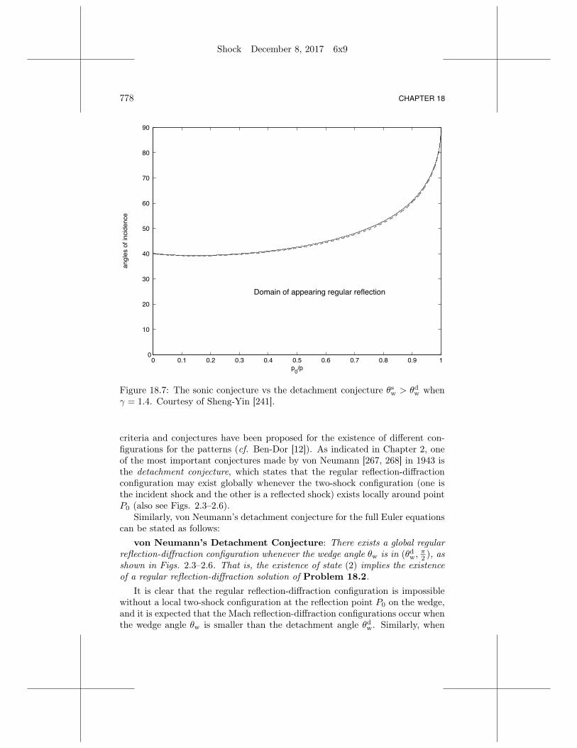
778
Shock December 8, 2017 6x9
CHAPTER 18
0 0.1 0.2 0.3 0.4 0.5 0.6 0.7 0.8 0.9 10
10
20
30
40
50
60
70
80
90
p0/p
angl
es o
f inc
iden
ce
Domain of appearing regular reflection
Figure 18.7: The sonic conjecture vs the detachment conjecture θsw > θd
w whenγ = 1.4. Courtesy of Sheng-Yin [241].
criteria and conjectures have been proposed for the existence of different con-figurations for the patterns (cf. Ben-Dor [12]). As indicated in Chapter 2, oneof the most important conjectures made by von Neumann [267, 268] in 1943 isthe detachment conjecture, which states that the regular reflection-diffractionconfiguration may exist globally whenever the two-shock configuration (one isthe incident shock and the other is a reflected shock) exists locally around pointP0 (also see Figs. 2.3–2.6).
Similarly, von Neumann’s detachment conjecture for the full Euler equationscan be stated as follows:
von Neumann’s Detachment Conjecture: There exists a global regularreflection-diffraction configuration whenever the wedge angle θw is in (θd
w,π2 ), as
shown in Figs. 2.3–2.6. That is, the existence of state (2) implies the existenceof a regular reflection-diffraction solution of Problem 18.2.
It is clear that the regular reflection-diffraction configuration is impossiblewithout a local two-shock configuration at the reflection point P0 on the wedge,and it is expected that the Mach reflection-diffraction configurations occur whenthe wedge angle θw is smaller than the detachment angle θd
w. Similarly, when

THE FULL EULER EQUATIONS AND THE POTENTIAL FLOW EQUATION
Shock December 8, 2017 6x9
779
the wedge angle θw is larger than the detachment angle θdw, the local theory
indicates that there are two possible states for state (2), and there has longbeen a debate as to which one is physically admissible; see Courant-Friedrichs[99], Ben-Dor [12], and the references cited therein.
Since the reflection-diffraction problem is not a local problem, we take a dif-ferent point of view, as in §7.5, for the potential flow case. The selection of state(2) should be determined by not only the local feature of the problem but also theglobal features of the problem, and more precisely, by the stability/continuityof the configuration with respect to the wedge angle θw as θw → π
2 .Stability/Continuity Criterion to Select the Correct State (2): Since
the solution is uniquely determined when the wedge angle θw = π2 , it is necessary
that the global regular reflection-diffraction configurations should converge tothe unique normal reflection solution when θw → π
2 , provided that such globalconfigurations can be constructed.
As for the potential flow equation, we employ this stability criterion to con-clude that the choice for state (2) should be (Ua2 , V
a2 , p
a2 , ρ
a2), which is a weaker
state (i.e., the jump of the corresponding shock is smaller), if such a globalconfiguration can be constructed.
In general, (Ua2 , Va2 , p
a2 , ρ
a2) may be supersonic or subsonic. If it is supersonic,
the characteristic propagation speeds are finite, and state (2) is completely de-termined by the local information: state (1), state (0), and the location of pointP0. That is, any information from the reflection region, especially the distur-bance at corner P3, cannot travel towards the reflection point P0. However, ifit is subsonic, the information can reach P0 and interact with it, potentiallycreating a new type of shock reflection-diffraction configurations. In particular,it is clear that no supersonic reflection configurations exist beyond the sonicangle. This argument motivated the following conjecture:
von Neumann’s Sonic Conjecture: There exists a supersonic regularreflection-diffraction configuration when θw ∈ (θs
w,π2 ) for θs
w > θdw, as shown
in Figs. 2.3 and 2.5. This is, the supersonicity of the weak state (2) (i.e.,|(Ua2 , V a2 )| > ca2) at P0 implies the existence of a supersonic regular reflection-diffraction solution of Problem 18.2.
There has been a long debate in the literature as to whether there still ex-ists a global regular reflection-diffraction configuration beyond the sonic angleup to the detachment angle; see Ben-Dor [12] and the references cited therein.As shown in Fig. 18.7, the difference between the wedge angles of the sonicconjecture and the detachment conjecture is only fractions of a degree; a reso-lution has greatly challenged even sophisticated modern numerical and labora-tory experiments. In Part IV, we have rigorously proved that the global regularreflection-diffraction configuration does exist beyond the sonic angle up to thedetachment angle for potential flow.
Similarly, to solve von Neumann’s conjectures, we can also reformulateProb-lem 18.2 into the following free boundary problem:

780
Shock December 8, 2017 6x9
CHAPTER 18
Problem 18.3 (Free Boundary Problem). For θw ∈ (θdw,
π2 ), find a free bound-
ary (curved reflected-diffracted shock) Γshock and a vector function (U, p, ρ) de-fined in region Ω, as shown in Figs. 2.3–2.6, such that ϕ satisfies:
(i) Equation (18.3.1) in Ω;
(ii) On the free boundary Γshock,
U · τ = U1 · τ , ρU · ν = ρ1U1 · ν, p+ ρ(U · ν)2 = p1 + ρ1(U1 · ν)2,
γp
(γ − 1)ρ+
1
2(U · ν)2 =
γp1
(γ − 1)ρ1+
1
2(U1 · ν)2,
ρ > ρ1,
where ν and τ are the unit normal and tangent vectors of the free boundaryΓshock;
(iii) (U, p, ρ) = (U2, p2, ρ2) on Γsonic in the supersonic reflection case as shownin Figs. 2.3 and 2.5, and at P0 in the subsonic reflection case as shown inFigs. 2.4 and 2.6;
(iv) U · ν = 0 on Γwedge ∪ Γsym,
where ν is the interior unit normal to Ω on Γwedge ∪ Γsym.
If the free boundary can be written as Γshock = ξ2 = fsh(ξ1) with fsh(ξ01) =
ξ01 tan θw, then the free boundary conditions can be written as
dfsh
dξ1=U1V1 − c1
√|U1|2 − c21
U21 − c21
= −u− u1
v − v1,
p
p1=ρ− µ2ρ1
ρ1 − µ2ρ,
p− p1 = −ρ1
(U1u− u1
v − v1+ V1
)(v − v1),
ρ > ρ1,
where c21 = ρρ1
p−p1
ρ−ρ1and µ2 = γ−1
γ+1 .The boundary condition (U, V, p, ρ) along the sonic circle is the Dirichlet
boundary condition, so that (U, V, p, ρ) is continuous across the sonic circle.Similarly, we notice that the key obstacle to the existence of regular reflection-
diffraction configurations is a new additional possibility that, for some wedgeangle θc
w ∈ (θdw,
π2 ), the reflected-diffracted shock P0P2 may attach to the wedge
vertex P3, as observed by experimental results (cf. [263, Fig. 238]).On the other hand, solutions with an attached shock do not exist when the
initial data of Problem 18.1 (or equivalently, the parameters of state (1) inProblem 18.2) satisfyMI ≤ 1, or equivalently, u1 ≤ c1, since the front state

THE FULL EULER EQUATIONS AND THE POTENTIAL FLOW EQUATION
Shock December 8, 2017 6x9
781
of the shock must be supersonic. Moreover, in this case, the regular reflection-diffraction solution of Problem 18.2 should exist for each θw ∈ (θd
w,π2 ), as von
Neumann conjectured [267, 268].In the other case, MI > 1, there is a possibility that there exists θc
w ∈(θd
w,π2 ) such that a regular reflection-diffraction solution with an attached shock
of Problem 18.2 exists for each θw ∈ (θcw,
π2 ) in the sense that a solution with
P2 = P3 exists for θw = θcw.
SinceMI is a function of nI = ρ1
ρ0for fixed γ > 1, determined by (18.2.4), the
condition thatMI ≤ 1 orMI > 1 is equivalent to the corresponding conditionon nI ; that is to say, there exists n∗ > nI such that
(i) MI < 1 for any nI ∈ (1, n∗);
(ii) MI = 1 for nI = n∗;
(iii) MI > 1 for any nI ∈ (n∗,∞).
Thus, Case (i) corresponds to the case of a relatively weaker incident shock,while Case (iii) corresponds to the case of a relatively stronger incident shock.
In fact, the regime between angles θsw and θd
w is very narrow and only frac-tions of a degree apart; see Fig. 18.7 from Sheng-Yin [241], where the solidcurve is the detachment angle curve with respect to p0
p1and the dash curve is
the sonic angle curve with respect to p0
p1. This shows that the difference between
the two conjectures is only fractions of a degree. Therefore, a complete un-derstanding of the behavior of the two different configurations requires furtherrigorous mathematical analysis.
18.7 CONNECTIONS WITH THE POTENTIAL FLOWEQUATION
In this section, we discuss the role of the potential flow equation for shockreflection-diffraction, even in the realm of the full Euler equations.
Under the Hodge-Helmoltz decomposition:
U = Dϕ+ W, divW = 0
for some function ϕ and vector W, the Euler equations (18.3.1) become
div(ρDϕ) + 2ρ = −div(ρW), (18.7.1)
D(1
2|Dϕ|2 + ϕ
)+Dp
ρ= (Dϕ+ W) ·DW + (D2ϕ+ I)W, (18.7.2)
(Dϕ+ W) ·Dω + (1 + ∆ϕ)ω = −curl(Dpρ
), (18.7.3)
(Dϕ+ W) ·DS = 0, (18.7.4)
divW = 0, (18.7.5)

782
Shock December 8, 2017 6x9
CHAPTER 18
where ω = curlW = curlU is the vorticity of the fluid, S = cv ln(pρ−γ) theentropy, and D the gradient with respect to the self-similar variables ξ.
When ω = 0, S = const., and W = 0 on a curve Γ transverse to the fluiddirection, we conclude from (18.7.4) that, in domain ΩE formed by the fluidtrajectories past Γ:
d
dtξ = (Dϕ+ W)(ξ),
we haveS = const.
This impliesp = const. ργ in ΩE ,
so thatcurl
(Dpρ
)= const. curl(Dργ−1) = 0 in ΩE .
Notice that, if U = Dϕ+W ∈ C0,1, the theory of ordinary differential equationsimplies that ΩE has an open interior, as long as curve Γ has a relatively openinterior.
Then equation (18.7.3) becomes
(Dϕ+ W) ·Dω + (1 + ∆ϕ)ω = 0,
which implies that
ω = 0, i.e., curlW = 0 in ΩE .
This yields that W = const. in ΩE , since divW = 0. Then we conclude
W = 0 in ΩE ,
since W|Γ = 0, which yields that the right-hand side of equation (18.7.2) van-ishes.
By scaling, we finally conclude that any solution of system (18.7.1)–(18.7.4)in domain ΩE is determined by the potential flow equation (2.2.8) with (2.2.9)for self-similar solutions.
In our case, when θw ∈ (θsw,
π2 ), the weak state (2) is supersonic and satisfies
ω = 0, W = 0, S = S2. (18.7.6)
If our solution (U, p, ρ) is C0,1 in domain P0P1P2P3 (as shown in Figs. 2.3 and2.5) and the tangential derivative of U is continuous across the sonic arc Γsonic,(18.7.6) still holds along Γsonic on the side of Ω. Therefore, we conclude byasserting the following theorem:
Theorem 18.7.1. Let (U, p, ρ) be a solution of Problem 18.2 such that (U, p, ρ)is C0,1 in the open domain P0P1P2P3 and the tangential derivative of U is con-tinuous across the sonic arc Γsonic. Let ΩE be the subdomain of Ω formed by the

THE FULL EULER EQUATIONS AND THE POTENTIAL FLOW EQUATION
Shock December 8, 2017 6x9
783
1ξPotential flow
0ω2S=S
0ω2S=S=
=
Figure 18.8: The potential flow equation coincides with the full Euler equationsin an important domain ΩE
fluid trajectories past the sonic arc Γsonic. Then, in ΩE, the full Euler equations(18.7.1)–(18.7.4) coincide with the potential flow equation (2.2.8) with (2.2.9) forself-similar solutions, that is, equation (2.2.8) with (2.2.9) is exact in domainΩE for Problem 18.2; see Fig. 18.8.
Remark 18.7.2. The domains like ΩE also exist in several Mach reflection-diffraction configurations. Theorem 18.7.1 applies to such domains wheneversolution (U, p, ρ) is C0,1 and the tangential derivative of U is continuous. Infact, Theorem 18.7.1 indicates that, for any solution ϕ of the potential flowequation (2.2.8) with (2.2.9), the C1,1–regularity of ϕ and the continuity of thetangential component of the velocity field U = Dϕ are optimal across the sonicarc Γsonic in general.
Remark 18.7.3. The importance of the potential flow equation (1.5) with (1.4)in the time-dependent Euler flows was also observed by Hadamard [146] through adifferent argument. Moreover, as indicated in §2.1, for the solutions containinga weak shock, especially in many aerodynamic applications, the potential flowmodel (2.2.8)–(2.2.9) and the full Euler flow model (18.7.1)–(18.7.4) match eachother well up to the third order of the shock strength. For more on this, see Bers[16], Glimm-Majda [139], and Morawetz [221].
Remark 18.7.4. Since two eigenvalues of system (18.7.1)–(18.7.4) are alwaysreal and repeated, with two linearly independent eigenvectors, system (18.7.1)–(18.7.4) can be decomposed of two transport-type equations and two nonlinearequations of mixed hyperbolic-elliptic type. While we have developed essentialtechniques in Parts I–IV to handle two mixed-type nonlinear equations with sim-ilar difficulties as for the potential flow equation (2.2.8) with (2.2.9), there maybe an additional new difficulty for the two coupled transport-type equations in the
784
Shock December 8, 2017 6x9
CHAPTER 18
other domain Ω \ ΩE containing the stagnation points U = 0 at which pressurep and vorticity ω may have additional singularity (cf. Serre [236]).
Notes: Theorem 18.5.2 was rigorously proved in Chang-Chen [31] based onthe work by Bleakney-Taub [18] and von Neumann [267, 268], while Theorem18.5.3 is due to Sheng-Yin [241]. Theorem 18.7.1 and related analysis for therole of the potential flow equation are due to Chen-Feldman [55].

Shock December 8, 2017 6x9
Chapter Nineteen
Shock Reflection-Diffraction and
New Mathematical Challenges
As demonstrated in Chapters 1–18, the analysis of shock reflection-diffractionhas advanced the development of new mathematical approaches, techniques, andideas that will be useful for solving further problems involving shock reflectionand/or diffraction, as well as other related problems involving similar analyticaldifficulties. Nevertheless, further understanding of these phenomena requiresthe development of ever more powerful new mathematics.
19.1 MATHEMATICAL THEORY FOR MULTIDIMENSIONALCONSERVATION LAWS
As we have indicated, shock reflection-diffraction configurations are a funda-mental class of structural patterns of solutions of the two-dimensional Riemannproblem for the Euler equations for compressible fluids. In addition, the Eulerequations are core fundamental nonlinear PDEs in the multidimensional hyper-bolic systems of conservation laws, and the Riemann solutions are expected to bethe global attractors and determine the local structure of general entropy solu-tions of the Cauchy problem (the initial value problem). Therefore, any furtherunderstanding of the shock reflection-diffraction configurations will advance ourunderstanding of the behavior of general entropy solutions of multidimensionalhyperbolic systems of conservation laws, which plays an important role in themultidimensional mathematical theory of hyperbolic conservation laws.
In this book, we have established the global existence, regularity, and struc-tural stability of regular reflection-diffraction configurations for potential flowup to the detachment angle or the critical angle. Further fundamental mathe-matical problems include the following:
Problem 19.1. Establish a mathematical theory for shock reflection-diffractionfor the two-dimensional isentropic and/or full Euler equations.
As seen in Chapters 1–18, we have understood the mathematical difficultiesrelatively well for the transonic shocks, the Kelydsh degeneracy near the sonicarc, the singularities of solutions near the wedge vertex and the corner betweenthe transonic shock and the sonic arc for the nonlinear second-order ellipticequations (cf. Theorem 18.7.1), as well as a one-point singularity at the corner

786
Shock December 8, 2017 6x9
CHAPTER 19
I
R
II
RR
(a) (b) (c)
Figure 19.1: Different types of Mach reflection-diffraction configurations
between the reflected shock and the wedge at the reflection point for the tran-sition from the supersonic to subsonic reflection configurations when the wedgeangle decreases across the sonic angle up to the detachment angle or the criticalangle. On the other hand, the following two new features of the problem for theisentropic and/or full Euler equations still need to be understood:
(i) Solutions of transport-type equations with rough coefficients and station-ary transport velocity;
(ii) Estimates of the vorticity of the pseudo-velocity.Indeed, the calculations in Serre [236] have shown difficulties in estimating
vorticity ω = ∇×U. It is possible that the vorticity will have some singularitiesin the region, perhaps near the wedge boundary and/or corner. In fact, evenfor potential flow, the second derivatives of the velocity potential, i.e., the firstderivatives of the velocity, may blow up at the wedge corner.
Problem 19.2. Analyze Mach reflection-diffraction configurations for the two-dimensional isentropic and/or full Euler equations.
When the wedge angle θw decreases across the detachment angle θdw, or
the incident-shock strength decreases, there is a transition from the RegularReflection (RR) to a Mach Reflection (MR). The MR configurations include theSimple Mach Reflection and become increasingly complex when they includethe Complex Mach Reflection, the Double Mach Reflection, the von NeumannReflection, and the Guderley Reflection, among others, as the wedge angle θw
decreases; see Fig. 19.1, as well as Figs. 1.2–1.6, for the types of the MachReflection and the Guderley Reflection. A detailed analysis based on the shockpolar can be found in [12, 13, 31, 151], while [96, 159, 230, 233, 257, 258, 259]and the references cited therein provide supportive numerical experiments.
There are several additional difficulties for the Mach reflection-diffractionconfigurations, including:
(i) A priori understanding of the location of the triple-point where the inci-dent shock and the reflected-diffracted shock meet;
(ii) At the triple-point of the Mach reflection, an additional shock called aMach stem connects this point to the wedge. Since a pure three-shock pattern

SHOCK REFLECTION-DIFFRACTION AND NEW MATHEMATICAL CHALLENGES
Shock December 8, 2017 6x9
787
Reflected-diff
racted
shock
Incident shock
Figure 19.2: Vorticity waves in the Mach reflection-diffraction configurations
is not normally possible, as indicated in Courant-Friedrichs [99] and Serre [236],a fourth wave – vortex sheet, or other types of waves, must originate fromthis triple-point generally. See Fig. 19.2 for a possible vorticity wave formedby the vortex sheet originating from the triple-point in the Mach reflectionconfiguration as observed experimentally. The stability of vortex sheets is a verysensitive issue, as indicated by Artola-Majda [2, 3]; for example, such waves areknown to be nonlinearly unstable dynamically in general, unless the jump ofthe tangential velocity exceeds 2
√2c (see [97, 98]). The question is whether
the self-similarity stabilizes such vortex sheets. In particular, it is important toidentify the right function space for the vorticity function ω = ∇×U, especiallyto examine whether the vortex sheet for the vorticity wave is a chord-arc withthe form:
z(s) = z0 + a(s)
∫ s
0
eib(τ)dτ, b ∈ BMO,
or a similar form.
Problem 19.3. Study the shock reflection-diffraction configurations for thehigher dimensional potential flow equations and isentropic/full Euler equations.
When a planar shock hits an n-dimensional cone, n ≥ 3, higher dimensionalshock reflection-diffraction phenomena occur. Then the supersonic part of thereflection-diffraction region, corresponding to state (2) in the two-dimensionalcase, is no longer a constant physical state, and the reflected-diffracted shock isno longer a straight cone. In particular, for the higher dimensional potential flowequation, the pseudo-potential function is no longer a quadratic function and thesupersonic part of the reflected-diffracted shock should also be treated as a freeboundary. The supersonic state is determined by the degenerate second-orderhyperbolic equations, which has to be solved first.

788
Shock December 8, 2017 6x9
CHAPTER 19
Another additional difficulty is that the boundary of the physical domain hasa more delicate singularity at the origin, i.e., the cone vertex. It is importantto understand how the pseudo-velocity vanishes in the subsonic domain in theself-similar coordinates. Further points to understand include the degeneracyof solutions across the sonic surface (in the RR case) and the singularity ofsolutions near the curved wedge-like corner between the transonic shock andthe sonic surface in the higher dimensional case.
It is also important to study the problem for higher dimensional isentropicand/or full Euler equations.
19.2 NONLINEAR PARTIAL DIFFERENTIAL EQUATIONS OFMIXED ELLIPTIC-HYPERBOLIC TYPE
As we have known from the previous chapters, nonlinear PDEs of mixed elliptic-hyperbolic type arise naturally from the shock reflection-diffraction problem.Such mixed equations also arise naturally in many other fundamental prob-lems in fluid mechanics, differential geometry, elasticity, relativity, calculus ofvariations, and related areas. The mathematical approaches and techniquesdeveloped in this book will be useful for solving a variety of nonlinear PDEsinvolving similar analytical difficulties. Nevertheless, further new mathematicalideas, techniques, and approaches need to be developed for solving these PDEs.
Problem 19.4. Study further elliptic free boundary problems for nonlinearequations of mixed type, and the corresponding nonlinear degenerate ellipticequations and systems.
From our solution of the regular shock reflection-diffraction problem for thepotential flow equation, the physical problem has been formulated into a freeboundary problem for a nonlinear second-order degenerate elliptic equation withellipticity degenerating on a part of the fixed boundary (the sonic curve), andmathematical techniques have been developed for this specific form of ellipticdegeneracy. Our analysis has the following features:
(i) The problem is global. In particular, even the local regularity estimatesfor the nonlinear degenerate elliptic equation near the sonic arc require someglobal properties of the solutions, including the positivity of ψ in §11.4. Sim-ilarly, in the subsonic reflection case, the estimates for the uniformly ellipticequation in the domain with free boundary near the reflection point in §16.6also rely on a global property – the monotonicity cone of ϕ1 − ϕ. Furthermore,the use of global properties is essential in the other estimates; for example, theestimates in §11.4 do not hold definitely if ψ is negative or changes its sign. Formore on this, see the estimates in §9.5.
(ii) In order to obtain the elliptic solution of a mixed-type nonlinear equation,the formulation of the free boundary problem should match with the nonlinearequation naturally.

SHOCK REFLECTION-DIFFRACTION AND NEW MATHEMATICAL CHALLENGES
Shock December 8, 2017 6x9
789
(iii) Our regularity estimates near the sonic arc, where the equation is degen-erate elliptic, are obtained by using a comparison function (which utilizes theKeldysh-type elliptic degeneracy and depends on the detailed structure of theself-similar potential flow equation), combined with rescaling techniques whosescaling is determined by both the equation and the structure of the domain.Indeed, we have developed three different scalings; see §11.4 and §16.4–§16.5.
Since nonlinear degenerate elliptic problems for PDEs of mixed type arisein many applications, it is important to obtain a deeper understanding of thedifferent types of elliptic degeneracy and the natural global settings for suchproblems.
Problem 19.5. Study further nonlinear degenerate hyperbolic equations andsystems.
Nonlinear degenerate hyperbolic equations/systems also arise in many shockreflection/diffraction problems, especially in the high dimensional case withsonic boundaries, as described in Problem 19.3. There are two types of de-generacy near the degenerate sets: hyperbolic degeneracy (Tricomi-type) andparabolic degeneracy (Keldysh-type). The prototype for linear degenerate hy-perbolic equations is the celebrated Euler-Poisson-Darboux equation (cf. [37,38, 41]), which has been successfully applied in solving some important one-dimensional nonlinear problems involving nonlinear degenerate hyperbolic sys-tems (cf. [38, 61, 62, 63, 64] and the references cited therein). The degeneracybehavior of self-similar flow for the two-dimensional Euler equations near thevacuum has been exhibited through the characteristic decompositions in Zheng[289]; see also [182, 180, 161]. Further understanding of nonlinear degeneratehyperbolic equations and systems in the multidimensional case deserves specialattention.
Problem 19.6. Develop further new ideas, techniques, and approaches to ana-lyze nonlinear PDEs of mixed elliptic-hyperbolic type
The study of degenerate hyperbolic equations and degenerate elliptic equa-tions as proposed in Problems 19.4–19.5 will be very helpful for developingfurther new ideas for nonlinear PDEs that change the type from hyperbolic toelliptic. The unification of the mathematical theory for these two classes of non-linear PDEs is at the cutting edge of modern mathematical research, and hasimportant implications for the parts of the wider scientific community which usenonlinear PDEs. Despite this, nonlinear mixed-type PDEs still remain poorlyunderstood and are exceedingly challenging from both the theoretical and nu-merical point of view. The mathematics of nonlinear mixed-type PDEs is largelyuncharted territory. Any advance in this direction can be expected to fertilizeand provide deeper insights into the theory of nonlinear PDEs in general, tolead to efficient new algorithms for the computation of solutions, and to impactupon developments in other branches of mathematics.
The mathematical methods expected for further development may includeweak convergence methods, entropy methods, energy estimate techniques, pos-

790
Shock December 8, 2017 6x9
CHAPTER 19
itive symmetrization techniques, and measure-theoretical methods, among oth-ers. These methods are largely independent of the types of PDEs under consid-eration (cf. [54, 69, 70, 115, 126]) and will therefore work well within a unifiedframework of nonlinear mixed-type PDEs.
19.3 FREE BOUNDARY PROBLEMS AND TECHNIQUES
As presented in this book, the shock reflection-diffraction problem can be for-mulated as free boundary problems involving nonlinear PDEs of mixed elliptic-hyperbolic type. Similarly, many other transonic problems can also be formu-lated as free boundary problems involving nonlinear PDEs of mixed type (cf.[38, 58] and the references cited therein). The understanding of these tran-sonic problems requires a complete mathematical solution of the correspond-ing free boundary problems for nonlinear mixed PDEs, such as what we havedone for the shock reflection-diffraction problem in this book. These problemsare not only longstanding open problems in fluid mechanics, but also funda-mental in the mathematical theory of multidimensional conservation laws; see[58, 139, 236, 286] and the references cited therein. In this sense, we have tounderstand these free boundary problems in order to fully understand globalentropy solutions to multidimensional hyperbolic systems of conservation laws.
Problem 19.7. Develop further free boundary techniques for solving transonicshock problems.
As we have shown, the shock reflection-diffraction problem has been for-mulated as a one-phase free boundary problem for nonlinear degenerate ellip-tic PDEs. Similarly, other shock reflection/diffraction problems such as thePrandtl-Meyer problem for supersonic flow impinging onto solid wedges can beformulated as one-phase free boundary problems involving other mathematicaldifficulties (cf. [5, 6]). Similar one-phase, or even two-phase, free boundary prob-lems also arise in many other transonic flow problems, such as steady transonicflow problems including transonic nozzle flow problems (cf. [7, 38, 53, 179]),steady transonic flows past obstacles (cf. [38, 43, 47, 85]), and the local stabil-ity of Mach configurations (cf. [81, 82]), as well as higher dimensional versions ofProblem 19.3 (shock reflection-diffraction by a solid cone). Some of these involvevarious types of degeneracy of free boundaries (i.e., the strength of jump tendsto zero at some points or singularities along the free boundary). In Chapters1–18, we have discussed recently developed mathematical approaches and tech-niques for solving some of these free boundary problems. On the other hand,the analysis of other types of transonic problems demands further developmentof mathematical ideas, techniques, and approaches.
Problem 19.8. Develop mathematical techniques for continuous transition be-tween the supersonic and subsonic phases.
Consider, for example, transonic flow problems involving supersonic bubblesin subsonic flow (cf. [95, 159, 217, 218, 219, 257, 258, 259]) and steady transonic

SHOCK REFLECTION-DIFFRACTION AND NEW MATHEMATICAL CHALLENGES
Shock December 8, 2017 6x9
791
flows past obstacles and nozzles (cf. [7, 38, 43, 47, 53, 85, 179]). Some recentexperimental and numerical results have shown that supersonic bubbles may oc-cur even in the shock reflection-diffraction configurations, such as the Guderleyreflection-diffraction configurations (cf. [243, 257, 258, 259]). The common fea-ture of these problems is the involvement of the continuous transition betweenthe supersonic and subsonic phases. Many of these problems can be formulatedas free boundary problems for nonlinear PDEs of mixed elliptic-hyperbolic type,whose free boundary is the phase boundary between the elliptic and hyperbolicphases, which degenerate at least on some part of the transition set. There havenot yet emerged mathematical techniques and approaches efficient enough totackle such free boundary problems. One of the strategies is to deal first withsome fundamental, concrete physical transonic problems involving supersonicbubbles in subsonic flow.
Problem 19.9. Develop mathematical techniques to understand the behavior ofsolutions near a point or set where a free boundary meets a fixed boundary, es-pecially when the free and/or fixed boundaries are transition boundaries betweenthe hyperbolic and elliptic phases.
As we have presented in this book, the free boundary problem formulatedfrom the shock reflection-diffraction problem involves the corner between thefree boundary and a fixed boundary that is a degenerate sonic curve for thenonlinear PDE. In this book, as well as in earlier papers [4, 54], we have devel-oped mathematical techniques for handling the optimal regularity of both thefree boundary and the corresponding solution at corner P1 on Fig. 2.3. Thereflected shock P0P2 is C2 near P1, so that the curved free boundary Γshock
matches at P1 not only the slope but also the curvature of the straight reflectedshock P0P1. The corresponding solution in Ω is C1,1 near P1, but not C2 up toP1. Our techniques have been developed based on the features of the underly-ing nonlinear PDE. It would be interesting to develop further the mathematicaltechniques and approaches for understanding the behavior of solutions near thepoint or set where a free boundary meets a fixed boundary, especially when thefree and/or fixed boundaries are transition boundaries between the hyperbolicand elliptic phases for general second-order PDEs of mixed type.
19.4 NUMERICAL METHODS FOR MULTIDIMENSIONALCONSERVATION LAWS
The main challenge in designing numerical algorithms for hyperbolic conserva-tion laws is that weak solutions are not unique, and multidimensional wavessuch as vortex sheets and entropy waves are often sensitive with perturbations,so that the numerical schemes should be consistent with the Clausius inequality(the entropy inequality), as well as other physical requirements to capture thesensitivity of multidimensional waves. Excellent numerical schemes should alsobe numerically simple, robust, fast, and low cost, and have sharp oscillation-free
792
Shock December 8, 2017 6x9
CHAPTER 19
resolutions and high accuracy in the domains where the solution is smooth. Itis also desirable that the schemes capture vortex sheets, vorticity waves, andentropy waves, as they appear in the shock reflection-diffraction configurations,and are coordinate invariant, among other features. The main difficulty in cal-culating fluid flows with discontinuities is that it is very hard to predict, even inthe process of a flow calculation, when and where new discontinuities arise andinteract. Moreover, tracking the discontinuities, especially their interactions, isnumerically burdensome (see [20, 100, 150, 174]).
Problem 19.10. Develop more efficient numerical methods for further under-standing shock reflection-diffraction phenomena.
Since its fundamental importance in fluid mechanics and the mathemati-cal theory of multidimensional conservation laws with rich structure, the shockreflection-diffraction problem has become a standard test problem for multidi-mensional numerical methods; see [12, 104, 105, 120, 133, 134, 135, 137, 138,139, 141, 149, 151, 152, 159, 160, 170, 174, 177, 221, 232, 236, 240, 256, 257,258, 259, 264, 273, 282] and the references cited therein. On the other hand,the sensitivity with respect to the wedge angle and the strength of the inci-dent shock, and the complexity of the shock reflection-diffraction configurationsurgently ask for more efficient numerical methods.
Problem 19.11. Develop more efficient numerical methods for multidimen-sional conservation laws.
Shock waves, vorticity waves, and entropy waves are, by nature, fundamentaldiscontinuity waves, and they arise in supersonic or transonic gas flow, or froma very sudden release (explosion) of chemical, nuclear, electrical, radiate, ormechanical energy in a limited space. Tracking these discontinuities and theirinteractions, especially when and where new waves arise and interact in themotion of gases, is one of the main motivations for numerical computation forthe gas dynamics equations.
An efficient numerical approach is shock capturing algorithms for general hy-perbolic conservation laws with form (1.10) or (1.11). Modern numerical ideasof shock capturing for computational fluid dynamics date back to 1944 when vonNeumann first proposed a new numerical method, a centered difference scheme,to treat the hydrodynamical shock problem, for which numerical calculationsshowed oscillations on the mesh scale (see Lax [173]). In 1950, von Neumann’sdream of capturing shocks was first realized when he and Richtmyer [271] intro-duced the ingenious idea of adding a numerical viscous term of the same size asthe truncation error into the hydrodynamic equations. Their numerical viscosityguarantees that the scheme is consistent with the Clausius inequality, i.e., theentropy inequality. The shock jump conditions – the Rankine-Hugoniot condi-tions – are satisfied, provided that the Euler equations of gas dynamics are dis-cretized in conservation form. Then oscillations are eliminated by the judicioususe of the artificial viscosity; the solutions constructed by this method converge

SHOCK REFLECTION-DIFFRACTION AND NEW MATHEMATICAL CHALLENGES
Shock December 8, 2017 6x9
793
uniformly, except in a neighborhood of shocks where they remain bounded andare spread out over a few mesh intervals.
In the one-dimensional case, further examples of success include the Lax-Friedrichs scheme (1954), the Glimm scheme (1965), the Godunov scheme (1959)and related high order shock capturing schemes; for example, van Leer’s MUSCL(1981), Colella-Wooward’s PPM (1984), Harten-Engquist-Osher-Chakravarthy’sENO (1987), the more recent WENO (1994, 1996), the Lax-Wendroff scheme(1960) and its two-step version, the Richtmyer scheme (1967), as well as theMacCormick scheme (1969). See also [66, 71, 100, 120, 141, 178, 256, 261] andthe references cited therein.
In the multidimensional case, one approach is to generalize directly the one-dimensional methods for solving multidimensional problems; such an approachhas led to several useful numerical methods including semi-discrete methods andStrang’s dimension-dimension splitting methods.
Observe that multidimensional effects do play a significant role in the behav-ior of the solution locally, as shown in the shock reflection-diffraction configura-tions. Also note that the approach that only solves one-dimensional Riemannproblems in the coordinate directions clearly lacks the use of all the multidi-mensional information. The development of fully multidimensional methodsrequires a good mathematical theory in order to understand the multidimen-sional behavior of entropy solutions, especially the shock reflection-diffractionconfigurations that have been analyzed in this book. However, further under-standing of the shock reflection-diffraction configurations requires more efficientnumerical methods. Current efforts in this direction include employing moreinformation about the multidimensional behavior of solutions, determining thedirection of primary wave propagation and applying wave propagation in otherdirections, and using transport techniques, upwind techniques, finite volumetechniques, relaxation techniques, and kinetic techniques from the microscopiclevel; see [33, 169, 203, 256], [120, 139, 141, 178, 261], and the references citedtherein.
Other useful methods for calculating sharp fronts for gas dynamics equationsinclude front-tracking algorithms [91, 138] and level set methods [223, 239].

Shock December 8, 2017 6x9
Bibliography
[1] Alt, H. W., Caffarelli, L. A. and Friedman A. (1985). Compressible flowsof jets and cavities, J. Diff. Eqs. 56: 82–141.
[2] Artola, M. and Majda, A. (1987). Nonlinear development of instability insupersonic vortex sheets, I: The basic kink modes, Phys. D. 28: 253–281.
[3] Artola, M. and Majda, A. (1989). Nonlinear development of instabilityin supersonic vortex sheets, II: Resonant interaction among kink modes,SIAM J. Appl. Math. 49: 1310–1349.
[4] Bae, M., Chen, G.-Q. and Feldman, M. (2009). Regularity of solutions toregular shock reflection for potential flow, Invent. Math. 175: 505–543.
[5] Bae, M., Chen, G.-Q. and Feldman, M. (2013). Prandtl-Meyer reflectionfor supersonic flow past a solid ramp, Quart. Appl. Math. 71: 583–600.
[6] Bae, M., Chen, G.-Q. and Feldman, M. (2017). Prandtl-Meyer ReflectionConfigurations, Transonic Shocks, and Free Boundary Problems, ResearchMonograph, In preparation.
[7] Bae, M.-J. and Feldman, M. (2011). Transonic shocks in multidimensionaldivergent nozzles, Arch. Rational Mech. Anal. 201: 777–840.
[8] Ball, J. M. and Carstensen, C. (1999). Compatibility conditions for mi-crostructures and the austenite-martensite transition, Mater. Sci. Eng. A.273–275: 231–236.
[9] Ball, J. M. and James, R. D. (1987). Fine phase mictures as minimizersof energy, Arch. Rational Mech. Anal. 100: 13–52.
[10] Ball, J. M., Kirchheim, B. and Kristensen, J. (2000). Regularity of qua-siconvex envelopes, Calc. Var. Partial Diff. Eqs. 11: 333–359.
[11] Bazhenova, T. V., Gvozdeva, L. G. and Nettleton, M. A. (1984). Unsteadyinteraction of shock waves, Prog. Aero. Sci. 21: 249–331.
[12] Ben-Dor, G. (1991). Shock Wave Reflection Phenomena, Springer-Verlag:New York.
BIBLIOGRAPHY
Shock December 8, 2017 6x9
795
[13] Ben-Dor, G. (2001). Oblique shock wave reflections, In: Handbook ofShock Waves (Eds. G. Ben-Dor, O. Igra, and T. Elperin), Vol. 2, pp. 67–179, Academic Press: San Diego.
[14] Benzoni-Gavage, S. and Serre, D. (2007). Multidimensional HyperbolicPartial Differential Equations: First-Order Systems and Applications, TheClarendon Press and Oxford University Press: Oxford.
[15] Bernoulli, D. (1738). Hydrodynamica, Argentorati.
[16] Bers, L. (1958). Mathematical Aspects of Subsonic and Transonic GasDynamics, John Wiley & Sons, Inc.: New York; Chapman & Hall, Ltd.:London.
[17] Bitsadze, A. V. (1964). Equations of the Mixed Type, Macmillan Company:New York.
[18] Bleakney, W. and Taub, A. H. (1949). Interaction of shock waves, Rev.Modern Phys. 21: 584–605.
[19] Bressan, A. (2000). Hyperbolic Systems of Conservation Laws: The One-dimensional Cauchy Problem, Oxford University Press: Oxford.
[20] Bressan, A., Chen, G.-Q., Lewicka, M. and Wang D.-H. (2011). NonlinearConservation Laws and Applications, IMA Volume in Mathematics and ItsApplications, 153, Springer-Verlag: New York.
[21] Caffarelli, L. A. (1987). A Harnack inequality approach to the regu-larity of free boundaries, I: Lipschitz free boundaries are C1,α, Rev. Mat.Iberoamericana, 3: 139–162.
[22] Caffarelli, L. A. (1989a). A Harnack inequality approach to the regularityof free boundaries, II: Flat free boundaries are Lipschitz, Comm. Pure Appl.Math. 42: 55–78.
[23] Caffarelli, L. A. (1989b). A Harnack inequality approach to the regularityof free boundaries, III: Existence theory, compactness, and dependence onX, Ann. Scuola Norm. Sup. Pisa Cl. Sci. (4), 15: 583–602.
[24] Caffrelli, L. A., Jerison, D. and Kenig, C. (2002). Some new monotonicitytheorems with applications to free boundary problems, Ann. of Math. 155:369–404.
[25] Caffarelli, L. and Salsa, S. (2005). A Geometric Approach to Free Bound-ary Problems, American Mathematical Society: Providence, RI.
[26] Canić, S., Keyfitz, B. L. and Kim, E. H. (2000). Free boundary problemsfor the unsteady transonic small disturbance equation: Transonic regularreflection, Meth. Appl. Anal. 7: 313–335.

796
Shock December 8, 2017 6x9
BIBLIOGRAPHY
[27] Canić, S., Keyfitz, B. L. and Kim, E. H. (2002). A free boundary problemfor a quasilinear degenerate elliptic equation: regular reflection of weakshocks, Comm. Pure Appl. Math. 55: 71–92.
[28] Canić, S., Keyfitz, B. L. and Lieberman, G. M. (2000). A proof of ex-istence of perturbed steady transonic shocks via a free boundary problem,Comm. Pure Appl. Math. 53: 484–511.
[29] Cauchy, A.-L. (1827). Sur les relations qui existent dans l’état d’équilibred’un corps solide ou fluide, entre les pressions ou tensions et les forcesaccélératrices, Exercises de Mathématiques, 2: 108–111.
[30] Cauchy, A.-L. (1829). Sur l’équilibre et le mouvenment intérieur des corpsconsidérés comme des masses continues, Exercises de Mathématiques, 4:293–319.
[31] Chang, T. and Chen, G.-Q. (1986). Diffraction of planar shock along thecompressive corner, Acta Math. Scientia, 6: 241–257.
[32] Chang, T., Chen, G.-Q. and Yang, S. (1992). 2-D Riemann problem in gasdynamics and formation of spiral, In: Nonlinear Problems in Engineeringand Science–Numerical and Analytical Approach (Beijing, 1991), pp. 167–179, Science Press: Beijing.
[33] Chang, T., Chen, G.-Q. and Yang, S. (1995). On the Riemann problemfor two-dimensional Euler equations I: Interaction of shocks and rarefactionwaves, Discrete Contin. Dynam. Systems, 1: 555–584.
[34] Chang, T., Chen, G.-Q. and Yang, S. (2000). On the Riemann problem fortwo-dimensional Euler equations II: Interaction of contact discontinuities,Discrete Contin. Dynam. Systems, 6: 419–430.
[35] Chang, T. and Hsiao, L. (1989). The Riemann Problem and Interactionof Waves in Gas Dynamics, Longman Scientific & Technical: Harlow; andJohn Wiley & Sons, Inc.: New York.
[36] Chapman, C. J. (2000). High Speed Flow, Cambridge University Press:Cambridge.
[37] Chen, G.-Q. (1997). Euler-Poisson-Darboux equations and hyperbolic con-servation laws. In: Nonlinear Evolutionary Partial Differential Equations,pp. 11–25, AMS/IP Studies in Advanced Mathematics, Vol. 3, InternationalPress: Cambridge, Massachusetts.
[38] Chen, G.-Q. (2005). Euler equations and related hyperbolic conservationlaws, Chapter 1, Handbook of Differential Equations, Evolutionary Equa-tions, Vol. 2, Eds. C. M. Dafermos and E. Feireisl, Elsevier: Amsterdam,The Netherlands.

BIBLIOGRAPHY
Shock December 8, 2017 6x9
797
[39] Chen, G.-Q. (2008). On nonlinear partial differential equations of mixedtype, In: Proceedings of the 4th International Congress of Chinese Mathe-maticians, Eds. L. Jin, K.-F. Liu, L. Yang, and S.-T. Yau, Higher EducationPress: Beijing.
[40] Chen, G.-Q. (2015a). Gas dynamics equations: Computation. In: En-cyclopedia of Applied and Computational Mathematics, Ed. B. Engquist,Springer-Verlag: Berlin and Heidelberg. arXiv:1205.4433.
[41] Chen, G.-Q. (2015b). The Tricomi equation. In: Equations, Laws andFunctions of Applied Mathematics, the Princeton Companion to AppliedMathematics, Ed. N. J. Higham, III. 30, pp. 170, Princeton UniversityPress. arXiv:1311.3338.
[42] Chen, G.-Q., Chen, J. and Feldman, M. (2007). Transonic shocks andfree boundary problems for the full Euler equations in infinite nozzles, J.Math. Pures Appl. 88: 191–218.
[43] Chen, G.-Q., Chen, J. and Feldman, M. (2016). Transonic flows withshocks past curved wedges for the full Euler equations, Discrete Contin.Dyn. Syst. 36: 4179–4211.
[44] Chen, G.-Q., Chen, J. and Song, K. (2006). Transonic nozzle flows andfree boundary problems for the full Euler equations, J. Diff. Eqs. 229:92–120.
[45] Chen, G.-Q., Clelland, J., Slemrod, M., Wang, D. and Yang, D. (2017).Isometric embedding via strongly symmetric positive systems, Asian J.Math. (in press). arXiv:1502.04356.
[46] Chen, G.-Q., Dafermos, C. M., Slemrod, M. and Wang, D. (2007). Ontwo-dimensional sonic-subsonic flow, Commun. Math. Phys. 271: 635–647.
[47] Chen, G.-Q. and Fang, B.-X. (2009). Stability of transonic shock-frontsin steady potential flow past a perturbed cone, Discrete Conti. DynamicalSystems, 23: 85–114.
[48] Chen, G.-Q. and Fang, B.-X. (2017). Stability of transonic shocks insteady supersonic flow past multidimensional wedges, Adv. Math. 314: 493–539.
[49] Chen, G.-Q. and Feldman, M. (2003). Multidimensional transonic shocksand free boundary problems for nonlinear equations of mixed type, J.Amer. Math. Soc. 16: 461–494.
[50] Chen, G.-Q. and Feldman, M. (2004a). Steady transonic shocks and freeboundary problems in infinite cylinders for the Euler equations, Comm.Pure Appl. Math. 57: 310–356.
798
Shock December 8, 2017 6x9
BIBLIOGRAPHY
[51] Chen, G.-Q. and Feldman, M. (2004b). Free boundary problems and tran-sonic shocks for the Euler equations in unbounded domains, Ann. ScuolaNorm. Sup. Pisa Cl. Sci. (5), 3: 827–869.
[52] Chen, G.-Q. and Feldman, M. (2005). Potential theory for shock reflectionby a large-angle wedge, Proc. Nat. Acad. Sci. U.S.A. 102: 15368–15372.
[53] Chen, G.-Q. and Feldman, M. (2007). Existence and stability of multi-dimensional transonic flows through an infinite nozzle of arbitrary cross-sections, Arch. Rational Mech. Anal. 184: 185–242.
[54] Chen, G.-Q. and Feldman, M. (2010a). Global solutions to shock reflectionby large-angle wedges for potential flow, Ann. of Math. 171: 1019–1134.
[55] Chen, G.-Q. and Feldman, M. (2010b). Shock reflection-diffraction andmultidimensional conservation laws, In: Hyperbolic Problems: Theory, Nu-merics and Applications, Proc. Sympos. Appl. Math. 67: 25–52, Amer.Math. Soc.: Providence, RI.
[56] Chen, G.-Q. and Feldman, M. (2011). Shock reflection-diffraction andnonlinear partial differential equations of mixed type, In: Complex Anal-ysis and Dynamical Systems IV, Contemporary Mathematics, 554: 55–72,Amer. Math. Soc.: Providence, RI.
[57] Chen, G.-Q. and Feldman, M. (2012). Comparison principles for self-similar potential flow, Proc. Amer. Math. Soc. 140: 651–663.
[58] Chen, G.-Q. and Feldman, M. (2015). Free boundary problems in shockreflection/diffraction and related transonic flow problems, In: Free Bound-ary Problems and Related Topics. Theme Volume: Phil. Trans. R. Soc.A373: 20140276, The Royal Society: London.
[59] Chen, G.-Q., Feldman, M., Hu, J. and Xiang, W. (2017). Loss of regularityof solutions of the shock diffraction problem by a convex corned wedge forthe potential flow equation, Preprint, arXiv:1705.06837.
[60] Chen, G.-Q., Feldman, M. and Xiang, W. (2017). Convexity of self-similartransonic shock waves for potential flow, Preprint.
[61] Chen, G.-Q. and Kan, P. T. (1995). Hyperbolic conservation laws withumbilic degeneracy, I. Arch. Rational Mech. Anal. 130: 231–276.
[62] Chen, G.-Q. and Kan, P. T. (2001). Hyperbolic conservation laws withumbilic degeneracy, II. Arch. Rational Mech. Anal. 160: 325–354.
[63] Chen, G.-Q. and LeFloch, P. G. (2000). Compressible Euler equationswith general pressure law, Arch. Rational Mech. Anal. 153: 221–259.
[64] Chen, G.-Q. and LeFloch, P. G. (2003). Existence theory for the isentropicEuler equations, Arch. Rational Mech. Anal. 166: 81–98.

BIBLIOGRAPHY
Shock December 8, 2017 6x9
799
[65] Chen, G.-Q. and Li, T.-H. (2008). Well-posedness for two-dimensionalsteady supersonic Euler flows past a Lipschitz wedge, J. Diff. Eqs. 244:1521–1550.
[66] Chen, G.-Q. and Liu, J.-G. (1997). Convergence of difference schemeswith high resolution for conservation laws, Math. Comp. 66: 1027–1053.
[67] Chen, G.-Q., Shahgholian, H. and Vázquez, J.-V. (2015). Free bound-ary problems: The forefront of current and future developments, In: FreeBoundary Problems and Related Topics. Theme Volume: Phil. Trans. R.Soc. A373: 20140285, The Royal Society: London.
[68] Chen, G.-Q., Slemrod, M. and Wang, D. (2008). Vanishing viscositymethod for transonic flow, Arch. Rational Mech. Anal. 189: 159–188.
[69] Chen, G.-Q., Slemrod, M. and Wang, D. (2010a). Isometric embeddingand compensated compactness, Commun. Math. Phys. 294: 411–437.
[70] Chen, G.-Q., Slemrod, M. and Wang, D. (2010b). Weak continuity of theGauss-Codazzi-Ricci system for isometric embedding, Proc. Amer. Math.Soc. 138: 1843–1852.
[71] Chen, G.-Q. and Toro, E.-F. (2004). Centered difference schemes fornonlinear hyperbolic equations, J. Hyper. Diff. Eqs. 1: 531–566.
[72] Chen, G.-Q. and Wang, Y.-G. (2012). Characteristic discontinuities andfree boundary problems for hyperbolic conservation laws, In: NonlinearPartial Differential Equations, The Abel Symposium 2010, Chapter 5, pp.53–82, H. Holden and K. H. Karlsen (Eds.), Springer-Verlag: Heidelberg.
[73] Chen, G.-Q. and Yuan, H. (2009). Uniqueness of transonic shock solutionsin a duct for steady potential flow, J. Diff. Eqs. 247: 564–573.
[74] Chen, G.-Q., Zhang, Y. and Zhu, D. (2006). Existence and stability ofsupersonic Euler flows past Lipschitz wedges, Arch. Rational Mech. Anal.181: 261–310.
[75] Chen, S.-X. (1996). Linear approximation of shock reflection at a wedgewith large angle, Comm. Partial Diff. Eqs. 21: 1103–1118.
[76] Chen, S.-X. (1998a). Asymptotic behavior of supersonic flow past a convexcombined wedge, Chinese Ann. of Math. 19B: 255–264.
[77] Chen, S.-X. (1998b). Supersonic flow past a concave double wedge, Sci.China Mathematics, 41A: 39–47.
[78] Chen, S.-X. (1998b). Global existence of supersonic flow past a curvedconvex wedge, J. Partial Diff. Eqs. 11: 73–82.

800
Shock December 8, 2017 6x9
BIBLIOGRAPHY
[79] Chen, S.-X. (2001). Existence of stationary supersonic flows past a pointbody, Arch. Rational Mech. Anal. 156: 141–181.
[80] Chen, S.-X. (2005). Stability of transonic shock fronts in two-dimensionalEuler systems, Trans. Amer. Math. Soc. 357: 287–308.
[81] Chen, S.-X. (2006). Stability of a Mach configuration, Comm. Pure Appl.Math. 59: 1–35.
[82] Chen, S.-X. (2008). Mach configuration in pseudo-stationary compressibleflow, J. Amer. Math. Soc. 21: 63–100.
[83] Chen, S.-X. (2012). E-H type Mach configuration and its stability, Com-mun. Math. Phys. 315: 563–602.
[84] Chen, S.-X. (2015). Global existence and stability of a stationary Machreflection, Sci. China Mathematics, 58: 11–34.
[85] Chen, S.-X. and Fang, B. (2007). Stability of transonic shocks in super-sonic flow past a wedge, J. Diff. Eqs. 233: 105–135.
[86] Chen, S.-X., Hu, D. and Fang, B. (2013). Stability of the E-H type regularshock refraction, J. Diff. Eqs. 254: 3146–3199.
[87] Chen, S.-X. and Li, D. (2014). Cauchy problem with general discontinuousinitial data along a smooth curve for 2-D Euler system, J. Diff. Eqs. 257:1939–1988.
[88] Chen, S.-X. and Qu, A. (2012). Two-dimensional Riemann problems forChaplygin gas, SIAM J. Math. Anal. 44(3): 2146–2178.
[89] Chen, S.-X., Xin, Z. and Yin, H. (2002). Global shock waves for thesupersonic flow past a perturbed cone, Commun. Math. Phys. 228: 47–84.
[90] Chen, S.-X. and Yuan, H. (2008). Transonic shocks in compressible flowpassing a duct for three-dimensional Euler systems, Arch. Rational Mech.Anal. 187: 523–556.
[91] Chern, I.-L., Glimm, J., McBryan O., Plohr B. and Yaniv S. (1986). Fronttracking for gas dynamics, J. Comp. Phys. 62: 83–110.
[92] Chorin, A. J. (1994). Vorticity and Turbulence, Springer-Verlag: NewYork.
[93] Ciarlet, P. G. and Mardare, C. (2010). Existence theorems in intrinsicnonlinear elasticity, J. Math. Pures Appl. 94: 229–243.
[94] Clausius, R. (1865). Über verschiedene für die Anwendung bequeme For-men der Hauptgleichungen der mechanischen Wärmatheorie, Annalen derPhysik und Chemie, 125: 353–400.

BIBLIOGRAPHY
Shock December 8, 2017 6x9
801
[95] Cole, J. D. and Cook, L. P. (1986). Transonic Aerodynamics, North-Holland: Amsterdam.
[96] Colella, P. and Henderson, L. F. (1990). The von Neumann paradox forthe diffraction of weak shock waves, J. Fluid Mech. 213: 71–94.
[97] Coulombel, J. F. and Secchi, P. (2004). Stability of compressible vortexsheet in two space dimensions, Indiana Univ. Math. J. 53: 941–1012.
[98] Coulombel, J. F. and Secchi, P. (2008). Nonlinear compressible vortexsheets in two space dimensions, Ann. Sci. Ecole Norm. Sup. 41: 85–139.
[99] Courant, R. and Friedrichs, K. O. (1948). Supersonic Flow and ShockWaves, Springer-Verlag: New York.
[100] Dafermos, C.-M. (2016). Hyperbolic Conservation Laws in ContinuumPhysics, 4th Edition, Springer-Verlag: Berlin.
[101] Dafermos, C.-M. and Feireisl, E. (2004–06). Handbook of DifferentialEquations, Vols. 1–3, Elsevier: Amsterdam.
[102] Dafermos, C.-M. and Pokorny, M. (2008–09). Handbook of DifferentialEquations, Vols. 4–5, Elsevier: Amsterdam.
[103] Daskalopoulos, P. and Hamilton, R. (1999). The free boundary in theGauss curvature flow with flat sides, J. Reine Angew. Math. 510: 187–227.
[104] Dem’yanov, A. Yu. and Panasenko, A. V. (1981). Numerical solution tothe problem of the diffraction of a plane shock wave by a convex corner,Fluid Dynamics 16: 720–725 (Translated from the original Russian).
[105] Deschambault, R L. and Glass, I. I. (1983). An update on non-stationaryoblique shock-wave reflections: actual isopycnics and numerical experi-ments, J. Fluid Mech. 131: 27–57.
[106] Ding, X., Chen, G.-Q. and Luo P. (1989). Convergence of the fractionalstep Lax-Friedrichs scheme and Godunov scheme for isentropic gas dynam-ics, Commun. Math. Phys. 121: 63–84.
[107] Dong, G. (1991). Nonlinear Partial Differential Equations of Second Or-der, Transl. Math. Monographs, 95, Amer. Math. Soc.: Providence, RI.
[108] Elling, V. (2009). Counter exammples to the sonic criterion, Arch. Ra-tional Mech. Anal. 194 (3): 987–1010.
[109] Elling, V. (2012). Non-existence of strong regular reflections in self-similar potential flow, J. Diff. Eqs. 252: 2085–2103.
[110] Elling, V. and Liu, T.-P. (2005). The ellipticity principle for self-similarpotential flows, J. Hyper. Diff. Eqs. 2: 909–917.
802
Shock December 8, 2017 6x9
BIBLIOGRAPHY
[111] Elling, V. and Liu, T.-P. (2008). Supersonic flow onto a solid wedge,Comm. Pure Appl. Math. 61: 1347–1448.
[112] Euler, L. (1755). Principes géenéraux du mouvement des fluides, Mém.Acad. Sci. Berlin 11: 274–315.
[113] Euler, L. (1759). Supplément aux recherches sur la propagation du son,Mém. Acad. Sci. Berlin 15: 210–240.
[114] Euler, L. (1759, 1761). De principiis motus fluidorum, Novi Comm. Acad.Petrop. xiv & vi.
[115] Evans, L. C. (1990). Weak Convergence Methods for Nonlinear PartialDifferential Equations, CBMS-RCSM, 74, Amer. Math. Soc.: Providence,RI.
[116] Evans, L. C. (2010). Partial Differential Equations, Amer. Math. Soc.:Providence, RI.
[117] Fang, B.-X. (2006). Stability of transonic shocks for the full Euler systemin supersonic flow past a wedge, Math. Methods Appl. Sci. 29: 1–26.
[118] Feldman, M. (2001). Regularity of Lipschitz free boundaries in two-phaseproblems for fully nonlinear elliptic equations, Indiana Univ. Math. J. 50:1171–1200.
[119] Ferrari, C. and Tricomi, F. G. (1968). Transonic Aerodynamics, Aca-demic Press: New York, English Transl. of Aerodinamica Transonica, Cre-monese (1962).
[120] Fey, M. and Jeltsch, R. (1999). Hyperbolic Problems: Theory, Numerics,and Applications, I, II, International Series of Numerical Mathematics 130,Birkhäuser Verlag: Basel.
[121] Finn, R. and Gilbarg, D. (1957). Three-dimensional subsonic flows, andasymptotic estimates for elliptic partial differential equations, Acta Math.98: 265–296.
[122] Francheteau, J. and Métivier, G. (2000). Existence de Chocs Faiblespour des Systèmes Quasi-linéaires Hyperboliques Multidimensionnels,Astérisque, 268, SMF: Paris.
[123] Freistühler, H. and Szepessy, A. (2001). Advances in the Theory of ShockWaves, Birkhäuser: Boston.
[124] Friedman, A. (1988). Variational Principles and Free-Boundary Prob-lems, 2nd Edition. Robert E. Krieger Publishing Co., Inc.: Malabar, FL[First edition, John Wiley & Sons, Inc.: New York, 1982].

BIBLIOGRAPHY
Shock December 8, 2017 6x9
803
[125] Friedlander, S. and Serre, D. (2002-07). Handbook of Mathematical FluidDynamics. Elsevier: Amsterdam.
[126] Friedrichs, K. O. (1958). Symmetric positive linear differential equations,Comm. Pure Appl. Maths. 11: 333–418.
[127] Gamba, I. M. and Morawetz, C. S. (1996). A viscous approximationfor a 2-D steady semiconductor or transonic gas dynamic flow: existencetheorem for potential flow, Comm. Pure Appl. Math. 49: 999–1049.
[128] Gamba, I., Rosales, R. R. and Tabak, E. G. (1999). Constraints onpossible singularities for the unsteady transonic small disturbance (UTSD)equations, Comm. Pure Appl. Math. 52: 763–779.
[129] Gibbs, J. W. (1873). A method of geometrical representation of thethermodynamic properties of substances by means of surfaces, Trans. Con-necticut Acad. 2: 382–404.
[130] Gilbarg, D. and Hörmander, L. (1980). Intermediate Schauder estimates,Arch. Rational Mech. Anal. 74(4): 297–318.
[131] Gilbarg, D. and Trudinger, N. (1983). Elliptic Partial Differential Equa-tions of Second Order, 2nd Edition, Springer-Verlag: Berlin.
[132] Glass, I. I. (1974). Shock Waves and Man, University of Toronto Press:Toronto.
[133] Glaz, H. M., Colella, P., Glass, I. I. and Deschambault, R. L. (1985a).A numerical study of oblique shock-wave reflection with experimental com-parisons, Proc. Roy. Soc. Lond. A398: 117–140.
[134] Glaz, H. M., Colella, P., Glass, I. I. and Deschambault, R. L. (1985b).A detailed numerical, graphical, and experimental study of oblique shockwave reflection, Lawrence Berkeley Laboratory Report, LBL-20033.
[135] Glaz, H. M., Walter, P. A., Glass, I. I. and Hu, T. C. J. (1986). Obliqueshock wave reflections in SF6: A comparison of calculation and experiment,AIAA J. Prog. Astr. Aero. 106: 359–387.
[136] Glimm, J. (1991). Nonlinear waves: overview and problems. In: Mul-tidimensional Hyperbolic Problems and Computations (Minneapolis, MN,1989), IMA Vol. Math. Appl. 29: 89–106, Springer: New York.
[137] Glimm, J., Ji, X.-M., Li, J.-Q., Li, X.-L., Zhang, P., Zhang, T. and Zheng,Y.-X. (2008). Transonic shock formation in a rarefaction Riemann problemfor the 2-D compressible Euler equations, SIAM J. Appl. Math. 69: 720–742.

804
Shock December 8, 2017 6x9
BIBLIOGRAPHY
[138] Glimm, J., Klingenberg, C., McBryan, O., Plohr, B., Sharp, D. and Yaniv,S. (1985). Front tracking and two-dimensional Riemann problems, Adv.Appl. Math. 6: 259–290.
[139] Glimm, J. and Majda, A. (1991). Multidimensional Hyperbolic Problemsand Computations, Springer-Verlag: New York.
[140] Glimm, J., Kranzer, H. C., Tan, D. and Tangerman, F. M. (1997).Wave fronts for Hamilton-Jacobi equations: the general theory for Riemannsolutions in Rn, Commun. Math. Phys. 187: 647–677.
[141] Godlewski, E. and Raviart, P. (1996). Numerical Approximation of Hy-perbolic Systems of Conservation Laws, Springer-Verlag: New York.
[142] Gu, C.-H. (1962). A method for solving the supersonic flow past a curvedwedge (in Chinese), Fudan Univ. J. 7: 11–14.
[143] Guderley, K. G. (1962). The Theory of Transonic Flow, Translated fromthe German by J. R. Moszynski, Pergamon Press: Oxford-London-Paris-Frankfurt; Addison-Wesley Publishing Co. Inc.: Reading, Mass.
[144] Guès, O., Métivier, G., Williams, M. and Zumbrun, K. (2005). Existenceand stability of multidimensional shock fronts in the vanishing viscositylimit, Arch. Rational Mech. Anal. 175: 151–244.
[145] Guès, O., Métivier, G., Williams, M. and Zumbrun, K. (2006). Navier-Stokes regularization of multidimensional Euler shocks, Ann. Sci. ÉcoleNorm. Sup. (4) 39: 75–175.
[146] Hadamard, J. (1903). Leçons sur la Propagation des Ondes et les Équa-tions de l’Hydrodynamique, Hermann: Paris (Reprinted by Chelsea 1949).
[147] Han, Q. and Hong, J.-X. (2006). Isometric Embedding of RiemannianManifolds in Euclidean Spaces, Amer. Math. Soc.: Providence, RI.
[148] Harabetian, E. (1987). Diffraction of a weak shock by a wedge, Comm.Pure Appl. Math. 40: 849–863.
[149] Hindman, R. G., Kutler, P. and Anderson, D. (1979). A two-dimensionalunsteady Euler-equation solver for flow regions with arbitrary boundaries,AIAA Report 79-1465.
[150] Holden, H. and Risebro, N. H. (2002). Front Tracking for HyperbolicConservation Laws, Springer-Verlag: New York.
[151] Hornung, H. G. (1986). Regular and Mach reflection of shock waves,Ann. Rev. Fluid Mech. 18: 33–58.

BIBLIOGRAPHY
Shock December 8, 2017 6x9
805
[152] Hornung, H. G., Oertel, H. and Sandeman, R. J. (1979). Transition toMach reflexion of shock waves in steady and pseudosteady flow with andwithout relaxation, J. Fluid Mech. 90: 541–560.
[153] Hugoniot, H. (1887). Sur la propagation du mouvement dans les corpset spécialement dans les gaz parfaits, I. J. Ecole Polytechnique 57: 3–97.
[154] Hugoniot, H. (1889). Sur la propagation du mouvement dans les corps etspécialement dans les gaz parfaits, II. J. Ecole Polytechnique 58: 1–125.
[155] Hunter, J. K. (1988). Transverse diffraction of nonlinear waves and sin-gular rays, SIAM J. Appl. Math. 48: 1–37.
[156] Hunter, J. (1989). Hyperbolic waves and nonlinear geometrical acous-tics, In: Transactions of the 6th Army Conference on Appl. Math. andComputing, Boulder CO., pp. 527–569.
[157] Hunter, J. (1997). Nonlinear wave diffraction. In: Geometrical Opticsand Related Topics (Cortona, 1996), Progr. Nonlinear Diff. Eqs. Appl. 32,pp. 221–243, Birkhäuser Boston: Boston, MA.
[158] Hunter, J. and Keller, J. B. (1984). Weak shock diffraction, Wave Motion6: 79–89.
[159] Hunter, J. K. and Tesdall, A. (2002). Self-similar solutions for weakshock reflection, SIAM J. Appl. Math. 63: 42–61.
[160] Ivanov, M. S., Vandromme, D., Formin, V. M., Kudryavtsev, A. N., Had-jadj, A. and Khotyanovsky, D. V. (2001). Transition between regular andMach reflection of shock waves: new numerical and experimental results,Shock Waves 11: 199–207.
[161] Ji, X. and Zheng, Y. (2013). Characteristic decouplings and interactionsof rarefaction waves of 2D Euler equations, J. Math. Anal. Appl. 406: 4–14.
[162] Keller, J B. and Blank, A. A. (1951). Diffraction and reflection of pulsesby wedges and corners, Comm. Pure Appl. Math. 4: 75–94.
[163] Keyfitz, B. L. and Warnecke, G. (1991). The existence of viscous profilesand admissibility for transonic shocks, Comm. Partial Diff. Eqs. 16: 1197–1221.
[164] Kinderlehrer, D. and Nirenberg, L. (1977). Regularity in free boundaryproblems, Ann. Scuola Norm. Sup. Pisa Cl. Sci. (4) 4: 373–391.
[165] Kirchhoff, G. (1868). Über den Einfluss der Wärmeleitung in einem Gaseauf die Schallbewegung, Ann. Physik 134: 177–193.
[166] Korobeinikov, V. P. (1986). Nonstationary Interactions of Shock andDetonation Wave in Gases, Nauka: Moscow, USSR (in Russian).

806
Shock December 8, 2017 6x9
BIBLIOGRAPHY
[167] Krehl, V. P. and van der Geest, M. (1991). The discovery of the Machreflection effect and its demonstration in an auditorium, Shock Waves 1:3–15.
[168] Kristensen, J. (1999). On the non-locality of quasiconvexity, Ann. Inst.H. Poincaré Anal. Non Linéaire 16: 1–13.
[169] Kurganov, A. and Tadmor, E. (2002). Solution of two-dimensional Rie-mann problems for gas dynamics without Riemann problem solvers, Numer.Methods Partial Diff. Eqs. 18: 584–608.
[170] Kutler, P. and Shankar, V. (1977). Diffraction of a shock wave by acompression corner, Part I: Regular reflection, AIAA J. 15: 197–203.
[171] Lax, P. D. (1973). Hyperbolic Systems of Conservation Laws and theMathematical Theory of Shock Waves, CBMS-RCSM, SIAM: Philiadelphia.
[172] Lax, P. D. (1986a). Hyperbolic systems of conservation laws in severalspace variables, In: Current Topics in Partial Differential Equations, pp.327–341, Kinokuniya: Tokyo.
[173] Lax, P. D. (1986b). On dispersive difference schemes, Physica D 18:250–254.
[174] Lax, P. D. (2000). Mathematics and computing, In: Mathematics: Fron-tiers and Perspectives, pp. 417–432, Arnold, V.I., Atiyah, M., Lax, P. andMazur, B. (Eds.), Amer. Math. Soc.: Providence, RI.
[175] Lax, P. D. and Liu, X.-D. (1998). Solution of two-dimensional Riemannproblems of gas dynamics by positive schemes, SIAM J. Sci. Comput. 19:319–340.
[176] LeFloch, Ph. G. (2002). Hyperbolic Systems of Conservation Laws:The Theory of Classical and Nonclassical Shock Waves, Birkhäuser-Verlag:Basel.
[177] LeVeque, R. J. (1992). Numerical Methods for Conservation Laws, Sec-ond Ed., Birkhäuser-Verlag: Basel.
[178] LeVeque, R. J. (2002). Finite Volume Methods for Hyperbolic Problems,Cambridge University Press: Cambridge.
[179] Li, J., Xin, Z. and Yin, H. (2003). Transonic shocks for the full com-pressible Euler system in a general two-dimensional de Laval nozzle, Arch.Rational Mech. Anal. 207: 533–581.
[180] Li, J., Yang, Z. and Zheng, Y. (2011). Characteristic decompositionsand interactions of rarefaction waves of 2-D Euler equations, J. Diff. Eqs.250: 782–798.

BIBLIOGRAPHY
Shock December 8, 2017 6x9
807
[181] Li, J., Zhang, T. and Yang, S. (1998). The Two-Dimensional RiemannProblem in Gas Dynamics, Longman (Pitman Monographs 98): Essex.
[182] Li, J. and Zheng, Y. (2009). Interaction of rarefaction waves of the two-dimensional self-similar Euler equations, Arch. Rational Mech. Anal. 193:623–657.
[183] Li, T.-T. (1980). On a free boundary problem, Chinese Ann. Math. 1:351–358.
[184] Lieberman, G. M. (1985a). The Perron process applied to oblique deriva-tive problems, Adv. Math. 55: 161–172.
[185] Lieberman, G. M. (1985b). Regularized distance and its applications,Pacific J. Math. 117: 329–352.
[186] Lieberman, G. M. (1986a). Intermediate Schauder estimates for obliquederivative problems, Arch. Rational Mech. Anal. 93: 129–134.
[187] Lieberman, G. M. (1986b). Mixed boundary value problems for ellipticand parabolic differential equations of second order, J. Math. Anal. Appl.113: 422–440.
[188] Lieberman, G. M. (1986c). Regularity of solutions of nonlinear ellipticboundary value problems, J. Reine Angew. Math. 369: 1–13.
[189] Lieberman, G. M. (1987a). Local estimates for subsolutions and super-solutions of oblique derivative problems for general second order ellipticequations, Trans. Amer. Math. Soc. 304: 343–353.
[190] Lieberman, G. M. (1987b). Hölder continuity of the gradient of solutionsof uniformly parabolic equations with conormal boundary conditions, Ann.Mat. Pura Appl. (4) 148: 77–99.
[191] Lieberman, G. M. (1987c). Two-dimensional nonlinear boundary valueproblems for elliptic equations, Trans. Amer. Math. Soc. 300: 287–295.
[192] Lieberman, G. M. (1988a). Hölder continuity of the gradient at a cornerfor the capillary problem and related results, Pacific J. Math. 133: 115–135.
[193] Lieberman, G. M. (1988b). Oblique derivative problems in Lipschitzdomains. II. Discontinuous boundary data, J. Reine Angew. Math. 389:1–21.
[194] Lieberman, G. M. (1989). Optimal Hölder regularity for mixed boundaryvalue problems, J. Math. Anal. Appl. 143: 572–586.

808
Shock December 8, 2017 6x9
BIBLIOGRAPHY
[195] Lieberman, G. M. (1999). Nonuniqueness for some linear oblique deriva-tive problems for elliptic equations, Comment. Math. Univ. Carolinae40(3): 477–481.
[196] Lieberman, G. M. (1996). Second Order Parabolic Differential Equations,World Scientific Publishing Co. Inc.: River Edge, NJ.
[197] Lieberman, G. M. and Trudinger, N. S. (1986). Nonlinear oblique bound-ary value problems for nonlinear elliptic equations, Trans. Amer. Math. Soc.295: 509–546.
[198] Lien, W.-C. and Liu, T.-P. (1999). Nonlinear stability of a self-similar3-dimensional gas flow, Commun. Math. Phys. 204: 525–549.
[199] Lighthill, M. J. (1949). The diffraction of a blast I, Proc. Roy. Soc.London 198A: 454–470.
[200] Lighthill, M. J. (1950). The diffraction of a blast II, Proc. Roy. Soc.London 200A: 554–565.
[201] Lin, F. H. and Wang, L. (1998). A class of fully nonlinear elliptic equa-tions with singularity at the boundary, J. Geom. Anal. 8: 583–598.
[202] Liu, T.-P. (2000). Hyperbolic and Viscous Conservation Laws, CBMS-NSF Regional Conf. Series in Appl. Math. 72, SIAM: Philadelphia.
[203] Liu, X. D. and Lax, P. D. (1996). Positive schemes for solving multi-dimensional hyperbolic systems of conservation laws, J. Comp. Fluid Dy-namics 5: 133–156.
[204] Lock, G. D. and Dewey, J. M. (1989). An experimental investigation ofthe sonic criterion for transition from regular to Mach reflection of weakshock waves, Exp. in Fluids 7: 289–292.
[205] Lyakhov, V. N., Podlubny, V. V. and Titarenko, V. V. (1989). Influ-ence of Shock Waves and Jets on Elements of Structures, Mashinostroenie:Moscow (in Russian).
[206] Mach, E. (1878). Über den verlauf von funkenwellenin der ebene und imraume, Sitzungsber. Akad. Wiss. Wien 78: 819–838.
[207] Majda A. and Thomann, E. (1987). Multidimensional shock fronts forsecond order wave equations, Comm. Partial Diff. Eqs. 12: 777–828.
[208] Majda, A. (1983a). The stability of multidimensional shock fronts, Mem.Amer. Math. Soc. 41, no. 275.
[209] Majda, A. (1983b). The existence of multidimensional shock fronts,Mem.Amer. Math. Soc. 43, no. 281.

BIBLIOGRAPHY
Shock December 8, 2017 6x9
809
[210] Majda, A. (1984). Compressible Fluid Flow and Systems of ConservationLaws in Several Space Variables, Springer-Verlag: New York.
[211] Majda, A. (1991). One perspective on open problems in multi-dimensional conservation laws, In: Multidimensional Hyperbolic Problemsand Computations (Minneapolis, MN, 1989), IMA Vol. Math. Appl. 29,pp. 217–238, Springer: New York.
[212] Majda, A. and Bertozzi, A. (2002). Vorticity and Incompressible Flow,Cambridge University Press: Cambridge.
[213] Métivier, G. (1990). Stability of multi-dimensional weak shocks, Comm.Partial Diff. Eqs. 15: 983–1028.
[214] Michael, J. H. (1981). Barriers for uniformly elliptic equations and theexterior cone condition, J. Math. Anal. Appl. 79: 203–217.
[215] Michael, J. H. (1977). A general theory for linear elliptic partial differen-tial equations, J. Diff. Eqs. 23: 1–29.
[216] Mises, R. V. (1958). Mathematical Theory of Compressible Fluid Flow,Academic Press: New York.
[217] Morawetz, C. S. (1956). On the non-existence of continuous transonicflows past profiles I, Comm. Pure Appl. Math. 9: 45–68.
[218] Morawetz, C. S. (1957). On the non-existence of continuous transonicflows past profiles II, Comm. Pure Appl. Math. 10: 107–131.
[219] Morawetz, C. S. (1958). On the non-existence of continuous transonicflows past profiles III, Comm. Pure Appl. Math. 11: 129–144.
[220] Morawetz, C. S. (1985). On a weak solution for a transonic flow problem,Comm. Pure Appl. Math. 38: 797–818.
[221] Morawetz, C. S. (1994). Potential theory for regular and Mach reflectionof a shock at a wedge, Comm. Pure Appl. Math. 47: 593–624.
[222] Morawetz, C. S. (1994). On steady transonic flow by compensated com-pactness, Meth. Appl. Anal. 2: 257–268.
[223] Osher, S. and Fedkiw, R. (2003). Level Set Methods and Dynamic Im-plicit Surfaces, Springer-Verlag: New York.
[224] Otway, T. H. (2015). Elliptic-Hyperbolic Partial Differential Equations:A Mini-Course in Geometric and Quasilinear Methods, Springer-Verlag:New York.
[225] Otway, T. H. (2012). The Dirichlet Problem for Elliptic-Hyperbolic Equa-tions of Keldysh Type, Springer-Verlag: Berlin-Heidelberg.
810
Shock December 8, 2017 6x9
BIBLIOGRAPHY
[226] Rankine, W. J. M. (1870). On the thermodynamic theory of waves offinite longitudinal disturbance, Phil. Trans. Royal Soc. London, 160: 277–288.
[227] Rayleigh, Lord (J. W. Strutt) (1910). Aerial plane waves of finite ampli-tude, Proc. Royal Soc. London 84A: 247–284.
[228] Reichenbach, H. (1983). Contribution of Ernst Mach to fluid mechanics,Ann. Rev. Fluid Mech. 15: 1–28.
[229] Riemann, B. (1860). Über die Fortpflanzung ebener Luftvellen vonendlicher Schwingungsweite, Gött. Abh. Math. Cl. 8: 43–65.
[230] Sakurai, A., Henderson, L. F., Takayama, K., Walenta, Z. and Collela,P. (1989). On the von Neumann paradox of weak Mach reflection, FluidDyn. Research 4: 333–345.
[231] Schaeffer, D. G. (1976). Supersonic flow past a nearly straight wedge,Duke Math. J. 43: 637–670.
[232] Schneyer, G. P. (1975). Numerical simulation of regular and Mach re-flection, Phy. Fluids 18: 1119–1124.
[233] Schulz-Rinne, C. W., Collins, J. P. and Glaz, H. M. (1993). Numericalsolution of the Riemann problem for two-dimensional gas dynamics, SIAMJ. Sci. Comput. 14: 1394–1414.
[234] Serre, D. (1995). Perfect fluid flow in two independent space variables:Reflection of a planar shock by a compressive wedge, Arch. Rational Mech.Anal. 132: 15–36.
[235] Serre, D. (1996). Spiral waves for the two-dimensional Riemann problemfor a compressible fluid, Ann. Fac. Sci. Toulouse Math. (6) 5: 125–135.
[236] Serre, D. (2007). Shock reflection in gas dynamics. In: Handbook ofMathematical Fluid Dynamics, Vol. 4, pp. 39–122, Eds: S. Friedlander andD. Serre, Elsevier: North-Holland.
[237] Serre, D. (2009). Multidimensional shock interaction for a Chaplygin gas,Arch. Rational Mech. Anal. 191: 539–577.
[238] Serre, D. (2000). Systems of Conservation Laws, Vols. 1–2, CambridgeUniversity Press: Cambridge.
[239] Sethian, J. A. (1999). Level Set Methods and Fast Marching Methods:Evolving Interfaces in Computational Geometry, Fluid Mechanics, Com-puter Vision, and Materials Science, 2nd Edition. Cambridge UniversityPress: Cambridge.

BIBLIOGRAPHY
Shock December 8, 2017 6x9
811
[240] Shankar, V., Kutler, P. and Anderson, D. (1978). Diffraction of a shockwave by a compression corner, Part II: Single Mach reflection, AIAA J. 16:4–5.
[241] Sheng, W.-C. and Yin, G. (2009). Transonic shock and supersonic shockin the regular reflection of a planar shock, Z. Angew. Math. Phys. 60: 438–449.
[242] Shiffman, M. (1952). On the existence of subsonic flows of a compressiblefluid, J. Rational Mech. Anal. 1: 605–652.
[243] Skews, B. and Ashworth, J. (2005). The physical nature of weak shockwave reflection, J. Fluid Mech. 542: 105–114.
[244] Smirnov, M. M. (1978). Equations of Mixed Type, Translated from theRussian. Translations of Mathematical Monographs 51, American Math-ematical Society: Providence, RI.
[245] Smoller, J. (1994). Shock Waves and Reaction-Diffusion Equations,Springer-Verlag: New York.
[246] Song, K. (2003). The pressure-gradient system on non-smooth domains,Comm. Partial. Diff. Eqs. 28: 199–221.
[247] Song, K., Wang, Q. and Zheng, Y. (2015). The regularity of semihyper-bolic patches near sonic lines for the 2-D Euler system in gas dynamics,SIAM J. Math. Anal. 47(3): 2200–2219.
[248] Srivastava, R. S. (1995). Starting point of curvature for reflecteddiffracted shock wave, AIAA J. 33: 2230–2231.
[249] Srivastava, R. S. (2007). Effect of yaw on the starting point of curvaturefor reflected diffracted shock wave (subsonic and sonic cases), Shock Waves17: 209–212.
[250] Stefan, J. (1889). Über die Theorie der Eisbildung, insbesondereüber die Eisbildung im Polarmeere, Sitzungsberichte der Österreichis-chen Akademie der Wissenschaften, Mathematisch-NaturwissenschaftlicheKlasse, Abteilung 2, Mathematik, Astronomie, Physik, Meteorologie undTechnik 98: 965–983.
[251] Stein, E. M. (1970). Singular Integrals and Differentiability Properties ofFunctions, Princeton Mathematical Series 30, Princeton University Press:Princeton, NJ.
[252] Stein, E. M. (1993). Harmonic Analysis: Real-Variable Methods, Or-thogonality, and Oscillatory Integrals, Princeton Mathematical Series 43,Princeton University Press: Princeton, NJ.

812
Shock December 8, 2017 6x9
BIBLIOGRAPHY
[253] Stokes, G. G. (1848). On a difficulty in the theory of sound, Philos.Magazine, Ser. 3, 33: 349–356.
[254] Sturtevant, B. and Kulkarny, V. A. (1976). The focusing of weak shockwaves, J. Fluid. Mech. 73: 1086–1118.
[255] Tabak, E. and Rosales, R. (1994). Focusing of weak shock waves and thevon Neumann paradox of oblique shock reflection, Phys. Fluids, 6: 1874–1892.
[256] Tadmor, E., Liu, J.-G. and Tzavaras, A. (2009). Hyperbolic Problems:Theory, Numerics and Applications, Parts I, II, Amer. Math. Soc.: Provi-dence, RI.
[257] Tesdall, A. M. and Hunter, J. K. (2002). Self-similar solutions for weakshock reflection, SIAM J. Appl. Math. 63: 42–61.
[258] Tesdall, A. M., Sanders, R. and Keyfitz, B. (2006). The triple pointparadox for the nonlinear wave system, SIAM J. Appl. Math. 67: 321–336.
[259] Tesdall, A. M., Sanders, R. and Keyfitz, B. (2008). Self-similar solutionsfor the triple point paradox in gasdynamics, SIAM J. Appl. Math. 68:1360–1377.
[260] Timman, R. (1964). Unsteady motion in transonic flow, In: Sympo-sium Transsonicum (IUTAM, Aachen, Sept. 1962), pp. 394–401, ed. K.Oswatitsch, Springer-Verlag: Berlin.
[261] Toro, E. (2009). Riemann Solvers and Numerical Methods for Fluid Dy-namics: A Practical Introduction, 3rd Edition. Springer-Verlag: Berlin.
[262] Trudinger, N. (1985). On an interpolation inequality and its applicationsto nonlinear elliptic equations, Proc. Amer. Math. Soc. 95: 73–78.
[263] Van Dyke, M. (1982). An Album of Fluid Motion, The Parabolic Press:Stanford.
[264] Vasil’ev, K. and Kraiko, A. (1999). Numerical simulation of weak shockdiffraction over a wedge under the von Neumann paradox conditions, Com-put. Math. & Math. Phys. 39: 1335–1345.
[265] von Karman, T. (1947). The similarity law of transonic flow, J. Math.Phys. 26: 182–190.
[266] von Neumann, J. (1943). Theory of shock waves, Progress Report, U.S.Dept. Comm. Off. Tech. Serv. No. PB32719, Washington, DC.
[267] von Neumann, J. (1943). Oblique reflection of shocks, Explo. Res. Rep.12, Navy Department, Bureau of Ordnance, Washington, DC.

BIBLIOGRAPHY
Shock December 8, 2017 6x9
813
[268] von Neumann, J. (1945). Refraction, intersection, and reflection of shockwaves, NAVORD Rep. 203-45, Navy Department, Bureau of Ordnance,Washington, DC.
[269] von Neumann, J. (1963). Collected Works, Vol. 6, Pergamon: New York.
[270] von Neumann, J. (2010). Discussion on the existence and uniquenessor multiplicity of solutions of the aerodynamical equation [Reprinted fromMR0044302], Bull. Amer. Math. Soc. (N.S.) 47: 145–154.
[271] von Neumann, J. and Richtmyer, R. D. (1950). A method for the nu-merical calculation of hydrodynamical shocks, J. Appl. Phys. 21: 380–385.
[272] Wang, P.-Y. (2000). Regularity of free boundaries of two-phase prob-lems for fully nonlinear elliptic equations of second order. I. Lipschitz freeboundaries are C1,α, Comm. Pure Appl. Math. 53: 799–810.
[273] Woodward, P. and Colella, P. (1984). The numerical simulation of two-dimensional fluid flow with strong shocks, J. Comp. Phys. 54: 115–173.
[274] Woodward, P. (1985). Simulation of the Kelvin-Helmholtz instability ofa supersonic slip surface with the piecewise-parabolic method (PPM). In:Numerical Methods for the Euler Equations of Fluid Dynamics (Rocquen-court, 1983), pp. 493–508, SIAM: Philadelphia, PA.
[275] Wu, X.-M. (1956). Equations of Mathematical Physics, Higher EducationPress: Beijing (in Chinese).
[276] Xie, C. and Xin, Z. (2007). Global subsonic and subsonic-sonic flowsthrough infinitely long nozzles, Indiana Univ. Math. J. 56: 2991–3023.
[277] Xin, Z. and Yin, H. (2005). Transonic shock in a nozzle: two-dimensionalcase, Comm. Pure Appl. Math. 58: 999–1050.
[278] Yang, G.-J. (1989). The Euler-Poisson-Darboux Equations, Yunnan Uni-versity Press: Yunnan (in Chinese).
[279] Yuan, H. (2006). On transonic shocks in two-dimensional variable-areaducts for steady Euler system, SIAM J. Math. Anal. 38: 1343–1370.
[280] Yuan, H. (2007). Transonic shocks for steady Euler flows with cylindricalsymmetry, Nonlinear Analysis 66: 1853–1878.
[281] Zabolotskaya, G. I. and Khokhlov, R. V. (1969). Quasi-plane waves inthe nonlinear acoustics of confined beams, Sov. Phys.-Acoustics 15: 35–40.
[282] Zakharian, A. R., Brio, M., Hunter, J. K. and Webb, G. M. (2000).The von Neumann paradox in weak shock reflection, J. Fluid Mech. 422:193–205.

814
Shock December 8, 2017 6x9
BIBLIOGRAPHY
[283] Zeidler, E. (1986). Nonlinear Functional Analysis and Its ApplicationsI: Fixed-Point Theorems, Translated from the German by P. R. Wadsack,Springer-Verlag: New York.
[284] Zhang, T. and Zheng, Y. (1990). Conjecture on the structure of solutionsof the Riemann problem for two-dimensional gas dynamics, SIAM J. Math.Anal. 21: 593–630.
[285] Zhang, Y.-Q. (2003). Steady supersonic flow past an almost straightwedge with large vertex angle, J. Diff. Eqs. 192: 1–46.
[286] Zheng, Y. (2001). Systems of Conservation Laws: Two-Dimensional Rie-mann Problems, Birkhäuser: Boston.
[287] Zheng, Y. (2003). A global solution to a two-dimensional Riemann prob-lem involving shocks as free boundaries, Acta Math. Appl. Sin. Engl. Ser.19: 559–572.
[288] Zheng, Y. (2006). Two-dimensional regular shock reflection for the pres-sure gradient system of conservation laws, Acta Math. Appl. Sin. Engl. Ser.22: 177–210.
[289] Zheng, Y. (2009). The compressible Euler system in two space dimen-sions, In: Nonlinear Conservation Laws, Fluid Systems and Related Topics,pp. 301–390, Ser. Contemp. Appl. Math. CAM 13, World Sci. Publishing:Singapore.

Shock December 8, 2017 6x9
Index
admissible solutionssubsonic, 56, 615supersonic, 39, 281, 615
comparison principle, 71comparison principle
mixed boundary conditions,142–145
compressible fluids, 3conservation laws, 3, 6, 785
ellipticity, 71ellipticity
degenerate, 71strict, 71uniform, 71
entropy condition, 17, 758, 763equation
elliptic, 71hyperbolic, 6mixed elliptic-hyperbolic, 21
Euler equationsself-similar, 762time-dependent, 3, 5, 757
free boundary, 13, 29, 38, 51
Hölder norms, 69Hölder norms
partially interior, 70weighted, 70, 695with parabolic scaling, 192
Leray-Schauderdegree theory, 66fixed point theorem, 65
potential flowself-similar, 10time-dependent, 3
Rankine-Hugoniot condition, 16,18, 21, 758, 763
reflected shock, 26, 281, 616reflection
Mach, xinormal, 37, 238, 768regular
subsonic, 27, 615supersonic, 26, 39, 281, 615
regular, xi
shock, 17shock polar, 248shock reflection-diffraction
configurations, 6Shock waves, 3, 21, 760sonic arc, 26, 276, 282
transonic shock, xii, 3, 26, 785
von Neumann’s conjectures, 28,279
vorticity, 5, 18, 782
weak solution, 16, 21, 23–24, 559,758, 763
wedge anglecritical, 390, 626detachment, 28sonic, xii, 28subsonic, 273supersonic, 273