book April 3, 2009

Annals of Mathematics StudiesNumber 171

book April 3, 2009

book April 3, 2009

Outer Billiards on Kites

Richard Evan Schwartz

PRINCETON UNIVERSITY PRESS

PRINCETON AND OXFORD

2009

book April 3, 2009

Copyright ©2009 by Princeton University Press

Published by Princeton University Press,41 William Street, Princeton, New Jersey 08540

In the United Kingdom: Princeton University Press,6 Oxford Street, Woodstock, Oxfordshire OX20 1TW

All Rights Reserved

ISBN 978-0-691-14248-7

ISBN (pbk.) 978-0-691-14249-4

British Library Cataloging-in-Publication Data is available

This book has been composed in LATEX

Printed on acid-free paper.∞

press.princeton.edu

Printed in the United States of America

10 9 8 7 6 5 4 3 2 1

book April 3, 2009

Contents

Preface xi

Chapter 1. Introduction 1

1.1 Definitions and History 11.2 The Erratic Orbits Theorem 31.3 Corollaries of the Comet Theorem 41.4 The Comet Theorem 71.5 Rational Kites 101.6 The Arithmetic Graph 121.7 The Master Picture Theorem 151.8 Remarks on Computation 161.9 Organization of the Book 16

PART 1. THE ERRATIC ORBITS THEOREM 17

Chapter 2. The Arithmetic Graph 19

2.1 Polygonal Outer Billiards 192.2 Special Orbits 202.3 The Return Lemma 212.4 The Return Map 252.5 The Arithmetic Graph 262.7 Low Vertices and Parity 282.8 Hausdorff Convergence 30

Chapter 3. The Hexagrid Theorem 33

3.1 The Arithmetic Kite 333.2 The Hexagrid Theorem 353.3 The Room Lemma 373.4 Orbit Excursions 38

Chapter 4. Period Copying 41

4.1 Inferior and Superior Sequences 414.2 Strong Sequences 43

Chapter 5. Proof of the Erratic Orbits Theorem 45

5.1 Proof of Statement 1 455.2 Proof of Statement 2 495.3 Proof of Statement 3 50

book April 3, 2009

vi CONTENTS

PART 2. THE MASTER PICTURE THEOREM 53

Chapter 6. The Master Picture Theorem 55

6.1 Coarse Formulation 556.2 The Walls of the Partitions 566.3 The Partitions 576.4 A Typical Example 596.5 A Singular Example 606.6 The Reduction Algorithm 626.7 The Integral Structure 636.8 Calculating with the Polytopes 656.9 Computing the Partition 66

Chapter 7. The Pinwheel Lemma 69

7.1 The Main Result 697.2 Discussion 717.3 Far from the Kite 727.4 No Sharps or Flats 737.5 Dealing with 4♯ 747.6 Dealing with 6♭ 757.7 The Last Cases 76

Chapter 8. The Torus Lemma 77

8.1 The Main Result 778.2 Input from the Torus Map 788.3 Pairs of Strips 798.4 Single-Parameter Proof 818.5 Proof in the General Case 83

Chapter 9. The Strip Functions 85

9.1 The Main Result 859.2 Continuous Extension 869.3 Local Affine Structure 879.4 Irrational Quintuples 899.5 Verification 909.6 An Example Calculation 91

Chapter 10. Proof of the Master Picture Theorem 93

10.1 The Main Argument 9310.2 The First Four Singular Sets 9410.3 Symmetry 9510.4 The Remaining Pieces 9610.5 Proof of the Second Statement 97

PART 3. ARITHMETIC GRAPH STRUCTURE THEOREMS 99

Chapter 11. Proof of the Embedding Theorem 101

11.1 No Valence 1 Vertices 10111.2 No Crossings 104

book April 3, 2009

CONTENTS vii

Chapter 12. Extension and Symmetry 107

12.1 Translational Symmetry 10712.2 A Converse Result 11012.3 Rotational Symmetry 11112.4 Near-Bilateral Symmetry 113

Chapter 13. Proof of Hexagrid Theorem I 117

13.1 The Key Result 11713.2 A Special Case 11813.3 Planes and Strips 11913.4 The End of the Proof 12013.5 A Visual Tour 121

Chapter 14. The Barrier Theorem 125

14.1 The Result 12514.2 The Image of the Barrier Line 12714.3 An Example 12914.4 Bounding the New Crossings 13014.5 The Other Case 132

Chapter 15. Proof of Hexagrid Theorem II 133

15.1 The Structure of the Doors 13315.2 Ordinary Crossing Cells 13515.3 New Maps 13615.4 Intersection Results 13815.5 The End of the Proof 14115.6 The Pattern of Crossing Cells 142

Chapter 16. Proof of the Intersection Lemma 143

16.1 Discussion of the Proof 14316.2 Covering Parallelograms 14416.3 Proof of Statement 1 14616.4 Proof of Statement 2 14816.5 Proof of Statement 3 149

PART 4. PERIOD-COPYING THEOREMS 151

Chapter 17. Diophantine Approximation 153

17.1 Existence of the Inferior Sequence 15317.2 Structure of the Inferior Sequence 15517.3 Existence of the Superior Sequence 15817.4 The Diophantine Constant 15917.5 A Structural Result 161

Chapter 18. The Diophantine Lemma 163

18.1 Three Linear Functionals 16318.2 The Main Result 16418.3 A Quick Application 16518.4 Proof of the Diophantine Lemma 166

book April 3, 2009

viii CONTENTS

18.5 Proof of the Agreement Lemma 16718.6 Proof of the Good Integer Lemma 169

Chapter 19. The Decomposition Theorem 171

19.1 The Main Result 17119.2 A Comparison 17319.3 A Crossing Lemma 17419.4 Most of the Parameters 17519.5 The Exceptional Cases 178

Chapter 20. Existence of Strong Sequences 181

20.1 Step 1 18120.2 Step 2 18220.3 Step 3 183

PART 5. THE COMET THEOREM 185

Chapter 21. Structure of the Inferior and Superior Sequences 187

21.1 The Results 18721.2 The Growth of Denominators 18821.3 The Identities 189

Chapter 22. The Fundamental Orbit 193

22.1 Main Results 19322.2 The Copy and Pivot Theorems 19522.3 Half of the Result 19722.4 The Inheritance of Low Vertices 19822.5 The Other Half of the Result 20022.6 The Combinatorial Model 20122.7 The Even Case 203

Chapter 23. The Comet Theorem 205

23.1 Statement 1 20523.2 The Cantor Set 20723.3 A Precursor of the Comet Theorem 20823.4 Convergence of the Fundamental Orbit 20923.5 An Estimate for the Return Map 21023.6 Proof of the Comet Precursor Theorem 21123.7 The Double Identity 21323.8 Statement 4 216

Chapter 24. Dynamical Consequences 219

24.1 Minimality 21924.2 Tree Interpretation of the Dynamics 22024.3 Proper Return Models and Cusped Solenoids 22124.4 Some other Equivalence Relations 225

Chapter 25. Geometric Consequences 227

25.1 Periodic Orbits 227

book April 3, 2009

CONTENTS ix

25.2 A Triangle Group 22825.3 Modularity 22925.4 Hausdorff Dimension 23025.5 Quadratic Irrational Parameters 23125.6 The Dimension Function 234

PART 6. MORE STRUCTURE THEOREMS 237

Chapter 26. Proof of the Copy Theorem 239

26.1 A Formula for the Pivot Points 23926.2 A Detail from Part 5 24126.3 Preliminaries 24226.4 The Good Parameter Lemma 24326.5 The End of the Proof 247

Chapter 27. Pivot Arcs in the Even Case 249

27.1 Main Results 24927.2 Another Diophantine Lemma 25227.3 Copying the Pivot Arc 25327.4 Proof of the Structure Lemma 25427.5 The Decrement of a Pivot Arc 25727.6 An Even Version of the Copy Theorem 257

Chapter 28. Proof of the Pivot Theorem 259

28.1 An Exceptional Case 25928.2 Discussion of the Proof 26028.3 Confining the Bump 26328.4 A Topological Property of Pivot Arcs 26428.5 Corollaries of the Barrier Theorem 26528.6 The Minor Components 26628.7 The Middle Major Components 26828.8 Even Implies Odd 26928.9 Even Implies Even 271

Chapter 29. Proof of the Period Theorem 273

29.1 Inheritance of Pivot Arcs 27329.2 Freezing Numbers 27529.3 The End of the Proof 27629.4 A Useful Result 278

Chapter 30. Hovering Components 279

30.1 The Main Result 27930.2 Traps 28030.3 Cases 1 and 2 28230.4 Cases 3 and 4 285

Chapter 31. Proof of the Low Vertex Theorem 287

31.1 Overview 28731.2 A Makeshift Result 288

book April 3, 2009

x CONTENTS

31.3 Eliminating Minor Arcs 29031.4 A Topological Lemma 29131.5 The End of the Proof 292

Appendix 295

A.1 Structure of Periodic Points 295A.2 Self-Similarity 297A.3 General Orbits on Kites 298A.4 General Quadrilaterals 300

Bibliography 303

Index 305

book April 3, 2009

Preface

Outer billiards is a dynamical system defined relative to a convex shape in theplane. B. H. Neumann introduced outer billiards in the 1950s, and J. Moser pop-ularized the system in the 1970s as a toy model for celestial mechanics. Whenthe underlying shape is smooth, outer billiards has connections to area-preservingtwist maps and Kolmogorov-Arnold-Moser (KAM) theory. Whenthe underlyingshape is a polygon, outer billiards is related to interval exchange transformationsand piecewise isometric actions. Outer billiards is an appealing dynamical systembecause it is quite simple to define and yet gives rise to a richintricate structure.

The Moser-Neumann questionhas been one of the basic questions guiding thesubject of outer billiards. This question asks,Does there exist an outer billiardssystem with an unbounded orbit? Until recently, all the results on the subject havegiven negative answers to the question in particular cases.That is, it has been shownthat all orbits are bounded for various classes of shape.

Recently, we answered the Moser-Neumann question in theaffirmativeby showingthat outer billiards has an unbounded orbit when defined relative to the Penrose kite,the convex quadrilateral that arises in the famous Penrose kite-and-dart tilings. Evenmore recently, D. Dolgopyat andB. Fayadproved, using different methods, that outerbilliards has unbounded orbits when defined relative to a half-disk.

Our original unboundedness proof involves special properties of the Penrose kiteand naturally raises questions about generalizations. In this book, we will provethat outer billiards has unbounded orbits when defined relative to any irrational kite.A kite is a convex quadrilateral having a diagonal that is also a line of symmetry.The kite isirrational if the other diagonal divides the kite into two triangles whoseareas are not rational multiples of each other.

As we prove the unboundedness result for irrational kites, we will explore thedeep structure underlying outer billiards on kites. Our analysis reveals connec-tions between outer billiards on kites and self-similar sets, higher-dimensional poly-tope exchange maps, Diophantine approximation, the modular group, the universalodometer, and renormalization. The structural results in this book perhaps point theway toward a broader theory of polygonal outer billiards.

I discovered most of the phenomena discussed in this book through computerexperimentation with my program Billiard King and only later found conventionalproofs. I encourage the reader of this book to download Billiard King and play withit. This Java program is platform-independent and heavily documented. The readercan download Billiard King from http://press.princeton.edu/titles/9105.html or frommy Brown University website, http://www.math.brown.edu/∼/res/BilliardKing. Mywebsite also has an interactive guide to this book.

book April 3, 2009

xii PREFACE

I thank Sergei Tabachnikov for both encouragement and mathematical input. I firstheard about the Moser-Neumann problem from Sergei and subsequently learned alot about outer billiards from reading his excellent book,Geometry and Billiards.

This book owes an intellectual debt to the beautiful result of Vivaldi-Shaidenko,Kolodziej, and Gutkin-Simanyi about the periodicity of outer billiards orbits forrational polygons. This result provided the theoretical underpinnings for my initialcomputer investigations. This work also owes an intellectual debt to the work ofYair Minsky on the punctured torus case of the Ending Lamination Conjecture. Thenotion of indexing 3-manifolds by nodes of the Farey graph inspired my idea ofindexing outer billiards systems on rational kites in a similar way. I would also liketo acknowledge Dan Genin’s boundedness result about outer billiards on trapezoids.Some of my work on kites is very similar in spirit to the work Dan did on trapezoids.

I would like to thank Peter Ashwin, Jeff Brock, Yitwah Cheung, Dmitry Dolgo-pyat, Peter Doyle, David Dumas, Bernold Fiedler, Giovanni Forni, Dan Genin, ArekGoetz, Eugene Gutkin, Pat Hooper, Richard Kent, Howie Masur, Yair Minsky, CurtMcMullen, Jill Pipher, John Smillie, Sergei Tabachnikov, Franco Vivaldi, and BenWieland for various helpful conversations about this work.Thanks are also due toVickie Kearn and Anna Pierrehumbert at Princeton University Press for their en-couragement while I worked on this project. I also thank Gerree Pecht of PrincetonUniversity for her expert LATEX advice.

I am grateful to the National Science Foundation for its continued support, cur-rently in the form of grant DMS-0604426. I also thank the ClayMathematics In-stitute for its support, in the form of a Clay Research Scholarship. I am indebted tomy home institution, Brown University, for providing an excellent research environ-ment during the writing of this book. I also extend thanks to the Institut des HautesÉtudes Scientifiques, Harvard University,and the California Institute of Technology,for their hospitality during various periods of my sabbatical in 2008-2009.

I especially thank my wife, Brienne Brown, and my daughters,Lucy and Lily, fortheir support and understanding while I worked on this project.

I dedicate this book to my parents, Karen and Uri.

book April 3, 2009

Outer Billiards on Kites

book April 3, 2009

book April 3, 2009

Chapter One

Introduction

1.1 DEFINITIONS AND HISTORY

B. H. Neumann [N] introducedouter billiards in the late 1950s. In the 1970s, J.Moser [M1] popularized outer billiards as a toy model for celestial mechanics. See[T1], [T3], and [DT1] for expositions of outer billiards and many references on thesubject.

Outer billiards is a dynamical system defined (typically) inthe Euclidean plane.Unlike the more familiar variant, which is simply calledbilliards, outer billiardsinvolves a discrete sequence of moves outside a convex shaperather than inside it.To define an outer billiards system, one starts with a boundedconvex setK ⊂ R2

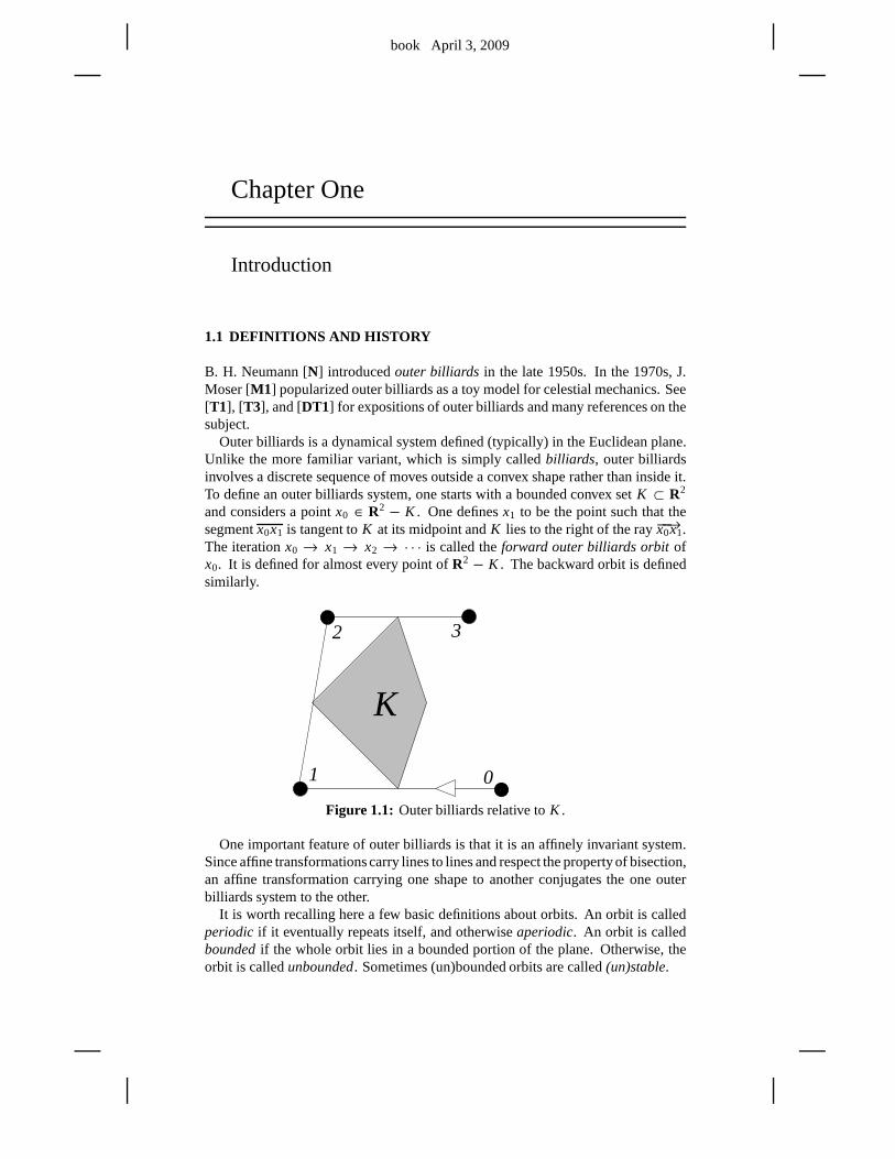
and considers a pointx0 ∈ R2 − K . One definesx1 to be the point such that thesegmentx0x1 is tangent toK at its midpoint andK lies to the right of the ray−−→x0x1.The iterationx0 → x1 → x2 → · · · is called theforward outer billiards orbitofx0. It is defined for almost every point ofR2 − K . The backward orbit is definedsimilarly.

2

K

3

1 0

Figure 1.1: Outer billiards relative toK .

One important feature of outer billiards is that it is an affinely invariant system.Since affine transformations carry lines to lines and respect the propertyof bisection,an affine transformation carrying one shape to another conjugates the one outerbilliards system to the other.

It is worth recalling here a few basic definitions about orbits. An orbit is calledperiodic if it eventually repeats itself, and otherwiseaperiodic. An orbit is calledboundedif the whole orbit lies in a bounded portion of the plane. Otherwise, theorbit is calledunbounded. Sometimes (un)bounded orbits are called(un)stable.

book April 3, 2009

2 CHAPTER 1

J. Moser [M2, p. 11] attributes the following question1 to Neumann ca. 1960,though it is sometimes called Moser’s question.Is there an outer billiards systemwith an unbounded orbit? This is an idealized version of the question about thestability of the solar system. Here is a chronological list of much of the work relatedto this question.

• J. Moser [M2] sketches a proof, inspired by KAM theory, that outer billiardson K has all bounded orbits provided that∂K is at leastC6 smooth andpositively curved. R. Douady gives a complete proof in his thesis [D].

• In Vivaldi-Shaidenko [VS], Kolodziej [Ko], and Gutkin-Simanyi [GS], it isproved (each with different methods) that outer billiards on aquasirationalpolygonhas all orbits bounded. This class of polygons includes rationalpolygons – i.e., polygons with rational-coordinate vertices – and also regularpolygons. In the rational case, all defined orbits are periodic.

• S. Tabachnikov [T3] analyzes the outer billiards system for a regular pentagonand shows that there are some nonperiodic (but bounded) orbits.

• P. Boyland [B] gives examples ofC1 smooth convex domains for which anorbit can contain the domain boundary in itsω-limit set.

• F. Dogru and S. Tabachnikov [DT2] show that, for a certain class of polygonsin the hyperbolic plane, calledlarge, all outer billiards orbits are unbounded.(One can define outer billiards in the hyperbolic plane, though the dynamicshas a somewhat different feel to it.)

• D. Genin [G] shows that all orbits are bounded for the outer billiards systemsassociated to trapezoids. See §A.4. Genin also makes a briefnumerical studyof a particular irrational kite based on the square root of 2,observes possiblyunbounded orbits, and indeed conjectures that this is the case.

• In [S] we prove that outer billiards on the Penrose kite has unbounded or-bits, thereby answering the Moser-Neumann question in the affirmative. ThePenrose kite is the convex quadrilateral that arises in the Penrose tiling.

• Recently, D. Dolgopyat and B. Fayad [DF] showed that outer billiards ona half-disk has some unbounded orbits. Their proof also works for regionsobtained from a disk by nearly cutting it in half with a straight line. This is asecond affirmative answer to the Moser-Neumann question.

The result in [S] naturally raises questions about generalizations. The purposeof this book is to develop the theory of outer billiards on kites and show that thephenomenon of unbounded orbits for polygonal outer billiards is (at least for kites)quite robust.

1It is worth pointing out that outer billiards relative to a line segment has unbounded orbits. Thistrivial case is meant to be excluded from the question.

book April 3, 2009

INTRODUCTION 3

1.2 THE ERRATIC ORBITS THEOREM

A kite is a convex quadrilateralK having a diagonal that is a line of symmetry. Wesay thatK is (ir)rational if the other diagonal dividesK into two triangles whoseareas are (ir)rational multiples of each other. Equivalently, K is rational iff it isaffinely equivalent to a quadrilateral with rational vertices. To avoid trivialities, werequire that exactly one of the two diagonals ofK is a line of symmetry. This meansthat a rhombus does not count as a kite.

Since outer billiards is an affinely natural system, we find ituseful to normalizekites in a particular way. Any kite is affinely equivalent to the quadrilateralK (A)having vertices

(−1,0), (0,1), (0,−1), (A,0), A ∈ (0,1). (1.1)

Figure 1.1 shows an example. The omitted caseA = 1 corresponds to rhombuses.Henceforth, when we saykite, we meanK (A) for someA. The kite K (A) is(ir)rational iff A is (ir)rational.

Let Zodd denote the set of odd integers. Reflection in each vertex ofK (A) pre-servesR × Zodd. Hence outer billiards onK (A) preservesR × Zodd. We call anouter billiards orbit onK (A) specialif (and only if) it is contained inR×Zodd. Wediscuss only special orbits in this book. The special orbitsare hard enough for usalready. In the appendix, we will say something about the general case. See §A.3.

We call an orbitforward erraticif the forward orbit is unbounded and also returnsto every neighborhood of a kite vertex. We state the same definition for the backwarddirection. We call an orbiterratic if it is both forward and backward erratic. In Parts1–4 of the book we will prove the following result.

Theorem 1.1 (Erratic Orbits) The following hold for any irrational kite.

1. There are uncountably many erratic special orbits.

2. Every special orbit is either periodic or unbounded in both directions.

3. The set of periodic special orbits is open dense inR × Zodd.

It follows from the work on quasirational polygons cited above that all orbits areperiodic relative to a rational kite. (The analysis in this book gives another proof ofthis fact, at least for special orbits. See the remark at the end of §3.2.) Hence theErratic Orbits Theorem has the following corollary.

Corollary 1.2 Outer billiards on a kite has an unbounded orbit if and only ifthekite is irrational.

The Erratic Orbits Theorem is an intermediate result included so that the readercan learn a substantial theorem without having to read the whole book. We willdescribe our main result in the next two sections.

book April 3, 2009

4 CHAPTER 1

1.3 COROLLARIES OF THE COMET THEOREM

In Parts 5 and 6 of the book we will go deeper into the subject and establish our mainresult, the Comet Theorem. The Comet Theorem and its corollaries considerablysharpen the Erratic Orbits Theorem. We defer statement of the Comet Theoremuntil the next section. In this section, we describe some of its corollaries.

Given a Cantor setC contained in a lineL, we letC# be the set obtained fromC by deleting the endpoints of the components ofL − C. We callC# a trimmedCantor set. Note thatC − C# is countable.

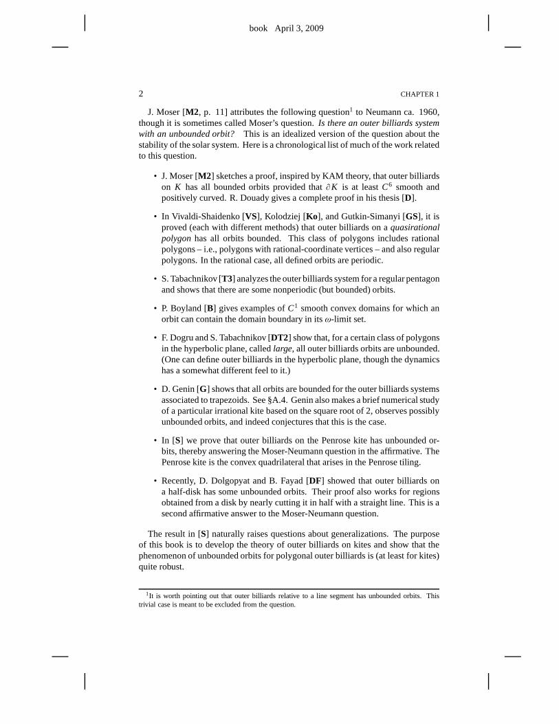
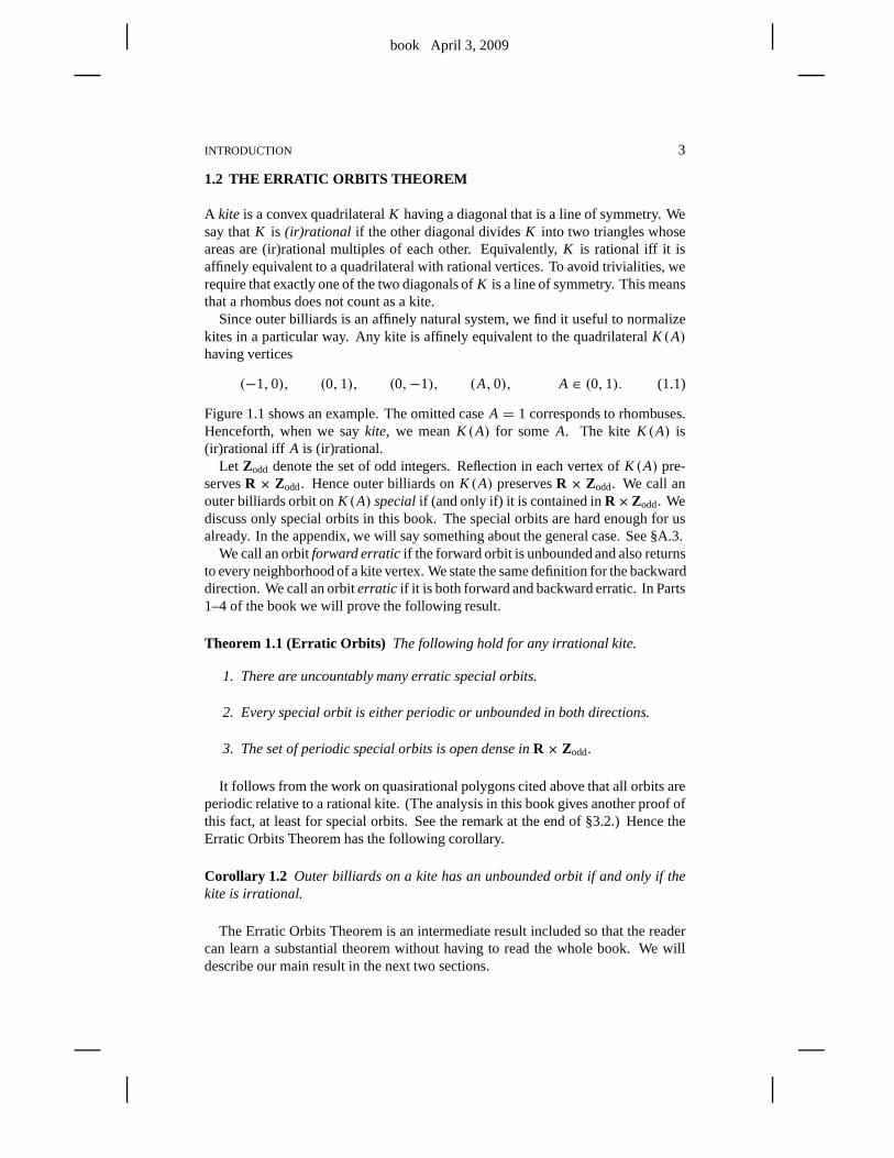
The interval

I = [0,2]× {−1} (1.2)

turns out to be a very useful interval. Figure 1.2 showsI and its first 3 iterates underthe outer billiards map.

I

Figure 1.2: I and its first 3 iterates.

Let UA denote the set of unbounded special orbits relative toA.

Theorem 1.3 Relative to any irrational A∈ (0,1), the following are true.

1. UA is minimal: Every orbit in UA is dense in UA and all but at most2 orbitsin UA are both forward dense and backward dense in UA.

2. UA is locally homogeneous: Every two points in UA have arbitrarily smallneighborhoods that are isometric to each other.

3. UA ∩ I = C#A for some Cantor set CA.

Remarks:(i) One endpoint ofCA is the kite vertex(0,−1). Hence Statement 1 implies thatall but at most 2 unbounded special orbits are erratic. The remaining special orbits,if any, are each erratic in one direction.(ii) Statements 2 and 3 combine to say that every point inUA lies in an interval thatintersectsUA in a trimmed Cantor set. This gives us a good local picture ofUA.One thing we are missing is a good global picture ofUA.(iii) The Comet Theorem describesCA explicitly.

book April 3, 2009

INTRODUCTION 5

Given Theorem 1.3, it makes good sense to speak of the first return map to anyinterval inR× Zodd. From the minimality result, the local nature of the return mapis essentially the same around any point ofUA. To give a crisp picture of this firstreturn map, we consider the intervalI discussed above.

For j = 1,2, let f j : X j → X j be a map such thatf j and f −1j are defined on all

but perhaps a finite subset ofX j . We call f1 and f2 essentially conjugateif thereare countable setsC j ⊂ X j , each one contained in a finite union of orbits, and ahomeomorphism

h: X1 − C1→ X2 − C2

that conjugatesf1 to f2.An odometeris the mapx→ x + 1 on the inverse limit of the system

· · · → Z/D3→ Z/D2→ Z/D1, Dk|Dk+1 ∀k. (1.3)

Theuniversal odometeris the mapx→ x+1 on theprofinite completionof Z. Thisis the inverse limit taken over the system of all finite cyclicgroups. For concreteness,Equation 1.3 defines the universal odometer whenDk = k factorial. See [H] for adetailed discussion of the universal odometer.

Theorem 1.4 LetρA be the first return map to UA ∩ I .

1. For any irrational A∈ (0,1), the mapρA is defined on all but at most onepoint and is essentially conjugate to an odometerZ A.

2. Any given odometer is essentially conjugate toρA for uncountably manydifference choices of A.

3. ρA is essentially conjugate to the universal odometer for almost all A.

Remarks:(i) The Comet Theorem explicitly describesZ A in terms of a sequence we call

the remormalization sequence. This sequence is related to the continued fractionexpansion ofA. We will give a description of this sequence in the next section.(ii) Theorem 1.4 is part of a larger result. There is a certainsuspension flow overthe odometer, which we callgeodesic flow on the cusped solenoid. It turns out thatthe time-one map for this flow serves as a good model, in a certain sense, for thedynamics onUA. §24.3.

Our next result highlights an unexpected connection between outer billiards onkites and the modular groupSL2(Z). The groupSL2(Z) acts naturally on the upperhalf-plane model of the hyperbolic plane,H2, by linear fractional transformations.Closely related toSL2(Z) is the(2,∞,∞)-triangle groupŴgenerated by reflectionsin the sides of the geodesic triangle with vertices(0,1, i ). The points 0 and 1 arethecusps, and the pointi is the internal vertex corresponding to the right angle ofthe triangle. See §25.2 for more details.Ŵ andSL2(Z) are commensurable: Theirintersection has finite index in both groups. In our next result, we interpret our kiteparameter interval(0,1) as the subset of the ideal boundary ofH2.

book April 3, 2009

6 CHAPTER 1

Theorem 1.5 Let S= [0,1]−Q. Let u(A) be the Hausdorff dimension of UA.

1. For all A ∈ S, the set UA has length0. Hence almost all points inR × Zodd

have periodic orbits relative to outer billiards on K(A).

2. If A, A′ ∈ S are in the sameŴ-orbit, then UA and UA′ are locally similar. Inparticular, u(A) = u(A′).

3. If A ∈ S is quadratic irrational, then every point of UA lies in an interval thatintersects UA in a self-similar trimmed Cantor set.

4. The function u is almost everywhere equal to some constantu0 and yet mapsevery open subset of S onto[0,1].

Remarks:(i) We do not know the value ofu0. We guess that 0< u0 < 1. Theorem 25.9 givesa formula foru(A) in many cases.(ii) The wordsimilar in statement 2 means that the two sets have neighborhoodsthat are related by a similarity. In statement 3, aself-similarset is a disjoint finiteunion of similar copies of itself.(iii) We will see that statement 2 essentially implies both statements 3 and 4. State-ment 2 is the first hint that outer billiards on kites is connected to the modular group.The Comet Theorem says more about this.(iv) Statement 3 of Theorem 1.4 combines with statement 4 of Theorem 1.5 to saythat there is a “typical behavior” for outer billiards on kites, in a certain sense. Foralmost every parameterA, the dimension ofUA is the (unknown) constantu0 andthe return mapρA is essentially conjugate to the universal odometer.

We end this section by comparing our results here with the main theorems in [S]concerning the Penrose kite. The Penrose kite parameter is

A =√

5− 2= φ−3,

whereφ is the golden ratio. In [S], we prove2 thatC#A ⊂ UA and that the first return

map toC#A is essentially conjugate to the 2-adic odometer. Theorems 1.3 and 1.4

subsume these results about the Penrose kite.As in §25.5.2, we might have computed in [S] that dim(CA) = log(2)/ log(φ3).

However, at the time we did not know how this number was related to dim(UA),the real quantity of interest to us. From Theorem 1.3, we knowadditionally thatC#

A = UA ∩ I and dim(UA) = dim(CA).While we recover and improve all the maintheoremsin [S], there is one way that

the work we do in [S] for the Penrose kite goes deeper than what we do here (forevery irrational kite). The work in [S] establishes a deeper kind of self-similarityfor the Penrose kite orbits than we have established in statement 3 of Theorem 1.5.See §A.2 for a discussion.

2Technically, we prove these results for a smaller Cantor setwhich is the left half ofCA. However,the arguments usingCA in place of its left half would be just about the same.

book April 3, 2009

INTRODUCTION 7

1.4 THE COMET THEOREM

Now we describe our main result. Say thatp/q is oddor evenaccording to whetherpq is odd or even. There is a unique sequence{pn/qn} of distinct odd rationals,converging toA, such that

p0

q0= 1

1, |pnqn+1− qn pn+1| = 2, ∀n. (1.4)

We call this sequence theinferior sequence. See §4.1. This sequence is closelyrelated to continued fractions.

We define

dn = floor

(qn+1

2qn

), n = 0,1,2, ... (1.5)

Say that asuperior termis a termpn/qn such thatdn ≥ 1. We will show that there areinfinitely many superior terms. Say that thesuperior sequenceis the subsequenceof superior terms. Say that therenormalization sequenceis the corresponding sub-sequence of{dn}. We reindex so that the superior and renormalization sequencesare indexed by 0,1,2, ....

Example: To fix ideas, we demonstrate how this works for the Penrose kite pa-rameter.A = φ−3. The inferior sequence forA is

11

1

3

15

3

13

521

13

55

2189

55

233

89377

. . . .

The bold terms are the terms of the superior sequence. The superior sequenceobeys the recurrence relationrn+2 = 4rn+1 + rn, wherer stands for eitherp or q.The initial sequence{dn} is 1,0,1,0, .... The renormalization sequence is 1,1,1, ....

The definitions that follow work entirely with the superior sequence. We defineZ A to be the inverse limit of the system

. . .→ Z/D3→ Z/D2→ Z/D1, Dn =n−1∏

i=0

(di + 1). (1.6)

We equipZ A with a metric, definingdA(x, y) = q−1n−1, wheren is the smallest index

such that [x] and [y] disagree inZ/Dn. In the Penrose kite example above,Z A isnaturally the 2-adic integers anddA gives the same topology as the classical 2-adicmetric.

We can identify the points ofZ A with the sequence space

5A =∞∏

i=0

{0, ...,di }. (1.7)

The identification works like this.

φ1:∞∑

j=0

k j D j ∈ Z A −→ {k j } ∈ 5A. (1.8)

book April 3, 2009

8 CHAPTER 1

The elements on the left hand side are formal series, and

k j ={ k j if p j /q j < A.

d j − k j if p j /q j > A.(1.9)

Our identification is nonstandard in that it usesk j in place of the more obviouschoice ofk j . Needless to say, we make this less-than-obvious choice because itreflects the structure of outer billiards.

There is a mapφ2:5A→ R × {−1}, defined as follows.

φ2: {k j } −→( ∞∑

j=0

2k jλ j ,−1

), λ j = |Aqj − p j |. (1.10)

We defineCA = φ2(5A). Equivalently,

CA = φ(Z A), φ = φ2 ◦ φ1. (1.11)

(The mapφ depends onA, but we suppress this from our notation.) It turns outthatφ:Z A→ CA is a homeomorphism andCA is a Cantor set whose convex hull isexactlyI , the interval discussed in the previous section. LetC#

A denote the trimmedCantor set based onCA.

Define

Z [ A] = {m A+ n|m,n ∈ Z}. (1.12)

Say that theexcursion distanceof a portion of an outer billiards orbit is themaximum distance from a point on this orbit portion to the origin.

Theorem 1.6 (Comet)Let UA denote the set of unbounded special orbits relativeto an irrational A∈ (0,1).

1. For any N, there is an N′ with the following property. Ifζ ∈ UA satisfies‖ζ‖ < N, then the kth outer billiards iterate ofζ lies in I for some|k| < N′.Here N′ depends only on N and A.

2. UA ∩ I = C#A. The first return mapρA: C#

A → C#A is defined precisely on

C#A − φ(−1). The mapφ−1 ◦ ρA ◦ φ, wherever defined onZ A, equals the

odometer.

3. For anyζ ∈ C#A−φ(−1), the orbit portion betweenζ andρA(ζ )has excursion

distance in[c−1

1 d−1, c1d−1]

and length in[c−1

2 d−2, c2d−3]. Here c1, c2 are

universal positive constants and d= dA(− 1, φ−1(ζ )

).

4. C#A = CA − (2Z [ A] × {−1}). Two points in UA lie on the same orbit if and

only if the difference between their first coordinates lies in 2Z [ A].

Remarks:(i) To use a celestial analogy, the unbounded special orbitsare comets andI is thevisible sky. Item 1 says roughly that any comet is always either approachingI orleavingI . Item 2 describes the geometry and combinatorics of the visits to I . Item3 gives a model of the behavior between visits. Item 4 gives analgebraic view.

book April 3, 2009

INTRODUCTION 9

(ii) Lemma 23.7 replaces the bounds in item 3 with explicit estimates. The orderson all the bounds in item 3 are sharp except perhaps for the length upper bound. Seethe remarks following Lemma 23.7 for a discussion, and also §A.2.(iii) The Comet Theorem has an analog for the backward orbits. The statement isthe same except that the pointφ(0) replaces the pointφ(−1) and the mapx→ x−1replaces the odometer. We have the general identityφ(0)+ φ(−1) = (2,−2).(iv) Our analysis will show thatφ(0) andφ(−1) have well defined orbits iff they liein C#

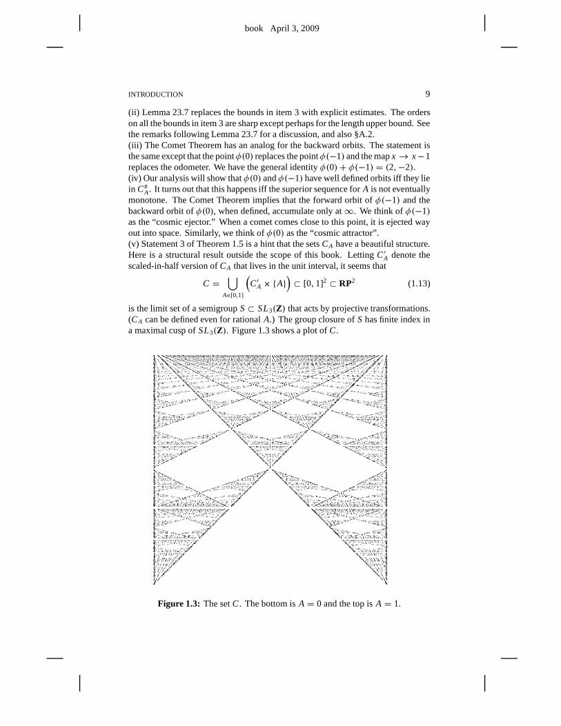
A. It turns out that this happens iff the superior sequence forA is not eventuallymonotone. The Comet Theorem implies that the forward orbit of φ(−1) and thebackward orbit ofφ(0), when defined, accumulate only at∞. We think ofφ(−1)as the “cosmic ejector.” When a comet comes close to this point, it is ejected wayout into space. Similarly, we think ofφ(0) as the “cosmic attractor”.(v) Statement 3 of Theorem 1.5 is a hint that the setsCA have a beautiful structure.Here is a structural result outside the scope of this book. Letting C′A denote thescaled-in-half version ofCA that lives in the unit interval, it seems that

C =⋃

A∈[0,1]

(C′A × {A}

)⊂ [0,1]2 ⊂ RP2 (1.13)

is the limit set of a semigroupS⊂ SL3(Z) that acts by projective transformations.(CA can be defined even for rationalA.) The group closure ofS has finite index ina maximal cusp ofSL3(Z). Figure 1.3 shows a plot ofC.

Figure 1.3: The setC. The bottom isA = 0 and the top isA = 1.

book April 3, 2009

10 CHAPTER 1

1.5 RATIONAL KITES

Like most authors who have considered outer billiards, we find it convenient towork with the square of the outer billiards map. LetO2(x) denote the square outerbilliards orbit ofx. Let I = [0,2]× {−1}, as above, and let

4 = R+ × {−1,1}. (1.14)

Whenǫ ∈ (0,2/q), the orbitO2(ǫ,−1) has a combinatorial structure independentof ǫ. See Lemma 2.2. ThusO2(1/q,−1) is a natural representative of this orbit. Weoften call this orbit thefundamental orbit. The fundamentalorbit plays a crucial rolein our proofs. The following result is a basic mechanism for producing unboundedorbits.

Theorem 1.7 Relative to p/q, the set O2(1/q,−1) ∩ 4 has diameter betweenλ(p+ q)/2 andλ(p+ q)+ 2. Hereλ = 1 if p/q is odd andλ = 2 if p/q is even.

Any odd rationalp/q appears as (say) thenth term in a superior sequence{pi/qi }.The terms beforep/q are uniquely determined byp/q. This is similar to whathappens for continued fractions. Define5n to be the product of the firstn factorsof5A, the space from Equation 1.7.

Theorem 1.8 Letµi = |pnqi − qn pi |.

O2

( 1

qn,−1

)∩ I =

⋃

κ∈5n

(Xn(κ),−1

), Xn(κ) =

1

qn

(1+

n−1∑

i=0

2kiµi

).

Example: Here we show Theorem 1.8 in action. The odd rational 19/49 determinesthe inferior sequence

p0

q0= 1

1,

1

3,

5

13,

19

49= p3

q3.

All terms are superior, so this is also the superior sequence. In our example,

• n = 3.

• The superior sequence is 1,2,1.

• Theµ sequence is 30,8,2.

Therefore the first coordinates of the 12 points ofO2(1/49) ∩ I are given by

1⋃

k0=0

2⋃

k1=0

1⋃

k2=0

2(30k0+ 8k1+ 2k2)+ 1

49.

Writing these numbers in a suggestive way, we see that the union above works outto

1

49×(1 5 17 21 33 37 61 65 77 81 93 97

).

book April 3, 2009

INTRODUCTION 11

Remarks:(i) Theorem 1.8 is a good example of a result that is easy to check on a computer.One can check the result for the example we give, or for any other smallish param-eter, using Billiard King.(ii) A version of Theorem 1.8 holds in the even case as well. Wewill discuss theeven case of Theorem 1.8 in §22.7.(iii) We view statements 2 and 3 as the heart of the Comet Theorem. We will provethese two statements by combining Theorems 1.7 and 1.8 and then taking a geo-metric limit. The proofs for statements 1 and 4 of the Comet Theorem require someother ideas that we cannot describe without a buildup of machinery.(iv) Theorem 1.8 has a nice conjectural extension, which describes the entire returnmap toI . See §A.1. A suitable geometric limit of the conjecture in §A.1 describesthe structure of the orbits inI −C#

A in the case whenA is irrational. See ConjectureA.1.

We mention two more results about outer billiards on rational kites. These resultsdo not play such an important role in our proof of the Comet Theorem, but they areappealing and fairly easy by-products of our analysis.

Here is an amplification of the upper bound in Theorem 1.7.

Theorem 1.9 If p/q is odd, letλ = 1. If p/q is even, letλ = 2. Each special orbitintersects4 in exactly one set of the form Ik × {−1,1}, where

Ik = (λk(p+ q), λ(k+ 1)(p+ q)), k = 0,1,2,3, ....

Hence any special orbit intersects4 in a set of diameter at mostλ · (p+ q)+ 2.

Theorem 1.9 is similar in spirit to a result in [K ]. See §3.4 for a discussion.We call an outer billiards orbit onK (A) persistent3 if there are nearby and com-

binatorially identical orbits onK (A′) for all A′ sufficiently close toA. Otherwise,we call the orbitfleeting. In the odd case,O2(1/q,±1) is fleeting.

Theorem 1.10 In the even rational case, all special orbits are persistent. In the oddcase, the set Ik×{−1,1} contains exactly two fleeting orbits, U+k and U−k , and theseare conjugateby reflection in the x-axis. In particular, we haveU±0 = O2(1/q,±1).

Remark: None of our structure theorems holds, as stated, for generalquadrilateralsor even for nonspecial orbits on kites. We do not really have agood understandingof the structure of outer billiards on a general rational quadrilateral, though we cansee that it promises to be quite interesting. We take up this discussion in §A.4.

3It would be more usual to call such orbitsstable, but in the subject of outer billiards, the wordstablehas historically meant the same as the wordbounded.

book April 3, 2009

12 CHAPTER 1

1.6 THE ARITHMETIC GRAPH

Here we describe thearithmetic graph, a central construction in the book. Oneshould think of the first return map to4 = R+ × {−1,1}, for rational parameters,as an essentially combinatorial object. The arithmetic graph gives a 2-dimensionalrepresentation of this combinatorial object. The principle guiding our constructionis that sometimes it is better to understand the Abelian group Z [ A] as a moduleoverZ rather than as a subset ofR. Our arithmetic graph is similar in spirit to thelattice vector fields studied by Vivaldi et al. in connectionwith interval exchangetransformations. See, e.g., [VL ].

Here we explain the idea roughly. See §2.4 for precise details. The arithmeticgraph is most easily explained in the rational case. Letψ be the square of the outerbilliards map. It turns out that every orbit starting on4 eventually returns to4. SeeLemma 2.3. Thus we can define the first return map

9:4→ 4. (1.15)

We define the mapT : Z2→ 2Z [ A] × {−1,1} by the formula

T(m,n) =(2Am+ 2n+ 1/q, (−1)p+q+1

). (1.16)

HereA = p/q.Up to the reversal of the direction of the dynamics, every point of4 has the same

orbit as a point of the formT(m,n), where(m,n) ∈ Z2. For instance, the orbitof T(0,0) = (1/q,−1) is what we called the fundamental orbit above. We formthe graphŴ(p/q) by joining the points(m1,m2) to (m2,n2) when these points aresufficiently close together and alsoT(m1,n1) = 9±1(m2,n2). (The mapT is notinjective, so we have choices to make. That is the purpose of thesufficiently closecondition.)

We letŴ(p/q) denote the component ofŴ(p/q) that contains(0,0). This com-ponent tracks the orbitO2(1/q,−1), the main orbit of interest to us. Whenp/q isodd,Ŵ(p/q) is an infinite periodic polygonal arc, invariant under translation by thevector(q,−p). Note thatT(q,−p) = T(0,0). When p/q is even,Ŵ(p/q) is anembedded polygon. We prove many structural theorems about the arithmetic graph.Here we informally mention three central ones.

• The Embedding Theorem(Chapter 2):Ŵ(p/q) is a disjoint union of embed-ded polygons and infinite embedded polygonal arcs. Every edge of Ŵ(p/q)has length at most

√2. The persistent orbits correspond to closed polygons,

and the fleeting orbits correspond to infinite (but periodic)polygonal arcs.

• The Hexagrid Theorem(Chapter 3): The structure ofŴ(p/q) is controlledby 6 infinite families of parallel lines. See Figure 3.3. Thequasiperiodicstructure is similar to what one sees in DeBruijn’s famous pentagrid con-struction of the Penrose tilings. See [DeB].

• The Copy Theorem(Chapter 18; also Lemmas 4.2 and 4.3): IfA1 andA2 aretwo rationals that are close in the sense of Diophantine approximation, thenthe corresponding arithmetic graphsŴ1 andŴ2 have substantial agreement.

book April 3, 2009

INTRODUCTION 13

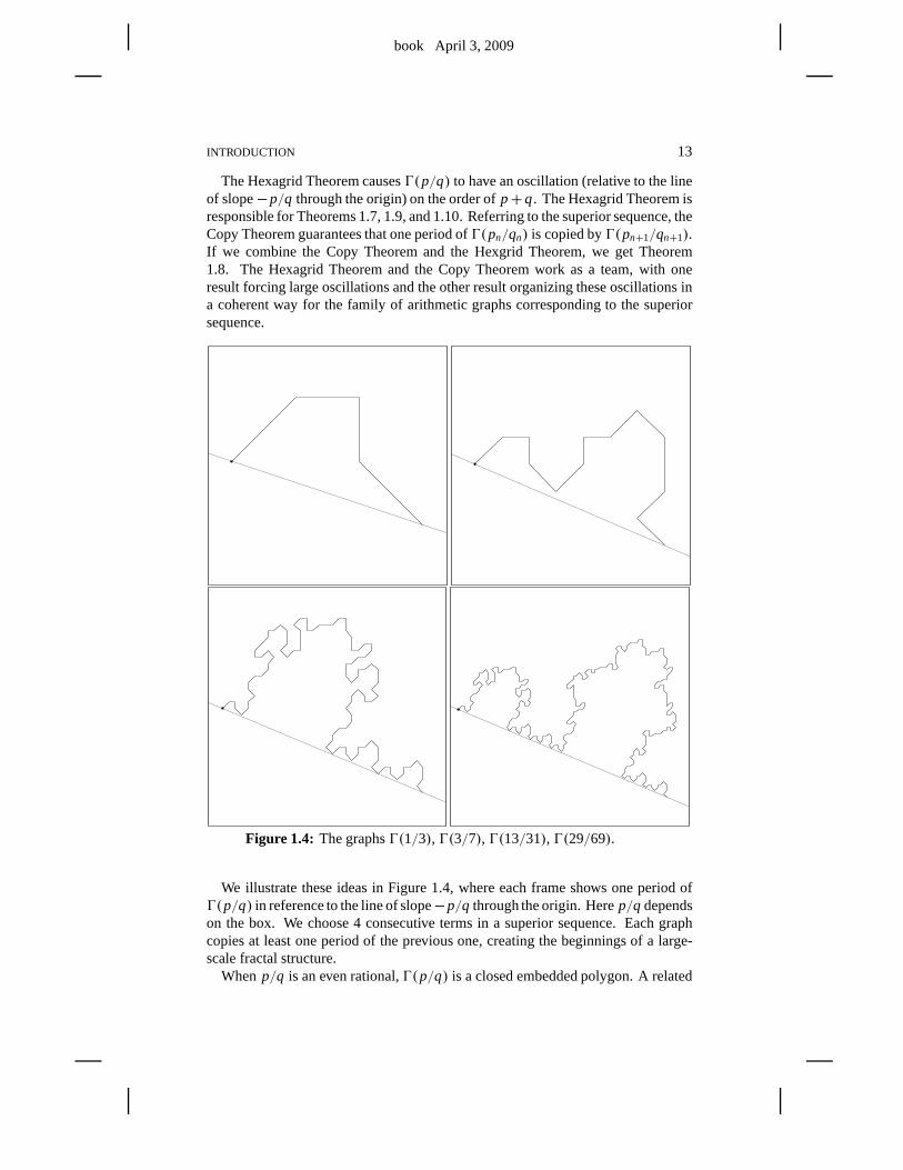
The Hexagrid Theorem causesŴ(p/q) to have an oscillation (relative to the lineof slope−p/q through the origin) on the order ofp+q. The Hexagrid Theorem isresponsible for Theorems 1.7, 1.9, and 1.10. Referring to the superior sequence, theCopy Theorem guarantees that one period ofŴ(pn/qn) is copied byŴ(pn+1/qn+1).If we combine the Copy Theorem and the Hexgrid Theorem, we getTheorem1.8. The Hexagrid Theorem and the Copy Theorem work as a team,with oneresult forcing large oscillations and the other result organizing these oscillations ina coherent way for the family of arithmetic graphs corresponding to the superiorsequence.

Figure 1.4: The graphsŴ(1/3), Ŵ(3/7), Ŵ(13/31), Ŵ(29/69).

We illustrate these ideas in Figure 1.4, where each frame shows one period ofŴ(p/q) in reference to the line of slope−p/q through the origin. Herep/q dependson the box. We choose 4 consecutive terms in a superior sequence. Each graphcopies at least one period of the previous one, creating the beginnings of a large-scale fractal structure.

When p/q is an even rational,Ŵ(p/q) is a closed embedded polygon. A related

book April 3, 2009

14 CHAPTER 1

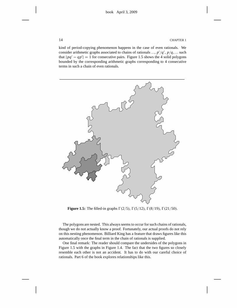
kind of period-copying phenomenon happens in the case of even rationals. Weconsider arithmetic graphs associated to chains of rationals ..., p′/q′, p/q, ... suchthat |pq′ − qp′| = 1 for consecutive pairs. Figure 1.5 shows the 4 solid polygonsbounded by the corresponding arithmetic graphs corresponding to 4 consecutiveterms in such a chain of even rationals.

Figure 1.5: The filled-in graphsŴ(2/5), Ŵ(5/12), Ŵ(8/19), Ŵ(21/50).

The polygons are nested. This always seems to occur for such chains of rationals,though we do not actually know a proof. Fortunately, our actual proofs do not relyon this nesting phenomenon. Billiard King has a feature thatdraws figures like thisautomatically once the final term in the chain of rationals issupplied.

One final remark: The reader should compare the undersides ofthe polygons inFigure 1.5 with the graphs in Figure 1.4. The fact that the twofigures so closelyresemble each other is not an accident. It has to do with our careful choice ofrationals. Part 6 of the book explores relationships like this.

book April 3, 2009

INTRODUCTION 15

1.7 THE MASTER PICTURE THEOREM

The logic of the book works like this. After we define the arithmetic graph, we provea number of structural results about it. We then deduce the Comet Theorem andits corollaries from these structural results. The way we understand the arithmeticgraph is to obtain a kind of closed-form expression for it. The Master PictureTheorem gives this expression. Here we will give a rough description of this result.We formulate and prove the Master Picture Theorem in Part 2 ofthe book.

Let us first discuss the Master Picture Theorem in vague terms. It sometimeshappens that one has a dynamical system ona high-dimensional manifoldM togetherwith an embeddingof a lower-dimensionalmanifoldX into M that is, in some sense,compatible with the dynamics onM. The dynamics onM then induces a dynamicalsystem onX. Sometimes the higher-dimensionalsystem onM is much simpler thanthe system onX, and most of the complexity of the system onX comes from itscomplicated embedding intoM. The Master Picture Theorem says that this situationhappens for outer billiards on kites.

Now we will say something more precise. Recall that4 = R+ × {−1,1}. Thearithmetic graph encodes the dynamics of the first return map9:4→ 4. It turnsout that9 is an infinite interval exchange map. The Master Picture Theorem revealsthe following structure for each parameterA.

1. There is a locally affine mapµ from4 into a union4 of two 3-dimensionaltori.

2. There is a polyhedron exchange map9: 4→ 4 defined relative to a partitionof 4 into 28 polyhedra.

3. The mapµ is a semiconjugacy between9 and9.

In other words, the return dynamics of9 has a kind of compactification into a3 dimensional polyhedron exchange map. All the objects above depend on theparameterA, but we have suppressed them from our notation.

There is one master picture, a union of two 4-dimensional convex lattice polytopespartitioned into 28 smaller convex lattice polytopes, thatcontrols everything. Foreach parameter, one obtains the 3-dimensional picture by taking a suitable slice.

The fact that nearby slices give almost the same picture is the source of the CopyTheorem. The interaction between the mapµ and the walls of our convex polytopepartitions is the source of the Hexagrid Theorem. The Embedding Theorem followsfrom basic geometric properties of the polytope exchange map in an elementaryway that is hard to summarize here.

My investigation of the Master Picture Theorem is really just starting, and thisbook has only the beginnings of a theory. First, I believe that a version of the MasterPicture Theorem should hold much more generally. (This is something that JohnSmillie and I hope to work out together.) Second, some recentexperiments convinceme that there is a renormalization theory for this object grounded in real projectivegeometry. All of this will perhaps be the subject of a future work.

book April 3, 2009

16 CHAPTER 1

1.8 REMARKS ON COMPUTATION

As I mentioned in the preface, I discovered most of the phenomena discussed inthis book using my program Billiard King. Billiard King and this book developedside by side in a kind of feedback loop. Since I am ultimately trying to verifyphenomena that I discovered with the aid of a computer, one might expect somecomputational aspects to the formal proofs. The overall proof here uses considerablyless computation than the proof in [S], but I still use a computer-aided proof in severalplaces.

Mainly, I use a computer to check that various 4-dimensionalconvex integralpolytopes have disjoint interiors. This involves a small amount of linear algebra,using exact integers, that one could in principle do by hand.One could do thesecalculations by hand in the same way that one could count all the coins filling up abathtub. One could do it,but it is better left to a machine. Most of these computationscome from Part 3 of the book.

The experimental method I used has the advantage that I checked essentiallyall the results with extensive and visually surveyable computation. The interestedreader can make many of the same visual checks by downloadingthe program andplaying with it. I suppose I cannot guarantee Billiard King does not have a subtlebug, but the output from the program makes sense in a way that would be unlikelyin the presence of a serious problem. Also, the output of Billiard King matches theresults I have proved in a traditional way in this book.

1.9 ORGANIZATION OF THE BOOK

The book has 6 parts. Parts 1–4 comprise the core of the book. In Part 1, we provethe Erratic Orbits Theorem modulo some auxilliary results such as the HexagridTheorem. In Part 2, we prove the Master Picture Theorem, our main structuralresult. in Parts 3 and 4, we use the Master Picture Theorem to prove the variousauxilliary results assumed in Part 1.

In Part 5, we prove the Comet Theorem and its corollaries modulo various aux-illiary results. In Part 6, we prove these auxilliary results.

In the Appendix, we discuss some additional phenomena, bothfor kites and forquadrilaterals, that we have observed but not proved.

Before each part of the book, we include an overview of that part.

book April 3, 2009

Part 1. The Erratic Orbits Theorem

In this part of the book, we will prove the Erratic Orbits Theorem modulo a numberof auxilliary results that we prove in Parts 2–4.

• In Chapter 2, we establish some basic results that allow fordefinition of thearithmetic graph. The arithmetic graph is our main object ofstudy. We alsostate the Embedding Theorem, a basic structural result about the arithmeticgraph that we prove in Part 3.

• In Chapter 3, we state the Hexagrid Theorem, another structural result aboutthe arithmetic graph. We then deduce Theorems 1.7, 1.9, and 1.10 from theHexagrid Theorem. We prove the Hexagrid Theorem in Part 3.

• In Chapter 4, we discuss the period-copying results neededto prove the Er-ratic Orbits Theorem. Along the way, we introduce the inferior and superiorsequences, two basic ingredients in our overall theory. We prove the period-copying results in Part 4.

• In Chapter 5, we assemble the ingredients from previous chapters and provethe Erratic Orbits Theorem. We note that the arguments we usein Parts 5and 6 to prove the Comet Theorem are independent of Chapter 5.Thus, forthe reader who plans to work through the proof of the Comet Theorem, thematerial in Chapter 5 is redundant.

We mention several conventions that we use repeatedly throughout the book.Recall thatp/q is an odd rational ifpq is odd. When we sayodd rational, we meanthat the odd rational lies in(0,1). On very rare occasions, we also consider the oddrational 1/1. However, we never consider negative odd rationals, or oddrationalsgreater than 1. Also,A always stands for a kite parameter, and we writeA = p/q.Similarly, An stands forpn/qn, andA+ stand forp+/q+, etc. Sometimes we willfail to mention these conventions explicitly.

We imagine that certain readers will be interested mainly instatement 1 of theErratic Orbits Theorem – i.e., the existence of unbounded orbits. For such readers,we sometimes add remarks indicating sections that are not necessary for this part ofthe proof.

book April 3, 2009

book April 3, 2009

Chapter Two

The Arithmetic Graph

2.1 POLYGONAL OUTER BILLIARDS

Let P be a convex polygon. We denote the outer billiards map relative to P byψ ′,and the square of the outer billiards map byψ = (ψ ′)2. Our convention is thata person walking fromp to ψ ′(p) sees theP on the right side. These maps aredefined away from a countable set of line segments inR2 − P. This countable setof line segments is sometimes called thelimit set.

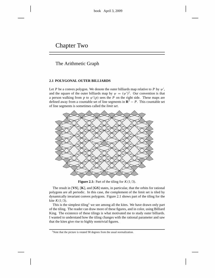
Figure 2.1: Part of the tiling forK (1/3).

The result in [VS], [K ], and [GS] states, in particular, that the orbits for rationalpolygons are all periodic. In this case, the complement of the limit set is tiled bydynamically invariant convex polygons. Figure 2.1 shows part of the tiling for thekite K (1/3).

This is the simplest tiling1 we see among all the kites. We have drawn only partof the tiling. The reader can draw more of these figures, and incolor, using BilliardKing. The existence of these tilings is what motivated me to study outer billiards.I wanted to understand how the tiling changes with the rational parameter and sawthat the kites give rise to highly nontrivial figures.

1Note that the picture is rotated 90 degrees from the usual normalization.

book April 3, 2009

20 CHAPTER 2

2.2 SPECIAL ORBITS

Until the last result in this section, the parameterA = p/q is rational. Say that aspecial intervalis an open horizontal interval of length 2/q centered at a point ofthe form(a/q,b) with a odd. Herea/q need not be in lowest terms.

Lemma 2.1 The outer billiards map is entirely defined on any special interval andindeed permutes the special intervals.

Proof: The four order 2 rotations about the vertices ofK (A) send the point(x, y),respectively, to each of the following points.

(−2− x,−y), (−x,2− y), (−x,−2− y), (2A− x,−y). (2.1)

The corresponding outer billiards mapψ ′ is built out of these rotations.Define

3 = 2Z [ A] × Zodd; Z[ A] = {m A+ n| m,n ∈ Z} (2.2)

From Equation 2.1, both3 andR × Zodd are invariant underψ ′. Therefore thecomplementary set3c = R× Zodd−3 is also invariant underψ ′. Note that3c isprecisely the union of special intervals.

To find the points ofR × Zodd whereψ ′ is not defined, we extend the sides ofK (A) and intersect them withR × Zodd. We get 4 families of points.

(2n,2n+ 1), (2n,−2n− 1), (2An,2n− 1), (2An,−2n+ 1). (2.3)

Heren ∈ Z. Notice that all these points lie in3. Henceψ ′ is defined on allpoints of3c. The first statement of our result now follows from the fact that3c isψ ′-invariant.

For the second statement, note thatψ ′ is completely defined on any special in-terval. Butψ ′ is a piecewise isometric map. By continuity,ψ ′ is an isometry whenrestricted to each special interval. But thenψ ′ must map each special interval toanother one. This proves the second statement. 2

Remark: For rational kites, the dynamics onR×Zodd is essentially combinatorial.It is just a question of how the special intervals are permuted by the dynamics. Thuswe are really dealing with an infinite permutation. Of course, we will sometimesprofit from considering this situation geometrically..

Lemma 2.2 Let A∈ (0,1) be arbitrary. Relative to the kite K(A), the entire outerbilliards orbit of any point(α,n) is defined provided thatα 6∈ 2Z [ A] and n∈ Zodd.

Proof: The orbit of the point(α,n) never lands in any of the 4 families of pointsdiscussed in the previous result. Hence, at any step in the orbit, both the forwardand backward iterates are defined. 2

WhenA is irrational, the set 2Z [ A] is a countable dense subset ofR. Likewise,2Z [ A] × Zodd is a countable dense set ofR × Zodd.

book April 3, 2009

THE ARITHMETIC GRAPH 21

2.3 THE RETURN LEMMA

Letψ be the square map relative to some kite, as above. As in §1.5, let

4 = R+ × {−1,1}. (2.4)

Lemma 2.3 (Return) Let p ∈ 4. be a point with a well defined outer billiardsorbit. Thenψa(p), ψ−b(p) ∈ 4 for some a,b > 0.

Remark: The main goal of this section is to prove the Return Lemma. Thereaderinterested in the broad picture might want to skip this rather tedious section on thefirst pass. To accommodate such a reader, we give a quick heuristic explanation ofwhy the Return Lemma is true. Theψ-orbits generally circulate around the kite,skipping at most 2 lines ofR× Zodd with each iterate. Being made from 2 consec-utive rays,4 serves as an impenetrable barrier to the progress of the orbit in boththe forward and backward directions.

To prepare for our proof of the Return Lemma, and also for later use in the proofof the Pinwheel Lemma in Part 2, we discuss some structure ofthe mapψ. Foreachp ∈ R2 at whichψ is well defined, we haveψ(p) = p+ V for some vectorV that is twice the difference between a pair of vertices ofK (A). There are a priori12 possibilities forV , and the following 10 actually occur.

• V1 = −V5 = (0,4).

• V2 = −V6 = (−2,2).

• V3 = −V7 = (−2− 2A,0).

• V4 = −V8 = (−2,−2).

• V ♯4 = −V ♭

6 = (−2A,2).

When listed in the order 1,2,3,4,4♯,5,6♭,6,7,8, the vectors defined above turnin counterclockwise fashion.

For each indexj , there is some regionRj ⊂ R2 − K (A) such that

p ∈ Rj ⇐⇒ ψ(p) = p+ Vj . (2.5)

The two regionsR♯4 andR♭6 are bounded regions. These regions ultimately turn outto be of no importance to us. The remaining regionsR1, ..., R8 are unbounded andplay an important role. The 10 regions partitionR2− K (A). One can compute thispartition by extending the sides ofK in pinwheel fashion and then suitably pullingthese sides back under the outer billiards map.

We now give a precise but terse description of the partition.For R♯4 andR♭6, welist just the vertices of the polygon. The remaining regionsare unbounded. Thenotation−→q1 , p1, ..., pk,

−→q2 indicates the following.

• The two unbounded edges are the rays−−→p1q1 and−−→pkq2.

• p2, ..., pk−1 are any additional intermediate vertices.

book April 3, 2009

22 CHAPTER 2

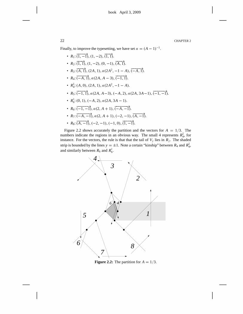
Finally, to improve the typesetting, we have setα = (A− 1)−1.

• R1:−−−−→(1,−1), (1,−2),

−−−→(1,1).

• R2:−−−→(1,1), (1,−2), (0,−1),

−−−→(A,1).

• R3:−−−→(A,1), (2A,1), α(2A2,−1− A),

−−−−→(−A,1).

• R4:−−−−→(−A,1), α(2A, A− 3),

−−−−→(−1,1).

• R♯4: (A,0), (2A,1), α(2A2,−1− A).

• R5:−−−−→(−1,1), α(2A, A−3), (−A,2), α(2A,3A−1),

−−−−−→(−1,−1).

• R♭6: (0,1), (−A,2), α(2A,3A− 1).

• R6:−−−−−→(−1,−1), α(2, A+ 1),

−−−−−−→(−A,−1).

• R7:−−−−−−→(−A,−1), α(2, A+ 1), (−2,−1),

−−−−→(A,−1).

• R8:−−−−→(A,−1), (−2,−1), (−1,0),

−−−−→(1,−1).

Figure 2.2 shows accurately the partition and the vectors for A = 1/3. Thenumbers indicate the regions in an obvious way. The small 4 representsR♯4, forinstance. For the vectors, the rule is that that the tail ofVj lies in Rj . The shadedstrip is bounded by the linesy = ±1. Note a certain “kinship” betweenR4 andR♯4,and similarly betweenR6 andR♭6.

5

4

2

6

6

4

78

1

3

Figure 2.2: The partition forA = 1/3.

book April 3, 2009

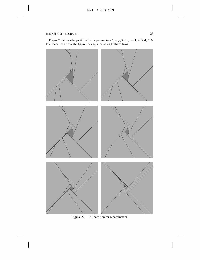
THE ARITHMETIC GRAPH 23

Figure 2.3 shows the partition for the parametersA = p/7 for p = 1,2,3,4,5,6.The reader can draw the figure for any slice using Billiard King.

Figure 2.3: The partition for 6 parameters.

book April 3, 2009

24 CHAPTER 2

We define

Ri = Ri + Vi , Si j = Ri ∩ Rj ∩ (R × Zodd). (2.6)

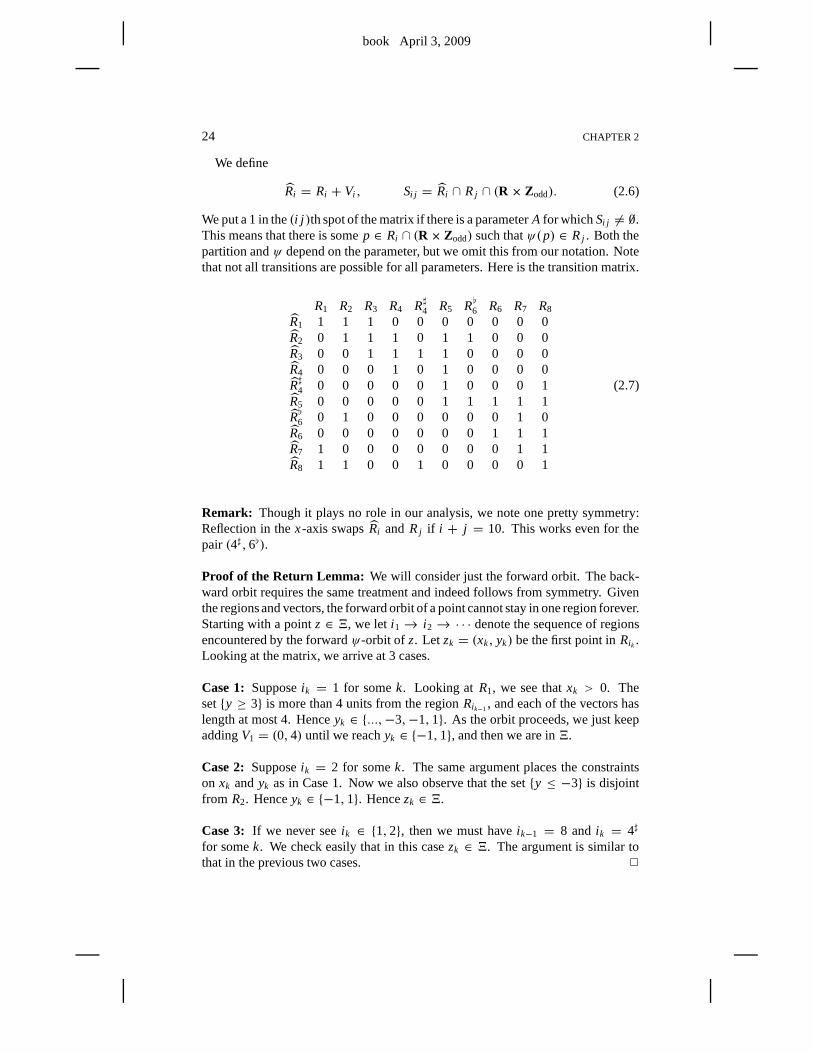
We put a 1 in the(i j )th spot of the matrix if there is a parameterA for whichSi j 6= ∅.This means that there is somep ∈ Ri ∩ (R× Zodd) such thatψ(p) ∈ Rj . Both thepartition andψ depend on the parameter, but we omit this from our notation. Notethat not all transitions are possible for all parameters. Here is the transition matrix.

R1 R2 R3 R4 R♯4 R5 R♭6 R6 R7 R8

R1 1 1 1 0 0 0 0 0 0 0R2 0 1 1 1 0 1 1 0 0 0R3 0 0 1 1 1 1 0 0 0 0R4 0 0 0 1 0 1 0 0 0 0R♯4 0 0 0 0 0 1 0 0 0 1R5 0 0 0 0 0 1 1 1 1 1R♭6 0 1 0 0 0 0 0 0 1 0R6 0 0 0 0 0 0 0 1 1 1R7 1 0 0 0 0 0 0 0 1 1R8 1 1 0 0 1 0 0 0 0 1

(2.7)

Remark: Though it plays no role in our analysis, we note one pretty symmetry:Reflection in thex-axis swapsRi and Rj if i + j = 10. This works even for thepair (4♯,6♭).

Proof of the Return Lemma: We will consider just the forward orbit. The back-ward orbit requires the same treatment and indeed follows from symmetry. Giventhe regions and vectors, the forward orbit of a point cannot stay in one region forever.Starting with a pointz ∈ 4, we let i1→ i2 → · · · denote the sequence of regionsencountered by the forwardψ-orbit of z. Let zk = (xk, yk) be the first point inRik .Looking at the matrix, we arrive at 3 cases.

Case 1: Supposeik = 1 for somek. Looking at R1, we see thatxk > 0. Theset{y ≥ 3} is more than 4 units from the regionRik−1, and each of the vectors haslength at most 4. Henceyk ∈ {...,−3,−1,1}. As the orbit proceeds, we just keepaddingV1 = (0,4) until we reachyk ∈ {−1,1}, and then we are in4.

Case 2: Supposeik = 2 for somek. The same argument places the constraintson xk andyk as in Case 1. Now we also observe that the set{y ≤ −3} is disjointfrom R2. Henceyk ∈ {−1,1}. Hencezk ∈ 4.

Case 3: If we never seeik ∈ {1,2}, then we must haveik−1 = 8 andik = 4♯

for somek. We check easily that in this casezk ∈ 4. The argument is similar tothat in the previous two cases. 2

book April 3, 2009

THE ARITHMETIC GRAPH 25

2.4 THE RETURN MAP

The Return Lemma implies that thefirst return map9:4→ 4 is well defined onany point with an outer billiards orbit. This includes the set

(R+ − 2Z [ A])× {−1,1},

as we saw in Lemma 2.2.Given the nature of the maps in Equation 2.1 comprisingψ, we see that

9(p)− (p) ∈ 2Z [ A] × {−2,0,2}.

In Part 2, we will prove the main structural result about the first return map,namely, the Master Picture Theorem. As a consequence of the Master PictureTheorem, we get the following result.

9(p)− (p) = 2(Aǫ1+ ǫ2, ǫ3), ǫ j ∈ {−1,0,1},3∑

j=1

ǫ j ≡ 0 mod 2.

(2.8)The parity result in Equation 2.8 has the following proof. The vectorsVj consid-

ered above all have the form

(2a A+ 2b,2c), a+ b+ c ≡ 0 mod 2.

The vector9(p)− p is some finite sum of these vectors.We do not have an easy proof for the bound|ǫ j | = 1, but we can easily give a

rough idea. For the reader who skipped the proof of the ReturnLemma above, weremark that our explanation here also gives a rough reason why the Return Lemmais true. Consider the forwardψ-orbit of a point of4 that is far from the origin.This orbit essentially circulates counterclockwise around the origin, nearly makinga giant octagon. Looking at our vectorsV1, ...,V8, we see that this near octagon hasapproximate 4-fold bilateral symmetry. Thereturn pair (ǫ1(p), ǫ2(p)) essentiallymeasures theapproximation errorbetween the true orbit and the closed octagon.There is almost complete cancellation as one goes around this near octagon, andthis keeps the return pair uniformly small.

Remarks:(i) Some version of the first return map is considered in many papers on outer bil-liards – e.g., [GS], [G], and [DF].(ii) On a nuts-and-bolts level, this book concerns how the pair (ǫ1(p), ǫ2(p)) de-pends onp ∈ 4. The pair(ǫ1, ǫ2) and the parity condition determineǫ3. I like tosay that this book is really about the infinite accumulation of small errors.(ii) Reflection in thex-axis conjugates the mapψ to the mapψ−1. Thus, once weunderstand the orbit of the point(x,1), we automatically understand the orbit of thepoint(x,−1). Put another way, the unordered pair of return points{9(p),9−1(p)}for p = (x,±1) depends only onx.

book April 3, 2009

26 CHAPTER 2

2.5 THE ARITHMETIC GRAPH

Fundamental Map: Recall that4 = R+×{−1,1}. Givenα ∈ R and a parameterA, define

M = MA,α : Z2→ R × {−1,1}by

MA,α(m,n) =(2Am+ 2m+ 2α, (−1)m+n+1

). (2.9)

The second coordinate ofM is either 1 or−1, depending on the parity ofm+ n.This definition is adapted to the parity condition in Equation 2.8. We callM afundamental map. Each choice ofα gives a different map.

Main Definition: M is injective whenA is irrational andM is injective on anydisk of radiusq when A = p/q. Given p1, p2 ∈ Z2, we write p1 → p2 iff thefollowing hold.

• ζ j = M(p j ) ∈ 4.

• 9(ζ1) = ζ2.

• ‖p1− p2‖ is as small as possible.

The third condition is relevant only in the rational case. According to Equation2.8, the choice ofp2 depends uniquely onp1, in all cases, and‖p1 − p2‖ ≤

√2.

Our construction gives a directed graph with vertices inZ2. We call this graphthearithmetic graphand denote it byŴα(A). We usually ignore the isolated ver-tices of the graph. These correspond to points on which the return map is the identity.

A Convention: When A = p/q, any choice ofα ∈ (0,2/q) gives the sameresult. This is a consequence of Lemma 2.1. To simplify the formulas, we chooseα = 0+, where 0+ is an infinitesimally small positive number. When we writeformulas, we usually takeα = 0, but we always use the convention that the latticepoint (m,n) tracks the orbits just to the right of the points(2Am+ 2n,±1). Withthis convention, we have

Ŵ( p

q

)= Ŵ0+

( p

q

), M(m,n) =

(2( p

q

)m+ 2n, (−1)m+n+1

). (2.10)

We say that thebaselineof Ŵ(A) is the lineM−1(0). The baseline is the line of slope−A through a point infinitesimally far beneath the origin. In practice, we think ofthe baseline as the line of slope−A through the origin.

Translation Symmetry: When p/q is odd, Equation 2.10 gives

M(ζ + V) = M(ζ ), V = (q,−p), (2.11)

for any ζ ∈ Z2. Hence translation byV preservesŴ(p/q) as a directed graph.Whenp/q is even, we haveM(ζ +V) = R◦M(ζ ), whereR is the reflection in thex-axis. The mapR conjugates9 to9−1. In this case, translation byV preservesŴ(p/q) as a graph but reverses the direction.

book April 3, 2009

THE ARITHMETIC GRAPH 27

In Part 3 we will prove the following result.

Theorem 2.4 (Embedding)Any well defined arithmetic graph is the disjoint unionof embedded polygons and bi-infinite embedded polygonal curves.

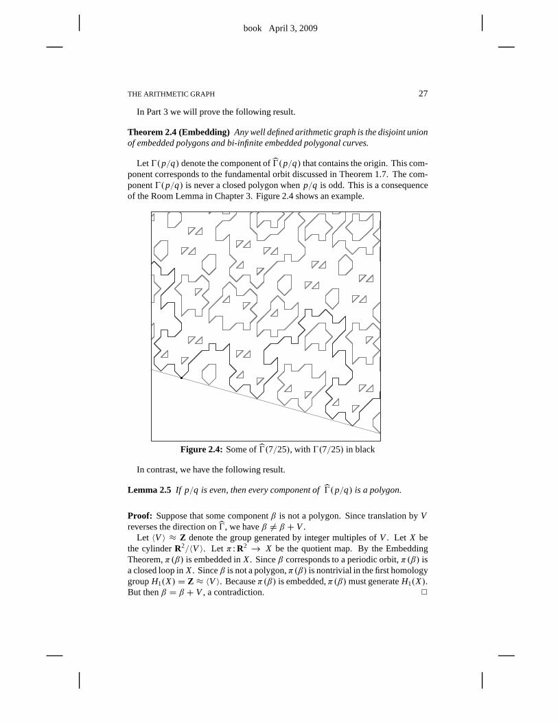
LetŴ(p/q) denote the component ofŴ(p/q) that contains the origin. This com-ponent corresponds to the fundamental orbit discussed in Theorem 1.7. The com-ponentŴ(p/q) is never a closed polygon whenp/q is odd. This is a consequenceof the Room Lemma in Chapter 3. Figure 2.4 shows an example.

Figure 2.4: Some ofŴ(7/25), with Ŵ(7/25) in black

In contrast, we have the following result.

Lemma 2.5 If p/q is even, then every component ofŴ(p/q) is a polygon.

Proof: Suppose that some componentβ is not a polygon. Since translation byVreverses the direction onŴ, we haveβ 6= β + V .

Let 〈V 〉 ≈ Z denote the group generated by integer multiples ofV . Let X bethe cylinderR2/〈V 〉. Let π : R2 → X be the quotient map. By the EmbeddingTheorem,π(β) is embedded inX. Sinceβ corresponds to a periodic orbit,π(β) isa closed loop inX. Sinceβ is not a polygon,π(β) is nontrivial in the first homologygroupH1(X) = Z ≈ 〈V 〉. Becauseπ(β) is embedded,π(β)must generateH1(X).But thenβ = β + V , a contradiction. 2

book April 3, 2009

28 CHAPTER 2

2.6 LOW VERTICES AND PARITY

Remark: The material in this section is not needed for the proofs of statements 1and 2 of the Erratic Orbits Theorem.

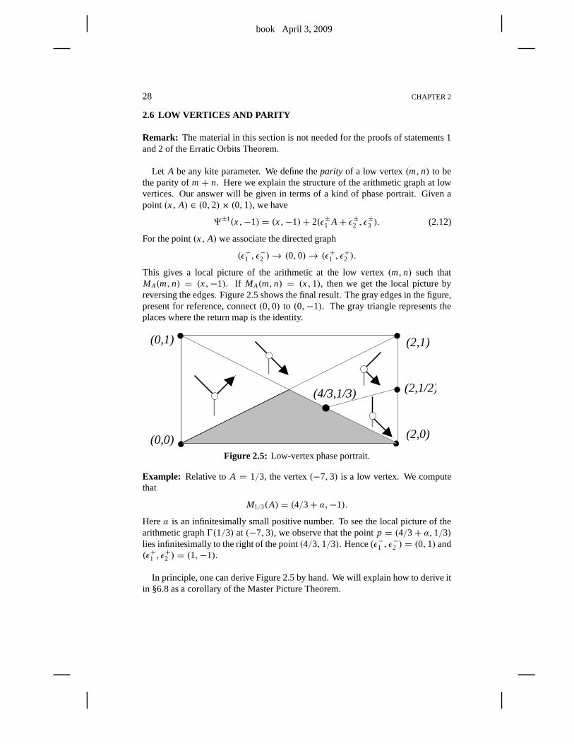
Let A be any kite parameter. We define theparity of a low vertex(m,n) to bethe parity ofm+ n. Here we explain the structure of the arithmetic graph at lowvertices. Our answer will be given in terms of a kind of phase portrait. Given apoint (x, A) ∈ (0,2)× (0,1), we have

9±1(x,−1) = (x,−1)+ 2(ǫ±1 A+ ǫ±2 , ǫ±3 ). (2.12)

For the point(x, A) we associate the directed graph

(ǫ−1 , ǫ−2 )→ (0,0)→ (ǫ+1 , ǫ

+2 ).

This gives a local picture of the arithmetic at the low vertex(m,n) such thatMA(m,n) = (x,−1). If MA(m,n) = (x,1), then we get the local picture byreversing the edges. Figure 2.5 shows the final result. The gray edges in the figure,present for reference, connect(0,0) to (0,−1). The gray triangle represents theplaces where the return map is the identity.

(4/3,1/3) (2,1/2)

(0,0)

(0,1) (2,1)

(2,0)

Figure 2.5: Low-vertex phase portrait.

Example: Relative toA = 1/3, the vertex(−7,3) is a low vertex. We computethat

M1/3(A) = (4/3+ α,−1).

Hereα is an infinitesimally small positive number. To see the localpicture of thearithmetic graphŴ(1/3) at (−7,3), we observe that the pointp = (4/3+ α,1/3)lies infinitesimally to the right of the point(4/3,1/3). Hence(ǫ−1 , ǫ

−2 ) = (0,1) and

(ǫ+1 , ǫ+2 ) = (1,−1).

In principle, one can derive Figure 2.5 by hand. We will explain how to derive itin §6.8 as a corollary of the Master Picture Theorem.

book April 3, 2009

THE ARITHMETIC GRAPH 29

Lemma 2.6 No component ofŴ(A) contains low vertices of both parities.

Proof: Recall thatŴ is an oriented graph. Ifv is a nontrivial low vertex ofŴ, we cansay whetherŴ is left-travellingor right-travelling at v. The definition is this: Aswe travel along the orientation and pass throughv, the line segment connectingv tov − (0,1) lies on either our left or our right. This gives the name to ourdefinition.

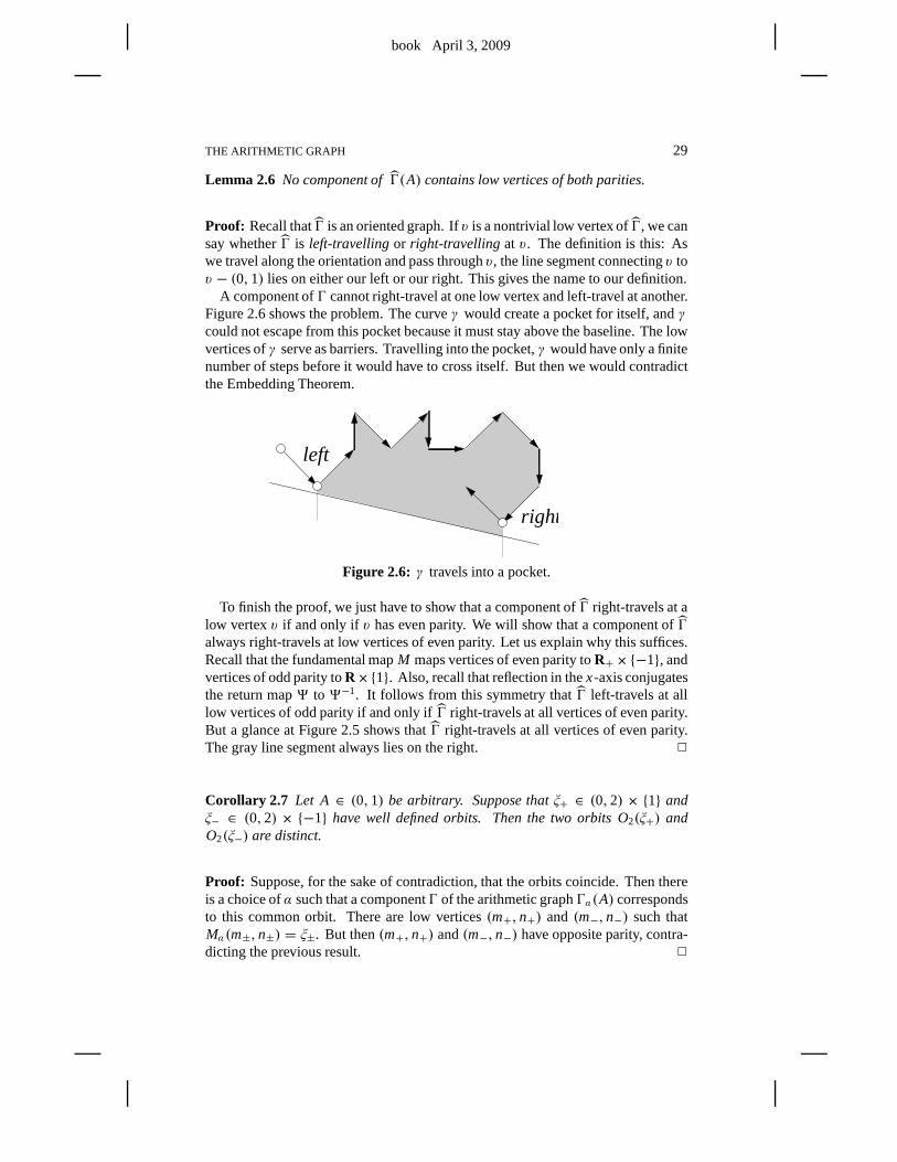
A component ofŴ cannot right-travel at one low vertex and left-travel at another.Figure 2.6 shows the problem. The curveγ would create a pocket for itself, andγcould not escape from this pocket because it must stay above the baseline. The lowvertices ofγ serve as barriers. Travelling into the pocket,γ would have only a finitenumber of steps before it would have to cross itself. But thenwe would contradictthe Embedding Theorem.

right

left

Figure 2.6: γ travels into a pocket.

To finish the proof, we just have to show that a component ofŴ right-travels at alow vertexv if and only if v has even parity. We will show that a component ofŴalways right-travels at low vertices of even parity. Let us explain why this suffices.Recall that the fundamental mapM maps vertices of even parity toR+×{−1}, andvertices of odd parity toR×{1}. Also, recall that reflection in thex-axis conjugatesthe return map9 to 9−1. It follows from this symmetry thatŴ left-travels at alllow vertices of odd parity if and only ifŴ right-travels at all vertices of even parity.But a glance at Figure 2.5 shows thatŴ right-travels at all vertices of even parity.The gray line segment always lies on the right. 2

Corollary 2.7 Let A ∈ (0,1) be arbitrary. Suppose thatξ+ ∈ (0,2) × {1} andξ− ∈ (0,2) × {−1} have well defined orbits. Then the two orbits O2(ξ+) andO2(ξ−) are distinct.

Proof: Suppose, for the sake of contradiction, that the orbits coincide. Then thereis a choice ofα such that a componentŴ of the arithmetic graphŴα(A) correspondsto this common orbit. There are low vertices(m+,n+) and (m−,n−) such thatMα(m±,n±) = ξ±. But then(m+,n+) and(m−,n−) have opposite parity, contra-dicting the previous result. 2

book April 3, 2009

30 CHAPTER 2

2.7 HAUSDORFF CONVERGENCE

Here we state the basic results that will allow us to take geometric limits of orbitsfor outer billiards systems with varying parameters. When it comes to taking limitsof arithmetic graphs, we will always use the Hausdorff topology.

The Hausdorff metric and topology: Given two compact subsetsK1, K2 ⊂ R2,we defined(K1, K2) to be the infimalǫ > 0 such that the setK1 is contained in theǫ-tubular neighborhood of the setK2, and vice versa. The functiond(K1, K2) isknown as theHausdorff metric. A sequence{Cn} of closed subsets ofR2 is said toHausdorff convergeto C ⊂ R2 if d(Cn ∩ K ,C ∩ K )→ 0 for every compact subsetK ⊂ R2. This notion of convergence is called theHausdorff topology.

Remark: In the cases of interest to us,Cn is always an arc of an arithmetic graphthat contains(0,0). In this case, the Hausdorff convergence has a simple meaning.{Cn} converges toC if and only if the following property holds true. For anyN,there is someN′ such thatn > N′ implies that the firstN steps ofCn away from(0,0) in either direction agree with the corresponding steps ofC.

Given a parameterA ∈ (0,1) and a pointζ ∈ 4, we say that a pair(A, ζ ) isN-definedif the first N iterates of the outer billiards map ofζ are defined relativeto A in both directions. We letŴ(A, ζ ) be as much of the arithmetic graph as isdefined. We callŴ(A, ζ ) a partial arithmetic graph.

Lemma 2.8 (Continuity Principle) Let {ζn} ∈ 4 converge toζ ∈ 4. Let {An}converge to A. Suppose the orbit ofζ is defined relative to A. Then for any N, thereis some N′ such that n> N′ implies that(ζn, An) is N-defined. The correspondingsequence{Ŵ(An, ζn)} of partially defined arithmetic graphs Hausdorff-convergesto Ŵ(A, ζ ).

Proof: Letψ ′n be the outer billiards map relative toAn. Letψ ′ be the outer billiardsmap defined relative toA. If pn → p andψ ′ is defined atp, thenψ ′n is definedat pn for n sufficiently large andψ ′n(pn)→ ψ(p). This follows from the fact thatK (An) → K (A) and from the fact that a piecewise isometric map is defined andcontinuous in open sets. The Continuity Principle now follows from induction. 2

In the case when the orbit ofζn relative toAn is already well defined, the partialarithmetic graph is the same as one component of the ordinaryarithmetic graph. Inthis case, we can state the Continuity Principle more simply.

Corollary 2.9 Let {ζn} ∈ 4 converge toζ ∈ 4. Let{An} converge to A. Supposethe orbit ofζ is defined relative to A and the orbit ofζn is defined relative to An forall n. Then{Ŵ(An, ζn)} Hausdorff converges toŴ(A, ζ ).

We will have occasion to use both versions of the Continuity Principle in ourproofs.

book April 3, 2009

THE ARITHMETIC GRAPH 31

Remark: The remaining material in this section is not needed for the proofs ofstatements 1 and 2 of the Erratic Orbits Theorem.

Lemma 2.10 Let s∈ (0,1). If (ψ ′)k(s,1) is not defined on K(A) for some|k| ≤ N,then s= 2Am+ 2n for some m,n ∈ Z such that|m| ≤ 2N.

Proof: We will consider the case whenk > 0. The other case is similar. Byinduction, we may suppose thatt = (t1, t2) = (ψ ′)N−1(s) is well defined. Lookingat the maps in Equation 2.1, we see inductively that|t2| ≤ 2N. If ψ ′(t) is notdefined, thent is one of the points in Equation 2.3 for some|n| ≤ N. Hence

t1 = 2Am′ + 2n′; |m′| ≤ N.

By Equation 2.1 and induction, we have

s= 2Am+ 2n; |m| ≤ N + |m′| ≤ 2N.

This completes the proof 2

We think of the next result as a rigidity lemma because it saysthat certain limitsare independent of how we take them.

Lemma 2.11 (Rigidity) Let An be any sequence of parameters converging to theirrational parameter A. Letζn ∈ [0,2]×{1} be any sequence of points convergingto (0,1). LetŴ(ζn, A) be the arithmetic graph ofζn relative to A. Then the sequence{Ŵ(ζn, A)}, if entirely defined, Hausdorff-converges.

Proof: Let ǫ ∈ (0,1) be given. Define

6ǫ(A) = {(s, A′)| s ∈ (0, ǫ), |A− A′| < ǫ}. (2.13)

Let O(s; A′) denote the outer billiards orbit of(s,1) relative toK (A′). Supposethat one of the firstN iterates ofO(s, A′) is not defined. By Lemma 2.10, we havem,n ∈ Z such that

s = 2A′m− 2n; |m| ≤ 2N. (2.14)

(We use a minus sign for convenience.) Note thatm 6= 0. Hence, by Equation 2.14and the triangle inequality,

∣∣∣A− n

m

∣∣∣ < |A− A′| +∣∣∣A′ − n

m

∣∣∣ < ǫ + s

2|m|< 2ǫ. (2.15)

This is impossible forǫ sufficiently small. Hence the firstN iterates ofO(s; A′) inboth directions are well defined when(s, A′) ∈ 6ǫ(A) andǫ is sufficiently small.

If all orbits in some interval are defined, then all orbits in that interval have thesame combinatorial structure. Hence, for anyN, there is someǫ > 0 such thatthe combinatorics of the firstN iterates, in either direction, ofO(s; A′) are in-dependent of(s, A′) ∈ 6ǫ(A). This lemma now follows from the Return Lemma,which guarantees that, asN →∞, the number of returns to4 tends to∞ as well.2

book April 3, 2009

book April 3, 2009

Chapter Three

The Hexagrid Theorem

3.1 THE ARITHMETIC KITE

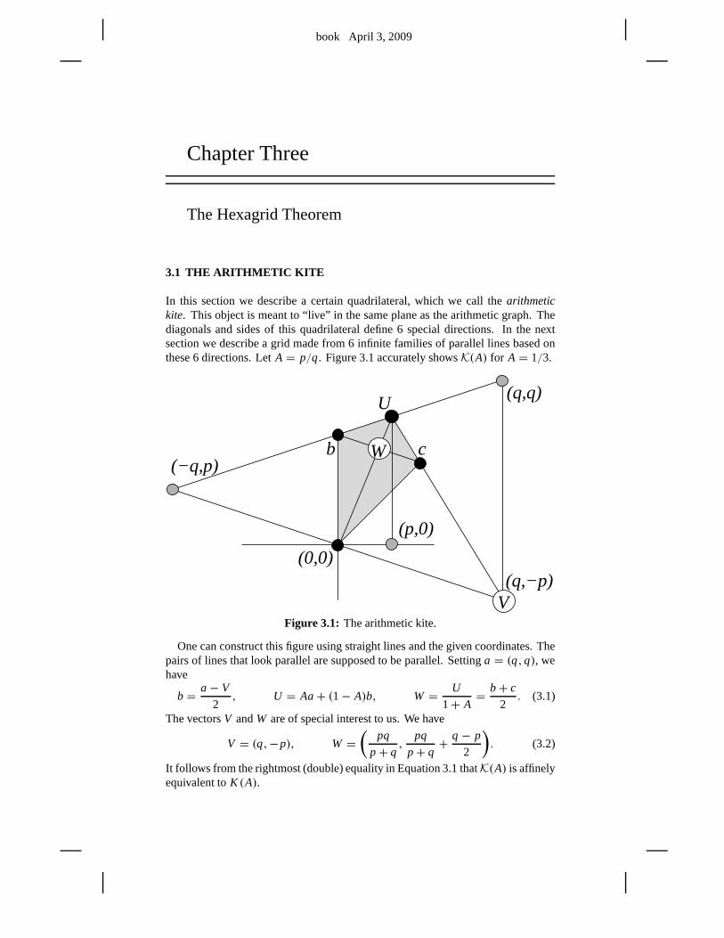
In this section we describe a certain quadrilateral, which we call thearithmetickite. This object is meant to “live” in the same plane as the arithmetic graph. Thediagonals and sides of this quadrilateral define 6 special directions. In the nextsection we describe a grid made from 6 infinite families of parallel lines based onthese 6 directions. LetA = p/q. Figure 3.1 accurately showsK(A) for A = 1/3.

(q,−p)

c

(0,0)

(−q,p)

(q,q)

b W

V

(p,0)

U

Figure 3.1: The arithmetic kite.

One can construct this figure using straight lines and the given coordinates. Thepairs of lines that look parallel are supposed to be parallel. Settinga = (q,q), wehave

b = a− V

2, U = Aa+ (1− A)b, W = U

1+ A= b+ c

2. (3.1)

The vectorsV andW are of special interest to us. We have

V = (q,−p), W =(

pq

p+ q,

pq

p+ q+ q − p

2

). (3.2)

It follows from the rightmost (double) equality in Equation3.1 thatK(A) is affinelyequivalent toK (A).

book April 3, 2009

34 CHAPTER 3

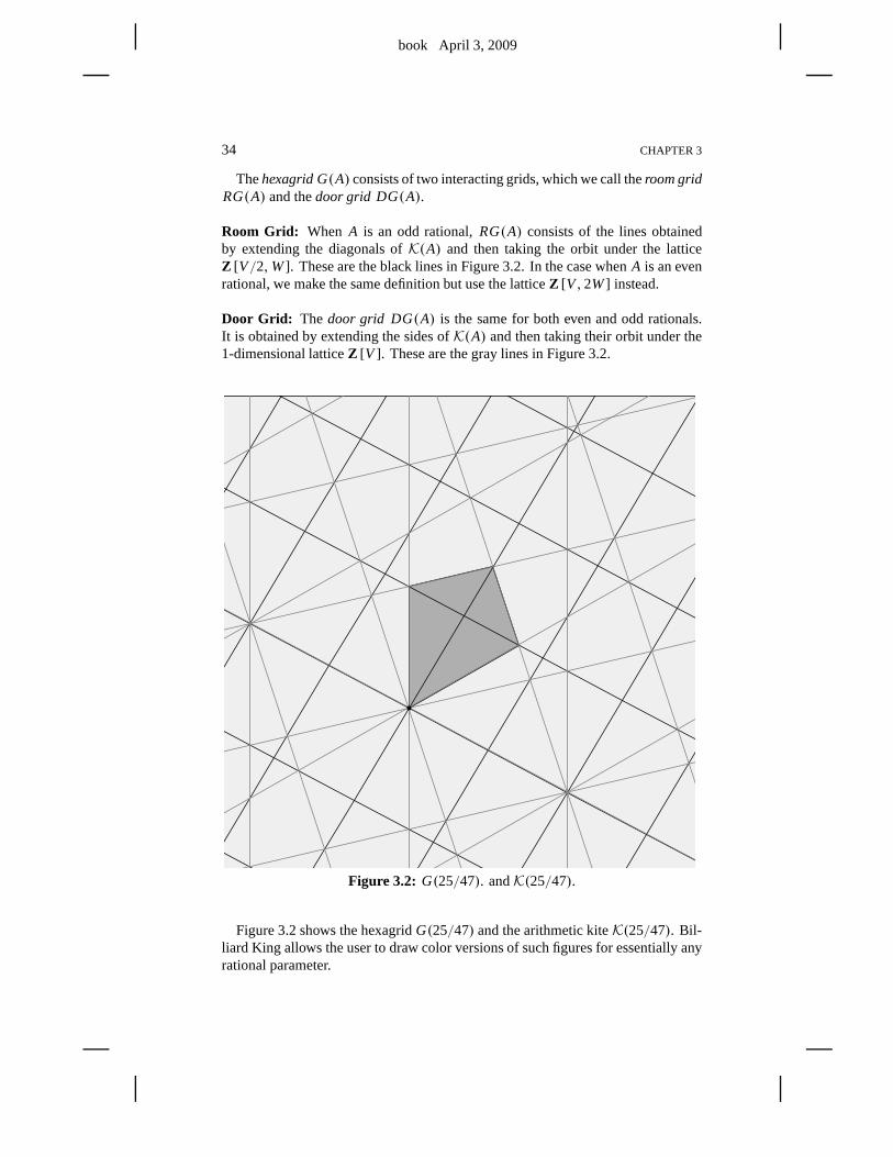
Thehexagrid G(A) consists of two interacting grids, which we call theroom gridRG(A) and thedoor grid DG(A).

Room Grid: When A is an odd rational,RG(A) consists of the lines obtainedby extending the diagonals ofK(A) and then taking the orbit under the latticeZ [V/2,W]. These are the black lines in Figure 3.2. In the case whenA is an evenrational, we make the same definition but use the latticeZ [V,2W] instead.

Door Grid: The door grid DG(A) is the same for both even and odd rationals.It is obtained by extending the sides ofK(A) and then taking their orbit under the1-dimensional latticeZ [V ]. These are the gray lines in Figure 3.2.

Figure 3.2: G(25/47). andK(25/47).

Figure 3.2 shows the hexagridG(25/47) and the arithmetic kiteK(25/47). Bil-liard King allows the user to draw color versions of such figures for essentially anyrational parameter.

book April 3, 2009

THE HEXAGRID THEOREM 35

3.2 THE HEXAGRID THEOREM

First we will talk informally about the Hexagrid Theorem. Inthe previous section,we defined two grids, the room grid and the door grid. The Hexagrid Theorem saysthat these two grids control the large-scale structure of the arithmetic graph. It turnsout that the lines of the room grid serve to “confine” the arithmetic graph, in thesense that the arithmetic graph can cross these lines only atvery specific locations.The door grid serves to define the locations – i.e., the doors –where the graph cancross the lines of the room grid. Thus the Hexagrid Theorem relates two kinds ofobjects,wall crossingsanddoors. Informally, the Hexagrid Theorem says that thearithmetic graph crosses a wall only at a door. Here are formal definitions.

Rooms and Walls: RG(A) dividesR2 into different connected components whichwe callrooms. Say that awall is the line segment of positive slope that divides twoadjacent rooms.

Doors: When p/q is odd, we say that adoor is a point of intersection betweena wall of RG(A) and a line ofDG(A). When p/q is even, we have the samedefinition, except that we exclude intersection points of the form(x, y), wherey isa half-integer. Every door is a triple point, and every wall has one door. The firstcoordinate of a door is always an integer. (See Lemma 15.1.) In exceptional cases– when the second coordinate is also an integer – the door liesin the corner of theroom. In this case, we associate the door to both walls containing it. The door(0,0)has this property.

Crossing Cells: Say that an edgee of Ŵ crosses a wallif e intersects a wall atan interior point. Say that a union of two incident edges ofŴ crosses a wallif thecommon vertex lies on a wall and the two edges point to opposite sides of the wall.The point(0,0) has this property. We say that acrossing cellis either an edge ora union of two edges that crosses a wall in the manner just described. For instance(−1,1)→ (0,0)→ (1,1) is a crossing cell for anyA ∈ (0,1).

In Part 3 of the book we will prove the following result. Let [y] denote the floorof y, the greatest integer less than or equal toy.

Theorem 3.1 (Hexagrid) Let A∈ (0,1) be rational.

1. Ŵ(A) never crosses a floor of RG(A). Any edges ofŴ(A) incident to a vertexcontained on a floor rise above that floor (rather than below it.)

2. There is a bijection between the set of doors and the set of crossing cells. Ify is not an integer, then the crossing cell corresponding to the door(m, y)contains(m, [y]) ∈ Z2. If y is an integer, then(x, y) corresponds to2 doors.One of the corresponding crossing cells contains(x, y), and the other onecontains(x, y− 1).

Figure 3.3 illustrates the Hexagrid Theoremforp/q= 25/47. We will explain theshaded parallelogramR(25/47) in the next section. We have shown only the fleeting

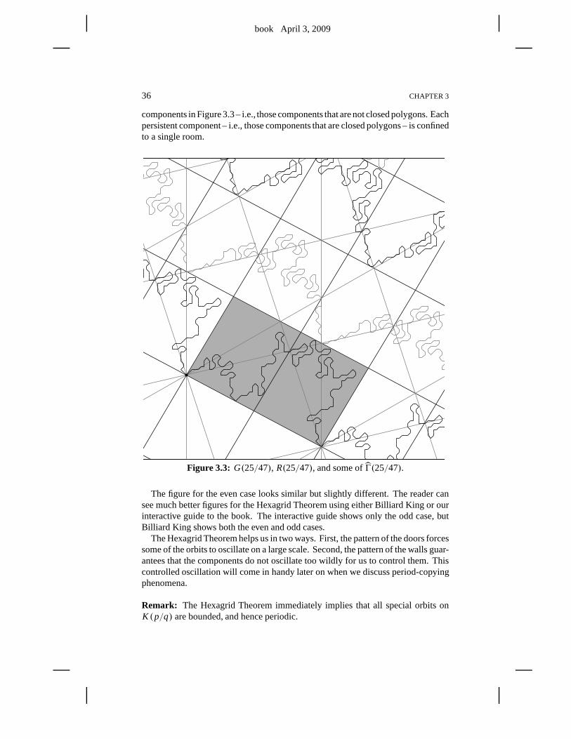
book April 3, 2009

36 CHAPTER 3

components in Figure 3.3 – i.e., those components that are not closed polygons. Eachpersistent component – i.e., those components that are closed polygons – is confinedto a single room.

Figure 3.3: G(25/47), R(25/47), and some ofŴ(25/47).

The figure for the even case looks similar but slightly different. The reader cansee much better figures for the Hexagrid Theorem using eitherBilliard King or ourinteractive guide to the book. The interactive guide shows only the odd case, butBilliard King shows both the even and odd cases.

The Hexagrid Theorem helps us in two ways. First, the patternof the doors forcessome of the orbits to oscillate on a large scale. Second, the pattern of the walls guar-antees that the components do not oscillate too wildly for usto control them. Thiscontrolled oscillation will come in handy later on when we discuss period-copyingphenomena.

Remark: The Hexagrid Theorem immediately implies that all special orbits onK (p/q) are bounded, and hence periodic.

book April 3, 2009

THE HEXAGRID THEOREM 37

3.3 THE ROOM LEMMA

The Room Lemma, an easy consequence of the Hexagrid Theorem,is the mainresult we use to force large oscillations of the fundamentalorbit O(1/q,−1).

Let R(p/q) denote the parallelogram whose vertices are

(0,0), V, W, V +W. (3.3)

HereV andW are as in Equation 3.2.R(p/q) is the shaded parallelogram in Figure3.3. We also define

d0 = (x, [y]), x = p+ q

2, y = q2− p2

4q(3.4)

d0 lies within 1 vertical unit of the centerline ofR(p/q), above the midpoint of thecenterline.d0 is just below the triple point contained in the interior of the shadedparallelogram in Figure 3.3.

Lemma 3.2 (Room) Let p/q be an odd rational. ThenŴ(p/q) is an open polyg-onal curve. One period ofŴ(p/q) connects(0,0) to d0 to (q,−p). This period iscontained in R(p/q).

Proof: First of all, for any value ofA, it is easy to check thatŴ(A) contains thearc(−1,1)→ (0,0)→ (1,1). One can see this from the phase portrait shown inFigure 2.6. This is to say thatŴ(p/q) entersR(p/q) from the left at(0,0). NowR(p/q) is the union of two adjacent roomsR1 andR2. Note that(0,0) is the onlydoor on the left wall ofR1, and(x, y) is the only door on the wall separatingR1

and R2, and(q,−p) is the only door on the right wall ofR2. Here(x, y) is as inEquation 3.4. From the Hexagrid Theorem and the Embedding Theorem,Ŵ(p/q)must connect(0,0) to d0 to (q,−p). The arithmetic graphŴ(p/q) is invariantunder translation by(q,−p), and so the whole pattern repeats endlessly to the leftand right ofR(p/q). HenceŴ(p/q) is an open polygonal curve. 2

We remark that we did not really need the Embedding Theorem inour proofabove.1 All we require is thatŴ(p/q) cannot backtrack as we travel from onecorner ofR(p/q) to the other. Lemma 3.3 below gives a self-contained proof ofwhat we need.

Lemma 3.3 Ŵ(p/q) has valence2 at every vertex.

Proof: Recall that9 is the first return map toR+ ×{−1,1}. As in our proof of theRoom Lemma,Ŵ(p/q) has valence 2 at(0,0). ButŴ(p/q) describes the forwardorbit of p = (1/q,1) under9. If some vertex ofŴ(p/q) has valence 1, then9 hasorder 2 when evaluated at the corresponding point. But then9 has order 2 whenevaluated atv. But thenŴ(p/q) has valence 1 at(0,0). This is a contradiction.2

1I am grateful to Dmitry Dolgopyat and Giovanni Forni for pointing this out to me.

book April 3, 2009

38 CHAPTER 3

3.4 ORBIT EXCURSIONS

Remark: The material in this section is not needed for the proof of theErraticOrbits Theorem.

In this section, we prove Theorems 1.7, 1.9, and 1.10.Let M1 be the first coordinate of the mapM in Equation 2.10. Letλ = 1 if p/q

is odd andλ = 2 if p/q is even.

Lemma 3.4 No point of O2(1/q)∩4 has a first coordinate greater thanλ(p+ q).

Proof: Let L be the line of the room grid parallel to the baseline that contains thepointλW. HereW is as in Equation 3.2. We compute thatM1(λW) = λ(p+ q).By the Hexagrid Theorem,Ŵ(p/q) lies in the strip bounded by the baseline andL.Looking at Equation 2.10, we see thatM1 is constant onL. Therefore we have theboundM1(m,n) ≤ λ(p+ q) for any vertex(m,n) of Ŵ(p/q). 2

Lemma 3.5 The first coordinate of some point in O2(1/q)∩4 exceedsλ(p+q)/2.

Proof: To avoid an irritating case in which the calculations yield abound that is offby 1 unit, we assume thatp > 1.

In the odd case,M1(d0) is the first coordinate of a point ofO2(1/q,−1)∩4, andwe compute thatM1(d0) > (p+ q)/2. Hered0 is as in the Room Lemma.

Consider the even case. LetL0 be the line of the room grid through(0,0) andparallel to the walls. By Lemma 2.5, the componentŴ(p/q) is a closed polygon.SinceŴ(p/q) contains the arc(−1,1) → (0,0) → (1,1), an arc that has pointson either side ofL0, the polygonŴ(p/q)must crossL0 at some point above(0,0)as well. The door onL0 immediately above(0,0) is within 1 unit ofU , the tip ofK(A). See Figure 3.1. By the Hexagrid Theorem,Ŵ(p/q) must crossL0 within 1unit of U . Call this crossing pointd′0. We compute thatM(d′0) > p+ q, at leastwhen p > 1. But M1(d′0) is the first coordinate of a point inO2(1/q,−1) ∩4. 2

Proof of Theorem 1.7: Lemma 3.5 immediately gives the lower bounds in Theo-rem 1.7, except in the casep = 1. The unimportant casep = 1 requires a separateargument which we omit. For the upper bounds, we note that thefirst coordinatesof points in O2(1/q,−1) ∩ 4 lie in [0, λ(p+ q)], by Lemma 3.4. The secondcoordinates belong to the set{−1,1}. This completes the proof. 2

Proof of Theorem 1.9: We will give the proof for odd rationals. The even case isjust about the same except for the factor of 2. Suppose thatp/q is odd. Sincepandq are relatively prime, we can realize any integer as an integer combination ofp andq. From this we see that every point of the forms/q, with s odd, lies in theimage ofM1. Hence some point ofZ2, above the baseline ofŴ(p/q), correspondsto the orbit of either(s/q,1) or (s/q,−1). Let thefloor grid denote the lines of

book April 3, 2009

THE HEXAGRID THEOREM 39

negative slope in the room grid. These lines all have slope−p/q. Thekth line Lk

of the floor grid contains the point

ζk =(

0,k(p+ q)

2

).

Modulo translation byV , the pointζk is the only lattice point onLk. Statement 1of the Hexagrid Theorem says that the edges ofŴ incident toζk lie betweenLk andLk+1 (rather than betweenLk−1 andLk).

We compute thatM1(ζk) = k(p+ q). For all lattice points(m,n) betweenLk

andLk+1, we therefore have

M1(m,n) ∈ Ik, (3.5)

the interval from Theorem 1.9. This theorem now follows fromEquation 3.5, state-ment 1 of the Hexagrid Theorem, and our remarks aboutζk. 2

Remark: We compare the odd case of Theorem 1.9 to a result in [K ]. (The evencase is similar.) The result in [K ] is quite general, and so we will specialize it tokites. In this case, a kite is quasirational iff it is rational. The (special case of the)result in [K ], interpreted in our language, says that every special orbit is containedin one of the intervalsJ0, J1, J2, ..., where

Ja =p+q−1⋃

i=0

Iak+i .

The endpoints of theJ intervals correspond tonecklace orbits. A necklace orbit (inour case) is an outer billiards orbit consisting of copies ofthe kite touching vertexto vertex. Compare Figure 2.1.

Recall that a periodic orbit relative toK (A) is persistent if there exists a nearbyand combinatorially identical orbit relative toK (A′) for all nearby parametersA′.

Lemma 3.6 Suppose that p∈ 4 is a periodic point relative to outer billiards onK (A). Then O2(p) is persistent if and only if the component of the arithmetic graphcorresponding to A and p is a closed polygon.

Proof: Let γ be a the component of interest. By Equation 2.8, we have

9k(p)− p = (2mk A+ 2nk,2ǫk), k = 1,2,3, . . . (3.6)

Heremk,nk ∈ Z andǫk ∈ {−1,0,1} andmk+nk+ ǫk is even. For any givenk, thetriple (mk,nk, ǫk) remains the same for small perturbations of the parameter. Thepoint is that a finite amount of combinatorial data determines (mk,nk). If γ is aclosed polygon, then(mk,nk, ǫk) = (0,0,0) for somek. But then9k(p) = p forall parameters nearA. HenceO2(p) is persistent. Conversely, ifO2(p) is persistentthenmk A′ + nk = 0 for somek and all A′ sufficiently close toA. But this forces(mk,nk) = (0,0). Henceγ is a closed polygon. 2

book April 3, 2009

40 CHAPTER 3

Proof of Theorem 1.10: Lemmas 2.5 and 3.6 combine to prove the even caseof Theorem 1.10. Now we establish the odd case. Letp/q be an odd rational. Saythat asuite is the region between two floors of the room grid. Each suite isparti-tioned into rooms. Each room has two walls, and each wall has adoor in it. Fromthe Hexagrid Theorem, we see that there is an infinite polygonal arc ofŴ(p/q) thatlives in each suite. LetŴk(p/q) denote the infinite polygonal arc that lives in thekth suite. HereŴ0(p/q) = Ŵ(p/q).

We have just described the infinite familyof fleetingcomponents listed inTheorem1.10. All the other components ofŴ(p/q) are closed polygons and must be confinedto single rooms. The corresponding orbits are persistent,by Lemma 3.6. The alreadydescribed polygonal arcs use up all the doors.

The point(m,n) ∈ Z2 lies on the component of the arithmetic graph correspond-ing to one of the two orbits(M(m,n),±1). HereM is the fundamental map fromEquation 2.9. By the parity result in Equation 2.8, these twopoints lie on different9-orbits. Therefore each component ofŴ corresponds to two distinct special or-bits. In particular, there are exactly two fleeting orbitsU+k andU−k contained in theinterval Ik, and these correspond toŴk(p/q). This completes the proof. 2

book April 3, 2009

Chapter Four

Period Copying

4.1 INFERIOR AND SUPERIOR SEQUENCES

We discussed inferior and superior sequences in §1.4. Here we say a bit more. Letp/q ∈ (0,1) be any odd rational. There are unique rationalsp−/q− and p+/q+such that

p−q−

<p

q<

p+q+, max(q−,q+) < q, qp± − pq± = ±1. (4.1)

See Chapter 17 for more details.We define the odd rational.

p′

q′= |p+ − p−||q+ − q−|

, (4.2)

wherep′/q′ is the unique odd rational satisfying the equation

q′ < q, |pq′ − qp′| = 2. (4.3)

We call p′/q′ the inferior predecessorof p/q, and we writep′/q′ ← p/q orp/q→ p′/q′. We can iterate this procedure. Anyp/q belongs to a finite chain

1

1← p1

q1← · · · ← pn

qn= p

q. (4.4)

Corresponding to this sequence, we define

dk = floor

(qk+1

2qk

). (4.5)

We define thesuperior predecessorof p/q to be pk/qk, wherek is the largestindex such thatdk ≥ 1. It might happen that the inferior and superior predecessorscoincide, and it might not.

For reference, we repeat the example from §1.4. Consider thesequence

11← 1

3← 1

5← 3

13← 5

21← 13

55← 21

89← 55

233← 89

377← . . . .

3/13 has 1/5 as both a superior and an inferior predecessor. 5/21 has 3/13 as aninferior predecessor and 1/5 as a superior predecessor. The implied limit of thissequence is

√5− 2, the Penrose kite parameter.

The inferior predecessor construction organizes all the odd rationals into a directedtree of infinite valence. The rational 1/1 is the terminal node of this tree. The nodesincident to 1/1 are 1/3, 3/5, 5/7, etc. Figure 4.1 shows part of this tree. The edgesare labelled with thed-values from Equation 4.5.

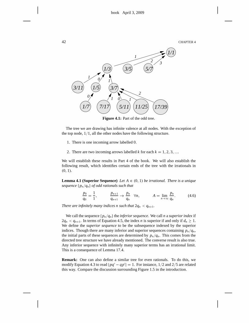
book April 3, 2009

42 CHAPTER 4

1/5 3/7

17/3911/255/117/171/7

3/11

1/3 3/5 5/7

1/1

10

1

3

0 1

2

1 0 1

2

Figure 4.1: Part of the odd tree.

The tree we are drawing has infinite valence at all nodes. Withthe exception ofthe top node, 1/1, all the other nodes have the following structure.

1. There is one incoming arrow labelled 0.

2. There are two incoming arrows labelledk for eachk = 1,2,3, ....

We will establish these results in Part 4 of the book. We will also establish thefollowing result, which identifies certain ends of the tree with the irrationals in(0,1).

Lemma 4.1 (Superior Sequence)Let A∈ (0,1) be irrational. There is a uniquesequence{pn/qn} of odd rationals such that

p0

q0= 1

1,

pn+1

qn+1→ pn

qn∀n, A = lim

n→∞

pn

qn. (4.6)

There are infinitely many indices n such that2qn < qn+1.

We call the sequence{pn/qn} theinferior sequence. We calln asuperior indexif2qn < qn+1. In terms of Equation 4.5, the indexn is superior if and only ifdn ≥ 1.We define thesuperior sequenceto be the subsequence indexed by the superiorindices. Though there are many inferior and superior sequences containingpn/qn,the initial parts of these sequences are determined bypn/qn. This comes from thedirected tree structure we have already mentioned. The converse result is also true.Any inferior sequence with infinitely many superior terms has an irrational limit.This is a consequence of Lemma 17.4.

Remark: One can also define a similar tree for even rationals. To do this, wemodify Equation 4.3 to read|pq′− qp′| = 1. For instance, 1/2 and 2/5 are relatedthis way. Compare the discussion surrounding Figure 1.5 in the introduction.

book April 3, 2009

PERIOD COPYING 43

4.2 STRONG SEQUENCES

4.2.1 The Main Result

Let A1 andA2 be two odd rationals. LetŴ1 andŴ2 be the corresponding arithmeticgraphs. We fix

ǫ = 1/8. (4.7)

This is an arbitrary but convenient choice.Let V1 = (q1,−p1). LetŴ1

1 denote the period ofŴ1 connecting(0,0) to V1 andlet Ŵ−1

1 denote the period ofŴ1 connecting(0,0) to−V1. We define

Ŵ1+ǫ1 = Ŵ1

1 ∪(Ŵ1 ∩ Bǫq1(V1)

), Ŵ−1−ǫ

1 = Ŵ−11 ∪

(Ŵ1 ∩ Bǫq1(−V1)

).

(4.8)We are extending one period ofŴ1 slightly beyond one of its endpoints. Say thata monotone convergent sequence of odd rationals{pn/qn} is strong if it has thefollowing properties.

1. |A− An| < Cq−2n for some universal constantC.

2. If An < An+1, thenŴ1+ǫn ⊂ Ŵ1

n+1.

3. If An > An+1, thenŴ−1−ǫn ⊂ Ŵ−1

n+1.

In other words,Ŵn+1 copies about 1+ ǫ periods ofŴn for everyn. As usual, wehave setAn = pn/qn.

In Part 4 we will prove the following result.

Theorem 4.2 Any superior sequence has a strong subsequence. In particular, anyirrational in (0,1) is the limit of a strong subsequence.

In the next chapter we will prove that any limit of a strong sequence satisfies theconclusions of the Erratic Orbits Theorem. Thus Theorem 4.2is one of the keyingredients in the proof of the Erratic Orbits Theorem.

4.2.2 An Easier Result

The proof of Theorem 4.2 is rather involved. It requires all the material in Part 4. Itturns out that we can prove a result nearly as strong as the Erratic Orbits Theorembased on the following easier result.

Lemma 4.3 Let Aj = p j /q j be odd rationals such that|A1− A2| < 1/(2q21).

• If A1 < A2, thenŴ1+ǫ1 ⊂ Ŵ1

2.

• If A1 > A2, thenŴ−1−ǫ1 ⊂ Ŵ−1

2 .

Hereǫ = 1/8 as above. The proof of Lemma 4.3, given in §17.4 and Chapter 18,requires only a small portion of Part 4.

book April 3, 2009

44 CHAPTER 4

Let1k ⊂ (0,1) denote the set of irrationalsA such that the equation

0<

∣∣∣∣A−p

q

∣∣∣∣ <1

kq2, p,q ∈ Zodd (4.9)

holds infinitely often. Lemma 4.3 has the following corollary.

Corollary 4.4 Every A∈ 12 is the limit of a strong sequence.

Proof: If A ∈ 12, then there exists a monotone sequence of solutions to Equation4.9 fork = 2. This sequence is strong, by Lemma 4.3. 2

Combining the last corollary with our work in the next chapter, we obtain theproof of the Erratic Orbits Theorem for allA ∈ 12. We close this section with someobservations on the size of the sets1k.

Lemma 4.5 1k has full measure in(0,1) for any k.

Proof: Any block of 3 consecutive odd terms≥ k in the continued fraction ex-pansion ofA guarantees a solution to Equation 4.9. It follows from the ergodicityof the Gauss map (or the ergodicity of the geodesic flow on the modular surface)that almost everyA has infinitely many such blocks. Hence1k has full measure in(0,1). See [BKS] for the relevant ergodic theory. 2

It turns out1 that every irrational in(0,1) belongs to11. This result is similar inspirit to Lagrange’s famous theorem stating that every irrational A satisfies∣∣∣∣A−

p

q

∣∣∣∣ <1√5q2

infinitely often. Lagrange’s theorem does not imply that every irrational lies in12

because the conditions on12 involve a parity restriction. In any case, the set12

seems to be pretty close to all of(0,1)−Q.For the interested reader, we sketch the proof of the result we have just mentioned.

Lemma 4.6 11 = (0,1)−Q.

Proof: (Sketch.) Consider the usual horodisk packing in the upper half-plane as-sociated to the modular group. The disk tangent toR at p/q has diameter 1/q2.Remove all horodisks except those based at odd rationals. Dilate each disk (in theEuclidean sense) by a factor of 2 about its tangency point. Observe that the comple-ment of these inflated disks in the hyperbolic plane has infinitely many components.Interpret this result in terms of11 using the usual connection between the modularhorodisk packing and rational approximation. 2

Lemma 4.6 plays no role in our proofs, however.

1I am grateful to Curt McMullen for pointing this out to me and also for supplying the proof sketchedhere.

book April 3, 2009

Chapter Five

Proof of the Erratic Orbits Theorem

5.1 PROOF OF STATEMENT 1

In this section we will prove the following result.

Lemma 5.1 Suppose that A is the limit of a strong sequence{An}. Then statement1 of the Erratic Orbits Theorem holds for A.

Statement 1 of the Erratic Orbits Theorem follows from Theorem 4.2 and Lemma5.1. The reader who is satisfied with the Erratic Orbits Theorem for all A ∈ 12 canuse the much easier Lemma 4.3 in place of Theorem 4.2.

In our proof of Lemma 5.1, we will consider the monotone increasing case.The monotone decreasing case is essentially the same. Letǫ = 1/8 be as in thedefinition of strong sequences. Note that our sequence remains strong if we pass toa subsequence. Passing to a subsequence, we arrange that

ǫqn+1 > 10qn (5.1)

Let Vn = (qn,−pn). Define

Ŵ2n = Ŵ1

n + Vn+1, (5.2)

Lemma 5.2

Ŵ1n ⊂ Ŵ1

n+1, Ŵ2n ⊂ Ŵ1

m ∀m ≥ n+ 2. (5.3)

Proof: We have

Ŵ1+ǫn ⊂ Ŵ1

n+1,

by definition, and

Ŵ1n + Vn+1 ⊂ Ŵn+1

becauseŴn+1 is invariant under translation byVn+1. Our choice of subsequencegives

Ŵ1n ⊂ Ŵ1+ǫ

n ⊂∗ B10qn(0,0) ⊂ Bǫqn+1(0,0) ∩ Ŵn+1. (5.4)

The starred containment comes from the Room Lemma. Translating by Vn+1, wehave

Ŵ1n + Vn+1 ⊂ Bǫqn+1(Vn+1) ∩ Ŵ1

n+1 ⊂ Ŵ1+ǫn+1 ⊂ Ŵ1

n+2. (5.5)

Equation 5.3 follows immediately. 2

Figure 5.1 shows schematicaly the sort of binary structure we have set up. In thisfigure, the notationi j stands forŴ j

i .

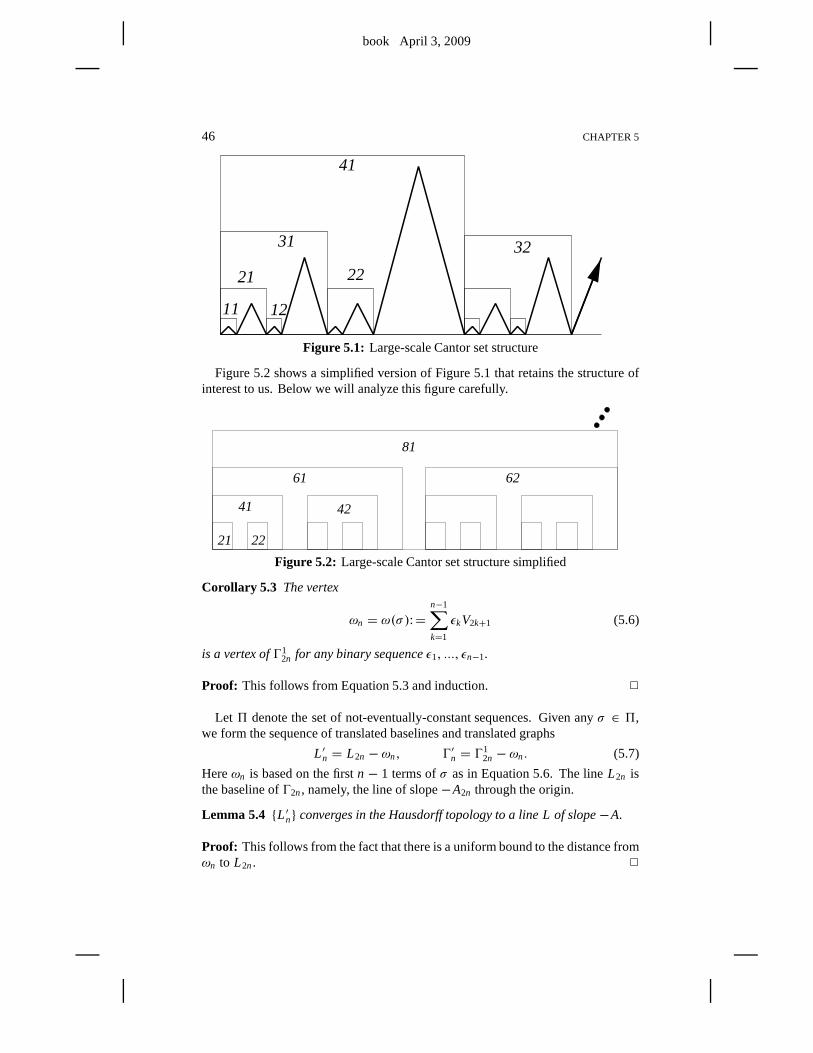
book April 3, 2009

46 CHAPTER 5

41

11 12

21 22

3231

Figure 5.1: Large-scale Cantor set structure

Figure 5.2 shows a simplified version of Figure 5.1 that retains the structure ofinterest to us. Below we will analyze this figure carefully.

21

81

61

41 42

62

22

Figure 5.2: Large-scale Cantor set structure simplified

Corollary 5.3 The vertex

ωn = ω(σ):=n−1∑

k=1

ǫkV2k+1 (5.6)

is a vertex ofŴ12n for any binary sequenceǫ1, ..., ǫn−1.

Proof: This follows from Equation 5.3 and induction. 2

Let 5 denote the set of not-eventually-constant sequences. Given anyσ ∈ 5,we form the sequence of translated baselines and translatedgraphs

L ′n = L2n − ωn, Ŵ′n = Ŵ12n − ωn. (5.7)

Hereωn is based on the firstn − 1 terms ofσ as in Equation 5.6. The lineL2n isthe baseline ofŴ2n, namely, the line of slope−A2n through the origin.

Lemma 5.4 {L ′n} converges in the Hausdorff topology to a line L of slope−A.

Proof: This follows from the fact that there is a uniform bound to thedistance fromωn to L2n. 2

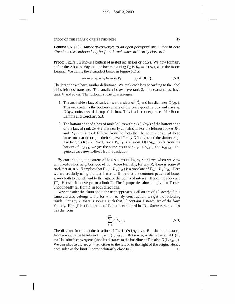
book April 3, 2009

PROOF OF THE ERRATIC ORBITS THEOREM 47

Lemma 5.5 {Ŵ′n} Hausdorff-converges to an open polygonal arcŴ that in bothdirections rises unboundedly far from L and comes arbitrarily close to L.

Proof: Figure 5.2 shows a pattern of nested rectangles orboxes. We now formallydefine these boxes. Say that the box containingŴ1

n is Rn = R(An), as in the RoomLemma. We define the 8 smallest boxes in Figure 5.2 as

R2 + ǫ1V3+ ǫ2V5+ ǫ3V7, ǫ j ∈ {0,1}. (5.8)

The larger boxes have similar definitions. We rank each box according to the labelof its leftmost translate. The smallest boxes have rank 2; the next-smallest haverank 4; and so on. The following structure emerges.

1. The arc inside a box of rank 2n is a translate ofŴ12n and has diameterO(q2n).

This arc contains the bottom corners of the corresponding box and rises upO(q2n) units toward the top of the box. This is all a consequence of the RoomLemma and Corollary 5.3.

2. The bottom edge of a box of rank 2n lies within O(1/q2n) of the bottom edgeof the box of rank 2n+ 2 that nearly contains it. For the leftmost boxesR2n

and R2n+2 this result follows from the facts that the bottom edges of theseboxes meet at the origin, their slopes differ byO(1/q2

2n), and the shorter edgehas lengthO(q2n). Next, sinceV2n+1 is at mostO(1/q2n) units from thebottom of R2n+2, we get the same result forR2n + V2n+1 and R2n+2. Thegeneral case now follows from translation.

By construction, the pattern of boxes surroundingωn stabilizes when we viewany fixed-radius neighborhood ofωn. More formally, for anyR, there is someNsuch thatm,n > N implies thatŴ1

2m∩ BR(ωm) is a translate ofŴ12n∩ BR(ωn). Here

we are crucially using the fact thatσ ∈ 5, so that the common pattern of boxesgrows both to the left and to the right of the points of interest. Hence the sequence{Ŵ′n} Hausdorff-converges to a limitŴ. The 2 properties above imply thatŴ risesunboundedly far fromL in both directions.

Now consider the claim about the near approach. Call an arc ofŴ′n steadyif thissame arc also belongs toŴ′m for m > n. By construction, we get the followingresult. For anyk, there is somen such thatŴ′n contains a steady arc of the formβ − ωn. Hereβ is a full period ofŴk but is contained inŴ1

2n. Some vertexv of βhas the form

n−1∑

j=k

ǫ j V2 j+1. (5.9)

The distance fromv to the baseline ofŴ2n is O(1/q2k+1). But then the distancefromv−ωn to the baseline ofŴ′n is O(1/q2k+1). Butv−ωn is also a vertex ofŴ (bythe Hausdorff-convergence)and its distance to the baseline ofŴ is alsoO(1/q2k+1).We can choose the arcβ − ωn either to the left or to the right of the origin. Henceboth sides of the limitŴ come arbitrarily close toL. 2

book April 3, 2009

48 CHAPTER 5

Now we will recognizeŴ as an arithmetic graph corresponding to the parameterA and a certain offset valueα. At the same time,L will be the baseline of this graph.

Similar to Equation 2.10, we define

M(m,n) =(

2Am+ 2n, (−1)m+n+1

). (5.10)

Givenσ = {ǫk} ∈ 5, the point

α(σ) =( ∞∑

k=1

2ǫk

(Aq2k+1 − p2k+1

),−1

)(5.11)

is well defined because thekth term in the series has sizeO(1/q2k+1) and thesequence{q2k+1} grows exponentially. The union of such limits, taken over all of5, contains an uncountable set. Throwing out all points in 2Z [ A] × {−1}, we stillhave an uncountable set. Takingσ from this uncountable set, the pointα = α(σ)we consider has a well defined orbit, by Lemma 2.2.

Lemma 5.6 Ŵ is the arithmetic graph ofα, and L is the baseline.

Proof: Let M2n be as in Equation 2.10 for the parameterA2n. Define

αn = M2n(σn) =( n−1∑

k=1

2ǫk

(A2nq2k+1 − p2k+1

),−1

). (5.12)

There is some constantC such that∣∣∣(A2nq2k+1−p2k+1)− (Aq2k+1−p2k+1)

∣∣∣ = q2k+1|A−A2n| < Cq−12n , ∀k ≤ n−1,

∣∣∣∣∞∑

k=n

2ǫk(Aq2k+1 − p2k+1)

∣∣∣∣ < Cq−12n .

It follows from these estimates and the triangle inequalitythat

|α − αn| < Cnq−12n .

Henceαn→ α.By construction,Ŵ′n is one period of the arithmetic graph ofαn relative toA2n.

The distance thatŴ′n extends from the origin in either direction tends to∞ with n.By the Continuity Principle,{Ŵ′n} converges to the arithmetic graph ofα. But {Ŵ′n}also converges toŴ. HenceŴ is the arithmetic graph ofα.

The lineL2n − ω is the baseline for the arithmetic graphŴ′n that tracks the orbitof αn. HenceL is the baseline ofŴ. 2

Combining Lemmas 5.5 and 5.6, we see thatα lies on an erratic orbit relative toouter billiards onK (A). But there are uncountably manyα to which our argumentapplies. This proves Lemma 5.1.

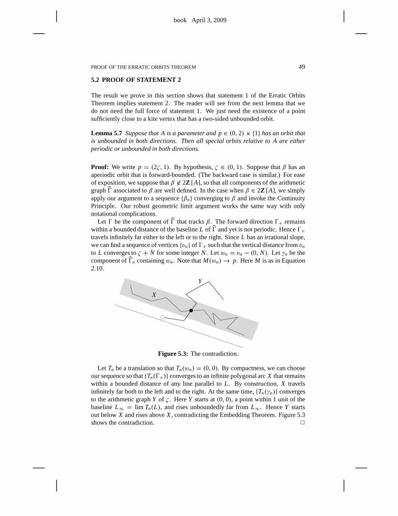
book April 3, 2009

PROOF OF THE ERRATIC ORBITS THEOREM 49

5.2 PROOF OF STATEMENT 2

The result we prove in this section shows that statement 1 of the Erratic OrbitsTheorem implies statement 2. The reader will see from the next lemma that wedo not need the full force of statement 1. We just need the existence of a pointsufficiently close to a kite vertex that has a two-sided unbounded orbit.

Lemma 5.7 Suppose that A is a parameter and p∈ (0,2)× {1} has an orbit thatis unbounded in both directions. Then all special orbits relative to A are eitherperiodic or unbounded in both directions.

Proof: We write p = (2ζ,1). By hypothesis,ζ ∈ (0,1). Suppose thatβ has anaperiodic orbit that is forward-bounded. (The backward case is similar.) For easeof exposition, we suppose thatβ 6∈ 2Z [ A], so that all components of the arithmeticgraphŴ associated toβ are well defined. In the case whenβ ∈ 2Z [ A], we simplyapply our argument to a sequence{βn} converging toβ and invoke the ContinuityPrinciple. Our robust geometric limit argument works the same way with onlynotational complications.

Let Ŵ be the component ofŴ that tracksβ. The forward directionŴ+ remainswithin a bounded distance of the baselineL of Ŵ and yet is not periodic. HenceŴ+travels infinitely far either to the left or to the right. Since L has an irrational slope,we can find a sequence of vertices{vn} of Ŵ+ such that the vertical distance fromvn

to L converges toζ + N for some integerN. Letwn = vn − (0, N). Let γn be thecomponent ofŴn containingwn. Note thatM(wn)→ p. HereM is as in Equation2.10.

X

Y

Figure 5.3: The contradiction.

Let Tn be a translation so thatTn(wn) = (0,0). By compactness, we can chooseour sequence so that{Tn(Ŵ+)} converges to an infinite polygonal arcX that remainswithin a bounded distance of any line parallel toL. By construction,X travelsinfinitely far both to the left and to the right. At the same time,{Tn(γn)} convergesto the arithmetic graphY of ζ . HereY starts at(0,0), a point within 1 unit of thebaselineL∞ = lim Tn(L), and rises unboundedly far fromL∞. HenceY startsout belowX and rises aboveX, contradicting the Embedding Theorem. Figure 5.3shows the contradiction. 2

book April 3, 2009

50 CHAPTER 5

5.3 PROOF OF STATEMENT 3

In this section we prove that statement 1 of the Erratic Orbits Theorem impliesstatement 3. LetA be an irrational parameter for which statement 1 of the ErraticOrbits Theorem holds. Since outer billiards is a piecewise isometry, the set ofperiodic orbits is open inR × Zodd. We just need to prove that the periodic orbitsare dense.

Let Ŵ be an arithmetic graph associated toA such thatŴ tracks an erratic orbit.SinceA is irrational, we can find a sequence of vertices{(mk,nk)} of odd parity thatconverges to the baseline ofA. Letγk be the component ofŴ that contains(mk,nk).Note thatγk 6= Ŵ because, by Lemma 2.6,Ŵ contains vertices only of even parity.By the Embedding Theorem,γk is trapped underneathŴ. Henceγk is a polygon.Let |γk| denote the maximal distance between a pair of low vertices onγk.

Lemma 5.8 |γk| → ∞ as k→∞.

Proof: By the Rigidity Lemma in §2.7, a very long arc ofγk, with one endpoint(mk,nk), agrees with the Hausdorff limit limn→∞ Ŵ(pn/qn). Here{pn/qn} is an ap-proximating strong sequence. But this limit has vertices withinǫ of the baseline andat least 1/ǫ apart for anyǫ > 0. Our result now follows from Hausdorff continuity.2

Let Sk denote the set of componentsγ ′ of Ŵ such thatγ ′ is translation equivalenttoγk and the corresponding vertices are low. The vertex(m,n) is low if the baselineof Ŵ separates(m,n) and(m,n− 1).

Lemma 5.9 There is some constant Nk so that every point of L is within Nk unitsof a member of Sk.

Proof: Say that a lattice point(m,n) is very low if it has depth less than 1/100(but is still positive.) The polygonγk corresponds to a periodic orbitξk. Sinceξk is periodic, there is an open neighborhoodUk of ξk such that all orbits inUk

are combinatorially identical toξk. Let M be a fundamental map associated toŴ. ThenM−1(Uk) is an open strip parallel toL. SinceL has an irrational slope,there is some constantNk so that every point ofL is within Nk of some point ofM−1(Uk) ∩ Z2. But the components ofŴ containing these points are translation-equivalent toγk. ChoosingUk small enough, we can guarantee that the translationstakingγk to the other components carry the very low vertices ofγk to low vertices.2

Given two polygonal componentsX andY of Ŵ, we write X ⊲⊳ Y if one lowvertex ofY lies to the left ofX and one low vertex ofY lies to the right ofX. SeeFigure 5.4. In this case,X is trapped underneathY, by the Embedding Theorem.

Now we pass to a subsequence so that

|γk+1| > 10(Nk + |γk|). (5.13)

Equation 5.13 has the following consequence. For any integer N, we can findcomponentsγ j of Sj , for j = N, ...,2N, suchγN ⊲⊳ · · · ⊲⊳ γ2N . Let L N denote

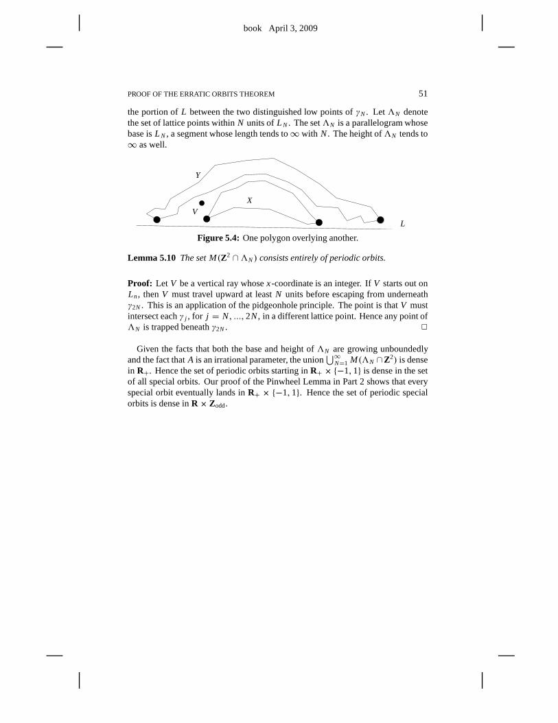
book April 3, 2009

PROOF OF THE ERRATIC ORBITS THEOREM 51

the portion ofL between the two distinguished low points ofγN . Let3N denotethe set of lattice points withinN units ofL N . The set3N is a parallelogram whosebase isL N , a segment whose length tends to∞ with N. The height of3N tends to∞ as well.

V

Y

X

L

Figure 5.4: One polygon overlying another.

Lemma 5.10 The set M(Z2 ∩3N) consists entirely of periodic orbits.

Proof: Let V be a vertical ray whosex-coordinate is an integer. IfV starts out onLn, thenV must travel upward at leastN units before escaping from underneathγ2N . This is an application of the pidgeonhole principle. The point is thatV mustintersect eachγ j , for j = N, ...,2N, in a different lattice point. Hence any point of3N is trapped beneathγ2N . 2

Given the facts that both the base and height of3N are growing unboundedlyand the fact thatA is an irrational parameter, the union

⋃∞N=1 M(3N ∩Z2) is dense

in R+. Hence the set of periodic orbits starting inR+ × {−1,1} is dense in the setof all special orbits. Our proof of the Pinwheel Lemma in Part2 shows that everyspecial orbit eventually lands inR+ × {−1,1}. Hence the set of periodic specialorbits is dense inR × Zodd.

book April 3, 2009

book April 3, 2009

Part 2. The Master Picture Theorem

In this part of the book, we will state and prove the Master Picture Theorem. Allthe auxilliary theorems left over from Part 1 rely on this central result. Here is anoverview of the material.

• In Chapter 6, we will state the Master Picture Theorem. Roughly, the MasterPicture Theorem says that the structure of the return map9 is determinedby a pair of maps into a flat 3-torusR3/3 together with a partition ofR3/3into polyhedra. Here3 is a certain 3-dimensional lattice that depends onthe parameter. We will consider the Master Picture Theorem from severalpoints of view, giving lots of example calculations. The remainder of Part2 is devoted to the proof of the Master Picture Theorem. The reader who iskeen to see the applications can skip directly from Chapter 6to Part 3.

• In Chapter 7, we will prove the Pinwheel Lemma, a key technical step alongthe way to the proof of the Master Picture Theorem. The Pinwheel Lemmastates that we can factor the return map9 into a composition of 8 simplermaps, which we callstrip maps. A strip map is a very simple map from theplane into an infinite strip.

• In Chapter 8, we prove the Torus Lemma, another key result. The TorusLemma implies that there exists some partition of the torus into open regionssuch that the regions determine the structure of the arithmetic graph. TheTorus Lemma reduces the Master Picture Theorem to a rough determinationof the singular set. The singular set is the (closure of the) set of points in thetorus corresponding to points where the return map is not defined.

• In Chapter 9, we verify, with the aid of symbolic manipulation, certain func-tional identities that arise in connection with the Torus Lemma. These func-tional identities are the basis for our analysis of the singular set.

• In Chapter 10, we combine the Torus Lemma with the functional identities toprove the Master Picture Theorem.

Billiard King has a module that shows the torus partition anddemonstrates theMaster Picture Theorem. A separate module on Billiard King shows all the setsinvolved in the proof of the Pinwheel Lemma. We hope that the material in Chapters6 and 7 stands on its own, but we strongly recommend that the reader use BilliardKing as a guide to this material.

book April 3, 2009

book April 3, 2009

Chapter Six

The Master Picture Theorem

6.1 COARSE FORMULATION

Recall that4 = R+ × {−1,1}. We distinguish two special subsets of4.

4+ =∞⋃

k=0

(2k,2k+2)×{(−1)k}, 4− =∞⋃

k=1

(2k,2k+2)×{(−1)k−1}. (6.1)

Each set is an infinite disconnected union of open intervals of length 2. The reflectionin the x-axis interchanges4+ and4−. The union4+ ∪ 4− partitions the set(R+ − 2Z)× {±1}.

Define

RA = [0,1+ A] × [0,1+ A] × [0,1] . (6.2)

RA is a fundamental domain for the action of a certain lattice3A. This lattice isdefined by the following matrix.

3A =[ 1+ A 1− A −1

0 1+ A −10 0 1

]Z3. (6.3)

We mean to say that3A is theZ-span of the column vectors of the above matrix.We define maps

µ±:4±→ RA (6.4)

by the equations

µ±(t, ∗) =(

t − 1

2,

t + 1

2,

t

2

)±(

1

2,

1

2,0

)mod3. (6.5)

The maps depend on only the first coordinate. In each case, we mean to mapt intoR3 and then use the action of3A to move the image intoRA. It might happen thatthere is not a unique representative inRA. (There is an issue with boundary points,as is usual with fundamental domains.) However, ift 6∈ 2Z [ A], this situation doesnot occur. The mapsµ+ andµ− are locally affine.

Here is a coarse formulation of the Master Picture Theorem. We will state theentire result in terms of(+), with the understanding that the same statement holdswith (−) replacing(+) everywhere. Let9:4→ 4 be the first return map.

Theorem 6.1 For each parameter A, there is a partition(P A)+ of RA into finitelymany convex polyhedra. If9 is defined onξ1, ξ2 ∈ 4+ andµ+(ξ1) andµ+(ξ2) liein the same open polyhedron of(P A)+, then9(ξ1)− ξ1 = 9(ξ2)− ξ2.

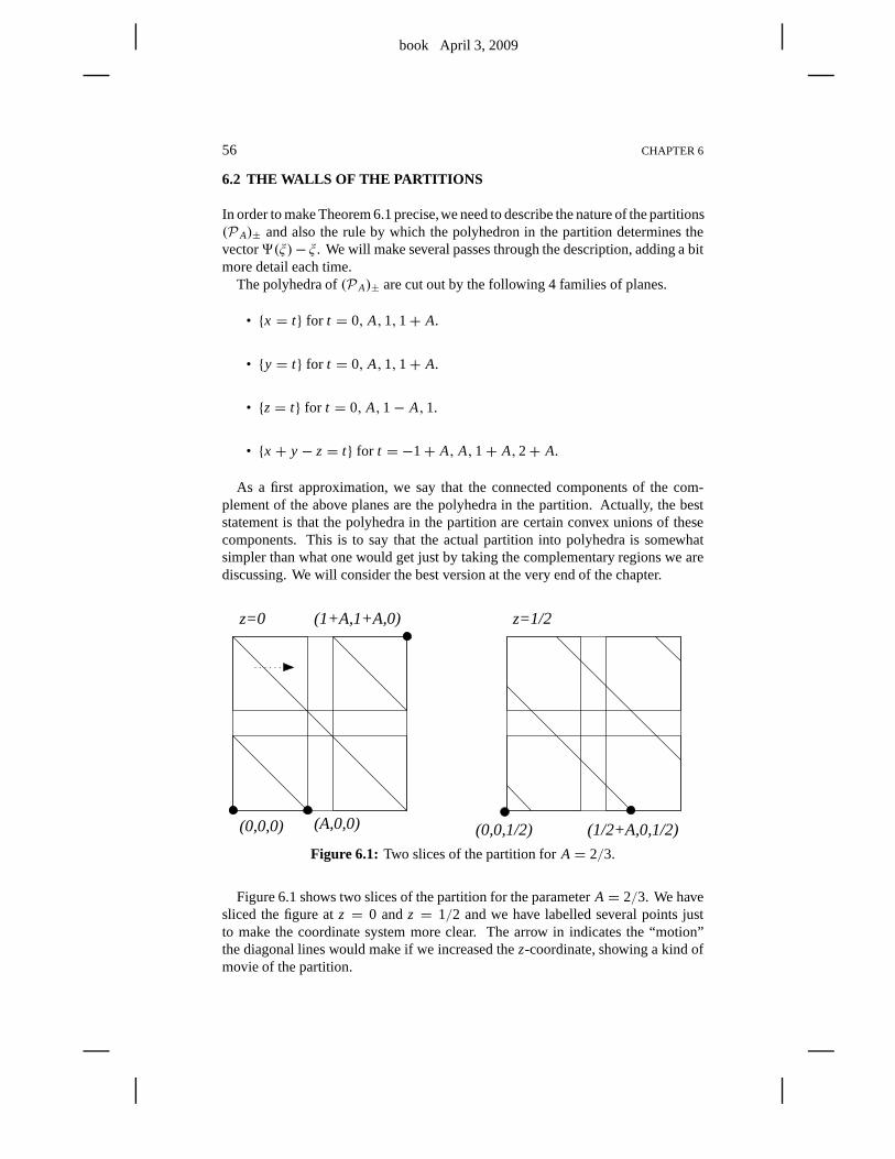
book April 3, 2009

56 CHAPTER 6

6.2 THE WALLS OF THE PARTITIONS

In order to make Theorem 6.1 precise,we need to describe the nature of the partitions(P A)± and also the rule by which the polyhedron in the partition determines thevector9(ξ)− ξ . We will make several passes through the description, adding a bitmore detail each time.

The polyhedra of(P A)± are cut out by the following 4 families of planes.

• {x = t} for t = 0, A,1,1+ A.

• {y = t} for t = 0, A,1,1+ A.

• {z= t} for t = 0, A,1− A,1.

• {x + y− z= t} for t = −1+ A, A,1+ A,2+ A.

As a first approximation, we say that the connected components of the com-plement of the above planes are the polyhedra in the partition. Actually, the beststatement is that the polyhedra in the partition are certainconvex unions of thesecomponents. This is to say that the actual partition into polyhedra is somewhatsimpler than what one would get just by taking the complementary regions we arediscussing. We will consider the best version at the very endof the chapter.

(1/2+A,0,1/2)(0,0,0) (A,0,0)

z=0 z=1/2(1+A,1+A,0)

(0,0,1/2)

Figure 6.1: Two slices of the partition forA = 2/3.

Figure 6.1 shows two slices of the partition for the parameter A = 2/3. We havesliced the figure atz = 0 andz = 1/2 and we have labelled several points justto make the coordinate system more clear. The arrow in indicates the “motion”the diagonal lines would make if we increased thez-coordinate, showing a kind ofmovie of the partition.

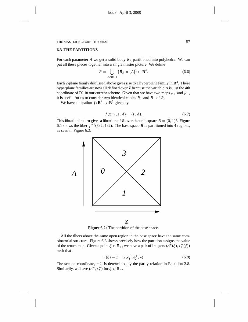
book April 3, 2009

THE MASTER PICTURE THEOREM 57

6.3 THE PARTITIONS

For each parameterA we get a solid bodyRA partitioned into polyhedra. We canput all these pieces together into a single master picture. We define

R=⋃

A∈(0,1)

(RA × {A}

)⊂ R4. (6.6)

Each 2-plane family discussed above gives rise to a hyperplane family inR4. Thesehyperplane families are now all defined overZ because the variableA is just the 4thcoordinate ofR4 in our current scheme. Given that we have two mapsµ+ andµ−,it is useful for us to consider two identical copiesR+ andR− of R.

We have a fibrationf : R4→ R2 given by

f (x, y, z, A) = (z, A). (6.7)

This fibration in turn gives a fibration ofR over the unit squareB = (0,1)2. Figure6.1 shows the fiberf −1(3/2,1/2). The base spaceB is partitioned into 4 regions,as seen in Figure 6.2.

z

2

3

0

1

A

Figure 6.2: The partition of the base space.

All the fibers above the same open region in the base space havethe same com-binatorial structure. Figure 6.3 shows precisely how the partition assigns the valueof the return map. Given a pointξ ∈ 4+, we have a pair of integers(ǫ+1 (ξ), ǫ

+2 (ξ))

such that

9(ξ)− ξ = 2(ǫ+1 , ǫ+2 , ∗). (6.8)

The second coordinate,±2, is determined by the parity relation in Equation 2.8.Similarily, we have(ǫ−1 , ǫ

−2 ) for ξ ∈ 4−.

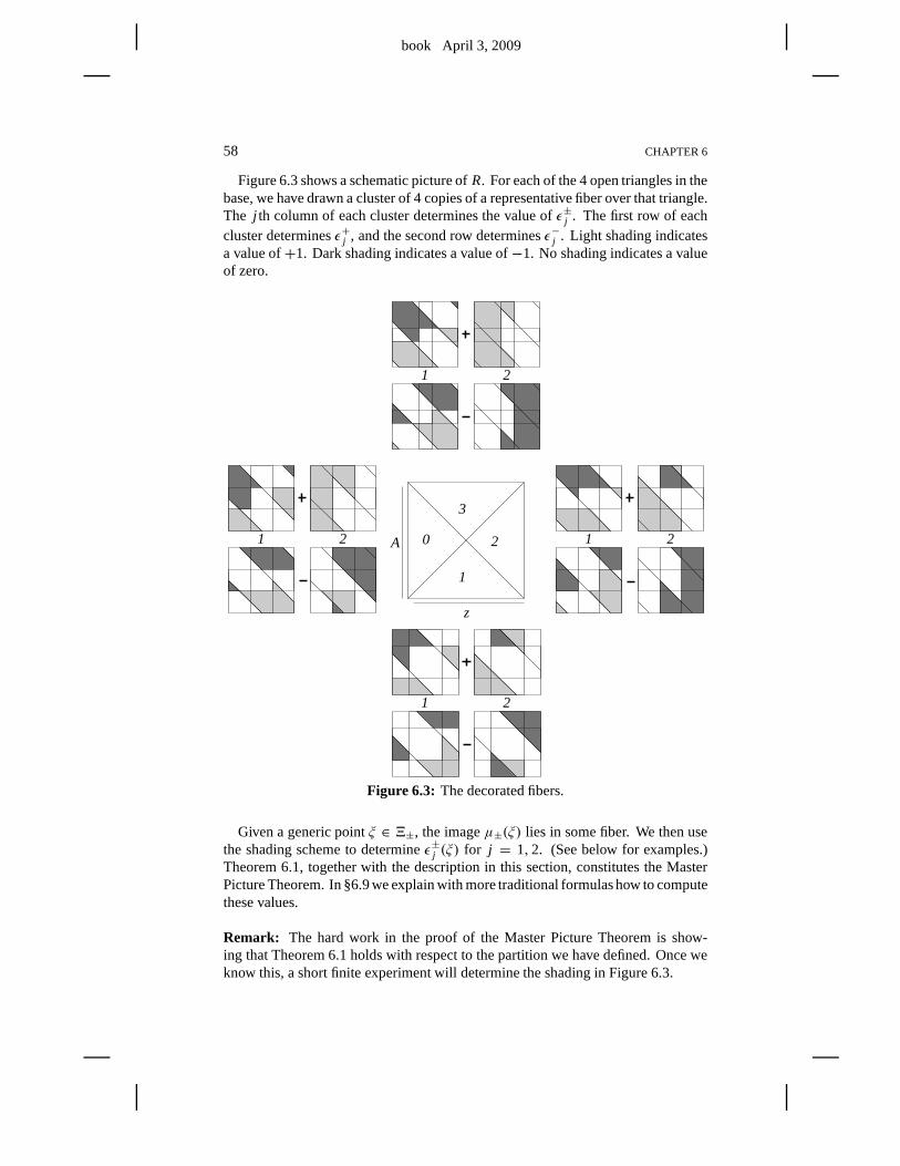
book April 3, 2009

58 CHAPTER 6

Figure 6.3 shows a schematic picture ofR. For each of the 4 open triangles in thebase, we have drawn a cluster of 4 copies of a representative fiber over that triangle.The j th column of each cluster determines the value ofǫ±j . The first row of eachcluster determinesǫ+j , and the second row determinesǫ−j . Light shading indicatesa value of+1. Dark shading indicates a value of−1. No shading indicates a valueof zero.

2

3

0

1

z

A1

1

1

1

2

2

2

2

Figure 6.3: The decorated fibers.

Given a generic pointξ ∈ 4±, the imageµ±(ξ) lies in some fiber. We then usethe shading scheme to determineǫ±j (ξ) for j = 1,2. (See below for examples.)Theorem 6.1, together with the description in this section,constitutes the MasterPicture Theorem. In §6.9 we explain with more traditional formulas how to computethese values.

Remark: The hard work in the proof of the Master Picture Theorem is show-ing that Theorem 6.1 holds with respect to the partition we have defined. Once weknow this, a short finite experiment will determine the shading in Figure 6.3.

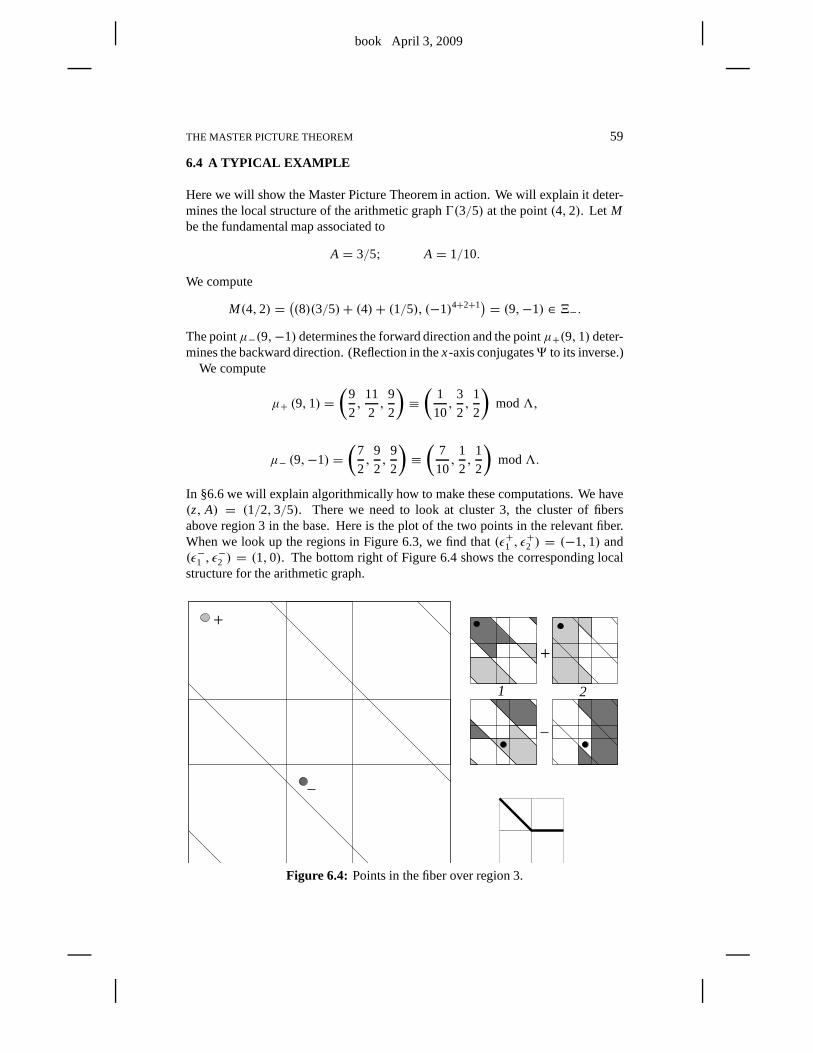
book April 3, 2009

THE MASTER PICTURE THEOREM 59

6.4 A TYPICAL EXAMPLE

Here we will show the Master Picture Theorem in action. We will explain it deter-mines the local structure of the arithmetic graphŴ(3/5) at the point(4,2). Let Mbe the fundamental map associated to

A = 3/5; A = 1/10.

We compute

M(4,2) =((8)(3/5)+ (4)+ (1/5), (−1)4+2+1

)= (9,−1) ∈ 4−.

The pointµ−(9,−1) determines the forward direction and the pointµ+(9,1) deter-mines the backward direction. (Reflection in thex-axis conjugates9 to its inverse.)

We compute

µ+ (9,1) =(

9

2,

11

2,

9

2

)≡(

1

10,

3

2,

1

2

)mod3,

µ− (9,−1) =(

7

2,

9

2,

9

2

)≡(

7

10,

1

2,

1

2

)mod3.

In §6.6 we will explain algorithmically how to make these computations. We have(z, A) = (1/2,3/5). There we need to look at cluster 3, the cluster of fibersabove region 3 in the base. Here is the plot of the two points inthe relevant fiber.When we look up the regions in Figure 6.3, we find that(ǫ+1 , ǫ

+2 ) = (−1,1) and

(ǫ−1 , ǫ−2 ) = (1,0). The bottom right of Figure 6.4 shows the corresponding local

structure for the arithmetic graph.

+

+

21

Figure 6.4: Points in the fiber over region 3.

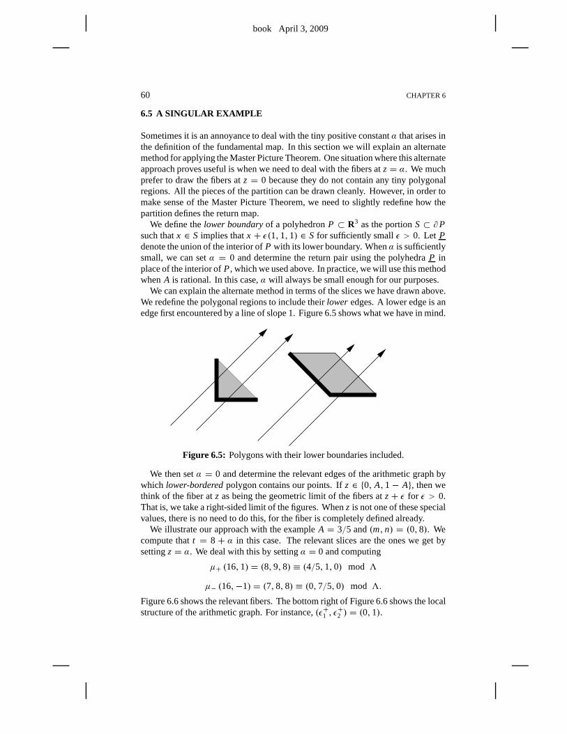
book April 3, 2009

60 CHAPTER 6

6.5 A SINGULAR EXAMPLE

Sometimes it is an annoyance to deal with the tiny positive constantα that arises inthe definition of the fundamental map. In this section we willexplain an alternatemethod for applying the Master Picture Theorem. One situation where this alternateapproach proves useful is when we need to deal with the fibers at z= α. We muchprefer to draw the fibers atz = 0 because they do not contain any tiny polygonalregions. All the pieces of the partition can be drawn cleanly. However, in order tomake sense of the Master Picture Theorem, we need to slightlyredefine how thepartition defines the return map.

We define thelower boundaryof a polyhedronP ⊂ R3 as the portionS⊂ ∂Psuch thatx ∈ S implies thatx + ǫ(1,1,1) ∈ S for sufficiently smallǫ > 0. Let Pdenote the union of the interior ofP with its lower boundary. Whenα is sufficientlysmall, we can setα = 0 and determine the return pair using the polyhedraP inplace of the interior ofP, which we used above. In practice, we will use this methodwhenA is rational. In this case,α will always be small enough for our purposes.

We can explain the alternate method in terms of the slices we have drawn above.We redefine the polygonal regions to include theirlower edges. A lower edge is anedge first encountered by a line of slope 1. Figure 6.5 shows what we have in mind.

Figure 6.5: Polygons with their lower boundaries included.

We then setα = 0 and determine the relevant edges of the arithmetic graph bywhich lower-borderedpolygon contains our points. Ifz ∈ {0, A,1− A}, then wethink of the fiber atz as being the geometric limit of the fibers atz+ ǫ for ǫ > 0.That is, we take a right-sided limit of the figures. Whenz is not one of these specialvalues, there is no need to do this, for the fiber is completelydefined already.

We illustrate our approach with the exampleA = 3/5 and(m,n) = (0,8). Wecompute thatt = 8+ α in this case. The relevant slices are the ones we get bysettingz= α. We deal with this by settingα = 0 and computing

µ+ (16,1) = (8,9,8) ≡ (4/5,1,0) mod 3

µ− (16,−1) = (7,8,8) ≡ (0,7/5,0) mod 3.

Figure 6.6 shows the relevant fibers. The bottom right of Figure 6.6 shows the localstructure of the arithmetic graph. For instance,(ǫ+1 , ǫ

+2 ) = (0,1).

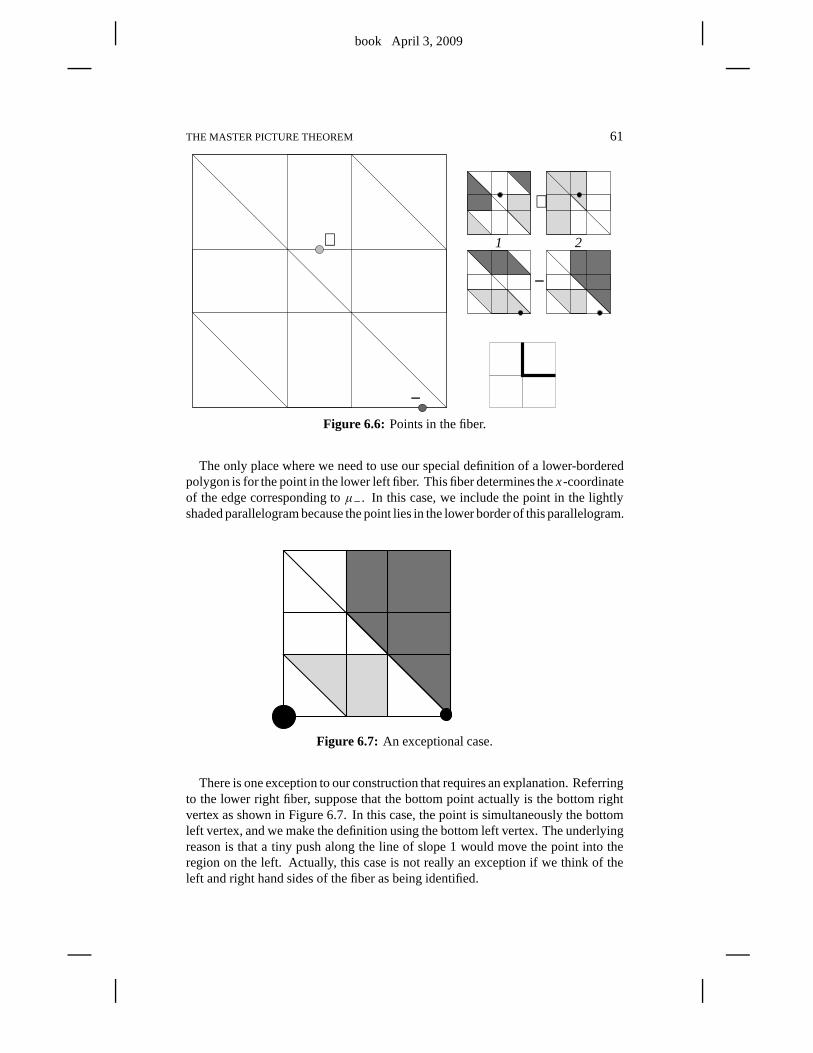
book April 3, 2009

THE MASTER PICTURE THEOREM 61

1

+

−

+

−

2

Figure 6.6: Points in the fiber.

The only place where we need to use our special definition of a lower-borderedpolygon is for the point in the lower left fiber. This fiber determines thex-coordinateof the edge corresponding toµ−. In this case, we include the point in the lightlyshaded parallelogram because the point lies in the lower border of this parallelogram.

Figure 6.7: An exceptional case.

There is one exception to our construction that requires an explanation. Referringto the lower right fiber, suppose that the bottom point actually is the bottom rightvertex as shown in Figure 6.7. In this case, the point is simultaneously the bottomleft vertex, and we make the definition using the bottom left vertex. The underlyingreason is that a tiny push along the line of slope 1 would move the point into theregion on the left. Actually, this case is not really an exception if we think of theleft and right hand sides of the fiber as being identified.

book April 3, 2009

62 CHAPTER 6

6.6 THE REDUCTION ALGORITHM

Let A be a parameter and letα be an offset value. LetM be the fundamental mapassociated to the pair(A, α), as in Equation 2.9. We define

M+ = µ+ ◦ M, M− = µ− ◦ ρ ◦ M. (6.9)

Hereµ± is as in Equation 6.5 andρ is the reflection in thex-axis. The domainof µ± is4±, the set from Equation 6.1. Note thatµ+ andµ− depend on only thefirst coordinate, and this first coordinate is not changed byρ. The mapρ is presentmainly for bookkeeping purposes becauseρ(4+) = 4−.

Given a pointp ∈ Z2, the polyhedron ofR+ containingM+(p) determines theforward edge ofŴ incident to p, and the polyhedron ofR− containingM−(p)determines the backward edge ofŴ incident top. Concretely, we have

M+(m,n) = (s, s+ 1, s) mod 3,

M−(m,n) = (s− 1, s, s) mod 3,

s= Am+ n+ α. (6.10)

Let (m,n) ∈ Z2 be a point above the baseline ofŴα(A). Here we describe howto compute the points

µ±(Mα(m,n)).

This algorithm will be important when we prove the Diophantine Lemma in Part 4.

1. Letz= Am+ n+ α.

2. Let Z = floor(z).

3. Let y = z+ Z.

4. LetY = floor(y/(1+ A)).

5. Letx = y− Y(1− A)− 1.

6. Let X = floor(x/(1+ A)).

We then have

µ−(Mα(m,n)) =( x − (1+ A)X

y− (1+ A)Yz− Z

). (6.11)

The description ofµ+ is identical except that the third step above is replaced by

y = z+ Z + 1. (6.12)

All this algorithm does is use the lattice3A to move the point(x, y, z) into thefundamental domainRA.

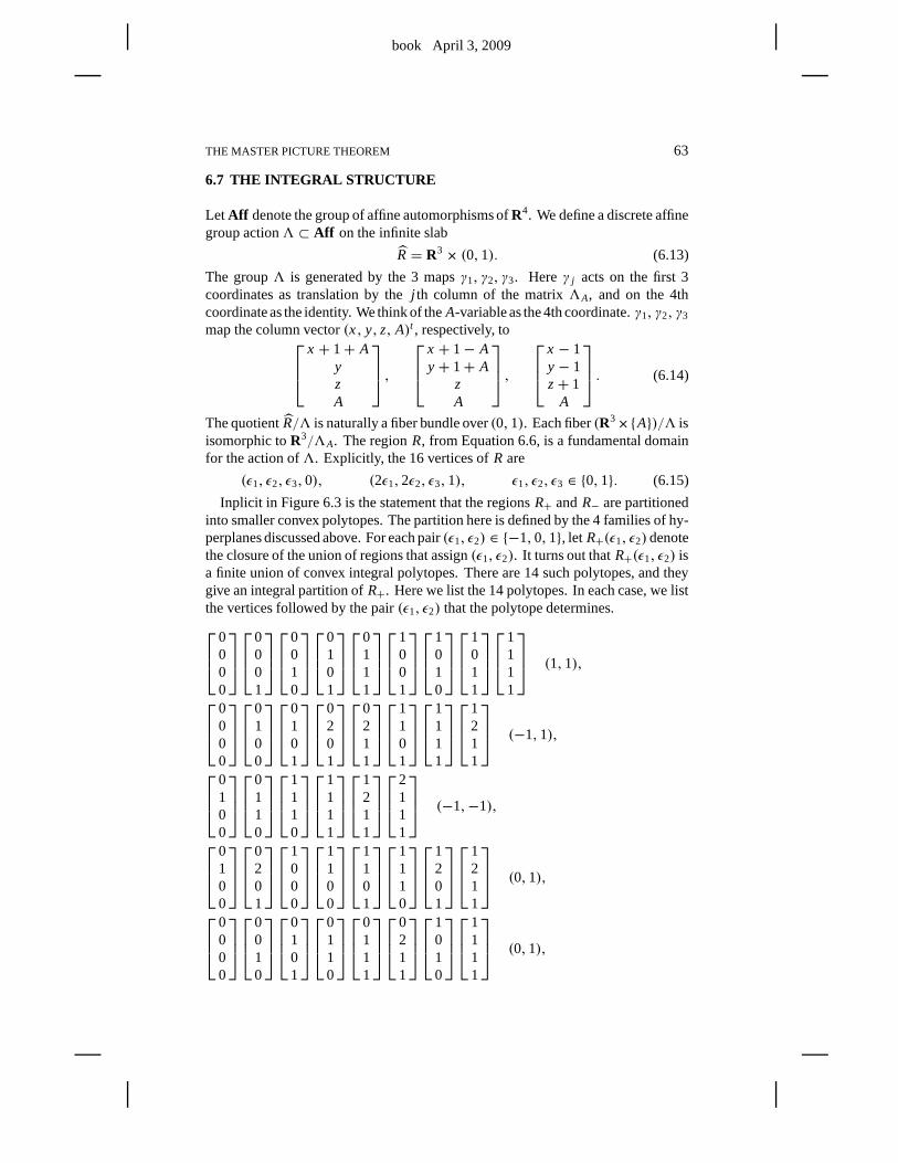
book April 3, 2009

THE MASTER PICTURE THEOREM 63

6.7 THE INTEGRAL STRUCTURE

Let Aff denote the group of affine automorphisms ofR4. We define a discrete affinegroup action3 ⊂ Aff on the infinite slab

R= R3 × (0,1). (6.13)

The group3 is generated by the 3 mapsγ1, γ2, γ3. Hereγ j acts on the first 3coordinates as translation by thej th column of the matrix3A, and on the 4thcoordinate as the identity. We think of theA-variable as the 4th coordinate.γ1, γ2, γ3

map the column vector(x, y, z, A)t , respectively, to

x + 1+ AyzA

,

x + 1− Ay+ 1+ A

zA

,

x − 1y− 1z+ 1

A

. (6.14)

The quotientR/3 is naturally a fiber bundle over(0,1). Each fiber(R3×{A})/3 isisomorphic toR3/3A. The regionR, from Equation 6.6, is a fundamental domainfor the action of3. Explicitly, the 16 vertices ofR are

(ǫ1, ǫ2, ǫ3,0), (2ǫ1,2ǫ2, ǫ3,1), ǫ1, ǫ2, ǫ3 ∈ {0,1}. (6.15)

Inplicit in Figure 6.3 is the statement that the regionsR+ andR− are partitionedinto smaller convex polytopes. The partition here is definedby the 4 families of hy-perplanes discussed above. For each pair(ǫ1, ǫ2) ∈ {−1,0,1}, let R+(ǫ1, ǫ2) denotethe closure of the union of regions that assign(ǫ1, ǫ2). It turns out thatR+(ǫ1, ǫ2) isa finite union of convex integral polytopes. There are 14 suchpolytopes, and theygive an integral partition ofR+. Here we list the 14 polytopes. In each case, we listthe vertices followed by the pair(ǫ1, ǫ2) that the polytope determines.

0000

0001

0010

0101

0111

1001

1010

1011

1111

(1,1),

0000

0100

0101

0201

0211

1101

1111

1211

(−1,1),

0100

0110

1110

1111

1211

2111

(−1,−1),

0100

0201

1000

1100

1101

1110

1201

1211

(0,1),

0000

0010

0101

0110

0111

0211

1010

1111

(0,1),

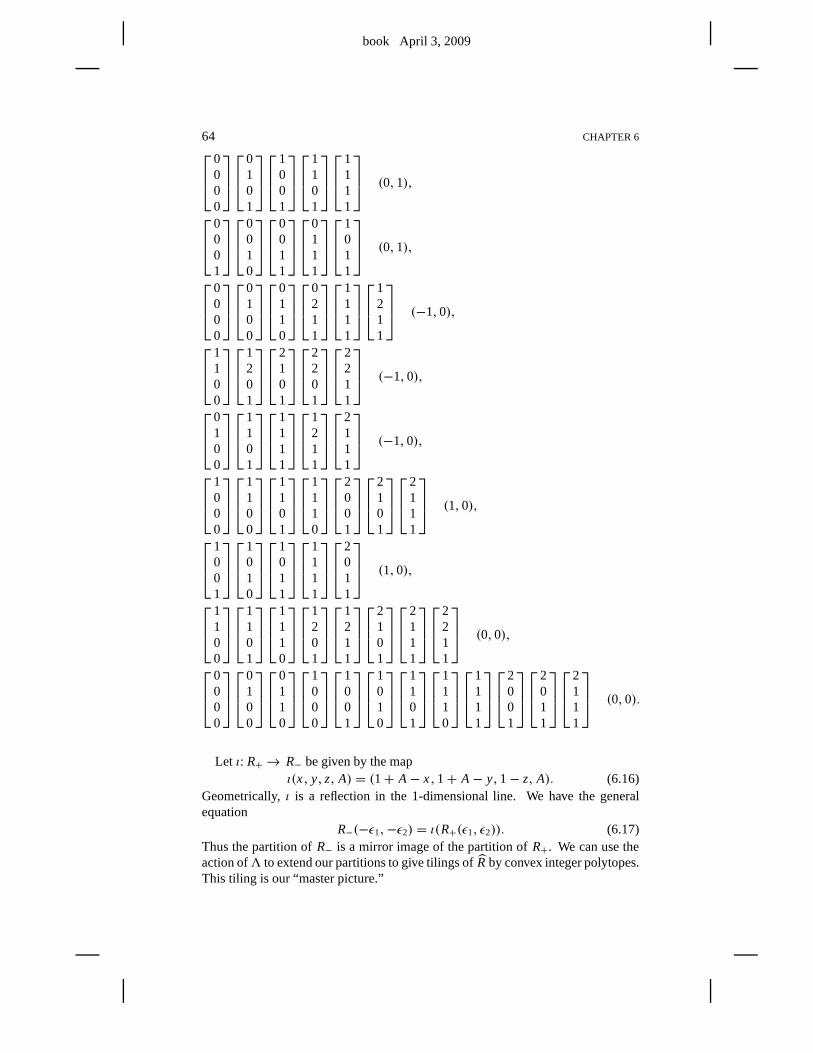
book April 3, 2009

64 CHAPTER 6

0000

0101

1001

1101

1111

(0,1),

0001

0010

0011

0111

1011

(0,1),

0000

0100

0110

0211

1111

1211

(−1,0),

1100

1201

2101

2201

2211

(−1,0),

0100

1101

1111

1211

2111

(−1,0),

1000

1100

1101

1110

2001

2101

2111

(1,0),

1001

1010

1011

1111

2011

(1,0),

1100

1101

1110

1201

1211

2101

2111

2211

(0,0),

0000

0100

0110

1000

1001

1010

1101

1110

1111

2001

2011

2111

(0,0).

Let ι: R+→ R− be given by the mapι(x, y, z, A) = (1+ A− x,1+ A− y,1− z, A). (6.16)

Geometrically,ι is a reflection in the 1-dimensional line. We have the generalequation

R−(−ǫ1,−ǫ2) = ι(R+(ǫ1, ǫ2)). (6.17)Thus the partition ofR− is a mirror image of the partition ofR+. We can use theaction of3 to extend our partitions to give tilings ofR by convex integer polytopes.This tiling is our “master picture.”

book April 3, 2009

THE MASTER PICTURE THEOREM 65

6.8 CALCULATING WITH THE POLYTOPES

We will illustrate a calculation with the polytopes we have listed. Letι andγ2 bethe maps from Equation 6.7. The regionR+(0,0) consists of two polygonsP1 andP2. These are the last two listed above. We will show that

ι(P2)+ (1,1,0,0) = γ2(P2).

As above, the coordinates forP2 are

0000

0100

0110

1000

1001

1010

1101

1110

1111

2001

2011

2111

.

Recall thatι(x, y, z, A) = (1 + A − x,1 + A − y,1 − z, A). For example,ι(0,0,0,0) = (1,1,1,0). The coordinates forι(P2) are

1110

1010

1000

0110

1211

0100

1111

0000

1101

0211

0201

0101

.

The coordinates forι(P2)+ (1,1,0,0) are

2210

2110

2100

1210

2311

1200

2211

1100

2201

1311

1301

1201

.

We haveγ2(x, y, z, A) = (x+ 1− A, y+ 1+ A, z, A). For instance, we computethatγ2(0,0,0,0) = (1,1,0,0). The coordinates forγ (P2) are

1100

1200

1210

2100

1201

2110

1301

2210

1311

2201

2211

2311

.

These are the same vectors as listed forι(P2)+ (1,1,0,0), but in a different order.

Finally, we illustrate how the general form of the integral partition can justify nu-merical calculations. Consider the phase portrait described in Figure 2.5. Considerthe two rectangles

Q+ = {(t, t + 1, t)| t ∈ (0,1)} × [0,1] ,

Q− = {(t − 1, t, t)| t ∈ (0,1)} × [0,1] .

Allow Q± to intersect the polytopeR±. These intersections partitionQ+ andQ−into a small finite number of polygons. The partition ofQ± tells the behavior of9± on points of(0,2) × {1}. By symmetry, the partition ofQ∓ tells the behaviorof 9± on (0,2) × {−1}. The partition ofQ± gives us the information needed tobuild Figure 2.5. Given the simplicity of the partitions involved, we can determinethe figure just by plotting (say) 10,000 fairly dense points in the rectangles. This iswhat we did.

book April 3, 2009

66 CHAPTER 6

6.9 COMPUTING THE PARTITION

Here we explain how Billiard King implements the Master Picture Theorem. Wecannot imagine that a person would want to do this by hand, butit seems worthexplaining what the computer actually does.

6.9.1 Step 1

Suppose(a,b, c) ∈ RA lies in the range ofµ+ or µ−. Now we describe how toattach a 5-tuple(n0, ...,n4) to (a,b, c).

• Determiningn0:

– If we are interested inµ+, thenn0 = 0.

– If we are interested inµ−, thenn0 = 1.

• Determiningn1:

– If c < A andc < 1− A, thenn1 = 0.

– If c > A andc < 1− A, thenn1 = 1.

– If c > A andc > 1− A, thenn1 = 2.

– If c < A andc > 1− A, thenn1 = 3.

• Determiningn2:

– If a ∈ (0, A), thenn2 = 0.

– If a ∈ (A,1), thenn2 = 1.

– If a ∈ (1,1+ A), thenn2 = 2.

• Determiningn3:

– If b ∈ (0, A), thenn3 = 0.

– If b ∈ (A,1), thenn3 = 1.

– If b ∈ (1,1+ A), thenn3 = 2.

• Determiningn4:

– Let t = a+ b− c.

– Let n4 = floor(t − A).

Notice that each 5-tuple(n0, ...,n4) corresponds to a (possibly empty) convex poly-hedron inRA. The polyhedron does not depend onn0. It turns out that this polyhe-dron is empty unlessn4 ∈ {−2,−1,0,1,2}.

book April 3, 2009

THE MASTER PICTURE THEOREM 67

6.9.2 Step 2

Let n = (n0, ...,n4). We now describe two functionsǫ1(n) ∈ {−1,0,1} andǫ2(n) ∈ {−1,0,1}.

Here is the definition ofǫ1(n).

• If n0 + n4 is even, then

– If n2 + n3 = 4 or x2 < x3 setǫ1(n) = −1.

• If n0 + n4 is odd, then

– If n2 + n3 = 0 or x2 > x3, setǫ1(n) = +1.

• Otherwise, setǫ1(n) = 0.

Here is the definition ofǫ2(n).

• If n0 = 0 andn1 ∈ {3,0}, then

– If n2 = 0, letǫ2(n) = 1.

– If n2 = 1, andn4 6= 0 let ǫ2(n) = 1.

• If n0 = 1 andn1 ∈ {0,1}, then

– if n2 > 0 andn4 6= 0, letǫ2(n) = −1.

– If n2 < 2 andn3 = 0 andn4 = 0, letǫ2(n) = 1.

• If n0 = 0 andn1 ∈ {1,2}, then

– If n2 < 2 andn4 6= 0, letǫ2(n) = 1.

– If n2 > 0 andn3 = 2 andn4 = 0, letǫ2(n) = −1.

• If n0 = 1 andn1 ∈ {2,3}, then

– If n2 = 2, letǫ2(n) = −1.

– If n2 = 1 andn4 6= 0, letǫ2(n) = −1.

• Otherwise, letǫ2(n) = 0.

6.9.3 Step 3

Let A ∈ (0,1) be any parameter and letα > 0 be some parameter such thatα 6∈ 2Z [ A]. Given any lattice point(m,n), we perform the following construction.

• Let (a±,b±, c±) = µ±(A,m,n). See §6.6.

• Let n± be the 5-tuple associated to(a±,b±, c±).

• Let ǫ±1 = ǫ1(n±) andǫ±2 = ǫ2(n±).

The Master Picture Theorem says that the two edges ofŴα(m,n) incident to(m,n)are(m,n)+ (ǫ±1 , ǫ

±2 ).

book April 3, 2009

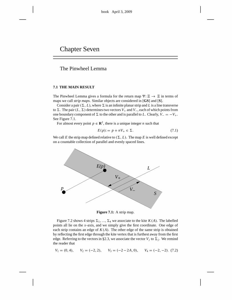
book April 3, 2009

Chapter Seven

The Pinwheel Lemma

7.1 THE MAIN RESULT

The Pinwheel Lemma gives a formula for the return map9:4 → 4 in terms ofmaps we callstrip maps. Similar objects are considered in [GS] and [S].

Consider a pair(6, L), where6 is an infinite planar strip andL is a line transverseto6. The pair(L,6) determines two vectorsV+ andV−, each of which points fromone boundary component of6 to the other and is parallel toL. Clearly,V− = −V+.See Figure 7.1.

For almost every pointp ∈ R2, there is a unique integern such that

E(p):= p+ nV+ ∈ 6. (7.1)

We callE the strip map defined relative to(6, L). The mapE is well defined excepton a countable collection of parallel and evenly spaced lines.

p

L

S

E(p)

V

+V

−

Figure 7.1: A strip map.

Figure 7.2 shows 4 strips61, ..., 64 we associate to the kiteK (A). The labelledpoints all lie on thex-axis, and we simply give the first coordinate. One edge ofeach strip contains an edge ofK (A). The other edge of the same strip is obtainedby reflecting the first edge through the kite vertex that is furthest away from the firstedge. Referring to the vectors in §2.3, we associate the vector Vj to6 j . We remindthe reader that

V1 = (0,4), V2 = (−2,2), V3 = (−2−2A,0), V4 = (−2,−2). (7.2)

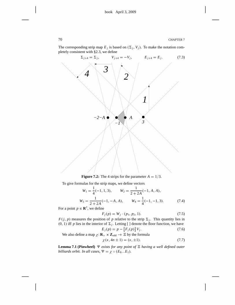
book April 3, 2009

70 CHAPTER 7

The corresponding strip mapE j is based on(6 j ,Vj ). To make the notation com-pletely consistent with §2.3, we define

6 j+4 = 6 j , Vj+4 = −Vj , E j+4 = E j . (7.3)

32

1

−2−A

4

3A

−1

Figure 7.2: The 4 strips for the parameterA = 1/3.

To give formulas for the strip maps, we define vectors

W1 =1

4(−1,1,3), W2 =

1

2+ 2A(−1, A, A),

W3 =1

2+ 2A(−1,−A, A), W4 =

1

4(−1,−1,3). (7.4)

For a pointp ∈ R2, we define

F j (p) = Wj · (p1, p2,1). (7.5)

F( j , p) measures the position ofp relative to the strip6 j . This quantity lies in(0,1) iff p lies in the interior of6 j . Letting [ ] denote the floor function, we have

E j (p) = p−[F j (p)

]Vj . (7.6)

We also define a mapχ : R+ × Zodd→ 4 by the formula

χ(x,4n± 1) = (x,±1). (7.7)

Lemma 7.1 (Pinwheel)9 exists for any point of4 having a well defined outerbilliards orbit. In all cases,9 = χ ◦ (E8...E1).

book April 3, 2009

THE PINWHEEL LEMMA 71

7.2 DISCUSSION

We call the map in the Pinwheel Lemma thepinwheel map. Results like the PinwheelLemma seem to be foundational for polygonal outer billiards. Similar ideas appearin [K ] and [GS], for instance. As we will see in the next section, the PinwheelLemma is quite easy for points far from the kite. We are forcedto consider allpoints in4 because all the unbounded orbits turn out to be erratic; theyinevitablycome close to the kite.

To prove the Pinwheel Lemma in general, we follow the strategy used for theReturn Lemma. We consider all possible sequences of the form

i1→ i2→ i3→ · · · ,whereRi1, Ri2, ... denotes the list of successive regions of the partition encounteredby the forwardψ-orbit of some pointz1 ∈ 4. We let z j be the first point in theforward orbit inRa j . Our proof boils down to a case-by-case analysis of the possiblesequences. In some cases, the proof relies on some lucky cancellations.

Clearly, something nontrivial must happen to make the Pinwheel Lemma true forall points. Notice that the pinwheel map does not involve thevectorsV ♯

4 andV ♭6 ,

and yet these vectors and their corresponding regions are involved in the dynamics.Some kind of lucky cancellation must take place that “edits out” these vectors andregions from the final reckoning. There are two “symmetrically related” luckyaccidents, and they are depicted in Figures 7.4 and 7.5 below. The nature of theseaccidents dictates the order of our proof. First we deal withsequences that do notinvolve 4♯ and 6♭ and then we consider the general case.

As in §2.3, we strongly recommend that the reader use Billiard King to betterfollow the claims we make here. This program allows the reader to draw all theregions in the partition and their translates, superimposing them as desired over thestrips. At the same time, the reader can plot the dynamics of the outer billiards map,checking that all the sets have their advertised properties.

Since the Pinwheel Lemma is a nontrivial result for points near the kite, it seemsworth presenting some numerical evidence for the result. Using Billiard King, wecompute that the Pinwheel Lemma holds true at the points(x,±1) relative to theparameterA for all

A = 1

256, ...,

255

256, x = ǫ + 1

1024, ..., ǫ + 16384

1024, ǫ = 10−6.

The small numberǫ is included to make sure that the outer billiards orbit is actuallydefined for all the points we sample. This calculation fairlywell carpets the “nearregion” with instances of the truth of the result. While thiscalculation does notprove anything formally, it serves as a good sanity check that the Pinwheel Lemmais true.

We close this section with a discussion of how the Pinwheel Lemma fits into theproof of the Master Picture Theorem. The Master Picture Theorem really makesa statement about the pinwheel map. The Pinwheel Lemma then translates thisstatement to a statement about the map9. Thus, if we want to use the MasterPicture Theorem to verify a particular statement solely about the pinwheel map, wedo not need to know about the truth of the Pinwheel Lemma. Thisprinciple willcome in handy at the end, saving us some tedious work.

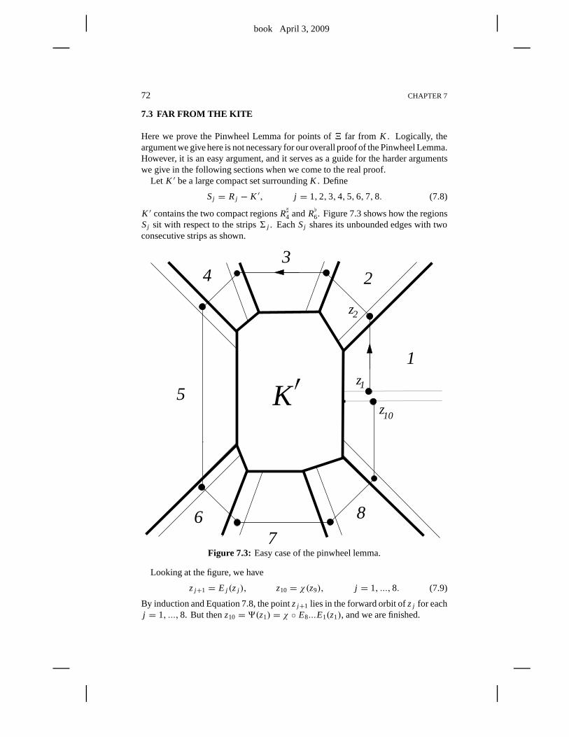
book April 3, 2009

72 CHAPTER 7

7.3 FAR FROM THE KITE

Here we prove the Pinwheel Lemma for points of4 far from K . Logically, theargumentwe give here is not necessary for our overall proof of the Pinwheel Lemma.However, it is an easy argument, and it serves as a guide for the harder argumentswe give in the following sections when we come to the real proof.

Let K ′ be a large compact set surroundingK . Define

Sj = Rj − K ′, j = 1,2,3,4,5,6,7,8. (7.8)

K ′ contains the two compact regionsR♯4 andR♭6. Figure 7.3 shows how the regionsSj sit with respect to the strips6 j . EachSj shares its unbounded edges with twoconsecutive strips as shown.

8

1

6

43

7

5z10

z2

z1

2

K

Figure 7.3: Easy case of the pinwheel lemma.

Looking at the figure, we have

z j+1 = E j (z j ), z10 = χ(z9), j = 1, ...,8. (7.9)

By induction and Equation 7.8, the pointz j+1 lies in the forward orbit ofz j for eachj = 1, ...,8. But thenz10 = 9(z1) = χ ◦ E8...E1(z1), and we are finished.

book April 3, 2009

THE PINWHEEL LEMMA 73

7.4 NO SHARPS OR FLATS

Now we turn to the general proof of the Pinwheel Lemma. In thissection, weprove the Pinwheel Lemma for sequences that contain neither4# or 6♭. Since4 ⊂ R1∪R2∪R♯4, our sequence has the formi1→ · · · → ik, wherei1 ∈ {1,2} andik ∈ {9,10}. By Equation 2.7, the indices increase, and furthermore they increaseby at most 3 each time. We observe, using Billiard King, that

0< k − j < 4, H⇒ Rj ∩ Rk ⊂ 6 j ∩ · · · ∩6k−1. (7.10)

Since no sharps and flats are involved, Equation 7.10 implies

z j+1 = Ei j (z j ). (7.11)

We check thatR2 ∩ 4 ⊂ 61. Hence, ifi1 = 2, we haveE1(z1) = z1. Therefore,whetheri1 = 1 or i1 = 2, Equation 7.11 yields

z2 = Ei1...E1(z1). (7.12)

By Equation 7.10, we have

z2 ∈ Ri1 ∩ Ri2 ⊂ 6i1 ∩ · · · ∩6i2−1, Ei2−1...Ei1+1(z2) = z2. (7.13)

The first equation above implies the second. Combining Equations 7.11–7.13, wehave

z3 = Ei2(z2) = Ei2...Ei1+1(z2) = Ei2...E1(z1). (7.14)

Repeating the same argument, we have

z4 = Ei3...E1(z1). (7.15)

This pattern continues in this way until we arrive atzk ∈ R9 ∪ R10.

Case 1:Supposezk ∈ R9 = R1. Then

zk = E8...E1(z1). (7.16)

The forward iterates ofzk are obtained by repeatedly addingV1. This is the sameas applying the mapχ . Hence

9(z1) = χ(zk) = χ ◦ E8...E1(z1). (7.17)

Hence the Pinwheel Lemma holds in this case.

Case 2:Supposezk ∈ R10 = R2. Then

zk = E9...E1(z1) =∗ E8...E1(z1) ⊂ 4 (7.18)

The starred equality comes from the fact that

E8...E1(z1) ∈ 69 = 61, (7.19)

by Equation 7.10. HenceE9 = E1 acts trivially. The containment in Equation 7.18comes from the same argument we gave in case 2 of the proof of the Return Lemmain §2.3. By Equation 7.18, we haveχ(zk) = zk, and again the Pinwheel Lemmaholds.

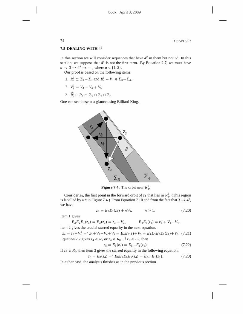
book April 3, 2009

74 CHAPTER 7

7.5 DEALING WITH 4♯

In this section we will consider sequences that have 4# in them but not 6♭. In thissection, we suppose that 4# is not the first term. By Equation 2.7, we must havea→ 3→ 4#→ · · ·, wherea ∈ {1,2}.

Our proof is based on the following items.

1. R♯4 ⊂ 64−63 andR♯4 + V3 ∈ 63−64.

2. V ♯4 = V3 − V4+ V5.

3. R♯4 ∩ R8 ⊂ 65 ∩66 ∩67.

One can see these at a glance using Billiard King.

z

z4

3

Σ

#

−V

3

V3

V5

4

4

ΣFigure 7.4: The orbit nearR♯4.

Considerz3, the first point in the forward orbit ofz1 that lies inR♯4. (This regionis labelled by a # in Figure 7.4.) From Equation 7.10 and from the fact that 3→ 4♯ ,we have

z3 = E2E1(z1)+ nV3, n ≥ 1. (7.20)

Item 1 gives

E3E2E1(z1) = E3(z3) = z3 + V3, E4E3(z3) = z3+ V3−V4.

Item 2 gives the crucial starred equality in the next equation.

z4 = z3+V ♯4 =∗ z3+V3−V4+V5 = E4E3(z)+V5 = E4E3E2E1(z1)+V5. (7.21)

Equation 2.7 givesz4 ∈ R5 or z4 ∈ R8. If z5 ∈ E5, then

z5 = E5(z4) = E5...E1(z1). (7.22)

If z4 ∈ R8, then item 3 gives the starred equality in the following equation.

z5 = E8(z4) =∗ E8E7E6E5(z4) = E8...E1(z1). (7.23)

In either case, the analysis finishes as in the previous section.

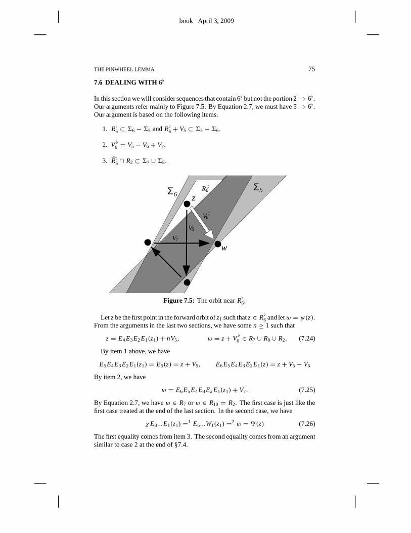
book April 3, 2009

THE PINWHEEL LEMMA 75

7.6 DEALING WITH 6♭

In this section we will consider sequences that contain 6♭ but not the portion 2→ 6♭.Our arguments refer mainly to Figure 7.5. By Equation 2.7, wemust have 5→ 6♭.Our argument is based on the following items.

1. R♭6 ⊂ 66 −65 andR♭6 + V5 ⊂ 65 −66.

2. V ♭6 = V5− V6+ V7.

3. R♭6 ∩ R2 ⊂ 67 ∪68.

6R6

w

5

7

V6

Σ

V5

zΣ

V

Figure 7.5: The orbit nearR♭6.

Letzbe the first point in the forward orbit ofz1 such thatz ∈ R♭6 and letw = ψ(z).From the arguments in the last two sections, we have somen ≥ 1 such that

z= E4E3E2E1(z1)+ nV5, w = z+ V ♭6 ∈ R7 ∪ R8 ∪ R2. (7.24)

By item 1 above, we have

E5E4E3E2E1(z1) = E5(z) = z+ V5, E6E5E4E3E2E1(z) = z+ V5− V6

By item 2, we have

w = E6E5E4E3E2E1(z1)+ V7. (7.25)

By Equation 2.7, we havew ∈ R7 orw ∈ R10 = R2. The first case is just like thefirst case treated at the end of the last section. In the secondcase, we have

χE8...E1(z1) =1 E6...W1(z1) =2 w = 9(z) (7.26)

The first equality comes from item 3. The second equality comes from an argumentsimilar to case 2 at the end of §7.4.

book April 3, 2009

76 CHAPTER 7

7.7 THE LAST CASES

Now we treat the two cases we have not yet treated.First, suppose the sequence has the portion 2→ 6♭. Letw be the orbit point in

R♭6. We have

w ∈ R2 ∩ R♭6 ⊂ (−2A,0)× {1}. (7.27)

This forces the entire orbit sequence to be 2→ 6♭ → 2, and

z1 ∈ (2− 2A,2)× {−1}, 9(z1) = z1 − (2− 2A,0). (7.28)

Second, suppose the sequence starts with 4♯ . A similar calculation shows that

z1 ∈ (0,2A)× {1}, 9(z1) = z1 + (2− 2A,0). (7.29)

To finish the proof, we just have to compute the pinwheel map onthe aboveintervals and see that it matches9. One can achieve this with the same kind ofanalysis used in the previous sections. However, we prefer adifferent method. Wecan use the formula from the Master Picture Theorem to see that the pinwheel mapdoes the right thing on the above intervals. This is not a circular argument, as wediscussed at the end of §7.2.

book April 3, 2009

Chapter Eight

The Torus Lemma

8.1 THE MAIN RESULT

For ease of exposition, we state and prove the(+) halves of our results. The(−)halves have the same formulation and proof.

Let µ+ be as in Equation 6.5. We write(µ+)A to emphasize the dependence onthe parameterA. Let T4 = R/3, the 4-dimensional quotient discussed in §6.7.Topologically,T4 is the product of a 3-torus with(0,1). We now define

µ+:4+ × (0,1)→ T4

by the obvious formula

µ+(p, A) = ((µ+)A(p), A). (8.1)

We are just stacking all these maps together.Referring to the Pinwheel Lemma, we have9(p) = χ ◦ E8...E1(p) whenever

both maps are defined. Letp ∈ 4+. We setp0 = p and inductively define

p j = E j (p j−1) ∈ 6 j . (8.2)

We also define

θ(p) = minθ j (p), θ j (p) = distance(p j , ∂6 j ). (8.3)

The quantityθ(p) depends on the parameterA, so we will writeθ(p, A) when wewant to be clear about this.

Lemma 8.1 (Torus) Let (p, A), (q∗, A∗) ∈ 4+ × (0,1). There is someη > 0,depending only onθ(p, A) andmin(A,1− A), with the following property. Sup-pose that the pinwheel map is defined at(p, A). Suppose also thatµ+(p, A) andµ+(q∗, A∗) are withinη of each other. Then the pinwheel map is defined at(q∗, A∗)and(ǫ1(q∗), ǫ2(q∗)) = (ǫ1(p), ǫ2(p)).

Remarks:(i) In the proof of the Pinwheel Lemma, we started our labelling with z1, thenconsideredz2 = E1(z1), etc. Here we find it convenient to takep j = z j+1.(ii) I discovered the Torus Lemma experimentally, but my formal proof owes aconsiderable intellectual debt to the ideas presented in [K ] and [GS] concerningouter billiards on quasirational polygons. (Compare the remark in the next section.)My proof also owes an intellectual debt to the paper [T2], in which S. Tabachnikovdescribes unpublished work of C. Culter on the existence of periodic orbits forpolygonal outer billiards. If all these written sources were not enough, I was alsoinfluenced by conversations with John Smillie.

book April 3, 2009

78 CHAPTER 8

8.2 INPUT FROM THE TORUS MAP

We first prove the Torus Lemma assuming thatA = A∗. Letq = q∗. In this section,we explain the significance of the mapµ+. We introduce the quantities

λ j = λ0 × · · · × λ j , λ j =area(6 j−1 ∩6 j )

area(6 j ∩6 j+1), j = 1, ...,7. (8.4)

Remark: For a general convexn-gon, one can make the strip construction alongthe lines of what we have done. The polygon is said to bequasirationalif all thenumbersλ j are rational. As mentioned in the introduction, the result in [VS], [K ],and [GS] is that all outer billiards orbits are bounded relative to quasirational poly-gons. In hindsight, it is no surprise that these quantities arise in our proof of theMaster Picture Theorem.

Let p = (x,±1) andq = (y,±1). We have

µ+(q)− µ+(p) = (t, t, t) mod 3, t = y− x

2. (8.5)

Lemma 8.2 For any ǫ > 0, there is aδ > 0 with the following property. Ifdist(µ+(x), µ+(y)) < δ in T3, then for each k, the quantity tλk is within ǫ of someinteger Ik.

Proof: We compute

area(60 ∩61) = 8, area(61 ∩62) =8+ 8A

1− A,

area(62 ∩63) =2(1+ A)2

A, area(63 ∩64) =

8+ 8A

1− A. (8.6)

This leads to

λ0 = λ4 = 1, λ1 = λ3 = λ5 = λ7 =1− A

1+ A, λ2 = λ6 =

4A

(1+ A)2. (8.7)

The matrix

H =

11+A

A−1(1+A)2

2A(1+A)2

0 11+A

11+A

0 0 1

(8.8)

conjugates the columns of the matrix defining3 to the standard basis. Therefore,if µ+(x) andµ+(y) are close inT3 then H (t, t, t) is close to a point ofZ3. Wecompute

H (t, t, t) =(

4A

(1+ A)2,

2

1+ A,1

)t = (λ2, λ1 + 1,1)t . (8.9)

Equations 8.7 and 8.9 now finish the proof. 2

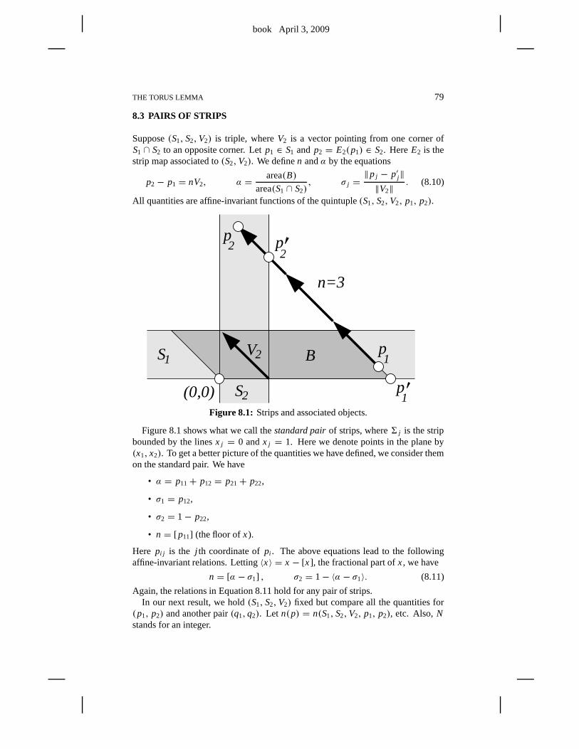
book April 3, 2009

THE TORUS LEMMA 79

8.3 PAIRS OF STRIPS

Suppose(S1, S2,V2) is triple, whereV2 is a vector pointing from one corner ofS1 ∩ S2 to an opposite corner. Letp1 ∈ S1 and p2 = E2(p1) ∈ S2. HereE2 is thestrip map associated to(S2,V2). We definen andα by the equations

p2 − p1 = nV2, α =area(B)

area(S1 ∩ S2), σ j =

‖p j − p′j‖‖V2‖

. (8.10)

All quantities are affine-invariant functions of the quintuple(S1, S2,V2, p1, p2).

n=3

1

p2

p1

p

BS

(0,0)

1

S2

2V

p2

Figure 8.1: Strips and associated objects.

Figure 8.1 shows what we call thestandard pairof strips, where6 j is the stripbounded by the linesx j = 0 andx j = 1. Here we denote points in the plane by(x1, x2). To get a better picture of the quantities we have defined, we consider themon the standard pair. We have

• α = p11+ p12= p21+ p22,

• σ1 = p12,

• σ2 = 1− p22,

• n = [ p11] (the floor ofx).

Here pi j is the j th coordinate ofpi . The above equations lead to the followingaffine-invariant relations. Letting〈x〉 = x − [x], the fractional part ofx, we have

n = [α − σ1] , σ2 = 1− 〈α − σ1〉. (8.11)

Again, the relations in Equation 8.11 hold for any pair of strips.In our next result, we hold(S1, S2,V2) fixed but compare all the quantities for

(p1, p2) and another pair(q1,q2). Let n(p) = n(S1, S2,V2, p1, p2), etc. Also,Nstands for an integer.

book April 3, 2009

80 CHAPTER 8

Lemma 8.3 (Strip) Letǫ > 0. There is someδ > 0 with the following property. If

|σ(p1)− σ(q1)| < δ, |α(q)− α(p)− N| < δ,

then

|σ(p2)− σ(q2)| < ǫ, N = n(q)− n(p).

The numberδ depends on onlyǫ and the distance fromσ(p1) andσ(p2) to {0,1}.

Proof: If δ is small enough, then〈α(p) − σ(p1)〉 and 〈α(q) − σ(q1)〉 are veryclose and relatively far from 0 or 1. Equation 8.11 now says thatσ(p2) andσ(q2)are close. Also, the following two quantities are both nearN, while the individualsummands are all relatively far from integers.

α(q)− α(p),(α(q)− σ(q1)

)−(α(p)− σ(p1)

).

But the second quantity is near the integern(q)− n(p), by Equation 8.11. 2

Suppose now thatS1, S2, S3 is a triple of strips andV2,V3 is a pair of vectors,such that(S1, S2,V2) and(S2, S3,V3) are as above. Letp j ∈ Sj , for j = 1,2,3, besuch thatp2 = E2(p1) and p3 = E3(p2). For j = 1,2, define

α j = α(Sj , Sj+1,Vj+1, p j , p j+1), λ = area(S1 ∩ S2)

area(S2 ∩ S3). (8.12)

It is convenient to setσ2 = σ(p2).

Lemma 8.4 There are constants C and D such thatα2 = λα1 + Cσ2 + D. Theconstants C and D depend on the strips.

Proof: We normalize so that we have the standard pair. Then

p2 = (1− σ2, α1 + σ2 − 1). (8.13)

There is a unique orientation-preserving affine mapT such thatT(Sj+1) = Sj forj = 1,2, andT carries the linex2 = 1 to the linex1 = 0. Given thatS1 ∩ S2 hasunit area, we have det(T) = λ. Given the description ofT , we have

T(x1, x2) =(

a λ−1 0

)(x1, x2)+ (b,1) = (ax1+ b+ λx2,1− x1). (8.14)

Herea andb are constants depending onS2 ∩ S3. Settingq = T(p2), the relationsabove giveα = q1+ q2. Hence

α2 = a(1− σ2)+ b+ λ(α1 + σ2 − 1)+ σ2 = λα1 + Cσ2 + D. (8.15)

This completes the proof. 2

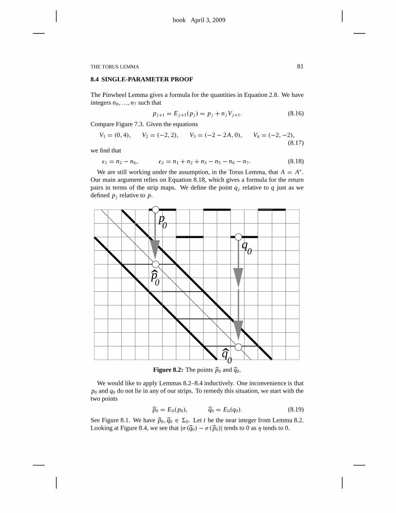
book April 3, 2009

THE TORUS LEMMA 81

8.4 SINGLE-PARAMETER PROOF

The Pinwheel Lemma gives a formula for the quantities in Equation 2.8. We haveintegersn0, ...,n7 such that

p j+1 = E j+1(p j ) = p j + n j Vj+1. (8.16)

Compare Figure 7.3. Given the equations

V1 = (0,4), V2 = (−2,2), V3 = (−2− 2A,0), V4 = (−2,−2),(8.17)

we find that

ǫ1 = n2 − n6, ǫ2 = n1 + n2 + n3 − n5 − n6 − n7. (8.18)

We are still working under the assumption, in the Torus Lemma, that A = A∗.Our main argument relies on Equation 8.18, which gives a formula for the returnpairs in terms of the strip maps. We define the pointq j relative toq just as wedefinedp j relative top.

p0

q0

p0

q0

Figure 8.2: The pointsp0 andq0.

We would like to apply Lemmas 8.2–8.4 inductively. One inconvenience is thatp0 andq0 do not lie in any of our strips. To remedy this situation, we start with thetwo points

p0 = E0(p0), q0 = E0(q0). (8.19)

See Figure 8.1. We havep0, q0 ∈ 60. Let t be the near integer from Lemma 8.2.Looking at Figure 8.4, we see that|σ (q0)− σ( p0)| tends to 0 asη tends to 0.

book April 3, 2009

82 CHAPTER 8

We define

αk(p) = α(6k,6k+1,Vk+1, pk, pk+1) (8.20)

It is also convenient to write

σk(p) = σ(pk), 1σk = σk(q)− σk(p). (8.21)

Fork = 0, we usep0 in place ofp0, andq0 in place ofq0, for these formulas.

Remarks:(i) The functionsσk play a big role in our overall proof. The next chapter is devotedentirely to obtaining, in a certain sense, closed-form expressions for the functionsσk. For later reference, we call these functionsstrip functions.(ii) Our next lemma is stated in a slightly peculiar way because the last-mentionedquantitynk(p)−nk(q) is an integer. But that is the whole point of the lemma: Oncean integer quantity is sufficiently close to 0, it must actually be 0.

Lemma 8.5 Asη→ 0, the pairwise differences between the3 quantities

αk(q)− αk(p), nk(q)− nk(p), t λk

converge to0 for all k.

Proof: Referring to Figure 8.2, we have

area(60 ∩61) = 8, area(B( p0))− area(B(q0)) = 4y− 4x.

This givesα0(q)− α0(p) = t . Applying Lemma 8.4 inductively, we find that

αk = α0λk +k∑

i=1

ξiσi + Ck (8.22)

for constantsξ1, ..., ξk andCk that depend analytically onA. Therefore

αk(q)− αk(p) = t λk +k∑

i=1

ξi1σi , k = 1, ...,7. (8.23)

By Lemma 8.2, the termtλk is near an integer for allk. By Lemma 8.3 and induc-tion, the remaining terms on the right hand side are near 0. This lemma now followsfrom Lemma 8.3. 2

Combining our last result with Equation 8.7, we see that

n1(q)− n1(p) = n3(q)− n3(p) = n5(q)− n5(p) = n7(q)− n7(p),

n2(q)− n2(p) = n6(q)− n6(p), (8.24)

onceη is small enough. Given the dependence of constants in Lemma 8.3, thenecessary bound onη depends on only min(A,1− A) andθ(p). Equation 8.18 nowtells us thatǫ j (p) = ǫ j (q), for j = 1,2, onceη is small enough.

book April 3, 2009

THE TORUS LEMMA 83

8.5 PROOF IN THE GENERAL CASE

Now we turn to the proof of the Torus Lemma in the general case.Our first resultis the key step that allows us to handle pairs of distinct parameters. Once we set upthe notation, the proof is almost trivial. Our second resultis a variant that will beuseful in the next chapter.

Suppose that(S1, S2,V2, p1, p2) and(S∗1, S∗2,V∗2 ,q

∗1,q

∗2) are two quintuples. To

fix the picture in our minds, we imagine that(S1, S2,V2) is near(S∗1, S∗2,V∗2 ), though

this is not necessary for the proof of the result to follow. Wecan define the quantitiesα, ρ j ,n for each of these quintuples. We place a∗ by each quantity associated tothe second triple.

Lemma 8.6 Let ǫ > 0. There is someδ > 0 with the following property. If|σ(p1)− σ(q∗1)| < δ and |α(q∗)− α(p)− N| < δ, then|σ(p2)− σ(q∗2)| < ǫ andN = n(q∗)− n(p). The numberδ depends on onlyǫ and the distance fromσ(p1)andσ(p2) to {0,1}.

Proof: There is an affine transformation such thatT(X∗) = X for each objectX = S1, S2,V2. We setq j = T(q∗j ). Thenα(q∗1) = α(q1), by affine invariance.Likewise for the other quantities. Now we apply Lemma 8.3 to the triple(S1, S2,V2)and the pairs(p1, p2) and(q1,q2). The conclusion involves quantities with no∗,but returning the∗ does not change any of the quantities. 2

For use in the next chapter, we state a variant of Lemma 8.6. For this result, weinterpret〈x〉 as the image of a real numberx in R/Z.

Lemma 8.7 Let ǫ > 0. There is someδ > 0 with the following property. If|σ(p1)− σ(q∗1)| < δ and|α(q∗)− α(p)− N| < δ, then the distance from〈σ(p2)〉to 〈σ(q∗2)〉 in R/Z is less thanǫ and N = n(q∗) − n(p). The numberδ dependsonly onǫ and the distance fromσ(p1) andσ(p2) to {0,1}.

Proof: Using the same trick as in Lemma 8.3, we reduce to the single-variablecase. In this case, we mainly repeat the proof of Lemma 8.3. Ifδ is small enough,then〈α(p)− σ(p1)〉 and〈α(q)− σ(q1)〉 are very close and relatively far from〈0〉.Equation 8.11 now says that〈σ(p2)〉 and〈σ(q2)〉 are close inR/Z. 2

In proving the general version of the Torus Lemma, we no longer suppose thatA = A∗ and we return to the original notation(q∗, A∗) for the second point. In ourproof of this result, we attach a∗ to any quantity that depends on(q∗, A∗). We firstneed to repeat the analysis from §8.2, this time keeping track of the parameter. Letη be as in the Torus Lemma. We use the “big O” notation.

Lemma 8.8 There is an integer Ik such that|α∗0λ∗k − α0λk − Ik| < O(η).

Proof: Let H be the matrix in Equation 8.8. Let〈V〉 denote the distance fromV ∈ R3 to the nearest point inZ3. Let p = (x,±1) andq∗ = (x∗,±1). Recalling

book April 3, 2009

84 CHAPTER 8

the definition ofµ+, the hypotheses in the Torus Lemma imply that the fractionalpart of

H ∗(

x∗

2,

x∗

2+ 1,

x∗

2

)− H

(x

2,

x

2+ 1,

x

2

)(8.25)

has sizeO(η). We compute thatα0 = x/2+1/2 independent of parameter. There-fore

H(x

2,

x

2+ 1,

x

2

)= H (α0, α0, α0)+

1

2H (−1,1,−1).

The same is true for the starred quantities. Therefore

〈〈(λ∗2, λ∗1 − 1,1)α∗0 − (λ2, λ1 − 1,1)α0〉

= 〈H ∗(α∗0, α∗0, α∗0)− H (α0, α0, α0)〉 < O(η)+‖(H ∗− H )(−1,1,−1)‖ < O(η).

The lemma now follows immediately from Equation 8.7. 2

The integerIk of course depends on(p, A) and(q∗, A∗), but in all cases Equation8.7 gives us

I0 = I4, I1 = I3 = I5 = I7, I2 = I6, (8.26)

Lemma 8.9 Asη → 0, the pairwise differences between the3 quantitiesα∗k − αk

and n∗k − nk and Ik tend to0 for all k.

Proof: Hereα∗k stands forαk(q∗), etc. Equation 8.22 works separately for eachparameter. The replacement for Equation 8.23 is

α∗k − αk = W + X + Y, W = α∗0λ∗k − α0λk (8.27)

X =k∑

i=1

ξ∗i σ∗i (q∗)−

k∑

i=1

ξiσi (p) =k∑

i=1

ξi(σ ∗i − σi

)+ O(|A− A∗|), (8.28)

Y =k∑

i=1

C∗i −k∑

i=1

Ci = O(|A− A∗|). (8.29)

The estimates onX andY come from the fact thatξi andCi vary smoothly withA.Putting everything together, we have the following.

α∗k − αk =(α∗0λ

∗k − α0λk

)+

k∑

i=1

ξi(σ ∗i − σi

)+ O(|A− A∗|). (8.30)

In light of Lemma 8.8, it suffices to show thatσ ∗i −σi tends to 0 asη tends to 0. Thesame argument as in the single-parameter case works here, with Lemma 8.6 used inplace of Lemma 8.3. 2

As in the single-parameter case, Equations 8.18 and 8.26 nowfinish the proof.

book April 3, 2009

Chapter Nine

The Strip Functions

9.1 THE MAIN RESULT

The purpose of this chapter is to understand the functionsσ j that arose in the proofof the Torus Lemma. See Equation 8.21. We continue using the notation fromthe previous chapter. We call these functionsstrip functions. Let 〈x〉 denote thefractional part ofx. Sometimes we interpret〈x〉 as an element ofR/Z.

Let Wk ⊂ 4+ × (0,1) denote the set of points whereEk...E1 is defined butEk+1Ek...E1 is not defined. LetSk denote the closure ofµ+(Wk) in R. HereR isas in Equation 6.6. Finally, let

W′k =k−1⋃

j=0

Wj , S′k =k−1⋃

j=0

Sj , k = 1, ...,7. (9.1)

The Torus Lemma applies to any point that does not lie in thesingular set

S= S0 ∪ · · · ∪ S7. (9.2)

If p ∈ 4+ − W′k, then the pointsp = p0, ..., pk are defined. Here, as in theprevious chapter,p j = E j (p j−1). The functionsσ1, ..., σk andα1, ..., αk are definedfor such a choice ofp. Again,σ j measures the position ofp j in6 j relative to∂6 j .Even if Ek+1 is not defined onpk, the equivalence class orpk+1 is well defined inthe cylinderR2/〈Vk+1〉. The corresponding functionσk+1(q) = σ(qk+1) is welldefined as an element ofR/Z.

Let π j : R4→ R be the j th coordinate projection. The following identities referto the(+) case. We discuss the(−) case at the end of the chapter.

σ1 =⟨2− π3

2

⟩◦ µ+ on 4+. (9.3)

σ2 =⟨1+ A− π2

1+ A

⟩◦ µ+ on 4+ −W′1. (9.4)

σ3 =⟨1+ A− π1

1+ A

⟩◦ µ+ on 4+ −W′2. (9.5)

σ4 =⟨1+ A− π1 − π2 + π3

2

⟩◦ µ+ on 4+ −W′3. (9.6)

In the next chapter we deduce the Master Picture Theorem fromthese identitiesand the Torus Lemma. In this chapter, we establish the identities. Equation 9.3 istrue by inspection. The other 3 identities are the nontrivial ones.

book April 3, 2009

86 CHAPTER 9

9.2 CONTINUOUS EXTENSION

Since the mapµ+(4+ × (0,1)) is dense inR− S′k, we define

σ j (τ ):= limn→∞

σ j (pn, An), τ ∈ R− S′k. (9.7)

Here(pn, An) is chosen so that all functions are defined andµ+(pn, An)→ τ . Notethat the sequence{pn} need not converge. So far, we do not know that the limit wetake is well defined. However, the next result clears this up.

Lemma 9.1 The functionsσ1, ..., σk+1, consideredR/Z-valued functions, are welldefined and continuous on R− S′k.

Proof: For the sake of concreteness, we will give the proof in the case whenk = 2.This representative case explains the idea. First of all, the continuity follows fromthe well-definedness. We just have to show that the limit above is always welldefined. We need to considerσ1, σ2, andσ3. Our argument is essentially inductive.

Here is the base case.σ1 is well defined and continuous on all ofR, by Equation9.3.

SinceS′1 ⊂ S′2, we see thatτ ∈ R− S′1. Henceτ does not lie in the closure ofµ+(W0). Hence there is someθ1 > 0 such thatθ1(pn, An) > θ1 for all sufficientlylargen. Note also that there is a positive and uniform lower bound tothe quantitymin(An,1− An). Note that

〈α1(pn, An)〉 = 〈π3(µ+(pn, An)〉.Hence

{〈α1(pn, An)〉} (9.8)

forms a Cauchy sequence inR/Z.Lemma 8.7 now applies uniformly to

(p, A) = (pm, Am), (q∗, A∗) = (pn, An)

for all sufficiently large pairs(m,n). Since{µ+(pn, An)} forms a Cauchy sequencein R, Lemma 8.7 implies that{σ2(τm, Am)} forms a Cauchy sequence inR/Z. Henceσ2 is well defined onR− S′1 and continuous.

Sinceτ ∈ R− S′2, we see thatτ does not lie in the closure ofµ+(W1). Hencethere is someθ2 > 0 such thatθ j (pn, An) > θ j for j = 1,2 and sufficiently largen. As in the proof of the General Torus Lemma, Equation 8.30 nowshows that

{〈α2(pn, An)〉} (9.9)

forms a Cauchy sequence inR/Z. We now repeat the previous argument to see that{σ3(τm, Am)} forms a Cauchy sequence inR/Z. Henceσ3 is well defined onR−S′2and continuous. 2

Referring to Equations 9.8 and 9.9, we define

βk = 〈αk〉 ∈ R/Z. (9.10)

This function will come in handy in our next result.

book April 3, 2009

THE STRIP FUNCTIONS 87

9.3 LOCAL AFFINE STRUCTURE

Let X = R−∂R⊂ R4. Note thatX is an open and convex polytope,combinatoriallyequivalent to the 4-dimensional cube.

Lemma 9.2 Suppose X⊂ R− S′k. Thenσk+1 is locally affine on XA.

Proof: Sinceσk+1 is continuous onX, it suffices to prove this lemma for a denseset of kite parametersA. We can chooseA so thatµ+(4+) is dense inXA.

We already know thatσ1, ..., σk+1 are all defined and continuous onX. We havealready remarked that Equation 9.3 is true by direct inspection. As we have alreadyremarked in the previous proof,

β0 = π3 ◦ µ+.

Thus we define

β0 = 〈π3〉. (9.11)

Both σ0 andβ0 are locally affine onXA.Let m ≤ k. The second half of Equation 8.11 tells us thatσm is a locally affine

function of σm−1 and βm−1. Below we will prove thatβm is defined onXA andlocally affine, provided thatσ1, ..., σm are defined and locally affine onXA. Thelemma follows from this claim and induction.

Now we prove the claim. All the addition below is done inR/Z. Sinceµ+(4+)is dense inXA, we can at least defineβm on a dense subset ofXA. Define

p = (x,±1), p′ = (x′,±1), τ = µ+(p), τ ′ = µ+(p′), t = x′ − x

2.

(9.12)We choosep and p′ so that the pinwheel map is entirely defined.

From Equation 8.23, we have

βm(τ′)− βm(τ ) = 〈t λk〉 +

m∑

j=1

〈ξ j × (σ j (τ′)− σ j (τ ))〉. (9.13)

Hereξ1, ..., ξm are constants that depend onA. Let H be the matrix in Equation8.8. We haveH (t, t, t) ≡ H (τ ′ − τ ) modZ3 because(t, t, t) ≡ τ ′ − τ mod3.Our analysis in §8.2 shows that

〈t λk〉 = 〈π ◦ H (t, t, t)− ǫt〉 = 〈(π − ǫπ3) ◦ H (τ ′ − τ )〉. (9.14)

Hereǫ ∈ {0,1} andπ is some coordinate projection. The choice ofǫ andπ dependsonk. We now see that

βm(τ′) = βm(τ )+〈(π + ǫ3π) ◦ H (τ ′− τ )〉 +

m∑

j=1

〈ξ j × (σ j (τ′)− σ j (τ ))〉. (9.15)

The right hand side is everywhere defined and locally affine. Hence we defineβm

on all of XA using the right hand side of the last equation. 2

book April 3, 2009

88 CHAPTER 9

Now we come to a subtle point. We have shown that our functionsare locallyaffine when restricted to eachA-slice. We would like to remove this caveat and saysimply that our functions are locally affine even whenA is allowed to vary. The nextresult makes a weaker statement along these lines. Once we have this result, we willuse a bootstrap argument to improveanalyticto affine. Note that the setX, definedabove, is an open convex polytope. Thus it makes sense to say that a function isanalytic onX. Logically, we could give our overall proof without Lemma 9.3 below.However, Lemma 9.3 is a labor-saving device. The analyticity in Lemma 9.3 allowsus to check the identities above on just a fairly small subsetof X.

Lemma 9.3 Suppose X⊂ R− S′k. Thenσk+1 is analytic on X.

Proof: The constantsξ j in Equation 9.13 vary analytically withA. Our argumentin Lemma 9.2 therefore shows thatσk+1 is an affine function onXA whose linearpart varies analytically withA. We just have to check the additive term. SinceXA

is connected, we can compute the additive term ofσk+1 at A from a single point.We choosep = (ǫ,1), whereǫ is very close to 0. The fact thatA→ σk+1(p, A)varies analytically follows from the fact that the strips vary analytically. 2

Equations 9.4, 9.5, and 9.6 are formulas forσ2, σ3, andσ4, respectively. Let

fk+1 = σk+1 − σ ′k+1, k = 2,3,4. (9.16)

Hereσ ′k+1 is the right hand side of the identity forσk+1. Our goal is to show thatfk+1 ≡ 〈0〉 for k = 1,2,3. Call a parameterA goodif fk+1 ≡ 〈0〉 on XA. Call asubsetS⊂ (0,1) substantialif S is dense in some open interval of(0,1).

Lemma 9.4 fk+1 ≡ 0 provided that a substantial set of parameters is good.

Proof: By hypothesis and by continuity,fk+1 vanishes on some open subset ofX.But the 0-function is the only analytic function that can vanish on an open subset ofX. 2

In the next section we explain how to verify that a parameter is good. If fk+1 werea locally affine map fromXA into R, we would just need to check thatfk+1 = 0on some tetrahedron onXA to verify thatA is a good parameter. Since the range offk+1 is R/Z, we have to work a bit harder.

Before we launch into the method, we make one more remark about the detailsof the verification process. We want to be sure that, at each stage, we can actuallyapply Lemma 9.3. Here we explain why we can do this. Observe that, in general,we have

Sk ⊂ σ−1k+1(〈0〉).

Given Equation 9.3, we see thatX ⊂ R− S′1. Henceσ2 is defined onX. Henceσ2 is analytic onX and locally affine on eachXA. We use these two properties toshow that Equation 9.4 is true. But thenX ⊂ R− S′2, etc. So, we will know at eachstage of our verification that Lemmas 9.2 and 9.3 apply to the function of interest.

book April 3, 2009

THE STRIP FUNCTIONS 89

9.4 IRRATIONAL QUINTUPLES

We will give a construction inR3. When the time comes to use the construction,we will identify XA as an open subset of a copy ofR3.

Let ζ1, ..., ζ5 ∈ R3 be 5 distinct points. By taking these points 4 at a time, we cancompute 5 volumesv1, ..., v5. Herev j is the volume of the tetrahedron obtained byomitting the j th point. We say that(ζ1, ..., ζ5) is anirrational quintupleif there isno rational relation

5∑

i=1

c j ζ j = 0, c j ∈ Q, c1c2c3c4c5 = 0. (9.17)

If we allow all the constants to be nonzero, then there is always a relation.

Lemma 9.5 Let C be an open convex subset ofR3. Let f: C→ R/Z be a locallyaffine function. Suppose that there is an irrational(ζ1, ..., ζ5) such thatζ j ∈ C andf (ζ j ) is the same for all j . Then f is constant on C.

Proof: SinceC is simply connected, we can liftf to a locally affine functionF : C → R. But thenF is affine onC, and we can extendF to be an affine mapfrom R3 to R. By construction,F(ζi )− F(ζ j ) ∈ Z for all i , j . Adding a constantto F , we can assume thatF is linear. There are several cases.

Case 1: If F(ζ j ) is independent ofj , then all the points lie in the same plane.Hence all the volumes are zero. This violates the irrationality condition.

Case 2: Suppose we are not dealing with case 1 and the following is true. Forevery indexj there is a second indexk such thatF(ζk) = F(ζ j ). Since there are5 points total, this means that the set{F(ζ j )} has a total of only 2 values. But thismeans that our 5 points lie in a pair of parallel planes51 ∪52, with 2 points in51

and 3 points in52. Let us say that thatζ1, ζ2, ζ3 ∈ 51 andζ4, ζ5 ∈ 52. But thenv4 = v5, and we violate the irrationality condition.

Case 3: If we are not dealing with the above two cases, then we can relabel sothat F(ζ1) 6= F(ζ j ) for j = 2,3,4,5. Let

ζ ′j = ζ j − ζ1.

Thenζ ′1 = (0,0,0) andF(ζ ′1) = 0. But thenF(ζ ′j ) ∈ Z − {0} for j = 2,3,4,5.Note thatv ′j = v j for all j . For j = 2,3,4,5, let

ζ ′′j =ζ ′j

F(ζ ′j ).

Thenv ′′j /v′j ∈ Q for j = 2,3,4,5. Note thatF(ζ ′′j ) = 1 for j = 2,3,4,5. Hence

there is a plane5 such thatζ ′′j ∈ 5 for j = 2,3,4,5.There is always a rational relation among the areas of the 4 triangles defined by 4

points in the plane. Hence there is a rational relation amongv ′′2, v′′3, v′′4, v′′5 . But then

there is a rational relation betweenv2, v3, v4, v5. This contradicts the irrationalitycondition. 2

book April 3, 2009

90 CHAPTER 9

9.5 VERIFICATION

We consider the(+) case first and discuss the(−) case at the end. Proceedingsomewhat at random, we define

φ j =(

8 j A+ 1/(2 j ),1

), j = 1,2,3,4,5. (9.18)

We check thatφ j ∈ 4+ for A near 1/2. Letting

ζ j = µ+(φ j ), (9.19)

we check that

fk+1(ζ j ) = 〈0〉, j = 1,2,3,4,5. (9.20)

In the next section, we give an example calculation.

Lemma 9.6 (ζ1, ..., ζ5) form an irrational quintuple for a dense set of parametersA. In fact this is true for the complement of a countable set ofparameters.

Proof: The 5 volumes associated to our quintuple are as follows.

• v5 = 5/24− 5A/12+ 5A2/24.

• v4 = 71/40+ 19A/20− 787A2/120− 4A3.

• v3 = 119/60+ 7A/60− 89A2/15− 4A3.

• v2 = −451/240− 13A/40+ 1349A2/240+ 4A3.

• v1 = −167/80− 13A/40+ 533A2/80+ 4A3.

If there is an open set of parameters for which the first 4 of these volumes has arational relation, then there is an infinite set for which thesame rational relationholds. Since every formula in sight is algebraic, this meansthat there must be asingle rational relation that holds for all parameters. Butthen the parametrized curveA→ (v5, v4, v3, v2) lies in a proper linear subspace ofR4. We evaluate this curveat A = 1,2,3,4 and see that the resulting points are linearly independentin R4.Hence there is no global rational relation. Hence, for a dense set of parameters,there is no rational relation among the first 4 volumes listed. A similar argumentrules out rational relations among any other 4-tuple of these volumes. 2

The (−) Case: Equations 9.4 and 9.5 do not change, except thatµ− replacesµ+and all the sets are defined relative to4− andµ−. Equations 9.3 and 9.6 become

σ1 =⟨1− π3

2

⟩◦ µ− on 4−. (9.21)

σ4 =⟨

A− π1− π2 + π3

2

⟩◦ µ− on 4− − S′3. (9.22)

Lemmas 9.2 and 9.3 have the same proof in the(−) case. We use the same methodas above, except that we use the points

φ j + (2,0); j = 1,2,3,4,5. (9.23)

These points all lie in4− for A near 1/2.

book April 3, 2009

THE STRIP FUNCTIONS 91

9.6 AN EXAMPLE CALCULATION

Here we work out by hand one of the cases of Equation 9.20. We dothe rest of thecases in Mathematica [W]. Consider the casek = 1 and j = 1.

When A = 1/2, the length spectrum forφ1 starts out as(1,1,2,1). Hence thisremains true for nearbyA. Knowing the length spectrum allows us to compute, forinstance, that

E2E1(φ1) = φ1 + V1 + V2 =(−3

2+ 8A,7

)∈ 62

for A near 1/2. The affine functional

(x, y)→ (x, y,1) ·(−1, A, A)

2+ 2A(9.24)

takes on the value 0 on the linex = Ay+Aand the value 1 on the linex = Ay−2−A.These are the two edges of62. (See §7.1.) Therefore

σ2(φ1) =(−3

2+ 8A,7,1

)· (−1, A, A)

2+ 2A= 3

4+ 4A.

At the same time, we compute that

µ+(φ1) = (1/4)(−7+ 24A,1+ 4A,−7+ 16A),

at least forA near 1/2. WhenA is far from 1/2, this point will not lie inRA. Wethen compute

1+ A− π2(µ+(φ1))

1+ A= 3

4+ 4A.

This shows thatf2(ζ1) = 〈0〉 for all A near 1/2.

book April 3, 2009

book April 3, 2009

Chapter Ten

Proof of the Master Picture Theorem

10.1 THE MAIN ARGUMENT

First we recall some notation from previous chapters.

• Let S be the singular set defined in Equation 9.2.

• Let S denote the union of hyperplanes listed in Chapter 6.2.

• Let d denote distance on the polytopeR.

• Let θ(p, A) be the quantity from the Torus Lemma in §8.

Below we will establish the following result.

Lemma 10.1 (Hyperplane) S⊂ S andθ(p, A) ≥ d(µ+(p, A), S).

The Hyperplane Lemma essentially says that the singular setis small and simple.Before we prove the Hyperplane Lemma, we will finish the proofof the MasterPicture Theorem.

Say that aball of constancyin R − S is an open ballB with the followingproperty. If(p0, A0) and(p1, A1) are two pairs andµ+(p j , Ak) ∈ B for j = 0,1,then(p0, A0) and(p1, A1) have the same return pair. Here is a consequence of theTorus Lemma.

Corollary 10.2 Any pointτ of R− S is contained in a ball of constancy.

Proof: If τ is in the image ofµ+, this result is an immediate consequence of theTorus Lemma. In general, the imageµ+(4+× (0,1)) is dense inR. Hence we canfind a sequence{τn} such thatτn → τ andτn = µ+(pn, An). Let 2θ0 > 0 be thedistance fromτ to S. From the triangle inequality and the second statement of theHyperplane Lemma,

θ(pn, An) ≥ θ0 = θ1 > 0

for largen. By the Torus Lemma,τn is the center of a ballBn of constancy whoseradius depends only onθ0. In particular – and this is really all that matters in ourproof – the radius ofBn does not tend to 0. Hence, forn large enough,τ itself iscontained inBn. 2

book April 3, 2009

94 CHAPTER 10

Lemma 10.3 Let (p0, A0) and (p1, A1) be two points of4+ × (0,1) such thatµ+(p0, A0) andµ+(p1, A1) lie in the same path-connected component of R− S.Then the return pair for(p0, A0) equals the return pair for(p1, A1).

Proof: Let L ⊂ R− Sbe a path joining points

τ0 = µ+(p0, A0), τ1 = µ+(p1, A1).

By compactness, we can coverL by finitely many overlappingballs of constancy.2

Now we just need to see that the Master Picture Theoremholds for one componentof the partition ofR− S. Here is an example calculation that does the job. For eachα = j/16, for j = 1, ...,15, we plot the image

µA(2α + 2n), n = 1, ...,215. (10.1)

The image is contained in the slicez= α. We see that the Master Picture Theoremholds for all these points. The reader can use Billiard King to plot and inspectmillions of points for any desired parameter.

We have really proved only the half of the Master Picture Theorem that deals with4+ andµ+. The proof of the half that deals with4− andµ− is exactly the same.In particular, both the Torus Lemma and the Hyperplane Lemmahold verbatim inthe(−) case. The proof of the Hyperplane Lemma in the(−) case differs only inthat the two identities in Equation 9.21 replace Equations 9.3 and 9.6. We omit thedetails in the(−) case.

10.2 THE FIRST FOUR SINGULAR SETS

The strip function identites make short work of the first fourpieces of the singularset.

• Given Equation 9.3,

S0 ⊂ {z= 0} ∪ {z= 1}. (10.2)

• Given Equation 9.4,

S1 ⊂ {y = 0} ∪ {y = 1+ A}. (10.3)

• Given Equation 9.5,

S2 ⊂ {x = 0} ∪ {x = 1+ A}. (10.4)

• Give Equation 9.6,

S3 ⊂ {x + y− z= 1+ A} ∪ {x + y− z= −1+ A}. (10.5)

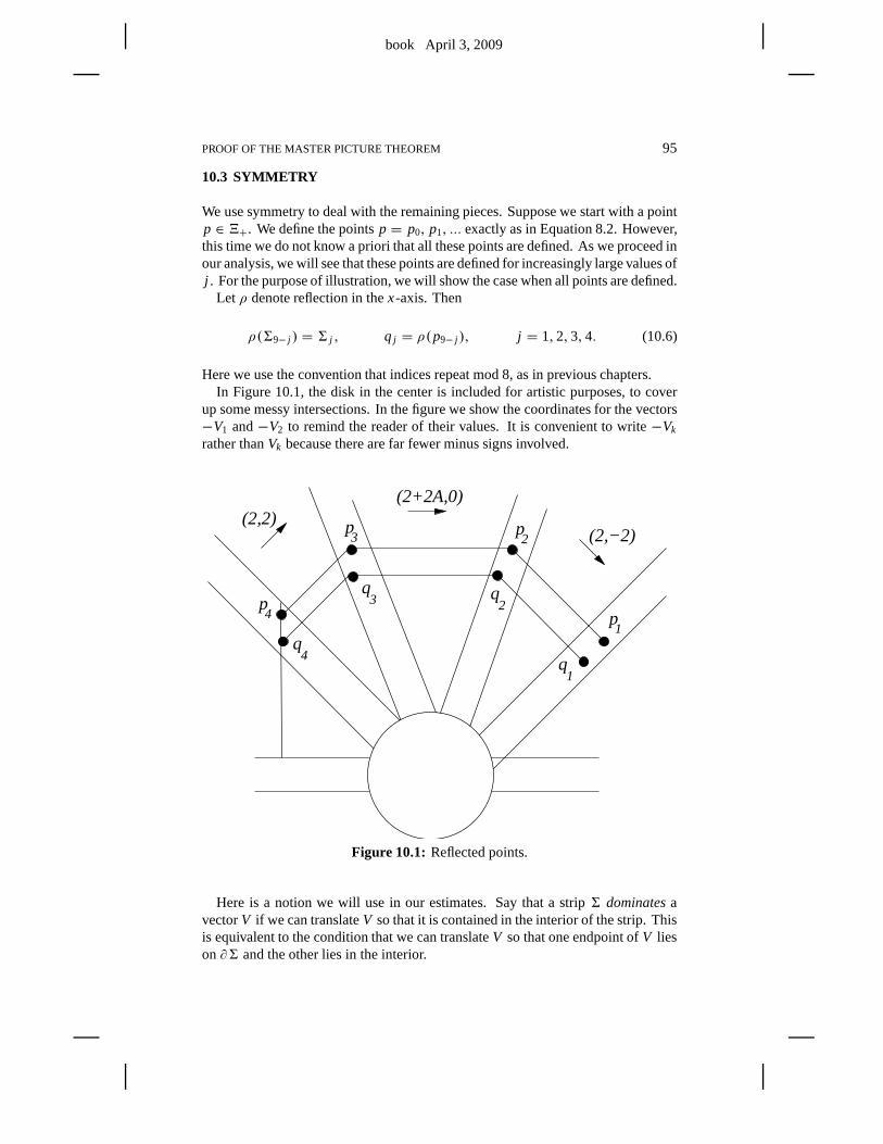
book April 3, 2009

PROOF OF THE MASTER PICTURE THEOREM 95

10.3 SYMMETRY

We use symmetry to deal with the remaining pieces. Suppose westart with a pointp ∈ 4+. We define the pointsp = p0, p1, ... exactly as in Equation 8.2. However,this time we do not know a priori that all these points are defined. As we proceed inour analysis, we will see that these points are defined for increasingly large values ofj . For the purpose of illustration, we will show the case when all points are defined.

Let ρ denote reflection in thex-axis. Then

ρ(69− j ) = 6 j , q j = ρ(p9− j ), j = 1,2,3,4. (10.6)

Here we use the convention that indices repeat mod 8, as in previous chapters.In Figure 10.1, the disk in the center is included for artistic purposes, to cover

up some messy intersections. In the figure we show the coordinates for the vectors−V1 and−V2 to remind the reader of their values. It is convenient to write−Vk

rather thanVk because there are far fewer minus signs involved.

(2,−2)

1

p2

p3

p4

q4

q3 q

2

q1

(2+2A,0)(2,2)

p

Figure 10.1: Reflected points.

Here is a notion we will use in our estimates. Say that a strip6 dominatesavectorV if we can translateV so that it is contained in the interior of the strip. Thisis equivalent to the condition that we can translateV so that one endpoint ofV lieson∂6 and the other lies in the interior.

book April 3, 2009

96 CHAPTER 10

10.4 THE REMAINING PIECES

10.4.1 The SetS4

Supposep ∈ W4. Thenp5 andq4 are defined, andq4 ∈ ∂64. Given that

V5 = (0,−4)

and they-coordinates of all the points are odd integers, we have

p4− q4 = (0,2)+ k(0,4)

for somek ∈ Z. Given that64 dominatesp4 − q4, we havek ∈ {−1,0}. Hencep4 = q4± (0,2). If p5 ∈ ∂65, thenq4 ∈ ∂64. Any vertical line intersects64 in asegment of length 4. From this we see thatp4 lies on the centerline of64. That is,σ4(p) = 1/2. Given Equation 9.6, we have

S4 ⊂ {x + y− z= A} ∪ {x + y− z= 2+ A}.

10.4.2 The SetS5

Suppose thatp ∈ W5. Thenp6 andq3 are defined, andq3 ∈ ∂63. Given that

V6 = −V4 = (−2,2),

we see that

p3− q3 = ǫ(0,2)+ k(2,2), ǫ ∈ {−1,1}, k ∈ Z.

The criterion that63 dominates a vector(x, y) is that|x + Ay| < 2+ 2A.63 dominates the vectorq3− p3. If ǫ = 1, then

|2k+ 2+ 2Ak| < 2+ 2A

forcesk ∈ {−1,0}. If ǫ = −1, then the condition

|2k− 2+ 2Ak| < 2+ 2A

forcesk ∈ {0,1}. Hencep3− q3 is one of the vectors(±2,0) or (0,±2). Now wehave a case-by-case analysis.

Suppose thatq3 lies in the right boundary of63. Then we have one of thefollowing two conditions.

p3 = q3− (2,0), p3 = q3+ (0,2).

Any horizontal line intersects63 in a strip of width 2+ 2A. So, σ3(p) equalseither 1/(1+ A) or A/(1+ A), depending on whether or notp3 = q3 − (2,0) orp3 = q3 + (0,2). A similar analysis reveals the same two values whenq3 lies onthe left boundary of63. Given Equation 9.5, we have

S5 ⊂ {x = A} ∪ {x = 1}.

book April 3, 2009

PROOF OF THE MASTER PICTURE THEOREM 97

10.4.3 The SetS6

Suppose thatp ∈ W6. Thenp7 andq2 are defined, andq2 ∈ ∂62. We have

p2− q2 = (p3− q3)+ k(2+ 2A,0). (10.7)

The criterion that63 dominates a vector(x, y) is that|x − Ay| < 2+ 2A.Let X1, ..., X4 be the possible values forp3 − q3 as determined in the previous

section. Using the values of the vectorsX j and the fact that62 dominatesp2− q2,we see that

p2− q2 = X j + ǫ(2A,2), ǫ ∈ {−1,0,1}, j ∈ {1,2,3,4}. (10.8)

Note that the vector(2A,2) is parallel to the boundary of62. Hence, for the pur-pose of computingσ2(p), this vector plays no role. Essentially the same calculationas in the previous section now gives us the same choices forσ2(p) as we had forσ3(p) in the previous section. Given Equation 9.4, we have

S6 ⊂ {y = A} ∪ {y = 1}.

10.4.4 The SetS7

Suppose thatp ∈ W7. Thenp8 andq1 are defined, andq1 ∈ ∂61. We have

p1− q1 = (p2− q2)+ k(−2,2). (10.9)

Note that the vector(2,2) is parallel to61. For the purpose of findingσ1(p), we cando our computation mod(2,2). For instance,(2,−2) ≡ (0,4) mod(2,2). GivenEquation 10.8, we have

p1− q1 = ǫ1(0,2)+ ǫ2(2A,2)+ k(0,4) mod (2,2). (10.10)

Hereǫ1, ǫ2 ∈ {−1,0,1}. Given that any vertical line intersects61 in a segment oflength 4, we see that the only choices forσ1(p) are

(k/2)+ 2ǫA, ǫ ∈ {−1,0,1}, k ∈ Z.

Given Equation 9.3, we see thatS7 ⊂ {z= A} ∪ {z= 1− A}.

10.5 PROOF OF THE SECOND STATEMENT

Our analysis above establishes the first statement of the Hyperplane Lemma. Forthe second statement, suppose thatd(µ+(p, A), S) = ǫ. Given Equations 9.3–9.6,we have

θ j (p) ≥ ǫ, j = 1,2,3,4.

Given our analysis of the remaining points using symmetry, the same bound holdsfor j = 5,6,7,8. In these cases,θ j (p, A) is a linear function of the distance fromµ+(p, A) to Sj−1, and the constant of proportionality is the same as for the index9− j .

book April 3, 2009

book April 3, 2009

Part 3. Arithmetic Graph Structure Theorems

In this part of the book, we use the Master Picture Theorem to prove most of thestructural results for the arithmetic graph that we quoted in Part 1.

• In Chapter 11, we prove the Embedding Theorem.

• In Chapter 12, we prove some results about the symmetries ofthe arithmeticgraph and the hexagrid.

• In Chapter 13, we prove statement 1 of the Hexagrid Theorem,namely, thatthe arithmetic graph does not cross any floor lines.

• In Chapter 14, we prove a variant of statement 1 of the HexagridTheorem. Wecall the result the Barrier Theorem. Though we do not need this result untilPart 6, the proof fits best right after the proof of statement 1of the HexagridTheorem.

• In Chapter 15, we prove statement 2 of the Hexagrid Theorem,namely, thatthe arithmetic graph crosses the walls only near the doors. The two statementsof the Hexagrid Theorem have similar proofs, though statement 2 has a moreelaborate proof. We think of the proof of statement 2 of the Hexagrid Theoremas the main event in this part of the book. To make our argumentgo moresmoothly, we defer a technical result, the Intersection Lemma, until the nextchapter.

• In Chapter 16, we prove the Intersection Lemma, the technical result left overfrom the proof given in Chapter 15.

Many of the proofs in this part of the book require us to prove various disjointnessresults about some 4-dimensional polytopes. We will give short computer-aidedproofs of these disjointness results. The proofs involve only a small amount ofinteger linear algebra. To help make the proofs surveyable,we will include computerimages of 2 dimensional slices of our polytopes. These figures, all reproducible onBilliard King, serve as sanity checks for the computer calculations. We will includemany figures from Billiard King, but it usually goes without saying that the readercan see much more using the program.

book April 3, 2009

book April 3, 2009

Chapter Eleven

Proof of the Embedding Theorem

11.1 NO VALENCE 1 VERTICES

Let Ŵ = Ŵα(A) be the arithmetic graph for a parameterA and someα 6∈ 2Z [ A].The reader will see from our proof that the choice ofα is not important. As a firststep in the proof of the Embedding Theorem, we show that all nontrivial vertices ofŴ have valence 2. Dynamically, a vertex of valence 1 corresponds to a pointx ∈ 4such thatx 6= 9(x) = 9−1(x).

Let p ∈ Z2 be a nontrivial vertex ofŴ. Letq+ andq− be the two neighbors ofp.We would like to show thatŴ has valence 2 atp. If this fails, then we must have

p 6= q+ = q−. (11.1)

This means that the mapsM+ andM− from §6.6 assign the same vector top. Putanother way, this situation occurs iff there is some nontrivial (ǫ1, ǫ2) ∈ {−1,0,1}such that

3R+(ǫ1, ǫ2) ∩(R−(ǫ1, ǫ2)+ (1,1,0,0)

)6= ∅. (11.2)

A visual inspection and/or a computer search reveals that atleast one of the two setsabove is empty unless(ǫ1, ǫ2) is one of

(1,1), (−1,−1), (1,0), (−1,0). (11.3)

It follows from Equation 6.17 that Equation 11.2 holds for(ǫ1, ǫ2) if and only if itholds for(−ǫ1,−ǫ2). Thus we have to deal just with the pairs(1,1) and(1,0).

Below we will give a formal argument, based on a small amount of machinecomputation, that rules out the above kind of intersection.Before we do this,however, we will show some convincing pictures of the relevant sets. As in §6.3,we show(z, A) slices of polytopes inR+ andR−. We draw the slices ofR+with darkshading and the slices ofR− with light shading. LetB j denote thej th componentof the base spaceB, as in Figure 6.2.

Over the regionsB2 andB3, at least one ofR+(1,1) or R−(1,1) is empty. Figure11.1 shows typical slices of

3R+(1,1), 3(R−(1,1)+ (1,1,0,0))

overB0 andB1. In all cases, we see that the interiors of the two kinds of pieces aredisjoint from each other.

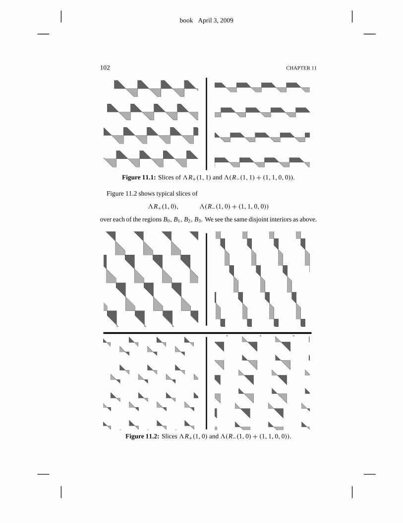
book April 3, 2009

102 CHAPTER 11

Figure 11.1: Slices of3R+(1,1) and3(R−(1,1)+ (1,1,0,0)).

Figure 11.2 shows typical slices of

3R+(1,0), 3(R−(1,0)+ (1,1,0,0))

over each of the regionsB0, B1, B2, B3. We see the same disjoint interiors as above.

Figure 11.2: Slices3R+(1,0) and3(R−(1,0)+ (1,1,0,0)).

book April 3, 2009

PROOF OF THE EMBEDDING THEOREM 103

Now we give a formal argument. We work inR4, as discussed in §6.7. All thepolytopes of interest are convex integral polytopes. To rule out Equation 11.2, weneed to consider all possible pairs(P1, P2) of integral convex polytopes such that

P1 ⊂ 3R+(ǫ1, ǫ2), P2 ⊂ R−(ǫ1, ǫ2)+ (1,1). (11.4)

We hold the second polytope fixed and move the first one around by the action ofthe entire lattice. At first it looks as if we have an infinite calculation, but actuallywe will reduce the problem to a finite calculation.

Recall that3 is generated by the three elementsγ1, γ2, γ3. Let3′ ⊂ 3 denotethe subgroup generated byγ1 andγ2. We also define3′10 ⊂ 3′ by the equation

3′10 = {a1γ1 + a2γ2| |a1|, |a2| ≤ 10}. (11.5)

Lemma 11.1 Letγ ∈ 3−3′10.

P1 = γ (Q1), Q1 ⊂ R+(ǫ1, ǫ2), P2 ⊂ R−(ǫ1, ǫ2)+ (1,1,0,0).

Then P1 and P2 have disjoint interiors.

Proof: If γ 6∈ 3′, then the third coordinates of points inP1 lie in [n,n+ 1] forsome integern 6= 0. On the other hand, the third coordinates of points inP2 liein [0,1]. HenceP1 andP2 have disjoint interiors in this case. This means that wehave to worry only about elements of3′.

Suppose now thatγ ∈ 3′−3′10. In this case,Q1 is contained in the ball of radius4 aboutP2, butγ moves this ball entirely off itself. 2

Now we have a finite problem. Given

γ ∈ 3′10, P1 = γ (Q1), Q1 ⊂ R+(ǫ1, ǫ2), P2 ⊂ R−(ǫ1, ǫ2)+ (1,1,0,0),

we produce a vector

w = w(P1, P2) ∈ {−1,0,1}4 (11.6)

such that

maxv∈vtx(P1)

v · w ≤ minv∈vtx(P2)

v · w. (11.7)

This means that a hyperplane separates the interior ofP1 from P2. In each casewe find v(P1, P2) by a short computer search and perform the verification usingarithmetic with integers.

Remark: It seems rather lucky that we could find such simple hyperplanes sepa-rating the polytopes. However, every coordinate of every polytope lies in{0,1,2},and the relevant pairs of polytopes often have several pairsof vertices in common.This situation makes the existence of the very simple separating hyperplanes lesssurprising.

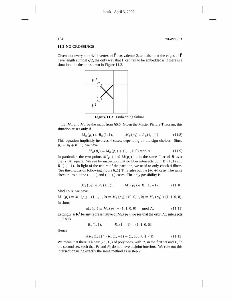
book April 3, 2009

104 CHAPTER 11

11.2 NO CROSSINGS

Given that every nontrivial vertex ofŴ has valence 2, and also that the edges ofŴhave length at most

√2, the only way thatŴ can fail to be embedded is if there is a

situation like the one shown in Figure 11.3.

p1

p2

Figure 11.3: Embedding failure.

Let M+ andM− be the maps from §6.6. Given the Master Picture Theorem, thissituation arises only if

M±(p1) ∈ R±(1,1), M±(p2) ∈ R±(1,−1) (11.8)

This equation implicitly involves 4 cases, depending on thesign choices. Sincep2 = p1+ (0,1), we have

M±(p2) = M±(p1)+ (1,1,1,0)mod3. (11.9)

In particular, the two pointsM(p1) and M(p2) lie in the same fiber ofR overthe(z, A) square. We see by inspection that no fiber intersects bothR+(1,1) andR+(1,−1). In light of the nature of the partition, we need to only check4 fibers.(See the discussion following Figure 6.2.) This rules out the(+,+) case. The samecheck rules out the(−,−) and(−,+) cases. The only possibility is

M+(p1) ∈ R+(1,1), M−(p2) ∈ R−(1,−1). (11.10)

Modulo3, we have

M−(p2) ≡ M−(p1)+(1,1,1,0) ≡ M+(p1)+(0,0,1,0) ≡ M+(p1)+(1,1,0,0).In short,

M+(p1) ≡ M−(p2)− (1,1,0,0) mod3. (11.11)

Lettingx ∈ R4 be any representative ofM+(p1), we see that the orbit3x intersectsboth sets

R+(1,1), R−(1,−1)− (1,1,0,0).Hence

3R+(1,1) ∩ (R−(1,−1)− (1,1,0,0)) 6= ∅. (11.12)

We mean that there is a pair(P1, P2) of polytopes, withP1 in the first set andP2 inthe second set, such thatP1 andP2 do not have disjoint interiors. We rule out thisintersection using exactly the same method as in step 2.

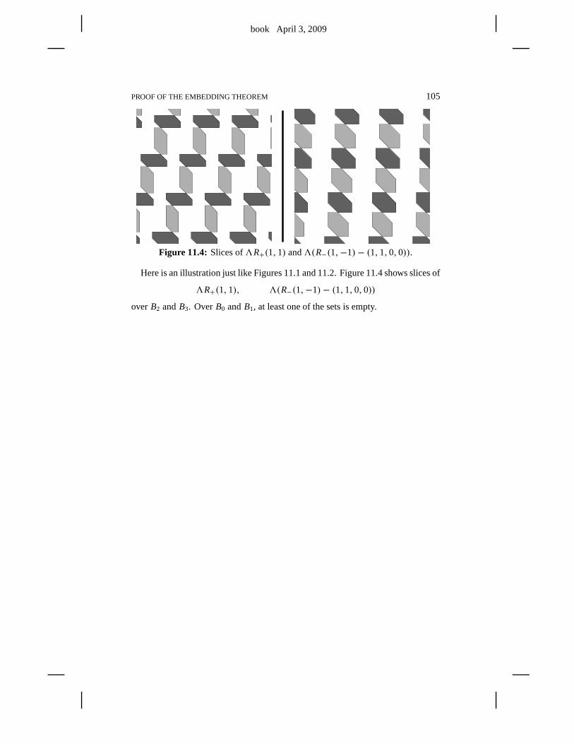
book April 3, 2009

PROOF OF THE EMBEDDING THEOREM 105

Figure 11.4: Slices of3R+(1,1) and3(R−(1,−1)− (1,1,0,0)).

Here is an illustration just like Figures 11.1 and 11.2. Figure 11.4 shows slices of

3R+(1,1), 3(R−(1,−1)− (1,1,0,0))

overB2 andB3. OverB0 andB1, at least one of the sets is empty.

book April 3, 2009

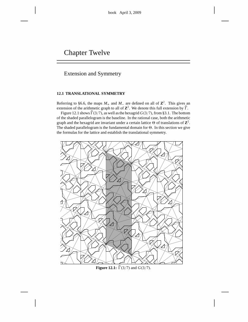
book April 3, 2009

Chapter Twelve

Extension and Symmetry

12.1 TRANSLATIONAL SYMMETRY

Referring to §6.6, the mapsM+ and M− are defined on all ofZ2. This gives anextension of the arithmetic graph to all ofZ2. We denote this full extension byŴ.

Figure 12.1 showsŴ(3/7), as well as the hexagridG(3/7), from §3.1. The bottomof the shaded parallelogram is the baseline. In the rationalcase, both the arithmeticgraph and the hexagrid are invariant under a certain lattice2 of translations ofZ2.The shaded parallelogram is the fundamental domain for2. In this section we givethe formulas for the lattice and establish the translational symmetry.

Figure 12.1: Ŵ(3/7) andG(3/7).

book April 3, 2009

108 CHAPTER 12

Lemma 12.1 The extended arithmetic graph does not cross the baseline.

Proof: The arithmetic graph describes the dynamics of the pinwheelmap8. Notethat8 is generically defined and invertible onR+×{−1,1}. Reflection in thex-axisconjugates8 to8−1. By the Pinwheel Lemma,8 mapsR+ × {−1,1} into itself.By symmetry the same goes for8−1. Hence8 and8−1 also mapR− × {−1,1}into itself. If some edge ofŴ crosses the baseline, then one of8 or8−1 will mapa point ofR+ × {−1,1} into R− × {−1,1}. This is a contradiction. 2

Let λ(p/q) = 1 if p/q is odd and letλ(p/q) = 2 if p/q is even. Define

2 = ZV + ZV ′, V ′ = λ2

(0,(p+ q)2

4

), λ = λ(p/q). (12.1)

Referring to Figure 12.1, the short edges of the parallelogram are translates ofV and the long edges are translates ofV ′. Thus the shaded parallelogram is afundamental domain for the action of2 onR2.

Lemma 12.2 The arithmetic graphŴ(p/q) is invariant under2.

Proof: We will consider the odd case. The even case is similar. We have alreadyseen thatŴ is invariant underV . We just have to show invariance forV ′. Referringto the notation in §6.6, we have

M±(x + V ′)− M±(x) = (t, t, t) mod3, t = (p+ q)2

4. (12.2)

By the Master Picture Theorem, it suffices to prove that(t, t, t) ∈ 3. Setting

a = pq, b = pq+ q2

2, c = t, (12.3)

we express(t, t, t) as an integer combination of vectors in3 as follows.

a

[1+ A00

]+ b

[1− A1+ A

0

]+ c

[−1−11

]=[ t

tt

]. (12.4)

This completes the proof. 2

Remark: One can probably also see rotational symmetry by looking at Figure 12.1.We will treat this kind of symmetry below.

Our next result deals with the hexagrid and the arithmetic kiteK(A). Both objectsare defined in §3.1. Recall that the hexagrid consists of a room grid RGand a doorgrid DG. HereRG is composed of 2 families of parallel lines andDG is composedof 4 families of parallel lines. The lines ofRG are all parallel to the two diagonalsof K(A), and the lines ofDG are all parallel to the sides ofK(A). Referring toFigure 12.1, notice that each corner of the shaded parallelogram lies on 6 lines –one per family – of the hexagrid. Our proof of the following result is based on thisphenomenon.

book April 3, 2009

EXTENSION AND SYMMETRY 109

Lemma 12.3 The hexagrid is invariant under the action of2.

Proof: Again, we treat the only odd case. LetG = G(p/q) denote the hexagrid.By construction,G is invariant under translation byV . We just have to show thatthe same holds forV ′. We will show thatV ′ contains 6 lines ofG. Translation byV ′ then maps each family of parallel lines in the hexagrid to itself, and so the wholehexagrid is invariant.

Let W be as in Equation 3.2. For convenience, we repeat the formulafor W.

W =(

pq

p+ q,

pq

p+ q+ q − p

2

).

We compute that

V ′ = −p

2V +

p+ q

2W. (12.5)

The second coefficient is an integer. Given that the room gridRG is invariant underthe latticeZ [V/2,W], the room gridRG is also invariant under translation byV ′.This gives 2 linesL1 andL2, one from each family ofRG.

Note that the door gridDG is invariant only underZ [V ], so we have to workharder. We need to produce 4 lines ofDG that containV ′. Here they are.

• The vertical lineL3 through(0,0) certainly containsV ′. This line extendsthe bottom left edge ofK(A) and hence belongs toDG.

• Let L4 be the line containingV ′ and the point

−(p+ q)

2V ∈ Z [V ] .

We compute that the slope ofL4 coincides with the slope of the top left edgeof K(A). The origin contains a line ofDG parallel to the top left edge ofK(A), and hence every point inZ [V ] contains such a line. HenceL4 belongsto DG.

• Let L5 be the line containingV ′ and the point

−pV ∈ Z [V ] .

We compute that the slope ofL5 coincides with the slope of the bottom rightedge ofK(A). The same argument as in the previous case shows thatL5

belongs toDG.

• Let L6 be the line containingV ′ and the point

q − p

2V ∈ Z [V ] .

We compute that the slope ofL6 coincides with the slope of the top right edgeof K(A). The same argument as above shows thatL6 belongs toDG.

The linesL1, ..., L6 are the desired lines. 2

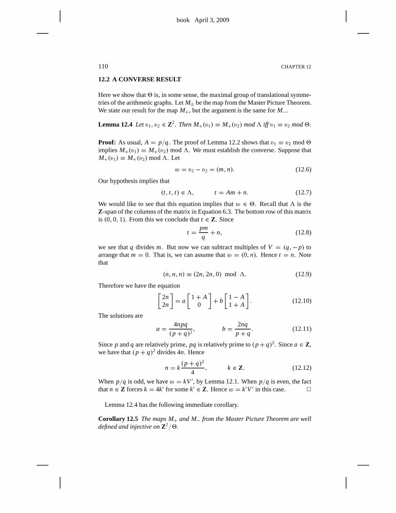
book April 3, 2009

110 CHAPTER 12

12.2 A CONVERSE RESULT

Here we show that2 is, in some sense, the maximal group of translational symme-tries of the arithmetic graphs. LetM± be the map from the Master Picture Theorem.We state our result for the mapM+, but the argument is the same forM−.

Lemma 12.4 Letv1, v2 ∈ Z2. Then M+(v1) ≡ M+(v2) mod3 iff v1 ≡ v2 mod2.

Proof: As usual,A = p/q. The proof of Lemma 12.2 shows thatv1 ≡ v2 mod2implies M+(v1) ≡ M+(v2) mod3. We must establish the converse. Suppose thatM+(v1) ≡ M+(v2)mod3. Let

w = v2 − v2 = (m,n). (12.6)

Our hypothesis implies that

(t, t, t) ∈ 3, t = Am+ n. (12.7)

We would like to see that this equation implies thatw ∈ 2. Recall that3 is theZ-span of the columns of the matrix in Equation 6.3. The bottomrow of this matrixis (0,0,1). From this we conclude thatt ∈ Z. Since

t = pm

q+ n, (12.8)

we see thatq dividesm. But now we can subtract multiples ofV = (q,−p) toarrange thatm = 0. That is, we can assume thatw = (0,n). Hencet = n. Notethat

(n,n,n) ≡ (2n,2n,0) mod 3. (12.9)

Therefore we have the equation[

2n2n

]= a

[1+ A

0

]+ b

[1− A1+ A

]. (12.10)

The solutions are

a = 4npq

(p+ q)2, b = 2nq

p+ q. (12.11)

Sincep andq are relatively prime,pq is relatively prime to(p+ q)2. Sincea ∈ Z,we have that(p+ q)2 divides 4n. Hence

n = k(p+ q)2

4, k ∈ Z. (12.12)

When p/q is odd, we havew = kV′, by Lemma 12.1. Whenp/q is even, the factthatn ∈ Z forcesk = 4k′ for somek′ ∈ Z. Hencew = k′V ′ in this case. 2

Lemma 12.4 has the following immediate corollary.

Corollary 12.5 The maps M+ and M− from the Master Picture Theorem are welldefined and injective onZ2/2.

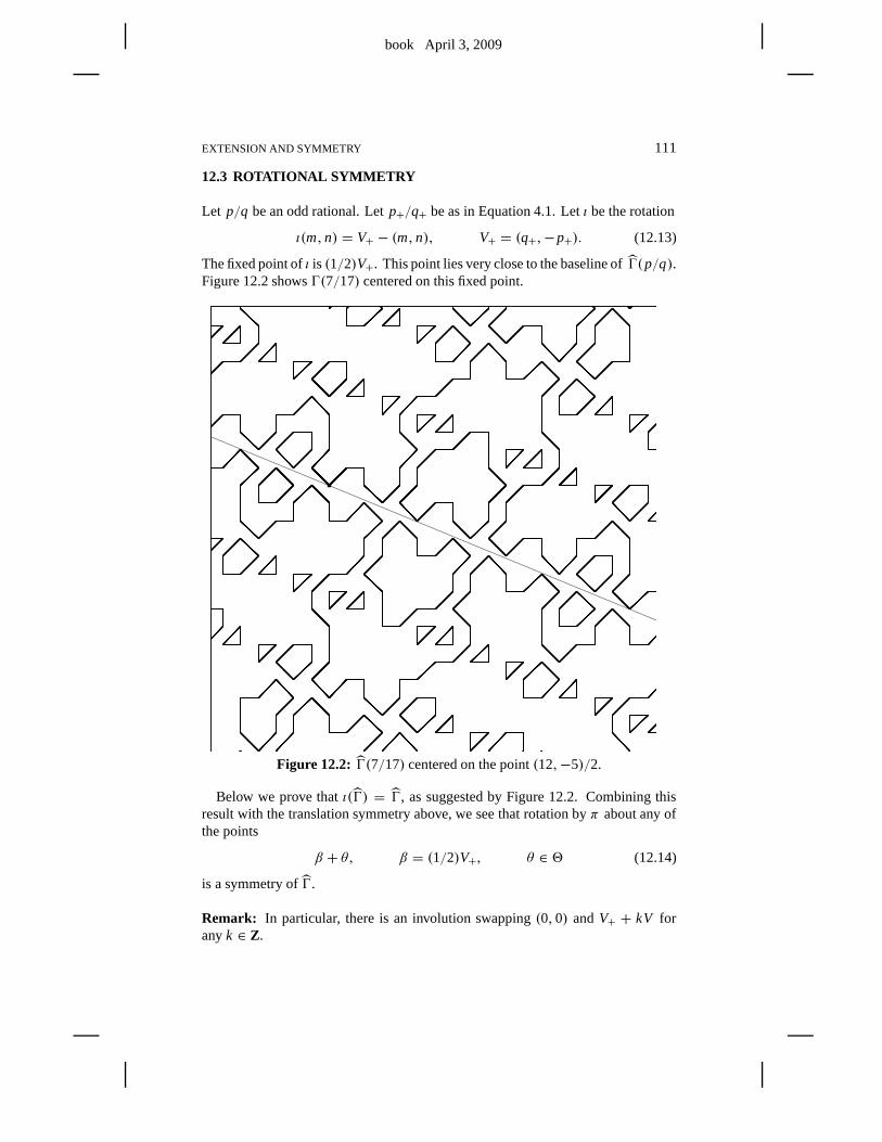
book April 3, 2009

EXTENSION AND SYMMETRY 111

12.3 ROTATIONAL SYMMETRY

Let p/q be an odd rational. Letp+/q+ be as in Equation 4.1. Letι be the rotation

ι(m,n) = V+ − (m,n), V+ = (q+,−p+). (12.13)

The fixed point ofι is (1/2)V+. This point lies very close to the baseline ofŴ(p/q).Figure 12.2 showsŴ(7/17) centered on this fixed point.

Figure 12.2: Ŵ(7/17) centered on the point(12,−5)/2.

Below we prove thatι(Ŵ) = Ŵ, as suggested by Figure 12.2. Combining thisresult with the translation symmetry above, we see that rotation byπ about any ofthe points

β + θ, β = (1/2)V+, θ ∈ 2 (12.14)

is a symmetry ofŴ.

Remark: In particular, there is an involution swapping(0,0) andV+ + kV foranyk ∈ Z.

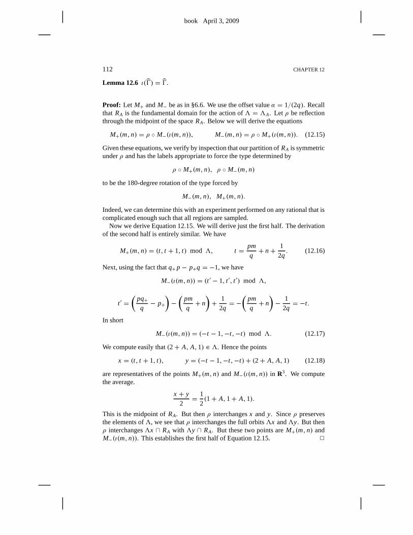
book April 3, 2009

112 CHAPTER 12

Lemma 12.6 ι(Ŵ) = Ŵ.

Proof: Let M+ andM− be as in §6.6. We use the offset valueα = 1/(2q). Recallthat RA is the fundamental domain for the action of3 = 3A. Let ρ be reflectionthrough the midpoint of the spaceRA. Below we will derive the equations

M+(m,n) = ρ ◦ M−(ι(m,n)), M−(m,n) = ρ ◦ M+(ι(m,n)). (12.15)

Given these equations, we verify by inspection that our partition of RA is symmetricunderρ and has the labels appropriate to force the type determined by

ρ ◦ M+(m,n), ρ ◦ M−(m,n)

to be the 180-degree rotation of the type forced by

M−(m,n), M+(m,n).

Indeed, we can determine this with an experiment performed on any rational that iscomplicated enough such that all regions are sampled.

Now we derive Equation 12.15. We will derive just the first half. The derivationof the second half is entirely similar. We have

M+(m,n) = (t, t + 1, t) mod 3, t =pm

q+ n+

1

2q. (12.16)

Next, using the fact thatq+p− p+q = −1, we have

M−(ι(m,n)) = (t ′ − 1, t ′, t ′) mod 3,

t ′ =(

pq+q− p+

)−(

pm

q+ n

)+ 1

2q= −

(pm

q+ n

)− 1

2q= −t .

In short

M−(ι(m,n)) = (−t − 1,−t,−t) mod 3. (12.17)

We compute easily that(2+ A, A,1) ∈ 3. Hence the points

x = (t, t + 1, t), y = (−t − 1,−t,−t)+ (2+ A, A,1) (12.18)

are representatives of the pointsM+(m,n) and M−(ι(m,n)) in R3. We computethe average.

x + y

2=

1

2(1+ A,1+ A,1).

This is the midpoint ofRA. But thenρ interchangesx and y. Sinceρ preservesthe elements of3, we see thatρ interchanges the full orbits3x and3y. But thenρ interchanges3x ∩ RA with 3y ∩ RA. But these two points areM+(m,n) andM−(ι(m,n)). This establishes the first half of Equation 12.15. 2

book April 3, 2009

EXTENSION AND SYMMETRY 113

12.4 NEAR-BILATERAL SYMMETRY

Our pictures of arithmetic graphs show near-bilateral symmetry. In this sectionwe explain how this arises. Looking at Figure 12.2, we see that there is a naturalcorrespondence between components above the baseline and components below thebaseline. Our first result explains this near-bilateral symmetry. There is a secondkind of bilateral symmetry that meets the eye in Figure 1.5 or12.3. After provingour first result, we will explain how this other kind of near-bilateral symmetry arises.

Figure 12.3:Ŵ(15/52).

We say that a mapJ from Ŵ to Ŵ is a combinatorial isomorphismif J mapsvertices to vertices and edges to edges.

Recall that a low vertex is one that is above the baseline but within 1 vertical unitof it. Say that alow componentis a component ofŴ above the baseline that containsa low vertex. Say that this component isodd if it contains odd low vertices, andevenif it contains even low vertices. By Lemma 2.6, this notion iswell defined.

Lemma 12.7 For any rational A, there is a combinatorial isomorphismJ: Ŵ→ Ŵthat swaps the components ofγ above the baseline with the one below the baseline.

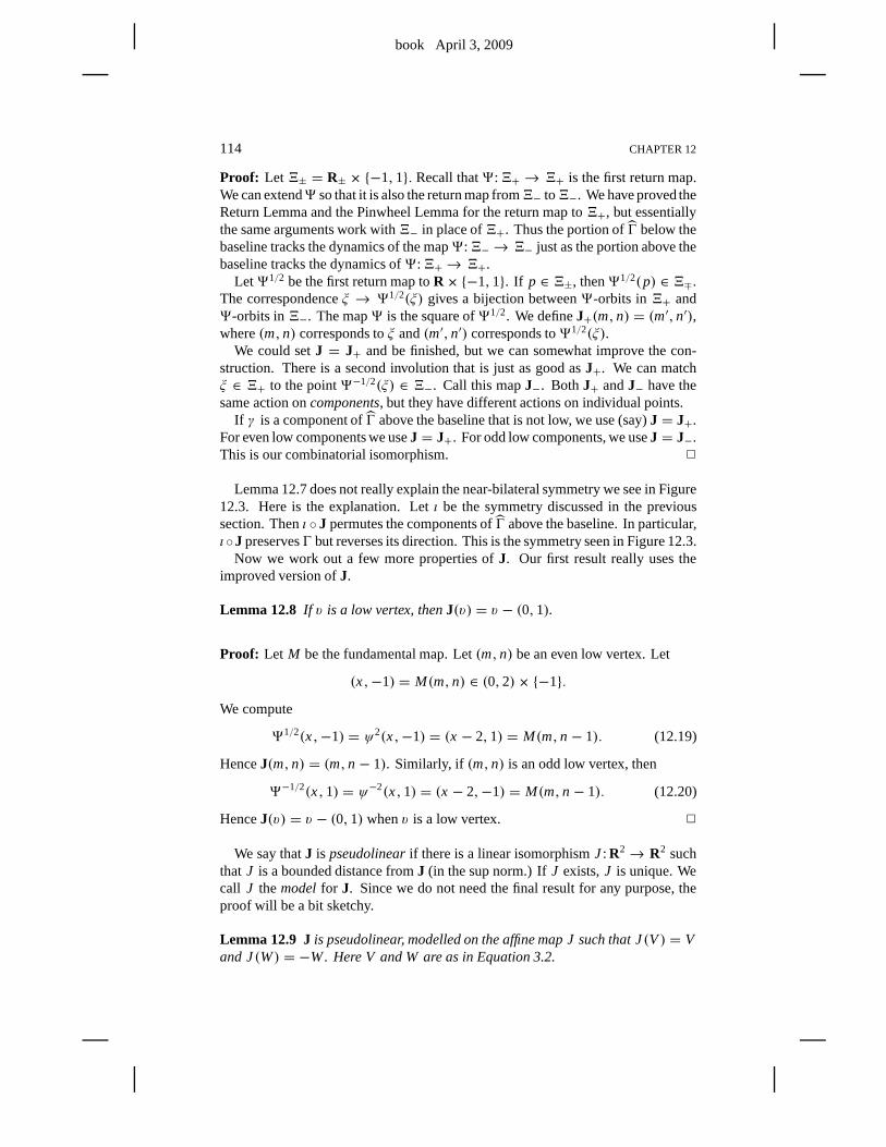
book April 3, 2009

114 CHAPTER 12

Proof: Let4± = R± × {−1,1}. Recall that9:4+ → 4+ is the first return map.We can extend9 so that it is also the return map from4− to4−. We have proved theReturn Lemma and the Pinwheel Lemma for the return map to4+, but essentiallythe same arguments work with4− in place of4+. Thus the portion ofŴ below thebaseline tracks the dynamics of the map9:4−→ 4− just as the portion above thebaseline tracks the dynamics of9:4+→ 4+.

Let91/2 be the first return map toR× {−1,1}. If p ∈ 4±, then91/2(p) ∈ 4∓.The correspondenceξ → 91/2(ξ) gives a bijection between9-orbits in4+ and9-orbits in4−. The map9 is the square of91/2. We defineJ+(m,n) = (m′,n′),where(m,n) corresponds toξ and(m′,n′) corresponds to91/2(ξ).

We could setJ = J+ and be finished, but we can somewhat improve the con-struction. There is a second involution that is just as good as J+. We can matchξ ∈ 4+ to the point9−1/2(ξ) ∈ 4−. Call this mapJ−. BothJ+ andJ− have thesame action oncomponents, but they have different actions on individual points.

If γ is a component ofŴ above the baseline that is not low, we use (say)J = J+.For even low components we useJ = J+. For odd low components, we useJ = J−.This is our combinatorial isomorphism. 2

Lemma 12.7 does not really explain the near-bilateral symmetry we see in Figure12.3. Here is the explanation. Letι be the symmetry discussed in the previoussection. Thenι ◦ J permutes the components ofŴ above the baseline. In particular,ι◦J preservesŴ but reverses its direction. This is the symmetry seen in Figure 12.3.

Now we work out a few more properties ofJ. Our first result really uses theimproved version ofJ.

Lemma 12.8 If v is a low vertex, thenJ(v) = v − (0,1).

Proof: Let M be the fundamental map. Let(m,n) be an even low vertex. Let

(x,−1) = M(m,n) ∈ (0,2)× {−1}.

We compute

91/2(x,−1) = ψ2(x,−1) = (x − 2,1) = M(m,n− 1). (12.19)

HenceJ(m,n) = (m,n− 1). Similarly, if (m,n) is an odd low vertex, then

9−1/2(x,1) = ψ−2(x,1) = (x − 2,−1) = M(m,n− 1). (12.20)

HenceJ(v) = v − (0,1) whenv is a low vertex. 2

We say thatJ is pseudolinearif there is a linear isomorphismJ: R2→ R2 suchthat J is a bounded distance fromJ (in the sup norm.) IfJ exists,J is unique. Wecall J themodelfor J. Since we do not need the final result for any purpose, theproof will be a bit sketchy.

Lemma 12.9 Jis pseudolinear, modelled on the affine map J such that J(V) = Vand J(W) = −W. Here V and W are as in Equation 3.2.

book April 3, 2009

EXTENSION AND SYMMETRY 115

Proof: (Sketch) Letting(x,1) be a point on4+ aboutN units from the origin,we roughly trace out the Pinwheel map. First we add some integer multiple of thevector(0,4), then we add some integer multiple of the vector(−2,2), etc. Whenwe reach4− we have a vector of the form

x + (2AcN + 2dN,±1).

Here (cN,dN) depends linearly onN up to a uniformly bounded error. Given apointv = (m,n), we have

J(v) = v + (cN,dN), N = 2Am+ 2n. (12.21)

This shows thatJ is pseudolinear.Let J be the linear map on whichJ is modelled. Given the action ofJ on low

vertices, we see thatJ(V) = V . To show thatJ(W) = −W, we consider how thepair (ck,dk) associated tokW depends onk. Taking the limit ask → ∞, we getan exact formula that showsJ(W) = −W. We omit the details of this calculation.2

book April 3, 2009

book April 3, 2009

Chapter Thirteen

Proof of Hexagrid Theorem I

13.1 THE KEY RESULT

The proof of Hexagrid Theorem I is the same in the odd and even cases.Say that afloor line is a negatively sloped line of the floor grid. Floor lines all

have slope−A. Say that afloor point is a point on a floor line. Such a point neednot have integer coordinates. The mapsM+ andM− from §6.6 are constant on floorlines. Thus, ifL is a floor line,M±(L) is a single point.

Lemma 13.1 If p is a floor point, then M−(p) ≡ (β,0,0) mod3 for someβ ∈ R.

Proof: Suppose first thatp/q is odd. SinceM− is constant on floor lines, it sufficesto consider floor points of the form

(0, t), t =k(p+ q)

2, k ∈ Z. (13.1)

These points are the intersections of the floor lines with they-axis. Note thatt is aninteger becausep+ q is even.

To compute the image of the point(0, t), we just have to subject the pointt tothe reduction algorithm from §6.6. The first 4 steps of the algorithm lead to thefollowing result.

1. z= t .

2. Z = floor(t) = t becauset is an integer.

3. y = 2t = k(p+ q) = kq(1+ A).

4. Y = floor(y/(1+ A)) = kq.

Hencez= Z andy = (1+ A)Y. Hence

M−(0, t) = (x − (1+ A)X, y− (1+ A)Y, z− Z) = (β,0,0) (13.2)

for some numberβ ∈ R that depends onA andk.When p/q is even, the floor grid has a different definition: Only the even floor

lines are present in the grid. That is, the numberk in Equation 13.1 is an eveninteger. Hence, for the floor lines in the even case, the number t is an integer. Therest of the proof is the same. 2

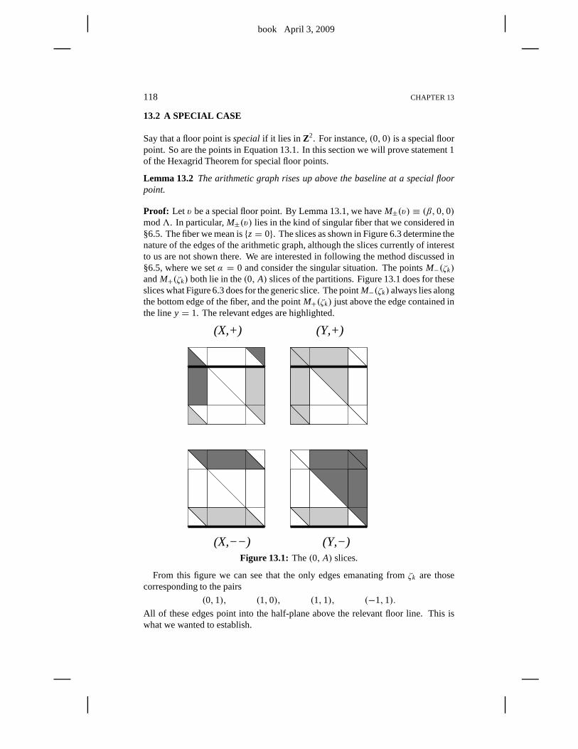
book April 3, 2009

118 CHAPTER 13

13.2 A SPECIAL CASE

Say that a floor point isspecialif it lies in Z2. For instance,(0,0) is a special floorpoint. So are the points in Equation 13.1. In this section we will prove statement 1of the Hexagrid Theorem for special floor points.

Lemma 13.2 The arithmetic graph rises up above the baseline at a specialfloorpoint.

Proof: Let v be a special floor point. By Lemma 13.1, we haveM±(v) ≡ (β,0,0)mod3. In particular,M±(v) lies in the kind of singular fiber that we considered in§6.5. The fiber we mean is{z= 0}. The slices as shown in Figure 6.3 determine thenature of the edges of the arithmetic graph, although the slices currently of interestto us are not shown there. We are interested in following the method discussed in§6.5, where we setα = 0 and consider the singular situation. The pointsM−(ζk)andM+(ζk) both lie in the(0, A) slices of the partitions. Figure 13.1 does for theseslices what Figure 6.3 does for the generic slice. The pointM−(ζk) always lies alongthe bottom edge of the fiber, and the pointM+(ζk) just above the edge contained inthe liney = 1. The relevant edges are highlighted.

(Y,−)

(Y,+)(X,+)

(X,−−)Figure 13.1: The(0, A) slices.

From this figure we can see that the only edges emanating fromζk are thosecorresponding to the pairs

(0,1), (1,0), (1,1), (−1,1).

All of these edges point into the half-plane above the relevant floor line. This iswhat we wanted to establish.

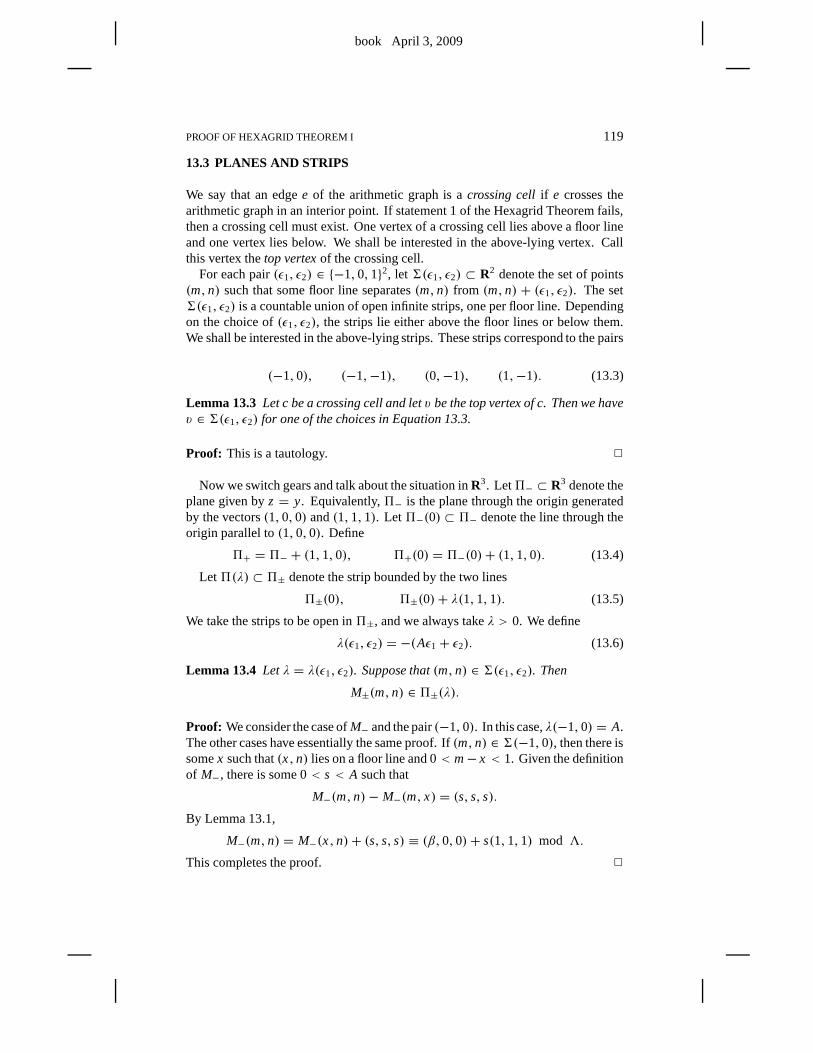
book April 3, 2009

PROOF OF HEXAGRID THEOREM I 119

13.3 PLANES AND STRIPS

We say that an edgee of the arithmetic graph is acrossing cellif e crosses thearithmetic graph in an interior point. If statement 1 of the Hexagrid Theorem fails,then a crossing cell must exist. One vertex of a crossing celllies above a floor lineand one vertex lies below. We shall be interested in the above-lying vertex. Callthis vertex thetop vertexof the crossing cell.

For each pair(ǫ1, ǫ2) ∈ {−1,0,1}2, let6(ǫ1, ǫ2) ⊂ R2 denote the set of points(m,n) such that some floor line separates(m,n) from (m,n) + (ǫ1, ǫ2). The set6(ǫ1, ǫ2) is a countable union of open infinite strips, one per floor line. Dependingon the choice of(ǫ1, ǫ2), the strips lie either above the floor lines or below them.We shall be interested in the above-lying strips. These strips correspond to the pairs

(−1,0), (−1,−1), (0,−1), (1,−1). (13.3)

Lemma 13.3 Let c be a crossing cell and letv be the top vertex of c. Then we havev ∈ 6(ǫ1, ǫ2) for one of the choices in Equation 13.3.

Proof: This is a tautology. 2

Now we switch gears and talk about the situation inR3. Let5− ⊂ R3 denote theplane given byz = y. Equivalently,5− is the plane through the origin generatedby the vectors(1,0,0) and(1,1,1). Let5−(0) ⊂ 5− denote the line through theorigin parallel to(1,0,0). Define

5+ = 5− + (1,1,0), 5+(0) = 5−(0)+ (1,1,0). (13.4)

Let5(λ) ⊂ 5± denote the strip bounded by the two lines

5±(0), 5±(0)+ λ(1,1,1). (13.5)

We take the strips to be open in5±, and we always takeλ > 0. We define

λ(ǫ1, ǫ2) = −(Aǫ1+ ǫ2). (13.6)

Lemma 13.4 Letλ = λ(ǫ1, ǫ2). Suppose that(m,n) ∈ 6(ǫ1, ǫ2). Then

M±(m,n) ∈ 5±(λ).

Proof: We consider the case ofM− and the pair(−1,0). In this case,λ(−1,0) = A.The other cases have essentially the same proof. If(m,n) ∈ 6(−1,0), then there issomex such that(x,n) lies on a floor line and 0< m− x < 1. Given the definitionof M−, there is some 0< s < A such that

M−(m,n)− M−(m, x) = (s, s, s).By Lemma 13.1,

M−(m,n) = M−(x,n)+ (s, s, s) ≡ (β,0,0)+ s(1,1,1) mod 3.

This completes the proof. 2

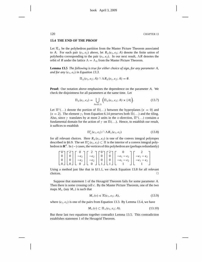
book April 3, 2009

120 CHAPTER 13

13.4 THE END OF THE PROOF

Let R± be the polyhedron partition from the Master Picture Theoremassociatedto A. For each pair(ǫ1, ǫ2) above, letR±(ǫ1, ǫ2; A) denote the finite union ofpolyhedra corresponding to the pair(ǫ1, ǫ2). In our next result,3R denotes theorbit of R under the lattice3 = 3A from the Master Picture Theorem.

Lemma 13.5 The following is true for either choice of sign, for any parameter A,and for any(ǫ1, ǫ2) in Equation 13.3.

5±(ǫ1, ǫ2; A) ∩3R±(ǫ1, ǫ2; A) = ∅.

Proof: Our notation above emphasizes the dependence on the parameter A. Wecheck the disjointness for all parameters at the same time. Let

5±(ǫ1, ǫ2) =⋃

A∈(0,1)

(5±(ǫ1, ǫ2; A)× {A}

). (13.7)

Let 5∗(. . .) denote the portion of5(. . .) between the hyperplanes{x = 0} and{x = 2}. The elementγ1 from Equation 6.14 preserves both5(. . .) and the tiling.Also, sinceγ translates by at most 2 units in thex-direction,5∗(. . .) contains afundamental domain for the action ofγ on5(. . .). Hence, to establish our result,it suffices to establish

5∗±(ǫ1, ǫ2) ∩3R±(ǫ1, ǫ2) (13.8)

for all relevant choices. HereR±(ǫ1, ǫ2) is one of the convex integral polytopesdescribed in §6.9. The set5∗±(ǫ1, ǫ2) ⊂ 5 is the interior of a convex integral poly-hedron inR4. In (−) cases, the vertices of this polyhedronare (perhaps redundantly)

0000

2000

0−ǫ2

−ǫ2

0

2−ǫ2

−ǫ2

0

0001

2001

0−ǫ1 − ǫ2

−ǫ1 − ǫ2

1

2−ǫ1− ǫ2

−ǫ1− ǫ2

1

Using a method just like that in §11.1, we check Equation 13.8for all relevantchoices. 2

Suppose that statement 1 of the Hexagrid Theorem fails for some parameterA.Then there is some crossing cellc. By the Master Picture Theorem, one of the twomapsM± (sayM+) is such that

M+(v) ∈ R(ǫ1, ǫ2; A), (13.9)

where(ǫ1, ǫ2) is one of the pairs from Equation 13.3. By Lemma 13.4, we have

M+(v) ⊂ 5+(ǫ1, ǫ2; A). (13.10)

But these last two equations together contradict Lemma 13.5. This contradictionestablishes statement 1 of the Hexagrid Theorem.

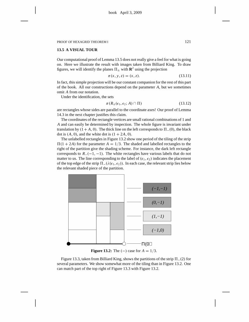
book April 3, 2009

PROOF OF HEXAGRID THEOREM I 121

13.5 A VISUAL TOUR

Our computational proof of Lemma 13.5 does not really give a feel for what is goingon. Here we illustrate the result with images taken from Billiard King. To drawfigures, we will identify the planes5± with R2 using the projection

π(x, y, z) = (x, z). (13.11)

In fact, this simple projection will be our constant companion for the rest of this partof the book. All our constructions depend on the parameterA, but we sometimesomit A from our notation.

Under the identification, the sets

π(R±(ǫ1, ǫ2; A) ∩5) (13.12)

are rectangles whose sides are parallel to the coordinate axes! Our proof of Lemma14.3 in the next chapter justifies this claim.

The coordinates of the rectangle vertices are small rational combinations of 1 andA and can easily be determined by inspection. The whole figure is invariant undertranslation by(1+ A,0). The thick line on the left corresponds to5−(0), the blackdot is(A,0), and the white dot is(1+ 2A,0).

The unlabelled rectangles in Figure 13.2 show one period of the tiling of the strip5(1+ 2A) for the parameterA = 1/3. The shaded and labelled rectangles to theright of the partition give the shading scheme. For instance, the dark left rectanglecorresponds toR−(−1,−1). The white rectangles have various labels that do notmatter to us. The line corresponding to the label of(ǫ1, ǫ2) indicates the placementof the top edge of the strip5−(λ(ǫ1, ǫ2)). In each case, the relevant strip lies belowthe relevant shaded piece of the partition.

Π(0)

(0,−1)

(−1,0)

(1,−1)

(−1,−1)

Figure 13.2: The(−) case forA = 1/3.

Figure 13.3, taken from Billiard King, shows the partitionsof the strip5−(2) forseveral parameters. We show somewhat more of the tiling thanin Figure 13.2. Onecan match part of the top right of Figure 13.3 with Figure 13.2.

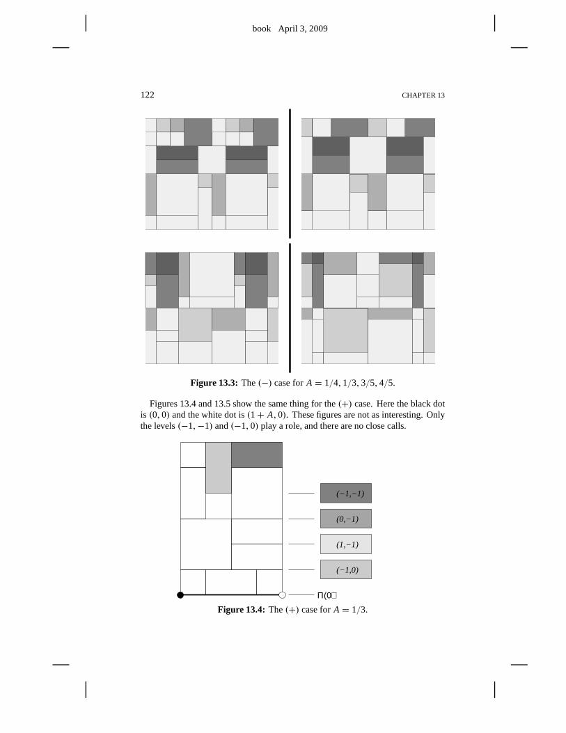
book April 3, 2009

122 CHAPTER 13

Figure 13.3: The(−) case forA = 1/4,1/3,3/5,4/5.

Figures 13.4 and 13.5 show the same thing for the(+) case. Here the black dotis (0,0) and the white dot is(1+ A,0). These figures are not as interesting. Onlythe levels(−1,−1) and(−1,0) play a role, and there are no close calls.

Π(0)

(0,−1)

(−1,0)

(−1,−1)

(1,−1)

Figure 13.4: The(+) case forA = 1/3.

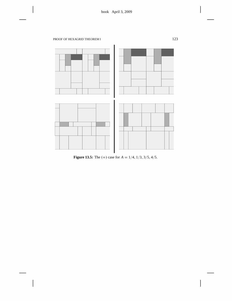
book April 3, 2009

PROOF OF HEXAGRID THEOREM I 123

Figure 13.5: The(+) case forA = 1/4,1/3,3/5,4/5.

book April 3, 2009

book April 3, 2009

Chapter Fourteen

The Barrier Theorem

14.1 THE RESULT

Let p/q be an even rational. LetV = (q,−p). Referring to Equation 4.1, one ofthe two rationalsp±/q± is even and one is odd. Letp′/q′ denote whichever of theserationals is odd. (We allow the case whenp′/q′ = 1/1.) We call p′/q′ the oddpredecessorof p/q. We say that thebarrier is the line parallel toV that containsthe point

(0,

p′ + q′

2

). (14.1)

Theorem 14.1 (Barrier) Let e be an edge ofŴ(p/q) that crosses the barrier line.Then there is some k∈ Z such that the translate e+ kV is an edge ofŴ(p/q).Moreover, there are only two such edges modulo translation by Z [V ].

We will not need the Barrier Theorem until Part 6 of the book. The reader who isinterested in only the Erratic Orbits Theorem can skip this chapter. The reason thatwe prove the Barrier Theorem here is that the proof involves amodification of theargument we gave in the last chapter. Also, our proof of statement 2 of the HexagridTheorem uses some of the ideas we present first in the proof of the Barrier Theorem.Compare §16.5.

The interested reader can observe, using Billiard King, that the Barrier Theoremand the Hexagrid Theoremare specially related: The arithmetic graph always crossesthe barrier line within 1 unit of a line from the door grid. We will not establish thisfact because we do not need it for any purpose.

We have stated the precise version of the Barrier Theorem that we need for ourapplications, but the Barrier Theorem is really part of a more robust general theorem.If we replaceA′ by some parameterA∗ that is close toA in the sense of Diophantineapproximation, then we get the general result that the corresponding “barrier line”is not frequently crossed byŴ. The basic reason is that3∗ serves as a kind ofmemory of the Hexagrid Theorem for the parameterA∗. The two graphsŴ andŴ∗

mainly agree along3∗, and the only crossings take place at the few mismatches inthe graphs.

Figure 14.1 illustrates the Barrier Theorem for the parameter A = 12/47. Thebottom straight line in the figure is the baseline. The top straight line is the barrier.The black component isŴ(12/47). The reader can see other parameters usingBilliard King.

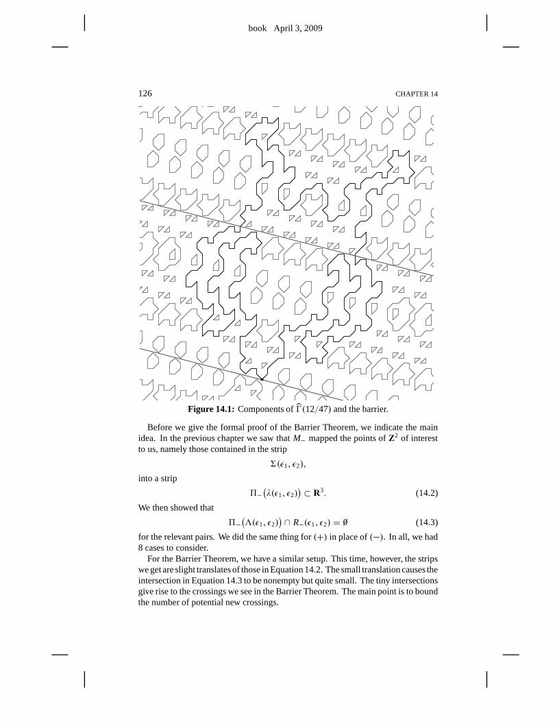
book April 3, 2009

126 CHAPTER 14

Figure 14.1: Components ofŴ(12/47) and the barrier.

Before we give the formal proof of the Barrier Theorem, we indicate the mainidea. In the previous chapter we saw thatM− mapped the points ofZ2 of interestto us, namely those contained in the strip

6(ǫ1, ǫ2),

into a strip

5−(λ(ǫ1, ǫ2)

)⊂ R3. (14.2)

We then showed that

5−(3(ǫ1, ǫ2)

)∩ R−(ǫ1, ǫ2) = ∅ (14.3)

for the relevant pairs. We did the same thing for(+) in place of(−). In all, we had8 cases to consider.

For the Barrier Theorem, we have a similar setup. This time, however, the stripswe get are slight translates of those in Equation 14.2. The small translation causes theintersection in Equation 14.3 to be nonempty but quite small. The tiny intersectionsgive rise to the crossings we see in the Barrier Theorem. The main point is to boundthe number of potential new crossings.

book April 3, 2009

THE BARRIER THEOREM 127

14.2 THE IMAGE OF THE BARRIER LINE

Let 3 be the barrier line. Here we prove an analog of Lemma 13.1 fromtheprevious chapter. There is one result forA′ > A and one result forA′ < A. Wewill concentrate on the caseA′ > A. At the end of the chapter, we will deal withthe other case.

Lemma 14.2 Suppose that A′ > A. There is some realβ such that

M−(3) =(β,1/q,0

). (14.4)

Proof: The key fact here is that

q′(A′ − A) = 1/q. (14.5)

Since3 is parallel to the baseline,M− is constant on3. Hence we just have tocompute

M−(0, t ′), t ′ = p′ + q′

2.

To compute the image of the point(0, t ′), we just have to subject the pointt ′ tothe reduction algorithm from §6.6. The first 4 steps of the algorithm lead to thefollowing result.

1. z= t ′.

2. Z = floor(t ′) = t ′ becauset ′ is an integer.

3. y=2t= p′+ q′=q′(1+ A′)=q′(1+ A)+ q′(A′− A)=q′(1+ A)+ (1/q).

4. Y = floor(y/(1+ A)) = q′.

Hencez= Z andy = (1+ A)Y + (1/q). Hence

M−(0, t) = (x − (1+ A)X, y− (1+ A)Y, z− Z) = (β,1/q,0) (14.6)

for some numberβ ∈ R that depends onA andk. 2

For any relevant setX ⊂ R3, we define

X′ = X + (0,1/q,0). (14.7)

We define the strips6(ǫ1, ǫ2) exactly as in the previous chapter, except that we usethe barrier line3 as the bottom of the strips rather than the floor lines. We are justtranslating the strips. Now that we know Lemma 14.2, the sameargument as in theprevious chapter shows that

M±(6(ǫ1, ǫ2)

)= 5′±

(λ(ǫ1, ǫ2)

). (14.8)

We draw figures using the projection map

π(x, y, z) = (x, y), (14.9)

book April 3, 2009

128 CHAPTER 14

just as in the previous chapter. Note thatπ(X′) = π(X). Therefore the compositionπ ◦ M± maps6(ǫ1, ǫ2) to precisely the same planar set as in the previous chapter.Even though the domains have changed, the ranges have not.

What changes is the projection of the intersection of5′± with the partitionR±.That is, there is a difference between the two planar patterns of rectangles:

π(5± ∩ R±), π(5′± ∩ R±). (14.10)

Say that the planes cutting out the partition ofR± are thepartition planes. Theseplanes belong to 4 families and are listed in §6.2. The following result explains howthe rectangle pattern changes. Incidentally, this result explains why we really doget a pattern of rectangles.

Lemma 14.3 Let W be a partition plane. Then the two linesπ(W ∩ 5±) andπ(W ∩5′±) either coincide or are exactly1/q apart in the plane.

Proof: The result depends on only the normals of the planes involvedand not onthe (initial) positions. Thus we can work with5− and with 4 planes through theorigin, each parallel to one of the partition planes in the 4 different families. Forease of notation, let5 = 5− and lets= 1/q. Here are the 4 cases.

• Let W = {z = 0}. The mapX → X′ preservesW. Therefore we have5′ ∩W = (5 ∩W)′. But thenπ(5′ ∩W) = π(5 ∩W). We remark that5 ∩W is the line through the origin parallel to(1,0,0). Henceπ(5 ∩W)is a horizontal line.

• Let W = {z = 0}. The mapX → X′ preservesW, and the same argumentworks as in the previous case. We remark that5 ∩W is the line through theorigin parallel to(0,0,1). Henceπ(5 ∩W) is a vertical line.

• Let W = {y = 0}. In this case,W ∩5 is thex-axis andW ∩5′ is parallelto thex-axis but contains the point

(0,0,−s) = (0, s,0)− s(1,1,1)+ s(1,0,0).

In this case,5 ∩W and5′ ∩W are exactlys units apart and the mapπ isan isometry. The images underπ are parallel horizontal lines exactlys unitsapart from each other.

• Let W = {x+ y− z= 0}. In this case, we compute thatW ∩5 andW ∩5′are the lines given by the parametric equations

t (0,1,1), (−s, s,0) + t (0,1,1).

The corresponding linesπ(W∩5) andπ(W ∩5′) are parallel vertical linesexactlys units apart.

This completes the proof. 2

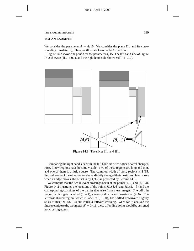
book April 3, 2009

THE BARRIER THEOREM 129

14.3 AN EXAMPLE

We consider the parameterA = 4/15. We consider the plane5− and its corre-sponding translate5′−. Here we illustrate Lemma 14.3 in action.

Figure 14.2 shows one period for the parameter 4/15. The left hand side of Figure14.2 showsπ(5− ∩ R−), and the right hand side showsπ(5′− ∩ R−).

(8,−3)(4,6)

Figure 14.2: The slices5− and5′−.

Comparing the right hand side with the left hand side, we notice several changes.First, 3 new regions have become visible. Two of these regions are long and thin,and one of them is a little square. The common width of these regions is 1/15.Second, some of the other regions have slightly changed their positions. In all caseswhen an edge moves, the offset is by 1/15, as predicted by Lemma 14.3.

We compute that the two relevant crossings occur at the points(4,6) and(8,−3).Figure 14.2 illustrates the locations of the pointsM−(4,6) andM−(8,−3) and thecorresponding crossings of the barrier that arise from these images. The tall thinregion, which gets labelled(0,−1), causes a downward crossing at(4,6). Theleftmost shaded region, which is labelled(−1,0), has shifted downward slightlyso as to meetM−(8,−3) and cause a leftward crossing. Were we to analyze thefigure relative to the parameterA′ = 3/11, these offendingpoints would be assignednoncrossing edges.

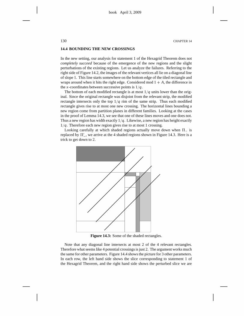
book April 3, 2009

130 CHAPTER 14

14.4 BOUNDING THE NEW CROSSINGS

In the new setting, our analysis for statement 1 of the Hexagrid Theorem does notcompletely succeedbecause of the emergence of the new regions and the slightperturbations of the existing regions. Let us analyze the failures. Referring to theright side of Figure 14.2, the images of the relevant vertices all lie on a diagonal lineof slope 1. This line starts somewhere on the bottom edge of the tiled rectangle andwraps around when it hits the right edge. Considered mod 1+ A, the difference inthex-coordinates between successive points is 1/q.

The bottom of each modified rectangle is at most 1/q units lower than the orig-inal. Since the original rectangle was disjoint from the relevant strip, the modifiedrectangle intersects only the top 1/q rim of the same strip. Thus each modifiedrectangle gives rise to at most one new crossing. The horizontal lines bounding anew region come from partition planes in different families. Looking at the casesin the proof of Lemma 14.3, we see that one of these lines movesand one does not.Thus a new region has width exactly 1/q. Likewise, a new region has height exactly1/q. Therefore each new region gives rise to at most 1 crossing.

Looking carefully at which shaded regions actually move down when5− isreplaced by5′−, we arrive at the 4 shaded regions shown in Figure 14.3. Here is atrick to get down to 2.

Figure 14.3: Some of the shaded rectangles.

Note that any diagonal line intersects at most 2 of the 4 relevant rectangles.Therefore what seems like 4 potential crossings is just 2. The argument works muchthe same for other parameters. Figure 14.4 shows the picturefor 3 other parameters.In each row, the left hand side shows the slice correspondingto statement 1 ofthe Hexagrid Theorem, and the right hand side shows the perturbed slice we are

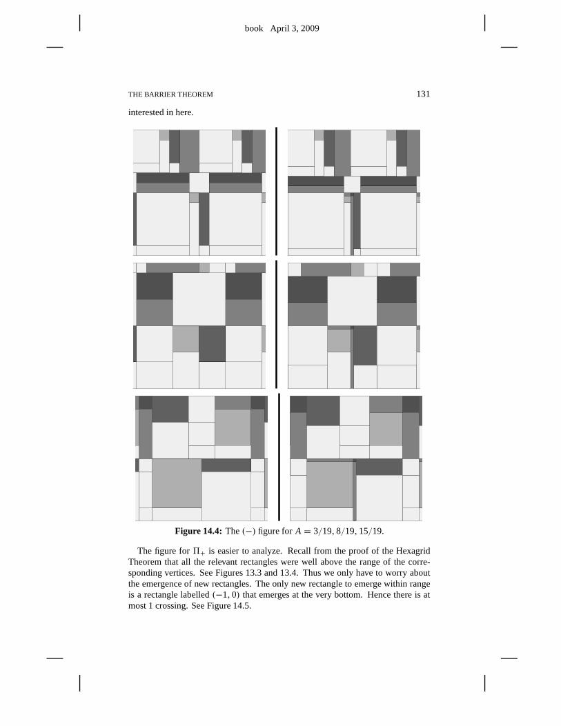
book April 3, 2009

THE BARRIER THEOREM 131

interested in here.

Figure 14.4: The(−) figure for A = 3/19,8/19,15/19.

The figure for5+ is easier to analyze. Recall from the proof of the HexagridTheorem that all the relevant rectangles were well above therange of the corre-sponding vertices. See Figures 13.3 and 13.4. Thus we only have to worry aboutthe emergence of new rectangles. The only new rectangle to emerge within rangeis a rectangle labelled(−1,0) that emerges at the very bottom. Hence there is atmost 1 crossing. See Figure 14.5.

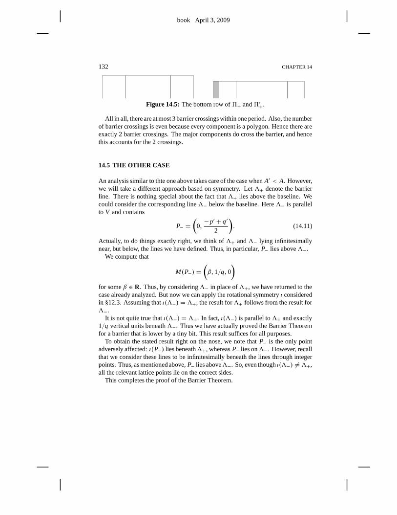
book April 3, 2009

132 CHAPTER 14

Figure 14.5: The bottom row of5+ and5′+.

All in all, there are at most 3 barrier crossings within one period. Also, the numberof barrier crossings is even because every component is a polygon. Hence there areexactly 2 barrier crossings. The major components do cross the barrier, and hencethis accounts for the 2 crossings.

14.5 THE OTHER CASE

An analysis similar to thte one above takes care of the case whenA′ < A. However,we will take a different approach based on symmetry. Let3+ denote the barrierline. There is nothing special about the fact that3+ lies above the baseline. Wecould consider the corresponding line3− below the baseline. Here3− is parallelto V and contains

P− =(

0,−p′ + q′

2

). (14.11)

Actually, to do things exactly right, we think of3+ and3− lying infinitesimallynear, but below, the lines we have defined. Thus, in particular, P− lies above3−.

We compute that

M(P−) =(β,1/q,0

)

for someβ ∈ R. Thus, by considering3− in place of3+, we have returned to thecase already analyzed. But now we can apply the rotational symmetryι consideredin §12.3. Assuming thatι(3−) = 3+, the result for3+ follows from the result for3−.

It is not quite true thatι(3−) = 3+. In fact,ι(3−) is parallel to3+ and exactly1/q vertical units beneath3−. Thus we have actually proved the Barrier Theoremfor a barrier that is lower by a tiny bit. This result suffices for all purposes.

To obtain the stated result right on the nose, we note thatP− is the only pointadversely affected:ι(P−) lies beneath3+, whereasP− lies on3−. However, recallthat we consider these lines to be infinitesimally beneath the lines through integerpoints. Thus, as mentionedabove,P− lies above3−. So, even thoughι(3−) 6= 3+,all the relevant lattice points lie on the correct sides.

This completes the proof of the Barrier Theorem.

book April 3, 2009

Chapter Fifteen

Proof of Hexagrid Theorem II

We will prove statement 2 of the Hexagrid Theorem for odd rationals. The even casehas an essentially identical proof. Here we remark on one small difference. Call apoint in R2 bad if it has the form(m, y), wherey is a half-integer. According tostatement 3 of Lemma 15.1 below, a door cannot be a bad point inthe odd case. Inthe even case, we simply declare that a door cannot be a bad point. See the definitionin Chapter 3. Having ruled out the bad points in both cases, our proof is practicallyindependent of parity.

15.1 THE STRUCTURE OF THE DOORS

Our proof of statement 2 of the Hexagrid Theorem requires a careful analysis ofthe doors. In this first section, we will establish a technical result about the doors.Say that awall line is a line of positive slope in the room grid. These lines are allparallel to the vectorW, from Equation 3.2. Recall that2 is the lattice, from §12.1.We distinguish two special kinds of points inR2.

• Type 1:(aq,b/p), with a,b ∈ Z.

• Type 2:(ap,b/q), with a,b ∈ Z.

A point could have both types. Here is our structural result.

Lemma 15.1 The following are true.

1. Any two wall lines are equivalent mod2.

2. The only points ofZ2 lying on wall lines are elements of2.

3. Every door on L0 has type 1 or type 2 (or both).

Proof: Statement 1: Recall that2 is generated byV andV ′, the vectors fromEquation 12.1. Modulo translation byZ [V ], any wall line is equivalent toL0 orL1. We just need to show that these two wall lines are equivalentto each other mod2. We check explicitly that the following equation holds.

V ′ + p+ 1

2V ∈ 2 ∩ L1.

Hence addition by some vector in2 carriesL0 to L1. HenceL0 andL1 are equiv-alent mod2.

book April 3, 2009

134 CHAPTER 15

Statement 2: By statement 1, it suffices to consider the case when(m,n) ∈ L0.Any point in L0 is a real multiple ofW. Such a point has the form

sW= s

2(p+ q)(2pq, (p+ q)2− 2p2). (15.1)

In order for this point to lie inZ2, the first coordinate must be an integer. Hence

s =k(p+ q)

pq, k ∈ Z. (15.2)

Hence

n = k× pq+ (q2− p2)/2

pq∈ Z. (15.3)

Sincep andq are relatively prime, the numerator and denominator of the rationalon the right side of Equation 15.3 are relatively prime. Hence pq dividesk. Hence(m,n) is an integer multiple of the point

(p+ q)W =(

pq,(p+ q)2

2− p2

)= 2V ′ + pV ∈ 2.

HereV andV ′ are the vectors generating2, as in Equation 12.1.

statement 3: Let K denote the arithmetic kite associated to the parameter. Calla line in the door gridtop if it is parallel to one of the top two edges ofK. Call a linein the door gridbottomif it is parallel to one of the bottom two edges ofK. Call adoortop if it lies on a top door line, andbottomif it lies on a bottom door line.

Our argument crucially uses the pointU in Figure 3.1. We have

U =(

p,q2− p2 + 2pq

2q

). (15.4)

The bottom doors are evenly spaced onL0. Two consecutive ones are

(0,0),q

pU =

(q,

q2− p2+ 2pq

2p

)=(

q,b

p

). (15.5)

Every bottom door onL0 is a multiple of the nontrivial one we have listed. Henceevery bottom door has type 1.

The top doors are evenly spaced onL0. Two consecutive ones are

(0,0), U = (p,b/q). (15.6)

Every top door onL0 is an integer multiple of the nontrivial one we have listed.Hence such doors have type 2. 2

Remark: In the even case, statement 1 of Lemma 15.1 has a trivial proof: Any twowall lines are equivalent modulo translations by integer multiples of V .

book April 3, 2009

PROOF OF HEXAGRID THEOREM II 135

15.2 ORDINARY CROSSING CELLS

The bijection between crossing cells and doors described instatement 2 of theHexagrid Theorem commutes with the action of the symmetry group2. The pointis that2 preserves both the hexagrid and the arithmetic graph. Hence, by statement1 of Lemma 15.1, it suffices to consider those crossing cells that crossL0.

We first deal with two trivial cases. Recall that the point(0,0) gives rise to twodoors. One of the doors, which we denote(0,0)+, is attached to the wall above(0,0). The other door, which we denote(0,0)−, is attached to the wall below(0,0). Any door lying in2 is equivalent to one of these, by statement 2 of Lemma15.1. One of the crossing cells has vertices(−1,1), (0,0), and(1,1). We associate(0,0)+ to this crossing cell. Another crossing cell has vertices(0,−1) and(−1,0).We associate the door(0,0)− to this cell.

Henceforth we consider crossing cells that crossL0 but are not equivalent mod2to either of the ones we have just described. We call these remaining crossing cellsordinary cells. Given an ordinary cellc, let vc denote the vertex ofc that lies to theright of L0. (The first statement of the next lemma justifies the existence ofvc.)

Lemma 15.2 An ordinary cell c has a single edge that crosses L0 in its interior.Moreover,vc + (ǫ1, ǫ2) 6∈ L0 for any choice of(ǫ1, ǫ2) ∈ {−1,0,1}2.

Proof: Let c be a crossing cell. If an edge ofc fails to crossL0 at an interior point,then a vertex ofc lies onL0. But thenc ≡ (0,0)mod2, by statement 2 of Lemma15.1. Ifvc+ (ǫ1, ǫ2) ∈ L0, thenvc ≡ (−ǫ1,−ǫ2)mod2, by statement 2 of Lemma15.1. Hence(−ǫ1,−ǫ2) is the right vertex of a crossing cell. This happens for(1,1)and(0,−1), but these are the special crossing cells we have already handled. Theonly point in L0 within reach of either(1,−1) or (1,0) is (0,0), and we alreadyknow that(0,0) does not connect to these points. The remaining 4 choices lietothe left ofL0. This rules out all cases. 2

Now we describe the bijection between ordinary crossing cells and doors. Belowwe will prove the following result.

Lemma 15.3 (Separation)Let c be an ordinary cell and letvc be the right vertexof c. Then L0 separatesvc from vc + (0,1).

We writevc = (m,n). Letθ ∈ (n,n+1) be the point such that(m, θ) ∈ L0. Wedefine

ϒ(c) = (n, θ). (15.7)

Lemma 15.4 (Door) Let v be an ordinary crossing cell. Thenϒ(c) is a door.

The mapc → ϒ(c) is certainly injective. To finish our proof of the HexagridTheorem, we will prove the following result.

Lemma 15.5 (Surjection) The mapϒ is a surjective map from the set of ordinarycrossing cells to the set of doors on L0 that do not lie in2.

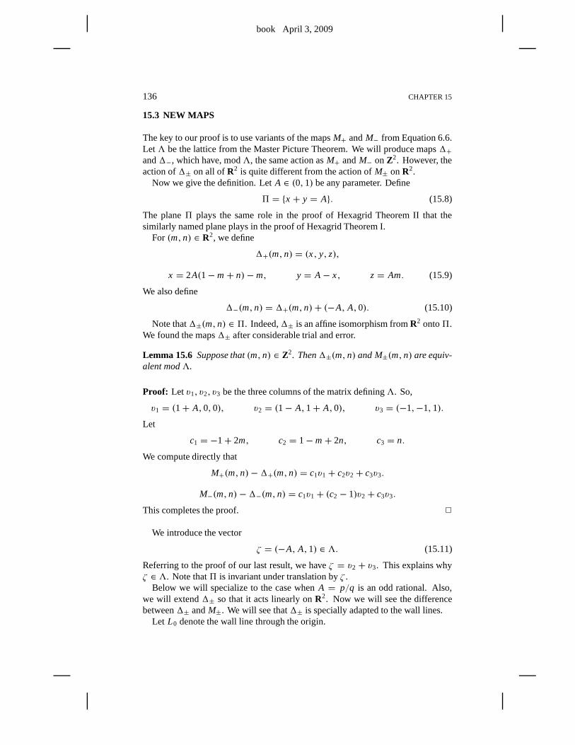
book April 3, 2009

136 CHAPTER 15

15.3 NEW MAPS

The key to our proof is to use variants of the mapsM+ andM− from Equation 6.6.Let3 be the lattice from the Master Picture Theorem. We will produce maps1+and1−, which have, mod3, the same action asM+ andM− on Z2. However, theaction of1± on all ofR2 is quite different from the action ofM± onR2.

Now we give the definition. LetA ∈ (0,1) be any parameter. Define

5 = {x + y = A}. (15.8)

The plane5 plays the same role in the proof of Hexagrid Theorem II that thesimilarly named plane plays in the proof of Hexagrid TheoremI.

For (m,n) ∈ R2, we define

1+(m,n) = (x, y, z),

x = 2A(1−m+ n)−m, y = A− x, z= Am. (15.9)

We also define

1−(m,n) = 1+(m,n)+ (−A, A,0). (15.10)

Note that1±(m,n) ∈ 5. Indeed,1± is an affine isomorphism fromR2 onto5.We found the maps1± after considerable trial and error.

Lemma 15.6 Suppose that(m,n) ∈ Z2. Then1±(m,n) and M±(m,n) are equiv-alent mod3.

Proof: Let v1, v2, v3 be the three columns of the matrix defining3. So,

v1 = (1+ A,0,0), v2 = (1− A,1+ A,0), v3 = (−1,−1,1).

Let

c1 = −1+ 2m, c2 = 1−m+ 2n, c3 = n.

We compute directly that

M+(m,n)−1+(m,n) = c1v1 + c2v2 + c3v3.

M−(m,n)−1−(m,n) = c1v1 + (c2 − 1)v2 + c3v3.

This completes the proof. 2

We introduce the vector

ζ = (−A, A,1) ∈ 3. (15.11)

Referring to the proof of our last result, we haveζ = v2 + v3. This explains whyζ ∈ 3. Note that5 is invariant under translation byζ .

Below we will specialize to the case whenA = p/q is an odd rational. Also,we will extend1± so that it acts linearly onR2. Now we will see the differencebetween1± andM±. We will see that1± is specially adapted to the wall lines.

Let L0 denote the wall line through the origin.

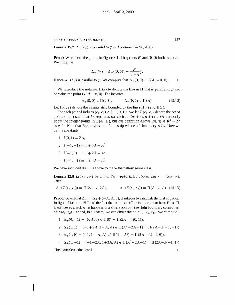
book April 3, 2009

PROOF OF HEXAGRID THEOREM II 137

Lemma 15.71±(L0) is parallel toζ and contains(−2A, A,0).

Proof: We refer to the points in Figure 3.1. The pointsW and(0,0) both lie onL0.We compute

1+(W)−1+((0,0)) =p2

p+ qζ.

Hence1+(L0) is parallel toζ . We compute that1+(0,0) = (2A,−A,0). 2

We introduce the notation5(x) to denote the line in5 that is parallel toζ andcontains the point(x, A− x,0). For instance,

1+(0,0) ∈ 5(2A), 1−(0,0) ∈ 5(A). (15.12)

Let5(r, s) denote the infinite strip bounded by the lines5(r ) and5(s).For each pair of indices(ǫ1, ǫ2) ∈ {−1,0,1}2, we let6(ǫ1, ǫ2) denote the set of

points(m,n) such thatL0 separates(m,n) from (m+ ǫ1,n + ǫ2). We care onlyabout the integer points in6(ǫ1, ǫ2), but our definition allows(m,n) ∈ R2 − Z2

as well. Note that6(ǫ1, ǫ2) is an infinite strip whose left boundary isL0. Now wedefine constants

1. λ(0,1) = 2A,

2. λ(−1,−1) = 1+ 0A− A2,

3. λ(−1,0) = 1+ 2A− A2,

4. λ(−1,+1) = 1+ 4A− A2.

We have included 0A = 0 above to make the pattern more clear.

Lemma 15.8 Let (ǫ1, ǫ2) be any of the4 pairs listed above. Letλ = λ(ǫ1, ǫ2).Then

1+(6(ǫ1, ǫ2)) = 5(2A−λ,2A), 1−(6(ǫ1, ǫ2)) = 5(A−λ, A). (15.13)

Proof: Given that1− = 1++ (−A, A,0), it suffices to establish the first equation.In light of Lemma 15.7 and the fact that1+ is an affine isomorphism fromR2 to5,it suffices to check what happens to a single point on the rightboundary componentof 6(ǫ1, ǫ2). Indeed, in all cases, we can chose the point(−ǫ1, ǫ2). We compute

1. 1+(0,−1) = (0, A,0) ∈ 5(0) = 5(2A− λ(0,1)).

2. 1+(1,1) = (−1+2A,1−A, A) ∈ 5(A2+2A−1) = 5(2A−λ(−1,−1)).

3. 1+(1,0) = (−1,1+ A, A) ∈∗ 5(1− A2) = 5(2A− λ(−1,0)).

4. 1+(1,−1) = (−1−2A,1+3A, A) ∈ 5(A2−2A−1) = 5(2A−λ(−1,1)).

This completes the proof. 2

book April 3, 2009

138 CHAPTER 15

15.4 INTERSECTION RESULTS

Here we describe some intersection results that we prove in the next chapter.For ease of notation, we define

5+((ǫ1, ǫ2; A)) = 5(2A− λ(ǫ1, ǫ2),2A), (15.14)

5−((ǫ1, ǫ2; A)) = 5(A− λ(ǫ1, ǫ2), A). (15.15)

To be precise, we take5±((ǫ1, ǫ2)) to be the interior (relative to5) of the strip.These strips correspond to those in Lemma 15.8.

As usual,3R denotes the orbit ofR under the lattice3. In the next result,Xo

denotes the interior ofX. We prove the following result in Chapter 16.

Lemma 15.9 (Intersection) The following hold for all A∈ (0,1).

1. For each pair(ǫ1, ǫ2) from Lemma 15.8,

5±((ǫ1, ǫ2; A)) ∩3Ro±(ǫ1, ǫ2; A) ≡ (0,0).

2. Let(ǫ1, ǫ2) be either(−1,−1) or (−1,1). Then

5±((ǫ1, ǫ2; A)) ∩3R±(ǫ1, ǫ2; A) ⊂ ∂5±((0,1)).

3. Let(ǫ1, ǫ2) be either(−1,0) or (0,1). Then

5±((ǫ1, ǫ2; A)) ∩3R±(ǫ1, ǫ2; A) ⊂ 5o±(0,1).

Remark: Let5old denote the plane we considered in the proof of Hexagrid Theo-rem I. By construction, the vector(1,1,1) is contained in5old. Thus, when we usethe method of §6.5 to implement the Master Picture Theorem, we need only lookat how5old intersects theinteriors of the polyhedra in the partitions. On the otherhand,(1,1,1) is not contained in the plane5new = 5. It turns out that5 doesintersect the lower boundaries of some of the polyhedra in the partition, and thiscreates the crossings. In other words, case 3 of the Intersection Lemma is nontrivial.

Proof of the Separation Lemma: Supposec is an ordinary crossing cell. Letv = vc be the right vertex. Suppose that the left vertex isv + (ǫ1, ǫ2). There issome choice of sign (say+) such that

1+(v) ∈ 5+((ǫ1, ǫ2; A)) ∩3R+(ǫ1, ǫ2; A). (15.16)

The first containment comes from Lemma 15.8. The second containment comesfrom the Master Picture Theorem. Applied directly, the Master Picture Theoremrefers to the mapsM±, but Lemma 15.6 lets us replaceM± with 1±.

The intersection in Equation 15.16 is empty in case 1 of the Intersection Lemma.By Lemma 15.2, we havev 6∈ 6±(0,1). Hence1+(v) 6∈ ∂5+(0,1). Hence case2 of the Intersection Lemma does not apply here. We must have case 3. By case 3,we havev ∈ 5±(0,1). But then, by Lemma 15.8, we havev ∈ interior(6(0,1)). 2

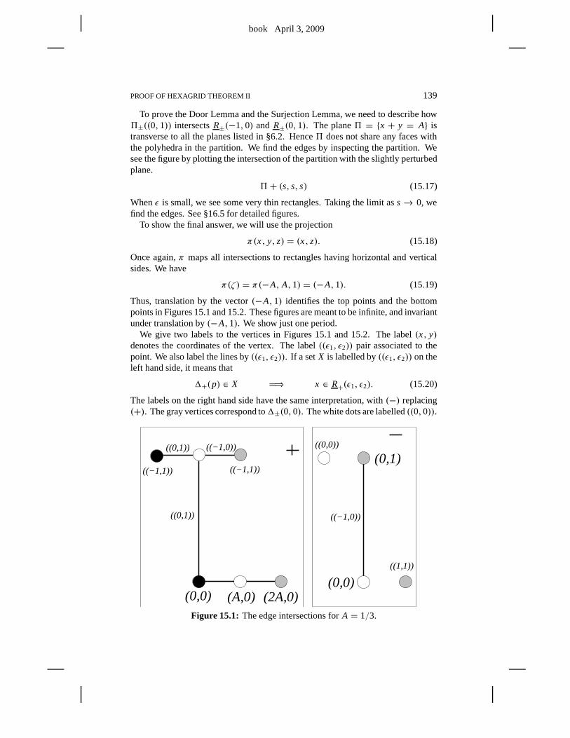
book April 3, 2009

PROOF OF HEXAGRID THEOREM II 139

To prove the Door Lemma and the Surjection Lemma, we need to describe how5±((0,1)) intersectsR±(−1,0) and R±(0,1). The plane5 = {x + y = A} istransverse to all the planes listed in §6.2. Hence5 does not share any faces withthe polyhedra in the partition. We find the edges by inspecting the partition. Wesee the figure by plotting the intersection of the partition with the slightly perturbedplane.

5+ (s, s, s) (15.17)

Whenǫ is small, we see some very thin rectangles. Taking the limit as s→ 0, wefind the edges. See §16.5 for detailed figures.

To show the final answer, we will use the projection

π(x, y, z) = (x, z). (15.18)

Once again,π maps all intersections to rectangles having horizontal andverticalsides. We have

π(ζ ) = π(−A, A,1) = (−A,1). (15.19)

Thus, translation by the vector(−A,1) identifies the top points and the bottompoints in Figures 15.1 and 15.2. These figures are meant to be infinite, and invariantunder translation by(−A,1). We show just one period.

We give two labels to the vertices in Figures 15.1 and 15.2. The label(x, y)denotes the coordinates of the vertex. The label((ǫ1, ǫ2)) pair associated to thepoint. We also label the lines by((ǫ1, ǫ2)). If a setX is labelled by((ǫ1, ǫ2)) on theleft hand side, it means that

1+(p) ∈ X H⇒ x ∈ R+(ǫ1, ǫ2). (15.20)

The labels on the right hand side have the same interpretation, with (−) replacing(+). The gray vertices correspond to1±(0,0). The white dots are labelled((0,0)).

((−1,0))

((−1,1))((−1,1))

(0,0) (A,0) (2A,0)(0,0)

((0,0))

((1,1))

(0,1)((0,1)) ((−1,0))

((0,1))

Figure 15.1: The edge intersections forA = 1/3.

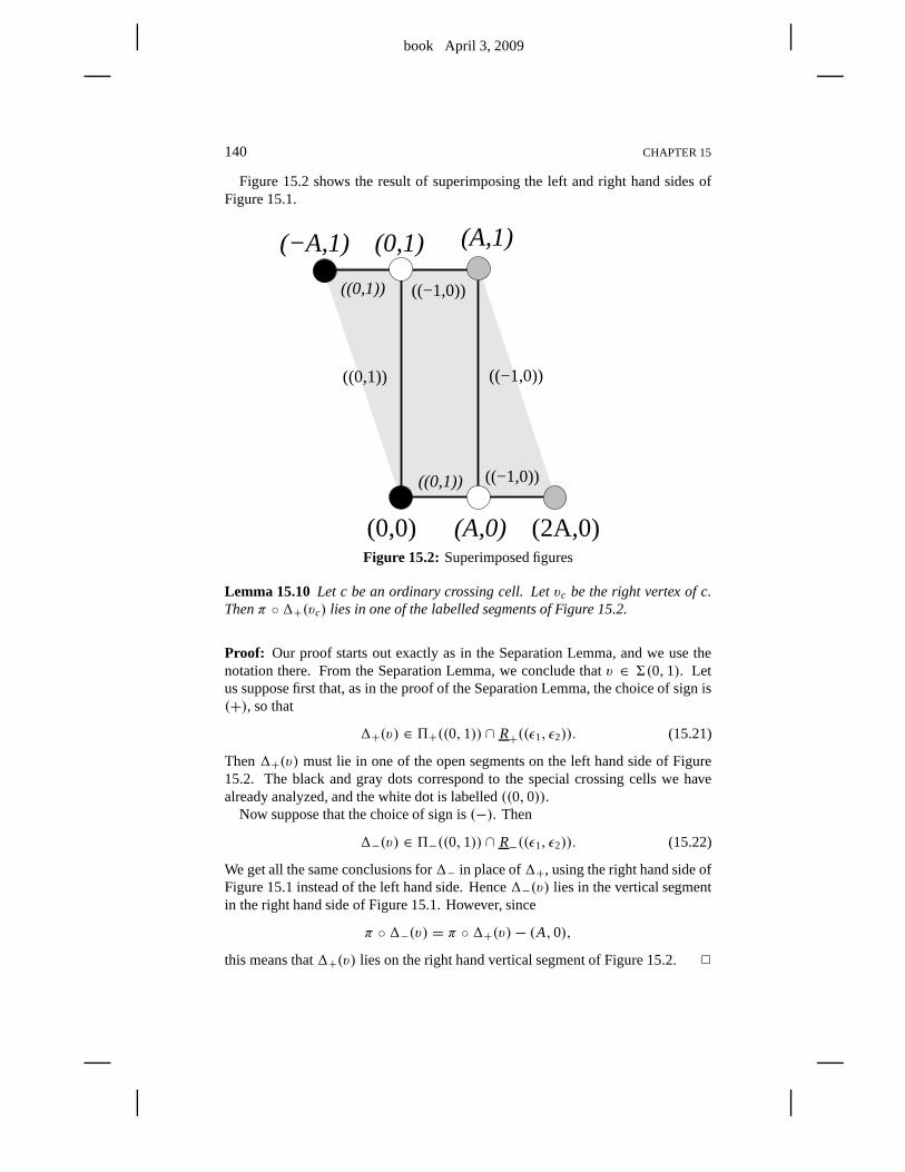
book April 3, 2009

140 CHAPTER 15

Figure 15.2 shows the result of superimposing the left and right hand sides ofFigure 15.1.

((−1,0))((0,1))

((−1,0))

(A,1)(−A,1) (0,1)

((0,1))

(A,0) (2A,0)(0,0)

((−1,0))((0,1))

Figure 15.2: Superimposed figures

Lemma 15.10 Let c be an ordinary crossing cell. Letvc be the right vertex of c.Thenπ ◦1+(vc) lies in one of the labelled segments of Figure 15.2.

Proof: Our proof starts out exactly as in the Separation Lemma, and we use thenotation there. From the Separation Lemma, we conclude thatv ∈ 6(0,1). Letus suppose first that, as in the proof of the Separation Lemma,the choice of sign is(+), so that

1+(v) ∈ 5+((0,1)) ∩ R+((ǫ1, ǫ2)). (15.21)

Then1+(v) must lie in one of the open segments on the left hand side of Figure15.2. The black and gray dots correspond to the special crossing cells we havealready analyzed, and the white dot is labelled((0,0)).

Now suppose that the choice of sign is(−). Then

1−(v) ∈ 5−((0,1)) ∩ R−((ǫ1, ǫ2)). (15.22)

We get all the same conclusions for1− in place of1+, using the right hand side ofFigure 15.1 instead of the left hand side. Hence1−(v) lies in the vertical segmentin the right hand side of Figure 15.1. However, since

π ◦1−(v) = π ◦1+(v)− (A,0),

this means that1+(v) lies on the right hand vertical segment of Figure 15.2.2

book April 3, 2009

PROOF OF HEXAGRID THEOREM II 141

15.5 THE END OF THE PROOF

Proof of the Door Lemma: Let v = (m,n) be the right vertex of an ordinarycrossing cell. Letϒ(c) = (m, θ). Heren is the floor ofθ . Let

1+(v) = (x, y, z). (15.23)

There are two cases to consider. Supposeπ ◦ 1+(v) lies in one of the openhorizontal segments of Figure 15.2. Then

(x, y, z) ≡ (t, A− t,0) mod 3, t ∈ (0, A) ∪ (A,2A). (15.24)

By Equation 15.24, the third coordinate of1+(v) is an integer. By the definition of1+, we haveAm= pm/q ∈ Z. Henceq dividesm. Hencev = (kq,n) for somek ∈ Z. Hencev lies in the intersection ofL0 with a door line. Hencev is a door.

Supposeπ ◦ 1+(v) lies in a vertical segment in Figure 15.2. Looking at thepositions of the vertical line segments in Figure 15.2, we have

x = k A, k ∈ Z. (15.25)

From the definition of1+, we have

2(1−m+ n)−m

A=

x

A∈ Z. (15.26)

Hencem/A ∈ Z. Hencem = kp. But then the first coordinate ofϒ(c) coincideswith the first coordinate of a door onL0, by statement 3 of Lemma 15.1. Sinceϒ(c) ∈ L0, we now see thatϒ(c) is a door. 2

Proof of the Surjection Lemma: We would like to see that each door actuallyarises in our construction above. There are two cases.

Type 1: By statement 3 of Lemma 15.1, each type 1 door has the form(aq,b/p),wherea ∈ Z and b/p is not a half-integer. Letn be the floor of(b/p), letv = (aq,n), andet(x, y, z) = 1+(v). We will show thatv is the right vertexof an ordinary crossing cell.

Since the first coordinate ofv has the formaq, we havex ∈ Z. Sincev ∈ 6(0,1),we have1+(v) ∈ 5(0,2A). Hence Equation 15.24 holds. We rule out the casethat t = A becauseb/p is not a half-integer. Hence1+(v) lands in a horizontalstrip in Figure 15.2. Hence one of the edges ofŴ emanating fromv is either(0,1)or (−1,0). This edge crossesL0 becausev ∈ 6(0,1) ⊂ 6(−1,0). Hencev is theright vertex of a crossing cell.

Type 2: By symmetry, it suffices to consider the type 2 doors onL0. By state-ment 3 of Lemma 15.1, such a door has the form(ap,b/q). Let v = (ap,n), as inthe first case. With the same notation as above,

x = 2A(1− ap− n)− aq A= a′A (15.27)

for somea′ ∈ Z. Also, 1+(v) ∈ 5(0,2A). Hence1+(v) lands in one of thevertical strips of Figure 15.2. The same argument as in the previous case finishesthe proof. 2

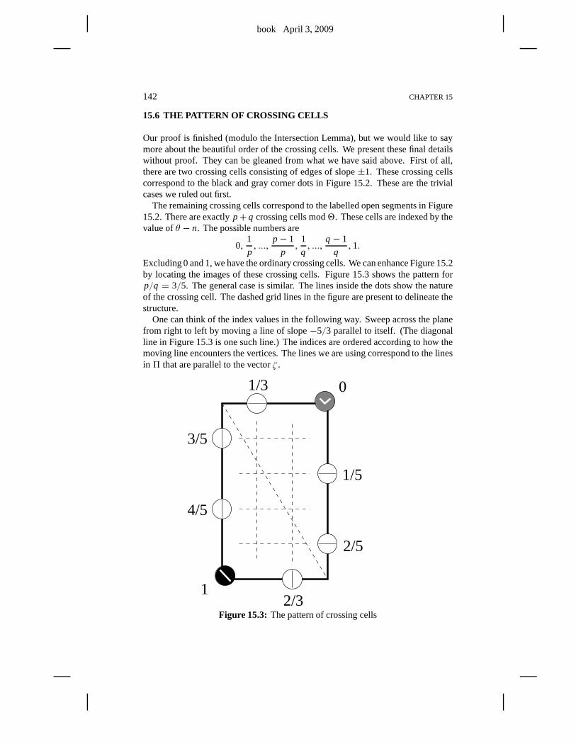
book April 3, 2009

142 CHAPTER 15

15.6 THE PATTERN OF CROSSING CELLS

Our proof is finished (modulo the Intersection Lemma), but wewould like to saymore about the beautiful order of the crossing cells. We present these final detailswithout proof. They can be gleaned from what we have said above. First of all,there are two crossing cells consisting of edges of slope±1. These crossing cellscorrespond to the black and gray corner dots in Figure 15.2. These are the trivialcases we ruled out first.

The remaining crossing cells correspond to the labelled open segments in Figure15.2. There are exactlyp+ q crossing cells mod2. These cells are indexed by thevalue ofθ − n. The possible numbers are

0,1

p, ...,

p− 1

p,

1

q, ...,

q − 1

q,1.

Excluding 0 and 1, we have the ordinary crossing cells. We canenhance Figure 15.2by locating the images of these crossing cells. Figure 15.3 shows the pattern forp/q = 3/5. The general case is similar. The lines inside the dots showthe natureof the crossing cell. The dashed grid lines in the figure are present to delineate thestructure.

One can think of the index values in the following way. Sweep across the planefrom right to left by moving a line of slope−5/3 parallel to itself. (The diagonalline in Figure 15.3 is one such line.) The indices are orderedaccording to how themoving line encounters the vertices. The lines we are using correspond to the linesin 5 that are parallel to the vectorζ .

2/3

0

1

4/5

3/5

1/5

2/5

1/3

Figure 15.3: The pattern of crossing cells

book April 3, 2009

Chapter Sixteen

Proof of the Intersection Lemma

16.1 DISCUSSION OF THE PROOF

One way to prove the Intersection Lemma is just by inspection. One can play withBilliard King and see that the result is true. Given the simple nature of the partitionsinvolved, a falsehood in the lemma would be easily detectable by a small amountof experimentation.

Rather than just appeal to experimentation, we will explaina proof that involvesfinding the intersection patterns of finitely many convex lattice polytopes inR4. Theproof we give is similar to that presented in previous chapters. Previously, e.g., in§11.1, our method was straightforward. Here there is a technical complication thatwe need to address. This chapter is really about dealing withthis complication.

Let X(. . . ; A) ⊂ R3 denote some subset ofR3 that depends on the parameterA.For such an object, we define

X(. . .) =⋃

A

(X(. . . ; A)× {A}

). (16.1)

For instance, the setsR±(ǫ1, ǫ2) are exactly the convex polytopes from §6.7.Let S⊂ R3 denote the infinite slab bounded by the planes{z = 0} and{z = 1}.

Let

6∗±(ǫ1, ǫ2; A) = 6±(ǫ1, ǫ2; A) ∩ S. (16.2)

We include the boundary pieces6(. . .) ∩ ∂S. Thus we are including the topsand bottoms of the parallelogram but not its sides. Figure 15.2 provides a goodimpression of what this parallelogram looks like.

The set6∗±(ǫ1, ǫ2) is contained in a hyperplane ofR3. Unfortunately, this set isnot a polyhedron. For instance, the vertices vary quadratically with the parameter.Thus our method breaks down: We cannot control6∗±(ǫ1, ǫ2) just by its vertices inR4.

The trick is to cover6(. . . ; A) by 2 quadrilateralsQ1(. . . ; A) and Q2(. . . ; A)whose vertices vary linearly with the parameter. The linearvariation in itself is notenough to guarantee that the corresponding unionsQ1(. . .) andQ2(. . .) are convex,but it turns out that these unions are indeed convex integralpolyhedra. When weuseQ1(. . .) and Q2(. . .) in place of6(. . .), we create no new interesections – atleast not in the interiors. Thus], we prove the IntersectionLemma for these largersets by the same method we used in §11.1. When we are finished weinterpret theresults in terms of the original sets.

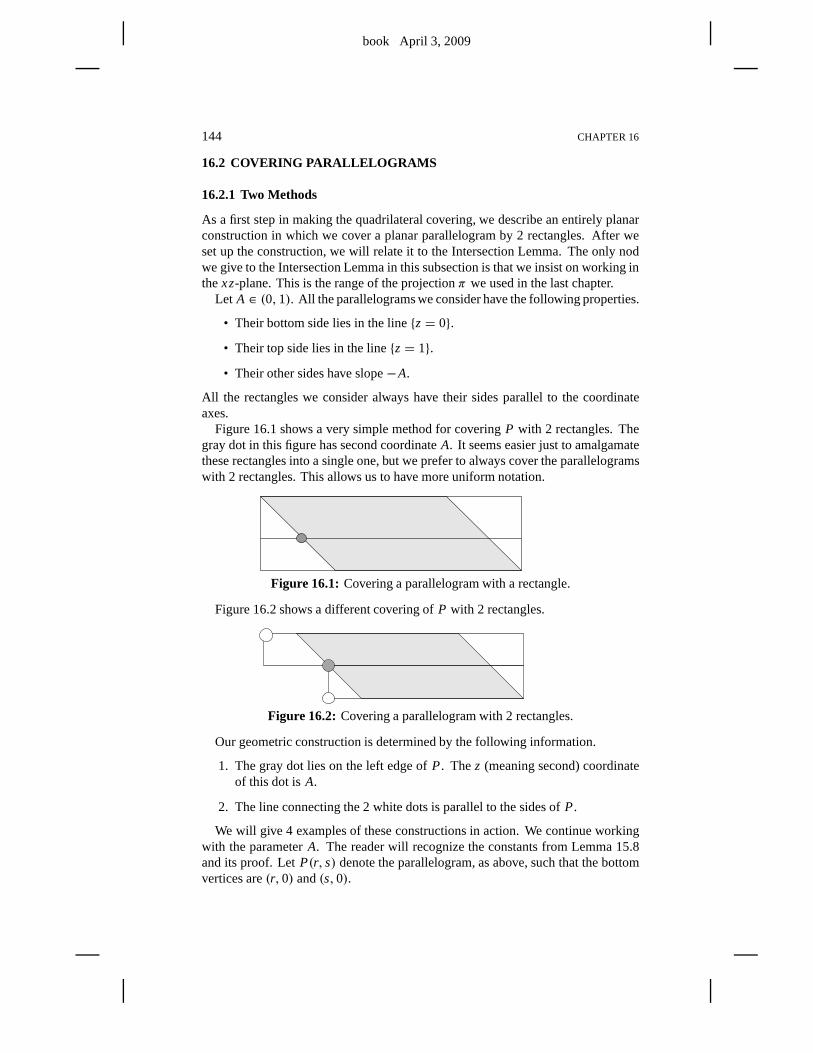
book April 3, 2009

144 CHAPTER 16

16.2 COVERING PARALLELOGRAMS

16.2.1 Two Methods

As a first step in making the quadrilateral covering, we describe an entirely planarconstruction in which we cover a planar parallelogram by 2 rectangles. After weset up the construction, we will relate it to the Intersection Lemma. The only nodwe give to the Intersection Lemma in this subsection is that we insist on working inthexz-plane. This is the range of the projectionπ we used in the last chapter.

Let A ∈ (0,1). All the parallelograms we consider have the following properties.

• Their bottom side lies in the line{z= 0}.

• Their top side lies in the line{z= 1}.

• Their other sides have slope−A.

All the rectangles we consider always have their sides parallel to the coordinateaxes.

Figure 16.1 shows a very simple method for coveringP with 2 rectangles. Thegray dot in this figure has second coordinateA. It seems easier just to amalgamatethese rectangles into a single one, but we prefer to always cover the parallelogramswith 2 rectangles. This allows us to have more uniform notation.

Figure 16.1: Covering a parallelogram with a rectangle.

Figure 16.2 shows a different covering ofP with 2 rectangles.

Figure 16.2: Covering a parallelogram with 2 rectangles.

Our geometric construction is determined by the following information.

1. The gray dot lies on the left edge ofP. Thez (meaning second) coordinateof this dot isA.

2. The line connecting the 2 white dots is parallel to the sides of P.

We will give 4 examples of these constructions in action. We continue workingwith the parameterA. The reader will recognize the constants from Lemma 15.8and its proof. LetP(r, s) denote the parallelogram, as above, such that the bottomvertices are(r,0) and(s,0).

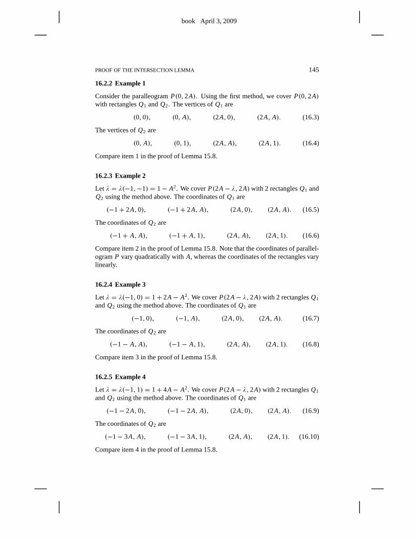
book April 3, 2009

PROOF OF THE INTERSECTION LEMMA 145

16.2.2 Example 1

Consider the paralleogramP(0,2A). Using the first method, we coverP(0,2A)with rectanglesQ1 andQ2. The vertices ofQ1 are

(0,0), (0, A), (2A,0), (2A, A). (16.3)

The vertices ofQ2 are

(0, A), (0,1), (2A, A), (2A,1). (16.4)

Compare item 1 in the proof of Lemma 15.8.

16.2.3 Example 2

Let λ = λ(−1,−1) = 1− A2. We coverP(2A− λ,2A) with 2 rectanglesQ1 andQ2 using the method above. The coordinates ofQ1 are

(−1+ 2A,0), (−1+ 2A, A), (2A,0), (2A, A). (16.5)

The coordinates ofQ2 are

(−1+ A, A), (−1+ A,1), (2A, A), (2A,1). (16.6)

Compare item 2 in the proof of Lemma 15.8. Note that the coordinates of parallel-ogramP vary quadratically withA, whereas the coordinates of the rectangles varylinearly.

16.2.4 Example 3

Let λ = λ(−1,0) = 1+ 2A− A2. We coverP(2A− λ,2A) with 2 rectanglesQ1

andQ2 using the method above. The coordinates ofQ1 are

(−1,0), (−1, A), (2A,0), (2A, A). (16.7)

The coordinates ofQ2 are

(−1− A, A), (−1− A,1), (2A, A), (2A,1). (16.8)

Compare item 3 in the proof of Lemma 15.8.

16.2.5 Example 4

Let λ = λ(−1,1) = 1+ 4A− A2. We coverP(2A− λ,2A) with 2 rectanglesQ1

andQ2 using the method above. The coordinates ofQ1 are

(−1− 2A,0), (−1− 2A, A), (2A,0), (2A, A). (16.9)

The coordinates ofQ2 are

(−1− 3A, A), (−1− 3A,1), (2A, A), (2A,1). (16.10)

Compare item 4 in the proof of Lemma 15.8.

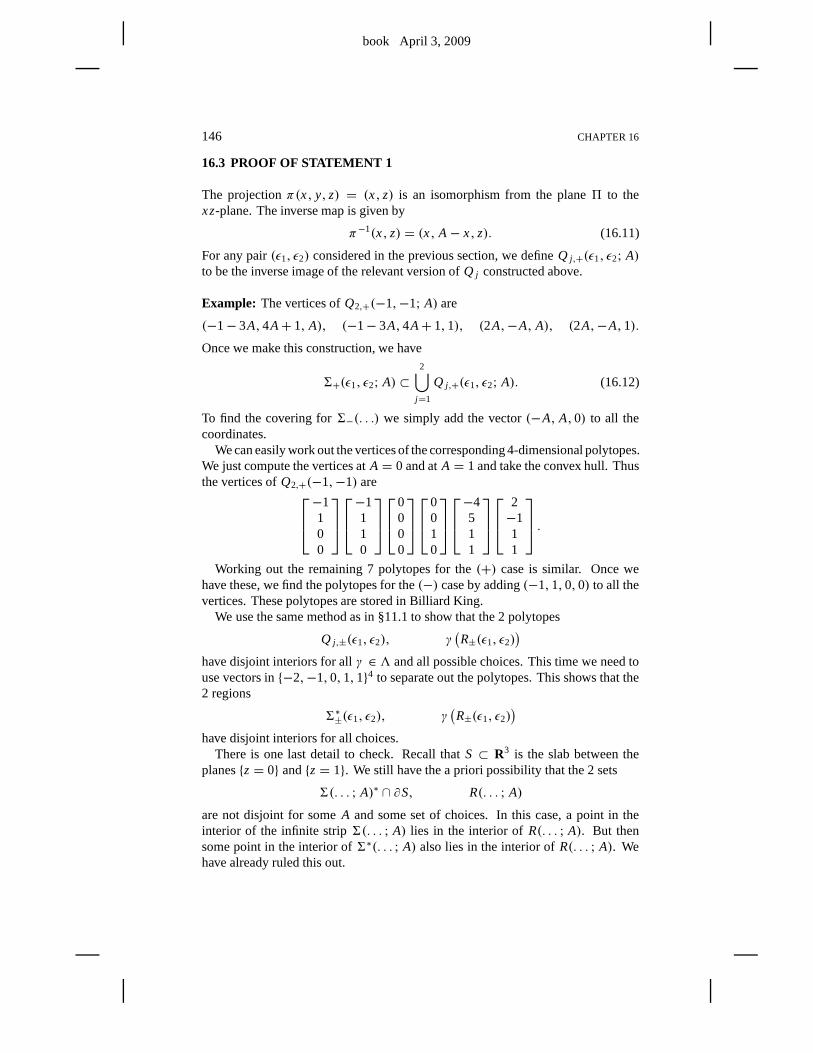
book April 3, 2009

146 CHAPTER 16

16.3 PROOF OF STATEMENT 1

The projectionπ(x, y, z) = (x, z) is an isomorphism from the plane5 to thexz-plane. The inverse map is given by

π−1(x, z) = (x, A− x, z). (16.11)

For any pair(ǫ1, ǫ2) considered in the previous section, we defineQ j ,+(ǫ1, ǫ2; A)to be the inverse image of the relevant version ofQ j constructed above.

Example: The vertices ofQ2,+(−1,−1; A) are

(−1− 3A,4A+ 1, A), (−1− 3A,4A+ 1,1), (2A,−A, A), (2A,−A,1).

Once we make this construction, we have

6+(ǫ1, ǫ2; A) ⊂2⋃

j=1

Q j ,+(ǫ1, ǫ2; A). (16.12)

To find the covering for6−(. . .) we simply add the vector(−A, A,0) to all thecoordinates.

We can easily work out the vertices of the corresponding 4-dimensional polytopes.We just compute the vertices atA = 0 and atA = 1 and take the convex hull. Thusthe vertices ofQ2,+(−1,−1) are

−1100

−1110

0000

0010

−4511

2−111

.

Working out the remaining 7 polytopes for the(+) case is similar. Once wehave these, we find the polytopes for the(−) case by adding(−1,1,0,0) to all thevertices. These polytopes are stored in Billiard King.

We use the same method as in §11.1 to show that the 2 polytopes

Q j ,±(ǫ1, ǫ2), γ(R±(ǫ1, ǫ2)

)

have disjoint interiors for allγ ∈ 3 and all possible choices. This time we need touse vectors in{−2,−1,0,1,1}4 to separate out the polytopes. This shows that the2 regions

6∗±(ǫ1, ǫ2), γ(R±(ǫ1, ǫ2)

)

have disjoint interiors for all choices.There is one last detail to check. Recall thatS ⊂ R3 is the slab between the

planes{z= 0} and{z= 1}. We still have the a priori possibility that the 2 sets

6(. . . ; A)∗ ∩ ∂S, R(. . . ; A)

are not disjoint for someA and some set of choices. In this case, a point in theinterior of the infinite strip6(. . . ; A) lies in the interior ofR(. . . ; A). But thensome point in the interior of6∗(. . . ; A) also lies in the interior ofR(. . . ; A). Wehave already ruled this out.

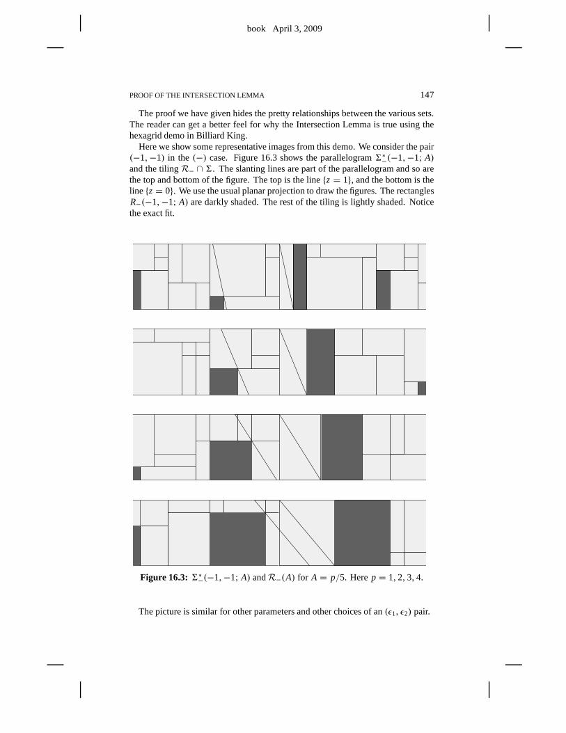
book April 3, 2009

PROOF OF THE INTERSECTION LEMMA 147

The proof we have given hides the pretty relationships between the various sets.The reader can get a better feel for why the Intersection Lemma is true using thehexagrid demo in Billiard King.

Here we show some representative images from this demo. We consider the pair(−1,−1) in the (−) case. Figure 16.3 shows the parallelogram6∗−(−1,−1; A)and the tilingR− ∩ 6. The slanting lines are part of the parallelogram and so arethe top and bottom of the figure. The top is the line{z = 1}, and the bottom is theline {z= 0}. We use the usual planar projection to draw the figures. The rectanglesR−(−1,−1; A) are darkly shaded. The rest of the tiling is lightly shaded. Noticethe exact fit.

Figure 16.3:6∗−(−1,−1; A) andR−(A) for A = p/5. Herep = 1,2,3,4.

The picture is similar for other parameters and other choices of an(ǫ1, ǫ2) pair.

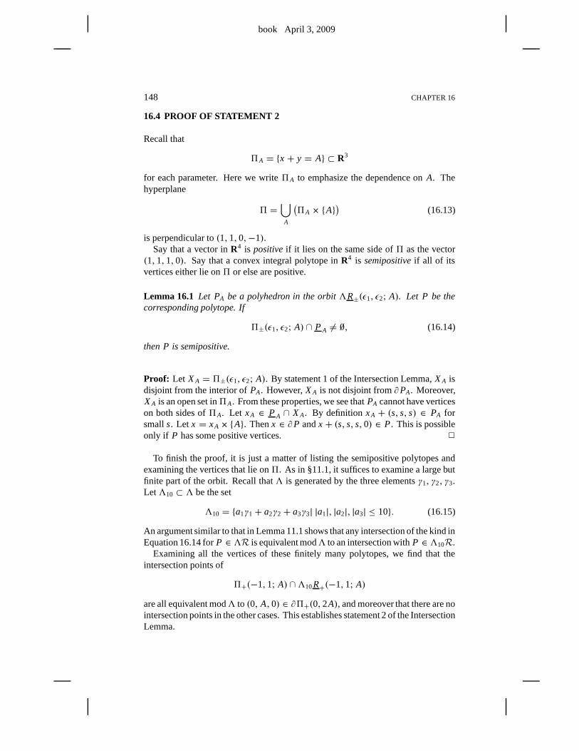
book April 3, 2009

148 CHAPTER 16

16.4 PROOF OF STATEMENT 2

Recall that

5A = {x + y = A} ⊂ R3

for each parameter. Here we write5A to emphasize the dependence onA. Thehyperplane

5 =⋃

A

(5A × {A}

)(16.13)

is perpendicular to(1,1,0,−1).Say that a vector inR4 is positiveif it lies on the same side of5 as the vector

(1,1,1,0). Say that a convex integral polytope inR4 is semipositiveif all of itsvertices either lie on5 or else are positive.

Lemma 16.1 Let PA be a polyhedron in the orbit3R±(ǫ1, ǫ2; A). Let P be thecorresponding polytope. If

5±(ǫ1, ǫ2; A) ∩ PA 6= ∅, (16.14)

then P is semipositive.

Proof: Let XA = 5±(ǫ1, ǫ2; A). By statement 1 of the Intersection Lemma,XA isdisjoint from the interior ofPA. However,XA is not disjoint from∂PA. Moreover,XA is an open set in5A. From these properties, we see thatPA cannot have verticeson both sides of5A. Let xA ∈ PA ∩ XA. By definitionxA + (s, s, s) ∈ PA forsmalls. Let x = xA× {A}. Thenx ∈ ∂P andx+ (s, s, s,0) ∈ P. This is possibleonly if P has some positive vertices. 2

To finish the proof, it is just a matter of listing the semipositive polytopes andexamining the vertices that lie on5. As in §11.1, it suffices to examine a large butfinite part of the orbit. Recall that3 is generated by the three elementsγ1, γ2, γ3.Let310 ⊂ 3 be the set

310 = {a1γ1+ a2γ2 + a3γ3| |a1|, |a2|, |a3| ≤ 10}. (16.15)

An argument similar to that in Lemma 11.1 shows that any intersection of the kind inEquation 16.14 forP ∈ 3R is equivalent mod3 to an intersection withP ∈ 310R.

Examining all the vertices of these finitely many polytopes,we find that theintersection points of

5+(−1,1; A) ∩310R+(−1,1; A)

are all equivalent mod3 to (0, A,0) ∈ ∂5+(0,2A), and moreover that there are nointersection points in the other cases. This establishes statement 2 of the IntersectionLemma.

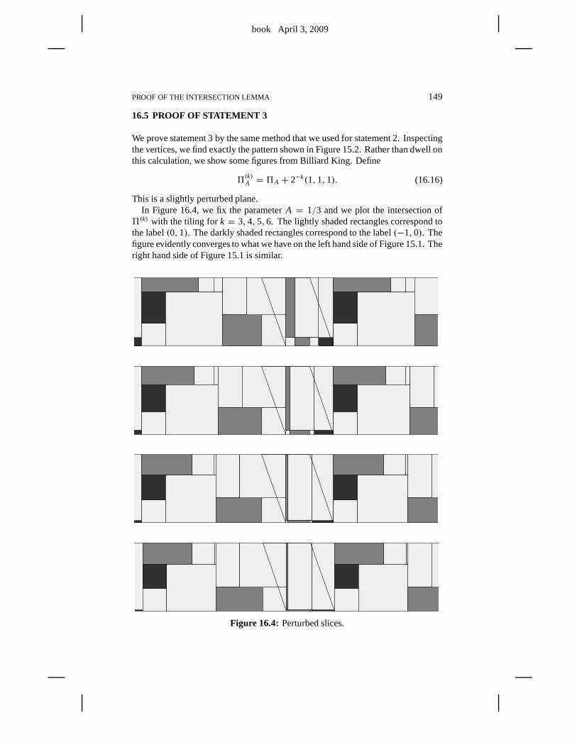
book April 3, 2009

PROOF OF THE INTERSECTION LEMMA 149

16.5 PROOF OF STATEMENT 3

We prove statement 3 by the same method that we used for statement 2. Inspectingthe vertices, we find exactly the pattern shown in Figure 15.2. Rather than dwell onthis calculation, we show some figures from Billiard King. Define

5(k)A = 5A + 2−k(1,1,1). (16.16)

This is a slightly perturbed plane.In Figure 16.4, we fix the parameterA = 1/3 and we plot the intersection of

5(k) with the tiling for k = 3,4,5,6. The lightly shaded rectangles correspond tothe label(0,1). The darkly shaded rectangles correspond to the label(−1,0). Thefigure evidently converges to what we have on the left hand side of Figure 15.1. Theright hand side of Figure 15.1 is similar.

Figure 16.4: Perturbed slices.

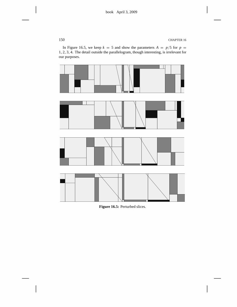
book April 3, 2009

150 CHAPTER 16

In Figure 16.5, we keepk = 5 and show the parametersA = p/5 for p =1,2,3,4. The detail outside the parallelogram, though interesting, is irrelevant forour purposes.

Figure 16.5: Perturbed slices.

book April 3, 2009

Part 4. Period-Copying Theorems

In this part of the book, we will establish some results on period-copying. Ourefforts culminate in the proof of Theorem 4.2, the final result needed for the proofof the Erratic Orbits Theorem. In Parts 5 and 6 we will use someof the other resultswe prove in this part.

• In Chapter 17, we prove some results about Diophantine approximation.There are two main topics. The first is an analysis of the inferior and su-perior sequences from Chapter 4, including a proof of the Superior SequenceLemma. The second is the analysis of a device we call theDiophantineconstant. We introduce the Diophantine constant in §17.4 and it playsan im-portant role in our subsequent results. The reader interested only in Lemma4.3 can skip everything in this chapter except §17.4.

• In Chapter 18, we prove the Diophantine Lemma. This result is the sourceof most of our period-copying results. As a quick application, we use theDiophantine Lemma to prove Lemma 4.3, the final ingredient inthe proof ofthe Erratic Orbits Theorem for almost every parameter. The reader who issatisfied with the Erratic Orbits Theorem for almost every parameter can stopreading the book after this chapter.

• In Chapter 19, we state and prove the Decomposition Theorem. This theoremis an enhancement of the Room Lemma in §3.3. Our proof of the Decom-position Theorem is somewhat more tedious than we would like, but it turnsout that Theorem 4.2 requires only a part of the Decomposition Theorem thatis easier to prove. When the time comes, we will indicate whatis necessaryand what is not. We do need the full Decomposition Theorem forour workin Parts 5 and 6, however.

• In Chapter 20, we prove Theorem 4.2 by combining the Diophantine Lemmaand the Decomposition Theorem.

book April 3, 2009

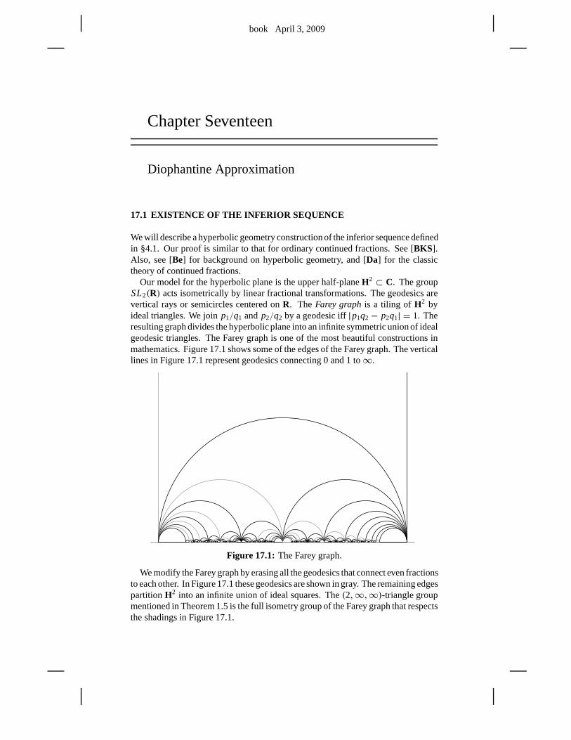
book April 3, 2009

Chapter Seventeen

Diophantine Approximation

17.1 EXISTENCE OF THE INFERIOR SEQUENCE

We will describe a hyperbolic geometry construction of the inferior sequence definedin §4.1. Our proof is similar to that for ordinary continued fractions. See [BKS].Also, see [Be] for background on hyperbolic geometry, and [Da] for the classictheory of continued fractions.

Our model for the hyperbolic plane is the upper half-planeH2 ⊂ C. The groupSL2(R) acts isometrically by linear fractional transformations.The geodesics arevertical rays or semicircles centered onR. TheFarey graphis a tiling of H2 byideal triangles. We joinp1/q1 andp2/q2 by a geodesic iff|p1q2− p2q1| = 1. Theresulting graph divides the hyperbolicplane into an infinite symmetric union of idealgeodesic triangles. The Farey graph is one of the most beautiful constructions inmathematics. Figure 17.1 shows some of the edges of the Fareygraph. The verticallines in Figure 17.1 represent geodesics connecting 0 and 1 to∞.

Figure 17.1: The Farey graph.

We modify the Farey graph by erasing all the geodesics that connect even fractionsto each other. In Figure 17.1 these geodesics are shown in gray. The remaining edgespartitionH2 into an infinite union of ideal squares. The(2,∞,∞)-triangle groupmentioned in Theorem 1.5 is the full isometry group of the Farey graph that respectsthe shadings in Figure 17.1.

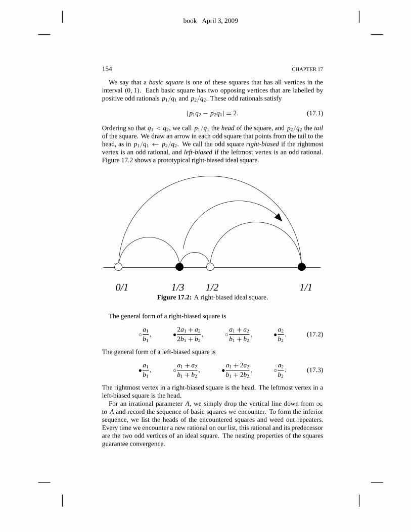
book April 3, 2009

154 CHAPTER 17

We say that abasic squareis one of these squares that has all vertices in theinterval (0,1). Each basic square has two opposing vertices that are labelled bypositive odd rationalsp1/q1 and p2/q2. These odd rationals satisfy

|p1q2 − p2q1| = 2. (17.1)

Ordering so thatq1 < q2, we call p1/q1 theheadof the square, andp2/q2 the tailof the square. We draw an arrow in each odd square that points from the tail to thehead, as inp1/q1 ← p2/q2. We call the odd squareright-biasedif the rightmostvertex is an odd rational, andleft-biasedif the leftmost vertex is an odd rational.Figure 17.2 shows a prototypical right-biased ideal square.

1/3 1/2 1/10/1Figure 17.2: A right-biased ideal square.

The general form of a right-biased square is

◦a1

b1, •2a1+ a2

2b1+ b2, ◦a1+ a2

b1+ b2, •a2

b2. (17.2)

The general form of a left-biased square is

•a1

b1, ◦a1+ a2

b1+ b2, •a1+ 2a2

b1+ 2b2, ◦a2

b2. (17.3)

The rightmost vertex in a right-biased square is the head. The leftmost vertex in aleft-biased square is the head.

For an irrational parameterA, we simply drop the vertical line down from∞to A and record the sequence of basic squares we encounter. To form the inferiorsequence, we list the heads of the encountered squares and weed out repeaters.Every time we encounter a new rational on our list, this rational and its predecessorare the two odd vertices of an ideal square. The nesting properties of the squaresguarantee convergence.

book April 3, 2009

DIOPHANTINE APPROXIMATION 155

17.2 STRUCTURE OF THE INFERIOR SEQUENCE

Now suppose that{pn/qn} is the inferior sequence approximatingA. Referring toEquation 4.1, we writeAn = pn/qn and(An)± = (pn)±/(qn)±. We have

(An)− < An < (An)+, (17.4)

and these numbers form 3 vertices of an ideal square.An is the tail of the square.

Lemma 17.1 The following are true for all indices m.

1. Let N> m. Then Am−1 < Am iff Am−1 < AN .

2. If Am−1 < Am, then(qm)− = qm−1+ (qm)+.

3. If Am−1 > Am, then(qm)+ = qm−1+ (qm)−.

4. Either Am < A < (Am)+ or (Am)− < A < Am.

Proof: Statement 1 follows from the nesting properties of the idealsquares encoun-tered by the vertical geodesicγ as it converges toA.

For statement 2, note thatAm−1 < Am iff these two rationals participate in aleft-biased basic square, which happens iff(qm)+ < (qm)−. By definition,

qm−1 = |(qm)− − (qm)+|.When(qm)+ < (qm)−, we can simply remove the absolute value symbol and solvefor (qm)−. statement 3 is similar.

For statement 4, we will consider the case whenAm < Am−1. The other case issimilar. At some point,γ encounters the basic square with vertices

(Am)− < Am < (Am)+ < Am−1.

If Am+1 < Am, thenγ exitsS between(Am)− andAm. So,

(Am)− < A < Am.

If An+1 > Am, thenγ exitsS to the right ofAm. If γ exitsS to the right of(Am)+,thenγ next encounters a basic squareS′ with vertices

(Am)+ < O < E < Am−1,

whereO andE are odd and even rationals, respectively. But thenAm would not bethe term in the sequence afterAm−1. The term afterAm−1 would lie in the interval[O, Am−1). This is a contradiction. 2

Let [x] denote the floor ofx. Let dn be as in Equation 4.5. That is,

dn =[

qn+1

2qn

], n = 0,1,2,3...

Relatedly, define

δn =[

qn+1

qn

], n = 0,1,2,3... (17.5)

book April 3, 2009

156 CHAPTER 17

Now we come to our main technical result about inferior sequences. This resultis similar to results one sees for the successive terms of continued fraction approx-imants. See [Da]. Before we give the result, we make several clarifying remarksabout it.

Remarks:(i) In the result below, the notationAm−1 < Am > Am+1 means thatAm−1 < Am

andAm > Am+1, and similarly for the other lines.(ii) There is a basic symmetry in the result below. If we swap all inequalities, thenthe signs(+) and(−) all switch. This symmetry swaps cases 1 and 3 and likewiseswaps cases 2 and 4.(iii) The same results hold forp in place ofq. We usedq just for notational conve-nience.

Lemma 17.2 The following are true for any index m≥ 1.

1. If Am−1 < Am < Am+1, then

• δm is odd,

• (qm)+ < (qm)−,

• (qm+1)+ = dmqm + (qm)+,

• (qm+1)− = (dm + 1)qm+ (qm)+.

2. If Am−1 > Am < Am+1, then

• δm is even,

• (qm)− < (qm)+,

• (qm+1)+ = dmqm − (qm)−,

• (qm+1)− = dmqm + (qm)+.

3. If Am−1 > Am > Am+1, then

• δm is odd,

• (qm)− < (qm)+,

• (qm+1)+ = (dm + 1)qm+ (qm)−,

• (qm+1)− = dmqm + (qm)−.

4. If Am−1 < Am > Am+1, then

• δm is even,

• (qm)+ < (qm)−,

• (qm+1)+ = dmqm + (qm)−,

• (qm+1)− = dmqm − (qm)+.

book April 3, 2009

DIOPHANTINE APPROXIMATION 157

Proof: Cases 3 and 4 follow from cases 1 and 2 by symmetry. We will considercase 1 in detail, and case 2 briefly at the end.

In case 1, the vertical geodesicγ to A passes through the basic squareS withvertices

Am−1 < (Am)− < Am < (Am)+.

SinceAn < Am+1, the geodesicγ next crosses through the geodesicαm connectingAm to (Am)+. Following this,γ encounters the basic squaresS′k for k = 0,1,2, ...until it crosses a geodesic that does not haveAm as a left endpoint. By Equation17.3 and induction, we get the following list of vertices forthe squareS′k.

pm

qm<(k+ 1)pm+ (pm)+

(k+ 1)qm+ (qm)+<(2k+ 1)pm+ 2(pm)+

(2k+ 1)qm+ 2(qm)+<

kpm+ (pm)+

kqm+ (qm)+. (17.6)

HereS′k is a left-biased square. But then there is somek such that

pm+1

qm+1= (2k+ 1)pm+ 2(pm)+

(2k+ 1)qm+ 2(qm)+,

(pm+1)+

(qm+1)+= kpm+ (pm)+

kqm + (qm)+. (17.7)

Since(qm)+ < (qm)−, we have

2(qm)+ < qm. (17.8)

But then we havepm+1

qm+1−

pm

qm=

2

(2k+ 1)q2m+ 2qm(qm)+

∈(

2

(2k + 2)q2m

,2

(2k+ 1)qm

). (17.9)

Hence

δm = (2k + 1) ≡ 1 mod 2.

Herek = dm. This takes care of the second implication. Equation 17.7 istheformula for(qm+1)+. Lemma 17.1 now gives the formula for(qm+1)−.

In case 2, the vertical geodesicγ again encounters the basic squareS. This timeγ exits S through the geodesic joining(Am)− to Am. This fact follows from theinequality

Am > Am−1 > (Am)−,

a result of Lemma 17.1. Following this,γ encounters the basic squaresS′′k , fork = 0,1,2, ... until it crosses a geodesic that does not haveAm as a right endpoint.The coordinates for the vertices ofS′′k are just like those in Equation 17.7, exceptthat all the terms have been reversed and each(·)+ is switched to(·)−. The rest ofthe proof is similar. 2

Remark: An important corollary of Lemma 17.2 is that either of the following datadetermines the inferior sequence uniquely.

• The sequence{δn}.

• The sequence{dn} and the sequence{σn}, whereσn is the sign ofAn+1− An.

The sequence{dn} in itself does not have enough information to determine theinferior sequence uniquely.

book April 3, 2009

158 CHAPTER 17

17.3 EXISTENCE OF THE SUPERIOR SEQUENCE

The following result completes the proof of the Superior Sequence Lemma.

Lemma 17.3 dm ≥ 1 infinitely often.

Proof: We can sort the indices of the sequence into 4 types, depending on whichcase holds in Lemma 17.2. If this lemma is false, thenn eventually has odd type.But it is impossible forn to have type 1 and forn + 1 to have type 3. Henceneventually has constant type, say type 1. (The type 3 case hasa similar treatment.)Looking at the formula in case 1 of Lemma 17.2, we see that the sequence{(qn)+}eventually is constant. But then

r = limn→∞

(qn)+pn

qn

exists. Since

(qn)+ pn ≡ −1 mod qn,

qn →∞, we must haver ∈ Z. But then limpn/qn ∈ Q, and we have a contradic-tion. 2

Lemma 17.4 If dm ≥ 1, then∣∣∣∣

pN

qN−

pm

qm

∣∣∣∣ <2

dmq2m

∀N > m,

∣∣∣∣A−pm

qm

∣∣∣∣ ≤2

dmq2m

.

Proof: The first conclusion implies the second. We will consider thecase whenAm < Am+1. By Lemma 17.1, we have

|AN − Am| ≤ |(Am+1)+ − Am| =1

qm(qm+1)+. (17.10)

If m is an index of type 1, then

(qm+1)+ = dmqm+ (qm)+ > dmqm. (17.11)

If m is an index of type 2, then Lemma 17.2 tells us that

(qm+1)+ = (qm+1)− − qm = dmqm+ (qm)+ − qm >

(dm −

1

2

)qm ≥

1

2dmqm.

(17.12)Combining Equations 17.10–17.12 we obtain the result. 2

Remark: The superior sequence has Diophantine approximation properties similarto those of the sequence of continued fraction approximants. While these twosequences are related, they are generally not the same. For one thing, the superiorsequence involves only odd rationals. We can, for example, certainly find irrationalswhose sequence of continued fraction approximants consists of only even rationals.In this case, the two sequences are forced to be different.

book April 3, 2009

DIOPHANTINE APPROXIMATION 159

17.4 THE DIOPHANTINE CONSTANT

17.4.1 Basic Definition

We have two odd rationalsA1 = p1/q1 andA2 = p2/q2. We define the real numbera = a(A1, A2) by the formula

∣∣∣∣p1

q1− p2

q2

∣∣∣∣ =2

aq21

. (17.13)

We call(A1, A2) admissibleif a(A1, A2) > 1.Define

λ1 =(q1)+

q1∈ (0,1). (17.14)

If A1 < A2, we define

� = floor((a/2)− λ1

)+ 1+ λ1. (17.15)

If A1 > A2, we define

� = floor((a/2)+ λ1

)+ 1− λ1. (17.16)

Remark: The only fact relevant for Lemma 4.3 is thata > 4 implies that� > 2.The reader who cares mainly about Lemma 4.3 can skip the rest of this chapter.

17.4.2 Meaning of the Constant

Let [x] denote the floor ofx. We say that an integerµ is good if

[µA1] = [µA2] . (17.17)

Our next result is meant to apply when(A1, A2) is admissible. Also, we considerthe case whereA1 < A2.

Lemma 17.5 (Goodness)If µ ∈ (−q1,�q1) ∩ Z, thenµ is a good integer.

We will prove this result in two steps.

Lemma 17.6 If µ ∈ (−q1,0), thenµ is good.

Proof: Sinceq1 is odd, we have unique integersj andM such that

µA1 = M + ( j/q1), | j | < q1/2 (17.18)

By hypotheses,a > 1. Hence

|A2 − A1| < 2/q21 (17.19)

in all cases. If this result is false, then there is some integer N such that

µA2 < N ≤ µA1. (17.20)

Referring to Equation 17.18, we have

| j |q1

< µA1 − N ≤ µA1− µA2 <2|µ|q2

1

<2

q1. (17.21)

book April 3, 2009

160 CHAPTER 17

If j = 0, thenq1 dividesµ, which is impossible. Hence| j | = 1. If j = −1, thenµA1 is 1/q1 less than an integer. HenceµA1− N ≥ (q1 − 1)/q1. This is false, sowe must havej = 1.

From the definition ofλ1, we have the following implication.

µ ∈ (−q1,0) and µp1 ≡ 1 mod q1 H⇒ µ = −λ1q1.(17.22)

Equation 17.18 impliesµp1

q1− 1

q1∈ Z.

But thenµp1 ≡ 1 modq1. Equation 17.22 now tells us thatµ = −λ1q1. Hence|µ| < q1/2. But now Equation 17.21 is twice as strong and gives| j | = 0. This is acontradiction. 2

Lemma 17.7 If µ ∈ (0,�q1), thenµ is good.

Proof: We observe that� < a, by Equation 17.15. If this result is false, then thereis some integerN such thatµA1 < N ≤ µA2. If µA2 = N, thenq2 dividesµ. Butthen

µ ≥ q2 ≥ aq1 > �q1.

This is a contradiction. Hence

µA1 < N < µA2. (17.23)

Referring to Equation 17.18, we have| j |q1≤ N − µA1 < µ(A2− A1) =

2µ

aq21

<2

q1. (17.24)

Suppose thatj ∈ {0,1} in Equation 17.18. Then

1− 1

q1≤ N − µA1 ≤ µA2− µA1 <

1

q1,

a contradiction. Hencej = −1. Henceµ > aq1/2.Since j = −1, Equation 17.18 now tells us thatµp1+ 1≡ 0 modq1. But then

µ = kq1+ (q1)+ (17.25)

for somek ∈ Z. On the other hand, from Equation 17.15 and the fact thatµ < �q1,we have

µ < k′q1+ (q1)+, k′ =(floor

((a/2)− λ1

)+ 1

). (17.26)

Comparing the last two equations, we havek ≤ k′ − 1. Hence

k ≤(floor

((a/2)− λ1

)). (17.27)

Therefore

µ ≤(floor

((a/2)− λ1

))q1 + λ1q1 ≤ aq1/2.

But we have already shown thatµ > aq1/2. This is a contradiction. 2

book April 3, 2009

DIOPHANTINE APPROXIMATION 161

17.5 A STRUCTURAL RESULT

Now we will explain how the Diophantine constant interacts with the inferior se-quence we defined above. LetA = p/q be an odd rational. We say thatA′ is anearpredecessorof A if A′ precedesA in the inferior sequence but does not precede thesuperior predecessor ofA. The inferior and superior predecessors ofA are the twoextreme examples of near predecessors ofA. Here is a nice characterization of theDiophantine constant for these pairs of rationals.

Lemma 17.8 If A′ is a near predecessor of A, then the following are true.

1. If A′ < A, then�q′ = q′ + q+.

2. If A′ > A, then�q′ = q′ + q−.

Proof: There is a finite chain

A′ = A1← · · · ← Am = A. (17.28)

Referring to Equation 4.5, we have

d1 ≥ 0, d2 = · · · = dm−1 = 0.

By Lemma 17.1,A1 < A2 iff A′ < A. We will consider the case whenA1 < A2.The other case is similar. Recall that

A− A′ = 2

a(q′)2, � = floor

(a

2− λ

)+ 1+ λ, λ =

q′+q′. (17.29)

Hence

�q′ = q′(N + 1)+ q′+, N = floor((a/2)− λ

). (17.30)

There are two cases to consider, depending on whetherδ1 is odd or even. Hereδ1 is as in Equation 17.5. Ifδn is odd, then we have case 1 of Lemma 17.2. In thiscase, we will show below thatd1 = N. By case 1 of Lemma 17.2, we have

(q2)+ = d1q1+ (q1)+ = Nq1 + (q1)+. (17.31)

If δn is even, then we show below thatd1 = N + 1. By case 2 of Lemma 17.2, wehave

(q2)+ = d1q1 − (q1)− = (d1− 1)q1+ q+ = Nq1 + (q1)+. (17.32)

We obtain the same result in both cases.Repeated applications of Lemma 17.2, case 1, give us

q+ = (qm)+ = ... = (q2)+ =Nq′ + q′+ =

(N + 1)q′ − q′ + q′+ =�q′ − q′.

Rearranging this gives statement 1. 2

We have some unfinished business from the previous result. Asabove, we define

λ =q′+q′, N = floor

(a

2− λ

)(17.33)

Also, the sequences{δn} and{dn} are as in Lemma 17.2.

book April 3, 2009

162 CHAPTER 17

Lemma 17.9 If A1 < A2 andδ1 is odd, then d1 = N.

Proof: Rearranging the basic definition ofa(A′, A) and usingA′ = A1 andA = Am

in Equation 17.28, we have

a

2= 1

q21|A1− Am|

.

By Lemma 17.1 and monotonicity, we have

1

q21|A1− (A2)+|

<a

2<

1

q21|A1− A2|

. (17.34)

After some basic algebra, we have

d1+ λ1 =∗(q2)+

q1<

a

2<

q2

2q1. (17.35)

The starred inequality is case 1 of Lemma 17.2. The lower bound gives us

d1 < (a/2)− λ1 (17.36)

Hereλ1 is the same asλ in Equation 17.29. Sinced1 ∈ Z, we obtaind1 ≤ N. Onthe other hand, the upper bound gives us

N = floor

(a

2− λ1

)≤ floor

(q2

2q1− λ1

)≤ d1. (17.37)

In short,N ≤ d1. Combining the two halves givesN = d1. 2

Lemma 17.10 If A1 < A2 andδ1 is even, then d1 = N + 1.

Proof: The proof is very similar to that for the other case. Here we mention the2 changes. The first change is that(d1 − 1) + λ1 occurs on the left hand side ofEquation 17.35, by case 2 of Lemma 17.2. This gives us

d1 ≤ N + 1.

The second change occurs on the right hand side of Equation 17.37. By case 2 ofLemma 17.2, we know that floor(q2/q1) is even. Henceq2/(2q1) has a fractionalpart less than 1/2. But, also by case 2 of Lemma 17.2,λ1 has a fractional partgreater than 1/2. Hence

floor

(q1

2q1− λ1

)= floor

(q1

2q1

)− 1 ≤ d1 − 1.

This gives us the boundN ≤ d1−1, orN+1≤ d1. Putting the two halves together,we haved1 = N + 1. 2

book April 3, 2009

Chapter Eighteen

The Diophantine Lemma

18.1 THREE LINEAR FUNCTIONALS

Let p/q be an odd rational.Consider the following linear functionals.

F(m,n) =(

p

q,1

)· (m,n). (18.1)

G(m,n) =(

q− p

p+ q,−2q

p+ q

)· (m,n). (18.2)

H (m,n) =(−p2+ 4pq+q2

(p+ q)2,

2q(q− p)

(p+ q)2

)· (m,n). (18.3)

We haveF = (1/2)M, whereM is the fundamental map from Equation 2.10.We can understandG andH by evaluating them on a basis.

H (V) = G(V) = q; H (W) = −G(W) = q2

p+ q. (18.4)

HereV = (q,−p)andW are the vectors from Equation 3.2. We can also understandG by evaluating on a simpler basis.

G(q,−p) = q; G(−1,−1) = 1. (18.5)

We can also (further) relateG and H to the hexagrid in Chapter 3. A directcalculation establishes the following result.

Lemma 18.1 The fibers of G are parallel to the top left edge of the arithmetickite. The fibers of H are parallel to the top right edge of the arithmetic kite. Also,‖∇G‖ ≤ 3 and‖∇H‖ ≤ 3.

Here∇ is the gradient.Given any intervalI , define

1(I ) = {(m,n)| G(m,n), H (m,n) ∈ I } ∩ {(m,n)| F(m,n) ≥ 0}. (18.6)

This set is a triangle whose bottom edge is the baseline ofŴ(p/q).

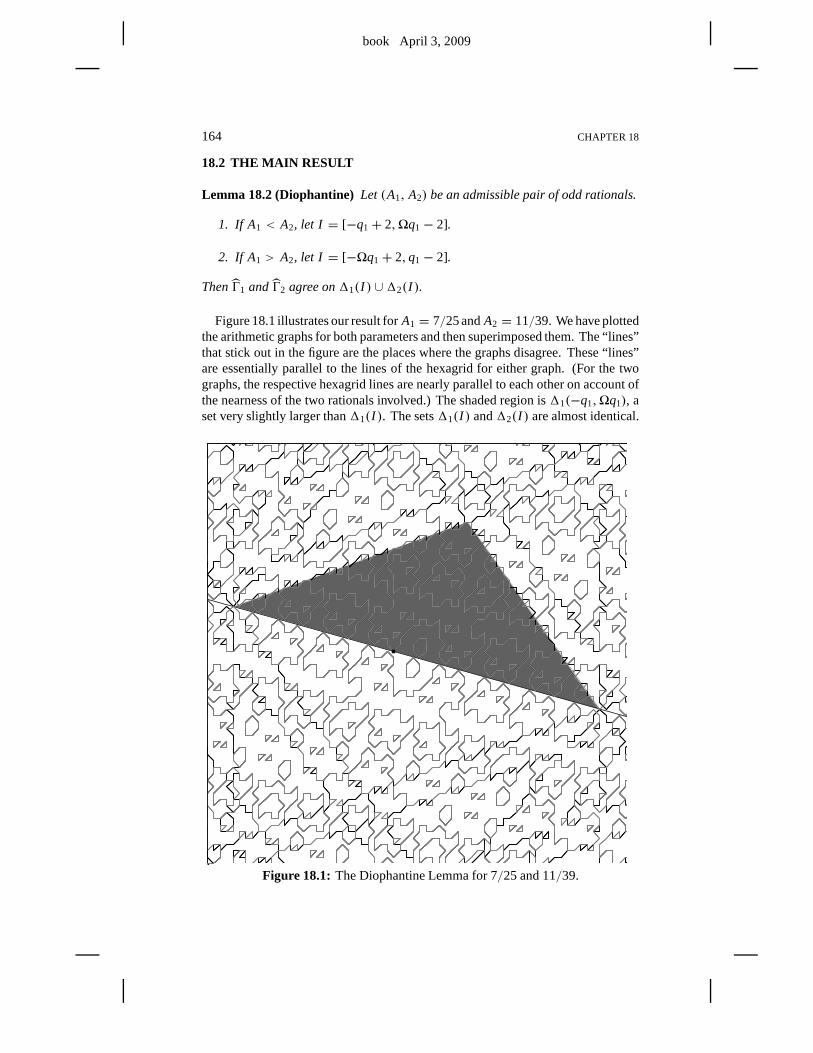
book April 3, 2009

164 CHAPTER 18

18.2 THE MAIN RESULT

Lemma 18.2 (Diophantine) Let (A1, A2) be an admissible pair of odd rationals.

1. If A1 < A2, let I = [−q1+ 2,�q1− 2].

2. If A1 > A2, let I = [−�q1+ 2,q1− 2].

ThenŴ1 andŴ2 agree on11(I ) ∪12(I ).

Figure 18.1 illustrates our result forA1 = 7/25 andA2 = 11/39. We have plottedthe arithmetic graphs for both parameters and then superimposed them. The “lines”that stick out in the figure are the places where the graphs disagree. These “lines”are essentially parallel to the lines of the hexagrid for either graph. (For the twographs, the respective hexagrid lines are nearly parallel to each other on account ofthe nearness of the two rationals involved.) The shaded region is11(−q1,�q1), aset very slightly larger than11(I ). The sets11(I ) and12(I ) are almost identical.

Figure 18.1: The Diophantine Lemma for 7/25 and 11/39.

book April 3, 2009

THE DIOPHANTINE LEMMA 165

18.3 A QUICK APPLICATION

Here we use the Diophantine Lemma to prove Lemma 4.3. This completes ourproof of the Erratic Orbits Theorem for almost every parameter, as we indicated inPart 1. The reader who is satisfied with this result can stop reading the book at theend of this chapter.

We will prove Lemma 4.3 whenA1 < A2. The other case is similar. By hypoth-esis, we have

a(A1, A2) > 4. (18.7)

From Equation 17.15, we get

� > 2. (18.8)

Let R1 = R(A1) be the parallelogram from the Room Lemma. Let

u = W1, w = V1 +W1 (18.9)

denote the top left and right vertices ofR1. We compute

G1(u) = −q2

1

p1+ q1> −q1+ 2, H1(w) =

q21

p1+ q1+ q1 < �q1− 2.

(18.10)The inequalities hold oncep1 is sufficiently large. Given the description of the fibersof G, we have

G(u) ≤ G(v) ≤ H (v) ≤ H (w), ∀v ∈ R1. (18.11)

The middle inequality uses the fact thatF(v) ≥ 0. In short, we have made theextremal calculations. This calculation shows thatv ∈ 11(I ) for all v ∈ R1. TheDiophantine Lemma now shows thatŴ1 andŴ2 agree inR1.

Whenv lies in the bottom edge ofR1, we have

G1(v), H1(v) ∈ [0,q1] . (18.12)

Given the gradient bounds‖∇G1‖ ≤ 3 and‖∇H1‖ ≤ 3, we see that

G1(v), H1(v) ∈ [−q1+ 2,�q1+ 2] , (18.13)

provided thatv is within q1/4 of the bottom edge ofR1. HenceŴ1 andŴ2 agree intheq1/4 neighborhood of the bottom edge ofR1.

By the Room Lemma,Ŵ11 ⊂ R1. HenceŴ1

1 ⊂ Ŵ2. The calculation involving thebottom edge ofR1 shows thatŴ1+ǫ

1 ⊂ Ŵ2 for ǫ = 1/4. Since the right endpoint ofŴ1

2 is far to the right of any point onŴ1+ǫ1 , we haveŴ1+ǫ

1 ⊂ Ŵ12, as desired.

Remark: We proved Lemma 4.3 forǫ = 1/4 rather thanǫ = 1/8, which iswhat we originally claimed. We do not care about the value ofǫ as long as it ispositive.

book April 3, 2009

166 CHAPTER 18

18.4 PROOF OF THE DIOPHANTINE LEMMA

We will establish the case whenA1 < A2. The other case has a nearly identicalproof. Recall that an integerµ is good if

[µA1] = [µA2] (18.14)

We callµ 1-good if µ + ǫ is good for allǫ ∈ {−1,0,1}. We can subject alattice point(m,n) to the reduction algorithm in §6.6. Forθ ∈ {1,2}, we performthe algorithm relative to the parameterAθ . This produces integersXθ , Yθ , andZθ .Below we prove the following result.

Lemma 18.3 (Agreement)Suppose, for at least one choice ofθ ∈ {1,2}, that thefollowing numbers are all1-good.

• m

• m− Xθ

• m− Yθ

• m+ Yθ − Xθ .

ThenŴ1 andŴ2 agree at(m,n).

Next, we prove the following result.

Lemma 18.4 (Good Integer) If (m,n) ∈ 11(I ) ∪ 12(I ), then the integers in theAgreement Lemma all lie in(−q1+ 1,�q1− 1) for at least1 choice ofθ ∈ {1,2}.

By the Goodness Lemma in §17.4, all the numbers in the Agreement Lemma are1-good. The Diophantine Lemma now follows immediately.

Remarks:(i) As one can see in Figure 18.1, the Diophantine Lemma also works for pointsbelow the baseline. One can give a proof for points below the baseline that is nearlyidentical to the proof we give for points above the baseline.We have stated only the“above” case because the restriction makes our argument a bit easier and this is theonly case we need for applications. In light of the symmetry results we establishedin §12.3 and §12.4, the fact that the result holds symmetrically above and below thebaseline should not be surprising.(ii) As one can see from Figure 18.1, the Diophantine Lemma isquite sharp. Wethink that the sharp version runs as follows. The two arithmetic graphs agree at anypoint in11(−q1,�q1) that is not adjacent to a point that lies outside11(−q1,�q1).The slight fudging of the boundaries is an artifact of our proof. Our proof of theDecomposition Theorem in Chapter 19 would go easier if we hadthe sharp versionof the Diophantine Lemma at our disposal, but the result we prove here is the bestwe can do.

book April 3, 2009

THE DIOPHANTINE LEMMA 167

18.5 PROOF OF THE AGREEMENT LEMMA

Lemma 18.5 Letµ, ν, N j ∈ Z and

N j =[µA j + ν1+ A j

].

Suppose there is someθ ∈ {1,2} such that bothµ− Nθ andµ− Nθ + 1 are good.Then N1 = N2.

Proof: Here [ ] is the floor function, as above. For the sake of contradiction, assumewithout loss of generality. thatN1 < N2. Then

µA1+ ν < N2(A1+ 1), (µ− N2)A1 < N2 − ν

N2(A2+ 1) ≤ µA2+ ν, N2 − ν ≤ (µ− N2)A2.

The first equation implies the second in each case. The seconditems imply thatµ− N2 is not good. On the other hand, we have

µA1 + ν < (N1 + 1)(A1+ 1), A1(m− N1 + 1) < N1 + 1− n.

(N1 + 1)(1+ A2) ≤ µA2+ ν, A2(m− N2 + 1) ≥ N1 − 1+ n.

The first equation implies the second in each case. The seconditems imply thatµ− N1 + 1 is not good. Now we have a contradiction. 2

Corollary 18.6 Referring to the Agreement Lemma,(X1,Y1, Z1) = (X2,Y2, Z2).

Proof: We apply the reduction algorithm from §6.6. We focus on the(−) case,indicating the small differences for the(+) case as we go along.

1. Letz j = A j m+ n.

2. Let Z j = floor(z j ). Sincem is good, we haveZ1 = Z2. Call this commonintegerZ.

3. y j = z j + Z j = z j + Z. Hencey j = m Aj + n′ for somen′ ∈ Z. [We havey j = z j + Z + 1 in the(+) case.]

4. Recall thatYj = floor(y j /(1+ A)). To see thatY1 = Y2 we apply Lemma18.5 to (µ, ν, N j ) = (m,n′,Yj ). Here we use the fact thatm − Yθ andm − Yθ + 1 are good. We setY = Y1 = Y2. [We apply Lemma 18.5 to(µ, ν, N j ) = (m,n′ + 1,Yj ) in the(+) case.]

5. Letx j = y j − Y(1− A j )− 1. Hencex j = (m+ Y)A j + n′′.

6. Recall thatX j = floor(x j /(1+ A)). To see thatX1 = X2, we apply Lemma18.5 to(µ, ν, N j ) = (m+Y,n′′, X j ). Here we use the fact thatm+Y− Xθ

andm+ Y − Xθ + 1 are good integers. 2

book April 3, 2009

168 CHAPTER 18

In the next result, all quantities exceptA1 andA2 are integers.

Lemma 18.7 If µ− d N− ǫ1 is good, then the statement

(µA j + ν)− N(d Aj + 1) < ǫ1A j + ǫ2

is true or false independent of j= 1,2.

Proof: Assume without loss of generality. that the statement is true for j = 1 andfalse for j = 2. Then

(µ− d N− ǫ1)A1 < ǫ2 + N − ν ≤ (µ− d N− ǫ1)A2,

a contradiction. 2

Let M+ andM− be as in §6.6. By the Master Picture Theorem, it suffices to showthat the two imagesM+(m,n) andM−(m,n) land in the same polyhedra for bothA1 and A2. We have already seen that the basic integers(X,Y, Z) are the samerelative to both parameters. Here we recall the planes from §6.2.

• Z, the union{z= 0} ∪ {z= A} ∪ {z= 1− A} ∪ {z= 1}.

• Y, the union{y = 0} ∪ {y = A} ∪ {y = 1} ∪ {y = 1+ A}.

• X , the union{x = 0} ∪ {x = A} ∪ {x = 1} ∪ {x = 1+ A}.

• T , the union{x + y− z= A+ j } for j = −2,1,0,2,1.

LettingS stand for one of these partitions, we say thatS is good if, for both signchoices and both parameters, the pointsM±(m,n) land in the same component ofR± − S. Here we setR± = R3/3, the domain of the mapsM±. By the MasterPicture Theorem,Ŵ1 andŴ2 agree at(m,n), provided all the partitions are good.The proof works the same for the(+) and the(−) cases.

• ForZ, we apply Lemma 18.7 to(µ, ν,d, N) = (m,n,0, Z) to show that thestatementz j − Z < ǫ1A j + ǫ2 is truly independent ofj for ǫ1 ∈ {−1,0,1}andǫ2 ∈ {0,1}. The relevant good integers arem− 1 andm andm+ 1.

• ForY, we apply Lemma 18.7 to(µ, ν,d, N) = (m,n′,1,Y) to show that thestatementz j − Z < ǫ1A j + ǫ2 is truly independent ofj for ǫ1 ∈ {0,1} andǫ2 ∈ {0,1}. The relevant good integers arem− Y andm− Y − 1.

• For X , we apply Lemma 18.7 to(µ, ν,d, N) = (m + Y,n′′,1, X). Therelevant good integers arem+ Y − X andm+ Y − X − 1.

• ForT , we define

σ j = (x j − X(1+ A j ))+ (y j − Y(1+ A j ))− (z j − Z).

We haveσ j = (m− X)A j + n′′′ for somen′′′ ∈ Z. Let h ∈ Z be arbitrary.To see that the statementσ j < A j + h is truly independent ofj , we applyLemma 18.7 to(µ, ν,d, N) = (m− X,n′′′,1,0). The relevant good integeris m− X − 1.

Remark: Our proof does not use the fact thatm− X + 1 is a good integer. Thistechnical detail is relevant for Lemma 18.10.

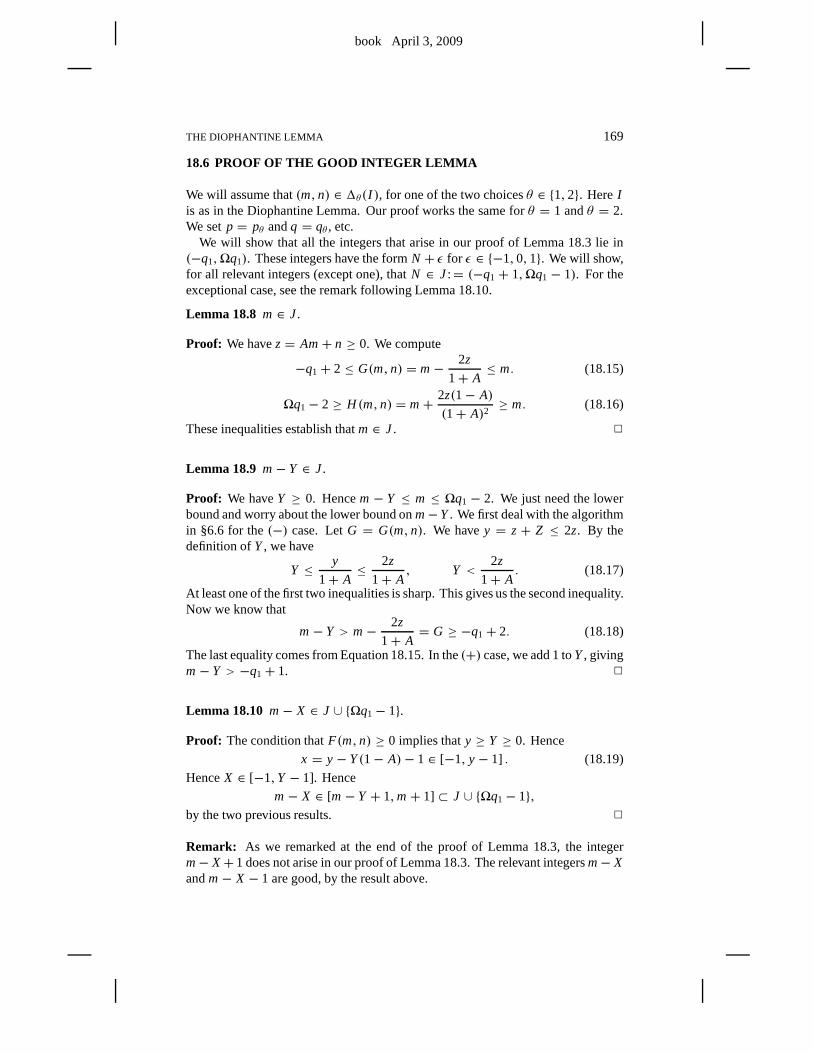
book April 3, 2009

THE DIOPHANTINE LEMMA 169

18.6 PROOF OF THE GOOD INTEGER LEMMA

We will assume that(m,n) ∈ 1θ (I ), for one of the two choicesθ ∈ {1,2}. HereIis as in the Diophantine Lemma. Our proof works the same forθ = 1 andθ = 2.We setp = pθ andq = qθ , etc.

We will show that all the integers that arise in our proof of Lemma 18.3 lie in(−q1,�q1). These integers have the formN + ǫ for ǫ ∈ {−1,0,1}. We will show,for all relevant integers (except one), thatN ∈ J:= (−q1 + 1,�q1 − 1). For theexceptional case, see the remark following Lemma 18.10.

Lemma 18.8 m ∈ J .

Proof: We havez= Am+ n ≥ 0. We compute

−q1+ 2 ≤ G(m,n) = m− 2z

1+ A≤ m. (18.15)

�q1− 2 ≥ H (m,n) = m+ 2z(1− A)

(1+ A)2≥ m. (18.16)

These inequalities establish thatm ∈ J. 2

Lemma 18.9 m− Y ∈ J .

Proof: We haveY ≥ 0. Hencem− Y ≤ m ≤ �q1 − 2. We just need the lowerbound and worry about the lower bound onm−Y. We first deal with the algorithmin §6.6 for the(−) case. LetG = G(m,n). We havey = z+ Z ≤ 2z. By thedefinition ofY, we have

Y ≤ y

1+ A≤ 2z

1+ A, Y <

2z

1+ A. (18.17)

At least one of the first two inequalities is sharp. This givesus the second inequality.Now we know that

m− Y > m− 2z

1+ A= G ≥ −q1+ 2. (18.18)

The last equality comes from Equation 18.15. In the(+) case, we add 1 toY, givingm− Y > −q1+ 1. 2

Lemma 18.10 m− X ∈ J ∪ {�q1− 1}.

Proof: The condition thatF(m,n) ≥ 0 implies thaty ≥ Y ≥ 0. Hence

x = y− Y(1− A)− 1 ∈ [−1, y− 1] . (18.19)

HenceX ∈ [−1,Y − 1]. Hence

m− X ∈ [m− Y + 1,m+ 1] ⊂ J ∪ {�q1− 1},by the two previous results. 2

Remark: As we remarked at the end of the proof of Lemma 18.3, the integerm− X+ 1 does not arise in our proof of Lemma 18.3. The relevant integersm− Xandm− X − 1 are good, by the result above.

book April 3, 2009

170 CHAPTER 18

Lemma 18.11 m+ Y − X ∈ J .

Proof: Our proof works the same in the(+) and(−) cases. Lemma 18.10 gives usY − X ≥ 0. Hence

m+ Y − X ≥ m> −q1+ 1.

This takes care of the lower bound. Now we treat the upper bound. We have

Y = floor

(y

1+ A

)≤ y

1+ A, 1+ X = floor

(1+ x

1+ A

)≥ x

1+ A.

Hence

Y − X − 1 ≤y− x

1+ A=1

Y1− A

1+ A+

1

1+ A<∗

2z1− A

(1+ A)2+ 1

1+ A=2

H −m+ 1

1+ A<

H −m+ 1.

The first equality comes from Equation 18.19. The second equality comes fromEquation 18.16. The starred inequality comes from the upperbound in Equation18.17. Addingm to both sides, we have

m+ Y − X < H + 1 ≤ �q1− 1.

This completes the proof. 2

book April 3, 2009

Chapter Nineteen

The Decomposition Theorem

19.1 THE MAIN RESULT

The Room Lemma confines one period ofŴ(p/q) to a certain parallelogramR(p/q)when p/q is odd. In this section we explain a sharper result, along thesame lines,that confines one period ofŴ(p/q) to a union of two parallelograms. The readermight want to glance at Figure 19.1 before reading the definitions that follow.

Given an odd rationalA = p/q, we construct the even rationalsA± = p±/q±.We letA′ be the inferior predecessor ofA, and we letA∗ be the superior predecessor,as in §4.1. For each rational, we use Equation 3.2 to construct the correspondingV andW vectors. For instance,V+ = (q+,−p−) andV∗ = (q∗,−p∗). Now wedefine the following lines.

• L−0 is the line parallel toV and containingW.

• L−1 is the line parallel toV and containingW∗.

• L− is the line parallel toV through(0,0).

• L+0 is the line parallel toW through(0,0).

• If q+ > q−, thenL+1 is the line parallel toW through−V−.

• If q+ < q−, thenL+1 is the line parallel toW through+V+.

• If q+ > q−, thenL+2 is the line parallel toW through+V+.

• If q+ < q−, thenL+2 is the line parallel toW through−V−.

The lines with the(−) superscript have negative slope, and the lines with the(+)superscript have positive slope. All the(−) lines are parallel to each other, and allthe(+) lines are parallel to each other. Now we define the following parallelograms:

• R1 is the parallelogram bounded byL− andL−1 andL+0 andL+1 .

• R2 is the parallelogram bounded byL− andL−0 andL+0 andL+2 .

The parallelogramR2 is the larger of the two parallelograms. It is both widerand taller. Note that translation byV carries the leftmost edge ofR1 ∪ R2 to therightmost edge.

Here is the main result of this chapter.

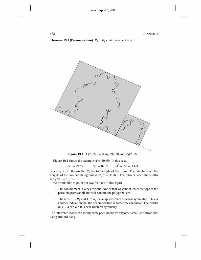
book April 3, 2009

172 CHAPTER 19

Theorem 19.1 (Decomposition)R1 ∪ R2 contains a period ofŴ.

Figure 19.1: Ŵ(29/69) andR1(29/69) andR2(29/69).

Figure 19.1 shows the exampleA = 29/69. In this case,

A− = 21/50, A+ = 8/19, A′ = A∗ = 13/31.

Sinceq+ < q−, the smallerR1 lies to the right of the origin. The ratio between theheights of the two parallelograms isq∗/q = 31/69. The ratio between the widthsis q+/q− = 19/50.

We would like to point out two features of this figure.

• The containment is very efficient. Notice that we cannot lower the tops of theparallelograms at all and still contain the polygonal arc.

• The arcsŴ ∩ R1 andŴ ∩ R2 have approximate bilateral symmetry. This isanother indication that the decomposition is somehow canonical. The resultsin §12.4 explain this near-bilateral symmetry.

The interested reader can see the same phenomena for any other smallish odd rationalusing Billiard King.

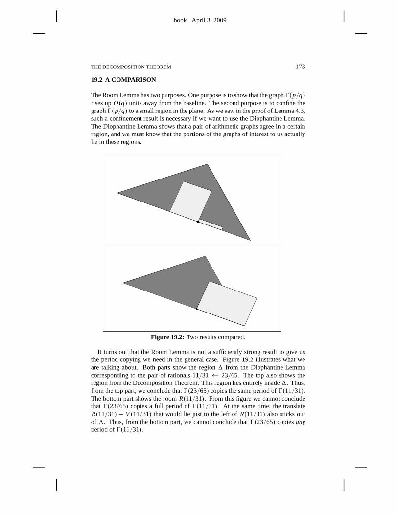
book April 3, 2009

THE DECOMPOSITION THEOREM 173

19.2 A COMPARISON

The Room Lemma has two purposes. One purpose is to show that the graphŴ(p/q)rises upO(q) units away from the baseline. The second purpose is to confinethegraphŴ(p/q) to a small region in the plane. As we saw in the proof of Lemma 4.3,such a confinement result is necessary if we want to use the Diophantine Lemma.The Diophantine Lemma shows that a pair of arithmetic graphsagree in a certainregion, and we must know that the portions of the graphs of interest to us actuallylie in these regions.

Figure 19.2: Two results compared.

It turns out that the Room Lemma is not a sufficiently strong result to give usthe period copying we need in the general case. Figure 19.2 illustrates what weare talking about. Both parts show the region1 from the Diophantine Lemmacorresponding to the pair of rationals 11/31← 23/65. The top also shows theregion from the Decomposition Theorem. This region lies entirely inside1. Thus,from the top part, we conclude thatŴ(23/65) copies the same period ofŴ(11/31).The bottom part shows the roomR(11/31). From this figure we cannot concludethatŴ(23/65) copies a full period ofŴ(11/31). At the same time, the translateR(11/31) − V(11/31) that would lie just to the left ofR(11/31) also sticks outof 1. Thus, from the bottom part, we cannot conclude thatŴ(23/65) copiesanyperiod ofŴ(11/31).

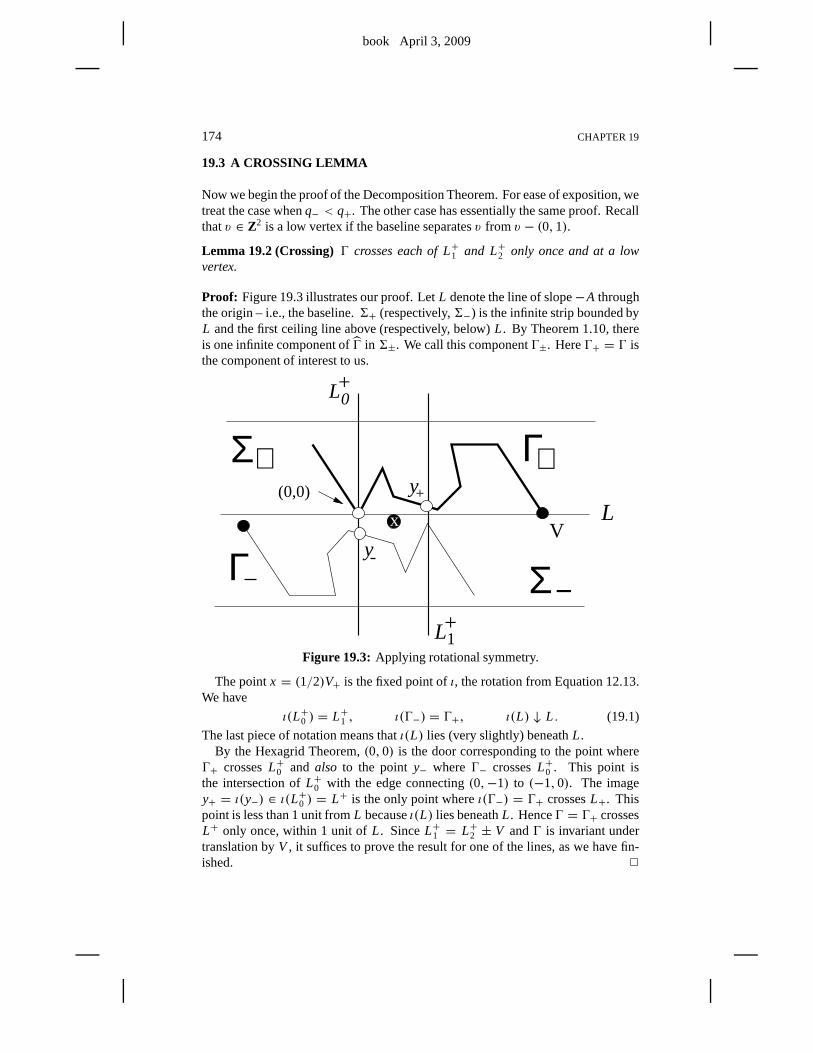
book April 3, 2009

174 CHAPTER 19

19.3 A CROSSING LEMMA

Now we begin the proof of the Decomposition Theorem. For easeof exposition, wetreat the case whenq− < q+. The other case has essentially the same proof. Recallthatv ∈ Z2 is a low vertex if the baseline separatesv from v − (0,1).

Lemma 19.2 (Crossing)Ŵ crosses each of L+1 and L+2 only once and at a lowvertex.

Proof: Figure 19.3 illustrates our proof. LetL denote the line of slope−A throughthe origin – i.e., the baseline.6+ (respectively,6−) is the infinite strip bounded byL and the first ceiling line above (respectively, below)L. By Theorem 1.10, thereis one infinite component ofŴ in 6±. We call this componentŴ±. HereŴ+ = Ŵ isthe component of interest to us.

L0+

L1+

Γ

Γ+y+

−

+

Σ

L

y

(0,0)

Σ

Vx

Figure 19.3: Applying rotational symmetry.

The pointx = (1/2)V+ is the fixed point ofι, the rotation from Equation 12.13.We have

ι(L+0 ) = L+1 , ι(Ŵ−) = Ŵ+, ι(L) ↓ L . (19.1)

The last piece of notation means thatι(L) lies (very slightly) beneathL.By the Hexagrid Theorem,(0,0) is the door corresponding to the point where

Ŵ+ crossesL+0 and also to the pointy− whereŴ− crossesL+0 . This point isthe intersection ofL+0 with the edge connecting(0,−1) to (−1,0). The imagey+ = ι(y−) ∈ ι(L+0 ) = L+ is the only point whereι(Ŵ−) = Ŵ+ crossesL+. Thispoint is less than 1 unit fromL becauseι(L) lies beneathL. HenceŴ = Ŵ+ crossesL+ only once, within 1 unit ofL. SinceL+1 = L+2 ± V andŴ is invariant undertranslation byV , it suffices to prove the result for one of the lines, as we havefin-ished. 2

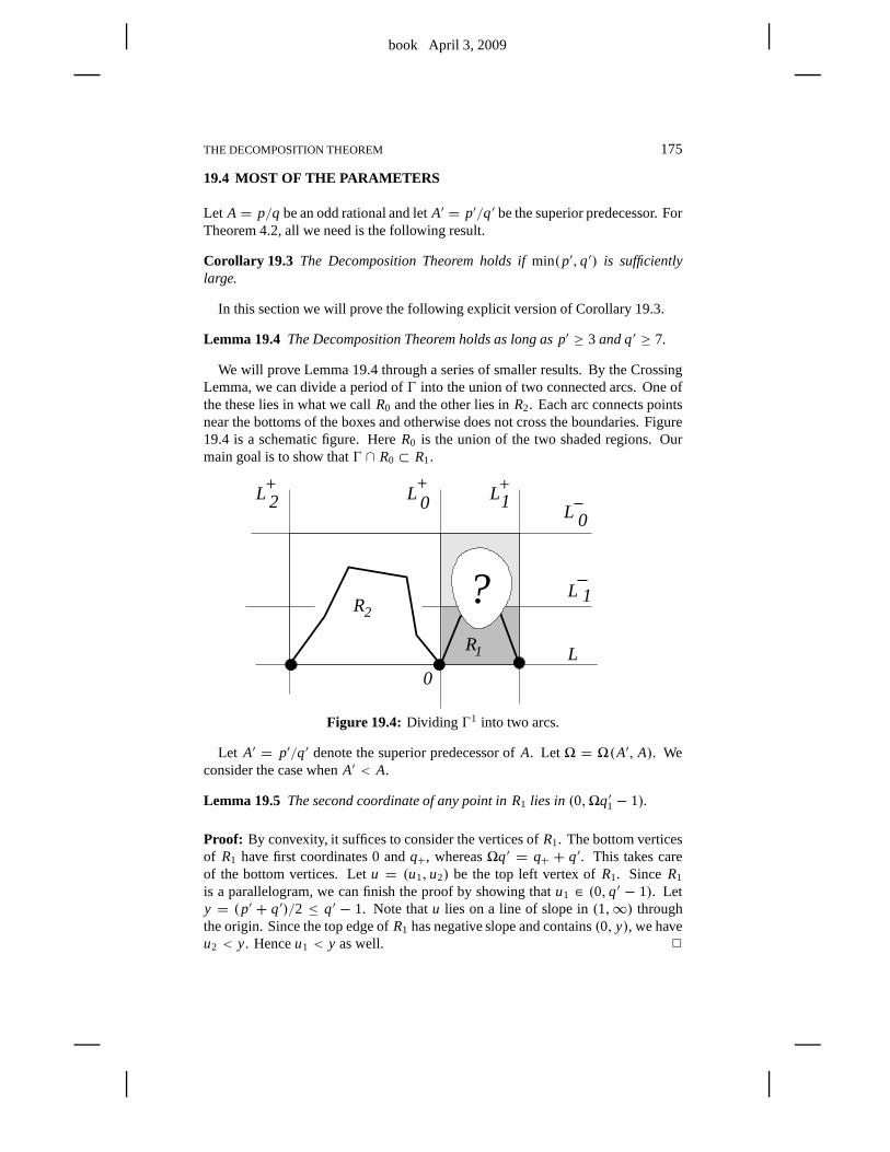
book April 3, 2009

THE DECOMPOSITION THEOREM 175

19.4 MOST OF THE PARAMETERS

Let A = p/q be an odd rational and letA′ = p′/q′ be the superior predecessor. ForTheorem 4.2, all we need is the following result.

Corollary 19.3 The Decomposition Theorem holds ifmin(p′,q′) is sufficientlylarge.

In this section we will prove the following explicit versionof Corollary 19.3.

Lemma 19.4 The Decomposition Theorem holds as long as p′ ≥ 3 and q′ ≥ 7.

We will prove Lemma 19.4 through a series of smaller results.By the CrossingLemma, we can divide a period ofŴ into the union of two connected arcs. One ofthe these lies in what we callR0 and the other lies inR2. Each arc connects pointsnear the bottoms of the boxes and otherwise does not cross theboundaries. Figure19.4 is a schematic figure. HereR0 is the union of the two shaded regions. Ourmain goal is to show thatŴ ∩ R0 ⊂ R1.

0

1 L

L 2 L 0 L1L 0

L 1

+ + +

R

R

2?

Figure 19.4: Dividing Ŵ1 into two arcs.

Let A′ = p′/q′ denote the superior predecessor ofA. Let� = �(A′, A). Weconsider the case whenA′ < A.

Lemma 19.5 The second coordinate of any point in R1 lies in (0,�q′1− 1).

Proof: By convexity, it suffices to consider the vertices ofR1. The bottom verticesof R1 have first coordinates 0 andq+, whereas�q′ = q+ + q′. This takes careof the bottom vertices. Letu = (u1,u2) be the top left vertex ofR1. SinceR1

is a parallelogram, we can finish the proof by showing thatu1 ∈ (0,q′ − 1). Lety = (p′ + q′)/2 ≤ q′ − 1. Note thatu lies on a line of slope in(1,∞) throughthe origin. Since the top edge ofR1 has negative slope and contains(0, y), we haveu2 < y. Henceu1 < y as well. 2

book April 3, 2009

176 CHAPTER 19

Lemma 19.6 Let A′ denote the superior predecessor of A. Suppose that A′ 6= 1/1.ThenŴ′ ∩ R0 ⊂ R1.

Proof: Let γ = Ŵ′ ∩ R0. Sinceγ starts out inR1 (at the origin), we just need to seethatγ never crosses the top edge ofR1. The top edge ofR1 is contained in the lineλ = L−1 of slope−A though the pointX = (0, (p′+q′)/2). By the Room Lemma,γ does not cross the (nearly identical) lineλ′ = (L−0 )′ of slope−A′ throughX.

If γ crosses the top edge ofR1, then there is a lattice point(m,n) betweenλ andλ′ and within 1 unit ofR1. But then

floor(Am) 6= floor(A′m), m ∈ (−1,q′ + q+) = (−q′,�q′). (19.2)

The second equation comes from our previous result. Our lastequations contradictLemma 17.5. 2

Corollary 19.7 Suppose thatŴ andŴ′ agree in R1. Then the Decomposition The-orem holds for A.

Proof: Let us traceŴ ∩ R0 from left to right, starting at(0,0). By hypothesis, thisarc does not cross the top ofR1 until it leavesR0. OnceŴ ∩ R0 leavesR0 from theright, it never reenters. This is a consequence of Lemma 19.2. 2

By Corollary 19.7, it suffices to prove thatŴ′ andŴ agree inR1.

Lemma 19.8 Ŵ′ ∩ R1 andŴ ∩ R1 have the same outermost edges.

Proof: The leftmost edge of both arcs is the edge connecting(0,0) to (1,1). Look-ing at the proof of Lemma 19.2, we see that the rightmost edgeeof Ŵ∩R0 connectsV+ + (0,1) to V+ + (1,0). HereV+ = (q+,−p+). Applying Lemma 19.2 toŴ′,we see that some edgee′ of Ŵ′ connectsV ′+ + (0,1) to V ′+ + (1,0). But repeatedapplications of case 1 or case 2 of Lemma 17.2 tell us thatV+ = V ′++kV′ for somek ∈ Z. SinceŴ′ is invariant under translation byV ′, we see thate is also an edgeof Ŵ′. 2

Mismatch Principle: Lemma 19.8 has the following corollary. IfŴ′ andŴ fail toagree inR1, then there are 2 adjacent vertices ofŴ′ ∩ R1 where the two arithmeticgraphsŴ andŴ′ do not agree. One can see this by tracing the 2 curves from leftto right, starting at the origin. Once we get the first mismatch onŴ′ the arcŴ hasveered off, and the next vertex onŴ′ is also a mismatch.

In our analysis below, we will treat the case whenA′ < A. The other case issimilar. The bottom right vertex ofR1 lies on a line of slope in(1,∞) that containsthe pointV+. The pointV+ has the same first coordinate as the very nearby point

V+ =q+q

V. (19.3)

book April 3, 2009

THE DECOMPOSITION THEOREM 177

Indeed, the 2 points differ by exactly 1/q. Let R1 denote the slightly smallerparallelogram whose vertices are

(0,0), u, V+, w = u+ V+. (19.4)

If the Decomposition Theorem fails forA, then at least one of the adjacent verticesof mismatch will lie in R1. (There are not 2 adjacent vertices between the nearlyidentical right edges ofR1 andR1.)

As in the previous chapter, it suffices to make the extremal calculations

G(u) ≥ −q′ + 2, H (w) ≤ �q′ − 2= q′ + q+ − 2. (19.5)

The Diophantine Lemma then finishes the proof.We first need to locateu. There is somer such thatv1 = rW. Letting M be the

map from Equation 2.10, relative to the parameterA, we have

M(v1) = M(rW) = p′ + q′.

Solving forr gives

v1 =(

p′ + q′

p+ q

)W. (19.6)

We compute

G(u)= p′ + q′

p+ qG(W)

=− p′ + q′

p+ q× q2

p+ q

= −(1+ A′)q′

(1+ A)2

>−q′

1+ A′. (19.7)

H (w)=H (u)+ (q+/q)H (V)

= (1+ A′)q′

(1+ A)2+ q+

<q′

1+ A′+ q+. (19.8)

The last inequality in each case uses the fact that 0< A′ < A. Notice the greatsimilarity between these two calculations. One can ultimately trace this symmetryback to the affine symmetry of the arithmetic kiteK(A) defined in Chapter 3.

The conditions in Equation 19.5 are simultaneously met, provided

−q′

1+ A′≥ −q′ + 2,

(⇐⇒

1

p′+

1

q′≤

1

2

). (19.9)

The equation on the right is equivalent to the one on the left.We easily see that itholds as long asp′ ≥ 3 andq′ ≥ 7.

In the next two sections we will make a more detailed study of the few exceptionsto Lemma 19.3. The reader mainly interested in the Erratic Orbits Theorem canstop reading here.

book April 3, 2009

178 CHAPTER 19

19.5 THE EXCEPTIONAL CASES

19.5.1 Case 1

We use the notation from the previous section. We assume firstthat A′ 6= 1/1 isone of the rationals not covered by Theorem 19.3. Our argument uses the linearfunctionalsG′ andH ′ associated toA′ in place of the linear functionalsG andHused above. Before we begin our argument, we warn the reader thatG′ is not thederivative ofG. We will denote the partial derivatives ofG′ by ∂xG′ and∂yG′.

Lemma 19.9 G′(v) ≥ −q′ + 2 for all v ∈ R1.

Proof: We have to worry only about points near the top left corner ofR1. Suchpoints lie on the first period ofŴ′ to the right of the origin. Call this periodβ ′. WhenA′ ∈ {3/5,3/7,5/7}, we check this result explicitly for every point onβ ′. WhenA′ = 1/q′, we note that∂xG′ > 0 and∂yG′ < 0. We also note that all points inR1

have positive first and second coordinates of at most(q′−1)/2. Thus the point thatminimizesG′ is v = (1, (q′ − 1)/2). We compute

G′(v)+ q − 2= q′ − 3

q′ + 1≥ 0.

The extreme case occurs whenq′ = 3. 2

H ′ is tougher to analyze because the points of interest to us arenear the top rightcorner ofR1, and this corner can vary drastically with the choice ofA. We willuse rotational symmetry to bring the points of interest backinto view, so to speak.Let ι be the isometric involution that swaps(0,0) andV+. Repeated applications ofLemma 17.2 show thatV+ = V ′+ + kV′ for somed ∈ Z. Henceι is a symmetry ofŴ′. See the remark following Equation 12.14.

The infinite arcι(Ŵ′) is the open component ofŴ′ that lies just beneath the baseline.One period ofι(Ŵ′) connects(0,−1) to (q′,−p′− 1). Let us denote this period byβ ′. Compare the proof of Lemma 19.2. The points ofR1 near the top right cornercorrespond to points onβ ′. To evaluateH ′ on the points near the top right cornerof R1, we evaluateH ′ on points ofβ ′ and then relate the results.

Lemma 19.10 For anyv ∈ R2, we have

|H ′(v)+ H ′(ι(v))− q+| < 2/q′.

Proof: SinceH ′ is a linear functional, it suffices to prove the result forv = (0,0).In this case, we must demonstrate that|H ′(V+) − q+| < 2/(q′). We have alreadyremarked thatV+ = V ′++kV′. Henceq+ = q′++kq′. From Lemma 18.1, we haveH ′(kV′) = kq′. Hence the equality is equivalent to

|H ′(V ′+)− q′+| < 2/q′. (19.10)

The pointV ′+ lies on the same vertical line as the pointu′ = (q′+/q′)V ′ and exactly1/q′ units away. Equation 19.10 now follows from the next 3 facts.

H ′(u′) = q′+, |∂yH ′| < 2, ‖u′ − V ′+‖ = 1/q′. (19.11)

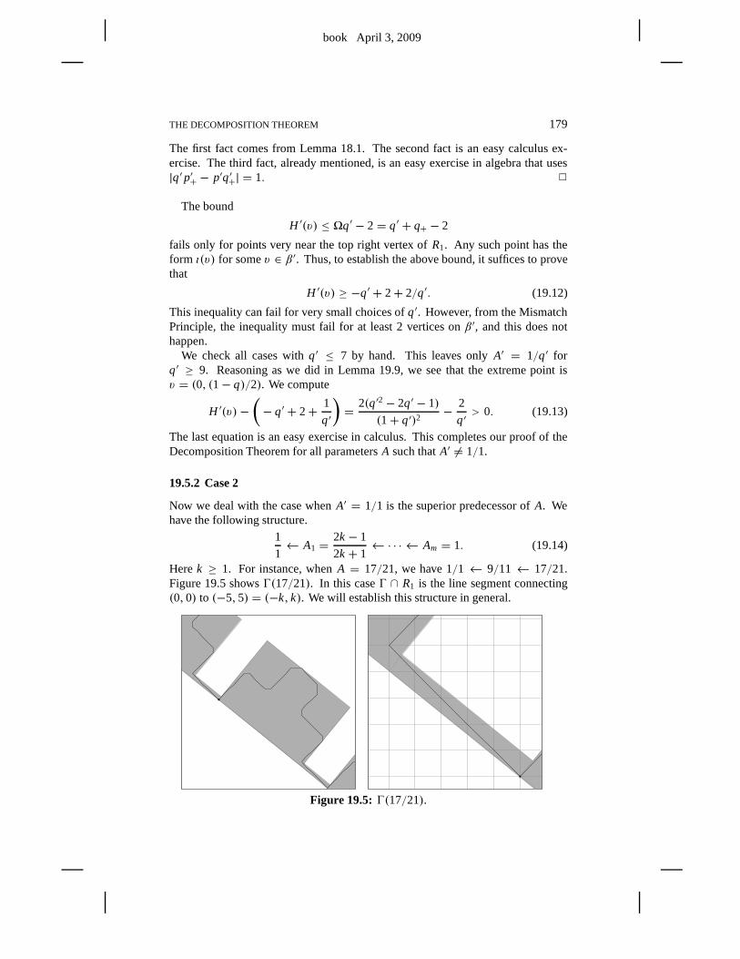
book April 3, 2009

THE DECOMPOSITION THEOREM 179

The first fact comes from Lemma 18.1. The second fact is an easycalculus ex-ercise. The third fact, already mentioned, is an easy exercise in algebra that uses|q′p′+ − p′q′+| = 1. 2

The bound

H ′(v) ≤ �q′ − 2= q′ + q+ − 2

fails only for points very near the top right vertex ofR1. Any such point has theform ι(v) for somev ∈ β ′. Thus, to establish the above bound, it suffices to provethat

H ′(v) ≥ −q′ + 2+ 2/q′. (19.12)

This inequality can fail for very small choices ofq′. However, from the MismatchPrinciple, the inequality must fail for at least 2 vertices on β ′, and this does nothappen.

We check all cases withq′ ≤ 7 by hand. This leaves onlyA′ = 1/q′ forq′ ≥ 9. Reasoning as we did in Lemma 19.9, we see that the extreme point isv = (0, (1− q)/2). We compute

H ′(v)−(− q′ + 2+ 1

q′

)= 2(q′2− 2q′ − 1)

(1+ q′)2− 2

q′> 0. (19.13)

The last equation is an easy exercise in calculus. This completes our proof of theDecomposition Theorem for all parametersA such thatA′ 6= 1/1.

19.5.2 Case 2

Now we deal with the case whenA′ = 1/1 is the superior predecessor ofA. Wehave the following structure.

1

1← A1 =

2k− 1

2k+ 1← · · · ← Am = 1. (19.14)

Herek ≥ 1. For instance, whenA = 17/21, we have 1/1 ← 9/11← 17/21.Figure 19.5 showsŴ(17/21). In this caseŴ ∩ R1 is the line segment connecting(0,0) to (−5,5) = (−k, k). We will establish this structure in general.

Figure 19.5: Ŵ(17/21).

book April 3, 2009

180 CHAPTER 19

R1 is the very short and squat parallelogram on the far left sideof Figure 19.5.This time R1 lies to the left of the origin. The right side of Figure 19.5 shows acloseup of this parallogram superimposed on the integer grid. The left side ofR1

lies in L+1 . Repeated applications of Lemma 17.2 show that(−k, k − 1) ∈ L+1 .The right side ofR0 lies in L+0 , the parallel line through the origin. The top ofR1

contains(0,1) and is parallel to the baseline.Let γ = Ŵ ∩ R0. The rightmost vertex ofγ is (0,0), and the rightmost edge of

γ connects(0,0) to (−1,1). Compare the proof of the Room Lemma.

Lemma 19.11 The leftmost edge ofγ connects(−k, k) to (−k+ 1, k− 1).

Proof: By Lemma 19.2, there is a unique edgee of Ŵ that crossesL+1 . Looking atthe proof of Lemma 19.2, we seee = ι(e′), wheree′ connects(0,−1) to (−1,0)andι is the order 2 rotation about the point

(−q−2,

p−2

)=(−k

2,

k − 1

2

). (19.15)

From this, we conclude thate connects(−k, k) to (−k + 1, k − 1). The leftmostedge ofγ crossesL+1 . This edge must bee. 2

Lemma 19.12 The line segmentγ ′ connecting(0,0) to (−k, k) lies beneath L−0 .Henceγ ′ ∩ R0 ⊂ R1.

Proof: Letting F(m,n) = Am+ n, we haveF(0,1) = 1. HenceF(x) = 1 forall x ∈ L−0 . On the other hand, we compute thatF(0,0) = 0 andF(−k, k) =2k/(2k+ 1) < 1. By convexity,F(y) < 1 for all y ∈ γ ′. 2

To finish our proof, we just have to show thatγ ′ = γ . The first and last edgesof γ andγ ′ agree, and these edges are±(1,−1), with the sign depending on whichway we orient the curves. Letp j = (− j , j ) for j = 2, ..., k− 1. By Lemma 17.1,we have

(A1)− =(

k− 1

k

)< A <

(k

k+ 1

)= (A1)+,

1

k + 1< 1− A <

1

k.

(19.16)The first equation implies the second. We compute

M+(p j ) = (x j , y j , z j ) = j (1− A,1− A,1− A)+ (0,1,0) mod3. (19.17)

Equation 19.16 combines with the fact thatj ∈ {1, ..., k− 1} to give

x j = z j ∈ [1− A, A) , x j + y j − z j = y j ∈ (1,1+ A) ⊂ (A,1+ A).(19.18)

We check that these inequalities always specify the edge(−1,1). Henceγ ′ andγare both line segments. Henceγ = γ ′. This takes care of the case whenA′ = 1/1.

Our proof of the Decomposition Theorem is complete.

book April 3, 2009

Chapter Twenty

Existence of Strong Sequences

In this chapter, we prove Theorem 4.2. For the sake of efficiency, our proof will beessentially algebraic. However, a clear geometric pictureunderlies our construc-tions. We discussed this geometric picture in §19.2. The reader might want to rereadthat section before going through the proof here. Also, the reader might want toreview the proof we gave of Lemma 4.3 in §18.3. Our proof here is similar to theone given there.

20.1 STEP 1

Let A be any irrational parameter. Let{pn/qn} denote the superior sequence asso-ciated toA. Let S be a monotone subsequence of the superior sequence. We willtreat the case whenS is monotone increasing. The other case is entirely similar.

By Corollary 19.3, we can cut off finitely many terms ofS, leaving a sequencefor which the Decomposition Theorem always holds. This is what we will do.

For any odd rationalp/q, let R∗(p/q) denote the rectangle with vertices

−V

2, −V +W

2,

V +W

2,

V

2. (20.1)

HereV andW are as in Equation 3.2. The parallelogramR∗ is just as wide asRbut half as tall. Also, the bottom edge ofR∗ is centered on the origin.

Lemma 20.1 If A1← A2 and p1 is sufficienly large, thenŴ1 andŴ2 agree in A1.Moreover,Ŵ1 andŴ2 agree in the q1/8 neighborhood of the bottom edge of R∗1.

Proof: The proof works the same way regardless of the sign ofA1− A2. The mainpoint is that� > 1. Note that(A1, A2) is admissible. We use the linear functionalsG1 andH1 associated toA1. Let

u = −V +W

2, w = V +W

2

denote the top left and right vertices ofR∗1, respectively. We compute

−G1(u) = H1(w) =q1(p1+ 2q1)

2p1+ 2q1)< q1− 2< �q1− 2. (20.2)

The same argument as in Lemma 4.3 now finishes the proof. 2

Remark: We have not yet used the Decomposition Theorem.

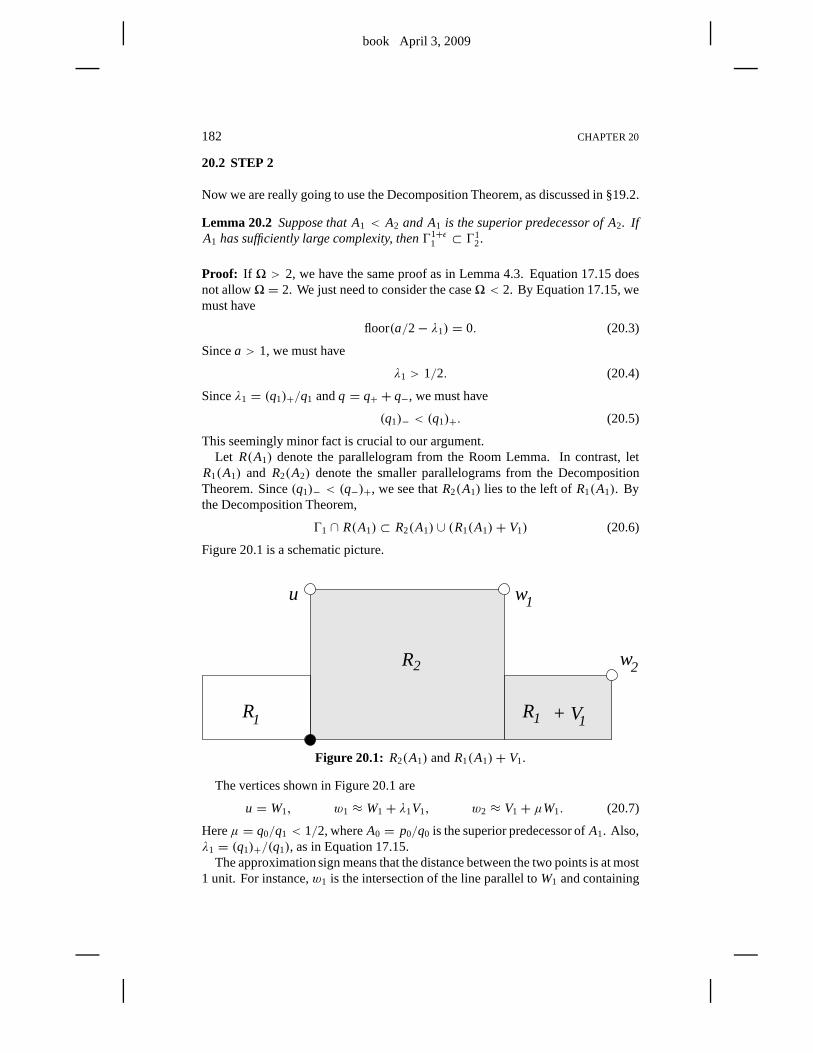
book April 3, 2009

182 CHAPTER 20

20.2 STEP 2

Now we are really going to use the Decomposition Theorem, as discussed in §19.2.

Lemma 20.2 Suppose that A1 < A2 and A1 is the superior predecessor of A2. IfA1 has sufficiently large complexity, thenŴ1+ǫ

1 ⊂ Ŵ12.

Proof: If � > 2, we have the same proof as in Lemma 4.3. Equation 17.15 doesnot allow� = 2. We just need to consider the case� < 2. By Equation 17.15, wemust have

floor(a/2− λ1) = 0. (20.3)

Sincea > 1, we must have

λ1 > 1/2. (20.4)

Sinceλ1 = (q1)+/q1 andq = q+ + q−, we must have

(q1)− < (q1)+. (20.5)

This seemingly minor fact is crucial to our argument.Let R(A1) denote the parallelogram from the Room Lemma. In contrast, let

R1(A1) and R2(A2) denote the smaller parallelograms from the DecompositionTheorem. Since(q1)− < (q−)+, we see thatR2(A1) lies to the left ofR1(A1). Bythe Decomposition Theorem,

Ŵ1 ∩ R(A1) ⊂ R2(A1) ∪ (R1(A1)+ V1) (20.6)

Figure 20.1 is a schematic picture.

2

R1

2

1 1

1

R

R

+ V

wu

w

Figure 20.1: R2(A1) andR1(A1)+ V1.

The vertices shown in Figure 20.1 are

u = W1, w1 ≈ W1 + λ1V1, w2 ≈ V1+ µW1. (20.7)

Hereµ = q0/q1 < 1/2, whereA0 = p0/q0 is the superior predecessor ofA1. Also,λ1 = (q1)+/(q1), as in Equation 17.15.

The approximation sign means that the distance between the two points is at most1 unit. For instance,w1 is the intersection of the line parallel toW1 and containing

book April 3, 2009

EXISTENCE OF STRONG SEQUENCES 183

V+ with the line parallel toV1 and containingW1. The pointV+ is O(q−21 ) of the

point λ1V1. Hencew1 is within O(q−21 ) of W1 + λ1V1. The argument forw2 is

similar.As in the proof of Lemma 4.3, we haveG1(u) > −q1+ 2 oncep1 is large. The

computations forH1(w1) and H1(w2) are the interesting ones. Case 1 of Lemma17.2 gives(q2)+ ≥ (q1)+. Hence, forp1 sufficiently large, we have the followinginequalities.

2+ H1(w1)≤(2+ ‖∇H‖

)+ H1(W1)+ λ1H1(V1)≤

5+ q21

p1+ q1+ (q1)+<

q1+ (q1)+≤q1+ (q2)+=

�q1. (20.8)

Here we use the bound‖∇H‖ ≤ 3. We have already remarked that(q2)+ ≥ (q1)+.We also know that(q1)+ > q1/2. Hence

�q1 = q1+ (q2)+ > (3/2)q1. (20.9)

For p1 large, we have

2+ H1(w2)≤(2+ ‖∇H‖

)+ H1(V1)+ µH1(W1)<

5+ H1(V1)+ (1/2)H1(W1)=

5+ q1+q2

1

2(p1+ q1)<

(3/2)q1<

�q1. (20.10)

These arguments show thatv ∈ 11(I ) for all v ∈ Ŵ11. The rest of the proof is just

like the proof of Lemma 4.3. 2

20.3 STEP 3

SupposeA′1 < A′2 are two consecutive terms inS when we have a finite chain

A′1 = A1← A2← · · · ← An = A′2, A1 < An, q2 > 2q1. (20.11)

The following result finishes the proof of Theorem 4.2.

Lemma 20.3 Ŵn+ǫ1 ⊂ Ŵ1

n.

Proof: We will change our notation slightly from the previous result. We letR1 = R(A1) denote the parallelogram from the Room Lemma. Likewise, we let

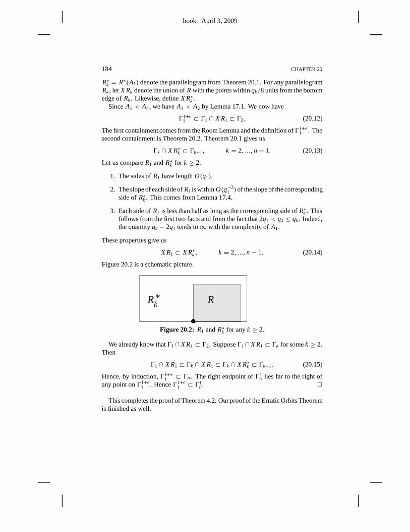
book April 3, 2009

184 CHAPTER 20

R∗k = R∗(Ak) denote the parallelogram from Theorem 20.1. For any parallelogramRk, let X Rk denote the union ofRwith the points withinqk/8 units from the bottomedge ofRk. Likewise, defineX R∗k .

SinceA1 < An, we haveA1 < A2 by Lemma 17.1. We now have

Ŵ1+ǫ1 ⊂ Ŵ1 ∩ X R1 ⊂ Ŵ2. (20.12)

The first containment comes from the Room Lemma and the definition ofŴ1+ǫ1 . The

second containment is Theorem 20.2. Theorem 20.1 gives us

Ŵk ∩ X R∗k ⊂ Ŵk+1, k = 2, ...,n− 1. (20.13)

Let us compareR1 andR∗k for k ≥ 2.

1. The sides ofR1 have lengthO(q1).

2. The slope of each side ofR1 is within O(q−21 )of the slope of the corresponding

side ofR∗k . This comes from Lemma 17.4.

3. Each side ofR1 is less than half as long as the corresponding side ofR∗k . Thisfollows from the first two facts and from the fact that 2q1 < q2 ≤ qk. Indeed,the quantityq2− 2q1 tends to∞ with the complexity ofA1.

These properties give us

X R1 ⊂ X R∗k , k = 2, ...,n− 1. (20.14)

Figure 20.2 is a schematic picture.

*Rk 1R

Figure 20.2: R1 andR∗k for anyk ≥ 2.

We already know thatŴ1∩ X R1 ⊂ Ŵ2. SupposeŴ1∩ X R1 ⊂ Ŵk for somek ≥ 2.Then

Ŵ1 ∩ X R1 ⊂ Ŵk ∩ X R1 ⊂ Ŵk ∩ X R∗k ⊂ Ŵk+1. (20.15)

Hence, by induction,Ŵ1+ǫ1 ⊂ Ŵn. The right endpoint ofŴ1

n lies far to the right ofany point onŴ1+ǫ

1 . HenceŴ1+ǫ1 ⊂ Ŵ1

n. 2

This completes the proof of Theorem 4.2. Our proof of the Erratic Orbits Theoremis finished as well.

book April 3, 2009

Part 5. The Comet Theorem

In this part of the book, we prove the Comet Theorem and its corollaries. As we didin Part 1, we defer the proofs of many of the auxilliary results. In Part 6, we takecare of all the remaining details.

• In Chapter 21, we prove some further results about the inferior and superiorsequences. We list the basic results in the first section and then spend the restof the chapter proving these results.

• In Chapter 22, we prove Theorem 1.8. We also build a rough model for theway the orbitO2(1/qn,−1) returns to the intervalI = [0,2] × {−1}. Ourwork here depends on two technical results, the Copy Theoremand the PivotTheorem, which we establish in Part 6.

• In Chapter 24, we prove the Comet Theorem, modulo some technical detailsthat we handle in Part 6.

• In Chapter 24, we deduce a number of dynamical consequencesof the CometTheorem, including minimality of the set of unboundedorbits. We also definethe cusped solenoids and explain how the time-one map of their geodesic flowmodels the outer billiards dynamics.

• In Chapter 25, we analyze the structure of the Cantor setCA from the CometTheorem. This chapter has a number of geometric results, such as a formulafor dim(CA) whenA is a quadratic irrational.

book April 3, 2009

book April 3, 2009

Chapter Twenty-One

Structure of the Inferior and Superior Sequences

21.1 THE RESULTS

Let{pn/qn} be the inferior sequence associated to an irrational parameter A ∈ (0,1)and let{dn} be the sequence obtained from Equation 4.5. We call{dn} the inferiorrenormalization sequence. We call the subsequence of{dn} corresponding to thesuperior terms thesuperior renormalization sequenceor just therenormalizationsequence. Referring to the inferior sequences, we havedn = 0 if and only if n isnot a superior term. In this case, we calln aninferior term. So, the renormalizationsequence is created from the inferior renormalization sequence simply by deletingall the 0s.

For any odd rationalp/q ∈ (0,1), define

p∗ = min(p−, p+); q∗ = min(q−,q+). (21.1)

Herep∗/q∗ is one of the rationalsp±/q±. It is convenient to define

p∗0q∗0= 1

0. (21.2)

Given the superior sequence{pn/qn}, we define

λn = |Aqn − pn|; λ∗n = |Aq∗n − p∗n|; (21.3)

Note that

λ∗0 = 1. (21.4)

For the purpose of making a clean statement, we defineλ−1 = +∞. All our resultsare meant to apply to the superior sequence for indicesn ≥ 0.

dnλn < 2q−1n , (21.5)

q2n > (5/4)nD2n, (21.6)

∞∑

k=n

dkλk = λ∗n < λn−1. (21.7)

Note that Equation 21.5 is an immediate consequence of Lemma17.4. The rest ofthe chapter is devoted to proving Equations 21.6 and 21.7.

book April 3, 2009

188 CHAPTER 21

21.2 THE GROWTH OF DENOMINATORS

Here we establish some terminology.

• Referring to Equation 17.5,we call{δn} theenhanced inferior renormalizationsequence(EIRS).

• We call the subsequence corresponding to the superior indices theenhancedrenormalization sequence.

The reason for the terminology is that we can determine the inferior renormalizationsequence from the EIRS, but not vice versa.

Say that a parameterA is superior toa parameterA′ if the EIRS forA′ is obtainedby inserting some 1s into the EIRS forA. For instance,

√5− 2 has EIRS

3,1,2,1,2, ...,

and√

2− 1 has EIRS sequence

3,2,2,2, ....

Hence√

2− 1 is superior to√

5− 2.

Lemma 21.1 Suppose that A is superior to A′. Then qn ≤ q′n for all n.

Proof: The EIRS determines the inferior sequence. We havep0 = δ0 − 2 andq0 = δ0. Then, by Lemma 17.2, each(qn+1)± is a nonnegative integer linearcombination of(qn)±, and the coefficients are determined by{δn}. Call this thepositivity property.

Consider the operation of inserting a 1 into themth position in the EIRS forAand recomputing{An}. Call this new sequence theA∗-sequence. We have

(q∗m+1)± ≥ (qm)±.

By induction, and the positivity property, we have

(q∗n+1)± ≥ (qn)±.

Now let us delete the(m+ 1)th term from theA∗-sequence. Call the new sequencetheA′-sequence. We haveq′n ≥ qn for all n. Our result now follows from induction.2

Call A superiorif the corresponding inferior sequence has no inferior terms. Thatis, the EIRS has no 1s in it. For instance,

√2−1 is a superior parameter. If we want

to find a lower bound on the growth of denominators, it sufficesto consider only thesuperior parameters. Equation 21.6 follows from inductionand our next lemma.

Lemma 21.2 Suppose that A1, A2, A3 are 3 consecutive terms in the superior se-quence. Let d1,d2,d3 be the corresponding terms of the renormalization sequence.Then q3 > (5/4)(d1+ 1)(d2+ 1)q1.

book April 3, 2009

STRUCTURE OF THE INFERIOR AND SUPERIOR SEQUENCES 189

Proof: It suffices to assume thatA is a superior parameter, so thatA1, A2, A3 are(also) 3 consecutive terms in the inferior sequence.

First of all, the estimates

qn+1 > 2dnqn, qn+1 > δnqn (21.8)

follow directly from the definitions. Our notation is as in Lemma 17.2. Now wehave 3 cases.

Case 1:Suppose that min(d1,d2) ≥ 2. Then

q3 > 4d1d2q1 > (4/3)(d1+ 1)(d2+ 1)q1. (21.9)

Case 2:Now suppose thatd1 = d2 = 1 and min(δ1, δ2) ≥ 3. Then

q3 > 6q1 = (3/2)(d1+ 1)(d2+ 1)q1. (21.10)

Case 3:Suppose finally thatd1 = d2 = 1 andδ1 = δ2 = 2. We will deal with thecase whenA1 < A2. The other case is similar. In this case, we must have

A0 > A1 < A2 > A3, (21.11)

by Lemma 17.2.By case 2 of Lemma 17.2,

(q2)− = q1+ (q1)+, (q2)+ = (q1)+. (21.12)

By case 4 of Lemma 17.2,

(q3)+ = q2+ (q2)−, (q3)− = (q2)−. (21.13)

Hence

q3 = (q3)+ + (q3)− = q2 + 2(q2)− =∗ q2 + 2q1+ 2(q2)+. (21.14)

The starred equality comes from Lemma 17.1 sinceA1 < A2.SinceA0 > A1, Lemma 17.2 says that

2(q1)+ > (q1)+ + (q1)− = q1. (21.15)

Combining Equations 21.12, 21.14, and 21.15, we have

q3 = q2+ 2q1+ 2(q1)+ > q2+ 3q1 > 5q1. (21.16)

Hence

q3 > (5/4)(d1+ 1)(d2+ 1)q1. (21.17)

This completes our proof. 2

21.3 THE IDENTITIES

We first verify the identity in Equation 21.7. In this identity,we sum over the superiorindices. However, notice that we get the same answer when we sum over all indices.The point is thatdn = 0 whenn is an inferior index. So, for our derivation, we workwith the inferior sequence. Let{pn/qn} be the inferior sequence associated toA.Define

1(n, N) = |pNqn − qN pn|, 1∗(n, N) = |pNq∗n − qN p∗n|, N ≥ n.(21.18)

book April 3, 2009

190 CHAPTER 21

Lemma 21.31∗(n, N) −1∗(n+ 1, N) = dn1(n, N).

Proof: The quantities relevant to the casen = 0 are

A0 =1

1, A∗0 =

1

0, A∗1 =

d0 − 1

d0< A1 =

2d0− 1

2d0+ 1.

In this case, a simple calculation checks the formula directly.Now supposen ≥ 1. We suppose thatAn−1 < An. The other case requires a

similar treatment. Letr stand for eitherp or q. There are two cases, depending onwhether the indexn has type 1 or type 4.

Case 1:Whenn has type 1, Lemma 17.2 gives

r ∗n = (rn)+, r ∗n+1 = (rn+1)+, r ∗n = dnrn − r ∗n+1. (21.19)

We have1∗(n, N) = |a1− a2|, where

a1 = dn pNqn − dnqN pn = dn1(n, N),

a2 = pNq∗n+1 − qN p∗n+1 = −1∗(n+ 1, N). (21.20)

The sign fora1 is correct becauseAN > An. The sign fora2 is correct because, byLemma 17.1, we haveAN < (An+1)+ = A∗n+1. The identity in this lemma followsimmediately.

Case 2:Whenn has type 4, Lemma 17.2 gives

r ∗n = (rn)+, r ∗n+1 = (rn+1)−, r ∗n = dnqn − r ∗n+1.

Hence1∗(n, N) = |a1 + a′2|, wherea′2 = −a2. The sign changes fora′2 becauseAN > (An+1)− = A∗n+1. In this case, we get the same identity. 2

Dividing the equation in Lemma 21.3 byqN , we have

|AN p∗n − q∗n| − |AN p∗n+1− q∗n+1| = dn|AN pn − qn|. (21.21)

Taking the limit asN →∞, we get

λ∗n − λ∗n+1 = dnλn. (21.22)

Summing this equation fromn+ 1 to∞ gives the equality in Equation 21.7.Now we will verify the inequality in Equation 21.7.

Lemma 21.4 λ∗n+1 < λn.

Proof: There are two cases to consider, depending on whetherAn < A or An > A.We will consider the case whenAn < A. The other case requires a similar treatment.By Lemma 17.1, we haveAn < An+1. Therefore, by Lemma 17.2 (applied tom= n+1), we have(qn+1)+ < (qn+1)−. But this means thatA∗n+1 = (An+1)+. ByLemma 17.1, we have

An < A < A∗n+1. (21.23)

book April 3, 2009

STRUCTURE OF THE INFERIOR AND SUPERIOR SEQUENCES 191

Given the above ordering, we have

λn = |Aqn − pn| = Aqn − pn

and

λ∗n+1 = |Aq∗n+1− p∗n+1| = p∗n+1− Aq∗n+1.

Hence

λn − λ∗n+1 = A(qn + q∗n+1)− (pn + p∗n+1). (21.24)

But

qn + q∗n+1 = qn + (qn+1)+ =(qn+1)− − (qn+1)+

)− (qn+1)+ = (qn+1)−.

Likewise,

pn + p∗n+1 = (pn+1)−.

Combining these identities with Equation 21.24, we have

λn − λ∗n+1 = A(qn+1)− − (pn+1)− = (qn+1)−(A− (An+1)−) > 0.

This completes the proof. 2

book April 3, 2009

book April 3, 2009

Chapter Twenty-Two

The Fundamental Orbit

22.1 MAIN RESULTS

We will assume thatp/q = pn/qn, thenth term in a superior sequence. We callO2(1/qn,−1) thefundamental orbit. Let Cn denote the set from Theorem 1.8. Let

C′n = O2(1/qn,−1) ∩ I , I = [0,2]× {−1}. (22.1)

Theorem 1.8 says thatCn = C′n. In this chapter, we will prove Theorem 1.8 andestablish some geometric results about how the orbits return toCn.

After we prove Theorem 1.8, we will establish a coarse model for how the pointsof O2(1/qn) return toCn. Statement 2 of the Comet Theorem is s kind of geomet-ric limit of the Discrete Theorem, and statement 3 of the Comet Theorem is the“geometric limit” of the coarse model we build here.

Let5n denote the truncation of the space defined in Equation 1.7. Let

χ :5n→ Cn (22.2)

denote the mapping that is implicit in the statement of Theorem 1.8. There is anordering on5n such thatχ(κ) returns toχ(κ+), whereκ+ is the successor ofκ inthe ordering. We will describe this ordering.

Here we will define two natural orderings on the sequence space5n associatedto pn/qn. Let {dn} be the renormalization sequence.

Reverse Lexicographic Ordering: Given two finite sequences{ai } and{bi } ofthe same length, letk be the largest index, whereak 6= bk. We define{ai } ≺′ {bi }if ak < bk, and{bi } ≺′ {ai } if ak > bk. This ordering is known as thereverselexicographicordering.

Twist Automorphism: Given a sequenceκ = {ki } ∈ 5n, we defineki = ki ifAi < An, andki = di − ki if Ai > An. We defineκ = {ki }. The mapκ → κ is aninvolution on5n. We call this involution thetwist involution.

Twirl Ordering: Any ordering on5n gives an ordering onCn via the formulain Theorem 1.8. Now we describe the ordering that comes from the first return map.Given two sequencesκ1, κ2 ∈ 5n, we defineκ1 ≺ κ2 if and only if κ1 ≺′ κ2. Wecall the ordering determined by≺ the twirl ordering. We think of the word twirlas a kind of acronym fortwisted reverse lexicographic. We will give an examplebelow.

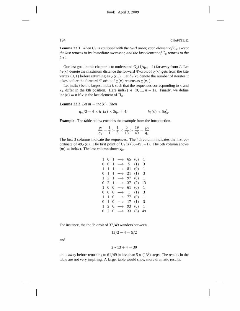
book April 3, 2009

194 CHAPTER 22

Lemma 22.1 When Cn is equipped with the twirl order, each element of Cn exceptthe last returns to its immediate successor, and the last element of Cn returns to thefirst.

Our last goal in this chapter is to understandO2(1/qn,−1) far away fromI . Leth1(κ) denote the maximum distance the forward9-orbit ofχ(κ) gets from the kitevertex(0,1) before returning asχ(κ+). Let h2(κ) denote the number of iterates ittakes before the forward9-orbit of χ(κ) returns asχ(κ+).

Let ind(κ) be the largest indexk such that the sequences corresponding toκ andκ+ differ in the kth position. Here ind(κ) ∈ {0, ...,n − 1}. Finally, we defineind(κ) = n if κ is the last element of5n.

Lemma 22.2 Let m= ind(κ). Then

qm/2− 4< h1(κ) < 2qm+ 4, h2(κ) < 5q2m.

Example: The table below encodes the example from the introduction.

p0

q0= 1

1>

1

3<

5

13>

19

49= p3

q3.

The first 3 columns indicate the sequences. The 4th column indicates the first co-ordinate of 49χ(κ). The first point ofC3 is (65/49,−1). The 5th column shows(m) = ind(κ). The last column showsqm.

1 0 1 −→ 65 (0) 10 0 1 −→ 5 (1) 31 1 1 −→ 81 (0) 10 1 1 −→ 21 (1) 31 2 1 −→ 97 (0) 10 2 1 −→ 37 (2) 131 0 0 −→ 61 (0) 10 0 0 −→ 1 (1) 31 1 0 −→ 77 (0) 10 1 0 −→ 17 (1) 31 2 0 −→ 93 (0) 10 2 0 −→ 33 (3) 49

For instance, the the9 orbit of 37/49 wanders between

13/2− 4= 5/2

and

2 ∗ 13+ 4= 30

units away before returning to 61/49 in less than 5× (132) steps. The results in thetable are not very inspiring. A larger table would show more dramatic results.

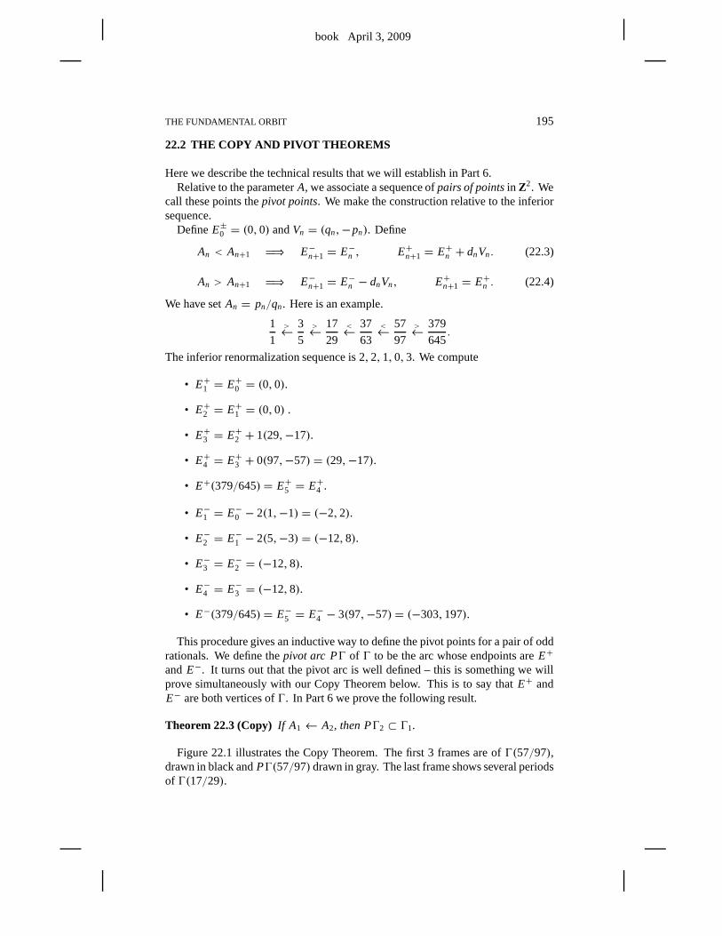
book April 3, 2009

THE FUNDAMENTAL ORBIT 195

22.2 THE COPY AND PIVOT THEOREMS

Here we describe the technical results that we will establish in Part 6.Relative to the parameterA, we associate a sequence ofpairs of pointsin Z2. We

call these points thepivot points. We make the construction relative to the inferiorsequence.

DefineE±0 = (0,0) andVn = (qn,−pn). Define

An < An+1 H⇒ E−n+1 = E−n , E+n+1 = E+n + dnVn. (22.3)

An > An+1 H⇒ E−n+1 = E−n − dnVn, E+n+1 = E+n . (22.4)

We have setAn = pn/qn. Here is an example.

1

1>← 3

5>← 17

29<← 37

63<← 57

97>← 379

645.

The inferior renormalization sequence is 2,2,1,0,3. We compute

• E+1 = E+0 = (0,0).

• E+2 = E+1 = (0,0) .

• E+3 = E+2 + 1(29,−17).

• E+4 = E+3 + 0(97,−57) = (29,−17).

• E+(379/645) = E+5 = E+4 .

• E−1 = E−0 − 2(1,−1) = (−2,2).

• E−2 = E−1 − 2(5,−3) = (−12,8).

• E−3 = E−2 = (−12,8).

• E−4 = E−3 = (−12,8).

• E−(379/645) = E−5 = E−4 − 3(97,−57) = (−303,197).

This procedure gives an inductive way to define the pivot points for a pair of oddrationals. We define thepivot arc PŴ of Ŵ to be the arc whose endpoints areE+

and E−. It turns out that the pivot arc is well defined – this is something we willprove simultaneously with our Copy Theorem below. This is tosay thatE+ andE− are both vertices ofŴ. In Part 6 we prove the following result.

Theorem 22.3 (Copy) If A1← A2, then PŴ2 ⊂ Ŵ1.

Figure 22.1 illustrates the Copy Theorem. The first 3 frames are ofŴ(57/97),drawn in black andPŴ(57/97) drawn in gray. The last frame shows several periodsof Ŵ(17/29).

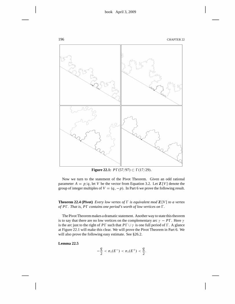
book April 3, 2009

196 CHAPTER 22

Figure 22.1: PŴ(57/97) ⊂ Ŵ(17/29).

Now we turn to the statement of the Pivot Theorem. Given an oddrationalparameterA = p/q, let V be the vector from Equation 3.2. LetZ [V ] denote thegroup of integer multiples ofV = (q,−p). In Part 6 we prove the following result.

Theorem 22.4 (Pivot) Every low vertex ofŴ is equivalent modZ [V ] to a vertexof PŴ. That is, PŴ contains one period’s worth of low vertices onŴ.

The Pivot Theorem makes a dramatic statement. Another way tostate this theoremis to say that there are no low vertices on the complementary arc γ − PŴ. Hereγis the arc just to the right ofPŴ such thatPŴ ∪ γ is one full period ofŴ. A glanceat Figure 22.1 will make this clear. We will prove the Pivot Theorem in Part 6. Wewill also prove the following easy estimate. See §26.2.

Lemma 22.5

−q

2< π1(E

−) < π1(E+) <

q

2.

book April 3, 2009

THE FUNDAMENTAL ORBIT 197

22.3 HALF OF THE RESULT

We will prove thatCn ⊂ C′n. This is almost an immediate consequence of the CopyTheorem.

For convenience, we recall the definition ofCn. Letµi = |pnqi − qn pi |.

Cn =⋃

κ∈5n

(Xn(κ),−1

), Xn(κ) =

1

qn

(1+

n−1∑

i=0

2kiµi

). (22.5)

It is convenient to write

Vk = sign(Ak+1 − Ak)Vk = ±(qk,−pk). (22.6)

When 1/1← A, the pivot arcPŴ(A) contains the points

kV0, k = 0, ...,d1, V0 = (−1,1). (22.7)

This is a consequence of the argument in §19.5.In general, supposeA1 ← A2 are two parameters. Then, by construction, the

pivot arcPŴ2 contains all points

v + kV1 k ∈ {0, ...,d}, d = floor(q2/2q1). (22.8)

Herev is any vertex ofPŴ1. It now follows from induction thatPŴn contains allpoints of the form

n−1∑

j=0

k j Vj , k j ∈ {0, ...,d j }. (22.9)

Let M denote the map from Equation 2.10. Usually we takeM so thatM(0,0) =0, but for the proof here, we adjust so that

M(0,0) = (1/qn,−1). (22.10)

(This makes no difference; see the discussion surrounding the definition ofM in§2.5.) Call a lattice pointevenif the sum of its coordinates is even. Note thatVj

is even for all j . Hence all points in Equation 22.9 are even. The images of thesepoints underM have their second coordinate equal to−1. We just have to worryabout the first coordinate. We have

M(Vj ) =1

qn+ 2|Aqj − p j | =

1

qn+

1

qn2|pnq j − qn p j |. (22.11)

The absolute value in the equation comes from the sign choicein the definition ofVj .

It now follows from the affine nature ofM and from the definition ofCn that

Cn ⊂ O2(1/qn,−1). (22.12)

It follows from the casen = 0 of Equation 21.7 thatCn ⊂ [0,2]× {−1}.

book April 3, 2009

198 CHAPTER 22

22.4 THE INHERITANCE OF LOW VERTICES

The rest of Theorem 1.8 follows from the Pivot Theorem and from what we havedone by applying the information contained in the Pivot Theorem to what we didin the previous section. To make the argument work, we first need to deal with atedious technical detail, which we take care of in this section.

Let A1← A2 be two odd rationals. As usual, we have

d1 = floor(q2/2q1). (22.13)

Let v1 be a vertex on the pivot arcPŴ1. Define

v2 = v1 + kV1, k ∈ {0, ...,d1}. (22.14)

Here we mean to choose some arbitraryk. The argument we give will work for anychoice. Notice that, ask ranges over all possibilities, we are considering exactly thesame vertices as in §22.3. Now we want to take a close look at these vertices. Hereis the main result of this section.

Lemma 22.6 v1 is low with respect to A1 iff v2 is low with respect to A2.

Proof: There are two cases to consider,depending on whetherA1 < A2 or A2 < A1.We will consider the former case. The latter case has essentially the same treatment.In our case, we haveV1 = V1. Let E±j be the pivot points forŴ j . Say that a vertexis high if it is not low.

We will first suppose thatv1 is low with respect toA1 and thatv2 is high withrespect toA2. This will lead to a contradiction. We writev j = (m j ,n j ). Let M j bethe fundamental map from Equation 2.10. Sincev1 is low andv2 is high, we have

2A1m1 + 2n1 +1

q1= M1(v1) ≤ 2− 1

q1,

2A2m2+ 2n2 +1

q2= M2(v2) ≥ 2+ 1

q2.

Rearranging terms,

2

(p2

q2m2 + n2

)− 2

(p1

q1m1 + n1

)≥ 2

q1. (22.15)

Plugging in the relationsm2 = m1 + kq1 andn2 = n1 − kp1 and simplifying, wehave

(m1+ kq1)(p2q1 − p1q2)

q1q2≥ 1

q1. (22.16)

SinceA1← A2 andA1 < A2, we have

p2q1− p1q2 = 2. (22.17)

Hence

m1 + kq1 ≥ q2/2. (22.18)

book April 3, 2009

THE FUNDAMENTAL ORBIT 199

Combining Equations 22.3 and 22.18, we have

E+1 (A2) = E+1 (A1)+ d1q1 ≥∗ m1+ kq1 > q2/2>∗ E+1 (A2).

This is a contradiction. The first starred inequality comes from the Pivot Theoremand the fact thatk ≤ d1. The second starred inequality comes from Corollary 22.5.

Now we will suppose thatv1 is high with respect toA1 andv2 is low with respectto A2. This also leads to a contradiction. LetM1 denote the first coordinate of thefundamental map relative to the parameterA1, adjusted so thatM1(0,0) = 1/q1.That is,

M1(m,n) = 2A1m+ 2n+ (1/q1). (22.19)

Sincev1 is high, we have the following dichotomy.

M1(v) ≥ 2+ 1

q1, M1(v) > 2+ 1

q1H⇒ M1(v) ≥ 2+ 3

q1. (22.20)

We will consider these two cases in turn.

Case 1:If M1(v1) = 2+ 1/q1, then

M1(m1,n1 − 1) = 1/q1 = M1(0,0).

But then

(m1,n1 − 1) = jV1

for some integerj . But then|m1| ≥ q1. Sincev1 ∈ PŴ1, this contradicts Corollary22.5. Hence

v1 = (0,1), v2 = kV1+ (0,1).

If v2 is low, then

0= 2k(A1q1 − p1) < 2k(A2q1− p1) = M2(v2)− M2(0,1) ≤ 0.

This is a contradiction. The first inequality comes fromA1 < A2.

Case 2: If M1(v1) ≥ 2 + 3/q, then the same reasoning as in Equations 22.15–22.17 (but with signs reversed) leads to

m1+ kq1 < −3q2. (22.21)

But then

−q2

2<−q1

2<∗ m1 ≤ m1+ kq1 < −3q2.

The starred inequality comes from Corollary 22.5. Again we have a contradiction,this time by a wide margin. 2

book April 3, 2009

200 CHAPTER 22

22.5 THE OTHER HALF OF THE RESULT

Now we finish the proof of Theorem 1.8.We revisit the construction in §22.3 and show that actuallyCn = C′n. Let 3n

denote the set of low vertices ofPŴn. By the Pivot Theorem, every low vertex onPŴn is equivalent to a point of3n modZ [Vn].

Lemma 22.7 For any n≥ 0, we have

3n+1 =dn⋃

k=0

(3n + kVn).

Proof: Induction. Forn = 0 we have

E−1 = (−d0,d0), E+1 = (0,0).

In this case, the right hand side of the equation precisely describes the set of pointson the line segment joining the pivot points. The casen = 0 therefore followsdirectly from the Pivot Theorem.

Let3′n+1 denote the right hand side of the main equation. SinceŴn is invariantunder translation byVn, every vertex of3′n+1 is low with respect toAn. Hence, byLemma 22.6, every vertex of3′n+1 is low with respect toAn+1. Combining this factwith Equation 22.8, we see that

3′n+1 ⊂ 3n+1. (22.22)

By Lemma 22.6 again, everyv ∈ 3n+1 is also low with respect toAn. Hence

v = v ′ + kVn, k ∈ Z (22.23)

for somev ′ ∈ 3n. If k 6∈ {0, ...,dn}, thenv lies either to the left of the left pivotpoint ofŴn+1 or to the right of the right pivot point ofŴn+1. Hencek ∈ {0, ...,dn}.This proves that

3n+1 ⊂ 3′n+1. (22.24)

Combining the two facts completes the induction step. 2

We proved Lemma 22.7 with respect to the inferior sequence. However, noticethat, if dn = 1, then3n+1 = 3n. Thus we get precisely the same result forconsecutive terms in the superior sequence. We have shown that v ∈ Ŵn is low ifand only ifv ∈ 3n modZ [V ]. But then

O2(1/qn,−1) ∩ I = M(3n), I = [0,2]× {−1}. (22.25)

HereM is the fundamental map. Recognizing3n as the set from Equation 22.9,we get precisely the equality in Theorem 1.8.

There is one last detail. One might worry thatM maps some points of3n topoints on [0,2]×{1} (rather than to [0,2]×{−1}). However, all points in3n haveeven parity. Hence this does not happen.

This completes the proof of Theorem 1.8.

book April 3, 2009

THE FUNDAMENTAL ORBIT 201

22.6 THE COMBINATORIAL MODEL

Here we prove Lemmas 22.1 and 22.2.

22.6.1 Combinatorics of the Return Map

Let6n denote the union of all points in Equation 22.9. We have

M(6n) = Cn. (22.26)

The ordering on6n determines the ordering of the return dynamics toCn. We set60 = {(0,0)} for convenience. We can determine the ordering on6n+1 from theordering on6n and the sign ofAn+1 − An. When An < An+1, we can write therelation

6n + kVn ≺ 6n + (k + 1)Vn, k = 0, ..., (dn − 1) (22.27)

to denote that each point in the left hand set precedes each point in the right handset. Within each set, the ordering does not change. WhenAn > An+1, we can writethe relation

6n − (k+ 1)Vn ≺ 6n − kVn, k = 0, ..., (dn − 1). (22.28)

Lemma 22.1 follows from these facts and induction.

22.6.2 Geometry of the Return Map

Let βn denote the arc ofPŴn, chosen so thatPŴn ∪ βn is one period ofPŴn. LetLn be the line of slope−An through the origin.

Lemma 22.8 No point ofβm lies more than qm vertical units away from Lm, andsome point ofβm lies at least qm/4 vertical units away from Lm.

Proof: By the Room Lemma,βm ⊂ R(Am). The upper bound follows immediatelyfrom this containment. For the lower bound, recall from the Room Lemma thatPŴm crosses the centerlineL of R(Am) once, and this crossing point lies at least(pm + qm)/4 > qm/4 vertical units fromLm. By Lemma 22.5 and symmetry, theleft endpoint ofβm lies to the left ofL and the right endpoint ofβm lies to the rightof L. Henceβm contains the crossing point we have mentioned. For an alternativeargument, we note that no point on the pivot arc crosses the line parallel to the floorand ceiling ofR(Am) and halfway between them, whereas the crossing point liesabove this midline. 2

Notice that the lineLn replaces the lineLm in the next lemma.

Lemma 22.9 Let m≤ n and qm > 10. Then some point ofβm lies at least qm/4−1vertical units from Ln. Moreover, no point ofβm lies more than qm+1vertical unitsaway from Ln.

book April 3, 2009

202 CHAPTER 22

Proof: Some pointv of βm is at leastqm vertical units fromLm, by the previousresult. From Lemma 17.4, we have

|Am − An| < 2/(q2m). (22.29)

On the other hand, by the Room Lemma and by construction,PŴm is contained intwo consecutive translates ofR(Am), one of which isR(Am) itself. HencePŴm

lies entirely inside the ballB of radius 4qm about the origin. By Equation 22.29, theHausdorff distance between the seqmentsLm ∩ B andLn ∩ B is less than 1 oncem> 10. By construction, the vertical line segment starting atv and dropping downqm − 1 units is disjoint fromLn ∩ B. But this segment is disjoint fromLn − B aswell. Hencev is at leastqm/2− 1 vertical units fromLn. The upper bound has asimilar proof. 2

Lemma 22.10βm has length at most5q2m.

Proof: βm is contained in one period ofPŴm. Hence it suffices to bound the lengthof any one period ofPŴm. By the Room Lemma, one such period is contained inR(Am). We compute easily that the area ofR(Am) is much less than 5q2

m. Hencethere are fewer than 5q2

m vertices inR(Am). Hence the length of one period ofPŴm

is less than 5q2m. 2

Suppose now thatκ andκ+ are two consecutive points of6n. By this we meanthat there is a portion ofPŴn connectingκ to κ+ when it is oriented from left toright.

We want to understand the arc ofPŴn that joins κ and κ+. Suppose thatind(κ) = m. It follows from induction and from the Copy Theorem that thereis some translationT such thatT(κ) andT(κ+) are the endpoints of the arcβm.The arc joiningκ to κ+ has the same length asβm, and this length is less than 5q2

m.This gives us the estimate forh2.

Now we deal withh1. We check the result by hand forqn < 10. So, supposethatqn > 10. All the verticesκ , κ+, T(κ), andT(κ+) lie within 1 vertical unit ofthe baselineLn. We know that the vertical distance from some point ofβm to Ln isat leastqm/2− 1. Hence the vertical distance from some point onT(βm) to Ln isat leastqm/2− 2. Similarly, the vertical distance from any point ofβm to Ln is atmostqm+ 2. If two points inZ2 have vertical distanced, then the images of thesepoints under the fundamental mapMn have horizontal distance 2d. In short, thefundamental map doubles the relevant distances. This fact gives us the estimate forh1.

This completes the proof of Lemma 22.2. 2

Remark: We have tried to give fairly precise estimates in our arguments, but actu-ally we do not use these estimates for any purpose.

book April 3, 2009

THE FUNDAMENTAL ORBIT 203

22.7 THE EVEN CASE

Here we discuss Theorem 1.8 in the even case. For each even rational A1 ∈ (0,1),there is a unique odd rationalA2 such that (in terms of Equation 4.1)A1 = (A2)±andq2 < 2q1. In Lemma 27.2, we will show thatŴ1 (a closed polygon) contains acopy of PŴ2, and all low vertices ofŴ1 lie on this arc. From this fact, we see that

O(1/q1,−1) = M1(61), (22.30)

just as in the odd case. HereM1 is the fundamental map defined relative to theparameterA1, and61 is the set of low vertices onPŴ1.

Note that61 = 62, where62 is the set of low vertices onPŴ2. The onlydifference between the two setsM1(61) andM2(62) is the difference in the mapsM1 and M2. Now we explain the precise form of Theorem 1.8 that this structureentails.

Switching notation, letA be an even rational. One of the two rationalsA± fromEquation 4.1 is odd, and we call this rationalA′. We can find the initial part of asuperior sequence{Ak} such thatA′ = An−1. We setA = An even thoughA doesnot belong to this sequence. Referring to Theorem 1.8, we define5n exactly as inthe odd case but for one detail. In case 2q′ > q, we simply ignore thenth factor of5n. That is, we treatq′ as an inferior term. Once changed in this way, Theorem 1.8holds in the even case and has a proof that follows the odd caseword for word.

Here we give an example. LetA1 = 12/31. ThenA2 = 19/49, exactly is in theintroduction. We haven = 3, and the sequence is

p0

q0= 1

1,

1

3,

5

13,

12

31= p3

q3.

All terms are superior, so this is also the superior sequence. The renormalizationsequence is 1,2,1. Theµ sequence is 19,5,1. The first coordinates of the 12 pointsof O2(1/49)∩ I are given by

1⋃

k0=0

2⋃

k1=0

1⋃

k2=0

2(19k0+ 5k1+ 1k2)+ 1

31.

Writing these numbers in a suggestive way, the union above works out to

1

31×(1 3 11 13 21 23 39 41 49 51 59 61

).

book April 3, 2009

book April 3, 2009

Chapter Twenty-Three

The Comet Theorem

23.1 STATEMENT 1

We fix an irrational parameterA ∈ (0,1). Let {An} be the superior sequenceapproximatingA. Let Ŵn be the arithmetic graph corresponding toAn. We say thata vertexv of Ŵn is D-low if v is within D vertical units of the baseline ofŴn.

Note that the low vertices considered in the previous chapter are 1-low vertices.These vertices play a special role in our arguments. The fundamental mapM fromEquation 2.10 maps the 1-low vertices into the interval

J = (0,2)× {−1,1}. (23.1)

In Part 6 we prove the following result.

Theorem 23.1 (Low Vertex) Fix N0. There are constants N1 and N2 with thefollowing property. Ifvn is an N0-low vertex contained in a component ofŴn

having diameter at least N1, then there is an arc ofŴn that has length at most N2and connectsvn to a1-low vertex. The constants N1 and N2 depend only on A andN0.

Now we will deduce statement 1 of the Comet Theorem. Looking at Figure 1.2,we see that

J = I ∪ (ψ ′)3(I ), (23.2)

whereψ ′ is the outer billiards map. Hence it suffices to prove statement 1 of theComet Theorem withJ in place of I . Sinceψ = (ψ ′)2, it suffices to prove theresult withJ in place ofI andψ in place ofψ ′. This is what we will do.

Fix N > 0. The constantsN0, N1, ... depend only onA and N. Recall that4 = R+ × {−1,1} and that9 is the first return map to4. Recall also thatUA isthe union of the unbounded special orbits.

Corollary 23.2 If ξ ∈ 4 ∩UA and‖ξ‖ < N then9k(ξ) ∈ J for some|k| < N2.

Proof: The arithmetic graphŴn tracks the orbits of the special intervals definedin §2.2. For eachn we choose some special intervalIn whose closure containsξ .Typically the choice is unique, but whenξ lies in the boundary of a special interval,there are two choices and we pick one arbitrarily.

Let vn be the vertex ofŴn corresponding toIn. From Equation 2.10 we see thatvn is N0-low, whereN0 = (N/2)+ 1. Letβn be the component ofŴn that containsvn. By the Continuity Principle in §2.7,

diam(βn)→∞. (23.3)

book April 3, 2009

206 CHAPTER 23

By Equation 23.3, the diameter ofβn exceedsN1 for n large.The Low Vertex Theorem says that there is some arcβ ′n of βn, having length at

mostN2, that connectsvn to a 1-low vertex.By the Continuity Principle, the firstN2 iterates of9n are defined onξ for n large.

Interpretingβ ′n dynamically we see that there is a sequence{kn} such that

9knn (ξ) ∈ J, |kn| < N2. (23.4)

By the Pidgeonhole Principle,somekappears infinitely often in the sequence{kn}.Applying the Continuity Principle to this subsequence, we see that9k(ξ) ∈ J. 2

Remark: Referring to the proof we just gave, one might worry that someof thepoints involved actually lie in the boundary ofJ. However, the boundary pointsof J do not have well defined orbits and all the points we considered do have welldefined orbits. Hence this problem does not occur.

Corollary 23.3 If ξ ∈ 4 ∩UA and‖ξ‖ < N, thenψk(ξ) ∈ J for some|k| < N5.

Proof: By Corollary 23.2, there is somem ∈ (−N2, N2) such that9m(ξ) ∈ J. Wewill consider the case whenm ≥ 0. The proof in the other case is essentially thesame. Letξ0 = ξ and inductively define

ξ j = 9(ξ j−1), j = 1, ...,m. (23.5)

Examining the proof of the Pinwheel Lemma, we see that there is some constantN3

such that

‖ξ j ‖ < N3, j = 0, ...,m. (23.6)

Again examining the proof of the Pinwheel Lemma, we see that there are constantsn1, ...,nm such that

ξ j = ψn j (ξ j−1), n j ∈ (0, N4). (23.7)

SettingN5 = N2N4 we see thatψk(ξ) ∈ J for some|k| < N5. 2

Corollary 23.4 If ζ ∈ UA and‖ζ‖ < N, thenψk(ζ ) ∈ J for some|k| < N8.

Proof: Examining the proof of the Pinwheel Lemma, we see that there is someconstantN6, some|m| < N6, and someξ ∈ 4 such that

ξ = ψm(ζ ), ‖ξ‖ < N6. (23.8)

Applying Corollary 23.3 withN6 in place of N, we haveψn(ξ) ∈ J for some|n| < N7. Thereforeψk(ζ ) ∈ J for some|k| < N8. Here we have setN8 = N6+N7.2

Corollary 23.4 is identical to statement 1 of the Comet Theorem, except that itusesψ in place ofψ ′ andJ in place ofI . This completes the proof.

book April 3, 2009

THE COMET THEOREM 207

23.2 THE CANTOR SET

Before we prove the remaining statements of the Comet Theorem we first need toresolve the technical point that the setCA is actually well defined. For convenience,we repeat the definition.

CA =⋃

κ∈5

(X(κ),−1

), X(κ) =

∞∑

i=0

2ki |Aqi − pi |. (23.9)

Lemma 23.5 The infinite sums in Equation 23.9 converge. Hence CA is well de-fined.

Proof: Combining Equation 21.5 with the bound 0≤ kn < dn, we see that thenthterm in the sum definingX(κ) is at most 2q−1

n . Given that 2qk < qk+1 for all k, weget

2q−1n < 2−n+1. (23.10)

The sequence definingX(κ) decays exponentially and hence converges. 2

For the purposes of this section, we equip the product space5 with the lexico-graphic ordering and the product topology. For instance, ifdn = 1 for all n, then5is just the space of binary sequences. The lexicographic order treats these sequencesas binary expansions of real numbers and then orders them as usual. The generalcase is similar.

Lemma 23.6 The map X:5 → CA is a homeomorphism that maps the lexico-graphic order to the linear order. Hence CA is a Cantor set.

Proof: We first show that the mapX is injective. In fact, we will show thatX isorder preserving. Ifκ = {ki } ≺ κ ′ = {k′i } in the lexicographic ordering, then thereis some smallest indexm such thatki = k′i for all indicesi = 0, ..., (m− 1) andkm < k′m. Letλm = |Aqm− pm|, as in Equation 21.5. Then

X(κ ′)− X(κ) ≥ 2λm −∞∑

k=m+1

2dkλk = λm − λ′m+1 > 0 (23.11)

by Equation 21.7.The mapX:5→ [0,2] is continuous with respect to the topology on5 because

thenth term in the sum definingX is always less than 2−n+1. We also know thatXis injective. HenceX is bijective onto its image. Any continuous bijection from acompact space to a Hausdorff topological space is a homeomorphism. 2

Remark: In Chapter 25 we will have much more to say about the geometry of CA.For instance,CA always has length 0.

book April 3, 2009

208 CHAPTER 23

23.3 A PRECURSOR OF THE COMET THEOREM

In this section we present two auxilliary results that combine to prove almost all theremaining statements of the Comet Theorem.

Let CA be the Cantor set considered in the previous section. Define

C′A = CA − (2Z [ A] × {−1}). (23.12)

One can view our next result as a precursor of the Comet Theorem.

Theorem 23.7 (Comet Precursor)Let UA denote the set of unbounded specialorbits relative to an irrational A∈ (0,1).

1. C′A ⊂ UA.

2. The first return mapρA: C′A→ C′A is defined precisely on C′A− φ(−1). Themapφ−1 conjugatesρA to the restriction of the odometer onZ A.

3. For ζ ∈ C′A − φ(−1), the orbit portion betweenζ andρA(ζ ) has excursiondistance in [

d−1

2− 4,2d−1+ 20

]

and length in[

d−2

32− d−1

4,100d−3+ 100d−2

].

Here d= d(−1, φ−1(ζ )).

Remarks:(i) The constants in item 3 are not optimal; some tedious elementary argumentswould improve them.(ii) Sinced−1 ≥ 1, the estimates in item 3 imply the less precise estimates intheComet Theorem – once we establish thatC#

A = C′A.(iii) As we remarked following the Comet Theorem, the only nonsharp bound initem 3 is the length upper bound. For instance, our proof in [S1], which establishesa kind of coarse self-similarity structure, would give a better bound forA =

√5−2

if carefully examined. We conjecture that−3 is the best bound that works for allparameters at once.

To relate Theorem 23.7 to the Comet Theorem, we prove the following doubleidentity.

Lemma 23.8 UA ∩ I = C#A = CA − (2Z [ A] × {−1}).

Statements 2 and 3 of the Comet Theorem follow from this result and Lemma 23.7.Lemma 23.8 also contains the first claim in statement 4 of the Comet Theorem. Atthe end of the chapter, we will prove the second claim made in statement 4 of theComet Theorem.

book April 3, 2009

THE COMET THEOREM 209

23.4 CONVERGENCE OF THE FUNDAMENTAL ORBIT

Let{pn/qn} denote the superior sequence associated toA. We use the notation fromthe previous chapter. HereŴn denotes the corresponding arithmetic graph and

Cn =⋃

κ∈5n

(Xn(κ),−1

), Xn(κ) =

1

qn+

n−1∑

i=0

2ki |Anqi − pi |. (23.13)

We have already proved that

Cn ⊂ O2(1/qn,−1). (23.14)

Let κ ∈ 5 be some infinite sequence. Letκn ∈ 5n be the truncated sequence.Let

σn = (Xn(κn),−1), σ = (X(κ),−1) (23.15)

Here is our basic convergence result.

Lemma 23.9 σn→ σ as n→∞.

Proof: For i < n, let τi,n denote thei th term in the sum forXn(κn). Let τn be thecorresponding term in the sum forX(κ). By Lemma 17.1, the sign ofA− Ai is thesame as the sign ofAn − Ai . Therefore

|τn − τi,n|=2k|A− An|qn < 2q−1

n <

2−n+1. (23.16)

Therefore

|σ − σn| =|X(κ)− X(κn)|=

n−1∑

i=0

|τn − τi,n| +∞∑

i=n

τi <

2n−1∑

i=0

2−n + 2∞∑

i=n

2−i <

(2n+ 4)2−n. (23.17)

This completes the proof. 2

The uniformity of convergence gives us the following immediate corollary.

Corollary 23.10 CA is the Hausdorff limit of{Cn}.

book April 3, 2009

210 CHAPTER 23

23.5 AN ESTIMATE FOR THE RETURN MAP

Let {ki } be a point in the sequence space5. We call{ki } first if ki = 0 for all i , andlast if ki = di for all i . The mapφ2:5A → CA is a homeomorphism. Usingφ2,we transfer the notions offirst andlast to points ofCA.

It turns out that the first and last points ofCA are the special points mentioned inconnection with the Comet Theorem. If these orbits are well defined, then it turns outthat the last point leavesCA under the forward dynamics and never returns. Likewise,the first point ofCA leaves under the backward dynamics and never returns. (Weprove these statements later on.) Here we will estimate the nature of how the nonlastpoints ofCA return toCA under the forward direction of the dynamics. The idea isto essentially take the geometric limit of the result from Lemma 22.2.

Let ζ ∈ C′A denote a point that is not last. Letκ denote the corresponding se-quence in5A. Say that two sequences in5 areequivalentif they have the sameinfinite tail end. We can define the reverse lexicographic order on any equivalenceclass. Likewise, we can extend the twirl order to any equivalence class. In particu-lar, we extend the twirl order to the equivalence class ofκ , the sequence currentlyof interest to us.

Remark: These orders on equivalence classes cannot be defined on the entirespace; points in different equivalence classes are often not comparable.

Sinceκ is not last, we can find some smallest indexm = m(ζ ) wherekm < di .In other words,m is the smallest index such thatκ differs from the last sequence inthemth spot.

The successorκ+ of κ is obtained by incrementingkm by 1 and settingki = 0for all i < m. This notion of successor is compatible with the twirl ordering on thefinite truncations5n. Define

ζ+ = (X(κ+),−1), (ζn)+ = (X(κn)+,−1). (23.18)

Lemma 23.11 Let ζ ∈ C′A be a point that is not last. Let m= m(ζ ). The forward9 orbit of ζ returns to CA as ζ+ in at most5q2

m steps. This portion of the orbitwanders between qm/2− 2 units and2qm + 2 units away from(0,−1).

Proof: By Lemma 2.2, the orbit ofζ is well defined. Referring to the notation inLemma 22.2, we get ind(κn) = m for n large enough. Hence the forward9n orbitof ζn returns to(ζn)+ after at most 5q2

m steps, moving away from(0,−1) by at leastqm/2− 2 units and at most 2qm + 2 steps. Herem is independent ofn. SinceXis continuous, we have(ζn)+ → ζ+ asn→∞. The Contintuity Principle impliesthat the forward9 orbit of ζ returns asζ+ after at most 5q2

m steps, moving awayfrom (0,−1) at leastqm/2− 2 units and at most 2qm + 2 steps. 2

There is an entirely analogous result for the backward return map. This resultholds for all but the first point.

book April 3, 2009

THE COMET THEOREM 211

23.6 PROOF OF THE COMET PRECURSOR THEOREM

23.6.1 Statement 1

Here we prove statement 1 of Theorem 23.7. We say that a sequence of5A isequivalent-to-firstif it differs from the first sequence in only a finite number ofpositions. We call a sequenceequivalent-to-lastif it differs from the last sequencein a finite number of positions. As in the previous section, wetransfer these notionstoCA. It is immediate from the definitions that no sequence in5A is both equivalent-to-first and equivalent-to-last.

Let ζ be a point inC′A that is not equivalent-to-last. We will show that the forwardorbit of ζ is unbounded. Letm= m(κ) be as in the proof of Lemma 23.11. Lemma22.2 says that the portion of the orbit betweenζ andζ+ wanders at leastqm/5 fromthe origin. Since we can achieve any initial sequence we likewith iterated successorsof κ , we can find iterated successorsκ ′ of κ such thatm(κ ′) is as large as we like.But this shows that the forward orbit ofζ is unbounded. Here we are using the factthat limm→∞ qm = ∞. This shows thatζ has an unbounded forward orbit.

Essentially the same argument works for the backward orbit of points that are notequivalent-to-first. This establishes statement 1.

23.6.2 Statement 2

The successor map on5A is defined except on the last sequenceκ of5A. Referringto the homeomorphismφ1 given in Equation 1.8, we have

φ1(−1) = κ.

Thus the pointφ2(κ) ∈ CA corresponding toκ is preciselyφ(−1). By Lemma23.11, the return mapρA: C′A→ C′A is defined onC′A − φ(−1).

The mapφ1 conjugates the odometer map onZ A to the successor map on5A.Combining this fact with Lemma 23.11, we see thatφ−1 conjugatesρA to therestriction of the odometer map onZ A.

It remains to understand what happens to the forward orbit ofx = φ(−1) in thecase whenx ∈ C′A. The following result completes the proof of statement 2.

Lemma 23.12 If x ∈ C′A, then the forward orbit of x does not return to C′A.

Proof: Suppose that the forward orbit ofx returns toC′A afterN steps. Since outerbilliards is a piecewise isometry, there is some open neighborhoodU of x suchthat every point ofC′A ∩ U returns toC′A in at mostN steps. But there is someuniformly smallm such that every pointζ ∈ C′A−U differs from the last sequenceκ at or before themth spot. Lemma 23.11 says that such points return toC′A in auniformly bounded number of steps. In short, all points ofC′A return toC′A in auniformly bounded number of steps. But then all orbits inC′A are bounded. This isa contradiction. 2

book April 3, 2009

212 CHAPTER 23

23.6.3 Statement 3

Let ζ ∈ C′A. Let Oζ denote the portion of the forward outer billiards orbit ofζbetweenζ andρA(ζ ). We mean to use the original outer billiards mapψ ′ here. Letm be such that

d(φ−1(ζ ),−1) = q−1m . (23.19)

By definitionφ−1(ζ ) and−1 disagree byZ/Dm+1, but then they agree inZ/Dk fork = 1, ...,m. In the case whenm = 0, the pointsφ−1(ζ ) and−1 already disagreein Z/D1. Let κ ∈ 5A denote the sequence corresponding toζ .

Finding the Index: Let ind(κ) be as in §22.1. Letλ be the sequence correspondingtoφ(−1). Thenλ is the last sequence in the twirl order. The sequencesκ andλagreein positionsk = 0, ...,m− 1 but then disagree in positionm. Hencem is the firstindex whereκ disagrees with the last sequence in the twirl order. But thenκ andκ+disagree in positions 0, ...,m and agree in positionk for k > m. Hence ind(κ) = m.

Excursion Distance Bounds:Lemma 23.11 tells us that the9-orbit of ζ betweenζ andρA(ζ ) wanders betweenqm/2− 4 and 2qm + 4 units from the origin. Herewe are interested in the full outer billiardsOζ . Since the9-orbit of ζ betweenζandρζ is a subset ofOζ , the lower bound follows from Lemma 23.11.

The upper bound follows from a simple geometric analysis of the PinwheelLemma. Starting at a point on4 that isR units from the origin, theψ-orbit remainswithin 2R+ 8 units of the origin before returning to4. Essentially, theψ-orbitfollows an octagon once around the kite before returning, asshown in Figure 7.3.The constant of 10 amply takes care of the small deviations from this path that arisein the proof of the Pinwheel Lemma. Sinceψ ′ always acts as the reflection in avertex that is within 1 unit of the origin, we see that the entireψ ′-orbit of interestto us is at most 2R+ 12 units from the origin. Hence the portion of the orbit ofinterest wanders at most 2(qm+ 4)+ 12= 2qm+ 20 units from the origin.

Orbit Length Bounds: The9-orbit of ζ betweenζ andρA(ζ ) has length at most5q2

m. Examining the proof of the Pinwheel Lemma, we see that a point on4 that isRunits from the origin returns to4 in less than 10R iterates. Given thatR= 2qm+2,the orbitOζ is at most 20qm+ 20 times as long as the corresponding9-orbit. Thisgives the upper bound.

Now we prove the lower bound. Some point in the9-orbit of ζ betweenζ andρA(ζ ) lies at leastqm/2− 4 vertical units from the origin. Consecutive iterates inthe9-orbit have vertical distance at most 4 units apart. Hence there are at leastqm/8−1 points in the9-orbit that are at leastqm/4 horizontal units from the origin.Inspecting the Pinwheel Lemma, we see that the length of theψ ′-orbit between twosuch points is at leastqm/4. HenceOζ has length at leastq2

m/32− qm/4.

This completes the proof of statement 3.

book April 3, 2009

THE COMET THEOREM 213

23.7 THE DOUBLE IDENTITY

In this section we will prove Lemma 23.8. Our proof of this result relies on thefollowing technical theorem.

Theorem 23.13 (Period)For any ǫ > 0, there is an N> 0 with the followingproperty. Ifζ ∈ I is more thanǫ units from Cn, then the period ofζ is at most N.The constant N depends only onǫ and A.

We will prove the Period Theorem in Part 6. Here is a corollaryof this result.

Corollary 23.14 UA ∩ I ⊂ CA.

Proof: The constantsN1, N2, ... depend only onǫ andA.We will suppose thatUA contains a pointζ 6∈ CA and derive a contradiction. By

compactness, there is someǫ > 0 such thatζ is at least 3ǫ from any point ofCA.SinceCA is the geometric limit ofCn, we see that there is someN1 such thatn > N1

implies thatζ is at least 2ǫ from Cn.Let {ζn} ∈ I be a sequence of points converging toζ . We can choose these points

so that the orbit ofζn relative toAn is well defined. There is a constantN2 suchthatn > N2 implies thatζn is at leastǫ from Cn. But then, by the Period Theorem,there is someN3 such that the period ofζn is at mostN3.

On the other hand, by the Continuity Principle in §2.7, the arithmetic graphŴ(ζn, An) converges to the arithmetic graphŴ(ζ, A). In particular, the period ofŴ(ζn, An) tends to∞. This is a contradiction. Henceζ cannot exist. 2

Now we state a useful principle that will help with the remainder of the proof ofLemma 23.8.

Odometer Principle: Let 5A be the sequence space from §1.7. Say that twosequences in5A are equivalent if they have the same infinite tail ends. Giventhenature of the odometer map, we have the following useful principle. Any two equiv-alent sequences are in the same orbit of the odometer map. Call this theOdometerPrinciple. We will use this principle several times in our proofs.

Lemma 23.15 No point of CA − C#A has a well defined orbit.

Proof: Let {dn} be the renormalization sequence, as above. Call a sequence in5A equivalent-to-trivialif it either differs from the 0 sequence by a finite numberof terms or it differs from the sequence{di } by a finite number of terms. Thehomeomorphismφ2 bijects the equivalent-to-trivial points in5A to CA − C#

A.Suppose first that the superior sequence forA is not eventually monotone. Refer-

ring to §23.6 for definitions, in this case an equivalent-to-trivial sequence is neitherequivalent-to-first nor equivalent-to-last.

Supposeσ ∈ CA−C#A has a well defined orbit. Letκ be the equivalent-to-trivial

sequence corresponding toσ . By Lemma 23.11 and the analog for the backward

book April 3, 2009

214 CHAPTER 23

orbit, both directions of the orbit ofσ return infinitely often toCA − C#A. If κ is

eventually 0, then by the Odometer Principle,κ is in the same sequence orbit asthe 0 sequenceκ0. But the point inCA corresponding toκ0 is exactly the vertex(0,−1). This vertex does not have a well defined orbit. This is a contradiction. Ifκis such thatki = di for largei , then by the Odometer Principle,κ is in the same orbitas the sequence{di }. By Equation 21.5, the corresponding point inCA is (2,−1).One can easily check that the orbit of(2,−1) is not defined after the second iterate.Again we have a contradiction.

Now suppose the superior sequence is eventually monotone. We will treat thecase whenA− An is eventually positive. In this case,{An} is eventually monotoneincreasing. Suppose thatκ is equivalent to the 0-sequence. We can iterate backwarda finite number of times untilσ returns as the first point ofCA. Hence, without lossof generality, we can assume thatκ is the first sequence in5A. But now we caniterate forward indefinitely, and we will reach every equivalent-to-zero sequence bythe Odometer Principle. Eventually, we reach the 0 sequenceand get the same con-tradiction as above. Ifκ is such thatki = di for largei , we run the same argumentbackward. 2

Corollary 23.16 UA ∩ I ⊂ C#A.

Proof: Corollary 23.14 says thatUA ∩ I ⊂ CA. Since all orbits ofUA are welldefined, Lemma 23.15 implies that

UA ∩ (CA − C#A) = ∅.

Our result follows immediately. 2

Lemma 23.17 No point of C#A has a first coordinate in2Z [ A].

Proof: Let{An}be the superior sequence approximatingA. We assume thatAn < Ainfinitely often. The other case has the same treatment. Suppose that

α = (2M A+ 2N,−1) ∈ C#A. (23.20)

By Equation 21.7, the setC#A is invariant under the map

(x,−1)→ (2− x,−1).

Indeed, the twist automorphism of5 induces this map onCA. From this symmetry,we can assume thatM > 0.

Let PŴk denote the pivot arc. Suppose, for the sake of contradiction, that(M, N)is a vertex ofPŴk for somek. Then 2AM + 2N is a finite sum of terms

λ j = |2Aqj − p j |, (23.21)

by Theorem 1.8. But such points all lie inCA −C#A. This contradiction shows that

(M, N) is not a vertex ofPŴk for anyk.

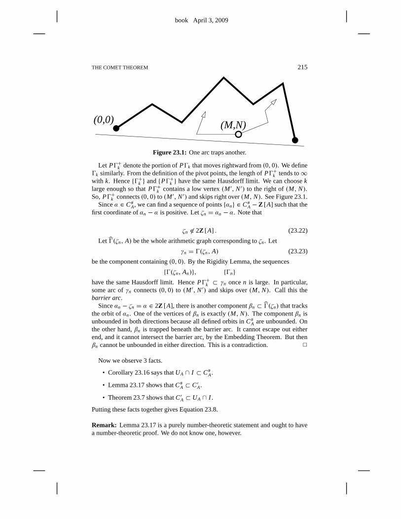
book April 3, 2009

THE COMET THEOREM 215

(0,0) (M,N)

Figure 23.1: One arc traps another.

Let PŴ+k denote the portion ofPŴk that moves rightward from(0,0). We defineŴk similarly. From the definition of the pivot points, the length of PŴ+k tends to∞with k. Hence{Ŵ+k } and{PŴ+k } have the same Hausdorff limit. We can chooseklarge enough so thatPŴ+k contains a low vertex(M ′, N′) to the right of(M, N).So,PŴ+k connects(0,0) to (M ′, N′) and skips right over(M, N). See Figure 23.1.

Sinceα ∈ C#A, we can find a sequence of points{αn} ∈ C#

A− Z [ A] such that thefirst coordinate ofαn − α is positive. Letζn = αn − α. Note that

ζn 6∈ 2Z [ A] . (23.22)

Let Ŵ(ζn, A) be the whole arithmetic graph corresponding toζn. Let

γn = Ŵ(ζn, A) (23.23)

be the component containing(0,0). By the Rigidity Lemma, the sequences

{Ŵ(ζn, An)}, {Ŵn}have the same Hausdorff limit. HencePŴ+k ⊂ γn oncen is large. In particular,some arc ofγn connects(0,0) to (M ′, N′) and skips over(M, N). Call this thebarrier arc.

Sinceαn − ζn = α ∈ 2Z [ A], there is another componentβn ⊂ Ŵ(ζn) that tracksthe orbit ofαn. One of the vertices ofβn is exactly(M, N). The componentβn isunbounded in both directions because all defined orbits inC#

A are unbounded. Onthe other hand,βn is trapped beneath the barrier arc. It cannot escape out eitherend, and it cannot intersect the barrier arc, by the Embedding Theorem. But thenβn cannot be unbounded in either direction. This is a contradiction. 2

Now we observe 3 facts.

• Corollary 23.16 says thatUA ∩ I ⊂ C#A.

• Lemma 23.17 shows thatC#A ⊂ C′A.

• Theorem 23.7 shows thatC′A ⊂ UA ∩ I .

Putting these facts together gives Equation 23.8.

Remark: Lemma 23.17 is a purely number-theoretic statement and ought to havea number-theoretic proof. We do not know one, however.

book April 3, 2009

216 CHAPTER 23

23.8 STATEMENT 4

We have already established the first part of statement 4 of the Comet Theorem.Now we prove the second part.

By statements 1 and 2 of the Comet Theorem, it suffices to consider pairs ofpoints inC#

A. It follows immediately from Equation 2.1 that two points ofC#A lie

on the same orbit only if their first coordinates differ by an element of 2Z [ A]. Ourgoal is to prove the converse.

Lemma 23.18 All but at most2 orbits in C#A are erratic.

Proof: By Theorem 23.7, Lemma 23.11, and the backward analog of Lemma 23.11,all orbits inC#

A are erratic except those corresponding to the eqivalent-to-first se-quences and the equivalent-to-last sequences. By the Odometer Principle, all thepoints inC#

A corresponding to equivalent-to-first sequences lie on the same orbit.Likewise, all the points inC#

A corresponding to equivalent-to-last sequences lie onthe same orbit. These two orbits are the only ones that can fail to be erratic. 2

Lemma 23.19 Suppose that two points in C#A have first coordinates that differ by

2Z [ A]. Suppose also that at least one of the points has an erratic orbit. Then thetwo points lie on the same orbit.

Proof: One direction follows immediately from Equation 2.1. For the converse,suppose that the two points have first coordinates that differ by 2Z [ A]. The firstcoordinates of the points do not lie in 2Z [ A], by Lemma 23.17. Hence one and thesame arithmetic graphŴ contains componentsγ1 andγ2 that, respectively, track thetwo orbits.

Since both orbits are dense inC#A, we know that both are erratic in at least one

direction. Suppose first thatγ1 is erratic in both directions. Sinceγ2 is erratic inone direction, we can find a low vertexv of γ1 that is not a vertex ofγ2. Sinceγ2 iserratic in both directions, we can find verticesw1 andw2 of γ1 lying to the left andto the right ofv, respectively. But then the arc ofγ1 starting atv is trapped beneaththe arc ofγ2 connectingw1 to w2. This contradicts the Embedding Theorem. Inshort,Ŵ is not big enough to contain both components. 2

It remains only to deal with the case when both points lie on orbits that are onlyerratic in only one direction..

Lemma 23.20 Suppose that two points in C#A have first coordinates that differ by

2Z [ A]. Suppose also that neither point lies on an erratic orbit. Then the two pointslie on the same orbit.

Proof: Let α ∈ C#A (respectively,β) be the unique point such that the forward

(respectively, backward) first return map toC#A atα (respectively,β) does not exist.

There are exactly 2 one-sided erratic orbits.α is one orbit, andβ is on the other.

book April 3, 2009

THE COMET THEOREM 217

It suffices to prove thatα − β 6∈ 2Z [ A] × {0}. We will suppose the contrary andderive a contradiction. Suppose thatα−β = (2Am+2n,0) for some(m,n) ∈ Z2.α is the last point in the twirl order, andβ is the first point. In terms of sequences,

α corresponds to the sequence{di } andβ corresponds to the sequence{0i }. Let{α j }be a sequence of points inC#

A converging toα, chosen so that the correspondingorbit is erratic. Define

β j = α j + (β − α). (23.24)

Then

α j − β j = (2Am+ 2n,0). (23.25)

By the case we have already considered,β j lies in the same orbit asα j .For j large, the sequence corresponding toα j matches the terms of the sequence

for α for many terms. Likewise, the sequence corresponding toβ j matches theterms of the sequence forβ for many terms. Hence these two sequences disagreefor many terms. Given that the return dynamics toC#

A is conjugate to the odometermap on the sequence space, we have

2Am+ 2n = π1(α j − β j ) =N j∑

i=0

a j i λi , |a j i | ≤ di . (23.26)

HereN j →∞ as j →∞, andπ1 denotes projection onto the first coordinate.Let M be the map from Equation 2.10. We have

M(m,n) =N j∑

i=0

b j i M(Vi ), |b j i | ≤ di . (23.27)

Hereb j i = ±a j i , depending on the sign ofAi − A. SinceA is irrational,M isinjective. Therefore, settingN = N j for ease of notation, we have

(m,n) =N∑

i=0

b j i Vi = bNi VN +N−1∑

i=0

b j i Vi . (23.28)

Looking at the second coordinates, we see that

qN −N−1∑

i=0

di qi ≤∣∣∣∣bNi qN −

N−1∑

i=0

b j i qi

∣∣∣∣ = |n|. (23.29)

However, it follows fairly easily from Equation 21.6 that the left hand side tends to∞ asN j →∞. This contradiction finishes the proof. 2

book April 3, 2009

book April 3, 2009

Chapter Twenty-Four

Dynamical Consequences

24.1 MINIMALITY

Here we prove Theorem 1.3. Statement 3 of this Theorem is contained in the CometTheorem. We just have to prove statements 1 and 2.

Recall from the introduction that a setS⊂ R2 is locally homogeneousif everytwo points ofShave arbitrarily small neighborhoods that are translationequivalent.Note that the points themselves need not be in the same positions within these sets.

Statements 1 and 2 of Theorem 1.3 say, respectively, thatUA is dynamicallyminimal and locally homogeneous. Statement 3 of Theorem 1.3is an immediateconsequence of the Comet Theorem.

Proof of Statement 1: Since every orbit inUA intersectsC#A, it suffices to prove

that every point ofC#A lies on an orbit that is forward dense inUA, backward dense

in UA, or both.Let ζ ∈ C#

A be the point. By the Comet Theorem, the orbit ofζ is forward densein C#

A, backward dense inC#A, or both. Assume thatζ lies on an orbit that is forward

dense inC#A. The case of backward-dense orbits requires a similar treatment.

Let β ∈ UA be some other point. Some pointα ∈ C#A lies on the orbit ofβ.

Hence(ψ ′)k(α) = β for somek. Hereψ ′ is the outer billiards map. But(ψ ′)k is apiecewise isometry. Hence(ψ ′)k maps small intervals centered atα isometricallyto small intervals centered atβ. The forward orbit ofζ enters any interval aboutαinfinitely often. Hence the forward orbit ofζ enters every interval aboutβ infinitelyoften. 2

Proof of Statement 2:For anyp ∈ UA, there is some integerk such that

(ψ ′)k(p) ∈ C#A.

Hereψ ′ is the outer billiards map. Butψk is a local isometry. Hence there arearbitrarily small neighborhoods ofp that are isometric to neighborhoods of pointsin C#

A. For this reason, it suffices to prove thatC#A is locally homogeneous. This is

a purely geometric problem.Let {dk} denote the renormalization sequence. The setCA breaks intod0 + 1

isometric copies of a smaller Cantor set. Each of these breaks intod1+ 1 isometriccopies of still smaller Cantor sets. And so on. From this we see that bothCA andC#

A are locally homogeneous. 2

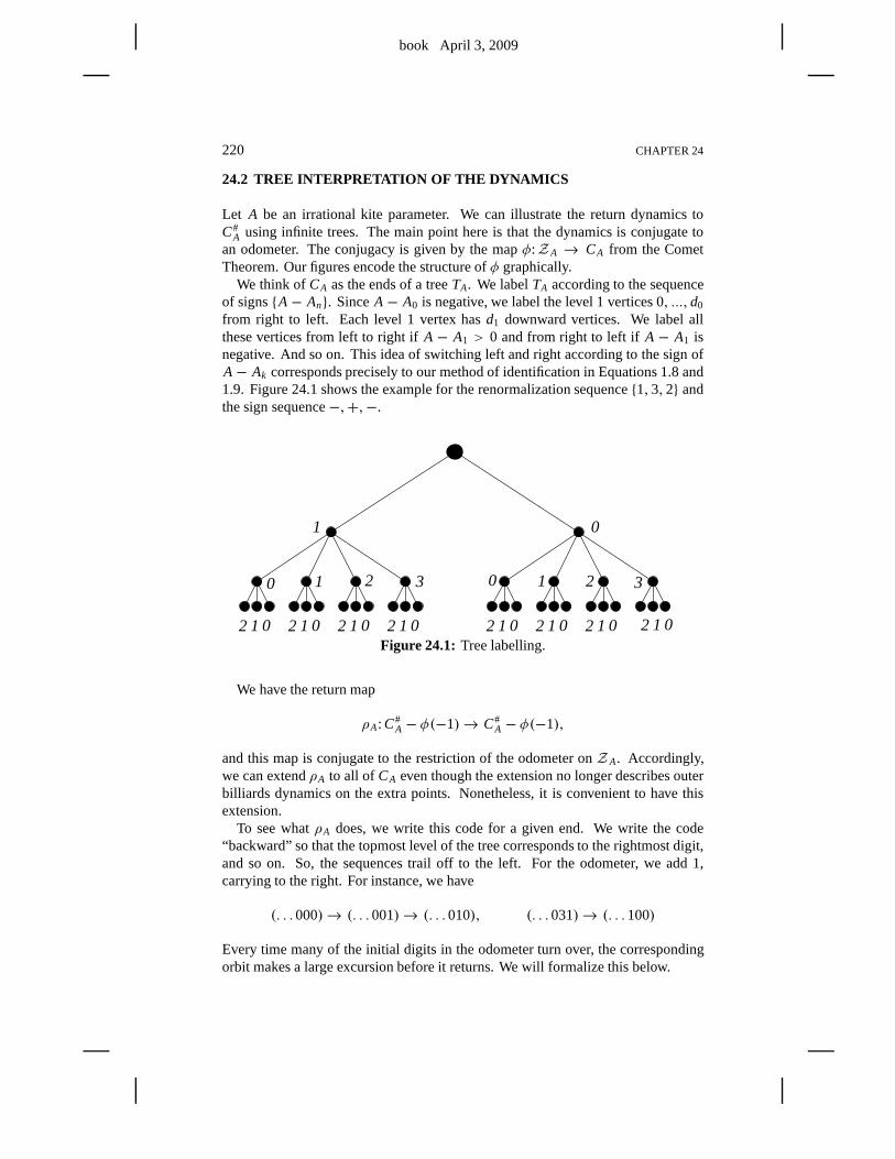
book April 3, 2009

220 CHAPTER 24

24.2 TREE INTERPRETATION OF THE DYNAMICS

Let A be an irrational kite parameter. We can illustrate the return dynamics toC#

A using infinite trees. The main point here is that the dynamicsis conjugate toan odometer. The conjugacy is given by the mapφ:Z A → CA from the CometTheorem. Our figures encode the structure ofφ graphically.

We think ofCA as the ends of a treeTA. We labelTA according to the sequenceof signs{A− An}. SinceA− A0 is negative, we label the level 1 vertices 0, ...,d0

from right to left. Each level 1 vertex hasd1 downward vertices. We label allthese vertices from left to right ifA− A1 > 0 and from right to left ifA− A1 isnegative. And so on. This idea of switching left and right according to the sign ofA− Ak corresponds precisely to our method of identification in Equations 1.8 and1.9. Figure 24.1 shows the example for the renormalization sequence{1,3,2} andthe sign sequence−,+,−.

0

01 01 01 01 01 01 01 01

100 1

1

2

2

2

2

2

3 3

22 2 2 2Figure 24.1: Tree labelling.

We have the return map

ρA: C#A − φ(−1)→ C#

A − φ(−1),

and this map is conjugate to the restriction of the odometer on Z A. Accordingly,we can extendρA to all of CA even though the extension no longer describes outerbilliards dynamics on the extra points. Nonetheless, it is convenient to have thisextension.

To see whatρA does, we write this code for a given end. We write the code“backward” so that the topmost level of the tree correspondsto the rightmost digit,and so on. So, the sequences trail off to the left. For the odometer, we add 1,carrying to the right. For instance, we have

(. . .000)→ (. . .001)→ (. . .010), (. . .031)→ (. . .100)

Every time many of the initial digits in the odometer turn over, the correspondingorbit makes a large excursion before it returns. We will formalize this below.

book April 3, 2009

DYNAMICAL CONSEQUENCES 221

24.3 PROPER RETURN MODELS AND CUSPED SOLENOIDS

24.3.1 Proper Models

Here we will describe the sense in which the Comet Theorem allows us to combina-torially model the dynamics onUA, the set of unbounded special orbits. The resultsin this section are really just a repackaging of some of the statements of the CometTheorem.

Let X be an unboundedmetric space and letf : X→ X be a bijection. We assumethat f 2 moves points by a small amount. That is, there is a universal constantCsuch that

d(x, f 2(x)) < C, ∀x ∈ X. (24.1)

The example we have in mind, of course, is the outer billiardsmap

ψ ′: UA→ UA. (24.2)

The square mapψ moves points by at most 4 units.Say that a compact subsetX0 ⊂ X is aproper sectionfor f if for every N there

is someN′ such thatd(x, X0) < N implies that f k(x) ∈ X0 for some|k| < N′. Inparticular, every orbit off intersectsX0. This condition is just the abstract versionof statement 1 of the Comet Theorem. Informally, all the orbits head either directlytowardX0 or directly away fromX0.

Let f0: X0→ X0 be the first return map. This is a slight abuse of notation becausef0 might not be defined on all points ofX0. Some points might exitX0 and neverreturn. We define two functions

e1,e2: X0→ R+ ∪∞. (24.3)

The functione1(x) is the maximum distance the forward orbit ofx gets away fromX0 before returning asf0(x). The functione2(x) is the length of this same portionof the orbit. If f0 is not defined onx, then obviouslye2(x) = ∞. The proper sectioncondition guarantees thate1(x) = ∞ as well.

The condition thatX0 is a proper section guarantees thate1 ande2 are properfunctions of each other. That is, if{xn} is a sequence of points inX0, thene1(x)→∞if and only if e2(x)→∞. This observation includes the statement thate1(x) =∞iff e2(x) = ∞ iff f0 is not defined onx0. For the purpose of getting a roughqualitative picture of the orbits, we consider just the function e1. We sete= e1 andcall e theexcursion function.

Suppose now thatf ′: X′ → X′ is another bijection andX′0 is a proper section.Let e′: X′0 → R + ∪∞ denote the excursion function for this system. We saythat(X, X0, f ) is properly equivalentto (X′, X′0, f ′) if there is a homeomorphismφ: X → X′ such that

• φ conjugatesf0 to f ′0.

• e′ ◦ φ ande are proper functions of each other onX0.

These conditions guarantee thatφ carries the points wheref0 is not defined to thepoints wheref ′0 is not defined.

book April 3, 2009

222 CHAPTER 24

The notion of proper equivalence turns out to be a little too strong for our purposes.We say that(X, X0, f ) and(X′, X′0, f ′) areessentially properly equivalentif φ hasall the above properties but is defined only on the complementof a finite numberof orbits of X0. In this case, the inverse map has the same property: It will bewell defined on all but a finite number of orbits ofX′0. In other words, an essentialproper equivalence is a proper equivalence, provided that we first delete a finitenumber of orbits from the spaces. We call(X, X0, f ) anessentially proper modelfor (X′, X′0, f ′).

24.3.2 The Cusped Solenoid

Statement 1 of the Comet Theorem says thatC#A is a proper section for the map in

Equation 24.2. Now we can describe the proper models for the triple (UA,C#A, ψ

′).Statements 2 and 3 in particular describe the excursion function up to a bi-Lipschitzconstant. Here we convert this information into a concrete essentially proper modelfor this dymamics.

Let Z A denote the metric Abelian group from the Comet Theorem. For conve-nience, we recall the definition of the metricd here.d(x, y) = q−1

n−1, wheren is thesmallest index such that [x] and [y] disagree inZ/Dn. Here{pn/qn} is the superiorsequence approximatingA.

We denote the odometer map onZ A by f0. That is, f0(x) = x+1. Topologically,thesolenoidbased onZ A is defined as the mapping cylinder

S A = Z A × [0,1] / ∼, (x,1) ∼ (x + 1,0). (24.4)

This is a compact metric space.We now modify this space a bit. First of all, we remove the point

(−1,1/2)

fromS A. This deleted point, the cusp, lies halfway between(−1,0) and(0,0). Wenow change the metric on the space by declaring the length of the segment between(x,0) and(x,1) to be

1

d(x,−1)Metrically, we simply rescale the length element on each interval by the appropriateamounts. We call the resulting spaceCA, thecusped solenoidbased onA.

24.3.3 The Main Results

We definef : CA→ CA to be the map such that

f (x, t) =(

x,t

d(x,−1)

). (24.5)

From the way we have scaled the distances,f maps each point by 1 unit. Indeed,some readers will recognizef as the time-one map of the geodesic flow onCA. Theoriginal setZ A is a proper section for the map, and the return map is precisely f0.Put another way,f is a suspension flow overf . Note thatf also depends onA, butwe suppress this from our notation.

book April 3, 2009

DYNAMICAL CONSEQUENCES 223

Theorem 24.1 (CA,Z A, f ) is an essentially proper model for(UA,C#A, ψ

′).

Proof: This is just a repackaging (and weakening) of statements 2 and 3 of theComet Theorem. 2

Remarks:(i) The model forgets the linear ordering onC#

A that comes from its inclusion inI ,but one can recover this from the discussion in §24.2.(ii) In a certain sense, the triple(CA,Z A, f ) provides abi-Lipschitz modelfor thenature of the unboundedness of the orbits inUA. However, it would be misleadingto call the model an actual bi-Lipschitz model for the dynamics onUA becausewe are not saying much about what happens to the orbits in the two systems afterthey leave their proper section. For instance, the excursion times could be wildlydifferent from each other even though they are proper functions of each other.

The following result contains statements 1 and 2 of Theorem 1.4.

Theorem 24.2 The time-one map of the geodesic flow on any cusped solenoidservesas an essentially proper model for the dynamics of the special unbounded orbitsrelative to uncountably many different parameters.

Proof: Up to a proper change of the excursion function, the model depends on onlythe renormalization sequence, and there are uncountably many parameters realizingany renormalization sequence. 2

24.3.4 Equivalence and Universality

To each parameterA, we associate the renormalization sequence{dn}. We thenassociate the sequence{Dn}, where

Dn =n−1∏

i=0

(di + 1). (24.6)

We call A and A′ broadly equivalentiff for each m there is somen such thatDm dividesD′n andD′m dividesDn. Each broad equivalence class has uncountablymany members.

Lemma 24.3 If A and A′ are broadly equivalent, then there is a homeomorphismfromZ A to Z A′ that conjugates one odometer to the other.

Proof: Each element ofZ A is a compatible sequence{am}with am ∈ Z/Dm. Usingthe divisibility relation, this element determines a corresponding sequence{a′m}.Herea′m is the image ofan under the factor mapZ/Dn → Z/D′m, wheren is suchthat D′m dividesDn. One can easily check that this map is well defined and deter-mines the desired homeomorphism. 2

book April 3, 2009

224 CHAPTER 24

Theorem 24.4 If A and B are broadly equivalent, then there is an essentially properequivalence between(UA,C#

A, ψ′A) and (UB,C#

B, ψ′B). In particular, the return

maps to CA and CB are essentially conjugate.

Proof: The homeomorphism fromZ A to ZB maps−1 to −1. By construc-tion, this homeomorphism sets up a proper equivalence between(CA,Z A, fA) and(CB,Z B, fB). This result now follows from Theorem 24.1. 2

One might wonder about the nature of the topological equivalence between thereturn maps toC#

A andC#B. One can reconstruct the conjugacy fromthe tree labellings

given in §24.2. The conjugacy is well defined for all points ofCA andCB, but wetypically have to ignore the countable sets of points on which the relevant returnmaps are not defined. This accounts for the precise statementof the theorem above.

LetZ denote the inverse limit over all finite cyclic groups. The map x→ x+1 isdefined onZ. This dynamical system is called theuniversal odometer. SometimesZ is called theprofinite completionof Z.

We call A universalif every k ∈ N divides someDn in the sequence. IfAis universal, then there is a group isomorphism fromZ to Z A that respects theodometer maps. In short, whenA is universal,Z A is the universal odometer. See[H, §5] for a proof of this fact – stated in slightly different terms – and for a detaileddiscussion of the universal odometer.

Lemma 24.5 Almost every parameter is universal.

Proof: A sufficient condition for a parameter to be universal is thatevery integer ap-pears in the renormalization sequence. We can express the fact that a certain numberappears in the renormalization sequence as a statement thata certain combinationappears in the continued fraction expansion ofA. Geometrically, as one drops ageodesic down from∞ to A, the appearance of a certain pattern of geodesics in theFarey graph forces a certain number in the renormalization sequence. As is wellknown, the continued fraction expansion for almost every number in(0,1) containsevery finite string of digits. 2

Statement 3 of Theorem 1.4 is contained in the following result.

Theorem 24.6 For almost every A∈ (0,1), the triple (UA,C#A, ψ

′) is properlymodelled by the time-one map of the geodesic flow on the universal cusped solenoid.

Proof: This result is an immediate consequence of the previous result and Theorem24.1. 2

Remark: One might wonder if there is a concrete parameter that exhibits thisuniversal behavior. It seems that the parameterA = e−2 has the following inferiorsequence.

1

1←

5

7←

51

71←

719

1001· · · , rn+2 = (4n+ 10)rn+1+ rn, n ≥ 0.

One can easily check that this sequence leads to the universal odometer. Thus thefractional part ofe has universal behavior.

book April 3, 2009

DYNAMICAL CONSEQUENCES 225

24.4 SOME OTHER EQUIVALENCE RELATIONS

Call A andB narrowly equivalentif they have the same renormalization sequenceand if the sign ofA− A j is the same as the sign ofB− B j for all j . Here{A j } and{B j } are the superior sequences approximatingA andB, respectively. Referring toEquation 1.9, the definition ofk j relative to the narrowly equivalent parameters isthe same for every index. Each narrow equivalence class is uncountable.

Theorem 24.7 If A and B are narrowly equivalent, then there is anorder-preservinghomeomorphism from I to itself that conjugates the return map on C#

A to the returnmap on C#

B. This map is a proper equivalence from(UA,C#A, ψ

′A) to (UB,C#

B, ψ′B).

Proof: The two spaces5A and5B are exactly the same, and the extended twirlorders on the (equivalence classes) of these spaces are the same. Thus the successormaps on the two spaces are identical. The maph = φ′2 ◦ φ−1

2 is a homeomorphismfrom CA to CB that carriesC#

A andC#B and conjugates one return dynamics to the

other. By construction,h preserves the linear ordering onI , and we can extendh tothe gaps ofI − CA in the obvious way. By construction, this map carriesφA(−1)to φB(−1) and is continuous. Hence it is a proper equivalence. 2

Thefirst renormalizationof the odometer mapx→ x + 1 on the inverse system

. . .→ Z/D3→ Z/D2→ Z/D1 (24.7)

is theD1th power of the map. This corresponds to the mapx→ x+1 on the inversesystem

. . .→ Z/D′3→ Z/D′2→ Z/D′1, D′n = Dn+1/D1. (24.8)

As in the Comet Theorem, eachDn divides Dn+1 for all n, so the constructionmakes sense. In terms of the symbolic dynamics on the sequence space5, therenormalization consists of the first return map to the subspace

5′ = {κ ∈ 5| k0 = 0}. (24.9)

In terms of the dynamics onCA, the first renormalization is the first return mapto the Cantor subset corresponding to5′. Thesecond renormalizationis the firstrenormalization of the first renormalization. And so on.

Let Ŵ denote the(2,∞,∞)-triangle group from the Comet Theorem. Giventhe construction of the inferior sequence, the enhanced renormalization sequencesfor two Ŵ-equivalent parameters have the same tail ends. Thus the tail ends of therenormalization sequences are the same, and the tail ends ofthe sign sequences arethe same. This gives us the following result.

Corollary 24.8 Suppose that A and B are equivalent underŴ2. Then some renor-malization of the return map to C#A is conjugate to some renormalization of thereturn map to C#

B. The conjugacy is given by an order-preserving homeomorphism.

Remark: The homeomorphism mentioned in the last corollary is a similary. Com-pare Statement 2 of Theorem 1.5 and see §25.3 for more details.

book April 3, 2009

book April 3, 2009

Chapter Twenty-Five

Geometric Consequences

25.1 PERIODIC ORBITS

Here we prove statement 1 of Theorem 1.5.

Lemma 25.1 UA has length0.

Proof: SinceUA is locally homogeneous, it suffices to prove thatCA has length 0.Let λn = |Aqn − pn|, as in Equation 21.5. We define

Gn =∞∑

k=n+1

2λkdk. (25.1)

Then

CA ⊂∑

κ∈5n

(In + X(κ)

). (25.2)

Here In is the interval with endpoints(0,1) and (Gn,1). In other words,CA iscontained inDn translates of an interval of lengthGn. We just need to prove thatDnGn→ 0. It suffices to prove this whenn is even. By Equation 21.6,

Dn < ǫ−nqn, ǫ =√

5/4. (25.3)

By Equation 21.5 we have

Gn < 2∞∑

k=n+1

q−1k < 2q−1

n

∞∑

k=1

2−k < 2q−1n . (25.4)

Here we have used the trivial bound thatqm/qn < 2n−m whenm> n. Therefore

DnGn < 2ǫ−n. (25.5)

This completes the proof. 2

Theorem 25.2 Any defined orbit in I− CA is periodic. There is a uniform boundon the period depending only on the distance from the point toCA.

Proof: The Comet Theorem combines with statement 2 of Theorem 1.1 toprovethat any defined orbit inI −CA is periodic. The period bound comes from taking alimit of the Period Theorem asn→∞ in the rational approximating sequence. Inother words, if this result were false, then we could contradict the Period Theoremusing the Continuity Principle. 2

Combining these results, we have statement 1 of Theorem 1.5:Almost everypoint ofR × Zodd lies on a periodic orbit.

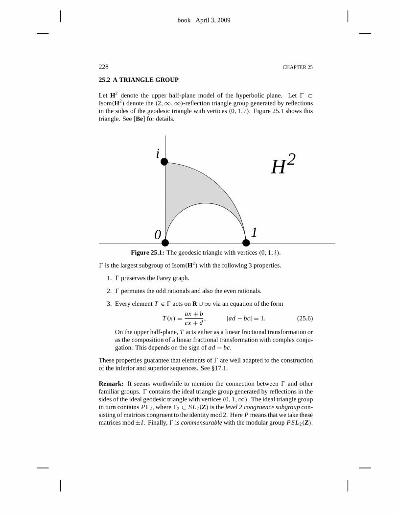
book April 3, 2009

228 CHAPTER 25

25.2 A TRIANGLE GROUP

Let H2 denote the upper half-plane model of the hyperbolic plane. Let Ŵ ⊂Isom(H2) denote the(2,∞,∞)-reflection triangle group generated by reflectionsin the sides of the geodesic triangle with vertices(0,1, i ). Figure 25.1 shows thistriangle. See [Be] for details.

2i

10

H

Figure 25.1: The geodesic triangle with vertices(0,1, i ).

Ŵ is the largest subgroup of Isom(H2) with the following 3 properties.

1. Ŵ preserves the Farey graph.

2. Ŵ permutes the odd rationals and also the even rationals.

3. Every elementT ∈ Ŵ acts onR ∪∞ via an equation of the form

T(x) = ax+ b

cx+ d, |ad− bc| = 1. (25.6)

On the upper half-plane,T acts either as a linear fractional transformation oras the composition of a linear fractional transformation with complex conju-gation. This depends on the sign ofad− bc.

These properties guarantee that elements ofŴ are well adapted to the constructionof the inferior and superior sequences. See §17.1.

Remark: It seems worthwhile to mention the connection betweenŴ and otherfamiliar groups.Ŵ contains the ideal triangle group generated by reflections in thesides of the ideal geodesic triangle with vertices(0,1,∞). The ideal triangle groupin turn containsPŴ2, whereŴ2 ⊂ SL2(Z) is thelevel 2 congruence subgroupcon-sisting of matrices congruent to the identity mod 2. HereP means that we take thesematrices mod±I . Finally,Ŵ is commensurablewith the modular groupPSL2(Z).

book April 3, 2009

GEOMETRIC CONSEQUENCES 229

25.3 MODULARITY

Here we will prove statement 2 of Theorem 1.5. Letλk andλ′k be the quantitiesassociated to parametersA andA′, as in Equation 1.10

Lemma 25.3 Let T ∈ Ŵ be such that T(A) = A′. Then there is some integer msuch that

d′k = dk+m,λ′kλk+m

= |T ′(A)|1/2

provided that k is sufficiently large.

Proof: Here T ′(A) = (cA+ d)−2 when T is as in Equation 25.6. Given ourconstruction of the inferior sequence, and the first two properties ofŴ, we haveT(Ak+m) = A′k for somem and all sufficiently largek. Henced′k = dk+m for thesechoices ofk andm. We compute

λ′k = |A′q′k − p′k|, A′ = a A+ b

cA+ d, T

( p

q

)= ap+ bq

cp+ dq. (25.7)

An exercise in modular arithmetic shows that the fraction onthe right is in lowestterms. Hence

p′k = aqk+m + bpk+m, q′k = cqk+m + dpk+m. (25.8)

Combining the last two equations, we have

λ′k =∣∣∣∣(a A+ b)(cqk+m + dpk+m)− (cA+ d)(aqk+m + bpk+m)

cA+ d

∣∣∣∣

=∣∣∣∣(ad− bc)(Aqk+m− pk+m)

cA+ d

∣∣∣∣ =∣∣∣∣Aqk+m − pk+m

cA+ d

∣∣∣∣ =λk+m

cA+ d= λk+m|T ′(A)|1/2.

This completes the proof. 2

Recall thatCA is defined by the formula

CA =⋃

κ∈5(X(κ),1), X(κ) =

∞∑

i=0

2kiλi , λi = |Aqi − pi |. (25.9)

If A andA′ areŴ-equivalent, as above, then we have the obvious map

∞∑

i=k0

km+iλm+i →∞∑

i=k0

kiλ′i . (25.10)

By the previous result, this map is well defined ifk0 is large enough. Also by theprevious result, this map is a similarity. HenceC#

A and C#A′ are locally similar.

HenceUA andUA′ are locally similar.

book April 3, 2009

230 CHAPTER 25

25.4 HAUSDORFF DIMENSION

In this section, we review some basic properties of the Hausdorff dimension. See[F] for more details.

We will work with sets inR × Zodd and especially sets in our favorite intervalI = [0,2]×{−1}. Given an intervalJ, let|J| denote its length. GivenS⊂ R×Zodd

and someδ > 0, we define

µ(S, s, δ) = inf∑|Jn|s. (25.11)

The infimum is taken over all countable covers ofS by intervals{Jn} such thatdiam(Jn) < δ. Next, we define

µ(S, s) = limδ→0

µ(S, s, δ) ∈ [0,∞] . (25.12)

This limit exists becauseµ(S, s, δ) is a monotone function ofδ. Note thatµ(S,1) <∞ becauseI has finite total length. Finally,

dim(S) = inf{s| µ(S, s) <∞}. (25.13)

The number dim(S) is called theHausdorff dimensionof S.Given an explicit family of covers, as we have constructed inthe proof of Lemma

25.1, it is easy for us to compute upper bounds on the Hausdorff dimension. Herewe recall a method for getting lower bounds on the Hausdorff dimension. LetS⊂ Ibe a compact set. We say thatf : I → R is aρ-densityrelative toS if f is monotonenondecreasing and constant on the complementary intervalsof S and

C|a− b|ρ ≥ f (b)− f (a) (25.14)

for someC > 0 and all intervals [a,b] ⊂ I such that|a− b| is sufficiently small.

Lemma 25.4 If S admits aρ-density, thendim(S) ≥ ρ.

Proof: This is essentially the Mass Distribution Principle 4.2 in [F, p. 55]. Thefunction f is the integral of the mass distribution described in connection with thisprinciple. 2

In computing the functionu(A) = dim(UA), we would prefer to work with thesetsCA. The following lemma justifies this.

Lemma 25.5 UA and CA and C#A all have the same dimension.

Proof: SinceCA − C#A is countable, we have dim(CA) = dim(C#

A). SinceUA islocally homogeneous dim(UA) = dim(UA ∩ J) for any intervalJ about a point inUA. In particular, dim(UA) = dim(C#

A). 2

book April 3, 2009

GEOMETRIC CONSEQUENCES 231

25.5 QUADRATIC IRRATIONAL PARAMETERS

25.5.1 Self Similarity

First, we prove statement 3 of Theorem 1.5.A Cantor set is commonly calledself-similarif it is a finite union of similar copies

of itself.

Lemma 25.6 Suppose that A∈ (0,1) is a quadratic irrational. Then CA is a finitedisjoint union of self-similar Cantor sets.

Proof: A has an eventually periodic continued fraction expansion. HenceA is thefixed point of some infinite-order elementT ∈ SL2(R), acting by linear fractionaltransformations. But some power ofT lies in the groupŴ. Hence, without loss ofgenerality, we can takeT ∈ Ŵ. But then the map from Equation 2.9 carries oneclopen subsetV2 of CA to a larger clopen subsetV1. (Hereclopenmeans simultane-ously closed and open.) Looking at Equation 2.9 and recalling the definition ofCA

from Equation 1.11, we see thatCA is a finite disjoint union of translates ofV1, andV1 is a finite disjoint union of translates ofV2. HenceV1 is a finite disjoint union ofsimilar copies of itself. HenceCA is a finite union of translates ofV1, each of whichis a self-similar Cantor set. 2

A self-similar Cantor set has the property that every point in it has arbitrarilysmall neighborhoods that are also self-similar Cantor sets. Statement 2 of Theorem1.3 says that any point ofUA has a neighborhood that is isometric to a neighborhoodin C#

A. Shrinking this neighborhood appropriately, we get a self-similar trimmedCantor set surrounding the point inUA. This proves statement 3 of Theorem 1.5.

25.5.2 Dimension Formula

Now we present a dimension formula in the quadratic irrational case. Actually, theformula is slightly more general. LetA ∈ (0,1) be irrational. Let{pn/qn} be theassociated superior sequence and let{dn} be the renormalization sequence. We callA tame if

1. qn+1 < Cqn for some constantC that is independent ofn.

2. The following limits exist.

D(A) = limn→∞

log(Dn)

n, Q(A) = lim

n→∞

log(qn)

n.

There are uncountably many tame parameters. In particular,we have the follow-ing result.

Lemma 25.7 Quadratic irrational parameters are tame.

Proof: Let A be a quadratic irrational parameter. From the work in §25.3,wesee that the renormalization sequence{dk} is eventually periodic. But this implies

book April 3, 2009

232 CHAPTER 25

that the limit D(A) exists. At the same time, we have integersc,d,n such thatqk+n = cqk+d for all sufficiently largek. This easily implies thatQ(A) exists andthatqk+1/qk is uniformly bounded. 2

Lemma 25.8 Suppose A is a tame parameter. Let{pn/qn} be the associated supe-rior sequence. Thenλn ∈ [C1,C2] q−1

n for positive constants C1,C2.

Proof: For tame parameters, the renormalization sequence{dn} is bounded. Wehave

λn = qn|A− An| < 2d−1n q−1

n < C2q−1n ,

by Lemma 17.4. For the lower bound, note first thatλn+1 < λ′n+1 < λn, by Equation21.7. By the triangle inequality,

|A− An| + |A− An+1| ≥ |An − An+1| ≥2

qnqn+1.

Hence

2λn > λn + λn+1 = qn|A− An| + qn+1|A− An+1|

> qn

(|A− An| + |A− An+1|

)≥ 2q−1

n+1 ≥ 2C1q−1n .

This gives the lower bound. 2

Here is the main result for this section.

Theorem 25.9 If A is a tame parameter then u(A) = D(A)/Q(A).

Proof: Let Cn be the covering we constructed in the proof of Lemma 25.1. Theintervals inCn are pairwise disjoint and have the same length. Each interval of Cn

contains(dn + 1) evenly and maximally spaced intervals ofCn+1.We first use these covers to get an upper bound on dim(UA). There areDn

intervals inCn, all having lengthGn. Choose anyǫ > 0. Forn large,

Dn ∈(

exp(n(D − ǫ)

),exp

(n(D + ǫ)

)). (25.15)

We have

Gn = 2λ∗n+1 ∈[2λn+1, λn

]∈[C1q−1

n+1,C2q−1n

]∈ [C3,C2] q−1

n , (25.16)

by the preceding lemma. Hence

Gn ∈(

exp(− n(Q+ ǫ)

),exp

(− n(Q− ǫ)

)). (25.17)

Settings = (D + ǫ)/(Q− ǫ) and lettingn→∞, we haveµ(UA, s) ≤ 1. Hencedim(UA) ≤ s. But ǫ is arbitrary. Hence dim(UA) ≤ D/Q.

For the lower bound, we setρ = (D− ǫ)/(Q+ ǫ) and construct aρ-density. LetX n denote the partition of [0,1] into Dn equally sized intervals. Going from left to

book April 3, 2009

GEOMETRIC CONSEQUENCES 233

right, we map thej th interval ofCn into the j th interval ofX n. We map the gapsbetween consecutive intervals ofCn to the obvious points common to consecutiveintervals ofX n. The maps{ fn} form a uniformly continuous family, and the limitf : I → [0,1] exists. By construction,f is monotone nondecreasing and constanton the components ofI −UA.

Consider [a,b] ⊂ I . By Equation 25.16, the sequence{Gn/Gn+1} is uniformlybounded. Hence we can assume without loss of generality that|a − b| = Gn forsomen. By construction [a,b] intersects at most 2 consecutive intervals ofCn.Hence f (b)− f (a) ≤ 2D−1

n . Hence

2|a− b|ρ = 2Gρn≥

2 exp

(− ρn

(Q+ ǫ

))=

2 exp

(− n

(D − ǫ

))>

2D−1n ≥

f (b)− f (a). (25.18)

This shows thatf is aρ-density relative toUA. Hence dim(UA) ≥ ρ. Again,ǫ isarbitrary, so dim(UA) ≥ D/Q. 2

Example 1: Let A =√

5− 2 = φ−3, the Penrose kite parameter. Hereφ is thegolden ratio. The inferior sequence forA is

11← 1

3← 1

5← 3

13← 5

21← 13

55← 21

89← 55

233← 89

377· · · .

The superior sequence obeys the recurrence relationrn+2 = 4rn+1 + rn, whererstands for eitherp or q. The inferior renormalization sequence is 1,0,1,0, .... Therenormalization sequence is 1,1,1, .... HenceD = log(2). From the recurrencerelation, we computeQ = log(

√5+ 2). Hence

u(A) = log(2)

log(√

5+ 2)= log(2)

log(φ3).

Example 2: Let A =√

2− 1. The inferior sequence forA is1

1← 1

3← 3

7← 7

17← · · · , rn+2 = 2rn+1 + rn.

All terms are superior. From the recurrence relation, we getD(A) = log(2) andQ(A) = log(

√2+ 1). The inferior sequence for 1− A is

1

1← 3

5← 17

29← 99

169← · · · , rn+2 = 6rn+1 − rn.

All terms are superior. From the recurrence relation, we have D(1− A) = log(3)andQ(1− A) = 2 log(

√2+ 1). Hence

u(A) = log(2)

log(√

2+ 1), u(1− A) = log(3)

2 log(√

2+ 1).

In particular,u(A) 6= u(1− A). The hyperbolic isometryz→ 1− z is a symmetryof the Farey graph that does not belong to the groupŴ. The calculation shows thatthe dimension function does not in general have this additional symmetry.

book April 3, 2009

234 CHAPTER 25

25.6 THE DIMENSION FUNCTION

Here we prove statement 4 of Theorem 1.5.TheBorelσ -algebraof subsets ofRn is the smallest collection that contains the

open sets and is closed under complementation and countableunions. ABorel setis a member of thisσ -algebra. A functionf : Rn → R is Borel-measurableif theset{x| f (x) ≥ a} is a Borel set for alla ∈ R.

Lemma 25.10 Let S⊂ [0,1]2 be a Borel subset. Let SA denote the intersection ofS with the line{y = A}. Suppose SA is compact for all A. Let f(A) = dim(SA).Then f is a Borel-measurable function of[0,1].

Proof: This is a special case of [MM , Theorem 6.1]. 2

Recall thatu(A) = dim(UA) the Hausdorff dimension of the set of unboundedspecial orbits.

Lemma 25.11 The function u is Borel-measurable.

Proof: When A = p/q, we letCA = O2(J) ∩ I . HereJ is the interval of length2/q in I whose left endpoint is(0,1). ThusCA is just a thickened version of partof the fundamental orbit. Having stated this definition, we defineC as in Equation1.13. By construction,CA is compact for allA ∈ [0,1]. In order to apply Lemma25.10, we just have to show thatC is a Borel set.

In the proof of Lemma 25.1 we produced a coveringCn of CA by intervals allhaving the same length. One can extend this definition to the rational case in a fairlyobvious way. LetC(n)

A denote the union of these intervals. LetC(n) be the corre-sponding union, withC(n)

A replacingCA in Equation 1.13. The sizes and positionsof the intervals inC(n)

A vary with A in a piecewise continuous way. HenceC(n) is aBorel set. HenceC = ∩C(n) is a Borel set. 2

Lemma 25.12 The function u is almost everywhere constant.

Proof: The functionu is aŴ-invariant Borel-measurable function on [0,1]. We canextendu by the action ofŴ so that the extended functionu has the same propertieson all ofR ∪∞. As is well known,Ŵ actsergodicallyonR ∪∞. See [BKS]. Butthen any invariant Borel-measurable function is almost everywhere constant. Thisapplies tou. Henceu is almost everywhere equal to some constantu0. 2

Let

S= [0,1]−Q. (25.19)

Now we want to see thatu maps every open subset ofS onto [0,1]. Sinceuis Ŵ-invariant and theŴ-orbits of S are dense in [0,1], it suffices to prove thatu(S) = [0,1]. We will prove this below.

Say thatA ∈ (0,1) issuperiorif all the terms in the inferior sequence are superior.Let D = D(A) be as in the dimension formula above.

book April 3, 2009

GEOMETRIC CONSEQUENCES 235

Lemma 25.13 If A is tame and superior, then u(A) ≥ D/(D + log 2).

Proof: Referring to the inferior sequence{pn/qn} and the inferior renormalizationsequence{dn}, we always have

qn+1 < 2(dn + 1)qn.

This bound directly applies to the superior sequence whenA is superior. By induc-tion,

qn ≤ 2Dn.

HenceQ ≤ D + log 2. The bound follows immediately. 2

Lemma 25.14 Let A be a superior parameter whose renormalization sequence{dn}diverges to∞. If dn+1/dn grows subexponentially, u(A) = 1.

Proof: The same argument as in Lemma 25.8 shows that

λn > (hnqn)−1, (25.20)

where{hn} grows subexponentially. From Equation 21.7, we get

Gn = 2λ′n > 2λn > 2(hnqn)−1. (25.21)

Therefore

limn→∞

log(Dn)

log(G−1n )

≥ limn→∞

log(Dn)

log(hnqn)

=∗ limn→∞

log(Dn)

log(qn)

≥ limn→∞

log(Dn)

log(Dn)+ log(2)= 1. (25.22)

The starred equality comes from the subexponential growth of hn. The same con-struction as in Theorem 25.9 shows thatu(A) ≥ 1. Henceu(A) = 1. 2

Lemma 25.15 There exists A∈ S such that u(A) = 0.

Proof: We takeA so that the inferior renormalization sequence consists entirely of0s and 1s. Our argument for the upper bound in Theorem 25.9 givesu(A) = 0 ifthe number of 0s between each pair of 1s grows at a fast enough rate. 2

Now we come to the main result.

book April 3, 2009

236 CHAPTER 25

Lemma 25.16 u(S) = [0,1].

Proof: In light of the results above, it suffices to prove(0,1) ⊂ u(S). Letx ∈ (0,1).We will consider only parameters having an odd enhanced inferior renormalizationsequence. Such parameters are determined by their inferiorrenormalization se-quences.

Let A(M, N) denote the parameter with inferior renormalization sequenceN,0M

repeating. Here 0M denotesM consecutive 0s. These parameters are all quadraticirrational and hence tame. By Lemma 25.13, we haveu(A(0, N)) > x for N large.Moreover, for fixedN, we haveu(A(M, N)) → 0 asM → ∞. Hence we canchooseM andN such that

u(A(M + 1, N)) < x < u(A(M, N)). (25.23)

(If we have equality on either side, we are finished, so we can assume strict inequal-ity.) We fix this pair(M, N) for the rest of the proof.

For any binary sequence,ǫ = {ǫk} we let A(ǫ) be the parameter with inferiorrenormalization sequence

N,0M+ǫ1 , N,0M+ǫ2 , N,0M+ǫ3, ....

By construction,

D(A(ǫ)) = D = log(N) (25.24)

independent ofǫ andM. Consider the sequence{qk} of denominators of superiorterms corresponding toA(ǫ). By Equation 25.23, we have

logqn

n< x D,

logqn

n> x D,

respectively, for the 0-sequence and for the 1-sequence, oncen is large. Insertingan additional 0 into the inferior renormalization sequencehas the effect of at mostdoubling the terms in the denominator sequence. (Compare the proof of Lemma21.1.) Therefore we can choose the firstn terms ofǫ such that

∣∣∣∣log(qn)

n− x D

∣∣∣∣ ≤log 2

n,

providedn is large. Passing to a subsequence and taking a limit, we can chooseǫso thatQ(A(ǫ)) = x D. But thenA(ǫ) is tame andu(A(ǫ)) = x. 2

We have already shown that the functionu is almost everywhere constant. Letr ∈ [0,1] be arbitrary. We have just shown thatu−1(r ) is nonempty. Butu isinvariant under the(2,∞,∞)-triangle group. Henceu−1(r ) is dense inS. Thisfinishes the proof of statement 4 of Theorem 1.5.

book April 3, 2009

Part 6. More Structure Theorems

In this part of the book, we will prove all the results left over from Part 5. Thematerial in this part is probably the most difficult, so it seems worthwhile to pointout that one can stop reading early and still take away partial results.

• In Chapter 26, we prove the Copy Theorem from §22.2. Knowingjust theCopy Theorem, we can conclude thatC#

A ⊂ UA. That is, the trimmed Cantorset from the Comet Theorem iscontainedin the union of special unboundedorbits. All the dynamical results onC#

A – e.g., the essential conjugacy to theodometer – follow just from the Copy Theorem. This might be a nice resultfor the reader interested mainly in the existence and natureof unboundedorbits.

• In Chapter 27, we define what we mean by the pivot arc relativeto an evenrational kite parameter. Along the way we will prove anotherversion of theDiophantine Lemma from §18.2. This lemma works for pairs of odd rationals,and the result here works for pairs of Farey-related rationals, either even orodd. This whole chapter is a prelude to the last 4 chapters.

• In Chapter 28, we prove the Pivot Theorem from §22.2. The Pivot Theoremworks in both the even and odd cases, and is proved in an inductive waythat requires both cases. From the Pivot Theorem and the CopyTheoremcombined, we have Theorem 1.8.

• In Chapter 29, we prove the Period Theorem. Combining the Copy Theorem,the Pivot Theorem, and the Period Theorem, we prove thatUA ∩ I = C#

A. Inother words, we completely characterize the set of unbounded orbits insidethe special intervalI from the Comet Theorem.

• In Chapter 30, we prove a technical result, the Hovering Lemma, which rulesout the existence of certain pathological components of thearithmetic graph.We use the Hovering Lemma as a step in the proof of the Low Vertex Theorem.

• In Chapter 31, we prove the Low Vertex Theorem. This is the technical resultwe needed for statement 1 of the Comet Theorem. Statement 1 ofthe CometTheorem is the result that gives us the minimality and homogeneity of UA.So, one needs to read all the way to the end to obtain the globalstructuralresults forUA.

book April 3, 2009

book April 3, 2009

Chapter Twenty-Six

Proof of the Copy Theorem

26.1 A FORMULA FOR THE PIVOT POINTS

Let A be an odd rational. LetA− be as in Equation 4.1. LetV− = (q−,−p−). Herewe give a formula for the pivot pointsE± associated toA. Recall that these pointsare the endpoints of the pivot arc, the subject of the Copy Theorem.

Lemma 26.1 The following are true.

• If q− < q+, then E+ + E− = −V− + (0,1).

• If q+ < q−, then E+ + E− = V+ + (0,1).

Proof: We will establish this result inductively. Suppose first that 1/1← A. Then

A = 2k− 1

2k+ 1, E− = (−k, k), E+ = (0,0), V− = (k,−k + 1).

A− =k− 1

k, q− = k− 1< k = q+.

The result works in this case.In general, we have

A = A2, A0← A1← A2.

There are 4 cases, depending on Lemma 17.2. Here the index ism = 1. We willconsider case 1. The other cases are similar. By case 1, we have (q1)+ < (q1)−.Hence, by induction,

E+1 + E−1 = (V1)+ + (0,1).SinceA1 < A2, we have

E−2 = E−1 , E+2 = E+1 + d1V1.

Therefore

E+2 + E−2 = (V1)+ + d1V1+ (0,1) = (V2)+ + (0,1).The last equality comes from case 1 of Lemma 17.2. As we remarked after statingLemma 17.2, this result works for both numerators and denominators.) In case 1,we have(q2)+ < (q2)−, so the result holds. 2

Recall thatR1 = R1(A) and R2 = R2(A) are the two parallelograms from theDecomposition Theorem. See Chapter 19.

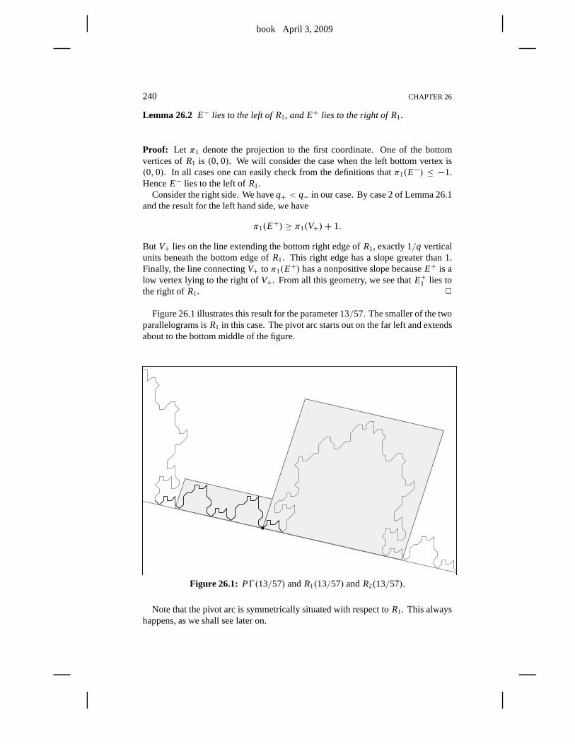
book April 3, 2009

240 CHAPTER 26

Lemma 26.2 E− lies to the left of R1, and E+ lies to the right of R1.

Proof: Let π1 denote the projection to the first coordinate. One of the bottomvertices ofR1 is (0,0). We will consider the case when the left bottom vertex is(0,0). In all cases one can easily check from the definitions thatπ1(E−) ≤ −1.HenceE− lies to the left ofR1.

Consider the right side. We haveq+ < q− in our case. By case 2 of Lemma 26.1and the result for the left hand side, we have

π1(E+) ≥ π1(V+)+ 1.

But V+ lies on the line extending the bottom right edge ofR1, exactly 1/q verticalunits beneath the bottom edge ofR1. This right edge has a slope greater than 1.Finally, the line connectingV+ to π1(E+) has a nonpositive slope becauseE+ is alow vertex lying to the right ofV+. From all this geometry, we see thatE+1 lies tothe right ofR1. 2

Figure 26.1 illustrates this result for the parameter 13/57. The smaller of the twoparallelograms isR1 in this case. The pivot arc starts out on the far left and extendsabout to the bottom middle of the figure.

Figure 26.1: PŴ(13/57) andR1(13/57) andR2(13/57).

Note that the pivot arc is symmetrically situated with respect to R1. This alwayshappens, as we shall see later on.

book April 3, 2009

PROOF OF THE COPY THEOREM 241

26.2 A DETAIL FROM PART 5

While we are in the neighborhood, we will clear up a detail from Part 5, namely,the proof of Lemma 22.5. For convenience, we repeat the statement here. In thisstatement,E+ and E− are the pivot points relative to the odd rational parameterA = p/q.

Lemma 26.3

−q

2< π1(E

−) < π1(E+) <

q

2.

Proof: We will prove this result inductively. Suppose that

A1← A2,

and the result is true forA1. We consider the case whenA1 < A2. The case whenA1 > A2 requires the same treatment. WhenA1 < A2, we have

E−1 = E−2 ,

so certainly the bound holds forE−1 .For the(+) case, we have

π1(E+2 ) = π1(E

+1 )+ d1q1 d1 = floor

(q2

2q1

). (26.1)

There are two cases to consider.

Case 1:Suppose thatδ1 = floor(q2/q1) is odd. In this case

(2d1+ 1)q1 < q2, H⇒ d1q1 <q2

2− q1

2.

The first equation implies the second. Hence, by induction,

π1(E+2 ) <

q1

2+ q2− q2

2<

q2

2.

Case 2: Suppose thatδ1 is even. Then we have case 2 of Lemma 17.2 appliedto the indexm= 1. This is to say that

(q1)− < (q1)+. (26.2)

From the formula above, the first coordinate ofE−2 + E+2 is negative. Hence

|π1(E−)| > |π1(E

+)|.

This fact finishes the proof. 2

book April 3, 2009

242 CHAPTER 26

26.3 PRELIMINARIES

As preparation for the main argument of our proof, we prove several easy results inthis section and also set up some notation.

The pivot points are well defined vertices, but so far, we do not know that thepivot arc is well defined. That is, we do not know thatE− and E+ are actuallyvertices ofŴ. These points might be vertices of some other component ofŴ. Wewill prove the well definedness result along with the proof ofthe Copy Theorem.

To start things off, we prove that the pivot arcs are well defined in the simplestcases.

Lemma 26.4 If 1/1← A, then the pivot arc is well defined relative to A.

Proof: Here

A = 2k− 1

2k+ 1. (26.3)

In §19.5, we showed that the line segment connecting(0,0) to (−k, k) is containedin the arithmetic graph. So, the pivot arc is well defined. 2

Notation: Here we introduce some notation that we will use repeatedly below. LetA1 be an odd rational. For each integerδ1 ≥ 1, there is a unique odd rationalA2 = A2(δ1) such thatA1← A2 and

δ1 = floor

(q2

q1

).

Thus the numbersA2(1), A2(2), ... give the complete list of odd rationals havingA1 as an inferior predecessor. Lemma 17.2 describes how to construct A2(δ1). Forinstance, ifA1 = 1/3 then

A2(1) =1

5, A2(3) =

3

11, A2(5) =

5

17, A2(2) =

3

7, A2(4) =

5

13.

We have listed the numbers this way to show the pattern better.

Lemma 26.5 Let E±j be the pivot points associated to the parameter A1. There isan arc PŴ1(δ1) ⊂ Ŵ1 whose endpoints are E−2 and E+2 .

Proof: Suppose thatA1 < A2. When A2 < A1 the proof is similar. Then, byEquation 22.3, we have

E−2 = E−1 , E+2 = E+1 + d1V1, V1 = (q1,−p1).

Hered1 is as in Equation 4.5 and Lemma 17.2. ButŴ1 is invariant under translationby V1. HenceE±2 is a vertex ofŴ1. 2

book April 3, 2009

PROOF OF THE COPY THEOREM 243

26.4 THE GOOD PARAMETER LEMMA

Call A1 a good parameterif

PŴ1 ⊂ 11(I ). (26.4)

Here11(I ) is the region from the Diophantine Lemma defined relative to the pair(A1, A2(1)). We call I thebase interval. We will give a formula below. Here is themain result in this section.

Lemma 26.6 (Good Parameter)If A1 is good and A1← A2, then the Copy The-orem holds for the pair(A1, A2).

We will prove this result in a case-by-case way. That is, we will treat the pair(A1, A2(k)

)for k = 1,3,5, ... and k = 2,4,6, .... The case whenk = 1 is

pretty easy. The cases whenk = 2 andk = 3 are the critical cases, and they haveessentially the same proof. The remaining cases are easy. For the rest of this section,we assume thatA is good.

Our proof will use the Mismatch Principle established in Chapter 19. For conve-nience, we repeat it here.

Mismatch Principle: Let Ŵ andŴ′ be two arithmetic graphs. IfŴ′ andŴ failto agree inR1, then there are two adjacent vertices ofŴ′ ∩ R1 where the two arith-metic graphsŴ andŴ′ do not agree.

26.4.1 An Easy Case

Here we show that the Copy Theorem holds forA1 andA2(1). Note that

PŴ1(1) = PŴ1. (26.5)

The pivot points do not change in this case:E±1 = E±2 . So, if A1 is good, thenthe Diophantine Lemma immediately implies thatPŴ1(1) = PŴ1 ⊂ Ŵ2. But thenthere is an arc ofŴ2 that connectsE−2 to E+2 , the two endpoints ofPŴ1(1). Thisshows that this pivot arc forA2 is well defined as a subarc ofŴ(A2) and moreoverthat his pivot arc is a subarc ofŴ1.

Before we leave this section, we establish some notation to be used below. LetA0 be such that the sequence

A0← A1← A2(1)

is part of the inferior sequence. LetI be the base interval, as above. We will considerthe case whenA0 < A1. The other case is similar. In the case at hand, the baseinterval is given by

I =[−q1+ 2,q1+ (q2)+ − 2

]=[−q1+ 2,q1+ (q1)+ − 2

]. (26.6)

The first equality is Lemma 17.8. The second equality is case 1of Lemma 17.2,with d1 = 0.

For later purposes, we write

I =[I left, Iright

]. (26.7)

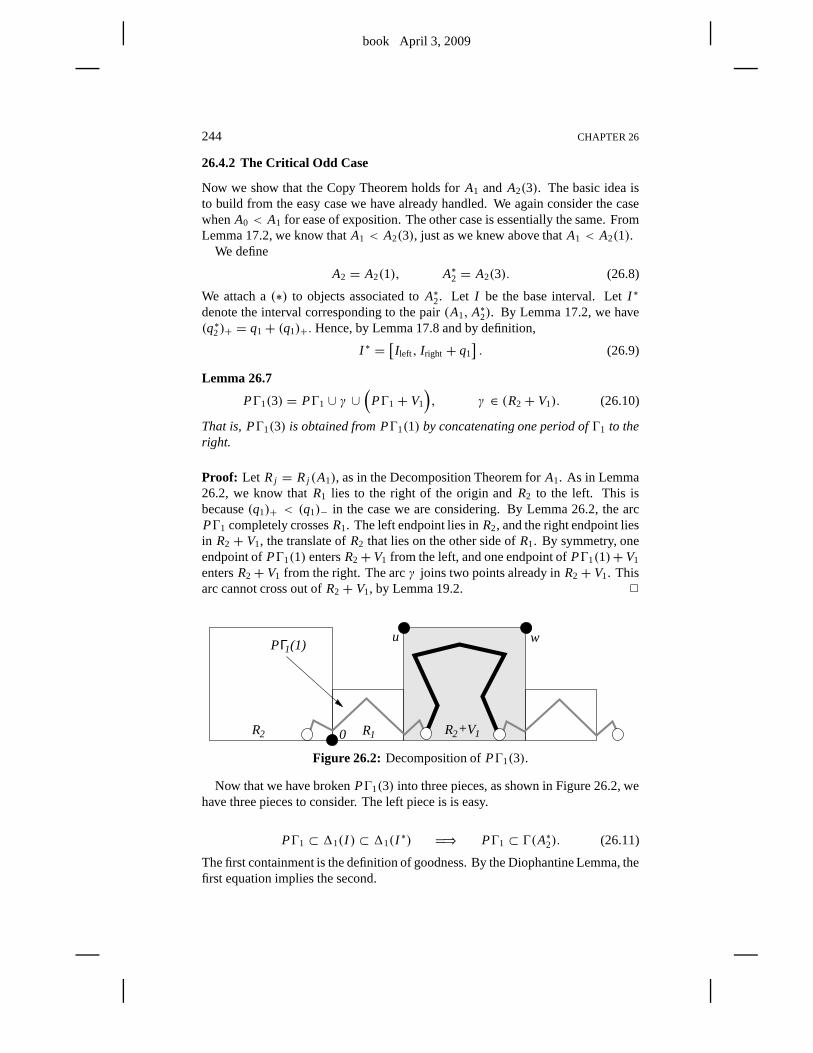
book April 3, 2009

244 CHAPTER 26

26.4.2 The Critical Odd Case

Now we show that the Copy Theorem holds forA1 and A2(3). The basic idea isto build from the easy case we have already handled. We again consider the casewhenA0 < A1 for ease of exposition. The other case is essentially the same. FromLemma 17.2, we know thatA1 < A2(3), just as we knew above thatA1 < A2(1).

We define

A2 = A2(1), A∗2 = A2(3). (26.8)

We attach a(∗) to objects associated toA∗2. Let I be the base interval. LetI ∗

denote the interval corresponding to the pair(A1, A∗2). By Lemma 17.2, we have(q∗2)+ = q1+ (q1)+. Hence, by Lemma 17.8 and by definition,

I ∗ =[I left, Iright + q1

]. (26.9)

Lemma 26.7

PŴ1(3) = PŴ1 ∪ γ ∪(

PŴ1 + V1

), γ ∈ (R2 + V1). (26.10)

That is, PŴ1(3) is obtained from PŴ1(1) by concatenating one period ofŴ1 to theright.

Proof: Let Rj = Rj (A1), as in the Decomposition Theorem forA1. As in Lemma26.2, we know thatR1 lies to the right of the origin andR2 to the left. This isbecause(q1)+ < (q1)− in the case we are considering. By Lemma 26.2, the arcPŴ1 completely crossesR1. The left endpoint lies inR2, and the right endpoint liesin R2 + V1, the translate ofR2 that lies on the other side ofR1. By symmetry, oneendpoint ofPŴ1(1) entersR2+ V1 from the left, and one endpoint ofPŴ1(1)+ V1

entersR2+ V1 from the right. The arcγ joins two points already inR2+ V1. Thisarc cannot cross out ofR2 + V1, by Lemma 19.2. 2

2 10 +

Γ

1

1(1)Pu w

2R R VR

Figure 26.2: Decomposition ofPŴ1(3).

Now that we have brokenPŴ1(3) into three pieces, as shown in Figure 26.2, wehave three pieces to consider. The left piece is is easy.

PŴ1 ⊂ 11(I ) ⊂ 11(I∗) H⇒ PŴ1 ⊂ Ŵ(A∗2). (26.11)

The first containment is the definition of goodness. By the Diophantine Lemma, thefirst equation implies the second.

book April 3, 2009

PROOF OF THE COPY THEOREM 245

The right piece is also easy. Anyv∗ ∈ PŴ1 + V1 has the formv + V1, wherev ∈ PŴ1. By Lemma 18.1, we have

G1(v∗) = G1(v)+ q1, H1(v

∗) = H1(v)+ q1.

Hencev ∈ 11(I ) impliesv∗ ∈ 1(I ∗). Therefore

PŴ1 + V1 ⊂ 11(I∗) H⇒ PŴ1 + V1 ⊂ Ŵ(A∗2). (26.12)

The middle piece is harder.

Lemma 26.8 γ ⊂ Ŵ(A∗2).

Proof: We will use the same argument that we used in §19.4. Sinceγ ⊂ R2, wejust have to show that the vertices ofR2 belong to the set11(I ∗)∪12(I ∗). This isa calculation just like the one in §19.4.

Now for the calculation. Letu andw, respectively, be the upper left and upperright vertices ofR2 + V1. We have

u ≈ W1 +(q1)+

q1V1, w = W1 + V1. (26.13)

Here the vectors are as in Equation 3.2,as usual. The approximation is good to within1/q1. To avoid approximations, we consider the very slightly altered parallelogramR2 + V1. The vertices are

(V1)+, u = W1 +

(q1)+

q1V1,

V1, w = V1+W1. (26.14)

Each vertex of the new parallelogram is within 1/q1 of the corresponding old paral-lelogram. Using the Mismatch Principle, it suffices to do thecalculation inR2+V1.Here is the calculation.

G1(u)− (−q1)

= (2q1+ q+)− H1(w)

=q1+ (q1)+ −q2

1

p1+ q1≥ 2. (26.15)

These bounds hold for all but a few exceptional parameters, as in Lemma 19.4. Theremaining few cases can be treated using exactly the same tricks as in §19.5. 2

Now we have shown thatPŴ1(3) ⊂ Ŵ2, as desired.

26.4.3 The Rest of the Odd Cases

We will consider the case whenδ1 = 5. The casesδ = 7,9,11, ... have the sametreatment.

In the case at hand,PŴ1(5) is obtained by concatenating 2 periods ofŴ1 to theright of PŴ1(1). We have decomposition of the form

PŴ1(5) = PŴ1(1) ∪ γ ∪(

PŴ1(1)+ 2V1

), γ ⊂ (R2 + V1) ∪ (R2 + 2V1).

(26.16)Hereγ is contained in a parallelogram that is twice as long as in thecaseδ = 3. Thecalculations are exactly the same in this case. The key pointis thatI ∗ = [a,b+ 2q1].

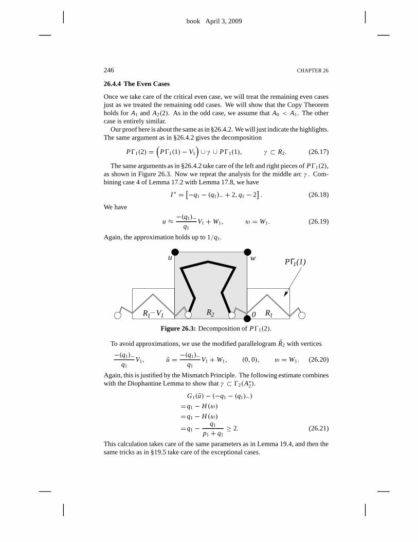
book April 3, 2009

246 CHAPTER 26

26.4.4 The Even Cases

Once we take care of the critical even case, we will treat the remaining even casesjust as we treated the remaining odd cases. We will show that the Copy Theoremholds for A1 and A2(2). As in the odd case, we assume thatA0 < A1. The othercase is entirely similar.

Our proof here is about the same as in §26.4.2. We will just indicate the highlights.The same argument as in §26.4.2 gives the decomposition

PŴ1(2) =(

PŴ1(1)− V1

)∪ γ ∪ PŴ1(1), γ ⊂ R2. (26.17)

The same arguments as in §26.4.2 take care of the left and right pieces ofPŴ1(2),as shown in Figure 26.3. Now we repeat the analysis for the middle arcγ . Com-bining case 4 of Lemma 17.2 with Lemma 17.8, we have

I ∗ =[−q1− (q1)− + 2,q1 − 2

]. (26.18)

We have

u ≈ −(q1)−

q1V1+W1, w = W1. (26.19)

Again, the approximation holds up to 1/q1.

1(1)P

1

Γ

11 2

u w

0R RRV

Figure 26.3: Decomposition ofPŴ1(2).

To avoid approximations, we use the modified parallelogramR2 with vertices

−(q1)−

q1V1, u = −(q1)−

q1V1 +W1, (0,0), w = W1. (26.20)

Again, this is justified by the Mismatch Principle. The following estimate combineswith the Diophantine Lemma to show thatγ ⊂ Ŵ2(A∗2).

G1(u)− (−q1− (q1)−)

=q1− H (w)

=q1− H (w)

=q1−q1

p1+ q1≥ 2. (26.21)

This calculation takes care of the same parameters as in Lemma 19.4, and then thesame tricks as in §19.5 take care of the exceptional cases.

book April 3, 2009

PROOF OF THE COPY THEOREM 247

26.5 THE END OF THE PROOF

The Good Parameter Lemma reduces our job to showing that any odd rationalparameter is good. We will give an inductive argument.

Lemma 26.9 If 1/1← A, then A is good.

Proof: We write 1/1← A← A. In this case, Lemma 17.2 tells us that

1/1> A > A (26.22)

(The first inequality is obvious.) We have

A =2k− 1

2k+ 1, A =

4k− 3

4k+ 1, q− = k.

By Lemma 17.8, we have

I =[−q− q− + 2,q − 2

]= [−3k+ 1,2k− 1]

The left vertex ofPŴ1 is u = (−k, k), and the right vertex isv = (0,0). Wecompute

G(u) = −k− 1 ≥ −3k+ 1, H (w) = 0 ≤ 2k − 1.

The extreme case occurs whenk = 1. 2

Lemma 26.10 A = p/q is good if q< 20or if p = 1.

Proof: We check the caseq < 20 by hand. Ifp = 1, the pivot arc is just theedge connecting(−1,1) to (0,0), whereas the intervalI contains [−q,q], a hugeinterval. This case is obvious. 2

Now we establish the inductive step. Suppose thatA1← A2 and thatA1 is good.Having eliminated the few exceptional cases by the result above, the argument inthe previous section shows thatPŴ2 ⊂ 11(I1). HereI1 is the interval based on theconstant�(A1, A2). This is the Diophantine constant defined in §17.4 relative tothe pair(A1, A2). To finish the proof of the Copy Theorem, we just have to establishthe following equation.

PŴ2 ⊂ 12(I2), (26.23)

whereI2 is the different interval based on the pairA2← A3, with δ(A2, A3) = 1.Here we establish two basic facts.

Lemma 26.11 I1 ⊂ I2, and either endpoint of I1 is more than1 unit from thecorresponding endpoint of I2.

book April 3, 2009

248 CHAPTER 26

Proof: By Lemma 17.8, applied to both parameters, we have

I1 ⊂ [−q2+ 3,q2− 3] ⊂ [−q2− 2,q2− 2] ⊂ I2.

This completes the proof. 2

Let G j and H j be the linear functionals associated toA j in the DiophantineLemma. See §18.1.

Lemma 26.12 |G1(v)− G2(v)| < 1 and|H1(v)− H2(v)| < 1 for v ∈ 11(I1).

Proof: From Lemma 17.8 and a bit of geometry, we get the bound

(m,n) ∈ 11(I1) H⇒ max(|m|, |n|) ≤ q2. (26.24)

Looking at Equation 18.2, we see that

G(m,n) =(

1− A

1+ A,−2

1+ A

)· (m,n) = (G1,G2) · (m,n).

H (m,n) =(

1+ 4A− A2

(1+ A)2,

2− 2A

(1+ A)2

)· (m,n) = (H1, H2) · (m,n). (26.25)

A bit of calculus shows that

|∂AG j | ≤ 2, |∂AH1| ≤ 6, |∂AH2| ≤ 2. (26.26)

SinceA1← A2, we have

|A1− A2| =2

q1q2. (26.27)

Putting everything together, and using basic calculus, we arrive at the bound

|G1(v)− G2(v)|, |H1(v)− H2(v)| < 16/q1 < 1, (26.28)

at least forq1 > 16. 2

We have already remarked, during the proof of the Decomposition Theorem, thatno lattice point lies between the bottom of12(I2) and the bottom of11(I2). HenceF1(v) > 0 iff F2(v) > 0. The two lemmas now show that11(I1) ⊂ 12(I2). Thiswas our final goal, from Equation 26.23.

This completes the proof of the Copy Theorem.

book April 3, 2009

Chapter Twenty-Seven

Pivot Arcs in the Even Case

27.1 MAIN RESULTS

Given two rationalsA1 = p1/q1 andA2 = p2/q2, we introduce the notation

A1 ⊢ A2 ⇐⇒ |p1q2− q1 p2| = 1, q1 < q2. (27.1)

In this case, we say thatA1 andA2 areFarey-related. We sometimes call(A1, A2)a Farey pair.

We have the notions ofFarey additionandFarey subtraction, respectively.

A1 ⊕ A2 =p1+ p2

q1+ q2, A2⊖ A1 =

p2− p1

q2− q1. (27.2)

Note thatA1 ⊢ A2 implies thatA1 ⊢ (A1 ⊕ A2) and thatA1 is Farey-related toA2 ⊖ A1.

Lemma 27.1 Let A1 be an even rational. Then there is a unique odd rational A2

such that A1 ⊢ A2 and2q1 > q2. In this case, we write A1 |H A2.

Proof: Equation 4.1 works for both even and odd rationals. WhenA1 is even, ex-actly one of the rationals(A1)± is also even. Call this rationalA′1. ThenA′1 ⊢ A1.We defineA2 = A1⊕ A′1. If B2 were another candidate, thenB2⊖ A′ would be therelevant choice of(A1)±. HenceB2 = A2. 2

Let A be an odd rational. Then eitherA− |H A or A+ |H A when A is anodd rational. IfA− |H A, then we writeA+ ⇐ A. The relationship implies that2q+ < q. Likewise we writeA− ⇐ A when 2q− < q. Here is an example: LetA = 3/7. Then

A+ = 1/2⇐ 3/7, A− = 2/5 |H 3/7.

So far we have defined pivot points and arcs for odd parameters. Now we definethem for even parameters. We have

E±(A1) = E±(A2), A1 |H A2. (27.3)

This makes sense because we have already defined the pivot points in the odd case.We still need to prove that these vertices lie onŴ1. We will do this below.

Assuming that the pivot pointsE±1 are vertices ofŴ1, we definePŴ1 to be thelower arc ofŴ1 that connectsE−1 to E+1 . SinceŴ1 is a polygon in the even case,it makes sense to speak of the lower arc. Figure 27.1 shows an example. HerePŴ1 = PŴ2. We will show that this always happens.

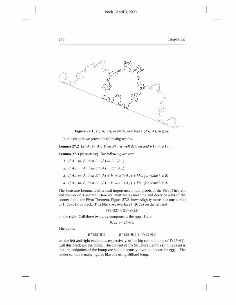
book April 3, 2009

250 CHAPTER 27

Figure 27.1: Ŵ(16/39), in black, overlaysŴ(25/61), in gray.

In this chapter we prove the following results.

Lemma 27.2 Let A1 |H A2. Then PŴ1 is well defined and PŴ1 = PŴ2.

Lemma 27.3 (Structure) The following are true.

1. If A− ⇐ A, then E+(A) = E+(A−).

2. If A+ ⇐ A, then E−(A) = E−(A+).

3. If A− ⇐ A, then E−(A)+ V = E−(A−)+ kV− for some k∈ Z.

4. If A+ ⇐ A, then E+(A)− V = E+(A+)+ kV+ for some k∈ Z.

The Structure Lemma is of crucial importance in our proofs ofthe Pivot Theoremand the Period Theorem. Here we illustrate its meaning and describe a bit of theconnection to the Pivot Theorem. Figure 27.2 shows slightlymore than one periodof Ŵ(25/61), in black. This black arc overlaysŴ(9/22) on the left and

Ŵ(9/22)+ 2V(9/22)

on the right. Call these two gray components the eggs. Here

9/22⇐ 25/61.

The points

E+(25/61), E−(25/61)+ V(25/61)

are the left and right endpoints, respectively, of the big central bump ofŴ(25/61).Call this black arc the bump. The content of the Structure Lemma (in this case) isthat the endpoints of the bump are simultaneously pivot points on the eggs. Thereader can draw many figures like this using Billiard King.

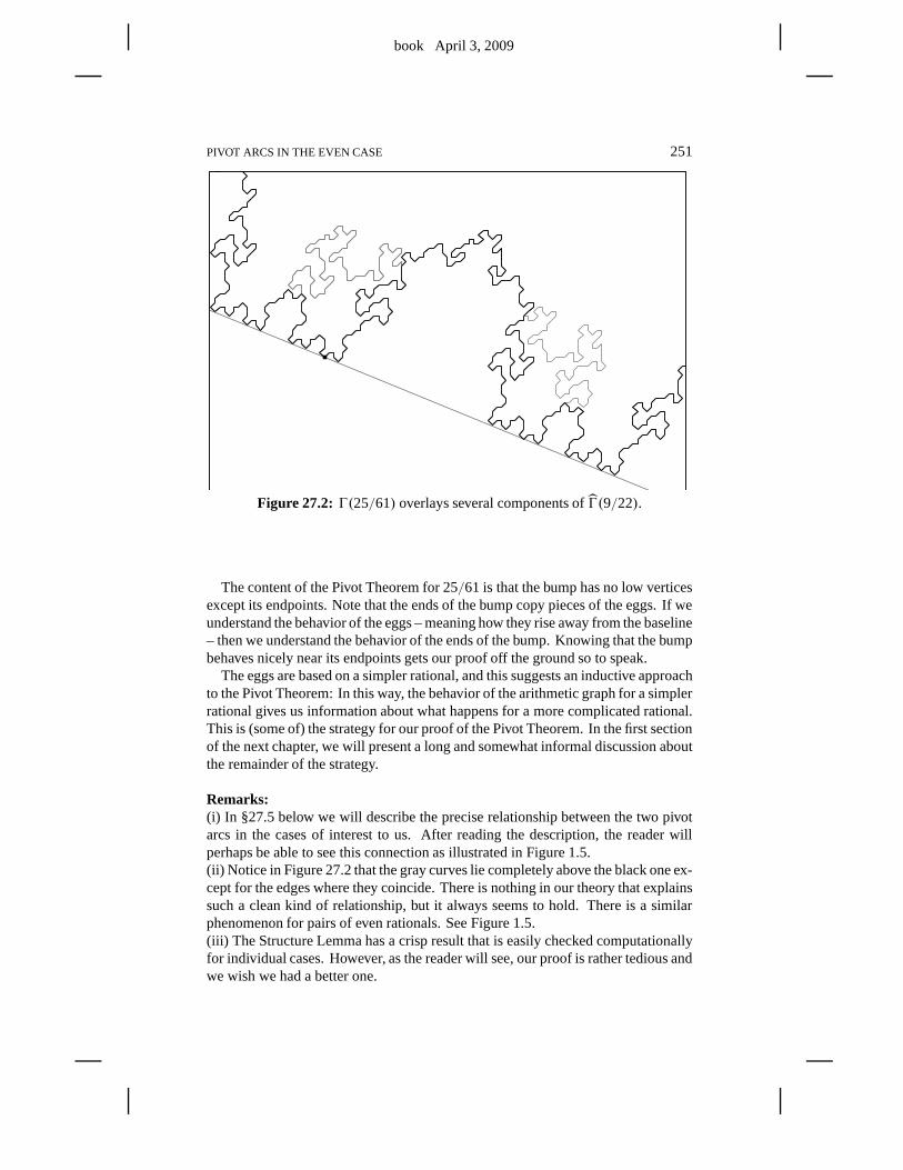
book April 3, 2009

PIVOT ARCS IN THE EVEN CASE 251

Figure 27.2: Ŵ(25/61) overlays several components ofŴ(9/22).

The content of the Pivot Theorem for 25/61 is that the bump has no low verticesexcept its endpoints. Note that the ends of the bump copy pieces of the eggs. If weunderstand the behavior of the eggs – meaning how they rise away from the baseline– then we understand the behavior of the ends of the bump. Knowing that the bumpbehaves nicely near its endpoints gets our proof off the ground so to speak.

The eggs are based on a simpler rational, and this suggests aninductive approachto the Pivot Theorem: In this way, the behavior of the arithmetic graph for a simplerrational gives us information about what happens for a more complicated rational.This is (some of) the strategy for our proof of the Pivot Theorem. In the first sectionof the next chapter, we will present a long and somewhat informal discussion aboutthe remainder of the strategy.

Remarks:(i) In §27.5 below we will describe the precise relationshipbetween the two pivotarcs in the cases of interest to us. After reading the description, the reader willperhaps be able to see this connection as illustrated in Figure 1.5.(ii) Notice in Figure 27.2 that the gray curves lie completely above the black one ex-cept for the edges where they coincide. There is nothing in our theory that explainssuch a clean kind of relationship, but it always seems to hold. There is a similarphenomenon for pairs of even rationals. See Figure 1.5.(iii) The Structure Lemma has a crisp result that is easily checked computationallyfor individual cases. However, as the reader will see, our proof is rather tedious andwe wish we had a better one.

book April 3, 2009

252 CHAPTER 27

27.2 ANOTHER DIOPHANTINE LEMMA

Here we prove a copying lemma that helps with Lemma 27.2. Our result works forFarey pairs. Let11(I ) and12(I ) be the sets defined exactly as in the DiophantineLemma. See §18.2. The result we prove here is actually more natural than ouroriginal result. However, the original result better suited our more elementarypurposes.

Lemma 27.4 Suppose that A1 ⊢ A2.

1. If A1 < A2, let I = [−q1+ 2,q2 − 2].

2. If A1 > A2, let I = [−q2+ 2,q1− 2].

ThenŴ1 andŴ2 agree on11(I ) ∪12(I ).

Proof: We will consider the case whenA1 < A2. The other case requires a verysimilar treatment. In the proof of the Diophantine Lemma we used only the oddnessof the rationals in Lemma 17.5. Once we prove the analog of this result in the evensetting, the rest of the proof works verbatim.

Recall that an integerµ is good if

[ A1µ] = [ A2µ] . (27.4)

Here [ ] denotes the floor function. The analog of Lemma 17.5 isthe statementthat an integerµ is good provided thatµ ∈ (−q1,q2). We will give a geometricproof. LetL1 (respectively,L2) denote the line segment of slope−A1 (respectively,−A2) joining the two points whose first coordinates are−q1 andq2. If we have acounterexample to our claim, then there is a lattice point(m,n) lying betweenL1

andL2.If m < 0, we consider the triangleT with vertices(0,0) and−V1 and(m,n).

HereV1 = (q1,−p1). The vertical distance between the left endpoints ofL1 andL2 is 1/q2. By the base-times-height formula for triangles,

area(T) < q1/(2q2) < 1/2. (27.5)

But this contradicts the fact that 1/2 is a lower bound for the area of a lattice triangle.If m > 0, we consider the triangleT with vertices(0,0) andV1 and(m,n). Thelattice point(m,n) is closer to the line containingL1 than is the right endpoint ofL2, namely,(q2,−p2). Hence

area(T) < area(T ′), (27.6)

whereT ′ is the triangle with vertices(0,0) andV1 andV2. But

area(T ′) = 1/2 (27.7)

becauseA1 andA2 are Farey-related. We have the same contradiction as in the firstcase. 2

book April 3, 2009

PIVOT ARCS IN THE EVEN CASE 253

27.3 COPYING THE PIVOT ARC

Here we prove Lemma 27.2. As we did for the Decomposition Theorem, we willfirst establish the result for most parameters. Then we will treat the exceptionalcases.

Suppose thatA1 |H A2. To show thatPŴ1 is well defined, we just have toshow PŴ2 ⊂ Ŵ1. This result simultaneously shows thatPŴ1 = PŴ2 because theendpoints of these two arcs are the same by definition.

In the case at hand, we haveA1 = (A2)−. To simplify the notation, we writeA = A2. ThenA1 = A−. By Lemma 27.4, it suffices to prove that

PŴ ⊂ 1(J), J =[−q− + 2,q − 2

]. (27.8)

We have actually already proved this, but it takes some effort to recognize the fact.Let A′← A denote the inferior predecessor ofA. Sinceq− > q+, we have

A′ = A− ⊖ A+. (27.9)In the previous chapter, when we proved the Copy Theorem, we established

PŴ ⊂ 1′(J ′), J ′ =[−q′ + 2,q′ + q+ − 2

], (27.10)

as long asp′ ≥ 3 andq′ ≥ 7. Here1′ is defined relative to the linear functionalsG′ andH ′, which are defined relative toA′. The right endpoint in Equation 27.10comes from Lemma 17.8. The point is that the calculation in Lemma 26.8 gives thesame bounds as the calculation for Lemma 19.4.

Now we observe that

q′ = q− − q+ < q− (27.11)and

q′ + q+ < (q− − q+)+ q+ = q− < q. (27.12)These calculations show thatJ ′ ⊂ J. Usually J is much larger.

The region1(J) is computed relative to the parameterA, whereas the region1′(J ′) is computed relative to the parameterA′. The same argument as in Lemma26.12 shows that

1(J) ⊂ 1′(J ′) (27.13)except whenq < 20. We check the cases whenq < 20 by hand, using BilliardKing.

The distance between the left endpoint ofJ ′ and the left endpoint ofJ is q−−q′.The same is true for the right endpoints. As long asq− − q′ ≥ 2, the argument inthe proof of Lemma 19.4 shows thatPŴ ⊂ 1(J). The point is that Equation 19.9is replaced by

−q′

1+ A′≥ −q′, (27.14)

which is always true. Whenq− = q′ + 1, we must havep = 1. In this case, thepivot points areE− = (−1,1) andE+ = (0,0). This case is trivially true.

Remark: The reader might wonder why we have so much slack in the (supposedly)tightest possible situation. The slack comes from the fact that, in Lemma 26.8, thearcγ is well inside the parallelogramR2. For the sake of robustness, we mentionthat any small size ofq− − q′ leads to a similar proof.

book April 3, 2009

254 CHAPTER 27

27.4 PROOF OF THE STRUCTURE LEMMA

We will consider the case whenA− ⇐ A. The other case is similar. LetB be theodd rational such thatA− |H B. ThenPŴ(A−) = PŴ(B), by definition.

Lemma 27.5 The Structure Lemma holds when1/1← A.

Proof: In this case

A = 2k− 1

2k+ 1, A− =

k− 1

k, B = 2k− 3

2k− 1. (27.15)

ThenPŴ(A) is the line segment connecting(0,0) to (−k, k), andPŴ(B) is the linesegment connecting(0,0) to (−k+ 1, k− 1). 2

In all other cases, we haveA′← A, whereA′ 6= 1/1. As in Lemma 17.2, let

δ = δ(A′, A) = floor(q′/q).

Lemma 27.6 If δ = 1, then the Structure Theorem holds.

Proof: If δ(A′, A) = 1, thend(A′, A) = 0. If d(A′, A) = 0, thenPŴ = PŴ′ bythe Copy Theorem and the definition of pivot arcs. At the same time, we can applyLemma 17.2 to the pairAm = A′ and Am+1 = A. Sinceδ(A′, A) = 1, we musthave Case 1 or Case 3. But we also haveA− < A+. Hence we have Case 3. Butthen A′− = A−. Hence we can replace the pair(A−, A) by the pair(A′−, A′), andthe result follows by induction on the size of the denominator of A. 2

Lemma 27.7 Suppose thatδ = 2. Then A′ = B.

Proof: B is characterized by the property thatA− andB are Farey-related, and

2q− > denominator(B) > q−.

We will show thatA′ has this same property. Note thatA′ andA− are Farey-related.The equations

2q′ < q, q = q+ + q−, q′ = q+ − q−

lead to

3q− > q+ H⇒ 2q− > (q+ − q−) = q′.

This establishes the first property forA′. The fact thatδ = 2 gives 3q′ > q. Thisleads to

q+ > 2q−, H⇒ q′ = q+ − q− > q−.

This is the second property forA′. 2

book April 3, 2009

PIVOT ARCS IN THE EVEN CASE 255

Lemma 27.8 Supposeδ ≥ 3. Then A′← B.

Proof: There is some even rationalC such that

B = A− ⊕ C. (27.16)

The denominator ofC is smaller than the denominator ofA− because of the factthat A− |H B. The inferior predecessor ofB is A− ⊖ C. At the same time,

A′ = A+ ⊖ A−. (27.17)

So, we are trying to show thatA+ ⊖ A− = A− ⊖ C. This is the same as showingthat

C = D = A− ⊕ A− ⊖ A+. (27.18)

SinceA+ andA− are Farey-related,D andA− are Farey-related. We claim that

2q− − q+ = denominator∈ (0,q−). (27.19)

The upper bound comes from the fact thatq+ > q−. The lower bound comes fromthe fact thatq+ < 2q−. To see this last equation, note that

q = q+ + q−, q′ = q+ − q−, 3q′ < q.

But C is the only even rational that is Farey related toA− and satisfies equation27.19. HenceC = D. 2

As we have already proved, the caseδ = 1 is handled by induction on thedenominator ofA. The caseδ = 2 gives

PŴ− = PŴ′.

In this case, the Structure Lemma follows from the definitionof the pivot points.Whenδ ≥ 3, the rationalA′ is a common inferior predecessor ofA andB. Since

A+ = A′ ⊕ A− andA− < A+, we haveA′ > A+. HenceA′ > A.

Lemma 27.9 A′ > B.

Proof: Lemma 27.8 gives

A′ = A− ⊖ C, A+ = A′ ⊕ A−, A = A+ ⊕ A−, B = A− ⊕ C. (27.20)

This gives

A⊖ B = A+ ⊖ C = A′ ⊕ A− ⊖ C = A′ ⊕ A′.

Hence

A = B⊕ A′ ⊕ A′. (27.21)

Since A+ = A′ ⊕ A− and A− < A+, we haveA′ > A+. HenceA′ > A. ByEquation 27.21,A lies betweenA′ andB. HenceB < A < A′. HenceA′ > B. Inshort,A′ > A andA′ > B. 2

book April 3, 2009

256 CHAPTER 27

Finally, from the definition of pivot points, we haveE+(A) = E+(B). Thisestablishes statement 1. Statement 2 has a similar proof.

Now for statement 3. By Lemma 26.1,

E+(A)+ E−(A) = −A− + (0,1), E+(B)+ E−(B) = −B+ + (0,1).

SinceE+(A) = E+(B), we have

E−(B)− E−(A) = A− − B+ = V(C) (27.22)

HereV(C) is, as in Equation 3.2, defined relative toC. We now have

E−(A)+ V − E−(A−)

=E−(A)− E−(B)+ V

=−V(C)+ V(A)

=V(A+ ⊕ A−)− V(A+ ⊖ A−)

=2V(A−) ∈ Z(V−). (27.23)

This completes the proof of statement 3. The proof of statement 4 is similar.

An Even Version: Now that we have established the Structure Lemma, we provea variant. For each even rationalA2 ∈ (0,1) that is not of the form 1/q2, there isanother even rationalA1 = p1/q1 ∈ (0,1) such thatq1 < q2 andA1 ⊢ A2.

Lemma 27.10 The Structure Lemma holds for the pair(A1, A2).

Proof: We will deduce this new version of the Structure Lemma from the originalversion we have just finished proving.

Consider statement 1. Let

A3 = A1 ⊕ A2. (27.24)

Then

A1⇐ A3, A2 |H A3 (27.25)

Note thatE+2 = E+3 by definition. Also,E+1 = E+3 , by the Structure Lemma.HenceE+1 = E+2 . This proves statement 1 for the pair(A1, A2). Statement 2 hasthe same kind of proof.

Consider statement 3. We haveE−2 = E−3 and

E−3 − E−1 + V3 ∈ ZV1. (27.26)

On the other hand

V3 = V2 + V1, H⇒ E−3 − E−1 + V2 ∈ ZV1. (27.27)

The first equation implies the second. ButE−3 = E−2 . This completes the proof ofstatement 3. Statement 4 has the same kind of proof. 2

book April 3, 2009

PIVOT ARCS IN THE EVEN CASE 257

27.5 THE DECREMENT OF A PIVOT ARC

Here we work out the precise relationship between the pivot arcs in the StructureLemma. One can see the structure we describe here in Figure 1.5.

Let A be an odd rational and letA′ be the superior predecessor ofA. By the CopyTheorem,PŴ contains at least one period ofŴ′ starting from either end. Letγ ′ beone period ofŴ′ starting from the right endpoint ofPŴ. We defineDPŴ by thefollowing formula.

PŴ = DPŴ ∗ γ ′. (27.28)

The operation on the right hand side of the equation is the concatenation of arcs.We call DPŴ thedecrementof PŴ.

The arcDPŴ is a pivot arc relative to a different parameter. (See the nextlemma.)DPŴ is obtained fromPŴ by deleting one period ofŴ′. Now we presentanaddendumto the Structure Lemma.

Lemma 27.11 If B ⇐ A, then PŴ(B) = DPŴ(A), up to translation.

Proof: We will consider the case whenA− ⇐ A. The other case, whenA+ ⇐ A,has essentially the same proof. We reexamine Lemmas 27.7 and27.8. In Lemma27.7, we have

PŴ− = PŴ′.

However, in this case,δ(A, A′) = 2, and from the definition of pivot points, we seethat PŴ is obtained fromPŴ′ by concatenating a single period ofŴ′. This gives uswhat we want.

In Lemma 27.8, we have Equation 27.21, which implies

denominator(A) = denominator(B)+ 2q′. (27.29)

But this implies thatd(A′, A) = d(A′, B)+1. Applying the Copy Theorem to bothpairs, we see thatPŴ is obtained fromPŴ′ by concatenatingd(A, B)+ 1 periodsof Ŵ′ wherePŴ− is obtained fromPŴ′ by contatenatingd(A′, B) periods ofŴ′.This gives us the desired relationship. 2

27.6 AN EVEN VERSION OF THE COPY THEOREM

Let A2 be an even rational. We writeA2 = A0 ⊕ A1, whereA0 is odd andA1 iseven.

Lemma 27.12 PŴ2 ⊂ Ŵ0.

Proof: We havePŴ2 = PŴ(A3), whereA3 is the odd rational such thatA2 |H A3.Since A1 ⊢ A2 and bothA1 and A2 are even, we haveA3 = A1 ⊕ A2. At thesame time, we haveA0 = A2 ⊖ A1. HenceA0← A3. But now we can apply theCopy Theorem to the pair(A0, A3) to conclude thatPŴ3 ⊂ Ŵ0. But PŴ3 = PŴ2. 2

book April 3, 2009

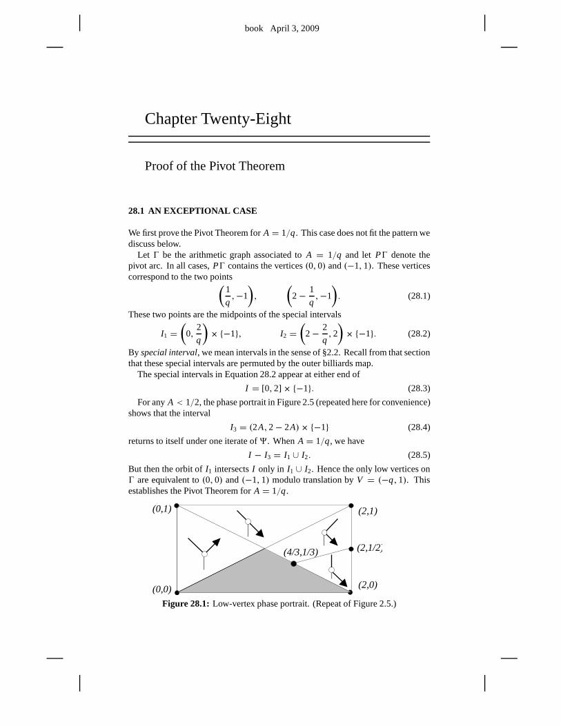
book April 3, 2009

Chapter Twenty-Eight

Proof of the Pivot Theorem

28.1 AN EXCEPTIONAL CASE

We first prove the Pivot Theorem forA = 1/q. This case does not fit the pattern wediscuss below.

Let Ŵ be the arithmetic graph associated toA = 1/q and let PŴ denote thepivot arc. In all cases,PŴ contains the vertices(0,0) and(−1,1). These verticescorrespond to the two points(

1

q,−1

),

(2−

1

q,−1

). (28.1)

These two points are the midpoints of the special intervals

I1 =(

0,2

q

)× {−1}, I2 =

(2−

2

q,2

)× {−1}. (28.2)

By special interval, we mean intervals in the sense of §2.2. Recall from that sectionthat these special intervals are permuted by the outer billiards map.

The special intervals in Equation 28.2 appear at either end of

I = [0,2]× {−1}. (28.3)

For anyA < 1/2, the phase portrait in Figure 2.5 (repeated here for convenience)shows that the interval

I3 = (2A,2− 2A)× {−1} (28.4)

returns to itself under one iterate of9. WhenA = 1/q, we have

I − I3 = I1 ∪ I2. (28.5)

But then the orbit ofI1 intersectsI only in I1 ∪ I2. Hence the only low vertices onŴ are equivalent to(0,0) and(−1,1) modulo translation byV = (−q,1). Thisestablishes the Pivot Theorem forA = 1/q.

(4/3,1/3) (2,1/2)

(0,0)

(0,1) (2,1)

(2,0)

Figure 28.1: Low-vertex phase portrait. (Repeat of Figure 2.5.)

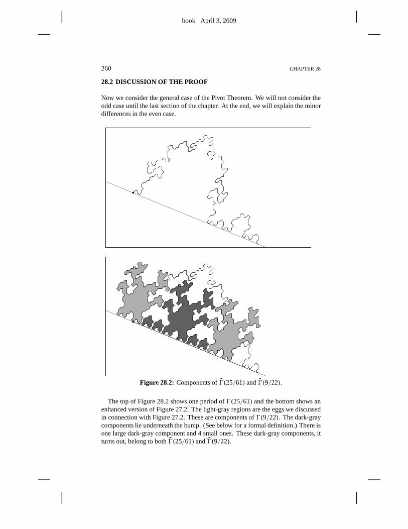
book April 3, 2009

260 CHAPTER 28

28.2 DISCUSSION OF THE PROOF

Now we consider the general case of the Pivot Theorem. We willnot consider theodd case until the last section of the chapter. At the end, we will explain the minordifferences in the even case.

Figure 28.2: Components ofŴ(25/61) andŴ(9/22).

The top of Figure 28.2 shows one period ofŴ(25/61) and the bottom shows anenhanced version of Figure 27.2. The light-gray regions arethe eggs we discussedin connection with Figure 27.2. These are components ofŴ(9/22). The dark-graycomponents lie underneath the bump. (See below for a formal definition.) There isone large dark-gray component and 4 small ones. These dark-gray components, itturns out, belong to bothŴ(25/61) andŴ(9/22).

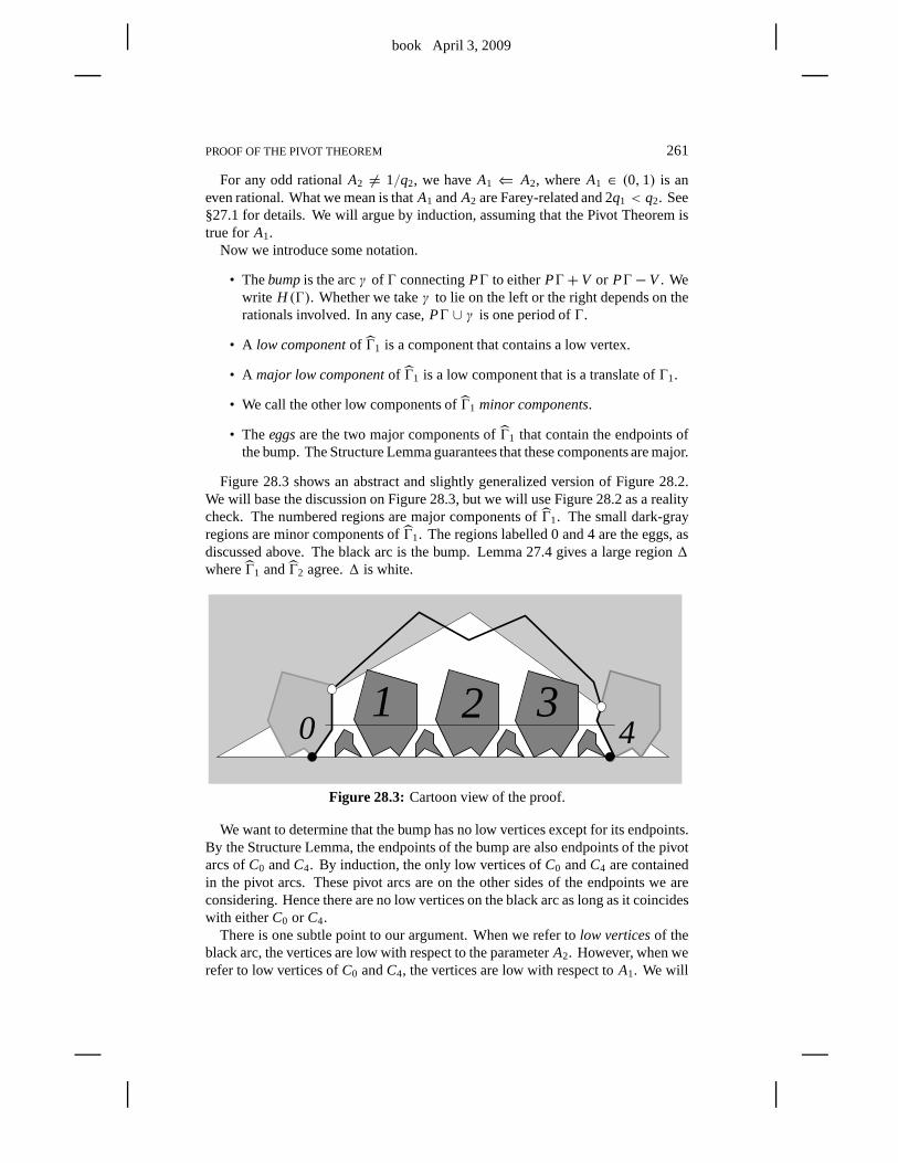
book April 3, 2009

PROOF OF THE PIVOT THEOREM 261

For any odd rationalA2 6= 1/q2, we haveA1 ⇐ A2, whereA1 ∈ (0,1) is aneven rational. What we mean is thatA1 andA2 are Farey-related and 2q1 < q2. See§27.1 for details. We will argue by induction, assuming thatthe Pivot Theorem istrue for A1.

Now we introduce some notation.

• Thebumpis the arcγ of Ŵ connectingPŴ to eitherPŴ+V or PŴ−V . Wewrite H (Ŵ). Whether we takeγ to lie on the left or the right depends on therationals involved. In any case,PŴ ∪ γ is one period ofŴ.

• A low componentof Ŵ1 is a component that contains a low vertex.

• A major low componentof Ŵ1 is a low component that is a translate ofŴ1.

• We call the other low components ofŴ1 minor components.

• Theeggsare the two major components ofŴ1 that contain the endpoints ofthe bump. The Structure Lemma guarantees that these components are major.

Figure 28.3 shows an abstract and slightly generalized version of Figure 28.2.We will base the discussion on Figure 28.3, but we will use Figure 28.2 as a realitycheck. The numbered regions are major components ofŴ1. The small dark-grayregions are minor components ofŴ1. The regions labelled 0 and 4 are the eggs, asdiscussed above. The black arc is the bump. Lemma 27.4 gives alarge region1whereŴ1 andŴ2 agree.1 is white.

30 4

1 2

Figure 28.3: Cartoon view of the proof.

We want to determine that the bump has no low vertices except for its endpoints.By the Structure Lemma, the endpoints of the bump are also endpoints of the pivotarcs ofC0 andC4. By induction, the only low vertices ofC0 andC4 are containedin the pivot arcs. These pivot arcs are on the other sides of the endpoints we areconsidering. Hence there are no low vertices on the black arcas long as it coincideswith eitherC0 or C4.

There is one subtle point to our argument. When we refer tolow verticesof theblack arc, the vertices are low with respect to the parameterA2. However, when werefer to low vertices ofC0 andC4, the vertices are low with respect toA1. We will

book April 3, 2009

262 CHAPTER 28

discuss this subtle point in the next section. What saves us is that the two notionsof low coincide, because of the way in whichA1 approximatesA2.

So, either end of the black arc starts out well: It rises away from the baseline. Thisis exactly the situation we discussed in the last chapter in connection with Figure27.2. Once the bump gets off the ground, what could go wrong? Answer: One ofthe ends could dip back down into1 and (at the boundary) merge with a componentof Ŵ1. In other words, some component ofŴ1 would have to stick out of1.

We will analyze the various possibilities in turn. We distinguish 3 basic cases.

The End Major Components: These are the components labelledC1 and C3

in Figure 28.3. In Figure 28.2, the single large component isthe only end majorcomponent. These components seem to give us the most troublebecause they comeclosest to sticking out of1. In fact, we cannot show that these components arecontained in1 even though experimentally we can see that this is true. However,Lemma 2.6 comes to the rescue. The low vertices on these components have oddparity, and the low vertices on the bump have even parity. We will see that thisimplies that the bump cannot merge withC1 andC3. The parity argument steps inwhere geometry fails.

The Middle Major Components: This is the component labelledC2 in Figure28.3. In Figure 28.2 there are no middle major components even though the largedark-gray component there sits in the middle in some obvioussense. In general,there aren+1 major components andn−1 middle major components. The middlemajor components are much farther inside1. We will show that the other majorcomponents are contained entirely inside1.

Minor Components: These are the remaining small dark-gray components inFigure 28.3. The Barrier Theorem from Chapter 14 handles these. The blackhorizontal line in Figure 28.3 represents the barrier whichno minor component cancross. Equipped with the Barrier Theorem, we will be able to show that all minorcomponents lie in1. The barrier line keeps them from sticking out.

This takes care of all the potential problems. Since the bumpcannot merge withany of the small dark-gray components, it just skips over everything and has no lowvertices except for its endpoints. As with the proof of the Decomposition Theorem,the estimates we make are true by a wide margin whenA1 is large. However, whenA1 is small, the estimates are close and we need to consider the situation in a case-by-case way. We hope that this dealing with small cases does not obscure the basicideas in the proof.

Remark: As we remarked above, it seems thatŴ2 copies all the low componentsof Ŵ2 that lie between the two endpoints of the bump. In light of what we said inthe case-by-case analysis, we will show that this is true except perhaps for the endmajor components. Our methods are not quite good enough to get these as well.This deficiency in our methods causes our proofs to be more complicated in a fewplaces.

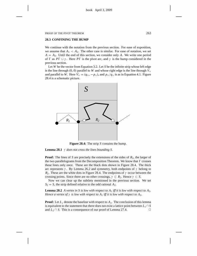
book April 3, 2009

PROOF OF THE PIVOT THEOREM 263

28.3 CONFINING THE BUMP

We continue with the notation from the previous section. Forease of exposition,we assume thatA1 < A2. The other case is similar. For ease of notation, we setA = A2. Until the end of this section, we consider onlyA. We write one periodof Ŵ as PŴ ∪ γ . Here PŴ is the pivot arc, andγ is the bump considered in theprevious section.

Let W be the vector from Equation 3.2. LetSbe the infinite strip whose left edgeis the line through(0,0) parallel toW and whose right edge is the line throughV+and parallel toW. HereV+ = (q+,−p+), andp+/q+ is as in Equation 4.1. Figure28.4 is a schematic picture.

1 2

S

R R

Figure 28.4: The stripScontains the bump.

Lemma 28.1 γ does not cross the lines bounding S.

Proof: The lines ofS are precisely the extensions of the sides ofR2, the larger ofthe two parallelograms from the Decomposition Theorem. We know thatŴ crossesthese lines only once. These are the black dots shown in Figure 28.4. The thickarc representsγ . By Lemma 26.2 and symmetry, both endpoints ofγ belong toR2. These are the white dots in Figure 28.4. The endpoints ofγ occur between thecrossing points. Since there are no other crossings,γ ⊂ R2. Henceγ ⊂ S.

Now we can clear up the subtlety mentioned in the previous section. We setS2 = S, the strip defined relative to the odd rationalA2.

Lemma 28.2 A vertex in S is low with respect to A1 iff it is low with respect to A2.Hence a vertex ofγ is low with respect to A1 iff it is low with respect to A2.

Proof: Let L j denote the baseline with respect toA j . The conclusion of this lemmais equivalent to the statement that there does not exist a lattice point betweenL1∩SandL2 ∩ S. This is a consequence of our proof of Lemma 27.4. 2

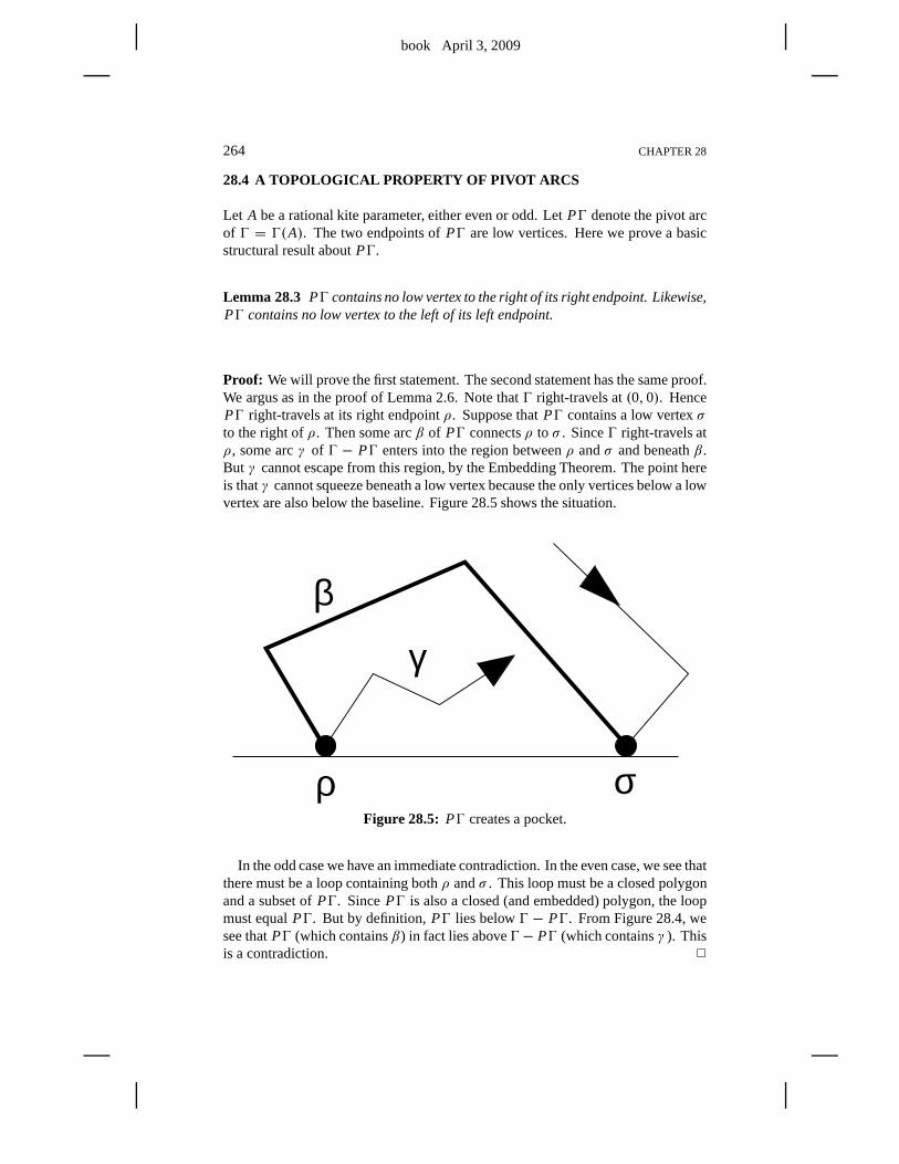
book April 3, 2009

264 CHAPTER 28

28.4 A TOPOLOGICAL PROPERTY OF PIVOT ARCS

Let A be a rational kite parameter, either even or odd. LetPŴ denote the pivot arcof Ŵ = Ŵ(A). The two endpoints ofPŴ are low vertices. Here we prove a basicstructural result aboutPŴ.

Lemma 28.3 PŴ contains no low vertex to the right of its right endpoint. Likewise,PŴ contains no low vertex to the left of its left endpoint.

Proof: We will prove the first statement. The second statement has the same proof.We argus as in the proof of Lemma 2.6. Note thatŴ right-travels at(0,0). HencePŴ right-travels at its right endpointρ. Suppose thatPŴ contains a low vertexσto the right ofρ. Then some arcβ of PŴ connectsρ to σ . SinceŴ right-travels atρ, some arcγ of Ŵ − PŴ enters into the region betweenρ andσ and beneathβ.But γ cannot escape from this region, by the Embedding Theorem. The point hereis thatγ cannot squeeze beneath a low vertex because the only vertices below a lowvertex are also below the baseline. Figure 28.5 shows the situation.

β

ρ σ

γ

Figure 28.5: PŴ creates a pocket.

In the odd case we have an immediate contradiction. In the even case, we see thatthere must be a loop containing bothρ andσ . This loop must be a closed polygonand a subset ofPŴ. SincePŴ is also a closed (and embedded) polygon, the loopmust equalPŴ. But by definition,PŴ lies belowŴ − PŴ. From Figure 28.4, wesee thatPŴ (which containsβ) in fact lies aboveŴ− PŴ (which containsγ ). Thisis a contradiction. 2

book April 3, 2009

PROOF OF THE PIVOT THEOREM 265

28.5 COROLLARIES OF THE BARRIER THEOREM

Here we derive a few corollaries of the Barrier Theorem. See Chapter 14 for thestatement. LetL0 be the line through(0,0) and parallel to the vectorW, fromEquation 3.2. Referring to our proof of statement 2 of the Hexagrid Theorem,L0

is the wall line we considered in detail.In this section we will suppose thatA is an even rational parameter. LetŴ = Ŵ(A)

be the corresponding arithmetic graph.

Corollary 28.4 A minor component ofŴ cannot cross L0.

Proof: Our line is one of the lines in the Hexagrid Theorem. By the HexagridTheorem, onlyŴ crosses this line beneath the barrier, and the crossing takes placeat (0,0). By definition,Ŵ is a major component. 2

We are trying to construct a parallelogram that bounds the minor components.The baseline contains the bottom edge. The barrier containsthe top edge. The linein Corollary 28.4 contains the left edge. Now we supply the right edge. Actually,there are many choices for this right edge.

Lemma 28.5 Let V+ = (q+,−p+). Let L be the line parallel to L0 and containingthe point V+ + kV for some k∈ Z. A minor component cannot cross L.

Proof: SinceŴ is invariant under translation byV , it suffices to prove this resultfor k = 0. Let L be the line throughV+ parallel toL0. Our result follows fromCorollary 28.4 and the rotational symmetry we established in §12.3.

Let3 be the barrier. Consider the symmetryι defined in §12.3. The two lines3andι(3) are equally spaced above and below the baseline up to an errorof at most1/q. Suppose that some minor componentβ crosses the lineL. Then the componentι(β) crosses the lineι(L). But ι(L) is the line from Lemma 28.4. Inspecting thehexagrid, we see thatι(L) contains the door(0,0), but no other door between thebaseline andι(3). Indeed, the doors above and below the baseline are just aboutevenly spaced from(0,0) going in either direction. See Figure 3.2, a representativefigure. (In this figure, we are talking about the long axis of the kite, and(0,0) is thebottom tip of the kite.)

The componentγ ′ of Ŵ that crossesι(L) near(0,0) is the same size asŴ. Hencethis component crosses throughι(3). Henceι(γ ′) is a major component. Henceβ 6= ι(γ ′). Henceι(β) 6= γ . Henceι(β) does not crossι(L). Henceβ does notcrossL. 2

Now that we have found some parallelograms that completely confine the minorcomponents, we will embed this picture, so to speak, in our proof of the PivotTheorem. This requires us to juggle two parameters at once.

book April 3, 2009

266 CHAPTER 28

28.6 THE MINOR COMPONENTS

28.6.1 The Minor Box

In our proof of the Pivot Theorem, we have two parametersA1⇐ A2. As above, wefocus our attention on the case whenA1 < A2. The other case involves a completelyparallel discussion. See §30.3 for a brief discussion of theother case.

Lemma 28.5 applies to vectors defined in terms ofA1, but ultimately we wouldlike to make a statement about the parameterA2. So, we would like to translatethe information in Lemma 28.5 into a statement about some lines that are defined(partly) in terms ofA2. Let (Vj )+ be as in §28.3. Then Lemma 28.5 applies to thevectors of the form

(V1)+ + kV1. (28.6)

However, we are also interested in the vector(V2)+.

Lemma 28.6 Suppose that A1 < A2. Then, there is some integer k such that(V2)+ = (V1)+ + kV1.

Proof: We setA = A2. ThenA− = A1. Let A−+ denote the parameter that relatesto A− in the same way thatA+ relates toA. That is,A−+ > A− are Farey-related andA−+ has a smaller denominator thanA−. We want to prove thatV+ = V−+ + kV−for somek. The rationalsA−+ and A− are Farey-related. Therefore so are theparameters

A−, A−+ ⊕ A− ⊕ · · · ⊕ A−. (28.7)

Here we are doing Farey addition. Conversely, if any rational A′ is Farey-related toA− and has a larger denominator, thenA′ ⊖ A− is also Farey-related toA−. Thusthe rationals in Equation 28.7 account for all the rationalsA′ with the properties justmentioned. ButA+ is one such rational. HenceA+ has the form given in Equation28.7. This completes the proof. 2

Let R denote the parallelogram defined by the following lines.

• The baseline relative toA1.

• The barrier forA1.

• The line parallel toW1 through(0,0).

• The line parallel toW1 through(V2)+.

Then any minor component with one vertex inR stays completely inR. This is aconsequence of the Barrier Theorem, its corollaries, and the lemma in this section.Modulo a tiny adjustment in the slopes, the left and right edges ofR are containedin the left and right edges of the stripS considered in §28.3. We callR theminorbox.

book April 3, 2009

PROOF OF THE PIVOT THEOREM 267

28.6.2 Trapping the Minor Components

We continue withA1⇐ A2, as above, andA1 < A2. Define1 = 11(I ) ∪12(I ), I = [−q1+ 2,q2 − 2] . (28.8)

Here1 is as in Lemma 27.4, the second Diophantine lemma. LetR be the minorbox.

Lemma 28.7 Letβ ⊂ Ŵ1 be any component that is contained in R. Thenβ ⊂ Ŵ2.

Proof: Our proof follows the same strategy as in the Decomposition Theorem.We will work with the functionalsG1 and H1 defined relative toA1. We want toshow R ⊂ 1 and apply Lemma 27.4. To avoid a messy calculation, we use theMismatch Principle from Chapter 19. We replaceR by the nearby parallelogramRwith vertices

(0,0), λW1, (V2)+, (V2)+ + λW1. (28.9)The constantλ has the following definition. The top left vertex ofR lies on the linethrough(0,0) and parallel toW1, as discussed above. Hence this vertex has theform λW1. We compute

M1(λW1) = p′1+ q′1 < p1+ q1 = M1(W). (28.10)Henceλ < 1. HereA′1 is the rational that appears in the Barrier Theorem. Thepoint here is that the barrier contains the point(0, (p′1+ q′1)/2).

Let u andw be the top left and top right vertices ofR, respectively. As usual, itsuffices to show that the quantities

G1(u)− (−q1+ 2) > 0, (q2− 2)− H1(w) > 0. (28.11)By affine symmetry (or a calculation, as we do), these quantities are equal. Wecompute

G1(u)− (−q1+ 2) = q1− λq2

1

p1+ q1− 2 (28.12)

By Lemma 28.6, we have(V2)+ + V1 = (V2)+ + (V2)− = V2 H⇒ V2− w = V1− λW1.

The first equation implies the second. Hence(q2− 2)− H1(w)

=−2+ H1(V2−w)=−2+ H1(V1− λW1)

=q1− λq2

1

p1+ q1− 2. (28.13)

Sinceλ ≤ 1, the quantities in Equation 28.11 are nonnegative as long as p1 ≥ 3andq1 ≥ 7. This is exactly the same estimate as in Lemma 19.3. Whenp1 = 2, wesee that

p′1 = 1, q′1 =q1− 1

2.

Thusλ ≈ 1/2, and we get massive savings. Whenp1 ≥ 2 andq1 ≤ 7, we checkthe cases by hand using the same trick as in §19.5.

When p1 = 1, the graphŴ1 has no minor components, as we saw in §28.1.2

book April 3, 2009

268 CHAPTER 28

28.7 THE MIDDLE MAJOR COMPONENTS

We keep the parametersA1⇐ A2 as above, withA1 < A2. We have already definedthe pivot points ofŴ1. We define the pivot points of the translatesCk = Ŵ1 + kV1

in the obvious way, by translation.By the Structure Lemma, there is some componentCk whose left pivot point is

E−2 + V2, the right endpoint of the bump. The componentsC0, ...,Ck are exactlyas in §28.2. By Lemma 2.6, the indexk is even. More generally,C j contains lowvertices of even parity if and only ifj is even.

As in §28.2, we are interested in bounding the componentsC2, ...,Ck−2. Actually,we care only about the even components, but the bound works equally well for theodd components betweenC2 andCk−2. If k = 2, as in Figure 28.2, this section isvacuous.

By the Hexagrid Theorem,C0 is contained in the parallelogramR0 with vertices

−V1, −V1+ 2W1, V1+ 2W1, V1. (28.14)

This means thatC j is contained in the translated parallelogram

Rj = R0 + jV1 (28.15)

We choosej ∈ {2, ..., k− 2}.Here we describe some features ofRj , as well as a method for symmetrizing it.

1. The bottom edge ofRj is contained in the line through(0,0) and is parallelto V1–i.e., the baseline– as usual.

2. The top edge ofRj is contained in the line through 2W1 and is parallel toV1.These lines are independent ofj .

3. The left edge ofRj is parallel to, and to the right of, the line3 parallel toW1

and containingV1. When j = 2, the left edge ofRj is contained in3.

4. The same argument as in Lemma 28.5 shows thatC2 lies to the left of the linethrough(V2)+−V1 and parallel toW1. Referring to the symmetryι in Lemma28.5, this is the lineι(3). In brief, if C j crossesι(3), thenι(C j ) crosses3,and this contradicts the Hexagrid Theorem, applied below the baseline. So,ι(3) is the fourth line bounding the symmetrized parallelogramR.

Let Rbe the parallelogram defined by the 4 lines above. By construction,C j ⊂ Rfor j ∈ {2, ...., k− 2}. We callR themajor box.

Lemma 28.8 Let β ⊂ Ŵ1 be any component ofŴ1 that is contained in R. Thenβ ⊂ Ŵ2.

Proof: The proof is exactly the same. Letu andw denote the top left and top rightvertices ofR. we have the same symmetry as in the previous bound, and so we justhave to computeG1(u) ≥ −q1+ 2. We compute

G1(u)− (−q2+ 2) = 2q1−2q2

1

p1+ q1− 2. (28.16)

This time we always get a positive number, though in small cases it is pretty close.2

book April 3, 2009

PROOF OF THE PIVOT THEOREM 269

28.8 EVEN IMPLIES ODD

Having assembled all the necessary technical ingredients,we now formalize the dis-cussion we gave in §28.2. We will present an inductive proof of the Pivot Theorem.This section contains half the proof, and the next section contains the other half.Again, we assume thatA1 < A2. Let P(A) be the statement that the Pivot Theoremis true forA.

Lemma 28.9 Let A1⇐ A2. Then P(A1) implies P(A2).

Our proof follows the format of the discussion in §28.2. As in§28.3, we definethecomplementary arcγ2 ⊂ Ŵ to be the arc to the right ofPŴ2 such thatPŴ2 ∪ γ2

is one period ofŴ2. The endpoints ofγ2 are

E+2 , E−2 + V2. (28.17)

Hereγ2 is the bump in §28.2.We say that aspoiler is a low vertex ofγ2 that is not an endpoint ofγ2. The Pivot

Theorem is equivalent to the statement that there are no spoilers.Let L(γ2) denote the left endpoint ofγ2. Likewise, letR(γ2) denote the right

endpoint ofγ2.

Lemma 28.10 Any spoiler lies between L(γ2) and R(γ2).

Proof: We will show that any spoiler lies to the right ofL(γ2). The statement thatany spoiler lies to the left ofR(γ2) is similar. By Lemma 28.1, all spoilers lie inthe stripS2. But PŴ2 crosses the left boundary ofS2. Any low vertices inS2 to theleft of L(γ2) lie either onPŴ2 or beneath it. By the Embedding Theorem,γ cannotcontain these vertices. 2

Recall that1 is the region from Lemma 27.4. This is the white triangle in Figure28.3.

Lemma 28.111 contains all the spoilers.

Proof: We will work with the linear functionalsG2 andH2 defined relative toA2.Thus we are really showing that the smaller set12(I ) contains all the spoilers.

Let v = (m,n) be a spoiler. It suffices to prove thatG2(v) ≥ −q0 + 2 andH2(v) ≤ q2 − 2. We havem ≥ 1. Sincev is a low vertex, we haven ≤ 0. Wecompute that∂yG2 < 0. Hence

G2(v) ≥ G2(m,0) = m1− A2

1+ A2> 0 ≥ −q1+ 2.

This takes care ofG2.Letw = v − V2 = (r, s). By Lemma 18.1, it suffices to show thatH2(w) ≤ −2.

We compute∂y H > 0. Sincew lies at most one vertical unit above the line of slope−A2 through the origin, we have

H2(w) ≤ H2(w′), w′ = (r,−A2r + 1). (28.18)

book April 3, 2009

270 CHAPTER 28

We compute

H2(w′) = r + 2(1− A2)

(1+ A2)2< r + 2. (28.19)

This shows thatH (w) < −2 as long asr ≤ −4. By Lemma 2.6, we haver + seven. We just have to rule out(−2,2) and(−3,1) as spoilers.

Case 1:If A2 < 1/2, then(−2,2) is not a low vertex. IfA2 > 1/2, then

2k− 1

2k+ 1← · · · ← A2

for somek ≥ 2. In this case,E−2 has first coordinate less than or equal to−2. Butthenr ≤ −3. This rules out(−2,2).

Case 2:We compute that

A ≥ 1

9H⇒ H2(−3,1) < −2.

When A < 1/9, we use the phase portrait in §2.6 to check thatŴ2 is trivial at(−3,1). This rules out(−3,1). 2

Let v be a spoiler. By the previous result, there is some componentβ of Ŵ1 thathasv as a vertex.

Lemma 28.12β is not a subset ofŴ2.

Proof: Suppose thatβ ⊂ Ŵ2. Note thatβ is a closed polygon. Recall thatγ2 is thebump. Supposedly,γ2 andβ share the vertexv. Let us start atv and traceγ2 insome direction. If the conclusion of this lemma is false, we remain simultanouslyon γ2 andβ until we loop around and return tov2. This is becauseβ is a closedpolygon. This contradicts the fact thatγ2 never visits the same vertex twice. 2

Here is the end of the argument.β cannot be a minor component, given the boundin §28.6.2. Next,β 6∈ {C2, ...,Ck−2}, given the bounds in §28.7. Next,

β 6∈ {C1,Ck−1}, (28.20)

by Lemma 2.6. Next,β 6= C0: By induction, all the low vertices ofC0 lie onPC0. By Lemma 28.3, these low vertices all lie to the left of the spoiler. Likewise,β 6= Ck. We have exhausted all the possibilities.β cannot exist. Hence there is nospoiler. ThereforeP(A2) holds.

We have shown thatP(A1) implies P(A2) when A1 ⇐ A2 and A1 is even andA2 is even. We have given the proof under the assumption thatA1 < A2, but theother case is essentially the same. See §30.3. It remains to consider the case whenboth A1 andA2 are even.

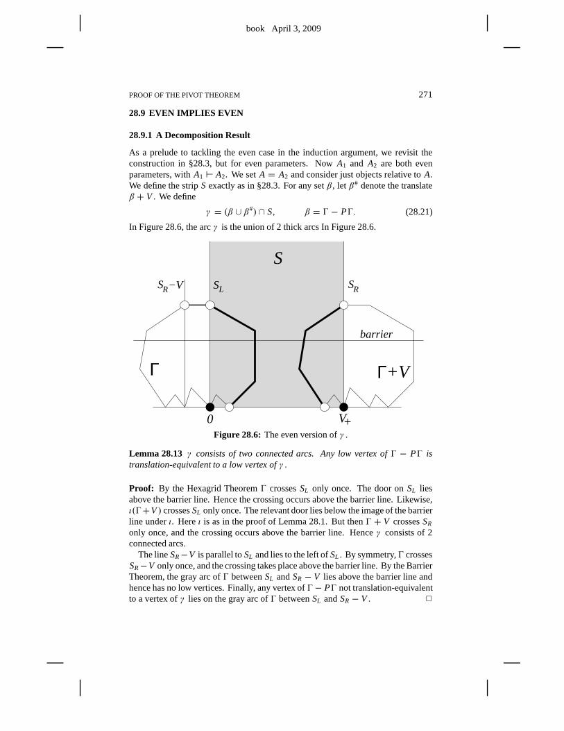
book April 3, 2009

PROOF OF THE PIVOT THEOREM 271

28.9 EVEN IMPLIES EVEN

28.9.1 A Decomposition Result

As a prelude to tackling the even case in the induction argument, we revisit theconstruction in §28.3, but for even parameters. NowA1 and A2 are both evenparameters, withA1 ⊢ A2. We setA = A2 and consider just objects relative toA.We define the stripS exactly as in §28.3. For any setβ, letβ# denote the translateβ + V . We define

γ = (β ∪ β#) ∩ S, β = Ŵ − PŴ. (28.21)

In Figure 28.6, the arcγ is the union of 2 thick arcs In Figure 28.6.

SR−V

barrier

S SL R

V+

S

0

Γ+VΓ

Figure 28.6: The even version ofγ .

Lemma 28.13 γ consists of two connected arcs. Any low vertex ofŴ − PŴ istranslation-equivalent to a low vertex ofγ .

Proof: By the Hexagrid TheoremŴ crossesSL only once. The door onSL liesabove the barrier line. Hence the crossing occurs above the barrier line. Likewise,ι(Ŵ+V) crossesSL only once. The relevant door lies below the image of the barrierline underι. Hereι is as in the proof of Lemma 28.1. But thenŴ + V crossesSR

only once, and the crossing occurs above the barrier line. Henceγ consists of 2connected arcs.

The lineSR−V is parallel toSL and lies to the left ofSL . By symmetry,Ŵ crossesSR−V only once, and the crossing takes place above the barrier line. By the BarrierTheorem, the gray arc ofŴ betweenSL andSR − V lies above the barrier line andhence has no low vertices. Finally, any vertex ofŴ− PŴ not translation-equivalentto a vertex ofγ lies on the gray arc ofŴ betweenSL andSR− V . 2

book April 3, 2009

272 CHAPTER 28

28.9.2 The Induction Argument

Let A1 ⊢ A2 be a pair of even rationals as in §27.4. This pair exists as long asA2 6= 1/q2. Referring to the terminology in Lemma 28.9, we prove the followingresult in this section.

Lemma 28.14 Let A1⇐ A2. Then P(A1) implies P(A2).

We have already taken care of the base case in the induction, the case whenA = 1/q. Lemmas 28.14 and 28.9 then imply the Pivot Theorem by induction. Theproof is essentially the same as in the odd case, once we see that the basic structuralresults hold. The result in §27.4 gives us the even/even version of the StructureLemma.

We consider the case whenA1 < A2. The other case is similar. We define spoilersjust as in the odd case. We just need to show that the arcγ2 defined in the previoussection has no spoilers. The same argument as in the odd case shows that a spoilermust lie betweenL(γ2) andR(γ2), the left and right endpoints, respectively.

Let 1 be the region of agreement betweenŴ1 andŴ2, as above. The formulasare exactly the same. Here is the even version of Lemma 28.11.

Lemma 28.151 contains all the spoilers.

Proof: The general argument in Lemma 28.11 works exactly the same here. It isonly at the end, when we consider the vertices(2,−2) and(3,−1), that we use thefact thatA2 is odd. Here we consider these special cases again. The argument for(−3,1) does not use the parity ofA2. We have to consider just(−2,2).

If A2 < 1/2, then(−2,2) is not a low vertex. We do not need to treat the ex-tremely trivial case whenA2 = 1/2. WhenA2 > 1/2, we haveA1 > 1/2 as well.The point is that no edge of the Farey graph crosses from(0,1/2) to (1/2,1). HenceA3 = A1 ⊕ A2 > 1/2 as well. But, by definition, the pivot points relative toA2

are the same as forA3. This is as in §27.4. Hence the same argument as in Lemma28.11 now rules out(2,−2). 2

Essentially the same argument as in the odd case now shows that γ2 contains nospoilers.

The Pivot Theorem now follows from induction. This completes the proof.

book April 3, 2009

Chapter Twenty-Nine

Proof of the Period Theorem

29.1 INHERITANCE OF PIVOT ARCS

Let A be some rational parameter. For each polygonal low component β of Ŵ(A),we define the pivot arcPβ to be the lower arc ofβ that joins the two low vertices thatare farthest apart. We saylower arcbecause all the components are closed polygons,and hence two arcs join the pivot points in all cases. WhenA is an even rational andβ = Ŵ, this definition coincides with the definition ofPŴ, by the Pivot Theorem.In general, we say that a pivot arc ofŴ is a pivot arc of some low component ofŴ.We call a pivot arc ofŴ minor if it is not a translate ofPŴ.

For each rational in(0,1), we are going to define anodd predecessorand anevenpredecessor. Aside from a few trivial cases, the predecessors exist and are rationalsin (0,1). The odd predecessor ofA will be denoted byA′, and we will use a singlearrow, as inA′← A. The even predecessor ofA will be denoted byA′′, and we willuse the notationA′′ ⇐ A. This notation should be compatible with our previoussimilar notation.

1. WhenA is odd,A′ is as in the inferior sequence.

2. WhenA is odd,A′′ is as in the Structure Lemma and Lemma 28.9.

3. WhenA is even,A′ is as in the Barrier Theorem.

4. WhenA is even,A′′ is as in Lemma 28.14.

It is worthwhile to mention another characterization of these numbers.

A even H⇒ A = A′ ⊕ A′′. (29.1)

A odd H⇒ A = A′ ⊕ A′′ ⊕ A′′. (29.2)

Just to cement the idea, we give an example.3

7← 7

17,

2

5⇐ 7

17,

3

7← 5

12,

2

5⇐ 5

12.

Here is our main technical tool for the Period Theorem.

Lemma 29.1 (Inheritance) Let A be any rational. Suppose that

A′← A, A′′ ⇐ A.

Then, every minor pivot arcβ of Ŵ is either a minor pivot arc ofŴ′ or a pivot arcof Ŵ′′. The set of low vertices ofβ is the same when considered either in A or in therelevant predecessor.

book April 3, 2009

274 CHAPTER 29

We first prove the odd case, and then we prove the even case. Theproof is almostthe same in both cases.

Proof in the Odd Case: Recall thatPŴ ∪ γ is one period ofŴ. There are 2kinds of minor components ofŴ.

1. Pivot arcs that lie underneathPŴ.

2. Pivot arcs that lie underneathγ .

We can push harder on Lemma 27.2. SincePŴ lies in the set1, from Lemma27.4, so does every low component ofŴ underneathPŴ. To see this, recall that ourproof involved showing thatPŴ ⊂ 1. But if a point ofPŴ lies in1, then so doesthe entire line segment connecting this point to the baseline. Hence all componentsof Ŵ beneathPŴ also belong to1. Hence the low components ofŴ lying underneathPŴ coincide with the low components ofŴ′ lying underneathPŴ′. This takes careof the first case.

Consider the second case. Our proof of Lemma 28.9 shows that every minorcomponent ofŴ′′ lying inside1(A′′, A) is contained inŴ. We showed the sameresult for every major component except the ones we labelledC1 andCk−1. Notethat the pivot arcs are subject to the Barrier Theorem. That is, the two crossings fromthe Barrier theorem occur on the upper arcs rather than on thepivot arcs. Hence thepivot arcs behave exactly like the minor components. Hence the pivot arcs ofC1 andCk−1 are copied byŴ even though the upper arcs might not be. By Lemma 28.11,every low vertex ofŴ lying underneathγ lies on the pivot arcs of the componentswe have just considered. This takes care of the second case.

There is only one detail we need to take care of. A vertex of thekind we areconsidering is low relative toA′ or A′′ if and only if it is low with respect toA.This follows from the basic property of1. See the geometric proof of Lemma 27.4.Thus every low component ofŴ of the kind we have considered is also low relativeto Ŵ′ or Ŵ′′, whichever is relevant. Likewise, the converse holds. 2

Proof in the Even Case:The minor pivot arcs ofŴ are of two kinds, those that lieunderneathPŴ and those that do not. By the same argument as in the odd case, thepivot arcs of the first kind are all minor pivot arcs ofŴ(A∗), whereA∗ is such thatA ⊲⊳ A∗. But thenA∗ = A⊕ A′′. HenceA′′ ⇐ A∗. At the same time,A′ = A⊖ A′′.HenceA′ ← A∗. Applying the odd case of the Inheritance Lemma to the triple(A∗, A′, A′′), we see that every pivot arc ofŴ beneathPŴ is a pivot arc of eitherŴ′ or Ŵ′′. This takes care of the first case. The second case is just likethe odd case.2

Remark: Implicit in the definitions ofpredecessoris the idea of atreeof rationals.Each rational has 2 ancestors who are simpler in some sense. The InheritanceLemma esplains how the traits – here meaning the pivot arcs – of the arithmeticgraph for a complicated parameter are inherited from the ancestors.

book April 3, 2009

PROOF OF THE PERIOD THEOREM 275

29.2 FREEZING NUMBERS

Every rational parameter has an odd and an even predecessor.Starting with (say)an odd rationalA, we can iterate the construction and produce a tree of simplerrationals. IfB lies on this tree, we writeB ≺ A. Here is an immediate corollary ofthe Inheritance Lemma.

Corollary 29.2 Every minor pivot arc ofŴ(A) is a pivot arc of Ŵ(B) for someeven B such that B≺ A.

Let A be an odd rational. Letβ be a minor component ofŴ(A). We defineF(β, A) to be the smallest denominator of a rationalB ≺ A such thatPβ is apivot arc of Ŵ(B). We call F(β, A) the freezing numberof β. Our terminologyhas the following meaning. As we move through the tree of rationals, from simpleto complicated, various features of the corresponding graphs change, but at variousstates certain features freeze. The freezing number of a component marks the pointwhen the component becomes a permanent feature.

Lemma 29.3 The9-period of a minor componentβ is at most

20s2, s= F(β, A).

Proof: This is an immediate consequence of the Hexagrid Theorem applied to therational B = r/s such thatβ is a component ofŴ(B). The Hexagrid Theoremconfinesβ to a parallelogram of area less than 20s2. 2

Let x ∈ I correspond to a point not onC(An). We let

F(x,n) = F(βx, An),

whereβx is the component ofŴn corresponding tox. We say that agrowing sequenceis a sequence{xn} such that

F(xn,n)→∞. (29.3)

Recall thatCA is the Cantor set from the Comet Theorem.

Lemma 29.4 Suppose every growing sequence accumulates on CA. Then the Pe-riod Theorem is true for A.

Proof: If the Period Theorem is false, then we can find a sequence of points {xn}in Gn such that the distance fromxn to Cn is uniformly bounded away from 0 andyet the period ofx tends to∞. But then Lemma 29.3 shows that{xn} is a growingsequence. By construction,{xn} does not have a limit point onCA. 2

book April 3, 2009

276 CHAPTER 29

29.3 THE END OF THE PROOF

Let {An} be the odd sequence of rationals above. For eachn, we can form the treeof predecessors, as above. Suppose we choose some proper functionm(n) such thatBm ≺ An is some even rational in the tree forAn.

Lemma 29.5 limn→∞ Bm = A.

Proof: We consider the situation in the hyperbolic plane relative to the Farey trian-gulation. See §17.1 for definitions. We consider the portionG of the Farey graphconsisting of edges having both endpoints in [0,1]. We direct each edge inG sothat it points from the endpoint of smaller denominator to the endpoint of larger de-nominator. The two endpoints never have the same denominator, so the definitionmakes sense. Say that thedisplacementof a directed path inG is the maximumdistance between a vertex of the path and its initial vertex.

Given anǫ > 0, there are only finitely many vertices inG that are the initialpoints of directed paths having displacement greater thanǫ. This follows from thenesting properties of the half-disks bounded by the edges inG, and from the factthat there are only finitely many edges inG having a diameter greater thanǫ.

Given the nature of the tree of predecessors, there is a directed path inG connect-ing Bm to An. The displacement of this path tends to 0 asn → ∞ because{Bm}is an infinite list of rationals with only finitely many repeaters. Also, the distancefrom An to A tends to 0. Hence the distance fromBm to A tends to 0 by the triangleinequality. 2

Now we bring in an idea from the Rigidity Lemma. See §2.7. Let{Bm} beany sequence of even rationals converging to the irrationalparameterA. Then theRigidity Lemma implies that the limits

limm→∞

Ŵ(Am), limm→∞

Ŵ(Bm) (29.4)

agree. In other words, longer and longer portions ofŴ(Am) look like longer andlonger pictures ofŴ(Bm). This is all we need to know from the Rigidity Lemma.

Now let Mm,A be the fundamental map associated toAm. This map is defined inEquation 2.10. In the proof of Theorem 1.6, we showed that

CA = limm→∞

Mm,A(6(Am)). (29.5)

The limit takes place in the Hausdorff topology. Here6(Am) is the set of lowvertices onŴm. Given Equation 29.4, we get the analogous result

CA = limn→∞

Mm,B(6(Bm)). (29.6)

Let us generalize this result. For eachm, suppose there is somen ≥ m. We alsohave

CA = limm→∞

Mn,A(6(Bm)). (29.7)

The reason is that the mapsMm,A andMn,B converge to each other on any compactsubset ofR2, and compact pieces of the limit in Equation 29.4 determine increasinglydense subsets ofCA.

book April 3, 2009

PROOF OF THE PERIOD THEOREM 277

Lemma 29.6 Suppose that6n ⊂ Ŵ(An) is a translate of6m consisting entirely oflow vertices. Then

CA = limm→∞

Mn,A(6n).

Proof: We have some vectorUm such that

6n = 6(Am)+Um. (29.8)

SinceMn,A is affine, we have

Mn,A(6n) = Mn,A6(Am)+ λm. (29.9)

Now we get to the moment of truth. Since6(Bm) consists entirely of low vertices,we have

MA,n(x) ∈ [0,2]

for all x ∈ 6(Bm). Since6n consists entirely of low vertices, we haveMA,n(x)+λn ∈ [0,2] as well. Puttingt = MA,n(x), we have

t, t + λm ∈ [0,2] . (29.10)

This last equation puts constraints onλm.By the case whenn = 0 of Equation 21.7, the setCA contains both 0 and 2.

Therefore, oncem is large, we can choosex ∈ 6(Bm) such thatt = MA,n(x) isvery close to 0. But this forces

lim inf λm ≥ 0.

At the same time, we can choosex such thatMA,m(x) is very close to 2. This showsthat

lim supλm ≤ 0.

In short,λm→ 0. 2

We just have to tie the discussion above together with the notion of a growingsequence. Suppose that{xn} is a growing sequence. Letβn denote the componentof Ŵn corresponding toxn. There is a proper functionm = mn such that the pivotarc Pβn is a translate of the major pivot arcPŴ(Bm). Here{Bm} is a sequenceof even rationals that satisfies the hypotheses of Lemma 29.5. Hence{Bm} → A.Hence the application of the Rigidity Lemma above applies.

Every low vertex onPβn is a translate of a low vertex onPŴ(Bm). By theInheritance Lemma, every low vertex onPβn relative toBm is also low with respectto An. Thus we have exactly the situation described in Lemma 29.6.

Let 6n denote the set of low vertices ofPβn. Then6n is a translate of the set6(Bm) of low vertices onPŴ(Bm), as in the lemma above. Since

xn ∈ MA,n(6n), (29.11)

we see that the Hausdorff distance from{x} to CA tends to 0 asn (andm) tend to∞.

This completes the proof of the Period Theorem.

book April 3, 2009

278 CHAPTER 29

29.4 A USEFUL RESULT

While we are in the neighborhood, we establish a technical result related by Lemma29.5 that we will use in the next chapter.

Let {Bn} be any sequence of rationals that converges toA. Recall from §29.2 thatany rational parameterB has a treeT(B) of predecessors. We can considerT(Bn)for each parameterBn in the sequence.

Lemma 29.7 Let N be any integer. Then there are only finitely many rationals inthe union

∞⋃

n=1

T(Bn)

having complexity less than N.

Proof: We will argue as in the proof of Lemma 29.5. SupposeC = r/s is a rationalin the treeT(Bn) such thatr is small ands andn are large. Then the directed Fareypath connectingC to Bn has tiny displacement and|Bn−A| is small. Hence|C−A|is small. Also,C is near 0. HenceA is near 0. This is a contradiction onces andn are large enough. Hence there is some functionf , depending on the sequence,such thats< f (r ). Hence the union contains only finitely many rationals having anumerator less thanN. Our result follows from this fact. 2

book April 3, 2009

Chapter Thirty

Hovering Components

30.1 THE MAIN RESULT

Let A ∈ (0,1) be a rational parameter. We say thatv ∈ Z2 is D-low if the baselineof Ŵ(A) separatesv from v − (0, D). HereD ∈ Z. We have the usual conventionthat the baseline is the line of slope−A through the point(0,−ǫ), whereǫ is aninfinitesimally small positive number. Thus(0,0) is 1-low. Previously, we wereinterested in 1-low vertices, which we calledlow.

Let β be a component ofŴ(A). We callβ a hovering componentif it has no1-low vertices. More specifically, we callβ a D-hovering componentof Ŵ(A) if βhas no 1-low vertices and ifβ contains aD-low vertex. The goal of this chapter isto prove the following result.

Lemma 30.1 (Hovering) Let{An} be the superior sequence approximating A. FixD. Then there is a constant D′ with the following property. If n is sufficiently large,thenŴn has no D-hovering components having diameter greater than D′. Here D′

is independent of n.

Now we start the proof of the Hovering Lemma. For each rational B, we forma tree of depth 2 by considering the 2 predecessors ofB and their 2 predecessors.We define the complexity ofB to be the minimum value of all the numerators ofthe rationals involved in this list of 7 rationals. In the case when some of thesepredecessors are not defined, we set the complexity to 0.

Lemma 30.2 Fix D. Let A2 be any rational with predecessors A0 and A1. Letβ be a D-hovering component ofŴ(A). Assuming that A2 has sufficiently highcomplexity,β is either a translate of a D-hovering component ofŴ0 or a translateof a D-hovering component ofŴ1.

Proof of the Hovering Lemma: Applying the Hovering Lemma recursively, wesee thatβ is the translate of aD-hovering component ofŴ(Bn), whereBn belongsto the tree of predecessors ofAn and has uniformly bounded complexity. But then,by Lemma 29.7, the sequence{Bn} has only finitely many different terms. Henceβ is the translate of one of finitely many different polygons. 2

The rest of the chapter is devoted to proving Lemma 30.2.

book April 3, 2009

280 CHAPTER 30

30.2 TRAPS

Let A be a rational parameter. As usual,Ŵ(A) is invariant under translation byZ [V ]. HereV = (q,−p). We say that amajor componentof Ŵ(A) is one that istranslation-equivalent toŴ(A).

Let X ⊂ R2 be a solid parallelogram. We callX a cap if the the following hold.

• The only components ofŴ that cross∂X are major components.

• If γ is a major component that crosses∂X, thenγ ∩ X is a finite union ofconnected arcs, each of which contains a 1-low vertex.

Remark: The second item requires a bit of interpretation. When we take γ ∩ X,we might cut an edge off right in the middle. We always add the full edge to thisintersection. Thusγ ∩ X could stick out a tiny bit fromX, and the low vertex inquestion could be just outside ofX. This small annoyance causes no trouble.

Let A0 andA1 be the predecessors ofA2. We take

A0← A2, A1⇐ A2 (30.1)

so thatA0 is odd andA1 is even. Forj = 0,1, let1 j denote the region of agreementbetweenŴ j andŴ2, as in the Diophantine lemma. Between the Diophantine Lemmaand Lemma 27.4, we cover all cases.

We say that a pair(X0, X1) of parallelograms is aD-trap for A2 if the followingaxioms hold.

1. X j ⊂ 1 j .

2. X j is a cap relative toA j .

3. Any vertex inX j is 1-low with respect toA j iff this vertex is 1-low withrespect toA2.

4. Any D-low vertex relative toA2 is translation-equivalent, modZ [V2], to apoint in X0 ∪ X1.

Lemma 30.3 Fix D. If A2 has sufficiently high complexity, then there is a D-trapfor A2.

Before we prove this result, we use it to prove Lemma 30.2.

Proof of Lemma 30.2: Let β2 be a D-hovering component ofŴ2. Let v ∈ β2

be aD-low vertex. By axiom 4, we can translate so thatv lies in eitherX0 or X1.Suppose without loss of generality thatv ∈ X0. Since translation by multiples ofV2 preserves the baseline forŴ2, we see thatv is D-low with respect toA2.

Axiom 3 says that a vertex inX0 is 1-low with respect toA0 iff it is 1-low withrespect toA2. But clearly this implies that a vertex inX0 is k-low with respect toA0 iff it is k-low with respect toA2. So, when we use the termk-low, it appliesequally well relative toA0 andA2.

book April 3, 2009

HOVERING COMPONENTS 281

Letβ0 be the component ofŴ0 that containsv. Suppose first thatβ0 crosses∂X0.Thenβ0 is a major component. SinceX0 is a cap relative toA0, the component ofβ0 ∩ R that containsv also contains a low vertex. So, tracingβ0 from v, we take apath

γ ⊂ X0 ⊂ 10 (30.2)

whose endpoint is a low vertex inX0. The second containment is axiom 1 above.But thenγ ⊂ Ŵ2. Sinceβ2 andγ agree atv, they must agree (by the EmbeddingTheorem) on the whole path. But thenβ2 contains a 1-low vertex. This is acontradiction.

Now we know thatβ0 does not cross∂X0. But thenβ0 ⊂ 10. Henceβ0 is acomponent ofŴ2. Sinceβ0 andβ2 agree atv, we haveβ0 = β2. By construction,β0 = β2 contains aD-low vertex and no 1-low vertex. Thereforeβ0 = β2 is aD-hovering component ofŴ0. 2

The rest of the chapter is devoted to the proof of Lemma 30.3. We have 4 casesto consider, and we will consider these cases in turn.

1. A2 is odd andA1 < A2.

2. A2 is odd andA1 > A2.

3. A2 is even andA1 < A2.

4. A2 is even andA1 > A2.

Now we reconcile the notation here with the notation in §4.1.In case 1, we have

A0 = (A2)+ − (A2)−, A1 = (A2)−. (30.3)

In case 2, we have

A0 = (A2)− − (A2)+, A1 = (A2)+. (30.4)

In case 3 we have

A0 = (A2)+, A1 = (A2)−. (30.5)

In case 4 we have

A0 = (A2)−, A1 = (A2)+. (30.6)

We will concentrate on cases 1 and 3. case 2 is essentially thesame as case 1, andcase 4 is essentially the same as case 3. When it comes time to deal with cases 2 and4, we will briefly indicate the modifications needed and then show some illustrationsfrom Billiard King.

The parallelograms come from two sources:

• The Decomposition Theorem in Chapter 19.

• The minor box in §28.6.1.

We will explain this precisely below. Mainly, we are repackaging constructions wehave already made. When it comes to verifying the axioms, we have essentiallyalready done all the hard work. The proof is mainly a matter oflocating the relevantresults in previous chapters.

book April 3, 2009

282 CHAPTER 30

30.3 CASES 1 AND 2

Case 1:We state the following definitions.

• X0 = R1(A2), the small parallelogram from the Decomposition Theorem forthe parameterA2. HereX0 lies to the left of the origin.

• X1 is the minor box, defined relative to the parameterA1, in §28.6.1. HereX1 lies to the right of the origin.

Remark: The top/bottom ofX0 has a slightly different slope from the top/bottomof X1, but the difference is tiny whenA2 has high complexity.X0 andX1 may ormay not have about the same height. The figures below show one case where thishappens and one case where it does not.

Lemma 30.4 (X0, X1) satisfies axiom 1.

Proof: In §28.6.1, we showed thatX1 ⊂ 11. We just have to considerX0. Theargument forX0 is really the same as that for the Decomposition Theorem. However,since we considered a different case there, we will work out the details here.

We will apply the Diophantine Lemma. Since we do not care about small cases,we write I1 ≈ I2 to denote the relation where two intervals are with 2 units ofeachother. We work with the linear functionalsG2 andH2 associated to the parameterA2. Let u andw denote the top left and right vertices ofX0, respectively. Theinterval in the Diophantine Lemma is

I2 ≈[−(q2)− − q0,q0

]. (30.7)

The lower bound comes from case 2 of Lemma 17.8.Hence it suffices to show that

G2(u)≫ −(q2)− − q0, H2(w)≪ q0. (30.8)

The symbol(≫) indicates an inequality in which the difference between thetwosides tends to∞ with the complexity ofA2.

We have the estimates

u ≈ −(V2)− + λW2, w ≈ λW2, λ = q∗2q2≤ q0

q2. (30.9)

Here A∗2 = p∗2/q∗2 is the superior predecessor ofA2. The approximation becomes

arbitrarily good as the complexity ofA2 tends to∞. Hence the approximation isgood to within 1 unit onceA2 has sufficiently high complexity.

We compute

G2(u) ≈ −(q2)− − λq2

2

p2+ q2≫ −(q2)− − λ(q2) ≥ −(q2)− − q0.

This takes care of the vertexu. Now we compute

H2(w) ≈ λq2

2

p2+ q2≪ λq2 = q0.

This takes care of the vertexw. 2

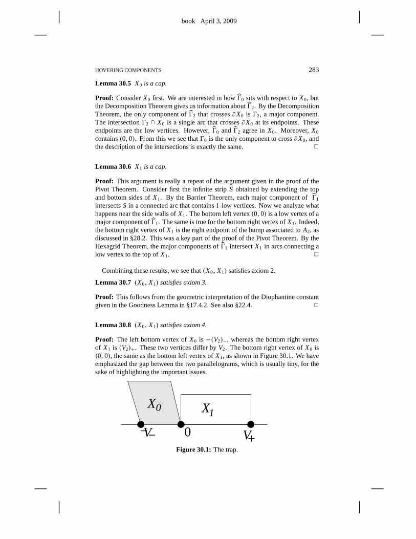
book April 3, 2009

HOVERING COMPONENTS 283

Lemma 30.5 X0 is a cap.

Proof: ConsiderX0 first. We are interested in howŴ0 sits with respect toX0, butthe Decomposition Theorem gives us information aboutŴ2. By the DecompositionTheorem, the only component ofŴ2 that crosses∂X0 is Ŵ2, a major component.The intersectionŴ2 ∩ X0 is a single arc that crosses∂X0 at its endpoints. Theseendpoints are the low vertices. However,Ŵ0 andŴ2 agree inX0. Moreover,X0

contains(0,0). From this we see thatŴ0 is the only component to cross∂X0, andthe description of the intersections is exactly the same. 2

Lemma 30.6 X1 is a cap.

Proof: This argument is really a repeat of the argument given in the proof of thePivot Theorem. Consider first the infinite stripS obtained by extending the topand bottom sides ofX1. By the Barrier Theorem, each major component ofŴ1

intersectsS in a connected arc that contains 1-low vertices. Now we analyze whathappens near the side walls ofX1. The bottom left vertex(0,0) is a low vertex of amajor component ofŴ1. The same is true for the bottom right vertex ofX1. Indeed,the bottom right vertex ofX1 is the right endpoint of the bump associated toA2, asdiscussed in §28.2. This was a key part of the proof of the Pivot Theorem. By theHexagrid Theorem, the major components ofŴ1 intersectX1 in arcs connecting alow vertex to the top ofX1. 2

Combining these results, we see that(X0, X1) satisfies axiom 2.

Lemma 30.7 (X0, X1) satisfies axiom 3.

Proof: This follows from the geometric interpretation of the Diophantine constantgiven in the Goodness Lemma in §17.4.2. See also §22.4. 2

Lemma 30.8 (X0, X1) satisfies axiom 4.

Proof: The left bottom vertex ofX0 is −(V2)−, whereas the bottom right vertexof X1 is (V2)+. These two vertices differ byV2. The bottom right vertex ofX0 is(0,0), the same as the bottom left vertex ofX1, as shown in Figure 30.1. We haveemphasized the gap between the two parallelograms, which isusually tiny, for thesake of highlighting the important issues.

X0 X1

V+0V−−Figure 30.1: The trap.

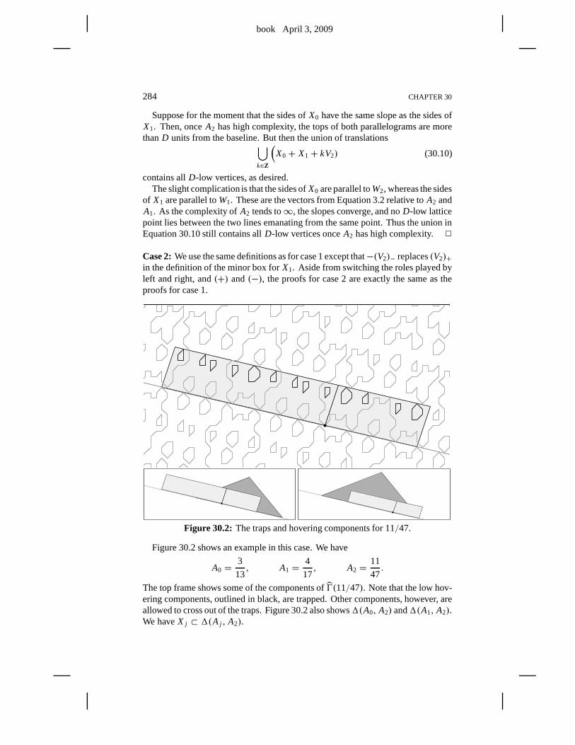
book April 3, 2009

284 CHAPTER 30

Suppose for the moment that the sides ofX0 have the same slope as the sides ofX1. Then, onceA2 has high complexity, the tops of both parallelograms are morethanD units from the baseline. But then the union of translations⋃

k∈Z

(X0 + X1+ kV2) (30.10)

contains allD-low vertices, as desired.The slight complication is that the sides ofX0 are parallel toW2, whereas the sides

of X1 are parallel toW1. These are the vectors from Equation 3.2 relative toA2 andA1. As the complexity ofA2 tends to∞, the slopes converge, and noD-low latticepoint lies between the two lines emanating from the same point. Thus the union inEquation 30.10 still contains allD-low vertices onceA2 has high complexity. 2

Case 2:We use the same definitions as for case 1 except that−(V2)− replaces(V2)+in the definition of the minor box forX1. Aside from switching the roles played byleft and right, and(+) and(−), the proofs for case 2 are exactly the same as theproofs for case 1.

Figure 30.2: The traps and hovering components for 11/47.

Figure 30.2 shows an example in this case. We have

A0 =3

13, A1 =

4

17, A2 =

11

47.

The top frame shows some of the components ofŴ(11/47). Note that the low hov-ering components, outlined in black, are trapped. Other components, however, areallowed to cross out of the traps. Figure 30.2 also shows1(A0, A2) and1(A1, A2).We haveX j ⊂ 1(A j , A2).

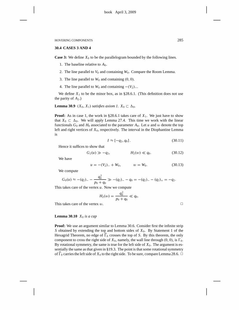
book April 3, 2009

HOVERING COMPONENTS 285

30.4 CASES 3 AND 4

Case 3:We defineX0 to be the parallelogram bounded by the following lines.

1. The baseline relative toA0.

2. The line parallel toV0 and containingW0. Compare the Room Lemma.

3. The line parallel toW0 and containing(0,0).

4. The line parallel toW0 and containing−(V2)−.

We defineX1 to be the minor box, as in §28.6.1. (This definition does not usethe parity ofA2.)

Lemma 30.9 (X0, X1) satisfies axiom 1. X0 ⊂ 10.

Proof: As in case 1, the work in §28.6.1 takes care ofX1. We just have to showthat X0 ⊂ 10. We will apply Lemma 27.4. This time we work with the linearfunctionalsG0 andH0 associated to the parameterA0. Let u andw denote the topleft and right vertices ofX0, respectively. The interval in the Diophantine Lemmais

I ≈ [−q2,q0] . (30.11)

Hence it suffices to show that

G2(u)≫ −q2, H2(w)≪ q0. (30.12)

We have

u = −(V2)− +W0, w = W0. (30.13)

We compute

G0(u) ≈ −(q2)− −q2

0

p0+ q0≫ −(q2)− − q0 = −(q2)− − (q2)+ = −q2.

This takes care of the vertexu. Now we compute

H2(w) =q2

0

p0+ q0≪ q0.

This takes care of the vertexw. 2

Lemma 30.10 X0 is a cap

Proof: We use an argument similar to Lemma 30.6. Consider first the infinite stripS obtained by extending the top and bottom sides ofX0. By Statement 1 of theHexagrid Theorem, no edge ofŴ0 crosses the top ofS. By this theorem, the onlycomponent to cross the right side ofX0, namely, the wall line through(0,0), isŴ0.By rotational symmetry, the same is true for the left side ofX0. The argument is es-sentially the same as that given in §19.3. The point is that some rotational symmetryof Ŵ0 carries the left side ofX0 to the right side. To be sure, compare Lemma 28.6.2

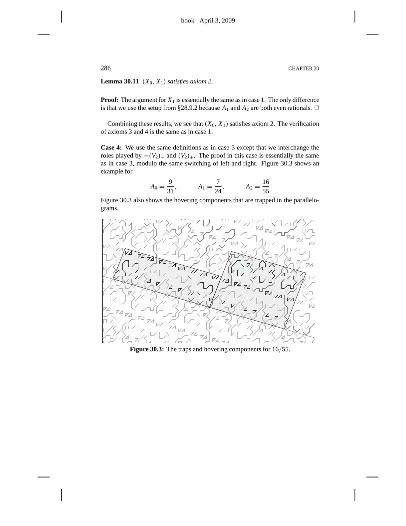
book April 3, 2009

286 CHAPTER 30

Lemma 30.11 (X0, X1) satisfies axiom 2.

Proof: The argument forX1 is essentially the same as in case 1. The only differenceis that we use the setup from §28.9.2 becauseA1 andA2 are both even rationals.2

Combining these results, we see that(X0, X1) satisfies axiom 2. The verificationof axioms 3 and 4 is the same as in case 1.

Case 4: We use the same definitions as in case 3 except that we interchange theroles played by−(V2)− and(V2)+. The proof in this case is essentially the sameas in case 3, modulo the same switching of left and right. Figure 30.3 shows anexample for

A0 =9

31, A1 =

7

24, A2 =

16

55Figure 30.3 also shows the hovering components that are trapped in the parallelo-grams.

Figure 30.3: The traps and hovering components for 16/55.

book April 3, 2009

Chapter Thirty-One

Proof of the Low Vertex Theorem

31.1 OVERVIEW

The Low Vertex Theorem in Chapter 23 is a consequence of the following result.

Lemma 31.1 (Descent)Let A∈ (0,1) be irrational. Let{Bn} be any sequence ofrationals in(0,1) that converges to A. Letβ be a low component ofŴ(Bn). Thereis some constant D′ such that every D-low vertex ofβ can be connected to a lowvertex ofβ in less than D′ steps. Here D′ depends on D and on A but not on n.

Proof of the Low Vertex Theorem: Let N0 and{vn} be as in the Low VertexTheorem. Letβn be the component ofŴn that containsvn. Here is the imputfrom the Hovering Lemma. If the constantN1 is chosen sufficiently large, then theinequality

diam(βn) > N1

implies thatβn is a low component. We chooseN1 in this way. Applying the DescentLemma to the sequence{An}, the componentβ = βn, and the constantD = N0,we immediately obtain the conclusion of Low Vertex Theorem with N2 = D′. 2

The rest of the chapter is devoted to proving the Descent Lemma. Our proof ofthe Descent Lemma is somewhat complicated by the fact that wecannot quite provea very useful conjecture. Experimentally, we observe the following improvementfor the Inheritance Lemma.

Conjecture 31.2 Let A2 be any rational having the predecessors A0 ← A2 andA1 ⇐ A2. Then every minor low component ofŴ2 is either the translate of a lowcomponent ofŴ0 or the translate of a low component ofŴ1.

Referring to the proof of the Pivot Theorem, the end major components give ustrouble. See the discussion at the end of §28.2.

As we will explain below, Conjecture 31.2 would be very useful in proving theDescent Lemma. See the remark in §31.3. Our strategy for proving the DescentLemma is to prove a somewhat weaker version of Conjecture 31.2 that captures allthe necessary features. We state this weaker result, Lemma 31.3, in the next section.One strategy for understanding this chapter is to first assume the truth of Conjecture31.2. Then, once the overall logic of the argument makes sense, one can learn thecomplications that arise from the fact that we must use Lemma31.3 in place ofConjecture 31.2.

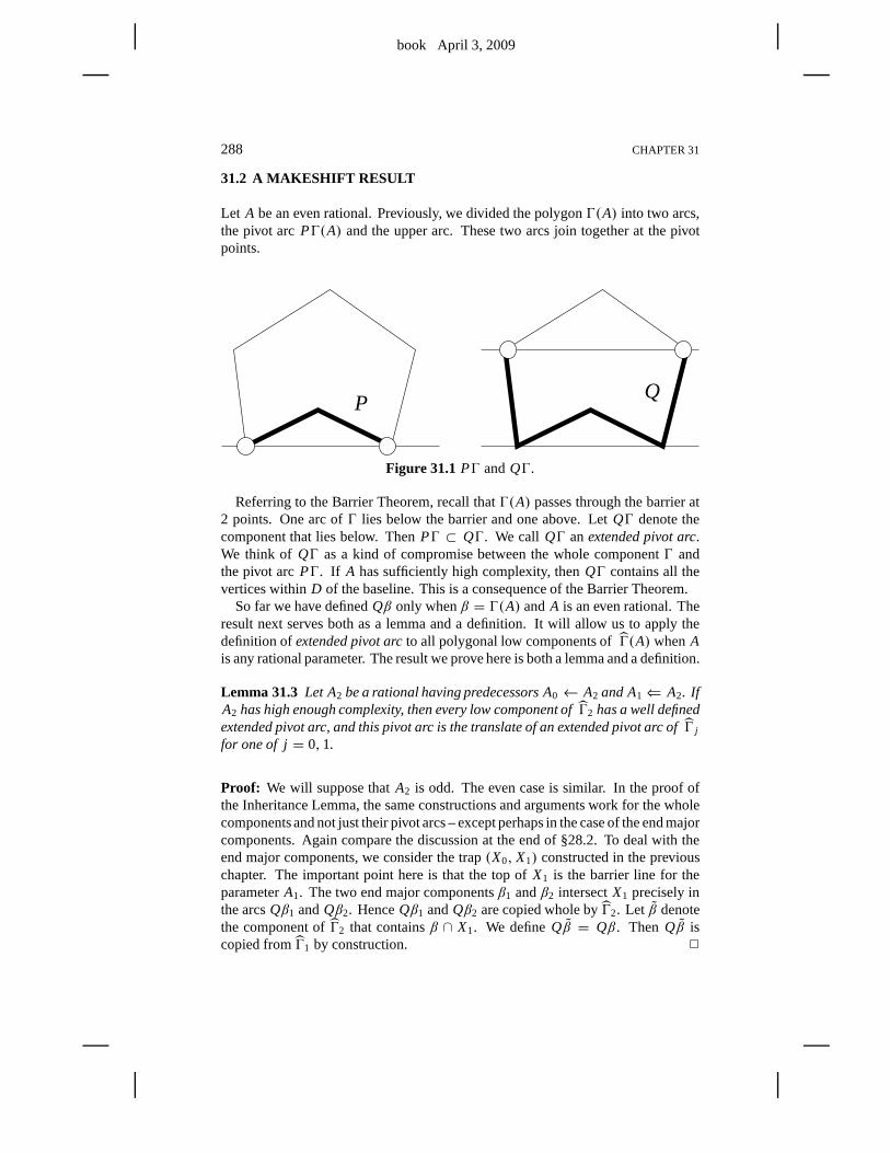
book April 3, 2009

288 CHAPTER 31

31.2 A MAKESHIFT RESULT

Let A be an even rational. Previously, we divided the polygonŴ(A) into two arcs,the pivot arcPŴ(A) and the upper arc. These two arcs join together at the pivotpoints.

QP

Figure 31.1PŴ andQŴ.

Referring to the Barrier Theorem, recall thatŴ(A) passes through the barrier at2 points. One arc ofŴ lies below the barrier and one above. LetQŴ denote thecomponent that lies below. ThenPŴ ⊂ QŴ. We call QŴ anextended pivot arc.We think of QŴ as a kind of compromise between the whole componentŴ andthe pivot arcPŴ. If A has sufficiently high complexity, thenQŴ contains all thevertices withinD of the baseline. This is a consequence of the Barrier Theorem.

So far we have definedQβ only whenβ = Ŵ(A) andA is an even rational. Theresult next serves both as a lemma and a definition. It will allow us to apply thedefinition ofextended pivot arcto all polygonal low components ofŴ(A) whenAis any rational parameter. The result we prove here is both a lemma and a definition.

Lemma 31.3 Let A2 be a rational having predecessors A0← A2 and A1⇐ A2. IfA2 has high enough complexity, then every low component ofŴ2 has a well definedextended pivot arc, and this pivot arc is the translate of an extended pivot arc ofŴ j

for one of j= 0,1.

Proof: We will suppose thatA2 is odd. The even case is similar. In the proof ofthe Inheritance Lemma, the same constructions and arguments work for the wholecomponents and not just their pivot arcs – except perhaps in the case of the end majorcomponents. Again compare the discussion at the end of §28.2. To deal with theend major components, we consider the trap(X0, X1) constructed in the previouschapter. The important point here is that the top ofX1 is the barrier line for theparameterA1. The two end major componentsβ1 andβ2 intersectX1 precisely inthe arcsQβ1 andQβ2. HenceQβ1 andQβ2 are copied whole byŴ2. Let β denotethe component ofŴ2 that containsβ ∩ X1. We defineQβ = Qβ. Then Qβ iscopied fromŴ1 by construction. 2

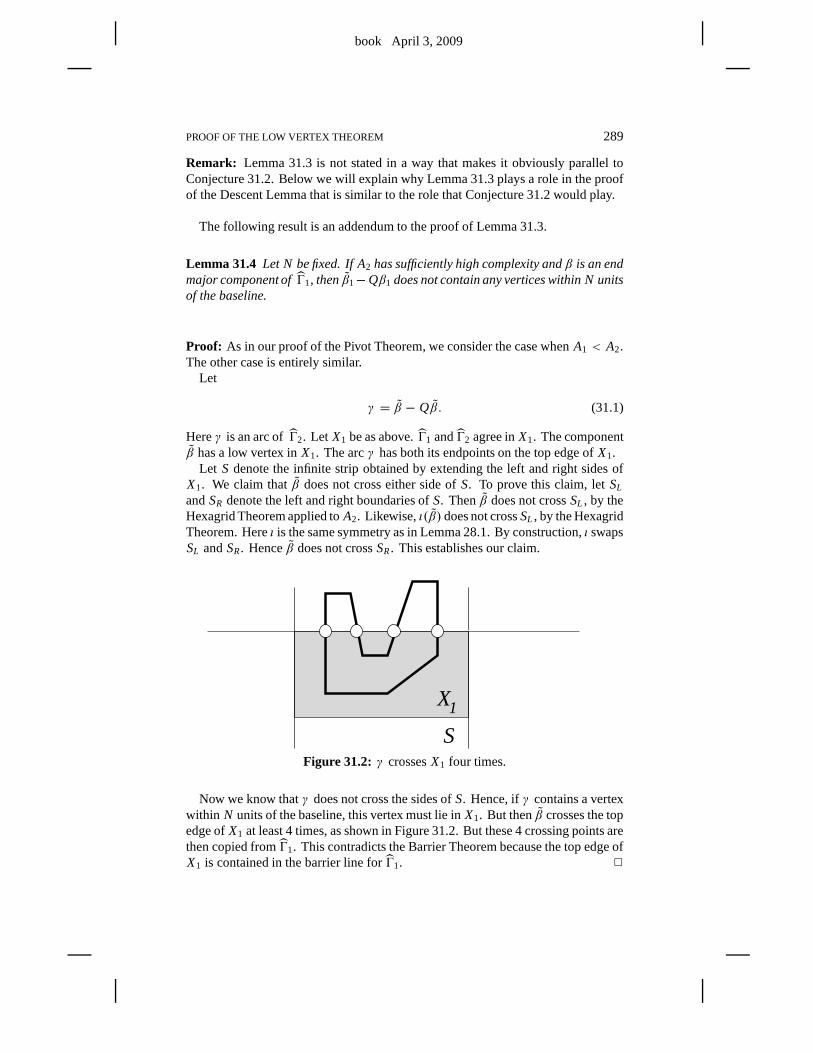
book April 3, 2009

PROOF OF THE LOW VERTEX THEOREM 289

Remark: Lemma 31.3 is not stated in a way that makes it obviously parallel toConjecture 31.2. Below we will explain why Lemma 31.3 plays arole in the proofof the Descent Lemma that is similar to the role that Conjecture 31.2 would play.

The following result is an addendum to the proof of Lemma 31.3.

Lemma 31.4 Let N be fixed. If A2 has sufficiently high complexity andβ is an endmajor component ofŴ1, thenβ1−Qβ1 does not contain any vertices within N unitsof the baseline.

Proof: As in our proof of the Pivot Theorem, we consider the case whenA1 < A2.The other case is entirely similar.

Let

γ = β − Qβ. (31.1)

Hereγ is an arc ofŴ2. Let X1 be as above.Ŵ1 andŴ2 agree inX1. The componentβ has a low vertex inX1. The arcγ has both its endpoints on the top edge ofX1.

Let S denote the infinite strip obtained by extending the left and right sides ofX1. We claim thatβ does not cross either side ofS. To prove this claim, letSL

andSR denote the left and right boundaries ofS. Thenβ does not crossSL , by theHexagrid Theorem applied toA2. Likewise,ι(β) does not crossSL , by the HexagridTheorem. Hereι is the same symmetry as in Lemma 28.1. By construction,ι swapsSL andSR. Henceβ does not crossSR. This establishes our claim.

S

X1

Figure 31.2: γ crossesX1 four times.

Now we know thatγ does not cross the sides ofS. Hence, ifγ contains a vertexwithin N units of the baseline, this vertex must lie inX1. But thenβ crosses the topedge ofX1 at least 4 times, as shown in Figure 31.2. But these 4 crossingpoints arethen copied fromŴ1. This contradicts the Barrier Theorem because the top edge ofX1 is contained in the barrier line forŴ1. 2

book April 3, 2009

290 CHAPTER 31

31.3 ELIMINATING MINOR ARCS

Suppose that the Descent Lemma is false. This means that we can find a sequence{vn} of vertices, all uniformly close to the baseline, such that then-neighborhoodof βn contains no low vertices. Hereβn is the component ofŴn that containsvn. Inthis section we reduce the several possible situations to one situation that is easierto manage.

Passing to a subsequence and using translation symmetry, wecan arrange one oftwo cases.

• βn is a minor component ofŴn for all n.

• βn = Ŵn for all n.

Here we will show that a counterexampleof the first kind forces a counterexampleof the second kind.

Remark: Assuming Conjecture 31.2, we can argue as follows. By Conjecture31.2, the componentβn is the translate ofŴ(B′n) for someB′n ∈ T(Bn). Sinceβn

is a low component, and yet then-ball aboutvn contains no low vertices, we seethat the diameter ofβn tends to∞ with n. But then the complexity ofB′n tends to∞ with n. Hence, by Lemma 29.5,B′n → A. Thus a counterexample to Lemma31.1 involving minor components leads to a counterexample involving major com-ponents. The new counterexample uses the parameters{B′n}.

Since we cannot prove Conjecture 31.2, we have to make do withLemma 31.3.We need one last result before we can make Lemma 31.3 work for us.

Lemma 31.5 Letβn be a low component ofŴ(Bn). Suppose that the diameter ofβn tends to∞. Then the distance from any point onβn − Qβn to the baseline ofŴ(Bn) tends to∞ as well.

Proof: This is a consequence of Lemma 31.4. Eachβn is a translate of a componentof the form

C, C = Ŵ(B′n). (31.2)

HereB′n is on the tree of predecessors ofBn. Since the diameter ofC tends to∞with n, we see than the complexity ofB′n tends to∞ with n by Lemma 29.7. Hencethe distance fromC − QC to the relevant baseline tends to∞ with n. 2

Now let us revisit the argumentabove. By Corollary 31.5, thepointsvn lie onQβn

oncen is sufficiently large. Indeed, by Lemma 31.5, the distance fromvn to a pointonβn−Qβn tends to∞with n. By Lemma 31.3, we know thatQβn is the translateof QŴ(B′n) for someB′n. The sequence{B′n} converges toA. ThenQŴ(B′n) has avertexv ′n that is uniformly close to the baseline but has ann-neighborhood with nolow vertices. This is a counterexample of the second kind.

To finish the proof, we just have to rule out counterexamples of the second kind.We will first present a topological lemma and then complete the proof.

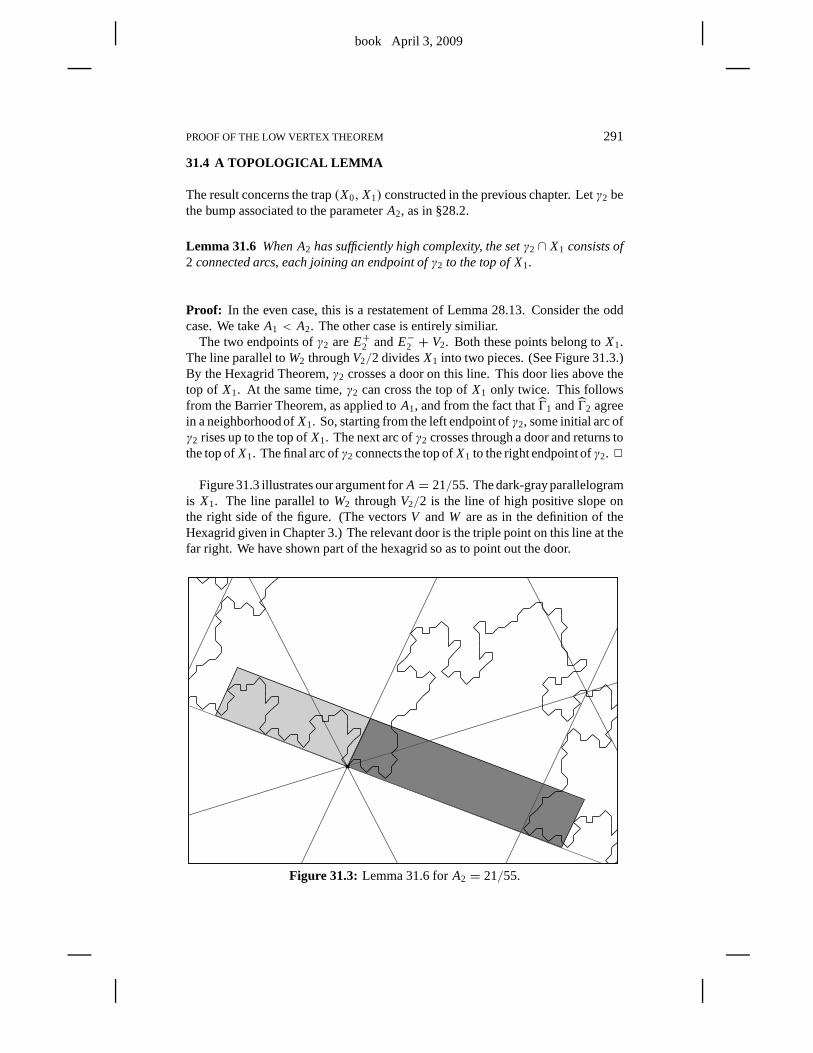
book April 3, 2009

PROOF OF THE LOW VERTEX THEOREM 291

31.4 A TOPOLOGICAL LEMMA

The result concerns the trap(X0, X1) constructed in the previous chapter. Letγ2 bethe bump associated to the parameterA2, as in §28.2.

Lemma 31.6 When A2 has sufficiently high complexity, the setγ2 ∩ X1 consists of2 connected arcs, each joining an endpoint ofγ2 to the top of X1.

Proof: In the even case, this is a restatement of Lemma 28.13. Consider the oddcase. We takeA1 < A2. The other case is entirely similiar.

The two endpoints ofγ2 areE+2 andE−2 + V2. Both these points belong toX1.The line parallel toW2 throughV2/2 dividesX1 into two pieces. (See Figure 31.3.)By the Hexagrid Theorem,γ2 crosses a door on this line. This door lies above thetop of X1. At the same time,γ2 can cross the top ofX1 only twice. This followsfrom the Barrier Theorem, as applied toA1, and from the fact thatŴ1 andŴ2 agreein a neighborhoodofX1. So, starting from the left endpoint ofγ2, some initial arc ofγ2 rises up to the top ofX1. The next arc ofγ2 crosses through a door and returns tothe top ofX1. The final arc ofγ2 connects the top ofX1 to the right endpoint ofγ2. 2

Figure 31.3 illustrates our argument forA = 21/55. The dark-grayparallelogramis X1. The line parallel toW2 throughV2/2 is the line of high positive slope onthe right side of the figure. (The vectorsV andW are as in the definition of theHexagrid given in Chapter 3.) The relevant door is the triplepoint on this line at thefar right. We have shown part of the hexagrid so as to point outthe door.

Figure 31.3: Lemma 31.6 forA2 = 21/55.

book April 3, 2009

292 CHAPTER 31

31.5 THE END OF THE PROOF

LetŴ2 = Ŵ(A2), as in the previous section. We say that aD-arc ofŴ2 is a connectedarcα that joins a low vertex to aD-low vertex. Let|α| denote the smallest integerN such thatα contains no vertices that are more thanN vertical units above thebaseline. Given aD-low vertexv ∈ α, let

F(A2) = max f (v; A2), f (v; A2) = min |α|. (31.3)

In the first equation, the maximum is taken over allD-low vertices. In the secondequation, the minimum is taken over allD-arcs havingv as an endpoint. (Actually,this minimum it taken over the two shortestD-arcs, each going out in a differentdirection fromv.) These functions depend implicitlyonD, which is fixed throughoutthe discussion.

Before we prove any results, we give some intuition about thefunction F . IfF(A2) is large, it means that there exists aD-low vertexv such that the only arcsconnectingv to an actual low vertex rise up very high away from the baseline. Atleast in a large neighborhood ofv, the component containingv would imitate ahovering component. This is the sort of thing we want to rule out.

Lemma 31.7 If A2 has sufficiently high complexity, then

F(A2) ≤ max(

F(A0), F(A1)).

Proof: We treat the odd case. The even case has the same proof except that we useLemma 27.12 in place of the Copy Lemma.

Let (X0, X1) be the trap forA2. Choose aD-low vertex v ∈ Ŵ2 such thatF(A2) = f (v). Recall thatγ2 is the bump corresponding toA2. The unionŴ2∪ γ2

is one period ofŴ modulo translations byV2. We have two cases.

Case 1: Suppose thatv ∈ PŴ2. By the Copy Theorem,PŴ2 ⊂ Ŵ0. By theargument in §22.4, a vertex onPŴ2 is k-low with respect toA0 iff it is k-low withrespect toA2. Since both endpoints ofPŴ2 are 1-low with respect to both param-eters, theD-arcs ofŴ2 realizing f (v, A2) coincide with theD-arcs ofŴ0 realizingf (v, A0). Hence

F(A0) ≥ f (v, A0) = f (v, A2) = F(A2).

Case 2: Suppose thatv ∈ γ2. Thenv ⊂ X1, andv is in one of the two arcs fromLemma 31.6. Let us say thatv is on the left arcλ. Thenλ ⊂ Ŵ1 ∩ Ŵ2 ∩ X1, byaxiom 1 for traps combined with Lemma 27.4. By axiom 3 for traps, a vertex ofλis k-low with respect toA1 iff it is k-low with respect toA2. Let α be aD-arc ofŴ1 such thatf (v; A1) = |α|. The left endpoint ofλ is 1-low, and the right endpointlies on the top ofX1. WhenA2 has high complexity,α ⊂ λ. The idea here is thatthe D-arc connectingv to the left endpoint ofλ remains inX1, whereas anyD-arcexitingλ must pass through the top ofX1. Sinceα ⊂ λ, we haveF(A1) ≥ F(A2)as in case 1. 2

Let {Bn} be the sequence in the Descent Lemma.

book April 3, 2009

PROOF OF THE LOW VERTEX THEOREM 293

Corollary 31.8 F(Bn) is uniformly bounded independent of n.

Proof: Applying the previous result recursively, we see that thereis some parameterCn ∈ T(Bn), of uniformly bounded complexity, such that

F(Bn) ≤ F(Cn).

But the sequence{Cn} has only finitely many distinct members, by Lemma 29.7.2

In light of the work in §31.3, the following corollary finishes the proof of theDescent Lemma.

Corollary 31.9 A D-low vertex ofŴ(Bn) can be connected to a low vertex ofŴ(Bn)by an arc that has length less than D′. Here D′ is independent of n.

Proof: Let vn be theD-low vertex in question. By Corollary 31.8 we can finda D-arcαn connectingvn to a low vertex ofŴ(Bn) such that|αn| < N and N isindependent ofn. But the same argument as in the proof of Lemma 5.7 shows thatthe diameter ofαn is uniformly bounded. The idea here is thatαn cannot grow along way in a thin neighborhood of the baseline. 2

This completes the proof of the Low Vertex Theorem. This was the last remainingpiece of business. Our work is done.

book April 3, 2009

book April 3, 2009

Appendix

In this appendix, we describe some additional experimentalobservations we havemade about outer billiards on kites and quadrilaterals.

A.1 STRUCTURE OF PERIODIC POINTS

A.1.1 Irrational Case

SupposeA is an irrational parameter. LetCA and I be as in the Comet Theorem.It follows from the Comet Theorem that all defined orbits inI − CA are periodic.Here we discuss a conjectural picture of the dynamics of these points. We use thenotation from the Comet Theorem.

As in §24.2, we can naturally identifyCA with the ends of an infinite directedtreeTA. Using the homeomorphism

φ:Z A→ CA,

we can formally extend the return map onC#A − φ(−1) to all of CA, even though

the extended return map does not correspond to the outer billiards dynamics on theextra points. The extended return map is induced by an automorphism

2A: TA→ TA

as discussed in §24.2. The complementary open intervals inI −CA – thegaps– arenaturally in bijection with the forward cones ofTA.

Conjecture A.1 The outer billiards map is entirely defined on a gap. The firstreturn map to I− CA permutes the gaps according to the action of2A on theforward cones of TA.

Some reflection should convince the reader that this is the simplest possible descrip-tion of the periodic dynamics that is compatible with the Comet Theorem.

With a lot of effort, we can prove the weaker result that Conjecture A.1 correctlydescribes the first return map for everydefinedorbit in I −CA. The part we cannotprove is that all the orbits ofI − CA are actually defined. This is a big difference.If all points in the same gap have well defined orbits, then thewhole gap moves asa single orbit. That is, all points in the same gap have the same combinatorial typeof orbit. Without knowing that all points in the gap have welldefined orbits, all wecan say is that two points in the same gap return toI in the correct way. The orbitsmight have different itineraries outside ofI .

We might have included the proof of the weak version of Conjecture A.1 in thisbook, but we would prefer to hold out for the definitive result.

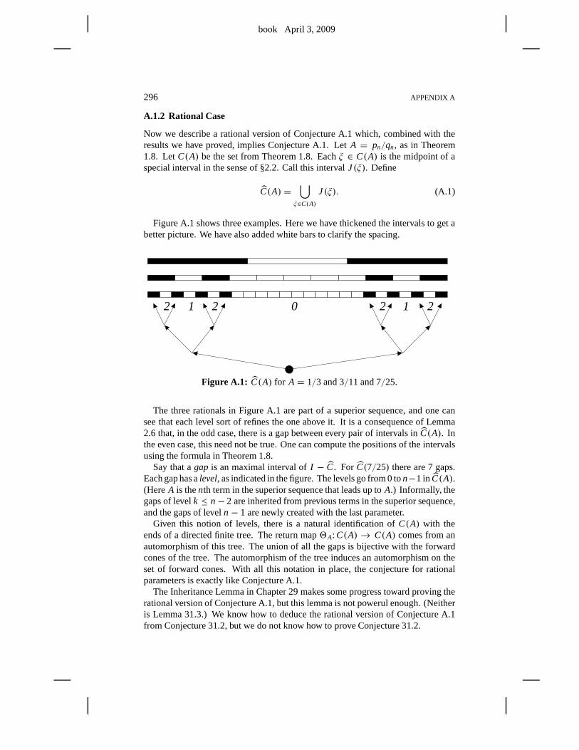
book April 3, 2009

296 APPENDIX A

A.1.2 Rational Case

Now we describe a rational version of Conjecture A.1 which, combined with theresults we have proved, implies Conjecture A.1. LetA = pn/qn, as in Theorem1.8. LetC(A) be the set from Theorem 1.8. Eachξ ∈ C(A) is the midpoint of aspecial interval in the sense of §2.2. Call this intervalJ(ξ). Define

C(A) =⋃

ξ∈C(A)

J(ξ). (A.1)

Figure A.1 shows three examples. Here we have thickened the intervals to get abetter picture. We have also added white bars to clarify the spacing.

2 2 2 21 10

Figure A.1: C(A) for A = 1/3 and 3/11 and 7/25.

The three rationals in Figure A.1 are part of a superior sequence, and one cansee that each level sort of refines the one above it. It is a consequence of Lemma2.6 that, in the odd case, there is a gap between every pair of intervals inC(A). Inthe even case, this need not be true. One can compute the positions of the intervalsusing the formula in Theorem 1.8.

Say that agap is an maximal interval ofI − C. For C(7/25) there are 7 gaps.Each gap has alevel, as indicated in the figure. The levels go from 0 ton−1 in C(A).(HereA is thenth term in the superior sequence that leads up toA.) Informally, thegaps of levelk ≤ n− 2 are inherited from previous terms in the superior sequence,and the gaps of leveln− 1 are newly created with the last parameter.

Given this notion of levels, there is a natural identification of C(A) with theends of a directed finite tree. The return map2A: C(A) → C(A) comes from anautomorphism of this tree. The union of all the gaps is bijective with the forwardcones of the tree. The automorphism of the tree induces an automorphism on theset of forward cones. With all this notation in place, the conjecture for rationalparameters is exactly like Conjecture A.1.

The Inheritance Lemma in Chapter 29 makes some progress toward proving therational version of Conjecture A.1, but this lemma is not powerul enough. (Neitheris Lemma 31.3.) We know how to deduce the rational version of Conjecture A.1from Conjecture 31.2, but we do not know how to prove Conjecture 31.2.

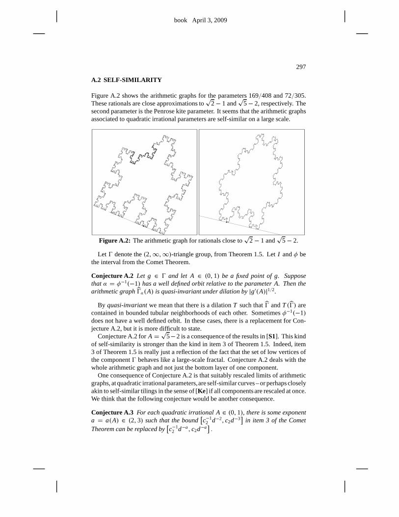
book April 3, 2009

297

A.2 SELF-SIMILARITY

Figure A.2 shows the arithmetic graphs for the parameters 169/408 and 72/305.These rationals are close approximations to

√2− 1 and

√5− 2, respectively. The

second parameter is the Penrose kite parameter. It seems that the arithmetic graphsassociated to quadratic irrational parameters are self-similar on a large scale.

Figure A.2: The arithmetic graph for rationals close to√

2− 1 and√

5− 2.

Let Ŵ denote the(2,∞,∞)-triangle group, from Theorem 1.5. LetI andφ bethe interval from the Comet Theorem.

Conjecture A.2 Let g ∈ Ŵ and let A ∈ (0,1) be a fixed point of g. Supposethat α = φ−1(−1) has a well defined orbit relative to the parameter A. Then thearithmetic graphŴα(A) is quasi-invariant under dilation by|g′(A)|1/2.

By quasi-invariantwe mean that there is a dilationT such thatŴ andT(Ŵ) arecontained in bounded tubular neighborhoods of each other. Sometimesφ−1(−1)does not have a well defined orbit. In these cases, there is a replacement for Con-jecture A.2, but it is more difficult to state.

Conjecture A.2 forA =√

5−2 is a consequence of the results in [S1]. This kindof self-similarity is stronger than the kind in item 3 of Theorem 1.5. Indeed, item3 of Theorem 1.5 is really just a reflection of the fact that theset of low vertices ofthe componentŴ behaves like a large-scale fractal. Conjecture A.2 deals with thewhole arithmetic graph and not just the bottom layer of one component.

One consequence of Conjecture A.2 is that suitably rescaledlimits of arithmeticgraphs, at quadratic irrational parameters,are self-similar curves – or perhaps closelyakin to self-similar tilings in the sense of [Ke] if all components are rescaled at once.We think that the following conjecture would be another consequence.

Conjecture A.3 For each quadratic irrational A∈ (0,1), there is some exponenta = a(A) ∈ (2,3) such that the bound

[c−1

2 d−2, c2d−3]

in item 3 of the CometTheorem can be replaced by

[c−1

2 d−a, c2d−a].

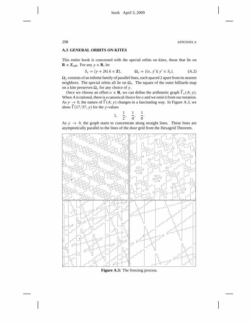
book April 3, 2009

298 APPENDIX A

A.3 GENERAL ORBITS ON KITES

This entire book is concerned with the special orbits on kites, those that lie onR × Zodd. For anyy ∈ R, let

Sy = {y+ 2k| k ∈ Z}, �y = {(x, y′)| y′ ∈ Sy}. (A.2)

�y consists of an infinite family of parallel lines, each spaced2 apart from its nearestneighbors. The special orbits all lie on�1. The square of the outer billiards mapon a kite preserves�y for any choice ofy.

Once we choose an offsetα ∈ R, we can define the arithmetic graphŴα(A; y).WhenA is rational, there is a canonical choice forα and we omit it from our notation.As y → 0, the nature ofŴ(A; y) changes in a fascinating way. In Figure A.3, weshowŴ(17/37; y) for they-values

1,1

2,

1

4,

1

8.

As y → 0, the graph starts to concentrate along straight lines. These lines areasymptotically parallel to the lines of the door grid from the Hexagrid Theorem.

Figure A.3: The freezing process.

book April 3, 2009

299

Informally, we think ofy ∈ [0,1] as being a kind of temperature, with 0 cor-responding to freezing and 1 corresponding to boiling. Notethat the figure fory ∈ [−1,0] is symmetric. Thus one sees a similar freezing process asy→ 0 frombelow.

We do have an explanation of sorts for the freezing phenomenon, though we havenot worked through all the details. The Master Picture Theorem seems to hold forthe general orbits. That is, there is one 5-dimensional picture that works for allorbits and all parameters at once. The Master Picture Theorem we proved here is aboundary case.

As y → 0, the regions in this master partition that assign nontrivial edges tothe arithmetic graph seem to concentrate along a finite unionof hyperplanes. Thepreimages of these hyperplanes are the asymptotic lines we see in the freezingprocess.

Here are some other observations about these generalized arithmetic graphs.

• The Embedding Theorem seems true in general.

• The Hexagrid Theorem is false in general.

• The Diophantine Lemma is false in general.

• All the results in §1.5 are false in general.

We think that most of our theorems ought to have (probably weaker) analogs forthe general orbit. We do not know which way to bet on the answer, however. Hereare some obvious questions one might ask:

Question 1: Is every orbit in a kite either periodic or unbounded?

Question 2: Is almost every orbit in a kite periodic?

Question 3: Are there any unbounded orbits that are not special orbits?

Question 4: Is every unbounded orbit oscillatory in at least one direction?

In the last question, an orbit isoscillatory if its ω-limit set is nonempty. Erraticorbits are oscillatory in both directions. Note that the Comet Theorem completelyanswers all these questions for orbits in�1.

What makes these questions difficult for us to answer (aside from a general lackof understanding of the situation) is the fact that the Hexagrid Theorem no longerholds. This precise result played a huge role in our overall proof. It is interestingthat one sees remnants of the hexagrid, as the asymptotic lines, as the temperatureytends to 0. One might wonder if there is a united Hexagrid Theorem that somehowgoverns the whole picture. Another difficulty is that the Copy Theorem no longerseems to hold in such a precise way as they did for special orbits.

book April 3, 2009

300 APPENDIX A

A.4 GENERAL QUADRILATERALS

First we discuss the situation for trapezoids. As mentionedin the introduction,Dan Genin worked out the complete picture for trapezoids. See [Ge]. His work issimilar in spirit to the work discussed in this book, though ultimately the situationfor trapezoids is simpler. Genin finds that all orbits are bounded, and most areaperiodic. Thus the orbit dichotomy, periodic or unbounded, does not work fortrapezoids.

One appealing feature about studying the general quadrilateral is that one canperhaps interpolate between the work in this book and Genin’s results. The finalpicture ought to be compatible with both kites and trapezoids. We have no ideahow to carry this out at present. However, in this section, wewill present someinteresting figures. Our latest version of Billiard King contains a separate programthat generalizes some of the features of Billiard King to general quadrilaterals.Indeed, Figure A.3 is taken from this other program.

The spaceQ of convex quadrilaterals modulo the affine group is 2-dimensional.For(a,b, c) in the positive orthant ofR3, we letQ(a,b, c) denote the quadrilateralwith vertices

(0,0), (1,0), (0,1), v =(

a+ b

a+ b+ c,

b+ c

a+ b+ c

).

Any convex quadrilateral is affinely equivalent to someQ(a,b, c). Our coordinati-zation is adapted to a certain action of the positive matrices in SL3(Z) onQ, whichwe will not discuss. The trapezoids correspond to points of the form(0,b, c) and(symmetrically)(a,b,0).

For the first return map, we take4 to be the stripR+ × [−1,1]. This time weconsider the solid strip and not just its boundary. Picking apoint (α1, α2) ∈ 4 andwatching the first return map, we see a sequence of points

(α1, α2)+ (2mk,2nk)+ 2okv, mk,nk,ok ∈ Z. (A.3)

The lattice path corresponding to the orbit, namely,{(mk,nk,ok}, lies very close toa plane inR3. The fact that they-coordinate lies in [−1,1] places a relationship onnk andok. We can project into this plane and draw a 2 dimensional figure.

When we do this carefully, taking into account the parity as in Equation 2.10,we get a notion of the arithmetic graph that extends what we have for kites. Weshow some illustrations below. In all the figures, we start with the offset value(α1, α2) = (0,−1). As for the case with kites, we mean to add an infinitesimallysmall vector to the offset, so as to track well defined orbits.Compare the discussionin §2.5.

Figure A.4.1 shows the figure for the trapezoid with coordinates(0,233,377).One of the main diagonals of our bounding box is approximately the baseline. Here233 and 377 are fairly large Fibonacci numbers. This figure istypical of what onesees for trapezoids.

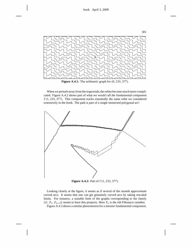
book April 3, 2009

301

Figure A.4.1: The arithmetic graph for(0,233,377).

When we perturb away from the trapezoids, the orbits become much more compli-cated. Figure A.4.2 shows part of what we would call the fundamental componentŴ(1,233,377). This component tracks essentially the same orbit we consideredextensively in the book. The path is part of a single immersedpolygonal arc!

Figure A.4.2: Part ofŴ(1,233,377).

Looking closely at the figure, it seems as if several of the strands approximatecurved arcs. It seems that one can get genuinely curved arcs by taking rescaledlimits. For instance, a suitable limit of the graphs corresponding to the family{(1, Fn, Fn+1)} seems to have this property. HereFn is thenth Fibonacci number.

Figure A.4.3 shows a similar phenomenon for a messier fundamental component.

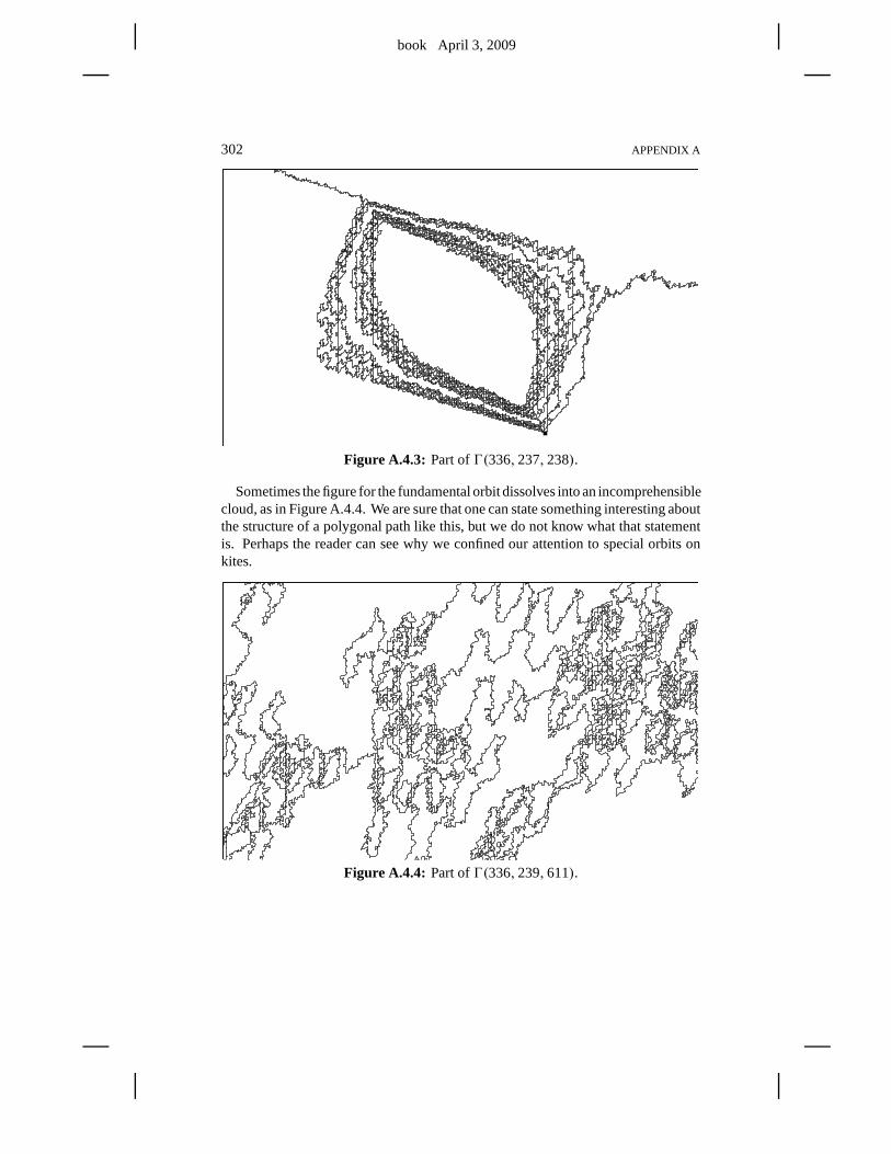
book April 3, 2009

302 APPENDIX A

Figure A.4.3: Part ofŴ(336,237,238).

Sometimes the figure for the fundamental orbit dissolves into an incomprehensiblecloud, as in Figure A.4.4. We are sure that one can state something interesting aboutthe structure of a polygonal path like this, but we do not knowwhat that statementis. Perhaps the reader can see why we confined our attention tospecial orbits onkites.

Figure A.4.4: Part ofŴ(336,239,611).

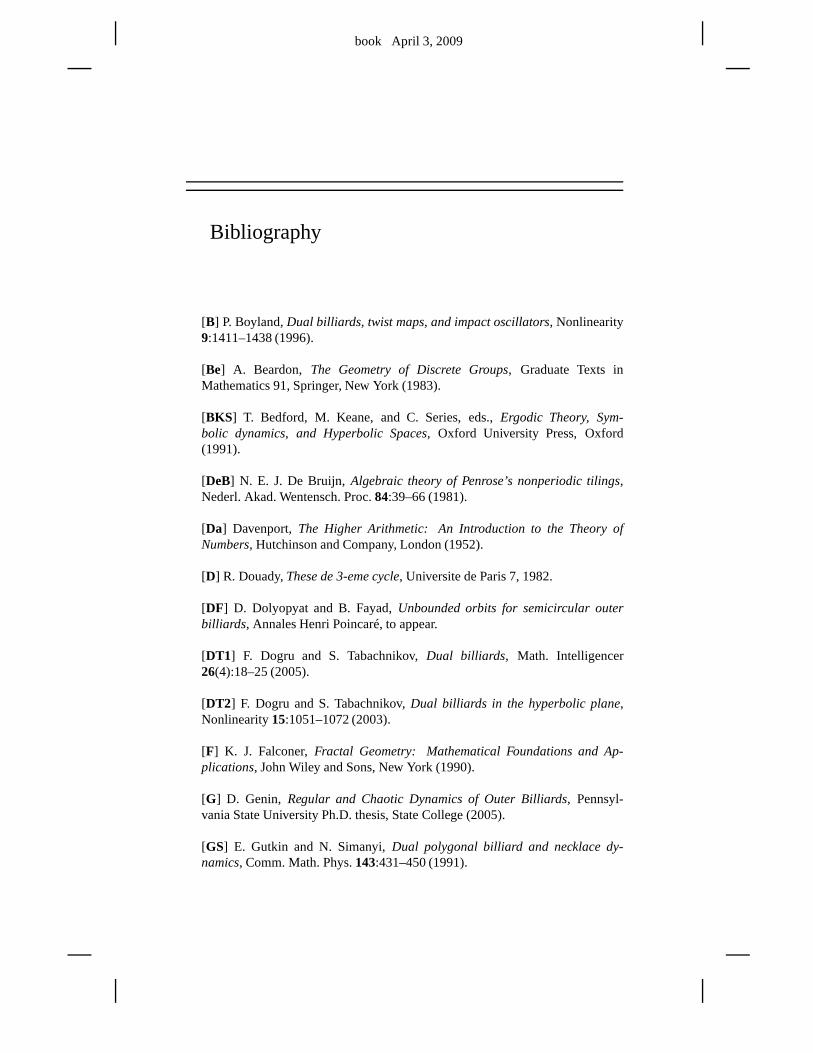
book April 3, 2009

Bibliography

[B] P. Boyland,Dual billiards, twist maps, and impact oscillators, Nonlinearity9:1411–1438 (1996).

[Be] A. Beardon, The Geometry of Discrete Groups, Graduate Texts inMathematics 91, Springer, New York (1983).

[BKS] T. Bedford, M. Keane, and C. Series, eds.,Ergodic Theory, Sym-bolic dynamics, and Hyperbolic Spaces, Oxford University Press, Oxford(1991).

[DeB] N. E. J. De Bruijn,Algebraic theory of Penrose’s nonperiodic tilings,Nederl. Akad. Wentensch. Proc.84:39–66 (1981).

[Da] Davenport,The Higher Arithmetic: An Introduction to the Theory ofNumbers, Hutchinson and Company, London (1952).

[D] R. Douady,These de 3-eme cycle, Universite de Paris 7, 1982.

[DF] D. Dolyopyat and B. Fayad,Unbounded orbits for semicircular outerbilliards, Annales Henri Poincaré, to appear.

[DT1] F. Dogru and S. Tabachnikov,Dual billiards, Math. Intelligencer26(4):18–25 (2005).

[DT2] F. Dogru and S. Tabachnikov,Dual billiards in the hyperbolic plane,Nonlinearity15:1051–1072 (2003).

[F] K. J. Falconer,Fractal Geometry: Mathematical Foundations and Ap-plications, John Wiley and Sons, New York (1990).

[G] D. Genin, Regular and Chaotic Dynamics of Outer Billiards, Pennsyl-vania State University Ph.D. thesis, State College (2005).

[GS] E. Gutkin and N. Simanyi,Dual polygonal billiard and necklace dy-namics, Comm. Math. Phys.143:431–450 (1991).

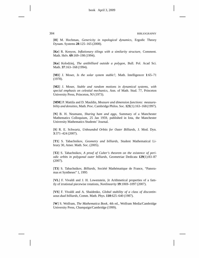
book April 3, 2009

304 BIBLIOGRAPHY

[H] M. Hochman, Genericity in topological dynamics, Ergodic TheoryDynam. Systems28:125–165 (2008).

[Ke] R. Kenyon, Inflationary tilings with a similarity structure, Comment.Math. Helv.69:169–198 (1994).

[Ko] Kolodziej, The antibilliard outside a polygon, Bull. Pol. Acad Sci.Math.37:163–168 (1994).

[M1] J. Moser, Is the solar system stable?, Math. Intelligencer1:65–71(1978).

[M2] J. Moser, Stable and random motions in dynamical systems, withspecial emphasis on celestial mechanics, Ann. of Math. Stud. 77, PrincetonUniversity Press, Princeton, NJ (1973).

[MM ] P. Mattila and D. Mauldin,Measure and dimension functions: measura-bility and densities, Math. Proc. Cambridge Philos. Soc.121(1):163–168(1997).

[N] B. H. Neumann,Sharing ham and eggs, Summary of a ManchesterMathematics Colloquium, 25 Jan 1959, published in Iota, theManchesterUniversity Mathematics Students’ Journal.

[S] R. E. Schwartz,Unbounded Orbits for Outer Billiards, J. Mod. Dyn.3:371–424 (2007).

[T1] S. Tabachnikov,Geometry and billiards, Student Mathematical Li-brary 30, Amer. Math. Soc. (2005).

[T2] S. Tabachnikov,A proof of Culter’s theorem on the existence of peri-odic orbits in polygonal outer billiards, Geometriae Dedicata129(1):83–87(2007).

[T3] S. Tabachnikov,Billiards, Société Mathématique de France, “Panora-mas et Syntheses” 1, 1995

[VL ] F. Vivaldi and J. H. Lowenstein, |it Arithmetical properties of a fam-ily of irrational piecewise rotations,Nonlinearity19:1069–1097 (2007).

[VS] F. Vivaldi and A. Shaidenko,Global stability of a class of discontin-uous dual billiards, Comm. Math. Phys.110:625–640 (1987).

[W] S. Wolfram,The Mathematica Book, 4th ed., Wolfram Media/CambridgeUniversity Press, Champaign/Cambridge (1999).

book April 3, 2009

Index

affine action, 63algorithm for the Master Picture Theorem, 66aperiodic orbits, 1arithmetic graph, 12, 26arithmetic kite, 33

backward erratic orbits, 3Barrier Theorem, 125baseline, 26billiards, 1bounded orbits, 1bump, 250, 260

Cantor set, 207caps, 280celestial mechanics, 1, 5Comet Theorem, 7, 205, 295Continuity Principle, 30convex integral polytopes, 63Copy Theorem, 12, 195, 239crossing cells, 135cusped solenoid, 5

Decomposition Theorem, 171density of periodic orbits, 50Descent Lemma, 287dimension formula, 231diophantine constant, 159door grid, 33doors, 35, 133

EIRS, 188Embedding Theorem, 12, 101end major components, 260enhanced renormalization sequence, 188erratic orbits, 3Erratic Orbits Theorem, 3, 45essential conjugacy, 5even predecessor, 273excursion distance, 8, 208

Farey pairs, 249Farey triangulation, 153first return map, 25fleeting orbits, 11forward erratic orbits, 3freezing phenomenon, 298

fundamental map, 26

general orbits, 298

half-disk, 2Hausdorff dimension, 6, 230, 231Hausdorff metric, 30Hausdorff topology, 30hexagrid, 33, 35, 136Hexagrid Theorem, 12, 35, 133homology, 27hovering components, 279Hovering Lemma, 279hyperbolic geometry, 153, 228hyperbolic triangle group, 5, 228Hyperplane Lemma, 93

inferior predecessor, 41inferior sequence, 7, 41, 153, 187Inheritance Lemma, 273Intersection Lemma, 143inverse limit, 7

lattice vector field, 12limit set, 9, 19low component, 287low vertex, 28, 196, 205Low Vertex Theorem, 205, 287

Master Picture Theorem, 15, 25, 55Master Picture Theorem example, 60middle major components, 260minimality, 4, 287minor box, 266minor components, 260Mismatch Principle, 171modular group, 5modularity, 229Moser-Neumann question, 1

odd predecessor, 273odometer, 5orbit dichotomy, 49ordering, reverse lexicographic, 193ordering, twirl, 193

partition, 21, 57, 66

book April 3, 2009

306 INDEX

Penrose kite, 6Period Theorem, 213, 273periodic orbits, 1persistent orbits, 11phase portrait, 28Pinwheel Lemma, 25, 69pinwheel map, 69, 70pivot arcs, 249pivot points, 239Pivot Theorem, 195polygonal outer billiards, 19polyhedron exchange, 15

quadratic irrational parameters, 231quadrilaterals, 300quasirational polygon, 2

rational kite, 10rational polygons, 19regular pentagon, 2renormalization sequence, 7return map, 4return times, 208Rigidity Lemma, 31, 50, 276room grid, 33Room Lemma, 37rooms, 35

self-similarity, 231, 297singular set, 93special intervals, 20special orbits, 3, 20square outer billiards map, 10, 21Strip Lemma, 79strip map, 69strips, 69strong sequences, 43, 181Structure Lemma, 249superior parameters, 188superior predecessor, 41superior sequence, 7, 41, 187superior term, 7symmetry, near-bilateral, 113symmetry, rotational, 111symmetry, translational, 107

temperature, 298tilings, 19Torus Lemma, 77Torus map, 78trapezoids, 2, 300traps, 280tree automorphism, 295triangle group, 228trimmed Cantor set, 4twist automorphism, 193

unbounded orbits, 1

universal odometer, 5

wall crossings, 35walls, 35walls of partition, 56