ANL-EAIS-8, 'Data Collection Handbook to Support Modeling ...

?,.I" l $ T i n

. - * a ., Distribution

Caregory UC-5 1 1

ANUEAIS-8

Data Collection Handbook to Support Modeling the Impacts of Radioactive Material in Soil

by C. Yu, C. Loureiro,* J.-J. Cheng, L.G. Jones, Y.Y. Wang, Y.P. Chia,* and E. Faillace

Environmental Assessment and Information Sciences Division, Argonne National Laboratory, 9700 South Cass Avenue, Argonne, Illinois 60439

April 1993

Work sponsored by United States Department of Energy, Assistant Secretary for Environment, Safety and Health, Off ice of Environmental Guidance, Assistant Secretary for Environmental Restoration and Waste Management, Off ice of Environmental Restoration

*Loureiro is affiliated with Escola de Engenharia da UFMG, Belo Horizonte, Brazil, and Chia with the Department of Geology, Taiwan University, Taiwan, Republic of China.

DISCLAIMER

This report was prepared as an account of work sponsored by an agency of the United States Government. Neither the United States Government nor any agency Thereof, nor any of their employees, makes any warranty, express or implied, or assumes any legal liability or responsibility for the accuracy, completeness, or usefulness of any information, apparatus, product, or process disclosed, or represents that its use would not infringe privately owned rights. Reference herein to any specific commercial product, process, or service by trade name, trademark, manufacturer, or otherwise does not necessarily constitute or imply its endorsement, recommendation, or favoring by the United States Government or any agency thereof. The views and opinions of authors expressed herein do not necessarily state or reflect those of the United States Government or any agency thereof.

DISCLAIMER Portions of this document may be illegible in electronic image products. Images are produced from the best available original document.

CONTENTS

ACKNOWLEDGMENTS . . . . . . . . . . . . . . . . . . . . . . . . . . . . . . . . . . . . . . . . . . . . . . xi

NOTATION . . . . . . . . . . . . . . . . . . . . . . . . . . . . . . . . . . . . . . . . . . . . . . . . . . . . . . . . xii

ABSTRACT . . . . . . . . . . . . . . . . . . . . . . . . . . . . . . . . . . . . . . . . . . . . . . . . . . . . . . . . 1

1 INTRODUCTION . . . . . . . . . . . . . . . . . . . . . . . . . . . . . . . . . . . . . . . . . . . . . . . . 1

2 SOIL DENSITY . . . . . . . . . . . . . . . . . . . . . . . . . . . . . . . . . . . . . . . . . . . . . . . . . . 13

2.1 Definition . . . . . . . . . . . . . . . . . . . . . . . . . . . . . . . . . . . . . . . . . . . . . . . . . . 13 2.1.1 Soil Particle Density . . . . . . . . . . . . . . . . . . . . . . . . . . . . . . . . . . . . . 14 2.1.2 Bulk Density . . . . . . . . . . . . . . . . . . . . . . . . . . . . . . . . . . . . . . . . . . . 14 2.1.3 Total Density . . . . . . . . . . . . . . . . . . . . . . . . . . . . . . . . . . . . . . . . . . . 16

2.2 Measurement Methodology . . . . . . . . . . . . . . . . . . . . . . . . . . . . . . . . . . . . . 16 2.2.1 Soil Particle Density Measurement . . . . . . . . . . . . . . . . . . . . . . . . . . 16 2.2.2 Dry Density Measurement . . . . . . . . . . . . . . . . . . . . . . . . . . . . . . . . . 19

2.3 RESRAD Data Input Requirements . . . . . . . . . . . . . . . . . . . . . . . . . . . . . . . 21

3 TOTAL POROSITY . . . . . . . . . . . . . . . . . . . . . . . . . . . . . . . . . . . . . . . . . . . . . . . 22

3.1 Definition . . . . . . . . . . . . . . . . . . . . . . . . . . . . . . . . . . . . . . . . . . . . . . . . . . 22 3.2 Measurement Methodology . . . . . . . . . . . . . . . . . . . . . . . . . . . . . . . . . . . . . 23 3.3 RESRAD Data Input Requirements . . . . . . . . . . . . . . . . . . . . . . . . . . . . . . . 24

4 EFFECTIVE POROSITY . . . . . . . . . . . . . . . . . . . . . . . . . . . . . . . . . . . . . . . . . . . 25


5 HYDRAULIC CONDUCTMW . . . . . . . . . . . . . . . . . . . . . . . . . . . . . . . . . . . . . . 27

5.1 Definition . . . . . . . . . . . . . . . . . . . . . . . . . . . . . . . . . . . . . . . . . . . . . . . . . . 27 5.2 Measurement Methodology . . . . . . . . . . . . . . . . . . . . . . . . . . . . . . . . . . . . . 29

5.2.1 Laboratory Methods . . . . . . . . . . . . . . . . . . . . . . . . . . . . . . . . . . . . . . 37

5.3 RESRAD Data Input Requirements . . . . . . . . . . . . . . . . . . . . . . . . . . . . . . . 42 5.2.2 Field Methods . . . . . . . . . . . . . . . . . . . . . . . . . . . . . . . . . . . . . . . . . . 39

6 VOLUMETRIC WATER CONTENT . . . . . . . . . . . . . . . . . . . . . . . . . . . . . . . . . . 44


... 111

CONTENTS (Cont.) I

I

7 EFFECTIVE RADON DIFFUSION COEFFICIENT . . . . . . . . . . . . . . . . . . . . . . 48

7.1 Definition . . . . . . . . . . . . . . . . . . . . . . . . . . . . . . . . . . . . . . . . . . . . . . . . . . 48

7.3 52 7.2 Measurement Methodology . . . . . . . . . . . . . . . . . . . . . . . . . . . . . . . . . . . . . 50

RESRAD Data Input Requirements . . . . . . . . . . . . . . . . . . . . . . . . . . . . . . .

8 RADON EMANATION COEFFICIENT . . . . . . . . . . . . . . . . . . . . . . . . . . . . . . . . 55

8.1 Definition . . . . . . . . . . . . . . . . . . . . . . . . . . . . . . . . . . . . . . . . . . . . . . . . . . 55


RESRAD Data Input Requirements . . . . . . . . . . . . . . . . . . . . . . . . . . . . . . .

. . . . . . . . . . . . . . . . . . . . . . . . . . . . . . . . . . . . . . . . . . . 9 PRECIPITATION RATE 59

9.1 Definition . . . . . . . . . . . . . . . . . . . . . . . . . . . . . . . . . . . . . . . . . . . . . . . . . . 59


RESRAD Data Input Requirements . . . . . . . . . . . . . . . . . . . . . . . . . . . . . . . 10 RUNOFF COEFFICIENT . . . . . . . . . . . . . . . . . . . . . . . . . . . . . . . . . . . . . . . . . . 65

10.1 Definition . . . . . . . . . . . . . . . . . . . . . . . . . . . . . . . . . . . . . . . . . . . . . . . . . . 65 10.2 Estimation Methodology . . . . . . . . . . . . . . . . . . . . . . . . . . . . . . . . . . . . . . . 65 10.3 RESRAD Data Input Requirements . . . . . . . . . . . . . . . . . . . . . . . . . . . . . . 65

11 IRRIGATIONRATE . . . . . . . . . . . . . . . . . . . . . . . . . . . . . . . . . . . . . . . . . . . . . . 67

11.1 Definition . . . . . . . . . . . . . . . . . . . . . . . . . . . . . . . . . . . . . . . . . . . . . . . . . . 67 11.2 Measurement Methodology . . . . . . . . . . . . . . . . . . . . . . . . . . . . . . . . . . . . . 67 11.3 RESRAD Data Input Requirements . . . . . . . . . . . . . . . . . . . . . . . . . . . . . . 68

12 EVAPOTRANSPIRATION COEFFICIENT . . . . . . . . . . . . . . . . . . . . . . . . . . . . . 70

12.1 Definition . . . . . . . . . . . . . . . . . . . . . . . . . . . . . . . . . . . . . . . . . . . . . . . . . . 70 12.2 Measurement Methodology . . . . . . . . . . . . . . . . . . . . . . . . . . . . . . . . . . . . . 73 12.3 RESRAD Data Input Requirements .............................. 74

13 SOIL-SPECIFIC EXPONENTIAL b PARAMETER . . . . . . . . . . . . . . . . . . . . . . . 75


14 EROSION RATE . . . . . . . . . . . . . . . . . . . . . . . . . . . . . . . . . . . . . . . . . . . . . . . . . 78


iu

........................................ L- .... . . . . . . . . .

CONTENTS (Cont.)

15 HYDRAULIC GRADIENT . . . . . . . . . . . . . . . . . . . . . . . . . . . . . . . . . . . . . . . . . . 80


16 LENGTH OF CONTAMINATED ZONE PARALLEL TO THE AQUIFER FLOW . . . . . . . . . . . . . . . . . . . . . . . . . . . . . . . . . . . . . . . . . 82


17 WATERSHED AREA FOR NEARBY STREAM OR POND . . . . . . . . . . . . . . . . . . 83


18 WATER TABLE DROP RATE . . . . . . . . . . . . . . . . . . . . . . . . . . . . . . . . . . . . . . . 85


19 WELL-PUMP INTAKE DEPTH . . . . . . . . . . . . . . . . . . . . . . . . . . . . . . . . . . . . . . 86

19.1 Definition . . . . . . . . . . . . . . . . . . . . . . . . . . . . . . . . . . . . . . . . . . . . . . . . . . 86 19.2 RESRAD Data Input Requirements . . . . . . . . . . . . . . . . . . . . . . . . . . . . . . 86

20 RADON VERTICAL DIMENSION OF MIXING . . . . . . . . . . . . . . . . . . . . . . . . . . 87


21 AVERAGE ANNUAL WIND SPEED . . . . . . . . . . . . . . . . . . . . . . . . . . . . . . . . . . 88


22 AVERAGE BUILDING AIR EXCHANGE RATE . . . . . . . . . . . . . . . . . . . . . . . . . 89


U

CONTENTS (Cont.)

23 BUILDING ROOM HEIGHT . . . . . . . . . . . . . . . . . . . . . . . . . . . . . . . . . . . . . . . . 91


24 BUILDING INDOOR AREA FACTOR . . . . . . . . . . . . . . . . . . . . . . . . . . . . . . . . . 92


25 THICKNESS OF UNCONTAMINATED UNSATURATED ZONE . . . . . . . . . . . . 93


26 BUILDING FOUNDATION THICKNESS . . . . . . . . . . . . . . . . . . . . . . . . . . . . . . 94


27 FOUNDATION DEPTH BELOW GROUND SURFACE . . . . . . . . . . . . . . . . . . . . 95


28 FRACTION OF TIME SPENT INDOORS ON-SITE . . . . . . . . . . . . . . . . . . . . . . . 96


29 FRACTION OF TIME SPENT OUTDOORS ON-SITE . . . . . . . . . . . . . . . . . . . . . 97


30 AREA OF CONTAMINATED ZONE . . . . . . . . . . . . . . . . . . . . . . . . . . . . . . . . . . 98


31 COVERDEPTH . . . . . . . . . . . . . . . . . . . . . . . . . . . . . . . . . . . . . . . . . . . . . . . . . 99


vi

. . . . . . . . . . . . ............ .......... ........................

CONTENTS (Cont.)

32 DISTRIBUTION COEFFICIENTS . . . . . . . . . . . . . . . . . . . . . . . . . . . . . . . . . . . . 100

32.1 Definition . . . . . . . . . . . . . . . . . . . . . . . . . . . . . . . . . . . . . . . . . . . . . . . . . . 100 32.2 Measurement Methodology . . . . . . . . . . . . . . . . . . . . . . . . . . . . . . . . . . . . . 100

32.2.1 Experimental Methods . . . . . . . . . . . . . . . . . . . . . . . . . . . . . . . . . . . 100

32.3 RESRAD Data Input Requirements . . . . . . . . . . . . . . . . . . . . . . . . . . . . . . 104 32.2.2 Empirical Determination of the Distribution Coefficient . . . . . . . . . . 103

33 RADIONUCLIDE CONCENTRATION IN GROUNDWATER . . . . . . . . . . . . . . . . 108


34 LEACHRATE . . . . . . . . . . . . . . . . . . . . . . . . . . . . . . . . . . . . . . . . . . . . . . . . . . . 109


35 MASS LOADING FOR INHALATION . . . . . . . . . . . . . . . . . . . . . . . . . . . . . . . . . 110


36 SHIELDING FACTOR FOR INHALATION PATHWAY . . . . . . . . . . . . . . . . . . . . 112


37 DEPTH OF ROOTS . . . . . . . . . . . . . . . . . . . . . . . . . . . . . . . . . . . . . . . . . . . . . . . 113


38 SOIL INGESTION RATE . . . . . . . . . . . . . . . . . . . . . . . . . . . . . . . . . . . . . . . . . . 114


39 THICKNESS OF CONTAMINATED ZONE . . . . . . . . . . . . . . . . . . . . . . . . . . . . . 117


40 RADIATION DOSE LIMIT . . . . . . . . . . . . . . . . . . . . . . . . . . . . . . . . . . . . . . . . . 118

uii

CONTENTS (Cont.)

41 SEAFOOD CONSUMPTION RATE . . . . . . . . . . . . . . . . . . . . . . . . . . . . . . . . . . . 119


42 FRUIT. VEGETABLE. AND GRAIN CONSUMPTION RATE . . . . . . . . . . . . . . . 121


43 INHALATION RATE . . . . . . . . . . . . . . . . . . . . . . . . . . . . . . . . . . . . . . . . . . . . . 123


44 LEAFY VEGETABLE CONSUMPTION RATE . . . . . . . . . . . . . . . . . . . . . . . . . . 125


45 LIVESTOCK WATER INTAKE RATE FOR BEEF CATTLE AND MILK COWS . . . . . . . . . . . . . . . . . . . . . . . . . . . . . . . . . . . . . . . . 126

45.1 Definition . . . . . . . . . . . . . . . . . . . . . . . . . . . . . . . . . . . . . . . . . . . . . . . . . . 126 45.2 RESRAD Data. Input Requirements . . . . . . . . . . . . . . . . . . . . . . . . . . . . . . 126

46 MEAT AND POULTRY CONSUMPTION RATE . . . . . . . . . . . . . . . . . . . . . . . . . 127

46.1 Definition . . . . . . . . . . . . . . . . . . . . . . . . . . . . . . . . . . . . . . . . . . . . . . . . . . 127 46.2 RESRAD Data Input Requirements . . . . . . . . . . . . . . . . . . . . . . . . . . . . . . . 127

47 MILK CONSUMPTION RATE . . . . . . . . . . . . . . . . . . . . . . . . . . . . . . . . . . . . . . . 128


48 SHIELDING FACTOR FOR EXTERNAL GAMMA RADIATION . . . . . . . . . . . . . 129


49 ELAPSED TIME OF WASTE PLACEMENT . . . . . . . . . . . . . . . . . . . . . . . . . . . . 130


. . .....................

... U l l l

..... . ~ ~-

CONTENTS (Cont.)

. . . . . . . . . . . . . . . . . . . . . . . . . . . . . . . . . . . . . . . . . . . . . . . . . 50 SHAPE FACTOR 131

. . . . . . . . . . . . . . . . . . . . . . . . . . . . . . . . . . . . . . . . . . . . . . . . . . 50.1 Definition 131 50.2 RESRAD Data Input Requirements . . . . . . . . . . . . . . . . . . . . . . . . . . . . . . 133

51 INITIAL CONCENTRATIONS OF PRINCIPAL RADIONUCLIDES . . . . . . . . . . 134

. . . . . . . . . . . . . . . . . . . . . . . . . . . . . . . . . . . . . . . . . . . . . . . . . . 134 51.1 Definition 51.2 RESRAD Data Input Requirements . . . . . . . . . . . . . . . . . . . . . . . . . . . . . . 135

52 DRINKING WATER INTAKE RATE . . . . . . . . . . . . . . . . . . . . . . . . . . . . . . . . . . 136


53 REFERENCES . . . . . . . . . . . . . . . . . . . . . . . . . . . . . . . . . . . . . . . . . . . . . . . . . . 138

FIGURES

2.1 U.S. Department of Agriculture Method for Naming Soils . . . . . . . . . . . . . . . . 17

9.1 Distribution of Average Annual Precipitation Rates over the U.S. Continental Territory . . . . . . . . . . . . . . . . . . . . . . . . . . . . . . . . . . . . . . . . 63

12.1 Distribution of Average Annual Potential Evapotranspiration Rates over the U.S. Continental Territory . . . . . . . . . . . . . . . . . . . . . . . . . . . . . . . . . 72

50.1 Irregularly Shaped Contaminated Zone Enclosed by Four Annuli . . . . . . . . . . . 132

TABLES

1.1 Input Parameters. Section Numbers. and Sources of Additional Information for All RESRAD Input Parameters . . . . . . . . . . . . . . . . . . . . . . . . 3

1.2 Applicable Pathways and Data Input Screen Locations for RESRAD Input Parameters . . . . . . . . . . . . . . . . . . . . . . . . . . . . . . . . . . . . . . . . . . . . . . . 5

1.3 Default Values. Lower Bounds. and Upper Bounds for RESRAD Input Parameters . . . . . . . . . . . . . . . . . . . . . . . . . . . . . . . . . . . . . . . . . . . . . . . 10

2.1 Typical Values of Dry Density of Various Soil Types and Concrete . . . . . . . . . . 16

ix

TABLES (Cont.)

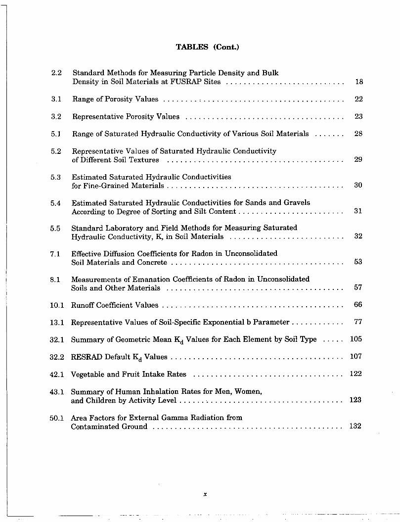
2.2 Standard Methods for Measuring Particle Density and Bulk Density in Soil Materials at FUSRAP Sites . . . . . . . . . . . . . . . . . . . . . . . . . . . 18

3.1 Range of Porosity Values . . . . . . . . : . . . . . . . . . . . . . . . . . . . . . . . . . . . . . . . . 22

3.2 Representative Porosity Values . . . . . . . . . . . . . . . . . . . . . . . . . . . . . . . . . . . . 23

5.1 Range of Saturated Hydraulic Conductivity of Various Soil Materials . . . . . . . 28

5.2 Representative Values of Saturated Hydraulic Conductivity of Different Soil Textures . . . . . . . . . . . . . . . . . . . . . . . . . . . . . . . . . . . . . . . . 29

5.3 Estimated Saturated Hydraulic Conductivities for Fine-Grained Materials . . . . . . . . . . . . . . . . . . . . . . . . . . . . . . . . . . . . . . . . 30

5.4 Estimated Saturated Hydraulic Conductivities for Sands and Gravels According to Degree of Sorting and Silt Content . . . . . . . . . . . . . . . . . . . . . . . . 31

5.5 Standard Laboratory and Field Methods for Measuring Saturated Hydraulic Conductivity. K, in Soil Materials . . . . . . . . . . . . . . . . . . . . . . . . . . 32

7.1 Effective Diffusion Coefficients for Radon in Unconsolidated Soil Materials and Concrete . . . . . . . . . . . . . . . . . . . . . . . . . . . . . . . . . . . . . . . 53

8.1 Measurements of Emanation Coefficients of Radon in Unconsolidated Soils and Other Materials . . . . . . . . . . . . . . . . . . . . . . . . . . . . . . . . . . . . . . . . 57

10.1 Runoff Coefficient Values . . . . . . . . . . . . . . . . . . . . . . . . . . . . . . . . . . . . . . . . . 66

13.1 Representative Values of Soil-Specific Exponential b Parameter . . . . . . . . . . . . 77

32.1 Summary of Geometric Mean Kd Values for Each Element by Soil Type . . . . . 105

32.2 RESRAD Default Kd Values . . . . . . . . . . . . . . . . . . . . . . . . . . . . . . . . . . . . . . . 107

42.1 Vegetable and Fruit Intake Rates . . . . . . . . . . . . . . . . . . . . . . . . . . . . . . . . . . 122

43.1 Summary of Human Inhalation Rates for Men. Women. and Children by Activity Level ...................................... 123

50.1 Area Factors for External Gamma Radiation from Contaminated Ground . . . . . . . . . . . . . . . . . . . . . . . . . . . . . . . . . . . . . . . . . . . 132

X

.................... . . . . . __.__ -. . -~ . ~ -~ . . ~ . ~~ _ _ . _ _

ACKNOWLEDGMENTS

The authors would like to thank Andrew Wallo 111, W. Alexander Williams, and Harold Peterson, Jr., of the US. Department of Energy for providing guidance, encouragement, discussion, and comments during the preparation of this report. We would also like to thank the following people for reviewing the draft report: Donald L. Mackenzie and Gary Hartman of the U.S. Department of Energy; Richard Swaja of Oak Ridge National Laboratory; John Russell of Booz-Allen & Hamilton, Inc.; YuChien Yuan of Square Y Consultants; and Shih-Yew Chen, Cheong-Yip R. Yuen, and Stephen C.L. Yin of Argonne National Laboratory. Finally, we thank Patricia Hollopeter for editorial assistance and the Information and Publishing Division Document Processing Center for document preparation.

xi

NOTATION

The following is a list of acronyms, initialisms, and abbreviations (including units of measure) used in this document.

ACRONYMS, INITIALISMS, AND ABBREVIATIONS

ANL ASTM DCG DOA DOE DO1 EPA FUSRAP ICRP LLD NAS NCI NMFS NOAA NRC scs TCDD USDA USLE

Argonne National Laboratory American Society for Testing and Materials derived concentration guide U.S. Department of the Army U.S. Department of Energy U.S. Department of the Interior U.S. Environmental Protection Agency Formerly Utilized Sites Remedial Action Program International Commission on Radiological Protection lower limit of detection National Academy of Sciences National Cancer Institute National Marine Fisheries Service National Oceanic and Atmospheric Administration U.S. Nuclear Regulatory Commission U.S. Soil Conservation Service tetrachlorodibenzo-p-dioxin U.S. Department of Agriculture Universal Soil Loss Equation

UNITS OF MEASURE

"C cm cm3 d R2

1 12 -

13 L lb

' M

degree(s) Celsius centime ter(s) cubic centimeteds) day(s) square foot (feet) g r a d s ) gallon(s1 houds) inch(es) kiloelectron volt(s) kilogram(s) square kilome teds) length length squared length cubed liteds) pound(s1 mass

m m2 m3 mi mi2 mm mol mrem mSv pCi

T V yr

S

xii

meteds) square meter(s) cubic meteds) mile(s) square mile(s) millimeteds) mole(s) milliremb) millisievert(s) picocurie(s) second(s) time volume yeads)

1

DATA COLLECTION HANDBOOK TO SUPPORT MODELING THE IMPACTS OF RADIOACTrVE

MATERIAL IN SOIL

C. Yu, C. Loureiro, J.J. Cheng, L.G. Jones, Y.Y. Wang, Y.P. Chia, and E. Faillace

ABSTRACT

A pathway analysis computer code called RESRAD has been developed for implementing U.S. Department of Energy Residual Radioactive Material Guidelines. Hydrogeological, meteorological, geochemical, geometrical (size, area, depth), and material-related (soil, concrete) parameters are used in the RESRAD code. This handbook discusses parameter definitions, typical ranges, variations, measurement methodologies, and input screen locations. Although this handbook was developed primarily to support the application of RESRAD, the discussions and values are valid for other model applications.

1 INTRODUCTION

In support of the U.S. Department of Energy (DOE) Order establishing residual radioactive material guidelines (DOE Order 5400.5), Argonne National Laboratory (ANL) developed a computer program called RESRAD (Gilbert et al. 1989). The models used by ANL to develop RESRAD were initially developed as part of a DOE-wide effort that began in the early 1980s and involved most of the national laboratories and DOE program offices. The DOE and other agencies and their contractors use the RESRAD program and its manual to derive cleanup criteria and dose calculations. Since its first release in June 1989, many new features and pathways have been added to the RESFLAD code. The DOE Offices of Environmental Guidance and Environmental Restoration provide periodic guidance regarding any significant changes to the code and manual. The purpose of this handbook is to give RESRAD users guidance on gathering, evaluating, and selecting input data for the RESRAD code.

The RESRAD code is a user-friendly, multiple pathways analysis code designed to be run on IBM-compatible personal computers. It was developed for use by radiological health physicists and environmental engineers for the calculation of radiation dose and risk resulting from exposure to residual radioactive material.

A sensitivity analysis of RESRAD parameters was conducted at ANL in 1991; the results for a generic run are presented in RESRAD Parameter Sensitivity Analysis

2 I

I

(Cheng et al. 1991). In general, parameters associated with the cover material or the contaminated zone influence results more than parameters associated with the unsaturated or saturated zone before the breakthrough time of the groundwater contamination.* The influence of these parameters changes, however, after the breakthrough time. The sensitivities of parameters involved in the leaching process have opposite effects on the total dose before and after the rise time.t

A built-in sensitivity analysis capability has been added to the RESRAD code. This capability gives users an easy way of studying RESRAD parameter sensitivity. Users are referred to the revised RESRAD Manual for Implementing Residual Radioactive Material Guidelines (Yu et al. 1993) and RESRAD Parameter Sensitivity Analysis (Cheng et al. 1991) for a description of and guidance on using this enhanced feature of the RESRAD code.

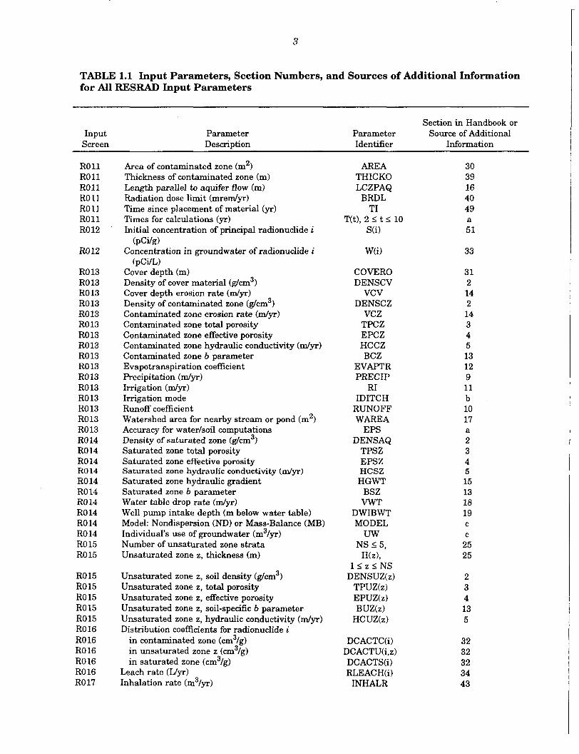
Fifty-one parameters are discussed in this handbook. Table 1.1 lists the RESRAD input parameters in the order of the RESRAD input screens and the sections of this handbook in which the parameters are discussed. For parameters not discussed in this handbook, users are referred to other sources (Table 1.1). Table 1.2 lists the applicable pathways and the data input screen locations for RESRAD input parameters.

This handbook provides the definition, typical range, default value used in RESRAD, relation to other parameters, and measurement methodology for most of the measurable parameters. Table 1.3 lists the default values and the lower and upper bounds set in the RESRAD code for each parameter used in the code. The intent of this handbook is to provide users with a better understanding of each input parameter in terms of its typical range, variation, and use in the RESRAD code.

The default parameter values listed in Table 1.3 have been carefully selected and are realistic, although conservative, parameter values. (In most cases, use of these values will not result in underestimation of the dose or risk.) Site-specific parameters should always be used whenever possible. Therefore, use of default values that significantly overestimate the dose or risk for a particular site is discouraged.

* Breakthrough time is the amount of time it takes contaminants to be transported through the unsaturated zone and reach the water table.

Rise time is the time for the contaminants to reach the maximum concentration in well water.

I

3

TABLE 1.1 Input Parameters, Section Numbers, and Sources of Additional Information for All RESRAD Input Parameters

Input Screen

Parameter DescriDtion

Section in Handbook or Parameter Source of Additional Identifier Information

R o l l R o l l R o l l R o l l R o l l R o l l RO 12

RO 12

RO 13 RO 13 RO 13 RO 13 RO 13 RO 13 RO 13 RO 13 RO 13 RO 13 RO 13 RO 13 RO 13 RO 13 RO 13 RO 13 RO 14 RO 14 RO 14 RO 14 RO 14 RO 14 R014 RO 14 RO 14 RO 14 RO 15 RO 15

RO 15 RO 15 RO 15 RO 15 RO 15 RO 16 RO 16 RO 16 RO 16 RO 16 RO 17

2 Area of contaminated zone (m ) Thickness of contaminated zone (m) Length parallel to aquifer flow (m) Radiation dose limit (mrem/yr) Time since placement of material (yr) Times for calculations (yr) Initial concentration of principal radionuclide i

Concentration in groundwater of radionuclide i

Cover depth (m) Density of cover material (g/cm3) Cover depth erosion rate ( d y r ) '

Density of contaminated zone (g/cm3) Contaminated zone erosion rate (m/yr> Contaminated zone total porosity Contaminated zone effective porosity Contaminated zone hydraulic conductivity (m/yr) Contaminated zone b parameter Evapotranspiration coefficient Precipitation (m/yr) Irrigation ( d y r ) Irrigation mode Runoff coefficient Watershed area €or nearby stream or pond (m2) Accuracy for watedsoil computations Density of saturated zone (g/cm3) Saturated zone total porosity Saturated zone effective porosity Saturated zone hydraulic conductivity ( d y r ) Saturated zone hydraulic gradient Saturated zone b parameter Water table drop rate (m/yr) Well pump intake depth (m below water table) Model: Nondispersion (ND) or Mass-Balance (MB) Individual's use of groundwater (m3/yr) Number of unsaturated zone strata Unsaturated zone z, thickness (m)

tpCi/g)

(pCi/L)

Unsaturated zone z, soil density (g/cm3) Unsaturated zone z, total porosity Unsaturated zone z, effective porosity Unsaturated zone z, soil-specific b parameter Unsaturated zone z, hydraulic conductivity (m/yr) Distribution coefficients for radionuclide i

in contaminated zone (cm3/g) in unsaturated zone z (cm3/g) in saturated zone (cm3/g)

Leach rate Inhalation rate (m3/yr)

AREA THICK0 LCZPAQ

BRDL TI

T(t), 2 I t I 10 S(i)

COVER0 DENSCV

vcv DENSCZ

vcz TPCZ EPCZ HCCZ BCZ

E V m R PRECIP

RI IDITCH

RUNOFF WAREA

EPS DENSAQ

TPSZ EPSZ HCSZ HGWT

BSZ VWT

DWIBWT MODEL

uw NS 1 5 ,

H(z), 1 1 z I N S

DENSUZ(z) TPUZ(z) EPUZ(z) BUZ(z)

HCUZ(z)

DCACTC(i) DCACTU(i,z) DCACTS(i) RLEACHG)

INHALR

30 39 16 40 49 a 51

33

31 2 14 2 14 3 4 5 13 12 9 11 b 10 17 a 2 3 4 5 15 13 18 19 C

C

25 25

2 3 4 13 5

32 32 32 34 43

4

TABLE 1.1 (Cont.)

Section in Handbook Input Parameter Parameter or Source of Additional

Screen Description Identifier Information

RO 17 RO 17 RO 17 RO 17 RO 17 RO 17 RO 17 RO 17 RO 17

RO 18 RO 18 RO 18 RO 18 RO 18 RO 18 RO 18 RO 18 RO 18 RO 18 RO 19 RO 19 RO 19 RO 19 RO 19 RO 19 RO 19 RO 19 RO 19 RO 19 R021 R021 R021 R021 R02 1 R021 R021 R021 R021 R021 R021 R02 1 R021 R021 R02 1 R02 1 R021 R021

Mass loading for inhalation (g/m3) Dilution length for airborne dust (m) Exposure duration Shielding factor, inhalation Shielding factor, external gamma Fraction of time spent indoors on-site Fraction of time spent outdoors on-site Shape factor, external gamma Fractions of annular areas within AREA

Fruit, vegetable, and grain consumption (kglyr) Leafy vegetable consumption (kglyr) Milk consumption (Uyr) Meat and poultry consumption &g/yr) Fish consumption (kglyr) Other seafood consumption &g/yr) Soil ingestion rate (glyr) Drinking water intake (Llyr) Fraction of drinking water from site Fraction of aquatic food from site Livestock fodder intake for meat (kg/d) Livestock fodder intake for milk (kg/d) Livestock water intake for meat (Lld) Livestock water intake for milk (Lld) Mass loading for foliar deposition (g/m3) Depth of soil mixing layer (m) Depth of roots (m) Drinking water fraction from groundwater Livestock water fraction from groundwater Irrigation fraction from groundwater Thickness of building foundation (m) Bulk density of building foundation (g/cm3) Total porosity of the cover material Total porosity of the building foundation Volumetric water content of the cover material Volumetric water content of the foundation Diffi ion coefficient for radon gas (m2/s):

in cover material in foundation material in contaminated zone soil

Radon vertical dimension of mixing (m) Average annual wind speed ( d s ) Average building air exchange rate (lh) Height of the building (room) (m) Building interior area factor Building depth below ground surface (m) Emanating power of radon-222 gas

MLINH LM ED

SHF3 SHFl FIND FOTD FS 1

FRACA(r) l S r S 1 2 DIET( 1) DIET(2) DIET(3) DIET(4) DIET(5) DIET(6)

SOIL DWI FDW FR9 LF15 LFI6 LWI5 LWI6 MLFD

DM DROOT FGWDW FGWLW FGWIR FLOOR

DENSFL TPCV TPFL

PH2OCV PH20FL

DIFCV DIFFL DIFCZ HMIX WIND REXG HRM FAI

DMFL EMANA( 1)

35 d

a,e 36 48

28,e 29,e 50 50

42 44 47 46 41 41 38 52 a a b b 45 45 b,f 35,f

b, c b, c b, c 26 2 3 3 6 6

7 7 7

20 21 22 23 24 27 8

37

Emanating power of radon-220 gas EMANA(2) 8

Sources: a Yu et al. (1993), Section 4; Appendix E;d Yu et al. (1993), Appendix B; e EPA (1990a1, Part I; and

Yu et al. (19931, Appendix D; Yu et al. (1993), Gilbert et al. (1983).

TABLE 1.2 Applicable Pathways and Data Input Screen Locations for RESRAD Input Parameters

Pathwavs

External Plant Meat Milk Aquatic Drinking Soil Input Parameter Gamma Inhalation Ingestion Ingestion Ingestion Foods Water Radon Ingestion Screen

Soil density Cover material Contaminated zone Unsaturated zone Saturated zone Building foundation material

used used used used

used used used used

a

used used used

used used used

used used used

used used used

used

used

used used used

used used used

used used used

used used used

used

used

used used used

used used used

used used used

used used used

used

used

used used used used used


used

used used used

used used

used used used

used

used

used

used

used

used

used

used

used

R013 R013 R015 R014 R021

R02 1 R013 R015 R014 R021

R013 R015 R014

R013 R015 R014

R021 R021

R021 R02 1 R021

R02 1

R013

R013

Total porosity Cover material Contaminated zone Unsaturated zone Saturated zone Building foundation material


used used used

Effective porosity Contaminated zone Unsaturated zone Saturated zone


used used used

Hydraulic conductivity Contaminated zone Unsaturated zone Saturated zone


used used used

Volumetric water content Cover material Building foundation material

Effective radon diffusion coefficient Cover material Contaminated zone Building foundation material

Radon emanation coefficient

used

used

Precipitation rate used used

used used

used

used Runoff coefilcient

TABLE 1.2 (Cont.)

Pathways


Irrigation rate

Evapotranspiration coefficient

Soil-specific b parameter Contaminated zone Unsaturated zone Saturated zone

Erosion rate Cover material Contaminated zone

Hydraulic gradient

Length of contaminated zone parallel to the aquifer flow

Watershed area for nearby stream or pond

Water table drop rate

Well-pump intake depth

Radon vertical dimension of mixing

Average annual wind speed

Average building air exchange rate

Building room height

Building indoor area factor

Thickness of uncontaminated unsaturated zone

used

used

used

used used

used used

used used

used used used used

used used used used

used

used

used

used

used

used

used

used

used used used

used used

used

used

used

used

used

used

used

used

used used used

used used

used

used

used

used

used

used

used

used

used used used

used used

used

used

used

used

used

used

used

used

used used used

used used

used

used

used

used

used

used

used

used

used used used

used used

used

used

used

used

used

used

used

used

used

used

used

used

used

used

used used

R013

R013

R013 R015 R014

R013 R013

R014

R011

R013

R014

R014

R02 1

R02 1

R021

R02 1

R02 1

R015

TABLE 1.2 (Cont.)

Pathways


Building foundation thickness

Foundation depth below ground surface

Fraction of time spent indoors on-site

Fraction of time spent outdoors on-site

Area of contaminated zone

Cover depth

Distribution coefficients

Fractions of annular areas within contaminated area

Radionuclide concentration in groundwater

Leach rate

Livestock fodder intake Meat Milk

Mass loading for inhalation

Milk consumption rate

Shielding factor for inhalation

Depth of roots

Soil ingestion rate

used

used

used

used

used

used

used

used

used

used

used

used

used

used

used

used

used

used

used

used

used

used

used

used

used

used

used

used

used

used

used

used

used

used

used

used

used

used

used

used

used

used

used

used

used

used

used

used

used

used

used

used

used

used

used

used

used

used

used

used

used

used

used

used

used

R02 1

R02 1

R017

R017

R o l l

R013

R016

R017

R012

R016

R019 R019

R017

R018

R017

R019

R018

TABLE 1.2 (Cont.)

Pathwavs

Parameter External Plant Meat Milk Aquatic Drinking Soil Input Gamma Inhalation Ingestion Ingestion Ingestion Foods Water Radon Ingestion Screen

Thickness of contaminated zone

Radiation dose limit

Dilution length for airborne dust

Seafood consumption rate

Fruit, vegetable, and grain consumption rates

Inhalation rate

Leafy vegetable consumption rate

Livestock water intake rate Meat Milk

Meat and poultry consumption rate

Shielding factor for external gamma radiation

Elapsed time of waste placement

Shape factor, external gamma

Initial concentrations of principal radionuclide

Drinking water intake rate

Fraction of drinking water from site

Fraction of aquatic food from site

Mass loading for foliar deposition

used

used

used

used

used

used

used

used

used

used

used

used

used used

used used

used used

used

used

used

used

used

used

used

used

used

used

used

used

used

used

used

used

used

used

used

used

used

used

used

used

used

used

used

used

used

used

used

used

used

used

used

used

used

used

R o l l

R o l l

R017

R018

R018

R017

R018

R019 R019

R018

R017

R o l l

R017

R012

R018

R018

R018

R019

I

TABLE 1.2 (Cont.)

Pathways

Parameter External Plant Meat Milk Aquatic Drinking Soil Input Gamma Inhalation Ingestion Ingestion Ingestion Foods Water Radon Ingestion Screen

~~~~~~~~~~~~ ~~~~~

Depth of soil mixing layer used used used R019

Fraction from groundwater Drinking water used R019 Livestock water used used R019 Irrigation water used R019

A hyphen indicates that the parameter is not used in the pathway calculations. a

10

TABLE 1.3 Default Values, Lower Bounds, and Upper Bounds for RESRAD Input Parameters

Parameter Default Lower' Uppera

Unit Value Bound Bound

Soil bulk density Cover material Contaminated zone Unsaturated zone Saturated zone Building foundation material

Total porosity Cover material Contaminated zone Unsaturated zone Saturated zone Building foundation materid

Effective porosity Contaminated zone Saturated zone Unsaturated zone

Hydraulic conductivity Contaminated zone Unsaturated zone Saturated zone

Volumetric water content Cover material Building foundation material

Effective radon diffusion coefficient Cover material Contaminated zone Building foundation material

Radon emanation coefficient (Rn-222/Rn-220)

Precipitation rate

Runoff coefficient

Irrigation rate

Evapotranspiration coefficient

Soil-specific b parameter Contaminated zone Unsaturated zone Saturated zone

Erosion rate Cover material Contaminated zone

Hydraulic gradient

Length of contaminated zone parallel to the aquifer flow

g/cm3 g/cm3 g/cm3 g/cm3 glcrn3

-b

dyr mlyr &Yr

m2ls m2/s m2/s

dy r

dy r

m/yr mJyr

m

1.5 1.5 1.5 1.5 2.4

.4

.4

.4

.4

.1

.2

.2

.2

10 10 100

0.05 0.03

2 x 10" 2 x 106 3 io-'

0.2510.15

1

0.2

0.2

0.5

5.3 5.3 5.3

0.001 0.001

0.02

100

0 0 0 0 0

0 0 0 0 0

0 0 0

0 0 0

0 0

C

C

C

0.01

0

0

0

0

0 0 0

0 0

0

0

100 100 100 100 100

1 1 1 1 1

1 1 1

1 x 10'0 1 x 1010 1 x 10'0

1 1

1 1 1

1

10

1

10

0.999

15 15 15

5 5

10

oc

. - . . . . . - .

11

TABLE 1.3 (Cont.)

Parameter Default Lowera Uppera


Watershed area for nearby stream or pond

Water table drop rate

Well-pump intake depth

Radon vertical dimension of mixing

Average annual wind speed

Average building air exchange rate

Building room height

Building indoor area factor

Thickness of uncontaminated unsaturated zone

Building foundation thickness

Foundation depth below ground surface

Fraction of time spent indoors on-site

Fraction of time spent outdoors on-site

Area of contaminated zone

Cover depth

Distribution coefficients

Fractions of annular areas within contaminated area

Radionuclide concentration in groundwater

Leach rate

Livestock fodder intake Meat Milk

Mass loading for inhalation

Milk consumption rate

Shielding factor for inhalation

Depth of roots

Soil ingestion rate

m2

dyr

m

m

d S

l/h

m

m

m

m

m2

m

cm3/g

pciiL

UYr

kg/d kg/d

g/m3

UYr

m

g/yr

1 x 106

0.001

10

2

2

0.5

2.5

0

4

0.15

1

0.5

0.25

10,000

0

d

0

0

0

68 55

2 10.4

92

0.4

0.9

36.5

0

0

0

0

0

0

0

0

0

0

0

0

0

0

0

0

0

0

0

0 0

0

0

0

0

0

oi

5

1,000

1,000

100

1,000

100

100

10,000

10

100

1

1

oc

100

1 x 10'0

1

1 x 1020

1 x 10'0

300 300

2

1,000

1

100

10,000

12

TABLE 1.3 (Cont.)

Parameter Default Lowera Uppera


Thickness of contaminated zone

Radiation dose limit

Dilution length for airborne dust

Seafood consumption rate Fish Other seafood

Fruit, vegetable, and grain consumption rates

Inhalation rate

Leafy vegetable consumption rate

Livestock water intake rate Meat Milk

Meat and poultry consumption rate

Shielding factor for external gamma

Elapsed time of waste placement

Shape factor, external gamma

Initial concentrations of principal radionuclide

Drinking water intake rate

Fraction of drinking water from site

Fraction of aquatic food from site

Mass loading for foliar deposition

Depth of soil mixing layer

Fraction from groundwater Drinking water Livestock water Irrigation water

2

30

3

5.4 0.9

160

8,400

14

50 160

63

0.7

0

1

d

510

1

0.5

1

0.15

1 1 1

1 x 10-10 1,000

0.01

0

0 0

0

0

0

0 0

0

0

0

OC

0

0

0

0

0

0

0 0 0

10,000

1,000

1,000 100

1,000

20,000

100

500 500

300

1

1,000

1

1 x 1020

1,000

1

1

1

1

1 1 1

The lower and upper bound values represent the lower and upper limit of an input parameter that can be used in RESRAD. For some secondary (derived) parameters (e.g., leach rate), the upper and lower bounds are derived from other primary (basic) parameters (e.g., thickness of contaminated zone).

A hyphen indicates that the parameter is dimensionless.

A negative value for this parameter serves as a flag in RESRAD. See the section in the handbook on the particular parameter for details.

The default value is radionuclide dependent.

13

2 SOILDENSITY

2.1 DEFINITION

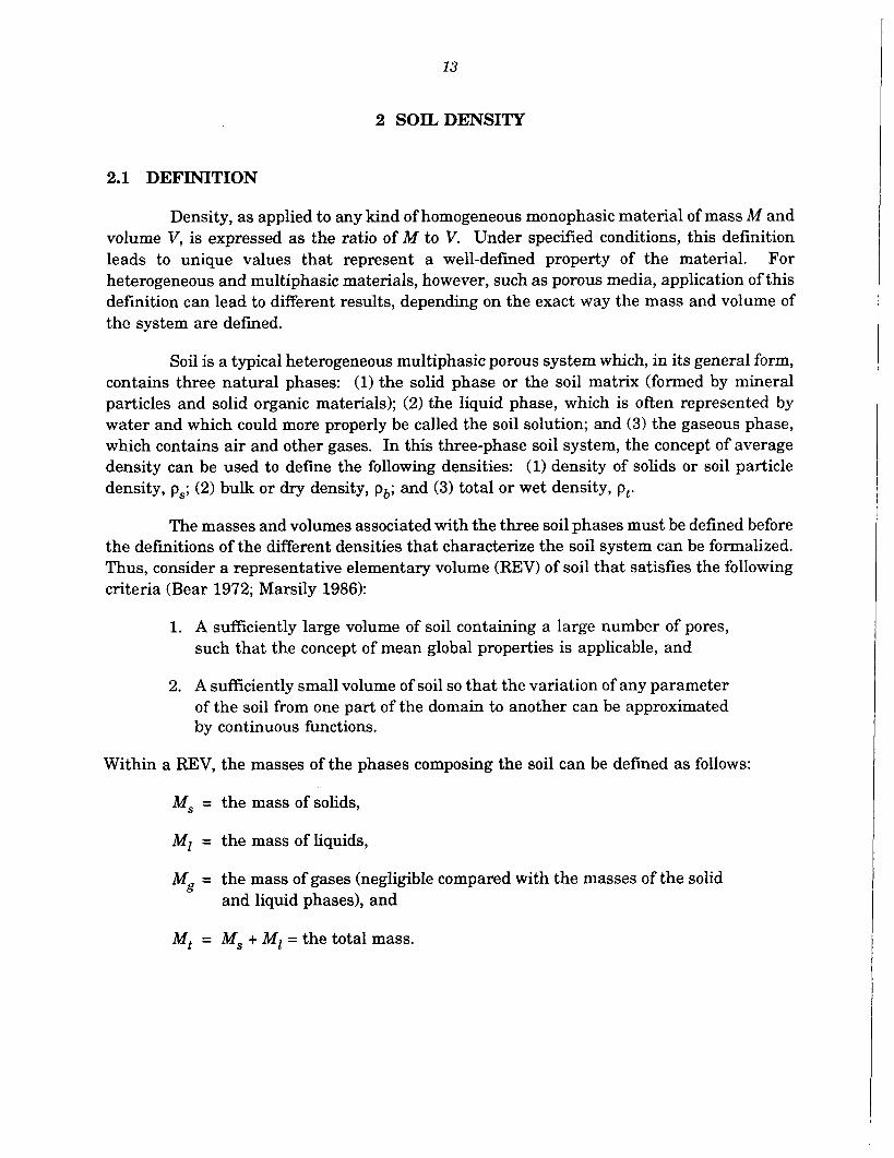
Density, as applied to any kind of homogeneous monophasic material of mass M and volume V, is expressed as the ratio of M to V. Under specified conditions, this definition leads to unique values that represent a well-defined property of the material. For heterogeneous and multiphasic materials, however, such as porous media, application of this definition can lead to different results, depending on the exact way the mass and volume of the system are defined.

Soil is a typical heterogeneous multiphasic porous system which, in its general form, contains three natural phases: (1) the solid phase or the soil matrix (formed by mineral particles and solid organic materials); (2) the liquid phase, which is often represented by water and which could more properly be called the soil solution; and (3) the gaseous phase, which contains air and other gases. In this three-phase soil system, the concept of average density can be used to define the following densities: (1) density of solids or soil particle density, p,; (2) bulk or dry density, pb; and (3) total or wet density, p t .

The masses and volumes associated with the three soil phases must be defined before the definitions of the different densities that characterize the soil system can be formalized. Thus, consider a representative elementary volume (REV) of soil that satisfies the following criteria (Bear 1972; Marsily 1986):

1. A sufficiently large volume of soil containing a large number of pores, such that the concept of mean global properties is applicable, and

2. A sufficiently small volume of soil so that the variation of any parameter of the soil from one part of the domain to another can be approximated by continuous functions.

Within a REV, the masses of the phases composing the soil can be defined as follows:

Ms = the mass of solids,

M z = the mass of liquids,

Mg = the mass of gases (negligible compared with the masses of the solid and liquid phases), and

Mt = M, + Mz = the total mass.

1 I

14

Similarly, within the REV, the volumes associated with the soil phases can be defined as follows:

Vs = the volume of solids,

Vl = the volume of liquids,

Vg = the volume of gases,

Vp = V, + Vg = the volume of pore space, and

Vt = Vs + V, + V' = the total volume.

These mass and volume definitions can be used to define the concepts of soil particle density, bulk (dry) soil density, and total (wet) soil density. The dimensional unit of soil density is mass per unit of cubic length (MT~) .

2.1.1 Soil Particle, Density

The soil particle density, ps, or the density of solids, represents the density of the soil (i.e., mineral) particles collectively and is expressed as the ratio of the solid phase mass to the volume of the solid phase of the soil. Soil particle density is defined as follows:

In most mineral soils, the soil particle density has a short range of 2.6-2.7 g/cm3 (Hillel 1980b). This density is close to that of quartz, which is usually the predominant constituent of sandy soils. A typical value of 2.65 gkm3 has been suggested to characterize the soil particle density of a general mineral soil (Freeze and Cherry 1979). Aluminosilicate clay minerals have particle density variations in the same range. The presence of iron oxides and other heavy minerals increases the value of the soil particle density. The presence of solid organic materials in the soil decreases the value.

2.1.2 Bulk (Dry) Density

The soil bulk or dry density, pb, is the ratio of the mass of the solid phase of the soil (i.e., dried soil) to its total volume (solid and pore volumes together) and is defined as follows:

15

The bulk density, p b , is related to the soil particle density, p,, by the total soil porosity, pt, according to the following equation:

where 1-p, is the ratio of the solid volume (V, ) to the total volume (Vl + Vg + V, 1. Section 3 discusses total porosity.

From the above definition, it should be obvious that the value of the dry density is always smaller than the value of the soil particle density. For example, if the volume of the pores (Vl + V' 1 occupies half of the total volume, the value of dry density is half the value of the soil particle density.

The dry density of most soils varies within the range of 1.1-1.6 g/cm3. In sandy soils, dry density can be as high as 1.6 g/cm3; in clayey soils and aggregated loams, it can be as low as 1.1 g/cm3 (Hillel 1980b). Because of its high degree of aggregation (i.e., small total porosity), concrete has, in general, a higher dry density than soil. Typical values of dry density in different types of soils and in concrete are shown in Table 2.1. Dry density depends on the structure of the soil matrix (or its degree of compaction or looseness) and on the soil matrix's swelling/shrinkage characteristics.

To use Table 2.1 to estimate dry bulk density (or any other soil properties discussed in this handbook), the user needs to know the soil texture type. The common method used in the field to classify a soil is the "feel" method (Brady 1984). This method consists of merely rubbing the soil between the thumb and fmgers. Usually it is helpful to wet the sample to estimate plasticity more accurately. The way a wet soil "slicks out," that is, develops a continuous ribbon when pressed between the thumb and fingers, gives a good idea of the amount of clay present. The slicker the wet soil, the higher the clay content. The sand particles are gritty, and the silt has a floury or talcum-powder feel when dry and is only slightly plastic and sticky when wet. Persistent cloddiness is generally the result of the presence of silt and clay. The accuracy of the feel method depends largely on experience. The laboratory method is more accurate but is time-consuming. The laboratory method to classifj. soil involves particle-size analysis, in which sieves are usually employed for coarser particles and the rate of settling in water for finer particles (Marshall and Holmes 1979). The U.S. Department of Agriculture (USDA) has developed a method for naming soils on the basis of particle-size analysis. The relationship between such an analysis and soil class names is shown diagrammatically in Figure 2.1. The legend in the figure explains the use of this soil texture triangle.

16

2.1.3 Total (Wet) Density TABLE 2.1 Typical Values of Dry Density of Various Soil Types and Concrete The total, or wet, density of soil, pt, is the

ratio of the total mass of soil to its total volume and can be defined as follows: Dry Density, pb

Soil Type (g/cm3)

Sand 1.52 Sandy loam 1.44 Loam 1.36 Silt loam 1.28 Clay loam 1.28

Pt = - Mt - - M, +ML (2.4) vt v, 4- Vl 4- vg *

Total density differs from dry density in that it is strongly dependent on the moisture content of the soil. For a dry soil, total density approximates the value of dry density. Concrete 2.40

Clay 1.20

Note: The dry density of most soils varies within the range of 1.1-1.6 g/cm3 (Hillel 1980b).

2.2 MEASUREMENT METHODOLOGY

For use in RESRAD, only the dry densities of five distinct materials (cover layer, contaminated zone, unsaturated and saturated

- Sources: Linsley et al. (1982); Poffijn (1988).

zones, and building foundation material) are needed as input parameters. However, because information on both soil particle and bulk (i.e., dry) density is required for the calculation of total porosity of the soil material, descriptions of the techniques and procedures for measuring both types of densities follow.

The standard methods used on Formerly Utilized Sites Remedial Action Program (FUSRAP) sites for determining the particle density and the dry density in soil materials are those prepared by the American Society of Testing Materials (ASTM 1992a-o) and the U.S. Department of the Army (DOA 1970), as listed in Table 2.2. A general discussion on these measurement methodologies is also presented in Blake and Hartge (1986a,b).

2.2.1 Soil Particle Density Measurement

The soil particle density of a soil sample is calculated on the basis of the measurement of two quantities: (1) M,, the mass of the solid phase of the sample (dried mass) and (2) Vs, the volume of the solid phase (Blake and Hartge 198613). Assuming that water is the only volatile in a soil sample, the mass (M,) can be obtained by drying the sample (usually at 110 * 5°C) until it reaches a constant weight, Ws. This method may not be valid for organic soils or soils with asphalt.

The solid phase volume, Vs, can be measured in different ways. One way is to measure the volume directly by observing the resulting increase in the volume of water as the sample of dried soil is introduced into a graduated flask that initially contains pure water (or another liquid). After making sure that the soiYwater mixture is free from air bubbles,

17

+ Percent sand

FIGURE 2.1 U.S. Department of Agriculture Method for Naming Soils (Note: Percentage of sand, silt, and clay in the major soil textural classes. To use the diagram, locate the percentage of clay first and project inward as shown by the arrow. Do the same for the percentage of silt [or sand]. The point at which the two projections cross will identify the class name.) (Source: Brady 1984)

the observed expansion in volume (i.e., the replaced volume of water) should be equal to Vs, the solid phase volume. The problem with this approach is that the techniques used to eliminate air bubbles from the mixture (such as heating) can also disturb the total volume and thus introduce errors into the calculations.

Another way to measure the solid phase volume (V,) is based on evaluating the mass and density of water (or another fluid) displaced by the sample (after being oven-dried). This second approach has been used for quite some time and is simple, direct, and accurate

18

TABLE 2.2 Standard Methods for Measuring Particle Density and Bulk (Dry) Density in Soil Materials at F'USRAP Sites

Parameter Type of Measured Measurement Standard Test Method Reference

Soil Soil sample particle testing density

Appendix Tv: Specific Gravity

ASTM D 854-91: Standard Test Method for Specific Gravity of Soils

Bulk (dry) Soil sample soil testing density

Appendix I 1 Unit Weights, Void Ratio, Porosity, and Degree of Saturation

In-situ near surface testing

In-situ below surface

ASTM D 1556: Standard Test Method for Density and Unit Weight of Soil in Place by the Sand-Cone Method

ASTM D 2167-84: Standard Test Method for Density and Unit Weight of Soil in Place by the Rubber Balloon Method

ASTM D 2922-91: Standard Test Methods for Density of Soil and Soil-Aggregate in Place by Nuclear Methods (shallow depth)

ASTM D 2937-83: Standard Test Method for Density of Soil in Place by the Drive-Cylinder Method

ASTM D 4564-86: Standard Test Method for Density of Soil in Place by the Sleeve Method

ASTM D 5195-91: Standard Test Method for Density of Soil and Rock In-Place at Depths below the Surface

DOA (1970)

ASTM (1992a)

DOA (1970)

ASTM (1992b)

ASTM (1992d)

ASTM (1992g)

ASTM (1992h)

ASTM (1992k)

ASTM (1992x1)

testing by Nuclear Methods

if done carefully (Blake and Hartge 1986a). It is based on the fact that if v d w , the volume of water displaced by the solids, is equal to V s , then

and

Ms Ps = Pw- 9

Mdw (2.6)

where M d w is the mass of the displaced water and pw is the water density. Therefore, to obtain the soil particIe density, it is necessary to evaluate the water density at the specific

19

pressure and temperature conditions and to measure Ms and Mdw (DOA 1970, Appendix W, ASTM 1992a).

The value of Mdw is obtained by using a graduated volumetric flask and by takmg the following measurements:

Mf = mass of the empty flask;

Mfs = mass of the flask plus the dried soil sample;

Mfsw = mass of the flask plus the soil and filled with water up to a fixed volume, Vp and

M f i = mass of the flask filled with pure water up to the fixed volume Vf

The mass of the displaced water, Mdw can then be calculated as follows:

Substituting Mdw into the expression for soil particle density, ps, yields

r 1

This method is very precise, but it requires careful measuring of volumes and masses and consideration of the effects of pressure and temperature conditions on the water density. Possible errors can result not only from determining the masses and volumes but from nonrepresentative sampling.

2.2.2 Dry Density Measurement

The dry (bulk) density ( p b ) of a soil sample is evaluated on the basis of two measured values: (1) Ms, the oven-dried mass of the sample and (2) Vt, the field volume or the total volume of the sample. As stated previously, for the calculation of soil particle density (p,), mass (M,) is measured after drying the sample at 110 * 5 "C until a near constant weight is reached. This laboratory technique directly determines the dry density of a soil sample (DOA 1970, Appendix 11). Possible direct methods of measuring the dry density include the core and excavation methods, which essentially consist of drying and weighing a known volume of soil.

Variations of these methods are related to different ways of collecting the soil sample and measuring volume. In the core method (Blake and Hartge 1986a; ASTM 1992h), a cylindrically shaped metal sampler is introduced into the soil, with care to avoid disturbing

20

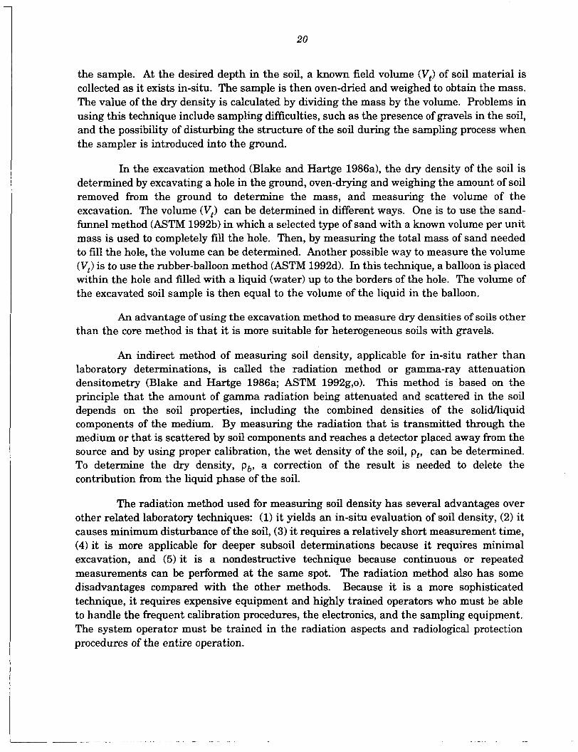
the sample. At the desired depth in the soil, a known field volume (V,) of soil material is collected as it exists in-situ. The sample is then oven-dried and weighed to obtain the mass. The value of the dry density is calculated by dividing the mass by the volume. Problems in using this technique include sampling difficulties, such as the presence of gravels in the soil, and the possibility of disturbing the structure of the soil during the sampling process when the sampler is introduced into the ground.

In the excavation method (Blake and Hartge 1986a), the dry density of the soil is determined by excavating a hole in the ground, oven-drying and weighing the amount of soil removed from the ground to determine the mass, and measuring the volume of the excavation. The volume (V,) can be determined in different ways. One is to use the sand- funnel method (ASTM 1992b) in which a selected type of sand with a known volume per unit mass is used to completely fill the hole. Then, by measuring the total mass of sand needed to fill the hole, the volume can be determined. Another possible way to measure the volume (V,) is to use the rubber-balloon method (ASTM 19928. In this technique, a balloon is placed within the hole and filled with a liquid (water) up to the borders of the hole. The volume of the excavated soil sample is then equal to the volume of the liquid in the balloon.

An advantage of using the excavation method to measure dry densities of soils other than the core method is that it is more suitable for heterogeneous soils with gravels.

An indirect method of measuring soil density, applicable for in-situ rather than laboratory determinations, is called the radiation method or gamma-ray attenuation densitometry (Blake and Hartge 1986a; ASTM 1992g,o). This method is based on the principle that the amount of gamma radiation being attenuated and scattered in the soil depends on the soil properties, including the combined densities of the solifliquid components of the medium. By measuring the radiation that is transmitted through the medium or that is scattered by soil components and reaches a detector placed away from the source and by using proper calibration, the wet density of the soil, p,, can be determined. To determine the dry density, pb, a correction of the result is needed to delete the contribution from the liquid phase of the soil.

The radiation method used for measuring soil density has several advantages over other related laboratory techniques: (1) it yields an in-situ evaluation of soil density, (2) it causes minimum disturbance of the soil, (3) it requires a relatively short measurement time, (4) it is more applicable for deeper subsoil determinations because it requires minimal excavation, and (5) it is a nondestructive technique because continuous or repeated measurements can be performed at the same spot. The radiation method also has some disadvantages compared with the other methods. Because it is a more sophisticated technique, it requires expensive equipment and highly trained operators who must be able to handle the frequent calibration procedures, the electronics, and the sampling equipment. The system operator must be trained in the radiation aspects and radiological protection procedures of the entire operation.

21

2.3 RESRAD DATA INPUT REQUIREMENTS

In RESRAD, one variable is assigned to represent the dry density, measured in units of grams per cubic centimeter, of each of the following five materials: (1) cover material, (2) contaminated zone, (3) unsaturated zone, (4) saturated zone, and (5) building foundation material (i.e., concrete). For the first four types of soil, a default value of 1.5 g/cm3 is assigned for the dry density, a value that is representative of a sandy soil. Although the building foundation material (i.e., concrete) has a solid phase density (i.e., particle density) similar to that of the soil, because of its small total porosity, concrete. has, in general, a higher dry density than soils. In RESRAD, a default value of 2.4 g/cm3 is assigned for the dry density of the foundation building material. This default value is provided for generic use of the RESRAD code. For more accurate use of the code, site-specific data should be used.

If the type of soil is known, then Table 2.1 can be used for a slightly more accurate determination of the input data values for dry density. If no information about the type of soils is available, however, then the values for dry density should be experimentally determined by using one of the methods described in Section 2.2.2.

22

3 TOTAL POROSITY

3.1 DEFINITION

The total porosity of a porous medium is the ratio of the pore volume to the total volume of a representative sample of the medium. Assuming that the soil system is composed of three phases - solid, liquid (water), and gas (air) - where Vs is the volume of the solid phase, V, is the volume of the liquid phase, Vg is the volume of the gaseous phase, Vp = VI + Vg is the volume of the pores, and Vt = Vs + Vl + V' is the total volume of the sample, then the total porosity of the soil sample, pt, is defined as follows:

Porosity is a dimensionless quantity and can be reported either as a decimal fraction or as a percentage. Table 3.1 lists representative total porosity ranges for various geologic materials. A more detailed list of representative porosity values (total and effective porosities) is provided in Table 3.2. In general, total porosity values for unconsolidated materials lie in the range of 0.25-0.7 (25%-70%). Coarse-textured soil materials such as gravel and sand tend to have a lower total porosity than fine-textured soils such as silts and clays. The total porosity in soils is not a constant quantity because the soil, particularly clayey soil, alternately swells, shrinks, compacts, and cracks.

TABLF: 3.1 Range of Porosity Values

Soil Type Porosity, p ,

Unconsolidated deposits Gravel 0.25 - 0.40 Sand 0.25 - 0.50 Silt 0.35 - 0.50 Clay 0.40 - 0.70

Rocks Fractured basalt 0.05 - 0.50 Karst limestone 0.05 - 0.50 Sandstone 0.05 - 0.30 Limes tone, dolomite 0.00 - 0.20 Shale 0.00 - 0.10 Fractured crystalline rock 0.00 - 0.10 Dense crystalline rock 0.00 - 0.05

Source: Freeze and Cherry (1979).

23

TABLE 3.2 Representative Porosity Values

Total Porosity, p t Effective Porosity,a p ,

Arithmetic Arithmetic Material Range Mean Range Mean

Sedimentary material Sandstone (fine) Sandstone (medium) Siltstone Sand (fine) Sand (medium) Sand (coarse) Gravel (fine) Gravel (medium) Gravel (coarse) Si1 t Clay Limestone

Wind-laid material Loess Eolian sand Tuff

Igneous rock Weathered granite Weathered gabbro Basalt

Metamorphic rock Schist

-b

0.14 - 0.49 0.21 - 0.41 0.25 - 0.53

0.31 - 0.46 0.25 - 0.38

0.24 - 0.36 0.34 - 0.51 0.34 - 0.57 0.07 - 0.56

0.34 - 0.57 0.42 - 0.45 0.03 - 0.35

0.04 - 0.49

0.34 0.35 0.43

0.39 0.34

0.28 0.45 0.42 0.30

0.45 0.43 0.17

0.38

0.02 - 0.40 0.12 - 0.41 0.01 - 0.33 0.01 - 0.46 0.16 - 0.46 0.18 - 0.43 0.13 - 0.40 0.17 - 0.44 0.13 - 0.25 0.01 - 0.39 0.01 - 0.18

-0 - 0.36

0.14 - 0.22 0.32 - 0.47 0.02 - 0.47

0.22 - 0.33

0.21 0.27 0.12 0.33 0.32 0.30 0.28 0.24 0.21 0.20 0.06 0.14

0.18 0.38 0.21

-

0.26

a Effective porosity is discussed in Section 4.

A hyphen indicates that no data are available.

Source: McWorter and Sunada (1977).


The standard method used on FUSRAP sites for determining the total porosity of soil materials is described in Appendix I1 of DOA (1970). Further discussion on this methodology is also presented in Danielson and Sutherland (1986).

On the basis of the definition of total porosity, a soil sample could be evaluated for total porosity by directly measuring the pore volume (V,) and the total volume (V,). The total volume is easily obtained by measuring the total volume of the sample. The pore volume can,

24

in principle, be evaluated directly by measuring the volume of water needed to completely saturate the sample. In practice, however, it is always difficult to saturate the soil sample exactly and completely and, therefore, the total porosity of the sample is rarely evaluated by a direct method. Usually, the total porosity is evaluated indirectly by using the following expression (DOA 1970, Appendix 11; Danielson and Sutherland 1986):

where p t is given as a decimal fraction, Vs is the soil particle volume, V, is the total volume, p, is the solid phase (soil particle) density, and pb is the dry bulk density of the sample. (Equation 3.2 can be obtained by rearranging Equation 2.3.) Under this approach, the values of ps and pb are evaluated by laboratory or in-situ measurements (Section 2.2) and are then used to calculate the total porosity p t .


To use RESRAD, the user is required to define or use the default values of the total porosity of five materials: (1) cover material, (2) contaminated zone, (3) unsaturated zone, (4) saturated zone, and (5) building foundation material (i.e., concrete). In RESRAD, the total porosities are entered as decimal fractions rather than as percentages. RESRAD adopts the following values as defaults: n = 0.4 for the first four materials listed above and n = 0.1 for the building foundation (i.e., concrete). These default values are provided for generic use of the RESRAD code. For more accurate use of the code, site-specific data should be used.

If site-specific data are not available and the type of soil is known, Tables 3.1 and 3.2 can be used for estimating total porosity. However, if no information is available on the type of soils, then the values for total porosity should be experimentally determined according to the method presented in Section 3.2.

4.1 DEFINITION

The effective porosity, pe, also called the kinematic porosity, of a porous medium is defined as the ratio of the part of the pore volume where the water can circulate to the total volume of a representative sample of the medium. In naturally porous systems such as subsurface soil, where the flow of water is caused by the composition of capillary, molecular, and gravitational forces, the effective porosity can be approximated by the specific yield, or drainage porosity, which is defined as the ratio of the volume of water drained by gravity from a saturated representative sample of the soil to the total volume of the sample.

The definition of effective (kinematic) porosity is linked to the concept of pore fluid displacement rather than to the percentage of the volume occupied by the pore spaces. The pore volume occupied by the pore fluid that can circulate through the porous medium is smaller than the total pore space, and, consequently, the effective porosity is always smaller than the total porosity. In a saturated soil system composed of two phases (solid and liquid) where (1) Vs is the volume of the solid phase, (2) Vw = (Vi, + Vmw) is the volume of the liquid phase, (3) Vi, is the volume of immobile pores containing the water adsorbed onto the soil particle surfaces and the water in the dead-end pores, (4) Vmw is the volume of the mobile pores containing water that is free to move through the saturated system, and (5) Vt = (V, + Vi, + V,,) is the total volume, the effective porosity can be defined as follows:

Another soil parameter related to the effective soil porosity is the field capacity, 8 , also called specific retention, irreducible volumetric water content, or residual water content, which is defined as the ratio of the volume of water retained in the soil sample, after all downward gravity drainage has ceased, to the total volume of the sample. Considering the terms presented above for a saturated soil system, the total porositypt and the field capacity 8, can be expressed, respectively, as follows:

and

e , = - . Viw vt

(4.3)

26

Therefore, the effective porosity is related to the total porosity and the field capacity according to the following expression:

p , = P t - Or * (4.4)

Several aspects of the soil system influence the value of its effective porosity: (1) the adhesive water on minerals, (2) the absorbed water in the clay-mineral lattice, (3) the existence of unconnected pores, and (4) the existence of dead-end pores. The adhesive water in the soil is that part of the water present in the soil that is attached to the surface of the soil grains through the forces of molecular attraction (Marsily 1988). The sum of the volumes of the adhesive and absorbed water plus the water that fills the unconnected and dead-end pores constitute the volume of the adsorbed water, Viw, that is unable to move through the system.

A detailed list of representative porosity values (total porosity and effective porosity) is presented in Table 3.2.

4.2 MEASURElMENT METHODOLOGY ,

Determination of the effective porosity, p,, of soils can be accomplished indirectly by measuring the total porosity, p t , and the field capacity, 8 , and then calculating p , from Equation 4.4. The total porosity is obtained indirectly by measuring the soil densities according to the method described in Section 3.2. To determine the field capacity of the soils, the soil sample is first saturated with water and is then allowed to drain completely under the action of gravity until it gets to its irreducible saturation. The value of 8, can then be obtained according to the methods used for measuring volumetric water content (Section 6.2).


To use RESRAD, the user is required to define (or to use the default values) of the effective porosity of three distinct materials: (1) contaminated zone, (2) saturated zone, and (3) unsaturated zone. In RESRAD, the effective porosity values are entered as decimal fractions rather than as percentages. As a default value, RESRAD adopts the value of p , = 0.2 for all three materials. These default values are provided for generic use of the RESRAD code. For more accurate utilization of the model, site-specific data should be used.

If site-specific data are not available and the soil type is known, Table 3.2 can be used for estimating effective porosity. However, if no information is available on soil type, then the values of effective porosity should be experimentally determined according to the method presented in Section 4.2. Effective porosity values should not be greater than total porosity values. Total porosity is discussed in Section 3.

~ _ _ _ - - ~

27

5 HYDRAULIC CONDUCTIVITY

5.1 DEFINITION

The hydraulic conductivity of a soil is a measure of the soil’s ability to transmit water when submitted to a hydraulic gradient. Hydraulic conductivity is defined by Darcy’s law, which, for one-dimensional vertical flow, can be written as follows:

d h dz

U = - K - , (5.1)

where U is Darcy’s velocity (or the average velocity of the soil fluid through a geometric cross-sectional area within the soil), h is the hydraulic head, and z is the vertical distance in the soil. The coefficient of proportionality, K, in Equation 5.1 is called the hydraulic conductivity. The term coefficient of permeability is also sometimes used as a synonym for hydraulic conductivity. On the basis of Equation 5.1, the hydraulic conductivity is defined as the ratio of Darcy’s velocity to the applied hydraulic gradient. The dimension of K is the same as that for velocity, that is, length per unit of time (IT-l).

Hydraulic conductivity is one of the hydraulic properties of the soil; the other involves the soil’s fluid retention characteristics. These properties determine the behavior of the soil fluid within the soil system under specified conditions. More specifically, the hydraulic conductivity determines the ability of the soil fluid to flow through the soil matrix system under a specified hydraulic gradient; the soil fluid retention characteristics determine the ability of the soil system to retain the soil fluid under a specified pressure condition.

The hydraulic conductivity depends on the soil grain size, the structure of the soil matrix, the type of soil fluid, and the relative amount of soil fluid (saturation) present in the soil matrix. The important properties relevant to the solid matrix of the soil include pore size distribution, pore shape, tortuosity, specific surface, and porosity. In relation to the soil fluid, the important properties include fluid density, p, and fluid viscosity, p. For a subsurface system saturated with the soil fluid, the hydraulic conductivity, K, can be expressed as follows (Bear 1972):

where k, the intrinsic permeability of the soil, depends only on properties of the solid matrix, and pglp, called the fluidity of the liquid, represents the properties of the percolating fluid. The hydraulic conductivity, K, is expressed in terms of length per unit of time (lT-l), the intrinsic permeability, k, is expressed in 12, and the fluidity, pg/p, in 1-lT-l. By using

28

Equation 5.2, Darcy's law can be rewritten explicitly in terms of its coefficient of proportionality (hydraulic conductivity K):

(5.3)

When the fluid properties of density and viscosity are known, Equation 5.3 can be used to experimentally determine the value of the intrinsic permeability, k, and the hydraulic conductivity, K , as will be shown in Section 5.2.

The values of saturated hydraulic conductivity in soils vary within a wide range of several orders of magnitude, depending on the soil material. Table 5.1 lists the range of expected values of K for various unconsolidated and consolidated soil materials. The expected representative values of K for soil materials of different textures are presented in Table 5.2. A more detailed list of expected representative values of K based on the grain size distribution, degree of sorting, and silt content of several soil materials is presented in Tables 5.3 and 5.4. Section 2.1.2 discusses soil textures.

Because of the spatial variability usually found in the geological formation of soils, saturated hydraulic conductivity values also show variations throughout the space domain

TABLE 5.1 Range of Saturated Hydraulic Conductivity of Various Soil Materials

Saturated Hydraulic Soil Type Conductivity, K ( d y r )

Unconsolidated deposits Gravel Clean sand Silty sand Silt, loess Glacial till Unweathered marine clay

1 io4 - 1 io7 1 lo2 - 1 lo5 1 lo1 - 1 io4 1 x 10-2 - 1 x 102 1 10'~ - 1 io1 1 10-~ - 1 io-2

Rocks Shale Unfractured metamorphic and

Sandstone Limestone and dolomite Fractured metamorphic and

igneous rocks Permeable basalt Karst limestone

igneous rocks

1 x 10-6 - 1 x 10-2 1 10-~ - 1 10-~

1 - 1 10' 1 x 10-2 - 1 x 101 1 io - l - 1 io3 1 x io1- 1 io5 1 io1 - 1 io5

Source: Adapted from Freeze and Cherry (1979).

29

within a subsurface geological formation. Such a geological formation is said to be heterogeneous. If the properties of the geologic formation are invariable in space, the formation is homogeneous. A geological formation is said to be isotropic if at any point in the medium, the values of the saturated hydraulic conductivity (IO are independent of the direction of measurement. Again, because of the usually stratified nature of unconsolidated sedimentary soil materials, soils are usually anisotropic. Within an anisotropic geological formation, the vertical component of the saturated hydraulic conductivity is usually smaller (one to two orders of magnitude) than the horizontal component.


TABLE 5.2 Representative Values of Saturated Hydraulic Conductivity of Different Soil Textures

Saturated Hydraulic

Conductivity, Texture K ( d y r )

Sand Loamy sand Sandy loam Silty loam Loam Sandy clay loam Silty clay loam Clay loam Sandy clay Silty clay Clay

5.55 io3 4.93 io3 1.09 io3

1.99 x 102

7.73 x 10'

2.27 x 10' 2.19 x lo2

5.36 x 10'

6.84 x 10' 3.21 x 10' 4.05 x lo1

The saturated hydraulic conductivity of water in soil (or the intrinsic permeability of the soil) can be measured by both field and

Source: Clapp and Hornberger (1978).

laboratory experiments. Either way, the experimental measurement of K (or k) consists in determining the numerical value for the coefficient in Darcy's equation.

The methodology used for the experimental determination of K (or i z ) in either laboratory or field experiments is based on the following procedures (Bear 1972):

1. Assume a flow pattern (such as one-dimensional flow in a porous medium) that can be described analytically by Darcy's law,

2. Perform an experiment reproducing the chosen flow pattern and measure all measurable quantities in Equation 5.4, including fluid density, dynamic viscosity, flow velocity, and the gradient of the hydraulic head; and

3. Compute the coefficient K (or k) by substituting the measured quantities into Equation 5.4 above.

(5.4)

Many different laboratory or field experiments can be used to determine the coefficient K (or k).

30

TABLE 5.3 Estimated Saturated Hydraulic Conductivities for Fine-Grained Materials

Saturated Hydraulic Conductivity,

Grain-Size Class K (io3 m/yr)

Clay <0.0001 Silt, clayey 0.1 - 0.4 Silt, slightly sandy 0.5 Silt, moderately sandy 0.8 - 0.9 Silt, very sandy 1.0 -1.2 Sandy silt 1.2 Silty sand 1.4

Source: EPA (1986).

An extensive discussion on the respective measurement methodologies for laboratory and field experiments is presented in Klute and Dirksen (1986) and Amoozegar and Warrick (1986), respectively. For FUSRAP sites, the standard methods used for determining saturated hydraulic conductivity in soil materials are those prepared by the American Society for Testing and Materials (ASTM 1992a-o), the U.S. Environmental Protection Agency (EPA 1986), the U.S. Department of the Army (DOA 1970), and the US. Department of the Interior (DO1 1990a,b). Brief descriptions of these pertinent standard methods are presented in Table 5.5.

Laboratory tests are carried out on small samples of soil materials collected during core-drilling programs. Because of the small sizes of the soil samples handled in the laboratory, the results of these tests are considered a point representation of the soil properties. If the soil samples used in the laboratory test are truly undisturbed samples, the measured value of K (or k) should be a true representation of the in-situ saturated hydraulic conductivity at that particular sampling point.

Laboratory methods may be used to evaluate the vertical and horizontal hydraulic conductivity in soil samples. For instance, in undisturbed samples of either cohesive or cohesionless soils, the values of K obtained through laboratory tests correspond to the direction in which the sample was taken, that is, generally vertical. The conductivity of disturbed (remolded) samples of cohesionless soils obtained in the laboratory can be used to approximate the actual value ofKin the undisturbed (natural) soil in the horizontal direction (DOA 1970). For fine-grained soils, the undisturbed cohesive sample can be oriented accordingly, to obtain the hydraulic conductivity in either the vertical or horizontal direction.

In contrast to laboratory methods for measuring conductivity in soil samples, field methods, in general, involve a large region of the soil. Consequently, the results obtained from field methods should reflect the influences of both the vertical and horizontal directions and should represent an average value of K. This situation is especially important in highly

31

TABLE 5.4 Estimated Saturated Hydraulic Conductivities for Sands and Gravels According to Degree of Sorting and Silt Contenta

Saturated Hydraulic Conductivity, K ( 103m/yr)

Degree of Sorting Silt Content

Grain-Size Class or Range Poor Moderate Well Slight Moderate High

Very fine sand Very fine to fine sand Very fine to medium sand Very fine to coarse sand Very fine to very coarse sand Very fine sand to fine gravel Very fine sand to medium gravel Very fine sand to coarse gravel Fine sand Fine t o medium sand Fine to coarse sand Fine to very coarse sand Fine sand to fine gravel Fine sand to medium gravel Fine sand to coarse gravel Medium sand Medium to coarse sand Medium to very coarse sand Medium sand to fine gravel Medium sand to medium gravel Medium sand to coarse gravel Coarse sand Coarse to very coarse sand Coarse sand to fine gravel Coarse sand to medium gravel Coarse sand to coarse gravel Very coarse sand Very coarse to fine gravel Very coarse to medium gravel Very coarse sand to coarse gravel Fine gravel Fine to medium gravel Fine to coarse gravel Medium gravel Medium to coarse gravel Coarse gravel

1 3 4 5 7 8

11 14 3 6 6 8

10 13 16 7 8 9

11 15 18 9

10 13 16 20 12 15 19 23 18 22 27 27 33 37

2 3 5

4 7 8

9 10 12

12 15 16

16 24 25

24 37 37 26 52 52

3 -b

6

10

15

21

30

45

67

3 3 4 4 6 7 9

12 4 5 6 7 8

10 12 7 8 8 9

13 15 10 10 12 13 15 13 13 16 18 25 22 26 27 33 37

2 2 3 3 4 6 7

10 3 4 5 5 7 8

10 6 6 7 8 9

12 8 8

10 10 11 10 12 14 15 16 19 21 22 27 32

1 1 2 3 3 4 5 7 2 3 4 4 5 6 8 4 5 5 6 7 9 6 6 8 8

10 8

10 11 12 12 15 16 18 21 26

a Reduce conductivities by 10% if grains are subangular.

A hyphen indicates that no data are available.

Source: EPA (1986).

TABLE 5.5 Standard Laboratory and Field Methods for Measuring Saturated Hydraulic Conductivity, K, in Soil Materials

Method Method References Type Specification Application Remarks

Laboratory Constant-head conductivity test with permeameter cylinder

Falling-head conductivity test with permeameter cylinder

Conductivity test with sampling tubes

Conductivity test with pressure chamber

Conductivity test with back pressure

Disturbed (remolded) samples of cohesionless coarse-grained soils with K > 1.0 x lo2 d y r .

Disturbed (remolded) samples of cohesionless fine- ained soils with K < 1.0 x 10 d y r . !T

Undisturbed samples of cohesionless soil that cannot be removed from the sampling tube without excessive disturbance.

Cohesive fine-grained soil samples in the undisturbed, disturbed (remolded), or compacted state in a fully saturated condition.

Cohesive fine-grained soil samples in the undisturbed, disturbed (remolded), or compacted state that are not fully saturated.

The conductivity of disturbed (remolded) cohesionless soil is generally used to approximate the conductivity of its original, undisturbed state in a horizontal direction.

The conductivity of disturbed (remolded) cohesionless soil is generally used to approximate the conductivity of its original, undisturbed state in a horizontal direction.

The measured conductivity corresponds to the direction in which the sample was taken (generally vertical); may be performed under constant-head or falling- head flow conditions, depending on the estimated conductivity of the sample.

Should be used only in soils that are originally fully saturated; can be performed under conditions of loading expected in the field; leakage along the sides of the sample can be prevented; usually performed under falling-head flow conditions.

The additional pressure (back pressure) applied to the pore fluid of the soil sample reduces the size of the gas bubbles in the pores, increasing the degree of water saturation; usually performed under constant-head flow conditions.

DOA (1970) EPA (1986) ASTM (19920 Klute and Dirksen (1986)

DOA (1970) EPA (1986) ASTM (1992m) Klute and Dirkson (1986)

DOA (1970)

DOA (1970) EPA (1986)

DOA (1970) EPA (1986) ASTM (1992m)

TABLE 5.5 (Cont.)

Method Method M e Specification Application

Laboratory Conductivity Cohesive fine-grained soil test with consolidometer condition.

samples in a fully saturated

Grain-size based empirical method

To evaluate the intrinsic permeability, k, in disturbed samples of soil materials with known grain-size distribution.

(After determining K, the saturated hydraulic conductivity, K, can then be evaluated from Equation 5.2.)

Field Auger-hole method Saturated soil materials near the ground surface in the presence of a shallow water table.

Piezometer method

Saturated soil materials near the ground surface in the presence of a shallow water table.

Remarks References

Can be used as an alternative method to the conductivity test with pressure chamber.

DOA (1970)

The intrinsic permeability, K, can be predicted from the expression k = cda, where c = constant found through regression analysis; d = the mean or particle diameter; and a = exponent constant, ranging from 1.65 to 1.85.

ASTM (19921-1)

The method consists of pumping the water out of an auger-hole extending below the water table and then measuring the rate of the rise of the water in the hole; most widely used procedure to measure the saturated hydraulic conductivity in saturated soils; the measured result is dominated by the average value of the horizontal conductivity of the profile.

Amoozegar and Warrick (1986)

The method consists of installing a piezometer tube or pipe into an auger hole with a cavity a t the bottom; water is removed from the tube and the rate of the rise of the water in the tube is measured; can be used to measure either horizontal or vertical hydraulic conductivity; in stratified soils, the method can be used to measure K in each individual layer.

Amoozegar and Warrick (1986)

I

TABLE 6.5 (Cont.)

Method Method Type Specification Application Remarks References

Field Single-well (slug) test in moderately permeable formations under unconfined conditions

Single-well (slug) test i n moderately perm e ab 1 e formations under confined conditions

Single-well (modified slug) test in extremely tight formations under confined conditions

Saturated soil materials of moderate K i n aquifers under unconfined conditions.

Saturated soil materials of moderately hydraulic conductivity in testing zones under confined conditions, entirely open to the well screen or open borehole.

Saturated soil materials with low to extremely low conductivity such as silts, clays, and shales. (For K as low as 1.0 x d y r ) .

Pump-out test method developed primarily for groundwater systems; the method consists of removing a slug of water instantaneously from a well and measuring the recovery of the water in the well; applicable to wells that fully or partially penetrate the interval of interest in the unconfined aquifer; the measured K primarily reflects the value in the horizontal direction.

EPA (1986)

Pump-out test method developed primarily for groundwater systems; the method consists of removing a slug of water instantaneously from a well and measuring the recovery of the water in the well; used in confined aquifer (saturated zone of the soil under confined conditions); the method assumes that the tested zone is uniform in all radial directions from the test well.

EPA (1986)

Pump-out test method developed primarily for groundwater systems; the test is conducted by suddenly pressurizing a packed-off zone of the soil in a portion of a borehole or well within the confined zone and then monitoring the pressure decay afterwards; used in confined aquifer (saturated zone of the soil under confined conditions).

EPA (1986)

TABLE 5.5 (Cont.)

Method Method References Type Specification Application Remarks

Field Constant-head conductivity test by the well permeameter method (also referred to as shallow-well pump-in, or dry- auger hole, method)

Double-tube method

To measure field-saturated hydraulic conductivity of soil- materials in the unsaturated (vadose) zone near the ground surface.

Soil types ranging from sand, silt and clay mixtures, with K larger than 1.0 x 10' dyr, to relatively clean sand or sandy gravel with K <LO x io4 m/p.

To measure field-saturated hydraulic conductivity of soil- materials in the unsaturated (vadose) zone, near the ground surface.

Pump-in test consisting of measuring the rate at which water flows out of an uncased well into the soil under constant-head flow conditions; specially used to determine the field-saturated hydraulic conductivity in unsaturated zones of the soil (but can also be used in saturated zones); for a very high groundwater condition, a "pump-out" test for saturated soils is often more satisfactory than any "pump-in" type of test; the calculated K is dominated by the conductivity of the most permeable layer of the soil profile; in uniform soils, the measured K reflects the conductivity in the horizontal direction; requires a large quantity of water and a long time for execution (several days).

Utilizes two concentric cylinders installed in a n auger hole; water is introduced into these cylinders and K is evaluated by measuring the flow in the cylinders; can measure field-saturated K in the horizontal and vertical directions; the method requires over 200 L of water and two to six hours for completion.

Amoozegar and Warrick (1986) ASTM (1992) DO1 (1990a)

Amoozegar and Warrick (1986) ASTM (199211)

TABLE 5.5 (Cont.)

Method Method Type Specification Application Remarks References

Field Cylindrical permeameter method (also referred to as ring infiltrometer test method)

-Air-entry permeameter method

Constant-head conductivity test in single drill hole


Soil materials with K ranging between 1.0 x and 1.0 io3 dYr.


To measure field-saturated hydraulic conductivity of soil- materials at any depth within the unsaturated (vadose) zone.

Soil or rock mgterials with K ranging between 1.0 x 10' and 1.0 io4 dYr.

The method consists of ponding water within a cylindrical ring placed over the soil surface and measuring the volumetric rate of water needed to maintain a constant head; measures the field-saturated K i n the vertical direction near the ground surface; time-consuming procedure, requiring an excess of 100 L of water; variations of the method include the single-ring and double- ring infiltrometers.

Fast technique to determine the field- saturated K, requires approximately 10 L of water; is a variation of the single-ring infiltrometer method.

Pump-in test consisting of injecting water into an isolated interval of a drill hole in soil or rock under constant-head flow conditions; the only currently available test that can measure field-saturated K at large depths within the unsaturated zone; designed to determine an approximate value of K in a specific interval of a drill hole.

Amoozegar and Warrick (1986) ASTM (1992i,n)

Amoozegar and Warrick (1986) ASTM 1992n

Amoozegar and Warrick (1986) ASTM (199211) DO1 (1990b)

37

stratified soils where the values of K measured from field methods would reflect the domi- nation of the most permeable layer in the soil profile. However, by appropriately selecting the specific method to be used in the field, the in-situ values of the vertical and horizontal components of K could be determined independently in each layer of stratified soils.

Selection of a specific method for a particular application will depend on the objectives to be achieved. Because of the difficulty in obtaining a perfectly undisturbed sample of unconsolidated soil, the K value determined by laboratory methods may not accurately reflect the respective value in the field. Therefore, field methods should be used whenever the objective is to characterize the physical features of the subsurface system in question as accurately as possible. Field methods, however, are usually more expensive than laboratory methods and, consequently, when the question of cost becomes decisive, or when actual representation of field conditions is not of fundamental importance and in-situ hydraulic conductivity is not available, laboratory methods may be used to determine the saturated hydraulic conductivity K.

5.2.1 Laboratory Methods

In the laboratory, the value of K can be determined by several different instruments and methods such as the permeameter, pressure chamber, and consolidometer (DOA 1970). A common feature of all these methods is that a soil sample is placed in a small cylindrical receptacle representing a one-dimensional soil configuration through which the circulating liquid is forced to flow. Depending on the flow pattern imposed through the soil sample, the laboratory methods for measuring hydraulic conductivity are classified as either a constant-head test with a steady-state flow regimen or a falling-head test with an unsteady- state flow regimen.

Constant-head methods are primarily used in samples of soil materials with an estimated K above 1.0 x lo2 dy r , which corresponds to coarse-grained soils such as clean sands and gravels. Falling-head methods, on the other hand, are used in soil samples with estimated values of K below 1.0 x lo2 d y r (DOA 1970). A list of standard laboratory methods for determining K, with variations of the constant-head and falling-head flow conditions, is presented in Table 5.5. Also listed in Table 5.5, as a laboratory method for measuring K, is the grain-size based empirical method, in which the intrinsic permeability, k, of the soil sample is empirically determined from the otherwise laboratory-measured grain- size distribution of the soil sample.

Important considerations regarding the laboratory methods for measuring K are related to the soil sampling procedure and preparation of the test specimen and circulating liquid. The sampling process, if not properly conducted, usually disturbs the matrix structure of the soil and results in a misrepresentation of the actual field conditions. Undisturbed sampling of soils is possible, but it requires the use of specially designed techniques and instruments (Klute and Dirksen 1986).

38

A detailed guide on the standard methods for soil sampling is presented in ASTM D 4700-91, Standard Guide for Soil Sampling from the Vadose Zone (ASTM 19921). Relatively undisturbed soil samples, suitable for the determination of hydraulic conductivity in the laboratory, could be obtained, for example, by using the thin-walled tube sampling method in ASTM D 1587-83, Standard Practice for the Thin-Walled Tube Sampling of Soils (ASTM 1992~). In this technique, a relatively undisturbed soil sample is obtained by pressing a thin-walled metal tube into the soil, removing the soil-filled tube, and sealing its ends to prevent physical disturbance in the soil matrix.

Selecting the test fluid is also of fundamental importance for the laboratory determination of the saturated hydraulic coefficient. The objective is to have the test fluid mimic the actual properties of the soil fluid as closely as possible. When an inappropriate test fluid is selected, the test sample can get clogged with entrapped air, bacterial growths, and fines. To avoid such problems, a standard test solution such as a deaerated 0.005-mol calcium sulfate (CaS04) solution, saturated with thymol (or sterilized with another substance such as formaldehyde) should be in the permeameter, unless there are specific reasons to choose another solution (Klute and Dirksen 1986).

5.2.1.1 Constant-Head Method

The constant-head test with the permeameter is one of the most commonly used methods for determining the saturated hydraulic conductivity of coarse-grained soils in the laboratory. The test operates in accordance with the direct application of Darcy’s law to a soil liquid configuration representing a one-dimensional, steady flow of a percolating liquid through a saturated column of soil from a uniform cross-sectional area. In this method, a cylindrical soil sample of cross-sectional area A and length L is placed between two porous plates that do not provide any extra hydraulic resistance to the flow. A constant head difference, H2 - H,, is then applied across the test sample. By measuring the volume V of the test fluid that flows through the system during time t , the saturated hydraulic conductivity K of the soil can be determined directly from Darcy’s equation:

(5.5)

To improve the results, it is recommended that the test be performed several times under different head differences, H2 - H,. It is also recommended that the quantity of liquid collected should be sufficient to provide at least three significant figures in the measured volume. In a simple version of the constant-head permeameter, the lower limit of the measurement of K is approximately 1 x lo1 d y r , which corresponds to the lower limit of the conductivity of sandy clay soils. For lower values of K, it is recommended that either an enhanced version of the constant-head permeameter (i.e., one that has a more sensitive method of measuring the volume flow rate) or the falling-head permeameter be used (Klute and Dirksen 1986). Table 5.5 presents variations of the constant-head method for measuring saturated hydraulic conductivity of soil materials in the laboratory.

39

5.2.1.2 FallingHead Method

The falling-head test with the permeameter is primarily used for determining the K (or A?) value of fine-grained soils in the laboratory. Like the constant-head method, the falling-head test also operates in accordance with direct application of Darcy’s law to a one-dimensional, saturated column of soil with a uniform cross-sectional area. The falling- head method differs from the constant-head method in that the liquid that percolates through the saturated column is kept at an unsteady-state flow regimen in which both the head and the discharged volume vary during the test. In the falling-head test method, a cylindrical soil sample of cross-sectional areaA and length L is placed between two highly conductive plates. The soil sample column is connected to a standpipe of cross-sectional area a, in which the percolating fluid is introduced into the system. Thus, by measuring the change in head in the standpipe from H I to H2 during a specified interval of time t , the saturated hydraulic conductivity can be determined as follows (Klute and Dirksen 1986):

K = [g)ln[z) . (5.6)

The lower limit of K , which can be measured in a falling-head permeameter, is about d y r . This value corresponds approximately to the lower limit of conductivity of silts 1 x

and coarse clays (Klute and Dirksen 1986).

A common problem encountered in using either the constant-head or falling-head test with the permeameter is related to the degree of saturation achieved within the soil samples during the test. Air bubbles are usually trapped within the pore space, and although they tend to disappear slowly by dissolving into the deaerated water, their presence in the system may alter the measured results. Therefore, aRer using these instruments to measure K, it is always recommended that the degree of saturation of the sample be verified by measuring the sample’s volumetric water content and comparing the result with the total porosity calculated from the particle density.

For a more accurate laboratory measurement of K in soil samples in which the presence of air bubbles becomes critical, the conductivity test with back pressure is recommended. In this method, additional pressure (back pressure) is applied to the pore fluid of the soil sample, which reduces the size of the gas bubbles in the pores, and, consequently, increases the degree of water saturation.

5.2.2 Field Methods

The several methods developed for in-situ determination of saturated hydraulic conductivity of soils can be separated into two groups: (1) those that are applicable to sites near or below a shallow water table and (2) those that are applicable to sites well above a deep water table or in the absence of a water table. More specifically, these groups are

40

applicable to sites located, respectively, in the saturated and unsaturated zones of the soil. In either group (similar to the laboratory methods), the determination of K is obtained from Darcy’s law aRer measuring the gradient of the hydraulic head at the site and the resulting soil water flux. Table 5.5 lists several standard methods used for in-situ determination of K in saturated and unsaturated regions of the soil.

5.2.2.1 Field Methods Used in Saturated Regions of the Soil

Many in-situ methods have been developed for determining the saturated hydraulic conductivity of saturated soils within a groundwater formation under unconfined and confined conditions. These methods include (1) the auger-hole and piezometer methods, which are used in unconfined shallow water table conditions (Amoozegar and Warrick 19861, and (2) well-pumping tests, which were primarily developed for the determination of aquifer properties used in the development of confined and unconfined groundwater systems (EPA 1986).

5.2.2.1.1 Auger-Hole Method. The auger-hole method is the field procedure most commonly used for in-situ determination of saturated hydraulic conductivity of soils. This method has many possible variations (Amoozegar and Warrick 1986). In its simplest form, it consists of the preparation of a cavity partially penetrating the aquifer, with minimal disturbance of the soil. After preparation of the cavity, the water in the hole is allowed to equilibrate with the groundwater; that is, the level in the hole becomes coincident with the water table level. The actual test starts by removing the entire amount of water from the hole and by measuring the rate of the rise of the water level within the cavity.

Because of the three-dimensional aspect of the flow pattern of the water near the cavity, there is no simple equation for accurately determining the conductivity. Numerous available semiempirical expressions, however, can be used for approximating the saturated hydraulic conductivity for different soil configurations. These expressions are functions of the geometrical dimensions of the auger hole and the aquifer and the measured rate at which the water level in the hole changes with time (Amoozegar and Warrick 1986).

The auger-hole method is applicable to an unconfined aquifer with homogeneous soil properties and a shallow water table. In its simplest form, this method provides an estimate of the average horizontal component of the saturated hydraulic conductivity of the soil within the aquifer. Enhanced variations of the method have been developed to account for layered soils and for the determination of either horizontal or vertical components of saturated hydraulic conductivity. Results obtained by the auger-hole method are not reliable for cases in which (1) the water table is above the soil surface, (2) artesian conditions exist, (3) the soil structure is extensively layered, and (4) highly permeable small strata occur.

5.2.2.1.2 Piezometer Method. The piezometer method, like the auger-hole method, is applicable for determining the saturated hydraulic conductivity of soils in an unconfined

41

aquifer with a shallow water table level. Unlike the auger-hole method, however, the piezometer method is appropriately designed for applications in layered soil aquifers and for determining either horizontal or vertical components of the saturated hydraulic conductivity.

This method consists of installing a piezometer tube or pipe into an auger hole drilled through the subsurface system without disturbing the soil. The piezometer tube should be long enough to partially penetrate the unconfined aquifer. The walls of the piezometer tube are totally closed except at its lower extremity, where the tube is screened open to form a cylindrical cavity of radius r and height h, within the aquifer. The water in the piezometer tube is first removed to clean the system and is then allowed to equilibrate with the groundwater level.

Similar to the auger-hole method, the piezometer method is conducted by removing the water from the pipe and then measuring the rate of the rise of the water within the pipe. The saturated hydraulic conductivity is then evaluated as a function of the geometrical dimension of the cavity in the piezometer tube, the dimensions of the aquifer, and the measured rate of rise of the water table in the tube. The value for the conductivity is calculated with the help of a nomograph and tables (Amoozegar and Warrick 1986).

Depending on the relative length (h,) of the cavity as compared with its radius ( r ) , the piezometer method can be used to determine the horizontal or vertical component of the saturated hydraulic conductivity. Thus, if h, is large compared to r, the results obtained reflect the horizontal component of K. Otherwise, if h, is small compared to r, then the vertical component of K is estimated.

The piezometer method is especially suitable for determining the conductivity of individual layers in stratified subsurface systems.

5.2.2.1.3 Well-Pumping (Slug) Methods. "he well-pumping (slug) test is applicable for in-situ determination of the saturated hydraulic conductivity in soil materials of unconfined and confined aquifers. This method consists of removing a slug of water instantaneously from a well and measuring the recovery of the water in the well. Variations of the well-pumping test, called single-well tests (EPA 1986), are listed in Table 5.5.

In contrast to the auger-hole and piezometer methods, the results of which reflect an in-situ average of a relatively small region of soil around the created cavity in the soil, well-pumping tests also provide an in-situ representation of the soil hydraulic conductivity, but averaged over a larger representative volume of the soil. The measured results of K primarily reflect the value in the horizontal direction. (Further references for these methods can be found in EPA [19861, Freeze and Cherry [19791, and Amoozegar and Warrick [1986].)

42

I

5.2.2.2 Field Methods Used in the Unsaturated Region of the Soil

Measuring the saturated hydraulic conductivity of unsaturated soils located above the water table (or in the absence of a water table) by in-situ methods is more difficult than measuring K for saturated soils. The important difference is that the original unsaturated soil must be artificially saturated to perform the measurements. An extra large quantity of water may be needed to saturate the medium, which results in a more elaborate and time- consuming measurement. The results of these in-situ measurements of K are commonly called the field-saturated hydraulic conductivity.

Many in-situ methods have been developed for determining the field-saturated hydraulic conductivity of soil materials within the unsaturated (vadose) zone of the soil. As listed in Table 5.4, the available standard methods for measuring field-saturated K include (1) the shallow-well pump-in or dry auger-hole, (2) the double-tube, (3) the ring infiltrometer, (4) the air-entry permeameter, and (5) the constant-head test in a single drill hole. A complete guide for comparing these standard methods is presented in ASTM D5126-90, Standard Guide for Comparison of Field Methods for Determining Hydraulic Conductivity in the Vadose Zone (ASTM 199211). Further detailed discussion on these standard methods can also be found in Amoozegar and Warrick (1986).


In RESRAD, the user is requested to input a saturated hydraulic conductivity value in units of meters per year ( d y r ) for three soil materials: contaminated, unsaturated, and saturated zones.

The vertical infiltration of water within the contaminated zone and through the unsaturated region of the soil, the subsequent vertical leaching, and the transport of contaminants into the underlying aquifer are the important aspects of the problem being modeled. Consequently, in RESRAD, the saturated hydraulic conductivity values related to the contaminated and unsaturated zones of the soil should represent the vertical component of K. For isotropic soil materials, the vertical and horizontal components of K are the same; for anisotropic soils, however, the vertical component of K is typically one or two orders of magnitude lower than the horizontal component.

The major concern within the saturated zone is related to the horizontal transport of the contaminants that have infiltrated through the unsaturated zone and reached the aquifer. Therefore, the input value for the saturated hydraulic conductivity (K) of the soil material in the saturated zone should reflect the horizontal component of K.

The estimation of the values of K to be used in RESRAD can be performed at different levels of site-specific accuracy, depending on the amount of information available. For generic use of the code, a set of default values of K is defined as 10 d y r for the contaminated and unsaturated zones and 100 d y r for the saturated zone. These values approximately represent the condition of an anisotropic sedimentary soil material, that is,

I

I

43

silt, loess, or silty sand, in which the vertical component of K is one order of magnitude lower than the horizontal component.

If the geological stratigraphy and the soil textures at the site are known, a better (i.e., more accurate and site-specific) estimation of K can be performed with the help of Tables 5.1, 5.2, 5.3, or 5.4. However, if values in the literature are used in place of actual site data, no more than one significant digit is appropriate.

For an accurate site-specific estimation of the input data for RESRAD, the values of K should be measured either in the laboratory or in field experiments according to one of the standard methods listed in Table 5.5.

Because of the intrinsic difficulties of the methods available for in-situ measurements of field-saturated K in unsaturated regions of the soil, it is recommended that laboratory methods be used for determining the vertical component of K in the contaminated and unsaturated zones. In these cases, either variation of the constant-head or falling-head method can be used, depending solely on the actual values of K being measured. As mentioned previously, the constant-head method is more applicable for large values of K (in the range of 10'-lo6 d y r ) , and the falling-head method is more applicable for lower values of K (in the range of 10-2-102 d y r ) .

Determination of the horizontal component of K in the saturated zone of the soil can be accomplished either by laboratory (i.e., constant-head and falling-head) or field methods (i.e., auger-hole, piezometer, and well-pumping). In the laboratory, the value of the horizontal component of K in cohesionless soil materials can be approximated by the conductivity of a disturbed soil sample obtained by the permeameter method. For cohesive soil materials, the undisturbed cohesive soil sample can then be oriented in the horizontal direction to obtain the appropriate value of K. In the field, most of the methods available for the determination of K in the saturated zone will reflect the value in the horizontal direction.

44

6 VOLUMETRIC WATER CONTENT

6.1 DEFINITION

The water content in soils is usually expressed as either a dimensionless ratio of two masses or two volumes, or is given as a ratio of a mass per unit volume. These dimensionless ratios can be reported either as decimal fractions or percentages, if multiplied by 100. To avoid confusion between the two dimensionless water content ratios, their basis (i.e., mass or volume) should always be stated. However, in cases in which no indication is given, the figure is assumed to be based on mass because in the determination of the soil water content, the mass-basis figure is usually obtained first and then converted to a volume-basis figure (Gardner 1986). In RESRAD, the input data related to the water content in soil materials are entered on a volume basis (volumetric water content).

The water content in soils on a mass basis, w, is defined as the ratio of the mass of the liquid phase (water), Ml, in the given soil sample to the mass of the solid material, Ms, according to the following expression:

Ml

MS

w = - . (6.1)

The volumetric water content, 6, in the soil (also called the volume wetness or volume fraction of soil water) represents the fraction of the total volume of soil that is occupied by the water contained in the soil. Assuming that V, is the volume of the liquid phase (water) in the soil sample and that Vt is the total volume of the sample, the volumetric water content, 6, can then be defined as follows:

where Vs and Vp represent, respectively, the

Vl v s + v p ’

(6.2)

volumes of the solid phase and the pore space.

From the definition presented in Equations 6.1 and 6.2, the volumetric water content, 0, can be expressed in terms of the mass-basis water content, w, according to the following formula:

(6.3)

where p b is the bulk density of the soil (see Section 2) and p, is the water density.

1 .. . ~ . .

45

The volumetric water content is also expressed in terms of the total porosity, p t , and the water saturation (or saturation ratio), R,, according to the following expression:

8 = PtR, , (6.4)

where p t is the total porosity (Section 3.1 for parameter definition), and R,, the saturation ratio, is defined as the ratio of the volume of water, VI, to the volume of the pore space, Vp. Therefore, considering the definitions of p t and R,, the expression for the volumetric water content 8 can be rewritten as follows:

The possible values for 8 range from near zero for dry soils approaching zero saturation, up to the value of the total porosity for fully saturated soils. The lower limit of zero for the volumetric water content is hardly achievable because it is difficult to completely eliminate the water from the soil. In sandy soils, the upper limit of e, which is equal to the total porosity p t , is also hardly achievable because of the difficulty of eliminating all the air bubbles in the soil in order to saturate it completely. Yet, because clayey soils swell upon wetting, the values of 0 for these soils can exceed their total porosity.


Direct and indirect methods can be used to determine the volumetric water content of soils. The direct methods consist essentially of drying and weighing a known volume of a soil sample. The indirect methods are based on the correlation of certain physical and physicochemical properties of the soil with its water content.

An extensive discussion on both direct and indirect methodologies for measuring water content in soils is presented in Gardner (1986). On FUSRAP sites, the standard method used for determining the (mass-basis) water content in soil materials is ASTM D 2216-90, Standard Test Method for Laboratory Determination of Water (Moisture) Content of Soil and Rock (ASTM 1992e). This method is related to the determination of the mass-basis water content, w, rather than to the volumetric water content, 8, as required in RESRAD. However, the volumetric water content can be determined from Equation 6.3. when the mass-basis water content and the bulk density of the soil material (Section 2) are known.

Generally, in a direct measurement method, the volumetric water content 8 of a soil sample is evaluated on the basis of three measured quantities: (1) WW the wet weight of the soil sample; (2) W,, the oven-dried weight of the sample; and, (3) Vt, the field volume or the

46

total volume of the sample. With these measured quantities available, the volume of the liquid phase (water), VI, in the sample can then be calculated as

(6.6) Pw

and the volumetric water content (e) can finally be determined from Equations 6.2 and 6.6 as

where pw is the density of water

Variations in the direct methods for determining the volumetric water content are related to different ways of collecting the soil samples, measuring the field volume (Vt 1, and drying the samples. Possible direct methods of collecting the soil samples and measuring Vt have been discussed in Section 2.2 in regard to soil densities.

The definition of a dry state for the soil sample (and the establishment of a method to achieve this state) constitutes the key problem in determining the volumetric water content in soils. As a common practice, such as that described in Section 2.2, the oven-dried weight of the soil sample is measured after drying the sample at 105°C until a near constant weight is reached (Hillel 1980b). As discussed by Gardner (19861, however, this procedure for the ovendry method is not precise enough and could create uncertainties and inaccuracies in the measured result. Therefore, if the determinations of water content for a particular site are considered critical, other procedures than the ovendry method should be adopted (Gardner 1986).

The indirect methods of measuring the water content in soils rely on certain physical and physicochemical properties of the soil and their relation to the volumetric water content (e). Usually these relationships are complicated and require a sophisticated methodology and equipment to express them. The indirect methods of measuring volumetric water content are applicable for in-situ rather than laboratory determinations and involve measuring some property of the soil that is affected by the soil water content such as (1) electrical conductivity, (2) neutron scattering, or (3) neutron and gamma-ray absorption (Gardner 1986).

Similar to the discussion of the determination of soil densities, the indirect methods used for measuring volumetric water content present some advantages over the other related laboratory techniques. The main advantages are (1) in-situ evaluation of the water content; (2) minimum disturbance of the soil; (3) relatively short measurement time, (4) applicability to deeper subsoil determinations because of minimum excavation requirements; and (5) non- destructiveness, with the possibility of continuous or repeated measurements at the same spot. The disadvantages of such indirect methods are that they are more sophisticated and

- . . . . . . - . . . - . . . . . . - .

47

require expensive equipment and highly trained operators who must be able to handle the frequent calibration procedures, the electronics, and the sampling equipment. In the case of a system that uses radioactive elements, the operator must be particularly trained in the radiation aspects and radiological protection procedures of the whole operation.


To use RESRAD, it is necessary to defme an input value for the volumetric water content ((3) of the soil of the cover zone and the building foundation material (i.e., concrete). In RESRAD, the dimensionless values of the volumetric water content are entered as decimal fractions rather than as percentages.

For generic use of the model, a set of default values for the volumetric water content is defined internally in the code. The default values are 8 = 0.05 for the cover material and 8 = 0.01 for the building foundation material (i.e., concrete). Considering the default values for total porosity, 0.4 and 0.1, the volumetric water content values correspond to saturations of 0.125 and 0.1 for the cover material and concrete, respectively.

For more accurate use of the RESRAD code, site-specific values of the volumetric water content should be experimentally determined according to the methods presented in Section 6.2.

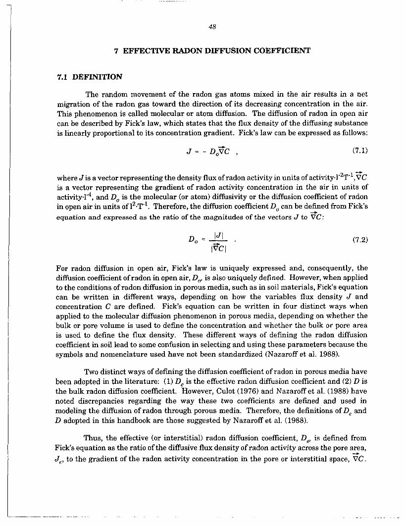
48

7 EFFECTIVE RADON DIFFUSION COEFFICIENT

7.1 DEFINITION

The random movement of the radon gas atoms mixed in the air results in a net migration of the radon gas toward the direction of its decreasing concentration in the air. This phenomenon is called molecular or atom diffusion. The diffusion of radon in open air can be described by Fick’s law, which states that the flux density of the diffusing substance is linearly proportional to its concentration gradient. Fick‘s law can be expressed as follows:

J = - DoFC , (7.1)

2 -1 - where J is a vector representing the density flux of radon activity in units of activity.1- T ,VC is a vector representing the gradient of radon activity concentration in the air in units of activity.14, and Do is the molecular (or atom) difisivity or the diffusion coefficient of radon in open air in units of l2-T-l. Therefore, the diffusion coefficient Do can be defined from Fick’s equation and expressed as the ratio of the magnitudes of the vectors J to VC:

4

For radon diffusion in open air, Fick’s law is uniquely expressed and, consequently, the diffusion coefficient of radon in open air, De is also uniquely defined. However, when applied to the conditions of radon diffision in porous media, such as in soil materials, Fick’s equation can be written in different ways, depending on how the variables flux density J and concentration C are defined. Fick’s equation can be written in four distinct ways when applied to the molecular diffusion phenomenon in porous media, depending on whether the bulk or pore volume is used to define the concentration and whether the bulk or pore area is used to define the flux density. These different ways of defining the radon diffusion coefficient in soil lead to some confusion in selecting and using these parameters because the symbols and nomenclature used have not been standardized (Nazaroff et al. 1988).

Two distinct ways of defining the diffusion coefficient of radon in porous media have been adopted in the literature: (1) De is the effective radon diffusion coefficient and (2) D is the bulk radon diffision coefficient. However, Culot (1976) and Nazaroff et al. (1988) have noted discrepancies regarding the way these two coefficients are defined and used in modeling the diffusion of radon through porous media. Therefore, the definitions of De and D adopted in this handbook are those suggested by Nazaroff et al. (1988).

Thus, the effective (or interstitial) radon diffusion coefficient, D, is defined from Fick‘s equation as the ratio of the diffusive flux density of radon activity across the pore area, Je, to the gradient of the radon activity concentration in the pore or interstitial space, VC.

+

49

This definition is equivalent to that relating the bulk flux density to the gradient of the bulk concentration of radon activity in the soil and can be expressed as follows:

IJeI D e = - . IO'C I

(7.3)

The bulk radon diffusion coefficient, D, is defined as the ratio of the diffusive flux density of radon activity across a geometric or superficial area of the medium, Jb, to the gradient of the radon activity concentration in the pore space, VC, and can be expressed as follows:

.--)

(7.4)

The bulk and the effective radon diffusion coefficients in soil, D and D, respectively, are correlated by the total soil porosity, p t , according to the following expression:

D = p t D e . (7.5)

In general, the diffusion coefficient in porous media is a property of the diffusing species, the pore structure, the type of fluids present in the pores, the adsorption properties of the solid matrix, the fluid saturations, and temperature. For radon diffusion in porous media, the diffusivity for the other isotopes of radon (e.g., radon-220) has been observed to be comparable to that for the isotope radon-222 (Nazaroff et al. 1988).

Several attempts have been made to correlate the radon diffusion coefficients in porous media ( D and De) to the radon diffusion coefficient in open air (Do) and the physical properties of the medium such as the total porosity (pt) . These attempts have not been conclusive. According to experimental work performed by Currie (1960a,b) and quoted by Rolston (1986) and Nazaroff et al. (1988), the coefficients D and Do can be correlated by an expression of the following form:

where y and p represent measures of pore shape of the soil materials. This empirical relationship can fit data from a wide range of dry porous materials in which the values of y generally lie between 0.8 and 1.0 and the values of p lie around 1.0. This empirical relationship is not applicable, however, for very wet soil and strongly aggregate soil (Rolston 1986).

50

The influence of soil moisture content on the effective difision coefficient of radon in soil has been investigated by Rogers and Nielson (1991), who proposed the following expression:

De = D s t exp(-6ptR,-6R, 14Pt , (7.7)

-5 2 where Do = 1.1 x 10 m /s is the radon diffusivity in open air, pt is the total soil porosity, and R, is the water saturation in the soil (or the fraction of the pore space filled with water, also called the saturation ratio).


The diffusivity (or the diffusion coefficient) of radon in soils can be measured by both field and laboratory experiments. In either case, the experimental evaluation of the diffusivity consists in determining the numerical value of the coefficient appearing in Fick’s equation. Because of the difficulties in implementing field methods, laboratory methods are generally used to determine the radon diffusivity in porous media and particularly in soil materials.

Variations of the laboratory methods for measuring radon difisivity in porous media have been developed and as yet no standard (or recommended) method exists. All the various laboratory methods are based on the solution of the mass balance equation that represents the diffusion process in a one-dimensional configuration. Depending on the approximation taken on the time domain for the solution of the diffusion equation, these methods can be separated into two distinct groups: (1) the steady-state diffusion method and (2) the transient diffusion method (Nielson et al. 1982).

The steady-state method used in the laboratory for the determination of the radon diffusivity in soil material without a source of radon within it is based on the solution of a one-dimensional diffusion equation in the x-direction, expressed as follows:

d2C h ---c=o . dx2 De

This steady-state equation is obtained by coupling the one-dimensional Fick’s equation,

Je = - D e- 9 dx (7.9)

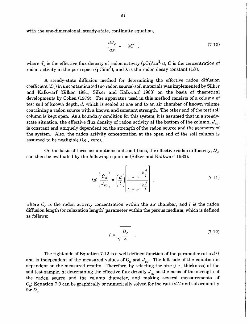
51

with the one-dimensional, steady-state, continuity equation,

- dJe = - h C , dx

(7.10)

where Je is the effective flux density of radon activity (pCi)/(m2-s), C is the concentration of radon activity in the pore space (pCi/m3), and X is the radon decay constant (Vs).

A steady-state diffusion method for determining the effective radon diffusion coefficient (De) in uncontaminated (no radon source) soil materials was implemented by Silker and Kalkwarf (Silker 1981; Silker and Kalkwarf 1983) on the basis of theoretical developments by Cohen (1979). The apparatus used in this method consists of a column of test soil of known depth, d, which is sealed at one end to an air chamber of known volume containing a radon source with a known and constant strength. The other end of the test soil column is kept open. As a boundary condition for this system, it is assumed that in a steady- state situation, the effective flux density of radon activity at the bottom of the column, Jeo, is constant and uniquely dependent on the strength of the radon source and the geometry of the system. Also, the radon activity concentration at the open end of the soil column is assumed to be negligible (i.e., zero).

On the basis of these assumptions and conditions, the effective radon difisivity, De, can then be evaluated by the following equation (Silker and Kalkwarf 1983):

r 1

(7.11)

where C, is the radon activity concentration within the air chamber, and I is the radon diffusion length (or relaxation length) parameter within the porous medium, which is defined as follows:

(7.12) h

The right side of Equation 7.12 is a well-defined function of the parameter ratio d / I and is independent of the measured values of Co and Jeo. The leR side of the equation is dependent on the measured results. Therefore, by selecting the size (i.e., thickness) of the soil test sample, d ; determining the effective flux density Jeo on the basis of the strength of the radon source and the column diameter; and making several measurements of C; Equation 7.9 can be graphically or numerically solved for the ratio d / l and subsequently for De.

52

Typically, the soil samples used in the determination of De have a cylindrical shape with a height to 10 cm and an inner diameter of 14 cm. After equilibration, the steady-state radon concentration in the bottom chamber, C, is determined by several measurements taken over a 7- to 14-day period. Each measurement consists of withdrawing about 5 cm3 of gas from a typical 800-cm3 bottom chamber and determining the radon concentration by using either a scintillation flask technique (such as a Lucas cell) or charcoal absorption and gamma-ray spectrometry (Silker 1983).


In RESRAD, the user is requested to input an effective diffusion coefficient value of radon for three materials: (1) the soil of the cover zone, (2) the soil of the contaminated zone, and (3) the building foundation material (i.e., concrete). The dimensions of these input values of De are in units of square meters per second (m2/s). For each porous material considered, the value of De is assumed to be the same for both radon isotopes addressed in RESRAD, that is, radon-222 and radon-220.

The effective radon diffusivity values in porous media (soils and concrete included) vary over a wide range of several orders of magnitude depending on the porous material and particularly on its degree of water saturation. Table 7.1 lists representative values of effective diffusion coefficients of radon obtained by different researchers for a range of unconsolidated soil materials, concrete, and other building materials. Because of the differences in the experimental methodologies adopted by the various researchers, these experimental data are not easily comparable. Nevertheless, they may give an indication of the expected values of De in the field.

Typically, the effective diffusion coefficient of radon in unconsolidated soil material with a low moisture content is about 10- m /s. The upper limit is represented by the radon diffusion coefficient in open air, D, which is about 1.1 x 10 m /s. At the lower extreme, in a fully saturated soil material the radon diffusion coefficient may be as low as 10-l' rn2/s. In RESRAD, a default value of De equal to 2.0 x m-2/s was adopted for both the cover and contaminated zones. According to the data presented in Table 7.1, this default value of De would represent the average effective radon diffusion coefficient in soils with a lower moisture content and composed of silty and clayey sands. The observed range of variation ofD, in concrete, as presented in Table 7.1, goes from 8.0 x to 4.0 x 10- m /s. A default value of De equal to 3.0 x m2/s was adopted in the RESRAD model to represent the effective radon diffusion coefficient in concrete.

6 2

-5 2

7 2

The estimation of the values of the effective radon diffusion coefficient (De) to be used in RESRAD can be performed at different levels of site-specific accuracy, depending on the amount of information available. For generic use of the code, a set of default values of De was defined as 2.0 x 10- m /s for the cover and contaminated zones and 3.0 x 10- m /s for the building foundation (i.e., concrete). If the type of soil materials at the site is known, a

6 2 7 2

TABLE 7.1 Effective Diffusion Coefficients for Radon in Unconsolidated Soil Materials and Concretea

Effective Radon Diffusion Porous Material Coefficient, D, (m2s-'> Comment Reference

Unconsolidated soil material Compacted silty sands

Compacted clayey sands

Compacted inorganic clays

Silty sandy clay

Uranium mill tailings

Loams

Mud

Concrete

Other materials Brick Gypsum

(3.01t1.3) x

(3.21t1.5) x

(2.5k1.0) x

2.7 x

6.0 x

(5.4-7.2) x

8 x lo-'

2.5

5.7 x 10-10

1.2 x 10-8 3.4 x 10-8 3.3 x 10-8

(1.1-4.0) x

(0.8-8.4) x los

(0.8-3.0) x (1.0-4.0) x

p t = 0.29-0.36

p t = 0.32-0.39

p t = 0.32-0.43

w = 1.5% dry weight w = 10.5% dry weight w = 17.3% dry weight

Silker and Kalkwarf (1983)



Strong et al. (1981)

R, = 0.05-0.34

R, = 0.09-0.55

R, = 0.06-0.34

w = (0.7-1.5)% dry weight Strong et al. (1981)

Dry Tanner (1964)

8 = 37% Tanner (1964)

p t = 0.11-0.13 p t = 0.25 p t = 0.05 p t = 0.068 Zapalac (1983)

PoEjn et al. (1988) Culot et al. (1976) Culot et al. (1976)

Stranden (1988)

Stranden (1988) Stranden (1988)

p t = total porosity, R, = volumetric water saturation, w = percent water content by weight, and

8 = percent volumetric water content.

a

Source: Adapted from Nazaroff et al. (1988).

8

54

slightly more accurate estimation of De can be performed with the help of Table 7.1. For most applications, this approach will suffice because of the natural variability of De within the soil and building materials of any specific site.

In cases in which there are reasons to suspect that the default values of the effective radon diffision coefficient (De) do not reflect the conditions at a specific site and there is no possibility of measuring De, the RESRAD code is able to estimate it internally on the basis of the values of the water saturation (calculated from the volumetric water content) and total porosity, according to Equation 7.7. To implement this option, the user should enter any negative number as an input value of De to RESRAD.

For an accurate site-specific estimate of the input data to RESRAD, however, the values of De should be measured in either the laboratory or field experiments. Whenever necessary and possible, the measurement of De in the soil cover zone (it is assumed that it is not contaminated with radon sources) should be performed in the laboratory by using a method such as the Silker and Kalkwarf(1983) technique.

55

8 RADON EMANATION COEFFICIENT

8.1 DEFINITION

The radon emanation coefficient, E, is the fraction of the total amount of radon produced by radium decay that escapes from the soil particles and gets into the pores of the medium. It is also called the emanating power, emanating fraction, release ratio, and escape-to-production ratio. The radon emanation coefficient is a dimensionless parameter and is represented as either a fraction or a percentage.

The two most common radioisotopes of radon gas, radon-222 and radon-220, are generated by a radioactive process of alpha decay from two radium isotopes, radium-226 and radium-224, respectively. Because of the conservation of linear momentum in the alpha-decay process, the newly created radon-222 and radon-220 atoms are left with a kinetic (usually called "recoil") energy of about 86 and 103 keV, respectively (Nazaroff et al. 1988).

Thus, after being generated, the radon atoms tend to move away from their original location until their recoil energy is totally transferred to the medium. Consequently, depending on their original location within the solid phase of the soil, the soil pore distribution, and the soil moisture content, the newly created radon atoms may end up within the same soil particle in which they were created, within the adjacent soil particle because of posterior penetration aRer escaping from the host soil grain, or within the pore of the medium.

Experimental data reported by several investigators indicate that the radon emanation coefficient is strongly influenced by the moisture content of the medium, particularly within the range of low water saturation (Nazaroff et al. 1988). On the basis of results of this kind, it has been hypothesized that the amount of water present in the pore increases the absorption of the recoil energy of the radon atom passing through it, thus enhancing the chance that the atom will terminate its recoil within the water. Partition equilibrium of radon in the water and air phases in the pore will follow afterwards based on Henry's law.

Although temperature may influence the magnitude of the radon emanation coefficient, it has been demonstrated that within the normal range of temperature variability of surface soils, this effect is of minor importance (Nazaroff et al. 1988).

The radon emanation coefficient, E, is one of the characteristic soil parameters that determine the rate of radon emanation into the pores of the soil matrix. The other soil characteristic parameter in relation to radon production is the concentration of radium (radium-226 and/or radium-224) in the soil particles, SRa. In RESFUD, the source of radon

56

generation in the pore air or the rate of radon generation and emanation into the soil gas phase (pore air), S, in units of pCi/m3.s, is calculated as follows:

where E is the (kg/m3), SRa is

radon emanation coefficient (dimensionless), p, is the soil particle density the mass concentration of radium (radium-226 or radium-224*) in the soil

particles (pCi/kg), h is the radon (radon-222 or radon-220) decay constant (Us), andp, is the total porosity of the contaminated soil.

The values of the radon emanation coefficient in soils depend on the radon isotope being considered, the soil material, and the moisture content. Experimental measurements of E in different soils, rocks, and other materials have been reported by many investigators. Table 8.1 presents a summary of these available data. Because of the differences in the experimental methodologies adopted by the various investigators, these data are not easily comparable. The data are also incomplete in that they do not reflect a rigorous and systematic analysis of the radon emanation coefficient for all radon isotopes in a broad range of soil materials and rocks under different degrees of water saturation. Although incomplete, these available data may give an indication of the expected values of E in the field.


The methodology for measuring the radon emanation coefficient (E) of a porous material contaminated with radium consists basically of measuring the radon concentration in the air within a sealed accumulation chamber in which a sample of the contaminated soil material has been left for a period of time (around four days) until the radon concentration reaches equilibrium. A detailed description of a variation of this method is presented in Strong and Levins (1982). Their experimental apparatus consisted of an ingrowth (accumulation) chamber, a sampling cylinder, a diaphragm pump, a scintillation cell, and supporting electronics for the radiation measurement.


In RESRAD, the user is requested to input a value for the radon emanation coefficient (E ) that is related to the soil material of the contaminated zone for the two radon isotopes, radon-222 and radon-220. This parameter is dimensionless and its value should be entered as a fraction (rather than as a percentage).

* In the RESRAD code, radium-224 is considered an associated radionuclide because its half-life is less than one-half year. Therefore, its principal parent radionuclide, thorium-228, is used as the source for radon-220.

TABLE 8.1 Measurements of Emanation Coefficients of Radon (Rn-222 and Rn-220) in Unconsolidated Soils and Other Materials

Number .of Emanation Moisture Material Samples Isotope Coefficient" Content Reference

Unconsolidated soils Sand Sandy loam Silty loam (Heavy) loam Clay

Various soils (Danish) Soil Soil

Other materials Uranium ore (crushed)

Uranium mill tailings

7 7 7 12 5

70 21 2

17

2

Rn-222 Rn-222 Rn-222 Rn-222 Rn-222

Rn-222 Rn-222 Rn-220

Rn-222

Rn-222

0.14 (0.06 - 0.18) 0.21 (0.10 - 0.36) 0.24 (0.18 - 0.40) 0.20 (0.17 - 0.23) 0.28 (0.18 - 0.40)

0.22 (0.02 - 0.70) 0.30 (0.03 - 0.55) 0.12 (0.09 - 0.15)

0.28 (0.06 - 0.55)

0.14 (0.02 - 0.36) (0.29 - 0.31)

(0.067 - 0.072)

Unknown Unknown Unknown Unknown Unknown

0-70% dry wt Unknown Oven-dried

Moist, saturated

Vacuum-dried Saturated Oven - d r i e d

Sisigina (1974) Sisigina (1974) Sisigina (1974) Sisigina (1974) Sisigina (1974)

Damkjaer and Korsbech (1985) Barreto (1974) Megumi and Mamuro (1974)

Thamer et al. (1981)

Thamer et al. (1981) Strong and Levins (1982) Strong and Levins (1982)

" Arithmetic mean (range of values).

Source: Adapted from Nazaroff et al. (1988).

58

As shown in Table 8.1, the radon emanation coefficient varies from 0.02 to 0.70 in soils. The values of E for radon-222 are usually higher than those for radon-220 under the same circumstances. In RESRAD, the adopted default values of the radon emanation coefficient (E) for radon isotopes radon-222 and radon-220 are, respectively, 0.25 and 0.15, in the soil of the contaminated zone. These default values approximately represent the conditions in a silty loam soil with a low moisture content (i.e., not dry).

The estimation of the values of E for radon-222 and radon-220 for use in RESRAD can be performed at different levels of site-specific accuracy, depending on the amount of information available. For generic use of the code, a set of default values for E (0.25 for radon-222 and 0.15 for radon-220) was defined to approximately represent the condition of a silty loam soil with a low moisture content in the contaminated zone.

If the type of soil materials at the site is known, a slightly more accurate estimation of E can be performed with the help of the data in Table 8.1. For most applications, this approach will suffice because of the natural variability of E within the soil of the contaminated zone of any specific site.

In cases in which it is absolutely necessary to have an accurate estimate of E and there are reasons to suspect that the data in Table 8.1 do not reflect the conditions at a specific site, the values of E for radon-222 and radon-220 can be determined experimentally in the laboratory by using the previously mentioned method of Strong and Levins (1982).

59

9 PRECIPITATION RATE

9.1 DEFINITION

The precipitation rate, Pry is the average volume of water in the form of rain, snow, hail, or sleet that falls per unit of area and per unit of time at the site. It is measured in units of volume per area per time (1T-l).

Precipitation is one of the primary processes of the hydrologic cycle, that is, the endless movement of water through the various elements of the environment (oceans, atmosphere, land surface water bodies, and subsurface soil systems). Other processes of the hydrologic cycle include evapotranspiration, infiltration, overland flow (runoff), streamflow, deep percolation, and groundwater flow. Thorough descriptions of these processes have been presented in numerous texts in the hydrology literature (Chow 1964; Linsley et al. 1982; Bedient and Huber 1988).

A simplified description of the hydrologic cycle could start with considering the water vapor contained in the atmosphere, which under appropriate conditions, condenses and precipitates over the oceans and the continental land. The portion of the water that falls over the surface land, that is, precipitation, is subsequently dispersed by following different pathways. Thus, from the precipitation, a parcel of water is retained in the vicinity of the place where the precipitation falls and is then transferred back to the atmosphere through evaporation (i.e., the water changes from a liquid at the soil surface to a vapor) and transpiration (i.e., the indirect loss of water vapor from the soil to the atmosphere through plant tissue). The combined effect of evaporation and transpiration is commonly called evapotranspiration. Another parcel of the precipitation water penetrates the subsurface soil system, that is, the process of deep percolation, and is added to the groundwater flow system. Finally, the last parcel of precipitation water (the one that is not transferred back to the atmosphere and does not percolate deep into the soil) becomes overland flow, also called surface runoff, and feeds local streams, rivers, or lakes. Both the surface and the subsurface flows of water move toward low elevations and eventually reach the oceans. Evaporation, primarily from the oceans and inland surface waters transfers water vapor back to the atmosphere, thus completing the hydrologic cycle.

The concept of the hydrologic cycle is applicable to a large-scale hydrologic system on earth and can be represented mathematically by a water balance (or budget) equation based on the law of the conservation of matter. The same principle can be applied to any hydrologic system of any scale, whether it is a small basin or a large watershed, to generate a water balance equation that, in its simplest form, can be expressed as follows:

- ds dt Qin- Qout - - , (9.1)

60

where qi, is the water inflow rate into the system, 4out is the outflow rate, and dsldt is the change in time of the water stored within the system.

To illustrate the application of the water balance concept, consider a hydrologic system represented by irrigated agricultural land and the movement of water through it. According to the law of the conservation of matter, the variation of A S (i.e., the change in the volume of water stored in the soil per unit of surface area of the land) during a given time period AT must be equal to the difference between the average inflow rate in time and space (i.e., precipitation, P,, plus irrigation, IR,, rates) minus the outflow rate (i.e., deep percolation, I,, plus runoff, R,, and evapotranspiration, ET,, rates). The water balance equation for this system could then be represented as follows:

- = (P, + IB,) - (I , + R, + ET,) , AT (9.2)

where all the inflow and outflow rates are expressed in units of 1T-1

The precipitation over a specific hydrologic system is an erratic process with large fluctuations in the time domain. Consequently, because all the inflow and outflow processes mentioned previously are related to the precipitation, they also present large and erratic variations along the time. As a result, the change in A S is highly dependent on the period of time (AT) being considered. For short periods, the change in the soil-water storage (AS) is also an erratic process and can present relatively large values. However, for a long period, such as an entire season or a whole seasonal cycle of one year, the change in the soil-water storage (AS), particularly in the upper part of the soils, is likely to be small in relation to the total water balance of the system (Hillel 1980a).

Thus, considering annual averages of the inflow and outflow water rates in this hypothetical hydrologic system of a generic irrigated agricultural land, the respective water budget equation can be reduced to the following:

P, + IR, = I,. + R, + ET, . (9.3)

Except for the deep percolation rate, I,, all other terms of Equation 9.3 can be determined either by direct field measurements or by using specific coefficients derived from soil and other environmental characteristics. The experimental methodologies for field measurement of the precipitation, runoff, irrigation, and evapotranspiration rates are described in this handbook (Sections 9.2, 10.2, 11.2, and 12.2, respectively). Direct field measurement of the deep percolation (infiltration) component of the field water balance has not yet proven to be practical (Hillel 1980a) and, therefore, the deep percolation rate is often determined from the other measured components of the equation as follows:

I, = (P, + IR,) - (R, + ET,) . (9.4)

61

The parameter I,, or the water deep percolation rate, represents the amount of water that percolates through the upper layers of the soil and eventually ends up being added to the groundwater flow underneath the hydrologic system. In the RESRAD model, the parameter I , is used to calculate the radionuclide leaching from the contaminated zone and the final contamination of the groundwater. The deep percolation rate is calculated internally in the code as a function of the precipitation (P,) and irrigation (IR,) rates and the runoff (C,) and evapotranspiration (C,) coefficients. The latter two parameters are defined, respectively, as follows:

c , = - , Rr Pr

and

ET, (1 - C,)P, + IR,

c, =

(9.5)

(9.6)

Detailed discussion of the runoff (C,) and evapotranspiration (C,) coefficients and the irrigation rate (IR,) are presented in Sections 10.1, 12.1, and 11.1, respectively.

Thus, from Equations 9.4,9.5, and 9.6, the deep percolation rate, I,, can be expressed as follows:

The mass balance equation (Equation 9.7) is the one used in RESRAD to calculate the deep percolation rate of water into the soil.


Measurement of the precipitation rate at a site-specific location can be performed with a precipitation gage, which basically consists of a receptacle with vertical walls and an opening at the top with a specified area. The ratio of the volume collected in the receptacle during a specified period of time to the area of the opening at the top of the receptacle gives the point estimate of the precipitation rate at a specific location and time.

In principle, any receptacle with an open collector area of known dimensions, plus a volume measuring device can be used as a precipitation gage. However, because of some operational features of these devices, unless they are of the same shape and dimensions and similarly exposed, precipitation rate measurements are usually not comparable (Linsley et al. 1982).

62

The standard precipitation gage adopted by the U.S. National Weather Service has a collector (receiver) with an 8-in. (20.3-cm) diameter and can measure the precipitation to the nearest 0.25 mm. Two types of precipitation gages can be used, recording and nonrecording. The recording gage, the most commonly used, records on a strip of paper, paper punch, or data logger every 0.01 in. (0.0254 cm) of precipitation along the time scale. The recorded data are then reported as an average precipitation rate, total volume, or intensity variation.

According to Bedient and Huber (19881, a network of five to ten gages per 260 km2 (100 mi2) is usually required in urban areas to define precipitation variability. The maintenance costs of such networks are high and, therefore, for a particular application, it is usually more convenient to rely on data collected locally from existing networks with gages already installed near the site of interest. Local rain gage networks that are usually maintained by cities and sewage treatment plants, for example, could serve as a first source of information on the precipitation rate at the site. On a larger scale, information on the precipitation rate could be obtained from national networks. Precipitation gage networks designed to provide point estimates of precipitation rates in the United States and its territories are maintained by the U.S. National Weather Service and the U.S. Geological Survey.

Data on the point estimates of precipitation rates obtained from either local or national networks can be used to estimate the average areal precipitation rate over a specific area. The areally averaged values of the precipitation rate can be derived by three methods (Bedient and Huber 1988): arithmetic mean, the Thiessen polygon method, and the isohyetal method.

The arithmetic mean of the point precipitation rates provides the simplest and most straightforward way to obtain an estimate of the areal precipitation rate at a particular site. For cases in which the gages are uniformly distributed and the point values have minimal variations, this method provides satisfactory results.

The "hiessen polygon method consists of areally weighing the point precipitation from each gage. This is the most commonly used method, although not the most accurate.

The isohyetal method consists of drawing contour lines of equal precipitation (isohyets) and areally weighing the average precipitation between pairs of contour lines crossing over the area of the site being considered. It is the most accurate among the methods for determining areally averaged values of the precipitation rate but requires an extensive gage network to draw the isohyets accurately.

A distribution of values of average annual precipitation rates over the U.S. continental territory, transcribed from the Water Atlas ofthe United States (Geraghty 1973), is shown in Figure 9.1.

64

If measurements are taken for a site-specific precipitation rate, users are referred to DOE'S environmental regulatory guide (DOE 1991a) on radiological effluent monitoring.

9.3 RESE%AID DATA ENpeTg REQUIREMENl"g

In RESRAD, the user is requested to input a value for the annual average areal precipitation rate (P,) that is representative of the conditions at the site. The precipitation rate is expressed as an annual average rate in units of meters per year (dyr ) .

The precipitation rate and other input parameters, such as the irrigation rate and the runoff and evapotranspiration coefficients (Sections 11.1,10.1, and 12.1, respectively), are used in RESRAD to determine the water deep percolation rate, according to Equation 9.7. The deep percolation rate is ultimately used to calculate the radionuclide leaching rate of the contaminated zone and the subsequent contamination of the underlying groundwater system.

For generic use of the code, a default value of the precipitation rate (P,) equal to 1 d y r (about 40 in&) was adopted in the RESRAD model. This value approximately represents the condition of a relatively humid region. Whenever possible, however, and especially for sites located in a dry region of the country, such as in the western United States, site-specific input data for P, should be used in the R E S W calculations.

Annual average values of P, in units of in./yr for the US. continental territory, based on 40 years of recording, are presented in the Water Atlas of the United States (Geraghty 1973). In the absence of site-specific data, the information provided in this atlas can be used as a provisional and gross estimate of the site-specific value of P, at any particular location in the United States.

Site-specific data on the precipitation rate at a site can be obtained from a rain gage network installed around the site or from already installed networks, such as those maintained by cities. In cases in which data are available on the annual average point precipitation rates at specific locations in the vicinity of a site, the user can estimate the site-specific areal precipitation rate by using one of three averaging methods described in Section 9.2.

If data on the precipitation rate (P,) are not being collected at a site or its vicinity, a site-specific estimation of P, can be obtained from the U.S. National Weather Service or the US. Geological Survey network database. The user may also refer to Climatological Data, National Summary and Climatic Atlas of the United States, published by the U.S. Environmental Data Service, for a site-specific estimate of P,, if no local data are available.

65

10 RUNOFF COEFFICIENT

10.1 DEFINITION

The average annual runoff coefficient, C,, is the fraction of the average annual precipitation that does not infiltrate into the soil and is not transferred back to the atmosphere through evapotranspiration. The runoff coefficient represents the fraction of the precipitation, in excess of the deep percolation and evapotranspiration, that becomes surface flow and ends up in either perennial or intermittent surface water bodies. The runoff coefficient is a dimensionless parameter.

In a well-designed and well-operated irrigation system, the flow and the quantity of the irrigation water are controlled by an appropriate drainage system (ditching) and the duration of each application. Consequently, under normal circumstances, the irrigation water does not contribute significantly to the overall average annual runoff. On the basis of these assumptions, the average annual runoff coefficient (C,) can be defined mathematically by the following expression:

c , = - , Rr Pr

(10.1)

where R, is the average annual runoff rate and P, is the average annual precipitation rate. Because R, is always smaller than (or at the most equal to) P,, the values of C, vary within the range of zero to one.

The runoff rate at a specific location is influenced by the morphology of the region, the degree of the slopes, the type of soil material, and the type of soil utilization. Table 10.1 lists values for the runoff coefficient, C,, under various conditions of soils and soil uses.

10.2 ESTIMATION METHODOLOGY

A methodology for estimating the runoff coefficient (C,) is presented in Table 10.1. The value of C, can be evaluated on the basis of the type of soil and its land utilization at the specific site.

10.3 R E S W DATA INPUT REQUIREMENTS

In RESRAD, the user is requested to input a value for the average annual runoff coefficient (C,) that represents conditions at the site. The runoff coefficient is a dimensionless parameter and its input value should be entered in the form of a decimal fraction rather than as a percentage.

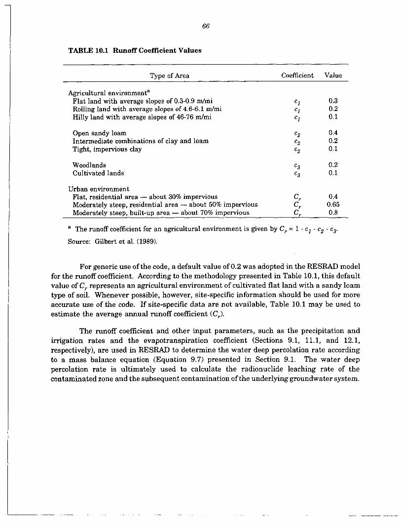
66

TABLE 10.1 Runoff Coefficient Values

Type of Area Coeficient Value

Agricultural environmenta Flat land with average slopes of 0.3-0.9 d m i Rolling land with average slopes of 4.6-6.1 &mi Hilly land with average slopes of 46-76 d m i

C I 0.3 CI 0.2 C l 0.1

Open sandy loam Intermediate combinations of clay and loam Tight, impervious clay

c2 0.4 c2 0.2 c2 0.1

Woodlands Cultivated lands

c3 0.2 c3 0.1

Urban environment Flat, residential area - about 30% impervious Cr 0.4 Moderately steep, residential area - about 50% impervious Cr 0.65 Moderately steep, built-up area - about 70% impervious Cr 0.8

a The runoff coefficient for an agricultural environment is given by Cr = 1 - c I - c2 - c3.

Source: Gilbert et al. (1989).

For generic use of the code, a default value of 0.2 was adopted in the RESFWD model for the runoff coefficient. According to the methodology presented in Table 10.1, this default value of C, represents an agricultural environment of cultivated flat land with a sandy loam type of soil. Whenever possible, however, site-specific information should be used for more accurate use of the code. If site-specific data are not available, Table 10.1 may be used to estimate the average annual runoff coefficient (C,).

The runoff coefficient and other input parameters, such as the precipitation and irrigation rates and the evapotranspiration coefficient (Sections 9.1, 11.1, and 12.1, respectively), are used in RESFUD to determine the water deep percolation rate according to a mass balance equation (Equation 9.7) presented in Section 9.1. The water deep percolation rate is ultimately used to calculate the radionuclide leaching rate of the contaminated zone and the subsequent contamination of the underlying groundwater system.

67

11 IRRIGATION RATE

11.1 DEFINITION

The irrigation rate, IR,, is the average volume of water that is added to the soil at the site, per unit of surface area and per unit of time. It is measured in units of volume per area per time, or 1T-l. In the RESRAD code, the irrigation rate is expressed as an annual average rate in units of meters per year (dy r ) .

Irrigation is the practice of supplying water artificially to the soil in order to permit agricultural use of the land in an arid region or to compensate for occasional droughts in semidry or semihumid regions. Irrigation is closely dependent on the precipitation rate at the site, in the sense that a well-designed and well-operated irrigation system should optimize the spatial and temporal availability of water in the soil.

As discussed earlier (Section 9.11, irrigation, in conjunction with precipitation, provides the inflow water into a hydrologic system formed by the soil in an agricultural land and the water that circulates through it. The outflow of water in this system is the result of processes such as surface runoff and evapotranspiration and deep percolation rates.

The irrigation rate and other input parameters such as the precipitation rate and the runoff and evapotranspiration coefficients (Sections 9.1,10.1, and 12.1, respectively) are used in RESRAD to determine the water deep percolation rate according to Equation 9.7 in Section 9.1. The water deep percolation rate is ultimately used to calculate the radionuclide leaching rate of the contaminated zone and the subsequent contamination of the underlying groundwater system.


The average annual irrigation rate at a site is determined as a ratio of the total volume of irrigation water added to the field during the year to the surface area of the irrigated land. This quantity is not measured in the field per se but is obtained from the operational activities of the irrigation system.

A well-designed and well-operated irrigation system should be able to supply water to plants at a rate sufficient to balance their transpiration rate requirements. The objective is to provide water to the soil in a well-distributed manner during the crop season so that the plants can maintain their own hydration without loss of continuity. As long as the water uptake rate from the plants’ roots matches the water loss due to the plants’ transpiration from their foliage, they can maintain their hydration. As soon as the water intake from the roots becomes lower than the transpiration, however, the plants start losing moisture, resulting in a stressful situation for the development of the crop (Hillel 1980a).

Therefore, the required rate of irrigation at a specific agricultural site is governed by the properties of the soil and the plants, and, fundamentally, by the meteorological

68

conditions at the site. The soillplant system properties determine the ability of the soil to supply and transmit water to the roots, as well as the ability of the roots to extract water from the soil at a rate needed to overcome transpiration. The meteorological conditions, however, dictate the rate at which the plants are required to transpire and, therefore, the amount of water needed for their survival.

Estimation of the annual irrigation rate at a specific site can be obtained in different ways, depending on the degree of knowledge about site agricultural activities. When information on irrigation systems in operation at the site or at its vicinity is available, the annual irrigation rate can be obtained from operational records. When little information is available on the irrigation procedures at a site, an estimation of the irrigation rate can be obtained on the basis of the measured (or assessed) values of the potential evapotranspiration and precipitation rates and on the basis of an estimated "irrigation efficiency."

Irrigation efficiency is the ratio of the volume of water used consumptively (such as in evapotranspiration) to the total volume of water applied to the field (Hillel 1980a). This definition is similar to the one for the evapotranspiration coefficient, C,, (Section 12.1) and can be expressed as follows:

ET, (1 - C,)P, + IR,

Irrigation Eficiency = C, = (11.1)

According to Hillel (1980a), most irrigation projects are inherently inefficient and although irrigation efficiencies of 80 to 90% can be achieved in actual practice with proper water management, the average irrigation efficiency is less than 50%. Thus, by assuming a value for the irrigation efficiency (e.g., around 50%) at a specific site with little available data on agricultural activities; and by determining the potential evapotranspiration rate, ET,, the precipitation rate, P,, and the runoff coefficient, C,; the predicted, necessary average annual irrigation rate, I . , , at the site can be estimated as follows:

(11.2)

11.3 RESRAD DATA INPUT REQUIRERlENTS

In RESRAD, the user is required to input a value for the annual average irrigation rate, IR,, that represents conditions at the site. The IR, should be entered in units of meters per year (dyr) .

A default value of IR, equal to 0.2 d y r was adopted in the RESRAD model. This value approximately represents the conditions of a relatively humid region where only a small amount of irrigation is needed per year. For an arid region, 1 d y r is considered to be an appropriate generic value for IR,.

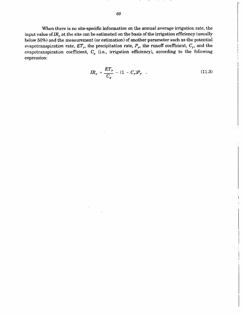
69

When there is no site-specific information on the annual average irrigation rate, the input value of IR, at the site can be estimated on the basis of the irrigation efficiency (usually below 50%) and the measurement (or estimation) of another parameter such as the potential evapotranspiration rate, ET,, the precipitation rate, PF, the runoff coefficient, CF, and the evapotranspiration coefficient, Ce (i.e., irrigation efficiency), according to the following expression:

(11.3)

70

12 EVAPO"SPIRATI0N COEFFICIENT

12.1 DEFINITION

Evapotranspiration is one of the processes of the hydrologic cycle and represents the total volume of water that changes phase, that is, from the liquid or solid state to the gaseous state, near the ground surface and is transferred to the atmosphere during a fixed period of time. Consequently, it represents the combination of two separate processes: (1) evaporation (i.e., the change of phase of water near the ground surface and the direct transfer of water vapor from the ground to the atmosphere) and (2) transpiration (i.e., the transfer of water from the ground to the atmosphere through the plants and their foliage).

Evapotranspiration is also called "consumptive use" in the hydrology literature and is defined as the quantity of water used by either cropped or natural vegetation in transpiration or in the building of plant tissue, together with water evaporated from the adjacent soil or from intercepted precipitation, during a fixed period of time (Veihmeyer 1964).

Two parameters need to be defined in relation to the concept of evapotranspiration: (1) the evapotranspiration rate, ET,, and (2) the evapotranspiration coefficient, Ce.

The evapotranspiration rate, ET,, is the total volume of water vapor that is transferred to the atmosphere because of the combined effect of evaporation and transpiration, per unit of the ground surface area and per unit of time at the site. It is measured in units of volume per area per time (1T-l). The evapotranspiration rate is neither required as input data to the RESRAD code, nor is it used implicitly within the model. However, the measured or estimated site-specific value of ET, is used to estimate the input value of the evapotranspiration coefficient, which is used in the code. For consistency with other correlated parameters handled in the RESRAD code, the evapotranspiration rate is expressed as an annual average rate in units of meters per year (dy r ) .

The evapotranspiration coefficient, C,, is the ratio of the total volume of water leaving the ground as the result of evapotranspiration, ET,, to the total volume of water available within the root zone of the soil [(l-C,)P, + IR,] during a fixed period of time. It can then be expressed as follows:

ET, (1 - C,)P, + IR,

c, = ' (12.1)

where P, is the precipitation rate ( d y r ) , IR, is the irrigation rate ( d y r ) , and C, is the runoff coefficient (dimensionless). (All these parameters are defined in this handbook; see Sections 9.1, 11.1, and 10.1, respectively.)

In well-irrigated agricultural land, transpiration predominates over evaporation in Under these circumstances, the evapotranspiration composing the total evaporation.

71

coefficient represents the efficiency by which the water available in the root zone of the soil is actually transferred through the plant system and into the atmosphere. Thus, for cultivated land, the evapotranspiration coefficient (C,) is also called the "irrigation efficiency." Most irrigation projects are inherently inefficient; the average irrigation efficiency is less than 50% (Hillel 1980a).

The evapotranspiration process is fundamentally governed by the meteorological conditions at the site, as well as by the properties of the soiVplant system. Meteorological parameters such as air temperature, wind speed, atmospheric pressure, air humidity, and exposure to the sun, all have an important role in determining the evapotranspirational demand at a specific location and time of year. However, it is the amount of water available in the root zone of the soil that limits the occurrence of the evapotranspiration process. Thus, the power of the atmosphere to extract water from the ground surface because of evaporation decreases as the moisture content of the soil decreases. The smaller the moisture content is, the more strongly the water is bound to the porous matrix of the soil because of capillarity, and thus more energy is needed to extract it. Transpiration is also limited by the availability of water at the root zone, the ability of the soil to supply and transmit water toward the root zone, and the ability of the root system to absorb water from the soil in its vicinity. Below a certain value of soil moisture called the wilting point, the roots of the plants are not able to extract water from the soil, and the transpiration process is broken, resulting in dehydration and wilting. Therefore, as a combination of evaporation and transpiration, the actual evapotranspiration at a specific site depends on external climatic conditions and on the type and density of vegetation covering the ground surface as well as on soil moisture, root distribution, and other soil properties.

The concept of the "potential evapotranspiration rate," ETp,, has been introduced into the hydrology literature to represent the so-called "climatic demand" for water, independently of the transient properties of the soil (Hillel 1980a). As such, the potential evapotranspiration rate, ETp, (or the evaporating power of the atmosphere), is defined as the evapotranspiration rate that occurs on the ground of a land area totally covered with vegetation and where sufficient water is continuously available for the needs of plants. The actual evapotranspiration rate, ET,, is then a function of the potential evapotranspiration rate, ETp,, and the quantity of water available in the root zone of the soil. Where there is an excess of water in the root zone, the value of ET, is at its maximum, equal to ETp,, and the excess water percolates the soil toward the groundwater system. During a water shortage period, however, the value of ET, becomes lower than ET',, with no resulting percolation.

The potential evapotranspiration rate, ET',, at any location in the contiguous US. territory can be estimated from Evaporation Atlas for the Contiguous 48 United States (National Oceanic and Atmospheric Administration [NOAAI 1982a), Mean Monthly Seasonal and Annual Pan Evaporation for the United States (NOAA 1982b), and Water Atlas o f the United States (Geraghty 1973). A distribution of average potential evapotranspiration over the US. continental territory is shown in Figure 12.1.

FIGURE 12.1 Distribution of Average Annual Potential Evapotranspiration Rates (inJyr) over the U.S. Continental Territory (Source: Modified from Geraghty 1973)

73

The evapotranspiration coefficient and other input parameters such as the precipitation rate, the irrigation rate, and the runoff coefficient are used in RESRAD to determine the water percolation rate, according to Equation 9.7 in Section 9.1. The water percolation rate is ultimately used to calculate the radionuclide leaching rate of the contaminated zone and the subsequent contamination of the underlying groundwater system.


Estimation of the evapotranspiration coefficient, Ce (to be used as input data to the RESRAD code), should be obtained from measured (or otherwise estimated) values of the evapotranspiration rate, ET,, the precipitation rate, P,, the irrigation rate, IR,, and the runoff coefficient, C,, according to Equation 12.1.

There are many methods of measuring or estimating the actual (ET,) and the potential (ET,,) evapotranspiration rate. However, no one method can be used for all purposes (Veihmeyer 1964). Most of the methods used for estimating ET, can also be used for estimating ETp,, provided that the available water supply is sufficient for the area under observation during the duration of the test. These methods can be classified into three broad categories: (1) the theoretical approach, based on physical principles governing the process; (2) the analytical approach, based on conservation principles, either as a mass or as an energy balance; and (3) the empirical approach, based on experimental results expressing the correlation between measured evapotranspiration and local climatic conditions.

A generic description of various methods used for measuring evapotranspiration can be found in Veihmeyer (1964). The methods available are (1) soil-moisture sampling, (2) lysimeter measurement, (3) inflow-outflow measurements, (4) integration method, (5) energy balance, (6) vapor transfer, and (7) groundwater fluctuations. For example, the lysimeter method consists of using a large barrel (also called a tank or evapotranspirometer) with about a 1-m diameter and a 2-m depth that is filled with soil and buried in the ground so that its top is flush with the ground surface. Individual crops and/or natural vegetation are grown on and around the lysimeter. The evapotranspiration rate can then be determined on the basis of the mass balance by measuring the infiltration flux seeping out of the bottom of the lysimeter and the rainfall rate. The loss of water necessary to maintain satisfactory plant growth represents the evapotranspiration. When operated properly, the lysimeter can provide reasonably reliable values of potential evapotranspiration. However, reliable measurements of actual evapotranspiration (particularly when it is much lower than the potential) are rarely attainable because of the difficulty in maintaining comparable soil moisture and vegetation cover conditions on and around the lysimeter (Linsley et al. 1982).

Because of the inherent difficulties of field methods for measuring evapotranspiration, several empirical formulas have been developed to relate the potential evapotranspiration to some readily available climatic data, such as temperature, sunshine, wind velocity, and so forth. A list of typical evapotranspiration equations is presented in

74

Table 11.2 of the Handbook of Applied Hydrology (Veihmeyer 1964, pp. 11-27). Two publications from the N O M (1982a,b) have been used in estimating the potential evapotranspiration on FUSRAP sites for cases in which no site-specific data are available.

12.3 RESRAD DATA I" REQUIREMENTS

In RESRAD, the user is requested to input a value for the annual average evapotranspiration coefficient, C,, that is representative of conditions at the site. The input value of C, is given in dimensionless units.

In the process of estimating the value of C, as an input value for RESRAD, it is assumed that the cultivated land at the site under consideration is maintained with the necessary level of moisture in the soil for the growth and development of the crop. This condition is achieved either by natural precipitation or by the combination of precipitation and irrigation. In other words, it is assumed that the required moisture content for potential evapotranspiration based on the annual average is maintained in the soil.

Therefore, the estimation of the input value of C, for some site-specific conditions is based on a previously measured (or otherwise determined) value of the potential evapotranspiration, ET',, the precipitation rate, P,, the irrigation rate, IR,, and the runoff coefficient, C,, according to the definition of C, presented in Equation 12.1.

A default value of C, equal to 0.5 (dimensionless) was adopted in the RESRAD model. This value represents the condition of 50% efficiency in the irrigation process at a generic site. Under this condition, 50% of the water available in the root zone of the soil is transferred to the atmosphere, and 50% of the water infiltrates the soil and percolates toward the aquifer system. Whenever possible, however, site-specific input data for C, should be used in the RESRAD calculations.

Field measurements of the average annual evapotranspiration rate, ET,, usuaIly are expensive and time-consuming. Therefore, if data on ET, have not been collected at the site or its vicinity, a site-specific estimation of ET, (and ultimately of C,) should be obtained from information in the literature. For a gross estimation of ET',, the user can consult the annual average values of potential evapotranspiration for the US. continental territory as shown in Figure 12.1 (Geraghty 1973). Two NOAA publications (NOAA 1982a,b) provide useful information that can be used to estimate the value of ET, (and ultimately of C,) at any particular location in the United States. For most applications, in the absence of site-specific data, this approach should suffice because of the intrinsic uncertainties associated with the model itself and the natural variability of the potential evapotranspiration at any site.

75

13 SOIL-SPECIFIC EXPONENTIAL b PARAMETER

13.1 DEFINITION

The soil-specific exponential b parameter is one of several hydrological parameters used to calculate the radionuclide leaching rate of the contaminated zone. (See also precipitation rate, irrigation rate, runoff coefficient, evapotranspiration coeficient, hydraulic conductivity, and soil porosity.) The soil-specific b parameter is an empirical and dimensionless parameter that is used to evaluate the saturation ratio (or the volumetric water saturation), R , of the soil, according to a soil characteristic function called the conductivity function (i.e., the relationship between the unsaturated hydraulic conductivity, K, and the saturation ratio, R,).

It has been suggested that a power function is an acceptable form of representing the conductivity function. As cited by Clapp and Hornberger (1978), Campbell (1974) derived a partly empirical and partly theoretical conductivity function on the basis of the power function model; this function proved to be reasonably accurate over a large number of cases. Campbell suggested the following power expression to represent the working relationship for the conductivity function:

(2b+3) k =R, 9 (13.1)

where k is the relative conductivity (or relative permeability, dimensionless), R, is the saturation ratio (dimensionless), and b is the fitting parameter, called the soil-specific exponential parameter, which must be determined experimentally.

The relative permeability, k , at any location in the unsaturated zone, is defined as a ratio of the unsaturated hydraulic conductivity, K, at that point, to the saturated hydraulic conductivity, Ksat. Thus, K can be expressed as follows:

Substituting the definition of the relative permeability k into Equation 13.1 yields

(2b+3) = Rs K -

&at 9

or

(13.2)

(13.3)

(13.4)

76

In downward water infiltration into the unsaturated upper layer of the soil, the infiltration rate, I , (see also precipitation rate), can be approximated by the unsaturated hydraulic conductivity, K (Hillel 1980a). Therefore, substituting I , for K in Equation 13.4 yields

(13.5)

Equation 13.5 is used internally in the RESRAD model to evaluate the volumetric water saturation, R,, in all unsaturated regions of the soil system. According to Equation 13.5, under unsaturated infiltration conditions, the saturation ratio R, is a function of the infiltration rate I,, the saturated hydraulic conductivity Ksat, and the texture of the soil, as determined by the fitting parameter b. When the medium is fully saturated, I , equals ICsat, and R, equals unity.


The soil-specific b parameter is an empirical fitting parameter and, therefore, must be determined experimentally. For each type of soil, the best estimate of b can be obtained by adjusting the best-fit values of each soil t o an experimentally determined curve of relative permeability versus saturation, according to the power function model proposed above (Equation 13.1).

Determining the conductivity function of a soil sample experimentally by measuring the relative permeability and the saturation is not an easy laboratory task because of many technical and procedural difficulties. Yet some data have been reported in the literature that demonstrate reasonable agreement with the proposed model. For example, Clapp and Hornberger (1978) have reported that Campbell’s model (Campbell 1974) for the conductivity function has proven to be acceptable under different conditions of soil saturation over a wide range of b values (0.17-13.6) and even for values of saturation, R,, near unity (i.e., full saturation). Table 13.1 lists representative values of the soil-specific exponential b parameter for various soil textures. Section 2.1.2 provides a discussion on soil textures.

13.3 RESRAD DATA INPUT REQUrrtEMENTS

In RESRAD, the user is requested to define an input value for the soil-specific b parameter for (1) the contaminated zone, (2) the unsaturated zone strata, and (3) the saturated zone. Input for the saturated zone b parameter will only be required if the water table drop rate (Section 18.1) is greater than zero.

Reported measured data indicate that values of b vary within the range of 0.17-13.6 (Clapp and Hornberger 1978). A default value of 5.3 was adopted in the RESRAD model. This value represents the condition of a silty loam soil material. Whenever possible, however, site-specific input data for b should be used in the RESRAD calculation.

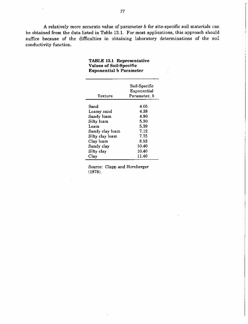
77

A relatively more accurate value of parameter b for site-specific soil materials can be obtained from the data listed in Table 13.1. For most applications, this approach should suffce because of the difficulties in obtaining laboratory determinations of the soil conductivity function.

TABLE 13.1 Representative Values of Soil-Specific Exponential b Parameter

Soil-Specific Exponential

Texture Parameter, b

Sand Loamy sand Sandy loam Silty loam Loam Sandy clay loam Silty clay loam Clay loam Sandy clay Silty clay Clay

4.05 4.38 4.90 5.30 5.39 7.12 7.75 8.52 10.40 10.40 11.40

Source: Clapp and Hornberger (1978).

78

14 EROSIONRATE

14.1 DEFINITION

The erosion rate is the average volume of soil material that is removed from one place to another by running water, waves and currents, wind, or moving ice per unit of ground surface area and per unit of time. The erosion rate represents the average depth of soil that is removed from the ground surface per unit of time at the site and is expressed in units of length per time (IT-').


Erosion rates can be estimated by means of the Universal Soil Loss Equation (USLE), an empirical model that has been developed for predicting the rate of soil loss by sheet and rill erosion. It should be emphasized, however, that orders of magnitude errors can result by using the USLE method without proper orientation. An appropriate guide for using the USLE method can be obtained from the U.S. Soil Conservation Service (SCS), which conducts county soil surveys on a regular basis. The SCS office near the site should be able to provide the USLE parameters mapped out for the site-specific soils and cover types for the area of interest.

If sufficient site-specific data are available, a site-specific erosion rate can be calculated by using the USLE method. Wischmeier and Smith (1978) and Foster (1979) discuss details of the calculation. Estimates based on the range of erosion rates for typical sites in humid areas east of the Mississippi River (based on model site calculations for locations in New York, New Jersey, Ohio, and Missouri) can also be used (Knight 1983). For example, for a site with a 2% slope, these model calculations predict a range of 8 x to 3 x d y r for natural succession vegetation, 1 x to 6 x d y r for permanent pasture, and 9 x loe5 to 6 x 10" d y r for row-crop agriculture. The rate increases by a factor of about 3 for a 5% slope, 7 for a 10% slope, and 15 for a 15% slope. If these generic values are used for a f adga rden scenario in which the dose contribution from food ingestion pathways is expected to be significant, an erosion rate of 6 x d y r should be assumed for a site with a 2% slope. This would lead to erosion of 0.6 m of soil in 1,000 yr. A proportionately higher erosion rate must be used if the slope exceeds 2%. An erosion rate of 6 x d y r , leading to erosion of 0.06 m of soil in 1,000 yr, can be used for a site with a 2% slope if it can be reasonably shown that the fardgarden scenario is unreasonable; for example, if the site is, and will likely continue to be, unsuitable for agricultural use.

Erosion rates are more difficult to estimate for arid than for humid sites. Although water erosion is generally more important than wind erosion, the latter can also be significant. Water erosion in the West is more difficult to estimate because it is likely to be due to infrequent heavy rainfalls for which the empirical constants used in the USLE may not be applicable. Long-term erosion rates are generally lower for sites in arid locations than for sites in humid locations. A more detailed discussion and data on soil erosion are

79

presented in Soil Physics (Marshall and Holmes 1979), Universal Soil Loss Equation: Past, Present, and Future (Peterson and Swan 1979), and the Nature and Properties of Soils (Brady 1984).

14.3 IRESW DATA I” REQUIREMENTS

In RESRAD, the user is requested to input a value for the annual average erosion rate for the cover zone and the contaminated zone. The dimensions of these input values of the erosion rate are given in units of meters per year (dyr) .

For generic use of the code, a default value of the annual erosion rate equal to 0.001 d y r was adopted in the RESRAD model for both the cover and the contaminated zones. This default value should suffice for screening estimates. For a particular site, however, a more accurate site-specific estimation of the erosion rates for both the cover and the contaminated zones should be attempted. The erosion rate of the contaminated zone only becomes significant if and when the cover zone is completely eroded, thus exposing the contaminated zone to the erosive effects of the environmental elements. If there is no initial cover, a greater erosion rate will remove the contaminated material faster. This may lead to lower doses than found for an initial cover case.

A site-specific estimation of the erosion rate for the cover and contaminated zones can be performed by means of the USLE.

~

80

15 HYDRAULIC GRADIENT

15.1 DEFINITION

The hydraulic gradient is the change in hydraulic head per unit of distance of the groundwater flow in a given direction. The hydraulic gradient, J,, in the flow direction x , is expressed as follows:

J, = hl - h2 , AX

(15.1)

where h, and h, represent the hydraulic head at points 1 and 2, respectively, and AX is the distance between these two points. Mathematically, the hydraulic gradient is a vector that can be expressed as grad h. The norm of the vector represents the maximum slope of the hydraulic gradient; its orientation represents the direction along the maximum slope. The hydraulic gradient is a dimensionless parameter, usually represented as a fraction rather than as a percentage.

In an unconfined (water table) aquifer, the horizontal hydraulic gradient of groundwater flow is approximately the slope of the water table. In a confined aquifer, it represents the difference in potentiometric surfaces over a unit distance. The potentiometric surface is the elevation to which water rises in a well that taps a confined aquifer. It is an imaginary surface analogous to a water table. In general, the hydraulic gradient of groundwater flow in a highly permeable geologic material, such as sand or gravel, is far less than that in a geologic material with a low permeability, such as silt and clay.


The hydraulic head at a point in the saturated zone can be measured in the field by installing a piezometric nest at the site. A piezometer is basically a tube or pipe long enough to be introduced through the unsaturated zone down into the saturated zone. Its walls must be completely sealed along all its length, but it must be open to the atmosphere at the top and to the water flow at the bottom. The water level measured inside the piezometer, as compared with a defined reference level (such as mean sea level), gives the hydraulic head of the aquifer at the point of measurement.

The distribution of the hydraulic head in a groundwater system is actually three- dimensional. Thus with the installation of three or more piezometers spatially distributed in an aquifer, it is possible to determine the spatial distribution of the hydraulic head at the site. By knowing the distances between the piezometers, the hydraulic gradient of the dominant aquifer flow at the site can be evaluated. A detailed description of piezometer nests can be found in Freeze and Cherry (1979).

81

In RESRAD, the user is requested to input a value for the hydraulic gradient in the dominant groundwater flow direction in the underlying aquifer at the site. This parameter is dimensionless and should be entered as a decimal fraction rather than as a percentage.

For generic use of the code, a default value of 0.02 was adopted for the hydraulic gradient in the RESRAD model. Because the hydraulic gradient varies significantly from one site to another, whenever possible, site-specific information should be used for more accurate use of the code.

Site-specific data on the hydraulic gradient and the general flow pattern of the groundwater system at the site can be obtained by installing a piezometric nest in the area, as suggested above. RESRAD users should also consider contacting a local or state hydrologist or geologist as a possible source of site-specific information.

82

16 LENGTH OF CONTAMINATED ZONE PARALLEL TO THE AQUIFER FLOW

16.1 DEFINITION

The length, 4, of the contaminated zone parallel to the aquifer flow is the maximum horizontal distance measured in the contaminated zone, from its upgradient edge to the downgradient edge, along the direction of the groundwater flow in the underlying aquifer.

The parameter 0 is used in RESRAD to evaluate the dilution of the contaminated inflow water (which percolates the contaminated zone vertically and reaches the aquifer underneath) by the uncontaminated inflow groundwater in the Nondispersion Model for a well located near the contaminated zone.


To evaluate the value of parameter P at a specific site, it is first necessary to determine the hydraulic gradient of groundwater flow at the site. As described in Section 15.2, the groundwater flow direction in the aquifer can be determined locally by installing a piezometric nest composed of three or more piezometers spatially distributed throughout the hydrogeological system. With a known groundwater flow direction and the horizontal extension of the contaminated zone, the parameter P can be determined by measuring the largest horizontal length of the contaminated zone parallel to the groundwater flow direction.


In RESRAD, the user is required to input a value of 0, that is, the length of the contaminated zone parallel to the groundwater flow, that represents the conditions at the site. The dimensions of P should be entered in units of meters (m).

A default value of 100 m was adopted in the RESRAD model for parameter 4. The default value of 100 m is the square root of the default contaminated zone area of 10,000 m2. Whenever possible, however, site-specific information should be used for more accurate use of the code.

83

17 WATERSMED AREA FOR NEARBY STREAM OR POND

17.1 DEFINITION

A watershed is a region contoured by an imaginary line connecting ridges or summits of high land and drained by or draining into a river, river system, or a body of water such as a lake or pond. The watershed area is the surface area of the draining region above the discharge measuring points. This parameter is expressed in units of length squared (12). In the RESRAD code, the watershed area parameter represents the area of the region draining into the nearby stream or pond located at the vicinity of the site.

The watershed area parameter is used in the RESRAD model to evaluate the dilution factor for the contamination of the water at the nearby stream or pond as it gets mixed with the inflow of water from the contaminated aquifer. Thus, the evaluation of the dilution factor for the ground/surface water pathway is based on the following assumptions (Gilbert et al. 1989): (1) the nearby body of water is a pond, (2) the inflow and outflow of water in the pond are in equilibrium, (3) the average annual inflow of radioactivity into the pond is equal to the average annual quantity of radioactivity that is leached from the contaminated zone into the groundwater system, and (4) the infiltrating water flow through the contaminated zone is vertically downward. Under these conditions and assumptions, the dilution factor is then defined as the ratio of the average annual volume of water that percolates through the contaminated zone to the average annual total inflow of water into the pond. More specifically, the dilution factor is calculated internally in the code as the ratio of the contaminated zone area (AREA) to the watershed area (WAREA).


The area of the watershed draining toward the pond located at the vicinity of the site can be evaluated by using a small-scale morphologic map of the region.


In RESRAD, the user is requested to input a value for the area of the watershed region draining into the stream or pond located at the vicinity of the site. The dimensions of the watershed area should be entered in units of square meters (m2).

A default value of one million (1 x lo6) m2 for the watershed area was adopted in the RESRAD model. Whenever possible, however, site-specific information should be used for more accurate use of the code.

Site-specific information on the watershed area can be obtained from small-scale hydrological and morphological maps covering the region under study. In the RESRAD code, the watershed area must be larger than or equal to the area of the contaminated zone. The

84

code will issue a warning if this condition is violated and will not proceed with the calculations until it is corrected.

85

18 WATER TABLE DROP RATE

18.1 DEFINITION

The water table drop rate is the rate, in units of length per time (lT-'), at which the depth of the water table is lowered. The level of the water table in a groundwater system fluctuates seasonally because of the erratically temporal variations of the processes involved in the hydrologic cycle (Section 9.11, as well as extra use of the water from the system. Under normal circumstances, the level of the water table is approximately stationary if averaged over long periods of time such as one year. For unusually high consumptive use of groundwater in the region, however, the water table may experience a significant drop during the annual period. In these cases, the average annual water table drop rate is not zero and results in the creation of an increase in the unsaturated zone thickness.


The site-specific water table drop rate can be estimated by observing the change of It can also be the water level of a monitoring well appropriately installed at the site.

estimated by consulting water table records of past decades.


In RESRAD, the user is required to input a value for the average annual water table drop rate that represents conditions at the site. The dimensions of the water table drop rate should be given in units of meters per year (dyr) .

A default value of 0.001 d y r was adopted in the RESRAD model for the water table drop rate. This value is the same as the default value used for the erosion rate. Whenever possible, however, site-specific information should be used for more accurate use of the code.

86

19.1 DEFINITION

The parameter well-pump intake depth is the screened depth of a well within the aquifer (the saturated zone). The well-pump intake depth is measured in units of length (1).

19.2 RESRAD DATA INPUT REQUIREMEN'I"T

In RESRAD, the user is required to input a value for the well-pump intake depth that represents conditions at the site. Its dimensions should be given in units of meters (m).

A default value of 10 m was adopted in the RESRAD model for the well-pump intake depth. For more accurate use of the code, however, site-specific data should be used whenever possible.

87

20 RADON VERTICAL DIMENSION OF MIXING

20.1 DEFINITION

The radon vertical dimension of mixing is the height of the atmospheric boundary layer near the ground surface into which the radon gas that emanates from the ground is uniformly mixed in the outdoor air. This parameter is measured in units of length (1).

20.2 PtESRAD DATA INPUT REQUIREMENTS

In RESRAD, the user is required to input a value for the radon vertical dimension of mixing that represents conditions at the site. This parameter's dimension should be given in units of meters (m).

A default value of 2 m was adopted in the RESRAD model for the radon vertical dimension of mixing. This value of 2 m is a conservative value, considering the height of humans. Unless other evidence indicates use of a different value, this value should be used in the RESRAD code.

88

21 AVERAGE ANNUAL WIND SPEED

21.1 DEFINITION

The average annual wind speed is the overall average of the wind speed, measured near the ground, in a one-year period. This parameter is measured in units of length per time (1T-’).


In RESRAD, the user is required to input a value for the average annual wind speed that represents conditions at the site. The dimensions of the wind speed input should be given in units of meters per second (m/s).

A default value of 2 m/s was adopted in the RESRAD model for the average annual wind speed. For more accurate use of the code, however, site-specific data should be used whenever possible. If measurements are performed to get site-specific data, these measurements should be consistent with guidance in DOE’S guide for radiological effluent monitoring (DOE 1991a).

Site-specific information on the time distribution of the wind speed and direction at the site can be obtained with the installation of a simple meteorological station instrumented with an anemometer (for measuring the wind speed) and wind vanes (for measuring wind direction). Although simple, the installation, operation, and maintenance of such systems are time-consuming and require the attention of trained personnel. A more general estimation of the average wind speed at a site can be obtained from other meteorological information systems in the area (such as at a commercial airport). For most applications, in the absence of site-specific data, this approach should suffice because of the intrinsic uncertainties associated with the natural variability of the wind speed and direction at the site.

89

22 AVERAGE BUILDING AIR EXCHANGE RATE

22.1 DEFINITION

The building air exchange (or ventilation) rate is the total volume of air contained in the building that is being exchanged with outside air per unit of time. This parameter expresses the rate at which the total air contained within the building is replaced (or renewed) per unit of time and is measured in units of inverse time (T'l). For example, a building with a ventilation rate of 1 h-' has its volume of air replaced once each hour on aver age.

Important factors affecting the ventilation rate include construction and operating features of the building (i.e., age, window and door weatherproofing, existence of unbalanced mechanical ventilation, the use of fireplaces, etc.), as well as environmental conditions (i.e., atmospheric pressure, temperature, and wind speed and direction). The total ventilation rate is based on three factors (Nero 1988): (1) the infiltration of air through small openings and imperfections in the building structure; (2) the exchange of air through windows, doors, or any other large openings that are kept partially or temporarily open; and (3) the mechanically supplied ventilation due to the operation of exhaust fans or other similar systems. Each of these factors varies significantly along time and, consequently, the total ventilation rate in a house is also strongly time dependent. In the United States, the average ventilation rate during the seasons when houses are kept closed lies within the range of 0.1-1.0 h-'.


Measurement of the ventilation rate in a building can be accomplished directly by injecting a tracer gas, sulfur hexafluoride (SF,), into the house and then, after a mixing time, measuring the gas concentration as a function of time by using an infrared analyzer. The ventilation rate is equal to the rate of decay of the tracer concentration (Nero 1988).

Another available passive measurement technique consists of releasing a gaseous tracer from a small source at a constant rate inside the building. A collecting monitor, consisting of a diffisive tube and an absorber, measures the average concentration during the time the system is in operation. The measured concentration is then proportional to the inverse of the ventilation rate. Further references for these ventilation rate measurement techniques, as well as some predictive quantitative models, can be found in Nazaroff et al. (19881, Nero (19881, and Sherman (1990).


In RESRAD, the user is required to input a value for the average building air exchange rate that represents conditions at the site. The ventilation rate should be given in units of inverse time (T-l).

90

For generic use of the code, a default value of 0.5 h-' was adopted in the RESRAD model for the average building air exchange rate. For more accurate use of the code, however, site-specific data should be used whenever possible. A compilation of air exchange rate data for various types of buildings and of data on the effectiveness of mechanical air exchangers can be found in Godish (1991).

91

23 BUILDING ROOM HEIGHT

23.1 DEFINITION

The building room height expresses the average height of the house. More specifically, it is defined as the ratio of the volume of the total internal space of the building to the internal area of its floor surface. This parameter is measured in units of length (1). For one-story houses without a basement, the values for the building room height typically lie within the range of 2.2-3.0 m.


In RESRAD, the user is required to input a value for the building room height that represents conditions at the site. The dimensions of the input value of the room height should be given in units of meters (m).

For generic use of the code, a default value of 2.5 m was adopted in the RESRAD model for the building room height. For more accurate use of the code, however, site-specific data should be used whenever possible.

92

24 BUILDING INDOOR AREA FACTOR

24.1 DEFINITION

The building indoor area factor is the fraction of the floor area built on the contaminated area.


A value of 1.0 means that the entire floor area was built on the contaminated area. Values greater than 1.0 indicate a contribution from walls extending into the contaminated '

zone.

If 0 is entered, the code will calculate a time-dependent area factor on the basis of an assumed floor area of 100 m2 and the amount of wall area extending into the contaminated zone. For example, if the walls extend to a depth of 0.5 m into the contaminated zone, the building indoor area factor is equal to 1+0.5 x 4/m, or 1.2. The building indoor area factor is time dependent because of soil erosion of the contaminated zone. The default value used in RESRAD for the building indoor area factor is 0.

93

25 THICKNESS OF UNCONTAMINATED UNSATURATED ZONE

25.1 DEFINITION

The uncontaminated unsaturated zone is the portion of the uncontaminated zone that lies below the bottom of the contaminated zone and above the water table. The RESRAD code has provisions for up to five different horizontal strata within this zone. Each stratum is characterized by six radionuclide-independent parameters: (1) thickness of the layer, (2) soil density, (3) total porosity, (4) effective porosity, (5) soil-specific b parameter, and (6) hydraulic conductivity.


In RESRAD, the user is required to input a value for each stratum used in the calculation. Entering a nonzero thickness for a stratum activates that stratum and, similarly, changing the thickness to zero deletes the stratum. Default values are supplied by the code for all parameters of an active stratum; however, the use of site-specific data is strongly recommended.

94

26 BUILDING FOUNDATION THICKNESS

26.1 DEFINITION

The building foundation thickness is the average thickness of the building shell structure in the subsurface of the soil. Typical values lie around 0.15 m.


In RESRAD, the user is required to input a value for the building foundation thickness that represents conditions at the site. The dimensions of the input value of the building foundation thickness should be given in units of meters (m).

A default value of 0.15 m was adopted in the RESRAD model for the building foundation thickness. For more accurate use of the code, however, site-specific data should be used whenever possible.

95

27 FOUNDATION DEPTH BELOW GROUND SURFACE

27.1 DEFINITION

The foundation depth below ground surface is the vertical distance in the soil from the very bottom of the basement floor slab to the ground surface. Typical values lie within the range of 0.0-3.0 m.


In RESRAD, the user is required to input a value for the foundation depth below the ground surface that represents conditions at the site. The dimensions of the input value for the foundation depth should be given in units of meters (m).

A default value of 1.0 m was adopted in the RESRAD model for the foundation For more accurate use of the code, however, site-specific data should be used depth.

whenever possible.

If a negative value is entered, the absolute value will be adjusted (if needed) so that the foundation depth will not extend into the contaminated zone. Thus, because of erosion of the cover and contaminated zones, the foundation depth can be time dependent and less than the (absolute) specified value.

96

28 FRACTION OF TIME SPENT INDOORS ON-SITE

28.1 DEFINITION

The fraction of time spent indoors on-site is the average fraction of time in a year during which an individual stays inside a house o r a building on the contaminated site. A typical value lies around 0.5 (dimensionless).


In RESRAD, the user is required to input a value for the fraction of time spent indoors that represents conditions at the site. This is a dimensionless parameter and should be entered as a decimal fraction rather than as a percentage. The sum of the fraction of time spent indoors on-site, the fraction of time spent outdoors on-site, and the fraction of time spent off-site (not an input data) should equal 1.

A default value of 0.5 was adopted in RESFUD for the fraction of time spent indoors on-site. For short-term realistic evaluations, site-specific data are more appropriate and should be used whenever possible. A typical local or regional value should be more representative, however, if long-term evaluations are considered.

97

29 FRACTION OF TIME SPENT OUTDOORS ON-SITE

29.1 DEFINITION

The fraction of time spent outdoors on-site is the average fraction of time in a year during which an individual stays outdoors on the site. This is a dimensionless parameter and the typical value lies around 0.25.


In RESRAD, the user is required to input a valde for the fraction of time spent outdoors that represents conditions at the site. It should be entered as a decimal fraction rather than as a percentage. The sum of the fraction of time spent indoors on-site, the fraction of time spent outdoors on-site, and the fraction of time spent off-site (not an input data) should equal 1.

A default value of 0.25 was adopted in RESRAD for the fraction of time spent outdoors on-site. For short-term realistic evaluations, site-specific data are more appropriate and should be used whenever possible. A typical local or regional value should be more representative, however, if long-term evaluations are considered.

98

30 AREA OF CONTAMINATED ZONE

30.1 DEFINITION

A contaminated zone is a compact area that contains the locations of soil samples with radionuclide concentrations clearly exceeding background levels. Background concentrations are determined from measurements in soil samples taken at several nearby off-site locations where contamination is highly unlikely. The concentration of a radionuclide is considered to clearly exceed background concentrations if it is greater than the mean background concentration plus twice the standard deviation of the background measurements. If the concentrations in the samples used for determining the background concentration are below the lower limit of detection (LLD) of the instrument used, the concentration of that radionuclide is considered to exceed background if it exceeds the LLD of the instrument. The sensitivity of the instrument used must comply with current standards for high quality commercial instruments.

To justify the use of two or more contaminated zones, credible evidence must be provided on the basis of radiological survey data that the intervening area between any two contaminated zones is uncontaminated; otherwise, the contaminated zone should be characterized by a single compact area that contains the locations of all soil samples with above-background radionuclide concentrations.


The actual area of the contaminated zone should be entered into RESRAD. The area should be specified in units of square meters (m2). A default value of 10,000 m2 is used in the RESRAD code for the area of the contaminated zone.

99

31 COVERDEPTH

31.1 DEFINITION

The cover depth is the distance, in meters (m), from the ground surface to the location of the uppermost soil sample with radionuclide concentrations that are clearly above background. The background concentration of a radionuclide is defined as the mean concentration in soil samples from nearby uncontaminated regions of the same soil type, plus twice the standard deviation of the counting statistics.


Because the actual radionuclide distributions in a contaminated zone are nonuniform, the cover depth measured in each sampling borehole may not be the same. For a contaminated zone with an area greater than 100 m2, the average cover depth over an integral subarea of 100 m2 is calculated first. If one or more boreholes in the 100-m2 subarea have a cover depth less than one-third of the average cover depth, then one third of the average value may be considered a conservative estimate for the cover depth. The cover depth for the entire contaminated zone is then determined to be the same as the minimum average cover depth over the subareas. For a contaminated zone with an area less than 100 m2, the average cover depth over the contaminated zone o r one-third of the average cover depth in a borehole (if it is less than one-third of the average value) is recommended as a conservative value of the cover depth for the contaminated zone. To determine a more realistic value, however, DOE-approved statistically based estimates are preferred (DOE 199 1 a).


In RESRAD, the user is required to input a value for the cover depth. The default value used for the cover depth is 0 m.

100

32 DISTRIBUTION COEFFICIENTS

32.1 DEFINITION

The distribution coefficient, Kd, is the ratio of the mass of solute species adsorbed or precipitated on the solids per unit of dry mass of the soil, S, to the solute concentration in the liquids, C. The distribution coeficient represents the partition of the solute in the soil matrix and soil water, assuming that equilibrium conditions exist between the soil and solution phases. A linear Freundlich isotherm, which assumes complete reversibility of ion adsorption, has been extensively used to correlate the relationship between S and C, that is,

(32.1)

The transfer of radionuclides from the liquid to the solid phase or vice versa may be controlled by mechanisms such as adsorption and precipitation, depending on the radionuclides. The dimensions of the distribution coefficient are given in units of length cubed per mass (13N).

In the literature, distribution coefficients measured from adsorption conditions abound, but it is well known that these experimental Kd values are not constant when used with soils. The Kd values are dependent on the soil's physical and chemical characteristics, which in themselves, do not necessarily remain constant over the long-term because soils are dynamic systems. Soil properties affecting the distribution coefficient include the texture of soils (sand, loam, clay, or organic soils) (Sheppard and Thibault 1991), the organic matter content of the soils, pH values (Coughtrey et al. 19851, the soil solution ratio (Sheppard et al. 1983), the solution or pore water concentration (Nikula 1982; Hoeffner 1985; Sheppard et al. 1987; Sheppard and Thibault 1990), and the presence of competing cations and complexing agents (Nikula 1982; Gee et al. 1983; Rouston et al. 1984; Hoeffner 1985; Uchida and Kamada 1987; Bond and Smiles 1988). Because of its dependence on many soil properties, the value of the distribution coefficient for a specific radionuclide in soils can range over several orders of magnitude under different conditions.


32.2.1 Experimental Methods

The two most common experimental techniques for the determination of Kd are the batch and column methods. Usually, the batch method is used to measure the distribution Coefficient, Kd, under saturated equilibrium conditions. The column method is used to approach a more "natural" soil condition.

101

32.2.1.1 Batch Method

Measurement of the distribution coefficient can be performed quickly by the batch method with any radionuclide on any soil material o r rock, independent of the porosity, brittleness, or other properties of the soil or rock. In most instances, the soil material or rock is continually agitated to facilitate mixing and contact. At specified times, to approach equilibrium conditions, the solid and solution are separated and the resultant distribution of the nuclide is determined. In the batch system, radionuclide desorption and adsorption are affected by the following: agitation effects (Barney and Brown 1980); solid-liquid separation techniques; and limitation of analytical determination, that is, multiple species of soil or rock cannot be differentiated if present (Serne and Relyea 1981).

The ASTM D4319 test method has been developed as a standard short-term batch method (ASTM 1992j) to measure the distribution coefficient under steady-state conditions. In this test, a specific solution to geomedium ratio of 4.0 is suggested. Because the distribution coefficient varies with the solution-medium ratio, it is also recommended that determination of the isotherm by making several runs with different ratios of solution to geomedium may be necessary. To demonstrate that a steady state is attained in this short- term test, each set of samples should be run minimally in triplicate. The soil solution mixtures in each contact tube should be gently agitated on a laboratory shakerhotator for a minimum of 6 hours for every three-day portion of the contact period. The contact periods should be for a minimum of 3 days, and the longest should extend to 14 days o r longer. The contact periods should differ by at least a three-day period. During the latter one or two days of the contact period, all mixtures should be allowed to stand and settle. The soil solution mixture should be separated by centrifugation at a minimum setting of 1,400 g for 20 minutes. The distribution ratio can then be calculated as

. (32.2) mass of solute on the solid phase per unit mass of solid phase mass of solute in solution per unit volume of the liquid phase

Kd =

32.2.1.2 Column Method

Column experiments are used to simulate the migration of radionuclides through soils under saturated and/or unsaturated conditions. They allow observation of radionuclide migration rates without significant soil particle alteration caused by grinding, as in batch experiments, and produce more representative site-specific results. However, even removing a core sample to the laboratory results in alteration of the soil from its field condition.

Typical equipment used in column experiments include a reservoir to the column, a cylindrical holder to contain the crushed or intact soil being tested, and a sample collector for the column effluent. For experimentation on intact and fissured soil with low permeability, a high-pressure apparatus has to be used. The associated equipment costs, time constraints, experimental complications, and uncertainty in data reduction usually

102

discourage potential users of the column system. Several operational problems of column experiments have been observed by numerous investigators: ( 1 ) homogeneity of column packing (Jackson et al. 1962; Hauth 1967; Ripple et al. 1974), ( 2 ) potential short-circuit effects (Danilk 1981; Klute and Dicksen 1986), and ( 3 ) residence time required for experimentation.

Theoretical models have been developed to describe solute transport in soil columns. Consider a situation in which water containing a dissolved tracer is introduced into a tracer- free soil column with a known dry density and volumetric water content. The hydrodynamic dispersion (i.e., the mechanical dispersion and molecular diffision) of radionuclides throughout the column and the adsorption of radionuclides to the soil cause the initial sharp- tracer front near the top end of the soil column to spread out downward. A mass balance equation for the radionuclide concentration in the liquid phase can be derived as follows:

(32.3)

where R is the retardation factor, D is the coefficient of hydrodynamic dispersion, u is the average pore water velocity, and C is the radionuclide concentration in the water. The retardation factor R is related to the distribution coefficient Kd of the radionuclide as follows:

where pb is the dry soil density and 8 is the volumetric water content of the soil. Therefore, Kd can be calculated if R is known. The solution to Equation 32.3 for a semi-infinite system is (Lapidus and Amundson 1952)

where C, is the initial radionuclide concentration applied to the system. The relative effluent concentration, C', expressed in terms of two number (P) and the number of pore volumes

dimensionless parameters, the column Peclet (27, is derived as follows:

where

(32.7)

(32.8)

103

and

P = uL/D . (32.9)

The average interstitial or pore-water velocity is represented by u and is approximately equivalent to the ratio of the water flow rate to the volumetric water content. The length of the soil column is represented by L. The parameter L, in the case of field-measured concentration-time curves, simply refers to the soil depth at which the concentration was observed. The following expression is frequently used to describe displacement experiments (Danckwerts 1953; Rifai et al. 1956):

(32.10)

This equation provides a close approximation to Equation 32.5 for relatively large values of (P>20). In terms of the Peclet number (P) and the number of pore volumes (27, when applied to the effluent concentration, Equation 32.10 can be written as follows:

(32.11)

Many empirical methods based on the measured relative effluent concentration (C') versus the number of pore volumes (7'9 have been used for the analysis of P and R. These include the trial-and-error, slope, log-normal plot, and least-squares methods (Rifai et al. 1956; Van Genuchten and Wierenga 1986). The parameters P and R can also be calculated by using the method of moments (Aris 1958; Agneessens et al. 1978; Skopp 1985; Valocchi 1985; Jury and Sposito 1985) and the methods for directly determining the coefficients Kd and D from the location and peak concentration of a short o r instantaneous surface-applied tracer pulse (Kerkham and Powers 1972; Saxena et al. 1974; Yu et al. 1984). (Application of these methods is discussed in the original studies.)

32.2.2 Empirical Determination of the Distribution Coefficient

In addition to the experimental methods for determining the distribution coefficient (Kd), Baes et al. (1984) and Sheppard and Sheppard (1989) proposed an empirical approach to calculate Kd for radionuclide i from the soil-to-plant concentration ratio (Biu), on the basis of the strong correlation between Biu and Kd. Sheppard and Thibault (1990) proposed the following correlation equation:

In Kd = a + b (In Bi,) , (32.12)

104

The default distribution coefficients used in the RESRAD code are listed in Table 32.2. From Tables 32.1 and 32.2, it can be seen that Kd is quite variant; that is, it

input parameters that has a strong influence on the calculated results in the RESRAD code, a site-specific value, if available, should always be used for risk assessment.

I assumes different values under different circumstances. Because Kd is one of the important

In addition to the direct input of Kd values from the screen, RESRAD provides four optional methods for deriving the distribution coefficient. The first method requires inputting

where a and b are constants. The value for the coefficient b is -0.5, on the basis of experimental data. The value of a depends on soil type: for sandy soil, a = 2.11; for loamy soil, a = 3.36; for clayey soil, a = 3.78; and for organic soil, a = 4.62. Equation 32.12 provides a method of estimating the distribution coefficient from the plant-soil concentration ratio, especially when experimental or literature data are not available. Table 32.1 lists the geometric mean values of Kd obtained from the literature or predicted by using concentration ratios (Sheppard and Thibault 1990).

I

105

r

TABLE 32.1 Summary of Geometric Mean Kd Values (cm3/g) for Each Element by Soil Type

Element Sand Loam Clay Organic

Actinium Silver Americium Beryllium Bismuth Bromine Carbon Calcium Cadmium Cerium Curium Cobalt Chromium Cesium Iron Hofnium Holmium Iodine Potassium Manganese Molybdenum Niobium Nickel Neptunium Phosphorus Protactinium Lead Palladium Polonium Plutonium Radium Rubidium Rhenium Ruthenium Antimony Selenium Silicon Samurium Tin Strontium Tantalum Technetium Tellurium Thorium Uranium

450 90'

1,900a 250 100 15 5a 5

80a 500'

4,000a 60a 70a

280' 220' 450 250

la 15 50' loa

160 400'

5' 5

550 270a

55 150' 550' 500a

55 10 55' 45a

150 35

245 130 15'

220 0. 1' 125

3,200' 35a

1,500 120a

9,600a 800 450

50 20 30 40'

8,100a 18,000a 1,300a

30a 4,600a

800' 1,500

800 5a

55 750a 125 550 300 25' 25

1,800 16,000a

180 400a

36,000a 180 40

150 500 110 800 450 20'

900 0. la 500

3,300 15'

1,200a

1,000'

2,400 180a

8,400' 1,300

600 75 1

50 560a

6,000 550'

1,500

165'

20,000a

1,900a

2,400 1,300

la 75

180a goa

900 650' 55a 35

2,700 550 250

3,000 5,100'

270 60

800a 250 740 180

1,300 670 l loa

1,200 la

720 5,800a 1,600a

9,100a

5,400 15,000a

3,000 1,500

180 70 90

gooa 3,300a 6,000'

270a 270a 600'

5,400 3,000

25' 200 150a 25'

2,000 1,100' 1,200'

22,000'

1,900a

112,000a

1,000'

90 6,600

670 7,300

2,400 670 150

6,600a 550

1,800 400

3,000 1,600

150' 3,300

la 1,900

89,000' 410a

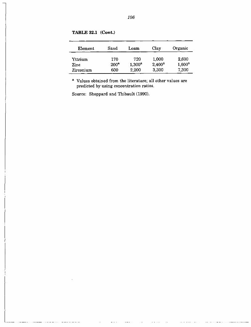
106

TABLE 32.1 (Cont.)

Element Sand Loam Clay Organic

Yttrium 170 720 1,000 2,600 Zinc 200a 1,300a 2,400a 1,600a Zirconium 600 2,200 3,300 7,300

a Values obtained from the literature; all other values are

Source: Sheppard and Thibault (1990).

predicted by using concentration ratios.

107

TABLE 32.2 RESI&AD Default aC, Values

RESRADa Element Kd Kd Rangeb

Hydrogen Carbon Sodium Chlorine Potassium Calcium Manganese Iron Cobalt Nickel Strontium Niobium Technetium Ruthenium Antimony Iodine Cesium Cerium Samarium Europium Lead Radium Actinium Thorium Protactinium Uranium Neptunium Plutonium Americium Curium Californium

0 0

20 0.1 5

50 200

1,000 1,000 1,000

30 0 0 0 0 0.1

500 1,000

0 0

100 70 20

60,000 50 50 0

2,000 20 0

200

NAc

NA NA

15 - 200 5 - 90

50 - 750 165 - 800

60 - 1,300 300 - 1,100

15 - 150 160 - 2,000

0.1 - 1 55 - 66,000

45 - 550 1 - 25

170 - 4,600 500 - 20,000 245 - 3,000

1 - 70

NA 270 - 22,000 500 - 36,000 450 - 5,400

3200 - 89,000 550 - 6,600

15 - 1,600 5 - 1,200

1900 - 112,000

NA

550 - 5,100

4000 - 18,000

Sources: Baes and Sharp (1983), Nuclear Safety Associates (19801, Isherwood (1981), U.S. Nuclear Regulatory Commission (1980), Gee et al. (19801, and Staley et al. (1979).

Source: Sheppard and Thibault (1990). The Kd range is taken from the geometric mean values of sand, loam, clay, and organic soils; therefore, when the default RESRAD Kd is outside the geometric mean range, it does not mean that the RESRAD value is outside the measured Kd range.

NA = not available.

108

33 RADIONUCLIDE CONCENTRATION IN GROUNDWATER

33.1 DEFINITION

This parameter is a measure of the concentration of the principal radionuclide in a well located at the downgradient edge of the contaminated zone. The groundwater concentration and the radionuclide concentration in soil should be measured simultaneously because they are used in RESRAD as a pair to estimate the distribution coefficient. Any natural or non-site related sources of groundwater contamination should be considered because such sources could increase groundwater concentrations and result in a false distribution coefficient.


This parameter should be entered in units of picocuries per liter (pCi/L). Input values for the radionuclide concentration in groundwater are required only if the value of the elapsed time since placement of waste material parameter is greater than zero. Only principal radionuclides with nonzero concentrations in soils will have nonzero concentrations in groundwater. These nonzero groundwater concentration inputs will invoke the calculation of soillwater distribution coefficients, and the input distribution coefficient values will be superseded by the calculated results.

I

109

34 LEACHRATE

34.1 DEFINITION

The leach rate is the fraction of the available radionuclide leached out from the contaminated zone per unit of time. It is assumed that the leaching process is driven by equilibrium distribution of the contaminant between the soil matrix and soil water. The leach rate is used in RESRAD for calculating the source factor for adjusting radionuclide concentrations in the contaminated zone.


In RESRAD, the leach rate should be entered in units of one over time (T-l). An input value of 0 for the leach rate will invoke the calculation of this parameter via a first- order leaching model that uses the value of the soil/water distribution coefficient in the contaminated zone. If the input value of this parameter is greater than 0, however, it will be used to derive the soil/water distribution coefficient of the contaminated zone on the basis of the same first order leaching model. The input soil/water distribution coefficients are then replaced by the derived value.

Because the leach rate constant and the soil-water distribution coefficients are two of the most critical parameters affecting the calculated results of water-related pathways, site-specific values should always be used whenever available. The default leach rate constant in RESRAD is 0.

The first-order ion-exchange leaching model used in RESRAD that estimates the leach rate from the distribution coefficient and other site-specific parameters is a conservative approach for estimating the leaching of radionuclides. When no leach rate data are available, the input of a site-specific Kd value is sufficient.

110

35 MASS LOADING FOR INHALATION

35.1 DEFINITION

The mass loading parameter is the concentration of soil particles in the air and is obtained directly from empirical data for locations and conditions similar to those applicable for the scenario used. This parameter is measured in grams per cubic meter (g/m3).

Three models are commonly used for the process by which dust becomes airborne. One is a resuspension factor model in which the airborne dust concentration (C,,,,) is given as a function of the resuspension factor (R$, the effective depth of the layer of dust from which resuspension occurs ( d J and the bulk soil density (06). The formula relating these variables is

'dust = Rf dr p b . (35.1)

The second is a resuspension rate model in which the airborne dust concentration is given as a function of the resuspension rate (Rr), surface dust concentration (os = &, dJ and the average deposition velocity (V,). The formula is

(35.2)

The third model used by the RESRAD code is a mass loading model in which an average value of the airborne dust concentration is specified on the basis of empirical data.

Use of a mass loading factor from empirical data eliminates consideration of details of the resuspension mechanisms; in particular, the effective depth of the disturbed layer can be ignored.

Average, ambient concentrations of transportable particles range from 3.3 x to 2.54 x g/m3 in nonurban locations (Gilbert et al. 1983). Anspaugh et al. (1974) and Healy and Rodgers (1979) used 1 x g/m3 for predictive purposes and found that the predicted results and the real cases are comparable. The EPA (EPA 1977) has used the same value to screen calculations.

g/m3 in urban locations and from 9 x to 7.9 x

The mass loading value will fluctuate above its ambient level depending on human activities such as plowing and cultivating dry soil or driving on an unpaved road. The estimated mass loading for construction activities is about 6.0 x g/m3; for exposure to construction traffic on unpaved roads it is 4.0 x 10" g/m3; and for agriculture-generated dust, it is about 3.0 x g/m3 (Oztunali et al. 1981). The maximum respirable dust loading inside the cab of heavy construction equipment during a surface coal mining operation was

111

found to be 1.8 x high as 1.3 g/m3 for instantaneous mass loadings during tilling.

g/m3 (Oztunali et al. 1981). Estimates of mass loadings have been as


Gilbert et al. (1983) suggest a mass loading factor of 2.0 x g/m3 for transportable particles at an on-site loading to take into account short periods of high mass loading and sustained periods of normal farmyard activities for which the dust level may be somewhat higher than ambient. This value (2.0 x g/m3) is the default value used in R E S W . Sehmel(1980) has conducted an excellent review of particle resuspension. Users are referred to this paper for a detailed review of particle resuspension and mass loading.

112

36 SHIELDING FACTOR FOR INHALATION PATHWAY

36.1 DEFINITION

This factor is the ratio of airborne dust concentration indoors on-site to the concentration outdoors on-site. It is based on the fact that a building provides shielding against entry of wind-blown dust particles. Therefore, calculation of the effective dose from the dust inhalation pathway should take into account this shielding effect. The occupancy factor, FO,, for the inhalation pathway can then be calculated by RESRAD according to the following equation:

FO2 = TF1 x 1 + TF2 x 0.4 + TF, x 0 , (36.1)

where TFl is the fraction of time spent outdoors on-site (an input parameter, Section 291, TF, is the fraction of time spent indoors on-site (an input parameter, Section 28), and TF3 is the fraction of time spent off-site (not an input parameter, Sections 28 and 29).


This parameter should be input as a fraction ranging from 0 to 1. The default shielding factor for dust inhalation in RESRAD is 0.4, which assumes that the dust level indoors is 40% of the outdoor level (Alzona et al. 1979).

113

37 DEPTH OF ROOTS

37.1 DEFINITION

This parameter is the average root depth of various plants grown in the contaminated zone. The root depth varies for different plants. For some plants, such as beets, carrots, lettuce, and so forth, it does not extend below about 0.3 m. For others, such as fruit trees, the roots may extend 2 or 3 m below the surface; tap roots for some crops (e.g., alfalfa) can extend to 5 m. Most of the plant roots from which nutrients are obtained, however, usually extend to less than 1 m below the surface.

This parameter is used to calculate the cover and depth factor for the plant, meat, and milk pathways because edible plants become contaminated through root uptake of radionuclides. Uptake of radionuclides from plant roots is assumed possible only when the roots extend to the contaminated zone and is limited to the fraction of roots that have direct contact with contaminated soil.


The average root depth should be entered in units of meters (m). The default value in the RESRAD code is 0.9 m.

114

38 SOIL INGESTION RATE

38.1 DEFINITION

This parameter is the accidental ingestion rate of soil material or soil dust. Children, especially those under 18 months, tend to mouth or ingest substances that are not considered to be food. When this behavior extends beyond the age of 18 months, the child is said to practice pica (Barltrop 1966; Robischon 1971; Ziai 1983). Many factors such as nutrition, quality of care, and parental relationship (Bicknell 1974; Glickman 198 1; Danford et al. 1982; Behrman and Vaughan 1983; Forf'ar and Arneil 1984; Bellinger et al. 1986) influence the extent of this behavior. However, it is believed that a child who practices pica is no different from one who does not because pica cannot be consistently predicted (Feldman 1986), even though severe pica usually occurs among grossly disturbed or mentally retarded children.

According to the literature, a wide variety of substances are ingested: soil, clay, sand, dust, grass, leaves, plaster, hair, starch, paint chips, string, soap, wood, powders, chalk, and paper. No quantitative ingestion rates have been suggested because children with known pica behavior have not been studied. "Abnormal" soil ingestion (pica) is believed to be uncommon and may need to be addressed separately.

On the basis of observational data, children are most likely to ingest soil from the age of 1 to 6 (Cooper 1957; Sayre et al. 1974; Charney et al. 1980; Walter et al. 1980). Beyond age 6 or 7, ingestion of nonfood substances is usually caused by inadvertent ingestion or developmental problems. Paustenbach et al. (1986) summarized the normal amount of soil ingested by children on the basis of the age of the child. Vermeer and Frate (1979) pointed out that the environmental setting is also an important factor for children in rural areas who tend to ingest a higher amount of soil. Hawley (1985) used data from the literature to develop scenarios to estimate ingestion amounts for young and older children and adults. He divided each year into two activity periods: May through October when individuals spend more time outdoors and November through April when most of the time, weather conditions eliminate outdoor activities. Hawley's study indicated that the amount ingested by young children (2.5 years old, weighing 13.2 kg), during outdoor activity between May and October (5 dweek) is 250 mg/d. During November through April, the ingestion during indoor activity is 100 mg/d. For children six-years old, weighing approximately 20.8 kg, the ingestion amount is 50 mg/d during outdoor activity from May through October and 3 mgld year-round for indoor activity. Working in attics or other uncleaned areas of a house can cause adults (weighing 70 kg) to ingest 110 mg/d of soil for an assumed duration of 12 dyr. For living space activities, the ingestion amount is 0.56 mg/d. For outdoor activities from May through October, the ingestion amount is 480 mglactive d, assuming 8 hours is spent outdoors per day, 2 dweek.

According to Binder et al. (1986), the average quantity of soil ingested by children is about 108 mg/d (within a range of 4-708 mg/d). Clausing et al. (1987) estimated that the ingestion rate of children is 105 mg/d, with a range of 23-362 mg/d. Binder et al. (1986) and

115

Clausing et al. (1987) have also provided some limited information on the upper limit of the soil ingestion rate on the basis of evidence that the upper range of the ingestion rate for children is around 800 mg/d or more.

An amount has not been estimated for abnormal soil ingestion behavior among children. However, some evidence suggests that a rate of 5 to 10 g/d may not be unreasonable. The EPA used 5 g/d in its risk assessment for tetrachlorodibenzo-p-dioxin (TCDD) (EPA 1984a). The USDA used a value of 10 g/d in conducting exposure assessments related to the use of sludge in gardens and soils.

After reviewing the limited data available, the EPA (1990a) decided that the studies of Binder et al. (1986) and Clausing et al. (1987) appear to be the most reliable and suggested that an estimate of 0.2 g/d be used as an average value for young children (under the age of 7). An upper range of soil ingestion is 0.8 g/d. For other age groups (children older than 7 years), 0.1 g/d should be used for the soil ingestion amount. These factors account for ingestion of both outdoor soil and indoor dust. Site conditions, for example, snow cover, will affect the soil ingestion rate because the cold weather will limit outdoor activities in the winter, and because snow also provides an additional cover for the contaminated soil. However, presently there is no recommended approach to correct these influences, and any correction should be conservatively applied.

According to EPA guidance (EPA 1990b), soil ingestion should be considered separately for adults and children for a residential scenario. For the first stage (for children), 0.2 gld is the recommended ingestion rate with an exposure duration of 6 years, and for the second stage, with an exposure duration of 24 years, the recommended ingestion rate is 0.1 g/d. In RESRAD, only one soil ingestion rate is required, which is the yearly intake rate (g/yr) without the differentiation between contaminated soil and uncontaminated soil. RESRAD will automatically adjust this soil ingestion rate with an area factor, an occupancy factor, and a cover-and-depth factor, so that only the contaminated source is accounted. The input value for the soil ingestion rate depends strongly on the assumed scenario. For a residential scenario with an exposure duration of 30 years, 43.8 g/yr K36.5 g/yr x 24 yr + 73 g/yr x 6 yr)/30 yrl is an applicable input value to RESRAD according to EPA guidance.

The EPA (1991) has chosen 50 mgld as the standard default value for adult soil ingestion in the workplace based on a pilot study by Calabrese et al. (1990). This 50 mg/d value is to be used in conjunction with an exposure frequency of 250 dyr and an exposure duration of 25 yr. For outdoor activities in the commercial/industrial setting (e.g., construction on landscaping) a soil ingestion rate of 480 mg/d is recommended by the EPA; however, this type of work is usually short-term and is often dictated by weather.


Several methods have been used to characterize soil ingestion by children. Lepow et al. (1975) measured hand dust by applying preweighed adhesive labels to the hands and

116

weighing the amount of dirt that was removed. They also observed “mouthing” behavior and reported that a child would put his or her fingers into the mouth about 10 times a day. Day et al. (1975) and Duggan and Williams (1977) also measured the amount of dust on children’s hands. Binder et al. (1986) studied the ingestion of soil among children 1 to 3 years of age who wear diapers. Both excreta and soil from the play yards were analyzed for materials that were thought to be poorly absorbed in the gut. Clausing et al. (1987) conducted a soil ingestion study by using a tracer element method similar to that of Binder et al. (1986). They also collected fecal samples for six hospitalized, bedridden children to represent a control group.

Presently there is no widely accepted method for determining the relative contribution of each medium (i.e., soil versus dust) to the daily ingestion amounts and the effect of climatic variations (e.g., snow cover).


In the RESRAD code, the soil ingestion rate should be entered in units of grams per year (dyr). The default value of 36.5 g/yr is used, which accounts for an average soil intake rate of 0.1 g/d for 365 d/yr. The 0.1 g/d ingestion rate is a value recommended by the EPA for adults in a residential scenario.

117

39 THICKNESS OF CONTAMINATED ZONE

39.1 DEFINITION

This parameter is the distance between the uppermost and lowermost soil samples that have radionuclide concentrations clearly above background. In determining whether the measured soil concentration is above the background level, a DOE-approved method based on a statistical analysis of site measurements in comparison to background measurements should be used (DOE 1991a, Section 7). In case such an approach is not available, then as a default approach, a soil sample should be treated as clearly contaminated if the radionuclide concentration is greater than the average background radionuclide concentration plus twice the standard deviation of the background measurements.


A DOE-approved statistical approach (DOE 1991a, Section 7) should always be considered first when estimating average, handling distribution analyses and estimating central tendency soil concentrations. The default approach provided below is a conservative method that may sometimes significantly overestimate the dose. To determine the thickness of a contaminated zone with an area greater than 100 m2, the average contamination thickness of boreholes drilled to take soil samples is calculated over any integral subarea of 100 m2. If one or more boreholes in the subarea have a contamination thickness exceeding the average thickness by a factor larger than three, then the average value is replaced by one-third the maximum contamination thickness. The thickness of the contaminated zone is then taken as the maximum average thickness calculated over a 100-m2 subarea. For a contaminated zone with an area less than 100 m2, the average contamination thickness over the contaminated zone or one-third of the maximum Contamination thickness in a borehole (if the thickness is greater than three times the average value) is taken as the representative value of the contaminated zone thickness.


In RESRAD, the thickness of this ideal contaminated zone is entered in units of meters (m). The default value is 2 m.

118

40 RADIATION DOSE LIMIT

The radiation dose used in the RESRAD code is the effective dose equivalent from external radiation plus the committed effective dose equivalent from internal radiation (International Commission on Radiological Protection [ICRP] 1984). The radiation dose limit is used in RESRAD to derive soil guidelines (i.e., cleanup criteria). The calculated guidelines are linearly proportional to the dose limit. If the RESRAD code is used to calculate doses (rather than soil guidelines), the input value of the radiation dose limit will not affect the calculated doses.

In the RESRAD code, 30 mredyr (0.3 mSv/yr) is used as the default value. This value is less than the 100 mrem/yr basic radiation dose limit specified in DOE Order 5400.5. The 100 mredyr dose limit has been used to calculate the derived concentration guides (DCGs) listed in Chapter 3 of DOE Order 5400.5. It is unacceptable, however, to derive authorized limits for soil by using the 100 mrem/yr primary dose limit as a dose standard, when actual or likely use of the sites is considered. As with DCGs, 100 mredyr represents a reasonable upper bound on concentration. Authorized limits for release must comply with the as Iow as reasonably achievable (ALARAI process (DOE 1991b) and should be a small fraction of the dose limit. Therefore, when using realistic parameters and considering likely use scenarios, a default dose limit of 30 mredyr (0.3 mSv/yr) is used in RESRAD.

119

41 SEAFOOD CONSUMPTION RATE

41.1 DEFINITION

National recreational catch data for coastal areas were obtained by the National Marine Fisheries Service (NMFS) in 1985. The NMFS conducted a direct survey of fishermen in the field and an independent telephone survey of households (NMFS 1986). Total fish consumption data were obtained from a one-year survey conducted by NPD Research, Inc., during 1973 and 1974 and funded by the Tuna Research Institute. Questionnaires were answered by 6,980 families representing the US. population.

Javitz (1980) used the data obtained by NPD Research, Inc., to calculate the mean and 95th percentile of seafood consumption for seafood consumers in the United States as 14.3 g/d (5.2 kg/yr) and 41.7 g/d (15.2 kg/yr), respectively. The mean average of 14.3 g/d (5.2 kg/yr) for seafood consumption includes 2.1 g/d (0.8 kg/yr) for nonfish seafood consumption, that is, lobsters, oysters, scallops, shrimps, squids, and so forth. Unfortunately, NPD Research, Inc.’s original survey data for seafood consumption did not distinguish between recreationally caught and purchased fish; therefore, this difference is not reflected in the calculated mean and 95th percentile values.

Puffer et al. (1982) conducted 1,059 interviews with sport fishermen in the Los Angeles Harbor area. The interviews revealed that sport fishermen keep 67 to 89% of the finfish and 97% of the shellfish that they catch. The median and 90th percentile seafood (fish plus shellfish) consumption rates of sport fishermen are 37 and 225 g/d, respectively.

Another source for the seafood consumption rate of sport fishermen is a survey conducted in Commencement Bay at Tacoma, Washington, by Pierce et al. (1981) in 1981. The sample size (304 fishermen) was smaller than that of Puffer et al. (1982) and the sampling frequency was lower. It was found that over half of the fishermen caught and consumed fish weekly. Pierce et al. (1981) concluded that the mean average seafood consumption rate for the surveyed fishermen was 23 g/d (within a range of 12-54 g/d); the 90th percentile was 54 g/d.

Although the surveys conducted by Puffer et al. (1982) and Pierce et al. (1981) are limited to the West Coast, the EPA (1990a) considers these studies to be representative of actual annual consumption rates for recreational fishermen. By averaging the results of these two surveys, the EPA (1990a) has suggested that the 50th and 90th percentile seafood consumption rates of fishermen are 30 g/d (11 kg/yr) and 140 g/d (51 kg/yr), respectively.

Because sport fishermen and their families consume much more seafood than other people, the EPA recommends that consumption rates of fishermen based on Puffer et al.’s (1982) and Pierce et al.’s (1981) surveys be used as comparative references for any area where there is a large body of water and widespread contamination is possible.

120

The NRC (1977) used values of 2.2, 5.2, and 6.9 kg/yr for average individual fish consumption for children, teenagers, and adults, respectively. Average individual consumption rates of other seafood were 0.33, 0.75, and 1.0 kg/yr for the three different groups. For a worst-case scenario, the fish consumption rates were 6.9, 16, and 21 kg/yr for children, teenagers, and adults, respectively. For other seafood consumption rates, values of 1.7, 3.8, and 5 kg/yr were used.

The input seafood consumption rate in RESRAD is the yearly total consumption rate, which does not take into account the difference between the contaminated and uncontaminated portion. It is assumed that if a surface water body (a pond) is located on a site, it will provide 50% of the consumed seafood. If a RESRAD user would like to use a different fraction, then the fraction of aquatic food from the site (an input parameter) needs to be modified so that the calculated dose accounts for the correct contaminated amount of the consumption rate.


In the RESRAD code, the seafood consumption rate should be entered in units of kilograms per year (kg/yr). The default value for the consumption rate is 5.4 kglyr for fish and 0.9 kg/yr for other seafood.

. . -. . . . . . . . . . . . . . . . . . . . . . . . . . . . . . . . . . . . . . . . . . . . . . . . . . . . . . . . . . . . .. . . . . . . . . . . . . . . .

121

42 FRUIT, VEGETABLE, AND GRAIN CONSUMPTION RATE

42.1 DEFINITION

According to the latest survey by the National Gardening Association (19871, 38% or a total of 34 million U.S. households participated in vegetable gardening in 1986. The size of the home vegetable garden, however, has decreased from 600 ft2 in 1982 to 325 ft2 in 1986 (National Gardening Association 1987). The distribution of home gardens varies geographically, with a large percentage located in the Midwest and South, and more in rural areas than in cities and suburbs. Therefore, homegrown fruits and vegetables make up a larger portion of the average consumption rate in rural areas than in cities or suburbs.

The EPA has made recommendations on the consumption rates of homegrown h i t s and vegetables on the basis of two sources: Foods Commonly Eaten by Individuals: Amount Per Day and Per Eating Occasion (Pa0 et al. 1982) and Food Consumption: Households in the United States, Seasons and Year 1977-1978 (USDA 1983). The first source used data collected by the USDA in 1977-1978 from home interviews of 37,874 respondents who were asked to recall food consumed one day before the interview, the day of the interview, and the day after the interview, to calculate percentiles of total fruit and vegetable consumption of the US. population. The consumption rate of homegrown fruits and vegetables can be calculated by subtracting the data of the "bought" category for all foods from the data of the "all" category in the USDA food consumption survey. Homegrown dark green vegetables make up approximately one-third of the dark green vegetables consumed. This category includes mustard greens, kale, kohlrabi, and broccoli. Consumption of homegrown corn, cucumbers, green beans, and tomatoes makes a significant contribution to total consumption. The proportion of homegrown h i t s consumed is highest for strawberries, peaches, and pears, and lowest for citrus fruits.

According to the EPA (1990), the average consumption rate of vegetables per person is 200 g/d (73 kg/yr); homegrown products account for 25% of the total consumption rate, which is 50 g/d (18 kg/yr). Total average daily fruit intake is 140 g/d (51 kg/yr) per individual. The total homegrown h i t consumption rate is 28 g/d (10 kg/yr), which is 20% of the total intake rate. For a reasonable worst case, it is suggested that 40% of the total intake be used for homegrown vegetable consumption and 30% of the total intake be used for homegrown fruit consumption. Table 42.1 summarizes the EPA's recommendations.

The EPA data provided above do not include information about grain product consumption. In NRC Regulatory .Guide 1.109 (NRC 1977), different total consumption amounts of fruits, vegetables, and grains are suggested for different age groups. The average individual consumption for a child is 200 kg/yr, for a teenager it is 240 kglyr, and for an adult it is 190 kg/yr. Suggested values for the maximally exposed individual in a worst-case scenario are 520, 630, and 520 kg/yr, for a child, teenager, and adult, respectively. The total consumption for the maximum exposure case consists of 22% for fruit consumption, 54% for vegetable consumption, and 24% for grain consumption.

122

TABLE 42.1 Vegetable and Fruit Intake Rates

Average Total Average Intake Worst-case Intake Intake Homegrown Homegrown

Vegetables 200 73 50 18 80 29

Fruit 140 51 28 10 42 15

Total 340 124 78 28 122 44

To run the RESRAD code, a yearly consumption rate for fruit, vegetables, and grain is needed that does not differentiate the contaminated fraction from the uncontaminated fraction. An area factor will automatically be calculated and used to adjust the consumption rate. It is assumed that if an area is greater than 1,000 m2, then 50% of the consumption is obtained from the site; if the area is smaller than 1,000 m2, then the fraction of the contaminated product is the ratio of the Contaminated area to an area of 2,000 m2. The upper bound in the RESRAD default adjustment for the fraction of contaminated products is 50%. If this value differs from that obtained from site-specific data, the user should adjust the yearly consumption rate so that an accurate consumption rate of the contaminated product is used to derive the total dose.

42.2 RESRAD DATA INPUT REQUPRE1VPENTS

In the RESRAD code, the consumption rate should be entered in units of kilograms per year (kg/yr). The default value for the consumption rate is 160 kg/yr for fruit, vegetables, and grains.

123

43 IWHALATIONRATE

43.1 DEFINITION

The inhalation rate varies with activity level, age, weight, sex, and general physical conhtion. Anthropometric data (EPA 1985) have been used to propose several formulas for calculating the inhalation rate for a human at rest. However, in general, the formulas are based on measurements from relatively small sample sizes and are limited to calculating the inhalation rate at rest only.

The EPA (1985) has compiled the available data, most of which is from early stuhes, and has derived an inhalation rate expressed in cubic meters per hour (m3/h). Inhalation rates were compiled for each agehex group at rest and at light, moderate, and heavy activity levels. The activity levels were categorized according to criteria developed by the Environmental Criteria and Assessment Ofice of the EPA for the air quality document for ozone. A male adult with a body weight of 70 kg was used as a reference, and activity level categories for the other agehex groups were extrapolated from the criteria for male adults on the basis of body weight (American Industrial Hygiene Association 1971). Table 43.1 gives a summary of human inhalation rates at different agehedactivity levels (EPA 1985). Resting is characterized by such activities as watching television, reading, or sleeping. Light activity includes level walking, meal cleanup, care of laundry and clothes, domestic work and other miscellaneous household chores, attending to personal needs, photography, hobbies, and conducting minor indoor repairs and home improvements. Moderate activity includes climbing stairs, heavy indoor cleanup, and performing major indoor repairs and alterations (e.g., remodeling). Heavy activity consists of vigorous physical exercise such as weight lifting, dancing, o r riding an exercise bike.

TABLE 43.1 Summary of Human Inhalation Rates (m3/h) for Men, Women, and Children by Activity Level

Activity Level

Resting Light Moderate Heavy

Adult male 0.7 0.8 2.5 4.8 Adult female 0.3 0.5 1.6 2.9 Average adult 0.5 0.6 2.1 3.9 Child, age 6 0.4 0.8 2.0 2.4 Child, age 10 0.4 1.0 3.2 4.2

Source: EPA (1985).

124

Assuming 16 hours of light activity and 8 hours of resting, the ICRP (1981) has reported a 23-m3/d inhalation rate for adult males and a 21-m3/d rate for adult females, yielding an average value of 22 m3/d (8,030 m3/yr) for adults.

Data presented by the EPA (1985) suggest lower inhalation rates for light and resting activity levels. Using the same assumption as the ICRP (1981), the daily inhalation rate would be about 14 m3/d (5,110 m3/yr). In addition to assuming lower rates for light and resting activity levels, the EPA also estimated the daily inhalation rate for moderate and heavy activity levels; therefore, it is possible to estimate the total inhalation rate for any combination of activity levels. The EPA's data suggest that the maximum inhalation rate is roughly twice the reported mean rates for all activity levels.

The EPA (1990) made the following recommendations on the basis of the above mentioned data: 20 m3/d (7,300 m3/yr) should be used as the average adult daily inhalation rate and 30 m3/d (11,000 m3/yr) as the reasonable worst-case inhalation rate, provided the activity patterns are unknown. For exposure scenarios in which the distribution of activity patterns is known, the values in Table 43.1 should be used for calculations because they are more representative rates.

For an individual performing outdoor activities, a typical activity mix can consist of 37% at a moderate activity level, 28% at both resting and light activity levels, and 7% at a heavy activity level, which results in a 1.4 m3/h (12,300 m3/yr) inhalation rate. A reasonable worst-case outdoor inhalation rate can account for 50% of the time at a heavy activity level and 50% at a moderate activity level, with an inhalation rate of 3.0 m3/h (26,300 m3/yr>, according to Table 43.1.

For an individual performing indoor activities, an average assumption would include 48% of the time at both a resting and light activity level, 3% at a moderate activity level, and 1% at a heavy activity level. A reasonable worst-case includes 25% at a resting activity level, 60% at a light activity level, 10% at a moderate activity level, and 5% at a heavy activity level. The first assumption has an average inhalation rate of 0.63 m3/h (5,500 m3/yr), and the second one has a reasonable worst-case inhalation rate of 0.89 m3/h (7,800 m3/yr).


In the RESRAD code, the inhalation rate should be entered in units of cubic meters per year (m3/yr). The default value used in the code is 8,400 m3/yr.

In the RESRAD code, the yearly inhalation rate is used. This rate is an average value that accounts for different activity levels both indoors and outdoors. Therefore, a site- specific value can be obtained with the assumed exposure scenario and an activity profile. The fraction of time spent on-site and off-site should not affect this input parameter, however, because in the RESRAD calculation, an occupancy factor is automatically derived and used for adjusting the calculated dose.

125

44 LEAFY VEGETABLE CONSUMPTION R.A"E

44.1 DEFINITION

The leafy vegetable consumption rate is a dietary factor for human food consumption that includes consumption of vegetables such as spinach and lettuce. On the basis of recommended values for the maximally exposed individual in NRC Regulatory Guide 1.109 (NRC 19771, the consumption rates of leafy vegetables for children, teenagers, and adults, respectively, are 26, 42, and 64 kg/yr. Average consumption rates used by the NRC to perform environmental dose analyses for releases of radioactive effluents from nuclear power plants into the atmosphere (Strenge 1987) are 10, 20, and 30 kg/yr for children, teenagers, and adults.

The RESRAD input leafy vegetable consumption rate does not differentiate the contaminated fraction from the uncontaminated fraction. Like the fruit, vegetable, and grain consumption rate stated in Section 42, a default adjustment is automatically performed, via the contaminated area, within the RESRAD code. If this value is different than that obtained from site-specific data, then the input consumption rate needs to be modified so that RESRAD calculates the correct dose for the contaminated product.


The default value used in RESRAD for the leafy vegetable consumption rate is 14 kg/yr.

126

45 LIVESTOCK WATER INTAKE RATE FOR BEEF CATTLE AND MILK COWS

45.1 DEFINITION

According to NRC Regulatory Guide 1.109 (NRC 19771, the water ingestion rate for beef cattle is 50 L/d. The water ingestion rate for milk cows is 14 g d d (approximately 50 L/d) plus 1 gal for every 3 lb of milk produced (Great Lakes Basin Commission 1975). If a production rate of 10 gaud of milk is assumed, then the water ingestion rate for milk cows would be about 160 L/d (Gilbert et al. 1983).


In the RESRAD code, the livestock water intake should be entered in units of liters per day (L/d). The default values for beef cattle and milk cows are set to 50 and 160 Ud, respectively, if the user does not specify otherwise.

127

46 MEAT AND POULTRY CONSUMPTION RATE

46.1 DEFINITION

The USDA conducted a national food consumption survey in 1977-1978 (USDA 1983). The average consumption rates for beef and dairy products, as adopted by the EPA (1984a,b), are based on the results of this survey.

According to USDA studies, 44% of annual consumption is homegrown beef. This finding is based on a survey of 900 rural farm households (USDA 1966). Because the total amount of beef consumed averages approximately 100 g/d (36.5 kg/yr), the average consumption of homegrown beef is about 44 g/d (EPA 1990), which corresponds to 16 kg/yr.

For a reasonable worst-case, the EPA (1990) has suggested that a consumption rate of 75 g/d (27 kg/yr) be used for homegrown beef in risk assessments until better data are available.

The average consumption rate of 36.5 kg/yr, as recommended by the EPA, accounts for beef only. The total consumption rate for meat and poultry should be much higher. According to NRC Regulatory Guide 1.109 (NRC 19771, the recommended average value for consumption of meat and poultry is 37 kg/yr for children, 59 kg/yr for teenagers, and 95 kg/yr for adults. Recommended values for use in a maximally exposed case are 41 kg/yr for children, 65 kg/yr for teenagers, and 110 kg/yr for adults.

Gilbert et al. (1983) used a value of 79 lb/yr (36 kg/yr) for meat, 20 lb/yr (9 kg/yr) for poultry, and 15 lb/yr (7 kg/yr) for egg consumption, with a total value of 114 lb/yr (52 kg/yr). The consumption rate used for meat is about the same as that recommended by the EPA (1990). If the same percentage of homegrown beef can be applied to consumption of poultry and eggs, then the average consumption of homegrown meat, poultry, and eggs would be 23 kg/yr; for a reasonable worst-case scenario, the value would be 39 kg/yr on the basis of data of Gilbert et al. (1983). ,

In the RESRAD code, it is assumed that all of the consumed meat is Contaminated if the area of the contaminated zone is greater than or equal to 20,000 m2. If the area is less than 20,000m2, then the fraction of the contaminated product is the ratio of the contaminated area to an area of 20,000 m2. If site-specific data differ from the RESRAD default values, the input data may need to be adjusted so that the correct dose from the contaminated meat product is obtained.

46.2 RESFtAD DATA INPUT REQUIREMENTS

In the RESRAD code, the consumption rate for meat and poultry should be entered in units of kilograms per year (kdyr). The default value for the consumption rate is 63 kg/yr.

128

47 MILK CONSUMPTION RATE

47.1 DEFINITION

According to the EPA (1984a) and Fries (19861, the milk (fresh milk only) consumption rate can range from 254 g/d to 1,000 g/d per person, with an average rate of 305 g/d (i.e., 110 Uyr). According to a USDA (1966) survey, 40% of the dairy products consumed in a typical farm household are from the milk cows on the farm. Applying this same percentage to a typical farm scenario, 44 Uyr of the fresh milk consumed is actually from cows owned by the farmer. On the basis of EPA (1990) suggestions for a worst-case scenario, if 75% of the fresh milk consumed is assumed to be from milk cows on the farm, the average consumption rate of fresh milk would then be 83 Uyr per person for a farm scenario.

In NRC Regulatory Guide 1.109 (NRC 1977), milk consumption rates for different age groups are reported. The average rates for children, teenagers, and adults are 170,200, and 110 Uyr, respectively. Recommended values for the maximally exposed individual are 330, 330, 400, and 310 Uyr for infants, children, teenagers, and adults.

The RESRAD code assumes that all of the consumed milk is contaminated if the area of the contaminated zone is greater than or equal to 20,000 m2. If the area is less than 20,000 m2, then the fraction of the contaminated product is the ratio of the contaminated area to an area of 20,000 rn2. Therefore, caution should be used in choosing the appropriate input data so that the correct site-specific dose level is obtained.


In RESRAD, the default milk consumption rate is set to 92 Uy-r per person.

129

48 SHIELDING FACTOR FOR EXTERNAL GAMMA RADHATHON

48.1 DEFINITION

This factor is the ratio of the external gamma radiation level indoors on-site to the radiation level outdoors on-site. It is based on the fact that a building provides shielding against penetration of gamma radiation. Therefore, the calculation of the effective dose from the ground pathway should take into account this shielding effect.

The occupancy factor, PO,, for the ground pathway can be obtained by using the following equation:

FO1 = TF, x 1 + TF2 x 0.7 + TF3 x 0 , (48.1)

where TF, is the fraction of time spent outdoors on-site (an input parameter, Section 291, TF2 is the fraction of time spent indoors on-site (an input parameter, Section 281, and TF3 is the fraction of time spent off-site (not an input parameter, Sections 28 and 29).


This parameter should be input as a fraction, ranging from 0 to 1. The default shield factor used in the RESRAD code for external gamma radiation is 0.7, which assumes that the external gamma radiation level indoors is 30% lower than the outdoor gamma radiation level.

130

49 ELAPSED TIME OF WASTE PLACEMENT

49.1 DEFINITION

The elapsed time of waste placement parameter is the duration between the placement of radioactive waste on-site and the performance of a radiological survey, It is possible that on-site radioactive wastes originated from different sources and have different placement times. Under these circumstances, an average value or a best representative value should be used.

When using RESRAD for risk assessment, the information obtained during the radiological survey is input to derive soil guidelines for cleanup criteria. This information includes soillwater distribution coefficients, soil radionuclide concentrations, and so forth. The soiVwater distribution coefficients are used for calculating the breakthrough and rise times of the groundwater contamination and for predicting the future radionuclide concentration in groundwater. In this case, the elapsed time of waste placement is zero. Nonzero values of this parameter should be input only when the soiVwater distribution

. coefficients are not available and above background level groundwater radionuclide concentrations are measured in a radiological survey. Under such conditions, the input radionuclide concentration in groundwater, together with the elapsed time of waste placement would be used to derive soiVwater distribution coefficients and to predict the future radionuclide concentration in groundwater.


In the RESRAD code, the elapsed time of waste placement should be entered in units of years (yr). The default value of this parameter is set at zero.

131

50 SHAPE FACTOR (EXTERNAL GAMMA)

50.1 DEFINITION

A shape factor is used to correct for a noncircular-shaped contaminated area on the basis of an ideally circular zone. The shape factor for a circular contaminated area is 1.0. For an irregularly shaped contaminated area, the shape factor may be obtained by enclosing the irregularly shaped contaminated area in a circle, multiplying the area factor of each annulus by the fraction of the annulus area that is contaminated, summing the products, and dividing by the area factor of a circular contaminated zone that is equivalent in area. The area factors of circular contaminated zones with different radii are listed in Table 50.1. The area factor of an annulus is the area factor from an annular zone bounded by the radii tabulated in Table 50.1.

If an irregularly shaped contaminated zone of 191.4 m2 is shaped like that in Figure 50.1, the shape factor can be calculated by surrounding the area with the appropriate annuli as indicated. The contamination fractions within each annulus are 1, 1, 0.97, and 0.22, respectively. The area factor of the irregularly shaped contaminated zone can be calculated as follows on the basis of the values in Table 50.1:

Ci=1,4 (area factor) x (contamination fraction)i (50.1)

= (0.016 x 1) + (0.4-0.016) x 1 + (0.55-0.4) x 0.97 + (0.8-0.55) x 0.22

= 0.601 .

Next, the area factor of a circular contaminated zone equivalent in area must be determined. The radius of a circle with an area of 191.4 m2 is 7.8 m. By interpolating the data of Table 50.1, the area factor of a circle equivalent in area can be determined as follows:

(0.8-0.55)/(13-5.6) x (7.8-5.6) + 0.55 = 0.62 . (50.2)

The final step in obtaining the shape factor of the contaminated zone is to divide the area factor of the contaminated zone by that of the circular zone with an equivalent area:

0.60U0.62 = 0.97 . (50.3)

Therefore, the shape factor of an irregularly shaped contaminated zone such as that in Figure 50.1 is determined to be 0.97.

132

TABLE 50.1 Area Factors for External Gamma Radiation from Contaminated Ground

Contaminated Radiusa Area Factor, Area (m2> (m) FA^

1 0.56 0.016 25 2.8 0.4

100 5.6 0.55 500 13 0.8

1.200 20 1.0

a Radius for a circular contaminated area.

Intermediate values may be obtained by linear interpolation.

Source: Napier et al. (1984).

Legend

Contaminated area of annulus 1



Contaminated area of annulus 4 1

FIGURE 50.1 Irregularly Shaped Contaminated Zone Enclosed by Four Annuli

..... . ~-.-

133


In the RESRAD code, the default contaminateG area is 10,000 m2, which is greater than the area of 1,200 m2 listed in Table 50.1 for an area factor of 1.0. Because the area factor is already equal to 1, the default value of the shape factor is 1.

If the input shape factor is negative, that is, between 0 and -1, then the SOILD model (Chen 1991) rather than the model mentioned in the original RESRAD report (Gilbert et al. 1989) is used for calculating the effective dose from external radiation. In this case, the shape factor is not actually used in SOILD calculations, it merely serves as a flag for the choice of options. Thus, the user should provide more detailed information about the fractions of annular areas within the contaminated zone for use in the SOILD calculations.

134

51 INITIAL CONCENTRATIONS OF PRINCIPAL RADIONUCLIDES

51.1 DEFINITION

A principal radionuclide is a radionuclide with a half-life longer than one-half year. Radionuclides with a half-life of one-half year or less are treated as associated radionuclides. The radionuclides "associated' with a principal radionuclide consist of all decay products down to, but not including, the next principal radionuclide in the chain. It is assumed that all associated radionuclides (except radon daughters) are in secular equilibrium with their principal radionuclide in the contaminated zone and also at the location of human exposure. Only the principal radionuclides in the contaminated zone need input values of radionuclide concentrations.

The single-radionuclide soil guidelines do not depend on the radionuclide concentrations in soil. Even if the radionuclide concentrations are not known, values for these guidelines can be obtained by entering any nonzero radionuclide concentration. The calculated doses, however, depend on the radionuclide concentrations; thus, doses calculated by RESRAD are valid only if the soil radionuclide concentrations are known. When the radionuclide concentrations in soil and groundwater are used with the elapsed time of waste placement to derive the soillwater distribution coefficient, the values of the initial concentrations of the principal radionuclide must be known to obtain accurate results.

A DOE-approved statistical approach (DOE 1991a, Section 7) should always be considered as the first priority regarding the estimation of the soil concentration. When such an application is impossible, then the following approach will serve as a default procedure in determining the average soil concentration; however, this approach will result in a conservative estimate of the effective dose.

For a site-specific case, the distributions of radionuclides are nonuniform. The potential annual individual dose received through a particular pathway is an average of the nonuniform residual radioactivity over an area determined by the scenario activities; for example, the area of daily activities for external radiation or the size of the garden for the plant food pathway, For the purpose of deriving soil guidelines, it is assumed that this area is 100 m2 for all pathways. The effect of vertical nonuniformities is taken into account by averaging the radionuclide concentrations in a 0.15-m-thick layer over the 100-m2 area.

The initial concentration of a principal radionuclide is determined by the following procedures. For a contaminated zone with an area greater than 100 m2, the average radionuclide concentration for any subzone with a 100-m2 area and 0.15-m thickness is determined. If one or more soil samples within this subzone have radionuclide concentrations greater than three times the average radionuclide concentration, then the average radionuclide concentration of this subzone is replaced by one-third the maximum measured soil radionuclide concentration. The initial concentration of a principal radionuclide in the contaminated zone is the maximum value of the average subzone radionuclide concentration. For a contaminated zone with an area less than 100 m2, the initial concentration of a

135

principal radionuclide is the maximum average radionuclide concentration of the 0.15-m-thick subzones.


In the RESRAD code, the initial concentrations of principal radionuclides in the contaminated zone are expressed in units of picocuries per gram (pCi/g). RESRAD treats the contaminated zone as a uniformly contaminated area with a single radionuclide concentration at every point.

I36

52 DRINKING WATER INTAKE RATE

52.1 DEFINITION

The EPA uses 2 L/d as the average amount of water consumed by an adult; this includes juices and beverages containing tap water (e.g., coffee). However, this value was established by the U.S. Army in determining the amount of water needed per person in the field and is believed to be an overestimate.

The National Academy of Sciences (NAS) (1977) calculated the average consumption rate of water to be 1.63 LJd per person. It is reasonable to assume that people in physically oriented occupations or living in warmer regions may have an intake rate exceeding this level. Although the consumption rate of 1.63 Wd seems to have a more scientific basis than the 2 L/d rate, the NAS (1977) still adopted the larger volume &e., 2 L/d) to represent the intake rate for the majority of people.

Several other drinking water intake rates have been suggested. The National Cancer Institute (NCI) in an investigation of the possible relationship between bladder cancer and drinking water, interviewed approximately 9,000 individuals by using a standardized questionnaire and suggests that the overall average tap water consumption rate is 1.39 L/d (Cantor et al. 1987). According to the NCI’s distribution data, 1.3 Wd is the approximate value of the 50th percentile and 2.0 L/d is the approximate value of the 90th percentile.

Gillies and Paulin (1983) suggest an average rate of 1.256 (+ 0.39) L/d and a 90th percentile rate of 1.9 LJd on the basis of a survey conducted in New Zealand. On the basis of data from the U.S. Food and Drug Administration’s total diet study, Pennington (1983) reported an average daily fluid consumption rate for water and water-based foods of 1.2 L/d. The ICRP has summarized the intake levels for adults as ranging from about 0.4 L/d to about 2.2 Wd under normal conditions.

The EPA (1984~) used data collected by the USDA in its 1977-1978 nationwide food consumption survey to determine daily beverage intake levels by age. The daily beverage intake level for adults ranged from 1.24 to 1.73 L. The EPA (1990) has suggested that the average adult drinking water consumption rate is 1.4 L/d; the reasonable worst-case value is 2.0 L/d on the basis of the above studies. These values correspond to 510 and 730 Uyr, respectively, if a 365 dyr is used. Further evidence to support these values is provided by Pennington (1983) and Cantor et al. (1987) who report average total fluid intake rates of 1.7 and 1.87 Wd among adults. Thus, the average water consumption rate should be less than the 2.0 Wd commonly used. Although data are available for the intake rate for the reasonable worst case, from the reported value of 1.90 LJd for the 90th percentile by Gillies and Paulin (1983) and 2.0 L/d by Cantor et al. (19871, it is reasonable to assume a worst-case value of 2.0 L/d in risk assessment.

The drinking water intake rate used by RESRAD does not differentiate the contaminated fraction from the uncontaminated fraction. A separate input parameter, that

137

is, fraction of drinking water from site, is used to adjust the contaminated fraction, and site- specific data can be used to reflect more realistic conditions.


In the RESRAD code, the drinking water intake should be entered in units of liters per year (Uyr). The default value currently used in RESRAD is 510 Uyr.

138

I

53 REFERENCES

Agneessens, J.P., et al. 1978, "Modelisation de la Migration #Elements dans les Sols. 11. Determination du Coefficient de Dispersion et de la Porosite Efficace," Pedologie 27:373-388.

Alzona, J., et al., 1979, "Indoor-Outdoor Relationships for Airborne Particulate Matter of Outdoor Origin," Atmospheric Environment 13:55-60.

American Industrial Hygiene Association, 197 1, "Ergonomics Guides: Ergonomics Guide to Assessment of Metabolic and Cardiac Costs of Physical Work," American Industrial Hygiene Association Journal 32560-564.

American Society for Testing and Materials, 1992a, "Standard Test Method for Specific Gravity of Soils (D 854-91)," in 1992 Annual Book ofASTM Standards, Sec. 4: Construction, Vol. 8: Soil and Rock; Dimension Stone; Geosynthetics, ASTM, Philadelphia, Penn.

American Society for Testing and Materials, 1992b, "Standard Test Method for Density and Unit Weight of Soil in Place by the Sand-Cone Method (D 1556-90)," in 1992 Annual Book of ASTM Standards, Sec. 4: Construction, Vol. 8: Soil and Rock; Dimension Stone; Geosynthetics, ASTM, Philadelphia, Penn.

American Society for Testing and Materials, 1992c, "Standard Practice for the Thin-Walled Tube Sampling of Soils (D 1587-83)," in 1992 Annual Book of ASTM Standards, Sec. 4: Construction, Vol. 8: Soil and Rock; Dimension Stone; Geosynthetics, ASTM, Philadelphia, Penn.

American Society for Testing and Materials, 1992d, "Standard Test Method for Density and Unit Weight of Soil in Place by the Rubber Balloon Method (D 2167-84)," in 1992 Annual Book of ASTM Standards, Sec. 4: Construction, Vol. 8: Soil and Rock; Dimension Stone; Geosynthetics, ASTM, Philadelphia, Penn.

American Society for Testing and Materials, 1992e, "Standard Test Method for Laboratory Determination of Water (Moisture) Content of Soil and Rock (D 2216-90)," in 1992 Annual Book of ASTM Standards, Sec. 4: Construction, Vol. 8: Soil and Rock; Dimension Stone; Geosynthetics, ASTM, Philadelphia, Penn.

American Society for Testing and Materials, 1992f, "Standard Test Method for Permeability of Granular Soils (Constant Head) (D 2434-681," in 1992 Annual Book of ASTM Standards, Sec. 4: Construction, Vol. 8: Soil and Rock; Dimension Stone; Geosynthetics, ASTM, Philadelphia, Penn.

American Society for Testing and Materials, 1992g, "Standard Test Methods for Density of Soil and Soil-Aggregate in Place by Nuclear Methods (Shallow Depth) (D 2922-91)," in 1992 Annual Book of ASTM Standards, Sec. 4: Construction, Vol. 8: Soil and Rock; Dimension Stone; Geosynthetics, ASTM, Philadelphia, Penn.

139

American Society for Testing and Materials, 1992h, "Standard Test Method for Density of Soil in Place by the Drive-Cylinder Method (D 2937-83)," in 1992 Annual Book of ASTM Standards, Sec. 4: Construction, Vol. 8: Soil and Rock; Dimension Stone; Geosynthetics, ASTM, Philadelphia, Penn.

American Society for Testing and Materials, 1992i, "Standard Test Method for Infiltration Rate of Soils in Field Using Double-Ring Infiltrometers (D 3385-88)," in 1992 Annual Book of ASTM Standards, Sec. 4: Soil and Rock; Dimension Stone; Geosynthetics, ASTM, Philadelphia, Penn.

Construction, Vol. 8:

American Society for Testing and Materials, 1992j, "Standard Test Method for Distribution Ratios by the Short-Term Batch Method (D 4319-83)," in 1992 Annual Book of ASTM Standards, Sec. 4: Construction, Vol. 8: Soil and Rock; Dimension Stone; Geosynthetics, ASTM, Philadelphia, Penn.

American Society for Testing and Materials, 1992k, "Standard Test Method for Density of Soil in Place by the Sleeve Method (D 4564-86)," in 1992Annual Book ofASTM Standards, Sec. 4: Construction, Vol. 8: Soil and Rock; Dimension Stone; Geosynthetics, ASTM, Philadelphia, Penn.

American Society for Testing and Materials, 19921, "Standard Guide for Soil Sampling from the Vadose Zone (D 4700-91)," in 1992 Annual Book of ASTM Standards, Sec. 4: Construction, Vol. 8: Soil and Rock; Dimension Stone; Geosynthetics; ASTM, Philadelphia, Penn.

American Society for Testing and Materials, 1992m, "Standard Test Method for Measurement of Hydraulic Conductivity of Saturated Porous Materials Using a Flexible Wall Permeameter (D 5084-go)," in 1992 Annual Book of ASTM Standards, Sec. 4: Construction, Vol. 8: Soil and Rock; Dimension Stone; Geosynthetics, ASTM, Philadelphia, Penn.

American Society for Testing and Materials, 1992n, "Standard Guide for Comparison of Field Methods for Determining Hydraulic Conductivity in the Vadose Zone (D 5126-90)," in 1992 Annual Book of ASTM Standards, Sec. 4: Construction, Vol. 8: Soil and Rock; Dimension Stone; Geosynthetics, ASTM, Philadelphia, Penn.

American Society for Testing and Materials, 19920, "Standard Test Method for Density of Soil and Rock In-Place at Depths Below the Surface by Nuclear Methods (D 5195-91)," in 1992 Annual Book of ASTM Standards, Sec. 4: Construction, Vol. 8: Soil and Rock; Dimension Stone; Geosynthetics, ASTM, Philadelphia, Penn.

Amoozegar, A., and A.W. Warrick, 1986, "Hydraulic Conductivity of Saturated Soils: Field Methods," in Methods of Soil Analysis: Part 1, Physical and Mineralogical Methods, 2nd ed., A. Klute (editor), American Society of Agronomy, Inc., and Soil Science Society of America, Madison, Wis., pp. 735-770.

140

Anspaugh, L.R., et al., 1974, "Evaluation of the Resuspension Pathway toward Protective Guidelines for Soil Contamination with Radioactivity," presented at the International Atomic Energy Agency/ World Health Organization Symposium on Radiological Safety Evaluation of Population Doses and Application of Radiological Safety Standards to Man and the Environment, Portoraz, Yugoslavia, May 20-24.

Aris, R., 1958, "On the Dispersion of Linear Kinematic Waves," Proceedings of the Royal Society of London, Series A, 245:268-277.

ASTM: See American Society for Testing and Materials.

Baes, C.F., and R.D. Sharp, 1983, "A Proposal for Estimation of Soil Leaching and Leaching Constants for Use in Assessment Models," Journal of Environmental Quality 12(1): 17-28.

Baes, C.F., 111, et al., 1984, A Review and Analysis of Parameters for Assessing Transport of Environmentally Released Radionuclides through Agriculture, prepared by Oak Ridge National Laboratory, Oak Ridge, Tenn., for Martin Marietta Energy Systems, Inc., under U.S. Department of Energy Contract No.DE-AC05-840R21400.

Barltrop, D., 1966, "The Prevalence of Pica," American Journal of Diseases in Children 1121116-123.

Barney, G.S., and G.E. Brown, 1980, "The Kinetics and Reversibility of Radionuclide Sorption Reaction with Rocks," Progress Report for Fiscal Year 1979, in Task 4, Third Contractor Information Meeting, J.F. Relyea (editor),Vol. 11, PNL-SA-8571, Pacific Northwest Laboratory, pp. 261-308.

Barreto, P.M.C., 1974, Emanation Characteristics of Terrestrial and Lunar Materials and the Radon-222 Loss Effect on the Uranium-Lead System Discordance, Ph.D. dissertation, Rice University, Houston, Texas.

Bear, J., 1972, Dynamics of Fluids in Porous Media, American Elsevier Publishing Company, Inc., New York, N.Y. (reprinted by Dover Publications, Inc., 1988).

Bedient, P.B., and W.C. Huber, 1988, Hydrology and Floodplain Analysis, Addison-Wesley Publishing Company, Reading, Mass.

Behrman, L.E., and V.C. Baughan, 111, 1983, Textbook of Pediatrics, W.B. Saunders Company, Philadelphia, Penn.

Bellinger, D., et al., 1986, "Correlates of Low-Level Lead Exposure in Urban Children at 2 Years of Age," Pediatrics 77:826-833.

Bicknell J., 1974, "Lead Poisoning in Childhood," Update (England) 9:653-659.

141

Binder, S., et al., 1986, "Estimating Soil Ingestion: The Use of Tracer Elements in Estimating the Amount of Soil Ingested by Young Children," Archives of Environmental Health 41:341-345.

Blake, G.R., and K.H. Hartge, 1986a, "Bulk Density," in Methods of Soil Analysis, Part I : Physical and Mineralogical Methods, 2nd ed., A. Klute (editor), American Society of Agronomy, Inc., and Soil Science Society of America, Madison, Wis., pp. 363-376.

Blake, G.R., and K.H. Hartge, 198613, "Particle Density," in Methods of Soil Analysis, Part I : Physical and Mineralogical Methods, 2nd ed., A. Klute (editor), American Society of Agronomy, Inc., and Soil Science Society of America, Madison, Wis., pp. 377-382.

Bond, W.J., and D.E. Smiles, 1988, "Predicting the Average Movement of Reactive Solutes in Soils," Soil Use Management 4:115-120.

Brady, N.C., 1984, The Nature and Properties of Soils, 9th ed., MacMillan Publishing Company, New York, N.Y.

Calabrese, E.J., et al., 1990, "Preliminary Adult Soil Ingestion Estimates: Results of a Pilot Study," Regulatory Toxicology and Pharmacology 12:88-95.

Campbell, G.S., 1974, "A Simple Method for Determining Unsaturated Conductivity from Moisture Retention Data," Soil Science 117:311-314.

Cantor, K.P., et al., 1987, "Bladder Cancer, Drinking Water Source, and Tap Water Consumption: A Case-Control Study," Journal of the National Cancer Institute 79:1269-1279.

Charney, E., et al., 1980, Yncreased Lead Absorption in Inner City Children: Where Does the Lead Come From?" Pediatrics 65226-231.

Chen, S.Y., 1991, "Calculation of Effective Dose Equivalent Responses for External Exposure from Residual Photon Emitters in Soil," Health Physics 60:411-426.

Cheng, J.-J., et al., 1991, RESRAD Parameter Sensitivity Analysis, ANUEMS-3, prepared by Argonne National Laboratory, Argonne, Ill., for U.S. Department of Energy, Office of Environmental Restoration and Waste Management, Aug.

Chow, V.T., 1964, Handbook of Applied Hydrology, McGraw-Hill, New York, N.Y

Clapp, R.B., and G.M. Hornberger, 1978, "Empirical Equations for Some Soil Hydraulic Properties," Water Resource Research 14:601-604.

Clausing, P., et al., 1987, "A Method of Estimating Soil Ingestion by Children," International Archives of Occupational and Environmental Health (W. Germany) 59:73-82.

Cohen, B.L., 1979, "Methods for Predicting the Effectiveness of Uranium Mill Tailings Covers," Nuclear Instrumentation and Methods 164:595-599.

142

Cooper M., 1957, Pica, Charles C. Thomas, Springfield, Ill.

Coughtrey, P.J., et al., 1985, Radionuclide Distribution and Transport in Terrestrial and Aquatic Ecosystems, A Compendium of Data, A.A. Balkema, Netherlands.

Culot, M.V.J., 1976, "Effective Diffusion Coefficient of Radon in Concrete: Theory and Method for Field Measurements," Health Physics 30963-270.

Currie, J.A., 1960a, "Gaseous Diffusion in Porous Media. Part 1. A Non-Steady State Method," British Journal of Applied Physics 11:314-317.

Currie, J.A., 1960b, "Gaseous Diffusion in Porous Media. Part 2. Dry Granular Materials," British Journal of Applied Physics 11:318-324.

Damkjaer, A., and U. Korsbech, 1985, "Measurement of the Emanation of Radon-222 from Danish Soils," Science of the Total Environment 45:343.

Danckwerts, P.V., 1953, Tontinuous Flow Systems," Chemical Engineering Science 2: 1-13.

Danford, D.E., et al., 1982, "Pica and Mineral Status in the Mentally Retarded," American Journal of Clinical Nutrition 35:958-967.

Danielson, R.E., and P.L. Sutherland, 1986, "Porosity," in Methods of Soil Analysis, Part 1: Physical and Mineralogical Methods, 2nd ed., A. Klute (editor), American Society of Agronomy, Inc., and Soil Science Society of America, Madison, Wis., pp. 443-462.

Danilk, W.R., 1981, Laboratory Studies of Radionuclide Media, Oct. 1, 1979-Sept. 30, 1980, LA-8586-PR, Los Alamos Scientific Laboratory, Los Alamos, N.M.

Day, J.P., et al., 1975, "Lead in Urban Street Dust," Nature 253:343-345.

DOA: See U.S. Department of the Army.

DOE: See U.S. Department of Energy.

DOI: See U.S. Department of the Interior.

Duggan, M.J., and S. Williams, 1977, "Lead-in-Dust in City Streets," Science of the Total Environment 7:91-97.

EPA See U.S. Environmental Protection Agency.

Feldman M.D., 1986, "Pica: Current Perspectives," Psychosomatics (USA) 27:519-523.

Forfar, J.O., and G.C. Arneil (editors), 1984, Textbook of Pediatrics, 3rd ed., Churchill Livingstone, London.

143

Foster, G.R., 1979, "Sediment Yield from Farm Fields: The Universal Soil Loss Equation and Onfarm 208 Plan Implementation," in Universal Soil Loss Equation: Past, Present, and Future, Soil Science Society of America Special Publication No. 8, pp. 17-24.

Freeze, R.A., and J.A. Cherry, 1979, Groundwater, Prentice Hall, Inc., Englewood Cliffs, N.J.

Fries, G.F., 1986, "Assessment of Potential Residues in Foods Derived from Animals Exposed to TCDD-Contaminated Soil," presented at Dioxin 87: 6th International Symposium on Chlorinated Dioxin and Related Compounds, Fukuoka, Japan, Sept.

Gardner, W.H., 1986, "Water Content," in Methods of Soil Analysis, Part 1: Physical and Mineralogical Methods, 2nd ed., A. Klute (editor), American Society of Agronomy, Inc., and Soil Science Society of America, Madison, Wis., pp. 493-544.

Gee, G.W., et al., 1980, Interaction of Uranium Mill Tailings Leachate with Soils and Clay Liners, NUREG/CR-1494, PNL-3381, prepared by Pacific Northwest Laboratory, Richland, Wash., for Office of Nuclear Regulatory Research, U.S. Nuclear Regulatory Commission, Washington, D.C.

Gee, G.W., et al., 1983, "Mobility of Radionuclides in Soil," in Chemical Mobility and Reactivity in Soil Systems, Soil Science Society of America Special Publication No. 11:203-227.

Geraghty, J.J., et al., 1973, Water Atlas of the United States, Water Information Center, Port Washington, N.Y.

Gilbert, T.L., et al., 1983, Pathways Analysis and Radiation Dose Estimates for Radioactive Residues at Formerly Utilized MEDIAEC Sites, 0R0-832 (Rev.), prepared by Argonne National Laboratory, Argonne, Ill., for U.S. Department of Energy, Oak Ridge Operations, Oak Ridge, Tenn., March (reprinted with corrections January 1984).

Gilbert, T.L., et al., 1989, A Manual for Implementing Residual Radioactive Material Guidelines, ANL/ES-160, DOE/CW8901, prepared by Argonne National Laboratory, Argonne, Ill., for U.S. Department of Energy, Washington, D.C., June.

Gillies, M.E., and H.V. Paulin, 1983, "Variability of Mineral Intakes from Drinking Water: A Possible Explanation for the Controversy over the Relationship of Water Quality to Cardiovascular Disease," International Journal of Epidemiology 12:45-50.

Glickman L.T., 1981, "Pica Patterns, Toxocariasis, and Elevated Blood Lead in Children," American Journal of Tropical Medicine and Hygiene 30:77-80.

Godish, T., 1991, Indoor Air Pollution Control, Lewis Publishers, Chelsea, Mich.

Great Lakes Basin Commission, 1975, Great Lakes Basin Commission Framework Study, Appendix 6: Water Supply - Municipal, Industrial, and Rural, sponsored by U.S. Environmental Protection Agency, Region V, Public Information Office, Ann Arbor, Mich.

144

Hauth, J.J., 1967, "Vibrational Compaction of Nuclear Fuels," pp. 253-276, in Vibratory Compacting, H.H. Hausner, K.H. Roll, and P.K. Johnson (editors), Plenum Press, New York, N.Y.

Hawley, J.K., 1985, "Assessment of Health Risk from Exposure to Contaminated Soil," Risk Analysis 5~289.

Healy, J.W., and J.C. Rodgers, 1979, Limits for the Burial of the Department of Energy Transuranic Waste, LA-UR-79-100, Los Alamos Scientific Laboratory, Los Alamos, N.M.

Hillel, D., 1980a, Applications of Soil Physics, Academic Press, Inc., New York, N.Y.

Hillel, D., 1980b, Fundamentals of Soil Physics, Academic Press, Inc., New York, N.Y.

Hoeffher, S.L., 1985, Radionuclide Sorption on Savannah River Plant Burial Ground Soil - A Summary and Interpretation of Laboratory Data, DP-1702, Savannah River Laboratory, E.I. du Pont de Nemours and Co., Aiken, S.C.

ICRP See International Commission on Radiological Protection.

International Commission on Radiological Protection, 1981, Report of the Task Group on Reference Man, ICRP Publication 23, Pergamon Press, New York, N.Y.

International Commission on Radiological Protection, 1984, A Compilation of the Major Concepts and Quantities in Use by ICRP, ICRP Publication 42, Pergamon Press, Oxford, United Kingdom.

Isherwood, D., 1981, Geoscience Data Base Handbook for Modeling a Nuclear Waste Repository, NUREG/CR-0912, Vols. 1 and 2, US. Nuclear Regulatory Commission, Washington, D.C.

Jackson, R.D., et al., 1962, "A Mechanized Device for Packing Soil Columns," U.S. Department of Agriculture Bulletin 41-42.

Javitz H., 1980, Seafood Consumption Data Analysis, prepared by SRI International, Stanford, Calif., for U.S. Environmental Protection Agency Office of Water Regulations and Standards, EPA Contract 68-01-3887.

Jury, W.A., and G. Sposito, 1985, "Field Calibration and Validation of Solute Transport Models for the Unsaturated Zone," Soil Science Society of America Journal 49:1331-1341.

Kirkham, D., and W.L. Powers, 1972, Advanced Soil Physics, Wiley-Interscience, New York, N.Y.

145

Klute, A., and C. Dirksen, 1986, "Hydraulic Conductivity and Diffusivity: Laboratory Methods," in Methods of Soil Analysis, Part 1: Physical and Mineralogical Methods, 2nd ed., A. Klute (editor), American Society of Agronomy, Inc., and Soil Science Society of America, Madison, Wis., pp. 687-734.

Knight, M.J., 1983, The Effect of Soil Erosion on the Long-Term Stability of FUSRAP Near- Surface Waste-Burial Sites, ANWEIS-18, Revised, prepared by Argonne National Laboratory, Argonne, Ill., for U.S. Department of Energy, Oak Ridge Operations Office, Oak Ridge, Tenn., April.

Lapidus, L., and N.R. Amundson, 1952, "Mathematics of Adsorption in Beds. IV. The Effect of Longitudinal Diffusion in Ion Exchange Chromatographic Columns," Journal of Physical Chemistry 56:984-988.

Lepow M.L., et al., 1975, "Investigations into Sources of Lead in the Environment of Urban Children," Environmental Research 10:415-426.

Linsley, R.K., et al., 1982, Hydrology for Engineers, 3rd ed., McGraw-Hill, New York, N.Y.

Marshall, T.J., and J.W. Holmes, 1979, Soil Physics, Cambridge University Press, New York, N.Y.

Marsily, G. de., 1986, Quantitative Hydrogeology, Academic Press, Orlando, Fla.

McWorter, D.B., and D.K. Sunada, 1977, Groundwater Hydrology and Hydraulics, Water Resources Publications, Fort Collins, Colo.

Megumi, K., and T. Mamuro, 1974, "Emanation and Exhalation of Radon and Thoron Gases from Soil Particles," Journal of Geophysical Research 79:3357.

Napier, B.A., et al., 1984, Intruder Dose Pathway Analysis for the Onsite Disposal of Radioactive Wastes: The ONSITE /MAXI1 Computer Program, NUREG/CR-3620, PNL-4054, prepared by Pacific Northwest Laboratory, Richland, Wash., for Division of Waste Management, US. Nuclear Regulatory Commission, Washington, D.C.

NAS: See National Academy of Sciences.

National Academy of Sciences, 1977, Drinking Water and Health, Academy Press, Washington D.C.

Volume 1, National

National Gardening Association, Inc., 1987, National Gardening Survey: 1986-1987, National Gardening Association, Inc., Burlington, Vt.

National Marine Fisheries Service, 1986, Fisheries of the United States, 1985, Current Fisheries Statistics No. 8368, U.S. Department of Commerce, National Oceanic and Atmospheric Administration, Washington, D.C.

146

National Oceanic and Atmospheric Administration, 1982a, Evaporation Atlas for the Contiguous 48 United States, N O M Technical Report NWS 33, U.S. Department of Commerce, Washington, D.C.

National Oceanic and Atmospheric Administration, 1982b, Mean Monthly, Seasonal, and Annual Pan Evaporation for the United States, N O M Technical Report NWS 34, U S . Department of Commerce, Washington, D.C.

Nazaroff, W.W., et al., 1988, "Soil as a Source of Indoor Radon: Generation, Migration, and Entry," in Radon and Its Decay Products in Indoor Air, W.W. Nazaroff and A.V. Nero (editors), John Wiley & Sons, New York, N.Y.

Nero, A.V., 1988, "Radon and Its Decay Products in Indoor Air: An Overview," in Radon and Its Decay Products in Indoor Air, W.W. Nazaroff and A.V. Nero (editors), John Wiley & Sons, New York, N.Y.

Nielson, K.K., et al., 1982, "Comparison of Radon Diffusion Coefficients Measured by Transient-Diffusion and Steady-State Laboratory Methods," NUREGKR-2875, U.S. Nuclear Regulatory Commission, Washington, D.C.

Nikula, A., 1982, Sorption in Typical Finnish Soils and Some Fracture Filling of Bedrock (in Finnish), Imatra Power Company, Helsinki, Finland.

NMFS: See National Marine Fisheries Service.

NOM: See National Oceanic and Atmospheric Administration.

NRC: See U.S. Nuclear Regulatory Commission.

Nuclear Safety Associates, Inc., 1980, Comparison ofAlternatives for Long-Term Management of High-Level Radioactive Waste at the Western New York Nuclear Service Center, prepared by Nuclear Safety Associates, Inc., Bethesda, Md., for Argonne National Laboratory, Argonne, Ill., Appendix IIIC.

Oztunali, O.I., et al., 1981, Data Base for Radioactive Waste Management, Impacts Analyses Methodology Report, NUREGKR-1759, Vol. 3, prepared by Dames and Moore, White Plains, N.Y., for Office of Nuclear Material Safety and Safeguards, U.S. Nuclear Regulatory Commission, Washington, D.C.

Pao, E.M., et al., 1982, Foods Commonly Eaten by Individuals: Amount Per Day and Per Eating Occasion, Home Economics Report No.44, US. Department of *culture, Washington, D.C.

Paustenbach, D.J., et al., 1986, "A Critical Examination of Assumptions Used in Risk Assessments of Dioxin Contaminated Soil," Regulatory Toxicology and Pharmacology 6:284- 307.

147

Pennington, J.A.T., 1983, "Revision of the Total Diet Study Food List and Diets," Journal of the American Dietetic Association 82:166-173.

Peterson, A.E., and J.B. Swan (editors), 1979, Universal Soil Loss Equation, Soil Science Society of America, Madison, Wis.

Pierce, R.S., et al., 1981, Commencement Bay Seafood Consumption Report, preliminary report, Tacoma-Pierce County Health Department, Tacoma, Wash.

Poffijn, A., et al., 1988, "On the Exhalation and Diffusion Characteristics of Concrete," Radiation Protection Dosimetry 24903-206.

Puffer H., et al., 1982, Consumption Rates of Potentially Hazardous Marine Fish Caught in the Metropolitan Los Angeles Area, EPA-600/3-82-070, prepared by US. Environmental Protection Agency for Coruallis Environmental Research Laboratory, Ore.

Rifai, M.N.E., et al., 1956, "Dispersion Phenomena in Laminar Flow through Porous Media," Engineering Research Series No. 93(2), Sanitary Engineering Research Laboratory, University of California, Berkeley, Calif.

Ripple, C.D., et al., 1974, "Packing-Induced Radial Particle-Size Segregation: Influence on Hydrodynamic Dispersion and Water Transfer Measurement," Soil Science Society of America Proceedings 3 8: 2 19-222.

Robischon, P., 1971, "Pica Practice and Other Hand-Mouth Behavior and Children's Developmental Level," Nursing Research 20:4-16.

Rogers, V.C., and K.K. Nielson, 1991, "Multiphase Radon Generation and Transport in Porous Materials," Health Physics 60907-815.

Rolston, D.E., 1986, "Gas Diffusivity," in Methods of Soil Analysis, Part 1, Physical and Mineralogical Methods, 2nd ed., A. Klute (editor), American Society of Agronomy, Inc., and Soil Science Society of America, Madison, Wis., pp. 1089-1102.

Rouston, R.C., et al., 1984, "Radionuclide Sorption on Low-Exchange Capacity Hanford Site Soils," Communication in Soil Science Plant Analysis 15375-400.

Saxena, S.K., et al., 1974, "Experimental Evaluation of Chemical Transport in Water- Saturated Porous Media: 1. Nonsorbing Media," Soil Science 118: 120-126.

Sayre, J.W., et al., 1974, "House and Hand Dust as a Potential Source of Childhood Lead Exposure," American Journal of Diseases in Children 127: 167-170.

Sehmel, G.A., 1980, "Particle Resuspension: A Review," Environment International 4:107-127.

148

Serne, R.J., and J.F. Relyea, 1981, "The Status of Radionuclide Sorption-Desorption Studies Performed by the WRIT Program," in The Technology of High-Level Nuclear Waste Disposal, P.L. Hoffman (editor), Vol. I, DOE/TIC-462 1, National Technical Information Service, U.S. Department of Commerce, Springfield, Va.

Sheppard, M.I., and D.H. Thibault, 1990, "Default Soil Solid/Liquid Partition Coefficients, K,s, for Four Major Soil Types: A Compendium," Health Physics 59:471-482.

Sheppard, M.I., and D.H. Thibault, 1991, "A Four-Year Mobility Study of Selected Trace Elements and Heavy Metals," Journal of Environmental Quality 20:lOl.

Sheppard, M.I., et al., 1983, "Technetium and Uranium: Sorption by and Plant Uptake from Peat and Sand," Health Physics 44:635-643.

Sheppard, M.I., et al., 1987, "Element Leaching and Capillary Rise in Sandy Soil Cores: Experimental Results," Journal of Environmental Quality 16:273-284.

Sheppard, S.C., and M.I. Sheppard, 1989, "Impact of Correlations on Stochastic Estimates of Soil Contamination and Plant Uptake," Health Physics 57:653-657.

Sherman, M.H. (editor), 1990, Air Change Rate and Airtightness in Buildings, American Society for Testing and Materials, Philadelphia, Penn.

Silker, W.B., 1981, A Radon Attenuation Test Facility, NUREGICR-2243, U.S. Nuclear Regulatory Commission, Washington, D.C.

Silker, W.B., and D.R. Kalkwarf, 1983, "Radon Diffusion in Candidate Soils for Covering Uranium Mill Tailings," NUREG/CR-2924, PNL-4434, prepared by Pacific Northwest Laboratory for U.S. Nuclear Regulatory Commission, Washington, D.C.

Sisigma, T.I., 1974, "Assessment of Radon Emanation from the Surface of Extensive Territories," in Nuclear Meteorology, Israeli Program of Scientific Translations, Jerusalem, p. 239.

Skopp, J., 1985, "Analysis of Solute Movement in Structured Soils," in Proceedings of International Society of Soil Science Symposium on Water and Solute Movement in Heavy Clay Soil, J. Bouma and P.A.C. Raats (editors), International Institute for Land Reclamation and Improvement, Wagemingen, Netherlands, pp. 220-228.

Staley, G.B., et al., 1979, "Radionuclide Migration from Low-Level Waste: A Generic Overview," in M.W. Carter et al. (editors), Management of Low-Level Radioactive Waste, Pergamon Press, New York, N.Y., pp. 1041-1072.

Stranden, E., 1988, "Building Materials as a Source of Indoor Radon," in Radon and Its Decay Products in Indoor Air, W.W. Nazaroff and A.V. Nero (editorsj, John Wiley & Sons, New York, N.Y.

149

Strenge, D.L., et al., 1987, GASPAR 11 - Technical Reference and Users Guide, NUREG/CR-4653, PNL-5907, Pacific Northwest Laboratory, prepared for US. Nuclear Regulatory Commission, Washington, D.C.

Strong, KIP., and D.M. Levins, 1982, "Effect of Moisture Content on Radon Emanation from Uranium Ore and Tailings," Health Physics 4297-32.

Strong, KIP., et al., 1981, "Radon Difision through Uranium Tailings and Earth Cover," in Radiation Hazards in Mining: Control, Measurement, and Medical Aspects, M. Gomez (editor), Society of Mining Engineers, New York, N.Y., p. 713.

Tanner, A.B., 1964, "Radon Migration in the Ground: A Review," in Natural Radiation Environment, J.A.S. Adams and W.M. Lowder (editors), University of Chicago Press, Chicago, Ill., p. 161.

Thamer, B.J., et al., 1981, The Effects ofMoisture on Radon Emanation, Including the Effects of Diffusion, Report BuMines OFR 184-82, PB83-136358, US. Department of Commerce, National Technical Information Service, Springfield, Va.

Uchida, S., and H. Kamada, 1987, "Sorption of Strontium on Soils in Layered and Aerated Zones," Hoken Butsuri 22179-187.

USDA See US. Department of Agriculture.

U.S. Department of Agriculture, 1966, Household Food Consumption Survey, 1965- 1966, Report 12, Food Consumption of Households in the United States - Seasons and Year, 1965-1966, Government Printing Office, Washington, D.C.

U.S. Department of Agriculture, 1983, Food Consumption: Households in the United States, Seasons, and Year 1977-1978, Government Printing Office, Washington, D.C.

U.S. Department of the Army, 1970, Engineering and Design: Laboratory Soils Testing, EM 1110-2-1906, US. Army Corps of Engineers, Washington, D.C.

US. Department of Energy, 1990, "Radiation Protection of the Public and the Environment," US. Department of Energy Order 5400.5.

U.S. Department of Energy, 1991a, Environmental Regulatory Guide for Radiological Effluent Monitoring and Environmental Surveillance, DOE/EH-O173T, U.S. Department of Energy, Washington, D.C.

U.S. Department of Energy, 1991b, Guidance for Implementation of- Requirements for Compliance with DOE 5400 Service Orders: For Interim Use and Comment, memorandum from R.F. Pelletier, Director, Office of Environmental Guidance, for distribution, Washington, D.C.

150

U.S. Department of the Interior, 1990a, "Procedure for Performing Field Permeability Testing by the Well Permeameter Method (USBR 7300-89)," in Earth Manual, Part 2, A Water Resources Technical Publication, 3rd ed., Bureau of Reclamation, Denver, Colo.

US. Department of the Interior, 1990b, "Procedure for Constant-Head Hydraulic Conductivity Tests in Single Drill Holes (USBR 7310-89)," in Earth Manual, Part 2, A Water Resources Technical Publication, 3rd ed., Bureau of Reclamation, Denver, Colo.

U.S. Environmental Protection Agency, 1977, Proposed Guidance on Dose Limits for Persons Exposed to Transuranium Elements in the General Environment, Office of Radiation Programs, Criteria and Standards Division, Washington, D.C.

U.S. Environmental Protection Agency, 1984a, An Estimation of the Daily Average Food Intake by Age and Sex for Use in Assessing the Radionuclide Intake of Individuals in the General Population, EPA-520/1-84-02, Washington, D.C.

U.S. Environmental Protection Agency, 1984b, Tolerance Assessment System: Crop to Food Map, draft report, Aug. (Data analyzed were compiled in the USDA Nationwide Food Consumption Survey, 1977-19781, Washington, D.C.

U.S. Environmental Protection Agency, 1984c, An Estimation of the Daily Food Intake Based on Data from the 1977-1978 USDA Nationwide Food Consumption Survey, EPA-52011-84-021, Office of Radiation Programs, Washington, D.C.

U.S. Environmental Protection Agency, 1985, Development of Statistical Distributions or Ranges of Standard Factor Used in Exposure Assessments, EPA-600/8-85-010, Washington, D.C.

U.S. Environmental Protection Agency, 1986, "Method 9100: Saturated Hydraulic Conductivity, Saturated Leachate Conductivity, and Intrinsic Permeability," in Test Methods for Evaluating Solid Waste, Volume IC: Laboratory Manual Physical /Chemical Methods, EPA SW-846, Part 3 of 4, 3rd ed., Washington, D.C.

U.S. Environmental Protection Agency, 1990a, Exposure Factors Handbook, EPA 600/8-89/043, Office of Health and Environmental Assessment, Washington, D.C.

U.S. Environmental Protection Agency, 1990b, Risk Assessment Guidance for Superfund, Vol. I - Human Health Evaluation Manual, Part A, OSWER Directive 9285.6-01, Washington, D.C.

U.S. Environmental Protection Agency, 1991, Risk Assessment Guidance for Superfind, Vol. I: Human Health Evaluation Manual, Supplemental Guidance - Standard Default Exposure Factors, OSWER Directive 9285.6-03, Washington, D.C.

151

U.S. Nuclear Regulatory Commission, 1977, Calculation of Annual Doses to Man from Routine Releases o f Reactor Effluents for the Purpose of Evaluating Compliance with 10 CFR 50, Appendix 2, Regulatory Guide 1.109, Office of Standards Development, Rev. 1, Washington, D.C., Oct.

US. Nuclear Regulatory Commission, 1980, Final Generic Environmental Impact Statement on Uranium Milling - Vol. 1, Summary and Text; Vol. 2, Appendices A-F; Vol. 3, Appendices G-V, NUREG-0706, Ofice of Nuclear Material Safety and Safeguards, Washington, D.C.

Valocchi, A. J., 1985, "Validity of the Local Equilibrium Assumption for Modeling Sorbing Solute Transport through Homogeneous Soils," Water Resources Research 21:808-820.

Van Genuchten, M. Th. V., and P.J. Wierenga, 1986, "Solute Dispersion Coefficients and Retardation Factors," in Methods o f Soil Analysis, Part I: Physical and Mineralogical Methods, 2nd ed., A. mute (editor), American Society of Agronomy, Inc., and Soil Science Society of America, Madison, Wis.

Veihmeyer, F.J., 1964, "Evapotranspiration," in Handbook of Applied Hydrology, V.T. Chow (editor), McGraw-Hill, New York, N.Y.

Vermeer, D.E., and D.A. Frate, 1979, "Geophagia in Rural Mississippi: Environmental and Cultural Contexts and Nutritional Implications," American Journal of Clinical Nutrition 32:2129-2135.

Walter, S.D., et al., 1980, "Age-Specific Risk Factors for Lead Absorption in Children," Archives of Environmental Health 35:53-58.

Wischmeier, W.H., and D.D. Smith, 1978, Predicting Rainfall Erosion Losses - A Guide to Conservation Planning, Agricultural Handbook No. 537, prepared for US. Department of Agnculture by Science and Education Administration, Washington, D.C.

Yu, C., et al., 1984, "Simultaneous Determination of Dispersion Coefficients and Retardation Factors for a Low-Level Radioactive Waste Burial Site," Radioactive Waste Management Nuclear Fuel Cycle 4:401-420.

Yu, C., et al., 1993, unpublished information, Argonne National Laboratory, Argonne, Ill.

Zapalac, G.H., 1983, "Time-Dependent Method for Characterizing the Difision of Rn-222 in Concrete," Health Physics 45:377-383.

Ziai, M., 1983, Bedside Pediatrics, Mohsen Ziai, Rochester, N.Y.

152

DISTRIBUTION FOR ANL/EAIS-8

Internal

ANL Technical Publications Services N. Clodi (5)

P. Hollopeter C. Yu (678)

External

U.S. Department of Energy Office of Scientific and Technical Information (12) Manager, US. Department of Energy Chicago Field Office ANL-E Libraries ANL-W Library

ANL-EAIS-8, 'Data Collection Handbook to Support Modeling ...

Documents

Transcript of ANL-EAIS-8, 'Data Collection Handbook to Support Modeling ...