Geophysical Prospecting 40,761-783, 1992

ANISOTROPIC Q AND VELOCITY DISPERSION O F FINELY LAYERED MEDIA’

JOSE M . C A R C I O N E 2 , 3

ABSTRACT CARCIONE, J. M. 1992. Anisotropic Q and velocity dispersion of finely layered media. Geo- physical Prospecting 40, 761-783.

When a seismic signal propagates through a finely layered medium, there is anisotropy if the wavelengths are long enough compared to the layer thicknesses. It is well known that in this situation, the medium is equivalent to a transversely isotropic material. In addition to anisotropy, the layers may show intrinsic anelastic behaviour. Under these circumstances, the layered medium exhibits Q anisotropy and anisotropic velocity dispersion.

The present work investigates the anelastic effect in the long-wavelength approximation. Backus’s theory and the standard linear solid rheology are used as models to obtain the directional properties of anelasticity corresponding to the quasi-compressional mode qP, the quasi-shear mode qSV, and the pure shear mode SH, respectively. The medium is described by a complex and frequency-dependent stiffness matrix. The complex and phase velocities for homogeneous viscoelastic waves are calculated from the Christoffel equation, while the wave- fronts (energy velocities) and quality factor surfaces are obtained from energy considerations by invoking Poynting’s theorem.

We consider two-constituent stationary layered media, and study the wave character- istics for different material compositions and proportions. Analyses on sequences of sandstone-limestone and shalelimestone with different degrees of anisotropy indicate that the quality factors of the shear modes are more anisotropic than the corresponding phase velocities, cusps of the qSV mode are more pronounced for low frequencies and midrange proportions, and in general, attenuation is higher in the direction perpendicular to layering or close to it, provided that the material with lower velocity is the more dissipative. A numerical simulation experiment verifies the attenuation properties of finely layered media through comparison of elastic and anelastic snapshots.

Paper read at the 53rd EAEG meeting, Florence, May 1991; received May 1991, revision accepted April 1992.

Geophysical Institute, Hamburg University, Bundesstrasse 55,2000 Hamburg 13, Germany. * Present address: Osservatorio Geofisico Sperimentale, P.O. Box 201 1, 34016 Trieste, Italy.

761

162 JOSE M . CARCIONE

INTRODUCTION

Fine layering is one of the geological systems that frequently contribute to the for- mation of sedimentary basins. Moreover, the consituents of a fine-layered medium are among the components of reservoir rocks: sandstones and limestones, for instance, which are the recipient rocks, and shales, which form the seal rocks. By fine layering we mean that the dominant wavelength of the seismic pulse is long compared with the thicknesses of the individual layers. When this occurs, effective anisotropy takes place. In particular if the layers are parallel to the earth’s surface, the equivalent medium is transversely isotropic with a vertical symmetry axis. More- over, in the presence of hydrocarbons, the media may show substantial attenuation properties and velocity dispersion. This is the case with porous or cracked rocks such as sandstones and limestones, respectively, and even shale formations with considerable fluid content.

The combination of effective anisotropy and attenuation implies anisotropic anelasticity of seismic waves, which means Q anisotropy and anisotropic velocity dispersion. EATective anisotropy of plane layering can be described using the well- known model of Backus (1962). If each component layer is isotropic, the result is a transversely isotropic equivalent medium represented by five averaged elasticities and an average density. On the other hand, anelasticity is well described by con- sidering rocks as viscoelastic solids. It is important, particularly in exploration seis- mology, that the material exhibits causal behaviour and an approximately constant Q factor. The viscoelastic model is based on the standard linear solid rheology. A series or a parallel connection of these elements can give any type of frequency- dependent Q factor. In particular, a continuous distribution of relaxation mecha- nisms is suitable for obtaining a nearly constant quality factor. For numerical simulations, a discrete set of elements is needed, two being enough to obtain a constant Q factor.

The content of the next sections is, in outline, as follows. First, the equation of motion and the constitutive relation are derived. Then, the complex stiffness com- ponents of the long-wavelength transversely-isotropic viscoelastic medium are obtained from the averaging theory of Backus. The complex and phase velocities for homogeneous viscoelastic plane waves are calculated from the dispersion relation. In elastic media, the group and energy velocities coincide. Then the wavefront envelopes are obtained from the group velocity surfaces, since they are easier to calculate than the energy velocities. However, in anelastic media, the group velocity loses its physical meaning due to the spreading of the wave packet. Therefore, calcu- lation of the energy velocities is required. The calculation of the energy velocities and quality factors requires energy considerations. The energy balance equation describes the dynamic process of wave propagation, and allows the calculation of the previous quantities as a function of frequency.

The examples considered are two-constituent, stationary layered media, and two cases are analysed, a sandstone-limestone system and a shale-limestone system, which exhibit different degrees of anisotropy. Phase and energy velocities, and the quality factor of the three propagating modes are computed as functions of material

ANISOTROPIC Q A N D VELOCITY DISPERSION 763

composition and frequency. To verify the anisotropic attenuation properties of viscoelastic layered media, a wave simulation is carried out, which compares elastic and anelastic snapshots.

CONSTITUTIVE RELATION A N D EQUATION O F M O T I O N

Stress components oij and strain components cij in anisotropic linear viscoelastic media are related by the following constitutive equation (e.g. Christensen 1982) :

6i,(x, t ) = $ijkl(x, t)*ckkl(x, t), i, j , k, 1 = 1, . . . , 3 (1)

where t is the time variable, x is the position vector, $i jk l are the components of a fourth-order tensorial relaxation function, and the symbol* indicates time convolu- tion. A dot above a variable denotes time differentiation, and the Einstein conven- tion for repeated indices is used.

The fourth-rank tensor $i jk l contains all the information about the behaviour of the medium under infinitesimal deformations. In the most general case, the number of components is 81, but since the stress and strain tensors are symmetrical, and from the positive real nature of the strain and loss in energy densities (Auld 1973), it follows that the number of independent components reduces to 21.

By using a convenient matrix notation, (1) can be written as

T ( x , t ) = \y(x, t)*S(x, t), or T, = I(IIJ*SJ, I, J = 1, ..., 6 (2)

T T = [Tl, T2, T3, T4, T S , T6i = cbll, 6 2 2 , 6 3 3 , q 2 3 , O139 a121, (3)

ST = [sl, s2, s 3 , s4, s 5 , s6i = [ E I I , E 2 2 , 8 3 3 , 3 8 2 3 , 2E13, 2E121, (4)

where the stress vector

the strain vector

and 'y is the relaxation matrix. Applying the convolutional theorem to (2) gives -

T; = * [ J J = c&,

where the tilde indicates a time Fourier transform. Equation (9) defines the frequency-domain complex stiffness matrix as -

c I J ( o ) = $IJ(o)? (6)

c = 9. (7)

V * T = pii + f, or VijT'= pUi + A , (8)

where o is the angular frequency. In matrix notation (6) can be written - The equation of motion for a linear anelastic medium is

764 JOSE M . CARCIONE

where u(x, t ) is the displacement vector, f(x, t ) is the body forces vector, p(x) is the density, and ' V - ' is a divergence operator defined by

(9) o o a/az slay alax o

(10)

The strain-displacement relation can be written as

S = VTu or S K = VKjuj.

Considering zero body forces and Fourier transforming (8) with respect to time gives

(1 1)

(12)

(13)

w vi, TJ = - pw2iii.

vij c J K S K = -poZiii,

(Vij c J K V K j + ~0'6ij)iij = 0,

Substituting from (5 ) yields

or

by virtue of (10). Equation (13) is the frequency-domain equation of motion for a general anisotropic linear viscoelastic medium.

THE MODEL

The model represents a stratified medium by a set of isotropic linear viscoelastic plane layers. The complex stiffness matrix of each individual component is given by

where

/I= ( / I e + tpe)M, - 5peM2, and p = peMz, (15a, b)

are the complex Lame constants, with M, , v = 1, 2 being dimensionless complex moduli in dilatation and shear, respectively, and 1" and ,U', the low-frequency limit Lame constants.

The theory assumes constant quality factors over the frequency range of interest. Such behaviour is modelled by a continuous distribution of relaxation mechanisms based on the standard linear solid (Liu, Anderson and Kanamori 1976; Ben- Menahem and Singh 1981, p. 909). The dilatational and shear dimensionless complex moduli can be expressed as

, v = l , 2 ,

A N I S O T R O P I C Q AND VELOCITY D I S P E R S I O N 765

where z1 and z2 are time constants, and Q, defines the value of the quality factor which remains nearly constant over the selected frequency fange. The elastic limit is reached when z1 + z 2 , in which case M, + 1. Note that Q, = Re [M,]/Im [M,], v = 1, 2 represent the bulk and shear quality factors, respectively, and that the quality factor of the compressional wave is given by QP = Re [A + 2p]/Im [A + 2 p ] .

Assuming that the relative proportional contribution of each material is Pe , we have 1 Pe = 1, where the summation is over the number of different materials. Now let us assume that wavelengths of the seismic pulse are long compared to the layer thicknesses. In this case, the layered medium can be replaced by an equivalent trans- versely isotropic medium. For a viscoelastic medium, this can be done in the frequency-domain by invoking the correspondence principle (e.g. Bland, 1960). The elasticities, as given by Backus (1962), become complex and frequency-dependent. Then, in the long-wavelength limit, the complex frequency-dependent stiffness com- ponents of the equivalent medium are

CIZ = (”) + ( 2 ) - l ( + 1 1 + 2p I + 2 p 1 + 2 p ’

1 - l

c33 = (m) ’ - 1

c 5 5 = (;) 7

and

c66 = (p), (17f) where (*) denotes the thickness weighted average. The averaged density is simply ( p ) . In the case of a periodic sequence composed of two alternating plane, parallel, and homogeneous elastic isotropic layers, (17a-f) lead to the elasticities obtained by Postma (1955).

ENERGY B A L A N C E EQUATION In the absence of sources, the complex Poynting’s theorem or energy balance equa- tion for homogeneous viscoelastic plane waves in a dissipative medium is given by (e.g. Carcione 1990)

’ P - im[(Es)peak - (&v)peak] + m(&d)AV = 0, (18)

T, v = (vX, v,) = U, (19) p = - +v* . where p is the complex Poynting vector defined as

766 JOSE M . CARCIONE

and the superscript ‘ * ’ denotes complex conjugate. The real part of the Poynting vector gives the average power flow density over a cycle. The quantities

(&,)peak = is : Re [C] : s*,

(%)peak = 3 P I 1’ (21)

(20)

and

are the peak strain and peak kinetic energy densities. The double dot product ’ : ’ is defined by summation over a single abbreviated subscript, for instance, S : Re [C] : S* S , Re [ ~ i j ] S , * . The quantity

(&d)AV = is : Im [c] : s*, (22)

is the dissipated energy density. The average stored energy density is

In elastic media, (&(,)AV = 0, and since in the absence of sources the net energy flow into, or out of, a given closed surface S must vanish V - p = 0. Thus, the peak kinetic energy equals the peak potential energy. As a consequence, the average stored energy is half the peak potential energy.

The Poynting vector and energy densities are derived in the Appendix. The cal- culation assumes, without loss of generality, propagation in the (x, z)-plane with the symmetry axis of the transversely isotropic solid in the z-direction.

DISPERSION RELATIONS A N D COMPLEX VELOCITIES Let a plane wave solution to (13) be of the form

I I 9 (24)

(25)

f, = u , , - i k . x

where k is the complex wavenumber vector defined by

k = K - ia,

and K and a are real vectors indicating the directions and magnitudes of propaga- tion and attenuation, respectively. In general, these directions are different, and the wave (24) is termed inhomogeneous, with K a strictly different from zero unlike the interface waves in isotropic elastic media. When the directions coincide, the wave is called homogeneous. Alternatively, the complex wavenumber can be written as

k = k , Ex + k, E, + k , E, k(1, E, + 1,E, + 2, E J , (26) where

A N I S O T R O P I C Q A N D VELOCITY D I S P E R S I O N 767

are the direction cosines of the complex wavenumber direction. In general, these are complex quantities, but for homogeneous waves they are real and correspond also to the direction cosines of the propagation direction ii = K/ I K I . For this kind of wave, planes of constant phase (planes normal to the propagation vector 2) are parallel to planes of constant amplitude (defined by a * x = const).

Substitution of (24) in the equation of motion (13) yields the Christoffel equation,

( k 2 r - pd1)U = 0, (28) where is the Christoffel matrix and 1 the identity matrix. The determinant of this homogeneous system must be zero in order for U to have a non-zero value. There- fore,

det (k2r - pw21J = 0 (29)

is the dispersion relation. Since we consider wave propagation in the (x, z)-plane (1, = 0), the Christoffel components reduce to

and the dispersion relation (29) separates into a linear factor

and a quadratic factor

(rll - ~ v ; ) ( r ~ ~ - pv;) - rf3 = 0, rn = 1, 2 (31b)

respectively, where

w V m =-, rn = 1, ..., 3

k m

are the complex velocities of the three modes, qP, qSV and SH, respectively. The letter q denotes ' quasi '. The last mode is uncoupled from the first two, with particle motion normal to the (x, z)-plane and, therefore, is a pure propagating mode. Solving (3 la, b) for the complex velocities and replacing the Christoffel components (30) gives

Vl = J7, c55 + cll 1,' + c33 1; + E ) (334

and

768 JOSE M . CARCIONE

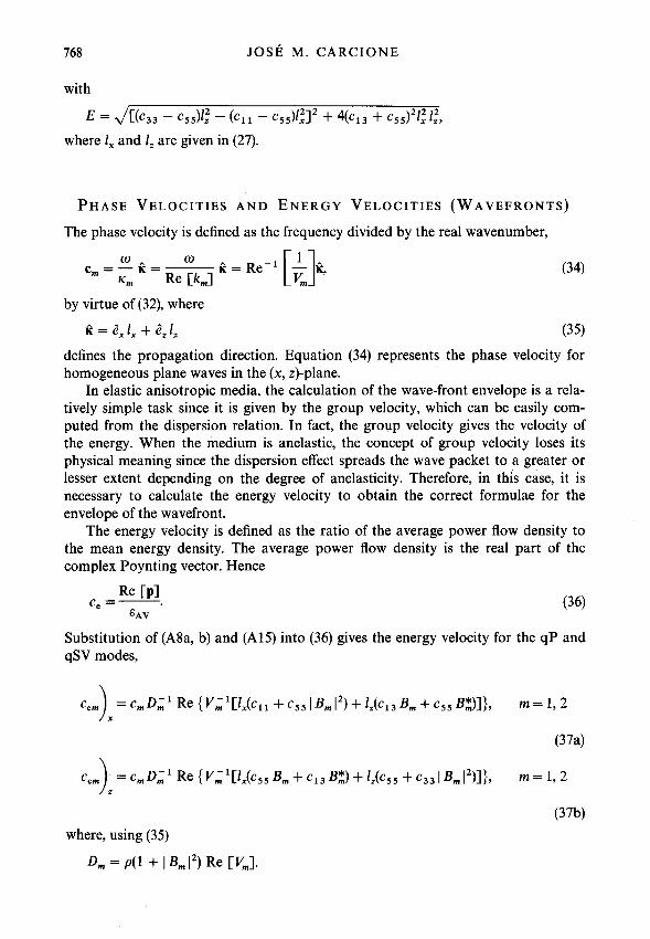
PHASE VELOCITIES A N D ENERGY VELOCITIES (WAVEFRONTS)

The phase velocity is defined as the frequency divided by the real wavenumber,

by virtue of (32), where

I? = 8,1, + c,1, (35) defines the propagation direction. Equation (34) represents the phase velocity for homogeneous plane waves in the (x, z)-plane.

In elastic anisotropic media, the calculation of the wave-front envelope is a rela- tively simple task since it is given by the group velocity, which can be easily com- puted from the dispersion relation. In fact, the group velocity gives the velocity of the energy. When the medium is anelastic, the concept of group velocity loses its physical meaning since the dispersion effect spreads the wave packet to a greater or lesser extent depending on the degree of anelasticity. Therefore, in this case, it is necessary to calculate the energy velocity to obtain the correct formulae for the envelope of the wavefront.

The energy velocity is defined as the ratio of the average power flow density to the mean energy density. The average power flow density is the real part of the complex Poynting vector. Hence

Re [PI Ce =-.

&AV

Substitution of (A8a, b) and (A15) into (36) gives the energy velocity for the qP and qSV modes,

ANISOTROPIC Q A N D VELOCITY DISPERSION 769

Special care has to be taken for a numerical evaluation of equations (37a, b) when either I , or 1, -, 0. For instance, when I , -+ 0 and 1, -, 1, B , -+ CO and B, -, 0. Taking these limits gives the appropriate formulae.

The energy velocity for the SH mode (m = 3) is calculated in a similar way. In this case, the wave is polarized normal to the (x, z)-plane and, therefore, normal to the propagation direction. Only the strains S , and S6 are different from zero. The calculation is much more simple than before, and the energy velocity can be written as

CV3I Re {v;1[zx1xc66 + z z 1 z c 5 5 1 } * (374 -1 Re-' Ce3 = C3 P

The symmetry axis of a transversely isotropic viscoelastic medium is a pure mode direction in the sense that the displacement vector is either parallel or normal to the real wavenumber K. In this direction, the wave solutions become purely transverse and purely longitudinal, and the energy and phase velocities coincide.

QUALITY FACTORS

The quality factor is defined as the ratio of the peak strain energy density (20) to the loss in energy density due to anelasticity (22). Then

Substitution of (A13) and (A16) into (38) gives the quality factor for the qP and qSV modes. A similar expression is obtained for the SH mode. The result is

Since the complex velocities depend on the propagation direction, the quality factors are anisotropic.

ANELASTIC PROPERTIES O F 3-D MEDIA The first example considers a two-constituent stationary layered medium. Two dif- ferent combinations are analysed, a sandstone-limestone system and a shale- limestone system, which show different degrees of anisotropy. The properties of the isotropic viscoelastic materials are given in Table 1 : the low-frequency Lam6 con- stants and body-wave velocities, the density and the respective quality factors. The sandstone-limestone sequence was used by Postma (1955) to demonstrate the aniso- tropic properties of layering, while the shale properties are taken from Thomsen (1986). Let the time constants in (16) be z, = 0.16 s and z2 = 3 x lO- , s, so that the quality factors are nearly constant over the exploration seismic band.

770 JOSE M. CARCIONE

TABLE 1. Material properties of the isotropic constituents.

Material A'(Gpa) p'(GPa) p(Kg/m3) VAm/s) &(m/s) Q, Q,

Limestone 30 25 2700 5443 3043 80 40 Sandstone 8 6 2300 2949 1615 60 20 Shale 6.28 1.70 2250 2074 869 60 20

In the long-wavelength limit, the wave characteristics of the layered medium are defined by the phase velocities (34) which give the velocity of a plane-wave com- ponent, the energy velocities (37) whose geometrical representation is the wavefront envelope, and the quality factors (39) which give the dependence of the energy dissi- pation on the propagation direction.

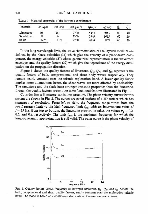
Figure 1 shows the quality factors of limestone. Qk, QP, and Qs represents the quality factors of bulk, compressional, and shear body waves, respectively. They remain nearly constant over the seismic exploration band. A lower quality factor implies more attenuation; hence, the shear waves are more affected by anelasticity. The sandstone and the shale have stronger anelastic properties than the limestone, though the quality factors present the same functional features illustrated in Fig. 1.

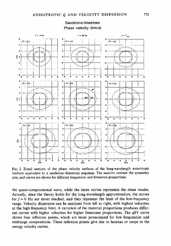
Consider first a limestone-sandstone structure. The phase velocity curves for this system are shown in Fig. 2. The curves are zonal sections of a 3D surface which has symmetry of revolution. From left to right, the frequency range varies from the low-frequency limit to the high-frequency limit f,,, with an intermediate value of f = 25 Hz; from top to bottom, the limestone proportion takes the values PI = 0.2, 0.5, and 0.8, respectively. The limit f,,, is the maximum frequency for which the long-wavelength approximation is still valid. The outer curve is the phase velocity of

0~ I I I I

0 20 40 60 80 11 frequency (Hz)

0

FIG. 1. Quality factors versus frequency of isotropic limestone. Qk, Qp, and Qs denote the bulk, compressional and shear quality factors, nearly constant over the exploration seismic band. The model is based on a continuous distribution of relaxation mechanisms.

ANISOTROPIC Q AND VELOCITY DISPERSION

Sandstone-limestone Phase velocity (km/s)

f = O H Z

6

4

2

2

4

6 -8 -4 -2 0 2 4 0

f - 2 5 H r

77 1

f - f,

-6 -4 -2 0 2 4 0

- 8 4 - 2 0 2 4

ICIX (CIX ICIX

FIG. 2. Zonal sections of the phase velocity surfaces of the long-wavelength anisotropic medium equivalent to a sandstone-limestone sequence. The sections contain the symmetry axis, and curves are shown for different frequencies and limestone proportions.

the quasi-compressional wave, while the inner curves represents the shear modes. Actually, since the theory holds for the long-wavelength approximation, the curves for f = 0 Hz are never reached, and they represent the limit of the low-frequency range. Velocity dispersion can be analyzed from left to right, with highest velocities at the high-frequency limit. A variation of the material proportions produces differ- ent curves with higher velocities for higher limestone proportions. The qSV curve shows four inflexion points, which are more pronounced for low frequencies and midrange compositions. These inflexion points give rise to lacunas or cusps in the energy velocity curves.

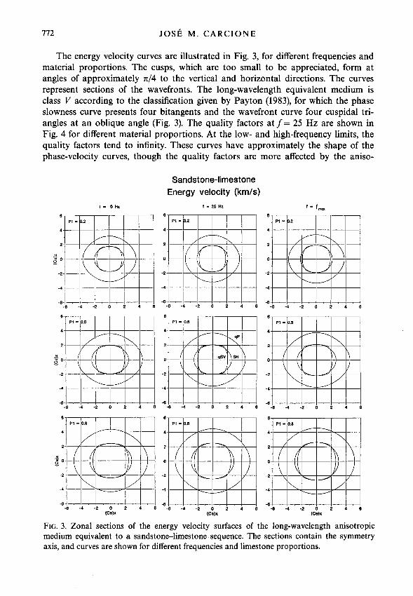
112 JOSE M . CARCIONE

The energy velocity curves are illustrated in Fig. 3, for different frequencies and material proportions. The cusps, which are too small to be appreciated, form at angles of approximately 71/4 to the vertical and horizontal directions. The curves represent sections of the wavefronts. The long-wavelength equivalent medium is class V according to the classification given by Payton (1983), for which the phase slowness curve presents four bitangents and the wavefront curve four cuspidal tri- angles at an oblique angle (Fig. 3). The quality factors at f = 25 Hz are shown in Fig. 4 for different material proportions. At the low- and high-frequency limits, the quality factors tend to infinity. These curves have approximately the shape of the phase-velocity curves, though the quality factors are more affected by the aniso-

Sandstone-limestone Energy velocity (km/s)

f - OH2

-8 -4 -2 0 2 4 8

f - 2 6 H Z

- 8 - 4 - 2 0 2 4 8

f - f,

-8 -4 -2 0 2 4 8

-8 -4 -2 0 2 4 I C O h

FIG. 3. Zonal sections of the energy velocity surfaces of the long-wavelength anisotropic medium equivalent to a sandstone-limestone sequence. The sections contain the symmetry axis, and curves are shown for different frequencies and limestone proportions.

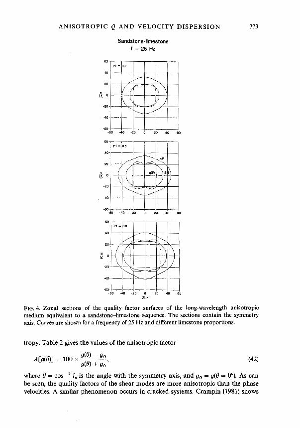
ANISOTROPIC Q A N D VELOCITY D I S P E R S I O N 773

Sandstone-limestone f = 25 Hz

-60 I -- I ILW -60 -40 -20 0 20 40 60

w x

FIG. 4. Zonal sections of the quality factor surfaces of the long-wavelength anisotropic medium equivalent to a sandstonelimestone sequence. The sections contain the symmetry axis. Curves are shown for a frequency of 25 Hz and different limestone proportions.

tropy. Table 2 gives the values of the anisotropic factor

where 0 = cos-’ I , is the angle with the symmetry axis, and go = g(O = 00). As can be seen, the quality factors of the shear modes are more anisotropic than the phase velocities. A similar phenomenon occurs in cracked systems. Crampin (1981) shows

774 JOSE M . CARCIONE

I - OHz

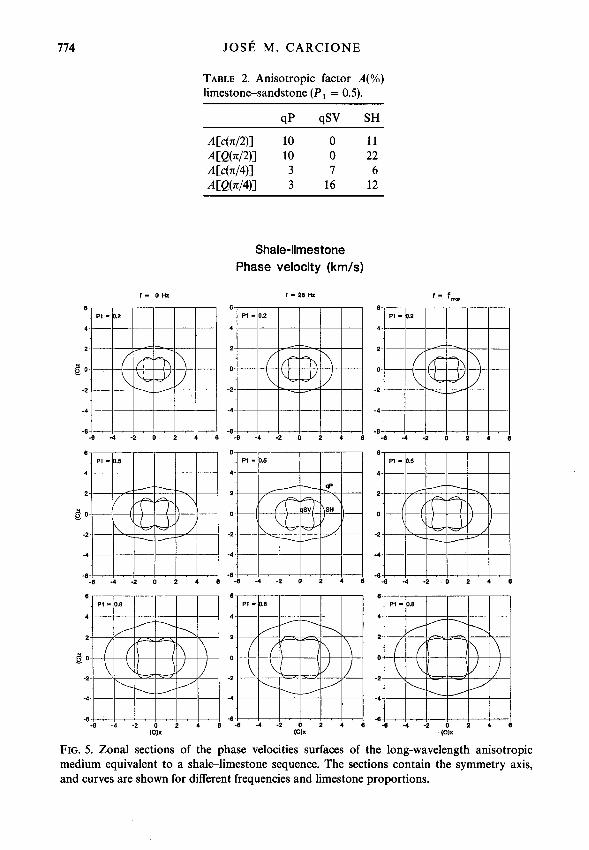
TABLE 2. Anisotropic factor A(%) limestonesandstone (PI = 0.5).

qP qSV SH

Shale-limestone Phase velocity (km/s)

f - 21 Hz I - f,

-0 -4 -2 0 2 4 0

-0 -4 -2 0 2 4 8 (CIX (CIX

FIG. 5. Zonal sections of the phase velocities surfaces of the long-wavelength anisotropic medium equivalent to a shalelimestone sequence. The sections contain the symmetry axis, and curves are shown for different frequencies and limestone proportions.

ANISOTROPIC Q A N D VELOCITY D I S P E R S I O N 775

8

4

2

x 8 0

-2

-4

-8

Shale-limestone Energy velocity (km/s)

I - OH2 I - 25 Hr f.. f,

- 4 - 2 0 2 4 8

-8 -4 -2 0 2 4 8

-8 -4 -2 0 2 4 8 (CO)%

-8 -4 -2 0 2 4 8

-8 4 -2 0 2 4 0 LC8)X

FIG. 6. Zonal sections of the energy velocities surfaces of the long-wavelength anisotropic medium equivalent to a shale-limestone sequence. The sections contain the symmetry axis, and curves are shown for different frequencies and limestone proportions.

that attenuation has a much greater anisotropy than the corresponding phase veloc- ity.

A more anisotropic system is obtained by substituting the sandstone by shale. Phase velocities, energy velocities and quality factors are shown in Figs. 5, 6, and 7, respectively. As before, the equivalent medium has four cuspidal triangles, and can be classified as class V . Both equivalent media, limestone-sandstone and limestone- shale, differ mainly in their degree of anisotropy, but in many respects they are similar. However, a close look at the quality factor curves indicates that, for the qP wave, the attenuation is higher for limestone-sandstone, although the anelastic characteristics of the sandstone and the shale are similar. On the other hand, the

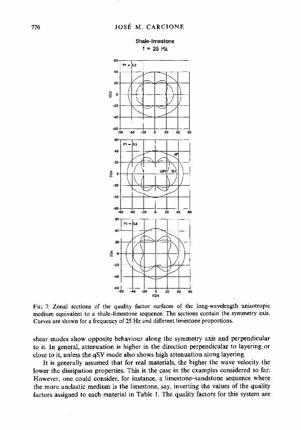
776 JOSE M . CARCIONE

Shale-limestone f = 25 Hz

-60 -40 -20 0 20 40 60

60

40

20

8 0

-20

-40

-60 I -40 -20 0 20 40 I

60

40

20

-20

-40

-60 - 1- -60 -40 -20 0 20 40 60

(9)x

FIG. 7. Zonal sections of the quality factor surfaces of the long-wavelength anisotropic medium equivalent to a shale-limestone sequence. The sections contain the symmetry axis. Curves are shown for a frequency of 25 Hz and different limestone proportions.

shear modes show opposite behaviour along the symmetry axis and perpendicular to it. In general, attenuation is higher in the direction perpendicular to layering or close to it, unless the qSV mode also shows high attenuation along layering.

It is generally assumed that for real materials, the higher the wave velocity the lower the dissipation properties. This is the case in the examples considered so far. However, one could consider, for instance, a limestone-sandstone sequence where the more anelastic medium is the limestone, say, inverting the values of the quality factors assigned to each material in Table 1. The quality factors for this system are

ANISOTROPIC Q AND VELOCITY DISPERSION 777

60

40

20

N

-20

-40

-60 -40 -20 0 20 40 60 (Qh

FIG. 8. Zonal sections of the quality factor surfaces of the long-wavelength anisotropic medium equivalent to a sandstone-limestone sequence, where the more dissipative medium is the limestone.

shown in Fig. 8, where midrange compositions have been considered. As can be seen, opposite behaviour occurs compared with Fig. 7; attenuation here is higher along layering, and the qSV mode has maxima in the quality factor at approx- imately 45".

W A V E M O D E L L I N G I N 2-D M E D I A

To verify the anelastic properties of fine layering, a set of modelling experiments is carried out. The modelling scheme solves the wave equation in the time-domain, an approach that requires a discrete set of relaxation mechanisms (Carcione, Kosloff and Kosloff 1988). The numerical integration algorithm is described by Tal-Ezer, Carcione and Kosloff (1990). The calculation of the theoretical quality factors and energy velocities is performed using the formulae previously developed, provided that the complex stiffnesses are chosen according to the dimensionality of the media; two in this case. Moreover, the complex moduli of the generalized standard linear solid are used (Carcione et al. 1988). Figure 9 shows (a) the quality factors and (b) the energy velocities of the 2D medium equivalent to a sandstone-limestone sequence, where Qk = 40 and Qs = 20 for limestone, and Qk = 20 and Qs = 10 for sandstone.

The numerical mesh has N, = 143 and N , = 429 with grid spacings of D, = 30 m and D, = 10 m. The thickness of the individual layers is 10 m with layering normal to the z-direction. The time function of the source is a causal Ricker wavelet with central frequency of 12 Hz. The ratios dominant wavelength to spatial period of the sequence along the vertical directions, are 17 and 8 for qP and qSV waves, respectively. This assures that the long-wave approximation is valid (Carcione, Kosloff and Behle 1991).

778 JOSE M . CARCIONE

ENERGY VELOCITY (0 Hz) ENERGY VELOCITY (12 Hz)

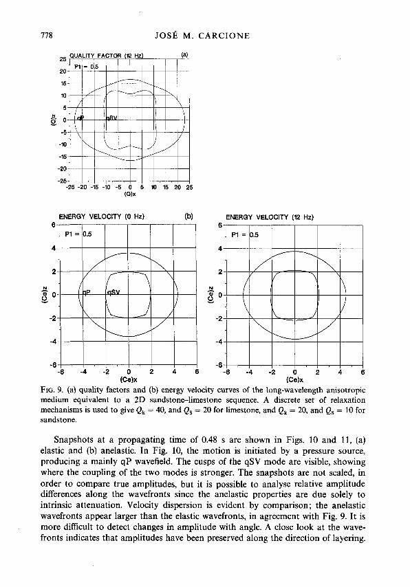
( W x (Ce)x FIG. 9. (a) quality factors and (b) energy velocity curves of the long-wavelength anisotropic medium equivalent to a 2D sandstone-limestone sequence. A discrete set of relaxation mechanisms is used to give Qk = 40, and Qs = 20 for limestone, and Q , = 20, and Q, = 10 for sandstone.

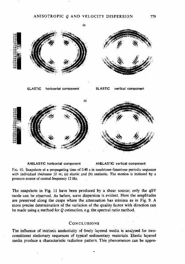
Snapshots at a propagating time of 0.48 s are shown in Figs. 10 and 11, (a) elastic and (b) anelastic. In Fig. 10, the motion is initiated by a pressure source, producing a mainly qP wavefield. The cusps of the qSV mode are visible, showing where the coupling of the two modes is stronger. The snapshots are not scaled, in order to compare true amplitudes, but it is possible to analyse relative amplitude differences along the wavefronts since the anelastic properties are due solely to intrinsic attenuation. Velocity dispersion is evident by comparison; the anelastic wavefronts appear larger than the elastic wavefronts, in agreement with Fig. 9. It is more difficult to detect changes in amplitude with angle. A close look at the wave- fronts indicates that amplitudes have been preserved along the direction of layering.

ANISOTROPIC Q A N D VELOCITY DISPERSION 779

0.46 0 99 034 0 28 0 24 om a13 008 0 03

-003 408 -0 13 -018 -0.24 4 20

-a30 -046 -060

-a 34

a46 0 38 0 34 0 10 024 om an a08 008

-003 -a08 -an QU -024 -020 -0 34 -038 -046 -as0

ELASTIC horizovtal component

(b)

ANELASTIC horizontal component

ELASTIC vertical component

ANELASTIC vertical component

FIG. 10. Snapshots at a propagating time of 0.48 s in sandstonelimestone periodic sequence with individual thickness 10 m; (a) elastic and (b) anelastic. The motion is initiated by a pressure source of central frequency 12 Hz.

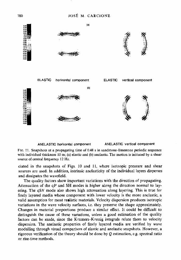
The snapshots in Fig. 11 have been produced by a shear source; only the qSV mode can be observed. As before, wave dispersion is evident. Here the amplitudes are preserved along the cusps where the attenuation has minima as in Fig. 9. A more precise determination of the variation of the quality factor with direction can be made using a method for Q estimation, e.g. the spectral ratio method.

CONCLUSIONS The influence of intrinsic anelasticity of finely layered media is analysed for two- constituent stationary sequences of typical sedimentary materials. Elastic layered media produce a characteristic radiation pattern. This phenomenon can be appre-

780 JOSE M . CARCIONE

(a)

ELASTIC horizontal component ELASTIC vertical component

(b)

ANELASTIC horizontal component ANELASTIC vertical component

FIG. 11. Snapshots at a propagating time of 0.48 s in sandstone-limestone periodic sequence with individual thickness 10 m; (a) elastic and (b) anelastic. The motion is initiated by a shear source of central frequency 12 Hz.

ciated in the snapshots of Figs. 10 and 11, where isotropic pressure and shear sources are used. In addition, intrinsic anelasticity of the individual layers disperses and dissipates the wavefield.

The quality factors show important variations with the direction of propagating. Attenuation of the qP and SH modes is higher along the direction normal to lay- ering. The qSV mode also shows high attenuation along layering. This is true for finely layered media whose component with lower velocity is the more anelastic, a valid assumption for most realistic materials. Velocity dispersion produces isotropic variations in the wave velocity surfaces, i.e. they preserve the shape approximately. Changes in material proportions produce a similar effect. It could be difficult to distinguish the cause of these variations, unless a good estimation of the quality factors can be made, since the Kramers-Kronig integrals relate them to velocity dispersion. The anelastic properties of finely layered media are verified by wave modelling through visual comparison of elastic and anelastic snapshots. However, a rigorous verification of the theory should be done by Q estimation, e.g. spectral ratio or rise-time methods.

ANISOTROPIC Q A N D VELOCITY DISPERSION 78 1

ACKNOWLEDGEMENT

This work was supported in part by the Commission of the European Communities under the GEOSCIENCE project.

REFERENCES AULD, B.A. 1973. Acoustic Fields and Waves in Solids. Vol. 1. John Wiley & Sons, Inc. BACKUS, G.E. 1962. Long-wave elastic anisotropy produced by horizontal layering. Journal of

BEN-MENAHEM, A.B. and SINGH, S.J. 198 1. Seismic Waves and Sources. Springer-Verlag. BLAND, D. 1960. The Theory of Linear Viscoelasticity. Pergamon Press Inc. CARCIONE, J.M. 1990. Wave propagation in anisotropic linear viscoelastic media: theory and

CARCIONE, J.M., KOSLOFF, D. and BEHLE, A. 1991. Long-wave anisotropy in stratified media:

CARCIONE, J.M., KOSLOFF, D. and KOSLOFF, R. 1988. Wave propagation simulation in a linear

CHRISTENSEN, R.M. 1982. Theory of Viscoelasticity, an Introduction. Academic Press Inc. CRAMPIN, S. 1981. A review of wave motion in anisotropic and cracked elastic media. Wave

Motion 3, 341-391. LIU, H.P., ANDERSON, D.L. and KANAMORI, H. 1976. Velocity dispersion due to anelasticity;

implications for seismology and mantle composition. Geophysical Journal of the Royal Astronomical Society 47,41-58.

PAYTON, R.G. 1983. Elastic Wave Propagation in Transversely Isotropic Media. Martinus Nijhoff Publishers.

POSTMA, G.W. 1955. Wave propagation in a stratified medium. Geophysics 20,780-806. TAL-EZER, H., CARCIONE, J.M. and KOSLOFF, D. 1990. An accurate and efficient scheme for

THOMSEN, L. 1986. Weak elastic anisotropy. Geophysics 51, 1954-1966.

Geophysical Research 67,4427-4440.

simulated wavefields. Geophysical Journal International 101, 739-750.

A numerical test. Geophysics 56, 245-254.

viscoelastic medium. Geophysical Journal of the Royal Astronomical Society 95, 597-61 1.

wave propagation in linear viscoelastic media. Geophysics 55, 1366-1379.

A P P E N D I X

Poynting vector and energy densities

ment components Let us consider a plane wave polarized in the (x, z)-plane with particle displace-

X X 9 (A 1 a)

(A 1 b)

(A2)

= U ei(wr-kxx-kzz)

= ~ ~ ~ i ( r n t - k ~ x - k . z ) >

with

k = k x d x + k ,d , = ( K - ia)i?,

i.e. a homogeneous viscoelastic plane wave.

782 JOSE M . CARCIONE

The associated strain components are

and

For a transversely isotropic and viscoelastic medium, the stress components are

TI =c l1S1 +c13S3 = - i (c11k,U,+c13k,U,)e-a'xei~"~-K'x~,

T3 = ~ 1 3 S1 + c33S3 = -i(c13 k, U, + c33 k, U,)e-a'xei("t-K'"),

(A44

(A4b)

and

T, = c,, S, = -ic,,(k, U, + k, U,)e-a'"ei("t-K'x). (A44

From (19) the complex Poynting vector is

645) p = -1 2C*x( e U* ', Tl + li: T,) + &,(li: T, + ti,* T3)].

Replacing (A3a-c) into (A4a-c), and the results into (A5) yields

where (30) has been used. In (A6a, b), m = 1 identifies the qP mode and m = 2 the qSV mode. The ratio U x to U, is obtained by substitution of (A6a, b) into the Christoffel equation (28). For instance, from the first line,

and from the third line,

B,= - r13 m = l , 2 r33 - P V i '

according to (32). Replacing B,, the Poynting vector components (A6a, b) become

~ x = ~ ~ k m e - ~ " ~ ' " I ~ x l ~ C ~ x ( c ~ l + c 5 5 I B m I 2 ) + I ~ ( ~ 1 3 ~ m + ~55B:)], ('484

(A8b) p = && m e-2a ' " 1 U , 12Clx(C55 Bm + c13 + ' ~ (~55 + c33 1 B m 12)1.

The peak kinetic energy density from (21) and (Ala, b) is

= +po2 I U, 12e-2am ' "(1 + I B, 1'). 649)

ANISOTROPIC Q AND VELOCITY DISPERSION 783

The peak potential energy density from (20) is 1

(%)peak = 3 Re [sl(cll s: + c13 s:) + s3(c13 s: + c33 s:) + c 5 5 1 s5 121. (A1O) After substitution of the strain components (A3a-c) and equations (A7a, b), the potential energy density becomes

Re [l:cll + 1:c5, + B,B;(lZc,, + 12c3,) 1 (%)peak = 7 I km l 2 1 1 2 e '

+ (c13 + c 5 5 ) l x l z ( B m + Bf)l, (All) or, replacing the Christoffel components (30),

= 3 I k, l 2 I U, 12e- 2am ' Re IT11 + BmBzr33 + ( B m + Bf)r13], (A12) which by virtue of (A7a, b) reduces to

(Es)peak= 3pIkm121Ux12e-2am'X (1 + I Bm 1') Re CV3.

eAV = $pw2( U,Iz(l + IBm12)e-2am'X{1 + I V,'12 Re [ V ; ] } ,

cAV = )pw2IU,I2(1 + IB,12)e-2am'x Re [V,] Re [V,'].

(A 13)

('414)

(A 15)

In consequence, using (32), the average stored energy density (23) is

Using properties of complex numbers, (A 14) becomes

The loss energy density (22) is calculated in the same way as the potential energy. It gives

(&JAv = )pIk,121Ux12e-2am'X (1 + I Bm 1') Im 1 ~ 3 . (A 16)