ANIMAL-VEHICLE COLLISIONS IN TEXAS: 1

HOW TO PROTECT TRAVELERS AND ANIMALS ON ROADWAYS 2

3

4

5

6

7

8

9

10

11

12

13

14

15

16

17

18

19

20

21

22

23

24

25

26

27

28

29

30

31

32

33

34

35

36

37

38

39

40

41

42

43

44

45

Devin C. Wilkins

Department of Civil, Architectural and Environmental Engineering

The University of Texas at Austin – E. Cockrell Jr. Hall

Austin, TX 78712-1076

devinwilkins@utexas.edu

Kara M. Kockelman, Ph.D., P.E. (corresponding author)

Dewitt Greer Centennial Professor of Transportation Engineering

Department of Civil, Architectural and Environmental Engineering

The University of Texas at Austin

Austin, TX 78712-1076

kkockelm@mail.utexas.edu

Nan Jiang, Ph.D., P.E.

Research Associate

Center for Transportation Research

The University of Texas at Austin

Austin, TX 78759

jiang@utexas.edu

Published in Accident Analysis & Prevention 131: 157-170 (2019).

ABSTRACT

Animal-vehicle collisions (AVCs) are a growing problem in the United States, resulting in

countless loss of animal life and considerable human injury and death every year, especially to

motorcyclists. In addition to being a serious safety concern, these collisions can create trauma

among all animal populations including declining species, household pets, and livestock

investments. Due to underreporting, collision data is usually a gross underestimation of the actual

impact of AVCs and often lacks key details such as the species of animals involved. This

paper investigates both wild and domestic animal-vehicle collisions through statistical and

spatial analysis of police-reported collision data in Texas.

51,522 animal-related crashes were reported in Texas from 2010 through 2016, at a total cost

over $1.3 billion annually to Texas motorists – not including the value of lost animal lives.

Wildlife-vehicle collisions (WVC) are 64% of total reports, events involving domestic animals

(like dogs and cattle) are 31%, and the remaining 5% of reports are unspecified. Most AVCs in

the state occur at night in unlit locations, usually on rural roads with very low traffic volumes.

Using ordinary least-squares (OLS) regression analysis across Texas’ n=254 counties, this work

finds that less densely populated counties, marked as rural, and those with fewer vehicle-miles

traveled (VMT) per capita but more lane-miles per capita, tend to experience the greatest number

of AVCs per VMT after controlling for rainfall, share of VMT on on-system roadways, job

densities, and vehicles per capita. 46

2

1

Intervention options for the mitigation of animal-vehicle collisions are numerous and diverse. 2

Overpasses and culverts, along with wildlife fencing (which can steer animals to safe crossings), 3

show promising results for both AVC reduction and habitat connectivity. Longer term, mobile 4

reporting, by DOT employees, smartphone users, intelligent cameras and other devices, plus real-5

time information dissemination (tied to existing navigation apps) can enable safer driving along 6

specific roadway sections as animals arrive. 7

8

For wildlife collisions specifically, this work finds that large crossing structures (underpasses and 9

overpasses) at the highway link level return benefit-to-cost ratios near 3.0, while their lower cost 10

counterparts (wildlife fencing and animal detection systems) delivered ratios of values up to 30. 11

12

BACKGROUND 13

14

Animal-vehicle collisions (AVCs) makeup 5% of all U.S-reported motor vehicle collisions every 15

year and represent a growing problem (FHWA, 2008; Sullivan,2011). In fact, between 2014 and 16

2017, insurance claims related to animal collisions increased a total of 6% in the United States 17

(NICB, 2018). About 200 people – often motorcyclists – lose their lives on U.S roadways each 18

year from collisions involving wild or domestic animals, and thousands more are seriously injured 19

(Donaldson and Lafon, 2008). In addition to being a serious safety concern for human travelers 20

and their property, such collisions create trauma among animal populations and endanger 21

dwindling species. A five-state study found that, in a single month, 15,000 reptiles and amphibians, 22

48,000 mammals, and 77,000 birds die due to collisions with vehicles (Havlick, 2014). For some 23

animals, including the endangered Texas ocelot, the number one threat to survival is vehicle 24

collisions (Haines et al., 2005; Miller, 2016). Many collisions also destroy household pets and 25

livestock investments. 26

This research focuses on the centrally located state of Texas, the U.S.’s second largest state 27

spatially (after Alaska) and with regards to population (after California). The Texas Department 28

of Transportation is responsible for more centerline-miles of highway than any other U.S state1 , 29

and the state’s landscape offers a wonderful diversity of wildlife, topography, and climate. 30

Following the literature review and numerical and spatial analysis of collision data, this paper 31

offers further details on the state of animal-vehicle collisions in the state of Texas and suggests 32

similar realities at a national or global context. Specifically, the following information clarifies 33

and highlights at-risk persons, travel times, and locations and assesses the benefits of possible 34

mitigation strategies. 35

36

Wildlife Impact 37

Millions of animals die every year in the U.S. as a result of animal-vehicle collisions (AVCs) 38

(Donaldson and Lafon, 2008). Most animal-vehicle collisions go unreported - with the exception 39

of those involving large ungulates, such as deer, elk, and moose. In insurance claims, when a 40

species of animal is named, the most commonly reported animal is deer. In fact, deer show up over 41

25 times more than the next animal, raccoons (NICB, 2018). Smaller species, though they might 42

not pose immediate threat of injury to a driver, also face great impacts from collisions. Turtle 43

populations including red-eared sliders and Missouri River Cooters suffer from AVCs, especially 44

1 https://www.fhwa.dot.gov/policyinformation/statistics/2008/hm60.cfm

3

females as they travel to higher lands to lay their eggs (Steen and Gibbs 2004). These populations 1

then become male dominated and cannot maintain reproductive sustainability. Endangered 2

animals - like the Texas ocelot (Leopardus pardalis, which has fewer than 50 living individuals 3

[U.S Fish and Wildlife Service, 2010]) - have populations that are especially vulnerable to vehicle 4

collisions because even a few deaths notably impacts this species’ potential for reproductive 5

continuation. Further, carcass counts will normally be very low for endangered species, relative to 6

more common species, resulting in “bias(ed) mitigation measures based on small samples” 7

(Neumann et al., 2012) and generally inadequate protective measures for these species. 8

9

Crash Costs and Under-reporting 10

There were 51,522 animal-related crashes reported to authorities in Texas from 2010 through 2016. 11

However, most property-damage-only crashes go unreported, and wildlife experts tend to find 5 12

to 10 wildlife carcasses for every reported wildlife crash (Donaldson and Lafon, 2008; Olson et 13

al., 2014). Even in documented cases, police reports often fail to specify the species of animal hit, 14

which would be of obvious value in targeted mitigation strategies. Stewart (2015) found that more 15

than 50% of US deer‐vehicle collisions nationwide go unreported. 16

17

The FHWA’s (2008) best estimate of US AVC collision costs was $8.39 billion annually based on 18

2007 numbers. The economic costs of death and injuries arising from US AVCs exceed $1 billion 19

per year (Donaldson and Lafon, 2008). Approximately 26,000 AVCs each year (4-10% of total 20

AVCs in the US) result in injuries to vehicle occupants each year (FHWA, 2008). Overall, these 21

types of collisions represent roughly 0.6% of all injurious crashes nationwide (GES, 2015). 22

Though motorist injuries may be relatively rare, “more than 90 percent of collisions with deer 23

result in damage to the driver’s car or truck” (FHWA, 2008, p. 8). State Farm Insurance Company 24

(2015) estimates that 1 out of 169 US drivers had a claim from hitting a deer, moose or elk in 2015. 25

The company’s analysis shows an average cost of $4,135 per claim involving a collision with one 26

of these 3 animals, an increase of 6% from 2014. However, these estimates cannot paint a complete 27

picture of AVC-related property damages, since many motorists do not file a claim with their 28

insurance company (to avoid increased coverage costs in future years, for example). 29

30

A 2008 US Federal Highway Administration (FHWA, 2008) investigation identified “21 federally 31

listed threatened or endangered animal species in the United States for which road mortality is 32

among the major threats to the survival of the species.” While the survival of species is of clear 33

significance to biodiversity on our planet and humanity as a whole, it is hard to ascribe an exact 34

cost to losing an endangered animal. This ‘intrinsic value of a species’ is an under-researched 35

topic. Economic value estimates for the Texas ocelot, for example, range from $50,000 to $5 36

million (Haines et al., 2007). Deaths of such animals can also become a liability risk as well as a 37

public-perception hazard for transportation departments, since these animals are irretrievable 38

assets in a diverse ecosystem. 39

40

Other less easily quantifiable but very common consequences of most animal-vehicle collisions 41

include traffic delays, diversions of law enforcement or emergency personnel and road 42

maintenance crews. For example, deer carcass removal costs are estimated to be $30.50 per deer 43

(FHWA, 2008). 44

45

Wildlife Crossing Mitigation 46

4

U.S. infrastructure project planning and delivery normally requires an environmental review 1

process to avoid or at least mitigate detrimental project impacts on human and natural 2

communities, as well as historic and cultural sites. For complex transportation projects, this 3

process often is the most time-consuming part of project delivery (Evink, 2002; US GAO, 2003). 4

Brown’s (2006) “Eco-Logical: An Ecosystem Approach to Developing Infrastructure Projects” 5

report provides guidance and examples for streamlining environmental reviews while more 6

effectively protecting natural resources and ecosystem processes (Brown, 2006). Planners and 7

engineers applied these ideas to create the Integrated Transportation and Ecosystem Enhancements 8

for Montana (ITEEM) process. Many measures can be taken to connect habitats and wildlife 9

populations and increase motorist safety while lowering wildlife mortality. Iuell et al. (2005) 10

summarized these measures into five categories: 11

• Wildlife overpasses 12

• Wildlife underpasses 13

• Specific measures: fencing, gates and escape ramps, signage, vehicle-animal detection 14

systems, speed reduction, lighting and reflectors 15

• Habitat adaptation: manage habitat and right-of-way, intercept feeding 16

• Infrastructure adaptation: modify road infrastructure (curbs, drainage, gates, etc.) to better 17

accommodate wildlife movement (e.g. increase width of road median). 18

19

Many U.S. states have been implementing some of these measures and other strategies. For 20

example, work done on Florida’s I-75 seeks to protect the endangered Florida Panther, North 21

Carolina is building several wildlife underpasses on U.S. 64 to reduce vehicle conflict with white-22

tailed deer, American black bears, and red wolves, a federally-listed endangered species (Jones et 23

al., 2010). TxDOT budgeted $5 million for four wildlife crossings under Highway 100 (between 24

Laguna Vista and Los Fresnos) to reduce ocelot deaths (Sommer, 2014). States like Washington 25

and Montana have recently pursued major crash-mitigation projects, with Montana providing more 26

than 40 new wildlife crossings in the reconstruction of a 56-mile segment of US-93 (Jones et al., 27

2013). As of 2007, Texas had 10 major terrestrial wildlife crossings (Bissonette and Cramer, 28

2008). The following data analyses help us understand where AVCs are high and investments may 29

be most cost-effective. 30

DATA ANALYSIS 31

The AVCs analyzed in this paper come from the TxDOT Crash Records Information System 32

(CRIS), an online database containing crash data for the state of Texas submitted by law 33

enforcement officers and available at https://cris.dot.state.tx.us. Almost all (with the exception of 34

a few collisions of unspecified animal type) of these AVCs are coded as ‘wild’ or ‘domestic’ 35

animals involved. The data referenced here contains incidents from the years 2010 through 2016. 36

The spatial and temporal accuracy of the data may vary by region and setting (e.g., under-reporting 37

may be higher in rural contexts, at night, and for larger vehicles). 38

39

Using these 2010-2016 AVC data, with TxDOT's (2018) comprehensive crash costs (, the loss 40

from reported AVCs is about $21 per Texan per year. 67% of this is attributable to wild-animal 41

collisions, and 33% is attributable to domestic-animal collisions. Interestingly, though the 42

domestic animals are often smaller (e.g., dogs rather than deer) and just one-third of all reported 43

AVCs in Texas, the costs of these crashes is 44% of total costs, indicating higher crash severity 44

for domestic animals. This may be due to their occurring in higher-population-density settings (see 45

Figure 9 vs 10), with more cars and trucks alongside when the collision occurs. Alternatively, it 46

5

may be due to drivers swerving more dramatically to avoid harming someone's beloved pet. Table 1

1 provides costs estimates of the AVCs analyzed in this paper. 2

3

TABLE 1 CRIS Crash Cost Estimates (Texas AVCs, 2010-2016) 4

Crash

Year Contributing Factor Killed

Incapacit.

Injury

Non-

Incapacit.

Injury

Possible

Injury

Not

Injured

Not

Known

Cost

($M)

2010

Animal - Domestic 9 43 194 214 1997 12 $279

Animal - Wild 6 52 173 185 3722 12 $290

Total 15 95 367 399 5719 24 $568

2011

Animal - Domestic 9 38 214 225 1936 14 $272

Animal - Wild 12 67 230 191 3981 14 $392

Other 1 1 1 $0.48

Total 21 105 445 417 5918 28 $664

2012

Animal - Domestic 9 51 207 197 1943 18 $ 314

Animal - Wild 5 65 191 207 3828 20 $340

Other 1 $ -

Total 14 116 398 404 5772 38 $654

2013

Animal - Domestic 13 37 163 191 1781 11 $256

Animal - Wild 4 49 201 215 4108 16 $286

Other 1 1 2 $0.48

Total 17 86 365 407 5891 27 $543

2014

Animal - Domestic 7 42 135 158 1668 19 $239

Animal - Wild 13 61 172 234 4115 22 $345

Other 1 1 $0.48

Total 20 103 308 392 5784 41 $584

2015

Animal - Domestic 10 40 172 183 1761 12 $261

Animal - Wild 12 61 206 250 4610 23 $358

Total 22 101 378 433 6371 35 $620

2016

Animal - Domestic 5 46 181 181 1876 17 $269

Animal - Wild 10 74 246 287 5131 44 $417

Other 1 $ -

Total 15 120 427 468 7008 61 $686

5

Crash Time of Day 6

As shown in Figures 1 and 2, (reported) AVCs peak twice a day: between 5 and 8 AM (with 20% 7

of AVCs happening) and from 6 PM to midnight (47%), with heavy peaking between 6 and 7 am 8

(8.6%) and between 8 and 9 pm (9.3%). When the times of day are adjusted (Figure 2) for daylight 9

savings time shifts, the evening peak consolidates further (vs. Figure 1’s wide evening peak). Since 10

travel or VMT demand does not peak at those same times of day or in quite the same way, AVC 11

peaking implies that animal movement choices are key. Animal behavior is regularly based on the 12

sun’s placement, while human behavior is dictated more often by clock time (for work and school 13

start and end times, for example), as well as day of week (with Friday and Saturday nights often 14

6

involving late-night socializing and the associated return travel). Interestingly, domestic animals 1

tend to experience more crashes earlier in the day than wild animals do (e.g., a 5 or 6 am peak). 2

Deer, unlike most domestic animals, are a crepuscular species, meaning they are most active during 3

dusk and dawn (“White-Tailed Deer”, n.d.). 4

5 FIGURE 1 Crash counts by time of day (30-min intervals, Texas AVCs, 2010-2016) 6

7

8 FIGURE 2 Crash counts by adjusted time of day (to eliminate daylight savings time effects, 9

30-min intervals, Texas AVCs, 2010-2016) 10

Time of Year 11

State Farm indicates that drivers are more than twice as likely to have a collision with a deer, elk, 12

or moose during the months October, November and December (State Farm, 2015). Texas AVC 13

data delivers similar results, as shown in Figure 3. 14

0

200

400

600

800

1000

1200

1400

1600

1800

0:0

0

1:0

0

2:0

0

3:0

0

4:0

0

5:0

0

6:0

0

7:0

0

8:0

0

9:0

0

10

:00

11

:00

12

:00

13

:00

14

:00

15

:00

16

:00

17

:00

18

:00

19

:00

20

:00

21

:00

22

:00

23

:00

24

:00

Nu

mb

er o

f C

rash

es

Time of Day

Domestic Wild

0

200

400

600

800

1000

1200

1400

1600

1800

2000

0:0

0

1:0

0

2:0

0

3:0

0

4:0

0

5:0

0

6:0

0

7:0

0

8:0

0

9:0

0

10

:00

11

:00

12

:00

13

:00

14

:00

15

:00

16

:00

17

:00

18

:00

19

:00

20

:00

21

:00

22

:00

23

:00

24

:00

Nu

mb

er o

f C

rash

es

Time of Day - adjusted for daylight savings

Domestic Wild

7

1 FIGURE 3 Crash counts by month of year (Texas AVCs, 2010-2016) 2

3

Light Condition 4

Most AVCs (71%) occur at night in unlit locations. Unlike cars and trucks - with their headlights 5

on, animals running across the road are virtually invisible in the darkness until it is too late. 6

Reported crash frequencies are also much higher in dark settings, as shown in Figure 4. Such 7

settings can be especially problematic for smaller animals, such as turtles, armadillos, raccoons, 8

possums, and the endangered Texas ocelot. It is difficult to know the rates of such incidents 9

because crashes involving small animals are rarely detected by the involved motorists (excepting, 10

for example, motorcyclists) and almost never reported. Swedish research (Neumann et al. 2012, p. 11

70) notes how higher collision risk for moose is “largely due to low light and poor road surface 12

conditions rather than to more animal road-crossings”. 13

14

15 FIGURE 4 Number of crashes by light condition (Texas AVCs, 2010-2016) 16

0

1000

2000

3000

4000

5000

6000

7000

8000

Domestic Wild

0

5000

10000

15000

20000

25000

Dark,Lighted

Dark, NotLighted

Dark,UnknownLighting

Dawn Daylight Dusk Other

# o

f cr

ash

es

Light Condition

Domestic Wild

8

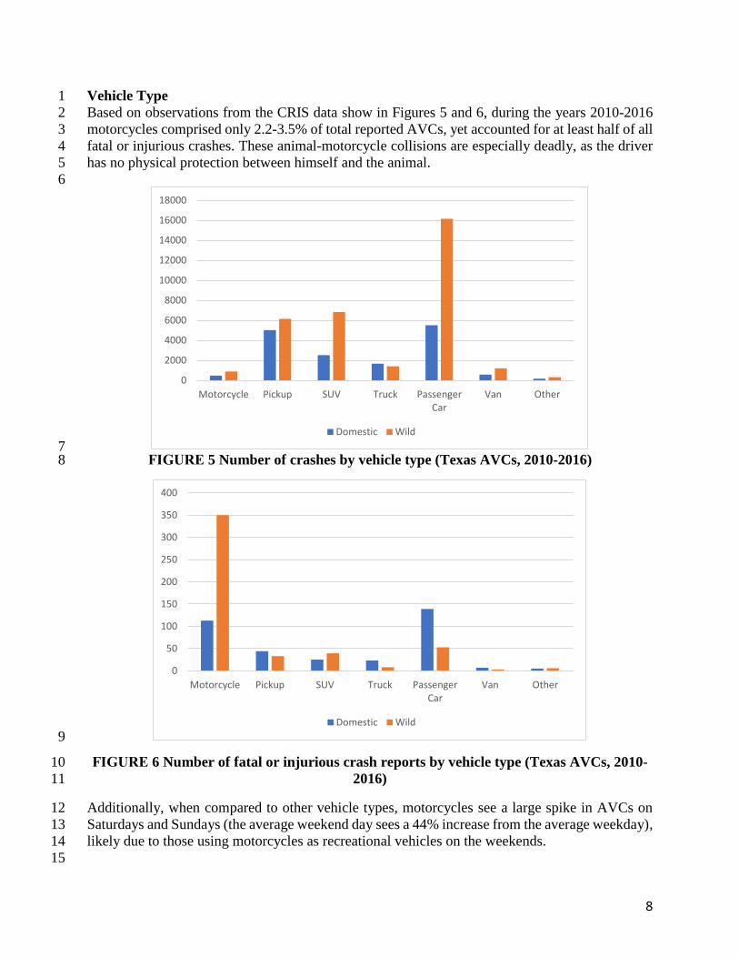
Vehicle Type 1

Based on observations from the CRIS data show in Figures 5 and 6, during the years 2010-2016 2

motorcycles comprised only 2.2-3.5% of total reported AVCs, yet accounted for at least half of all 3

fatal or injurious crashes. These animal-motorcycle collisions are especially deadly, as the driver 4

has no physical protection between himself and the animal. 5

6

7 FIGURE 5 Number of crashes by vehicle type (Texas AVCs, 2010-2016) 8

9

FIGURE 6 Number of fatal or injurious crash reports by vehicle type (Texas AVCs, 2010-10

2016) 11

Additionally, when compared to other vehicle types, motorcycles see a large spike in AVCs on 12

Saturdays and Sundays (the average weekend day sees a 44% increase from the average weekday), 13

likely due to those using motorcycles as recreational vehicles on the weekends. 14

15

0

2000

4000

6000

8000

10000

12000

14000

16000

18000

Motorcycle Pickup SUV Truck PassengerCar

Van Other

Domestic Wild

0

50

100

150

200

250

300

350

400

Motorcycle Pickup SUV Truck PassengerCar

Van Other

Domestic Wild

9

Location and Density 1

51,522 collisions with wild animals were reported by Texas law enforcement between 2010-2016, 2

including 254 human fatalities, 6,914 human injuries, and thousands more animal deaths. Most of 3

these crashes happen on rural roads with very low traffic, as demonstrated in Figure 7. 4

5

6 FIGURE 7 Crash counts by average annual daily traffic (Texas AVCs, 2010-2016) 7

Using location coordinate data provided in the CRIS reports, a detailed map of all studied collisions 8

(excepting 4% of reports lacking coordinate data) was created in ESRI’s ArcGIS software, shown 9

in Figure 8. 10

11

12 FIGURE 8 All reported-AVC locations across Texas (2010-2016) 13

14

0

1000

2000

3000

4000

5000

6000

# o

f cr

ash

es

AADT (thousand)

Domestic Wild

10

From these coordinates, it is possible to develop a generic heat map (Figures 9 and 10) based on 1

the respective concentrations of the data points shown in Figure 8. A bright yellow spot indicates 2

a very dense collection of data points whereas a light blue area suggests that crashes are fewer and 3

farther between. The heat maps for all animal vehicle collisions indicated that the San Antonio 4

metropolitan area had the most concentrated AVCs. This is consistent with a 2018 report by the 5

National Insurance Crime Bureau which stated that San Antonio and Austin, TX are the top 2 cities 6

for animal loss claims across the whole U.S (NICB, 2018). 7

8

9 FIGURE 9 Crash count hot spots for wild animals (Texas AVCs, 2010-2016) 10

11

12

11

1 FIGURE 10 Crash counts hot spots for domestic animals (Texas AVCs, 2010-2016) 2

3

Though collisions with domestic animals make up a smaller proportion of total reported crashes 4

than collisions with wild animals and are researched less often, they are not to be discounted. Out 5

of the 51,522 AVCs reported in the state of Texas between 2010-2016, 15,890 (31%) of these can 6

be attributed to collisions with domestic animals and 32,920 (64%) with wild animals, where the 7

rest were unspecified in the data. 8

9

As shown in Figure 10, collisions with domestic animals seem to experience a high spike in the 10

Rio Grande Valley region. This is possibly due to the unusually high number of stray animals in 11

the region. According to Keely Lewis, board secretary for the Palm Valley Animal Center, the 12

Valley has one of the highest populations of stray animals in the country. Owner of a no-kill 13

shelter in the city of McAllen suggests that many, if not most, residents of the Valley do not opt 14

for rabies shots or microchips or will decline spaying and neutering services in favor of trying to 15

turn a profit on the animal’s offspring (Gonzalez 2018). He believes that McAllen’s main roads 16

are more residential than those in neighboring cities like Brownsville, making it more likely for 17

runaway dogs to access the streets and cause crashes in that area (Gonzalez 2018). However, it is 18

worth noting that according to national data, dogs made up only 1.2% of animal-related insurance 19

claims between 2014 and 2017 (NICB 2018). 20

21

The heat maps developed in Figures 9 and 10 are very helpful in visualizing the density of crash 22

occurrence. However, the results of such a process are dependent upon user-defined “class and 23

cell ranges to set up the gradient,” and therefore are highly subjective (Dempsey, 2014). 24

Developing a hotspot map, however, “uses statistical analysis in order to define areas of high 25

occurrence versus areas of low occurrence,” (Dempsey, 2014). Since the resulting areas are 26

statistically significant, they are much less subjective. 27

28

12

Figure 11 shows the results of ArcGIS’ Optimized Hot Spot Analysis Tool for the entire state. 1

Figure 12, on the other hand, displays a closer look at just the results for the San Antonio area, to 2

demonstrate the model’s enhanced capability for showing specific problem areas on a detailed 3

scale. The software uses the Getis-Ord Gi* statistic (Getis and Ord, 2002, Ord and Getis, 2005) to 4

create a map of statistically significant hot and cold spots or crash clusters. 5

6

The Gi* values were then interpolated using ArcGIS’ Inverse Distance Weighting (IDW) tool to 7

create a legible map of hotspots over the whole state, as shown in Figure 13. The darkest red areas 8

indicate the most significant hotspots, and darkest blues indicate the most significant cold spots, 9

where AVCs are much less of a concern for that area. 10

11 FIGURE 11 Getis-Ord Gi* Hotspot Map of AVCs 2010-2016 12

13

13

1 FIGURE 12 Getis-Ord Gi* Hotspot Map of AVCs 2010-2016 in the San Antonio Area 2

3

4 FIGURE 13 Getis-Ord Gi* Hotspot Analysis with IDW Interpolation 5

6

14

Regression Analysis 1

Using ordinary least-squares (OLS) regression across n=254 Texas counties, the following 2

analysis highlights county attributes that are strong predictors of AVC crash rates (per VMT in 3

each county). For further investigation, similar methods can be implemented at a link-based level, 4

to identify problematic road segments. 5

6

Table 2 summarizes key statistics for the explanatory variables used in this analysis. Collision data 7

were averaged over the 7-year data set (Texas AVCs 2010-2016 CRIS data). 8

9

TABLE 2 Summary Statistics for Texas County Data 10

Variable Description Min Max Mean Median SD

AVC/VMT Animal-vehicle collisions per

million annual VMT

1.17E-03 0.60 0.11 0.09 0.08

POP DENS Population per square mile 2.6E-04 4.62 0.18 0.03 0.53

VMT/CAP Annual VMT per capita 498.53 312,372 18,948 11081 33,402

VEH/CAP Vehicles registered per capita 0.04 8.81 1.21 1.12 0.78

LANEMI/CAP Lane-miles per capita 4.59E-03 2.10 0.19 0.10 0.27

RAINFALL Average annual rainfall

(inches)

9.10 60.57 31.39 28.57 11.93

ON SYSTEM % VMT occurring on TxDOT

managed-roadways

34.60 180.66 88.96 91.05 12.61

RURAL POP Proportion of population that

lives in rural areas

0 2.53 0.063 0.54 0.24

JOBS DENS Employees per acre 0.0069 1.00 0.56 0.01 0.32

11

TABLE 3 OLS Regression Results for Y = AVC per Million-VMT Prediction 12

Explanatory

Variable

Coef.

Estimates

Std.

Error t Stat p-value Std. Coef.

Intercept 0.08 0.04 2.26 0.025 POP DENS -0.03 0.03 -0.91 0.36 -0.18

VMT/CAP -1.1E-06 1.7E-07 -6.66 0.000 -0.45

VEHICLES/CAP -0.01 0.01 -1.40 0.16 -0.08

LANEMI/CAP 0.15 0.03 6.01 0.000 +0.48

RAINFALL 4.0E-04 4.2E-04 0.95 0.34 +0.06

ON SYSTEM -2.9E-04 3.9E-04 -0.75 0.45 -0.04

RURAL POP 0.09 0.02 4.60 0.00 +0.33

JOBS DENS 0.01 0.07 0.16 0.87 +0.03

13

14

Model Results 15

Table 3 offers a column of standardized coefficient (Std. Coef.) values, which are a valuable way 16

to compare the relative (predicted) impacts of competing explanatory variables. The Std. Coef. is 17

is simply the coefficient estimate itself times the standard deviation of the associated X variable 18

divided by 1 std. deviation in the response variable (Y = AVC/VMT), and is the model’s estimate 19

15

of how much of a change in AVCs per VMT will result from a one-standard-deviation increase in 1

the associated X. In this way, one can sense that roadway provision per capita (LANEMI/CAP) 2

and driving per capita (VMT/CAP) are the two most important or impactful predictive variables 3

in this count-level AVC-focused data set, with standardized coefficients of almost one-half (+0.48 4

and -0.45),which means that a single standard deviation increase in those variables changes AVC 5

rates by nearly 50 percent. This is a substantial effect, but these two variables’ impacts are at odds 6

with one another: everything else constant, higher VMT/CAP tends to tends to reduce AVCs, 7

because of slower speeds (due to greater congestion on the existing roadways) and because of 8

animals avoiding relatively congested/high-demand roadways (thanks to motor-vehicle noise, 9

greater risk perceptions when more vehicles are visible, and perhaps more visible dead animals on 10

the roadside - making some species more aware of the dangers ahead). Of course, high VMT is 11

often followed by more road building (LANEMI) and vice versa, so these two variables often rise 12

together. Thus, in practice, it can be difficult to find counties with low VMT/CAP but high 13

LANEMI/CAP, which would result in very high AVC rate predictions. 14

15

As also evident in Table 3’s Coef. and Std. Coef. columns, when a county’s rural-population share 16

rises, its AVC rates are found to rise (per VMT), everything else constant. Jobs densities and 17

rainfall also have slightly positive impacts on AVC rates here, but they are not practically 18

significant (with Std. Coef. values of just +0.03 and +0.06, respectively). Conversely, higher 19

population density and higher vehicle ownership rates tend to lower AVC rates, along with 20

VMT/CAP, as discussed above, since those counties and their highways are presumably less 21

welcoming to wild animals and may have lower shares of domesticated animal ownership (due to 22

less land for raising and exercising cattle, dogs, and such). 23

24

Benefit-Cost Analysis of Treatments to Reduce AVCs 25

While heat mapping and an OLS regression can alert DOTs, states, nations, counties and cities to 26

a potential issue or even show a fairly specific idea of where the problems are located, more 27

localized methods are needed to identify specific problem areas on specific roadways. Moreover, 28

choice of intervention needs to be done thoughtfully, to maximize return and cost-effectiveness. 29

This work estimates benefit-cost ratios (BCRs) at the link or segment level for four kinds of 30

treatments, to identify and quantify which locations are likely to benefit most from mitigation. 31

32

Using the 2010-2016 CRIS data set, 31,677 WVCs were mapped by latitude and longitude and 33

overlaid on TxDOT’s 2016 Roadway Inventory Routed Network. Each collision data point was 34

matched to its closest link to deliver total AVC counts for each of the 640,123 links. CRIS sorts 35

collisions into six categories: Killed (K), Incapacitating Injury (A), Non-Incapacitating Injury (B), 36

Possible Injury (C), No Injury (O), and Unknown, as reflected in Table 4. 37

TABLE 4 Crash shares by type in CRIS 2010-2016 AVC data 38

39

Type of Crash # of Crashes % of Total WVC

K 60 0.19 %

A 407 1.28%

B 1276 4.03%

C 1491 4.71%

16

O 28317 89.39%

Unknown 126 0.40%

TOTAL 31,677 AVCs reported

1

The following formula was used to calculate the BCR: 2

3

𝐵𝐶𝑅 =

∑ (𝐵𝑖𝑗

(1 + d)𝑖)𝑖=𝑛𝑖=0

∑ (𝐶𝑖𝑗

(1 + d)𝑖)𝑖=𝑛𝑖=0

4

5 where 𝐵𝑖𝑗 represents the benefits of the project in year i for mitigation strategy j and is calculated 6

for each network link as follows: 7

8

𝐵𝑖𝑗 =[∑ (𝑁𝑖𝑘 ∗ 𝐶𝑘)𝑘=𝑂

𝑘=𝐾𝐴 ] ∗ (𝐸𝑗)

7 9

10

where 𝑁𝑖𝑘 is the number of collisions of type k in year i, 𝐶𝑘 is the average cost for collision type k 11

(as detailed in Table 5), and Ej represents the effectiveness of mitigation strategy j. Additionally, 12

the term Cij, or the costs of the project in year i for mitigation strategy j, is equal to the initial cost 13

of the structure for year i=0, and is equal to the annual maintenance cost for all consecutive years 14

i=1 through i=n. Finally, d represents the discount rate, to bring all future crash costs and treatment 15

maintenance costs into present dollars. 16

17

Estimation of 𝐶𝑖𝑗 consists of imposing a baseline cost for shorter segments by assuming 1-mile 18

and 2-mile fencing minima, on both sides of the highway, for animal-crossing underpasses and 19

overpasses, respectively. The assumed treatment costs rises linearly with segment length for those 20

segments above 1 mile in length. This approach may favor longer segments. 21

22

The following BCR results assume discount rate of 7%, which is the same rate used by the Army 23

Corps of Engineers for BCRs, as established by the Office of Management and Budget (OMB) 24

Circular A-94 (Economagic.com, 2015). They also assume comprehensive crash costs by severity, 25

as shown in Table 5, based on the FHWA’s 2018 Crash Costs for Highway Safety Analysis report. 26

Due to the very rare nature of fatal (K-type) collisions, K and A counts were summed into one 27

category, with one average cost. 28

TABLE 5 FHWA-based Crash Costs 29

Severity Comprehensive Crash Unit Cost

(2016 Dollars)

K+A (fatal & severe injury) $2,244,210*

B (injurious) $198,500

C (what’s this?) $125,600

O (property-damage only) $11,900 * K+A cost is a crash-weighted average of the K and A costs ($11,295,400 & $655,000) separately. 30

17

1

Four design treatments were identified as both effective and well-tested in the literature and in 2

practice. These are fencing with double cattle guards, fencing in combination with overpass 3

structures, fencing in combination with underpass structures, and animal detection systems or 4

“ADS”. Their assumed costs and effectiveness are shown in Tables 6 and 7, respectively. 5

6

TABLE 6 Costs (Initial and Annual Maintenance) of Mitigation Strategies 7

Wildlife Items Initial Cost

(USD$ 2015)

Annual Maintenance

Cost (USD$ 2015) Source

Overpass $2,059,210 each $3363 each CDOT (2016)

Underpass $1,569,271 each $3363 each CDOT (2016)

Deer Fence $153,785 each $1657 per mile CDOT (2016), Huijser &

Duffield et al. (2009)

Double Cattle Guard2

$45,000 per

driveway entrance negligible Cramer & Flower (2017)

Animal Detection

Systems $135,000 per mile $17,800 Huijser et al. (2006)

TABLE 7 Assumed Effectiveness Rates of Intervention Options 8

Mitigation

Strategy

Crash Count

Reduction

(Estimate)

Notes Source Location Species

Overpass +

Fencing 90% Stewart (2015) Nevada Deer

Underpass +

Fencing 70% Cramer (2014)

Olsson et al. Utah Mule Deer

Animal

Detection

Systems

(ADS)

80%

1 mile hypothetical

segment used to

estimate

effectiveness

Huijser et al.

(2006) Arizona Deer

Fencing with

Double

Cattleguards

94%

Warning: treatment

greatly reduces

habitat connectivity

Cramer and

Flower (2017) Utah Mule Deer

9

10

This analysis also assumes that an AVC always results in the eventual death of the animal, so the 11

value of each reported collision’s animal’s life was added to collision costs. Since the CRIS data 12

do not generally specify the animal type involved in the motorist-reported crash, this work assumes 13

an animal life value of $4,990, which is the value assigned to deer by the Nevada Department of 14

Transportation (Stewart, 2015). To account for the gap between reported and actual collisions, 15

additional factors were added when calculating total collision costs per link. First, all costs 16

attributed to O-type crashes were multiplied by a factor of 2, since property-damage-only crashes 17

often go unreported, by about 50 percent (Munro, 2011). Second, the cost attributed to species 18

value was multiplied by factor of 8.5, since 8.5 carcasses tend to be counted by maintenance crews 19

2 Little information is available regarding the costs of installing such a design. The initial cost of $45,000 was inferred

as an average of the $30000-$60000 estimate provided in Cramer & Flower (2017). A maintenance cost of $0 was

inferred from the following reference to the same report: “double cattle guards and wildlife guards require minimal

post-installation maintenance” (p. 32).

18

for each collision reported (Donaldson, 2018). 1

2

When assessing the possibility of implementing an overpass structure, this study assumed a 3

frequency of one structure every two miles. When looking 100 segments that showed the greatest 4

potential benefit form mitigation (highest BCRs), the BCRs ranged from 1.32 to 2.00. The average 5

length of these top 100 segments was 1.43 miles. 6

7

When assessing the possibility of implementing an underpass structure, this study assumes the 8

placement of one structure every mile. The benefit to cost ratios returned from the top 100 9

segments ranged from 1.46 to 2.97, with an average length of 1.15 miles. 10

11

Finally, in order to avoid very large BCRs for fencing and ADS along very short segments, a 12

minimum of 1 mile of treatment was assumed for these two treatments, with costs scaled upward 13

(i.e., rising in proportion to length) for segments over 1 mile. Due to their similar costs, cattle 14

guards and roadside, camera-based ADS provided near-identical results in the benefit-cost 15

analysis, with the exception of the scale of the BCRs. For the animal detection system, the benefit-16

to-cost ratios of these top 100 segments ranged from 7.16 to 14.55. Those same segments, for the 17

strategy of animal fencing in combination with cattle guards, have BCR values ranging from 14.59 18

to 29.65, with an average length of just 0.54 miles. While this may seem to suggest an advantage 19

for the fencing option, it is critical to be aware of the loss of species’ habitat connectivity that 20

comes with fencing. 21

22

Looking at the 100 highest-BCR segments for each of the 4 treatments, underpasses tend to favor 23

longer segments, suggesting that some strategies might be better suited to more widely distributed 24

concentrations of AVCs than others. Crash types for the ADS and fencing options tended to have 25

higher shares of severe crashes (56.0% KA-type) than those for overpasses (33.6% KA-type) or 26

underpasses (43.2% KA-type). 27

28

For actual BCR determination, reduction calculations should be based on actual animal collisions 29

reduced over at least 2 years. Mitigation selection must also recognize the effects such strategies 30

can have on the greater ecosystem and animal populations. Ungulates like deer and elk tend to 31

prefer overpass structures, while feline species - such as the ocelot - prefer to use underpasses 32

(FHWA, 2008). The translation of effectiveness rates to Texas roadways certainly requires further 33

investigation as Texas’ wildlife composition varies from that of the locations of in previous studies. 34

35

The options detailed here offer possible partial solutions and mitigation strategies that are most 36

likely to reduce AVCs. Long-term monitoring is necessary to ensure the effectiveness of any 37

mitigation technique for an area and to determine local species’ preferences. It is important to 38

remember that this analysis makes many assumptions and there are still many variables to explore. 39

40

41

External Factors and Driver Attitudes 42

There is evidence to suggest that driver attitudes and many other non-animal related conditions 43

may have a large impact on crash density, as in the case of light condition. Therefore, solutions 44

such as improved lighting or driver awareness of road conditions conducive to AVCs should be 45

considered. 46

19

1

Unfortunately, there is some evidence to suggest that AVC rates’ correlation with lighting 2

conditions may not have a cause-and-effect relationship. Though there have been a very limited 3

number of studies conducted to analyze roadway lighting’s effect on AVCs, one of these studies 4

reported no observable reduction of AVCs in the presence of new lighting (Reed & Woodward, 5

1981). However, Sullivan et al. (2009) used a logistic regression model to find that night vision 6

enhancement “may provide valuable assistance in helping drivers avoid animal-vehicle 7

collisions.” 8

9

Dynamic signage (warning signs that are initiated at the detection of an animal’s presence) can 10

impact the mindset of drivers and encourage them both to be alert and to reduce speed, possibly 11

preventing and certainly lessening the impact of a collision were it to occur (Sullivan, 2009). In 12

the case of domestic animal collisions, it is recommended that cities and states cultivate cultures 13

where dogs are spayed and neutered rather than being raised as an investment. City animal control 14

agents should have the appropriate resources delegated so that they can actively and effectively 15

keep these animals off the road. Sharpshooting to reduce the abundance of deer populations has 16

been considered (DeNicola et al., 2008) but has drawbacks including population impacts and 17

public perception. 18

19

Looking to the future, some experts believe that the proliferation of sensing-enabled vehicles, 20

which may be able to thoughtfully avoid or at least notify drivers of the presence of an obstacle, 21

will greatly reduce the number of animal-vehicle collisions and may even result in a “rewilding” 22

of the predators that have been methodically killed off by animal-vehicle collisions over the last 23

100 years (Wollan, 2018). Connected vehicles may also provide awareness of “hot spots for 24

migrations of all animal types, even ones that will not harm cars or their occupants,” which may 25

encourage a driver to reroute around that critical path for the day. 26

27

Improving Animal-Vehicle Collision Reporting 28

Mobile reporting, both from DOT employees and the average smartphone user, shows potential 29

for increased frequency and specificity of WVC reporting. The Washington and Utah state 30

Departments of Transportation for employees to report carcasses upon spotting them (Myers et al., 31

2008; Lee, 2018). In Malaysia and Israel, government and non-profit organizations, respectively, 32

are working with popular navigation app Waze to show WVC hotspots on their maps so that drivers 33

may be alerted and consider slowing down as they approach these areas (Udasin, 2017; Malaymail 34

2018). WIRES, a wildlife rescue app based in Australia, claims to have rescued over 68,000 35

animals in 2014 with the help of mobile reporting from citizens (Inverell Times, 2014). These 36

promising applications demonstrate that ordinary citizens may be eager to download and utilize 37

wildlife reporting apps. 38

39

Some researchers point to more detailed crash reports as simple strategy for fostering an 40

environment of reliable data-gathering regarding AVC and its mitigation in the future. In the state 41

of Nevada, officers reporting WVCs “have 14 species to select from a computer software pull 42

down menu of species options, which includes wildlife and domestic animals” (Olson et al., 2014). 43

Such detailed reporting provides transportation and wildlife departments with more accurate data 44

to use in planning future mitigation strategies (Loftus-Otway et al., 2017). 45

46

20

CONCLUSIONS 1

2

In this report, the authors look at the typical attributes and spatial frequency of animal vehicle 3

collisions in Texas over a 7-year period. Each of the methods presented can hint at part of a 4

complete idea of what future crashes will look like or where they will happen. Hotspot analysis of 5

AVC collision data demonstrates clusters in the San Antonio region for wild animal collisions, and 6

along the national border near the city of McKinney for domestic animal collisions. An ordinary 7

least squares regression suggests that county-level attributes including population density, lane-8

miles per capita, vehicle-miles traveled per capita, and percent of population which live in rural 9

areas are among the strongest predictors of AVC collision density. In a benefit-cost analysis, the 10

lowest-cost methods of mitigating AVC returned the highest benefit-to-cost ratios. Crossing 11

structures tended to favor longer segments (more spread out collisions) and segments with more 12

property-damage-only (non-injurious) collisions than their counterparts. That being said, it may 13

be helpful to consider a variety of strategies when making decisions about the placement of AVC 14

mitigation. Ultimately, long-term monitoring is necessary to ensure effectiveness of any mitigation 15

for the area and to determine local species’ specific preferences for such devices. 16

17

Animal-vehicle collisions are a rising share of crash counts, but can be thoughtfully addressed by 18

recognizing their specific locations, times of day, and months of year, as well as employing 19

meaningful crossings, lighting, and/or real-time warnings. Best-practice projects, including 20

infrastructure changes and behavioral strategies, are lowering such crash rates while raising driver 21

awareness of AVCs. Communities and authorities throughout the world can address these issues 22

by not only looking to infrastructure investments of the past but also to innovations of the future – 23

including image processing on cameras, linked to smartphones and smarter cars and trucks – 24

shifting crash reduction responsibilities to motorists. Intelligent investments, designs, and 25

applications can save many lives and much property, while enabling longevity of endangered and 26

near-endangered species in Texas. 27

28

REFERENCES 29

A-Z Animals. 2018. Ocelot. Retrieved November 10, 2018 from: https://a-z-30

animals.com/animals/ocelot/ 31

Beck, Alan. (2002). The Ecology of Stray Dogs: A Study of Free-ranging Urban Animals. 32

Retrieved from: https://books.google.com/books?id=9k11of3lHJUC&source=gbs_navlinks_s 33

Bissonette, J. A., P. C. Cramer. 2008. Evaluation of the use and effectiveness of wildlife crossings. 34

Report 615 for National Academies’, Transportation Research Board, National Cooperative Highway 35

Research Program, Washington, D.C. URL: 36

http://onlinepubs.trb.org/onlinepubs/nchrp/nchrp_rpt_615.pdf’ 37

Clean Malaysia. 2018. Navigation App could help Save Wildlife. URL: 38

http://cleanmalaysia.com/2018/03/27/navigation-app-could-help-save-wildlife/ 39

Cramer, Patricia. 2013. Culvert, Bridge, and Fencing Recommendations for Big Game Wildlife 40

Crossings in Western United States Based on Utah Data. Accessed at https://www.ail.ca/wp-41

content/uploads/2017/07/Utah-Wildlife-Paper.pdf 42

Cramer, Patricia. 2012. Determining Wildlife Use of Wildlife Crossing Structures Under Different 43

Scenarios. Accessed at: https://rosap.ntl.bts.gov/view/dot/24501 44

21

Cramer, P. and J. Flower. 2017. Testing new technology to restrict wildlife access to highways: 1

Phase 1. Final Report to Utah Department of Transportation. 2

http://www.udot.utah.gov/main/uconowner.gf?n=37026229956376505 3

Dempsey, Caitlin (2014).What is the Difference Between a Heat Map and a Hot Spot Map? 4

Gislounge.com Accessed at https://www.gislounge.com/difference-heat-map-hot-spot-map/ 5

DeNicola, A. J. and S. C. Williams. 2008. Sharpshooting suburban white-tailed deer reduces deer-6

vehicle collisions. Human-Wildlife Conflicts, 1(1): 28-33. 7

Donaldson, B. and N. Lafon. 2008. Testing an Integrated PDA-GPS System to Collect 8

Standardized Animal. Carcass Removal Data. VTRC Report 08-CR10. Available at 9

http://www.virginiadot.org/vtrc/main/online_reports/pdf/08-cr10.pdf. 10

Federal Highway Traffic Safety Administration, 2008. Wildlife-Vehicle Collision Reduction 11

Study: Report to Congress, FHWA-HRT-08-034. 12

Frair, J.L., Merrill, E.H., Beyer, H.L., Morales, J.M., 2008. Thresholds in landscape connectivity 13

and mortality risks in response to growing road networks. Journal of Applied Ecology 45, 1504–14

1513. 15

Getis, A. and J.K. Ord. 1992. The Analysis of Spatial Association by Use of Distance Statistics. 16

Geographical Analysis 24 (3). 17

Gonzalez, C. 2018. Phone interview with Dr Kara Kockelman on May 15, Texas Pet Rescue 18

owner. 19

Haines, A. M., Tewes, M. E., Janecka, J. E., & Grassman, L. I. (2007, Evaluating the benefits and 20

costs of ocelot recovery in southern texas. Endangered Species Update, 24, 35-41. Retrieved from 21

http://ezproxy.lib.utexas.edu/login?url=https://search-proquest-22

com.ezproxy.lib.utexas.edu/docview/215052745?accountid=7118 23

Haines, A., Tewes, M., & Laack, L. (2005). Survival and Sources of Mortality in Ocelots. The 24

Journal of Wildlife Management, 69 (1), 255-263. Retrieved from 25

http://www.jstor.org/stable/3803603 26

Inverell Times. 2014. Wildlife rescue volunteers receive thanks for dedication. January 10. 27

Accessed at: https://www.inverelltimes.com.au/story/2015444/wildlife-rescue-volunteers-28

receive-thanks-for-dediation/ 29

Iuell, B., G.J. Becker, R. Cuperus, J. Dufek, G. Fry, C. Hicks, C. Hlavac, V.B. Keller, C. Rosell, 30

T. Sangwine, N. Torslov, and B. le Maire Wanddall. 2003. Cost 341 – wildlife and traffic: A 31

European handbook for identifying conflicts and designing solutions. Office for Official 32

Publications of European Communities, Luxembourg. 33

Jones, G., Parker, C., & Scott, C. 2013. Designing America’s Wildlife Highway: Montana’s U.S. 34

Highway 93. Accessed at: http://articles.extension.org/pages/26900/designing-americas-wildlife-35

highway:-montanas-us-highway-93 36

Jones, Mark & Manen, Frank & W. Wilson, Travis & R. Cox, David. (2010). Wildlife Underpasses 37

on U.S. 64 in North Carolina: Integrating Management and Science Objectives. 223-238. Accessed 38

at: 39

https://www.researchgate.net/publication/322661665_Wildlife_Underpasses_on_US_64_in_Nort40

h_Carolina_Integrating_Management_and_Science_Objectives 41

22

Lee, Jasen. 2015. UDOT Launches New Mobile App to Help Drivers Report Road Concerns. 1

Accessed at : https://www.deseretnews.com/article/865619035/UDOT-launches-new-mobile-2

app-to-help-drivers-report-road-concerns.html 3

Lewis, Keely. 2016. Reducing Stray Animals in the RGV. The Monitor April 15. 4

Accessed at: http://www.themonitor.com/opinion/columnists/article_0c249a06-715d-11e6-9e80-5

073e40f45585.html 6

Loftus-Otway, L., Oaks, N., Cramer, P., Kockelman, K., Jiang, N., Murphy, M., Sciara, G. 2018. 7

Final Report for TxDOT Project 0-6971. Accessed at: https://library.ctr.utexas.edu/ctr-8

publications/0-6971-1.pdf 9

Malaymail (2018) Wildlife Department to work with Waze on roadkill hot spots. Available at 10

https://www.malaymail.com/s/1606581/wildlife-department-to-work-with-waze-on-roadkill-hot-11

spotshttps://www.malaymail.com/s/1606581/wildlife-department-to-work-with-waze-on-12

roadkill-hot-spots. Miller, Matthew. 2016. A Shocking Surge of Ocelot Deaths in Texas. Cool 13

Green Science. https://blog.nature.org/science/2016/05/25/shocking-surge-ocelot-deaths-texas-14

roadkill-wildlife/ 15

National Geographic. 2018. White-Tailed Deer. Retrieved November 10, 2018 from: 16

https://www.nationalgeographic.com/animals/mammals/w/white-tailed-deer/ 17

National Insurance Crime Bureau. 2018. ForeCAST Report Regarding: 2014-2017 United States 18

Animal Loss Claims. Accessed at: https://www.nicb.org/news/news-releases/animal-related-19

insurance-claims-top-17-million-four-years 20

Neumann, W., G. Ericsson, H. Dettki, N. Bunnefeld, N. S. Keuler, D. P. Helmers, and V.C. 21

Radeloff. 2012. Difference in spatiotemporal patterns of wildlife road-crossings and wildlife-22

vehicle collisions. Biological Conservation, 145:70-78. Accessed at: 23

https://pdfs.semanticscholar.org/56a7/da3f915f4c8390017b452a4ebc1a013d24aa.pdf 24

Olson, D., J. Bissonette, P. Cramer, A. Green, S. Davis, P. Johnson and Daniel Coster, 2014. 25

Monitoring Wildlife-Vehicle Collisions in the Information Age: How Smartphones Can Improve 26

Data Collection 27

Ord, J.K. and A. Getis (1995) Local Spatial Autocorrelation Statistics: Distributional Issues and 28

an Application. Geographical Analysis 27 (4). 29

Reed, D., & Woodward, T. 1981. Effectiveness of Highway Lighting in Reducing Deer-Vehicle 30

Accidents. Accessed at: https://www-jstor-org.ezproxy.lib.utexas.edu/stable/3808706 31

Sommer, K. 2014. TxDOT to pay $5M for Ocelot crossings on Highway 100. The Monitor October 32

17. Accessed At: https://www.themonitor.com/premium/article_137a4732-55a4-11e4-bd8f-33

001a4bcf6878.html 34

State Farm Insurance. 2015. Drivers Beware: The Odds Aren’t In Your Favor. Newsroom 35

September 14. Accessed at: https://www.statefarm.com/about-us/newsroom/2015/09/14/deer-36

collision-data 37

Steen, D. A., and J. P. Gibbs. 2004. Effects of Roads on the Structure of Freshwater Turtle 38

Populations. Conservation Biology 18:1143–1148 39

23

Stewart, Kelly. 2015. Effectiveness of Wildlife Crossing Structures to Minimize Traffic Collisions 1

with Mule Deer and Other Wildlife in Nevada. Accessed at: 2

https://www.nevadadot.com/home/showdocument?id=6485 3

Sullivan, John. 2009. Relationships between Lighting and Animal-Vehicle Collisions. Accessed 4

at: http://citeseerx.ist.psu.edu/viewdoc/download?doi=10.1.1.581.5895&rep=rep1&type=pdf 5

TxDOT. 2018. Texas Dept. of Traffic, Highway Safety Improvement Program Call, 6

http://ftp.dot.state.tx.us/pub/txdot-info/trf/hsip/2018/program-call.pdf 7

Udasin. 2017. SPNI, Waze Identify Most Dangerous Roads for Animals. Accessed At: 8

https://www.jpost.com/Business-and-Innovation/Tech/SPNI-Waze-identify-most-dangerous-9

roads-for-animals-497206 10

U.S. Fish and Wildlife Service. 2010. Draft Ocelot (Leopardus pardalis) Recovery Plan, First 11

Revision. U.S. Fish and Wildlife Service, Southwest Region, Albuquerque, New Mexico. 12

Wollan, M. 2018. The End of Roadkill. The New York Times Magazine (Nov 8): 62. 13

Washington State Department of Transportation (WSDOT). 2018. Tracking Wildlife Carcasses 14

Removed by WSDOT Maintenance Staff. Accessed at: 15

https://www.wsdot.wa.gov/environment/technical/disciplines/fish-wildlife/ 16

17