
Anharmonic Infrared Spectra from Short QM/MM Simulations
106
Master’s Thesis Anharmonic Infrared Spectra from Short QM/MM Simulations prepared by Timo Marcel Daniel Graen from Hannover at the Vrije Universiteit Amsterdam and the Max Planck Institute for Biophysical Chemistry Göttingen Thesis period: 1st August 2010 until 30th July 2011 Supervisor: Dr. Gerrit Groenhof First Referee: Prof. Dr. Marloes Groot Second Referee: Dr. Daan P. Geerke
Transcript of Anharmonic Infrared Spectra from Short QM/MM Simulations
Master’s Thesis
Anharmonic Infrared Spectra from ShortQM/MM Simulations
prepared by
Timo Marcel Daniel Graenfrom Hannover
at the Vrije Universiteit Amsterdam and theMax Planck Institute for Biophysical Chemistry Göttingen
Thesis period: 1st August 2010 until 30th July 2011
Supervisor: Dr. Gerrit Groenhof
First Referee: Prof. Dr. Marloes Groot
Second Referee: Dr. Daan P. Geerke


AbstractProteins are the workhorses of life. Understanding protein function on the molecularlevel is a very active field of research. Experimental infrared difference spectracontain valuable information about protein dynamics but the experimental data isdifficult to interpret. Calculated infrared spectra from simulated protein dynamicscontain the desired all-atom information but rely on many approximations whichrequire experimental validation. Together, experiment and simulation can greatlyincrease the knowledge gained about the investigated system.This thesis presents a method which enables the calculation of anharmonic vibra-
tional difference spectra from short quantum mechanics/molecular mechanics sim-ulations including the full protein environment. The developed simulation schemeextends state of the art dipole moment time series analysis methods to active centersof large solvated proteins. The method does not depend on the choice of quantummethod and can be applied to ground and excited states. Short trajectory lengthslimit the spectral resolution of Fourier spectra. Parameter based alternatives wereinvestigated to overcome the Fourier resolution limit.The vibrational difference spectrum for the photoactive yellow protein and its
locked mutant was calculated. The computational cost of simulating the greenfluorescent protein active pocket exceeded the available resources and low spectralresolution was obtained. The parametric Burg method was identified as a workingFourier transform alternative for data analysis. A suitable model order estimationscheme was developed based on the normal mode frequency density. High levelanharmonic vibrational spectra make harmonic normal mode spectra obsolete.
Keywords: Infrared spectrum, anharmonic spectrum, difference spectra, dipolemoment time series analysis, charged dipole moment, GFP, PYP, QM/MM simula-tions
iii

Contents
1 Introduction 1
2 Theory 72.1 Propagating Proteins in Time . . . . . . . . . . . . . . . . . . . . . . 72.2 Molecular Dynamics Principles . . . . . . . . . . . . . . . . . . . . . 7
2.2.1 Born-Oppenheimer Approximation . . . . . . . . . . . . . . . 82.2.2 Classical Equations of Motion . . . . . . . . . . . . . . . . . . 82.2.3 Hartree-Fock Theory . . . . . . . . . . . . . . . . . . . . . . . 92.2.4 CASSCF . . . . . . . . . . . . . . . . . . . . . . . . . . . . . . 112.2.5 DFT . . . . . . . . . . . . . . . . . . . . . . . . . . . . . . . . 132.2.6 Force Field Approximation . . . . . . . . . . . . . . . . . . . . 14
2.3 QM/MM Simulations . . . . . . . . . . . . . . . . . . . . . . . . . . . 15
3 Spectral Analysis of QM/MM Trajectories 193.1 The Challenge . . . . . . . . . . . . . . . . . . . . . . . . . . . . . . . 19
3.1.1 IR Transition Probabilities . . . . . . . . . . . . . . . . . . . . 193.1.2 Normal Mode Analysis . . . . . . . . . . . . . . . . . . . . . . 233.1.3 Dipole Moments in QM/MM Simulations . . . . . . . . . . . . 263.1.4 Wiener-Khinchin Theorem . . . . . . . . . . . . . . . . . . . . 303.1.5 Assumptions, Approximations and Limitations . . . . . . . . . 31
3.2 Estimating Power Spectral Densities . . . . . . . . . . . . . . . . . . 333.2.1 Fourier Spectra . . . . . . . . . . . . . . . . . . . . . . . . . . 333.2.2 Maximum Entropy Method . . . . . . . . . . . . . . . . . . . 353.2.3 Burgs Method . . . . . . . . . . . . . . . . . . . . . . . . . . . 373.2.4 Burg Alternatives for Autoregressive Filters . . . . . . . . . . 38
3.3 Simulation Scheme . . . . . . . . . . . . . . . . . . . . . . . . . . . . 393.4 Assumptions, Approximations and Limitations . . . . . . . . . . . . . 40
v
Contents
4 Applications 434.1 Green Fluorescent Protein . . . . . . . . . . . . . . . . . . . . . . . . 43
4.1.1 GFP Model Order Prediction . . . . . . . . . . . . . . . . . . 444.1.2 Simulation Setup . . . . . . . . . . . . . . . . . . . . . . . . . 494.1.3 Anharmonic GFP Spectra from QM/MM Simulation . . . . . 54
4.2 Photoactive Yellow Protein . . . . . . . . . . . . . . . . . . . . . . . . 584.2.1 PYP Model Order Prediction . . . . . . . . . . . . . . . . . . 594.2.2 Simulation Setup . . . . . . . . . . . . . . . . . . . . . . . . . 604.2.3 CASSCF Results . . . . . . . . . . . . . . . . . . . . . . . . . 654.2.4 PYP WTL-WT Difference Spectrum . . . . . . . . . . . . . . 66
5 Discussion 71
6 Conclusions 756.1 Outlook . . . . . . . . . . . . . . . . . . . . . . . . . . . . . . . . . . 75
7 Appendix 85
vi
1 Introduction
Atoms are peculiar objects. The quantum mechanical behavior of atoms is counter-intuitive to the human perception of the world. In the classical world, objects canstore continues amounts of energy and trajectories are deterministic. The propertiesof atomic systems remain hidden to human sensory organs and can rarely be foundin the macroscopic world. Music instruments are a simple example of quantum prop-erties in the macroscopic world. The oscillation of the guitar string is a particularlygood example. The guitar string can be extended continuously out of its equilibriumposition. However, the boundary conditions of the instrument restrict the solutionsof the resulting differential equation to discrete harmonic sine functions. This hadimportant implications for scientists in the eighteenth century [53]. An arbitraryfunction of the string extension was expressed as an infinite sum of harmonic sinefunctions. This result is a substantial cornerstone in the formulation of Fourier trans-forms. In the early twenties century, a series of publications by Erwin Schrödinger[57] beautifully illustrates how the discrete nature of the experimentally measuredhydrogen spectrum contributed to the formulation of modern quantum physics. Thepublications relate the differential equation describing the oscillating string to thespectrum of the hydrogen atom and solve the discrete eigenvalues of the hydrogenatom wave function.Today, state of the art experiments reach atomic time and length scales. The focus
has shifted from single atoms towards molecules and large protein systems. This hasvastly increased the complexity of both experimental setups and data analysis. Thepurpose is to understand life on all its levels ranging from macroscopic understandingof the ecosystem earth all the way down to single molecule mechanisms at atomicresolution. The author of this thesis is interested in the later, namely understandingthe dynamics of life at the atomic scale.All life is sustained by proteins. Proteins are a diverse set of molecules which are
predominantly assembled from 20 main amino acids found in nature. Interestingly,certain chain combinations of amino acids form stable reoccurring structures under
1

1 Introduction
narrow environmental conditions while others do not. This process is known asself-assembly or protein folding. Predicting how a sequence of amino acids will foldis currently only possible for very small proteins [22]. Nature solved the foldingproblem in a long natural evolutionary process which is still ongoing today. Adisruption in the expected protein fold will almost certainly result in miss foldingand death of the cell up to the death of the human host. However, it is important tonotice that only part of the information needed to understand life on the atomic scaleis contained in the protein structure. The more important part of the informationis contained in the protein dynamics [40]. This can be related to knowing the shapeof a tool without knowing how to use it or better, how to build a new one.
To the physicist, proteins are molecular machines preassembled by nature with lostconstruction manuals. Proteins self assemble without eminent presence of symmetryor a deterministic relation between folded structure and function. Proteins consist ofbosons and fermions which are subject to electromagnetism. The laws of statisticaland quantum physics describe protein motion and do, in principle, solve all problemsin biology and chemistry. However, the reach of analytical molecular physics endssomewhere between the hydrogen atom and the hydrogen molecule. From thereon, many approximations are necessary to study and predict protein dynamics fromtheory. Without approximations, the computational cost of predicting the timeevolution for thousands of atoms is far out of reach even for the most advancedcomputers today and at the current rate of chip development also for many years tocome. Approximations enormously reduce the cost of calculating protein dynamicsbut the list of required approximation is long and it is not always clear beforehandwhether a theoretical model will hold or not. Therefore, computational studies ofprotein systems must heavily rely on experimental input.
Studying proteins in experiments is not an easy task either. A major challenge inthe experimental quest is information gathering at length scales of nuclear resolutionwhich corresponds to around 10−10 m. This is well below the wavelength of visuallight and can therefore not be observed using conventional microscopy. X-ray scat-tering is a powerful tool to overcome this barrier for structure determination. Here,a periodic crystal of the bio-molecule is required. In the experiment, the diffractionpattern of the crystal is measured. This corresponds to the absolute square value ofthe Fourier coefficients of the structure, the intensity. As only these intensities canbe measured, the complex phase information is lost. The phase information has tobe recovered using computational models of the structure. An alternative method
2
are NMR experiments. No crystal is required and measurements can be performedon solvated proteins. NMR experiments measure the spin coupling of 1H and 13C
atoms. The experimental data is an average of atomic distances r as 〈r−6〉 whichcan then be used as constrains in computational structure prediction models. How-ever, direct determination of molecular structure and especially dynamics currentlyremains an unsolved problem.
The inaccessibility of molecular dynamics at atomic resolution challenged thecreativity of the scientific community. The holy grail is the creation of molecularmovies with very high time and spatial resolution. Light is a powerful tool to studyprotein dynamics. The effects of light are diverse and can be roughly separated intothree groups.
First, the UV range of the spectrum which carries enough energy to break molec-ular bonds and can be used to study repair dynamics, i.e. after DNA photo damage.Second, the visible spectrum of light which excites electronic states of molecules tohigher energy states. This changes the energy landscape generated by the electronson the nuclei. The absorbed energy can be passed on as is naturally observed inthe dynamics of plant photo systems or used in the design of FRET experiments.The energy can also dissipate into heat causing molecular vibrations to increase inamplitude. Alternatively, the molecular vibrations can directly be excited throughinfrared light. Infrared light is the third region of light which is highly interestingfor studying molecular dynamics.
The interaction of infrared light with molecules probes the vibrational degreesof freedom of the nuclear wave function. In the picture of quantum mechanics,the motion of atomic nuclei in a molecule is coupled and quantized. For N atomsthere are 3N degrees of freedom which is reduced to 3N − 6 by removing threetranslational and three rotational degrees of freedom for the whole molecule. Thus,a water molecule of three atoms has three collective nuclear degrees of freedom orcollective vibrational modes. Vibrational modes can be localized to a few atomsor extended over many bonds involving a large number of atoms simultaneously.Modes can be coupled and exchange energy depending on the overlap between theirvibrational wave functions. According to the standard model, the photon is theforce carrier of electromagnetism. This allows an intuitive description of molecularorbitals in terms of photon energies. The same holds for molecular vibrations.Vibrational modes can be quantified in terms of photon energies. For low excitationnumbers, the allowed quantized energy states of each collective vibrational mode are
3
1 Introduction
an integer multiple of the corresponding ground state photon energy. For a singlewater molecule, this results in three distinct ground state photon energies for allthree vibrational modes. Each mode acts as a photon bin which can collect photonsmatching its energy signature. For the first few collected photons this signatureis roughly constant but decreased with the number of collected infrared photons.This corresponds to the solutions of the anharmonic oscillator. The physical effectof collecting photons is an increase in amplitude of the collective vibrations. At acertain point the amplitude increases to a point where the molecule falls apart andthe atoms are no longer bound.
Vibrational spectra of proteins can be measured experimentally. The protein isexposed to a broad pulse of infrared light which is partially absorbed by the protein.Unfortunately, this experimental pathway towards obtaining vibrational spectra isnot accessible in computer simulations. This is mainly due to the fact that thecollective modes are unknown beforehand and the vibrational wave function is tooexpensive to calculate. An elegant way to circumvent the computational complexityof calculating the vibrational wave function is to explore the potential energy land-scape using quantum (QM), classical (MM) or combined QM/MM simulations. Thetime series data generated from multiple simulation trajectories can then be used toreconstruct frequency information about the energy landscape [6].
Vibrational difference spectra can be measured in experiments. The experimentaldata contains high quality information about differences in protein dynamics be-tween two protein states. This can be the difference between two protein mutantsor the difference between ground and excited states. However, the data analysis isoften very difficult due to the large number of modes and the lack of all-atom resolu-tion. This is were simulations can greatly help to extend the knowledge gained fromthe experiment. The aim of this thesis is to calculate protein difference spectra fromall-atom molecular simulations which can then be compared to the experimentallymeasured spectra.
This thesis attempts to extend the state of the art anharmonic infrared simulationmethodology [1, 9, 24, 37, 38, 44, 58, 74, 77]. The presented method enables the cal-culation of anharmonic vibrational spectra from QM regions in QM/MM simulationswhile the full protein environment is included. The method does not depend on thechoice of QM method which is why excited state spectra can also be calculated. Itdoes not make assumptions about the underlying potential and does not require theharmonic approximation. Temperature effects are naturally included and spectral
4
bands contain absolute values for the power.Applications for this method are chromophores and photoactive protein centers.
Two important experimental systems are discussed in this thesis, the green fluores-cent protein (GFP) and the photoactive yellow protein (PYP). Both proteins arecomplex enough to be interesting but also small enough to allow QM/MM simula-tions. As both systems have charged active pockets, the behavior of the ill-defineddipole moments for charged systems is investigated and a correction scheme is in-troduced. The influence of short simulation trajectories from high level QM/MMsimulations is discussed with respect to the spectral resolution limit of the Fouriertransform. It is investigated how the resolution limit can be increased by usingparameter based Fourier transform alternatives. The maximum entropy method aswell as the autoregressive filter based Burg method are investigated. As param-eter based spectra strongly depend on the model order, an objective model orderestimation scheme is introduced based on the normal mode frequency distribution.High level anharmonic vibrational difference spectra of the PYP chromophore and
its locked mutant are calculated to illustrate the power of the developed simulationscheme. The quality of the results render normal mode spectra obsolete. QM/MMsimulations are far superior for the calculation of protein difference spectra.
5

2 Theory
2.1 Propagating Proteins in Time
The focus of this study are proteins. The most accurate description of the nuclearand electronic processes within proteins is the framework of quantum mechanics. Formost proteins relativistic effects are negligible and the time dependent Schrödingerequation [57] is a very accurate model for propagating quantum mechanical systemsin time.
i~∂Ψ(t)∂t
= HΨ(t) (2.1)
Unfortunately, the Schrödinger equation can only be solved analytically for thesmallest of all systems such as the Hydrogen atom, the rigid rotor, the harmonicoscillator or the particle in a box [2]. The following sections will focus on approxi-mations which help to extend the Schrödinger equation to large protein systems.
2.2 Molecular Dynamics Principles
The Molecular Dynamics simulation framework reduces the vast computational com-plexity of solving the time dependent Schrödinger equation down to solving the timeevolution of many classical point charges in a classical, often even partially harmonic,potentials. Many approximations are necessary to propagate thousands of atoms onmicrosecond timescales. Three main approximations are introduced in the followingparagraphs. First, the Born-Oppenheimer approximation is applied to separate thewave function. Second, classical Newton mechanics are introduced to propagate thenuclei in time. At this point Hartree-Fock (HF) theory and the post HF completeactive space self consistent field (CASSCF) method are introduced to describe theelectronic wave function. The density formulation of the electron wave function isintroduced subsequently in terms of Density Functional Theory (DFT). Third, the
7
2 Theory
efficient force field approximation to the electronic wave function is introduced.
2.2.1 Born-Oppenheimer Approximation
The Born-Oppenheimer Approximation [8] decouples the electronic from the nucleardegrees of freedom. In the following, the time independent Schödinger equation isused but all assumptions directly relate to the time dependent version through thetime propagation operator. First, the wave function Ψ(r, R) is expanded as a productof the electronic wave function φe(r, R) and the nuclear wave function ψn(R) whilethe expansion is truncated after the first term,
Ψ(r, R) ≈ φe(r, R)ψn(R). (2.2)
Here, r are the coordinates of the electrons and R are the coordinates of the nu-clei. Next, the nuclear degrees of freedom are assumed to be much slower than theelectronic degrees of freedom. One argument to support this approximation is thelarge difference in mass between nuclei and electrons leading to much faster elec-tronic motion. The consequence of this approximation is a parametric dependenceof the nuclear positions in the electronic wave function φe(r;R) instead of a variabledependence φe(r, R).
2.2.2 Classical Equations of Motion
Within the framework of the Born-Oppenheimer approximation, the Schrödingerequation can now be solved in two steps. First, the electronic wave function for agiven set of nuclear positions is solved. Second, the electronic potential enters thenuclear Schrödinger equation as
(Tn + Vnn + Ee(R))ψn(R) = Vn(R)ψn(R). (2.3)
The energy Vn(R) of the nuclear wave function is then determined by the nuclearkinetic energy operator Tn, the nuclear-nuclear potential energy operator Vnn and thecontribution from the electronic potential Ee(R). In this approximation, quantumeffects of the nuclear motion are neglected and the nuclear positions are propagatedusing Newton’s equations of motion:
F = md2R(t)dt2
= −∇Vn(R) (2.4)
8
2.2 Molecular Dynamics Principles
At this point the electronic wave function is required to propagate the system intime. The problem of obtaining this wave function for reasonably large systems isthe central problem of computational quantum chemistry. Before continuing withthe Molecular Dynamics (MD) force field approximation to the electronic wave func-tion, three methods of quantum chemistry are introduced. First, the fundamentalHartree-Fock theory [section 2.2.3] and its extension the Complete Active SpaceSCF method [section 2.2.4] are discussed, followed by a short introduction to den-sity functional theory [section 2.2.5].
2.2.3 Hartree-Fock Theory
Describing wave functions of many electron molecules cannot be handled analyticallyand must currently rely on approximations to reduce the computational cost ofthe calculation. Hartree-Fock (HF) theory [56, 79] is a fundamentally importantapproach for solving the electronic wave function. The theory is mathematicallyelegant and computationally efficient. Even though HF theory neglects correlationeffects beyond Coulomb and electron exchange, it provides a suitable basis for higherlevel quantum chemical methods. Hartree-Fock theory produces relatively goodground state structures but fails to describe almost all relevant chemical propertiesof molecular systems. More accurate multi Slater determinant and perturbationbased methods exist for including the missing correlation effects and describingexcited states but only at very high computational cost. The reader is referred tomethods such as CCSD, CISD, MP4, CASSCF as described in the literature [35].Hartree-Fock theory is formulated as an optimization problem [2, 35, 45] where the
optimal solution to the Schrödinger equation is obtained by minimizing the energyE as a function of a trial wave function Ψ. The energy estimation is obtained fromthe expectation value of the Hamiltonian
He = Te + Vne + Vee + Vnn (2.5)
asEe = 〈Ψ|He|Ψ〉
〈Ψ|Ψ〉 . (2.6)
The electron/nuclei interaction is described by Vne and analogously the elec-tron/electron and nuclei/nuclei interaction as Vee and Vnn. The kinetic energy ofthe electrons is Te and the energy is given in 〈bra|ket〉 notation. Individual contribu-tions to equation 2.5 can be grouped together according to their number of electron
9
2 Theory
different indices. This leads to the electron operators
hi = −12∇
2i −
Nnucl∑a
Za|Ra − ri|
,
gij = 1|ri − rj|
. (2.7)
The ri denote electron coordinates, Ri and Zi nuclear coordinates and chargesrespectively. For normalized wave functions, the denominator in equation 2.6 is〈Ψ|Ψ〉 = 1. And equation 2.6 can be simplified to
Ee =⟨
Ψ|Nelec∑i
hi +Nelec∑j>i
gij + Vnn|Ψ⟩. (2.8)
The molecular orbitals φi in the trial wave function Ψtrial are products of a spatialand a spin function. The required antisymmetry of the wave function as is requiredby the Pauli principle is included using the mathematical properties of determinants.Thus, a possible guess Ψtrial for the HF minimization problem is often a so calledSlater determinant ΦSD,
Ψtrial = ΦSD = 1√N !
φ1(1) φ2(1) · · · φN(1)φ1(2) φ2(2) · · · φN(2)... ... . . . ...
φ1(N) φ2(N) · · · φN(N)
. (2.9)
Equation 2.6 can now be written as a Lagrange optimization problem under thecondition that the molecular orbitals remain orthogonal, 〈φi|φj〉 = δij:
L = Ee −Nelec∑ij
λij(〈φi|φj〉 − δij). (2.10)
The variation of the Lagrangian follows as
δL = δEe −Nelec∑ij
λij(〈δφi|φj〉 − 〈φi|δφj〉). (2.11)
while δEe can be reduced to
δEe =Nelec∑i
(〈δφi|Fi|φi〉+ 〈φi|Fi|δφi〉) . (2.12)
10
2.2 Molecular Dynamics Principles
Here,
Fi = hi +Nelec∑j
(Ji −Ki) (2.13)
is the Fock operator and Ji and Ki are the Coulomb and exchange operators, re-spectively. The Lagrange condition can be reduced further to the final Hartree-Fockequations in matrix notation:
Fiφi =Nelec∑j
λijφi. (2.14)
Through unitary transformation, the matrix of Lagrange multipliers λi can be madeorthogonal resulting in a pseudo eigenvalue problem of the canonical molecular or-bitals (MO) φ′i:
Fiφ′i = εiφ
′i. (2.15)
Specific Fock orbitals cannot be calculated individually. This requires the Hartree-Fock equations to be solved iteratively. Thus, solutions to the HF equations arecalled self consistent field (SCF) orbitals.
2.2.4 CASSCF
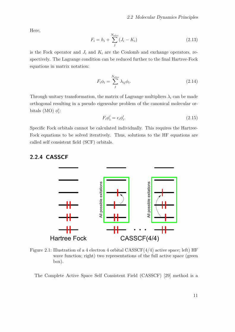
Figure 2.1: Illustration of a 4 electron 4 orbital CASSCF(4/4) active space; left) HFwave function; right) two representations of the full active space (greenbox).
The Complete Active Space Self Consistent Field (CASSCF) [29] method is a
11
2 Theory
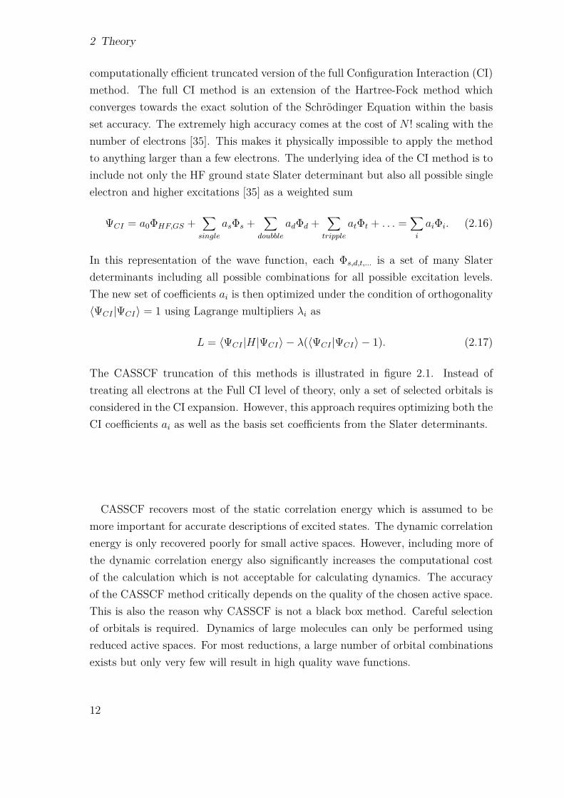
computationally efficient truncated version of the full Configuration Interaction (CI)method. The full CI method is an extension of the Hartree-Fock method whichconverges towards the exact solution of the Schrödinger Equation within the basisset accuracy. The extremely high accuracy comes at the cost of N ! scaling with thenumber of electrons [35]. This makes it physically impossible to apply the methodto anything larger than a few electrons. The underlying idea of the CI method is toinclude not only the HF ground state Slater determinant but also all possible singleelectron and higher excitations [35] as a weighted sum
ΨCI = a0ΦHF,GS +∑single
asΦs +∑
doubble
adΦd +∑tripple
atΦt + . . . =∑i
aiΦi. (2.16)
In this representation of the wave function, each Φs,d,t,... is a set of many Slaterdeterminants including all possible combinations for all possible excitation levels.The new set of coefficients ai is then optimized under the condition of orthogonality〈ΨCI |ΨCI〉 = 1 using Lagrange multipliers λi as
L = 〈ΨCI |H|ΨCI〉 − λ(〈ΨCI |ΨCI〉 − 1). (2.17)
The CASSCF truncation of this methods is illustrated in figure 2.1. Instead oftreating all electrons at the Full CI level of theory, only a set of selected orbitals isconsidered in the CI expansion. However, this approach requires optimizing both theCI coefficients ai as well as the basis set coefficients from the Slater determinants.
CASSCF recovers most of the static correlation energy which is assumed to bemore important for accurate descriptions of excited states. The dynamic correlationenergy is only recovered poorly for small active spaces. However, including more ofthe dynamic correlation energy also significantly increases the computational costof the calculation which is not acceptable for calculating dynamics. The accuracyof the CASSCF method critically depends on the quality of the chosen active space.This is also the reason why CASSCF is not a black box method. Careful selectionof orbitals is required. Dynamics of large molecules can only be performed usingreduced active spaces. For most reductions, a large number of orbital combinationsexists but only very few will result in high quality wave functions.
12

2.2 Molecular Dynamics Principles
2.2.5 DFT
Large effort has been put into the development of electron density and time de-pendent density based theories which do not require explicit electron coordinatesbut calculate the wave function based on its spatial electron density [4, 14, 21, 55].Thus, the integration is reduced from 3N to 3 dimensions with a vast increase inperformance compared to multi determinant methods. However, currently there isno sufficiently physical description of the correlation/exchange contribution with re-spect to the electron density. Therefore, Density Functional Theory (DFT) requiresfitting against high level quantum Monte Carlo simulations and/or experimentaldata which is why many DFT based methods are considered semi empirical.The underlying idea of Density Functional Theory (DFT) [32, 41] is to separate
the density dependent energy
E[ρ] = Ts[ρ] + Ene[ρ] + J [ρ] + Exc[ρ] (2.18)
into single electron contributions for kinetic energy Ts[ρ], electron/nuclear interac-tion Ene[ρ] and Coulomb interaction J [ρ]. The correlation and exchange part of theenergy is excluded from the description and stored in the undefined Exc contribution.The correlation part Ec of this energy is also the motivation for expanding the HFdeterminants in the full CI expansion. In HF theory, Ex is exact while Ec is missingcompletely. Unfortunately, the HF exact exchange is not directly compatible withthe DFT Exc energy. The first approaches towards describing the correlation ex-change energy were based on tabulating exact results from high level homogeneouselectron gas simulations. These are homogeneous local density (LDA) and localgradient extended generalized gradient (GGA) functionals [42]. Note, the oftenmentioned non-local corrections refer only to the inclusion of local gradients. Thisgroup of xc functionals fails to describe charge transfer as the needed 1/r behavioris not recovered with respect to the distance r. Instead, they decay exponentially.The reader is referred to a graphical representation of non-locality of the correlationand exchange holes as was calculated by Towler [61] using the variational MonteCarlo method.Second, a set of hybrid functionals was developed [42], including B3LYP, PBE0,
Half/Half and others. For these functionals, some part of the missing long rangeexchange is mixed into the pure adiabatic approximation (AA) DFT exchange bydirectly including Hartree-Fock (HF) exchange. The amount of exact HF exchange
13
2 Theory
then determines the long range scaling of the functional, 0.2/r in the case of B3LYP.Note, further increasing the amount of HF exchange reduces the needed cancellationof errors in xc-functionals between the correlation and exchange energies. Thus, sim-ply increasing HF exchange in B3LYP until the 1/r long range behavior is recoveredwill introduce large errors in the local description.Third, long range corrected, Coulomb attenuated or range separated xc-functionals
[13, 28, 67, 68] have been developed in recent years, referred to as LC-functionalsin the following text. They all rely on the separation of the two particle electron-electron interaction into a short and a long range part as described by Leininger etal. [46] as
1ri,j
= g(ri,j)ri,j︸ ︷︷ ︸LR
+ 1− g(ri,j)ri,j︸ ︷︷ ︸SR
. (2.19)
The separating function was conveniently chosen as g(ri,j) = erf(µri,j), the errorfunction. From this definition, it becomes clear that LC-functionals introduce anadditional parameter µ which determines the transition between the short rangeand the long range description [54, 55]. The underlying idea is to leave the localdescription of the xc-functionals, i.e. LDA, GGA unchanged. Thus, retaining theimportant cancellation of errors while including exact HF exchange for long rangeinteractions. The error function is then used to mediate the two contributions tothe energy. Therefore LC-functionals do not fully correct for the one electron SIE[68], as the local SIE still remains and only the long range SIE is compensated bythe correct 1/r behavior.All of the mentioned DFTmethods are single configuration methods and especially
for the long range corrected functionals the computational cost becomes similar tosmall multiconfigurational CAS active spaces. Thus, excited state simulations usingthe CASSCF method are still appealing for QM/MM simulations.
2.2.6 Force Field Approximation
The approximations up to this point allow the accurate time propagation of severaldozen atoms. This level of theory is referred to as Born-Oppenheimer dynamics(BO) and still too expensive to model large bio-organic systems in solution. Thequantum mechanical potential from equation 2.4 is now replaced by a purely classicalspring potential, the force field.The basis for the molecular dynamics (MD) simulations performed in this thesis
14

2.3 QM/MM Simulations
is the 2006 AMBER99sb force field [33] which is based on the Wang et al. AM-BER99 [69] and Cornell et al. AMBER94 force field [17]. The AMBER force fieldsoriginate from the 1984 Weiner force field [72]. The AMBER force field is a pairwiseempirical fit to the potential of the electronic wave function. The functional formhas not changed over the years and the differences are in the fitting of the functionalparameters. The function used is a classical ball and spring model of the form
Etotal =∑bonds
Kr(r − req)2 +∑angles
Kθ(θ − θeq)2 +
∑dihedrals
Vn2 [1 + cos(nϕ− γ)] +
∑i<j
[AijR1ij2− Bij
R6ij
+ qiqjεRij
]. (2.20)
The function describes the equilibrium bond distance req and the spring constantof bond oscillation Kr. The angles between three atoms are described using aharmonic angle potential with equilibrium angle θeq and force constant Kθ. Out ofplane dihedral motion of an atom chain a-b-c-d describes the rotation of atoms aand d around the axis of atoms b and c at angle θ. This motion is described by aTaylor series of a multi well potential whose Fourier coefficients are Vn and the phaseis γ. The Van der Waals potential is described by the parameter for repulsion Aijand the attraction Bij over the distance Rij. Finally, the last term of the potentialfunction describes the Coulomb interaction between the atom point charges qi andqj at distance Rij.Notice, how for a given set of protein atoms all possible two, three and four atom
connections need to be parametrized. This easily sums up to several ten thousandforce field parameters and implicitly explains why there are so many different forcefields [33]. The problem of generating a good force field is under determined given theavailable experimental parameters. This is why after over almost thirty years thereare still improvements made to the original parameter set. Force field developmentis a tedious task that will likely continue for many years to come.
2.3 QM/MM Simulations
Molecular dynamics simulations are a powerful tool to describe equilibrium prop-erties of large molecular systems such as proteins. The approximations made inthe molecular dynamics framework completely neglect explicit electrons and reducethe effect of the electronic wave function on the nuclei to an empirical classical
15
2 Theory
potential, the force field. However, the force field approximation will completelyfail to describe chemical reactions which involve bond breaking or photon absorp-tion. This renders molecular dynamics useless for the simulation of proton transferand excited state processes. The idea behind QM/MM simulations is to lift theforce field approximations on certain parts of the protein by including the electronicwave function directly through quantum mechanical calculations. This QM/MMapproach enables simulations of processes which require explicit electrons while alsoexplicitly including the protein environment at low computational cost.The QM/MM method is consistent with the three main approximations described
above. The efficient propagation of the quantum region (QM) requires the Born-Oppenheimer approximation as well as Newtons equation of motion for the nuclearmotion. In addition to these two approximations, the protein environment (MM) isdescribed using also the force field approximation which replaces explicit electronswith an empirical force field. As both regions approximate nuclear motion by New-tons equations of motion, the same time propagation algorithm is used for both theQM and MM region of the system. The MM forces are calculated from the forcefield while the QM forces are derived from the electronic wave function.In order to create a physically meaningful simulation, the QM region must be
allowed to interact with the MM environment. This can be achieved by directlycoupling the quantum region to the environment via embedding of the classicalnuclei into the electronic wave function. This method is called electronic embeddingand includes the classical point charges from the MM region into the quantumHamiltonian via [18]:
Hqm/mm = Hqmelectrons −
n∑i
M∑J
e2QJ
4πε0riJ+
N∑I
M∑J
e2ZIQJ
πε0RIJ
. (2.21)
In this equation, the first double sum describes the coupling of n quantum me-chanical electrons to M classical point charges QJ via Coulomb interaction over thedistance riJ . The second double sum couples the N nuclei with charge ZI in theQM region toM point charges QJ in the MM region with distance RIJ via Coulombinteraction.At the border between QM and MM regions, the angles, dihedrals and impropers
connecting the MM to the QM region are taken from the MM force field. A distanceconstraint is used to replace the bond between QM and MM region and set to thecorresponding equilibrium distance. As this bond is missing in the QM calculation a
16

2.3 QM/MM Simulations
lone electron pair is created. This artifact is removed by placing a virtual hydrogenatom along the constrained bond. The virtual hydrogen is included in the QMcalculation and ignored by the MM force field. The resulting force on the hydrogenis evenly distributed among the QM and MM binding partner.
17

3 Spectral Analysis of QM/MMTrajectories
3.1 The Challenge
The calculation of an-harmonic infrared spectra is a challenging task for largemolecules. A good model should be able to describe the system of interest in itsnatural environment rather than in vacuum [59]. It should also include native sup-port for anharmonicity without having to rely on anharmonic corrections as donein the case of harmonic normal modes . Additionally, the quality of the calculatedpower density spectra should be high enough to allow the calculation of differencespectra between states of interest. Thus a high resolution in frequency space is de-sirable. The method of choice should also capture temperature effects and systemdynamics at both the ground as well as the excited state. The method presentedin the following chapters includes all of the mentioned features as it is based on thetime series analysis of finite temperature QM/MM simulations. Here, the systemof interest is simulated at room temperature in its natural environment. From thetrajectory of this simulation, the dipole moment time series is recorded which is thebasis for the calculation of the anharmonic IR spectrum.
3.1.1 IR Transition Probabilities
In short summary, the vibrational spectrum of a molecular system is a representa-tion of periodic motion among the nuclei. The oscillation frequencies of the differentcollective nuclear motions appear as peaks in the spectrum. This motion behavesquantum mechanically, thus not all vibrations are allowed and their energies arequantized. In theory, these allowed collective frequencies can be obtained by apply-ing perturbation theory to the time dependent Schrödinger Equation:
19

3 Spectral Analysis of QM/MM Trajectories
Hψ(x, t) = −~i
∂ψ(x, t)∂t
(3.1)
This section was inspired by the discussion on quantum mechanical transitionprobabilities in references [58] and [43]. The perturbation H ′ is the effect of theelectric field due to infrared light passing the system. This leads to the perturbedSchrödinger equation
(H + H ′)ψ′(x, t) = −~i
∂
∂tψ′(x, t). (3.2)
The resulting perturbed wave function ψ′(x, t) can be expanded in the basis ofthe eigenfunctions ψn(x, t) = ψn(x)e−iEnt/~ of the unperturbed Hamiltonian H as
ψ′(x, t) =∑n
an(t)ψn(x)e−iEnt/~. (3.3)
The expansion coefficients an(t) contain valuable information about the probabilitypm(t) = |am(t)|2 of finding the original system ψs(x) in the final state ψm(x) aftera time t. Thus, an expression for the expansion coefficient will be derived in thefollowing paragraphs. First, inserting equation 3.3 into equation 3.2 results in
(H + H ′)∑n
an(t)ψn(x)e−iEnt/~ = −~i
∂
∂t
∑n
an(t)ψn(x)e−iEnt/~
= −~i
∑n
an(t)ψn(x)e−iEnt/~
−~i
∑n
an(t) ∂∂tψn(x)e−iEnt/~. (3.4)
The relation
∑n
an(t)Hψn(x)e−iEnt/~ = −∑n
an(t)~i
∂
∂tψn(x)e−iEnt/~ (3.5)
is applied to the last term of equation 3.4 resulting in a simplified expression for thederivative of the expansion coefficients an,
∑n
an(t)H ′ψn(x)e−iEnt/~ = −~i
∑n
an(t)ψn(x)e−iEnt/~. (3.6)
20
3.1 The Challenge
This equation can be reduced further by left-multiplying ψm(x, t), applying
Em,n = (Em − En) = ~ωm,n
and switching to 〈bra|ket〉 notation resulting in
∑n
an(t) 〈ψm| H ′ |ψn〉 eiωm,nt = −~i
∑n
an(t) 〈ψm|ψn〉 eiωm,nt
∑n
an(t)H ′m,neiωm,nt = −~iam(t). (3.7)
The last step requires the orthogonality relation 〈ψm|ψn〉 = δmn and introducesa shortened notation for the matrix element H ′m,n = 〈ψm| H ′ |ψn〉. equation 3.7provides a set of linear differential equations from which an can be obtained.
However, the infrared relevant first order term can also be obtained by assumingthe perturbation H ′ to be weak and short lived. This implies that the expansioncoefficients at time t can be approximated by their value at t = 0, analog to a zerothorder Taylor expansion. Further, the system is assumed to be in state ψ(x, t = 0) =ψs(x). The ψs(x) state has all zero an coefficients except for as = 1. This simplifiesequation 3.7 to
am(t) = − i~H ′m,se
iωm,st. (3.8)
For time dependent perturbations H ′(t) = H ′e−iωt with frequency ω, equation 3.8changes slightly into
am(t) = − i~H ′m,se
i(ωm,s−ω)t. (3.9)
Equation 3.9 can be integrated on the interval t′ = [0..t] under the assumption thatthe final state |m〉 is unoccupied at t = 0, am(t = 0) = 0. The resulting coefficientequation is
am(t) = 1~H ′m,s
1− ei(ωm,s−ω)t
(ωm,s − ω) . (3.10)
The last result is useful for calculating the transition probability
pm,s(t) = |am(t)|2 = 2~|H ′m,s|2
1− cos((ωm,s − ω)t)(ωm,s − ω)2 (3.11)
from state |s〉 to state |m〉 via light absorption or emission. This in itself is a very
21
3 Spectral Analysis of QM/MM Trajectories
interesting result, as it directly relates the transition probability to the square of thetransition matrix elements. Thus, understanding the factors that influence transi-tions requires further information about the perturbation. One example for theseperturbations is the electric field ~E(x, t) = ~E0(x)e−iωt of photons which interactwith the electronic dipole µ of the molecule. A simple interaction Hamiltonian
H ′ = ~µ · ~E(x, t) (3.12)
can be defined for this interaction. The coupling will be maximal when field anddipole moment are aligned parallel and zero for perpendicular orientations. Insertingequation 3.12 into 3.11 results in
pm,s(t) = 4~2 | 〈ψm| ~µ |ψs〉 |
2| ~E0|2cos2(θµ,E0)1− cos((ωm,s − ω)t)(ωm,s − ω)2 . (3.13)
At this point the transition to the experiment can be made. Equation 3.13 directlyrelates the transition probability, or intensity Im,s, to the dipole moment operator~µ = ∑
i ei~qi. In this representation, ei is the effective charge at atom i and ~qi is thevector of atom i to the center of mass of the system. Choosing ~qi this way createsa well defined point of reference even for charged systems, see chapter 3.1.3. Thetransition intensity Im,s from state |s〉 to state |m〉 can be expressed in relation toequation 3.13 as
Im,s ∝([µx]2m,s + [µy]2m,s + [µz]2m,s
), (3.14)
where[µj]m,s = 〈ψm| µj |ψs〉 . (3.15)
Based on this relation for the intensities, transition rules can be obtained for theharmonic case by Taylor expanding the dipole moment operator with respect to thenormal coordinates Qi as
~µ ≈ ~µ0 +3N−6∑i=1
(∂~µ
∂Qi
)µ0
Qi. (3.16)
The harmonic approximation results in a finite Taylor series which is convenientbut not required if generalized normal coordinates are available. The expression canbe inserted back into equation 3.15 which finally leads to the important connection
22
3.1 The Challenge
between the change of the dipole moment and vibrational intensities through
[µj]m,s = 〈ψm| µj |ψs〉
≈ 〈ψm|µ0 +3N−6∑i=1
(∂µ
∂Qi
)µ0
Qi |ψs〉
= µ0 〈ψm|ψs〉︸ ︷︷ ︸=0
+3N−6∑i=1〈ψm|
(∂µ
∂Qi
)µ0
Qi |ψs〉
=3N−6∑i=1〈ψm|
(∂µ
∂Qi
)µ0
Qi |ψs〉 . (3.17)
From this equation the important transition condition
〈ψm|(∂µ
∂Qi
Qi
)µ0
|ψs〉 6= 0 (3.18)
can be derived. The condition explicitly states that the molecular dipole momentof a given molecule must change with respect to the normal coordinates for allowedtransitions from |s〉 to |m〉. Of course these statements only hold for the truncatedTaylor expansion in equation 3.16 and thus only in harmonic approximation. How-ever, even for the anharmonic case equation 3.18 is expected to be the dominatingterm in the transition probability and therefore also the transition intensities. Ob-taining the required normal coordinates is highly non trivial especially for largesystems and anharmonic contributions beyond the truncated Taylor expansion, seesection 3.1.5 for further discussion. An additional feature of equation 3.14 is itsdependence on all absolute square value of the transition dipole moment. In thisformulation, forbidden transitions can exist in either one, two or three dimensionswhich allows experiments to probe molecules using polarized light. Individual con-tributions to the total intensity can be probed this way.
3.1.2 Normal Mode Analysis
The Normal Mode Analysis (NMA) provides a framework for obtaining the normalcoordinates Qi in equation 3.16 as well as harmonic frequencies [11, 15, 58]. In thisframework the nuclear motion is approximated by harmonic potentials. The motionof the nuclei is described using Newton mechanics and Hook’s law mx = −kx. Thedisplacement of the atoms from their equilibrium positions is x, x is the acceleration,m the mass and k the harmonic spring constant. Figure 3.1 shows a simple mechan-
23
3 Spectral Analysis of QM/MM Trajectories
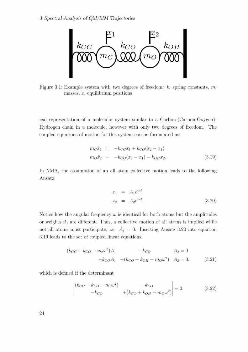
Figure 3.1: Example system with two degrees of freedom: ki spring constants, mi
masses, xi equilibrium positions
ical representation of a molecular system similar to a Carbon-(Carbon-Oxygen)-Hydrogen chain in a molecule, however with only two degrees of freedom. Thecoupled equations of motion for this system can be formulated as:
mC x1 = −kCCx1 + kCO(x2 − x1)mOx2 = −kCO(x2 − x1)− kOHx2. (3.19)
In NMA, the assumption of an all atom collective motion leads to the followingAnsatz:
x1 = A1eiωt
x2 = A2eiωt. (3.20)
Notice how the angular frequency ω is identical for both atoms but the amplitudesor weights Ai are different. Thus, a collective motion of all atoms is implied whilenot all atoms must participate, i.e. Aj = 0. Inserting Ansatz 3.20 into equation3.19 leads to the set of coupled linear equations
(kCC + kCO −mcω2)A1 −kCO A2 = 0
−kCOA1 +(kCO + kOH −mOω2) A2 = 0. (3.21)
which is defined if the determinant∣∣∣∣∣∣(kCC + kCO −mcω2) −kCO
−kCO +(kCO + kOH −mOω2)
∣∣∣∣∣∣ = 0. (3.22)
24
3.1 The Challenge
The determinant equation 3.22 can easily to transformed into an eigenvalue problemby substituting ω2 with λ. For the sake of clarity, the spring constants kCC , kCO,kOH and the masses mO, mC are reduced to the unit mass m as well as the arbitraryspring constant k using the following set of substitution rules:
kOH = k; kCC = 5k; kCO = 6k; mC = m; mO = (3/4)m. (3.23)
This leads to the two eigenvalues
λ1 =(
31−√
4336
)k
m' 1.7 k
m(3.24)
λ2 =(
31 +√
4336
)k
m' 8.6 k
m(3.25)
and thus the frequencies
ω1 = ±√λ1 ' 1.3
√k
m(3.26)
ω2 = ±√λ2 ' 2.9
√k
m(3.27)
The set of eiqenvalues now leads to a set of eigenvectors by substituting ω1 and ω2
back into equation 3.21
A1
A2= kCO
(kCC+kCO−mcω21) ≈ −0.8
A1
A2= (kCO+kOH−mOω
22)
kCO≈ 0.9 (3.28)
and therefore
~v1 = −0.8
1
; ~v2 = 0.9
1
. (3.29)
The simple two DOF system discussed above already shows how amplitudes canonly be obtained relative to each other in NMA and not in absolute values. There-fore, A2 = 1 was arbitrarily chosen. It also illustrates how harmonic normal modescan be projected back onto the molecular structure via the original Ansatz of equa-tion 3.20 using eigenfrequencies ωi and eigenvectors ~vi. This allows for a visualinspection of the different normal modes as well as the assignment of spectral bandsto localized groups of atoms. This projection results in a phasic motion (v2) and
25
3 Spectral Analysis of QM/MM Trajectories
an antiphasic motion (v1) of the two atoms in figure 3.1. In the reference frame ofnormal coordinates, there is no energy transfer from these two motions as there areno anharmonic off diagonal coupling elements included.
3.1.3 Dipole Moments in QM/MM Simulations
An alternative approach towards calculating vibrational spectra is the direct analysisof system dynamics through time series analysis. In the previous chapters, theexpansion of the wave function in eigenfunctions ψn(x)
ψ(x, t) =∑n
an(t)ψn(x)e−iEnt/~
was introduced and explicitly solved for the expansion coefficients an(t), see equation3.10. This is not practical for larger systems, as the vibrational wave function is com-putationally not accessible. In order to derive a more feasible simulation scheme, thecoefficients an are related directly to the time series of the time depended Schrödingerequation solution. This can be archived by rewriting the Fourier transform of thewave function time correlation function [60]
p(ω) = (2π)−1∫ ∞−∞〈ψ(0)|ψ(t)〉 eiωtdt
as
p(ω) = (2π)−1∫∫ ∞−∞
(∑m
cmψm(x)e−iωnt
)∗ (∑n
cnψn(x)e−iωnt
)dxeiωtdt
= (2π)−1∫ ∞−∞
∑m,n
c∗mcnδmnei(ω−ωn)tdt
=∑m
|cm|2δ(ω − ωm) (3.30)
using the orthogonality〈ψm|ψn〉 = δmn (3.31)
and the relation ∫ ∞−∞
ei(ω−ωn)tdt = 2πδ(ω − ωn). (3.32)
Here, equation 3.30 is identical to equation 3.11. Thus the spectrum of a quantummechanical system can directly be obtained from the system dynamics without theneed of Normal Mode Analysis. Instead of relying purely on a harmonic approxima-
26

3.1 The Challenge
tion of the underlying energy landscape, the system is allowed to relax and explorethe energy landscape at finite temperature. This intrinsically includes anharmoniceffects and temperature. Unfortunately, the time dependent Schrödinger equationcan currently not be solved for system sizes of interest in this thesis. Instead, thecheaper QM/MM simulation scheme is used to propagate the wave function in time.In this section, the dipole moment operator is applied to the QM/MM wave
function and the resulting dipole moment time series is related to the spectrum viathe Wiener−Khinchin Theorem. By choosing the dipole moment as the observable,the IR activity criterion from equation 3.18 is explicitly met as only dipole activemodes can be identified. Modes which do not change the dipole moment will notcontribute to the dipole moment time series and thus will not be resolved in thedipole time series analysis.First, the concept of dipole moment analysis is introduced and sequentially ex-
tended towards charged molecules. The concept of dipole moments arises fromthe multipole expansion of the Coulomb potential. In the multipole expansion, thedipole moment ~p of a continuous charge distribution ρ(~r0) in the volume V is definedas
~p =∫Vρ(~r0)(~r0 − ~rref )d3r0. (3.33)
In addition to the dependence of the dipole moment on the charge density ρ andthe position r, the dipole moment also depends on a reference point ~rref . It caneasily be shown that this explicit dependence only holds for charged systems. Forsystems with a neutral overall charge Q =
∫V ρ(~r0)d3r0 = 0, the explicit dependence
vanishes as
~p =∫Vρ(~r0)(~r0 − ~rref )d3r0
=∫Vρ(~r0)~r0d
3r0 −∫Vρ(~r0)~rrefd3r0
=∫Vρ(~r0)~r0d
3r0 −Q · ~rref (3.34)
=∫Vρ(~r0)~r0d
3r0
However, the analysis of neutral systems is not sufficient for the analysis of neithergreen fluorescent nor photoactive yellow protein as both systems have charged activesites. It is therefore desirable to find a good reference point. There are a number ofpossible candidates for reference points and intuitively, the origin seems like a goodchoice. With rref = (0, 0, 0), the second term of the right hand site in equation 3.34
27
3 Spectral Analysis of QM/MM Trajectories
vanishes. However, this is not sufficient as the integral∫V ρ(~r0)~r0d
3r0 will not onlydepend on position differences but also on the absolute position of the system for∫V ρ(~r0)d3r0 6= 0. In this case the dipole moment will no longer be translation orrotation invariant as global motion changes the absolute distance towards the origin.As translational and rotational invariance is desired, the center of mass
rCOM =∑Nn=1 mnrn∑Nn=1 mn
(3.35)
can be chosen as reference point for all dipole time series. This effectively shiftsthe problem of reference into the internal coordinate frame of the molecule. Areference bias in the spectrum can only be reduced and will likely not be excludedthis way. To approach this problem, the center of reference is explicitly includedand monitored during all simulations conducted as part of this thesis. Additionally,the spectral contribution of rCOM motion is calculated in analogy to the dipole timeseries analysis. This enables band specific bias estimation which is expected tobecome less important for increasing system size as more atoms are included in therCOM average.
Choosing a proper reference point is not the only obstacle when applying dipoletime series analysis (DTSA) to large QM/MM simulation trajectories. The largecomputational cost of quantum calculations in the QM/MM scheme effectively limitsthe number of vibrations that can be identified. For medium sized QM systems,1000-1500 fs trajectory lengths are feasible which also equals about 1500 samples ofthe underlying dynamics. It therefore is no surprise that not all 3N -6 modes for theentire simulation box can be determined. For GFP and PYP the total number ofDOFs surpasses 105 and can no longer be handled at the QM/MM level.
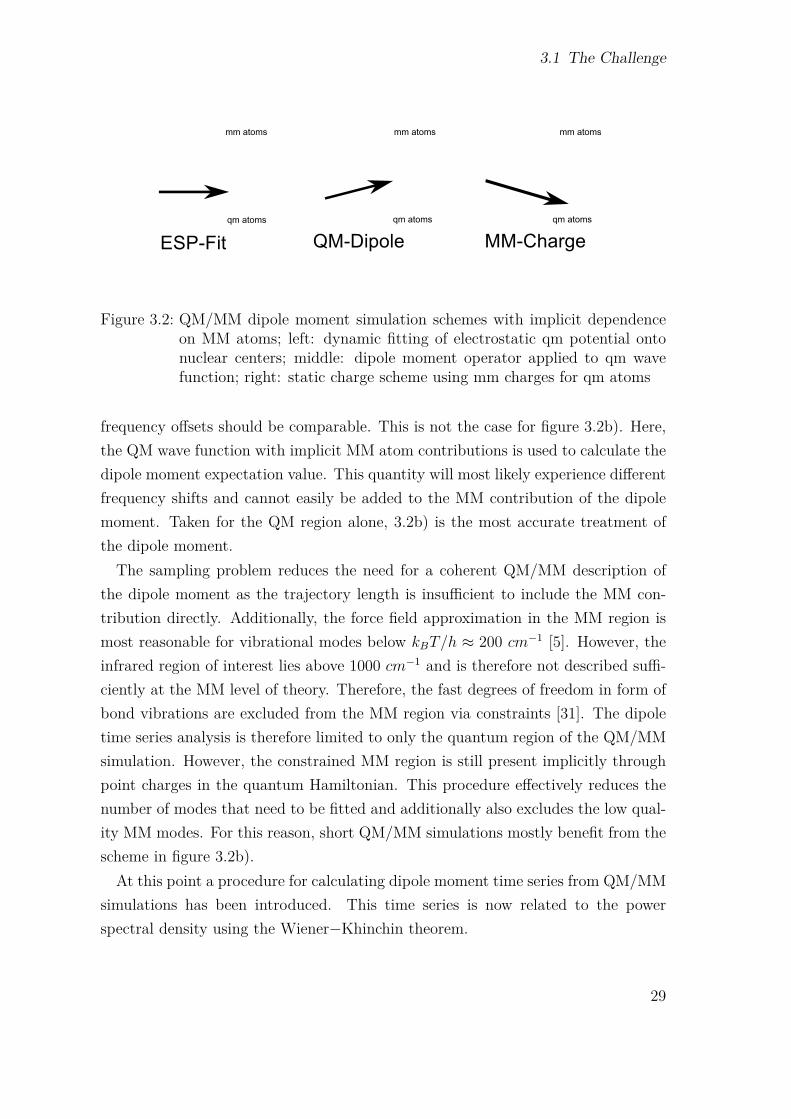
Figure 3.2 illustrates three ways of calculating the dipole moments for the QMregion in QM/MM simulations. Figure 3.2c) represents the simplest solution whichonly includes static MM charges for the QM region. This ensures compatibilitywith the MM charges as there are no contributions from induced dipole moments.There is also no explicit dependence on the electron dynamics which is also missingin the MM force field. Figure 3.2a) extends this simple picture by refitting theelectron generated electrostatic potential at each time step. This can be done inanalogy to the original parametrization of the MM force field [33] which ensuresconsistency with the dipole contribution from the MM region. Both QM methods forcalculating the dipole moment are in good agreement with the MM description. Thus
28
3.1 The Challenge
Figure 3.2: QM/MM dipole moment simulation schemes with implicit dependenceon MM atoms; left: dynamic fitting of electrostatic qm potential ontonuclear centers; middle: dipole moment operator applied to qm wavefunction; right: static charge scheme using mm charges for qm atoms
frequency offsets should be comparable. This is not the case for figure 3.2b). Here,the QM wave function with implicit MM atom contributions is used to calculate thedipole moment expectation value. This quantity will most likely experience differentfrequency shifts and cannot easily be added to the MM contribution of the dipolemoment. Taken for the QM region alone, 3.2b) is the most accurate treatment ofthe dipole moment.The sampling problem reduces the need for a coherent QM/MM description of
the dipole moment as the trajectory length is insufficient to include the MM con-tribution directly. Additionally, the force field approximation in the MM region ismost reasonable for vibrational modes below kBT/h ≈ 200 cm−1 [5]. However, theinfrared region of interest lies above 1000 cm−1 and is therefore not described suffi-ciently at the MM level of theory. Therefore, the fast degrees of freedom in form ofbond vibrations are excluded from the MM region via constraints [31]. The dipoletime series analysis is therefore limited to only the quantum region of the QM/MMsimulation. However, the constrained MM region is still present implicitly throughpoint charges in the quantum Hamiltonian. This procedure effectively reduces thenumber of modes that need to be fitted and additionally also excludes the low qual-ity MM modes. For this reason, short QM/MM simulations mostly benefit from thescheme in figure 3.2b).At this point a procedure for calculating dipole moment time series from QM/MM
simulations has been introduced. This time series is now related to the powerspectral density using the Wiener−Khinchin theorem.
29
3 Spectral Analysis of QM/MM Trajectories
3.1.4 Wiener-Khinchin Theorem
The Wiener-Khinchin Theorem is a fundamental part of signal analysis. It relatesthe time autocorrelation function R(τ) of a wide sense stationary (WSS) signalµ(t) to its power spectral density S(ω). However, it was also shown to hold fordeterministic signals as well [16]. The Wiener-Khinchin Theom will be derived inanalogy to derivation by Leon Cohen [16] with the extension of equation block 3.41for clarity. For the case of random, zero mean, stationary time dependent signals
µ(t) = µ(t) |t|<T
0 |t|>T.(3.36)
the signal Fourier transform F (ω) and inverse Fourier transform can be defined as
F (ω) =∫ ∞−∞
µ(t)e−iωtdt (3.37)
µ(t) = (2π)−1∫ ∞−∞
F (ω)eiωtdω. (3.38)
The process autocorrelation function R(t, τ) is defined as the ensemble average E[]of the signal as
R(τ) = E[µ∗(t)µ(t+ τ)]. (3.39)
Under the assumption of ergodicity, the ensemble averaged autocorrelation functionequals the time autocorrelation function.
The power spectral density S(ω) is defined as
S(ω) = limT→∞
12T E[|FT (ω)|2] (3.40)
30
3.1 The Challenge
and can be rewritten to result the Wiener-Khinchin theorem since
S(ω) = limT→∞
12T E[|FT (ω)|2]
= limT→∞
12T E
[∫ T
−Tµ(t)e−iωtdt
]2
= limT→∞
12T E
[∫∫ T
−Tµ∗(τ)µ(t)e−iω(t−τ)dtdτ
]
= limT→∞
12T
∫∫ T
−TE[µ(τ)µ(t)]e−iω(t−τ)dtdτ
= limT→∞
12T
∫∫ T
−TdtR(t− τ)e−iω(t−τ)dtdτ
= limT→∞
12T
∫ T
−Tdt︸ ︷︷ ︸
=1
∫ ∞−∞
R(τ ′)e−iωτ ′dτ ′. (3.41)
Here, the autocorrelation function R(τ) does no longer depend on the time t butrather on the lag window length τ and therefore the time integral drops out.
S(ω) =∫ ∞−∞
R(τ)e−iωτdτ. (3.42)
Equation 3.42 is the Wiener-Khinchin theorem. It enables direct calculation ofpower spectra from time autocorrelation functions. In strict mathematical terms,the autocorrelation function detour is not necessarily required to calculate powerspectra, as can be seen from equation 3.40. The time autocorrelation function issmooth, time independent and can also exist for signals which cannot be Fouriertransformed directly. This is the case for signals which do not fulfill the conditionof finite energy. Additionally, autocorrelation based spectral estimation has lowervariance than direct spectra, which is desirable [39]. The reason for discussingthe Wiener-Khinchin theorem will become more imminent when introducing themaximum entropy spectral estimation. Here, the autocorrelation function for shortsignals is extended under the boundary condition of maximum entropy.
3.1.5 Assumptions, Approximations and Limitations
The first section of this chapter promised a method for calculating infrared spectrafrom QM/MM simulations providing the following feature set:
31
3 Spectral Analysis of QM/MM Trajectories
• Native support for anharmonicity and temperature effects
• High frequency resolution for difference spectra
• Natural protein environment is included
• Covers both the ground as well as the excited state
These features have all been provided, except for the high resolution in frequencyspace which is discussed in chapter 3.2. However, the efficient implementation of thedescribed method requires several implicit assumptions and approximations whichare important in order to understand the limitations of this approach. Figure 3.3
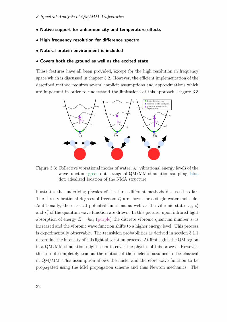
Figure 3.3: Collective vibrational modes of water; si: vibrational energy levels of thewave function; green dots: range of QM/MM simulation sampling; bluedot: idealized location of the NMA structure
illustrates the underlying physics of the three different methods discussed so far.The three vibrational degrees of freedom ~vi are shown for a single water molecule.Additionally, the classical potential functions as well as the vibronic states si, s′iand s′′i of the quantum wave function are drawn. In this picture, upon infrared lightabsorption of energy E = ~ωi (purple) the discrete vibronic quantum number si isincreased and the vibronic wave function shifts to a higher energy level. This processis experimentally observable. The transition probabilities as derived in section 3.1.1determine the intensity of this light absorption process. At first sight, the QM regionin a QM/MM simulation might seem to cover the physics of this process. However,this is not completely true as the motion of the nuclei is assumed to be classicalin QM/MM. This assumption allows the nuclei and therefore wave function to bepropagated using the MM propagation scheme and thus Newton mechanics. The
32
3.2 Estimating Power Spectral Densities
consequences of this approximation are severe as the vibrational energy states areapproximated classically and the energy dissipation among the vibrational modesis no longer quantized. Vibrational degrees of freedom can have continuous energylevels as opposed to discrete quantum levels in the experiment. With respect tothis energy partition issue, the dipole time series analysis (sampled region shown ingreen) cannot be expected to significantly improve on the Normal Mode Analysisresults.However, the dipole time series analysis does have other clear advantages over
NMA. Figure 3.3 illustrates the strong dependence of Normal Mode Analysis onfinding a well energy minimized structure. The blue dot represents the idealizedsingle starting point configuration for Normal Mode Analysis. Obtaining this be-forehand unknown point is not trivial especially for large QM systems in a proteinenvironment such as the GFP active pocket. With dipole time series analysis, theclose proximity of this point is also taken into account through sampling of the dy-namics. A more severe limitation of Normal Mode Analysis is the assumption of anharmonic potential energy landscape around the equilibrium position. In physicalterms this can be seen as a very low order Taylor expansion to the potential en-ergy landscape. Deviations from this set of harmonic orthogonal potentials are notallowed and energy transfer between different normal coordinates is not possible.This effectively biases the identified modes towards their closest harmonic equiva-lent. The time series analysis is more general as it identifies periodic contributionsto a signal without making assumption about the underlying energy landscape.
3.2 Estimating Power Spectral Densities
3.2.1 Fourier Spectra
The relation between the power spectral density and the Fourier transform wasderived in section 3.1.4. The Wiener-Khinchin Theorem was derived under theassumption of infinite sampling of a periodic signal s(t). Therefore, an exact auto-correlation function R(τ) = E[s(t)s∗(t + τ)] and infinite boundaries in the Fourierintegral were assumed for the power spectral density
S(ω) =∫ ∞−∞
R(τ)e−iωτdτ. (3.43)
33

3 Spectral Analysis of QM/MM Trajectories
In real world applications such as simulated IR spectra of proteins, this assumptionis not valid as only a finite set of sampling points is available. The high cost ofperforming QM/MM simulations severely shortens the available trajectory lengthsto about 1000 sampling points. The transition between the infinite S∞ and finiteST time series on the interval [−T..T ] can be formulated as a multiplication of Sfwith a rectangular window function
ςrect(t) = 1 |t|≤|T|
0 |t|>|T|(3.44)
asST = S∞ ∗ ςrect(t). (3.45)
The window multiplication or convolution operation also affects the Fourier repre-sentation of the signal. The Fourier spectrum of the finite length signal is smoothenedwith decreasing window length and spectral resolution is lost. In the ideal case ofinfinite sampling, the window function has infinite width and its Fourier transform,the delta function, does not influence the spectrum. A second effect of finite windowlengths is caused by the truncation of the maximum lag length τ . This results in anincrease in variance of the autocorrelation function estimate for long lag times. Theuneven variance of the estimate is due to the nature of the finite autocorrelationfunction in which short lag times τ are better sampled that long ones.
The undesirable variance can be reduced by introducing a lag dependent weightingfunction ς(τ) into the autocorrelation function estimate R(τ). This method wasintroduced by R.B. Blackman and J.W. Tukey [7] in 1959. The Blackman andTukey method describes the weighted power spectral density
S(ω) =∫ ∞−∞
ς(τ)R(τ)e−iωτdτ. (3.46)
As a consequence, the weighted power spectrum effectively becomes the convolutionof the true spectral estimate and the Fourier transform of the weighting window.This convolution can have severe effects on the spectrum as the positivity is not nec-essarily conserved and spectral amplitude can leak into neighboring peaks. Spectralpositivity can be conserved by using a triangular window of the form
ςtriang(t) =
2τL+1 1 ≤ τ ≤ L+1
22(L−τ+1)L+1
L+12 < τ ≤ L
(3.47)
34

3.2 Estimating Power Spectral Densities
at the cost of effectively reducing the information used to obtain the spectrum inhalf. Triangular windows are a simple but wasteful way of reducing spectral variance.Additionally, triangular windows increase the spectral bias through the mentionedsidelobe leakage of power as a result of the convolution procedure.An alternative way of reducing spectral variance is the Bartlett method. The
Bartlett method is simply an average over N statistically independent spectral es-timates Si(ω) as
S(ω) = 1N
N∑i=1
Si(ω). (3.48)
This approach decreases the spectral resolution but also decreases the variance bya factor of 1/N . It is therefore desirable to have high resolution spectral estimatesSi(ω) before averaging. The Bartlett method is especially appealing for QM/MMtrajectories as many short trajectories are significantly cheaper to calculate thansingle long trajectories.
3.2.2 Maximum Entropy Method
The windowing methods discussed so far all assume the autocorrelation estimateto be zero outside the interval [−2T..2T ]. However, this assumption can be liftedby extending the signal autocorrelation function under the condition of maximumentropy. This approach is called Maximum Entropy Method (MEM). The MEMgenerates additional information on the autocorrelation function which can thenbe used to calculate a Fourier spectrum. The extended autocorrelation functionfrom approximated data has a higher spectral resolution but will not significantlydecrease the spectral variance. Additionally, the extension of the autocorrelationfunction may introduce pseudo peaks into the spectrum due to over fitting for largeextension ranges. MEM should therefore be considered a parametric method forspectral estimation in contrast to the parameter free Fourier spectrum. The param-eter estimation and optimization is matter of section 3.3.In this section, the basic mathematical concepts of the MEM according to the
work of J.P. Burg [12] are introduced and connected to the all pole autoregressive(AR) filter in analogy to A. van den Bos [64] and D.A. Gray [26]. The definition ofentropy
HN = log(2πe)N/2det{R}1/2 (3.49)
in the MEM originates from statistical physics but is equally important in informa-
35
3 Spectral Analysis of QM/MM Trajectories
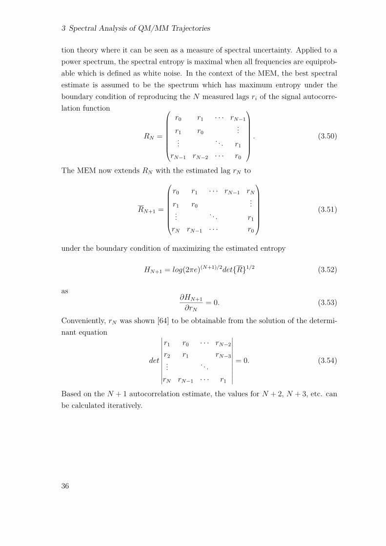
tion theory where it can be seen as a measure of spectral uncertainty. Applied to apower spectrum, the spectral entropy is maximal when all frequencies are equiprob-able which is defined as white noise. In the context of the MEM, the best spectralestimate is assumed to be the spectrum which has maximum entropy under theboundary condition of reproducing the N measured lags ri of the signal autocorre-lation function
RN =
r0 r1 · · · rN−1
r1 r0...
... . . . r1
rN−1 rN−2 · · · r0
. (3.50)
The MEM now extends RN with the estimated lag rN to
RN+1 =
r0 r1 · · · rN−1 rN
r1 r0...
... . . . r1
rN rN−1 · · · r0
(3.51)
under the boundary condition of maximizing the estimated entropy
HN+1 = log(2πe)(N+1)/2det{R}1/2 (3.52)
as∂HN+1
∂rN= 0. (3.53)
Conveniently, rN was shown [64] to be obtainable from the solution of the determi-nant equation
det
∣∣∣∣∣∣∣∣∣∣∣∣
r1 r0 · · · rN−2
r2 r1 rN−3... . . .rN rN−1 · · · r1
∣∣∣∣∣∣∣∣∣∣∣∣= 0. (3.54)
Based on the N + 1 autocorrelation estimate, the values for N + 2, N + 3, etc. canbe calculated iteratively.
36

3.2 Estimating Power Spectral Densities
3.2.3 Burgs Method
In the previous section, the Maximum Entropy Method was introduced which al-lowed the calculation of power spectra by Fourier transforming an extended auto-correlation function.
Figure 3.4: All pole autoregressive filter in time domain.
This is just one example of how the spectral resolution can be increased. Analternative way is to rewrite a signal si in terms of its last P samples and a randomnoise input ui as
si = −P∑k=1
aksi−k + PNui. (3.55)
This model is known as the all-pole model [47], see figure 3.4. The weights ak arecalled filter coefficients. PN is the gain or output power obtained from the resultinglinear prediction model [26], or autoregressive filter. The frequency representationof this model can be written in terms of a z transform ∑N
n=0 anz−n as
Sout(z) = PN
[∑Pn=0 anz
−n][∑Pn=0 a
∗nz
n]. (3.56)
No Fourier transform is needed and the spectrum Sout(z) is obtained in a P polespolynomial representation.The work of J.P. Burg [10, 12, 51] extended this approach by relaying the power
spectrum directly to the prediction error filter coefficients (p.e.f.c.s.). Burg decom-posed the N + 1 signal samples into an all pole autoregressive filter of order P . Themeasured signal si is approximated by the estimate si as
si = −P∑k=1
aksi−k. (3.57)
A forward p.e.f.c.s. estimator fi(n) = si − si is constructed for all P filter coeffi-
37
3 Spectral Analysis of QM/MM Trajectories
cients ai as
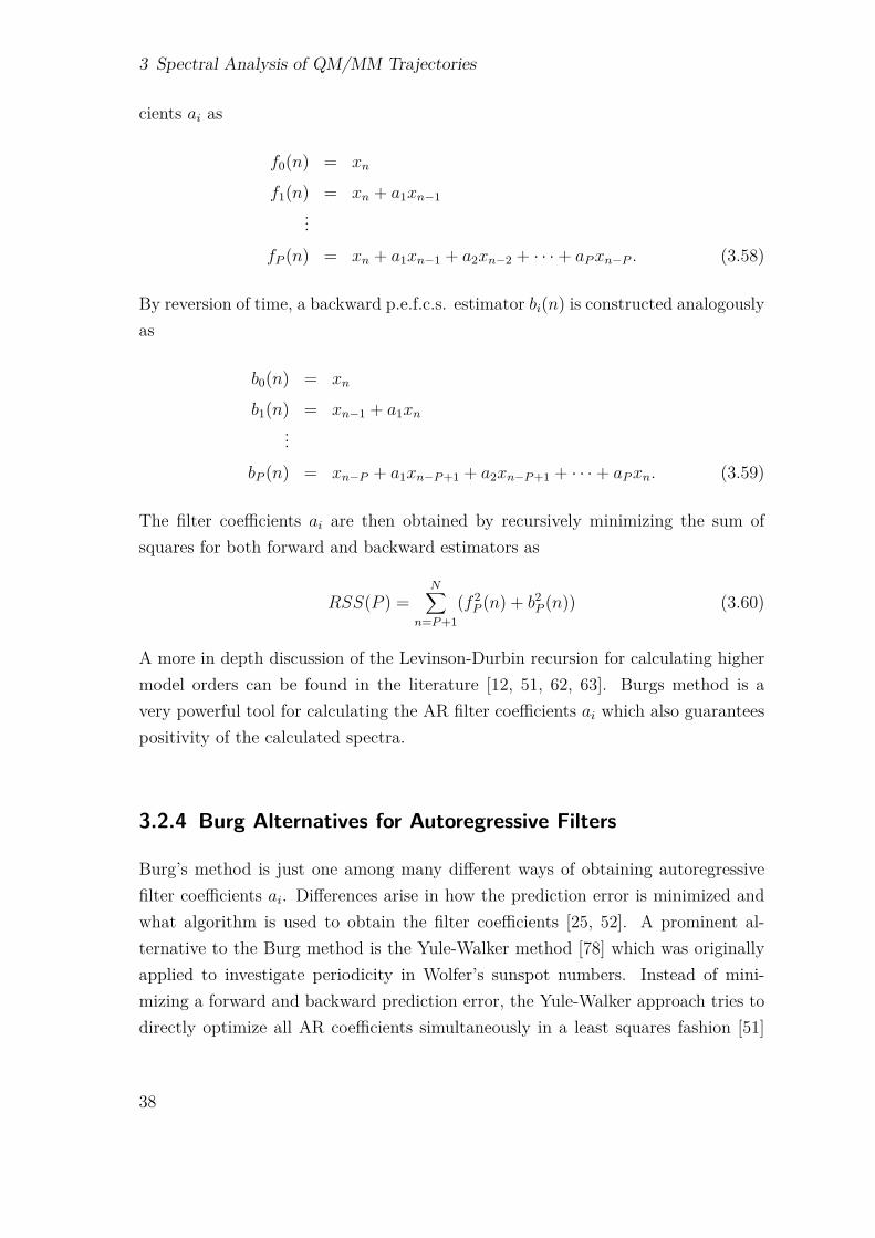
f0(n) = xn
f1(n) = xn + a1xn−1...
fP (n) = xn + a1xn−1 + a2xn−2 + · · ·+ aPxn−P . (3.58)
By reversion of time, a backward p.e.f.c.s. estimator bi(n) is constructed analogouslyas
b0(n) = xn
b1(n) = xn−1 + a1xn...
bP (n) = xn−P + a1xn−P+1 + a2xn−P+1 + · · ·+ aPxn. (3.59)
The filter coefficients ai are then obtained by recursively minimizing the sum ofsquares for both forward and backward estimators as
RSS(P ) =N∑
n=P+1(f 2P (n) + b2
P (n)) (3.60)
A more in depth discussion of the Levinson-Durbin recursion for calculating highermodel orders can be found in the literature [12, 51, 62, 63]. Burgs method is avery powerful tool for calculating the AR filter coefficients ai which also guaranteespositivity of the calculated spectra.
3.2.4 Burg Alternatives for Autoregressive Filters
Burg’s method is just one among many different ways of obtaining autoregressivefilter coefficients ai. Differences arise in how the prediction error is minimized andwhat algorithm is used to obtain the filter coefficients [25, 52]. A prominent al-ternative to the Burg method is the Yule-Walker method [78] which was originallyapplied to investigate periodicity in Wolfer’s sunspot numbers. Instead of mini-mizing a forward and backward prediction error, the Yule-Walker approach tries todirectly optimize all AR coefficients simultaneously in a least squares fashion [51]
38
3.3 Simulation Scheme
by minimizing
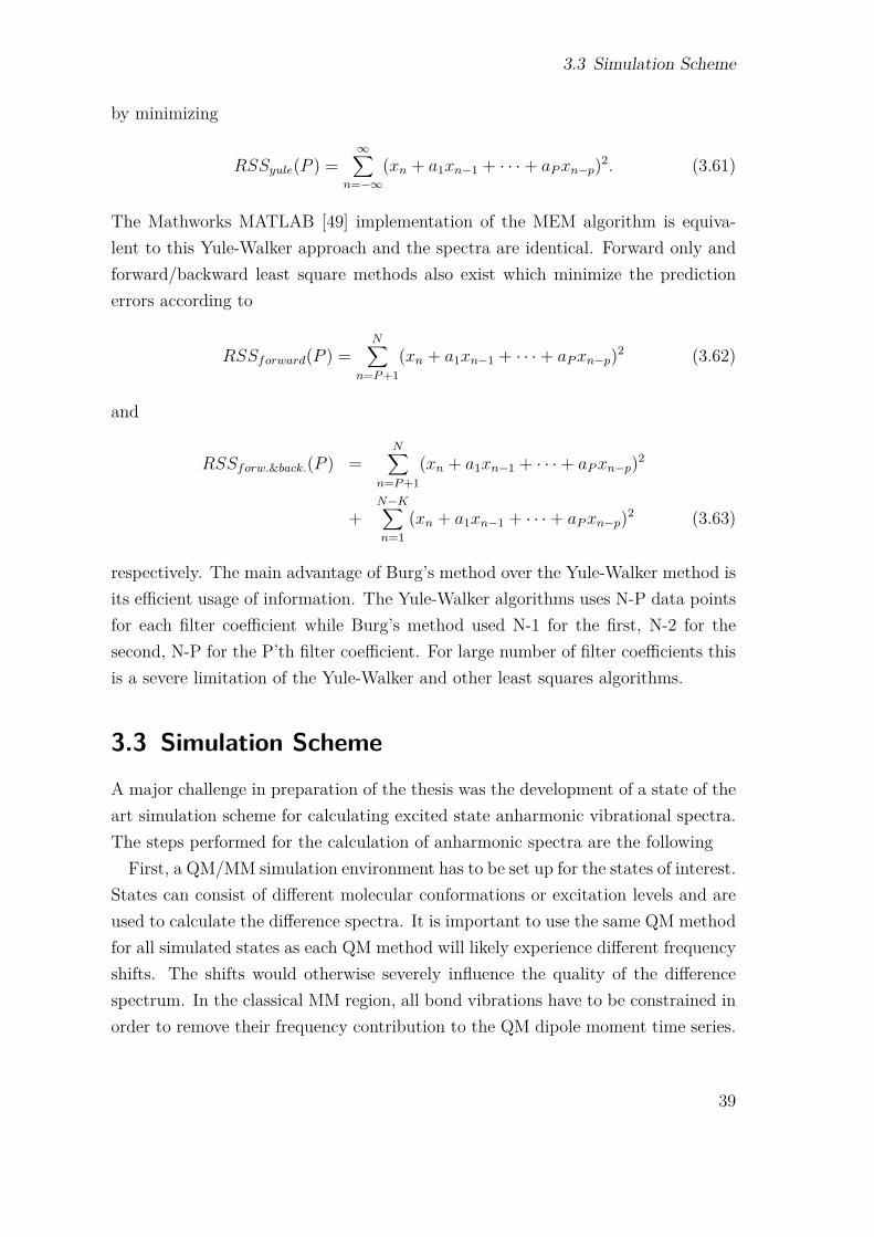
RSSyule(P ) =∞∑
n=−∞(xn + a1xn−1 + · · ·+ aPxn−p)2. (3.61)
The Mathworks MATLAB [49] implementation of the MEM algorithm is equiva-lent to this Yule-Walker approach and the spectra are identical. Forward only andforward/backward least square methods also exist which minimize the predictionerrors according to
RSSforward(P ) =N∑
n=P+1(xn + a1xn−1 + · · ·+ aPxn−p)2 (3.62)
and
RSSforw.&back.(P ) =N∑
n=P+1(xn + a1xn−1 + · · ·+ aPxn−p)2
+N−K∑n=1
(xn + a1xn−1 + · · ·+ aPxn−p)2 (3.63)
respectively. The main advantage of Burg’s method over the Yule-Walker method isits efficient usage of information. The Yule-Walker algorithms uses N-P data pointsfor each filter coefficient while Burg’s method used N-1 for the first, N-2 for thesecond, N-P for the P’th filter coefficient. For large number of filter coefficients thisis a severe limitation of the Yule-Walker and other least squares algorithms.
3.3 Simulation Scheme
A major challenge in preparation of the thesis was the development of a state of theart simulation scheme for calculating excited state anharmonic vibrational spectra.The steps performed for the calculation of anharmonic spectra are the followingFirst, a QM/MM simulation environment has to be set up for the states of interest.
States can consist of different molecular conformations or excitation levels and areused to calculate the difference spectra. It is important to use the same QM methodfor all simulated states as each QM method will likely experience different frequencyshifts. The shifts would otherwise severely influence the quality of the differencespectrum. In the classical MM region, all bond vibrations have to be constrained inorder to remove their frequency contribution to the QM dipole moment time series.
39
3 Spectral Analysis of QM/MM Trajectories
The motivation for this is the large number of 3N-6 vibrational degrees of freedom.Only the smaller subset of vibrations in the QM region can be resolved from thesmall number of samples generated in QM/MM simulations. A suitable algorithmfor constraining bonds is the LINCS algorithm by B. Hess et al. [31]. The QM/MMsimulation system should be small enough to propagate it for around 2000-3000 timesteps of 1 fs but shorter trajectories lengths are possible for very small QM regions.Longer trajectories will increase the quality of the spectra and increase the numberof vibrational degrees of freedom which can be identified. During the Simulation,the coordinates of all QM atoms are recorded each time step together with the dipolemoment vector from the QM wave function. A set of multiple simulation trajectoriesis required to reduce the spectral variance.Second, the QM/MM dipole moment time series is analyzed to obtain the spec-
trum. The post processing of the coordinate and dipole information consists ofremoving the QM system center of mass motion as described in section 3.1.3. TheFourier and the parametric Burg method, as described in section 3.2.3, are usedto calculate the spectrum. The number of AR parameters needs to be determinedbeforehand to reduce artifacts of line splitting and zombie peaks in the Burg spec-trum. Therefore, a normal mode spectrum is calculated beforehand for the systemof interest, see section 3.1.2. This normal mode spectrum is assumed to have asimilar but different peak distribution and peak number compared to the spectrumgenerated from the QM/MM trajectory. Therefore, the NMA frequency distribu-tion is used to generate a stationary signal composed of sinusoids in additive whitenoise. The initial phase of each sine functions corresponding to a NMA frequency ischosen randomly. The Burg method is applied to the generated spectrum and theoptimal model order P is determined based on the quality of the identified peaks.Afterward, the Burg method of model order P is applied to the measured signalfrom the QM/MM simulation trajectories. A variance reduced averaged vibrationalspectrum is calculated from multiple QM/MM trajectories as described in equation3.48. Finally, the difference spectrum can be calculated from the averaged singlestate spectra by subtraction of the spectra.
3.4 Assumptions, Approximations and Limitations
The method presented in this chapter greatly improves the sampling of the energylandscape compared to the Normal Mode Analysis. It also removes the harmonic
40
3.4 Assumptions, Approximations and Limitations
approximation and directly connects QM/MM simulation trajectories to spectralanalysis. This makes experimental infrared spectra a new, valuable source of in-formation about the quality of simulated protein dynamics. A simulated infraredspectrum which agrees with the experimental data greatly improves the confidencein the physical correctness of the simulation.
However, the method does make several approximations and assumptions aboutthe system and its environment which inevitably lead to limitations in applicabil-ity. First, all frequency analysis methods discussed in section 3.2 require stationarysignals. This explicitly limits the presented method to static processes. Duringthe simulation, no transitions into other states may occur and large conformationalchanges must be avoided. Conformational changes can be described by simulatingthe initial and the final state in two separate simulations. The initial velocity dis-tribution should already be converged to the target temperature and must not becoupled to a thermostat during the simulation. The rescaling of velocities in ther-mostats has unpredictable effects on the spectrum as it introduces discontinuitiesin the dipole moment time series. The spectra generated from time series shouldbe averaged over multiple simulation trajectories to reduce artifacts of poor startingconformations. The number of required trajectories is not well defined beforehandbut can be estimated by monitoring the variance of the identified peaks as a functionof included trajectories.
Second, the nuclear motion is assumed to be classical in QM/MM simulations.This introduces errors in the power distribution as the energy stored in each modeis not discrete but continuous. This should in principle also effect normal modespectra. The common frequency scaling of harmonic normal modes to correct foranharmonic effects [34] is not required for time series based spectra. Normal modefrequencies are too high because the harmonic approximation to the true potentialis too narrow. Therefore, the resulting spectrum is commonly scaled by a factorof around of 0.9 for DFT based spectra. Time series based spectra do not makeharmonic approximations to the underlying potential and identify periodic motiondirectly which makes the scaling obsolete.
Third, systematic errors in the simulation setup may greatly reduce the qualityof the calculated spectra. QM/MM simulations usually describe electrostatic in-teractions using a cutoff scheme which is known to produce artifacts on long timescales. For short trajectory lengths the error is assumed to be small. The motion ofbond vibrations is not well approximated by harmonic MM bond potentials which
41

3 Spectral Analysis of QM/MM Trajectories
is why the bond motion is constrained to the equilibrium value. This also reducesartifacts in the bond vibrational part of the final spectrum. However, errors in theQM region itself are likely more severe than in the MM region. The excited statesimulations performed using the CASSCF method with a reduced active space mayintroduce further errors. It was not investigated how the reduction of the activespace effects the dynamics of the dipole moment. Only the static case was consid-ered which showed a considerable change in the overall dipole moment for differentreduced active spaces.
42
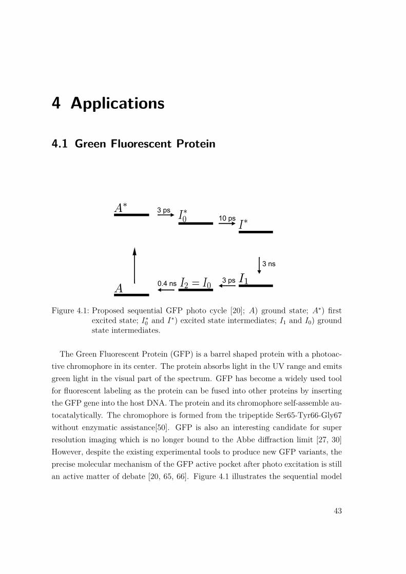
4 Applications
4.1 Green Fluorescent Protein
Figure 4.1: Proposed sequential GFP photo cycle [20]; A) ground state; A∗) firstexcited state; I∗0 and I∗) excited state intermediates; I1 and I0) groundstate intermediates.
The Green Fluorescent Protein (GFP) is a barrel shaped protein with a photoac-tive chromophore in its center. The protein absorbs light in the UV range and emitsgreen light in the visual part of the spectrum. GFP has become a widely used toolfor fluorescent labeling as the protein can be fused into other proteins by insertingthe GFP gene into the host DNA. The protein and its chromophore self-assemble au-tocatalytically. The chromophore is formed from the tripeptide Ser65-Tyr66-Gly67without enzymatic assistance[50]. GFP is also an interesting candidate for superresolution imaging which is no longer bound to the Abbe diffraction limit [27, 30]However, despite the existing experimental tools to produce new GFP variants, theprecise molecular mechanism of the GFP active pocket after photo excitation is stillan active matter of debate [20, 65, 66]. Figure 4.1 illustrates the sequential model
43
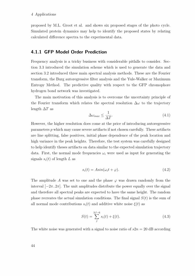
4 Applications
proposed by M.L. Groot et al. and shows six proposed stages of the photo cycle.Simulated protein dynamics may help to identify the proposed states by relatingcalculated difference spectra to the experimental data.
4.1.1 GFP Model Order Prediction
Frequency analysis is a tricky business with considerable pitfalls to consider. Sec-tion 3.3 introduced the simulation scheme which is used to generate the data andsection 3.2 introduced three main spectral analysis methods. These are the Fouriertransform, the Burg autoregressive filter analysis and the Yule-Walker or MaximumEntropy Method. The predictive quality with respect to the GFP chromophorehydrogen bond network was investigated.The main motivation of this analysis is to overcome the uncertainty principle of
the Fourier transform which relates the spectral resolution ∆ω to the trajectorylength ∆T as
∆ωmax ≤1
∆T . (4.1)
However, the higher resolution does come at the price of introducing autoregressiveparameters p which may cause severe artifacts if not chosen carefully. These artifactsare line splitting, false positives, initial phase dependence of the peak location andhigh variance in the peak heights. Therefore, the test system was carefully designedto help identify theses artifacts on data similar to the expected simulation trajectorydata. First, the normal mode frequencies ωi were used as input for generating thesignals si(t) of length L as
si(t) = Asin(ωit+ ϕ). (4.2)
The amplitude A was set to one and the phase ϕ was drawn randomly from theinterval [−2π..2π]. The unit amplitudes distribute the power equally over the signaland therefore all spectral peaks are expected to have the same height. The randomphase recreates the actual simulation conditions. The final signal S(t) is the sum ofall normal mode contributions si(t) and additive white noise ξ(t) as
S(t) =3J−6∑j
si(t) + ξ(t). (4.3)
The white noise was generated with a signal to noise ratio of s2n = 20 dB according
44
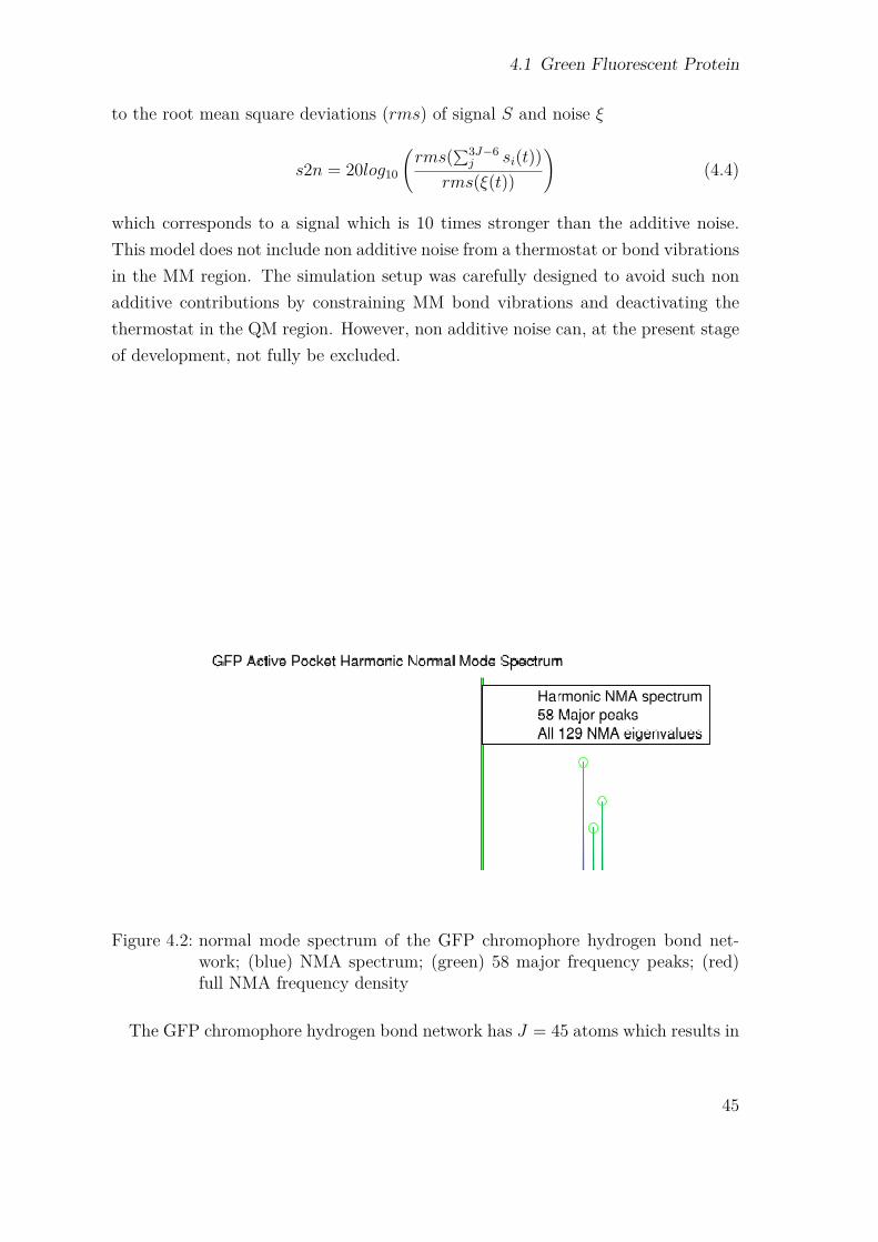
4.1 Green Fluorescent Protein
to the root mean square deviations (rms) of signal S and noise ξ
s2n = 20log10
(rms(∑3J−6
j si(t))rms(ξ(t))
)(4.4)
which corresponds to a signal which is 10 times stronger than the additive noise.This model does not include non additive noise from a thermostat or bond vibrationsin the MM region. The simulation setup was carefully designed to avoid such nonadditive contributions by constraining MM bond vibrations and deactivating thethermostat in the QM region. However, non additive noise can, at the present stageof development, not fully be excluded.
Figure 4.2: normal mode spectrum of the GFP chromophore hydrogen bond net-work; (blue) NMA spectrum; (green) 58 major frequency peaks; (red)full NMA frequency density
The GFP chromophore hydrogen bond network has J = 45 atoms which results in
45
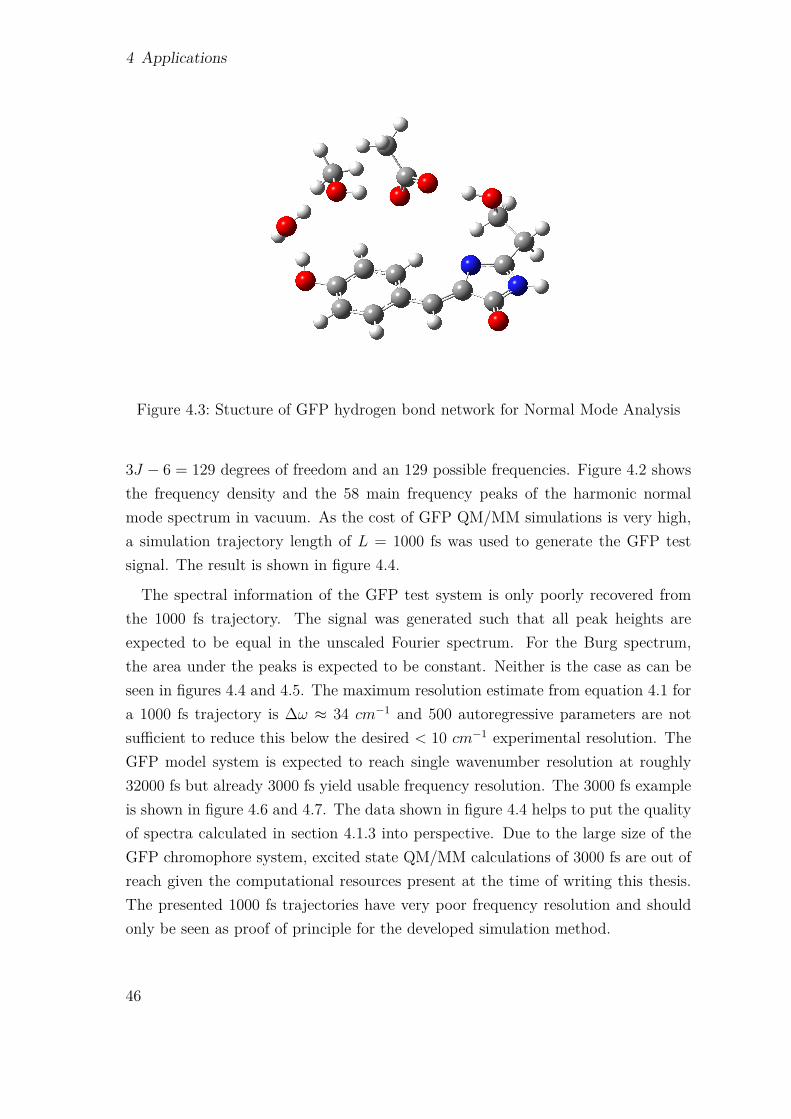
4 Applications
Figure 4.3: Stucture of GFP hydrogen bond network for Normal Mode Analysis
3J − 6 = 129 degrees of freedom and an 129 possible frequencies. Figure 4.2 showsthe frequency density and the 58 main frequency peaks of the harmonic normalmode spectrum in vacuum. As the cost of GFP QM/MM simulations is very high,a simulation trajectory length of L = 1000 fs was used to generate the GFP testsignal. The result is shown in figure 4.4.
The spectral information of the GFP test system is only poorly recovered fromthe 1000 fs trajectory. The signal was generated such that all peak heights areexpected to be equal in the unscaled Fourier spectrum. For the Burg spectrum,the area under the peaks is expected to be constant. Neither is the case as can beseen in figures 4.4 and 4.5. The maximum resolution estimate from equation 4.1 fora 1000 fs trajectory is ∆ω ≈ 34 cm−1 and 500 autoregressive parameters are notsufficient to reduce this below the desired < 10 cm−1 experimental resolution. TheGFP model system is expected to reach single wavenumber resolution at roughly32000 fs but already 3000 fs yield usable frequency resolution. The 3000 fs exampleis shown in figure 4.6 and 4.7. The data shown in figure 4.4 helps to put the qualityof spectra calculated in section 4.1.3 into perspective. Due to the large size of theGFP chromophore system, excited state QM/MM calculations of 3000 fs are out ofreach given the computational resources present at the time of writing this thesis.The presented 1000 fs trajectories have very poor frequency resolution and shouldonly be seen as proof of principle for the developed simulation method.
46
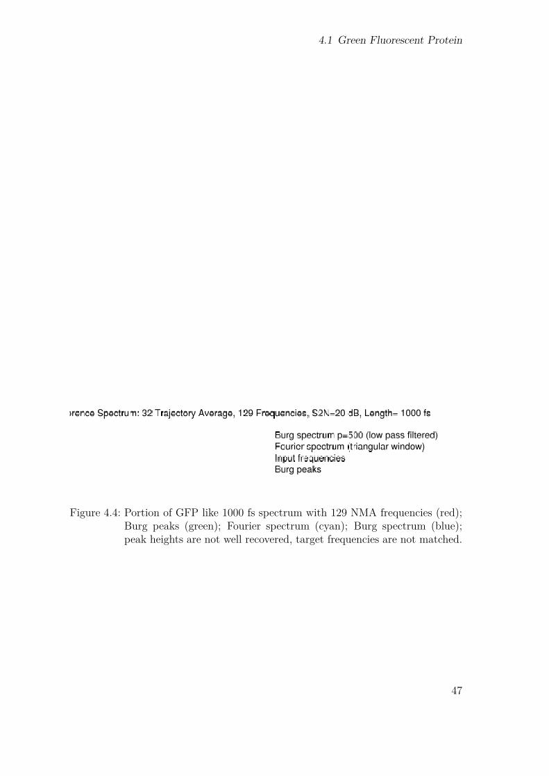
4.1 Green Fluorescent Protein
Figure 4.4: Portion of GFP like 1000 fs spectrum with 129 NMA frequencies (red);Burg peaks (green); Fourier spectrum (cyan); Burg spectrum (blue);peak heights are not well recovered, target frequencies are not matched.
47
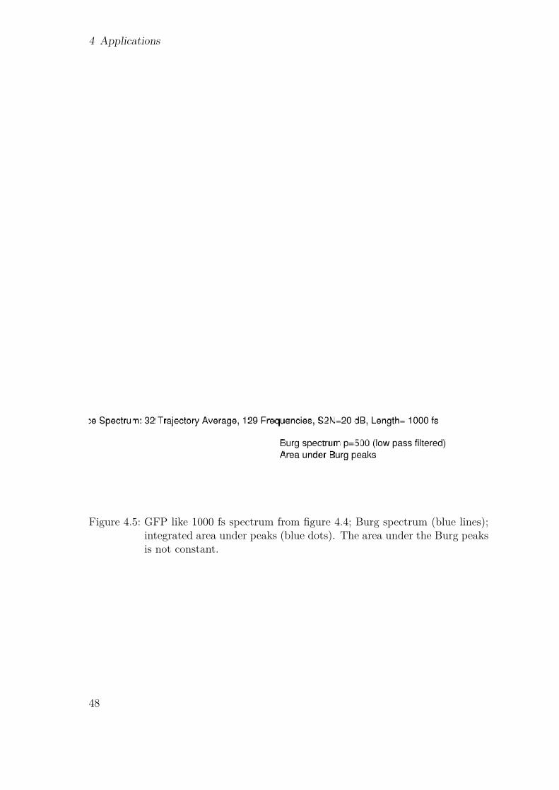
4 Applications
Figure 4.5: GFP like 1000 fs spectrum from figure 4.4; Burg spectrum (blue lines);integrated area under peaks (blue dots). The area under the Burg peaksis not constant.
48
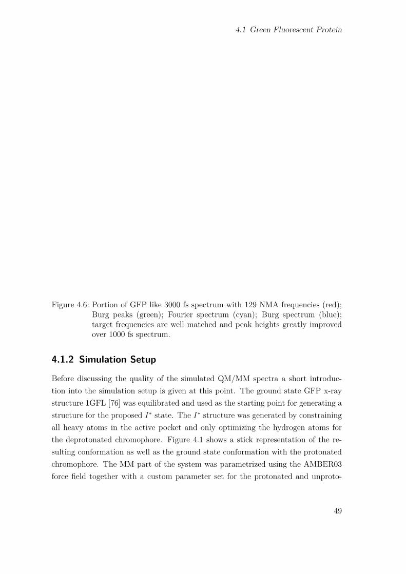
4.1 Green Fluorescent Protein
Figure 4.6: Portion of GFP like 3000 fs spectrum with 129 NMA frequencies (red);Burg peaks (green); Fourier spectrum (cyan); Burg spectrum (blue);target frequencies are well matched and peak heights greatly improvedover 1000 fs spectrum.
4.1.2 Simulation Setup
Before discussing the quality of the simulated QM/MM spectra a short introduc-tion into the simulation setup is given at this point. The ground state GFP x-raystructure 1GFL [76] was equilibrated and used as the starting point for generating astructure for the proposed I∗ state. The I∗ structure was generated by constrainingall heavy atoms in the active pocket and only optimizing the hydrogen atoms forthe deprotonated chromophore. Figure 4.1 shows a stick representation of the re-sulting conformation as well as the ground state conformation with the protonatedchromophore. The MM part of the system was parametrized using the AMBER03force field together with a custom parameter set for the protonated and unproto-
49
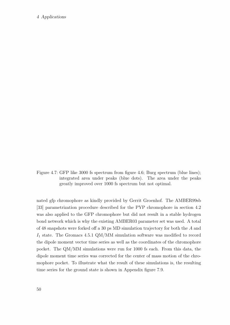
4 Applications
Figure 4.7: GFP like 3000 fs spectrum from figure 4.6; Burg spectrum (blue lines);integrated area under peaks (blue dots). The area under the peaksgreatly improved over 1000 fs spectrum but not optimal.
nated gfp chromophore as kindly provided by Gerrit Groenhof. The AMBER99sb[33] parametrization procedure described for the PYP chromophore in section 4.2was also applied to the GFP chromophore but did not result in a stable hydrogenbond network which is why the existing AMBER03 parameter set was used. A totalof 48 snapshots were forked off a 30 ps MD simulation trajectory for both the A andI1 state. The Gromacs 4.5.1 QM/MM simulation software was modified to recordthe dipole moment vector time series as well as the coordinates of the chromophorepocket. The QM/MM simulations were run for 1000 fs each. From this data, thedipole moment time series was corrected for the center of mass motion of the chro-mophore pocket. To illustrate what the result of these simulations is, the resultingtime series for the ground state is shown in Appendix figure 7.9.
50
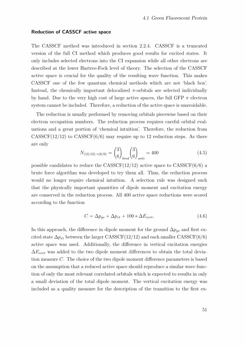
4.1 Green Fluorescent Protein
Reduction of CASSCF active space
The CASSCF method was introduced in section 2.2.4. CASSCF is a truncatedversion of the full CI method which produces good results for excited states. Itonly includes selected electrons into the CI expansion while all other electrons aredescribed at the lower Hartree-Fock level of theory. The selection of the CASSCFactive space is crucial for the quality of the resulting wave function. This makesCASSCF one of the few quantum chemical methods which are not ‘black box’.Instead, the chemically important delocalized π-orbitals are selected individuallyby hand. Due to the very high cost of large active spaces, the full GFP π electronsystem cannot be included. Therefore, a reduction of the active space is unavoidable.
The reduction is usually performed by removing orbitals piecewise based on theirelectron occupation numbers. The reduction process requires careful orbital eval-uations and a great portion of ‘chemical intuition’. Therefore, the reduction fromCASSCF(12/12) to CASSCF(6/6) may require up to 12 reduction steps. As thereare only
N(12/12)→(6/6) =(
36
)bind
(36
)anti
= 400 (4.5)
possible candidates to reduce the CASSCF(12/12) active space to CASSCF(6/6) abrute force algorithm was developed to try them all. Thus, the reduction processwould no longer require chemical intuition. A selection rule was designed suchthat the physically important quantities of dipole moment and excitation energyare conserved in the reduction process. All 400 active space reductions were scoredaccording to the function
C = ∆pgs + ∆ps1 + 100 ∗∆Evert. (4.6)
In this approach, the difference in dipole moment for the ground ∆pgs and first ex-cited state ∆ps1 between the larger CASSCF(12/12) and each smaller CASSCF(6/6)active space was used. Additionally, the difference in vertical excitation energies∆Evert was added to the two dipole moment differences to obtain the total devia-tion measure C. The choice of the two dipole moment difference parameters is basedon the assumption that a reduced active space should reproduce a similar wave func-tion of only the most relevant correlated orbitals which is expected to results in onlya small deviation of the total dipole moment. The vertical excitation energy wasincluded as a quality measure for the description of the transition to the first ex-
51
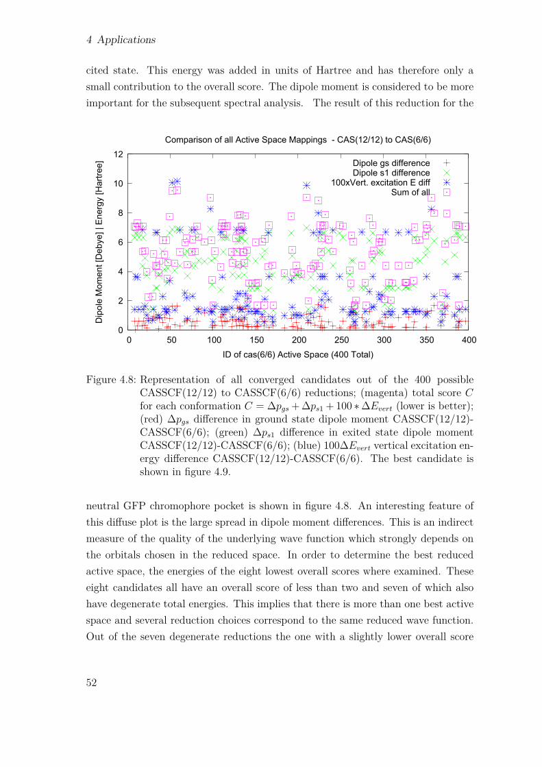
4 Applications
cited state. This energy was added in units of Hartree and has therefore only asmall contribution to the overall score. The dipole moment is considered to be moreimportant for the subsequent spectral analysis. The result of this reduction for the
0
2
4
6
8
10
12
0 50 100 150 200 250 300 350 400
Dip
ole
Mom
ent [
Deb
ye] |
Ene
rgy
[Har
tree
]
ID of cas(6/6) Active Space (400 Total)
Comparison of all Active Space Mappings - CAS(12/12) to CAS(6/6)
Dipole gs differenceDipole s1 difference
100xVert. excitation E diffSum of all
Figure 4.8: Representation of all converged candidates out of the 400 possibleCASSCF(12/12) to CASSCF(6/6) reductions; (magenta) total score Cfor each conformation C = ∆pgs + ∆ps1 + 100 ∗∆Evert (lower is better);(red) ∆pgs difference in ground state dipole moment CASSCF(12/12)-CASSCF(6/6); (green) ∆ps1 difference in exited state dipole momentCASSCF(12/12)-CASSCF(6/6); (blue) 100∆Evert vertical excitation en-ergy difference CASSCF(12/12)-CASSCF(6/6). The best candidate isshown in figure 4.9.
neutral GFP chromophore pocket is shown in figure 4.8. An interesting feature ofthis diffuse plot is the large spread in dipole moment differences. This is an indirectmeasure of the quality of the underlying wave function which strongly depends onthe orbitals chosen in the reduced space. In order to determine the best reducedactive space, the energies of the eight lowest overall scores where examined. Theseeight candidates all have an overall score of less than two and seven of which alsohave degenerate total energies. This implies that there is more than one best activespace and several reduction choices correspond to the same reduced wave function.Out of the seven degenerate reductions the one with a slightly lower overall score
52
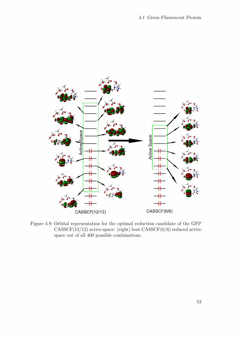
4.1 Green Fluorescent Protein
Figure 4.9: Orbital representation for the optimal reduction candidate of the GFPCASSCF(12/12) active space: (right) best CASSCF(6/6) reduced activespace out of all 400 possible combinations.
53
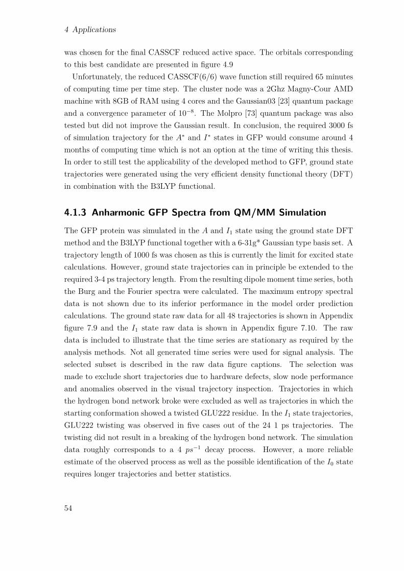
4 Applications
was chosen for the final CASSCF reduced active space. The orbitals correspondingto this best candidate are presented in figure 4.9Unfortunately, the reduced CASSCF(6/6) wave function still required 65 minutes
of computing time per time step. The cluster node was a 2Ghz Magny-Cour AMDmachine with 8GB of RAM using 4 cores and the Gaussian03 [23] quantum packageand a convergence parameter of 10−8. The Molpro [73] quantum package was alsotested but did not improve the Gaussian result. In conclusion, the required 3000 fsof simulation trajectory for the A∗ and I∗ states in GFP would consume around 4months of computing time which is not an option at the time of writing this thesis.In order to still test the applicability of the developed method to GFP, ground statetrajectories were generated using the very efficient density functional theory (DFT)in combination with the B3LYP functional.
4.1.3 Anharmonic GFP Spectra from QM/MM Simulation
The GFP protein was simulated in the A and I1 state using the ground state DFTmethod and the B3LYP functional together with a 6-31g* Gaussian type basis set. Atrajectory length of 1000 fs was chosen as this is currently the limit for excited statecalculations. However, ground state trajectories can in principle be extended to therequired 3-4 ps trajectory length. From the resulting dipole moment time series, boththe Burg and the Fourier spectra were calculated. The maximum entropy spectraldata is not shown due to its inferior performance in the model order predictioncalculations. The ground state raw data for all 48 trajectories is shown in Appendixfigure 7.9 and the I1 state raw data is shown in Appendix figure 7.10. The rawdata is included to illustrate that the time series are stationary as required by theanalysis methods. Not all generated time series were used for signal analysis. Theselected subset is described in the raw data figure captions. The selection wasmade to exclude short trajectories due to hardware defects, slow node performanceand anomalies observed in the visual trajectory inspection. Trajectories in whichthe hydrogen bond network broke were excluded as well as trajectories in which thestarting conformation showed a twisted GLU222 residue. In the I1 state trajectories,GLU222 twisting was observed in five cases out of the 24 1 ps trajectories. Thetwisting did not result in a breaking of the hydrogen bond network. The simulationdata roughly corresponds to a 4 ps−1 decay process. However, a more reliableestimate of the observed process as well as the possible identification of the I0 staterequires longer trajectories and better statistics.
54
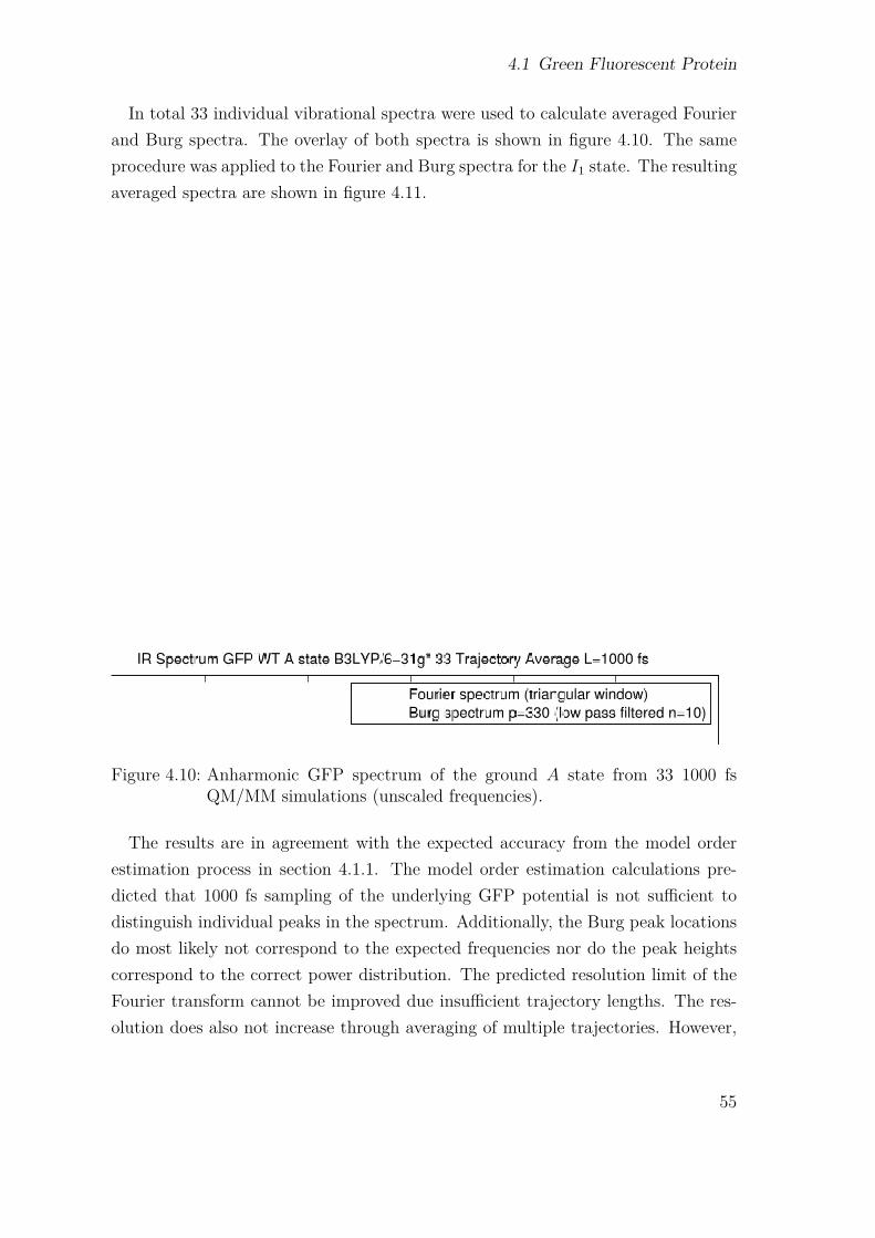
4.1 Green Fluorescent Protein
In total 33 individual vibrational spectra were used to calculate averaged Fourierand Burg spectra. The overlay of both spectra is shown in figure 4.10. The sameprocedure was applied to the Fourier and Burg spectra for the I1 state. The resultingaveraged spectra are shown in figure 4.11.
Figure 4.10: Anharmonic GFP spectrum of the ground A state from 33 1000 fsQM/MM simulations (unscaled frequencies).
The results are in agreement with the expected accuracy from the model orderestimation process in section 4.1.1. The model order estimation calculations pre-dicted that 1000 fs sampling of the underlying GFP potential is not sufficient todistinguish individual peaks in the spectrum. Additionally, the Burg peak locationsdo most likely not correspond to the expected frequencies nor do the peak heightscorrespond to the correct power distribution. The predicted resolution limit of theFourier transform cannot be improved due insufficient trajectory lengths. The res-olution does also not increase through averaging of multiple trajectories. However,
55
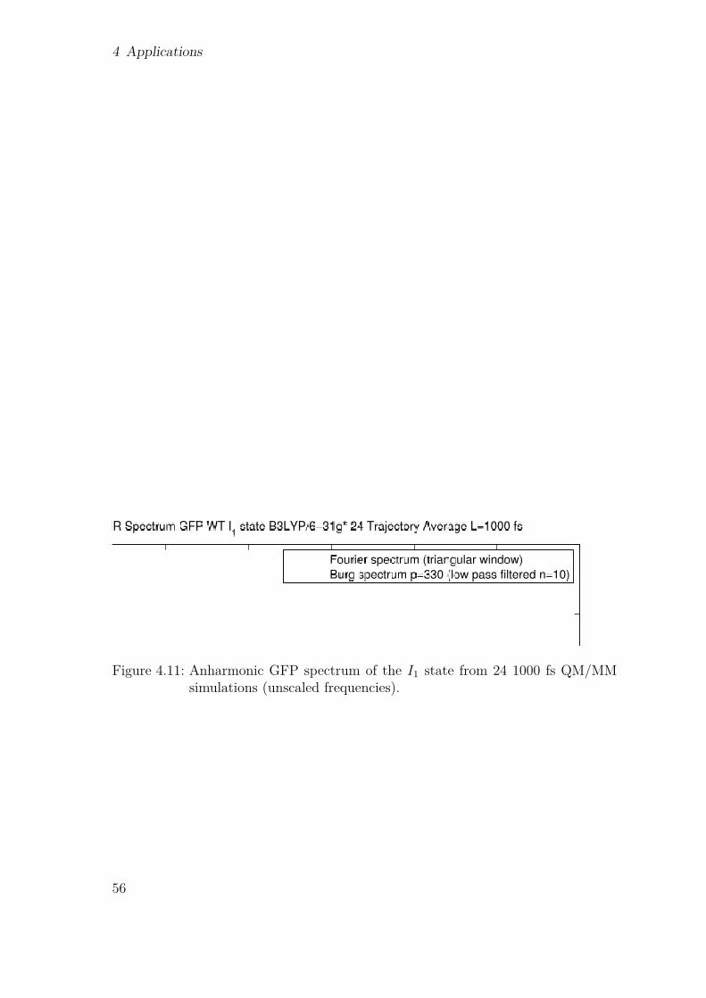
4 Applications
Figure 4.11: Anharmonic GFP spectrum of the I1 state from 24 1000 fs QM/MMsimulations (unscaled frequencies).
56
4.1 Green Fluorescent Protein
the simulations do reveal an interesting effect of the MM environment on the QMdipole moment time series which the model order prediction calculations in section4.1.1 do not consider. The effect becomes visible when the full spectrum is ex-amined. Figure 4.12 illustrates how the MM environment contributes to the lowfrequency part of the spectrum below 1000 cm−1. The contribution is likely causedby angle and dihedral vibrations. The bond vibrations from the MM region wereconstrained during the QM/MM simulation and should not appear in the spectrum.However, the angle and dihedral degrees of freedom were not constrained to ensurea physically correct behavior of the protein. The center of mass motion of the activepocket which was removed beforehand also contributes to this part of the spectrum.It becomes eminent that the low frequency bias to the spectrum is the price to paywhen including the protein explicitly into the analysis of the chromophore spec-trum. The MM contribution also increases the total number of degrees of freedomwhich have to be identified. The total required trajectory length and autoregressiveparameter number may increase beyond the predictions made in section 4.1.1 dueto this effect. The spectral analysis of GFP is concluded at this point, as longersimulation trajectories are required for further analysis.
57
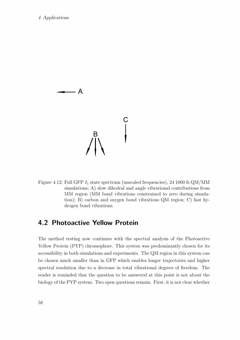
4 Applications
Figure 4.12: Full GFP I1 state spectrum (unscaled frequencies), 24 1000 fs QM/MMsimulations; A) slow dihedral and angle vibrational contributions fromMM region (MM bond vibrations constrained to zero during simula-tion); B) carbon and oxygen bond vibrations QM region; C) fast hy-drogen bond vibrations.
4.2 Photoactive Yellow Protein
The method testing now continues with the spectral analysis of the PhotoactiveYellow Protein (PYP) chromophore. This system was predominantly chosen for itsaccessibility in both simulations and experiments. The QM region in this system canbe chosen much smaller than in GFP which enables longer trajectories and higherspectral resolution due to a decrease in total vibrational degrees of freedom. Thereader is reminded that the question to be answered at this point is not about thebiology of the PYP system. Two open questions remain. First, it is not clear whether
58
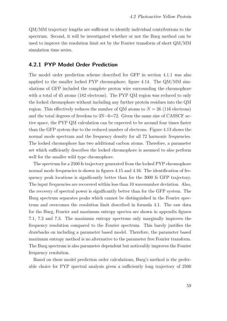
4.2 Photoactive Yellow Protein
QM/MM trajectory lengths are sufficient to identify individual contributions to thespectrum. Second, it will be investigated whether or not the Burg method can beused to improve the resolution limit set by the Fourier transform of short QM/MMsimulation time series.
4.2.1 PYP Model Order Prediction
The model order prediction scheme described for GFP in section 4.1.1 was alsoapplied to the smaller locked PYP chromophore, figure 4.14. The QM/MM sim-ulations of GFP included the complete proton wire surrounding the chromophorewith a total of 45 atoms (182 electrons). The PYP QM region was reduced to onlythe locked chromophore without including any further protein residues into the QMregion. This effectively reduces the number of QM atoms to N = 26 (116 electrons)and the total degrees of freedom to 3N−6=72. Given the same size of CASSCF ac-tive space, the PYP QM calculation can be expected to be around four times fasterthan the GFP system due to the reduced number of electrons. Figure 4.13 shows thenormal mode spectrum and the frequency density for all 72 harmonic frequencies.The locked chromophore has two additional carbon atoms. Therefore, a parameterset which sufficiently describes the locked chromophore is assumed to also performwell for the smaller wild type chromophore.The spectrum for a 2500 fs trajectory generated from the locked PYP chromophore
normal mode frequencies is shown in figures 4.15 and 4.16. The identification of fre-quency peak locations is significantly better than for the 3000 fs GFP trajectory.The input frequencies are recovered within less than 10 wavenumber deviation. Also,the recovery of spectral power is significantly better than for the GFP system. TheBurg spectrum separates peaks which cannot be distinguished in the Fourier spec-trum and overcomes the resolution limit described in formula 4.1. The raw datafor the Burg, Fourier and maximum entropy spectra are shown in appendix figures7.1, 7.2 and 7.3. The maximum entropy spectrum only marginally improves thefrequency resolution compared to the Fourier spectrum. This barely justifies thedrawbacks on including a parameter based model. Therefore, the parameter basedmaximum entropy method is no alternative to the parameter free Fourier transform.The Burg spectrum is also parameter dependent but noticeably improves the Fourierfrequency resolution.Based on these model prediction order calculations, Burg’s method is the prefer-
able choice for PYP spectral analysis given a sufficiently long trajectory of 2500
59
4 Applications
Figure 4.13: normal mode spectrum of the locked PYP chromophore; (blue) NMAspectrum; (green) 48 major frequency peaks; (red) full NMA frequencydensity
fs. The performance for shorter trajectories was also examined and 1000 fs spectraare shown in appendix figures 7.4, 7.5, 7.6, 7.7 and 7.8. The quality of the 1000fs spectrum is sightly better than the 1000 fs GFP spectrum but not sufficient forthe calculation of accurate difference spectra. At 1000 fs simulation length, onlyqualitative spectral differences and large shifts are visible.
4.2.2 Simulation Setup
Simulations of the Photoactive Yellow Protein (PYP) wild type and three selectedmutants, see figure4.17, were performed. All systems were simulated in the groundstate at the DFT-B3LYP/6-31g* level of theory while the locked mutant was also
60

4.2 Photoactive Yellow Protein
Figure 4.14: Stucture of locked PYP chromophore for Normal Mode Analysis
simulated at the CASSCF(6/6) level of theory.
The wild type PYP x-ray crystal structure, pdb code 2ZOH [75], was used as thestarting conformation. Based on this conformation, three mutants were generated.First, the wild type chromophore was replaced by a locked PYP chromophore whichdisables one of the two known isomerization channels by locking the single bonddihedral. Second, two additional mutants were generated by replacing the arginineresidue 52 by alanine (R52A) in the wild type and locked protein. The Gromacsmolecular dynamics program [18] was used to assign AMBER99sb [33] force fieldparameters to the amino acid residues. The AMBER99sb force field was chosenfor its good description of protein interactions together with the computationallyefficient tip3p[36] water model. The AMBER99sb force field was also chosen forits strong dependence on quantum mechanical calculations. This greatly simplifiesthe procedure of extending the force field with new residues. However, force fieldparametrization remains a tedious process that also requires experimental validation.The setup up to this point covers most of the protein and water dynamics but doesnot yet describe the dynamics of the most important part of the PYP protein, thechromophore.
The chromophore of the PYP protein is not part of any modern force field. Thisimplies that this part of the protein cannot be simulated using the molecular dynam-ics methods. To resolve this issue, a custom force field parameter set was generated.
61
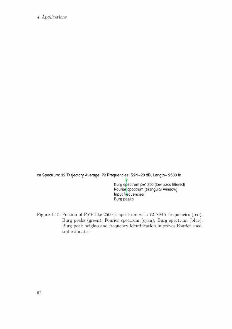
4 Applications
Figure 4.15: Portion of PYP like 2500 fs spectrum with 72 NMA frequencies (red);Burg peaks (green); Fourier spectrum (cyan); Burg spectrum (blue);Burg peak heights and frequency identification improves Fourier spec-tral estimates.
62
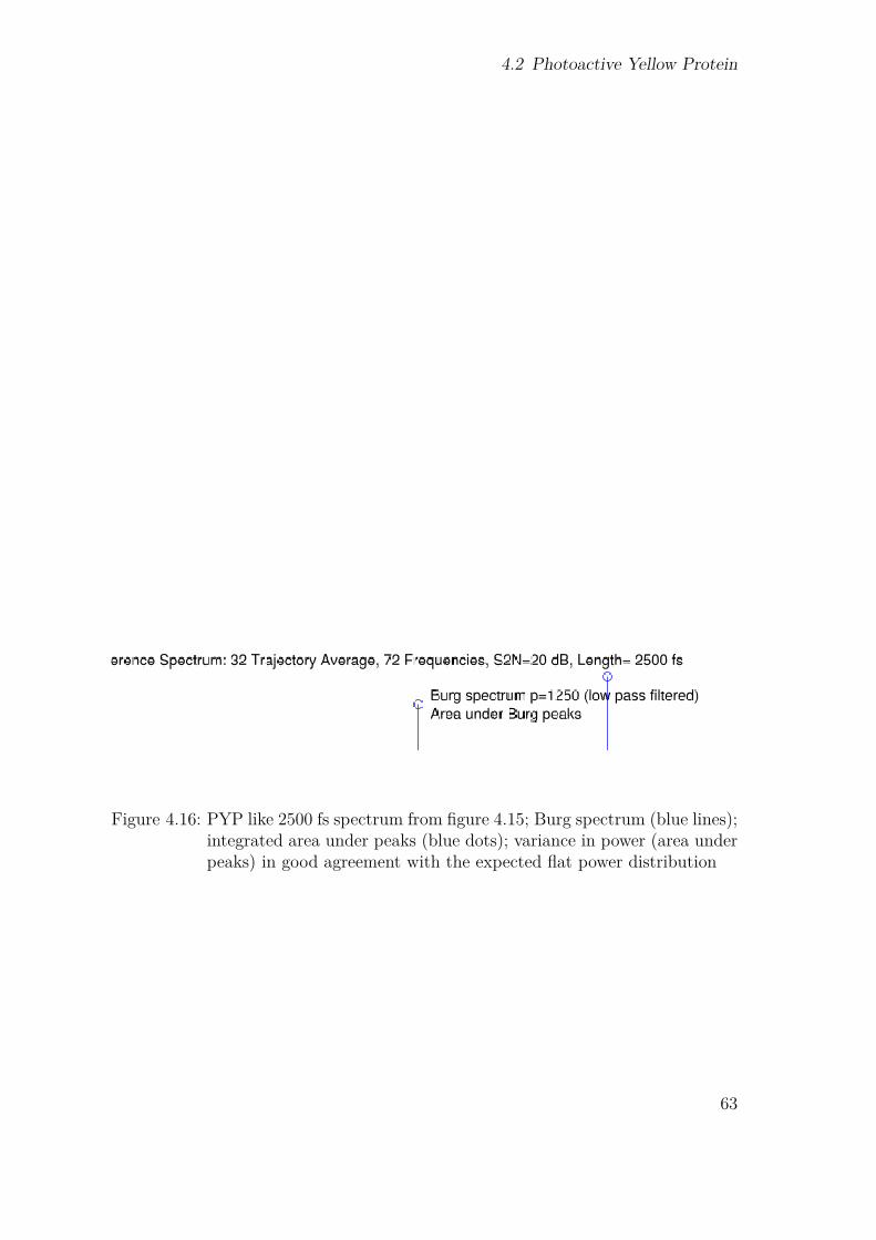
4.2 Photoactive Yellow Protein
Figure 4.16: PYP like 2500 fs spectrum from figure 4.15; Burg spectrum (blue lines);integrated area under peaks (blue dots); variance in power (area underpeaks) in good agreement with the expected flat power distribution
63

4 Applications
Figure 4.17: PYP wild type and three selected mutants; top left: PYP wild type(WT); top right: PYP locked WTL mutant; bottom left: PYPWTR52A mutant; bottom right: PYP locked WTLR52A mutant;
This was done following the parametrization philosophy of the previously appliedAMBER99sb forcefield. However, the generated parameter set for the WT andlocked PYP chromophore should be considered of comparable but not of equal qual-ity as AMBER99sb. Modern protein force fields heavily rely on experimental inputin form of configurational energies and solvation free energies, among many others.At the time of writing, this data was not available for the two PYP chromophorevariants parametrized in this thesis.The chromophore parameters were generated using the Generalized Amber Force
Field (GAFF) [70] . The initial guess was generated using the automated atomand bondtype assignment procedure [71] developed in the lab of D. Case and theformer Kollman group. The automatically generated parameters were subsequentlychecked and corrected by hand to match the known chemical topology. At thisstage, the bonded parameters, i.e. bond stretching, angle bending, dihedral torsionsand the ring planarity are covered. The Lennard-Jones parameters were taken asfound in the AMBER99sb and GAFF parameter set.The electrostatic potential wasreduced onto the nuclear centers using the Restrained Electrostatic Potential Fit
64
4.2 Photoactive Yellow Protein
(RESP)[3]. Here, the backbone atomic charges were restrained to match the stan-dard AMBER values to avoid incompatibilities. At this point the standard AM-BER99sb parametrization philosophy was left. Instead of using the Hartree-FockRESP charges from a vacuum calculation, the chromophores were placed inside theprotein and the RESP charges were calculated using Density Functional TheoryDFT and the B3LYP exchange/correlation functional. This procedure was cho-sen to better mimic the charge polarization of the chromophore inside the proteinpocket.The generated parameter sets for the WT and the locked WTL mutant were used
to generate 6 ns of classical MD trajectories. From each trajectory, 48 snap shotswere forked off as input for subsequent ground state QM/MM simulations. TheDFT B3LYP/6-31g* QM/MM simulations were setup to run 1000 fs. However, thecalculations for the model prediction error suggested that much longer trajectoriesare required to achieve reasonably high frequency resolutions. Therefore, the PYPWT as well as the PYP WTL mutant simulation trajectories were extended to upto 4 ps. In the following, only the data for these extended trajectories is shown. Thequality of the 1000 fs spectra for the WTR52A and WTLR52A mutants is slightlybetter than those for the short GFP trajectories but still not sufficient to calculatedifference spectra.
4.2.3 CASSCF Results
Much of the interesting PYP dynamics takes place in the excited state. Therefore,CASSCF simulations were prepared in order to simulate the excited state dynamics.This short section summarizes the problems in generating dipole time series for theexcited chromophore. The active space of the PYP WTL chromophore was reducedin the same way as the GFP chromophore in section 4.1.2. The chromophore orien-tations from 48 DFT/B3LYP ground state frames were used to create CASSCF(6/6)guess wave functions. The chromophore structures from the snap shots were opti-mized at the HF/6-31g* level of theory followed by a CASSCF(12/12) single pointcalculation and the subsequent reduction to CASSCF(6/6). The same active spaceorbital selection was generated for each frame. Similar to the GFP reduction, theCASSCF(6/6) active space with the lowest overall score was used. The simulationswere started in the ground state for each frame.The resulting trajectories clearly speak against the described automated active
space reduction. Out of 48 trajectories, only three trajectories reached 300 fs trajec-
65
4 Applications
tory length without convergence failure. The proposed reduction is appealing as itdoes not require chemical intuition. However, this is also what seems to be missing.Usage of the proposed scheme is therefore not advised.
4.2.4 PYP WTL-WT Difference Spectrum
The extended ground state simulation trajectories for the PYP wild type and thelocked mutant were used to generate averaged anharmonic Fourier and Burg spectra.The raw time series data is shown in Appendix figures 7.11 and 7.12. From the setof all trajectories, only a small subset of 11 long trajectories of at least 2800 fswere selected for both systems. Longer trajectories are expected to result in higherfrequency resolution. From these subsets, averaged spectra for the WT and WTLchromophore were calculated which are shown in figures 4.18 and 4.19. Both figuresalso include the corresponding normal mode spectra for the isolated chromophoresin vacuum. In addition, the WTL spectrum highlights three important spectralfeatures.First, the Burg spectrum contains several smaller side peaks. These side peaks
were not present in the model order estimation calculations for the PYP WTLsystem. However, the nature of these peaks is likely not related to the vibrationsof the chromophore but rather an artifact of the high model order. The number ofsuspected artifacts reduced significantly by increasing the trajectory lengths from2300 to 2800 fs. A commonly applied upper bound for the Burg parameter numberp in the literature is L/3 for L samples. In both of the PYP spectra, model orders aslarge as L/2 were used in combination with a low pass filter to smooth the resultingclosely split lines. In the model order estimation section, this procedure was foundto be in good agreement with the Fourier results as the closely split lines gatheredaround the expected frequencies and their convoluted heights corresponded to theFourier amplitudes. However, the low pass filter also causes sightly lower Burg peakamplitudes in the PYP spectrum. An alternative way to reduce the side peaks couldalso be to include the full trajectory set into the average instead of just the smallsubset given sufficiently long simulation times.Second, the normal mode spectrum fails to correctly predict the peak amplitudes
at 300K. Instead, the NMA predicts a high spectral amplitude for a WTL peaklocated at 1590 cm−1 which is much lower in the actual simulated spectrum. Normalmode spectra are by design calculated at 0K which makes it difficult to predicttemperature effects. The B) label in the WTL spectrum also shows a peak without
66
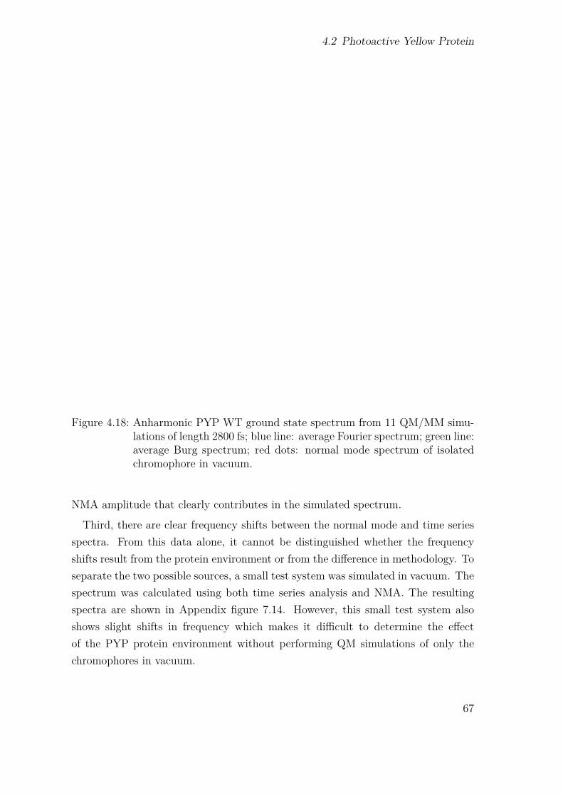
4.2 Photoactive Yellow Protein
Figure 4.18: Anharmonic PYP WT ground state spectrum from 11 QM/MM simu-lations of length 2800 fs; blue line: average Fourier spectrum; green line:average Burg spectrum; red dots: normal mode spectrum of isolatedchromophore in vacuum.
NMA amplitude that clearly contributes in the simulated spectrum.
Third, there are clear frequency shifts between the normal mode and time seriesspectra. From this data alone, it cannot be distinguished whether the frequencyshifts result from the protein environment or from the difference in methodology. Toseparate the two possible sources, a small test system was simulated in vacuum. Thespectrum was calculated using both time series analysis and NMA. The resultingspectra are shown in Appendix figure 7.14. However, this small test system alsoshows slight shifts in frequency which makes it difficult to determine the effectof the PYP protein environment without performing QM simulations of only thechromophores in vacuum.
67

4 Applications
Figure 4.19: Anharmonic PYP WTL ground state spectrum from 11 QM/MM sim-ulations of length 2800 fs; blue line: average Fourier spectrum; greenline: average Burg spectrum; red dots: normal mode spectrum of iso-lated chromophore in vacuum. A) Burg line splitting due to over fitting.B) Failure of NMA to determine IR amplitude of the circled mode. C)Frequency shift between NMA and QM/MM spectrum.
Finally, the subset of long simulation trajectories was used to calculate a truelyanharmonic vibrational difference spectrum between the WTL and the WT groundstate spectrum. The resulting difference spectrum is especially exciting as it candirectly be related to future experimental data which was not available at the timeof writing this thesis. The calculated spectra reflect the frequency resolved averagepower distribution over the full trajectory length. An increase in trajectory lengthwill also increases the accuracy at which power contributions can be located in thespectrum. This results in higher but narrower peaks which has to be considered when
68
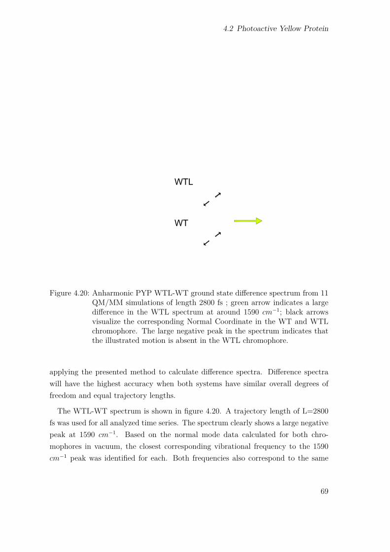
4.2 Photoactive Yellow Protein
Figure 4.20: Anharmonic PYP WTL-WT ground state difference spectrum from 11QM/MM simulations of length 2800 fs ; green arrow indicates a largedifference in the WTL spectrum at around 1590 cm−1; black arrowsvisualize the corresponding Normal Coordinate in the WT and WTLchromophore. The large negative peak in the spectrum indicates thatthe illustrated motion is absent in the WTL chromophore.
applying the presented method to calculate difference spectra. Difference spectrawill have the highest accuracy when both systems have similar overall degrees offreedom and equal trajectory lengths.
The WTL-WT spectrum is shown in figure 4.20. A trajectory length of L=2800fs was used for all analyzed time series. The spectrum clearly shows a large negativepeak at 1590 cm−1. Based on the normal mode data calculated for both chro-mophores in vacuum, the closest corresponding vibrational frequency to the 1590cm−1 peak was identified for each. Both frequencies also correspond to the same
69

4 Applications
nuclear motion which is illustrated by the black arrows. The absence of this motionin the WTL chromophore could be explained by the mechanical restrain on thismotion introduced by the additional two carbon atoms in the WTL chromophore.To avoid overinterpretation of the simulated spectrum, only the most intense dif-
ference is considered for now but further analysis is possible. Hopefully, experimentaldata will shed light on the true predictive power of the smaller peaks.
70
5 Discussion
The attempt to increase the spectral resolution using parameter based methodsrevealed many pitfalls which turned out to be difficult to control. The quality ofmodel based spectra strongly depends on the model order. It is tempting to increasethe subjective quality of a spectrum by tuning the Burg model order. However,the predictive quality of these tuned spectra will be meaningless as any result canbe obtained this way. Therefore, the model order was carefully estimated usinga reference signal generated from the normal mode frequency density. The modelorder obtained this way was not changed during data analysis which restores theobjectivity of the spectra.It is noteworthy that the estimated optimal Burg model orders were fairly high
with p=1250 for the PYP and p=1500 for the GFP case. This is due to the fact thatall-pole models, such as Burg’s method, only poorly describe gaps in the spectrumwhich greatly increases the required model order. Combined all-pole|all-zero ARMAmodels also exist in the literature which combine autoregressive filters with movingaverage models at the cost of introducing another model parameter. However, asecond model parameter only complicates the already difficult process of determiningthe right models order. Therefore, high Burg model orders are likely unavoidable toincrease the spectral resolution.Burg’s method does increase the resolution limit compared to Fourier spectra.
However, parameter based methods should not be seen as a replacement for theFourier transform. Instead, Burg’s method offers an alternative and independentway of analyzing the QM/MM time series. Fourier spectra of short trajectories arevery smooth and tend to combine closely separated peaks into one. Burg spectra onthe other hand tend to overshoot due to their all-pole nature and quickly separatebroad Fourier peaks into two or more peaks. When long simulation trajectoriesare available, it turned out to be very useful to analyze also shorter versions of thegenerated time series while increasing the amount analyzed data stepwise. Thisrevealed that the Burg spectrum already identifies features in short data sets which
71
5 Discussion
later also become visible in the Fourier spectrum. The sequential analysis helps toidentify regions were the peak identification is converged as well as rapidly changingregions. The confidence in the accuracy of the peaks in the difference spectrum canbe increased this way. Results obtained from the Yule-Walker or Maximum Entropymethod do not justify the drawbacks of introducing a parameter based model.
Ground state QM/MM simulations of GFP in combination with the model orderprediction scheme revealed that excited state simulations of at least 3 ps are requiredto achieve acceptable frequency resolution. This can currently not be achieved usingthe available software and hardware resources at the time of writing. Considerableeffort is required before anharmonic excited state GFP difference spectra can becalculated using the presented approach. Additionally, there is currently no afford-able QM method which correctly describes short hydrogen bonds. This makes itespecially difficult to calculate spectra for the I∗0 state in the GFP photo cycle. The1 ps ground state simulation trajectories from figure 4.10 and 4.11 are not sufficientto compare the simulations to experimental difference spectra which is why no dif-ference spectrum is shown. It is also unclear whether the structure generated forthe I1 state is close enough to the true I1 state to match experimental differencespectra. It might be worth trying a multilayer ONIOM [19] approach to record onetime series for the hydrogen bond network using a fast ground state method andone time series for the excited state chromophore. However, the accuracy of thisapproach will be lower than the presented full electronic embedding of the activepocket.
The PYP simulation results are promising. However, the calculated differenceWTL-WT spectrum in figure 4.20 only considers differences in the chromophore.Changes in Protein modes are only included indirectly and will likely not be visiblein the difference spectrum. The difference spectrum in figure 4.20 also shows twocorresponding normal mode eigenvectors which match the target frequency. Theidentified mode is reasonable as the lock in the WTL mutant might suppress theillustrated motion. However, it is not guaranteed to actually correspond to the truemotion. This is due to the fact that the normal mode eigenvectors were calculatedin vacuum using the harmonic approximation. Experimental data is highly desirableto see if the dominant peak at 1590 cm−1 is also present in the experiment.
The author of this thesis was not satisfied with the way CASSCF active spacesare identified and reduced using mostly chemical intuition. Therefore, considerableeffort was put into automatically reducing the CASSCF active space by calculating
72
all possible one step reductions. The resulting active spaces for PYP and GFPsuffered from convergence problems and poor performance. The developed scoringfunction is clearly missing part of the information required to select good activespace reductions. Considering that the reduction process has to be performed onceper system and takes less than one day, it is likely not worth the effort to pursuitthis automated reduction scheme any further.The calculated vibrational spectra take the full protein environment into account
without relying on harmonic approximations. Spectral amplitudes are recoveredfrom the simulated protein dynamics in absolute values. This is a clear improvementover the relative normal mode amplitudes. No modifications to the QM/MM codeother than recording the dipole moment time series with respect to the center ofmass motion of the QM region are required. The only approximation made forcalculating dipole time series based spectra is that the electric field of the infraredphoton is only a small perturbation to the molecular wave function. The identifiedminimum required trajectory lengths of 2-3 ps are barely reachable with post HartreeFock methods but certainly not impossible to simulate. Vibrational spectra shouldbe representative and should not be calculated from single trajectories but ratherconsist of a statistically independent ensemble of many trajectories. The progressin computer performance does no longer justify using single trajectory data forquantitative predictions. The calculation of high level QM/MM difference spectrawas shown to be a practical method that can be applied using today’s computingresources.Normal mode analysis remains a popular tool for calculating vibrational spectra
because it is simple to use not because it is very accurate. The comparative resultspresented for PYP in figures 4.18 and 4.19 clearly show that vacuum NMA spec-tra do not reflect the in protein behavior of the chromophore. Comparison to theexperimental difference spectra will likely support this statement further.
73

6 Conclusions
Anharmonic vibrational difference spectra can be calculated from QM/MM simu-lations including the full protein environment. The developed simulation schemeis capable of calculating vibrational difference spectra for charged QM regions andexcited states.The parametric Burg method was identified as a valuable alternative to state of
the art Fourier dipole time series analysis. An objective Burg model order estimationmethod was developed based on the normal mode frequency density.
6.1 OutlookComparison to experimental IR difference spectra is the next logical step in thedevelopment of the presented method. Without experimental data, the quality ofthe calculated results is difficult to evaluate.The presented model order estimation scheme would greatly benefit from including
the large number of protein degrees of freedom in the low frequency range below 1000cm−1. This can easily be included into the test signal in terms of many additionallow frequency sinusoid.Currently, the presented time series analysis of QM/MM trajectories does not
allow a visual inspection of the motion corresponding to the identified peaks inthe spectrum. Promising methods for calculating normal coordinates without theharmonic approximation exist in the literature [48] but have not been included inthis thesis. The short QM/MM trajectory lengths will likely reduce the quality ofthe identified modes.
75

Bibliography
[1] A. Amadei, I. Daidone, A. Di Nola, and M. Aschi. Theoretical-computationalmodelling of infrared spectra in peptides and proteins: a new frontier for com-bined theoretical-experimental investigations. Current opinion in structuralbiology, 20(2):155–161, 2010. ISSN 0959-440X.
[2] P.W. Atkins, R.S. Friedman, and Inc NetLibrary. Molecular quantum mechan-ics. 3, 1997.
[3] C.I. Bayly, P. Cieplak, W. Cornell, and P.A. Kollman. A well-behaved elec-trostatic potential based method using charge restraints for deriving atomiccharges: the resp model. The Journal of Physical Chemistry, 97(40):10269–10280, 1993.
[4] A.D. Becke. Density-functional thermochemistry. III. The role of exact ex-change. Chem. Phys, 98(1):5648–5652, 1993.
[5] H.J.C. Berendsen. Simulating the physical world. Cambridge University PressCambridge, UK, 2007.
[6] P.H. Berens and K.R. Wilson. Molecular dynamics and spectra. i. diatomicrotation and vibration. The Journal of Chemical Physics, 74:4872, 1981.
[7] R.B. Blackman, J.W. Tukey, J.W. Tukey, and J.W. Tukey. The measurementof power spectra from the point of view of communications engineering. DoverNew York., 1959.
[8] M. Born and R. Oppenheimer. Zur quantentheorie der molekeln. Annalen derPhysik, 389(20):457–484, 1927.
[9] B. Brauer, M. Pincu, V. Buch, I. Bar, J.P. Simons, and R.B. Gerber. Vibra-tional spectra of α-glucose, β-glucose, and sucrose: Anharmonic calculationsand experiment. The Journal of Physical Chemistry A, 2011.
77
Bibliography
[10] P.M.T. Broersen. Automatic autocorrelation and spectral analysis. Springer-Verlag New York Inc, 2006.
[11] M. Buchner, B.M. Ladanyi, and R.M. Stratt. The short-time dynamics ofmolecular liquids. Instantaneous-normal-mode theory. The Journal of chemicalphysics, 97:8522, 1992.
[12] John Parker Burg. Maximum Entropy Spectral Analysis. PhD thesis, StanfordUniversity, 1975.
[13] J. Chai and M. Head-Gordon. Long-range corrected hybrid density functionalswith damped atom–atom dispersion corrections. Physical Chemistry ChemicalPhysics, 10:6615, 2008.
[14] B. Champagne, E.A. Perpete, D. Jacquemin, S.J.A. van Gisbergen, E.J.Baerends, C. Soubra-Ghaoui, K.A. Robins, and B. Kirtman. Assessment ofConventional Density Functional Schemes for Computing the Dipole Momentand (Hyper) polarizabilities of Push- Pull [pi]-Conjugated Systems†. J. Phys.Chem. A, 104(20):4755–4763, 2000.
[15] M. Cho, G.R. Fleming, S. Saito, I. Ohmine, and R.M. Stratt. Instantaneousnormal mode analysis of liquid water. The Journal of chemical physics, 100:6672, 1994.
[16] L. Cohen. Generalization of the wiener-khinchin theorem. Signal ProcessingLetters, IEEE, 5(11):292–294, 1998.
[17] W.D. Cornell, P. Cieplak, C.I. Bayly, I.R. Gould, K.M. Merz, D.M. Fergu-son, D.C. Spellmeyer, T. Fox, J.W. Caldwell, and P.A. Kollman. A secondgeneration force field for the simulation of proteins, nucleic acids, and organicmolecules. Journal of the American Chemical Society, 117(19):5179–5197, 1995.
[18] B. Hess A. R. van Buuren E. Apol P. J. Meulenhoff D. P. Tieleman A. L. T.M. Sijbers K. A. Feenstra R. van Drunen D. van der Spoel, E. Lindahl andH. J. C. Berendsen. Gromacs User Manual version 4.5.4, 2010.
[19] S. Dapprich, I. Komáromi, K.S. Byun, K. Morokuma, and M.J. Frisch. A newoniom implementation in gaussian98. part i. the calculation of energies, gradi-ents, vibrational frequencies and electric field derivatives. Journal of MolecularStructure: THEOCHEM, 461:1–21, 1999.
78
Bibliography
[20] Mariangela Di Donato, Luuk J.G.W. van Wilderen, Ivo H.M. Van Stokkum,Thomas Cohen Stuart, John T.M. Kennis, Klaas J. Hellingwerf, Rienk vanGrondelle, and Marie Louise Groot. Proton transfer events in gfp. submitted,2011.
[21] A. Dreuw and M. Head-Gordon. Single-reference ab initio methods for thecalculation of excited states of large molecules. Chemical reviews, 105(11):4009–4037, 2005. ISSN 0009-2665.
[22] P.L. Freddolino, C.B. Harrison, Y. Liu, and K. Schulten. Challenges in protein-folding simulations. Nature physics, 6(10):751–758, 2010.
[23] M.J. Frisch, GW Trucks, HB Schlegel, GE Scuseria, MA Robb, JR Cheeseman,JA Montgomery, T. Vreven, KN Kudin, JC Burant, et al. Gaussian 03, revisionc. 02. 2008.
[24] M.P. Gaigeot, R. Vuilleumier, and M. Martinez. Infrared spectroscopy in the gasand liquid phase from first principle molecular dynamics simulations-applicationto small peptides. 2008.
[25] J.F. Giovannelli, G. Demoment, and A. Herment. A Bayesian method for longAR spectral estimation: A comparative study. Ultrasonics, Ferroelectrics andFrequency Control, IEEE Transactions on, 43(2):220–233, 1996. ISSN 0885-3010.
[26] DA Gray. Maximum entropy spectrum analysis technique-a review of its theo-retical properties. Technical Report 1812, 1977.
[27] S. Habuchi, R. Ando, P. Dedecker, W. Verheijen, H. Mizuno, A. Miyawaki, andJ. Hofkens. Reversible single-molecule photoswitching in the gfp-like fluorescentprotein dronpa. Proceedings of the National Academy of Sciences of the UnitedStates of America, 102(27):9511, 2005.
[28] M. Head-Gordon. Systematic optimization of long-range corrected hybrid den-sity functionals. The Journal of chemical physics, 128:084106, 2008.
[29] Dermot Hegarty and Michael Robb. Application of unitary group methods toconfiguration interaction calculations. Molecular Physics, 38:1795–1812, 1979.doi: 10.1080/00268977900102871.
79
Bibliography
[30] S.W. Hell and J. Wichmann. Breaking the diffraction resolution limit by stim-ulated emission: stimulated-emission-depletion fluorescence microscopy. Opticsletters, 19(11):780–782, 1994.
[31] B. Hess, H. Bekker, H.J.C. Berendsen, and J.G.E.M. Fraaije. Lincs: a linearconstraint solver for molecular simulations. Journal of computational chemistry,18(12):1463–1472, 1997.
[32] P. Hohenberg, W. Kohn, et al. Inhomogeneous electron gas. Physical Review,136(3B):B864–B871, 1964.
[33] V. Hornak, R. Abel, A. Okur, B. Strockbine, A. Roitberg, and C. Simmerling.Comparison of multiple amber force fields and development of improved proteinbackbone parameters. Proteins: Structure, Function, and Bioinformatics, 65(3):712–725, 2006.
[34] K.K. Irikura, R.D. Johnson III, and R.N. Kacker. Uncertainties in scalingfactors for ab initio vibrational frequencies. The Journal of Physical ChemistryA, 109(37):8430–8437, 2005.
[35] F. Jensen. Introduction to computational chemistry. Wiley, 2007.
[36] W.L. Jorgensen, J. Chandrasekhar, J.D. Madura, R.W. Impey, and M.L. Klein.Comparison of simple potential functions for simulating liquid water. The Jour-nal of chemical physics, 79:926, 1983.
[37] A. Kaczmarek, M. Shiga, and D. Marx. Quantum effects on vibrational andelectronic spectra of hydrazine studied by “on-the-fly” ab initio ring polymermolecular dynamics†. The Journal of Physical Chemistry A, 113(10):1985–1994,2009.
[38] M. Kaledin, A.L. Kaledin, J.M. Bowman, J. Ding, and K.D. Jordan. Calculationof the vibrational spectra of h5o2+ and its deuterium-substituted isotopologuesby molecular dynamics simulations†. The Journal of Physical Chemistry A, 113(26):7671–7677, 2009.
[39] E.R. Kanasewich. Time sequence analysis in geophysics. University of AlbertaPress, 1975.
80
Bibliography
[40] J.L. Klepeis, K. Lindorff-Larsen, R.O. Dror, and D.E. Shaw. Long-timescalemolecular dynamics simulations of protein structure and function. Currentopinion in structural biology, 19(2):120–127, 2009.
[41] W. Kohn, LJ Sham, et al. Self-consistent equations including exchange andcorrelation effects. Physical Review, 140(4A):A1133–A1138, 1965.
[42] W. Kohn, A.D. Becke, and R.G. Parr. Density functional theory of electronicstructure. The Journal of Physical Chemistry, 100(31):12974–12980, 1996.
[43] E. Krügel. The physics of interstellar dust. Taylor & Francis, 2003.
[44] H.P. Lamichhane and G. Hastings. Calculated vibrational properties of pig-ments in protein binding sites. Proceedings of the National Academy of Sciences,108(26):10526, 2011.
[45] A.R. Leach. Molecular modelling: principles and applications. Addison-WesleyLongman Ltd, 2001.
[46] T. Leininger, H. Stoll, H.J. Werner, and A. Savin. Combining long-range con-figuration interaction with short-range density functionals. Chemical PhysicsLetters, 275(3-4):151–160, 1997.
[47] J. Makhoul. Linear prediction: A tutorial review. Proceedings of the IEEE, 63(4):561–580, 1975.
[48] G. Mathias and M.D. Baer. Generalized normal coordinates for the vibrationalanalysis of molecular dynamics simulations. Journal of Chemical Theory andComputation.
[49] U. Matlab. The mathworks. Inc., Natick, MA, 1992, 1760.
[50] G.U. Nienhaus. The green fluorescent protein: a key tool to study chemicalprocesses in living cells. Angewandte Chemie International Edition, 47(47):8992–8994, 2008.
[51] D.B. Percival and A.T. Walden. Spectral analysis for physical applications:multitaper and conventional univariate techniques. Cambridge Univ Pr, 1993.
[52] AR Rao and A. Durgunoglu. AR and ARMA spectral estimation. StochasticHydrology and Hydraulics, 2(1):35–50, 1988. ISSN 0931-1955.
81

Bibliography
[53] E.A. Robinson. A historical perspective of spectrum estimation. Proceedingsof the IEEE, 70(9):885–907, 1982.
[54] M.A. Rohrdanz and J.M. Herbert. Simultaneous benchmarking of ground-andexcited-state properties with long-range-corrected density functional theory.The Journal of chemical physics, 129:034107, 2008.
[55] M.A. Rohrdanz, K.M. Martins, and J.M. Herbert. A long-range-correcteddensity functional that performs well for both ground-state properties andtime-dependent density functional theory excitation energies, including charge-transfer excited states. The Journal of chemical physics, 130:054112, 2009.
[56] C. C. J. Roothaan. New developments in molecular orbital theory. Rev. Mod.Phys., 23(2):69–89, Apr 1951. doi: 10.1103/RevModPhys.23.69.
[57] E. Schrödinger. Quantisierung als eigenwertproblem (series of four publica-tions). Annalen der Physik, 79-81(multiple):361–76,489–527,437–90,109–39,1926.
[58] F. Siebert and P. Hildebrandt. Vibrational spectroscopy in life science, volume 3.Vch Verlagsgesellschaft Mbh, 2008.
[59] P.J. Steinbach, R.J. Loncharich, and B.R. Brooks. The effects of environmentand hydration on protein dynamics: a simulation study of myoglobin. Chemicalphysics, 158(2-3):383–394, 1991.
[60] D.J. Tannor. Introduction to quantum mechanics. University Science Books,2007.
[61] M.D. Towler. Computational Methods for Large Systems, chapter QuantumMonte Carlo, or, how to solve the many-particle Schrödinger equation accu-rately whilst retaining favourable scaling with system size. Wiley, 2010.
[62] T.J. Ulrych and T.N. Bishop. Maximum entropy spectral analysis and au-toregressive decomposition. Reviews of Geophysics, 13(1):183–200, 1975. ISSN8755-1209.
[63] T.J. Ulrych and R.W. Clayton. Time series modelling and maximum entropy.Physics of the Earth and Planetary Interiors, 12(2-3):188–200, 1976. ISSN0031-9201.
82
Bibliography
[64] A. Van den Bos. Alternative interpretation of maximum entropy spectral anal-ysis (corresp.). Information Theory, IEEE Transactions on, 17(4):493–494,1971.
[65] J.J. van Thor, G. Zanetti, K.L. Ronayne, and M. Towrie. Structural events inthe photocycle of green fluorescent protein. The Journal of Physical ChemistryB, 109(33):16099–16108, 2005.
[66] J.J. Van Thor, K.L. Ronayne, M. Towrie, and J.T. Sage. Balance betweenultrafast parallel reactions in the green fluorescent protein has a structuralorigin. Biophysical journal, 95(4):1902–1912, 2008.
[67] O.A. Vydrov and G.E. Scuseria. Assessment of a long-range corrected hybridfunctional. The Journal of chemical physics, 125:234109, 2006.
[68] O.A. Vydrov, G.E. Scuseria, and J.P. Perdew. Tests of functionals for systemswith fractional electron number. The Journal of Chemical Physics, 126:154109,2007.
[69] J. Wang, P. Cieplak, and P.A. Kollman. How well does a restrained electrostaticpotential(resp) model perform in calculating conformational energies of organicand biological molecules? Journal of Computational Chemistry, 21(12):1049–1074, 2000.
[70] J. Wang, R.M. Wolf, J.W. Caldwell, P.A. Kollman, and D.A. Case. Devel-opment and testing of a general amber force field. Journal of computationalchemistry, 25(9):1157–1174, 2004.
[71] J. Wang, W. Wang, P.A. Kollman, and D.A. Case. Automatic atom typeand bond type perception in molecular mechanical calculations. Journal ofmolecular graphics and modelling, 25(2):247–260, 2006.
[72] S.J. Weiner, P.A. Kollman, D.A. Case, U.C. Singh, C. Ghio, G. Alagona, S. Pro-feta, and P. Weiner. A new force field for molecular mechanical simulation ofnucleic acids and proteins. Journal of the American Chemical Society, 106(3):765–784, 1984.
[73] H.-J. Werner, P. J. Knowles, G. Knizia, F. R. Manby, M. Schütz, et al. Molpro,version 2010.1, a package of ab initio programs. 2010. see.
83

Bibliography
[74] J. Xu, Y. Zhang, and G.A. Voth. Infrared Spectrum of the Hydrated Protonin Water. The Journal of Physical Chemistry Letters, 2:81–86, 2011. ISSN1948-7185.
[75] S. Yamaguchi, H. Kamikubo, K. Kurihara, R. Kuroki, N. Niimura, N. Shimizu,Y. Yamazaki, and M. Kataoka. Low-barrier hydrogen bond in photoactiveyellow protein. Proceedings of the National Academy of Sciences, 106(2):440,2009.
[76] F. Yang, L.G. Moss, G.N. Phillips Jr, et al. The molecular structure of greenfluorescent protein. Nature biotechnology, 14(10):1246–1251, 1996.
[77] S. Yang and M. Cho. IR spectra of N-methylacetamide in water predictedby combined quantum mechanical/molecular mechanical molecular dynamicssimulations. The Journal of chemical physics, 123:134503, 2005.
[78] G.U. Yule. On a method of investigating periodicities in disturbed series, withspecial reference to Wolfer’s sunspot numbers, volume 226. The Royal Society,1927.
[79] M.C. Zerner. Perspective on “new developments in molecular orbital theory”.Theoretical Chemistry Accounts: Theory, Computation, and Modeling (Theo-retica Chimica Acta), 103(3):217–218, 2000.
84
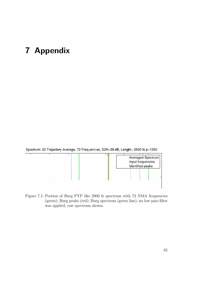
7 Appendix
Figure 7.1: Portion of Burg PYP like 2000 fs spectrum with 72 NMA frequencies(green); Burg peaks (red); Burg spectrum (green line); no low pass filterwas applied, raw spectrum shown.
85
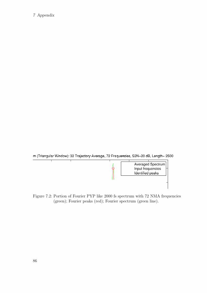
7 Appendix
Figure 7.2: Portion of Fourier PYP like 2000 fs spectrum with 72 NMA frequencies(green); Fourier peaks (red); Fourier spectrum (green line).
86

Figure 7.3: Portion of maximum entropy PYP like 2000 fs spectrum with 72 NMAfrequencies (green); maximum entropy peaks (red); maximum entropyspectrum (green line).
87
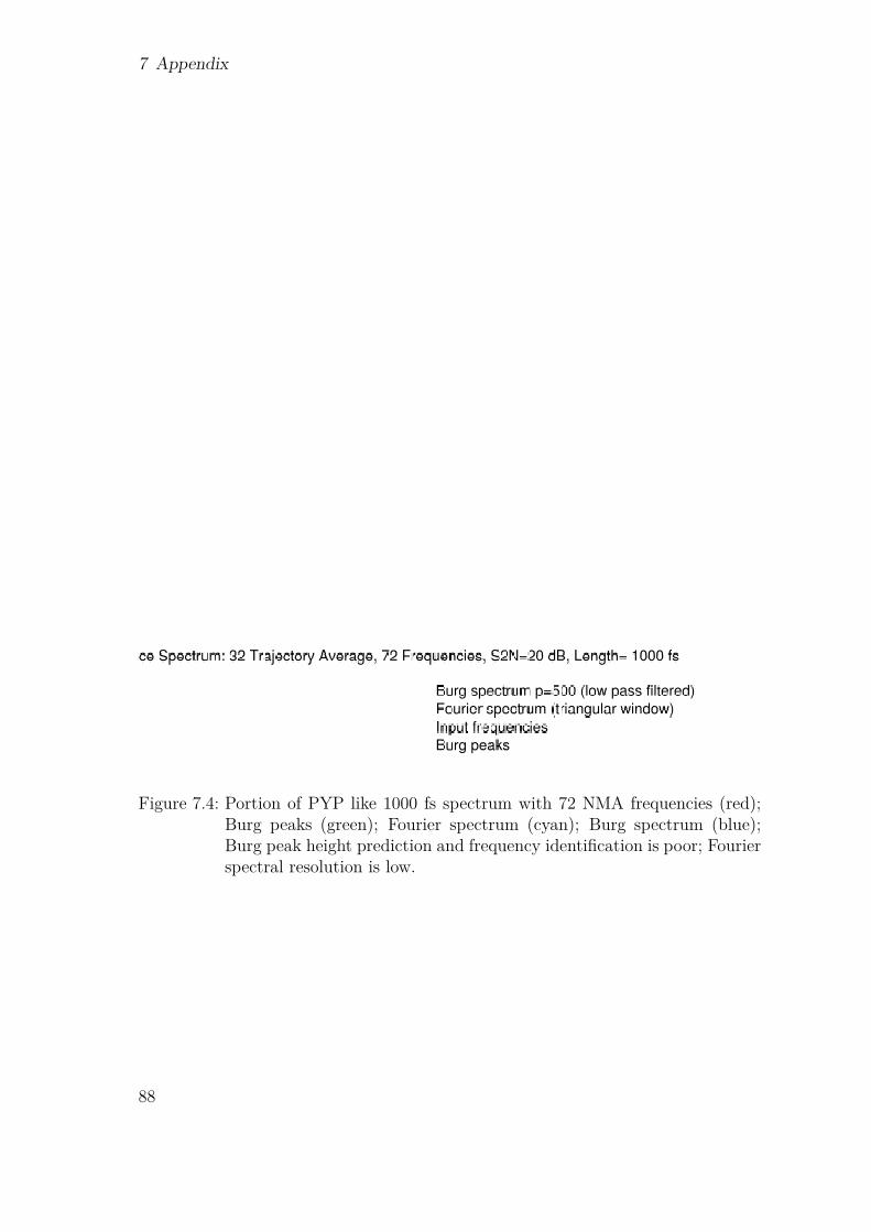
7 Appendix
Figure 7.4: Portion of PYP like 1000 fs spectrum with 72 NMA frequencies (red);Burg peaks (green); Fourier spectrum (cyan); Burg spectrum (blue);Burg peak height prediction and frequency identification is poor; Fourierspectral resolution is low.
88
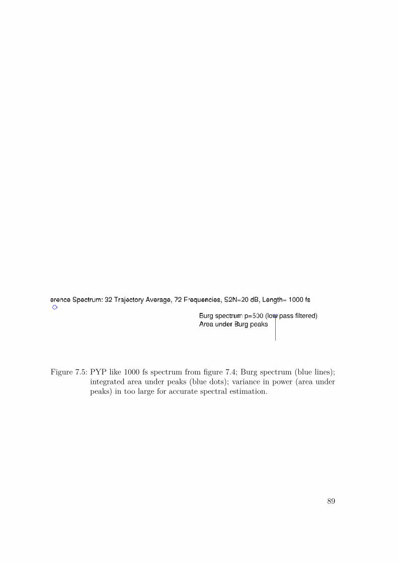
Figure 7.5: PYP like 1000 fs spectrum from figure 7.4; Burg spectrum (blue lines);integrated area under peaks (blue dots); variance in power (area underpeaks) in too large for accurate spectral estimation.
89
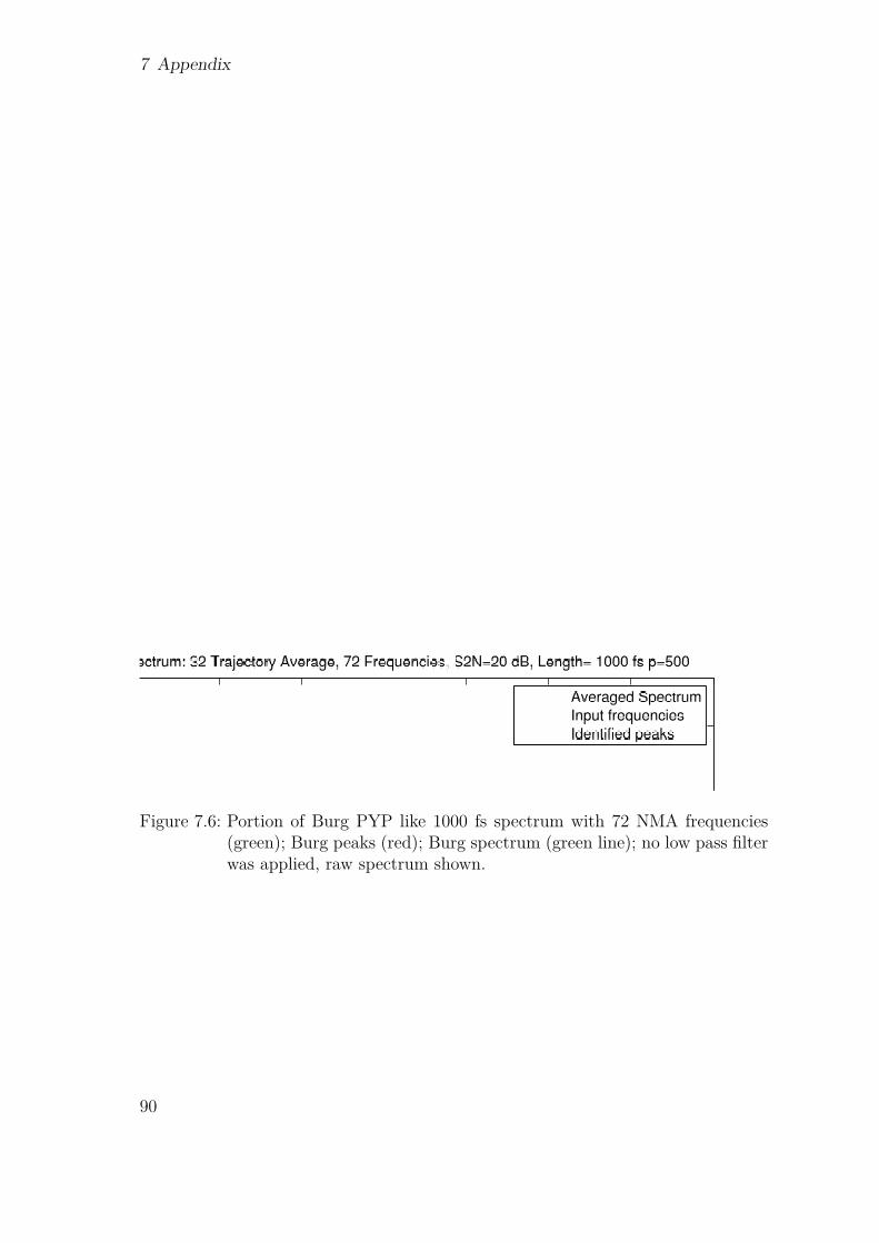
7 Appendix
Figure 7.6: Portion of Burg PYP like 1000 fs spectrum with 72 NMA frequencies(green); Burg peaks (red); Burg spectrum (green line); no low pass filterwas applied, raw spectrum shown.
90
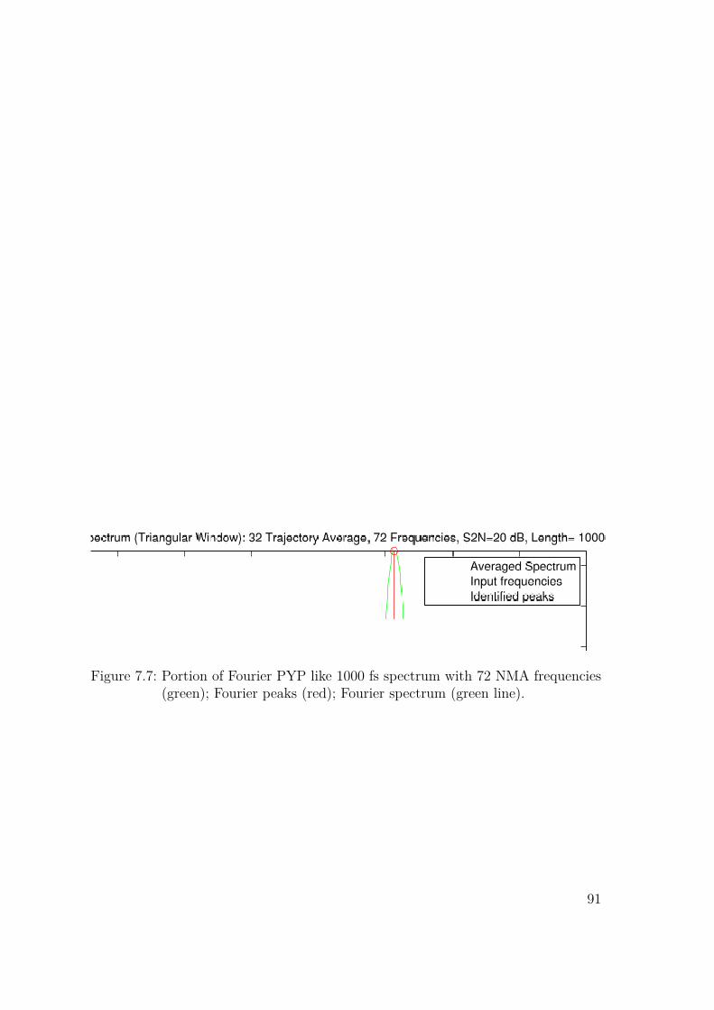
Figure 7.7: Portion of Fourier PYP like 1000 fs spectrum with 72 NMA frequencies(green); Fourier peaks (red); Fourier spectrum (green line).
91
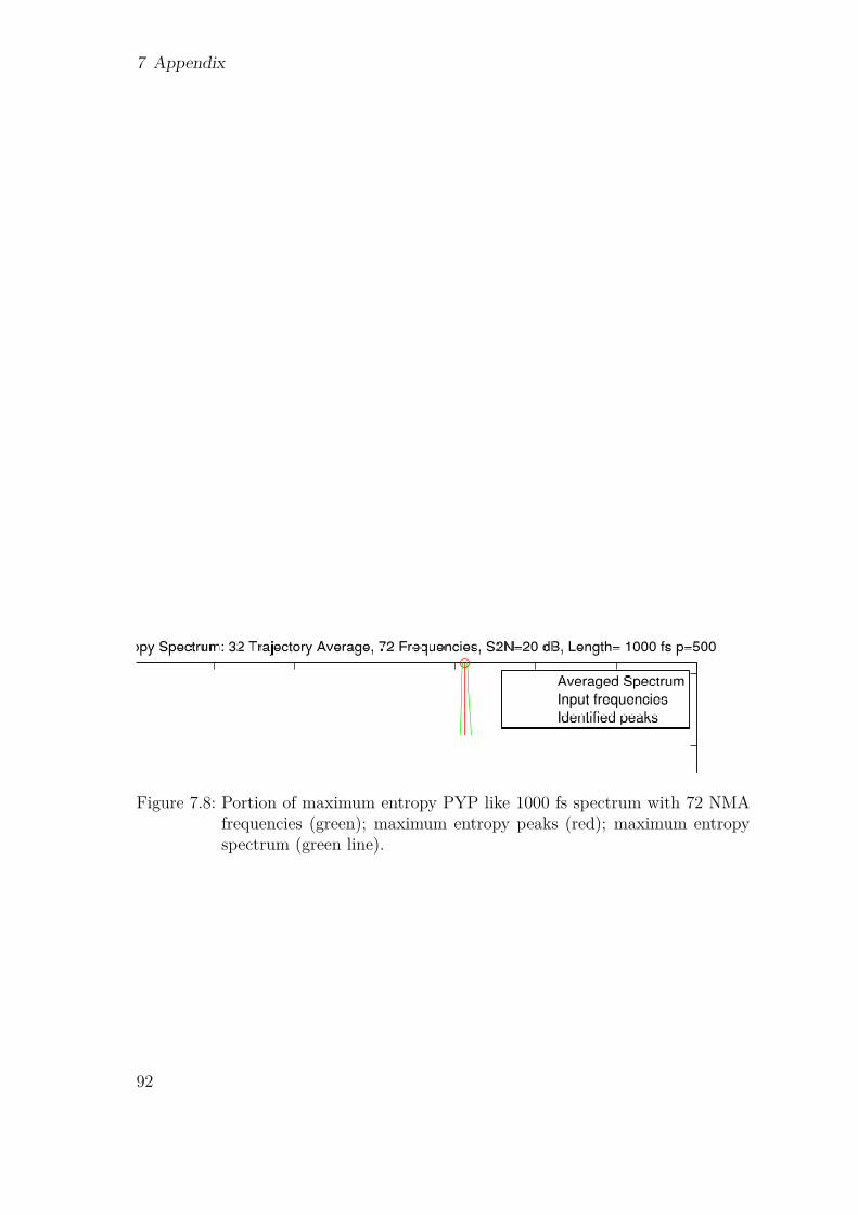
7 Appendix
Figure 7.8: Portion of maximum entropy PYP like 1000 fs spectrum with 72 NMAfrequencies (green); maximum entropy peaks (red); maximum entropyspectrum (green line).
92
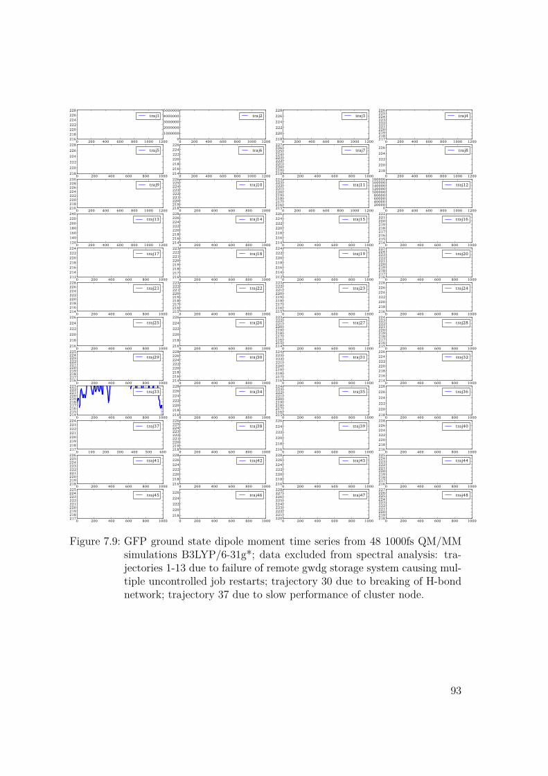
Figure 7.9: GFP ground state dipole moment time series from 48 1000fs QM/MMsimulations B3LYP/6-31g*; data excluded from spectral analysis: tra-jectories 1-13 due to failure of remote gwdg storage system causing mul-tiple uncontrolled job restarts; trajectory 30 due to breaking of H-bondnetwork; trajectory 37 due to slow performance of cluster node.
93
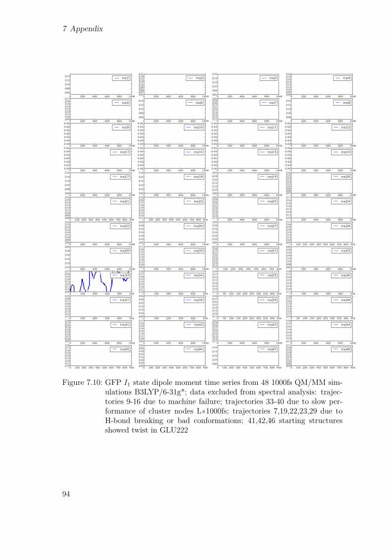
7 Appendix
Figure 7.10: GFP I1 state dipole moment time series from 48 1000fs QM/MM sim-ulations B3LYP/6-31g*; data excluded from spectral analysis: trajec-tories 9-16 due to machine failure; trajectories 33-40 due to slow per-formance of cluster nodes L«1000fs; trajectories 7,19,22,23,29 due toH-bond breaking or bad conformations; 41,42,46 starting structuresshowed twist in GLU222
94
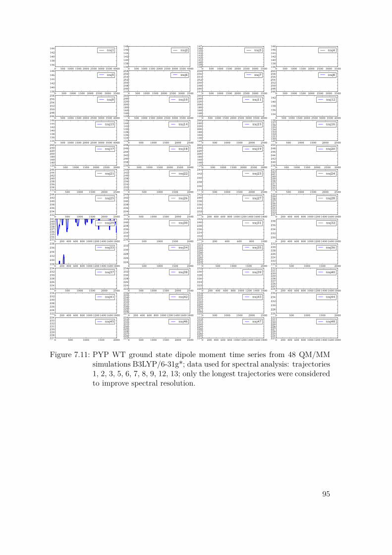
Figure 7.11: PYP WT ground state dipole moment time series from 48 QM/MMsimulations B3LYP/6-31g*; data used for spectral analysis: trajectories1, 2, 3, 5, 6, 7, 8, 9, 12, 13; only the longest trajectories were consideredto improve spectral resolution.
95

7 Appendix
Figure 7.12: PYP WTL ground state dipole moment time series from 48 QM/MMsimulations B3LYP/6-31g*; data used for spectral analysis: trajecto-ries 1, 2, 3, 4, 5, 6, 7, 8, 9, 17, 18; only the longest trajectories wereconsidered to improve spectral resolution.
96

Figure 7.13: Effect of removing the center of mass motion (COM) from the dipolemoment time series; COM spectral contribution localized below 1000cm−1
97
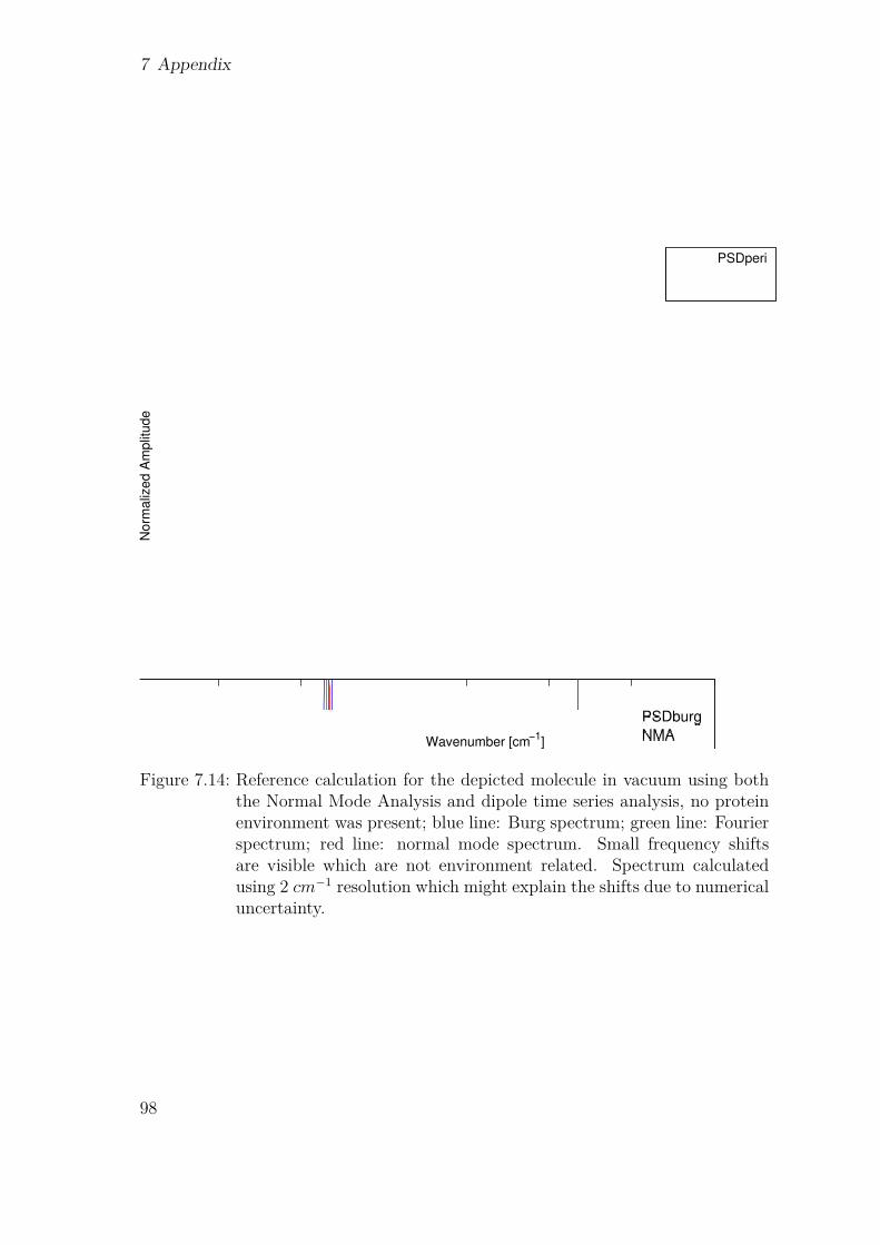
7 Appendix
Figure 7.14: Reference calculation for the depicted molecule in vacuum using boththe Normal Mode Analysis and dipole time series analysis, no proteinenvironment was present; blue line: Burg spectrum; green line: Fourierspectrum; red line: normal mode spectrum. Small frequency shiftsare visible which are not environment related. Spectrum calculatedusing 2 cm−1 resolution which might explain the shifts due to numericaluncertainty.
98
Acknowledgment
Financial Acknowledgments: Marloes Groot for supporting my scholarship applica-tions and Helmut Grubmüller for partially financing my studies in Amsterdam, thuskeeping me from flipping burgers at McDonalds. MPIBPC for affordable housing.Scientific Acknowledgments: Gerrit Groenhof, Marloes Groot and Helmut Grub-
müller for fruitful discussions and critical input throughout my project; CarstenKutzner and Sören Wacker for many helpful discussions on all aspects of my work;Daan P. Geerke for introducing me to polarizable force fields; Bela Voß for quotingme in his thesis and discussions; Maarten Wolf and Martin Hoefling for highly valueddiscussions on the multipole expansion and charged dipole moments; David Köpfer,Ulrich Zachariae and Jan Peters for listening; Maike Clemens, Mehdi Davari, CarlBurmeister and Ludger Inhester for discussions on various quantum chemistry prob-lems; Ulrike Gerischer helping me with by poster designs; Ansgar Esztermann andMartin Fechner for administrating the department’s supreme computing facilities;Eveline Heinemann for keeping everyone organized.Many thanks again to Marloes Groot and Gerrit Groenhof for letting me become
part of their groups.
99
Declaration
This thesis is mine and I wrote it myself. It presents myresearch work in the specified time period. Contributionsby others were indicated to my best knowledge by refer-ence to the literature. Research input and discussions wereacknowledged. All figures in this thesis were generated byme but you may use them under the CC0 1.0 Universal li-cense (http://creativecommons.org/publicdomain/zero/1.0/).All other thesis related elements may be used un-der Attribution 3.0 Unported license (CCBY3.0)(http://creativecommons.org/licenses/by/3.0/). I also de-clare that this thesis, or parts of it, were only submitted tothe VU University as part of the thesis requirement of theinternational masters program in physics.
Göttingen, August 1, 2011
(Timo Marcel Daniel Graen)