ANFOG Slocum CTD data correction

Claire Gourcuff

March 2014

Contents 1. Introduction .................................................................................................................................... 3

1.1. Purpose of the document ....................................................................................................... 3

1.2. Background ............................................................................................................................. 3

1.2.1. The known issues ............................................................................................................ 3

1.2.2. Examples of CTD data problems in ANFOG data ............................................................ 4

1.2.3. Correction strategy ......................................................................................................... 6

2. Temperature alignment .................................................................................................................. 6

3. Thermal lag correction .................................................................................................................... 9

3.1. Pumped CTD ............................................................................................................................ 9

3.2. Un-pumped CTD ...................................................................................................................... 9

4. Conductivity alignment ................................................................................................................. 10

5. Results ........................................................................................................................................... 12

6. Conclusion ..................................................................................................................................... 14

Bibliography .......................................................................................................................................... 16

1. Introduction

1.1. Purpose of the document This document describes the problems encountered in temperature, conductivity and salinity measurements from the SeaBird CTD on board ANFOG Slocum gliders, and the different corrections tested and implemented to improve the data.

Different methods are proposed in the literature to correct and improve glider’s CTD data. After many tests performed on many different ANFOG missions, corrections have been implemented on raw data, from v3.13 of the Slocum processing (first mission with correction applied: Pilbara20130310 (missionID 0154, processingID 1033, processed and released to emII in September 2013). However, the corrections, although globally leading to improved quality data, are still not completely satisfactory and the chosen methods seem not to be appropriate for all of the ANFOG missions. Thus, at that stage, the choice of applying or not the corrections is left to the operator, by setting the associated fields in the processing configuration file (ANFOG 2013) .

1.2. Background

1.2.1. The known issues All the ANFOG Slocum gliders have been equipped with a Conductivity Temperature Depth recorder (CTD) from Sea-Bird manufacturer, optimized for low power consumption. Sea water salinity is computed by combining temperature, conductivity and pressure measurements acquired by this CTD. Among the many ANFOG Slocum mission, two different types of CTD sensor have been used: the CTD41CP before June 2011 and the GPCTD after. Both sensors have a sampling rate of ~0.5Hz and their principal difference is that the former was an un-pumped CTD, whereas the GPCTD specifically designed for Slocum gliders now installed on all the current ANFOG Slocum gliders is equipped with a pump that allows for a constant flow inside the conductivity cell. Note that otherwise specified the data presented here were obtained with a GPCTD (pumped).

Sensor dynamics issues related to typical profiling CTD – mainly high frequency sampling CTD mounted on rosettes for measurements from ship - have been described in the past (Horne and Toole (1980), Gregg and Hess (1985), Morison et al. (1994)). The issues usually come out as spikes in salinity profiles as well as differences between a downward salinity profile and the following upward profile.

Two main sources can cause these data imperfections observed on salinity profiles: different sensor time responses for the thermistor, the conductivity sensor and the pressure sensor, and what is commonly referred to as a thermal lag effect. In the presence of differences in sensor time responses, the salinity is then computed from pressure, conductivity and temperature measurement that don’t match with each other. The thermal lag effect is due to the conductivity cell inertia: the conductivity used to compute salinity is measured inside a conductivity cell, which has the capacity of storing heat. The temperature inside the cell can be different from the one used to compute salinity, measured outside the cell, especially when the glider is flying through strong temperature

gradients. The thermal lag issue was shown to be much reduced when using pumped CTD on gliders, where the flushed water sample is supposed to be the same as the one sampled by the thermistor (Janzen and Creed 2011). However, the issue is still present in data from pumped CTDs (see examples below), although more easily correctable as the flow in the conductivity cell is known and constant.

1.2.2. Examples of CTD data problems in ANFOG data Figure 1 and Figure 2 show examples of salinity spikes occurring in the thermocline. Indeed, the phenomenon is intensified in cases of strong gradients. Salinity spikes in Figure 2 appear although temperature and conductivity don’t show any spike or bad data (apart from around 18m depth, where the salinity spike is associated with a spike in conductivity).

Figure 1. Salinity section of the first 2 days of a Kimberly deployment, in September 2012. X axis represents time and y axis represents pressure. Salinity in psu is plotted as coloured dots.

Figure 2. Associated Conductivity (left), Temperature (middle) and Salinity (right) downward profiles from a Yamba deployment (Sept 2012) (day 18.896).

A difference between up and down casts is observed in Figure 3, where downward profiles exhibit negative spikes and upward profiles positive spikes in the thermocline. Given the fact that temperature and salinity are decreasing with pressure, negative salinity spikes on downward is the sign that conductivity leads temperature (see Sea-Bird documentation). Between 20 and 30 db (20-30m depth), salinity measured on upward profiles appears weaker than salinity measured on downward profiles. This difference is highlighted on T/S plots, as can be seen on Figure 4. In this example the difference in salinity for a given temperature reaches 0.05 psu between upward and downward profiles. This important difference observed on T/S plots is the sign of a thermal lag issue (Garau et al. 2011).

Figure 3. Four downward (blue) and four upward (grey) consecutive salinity profiles measured during the September 2012 Kimberly deployment.

Figure 4. Temperature versus salinity plot for four downcasts (blue) and four upcasts of the September 2012 Yamba deployment (same as previous Figure).

1.2.3. Correction strategy The specificities of gliders, that sample at low frequency and which vertical speed is non uniform, make generic CTD corrections hard to apply. A few studies have been performed to define specific methods for glider’s CTD data corrections, that have inspired the work presented here: Bishop (2008), Garau et al. (2011) and Kerfoot et al. (2006).

The correction process is split in three different phases. The first phase (section 2) consists in re-aligning the temperature with pressure, taking into account the temperature sensor time response. We assume that the pressure sensor time response is negligible. The second phase (section 3) relates to the thermal lag effect and consists in estimating the temperature inside the conductivity cell to be used to compute salinity. Finally, we estimate the conductivity misalignment and correct conductivity data before computing the final salinity data (section 4).

2. Temperature alignment Salinity is a function of both temperature and conductivity. The best way to test the validity of corrections on temperature and conductivity is to analyse the resulting salinity. But to check the validity of the correction on one of the two parameters, one has to make sure that the values of the other parameter used to compute salinity are correct. The strategy we followed here was to correct temperature independently to salinity, just by looking for the best match between upward and downward profiles of temperature. Once the best correction for temperature has been defined, we use this corrected temperature to define the temperature inside the conductivity cell as part of the thermal lag correction, and then correct the conductivity misalignment, looking for the best salinity match.

In recent studies regarding CTD data correction, temperature measurements from the CTD is corrected from sensor time lag (relative to pressure) by filtering the data, and then applying the equation from Fofonoff et al. (1974):

𝑇𝑜 = 𝑇 + 𝜏𝑑𝑇𝑑𝑡

Where 𝑇𝑜 is the true temperature, 𝑇 the temperature measured, and 𝜏 is a time constant (Bishop (2008), Johnson et al. (2007). However, this equation is only valid if the time constant is at least two times higher than the sampling interval (Nyquist theorem), and this is not the case for Slocum gliders. Indeed, the sensor time response is of the order of 1s, and the CTD on Slocum gliders has a sampling frequency of ~0.5Hz (2s), i. e. we are just at the limit of validity of Nyquist theorem.

Our tests trying to correct temperature as above did not lead to any satisfying results (not shown).

Instead, we decided to follow the method described in Kerfoot et al. (2006) and simply apply a linear time shift to the temperature data. Kerfoot et al. (2006) compute mean temperature profiles of 100

upcasts and 100 downcasts and compare the two mean profiles, time-shifted from 0 to 5 seconds by intervals of 0.1 seconds. They look for the time shift value which gives the best match between the mean downcast and the mean upcast profiles. This method has the disadvantage of 1) considering only a sample of the available mission data, that has to be chosen, and 2) averaging profiles of different maximum depths and where measurements are taken at different depths. Rather, we chose to apply the time shifts ([0:0.1:3] secs) to the temperature data of the whole mission.

Here is how we proceed, for each time shift:

1) We compute two metrics for each pair of down and up profiles: the RMS difference and the BIAS between the down and the up cast.

2) We compute the median of these RMS and BIAS. Thus, for one given mission, we end up with 2 global estimates of the match between upward and downward temperature measurements for each time shift. Figure 5 shows an example of these metrics as a function of the time shift for the Yamba mission of October 2013. For each mission, both metrics (we consider the absolute value for the BIAS) reach a minimum value before increasing again for higher time shifts. The minimum is reach for different time shift for the RMS (1.1s for the present example) and for the BIAS (1.3s for the present example), although usually close. The resulting time shifts are given in Table 1 for 21 missions. As the reduction in RMS difference between the original value and the minimum value is proportionally very small (see Figure 5 for an example, but this is true for all the missions), we decided to use the BIAS value to determine the best match between up and down casts.

3) The time shift that gives the smallest absolute BIAS between upward and downward temperature profiles is the one that is used to correct the data.

Figure 5. Absolute value of the median Bias and the median Rms difference between up and down temperature casts for the Yamba October 2013 mission, as a function of time shift.

This adapted method was tested on more than 20 ANFOG missions (with CTDs of the CTD41CP type). Our results are comparable to those of Kerfoot et al. (2006), with a time shift between 0.9 and 2.7 seconds depending on the mission (Table 1) . We observe that the results are different even for missions using the same CTD. Interestingly, although the number of missions of each CTD is too small to conclude anything on that point, it seems that for each CTD, the time shift tends to increase with time since last calibration. For instance for CTD SN 0027 (calibrated on the 1st of September 2010, in blue), the time shift was 1.0 s in September 2012, 1.4 s in November 2012 and 1.6 s in February 2013. For the CTD SN 0095 (calibrated on the 30th of November 2011, in black), the time shift was 1.3 on September 2012, 1.6 in November 2012 and 1.8 in March 2013.

Table 1.Time shifts value to apply to correct temperature, obtained using our new method, for a few ANFOG missions. Same colours indicate same CTD SN and calibration date.

Mission ID - name

CTD SN – calibration date

Temperature time shift (seconds) RMS

Temperature time shift (seconds) BIAS

0132 Yamba20120904 0095 30-Nov-2011 1.0 1.3 0136 Kimberly20120914 0116 15-Feb-2012 2.4 (1.6???) 1.9 0137 StormBay20120904 0115 05-Feb-2012 1.4 1.9 0138 StormBay20120921 0027 01-Sep-2010 1.0 1.0 0140 StormBay20121019 0115 05-Feb-2012 1.3 1.5 0142 Yamba20121114 0095 30-Nov-2011 1.2 1.6 0143 StormBay20121114 0027 01-Sep-2010 1.2 1.4 0144 SpencerGulf20121127 0096 30-Nov-2011 0.8 0.9 0145 PerthCanyon20121206 0070 11-Jul-2012 1.2 2.5 0146 Kimberly20130214 0116 15-Feb-2012 1.7 1.9 0149 StormBay20130208 0115 05-Feb-2012 1.4 1.8 0151 TwoRocks20130215 0096 30-Nov-2011 1.0 1.2 0152 Bremer20130221 0070 11-Jul-2012 31 37 0153 StormBay20130226 0027 01-Sep-2010 1.6 1.6 0154 Pilbara20130310 0095 30-Nov-2011 1.1 1.8 0168 StormBay20130620 0115 05-Feb-2012 1.2 1.4 0169 Kimberly20130925 0058 21-Jul-2012 1.1 1.4 0170 Pilbara20130919 0116 15-Feb-2012 2.4 2.4 0174 Yamba20131009 0096 30-Nov-2011 1.0 1.3 0177 SpencerGulf20131031 0116 15-Feb-2012 2.5 2.7 0178 Yamba20131120 0058 21-Jul-2012 1.1 1.3

3. Thermal lag correction

3.1. Pumped CTD In the case of a pumped CTD, the flow inside the conductivity cell is known and constant and we can easily apply the common method of Lueck and Picklo (1990), generalised by Morison et al. (1994). This method consists in estimating the temperature inside the conductivity cell and use this temperature to compute the salinity instead of the one measured by the thermistor, outside the cell. According to Lueck and Picklo (1990) the temperature inside the cell can be estimated applying the following recursive filter:

𝑇𝑇(𝑛) = −𝑏𝑇(𝑛 − 1) + 𝑎[𝑇(𝑛) − 𝑇(𝑛 − 1)] ( 1 )

Where 𝑇𝑇 is the temperature correction substracted from the measured temperature 𝑇, 𝑛 is the sample index, and the constant 𝑎 and 𝑏 are given by:

𝑎 = 4𝑓𝑛𝛼𝜏(1+4𝑓𝑛𝜏)

and 𝑏 = 1 − 2𝑎𝛼

Where 𝑓𝑛 is the Nyquist frequency, ie ½ the CTD sampling interval (Kerfoot et al. 2006).

Morison et al. (1994) show that if the flow in the conductivity cell is constant, α and τ can be estimated using the following empirical relation:

𝛼 = 0.0264 𝑉−1 + 0.0135 𝑎𝑛𝑑 𝜏 = 2.7858 𝑉−1 2� + 7.1499 ( 2 )

In our case (GPCTD), the flow rate in the conductivity cell is 10ml/s, the volume of the cell is 3ml and its length 146mm, which gives a velocity:

𝑉 = 0.4867 𝑚 𝑠−1

As this velocity value is inside the validity range given by Morison et al. (1994), we can compute 𝑎 and 𝑏 and then the temperature inside the conductivity cell using equations ( 2 ) and ( 1 ).

3.2. Un-pumped CTD Garau et al. (2011) provide improvement to the commonly used method of Morison et al. (1994) for thermal lag correction on CTD data in the case of un-pumped CTD mounted on gliders, which implies that:

1) The flow speed inside the conductivity cell (assumed as constant in (Morison et al. 1994)) depends on glider surge speed, 2) The gliders’ CTD sampling has a low temporal resolution (~0.5Hz) in comparison to CTD operated from ships,

3) The gliders’ CTD sampling interval is irregular.

Thanks to an experiment with ship CTD measurements used as reference, the authors show that thermal-lag correction is improved when using data from following up and down gliders casts to estimate the 4 parameters [α0 αS τ0 τS] defined by Morison et al. (1994) (equation ( 2 )) instead of using the values proposed by Morison et al. (1994): α0 = 0.0135, αS = 0.0264, τ0 = 7.1499 and τS = 2.7858 . Practically, they look for a set of parameters that minimize the area between the 2 T-S curves for each pair of casts and then use the median value of the total parameter sets to apply a thermal-lag correction to each of the glider CTD profiles data.

However, this method is time consuming, especially if we want to take into account the conductivity sensor time response, which force us to iterate through many loops to get the best parameters and time lag. Our tests of this method did not lead to better results than when recomputing α and τ using an estimate of V per profile, defined as the glider’s velocity across the water column. Indeed, we make the strong hypothesis that the velocity in the conductivity cell is the same as the one of the glider. Once we estimated this velocity, we simply estimate the temperature inside the conductivity cell applying equations ( 1 ) and ( 2 ). This method yields to salinity data improvements through a significantly better match between consecutive dives and climbs, especially well observed when looking at data in T/S diagramms (see section 5).

4. Conductivity alignment

Once the temperature is corrected, i.e. aligned with pressure, and the thermal lag correction has been applied, the conductivity time lag can be estimated through examination of salinity data.

During the test phase, we noted that the conductivity time lag does not look constant through one given deployment. The cause of such variations is still unknown. It could be related to a geometrical induced lag, with the distance between the conductivity cell and the pressure sensor inducing time lag depending on the glider pitch and depth rate (not always constant during a deployment). However, our attempts to correct for such a time lag failed, probably due to the fact that the depth rate and pitch parameters are too variable on a single profile, which makes it hard to define adequate values for these parameters and thus to define a proper “geometrical time lag”.

Despite the apparent variability in time lag along one mission, we believe that correcting the conductivity pair by pair is not appropriate. Indeed, the hypothesis of match between up and down profiles is only valid on a global basis, on a large set of profiles. Different factors can introduce differences between one downcast and the following upcast, like for instance the presence of internal waves.

After various tests, it came that the method giving the best salinity data was the following:

1) For each pair of profiles, we estimate the time shift to apply to the conductivity to get the best match between the two salinity profiles (values tested: between -10 and 10 seconds,

with 0.1s interval). Unlike for temperature, we consider here the Root Mean Square difference (RMS) to determine the best match. For the Yamba September 2012 mission, for instance, we see in Figure 6 that the RMS significantly drops from values of the order of 0.1 psu before any shift has been applied, to values of the order of 0.01 psu. Given the presence of spikes in salinity profiles, which can change the sign of the BIAS difference between the 2 profiles of a pair, the RMS metric seems more appropriate in that case.

2) Once we get one time shift value for each pair of profiles (a plot is generated to give an idea of the time shift variability along the deployment), the median is computed and this average time shift is applied to the whole conductivity time series.

Figure 6. Salinity RMS difference between up and down consecutive casts. Raw data are plotted in blue, and RMS after the best individual time shifts (shown in Figure 7) have been applied to conductivity are plotted in red.

The chosen limits for the time shift vector ([-10 10]) may induce a bias in the method, in case the time lag is higher or lower than the limits for several pairs. However, in such a case, the validity of the final time shift used to correct conductivity data is left to the processing operator who has access to the plot of time shifts as a function of pair number (Figure 7).

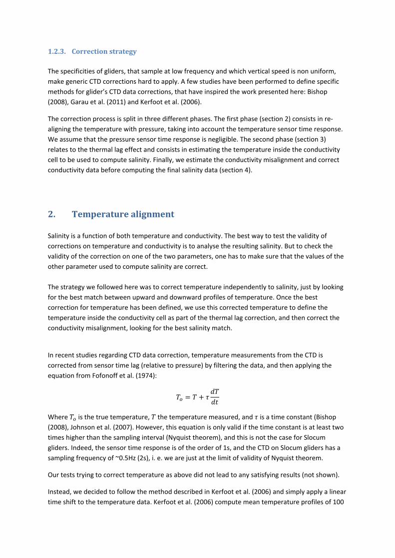
Figure 7 shows the individual time lags (applied to the conductivity data) that give the best match between each downward salinity profile and its following upward salinity profile, for the Yamba September 2012 mission.

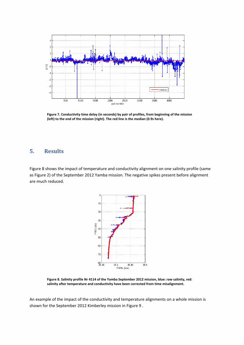
Figure 7. Conductivity time delay (in seconds) by pair of profiles, from beginning of the mission (left) to the end of the mission (right). The red line is the median (0.9s here).

5. Results

Figure 8 shows the impact of temperature and conductivity alignment on one salinity profile (same as Figure 2) of the September 2012 Yamba mission. The negative spikes present before alignment are much reduced.

Figure 8. Salinity profile Nr 4114 of the Yamba September 2012 mission, blue: raw salinity, red: salinity after temperature and conductivity have been corrected from time misalignment.

An example of the impact of the conductivity and temperature alignments on a whole mission is shown for the September 2012 Kimberley mission in Figure 9 .

Figure 9. Salinity section of the September 2012 Kimberley mission. Top panel: raw data. Bottom panel: data after temperature and conductivity have been aligned to pressure.

Salinity data is globally significantly improved by the corrections, as can be seen for instance on Figure 9 for a recent Kimberly mission. The impact of the corrections on 8 salinity profiles taken around the beginning of the mission is shown in Figure 10: the alignment of both temperature and conductivity reduces the spikes (middle plot), both on up and down profiles. If no thermal lag is applied, a difference is still present in the first 30 meters, that disappears if we add the thermal lag correction (right plot).

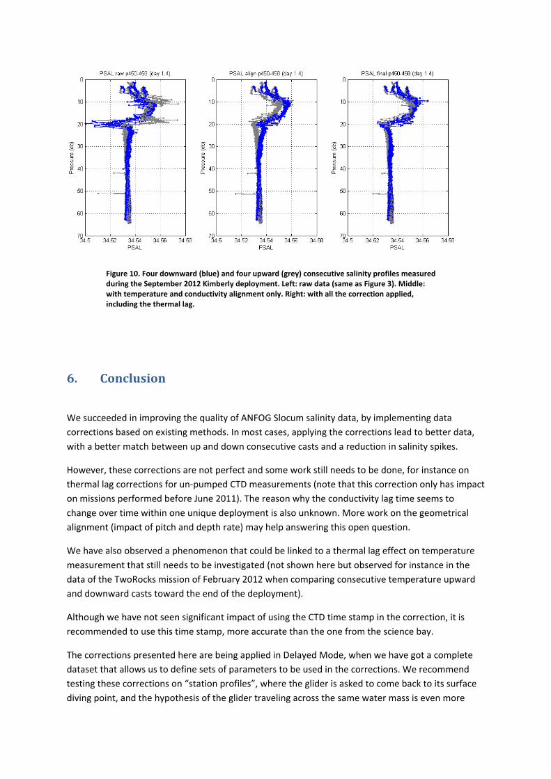
Figure 10. Four downward (blue) and four upward (grey) consecutive salinity profiles measured during the September 2012 Kimberly deployment. Left: raw data (same as Figure 3). Middle: with temperature and conductivity alignment only. Right: with all the correction applied, including the thermal lag.

6. Conclusion

We succeeded in improving the quality of ANFOG Slocum salinity data, by implementing data corrections based on existing methods. In most cases, applying the corrections lead to better data, with a better match between up and down consecutive casts and a reduction in salinity spikes.

However, these corrections are not perfect and some work still needs to be done, for instance on thermal lag corrections for un-pumped CTD measurements (note that this correction only has impact on missions performed before June 2011). The reason why the conductivity lag time seems to change over time within one unique deployment is also unknown. More work on the geometrical alignment (impact of pitch and depth rate) may help answering this open question.

We have also observed a phenomenon that could be linked to a thermal lag effect on temperature measurement that still needs to be investigated (not shown here but observed for instance in the data of the TwoRocks mission of February 2012 when comparing consecutive temperature upward and downward casts toward the end of the deployment).

Although we have not seen significant impact of using the CTD time stamp in the correction, it is recommended to use this time stamp, more accurate than the one from the science bay.

The corrections presented here are being applied in Delayed Mode, when we have got a complete dataset that allows us to define sets of parameters to be used in the corrections. We recommend testing these corrections on “station profiles”, where the glider is asked to come back to its surface diving point, and the hypothesis of the glider traveling across the same water mass is even more

realistic than on its usual operating mode. Such “station profiles” could be performed routinely at the start of any deployment, and if relevant, used to define parameters to be used to correct the data of the upcoming deployment, in real time.

Bibliography

ANFOG 2013 ANFOG QA/QC Officer's Manual, Australian National Facility for Ocean Gliders. Bishop, C.M. 2008 Sensor Dynamics of Autonomous Underwater Gliders, Memorial University of

Newfoundland, Newfoundland, USA. Fofonoff, N.P., S.P. Hayes, R.C. Millard and M. Woods Hole Oceanographic Institution 1974

W.H.O.I./Brown CTD Microprofiler: Methods of Calibration and Data Handling: Defense Technical Information Center.

Garau, B., S. Ruiz, W. Zhang, A. Pascual, E. Heslop, J. Kerfoot and J. Tintoré 2011 Thermal Lag Corrections on Slocum CTD Glider Data. Journal of Atmospheric and Oceanic Technology 28:1065-1071.

Gregg, M.C. and W.C. Hess 1985 Dynamic Response Calibration of Sea-Bird Temperature and Conductivity Probes. Journal of Atmospheric and Oceanic Technology 2:304-313.

Horne, E.P.W. and J.M. Toole 1980 Sensor Response mismatches and Lag Correction Techniques for Temperature-Salinity Profilers. Journal of Physical Oceanography 10:1122-1130.

Janzen, C. and E. Creed 2011 Physical Oceanographic Data from Seaglider Trials in Stratified Coastal Waters Using a New Pumped Payload CTD. OCEANS 2011 MTS/IEEE, Kona, Hawaii, USA.

Johnson, G.C., J.M. Toole and N.G. Larson 2007 Sensor Corrections for Sea-Bird SBE-41CP and SBE-41 CTDs. Journal of Atmospheric and Oceanic Technology 24:1117-1130.

Kerfoot, J., S. Glenn, J. Kohut, O. Schofield and H. Roarty 2006 Correction for Sensor Mismatch and Thermal Lag effects in Non-Pumped Conductivity-Temperature Sensors on the Slocum Coastal Electric Glider. Ocean Science, Honolulu, Hawaii.

Lueck, R.G. and J.J. Picklo 1990 Thermal inertia of conductivity cells: Observations with a Sea-Bird cell. Journal of Atmospheric and Oceanic Technology 7:756-768.

Morison, J., N.L. Andersen, E. D'Asaro and T. Boyd 1994 The correction for thermal-lag effects in Sea-Bird CTD data. Journal of Atmospheric and OCeanic Technology 11:1151-1164.