Anewquasi-MonteCarlotechniquebasedonnon...

NUMERICAL MATHEMATICS: Theory, Methods and ApplicationsNumer. Math. Theor. Meth. Appl., Vol. xx, No. x, pp. 1-24 (200x)

A new quasi-Monte Carlo technique based on non-negative least squares and approximate Fekete points

Claudia Bittante, Stefano De Marchi∗, Giacomo ElefanteUniversity of Padova, Department of Mathematics, Via Trieste, 63, I-35121Padova

Abstract. The computation of integrals in higher dimensions and on general do-mains, when no explicit cubature rules are known, can be "easily" addressed bymeans of the quasi-Monte Carlo method. The method, simple in its formulation,becomes computationally inefficient when the space dimension is growing and theintegration domain is particularly complex. In this paper we present two new ap-proaches to the quasi-Monte Carlo method for cubature based on nonnegative leastsquares and approximate Fekete points. The main idea is to use less points and es-pecially good points for solving the system of the moments. Good points are hereintended as points with good interpolation properties, due to the strict connectionbetween interpolation and cubature. Numerical experiments show that, in average,just a tenth of the points should be used mantaining the same approximation orderof the quasi-Monte Carlo method. The method has been satisfactory applied to 2 and3-dimensional problems on quite complex domains.

AMS subject classifications: 11K45; 41A45; 65D30; 65D32Key words: Cubature, quasi-Monte Carlo method, nonnegative least squares, approximateFekete points.

1. Introduction

Consider the problem of calculating the integral I( f ) =

∫

Ω

f (x)d x , Ω ⊂ Rd . We

know that if λd(Ω) < ∞ (the d dimensional Lebesgue measure of Ω) we can turn Ωinto a probability space with probability measure dµ(x) = 1

λd (Ω)dx . Then for f ∈ L1(µ)

we have

I( f ) =

∫

Ω

f (x)dx = λd(Ω)

∫

Ω

f dµ(x) = λd(Ω)E( f )

where E( f ) is the expected value of f .

∗Corresponding author. Email address: [email protected] (Claudia Bittante),[email protected] (Stefano De Marchi), [email protected] (Giacomo Ele-fante)

http://www.global-sci.org/nmtma 1 c©200x Global-Science Press

2 Claudia Bittante, Stefano De Marchi, Giacomo Elefante

The Monte Carlo (MC) method for numerical integration is obtained by taking Nindependent µ-distributed random samples x1, . . . , xN ∈ Ω and, then approximatingthe integral as follows

I( f )≈ λd(Ω)1

N

N∑

i=1

f (x i) = IN ( f ). (1.1)

For the strong law of large numbers, as N →∞ we then know that the r.h.s. in (1.1)converges in the Lebesgue measure to the value of the integral.

Differently to the classical Monte Carlo method or Monte Carlo integration, whichis based on sequences of pseudo-random numbers, a quasi-Monte Carlo (qMC) methodis a method for numerical integration that uses the so-called low-discrepancy sequences(also known as quasi-random sequences or sub-random sequences). Well known lowdiscrepancy sequences are Halton (also known as Van de Corput-Halton), Hammersleyand the so-called (t, s)-sequences, such as the Sobol sequence. For the definition andproperties of all these sequences we invite interested readers to refer to the book [15].

When dealing with a (quasi-)Monte Carlo method of integration we need to find alarge number N of points in order to approximate the value of the integral. This meansa lot of flops and storage, which become unpractical when the space dimension d grows.How can we avoid this?

In the paper we propose two techniques aimed to reduce the number of quasi-random nodes, while still keeping the same accuracy of the quasi-Monte Carlo approach.The new approaches are ”compressed cubature" that we then apply to quite general do-mains in space dimensions d = 2, 3.

In the next section we introduce some useful results on low-discrepancy sequencesand their use in cubature, then in Section 3 we describe the new approaches based onnonnegative least squares (NNLS) and approximate Fekete points (AFP). In Section 4 weprovide an error analysis for the NNLS case that can be adapted to the case of the AFPwhen the measure of stability, ρ (cf. formula (4.4)), is not too big. In Section 5 wepresent some numerical tests supporting the validity of our new approaches. We alsopoint out that all the algorithms have been implemented in Matlab for consistency withprevious works done by collaborators at the CAA-research group for the constructionof cubature formulas on various 2 and 3-dimensional domains (cf. e.g. [27, 30]). Toconclude the Introduction, we observe that our approaches can be extended to anyspace dimension. The reason why we have confined ourselves to d = 2, 3 is mainly dueto hardware limitations on which the numerical experiments have been performed.

2. Briefly on low discrepancy sequences

In what follows let Ω = [0, 1]d be the d-dimensional unit cube, f : Ω→ R a (con-tinuous) function and X = x1, . . . , xN be a finite set of points on Ω.

A new quasi-Monte Carlo technique based on nonnegative least squares and approximate Fekete points.3

The discrepancy DN of X is

DN (X ) := supB∈J

#(B, X )N

−λd(B)

where J is the family of sets of the form∏d

i=1[ai, bi) = x ∈ Rd : ai ≤ x i < bi and#(B, X ) :=

∑Nj=1χB(x j) (i.e. the number of points x j falling in B).

The star discrepancy of X ,D∗N := DN (J

∗; X ) ,

where J∗ is the family of subintervals of Ω of the form∏d

i=1[0, ai).As we have already seen in the quasi-Monte Carlo method the set X is chosen as a

low-discrepancy sequence.In Figure 1 we show the plots of 500 Halton and Sobol points on the square [−1, 1]2.

In Figure 2 we plot the corresponding star discrepancies in 2 and 3-dimensions for more

Figure 1: 500 Halton (left) and Sobol (right) points on [−1,1]2

than 6000 Halton, Sobol and Hammersley points that show the typical logaritmic decayto infinity. In fact, the exact lower bound of the star discrepancy D∗N is an open problembut it is believed that there exist some small positive constant cd such that for any pointset X consisting of N distinct points in the d-dimensional unit-cube, the inequality

D∗N (X )> cd(log N)d−1

N,

holds [15]. To generate such sequences on the unit cube one can use the Matlab codeshaltonset, sobolset, or those available at the Matlab Central File Exchangehttp://www.mathworks.com/matlabcentral/fileexchange/.

Let IN ( f ) be the cubature rule given by the quasi-Monte Carlo method and

EN ( f ) :=

∫

Ω

f (x)d x − IN ( f )

, (2.1)


Figure 2: Star discrepancies in dimension 2 and dimension 3 for nearly 7000 points

the corresponding cubature error. If f : Ω → R is a bounded variation function, withvariation V ( f ), the Koksma-Hlawka inequality (cf. e.g. [23,24]) says

EN ( f )≤ V ( f )D∗N . (2.2)

The definition and analysis of the multidimensional bounded variation of a function, inthe sense of Hardy-Krause, is well detailed in the paper [25].

Once we know V ( f ), by the inequality (2.2), the quality of quasi-Monte Carlo inte-gration rule depends on the star discrepancy. On the other hand, the inequality (2.2) isnot of practical use. As observed in [20] it has some problems

(i) O (N−1 logd(N)) is smaller than O (N−1/2) when d is small and N is large;

(ii) for many functions V ( f ) can be +∞;

(iii) to compute DN , D∗N and V ( f ) is not always easy, while (2.2) gives only an upperbound.

Such drawbacks can be avoided by using a radomized qMC method, for example byrandom shift of the sequence X , as detailed in [34] or by the two new alternatives,presented in this article, aimed to reduce the computation efford essentially by reducingthe number of points considered.

3. The new approaches

In the majority of real applications in which we need to approximate an integral, thedomain of integration could have a quite complicated shape. For instance, in dimensiond = 2, there exist many methods (and the corresponding algorithms) that allow to com-pute nodes and (positive) weights for the corresponding cubature rules. As an examplefor polygonal domains (convex or not convex), polygauss is a Matlab function that,thanks to Green’s integration formula, allows to easily determine the cubature nodesand weights combining the Gauss-Legendre cubature formula with the Green’s formula(cf. [27]). Other known examples for general 2-dimensional domains, with piecewise


regular boundary, are those that make use again of the Gauss-Green approach and im-plemented in the Matlab functions Splinegauss, ChebfunGauss (cf. [30, 31]). Insome of these domains, these formulas use a number of points greater or equal to thedimension of the underlying polynomial space, positive weights (for convergence rea-sons) and algebraic prefixed precision. Unluckily this is in general not the case! This isthe reason why we are looking for cubature formulas also with some negative weights,risking instability, but gaining the possibility to work with more general domains avoid-ing, on the other hands, to use a lot of points as in the quasi-Monte Carlo approach.

3.1. Nonnegative Least Squares

This is the purpose of the Matlab function lsqnonneg, based on a variant of thealgorithm developed by Lawson and Hanson in [19]. Readers interested to the use ofthe function lsqnonneg may refer to the Matlab’s online documention.

NonNegative Least Squares (NNLS) problems are least squares problems that satisfylinear constraints inequalities (cf. [19, p. 161])

Definition 3.1. Let A be a m× n matrix and b ∈ Rm a column vector, G a r × n matrixand h ∈ Rr . A Linear System of Inequalities (LSI) problem is a least squares problem withlinear constraints, that is the optimization problem

minx∈Rn‖Ax − b‖2 (3.1)

Gx ≥ h .

A special instance of the previous problem, used in curve fitting, consists in findinga solution with positive components.

Definition 3.2. Let A be a m× n matrix and b ∈ Rm a column vector. A NNLS problem isthe LSI problem

minx∈Rn‖Ax − b‖2 (3.2)

x ≥ 0 .

As described in [19, p. 161], the algorithm starts with a set of possible basis vectorsand computes the associated dual vector, say λ. It then selects the basis vector corre-sponding to the maximum value in λ in order to swap out of the basis in exchange foranother possible candidate. This process continues until λi ≤ 0, ∀ i.If in the previous definition we consider

• A = V T , with V the Vandermonde matrix at the sequence X = x i, i = 1, . . . , nfor the polynomial basis p j, j = 1, . . . , m;


• b being the column vector of size m of the moments, that is

b j =

∫

Ω

p j(x)dµ(x)

for some measure µ on Ω

• G = I , i.e. the identity of order n and h= (0, . . . , 0)T of order n

then the LSI problem consists in finding the vector x that minimizes ‖V T x− b‖2 subjectto x ≥ 0. This will give the nonnegative weights x for the cubature at the point set X .Hence, by using lsqnonneg we get the positive weights (given by the solution of theLSI problem) so that we can approximate the integrals at the corresponding point setX .

Notice that, from the Kuhn-Tucker theorem, the previous optimization problem hasa solution x with some components that are strictly positive and some other ones thatvanish. Indeed, the residual of the solution of the NNLS problem, say

ε= ‖c − b‖2, c = c j= Ax∗, c j =n∑

k=1

wkp j(qk) ,

will not be zero in general (as before the p j are a polynomial basis on which we canwrite the solution). Then, the nodes qk and the weights w = wk are extracted corre-spondingly to the nonzero components of x∗.

3.2. Approximate Fekete Points

Another idea for approximating the integral, is by using the so-called ApproximateFekete Points (AFP) extracted from a suitable discretizion of the domain known as WeaklyAdmissible Meshes (WAM) (cf. e.g. [4, 5, 28]). For the definition and the properties ofWAMs we refer to the paper [5].

The AFP are good approximation of the true Fekete points as proved in [4] andthey are determined by a “simple” numerical procedure which turns out to be equiva-lent to the QR factorization with column pivoting of the transposed of the rectangularVandermonde matrix associated to the approximation process.

More specifically, consider a WAM An of a compact set K ⊂ Rd (or K ⊂ Cd), sayAn = a1, . . . , am, m ≥ νn = dim(Pd

n), and the associated rectangular Vandermonde-like matrix

V (a; p) = V (a1, . . . , am; p1, . . . , pνn) = [p j(ai)] , 1≤ i ≤ m , 1≤ j ≤ νn , (3.3)

where a = (ai) is the array of mesh points, and p = (p j) is the array of basis polynomialsfor Pd

n (both ordered in some manner). The AFP algorithm can be described in thesesimple Matlab-like notation

algorithm AFP (Approximate Fekete Points):


W = (V (a, p))t ; b = (1, . . . , 1)t ∈ Cνn;w =W\b ;ind = find(w 6= 0); ξ= a(ind)

For details about the AFP algorithm and its Matlab implementation we suggest thereaders to refer to the papers [4, 5, 28]. Here we simply recall that at the web pagehttp://www.math.unipd.it/∼marcov/CAAsoft.html once can find all the neces-sary scripts for polynomial fitting and interpolation on WAMs.

Among the applications of the AFP, a natural one is numerical cubature. In fact, if inthe algorithm AFP we take as right-hand side b =m =

∫

K p(x) dµ (the moments of thepolynomials basis with respect to a given measure µ), the vector w (ind) gives directlythe weights of an algebraic cubature formula at the corresponding Approximate FeketePoints. As a remark, when the boundary of K is approximated by polynomial splines,for dµ= d x the moments can be computed by the formulas developed in [32].

4. Error analysis

In [29, §2], the authors have provided an error analysis, estimating the effect of themoments error in integrating a function, at least when the integrand f is defined on thewhole domain Ω. Just to give an idea on how this error analysis has been done, we con-sider a multivariate discrete measure ν supported at a finite set X = X i ⊂ Ω ⊂ Rd , i =1, . . . , N with correspondent (positive) weightsωi. The idea of “measure compression”,which is essentially our goal, consists in computing an integral by a extracting a subsetof the point set X and the corresponding weights so that

∫

Ω

f (X )dν=N∑

i=1

ωi f (X i)≈M∑

j=1

w j f (Yj) , (4.1)

where Y = Yj ⊂ X and M = card(Yj) ≤ dim(Pdn) < N in such a way that the

cubature formula is (nearly) exact on total-degree polynomials of degree ≤ n in Rd .Following [29],

∫

Ω

p(S)dν=

∫

Xp(S)dν= ⟨c, m⟩, ∀ p ∈ Pd

n

where the c j are the Fourier coefficients of p in the orthogonal basis, sayΦ= φ1, . . . ,φMw.r.t. the dλ, the measure of the domain, and m j the corresponding dν-moments of theΦ. Furthermore

M∑

j=1

w j p(Yj) = ⟨c,µ⟩

where theµ are the approximate moments with moment error εmom. Then, immediately


we get

∫

Ω

p(S)dν−M∑

j=1

w j p(Yj)

= |⟨c, m −µ⟩| ≤ ‖c‖2‖m −µ‖2 ≤ ‖p‖L2dλ(Ω)

εmom .

Theorem 4.1. For f ∈ C (Ω), let RM ( f ) :=

∫

Ω

f (S)dν−M∑

j=1

w j f (Yj)

be the cubature

error using the “compressed” point set Y instead of X . We get

RM ( f )≤ C En( f ;Ω) + ‖ f ‖L2dλ(Ω)

εmom, ∀ f ∈ C (Ω) , (4.2)

Proof. Let p∗n be the polynomial of best approximation of f of degree not greaterthan n in Ω. Then

RM ( f ) =

∫

Ω

f (S)dν−M∑

j=1

w j f (Yj)

≤

∫

Ω

f (S)dν−∫

Ω

p∗n(S)dν

+

∫

Ω

p∗n(S)dν−M∑

j=1

w j p∗n(Yj)

+

M∑

j=1

w j p∗n(Yj)−

M∑

j=1

w j f (Yj)dν

≤

ν(Ω) +M∑

j=1

|w j|

!

En( f ;Ω) + ‖p∗n‖L2dλ(Ω)

εmom ,

where En( f ;Ω) = ‖ f − p∗n‖L2dλ(Ω)

is the best polynomial approximation error. To con-clude, it is enough using the inequality

‖p∗n‖L2dλ(Ω)

≤ ‖p∗n − f ‖L2dλ(Ω)

+ ‖ f ‖L2dλ(Ω)

≤Æ

λ(Ω)‖p∗n − f ‖L∞(Ω) + ‖ f ‖L2dλ(Ω)

gettingRM ( f )≤ C En( f ;Ω) + ‖ f ‖L2

dλ(Ω)εmom, ∀ f ∈ C (Ω) ,

with

C = ν(Ω) +M∑

j=1

|w j|Æ

λ(Ω)εmom . (4.3)

This conclude the proof. Due to the assumed positivity of the weights, the constant C in (4.3) can be written

as follows C = ν(Ω) +ρ

∑Mj=1 w j

p

λ(Ω)εmom with

ρ =

∑

i |wi||∑

i wi|∈ [1,+∞) , (4.4)


that measures how many cubature weights of negative sign are present among all theweights. This quantity can be consider as a measure of stability of the method: if itassumes the value 1, then there is complete stability and so the capability of comput-ing the integrals, with the prescribed precision, but with much less points (big valuesindicate a worsening of the process).

Therefore the cubature error depends on the moment error εmom and the stabilityconstant ρ. Hence, the inequality (4.2) gives practical information on the error growthwith NNLS (where ρ = 1) while with AFP it will be of practical use when the ratio ρ isnot too big.

5. Numerical tests

We present some examples of cubature in 2 and 3 dimensional domains. The do-mains we consider could be either convex and non-convex, discretized with Haltonpoints (i.e. using low-discrepancy sequences), but can obviously be discretized withother low-discrepancy set of points, with random points or grids. Halton points on agiven convex or union of convex can also be considered as a superset of a WAM for thedomain. Then, by the properties P3 and P4 of WAMs, they are a “WAM” from which wecan extract the corresponding AFP.

The functions we considered in the 2-dimensional domains are test functions usedin many problems and applications (cf. e.g. [9,13]):

f1(x , y) =3

4e−

14((9x−2)2+(9y−2)2) +

3

4e−

149(9x+1)2− 1

10(9y+1)

+1

2e−

14((9x−7)2+(9y−3)2) −

1

5e−(9x−4)2−(9y−7)2 (5.1)

f2(x , y) =Æ

(x − 0.5)2 + (y − 0.5)2 (5.2)

f3(x , y) = cos(30(x + y)). (5.3)

The first one is the well-known Franke test function. The function f2 has a singularityat (0.5, 0.5), while the functions f3 is infinitely differentiable with many ripples makingthe computation of its integral quite difficult.

For the 3-dimensional domains, we considered the following test functions (as al-


ready has been done in, e.g. [13,14])

g1(x , y, z) =3

4e−

14((9x−2)2+(9y−2)2+(9z−2)2)

+3

4e−

149(9x+1)2− 1

10(9y+1)− 1

10(9z+1)

+1

2e−

14((9x−7)2+(9y−3)2+(9z−5)2)

−1

5e−(9x−4)2−(9y−7)2−(9z−5)2 (5.4)

g2(x , y, z) =Æ

(x − 0.4)2 + (y − 0.4)2 + (z − 0.4)2 (5.5)

g3(x , y, z) = cos(4(x + y + z)) (5.6)

which are similar to those considered in the 2-dimensional case.All experiments have been performed on a laptop equipped with an Intel Core 2,

3.00 GHz processor, with 4GB of RAM by Matlab 7.10.0. Here we present only someexperiments among the many more done in the Master’s thesis of the first author [1].

5.1. Experiments in R2

To show that the cubature compression is working, we start with two simple convexdomains: the square [0, 1]2 and the unit disk x2 + y2 ≤ 1. Notice that for these twodomains cubature formulas with prescribed exactness are well-known (cf. e.g. [6, 21]and references therein). Both have been discretized with 104, 2 ·104 and 5 ·104 Haltonpoints. In Tables 1–3 we display the relative errors obtained with the qMC method, thenonnegative least-squares (NNLS) and the extracted AFP for n= 10,20, 30. The valuesof the integrals of the functions f1, f2, f3 have been computed with the Matlab functiondblquad giving the values (rounded to 4 decimal digits): 0.4070, 0.3826,2.9 · 10−4

respectively. For the functions f1, f2 the validity of our new approaches is clearly con-firmed by a decrease of the error with n. As we noticed, the function f3 oscillates whichmakes difficult an accurate approximation, that is why errors are in general bigger.

In Figure 3 we display the extracted AFP for n = 30 from the discretization of thesquare with 5·104 Halton points (not displayed). The distribution of the points remindsthe arc-cosine distribution typical of nearly-optimal point sets [9]: indeed the AFP haveasymptotically the same distribution of the true Fekete points, as proved in [4].

The results for the disk are in Tables 4–6 while in Figure 3) we show the correspond-ing AFP for n = 30. In this example, for almost all functions we see that both methodsdo not need to increase either N or n. In fact for the N = 104 and n = 10 we havealmost the same results both with NNLS and AFP.

It is quite easy to observe that both methods compress the cubature, even if in av-erage the AFP approach seems to perform better, even if the gain in precision is notsensible. For instance, Tables 4 and 5 show columns with the same values, because


Figure 3: AFP on the square [0, 1]2 and the unit disk centered in the origin for n = 30 extracted from5 104 Halton points

the differences are evident from the 4-th digit. In both these two tests, except for thefunction f3, it is therefore reasonable to use the smallest n, i.e. n= 10.

method N = 10000 N = 20000 N = 50000

qMC 3.1e-04 1.3e-04 6.8e-05

n= 10 NNLS 3.4e-03 6.3e-03 1.4e-03AFP 3.4e-03 2.9e-03 9.3e-04

n= 20 NNLS 5.0e-04 5.4e-04 3.2e-05AFP 5.1e-04 2.0e-04 6.1e-05

n= 30 NNLS 3.1e-04 1.3e-04 6.4e-05AFP 3.1e-04 1.3e-04 6.9e-05

Table 1: Relative errors for f1 on the square [0,1]2.

method N = 10000 N = 20000 N = 50000

qMC 4.4e-06 2.3e-05 9.1e-06

n= 10 NNLS 5.4e-03 2.3e-03 3.2e-03AFP 2.2e-03 4.4e-03 3.7e-03

n= 20 NNLS 5.6e-04 4.7e-04 2.8e-04AFP 3.9e-04 4.6e-04 5.2e-04

n= 30 NNLS 7.8e-05 1.4e-04 1.8e-04AFP 1.2e-04 1.7e-04 1.3e-04


We present two other experiments on two more complicated domains.The first one considers the domain whose shape is a lens (shown in Figure 4), con-

sisting of the intersection of two disks with centers and radii C1 = (0,0), r1 = 5 andC2 = (4,0), r2 = 3, respectively. The initial grids used to extract “good points” arecomposed by Halton points. The exact moments have been computed using nodesand weights provided by the Matlab function gqlens, which uses subperiodic trigono-


method N = 10000 N = 20000 N = 50000

qMC 3.7e-01 1.3e+0 4.0e-01

n= 10 NNLS 2.2e+02 2.7e+02 9.7e+02AFP 2.4e+01 1.6e+02 1.7e+02

n= 20 NNLS 8.3e+01 2.5e+02 6.1e+02AFP 2.2e+01 4.8e+01 4.1e+01

n= 30 NNLS 2.1e+01 1.5e+01 3.3e+00AFP 1.4e+00 4.0e+00 1.3e+00


method N = 10000 N = 20000 N = 50000

qMC 7.4e-01 7.4e-01 7.4e-01

n= 10 NNLS 7.3e-01 7.3e-01 7.4e-01AFP 7.4e-01 7.4e-01 7.4e-01

n= 20 NNLS 7.4e-01 7.4e-01 7.4e-01AFP 7.4e-01 7.4e-01 7.4e-01

n= 30 NNLS 7.4e-01 7.4e-01 7.4e-01AFP 7.4e-01 7.4e-01 7.4e-01

Table 4: Relative errors for f1 on the unit disk.

method N = 10000 N = 20000 N = 50000

qMC 6.7e-01 6.7e-01 6.7e-01

n= 10 NNLS 6.7e-01 6.7e-01 6.7e-01AFP 6.7e-01 6.7e-01 6.7e-01

n= 20 NNLS 6.7e-01 6.7e-01 6.7e-01AFP 6.7e-01 6.7e-01 6.7e-01

n= 30 NNLS 6.7e-01 6.7e-01 6.7e-01AFP 6.7e-01 6.7e-01 6.7e-01

Table 5: Relative errors for f2 on the unit disk.

method N = 10000 N = 20000 N = 50000

qMC 8.3e-03 9.1e-03 6.7e-03

n= 10 NNLS 3.3e+00 3.7e+00 1.2e+01AFP 1.0e+02 4.2e+00 5.8e+00

n= 20 NNLS 5.1e+00 9.9e-03 3.5e-01AFP 4.0e+00 2.9e+00 2.3e-01

n= 30 NNLS 5.2e+00 4.7e+00 3.8e+00AFP 4.2e-01 1.1e+00 4.8e-01

Table 6: Relative errors for f3 on the unit disk

metric gaussian formulas studied in [12] (the corresponding code can be found herewww.math.unipd.it/∼marcov/CAAsoft.html). The qMC moments have been com-


Figure 4: The lens approximated with N = 2 · 105 Halton points and n= 10 (i.e. 66 points).The pointswith gqlens are indicated with (+), the ones with lsqnonneg with exact moments with (∆) and theAFP () .

puted by starting from an initial grid of 6 · 105 Halton points. In Figure 4 we showthe nodes determined by gqlens, NNLS and the AFP. It is worth noticing that the nodesobtained with the lsqnonneg and the AFP accumulate along the boundary of the lens.In Table 7 we show, the number n of the points extracted with different methods andthe corresponding N (number of points of the discretizion). Notice that gqlens usesslightly more nodes than the AFP, while lsqnonneg uses almost the same number ofnodes as the AFP, except for the case in which the moments are exact (see the casesn= 20, 30).

We also computed the quantity ρ (cf. (4.4)) which give information on the stabilityas detailed above. In Table 8 we present the values of the integrals of the functionsf1, f2, f3 at different values of n by using gqlens starting from 5 · 104 Halton points todiscretize the domain. The values of the integrals of f3 show significant differences atdifferent n due, as noticed, to the oscillating behaviour of the function on the domain.We then expect that the corresponding relative errors will be quite big as well. In Tables9–11 we provide the relative errors compared with the values of the integrals of Table8.

As expected the errors f3 are the biggest. For the functions f1 and f2 the errors aresmall and in agreement with the Koksma-Hlawka theorem. We notice that in all casesthe integration with qMC shows little improvements on varying the cardinality N . Inparticular, by using the compression given by the NNLS and AFP with exact moments,the errors decrease with n, especially for the function f2. Both the methods, when themoments are approximated with qMC, improve with N and n, slowly for f1 and fasterfor f2. Actually for f1 all methods behave in the same way. For f2 the best results arethose obtained with NNLS and AFP with exact moments.

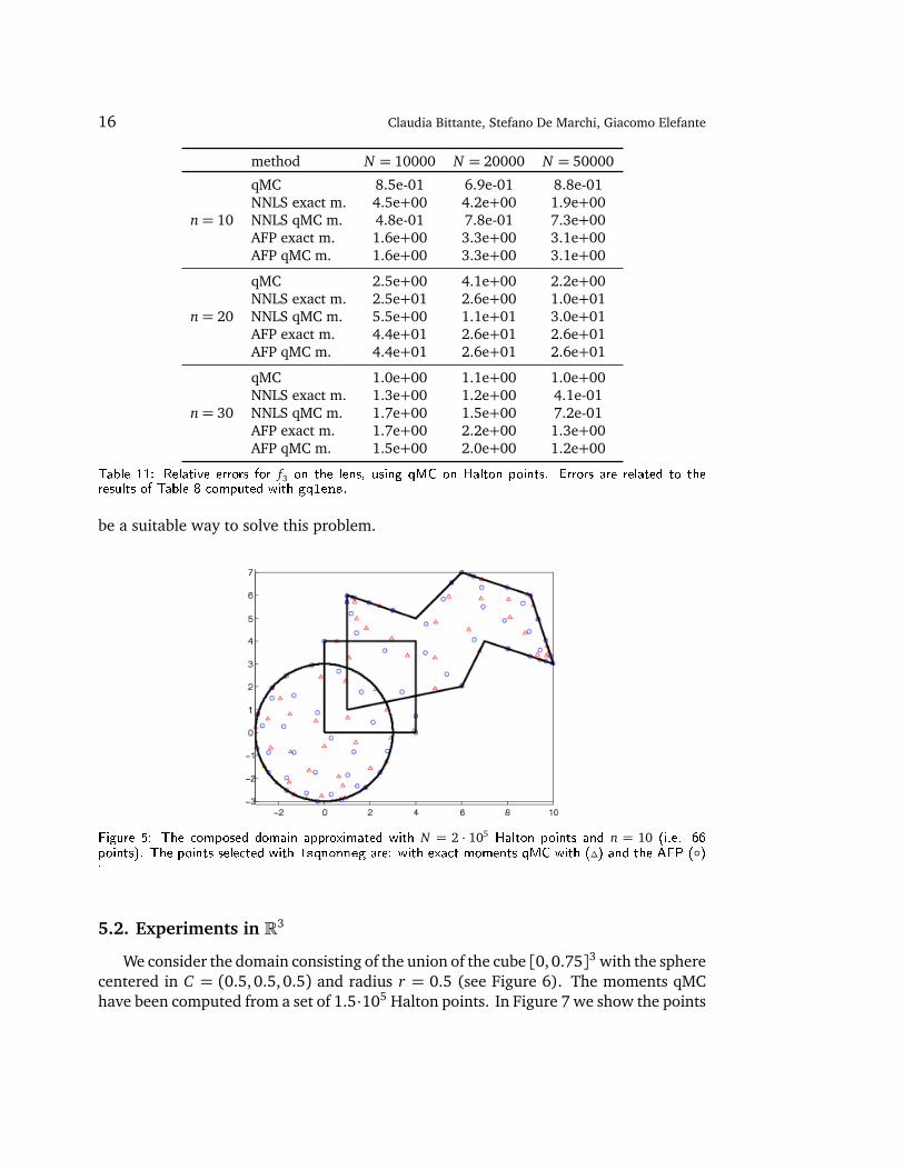
We consider now the non-convex domain, illustrated in Figure 5, obtained by over-lapping the disk with center C = (0, 0) and radius r = 3, the square [0,4]× [0, 4] andthe closed polygon with vertices V1 = (1, 1), V2 = (6,2), V3 = (7,4), V4 = (10,3), V5 =


method N = 10000 N = 20000 N = 50000

n= 10

gqlens 72 (1.00) 72 (1.00) 72 (1.00)qMC 786 15179 37968NNLS exact m. 66 66 66NNLS qMC m. 66 66 66AFP exact m. 66 (1.01) 66 (1.02) 66 (1.02)AFP qMC m. 66 (1.01) 66 (1.02) 66 (1.02)

n= 20


n= 30


Table 7: Nodes on the lens extracted by gqlens, qMC, lsqnonneg with exact moments and approxi-mated ones by qMC and the AFP, again with exact moments or approximated by qMC. In parenthesesthe ratio (4.4).

f1

n= 10 5.2e-02

f2

n= 10 5.5e+01

f3

n= 10 -5.3e-01

n= 20 5.4e-02 n= 20 5.5e+01 n= 20 5.2e-02

n= 30 5.3e-02 n= 30 5.5e+01 n= 30 1.6e+00

Table 8: Values of the integrals on the lens obtained with gqlens for the functions f1, f2, f3 at n =10,20, 30.

(9,6), V6 = (6,7), V7 = (4,5), V8 = (1,6), V9 = V1. For this domain we do not know,indeeddoes not exist, a cubature formula exact on the polynomials neither a way to computethe exact moments. The methods we compare are the ones that compute the momentsby qMC, the NNLS and the one that use the AFP with moments approximated with qMC.The relative errors have been computed with respect to the first one (that computes themoments with the qMC). The qMC moments were computed using 6·106 Halton points.

In Figure 5 we show the points extracted by lsqnoneneg and the AFP for n = 10from a set of N = 50 104 Halton points (see also Table 12 for different values of Nand n). In Table 13 we show the integrals of the functions f1, f2, f3 computed with theqMC method. Finally in Tables 14–16 we display the corresponding relative errors atdifferent N and n. At first glance, the errors computed with the AFP for n = 30 arenot satisfactory, essentially because of the ratio ρ, as displayed in Table 12, that showsquite big values. This is an heuristic explaination of the important role of such a ratioin the comprehension of the approximation given by this approach. For n= 10, 20 the


method N = 10000 N = 20000 N = 50000

n= 10

qMC 2.9e-06 1.2e-02 2.0e-02NNLS exact m. 5.6e-02 5.1e-02 3.0e-02NNLS qMC m. 5.1e-02 1.6e-01 6.8e-02AFP exact m. 3.3e-03 2.7e-02 1.8e-02AFP qMC m. 3.6e-03 2.7e-02 1.8e-02

n= 20


n= 30


Table 9: Relative errors for f1 on the lens, using qMC on Halton points. Errors are related to the resultsof Table 8 computed with gqlens.

method N = 10000 N = 20000 N = 50000

n= 10


n= 20


n= 30


Table 10: Relative errors for f2 on the lens, using qMC on Halton points. Errors are related to theresults of Table 8 computed with gqlens.

results with NNLS are almost equivalent with those obtained with the AFP.In Table 17 we show the cputime for generating the Halton sequence in the qMC

method (qMC tot), for extracting the positive weights with NNLS (NNLS tot) and thetime for extracting the AFP (AFP tot). Moreover, in the same Table, we report thecputime for computing the integrals with the qMC, NNLS and AFP. To reduce the con-struction time for the NNLS and AFP is not so easy and it is not yet clear to us what can


method N = 10000 N = 20000 N = 50000

n= 10

qMC 8.5e-01 6.9e-01 8.8e-01NNLS exact m. 4.5e+00 4.2e+00 1.9e+00NNLS qMC m. 4.8e-01 7.8e-01 7.3e+00AFP exact m. 1.6e+00 3.3e+00 3.1e+00AFP qMC m. 1.6e+00 3.3e+00 3.1e+00

n= 20

qMC 2.5e+00 4.1e+00 2.2e+00NNLS exact m. 2.5e+01 2.6e+00 1.0e+01NNLS qMC m. 5.5e+00 1.1e+01 3.0e+01AFP exact m. 4.4e+01 2.6e+01 2.6e+01AFP qMC m. 4.4e+01 2.6e+01 2.6e+01

n= 30

qMC 1.0e+00 1.1e+00 1.0e+00NNLS exact m. 1.3e+00 1.2e+00 4.1e-01NNLS qMC m. 1.7e+00 1.5e+00 7.2e-01AFP exact m. 1.7e+00 2.2e+00 1.3e+00AFP qMC m. 1.5e+00 2.0e+00 1.2e+00

Table 11: Relative errors for f3 on the lens, using qMC on Halton points. Errors are related to theresults of Table 8 computed with gqlens.

be a suitable way to solve this problem.

Figure 5: The composed domain approximated with N = 2 · 105 Halton points and n = 10 (i.e. 66points). The points selected with lsqnonneg are: with exact moments qMC with (∆) and the AFP ().

5.2. Experiments in R3

We consider the domain consisting of the union of the cube [0,0.75]3 with the spherecentered in C = (0.5,0.5, 0.5) and radius r = 0.5 (see Figure 6). The moments qMChave been computed from a set of 1.5·105 Halton points. In Figure 7 we show the points


method N = 10000 N = 20000 N = 50000

n= 10qMC 4658 9331 23323NNLS 66 66 66AFP 66 (1.02) 66 (1.02) 66 (1.03)

n= 20qMC 4658 9331 23323NNLS 231 231 231AFP 231 (1.73) 231 (1.43) 231 (1.35)

n= 30qMC 4658 9331 23323NNLS 496 496 496AFP 496 (2317.28) 496 (1844.71) 496 (3670.71)

Table 12: For the composite domain of Fig. 5, varying the number N of Halton points, we show thepoints extracted by lsqnonneg and the AFP at dierent n. We also show the ratio ρ (in brackets).

f1

N = 10000 1.5e+01N = 20000 1.5e+01N = 50000 1.5e+01

f2

N = 10000 2.5e+02N = 20000 2.5e+02N = 50000 2.5e+02

f3

N = 10000 1.5e+00N = 20000 1.6e+00N = 50000 3.7e-01

Table 13: The integrals of f1, f2, f3, computed with the qMC method with Halton points covering therectangle that contains the composite domain.

method N = 10000 N = 20000 N = 50000

n= 10NNLS 4.5e-02 1.7e-01 4.1e-02AFP 2.4e-02 9.1e-02 5.7e-02

n= 20NNLS 2.3e-02 8.0e-03 8.4e-03AFP 1.0e-02 1.0e-03 3.0e-02

n= 30NNLS 4.0e-03 1.0e-02 9.7e-03AFP 4.7e+00 2.8e-01 7.7e+00

Table 14: Relative errors for f1 on the composite domain of Fig. 5.

extracted by lsqnonneg and the corresponding AFP. Both sets are well distributed inthe domain except small clusterings close to the boundary of the domain. The testfunctions we considered are those given in (5.4)–(5.6). The results have been donetaking a discretization of the domains with N = 104, 2 · 104 and 5 · 104 Halton pointsand for n≤ 9 (the small values of n depend on hardware limitations).

In Table 19 we report the number of points extracted on varying N and n. Once againwe recall that the AFP extracted are as many as the dimension of the 3-variate space ofpolynomials of degree n, i.e. ηn, while those determined by lsqnonneg sometimes are


method N = 10000 N = 20000 N = 50000

n= 10NNLS 2.5e-03 1.6e-03 3.1e-03AFP 8.6e-06 3.4e-05 1.7e-04

n= 20NNLS 4.4e-04 3.6e-05 3.1e-04AFP 3.0e-04 9.3e-04 9.2e-04

n= 30NNLS 4.7e-05 7.0e-07 1.2e-04AFP 4.2e-01 1.2e-01 3.8e-01


method N = 10000 N = 20000 N = 50000

n= 10NNLS 2.2e+00 2.3e-01 3.5e+00AFP 4.0e+00 3.8e+00 9.5e+00

n= 20NNLS 2.1e-01 3.4e+00 1.7e+01AFP 1.8e+00 4.4e-01 3.9e+00

n= 30NNLS 2.4e+00 2.2e+00 3.4e+00AFP 6.2e+02 8.6e+02 1.2e+04


f1 f2 f3

n= 10

qMC tot 1.2e-01 1.5e-01 1.3e-01NNLS tot 2.3e-01 3.1e-01 2.7e-01AFP tot 4.3e-01 4.2e-01 4.0e-01qMC 2.1e-05 4.1e-05 1.8e-05NNLS 6.0e-06 9.0e-06 6.0e-06AFP 9.0e-06 5.0e-06 5.0e-06

n= 20

qMC tot 1.4e-01 1.4e-01 1.2e-01NNLS tot 3.4e+00 2.8e+00 2.7e+00AFP tot 2.7e+00 2.7e+00 3.1e+00qMC 5.0e-05 2.8e-05 2.0e-05NNLS 1.0e-05 1.1e-05 8.0e-06AFP 8.0e-06 5.0e-06 7.0e-06

n= 30


Table 17: Cputime (in seconds) to compute the integrals on the composite domain of Fig. 5 startingfrom N = 2 · 104 Halton points.

a little less (see for example the case n= 9 and N = 5 · 104).In Table 18 we show the values of the integrals of the functions obtained with the


qMC at different sets of Halton points. The integrals have been computed by consider-ing the parallelepiped surrounding the domain (its convex-hull) and taking the pointsfalling into the domain. As we can see, with an approximation with 2 decimal digits,their values do not change with N .

In Tables 20–22 we show the relative errors of the cubature with the points deter-mined by lsqnonneg and the AFP. In almost all examples, the approximation providedis quite good and the errors show a decreasing behavior. Moreover, errors computedwith the lsqnonneg and the AFP are similar for all N .

Figure 6: The 3-dimensional composite domain union of a cube and a sphere

Figure 7: The points extracted by lsqnonneg and AFP () for n= 5 from N = 105 Halton points.

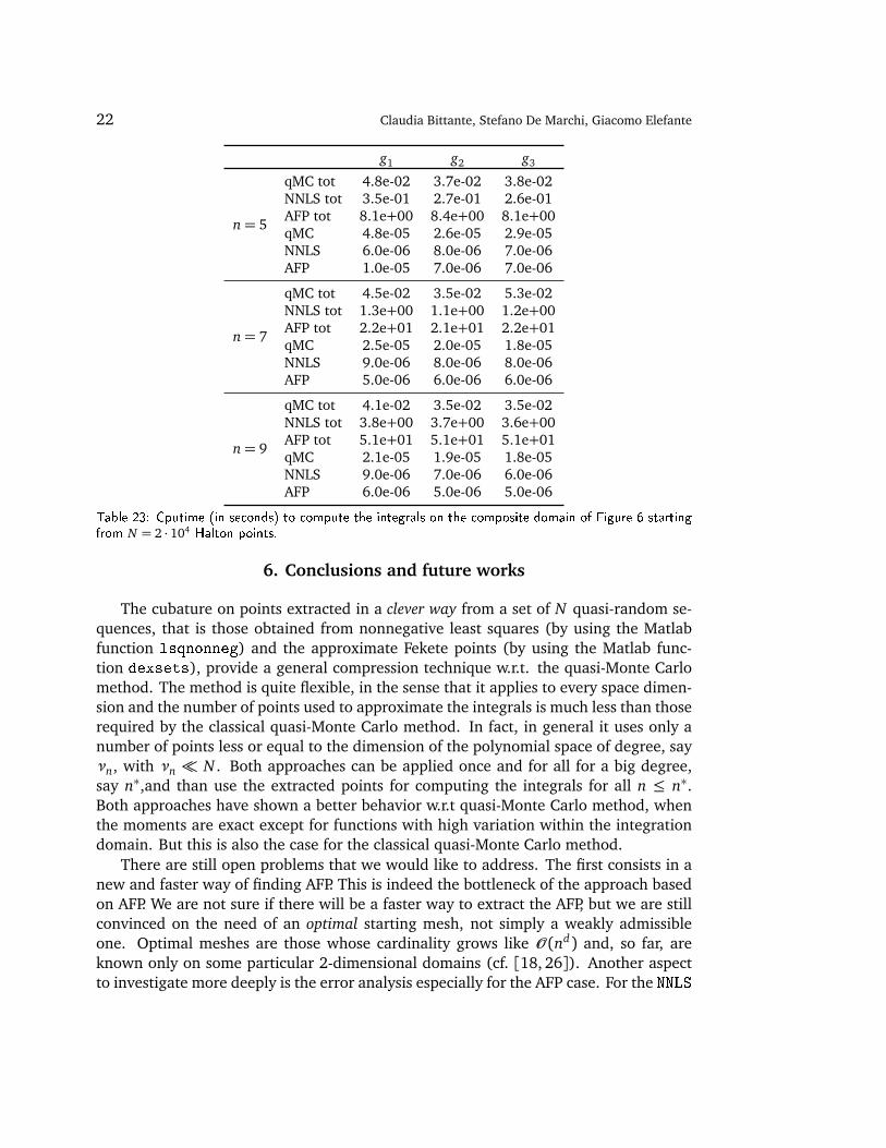
In Table 23 we show the cputime for generating the Halton sequence in the qMCmethod (qMC tot), for extracting the positive weights with NNLS (NNLS tot) and thetime for extracting the AFP (AFP tot). Moreover, in the same Table, we report thecputimes for computing the integrals with the qMC, NNLS and AFP. As it is clear, themore time spent in the construction is significantly gained in the computation of theintegrals. This is the advange of the compression. As observed above, to reduce theconstruction time for the NNLS and AFP is not so easy and it is not yet clear to us whichcan be a suitable way to solve this problem.

We have done many other experiments in [1, Ch. 6] for classical domains, suchas the unit cube, the cone (centered at the origin), the pyramid with square basis


g1

N = 10000 1.7e-01N = 20000 1.7e-01N = 50000 1.7e-01

g2

N = 10000 2.7e-01N = 20000 2.7e-01N = 50000 2.7e-01

g3

N = 10000 4.4e-02N = 20000 4.4e-02N = 50000 4.4e-02

Table 18: Integrals of the functions g1, g2, g3 on the composite domain of Fig. 6 using the qMC methodat dierent sets of Halton points.

method N = 10000 N = 20000 N = 50000

n= 5qMC 6436 12882 32212NNLS qMC m. 56 56 56AFP qMC m. 56 (1.26) 56 (1.20) 56 (1.47)



Table 19: For the composite domain of Fig. 6, varying the number N of Halton points, we show thepoints extracted by lsqnonneg, the AFP at dierent n. We also show the ratio ρ (in brackets).

method N = 10000 N = 20000 N = 50000

n= 5NNLS qMC m. 4.21e-02 1.01e-02 2.53e-02AFP qMC m. 2.07e-02 2.98e-02 1.99e-02



Table 20: Relative errors for g1 on the composite domain of Fig. 6. Errors are computed with respectto the qMC method.

[−0.5, 0.5]× [−0.5, 0.5]. Here we have presented the more interesting case where thedomain is the union of two classical domains (cube and sphere).

We observe that the methods behave differently depending on n and N . For instance

• the tensor-product Gauss-Chebyshev points, used for the cube, depends only on


method N = 10000 N = 20000 N = 50000





method N = 10000 N = 20000 N = 50000





n, and the number of nodes produced is always O (n3);

• the cubature given by the Matlab function 3dWAM, used for (generalized) conesand pyramids in [14], depends only on n.

• the cubature with qMC depends only on N , i.e. the cardinality of the Haltonpoints;

• the cubature based on NNLS depends both on n and N ;

• the AFP depend both on n and N . However, while the integrals using the AFPdepend both on n and N , the number of the nodes correspond to the dimensionof the polynomial space.

Finally, since the exact moments are not known either for the cone, the pyramid andthe composite domain here presented, we have used the qMC for approximating theintegrals in lsqnonneg or, alternatively, the cubature weights were computed by thesame function that extracts the AFP from a discretizion of the domain. In the case ofthe cone and the pyramid we actually know suitable WAMs (cf. [14]).


g1 g2 g3

n= 5

qMC tot 4.8e-02 3.7e-02 3.8e-02NNLS tot 3.5e-01 2.7e-01 2.6e-01AFP tot 8.1e+00 8.4e+00 8.1e+00qMC 4.8e-05 2.6e-05 2.9e-05NNLS 6.0e-06 8.0e-06 7.0e-06AFP 1.0e-05 7.0e-06 7.0e-06

n= 7


n= 9


Table 23: Cputime (in seconds) to compute the integrals on the composite domain of Figure 6 startingfrom N = 2 · 104 Halton points.

6. Conclusions and future works

The cubature on points extracted in a clever way from a set of N quasi-random se-quences, that is those obtained from nonnegative least squares (by using the Matlabfunction lsqnonneg) and the approximate Fekete points (by using the Matlab func-tion dexsets), provide a general compression technique w.r.t. the quasi-Monte Carlomethod. The method is quite flexible, in the sense that it applies to every space dimen-sion and the number of points used to approximate the integrals is much less than thoserequired by the classical quasi-Monte Carlo method. In fact, in general it uses only anumber of points less or equal to the dimension of the polynomial space of degree, sayνn, with νn N . Both approaches can be applied once and for all for a big degree,say n∗,and than use the extracted points for computing the integrals for all n ≤ n∗.Both approaches have shown a better behavior w.r.t quasi-Monte Carlo method, whenthe moments are exact except for functions with high variation within the integrationdomain. But this is also the case for the classical quasi-Monte Carlo method.

There are still open problems that we would like to address. The first consists in anew and faster way of finding AFP. This is indeed the bottleneck of the approach basedon AFP. We are not sure if there will be a faster way to extract the AFP, but we are stillconvinced on the need of an optimal starting mesh, not simply a weakly admissibleone. Optimal meshes are those whose cardinality grows like O (nd) and, so far, areknown only on some particular 2-dimensional domains (cf. [18, 26]). Another aspectto investigate more deeply is the error analysis especially for the AFP case. For the NNLS


the recent error analysis provided in [29] and reported in §4, inequality (4.2), gives anoverestimate for the cubature error. For the case of the moments approximated by AFPthere is still room for such an analysis.

In any case, the new approaches presented in this work are promising, that is whyit is worth to continue to investigate on them.

Acknowledgments

We thank an anonymous referee for the precise comments that have allowed tosignificantly improve the paper. This work has been supported by the University ofPadova Project CPDA124755 “Multivariate approximation with applications to imagereconstruction” and GNCS-INdAM funds.

References

[1] C. BITTANTE, Una nuova tecnica di cubatura quasi-Monte Carlo su domini 2D e 3D, (inItalian), Master’s thesis, University of Padua, March 2014.

[2] M. BRIANI, A. SOMMARIVA, M. VIANELLO, Computing Fekete and Lebesgue points: simplex,square, disk, J. Comput. Appl. Math. 236 (2012), no. 9, 2477–2486.

[3] L. BOS, J.-P. CALVI, N. LEVENBERG, A. SOMMARIVA AND M. VIANELLO, Geometric weakly ad-missible meshes, discrete least squares approximation and approximate Fekete points, Math.Comp. 80(275) (2011), 1623–1638.

[4] L. BOS, S. DE MARCHI, A. SOMMARIVA AND M. VIANELLO, Computing multivariate Feketeand Leja points by numerical linear algebra, SIAM J. Num. Anal. Vol. 48(5) (2010), 1984–1999.

[5] L. BOS, S. DE MARCHI, A. SOMMARIVA AND M. VIANELLO, Weakly Admissible Meshes andDiscrete Extremal Sets, Numer. Math. Theor. Meth. Appl. Vol. 4(1) (2011), 1–12.

[6] B. BOJANOV AND G. PETROVA, Numerical integration over a disc. A new Gaussian quadratureformula, Numer. Math. 80 (1998), 39–59.

[7] L. BOS AND M. VIANELLO, Low cardinality admissible meshes on quadrangles, triangles anddisks, Math. Inequal. Appl. 15 (2012), 229–235.

[8] R. E. CAFLISCH, Monte Carlo and quasi-Monte Carlo methods, Acta Numerica vol. 7, Cam-bridge University Press (1998), 1–49.

[9] M. CALIARI, S. DE MARCHI AND M. VIANELLO, Bivariate polynomial interpolation on thesquare at new nodal sets, Appl. Math. Comput. 165(2) (2005), 261–274

[10] J. P. CALVI AND N. LEVENBERG, Uniform approximation by discrete least squares polynomials,J. Approx. Theory 152 (2008), 82–100.

[11] A. CIVRIL AND M. MAGDON-ISMAIL, On selecting a maximum volume sub-matrix of a matrixand related problems, Theoretical Computer Science 410 (2009), 4801–4811.

[12] G. DA FIES AND M. VIANELLO, Agebraic cubature on planar lenses and bubbles, DolomitesRes. Notes Approx. 5 (2012), 7–12.

[13] S. DE MARCHI, M. MARCHIORI AND A. SOMMARIVA, Polynomial approximation and cubatureat approximate Fekete and Leja points of the cylinder, Appl. Math. Comput. Vol. 218(21)(2012), 10617–10629.

[14] S. DE MARCHI AND M. VIANELLO, Polynomial approximation on pyramids, cones and solidsof rotation, Dolomites Res. Notes Approx, Proceedings DWCAA12, Vol. 6 (2013), 20–26.


[15] J. DICK AND F. PILLICHSHAMMER, Digital Nets and Sequences. Discrepancy Theory and Quasi-Monte Carlo Integration, Cambridge University Press, Cambridge, 2010.

[16] M. DRMOTA AND R. F. TICHY, Sequences, discrepancies and applications, Lecture Notes inMath., 1651, Springer, Berlin, 1997.

[17] A. KLENKE, Probability Theory: A Comprehensive course., Springer-Verlag London, 2014.[18] A. KROÓ, On optimal polynomial meshes, J. Approx. Theory 163 (2011), 1107–1124.[19] C. L. LAWSON AND R. J. HANSON, Solving Least Squares Problems, Prentice-0Hall 1974, p.

161.[20] C. LEMIEUX, Monte Carlo and Quasi-Monte Carlo Sampling, Springer 2009.[21] C. R. MORROW AND T. N. L. PATTERSON, Construction of algebraic cubatures rules using

polynomial ideal theory, SIAM J. Numer. Anal.15 (1978), 953–976.[22] W. J. MOROKOFF AND R. E. CAFLISCH, Quasi-random sequences and their discrepancies,

SIAM J. Sci. Comput. 15 (1994), no. 6, 1251–1279.[23] H. NIEDERREITER, Random Number Generation and Quasi-Monte Carlo Methods., Society

for Industrial and Applied Mathematics, 1992.[24] H. G. NIEDERREITER, Quasi-Monte Carlo methods and pseudo-random numbers, Bull. Amer.

Math. Soc. 84 (1978), no. 6, 957–1041.[25] A. B. OWEN, Multidimensional variation for quasi-Monte Carlo,

http://finmath.stanford.edu/∼owen/reports/ktfang.pdf.[26] F. PIAZZON, M. VIANELLO, Analytic transformations of admissible meshes, East J. Approx.

16 (2010), 389–398.[27] A. SOMMARIVA, M. VIANELLO, Product Gauss cubature over polygons based on Green’s inte-

gration formula, BIT Num. Mathematics 47 (2007), 441–453.[28] A. SOMMARIVA, M. VIANELLO, Approximate Fekete points for weighted polynomial interpo-

lation, Electron. Trans. Numer. Anal. 37 (2010), 1–22.[29] A. SOMMARIVA, M. VIANELLO, Compression of multivariate discrete measures and applica-

tions, Numer. Funct. Anal. Optim. 36 (2015), 1198–1223.[30] G. SANTIN, A. SOMMARIVA, M. VIANELLO, An algebraic cubature formula on curvilinear

polygons. Appl. Math. Comput. 217 (2011), 10003–10015.[31] A. SOMMARIVA, M. VIANELLO, ChebfunGauss: Matlab code for Gauss-Green cubature by the

Chebfun package, available at www.math.unipd.it/∼marcov/CAAsoft.html[32] A. SOMMARIVA AND M. VIANELLO, Gauss-Green cubature and moment computation over

arbitrary geometries, J. Comput. Appl. Math. 231 (2009), 886–896.[33] O. STRAUCH AND Š. PORUBSKÝ, Distribution of Sequences: A Sampler, Peter Lang Publishing

House, Frankfurt am Main 2005.[34] B. TUFFIN, Radomization of quasi-Monte Carlo methods for error estimation: survey and

normal approximation, Monte Carlo Methods and Applications, 10(3-4) (2008), 617–628.

Anewquasi-MonteCarlotechniquebasedonnon...

Documents

Transcript of Anewquasi-MonteCarlotechniquebasedonnon...