Andrzej Truty ZACE Services - Z_SOIL · Hardening Soil model with small strain sti ness Andrzej...
42
Hardening Soil model with small strain stiffness Andrzej Truty ZACE Services 1.09.2008 Andrzej Truty ZACE Services Hardening Soil model with small strain stiffness
Transcript of Andrzej Truty ZACE Services - Z_SOIL · Hardening Soil model with small strain sti ness Andrzej...
Hardening Soil model with small strain stiffness
Andrzej TrutyZACE Services
1.09.2008
Andrzej Truty ZACE Services Hardening Soil model with small strain stiffness

Introduction
Hardening Soil (HS) and Hardening Soil-small (HS-small)models are designed to reproduce basic phenomena exhibitedby soils:
densificationstiffness stress dependencyplastic yieldingdilatancystrong stiffness variation with growing shear strain amplitudein the regime of small strains (γ = 10−6 to γ = 10−3)this phenomenon plays a crucial role for modeling deepexcavations and soil-structure interaction problems
NB. This model is limited to monotonic loads
Andrzej Truty ZACE Services Hardening Soil model with small strain stiffness

Introduction
HS model was initially formulated by Schanz, Vermeer andBonnier (1998, 1999) and then enhanced by Benz (2006)
Current implementation is slightly modified with respect tothe theory given by Benz:
simplified treatment of dilatancy for the small strain version(HS-small)modified hardening law for preconsolidation pressure
This model seems to be one of the simplest in the class ofmodels designed to handle small strain stiffness
It consists of the two plastic mechanisms, shear and volumetric
Small strain stiffness is incorporated by means of nonlinearelasticity which includes hysteretic effects
Andrzej Truty ZACE Services Hardening Soil model with small strain stiffness

Triaxial test: illustration
Undrained triaxial test: video
Drained triaxial test : video
Annimations by P.Baran (University of Agriculture, Krakow,Poland)
Andrzej Truty ZACE Services Hardening Soil model with small strain stiffness

Notion of tangent and secant stiffness moduli
Initial stiffness modulus Eo
Unloading-reloading modulus Eur
Secant stiffness modulus at 50 % of the ultimate deviatoricstress qf
0
50
100
150
200
250
0 0.05 0.1 0.15 0.2 0.25
EPS-1 [-]
q [k
pa] 1
Eo
1E50
1Eur
qf
0.5 qf
σ3=const
q50
qun
Remark: All classical soil models require specification of Eur
modulus (Cam-Clay, Cap etc..)Andrzej Truty ZACE Services Hardening Soil model with small strain stiffness

Stiffness-strain relation for soils (G/Go (γ))
G - current secant shear modulus
Go - shear modulus for very small strains
Atkinson 1991
Andrzej Truty ZACE Services Hardening Soil model with small strain stiffness

Notion of treshold shear strain γ07
To describe the shape ofG
Go(γ) curve an additional
characteristic point is needed
It is common to specify the shear strain γ0.7 at which ratioG
Go= 0.7
0.7
γ07
Andrzej Truty ZACE Services Hardening Soil model with small strain stiffness

Dynamic vs static modulus
Relation between ”static” Young modulus Es , obtained fromstandard triaxial test at axial strain ε1 ≈ 10−3, and ”dynamic”Young modulus (the one at very small strains) Ed = Eo isshown in diagram published by Alpan (1970) (after Benz)
1
10
100
1000 10000 100000 1000000
cohesive soils
granular soils
Rockss
d
EE
[kPa]sE
Andrzej Truty ZACE Services Hardening Soil model with small strain stiffness

HS model: general concept
Double hardening elasto-plastic model (Schanz, Vermeer,Benz)Nonlinear elasticity for stress paths penetrating the interior ofthe elastic domain
0
100
200
300
400
500
600
0 100 200 300 400 500
p [kPa]
q [k
Pa]
Cap surface
Graphical representation of shear mechanism and cap surfaceAndrzej Truty ZACE Services Hardening Soil model with small strain stiffness

HS model: shear mechanism
Duncan-Chang model as the origin for shear mechanism
0
50
100
150
200
250
0 0.01 0.02 0.03 0.04 0.05
eps-1
q [k
Pa]
1E50
qfM-C limit
1
Eur½ qf
Andrzej Truty ZACE Services Hardening Soil model with small strain stiffness

Stiffness stress dependency
Eur = E refur
(σ∗3 + c cotφ
σref + c cotφ
)m
E50 = E ref50
(σ∗3 + c cotφ
σref + c cotφ
)m
Remarks
1 Stiffness degrades with decreasing σ3 up to σ3 = σL (bydefault we assume σL=10 kPa)
Andrzej Truty ZACE Services Hardening Soil model with small strain stiffness

Extension to small strain: new ingredients
To extend standard HS model to the range of small strain Benzintroduced few modifications:
1 Strain dependency is added to the stress-strain relation, forstress paths penetrating the elastic domain
2 The modified Hardin-Drnevich relationship is used to relatecurrent secant shear modulus G and equivalent monotonicshear strain γhist
3 Reversal points are detected with aid of deviatoric strainhistory second order tensor Hij ; in addition the currentequivalent shear strain γhist is computed by using this tensor
Andrzej Truty ZACE Services Hardening Soil model with small strain stiffness
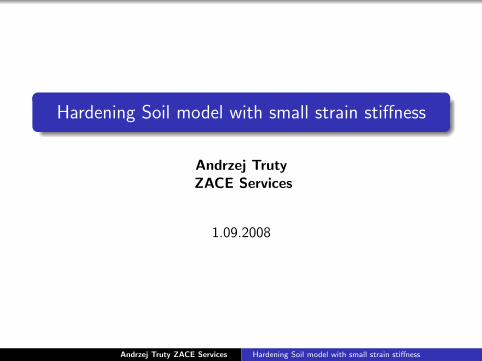
How does it work ?
N
N+1N-1
plot from paper by Ishihara 1986
At step N : γhistN−1= 8× 10⁻⁵ γhistN = 10−4
At step N + 1 : γhistN = 0 γhistN+1= 2× 10⁻⁵
Primary loading: γhistN+1> γmax
hist
Unloading/reloading: γhistN+1≤ γmax
hist
Hardin-Drnevich law: G =Go
1 + aγhist
γ0.7
(secant modulus)
Andrzej Truty ZACE Services Hardening Soil model with small strain stiffness
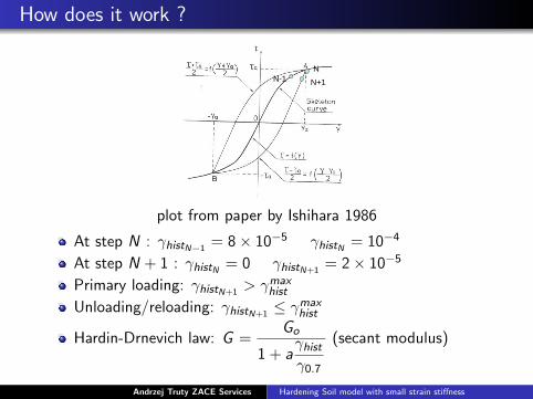
Shear tangent modulus cut-off
γc
G
γ
Gur
γc =γ0.7
a
(√Go
Gur− 1
)Andrzej Truty ZACE Services Hardening Soil model with small strain stiffness
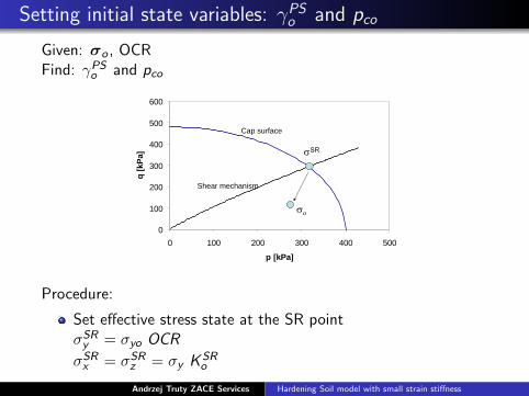
Setting initial state variables: γPSo and pco
Given: σo , OCRFind: γPS
o and pco
0
100
200
300
400
500
600
0 100 200 300 400 500
p [kPa]
q [k
Pa]Cap surface
Shear mechanism
σSR
σο
Procedure:
Set effective stress state at the SR pointσSR
y = σyo OCR
σSRx = σSR
z = σy KSRo
Andrzej Truty ZACE Services Hardening Soil model with small strain stiffness
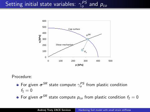
Setting initial state variables: γPSo and pco
0
100
200
300
400
500
600
0 100 200 300 400 500
p [kPa]
q [k
Pa]
Cap surface
Shear mechanism
σSR
σο
Procedure:
For given σSR state compute γPSo from plastic condition
f1 = 0
For given σSR state compute pco from plastic condition f2 = 0
Andrzej Truty ZACE Services Hardening Soil model with small strain stiffness
Setting initial state variables: γPSo and pco
Remarks
1 KSRo = KNC
o ≈ 1− sin(φ) in the standard applications(approximate Jaky’s formula)
2 KSRo = 1 for case of isotropic consolidation (used in triaxial
testing for instance)
3 For sands notion of preconsolidation pressure is not asmeaningful as for cohesive soils hence one may assumeOCR=1 and effect of density will be embedded in H and Mparameters
Andrzej Truty ZACE Services Hardening Soil model with small strain stiffness

Setting M and H parameters based on oedometric test
0
100
200
300
400
500
600
0 100 200 300 400 500
p [kPa]
q [k
Pa]
p*
q*
σ
εσref
1
Eoed
oed
Andrzej Truty ZACE Services Hardening Soil model with small strain stiffness

Material properties
Parameter Unit HS-standard HS-smallE ref
ur [kPa] yes yesE ref
50 [kPa] yes yesσref [kPa] yes yesm [—] yes yesνur [—] yes yesRf [—] yes yesc [kPa] yes yesφ [o ] yes yesψ [o ] yes yesemax [—] yes yesft [kPa] yes yesD [—] yes yesM [—] yes yesH [kPa] yes yesOCR/qPOP [—/kPa] yes yesE ref
o [kPa] no yesγ0.7 [—] no yes
Andrzej Truty ZACE Services Hardening Soil model with small strain stiffness
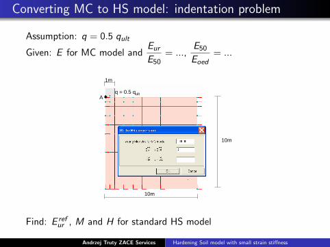
Converting MC to HS model: indentation problem
Assumption: q = 0.5 qult
Given: E for MC model andEur
E50= ...,
E50
Eoed= ...
10m
10m
q = 0.5 qult
1m
A
Find: E refur , M and H for standard HS model
Andrzej Truty ZACE Services Hardening Soil model with small strain stiffness
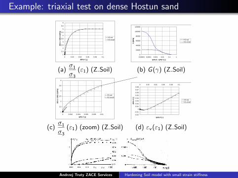
Example: triaxial test on dense Hostun sand
1
1.5
2
2.5
3
3.5
4
4.5
5
5.5
6
0 0.02 0.04 0.06 0.08 0.1-EPS-Y [-]
SIG
-1 /
SIG
-3 [k
Pa]
HS-stdHS-small
0
20000
40000
60000
80000
100000
120000
0.00001 0.0001 0.001 0.01 0.1 1EPS-X - EPS-Y [-]
G [k
Pa]
HS-stdHS-small
(a)σ1
σ3
(ε1) (Z Soil) (b) G (γ) (Z Soil)
1
1.5
2
2.5
3
3.5
4
0 0.002 0.004 0.006 0.008 0.01-EPS-Y [-]
SIG
-1 /
SIG
-3 [k
Pa]
HS-stdHS-small
-0.02
-0.01
0
0.01
0.02
0.03
0.04
0.05
0.06
0.07
0.080 0.02 0.04 0.06 0.08 0.1
-EPS-Y [-]
-EPS
-V [-
]
HS-stdHS-small
(c)σ1
σ3
(ε1) (zoom) (Z Soil) (d) εv (ε1) (Z Soil)
(e) Solution by Benz [?]
Andrzej Truty ZACE Services Hardening Soil model with small strain stiffness

Example: triaxial test on dense Hostun sand
1
1.5
2
2.5
3
3.5
4
4.5
5
5.5
6
0 0.02 0.04 0.06 0.08 0.1EPS-1 [-]
SIG
-1 /
SIG
-3 [k
Pa]
HS-stdHS-small
0
20000
40000
60000
80000
100000
120000
140000
160000
180000
200000
0.00001 0.0001 0.001 0.01 0.1 1EPS-1 - EPS-3 [-]
G [k
Pa]
HS-stdHS-small
(a)σ1
σ3
(ε1) (Z Soil) (b) G (γ) (Z Soil)
1
1.5
2
2.5
3
3.5
4
0 0.002 0.004 0.006 0.008 0.01EPS-1 [-]
SIG
-1 /
SIG
-3 [k
Pa]
HS-stdHS-small
-0.02
-0.01
0
0.01
0.02
0.03
0.04
0.05
0.06
0.07
0.080 0.02 0.04 0.06 0.08 0.1
EPS-1 [-]
EPS-
V [-]
HS-stdHS-small
(c)σ1
σ3
(ε1) (zoom) (Z Soil) (d) εv (ε1) (Z Soil)
(e) Solution by Benz [?]
Andrzej Truty ZACE Services Hardening Soil model with small strain stiffness

Example: triaxial test on dense Hostun sand
1
1.5
2
2.5
3
3.5
4
4.5
5
5.5
6
0 0.02 0.04 0.06 0.08 0.1
EPS-1 [-]SI
G-1
/ SI
G-3
[kPa
]
HS-stdHS-small
0
50000
100000
150000
200000
250000
300000
0.00001 0.0001 0.001 0.01 0.1 1EPS-1-EPS-3 [-]
G [k
Pa]
HS-stdHS-small
(a)σ1
σ3
(ε1) (Z Soil) (b) G (γ) (Z Soil)
1
1.5
2
2.5
3
3.5
4
0 0.002 0.004 0.006 0.008 0.01
EPS-1 [-]
SIG
-1 /
SIG
-3 [k
Pa]
HS-stdHS-small
-0.02
-0.01
0
0.01
0.02
0.03
0.04
0.05
0.06
0.07
0.080 0.02 0.04 0.06 0.08 0.1
EPS-1 [-]
EPS-
V [-]
HS-stdHS-small
(c)σ1
σ3
(ε1) (zoom) (Z Soil) (d) εv (ε1) (Z Soil)
(e) Solution by Benz [?]Andrzej Truty ZACE Services Hardening Soil model with small strain stiffness

Estimation of material properties: input data
Given 3 drained triaxial test results for 3 confining pressures:σ3 = 100 kPaσ3 = 300 kPaσ3 = 600 kPa
Shear characteristics q − ε1
Dilatancy characteristics εv − ε1
Stress paths in p − q planeMeasurements of small strain stiffness moduli Eo (σ3) for theassumed confining pressures (through direct measurement ofshear wave velocity in the sample)
Andrzej Truty ZACE Services Hardening Soil model with small strain stiffness

Estimation of material properties: stress paths in p-q plane
Estimation of friction angle φ = φcs and cohesion c
p
q
φφ
sin3cos6*−
=cc
1
φφ
sin3sin6*−
=MResidual M-C envelope
If we know M∗ and c∗ then we can compute φ and c :
φ = arcsin3 M∗
6 + M∗ c = c∗3− sinφ
6 cosφ
Andrzej Truty ZACE Services Hardening Soil model with small strain stiffness

Estimation of material properties: stress paths in p-q plane
Estimation of friction angle φ = φcs and cohesion c
0
500
1000
1500
2000
2500
3000
0 300 600 900 1200 1500 1800
p [kPa]
q [k
Pa]
1386
2358 12358/1386=1.7
Here: φ = arcsin3 ∗ 1.7
6 + 1.7≈ 42o c = 0
Andrzej Truty ZACE Services Hardening Soil model with small strain stiffness
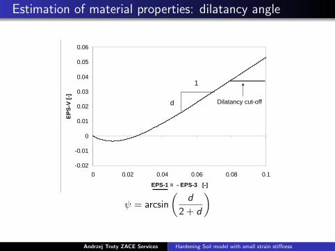
Estimation of material properties: dilatancy angle
-0.02
-0.01
0
0.01
0.02
0.03
0.04
0.05
0.06
0 0.02 0.04 0.06 0.08 0.1
EPS-1 = - EPS-3 [-]
EPS-
V [-]
1
d Dilatancy cut-off
ψ = arcsin
(d
2 + d
)
Andrzej Truty ZACE Services Hardening Soil model with small strain stiffness

Estimation of material properties: dilatancy angle
-0.02
-0.01
0
0.01
0.02
0.03
0.04
0.05
0.06
0 0.01 0.02 0.03 0.04 0.05 0.06 0.07 0.08 0.09 0.1
1
d=0.75Vε
1ε
ψ = arcsin
(0.75
2 + 0.75
)≈ 16o
Andrzej Truty ZACE Services Hardening Soil model with small strain stiffness

Estimation of material properties: E refo and m
Analytical formula: Eo = E refo
(σ∗3 + c cotφ
σref + c cotφ
)m
Measured: shear wave velocity vs at ε1 = 10−6 and at givenconfining stress σ3
Compute : shear modulus Go = ρv2s
Compute : Young modulus Eo = 2 (1 + ν) Go
σ3 [kPa] Eo [kPa]
100 250000
300 460000
600 675000
Andrzej Truty ZACE Services Hardening Soil model with small strain stiffness

Estimation of material properties: E refo and m
Reanalyze Eo vs σ3 in logarithmic scales
Averaged slope yields m; here m =13.1− 12.55
1.0= 0.55
Find intersection of the line with axis ln Eo at
ln
(σ∗3 + c cotφ
σref + c cotφ
)= 0
Here the intersection is at 12.43 henceE ref
o = e12.43 ≈ 2.71812.43 = 250000 kPa
12.2
12.4
12.6
12.8
13
13.2
13.4
13.6
0 0.2 0.4 0.6 0.8 1 1.2 1.4 1.6 1.8 2
⎟⎟⎠
⎞⎜⎜⎝
⎛++
φσφσ
cotcotln 3
cc
ref
oEln
1
m
12.43
Andrzej Truty ZACE Services Hardening Soil model with small strain stiffness

Estimation of E refo from CPT testing
To estimate small strain modulus Go at a certain depth onemay use empirical formula by Mayne and Rix:
Go = 49.4q0.695t
e1.13[MPa]
qt is a corrected tip resistance expressed in MPa
e is the void ratio
Andrzej Truty ZACE Services Hardening Soil model with small strain stiffness
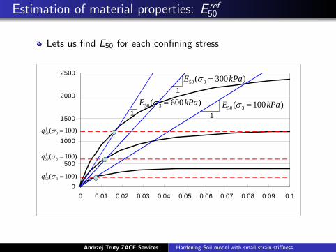
Estimation of material properties: E ref50
Lets us find E50 for each confining stress
0
500
1000
1500
2000
2500
0 0.01 0.02 0.03 0.04 0.05 0.06 0.07 0.08 0.09 0.1
1)100( 350 kPaE =σ
)300( 350 kPaE =σ1
)600( 350 kPaE =σ1
)100( 350 =σfq
)100( 350 =σfq
)100( 350 =σfq
Andrzej Truty ZACE Services Hardening Soil model with small strain stiffness

Estimation of material properties: E ref50
Reanalyze E50 vs σ3 in logarithmic scalesHere we can fix m to the one obtained for small strain moduliFind intersection of the line with axis ln E50 at
ln
(σ∗3 + c cotφ
σref + c cotφ
)= 0
Here the intersection is at ≈ 10.30 henceE ref
50 ≈ e10.30 ≈ 2.71810.30 ≈ 30000 kPa
10.2
10.4
10.6
10.8
11
11.2
11.4
0 0.2 0.4 0.6 0.8 1 1.2 1.4 1.6 1.8 2
50ln E
⎟⎟⎠
⎞⎜⎜⎝
⎛++
φσφσ
cotcotln 3
cc
ref10.30
Andrzej Truty ZACE Services Hardening Soil model with small strain stiffness

Estimation of material properties: E refur
The unloading reloading modulus as well as oedometricmoduli are usually not accessible
We can use Alpans diagram to deduce E refur once we know
E refo (default is
E refur
E refo
= 3); for cohesive soils like tertiary clays
this value is larger
For oedometric modulus at the reference stress σref = 100kPa we can assume E ref
oed = E ref50
γ0.7 = 0.0001...0.0002 for sands and γ0.7 = 0.00005...0.0001for clays
Smaller γ0.7 values yield softer soil behavior
Andrzej Truty ZACE Services Hardening Soil model with small strain stiffness

Excavation in Berlin Sand: engineering draft
Andrzej Truty ZACE Services Hardening Soil model with small strain stiffness

Excavation in Berlin Sand: FE discretization
Andrzej Truty ZACE Services Hardening Soil model with small strain stiffness

Excavation in Berlin Sand: Bending moments
-35
-30
-25
-20
-15
-10
-5
0-500 -400 -300 -200 -100 0 100 200 300 400 500
M [kNm/m]
Y [m
[] HSHS-smallMC
Andrzej Truty ZACE Services Hardening Soil model with small strain stiffness

Excavation in Berlin Sand: Wall deflections
-35
-30
-25
-20
-15
-10
-5
0-0.015 -0.01 -0.005 0 0.005 0.01
Ux [m]
Y [m
] HS-smallHSMC
Andrzej Truty ZACE Services Hardening Soil model with small strain stiffness

Excavation in Berlin Sand: Soil deformation in crosssection x =20m
-100
-90
-80
-70
-60
-50
-40
-30
-20
-10
00 0.01 0.02 0.03 0.04
Uy [m]
Y [m
] HSHS-smallMC
Vertical heaving of subsoil at last stage of excavation, relative tothe step when dewatering was finished (t = 2)
Andrzej Truty ZACE Services Hardening Soil model with small strain stiffness

Excavation in Berlin Sand: Soil deformation in crosssection x =20m
-100
-90
-80
-70
-60
-50
-40
-30
-20
-10
0-0.004 -0.003 -0.002 -0.001 0
Ux [m]
Y [m
] HSHS-smallMC
Horizontal movement in cross section x=20m at last stage ofexcavation, relative to the step when dewatering was finished
(t = 2)
Andrzej Truty ZACE Services Hardening Soil model with small strain stiffness
Conclusions
Model properly reproduces strong stiffness variation with shearstrain
It can be used in simulations of soil-structure interactionproblems
Implementation is ”rather heavy”
It should properly predict deformations near the excavations
Model reduces excessive heavings at the bottom of theexcavation
Andrzej Truty ZACE Services Hardening Soil model with small strain stiffness