Andrew Leigh - econstor.eu
55
econstor Make Your Publications Visible. A Service of zbw Leibniz-Informationszentrum Wirtschaft Leibniz Information Centre for Economics Cornaglia, Francesca; Feldman, Naomi E.; Leigh, Andrew Working Paper Crime and Mental Wellbeing IZA Discussion Papers, No. 8014 Provided in Cooperation with: IZA – Institute of Labor Economics Suggested Citation: Cornaglia, Francesca; Feldman, Naomi E.; Leigh, Andrew (2014) : Crime and Mental Wellbeing, IZA Discussion Papers, No. 8014, Institute for the Study of Labor (IZA), Bonn This Version is available at: http://hdl.handle.net/10419/96730 Standard-Nutzungsbedingungen: Die Dokumente auf EconStor dürfen zu eigenen wissenschaftlichen Zwecken und zum Privatgebrauch gespeichert und kopiert werden. Sie dürfen die Dokumente nicht für öffentliche oder kommerzielle Zwecke vervielfältigen, öffentlich ausstellen, öffentlich zugänglich machen, vertreiben oder anderweitig nutzen. Sofern die Verfasser die Dokumente unter Open-Content-Lizenzen (insbesondere CC-Lizenzen) zur Verfügung gestellt haben sollten, gelten abweichend von diesen Nutzungsbedingungen die in der dort genannten Lizenz gewährten Nutzungsrechte. Terms of use: Documents in EconStor may be saved and copied for your personal and scholarly purposes. You are not to copy documents for public or commercial purposes, to exhibit the documents publicly, to make them publicly available on the internet, or to distribute or otherwise use the documents in public. If the documents have been made available under an Open Content Licence (especially Creative Commons Licences), you may exercise further usage rights as specified in the indicated licence. www.econstor.eu
Transcript of Andrew Leigh - econstor.eu
econstorMake Your Publications Visible.
A Service of
zbwLeibniz-InformationszentrumWirtschaftLeibniz Information Centrefor Economics
Cornaglia, Francesca; Feldman, Naomi E.; Leigh, Andrew
Working Paper
Crime and Mental Wellbeing
IZA Discussion Papers, No. 8014
Provided in Cooperation with:IZA – Institute of Labor Economics
Suggested Citation: Cornaglia, Francesca; Feldman, Naomi E.; Leigh, Andrew (2014) : Crimeand Mental Wellbeing, IZA Discussion Papers, No. 8014, Institute for the Study of Labor (IZA),Bonn
This Version is available at:http://hdl.handle.net/10419/96730
Standard-Nutzungsbedingungen:
Die Dokumente auf EconStor dürfen zu eigenen wissenschaftlichenZwecken und zum Privatgebrauch gespeichert und kopiert werden.
Sie dürfen die Dokumente nicht für öffentliche oder kommerzielleZwecke vervielfältigen, öffentlich ausstellen, öffentlich zugänglichmachen, vertreiben oder anderweitig nutzen.
Sofern die Verfasser die Dokumente unter Open-Content-Lizenzen(insbesondere CC-Lizenzen) zur Verfügung gestellt haben sollten,gelten abweichend von diesen Nutzungsbedingungen die in der dortgenannten Lizenz gewährten Nutzungsrechte.
Terms of use:
Documents in EconStor may be saved and copied for yourpersonal and scholarly purposes.
You are not to copy documents for public or commercialpurposes, to exhibit the documents publicly, to make thempublicly available on the internet, or to distribute or otherwiseuse the documents in public.
If the documents have been made available under an OpenContent Licence (especially Creative Commons Licences), youmay exercise further usage rights as specified in the indicatedlicence.
www.econstor.eu
DI
SC
US
SI
ON
P
AP
ER
S
ER
IE
S
Forschungsinstitut zur Zukunft der ArbeitInstitute for the Study of Labor
Crime and Mental Wellbeing
IZA DP No. 8014
March 2014
Francesca CornagliaNaomi E. FeldmanAndrew Leigh
Crime and Mental Wellbeing
Francesca Cornaglia Queen Mary University of London
and IZA
Naomi E. Feldman Federal Reserve Board
Andrew Leigh
House of Representatives, Australia and IZA
Discussion Paper No. 8014 March 2014
IZA
P.O. Box 7240 53072 Bonn
Germany
Phone: +49-228-3894-0 Fax: +49-228-3894-180
E-mail: [email protected]
Any opinions expressed here are those of the author(s) and not those of IZA. Research published in this series may include views on policy, but the institute itself takes no institutional policy positions. The IZA research network is committed to the IZA Guiding Principles of Research Integrity. The Institute for the Study of Labor (IZA) in Bonn is a local and virtual international research center and a place of communication between science, politics and business. IZA is an independent nonprofit organization supported by Deutsche Post Foundation. The center is associated with the University of Bonn and offers a stimulating research environment through its international network, workshops and conferences, data service, project support, research visits and doctoral program. IZA engages in (i) original and internationally competitive research in all fields of labor economics, (ii) development of policy concepts, and (iii) dissemination of research results and concepts to the interested public. IZA Discussion Papers often represent preliminary work and are circulated to encourage discussion. Citation of such a paper should account for its provisional character. A revised version may be available directly from the author.
IZA Discussion Paper No. 8014 March 2014
ABSTRACT
Crime and Mental Wellbeing* We provide empirical evidence of crime’s impact on the mental wellbeing of both victims and non-victims. We differentiate between the direct impact to victims and the indirect impact to society due to the fear of crime. The results show a decrease in mental wellbeing after violent crime victimization and that the violent crime rate has a negative impact on mental wellbeing of non-victims. Property crime victimization and property crime rates show no such comparable impact. Finally, we estimate that society-wide compensation due to increasing the crime rate by one victim is about 80 times more than the direct impact on the victim. JEL Classification: I31, R28 Keywords: crime, mental wellbeing, neighbourhood effects, non-victims Corresponding author: Francesca Cornaglia School of Economics and Finance Queen Mary, University of London Mile End Road London E1 4NS United Kingdom E-mail: [email protected]
* The authors wish to thank Christian Dustmann, Nicole Au, John Brazier, Deborah Cobb-Clark, Phil Cook, Paul Dolan, Roberto Galbiati, Anthony Harris, Martin Knapp, Emily Lancsar, Sandra McNally, Ceri J. Phillips, and numerous other seminar and conference participants. They also thank the state governments of New South Wales, Queensland, South Australia, Tasmania, Victoria and Western Australia for supplying them with detailed crime data. Funding through the Australian Research Council (LX0775777) and the UK Economic and Social Research Council (grant number: RES-000-22-1979) is gratefully acknowledged. This paper uses restricted-use unit record file data from the Household, Income and Labor Dynamics in Australia (HILDA) survey. The HILDA Project was initiated and is funded by the Commonwealth Department of Families, Community Services and Indigenous Affairs (FaCSIA) and is managed by the Melbourne Institute of Applied Economic and Social Research (MIAESR). These data are proprietary and belong to MIAESR. Researchers wishing to use it must seek approval from the MIAESR. The authors are willing to offer guidance about the process of seeking approval, and supply their Stata code. The findings and views reported in this paper are those of the authors and should not be attributed to the above individuals, organizations or the Board of Governors of the Federal Reserve. All errors are theirs.
Cornaglia, Feldman, Leigh 3
!
I. Introduction
In 2006, the US Senate Judiciary Committee heard evidence from two sources on the
economic cost of crime. The director of the Bureau of Justice Statistics told the committee that
according to victimization surveys, the financial cost of crime to victims and their families is $16
billion annually. Immediately afterwards, economist Jens Ludwig told the committee that, based
on survey respondents’ willingness to pay to reduce crime in their communities, the cost of crime
to victims is $694 billion per year. This 40-fold disparity between direct victimization costs and
willingness to pay to reduce crime highlights the fact that much of the social cost of crime is
intangible and is not suffered by victims, but by nonvictims.
The notion that crime costs to nonvictims may be important is not new. The English jurist
and philosopher Jeremy Bentham (1748-1832), provided the example of a man who is robbed on
a road. The “primary mischief,” wrote Bentham, arise from the physical harm and loss of
possessions occurring from the robbery. But the crime also has a “secondary mischief.”
“The report of this robbery circulates from hand to hand, and spreads itself in the
neighbourhood. It finds its way into the newspapers, and is propagated over the whole country.
Various people, on this occasion, call to mind the danger which they and their friends, as it
appears from this example, stand exposed to in traveling; especially such as may have occasion
to travel the same road.”
[“ An Introduction to the Principles of Morals and Legislation,” (1781) Ch. XII.6]
What is important about this aspect of crime (which Bentham referred to as “the alarm”)
is that it affects a much larger number of people than the direct impact would suggest. As Wolff
(2005) points out, even if the probability of harm is very low, “the fear can be ever-present for a
great number of people, depressing their lives.”
Cornaglia, Feldman, Leigh 4
!
In this paper, we provide the first empirical estimates of crime’s impact on the mental
health of both victims and nonvictims using a unique dataset that allows us to measure the same
individual’s mental wellbeing over successive years. Because we have data on victimization
status, we are able to measure the “direct” impact to victims and the “indirect” impact to victims
and nonvictims that occurs through the crime rate. Moreover, we are also able to measure the
impact of violent crimes separately from property crimes. Our outcome measure is based on
detailed and repeated survey information that allows distinction of different dimensions of
mental wellbeing. By matching each individual to detailed local-area crime statistics for various
types of crimes, and using repeated information of area criminal activity, victimization and
measures of mental wellbeing, we are able to assess the effect that different types of crimes have
on the mental wellbeing of victims and nonvictims.
We find that an individual suffers a decrease in mental wellbeing in the immediate three
months after violent crime victimization occurs with the largest negative effect of 9.8 percentage
points (13 percent) on social functioning – the mental wellbeing measure that captures the ability
to perform normal social activities without emotional problems. Overall, the negative effects of
victimization are fairly robust across the numerous mental wellbeing measures. The effect
generally remains, but is economically and statistically weaker, when we measure the impact of
victimization in the four to 12 months prior to interview. Likewise, the violent crime rate has a
negative impact on some measures of mental wellbeing for both victims and nonvictims, with the
largest effect again on social functioning. Property crime victimization, alternatively, shows no
statistically significant impact on mental wellbeing once controlling for individual fixed effects.
Nor does the property crime rate.
Cornaglia, Feldman, Leigh 5
!
We also find that local area geographic size matters. On one hand, the effect of violent
crime victimization is fairly larger and more robust in larger geographic areas while, on the other
hand, crime rates have a stronger negative impact on mental wellbeing in smaller geographic
areas. We hypothesize that in larger areas, conditional on a particular crime rate, individuals may
feel that the odds of being victimized are lower than they actually are and therefore, when it does
happen, the impact is all the more severe. Crime rates are more probabilistic. In smaller
geographic areas, the recorded crime rate is more likely to represent the actual crime rate where a
person lives and accordingly reacts.
Finally, we quantify the dollar value of the benefits from reductions in crime. Two well-
known strategies exist to perform this exercise: an ex post perspective, which focuses on
calculating the cost to society of crimes that have already taken place, and an ex ante approach
that reflects the willingness to pay (WTP) of the public for a reduction in the risk of crime
victimization in the future.
We estimate that the average victim requires ex post compensation of about $930
Australian Dollars (AUD) and that all local area residents’ WTP to reduce crime rate by one
victim is $76,600 AUD.1 Thus, society wide level ex ante cost is about 80 times more than the
direct ex post impact on the victim herself. While the certainty of victimhood is worth paying
about $930 to avoid (in terms of mental wellbeing–there are, of course, other costs that are
beyond the scope of our paper), the WTP for small reductions in the risk of victimhood, as
captured by the violent crime rate, is smaller for the average individual. Multiplying this amount
by the population gives us the “value of a statistical victim” – the amount society would spend to
reduce the number of victims by one person. This finding is similar in concept to the “value of a
statistical life” that Cook and Ludwig (2000) discuss in their book on gun violence.2
Cornaglia, Feldman, Leigh 6
!
The reminder of the paper is structured as follows. In Section 2, we present related
literature on the topic and in Section 3, we describe the mental health and crime data. In Section
4, we discuss the methodology we follow for our analysis and present the results for both victims
and nonvictims in Section 5. Section 6 presents robustness tests and model extensions and
Section 7 investigates threats to identification. Section 8 discusses the monetary impact of the
loss in mental wellbeing and the final section reviews the implications of our findings and
concludes.
II. Literature
Our research is related to two distinct literatures. First, a number of studies that look at
the effect of neighborhoods on individuals’ mental wellbeing show that individuals in
disadvantaged neighborhoods tend to have worse mental health outcomes (see, for example,
Aneshensel and Sucoff 1996; Schulz et al. 2000; Ross 2000 and 2001; Strafford and Marmot
2003; Strafford, Chandola and Marmot 2007). However, most of these studies lack a convincing
research design to establish the causality of any measured relationship. As Propper et al. (2006)
point out, it is difficult to know whether these studies reflect the impact of places on people, or
merely the correlation between neighborhood choice and mental wellbeing. One way of
disentangling this issue is by exploiting some random variation in the neighborhoods where
individuals live. Based on the Moving to Opportunity (MTO) experiment, Katz, Kling and
Liebman (2001); Kling, Liebman and Katz (2001) and Kling et al. (2004) do just that. Their
findings suggest that a primary reason that participants wished to move out of public housing
was fear of crime. And indeed, one of the major impacts of receiving a housing voucher to move
into a low-poverty neighborhood was a reduction in crime victimization and improved mental
wellbeing. We add to this literature by providing a direct assessment of the effect of
Cornaglia, Feldman, Leigh 7
!
victimization status and area crime on mental wellbeing. Although we do not have a randomized
experiment, panel data on both mental wellbeing and crime allow us to eliminate sorting effects.
The second literature is a number of economic studies that have attempted to identify the
net cost of crime (to victims and nonvictims) by using revealed preference techniques.
Assessment of these net costs is particularly important from a policy perspective. One approach
has been to look at the effect of changes in crime risk on house prices (Thaler 1978; Schwartz,
Susin and Voicu 2003; Gibbons 2004; Linden and Rockoff 2008). The amount that an individual
would be willing to pay for a house that reduces the future risk of victimization underestimates
the willingness to pay to reduce the overall crime rate in the neighborhood, since the latter also
includes the added value that the individual places on a reduction in crime risk to the rest of
society. Our approach focuses on the total effect when estimating the impact of reducing crime
rates on mental health.
III. Background
Our empirical analysis is for Australia. By developed country standards, crime rates in
Australia are high. The aggravated assault rate (the most common violent crime) stood at 724
victims per 100,000 individuals in 2000, peaked at a crime rate of 840 in 2007 and has since
slightly declined. In comparison, the aggravated assault rate in the United States stood at 324 per
100,000 individuals in 2000 and has been in decline since then.3 In the 2000 International Crime
Victims Survey, covering 17 countries, a higher share of Australians reported that they had been
the victim of a crime in the previous 12 months than in any other nation, including the United
States (Kesteren, van Mayhew and Nieuwbeerta 2000). Despite that fact that the homicide rate is
lower in Australia than in the United States, these statistics suggest that Australia provides a rich
context in which to explore the relationship between crime and mental wellbeing.
Cornaglia, Feldman, Leigh 8
!
A. Data on Mental Wellbeing
The data on mental wellbeing, as well as respondents’ background information, are
drawn from the Australian “Household, Income and Labour Dynamics in Australia” (HILDA)
survey, a household-based panel study which began in 2001. Our observation window is from
2002-2006 as the questions on victimization were not asked in 2001. The survey is unique in that
it administers in each wave a detailed measure of mental wellbeing, based on the 36-Item Short
Form Health Survey (SF-36). Alternative measures of the subjective perception of mental health
(for example, the GHQ) perform similarly (Failde, Ramos and Fernandez-Palacin 2000) but the
SF-36 has become the most widely used health measure in clinical studies throughout the world.
The SF-36 is a multi-purpose, short-form health survey. It is a generic measure, as
opposed to one that targets a specific age, disease, or treatment group and its reliability in terms
of internal consistency and stability over time has been tested and found to meet psychometric
criteria. These measures rely upon patient self-reporting and are now widely utilized by managed
care organizations and by Medicare in the United States for routine monitoring and assessment
of care outcomes in adult patients. Because the SF-36 is such a reliable measure of health status,
it is commonly used in health economics as a variable in the quality-adjusted life year calculation
to determine the cost-effectiveness of a health treatment (see Räsänen et al 2006 for a literature
review). The mental health measures in the SF-36 have been used to answer economic questions
such as the relationship between mental health and labor market participation (Frijters, Johnston
and Shields 2010), between the feeling of safety and mental health (Green, Gilbertson and
Grimsley 2002) and between the external environment and mental wellbeing (Guite, Clark and
Ackrill 2009). However, to our knowledge, no study examines the direct relationship between
local area crime and different mental health measures for both victims and nonvictims of crime.
Cornaglia, Feldman, Leigh 9
!
The 36 items can be grouped into two broad sub-groups: “physical health” and “mental
health.” Within each sub-group, questions are combined to reflect more detailed expressions of
wellbeing. Here, we will focus on mental health outcomes (and will later consider the physical
measures in robustness tests). The 14 questions that refer to mental health are used to construct
four multi-item scales, each of which measures a particular aspect of mental wellbeing. These
are: 1. The Vitality scale, a measure of tiredness (constructed using four items); 2. The Social
Functioning score (constructed using two items), which picks up the interference of emotional
problems with normal social activities; 3. The Role Emotional scale (constructed using three
items), a measure of the difficulties with daily activities because of emotional problems; and 4.
The Mental Health scale (constructed using five items), a measure of nervousness and
depression.
These scales can be aggregated into a summary measure of mental wellbeing - the Mental
Component Summary (MCS) - using a standard scoring algorithm. As the different measures
capture various symptoms, for the purpose of our study, these are likely to pick up different types
of disturbances that may be caused by crime incidents. Unsurprisingly, they are highly
correlated. Excluding the summary measure that is correlated with the four measures
mechanically, the correlations among the four measures range from .47 (between Role Emotional
and Vitality) to .68 (between Mental Health and Vitality).
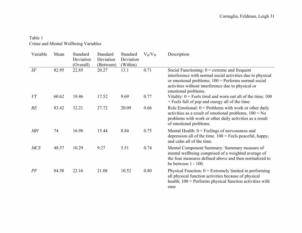
The top panel of Table 1 provides definitions of the lowest and highest possible scores of
the four SF-36’s mental health scales and reports the means and standard deviations of each of
the measures. Most of the variation in the data is cross sectional, though, roughly a quarter of
the variation is within an individual over time.
B. Data on Crime
Cornaglia, Feldman, Leigh 10
!
Local area crime statistics are tabulated at the Local Government Area (LGA) level.
LGAs in Australia are the third and lowest tier of government, administered by the states and
territories, which, in turn, are beneath the Commonwealth or federal tier. Unlike the US or the
UK, there is only one level of local government in all states, with no distinction such as counties
and cities. We separately approached each state and territory government to request crime data.
In some cases, this involved filing requests under the relevant Freedom of Information Acts,
although these really served only to prompt the relevant data-holders, and ultimately none of the
data were obtained in this manner. Eventually, we were able to obtain data for seven of the eight
states and territories, covering 99 percent of the Australian population. Since the states do not
apply a uniform crime classification system, we recoded crimes into 16 categories using the
Australian Standard Offence Classification (ASOC), though, throughout the paper, our results
are based on further aggregating these categories into violent and property crime.4
With the restricted use version of the HILDA dataset (which contains information on the
respondent’s postcode and the date of interview), we are able to match each individual to the
crime rate in their local government area during the 12 month period before answering the
questionnaire. In addition, the survey interviews individuals in each wave about whether they
have been victims of crime, which allows us to distinguish the responses of victims and
nonvictims.
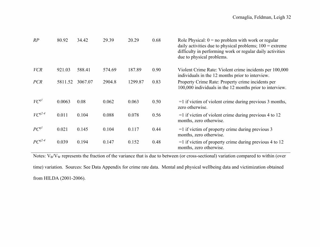
In the bottom panel of Table 1, we present summary statistics on crime rates for the years
2002 - 2006. We distinguish between property crimes and violent crimes - a distinction which
we will follow in our empirical specifications. Violent crimes include homicide, assault, sexual
assault, abduction and robbery. Property crimes include burglary and theft. Crime rates represent
the crime incidents per 100,000 individuals in Australian metropolitan areas in the 12 months
Cornaglia, Feldman, Leigh 11
!
prior to the interview date.5 As the first row shows, the average violent crime rate in our data is
921 incidents per 100,000 individuals and 90 percent of the variation in crimes rates is across
individuals that derives from differences in interview date and LGA. The remaining 10 percent is
within individual over time. Property crime shows more variation at the individual level where
17 percent derives from changes within individual over time and the remaining 83 percent
reflects cross sectional variation. While not shown in this Table, property crime fell quite
considerably over 2001-2006.6 The criminology literature has not reached a consensus on the
factors that explain this drop, though possible explanations include changes in the age structure,
shifts in heroin supply, reduced availability of firearms, and improved antitheft devices in new
motor vehicles (see, for example, Moffatt and Poynton 2006; Brickell 2008). Violent crime
shows no such pattern.
The next four rows of Table 1 present the fraction of respondents that were victimized
during the quarter before the interview and/or during the two to four quarters prior to the
interview. Roughly 0.6 percent of our observations are violent crime victimization incidents
within the previous quarter. Another 1.1 percent are victims two to four quarters before the
interview. Property crime is more prevalent with 2.1 percent of individuals having suffered a
property crime in the previous quarter and another 3.9 percent in the two to four quarters before
the interview. The identifying variation for these variables is roughly equally divided between
cross-section and time and the crime rate from these self-reported surveys is of a similar
magnitude to police-reported crime rates.
C. Data on Individual Characteristics
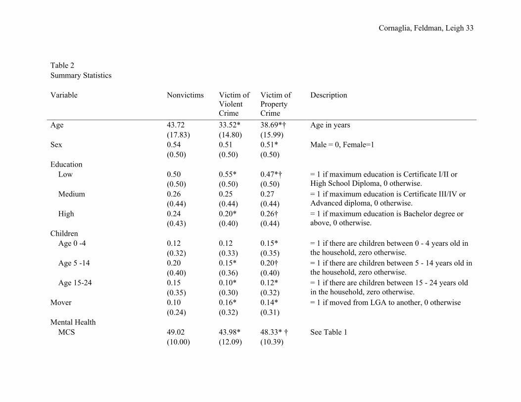
In Table 2 we summarize the individual characteristics of the respondents in our data,
where we report in the first column means and standard deviations for individuals in the sample
Cornaglia, Feldman, Leigh 12
!
that are never victimized. We then distinguish between those who are victims of violent or
property crime (not necessarily mutually exclusive) at some point during 2001 - 2006. For the
last two columns, all demographic and mental health measures apply to pre-victimization
periods, that is, using only the data prior to becoming a victim as we consider mental health
endogenous to victimization status.
The Table entries suggest that, generally speaking, nonvictims and victims differ on a
number of dimensions. Nonvictims are more likely to be older, have children between 5 - 24 and
are less likely to move out of their LGA. When breaking victims down into violent and property
it becomes clearer that victims of violent crimes differ much more from nonvictims than do
victims of property crimes. This is particularly true for the mental wellbeing variables. Victims
of violent crimes have, on average, lower mental wellbeing. We can also see that there are
significant differences between the two types of victims. Victims of violent crimes are younger,
less educated, have fewer children and lower mental and physical wellbeing than victims of
property crimes. This table illustrates the importance of controlling for demographics in the
empirical analysis as well as focusing on changes in mental health rather than cross-sectional
differences.
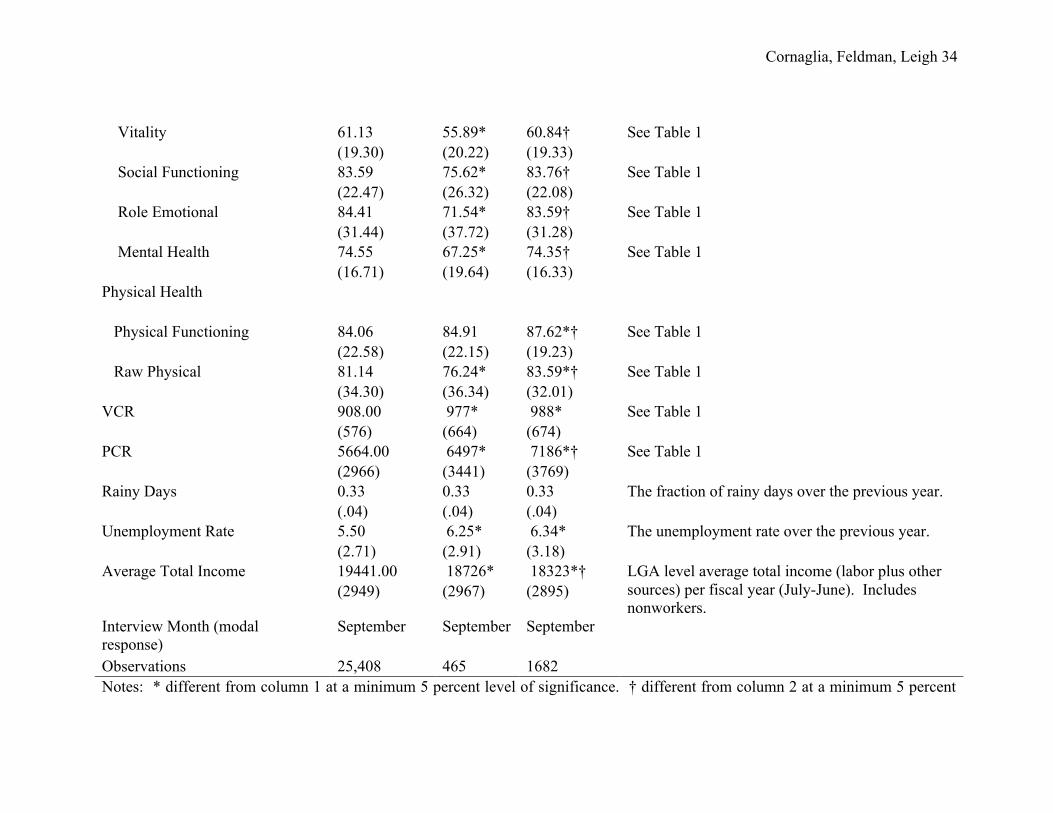
Our analysis also accounts for other time-varying characteristics known to affect mental
wellbeing: the local area unemployment rate, local area average total income, and the share of
rainy days. The unemployment rate is included in order to capture the possibility that local
economic booms or busts may affect both crime and mental wellbeing (see, for example,
Kapuscinski, Braithwaite, and Chapman 1998; Raphael and Winter Ebmer 2001). Average
incomes may capture degrees of financial stress as well as being correlated with crime. Finally,
the number of rainy days is included on the basis that good or bad weather may have a direct
Cornaglia, Feldman, Leigh 13
!
impact on both crime and mental wellbeing (see, for example, Cohn 1990; Jacob, Lefgren, and
Moretti 2007). The unemployment rate and rainy days are measured over the same period as the
crime rate (the 12 months prior to the interview) whereas average income is measured over the
calendar year due to data availability.7 As Table 2 shows, both property and violent crime
victims live in LGAs with higher unemployment, lower average earnings, and higher violent and
property crime rates.
IV. Empirical Methodology
In our analysis, we concentrate on individuals living in metropolitan Australia, such as
Sydney, Melbourne, and Canberra as nearly all variation in crime rates is derived from urban
areas. Since Australians mainly live in cities, by restricting the analysis to metropolitan areas, we
use around 67 percent of the overall Australian population and 63 percent of our data. The
typical respondent in our survey lived in an LGA with a population of approximately 215,000
people (the interquartile range is 95,000 to 945,000 people). The total number of LGAs in our
analysis is 110.
Our estimation equation is given by
(1)
where is the mental wellbeing index of individual in area in interview year .
and are binary indicators equal to one, zero otherwise, if individual has been a
victim of a violent or property crime during the quarter (3 months) prior to the interview. Thus,
while both the mental health index and the victimization variables are both indexed by time , it
irtritrtitirtirt
qirt
qirt
qirt
qirtirt
LGATZXPCRVCRPCPCVCVCM
εαγγββ
ββββα
++++++++
++++
%%
−−
2165
424
13
422
110=
irtM i r t
1qVC 1qPC i
t
Cornaglia, Feldman, Leigh 14
!
should be clear that there is a built in lag for the victimization variables, crime and other relevant
variables. Similarly, and are binary indicators equal to one if the individual has
been a victim of a violent or property crime two to four quarters prior to the interview,
respectively. We view and as capturing the more immediate impacts of victimization
whereas and capture longer run results. The variables and
represent the violent and property crime rates in the 12 months prior to the interview date.
are individual characteristics as previously described: age, age squared, sex, education, number
of children and binary indicators for month of interview, consists of the LGA level time
varying characteristics of the number of rainy days, the unemployment rate and the log of
average earnings. , and represent time, individual and area fixed effects,
respectively and represents the idiosyncratic error term.8 Our preferred estimation is by
individual fixed effects estimation and standard OLS is provided for comparison. Standard errors
are clustered by LGA.9
V. Results
A. Victimization
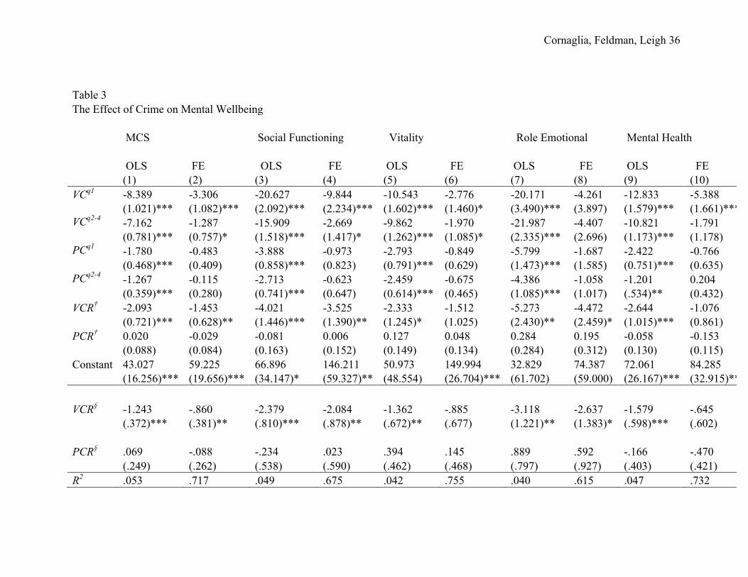
Table 3 presents the results for each of the five measures of mental wellbeing. The odd
numbered columns present results from the OLS models and the even numbered columns present
the individual fixed effects models. Consider the first row. Generally speaking, the estimates
show that victimization within a quarter prior to interview is strongly and significantly related to
a deterioration of mental wellbeing for all mental categories we consider here. For instance, to
have been a victim of a violent crime is associated with a mental health outcome (measured by
the Mental Component Summary Measure - MCS) that is about 8.4 percentage points (or 19
42−qVC 42−qPC
1qVC 1qPC
42−qVC 42−qPC irtVCR irtPCR
itX
Z
tT iα rLGA
irtε
Cornaglia, Feldman, Leigh 15
!
percent when evaluated at the mean ) lower in the OLS specification and 3.3 percentage points
(or 7.5 percent when evaluated at the mean) lower in the fixed effects specification. The OLS
estimates are likely biased as victims of crime are arguably a selected subgroup with larger
mental health issues. The estimated associations of crime with the four mental health scales that
make up the mental component summary measure (Vitality, Role Emotional, Social Functioning
and Mental Health) are generally even larger (columns 3 - 10). All results are significant at the
one percent level with the exceptions of Vitality (FE specification) that is significant at the ten
percent level and Role Emotional (FE specification) that is not statistically significant. In
particular, focusing on the fixed effects specifications, the effects of victimization are largest for
social functioning where the reduction is 9.8 percentage points (or about 13 percent) in the
quarter after victimization. According to literature in psychology, the largest impact of
victimization on mental health is reflected in the tendency of victims towards avoidance (see for
instance Kilpatrick and Acierno 2003). This may be in the form of behavioral or cognitive escape
from thoughts, feelings, individuals, or places associated with the trauma, as well as the
experience of feelings of detachment, and restricted affect. This tendency towards increased
avoidance is in our data best captured by the social functioning measure of mental wellbeing.
This scale tells us how well the victim can perform normal social activities without interference
due to emotional problems.
The longer run impacts of victimization are less straightforward. Focusing on the FE
specifications in the second row (victim of violent crime in 4 - 12 months before the interview
date), at best the results are significant at 10 percent and are fairly smaller in magnitude than the
corresponding coefficient in the row above. For example, the estimated coefficient for MCS
(column 2) drops from -3.3 percentage points to -1.3 percentage points. These results suggest
Cornaglia, Feldman, Leigh 16
!
that violent crime victimization has an immediate impact on mental health that is fairly large but
this impact dissipates fairly quickly after a quarter. One particularly interesting result is that
mental health (column 8) is the one measure that is significant in the quarter prior to interview
but not in the 4 - 12 months prior to interview, conditional on the former being significant. Based
on this, it appears that feelings of depression (what the Mental Health measure captures) are
shorter lived that those areas of mental wellbeing that involve interaction with society (aspects of
which the three remaining measures capture).
In contrast to the violent crime victimization results, the effect of being a victim of a
property crime on mental wellbeing is smaller across all specifications and statistically weaker.
Once we control for individual fixed effects, there is no statistically significant impact of being a
victim of a property crime on mental wellbeing. This holds for both the immediate quarter prior
to interview as well as longer lags.
B. Interpretation of the Magnitudes
Overall, the effect of violent crime victimization on mental wellbeing is fairly large when
we compare it to other events that impact mental wellbeing that we included as controls in our
regressions. For example, the effect of accomplishing a low level of education10 is associated
with 1.03 percentage points (unreported) lower MCS compared to those who achieve at least a
bachelor degree–roughly one-third the impact of violent crime victimization. If the number of
rainy days were to increase from zero to 100 percent, MCS would be estimated to be 1.86
percentage points lower (unreported)–still only just more than half the impact of violent crime
victimization in the previous quarter. Another way of conceptualising the size of the effects we
observe is to compare them with the impact on mental wellbeing for New Yorkers of being
explosed to the September 11 attacks. Comparing our results with those of that of Adams and
Cornaglia, Feldman, Leigh 17
!
Boscarino (2005), we estimate that the effect of falling victim to a violent crime is 2 1/2 times
larger than each unit increase in exposure to the September 11 attacks on New York City.11
C. Crime Rates
We next consider the impact of crime rates on mental wellbeing. Violent crime rates
show a fairly consistent and robust negative effect on mental wellbeing (with the exceptions of
the fixed effects estimations for Vitality and Mental Health). An increase of one unit in the crime
rate (equivalent to one more victim in an LGA with population of 100,000) is associated with a
.0021 and .0015 percentage point decline in MCS in the OLS and fixed effects specifications,
respectively.12 Overall, the OLS results are larger with higher statistical significance. Again, this
difference may be partially explained by sorting. Individuals may sort according to their mental
well-being and this may be correlated with area characteristics such as crime rates. If we treat
this problem as simply one that affects the levels of mental wellbeing then controlling for
individual and LGA fixed effects will correct the endogeneity problem.13 In contrast to these
results, the effect of property crime on mental health is economically and statistically zero.
For an alternative interpretation of the crime rate results, we calculated the normalized
versions of the crime rates and used those instead of the level crime rates in a regression where
all other variables remained the same. The estimated results of the two crime rate variables are
presented below the line. As is expected, statistical significance is not impacted by the
transformation but the normalization allows us to measure the impact of a one standard deviation
change in the crime rates on mental wellbeing. Increasing the crime rate by one standard
deviation is associated with .86 percentage points lower MCS (column 2), 2.08 percentage points
lower Social Functioning (column 4), and 2.64 percentage points lower Role Emotional (column
8). We calculate that a two standard deviation increase in the violent crime rate has roughly the
Cornaglia, Feldman, Leigh 18
!
same effect on MCS over the course of a year as does violent crime victimization (where we
calculate the effect of violent crime victimization over the course of a year as the weighted
average of the two estimated victimization coefficients). As before, property crime shows no
such similar impact on mental wellbeing.
Finally, we note that we also estimated an expanded model where we allowed the effect
of crime rates on mental wellbeing to differ between victims and nonvictims (by including
interaction terms). The results across the board showed that the estimated coefficients on the
interaction effects were economically small and not statistically significant at conventional
levels.14 Thus, after conditioning on victimization status, we do not reject the hypothesis that
crime rates themselves impact the mental health of victims and nonvictims alike.
VI. Extensions of the Baseline Model and Robustness Tests
Crime rates are defined at the local government area but due to heterogeneity in the
geographic size of LGAs, one may imagine that the impact of crime rates may very well depend
upon variation within an LGA. More precisely, the crime rate in a LGA captures the average of
crime rates in smaller neighborhoods within the LGA. The larger the geographic size of the
LGA, the more the average may be less representative of the actual crime rate where a person
lives. Thus, LGA level crime rates may not reflect the reality of day-to-day existence for an
individual as the size of the LGA grows. A literature in psychology has stressed the important
role played by the perception of the level of violence on mental health. Building upon this,
sociological literature has stressed that in order to understand the effect of the fear of crime on
anxiety it is not enough to know who individuals are (looking at observable characteristics) but,
rather, to account for the characteristics of the area where they live (Pain 2000; Smith 1987).
Cornaglia, Feldman, Leigh 19
!
Due to data constraints, we cannot capture the within-LGA variation in “very” local
crime rates. However, under the assumption that smaller LGAs are likely to have less internal
variance in crime rates we can break the data into two groups–those below the median LGA size
and those above. Doing this, we repeated our fixed effects analysis for each of the five mental
wellbeing measures with results presented in Table 4. The table reveals an interesting pattern.
When we consider the first five columns (below median area), the statistically significant
negative effect of victimization on mental health that we saw in Table 3 nearly completely
disappears. The one exception is social functioning where the effect is negative and significant at
the five percent level for victimization in the previous quarter (column 2, row 1). On the other
hand, the second five columns (above median area) show an effect of victimization on mental
wellbeing that is comparable to that found in Table 3. We hypothesize that larger geographical
areas may make residents feel artificially safe even conditional on the crime rate. Because
residents may mentally minimize the true risks of victimization, when it does occur the effect is
particularly acute. This being said, while there appears to be noticeable statistical difference
between LGAs above and below the median size, many of the point estimates are similar in
magnitude. We tested whether each estimated coefficient in the “Below Median” regressions
(columns 1-5) was statistically different from its counterpart in the “Above Median” regressions
(columns 6-10). For the most part, there is no statistical difference between the coefficients with
the exception of the estimated coefficients on the violent crime victimization two to four quarters
prior to the interview ( ) variables and similarly for property crime victimization (
) for MCS and Social Functioning.
Turning next to crime rates in the same Table, violent crime rates show the opposite
pattern of victimization. While the statistical significance is a bit weaker as compared to Table 3,
42−qVC 42−qPC
Cornaglia, Feldman, Leigh 20
!
crime rates in smaller LGAs have negative impacts on mental wellbeing whereas they do not
appear to impact mental wellbeing in larger LGAs. This is consistent with hypothesis that the
crime rates for a larger LGA may be weakly correlated with the true neighborhood crime rate in
which the individual lives. In contrast to Table 3, property crime victimization shows some
impact on mental wellbeing in relatively large geographic areas where MCS and three of the four
primary measures are negatively impacted. Again, this may be because residents in larger
geographic areas mentally downplay the risks (or do not believe that actual crime rates apply to
their “very” local area). Property crime rates, alternatively, continue to show no association with
mental wellbeing. Similar to the victimization variables, there is no statistical difference in the
estimated coefficients above and below the median.
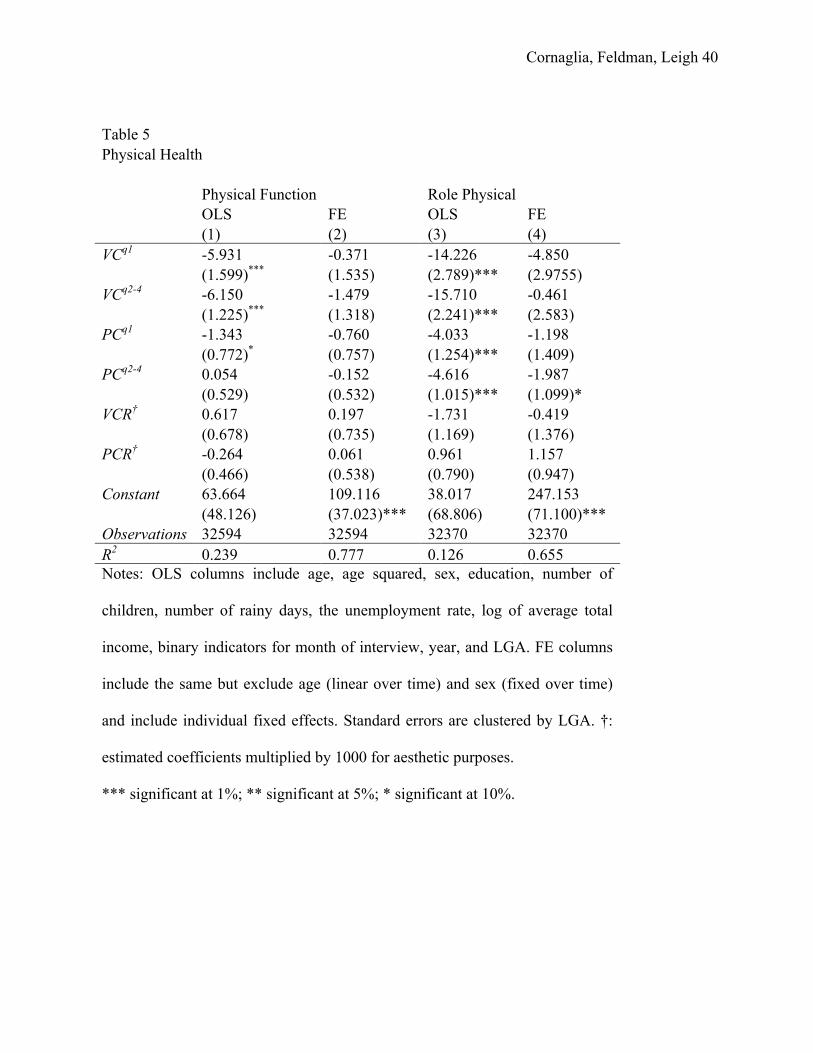
Next, as a placebo test, we repeated our baseline specification using two physical health
measures that we obtained from the SF-36. These are Physical Function and Role Physical (see
Table 1 for definitions).15 The results are reported in Table 5. The even columns (OLS) show that
victimization–both violent and property–is associated with lower physical wellbeing, though,
like mental wellbeing, it is likely that those individuals with lower physical ability are more
likely to become victims. Controlling for individual fixed effects, the odd numbered columns
show that there is no impact of victimization on physical wellbeing. While it may be somewhat
surprising that a violent attack has no effect on physical wellbeing, we note that the types of
activities that comprise the Physical Function and Role Physical measures are fairly basic in
nature. For example, the ability to lift a bag of groceries, bend at the knee or difficulty
performing work due to physical reasons. In line with our expectations, there is no correlation
between violent and property crime rates and physical wellbeing.
Cornaglia, Feldman, Leigh 21
!
Finally, we investigated whether there is any spillover effect on other household
members. That is, when one person in the household is victimized, how does this impact the
other family members? We find that there is a negative impact but statistical significance is
generally weak (unreported but available upon request.)16
VII. Threats to Identification
There are a number of issues that challenge our identification assumptions. One such
challenge is omitted variable bias. If a deterioration in socioeconomic conditions leads to an
increase in crime, we may be attributing decreases in mental wellbeing to increases in crime
when, more accurately, they are due in large part to these broader socioeconomic changes. One
way to address this concern is to allow for a more flexible time trend at the LGA level. While
this solution addresses the identification concern for the effect of victimization, it is less
satisfactory for the crime rate variables. Because the crime rate variables capture LGA level
crime rates in the 12 month prior to interview we technically have additional variation within the
LGA-year because individuals were interviewed at different months during the year. Thus, two
individuals, both living in the same LGA in year but interviewed in different months during
year will have different crime rates. Given that crime rates do not vary a great deal within such
short time spans (and that most respondents are interviewed at the same time of the year) the
additional variation it provides at the LGA-year level is relatively minor and likely insufficient to
identify the effect of crime rates on mental wellbeing once controlling for LGA-year fixed
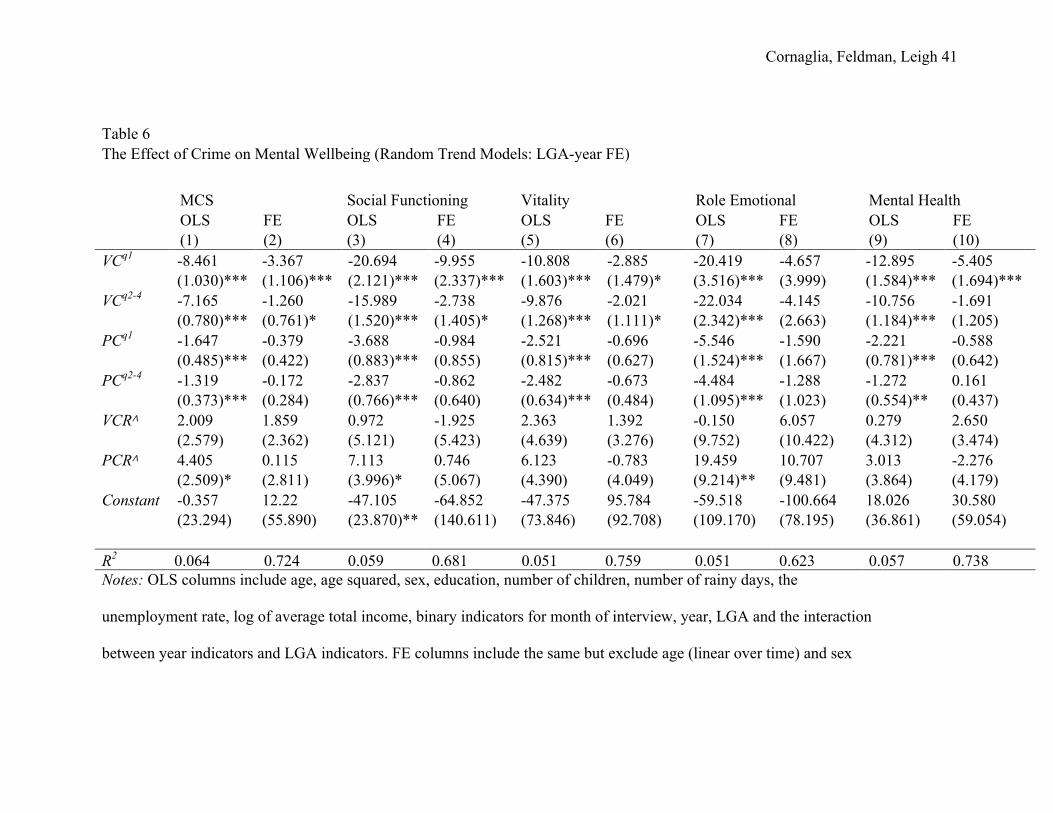
effects. The results from this specification are provided in Table 6. Broadly speaking, the effect
of violent crime victimization in the quarter prior to interview is negative and robust across the
various mental wellbeing measures (consistent with the results in Table 3). With the exception of
Vitality and Role Emotional, all FE estimates are statistically significant at a minimum
t
t
Cornaglia, Feldman, Leigh 22
!
significance level of one percent. The lagged victimization variable shows a weaker effect,
though significant at the ten percent level, in a number of the FE specifications. Property crime
victimization, like in Table 3, shows no significant impact on mental wellbeing once controlling
for individual fixed effects.
As anticipated, the property and violent crime rate variables show virtually no
significance. Due to the weak variation once controlling for LGA-time fixed effects, little weight
should be placed on these latter findings. While we attempt to control for a number of these
socioeconomic changes at the LGA-year level in our baseline model, such as number of rainy
days, unemployment rates and average incomes in our baseline specifications, we acknowledge
that it is difficult to account for all relevant changes in socioeconomic conditions and these may
be correlated with crime rates. If exogenous shocks (which are not captured in our
socioeconomic controls) cause mental wellbeing to fall and crime to rise then our estimated
coefficients on crime may be downward biased, that is, we are attributing too large of a negative
impact to crime. Conversely, if exogenous changes in crime affect mental wellbeing via one of
our controls (eg. by raising unemployment or lowering income), then we may be failing to
capture part of the negative impact of crime on mental wellbeing.
A second identification concern is that of reverse causality. One could imagine that given
some negative shock to mental health the probability of becoming a victim may increase. Thus,
what we estimate as crime’s affect on mental health is simply capturing this reverse causality
between victimization and mental health. Given the discrete nature of our data, we cannot
completely eliminate this alternative explanation.17 Nonetheless, there are tests that we can
undertake to alleviate some of the concern that reverse causality is a primary driver of our
findings. Table 7 presents the results from a regression of our mental wellbeing measures on
Cornaglia, Feldman, Leigh 23
!
binary indicators for a two-year window around the year of victimization (violent crime). The
omitted category in this case is the year prior to victimization. In particular, we are concerned
that prior to victimization there is a dip down in mental health. We can see from the results in the
first row of the Table that there is no statistical difference between years and
suggesting that mental wellbeing is not significantly lower just prior to victimization. Moreover,
this Table also shows that there is a fairly robust and large statistical difference between the year
prior to and the year of ( ) victimization. We interpret this as the impact of victimization.
Subsequent years show some rebound in mental health, where we no longer reject equality
between the year prior to victimization and the one or two years after.18
In a similar vein, we estimated the effect of changes in mental health on the probability of
violent crime victimization in the subsequent year. The results (unreported, but available upon
request) do not indicate any correlation between changes in mental health in year and violent
crime victimization in .19
VIII. Discussion
In this paper we investigate the effects area crime may have on both victims and
nonvictims of crime. As we discuss in the Introduction, the difference between direct
victimization costs and WTP to reduce crime suggests that most of the social cost of crime is
suffered by nonvictims. We now quantify the mental wellbeing cost to the victim and society at
large in monetary terms. We start with asking how much do victims need be compensated in
order to return their mental wellbeing to the levels prior to victimization and, likewise,
nonvictims for the increased crime rate that impacts the probability of future victimization.20 In
order to obtain this information we first converted the SF-36 data into an SF-6D health state for
2= −t 1= −t
0=tVC
t
1+t
Cornaglia, Feldman, Leigh 24
!
each observation in our dataset using an algorithm based on Brazier and Roberts (2004) adapted
to HILDA by researchers at Monash University.21 The SF-6D is a generic preference-based
single index measure of health that can be used to generate QALYs and, hence, can be used in
cost-utility analysis. We then multiplied the SF-6D measure by $50,000, which is the rough
estimate given to the “value of a high-quality life" in Australia and estimate that each percentage
point loss in Social Functioning is worth $211 (se 0.98).22 Taking our baseline results from
column 4 of Table 3, the percentage point loss in Social Function over the year is equal to -4.59
(s.e. 1.03) for victims and -0.0035 (se 0.0014) for nonvictims.23 That is, the average nonvictim
living in an LGA with a population of 100,000 experiences a decline of 0.0035 percentage points
in Social Functioning with a one victim increase in the crime rate. Using these estimates, we can
calculate the amount of income that would be necessary to compensate the victim as well as the
rest of society for the increase in crime rate. We bootstrap the estimation procedure using 1000
bootstrap replications to take into account the uncertainty in the previous estimates. We estimate
an ex post monetary loss to a victim of $928 (se $287) and an ex ante amount society would pay
to reduce crimes by one of $76,583 (se $29,534) – roughly 80 times the ex post cost to the
victim. In line with Cook and Ludwig (2000), we call this the “value of a statistical victim” – the
amount society would sacrifice to reduce the number of victims by one person and maintain
mental wellbeing at its previous level.
We also point out that total nonvictim compensation is independent of the number of
victims and population. LGAs with larger populations will tend to have per victim amounts that
are lower (because increasing the number of victims by one has a smaller impact on the overall
crime rate and therefore a lower impact on mental wellbeing) but these lower amounts are then
multiplied by larger population values. The opposite is true for low population LGAs. Increasing
Cornaglia, Feldman, Leigh 25
!
the number of victims by one has a much larger impact on the crime rate and a larger negative
impact on mental wellbeing. These larger numbers, however, are then multiplied by a smaller
population number.
IX. Conclusion
In this paper, we combine detailed crime statistics with panel survey data that provides a
detailed set of mental wellbeing indicators for the same individuals over a six-year period. We
find that even when controlling for individual and local area fixed effects, an individual suffers a
decrease in mental wellbeing in the immediate three months after violent crime victimization
occurs. This effect is fairly robust across the numerous mental wellbeing measures and ranges
between 2.8 to 9.8 percentage points with the strongest effect on social functioning–the ability to
perform normal social activities without emotional problems. The effect generally remains, but is
economically and statistically weaker, when we measure the impact of victimization in the four
to 12 months prior to interview. Likewise, the violent crime rate has a negative impact on mental
wellbeing for both victims and nonvictims with the largest effect again on social functioning.
Property crime victimization, alternatively, shows no statistically significant impact on mental
wellbeing once controlling for individual fixed effects. Nor does the property crime rate. As a
placebo test, we replace our mental health measures with physical health measures and find no
impact of victimization and crime rates on physical wellbeing once controlling for individual
fixed effects. Moreover, we subject our main findings to a number of robustness tests and resolve
that neither reverse causality nor omitted variables are the likely drivers of our main findings.
The impact of victimization and crime rates also vary by geographic size of the area. Our
baseline victimization results are driven primarily by larger local areas. We hypothesize that
larger geographical areas may make residents feel artificially safe even conditional on the crime
Cornaglia, Feldman, Leigh 26
!
rate. Because residents may mentally minimize the true risks of victimization, when it does occur
the effect is particularly acute. Interestingly, violent crime rates show the opposite pattern of
victimization. While the statistical significance is a bit weaker, crime rates in smaller LGAs have
negative impacts on mental wellbeing whereas they do not appear to impact mental wellbeing in
larger LGAs. This is consistent with the hypothesis that crime rates in larger LGAs may be
weakly correlated with the true neighborhood crime rate in which the individual lives.
Finally, we estimate that the average victim requires compensation of about $930
Australian Dollars (AUD) and that all local area residents place ex ante negative valuation on
mental wellbeing of about $76,600 from the increase in the crime rate due to one additional
victim. Thus, society wide level compensation is about 80 times more than the direct impact on
the victim herself.
X. References
Adams, Richard, and Joseph Boscarino. 2005. “Stress and Well-Being in the Aftermath
of the World Trade Center Attack: the Continuing Effects of a Communitywide Disaster.”
Journal of Community Psychology 33(2): 175-190.
Aneshensel, Carol, and Clea Sucoff. 1996. “The Neighborhood Context of Adolescent
Mental Health.” Journal of Health and Social Behavior 37: 293-310.
Bentham, Jeremy. 1781 (1996). An Introduction to the Principles of Morals and
Legislation, ed. J.H. Burns and H.L.A. Hart. Oxford: Clarendon Press.
Brazier, John E, and Jennifer Roberts. 2004. “The Estimation of a Preference-Based
Measure of Health from the SF-12.” Medical Care 42: 851-859.
Brickell, Samantha. 2008. “Trends in Violent Crime.” Trends and Issues in Crime and
Criminal Justice. No. 359, Canberra: Australian Institute of Criminology.
Cornaglia, Feldman, Leigh 27
!
Cohn, Ellen. 1990. “Weather and Crime.” British Journal of Criminology. 30: 51-64.
Cook, Philip J, and Jens Ludwig. 2000. Gun Violence: the Real Costs. New York:
Oxford University Press.
Cornaglia, Francesca, and Andrew Leigh. 2011. “Crime and Mental Wellbeing.” CEP
Discussion Paper 1049.
Failde, Inmaculada, Ramos, I, and Fernando Fernandez-Palacin. 2000. “Comparison
Between the GHQ-28 and SF-36 (MH 1-5) for the Assesement of the Mental Health in Patients
with Ischaemic Heart Disease.” European Journal of Epidemiology 16(4): 311-316.
Frijters, Paul, David Johnston, and Michael Shields. 2010. “Mental Health and Labour
Market Participation: Evidence from IV Panel Data Models.” IZA Discussion Paper 4883.
Gibbons, Stephen. 2004. “The Costs of Urban Property Crime.” The Economic Journal
114(499): F441-F463.
Green, Geoff, Jan Gilbertson, and Michael Grimsley. 2002. “Fear of Crime and Health in
Residential Tower Blocks.” European Journal of Public Health 12: 10-15.
Guite, Hillary, Charlotte Clark, and Gill Ackrill. 2009. “The Impact of the Physical and
Urban Environment on Mental Well-being.” Public Health 120(12): 1117-1126.
Jacob, Brian, Lars Lefgren, and Enrico Moretti. 2007. “The Dynamics of Criminal
Behavior: Evidence from Weather Shocks.” Journal of Human Resources 42(3): 489-527.
Kapuscinski, Cezary, John Braithwaite, and Bruce Chapman. 1998. “Unemployment and
Crime: Toward Resolving the Paradox.” Journal of Quantitative Criminology 14(3): 215-243.
Katz, Lawrence, Jeffrey Kling, and Jeffrey Liebman. 2001. “Moving To Opportunity In
Boston: Early Results Of A Randomized Mobility Experiment.” Quarterly Journal of
Economics 116(2): 607-654.
Cornaglia, Feldman, Leigh 28
!
Kesteren van, John, Pat Mayhew, and Paul Nieuwbeerta. 2000. “Criminal Victimisation
in Seventeen Industrialised Countries: Key Findings from the 2000 International Crime Victims
Survey.” The Hague: Ministry of Justice, WODC. Onderzoek en beleid, nr. 187.
Kilpatrick, Dean, and Ron Acierno. 2003. “Mental Health Needs of Crime Victims:
Epidemiology and Outcomes.” Journal of Traumatic Stress 16(2): 119-132.
Kling, Jeffrey, Jeffrey Liebman, and Lawrence Katz. 2001. “Bullets Don’t Got No Name:
Consequences of Fear in the Ghetto.” Joint Center on Poverty Research, Working Paper 225.
__________, Jeffrey Liebman, Lawrence Katz, and Lisa Sanbonmatsu. 2004. “Moving to
Opportunity and Tranquility: Neighborhood Effects on Adult Economic Self-Sufficiency and
Health from a Randomized Housing Voucher Experiment.” Kennedy School of Government
Working Paper No. RWP04-035.
Linden, Leigh, and Jonah Rockoff. 2008. “Estimates of the Impact of Crime Risk on
Property Values from Megan’s Laws.” American Economic Review 98(3): 1103–1127.
Moffatt, Steve, and Suzanne Poynton. 2006. “Long-term Trends in Property and Violent
Crime in New South Wales: 1990-2004." Crime and Justice Bulletin No 90, Sydney: NSW
Bureau of Crime Statistics and Research.
Pain, Rachel. 2000. “Place, Social Relations and the Fear of Crime: a Review.” Progress
in Human Geography 24(3): 365-387.
Propper, Carol, Simon Burgess, Anne Bolster, George Leckie, Kelvyn Jones, and Ron
Johnson. 2006. “The Impact of Neighbourhood on the Income and Mental Health of British
Social Renters.” Bristol: University of Bristol, Centre for Market and Public Organisation
Working Paper No. 06/161.
Cornaglia, Feldman, Leigh 29
!
Räsänen, Pirjo, Eija Roine, Harri Sintonen, Virpi Semberg-Konttinen, Olli-Pekka
Ryynänen, and Risto Roine. 2006. “Use of Quality-adjusted Life Years for the Estimation of
Effectiveness of Health Care: A Systematic Literature Review.” International Journal of
Technology Assessment in Health Care 22: 235-241.
Raphael, Stephen, and Rudolph Winter Ebmer. 2001. “Identifying the Effect of
Unemployment on Crime.” Journal of Law and Economics 44(1): 259-283.
Ross, Catherine. 2000. “Neighborhood Disadvantage and Adult Depression.” Journal of
Health and Social Behavior 41: 177-187.
__________, and John Mirowsky. 2001. “Neighborhood Disadvantage, Disorder, and
Health." Journal Health Social Behaviour 42: 258-276.
Roy, John, and Stefanie Schurer. 2012. “Getting Stuck in the Blues: Persistence of
Mental Health Problems and Health Care Utilisation.” Wellington: Working Paper, Victoria
University of Wellington.
Schulz, Amy, David Williams, Barbara Israel, Adam Becker, Edith Parker, Sherman
James, and James Jackson. 2000. “Unfair Treatment, Neighborhood Effects, and Mental Health
in the Detroit Metropolitan Area.” Journal of Health and Social Behavior 41(3): 314-332.
Schwartz, Amy Ellen, Scott Susin, and Ioan Voicu. 2003. “Has Falling Crime Driven
New York City’s Real Estate Boom?” Journal of Housing Research 14(1): 101-135.
Smith, Susan J. 1987. “Fear of Crime: Beyond a Geography of Deviance”, Progress in
Human Geography 11: 1-23.
Strafford, Mai, Tarani Chandola, and Michael Marmot. 2007. “Association Between Fear
of Crime and Mental Health and Physical Functioning.” American Journal of Public Health
97(11): 2076-2081.
Cornaglia, Feldman, Leigh 30
!
__________, and Michael Marmot. 2003. “Neighbourhood Deprivation and Health: Does
it Affect Us All Equally?” International Journal of Epidemiology 32(3): 357 - 366.
Thaler, Richard. 1978. “A Note on the Value of Crime Control: Evidence from the
Property Market.” Journal of Urban Economics 5(1): 137-145.
Ware, John, Mark Kosinski, and Susan Keller. 1994. “SF-36 Physical and Mental Health
Summary Scales: A User’s Manual.” Boston, MA: The Health Institute.
Wolff, Jonathan. 2005. “What’s So Bad About Crime?” Bentham Lecture, University
College London, 30 November.
Cornaglia, Feldman, Leigh 31
!
Table 1 Crime and Mental Wellbeing Variables Variable Mean Standard
Deviation (Overall)
Standard Deviation (Between)
Standard Deviation (Within)
VB/VW Description
SF 82.95 22.85 20.27 13.1 0.71 Social Functioning: 0 = extreme and frequent interference with normal social activities due to physical or emotional problems; 100 = Performs normal social activities without interference due to physical or emotional problems.
VT 60.62 19.46 17.52 9.69 0.77 Vitality: 0 = Feels tired and worn out all of the time; 100 = Feels full of pep and energy all of the time.
RE 83.42 32.21 27.72 20.09 0.66 Role Emotional: 0 = Problems with work or other daily activities as a result of emotional problems, 100 = No problems with work or other daily activities as a result of emotional problems.
MH 74 16.98 15.44 8.84 0.75 Mental Health: 0 = Feelings of nervousness and depression all of the time. 100 = Feels peaceful, happy, and calm all of the time.
MCS 48.57 10.29 9.27 5.51 0.74 Mental Component Summary: Summary measure of mental wellbeing comprised of a weighted average of the four measures defined above and then normalized to be between 1 - 100.
PF 84.58 22.16 21.08 10.52 0.80 Physical Function: 0 = Extremely limited in performing all physical function activities because of physical health; 100 = Performs physical function activities with ease
Cornaglia, Feldman, Leigh 32
!
RP 80.92 34.42 29.39 20.29 0.68 Role Physical: 0 = no problem with work or regular daily activities due to physical problems; 100 = extreme difficulty in performing work or regular daily activities due to physical problems.
VCR 921.03 588.41 574.69 187.89 0.90 Violent Crime Rate: Violent crime incidents per 100,000
individuals in the 12 months prior to interview. PCR 5811.52 3067.07 2904.8 1299.87 0.83 Property Crime Rate: Property crime incidents per
100,000 individuals in the 12 months prior to interview. VCq1 0.0063 0.08 0.062 0.063 0.50 =1 if victim of violent crime during previous 3 months,
zero otherwise. VCq2-4 0.011 0.104 0.088 0.078 0.56 =1 if victim of violent crime during previous 4 to 12
months, zero otherwise.
PCq1 0.021 0.145 0.104 0.117 0.44 =1 if victim of property crime during previous 3 months, zero otherwise.
PCq2-4 0.039 0.194 0.147 0.152 0.48 =1 if victim of property crime during previous 4 to 12 months, zero otherwise.
Notes: VB/VW represents the fraction of the variance that is due to between (or cross-sectional) variation compared to within (over
time) variation. Sources: See Data Appendix for crime rate data. Mental and physical wellbeing data and victimization obtained
from HILDA (2001-2006).
!!
Cornaglia, Feldman, Leigh 33
!
Table 2 Summary Statistics Variable Nonvictims Victim of
Violent Crime
Victim of Property Crime
Description
Age 43.72 33.52* 38.69*† Age in years (17.83) (14.80) (15.99) Sex 0.54 0.51 0.51* Male = 0, Female=1 (0.50) (0.50) (0.50) Education Low 0.50 0.55* 0.47*† = 1 if maximum education is Certificate I/II or
High School Diploma, 0 otherwise. (0.50) (0.50) (0.50) Medium 0.26 0.25 0.27 = 1 if maximum education is Certificate III/IV or
Advanced diploma, 0 otherwise. (0.44) (0.44) (0.44) High 0.24 0.20* 0.26† = 1 if maximum education is Bachelor degree or
above, 0 otherwise. (0.43) (0.40) (0.44) Children Age 0 -4 0.12 0.12 0.15* = 1 if there are children between 0 - 4 years old in
the household, zero otherwise. (0.32) (0.33) (0.35) Age 5 -14 0.20 0.15* 0.20† = 1 if there are children between 5 - 14 years old in
the household, zero otherwise. (0.40) (0.36) (0.40) Age 15-24 0.15 0.10* 0.12* = 1 if there are children between 15 - 24 years old
in the household, zero otherwise. (0.35) (0.30) (0.32) Mover 0.10 0.16* 0.14* = 1 if moved from LGA to another, 0 otherwise (0.24) (0.32) (0.31) Mental Health MCS 49.02 43.98* 48.33* † See Table 1 (10.00) (12.09) (10.39)
Cornaglia, Feldman, Leigh 34
!
Vitality 61.13 55.89* 60.84† See Table 1 (19.30) (20.22) (19.33) Social Functioning 83.59 75.62* 83.76† See Table 1 (22.47) (26.32) (22.08) Role Emotional 84.41 71.54* 83.59† See Table 1 (31.44) (37.72) (31.28) Mental Health 74.55 67.25* 74.35† See Table 1 (16.71) (19.64) (16.33) Physical Health Physical Functioning 84.06 84.91 87.62*† See Table 1 (22.58) (22.15) (19.23) Raw Physical 81.14 76.24* 83.59*† See Table 1 (34.30) (36.34) (32.01) VCR 908.00 977* 988* See Table 1 (576) (664) (674) PCR 5664.00 6497* 7186*† See Table 1 (2966) (3441) (3769) Rainy Days 0.33 0.33 0.33 The fraction of rainy days over the previous year. (.04) (.04) (.04) Unemployment Rate 5.50 6.25* 6.34* The unemployment rate over the previous year. (2.71) (2.91) (3.18) Average Total Income 19441.00 18726* 18323*† LGA level average total income (labor plus other
sources) per fiscal year (July-June). Includes nonworkers.
(2949) (2967) (2895)
Interview Month (modal response)
September September September
Observations 25,408 465 1682 Notes: * different from column 1 at a minimum 5 percent level of significance. † different from column 2 at a minimum 5 percent
Cornaglia, Feldman, Leigh 35
!
level of significance. Education: Certificate I/II provides basic vocational skills and knowledge (6 - 12 months of secondary
education). Certificate III/IV provides training in more advanced skills and knowledge. A Certificate IV is generally accepted by
universities to be the equivalent of six to twelve months of a Bachelor's degree, and credit towards studies may be granted
accordingly. Courses at Diploma, Advanced Diploma level take between two to three years to complete, and are generally
considered to be equivalent to one to two years of study at degree level. Source: HILDA except for crime rates, rainy days and
unemployment rate (see Data Appendix).
Cornaglia, Feldman, Leigh 36
!
Table 3 The Effect of Crime on Mental Wellbeing MCS Social Functioning Vitality Role Emotional Mental Health OLS FE OLS FE OLS FE OLS FE OLS FE
(1) (2) (3) (4) (5) (6) (7) (8) (9) (10) VCq1 -8.389 -3.306 -20.627 -9.844 -10.543 -2.776 -20.171 -4.261 -12.833 -5.388 (1.021)*** (1.082)*** (2.092)*** (2.234)*** (1.602)*** (1.460)* (3.490)*** (3.897) (1.579)*** (1.661)*** VCq2-4 -7.162 -1.287 -15.909 -2.669 -9.862 -1.970 -21.987 -4.407 -10.821 -1.791 (0.781)*** (0.757)* (1.518)*** (1.417)* (1.262)*** (1.085)* (2.335)*** (2.696) (1.173)*** (1.178) PCq1 -1.780 -0.483 -3.888 -0.973 -2.793 -0.849 -5.799 -1.687 -2.422 -0.766 (0.468)*** (0.409) (0.858)*** (0.823) (0.791)*** (0.629) (1.473)*** (1.585) (0.751)*** (0.635) PCq2-4 -1.267 -0.115 -2.713 -0.623 -2.459 -0.675 -4.386 -1.058 -1.201 0.204 (0.359)*** (0.280) (0.741)*** (0.647) (0.614)*** (0.465) (1.085)*** (1.017) (.534)** (0.432) VCR† -2.093 -1.453 -4.021 -3.525 -2.333 -1.512 -5.273 -4.472 -2.644 -1.076 (0.721)*** (0.628)** (1.446)*** (1.390)** (1.245)* (1.025) (2.430)** (2.459)* (1.015)*** (0.861) PCR† 0.020 -0.029 -0.081 0.006 0.127 0.048 0.284 0.195 -0.058 -0.153 (0.088) (0.084) (0.163) (0.152) (0.149) (0.134) (0.284) (0.312) (0.130) (0.115) Constant 43.027 59.225 66.896 146.211 50.973 149.994 32.829 74.387 72.061 84.285 (16.256)*** (19.656)*** (34.147)* (59.327)** (48.554) (26.704)*** (61.702) (59.000) (26.167)*** (32.915)**
VCR§ -1.243 -.860 -2.379 -2.084 -1.362 -.885 -3.118 -2.637 -1.579 -.645 (.372)*** (.381)** (.810)*** (.878)** (.672)** (.677) (1.221)** (1.383)* (.598)*** (.602)
PCR§ .069 -.088 -.234 .023 .394 .145 .889 .592 -.166 -.470 (.249) (.262) (.538) (.590) (.462) (.468) (.797) (.927) (.403) (.421) R2 .053 .717 .049 .675 .042 .755 .040 .615 .047 .732
Cornaglia, Feldman, Leigh 37
!
Notes: OLS columns include age, age squared, sex, education, number of children, number of rainy days, the unemployment rate, log of average
total income, binary indicators for month of interview, year, and LGA. FE columns include the same but exclude age (linear over time) and sex
(fixed over time) and include individual fixed effects. Standard errors are clustered by LGA. †: estimated coefficients multiplied by 1000 for
aesthetic purposes. §: normalized. Observations: 32,594. *** significant at 1%; ** significant at 5%; * significant at 10%.

Cornaglia, Feldman, Leigh 38
!
Table 4 The Effect of Crime on Mental Wellbeing by LGA size
MCS Social Functioning Vitality
Role Emotional
Mental Health MCS
Social Functioning Vitality
Role Emotional
Mental Health
(1) (2) (3) (4) (5) (6) (7) (8) (9) (10) VCq1 -1.723 -8.919 -2.831 -1.539 -2.474 -3.945 -9.523 -2.818 -5.512 -6.543 -2.039 (3.486)** -3.029 -7.094 -2.889 (1.250)*** (2.985)*** (1.647)* -4.663 (1.988)*** VCq2-4 1.232 1.763 -0.089 2.885 1.448 -2.759 -4.989 -3.248 -8.108 -3.963 (1.390)† (2.385)† (1.906)† (5.079)† (2.079)† (.981)*** (1.905)*** (1.471)** (3.429)** (1.548)** PCq1 -0.18 -0.807 -0.205 -2.571 -0.166 -0.656 -1.091 -1.344 -0.705 -1.223 -0.739 -1.473 -1.082 -2.024 -1.156 -0.544 -1.06 (.784)* -2.488 -0.796 PCq2-4 0.481 0.545 0.214 1.095 0.606 -0.514 -1.365 -1.252 -2.207 -0.133 (.478)† (1.174)† -0.744 -1.672 -0.679 (.301)* (.689)** (.556)** (1.225)* -0.562 VCR† -1.495 -3.776 -0.492 -6.908 -0.939 -1.219 -2.277 -1.54 -2.327 -0.872 (.877)* (2.158)* -1.525 (3.571)* -1.251 -1.03 -2.199 -1.519 -3.144 -1.508 PCR† -0.007 0.082 -0.121 0.61 -0.201 -0.086 -0.087 0.167 -0.526 0.023 -0.109 -0.212 -0.194 -0.426 -0.164 -0.178 -0.355 -0.257 -0.571 -0.258 Constant 61.797 215.338 127.894 303.276 26.834 69.513 163.669 162.535 58.432 106.157
-60.74 -139.568 -103.4 -208.632 -102.509 (21.201)***
(57.148)***
(30.096)*** -60.784
(35.666)***
Observations 12464 12464 12464 12464 12464 20025 20025 20025 20025 20025 R2 0.728 0.675 0.764 0.622 0.741 0.724 0.686 0.761 0.626 0.738
Cornaglia, Feldman, Leigh 39
!
Notes: Columns 1 - 5 use the subsample of LGAs with area below the median. Columns 6 - 10 use the subsample of LGAs with area above the
median. Fixed Effects estimation. All columns control for time variant individual characteristics (age squared, education, number of children),
LGA level variables (rainy days, unemployment rate and log of average total income) and month of interview, year, LGA, and individual fixed
effects. Standard errors are clustered by LGA. *** significant at 1%; ** significant at 5%; *significant at 10%. †represents a statistically
significant difference at a minimum 10% level between the estimated coefficients in the Below and Above Median regressions. For example, the
estimated coefficient of 1.232 in the second row of column 1 is statistically significantly different from its corresponding estimate in the second
row of column 6 of -2.759.
Cornaglia, Feldman, Leigh 40
!
Table 5 Physical Health Physical Function Role Physical OLS FE OLS FE (1) (2) (3) (4) VCq1 -5.931 -0.371 -14.226 -4.850 (1.599)*** (1.535) (2.789)*** (2.9755) VCq2-4 -6.150 -1.479 -15.710 -0.461 (1.225)*** (1.318) (2.241)*** (2.583) PCq1 -1.343 -0.760 -4.033 -1.198 (0.772)* (0.757) (1.254)*** (1.409) PCq2-4 0.054 -0.152 -4.616 -1.987 (0.529) (0.532) (1.015)*** (1.099)* VCR† 0.617 0.197 -1.731 -0.419 (0.678) (0.735) (1.169) (1.376) PCR† -0.264 0.061 0.961 1.157 (0.466) (0.538) (0.790) (0.947) Constant 63.664 109.116 38.017 247.153 (48.126) (37.023)*** (68.806) (71.100)*** Observations 32594 32594 32370 32370 R2 0.239 0.777 0.126 0.655 Notes: OLS columns include age, age squared, sex, education, number of
children, number of rainy days, the unemployment rate, log of average total
income, binary indicators for month of interview, year, and LGA. FE columns
include the same but exclude age (linear over time) and sex (fixed over time)
and include individual fixed effects. Standard errors are clustered by LGA. †:
estimated coefficients multiplied by 1000 for aesthetic purposes.
*** significant at 1%; ** significant at 5%; * significant at 10%.
Cornaglia, Feldman, Leigh 41
!
Table 6 The Effect of Crime on Mental Wellbeing (Random Trend Models: LGA-year FE)
MCS Social Functioning Vitality Role Emotional Mental Health OLS FE OLS FE OLS FE OLS FE OLS FE (1) (2) (3) (4) (5) (6) (7) (8) (9) (10) VCq1 -8.461 -3.367 -20.694 -9.955 -10.808 -2.885 -20.419 -4.657 -12.895 -5.405 (1.030)*** (1.106)*** (2.121)*** (2.337)*** (1.603)*** (1.479)* (3.516)*** (3.999) (1.584)*** (1.694)*** VCq2-4 -7.165 -1.260 -15.989 -2.738 -9.876 -2.021 -22.034 -4.145 -10.756 -1.691 (0.780)*** (0.761)* (1.520)*** (1.405)* (1.268)*** (1.111)* (2.342)*** (2.663) (1.184)*** (1.205) PCq1 -1.647 -0.379 -3.688 -0.984 -2.521 -0.696 -5.546 -1.590 -2.221 -0.588 (0.485)*** (0.422) (0.883)*** (0.855) (0.815)*** (0.627) (1.524)*** (1.667) (0.781)*** (0.642) PCq2-4 -1.319 -0.172 -2.837 -0.862 -2.482 -0.673 -4.484 -1.288 -1.272 0.161 (0.373)*** (0.284) (0.766)*** (0.640) (0.634)*** (0.484) (1.095)*** (1.023) (0.554)** (0.437) VCR∧ 2.009 1.859 0.972 -1.925 2.363 1.392 -0.150 6.057 0.279 2.650 (2.579) (2.362) (5.121) (5.423) (4.639) (3.276) (9.752) (10.422) (4.312) (3.474) PCR∧ 4.405 0.115 7.113 0.746 6.123 -0.783 19.459 10.707 3.013 -2.276 (2.509)* (2.811) (3.996)* (5.067) (4.390) (4.049) (9.214)** (9.481) (3.864) (4.179) Constant -0.357 12.22 -47.105 -64.852 -47.375 95.784 -59.518 -100.664 18.026 30.580 (23.294) (55.890) (23.870)** (140.611) (73.846) (92.708) (109.170) (78.195) (36.861) (59.054) R2 0.064 0.724 0.059 0.681 0.051 0.759 0.051 0.623 0.057 0.738 Notes: OLS columns include age, age squared, sex, education, number of children, number of rainy days, the
unemployment rate, log of average total income, binary indicators for month of interview, year, LGA and the interaction
between year indicators and LGA indicators. FE columns include the same but exclude age (linear over time) and sex

Cornaglia, Feldman, Leigh 42
!
(fixed over time) and include individual fixed effects. ∧: estimated coefficients multiplied by 1000 for aesthetic
purposes. Standard errors are clustered by LGA. Observations: 32,594. *** significant at 1%; ** significant at 5%; *
significant at 10%.
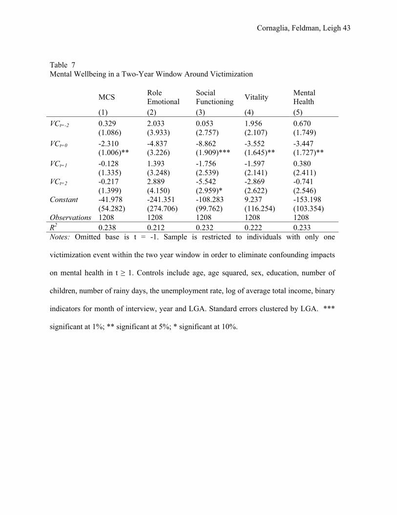
Cornaglia, Feldman, Leigh 43
!
Table 7 Mental Wellbeing in a Two-Year Window Around Victimization
MCS Role Emotional
Social Functioning Vitality Mental
Health (1) (2) (3) (4) (5) VCt=-2 0.329 2.033 0.053 1.956 0.670 (1.086) (3.933) (2.757) (2.107) (1.749) VCt=0 -2.310 -4.837 -8.862 -3.552 -3.447 (1.006)** (3.226) (1.909)*** (1.645)** (1.727)** VCt=1 -0.128 1.393 -1.756 -1.597 0.380 (1.335) (3.248) (2.539) (2.141) (2.411) VCt=2 -0.217 2.889 -5.542 -2.869 -0.741 (1.399) (4.150) (2.959)* (2.622) (2.546) Constant -41.978 -241.351 -108.283 9.237 -153.198 (54.282) (274.706) (99.762) (116.254) (103.354) Observations 1208 1208 1208 1208 1208 R2 0.238 0.212 0.232 0.222 0.233 Notes: Omitted base is t = -1. Sample is restricted to individuals with only one
victimization event within the two year window in order to eliminate confounding impacts
on mental health in t ≥ 1. Controls include age, age squared, sex, education, number of
children, number of rainy days, the unemployment rate, log of average total income, binary
indicators for month of interview, year and LGA. Standard errors clustered by LGA. ***
significant at 1%; ** significant at 5%; * significant at 10%.

Cornaglia, Feldman, Leigh 44
!
Appendix I
A. Crime Statistics
In Australia, the collation of crime statistics is a state government responsibility.
Although some data are routinely provided to the Australian Institute of Criminology, this does
not include the high-frequency, regionally disaggregated data that we use in this paper.
After repeated contact with the governments of the six states and two territories that
comprise Australia, we were able to obtain crime statistics data for all areas except the Northern
Territory. In some cases, this contact also included lodging Freedom of Information requests,
though ultimately none of the data were provided through this channel. Only Victoria required us
to pay for the data while the other states provided it free of charge. Since only 0.9 percent of
Australians live in the Northern Territory, our crime data theoretically covers 99.1 percent of the
Australian population. We are also unable to match data for a small number of observations in
our dataset, so end up with crime data for 98.7 percent of our survey sample.
In the Australian Capital Territory, New South Wales, South Australia, and Victoria,
crime data are coded by police stations on a Local Government Area (LGA) basis (the Australian
Capital Territory is a single LGA). In Tasmania, crime data are coded on a suburb basis, and
matched to postcodes using a crosswalk supplied by the Australian Bureau of Statistics. In
Western Australia, crime data are coded on by locality, and we match them to postcodes using a
crosswalk supplied by the Western Australian Police. Both suburbs (Tasmania) and localities
(Western Australia) are a finer geographic coding than postcodes.
Geographically matching crime data to regional areas is more complicated in
Queensland, whose crime data are coded to geographic areas known as Police Divisions. These
Police Divisions were then matched to LGAs for us by the Queensland Police Service. The
Cornaglia, Feldman, Leigh 45
!
Queensland crime data spanned 328 police divisions, and 128 LGAs. The Queensland Police
Service also provided information on the match quality. The median Police Division was
matched to an LGA containing 99.7 percent of its population (the mean was 91.4 percent).
In the case of Victoria, the data was confidentialized, such that cells containing between 1
and 3 crimes were replaced with an asterisk. In addition, the statistics contained data on the total
number of crimes (across all categories) for each month. Using these totals, we imputed values
for the confidentialized cells using the following procedure:
• If the total was confidentialized, assume the total was 2
• Calculate the gap between the total and the sum of the non-confidentialized cells
• Divide this gap by the number of confidentialized cells, and assign that number to
each of the confidentialized cells.
For all states and territories except the Australian Capital Territory, crime statistics are
reported on a monthly basis. For the Australian Capital Territory, data are tabulated on a
quarterly basis, and we assign the same crime rate to each month in the quarter. Criminal
incidents are classified by the date that they were reported to or detected by police. We expect
that in most cases this will correspond to the date on which the offence occurred, but we have no
way of verifying this.
Population data are drawn from the Australian Bureau of Statistics publication Regional
Population Growth (Cat No 3218.0). This provides the population for each LGA as at June in
each year. We linearly interpolate population figures for intervening months. In a small number
of cases, the ABS does not report population statistics for an LGA, but we still have crime
statistics for that area. In these instances, we assume the population is unchanged from the
Cornaglia, Feldman, Leigh 46
!
closest date for which we have population statistics. (In other words, we do not extrapolate
beyond the available population data.)
The states do not apply a uniform crime classification system. The number of different
crime categories in which the data were provided was 16 for the Australian Capital Territory, 60
for New South Wales, 87 for Queensland, 119 for South Australia, 206 for Tasmania, 27 for
Victoria, and 24 for Western Australia. We recoded crimes into 16 categories using the
Australian Standard Offence Classification (ASOC). These categories are described in Table A1.
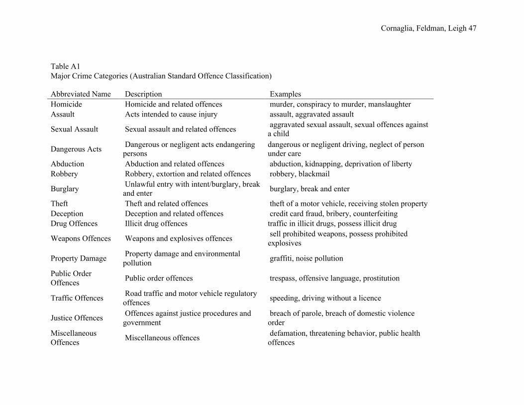
Cornaglia, Feldman, Leigh 47
!
Table A1 Major Crime Categories (Australian Standard Offence Classification) Abbreviated Name Description Examples Homicide Homicide and related offences murder, conspiracy to murder, manslaughter Assault Acts intended to cause injury assault, aggravated assault
Sexual Assault Sexual assault and related offences aggravated sexual assault, sexual offences against a child
Dangerous Acts Dangerous or negligent acts endangering persons
dangerous or negligent driving, neglect of person under care
Abduction Abduction and related offences abduction, kidnapping, deprivation of liberty Robbery Robbery, extortion and related offences robbery, blackmail
Burglary Unlawful entry with intent/burglary, break and enter burglary, break and enter
Theft Theft and related offences theft of a motor vehicle, receiving stolen property Deception Deception and related offences credit card fraud, bribery, counterfeiting Drug Offences Illicit drug offences traffic in illicit drugs, possess illicit drug
Weapons Offences Weapons and explosives offences sell prohibited weapons, possess prohibited explosives
Property Damage Property damage and environmental pollution graffiti, noise pollution
Public Order Offences Public order offences trespass, offensive language, prostitution
Traffic Offences Road traffic and motor vehicle regulatory offences speeding, driving without a licence
Justice Offences Offences against justice procedures and government
breach of parole, breach of domestic violence order
Miscellaneous Offences Miscellaneous offences defamation, threatening behavior, public health
offences
Cornaglia, Feldman, Leigh 48
!
B. Unemployment
Unemployment statistics are produced on a quarterly basis for each Statistical Local
Area (SLA) by the Department of Employment and Workplace Relations. This is the finest level
of aggregation at which we are able to obtain unemployment rate data. These estimates are based
on data from the monthly Labour Force Survey conducted by the Australian Bureau of Statistics,
adjusted using Centrelink data on the number of Newstart and Youth Allowance (Other)
recipients and Census data. The Department of Employment and Workplace Relations have
smoothed these data by averaging over four quarters.
The unemployment rate is not available for all SLAs. Where it is available in some later
months, but not earlier months, we use the later months to estimate the ratio of unemployment in
that SLA to the national unemployment rate, and multiply the national unemployment rate by
this ratio to impute missing values for earlier months. Where the unemployment rate is missing
in all quarters, we assign the national unemployment rate. In some cases, unemployment rates
are based on labor force estimates of less than 100 people. In these cases, we assume that
measurement error renders them unusable, and instead assign the unemployment rate of the
nearest SLA.
There are 932 SLAs in Australia (in many cases SLAs cover the same area as LGAs). We
match each respondent to their SLA using a crosswalk prepared by the ABS. This crosswalk
does not contain information on the proportion of the population in each postcode area who live
in the SLA.
When analyzing crime in the month or quarter of interview, we use the unemployment
rate in the quarter of interview. When analyzing the effect of crime in the previous six months,
we use the average unemployment rate over the current and previous quarter. And when
Cornaglia, Feldman, Leigh 49
!
analyzing crime in the previous twelve months, we use the average unemployment rate over the
current quarter and the previous three quarters.
C. Rain Days
Using daily data provided by the Bureau of Meteorology, and taken from weather
stations in the capital cities, we calculate the share of rain days in a given month. For example, if
some rainfall was recorded on ten days in a 30-day month, the share of rain days would be 0.33.
We also calculate the share of rain days over the previous quarter, half-year and year.
D. Matching
Matching Crime Statistics to Mental Health Data Mental health questions are answered
using a self-completion questionnaire. Although the HILDA dataset does not contain the date on
which the self-completion questionnaire was filled out, it does contain the date on which the
person was interviewed (xHHIDATE), and whether the self-completion questionnaire was
picked up at that time (xHGS). For example, in the 2004 wave, the interviewer collected the self-
completion questionnaire from two-thirds of respondents at the time of the interview. We
therefore code the mental health questions as relating to the date on which the person was
interviewed. Where that variable is missing, we use the date of the household interview instead
(xHHHQIVW). From this point on, we refer to this as the interview date.
Since our crime data are only monthly, we assume that crime is spread evenly across the
month. Where the interview date is on or after the 15th day of the month, we assign that month’s
crime rate to the respondent. Where the interview date is before the 15th day of the month, we
assign the previous month’s crime rate to the respondent.
For example, suppose the interview date for a respondent living in the center of Brisbane
was 13 March 2004. In that case, the current quarter crime rate assigned to her would be the
Cornaglia, Feldman, Leigh 50
!
average crime rate in the Brisbane Local Government Area (LGA) from December 2003 to
February 2004, the previous quarter rate would be the average crime rate for that LGA from
September 2003 to November 2003, and so on.
The finest geographic coding available in HILDA is the respondent’s postcode (zipcode).
The match from postcodes to LGAs is updated by the Small Area Population Unit of the
Australian Bureau of Statistics. Since both sets of boundaries occasionally change, we use the
crosswalk closest in time to the collection of the data (which means that we sometimes use
multiple crosswalks).
Postcodes are a finer level of aggregation than LGAs. In the areas covered by this
analysis, there are 2409 postcode areas, and 622 LGAs. The median LGA contains 8 postcode
areas (the mean is 10.4). We match postcodes to the LGA in which the majority of that postcode
lives. The median postcode is 100 percent contained within an LGA (the mean is 95.6 percent).
!!!!!!!!!!!!!!!!!!!!!!!!!!!!!!!!!!!!!!!!!!!!!!!!!!!!!!!!
1 At the time our article was accepted for publication, the Australian dollar was around
parity with the US dollar. We estimate that each person in a community of 100,000 people
would in fact pay up to $0.77 to reduce the number of victims by one and thereby maintain his or
her level of mental wellbeing.
2 From a policy perspective, the ex ante approach is preferable as it allows to more
accurately compare benefits to costs in dollar terms whereas the ex post approach attempts to
monetize intangible values such as the loss to quality of life after such a loss has occurred. This
latter approach, otherwise known as the “willingness to accept” (WTA) can be problematic
Cornaglia, Feldman, Leigh 51
!
because in practice individuals often feel that there is no sum of money that can compensate for
their loss.
3 Sources: Australian Institute of Criminology: Fact and Figures 1994-2010
(www.aic.gov.au) and The Disaster Center: US Crime Rates, 1960 -2010
(www.diastercenter.com/crime/uscrime).
4 See Data Appendix.
5 Note that this is not necessarily the same thing as LGA-year as individuals were
interviewed at different points during the year.
6 This stands in contrast to the US, where property crime over this period did not change
substantially.
7 Average total income is calculated as the weighted average of all households within an
LGA using the HILDA data. The Data Appendix contains more precise details on data sources
and how the other variables were calculated.
8 Eleven percent of our observations represent individuals that move from one LGA to
another, which allows us to separately identify both individual and LGA effects.
9 Alternative clustering by individual provided nearly identical results.
10 At most a high school diploma.
11 A unit increase in exposure was associated with 0.53 percentage points lower MCS
scores where each unit involves answering yes to a question such as “Were you in the WTC at
the time of the attacks?”; “Did you have difficulty breathing due to the smoke?” or “Did you lose
your job because of the disaster?” As their study was done a year after the event, we use the
longer run estimated effect in row 3 of column 2 as a comparison.
Cornaglia, Feldman, Leigh 52
!
12 Note that the estimated crime rate coefficients in Table 3 are multiplied by 1000 for
aesthetic purposes.
13 One may imagine that there is a positive correlation between high crime LGAs and
low mental health individuals. However, given that people may freely sort, it may be that the
most resilient individuals stay in high crime rate areas and weaker individuals tend to move out
of high crime rate areas. The latter effect would lead to a downward bias in our OLS estimates.
14 Unreported but available upon request.
15 There are two other measures of physical fitness–Bodily Pain and General Health–in
addition to a summary measure analogous to MCS. However, because there is often a fine line
between mental and physical wellbeing, these latter two measures (and hence the summary
measure) have been found to be fairly correlated with mental wellbeing. If one wants to measure
pure physical wellbeing, Physical Function and Role Physical are superior measures that are
virtually uncorrelated with mental wellbeing. See Ware, Kosinski and Keller (1994) for
additional details.
16 In earlier work, we found some evidence that the effect of crime on mental wellbeing
was magnified by newspaper reports (Cornaglia and Leigh 2011). However, given declining
newspaper readership rates, we believe a proper analysis of crime reporting should also include
other media. We have therefore dropped this aspect of the discussion from the paper.
17 What we would ideally like to have is a more continuous measure of mental health
and victimization. A case we cannot rule out is a negative shock to mental health on day one that
increases the probability of victimization on day two and interviewed for the survey on day three.
We imagine that this sort of timing, while exaggerated, is of relatively low probability.
Cornaglia, Feldman, Leigh 53
!
18 Roy and Schurer (2012) in their paper on the persistence of mental health shocks find
that mental welling tends to revert to its prior level in 2 - 3 years after a shock.
19 This is also true if we consider only victimization in the quarter after the interview
date rather than the full year after the interview date.
20 The latter compensation may also internalize the additional value that one places on
the increased risk to family members and others in society, not just one’s own self.
21 Coded by Janel Hanmer (July 2005) and later updated by John Brazier and Quality
Metric, and Jenny Beuchner.
22 The use of $50,000 as a benchmark for assessing the cost-effectiveness of an
intervention first emerged in 1992 and became widely used after 1996. Similar measures for the
UK and the USA are £20,000 and $50,000, respectively. We focus on social functioning because
it is the mental wellbeing measure that is consistently impacted by crime in our analysis.
23 The -4.59 estimate is derived from a weighted average of the two violent crime
victimization estimates and recall that for aesthetic reasons, the estimated coefficient on the
violent crime rate was multiplied by 1000.