
ANDREW COLIN STONE OIL/WATER SEPARATION IN A NOVEL …
238
CRANFIELD UNIVERSITY ANDREW COLIN STONE OIL/WATER SEPARATION IN A NOVEL CYCLONE SEPARATOR School of Engineering PhD Thesis
Transcript of ANDREW COLIN STONE OIL/WATER SEPARATION IN A NOVEL …

CRANFIELD UNIVERSITY
ANDREW COLIN STONE
OIL/WATER SEPARATION IN A NOVEL CYCLONE SEPARATOR
School of Engineering
PhD Thesis

CRANFIELD UNIVERSITY
SCHOOL OF ENGINEERING
PhD THESIS
ACADEMIC YEAR 2006-2007
ANDREW COLIN STONE
OIL/WATER SEPARATION IN A NOVEL CYCLONE SEPARATOR
SUPERVISOR: H YEUNG
AUGUST 2007
©CRANFIELD UNIVERSITY, 2007. ALL RIGHTS RESERVED. NO PART OF
THIS PUBLICATION MAY BE REPRODUCED WITHOUT THE WRITTEN
PERMISSION OF THE COPYRIGHT HOLDER.

Page iii
Abstract
Conventional bulk oil-water separation is performed in large gravity separators that take
up large areas and potentially contain large volumes of hazardous material. An
intensified bulk separator has the potential to provide significant benefit in saving space,
especially where this is at a premium, and in improving safety.
The I-SEP, a novel geometry of Axial-Flow Cyclone (also known as Uniflow or
straight-through) separator, has been tested as an intensified bulk oil-water separator.
The objective of this work is to quantify performance by producing a map of separation
performance with variation of inlet conditions, using variation of outlet back pressure to
make the separator adaptable to variable inlet flow. A second objective is to compare
the experimental performance of the I-SEP with a mathematical model.
Using a Perspex test-unit with kerosene, or a silicone-based oil, and water in a batch
flow loop, a map has been produced for outlet compositions and separation efficiencies
at multiple inlet velocities. This was done for a range of inlet water cuts from 10% to
90% and with a geometry varied by lengthening the separating chamber of the test unit.
A Computational Fluid Dynamics model using the Reynolds-Stress model has been
developed with the FLUENT 6.0 CFD code. This has been compared with quantitative
flow visualisation data and drop sizing information to model the separation of the
cyclone by a discrete-phase technique.
An optimum configuration and operating conditions has been found, with peak
efficiencies in excess of 80%. This shows the important effect in improving
performance achieved by the manipulation of outlet flow splits using backpressure. This
Axial-Flow Cyclone design achieves a broader range of separation effect than published
Reverse-Flow Cyclone designs. However, the unit will need to undergo further
development to reduce shear and maximise residence time at high swirl.

Page iv
Acknowledgements
I would like to thank all those who have given me help and assistance, and with whose
indulgence I have been able to complete this thesis.
In particular, I would like to thank my BHR Group line manager, Andrew Green and
my Cranfield University supervisor, Hoi Yeung. Also Carl Wordsworth, Najam Beg,
Ewan Allstaff and Matt Davies. To my proofreaders, thank you. I am grateful to these
people and many other friends whose relentless encouragement has meant a great deal. I
would also like to thank and acknowledge the impressive ability of the creator of the I-
SEP, Emil Arato.
Finally, and most highly of all, I would like to thank my family for their support.

Page v
For Albert, Muriel, Dorothy and Albert

Page vi
Table of Contents
1 INTRODUCTION ..................................................................................... 1
1.1 Research Objectives ........................................................................................... 2
1.2 Outline of thesis .................................................................................................. 3
2 REVIEW OF CYCLONE SEPARATION.................................................. 5
2.1 Introduction ........................................................................................................ 5
2.2 Overview of cyclone separation......................................................................... 5
2.3 Liquid-liquid separation .................................................................................... 7
2.3.1 Bradley-type liquid-liquid cyclone separator ............................................... 7
2.3.2 Thew-type liquid-liquid cyclone separator................................................. 14
2.4 Axial-Flow Cyclones ......................................................................................... 21
2.5 Computational Fluid Dynamics ...................................................................... 29
2.6 Conclusions ....................................................................................................... 33
3 FLOW AND SEPARATION PROCESSES IN THE I-SEP..................... 36
3.1 Introduction ...................................................................................................... 36
3.2 Factors affecting separation ............................................................................ 36
3.2.1 Droplet migration ....................................................................................... 37
3.2.2 Particle size................................................................................................. 41
3.3 Conclusions ....................................................................................................... 44
4 EXPERIMENTAL METHODS................................................................ 45
4.1 Introduction ...................................................................................................... 45

Page vii
4.2 Experimental Facility ....................................................................................... 45
4.2.1 Description of flow scheme........................................................................ 46
4.2.2 Test units .................................................................................................... 48
4.2.3 Liquid supply.............................................................................................. 55
4.2.4 Instrumentation........................................................................................... 57
4.2.5 Pre-mixing .................................................................................................. 59
4.2.6 Observation of flow.................................................................................... 59
4.3 Methodology...................................................................................................... 61
4.3.1 Setting up flow conditions.......................................................................... 61
4.3.2 Backpressure............................................................................................... 61
4.3.3 Sampling..................................................................................................... 62
4.3.4 Data acquisition .......................................................................................... 63
4.4 Structure of testing ........................................................................................... 64
4.4.1 Variables available for investigation .......................................................... 64
4.4.2 Initial test plan ............................................................................................ 67
4.4.3 Subsequent tests.......................................................................................... 68
4.5 Processing of results ......................................................................................... 69
4.6 Droplet size measurement................................................................................ 69
4.7 Flow visualisation ............................................................................................. 71
4.8 Conclusions ....................................................................................................... 74
5 EXPERIMENTAL RESULTS................................................................. 75
5.1 Introduction ...................................................................................................... 75
5.2 Qualitative results and observations............................................................... 75
5.3 Outlet Composition Results ............................................................................. 79
5.3.1 Data accuracy ............................................................................................. 79
5.3.2 Results ........................................................................................................ 79

Page viii
5.3.3 Inlet water cut and velocity effects............................................................. 84
5.4 Separation Efficiency ....................................................................................... 88
5.4.1 Data accuracy ............................................................................................. 89
5.4.2 Effect of flow split on efficiency................................................................ 90
5.4.3 Inlet velocity ............................................................................................. 101
5.4.4 Length of separator................................................................................... 103
5.5 Pressure drop .................................................................................................. 106
5.6 Testing with an alternative oil ....................................................................... 111
5.7 Comparison with other separators ............................................................... 113
5.7.1 Simkin and Olney (1956) ......................................................................... 114
5.7.2 Smyth et al. ............................................................................................... 120
5.8 Inlet flow conditions ....................................................................................... 127
5.8.1 Droplet size prediction ............................................................................. 127
5.9 Drop size measurement.................................................................................. 133
5.10 Inlet section turbulence.................................................................................. 136
5.11 Conclusions ..................................................................................................... 138
6 MATHEMATICAL MODELLING OF THE I-SEP................................. 141
6.1 Introduction .................................................................................................... 141
6.2 CFD Modelling................................................................................................ 142
6.2.1 Introduction to CFD ................................................................................. 142
6.2.2 CFD background ...................................................................................... 143
6.2.3 Multiphase oil-water flow ........................................................................ 144
6.2.4 Swirl ......................................................................................................... 145
6.3 Multiphase models.......................................................................................... 146
6.3.1 Discrete Phase Model ............................................................................... 146

Page ix
6.3.2 Mixture and Eulerian models ................................................................... 147
6.3.3 Choice of models ...................................................................................... 148
6.3.4 CFD Modelling method............................................................................ 148
6.4 Discrete Phase Model ..................................................................................... 152
6.4.1 Solution method........................................................................................ 152
6.5 Quality and validation.................................................................................... 154
6.5.1 Wall modelling ......................................................................................... 154
6.5.2 Flow visualisation validation.................................................................... 156
6.6 Results.............................................................................................................. 162
6.7 Mixture model................................................................................................. 167
6.7.1 Solution method........................................................................................ 167
6.7.2 Results ...................................................................................................... 168
6.8 Discussion ........................................................................................................ 174
6.9 Key Results and Conclusions......................................................................... 178
7 GENERAL DISCUSSION.................................................................... 180
8 CONCLUSIONS AND RECOMMENDATIONS FOR FURTHER WORK .. ............................................................................................................ 185
8.1 Research contributions .................................................................................. 185
8.2 Concluding remarks....................................................................................... 185
8.3 Recommendations for further work ............................................................. 188
9 REFERENCES .................................................................................... 190
APPENDICES………………………………………………………………199

Page x
List of Figures and Tables
Figure 2.1: Reverse flow cyclone (after Svarovsky, 1984) .............................................. 6
Figure 2.2: Uni-flow Cyclone (after Jackson, 1963) ........................................................ 6
Figure 2.3: Liquid-liquid cyclone (after Johnson, 1976, modified for clarity) ................ 8
Figure 2.4: Cyclone geometry investigated by Listewnik.............................................. 11
Figure 2.5: Low flow rate separation efficiency showing separate peaks, redrawn from
Simkin and Olney (1956) ....................................................................................... 12
Figure 2.6: Hybrid RFC + AFC three-phase separator (Changirwa, 1999) ................... 14
Figure 2.7: Comparison of geometry of Bradley-type (left) and Thew-type cyclones
(right) (after Thew, 1986)....................................................................................... 15
Figure 2.8: A system unit comprising many manifolded Vortoils ready to be put into
service..................................................................................................................... 16
Figure 2.9: Hydrocyclone geometry of Colman (1984) ................................................. 18
Figure 2.10: Hydrocyclone geometry of Smyth (1984) ................................................. 19
Figure 2.11: Hydrocyclone geometry of Young (1994) ................................................. 20
Figure 2.12: Umney's (‘high efficiency’) Uni-flow Cyclone ......................................... 22
Figure 2.13: Sketch of I-SEP geometry.......................................................................... 23
Figure 2.14: Effect of inlet geometry on cut size after Jackson (1963).......................... 23
Figure 2.15: Axial flow cyclone geometry of Gaultier (1992)....................................... 24
Figure 2.16: Velocity profiles in an Axial Flow Cyclone after Stenhouse (1985)......... 26
Figure 2.17: WELLSEP during testing .......................................................................... 27
Figure 2.18: Velocity profile in the WELLSEP Axial Flow Cyclone (White, 1999) .... 28
Figure 2.19: Geometry modelled by Modigell ............................................................... 31
Figure 2.20: Geometry studied by Hargreaves and Silvester (1990) ............................. 32
Figure 3.1: Circular motion of a particle ........................................................................ 38
Figure 3.2: Force balance on a particle........................................................................... 38
Figure 3.3: Droplet movement to separation radius ....................................................... 40
Figure 4.1: Simplified representation of flow scheme ................................................... 46
Figure 4.2: Photograph of separator installed in test rig................................................. 48
Figure 4.3: Dimensions of the I-SEP previously used for gas-liquid separation (Allstaff,

Page xi
2000)....................................................................................................................... 49
Figure 4.4: Extended separator test unit at nominal length 3 (3x) ................................. 50
Figure 4.5: Extended separator test unit at nominal length 3 (3x) ................................. 51
Figure 4.6: Outlets of I-SEP showing the vortex finder ................................................. 52
Figure 4.7: Design of involutes ...................................................................................... 54
Figure 4.8: Configuration of pressure sensors around the I-SEP ................................... 58
Figure 4.9: Sulzer SMV static mixer .............................................................................. 59
Figure 4.10: Observed flows from both outlets for 'pure' tangential outlet flow (90%
IWC, 2m/s inlet velocity) ....................................................................................... 60
Figure 4.11: Outlet sampling line configuration ............................................................ 63
Figure 4.12: Arrangement of Malvern Mastersizer S for droplet sizing at the inlet ...... 70
Figure 4.13: Arrangement of camera and laser in PIV measurements........................... 72
Figure 4.14: Sample image of tracer particles (left) and tracking grid (right - inlet
involute highlighted in red) .................................................................................... 74
Figure 5.1: Photograph of oil core generated at 75% inlet water cut ............................. 76
Figure 5.2: Oily core inside the vortex finder expands as tangential backpressure is
released, with more and more oil escaping into the tangential outlet..................... 77
Figure 5.3: Composition of outlet flows for the I-SEP with single-length separating
chamber, with 2m/s inlet velocity........................................................................... 81
Figure 5.4: Composition of outlet flows for the I-SEP with triple-length separating
chamber, with 2m/s inlet velocity........................................................................... 81
Figure 5.5: Composition of outlet flows for the I-SEP with triple-length separating
chamber, with 4m/s inlet velocity........................................................................... 82
Figure 5.6: Composition of outlet flows for the I-SEP with length five separating
chamber, with 2m/s inlet velocity........................................................................... 82
Figure 5.7: Composition of outlet flows for the I-SEP with length five separating
chamber, with 4m/s inlet velocity........................................................................... 83
Figure 5.8: Maximum tangential outlet water cut and minimum axial outlet water cuts
achieved with 1x unit.............................................................................................. 87
Figure 5.9: Maximum tangential outlet water cut and corresponding simultaneous axial
outlet water cut achieved with 3x and 5x units ...................................................... 87
Figure 5.10: Maximum axial outlet water cut and corresponding simultaneous tangential

Page xii
outlet water cut achieved with 3x and 5x units ...................................................... 88
Figure 5.11: Concentric zones of different separation levels ......................................... 91
Figure 5.12: Re-entrainment of flow from vortex finder................................................ 92
Figure 5.13: Conical shape of boundaries of zones shearing against each other as
backpressure is applied to the tangential outlet ...................................................... 93
Figure 5.14: Efficiency of separation for single-length unit at 2m/s inlet velocity........ 95
Figure 5.15: Efficiency of separation with triple-length unit at 2m/s inlet velocity ...... 96
Figure 5.16: Efficiency of separation with triple-length unit at 4m/s inlet velocity ...... 96
Figure 5.17: Efficiency of separation with length five unit at 2m/s inlet velocity ......... 97
Figure 5.18: Efficiency of separation with length five unit at 4m/s inlet velocity ......... 97
Figure 5.19: Flow split at which efficiency curves peak for each inlet water cut ........ 101
Figure 5.20: Comparison of efficiency for different separator lengths at 10% inlet water
cut ......................................................................................................................... 105
Figure 5.21: Comparison of efficiency for different separator lengths at 25% and 75%
inlet water cut ....................................................................................................... 105
Figure 5.22: Comparison of efficiency for different separator lengths at 90% and 50%
inlet water cut ....................................................................................................... 106
Figure 5.23: Inlet to tangential outlet pressure drop for the 3x I-SEP at 2m/s............. 108
Figure 5.24: Inlet to tangential outlet pressure drop for the 3x I-SEP at 4m/s............. 109
Figure 5.25: Inlet to tangential outlet pressure drop for the 5x I-SEP at 2m/s............. 109
Figure 5.26: Inlet to tangential outlet pressure drop for the 5x I-SEP at 4m/s............. 110
Figure 5.27: Euler number for the I-SEP at various flow splits ................................... 110
Figure 5.28: Outlet water compositions for silicon-based oil and equivalent test data for
kerosene and water at 2m/s and 5.5m/s inlet velocity .......................................... 111
Figure 5.29: Separation efficiency for silicon-based oil and equivalent data for
kerosene-water at 2m/s inlet velocity ................................................................... 112
Figure 5.30: Configuration of Simkin and Olney cyclone (after fig. 1 of Simkin and
Olney, 1956) ......................................................................................................... 115
Figure 5.31: Comparison of Simkin and Olney cyclone data for kerosene-water
separation at 1.87 m/s with the 3x I-SEP at 2m/s................................................. 117
Figure 5.32: Comparison of Simkin and Olney cyclone data for kerosene-water
separation at 2.5 m/s with the 3x I-SEP at 2m/s................................................... 117

Page xiii
Figure 5.33: Comparison of Simkin and Olney cyclone data for kerosene-water
separation at 0.62 m/s with the 3x I-SEP at 2m/s................................................. 118
Figure 5.34: Plot showing Smyth 1980 cyclone (12% IWC, 0.7m/s inlet velocity) and
the 3x I-SEP (10% IWC, 2m/s inlet velocity) efficiency and outlet compositions
.............................................................................................................................. 122
Figure 5.35: Smyth (1980) cyclone performance with inlet water cut at 0.7m/s inlet
velocity, 15% flow split........................................................................................ 123
Figure 5.36: Comparison between Inlet - Axial / Overflow outlet pressure drop of
Smyth (1980) cyclone (0.7m/s inlet velocity) and the 3x I-SEP (2m/s inlet velocity)
.............................................................................................................................. 123
Figure 5.37: Comparison between Inlet - Tangential / Underflow outlet pressure drop of
Smyth (1980) cyclone (0.7m/s inlet velocity) and the 3x I-SEP (2m/s inlet velocity)
.............................................................................................................................. 124
Figure 5.38: Comparison of pressure drop between inlet and oily outlet for Smyth
(1984) cyclone (5.7m/s inlet velocity) and the I-SEP (4m/s inlet velocity) ......... 126
Figure 5.39: Comparison of composition achieved in oily outlet for Smyth (1984)
cyclone (5.7m/s inlet velocity) and the I-SEP (4m/s inlet velocity)..................... 127
Figure 5.40 : Dmax predicted from static mixer elements for different I-SEP inlet
conditions ............................................................................................................. 130
Figure 5.41 : Droplet distribution for 10% water cut at various inlet velocities .......... 132
Figure 5.42: Droplet distribution for 90% water cut at various inlet velocities ........... 132
Figure 5.43: Cumulative droplet distribution prediction from static mixer array from
Streiff, 1997.......................................................................................................... 133
Figure 5.44: Measured (by MS – Malvern Mastersizer) and predicted droplet
distributions at 90% IWC ..................................................................................... 136
Figure 5.45: Reynolds number at the I-SEP inlet......................................................... 138
Figure 6.1: View of the I-SEP mesh............................................................................. 149
Figure 6.2: Elevated view of the I-SEP mesh............................................................... 150
Figure 6.3: Subtle geometry alteration to improve mesh quality ................................. 151
Figure 6.4: y* values for 4ms-1 case ............................................................................. 155
Figure 6.5: Tangential velocities in the I-SEP separating chamber as derived from CFD
model of PIV test conditions (0.96 flow split, 5.6m/s inlet velocity)................... 156

Page xiv
Figure 6.6: Tangential velocity profile illustrating vortex within the I-SEP................ 157
Figure 6.7: Observed core oscillations ......................................................................... 158
Figure 6.8: Keyed diagram showing locations of PIV/CFD velocity comparisons ..... 160
Figure 6.9: Correlation of CFD and PIV velocity values for tangential velocity at
positions A to G.................................................................................................... 161
Figure 6.10: Probability of kerosene droplets being separated to the I-SEP axial outlet at
0.81 flow split ....................................................................................................... 163
Figure 6.11: Axial velocity profile through a slice of the I-SEP separating chamber in
2ms-1 CFD model ................................................................................................. 165
Figure 6.12: Speculated recirculation in the I-SEP ...................................................... 167
Figure 6.13: Comparison of CFD axial outlet pressure with experiments ................... 169
Figure 6.14: Comparison of CFD tangential outlet pressure with experiments ........... 169
Figure 6.15: Comparison of CFD differential pressure between outlets (DPA/T) with
experiments........................................................................................................... 170
Figure 6.16: Comparison of CFD Axial outlet composition with experiments ........... 171
Figure 6.17: Comparison of CFD tangential outlet composition with experiments..... 171
Figure 6.18: CFD mass balance errors for mixture model ........................................... 172
Figure 6.19: Comparison of DPM-predicted separation efficiency with inlet
composition at 90% IWC ..................................................................................... 176
Figure 6.20: Particle motion in WELLSEP (left) and possible recirculation in the I-SEP
(right) .................................................................................................................... 177
Figure 7.1: Possible modification to the I-SEP geometry ............................................ 181
Figure 7.2: Schematic of the I-SEP separation train for 'clean' oil and water .............. 183
Figure 7.3: The I-SEP to enhance operation of gravity separator ................................ 184
Figure B.1: General Assembly drawing of 1x I-SEP test unit...................................... 214
Figure B.2: Plan view (left) and side elevation (right) of outlet transition .................. 215
Figure B.3: Plan view and front side elevation of Perspex slice forming inlet involute
.............................................................................................................................. 216
Figure B.4: Plan view and front side elevation of Perspex slice forming outlet involute
.............................................................................................................................. 217
Figure B.5: Separator body of original unit.................................................................. 218
Figure B.6: Vortex finder assembly and axial outlet transition to 1-inch pipe ............ 219

Page xv
Tables
Table 2.1: Ideal split ratio for Simkin and Olney (1956) ............................................... 13
Table 4.1: Length to diameter ratio of I-SEPs with different lengths of separating
chamber .................................................................................................................. 53
Table 4.2: Key I-SEP dimensions .................................................................................. 55
Table 4.3: Details of pressure measurement sensors...................................................... 58
Table 4.4: Densities of separation fluids ........................................................................ 67
Table 4.5: Experimental conditions investigated ........................................................... 68
Table 5.1: Magnitude of difference between axial and tangential outlet compositions for
3x 2m/s ................................................................................................................... 83
Table 5.2: Vortex finder area.......................................................................................... 99
Table 5.3: Values of flow split at which peak efficiency occurs.................................. 100
Table 5.4: Impact pressure at different inlet conditions for kerosene-water ................ 107
Table 5.5: Typical Cn values for calculations of drop size distribution for L/Dt > 5
(Streiff, 1997) ....................................................................................................... 129
Table 5.6 : Predicted maximum droplet size, Dmax [m], from static mixers under various
conditions ............................................................................................................. 130
Table 5.7: Mean droplet size distribution values.......................................................... 135
Table 5.8 : Mixture viscosity by inlet water fraction ................................................... 137
Table 6.1: DPM model boundary conditions ............................................................... 152
Table 6.2: Comparison of CFD prediction with PIV measurements for tangential
velocity ................................................................................................................. 161
Table 6.3: Summary of CFD mixture model runs to model experimental data ........... 168

Page xvi
Nomenclature
Roman Units
a Experimental quantity Any
b Experimental quantity Any
Aw Wetted area m2
B Constant (Equation 5.13) -
B Buoyancy force N
Cn Drop size category parameter (Equation 5.13) -
Cµ Constant = 0.09 (Equation 6.3) -
)( dd φ Characteristic drop size of interest m
d Droplet diameter m
dx Droplet diameter with x% probability of separation m
D Diameter m
dcyc Representative cyclone dimension (taken as cyclone diameter) m
Dh Hydraulic diameter of duct m
dp particle diameter m
ds diameter of separating chamber m
Dt Pipe diameter m
E Component of involute geometry m
E empirical constant (= 9.81) (Equation 6.3) -
F Stokes’ law drag force N
I Turbulence intensity m/s
k Constant (Equation 5.13) -
kl Loss coefficient / Euler number -
kP turbulent kinetic energy at point P J/kg
k Concentration (water cut) at underflow outlet, inlet %
L Length of mixer array m
Lcyc Length of cyclone body m
Page xvii
L/D Ratio of length of cyclone to initial separating chamber diameter m
Lu Length of underflow tube m
m Penetration of vortex finder into separation chamber m
mc Mass of a droplet, diameter dp, composed of continuous phase kg
md Mass of a droplet kg
M Mass of collected sample g
n Number of samples -
Ne Newton number -
Pw Wetted perimeter m
Q Flow rate l/s
Re’ Particle Reynolds number -
ReDH Reynolds number based on hydraulic diameter of duct. -
rx Constituent radius of involute with numeric subscript x m
rinlet Radius of droplet at inlet m
rseparated Radius at which droplet is deemed to be separated m
T Residence time within separator s
u Particle velocity m/s
ur0 Radial terminal velocity m/s
ux Droplet velocity within the fluid (with subscript x) m/s
U Flow velocity m/s
UP mean velocity of the fluid at point P m/s
V Volume of collected sample ml
VI Viscosity number -
V Velocity m/s
vin Cyclone inlet velocity m/s
vr Radial superficial velocity relative to cyclone m/s
vS Superficial velocity m/s
VSC Volume of separation chamber m3
vx Velocity of droplet relative to cyclone axes (with subscript x) m/s
We Weber number -
Wec Critical Weber number -
yP distance from point P to the wall m

Page xviii
z Specimen experimental quantity Any
Greek Units
α Cone angle of initial separation section °
θ Cone angle °
ε Mass specific energy dissipation rate W/kg
σ Surface / interfacial tension N/m
σ Standard deviation of sample -
φ , φ Dispersed phase hold-up -
ρC Density of continuous phase kg/m3
ρD Density of dispersed phase kg/m3
ρ Density of fluid mixture kg/m3
εV Void volume fraction of mixer -
∆P Pressure drop bar
∆ρ Density difference between drop and surrounding fluid kg/m3
∆ Error quantity
µ Dynamic viscosity Pa.s
η Efficiency %
κ von Kármán constant (= 0.42) -
τw Wall shear stress Pa
Subscripts
c Continuous phase
d Dispersed phase
i Inlet
max Maximum attainable
o Overflow (axial outlet in the I-SEP)
r Radial
t Tangential

Page xix
u Underflow (tangential outlet in the I-SEP)
z Axial
Abbreviations
AFC Axial Flow Cyclone
CFD Computational Fluid Dynamics
DP-A/T Differential pressure between Axial and Tangential outlets of I-SEP
DP-I/A Differential pressure between Inlet and Axial outlet of I-SEP
DP-I/T Differential pressure between Inlet and Tangential outlet of I-SEP
DPM Discrete Phase Model
I-SEP Involute SEParator
IWC Inlet Water Cut
LDV Laser Doppler Velocimetry
PIV Particle Image Velocimetry
RFC Reverse Flow Cyclone
RNG ReNormalisation Group theory model
RSM Reynolds Stress Model (CFD)
WC Water Cut
WELLSEP WELL commingling system SEParator

Page 1
1 Introduction
This thesis examines the use of the I-SEP compact cyclonic separator as applied to the
separation of water from oil. The I-SEP cyclone geometry has been developed for use in
gas-liquid and gas-solid separation and, after some changes to the design, is being
investigated with the much more challenging problem of liquid-liquid separation. Oil-
water separation attracts a great deal of development work to produce new technologies
and improve old ones. The goal is to make a process more effective that is of great
importance to the business of many sectors of industry, particular in terms of the
production and processing of oil and gas.
A great many techniques exist for liquid-liquid separation. The advantages of using a
cyclonic device include the reduced space and weight requirements of such a device,
which are especially important given that a major application of oil-water separation is
on production platforms located at sea. Cyclone separators are now increasingly used to
clean oil from water, but this is not as a replacement for large bulk separator vessels.
More often, the cyclones are generally used as a final stage to clean up water effluent to
make it suitable for discharge to sea.
The I-SEP separator is an Axial Flow Separator, which is a different class of cyclonic
separators to those that are most widely used, called Reverse Flow Cyclones. Axial
Flow Cyclones (AFCs) have traditionally been used as low-efficiency pre-separators,
usually for the separation of dust from air, but previous work at BHR Group Ltd. has
led to the development of a series of novel separator concepts that have been shown to
be effective in the separation of gas-solid and gas-liquid flows. The most recent of these
devices, the I-SEP or Involute-SEParator is tested as an oil-water separator in this
thesis. However, the concept for its use goes beyond the accepted niche use of cyclones
as oil water separators, into the area of bulk separation. Drawing a parallel with the use
of Axial Flow Cyclones as pre-separators, it is speculated that the I-SEP could be used
to perform a bulk oil-water separation role, to replace or supplement conventional
equipment for primary separation such as large gravity separator vessels.

Page 2
The attraction of an I-SEP-based system is the replacement of large vessels with
potentially small cyclone systems, with large decreases in size and weight of equipment
and associated cost savings. Furthermore, a decrease in system inventory due to a
smaller system makes for inherent safety improvements, by reducing the content of
potentially explosive hydrocarbon mixtures.
The work detailed in this thesis explores the separation performance of the I-SEP and
attempts to model its operation. The I-SEP has not been previously used for the
separation of immiscible liquids and its design comes from a unit that functioned well
with the much ‘easier’ separation of gas from liquids. The results of the studies will
therefore provide a basis for further development work to refine the I-SEP’s geometry
and operating methodology.
The experimental work presented here includes separation studies on kerosene and
water as well as water with a more emulsifying oil. This is expanded by changing the I-
SEP geometry and also by using valves to restrict the outlet flows (i.e. applying ‘back-
pressure’) to alter the unit performance as a function of conditions at the inlet. This also
provides a method for control of the separator.
Modelling work is presented with the use of a modern Computational Fluid Dynamics
code to simulate the processes occurring in the separator. Experimental work has been
done to validate droplet sizes and flow velocities. The model was extended to attempt to
simulate the real separation occurring in the system, with limited success.
1.1 Research Objectives
The work detailed in this thesis attempts to explore the operation of the I-SEP in terms
of a bulk separation function for oil and water that would be applicable to use in the oil
and gas industry. As the I-SEP has not been used for a liquid-liquid separation duty
previously, the programme of work is constructed to begin at the most general level
Page 3
before addressing some specifics of operation.
The scope of work is as follows:
1. Conduct a review of cyclonic systems for oil and water separation.
2. Analyse the flow phenomena entering and within the I-SEP by making
qualitative and quantitative assessments of these and of the flow regime entering
the separator.
3. Perform laboratory-scale tests of the I-SEP with kerosene and water to produce a
‘flow-map’ of the separation performance of the I-SEP unit. Further testing with
alternative oil-water systems will begin to demonstrate the scope of application
of the I-SEP to other multiphase systems.
4. Conduct further tests to determine the effect of geometric alterations to the I-
SEP unit and whether these can be used to improve performance.
5. Develop a numerical model of the I-SEP’s internal flows and performance and
evaluate the results of the model given the experimental results obtained.
6. Produce recommendations for improvements to the I-SEP design in the light of
this work.
1.2 Outline of thesis
This thesis is organised by presenting, in Chapter 2, a review of cyclonic separation
technology. This is both in terms of traditional Reverse Flow Cyclones commonly used
for oil-water separation, as well as the Axial Flow Cyclones of which the I-SEP is an

Page 4
example.
Chapter 3 gives an analysis of the processes that govern liquid-liquid separation.
Chapter 4 sets out the experimental methods and equipment, including the construction
and geometry of the I-SEP compact separator used, along with the experimental rig
used.
The results of the oil-water separation tests are presented in Chapter 5. They are
analysed and discussed in terms of the physical processes and phenomena that could
explain the measured performance. The results are also compared with data, available in
published literature, for Reverse Flow Cyclones.
Chapter 6 presents the work to model the I-SEP numerically, in terms of flow behaviour
and separation. It goes on to validate this against experimentally derived flow-field
velocity measurements.
Chapter 7 considers and discusses the results presented in the previous chapters and
suggests developments that could be made in future to improve performance.
Finally, Chapter 8 presents the conclusions of the thesis and suggestions are made for
further work

Page 5
2 Review of Cyclone Separation
2.1 Introduction
Cyclone separators have been used for over a hundred years in the minerals processing
industry to separate and classify solid particles being carried by gasses, but the use of
cyclone separators for liquid-liquid separation, the subject of this thesis, is a much more
recent endeavour.
In this chapter, the use of cyclones to separate liquids from other liquids is reviewed.
This covers the use of reverse-flow cyclones (commonly referred to as hydrocyclones
when liquids are involved in the separation). The published literature pertaining to Axial
Flow Cyclones (AFCs , the class of device to which the I-SEP belongs) will also be
considered.
Computational Fluid Dynamics (CFD) has been used to produce a mathematical model
of the I-SEP in terms of the mechanics of its operation. Whilst this is another very
involved subject area, there is an evaluation of the work that has been published on the
use of CFD to model cyclonic separation.
2.2 Overview of cyclone separation
Cyclone separators (hydrocyclones if a liquid phase is involved) are divided into two
broad categories, Reverse-Flow Cyclones (RFCs) and Axial-Flow Cyclones (AFCs).
The RFCs (also sometimes called return-flow cyclones) are generally termed
‘cyclones’. They consist of a frusto-conical chamber with an inlet that causes incoming
fluids to spin as they enter the unit (Figure 2.1). With reference to the diagram, the
fluids to be separated enter through the inlet on the left. The less dense phase is
displaced, by the denser phase, to the centre and leaves though the outlet at the inlet
end, termed the overflow. The denser phase moves to the wall of the cyclone and down
the wall to the outlet at the opposite end from the inlet. This outlet is termed the

Page 6
underflow. The key difference with the Axial-Flow Cyclone (also known as a straight-
through or Uniflow cyclone) is that the whole flow moves co-currently towards both
outlets, which are located at the same end of the device. As such, there is not the same
reversal of axial direction of the less dense phase at the centre of the cyclone, which
gives the RFC its name.
Figure 2.1: Reverse flow cyclone (after Svarovsky, 1984)
Figure 2.2: Uni-flow Cyclone (after Jackson, 1963)
Figure 2.2 shows an Axial Flow Cyclone used for dust removal from air; the flow enters
Inlet
Overflow outlet
Underflow outlet
Denser phase
Lighter phase
Denser phase
Page 7
from the left and imparts spin by means of helical guide vanes. The denser phase is
forced out to the walls of the separator, where it leaves separately from the lighter
phase, which exits from the centre.
2.3 Liquid-liquid separation
On reviewing the available literature for examples of liquid-liquid separation using
cyclonic devices, it is apparent that it is much scarcer than for any other phase
combination. The reason for this lies in the comment by Bradley (1965), which
crystallises the problems faced in liquid-liquid cyclonic separation:
“The separation of immiscible liquids in the cyclone is equally as feasible as the
separation of solid from liquid. It is inevitably, however, more difficult. The reasons are
that density differences are generally smaller and the existence of shear can cause the
break-up rather than the coalescence of droplets of the dispersed phase.”
These reasons make it difficult to separate the two immiscible phases from each other
and the attempts to do so are far less numerous than the published work on separating
solid particles from gas or liquid.
Previous work comprises attempts to separate oil and water using one of two basic types
of reverse flow cyclone. There are no published attempts to use an axial-flow cyclone to
separate immiscible liquids. Here, these two general classes of device are termed the
‘Bradley-type’ and the ‘Thew-type’, named after researchers who have made significant
contributions to their fields and have developed the respective devices.Both types of
cyclone are considered, and literature relating to them is analysed below.
2.3.1 Bradley-type liquid-liquid cyclone separator
Famously covered by the work by Bradley in 1965 (although deriving from much older
cyclone designs), this cyclone configuration is most similar to the cyclone separators

Page 8
used for solid-fluid separations, an example is shown in Figure 2.3. These cyclones
incorporate the standard features of a conventional hydrocyclone; an inlet directing flow
into a cylindrical section of the cyclone next to the overflow outlet with its vortex
finder, with the underflow at the apex of a truncated cone.
Figure 2.3: Liquid-liquid cyclone (after Johnson, 1976, modified for clarity)
The Bradley type of cyclone has a comparatively large overflow in relation to the
underflow. This would imply that the dense phase is the dispersed phase separating
from a lighter, continuous phase. Indeed, this is the point of the tests carried out by
Johnson, where they study the separation of a 1-5% Freon (S.G. about 1.5) from water
(which includes ice and so is a three-phase separation with ice joining water at the
overflow outlet). Johnson presents a theoretical approach to prediction of the cyclone
performance based on a consideration of droplet break-up, and gives a theoretical
efficiency curve for droplets arriving at the cyclone inlet. It is unfortunate that Johnson
Vortex finder tube
QO
DC
DO
Di
Qi
θ
Qu
Inlet
Overflow Outlet
Underflow Outlet
Dcyc

Page 9
does not present the experimental separation performance of the device itself. This
means that it is not possible to compare the model's efficiency prediction with the actual
performance of the device it is intended to describe. Johnson presents a model that is
claimed to work well for one size (50mm diameter – Dcyc in Figure 2.3) of cyclone, but
less well for the smaller (25mm diameter) unit. It is suggested that the droplet size
measurement at various points in the cyclone can be used in an attempt to apply
corrections to the performance predicted by the model, but uncertainty about the settling
regime of particles at all points in the cyclone, related to uncertainty about the flow field
undermine the accuracy of the prediction. Johnson suggests that the drop break-up
component of the model should be deduced by sampling the inlet and outlets, but this
neuters the model as a predictive tool. However, it does underline the difficulty in
modelling droplet interaction in liquid-liquid separation.
The conclusion made is that the theory is only applicable where droplet break-up is
negligible. In this case, an attempt to account for these effects in a model based on the
equilibrium orbit approach can give reasonable predictions of cyclone performance.
This is a separation model used in solid-fluid separations in cyclones where a given
particle size is assumed to come to an equilibrium position around the axis of the
separator (hence orbiting it) due to the balancing of the outward settling velocity of the
particle with the inward force applied by the inward radial velocity effect (and drag). It
is therefore only applicable to dense dispersions where the settling velocity is in the
opposite direction to the inward radial velocity profile found in the cone of a reverse-
flow cyclone, covering its main use in solid particulate separation.
A mechanistic model, using particles as metaphors for droplets is reasonable as long as
droplets do not interact. The key is to know when this is a valid assumption. It also
requires that the flow field (velocities, turbulence etc.) is known as accurately as
possible.
Whilst some sources quote 30% dispersed-phase concentration as the maximum duty
that hydrocyclones can handle (Anon, 1996), it seems unlikely that the avoidance of

Page 10
droplet-droplet interaction would be reasonable at such high concentrations. That said,
Baranov (1986) suggests that a viscosity ratio of dispersed phase to continuous phase
greater than 30 should prevent droplet break-up being a problem due to the turbulence
associated with entering a cyclone volume from the inlet. However, most systems of
interest are likely to fail to satisfy this criterion.
Droplet break-up modelling is given a great deal of attention for de-oiling cyclones for
use in cleaning up oil tanker ballast water containing up to 5% oil (Listewnik, 1984).
The design of this unit is rather unusual, being non-conical with secondary inlets
partway down the cylinder to compensate for the decay of swirl due to flow through the
inlet (Figure 2.4).
Diesel oil and lube oil give efficiencies of up to 80%, although the efficiency definition
does not take into account the flows of ‘cleaned’ oil. We therefore cannot determine if
the separation is anything other than trivial (efficiency only defined in terms of
concentrations). The definitions and suitability of the expression for efficiency are
further considered in Section 4.4 of the next chapter.
Two more papers appear to use a Bradley-type cyclone. The first, by Sheng (1974)
appears to conform to the geometry, although the only indication is in terms of non-
dimensioned sketches, except that the paper gives cyclone diameter as 30mm. Nothing
is known about the inlet condition to the cyclone (either in terms of velocity of droplet
distribution) or of the pressure drop profile across the unit (as has been the case for all
references mentioned so far). Peak separation efficiency is about 80% for paraffinic oil,
in the presence of oil-wetting polyethylene beads dispersed in the oil phase. This was
introduced as a means of inhibiting emulsification, which can have a strong tendency to
happen in an oil-water system. This is an interesting addition to the problem, but means
that these results are not comparable to other liquid-liquid cyclones. It would also
reduce the applicability of the system to situations where it is possible to add such anti-
emulsification agents to the oil phase before it enters the cyclone.

Page 11
Figure 2.4: Cyclone geometry investigated by Listewnik
Perhaps the most comprehensive data published on a Bradley-type cyclone is that of
Simkin and Olney (1956). Again, there is no data relating to the pressure drop required
to perform the separation and therefore the energy requirements, but data relating to the
separation efficiency (a definition referring to the recovery flows as well as
concentrations leaving the separator) for a kerosene-water separation as well as what is
describe as a ‘white oil’-water system are given. One point of note is that the inlet water
cuts are ‘bulk’ compositions rather than just 5-10% dispersed phase, as is studied for
some de-watering/de-oiling cyclones.
Lcyc
Di
Di

Page 12
Simkin makes an observation about the position of the ‘optimum flow split’ and ‘ideal
flow split’. For the highest tested water cuts, the peaks of separation efficiency versus
flow split, those giving an optimum flow split for that inlet condition, are located near to
their ideal position. Ideal flow split means that the split value that gives peak separation
efficiency coincides with the split value that is seen with perfect separation. For
example, if an inlet flow containing 75% light oil and 25% water were to perfectly
separate into pure components, overflow (light phases outlet) would be three times the
underflow (heavy phase), giving a split ratio as defined by Simkin as 3.0. The
implication is that the closer the tested optimum flow split peak is to the calculated ideal
value, the closer the separator is to the best separation it can possible achieve.
The difference between experimental peaks and ideal separation can be seen from
Figure 2.5 and Table 2.1. At higher water cuts (square and diamond data points), the
separation efficiency peaks are located closer to ideal values, suggesting that cyclone
performance approaches ideality more closely at high water cuts compared to lower
water cuts (circle and triangle data points).
0102030405060708090
100
0.1 1 10 100
Split = Overflow/Underflow
Sep
arat
ion
Effi
cien
cy, %
Figure 2.5: Low flow rate separation efficiency showing separate peaks, redrawn from Simkin and Olney (1956)
Cyclone volume, 2.16 l, Inlet tube ID, 0.0254m

Page 13
Data point marker Flow Rate Kerosene (l/s) Flow Rate Water (l/s) ‘Ideal’ Split
Square 0.0789 0.2366 1/3
Diamond 0.1577 0.1577 1
Circle 0.2366 0.0789 3
Triangle 0.2839 0.0315 9
Table 2.1: Ideal split ratio for Simkin and Olney (1956)
Whilst not actually including performance data (merely giving measured vs. predicted
settling velocities for tested particles), Chagirwa (1999) has an interesting concept for
three-phase separation (oil water and sand). This would appear to combine the reverse
flow cyclone with a downstream axial flow cyclone (Figure 2.6). It certainly
incorporates a de-oiling cyclone from where the underflow, containing the solid phase
(doubtlessly at very high efficiency) plus the majority of the water, passes through a
second-stage. This obviously depends on the first stage liquid-liquid efficiency. This
appears to be an axial-flow cyclone that separates the sand from the water. Presumable
this does nothing for the oil absorbed by the sand or drill cuttings, and also provides the
maximum surface area for abrasion by the solids (especially if being used atop a
wellhead) but it is nevertheless an interesting concept, not least by the incorporation of
an AFC downstream of what would usually be considered a higher efficiency separator.

Page 14
Figure 2.6: Hybrid RFC + AFC three-phase separator (Changirwa, 1999)
2.3.2 Thew-type liquid-liquid cyclone separator
The majority of work that has been carried out on the use of cyclonic separation of
immiscible liquid-liquid mixtures, and specifically oil-water separation, is based around
a design of the type developed at Southampton University and is now being
commercially exploited under the trade name ‘Vortoil’. This device is significantly
different from the Bradley-type as can be instantly seen from Figure 2.7.
Key differences are:
• Twin (tangential) inlets
• No vortex finder protrusion
• Second, low-angle, cone section with long parallel section on the underflow
outlet.

Page 15
Figure 2.7: Comparison of geometry of Bradley-type (left) and Thew-type cyclones (right) (after Thew, 1986)
Thew’s research group has published a number of papers, beginning with Kimber
(1974). This paper discusses the cyclonic de-watering of ship oil using a lengthened
cyclone with twin tangential inlets, but tantalisingly it lacks in a comprehensive
definition of geometry. The paper does say that the cyclone has been significantly
lengthened to increase residence time. Twin outlets are also present on the overflow and
underflow to minimise the turbulence at these locations (the same reason as using twin
tangential inlets). One distinction from the cyclone shown on the right of Figure 2.7 is
the inclusion of a vortex finder. The paper notes that making this too large makes the
water core unstable near the overflow outlet, due to turbulence caused by the outward
radial fluid movement.

Page 16
Figure 2.8: A system unit comprising many manifolded Vortoils ready to be put into service
At 1.7 bar pressure drop this device could be similar in energy use to the other Thew
devices mentioned below; however, the paper does not give the inlet velocity and so this
conclusion cannot be substantiated. The wall friction effect associated with lengthening
the cyclone raised the inlet-to-overflow pressure drop and slowed the fluid spin
(detrimental to separation). The residence time increase balances with the effects of a
longer cyclone (improving separation performance) and gives an optimum length to
diameter ratio of 10-20. This compares to a Bradley-type cyclone with L/D in the range
1.5-7. Using lube oil and crude, efficiencies (based purely on composition) were
obtained with a mean droplet size of 40-50µm of 80-90%.
By 1980 (Colman, Thew and Corney, 1980), the direction of research at Southampton
had moved onwards, with Kimber’s cyclone design being abandoned after achieving
‘moderate success’, in favour of a new design, again insufficiently detailed in the
published paper. Apart from significant design changes (though no diagram of the

Page 17
cyclone geometry is presented), the other main difference is one of the challenge placed
on the cyclone, dealing with up to 3% oil concentration, several orders of magnitude
higher than Kimber.
Achieving up to 93% efficiency, this cyclone employs an optimised vortex-finder
protrusion of 1.1 times the cyclone diameter. Thew (1986) describes the rationale
behind the removal of vortex-finder removal in the case of a light-dispersion case in
terms of it being unnecessary. A main reason for the use of a vortex finder is to prevent
the short-circuiting of a heavy phase dispersion across the roof of the cyclone and out
through the overflow, which should contain the less-dense phase. If the less dense phase
is the dispersed phase, then droplets of the less dense phase do not need to be protected
from the overflow. The vortex finder protrusion is therefore redundant. This provides
the design shown in Figure 2.7. The diameter of the outlet and the manipulation of flow
split using the outlet valves prevents the water phase from leaving via the overflow.
Colman considers three geometries of de-oiling cyclone, with one experiencing
significantly higher drop break-up than shown by the other. It is regrettable that the
published literature does not give details of the geometry. Efficiency is again presented
here as the ratio of concentrations, which potentially extols the virtues of a trivial
separation performance, as the oil recovery and not the water that leaves mixed with it
is only taken into account (see Section 5.4). However, if only very low oil
concentrations are involved, and if the oil leaves essentially free of water (the de-oiling
duty is typically less than 1% oil) concentration ratio is a reasonable definition of the
efficiency.
Colman (1984) studied the geometry shown below in Figure 2.9. The twin inlets
discharge into a relatively large chamber that generates a slow swirl. The transition to
the steeper cone section intensifies the spin by conservation of angular momentum and,
so the authors claim, dissipates less energy as pressure drop, causing droplet break-up at
the same time.

Page 18
Figure 2.9: Hydrocyclone geometry of Colman (1984)
The tests for this de-oiling cyclone were at less than 1% oil content. As such is likely to
be useful as a final polishing stage for cleaning water with oil concentrations ranging
from thousands of parts per million to hundreds.
Smyth (1984) modifies the same basic geometry for far higher inlet water cuts, up to
35%, to for an application such as de-watering light crude at the wellhead.
Upstream Axial Outlet (Overflow)
Do 0.35D
2D 2D
D
20°
~1.5°
0.5D
20D
Underflow (clean stream)
Do ≤ 0.14D
Major diameter D
Circular tangential inlets
Swirl Chamber section
Fine taper section

Page 19
Figure 2.10: Hydrocyclone geometry of Smyth (1984)
As can be seen from Figure 2.10, the cyclone differs from the de-oiler design by:
• Comparable outlet areas (de-oiler has much smaller overflow than underflow)
• Steeper angle on first cone section (90o whole angle as opposed to 20o)
• Steeper angle on long cone section (6o compared to 1.5o)
• Far shorter underflow outlet leg (whole cyclone is 9.3D compared to 20D for
just the outlet leg on the de-oiler)
With overflow (oil enriched) pressure drop up to 3 bar and underflow (oil depleted)
pressure drop of between 0.3 and 0.8 bar for tested conditions, the cyclone removes
water in the oily outlet to below 1% for the inlet conditions up to 25% water cut. The
separation results show a critical split below which the overflow composition varies
little. Beyond this, the overflow rapidly becomes increasingly contaminated with water.
This would appear to be the point at which the pure oil core is fully extracted – more

Page 20
flow causes the surrounding water layer to be extracted as well. Unfortunately Colman
et al. present no pressure drop data in their papers to allow comparison.
Young (1994) set out to ‘optimise’ the de-oiling cyclone presented above. Conducted as
research work by Amoco, the details released into the public domain are limited.
However, the Amoco researchers claim to be able to achieve the same performance (in
terms of separation of a certain drop size) with about twice the throughput. This
involves taking the Thew cyclone, with a single involute inlet, (intended to have the
same mitigating effect on pressure loss at the inlet) and making other changes to the
geometry as shown in Figure 2.11. Further work mentioned in the same paper claims to
have improved this.
Figure 2.11: Hydrocyclone geometry of Young (1994)
The key changes between Thew and Young appear to be the consolidation of the two-
stage cone (20o then 1.5o) into a single 6o cone prior to a similarly long straight section
at the underflow. The thinking would appear to be the provision of an adequately (but
not too long) cylinder to accept the feed without excessive turbulence. This is then spun
up sufficiently quickly to avoid energy loss to the walls. The balancing act between wall
friction causing the fluids to cease separating and the factors that enhance separation
(residence time, spin acquisition) is the key to finding the best cyclone geometry.
Colman and Thew (1983) and Wolbert (1995) both analyse the performance of the
Thew-type hydrocyclonic de-oiler by analysis of droplet size effects. Colman takes the
concept of grade efficiency curves (curves of separation efficiency as a function of solid
particle size) forward as migration probability to the outlet of droplets that enter the
Du
m
D
Di
LCYC

Page 21
cyclone. By normalising this function with respect to the droplet size with a 75%
probability of separation, he shows that the normalised probability curve is the same for
geometrically similar cyclones:
• Of similar geometry
• Separating a light dispersion
This is applicable to the interrelation of experimental results, but Wolbert produces an
efficiency model based on consideration of the potential for a droplet to move to an
outlet within the residence-time of the cyclone. This gives dx, the smallest droplet size
with x% probability of being separated, by using simplified velocity distributions
derived from published LDV measurements. A plot of efficiency vs. droplet size can be
derived and used to calculate the overall flow efficiency in terms of the inlet droplet
distribution. This is done by considering the trajectory of droplets at the inlet and the
varying flow field within the separator. Obviously, both the methods above rely on the
ability to measure the inlet distribution, but the analysis of the problem presented by
Wolbert again makes it essential that droplet-droplet interaction is negligible. Colman’s
relation would also require that the extent of the droplet interaction in related cyclones
were similar. This is surely valid for the kind of inlet oil concentrations they study, but
becomes progressively less valid for higher oil concentrations.
2.4 Axial-Flow Cyclones
Umney (1949) and Daniels (1957) published the first significant work on a newer
variant of cyclone to the reverse-flow type, used as gas-solid separators. Diagrams of
the Umney and Daniels cyclones are shown as Figure 2.12 and Figure 2.2 respectively.
The device shown schematically in Figure 2.12 shows the manner in which particles are
thrown to the outer cyclone wall by guide vanes mounted on the central ‘lozenge’ in the
diagram. To be separated, a particle must leave the main air stream at the radial slot
shown at position F.

Page 22
Figure 2.12: Umney's (‘high efficiency’) Uni-flow Cyclone
The work of Umney and Daniels is reviewed by Jackson (1963), who was conducting
development work on AFC dust and particle pre-separators. Jackson looks at various
geometric factors including the method of swirl generation, which in almost all the
literature is produced by helical vanes. Daniels was the exception, using a tangential
‘scroll’ inlet, which is much closer to the method of swirl generation used in the I-SEP,
shown in Figure 2.13, illustrating the inlet involute. However, Daniels discovered that
the degree of re-entrainment of solids from the wall was much lower that for vane-inlet
devices, giving significant increases in separation efficiency with respect to particle size
– above 30µm (Figure 2.14). This, Jackson suggests, was due to the guide vanes
imparting more radial velocity to the particles, causing a steeper contact angle with the
walls.

Page 23
Figure 2.13: Sketch of I-SEP geometry
Figure 2.14: Effect of inlet geometry on cut size after Jackson (1963)
Other papers that publish experimental test data for gas-solid or gas-liquid separation
include Gaultier (1990, 1992). Using a cyclone with a tangential or involute inlet with a
annular collection outlet forming the end of the separator pipe (with a central gas outlet
Inlet
Heavy-phase
outlet
Light-phase
outlet

Page 24
pipe), he showed that the vortex would extend beyond the gas outlet pipe and into the
annulus if the length of the separating section were too long, with a consequent decrease
in efficiency. This was used to separate pyrolysed (and possibly catalyst) solids from
the gaseous product in a fluidised reactor. The effect of the tangential inlet was to
remove undesirable ‘interference’ effects where the flow meets new inlet flow after one
revolution. By using a descending roof (or involute), this problem was reduced by
preventing solids that had just entered the cyclone from encountering inlet solids after
one revolution. Whilst a relatively sparse test mixture (1-6wt%), the separator was able
to separate glass beads with a Sauter mean diameter of 29µm particles with a quoted
nominal 99.9% efficiency.
Figure 2.15: Axial flow cyclone geometry of Gaultier (1992)
Helical vane separators are the general configuration for inlet swirl generation in AFCs
(Vaughan 1987, 1988; Ramachandran, 1994), sometimes referred to specifically as ‘pre-
separators’ and being used in air cleaning systems.
Ramachandran gives the efficiency for his oil mist separator as 100% for a 10µm
particle size in his helical vane separator. The flow patterns are merely described as
‘helical’. In general, within the literature, little work has been conducted to study flow

Page 25
patterns within the separator to provide a basis for modelling particle or droplet flow.
Nepomnyashchii (1983a and 1983b) attempts to formulate a separation model for an
axial flow cyclone assuming that the radial velocities are inversely proportional to the
radial position and that the tangential velocities are constant. The experimental
measurements to back this up are not given. The experimental model devised requires
the experimental fitting of coefficients and there is no evidence of its effectiveness as a
model.
Some work to measure the flow field was carried out by Stenhouse and Trow (1979,
1985) using laser fringe anemometry for flow velocity measurement in an AFC with
inlet guide vanes. They initially stated that the flow was a forced vortex, and then that it
was described by neither a forced nor a free vortex, although a forced vortex was more
suitable. Figure 2.16 shows the measurements made by Stenhouse and Trow at different
radial positions in the cyclone (x-axis) outside of the centremost section of flow, where
their measurements were unable to resolve the flow fluctuations. Tangential velocity is
shown as a continuous line and axial velocity is shown as a dashed line, at various
distances from the exit tube. There is clear slowing in both the axial and tangential
components of velocity near the wall as the flow nears the exit tube and there is a clear
tangential velocity peak, though the data is taken at quite a low resolution.

Page 26
Figure 2.16: Velocity profiles in an Axial Flow Cyclone after Stenhouse (1985)

Page 27
Figure 2.17: WELLSEP during testing
White (1999) studied the WELLSEP AFC device (Figure 2.17) and measured the
velocity profile in air flowing through the separator with LDV. He determined that there
was no reversal of flow in the axial direction back towards the outlet, as would be
expected with a device where all flow exits at the same end of the separator. White also
measured the tangential component of velocity, shown in Figure 2.18., where a multi-
zone tangential flow pattern can be seen. Moving from the left-hand side of the graph,
near the wall, wall friction is dominant and velocity increases rapidly with decreasing
radius. Up to a critical radius, the velocity is described by White as an approximation to
a free vortex, where the tangential velocity is inversely proportional to radial distance.
From the critical radius to the centre, the tangential velocity approximates to a forced
vortex, where the tangential velocity is proportional to the radial distance. This flow
pattern follows the combined vortex structure shown by reverse-flow cyclones, at least
in terms of tangential velocities, although White believed that the vortices shed by the
boss at the centre of the vane caused this.
Heavy-phase
outlet
Light-phase
outlet
Inlet

Page 28
Figure 2.18: Velocity profile in the WELLSEP Axial Flow Cyclone (White, 1999)
The devices that use vanes to generate their swirl do not necessarily share the same flow
field structure as the I-SEP, but it would seem that White has made the most detailed
measurements of the critical tangential velocities in a similar device. It would therefore
seem reasonable to consider that the I-SEP flow field would be a combined vortex, but

Page 29
this should be investigated further to take into account the different method of swirl
generation.
A number of authors cover the modelling of separation performance (Ramachandran,
1994; Kogan, 1980; Nepomnyashchii, 1983a,b). Nieuwstadt (1995) considers the
modelling of liquid-liquid separation, but performs this in the same way as for a solid
particle. A Stokes streamline function is used to model particle trajectories with particle
settling under Stokes’ law. Droplet-droplet interaction is not considered. Nieuwstadt
also comments that AFCs are more suited to liquid-liquid separation, avoiding the
turbulence that would be associated with the flow reversal in a reverse-flow cyclone.
Sadly, the paper presents no experimental data to demonstrate the effectiveness of an
AFC in liquid-liquid separation.
In terms of other solid-gas modelling, the models generally neglect wall-bounce of
particles, turbulence and particle re-entrainment from the walls. Particles are assumed to
separate if they reach the walls or are outside the gas outlet radius within the residence
time of the separator.
2.5 Computational Fluid Dynamics
In a later chapter, the use of CFD will be made to attempt to model the I-SEP. However,
the use of CFD to model cyclone separators is by no means new. Below is a
consideration of the key papers published on this subject.
CFD is used to produce a mathematical model of fluid flow in terms of the physical and
flow properties of the fluid. The solution derived from this gives point values of the
energy properties of the flow and can be used to model multi-phase interaction in the
separator flow. It can potentially be used to explore in detail the flows within a cyclone
separator and produce a model of those flows. This would be far more specific to the
nuances of a cyclone geometry than previous, semi-theoretical models that, due to
limited computational power, had to remain simple in the past. That said, a CFD model

Page 30
that is unvalidated against experimental data might bear little relation to the physical
reality.
A detailed description of CFD modelling methods is beyond the scope of this thesis, but
pertinent issues relating to the modelling work conducted on the I-SEP are covered later
on, in chapter 6.
In terms of published CFD cyclone modelling work, Modigell (2000) uses an axially
symmetric simulation of an AFC to model the flow patterns and separation efficiency in
terms of particle size for a gas-solid system. Experimental results in terms of LDV data
are presented to allow validation of the results. There is also a consideration of the
turbulence model required. In theory, the Reynolds Stress Model should be necessary to
allow resolution of the flow field with the strong swirl present in a cyclone separator.
Modigell concludes that the k-ε model fails to predict the tangential velocities and that
that RSM fares far better. However, Modigell’s simulation does not take account of the
fact that the cyclone is not symmetric (the swirl vanes are not planar symmetric and the
air outlet pipe exits to one side - Figure 2.19) and does not directly simulate the swirl
generation by the inlet vanes. He also has a small number (3500) of cells for the
solution. However, the conclusion about the suitability of the RSM turbulence model is
drawn from the fact that the velocity results are much closer to experimental
measurements than are obtained with k-ε.
Modigell makes the point that the separation predictions are better with RSM, but still
do not eliminate the need for experimental work, which is true for any CFD modelling
case.

Page 31
Figure 2.19: Geometry modelled by Modigell
Hargreaves and Silvester (1990) attempt to simulate the performance of a de-oiling
Vortoil (see Figure 2.20) with around 1% oil concentration with a Algebraic Stress
Model – an attempt (in a four-equation model) to model the turbulence more rigorously
than k-ε (two-equation) but not to the extent of the Reynolds Stress Model (seven
equation). In 1990, the computational power required to model a cyclone using RSM,
with a mesh that could show important flow phenomena, was beyond the capabilities of
readily accessible computing power.
The Hargreaves results are derived using a particle-tracking approach, which is valid for
small dispersed-phase concentrations. These are compared against data derived from
experiment for migration probability of differently-sized droplets in the cyclone, with
the conclusion that the 4-equation model tends to over predict the migration probability
of droplets, due to an over prediction of recirculation within the cyclone by the model.

Page 32
Figure 2.20: Geometry studied by Hargreaves and Silvester (1990)
Researchers agree that the Boussinesq assumption, that turbulence can be modelled as
being isotropic, is invalid for strongly swirling flows, such as those within a cyclonic
device. However, the method that many papers use to improve upon this varies. Some
attempt to eliminate the Boussinesq assumption by means of a modified k-ε model
(Petty 2001, Salcudean 2003). Others alter the constants that were experimentally
‘tuned’ in the standard k-ε model, causing the calculations to better fit the experimental
data (Boysan 1982, Dai 1999). The second strategy seems suspect, as the k-ε model is
theoretically unsound for swirling flows. As to the effectiveness of the modifications to
the model structure to mitigate the isotropic treatment of turbulent viscosity, it is
difficult to judge from published papers whether this works as well as RSM.
Hoekstra et al. (1999) compared three turbulence models in a reverse-flow gas cyclone,

Page 33
namely k-ε, RNG k-ε (renormalisation group theory k-ε), and RSM. The conclusion was
that the first two models failed to predict the flow field reasonably, despite the inclusion
in RNG k-ε of an equation to attempt to account for the effects of swirl. RSM is much
more accurate in terms of velocity prediction of the gas, although there is increased
deviation from experimental results at the vortex core.
2.6 Conclusions
This chapter evaluates published work relating to the use of cyclone separators of both
the reverse-flow and axial-flow types. The work on oil-water separation with an axial
flow cyclone that is presented in the rest of this thesis can be taken in the context of the
literature considered here. This is that no other use of an axial flow cyclone for liquid-
liquid separation has been found and therefore any work in this area is novel. Literature
that describes the performance of axial flow cyclones is confined to the use of these
devices as dust or oil mist pre-separators from air. The liquid-liquid separation
performance of hydrocyclones has been confined to the use of reverse-flow cyclones,
mainly for oil and gas industry work.
Whilst axial flow cyclones have not been used to separate oil-water mixtures, the lack
of turbulence caused by flow reversal may make them more suitable for this task than
reverse-flow separators. They are often characterised as pre-separators (i.e. low
pressure-drop concentrating devices), but experimental work from two different authors
describes AFCs as having high efficiencies for low loadings of solid.
The reverse flow hydrocyclone designs found, with published performance data, have
been developed from those used to separate solids from fluids into designs more suited
to the special problems of liquid-liquid separation. The key challenges identified for
these separators are to prevent droplet break-up within the cyclone and to generate
sufficient spin intensity and residence time. This must occur whilst minimising the
pressure drop and the spin decay caused by interaction with the cyclone walls.

Page 34
The problem has been most extensively studied for de-oiling applications on high
(>95%) water cuts and a number of commercial designs are now in use as final
polishing stages in water treatment. Studies of the application of hydrocyclones to de-
watering do not appear to have been taken up commercially. The design of de-watering
units follows the same principles as the de-oilers except that the unit is designed to
reduce the oil (overflow) outlet pressure drop. This outlet would experience much more
flow than when de-oiling. The de-watering cyclones have a vortex finder projection,
which is absent in the de-oiling cyclones.
Modelling work has been carried out by trajectory analysis of particles and enables the
prediction of efficiency for reverse-flow cyclones and the comparison of efficiency
between similar cyclones. Predictive models for solid-gas separation tend to use
simplified models of the flow field, which may be sufficient in the outer region of the
vortex flow where particle migration is important. Techniques that consider movement
of discrete particles are valid for low concentrations of dispersed phase, and have been
used for both solid particles and liquid droplets in air. As these techniques do not
account for particle-particle or droplet-droplet interaction, the accuracy will reduce in
regions where concentration makes interaction significant.
Computational Fluid Dynamics (CFD) has been used for over 20 years to attempt to
model cyclone separators. The sophistication of these models has increased as the flow
patterns within cyclone separators have become better understood and new models of
the flow have been developed.
It is generally recognised that the anisotropic nature of turbulent viscosity within
strongly swirling flows means that models that are more sophisticated are required. The
continual increase in practically available computing power means that more
computationally intensive but more theoretically rigorous methods of doing this are now
realistic. Comparative work has shown that the Reynolds-Stress Model reproduces
experimental results better than simpler models, and is no longer prohibitively
expensive in terms of computer time.

Page 35
In the next chapter, an analysis of the mechanics of separation processes will be
presented.

Page 36
3 Flow and Separation Processes in the I-SEP
3.1 Introduction
The previous chapter reviewed the use of cyclones to separate various multiphase
mixtures, from dust particles in air, to liquid droplets in an immiscible liquid phase. An
understanding of the mechanisms at work in cyclone separation gives a basis for
investigating and modelling these devices, enabling prediction of performance and
improvement of design methodologies.
In this chapter, the mechanistic modelling of multiphase liquid-liquid flow within a
cyclonic device will be explored, looking at the effects of process parameters on the
fluid behaviour. This is discussed in terms of:
• qualification of inlet flow conditions
• consideration of the separation process on a parametric basis
The following is a discussion of the different flow phenomena present in and around the
I-SEP and a consideration of the droplet distribution entering the separator.
3.2 Factors affecting separation
The variables affecting the separation of flow components in the I-SEP can be divided
into properties of the fluids and those of the flow. A logical starting point in looking at a
model of performance is to consider the effects of these properties on fluid motion.
These are listed below:
Fluid properties:
Phase (solid/liquid/gas)
Density (ρ)

Page 37
Viscosity (µ)
Surface tension (σ)
Flow properties:
Inlet velocity (V)
Inlet pressure (P)
Inlet temperature (T)
Flow split between the two outlets (F)
Of the above flow properties, pressure will only have an effect on a system where gas is
present (considering the liquids incompressible at low pressures), and so is neglected for
the analysis of liquid-liquid separation. Temperature will have an effect on density,
viscosity and surface tension. For the measured and controlled conditions that apply to
the data produced here, this will not have an effect on the flow properties (chiefly
viscosity) and performance. The experimental data gathered in the previous chapter
included inlet temperature of fluids to the I-SEP. There was a variation of around 5oC,
which would have the effect of decreasing the viscosity of water by around 10% and by
a similar proportion for kerosene. This should be borne in mind when considering the
4m/s inlet velocity cases, which were conducted during warmer weather than the 2m/s
cases.
The following represents a short analysis of the salient separation phenomena.
3.2.1 Droplet migration
The motion of particles or droplets of (in this case) oil in a water continuous phase in
the I-SEP can be assumed to correspond to the motion of a particle in a circular path as
shown in Figure 3.1.

Page 38
Figure 3.1: Circular motion of a particle
This movement is subject to forces exerted on the droplet causing it to move outwards
towards the separator wall (centrifugal force) and also a drag force retarding that
movement. As the oil droplet is less dense than the surrounding fluid, by Archimedean
displacement, the centrifugal force causes inward movement of the droplet.
Figure 3.2: Force balance on a particle
At some point the two forces will balance (although this does not necessarily take place
within the separator) such that F=B and the particle will have obtained its terminal
settling velocity.
r
vt
B
F
B: Buoyancy
F: Drag

Page 39
( )r
vd
rvmm
B tp
tcd2
32
6ρπ
∆=−
= (3.1)
rpudF πµ3= (3.2)
Equation 5.1 and Equation 5.2 describe the forces acting on a spherical particle that is
experiencing drag moving inwards. The expression for drag assumes that Stokes’ law is
valid, which is generally considered to be reasonable for Re’ < 1.
µρ pud
=Re' (3.3)
This analysis also assumes that droplets can be treated as particles, i.e. that the drag that
they experience does not have a distorting effect on them. This is decreasingly true as
droplets get larger.
Expressing the resultant force in terms of the diameter of the particle and taking the case
where drag balances centrifugal force:
036
23
=−∆
rct du
rvd πµρπ (3.4)
rvd
uc
tpr µ
ρ18
22
0
∆= (3.5)
Approach to the terminal velocity is exponential and may not occur within the residence
time of the separator, therefore:

Page 40
SCVQT =
(3.6)
If Tvr ≥ rinlet – rseparated then the particle will be separated in the tangential outlet, where
rinlet and rseparated are radii at which the particle enters the cyclone and that which it would
have to reach to be separated in the axial outlet.
Figure 3.3: Droplet movement to separation radius
Above we refer to the settling velocity of a particle, vr, which is the superficial velocity
of the particle moving relative to the cyclone. This is distinct from ur, the relative
velocity of the particle to the surrounding fluid, which is relevant for drag calculation.
However, if we assume the radial velocity of the flow within the I-SEP to be zero, then
vr=ur0 above. This would not be valid for a reverse flow cyclone, but if we approximate
the flow through the I-SEP to be a rotating plug then this is reasonable.
The tendency of a particle to move inwards from its radial position at the entry, to the
separating chamber to one where it is separated at the axial outlet, can be taken as the
migration probability. This in turn can be taken to be proportional to the terminal
velocity of that particle.
rinlet
rseparated
Inlet trajectory
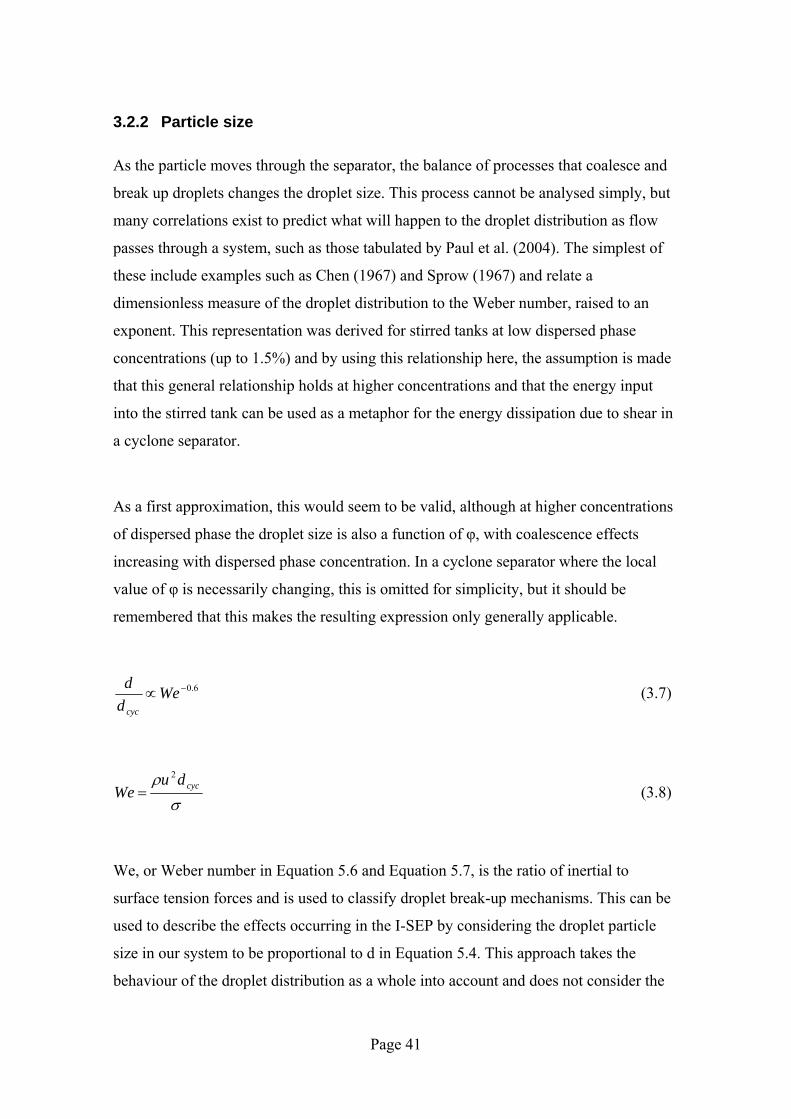
Page 41
3.2.2 Particle size
As the particle moves through the separator, the balance of processes that coalesce and
break up droplets changes the droplet size. This process cannot be analysed simply, but
many correlations exist to predict what will happen to the droplet distribution as flow
passes through a system, such as those tabulated by Paul et al. (2004). The simplest of
these include examples such as Chen (1967) and Sprow (1967) and relate a
dimensionless measure of the droplet distribution to the Weber number, raised to an
exponent. This representation was derived for stirred tanks at low dispersed phase
concentrations (up to 1.5%) and by using this relationship here, the assumption is made
that this general relationship holds at higher concentrations and that the energy input
into the stirred tank can be used as a metaphor for the energy dissipation due to shear in
a cyclone separator.
As a first approximation, this would seem to be valid, although at higher concentrations
of dispersed phase the droplet size is also a function of φ, with coalescence effects
increasing with dispersed phase concentration. In a cyclone separator where the local
value of φ is necessarily changing, this is omitted for simplicity, but it should be
remembered that this makes the resulting expression only generally applicable.
6.0−∝Wedd
cyc
(3.7)
σρ cycdu
We2
= (3.8)
We, or Weber number in Equation 5.6 and Equation 5.7, is the ratio of inertial to
surface tension forces and is used to classify droplet break-up mechanisms. This can be
used to describe the effects occurring in the I-SEP by considering the droplet particle
size in our system to be proportional to d in Equation 5.4. This approach takes the
behaviour of the droplet distribution as a whole into account and does not consider the

Page 42
local mechanistic effects of the flow on any particular droplet, but it is a way to describe
the important effects that changing droplet sizes have on separation. By combining
Equation 5.6 and Equation 5.7:
cyccycd
p ddu
d6.02 −
⎟⎟⎠
⎞⎜⎜⎝
⎛∝
σρ
(3.9)
Further assuming that fluid velocities are proportional to the inlet velocity vin, by
substituting for dp in Equation 5.4, to give an expression that is proportional to radial
terminal velocity:
uro ( ) 2.12
222.1
cycindc
incyc
dvr
vd
ρµ
ρσ∆∝ (3.10)
As the terminal velocity is derived from a force balance, the larger the value of terminal
velocity, the greater the initial acceleration on a particle must be due to unbalanced
force. Therefore, a particle with a greater terminal velocity in a cyclone flow field
would be expected to separate better and the factors affecting the terminal velocity
would likewise affect that particle’s separability. Hence, a pseudo-quantitative term,
separability, is an alternative term for radial terminal velocity that describes whether
separation improves or worsens as system parameters are changed. This is described by
simplification of Equation 5.9 and is shown as Equation 5.10.
‘Separability’ 4.0
8.02.1
2.1 ..in
cyc
cd vd
rµσ
ρρ∆
∝ (3.11)
As r, the radial position of the droplet in question, can be related to the path length a
droplet must travel to be separated (separation is inversely proportional to its value), we
can say that:

Page 43
Separability 2.04.0
2.1
2.1 .cycincd dvµ
σρρ∆
∝ (3.12)
The complexity of the actual system means that the assumptions made in deriving the
expression above make it overly simplistic, but the trends it suggests give the following
points.
• Increase density difference between phases ⎟⎟⎠
⎞⎜⎜⎝
⎛ ∆2.1
dρρ and separation improves.
This would be expected due to the density driving force inherent in the
separation process.
• Increase surface tension, separation increases. The surface forces have the effect
of stabilising droplets, resisting drop break-up and helping coalescence. Since
larger droplets settle more readily, this has a positive effect.
• Increase the viscosity of the continuous phase, separation decreases. The
continuous phase will inhibit droplet mobility and so droplet coalescence if its
viscosity increases.
There will be an effect of concentration, but this has been neglected in the above
analysis. The effects of both cyclone diameter and inlet velocity would appear to be
weak, but increasing either is detrimental to cyclone performance. Whilst scale effects
have not been explored in this work, there is a measurable separation reduction at higher
velocities – though this is much more evident at certain water cuts.
This analysis is a very simple one that ignores the complexities of cyclone flow. In
order to appreciate them better, a much more sophisticated model is required, such as
that produced in the next chapter with a CFD model. This implicitly calculates the flow
velocities and avoids making many of the assumptions used above. However, the
modelling technique used does not attempt to analyse droplet size changes within the
separator, and with this in mind the simple analysis makes a useful, if simplistic,

Page 44
contribution.
3.3 Conclusions
A simple model has been produced to describe the relative effects of the importance of
different parameters on the separation performance of the I-SEP. However, the
simplifications involved make this imprecise. Fewer assumptions are required for a
more sophisticated simulation and this will be attempted in the next chapter.
In this chapter, an analysis of the phenomena occurring inside the I-SEP compact
separator has been set out. The next two chapters will present the method and results of
experimental work to investigate the performance of a novel geometry of the I-SEP
Axial Flow Cyclone.

Page 45
4 Experimental Methods
In the previous chapter, the phenomena that affect the behaviour of oil and water
droplets as they approach and move through the I-SEP have been considered. This
chapter details the methods used in conducting experimental work undertaken to
determine the performance of the I-SEP in separating oil and water mixtures.
4.1 Introduction
In this chapter, the laboratory work concerning the use of an I-SEP with oil and water is
covered, along with the methods used for performing flow visualisation and measuring
droplet sizes.
The tests were used to construct a performance map for the I-SEP. Initial tests were
performed with a nominal unit-length cyclone and, based on a qualitative and
quantitative assessment of these first data, a second more flexible test unit was
constructed and tested. This allowed the length of the separating chamber to be varied to
investigate the effects of this change.
These tests are to allow the evaluation of the I-SEP in terms of a commercially relevant
technology. Also, to provide the data to compare with models of the device and to
provide the basis for improvement of the design of the cyclone separator.
4.2 Experimental Facility
The test rig for the experimental investigations in this project was constructed as a new
system, designed from scratch by the author. It was designed on the basis that it should
permit a practical duration of test with reasonable volumes of test fluids; this affected
the sizing of all the rig components, including the test separator. This imposed
restrictions on the design and operation of the rig because of the need to supply oil and
water feed and deal with the outlet streams. Previous investigation of the I-SEP, and
related devices, mainly dealt with air-solid or air-water systems where the phases easily
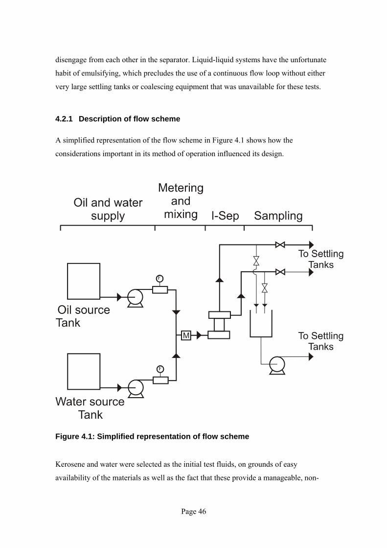
Page 46
disengage from each other in the separator. Liquid-liquid systems have the unfortunate
habit of emulsifying, which precludes the use of a continuous flow loop without either
very large settling tanks or coalescing equipment that was unavailable for these tests.
4.2.1 Description of flow scheme
A simplified representation of the flow scheme in Figure 4.1 shows how the
considerations important in its method of operation influenced its design.
Figure 4.1: Simplified representation of flow scheme
Kerosene and water were selected as the initial test fluids, on grounds of easy
availability of the materials as well as the fact that these provide a manageable, non-
F
F

Page 47
emulsifying experimental system that can be compared with the work of other
researchers. This will not be fully representative of all likely separation applications, but
provides a starting point to determine whether the I-SEP can perform a useful separation
function. The significant volumes of potentially mixed outlet flow from the I-SEP do
however require a clean up stage to allow the reuse of the test fluids. In order to
mitigate the volumes of liquid needed, the scale of the I-SEP itself was chosen, in part,
to reduce the volumes required to a manageable level. The scale chosen gives about 45
minutes of continuous testing at 90% or 10% water cut with a 10 m/s velocity at the
inlet to the separator before either feed tank would be exhausted. The value of 10m/s
was not thought to be practically useful but represents a conservative ceiling on possible
test measurements parameters.
The possibility of using coalescers, or other equipment that would be capable of
purifying the outlet water and oil mixtures was explored, but the recommissioning of
these was unjustifiable for a first set of tests on an unproven device. Instead, tanks
similar to the water and oil feed tanks were used to hold the outlet streams. After the
completion of each test run, the contents of settling tanks were left for a number of
hours, before decanting the two resulting liquid layers back to the feed tanks.
Referring to Figure 4.1, moving from left to right, the components of the feed to the test
unit are separately pumped and metered using progressing cavity pumps and hall
effect/turbine flow meters (marked with an ‘F’ in the diagram). The two streams are
brought together and mixed in the static mixer array marked ‘M’ just prior to the inlet to
the I-SEP, which is shown as an I-shaped block in the centre of the diagram. The block
marked ‘M’ is the inlet static mixer array. The test liquids leave the separator through
either the axial outlet line (shown vertically) or the tangential outlet line (shown leaving
horizontally) and pass to settling tanks.
A modification was made to the test rig after initial test work, allowing continuous flow
through the sample lines to the outlet tanks via an additional pump. This avoided the
need to divert flow from the direct path to the settling tanks when sampling. Until this

Page 48
point, sampling had caused a step change in flow leaving the separator and made it
impossible accurately to determine the outlet flow split by sampling. The change meant
the sampling lines collected the full outlet flow, thereby eliminating sampling errors.
Figure 4.2 shows the separator installed in the test rig.
Figure 4.2: Photograph of separator installed in test rig
4.2.2 Test units
An initial design of test unit was based on the previous design of the I-SEP that had
demonstrated good performance in gas-liquid separation tests. The changes made to the
gas-liquid geometry for liquid-liquid duty were in terms of rescaling outlet areas so that:
• Areas of the two outlets were made equal
• Total outlet area was increased by 25%
These changes reflect the fact that none of the feed was gaseous, and therefore a higher
pressure-drop would occur in the lower density (axial) outlet with liquid flow replacing
gas. Equalising the two outlet areas (and therefore enlarging the axial outlet) mitigates
the effect of this, and increasing the total area for an all-liquid system would further
help to reduce the pressure drop in the unit. The changes are intended to produce a bulk

Page 49
liquid-liquid separation device – one which has relatively low pressure drop whilst
performing an initial stage of separation, and may be followed by further devices to
‘polish’ the separator outlet flows.
It would seem obvious that the ratio of outlet areas would influence the performance of
the separator, and the optimum conditions at which that separator ought to operate.
Increasing the axial outlet area in relation to the tangential outlet would make the I-SEP
more amenable to separating inlet mixtures richer in the lower density phase (hence
more oily for the case of kerosene and water) and vice versa. This geometry is an initial
design to experimentally investigate, and subsequently judge, the suitability of the I-
SEP’s performance to solving relevant engineering challenges, i.e. a de-oiling cyclone
to recover oil produced from end-of-life oil wells that have a high produced water cut.
The original dimensions of the gas-liquid separator as summarised in Figure 4.3, below.
Figure 4.3: Dimensions of the I-SEP previously used for gas-liquid separation (Allstaff, 2000)

Page 50
Figure 4.4: Extended separator test unit at nominal length 3 (3x)
Inlet involute
Separating chamber
Outlet involute
Vortex finder (axial outlet)
Inlet

Page 51
Figure 4.5: Extended separator test unit at nominal length 3 (3x)
With reference to the photos of the test unit, Figure 4.4 and Figure 4.5, flow enters the
unit via the inlet duct, bottom right. This moves to the left into the inlet involute giving,
in the sense of the photos, an anti-clockwise spin as viewed from above. Refer also to
Figure 2.13, showing a simplified representation of the separator. Flow passes upwards
from the inlet involute into the separating chamber and further up the chamber towards
the outlets. A vortex finder, positioned on the unit axis, is a protrusion into the top
involute of the separator and takes the less-dense separated flow as defined by the
separator flow split (controlled by downstream valves). This vortex finder, shown in a
simplified form in Figure 4.6, forms the axial outlet. It is a standard feature of reverse
flow cyclones used for separating dispersions of the denser phase, but not in some
cyclones where the less dense phase is dispersed (see section 2.3.2). The effect on
performance of whether a vortex finder is included or not, will not be investigated in
Inlet involute
Outlet involute
Vortex finder (axial outlet, obscured by bolt)
Separating chamber – shown with 3 unit lengths (3x)
Inlet
Inlet pressure tapping

Page 52
this work. At the circumference of the top of the separating chamber is the outlet
involute. The separated heavy phase would flow to this outlet and it is the equivalent of
the underflow outlet of a reverse-flow cyclone. This is the tangential outlet.
Inlet
TangentialOutlet
AxialOutlet
Vortex Finder
Figure 4.6: Outlets of I-SEP showing the vortex finder
The separator (Figure 4.4) has transition pieces that smooth the change between the 1-
inch inlet pipe work and the 49mm2 cross section of the inlet to the separators and the
outlets. This avoids sharp changes in diameter and geometry. On the separator side of
the transition, tappings are located at the walls for impulse lines that are connected to an
array of pressure sensors (see Section 4.2.4.2). Construction drawings of the I-SEP test
unit used are included in Appendix B.
The initial unit (designated 1x) was capable of different orientations of inlet and outlet
involutes but not of varying the length of separating chamber. The unit shown in Figure
4.4 has been modified to allow the elongation of the separating chamber, shown with an
extension ‘slice’ sandwiched between equally long lengths of separating chamber to
create a unit that is three times the length of the original test unit (designated 3x). The

Page 53
separating chamber of the 1x I-SEP unit kept a similar taper (decreasing towards the
outlet end of the I-SEP) to the air-water unit on which it was based. The taper was
originally included to echo the taper present in reverse-flow cyclones. In these devices,
the taper is present to maintain spin velocity in the cone despite the removal of material
that makes up part of the spinning flow through the overflow. However this does not
occur in the I-SEP (the material removal effect does not require mitigation, as all flow
leaves the I-SEP at the same end), where the taper just compensates for the slowing of
the swirl due to wall friction.
Tests with the original unit and further analysis of the problem indicated that it could be
worthwhile to investigate the performance of a significantly longer separator body with
the intent of increasing residence time for the flow within the vortex field. This meant
definition of the original unit as having length 1 (or 1x). The new unit was capable of
separator lengths of between twice and five times that of the original unit (2x to 5x). In
order to allow a variable separator length, it was geometrically necessary to remove the
small taper present in the 1x unit and therefore slightly alter the dimensions of the outlet
involute to accommodate this. Apart from this minor change, and the intentional
increase in L/ds, the unit was identical. A standard way describing cyclone geometry,
the length-to-diameter ratio, is tabulated in Table 4.1.
1x 2x 3x 4x 5x
l:d ratio 1.44 2.71 4.07 5.43 6.79
Table 4.1: Length to diameter ratio of I-SEPs with different lengths of separating chamber
The removal of the small taper present in the 1x unit to allow an extendible geometry is
something that is assumed not to have a material effect on separation performance.
However, it would not be possible to maintain the taper present in the 1x unit whilst
extending the separating chamber. To do so would ultimately make the separating
chamber in to a cone. The effect of taper was not investigated in this work.

Page 54
Figure 4.7: Design of involutes
Figure 4.7 shows the derivation of the involute shape, used to form the inlets and outlets
of the I-SEP design and gives the I-SEP its name. The involute is a geometry know as
the roulette of a line, that is a curve formed by a point fixed on a line as the line rolls
around a circle. It is found in various contexts, including drop shaft design, and was
chosen by the designers of the I-SEP as a favourable geometry for pressure recovery
from the spinning flow, and therefore for minimising turbulence, in gas-liquid
separation (Saunders, 1998a). Another example of an application of this is the involute
casing found on a centrifugal pump, to maximise recovery of pressure from a spinning
fluid. Analogy can be made between this and the involute that forms the tangential
outlet of the I-SEP. By precedent (Allstaff, 2000), an involute has not been used for
pressure recovery on the axial outlet of the separator, and this is not a parameter that
will be studied here.
The dimensions shown in Figure 4.7 are defined around a grid positioned on what
would become the axis of the separating chamber according to the following
relationships:
r1 = b + (0.5 ds – e) (4.1)
r2 = r1 – 2e (4.2)
r3 = r1 – 4e (4.3)
r4 = r1 – 5e (4.4)

Page 55
e = ds/5 (4.5)
In addition, b is the width of the inlet (or outlet) in question, and ds is the diameter of
the separating chamber. Key inlet and outlet dimensions are given in Table 4.2.
Cross sectional
area / mm2
Width / mm Height / mm Diameter / mm
Inlet 48.9 10.29 4.75 -
Tangential outlet 31.36 11.2 2.8 -
Axial outlet 31.17 - - 6.3
Table 4.2: Key I-SEP dimensions
The unit was designed to a test pressure of 3 barg, operating at a maximum of 1.5 barg.
The hydraulic design methodology for this design of separator is given in Saunders
(1998b). This is a BHR Group confidential report and the methodology it describes
cannot be reproduced here.
4.2.3 Liquid supply
Oil and water are supplied from separate tanks that are drawn into progressive-cavity
pumps, each capable of delivering up to 8 litre/s of liquid at up to 5 bar (the maximum
pressure is limited by the pumps). Pressure relief valves located on the outlet of each
pump further protect the test section. The progressive cavity pumps, combined with the
length of supply pipe work (>6m at 1 inch diameter) before the test section, give
relatively pulse-free flow for a wide variety of flow conditions. The pumps are equipped
with variable speed drives to afford extra control over the system.
With reference to Figure 4.1, the liquid passes from the pumps on the left hand side,

Page 56
through a strainer and control valve arrangement, before being metered (meters marked
with a ‘F’ on the diagram). The control valves are installed in a bank on each liquid line
so that a full-bore gate valve and small-bore needle valve work in parallel to give fine
control over the whole flow range. Combined with the variable delivery characteristics
of the pumps, control is obtained that allows steady flow conditions (within metering
accuracy) to be set for each test condition within 5 minutes. It should be borne in mind
that it is necessary to obtain set inlet velocity and flow split by an iterative process.
Every increase in flow of one phase will cause a decrease in the flow of the other, but
eventually the desired conditions can be reached.
The oil used is kerosene dyed with oilsol red tax powder (Rohm and Haas, Batley, West
Yorkshire), which provides good contrast with the colourless water. Initially the water
used was tap water. However, after being recycled though the system a number of times
and contacting oil (creating droplets with a very long settling time to remain in the
settled water), problematic biological growth was observed as a scum that appeared on
the surface of the water. Adding an isothiazolone-based biocide (Acticide SPX from
Thor Specialities UK, Northwich, Cheshire) to the water at 100ppm, as per the
manufacturers’ instructions, mitigated this.
The process of allowing the water and oil to settle cannot fully purify either component
but the system is closed. The oil and the water therefore have the opportunity to reach
equilibrium in terms of physical properties after having been mixed together and
allowed to settle. This removes uncontrolled variability of feed liquids from the
consideration of performance of the separator.
A silicone-based oil was provided for an investigation of the suitability of developing an
I-SEP design for a client company of BHR group. This fluid was tested on several
experimental runs until the feed had been exhausted. This was done without recycling
or the addition of dye to the oil and formed and was therefore a limited illustration of
how a different oil will separate. This will be covered in more detail in later sections.

Page 57
4.2.4 Instrumentation
Instrumentation facilities comprised flow and pressure metering sensors, together with
an inlet temperature transducer to ensure that liquid temperature did not vary by more
than 5oC. The output signals from the transducers were converted from 4-20mA current
to voltage. Analogue to digital conversion was via a National Instruments data
acquisition card fed into a PC running LABVIEW. The LABVIEW runtime software
provided data acquisition and recording whilst also giving a readout of the key data to
facilitate the setting of flow conditions.
4.2.4.1 Flow metering and control
In order to be able to set the flow rates of water and oil entering the separator reliably, it
was vital to have online metering of both flows. This directly provides the inlet flow-
split and velocity at the I-SEP. A bank of flow meters, each comprising two flow meters
in parallel, was installed on the water and oil inlet lines to allow a wide range of flow
rates. The inlet flow for each phase was physically diverted to only flow through the
flow meter of the appropriate range by means of ball valves on the inlet pipe to each
meter.Each meter had a minimum of 10 pipe diameters of straight pipe upstream and 5
pipe diameters downstream to ensure the measurement of fully developed flow. This is
the recommended practice within BHR, consistent with British Standards though the
actual installation, especially for the small-bore meters, gave a considerably greater
length of pipe work.
4.2.4.2 Pressure Sensors
Previous investigations carried out on axial-flow cyclones have shown that the
performance of the I-SEP, with respect to one stream, can be improved by restricting
the flow from one or other outlet. This is termed the ‘application of backpressure’. In
order to be able to quantify this, as well as being able to describe the pressure-drop
profile of the separator, three pressure sensors were connected to the impulse lines
leading to the pressure tappings on the unit as shown in Figure 4.8. This shows the
configuration of three differential pressure cells to measure pressure drop and a single-
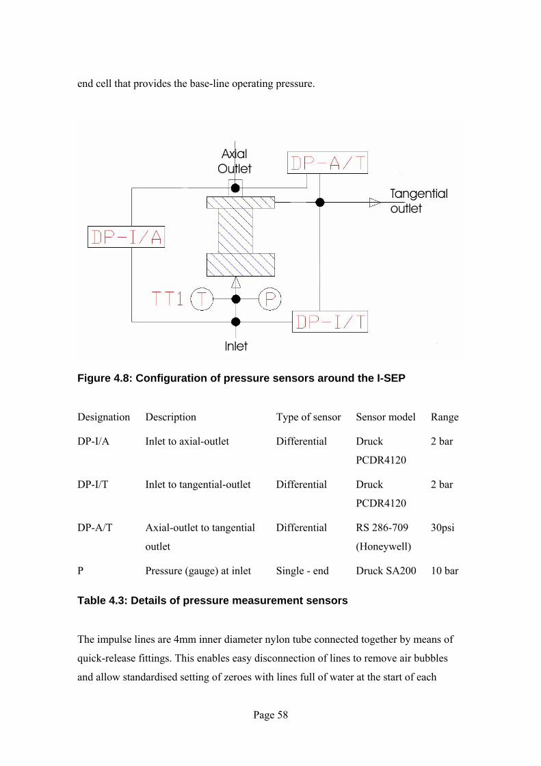
Page 58
end cell that provides the base-line operating pressure.
Figure 4.8: Configuration of pressure sensors around the I-SEP
Designation Description Type of sensor Sensor model Range
DP-I/A Inlet to axial-outlet Differential Druck
PCDR4120
2 bar
DP-I/T Inlet to tangential-outlet Differential Druck
PCDR4120
2 bar
DP-A/T Axial-outlet to tangential
outlet
Differential RS 286-709
(Honeywell)
30psi
P Pressure (gauge) at inlet Single - end Druck SA200 10 bar
Table 4.3: Details of pressure measurement sensors
The impulse lines are 4mm inner diameter nylon tube connected together by means of
quick-release fittings. This enables easy disconnection of lines to remove air bubbles
and allow standardised setting of zeroes with lines full of water at the start of each
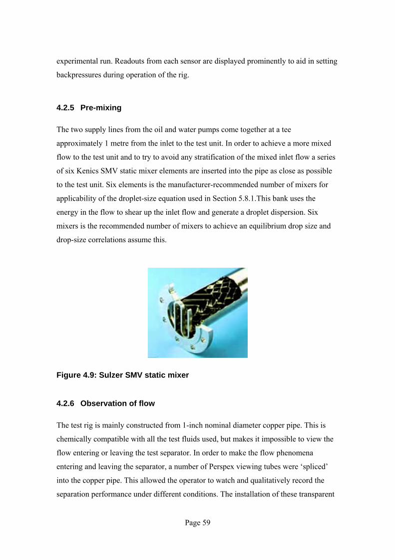
Page 59
experimental run. Readouts from each sensor are displayed prominently to aid in setting
backpressures during operation of the rig.
4.2.5 Pre-mixing
The two supply lines from the oil and water pumps come together at a tee
approximately 1 metre from the inlet to the test unit. In order to achieve a more mixed
flow to the test unit and to try to avoid any stratification of the mixed inlet flow a series
of six Kenics SMV static mixer elements are inserted into the pipe as close as possible
to the test unit. Six elements is the manufacturer-recommended number of mixers for
applicability of the droplet-size equation used in Section 5.8.1.This bank uses the
energy in the flow to shear up the inlet flow and generate a droplet dispersion. Six
mixers is the recommended number of mixers to achieve an equilibrium drop size and
drop-size correlations assume this.
Figure 4.9: Sulzer SMV static mixer
4.2.6 Observation of flow
The test rig is mainly constructed from 1-inch nominal diameter copper pipe. This is
chemically compatible with all the test fluids used, but makes it impossible to view the
flow entering or leaving the test separator. In order to make the flow phenomena
entering and leaving the separator, a number of Perspex viewing tubes were ‘spliced’
into the copper pipe. This allowed the operator to watch and qualitatively record the
separation performance under different conditions. The installation of these transparent

Page 60
sections can be seen in Figure 4.2. Figure 4.10 shows the usefulness of the transparent
tubes at he outlet where it is immediately apparent that there is no visible oil leaving the
separator in the tangential outlet.
Figure 4.10: Observed flows from both outlets for 'pure' tangential outlet flow (90% IWC, 2m/s inlet velocity)
Test fluids, once settled in outlet settling tanks are recycled back to the feed tanks. This
makes use of the difference in colour between the oil (with a red dye added) and the
colourless water. The operator makes use of a Perspex tube at the pump outlet to switch
the flow being pumped out of the settling tanks between feed tanks when the fluid being
pumped from the bottom of the settling tanks changes colour from colourless water to
red oil. The construction of the test units from Perspex also allows good visualisation of
the characteristics of the vortex and separating flow within the separator. It has also
permitted further investigations with PIV techniques (see Section 4.7.).

Page 61
4.3 Methodology
The methodology followed for each test run with the extended test unit is detailed
below.
4.3.1 Setting up flow conditions
With liquid in each feed tank, valves upstream of the test unit closed and outlet valves
on the separator open, the pumps are started at their lowest speed. A bypass-valve
allows the flow to return to the supply tank for each pump. The correct flow meters for
the target flow condition are selected, both by the isolation valves, and in the data
acquisition software. By reference to the data acquisition PC screen, the flow control
valves are manipulated to give the flow rates of both water and oil at the desired inlet
velocity and water cut. Care is needed to ensure that the pressures on each supply line,
as indicated by bourdon pressure gauges on each pump outlet, are sufficiently close to
avoid pumping one liquid the wrong way back down towards a pump. This can be
eliminated by observing the viewing tubes on the inlet lines. It is likely that the pump
flows will need to be raised, especially for higher test flow rates, and this is done by a
combination of closing pump bypass line valves and increasing the pump speed.
The ultimate limit on liquid delivery, reached during operation of the rig, derives from
the need to avoid over-pressurising the test unit and because of excessive vibration in
the rig at higher flow rates (despite attempts to reduce this).
4.3.2 Backpressure
An important operating variable that was investigated in the tests was the use of
backpressure (i.e. closing the valve on one or other of the test unit’s outlets to restrict
flow) to vary the flow split between outlets, and observe the effect on outlet purity.
In order to set the backpressure for a certain flow condition, that condition (in terms of
flow rate and water cut) would be set up and then the relevant valve would be closed

Page 62
until the data acquisition output showed the target backpressure being measured.
Because this resistance would decrease the total flow moving through the unit, the inlet
flow conditions would then need to be re-set as detailed in 4.3.1. This would, in turn,
change the backpressure reading and require an iterative process of adjusting valves and
pumps.
4.3.3 Sampling
A great deal of thought was given to determining the properties of the outlets in order to
derive the performance of the I-SEP. The magnitude of the flow is relatively simple to
measure with turbine flow meters, as these are essentially unaffected by different liquids
and liquid mixtures. However, the wide range of composition achievable at either outlet
of the test unit (from all-water to all-oil) meant that most analytical methods were
unsuitable. Capacitance / conductance methods were considered, but the time required
to calibrate and commission these sensors meant that instead the content of samples
from the outlets was determined manually. The flow rates of oil and water tested
allowed collection of the complete flow exiting the separator, thus removing the
problem of achieving a representative sample.
The test rig was initially configured so that the total flow to be sampled would divert
through a three-way valve on the outlet line to flow into a collection pot. However, it
soon became clear that switching the flow in this way caused a major change in the flow
rate in the outlet line and changed the proportion of flow leaving in each outlet. This
meant it was impossible to gauge the outlet flows and also that multiple samples could
only be taken after resetting the three-way valve and allowing the system to return to
steady state. This wasted valuable feed fluid and consequently testing time. Therefore,
the system was modified so that the full flow of each outlet from the I-SEP continuously
fed into an open bucket that was, in turn, pumped out by a Jabsco pump. Samples were
then taken from each line to determine composition (overall water cut) and flow rate. A
photograph of the sampling lines used is shown as Figure 4.11.
The volume of the pipe work between an I-SEP outlet and the corresponding sample

Page 63
point was significant in terms of generating many seconds of hold-up at a given outlet
volumetric flow rate. Flow was therefore allowed to run through the I-SEP for a
sufficient length of time (given the volume of liquid in the pipe between test unit and
sample point, and the flow rate from that sample point) to ensure that the sampled flow
was at the same composition to the I-SEP outlet flow.
Figure 4.11: Outlet sampling line configuration
4.3.4 Data acquisition
The data acquisition system was set up to show real-time flow data as well as record
these to a data file for subsequent analysis.
Axial outlet line
Tangential outlet line
Tangential outlet backpressure valve
Flexible outlet
sampling line

Page 64
4.4 Structure of testing
4.4.1 Variables available for investigation
4.4.1.1 Water cut
The initial hypothesis for testing the I-SEP design was that it could be used as a bulk
separator of oil and water. This is a broad remit, arguably encompassing water cuts
from 99% to 1%.
It is axiomatic that the water cut experienced by the test unit inlet will influence its
performance. Testing across such a wide range of inlet conditions will cross the
inversion point, where the mixture of oil droplets in water becomes a mixture of water
droplets in oil. Because of the different mobilities of one phase in the other, we would
expect to see different performance with varying water cut. This means that equal
concentrations of dispersed phase will perform differently on either side of the inversion
point. The concentrations at the outlets must change, but it is likely that (depending on
the definition of efficiency used) efficiency will also be a function of inlet water cut.
4.4.1.2 Inlet Velocity
The intensity of rotation of the vortex within a cyclonic device is a critical factor for
separation. As the spin increases, so too does the centripetal force within the separator
acting on the flow components. The means for spinning flow in a cyclone separator is
the inlet involute within the I-SEP. Therefore the faster the inlet velocity, the faster the
spin will be. However, as the energy in the inlet mixture increases, so will the tendency
for this to create turbulence and to mix up the components more, counteracting the
separating action of the cyclone vortex. This is likely to give a trade-off for inlet
velocity that minimises turbulence whilst providing the energy for separation and giving
acceptable throughput. Minimising turbulence is key to the design of oil-water
separator.
Analysing the trend of performance with inlet velocity will allow determination or

Page 65
inference of an optimum inlet condition for the separator. Whilst optimisation of the
geometry is not an objective of this work, the effect of the length of separating chamber
will be explored.
4.4.1.3 Extent of mixing at inlet
There is a degree of mixing intentionally caused by the liquid moving through the static
mixer elements at the inlet to the test unit. The dispersion generated by the mixer
elements is a function of pipe velocity. When designing, building and revising the
operation of the experimental rig, much thought was given to attempting to control the
droplet sizes that the test unit would experience. This would ensure that this variable did
not influence the performance of the I-SEP. However, the need to make inlet velocity
and water cut variable meant that controlling the inlet droplet size was a challenging
task.
Various options were considered. One example was forming the inlet flow from a
number of small-bore tubes, each containing a static mixer that would be exposed to the
same flow velocity and water cut. Thus each of, say, eight small-bore pipes would feed
into a plenum prior to the test unit inlet. Progressively ‘switching on’ more pipes would
incrementally increase the inlet velocity. However, even with this effort being taken, the
extent of mixing in the recombining plenum would still vary with throughput so would
still not guarantee the same drop size. Finally, it was decided not to attempt
maintenance of constant drop size and this should be borne in mind when considering
the results.
4.4.1.4 Length of separating chamber
The test unit geometry is variable in terms of the length of the separating chamber. This
parameter can be investigated as a first stage to improving the performance of the I-SEP
as a separation device. Work with air-water separation has determined that the
orientation of the inlet and outlet are not significant and these will not be investigated
here.

Page 66
Increased residence time, due to longer separating chamber, would be expected to
improve performance. We would therefore expect to see better separation of
components to their desired outlets reduced emulsification of the misdirected
components.
4.4.1.5 Restriction of outlet flow (backpressure)
Previous work (Allstaff, 2000) has shown how the application of backpressure to one of
the I-SEP outlets can be used to reduce the flow of unwanted phase from that outlet.
The unwanted component (water in the axial outlet for a light oil, oil in the tangential
outlet where the water is denser than the oil) is then rejected into the other outlet. Being
able to manipulate the flow split between outlets by applying backpressure means that
the separation performance can be controlled and improved when the inlet composition
changes from the ideal composition for the separator, if indeed one exists. This would
have major value in improving the flexibility of the separator and will be investigated in
this work.
In order to investigate the application of backpressure to an outlet of the I-SEP being
tested, a gate valve is located in the line, approximately 1 metre downstream of each I-
SEP outlet, which can be used to apply backpressure to either outlet. For this to be
useful in providing repeatable control, pressure drop and inlet gauge pressure is
measured by using pressure sensors. The configuration of sensors is set out in Section
4.2.4.2, where the backpressure is measured as pressure drop across the unit. As flow is
restricted at one outlet, the measured differential pressure between that outlet and the
inlet decreases. The backpressure can be related to the flow split of the unit and the
change to the flow split between outlets under test conditions, as will be investigated.
4.4.1.6 Test fluids
Table 4.4 shows the fluids used in testing. The majority of tests were conducted with
de-aromatised kerosene (Alcosol D70 from Alcohols Ltd. of Bishops Stortford) and
water. In addition, a synthetic oil was tested with water as part of a determination of the

Page 67
suitability of using the I-SEP for separation of this oil. Only testing within the scope of
the work for the client was possible, but this gave useful data.
Fluid Density / (kg/m3) @
20°C
Dynamic
Viscosity /
(kg/m.s) @20°C
Surface tension /
(N/m) @20°C
Water 1000 0.0011 0.073
Kerosene (Alcosol
D70)
820 0.0023 0.025
Silicone-based oil 960 0.0168 0.019
Table 4.4: Densities of separation fluids
4.4.2 Initial test plan
The initial tests were conducted with the flow loop in place using the original design of
the I-SEP. This has a separating chamber length of a nominal 1-unit length, based on the
previously investigated air-water separator (with rescaled outlet areas and a lengthened
separating chamber compared to that design). Tests with this original unit explored the
performance map of the unit and investigated the effects of backpressure. This was
initially done by counting the number of turns of the gate valves on the outlets, but it
was apparent that this was too crude and an inadequate way of quantifying the
backpressure applied. By extension of previous work on gas-liquid separation, the three
pressure sensors were installed (see Section 4.2.4.2).
Various tests were conducted, but visual inspection of separating flow led to the
suggestion that the separator body was insufficiently long to give the residence time
within the separator necessary for a good separation. With this in mind, a new unit with
longer (and variable) separator length was constructed.

Page 68
4.4.3 Subsequent tests
The main body of test work was carried out after the initial work on the 1x unit, with
units of three times and five times the length of the initial unit separator body (denoted
3x and 5x respectively, the initial unit denoted 1x). These tests were organised to move
through the matrix shown below for a range of values of DPA/T (differential pressure
between separator outlets). The actual DPA/T values tested were referenced to the
achievable values in the conditions on test and also those that seemed reasonable – i.e. a
test where one outlet flow was negligible compared to the other was deemed pointless
as any result would be trivial.
Lengths Inlet Velocities / (m/s)* Inlet Water Cuts
1x* 2 10%
3x 4 25%
5x 50%
75%
90%
*1x separator length was investigated in preliminary tests; other velocities were
investigated, but for a limited water cut range
Table 4.5: Experimental conditions investigated
Each experimental condition was measured by taking five repeat measurements of
outlet composition and flow rate from each outlet. This means that, for each
composition, the data point in the results chapter comprises the mean of five
measurements and each efficiency value combines ten composition and ten flow rate
measurements.A wider range of inlet velocity measurements were taken for the 1x unit,
up to 8m/s, the upper limit of 4m/s being arrived at based on these first results with the
1x unit.

Page 69
4.5 Processing of results
The raw data were in the form of text data files and written notes detailing experimental
conditions and the results of sampling. Sampling was done by intercepting the
continuous flows from the outlet sample lines to the pump-drained container (see
Section 4.2.1 and 4.2.3). The sampling was begun after allowing outlet pipe work to fill
with liquid at the composition generated by the selected test conditions. A sample
container of nominal 400ml volume was filled from the sample hose and allowed to
settle for subsequent analysis, and so the sampling duration varied depending on the
particular outlet flow rate. When the test run was complete, all the sample bottles were
weighed and the weights of the containers subtracted from the reading to give the mass
of liquid collected.
The liquid was poured into a 250ml measuring cylinder (this size was used to make use
of a scale graduated in 2ml marks – finer than larger measuring cylinders) and the total
volume recorded. This, combined with the time taken to collect the sample gave
volumetric flow rate; composition was determined, in terms of water cut for each
sample, in terms of the expression for the binary density method:
wateroil
oil
MM
VM
WC
ρρ
ρ
−
−=
1000 (4.6)
The factor of 1000 is to give consistency of units between mass in grams and volume in
millilitres.
4.6 Droplet size measurement
The effect upon the droplet size distribution at the inlet caused by the transition piece at
the inlet was likely to cause a decrease in droplet size. This is due to the approximately
1:10 velocity increase caused by the change in area. Whilst correlations are used later in

Page 70
this thesis to predict the droplet size distribution leaving the static mixer array just
before the I-SEP inlet, attempts were also made to directly measure the size distribution
experienced by the I-SEP inlet.
A Malvern Mastersizer S was obtained on loan from the EPSRC instrument loan pool.
This was connected via 6mm ID Tygon tubing to the pressure tapping on the inlet (i.e.
after the inlet transition), linking this to the flow cell in the Malvern instrument as
shown in Figure 4.12. The outlet flow was collected in a container and returned to the
outlet settling tanks. This configuration is based on Thapar (2001).
In order to dilute the flow leaving the I-SEP inlet, it was necessary to connect diluting
water flow, supplied from a peristaltic pump with three heads, upstream of the flow cell
to reduce the concentration of the dispersed phase to render it measurable by the
Mastersizer. In order to achieve a meaningful measurement, the obscuration measured
by the instrument ought to be in the range 20-60%. The flow rate of diluting water was
varied in order to bring the measured obscuration within the required range.
Figure 4.12: Arrangement of Malvern Mastersizer S for droplet sizing at the inlet
Inlet flow
Flow leaves through inlet pressure tapping (see Figure 4.5)
Diluting water flow
Diluted flow enters flow cell
Flow leaves after measurement

Page 71
It is recognised that direct measurement of droplet sizes can be very problematic. In the
case of the above arrangement, whist every effort has been made to minimise the
disturbance caused by the measurement technique, the disturbance will in some way
affect the measurement. The Mastersizer unit was positioned as close as possible to the
I-SEP in order to minimise the length of tube between flow leaving the inlet and
entering the measurement cell, in order to avoid an excess length of time for the flow to
coalesce. The flow Reynolds number in the sampling tube was also maintained as low
as possible (calculated at a value of around 100), in order to avoid turbulence in the
flow before measurement.
Given the efforts made to maximise the validity of the measured data there will
inevitably be change in droplet size due to the change in concentration caused by
dilution. Due to the small scale of the geometry in which the droplet size is being
investigated, other techniques, such as the use of a video-probe for offline droplet
sizing, are impractical. The message from this is that data produced by this droplet
sizing technique should be analysed with caution.
4.7 Flow visualisation
A PIV technique was used in an attempt made to measure the internal flow field of the
I-SEP. This involved the use of a video camera capturing a ‘slice’ of the flow in the I-
SEP that is illuminated by a sheet of laser light projected through the unit at a normal to
the direction in which the camera faces (see Figure 4.13). Water dosed with 0.013g/l of
neutrally buoyant 10µm silvered hollow-glass spheres was observed flowing through
the separator.

Page 72
Figure 4.13: Arrangement of camera and laser in PIV measurements
The equipment used was borrowed from the EPSRC instrument loan pool. Illumination
was provided by an Oxford Lasers CU-15 Class IV 15W output copper-vapour laser.
Attached optics produced a sheet of laser light of 50mm thickness. The laser produces
pulses of 9ns duration, with maximum intensity when running at 10kHz. The camera
used was a high speed Kodak Ektapro EM. The camera is capable of capturing images
in greyscale at 1 kHz, or up to 12 kHz with a reduced frame size.
The PIV technique functions by defining ‘interrogation cells’, and using a statistical
method, in a process called cross-correlation, to track particles between successive
frames of the video footage. This can then be used to build up a series of velocity
vectors in the volume (taking into account the thickness of the laser sheet) being
observed. However, multiple attempts at capturing data suitable for analysis using the
Visiflow software (accompanying the laser) from AEA Technology, using the PIV
technique were unsuccessful. This was due to a combination of problems with the
stability of the software and ultimately, the speed of particles in the flow that was being
measured was too high for analysis by the available equipment and software.

Page 73
For a particle to be tracked successfully by PIV algorithms, it must not move across
more than a certain fraction of the frame (around 1/3) visible to the camera. Even with
maximum magnification available, and thus the smallest possible frame size, the scale
of the I-SEP test unit used means that frame rates at the high end of the camera’s
capabilities were necessary for this criterion to be satisfied. With slower frame rates,
particles would move too far between successive frames (possibly even leaving the
frame) and so would be impossible to track. With increased frame rates, the amount of
light required to register images also increases, but the intensity of laser light decreases
with increased pulse frequency (required to match the laser and camera frequencies so
that each particle appears once in a frame). The laser and camera used were the most
suitable equipment available, but nonetheless were unable to generate useable images of
moving particles at operating velocities on test-unit scale. The requirement to illuminate
each particle once per image was therefore relaxed both to allow a reduction of the light
required by the camera, and an increase of the light intensity provided by the laser. This
gives images where a given particle is illuminated and appears on an image more than
once, (an example is on the left of Figure 4.14) but which can still be useful. Using
these images, it was possible to determine the movement of a number of tracer particles
manually, in order to obtain some measure of the velocities in the viewed plane.
In order to obtain necessary illumination by the laser to register an image with the
camera, the laser pulse frequency (10 kHz) was five times that of the camera (2 kHz)
causing each frame recorded by the camera to show each particle illuminated five times.
It was therefore possible to measure the number of pixels crossed by a given particle in
the know time step, and by use of a calibration image, derive the velocity of that
particle. As shown in Section 6.5.2, vectors were manually assembled from the average
of 10 velocities calculated in squares of a 10mm2 grid drawn on the base (parallel with
the inlet involute - Figure 4.14) of the I-SEP.

Page 74
Figure 4.14: Sample image of tracer particles (left) and tracking grid (right - inlet involute highlighted in red)
4.8 Conclusions
In this chapter, the method for obtaining data on the performance of the I-SEP has been
laid out. By measuring the outlet compositions and flow rates at various inlet
compositions and velocities, a performance map of the separator can be obtained, along
with the pressure characteristics of the I-SEP.
These tests involve the variation of the length of the separating chamber in the unit. The
results of the test program are presented in the next chapter..
Page 75
5 Experimental Results
5.1 Introduction
With a novel separation device, the logical first exercise is to map the performance of
the device with test fluids.
In this chapter, the key findings are presented from the experimental work detailed in
the previous chapter. This is for performance of the I-SEP with the nominal separating
chamber lengths of 1x, 3x and 5x. These are given in detail for the kerosene-water test
system. In addition, the I-SEP is compared with published results for other cyclonic
separation systems.
Directly measured variables were:
• Outlet flow rates
• Outlet composition (by binary density method – see Section 4.5)
• Pressure differences across the unit, including imposed ‘backpressure’ to
manipulate the outlet flow split
From these the outlet composition, flow split, separation efficiency and pressure drop
can be derived. The results of inlet droplet-size measurement are also presented.
5.2 Qualitative results and observations
The kerosene-water mixture enters the I-SEP, and for test cases where the colourless
water phase is continuous, the internal flow structure can be seen through the sides of
the Perspex unit (Figure 5.1). The red kerosene, the less-dense phase, moves to the
centre of the cyclone body and forms a cylindrically or conically shaped core along the
axis of the unit. The initial configuration of the rig (Section 4.2.1) has both outlet valves
fully open. The outlets are therefore restricted only by frictional pressure drop through

Page 76
the outlet of the I-SEP and the pipe work. For the measured test conditions with a
continuous water phase, the core will tend to reach the end of the separating chamber
outside the radius of the vortex finder. This results in the oily core not being completely
‘captured’ by the vortex finder, with the result that the oil spills over into the tangential
outlet steam, which ideally would be pure water.
Figure 5.1: Photograph of oil core generated at 75% inlet water cut
In theory, if the flow within the I-SEP were to cause a completely coalesced core of oil
with pure water enveloping this, varying the flow split between the outlets using outlet
valves would allow perfect separation. The two outlet streams would be pure.

Page 77
Figure 5.2: Oily core inside the vortex finder expands as tangential backpressure is released, with more and more oil escaping into the tangential outlet
As the tangential outlet flow is restricted by closing the outlet valve, the cone of the oil
core shrinks so that its radius at the vortex finder decreases. Figure 5.2 shows
diagrammatic representations of experimental observations that cannot be readily
reproduced photographically. Because the changing flow split moves flow towards the
axial outlet, the oil core is shrunk radially as the outlet flow increases. Optimum
performance results at the point where the oil core just falls inside the vortex finder.
Restricting the tangential outlet flow beyond this point means that the water
surrounding the central oil core will also leave the separator via the axial outlet, to an
Oil
Water
1 2
3
Tangential back-pressure decreased
Tangential back-pressure decreased
Oil + water

Page 78
increasing extent as the valve is closed, and so the performance of the separator will
decrease from the optimum.
With oil dispersed, and therefore comprising less than 50% of the volume for the
kerosene-water system, the oil core can be clearly seen for the 2m/s cases. For higher
inlet velocities, it is immediately apparent that the flow within the separating chamber
(and in the outlet flows) is much more dispersed. This makes it more difficult to observe
the oil core. For oil-continuous cases, the high fraction of oil makes it impossible to
distinguish the oil core from the water phase, although an oil core will still be present,
where separation occurs.
Where the inlet flow is mostly water, test conditions are perhaps those most relevant, in
terms of the test matrix, to oil field production in ageing wells with high water content.
Manipulation of the outlet valves to improve the outlet water cut was most visibly
effective with high inlet water cuts (75% and 90%). Useful manipulation of the flow
split, for the conditions tested, only required a restriction of the tangential outlet valve.
For the 90% inlet water cut case, with valves fully open, oil spilled into the tangential
outlet. Closing the tangential outlet valve drove oil into the axial outlet, producing a
cleaner water outlet flow and enhancing the oil recovery. Closing the axial outlet valve
had the reverse effect by preventing oil leaving in this outlet.
The term ‘oil core’ may suggest a central region in the separator where the oil phase is
highly pure. Observations of the red oil core through the side of the separator cannot
totally confirm this (it is difficult to observe a colourless liquid contained within a red
one), although some test conditions appeared to give a sharply defined boundary
between phases. Other conditions (those at higher inlet velocities and lower inlet water
cuts) gave flow that appeared more mixed in the separating chamber and also in the
outlet flows. More mixing in the separator and of flows at the outlet suggests poorer
separation.
For low inlet flow rates (2m/s) the inlet flow produced a lower level of inlet mixing

Page 79
which was sufficiently small to make the separated phases appear visually free of
contamination throughout the separator body. For higher flows (4m/s and certainly 6
and 8m/s) the flow appeared much more mixed throughout its passage through the
separator and in the outlet lines. Here the outlets were strongly mixed although they
were not homogeneous, with an obvious graduation of colour from top to bottom within
the viewing tubes for both outlets, indicating a composition gradient.
5.3 Outlet Composition Results
Outlet composition data are plotted against the split between outlets, for given lengths
of separator chamber and inlet velocity. These results are shown in Figure 5.3 to Figure
5.7.
5.3.1 Data accuracy
The data have been collected as described in the experimental methods chapter, with
each composition data point being calculated from five separate measurements of the
outlet composition at the relevant outlet. To quantify the error associated with data
points for composition at the outlets, error bars are plotted on Figure 5.3 to Figure 5.7,
which represent the standard error for the mean of axial and tangential water cuts that
comprise each data point.
nError σ
±=± (5.1)
5.3.2 Results
Data has been collected spanning the inlet composition range from 10% inlet water cut
to 90% across a range of flow splits between the two outlets. As described in Section
5.2, this is achieved by manipulation of a valve downstream of the outlets concerned.
The data collected produce a separation map for the I-SEP unit, giving curves of outlet

Page 80
composition (plotted as outlet water cut for each outlet) that generally exhibit a peak.
This is not apparent in all cases, generally because testing to produce a particular outlet
water cut line was ended when one outlet became ‘pure’ (with a minimal volume of one
phase in the other or because the flow split reduced an outlet flow to a minimal level).
For this reason, flow splits (changed by manipulating outlet backpressure) in the ranges
0-0.1 and 0.9-1 are infrequently investigated.
The data are produced with different lengths of separating chamber (1, 3 and 5x) and
inlet velocity (2 and 4 m/s). Some test work was conducted with a wider range of inlet
velocity, up to a maximum of 8m/s, which was the operational limit of the test rig as it
produced excessive vibration and necessitated that testing at this velocity was kept brief.
Observation of the outlet flow suggested that outlet droplet sizes were much smaller at
higher inlet velocities, in dictating that the outlet flows were much more mixed than at
lower velocities. This effect was most evident at inlet velocities above 4m/s as the
colour difference radially across the outlet pipe (inversely related to homogeneity due to
mixing) was lower at higher velocities.
Figure 5.3 to Figure 5.7 shows the degree of separation apparent from the difference
between outlets for a given inlet composition. When separation is perfect, the axial
outlet composition would be 0% water cut and the tangential outlet water cut would be
100%; as the compositions approach perfect values, separation must be improving. It is
readily apparent that inlet water cuts (IWC) above the inversion point, at around 50%
inlet water cut, cause outlet water cuts to be further apart from each other than when the
inlet water cut is lower than the inversion point. For example, referring to Figure 5.4,
the oily side of the phase inversion (25% and 10% inlet water cut) the lines for each
inlet condition are relatively close together, which shows poor separation, compared to
the lines for 75% and 90% IWC. However, there is a much greater degree of separation
occurring at the 25% water cut case than for the 10% water cut case. These results
suggest better separation when water is continuous compared to when water is
continuous, and that the more oil, the worse the performance.
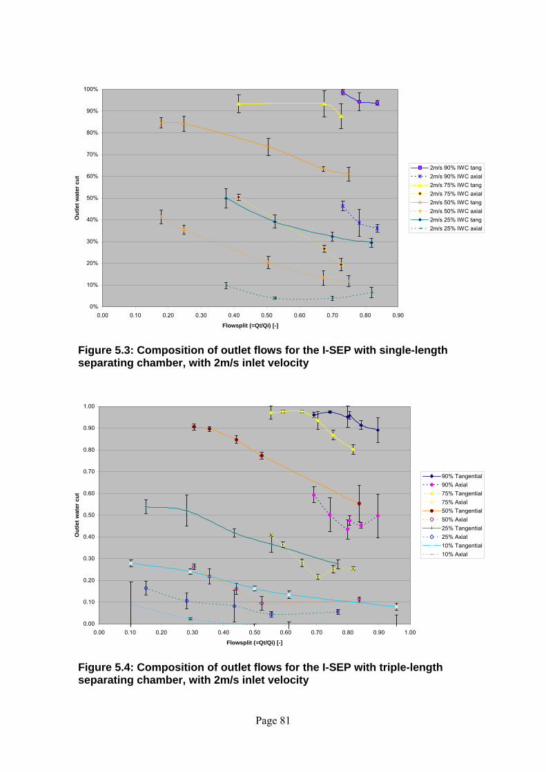
Page 81
0%
10%
20%
30%
40%
50%
60%
70%
80%
90%
100%
0.00 0.10 0.20 0.30 0.40 0.50 0.60 0.70 0.80 0.90
Flowsplit (=Qt/Qi) [-]
Out
let w
ater
cut
2m/s 90% IWC tang2m/s 90% IWC axial2m/s 75% IWC tang2m/s 75% IWC axial2m/s 50% IWC tang2m/s 50% IWC axial2m/s 25% IWC tang2m/s 25% IWC axial
Figure 5.3: Composition of outlet flows for the I-SEP with single-length separating chamber, with 2m/s inlet velocity
0.00
0.10
0.20
0.30
0.40
0.50
0.60
0.70
0.80
0.90
1.00
0.00 0.10 0.20 0.30 0.40 0.50 0.60 0.70 0.80 0.90 1.00
Flowsplit (=Qt/Qi) [-]
Out
let w
ater
cut
90% Tangential90% Axial75% Tangential75% Axial50% Tangential50% Axial25% Tangential25% Axial10% Tangential10% Axial
Figure 5.4: Composition of outlet flows for the I-SEP with triple-length separating chamber, with 2m/s inlet velocity

Page 82
0.00
0.10
0.20
0.30
0.40
0.50
0.60
0.70
0.80
0.90
1.00
0.00 0.10 0.20 0.30 0.40 0.50 0.60 0.70 0.80 0.90 1.00
Flowsplit (=Qt/Qi) [-]
Out
let w
ater
cut
90% Tangential90% Axial75% Tangential75% Axial50% Tangential50% Axial25% Tangential25% Axial10% Tangential10% Axial
Figure 5.5: Composition of outlet flows for the I-SEP with triple-length separating chamber, with 4m/s inlet velocity
0.00
0.10
0.20
0.30
0.40
0.50
0.60
0.70
0.80
0.90
1.00
0.00 0.10 0.20 0.30 0.40 0.50 0.60 0.70 0.80 0.90 1.00
Flowsplit (=Qt/Qi) [-]
Out
let w
ater
cut
90% Tangential90% Axial75% Tangential75% Axial50% Tangential50% Axial25% Tangential25% Axial10% Tangential10% Axial
Figure 5.6: Composition of outlet flows for the I-SEP with length five separating chamber, with 2m/s inlet velocity

Page 83
0.00
0.10
0.20
0.30
0.40
0.50
0.60
0.70
0.80
0.90
1.00
0.00 0.10 0.20 0.30 0.40 0.50 0.60 0.70 0.80 0.90 1.00
Flowsplit (=Qt/Qi) [-]
Out
let w
ater
cut
90% Tangential90% Axial75% Tangential75% Axial50% Tangential50% Axial25% Tangential25% Axial10% Tangential10% Axial
Figure 5.7: Composition of outlet flows for the I-SEP with length five separating chamber, with 4m/s inlet velocity
Referring to Table 5.1 we can see that making the dispersed phase water, rather than oil,
means that there is a much narrower difference in composition between outlets. This is
true for both the 10% IWC (compared with 90% IWC) and the 25% IWC case
(compared with 75% IWC).
IWC 10 25 50 75 90
Max. composition difference between the I-SEP outlets
(percentage points)
20 40 65 75 50
Table 5.1: Magnitude of difference between axial and tangential outlet compositions for 3x 2m/s
This is consistent with expectation, where a dispersed phase would be more mobile in a
less viscous continuous phase. With a higher viscosity, the kerosene impedes the
movement of water droplets more than the converse case, and so we see better
separation with a continuous water phase – at high IWC.

Page 84
5.3.3 Inlet water cut and velocity effects
For the cases with 90% inlet water cut separation in Figure 5.4 to Figure 5.6, the
tangential outlet flows can be produced essentially free of oil, to the accuracy of the test
method. This is confirmed visually. In the case of 90% IWC in Figure 5.7, the 5x unit at
4m/s inlet velocity, there is a thicker oil layer on the top of the water compared to the 3x
I-SEP and the 5x I-SEP at 2m/s (for tangential outlet samples). This gives an increased
tangential outlet oil content, at about 95% water cut, compared with that found in the
other cases. The axial outlet has a higher oil content, reducing the water cut to around
60%, in this stream compared to the inlet concentration.
If we compare the maximum measured tangential outlet concentration at 2m/s inlet
velocity for the 5x unit (Figure 5.6) with the same length unit at 4m/s (Figure 5.7), the
2m/s case has a film of oil on the water constituting 2 or 3 percent oil. Whereas at 4m/s,
there is around 5% oil in the tangential outlet flow, a visibly thicker layer after settling.
There are no defined peak/trough on the outlet water cut curves in Figure 5.7, which are
present in Figure 5.6 (though not greatly defined features). This shows a slightly greater
maximum compositional difference between outlets (40% on the scale rather than 30%
for Figure 5.7), suggesting that the increase in inlet velocity has hindered separation.
For 75% inlet water cut on Figure 5.6 and Figure 5.7 the separation is better (outlet
water curves are farther apart at up to 55% points for 2m/s and 60 points for 4m/s).
Comparing Figure 5.4 and Figure 5.5 – the same velocities for the 3x unit, we see a
similar story for 75% and 90% IWC. With the dispersed phase changed, on the other
side of the inversion point, 10% IWC has a very small difference in composition
between outlets for 2m/s and 4m/s at 5x length. In the latter case, it cannot be shown
that separation occurs at all – there is no demonstrable difference in outlet
compositions.
The higher velocities (Figure 5.5 and Figure 5.7) show less separation between curves

Page 85
than their lower inlet velocity counterparts (Figure 5.4 and Figure 5.6) for 25% inlet
water cut. This suggests that the lower velocity brings with it better performance,
despite the increase in centripetal force that comes with increased inlet velocity.
Additional effects of the velocity decrease would be to increase residence time (and
therefore coalescence) within the separator and also reduce shear due to turbulence.
Both of these would act to improve separation.
Figure 5.8 shows the best outlet water cuts (maximum outlet water cut for the tangential
outlet, minimum for the axial outlet) that were achieved at each tested inlet water cut at
various velocities for the 1x unit. Each data point is still an average of five sample
compositions, as explained in Section 4.4.3. It should be noted that the tangential and
axial outlet water cuts were not achieved simultaneously; the data shown are the highest
achieved with different flow splits to summarise the extent of the separator’s capability
at 1x length.
Figure 5.9 shows the highest achieved tangential outlet water cut for the 3x and 5x
units, and Figure 5.10 shows the lowest axial outlet water cuts, again. The solid lines
show the best compositions from each outlet and the dashed lines show the outlet water
cut found simultaneously at the other outlet. It should be borne in mind that these
maxima and minima curves are those found within the limits of flow split tested.
However, from these figures (especially Figure 5.9 and Figure 5.10) we can see that a
high degree of tangential outlet purity is achievable for a reasonable wide range of inlet
water cut – the fitted curves to Figure 5.9 and Figure 5.10 suggests a plateau at the
95%+ outlet water cut range applicable to inlet water cuts of 60% upwards.
For the 75% inlet water cut case, separation was better. Consider the 3x unit at 2m/s
inlet velocity (Figure 5.4). The highest measured tangential water cut is the same as that
for the 90% inlet water cut case on the same graph. For the axial outlet with 75% IWC,
measured water cut drops to around 25% for the same test, demonstrating a large
difference in compositions between outlets (a similar minimum value of around 25%
axial outlet water cut is achieved at 4m/s - Figure 5.5).

Page 86
This large difference between outlet compositions continues to exist at 50% inlet water
cut, but where the inlet condition has crossed to the other side of the inversion point, the
behaviour changes. The continuous phase now has a significantly increased viscosity,
thereby changing the way a droplet of a given size will move.
In Figure 5.4 (3x, 2m/s) for 50% inlet water cut, a flow split of 0.3 gives the maximum
measured tangential outlet water cut of 90%, whilst the axial outlet water cut is 27%
(there is no peak observed on this curve). At 25% inlet water cut, the next lower IWC
tested, the outlet water cuts are 50% (tangential) and 10% (axial). The 75% IWC
condition has the same concentration of dispersed phase to the 25% inlet water cut case
– except of oil rather than water. However, the 40 percentage-point maximum
difference between water cuts for the 25% IWC case at 3x 2m/s (Figure 5.4) compares
with a maximum difference of 75 percentage points for the 75% IWC, showing the
significant effect of changing the continuous phase. For 5x, 4m/s inlet velocity (Figure
5.6), there is very little difference between outlet compositions for the 10% IWC case –
it is below the minimum concentration that can be resolved by the method of
measurement (see Section 5.3.1).

Page 87
0.00
0.10
0.20
0.30
0.40
0.50
0.60
0.70
0.80
0.90
1.00
0.00 0.10 0.20 0.30 0.40 0.50 0.60 0.70 0.80 0.90 1.00
Inlet water cut
Out
let w
ater
cut
Tangential max 1x, 1m/sTangential max 1x, 2m/sTangential max 1x, 3m/sTangential max 1x, 4m/sTangential max 1x, 5m/sTangential max 1x, 6m/sTangential max 1x, 8m/sAxial min 1x, 1m/sAxial min 1x, 2m/sAxial min 1x, 3m/sAxial min 1x, 4m/sAxial min 1x, 5m/sAxial min 1x, 6m/sAxial min 1x, 8m/s
Figure 5.8: Maximum tangential outlet water cut and minimum axial outlet water cuts achieved with 1x unit
0.00
0.10
0.20
0.30
0.40
0.50
0.60
0.70
0.80
0.90
1.00
0.00 0.10 0.20 0.30 0.40 0.50 0.60 0.70 0.80 0.90 1.00
Inlet water cut
Tang
entia
l out
let w
ater
cut
(A) Tangential max 3x, 2m/s
(B) Tangential max 3x, 4m/s
(C) Tangential max 5x, 2m/s
(D) Tangential max 5x, 4m/s
(A) simultaneous axial WC
(B) simultaneous axial WC
(C) simultaneous axial WC
(D) simultaneous axial WC
Figure 5.9: Maximum tangential outlet water cut and corresponding simultaneous axial outlet water cut achieved with 3x and 5x units

Page 88
0.00
0.10
0.20
0.30
0.40
0.50
0.60
0.70
0.80
0.90
1.00
0.00 0.10 0.20 0.30 0.40 0.50 0.60 0.70 0.80 0.90 1.00
Inlet water cut
Axi
al o
utle
t wat
er c
ut
(E) Axial min 3x, 2m/s
(F) Axial min 3x, 4m/s
(G) Axial min 5x, 2m/s
(H) Axial min 5x, 4m/s
(E) simultaneous tang WC
(F) simultaneous tang WC
(G) simultaneous tang WC
(H) simultaneous tang WC
Figure 5.10: Maximum axial outlet water cut and corresponding simultaneous tangential outlet water cut achieved with 3x and 5x units
5.4 Separation Efficiency
Determining the effectiveness of the I-SEP as a separator is easier if we consider
separation efficiency. Merely looking at the outlet composition is insufficient to
illustrate the performance of a bulk separator. It is essential to look, in combination, at
the magnitude of the flow of each of the outlet streams.
There are a number of measures of efficiency that look at the extent of separation. The
definition used to calculate efficiency in the graphs below is from Smyth (1980) –
Equation 4.2. This definition incorporates both the flow split (Qu/Qi or Qt/Qi in I-SEP
terminology – the tangential outlet of the I-SEP is equivalent to the underflow of a
reverse-flow cyclone in receiving the denser phase) as well as the concentrations of the
inlet and underflow.

Page 89
i
u
i
u
i
u
kk
kk
−−−
=100100η (5.2)
This eliminates the problems of an alternative statement of efficiency, used in
applications such as cyclones that de-oil or de-water low (often less than 1%) dispersed
phase concentrations. In these cases, definitions such as Equation 4.3, for de-oilers, is
used, thereby only considering the change in concentration of the critical (in this case
the ‘oily’ outlet – the overflow, where the lighter-phase oil core leaves). This is
reasonable when comparing a specific class of cyclone, where the aim is to convert oil
concentrations measured in parts-per-million to concentrations measured in whole
percent. This is low oil flow in relation to the total inlet flow rates and therefore very
high outlet splits are the aim.
i
o
kk
=η (5.3)
Generally, and most importantly in the case of a device envisaged to provide a bulk
separation function, it is desirable to avoid trivial ‘high-efficiency’ results. These would
give a high efficiency value to a device that produced a ‘dribble’ of dispersed phase
from one outlet, whilst leaving the composition of the other outlet virtually unchanged.
Plainly, for bulk separation, where the flows fed to downstream polishing stages should
be minimised, this would miss the point. With this in mind, the expression in Equation
4.2 is used for efficiency and plots of efficiency vs. split are shown in Figure 5.14 to
Figure 5.18.
5.4.1 Data accuracy
The error bars shown on Figure 5.14 to Figure 5.18 are derived from combination of the
standard errors for measured outlet composition and flow rate.
With reference to the expression for efficiency given in Equation 4.2, and the results

Page 90
below in Equations 4.4 and 4.5 (Boas, 1983) that allow the combination of errors, we
can arrive at the expression given in Equation 4.6 for the error quantity associated with
our definition of separation efficiency.
(a) baz += 22 baz ∆+∆=∆ (5.4)
(b) baz =
22
⎟⎠⎞
⎜⎝⎛ ∆+⎟
⎠⎞
⎜⎝⎛ ∆=
∆bb
aa
zz (5.5)
It is rather unfortunate that the increased complexity of Equation 4.2 leaves us with a
considerably more complex error expression than that which would be derived from
efficiency as defined in Equation 4.3. However, it is a necessity to use an expression
such as Equation 4.2 to describe the performance of a bulk separator device realistically.
222
222
100100
⎟⎟⎟
⎠
⎞
⎜⎜⎜
⎝
⎛
⎟⎟
⎠
⎞
⎜⎜
⎝
⎛⎟⎟⎠
⎞⎜⎜⎝
⎛ ∆+⎟⎟
⎠
⎞⎜⎜⎝
⎛ ∆⎟⎟⎠
⎞⎜⎜⎝
⎛+
−−
+⎟⎟⎟
⎠
⎞
⎜⎜⎜
⎝
⎛
⎟⎟⎠
⎞⎜⎜⎝
⎛ ∆+⎟⎟
⎠
⎞⎜⎜⎝
⎛ ∆=
i
i
u
u
i
u
i
u
i
i
u
u
i
u
kk
kk
kk
kk
error (5.6)
5.4.2 Effect of flow split on efficiency
Analysing the general shape of plots of efficiency (see Figure 5.14 to Figure 5.18)
versus flow split shows a curve with a peak. The position of this peak would be
expected to be related to the inlet composition. As the inlet water cut increases, one
would expect more flow to leave from the tangential outlet, which is the target outlet for
water. Thus, a 75% flow split for a 75% inlet water cut would be consistent with the
separator operating perfectly and that backpressure on the unit was correctly set.
As well as perfect separation producing an optimal (in terms of efficiency) flow split
equalling the inlet water cut, we would expect the separator to function better for certain
inlet water cuts than others, given that perfect separation will not occur in practice. The

Page 91
inlet water cut at which the I-SEP gives highest efficiency should relate to the geometry
of the device and is theoretically expressed as the area ratio that the vortex finder ‘cuts’
into the cross-sectional area of the separating chamber. The reasoning for this is set out
as follows. If a core of well-separated oil forms, there is also likely to be a film of well-
separated water at the wall of the separating chamber, in between these will be an
annulus comprising one or more concentric zones where there is less good separation
(Figure 5.11).
Figure 5.11: Concentric zones of different separation levels
The highest efficiency for all inlet water cuts would occur at an inlet water cut where
the vortex finder has the same cross-sectional area fraction as the cross-sectional area
occupied by the ‘pure’ oil core, or the most oil-enriched region in the separating
chamber. At this state, the maximum oil is removed in the minimum flow and the
converse applies for water at the other outlet.
With flow split at an optimum, if the inlet composition gives an oil core diameter that is
not similar to that of the vortex finder, flow is disrupted in the region of the vortex
finder and this impedes separation. For example, with 75% inlet water cut and 75%
outlet split created by application of backpressure (so that 75% of flow leaves at the
Oil+Water
Oil
Water
Oil
Water

Page 92
tangential outlet, 25% at the axial outlet), in perfect separation conditions there will be
an oil core occupying the central 25% of the separating chamber area. If the vortex
finder cuts the central 75% of the area, there is an annulus of water between the oil core
and the vortex finder diameter that represents 50% of the separating chamber area.
However, because only 25% of the inlet flow can leave through the axial outlet, the
50% annular area of water is forced to move out around the vortex finder (Figure 5.12).
In fact, we would find that the 25% oil would try to expand to fill the vortex finder – for
a perfectly separating system, only oil would be able to leave due to the composition
matching the outlet flow. The acceleration necessary for increased water velocity
around the outlet, caused by the remaining 75% of the flow exiting the separator
through 25% of the cross-sectional area, would cause turbulence that undermines
separation and re-entrains already-separated oil into the less-dense phase outlet flow
(Figure 5.12). The qualitative appearance of this phenomenon was observed during
testing, but photographic evidence was not obtained to reproduce here.
Figure 5.12: Re-entrainment of flow from vortex finder
To reiterate the point, whilst an attempt can be made to use backpressure to restrict flow
from the tangential outlet to accommodate variability in the inlet composition, the aim

Page 93
should be to match outlet areas with inlet composition. This would theoretically give the
highest efficiency for that inlet water cut. However, restricting flow leaving at the
tangential outlet by using backpressure will act as a break on the outermost regions of
flow, slowing them down. This will have the consequence of reducing the centripetal
force available to move and separate droplets. At the same time the central zone of
liquid that is leaving by the axial outlet is accelerating in order to exit via a relatively
small (for the increase in flow caused by flow restriction at the other outlet) axial outlet
thus causing increased the shear between these two regions of increasingly dissimilar
velocity (Figure 5.13). The increased velocity of the axial flow through the separator
will also act to decrease the residence time of the central region of flow within the
separator, which will diminish the separation effect on this region.
Figure 5.13: Conical shape of boundaries of zones shearing against each other as backpressure is applied to the tangential outlet
The implication of this is that it is possible to increase the application of a particular
geometry of unit (in terms of relative outlet areas and the proportion of separating
chamber cross-sectional area) to different inlet compositions by manipulating the flow
split by means of external valves. However, the result will show a lower efficiency than
if the unit were geometrically tailored to that particular split.
Zone where rotation is slowed down by applying backpressure
Zone of accelerated flow due to more liquid being forced through axial outlet

Page 94
Data from other researchers (Simkin and Olney – see Section 5.7.1) shows variation of
efficiency with inlet velocity such that non-optimal configurations or conditions cause
the peaks to become harder to distinguish from each other. This is due to the
maximisation of efficiency by taking purer flow from the outlets.
With reference to Figure 5.11, minimising the proportion of the not-fully-separated
annulus (O/W) leaving through an outlet by manipulating the flow split by backpressure
will provide the peak of the efficiency curve. In the case where the inlet water cut is
greater than the inversion point (water continuous), the tangential outlet flow would
need to be reduced so that its outlet flow is as high as possible in fully-separated water
(located close to the I-SEP wall as shown in the top diagram). This would minimise the
oil-water mixed phase leaving by this outlet. The flow split (tangential flow divided by
inlet flow) consequently reduces the point at which we find the efficiency peak. For the
converse case, where the inlet water cut is below that of the inversion point (oil
continuous), poorer separation and more oil-water mixed phase means that less flow of
almost-pure oil phase is available to leave via the axial outlet. Flow split is defined in
terms of tangential outlet flow, and, by mass balance, the axial outlet flow fraction is (1-
tangential flow), so the result is that (1-flow split) will be reduced and the flow split will
therefore increase, relocating the efficiency peak to a higher flow split when separation
becomes poorer. Logically this will have the effect of pulling the peaks of the efficiency
curves for both the tangential and axial outlets towards a limiting flow split with poorer
and poorer separation. Because the movement of efficiency peak with respect to flow
split is dependent on which phase is continuous, this argument implies that both outlet
efficiency peaks will both end up at the point at with the continuous phase changes – the
inversion point, which is 50% water in the case of the kerosene-water system. The
corollary of this is that, in general, a separator is more effective the further away that the
efficiency peaks are from a flow split equal to the inversion point, and therefore from
each other.
The position of the maxima of the efficiency curves can therefore be used to gauge the
approach of a particular unit to ideality. The efficiency peaks from the I-SEP test results
do not lie at the theoretical ideal position where the flow split of maximum efficiency

Page 95
equals the inlet water cut.
0.00
0.10
0.20
0.30
0.40
0.50
0.60
0.70
0.80
0.90
1.00
0.00 0.10 0.20 0.30 0.40 0.50 0.60 0.70 0.80 0.90 1.00
Flowsplit (=Qt/Qi) [-]
Effic
ienc
y 2m/s 90% IWC2m/s 75% IWC2m/s 50% IWC2m/s 25% IWC
Figure 5.14: Efficiency of separation for single-length unit at 2m/s inlet velocity

Page 96
0.00
0.10
0.20
0.30
0.40
0.50
0.60
0.70
0.80
0.90
1.00
0.00 0.10 0.20 0.30 0.40 0.50 0.60 0.70 0.80 0.90 1.00
Flowsplit (=Qt/Qi) [-]
Effic
ienc
y
90% Water Cut75% Water Cut50% Water cut25% Water Cut10% Water Cut
Figure 5.15: Efficiency of separation with triple-length unit at 2m/s inlet velocity
0.00
0.10
0.20
0.30
0.40
0.50
0.60
0.70
0.80
0.90
1.00
0.00 0.10 0.20 0.30 0.40 0.50 0.60 0.70 0.80 0.90 1.00
Flowsplit (=Qt/Qi) [-]
Effic
ienc
y
90% Water Cut75% Water Cut50% Water cut25% Water cut10% Water cut
Figure 5.16: Efficiency of separation with triple-length unit at 4m/s inlet velocity
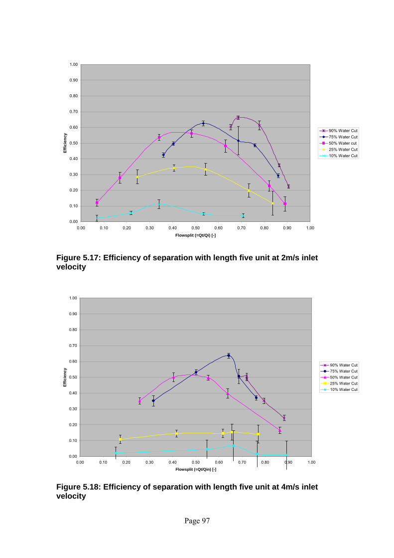
Page 97
0.00
0.10
0.20
0.30
0.40
0.50
0.60
0.70
0.80
0.90
1.00
0.00 0.10 0.20 0.30 0.40 0.50 0.60 0.70 0.80 0.90 1.00
Flowsplit (=Qt/Qi) [-]
Effic
ienc
y
90% Water Cut75% Water Cut50% Water cut25% Water Cut10% Water Cut
Figure 5.17: Efficiency of separation with length five unit at 2m/s inlet velocity
0.00
0.10
0.20
0.30
0.40
0.50
0.60
0.70
0.80
0.90
1.00
0.00 0.10 0.20 0.30 0.40 0.50 0.60 0.70 0.80 0.90 1.00
Flowsplit (=Qt/Qin) [-]
Effic
ienc
y
90% Water Cut75% Water Cut50% Water Cut25% Water Cut10% Water Cut
Figure 5.18: Efficiency of separation with length five unit at 4m/s inlet velocity

Page 98
Looking at the 3x unit with 2m/s inlet velocity (Figure 5.15) we can see a clear peak in
efficiency at around 70% for the 90% IWC curve. This occurs at about 75% flow split.
On the same figure, the 75% inlet water cut curve shows peak efficiency at about 65%
flow split. This is again below the ‘ideal’ value, as would be expected where separation
is incomplete. This peak efficiency is higher than for 90% IWC and therefore gives the
best performance for the 3x unit at 2m/s. After this high point, the lower compositions,
past the inversion point region at around 50% water cut and into the oil-continuous
region at inlet water cuts of 25% and 10%, show further declines in efficiency.
It should be noted that the peak efficiency of the 50% inlet water cut curve (Figure 5.15)
is close to, and with experimental error, indistinguishable from that of the 90% curve
(although at a different flow split). The decline in efficiency for the oil-continuous
system would be expected by considering just the reduced droplet mobility because of
viscosity. It is nevertheless interesting that the 10% inlet water cut efficiency line is
significantly higher than the 25% line. This is not behaviour that continues through to
the 5x unit results (see Figure 5.17 and Figure 5.18) or 3x 4m/s (Figure 5.16). Other
configurations show the same trend of decreasing efficiency with decreasing water cut,
although there is a certain amount of switching between the highest efficiency peak
being owned by the 90% or the 75% (5x unit at 4m/s inlet velocity and 3x unit at 2m/s
inlet velocity) inlet water cut condition – see later on in this section.
As discussed above, there is likely to be a connection between the vortex-finder-area
proportion and best performance. The vortex finder on the I-SEP cuts the portion of the
area that coincides with the best performance of the unit, as shown below in Table 5.2,
cutting the transitional zone between the oil core and the more mixed oil-water zone
surrounding this at 10% or 25% oil cut (90% and 75% inlet water cut). The vortex
finder configuration therefore should mean the unit performs best at 10-25% oil inlet
fraction.

Page 99
Inner diameter Outer diameter Percent cross-sectional area based
on inner diameter (outer diameter
in parentheses)
Vortex finder 6.3mm 9mm 12.9 (26.4)
Separator
body
17.5mm
Table 5.2: Vortex finder area
It is not obvious which of the vortex finder dimensions (inner or outer diameter) is the
pertinent one, though possibly it is the mean of the two. As a design detail, the
protruding edge of the vortex finder should be sharp – not least because this gives only
one ratio with which to predict the best operating condition of the separator! Also on a
small scale such as the I-SEP unit under test, where the thickness of the vortex finder is
significant, a sharp edge would give a smoother split between liquid in near proximity
to the vortex finder and being directed to different outlets.
It would seem reasonable to suggest that there is a link between the vortex finder and
the optimum inlet water cut. The variation of this aspect of geometry is not investigated
within this work, but it would be a logical next step for investigation in the further
development of the I-SEP.
Returning to the positions of efficiency peaks, the measured positions of these (to the
nearest 5% - generated by curve fitting) are tabulated in Table 5.3 and plotted in Figure
5.19.

Page 100
5x 3x 1x Length
Velocity 2m/s 4m/s 2m/s 2m/s 4m/s
0.10 0.35 N/A N/A 0.40 N/A
0.25 0.45 N/A 0.45 0.40 0.45
0.50 0.45 0.50 0.50 0.50 0.50
0.75 0.50 0.65 0.65 0.65 0.70
IWC
0.90 0.70 0.70 0.80 0.75 N/A
Table 5.3: Values of flow split at which peak efficiency occurs
These data are coarse, as the peak position is derived from a curve fitted to the data, so
data is taken to the nearest 5% increment of flow split. Despite the lowered resolution, it
can be seen that there is generally a greater deviation of efficiency peak maxima from
their ideal value when the inlet water cut is below the inversion point. This reflects the
poorer separation performance found below the inversion point.
Each of the flow conditions occupy similar positions relative to the y=x line, the
exception being in the 2m/s 1x case. These tests were in a unit with a slightly different
geometry, containing a slightly tapered separating chamber.

Page 101
0.00
0.10
0.20
0.30
0.40
0.50
0.60
0.70
0.80
0.90
1.00
0.00 0.10 0.20 0.30 0.40 0.50 0.60 0.70 0.80 0.90 1.00
Inlet water cut
Flow
spl
it at
whi
ch e
ffici
ency
pea
ks
2m/s, 1x2m/s, 3x2m/s, 5x4m/s, 3x4m/s, 5xy=x
Figure 5.19: Flow split at which efficiency curves peak for each inlet water cut
5.4.3 Inlet velocity
Considering the effect of inlet velocity on efficiency, initially for the 3x case there is a
significant difference between the 2m/s case (Figure 5.15) and the 4m/s case (Figure
5.16). The curves for 3x 4m/s decrease in efficiency with decreasing inlet water cut. For
3x 2m/s this is a general trend but peak efficiency for 25% inlet water cut is lower than
the peak efficiency for 10%, and also 90% inlet water cut shows a lower peak efficiency
than 75%. This in unexpected, but interesting in that this switching of the expected
positions of the curves happens for the same fraction of dispersed phase fraction – on
both sides of the inversion point. This suggests that there may be a factor causing the I-
SEP to separate the sparser end of dispersed phase fraction more poorly at lower inlet
velocities, since the graph error bars do not invalidate these observations.
Looking at the 2m/s 5x case (Figure 5.17) however, the expected order of the curves is
restored, and almost in the 4m/s case (Figure 5.18) where the 90% inlet water cut

Page 102
condition peak again drops below that of the 75% inlet water cut line. This behaviour is
puzzling as the error analysis shows them to be valid effects, but there are other clear
trends with velocity.
The performance of the I-SEP deteriorates when the inlet velocity is increased from
2m/s to 4m/s. Whilst this deterioration is insignificant in terms of high water cuts (75%,
90%), which show similar efficiencies between the two velocities, there is a significant
change between 25% and 10% IWC. The 50% IWC curve shows a modest decrease in
its peak – from 57% to 52% (Figure 5.17, Figure 5.18) with increased inlet velocity for
the 5x unit, but 25% inlet water cut decreases from 35% to 15% for the 3x unit. This is
even more pronounced with the 5x unit at 25% inlet water cut, decreasing from 50%
peak efficiency at 2m/s to 20% at 4m/s.
Whilst the 10% IWC curve varies from one low level of separation to another (10%
efficiency at 2m/s to 5% at 4m/s), for the 3x length the peak efficiency drops from 60%
to 20%. In general, these performances are probably so low as to make their practical
usefulness marginal – except in the case of the 10% IWC case at 2m/s 3x, but the
variability of these values indicates how sensitive separation efficiency is to inlet
velocity. In terms of experimental observation, the above results fit well with the fact
that outlet flows appeared much more mixed for higher velocities. Visual differences in
outlet flows between tests with differing lengths of the separator were much less easily
observed because of the necessarily greater time between tests caused by the need to
install a modified test unit.
It should be noted that inlet velocity does not merely have an effect on flow within the
separator. The droplet dispersion generated by the static mixer array is dependent on the
inlet velocity. A quantitative analysis of the interplay between different velocity effects
is included in the next chapter. However, these results would show that increased
velocity causes increased turbulence that outweighs the increase in centrifugal
separation force - more mixed flow separates less well.

Page 103
5.4.4 Length of separator
Early results and analysis of the problem of separation within a cyclonic device
suggested that it might be advantageous to lengthen the separating chamber of the I-
SEP. This would increase the residence time of the separator and therefore the time
spent by the oil-water mixture within a centripetal force-field.
The intention in these tests is to investigate the effect on performance of the device of
different lengths of separator and, if possible, to find an optimum length. This may just
be ‘as long as possible’, or it may be that, for example, the increase in wall effects due
to a longer unit would cause a deterioration in performance beyond a point. This may be
attributed to wall friction slowing the rotating flow down to a point where more
chamber length is counter-productive.
In relation to the 1x unit, the effect on separation with water cuts above 10% can be
compared. The lengthened 3x unit at 2m/s (Figure 5.15), in comparison with the 1x unit
at 2m/s (Figure 5.14) shows increased peak efficiency from 72% to 80% for 75% inlet
water cut. The 90% IWC line does not exhibit a peak for the flow splits investigated,
but the efficiency does rise above the maximum efficiency found for the 90% IWC
curve on the 3x unit at 2m/s. In comparison with the 5x 2m/s case (Figure 5.17) at 90%
and 75% IWC, the longer of the units has a lower peak efficiency.
For inlet water cuts below the inversion point, the 25% IWC line peaks at around 50%
efficiency for 1x and 3x but drops to a maximum efficiency of 35% for 5x at 2m/s. The
comparison between 3x and 5x for 10% inlet water cut at 2m/s is illustrated in Figure
5.20 and shows that there is a massive difference in efficiency at this high oil content.
The difference in length causes a deterioration from 60% peak efficiency to 10% and
correlates with a much larger compositional difference between the outlets at 10% IWC,
compared to 5m/s at 2m/s inlet velocity.
For the case where the inlet water cut is at or near the inversion point, 50% IWC, for the

Page 104
2m/s case the peak efficiency rises from 53% at 1x to 70% at 3x before dropping to
57% at 5x. At inlet conditions around the inversion point, the separation should be
difficult. The optimal length for best efficiency is found with the 3x unit.
The effect of length on separation efficiency at different lengths is crystallised in Figure
5.20 to Figure 5.22. The figures also show the dissimilarity of curves with the same
dispersed phase concentration – 25% compared with 75% IWC, 10% compared with
90%.
At 4m/s inlet velocity, comparing 3x (Figure 5.16) with 5x (Figure 5.18), the trends
shown at 2m/s are also shown – i.e. decreased peak efficiency with the 5x unit. The only
exception to this is for the 50% IWC case, where the error bars are taken into account it
cannot be shown that there is any difference in performance at the different lengths with
this inlet water cut.
The original (1x) unit gives results that are compatible with the observations given
above, with slightly lower peak efficiency for 75% IWC at 2m/s compared to the 3x
unit. The 25% case efficiency is also comparable, possibly even slightly higher. The
most remarkable difference is the 50% IWC line, which is much lower in the 1x unit
than the 3x unit. Peak efficiency for the latter case is around 70% at around 50% flow
split, but at the same flow split for the 1x unit, the efficiency is only 18%. Interestingly
the curve does not exhibit a peak, instead rising with lower flow split, but does not
approach the effectiveness of the extended unit at this inlet composition. Since the 50%
IWC is close to the inversion point, this suggests that a shorter unit is much less
effective at dealing with the highly complex droplet interactions at this point.

Page 105
0.00
0.10
0.20
0.30
0.40
0.50
0.60
0.70
0.80
0.90
1.00
0.00 0.10 0.20 0.30 0.40 0.50 0.60 0.70 0.80 0.90 1.00
Flowsplit (=Qt/Qi) [-]
Effic
ienc
y
5x 10% IWC3x 10% IWC
Figure 5.20: Comparison of efficiency for different separator lengths at 10% inlet water cut
0.00
0.10
0.20
0.30
0.40
0.50
0.60
0.70
0.80
0.90
1.00
0.00 0.10 0.20 0.30 0.40 0.50 0.60 0.70 0.80 0.90 1.00
Flowsplit (=Qt/Qi) [-]
Effic
ienc
y
1x 75% IWC3x 75% IWC5x 75% IWC1x 25% IWC3x 25% IWC5x 25% IWC
Figure 5.21: Comparison of efficiency for different separator lengths at 25% and 75% inlet water cut

Page 106
0.00
0.10
0.20
0.30
0.40
0.50
0.60
0.70
0.80
0.90
1.00
0.00 0.10 0.20 0.30 0.40 0.50 0.60 0.70 0.80 0.90 1.00
Flowsplit (Qt/Qi) [-]
Effic
ienc
y
1x 50% IWC3x 50% IWC5x 50% IWC1x 90% IWC3x 90% IWC5x 90% IWC
Figure 5.22: Comparison of efficiency for different separator lengths at 90% and 50% inlet water cut
5.5 Pressure drop
The pressure drop across the separator is measured as the differential pressure between
the inlet and each outlet. It is an important consideration in the operation of a separator.
It defines the energy required to perform a separation. The trend of pressure drop is
shown in Figure 5.23 to Figure 5.26. They show curves between the trivial conditions
where either outlet valve is closed (flow splits of 0 and 1) so that all flow leaves the
separator through the other outlet.
There is obviously a greater magnitude of pressure drop for the higher inlet velocities.
By comparing the inlet to tangential outlet pressure drop for the 3x unit between 2m/s
(Figure 5.23) and 4m/s inlet velocity (Figure 5.24), at 0.9 flow split, we see the pressure
drop increase from 0.12bar to 0.4 bar. As the velocity has doubled, the system shows
the expected four-times increase in pressure drop.

Page 107
Inlet to tangential pressure drop increases with flow-split, which is defined as the
fraction of inlet flow leaving through the tangential outlet. However, with tangential
outlet valve fully closed, the pressure drop reaches a minimum that corresponds to the
impact or stagnation pressure based in inlet conditions, equal to one velocity head
(Equation 4.7).
2
21 vP ρ=∆ (5.7)
Inlet water cut /%
Inlet velocity/ (m/s) 10 25 50 75 90
2 0.016 0.017 0.018 0.019 0.020
4 0.066 0.068 0.072 0.076 0.078
Table 5.4: Impact pressure at different inlet conditions for kerosene-water
There are differences between the DPI/T curves (Figure 5.23 to Figure 5.26) depending
on the inlet water cut as would be expected with different mean liquid densities passing
through the I-SEP. Therefore 90% IWC would be expected to give a lower pressure-
drop for the same flow split than 75% IWC because the kerosene has a higher viscosity
than water. The data collected produce lines that lie close together but are in no
consistent sequence across the data sets, at times overlapping. The difference between
pressure drop changes due to compositional change would therefore appear to be too
fine for measurement in this experimental configuration.
Figure 5.27 shows the relationship between flow split and Euler number or loss
coefficient for the separator. Defined in Equation 4.8, the loss coefficient is
characteristic of a cyclone (or other flow geometry), but is varied between 3 and 12 for
the axial outlet pressure drop and 1 and 7 for the tangential outlet. The flow split
manipulation is responsible for this variation.

Page 108
2.21
in
l
v
Pkρ
∆= (5.8)
0.00
0.02
0.04
0.06
0.08
0.10
0.12
0.14
0.00 0.10 0.20 0.30 0.40 0.50 0.60 0.70 0.80 0.90 1.00
Split ratio (=Qt/Qi) [-]
Pres
sure
dro
p be
twee
n in
let a
nd ta
ngen
tial o
utle
t (D
PI/T
) [ba
r]
90% IWC75% IWC50% IWC25% IWC10% IWC
Figure 5.23: Inlet to tangential outlet pressure drop for the 3x I-SEP at 2m/s

Page 109
0.00
0.05
0.10
0.15
0.20
0.25
0.30
0.35
0.40
0.45
0.00 0.10 0.20 0.30 0.40 0.50 0.60 0.70 0.80 0.90 1.00
Split ratio (=Qt/Qi) [-]
Pres
sure
dro
p be
twee
n in
let a
nd ta
ngen
tial o
utle
t (D
PI/T
) [ba
r]
90% IWC70% IWC50% IWC25% IWC10% IWC
Figure 5.24: Inlet to tangential outlet pressure drop for the 3x I-SEP at 4m/s
0.00
0.02
0.04
0.06
0.08
0.10
0.12
0.14
0.16
0.00 0.10 0.20 0.30 0.40 0.50 0.60 0.70 0.80 0.90 1.00
Split ratio (=Qt/Qi) [-]
Pres
sure
dro
p be
twee
n in
let a
nd ta
ngen
tial o
utle
t (D
PI/T
) [ba
r]
90% IWC75% IWC50% IWC25% IWC10% IWC
Figure 5.25: Inlet to tangential outlet pressure drop for the 5x I-SEP at 2m/s

Page 110
0.00
0.05
0.10
0.15
0.20
0.25
0.30
0.35
0.40
0.45
0.50
0.00 0.10 0.20 0.30 0.40 0.50 0.60 0.70 0.80 0.90 1.00
Split ratio (=Qt/Qi) [-]
Pres
sure
dro
p be
twee
n in
let a
nd ta
ngen
tial o
utle
t (D
PI/T
) [ba
r]
90% IWC75% IWC50% IWC25% IWC10% IWC
Figure 5.26: Inlet to tangential outlet pressure drop for the 5x I-SEP at 4m/s
0.00
2.00
4.00
6.00
8.00
10.00
12.00
0.00 0.20 0.40 0.60 0.80 1.00 1.20
Flow Split (=Qt/Qi) [-]
Eule
r num
ber [
-]
AxialTangential
Figure 5.27: Euler number for the I-SEP at various flow splits

Page 111
5.6 Testing with an alternative oil
As mentioned in Section 4.4.1.6, it was possible briefly to test the separation
performance of the I-SEP with an alternative oil to the kerosene used thus far. This oil
was a silicon-based oil, supplied by a client of BHR Group, to determine if the I-SEP
could separate the water-in-oil dispersion that was found in the client’s process.
The scope of the test work for the client, and the results presented here, allowed testing
at 25% inlet water cut only. Sufficient material was provided such that no recycling of
feed was necessary in the test work. Two separator lengths were tested, 3x and 5x and
the 3x unit was tested at 2m/s and 5.5m/s inlet velocity. The results of the tests enable
the presentation of outlet composition and efficiency data in Figure 5.28 and Figure
5.29, below.
0.00
0.10
0.20
0.30
0.40
0.50
0.60
0.70
0.80
0.90
1.00
0.00 0.10 0.20 0.30 0.40 0.50 0.60 0.70 0.80 0.90 1.00
Flow Split (=Qt/Qi) [-]
Out
let w
ater
cut
3x sep 2m/s TANGENTIAL3x sep 2m/s AXIAL3x sep 5.5 m/s TANGENTIAL3x sep 5.5 m/s AXIAL5x sep 2m/s AXIAL5x sep 2m/s TANGENTIALK-w 3x 25% IWC TangentialK-w 3x 25% IWC Axial
Figure 5.28: Outlet water compositions for silicon-based oil and equivalent test data for kerosene and water at 2m/s and 5.5m/s inlet velocity

Page 112
0.00
0.10
0.20
0.30
0.40
0.50
0.60
0.70
0.80
0.90
1.00
0 0.1 0.2 0.3 0.4 0.5 0.6 0.7 0.8 0.9 1
Flow Split (=Qt/Qi) [-]
Effic
ienc
y 3x sep 2m/s3x sep 5.5 m/s5x sep 2m/sK-w 3x 25% IWC
Figure 5.29: Separation efficiency for silicon-based oil and equivalent data for kerosene-water at 2m/s inlet velocity
Before any tests had been performed with the I-SEP it seemed clear that performance
was likely to be poorer that with the kerosene-water system. This was based on shake
tests carried out with the two liquids in boiling tubes with air excluded. With just
shaking by hand, the kerosene-water system settled in about 1 minute. However, the
alternative oil took around half-an-hour to appear similarly settled. Even at this point,
the water phase appeared milky. Looking at the graphs, the results are consistent with
these observations.
Comparison between the results for the two oils (Figure 5.28) shows that the silicon-
based oil separates less well than the kerosene-water system. Whilst there is around a 40
percentage-point difference between the outlet water cuts for the kerosene-water
system, the silicon-based oil and water system gives a maximum of 25% points in the
3x 2m/s case.
Looking at the efficiency data (Figure 5.29), the maximum efficiency achieved with

Page 113
silicon-based oil and water is around 15%, contrasting with 50% for kerosene-water.
Figure 5.28 also clearly shows the relative performance of the three tested silicon-based
oil configurations compared with kerosene-water, and the qualitative assessment of
these is consistent with the trends observed during testing with kerosene and water. The
best performance is seen with 2m/s inlet velocity with the 3x unit. The other conditions
produce a separation that is too small to be measurable. The separation tests with
kerosene and water showed that 3x 2m/s was a condition that produced more favourable
results than increased inlet velocity or length, and this is underlined by the result in the
figures above showing that the performance is much worse away from the 3x 2m/s
condition.
As shown in Table 4.4, the silicon-based oil has a viscosity fifteen times that of water,
compared to twice that of water for the kerosene. The density difference is also 4.5
times greater for kerosene-water (960 kg/m3 compared to 820 kg/m3 for kerosene,
giving density differences of 40 and 180 kg/m3 respectively). Combination of these
factors means that droplets of water in oil (as tested) have to move through a medium
that resists their movement far more than kerosene does, at the same time with a much
smaller driving force. It is therefore inevitable that performance will be far lower than
for kerosene-water. The 25% inlet water cut condition has been demonstrated to be less
efficient than inlet compositions in the 75% water region, both because the I-SEP
geometry is conducive to this and because a water-continuous separation should be
easier. However, in this circumstance, the driving force for separation has still been
reduced from the kerosene-water system. Whilst separation will be improved for 75%
inlet water cut, the performance will still be inferior to the kerosene-water system.
In order to improve this, the combination of separation force and residence time within
the unit should be improved, combined with a reduction of turbulence, especially
important for a liquid that tends to produce small droplets easily, such as for this oil.
5.7 Comparison with other separators
The I-SEP is a cyclone separator of the axial-flow type and as such, its use as a bulk oil-

Page 114
water separator is unique. By analysing the collected results from the experiments
earlier in this chapter, we can arrive at a description of how well the I-SEP performs,
but it would also be very pertinent to compare the performance of the unit with other
cyclonic separation devices in terms of performance. This will allow some insight into
the relative merits of the I-SEP and other cyclonic separators.
This task is not a simple one, because there is relatively little published data on
examples of cyclonic separation of oil and water, especially that which is in sufficient
detail to be useful. The comparison would ideally be across a wide range of inlet
compositions, in the same fashion as the data gathered here. Fortunately, there are a
small number of published papers that contain data that allow a comparison between the
I-SEP separation performance and that of other cyclonic oil-water separators. The data
used has been derived from three papers – read from the graphs and re-plotted together
with data from the I-SEP for a direct comparison. They are discussed below.
5.7.1 Simkin and Olney (1956)
Simkin and Olney (1956) looked at the performance of a reverse-flow cyclone as a
liquid-liquid separator and mass transfer device. The tested configuration of this device
is shown in Figure 5.30.
The data given is for kerosene-water separation. The exact properties of the oil are not
given, but are assumed to be the same as those used for the tests on the I-SEP.
Efficiency is defined as an equivalent expression to the function used here to describe
the I-SEP efficiency. This is given with respect to a split defined as the ratio of overflow
to underflow – which is readily converted to the same basis as used earlier in this
chapter.

Page 115
Figure 5.30: Configuration of Simkin and Olney cyclone (after fig. 1 of Simkin and Olney, 1956)
The cyclone shown in Figure 5.30 has a diameter of 3.75” (0.095m) compared with the
I-SEP separating chamber diameter of 0.0017m, so that in the I-SEP there is around 50
times the centripetal force acting on droplets moving through the separator as for the
Simkin & Olney cyclone with the same tangential velocity. However, the unit above
also has a volume of around 3.2x10⁻³ m3, compared to the I-SEP separating chamber
volume of 5.7x10⁻⁶ m3. This gives a volume ratio of over 500 times the volume of the I-
SEP. With the inlet size of 1-inch diameter for the Simkin and Olney cyclone, the
volumetric inlet flow is around ten times that of the I-SEP at the same inlet velocity, so
the residence time of the unit is around 50 times that of the I-SEP.
Whilst there may be a difference in the drop size distribution between the two
separators, to a first approximation the increased separation force in the I-SEP would be

Page 116
cancelled out by the increased residence time of the Simkin and Olney cyclone. It is
therefore reasonable to compare results between the two units.
Figure 5.31 to Figure 5.33 compare the performance of the Simkin and Olney cyclone at
various inlet velocities with the I-SEP results at 2m/s inlet velocity. This is the nearest
match in terms of collected inlet velocity data. Data has been converted to the same
basis as that used in this document and plotted alongside efficiency data for the I-SEP in
the figures below.
In order to compare the two cyclones, it would be preferable to keep as many
parameters the same as possible. However, because of the differences between axial
flow cyclones and reverse flow cyclones, and because available data is not necessarily
taken at data points that are entirely convenient, the data for the I-SEP tests has been
chosen to be as close as possible, or to the best performance of the I-SEP, as
appropriate. The graphs below are as similar as possible in terms of the inlet velocities.
The values obtained by Simkin and Olney are closest to the 2m/s inlet velocity test
condition and have been compared with the 3x test unit, which will be concluded as the
best I-SEP geometry, at the end of the chapter.

Page 117
0.00
0.10
0.20
0.30
0.40
0.50
0.60
0.70
0.80
0.90
0.00 0.10 0.20 0.30 0.40 0.50 0.60 0.70 0.80 0.90
Flow split (underflow/inlet)
Effic
ienc
y
S&O 25% IWCS&O 50% IWCS&O 75% IWCI-SEP 25% IWCI-SEP 50% IWCI-SEP 75% IWC
Figure 5.31: Comparison of Simkin and Olney cyclone data for kerosene-water separation at 1.87 m/s with the 3x I-SEP at 2m/s
0.00
0.10
0.20
0.30
0.40
0.50
0.60
0.70
0.80
0.90
0.00 0.10 0.20 0.30 0.40 0.50 0.60 0.70 0.80 0.90
Flow split (underflow/inlet)
Effic
ienc
y
S&O 25% IWCS&O 50% IWCS&O 75% IWCI-SEP 25% IWCI-SEP 50% IWCI-SEP 75% IWC
Figure 5.32: Comparison of Simkin and Olney cyclone data for kerosene-water separation at 2.5 m/s with the 3x I-SEP at 2m/s

Page 118
0.00
0.10
0.20
0.30
0.40
0.50
0.60
0.70
0.80
0.90
1.00
0.00 0.10 0.20 0.30 0.40 0.50 0.60 0.70 0.80 0.90 1.00
Flow split (underflow/inlet)
Effic
ienc
y
S&O 10% IWCS&O 25% IWCS&O 50% IWCS&O 75% IWCI-SEP 10% IWCI-SEP 25% IWCI-SEP 50% IWCI-SEP 75% IWC
Figure 5.33: Comparison of Simkin and Olney cyclone data for kerosene-water separation at 0.62 m/s with the 3x I-SEP at 2m/s
The 1.87m/s and 2.5m/s inlet velocity conditions from the Simkin and Olney data
(Figure 5.31 and Figure 5.32) cover the 25% to 75% inlet water cut range, whereas the
0.62 m/s inlet velocity case (Figure 5.33) also has the 10% inlet water cut condition for
comparison. Considering the higher velocity (1.87m/s and 2.5m/s) cases first, there are
higher separation efficiencies for the Simkin and Olney cyclone than for the I-SEP at
2m/s inlet velocity, with peak efficiency for the Simkin and Olney cyclone remaining
almost constant for the two higher velocities at 25 and 50% inlet water cut (at around
75% to 80% efficiency).
The improvement in performance over the I-SEP at the 25% inlet water cut case is quite
large (about 25 percentage points), whilst it is more modest at 50% (75 or 80%
efficiency compared to 70% for the I-SEP). However, at both 1.87m/s and 2.5m/s inlet
velocity, the 3x I-SEP unit running with 2m/s inlet velocity has a higher separation
efficiency for a 75% water mixture. The peak is about 8 percentage points higher for the

Page 119
I-SEP than Simkin and Olney at 1.87m/s and 20 percentage points higher than at
2.5m/s. At 80% peak efficiency (compared with 60% peak efficiency for the Simkin and
Olney device) the I-SEP is significantly better.
The reverse flow cyclone shows lower efficiency across the board at the highest flow
rate, but at 0.62m/s (Figure 5.33) has its highest demonstrated efficiency. This is at a
significantly lower inlet velocity than for the I-SEP data with which it is compared. The
data generated for the I-SEP shows that the efficiency of the unit decreases with
increased inlet velocity and so the increase in the Simkin and Olney unit efficiency at
lower speeds may be expected from this. Nevertheless, at this lower velocity, the
efficiencies achieved are high and peaks of these curves are shown close to their ‘ideal’
values. This is something that does not happen with the same cyclone at higher inlet
velocities. This would suggest that that cyclone is operating close to ideality and
therefore achieving a good level of coalescence and separation of the two phases at the
0.62m/s inlet velocity. This result is better than those achieved with the I-SEP, and it
applies across a similar range of inlet compositions to the I-SEP tests for bulk
separation.
There is no published data on the pressure drop of the unit, and this must be taken into
account when assessing the bulk separation potential.
The higher efficiencies achieved with the Simkin and Olney cyclone suggest that if the
unknown factors in the paper were the same as for the I-SEP, the increased separator
residence time is the critical factor in better performance. The separation force is
certainly less that for the I-SEP.
The length of the separating chamber has been varied to investigate the effect of this
within the I-SEP, but elongating the unit increases the effect of the cyclone wall in
slowing down flow and therefore undermining separation. By scaling the whole unit up,
we may see that the residence time increase also has beneficial effects on performance
as are suggested by comparison with the Simkin and Olney cyclone, but this requires

Page 120
further experimental investigation.
Is should be noted that the condition of the inlet flow into the Simkin and Olney
separator is not specified in the paper. This is an important consideration in defining the
inlet flow and the droplet distribution will play a part in determining the unit
performance. For the purpose of the comparison above, it has been assumed that the
droplet distribution in the paper is sufficiently similar to those in tests of the I-SEP not
to make a material difference. The data does not exist to make this statement
definitively, but it has to be assumed that the Simkin and Olney unit would be
industrially used on substantively similar inlet flow as I-SEP.
No mention has been made here of the fraction of cross-sectional area occupied by the
vortex finder in the Simkin and Olney cyclone as it does not have the same significance
for a Reverse-Flow Cyclone as for an Axial-Flow Cyclone. The reversal of flow in the
cyclone core for an RFC means that the residence time for different components in
different zones of flow varies significantly. For an AFC the flow structure should be
simpler, with the flow in the axial direction being much more akin to plug flow – the
separation occurs in the radial plane.
5.7.2 Smyth et al.
This comprises two papers, one published in 1980 and the other in 1984.
5.7.2.1 Smyth (1980)
The first is a paper from 1980 for a cyclone applied to de-watering light oils, with the
possible use of cleaning up spillages of oil at sea.
The description of the design of the cyclone does not include a detailed sketch, although
the cyclone body used is 30mm diameter with a 9mm overflow orifice. Since this paper
is from Southampton University, where foundation Vortoil development was done, it

Page 121
would be expected to have some of the features of this long, thin device. One of the
notable features that is mentioned is the presence of twin tangential inlets. This
difference in geometries with the I-SEP creates a difficulty in comparison between the
two cyclones – the flow from each inlet, of which inlet velocity is a measure, is only
responsible for half the flow that generates the separating force within the cone of the
cyclone. However, the two inlets to the separator would be configured to introduce flow
at a single velocity and should cause the vortex to rotate at the same velocity as a single
inlet introducing all flow at the same velocity – the twin inlets a design feature to
promote a stable vortex. Therefore, the inlet velocity is used here as a basis for
comparison, and the conclusions drawn are intended to be only generally qualitative in
nature.
The cyclone diameter is about twice that of the I-SEP, a far smaller dimensional
difference than between the I-SEP and the Simkin and Olney cyclone, giving half the
separational force at the same velocity. The relative volumes are unknown and therefore
an assessment of relative residence times cannot be made.
Figure 5.34 illustrates the difference in performance between the two devices. The
Smyth cyclone is intended to run at low inlet water cuts (a de-watering cyclone) and
reduces the level of water in the oily overflow (equivalent to the I-SEP axial outlet) to
fractions of a percent; it is much more efficient running at this condition than the I-SEP.
The I-SEP efficiency rises to a peak at far higher outlet splits than the other cyclone and
peaks at an efficiency, for this configuration, of around 60%, compared to the Smyth
cyclone efficiency of around 90%.

Page 122
0.00
0.10
0.20
0.30
0.40
0.50
0.60
0.70
0.80
0.90
1.00
0.00 0.05 0.10 0.15 0.20 0.25 0.30
Flow Split (=Qt/Qi or Qu/Qi) [-]
Out
let W
ater
Cut
or E
ffici
ency
Underflow concentrationOverflow concentrationEfficiencyI-SEP 10% IWCI-SEP Tangential outletI-SEP Axial outlet
Figure 5.34: Plot showing Smyth 1980 cyclone (12% IWC, 0.7m/s inlet velocity) and the 3x I-SEP (10% IWC, 2m/s inlet velocity) efficiency and outlet compositions
In Figure 5.35, below, there is an illustration of another difference between the
cyclones. This is the narrow band in which the Smyth cyclone works with high
efficiency. With the aim of the device being to maximise performance at low water cuts,
the envelope in which the I-SEP appears to perform least well, the performance drops
off at higher water content, as is not measured beyond 25%.
Efficiency

Page 123
0.00
0.10
0.20
0.30
0.40
0.50
0.60
0.70
0.80
0.90
1.00
0.00 0.05 0.10 0.15 0.20 0.25 0.30
Inlet water cut
Frac
tion Underflow composition
Overflow compositionSeparation efficiency
Figure 5.35: Smyth (1980) cyclone performance with inlet water cut at 0.7m/s inlet velocity, 15% flow split
0
0.05
0.1
0.15
0.2
0.25
0.3
0.35
0 0.1 0.2 0.3 0.4 0.5 0.6 0.7 0.8 0.9 1
Split ratio (=Qt/Qi or Qu/Qi) [-]
Pres
sure
dro
p be
twee
n in
let a
nd ta
ngen
tial o
utle
t (D
PI/T
) [ba
r]
I-SEP 90% IWCI-SEP 75% IWCI-SEP 50% IWCI-SEP 25% IWCI-SEP 10% IWC0.7m/s Smyth
Figure 5.36: Comparison between Inlet - Axial / Overflow outlet pressure drop of Smyth (1980) cyclone (0.7m/s inlet velocity) and the 3x I-SEP (2m/s inlet velocity)

Page 124
Whilst the reverse-flow cyclone is capable of much better performance than the I-SEP
at a lower inlet velocity, the reason for this would appear to lie in the pressure drop
across the separator, which is significantly higher. This is true when the velocity is 0.35
times that of the I-SEP, and the Smyth (1980) cyclone pressure drop would therefore be
expected to rise by more than 8 times if the inlet velocity were 2m/s.
Figure 5.37 shows the inlet to ‘watery’ outlet pressure drop, which is between 2.5 and 7
times the pressure drop of the I-SEP, which would scale to between 20 and 56 times the
I-SEP pressure drop at 2m/s inlet velocity. This increased energy usage is obviously the
cost of better separation, but the separator is effective over a narrow range of inlet water
cuts. This separator could not therefore be considered suitable for a bulk separation role,
instead being more suited to a final polishing stage.
0
0.05
0.1
0.15
0.2
0.25
0.3
0 0.1 0.2 0.3 0.4 0.5 0.6 0.7 0.8 0.9 1
Split ratio (=Qt/Qi or Qu/Qi) [-]
Pres
sure
dro
p be
twee
n in
let a
nd ta
ngen
tial o
utle
t [ba
r]
I-SEP 90% IWCI-SEP 75% IWCI-SEP 50% IWCI-SEP 25% IWCI-SEP 10% IWCSmyth data 0.7m/s
Figure 5.37: Comparison between Inlet - Tangential / Underflow outlet pressure drop of Smyth (1980) cyclone (0.7m/s inlet velocity) and the 3x I-SEP (2m/s inlet velocity)

Page 125
5.7.2.2 1984 Smyth paper
In Smyth (1984), the cyclone runs at higher inlet velocities, but is still a device intended
for the separation of a watery dispersed phase from oil. Figure 5.38 compares the
pressure drop between the inlet and overflow (analogous to the axial outlet for the I-
SEP) between the Smyth cyclone (at 5.7m/s inlet velocity) and the I-SEP (at 4m/s). The
disparity in inlet flow rates means that like-for-like we would expect pressure drop to
double. However, at the highest measured pressure drop for 50% inlet water cut, at the
same flow split the Smyth (1984) cyclone pressure drop is of the order of 3.6 times
greater, compared to the expected 2 times pressure drop due to the increase in inlet
velocity.
Considering the design of the cyclone (Figure 2.10), the underflow and the overflow
outlets are of similar diameters, though the overflow is much closer in distance to the
inlet. It would therefore be expected that the inlet-to-underflow pressure drop is
significantly higher than shown in Figure 5.38. The spinning flow is directed along a
long thin section to the underflow outlet and will have significant frictional losses.
Therefore, the underflow pressure drop would be higher than the inlet-to-overflow
pressure drop in Figure 5.38. The paper does not include this data.
Figure 5.39, however, shows the improved separation effect that can be achieved by this
higher pressure-drop. 10% and 25% inlet water cuts into the I-SEP are compared with
5%, 15% and 25% inlet water cuts in the Smyth cyclone. In the case of 25% Inlet Water
Cut at 4m/s for the I-SEP and 5.7m/s inlet velocity for the Smyth cyclone, the I-SEP
achieves an overflow (axial outlet) composition of the order of 20% at a typical flow
split of 0.3, whereas the Smyth cyclone is below 1%. The Smyth cyclone overflow
outlet stream that is far purer than that which the I-SEP achieves.
The best of the I-SEP outlet water cuts for 10% inlet water cut cases do approach the
worst performance figures quoted for the Smyth cyclone, though for the I-SEP this is at
higher flow splits than the reverse-flow cyclone. The Smyth cyclone results show ‘peak’
water concentration (or minimum oil concentration as shown on the graph) being

Page 126
achieved close to the ideal flow split that is equal to the inlet water cut. This is certainly
not demonstrated by the I-SEP. This suggests that the Smyth cyclone is operating more
effectively under these conditions than the I-SEP, allowing water to reach the cyclone
wall and coalesce sufficiently before leaving the cyclone via the underflow. The long,
conical section and the inlet design of the cyclone provide the two essential elements for
a liquid-liquid cyclone separator. Turbulence is minimised and there is sufficient
residence time in the force field to allow droplet migration.
0
0.5
1
1.5
2
2.5
3
3.5
0 0.1 0.2 0.3 0.4 0.5 0.6 0.7 0.8 0.9 1
Flow split (=Qt/Qi) [-]
Pres
sure
dro
p [b
ar]
Smyth (1984) 5% IWCSmyth (1984) 10% IWCSmyth (1984) 15% IWCSmyth (1984) 25% IWCI-SEP 10% IWCI-SEP 25% IWCI-SEP 50% IWCI-SEP 70% IWCI-SEP 90% IWC
Figure 5.38: Comparison of pressure drop between inlet and oily outlet for Smyth (1984) cyclone (5.7m/s inlet velocity) and the I-SEP (4m/s inlet velocity)

Page 127
0
0.05
0.1
0.15
0.2
0.25
0 0.1 0.2 0.3 0.4 0.5 0.6 0.7 0.8 0.9 1
Flow split (=Qt/Qi) [-]
Out
let W
ater
Cut
Smyth (1984) 5%Smyth (1984) 15.40%Smyth (1984) 25.5%I-SEP 10% IWC, 2m/sI-SEP 25% IWC 2m/sI-SEP 10% IWC, 4m/sI-SEP 25% IWC 4m/s
Figure 5.39: Comparison of composition achieved in oily outlet for Smyth (1984) cyclone (5.7m/s inlet velocity) and the I-SEP (4m/s inlet velocity)
5.8 Inlet flow conditions
This section covers the inlet condition found in the experimental rig.
5.8.1 Droplet size prediction
Prior to the I-SEP inlet, the two liquid phases are subject to mixing by means of an
array of six Sulzer SMV static mixers (Figure 4.9). This dispersion then flows
horizontally to the I-SEP inlet via a transition piece.
Because of the method by which the droplets are generated, there are open-literature
correlations to allow calculation of the size of droplets that leave the static mixers, in
terms of rig conditions. Determination of this gives a droplet size that can be used for
particle motion analysis and compared with the model’s prediction of sizes. The method
of generation of the droplet dispersion for the inlet to the I-SEP has the great advantage

Page 128
of being easily containable and generating a continuous droplet distribution that would
be available as long as a steady flow of liquid phases was pumped through. The
disadvantages of this method include the fact that the distribution is not independent of
inlet flow rate. It is very difficult without a much more complicated inlet arrangement,
if not impossible, to achieve constant droplet size generation at different flow rates.
Even if this were achieved, the different effects of the shear from pipe fittings etc.
would mean that the droplets would be unlikely to remain comparable between flow
velocities.
An alternative method of droplet generation would be to use produce a batch of feed
using a stirred tank. Given proper design, it would be possible to achieve a fixed droplet
distribution in the test fluids to be used for all test runs; however, the problem would
remain of pumping this droplet distribution through the I-SEP without being subject to
changes relating to inlet velocity. The main practical constraint however would be
sufficient volume in the feed tank to an adequate number of measurements to make
testing practical, something that was difficult even with the dual 1000 litre tanks used
for the tests here.
The expected droplet size distribution is taken from a relationship given by Streiff
(1997) and is widely used for the Sulzer SMV static mixer elements of the type used.
The equation is shown below.
( ) ( ) 4.01.06.06.0
211)( −
⎟⎟⎠
⎞⎜⎜⎝
⎛⎟⎟⎠
⎞⎜⎜⎝
⎛⎟⎠⎞
⎜⎝⎛ +
+= ερρ
ρσφφ
d
c
c
cdnd
WeViBkCd (5.9)
Using Equation 5.13 from Streiff (1997) to derive )( dd φ , the characteristic of drop size,
a prediction of the droplet distribution can be reached. By using the values of Cn given
in the Table 5.5, below (generally applicable to droplet dispersions and oil-water
dispersions in particular) and taking Wec as 1.8, the maximum and minimum droplets
sizes at the mixer exit can be derived as well as the cumulative droplet number values
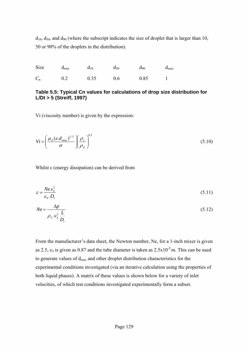
Page 129
d10, d50, and d90 (where the subscript indicates the size of droplet that is larger than 10,
50 or 90% of the droplets in the distribution).
Size dmin d10 d50 d90 dmax
Cn 0.2 0.35 0.6 0.85 1
Table 5.5: Typical Cn values for calculations of drop size distribution for L/Dt > 5 (Streiff, 1997)
Vi (viscosity number) is given by the expression:
5.03/1max ).(
⎟⎟⎠
⎞⎜⎜⎝
⎛⎟⎟⎠
⎞⎜⎜⎝
⎛=
d
cd dViρρ
σεµ (5.10)
Whilst ε (energy dissipation) can be derived from
tV
S
DvNe
.. 3
εε = (5.11)
tSC D
Lv
pNe2.ρ
∆= (5.12)
From the manufacturer’s data sheet, the Newton number, Ne, for a 1-inch mixer is given
as 2.5, εV is given as 0.87 and the tube diameter is taken as 2.5x10⁻² m. This can be used
to generate values of dmax and other droplet distribution characteristics for the
experimental conditions investigated (via an iterative calculation using the properties of
both liquid phases). A matrix of these values is shown below for a variety of inlet
velocities, of which test conditions investigated experimentally form a subset.

Page 130
I-SEP inlet velocity / (m/s) Inlet water cut / %
1 2 3 4 5 6 7 8 9 10
10 7.0E-03 3.1E-03 1.9E-03 1.3E-03 1.0E-03 8.2E-04 6.8E-04 5.8E-04 5.1E-04 4.5E-04
25 8.6E-03 3.7E-03 2.3E-03 1.6E-03 1.2E-03 1.0E-03 8.3E-04 7.1E-04 6.2E-04 5.4E-04
75 9.4E-03 4.1E-03 2.5E-03 1.8E-03 1.4E-03 1.1E-03 9.1E-04 7.7E-04 6.7E-04 5.9E-04
90 7.7E-03 3.3E-03 2.1E-03 1.5E-03 1.1E-03 9.0E-04 7.5E-04 6.3E-04 5.5E-04 4.9E-04
Table 5.6 : Predicted maximum droplet size, Dmax [m], from static mixers under various conditions
By using the model shown in Equation 5.9 with the constants from Table 5.5, a droplet
distribution produced by the static mixer array can be constructed for the tested inlet
velocities.
1.00E-04
1.00E-03
1.00E-020 2 4 6 8 10 12
Velocity at I-SEP inlet [m/s]
Dm
ax [m
] 10% WC25% WC75% WC90% WC
Figure 5.40 : Dmax predicted from static mixer elements for different I-SEP inlet conditions
The values that would be obtained from a 50% inlet water cut have been omitted, as it is
not clear which phase would be the dispersed phase (the inversion point for the system
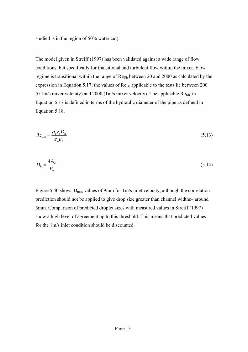
Page 131
studied is in the region of 50% water cut).
The model given in Streiff (1997) has been validated against a wide range of flow
conditions, but specifically for transitional and turbulent flow within the mixer. Flow
regime is transitional within the range of ReDh between 20 and 2000 as calculated by the
expression in Equation 5.17; the values of ReDh applicable to the tests lie between 200
(0.1m/s mixer velocity) and 2000 (1m/s mixer velocity). The applicable ReDh in
Equation 5.17 is defined in terms of the hydraulic diameter of the pipe as defined in
Equation 5.18.
cv
hscDh
Dvµε
ρ=Re (5.13)
w
wh P
AD
4= (5.14)
Figure 5.40 shows Dmax values of 9mm for 1m/s inlet velocity, although the correlation
prediction should not be applied to give drop size greater than channel widths– around
5mm. Comparison of predicted droplet sizes with measured values in Streiff (1997)
show a high level of agreement up to this threshold. This means that predicted values
for the 1m/s inlet condition should be discounted.

Page 132
1.00E-05
1.00E-04
1.00E-03
1.00E-020 2 4 6 8 10 12
Velocity at I-SEP inlet [m/s]
Dro
plet
siz
e [m
]
Dmind10d50d90Dmax
Figure 5.41 : Droplet distribution for 10% water cut at various inlet velocities
1.00E-05
1.00E-04
1.00E-03
1.00E-020 2 4 6 8 10 12
Velocity at I-SEP inlet [m/s]
Dro
plet
siz
e [m
]
Dmind10d50d90Dmax
Figure 5.42: Droplet distribution for 90% water cut at various inlet velocities

Page 133
0
0.1
0.2
0.3
0.4
0.5
0.6
0.7
0.8
0.9
1
0 0.0005 0.001 0.0015 0.002 0.0025 0.003 0.0035
Droplet size [m]
Cum
ulat
ive
num
ber f
ract
ion
2m/s 90% IWC4m/s 90% IWC
Figure 5.43: Cumulative droplet distribution prediction from static mixer array from Streiff, 1997
5.9 Drop size measurement
As a result of the transition section located between the static mixer array and the inlet
duct to the I-SEP, an investigation was attempted of the droplet size distribution that
exists under test conditions entering the separator. As detailed in Section 4.6 this was
carried out by the connection of a Malvern Mastersizer S to the inlet pressure tapping
with the intention of direct droplet size measurement.
The task of measuring droplet distributions is problematic on a number of levels and a
great deal of effort was required in order to produce any results that could provide any
value. Two main problems were encountered:
• laser obscuration
• droplet adherence to flow cell windows.

Page 134
The first issue had been addressed in the experimental technique that was developed by
Thapar (2001) in terms of providing dilution of the sample flow with clean water.
However, with this goes the associated risk of influencing the droplet distribution being
measured by altering the concentration of the oil in the stream. In addition, the diluting
flow has the effect of increasing speed in the sample line, therefore risking shear-
induced break-up, although it also has the effect of reducing the time between leaving
the sample point and reaching the measurement point.
During the measurement work, the diluting flow of water into the sample line upstream
of the flow measurement cell (see Figure 4.12) was varied in order to maintain the laser
obscuration in the acceptable 20-50% range. However, it was not possible to achieve
this when the inlet flow to the I-SEP being sampled was below 50% inlet water cut, or
for inlet velocities above 2m/s. The obscuration effect of low water cuts is evidently due
to the effect of the oil, which was dyed red. The pumping capacity available for dilution
flow was insufficient to reduce the oil concentration, locally in the measurement cell, to
a level that was measurable.
The second major problem encountered, droplet adherence to the flow cell windows
was considerably more problematic; it was often more likely that the measurements
being made were of window-droplets rather than the main flow. In the ultimate attempt
to remedy this, a coating of weak surfactant cleaner (DECON 90) was smeared onto the
internal surfaces of the flow cell windows with the intention of suppressing droplet
adherence without affecting flow in the flow-cell bulk. This seemed to reduce the
problem to allow a single measurement between cleaning the flow cell.
The trends observed, limited as they are, seem consistent with theory. It should be noted
that liquid-liquid droplet size measurement is to some extent subjective anyway, with
different measuring techniques producing different results. In terms of the scale of the
environment in which the droplet distribution was measured (the I-SEP inlet duct, with
a 41.2mm-wide inlet duct), few techniques are available. The size results are shown in
Table 5.7 below.

Page 135
Inlet velocity / (m/s) Inlet Water Cut / % d10 / µm d50 / µm d90 / µm
1 50 119.9 294.7 522.4
1 75 128.9 322.4 537.4
2 75 76.7 192.9 314.6
2 90 23.3 226.8 392.8
Table 5.7: Mean droplet size distribution values
Table 5.7 shows values of dxx where xx is a number representing the number fraction
of droplets with sizes less than the shown value. Thus, d10 is the size of droplet that
larger than 10% of the droplets in the measured sample (by number). The values shown
are the mean values of five measurement runs with acceptable obscuration.
The data obtained for the 2m/s inlet velocity at 90% inlet water cut are plotted below,
alongside the data previously shown in Figure 5.43.

Page 136
0
0.1
0.2
0.3
0.4
0.5
0.6
0.7
0.8
0.9
1
0 0.0005 0.001 0.0015 0.002 0.0025 0.003 0.0035
Droplet size [m]
Dro
plet
dis
trib
utio
n cu
mul
ativ
e nu
mbe
r fra
ctio
n
2m/s 90% IWC4m/s 90% IWC2m/s 90% IWC MS
Figure 5.44: Measured (by MS – Malvern Mastersizer) and predicted droplet distributions at 90% IWC
As can be seen from Figure 5.44, the measured droplet distribution approaches being an
order of magnitude smaller than that predicted from the Streiff model. As this model has
been validated by industrial researchers and would appear to be applicable to the
dispersion generated in the I-SEP test rig, the conclusion would seem to be that the inlet
transition is causing a significant degree of further mixing after the static mixer array. If
the measurements can be relied upon in this instance, and the evidence suggests that it is
not unreasonable, this transition significantly changes the droplet distribution of the
inlet stream.
5.10 Inlet section turbulence
In view of the fact that droplets generated by the static mixer array must flow through
an inlet transition and the inlet pipe of the I-SEP before reaching the inlet involute and
therefore region of swirl, it would seem prudent to determine the flow regime in this

Page 137
section, as far as possible.
Calculating the Reynolds number for the system at this point requires a value for
mixture viscosity. An expression for this is given below, selected because of its
simplicity and continued use in contemporary mixing research as demonstrated by Paul
et al. (2004).
µeffective = ⎟⎟⎠
⎞⎜⎜⎝
⎛+
+− cd
dc
µµφµ
φµ 5.11
1 (5.15)
Water cut 0.1 0.25 0.75 0.9
φ (volume fraction dispersed phase) 0.1 0.25 0.25 0.1
µc / (kg/m.s) @ 20oC 0.0023 0.0023 0.0011 0.0011
µd / (kg/m.s) @ 20oC 0.0011 0.0011 0.0023 0.0023
ρmix / (kg/m3) 820 850 949 979
µmix / (kg/m3) 0.0027 0.0034 0.0019 0.0014
Table 5.8 : Mixture viscosity by inlet water fraction
Using the values obtained in Table 5.8, the Reynolds numbers can be calculated at the
mixer inlet for the conditions investigated, and hence the droplet sizes shown in Table
5.6.
µρud
=Re (5.16)
In the case of Equation 5.20, d is taken as the hydraulic diameter of the rectangular duct
(cross sectional area of the duct divided by the wetted perimeter).

Page 138
0.00E+00
5.00E+03
1.00E+04
1.50E+04
2.00E+04
2.50E+04
3.00E+04
3.50E+04
4.00E+04
4.50E+04
5.00E+04
0 2 4 6 8 10 12
I-SEP Inlet velocity [m/s]
Rey
nold
s nu
mbe
r [-]
10% inlet water cut25% inlet water cut75% inlet water cut90% inlet water cut
Figure 5.45: Reynolds number at the I-SEP inlet
Figure 5.45 illustrates that the lower water cut test conditions are in the transitional
region whereas the higher water cuts are likely to be fully turbulent (for 2m/s and 4m/s).
5.11 Conclusions
1. The experimental results show that the I-SEP can be used to provide ‘clean’
water outlets for high inlet water cuts – to within the accuracy of the
measurement techniques. Manipulation of the outlet flow split enables a great
degree of control over the outlet flow split and the unit efficiency.
2. The experimental results from the I-SEP do not come close to achieving the
outlet purities of cyclonic de-watering cyclones. This is not something that
would necessarily be expected of a bulk separator device. Performance of other
cyclone separators in the literature is poorer than the I-SEP at low water cuts for
some test conditions.

Page 139
3. The I-SEP performs a bulk separation function and appears to operate at a lower
pressure drop than the cited reverse flow cyclones. It also performs best at high
water cuts, compared to the reverse flow cyclones in use in industry for de-
oiling, which are predictably best at low water cuts.
4. Whilst the reverse flow cyclonic de-oilers have been tailored in terms of
geometry to low water cuts, their efficiency would appear to decrease with inlet
water cut more quickly than is the case with the I-SEP. The implication is that
the I-SEP would respond more flexibly to changes in inlet composition. The I-
SEP performs an important separation function down to at least 25% inlet water
cut, even 10% for optimised configurations.
5. The I-SEP functions most efficiently at high water cuts at or above the inversion
point, with the tested geometry. For certain conditions, the I-SEP performs well
at inlet water cuts around the inversion point – at up to 70% efficiency. This
would be expected to be a difficult separation to perform.
6. Increased inlet velocity causes greater internal mixing due to turbulence and this
is not offset by increased centrifugal force. Therefore separation efficiency falls.
7. An optimum is observed in the length of the separator, the result of the balance
between residence time increase and increased re-mixing due to wall-imparted
shear and deceleration of flow due to the wall.
8. Optimum separation conditions are in a 3x unit at 2m/s inlet velocity. The
highest efficiency measured is >80% at 75% inlet water cut.
9. Alternative oil-water systems can produce greatly reduced separation
efficiencies, to the point where no separation occurs. This is evident if the oil
produces small droplets easily, compared to the kerosene-water system. The

Page 140
tested alternative oil had much greater viscosity and much reduced density
difference, resulting in no separation away from the optimum conditions
identified in point 8. At these conditions performance is much lower than for the
kerosene-water system.
10. Direct measurement of the inlet droplet distribution was attempted. This
suggests that the inlet drop-size distribution was around ten times smaller than
that predicted from the static mixer. This is likely to be because of mixing
effects due to an inlet transition.
In this chapter, the results of test work indicate that the envelope of performance in
which the I-SEP, in terms of the novel geometry used here, performs best. This allows a
target configuration and operating regime (3x unit, 2m/s inlet velocity, high inlet water
cut) to be defined. Whilst the device can still be improved (in the same path of evolution
that other cyclonic oil-water separators have trodden over many years) this work shows
the capabilities of the device. It is not as effective as the other cyclones in some ways,
but its intended use is also slightly different, and the low pressure-drop of the I-SEP is
suited to bulk separation.
In the next chapter, a mathematical model of the I-SEP using commercial
Computational Fluid Dynamics software will be constructed.

Page 141
6 Mathematical Modelling of the I-SEP
6.1 Introduction
In the previous chapter, the experimental performance of the I-SEP has been mapped
and compared with other devices. The droplet distribution entering the separator has
been looked at both from a theoretical and an empirical point of view and the
information from this enabled a description of the inlet flow conditions to the separator
to be produced. This gives an envelope in which further to study the operation and
separation effectiveness of the I-SEP.
For the case of cyclonic separation, if the inlet flow condition is know, then,
theoretically we can determine the probabilities for a certain geometry separating a
certain size of particle out to the desired outlet. This is sometimes expressed as a value
of what is termed the ‘cut-size’ of the particle that has an equal chance of leaving the
cyclone in either outlet. This expands to give grade partition curves that show the
separation probability for particles that are classified by the device. Whilst this is most
frequently applied to the separation of solid-fluid flows, it is also expressed for liquid-
liquid separation where it may be termed droplet migration probability (Colman 1981).
Rather than a fixed solid particle distribution in a fluid, multiphase liquid-liquid flow at
the inlet to the I-SEP can be found in states ranging from finely dispersed droplets to
slug flow, and performance would be expected to be a function of this state. In this
chapter, to simplify the inlet condition for oil-water flow, we will make the assumption
of continuous oil or water with droplets of the other phase. The droplet sizes can vary
by orders of magnitude, from tens of micrometres to those that approach the pipe
diameter, and the drops will interact with each other.
The interaction between droplets and the continuous phase is complex. The process of
droplet break-up from the continuous phase and coalescence with the same phase are
insufficiently well understood to be at the point where mathematical models can be used
to describe them with confidence. This is certainly true in a complex system such as the

Page 142
I-SEP. Notwithstanding this, it is still worth exploring the mechanistic modelling of
multiphase liquid-liquid flow within a cyclonic device and doing this by using the solid-
fluid models as a metaphor for liquid-liquid. This is discussed in this chapter in terms
of:
• construction of a Computational Fluid Dynamics (CFD) model of the I-SEP
• comparison of flow-visualisation data with the CFD model
The following is a discussion of the effects that different flow phenomena will have on
the qualitative performance of the separator.
6.2 CFD Modelling
6.2.1 Introduction to CFD
Traditional mechanistic models for cyclone separators are generally based theoretically
in terms of a simplification of the geometry being modelled. This allows for
manageable maths, with empirical factors often added to improve the model fit for the
data. These models pre-date the availability of the CFD software and computer
processing power that now enable iterative mathematical models to be solved for
complex flow problems.
The modelling of liquid-liquid droplet interactions is not available in commercial CFD
code because of the lack of understanding of the behaviour of such a complex system.
There are scaling rules, for example, that allow prediction of the conditions required to
change the scale of a mixing system to obtain the same droplet distribution (Middleton,
2003); this is not the same as a general expression to relate the effect of turbulence in a
multiphase system to its effect on the droplets in that system. Development of a CFD
model that addresses this would be beyond the scope of this theses and it is not
proposed to tackle such a problem here. Instead, an attempt has been made here to use
solid particles in a cyclone as a metaphor for liquid-liquid separation.

Page 143
The approach is to model the flow in a liquid-liquid cyclone (either reverse-flow or
axial-flow) by describing the behaviour of liquid ‘particles’ moving through a
continuous carrier fluid. This is valid for solid particles moving through gas or liquid,
where the particles are discrete and are subject to conservation of size and mass; it can
be postulated that this approach would also be valid where the dispersed liquid droplets
do not interact with each other.
The CFD code used to formulate and solve the model is the commercial FLUENT 6.0
code, which contains a number of approaches to modelling multiphase systems.
6.2.2 CFD background
By discretising a flow domain into a large number of small cells, the flow through a
domain can be found by an iterative solution to the Reynolds-Averaged Navier-Stokes
equations describing the mass and energy balance through that domain. These equations
and the methods in which they are solved are outside the scope of this thesis, but are
covered in many CFD textbooks.
The CFD modelling follows on from the work of White (1999), who used CFD and
LDV to study WELLSEP, the precursor to the I-SEP. This was used for solid-gas
separation using helical guide vanes (rather than involutes) to generate swirl, but is an
axial flow cyclone similar to the I-SEP. White’s CFD model was validated using LDV
measurements of flow within the WELLSEP, and used to predict the effectiveness of
the separator by predicting the paths of variously sized particles.
There are two areas of special consideration for the CFD modelling of liquid-liquid flow
through the I-SEP.
1. Multiphase oil-water flow
2. Swirl

Page 144
6.2.3 Multiphase oil-water flow
A comprehensive treatment of flow within an oil-water separator requires the
consideration of droplet break-up and coalescence and accurate determination of
behaviour of the mixture around the system inversion point so that the effect of the
movement of liquid as droplets and continuous phase can be determined. This is in
addition to the factors related to the hydraulic modelling of a liquid. These factors have
a fundamental effect on the composition of the outlet flows, resulting from the ability of
the I-SEP to handle and cause coalescence of the dispersed phase. This in turn
determines the effectiveness and separation efficiency of the separator.
As discussed, a meaningful handling of these complex processes is not possible within
the modelling software. Models do exist which attempt to handle droplet coalesce and
break-up, but these are only intended for use in the modelling of aerosol generators –
gas-liquid systems which are extremely sparse in liquid. This technique cannot be
applied to the problem in hand. However, this does suggest a method of managing the
complexity present in our system – the use of sparse droplet distributions.
If we neglect the effect upon the system due to droplet coalescence and break-up, it is
possible to attempt to model the I-SEP with a commercial CFD code. Considering the
experimental data collected for the I-SEP, the droplet-droplet interaction is assumed to
be at a minimum for the 10% dispersed phase fractions used in the test runs i.e. 90%
IWC and 10% IWC. Of the data collected, these test conditions are the most suitable for
CFD modelling that does not consider droplet break-up and coalescence. In general,
non-coalescing systems are considered to have less than 1% dispersed phase and so
10% dispersed phase would be far in excess of this. What would be achieved by the
simulation would be to model the droplets as if they were solid particles with the
density of the pseudo-solid phase. In such as case the 10% phase fraction would satisfy
the validity criterion of 10-12% maximum concentration (FLUENT user guide) for the
FLUENT Dispersed Phase Model (DPM), described below.
This approach can be viewed as an extension of the approach taken by workers such as

Page 145
Wolbert (1995), who used analysis of particle trajectories to predict separation
efficiency. In this case the trajectory analysis is performed by Fluent on a flow field
calculated for the I-SEP, rather than using measured velocities for a Rietema-standard
cyclone.
6.2.4 Swirl
Another fundamental aspect of CFD modelling is the treatment of viscosity and
turbulence. The approach to modelling turbulent viscosity in flows in cyclone separators
requires more care than the application of CFD to, for example, modelling a more
straightforward system.
The most frequently used method of modelling the effects of turbulence in flow is the k-
ε model and its variants. This system of equations is considered one that generally has
good stability in convergence and is quite ‘economical’ in obtaining solutions to
problems using reasonable computer resources. There is, however, an underlying
assumption made for the k-ε model that undermines its applicability to the modelling of
cyclone flows: the assumption of isotropic (equal in all directions) turbulent viscosity.
Called the Boussinesq assumption, this is not necessarily valid for zones of strong swirl,
such as those found in a cyclone separator, where the turbulence may be anisotropic.
The Reynolds-Stress Model does not make this assumption but requires more equations
to be solved on each iteration of the calculation. The disadvantages of this approach are
that the solution can be more difficult to converge and it is also much more ‘expensive’
in terms of processor time, and hence it is not used where other modelling methods have
been shown to be sufficiently accurate.
As well as being a more theoretically rigorous alternative to k-ε, the RSM has been
shown to produce more accurate results in modelling the flow fields in cyclone
separators (when compared to measurements by LDV). Whilst using RSM will mean
that fewer cases will be solvable in the available time (compared to the k-ε turbulence

Page 146
model), the benefits are the likely improvement in the accuracy of the flow field
prediction means that this is used as the basis for creating the CFD model of the I-SEP.
6.3 Multiphase models
Using the FLUENT package, the following methods could be applied to modelling a
multiphase liquid-liquid flow.
1. Discrete Phase Model (DPM)
2. Mixture model
3. Eulerian model
6.3.1 Discrete Phase Model
The DPM is an implementation of Lagrangian particle tracking which is essentially a
means of tracking discrete particles through a continuum of fluid. This is a suitable
method used in simulating a system that has a sparse dispersed phase, i.e. less than 10-
12% volume fraction (FLUENT 6.0 user guide, Fluent, 2001). The interaction between
phases in the simulations conducted here, in terms of the volume of one phase in
another, is in one direction only. Whilst it does not follow that droplets will not interact
with each other, as mentioned earlier, it is valid to assume at this concentration that the
volumetric concentration is not having a crowding effect at the inlet. It should be noted
that it is possible to make Fluent 6.0 calculate the effects of the dispersed phase on the
continuous phase, but this option is unnecessary given the assumptions made.
This modelling approach is comparable to semi-empirical models such as the
equilibrium-orbit or time-of-flight models, where the efficiency of separation is
predicted in terms of likely separation of a given size of oil droplet. By making
calculations of trajectories of many droplet sizes a curve can be obtained of separation
efficiency expected for a given inlet drop size. However, a major improvement on semi-
empirical modelling techniques is the fact that a detailed calculation is made of the flow
field through which the droplets pass. This stands a higher chance of correctly

Page 147
representing the physical reality than just assuming that flow is a perfect Rankine
vortex.
6.3.2 Mixture and Eulerian models
The discrete phase model is used to ‘seed’ the continuous phase flow with dispersed
phase droplets. However, a CFD model yields a variety of other data about the system
over the prediction of outlet composition, for example the pressure drop characteristics
of the I-SEP; these would be dependent on the two phase flow, rather than just the
pressure drop caused by the continuous phase. Two of the multiphase models in the
FLUENT 6.0 CFD code are the mixture model and the Eulerian model.
The mixture model uses the concept of interpenetrating continua to describe the
contents of each cell, defined in terms of phase fractions of the two mixed phases
throughout the flow domain. As such, the flow is modelled as a single fluid but the
components of this fluid are allowed to move at different velocities, with slip velocities
calculated between the two.
As in the DPM, there is a need to define the droplet diameter of the dispersed phase,
which allows the determination of the behaviour of particles in terms of drag and
buoyancy in a centripetal acceleration field. Droplet sizes are input by the user and not
determined by the code. Whilst modelling of droplet-droplet coalescence or break-up
can be attempted by methods such as population balancing, the physics are complicated
and are not implemented as standard in Fluent 6.0.
The Eulerian multiphase model introduces the use of multiple phases (rather than a
single fluid) each with their own conservation equations governing momentum, energy
and exchange terms calculated between the phases. As such, it is significantly more
complex to handle and for the purposes of this work was deemed an unnecessary extra
complication (therefore significantly increasing the time required for each solution) and
so detracting effort from the modelling methods above. In addition, the Eulerian model
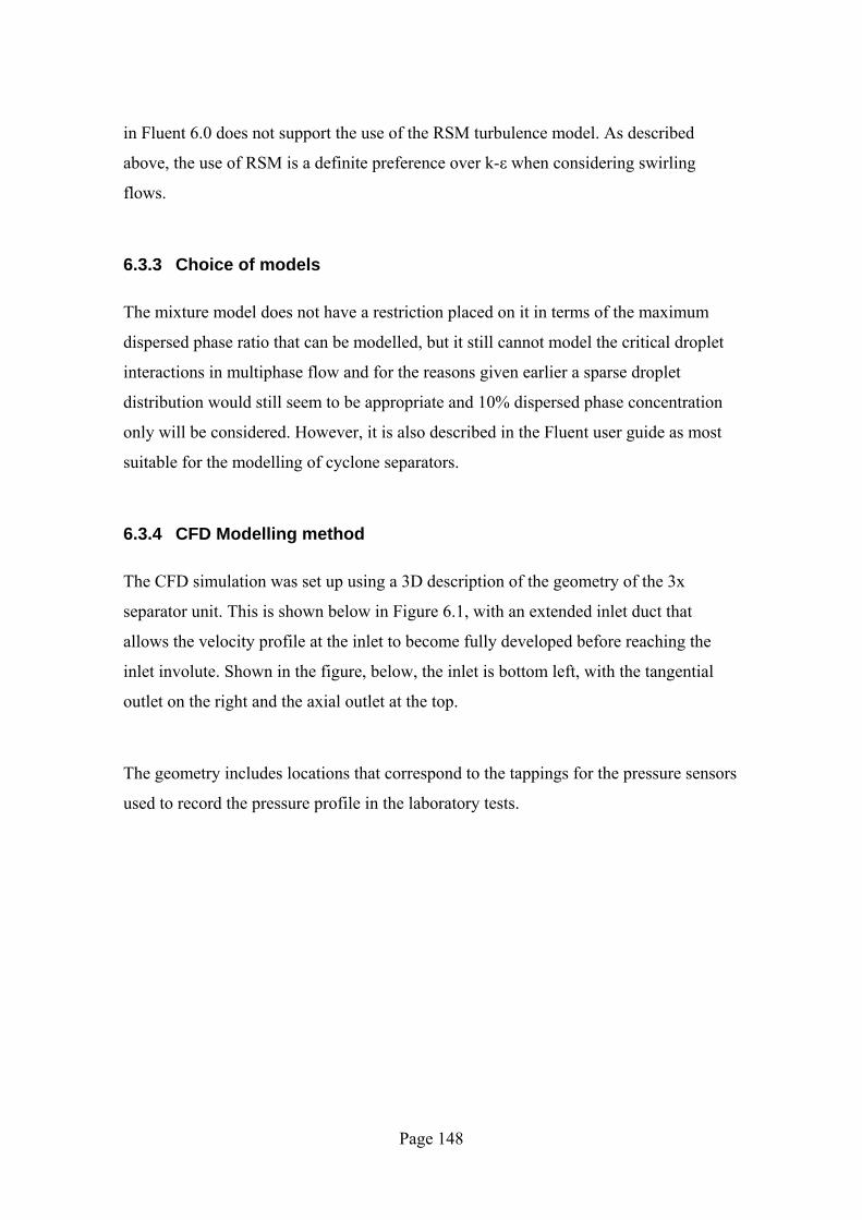
Page 148
in Fluent 6.0 does not support the use of the RSM turbulence model. As described
above, the use of RSM is a definite preference over k-ε when considering swirling
flows.
6.3.3 Choice of models
The mixture model does not have a restriction placed on it in terms of the maximum
dispersed phase ratio that can be modelled, but it still cannot model the critical droplet
interactions in multiphase flow and for the reasons given earlier a sparse droplet
distribution would still seem to be appropriate and 10% dispersed phase concentration
only will be considered. However, it is also described in the Fluent user guide as most
suitable for the modelling of cyclone separators.
6.3.4 CFD Modelling method
The CFD simulation was set up using a 3D description of the geometry of the 3x
separator unit. This is shown below in Figure 6.1, with an extended inlet duct that
allows the velocity profile at the inlet to become fully developed before reaching the
inlet involute. Shown in the figure, below, the inlet is bottom left, with the tangential
outlet on the right and the axial outlet at the top.
The geometry includes locations that correspond to the tappings for the pressure sensors
used to record the pressure profile in the laboratory tests.
Page 149
6.3.4.1 CFD mesh
Figure 6.1: View of the I-SEP mesh

Page 150
Figure 6.2: Elevated view of the I-SEP mesh
The mesh employed in the model was created using Gambit 2.0. It uses structured
hexahedral cells, allowing the mesh elements of the various geometric structures to fit
together whilst maintaining an acceptable mesh quality (that is, avoiding highly
contorted cells that would make the solution of the simulation less stable).
One of the challenges to be overcome was avoiding the creation of very small angles at
cell vertices where the involutes become tangential to the separator body. The mesh
would have had poor quality cells at this point (shown in Figure 6.3), which would
make convergence of the model problematic. This issue was resolved, as shown in
Figure 6.3, by cutting back on the involute just before the join with the main cylinder
body. This small change is a necessary concession to achieving a stable numerical
solution, but should have no significant effect on the quality of the solution.

Page 151
The mesh contains approximately 90,000 hexahedral cells. Cells have been evenly
spaced through the volume of the mesh, so as not to increase the resolution of the grid
in any one zone. This is sometimes done to better resolve zones expected to generate
high property (e.g. velocity) gradients, such as the central region of the separator
chamber, however, the indicators of mesh quality indicate that there is no cause for
concern in this respect (as detailed in the analysis of each modelling section).
An exhaustive study to show grid independence has not been performed. This was
because White (1999) successfully demonstrated grid independence on a similar
geometry with fewer than 3,000 cells. The massively increased resolution has therefore
been taken to indicate that this still holds.
Figure 6.3: Subtle geometry alteration to improve mesh quality

Page 152
6.4 Discrete Phase Model
6.4.1 Solution method
Using the mesh detailed in Section 6.3.4.1, the flow field using a continuous water
phase was solved at 2m/s and 4m/s inlet velocity. The flow boundaries were set as
follows:
Condition Setting
Inlet: Turbulence intensity fraction 0.045
Hydraulic diameter 0.007m
Tangential outlet Outflow
Axial outlet Outflow
Table 6.1: DPM model boundary conditions
The model was defined by specifying the inlet flow velocity and the split between the
two outlets. The latter was chosen to tally with a test condition that was achieved, so
that the two could be compared. Initially the pressure difference between the outlets was
specified, but this made it very difficult to obtain a viable converged solution. Using the
‘outflow’ outlet type in FLUENT allowed the fraction of exit flow in each outlet to be
defined and the model converged.
The inlet flow condition was assumed to have become fully developed flow and thus the
values shown in Table 6.1 were specified to reflect this. The face at the beginning of the
inlet duct is given an intensity of turbulence derived from the Reynolds number based
on the inlet duct hydraulic diameter. The hydraulic diameter is taken to be the diameter
of a circular duct with the same cross sectional area. The turbulence intensity is defined
as

Page 153
I= 81
).(Re16.0−
HD (6.1)
Where HDRe is the Reynolds number based on the hydraulic diameter of the inlet:
HDRe = µ
ρ HUD (6.2)
However, the length of inlet duct prior to flow reaching the inlet involute means that an
appropriate velocity profile will be encountered at this point.
In solving the model, the PRESTO! discretisation scheme was used for the treatment of
pressure, the SIMPLE differencing scheme for pressure-velocity coupling, and the
QUICK differencing scheme for the momentum, turbulent kinetic energy, turbulence
dissipation rate and Reynolds stresses. These are FLUENT recommendations that
should promote a more reliable solution for swirling flows. The solution was allowed to
converge until the residual on all monitored parameters had reached a flat profile, which
gave scaled residuals at or below 1x10⁻³.
Once the continuous phase flow field has been solved, the particle tracking is
accomplished by defining a number of droplet injections. These are seeded into the flow
via a user-defined plane positioned at the inlet. The inlet plane itself is not used, as more
control over the number of particles was desired (injected at the facet vertices of the
selected plane), instead a plane defining the release point for particles was used to give
a number of particles that was statistically significant. In this case 1980 particles were
released.
The injections were set up as kerosene droplets released from the plane according to the
inlet velocity profile. A single size of droplets was specified for injection in each run of
the simulation, and the results obtained initially for 1mm, 0.1mm and 0.01mm.
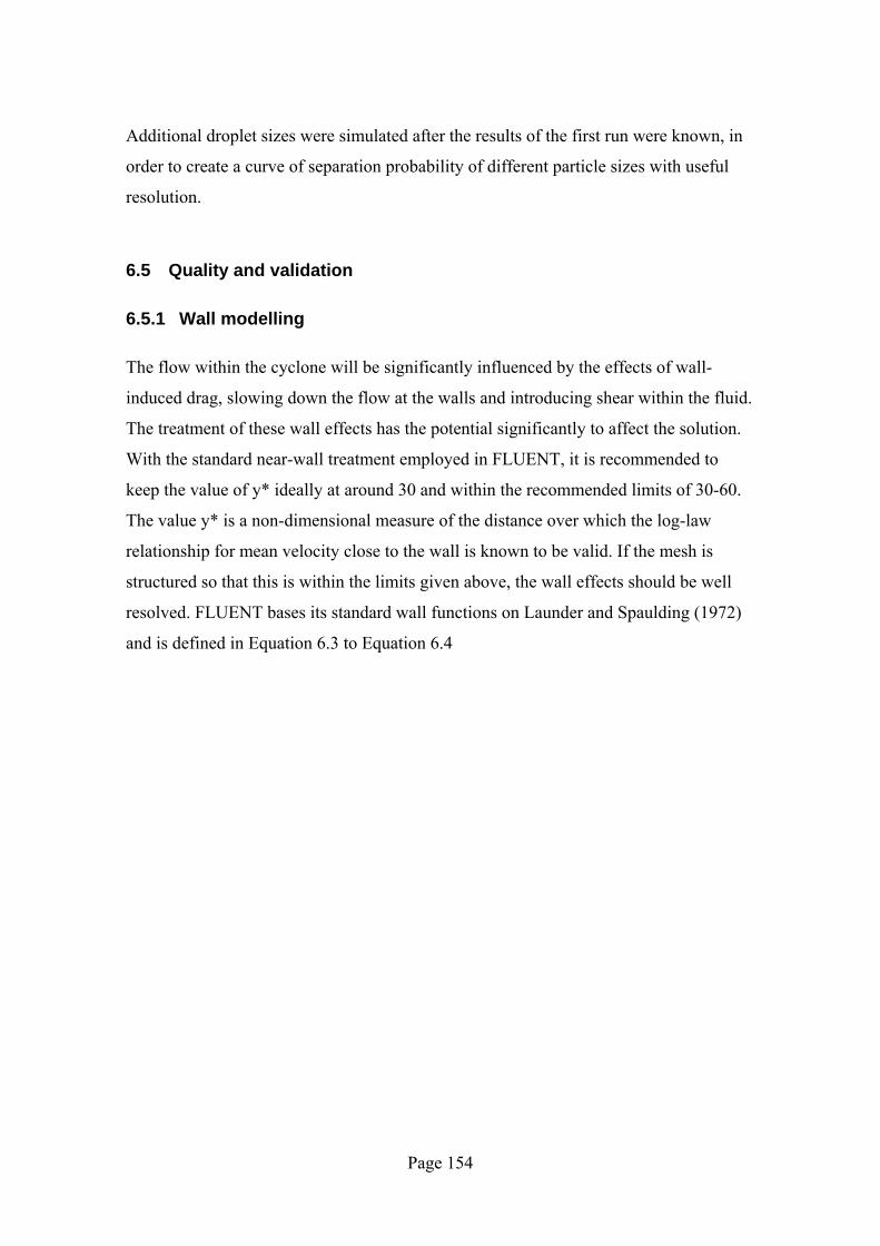
Page 154
Additional droplet sizes were simulated after the results of the first run were known, in
order to create a curve of separation probability of different particle sizes with useful
resolution.
6.5 Quality and validation
6.5.1 Wall modelling
The flow within the cyclone will be significantly influenced by the effects of wall-
induced drag, slowing down the flow at the walls and introducing shear within the fluid.
The treatment of these wall effects has the potential significantly to affect the solution.
With the standard near-wall treatment employed in FLUENT, it is recommended to
keep the value of y* ideally at around 30 and within the recommended limits of 30-60.
The value y* is a non-dimensional measure of the distance over which the log-law
relationship for mean velocity close to the wall is known to be valid. If the mesh is
structured so that this is within the limits given above, the wall effects should be well
resolved. FLUENT bases its standard wall functions on Launder and Spaulding (1972)
and is defined in Equation 6.3 to Equation 6.4

Page 155
)ln(1 ** EyUκ
= (6.3)
ρτµ
w
PP kCUU
5.025.0* ≡ (6.4)
µρ µ PP ykC
y5.025.0
* ≡ (6.5)
Figure 6.4: y* values for 4ms-1 case
The typical illustration of y* in Figure 6.4 shows that, with a few localised exceptions,
the value are well placed within the 30-60 range – that majority of the wall has a y*
(defined in Equation 6.5) value of around 30. With reference to the FLUENT 6.0 user

Page 156
manual, this is a value over which this modelling approach for effects at the wall is
valid.
6.5.2 Flow visualisation validation
0
1
2
3
4
5
6
7
8
9
-0.0100 -0.0080 -0.0060 -0.0040 -0.0020 0.0000 0.0020 0.0040 0.0060 0.0080 0.0100
Radial position [m]
Tang
entia
l vel
ocity
[m/s
]
z=0.001z=0.002z=0.003z=0.004
Figure 6.5: Tangential velocities in the I-SEP separating chamber as derived from CFD model of PIV test conditions (0.96 flow split, 5.6m/s inlet velocity)
Figure 6.5 shows the calculated tangential velocity profile across the diameter of the I-
SEP at various axial positions in the separating chamber at the same inlet velocity and
flow split as was obtained during the attempted PIV measurements (see Section 4.7).
The centre of the chamber, at a radial position of zero, is where we would expect to find
the minimum velocity of the combined Rankine vortex (inner forced vortex surrounded
by and outer free vortex) that has been shown to exist within reverse flow and axial
flow cyclones. However, this is not shown by the CFD model.

Page 157
Figure 6.6: Tangential velocity profile illustrating vortex within the I-SEP
It can clearly be seen in Figure 6.6 that there is an oscillation of the vortex along the
axis of the separator, so that the central minimum tangential velocity moves around the
geometric centre point. This was seen during the experimental testing with oil of the I-
SEP (Figure 6.7).
Tangential velocity (m/s)
Page 158
Figure 6.7: Observed core oscillations
The fact that the vortex predicted by the CFD code does not necessarily centre on the
separating chamber axis means that what is shown is not the classic inner forced vortex
surrounded by an outer free vortex (as found in reverse-flow cyclones and WELLSEP,
an axial flow cyclone – White (1999)).
The analysis of the predicted velocities shows decreasing tangential velocities moving
towards the outlet end of the separating chamber. This would be expected from wall-
friction losses. If the tangential velocity minima were not offset from the centre, it
would be expected that they would follow the relationship shown in Equation 6.6,
where V is the tangential velocity at a radius r. C is a constant of proportionality and n
is the vortex exponent, varying from 1 for a forced vortex to -1 for a free vortex.
V=Crn (6.6)
The CFD data does not conform to this mathematical relationship as the tangential
velocity minimum shown in Figure 6.5 does not fall to zero coincident with the I-SEP
axis, where r=0. However, by adjusting each dataset radially so that the minimum

Page 159
velocity for that dataset falls at r=0, a pseudo vortex exponent can be derived and give a
quantitative description of the way the vortex behaves. The inner ‘vortex exponent’ (n
in Equation 6.6) falls between 0.53 and 0.97, dependent on axial position in the
separating chamber.
PIV measurements of the velocity profile in the I-SEP were attempted with equipment
supplied by the EPSRC Instrumentation loan pool. This would allow the validation of
the CFD model by matching measured and predicted velocities. The model case shown
above (Figure 6.6) is for a 5.6m/s inlet velocity, which corresponded to the inlet
velocity achieved in the PIV tests. The method used in the PIV work is described in
Section 4.7. The limitations of the PIV work meant that velocity measurements were
only possible for the inlet involute, rather than the whole device.

Page 160
Figure 6.8: Keyed diagram showing locations of PIV/CFD velocity comparisons
The table below shows the comparative values between the PIV and CFD values at the
general locations shown on Figure 6.8.
E
C
B
D F
G
A

Page 161
Position PIV measured velocity
/ (m/s)
CFD predicted velocity
/ (m/s)
Difference / %
A 5.0 6.1 18%
B 4.7 4.4 -7%
C 5.1 5.3 3%
D 6.2 7.6 17%
E 4.4 4.9 9%
F 5.6 6.3 11%
G 7.6 7.3 -4%
Table 6.2: Comparison of CFD prediction with PIV measurements for tangential velocity
0.0
1.0
2.0
3.0
4.0
5.0
6.0
7.0
8.0
9.0
0.0 1.0 2.0 3.0 4.0 5.0 6.0 7.0 8.0 9.0
CFD Prediction [m/s]
PIV
mea
sure
men
t [m
/s]
Velocity dataCFD = PIV
Figure 6.9: Correlation of CFD and PIV velocity values for tangential velocity at positions A to G
The CFD and PIV values compare respectably, being mostly within 10% (all less than
20%) of each other. The exceptions are higher velocities in Table 6.2 (based on CFD
predictions) and locations in the inlet involute closer to the centre of the involute radii.

Page 162
In the latter case, resolving illuminated particles was more difficult because of stray
light and the high concentration of particles in this location, and so this may explain the
discrepancies. In the case of the higher predicted velocities, the suggestion is that there
is a tendency to under-measure PIV values – the data in the above figure are mostly
below the parity line.
It should be noted that the PIV values are averaged from vectors measured over a
comparatively coarse grid (the necessity to process the data manually and therefore
keep data set size manageable forced this). This means that where the velocity gradient
is highest (i.e. near the wall as shown in Figure 6.5), such an averaged grid square
would tend to underestimate the velocity, whereas the CFD velocity is that calculated in
a single, small, cell.
6.6 Results
Figure 6.10 shows the predicted destination for droplets of varying sizes entering the I-
SEP inlet.

Page 163
0.00
0.10
0.20
0.30
0.40
0.50
0.60
0.70
0.80
0.90
1.00
0.00 0.05 0.10 0.15 0.20 0.25 0.30
Droplet size [mm]
Frac
tion
of d
ropl
ets
reac
hing
axi
al o
utle
t
2m/s4m/s
Figure 6.10: Probability of kerosene droplets being separated to the I-SEP axial outlet at 0.81 flow split
The data was generated by seeding a plane at the inlet with 1980 droplets of the relevant
size and allowing the code to track their progress through the I-SEP. This is done by
calculating the force applied on the droplet by the movement of the continuum fluid and
updating the droplet position. It is critical that a suitable time-step (or spatial step) is
chosen to give adequate interaction of the droplets with the continuous phase. If this is
set too coarsely then the droplets will fail to migrate inwards (for less-dense droplets)
correctly. The actual DPM resolution needs to be increased to a point where the results
(for probability of separation) for small particle sizes become insensitive to this setting;
however this is at the expense of increased calculation time.
In Figure 6.10 it can be seen that for low particle sizes the separation efficiency
approaches that of (1- flow split), indicating that no separational effect is taking place.
This is the expected value, as separation is defined as particles leaving in the axial
outlet, whereas split relates to the tangential outlet. Larger droplets have a progressively
higher chance of leaving through the axial outlet after migrating inwards.

Page 164
The fraction reaching the axial outlet shown above in Figure 6.10 is more properly the
number not tracked to the tangential outlet. This difference from the number of particles
actually tracked to the axial outlet because a significant number of particles expected to
have sufficient diameter to migrate to the axial outlet are ‘timed out’ by the CFD code.
This means that they fail to reach either outlet within a threshold number of iterations of
the Discrete Phase Model tracking routine, even if this threshold number is massively
increased. Observation of particle tracks shows that these particles become locked in a
zone near the inlet end of the separating chamber inside a radius approximately
corresponding to that of the vortex finder. There would appear to be two possible
reasons for this:
1. A feature of the mathematical model that prevents the correct movement of
droplets
2. Simulation of a real phenomenon
The former is possible, but the mesh is believed to be sufficiently high-resolution to
give a mesh-independent solution. There is no evidence that there are velocity gradients
in the core area of the separating chamber that are too extreme (and therefore would
require a greater cell density).
Considering the second possibility, it was noted during shutdown of the rig during
testing that, when the oil feed was shut off before the water feed that there was a
persistence of oil droplets in the separating chamber. This was not measured or
rigorously observed, but could suggest that certain combinations of droplet diameter
and flow rate may give rise to the ‘trapping’ of oil droplets within the separator. For
these conditions, this would suggest that oil moves through the separator and out
because of displacement by other oil and not by the driving action of the general flow
field.
Looking in more detail at the flow patterns produced by the CFD simulation we can
identify some interesting features. Figure 6.11 shows the axial component of velocity in

Page 165
the continuous phase flow used for the DPM solution at 2ms-1. A slice through the
separating chamber has been coloured so that positive axial velocity (towards the axial
outlet) is red and negative axial velocity (towards the inlet involute) is coloured blue.
It can clearly be seen from Figure 6.11 that there is a significant zone positioned on the
axis of the separator where axial flow is back towards the inlet involute, surrounded by
an annular region of movement towards the outlets. This is interesting because it
suggests that there is a recirculation zone set up whereby flow that has progressed along
the separating chamber must, at least in part, be drawn backwards towards the inlet
involute. This could explain the phenomenon of droplets of the less-dense phase being
caught in the centre of the separation chamber.
Figure 6.11: Axial velocity profile through a slice of the I-SEP separating chamber in 2ms-1 CFD model

Page 166
Droplets that are sufficiently large to move straight to the axis of the separator would
move ‘backwards’ through the separator. At some point they would be expected to be
dislodged by turbulent flow to join the outer ‘positive’ flow, before standing a chance of
moving into the central region again. This has implications for the residence time of a
separator such as the I-SEP as some of the flow could be expected to pass much more
quickly through the separator in the outer region, whereas other flow could spend a
much longer time in the separator because of a recirculation zone. Longer residence
times would be favourable to the separation process, as they would provide a longer
time for droplet coalescence to take place. However, the converse of this, the possibility
of a much shorter path to exit through the annular region would confound separation
(see Figure 6.12 – shorter path coloured blue, recirculation zone in red). This is because
flow would pass through a volume reduced below that of the separation chamber by
subtracting the inner recirculation region through which this quick-exit flow would not
pass. Also, because the flow at the wall would mainly comprise oil droplets, this is
precisely the region that would benefit from increased residence time to aid
coalescence.
A continuous flow through the separator will continuously introduce new oil into the
separating chamber and therefore into any zone in which large oil droplets become
trapped. This zone is therefore akin to a tank that is filled by that continuous oil flow.
Eventually that tank will overflow and so the oil it contains will pass through the region
it represents and on to the outlets.

Page 167
Figure 6.12: Speculated recirculation in the I-SEP
6.7 Mixture model
6.7.1 Solution method
The DPM in Fluent 6.0 is a lagrangian particle-tracking model. The mixture model
instead defines and manipulates a scalar value representing the phase volume fraction in
each cell. The continuous and dispersed phases are defined in terms of percent volume
compositions for the dispersed phase and a single droplet size for the dispersed phase.
Other aspects of the solution method are as for DPM.

Page 168
6.7.2 Results
Test number Inlet velocity / (m/s) Water cut / % Flow split Droplet size / m
1 2 90 0.75 1x10⁻³
2 2 90 0.75 1x10⁻⁴
3 2 90 0.75 1x10⁻⁵
4 2 10 0.29 1x10⁻³
5 2 10 0.29 1x10⁻⁴
6 2 10 0.29 1x10⁻⁵
7 4 90 0.78 1x10⁻³
8 4 90 0.78 1x10⁻⁴
9 4 90 0.78 1x10⁻⁵
10 4 10 0.52 1x10⁻³
11 4 10 0.52 1x10⁻⁴
12 4 10 0.52 1x10⁻⁵
Table 6.3: Summary of CFD mixture model runs to model experimental data
Table 6.3 shows the CFD runs that were carried out for comparison with experimental
data. A set of three specimen droplet sizes were executed for the sparse (10% dispersed
phase) conditions for 2 and 4 m/s. The outlet split for each run was specified to enable
comparison with experimental data. Plots of the pressure profile and outlet composition
results are shown below.

Page 169
6.7.2.1 Pressure
-0.10
-0.05
0.00
0.05
0.10
0.15
0.20
0.25
0.30
1 2 3 4 5 6 7 8 9 10 11 12
Test number
Pres
sure
at a
xial
out
let [
barg
]
ExperimentalCFD
Figure 6.13: Comparison of CFD axial outlet pressure with experiments
0.00
0.05
0.10
0.15
0.20
0.25
0.30
0.35
0.40
1 2 3 4 5 6 7 8 9 10 11 12
Test number
Pres
sure
at t
ange
ntia
l out
let [
barg
]
ExperimentalCFD
Figure 6.14: Comparison of CFD tangential outlet pressure with experiments

Page 170
-0.05
0.00
0.05
0.10
0.15
0.20
0.25
0.30
0.35
0.40
1 2 3 4 5 6 7 8 9 10 11 12
Test number
Pres
sure
diff
eren
ce b
etw
een
outle
ts (D
PA/T
) [ba
r]
ExperimentalCFD
Figure 6.15: Comparison of CFD differential pressure between outlets (DPA/T) with experiments
At the higher inlet velocity (4m/s) the agreement between pressures from experimental
results and the pressure results from the mixture model simulation, specifically the
differential pressure between outlets (which drives the outlet flow split) are worse than
at 2m/s. This applies mainly to the water-continuous case (90% IWC), however at 1x10-
4 m droplet diameter the prediction is very good. A credible explanation for discrepancy
at 90% IWC for 4m/s inlet velocity has not been determined.

Page 171
6.7.2.2 Outlet Composition
0
0.1
0.2
0.3
0.4
0.5
0.6
0.7
0.8
0.9
1
1.00E-05 1.00E-04 1.00E-03
Modelled droplet size [m]
Axi
al o
utle
t wat
er c
ut
CFD 2m/s 0.75tCFD 2m/s 0.29tCFD 4m/s 0.78tCFD 4m/s 0.52tExperimental 2m/s 0.75tExperimental 2m/s 0.29tExperimental 4m/s 0.78tExperimental 4m/s 0.52t
Inlet velocity and outlet split
Figure 6.16: Comparison of CFD Axial outlet composition with experiments
0
0.1
0.2
0.3
0.4
0.5
0.6
0.7
0.8
0.9
1
1.00E-05 1.00E-04 1.00E-03
Modelled droplet size [m]
Tang
entia
l out
let w
ater
cut CFD 2m/s 0.75t
CFD 2m/s 0.29tCFD 4m/s 0.78tCFD 4m/s 0.52tExperimental 2m/s 0.75tExperimental 2m/s 0.29tExperimental 4m/s 0.78tExperimental 4m/s 0.52t
Inlet velocity and outlet split
Figure 6.17: Comparison of CFD tangential outlet composition with experiments
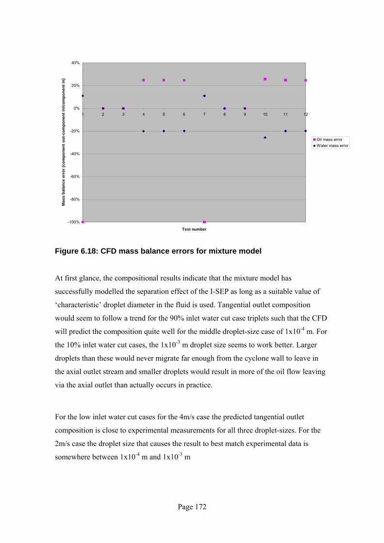
Page 172
-100%
-80%
-60%
-40%
-20%
0%
20%
40%
1 2 3 4 5 6 7 8 9 10 11 12
Test number
Mas
s ba
lanc
e er
ror (
com
pone
nt o
ut-c
ompo
nent
in/c
ompo
nent
in)
Oil mass errorWater mass error
Figure 6.18: CFD mass balance errors for mixture model
At first glance, the compositional results indicate that the mixture model has
successfully modelled the separation effect of the I-SEP as long as a suitable value of
‘characteristic’ droplet diameter in the fluid is used. Tangential outlet composition
would seem to follow a trend for the 90% inlet water cut case triplets such that the CFD
will predict the composition quite well for the middle droplet-size case of 1x10⁻⁴ m. For
the 10% inlet water cut cases, the 1x10⁻³ m droplet size seems to work better. Larger
droplets than these would never migrate far enough from the cyclone wall to leave in
the axial outlet stream and smaller droplets would result in more of the oil flow leaving
via the axial outlet than actually occurs in practice.
For the low inlet water cut cases for the 4m/s case the predicted tangential outlet
composition is close to experimental measurements for all three droplet-sizes. For the
2m/s case the droplet size that causes the result to best match experimental data is
somewhere between 1x10⁻⁴ m and 1x10⁻³ m

Page 173
From the DPM CFD modelling we have a predicted change in migration probability
between the two outlets of around 0.025mm (2.5x10⁻⁵m) leaving at the axial outlet and
0.15mm (1.5x10⁻⁴m) leaving at the tangential outlet with intermediate proportions
between these sizes. To be consistent, we would expect to see the results from the
mixture modelling giving the best tie-in with experimental data at some point within
this region. Also, because the measure we are using to make this judgement is the
volume of oil component leaving through an outlet, the characteristic drop size that
gives the best result would be towards the higher end of the range as this would account
for the majority of the droplet volume (v∝ d3).
For the axial outlet composition results, we see a poorer match with experimental
results for the 90% inlet water cut cases, especially at 4m/s inlet velocity. We also see
that at 1x10⁻³ m droplet diameter, the predicted axial outlet water cut is 100%, which
would not be expected for a case where droplets are large enough to move directly to
the axis of the separator and out via the axial outlet. When we look again at the
tangential outlet results we see that this outlet too is predicted to have a 100% water cut.
This prompts the obvious question of where the oil has gone!
There is a mass balance error in the simulation. The discrepancy between the total mass
of oil or water leaving the separator and that which enters it (as a percentage of the inlet
flow of that component) is shown in Figure 6.18. The mass balance error found only
occurs for the multiphase mixture model. For the single-phase solution used in the DPM
method there is no such error: inflow = outflow. The reason for this has not been
determined despite many attempts to resolve the issue. It is not remedied by changing
the turbulence model to k-ε, for example, not by varying the boundary conditions of the
simulation so that they are alternatively defined, for example, in terms of outlet
pressure. It may be related to the speculated recirculation observed in the DPM results –
there is a loss of oil from the simulation in the cases with the largest droplets – although
a converged steady-state simulation should reach a mass-balanced solution. In addition,
there is an error present for the water-dispersed cases, which could not be related to the
central recirculation zone (large water particles would remain at the periphery of the I-

Page 174
SEP).
6.8 Discussion
Considering the droplet migration probabilities shown in Figure 6.10 derived from the
discrete phase model in CFD, the predicted composition of the tangential outlet
increases in oil content (decreasing water cut) as the droplet size used in the model
decreases. This would be expected by considering that, as the drag forces increase and
the buoyancy forces decrease with a smaller droplet, the droplet becomes a flow
follower and oil droplets move (or oil continuous phase is displaced by water droplets)
towards the axial outlet. Furthermore, with sufficiently small droplets, at around
1x10⁻⁵m, no separation effect is predicted, such that both outlets have the same
composition.
Comparing the two curves for 2 and 4m/s (Figure 6.10), the discrete phase model
simulations predict that the smallest size of droplet (and these droplets were kerosene)
that will undergo separation by the cyclone is 0.01mm. The transition from this to
‘certain’ separation of a droplet to the axial outlet occurs over the 0.01 to 0.3 mm
droplet size range. The difference between the two velocities for the DPM is a sharper
shoulder on the partition curve for the 4m/s case, so that for particle sizes around
0.13mm the centripetal force versus drag balance allows smaller particles to reach the
axial outlet.
Because the outlet splits are defined as the same as the experimental results with which
they are compared, it follows that this would give the same efficiency as measured.
However, the results from the mixture model are of poor quality – the inlet and outlet
mass flows fail to balance in a way that is presumably an artefact of the multiphase
modelling technique itself (and is certainly physically impossible). These simulations
also fail to reach a level of convergence (measured in terms of fractional change in
certain values with successive iterations – ‘residual’ values) that would normally be
considered acceptable – at least values below 1x10⁻³. This is true both when the flow
split is explicitly defined (analogous to setting the flow split with outlet control valves)

Page 175
and when the outlet pressures are specified (although many more of the residual
indicators are below 1x10⁻³). Referring back to Section 6.5.2 and to Figure 6.6, the
oscillation of the core with axial position may indicate that the mathematical solution
tends towards a periodic oscillation in the core – vortex precession. As the solutions
obtained are steady state, a time-dependent phenomenon such as vortex precession may
not properly be resolved in steady-state simulations and may be manifested by a
solution that is not converged to levels that would ideally be required. This may explain
why a solution with the second, dispersed, phase solved separately fares better than one
where the two are solved concurrently as in the mixture model. However, the
description of separation of discrete particles from the DPM (without resolving a
discrete ‘core’ can be used to derive an overall separation efficiency based on a non-
coalescing, non-breaking-up system.
Of the two CFD methods used to model liquid-liquid separation within the I-SEP, the
discrete phase model produces results that do not appear to bear the ‘flaws’ of the
alternative mixture model when modelling the I-SEP flow. The mixture model results
do not pass a test of mass balance on inlet and outlet flows. This may also be explained
by the transient nature of the solution as mentioned above. Further work on a transient
solution would be required to investigate this, but there is no indication that the CFD
mesh is deficient, as this would have had effects for all simulation results, which is not
the case.
Figure 6.19, below, plots the inlet droplet distributions derived both theoretically (in
Section 5.8.1) and measured (in Section 5.9) alongside the DPM-predicted separation
for 90% IWC.

Page 176
0
0.1
0.2
0.3
0.4
0.5
0.6
0.7
0.8
0.9
1
0 0.0005 0.001 0.0015 0.002 0.0025 0.003 0.0035
Droplet size [m]
Frac
tion
(effi
cien
cy o
r dro
plet
dis
trib
utio
n by
num
ber)
Sep effcy 2m/sSep effcy 4m/s2m/s 90% IWC4m/s 90% IWC
Figure 6.19: Comparison of DPM-predicted separation efficiency with inlet composition at 90% IWC
If the Streiff model is used to predict a droplet size distribution for 2m/s inlet velocity at
90% inlet water cut, the separation efficiency values derived from CFD using the
Discrete Phase Model can be used over a range of arbitrarily-chosen droplet sizes to
determine the volume fraction of the inlet flow of dispersed oil that is separated to the
axial outlet. The result of this is a fraction separated that is 100%.This is compatible
with experimental results for the 3x unit, when viewed in terms of measurement error.
The measured distribution using the Malvern Mastersizer is much smaller than that
predicted by Streiff. The efficiency produced by the same analysis method as above is
99%, which is more consistent with the experimental data, given that a small volume of
oil was observed to reach the tangential outlet at this condition.
The results generated by the CFD model of the I-SEP and those produced by White

Page 177
(1999) for the WELLSEP device can be compared. Whilst White studied gas-particulate
separation, he did not find any suggestion of the recirculation pattern implied by the I-
SEP CFD results. Whereas both devices are axial-flow cyclones, the key difference is
the method of swirl generation employed in the two devices.
The WELLSEP imparts swirl through in-line multi-start helical guide vanes (see Figure
6.20) whereas the I-SEP uses an involute. The WELLSEP therefore adds a tangential
velocity component to an otherwise developed (axial) flow and White notes via LDA
measurements that this caused a more complex rotating flow than a standard Rankine
vortex. This means that the flow passing through the WELLSEP will inherently move
as a rotating plug (in the sense of axial flow, not that it will completely have solid-body
rotation). This is because there is no physical feature (for example edges to create
vortices in the radial plane) to cause recirculation. By contrast, the inlet involute to the
I-SEP takes flow entering in a direction normal to the separator axis and forces it to spin
in the radial plane. The axial velocities generated in the unit are due to the fact that the
flow must move towards the outlets and therefore turn to move along the unit axis. As a
result there is potential for flow elements to recirculate and deviate from the ‘plug-flow’
case in WELLSEP.
Figure 6.20: Particle motion in WELLSEP (left) and possible recirculation in the I-SEP (right)

Page 178
6.9 Key Results and Conclusions
1 CFD modelling using the RSM turbulence model has been successfully applied to
the I-SEP to determine the migration probabilities / grade efficiency curve for the
inlet droplet distribution to the I-SEP.
2 With current technology, it is not possible to model the coalescence / droplet break-
up effects in a deterministic manner as the mechanisms involved are insufficiently
well understood.
3 It is possible to conduct modelling based on the assumption of non-interaction
between droplets. This has been applied to 10% dispersed phase (kerosene)
concentration.
4 Using the discrete phase model within FLUENT, the tested geometry of the I-SEP
has an effective separation range for kerosene droplets between 0.01mm (very low
separation effect) and 0.2mm (near 100% efficiency). Above this, droplets are
completely separated to the axial outlet.
5 By combining inlet droplet distribution with droplet separation efficiency, it is
possible to derive a volumetric separation efficiency that may be compared with
experimental results. For 90% inlet water cut this is 100% for the 0.81 flow split
when the inlet droplet distribution is described on the basis of the theoretical static-
mixer generated dispersion.
6 The CFD model suggests that there may be an axial recirculation zone located at
the centre of the separating chamber.
7 Attempts to use the mixture multiphase model in FLUENT fail to produce results
that are self-consistent. The cause has not been determined, but it may relate to the

Page 179
unsteady nature of the flow or to the speculated recirculation zone.
8 PIV-type validation of the CFD flow field was carried out (for the inlet involute).
The experimental results were consistent with those predicted by CFD.
In this chapter, a mathematical model of the operation of the I-SEP compact separator
has been developed. Whilst the modelling is limited by the techniques available for
mathematically describing the different aspects of the flow, the I-SEP has been
characterised in terms of a simplified, non-coalescing, system. This has been done in a
more complex way, via detailed CFD flow description, than has been traditionally
considered for cyclonic flow.
In the next chapter, there will be a discussion of the results and conclusions of this work
and improvements that may be generated from it to make a more effective cyclonic bulk
oil-water separator.

Page 180
7 General Discussion
In the previous chapters, the results of test work using an I-SEP of nominal 0.25-scale with a
variable separating chamber length have been presented with kerosene and water and with a
Silicone-based oil and water. In addition to this, work to model and explain the performance
of this novel geometry of axial flow cyclone has been presented.
The experimental work shows that, with a kerosene and water system, outlet flows can be
achieved that are pure to within the accuracy of the measurement method. For other
conditions, efficiencies of greater than 80% can be achieved. The best operating condition
was found to be with a 3x length separating chamber with 75% inlet water cut. 75% IWC
correlates with the area ratios of the vortex finder and it is argued in Section 5.4.2 that this is
a design constraint on the unit. It therefore follows that an I-SEP unit design should be
tailored to the likely inlet conditions.
The effect on the length of separating chamber on performance and the observation of an
optimum efficiency with respect to separating chamber length suggests that flow is
destabilised beyond a critical length of separator (between that of a 3x and 5x unit in the
tests). This outweighs the likely benefit to be expected from an increase in residence time due
to increased volume and the conclusion is that the vortex slows down due to wall friction
effects as discussed in Section 5.4.4.
The problems associated with flow instabilities and turbulence are a critical factor for liquid-
liquid separation with cyclones over solid-liquid or solid-gas separation. This means that
there is a mixing effect present in the flow due to undesirable features of the flow geometry.
It is readily apparent from observing the outlet flows from the I-SEP that the droplet
distribution is smaller – flow is more mixed than when it enters the cyclone. In order to avoid
this there are suggested improvements following on from design elements of other cyclone
devices, specifically Vortoil, that may help in reducing shear from the inlet duct. The first of
these draws a parallel with the design of reverse-flow cyclones and derives from the inlet
swirl chamber on a Vortoil. This allows the formation of a stable vortex, before being
accelerated by a gradual taper into the cone section with the necessary small diameter to
produce sufficient force to separate the smallest droplets that the device handles. Figure 2.7 is

Page 181
an example of the device that evolved into the Vortoil.
The taper towards the ‘separation zone’ is a feature of the I-SEP geometry used in gas-liquid
separation, but has been omitted from the I-SEP 3x and 5x separating chamber lengths in
order to make elongation feasible. However, the purpose of the tapered separating chamber
was to counteract frictional slowing of the fluids at the walls and so this feature, if
incorporated, may allow longer residence times whilst maintaining swirl. This would give
higher efficiencies at longer separating chamber lengths, possibly surpassing those found in
this study. Incorporating the swirl chamber at the inlet along with a taper could produce a
geometry such as that shown in Figure 7.1.
Figure 7.1: Possible modification to the I-SEP geometry
Equally, the rapid acceleration at the outlet involute could be modified to make the transition
between the end of the separating chamber and the outlet involute less abrupt. Separation has
occurred by this point, but the mixture of fluids has the potential to be remixed here.
The outlet quality brings us on to the subject of the incorporation of the I-SEPs in to an actual
separation plant – the purpose for which the device is intended. It is hoped that the I-SEP
would be useful as a bulk oil-water separator unit that would, for example, allow replacement
of gravitational separation with this novel cyclonic unit. However, the concept of a compact

Page 182
separator performing bulk separation opens the door to new applications such as performing
separation downhole or at the wellhead. The first of these would allow the oil to be separated
from water, the latter being pumped back into a reservoir formation to enhance further oil
recovery. The good performance exhibited by the I-SEP at high (greater than 50%) water cuts
would appear to make it suitable for mature wells that produce an increasing fraction of
water. The second, well-head, application has an exciting benefit; separation can be
performed at high pressure before well chokes. High pressure separators are used in certain
environments but are still relatively large and therefore very expensive to operate at high
pressures. However, the much smaller pressure vessels required for an I-SEP vessel make it
suitable for very high-pressure applications. This means that separation can occur before the
mixing caused by high-pressure drop across a choke valve.
The results obtained from the kerosene-water studies suggest that a ‘train’ of I-SEPs could be
set up to process one component of the inlet flow to some ideal outcome. For example,
consider Figure 5.4, in which the outlet water cuts for the 3x separator at 2m/s inlet velocity
are presented. If a 50% inlet water cut mixture is fed into the separator, a 30% flow split
causes the tangential outlet to be 90% water. If this outlet stream is then processed by a
downstream I-SEP then, to within experimental measurement accuracy, the tangential outlet
of this second-stage I-SEP could be oil-free and suitable for passing to a polishing stage of
separation. The axial outlet flow from the first stage could be passed to a second stage with a
25% inlet water cut, producing a 10% axial outlet water cut. On the basis of the experimental
results a third stage could then be employed to reduce the axial outlet to a water-free state.
This is shown schematically in Figure 7.2, below.

Page 183
Figure 7.2: Schematic of the I-SEP separation train for 'clean' oil and water
The connection of flows back upstream could potentially be accomplished by the use of
ejectors driven by the upstream flow, or alternatively by using the ‘induction port’ concept
that has been already exploited commercially for gas-solid separation (Saunders 1998a). This
takes advantage of a low-pressure region in the centre of the radii of the inlet involute, so that
flow can be drawn into the separator – facilitating an external recirculation loop. Of course,
adding this to the geometry is likely to alter, perhaps radically, the performance of the I-SEP
and adds an additional factor of complexity to its operation.
The configuration shown in Figure 7.2 could also entail a significant degree of operational
complexity. The balancing of flows and maintenance of flow split would require a degree of
tuning, although countercurrent movement of the discarded flow would have a ‘second-
chance’ to be separated. The flowsheet shown above does ignore the effects of the mixing
process due to intra-separator and separator entrance/exit turbulence. The independent effect
of drop size has not been studied in this project and multiple I-SEPs have not been tested
‘head-to-tail’ in this manner.
30% split
10% water
cut
20% water cut
40% split
Water-
‘free’
Oil-‘free’
90% water cut
30% split
25% water cut
30% split
50% water cut 50%
inlet
water
cut
50% water cut

Page 184
Whilst the flowsheet given is based on the results obtained for the kerosene-water system,
other systems, such as the silicone-based oil system with water will separate more poorly. In
these circumstances a greater number of devices would be required and this may cause the
use of an I-SEP to be unviable. With modification and development of the geometry to
improve separation, however, the system would become applicable to more liquid-liquid
systems.
One major weakness that the I-SEP has as a bulk oil-water separator concept is that of coping
with flow fluctuations. The experimental results have shown the sensitivity of the separation
performance to inlet velocity. A sudden increase in inlet velocity would not be buffered by
the I-SEP in the same way as, for example, an API gravity separator. Furthermore, separation
stages positioned downstream would not be protected from flow fluctuations. This could pose
problems in terms of applying the I-SEP technology to oil and gas industry situations,
especially if they were to involve replacing tried and tested gravity separation technologies,
notwithstanding their faults. Perhaps a more feasible application of the separator would be to
improve gravity separator performance by initially separating the unit feed and therefore
increasing the concentration of the light phase in the upper vessel and the denser phase in the
lower vessel.
Figure 7.3: The I-SEP to enhance operation of gravity separator
In the next chapter, the conclusions of this thesis will be presented on the experimental
investigation of the I-SEP along with the modelling conclusions and recommendations on
further work to investigate and develop this axial flow cyclone.
Gravity separator
Heavy-phase
product
Light phase
product I-SEP Separated outlet flows enter
different zones of
downstream separator

Page 185
8 Conclusions and recommendations for further work
8.1 Research contributions
The following points cover the main contributions made from this research work:
• Production of a flow map for oil-water separation with an AFC using kerosene
and water and an alternative oil.
• Demonstration of the critical improvement of separation effectiveness by
manipulation of flow split.
• Testing with a range of inlet water cuts on both sides of the system inversion
point.
• Testing with variation in inlet velocity and geometry (length of separator).
• Construction of a new CFD model of the separator.
• Use of the model to predict separation for certain flow cases.
• Determination of the optimal configuration for the current geometry with the
kerosene and water system.
• Comparison of the I-SEP performance with that of other published liquid-liquid
cyclones.
8.2 Concluding remarks
This thesis analyses the performance and modelling of a novel axial-flow cyclone for
bulk liquid-liquid separation. The review of literature at the beginning of this project
revealed that the liquid-liquid separation performance of hydrocyclones has been
limited to reverse-flow cyclones, making the use of an axial flow cyclone, such as the I-
SEP, novel for liquid-liquid separation duties, although it has been shown to be
effective at gas-liquid and solid-liquid separation. The idea of using such a device for
bulk separation purposes is also novel and has the potential to offer many advantages
over larger and heavier conventional systems.
The accepted use of cyclonic devices (limited to reverse-flow cyclones) has been for de-
oiling applications on high (>95%) water cuts. Commercial systems based on this are
now commonplace in the oil and gas industry. Axial flow cyclones have not been
previously used to separate oil-water mixtures, although lower turbulence without the

Page 186
flow reversal in RFCs may make them more suitable for this task than reverse-flow
separators.
An experimental test programme has been carried out with kerosene and water to
determine the results that can be achieved by using the I-SEP separator. These show that
the I-SEP can be used to provided a water outlet flow that is free of oil, to within the
accuracy of the measurement techniques, for high inlet water cuts. They also
demonstrate how a unit could be controlled to maximise performance as inlet
composition is changed by varying the outlet flow split. These results do not come close
to achieving the performance of reverse-flow cyclonic de-watering cyclones in terms of
cleanliness of outlet streams, as there is a small (but below the resolution of the
measurement technique used) residual oil layer. However, this goes beyond the
expectations of a bulk separator device. Performance is poor at low water cuts for some
test conditions.
The design of the I-SEP used performs best at high water cuts, compared to the reverse
flow cyclones in use in industry for de-oiling, which are predictably best at low water
cuts. The results and analysis suggest, though, that altering the outlet configuration may
improve this at lower water cuts, and this is an avenue for future investigation.
The I-SEP functions most efficiently at high water cuts at or above the inversion point,
with the tested geometry. For certain conditions the I-SEP performs well at inlet water
cuts around the inversion point – at up to 70% efficiency – and this would be expected
to be a difficult separation to perform. A significant separation performance is found
down to at least 25% inlet water cut, even 10% for optimised configurations.
An optimum is observed in the length of the separator, the result of the balance between
residence time increase and increased re-mixing due to wall-imparted shear and
deceleration of flow due to the wall. Optimum separation conditions are in a 3x unit at
2m/s inlet velocity. The highest efficiency measured is >80% at 75% inlet water cut.

Page 187
Other, reverse-flow, cyclones are targeted at extreme water cuts and their operating
efficiency decreases sharply with decreasing inlet water cut; this happens much more
quickly than is the case with the I-SEP. The implication is that the I-SEP would respond
more flexibly to changes in inlet composition, a useful characteristic for a bulk
separator.
Comparison with the published data of other liquid-liquid separators shows that the I-
SEP operates at a lower pressure drop and also is more effective at a wide range of
water cuts. However, the available data is limited so a rigorous comparison is
impossible.
Alternative oil-water systems can greatly reduce separation efficiencies, to the point
where no separation occurs. The tested alternative oil had much greater viscosity and
much reduced density difference, resulting in no separation away from the optimum
conditions identified.
Using the FLUENT CFD code, a description of flow within the I-SEP has been
developed. This has not previously been done for this geometry.
In order to cope with the strong swirl in a cyclone and the anisotropic turbulence within
strongly swirling flows, the Reynolds-Stress model has been applied to the I-SEP to
determine the migration probabilities / grade efficiency curve for the inlet droplet
distribution using a droplet tracking approach with a 10% dispersed phase (kerosene)
concentration. This makes the assumption of non-interaction between droplets, as the
additional complexity involved in newly available changing droplet models was outside
the scope of this work. Using the discrete phase model within FLUENT, the tested
geometry of the I-SEP has an effective separation range for kerosene droplets between
0.01mm (very low separation effect) and 0.2mm (near 100% efficiency). Above this,
droplets are completely separated to the axial outlet.

Page 188
By combining inlet droplet distribution with droplet separation efficiency, it is possible
to derive a volumetric separation efficiency that may be compared with experimental
results. For 90% inlet water cut this is 100% for the 0.81 flow split when the inlet
droplet distribution is described on the basis of the theoretical static-mixer generated
dispersion. Direct measurement of the inlet droplet distribution was attempted. This
suggested that the inlet drop-size distribution was around one-tenth the size predicted by
the static mixer correlation. This is likely to be because of mixing effects due to an inlet
transition. When this is included, the volumetric separation efficiency becomes 99%,
which reflects the fact that a small oil flow is nonetheless found in the experimental
results for the 90% inlet water cut, 0.81 flow split condition.
The CFD model suggests that there may be an axial recirculation zone located at the
centre of the separating chamber. Attempts to use the mixture multiphase model in
FLUENT have failed to produce results that achieve a satisfactory oil mass balance. The
cause has not been determined, but it may relate to possible vortex precession or to the
speculated recirculation zone.
Based on the results of the test work suggestions have been made for alterations to the
unit to improve separation performance. This would be by reducing the degree of shear
in the system and preventing the speculated loss of fluid energy due to wall effects,
believed to reduce the effect of lengthened separating chambers.
The separator shows promise for use as a component part of a separation system for use,
for example, on an oil and gas production platform. However, there is a substantial
scope for improvement to the design to reduce remixing of oil with water and to
increase the effective time in which droplets experience intense separation force.
8.3 Recommendations for further work
The work presented here does not show that the I-SEP in its current state is ready to be

Page 189
exploited as a commercial system. It is merely the first stage of what would need to be
many more years of development, judging by the example of the Vortoil system, for
cyclonic de-oiling. However, the following areas of investigation would be useful, both
in the development cycle and also to understand better the operating principles, which
may further improve the system.
Further testing is required of cyclone dimensions not explored within this thesis. This
would include scale effects and the effect of relative outlet areas (in relation to each
other and to the inlet) on separation for different water cuts. It was speculated that the
highest efficiency of operation was related to inlet water cut and that this in turn could
be a function of geometry.
The I-SEP separator should be developed by investigating modified geometries that
include features suggested in the discussion chapter. These are separating chamber taper
and the introduction of an inlet swirl chamber. The theory connecting vortex finder area
and optimum inlet water cut should also be experimentally investigated.
Testing alternative liquid-liquid systems, increasing the knowledge of performance,
especially with fluids more akin to those produced from oil wells, would be a necessary
precursor to deploying the I-SEP as part of an industrial separation system.
Experimental investigation of separation performance would also be a required part of
the future I-SEP development programme, enabling it to be deployed on gas-liquid
wells.
Investigation with Laser Doppler Velocimetry, or another suitable technique, the flow
patterns that actually occur in the I-SEP. This will allow a more general validation of
the CFD data and will also confirm or deny the existence of the recirculation zone that
the model has predicted.
Page 190
9 References
Alexander, R.M. Fundamentals of Cyclone Design and Operation. Proceedings of the
Australian Institution of Mining and Metallic Processes, No. 152, 1949, pp. 203-228.
Allstaff, E. Study of the Performance of a High-Efficiency Gas-Liquid Separator.
Cranfield, Bedford, UK: BHR Group, 2000 (unpublished report).
Anonymous. Hydrocyclone for Oil-from-Water Separation. Filtration and Separation,
April 1996, pp. 291-292.
Arato, E.G. Oil/Water Separation by Means of a Ceramic Filter Tube. Filtration and
Separation, 19(4), 1982, pp. 285-287.
Arato, E.G. and Barnes, N.D. In-line Free Vortex Separator used for Gas/Liquid
Separation within a Novel Two-Phase Pumping System. In: 4th International Conference
on Hydrocyclones, Southampton, England, September 1992. Cranfield, Bedford, UK:
BHRA Fluid Engineering, pp. 377-396.
Baranov, D.A. Kutepov, A.M. and Ternovskii, I.G. Separation of Lube Oil
Emulsions in Hydrocyclone Vessels. Khimiya I Tekhnologiya Topliv I Masel, 3, 1986,
pp. 16-18.
Barth, W. Cyclone Separator Calculation and Design Based on Recent Investigations,
Brennstoff-Walme-Kraft, 8(1), 1956, pp. 1-9.
Bloor, M.I.G. and Ingham, D.B. A Theoretical Investigation of the Fluid Mechanics of
the Hydrocyclone. Filtration and Separation, July/August 1984, pp. 266-269.
Boas, M.L. Data analysis. In: Mathematical Methods in the Physical Sciences, 2nd
Edition. NYC USA, John Wiley and Sons, 1983, pp. 197-199.
Boysan, F. Ayers, W.H. and Swithenbank, J. A Fundamental Approach to Cyclone
Design, Transactions of The Institution of Chemical Engineers, 60(1), 1982, pp. 222-
230.
Bradley, D. The Hydraulic Cyclone as a Liquid-Liquid Contactor and Separator, Report

Page 191
AERE - CE/M177. Harwell, UK: Atomic Energy Research Establishment, 1959.
Bradley, D. and Pulling, D.J. Flow Patterns in the Hydraulic Cyclone and their
Interpretation in terms of Performance, Transactions of the Institution of Chemical
Engineers, 37, 1959, pp. 34-35.
Bradley, D. The Hydrocyclone, Pergamon, London, 1965.
Brownlee, K.A. Significance of Means. In: Industrial Experimentation, London,
HMSO, 1960, pp. 32-36.
Changirwa, R. Rockwell, M.C. Frimpong, S. and Szymanski, J. Hybrid simulation
for oil-solids-water separation in oil sands production, Minerals Engineering, 12(12),
1999, pp. 1459-1468.
Chiné, B. and Concha, F. Flow Patterns in Conical and Cylindrical Hydrocyclones,
Chemical Engineering Journal, 80, 2000, pp. 267-273.
Chen, W. Zydek, N. and Parma, F. Evaluation of Hydrocyclone Models for Practical
Applications, Chemical Engineering Journal, 80, 2000, pp. 295-303.
Colman, D.A. The Hydrocyclone for Separating Light Dispersions (PhD Thesis).
Southampton: University of Southampton, 1981.
Colman, D.A. Thew, M.T. and Corney, D.R. Hydrocyclones for Oil/Water
Separation. In: International Conference on Hydrocyclones, Cambridge, England, 1980.
Cranfield, Bedford, UK: BHRA Fluid Engineering, 1980, pp. 143-165.
Colman, D.A. and Thew, M.T. Hydrocyclone to Give a Highly Concentrated Sample
of a Lighter Dispersed Phase. In: International Conference on Hydrocyclones,
Cambridge, England, 1980. Cranfield, Bedford, UK: BHRA Fluid Engineering, 1980,
pp. 209-223.
Colman, D.A. and Thew, M.T. The Concept of Hydrocyclones for Separating Light
Dispersions and a Comparison of Field Data with Laboratory Work. In: 2nd
International Conference on Hydrocyclones, Bath, England, 19-21 September 1984.

Page 192
Cranfield, Bedford, UK: BHRA Fluid Engineering, 1984, pp. 217-232.
Crowe, C.T. and Pratt, D.T. Analysis of the Flow Field in Cyclone Separators.
Computers and Fluids, 2, 1974, pp. 249-260.
Castilho, L.R. and Medronho, R.A. A Simple Procedure for Design and Performance
Prediction of Bradley and Rietema Hydrocyclones, Minerals Engineering, 13(2), 2000,
pp. 183-191.
Dabir, B. and Petty, C.A. Laser Doppler Anemometry Measurements of Tangential
and Axial Velocities in a Hydrocyclone Operating Without and Air Core. In: 2nd
International Conference on Hydrocyclones, Bath, England, 19-21 September 1984.
Cranfield, Bedford, UK: BHRA Fluid Engineering, 1984, pp. 15-26.
Dai, G.Q. Li, J.M. and Chen, W.M. Numerical Prediction of the Liquid Flow Within a
Hydrocyclone. Chemical Engineering Journal, 74, 1999, pp. 217-223.
Daniels, T.C. Investigation of an Air Vortex Cleaner. The Engineer, 203, March 1957,
pp. 358-362.
Derksen, J.J. and Van den Akker, H.E.A. Simulation of Vortex Core Precession in a
Reverse-Flow Cyclone. AIChE Journal, 46(7), July 2000, pp. 1317-1331.
Dickson, P.J. Gas/Liquid Separation within a Novel Axial Flow Cyclone Separator
(PhD Thesis). Cranfield, Bedford, UK: Cranfield University, 1998.
Dietz, P.W. Collection Efficiency of Cyclone Separators, AIChE Journal, 27(6), 1981,
pp. 888-892.
Dirgo, J. and Leith, D. Cyclone Collection Efficiency: Comparison of Experimental
Results with Theoretical Predictions. Aerosol Science and Technology, 4(4), 1985a, pp.
401-415.
Dirgo, J.A. and Leith, D. Performance of Theoretically Optimised Cyclones. Filtration
and Separation, 1985b, pp. 119-125.
Dueck, J.G. Matvienko, O.V. and Neesse, T. Modelling of Hydrodynamics and

Page 193
Separation in a Hydrocyclone. Theoretical Foundations of Chemical Engineering, 34(5),
2000, pp. 428-438.
Fluent Inc. Fluent 6.0 User’s Manual, Grid Considerations for Turbulent Flow
Simulations. Lebanon, NH, USA, Fluent Inc., 2001 (electronic software
documentation).
Gaulthier, T.A. Briens, C.L. Crousle, O. Galtier, P. and Bergougnou, M.A. Study of
the Gas Circulation Patterns in a Uniflow Cyclone. Can. J. Chem. Eng., 70(1), April
1992, pp. 209-215.
Gaulthier, T.A. Briens, C.L. Bergougnou, M.A. and Galtier, P. Uniflow Cyclone
Efficiency Study. Powder Technology, 62, 1990, pp. 217-225.
Hargreaves, J.H. and Silvester, R.S. Computational Fluid Dynamics Applied to the
Analysis of De-oiling Hydrocyclone Performance. Transactions of The Institution of
Chemical Engineers, 68(A), 1990, pp.365-383.
Hitchon, J.W. Cyclones as Liquid-Liquid Contactor Separators, Report AERE CE/R
2777. Harwell, UK: UKAEA Research Group, Atomic Energy Research Establishment,
September 1959.
Hoekstra, A.J. Derksen, J.J. and Van Den Akker, H.E.A. An Experimental and
Numerical Study of Turbulent Swirling Flow in Gas Cyclones. Chem. Eng. Sci., 54,
1999, pp 2055-2065.
Hsieh, K.T. and Rajamani, R.K. Mathematical Model of the Hydrocyclone Based on
the Physics of Fluid Flow. AIChE Journal, 37(5), May 1991, pp. 735-746.
Iozia, D.L. and Leith, D. Cyclone Optimisation, Filtration and Separation, 51, 1989,
pp. 272-273.
Jackson, R. Uni-flow Cyclones, British Coal Utilisation Research Association Monthly
Bulletin, 27(8), 1963, pp. 329-351.
Johnson, R.A. Gibson, W.E. and Libby, D.R. Performance of Liquid-Liquid

Page 194
Cyclones. Ind. Eng. Chem. Fundam., 15(2), 1976, pp. 110-115.
Kelsall, D.F. A Study of the Motion of Solid Particles in a Hydraulic Cyclone.
Transactions of the Institution of Chemical Engineers, 30, 1952, pp. 87-108.
Kimber, G.R. and Thew, M.T. Experiments in oil/water separation with
hydrocyclones. In: First European Conference on Mixing and Centrifugal Separation,
Cambridge, England, 1974. Cranfield, Bedford, UK: BHRA Fluid Engineering, 1974,
pp. E1-1 – E1-28.
Klujszo, L.A.C. Rafaelof, M. and Rajamani, R.K. Dust Collection Performance of a
Swirl Air Cleaner. Powder Technology, 103, 1999, pp. 130-138.
Kogan, E.I. and Ginzburg, Y.L. A Method of Calculating the Effectiveness of
Separating Particles in a Uniflow Cyclone. Thermal Engineering, 27(6), 1980, pp. 344-
345.
Lagutkin, M.G. Kutepov, A.M. and Baranov, D.A. Calculation of Separation Indexes
for Slurry Processing in Hydrocyclones. Zhurnal Prikladnoi Khimii, 65(8), 1992, pp.
1806-1814.
Launder, B.E. and Spalding, D.B. The Numerical Computation of Turbulent Flows.
Computer Methods in Applied Mechanics and Engineering, 3, 1974, pp.269-289.
Leith, D. and Licht, W. The Collection Efficiency of Cyclone Type Separators – a
New Theoretical Approach. AIChE Symposium Series, 68(126), 1972, pp. 196-206.
Listewnik, J. Some factors influencing the performance of de-oiling cyclones for
marine applications. In: 2nd International Conference on Hydrocyclones, Bath,
England, 19-21 September 1984. Cranfield, Bedford, UK: BHRA Fluid Engineering,
1984, pp. 191-204.
Lu, Y. Zhou, L. and Shen, X. Numerical Simulation of Strongly Swirling Turbulent
Flows in a Liquid-Liquid Hydrocyclone using the Reynolds Stress Transport Equation
Model. Science in China Series E- Technological Sciences, 43(1), 2000, pp. 86-96.

Page 195
Malhotra, A. Branion, R.M.R. and Hauptmann, E.G. Modelling the Flow in a
Hydrocyclone. Can. J. Chem. Eng., 72, Dec 1994, pp. 953-960.
Middleton, J.C. and Brown, D.A.R. Design Report on Liquid-Liquid Mixing.
Cranfield, Bedford, UK, BHR Group Ltd, 2003 (unpublished report).
Modigell, M. and Weng, M. Pressure Loss and Separation Characteristics Calculation
of a Uniflow Cyclone with CFD Method. Chem. Eng. Technol., 23(9), 2000 pp. 753-
758.
Nepomnyashchii, E.A. Ternovskii, I.G. and Lagutkin, M.G. Description of the
Classification Process in a Co-flow Hydrocyclone. Zhurnal Prikladnoi Khimii, 56(7),
1983a, pp. 1582-1585.
Nepomnyashchii, E.A. Kutepov, A.M. Ternovskii, I.G. and Lagutkin, M.G.
Calculation of the Characteristics of Separation in a Cylindrical Co-flow Hydrocyclone.
Zhurnal Prikladnoi Khimii, 56(2), 1983b, pp. 438-441.
Nieuwstadt, F.T.M. and Dirkwager, M. A Fluid-Mechanics Model for an Axial
Cyclone Separator. Industrial and Engineering Chemistry Research, 34(10), 1995, pp.
3399-3404.
Paul, E.L. Atiemo-Obeng, V.A. and Kresta, S.M. Droplet break-up mechanisms,
Table 12-2, Handbook of Industrial Mixing – Science and Practice. NJ, USA: John
Wiley and Sons, 2004, pp.369.
Peachey, B.R. and Matthews, C.M. Downhole Oil/Water Separator Development.
Journal of Canadian Petroleum Technology, 33, September 1994, pp. 17-21.
Peachey, B.R. Solanki, S.C. Zahacy, T.A. and Piers, K. Downhole Oil/Water
Separation Moves into High Gear. Journal of Canadian Petroleum Technology, 37, July
1998, pp. 34-41.
Petty, C.A. and Parks, S.M. Flow Predictions within Hydrocyclones. Filtration and
Separation, July/August 2001, pp 28-34.

Page 196
Puracelli, C. Optimum Design of Horizontal Liquid-Vapour Separators. Chemical
Engineering, 15th Nov 1982, pp. 127-129.
Ramachandran, G. Raynor, P.C. and Leith, D. Collection Efficiency and Pressure
Drop for a Rotary-Flow Cyclone. Filtration and Separation, September/October 1994,
pp. 631-636.
Salcudean, M. Gartshore, I. and Statie, E.C. Test Hydrocyclones Before They Are
Built. Chemical Engineering, April 2003, pp 66-71.
Saunders, D. Adaption of BHR Group’s Separation Technology to the Domestic
Vacuum Cleaner Market, Report CR6767. Cranfield, Bedford, UK: BHR Group, 1998a
(unpublished report).
Saunders, D. I-SEP tests, Report CR6878. Cranfield, Bedford, UK: BHR Group, 1998b
(unpublished report).
Sheng, H.P. Welker, J.R. and Sliepcevich, C.M. Liquid-Liquid Separations in a
Conventional Hydrocyclone. Canadian Journal of Chemical Engineering, 52, 1974, pp.
487-491.
Shepherd, C.B. and Lapple, C.E. Flow pattern and pressure drop in cyclone dust
collectors. Industrial Engineering Chemistry, 31, 1939, pp. 972-984.
Simkin, D.J and Olney, R.B. Phase Separation and Mass Transfer in a Liquid-liquid
Cyclone. A.I.Ch.E. Journal, 2(4), 1956, pp. 545-551.
Smyth, I.C. Thew, M.T. Debenham, P.S. and Colman, D.A. Small-scale Experiments
on Hydrocyclones for De-watering Light Oils. In: International Conference on
Hydrocyclones, Cambridge, England, 1980. Cranfield, Bedford, UK, BHRA Fluid
Engineering, 1980, pp. 189-208.
Smyth, I.C. Thew, M.T. and Colman, D.A. The Effect of Split Ratio on Heavy
Dispersion Liquid-Liquid Separation in Hydrocyclones. In: 2nd International
Conference on Hydrocyclones, Bath, England, 19-21 September 1984. Cranfield,
Bedford, UK, BHRA Fluid Engineering, 1984, pp. 177-190.

Page 197
Snavely, E.S. and Yarborough, H.F. Offshore Oil-Water Separation. Journal of
Petroleum Technology, Jan. 1983, pp. 234-238.
Stairmand, C.J. Pressure Drop in Cyclone Separators. Engineering, 168, 1949, pp.
409-412.
Stallard, P. and Scowen, P. Developing Axial Flow Cyclone Separators for Nuclear
Gas Cleaning. Filtration, August 1989, pp. 47-50.
Stenhouse, J.I.T. and Trow, M., The Behaviour of Uniflow Cyclones. In: 2nd World
Filtration Congress, London, 1979, pp. 151-156.
Stenhouse, J.I.T. and Trow, M. Particle separation efficiency of Uniflow cyclones.
Proc. Meeting of the Filtration Society on Gas Cyclones, London, 1985, 11pp.
Streiff, F.A. Mathys, P. and Fischer, T.U. New Fundamentals for Liquid-Liquid
Dispersion using static mixers. Récents Progrès en Génie des Procédès, 11(51), 1997,
pp. 307-314.
Sumner, R.J. Briens, C.L. and Bergougnou, M.A. Study of a Novel Uniflow Cyclone
Design. Can. J. Chem. Eng., 65, June 1976, pp. 470-475.
Svarovsky, L. Hydrocyclones. 1st Ed. Holt, Rinehart and Winston Ltd., Eastbourne,
1989.
ter Linden, A.J. Investigations into Cyclone Dust Collectors. Proceedings of the
Institution of Mechanical Engineers, 1949, pp. 160-233.
ter Linden, A.J. and van Dongen, J.R.J. The application of gas/liquid cyclones in oil
refining. Transactions of the ASME, 80, 1958, pp. 245-251.
Thapar, N. Liquid Droplet Measurement Technique Using a Malvern Mastersizer,
Personal Communication, 2001.
Thew, M. Hydrocyclone design for liquid-liquid separation. The Chemical Engineer,
Jul/Aug 1986, pp. 17-23.

Page 198
Thew, M.T. Wright, C.M. and Colman, D.A. RTD Characteristics of Hydrocyclones
for the Separation of Light Dispersions. In: 2nd International Conference on
Hydrocyclones, Bath, England, 19-21 September 1984. Cranfield, Bedford, UK, BHRA
Fluid Engineering, 1984, pp. 163-176.
Umney, L.E.R. National Gas Turbine Establishment Report, no. RR33, Theory and
Design of an Improved Centrifugal Air Cleaner. Farnborough, UK, National Gas
Turbine Establishment, 1948.
Van Dongen, J.R.J. and ter Linden, A.J. The Application of Gas/Liquid Cyclones in
Oil Refining. Transactions of the ASME, Jan 1958, pp. 245-254.
Vaughan, N.P. Construction and Testing of an Axial Flow Cyclone Preseparator. J.
Aerosol Sci., 19(3), 1988, pp. 295-305.
Vaughan, N.P. Construction and Testing of an Axial Flow Cyclone Preseparator. J.
Aerosol Sci., 18(6), 1987, pp. 789-791.
Veil, J.A. Interest Revives in Downhole Oil-Water Separators. Oil and Gas Journal, 20th
Feb, 2001, pp. 47-56.
White, T. Investigating Gas/Solid Separation Using a Novel Compact Inline Separator
(PhD Thesis). Cranfield, Bedford, UK: Cranfield University, 1999.
Young, G.A.B. Wakeley, W.D. Taggart, D.L. Andrew, S.L. and Worrell, J.R. Oil-
Water Separation Using Hydrocyclones: An Experimental Search for Optimum
Dimensions. Journal of Petroleum Science and Engineering, 11, 1994, pp. 37-50.

Page 199
Appendix A
Test data

Page 200
Length of separation chamber 3 3 3 3 3 3 3 3 Test Reference - 23.jul.01 31.jul.01 27.jul.09.prn 24.jul.02 24.jul.01 23.jul.02 2.aug.01 01.aug.02 Inlet Water Cut % 90% 90% 90% 90% 90% 90% 75% 75% Inlet Velocity m/s 2.00 2.00 2.00 2.00 2.00 2.00 2.00 2.00 Inlet Water Flow Rate l/s 0.088 0.088 0.088 0.088 0.088 0.088 0.073 0.073 Inlet Oil Flow Rate l/s 0.010 0.010 0.010 0.010 0.010 0.010 0.024 0.024 Tangential Water cut % 0.89 0.91 0.96 0.95 0.97 0.96 0.80 0.87 Tangential Oil Cut % 0.11 0.09 0.04 0.05 0.03 0.04 0.20 0.13 Standard deviation - 0.04 0.02 0.01 0.04 0.00 0.01 0.02 0.02 Standard Error 0.02 0.01 0.01 0.02 0.00 0.00 0.01 0.01 Tangential Flow rate l/s 0.09 0.08 0.09 0.08 0.07 0.07 0.08 0.07 Standard deviation - 0.02 0.00 0.03 0.01 0.00 0.00 0.00 0.00 Standard Error 0.01 0.00 0.01 0.00 0.00 0.00 0.00 0.00 Axial Water cut % 0.50 0.45 0.47 0.44 0.50 0.59 0.25 0.25 Tangential Oil cut % 0.50 0.55 0.53 0.56 0.50 0.41 0.75 0.75 Standard deviation - 0.08 0.01 0.02 0.04 0.06 0.03 0.01 0.01 Standard Error 0.04 0.00 0.01 0.02 0.03 0.01 0.00 0.01 Axial Flow rate l/s 0.01 0.02 0.02 0.02 0.03 0.03 0.02 0.02 Standard deviation - 0.00 0.00 0.00 0.00 0.00 0.00 0.00 0.00 Standard error 0.00 0.00 0.00 0.00 0.00 0.00 0.00 0.00 Outlet Split (Tangential / inlet) - 0.90 0.84 0.81 0.80 0.74 0.69 0.82 0.75 Inlet pressure barg 0.20 0.22 0.21 0.18 0.21 0.20 0.08 Not measured DPI/T bar 0.10 0.10 0.08 0.09 0.08 0.07 0.10 Not measured DPI/A bar 0.07 0.07 0.07 0.09 0.11 0.12 0.07 Not measured DPA/T bar -0.04 -0.03 -0.01 0.01 0.03 0.05 -0.03 Not measured Inlet Temperature C 20.05 22.27 22.39 20.09 20.05 20.20 20.92 Not measured Efficiency - 0.287 0.457 0.645 0.641 0.717 0.604 0.391 0.563

Page 201
Length of separation chamber 3 3 3 3 3 3 3 3Test Reference - 01.aug.01 31.jul.02 31.jul.03 31.jul.04 6.aug.01 7.aug.02 6.aug.03 6.aug.02 Inlet Water Cut % 75% 75% 75% 75% 50% 50% 50% 50%Inlet Velocity m/s 2.00 2.00 2.00 2.00 2.00 2.00 2.00 2.00Inlet Water Flow Rate l/s 0.073 0.073 0.073 0.073 0.049 0.049 0.049 0.049Inlet Oil Flow Rate l/s 0.024 0.024 0.024 0.024 0.049 0.049 0.049 0.049Tangential Water cut % 0.93 0.98 0.98 0.97 0.55 0.77 0.85 0.90Tangential Oil Cut % 0.07 0.02 0.02 0.03 0.45 0.23 0.15 0.10Standard deviation - 0.03 0.01 0.01 0.02 0.07 0.01 0.01 0.01Standard Error 0.02 0.00 0.00 0.01 0.03 0.01 0.01 0.00Tangential Flow rate l/s 0.07 0.06 0.06 0.05 0.08 0.05 0.04 0.04Standard deviation - 0.00 0.00 0.00 0.00 0.00 0.00 0.00 0.00Standard Error 0.00 0.00 0.00 0.00 0.00 0.00 0.00 0.00Axial Water cut % 0.22 0.28 0.36 0.41 0.11 0.10 0.16 0.22Tangential Oil cut % 0.78 0.72 0.64 0.59 0.89 0.90 0.84 0.78Standard deviation - 0.01 0.01 0.01 0.00 0.01 0.02 0.02 0.03Standard Error 0.00 0.01 0.00 0.00 0.00 0.01 0.01 0.01Axial Flow rate l/s 0.03 0.03 0.04 0.04 0.02 0.05 0.06 0.07Standard deviation - 0.00 0.00 0.00 0.00 0.00 0.00 0.00 0.00Standard error 0.00 0.00 0.00 0.00 0.00 0.00 0.00 0.00Outlet Split (Tangential / inlet) - 0.70 0.65 0.59 0.55 0.84 0.52 0.44 0.36Inlet pressure barg 0.16 0.17 0.19 0.21 0.16 0.24 0.22 0.25DPI/T bar 0.06 0.06 0.05 0.05 0.10 0.05 0.04 0.04DPI/A bar 0.08 0.11 0.12 0.14 0.06 0.12 0.14 0.17DPA/T bar 0.02 0.05 0.07 0.09 -0.04 0.07 0.10 0.13Inlet Temperature C 21.26 22.47 22.73 23.06 21.04 21.20 21.47 21.27Efficiency - 0.746 0.811 0.743 0.688 0.242 0.684 0.681 0.624

Page 202
Length of separation chamber 3 3 3 3 3 3 3 3Test Reference - 8.aug.01 8.aug.02 8.aug.05 8.aug.04 8.aug.03 8.aug.06 8.aug.07 9.aug.03 Inlet Water Cut % 50% 25% 25% 25% 25% 25% 10% 10%Inlet Velocity m/s 2.00 2.00 2.00 2.00 2.00 2.00 2.00 2.00Inlet Water Flow Rate l/s 0.049 0.024 0.024 0.024 0.024 0.024 0.010 0.010Inlet Oil Flow Rate l/s 0.049 0.073 0.073 0.073 0.073 0.073 0.088 0.088Tangential Water cut % 0.91 0.27 0.37 0.42 0.52 0.54 0.08 0.13Tangential Oil Cut % 0.09 0.73 0.63 0.58 0.48 0.46 0.92 0.87Standard deviation - 0.01 0.02 0.03 0.01 0.06 0.03 0.01 0.01Standard Error 0.01 0.01 0.01 0.01 0.03 0.01 0.01 0.01Tangential Flow rate l/s 0.03 0.07 0.05 0.04 0.03 0.02 0.09 0.06Standard deviation - 0.00 0.02 0.00 0.00 0.00 0.00 0.00 0.00Standard Error 0.00 0.01 0.00 0.00 0.00 0.00 0.00 0.00Axial Water cut % 0.26 0.06 0.04 0.08 0.11 0.16 -0.01 -0.01Tangential Oil cut % 0.74 0.94 0.96 0.92 0.89 0.84 1.01 1.01Standard deviation - 0.01 0.01 0.01 0.06 0.03 0.03 0.02 0.01Standard Error 0.00 0.00 0.00 0.03 0.01 0.01 0.01 0.01Axial Flow rate l/s 0.07 0.02 0.04 0.06 0.07 0.09 0.00 0.04Standard deviation - 0.00 0.00 0.00 0.00 0.00 0.00 0.00 0.00Standard error 0.00 0.00 0.00 0.00 0.00 0.00 0.00 0.00Outlet Split (Tangential / inlet) - 0.31 0.77 0.55 0.44 0.28 0.15 0.96 0.61Inlet pressure barg 0.28 0.15 0.23 0.22 0.25 0.26 0.16 0.20DPI/T bar 0.02 0.07 0.05 0.03 0.02 0.02 0.12 0.05DPI/A bar 0.18 0.06 0.13 0.14 0.16 0.19 0.05 0.12DPA/T bar 0.16 -0.01 0.08 0.11 0.14 0.17 -0.06 0.06Inlet Temperature C 21.14 21.32 21.24 21.80 21.69 21.42 21.71 20.64Efficiency - 0.549 0.225 0.459 0.467 0.485 0.279 0.055 0.460

Page 203
Length of separation chamber 3 3 3 3 3 3 3 3Test Reference - 9.aug.02 9.aug.01 8.aug.08 9.aug.04 11.aug.03 9.aug.05 11.aug.01 11.aug.02 Inlet Water Cut % 10% 10% 10% 75% 75% 75% 75% 75%Inlet Velocity m/s 2.00 2.00 2.00 4.00 4.00 4.00 4.00 4.00Inlet Water Flow Rate l/s 0.010 0.010 0.010 0.147 0.147 0.147 0.147 0.147Inlet Oil Flow Rate l/s 0.088 0.088 0.088 0.049 0.049 0.049 0.049 0.049Tangential Water cut % 0.16 0.24 0.28 0.81 0.93 0.94 0.95 0.96Tangential Oil Cut % 0.84 0.76 0.72 0.19 0.07 0.06 0.05 0.04Standard deviation - 0.01 0.01 0.01 0.01 0.00 0.01 0.01 0.01Standard Error 0.00 0.00 0.01 0.00 0.00 0.00 0.00 0.00Tangential Flow rate l/s 0.05 0.03 0.01 0.16 0.13 0.12 0.12 0.12Standard deviation - 0.00 0.00 0.00 0.00 0.00 0.00 0.00 0.01Standard Error 0.00 0.00 0.00 0.00 0.00 0.00 0.00 0.01Axial Water cut % 0.00 0.02 0.09 0.28 0.26 0.34 0.39 0.42Tangential Oil cut % 1.00 0.98 0.91 0.72 0.74 0.66 0.61 0.58Standard deviation - 0.00 0.00 0.08 0.01 0.02 0.02 0.02 0.01Standard Error 0.00 0.00 0.04 0.00 0.01 0.01 0.01 0.01Axial Flow rate l/s 0.05 0.07 0.09 0.04 0.06 0.08 0.08 0.09Standard deviation - 0.00 0.00 0.00 0.00 0.00 0.00 0.00 0.00Standard error 0.00 0.00 0.00 0.00 0.00 0.00 0.00 0.00Outlet Split (Tangential / inlet) - 0.50 0.29 0.10 0.82 0.68 0.60 0.58 0.57Inlet pressure barg 0.20 0.21 0.24 0.39 0.64 0.81 0.87 0.91DPI/T bar 0.04 0.03 0.02 0.32 0.23 0.20 0.18 0.17DPI/A bar 0.13 0.15 0.18 0.27 0.48 0.59 0.63 0.67DPA/T bar 0.09 0.12 0.16 -0.06 0.25 0.40 0.46 0.50Inlet Temperature C 20.63 20.55 21.86 21.00 20.71 21.07 20.17 20.48Efficiency - 0.577 0.563 0.177 0.385 0.718 0.694 0.671 0.672

Page 204
Length of separation chamber 3 3 3 3 3 3 3 3 Test Reference - 12.aug.05 12.aug.02 12.aug.03 12.aug.04 28.nov.01 3.dec.03 28.nov.02 28.nov.03 Inlet Water Cut % 90% 90% 90% 90% 50% 50% 50% 50% Inlet Velocity m/s 4.00 4.00 4.00 4.00 4.00 4.00 4.00 4.00 Inlet Water Flow Rate l/s 0.176 0.176 0.176 0.176 0.098 0.098 0.098 0.098 Inlet Oil Flow Rate l/s 0.020 0.020 0.020 0.020 0.098 0.098 0.098 0.098 Tangential Water cut % 0.91 0.94 0.98 0.98 0.49 0.53 0.63 0.70 Tangential Oil Cut % 0.09 0.06 0.02 0.02 0.51 0.47 0.37 0.30 Standard deviation - 0.01 0.01 0.01 0.01 0.01 0.01 0.02 0.01 Standard Error 0.00 0.00 0.00 0.00 0.00 0.01 0.01 0.01 Tangential Flow rate l/s 0.17 0.17 0.16 0.16 0.15 0.16 0.12 0.10 Standard deviation - 0.00 0.00 0.00 0.00 0.06 0.00 0.00 0.00 Standard Error 0.00 0.00 0.00 0.00 0.03 0.00 0.00 0.00 Axial Water cut % 0.57 0.52 0.43 0.51 0.19 0.18 0.20 0.24 Tangential Oil cut % 0.43 0.48 0.57 0.49 0.81 0.82 0.80 0.76 Standard deviation - 0.01 0.01 0.01 0.00 0.00 0.02 0.01 0.01 Standard Error 0.00 0.01 0.00 0.00 0.00 0.01 0.00 0.01 Axial Flow rate l/s 0.03 0.04 0.04 0.04 0.02 0.03 0.07 0.10 Standard deviation - 0.00 0.00 0.00 0.00 0.00 0.00 0.00 0.00 Standard error 0.00 0.00 0.00 0.00 0.00 0.00 0.00 0.00 Outlet Split (Tangential / inlet) - 0.86 0.82 0.81 0.78 0.89 0.83 0.63 0.51 Inlet pressure barg 0.45 0.41 0.57 0.68 0.39 0.42 0.65 0.84 DPI/T bar 0.36 0.33 0.34 0.32 0.40 0.32 0.19 0.14 DPI/A bar 0.26 0.28 0.39 0.47 0.23 0.24 0.46 0.57 DPA/T bar -0.11 -0.05 0.05 0.15 -0.17 -0.11 0.28 0.45 Inlet Temperature C 20.77 20.28 20.40 20.59 15.54 14.29 15.84 16.14 Efficiency - 0.350 0.534 0.753 0.767 0.115 0.197 0.404 0.465

Page 205
Length of separation chamber 3 3 3 3 3 3 3 3Test Reference - 3.dec.02 3.dec.01 6.dec.01 6.dec.02 6.dec.03 3.dec.04 9.dec.01 11.dec.02 Inlet Water Cut % 50% 50% 25% 25% 25% 25% 25% 10%Inlet Velocity m/s 4.00 4.00 4.00 4.00 4.00 4.00 4.00 4.00Inlet Water Flow Rate l/s 0.098 0.098 0.049 0.049 0.049 0.098 0.049 0.020Inlet Oil Flow Rate l/s 0.098 0.098 0.147 0.147 0.147 0.098 0.147 0.176Tangential Water cut % 0.74 0.77 0.33 0.31 0.30 0.24 0.25 0.10Tangential Oil Cut % 0.26 0.23 0.67 0.69 0.70 0.76 0.75 0.90Standard deviation - 0.01 0.01 0.02 0.01 0.01 0.02 0.02 0.01Standard Error 0.00 0.00 0.01 0.00 0.00 0.01 0.01 0.01Tangential Flow rate l/s 0.07 0.04 0.04 0.08 0.10 0.14 0.16 0.18Standard deviation - 0.00 0.00 0.00 0.00 0.00 0.00 0.00 0.00Standard Error 0.00 0.00 0.00 0.00 0.00 0.00 0.00 0.00Axial Water cut % 0.34 0.39 0.21 0.17 0.16 0.14 0.15 0.09Tangential Oil cut % 0.66 0.61 0.79 0.83 0.84 0.86 0.85 0.91Standard deviation - 0.01 0.02 0.01 0.01 0.01 0.01 0.01 0.02Standard Error 0.01 0.01 0.00 0.00 0.00 0.01 0.00 0.01Axial Flow rate l/s 0.13 0.15 0.16 0.12 0.10 0.05 0.04 0.01Standard deviation - 0.00 0.00 0.00 0.00 0.00 0.00 0.00 0.00Standard error 0.00 0.00 0.00 0.00 0.00 0.00 0.00 0.00Outlet Split (Tangential / inlet) - 0.36 0.22 0.20 0.40 0.49 0.74 0.81 0.93Inlet pressure barg 0.91 1.02 0.77 0.65 0.57 0.39 0.46 0.40DPI/T bar 0.10 0.08 0.12 0.17 0.20 0.30 0.37 0.42DPI/A bar 0.70 0.80 0.60 0.52 0.45 0.26 0.23 0.19DPA/T bar 0.60 0.73 0.49 0.35 0.25 -0.08 -0.16 -0.24Inlet Temperature C 14.27 14.10 14.91 15.21 15.42 14.78 12.01 11.33Efficiency - 0.373 0.262 0.104 0.185 0.197 0.115 0.086 0.004
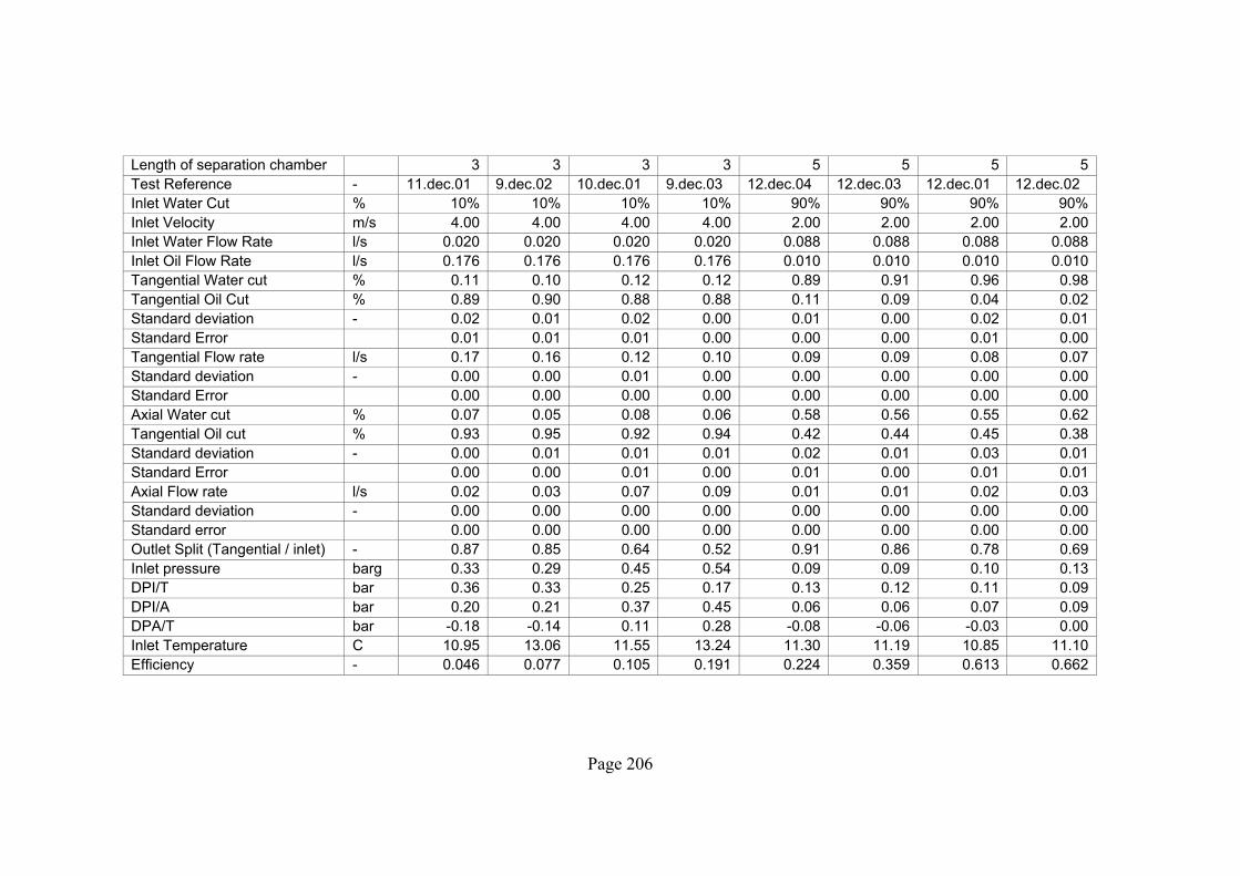
Page 206
Length of separation chamber 3 3 3 3 5 5 5 5 Test Reference - 11.dec.01 9.dec.02 10.dec.01 9.dec.03 12.dec.04 12.dec.03 12.dec.01 12.dec.02 Inlet Water Cut % 10% 10% 10% 10% 90% 90% 90% 90% Inlet Velocity m/s 4.00 4.00 4.00 4.00 2.00 2.00 2.00 2.00 Inlet Water Flow Rate l/s 0.020 0.020 0.020 0.020 0.088 0.088 0.088 0.088 Inlet Oil Flow Rate l/s 0.176 0.176 0.176 0.176 0.010 0.010 0.010 0.010 Tangential Water cut % 0.11 0.10 0.12 0.12 0.89 0.91 0.96 0.98 Tangential Oil Cut % 0.89 0.90 0.88 0.88 0.11 0.09 0.04 0.02 Standard deviation - 0.02 0.01 0.02 0.00 0.01 0.00 0.02 0.01 Standard Error 0.01 0.01 0.01 0.00 0.00 0.00 0.01 0.00 Tangential Flow rate l/s 0.17 0.16 0.12 0.10 0.09 0.09 0.08 0.07 Standard deviation - 0.00 0.00 0.01 0.00 0.00 0.00 0.00 0.00 Standard Error 0.00 0.00 0.00 0.00 0.00 0.00 0.00 0.00 Axial Water cut % 0.07 0.05 0.08 0.06 0.58 0.56 0.55 0.62 Tangential Oil cut % 0.93 0.95 0.92 0.94 0.42 0.44 0.45 0.38 Standard deviation - 0.00 0.01 0.01 0.01 0.02 0.01 0.03 0.01 Standard Error 0.00 0.00 0.01 0.00 0.01 0.00 0.01 0.01 Axial Flow rate l/s 0.02 0.03 0.07 0.09 0.01 0.01 0.02 0.03 Standard deviation - 0.00 0.00 0.00 0.00 0.00 0.00 0.00 0.00 Standard error 0.00 0.00 0.00 0.00 0.00 0.00 0.00 0.00 Outlet Split (Tangential / inlet) - 0.87 0.85 0.64 0.52 0.91 0.86 0.78 0.69 Inlet pressure barg 0.33 0.29 0.45 0.54 0.09 0.09 0.10 0.13 DPI/T bar 0.36 0.33 0.25 0.17 0.13 0.12 0.11 0.09 DPI/A bar 0.20 0.21 0.37 0.45 0.06 0.06 0.07 0.09 DPA/T bar -0.18 -0.14 0.11 0.28 -0.08 -0.06 -0.03 0.00 Inlet Temperature C 10.95 13.06 11.55 13.24 11.30 11.19 10.85 11.10 Efficiency - 0.046 0.077 0.105 0.191 0.224 0.359 0.613 0.662
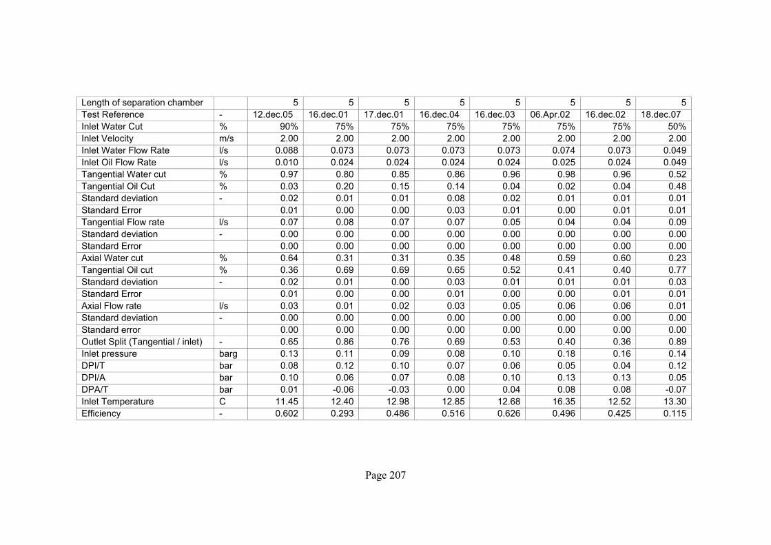
Page 207
Length of separation chamber 5 5 5 5 5 5 5 5 Test Reference - 12.dec.05 16.dec.01 17.dec.01 16.dec.04 16.dec.03 06.Apr.02 16.dec.02 18.dec.07 Inlet Water Cut % 90% 75% 75% 75% 75% 75% 75% 50% Inlet Velocity m/s 2.00 2.00 2.00 2.00 2.00 2.00 2.00 2.00 Inlet Water Flow Rate l/s 0.088 0.073 0.073 0.073 0.073 0.074 0.073 0.049 Inlet Oil Flow Rate l/s 0.010 0.024 0.024 0.024 0.024 0.025 0.024 0.049 Tangential Water cut % 0.97 0.80 0.85 0.86 0.96 0.98 0.96 0.52 Tangential Oil Cut % 0.03 0.20 0.15 0.14 0.04 0.02 0.04 0.48 Standard deviation - 0.02 0.01 0.01 0.08 0.02 0.01 0.01 0.01 Standard Error 0.01 0.00 0.00 0.03 0.01 0.00 0.01 0.01 Tangential Flow rate l/s 0.07 0.08 0.07 0.07 0.05 0.04 0.04 0.09 Standard deviation - 0.00 0.00 0.00 0.00 0.00 0.00 0.00 0.00 Standard Error 0.00 0.00 0.00 0.00 0.00 0.00 0.00 0.00 Axial Water cut % 0.64 0.31 0.31 0.35 0.48 0.59 0.60 0.23 Tangential Oil cut % 0.36 0.69 0.69 0.65 0.52 0.41 0.40 0.77 Standard deviation - 0.02 0.01 0.00 0.03 0.01 0.01 0.01 0.03 Standard Error 0.01 0.00 0.00 0.01 0.00 0.00 0.01 0.01 Axial Flow rate l/s 0.03 0.01 0.02 0.03 0.05 0.06 0.06 0.01 Standard deviation - 0.00 0.00 0.00 0.00 0.00 0.00 0.00 0.00 Standard error 0.00 0.00 0.00 0.00 0.00 0.00 0.00 0.00 Outlet Split (Tangential / inlet) - 0.65 0.86 0.76 0.69 0.53 0.40 0.36 0.89 Inlet pressure barg 0.13 0.11 0.09 0.08 0.10 0.18 0.16 0.14 DPI/T bar 0.08 0.12 0.10 0.07 0.06 0.05 0.04 0.12 DPI/A bar 0.10 0.06 0.07 0.08 0.10 0.13 0.13 0.05 DPA/T bar 0.01 -0.06 -0.03 0.00 0.04 0.08 0.08 -0.07 Inlet Temperature C 11.45 12.40 12.98 12.85 12.68 16.35 12.52 13.30 Efficiency - 0.602 0.293 0.486 0.516 0.626 0.496 0.425 0.115

Page 208
Length of separation chamber 5 5 5 5 5 5 5 5 Test Reference - 18.dec.01 18.dec.06 18.dec.05 18.dec.04 18.dec.03 18.dec.02 22.dec.01 19.dec.01 Inlet Water Cut % 50% 50% 50% 50% 50% 50% 25% 25% Inlet Velocity m/s 2.00 2.00 2.00 2.00 2.00 2.00 2.00 2.00 Inlet Water Flow Rate l/s 0.049 0.049 0.049 0.049 0.049 0.049 0.024 0.024 Inlet Oil Flow Rate l/s 0.049 0.049 0.049 0.049 0.049 0.049 0.073 0.073 Tangential Water cut % 0.56 0.68 0.79 0.89 0.90 0.92 0.30 0.31 Tangential Oil Cut % 0.44 0.32 0.21 0.11 0.10 0.08 0.70 0.69 Standard deviation - 0.01 0.02 0.02 0.01 0.03 0.02 0.02 0.01 Standard Error 0.00 0.01 0.01 0.00 0.01 0.01 0.01 0.01 Tangential Flow rate l/s 0.08 0.06 0.05 0.03 0.02 0.01 0.08 0.05 Standard deviation - 0.00 0.00 0.00 0.00 0.00 0.00 0.00 0.04 Standard Error 0.00 0.00 0.00 0.00 0.00 0.00 0.00 0.02 Axial Water cut % 0.17 0.17 0.23 0.30 0.40 0.46 0.13 0.11 Tangential Oil cut % 0.83 0.83 0.77 0.70 0.60 0.54 0.87 0.89 Standard deviation - 0.03 0.02 0.01 0.02 0.02 0.01 0.01 0.01 Standard Error 0.01 0.01 0.01 0.01 0.01 0.01 0.01 0.00 Axial Flow rate l/s 0.02 0.04 0.05 0.07 0.08 0.09 0.02 0.03 Standard deviation - 0.00 0.00 0.00 0.00 0.00 0.00 0.00 0.02 Standard error 0.00 0.00 0.00 0.00 0.00 0.00 0.00 0.01 Outlet Split (Tangential / inlet) - 0.82 0.63 0.48 0.34 0.17 0.07 0.84 0.62 Inlet pressure barg 0.14 0.13 0.15 0.16 0.14 0.15 0.14 0.13 DPI/T bar 0.11 0.07 0.05 0.04 0.03 0.03 0.12 0.10 DPI/A bar 0.06 0.07 0.09 0.11 0.13 0.14 0.05 0.06 DPA/T bar -0.06 0.00 0.04 0.07 0.10 0.11 -0.07 -0.05 Inlet Temperature C 12.39 13.18 13.08 12.97 12.76 12.63 12.51 12.47 Efficiency - 0.228 0.482 0.561 0.536 0.279 0.121 0.118 0.256

Page 209
Length of separation chamber 5 5 5 5 5 5 5 5 Test Reference - 19.dec.04 19.dec.03 19.dec.02 03.Mar.02 22.dec.02 03.Mar.01 22.dec.04 22.dec.03 Inlet Water Cut % 25% 25% 25% 10% 10% 10% 10% 10% Inlet Velocity m/s 2.00 2.00 2.00 2.00 2.00 2.00 2.00 2.00 Inlet Water Flow Rate l/s 0.024 0.024 0.024 0.088 0.010 0.088 0.010 0.010 Inlet Oil Flow Rate l/s 0.073 0.073 0.073 0.010 0.088 0.010 0.088 0.088 Tangential Water cut % 0.38 0.40 0.47 0.07 0.13 0.12 0.15 0.16 Tangential Oil Cut % 0.62 0.60 0.53 0.93 0.87 0.88 0.85 0.84 Standard deviation - 0.01 0.01 0.02 0.02 0.02 0.01 0.01 0.01 Standard Error 0.00 0.00 0.01 0.01 0.01 0.01 0.00 0.01 Tangential Flow rate l/s 0.05 0.04 0.02 0.07 0.05 0.03 0.02 0.01 Standard deviation - 0.00 0.00 0.00 0.00 0.00 0.00 0.00 0.00 Standard Error 0.00 0.00 0.00 0.00 0.00 0.00 0.00 0.00 Axial Water cut % 0.12 0.14 0.18 0.06 0.11 0.08 0.12 0.12 Tangential Oil cut % 0.88 0.86 0.82 0.94 0.89 0.92 0.88 0.88 Standard deviation - 0.02 0.01 0.01 0.01 0.00 0.01 0.01 0.03 Standard Error 0.01 0.00 0.01 0.00 0.00 0.00 0.00 0.01 Axial Flow rate l/s 0.04 0.06 0.07 0.03 0.04 0.06 0.08 0.09 Standard deviation - 0.00 0.00 0.00 0.00 0.00 0.00 0.01 0.00 Standard error 0.00 0.00 0.00 0.00 0.00 0.00 0.00 0.00 Outlet Split (Tangential / inlet) - 0.54 0.41 0.25 0.71 0.54 0.34 0.22 0.07 Inlet pressure barg 0.14 0.15 0.17 0.19 0.11 0.16 0.11 0.14 DPI/T bar 0.07 0.05 0.04 0.12 0.08 0.06 0.05 0.04 DPI/A bar 0.07 0.08 0.10 0.05 0.06 0.08 0.09 0.11 DPA/T bar 0.00 0.03 0.06 -0.06 -0.02 0.02 0.05 0.07 Inlet Temperature C 12.85 12.75 12.60 14.24 12.93 14.11 13.52 13.16 Efficiency - 0.334 0.343 0.286 0.040 0.050 0.112 0.056 0.023
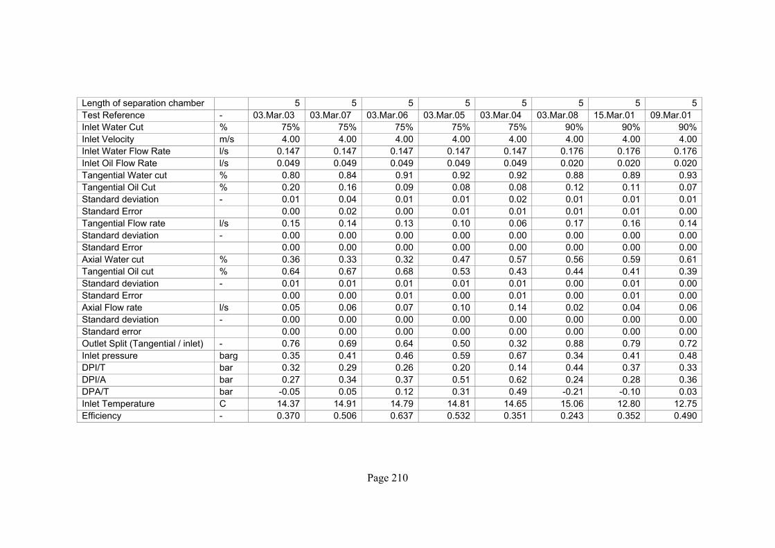
Page 210
Length of separation chamber 5 5 5 5 5 5 5 5 Test Reference - 03.Mar.03 03.Mar.07 03.Mar.06 03.Mar.05 03.Mar.04 03.Mar.08 15.Mar.01 09.Mar.01 Inlet Water Cut % 75% 75% 75% 75% 75% 90% 90% 90% Inlet Velocity m/s 4.00 4.00 4.00 4.00 4.00 4.00 4.00 4.00 Inlet Water Flow Rate l/s 0.147 0.147 0.147 0.147 0.147 0.176 0.176 0.176 Inlet Oil Flow Rate l/s 0.049 0.049 0.049 0.049 0.049 0.020 0.020 0.020 Tangential Water cut % 0.80 0.84 0.91 0.92 0.92 0.88 0.89 0.93 Tangential Oil Cut % 0.20 0.16 0.09 0.08 0.08 0.12 0.11 0.07 Standard deviation - 0.01 0.04 0.01 0.01 0.02 0.01 0.01 0.01 Standard Error 0.00 0.02 0.00 0.01 0.01 0.01 0.01 0.00 Tangential Flow rate l/s 0.15 0.14 0.13 0.10 0.06 0.17 0.16 0.14 Standard deviation - 0.00 0.00 0.00 0.00 0.00 0.00 0.00 0.00 Standard Error 0.00 0.00 0.00 0.00 0.00 0.00 0.00 0.00 Axial Water cut % 0.36 0.33 0.32 0.47 0.57 0.56 0.59 0.61 Tangential Oil cut % 0.64 0.67 0.68 0.53 0.43 0.44 0.41 0.39 Standard deviation - 0.01 0.01 0.01 0.01 0.01 0.00 0.01 0.00 Standard Error 0.00 0.00 0.01 0.00 0.01 0.00 0.01 0.00 Axial Flow rate l/s 0.05 0.06 0.07 0.10 0.14 0.02 0.04 0.06 Standard deviation - 0.00 0.00 0.00 0.00 0.00 0.00 0.00 0.00 Standard error 0.00 0.00 0.00 0.00 0.00 0.00 0.00 0.00 Outlet Split (Tangential / inlet) - 0.76 0.69 0.64 0.50 0.32 0.88 0.79 0.72 Inlet pressure barg 0.35 0.41 0.46 0.59 0.67 0.34 0.41 0.48 DPI/T bar 0.32 0.29 0.26 0.20 0.14 0.44 0.37 0.33 DPI/A bar 0.27 0.34 0.37 0.51 0.62 0.24 0.28 0.36 DPA/T bar -0.05 0.05 0.12 0.31 0.49 -0.21 -0.10 0.03 Inlet Temperature C 14.37 14.91 14.79 14.81 14.65 15.06 12.80 12.75 Efficiency - 0.370 0.506 0.637 0.532 0.351 0.243 0.352 0.490

Page 211
Length of separation chamber 5 5 5 5 5 5 5 5 Test Reference - 03.Mar.10 03.Mar.09 15.Mar.02 16.Mar.02 16.Mar.01 15.Mar.03 15.Mar.04 01.Apr.03 Inlet Water Cut % 90% 90% 50% 50% 50% 50% 50% 25% Inlet Velocity m/s 4.00 4.00 4.00 4.00 4.00 4.00 4.00 4.00 Inlet Water Flow Rate l/s 0.176 0.176 0.098 0.098 0.098 0.098 0.098 0.049 Inlet Oil Flow Rate l/s 0.020 0.020 0.098 0.098 0.098 0.098 0.098 0.147 Tangential Water cut % 0.94 0.94 0.51 0.61 0.69 0.76 0.79 0.28 Tangential Oil Cut % 0.06 0.06 0.49 0.39 0.31 0.24 0.21 0.72 Standard deviation - 0.01 0.01 0.00 0.01 0.01 0.02 0.01 0.03 Standard Error 0.00 0.00 0.00 0.01 0.00 0.01 0.00 0.01 Tangential Flow rate l/s 0.14 0.14 0.17 0.12 0.11 0.08 0.05 0.14 Standard deviation - 0.00 0.00 0.00 0.00 0.00 0.00 0.00 0.00 Standard Error 0.00 0.00 0.00 0.00 0.00 0.00 0.00 0.00 Axial Water cut % 0.61 0.62 0.16 0.19 0.19 0.25 0.33 0.14 Tangential Oil cut % 0.39 0.38 0.84 0.81 0.81 0.75 0.67 0.86 Standard deviation - 0.01 0.01 0.02 0.01 0.00 0.01 0.01 0.01 Standard Error 0.01 0.00 0.01 0.00 0.00 0.01 0.00 0.00 Axial Flow rate l/s 0.06 0.06 0.03 0.07 0.09 0.12 0.14 0.04 Standard deviation - 0.00 0.00 0.00 0.00 0.00 0.00 0.00 0.01 Standard error 0.00 0.00 0.00 0.00 0.00 0.00 0.00 0.00 Outlet Split (Tangential / inlet) - 0.72 0.69 0.86 0.64 0.55 0.40 0.26 0.77 Inlet pressure barg 0.52 0.58 0.35 0.41 0.52 0.68 0.75 0.31 DPI/T bar 0.32 0.32 0.39 0.25 0.20 0.14 0.11 0.33 DPI/A bar 0.40 0.46 0.21 0.32 0.38 0.48 0.56 0.19 DPA/T bar 0.07 0.14 -0.19 0.08 0.19 0.34 0.45 -0.14 Inlet Temperature C 15.39 15.22 12.93 13.27 13.08 13.16 13.36 16.13 Efficiency - 0.508 0.504 0.165 0.397 0.497 0.501 0.351 0.133
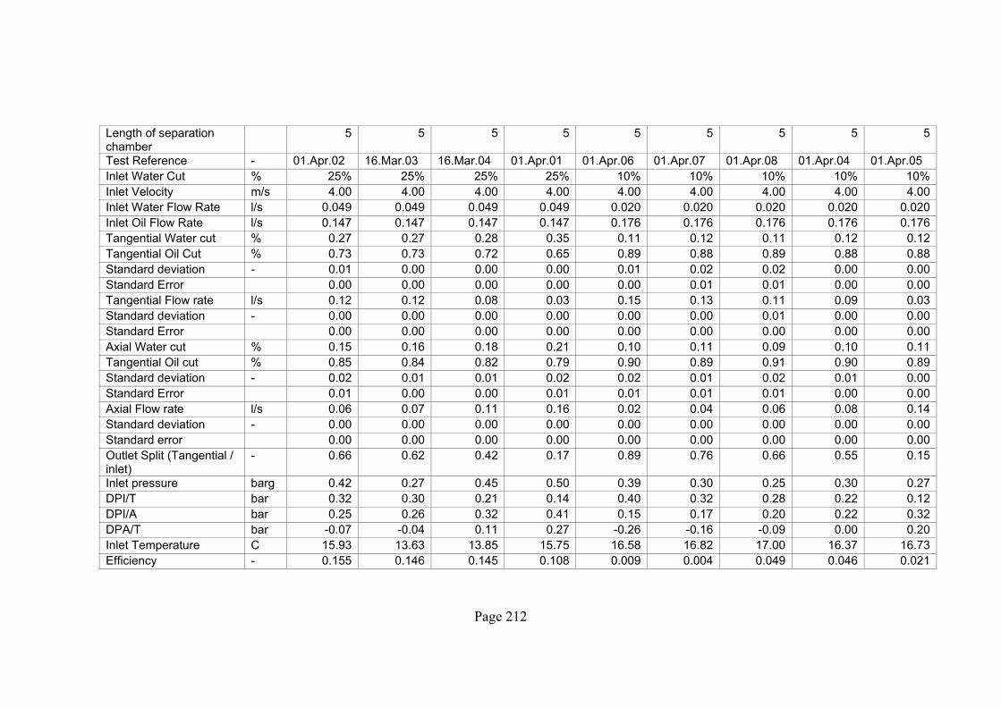
Page 212
Length of separation chamber
5 5 5 5 5 5 5 5 5
Test Reference - 01.Apr.02 16.Mar.03 16.Mar.04 01.Apr.01 01.Apr.06 01.Apr.07 01.Apr.08 01.Apr.04 01.Apr.05 Inlet Water Cut % 25% 25% 25% 25% 10% 10% 10% 10% 10% Inlet Velocity m/s 4.00 4.00 4.00 4.00 4.00 4.00 4.00 4.00 4.00 Inlet Water Flow Rate l/s 0.049 0.049 0.049 0.049 0.020 0.020 0.020 0.020 0.020 Inlet Oil Flow Rate l/s 0.147 0.147 0.147 0.147 0.176 0.176 0.176 0.176 0.176 Tangential Water cut % 0.27 0.27 0.28 0.35 0.11 0.12 0.11 0.12 0.12 Tangential Oil Cut % 0.73 0.73 0.72 0.65 0.89 0.88 0.89 0.88 0.88 Standard deviation - 0.01 0.00 0.00 0.00 0.01 0.02 0.02 0.00 0.00 Standard Error 0.00 0.00 0.00 0.00 0.00 0.01 0.01 0.00 0.00 Tangential Flow rate l/s 0.12 0.12 0.08 0.03 0.15 0.13 0.11 0.09 0.03 Standard deviation - 0.00 0.00 0.00 0.00 0.00 0.00 0.01 0.00 0.00 Standard Error 0.00 0.00 0.00 0.00 0.00 0.00 0.00 0.00 0.00 Axial Water cut % 0.15 0.16 0.18 0.21 0.10 0.11 0.09 0.10 0.11 Tangential Oil cut % 0.85 0.84 0.82 0.79 0.90 0.89 0.91 0.90 0.89 Standard deviation - 0.02 0.01 0.01 0.02 0.02 0.01 0.02 0.01 0.00 Standard Error 0.01 0.00 0.00 0.01 0.01 0.01 0.01 0.00 0.00 Axial Flow rate l/s 0.06 0.07 0.11 0.16 0.02 0.04 0.06 0.08 0.14 Standard deviation - 0.00 0.00 0.00 0.00 0.00 0.00 0.00 0.00 0.00 Standard error 0.00 0.00 0.00 0.00 0.00 0.00 0.00 0.00 0.00 Outlet Split (Tangential / inlet)
- 0.66 0.62 0.42 0.17 0.89 0.76 0.66 0.55 0.15
Inlet pressure barg 0.42 0.27 0.45 0.50 0.39 0.30 0.25 0.30 0.27 DPI/T bar 0.32 0.30 0.21 0.14 0.40 0.32 0.28 0.22 0.12 DPI/A bar 0.25 0.26 0.32 0.41 0.15 0.17 0.20 0.22 0.32 DPA/T bar -0.07 -0.04 0.11 0.27 -0.26 -0.16 -0.09 0.00 0.20 Inlet Temperature C 15.93 13.63 13.85 15.75 16.58 16.82 17.00 16.37 16.73 Efficiency - 0.155 0.146 0.145 0.108 0.009 0.004 0.049 0.046 0.021

Page 213
Appendix B
Engineering drawings of constructed I-SEP Unit

Page 214
Figure B.1: General Assembly drawing of 1x I-SEP test unit

Page 215
Figure B.2: Plan view (left) and side elevation (right) of outlet transition

Page 216
Figure B.3: Plan view and front side elevation of Perspex slice forming inlet involute

Page 217
Figure B.4: Plan view and front side elevation of Perspex slice forming outlet involute

Page 218
Figure B.5: Separator body of original unit

Page 219
Figure B.6: Vortex finder assembly and axial outlet transition to 1-inch pipe