ANDERSON LOCALIZATION IN SOME NONLINEARSYSTEMSYEVGENY BAR-LEV (NÉ KRIVOLAPOV)

ANDERSON LOCALIZATION IN SOME NONLINEAR SYSTEMSResearch thesis

IN PARTIAL FULFILLMENT OF THE REQUIREMENTSFOR THE DEGREE OF DOCTOR OF PHILOSOPHYYEVGENY BAR-LEV (NÉ KRIVOLAPOV)

SUBMITTED TO THE SENATE OF THE TECHNION � ISRAEL INSTITUTE OF TECHNOLOGYADAR 5770 HAIFA MARCH 2010

THE RESEARCH THESIS WAS DONE UNDER THE SUPERVISION OF PROF. SHMUELFISHMAN IN THE DEPARTMENT OF PHYSICS.THE GENEROUS FINANCIAL HELP OF THE TECHNION IS GRATEFULLYACKNOWLEDGED.I OWE A DEBT OF GRATITUDE TO MY SUPERVISOR, PROF. SHMUEL FISHMAN.DURING MY RESEARCH SHMUEL'S SUPPORT KNEW NO BOUNDARIES AND HISLOVE TO RESEARCH WAS CONTAGIOUS. BEFORE I HAVE MET HIM, I HAD NOT METANYONE WHO IS SO DEVOTED TO RESEARCH AND HIS STUDENTS. I WOULD LIKETO THANK SHMUEL FOR HIS DEVOTION AS ALSO FOR THE MULTIPLE THINGS HEHAS TAUGHT ME IN PHYSICS AND SCIENCE.I WOULD ALSO LIKE TO THANK PROF. AVY SOFFER FOR CONSIDERABLECONTRIBUTION TO THE RESEARCH AND VALUABLE DISCUSSIONS. CONSTRUCTIVECOMMENTS AND SUPPORT OF MICHAEL SHEINMAN ARE GRATEFULLYACKNOWLEDGED.SPECIAL THANKS GO TO PARENTS, MY SISTER AND MY WIFE FOR SUPPORT ANDPATIENCE DURING THE PREPARATION OF THIS WORK.THIS WORK WAS PARTLY SUPPORTED BY THE ISRAEL SCIENCE FOUNDATION (ISF),BY THE US-ISRAEL BINATIONAL SCIENCE FOUNDATION (BSF), BY THE USANATIONAL SCIENCE FOUNDATION (NSF DMS-0903651), BY THE MINERVA CENTEROF NONLINEAR PHYSICS OF COMPLEX SYSTEMS, BY THE SHLOMO KAPLANSKYACADEMIC CHAIR, BY THE FUND FOR PROMOTION OF RESEARCH AT THETECHNION AND BY THE E. AND J. BISHOP RESEARCH FUND.

Dedicated to my parents Lev and Lubov.

Contents1 Introduction 11.1 Disordered systems . . . . . . . . . . . . . . . . . . . . . . . . . . . . . . . . . . . . 31.2 Some nonlinear phenomena . . . . . . . . . . . . . . . . . . . . . . . . . . . . . . . 41.2.1 Nonlinear optics . . . . . . . . . . . . . . . . . . . . . . . . . . . . . . . . . 41.2.2 Nonlinearity in many-body physics . . . . . . . . . . . . . . . . . . . . . . . 61.2.3 Nonlinear classical problems . . . . . . . . . . . . . . . . . . . . . . . . . . . 91.2.4 Properties and conservation laws . . . . . . . . . . . . . . . . . . . . . . . . 91.3 Disorder and Nonlinearity . . . . . . . . . . . . . . . . . . . . . . . . . . . . . . . . 112 Organization of the perturbation theory 142.1 Assignment of eigenfunctions to sites . . . . . . . . . . . . . . . . . . . . . . . . . . 142.2 The perturbation expansion . . . . . . . . . . . . . . . . . . . . . . . . . . . . . . . 152.3 Elimination of secular terms . . . . . . . . . . . . . . . . . . . . . . . . . . . . . . . 162.4 The entropy problem . . . . . . . . . . . . . . . . . . . . . . . . . . . . . . . . . . . 202.5 Bounding the general term . . . . . . . . . . . . . . . . . . . . . . . . . . . . . . . 212.6 The remainder of the expansion . . . . . . . . . . . . . . . . . . . . . . . . . . . . . 293 Numerical results 314 Summary and Discussion 37A Bounding the remainder 40B Derivation of the modi�ed perturbation expansion 45C Nonlinear classical equations 51

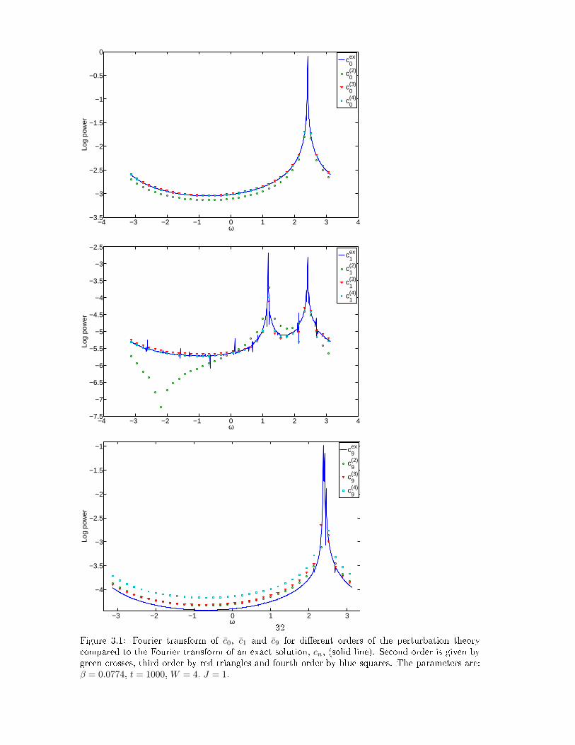
List of Figures2.1 A bound on the number of terms in the expansion . . . . . . . . . . . . . . . . . . 212.2 The logarithm of ⟨|f |−1/2⟩ as a function of the logarithm of R. . . . . . . . . . . . 242.3 An example of a graph that is used to construct the general term in the perturbationexpansion. . . . . . . . . . . . . . . . . . . . . . . . . . . . . . . . . . . . . . . . . . 283.1 Fourier transform of c0, c1 and c9 for di�erent orders of the perturbation theorycompared to the Fourier transform of an exact solution . . . . . . . . . . . . . . . . 323.2 Qlin

n as a function of time in the 4th order in β for all n's of the lattice (total 128lines). . . . . . . . . . . . . . . . . . . . . . . . . . . . . . . . . . . . . . . . . . . . 333.3 ‖Q‖2 (dashed blue) and ‖Q′‖2 (solid green) as a function of time. . . . . . . . . . . 343.4 R−1n as a function of n . . . . . . . . . . . . . . . . . . . . . . . . . . . . . . . . . . 343.5 ‖Qex‖2 (lines) and ‖Qlin‖2 (dotes) as a function of time, for various values of β (seelegend). The perturbation expansion is up to fourth order in β. . . . . . . . . . . . 353.6 log10 t∗ as a function of β−1 for di�erent orders. . . . . . . . . . . . . . . . . . . . . 353.7 log10 t∗ as a function of β−1 for the 4-th order. . . . . . . . . . . . . . . . . . . . . 364.1 β−N ‖Q (t)‖2 as a function of β. . . . . . . . . . . . . . . . . . . . . . . . . . . . . . 38

AbstractIn this work a perturbation theory for the Nonlinear Schrödinger Equation (NLSE) in one dimen-sion and in the presence of a random potential was developed. This equation was motivated byclassical nonlinear wave optics in disordered materials and by studies of Bose-Einstein Condensates(BEC) in disordered optical potentials. Here the NLSE is used to explore the competition betweene�ects of disorder and nonlinearity. In the absence of nonlinearity the NLSE reduces to the Ander-son model where in one dimension all the eigenstates are exponentially localized. Consequently, awavepacket will remain localized near its initial position. In the absence of the random potentialspreading takes place. Various contradicting arguments concerning the asymptotic behavior inspace and time were put forward. Nevertheless, in spite of the fact that many numerical calcula-tions were performed their signi�cance is not clear since it is not known what is the time scale thatdetermines when long time asymptotics is achieved. Therefore an analytic approach is required.In this work we have developed a perturbation theory in the nonlinearity parameter. Thisapproach enabled us to show that there is a front which propagates not faster than logarithmicallyin time. Beyond this front the wavepacket remains exponentially bounded in space, as in the casefor the linear disordered system. The perturbation expansion also allowed us to obtain a numericalsolution to the NLSE with some control of the error. The development of the perturbation theoryrequired to overcome many di�culties which are typical to nonlinear di�erential equations and itis therefore relevant for the study of other nonlinear problems, e.g. the Fermi-Pasta-Ulam (FPU)problem.

Nomenclatureβ Nonlinearity strengthγ Inverse localization lengthµ0 The vacuum permeabilityω A frequency - Chapter 1, Speci�c realization - Chapter 2ψ (x) Wavefunction on a lattice site xε0 The vacuum permittivityεx Potential at site xξ Localization lengthcn Coe�cients of the wavefunction in terms of the eigenstates of the linear problemc(k)n Expansion term of order kEn Eigenvalues of the linear Anderson modelE

(k)n Expansion term of order k of the renormalized eigenvalues

E′n Renormalized eigenvalues

J Hopping coe�cientN Expansion orderQn The remainder of the expansion for the state nt∗ Time of validity of the pertrubation expansionum (x) Eigenfunctions of the linear Anderson modelV m1m2m3n Overlap integralW Width of the distribution of the random potentialsBEC Bose-Einstein CondensateFPU Fermi-Pasta-Ulam problemGPE Gross-Pitaevskii EquationNLSE Nonlinear Schrödinger Equation

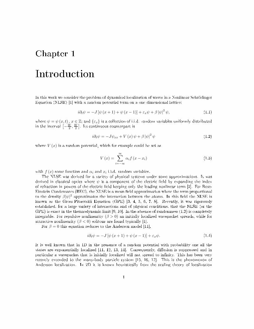
Chapter 1IntroductionIn this work we consider the problem of dynamical localization of waves in a Nonlinear SchrödingerEquation (NLSE) [1] with a random potential term on a one-dimensional lattice:i∂tψ = −J [ψ (x+ 1) + ψ (x− 1)] + εxψ + β |ψ|2 ψ, (1.1)where ψ = ψ (x, t) , x ∈ Z; and {εx} is a collection of i.i.d. random variables uniformly distributedin the interval [−W

2 ,W2

]. Its continuous counterpart isi∂tψ = −Jψxx + V (x)ψ + β |ψ|2 ψ (1.2)where V (x) is a random potential� which for example could be set as

V (x) =

∞∑

i=−∞

αif (x− xi) (1.3)with f (x) some function and αi and xi i.i.d. random variables.The NLSE was derived for a variety of physical systems under some approximations. It wasderived in classical optics where ψ is a component of the electric �eld by expanding the indexof refraction in powers of the electric �eld keeping only the leading nonlinear term [2]. For Bose-Einstein Condensates (BEC), the NLSE is a mean �eld approximation where the term proportionalto the density β|ψ|2 approximates the interaction between the atoms. In this �eld the NLSE isknown as the Gross-Pitaevskii Equation (GPE) [3, 4, 5, 6, 7, 8]. Recently, it was rigorouslyestablished, for a large variety of interactions and of physical conditions, that the NLSE (or theGPE) is exact in the thermodynamic limit [9, 10]. In the absence of randomness (1.2) is completelyintegrable. For repulsive nonlinearity (β > 0) an initially localized wavepacket spreads, while forattractive nonlinearity (β < 0) solitons are found typically [1].For β = 0 this equation reduces to the Anderson model [11],i∂tψ = −J [ψ (x+ 1) + ψ (x− 1)] + εxψ. (1.4)It is well known that in 1D in the presence of a random potential with probability one all thestates are exponentially localized [11, 12, 13, 14]. Consequently, di�usion is suppressed and inparticular a wavepacket that is initially localized will not spread to in�nity. This has been veryrecently extended to the many-body particle system [15, 16, 17]. This is the phenomenon ofAnderson localization. In 2D it is known heuristically from the scaling theory of localization1

[18, 13] that all the states are localized, while in higher dimensions there is a mobility edge thatseparates localized and extended states. This problem may be relevant for experiments in nonlinearoptics, for example disordered photonic lattices [19], where Anderson localization was found inthe presence of nonlinear e�ects as well as experiments on BECs in disordered optical lattices[20, 21, 22, 23, 24, 25, 26, 27, 28]. The interplay between disorder and nonlinear e�ects leads tonew interesting physics [26, 27, 29, 30, 31, 32]. In spite of the extensive research, many fundamentalproblems are still open, and in particular, it is not clear whether in one dimension (1D) Andersonlocalization can survive the e�ects of nonlinearities (see however [33, 34]).A natural question is whether a wave packet that is initially localized in space will inde�nitelyspread for dynamics controlled by (1.1). A simple argument indicates that spreading will besuppressed by randomness. If unlimited spreading takes place the amplitude of the wave functionwill decay since the L2 norm is conserved. Consequently, the nonlinear term will become negligibleand Anderson localization will take place as a result of the randomness. Contrary to this intuition,based on the smallness of the nonlinear term resulting from the spread of the wave function, itis claimed that for the kicked-rotor a nonlinear term leads to delocalization if it is strong enough[35]. It is also argued that the same mechanism results in delocalization for the model (1.1) withsu�ciently large β, while, for weak nonlinearity, localization takes place [35, 36]. Therefore, it ispredicted in that work that there is a critical value of β that separates the occurrence of localizedand extended states. However, if one applies the arguments of [35, 36] to a variant of (1.1), resultsthat contradict numerical solutions are found [37, 38]. Recently, it was rigorously shown thatthe initial wavepacket cannot spread so that its amplitude vanishes at in�nite time, at least forlarge enough β [39]. It does not contradict spreading of a fraction of the wavefunction. Indeed,subdi�usion was found in numerical experiments [35, 39, 40]. In di�erent works [40, 41, 42] sub-di�usion was reported for all values of β. It was also argued that nonlinearity may enhance discretebreathers [31, 32]. In conclusion, it is not clear what is the long time behavior of a wave packetthat is initially localized, if both nonlinearity and disorder are present. The major di�culty innumerical resolution of this question is integration of (1.1) to large time. Most researchers who runnumerical simulation use a split-step method for integration, however it is impossible to achieveconvergence for large times, and therefore some heuristic arguments assuming that the numericalerrors do not a�ect the results qualitatively, are utilized [35, 41]. However it is unclear whetherthose arguments apply to (1.1).The motivation of the current work was to establish an analytic method which will allow todecipher some of the contradicting results in this �eld. For this propose we have developed amodi�ed perturbation theory [43, 44] in the strength of the nonlinearity and also a symbolicalcomputational scheme for the computation of high terms in the perturbation expansion. Thisscheme allowed us integration of (1.1) up to large times and with some control of the error basedon the form of the remainder term obtained in [44].In this work the dynamics generated by the NLSE (1.1) will be explored in the framework of aperturbation theory in the nonlinearity parameter β. This equation was motivated by experimentalrealizations in classical optics as well as in atom optics. In the present work it will be studiedas a paradigm for the competition between e�ects of disorder and nonlinearity (and interactions)without speci�c reference to a speci�c realistic system which motivated this equation. In particularthe validity of this equation for description of speci�c physical systems will be left for furtherstudies. The present research is relevant for the exploration of other nonlinear equations that wereproposed for the description of various physical systems. Therefore this work should be consideredas an exploration of a possible phenomenon rather than a speci�c system.In the �rst chapter of this work we will brie�y review: Disordered linear systems, derivation ofNLSE in nonlinear optics and Bose-Einstein Condensates (BEC) and also the Fermi-Ulam-Pastaproblem and its similarity to the NLSE. In the second chapter we describe the perturbation theory2

developed in [44] and show how the error of the perturbation theory could be controlled. In Chapter3 we explain the numerical scheme used to compute the di�erent orders in the perturbation theory.The results are summarized in Chapter 4 and open problems are listed there.1.1 Disordered systemsIn 1958 Anderson has shown [11] that in materials with su�ciently strong disorder all eigenfunctionsare exponentially localized in space. It is contrary to the former beliefs that Bloch waves losecoherence at the length scale of elastic mean free path, but still remain extended through thesample and di�usion takes place. The existence of localized states could be understood in the limitof strong disorder. In this limit and in the leading order of the tight-binding approximation thewavefunctions are exponentially localized on the deep points of the potential. Two such nearbystates will be in generally far in energy and therefore will not mix signi�cantly, while two nearlydegenerate states will be in general far in space and therefore with a vanishing overlap. Thus, inthe strong disorder case the wavefunction would be exponentially localized. Mott and Twose haveshown [45] that in one dimension all states are localized, no matter how weak the disorder. In 2Dthe scaling theory for localization predicts that all states are localized, while in higher dimensions,there is a transition between intervals of energy where localized and extended states are found[18].We will now present some basic results for Anderson localization in one dimension, since our workis con�ned to 1D.Very often Anderson localization is analyzed in the framework of tight-binding models of theform [46]εxu (x) + J (u (x+ 1) + u (x− 1)) = Eu (x) (1.5)where εn is a disordered potential, E is the energy, J is the hopping matrix element and u (x) arethe amplitudes of the wavefunction. A recursive formula for the latter could be expressed in termsof a transfer matrix [12]u (x) ≡

(u (x+ 1)u (x)

)

= Tx

(u (x)

u (x− 1)

)

, (1.6)whereTx =

(E−εx

J −11 0

)

. (1.7)A value of the wavefunction at site N could be calculated by applying the transfer matrix N timesand the Frustenberg theorem [47] ensures the existence of the limitlim

N→∞

1

Nln |u (N)| = γ (E) > 0 (1.8)This ensures an exponential growth of the wavefunction and by matching the iterated functionsfrom both ends of the sample eigenfunctions could be obtained. This approach was rigorouslyestablished by Delyon, Levy and Souillard [48, 49] and yielded eigenfunctions of the following form

un (x) ∼ Anvn (x) exp [−γn |x− xn|] , (1.9)where xn is the localization center and γn is the inverse localization length. For models withnearest neighbor hopping, γ of (1.8) could be expressed as a function of density of states ρ usingthe Thouless formula [12, 50]γ (E) =

ˆ

ρ (x) ln|E − x|J

dx. (1.10)3

It is of importance to note, that knowing all the eigenfunctions of the linear Anderson problemsu�ce to determine the dynamics of the problem. Any initial wavefunction that is localized willdevelop in time as a superposition of localized eigenfunctions and therefore will remain localized.In nonlinear problems due to the absence of the superposition principle, knowing the stationarysolutions is not su�cient for determining the dynamics.1.2 Some nonlinear phenomenaNonlinear phenomena occur in various branches of physics. Probably the most familiar case is thesoliton, �rst discovered by Russel [51] on a water surface and latter demonstrated in plasma waves[52], sound waves in He4 [53] and optical spatial solitons [54].Nonlinear phenomena described by the NLSE could be crudely classi�ed into two main classes:Nonlinear optics and nonlinearity which approximate treatment of many-body physics. In theformer class the nonlinearity is due to propagating media, while in the latter the nonlinearity issolely due to simpli�cation (usually mean-�eld) of the many-body interaction (for excellent reviewsin the context of BEC see [5, 4]). Recently, a few works treating the linear many-body problem weredone, see [16, 17]. They �nd an insulator-metal transition for varying strength of the interactionbetween the partices.Although the underlining physics of nonlinear optics and many-body physics is di�erent, itseems that many of the dynamic properties are similar. In the next subsections we show thatsome systems belonging to both classes could be reduced (within some approximation) to thesame equation of motion, known as the Gross-Pitaevskii (GP) equation [6, 8], or the NonlinearSchrödinger Equation (NLSE).1.2.1 Nonlinear opticsTo derive the NLSE for nonlinear optics we follow [2] and start with the Maxwell equations inlossless and non-magnetic system∇×E= −∂tB (1.11)∇×B = µ0∂tDTaking the curl of the �rst equation results in

∇×∇×E= ∇ (∇ ·E)−∇2E = −∂t (∇×B) = −µ0∂ttD (1.12)or

∇ (∇ ·E) = ∇2E− µ0∂ttD, (1.13)were D is the electric displacement �eld,

D = ε0E+P (1.14)and P is the polarization of the material, which could be derived from the microscopic propertiesof the material. In terms of the applied electric �eld the Fourier transform of the polarization isgiven byPi (ω) = ε0

∑

k

χ(1)ik (ω)Ek + ε0

∑

jk

χ(2)ijk (ω = ωj + ωk)EjEk, (1.15)

+ ε0∑

jkl

χ(3)ijkl (ω = ωj + ωk + ωl)EjEkEl + · · ·4

where χ(k) are the k-order susceptibilities of the material. Symmetries of the molecular potentialof the material imply symmetries in the susceptibilities tensors. For example, for materials with acentro-symmetrical (CM) potential, χ(2)ijk, is zero, since for ~r → −~r,

χ(2)−i,−j,−kE−jE−k = −χ(2)

i,j,kEjEk. (1.16)Inserting (1.14) into (1.13) and Fourier transforming with respect to time gives∇ (∇ · F (E)) = ∇2F (E)− µ0ε0

(

1 + χ(1) (ω))

∂ttF (E)− µ0ε0∂ttPNL, (1.17)where F designates a Fourier transform. This equation generates new frequencies via the nonlinearpolarization term, however we will assume that it is su�ciently weak so that we can assume a wavepropagating at the direction k with a transverse polarization, ε,E = A (x, y, z) εei(k·r−ωt) + c.c. (1.18)The term, ∇ (∇ · F (E)) in (1.17) under this assumption is given by

∇ · F (E) = ∇(Aeik·r

)· ε = eik·r [∇A+ iAk] · ε = eik·r (∇A) · ε. (1.19)We will set ∇A⊥ε, namely the change in the amplitude is perpendicular to the polarization of thewave, such that the term ∇ (∇ · F (E)) is equal to zero. Choosing z as the propagation directionand taking χ(2) = 0 (a CM material) we have,

∂2Ai

∂z2+ 2ik

∂Ai

∂z− k2Ai +

n2ω2

c2Ai +

∂2Ai

∂x2+ω2

c2

∑

j,k,l

χ(3)ijklA

∗jAkAl = 0, (1.20)where k (ω) = ωn (ω) /c. Assuming that the polarization does not change too fast during thepropagation and using the de�nition n2 = χ

(3)yyyy/ (2n), we have

1

2k2∂2A

∂z2+i

k

∂A

∂z+

1

2k2∂2A

∂x2+n2

n|A|2A = 0 (1.21)Applying the slowly varying envelope approximation (or the paraxial approximation),

∣∣∣∣

∂2A

∂z2

∣∣∣∣� 2k0

∣∣∣∣

∂A

∂z

∣∣∣∣, (1.22)namely, the amplitude variations are slow with respect to the wavelength we neglect the termcontaining the second derivative with respect to z, by which (1.21) reduces to the NLSE (1.2),

i∂A

∂z= − 1

2k0

∂2A

∂x2− k0n2

n0|A|2A, (1.23)with ψ = A, J = 1

2k0and V (x) = −k0n2

n0.We will summarize for convenience the approximations which were used to derive (1.23):1. Lossless, non-magnetic, disperssionless and centro-symmetric media2. The electric �eld is not too strong such that only χ(3) in the expansion (1.15) is important.3. ∇A⊥ε which gives ∇ (∇ · E) = 0 . 5

4. The o�-diagonal terms of the susceptibility tensor χ(3)are negligible with respect to thediagonal terms, such that the transition of energy to other polarizations (1.17) is slow.5. The nonlinearity is su�ciently weak such that there is almost no higher frequencies generationand the norm of A in (1.20) is conserved (no norm loss to higher frequencies).6. Slowly varying envelope approximation: the amplitude variations are slow with respect tothe wavelength.The nonlinearity strengths achieved by materials with χ(3) nonlinearity (Kerr materials) are verylow since χ(3) is small. Another way to achieve stronger nonlinearity strengths is to use photore-fractive materials with external applied DC �eld. In those materials the beam excites electrons,which migrate in a presence of an external electric �eld and recombine in acceptors or donors ofthe material. The change in the refractive index is achieved using the linear Pockel's e�ect [2]P (2) (ω) = χ(2)EDCE (ω) , (1.24)and therefore much stronger nonlinearities could be reached. The drawback of this method is thatthe change in the refractive index is not instantaneous, since it depends on the migration velocityof the excited electrons.1.2.2 Nonlinearity in many-body physicsNonlinearity in many-body physics emerges after a mean-�eld approximation of the many-bodyHamiltonian [5, 4],H =

N∑

i=1

hi +∑

i<j

U (~ri − ~rj) (1.25)where U (~ri − ~rj) is a two particle interaction and hi is a one-particle Hamiltonian. Since the exactform of the interaction potential is complicated or even unknown, usually it is approximated by apseudopotential [55],U (r) = βδ (r)

(∂

∂rr

)

, (1.26)withβ =

4π~2a

m, (1.27)where a is the s-wave scattering length of the interaction potential. We will derive this pseu-dopotential using a hard-sphere potential of radius a (which serves also as the s-wave scatteringlength in this case) as an illustrative example. For this potential the wavefunction is given by theSchödinger equation,

(∇2 + k2

)ψ (r) = 0 (1.28)with the boundary condition

ψ (a) = 0. (1.29)The solution to this equation could be written as a superposition of spherical Bessel functions(jl, nl),

ψ (r) =

∞∑

l=0

Alm (jl (kr) − tan ηlnl (kr))Ylm (θ, ϕ) , (1.30)6

wheretan ηl =

jl (ka)

nl (ka)(1.31)is due to the boundary condition and Ylm are the spherical harmonics. For su�ciently low energies

k � 1, such that only s-wave scattering is important,ψ (r) ≈ A√

4πkr(sin kr − tanka · cos kr) = A√

4πk cos ka

sin k (r − a)

r, (1.32)where we have used,

j0 (x) =sinx

x, n0 (x) = −cosx

x, Y00 =

1√4π.The coe�cient A could be written as

A =∂

∂r(rψ)|r=0 . (1.33)Plugging (1.32) into (1.28) and using (1.33) gives,

(∇2 + k2

)ψ (r) = −A tanka√

4π

(∇2 + k2

) cos kr

kr= −4π tan ka

kδ (r)

∂

∂r(rψ) . (1.34)End for low energies expanding in powers of k gives,

(∇2 + k2

)ψ (r) = 4πaδ (r)

∂

∂r(rψ) . (1.35)This pseudopotential reconstructs the scattering properties of the original potential given a short-range interaction and su�ciently large inter-particle distance, ρa3 � 1 (ρ is the particle density).The total cross-section is given by,

σtot =4π

k2sin2 ka, (1.36)which for low energies, ka� 1, is given by

σtot = 4πa2. (1.37)When the Hamiltonian (1.25) describes a condensate at low temperatures it is natural to introducethe mean �eld ansatz|Ψ(~r1, . . . , ~rN , t)〉 =

N∏

i=1

|φ (~ri, t)〉 , (1.38)where |φ (~ri, t)〉 is a single-particle wavefunction normalized to unity. The energy of the systemtakes the formE = 〈Ψ|H |Ψ〉 = N 〈φ|h |φ〉+ N (N − 1)

2〈φ (~r)| 〈φ (~r′)|U (~r − ~r′) |φ (~r)〉 |φ (~r′)〉 (1.39)or by using (1.26),

E = N

ˆ

d3r

[~2

2m|∇φ|2 + V (~r) |φ|2 + β (N − 1)

2|φ|4

]

. (1.40)7

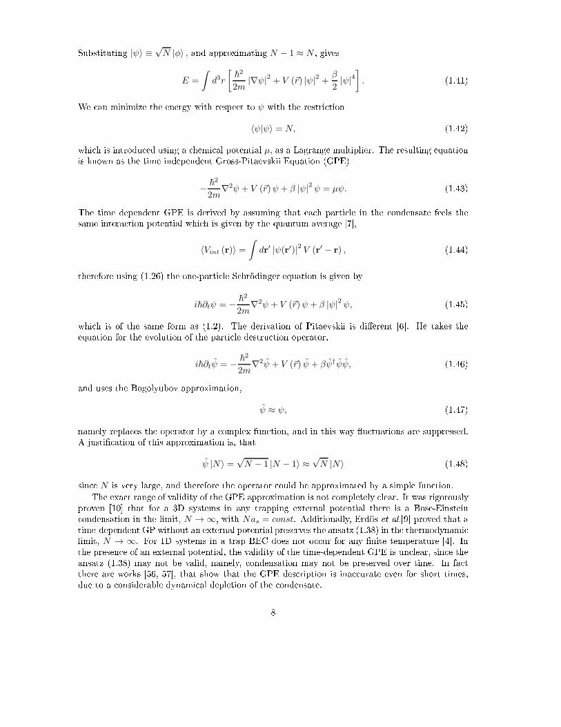
Substituting |ψ〉 ≡√N |φ〉 , and approximating N − 1 ≈ N , gives

E =

ˆ

d3r

[~2

2m|∇ψ|2 + V (~r) |ψ|2 + β

2|ψ|4

]

. (1.41)We can minimize the energy with respect to ψ with the restriction〈ψ|ψ〉 = N, (1.42)which is introduced using a chemical potential µ, as a Lagrange multiplier. The resulting equationis known as the time independent Gross-Pitaevskii Equation (GPE)

− ~2

2m∇2ψ + V (~r)ψ + β |ψ|2 ψ = µψ. (1.43)The time dependent GPE is derived by assuming that each particle in the condensate feels thesame interaction potential which is given by the quantum average [7],

〈Vint (r)〉 =ˆ

dr′ |ψ(r′)|2 V (r′ − r) , (1.44)therefore using (1.26) the one-particle Schrödinger equation is given byi~∂tψ = − ~

2

2m∇2ψ + V (~r)ψ + β |ψ|2 ψ, (1.45)which is of the same form as (1.2). The derivation of Pitaevskii is di�erent [6]. He takes theequation for the evolution of the particle destruction operator,

i~∂tψ = − ~2

2m∇2ψ + V (~r) ψ + βψ†ψψ, (1.46)and uses the Bogolyubov approximation,ψ ≈ ψ, (1.47)namely replaces the operator by a complex function, and in this way �uctuations are suppressed.A justi�cation of this approximation is, that

ψ |N〉 =√N − 1 |N − 1〉 ≈

√N |N〉 (1.48)since N is very large, and therefore the operator could be approximated by a simple function.The exact range of validity of the GPE approximation is not completely clear. It was rigorouslyproven [10] that for a 3D systems in any trapping external potential there is a Bose-Einsteincondensation in the limit, N → ∞, with Nas = const. Additionally, Erdös et al.[9] proved that atime-dependent GP without an external potential preserves the ansatz (1.38) in the thermodynamiclimit, N → ∞. For 1D systems in a trap BEC does not occur for any �nite temperature [4]. Inthe presence of an external potential, the validity of the time-dependent GPE is unclear, since theansatz (1.38) may not be valid, namely, condensation may not be preserved over time. In factthere are works [56, 57], that show that the GPE description is inaccurate even for short times,due to a considerable dynamical depletion of the condensate.8

1.2.3 Nonlinear classical problemsEquations similar to (1.1) are found also in classical mechanics. For example, a vibrating stringcould be approximated as a chain of nonlinear oscillators. This is the celebrated Fermi-Pasta-Ulam(FPU) problem [58]. The equation of motion of one oscillator in the chain is given by,mxn = k [(xn+1 − xn)− (xn − xn−1)] + α

[

(xn+1 − xn)2 − (xn − xn−1)

2] (1.49)which is known as the α-model, or

mxn = k [(xn+1 − xn)− (xn − xn−1)] + β[

(xn+1 − xn)3 − (xn − xn−1)

3] (1.50)which is known as the β-model. The eigenmodes and eigenvalues of the linear part for Direchletboundary condition and N oscillators are given by,

Ql (n) =

√

2

Nsin

πl

Nn (1.51)with frequencies

ωl = 2ω0 sinπl

2N, (1.52)where ω0 =

√

k/m and l = 1, 2, . . .N . Expanding xn using the eigenmodes of the linear problem,xn (t) =

N∑

l=1

cl (t)Ql (n) (1.53)and using the orthogonality of the modes, givescn = −ω2

ncn + α∑

m1m2

V m1m2n cm1cm2 (1.54)for the α-model and,

cn = −ω2ncn + β

∑

m1m2

V m1m2m3n cm1cm2cm3 (1.55)for the β-model, where V m1m2

n and V m1m2m3n are some complex expressions involving overlap sumsof three and four eigenmodes correspondingly. Those equations could be brought to a similar formas (1.1) written in linear problem eigenmodes (see Appendix C).1.2.4 Properties and conservation lawsThe NLSE (1.2) with V (x) = 0 is completely integrable and has an in�nite number of degrees offreedom and an in�nite number of constants of motion [59]. For V (x) 6= 0 only the norm,

N =

ˆ

|ψ|2 dx, (1.56)and the energy,E =

ˆ

J |∇ψ|2 + V (x) |ψ|2 + β

2|ψ|4 dx (1.57)9

are generally conserved. The mean momentumP = iJ

ˆ

dx (ψ∂xψ∗ − ψ∗∂xψ) (1.58)is not conserved, nevertheless the center of mass

X =1

N

ˆ

x |ψ|2 dx (1.59)obeys the classical equation of motionNdX

dt= P. (1.60)A relation for the variance of the wavefunction could be derived, known as the "Variance identity"or "The Virial relation". First using (1.46) and integration by parts, assuming ψ and its derivativesvanish at ±∞ we derive

∂2

∂t2⟨x2⟩= 2Ji

ˆ

[(ψtψ∗ − ψ∗

tψ) + 2x · (ψt∂xψ∗ − ψ∗

t ∂xψ)] dx, (1.61)where 〈.〉 is the quantum expectation. Using (1.46) combined and integrating by parts again one�nds,∂2

∂t2⟨x2⟩= 2J

[

4E −ˆ [

4V (x) |ψ|2 + 2 |ψ|2 x∂xV (x) + β |ψ|4]

dx

]

. (1.62)where E is given by (1.57). This expression is found to be very useful for proving �nite-time collapseof the wavefunction in dimensions higher than one [1]. Equivalent relations could be derived forthe discrete version of the NLSE.The conservation of the energy and the norm could be also used to derive a self-trappingproperty of the discrete version of the NLSE for a large nonlinearity [39]. Due to the variationalprinciple,〈ψ|H0 |ψ〉 ≥ E0, (1.63)where H0 is the linear part of (1.1) and E0 is its ground state energy. The nonlinear part isbounded from above,

∑

x

|ψ (x, t)|4 ≤ supx

(

|ψ (x, t)|2)∑

x

|ψ (x, t)|2 dx = N supx

(

|ψ (x, t)|2)

. (1.64)Therefore for a negative nonlinearity parameter, β = − |β|, the discrete version of the energy(1.57), is bounded from bellow,E ≥ E0 −

|β|2N sup

x

(

|ψ (x, t)|2)

. (1.65)This inequality is true for all times since the energy is conserved. If one assumes that ψ spreadsto zero, than the nonlinear term drops for in�nite times, E (t→ ∞) ≥ E0, but for a given initialdata, ψ (x, 0), one can always �nd su�ciently large |β|, such that,E (t = 0) = 〈ψ (x, 0)|H0 |ψ (x, 0)〉 − |β|

2

∑

x

|ψ (x, 0)|4 dx < E0, (1.66)which due to the conservation of the energy yields the contradictionE (t = 0) < E (t→ ∞) .10

This argument could be repeated also for positive nonlinearity, replacing the ground state energyof H0 by the ground state energy of −H0. It means that for any initial conditions there is asu�ciently large nonlinearity that prevents the wavepacket to spread to zero. Note, that thisargument cannot be applied to H0 with unbounded spectrum, and in particular to the continuousversion of the NLSE.1.3 Disorder and NonlinearityThe interplay between disorder and nonlinearity is intriguing, since disorder by itself yields lo-calization, while nonlinearity facilitates running solitons. Therefore it is of interest to study theinterplay between these two phenomena. Since Anderson localization is often studied theoreticallyon a lattice, while nonlinear phenomena are usually studied using continuous equations there aretwo ways of combining them:Continuum iψ = −Jψxx + V (x)ψ + β |ψ|2 ψ (1.67)Lattice iψ = −J (ψ (x+ 1) + ψ (x− 1)) + εxψ + β |ψ|2 ψwhere V (x) is a random function, εx is a random variable and J is a hopping constant. The discreteversion of the equation could be seen as a discretization of the continuous equation, neverthelesseven without the random potential these equations have di�erent features. While NLSE admitssoliton solutions and is completely integrable, discrete NLSE is not integrable, and does not haveexact soliton solutions [60].Contrary to the linear problem stationary or periodic solutions of nonlinear equations does notindicate quasi-periodic dynamics of a general initial data due to the absence of the superpositionprinciple. Therefore works that �nd periodic solutions to the NLSE, such as [61, 62, 63, 64] doesnot prove dynamical localization for a general initial data.In the literature there are various analytical approaches for studying (1.67). One approach teststhe stability of solitons to local perturbations [65, 66]; a second approach analyzes transmissioncoe�cients of planar waves through nonlinear media [67, 68, 69, 70]. There are also some numericalinvestigations [40, 71]. Below we summarize the important results of some of the approaches.The stability of solitons is investigated using perturbation techniques applied on Inverse Scat-tering Transform (IST), which was introduced by Kruskal and coworkers in [72]. There is anexcellent review on these techniques by Kivshar and Malomed [73]. The most important result ofthose techniques is an expression for the re�ection coe�cient of "quasi-particles" (soliton, boundstates), calculated at in�nite time and in a Born approximation (fast soliton, [65] Eq. 6,7,9):R =

1

4η

ˆ ∞

0

nrad (−λ) dλ (1.68)nrad (−λ) = n

(1)rad (λ)ˆ ∞

−∞

dxdx′f (x) f (x′) exp [iβ (λ) (x− x′)]

n(1)rad (λ) = πβ2 (λ)

28ξ4sech2

[

π(λ2 − ξ2 + η2

)

4ηξ

]

β (λ) =(λ− ξ)

2+ η2

ξwhere f (x) is a function de�ning the impurity, nrad (−λ) is radiation spectral density and 2η,−4ξare respectively the amplitude and the velocity of the initial soliton. The amplitude of the soliton11

as a function of space and time is given byu (x, t) = 2iη

exp[−2iξx− 4i

(ξ2 − η2

)t]

cosh [2η (x+ 4ξt)]. (1.69)Analytic expressions for R could be obtained for a soliton scattered by a small number of impurities(represented by peaked functions) [65]. For a large number of impurities and for soliton width muchsmaller than the typical distance between adjacent impurities, the scattering of each impurity istaken as independent. As a result the reduction of soliton mass is exponential in the length ofimpurities segment. Kivshar also suggested, on the basis of numerical investigation, that there is acritical value for the nonlinearity, above which the mass of the soliton is practically constant [66].Another common approach is based on the time independent version of (1.67). Impurity lo-calized stationary modes were obtained and analyzed for linear stability [74]. Investigation ofstationary modes on a nonlinear lattice was also performed by Henning and Tsironis [70] and byEilbeck [75]. Doucot and Rammal developed an "Invariant imbedding approach to localization"[67, 68, 69]. In this approach a transmission of linear waves through nonlinear media was studied.Imbedding of the boundary conditions on the ends of the nonlinear segment into the stationaryNLSE yields �rst-order nonlinear PDE's for the re�ection coe�cient (R = R1 + iR2) (Eq. 5 in [67])

dw/dL = kR2w · ε [L,w (1 +R) (1 +R∗)] (1.70)dR1/dL = −2kR2 − kR2 (1 + R1) · ε [L,w (1 +R) (1 +R∗)]

dR2/dL = 2kR1 +k

2

[

(1 +R1)2 −R2

2

]

· ε [L,w (1 +R) (1 +R∗)]

ε(

x, |ψ|2)

=[

−V (x) + β |ψ|2]

/k2where k is the wave number, w is the output intensity, V (x) is the potential and L is the lengthof the nonlinear segment. Doucot and Rammal [67, 68] then average these equations with respectto di�erent realizations of the random potential V (x) for small disorder, and obtain expressionsfor the transmission amplitude. For the �xed output problem a power law dependence in L isobtained, while for a �xed input problem the transmission amplitude is exponentially decreasingwith L.Yet another approach to the NLSE with a random potential is used by Pikovsky and Shep-elyansky (P-S) [36] and Flach and coworkers [41, 42]. They expand the solution of (1.1),ψ (x, t) =

∑

m

cm (t)um (x) (1.71)where um (x) and Em are the corresponding eigenmodes and eigenvalues of the linear part. Insertingthis expansion into (1.1) produces an equation for the coe�cients,i∂tcn = Encn + β

∑

m1,m2,m3

V m1m2m3n c∗m1

cm2cm3 (1.72)whereV m1m2m3n =

∑

x

un (x) um1 (x)um2 (x) um3 (x) . (1.73)The key assumption of both P-S and Flach is that the RHS of (1.72) acts as an e�ective noise. P-Scalculate the activation rate of a mode outside of a spreading packet using a Fermi golden rule,Γ ∼ ρ

(

β∑

m1,m2,m3

Vm1m2m3n c∗m1

cm2cm3

)2

, (1.74)12

where ρ is the typical density of states (the applicability is questionable since the excitation is toanother discrete state and not to a continuum). Assuming that, |cm|2 ∼ 1∆n , where ∆n is thewidth of the packet they get,

Γ ∼ ρβ2 |cm|6 ∼ ρβ2∆n−3. (1.75)Therefore the change in the width of the packet is given by,d

dt

(∆n2

)= Γ ∼ ρβ2∆n−3 (1.76)with the following solution,

∆n2 ∼ t2/5. (1.77)Flach et al. using the same consideration as P-S approximate (1.72) as,i∂tcn ∼ βP |cm|3 f (t) ∼ βP∆n−3/2f (t) (1.78)where P is the number of terms of the sum in (1.72) which contribute and f (t) is a white noise.They numerically estimate P to be proportional to P ∼ β

∆n , which givesi∂tcn ∼ β2∆n−5/2f (t) . (1.79)Therefore,

⟨

|cn|2⟩

∼(

β2∆n−5/2)2ˆ t

0

⟨f (t′)

∗f (t′′)

⟩dt′dt′′ =

(

β2∆n−5/2)2

t, (1.80)where for the last equality we have used the assumption, ⟨f (t′)∗ f (t′′)⟩ = δ (t′ − t′′). The timewhich is needed to �ll a mode to a level of |cn (T )|2 ∼ 1∆n , gives a di�usion coe�cient, D ∼ 1/T =

(β∆n

)4. And therefore the width of the packet grows as,∆n2 ∼ Dt =

(β

∆n

)4

t, (1.81)or∆n2 ∼ Dt = β4/3t1/3. (1.82)The problem with the results of P-S and Flach is that they use a rather uncontrollable approxi-mations, without any clear small parameter. In our work we develop a more systematic approach.

13

Chapter 2Organization of the perturbationtheoryOur goal is to analyze the nonlinear Schrödinger equation (1.1)i∂tψ = H0ψ + β |ψ|2 ψ (2.1)where H0 is the Anderson Hamiltonian,

H0ψ (x) = −J [ψ (x+ 1) + ψ (x− 1)] + εxψ (x) . (2.2)We assume throughout the paper thatH0 satis�es the conditions for localization, namely, for almostall the realizations, ω, of the disordered potential, all the eigenstates of H0, um, are exponentiallylocalized and have an envelope of the form of|um (x)| ≤ Dω,εe

ε|xm|e−γ|x−xm|, (2.3)where ε > 0, xm is the localization center which will be de�ned at the next subsection, γ isthe inverse of the localization length, ξ = γ−1, and Dω,ε is a constant dependent on ε and therealization of the disordered potential [76, 77] (better estimates were proven recently in [78, 79]).It is of importance that Dω,ε does not depend on the energy of the state. In the present work onlyrealizations ω, where|Dω,ε| ≤ Dδ,ε <∞ (2.4)are considered. This is satis�ed for a set of a measure 1− δ , since (2.3) is false only for a measurezero of potentials.2.1 Assignment of eigenfunctions to sitesIt is tempting to assign eigenfunctions to sites by their maxima, namely, uEi

is the eigenfunctionwith energy Ei and a maximum at site i. This assignment is very unstable with respect to thechange of realizations. This is due to the fact that the point where the maximum is found, whichis sometimes called the localization center, may change as a result of a very small change in theon-site energies {εx}. To avoid this, the assignment is de�ned as the center of mass [80],xE =

∑

xx |uEi

(x)|2 (2.5)De�nition 1. The state uEiis assigned to site i if i = [xE ] . If several states are assigned to thesame site we order them by energy. 14

2.2 The perturbation expansionThe wavefunction can be expandedψ (x, t) =

∑

m

cm (t) e−iEmtum (x) , (2.6)where um (x), and Em are the corresponding eigenstates and eigenvalues of H0. For the nonlinearequation the dependence of the expansion coe�cients, cm (t) , is found by inserting this expansioninto (2.1), resulting ini∂t∑

m

cme−iEmtum (x) = H0

∑

m

cme−iEmtum (x) (2.7)

+ β

∣∣∣∣∣

∑

m

cme−iEmtum (x)

∣∣∣∣∣

2∑

m3

cm3e−iEm3 tum3 (x) .Multiplying by un (x) and integrating gives

i∂tcn = β∑

m1,m2,m3

V m1m2m3n c∗m1

cm2cm3ei(Em1+En−Em2−Em3)t (2.8)where V m1m2m3

n is an overlap sumV m1m2m3n =

∑

x

un (x) um1 (x)um2 (x) um3 (x) . (2.9)By de�nition V m1m2m3n is symmetric with respect to an interchange of any two indices. Addition-ally, since the un (x) are exponentially localized around xn, V m1m2m3

n is not negligible only whenthe interval,δm ≡ max [xn, xmi

]−min [xn, xmi] , (2.10)is of the order of the localization length, around xn,

|V m1m2m3n | ≤ D4

δ,εeε(|xn|+|xm1 |+|xm2 |+|xm3 |)

∑

x

·e−γ(|x−xn|+|x−xm1 |+|x−xm2|+|x−xm3|) (2.11)≤ D4

δ,εeε(|xn|+|xm1 |+|xm2 |+|xm3 |)e−

(γ−ε′)3 (|xn−xm1 |+|xn−xm2 |+|xn−xm3 |)×

×∑

x

·e−ε′(|x−xn|+|x−xm1 |+|x−xm2 |+|x−xm3 |)

≤ V ε,ε′

δ eε(|xn|+|xm1 |+|xm2 |+|xm3 |)e− 13 (γ−ε′)(|xn−xm1 |+|xn−xm2 |+|xn−xm3 |).Here we have used the triangle inequality

(|x− xn|+ |x− xm1 |)+ (|x− xn|+ |x− xm2 |)+ (2.12)+(|x− xn|+ |x− xm3 |) ≥ |xn − xm1 |+ |xn − xm2 |+ |xn − xm3 |to obtain the second line. Our objective is to develop a perturbation expansion of the cm (t) inpowers of β and to calculate them order by order in β. The required expansion is

cn (t) = c(0)n + βc(1)n + β2c(2)n + · · ·+ βNc(N)n +Qn, (2.13)15

where the expansion is till order N and Qn is the remainder term. We will assume the initialconditioncn (t = 0) = δn0. (2.14)The equations for the two leading orders are presented in what follows. The leading order isc(0)n = δn0. (2.15)The equation for the �rst order is

i∂tc(1)n =

∑

m1,m2,m3

V m1m2m3n c∗(0)m1

c(0)m2c(0)m3

ei(En+Em1−Em2−Em3)t = V 000n ei(En−E0)t (2.16)and its solution is

c(1)n = V 000n

(1− ei(En−E0)t

En − E0

)

. (2.17)The resulting equation for the second order isi∂tc

(2)n =

∑

m1,m2,m3

V m1m2m3n c∗(1)m1

c(0)m2c(0)m3

ei(En+Em1−Em2−Em3)t+ (2.18)+ 2

∑

m1,m2,m3

V m1m2m3n c∗(0)m1

c(1)m2c(0)m3

ei(En+Em1−Em2−Em3)t.Substitution of the lower orders yieldsi∂tc

(2)n =

∑

m

V m00n V 000

m

[(1− e−i(Em−E0)t

Em − E0

)

ei(En+Em−2E0)t+ (2.19)+2

(1− ei(Em−E0)t

Em − E0

)

ei(En−Em)t

]

=∑

m

V m00n V 000

m

Em − E0

[(

ei(En+Em−2E0)t − ei(En−E0)t)

+

+2(

ei(En−Em)t − ei(En−E0)t)]

=∑

m

V m00n V 000

m

Em − E0

[

ei(En+Em−2E0)t − 3ei(En−E0)t + 2ei(En−Em)t]

.Computing the higher order terms can be done in a similar way. We notice that divergence of thisexpansion for any value of β may result from three major problems: the secular terms problem,the entropy problem (i.e., factorial proliferation of terms), and the small denominators problem.We address these problems in what follows.2.3 Elimination of secular termsThe ansatz (2.6) produces terms in the perturbation expansion which grow with time. Those termsare called secular terms. For example, the solution (2.17), in the �rst order in β, for n = 0 growslinearly with t. This term and similar terms in higher orders of expansion restrict the validity ofthe expansion up to short times and therefore we would like to systematically remove them. Todo this we introduce a new ansatz, which is given below.16

Proposition 1. To each order in β, ψ (x, t) can be expanded asψ (x, t) =

∑

n

cn (t) e−iE′

ntun (x) (2.20)withE′

n ≡ E(0)n + βE(1)

n + β2E(2)n + · · · (2.21)and E(0)

n are the eigenvalues of H0, in such a way that there are no secular terms to any givenorder. The E′n are called the renormalized energies.Here we �rst develop the general scheme for the elimination of the secular terms and thendemonstrate the construction of E′

n when the cn (t) are calculated to the second order in β(see (2.38),(2.37)). Inserting the expansion into (2.1) yieldsi∑

m

[∂tcm − iE′mcm] e−iE′

mtum (x) =∑

m

E(0)m cme

−iE′

mtum (x) + (2.22)+β

∑

m1m2m3

c∗m1cm2cm3e

i(E′

m1−E′

m2−E′

m3)tum1 (x) um2 (x)um3 (x) .Multiplication by un (x) and integration gives

i∂tcn =(

E(0)n − E′

n

)

cn + β∑

m1m2m3

V m1m2m3n c∗m1

cm2cm3ei(E′

n+E′

m1−E′

m2−E′

m3)t, (2.23)where the V m1m2m3

n are given by (2.9). Following (2.13) we expand cn in orders of β, namely,cn = c(0)n + βc(1)n + β2c(2)n + · · · , . (2.24)Inserting expansions (2.13) and (2.21) into (2.23) and comparing the powers of β without expandingthe exponent in β, produces the following equation for the k − th order

i∂tc(k)n = −

k−1∑

s=0

E(k−s)n c(s)n + (2.25)

+∑

m1m2m3

V m1m2m3n

[k−1∑

r=0

k−1−r∑

s=0

k−1−r−s∑

l=0

c(r)∗m1c(s)m2

c(l)m3

]

ei(E′

n+E′

m1−E′

m2−E′

m3)t.Note that the exponent is of order O (1) in β, and therefore we may choose not to expand it inpowers of β. However, it results in an expansion where both E

(l)m and c

(k)n depend on β. Forthe expansion (2.13) to be valid, both E

(l)m and c

(k)n should be O (1) in β, this is satis�ed, sincethe RHS of (2.25) contains only c(r)n such that r < k. Namely, this equation gives each order interms of the lower ones, with the initial condition of c(0)n (t) = δn0 . Solution of k equations (2.25)gives the solution of the di�erential equation (2.23) to order k, while the higher order terms whichare obtained from this equation are meaningless (see Appendix B for the reasoning). Since, theexponent in (2.25) is of order O (1) in β we can select its argument to be of any order in β. However,for the removal of the secular terms, as will be explained bellow, it is instructive to set the order ofthe argument to be k− 1, as the higher orders were not calculated at this stage. Secular terms aregenerated when there are time independent terms in the RHS of the equation above. We eliminatethose terms by using the �rst two terms in the �rst summation on the RHS. We make use of the17

fact that c(0)n = δn0 and c(1)n can be easily determined (see (2.28),(2.27)), and used to calculate

E(k)n=0 and E(k−1)

n6=0 that eliminate the secular terms in the equation for c(k)n , that isE(k)

n c(0)n + E(k−1)n c(1)n = E(k)

n δn0 + E(k−1)n (1− δn0)

V 000n

E′n − E′

0

, (2.26)where only the time-independent part of c(1)n was used. In other words, we choose E(k)n and E(k−1)

n6=0so that the time-independent terms on the RHS of (2.25) are eliminated. E(k)0 will eliminate allsecular terms with n = 0, and E(k−1)

n will eliminate all secular terms with n 6= 0. In the following,we will demonstrate this procedure for the �rst two orders.In the �rst order of the expansion in β we obtaini∂tc

(1)n = −E(1)

n c(0)n +∑

m1m2m3

V m1m2m3n c∗(0)m1

c(0)m2c(0)m3

ei(E′

n+E′

m1−E′

m2−E′

m3)t (2.27)

= −E(1)n δn0 + V 000

n ei(E′

n−E′

0)t.For n = 0 the equation produces a secular termi∂tc

(1)0 = −E(1)

0 + V 0000 (2.28)

c(1)0 = it ·

(

E(1)0 − V 000

0

)

.SettingE

(1)0 = V 000

0 (2.29)eliminates this secular term and givesc(1)0 = 0. (2.30)For n 6= 0 there are no secular terms in this order, therefore �nally

c(1)n = (1− δn0) V000n

(

1− ei(E′

n−E′

0)t

E′n − E′

0

)

, (2.31)where to this order E′n = En and E′

0 = E0.In the second order of the expansion in β we havei∂tc

(2)n = −E(1)

n c(1)n − E(2)n c(0)n + (2.32)

+∑

m1m2m3

V m1m2m3n

(

c∗(1)m1c(0)m2

c(0)m3+ 2c∗(0)m1

c(1)m2c(0)m3

)

ei(E′

n+E′

m1−E′

m2−E′

m3)t

= −E(2)n δn0 − E(1)

n c(1)n +∑

m1

V m100n

(

c∗(1)m1ei(E

′

n+E′

m1−2E′

0)t + 2c(1)m1ei(E

′

n−E′

m1)t)

.For n = 0 it takes the formi∂tc

(2)0 = −E(2)

0 +∑

m

V m000

(

c∗(1)m ei(E′

m−E′

0)t + 2c(1)m ei(E′

0−E′

m)t)

.18

Substitution of (2.28) and (2.31) yieldsi∂tc

(2)0 = −E(2)

0 +∑

m 6=0

V m000 V 000

m

E′m − E′

0

[(

1− e−i(E′

m−E′

0)t)

ei(E′

m−E′

0)t+ (2.33)+2(

1− ei(E′

m−E′

0)t)

ei(E′

0−E′

m)t]

= −E(2)0 +

∑

m 6=0

V m000 V 000

m

E′m − E′

0

(

ei(E′

m−E′

0)t + 2ei(E′

0−E′

m)t − 3)

,and the secular term could be removed by settingE

(2)0 = −3

∑

m 6=0

V m000 V 000

m

E′m − E′

0

. (2.34)For n 6= 0 we havei∂tc

(2)n = −E(1)

n V 000n

(

1− ei(E′

n−E′

0)t

E′n − E′

0

)

+ (2.35)+∑

m

V m00n

(

c∗(1)m ei(E′

n+E′

m−2E′

0)t + 2c(1)m ei(E′

n−E′

m)t)

=− E(1)n V 000

n

(

1− ei(E′

n−E′

0)t

E′n − E′

0

)

+

+∑

m 6=0

V m00n V 000

m

E′m − E′

0

(

ei(E′

n+E′

m−2E′

0)t + 2ei(E′

n−E′

m)t − 3ei(E′

n−E′

0)t)

.We notice that the second term in the sum produces secular terms for m = n. Those terms couldbe removed by setting−E

(1)n V 000

n

E′n − E′

0

+2V n00

n V 000n

E′n − E′

0

= 0 n 6= 0 (2.36)E(1)

n = 2V n00n n 6= 0.To conclude, up to the second order in β , the perturbed energies, which are required to removethe secular terms, are given by

E′n = E(0)

n + βV n00n (2− δn0)− 3β2δn0

∑

m 6=0

(V 000m

)2

E′m − E′

0

, (2.37)and the corresponding correction to c(0)n isi∂tc

(2)n =

∑

m 6=0V m000 V 000

m

E′

m−E′

0

(

ei(E′

m−E′

0)t + 2ei(E′

0−E′

m)t)

n = 0

2V n00n V 000

n

E′

n−E′

0ei(E

′

n−E′

0)t +∑

m 6=0,n2V m00

n V 000m

E′

m−E′

0ei(E

′

n−E′

m)t+

+∑

m 6=0V m00n V 000

m

E′

m−E′

0

(

ei(E′

n+E′

m−2E′

0)t − 3ei(E′

n−E′

0)t) n 6= 0

. (2.38)Note that in the calculation of cn to higher orders in β, a secular term of the order β2 will begenerated for n 6= 0 . Secular terms with increasing complexity are generated in the cancellation ofhigher orders, however, as demonstrated by (2.26), secular terms are removed with the same c(0)nand c(1)n which are presented in (2.15) and (2.31). In the next section, the entropy problem will bestudied. It will be shown that the proliferation of terms in the expansion is at most exponential.19

2.4 The entropy problemSince the time dependence of all orders is bounded (excluding the secular terms), we can boundeach order of the expansion by∣∣∣c(0)n

∣∣∣ = δn0 (2.39)

∣∣∣c(1)n

∣∣∣ =

∣∣∣∣∣V 000n

(

1− ei(E′

n−E′

0)t

E′n − E′

0

)∣∣∣∣∣≤ 2

∣∣∣∣

V 000n

E′n − E′

0

∣∣∣∣

∣∣∣c(2)n

∣∣∣ =

∣∣∣∣∣

∑

m

ˆ t

0

dt′(Vm00n V 000

m

E′m − E′

0

)(

ei(E′

n+E′

m−2E′

0)t′ − 3ei(E

′

n−E′

0)t′

+ 2ei(E′

n−E′

m)t′

)∣∣∣∣∣

≤ 2 ·∑

m

∣∣Vm00

n

∣∣∣∣V 000

m

∣∣

|E′m − E′

0|

(1

|(E′n + E′

m − 2E′0)|

+3

|E′n − E′

0|+

2

|E′n − E′

m|

)et cetera. However, for convergence for a �nite but possibly small β, it is essential that the numberof terms on the RHS of (2.39) will not increase faster than exponentially in k, e.g. not as k!, wherek is the expansion order. Next we will show that the number of terms indeed increases at mostexponentially in k.We will designate the number of di�erent products of order k of V ′s by Rk (on top of it thereis still a number of non vanishing terms in the sums over m, that will be estimated in the nextsection). The recursive expression for the number of terms in each c(l)n could be extracted from(2.25) (the integration with respect to time multiples the number of terms by a factor of 2, cf.(2.39)),

Rk =

k−1∑

r=0

k−1−r∑

l=0

RrRlRk−1−r−l R1 = 1 R0 = 1. (2.40)In order to �nd an upper bound on Rk we examine the structure of the products of V ′s we noticethat each product could be uniquely labeled by a vector of zeros and m′is

V m100n V m2m30

m1· · ·V 0mk−10

mk−2V 000mk−1

→ {m1, 0, 0,m2,m3, 0, · · · , 0,mk−1, 0, 0, 0, 0} , (2.41)where the number of di�erent summation indices mi is (k − 1) and the length of the labeling vectoris 3k. Since in each vector the last three elements should always be zeros the number of di�erentcon�gurations of this product is the number of ways to distribute (k − 1) m′s in 3 (k − 1) cells(superscripts), namely, Rk <(3(k−1)k−1

). This is only an upper bound, since there may be someadditional constraints, for example, the �rst three elements in the vector should never be all zeros.Subtracting the cases when all three �rst elements are zero (3(k−2)

k−1

) we obtain the boundRk <

(3 (k − 1)

k − 1

)

−(3 (k − 2)

k − 1

)

. (2.42)This bound has the following asymptoticslimk→∞

1

kln

[(3k − 3

k − 1

)

−(3k − 6

k − 1

)]

= ln27

4, (2.43)namely,

Rk ≤ ek ln 274 ≤ e2k. (2.44)From Fig.2.1 we conclude that this bound is a tight bound of the exact solution of the recur-rence relation. This bound shows that the number of terms in the expansion increases at mostexponentially in k and therefore there is no entropy problem.20

0 50 100 150 200 250 3000

50

100

150

200

250

300

350

400

450

500

550

k

ln R

k

Figure 2.1: The solid line denotes the exact numerical solution of the recurrence relation for Rkand dashed line is the asymptotic upper bound on this solution (e2k) .2.5 Bounding the general termAs clear from (2.25) after the subtraction of all the secular terms in the preceding orders thedi�erential equation for the k-th order term isi∂tc

(k)n = −

k−1∑

s=0

E(k−s)n c(s)n + (2.45)

+∑

m1m2m3

V m1m2m3n

[k−1∑

r=0

k−1−r∑

s=0

k−1−r−s∑

l=0

c(r)∗m1c(s)m2

c(l)m3

]

ei(E′

n+E′

m1−E′

m2−E′

m3)t.with the initial condition of c(0)n = δn0 and the �rst term on the RHS is designed (see Section 2.3)to eliminate all the time-independent part of of RHS of (2.45). Following the construction of thelower order terms in the preceding section by a repeated application of (2.45) the structure of thegeneral term in the expression for a given order k can be obtained. Note that the structure E(l)

n issimilar to the structure of c(l)n . The main blocks of the structure take the formζm1m2m3n ≡ V m1m2m3

n

E′n − {E′}mi

(2.46)where {E′}midenotes a sum of eigenenergies (shifted so that the secular terms are removed, see(2.21)) that may depend on the summation indices mi. Then any term of order k is a product of21

k factors of the form (2.46) and k − 1 summations over the indices mi

k terms︷ ︸︸ ︷

ζm1m2m3n ζm4m5m6

m1· · · ζ000m5

ζ000m6(2.47)and following the last section there is an exponentially increasing (in k) number of such terms. Inorder to bound the general term of order k we will �rst bound one typical block, namely,

ζm1m2m3n ≡ V m1m2m3

n

E′n − {E′}mi

(2.48)where {E′}miis some sum of E′

j . To bound (2.48) we will bound separately the denominator andthe numerator. Using Cauchy-Schwarz inequality,〈|ζm1m2m3

n |s〉 ≤⟨

1∣∣E′

n − {E′}mi

∣∣2s

⟩1/2⟨

|V m1m2m3n |2s

⟩1/2

, (2.49)where 0 < s < 12 .Conjecture 1. For the Anderson model, which is given by the linear part of (1.1), the jointdistribution of R eigenenergies is bounded,

p (E1, E2, . . . , ER) ≤ DRwhere DR ∝ R! <∞.The conjecture is inspired by Theorem 3.1 of the recent paper by Aizenman and Warzel [15].If one assumes that with probability one the pro�les of the eigenfunctions, namely, the squares ofthe eigenfunctions, which correspond to the eigenenergies {Ei}Ri=1 are substantially di�erent suchthat α (as de�ned in Theorem 3.1 of [15]) is bounded away from zero, than taking the intervalsIj = dEj one �nds that the joint probability density can be bounded by DR ∝ R!

αR . It is not knownhow to prove that for the Anderson model the pro�les of the wave functions are distinct and howto quantify this. However, it is reasonable to assume distinctness since di�erent eigenfunctions arelocalized in di�erent regions and therefore are a�ected by di�erent potentials. There are doublehumped states (consisting of nearly symmetric and antisymmetric combinations of two humps),which have approximately the same squares, and therefore are natural candidates for states thatmay result in violation of the conjecture. Nevertheless, those states are very rare and the di�erencebetween their squares is exponential in the distance between the humps. For this it is crucial thatmany sites are involved (therefore the counter example (2.1) of [15] is not generic). If the energiesare assigned to speci�c locations then the factorial term could be dropped, namely, DR ∝ α−R.This is due to the fact that speci�c assignment of energies chooses one of the R! permutations,mentioned in [15].Corollary 1. Given 0 < s < 1, for f =R∑

k=1

ckEik , where ck are integers (and the assignment ofeigenfunctions to sites is given by De�nition 1) the following mean is bounded from above⟨

1

|f |s⟩

≤ DR <∞. (2.50)where DR ∝ DR. 22

Proof. By Conjecture 1,⟨

1

|f |s⟩

=

ˆ

p (E1, E2, . . . , ER) dE1dE2 · · · dER∣∣∣∣∣

R∑

k=1

ckEik

∣∣∣∣∣

s ≤ DR

ˆ

dE1dE2 · · · dER∣∣∣∣∣

R∑

k=1

ckEik

∣∣∣∣∣

s , (2.51)changing the variables to {f, E2, E3, . . . , ER} gives⟨

1

|f |s⟩

≤ DR

ˆ ∆

−∆

dE2 · · · dER

|c1|

ˆ

f(~E)df

1

|f |s , (2.52)where |c1| is the Jacobian and 2∆ is the support of the energies. Due to the fact that f (E1) islinear the multiplicity is one. Since the integrand is positive we can only increase the integral byincreasing the domain of integration of f . Designating by f∞ the maximal value of f ,⟨

1

|f |s⟩

≤ 2DR∆R−1 f

1−s∞

1− s≡ DR. (2.53)Conjecture 2. In the limit of R → ∞, for 0 < s < 1 and for f =

R∑

k=1

ckEik , where ck are integers(and the assignment of eigenfunctions to sites is given by De�nition 1)⟨

1

|f |s⟩

� 1

Rs/2(2.54)For large R the sum, f =

R∑

k=1

ckEik , can be e�ectively separated into groups of terms thatdepend on di�erent diagonal energies, εj . Therefore by the central limit theorem, f is e�ectivelya Gaussian variable with 〈f〉 = 0 and ⟨f2⟩= σ2R, where σ2 is some constant. Therefore,

⟨1

|f |s⟩

� 2√2πσ2R

ˆ ∞

0

df

f se−f2/(2σ2R) =

2√2π(√

σ2R)s

ˆ ∞

0

df

f se−f2/2 � R− s

2 . (2.55)Conjecture 1 and Corollary 1 were tested numerically for lattice size 128, s = 12 and the uniformdistribution

µ (ε (x)) =

{12∆ |ε (x)| ≤ ∆

0 |ε (x)| > ∆, (2.56)with ∆ = 1. The results are presented in Fig. 2.2 for R ≤ 10. For R ≤ 3 all the combinations ofthe energies were used and the result is an average over all the combinations. For R ≥ 4 only apartial set of combinations of cardinality 104, chosen at random was used. For large R the decay isas R−s/2 in agreement with Conjecture 2. The above calculation was repeated for the case wherethe Ei are replaced by the renormalized energies E′

i. The calculation can be performed only to theorder β2 with the help of (2.37). The results are also presented in Fig. 2.2 for β = 0.1 and β = 1.Conjecture 3. Corollary 1 and Conjecture 2 hold also if the Ei are replaced by the renormalizedenergies E′i. 23

0.8 1 1.2 1.4 1.6 1.8 2 2.2 2.4 2.6−0.3

−0.2

−0.1

0

0.1

0.2

0.3

0.4

0.5

0.6

ln(R)

ln(<

|f|−

s >)

J = 1J = 0.5J = 0.25data 4data 5data 6data 7data 8data 9

Figure 2.2: The logarithm of ⟨|f |−1/2⟩ as a function of the logarithm of R. The lines designatedenominators with β = 0, with the solid line (blue) is for J = 0.25 the dashed line (green) is for

J = 0.5 and the dot-dashed line (red) is for J = 1. The solid circles and the squares are data withβ = 1, and E′

n calculated up to the second order in β, such that di�erent colors represent di�erentJ , in the similar manner as for the lines. The solid squares are for parameters similar to the oneswith the solid circles, but with the restriction that at least one of the states that corresponds toE′

n which is localized near the origin.The reason is that the various renormalized energies are dominated by di�erent independentrandom variables εi. The numerical calculations support this point of view. In what followsCorollary 1 and Conjecture 3 (and not Conjecture 1) are used, and these were tested numerically(Fig. 2.2).Using the bound on the overlap sum (2.11) and Corollary 1,〈|ζm1m2m3

n |s〉δ ≤ Dδ

∣∣∣V

ε,ε′

δ

∣∣∣

s

eεs(|xn|+|xm1 |+|xm2 |+|xm3 |)e− 13 (γ−ε′)s(|xn−xm1 |+|xn−xm2 |+|xn−xm3 |).(2.57)this proves the proposition:Proposition 2. For some δ, ε, ε′ > 0 and 0 < s < 1

2 ,〈|ζm1m2m3

n |s〉δ ≤ F ′eεs(|xn|+∑

i|xmi |)e− 13 (γ−ε′)s

∑i|xn−xmi | (2.58)where F ′ = Dδ

∣∣∣V

ε,ε′

δ

∣∣∣

s.Using the Chebyshev inequality,Pr (|x| ≥ a) ≤ 〈|x|〉 /a, (2.59)where x is a random variable and a is a constant, one �nds24

Corollary 2.Pr(

|ζm1m2m3n | ≥ F ′1/seε(|xn|+

∑i|xmi |)e− 1

3 (γ−ε′−η)∑

i|xn−xmi |)

≤ e−ηs3

∑i|xn−xmi | (2.60)where F ′ = Dδ

∣∣∣V

ε,ε′

δ

∣∣∣

s.A general term in the expression for di�erent orders of c(k)n is given by the form of |ζm1m2m3n |

∣∣ζm4m5m6

m1

∣∣ · · ·

∣∣∣ζ000mk−1

∣∣∣ ,i.e., it contains (k − 1) summations over indices which run over all the lattice. First we constructa general procedure to bound a product of k, ζ 's. A product of two ζ 's is bounded by

⟨∣∣∣∣∣

∑

m1

ζm1m2m3n ζm4m5m6

m1

∣∣∣∣∣

s⟩

δ

≤⟨∑

m1

|ζm1m2m3n |s

∣∣ζm4m5m6

m1

∣∣s

⟩

δ

,where 〈·〉δ denotes an average over realizations where (2.4) is satis�ed.Using the Cauchy-Shwarz inequality∑

m1

⟨|ζm1m2m3

n |s∣∣ζm4m5m6

m1

∣∣s⟩

δ≤∑

m1

⟨

|ζm1m2m3n |2s

⟩1/2

δ

⟨∣∣ζm4m5m6

m1

∣∣2s⟩1/2

δsetting 0 < s < 14 (notice, that s < 1

4 and not s < 12 , due to (2.49)) and inserting the bound onthe average ⟨|ζm1m2m3

n |2s⟩

δfrom Proposition 2 gives

⟨∣∣∣∣∣

∑

m1

ζm1m2m3n ζm4m5m6

m1

∣∣∣∣∣

s⟩

δ

(2.61)≤ F ′ exp

[

εs

(

|xn|+6∑

i=2

|xmi|)]

e−s γ−ε′

3 (|xn−xm2 |+|xn−xm3 |)×

×∑

m1

e2εs|xm1 | exp−sγ − ε′

3

(

|xn − xm1 |+6∑

i=4

|xm1 − xmi|)

,where we have used the inequality(∑

i

|xi|)s

≤∑

i

|xi|s 0 < s < 1.Using the triangle inequality in the same manner as in (2.12)|xn − xm1 |+

6∑

i=4

|xm1 − xmi| ≥ 1

3

6∑

i=4

|xn − xmi|+ 2

3

6∑

i=4

|xm1 − xmi| (2.62)25

we get⟨∣∣∣∣∣

∑

m1

ζm1m2m3n ζm4m5m6

m1

∣∣∣∣∣

s⟩

δ

(2.63)≤ F ′ exp εs

(

|xn|+6∑

i=2

|xmi|)

e−γ−ε′

3 s(|xn−xm2 |+|xn−xm3 |)×

× exp

[

−γ − ε′

9s

6∑

i=4

|xn − xmi|]∑

m1

e2εs|xm1 |e−2 γ−ε′

3 s6∑

i=4|xm1−xmi |

= F ′′ exp

[

sε

(

|xn|+6∑

i=2

|xmi|)

− γ − ε′

9s

6∑

i=4

|xn − xmi|]

e−γ−ε′

3 s(|xn−xm2 |+|xn−xm3 |),where F ′′ (γ, ε′, s, ε) = F ′∑

m1

e2εs|xm1 |e−2 γ−ε′

3 s6∑

i=4|xm1−xmi |

< ∞, in the following also other con-vergent sums of this type will be denoted by F ′′.If the term we consider is a term in the perturbation expansion it should include some factorsζm1m2m3m with some mi = 0. A simple example is where xm1 = xm2 = xm3 = 0

⟨∣∣ζ000m

∣∣s⟩

δ≤ F ′e−s(γ−ε′−ε)|xn|, (2.64)where the bound was calculated using Proposition 2. The product should terminate with a termof the form ζ000m therefore a term like (2.61) is a part of a product of the form,

∑

{mi}

|ζm1m2m3n |

∣∣ζm4m5m6

m1

∣∣∣∣ζ000m2

∣∣∣∣ζ000m3

∣∣∣∣ζ000m4

∣∣∣∣ζ000m5

∣∣∣∣ζ000m6

∣∣ . (2.65)To bound it we use the generalized Hölder inequality,

⟨k∏

i=1

|xi|⟩

≤k∏

i=1

⟨

|xi|k⟩1/k

.Applying it yields,∑

{mi}

⟨

|ζm1m2m3n |s

∣∣ζm4m5m6

m1

∣∣s ∣∣ζ000m2

∣∣s ∣∣ζ000m3

∣∣s ∣∣ζ000m4

∣∣s ∣∣ζ000m5

∣∣s ∣∣ζ000m6

∣∣s⟩

δ(2.66)

≤∑

{mi}

(⟨

|ζm1m2m3n |7s

⟩

δ

⟨∣∣ζm4m5m6

m1

∣∣7s⟩

δ

6∏

i=2

⟨∣∣ζ000mi

∣∣7s⟩

δ

)1/7

26

setting 0 < s < 114 and inserting the bounds on the averages (2.61) and (2.64) gives⟨

∑

{mi}

ζm1m2m3n ζm4m5m6

m1ζ000m2

ζ000m3ζ000m4

ζ000m5ζ000m6

s⟩

δ

(2.67)≤ F ′

∑

{mi}

exp εs

(

|xn|+6∑

i=2

|xmi|)

e−γ−ε′

3 s(|xn−xm2 |+|xn−xm3 |)×

× exp

[

−γ − ε′

9s

6∑

i=4

|xn − xmi| − (γ − ε′ − ε) s

6∑

i=2

|xmi|]

= F ′eεs|xn|∑

{mi}

e−γ−ε′

3 s(|xn−xm2 |+|xn−xm3 |)×

× exp

[

−γ − ε′

9s

6∑

i=4

|xn − xmi| − (γ − ε′ − 2ε) s

6∑

i=2

|xmi|]

,where {mi} stands for a sum over all the mi. Using the inequality,6∑

i=4

(|xn − xmi|+ |xmi

|) ≥ 3 |xn| , (2.68)we get⟨

∑

{mi}

ζm1m2m3n ζm4m5m6

m1ζ000m2

ζ000m3ζ000m4

ζ000m5ζ000m6

s⟩

δ

(2.69)≤ F ′e−(γ−ε′−ε)s|xn|

∑

{mi}

exp−2s

(γ − ε′

3− ε

) 6∑

i=2

|xmi|

= F ′e−(γ−ε′−ε)s|xn|.Let us study the form of a general graph (c.f. Fig. 2.3).It can be described as a tree starting from n, the "root" and four types of branching points,where q (0 ≤ q ≤ 3) branches continue while 3− q branches terminate. A branch which continuesis associated with a value mi 6= 0, while a branch terminates with mi = 0. In the above, boundson branches with q = 0 and 3 are calculated, and are given by (2.58) and (2.64), respectively. Thebounds for q = 1, 2 follow similarly from Proposition 2. Along each �bond� from the "root" to the�leaves� a term ζm1m2m3n is multiplied. At a point from where q branches continue the exponent isreduced by a factor of q. In other words, with xn and xm are connected by a path that is crossing

l branching points with ratios q1, . . . , ql the bound on the product of the zetas contains a factorexp− γ

q |xn − xm| where q = l∏

i=1

qi. The total number of branch ends is also q. To terminate all thebranches q factors of the form ζ000mi(bounded by (2.64)) should be multiplied resulting in the a27

Figure 2.3: An example of a graph that is used to construct the general term. The graph describesan 8-th order term, ζm1m2m3n ζ000m1

ζ000m3ζm4m50m2

ζm600m4

ζm700m5

ζ000m6ζ000m7

.term that multiplies the bound on a sum of the form∑

{mi}

exp

[

− (γ − ε′)

qs∑

i

|xn − xmi| − (γ − ε′) s

∑

i

|xmi|] (2.70)

≤ exp− (γ − ε′)

qs∑

i

|xn|∑

{mi}

exp−(

1− 1

q

)

(γ − ε′) s∑

i

|xmi|

= e−γ−ε′

qsq|xn|

∑

{mi}

exp−(

1− 1

q

)

(γ − ε′) s∑

i

|xmi| ≡ Sεe

−(γ−ε′)s|xn|restoring the original convergence rate. As the product consists of k terms the evaluation of|ζm1m2m3

n |sk is required for the use of the Hölder inequality. Therefore it is required that 0 < s <1/2k.Lemma 1. For a given k (the number of ζ's), δ, ε, ε′, η′ > 0 and 0 < s < 1

2k

⟨∣∣∣∣∣∣

∑

{mi}

ζm1m2m3n ζm4m5m6

m1· · · ζ000mN−1

∣∣∣∣∣∣

s⟩

δ

≤ F(k)δ e−(γ−ε−ε′)s|xn| (2.71)or using the Chebyshev inequality (2.59)

Pr

∣∣∣∣∣∣

∑

{mi}

ζm1m2m3n ζm4m5m6

m1· · · ζ000mN−1

∣∣∣∣∣∣

≥(

F(k)δ

)1/s

e−(γ−ε−ε′−η′)|xn|

≤ e−η′s|xn|, (2.72)where F (k)δ is a constant which is built iteratively by the construction demonstrated in (2.67) and(2.69) and is proportional to Dδ.It is of importance, that any product with the same number of zetas has the same boundwith the same probability. This allows us to bound c

(k)n by counting the number of di�erentcon�gurations, Rk, of the product for a given k and then multiplying it by the bound of eachproduct. This proves the theorem: 28

Theorem 1. For a given k and δ, ε, ε′, η′ > 0

Pr

(∣∣∣c(k)n

∣∣∣ ≥

(

F(k)δ

)k

eck2+c′ke−(γ−ε−ε′−η′)|xn|

)

≤ e−c′e−η′|xn|/k. (2.73)where F (k)δ which is proportional to Dδ and c and c′ are constants.Proof. Using Lemma 1 and summing over con�gurations denoted by ic one obtains the bound⟨∣∣∣c(k)n

∣∣∣

s⟩

δ=

⟨∣∣∣∣∣∣

Rk∑

ic=1

∑

{mi}

ζm1m2m3n ζm4m5m6

m1· · · ζ000mk−1

∣∣∣∣∣∣

s⟩

δ

(2.74)≤

Rk∑

ic=1

⟨∣∣∣∣∣∣

∑

{mi}

ζm1m2m3n ζm4m5m6

m1· · · ζ000mk−1

∣∣∣∣∣∣

s⟩

δ

≤ RkF(k)δ e−(γ−ε−ε′)s|xn|.Using (2.44)

⟨∣∣∣c(k)n

∣∣∣

s⟩

δ≤ e2kF

(k)δ e−(γ−ε−ε′)s|xn| (2.75)or

Pr

(∣∣∣c(k)n

∣∣∣ ≥ ec

′/s(

F(k)δ

)1/s

e−(γ−ε−ε′−η′)|xn|e2k/s)

≤ e−c′e−η′s|xn| (2.76)Choosing the largest s produces a bound where c, c′ are constants and F(k)δ is a constant whichis built iteratively by the construction demonstrated in (2.67) and (2.69) and is proportional to

Dδ.Remark 1. From (2.44) one sees that c w 2 and later we set c′ = cN .2.6 The remainder of the expansionIn order to control the solution we have to control, Qn, the remainder of the expansion (2.13) thatcan be written in the formcn (t) = cn +Qn, (2.77)withcn =

N∑

l=0

βlc(l)n . (2.78)It is useful to de�neψ (x, t) =

∑

m

cmum (x) e−iE′

mt (2.79)andQn = Qne

−iE′

nt. (2.80)Substituting (2.77) in (2.23) leads to the following equation for the remainder which is expressedin terms of (2.78), (2.79) and (2.80),i∂tQn =Wn (t) +

∑

m

Mnm (t) Qm +∑

m

Mnm (t) Q∗m + F

(

Q) (2.81)29

whereWn (t) =

(

E(0)n − E

′

n

)

cne−iE

′

nt − i (∂tcn) e−iE

′

nt (2.82)+ β

∑

x

un (x)∣∣∣ψ (x)

∣∣∣

2

ψ (x)is the inhomogeneous term,Mnm (t) = E(0)

n δnm + 2β∑

x

un (x)∣∣∣ψ (x)

∣∣∣

2

um (x) (2.83)andMnm (t) = β

∑

x

un (x)(

ψ (x))2

um (x) . (2.84)determine the linear terms, while the nonlinear term is,F(Q)

= β∑

x

un (x) ψ∗ (x)

(∑

m

Qmum (x)

)2 (2.85)+ 2β

∑

x

un (x) ψ (x)

∣∣∣∣∣

∑

m

Qmum (x)

∣∣∣∣∣

2

+ β∑

x

un (x)

∣∣∣∣∣

∑

m

Qmum (x)

∣∣∣∣∣

2(∑

m

Qmum (x)

)

.The linear part of (2.81) is given byi∂tQ

linn =Wn (t) +

∑

m

Mnm (t) Qlinm +

∑

m

Mnm (t)(

Qlinm

)∗

. (2.86)Using a bootstrap argument, which utilizes the continuity of (2.81) and smallness of the linearpart of (2.86) one can show (see Appendix A, (A.30)) that until some time t∗ = O(β−1

) , thedynamics of (2.81) is governed by the linear part and the remainder is bounded by,|Qn (t)| ≤ AβN+1t · e−γ|xn|, (2.87)where γ is the inverse localization length, and A ∼ eN

2

e−γ . Therefore to estimate the remainderwe can integrate (2.86) instead of (2.81) at least up to t∗. It is useful to integrate up to some largetime, t� t∗, and then to extrapolate using the linear bound (A.8) up to t∗. In the next section itwill be proposed how to determine t∗ in practice (with some assumptions).30

Chapter 3Numerical resultsIn order to compute the various orders in the perturbation theory we use equation (2.25), whichis a recursive equation of the orders. To compute order k we have to compute all c(l)n and E(l)n for

l ≤ k− 1. The numerical calculation is done in two stages: at the �rst stage a symbolic calculationof the expressions of all the c(l)n and E(l)n is performed, this has a complexity of O (e2k), which isdue to the increasing number of terms in each expression for c(l)n (see (2.44)). This stage does notdepend neither on the realization nor the nonlinearity strength, β. In the second stage realizationsand β are chosen and c

(l)n and E

(l)n are calculated. This stage has a complexity of O (e2k · Lk

),where L is the dimension of the lattice. The computation of this stage could be fully parallelized.When calculating E(l)n we encounter self-consistent equations of the type

E′

n = fn

({

E′

m

})

, (3.1)where f is some function, for example for the second order (2.37). Higher order equations arerequired in general. We solve those equations numerically by reinserting the LHS into the RHS,until a desired convergence is achieved. The �rst iteration is done by setting β = 0 at the RHS.Basically, at each iteration an order of β is gained in the accuracy of the solution and since we needto know E′

n only to a desired orderN (see Appendix B), only a small number of iterations is needed.The c(l)n are represented as vectors with elements (c(l)n,ω1 , c(l)n,ω2 , . . .

) identi�ed by frequencies suchthat terms with same frequencies are grouped together (by summing their amplitudes), namely,c(l)n,ωk

=∑

j c(l)n,ωk,j

e−iωkt, where ωk is a shared frequency. Due to the fact that most of theamplitudes are negligible, after grouping a thresholding step is performed where terms which aresmaller than 10−6 are eliminated. The error introduced by the tresholding can be easily controlled,since we know how many frequencies were left out. By having the vector of frequencies and theircorresponding amplitudes we can calculate the perturbative solution at any time. Even aftergrouping and thresholding the number of frequencies is growing rapidly with the order of theexpansion.We have calculated numerically all the c(l)n and E′

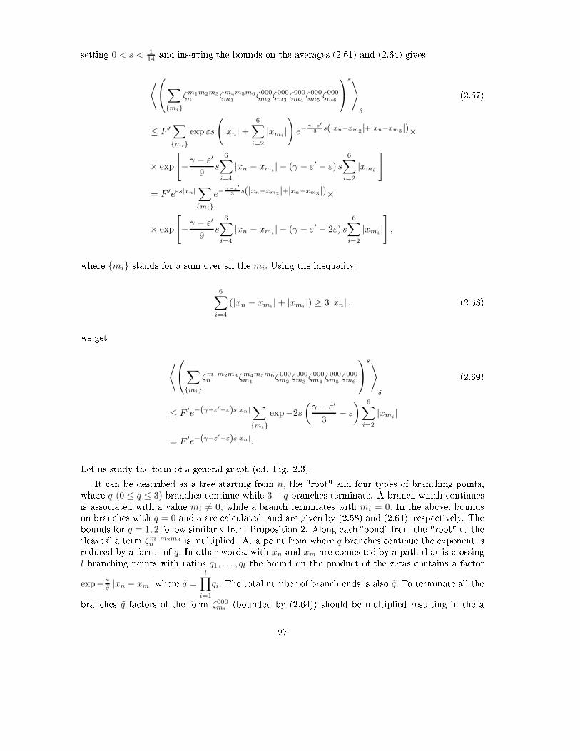
n for l ≤ 4 for a certain realization of therandom potential. To compare perturbation theory results to the exact results, we compute theirFourier transform for di�erent orders of expansion. On Fig. 3.1 we see the Fourier transform ofc0, c1 and c9 (see (2.78)) compared to the Fourier transform of an exact (numerical) solution, cn,calculated using a split-step method. We notice a reasonable agreement of the perturbation theorywith an exact solution for c0, c1 and a disagreement for c9 .31

−4 −3 −2 −1 0 1 2 3 4−3.5

−3

−2.5

−2

−1.5

−1

−0.5

0

ω

Log

pow

er

cex

0

c(2)0

c(3)0

c(4)0

−4 −3 −2 −1 0 1 2 3 4−7.5

−7

−6.5

−6

−5.5

−5

−4.5

−4

−3.5

−3

−2.5

ω

Log

pow

er

cex

1

c(2)1

c(3)1

c(4)1

−3 −2 −1 0 1 2 3

−4

−3.5

−3

−2.5

−2

−1.5

−1

ω

Log

pow

er

cex

9

c(2)9

c(3)9

c(4)9

Figure 3.1: Fourier transform of c0, c1 and c9 for di�erent orders of the perturbation theorycompared to the Fourier transform of an exact solution, cn, (solid line). Second order is given bygreen crosses, third order by red triangles and fourth order by blue squares. The parameters are:β = 0.0774, t = 1000, W = 4, J = 1. 32

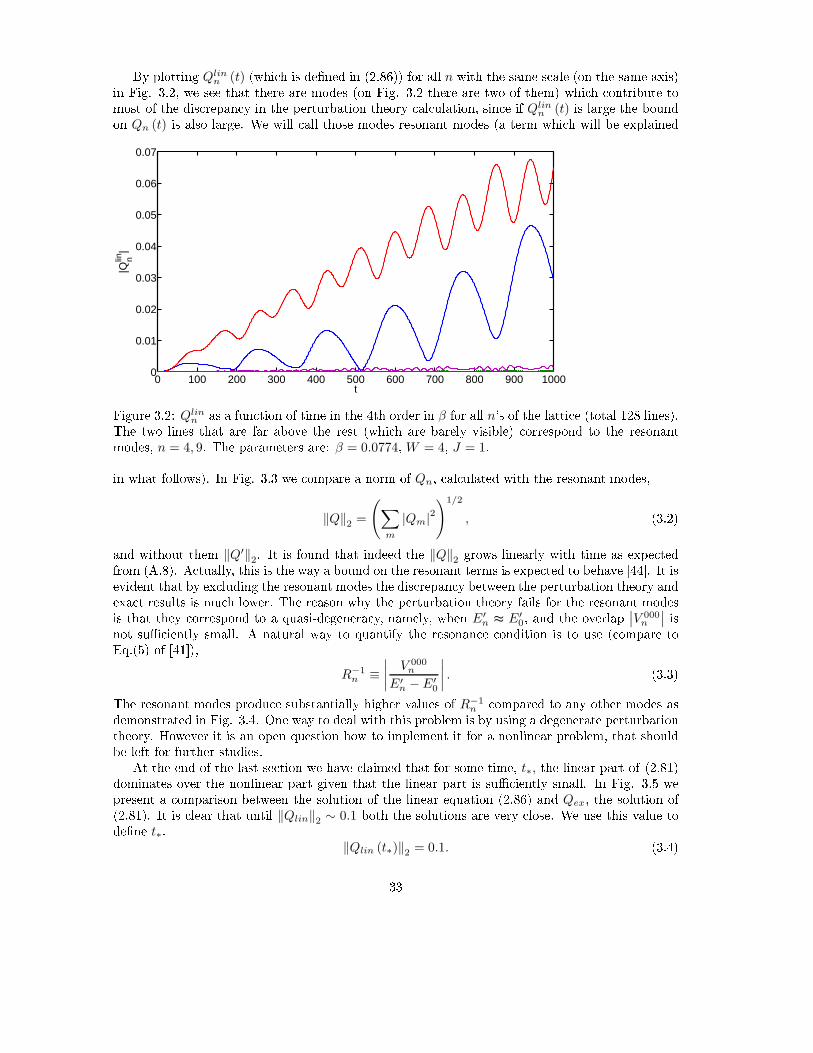
By plotting Qlinn (t) (which is de�ned in (2.86)) for all n with the same scale (on the same axis)in Fig. 3.2, we see that there are modes (on Fig. 3.2 there are two of them) which contribute tomost of the discrepancy in the perturbation theory calculation, since if Qlin

n (t) is large the boundon Qn (t) is also large. We will call those modes resonant modes (a term which will be explained

0 100 200 300 400 500 600 700 800 900 10000

0.01

0.02

0.03

0.04

0.05

0.06

0.07

|Qlin n

|

tFigure 3.2: Qlinn as a function of time in the 4th order in β for all n's of the lattice (total 128 lines).The two lines that are far above the rest (which are barely visible) correspond to the resonantmodes, n = 4, 9. The parameters are: β = 0.0774, W = 4, J = 1.in what follows). In Fig. 3.3 we compare a norm of Qn, calculated with the resonant modes,

‖Q‖2 =

(∑

m

|Qm|2)1/2

, (3.2)and without them ‖Q′‖2. It is found that indeed the ‖Q‖2 grows linearly with time as expectedfrom (A.8). Actually, this is the way a bound on the resonant terms is expected to behave [44]. It isevident that by excluding the resonant modes the discrepancy between the perturbation theory andexact results is much lower. The reason why the perturbation theory fails for the resonant modesis that they correspond to a quasi-degeneracy, namely, when E′n ≈ E′

0, and the overlap ∣∣V 000n

∣∣ isnot su�ciently small. A natural way to quantify the resonance condition is to use (compare toEq.(5) of [41]),

R−1n ≡

∣∣∣∣

V 000n

E′n − E′

0

∣∣∣∣. (3.3)The resonant modes produce substantially higher values of R−1

n compared to any other modes asdemonstrated in Fig. 3.4. One way to deal with this problem is by using a degenerate perturbationtheory. However it is an open question how to implement it for a nonlinear problem, that shouldbe left for further studies.At the end of the last section we have claimed that for some time, t∗, the linear part of (2.81)dominates over the nonlinear part given that the linear part is su�ciently small. In Fig. 3.5 wepresent a comparison between the solution of the linear equation (2.86) and Qex, the solution of(2.81). It is clear that until ‖Qlin‖2 ∼ 0.1 both the solutions are very close. We use this value tode�ne t∗,‖Qlin (t∗)‖2 = 0.1. (3.4)33

0 100 200 300 400 500 600 700 800 900 10000

1

2

3

4

5

6

7

8

9x 10−6

t

Qlin

Qlin

linearQ’

linFigure 3.3: ‖Q‖2 (dashed blue) and ‖Q′‖2 (solid green) as a function of time. The straight line isa linear �t to ‖Q‖2. The parameters are: 4th order, β = 0.01, W = 4, J = 1. The linear �t is:‖Q‖2 (t) = 2.3× 10−9 · t+ 5.7× 10−6.

−64 −48 −32 −16 0 16 32 48 64−2

−1.5

−1

−0.5

0

0.5

n

Rn−

1

n=4

n=9Figure 3.4: R−1n as a function of nFor small nonlinearity strength, β, t∗ is very large and therefore the integration of (2.86) to t∗is very time consuming. We therefore use the bound (A.8) to extrapolate linearly from the timeinterval where (2.86) is solved to t∗. Practically, we have calculated the linear behavior of Qlinlike it was done in Fig. 3.3 than we de�ned t∗ empirically by (3.4). In Fig. 3.6 we plot log10 t∗ asa function of β−1 for di�erent orders, while in Fig. 3.7 we compare the result found in 4-th orderwith ‖Qlin‖2 of (3.4) is replaced by ‖Q′

lin‖2 (where the resonant terms are removed) A systematicimprovement with the order of the perturbation theory is found, which suggests that t∗ = O(β−N

).34

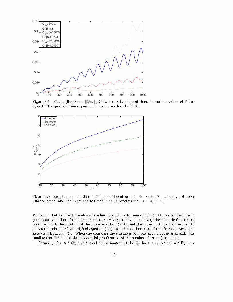
0 100 200 300 400 500 600 700 800 900 10000

0.05

0.1

0.15

0.2

0.25

0.3

0.35

Q

ex, β=0.1

Q, β=0.1Q

ex, β=0.0774

Q, β=0.0774Q

ex, β=0.0599

Q, β=0.0599

Figure 3.5: ‖Qex‖2 (lines) and ‖Qlin‖2 (dotes) as a function of time, for various values of β (seelegend). The perturbation expansion is up to fourth order in β.

10 20 30 40 50 60 70 80 90 1001

2

3

4

5

6

7

8

β−1

log 10

(t* )

4th order3rd order2nd order

Figure 3.6: log10 t∗ as a function of β−1 for di�erent orders. 4th order (solid blue), 3rd order(dashed green) and 2nd order (dotted red). The parameters are: W = 4, J = 1.We notice that even with moderate nonlinearity strengths, namely, β < 0.08, one can achieve agood approximation of the solution up to very large times. In this way the perturbation theorycombined with the solution of the linear equation (2.86) and the criterion (3.4) may be used toobtain the solution of the original equation (1.1) up to t < t∗. For small β the time t∗ is very longas is clear from Fig. 3.6. When one considers the smallness of β one should consider actually thesmallness of βe2 due to the exponential proliferation of the number of terms (see (2.44)).Assuming that the Q′n give a good approximation of the Qn for t < t∗, we can use Fig. 3.735

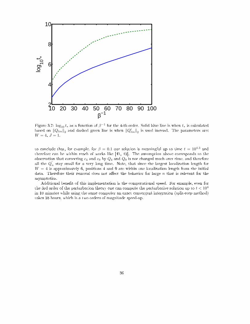
10 20 30 40 50 60 70 80 90 1002

4

6

8

10

β−1

log 10

t *

Figure 3.7: log10 t∗ as a function of β−1 for the 4-th order. Solid blue line is when t∗ is calculatedbased on ‖Qlin‖2 and dashed green line is when ‖Q′lin‖2 is used instead. The parameters are:

W = 4, J = 1.to conclude that, for example, for β = 0.1 our solution is meaningful up to time t = 104.3 andtherefore can be within reach of works like [41, 42]. The assumption above corresponds to theobservation that correcting c4 and c9 by Q4 and Q9 is not changed much over time, and thereforeall the Q′

n stay small for a very long time. Note, that since the largest localization length forW = 4 is approximately 6, positions 4 and 9 are within one localization length from the initialdata. Therefore their removal does not a�ect the behavior for large n that is relevant for theasymptotics.Additional bene�t of this implementation is the computational speed. For example, even forthe 3rd order of the perturbation theory one can compute the perturbative solution up to t < 104in 10 minutes while using the same computer an exact convergent integration (split-step method)takes 28 hours, which is a two orders of magnitude speed-up.

36

Chapter 4Summary and DiscussionIn this work a perturbation theory in the nonlinearity strength, β, for the NLSE with disorder(1.1) was developed. This required removal of secular terms (Sec. 2.3) and control of the smalldenominators (Sec. 2.5). We found that there is no entropy problem and the growth of the numberof terms with the order of the expansion, N , is at most exponential, namely, e2N (Sec. 2.4).Therefore the e�ective perturbation parameter is βe2 (rather than β). We obtain a probabilisticbound of the k-th order term in the expansion (2.73). A bound on the remainder of the expansionof the cn (an amplitude of a state localized near the site n) was obtained (Sec. 2.6) and it takesthe form|Qn (t)| ≤ AβN+1t · e−γ|xn|, (4.1)where γ = ξ−1 is the inverse localization length, and A ∼ eN

2

e−γ is a constant. We can showthat this inequality holds for t < t∗ = O(β−1

) (see Appendix A), however numerics indicate thatapproximatelly, t∗ = O(β−N

) (see Fig. 3.6). This will be assumed in the discussion, and its proofis left for future research. If we require that ∑|n|≥n |Qn|2 < ε2 , thann (t) = ξ ln

(AβN t

ε

)

. (4.2)It means that localization holds beyond a front n (t) that propagates logarithmically with time.This is in agreement with a conjecture made by Wang and Zhang on the basis of results obtainedin the limit of strong disorder [33]. From (4.1) one �nds thatlimβ→0

|Qn|βN

= 0, (4.3)which suggests that the series is asymptotic. In Fig. 4.1 we have plotted β−N ‖Q‖2 (de�ned by(3.2)) as a function of β, it is clear that (4.3) is supported by the �gure. In the case that the seriesis asymptotic there is an optimal order N such that,βN ∼ B

N !(4.4)and if one can calculate the terms up to the optimal order, one obtains the solution up to time,

t∗ = N ! , which for large N or small β scales as, t∗ ∼ β−β−1 [81]. The main di�culty is thatA ∼ eN

2 and this is also the way the bound on the typical term grows. We believe this is a result37

10−2

10−1

102

103

β

β−N ||

Q|| 2

Figure 4.1: β−N ‖Q (t)‖2 as a function of β. Solid blue is fourth order, dashed green is third orderand dotted red is second order. The parameters are: J = 1, W = 4, and t = 1000.of the method of the proof used. Numerically we see that A is of the order of unity. The derivationis not rigorous but we believe it is correct. The rigor is left for further studies.In this work we have also demonstrated how a perturbation theory can be numerically imple-mented for the solution of the NLSE with a random potential (1.1). In the perturbative methodthe computer is used to implement the symbolic recursive calculation of the various terms and alsofor their numerical evaluation. This method allows to estimate the errors since the remainder termis bounded. It was demonstrated (in the end of the previous section) how to evaluate the time ofvalidity of the perturbation theory. This approach has also a great advantage in the speed of thecalculation. In order to make the perturbation theory of a much greater value one has to solve theproblem of resonant terms (when R−1n of (3.3) is large).We are trying now to test the numerical results found in [36, 42, 41] with the help of thisperturbation theory. It is clear that if (4.2) is correct for any time than subdi�usion as predictedin [36, 42, 41] cannot be asymptotic in time.We also believe that this method can be generalized to other nonlinear di�erential equations,for example, the Fermi-Ulam-Pasta problem.This work leaves several open problems that should be subject of further research:1. Can the front x (t) ∝ ln t be found for arbitrarily long times ?38

2. What is the nature of the new timescale, t∗ ∼ β−β−1?3. The asymptotic nature of the series. Is it just an asymptotic series or a convergent one(probably not)?4. If the series is asymptotic can it be resummed ?5. The eck2+c′k in (2.73) and A ∼ e2N result from the repeated use of the Hölder inequalityand a very generous bound on the probability distributions. An e�ort should be made toimprove it.6. There are various properties of the Anderson model that have been used here. Some ofthem were tested numerically. It would be of great value if Conjecture 1, Corollary 1 andConjecture 2 were rigorously established, even at the limit of a strong disorder. In the presentwork we rely only on Corollary 1 (that was tested numerically, see Fig. 2.2).7. It would be very useful if Conjecture 3 could be rigorously obtained.8. A method to treat nearly resonant terms (3.3) should be developed.9. An e�ort should be made to show (4.1) rigorously.

39

Appendix ABounding the remainderIn order to bound the solution we have to bound, Qn, the remainder of the expansion (2.13)

cn (t) = c(0)n + βc(1)n + β2c(2)n + · · ·+ βNc(N)n +Qn. (A.1)This is achieved by applying the bootstrap argument to the remainder. Substituting the expansion(2.13) into the equation (2.23) and writing a di�erential equation for the remainder gives

i∂tQn = −∑

l1+l2>N

βl1+l2E(l1)n c(l2)n +

∑

m1m2m3

N∑

N≤k+l+q≤3N

βk+l+q+1V m1m2m3n c∗(q)m1

c(l)m2c(k)m3

ei(E′

n+E′

m1−E′

m2−E′

m3)t(A.2)

+∑

m1m2m3

N∑

0≤k+l≤2N

βl+k+1V m1m2m3n Q∗

m1c(l)m2

c(k)m3ei(E

′

n+E′

m1−E′

m2−E′

m3)t

+ 2∑

m1m2m3

N∑

0≤k+l≤2N

βl+k+1V m1m2m3n Qm3c

(l)∗m1

c(k)m2ei(E

′

n+E′

m1−E′

m2−E′

m3)t

+ 2∑

m1m2m3

N∑

k=0

βk+1V m1m2m3n Q∗

m1Qm2c

(k)m3ei(E

′

n+E′

m1−E′

m2−E′

m3)t

+∑

m1m2m3

N∑

k=0

βk+1V m1m2m3n c(k)∗m1

Qm2Qm3ei(E′

n+E′

m1−E′

m2−E′

m3)t

+∑

m1m2m3

βV m1m2m3n Q∗

m1Qm2Qm3e

i(E′

n+E′

m1−E′

m2−E′

m3)t40

where the sums over orders are understood as follows. By ∑NN≤k+l+q≤3N we mean ∑N

k,l,q=0 withthe constraint N ≤ k + l + q . Integrating and using the fact, Qn (t = 0) = 0,|Qn|t

≤∑

l1+l2>N

βl1+l2∣∣∣E(l1)

n

∣∣∣

∣∣∣c(l2)n

∣∣∣ (A.3)

+∑

m1m2m3

N∑

N≤k+l+q≤3N

βk+l+q+1 |V m1m2m3n | sup

0≤t′≤t

[∣∣∣c∗(k)m1

∣∣∣

∣∣∣c(l)m2

∣∣∣

∣∣∣c(q)m3

∣∣∣

] (A.4)+

∑

m1m2m3

N∑

0≤k+l≤2N

βl+k+1 |V m1m2m3n | sup

0≤t′≤t

[∣∣Q∗

m1

∣∣

∣∣∣c(l)m2

∣∣∣

∣∣∣c(k)m3

∣∣∣

]

+2∑

m1m2m3

N∑

0≤k+l≤2N

βl+k+1 |V m1m2m3n | sup

0≤t′≤t

[

|Qm3 |∣∣∣c(l)∗m1

∣∣∣

∣∣∣c(k)m2

∣∣∣

]

+2∑

m1m2m3

N∑

k=0

βk+1 |V m1m2m3n | sup

0≤t′≤t

[∣∣Q∗

m1

∣∣ |Qm2 |

∣∣∣c(k)m3

∣∣∣

]

+∑

m1m2m3

N∑

k=0

βk+1 |V m1m2m3n | sup

0≤t′≤t

[

|Qm2 | |Qm3 |∣∣∣c(k)∗m1

∣∣∣

]

+β∑

m1m2m3

|Vm1m2m3n | sup

0≤t′≤t

[∣∣Q∗

m1

∣∣ |Qm2 | |Qm3 |

],where t is the upper limit of the integration. Since Qn (t) is continuous and Qn (t = 0) = 0, forsmall t, Qn (t) ∼ t · S1. Therefore we can always �nd a su�ciently small τ > 0, such that

|Qn (τ)| < 2τ · S1, (A.5)whereS1 =

∑

l1+l2>N

βl1+l2∣∣∣E(l1)

n

∣∣∣ sup0≤t′≤t

∣∣∣c(l2)n

∣∣∣ (A.6)

+∑

m1m2m3

N∑

N≤k+l+q≤3N

βk+l+q+1 |Vm1m2m3n | sup

0≤t′≤t

[∣∣∣c∗(k)m1

∣∣∣

∣∣∣c(l)m2

∣∣∣

∣∣∣c(q)m3

∣∣∣

]

,is the non-homogeneous term. Assume, that there is some time, t, for which,|Qn (t)| > 2t · S1, (A.7)than since Qn (t) is continuous and (A.5) holds there is a time, t0, where|Qn (t0)| = 2t0 · S1. (A.8)Inserting this equality into the inequality (A.3), we get an interval 0 ≤ t ≤ t0 for which (A.5) holds(see (A.28)). We proceed by bounding S1 and other sums of (A.3).Using the Theorem 1 obtained in the end of the Section 2.5, we can bound, S1. The inequalityis violated with a probability found from (2.73). First we bound the �rst term of S1. Since E(l)

n isconstructed such that it contains only a few terms of c(l)n one can use 1 to bound also E(l)n , therefore

∑

l1+l2>N

βl1+l2∣∣∣E(l1)

n

∣∣∣ sup0≤t′≤t

∣∣∣c(l2)n

∣∣∣ ≤ Gδ (N) e−2(γ−ε−ε′−η′)|xn|, (A.9)41

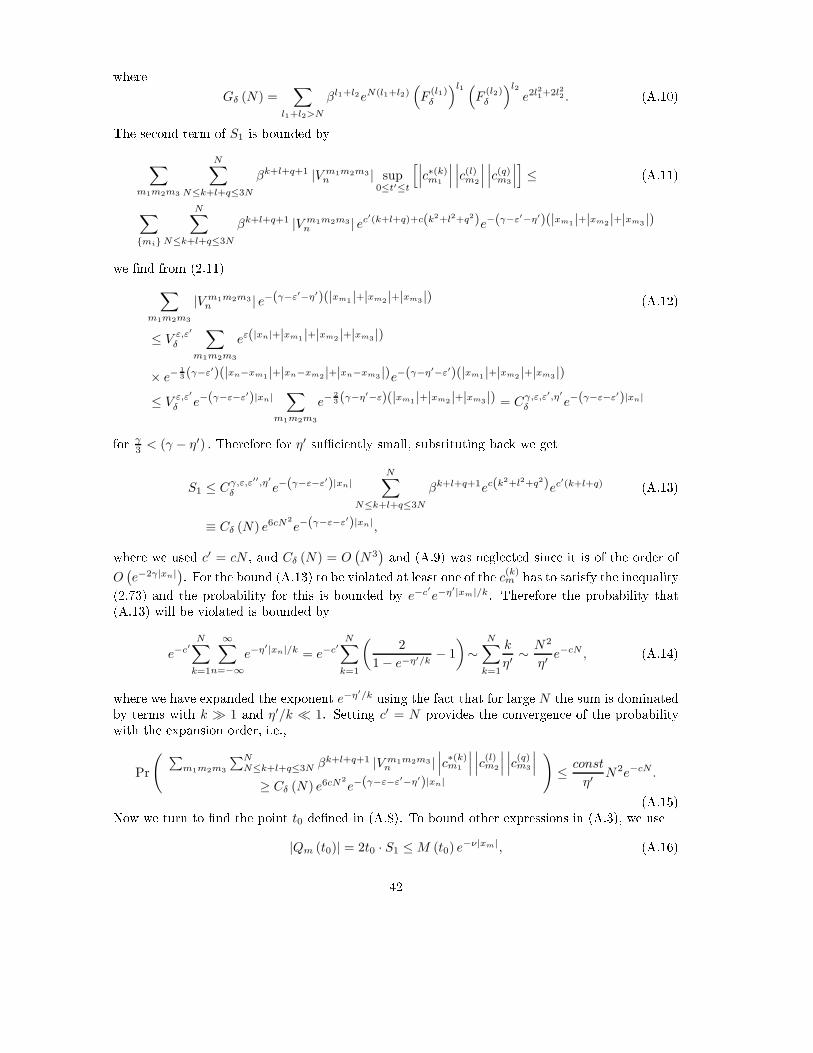
whereGδ (N) =

∑

l1+l2>N

βl1+l2eN(l1+l2)(

F(l1)δ

)l1 (

F(l2)δ

)l2e2l

21+2l22 . (A.10)The second term of S1 is bounded by

∑

m1m2m3

N∑

N≤k+l+q≤3N

βk+l+q+1 |V m1m2m3n | sup

0≤t′≤t

[∣∣∣c∗(k)m1

∣∣∣

∣∣∣c(l)m2

∣∣∣

∣∣∣c(q)m3

∣∣∣

]

≤ (A.11)∑

{mi}

N∑

N≤k+l+q≤3N

βk+l+q+1 |V m1m2m3n | ec′(k+l+q)+c(k2+l2+q2)e−(γ−ε′−η′)(|xm1 |+|xm2 |+|xm3 |)we �nd from (2.11)

∑

m1m2m3

|V m1m2m3n | e−(γ−ε′−η′)(|xm1 |+|xm2 |+|xm3 |) (A.12)

≤ V ε,ε′

δ

∑

m1m2m3

eε(|xn|+|xm1 |+|xm2 |+|xm3 |)

× e−13 (γ−ε′)(|xn−xm1 |+|xn−xm2 |+|xn−xm3 |)e−(γ−η′−ε′)(|xm1 |+|xm2 |+|xm3 |)

≤ V ε,ε′

δ e−(γ−ε−ε′)|xn|∑

m1m2m3

e−23 (γ−η′−ε)(|xm1 |+|xm2 |+|xm3 |) = Cγ,ε,ε′,η′

δ e−(γ−ε−ε′)|xn|for γ3 < (γ − η′) . Therefore for η′ su�ciently small, substituting back we get

S1 ≤ Cγ,ε,ε′′,η′

δ e−(γ−ε−ε′)|xn|N∑

N≤k+l+q≤3N

βk+l+q+1ec(k2+l2+q2)ec

′(k+l+q) (A.13)≡ Cδ (N) e6cN

2

e−(γ−ε−ε′)|xn|,where we used c′ = cN , and Cδ (N) = O(N3) and (A.9) was neglected since it is of the order of

O(e−2γ|xn|

). For the bound (A.13) to be violated at least one of the c(k)m has to satisfy the inequality(2.73) and the probability for this is bounded by e−c′e−η′|xm|/k. Therefore the probability that(A.13) will be violated is bounded bye−c′

N∑

k=1

∞∑

n=−∞

e−η′|xn|/k = e−c′N∑

k=1

(2

1− e−η′/k− 1

)

∼N∑

k=1

k

η′∼ N2

η′e−cN , (A.14)where we have expanded the exponent e−η′/k using the fact that for large N the sum is dominatedby terms with k � 1 and η′/k � 1. Setting c′ = N provides the convergence of the probabilitywith the expansion order, i.e.,

Pr

( ∑

m1m2m3

∑NN≤k+l+q≤3N βk+l+q+1 |V m1m2m3

n |∣∣∣c

∗(k)m1

∣∣∣

∣∣∣c

(l)m2

∣∣∣

∣∣∣c

(q)m3

∣∣∣

≥ Cδ (N) e6cN2

e−(γ−ε−ε′−η′)|xn|

)

≤ const

η′N2e−cN .(A.15)Now we turn to �nd the point t0 de�ned in (A.8). To bound other expressions in (A.3), we use

|Qm (t0)| = 2t0 · S1 ≤M (t0) e−ν|xm|, (A.16)42

where following (A.15),M (t0) := 2t0Cδ (N) e6cN

2 (A.17)with ν = γ − ε− ε′. In what follows, unless stated di�erently, M will mean M (t0).First we will bound the linear term in the Qn in (A.3). The sum over m2 and m3 is boundedsimilarly to the sums in the inhomogeneous term and the sum over m1 is bounded using thebootstrap assumption (A.16), resulting inS2 =

∑

m2m3

N∑

0≤k+l≤2N

βl+k+1∑

m1

|V m1m2m3n |

∣∣Q∗

m1

∣∣

∣∣∣c(l)m2

∣∣∣

∣∣∣c(k)m3

∣∣∣ (A.18)

≤M∑

m2m3

N∑

0≤k+l≤2N

βl+k+1ec(k2+l2)ec

′(k+l)∑

m1

|V m1m2m3n | e−ν|xm1 |e−(γ−η′−ε′)(|xm2 |+|xm3 |)for 1

3 (γ − ε′) < ν and γ3 < γ − η′. This is similar to the sum in equation (A.12) and gives a resultwith a similar dependence on |xn|,

S2 ≤∑

m2m3

N∑

0≤k+l≤2N

βl+k+1∑

m1

|V m1m2m3n |

∣∣Q∗

m1

∣∣

∣∣∣c(l)m2

∣∣∣

∣∣∣c(k)m3

∣∣∣ (A.19)

≤ Cδ (N) e2cN2

Me−(γ−ε−ε′)|xn|.with the same probability as in (A.14). Therefore the linear term in Qn is bounded by the proba-bilistic boundPr

( ∑

m1m2m3;l,kβl+k+1 |V m1m2m3

n |∣∣Q∗

m1

∣∣

∣∣∣c

(l)m2

∣∣∣

∣∣∣c

(k)m3

∣∣∣

≥ βCδ (N) e4cN2

Me−(γ−ε−ε′−η′)|xn|

)

≤ const

η′N2e−cN , (A.20)with Cδ = O

(N2). A similar bound is found for the third term on RHS of (A.3).The fourth sum of equation (A.3)

S4 =∑

m1m2m3;k

βk+1 |V m1m2m3n |

∣∣Q∗

m1

∣∣ |Qm2 |

∣∣∣c(k)m3

∣∣∣ (A.21)is bounded by

Pr

∑

m1m2m3;k

βk+1 |V m1m2m3n |

∣∣Q∗

m1

∣∣ |Qm2 |

∣∣∣c

(k)m3

∣∣∣

≥ Cδ (N) e2cN2

βN+1M2e−(γ−ε−ε′−η′)|xn|

≤ const

η′N2e−cN , (A.22)with Cδ = O (N). The last term in (A.3) is

S5 = β∑

m1m2m3

|V m1m2m3n |

∣∣Q∗

m1

∣∣ |Qm2 | |Qm3 | . (A.23)and it is bounded by

S5 ≤ βM3e−(γ−ε−ε′)|xn|. (A.24)To summarize, substitution of the equality (A.16) in (A.3) to �nd a time t0 for which assumption(A.7) is valid results in the following inequality which is satis�ed with the probability that is thesum of the probabilities given by the RHS of (A.15), (A.20), (A.22),2t0S1 ≤ t0 · S1 + t0Cδ (N)

(

e6cN2

+ 2βe4cN2

M + 4βe2cN2

M2 + 8βM3)

e−(γ−ε−ε′)|xn|, (A.25)43

with Cδ = O(N3). Multiplying by e(γ−ε−ε′)|xn| both sides of the inequality (A.25) and taking thein�mum with respect to n, gives

infn

(

S1e(γ−ε−ε′)|xn|

)

≤ 2Cδ (N)β(

e4cN2

M + 2e2cN2

M2 + 4M3)

. (A.26)Setting AN := e2cN2, C := infn

(

S1e(γ−ε−ε′)|xn|

) and using the de�nition of M (see (A.17))C ≤ 2βt0 ·A5

NCδ + 4βt20A7NC

2δ + 8βt30A

9N . (A.27)For su�ciently small βt0 the �rst term on the RHS of (A.27) is dominant and therefore,

t0 ≥ C

2βA5NCδ

. (A.28)Note, that C > 0, since it is an in�mum of a sum of positive quantities, however we do not calculateit explicitly in this work, nevertheless it is likely to be of the order of CδA3N . This proves that,

|Qn (t)| ≤M (t) · e−(γ−ε−ε′)|xn| = 2t · Cδe6cN2

e−(γ−ε−ε′)|xn|for times t ≤ t0 ∼ O(β−1

), where M (t) is given by extending the de�nition (A.17) by replacingt0 by t.Theorem 2. For t = O

(β−1

) with c ∼= 2, and assuming that Conjecture 1 holdsPr(

|Qn| ≥ 2t · Cδe6cN2

e−(γ−ε−ε′)|xn|)

≤ const

η′N2e−cN (A.29)The bound on the probability of statement (A.29) is calculated by summing the RHS of((A.15),(A.20),(A.22)). The contribution of the remainder term is

|Qn| ≤ AβN+1t · e6cN2

e−(γ−ε−ε′)|xn|, (A.30)where A is a constant. Note that for a given t the remainder is very small for large |xn|, namely,the perturbation expansion gives asymptotically correct results on the tails of the wavepacket.

44

Appendix BDerivation of the modi�edperturbation expansionIn the calculations of the paper we used the expansion (2.20) of the wavefunction and the expansioncoe�cients cn (t) are calculated from (2.13) and (2.25). The c(l)n (t) depend on β since the E′

n in(2.25) depend on it. Therefore (2.13) is not a Taylor series in β. In this Appendix it is shown thatthis expansion is equivalent to the Taylor series,cn =

∞∑

l=0

c(l)n βl.Contrary to the c(l)n the c(l)n are independent of β. The expansion of (2.23) in powers of β producesthe following equation for the r-th orderi∂tc

(r)n = −

r∑

l=1

l∑

l1=0

1

l1!

(

∂l1E(l−l1)n

∂βl1

)

β=0

c(r−l)n + (B.1)

+∑

∑i li=r−1

∑

{mi}

V m1m2m3n c∗(l1)m1

c(l2)m2c(l3)m3

(1

l4!

∂l4

∂βl4ei(E

′

n+E′

m1−E′

m2−E′

m3)t)

β=0

.We considered a di�erent expansion (2.25), where one does not expand the exponent, but stillcompares the implicit powers of β from both sides of the equation. The equation for the (r − k)order in this expansion is (that is just (2.25))i∂tc

(r−k)n = −

r−k∑

l=1

E(l)n c(r−k−l)

n (B.2)+∑

{mi}

∑

l1+l2+l3=r−k−1

V m1m2m3n c∗(l1)m1

c(l2)m2c(l3)m3

ei(E′

n+E′

m1−E′

m2−E′

m3)t.It can be shown that each term in this expansion is uniformly bounded in time, with a properselection of E′

n, that is the secular terms are removed. We will show that this expansion isequivalent to a Taylor series.Theorem 3. For any t,cn =

∞∑

k=0

c(k)n βk, (B.3)45

where c(k)n are de�ned using (B.2).Proof. Since cn =∑∞

k=0 c(k)n βk is the expansion of cn in powers of β, and due to the uniqueness ofthis expansion, the theorem is true if and only if

c(r)n =

r∑

k=0

1

k!

(

∂kc(r−k)n

∂βk

)

β=0

=

r−1∑

k=0

1

k!

(

∂kc(r−k)n

∂βk

)

β=0

, (B.4)where at the last equality we have used the fact that ∂rc(0)n

∂βr = 0, for any r ≥ 1. We proceed toprove this equality by induction. Suppose that this equality is true for all the orders till order r.We apply the linear operator∑r−1k=0

1k!

∂k

∂βk to both sides of (B.2). For the �rst part on the RHS wegetr−1∑

k=0

1

k!

r−k∑

l=1

∂k

∂βk

(

E(l)n c(r−k−l)

n

)

=

=r−1∑

k=0

1

k!

r−k∑

l=1

k∑

l1=0

k!

l1! (k − l1)!

∂l1E(l)n

∂βl1

∂(k−l1)c(r−k−l)n

∂β(k−l1)

=r−1∑

k=0

r−k∑

l=1

k∑

l1=0

(

1

l1!

∂l1E(l)n

∂βl1

)(

1

(k − l1)!

∂(k−l1)c(r−k−l)n

∂β(k−l1)

) (B.5)where at the �rst equality we have used the Leibniz generalized product rule. We now exchangevariables such thatl1 = l1 (B.6)l2 = k − l1

z = l + l1or in a matrix notation

l1l2z

= A1

l1lk

, (B.7)whereA1 =

1 0 0−1 0 11 1 0

.The region of summation is bounded by the planes0 ≤ k ≤ r − 1 (B.8)1 ≤ l ≤ r − k

0 ≤ l1 ≤ kor in matrix notationB1

l1lk

≤

r − 1r00−10

, (B.9)46

whereB1 =

0 0 10 1 11 0 −1−1 0 00 −1 00 0 −1

.Changing the variables by applying the transformation matrix producesB1 ·A−1

1

l1l2z

=

1 1 00 1 10 −1 0−1 0 01 0 −1−1 −1 0

l1l2z

≤

r − 1r00−10

(B.10)or the following inequalitiesl1 + l2 ≤ r − 1 (B.11)l2 + z ≤ r

0 ≤ l2

0 ≤ l1

l1 ≤ z − 1

0 ≤ l1 + l2.Removing redundant inequalities gives0 ≤ l1 ≤ z − 1 (B.12)

1 ≤ z ≤ r

0 ≤ l2 ≤ r − z.Therefore in the new variables the sum (B.5) takes the formr∑

z=1

z−1∑

l1=0

r−z∑

l2=0

(

1

l1!

∂l1E(z−l1)n

∂βl1

)(

1

l2!

∂l2c(r−z−l2)n

∂βl2

)

, (B.13)Since ∂zE(0)n

∂βz = 0 for any z ≥ 1,we can writer∑

z=1

z∑

l1=0

r−z∑

l2=0

(

1

l1!

∂l1E(z−l1)n

∂βl1

)(

1

l2!

∂l2c(r−z−l2)n

∂βl2

)

. (B.14)Taking β = 0 and using the assumption of the induction for orders lower than r we haver∑

z=1

z∑

l1=0

(

1

l1!

∂l1E(z−l1)n

∂βl1

)

c(r−z)n , (B.15)47

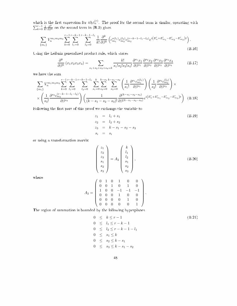
which is the �rst expression for i∂tc(r)n . The proof for the second term is similar, operating with∑r−1

k=01k!

∂k

∂βk on the second term in (B.2) gives∑

{mi}

Vm1m2m3n

r−1∑

k=0

r−k−1∑

l1=0

r−k−1−l1∑

l2=0

1

k!

∂k

∂βk

(

c∗(l1)m1c(l2)m2

c(r−k−1−l1−l2)m3

ei(E′

n+E′

m1−E′

m2−E′

m3)t)

.(B.16)Using the Leibniz generalized product rule, which states∂k

∂βk(x1x2x3x4) =

∑

s1+s2+s3+s4=k

k!

s1!s2!s3!s4!

∂s1x1∂βs1

∂s2x2∂βs2

∂s3x3∂βs3

∂s4x4∂βs4

(B.17)we have the sum∑

{mi}

V m1m2m3n

r−1∑

k=0

r−k−1∑

l1=0

r−k−1−l1∑

l2=0

k∑

s1=0

k−s1∑

s2=0

k−s1−s2∑

s3=0

(

1

s1!

∂s1c∗(l1)m1

∂βs1

)(

1

s2!

∂s2c(l2)m2

∂βs2

)

×

×(

1

s3!

∂s3c(r−k−1−l1−l2)m3

∂βs3

)(1

(k − s1 − s2 − s3)!

∂(k−s1−s2−s3)

∂β(k−s1−s2−s3)ei(E

′

n+E′

m1−E′

m2−E′

m3)t) (B.18)Following the �rst part of this proof we exchange the variable to

z1 = l1 + s1 (B.19)z2 = l2 + s2

z3 = k − s1 − s2 − s3

si = sior using a transformation matrix

z1z2z3s1s2s3

= A2

kl1l2s1s2s3

, (B.20)whereA2 =

0 1 0 1 0 00 0 1 0 1 01 0 0 −1 −1 −10 0 0 1 0 00 0 0 0 1 00 0 0 0 0 1

.The region of summation is bounded by the following hyperplanes0 ≤ k ≤ r − 1 (B.21)0 ≤ l1 ≤ r − k − 1

0 ≤ l2 ≤ r − k − 1− l1

0 ≤ s1 ≤ k

0 ≤ s2 ≤ k − s1

0 ≤ s3 ≤ k − s1 − s248

which could be represented in a matrix notation asB2

kl1l2s1s2s3

≤

r − 1r − 1r − 1000000000

, (B.22)where

B2 =

1 0 0 0 0 01 1 0 0 0 01 1 1 0 0 0−1 0 0 1 0 0−1 0 0 1 1 0−1 0 0 1 1 1−1 0 0 0 0 00 −1 0 0 0 00 0 −1 0 0 00 0 0 −1 0 00 0 0 0 −1 00 0 0 0 0 −1

.

Using the transformation matrix to change the variables results in the following

0 0 1 1 1 11 0 1 0 1 11 1 1 0 0 10 0 −1 0 −1 −10 0 −1 0 0 −10 0 −1 0 0 00 0 −1 −1 −1 −1−1 0 0 1 0 00 −1 0 0 1 00 0 0 −1 0 00 0 0 0 −1 00 0 0 0 0 −1

z1z2z3s1s2s3

≤

r − 1r − 1r − 1000000000

(B.23)49

or in the following inequalitiesz3 + s1 + s2 + s3 ≤ r − 1 (B.24)z1 + z3 + s2 + s3 ≤ r − 1

z1 + z2 + z3 + s3 ≤ r − 1

0 ≤ z3 + s2 + s3

0 ≤ z3 + s3

0 ≤ z3

0 ≤ z3 + s1 + s2 + s3

s1 ≤ z1

s2 ≤ z2

0 ≤ siRemoving redundant inequalities gives0 ≤ s1 ≤ z1 (B.25)0 ≤ s2 ≤ z2

0 ≤ s3 ≤ (r − 1)− z1 − z2 − z3

0 ≤ z1 ≤ (r − 1)− z3

0 ≤ z2 ≤ (r − 1)− z1 − z3

0 ≤ z3 ≤ r − 1which is equivalent to the sum∑

{mi}

V m1m2m3n

r−1∑

z3=0

r−1−z3∑

z1=0

r−1−z1−z3∑

z2=0

z1∑

s1=0

z2∑

s2=0

r−1−z1−z2−z3∑

s3=0

(

1

s1!

∂s1c∗(z1−s1)m1

∂βs1

)

×

×(

1

s2!

∂s2c(z2−s2)m2

∂βs2

)(

1

s3!

∂s3c(r−1−z1−z2−z3−s3)m3

∂βs3

)(1

z3!

∂z3

∂βz3ei(E

′

n+E′

m1−E′

m2−E′

m3)t) (B.26)Putting β = 0 and utilizing the assumption of the induction we get

∑

l1+l2+l3+l4=r−1

∑

{mi}

V m1m2m3n c(l1)∗m1

c(l2)m2c(l3)m3

(1

l4!

∂l4

∂βl4ei(E

′

n+E′

m1−E′

m2−E′

m3)t)

β=0

(B.27)which is exactly the second term in the equation for i∂tc(r)n . Since the zero order trivially satis�esthis theorem, this competes the proof by induction.One should be able to extend the results of this Appendix to other nonlinear equations, forexample, where the power of the nonlinearity is di�erent (in the last term of (1.1) 2 is replaced byanother integer). See next Appendix for a possible application in classical nonlinear problems.50

Appendix CNonlinear classical equationsWe consider a nonlinear system with N degrees of freedom, which can be approximated at thevicinity of its elliptic point by a chain of N nonlinear oscillators. The equations of motion of thischain of oscillators are given byd2Xn

dt2= −ω2

nXn + βF(

~X)

. (C.1)We will deal only with irrationally independent systems,N∑

n=1

mnωn 6= 0 mn ∈ Z. (C.2)We will also consider a nonlinearity which is a polynomial of degree, α ≥ 2, in the positions of theoscillators, namely,d2Xn

dt2= −ω2

nXn + β∑

{mi},~α

V m1m2···mNn (~α)Xα1

m1Xα2

m2· · ·XαN

mN(C.3)where V m1m2···mN

n (~α) are some coe�cients and α ∈ Z,∑N

i=1 αi = α. Introducing the variable,Pn = dXn

dt , we getd

dt

(Pn

Xn

)

=

(0 −ω2

n

1 0

)(Pn

Xn

)

+ β∑

{mi},~α

V m1m2···mNn

(Xα1

m1Xα2

m2· · ·XαN

mN

0

)

. (C.4)We proceed by changing the variables to(cnc∗n

)

=M−1n

(Pn

Xn

)

, (C.5)whereMn =

(−iωn iωn

1 1

)

M−1n =

1

2ωn

(i ωn

−i ωn

)

. (C.6)Equation (C.4) rewrites tod

dt

(cnc∗n

)

=

(−iωn 00 iωn

)(cnc∗n

)

+ (C.7)+β

∑

{mi},~α

V m1m2···mNn M−1

n

( (cm1 + c∗m1

)α1 · · ·(cmN

+ c∗mN

)αN

0

)51

or taking only the equation for cn,idcndt

= ωncn − β

2ωn

∑

{mi},~α

V m1m2···mNn (~α)

(cm1 + c∗m1

)α1 · · ·(cmN

+ c∗mN

)αN. (C.8)For example, for the Fermi-Pasta-Ulam, α- model

idcndt

= ωncn − β

2ωn

∑

{mi}

V m1m2n

(cm1 + c∗m1

) (cm2 + c∗m2

). (C.9)and β- model,

idcndt

= ωncn − β

2ωn

∑

{mi}

V m1m2m3n

(cm1 + c∗m1

) (cm2 + c∗m2

) (cm3 + c∗m3

). (C.10)This equation is of a similar form as (2.23), and therefore similar methods should apply.

52

Bibliography[1] C. Sulem and P. L. Sulem. The nonlinear Schrödinger equation self-focusing and wave collapse.Springer, 1999.[2] G. P. Agrawal. Nonlinear �ber optics, volume 4th. Academic Press, Burlington, MA ; London,2007.[3] F. Dalfovo, S. Giorgini, L. P. Pitaevskii, and S. Stringari. Theory of Bose-Einstein condensa-tion in trapped gases. Rev. Mod. Phys., 71(3):463�512, 1999.[4] L. P. Pitaevskii and S. Stringari. Bose-Einstein condensation. Clarendon Press, Oxford ; NewYork, 2003.[5] A. J. Leggett. Bose-Einstein condensation in the alkali gases: Some fundamental concepts.Rev. Mod. Phys., 73(2):307�356, 2001.[6] L.P. Pitaevskii. Zh. Eksp. Theor. Phys., 40:646, 1961.[7] E.P. Gross. Structure of a quantized vortex in boson systems. Nuovo Cimento, 20(3):454�477,1961.[8] L.P. Pitaevskii. J. Math. Phys., 4:195, 1963.[9] L. Erdös, B. Schlein, and H. T. Yau. Rigorous derivation of the Gross-Pitaevskii equation.Phys. Rev. Lett., 98(4):040404, 2007.[10] E. H. Lieb and R. Seiringer. Proof of Bose-Einstein condensation for dilute trapped gases.Phys. Rev. Lett., 88(17):170409, 2002.[11] P. W. Anderson. Absence of di�usion in certain random lattices. Phys. Rev., 109(5):1492,1958.[12] K. Ishii. Localization of eigenstates and transport phenomena in one-dimensional disorderedsystem. Suppl. Prog, Theor. Phys., 53(53):77�138, 1973.[13] P. A. Lee and T. V. Ramakrishnan. Disordered electronic systems. Rev. Mod. Phys., 57(2):287�337, 1985.[14] I. M. Lifshits, L. A. Pastur, and S. A. Gredeskul. Introduction to the theory of disorderedsystems. Wiley, New York, 1988.[15] M. Aizenman and S. Warzel. On the joint distribution of energy levels of random Schrödingeroperators. J. Phys. A, 42:045201, 2009. 53

[16] D.M. Basko, I.L. Aleiner, and B.L. Altshuler. Metal-insulator transition in a weakly interactingmany-electron system with localized single-particle states. Ann. Phys., 321:1126, 2006.[17] D.M. Basko, I.L. Aleiner, and B.L. Altshuler. Possible experimental manifestations of themany-body localization. Phys. Rev. B, 76:052203, 2007.[18] E. Abrahams, P. W. Anderson, D. C. Licciardello, and T. V. Ramakrishnan. Scaling theory oflocalization - absence of quantum di�usion in 2 dimensions. Phys. Rev. Lett., 42(10):673�676,1979.[19] T. Schwartz, G. Bartal, S. Fishman, and M. Segev. Transport and Anderson localization indisordered two-dimensional photonic lattices. Nature, 446(7131):52�55, 2007.[20] H. Gimperlein, S. Wessel, J. Schmiedmayer, and L. Santos. Ultracold atoms in optical latticeswith random on-site interactions. Phys. Rev. Lett., 95(17):170401, 2005.[21] J. E. Lye, L. Fallani, M. Modugno, D. S. Wiersma, C. Fort, and M. Inguscio. Bose-Einsteincondensate in a random potential. Phys. Rev. Lett., 95(7):070401, 2005.[22] D. Clement, A. F. Varon, M. Hugbart, J. A. Retter, P. Bouyer, L. Sanchez-Palencia, D. M.Gangardt, G. V. Shlyapnikov, and A. Aspect. Suppression of transport of an interactingelongated Bose-Einstein condensate in a random potential. Phys. Rev. Lett., 95(17):170409,2005.[23] D. Clement, A. F. Varon, J. A. Retter, L. Sanchez-Palencia, A. Aspect, and P. Bouyer.Experimental study of the transport of coherent interacting matter-waves in a 1D randompotential induced by laser speckle. New J. Phys., 8:165, 2006.[24] L. Sanchez-Palencia, D. Clement, P. Lugan, P. Bouyer, G. V. Shlyapnikov, and A. Aspect.Anderson localization of expanding Bose-Einstein condensates in random potentials. Phys.Rev. Lett., 98(21):210401, May 2007.[25] J. Billy, V. Josse, Z. C. Zuo, A. Bernard, B. Hambrecht, P. Lugan, D. Clement, L. Sanchez-Palencia, P. Bouyer, and A. Aspect. Direct observation of Anderson localization of matterwaves in a controlled disorder. Nature, 453(7197):891�894, June 2008.[26] C. Fort, L. Fallani, V. Guarrera, J. E. Lye, M. Modugno, D. S. Wiersma, and M. Inguscio.E�ect of optical disorder and single defects on the expansion of a Bose-Einstein condensate ina one-dimensional waveguide. Phys. Rev. Lett., 95(17):170410, 2005.[27] E. Akkermans, S. Ghosh, and Z. H. Musslimani. Numerical study of one-dimensional andinteracting Bose-Einstein condensates in a random potential. J. Phys. B, 41(4):045302, 2008.[28] T. Paul, P. Schlagheck, P. Leboeuf, and N. Pavlo�. Super�uidity versus Anderson localizationin a dilute Bose gas. Phys. Rev. Lett., 98(21):210602, 2007.[29] A. R. Bishop. Fluctuation phenomena : disorder and nonlinearity. World Scienti�c, Singapore; River Edge, NJ, 1995.[30] K. O. Rasmussen, D. Cai, A. R. Bishop, and N. Gronbech-Jensen. Localization in a nonlineardisordered system. Europhys. Lett., 47(4):421�427, 1999.[31] G. Kopidakis and S. Aubry. Intraband discrete breathers in disordered nonlinear systems. I.Delocalization. Physica D, 130(3-4):155�186, 1999.54

[32] G. Kopidakis and S. Aubry. Discrete breathers and delocalization in nonlinear disorderedsystems. Phys. Rev. Lett., 84(15):3236�3239, 2000.[33] W.-M. Wang and Z. Zhang. Long time Anderson localization for nonlinear random Schrödingerequation. J. Stat. Phys., 134:953, 2009.[34] W.-M. Wang. Logarithmic bounds on Sobolev norms for time dependent linear Schröingerequations. Comm. Part. Di�. Eq., 33(12):2164�2179, 2008.[35] D. L. Shepelyansky. Delocalization of quantum chaos by weak nonlinearity. Phys. Rev. Lett.,70(12):1787�1790, 1993.[36] A. S. Pikovsky and D. L. Shepelyansky. Destruction of Anderson localization by a weaknonlinearity. Phys. Rev. Lett., 100(9):094101, 2008.[37] M. Mulansky. Localization properties of nonlinear disordered lattices. Universität Potsdam,Diploma thesis, 2009. http://nbn-resolving.de/urn:nbn:de:kobv:517-opus-31469.[38] H. Veksler, Y. Krivolapov, and S. Fishman. Spreading for tbe generalized nonlinearSchrödinger equation with disorder. Phys. Rev. E, 80:037201, 2009.[39] G. Kopidakis, S. Komineas, S. Flach, and S. Aubry. Absence of wave packet di�usion indisordered nonlinear systems. Phys. Rev. Lett., 100(8):084103, 2008.[40] M. I. Molina. Transport of localized and extended excitations in a nonlinear Anderson model.Phys. Rev. B, 58(19):12547�12550, 1998.[41] S. Flach, D. Krimer, and Ch. Skokos. Universal spreading of wavepackets in disordered non-linear systems. Phys. Rev. Lett., 102:024101, 2009.[42] C. Skokos, D.O. Krimer, Komineas, and S. S. Flach. Delocalization of wave packets in disor-dered nonlinear chains. Phys. Rev. E, 79:056211, 2009.[43] S. Fishman, Y. Krivolapov, and A. So�er. On the problem of dynamical localization in thenonlinear Schrödinger equation with a random potential. J. Stat. Phys., 131(5):843�865, 2008.[44] S. Fishman, Y. Krivolapov, and A. So�er. Perturbation theory for the nonlinear Schrödingerequation with a random potential. Nonlinearity, 22:2861�2887, 2009.[45] N.F. Mott and W. D. Twose. The theory of impurity conduction. Adv. Phys., 10:107�163,1961.[46] S. Fishman. Quantum localization. In Quantum Dynamics of Simple Systems, Proc. of the44-th Scottish Universities Summer School in Physics, 1994.[47] H. Furstenberg. Noncommuting random products. Trans. Am. Math. Soc., 108(3):377�428,1963.[48] F. Delyon, Y. Levy, and B. Souillard. Anderson localization for one-dimensional and quasi-one-dimensional systems. J. Stat. Phys., 41(3-4):375�388, 1985.[49] F. Delyon, Y. E. Levy, and B. Souillard. Approach a là Borland to multidimensional localiza-tion. Phys. Rev. Lett., 55(6):618�621, 1985.[50] D. J. Thouless. Relation between density of states and range of localization for one dimensionalrandom systems. J. Phys. C: Solid State Phys., 5(1):77, 1972.55

[51] J.S Russel. On waves. In Report of the 14th Meeting of the British Association for theAdvancement of Science, York, pages 311�390, 1844.[52] K.E. Lonngren. Soliton experiments in plasmas. Plasma Phys., 25:943�982, 1983.[53] L. F. Mollenauer, R. H. Stolen, and J. P. Gordon. Experimental observation of picosecondpulse narrowing and solitons in optical �bers. Phys. Rev. Lett., 45(13):1095�1098, 1980.[54] M. Segev. Optical spatial solitons. Opt. Quantum Electron., 30:503�533, 1998.[55] Kerson Huang and C. N. Yang. Quantum-mechanical many-body problem with hard-sphereinteraction. Phys. Rev., 105(3):767�775, 1957.[56] H. Buljan, M. Segev, and A. Vardi. Incoherent matter-wave solitons and pairing instability inan attractively interacting Bose-Einstein Condensate. Phys. Rev. Lett., 95(18):180401, 2005.[57] Alexej I. Streltsov, O�r E. Alon, and Lorenz S. Cederbaum. Formation and dynamics ofmany-boson fragmented states in one-dimensional attractive ultracold gases. Phys. Rev. Lett.,100(13):130401, 2008.[58] David K. Campbell, Phillip Rosenau, and George M. Zaslavsky. Introduction: The Fermi�Pasta�Ulam problem�the �rst �fty years. Chaos, 15(1):015101, 2005.[59] V.E. Zakharov and S.V. Manakov. Complete integrability of the nonlinear Schrödinger equa-tion. Teor. Mat. Fiz., 19:332�343, 1974.[60] B. M. Herbst and Mark J. Ablowitz. Numerically induced chaos in the nonlinear Schrödingerequation. Phys. Rev. Lett., 62(18):2065�2068, 1989.[61] C. Albanese and J. Fröhlich. Periodic-solutions of some in�nite-dimensional hamiltonian-systems associated with non-linear partial di�erence-equations .1. Commun. Math. Phys.,116(3):475�502, 1988.[62] C. Albanese, J. Fröhlich, and T. Spencer. Periodic-solutions of some in�nite-dimensionalhamiltonian-systems associated with non-linear partial di�erence-equations .2. Commun.Math. Phys., 119(4):677�699, 1988.[63] C. Albanese and J. Fröhlich. Perturbation-theory for periodic-orbits in a class of in�nitedimensional hamiltonian-systems. Commun. Math. Phys., 138(1):193�205, 1991.[64] J. Fröhlich, T. Spencer, and C. E. Wayne. Localization in disordered, nonlinear dynamic-systems. J. Stat. Phys., 42(3-4):247�274, 1986.[65] Y.S. Kivshar, AM Kosevich, and CA Chubykalo. Resonant and nonresonant soliton scatteringby impurities. Phys. Lett. A, 125:35, 1987.[66] Yu. S. Kivshar, S. A. Gredeskul, A. Sánchez, and L. Vázquez. Localization decay induced bystrong nonlinearity in disordered systems. Phys. Rev. Lett., 64(15):1693�1696, 1990.[67] B. Doucot and R. Rammal. Invariant-imbedding approach to localization .2. nonlinearrandom-media. J. Phys., 48(4):527�545, 1987.[68] B. Doucot and R. Rammal. On anderson localization in nonlinear random-media. Europhys.Lett., 3(9):969�974, 1987. 56

[69] R. Rammal and B. Doucot. Invariant imbedding approach to localization .1. general frameworkand basic equations. J. Phys., 48(4):509�526, 1987.[70] D. Hennig and GP Tsironis. Wave transmission in nonlinear lattices. Phys. Rep., 307:334�432,1999.[71] JC Bronski. Nonlinear wave propagation in a disordered medium. J. Stat. Phys., 92:995�1015,1998.[72] Cli�ord S. Gardner, John M. Greene, Martin D. Kruskal, and Robert M. Miura. Method forsolving the Korteweg-deVries equation. Phys. Rev. Lett., 19:1095�1097, 1967.[73] YS. Kivshar and BA. Malomed. Dynamics of solitons in nearly integrable systems. Rev. Mod.Phys., 61:763�915, 1989.[74] AA. Sukhorukov, YS. Kivshar, O. Bang, JJ. Rasmussen, and PL. Christiansen. Nonlinear-ity and disorder: Classi�cation and stability of nonlinear impurity modes. Phys. Rev. E,63:036601, 2001.[75] JC. Eilbeck, PS. Lomdahl, and AC. Scott. The discrete self-trapping equation. Physica D,16:318�338, 1985.[76] R. del Rio, S. Jitomirskaya, Y. Last, and B. Simon. What is localization ? Phys. Rev. Lett.,75(1):117�119, 1995.[77] R. del Rio, S. Jitomirskaya, Y. Last, and B. Simon. Operators with singular continuousspectrum .IV. Hausdor� dimensions, rank one perturbations, and localization. J. Anal. Math.,69:153�200, 1996.[78] S. De Bièvre and F. Germinet. Dynamical localization for the random dimer Schrödingeroperator. J. Stat. Phys., 98(5-6):1135�1148, 2000.[79] F. Germinet and A. Klein. New characterizations of the region of complete localization forrandom Schrödinger operators. J. Stat. Phys., 122(1):73�94, 2006.[80] S. Fishman, Y. Krivolapov, and A. So�er. On the distribution of linear combinations ofeigenvalues of the Anderson model. work in progress.[81] A. Pikovsky, March 2010. private communication.

57

58