nguyen.hong.hai.free.frnguyen.hong.hai.free.fr/EBOOKS/SCIENCE AND... · Chapter 10 Eigenvalue...

Chapter 10

Eigenvalue Problems and Applications

10.1 Introduction

Eigenvalue problems occur often in mechanics, especially linear system dynam-ics, and elastic stability. Usually nontrivial solutions are sought for homogeneoussystems of differential equations. For a few simple systems like the elastic string,or a rectangular membrane, the eigenvalues and eigenfunctions can be determinedexactly. More often, some discretization methods such as Þnite difference or Þniteelement methods are employed to reduce the system to a linear algebraic form whichis numerically solvable. Several eigenvalue problems analyzed in earlier chaptersreduced easily to algebraic form where the function eig could immediately producethe desired results. The present chapter deals with several instances where reductionto eigenvalue problems is more involved. We will also make some comparisons ofexact, Þnite difference, and Þnite element analyses. Among the physical systemsstudied are Euler beams and columns, two-dimensional trusses, and elliptical mem-branes.

10.2 Approximation Accuracy in a Simple Eigenvalue Problem

One of the simplest but useful eigenvalue problems concerns determining nontriv-ial solutions of

y′′(x) + λ2y(x) = 0, y(0) = y(1) = 0.

The eigenvalues and eigenfunctions are

yn = sin(nπx), 0 ≤ x ≤ 1, where λn = nπ, n = 1, 2, 3, . . .

It is instructive to examine the answers obtained for this problem using Þnite differ-ences and spline approximations. We introduce a set of node points deÞned by

xj = j∆, j = 0, 1, 2, . . . , N + 1, ∆ = 1/(N + 1).

© 2003 by CRC Press LLC

Then a Þnite difference description for the differential equation and boundary condi-tions is

yj−1 − 2yj + yj+1 + ω2yj = 0, 1 ≤ j ≤ N, y0 = yN+1 = 0, ω = ∆λ.

Solving the linear difference equation gives

λdn = 2(N + 1) sin

(πn

2(N + 1)

), n = 1, . . . , N,

ydj = sin

(πjn

N + 1

), n = 1, . . . , N , j = 0, . . . , N + 1

where the superscript d indicates a Þnite difference result. The ratio of the approxi-mate eigenvalues to the exact eigenvalues is

λdn / λn = sin

(πn

2(N + 1)

)/

(πn

2(N + 1)

).

So, for large enough M, we get λd1 / λ1 = 1 and λd

N / λN = 2π ≈ 0.63. The

smallest eigenvalue is quite accurate, but the largest eigenvalue is too low by aboutthirty-seven percent. This implies that the Þnite difference method is not very goodfor computing high order eigenvalues. For instance, to get λ d

100 / λ100 = 0.999requires a rather high value of N = 2027.

An alternate approach to the Þnite difference method is to use a series representa-tion

y(x) =N∑

k=1

fk(x) ck

where the fk(x) vanish at the end points. We then seek a least-squares approximatesolution imposing

N∑k=1

f ′′k (ξj)ck + λ2

N∑k=1

fk(ξj) ck = 0

for a set of collocation points ξj , j = 1 . . . M with M taken much larger than N .With the matrix form of the last equation denoted asBC+λ2AC = 0, we make theerror orthogonal to the columns of matrixA and get the resulting eigenvalue problem

(A\B)C + λ2 C = 0

employing the generalized inverse ofA. A short program eigverr written to comparethe accuracy of the Þnite difference and the spline algorithms produced Figure 10.1.The program is also listed. The spline approximation method gives quite accurateresults, particularly if no more than half of the computed eigenvalues are used.


0 10 20 30 40 50 60 70 80 90 100−40

−35

−30

−25

−20

−15

−10

−5

0

5

10COMPARING TWO METHODS FOR EIGENVALUES OF Y"(X)+W2*Y(X)=0, Y(0)=Y(1)=0

Eigenvalue Index

Per

cent

Err

or

Using 100 cubic splines and 504 least square pointsUsing 100 finite differences points

Figure 10.1: Comparing an eigenvalue computation using the least squaresmethod and a second order Þnite differences method


Program eigverr

1: function eigverr(nfd,nspl,kseg)2: % eigverr(nfd,nspl,kseg)3: % This function compares two methods of computing4: % eigenvalues corresponding to5: %6: % y"(x)+w^2*y(x)=0, y(0)=y(1)=0.7: %8: % Results are obtained using 1) finite differences9: % and 2) cubic splines.

10: %11: % nfd - number of interior points used for the12: % finite difference equations13: % nspl - number of interior points used for the14: % spline functions.15: % kseg - the number of interior spline points is16: % kseg*(nspl+1)+nspl17:

18: if nargin==0, nfd=100; nspl=100; kseg=4; end19: [ws,es]=spleig(nspl,kseg); [wd,ed]=findieig(nfd);20: str=[’COMPARING TWO METHODS FOR EIGENVALUES ’,...21: ’OF Y"(X)+W^2*Y(X)=0, Y(0)=Y(1)=0’];22: plot(1:nspl,es,’k-’,1:nfd,ed,’k.’)23: title(str), xlabel(’Eigenvalue Index’)24: ylabel(’Percent Error’), Nfd=num2str(nfd);25: Ns=num2str(nspl); M=num2str(nspl+(nspl+1)*kseg);26: legend([’Using ’,Ns,’ cubic splines and ’,...27: M,’ least square points’],...28: [’Using ’,Nfd,’ finite differences points’],3)29: grid on, shg30: % print -deps eigverr31:

32: %==========================================33:

34: function [w,pcterr]=findieig(n)35: % [w,pcterr]=findieig(n)36: % This function determines eigenvalues of37: % y’’(x)+w^2*y(x)=0, y(0)=y(1)=038: % The solution uses an n point finite39: % difference approximation40: if nargin==0, n=100; end41: a=2*eye(n,n)-diag(ones(n-1,1),1)...


42: -diag(ones(n-1,1),-1);43: w=(n+1)*sqrt(sort(eig(a))); we=pi*(1:n)’;44: pcterr=100*(w-we)./we;45:

46: %==========================================47:

48: function [w,pcterr]=spleig(n,nseg)49: % [w,pcterr]=spleig(n,nseg)50: % This function determines eigenvalues of51: % y’’(x)+w^2*y(x)=0, y(0)=y(1)=052: % The solution uses n spline basis functions53: % and nseg*(n+1)+n least square points54:

55: if nargin==0, n=100; nseg=1; end56: nls=(n+1)*nseg+n; xls=(1:nls)’/(nls+1);57: a=zeros(nls,n); b=a;58: for k=1:n59: a(:,k)=splnf(k,n,1,xls,2);60: b(:,k)=splnf(k,n,1,xls);61: end62: w=sqrt(sort(eig(-b\a))); we=pi*(1:n)’;63: pcterr=100*(w-we)./we;64:

65: %==========================================66:

67: function y=splnf(n,N,len,x,ideriv)68: % y=splnf(n,N,len,x,ideriv)69: % This function computes the spline basis70: % functions and derivatives71: xd=len/(N+1)*(0:N+1)’; yd=zeros(N+2,1);72: yd(n+1)=1;73: if nargin<5, y=spline(xd,yd,x);74: elseif ideriv==1, y=splined(xd,yd,x);75: else, y=splined(xd,yd,x,2); end76:

77: %==========================================78:

79: % function val=splined(xd,yd,x,if2)80: % See Appendix B


10.3 Stress Transformation and Principal Coordinates

The state of stress at a point in a three-dimensional continuum is described in termsof a symmetric 3 x 3 matrix t = [t(ı, )] where t(ı, ) denotes the stress component inthe direction of the xı axis on the plane with it normal in the direction of the x axis[9]. Suppose we introduce a rotation of axes deÞned by matrix b such that row b(ı, :)represents the components of a unit vector along the new x ı axis measured relativeto the initial reference state. It can be shown that the stress matrix t correspondingto the new axis system can be computed by the transformation

t = btbT .

Sometimes it is desirable to locate a set of reference axes such that t is diagonal,in which case the diagonal components of t represent the extremal values of normalstress. This means that seeking maximum or minimum normal stress on a plane leadsto the same condition as requiring zero shear stress on the plane. The eigenfunctionoperation

[eigvecs,eigvals]=\beig(t);

applied to a symmetric matrix t produces an orthonormal set of eigenvectors stored inthe columns of eigvecs, and a diagonal matrix eigvals having the eigenvalueson the diagonal. These matrices satisfy

eigvecsT t eigvecs = eigvals.

Consequently, the rotation matrix b needed to transform to principal axes is simplythe transpose of the matrix of orthonormalized eigenvectors. In other words, theeigenvectors of the stress tensor give the unit normals to the planes on which thenormal stresses are extremal and the shear stresses are zero. The function prnstresperforms the principal axis transformation.

10.3.1 Principal Stress Program

Function prnstres

1: function [pstres,pvecs]=prnstres(stress)2: % [pstres,pvecs]=prnstres(stress)3: % ~~~~~~~~~~~~~~~~~~~~~~~~~~~~~~~4: %5: % This function computes principal stresses6: % and principal stress directions for a three-


7: % dimensional stress state.8: %9: % stress - a vector defining the stress

10: % components in the order11: % [sxx,syy,szz,sxy,sxz,syz]12: %13: % pstres - the principal stresses arranged in14: % ascending order15: % pvecs - the transformation matrix defining16: % the orientation of the principal17: % axis system. The rows of this18: % matrix define the surface normals to19: % the planes on which the extremal20: % normal stresses act21: %22: % User m functions called: none23:

24: s=stress(:)’;25: s=([s([1 4 5]); s([4 2 6]); s([5 6 3])]);26: [pvecs,pstres]=eig(s);27: [pstres,k]=sort(diag(pstres));28: pvecs=pvecs(:,k)’;29: if det(pvecs)<0, pvecs(3,:)=-pvecs(3,:); end

10.3.2 Principal Axes of the Inertia Tensor

A rigid body dynamics application quite similar to principal stress analysis occursin the kinetic energy computation for a rigid body rotating with angular velocityω = [ωx; ωy; ωz] about the reference origin [48]. The kinetic energy, K , of thebody can be obtained using the formula

K =12ωTJω

with the inertia tensor J computed as

J =∫∫∫

V

ρ[IrT r − rrT

]dV,

where ρ is the mass per unit volume, I is the identity matrix, and r is the Cartesianradius vector. The inertia tensor is characterized by a symmetric matrix expressed incomponent form as

J =∫∫∫

V

y2 + z2 −xy −xz

−xy x2 + z2 −yz−xz −yz x2 + y2

dxdydz.


Under the rotation transformation

r = br with bT b = I,

we can see that the inertia tensor transforms as

J = bJbT

which is identical to the transformation law for the stress component matrix dis-cussed earlier. Consequently, the inertia tensor will also possess principal axes whichmake the off-diagonal components zero. The kinetic energy is expressed more sim-ply as

K =12(ω2

1J11 + ω22J22 + ω2

3J33

)where the components ofω and J must be referred to the principal axes. The functionprnstres can also be used to locate principal axes of the inertia tensor since the sametransformations apply. As an example of principal axis computation, consider theinertia tensor for a cube of side length A and mass M which has a corner at (0, 0, 0)and edges along the coordinate axes. The inertia tensor is found to be

J =

2/3 −1/4 −1/4−1/4 2/3 −1/4−1/4 −1/4 2/3

MA2.

The computation

[pvl,pvc]=prnstres([2/3,2/3,2/3,-1/4,-1/4,-1/4]);

produces the results

pvl =

0.1667

0.91670.9167

, pvc =

−0.5574 −0.5574 −0.5574−0.1543 0.7715 −0.61720.8018 −0.2673 −0.5345

.

This shows that the smallest possible inertial component equals 1/6(≈ 0.1667) aboutthe diagonal line through the origin while the maximal inertial moments of 11/12(≈0.9167) occur about the axes normal to the diagonal.

10.4 Vibration of Truss Structures

Trusses are a familiar type of structure used in diverse applications such as bridges,roof supports, and power transmission towers. These structures can be envisioned as


a series of nodal points among which various axially loaded members are connected.These members are assumed to act like linearly elastic springs supporting tensionor compression. Typically, displacement constraints apply at one or more points toprevent movement of the truss from its supports. The natural frequencies and modeshapes of two-dimensional trusses are computed when the member properties areknown and the loads of interest arise from inertial forces occurring during vibration.A similar analysis pertaining to statically loaded trusses has been published recently[102].

Consider an axially loaded member of constant cross section connected betweennodes ı and which have displacement components (u ı, vı) and (u, v) as indicatedin Figure 10.2. The member length is given by

=√

(x − xı)2 + (y − yı)2,

and the member inclination is quantiÞed by the trigonometric functions

c = cos θ =x − xı

and s = sin θ =

y − yı

.

The axial extension for small deßections is

∆ = (u − uı)c+ (v − vı)s.

The axial force needed to extend a member having length , elastic modulus E, andcross section area A is given by

Pı =AE

∆ =

AE

[−c, −s, c, s]uı

whereuı = [uı; vı; u; v]

is a column matrix describing the nodal displacements of the member ends. Thecorresponding end forces are represented by

Fı = [Fıx; Fıy ; Fx; Fy] = Pı [−c, −s, c, s] ,

so that the end forces and end displacements are related by the matrix equation

Fı = KıUı,

where the element stiffness matrix is

Kı =AE

[−c; −s; c; s] [−c, −s, c, s] .

In regard to mass effects in a member, we will assume that any transverse motion isnegligible and half of the mass of each member can be lumped at each end. Hencethe mass placed at each end would be Aρ/2 where ρ is the mass per unit volume.


uı

vı

u

v

θ

Figure 10.2: Typical Truss Element

The deßection of a truss with n nodal points can be represented using a generalizeddisplacement vector and a generalized nodal force vector:

U = [u1; v1; u2; v2; . . . ; un; vn] , F = [F1x; F1y ; F2x; F2y ; . . . ; Fnx; Fny] .

When the contributions of all members in the network are assembled together, aglobal matrix relation results in the form

F = KU

where K is called the global stiffness matrix. Before we formulate procedures forassembling the global stiffness matrix, dynamical aspects of the problem will bediscussed.

In the current application, the applied nodal forces are attributable to the accelera-tion of masses located at the nodes and to support reactions at points where displace-ment constraints occur. The mass concentrated at each node will equal half the sumof the masses of all members connected to the node. According to DAlembertsprinciple [48] a particle having mass m and acceleration u is statically equivalentto a force −mu. So, the equation of motion for the truss, without accounting forsupport reactions, is

KU = −MU

where M is a global mass matrix given by

M = diag ([m1; m1; m2; m2; . . . ; mn; mn])

with mı denoting the mass concentrated at the ıth node. The equation of motionMU + KU = 0 will also be subjected to constraint equations arising when somepoints are Þxed or have roller supports. This type of support implies a matrix equa-tion of the form CU = 0.


Natural frequency analysis investigates states-of-motion where each node of thestructure simultaneously moves with simple harmonic motion of the same frequency.This means solutions are sought of the form

U = X cos(ωt)

where ω denotes a natural frequency and X is a modal vector describing the deßec-tion pattern for the corresponding frequency. The assumed mode of motion impliesU = −λU where λ = ω2. We are led to an eigenvalue problem of the form

KX = λMX

with a side constraint CX = 0 needed to satisfy support conditions.MATLAB provides the intrinsic functions eig and null which deal with the solu-

tion to this problem effectively. Using function null we can write

X = QY

where Q has columns that are an orthonormal basis for the null space of matrix C.Expressing the eigenvalue equation in terms of Y and multiplying both sides by Q T

givesKoY = λMoY

whereKo = QTKQ andMo = QTMQ.

It can be shown from physical considerations that, in general,K andM are symmet-ric matrices such that K has real non-negative eigenvalues and M has real positiveeigenvalues. This implies that Mo can be factored as

Mo = NTN

whereN is an upper triangular matrix. Then the eigenvalue problem can be rewrittenas

K1Z = λZ , Y = NZ , K1 =(NT

)−1KoN

−1.

Because matrix K1 will be real and symmetric, the intrinsic function eig generatesorthonormal eigenvectors. The function eigsym used by program trusvibs producesa set of eigenvectors in the columns of X which satisfy generalized orthogonalityconditions of the form

XTMX = I and XTKX = Λ,

where Λ is a diagonal matrix containing the squares of the natural frequencies ar-ranged in ascending order. The calculations performed in function eigsym illustratethe excellent matrix manipulative features that MATLAB embodies.

Before we discuss a physical example, the problem of assembling the global stiff-ness matrix will be addressed. It is helpful to think of all nodal displacements as if


they were known and then compute the nodal forces by adding the stiffness contri-butions of all elements. Although the total force at each node results only from theforces in members touching the node, it is better to accumulate force contributionson an element-by-element basis instead of working node by node. For example, amember connecting node ı and node will involve displacement components at rowpositions 2ı− 1, 2ı, 2− 1, and 2 in the global displacement vector and force com-ponents at similar positions in the generalized force matrix. Because principles ofsuperposition apply, the stiffness contributions of individual members can be added,one member at a time, into the global stiffness matrix. This process is implementedin function assemble which also forms the mass matrix. First, selected points con-strained to have zero displacement components are speciÞed. Next the global stiff-ness and mass matrices are formed. This is followed by an eigenvalue analysis whichyields the natural frequencies and the modal vectors. Finally the motion associatedwith each vibration mode is described by superimposing on the coordinates of eachnodal point a multiple of the corresponding modal vector varying sinusoidally withtime. Redrawing the structure produces an appearance of animated motion.

The complete program has several functions which should be studied individuallyfor complete understanding of the methods developed. These functions and theirpurposes are summarized in the following table.

trusvibs reads data and guides interactive input to ani-mate the various vibration modes

crossdat function typifying the nodal and element datato deÞne a problem

assemble assembles the global stiffness and mass datamatrices

elmstf forms the stiffness matrix and calculates thevolume of an individual member

eigc forms the constraint equations implied whenselected displacement components are set tozero

eigsym solves the constrained eigenvalue problempertaining to the global stiffness and massmatrices

trifacsm factors a positive deÞnite matrix into upperand lower global triangular parts

drawtrus draws the truss in deßected positionscubrange a utility routine to determine a window for

drawing the truss without scale distortion

The data in function crossdat contains the information for node points, elementdata, and constraint conditions needed to deÞne a problem. Once the data values areread, mode shapes and frequencies are computed and the user is allowed to observethe animation of modes ordered from the lowest to the highest frequency. The num-ber of modes produced equals twice the number of nodal points minus the number


of constraint conditions. The plot in Figure 10.3 shows mode eleven for the sampleproblem. This mode has no special signiÞcance aside from the interesting deßectionpattern produced. The reader may Þnd it instructive to run the program and selectseveral modes by using input such as 3:5 or a single mode by specifying a singlemode number.

Figure 10.3: Truss Vibration Mode Number 11


10.4.1 Truss Vibration Program

Program trusvibs

1: function trusvibs2: % Example: trusvibs3: % ~~~~~~~~~~~~~~~~~4: %5: % This program analyzes natural vibration modes6: % for a general plane pin-connected truss. The7: % direct stiffness method is employed in8: % conjunction with eigenvalue calculation to9: % evaluate the natural frequencies and mode

10: % shapes. The truss is defined in terms of a11: % set of nodal coordinates and truss members12: % connected to different nodal points. Global13: % stiffness and mass matrices are formed. Then14: % the frequencies and mode shapes are computed15: % with provision for imposing zero deflection16: % at selected nodes. The user is then allowed17: % to observe animated motion of the various18: % vibration modes.19: %20: % User m functions called:21: % eigsym, crossdat, drawtrus, eigc,22: % assemble, elmstf, cubrange23:

24: global x y inode jnode elast area rho idux iduy25: kf=1; idux=[]; iduy=[]; disp(’ ’)26: disp([’Modal Vibrations for a Pin ’, ...27: ’Connected Truss’]); disp(’ ’);28:

29: % A sample data file defining a problem is30: % given in crossdat.m31: disp([’Give the name of a function which ’, ...32: ’creates your input data’]);33: disp([’Do not include .m in the name ’, ...34: ’(use crossdat as an example)’]);35: filename=input(’>? ’,’s’);36: eval(filename); disp(’ ’);37:

38: % Assemble the global stiffness and39: % mass matrices40: [stiff,masmat]= ...


41: assemble(x,y,inode,jnode,area,elast,rho);42:

43: % Compute natural frequencies and modal vectors44: % accounting for the fixed nodes45: ifixed=[2*idux(:)-1; 2*iduy(:)];46: [modvcs,eigval]=eigc(stiff,masmat,ifixed);47: natfreqs=sqrt(eigval);48:

49: % Set parameters used in modal animation50: nsteps=31; s=sin(linspace(0,6.5*pi,nsteps));51: x=x(:); y=y(:); np=2*length(x);52: bigxy=max(abs([x;y])); scafac=.05*bigxy;53: highmod=size(modvcs,2); hm=num2str(highmod);54:

55: % Show animated plots of the vibration modes56: while 157: disp(’Give the mode numbers to be animated?’);58: disp([’Do not exceed a total of ’,hm, ...59: ’ modes.’]); disp(’Input 0 to stop’);60: if kf==1, disp([’Try 1:’,hm]); kf=kf+1; end61: str=input(’>? ’,’s’);62: nmode=eval([’[’,str,’]’]);63: nmode=nmode(find(nmode<=highmod));64: if sum(nmode)==0; break; end65: % Animate the various vibration modes66: hold off; clf; ovrsiz=1.1;67: w=cubrange([x(:),y(:)],ovrsiz);68: axis(w); axis(’square’); axis(’off’); hold on;69: for kk=1:length(nmode) % Loop over each mode70: kkn=nmode(kk);71: titl=[’Truss Vibration Mode Number ’, ...72: num2str(kkn)];73: dd=modvcs(:,kkn); mdd=max(abs(dd));74: dx=dd(1:2:np); dy=dd(2:2:np);75: clf; pause(1);76: % Loop through several cycles of motion77: for jj=1:nsteps78: sf=scafac*s(jj)/mdd;79: xd=x+sf*dx; yd=y+sf*dy; clf;80: axis(w); axis(’square’); axis(’off’);81: drawtrus(xd,yd,inode,jnode); title(titl);82: drawnow; figure(gcf);83: end84: end85: end


86: disp(’ ’);87:

88: %=============================================89:

90: function crossdat91: % [inode,jnode,elast,area,rho]=crossdat92: % This function creates data for the truss93: % vibration program. It can serve as a model94: % for other configurations by changing the95: % function name and data quantities96: % Data set: crossdat97: % ~~~~~~~~~~~~~~~~~~98: %99: % Data specifying a cross-shaped truss.

100: %101: %----------------------------------------------102:

103: global x y inode jnode elast area rho idux iduy104:

105: % Nodal point data are defined by:106: % x - a vector of x coordinates107: % y - a vector of y coordinates108: x=10*[.5 2.5 1 2 0 1 2 3 0 1 2 3 1 2];109: y=10*[ 0 0 1 1 2 2 2 2 3 3 3 3 4 4];110:

111: % Element data are defined by:112: % inode - index vector defining the I-nodes113: % jnode - index vector defining the J-nodes114: % elast - vector of elastic modulus values115: % area - vector of cross section area values116: % rho - vector of mass per unit volume117: % values118: inode=[1 1 2 2 3 3 4 3 4 5 6 7 5 6 6 6 7 7 7 ...119: 8 9 10 11 10 11 10 11 13];120: jnode=[3 4 3 4 4 6 6 7 7 6 7 8 9 9 10 11 10 ...121: 11 12 12 10 11 12 13 13 14 14 14];122: elast=3e7*ones(1,28);123: area=ones(1,28); rho=ones(1,28);124:

125: % Any points constrained against displacement126: % are defined by:127: % idux - indices of nodes having zero128: % x-displacement129: % iduy - indices of nodes having zero130: % y-displacement


131: idux=[1 2]; iduy=[1 2];132:

133: %=============================================134:

135: function drawtrus(x,y,i,j)136: %137: % drawtrus(x,y,i,j)138: % ~~~~~~~~~~~~~~~~~139: %140: % This function draws a truss defined by nodal141: % coordinates defined in x,y and member indices142: % defined in i,j.143: %144: % User m functions called: none145: %----------------------------------------------146:

147: hold on;148: for k=1:length(i)149: plot([x(i(k)),x(j(k))],[y(i(k)),y(j(k))]);150: end151:

152: %=============================================153:

154: function [vecs,eigvals]=eigc(k,m,idzero)155: %156: % [vecs,eigvals]=eigc(k,m,idzero)157: % ~~~~~~~~~~~~~~~~~~~~~~~~~~~~~~~158: % This function computes eigenvalues and159: % eigenvectors for the problem160: % k*x=eigval*m*x161: % with some components of x constrained to162: % equal zero. The imposed constraint is163: % x(idzero(j))=0164: % for each component identified by the index165: % matrix idzero.166: %167: % k - a real symmetric stiffness matrix168: % m - a positive definite symmetric mass169: % matrix170: % idzero - the vector of indices identifying171: % components to be made zero172: %173: % vecs - eigenvectors for the constrained174: % problem. If matrix k has dimension175: % n by n and the length of idzero is


176: % m (with m<n), then vecs will be a177: % set on n-m vectors in n space178: % eigvals - eigenvalues for the constrained179: % problem. These are all real.180: %181: % User m functions called: eigsym182: %----------------------------------------------183:

184: n=size(k,1); j=1:n; j(idzero)=[];185: c=eye(n,n); c(j,:)=[];186: [vecs,eigvals]=eigsym((k+k’)/2, (m+m’)/2, c);187:

188: %=============================================189:

190: function [evecs,eigvals]=eigsym(k,m,c)191: %192: % [evecs,eigvals]=eigsym(k,m,c)193: % ~~~~~~~~~~~~~~~~~~~~~~~~~~~~~194: % This function solves the constrained195: % eigenvalue problem196: % k*x=(lambda)*m*x, with c*x=0.197: % Matrix k must be real symmetric and matrix198: % m must be symmetric and positive definite;199: % otherwise, computed results will be wrong.200: %201: % k - a real symmetric matrix202: % m - a real symmetric positive203: % definite matrix204: % c - a matrix defining the constraint205: % condition c*x=0. This matrix is206: % omitted if no constraint exists.207: %208: % evecs - matrix of eigenvectors orthogonal209: % with respect to k and m. The210: % following relations apply:211: % evecs’*m*evecs=identity_matrix212: % evecs’*k*evecs=diag(eigvals).213: % eigvals - a vector of the eigenvalues214: % sorted in increasing order215: %216: % User m functions called: none217: %----------------------------------------------218:

219: if nargin==3220: q=null(c); m=q’*m*q; k=q’*k*q;


221: end222: u=chol(m); k=u’\k/u; k=(k+k’)/2;223: [evecs,eigvals]=eig(k);224: [eigvals,j]=sort(diag(eigvals));225: evecs=evecs(:,j); evecs=u\evecs;226: if nargin==3, evecs=q*evecs; end227:

228: %=============================================229:

230: function [stif,masmat]= ...231: assemble(x,y,id,jd,a,e,rho)232: %233: % [stif,masmat]=assemble(x,y,id,jd,a,e,rho)234: % ~~~~~~~~~~~~~~~~~~~~~~~~~~~~~~~~~~~~~~~~~235: %236: % This function assembles the global237: % stiffness matrix and mass matrix for a238: % plane truss structure. The mass density of239: % each element equals unity.240: %241: % x,y - nodal coordinate vectors242: % id,jd - nodal indices of members243: % a,e - areas and elastic moduli of members244: % rho - mass per unit volume of members245: %246: % stif - global stiffness matrix247: % masmat - global mass matrix248: %249: % User m functions called: elmstf250: %----------------------------------------------251:

252: numnod=length(x); numelm=length(a);253: id=id(:); jd=jd(:);254: stif=zeros(2*numnod); masmat=stif;255: ij=[2*id-1,2*id,2*jd-1,2*jd];256: for k=1:numelm, kk=ij(k,:);257: [stfk,volmk]= ...258: elmstf(x,y,a(k),e(k),id(k),jd(k));259: stif(kk,kk)=stif(kk,kk)+stfk;260: masmat(kk,kk)=masmat(kk,kk)+ ...261: rho(k)*volmk/2*eye(4,4);262: end263:

264: %=============================================265:


266: function [k,vol]=elmstf(x,y,a,e,i,j)267: %268: % [k,vol]=elmstf(x,y,a,e,i,j)269: % ~~~~~~~~~~~~~~~~~~~~~~~~~~~270: %271: % This function forms the stiffness matrix for272: % a truss element. The member volume is also273: % obtained.274: %275: % User m functions called: none276: %----------------------------------------------277:

278: xx=x(j)-x(i); yy=y(j)-y(i);279: L=norm([xx,yy]); vol=a*L;280: c=xx/L; s=yy/L; k=a*e/L*[-c;-s;c;s]*[-c,-s,c,s];281:

282: %=============================================283:

284: % function range=cubrange(xyz,ovrsiz)285: % See Appendix B

10.5 Buckling of Axially Loaded Columns

Computing the buckling load and deßection curve for a slender axially loadedcolumn leads to an interesting type of eigenvalue problem. Let us analyze a columnof length L subjected to a critical value of axial load P just large enough to hold thecolumn in a deßected conÞguration. Reducing the load below the critical value willallow the column to straighten out, whereas increasing the load above the bucklingvalue will result in a structural failure. To prevent sudden collapse of structuresusing axially loaded members, designers must be able to calculate buckling loadscorresponding to various end constraints. We will present an analysis allowing theßexural rigidity EI to vary along the length. Four common types of end conditionsof interest are shown in Figure 10.4. For each of these systems we will assume thatthe coordinate origin is at the left end of the column 1 with y(0) = 0. Cases I andII involve statically determinate columns. Cases III and IV are different becauseunknown end reactions occur in the boundary conditions.

All four problems lead to a homogeneous linear differential equation subjectedto homogeneous boundary conditions. All of these cases possess a trivial solu-tion where y(x) vanishes identically. However, the solutions of practical interestinvolve a nonzero deßection conÞguration which is only possible when P equalsthe buckling load. Finite difference methods can be used to accurately approximate

1Although columns are usually positioned vertically, we show them as horizontal for convenience.


P

y = 0m = 0

P

y = 0m = 0

I) Pinned-Pinned

P

y = 0m = 0

P

y = y()y′ = 0

II) Free-Fixed

M

P

y = 0m = 0

P

y = 0y′ = 0

III) Pinned-Fixed

V V

M

P

y = 0y′ = 0

P

y = 0y′ = 0

IV) Fixed-Fixed

V V

M1

M2

Figure 10.4: Buckling ConÞgurations


dx

y′(x) dxP

Pv

v + dvm

m+ dm

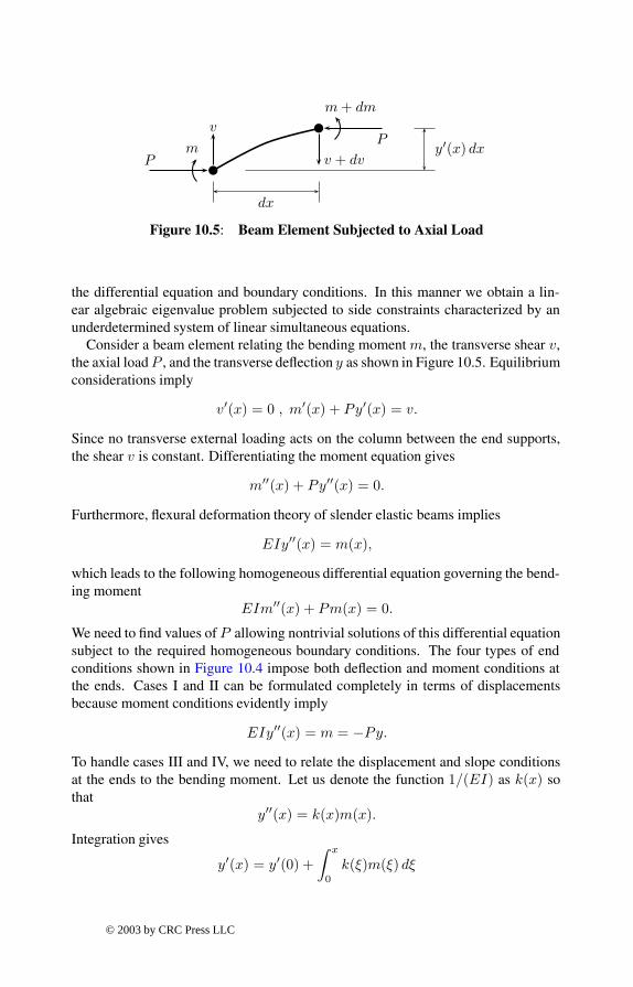
Figure 10.5: Beam Element Subjected to Axial Load

the differential equation and boundary conditions. In this manner we obtain a lin-ear algebraic eigenvalue problem subjected to side constraints characterized by anunderdetermined system of linear simultaneous equations.

Consider a beam element relating the bending moment m, the transverse shear v,the axial loadP , and the transverse deßection y as shown in Figure 10.5. Equilibriumconsiderations imply

v′(x) = 0 , m′(x) + Py′(x) = v.

Since no transverse external loading acts on the column between the end supports,the shear v is constant. Differentiating the moment equation gives

m′′(x) + Py′′(x) = 0.

Furthermore, ßexural deformation theory of slender elastic beams implies

EIy′′(x) = m(x),

which leads to the following homogeneous differential equation governing the bend-ing moment

EIm′′(x) + Pm(x) = 0.

We need to Þnd values of P allowing nontrivial solutions of this differential equationsubject to the required homogeneous boundary conditions. The four types of endconditions shown in Figure 10.4 impose both deßection and moment conditions atthe ends. Cases I and II can be formulated completely in terms of displacementsbecause moment conditions evidently imply

EIy′′(x) = m = −Py.To handle cases III and IV, we need to relate the displacement and slope conditionsat the ends to the bending moment. Let us denote the function 1/(EI) as k(x) sothat

y′′(x) = k(x)m(x).

Integration gives

y′(x) = y′(0) +∫ x

0

k(ξ)m(ξ) dξ


and

y(x) = y(0) + y′(0)x+∫ x

0

(x− ξ)k(ξ)m(ξ) dξ.

The boundary conditions for the pinned-Þxed case require that

a) y(0) = 0, b) y′(L) = 0, c) y(L) = 0.

Condition b) requires

y′(0) = −∫ L

0

k(ξ)m(ξ) dξ,

whereas a) and c) combined lead to

y(L) = y(0) − L

∫ L

0

kmdξ +∫ L

0

(L− ξ)kmdξ.

Consequently for Cases III and IV the governing equation is

EIm′′(x) + Pm(x) = 0.

The boundary conditions for Case III are

m(0) = 0 and∫ L

0

xk(x)m(x) dx = 0.

The boundary conditions for Case IV are handled similarly. Since we must havey′(0) = y′(L) = 0 and y(0) = y(L) = 0, the conditions are∫ L

0

k(x)m(x) dx = 0 and∫ L

0

xk(x)m(x) dx = 0.

The results for each case require a nontrivial solution of a homogeneous differ-ential equation satisfying homogeneous boundary conditions as summarized in thetable below.

Each of these boundary value problems can be transformed to linear algebraicform by choosing a set of evenly spaced grid points across the span and approximat-ing y′′(x) by Þnite differences. It follows from Taylors series that

y′′(x) =y(x− h) − 2y(x) + y(x+ h)

h2+O(h2).

For sufÞciently small h, we neglect the truncation error and write

y′′ =y−1 − 2y + y+1

h2

where y is the approximation to y at x = x = h for 1 ≤ ≤ n , where the stepsizeh = L/(n+ 1). Thus we have

(EI)[y−1 − 2y + y+1]h2

+ Py = 0


Case Differential BoundaryEquation Conditions

I: pinned-pinned EIy ′′(x) + Py(x) = 0 y(0) = 0

y(L) = 0

II: free-Þxed EIy ′′(x) + Py(x) = 0 y(0) = 0

y′(L) = 0

III: pinned-Þxed EIm′′(x) + Pm(x) = 0 m(0) = 0∫ L

0k(x)m(x) dx = 0

IV: Þxed-Þxed EIm′′(x) + Pm(x) = 0∫ L

0 k(x)m(x) dx = 0∫ L

0xk(x)m(x) dx = 0

Buckling Problem Summary

for Cases I or II, and

(EI)[m−1 − 2m +m+1]h2

+ Pm = 0

for Cases III or IV. At the left end, either y or m is zero in all cases. Case I alsohas y(L) = yn+1 = 0. Case II requires y′(L) = 0. This is approximated in Þnitedifference form as

yn+1 =4yn − yn−1

3which implies for Case II that

y′′n =2(yn−1 − yn)

3h2.

Cases III and IV are slightly more involved than I and II . The condition that

∫ L

0

mx

EIdx = 0

can be formulated using the trapezoidal rule to give

b1 ∗ [m1, . . . ,mn,mn+1]T = 0,

where the asterisk indicates matrix multiplication involving a row matrix b 1 deÞnedby

b1 = [1, 1, . . . , 1, 1/2] .* [x1, x2, . . . , xn, L] ./ [EI1, . . . , EIn, EIn+1].


Similarly, the condition ∫ L

0

m

EIdx = 0

leads to

b2 ∗ [m1, . . . ,mn]T +12

[m0

EI0+mn+1

EIn+1

]= 0

with

b2 =[

1EI1

, . . . ,1EIn

].

The Þrst of these equations involving b1 allows mn+1 to be eliminated in Case III,whereas the two equations involving b1 and b2 allow elimination of m0 and mn+1

(the moments at x = 0 and x = L) for Case IV. Hence, in all cases, we are led to aneigenvalue problem typiÞed as

EI(−m−1 + 2m −m+1) = λm

with λ = h2P , and we understand that the equations for = 1 and = nmay requiremodiÞcation to account for pertinent boundary conditions. We are led to solve

Am = λm

where the desired buckling loads are associated with the smallest positive eigenvalueof matrix A. Cases I and II lead directly to the deßection curve forms. However,Cases III and IV require that the deßection curve be computed from the trapezoidalrule as

y′(x) = y′(0) +∫ x

0

m

EIdx

and

y(x) = y(0) + y′(0) + x

∫ x

0

m

EIdx−

∫ x

0

mx

EIdx.

The deßection curves can be normalized to make y max equal unity. This completesthe formulation needed in the buckling analysis for all four cases studied. Thesesolutions have been implemented in the program described later in this section. Anexample, which is solvable exactly, will be discussed next to demonstrate that theÞnite difference formulation actually produces good results.

10.5.1 Example for a Linearly Tapered Circular Cross Section

Consider a column with circular cross section tapered linearly from diameter h 1

at x = 0 to diameter h2 at x = L. The moment of inertia is given by

I =πd4

64,

which leads to

EI = EoIo

(1 +

sx

L

)4

,


where

s =h2 − h1

h1, Io =

πh41

64and Eo is the elastic modulus which is assumed to have a constant value. The differ-ential equation governing the moment in all cases (and for y in Case I or II) is(

1 +sx

L

)4

m′′(x) +P

EoIom(x) = 0.

This equation can be reduced to a simpler form by making a change of variables. Letus replace x and m(x) by t and g(t) deÞned by

t =(1 +

sx

L

)−1

, g(t) = tm(x).

The differential equation for g(t) is found to be

g′′(t) + λ2g(t) = 0 where λ =L

|s|

√P

EoIo.

Therefore,

m(x) =(1 +

sx

L

)[c1 sin

(λ

1 + sxL

)+ c2 cos

(λ

1 + sxL

)]

where c1 and c2 are arbitrary constants found by imposing the boundary conditions.We will determine these constants for Cases I, II, and III. Case IV can be solvedsimilarly and is left as an exercise for the reader.

To deal with Cases I, II, and III it is convenient to begin with a solution thatvanishes at x = 0. A function satisfying this requirement has the form

m(x) =(1 +

sx

L

)sin

(λ

1 + sxL

− λ

).

This equation can also represent the deßection curve for Cases I and II or the momentcurve for Case III. Imposition of the remaining boundary conditions leads to aneigenvalue equation which is used to determine λ and the buckling load P . Thedeßection curve for Case I is taken as

y(x) =(1 +

sx

L

)sin

(λ

1 + sxL

− λ

)

and the requirement that y(L) = 0 yields

λs

1 + s=

(s

1 + s

)(L

s

√P

EoIo

)= π.

This means that the buckling load is

P =π2EoIoL2

(1 + s)2 where s =h2 − h1

h1.


Therefore the buckling load for the tapered column (s = 0) is simply obtained bymultiplying the buckling load for the constant cross section column (s = 0) by afactor

(1 + s)2 =(h2

h1

)2

.

This is also true for Cases III and IV, but is not true for Case II. Let us derive thecharacteristic equation for Case III. The constraint condition for the pinned-Þxedcase requires ∫ L

0

xm(x)EI

dx = 0.

So we need ∫ L

0

x(1 +

sx

L

)−3

sin(

λ

1 + sxL

− λ

)dx = 0.

This equation can be integrated using the substitution (1 + sx/L)−1 = t. This leadsto a characteristic equation of the form

θ = tan θ , θ =λs

1 + s=

L

1 + s

√P

EoIo.

The smallest positive root of this equation is θ = 4.4934, which yields

P =20.1906EoIo

L2(1 + s)2 for Case III.

Further analysis produces

P =4π2EoIoL2

(1 + s)2 for Case IV.

The characteristic equation for Case II can be obtained by starting with the Case Ideßection equation and imposing the condition y ′(L) = 0. This leads to

s sin θ + θ cos θ = 0 , θ =L

1 + s

√P

EoIo.

When s = 0, the smallest positive root of this equation is θ = π/2. Therefore, thebuckling load (when s = 0) is

P =π2EoIo

4L2

for Case II, and the dependence on s found in the other cases does not hold for thefree-Þxed problem.


10.5.2 Numerical Results

The function colbuc, which uses the above relationships, was written to analyzevariable depth columns using any of the four types of end conditions discussed. Theprogram allows a piecewise linear variation of EI . The program employs the func-tion lintrp for interpolation and the function trapsum to perform trapezoidal ruleintegration. Comparisons were made with results presented by Beer and Johnston[9] and a comprehensive handbook on stability [19]. We will present some examplesto show how well the program works. It is known that a column of length L andconstant cross section stiffness EoIo has buckling loads of

π2EoIoL2

,π2EoIo(2L)2

,π2EoIo

(0.6992L)2,π2EoIo(0.5L)2

for the pinned-pinned, the free-Þxed, the pinned-Þxed, and the Þxed-Þxed end con-ditions respectively. These cases were veriÞed using the program colbuc. Let us il-lustrate the capability of the program to approximately handle a discontinuous crosssection change. We analyze a column twenty inches long consisting of a ten inchsection pinned at the outer end and joined to a ten inch long section which is consid-ered rigid and Þxed at the outer end. We use EoIo = 1 for the ßexible section andEoIo = 10000 for the rigid section. This conÞguration should behave much like apinned-Þxed column of length 100 with a buckling load of (π/6.992) 2 = 0.2019.

Using 100 segments (nseq=100) the program yields a value of 0.1976, whichagrees within 2.2% of the expected value. A graph of the computed deßection con-Þguration is shown in Figure 10.6. The code necessary to solve this problem is:

ei=[1 0; 1 10; 10000 10; 10000 20];nseg=100; endc=3; len=20;[p,y,x]=colbuc(len,ei,nseg,endc)

For a second example we consider a ten inch long column of circular cross sectionwhich is tapered from a one inch diameter at one end to a two inch diameter at theother end. We employ a Þxed-Þxed end condition and use E o = 1. The theoreticalresults for this conÞguration indicate a buckling load of π 3/400 = 0.07752.

Using 100 segments the program produces a value of 0.07728, which agreeswithin 0.3% of the exact result. The code to generate this result utilizes functioneilt:

ei=eilt(1,2,10,101,1);[p,y,x]=colbuc(10,ei,100,4);

The examples presented illustrate the effectiveness of using Þnite difference meth-ods in conjunction with the intrinsic eigenvalue solver in MATLAB to compute buck-


0 2 4 6 8 10 12 14 16 18 200

0.1

0.2

0.3

0.4

0.5

0.6

0.7

0.8

0.9

1

axial direction

tran

sver

se d

efle

ctio

n

Pinned−Fixed Buckling Load = 0.1975

Figure 10.6: Analysis of Discontinuous Pinned-Fixed Column

ling loads. Furthermore, the provision for piecewise linear EI variation provided inthe program is adequate to handle various column shapes.

Program Output and Code

Function colbuc

1: function [p,y,x]=colbuc(len,ei,nseg,endc)2: % [p,y,x]=colbuc(len,ei,nseg,endc)3: % ~~~~~~~~~~~~~~~~~~~~~~~~~~~~~~~~4: %5: % This function determines the Euler buckling6: % load for a slender column of variable cross7: % section which can have any one of four8: % constraint conditions at the column ends.9: %

10: % len - the column length11: % ei - the product of Young’s modulus and the12: % cross section moment of inertia. This13: % quantity is defined as a piecewise


14: % linear function specified at one or15: % more points along the length. ei(:,1)16: % contains ei values at points17: % corresponding to x values given in18: % ei(:,2). Values at intermediate points19: % are computed by linear interpolation20: % using function lintrp which allows21: % jump discontinuities in ei.22: % nseg - the number of segments into which the23: % column is divided to perform finite24: % difference calculations.The stepsize h25: % equals len/nseg.26: % endc - a parameter specifying the type of end27: % condition chosen.28: % endc=1, both ends pinned29: % endc=2, x=0 free, x=len fixed30: % endc=3, x=0 pinned, x=len fixed31: % endc=4, both ends fixed32: %33: % p - the Euler buckling load of the column34: % x,y - vectors describing the shape of the35: % column in the buckled mode. x varies36: % between 0 and len. y is normalized to37: % have a maximum value of one.38: %39: % User m functions called: lintrp, trapsum40:

41: if nargin==0;42: ei=[1 0; 1 10; 1000 10; 1000 20];43: nseg=100; endc=3; len=20;44: end45:

46: % If the column has constant cross section,47: % then ei can be given as a single number.48: % Also, use at least 20 segments to assure49: % that computed results will be reasonable.50: if size(ei,1) < 251: ei=[ei(1,1),0; ei(1,1),len];52: end53: nseg=max(nseg,30);54:

55: if endc==156: % pinned-pinned case (y=0 at x=0 and x=len)57: str=’Pinned-Pinned Buckling Load = ’;58: h=len/nseg; n=nseg-1; x=linspace(h,len-h,n);


59: eiv=lintrp(ei(:,2),ei(:,1),x);60: a=-diag(ones(n-1,1),1);61: a=a+a’+diag(2*ones(n,1));62: [yvecs,pvals]=eig(diag(eiv/h^2)*a);63: pvals=diag(pvals);64: % Discard any spurious nonpositive eigenvalues65: j=find(pvals<=0);66: if length(j)>0, pvals(j)=[]; yvecs(:,j)=[]; end67: [p,k]=min(pvals); y=[0;yvecs(:,k);0];68: [ym,j]=max(abs(y)); y=y/y(j); x=[0;x(:);len];69: elseif endc==270: % free-fixed case (y=0 at x=0 and y’=0 at x=len)71: str=’Free-Fixed Buckling Load = ’;72: h=len/nseg; n=nseg-1; x=linspace(h,len-h,n);73: eiv=lintrp(ei(:,2),ei(:,1),x);74: a=-diag(ones(n-1,1),1);75: a=a+a’+diag(2*ones(n,1));76: % Zero slope at x=len implies77: % y(n+1)=4/3*y(n)-1/3*y(n-1). This78: % leads to y’’(n)=(y(n-1)-y(n))*2/(3*h^2).79: a(n,[n-1,n])=[-2/3,2/3];80: [yvecs,pvals]=eig(diag(eiv/h^2)*a);81: pvals=diag(pvals);82: % Discard any spurious nonpositive eigenvalues83: j=find(pvals<=0);84: if length(j)>0, pvals(j)=[]; yvecs(:,j)=[]; end85: [p,k]=min(pvals); y=yvecs(:,k);86: y=[0;y;4*y(n)/3-y(n-1)/3]; [ym,j]=max(abs(y));87: y=y/y(j); x=[0;x(:);len];88: elseif endc==389: % pinned-fixed case90: % (y=0 at x=0 and x=len, y’=0 at x=len)91: str=’Pinned-Fixed Buckling Load = ’;92: h=len/nseg; n=nseg; x=linspace(h,len,n);93: eiv=lintrp(ei(:,2),ei(:,1),x);94: a=-diag(ones(n-1,1),1);95: a=a+a’+diag(2*ones(n,1));96: % Use a five point backward difference97: % approximation for the second derivative98: % at x=len.99: v=-[35/12,-26/3,19/2,-14/3,11/12];

100: a(n,n:-1:n-4)=v; a=diag(eiv/h^2)*a;101: % Form the equation requiring zero deflection102: % at x=len.103: b=x(:)’.*[ones(1,n-1),1/2]./eiv(:)’;


104: % Impose the homogeneous boundary condition105: q=null(b); [z,pvals]=eig(q’*a*q);106: pvals=diag(pvals);107: % Discard any spurious nonpositive eigenvalues108: k=find(pvals<=0);109: if length(k)>0, pvals(k)=[]; z(:,k)=[]; end;110: vecs=q*z; [p,k]=min(pvals); mom=[0;vecs(:,k)];111: % Compute the slope and deflection from112: % moment values.113: yp=trapsum(0,len,mom./[1;eiv(:)]);114: yp=yp-yp(n+1); y=trapsum(0,len,yp);115: [ym,j]=max(abs(y)); y=y/y(j); x=[0;x(:)];116: else117: % fixed-fixed case118: % (y and y’ both zero at each end)119: str=’Fixed-Fixed Buckling Load = ’;120: h=len/nseg; n=nseg+1; x=linspace(0,len,n);121: eiv=lintrp(ei(:,2),ei(:,1),x);122: a=-diag(ones(n-1,1),1);123: a=a+a’+diag(2*ones(n,1));124: % Use five point forward and backward125: % difference approximations for the second126: % derivatives at each end.127: v=-[35/12,-26/3,19/2,-14/3,11/12];128: a(1,1:5)=v; a(n,n:-1:n-4)=v;129: a=diag(eiv/h^2)*a;130: % Write homogeneous equations to make the131: % slope and deflection vanish at x=len.132: b=[1/2,ones(1,n-2),1/2]./eiv(:)’;133: b=[b;x(:)’.*b];134: % Impose the homogeneous boundary conditions135: q=null(b); [z,pvals]=eig(q’*a*q);136: pvals=diag(pvals);137: % Discard any spurious nonpositive eigenvalues138: k=find(pvals<=0);139: if length(k>0), pvals(k)=[]; z(:,k)=[]; end;140: vecs=q*z; [p,k]=min(pvals); mom=vecs(:,k);141: % Compute the moment and slope from moment142: % values.143: yp=trapsum(0,len,mom./eiv(:));144: y=trapsum(0,len,yp);145: [ym,j]=max(abs(y)); y=y/y(j);146: end147:

148: close;


149: plot(x,y); grid on;150: xlabel(’axial direction’);151: ylabel(’transverse deflection’);152: title([str,num2str(p)]); figure(gcf);153: print -deps buck154:

155: %=============================================156:

157: function v=trapsum(a,b,y,n)158: %159: % v=trapsum(a,b,y,n)160: % ~~~~~~~~~~~~~~~~~~161: %162: % This function evaluates:163: %164: % integral(a=>x, y(x)*dx) for a<=x<=b165: %166: % by the trapezoidal rule (which assumes linear167: % function variation between succesive function168: % values).169: %170: % a,b - limits of integration171: % y - integrand which can be a vector valued172: % function returning a matrix such that173: % function values vary from row to row.174: % It can also be input as a matrix with175: % the row size being the number of176: % function values and the column size177: % being the number of components in the178: % vector function.179: % n - the number of function values used to180: % perform the integration. When y is a181: % matrix then n is computed as the number182: % of rows in matrix y.183: %184: % v - integral value185: %186: % User m functions called: none187: %----------------------------------------------188:

189: if isstr(y)190: % y is an externally defined function191: x=linspace(a,b,n)’; h=x(2)-x(1);192: Y=feval(y,x); % Function values must vary in193: % row order rather than column


194: % order or computed results195: % will be wrong.196: m=size(Y,2);197: else198: % y is column vector or a matrix199: Y=y; [n,m]=size(Y); h=(b-a)/(n-1);200: end201: v=[zeros(1,m); ...202: h/2*cumsum(Y(1:n-1,:)+Y(2:n,:))];203:

204: %=============================================205:

206: function ei=eilt(h1,h2,L,n,E)207: %208: % ei=eilt(h1,h2,L,n,E)209: % ~~~~~~~~~~~~~~~~~~~~210: %211: % This function computes the moment of inertia212: % along a linearly tapered circular cross213: % section and then uses that value to produce214: % the product EI.215: %216: % h1,h2 - column diameters at each end217: % L - column length218: % n - number of points at which ei is219: % computed220: % E - Young’s modulus221: %222: % ei - vector of EI values along column223: %224: % User m functions called: none225: %----------------------------------------------226:

227: if nargin<5, E=1; end;228: x=linspace(0,L,n)’;229: ei=E*pi/64*(h1+(h2-h1)/L*x).^4;230: ei=[ei(:),x(:)];231:

232: %=============================================233:

234: % function y=lintrp(xd,yd,x)235: % See Appendix B


10.6 Accuracy Comparison for Euler Beam Natural Frequenciesby Finite Element and Finite Difference Methods

Next we consider three different methods of natural frequency computation fora cantilever beam. Comparisons are made among results from: a) the solution ofthe frequency equation for the true continuum model; b) the approximation of theequations of motion using Þnite differences to replace the spatial derivatives; and c)the use of Þnite element methods yielding a piecewise cubic spatial interpolation ofthe displacement Þeld. The Þrst method is less appealing as a general tool than thelast two methods because the frequency equation is difÞcult to obtain for geometriesof variable cross section. Frequencies found using Þnite difference and Þnite ele-ment methods are compared with results from the exact model; and it is observedthat the Þnite element method produces results that are superior to those from Þnitedifferences for comparable degrees of freedom. In addition, the natural frequenciesand mode shapes given by Þnite elements are used to compute and animate the sys-tem response produced when a beam, initially at rest, is suddenly subjected to twoconcentrated loads.

10.6.1 Mathematical Formulation

The differential equation governing transverse vibrations of an elastic beam ofconstant depth is [69]

EI∂4Y

∂X4= −ρ∂

2Y

∂T 2+W (X,T ) 0 ≤ X ≤ , T ≥ 0

where

Y (X,T ) transverse displacement,X horizontal position along the beam length,T time,EI product of moment of inertia and Youngs modulus,ρ mass per unit length of the beam,

W (X,T ) external applied force per unit length.

In the present study, we consider the cantilever beam shown in Figure 10.7, havingend conditions which are

Y (0, T ) = 0 ,∂Y (0, T )∂X

= 0 , EI∂2Y (, T )∂X2

= ME(T ) , and EI∂3Y (, T )∂X3

= VE(T ).

This problem can be expressed more concisely using dimensionless variables

x =X

, y =

Y

and t =

√EI

ρ

(T

2

).


EI, ρ, l

ME

W(X)

VE

Y

X

Figure 10.7: Cantilever Beam Subjected to Impact Loading

Then the differential equation becomes

∂4y

∂x4= −∂

2y

∂t2+ w(x, t),

and the boundary conditions reduce to

y(0, t) = 0 ,∂y

∂x(0, t) = 0 ,

∂2y

∂x2(1, t) = me(t) and

∂3y

∂x3(1, t) = ve(t)

where

w = (W3)/(EI) , me = (ME)/(EI) and ve = (VE2)/(EI).

The natural frequencies of the system are obtained by computing homogeneous so-lutions of the form y(x, t) = f(x) sin(ωt) which exist when w = me = ve = 0.This implies

d4f

dx4= λ4f where λ =

√ω,

subject tof(0) = 0 , f ′(0) = 0 , f ′′(1) = 0 , f ′′′(1) = 0.

The solution satisfying this fourth order differential equation with homogeneousboundary conditions has the form

f = [cos(λx)−cosh(λx)][sin(λ)+sinh(λ)]−[sin(λx)−sinh(λx)][cos(λ)+cosh(λ)],

where λ satisÞes the frequency equation

p(λ) = cos(λ) + 1/ cosh(λ) = 0.

Although the roots cannot be obtained explicitly, asymptotic approximations existfor large n:

λn = (2k − 1)π/2.


These estimates can be used as the starting points for Þnding approximate roots ofthe frequency equation using Newtons method:

λNEW = λOLD − p(λOLD)/p′(λOLD).

The exact solution will be used to compare related results produced by Þnite differ-ence and Þnite element methods. First we consider Þnite differences. The followingdifference formulas have a quadratic truncation error derivable from Taylors series[1]:

y′(x) = [−y(x− h) + y(x+ h)]/(2h),y′′(x) = [y(x− h) − 2y(x) + y(x+ h)]/h2,

y′′′(x) = [−y(x− 2h) + 2y(x− h) − 2y(x+ h) + y(x+ 2h)]/(2h3),y′′′′(x) = [y(x− 2h) − 4y(x− h) + 6y(x) − 4y(x+ h) + y(x+ 2h)]/h4.

The step-size is h = 1/n so that x = h, 0 ≤ ≤ n, where x0 is at the left endand xn is at the right end of the beam. It is desirable to include additional Þctitiouspoints x−1, xn+1 and xn+2. Then the left end conditions imply

y0 = y1 and y−1 = y1,

and the right end conditions imply

yn+1 = −yn−1 + 2yn and yn+2 = yn−2 − 4yn−1 + 4yn.

Using these relations, the algebraic eigenvalue problem derived from the differenceapproximation is

7y1 − 4y2 + y3 = λy1,

−4y1 + 6y2 − 4y3 + y4 = λfy2,

y−2 − 4y−1 + 6y − 4y+1 + y+2 = λy , 2 < < (n− 1),

yn−3 − 4yn−2 + 5yn−1 − 2yn = λyn−1,

2yn−2 − 4yn−1 + 2yn = λyn,

where λ = h4λ.The Þnite element method leads to a similar problem involving global mass and

stiffness matrices [54]. When we consider a single beam element of mass m andlength , the elemental mass and stiffness matrices found using a cubically varyingdisplacement approximation are

Me =m

420

156 22 54 −1322 42 13 −32

54 13 156 −22−13 −32 −22 42

, Ke =

EI

3

6 3 −6 33 22 −3 2

−6 −3 6 −33 2 −3 22

,

and the elemental equation of motion has the form

MeY′′e +KeYe = Fe


whereYe = [Y1, Y

′1 , Y2, Y

′2 ]T and Fe = [F1,M1, F2,M2]T

are generalized elemental displacement and force vectors. The global equation ofmotion is obtained as an assembly of element matrices and has the form

MY ′′ +KY = F.

A system with N elements involves N + 1 nodal points. For the cantilever beamstudied here both Y0 and Y

′0 are zero. So removing these two variables leaves a

system of n = 2N unknowns. The solution of this equation in the case of a non-resonant harmonic forcing function will be discussed further. The matrix analog ofthe simple harmonic equation is

MY +KY = F1 cos(ωt) + F2, sin(ωt)

with initial conditionsY (0) = Y0 and Y (0) = V0.

The solution of this differential equation is the sum of a particular solution and ahomogeneous solution:

Y = YP + YH ,

whereYH = Y1 cos(ωt) + Y2 sin(ωt)

withY = (K − ω2M)−1F = 1, 2.

This assumes thatK−ω2M is nonsingular. The homogeneous equation satisÞes theinitial conditions

YH(0) = Y0 − Y1 , YH(0) = V0 − ωY2.

The homogeneous solution components have the form

YH = U cos(ωt+ φ)

where ω and U are natural frequencies and modal vectors satisfying the eigenvalueequation

KU = ω2MU.

Consequently, the homogeneous solution completing the modal response is

YH(t) =n∑

=1

U[cos(ωt)c + sin(ωt)d/ω]

where c and d are computed to satisfy the initial conditions which require

C = U−1(Y0 − Y1) and D = U−1(V0 − ωY2).

The next section presents the MATLAB program. Natural frequencies from Þnitedifference and Þnite element matrices are compared and modal vectors from theÞnite element method are used to analyze a time response problem.


10.6.2 Discussion of the Code

A program was written to compare exact frequencies from the original continuousbeam model with approximations produced using Þnite differences and Þnite ele-ments. The Þnite element results were also employed to calculate a time response bymodal superposition for any structure that has general mass and stiffness matrices,and is subjected to loads which are constant or harmonically varying.

The code below is fairly long because various MATLAB capabilities are appliedto three different solution methods. The following function summary involves ninefunctions, several of which were used earlier in the text.

cbfreq driver to input data, call computation modules, andprint results

cbfrqnwm function to compute exact natural frequencies by New-tons method for root calculation

cbfrqfdm forms equations of motion using Þnite differences andcalls eig to compute natural frequencies

cbfrqfem uses the Þnite element method to form the equationof motion and calls eig to compute natural frequenciesand modal vectors

frud function which solves the structural dynamics equationby methods developed in Chapter 7

examplmo evaluates the response caused when a downward loadat the middle and an upward load at the free end areapplied

animate plots successive positions of the beam to animate themotion

plotsave plots the beam frequencies for the three methods. Alsoplots percent errors showing how accurate Þnite ele-ment and Þnite difference methods are

inputv reads a sequence of numbers

Table 10.2: Functions Used in the Beam Code

Several characteristics of the functions assembled for this program are worth exam-ining in detail. The next table contains remarks relevant to the code.

Routine Line OperationOutput Natural frequencies are printed along with er-

ror percentages. The output shown here hasbeen extracted from the actual output to showonly the highest and lowest frequencies.

continued on next page


continued from previous pageRoutine Line Operationcbfrqnwm 99 Asymptotic estimates are used to start a New-

ton method iteration.102-108 Root corrections are carried out for all roots

until the correction to any root is sufÞcientlysmall.

cbfrqfdm 135-136 The equations of motion are formed withoutcorrections for end conditions.

138-145 End conditions are applied.149*150 eig computes the frequencies.

cbfrqfem 182-186 Form elemental mass matrix.189-192 Form elemental stiffness matrix.198-201 Global equations of motion are formed using

an element by element loop.205 Boundary conditions are applied requiring

zero displacement and slope at the left end,and zero moment and shear at the right end.

208-214 Frequencies and modal vectors are computed.Note that modal vector computation is madeoptional since this takes longer than onlycomputing frequencies.

frud Compute time response by modal superpo-sition. Theoretical details pertaining to thisfunction appear in Chapter 7.

examplmo 292-296 The time step and maximum time for re-sponse calculation is selected.

300-301 Function frud is used to compute displace-ment and rotation response. Only displace-ment is saved.

304-307 Free end displacement is plotted.314-319 A surface showing displacement as a function

of position and time is shown.324-326 Function animate is called.

animate 364-369 Window limits are determined.373-381 Each position is plotted. Then it is erased be-

fore proceeding to the next position.plotsave Plot and save graphs showing the frequencies

and error percentages.

Table 10.3: Description of Code in Example

10.6.3 Numerical Results

The dimensionless frequency estimates from the Þnite difference and the Þnite el-ement methods were compared for various numbers of degrees-of-freedom. Typical


0 10 20 30 40 50 60 70 80 90 10010

0

101

102

103

104

105

106

Cantilever Beam Frequencies

frequency number

freq

uenc

y va

lues

Exact freq.Felt. freq.Fdif. freq.

Figure 10.8: Cantilever Beam Frequencies

program output for n = 100 is shown at the end of this section. The frequency resultsand error percentages are shown in Figures 10.8 and 10.9. It is evident that the Þnitedifference frequencies are consistently low and the Þnite element results are consis-tently high. The Þnite difference estimates degrade smoothly with increasing order.The Þnite element frequencies are surprisingly accurate for ω k when k < n/2. Atk = n/2 and k = n, the Þnite element error jumps sharply. This peculiar error jumphalfway through the spectrum has also been observed in [54]. The most importantand useful result seen from Figure 10.9 is that in order to obtain a particular numberof frequencies, say N, which are accurate within 3.5%, it is necessary to employmore than 2N elements and keep only half of the predicted values.

The Þnal result presented is the time response of a beam which is initially at restwhen a concentrated downward load of Þve units is applied at the middle and a oneunit upward load is applied at the free end. The time history was computed usingfunction frud. Figure 10.10 shows the time history of the free end. Figure 10.11is a surface plot illustrating how the deßection pattern changes with time. Finally,Figure 10.12 shows successive deßection positions produced by function animate.The output was obtained by suppressing the graph clearing option for successiveconÞgurations.


0 10 20 30 40 50 60 70 80 90 1000

10

20

30

40

50

60Cantilever Beam Frequency Error Percentages

frequency number

perc

ent f

requ

ency

err

or

Fdif. pct. errorFelt. pct. error

Figure 10.9: Cantilever Beam Frequency Error Percentages

0 0.5 1 1.5 2 2.5 3 3.5 4 4.5 5−0.6

−0.5

−0.4

−0.3

−0.2

−0.1

0

0.1Position of the Free End of the Beam

dimensionless time

end

defle

ctio

n

Figure 10.10: Position of the Free End of the Beam versus Time


00.2

0.40.6

0.81 0

1

2

3

4

5

−0.6

−0.4

−0.2

0

0.2

0.4

0.6

time

Cantilever Beam Deflection for Varying Position and Time

x axis

defle

ctio

n

Figure 10.11: Beam Deßection History

Beam Animation

Figure 10.12: Beam Animation


MATLAB Example

Output from Example

>> cbfreq

CANTILEVER BEAM FREQUENCIES BY FINITE DIFFERENCE ANDFINITE ELEMENT APPROXIMATION

Give the number of frequencies to be computed(use an even number greater than 2)? > 100

freq. exact. fdif. fd. pct. felt. fe. pct.number freq. freq. error freq. error

1 3.51602e+00 3.51572e+00 -0.008 3.51602e+00 0.0002 2.20345e+01 2.20250e+01 -0.043 2.20345e+01 0.0003 6.16972e+01 6.16414e+01 -0.090 6.16972e+01 0.0004 1.20902e+02 1.20714e+02 -0.155 1.20902e+02 0.0005 1.99860e+02 1.99386e+02 -0.237 1.99860e+02 0.0006 2.98556e+02 2.97558e+02 -0.334 2.98558e+02 0.0017 4.16991e+02 4.15123e+02 -0.448 4.16999e+02 0.0028 5.55165e+02 5.51957e+02 -0.578 5.55184e+02 0.0039 7.13079e+02 7.07918e+02 -0.724 7.13119e+02 0.006

10 8.90732e+02 8.82842e+02 -0.886 8.90809e+02 0.00911 1.08812e+03 1.07655e+03 -1.064 1.08826e+03 0.01312 1.30526e+03 1.28884e+03 -1.257 1.30550e+03 0.01913 1.54213e+03 1.51950e+03 -1.467 1.54252e+03 0.02614 1.79874e+03 1.76830e+03 -1.692 1.79937e+03 0.03515 2.07508e+03 2.03497e+03 -1.933 2.07605e+03 0.04716 2.37117e+03 2.31926e+03 -2.189 2.37261e+03 0.06117 2.68700e+03 2.62088e+03 -2.461 2.68908e+03 0.07718 3.02257e+03 2.93951e+03 -2.748 3.02551e+03 0.09819 3.37787e+03 3.27486e+03 -3.050 3.38197e+03 0.12120 3.75292e+03 3.62657e+03 -3.367 3.75851e+03 0.149

====== INTERMEDIATE LINES OF OUTPUT DELETED ======

90 7.90580e+04 3.88340e+04 -50.879 1.09328e+05 38.28891 8.08345e+04 3.90347e+04 -51.710 1.11989e+05 38.54192 8.26308e+04 3.92169e+04 -52.540 1.14512e+05 38.58293 8.44468e+04 3.93804e+04 -53.367 1.16860e+05 38.38494 8.62825e+04 3.95250e+04 -54.191 1.18999e+05 37.91795 8.81380e+04 3.96507e+04 -55.013 1.20889e+05 37.15996 9.00133e+04 3.97572e+04 -55.832 1.22496e+05 36.08697 9.19082e+04 3.98445e+04 -56.648 1.23786e+05 34.68498 9.38229e+04 3.99125e+04 -57.460 1.24730e+05 32.94199 9.57574e+04 3.99611e+04 -58.268 1.25305e+05 30.857

100 9.77116e+04 3.99903e+04 -59.073 1.49694e+05 53.200

Evaluate the time response from twoconcentrated loads. One downward at themiddle and one upward at the free end.

input the time step and the maximum time(0.04 and 5.0) are typical. Use 0,0 to stop


? .04,5

Evaluate the time response resulting from aconcentrated downward load at the middle andan upward end load.

input the time step and the maximum time(0.04 and 5.0) are typical. Use 0,0 to stop

? 0,0

Program cbfrq

1: function cbfreq2: % Example: cbfreq3: % ~~~~~~~~~~~~~~~~4: % This program computes approximate natural5: % frequencies of a uniform depth cantilever6: % beam using finite difference and finite7: % element methods. Error results are presented8: % which demonstrate that the finite element9: % method is much more accurate than the finite

10: % difference method when the same matrix orders11: % are used in computation of the eigenvalues.12: %13: % User m functions required:14: % cbfrqnwm, cbfrqfdm, cbfrqfem, frud,15: % examplmo, beamanim, plotsave, inputv16:

17: clear, fprintf(’\n\n’)18: fprintf(’CANTILEVER BEAM FREQUENCIES BY ’)19: fprintf(’FINITE DIFFERENCE AND’)20: fprintf(...21: ’\n FINITE ELEMENT APPROXIMATION\n’)22:

23: fprintf(’\nGive the number of frequencies ’)24: fprintf(’to be computed’)25: fprintf(’\n(use an even number greater ’)26: fprintf(’than 2)\n’), n=input(’? > ’);27: if rem(n,2) ~= 0, n=n+1; end28:

29: % Exact frequencies from solution of30: % the frequency equation31: wex = cbfrqnwm(n,1e-12);32:


33: % Frequencies for the finite34: % difference solution35: wfd = cbfrqfdm(n);36:

37: % Frequencies, modal vectors, mass matrix,38: % and stiffness matrix from the finite39: % element solution.40: nelts=n/2; [wfe,mv,mm,kk] = cbfrqfem(nelts);41: pefdm=(wfd-wex)./(.01*wex);42: pefem=(wfe-wex)./(.01*wex);43:

44: nlines=17; nloop=round(n/nlines);45: v=[(1:n)’,wex,wfd,pefdm,wfe,pefem];46: disp(’ ’), lo=1;47: t1=[’ freq. exact. fdif.’ ...48: ’ fd. pct.’];49: t1=[t1,’ felt. fe. pct.’];50: t2=[’number freq. freq.’ ...51: ’ error ’];52: t2=[t2,’ freq. error ’];53: while lo < n54: disp(t1),disp(t2)55: hi=min(lo+nlines-1,n);56: for j=lo:hi57: s1=sprintf(’\n %4.0f %13.5e %13.5e’, ...58: v(j,1),v(j,2),v(j,3));59: s2=sprintf(’ %9.3f %13.5e %9.3f’, ...60: v(j,4),v(j,5),v(j,6));61: fprintf([s1,s2])62: end63: fprintf(’\n\nPress [Enter] to continue\n\n’);64: pause;65: lo=lo+nlines;66: end67: plotsave(wex,wfd,pefdm,wfe,pefem)68: nfe=length(wfe); nmidl=nfe/2;69: if rem(nmidl,2)==0, nmidl=nmidl+1; end70: x0=zeros(nfe,1); v0=x0; w=0;71: f1=zeros(nfe,1); f2=f1; f1(nfe-1)=1;72: f1(nmidl)=-5;73: xsav=examplmo(mm,kk,f1,f2,x0,v0,wfe,mv);74: close; fprintf(’All Done\n’)75:

76: %=============================================77:


78: function z=cbfrqnwm(n,tol)79: %80: % z=cbfrqnwm(n,tol)81: % ~~~~~~~~~~~~~~~~~82: % Cantilever beam frequencies by Newton’s83: % method. Zeros of84: % f(z) = cos(z) + 1/cosh(z)85: % are computed.86: %87: % n - Number of frequencies required88: % tol - Error tolerance for terminating89: % the iteration90: % z - Dimensionless frequencies are the91: % squares of the roots of f(z)=092: %93: % User m functions called: none94: %----------------------------------------------95:

96: if nargin ==1, tol=1.e-5; end97:

98: % Base initial estimates on the asymptotic99: % form of the frequency equation

100: zbegin=((1:n)-.5)’*pi; zbegin(1)=1.875; big=10;101:

102: % Start Newton iteration103: while big > tol104: t=exp(-zbegin); tt=t.*t;105: f=cos(zbegin)+2*t./(1+tt);106: fp=-sin(zbegin)-2*t.*(1-tt)./(1+tt).^2;107: delz=-f./fp;108: z=zbegin+delz; big=max(abs(delz)); zbegin=z;109: end110: z=z.*z;111:

112: %=============================================113:

114: function [wfindif,mat]=cbfrqfdm(n)115: %116: % [wfindif,mat]=cbfrqfdm(n)117: % ~~~~~~~~~~~~~~~~~~~~~~~~~118: % This function computes approximate cantilever119: % beam frequencies by the finite difference120: % method. The truncation error for the121: % differential equation and boundary122: % conditions are of order h^2.


123: %124: % n - Number of frequencies to be125: % computed126: % wfindif - Approximate frequencies in127: % dimensionless form128: % mat - Matrix having eigenvalues which129: % are the square roots of the130: % frequencies131: %132: % User m functions called: none133: %----------------------------------------------134:

135: % Form the primary part of the frequency matrix136: mat=3*diag(ones(n,1))-4*diag(ones(n-1,1),1)+...137: diag(ones(n-2,1),2); mat=(mat+mat’);138:

139: % Impose left end boundary conditions140: % y(0)=0 and y’(0)=0141: mat(1,[1:3])=[7,-4,1]; mat(2,[1:4])=[-4,6,-4,1];142:

143: % Impose right end boundary conditions144: % y’’(1)=0 and y’’’(1)=0145: mat(n-1,[n-3:n])=[1,-4,5,-2];146: mat(n,[n-2:n])=[2,-4,2];147:

148: % Compute approximate frequencies and149: % sort these values150: w=eig(mat); w=sort(w); h=1/n;151: wfindif=sqrt(w)/(h*h);152:

153: %=============================================154:

155: function [wfem,modvecs,mm,kk]= ...156: cbfrqfem(nelts,mas,len,ei)157: %158: % [wfem,modvecs,mm,kk]=159: % cbfrqfem(nelts,mas,len,ei)160: % ~~~~~~~~~~~~~~~~~~~~~~~~~~~~~~~~~~~~~~~~~~~~~161: % Determination of natural frequencies of a162: % uniform depth cantilever beam by the Finite163: % Element Method.164: %165: % nelts - number of elements in the beam166: % mas - total beam mass167: % len - total beam length


168: % ei - elastic modulus times moment169: % of inertia170: % wfem - dimensionless circular frequencies171: % modvecs - modal vector matrix172: % mm,kk - reduced mass and stiffness173: % matrices174: %175: % User m functions called: none176: %----------------------------------------------177:

178: if nargin==1, mas=1; len=1; ei=1; end179: n=nelts; le=len/n; me=mas/n;180: c1=6/le^2; c2=3/le; c3=2*ei/le;181:

182: % element mass matrix183: masselt=me/420* ...184: [ 156, 22*le, 54, -13*le185: 22*le, 4*le^2, 13*le, -3*le^2186: 54, 13*le, 156, -22*le187: -13*le, -3*le^2, -22*le, 4*le^2];188:

189: % element stiffness matrix190: stifelt=c3*[ c1, c2, -c1, c2191: c2, 2, -c2, 1192: -c1, -c2, c1, -c2193: c2, 1, -c2, 2];194:

195: ndof=2*(n+1); jj=0:3;196: mm=zeros(ndof); kk=zeros(ndof);197:

198: % Assemble equations199: for i=1:n200: j=2*i-1+jj; mm(j,j)=mm(j,j)+masselt;201: kk(j,j)=kk(j,j)+stifelt;202: end203:

204: % Remove degrees of freedom for zero205: % deflection and zero slope at the left end.206: mm=mm(3:ndof,3:ndof); kk=kk(3:ndof,3:ndof);207:

208: % Compute frequencies209: if nargout ==1210: wfem=sqrt(sort(real(eig(mm\kk))));211: else212: [modvecs,wfem]=eig(mm\kk);


213: [wfem,id]=sort(diag(wfem));214: wfem=sqrt(wfem); modvecs=modvecs(:,id);215: end216:

217: %=============================================218:

219: function [t,x]= ...220: frud(m,k,f1,f2,w,x0,v0,wn,modvc,h,tmax)221: %222: % [t,x]=frud(m,k,f1,f2,w,x0,v0,wn,modvc,h,tmax)223: % ~~~~~~~~~~~~~~~~~~~~~~~~~~~~~~~~~~~~~~~~~~~~~224: % This function employs modal superposition225: % to solve226: %227: % m*x’’ + k*x = f1*cos(w*t) + f2*sin(w*t)228: %229: % m,k - mass and stiffness matrices230: % f1,f2 - amplitude vectors for the forcing231: % function232: % w - forcing frequency not matching any233: % natural frequency component in wn234: % wn - vector of natural frequency values235: % x0,v0 - initial displacement and velocity236: % vectors237: % modvc - matrix with modal vectors as its238: % columns239: % h,tmax - time step and maximum time for240: % evaluation of the solution241: % t - column of times at which the242: % solution is computed243: % x - solution matrix in which row j244: % is the solution vector at245: % time t(j)246: %247: % User m functions called: none248: %----------------------------------------------249:

250: t=0:h:tmax; nt=length(t); nx=length(x0);251: wn=wn(:); wnt=wn*t;252:

253: % Evaluate the particular solution.254: x12=(k-(w*w)*m)\[f1,f2];255: x1=x12(:,1); x2=x12(:,2);256: xp=x1*cos(w*t)+x2*sin(w*t);257:


258: % Evaluate the homogeneous solution.259: cof=modvc\[x0-x1,v0-w*x2];260: c1=cof(:,1)’; c2=(cof(:,2)./wn)’;261: xh=(modvc.*c1(ones(1,nx),:))*cos(wnt)+...262: (modvc.*c2(ones(1,nx),:))*sin(wnt);263:

264: % Combine the particular and265: % homogeneous solutions.266: t=t(:); x=(xp+xh)’;267:

268: %=============================================269:

270: function x=examplmo(mm,kk,f1,f2,x0,v0,wfe,mv)271: %272: % x=examplmo(mm,kk,f1,f2,x0,v0,wfe,mv)273: % ~~~~~~~~~~~~~~~~~~~~~~~~~~~~~~~~~~~~274: % Evaluate the response caused when a downward275: % load at the middle and an upward load at the276: % free end is applied.277: %278: % mm, kk - mass and stiffness matrices279: % f1, f2 - forcing function magnitudes280: % x0, v0 - initial position and velocity281: % wfe - forcing function frequency282: % mv - matrix of modal vectors283: %284: % User m functions called: frud, beamanim, inputv285: %----------------------------------------------286:

287: w=0; n=length(x0); t0=0; x=[];288: s1=[’\nEvaluate the time response from two’,...289: ’\nconcentrated loads. One downward at the’,...290: ’\nmiddle and one upward at the free end.’];291: while 1292: fprintf(s1), fprintf(’\n\n’)293: fprintf(’Input the time step and ’)294: fprintf(’the maximum time ’)295: fprintf(’\n(0.04 and 5.0) are typical.’)296: fprintf(’ Use 0,0 to stop\n’)297: [h,tmax]=inputv;298: if norm([h,tmax])==0 | isnan(h), return, end299: disp(’ ’)300:

301: [t,x]= ...302: frud(mm,kk,f1,f2,w,x0,v0,wfe,mv,h,tmax);


303: x=x(:,1:2:n-1); x=[zeros(length(t),1),x];304: [nt,nc]=size(x); hdist=linspace(0,1,nc);305:

306: clf, plot(t,x(:,nc),’k-’)307: title(’Position of the Free End of the Beam’)308: xlabel(’dimensionless time’)309: ylabel(’end deflection’), figure(gcf)310: disp(’Press [Enter] for a surface plot of’)311: disp(’transverse deflection versus x and t’)312: pause313: print -deps endpos1314: xc=linspace(0,1,nc); zmax=1.2*max(abs(x(:)));315:

316: clf, surf(xc,t,x), view(30,35)317: colormap([1 1 1])318: axis([0,1,0,tmax,-zmax,zmax])319: xlabel(’x axis’); ylabel(’time’)320: zlabel(’deflection’)321: title([’Cantilever Beam Deflection ’ ...322: ’for Varying Position and Time’])323: figure(gcf);324: print -deps endpos2325: disp(’ ’), disp([’Press [Enter] to animate’,...326: ’ the beam motion’])327: pause328:

329: titl=’Cantilever Beam Animation’;330: xlab=’x axis’; ylab=’displacement’;331: beamanim(hdist,x,0.1,titl,xlab,ylab), close332: end333:

334: %=============================================335:

336: % function beamanim(x,u,tpause,titl,xlabl,ylabl)337: % See Appendix B338:

339: %=============================================340:

341: function plotsave(wex,wfd,pefd,wfe,pefem)342: %343: % function plotsave(wex,wfd,pefd,wfe,pefem)344: % ~~~~~~~~~~~~~~~~~~~~~~~~~~~~~~~~~~~~~~~~~345: % This function plots errors in frequencies346: % computed by two approximate methods.347: %


348: % wex - exact frequencies349: % wfd - finite difference frequencies350: % wfe - finite element frequencies351: % pefd,pefem - percent errors by both methods352: %353: % User m functions called: none354: %----------------------------------------------355:

356: % plot results comparing accuracy357: % of both frequency methods358: w=[wex(:);wfd(:);wfd];359: wmin=min(w); wmax=max(w);360: n=length(wex); wht=wmin+.001*(wmax-wmin);361: j=1:n;362:

363: semilogy(j,wex,’k-’,j,wfe,’k--’,j,wfd,’k:’)364: title(’Cantilever Beam Frequencies’)365: xlabel(’frequency number’)366: ylabel(’frequency values’)367: legend(’Exact freq.’,’Felt. freq.’, ...368: ’Fdif. freq.’,2); figure(gcf)369: disp([’Press [Enter] for a frequency ’,...370: ’error plot’]), pause371: print -deps beamfrq1372:

373: plot(j,abs(pefd),’k--’,j,abs(pefem),’k-’)374: title([’Cantilever Beam Frequency ’ ...375: ’Error Percentages’])376: xlabel(’frequency number’)377: ylabel(’percent frequency error’)378: legend(’Fdif. pct. error’,’Felt. pct. error’,4)379: figure(gcf)380: disp([’Press [Enter] for a transient ’,...381: ’response calculation’])382: pause383: print -deps beamfrq2384:

385: %=============================================386:

387: % function varargout=inputv(prompt)388: % See Appendix B


10.7 Vibration Modes of an Elliptic Membrane

10.7.1 Analytical Formulation

Examples using eigenvalues and modal functions of rectangular or circular mem-branes were presented in chapter 9. In this section we analyze modal vibrations ofan elliptic membrane. In this case the natural frequencies and modal functions can-not be obtained easily in explicit form. The problem can be formulated in ellipticalcoordinates leading to Mathieu type differential equations [74]. Library routines tocompute these functions are not widely available; so, a different approach is em-ployed using least squares approximation and the MATLAB function eig. Considera membrane with major and minor semi-diameters a and b. The analytic functionz = h cosh(ς) where h =

√a2 − b2 and ζ = ξ + i η maps the rectangle deÞned by

0 ≤ ξ ≤ R = tanh−1(b/a), −π ≤ η ≤ π onto the interior of the ellipse. Thistransformation takes lines of constant ξ into a system of confocal ellipses and linesof constant η into hyperbolas intersecting the ellipses orthogonally. The followingfunction was used to produce the elliptic coordinate plot in Figure 10.13.

function z = elipmap(a,b,neta,nxi)h=sqrt(a2-b2); R=atanh(b/a);[xi,eta]=meshgrid(...linspace(0,R,nxi),linspace(-pi,pi,neta));z=h*cosh(xi+i*eta); x=real(z); y=imag(z);plot(x,y,k,x,y,k)title(ELLIPTICAL COORDINATE SYSTEM)xlabel(x axis), ylabel(y axis)axis equal, grid off, shg

Transforming the wave equation to (ξ, η) coordinates gives

Uξξ + Uηη =h2

2[cosh(2ξ) − cos(2η)]Utt,

and assuming separable solutions of the form

U = f(η)g(ξ) sin(Ω t)

leads to

f ′′(η)f(η)

+g′′(ξ)g(ξ)

= −λ [cosh(2ξ) − cos(2η)],

where λ = Ω2h2/2. So f and g are found to satisfy the following two Mathieu typedifferential equations:

f ′′(η) + [α− λ cos(2η)]f(η) = 0, −π ≤ η ≤ π


−1 −0.8 −0.6 −0.4 −0.2 0 0.2 0.4 0.6 0.8 1

−0.6

−0.4

−0.2

0

0.2

0.4

0.6

ELLIPTICAL COORDINATE SYSTEM

x axis

y ax

is

Figure 10.13: Elliptic Coordinate Grid

and

g′′(ξ) − [α− λ cosh(2ξ)]g(ξ) = 0, 0 ≤ ξ ≤ R

where the eigenvalue parameters α and λ are determined to make f(η) have period2π and make g(ξ) vanish at ξ = R. The modal functions can be written in terms ofMathieu functions as products of the form

ce(η, q)Ce(ξ, q)

for modes symmetric about the x-axis and

se(η, q)Se(ξ, q)

for modes anti-symmetric about the x-axis. The functions ce and se are periodicMathieu functions pertaining to the circumferential direction, while Ce and Se aremodiÞed Mathieu functions pertaining to the radial direction. The structure of thesefunctions motivates using the following series approximation for the functions foreven modes:

f(η) =N∑

k=1

cos(η(k − 1)) ak, g(ξ) =M∑l=1

cos(πξ

R(l − 1/2)) bl.


The analogous approximations for the modes anti-symmetric about the x-axis are:

f(η) =N∑

k=1

sin(ηk) ak, g(ξ) =M∑l=1

sin(πξ

Rl) bl.

Thus the expressions for both cases take the form:

f(η) =N∑

k=1

fk(η) ak and g(ξ) =M∑l=1

gl(ξ) bl.

Let us choose a set of collocation points ηi, i = 1, . . . , n, and ξj , j = 1, . . . ,m.Then substituting the series approximation for f(η) into the differential equationgives the following over-determined system of equations:

N∑k=1

f′′k (ηi)ak + α

N∑k=1

fk(ni)ak − λ cos(2ηi)N∑

k=1

fk(ηi)ak = 0, i = 1, . . . , n.

Denote F as the matrix having fk(ηi) as the element in row i and column k. Thenmultiplying the last equation on the left by the generalized inverse ofF gives a matrixequation of the form

C A+ αA− λDA = 0,

where A is a column matrix consisting of the coefÞcients ak. A similar equationresults when the series for g(ξ) is substituted into the differential equation for theradial direction. It reduces to

E B − αB + λGB = 0.

The parameter α can be eliminated from the last two equations to yield a singleeigenvalue equation

W E ′ + C W = λ (−W G ′ +DW )

where W = AB ′, and the tic mark indicates matrix transposition. By addressingthe two-dimensional array W in terms of a single index, the eigenvalues λ and themodal multipliers deÞned by W can be computed using the function eig. Then thevalues of the other eigenvalue parameter α can also be obtained using the knownλ, W combinations. The mathematical developments just given are implementedbelow in a program which animates the various natural frequency vibration modesfor an elliptic membrane.

10.7.2 Computer Formulation

The program elipfreq was written to compute frequencies and mode shapes foran elliptic membrane. The primary data input includes the ellipse semi-diameters, aßag indicating whether even modes, odd modes, or both are desired, the number of


least squares points used, and the number of terms used in the approximation series.Natural frequencies and data needed to produce modal surfaces are returned. Theprogram also animates the various mode shapes arranged in the order of increasingfrequency. The modules employed are described in the following table.

elipfreq reads data, calls other computational mod-ules, and outputs modal plots

frqsimpl forms the matrix approximations of the Math-ieu equations and calls eigenrec to generatefrequencies and mode shapes

eigenrec solves the rectangular eigenvalue problemplotmode generates animated plots of the modal func-

tionsmodeshap computes modal function shapes using the

approximating function seriesfuncxi approximating series functions in the xi vari-

ablefunceta approximating series functions in the eta vari-

able

The accuracy of the formulation developed above was assessed by 1) comparisonwith circular membrane frequencies known in terms of Bessel function roots and2) results obtained from the commercial PDE toolbox from MathWorks employingtriangular Þnite element analysis. The elliptic coordinate formulation is singular fora circular shape, but a nearly circular shape with a = 1 and b = 0.9999 causes nonumerical difÞculty. Figure 10.14 shows how well frequencies from elipfreq withnlsq=[200,200] and nfuns=[30,30] compare with the roots of J n(r). The Þrst Þftyfrequencies were accurate to within 0.8 percent and the Þrst one hundred frequencieswere accurate to within 5 percent. The function pdetool from the PDE toolbox wasalso used to compute circular membrane frequencies with a quarter circular shapeand 2233 node points. The Þrst two hundred even mode frequencies from this modelwere accurate to within 1 percent for the Þrst one hundred frequencies and to within 7percent for the Þrst 200 frequencies. Since the function pdetool would probably givecomparable accuracy for an elliptic membrane, results from elipfreq were comparedwith those from pdetool using an ellipse with a = 1 and b = 0.5. The percentdifference between the frequencies from the two methods appears in Figure 10.15.This comparison suggests that the Þrst Þfty frequencies produced by elipfreq for theelliptic membrane are probably accurate to within about 2 percent.

The various modal surfaces of an elliptic membrane have interesting shapes. Theprogram elipfreq allows a sequence of modes to be exhibited by selecting vectors offrequency numbers such as 1:10 or 10:2:20. Two typical shapes are shown in Figures10.16 and 10.17. The particular modes shown have no special signiÞcance besidestheir esthetic appeal. A listing of some interactive computer output and the sourcecode for elipfreq follows.


0 10 20 30 40 50 60 70 80 90 10010

−3

10−2

10−1

100

101

COMPARING MEMBRANE FREQUENCIES FOR (a,b) = (1, 0.9999) WITH A CIRCLE

Frequency Number

Per

cent

Diff

eren

ce

Figure 10.14: Comparing Elipfreq Results with Bessel Function Roots

0 20 40 60 80 100 120 140 160 180 20010

−2

10−1

100

101

102

COMPARISON OF RESULTS FROM ELIPFREQ AND PDETOOL

frequency number

perc

ent d

iffer

ence

Figure 10.15: Comparing Elipfreq Results with PDE Toolbox


−1

−0.5

0

0.5

1

−0.5

0

0.5−1

−0.8

−0.6

−0.4

−0.2

0

0.2

0.4

0.6

0.8

1

x axis

ODD MODE 98, OMEGA = 43.85, B/A = 0.5

y axis

u(x,

y)

Figure 10.16: Surface for Anti-Symmetric Mode Number 98


−1

−0.5

0

0.5

1

−0.5

0

0.5−1

−0.8

−0.6

−0.4

−0.2

0

0.2

0.4

0.6

0.8

1

x axis

EVEN MODE 99, OMEGA = 41.37, B/A = 0.5

y axis

u(x,

y)

Figure 10.17: Surface for Symmetric Mode Number 99


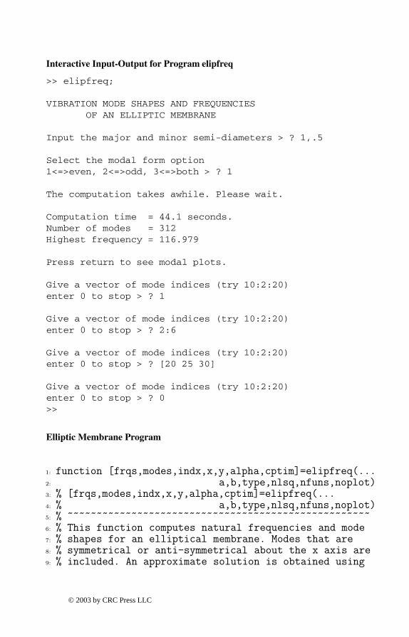
Interactive Input-Output for Program elipfreq

>> elipfreq;

VIBRATION MODE SHAPES AND FREQUENCIESOF AN ELLIPTIC MEMBRANE

Input the major and minor semi-diameters > ? 1,.5

Select the modal form option1<=>even, 2<=>odd, 3<=>both > ? 1

The computation takes awhile. Please wait.

Computation time = 44.1 seconds.Number of modes = 312Highest frequency = 116.979

Press return to see modal plots.

Give a vector of mode indices (try 10:2:20)enter 0 to stop > ? 1

Give a vector of mode indices (try 10:2:20)enter 0 to stop > ? 2:6

Give a vector of mode indices (try 10:2:20)enter 0 to stop > ? [20 25 30]

Give a vector of mode indices (try 10:2:20)enter 0 to stop > ? 0>>

Elliptic Membrane Program

1: function [frqs,modes,indx,x,y,alpha,cptim]=elipfreq(...2: a,b,type,nlsq,nfuns,noplot)3: % [frqs,modes,indx,x,y,alpha,cptim]=elipfreq(...4: % a,b,type,nlsq,nfuns,noplot)5: % ~~~~~~~~~~~~~~~~~~~~~~~~~~~~~~~~~~~~~~~~~~~~~~~~~~~~6: % This function computes natural frequencies and mode7: % shapes for an elliptical membrane. Modes that are8: % symmetrical or anti-symmetrical about the x axis are9: % included. An approximate solution is obtained using


10: % a separation of variables formulation in elliptical11: % coordinates.12: %13: % a,b - the ellipse major and minor semi-14: % diameters along the x and y axes15: % nlsq - two-component vector giving the number16: % of least square points in the eta and17: % xi directions18: % nfuns - two-component vector giving the number of19: % functions used to solve the differential20: % equations for the eta and xi directions.21: % type - use 1 for even modes symmetric about the22: % x-axis. Use 2 for odd modes anti-23: % symmetric about the x-axis. Use 3 to24: % combine both even and odd modes.25: %26: % frqs - a vector of natural frequencies27: % arranged in increasing order.28: % modes - a three dimensional array in which29: % modes(:,:,j) defines the modal30: % deflection surface for frequency31: % frqs(j).32: % indx - a vector telling whether each33: % mode is even (1) or odd (2)34: % x,y - curvilinear coordinate arrays of35: % points in the membrane where modal36: % function values are computed.37: % alpha - a vector of eigenvalue parameters in38: % the Mathieu equation: u’’(eta)+...39: % (alpha-lambda*cos(2*eta))*u(eta)=040: % where lambda=(h*freq)^2/2 and41: % h=atanh(b/a)42: % cptim - the cpu time in seconds used to43: % form the equations and solve for44: % eigenvalues and eigenvectors45: % noplot - enter any value to skip mode plots46: %47: % User m functions called:48: % frqsimpl eigenrec plotmode49: % modeshap funcxi funceta50:

51: if nargin==052: disp(’ ’)53: disp(’VIBRATION MODE SHAPES AND FREQUENCIES’)54: disp(’ OF AN ELLIPTIC MEMBRANE ’)


55: disp(’ ’)56:

57: nlsq=[300,300]; nfuns=[25,25];58:

59: v=input([’Input the major and minor ’,...60: ’semi-diameters > ? ’],’s’);61: v=eval([’[’,v,’]’]); a=v(1); b=v(2); disp(’ ’)62: disp(’Select the modal form option’)63: type=input(...64: ’1<=>even, 2<=>odd, 3<=>both > ? ’);65: disp(’ ’)66: disp([’The computation takes awhile.’,...67: ’ PLEASE WAIT.’])68: end69:

70: if type ==1 | type==2 % Even or odd modes71: [frqs,modes,x,y,alpha,cptim]=frqsimpl(...72: a,b,type,nlsq,nfuns);73: indx=ones(length(frqs),1)*type;74: else % Both modes75: [frqs,modes,x,y,alpha,cptim]=frqsimpl(...76: a,b,1,nlsq,nfuns);77: indx=ones(length(frqs),1);78: [frqso,modeso,x,y,alphao,cpto]=frqsimpl(...79: a,b,2,nlsq,nfuns);80: frqs=[frqs;frqso]; alpha=[alpha;alphao];81: modes=cat(3,modes,modeso);82: indx=[indx;2*ones(length(frqso),1)];83: [frqs,k]=sort(frqs); modes=modes(:,:,k);84: indx=indx(k); cptim=cptim+cpto;85: end86:

87: if nargin==6, return, end88:

89: % Plot a sequence of modal functions90: neig=length(frqs);91: disp(’ ’), disp([’Computation time = ’,...92: num2str(sum(cptim)),’ seconds.’])93: disp([’Number of modes = ’,num2str(neig)]);94: disp([’Highest frequency = ’,...95: num2str(frqs(end))]), disp(’ ’)96: disp(’Press return to see modal plots.’)97: pause, plotmode(a,b,x,y,frqs,modes,indx)98:

99: %==============================================


100:

101: function [frqs,Modes,x,y,alpha,cptim]=frqsimpl(...102: a,b,type,nlsq,nfuns)103: % [frqs,Modes,x,y,alpha,cptim]=frqsimpl(...104: % a,b,type,nlsq,nfuns)105: % ~~~~~~~~~~~~~~~~~~~~~~~~~~~~~~~~~~~~~~~~~~~~~~~~~~~106:

107: % a,b - ellipse major and minor semi-diameters108: % type - numerical values of one or two for modes109: % symmetric or anti-symmetric about the x axis110: % nlsq - vector [neta,nxi] giving the number of least111: % square points used for the eta and xi112: % directions113: % nfuns - vector [meta,mxi] giving the number of114: % approximating functions used for the eta and115: % xi directions116: % frqs - natural frequencies arranged in increasing117: % order118: % Modes - modal surface shapes in the ellipse119: % x,y - coordinate points in the ellipse120: % alpha - vector of values for the eigenvalues in the121: % Mathieu differential equation:122: % u’’(eta)+(alpha-lambda*cos(2*eta))*u(eta)=0123: % cptim - vector of computation times124: %125: % User m functions called: funceta funcxi126: % eigenrec modeshap127: if nargin==0128: a=cosh(2); b=sinh(2); type=1;129: nlsq=[200,200]; nfuns=[30,30];130: end131: h=sqrt(a^2-b^2); R=atanh(b/a); neta=nlsq(1); alpha=[];132: nxi=nlsq(2); meta=nfuns(1); mxi=nfuns(2);133: eta=linspace(0,pi,neta)’; xi=linspace(0,R,nxi)’;134: [Xi,Eta]=meshgrid(xi,eta); z=h*cosh(Xi+i*Eta);135: x=real(z); y=imag(z); cptim=zeros(1,3);136:

137: % Form the Mathieu equation for the circumferential138: % direction as: A*E+alpha*E-lambda*B*E=0139: tic; [Veta,A]=funceta(meta,type,eta);140: A=Veta\[A,repmat(cos(2*eta),1,meta).*Veta];141: B=A(:,meta+1:end); A=A(:,1:meta);142:

143: % Form the modified Mathieu equation for the radial144: % direction as: P*F-alpha*F+lambda*Q*F=0


145: [Vxi,P]=funcxi(a,b,mxi,type,xi);146: P=Vxi\[P,repmat(cosh(2*xi),1,mxi).*Vxi];147: Q=P(:,mxi+1:end); P=P(:,1:mxi);148: cptim(1)=toc; tic149:

150: % Solve the eigenvalue problem. This takes most151: % of the computation time152: [frqs,modes]=eigenrec(P’,A,-Q’,B);153: % Keep only half of the modes and frequencies154: nmax=fix(length(frqs)/2); frqs=frqs(1:nmax);155: modes=modes(:,:,1:nmax); cptim(2)=toc;156:

157: % Compute values of the second eigenvalue158: % parameter in Mathieu’s equation159: alpha=zeros(1,nmax); tic;160: s=size(modes); s=s(1:2); Vxi=Vxi’;161:

162: % Obtain the modal surface shapes163: Neta=91; Nxi=25; Modes=zeros(Neta,Nxi,nmax);164: for k=1:nmax165: Mk=modes(:,:,k); [dmk,K]=max(abs(Mk(:)));166: [I,J]=ind2sub(s,K); Ej=Mk(:,J);167: alpha(k)=(B(I,:)*Ej*frqs(k)-A(I,:)*Ej)/Mk(K);168: [Modes(:,:,k),x,y]=modeshap(a,b,type,Mk,Nxi,Neta);169: end170: frqs=sqrt(2*frqs)/h; cptim(3)=toc;171:

172: %==============================================173:

174: function [eigs,vecs,Amat,Bmat]=eigenrec(A,B,C,D)175: % [eigs,vecs,Amat,Bmat]=eigenrec(A,B,C,D)176: % Solve a rectangular eigenvalue problem of the177: % form: X*A+B*X=lambda*(X*C+D*X)178: %179: % A,B,C,D - square matrices defining the problem.180: % A and C have the same size. B and D181: % have the same size.182: % eigs - vector of eigenvalues183: % vecs - array of eigenvectors where vecs(:,:,j)184: % contains the rectangular eigenvector185: % for eigenvalue eigs(j)186: % Amat,187: % Bmat - matrices that express the eigenvalue188: % problem as Amat*V=lambda*Bmat*V189: %


190: n=size(B,1); m=size(A,2); s=[n,m]; N=n*m;191: Amat=zeros(N,N); Bmat=Amat; kn=1:n; km=1:m;192: for i=1:n193: IK=sub2ind(s,i*ones(1,m),km);194: Bikn=B(i,kn); Dikn=D(i,kn);195: for j=1:m196: I=sub2ind(s,i,j);197: Amat(I,IK)=A(km,j)’; Bmat(I,IK)=C(km,j)’;198: KJ=sub2ind(s,kn,j*ones(1,n));199: Amat(I,KJ)=Amat(I,KJ)+ Bikn;200: Bmat(I,KJ)=Bmat(I,KJ)+ Dikn;201: end202: end203: [vecs,eigs]=eig(Bmat\Amat);204: [eigs,k]=sort(diag(eigs));205: vecs=reshape(vecs(:,k),n,m,N);206:

207: %===========================================208:

209: function plotmode(a,b,x,y,eigs,modes,indx)210: %211: % plotdmode(a,b,x,y,eigs,modes,indx)212: % ~~~~~~~~~~~~~~~~~~~~~~~~~~~~~~~~~213: % This function makes animated plots of the214: % mode shapes of an elliptic membrane for215: % various frequencies216: % a,b - major and minor semi-diameters217: % x,y - arrays of points defining the218: % curvilinear coordinate grid219: % eigs - vector of sorted frequencies220: % modes - array of modal surfaces for221: % the corresponding frequencies222: % indx - vector of indices designating223: % each mode as even (1) or odd (2)224:

225: range=[-a,a,-b,b,-a,a];226: nf=25; ft=cos(linspace(0,4*pi,nf));227: boa=[’, B/A = ’,num2str(b/a,4)];228: while 1229: jlim=[];230: while isempty(jlim), disp(’ ’)231: disp([’Give a vector of mode ’,...232: ’indices (try 10:2:20) > ? ’]);233: jlim=input(’(input 0 to stop > ? ’);234: end


235: if any(jlim==0)236: disp(’ ’), disp(’All done’), break, end237: for j=jlim238: if indx(j)==1, type=’EVEN’; f=1;239: else, type =’ODD ’; f=-1; end240: u=a/2*modes(:,:,j);241:

242: for kk=1:nf243: surf(x,y,ft(kk)*u)244: axis equal, axis(range)245: xlabel(’x axis’), ylabel(’y axis’)246: zlabel(’u(x,y)’)247: title([type,’ MODE ’,num2str(j),...248: ’, OMEGA = ’,num2str(eigs(j),4),boa])249: %colormap([127/255 1 212/255])250: colormap([1 1 0])251: drawnow, shg252: end253: pause(1);254: end255: end256:

257: %==================================================258:

259: function [u,x,y]=modeshap(...260: a,b,type,modemat,nxi,neta,H)261: %262: % [u,x,y]=modeshap(a,b,type,modemat,nxi,neta,H)263: % ~~~~~~~~~~~~~~~~~~~~~~~~~~~~~~~~~~~~~~~~~~~~264: % This function uses the eigenvectors produced by265: % the rectangular eigenvalue solver to form modal266: % surface shapes in cartesian coordinates.267: % a,b - major and minor semi-diameters268: % type - 1 for even, 2 for odd269: % modemat - eigenvector matrix output by eigenrec270: % nxi,neta - number of radial and circumferential271: % coordinate values272: % H - maximum height of the modal surfaces.273: % The default value is one.274: % u,x,y - modal surface array and corresponding275: % cartesian coordinate matrices. u(:,:j)276: % gives the modal surface for the j’th277: % natural frequency.278:

279: if nargin<7, H=1; end


280: if nargin<6, neta=81; end; if nargin<5, nxi=22; end281: h=sqrt(a^2-b^2); r=atanh(b/a); x=[]; y=[];282: xi=linspace(0,r,nxi); eta=linspace(-pi,pi,neta);283: if nargout>1284: [Xi,Eta]=meshgrid(xi,eta); z=h*cosh(Xi+i*Eta);285: x=real(z); y=imag(z);286: end287: [Neta,Nxi]=size(modemat);288: mateta=funceta(Neta,type,eta);289: matxi=funcxi(a,b,Nxi,type,xi);290: u=mateta*modemat*matxi’; [umax,k]=max(abs(u(:)));291: u=H/u(k)*u;292:

293: %==================================================294:

295: function [f,f2]=funcxi(a,b,n,type,xi)296: %297: % [f,f2]=funcxi(a,b,n,type,xi)298: % ~~~~~~~~~~~~~~~~~~~~~~~~~~~299: % This function defines the approximating functions300: % for the radial direction301: % a,b - ellipse major and minor half-diameters302: % n - number of series terms used303: % type - 1 for even valued, 2 for odd valued304: % xi - vector of radial coordinate values305: % f,f2 - matrix of function and second derivative306: % values307:

308: xi=xi(:); nxi=length(xi); R=atanh(b/a);309: if type==1, N=pi/R*(1/2:n); f=cos(xi*N);310: else, N=pi/R*(1:n); f=sin(xi*N); end311: f2=-repmat(N.^2,nxi,1).*f;312:

313: %==================================================314:

315: function [f,f2]=funceta(n,type,eta)316: %317: % [f,f2]=funceta(n,type,eta)318: % ~~~~~~~~~~~~~~~~~~~~~~~~~319: % This function defines the approximating functions320: % for the circumferential direction321: % n - number of series terms used322: % type - 1 for even valued, 2 for odd valued323: % xi - vector of circumferential coordinate values324: % f,f2 - matrix of function and second derivative


325: % values326:

327: eta=eta(:); neta=length(eta);328: if type==1, N=0:n-1; f=cos(eta*N);329: else, N=1:n; f=sin(eta*N); end330: f2=-repmat(N.^2,neta,1).*f;


nguyen.hong.hai.free.frnguyen.hong.hai.free.fr/EBOOKS/SCIENCE AND... · Chapter 10 Eigenvalue...

Documents

Transcript of nguyen.hong.hai.free.frnguyen.hong.hai.free.fr/EBOOKS/SCIENCE AND... · Chapter 10 Eigenvalue...