Compensating & Retaining Community Health Workers_Christianson_5.11.11

Analyzing the Determinants of the Matching of Public School Teachers to Jobs: Estimating Compensating Differentials in Imperfect Labor Markets
Abstract Although there is growing recognition of the contribution of teachers to students’ educational outcomes, there are large gaps in our understanding of how teacher labor markets function. Most research on teacher labor markets use models developed for the private sector. However, markets for public school teachers differ in fundamental ways from those in the private sector. Collective bargaining and public decision making processes set teacher salaries. Thus it is unlikely that wages adjust quickly to equilibrate the supply and demand for worker and job attributes. The objective of this paper is to develop and estimate a model that more accurately characterizes the institutional features of teacher labor markets. The approach is based on a game-theoretic two-sided matching model and the estimation strategy employs the method of simulated moments. With this combination, we are able to estimate how factors affect the choices of individual teachers and hiring authorities, as well as how these choices interact to determine the equilibrium allocation of teachers across jobs. Although this paper focuses on worker-job match within teacher labor markets, many of the issues raised and the empirical framework employed are relevant in other settings as well.

I. Introduction
The 2.8 million elementary and secondary public school teachers in the United States
make up 8.5 percent of all college-educated workers 25 to 64 years old.1 Even though there is
growing recognition of the contribution of these teachers to students’ educational outcomes and
later economic success, large gaps exist in our understanding of how teacher labor markets
function. Most research on teacher labor markets has used models developed for the private
sector. However, markets for public school teachers, as well as markets for many other public
employees, differ in fundamental ways from those in the private sector. The objective of this
paper is to develop and estimate a model that more accurately characterizes the institutional
features of teacher labor markets. The approach is based on a game-theoretic two-sided
matching model and the estimation strategy employs the method of simulated moments. With
this combination, we are able to estimate how factors affect the choices of individual teachers
and hiring authorities, as well as how these choices interact to determine the equilibrium
allocation of teachers across jobs.
Low-income, low-achieving and non-white students, particularly those in urban areas,
often are taught by the least skilled teachers, a factor that likely contributes to the substantial
gaps in academic achievement among income and racial/ethnic groups of students. Such sorting
of teachers across schools and districts is the result of a range of decisions made by individual
teachers and school officials. Inefficient hiring and district assignment may contribute to the
disparities in teacher qualifications across schools; however, teacher preferences are likely to be
particularly influential.2 Teachers differ fundamentally from other school resources. Unlike
1 Digest of Education Statistics 2002 and U.S Census Bureau Educational Attainment in the United States 2000 Detailed Tables. 2 Few studies have explored district-hiring practices, though Pflaum & Abramson (1990), Ballou (1996) and Ballou and Podgursky (1997) do provide evidence that many districts are not hiring the most qualified candidates. Schools
1

textbooks, computers, and facilities, teachers have preferences about whether to teach, what to
teach, and where to teach. Potential teachers prefer one type of district to another; and within
districts, they prefer one school to another. Salaries are one job attribute that likely affects
sorting, but non-pecuniary job characteristics, such as class size, preparation time, facilities, or
characteristics of the student body, are important as well.3 A large literature suggests that
teachers respond to wages, yet research on the compensating wage differentials needed to attract
teachers with particular attributes to schools with particular characteristics has not produced
consistent results.4
The inconsistencies in the estimation of compensating differentials for teachers are not
surprising given that the estimates have been based on hedonic wage models which maintain that
wages adjust to equilibrate the supply and demand for worker and job attributes. This
assumption is unlikely to hold for public school teaching, given that salaries are set by collective
bargaining and public decision-making processes, not directly as a result of market forces. In
this context, some jobs may simply be “better jobs” than others, and teachers will sort into these
jobs based on their ability to obtain offers from the hiring authorities.
Non-price rationing in the market for public school teachers will result in complex
interdependencies in the choices made by job candidates and employers. In particular, a
candidate’s willingness to accept a particular job will depend upon her own preferences as well also vary in the political power they exert, which may lead to differences in teacher qualifications among schools within the same district. Bridges (1996) found that when parents and students complained about poor teachers, the teachers were likely to be transferred to schools with high student-transfer rates, large numbers of students receiving free or reduced-price lunches, and large numbers of minority students. 3 In Texas, Hanushek, Kain and Rivkin (1999) found teachers moving to schools with high-achieving students and, in New York City, Lankford (1999) found experienced teachers moving to high-socioeconomic status schools when positions became available. 4 As a group, these studies show that individuals are more likely to choose to teach when starting teacher wages are high relative to wages in other occupations (Baugh and Stone, 1982; Brewer, 1996; Dolton, 1990; Dolton and van der Klaaw, 1999; Dolton and Makepeace, 1993; Hanushek and Pace, 1995; Manski, 1987; Mont and Reece, 1996; Murnane, Singer & Willett, 1989; Rickman and Parker, 1990; Stinebrickner, 1998, 1999, 2000; Theobald, 1990; Theobald and Gritz, 1996). Baugh and Stone (1982), for example, find that teachers are at least as responsive to wages in their decision to quit teaching, as are workers in other occupations.
2

as her “effective” choice set, i.e., the set of schools willing to hire her given their own “effective”
alternatives. In turn, whether employers make the candidate an offer will depend upon whether
they prefer to employ alternative candidates who are willing to fill their positions, and so on. We
can analyze such an environment in a relatively straightforward manner using the standard two-
sided matching model extensively studied by game theorists (Roth and Sotomayer, 1990). The
contributions of this paper are to note the conceptual applicability of the game-theoretic, two-
side matching model as an attractive alternative to the standard hedonic model, and to show how
the underlying preferences of job candidates and employers in such a two-sided matching model
can be estimated using the method of simulated moments.
Our long-term goal is to identify policies that are effective for attracting and retaining
teachers in low-performing or otherwise difficult-to-staff schools. As we discuss further below,
such identification has many difficulties, not the least of which is the endogeneity of any district-
level policy we observe. The goal of this paper is more limited. We introduce our model for the
matching of teachers to schools and estimate this model with a limited set of school and teacher
measures. We focus on the initial match of teachers to schools in their first jobs both to simplify
the first implementation of the model and because, as we discuss later, the initial match appears
particularly important, in comparison to transfers and quits, in determining the disparities in the
qualifications of teachers across schools.
The following section of the paper briefly summarizes the data we employ and some key
features of teacher labor markets. Section III contrasts the hedonic approach with two alternative
models of job match. We outline our conceptual framework and empirical approach in section
IV and discuss identification in section V. Section VI presents estimates of several models, as
well as simulations of policy changes based on the results of these models. Section VII reports
3

estimates of hedonic wage equations and discusses simulation results that help to clarify the
difference between the wage-equation approach and our model. Section VII concludes.
II. Data
The data we use for this analysis comes from a larger database of teachers and schools
that links seven administrative datasets and various other information characterizing schools,
districts, communities, and local labor markets in New York State. It includes information for
every teacher and administrator employed in a New York public school at any time from 1969-
70 through 1999-2000. The core data comes from the Personnel Master File (PMF), part of the
Basic Education Data System of the New York State Education Department. In a typical year
there are approximately 200,000 teachers identified in the PMF. We have linked these annual
records through time, yielding detailed data characterizing the career history of each individual.
Several other databases that contain a range of information about the qualifications of
prospective and actual teachers, as well as the environments in which these individuals make
career decisions, substantially enrich this core data. For teachers this information includes age,
gender, race/ethnicity, salary, experience (in the district, in NYS public schools, and total), years
of education and degree attainment, and teacher certification exam scores of individual teachers
and whether they passed on their first attempts. In addition, we identify the institutions from
which individual teachers earned their undergraduate degrees and combine it with the Barron’s
ranking of college selectivity to construct variables measuring the selectivity of the college from
which each teacher graduated and the location of the institution. Measures for schools and
districts include enrollment, student poverty, racial composition, and district salary schedules, as
well as many other measures. Using information on the zip code of residence when each teacher
4

applied for certification and the zip code of each school, we create a “distance from home”
measure for each school-teacher combination in our sample. For a sub-sample of teachers we
know where they lived while in high school.
Our data is richer in its descriptions of teachers than other administrative datasets used to
date, particularly in that it includes teachers' certification test scores and undergraduate
institutions. It also allows us to match teachers to characteristics of the schools in which they
teach in a way that most national longitudinal surveys, such as High School and Beyond or the
National Longitudinal Survey of Youth, do not. This matching of employer and employee data
has proved useful in the analysis of labor markets more generally (Abowd and Kramarz, 1999;
Postel-Vinay and Robin, 2002; Rosen, 1986). In a series of papers, we have used this data for
teachers to document various characteristics of teacher labor markets, a number of which are
pertinent here.
First, as noted above, there is a marked sorting of teachers across schools. For example,
in schools in the highest quartile of student performance on the New York State 4th Grade
English Language Arts Exam only three percent of teachers are uncertified, only ten percent
earned their undergraduate degree from least competitive colleges, and only nine percent of those
who have taken a general knowledge teacher certification exam failed.5 In contrast, in schools in
the lowest quartile of student performance, 22 percent of teachers are uncertified, 26 percent
come from least competitive colleges, and 35 percent have failed a general-knowledge
certification exam (Lankford, Loeb and Wyckoff, 2002). Similar patterns are found when
schools are grouped based on student poverty, race/ethnicity and limited English proficiency.
5 Teachers in New York have had the option of taking the NTE General Knowledge Exam or the NYSTCE Liberal Arts and Science Exam. Throughout the paper “failure” refers to failing one of these exams on the first attempt.
5

These differences reflect urban-suburban differences in the qualifications of teachers as well as
meaningful differences across schools within urban areas.
Differences in the qualifications of teachers are the result of the decisions of individuals
and school officials that determine initial job matches and subsequent decisions that affect job
quits, transfers and terminations. Of these, initial job matches appear particularly important in
that they account for almost all of the urban-suburban differences in teacher qualifications as
well as a substantial portion of the differences between schools within urban districts. To
illustrate this, we track a cohort of entering teachers and assess the spread of teacher
qualifications across groups of schools in the first year and then in each following year for that
same cohort. We define groups either by urban-suburban-region-status or by quartiles of student
characteristics (race/ethnicity or achievement). On the initial match of the 1995 cohort, New
York City urban schools had 17.1 percentage points more teachers who had failed a teacher
certification exam than did non-NYC suburban schools. This difference had increased by 5.2
points by the end of six years, implying that the initial match accounted for 77 percent of the
disparity after six years, when most transfers had already taken place. Within urban areas, the
contributions of initial match and exits are roughly equal in determining the overall differences
in the qualifications of teachers across groups of schools. When we compare the proportion of
teachers failing the certification exam in New York City between schools in the top and bottom
quartiles of percentage of students who are non-white, the initial gap for the 1995 cohort is 11.3
percentage points. After five years of teaching, the gap enlarges to 19.7 percentage points,
implying that quits and transfers have added 8.4 percentage points and that the initial match
accounts for 58 percent of the total gap by 2000 (Boyd, Lankford, Loeb, and Wyckoff, 2002).
Given the relative importance of the initial matches of teachers to schools and the need to
6

simplify the first implementation of our empirical model, we focus on these initial job matches
and the sorting of teachers within local labor markets.
A final characteristic of teacher labor markets worth noting is the surprisingly large
number of individuals who take their first teaching job very close to where they grew up. Over
60 percent of teachers first teach within 15 miles of the school from which they graduated high
school and 85 percent teach within 40 miles. Even of those who travel over 100 miles to college,
most return home to teach (Boyd, Lankford, Loeb, and Wyckoff, forthcoming).6 This proximity
has two important implications for modeling the sorting of teachers across jobs. First, most
teachers make job choices within a very limited geographic area. Because of this, our empirical
analysis of job match presented below, focuses on the matching of teachers to jobs within
relatively small geographic areas (metropolitan areas) instead of across the entire state. Second,
even within each of these local labor markets, work proximity is likely to affect teachers’
rankings of alternative job opportunities. Teachers will rank otherwise identical jobs differently
because of differences in the relative proximity of jobs to the teachers’ own locations. These
ranking differences suggest that an accurate model of teacher labor markets will need to
incorporate this potentially important source of preference heterogeneity.
6 Information regarding home location is drawn from either College Board data for all individuals who attended a NYS high school and took the SAT since 1980 or SUNY data for all individuals who applied to a SUNY campus anytime since 1990. Thus, this analysis does not include individuals who did not apply to a SUNY school over this period and (1) attended high school out of state, (2) attended a NYS high school prior to 1980 or (3) attended a NYS high school but did not take the SAT. How the above statistics would be affected by including these individuals in the calculations is not clear as the longer distances traveled by out-of-state students could be more than offset by the many students in New York City who did not take the SAT because they planned to attend CUNY which did not require the test.
7

III. Common Approaches for Modeling Sorting
Before describing our empirical sorting model in detail, it is worth reviewing several
literatures pertinent to the study of the sorting of teachers across jobs. These include the
hedonics literature and at least two literatures concerned with two-sided matching.
Hedonic Models: Most previous studies of teacher labor markets, such as Antos and
Rosen (1975), employ a hedonic framework in which workers have preferences over job
attributes including both salary and non-pecuniary characteristics and employers have
preferences with respect to the attributes of workers and the salary paid. In the case where
salaries clear the market, the equilibrium wage function shows the salary a worker having given
qualifications would be paid when working in a job with given non-pecuniary attributes.
Maintaining the assumption of wage clearing, researchers have used wage equations to estimate
the pay differential needed to compensate individuals for working in jobs with particular
characteristics, as well as the pay increase needed to improve the quality of workers hired in jobs
with particular attributes. However, estimates of such wage equations in a wide range of
settings, including teacher labor markets, have proven inconsistent.
Researchers have posited a number of reasons for the inconsistencies including omitted
variables (Brown, 1980; Epple, 1987; Lucas, 1977), simultaneity (McLean, 1978), measurement
error, and labor market frictions (Hwang, Mortensen and Reed, 1998; Lang and Majumdar,
2001). In the case of teacher labor markets, omitted variables characterizing schools, students,
and teachers, as well as the endogenous determination of pertinent school policies have been
offered as possible explanations for counterintuitive wage equation results. However, there are
other problems with wage equations and hedonic models, more generally, in the context of
markets for public school teachers, as well as other public-sector employees.
8

First, contradicting a basic assumption of the wage equation approach, public-sector
salaries are unlikely to clear their respective markets and, as a result, do not fully adjust for
differences in both the attributes of workers and the non-pecuniary attributes of their jobs.
Salaries in the public sector often are inflexible because they are set through a combination of
political, administrative and collective bargaining processes, rather than as a result of direct
market forces. In the case of teacher labor markets, union contracts often set teacher salaries for
three or more years and social decision-making practices limit both the variation and the
flexibility of the wage. Furthermore, district wage schedules typically dictate that all teachers in
the district with the same number of years of education and experience earn the same salary,
regardless of either their other attributes or the characteristics of the schools in which they teach.
This limitation is especially restrictive in large urban districts and large countywide districts in
which there is considerable within-district variation in the non-wage attributes of schools.
In a setting where teacher salaries do not clear the labor market, those salaries will not
reflect compensating differentials for non-pecuniary job characteristics. In the extreme, if there
is no wage variation across jobs, and thus no variation in the wage equation’s dependent
variable, estimation is impossible. An alternative approach with teacher quality on the left-hand-
side of the estimated equation may be more appropriate, if such a one-dimensional measure of
quality is appropriate. However, there are other problems with approaches employing either
wage or quality equations.
A second problem with the regression-based approach arises from market thinness. As
noted above, labor markets for teachers tend to be quite small, so that there may not be sufficient
numbers of jobs and candidates in each local market to assure that the distributions of employer
and employee attributes are continuous. With choices being lumpy, some teachers and schools
9

will earn infra-marginal rents. In this setting, discrete choice models such as random utility
models are likely to be more pertinent in the analysis of job choice (Freeman, 1979; Palmquist
1991).
A third, and confounding, problem with the regression-based approach comes from
heterogeneity in preferences. As evidenced by the discussion of the importance of distance from
home to jobs, teachers may rank the same job differently because of their location relative to the
school. Some hedonic models have included distance measures; rent-gradient models, for
example, have assumed that individuals prefer living as close as possible to the central city.
However, this specification does not address the fact that each job candidate has a different
assessment of a particular job and its location because the assessment depends upon the
candidate’s own location. A conventional hedonic wage model that attempts to control for the
geographical distributions of jobs and candidates inevitably will rely on some ad hoc
specification that will misrepresent the way the resulting distances actually affect preferences. In
general, heterogeneity is difficult to incorporate into traditional regression-based models; and,
yet, estimates that do not account for the heterogeneity are likely to be biased. More broadly, the
specifications of regression based models typically are not directly linked to the underlying
preferences on both sides of the labor market. For example, the hedonic studies that actually
estimate preference parameters do so in a second stage only after first estimating reduced-form
wage equations. The approach that we now propose explicitly models the job match process and
allows direct estimation of preference parameters.
In what follows, we develop and estimate structural models drawing upon the game-
theoretic two-sided matching literature. These models account for pertinent features of teacher
labor markets, including wage rigidities and the resulting non-price rationing of jobs and
10

teachers, as well as for factors affecting the separate, but interdependent, choices made by job
candidates and school officials. Preferences with respect to distance and other sources of
preference heterogeneity enter in a straightforward manner. The estimated models that appear in
this paper are still preliminary. In particular, we use a small set of measures describing both
schools and teachers. Because of this, our estimates are subject to omitted variables bias, which
often has been cited as a concern with previous models. The purpose of this paper is to introduce
the model and demonstrate its applicability. We, thus, will discuss our results with the caveats
that our measures may be proxies for other characteristics of schools or teachers.
Two-sided matching: The two-sided matching literature is applicable to a broad range of
settings having the common feature that individuals in one group are matched with individuals,
agents or firms in a separate, second group. Examples include models of marriage, employment
and college attendance.7 In all of these cases, the matching is two-sided in that whether a
particular match occurs depends upon separate choices made by the two parties. Furthermore,
these choices are not made in isolation. “A worker’s willingness to accept employment at a firm
depends not only on the characteristics of the firm but also the other possible options open to the
worker. The better an individual’s opportunities elsewhere, the more selective he or she will be
in evaluating a potential partner,” (Burdett and Coles, 1999).
Within the two-sided matching literature, there are now a large number of papers that
build upon the work of Gale and Shapley (1962) and are concerned with the allocation
(matching) of fixed numbers of agents from two disjoint sets. This game-theoretic research has
considered both one-to-one matching such as marriage and many-to-one matching such as
7 These cases differ from the roommate problem where those being matched come from the same group. In two-sided match models all agents fall into one of two distinct groups and seek a match with one or more agents in the other group.
11
employment and college-admission, the former being a special case of the latter.8 While a
growing number of papers allow utility to be transferable so that the division of match surplus is
determined endogenously at the time partners match, most game-theoretic models have assumed
that utility is nontransferable; that is, how the surplus from any given match is split between the
matching pair is predetermined. This more traditional assumption is applicable to teacher labor
markets since salaries (set through collective bargaining), other conditions of work9, and the
attributes of teacher candidates are fixed in the short-run.
In addition to the game-theoretic studies, there is a large literature in labor economics
employing two-sided matching models with search. This research distinguishes itself in a
number of respects. First, whereas almost all the game-theoretic models assume full information
and no market frictions, such frictions are central to the labor-search models of marriage and job
match. A second difference is that the demand side of the labor-search models often is
characterized by free entry of profit maximizing firms, so that the number of jobs to be filled is
not fixed as in the game-theoretic match literature. A third difference that is especially pertinent
for our empirical analysis concerns the extent and nature of agent heterogeneity allowed in the
models. Game-theoretic two-sided match models typically only require that each agent’s
ranking of match partners is complete and transitive, with no restrictions regarding the extent of
preference heterogeneity. In contrast, the search models either maintain homogeneity of
preferences or allow for only limited heterogeneity. Some models maintain match
8 In addition to the papers focusing on decentralized allocation mechanisms, extensive research has addressed centralized mechanisms such as those used to assign medical interns to hospitals. Roth and Sotomayer (1990) provide a clear synthesis of both the theoretical literature to date and how the theoretical findings provide important insights regarding implications of the institutional features characterizing the centralized matching algorithms used, as well as factors that have contributed to the evolution of those features. 9 In teacher labor markets, many conditions of work are inflexible, including the location of the school and student body characteristics. Job attributes such as class size and teacher preparation time, while not completely inflexible, are constrained by the political process and collective bargaining.
12

heterogeneity, where agents in each group are ex-ante identical but some matches are relatively
more productive, with the productivity of each possible match determined by a random draw
from some known distribution. Other models maintain ex-ante heterogeneity where there are
systematic differences across agents independent of the partners to whom they are matched, with
all agents in one group having the same ranking of the potential partners in the other. For
example, some workers may be more productive than others and some jobs may be more or less
attractive. Limitations on the degree of heterogeneity are needed in order to solve for the search
equilibriums (Burdett and Coles, 1999). Such limited heterogeneity would be quite restrictive if
maintained in our analysis, in part because teachers’ rankings of school alternatives are likely to
differ reflecting their own proximity to those schools. For this reason, our model builds on the
game-theoretic approach, with the hope of incorporating market frictions into later work.
IV. The Model
Consider an environment in which 1, , JC c c= L represents the set of J individuals
seeking teaching jobs and 1, , KS s s= L represents the set of K schools having jobs to be filled,
. For now assume that each school has one job opening though this assumption is relaxed
in the empirical analysis. We assume that each agent has a complete and transitive preference
ordering over the agents on the other side of the market and that these orderings arise from job
candidates’ preferences over job attributes and hiring authorities’ preferences over the attributes
of candidates.
KJ ≥
Let u represent the utility of working in the kjkth school as viewed from the perspective
of the jth candidate where 1 2( , , )jk k jk j jkz d qu u β δ= + 1kz. is a vector of observed attributes of the
13

kth school pertinent to the jth individual and is the distance to the kjkd th job for the candidate.
Vector represents observed attributes of the j2jq th candidate that affect the individual’s
assessment of the kth alternative and β is a vector of parameters. jkδ is a random variable
reflecting unobserved heterogeneity in the attractiveness of a particular school for different
individuals. If no job match is entered, the individual’s utility is uj0 which depends upon
observed and unobserved attributes of the individual. Thus, the individual will always turn down
a job offer if . Here we assume that 0jk ju u< 0jk ju u> for all k and j but plan to allow for the
more general case when, in further research, we extend the empirical model to consider all
candidates, not just those actually obtaining jobs.
jkα +
jkω
jkδ 1 2jk jd
The hiring authority for the kth school is assumed to have preferences over the attributes
of job candidates. Let 1 2( , )jk j kq zv v ω=
2kz
represent the attractiveness of the jth candidate from
the perspective of the hiring authority for school k. The vector represents pertinent observed
attributes of the j
1jq
th candidate. The vector represents the observed attributes of the kth school
that might affect the authority’s assessment of the jth candidate. α is a vector of parameters. The
random error reflects unobserved factors. To simplify the analysis, we assume hiring
authorities prefer all of the candidates to the alternative of leaving job vacancies unfilled. This
assumption, combined with the assumption that there are sufficient numbers of willing
candidates, implies that all job openings will be filled.
Consider a case where the sets C and S are known, as are the values of for
each candidate and for each job. Given the vector of parameters β and a particular
set of random variable draws for the
1 2( , )j j jq q q≡
1 2( , )k k kz z z≡
, the formula ( , , )jk ku u z q jkβ δ= + implies the
14

matrix of candidates’ benefits represented in panel (A) of Figure 1. Each row shows the benefits
that a particular candidate attributes to being employed in each of the K school alternatives.
These rows of benefit values, in turn, imply candidates’ complete rankings of school alternatives
shown in panel (C). is the jth candidate’s ranking of the kth school alternative. In a similar
way, the vector of parameters α and a particular set of random variable draws for the
cjkr
jkω ,
together with the formula 1 2( , )jk j k jkq zv v α ω=
1 2
1 11 12 1
2 21 22 2
1 2
+ , imply the matrix of school benefits represented
in panel (B) of Figure 1 and the complete rankings of candidates by hiring authorities shown in
panel (D). Each column of panel B shows the benefits to a particular school of having an
opening filled by each of the alternative candidates. is the ranking of the jsjkr th candidate from
the perspective of the kth employer.
K
K
K
J J J JK
s s sc u u uc u u u
c u u u
L
L
L
M M M MO
L
1 2
1 11 12 1
2 21 22 2
1 2
Kc c c
Kc c c
K
c c cJ J J JK
s s sc r r rc r r r
c r r r
L
L
L
M M M MO
L
Figure 1: Utility and Rankings of Candidates and Schools
(A) (B) Candidates’ benefits Schools’ benefits from alternative from alternative employment candidates
1 2
1 11 12 1
2 21 22 2
1 2
K
K
K
J J J JK
s s sc v v vc v v v
c v v v
L
L
L
M M M MO
L
(C) (D) Candidates’ rankings Schools’ rankings of employers of candidates
1 2
1 11 12 1
2 21 22 2
1 2
Ks s s
Ks s s
K
s s sJ J J JK
s s sc r r rc r r r
c r r r
L
L
L
M M M MO
L
15

If each of the candidates unilaterally were able to choose the school in which to teach, the
framework summarized in panel A would imply that β in 1 2( , , )jk k jk j jku u z d q β δ= + could be
estimated using data characterizing those choices and a standard multinomial probit or logit
random utility model. Similarly, α could be estimated easily using the same type model, if each
hiring authority unilaterally chose among candidates. However, the empirical model we employ
is more complex for two reasons. First, it is the interaction of decisions made by a candidate and
a hiring authority for a school that determines whether the two are matched. Second, even
though any such interaction would complicate the model, the decisions made by the two parties
considering whether to match crucially depend upon the choices made by all other candidates
and employers. In particular, a candidate’s willingness to accept a particular match depends
upon her own preferences as well as her choice set, i.e., the set of schools willing to hire her
given their own alternatives. In turn, whether employers make the candidate an offer will
depend upon whether they prefer to employ alternative candidates who are willing to fill their
positions, and so on.
To see how one can have a model with joint decisions that avoids this complexity, one
need only consider a two-sided search model in which candidates and employers randomly meet
and individually decide whether they are willing to match based upon reservation-wage decision
rules, with a match occurring only if both agree. The relative simplicity of this model comes
from the underlying assumptions that imply the reservation-threshold for any agent is not
affected by the choices made by any other agent. In contrast, the model we use explicitly allows
for complex interactions. Furthermore, our model allows for unobserved heterogeneity in
agents’ rankings of alternatives whereas search models typically assume there are common
rankings or only very limited heterogeneity.
16

Because our framework is an empirical application of the standard two-sided matching
model extensively studied by game theorists, much in that literature directly applies to our
analysis (Roth and Sotomayer, 1990). We assume that a decentralized job-match mechanism
leads to a stable matching of teacher candidates to jobs. For a set of matches to be stable, there
must be no candidate-employer pair currently not matched together who both would prefer such
a new match rather than remain in their current matches. Otherwise, if allowed, the pair would
break their current matches in order to match with each other. More formally, without loss of
generality, suppose that candidate g is employed in job g’, with candidate h and job h’ similarly
matched. For these two pairings to be stable, it must be the case that (1) 'ghggu u′ >
'
or
, or both (i.e., either candidate g or employer h’ prefers the status quo to the alternative
of candidate g being employed in job h’) and, similarly, (2) or '
'hh ghv v> '
' 'hh hgu u> gg hv v> g , or both. 10
Equivalent expressions for these two conditions are ( ) ( )' 'ghv' 'gh hhu u1 1 0gg v< < = and
where ( ) ( )' ' ' '1 1gh gg hgv v< < 0=hhu u ( )1 is the indicator function which equals one if the
function argument is true and zero otherwise. Overall stability required that the condition
hold for every candidate (g) and job (h’) pairing not currently
matched.
( ) (' ' ' '1 1gh hh ghv v< < ) 0=
ggu u
Our empirical framework maintains that the observed matching of teachers to schools is
an employer-optimal stable matching (i.e., all employers weakly prefer this allocation to all other
stable matchings). The following decentralized job-match mechanism is one process that leads
to this employer-optimal matching. Each employer initially makes an offer to its highest ranked
10 Strict rankings of alternatives (i.e., no agent is indifferent between any two alternatives) are assumed here to simplify the discussion.
17

prospect. Job candidates receiving offers reject those that are dominated either by remaining
unemployed or by better job offers, and “hold” their best offers if they dominate being
unemployed. Employers whose offers are rejected make second round offers to their second
highest ranked choices. Employers whose offers remain open stay in communication with these
candidates but otherwise take no action. Job candidates receiving better offers inform employers
that they are rejecting the less attractive positions previously held. In subsequent steps each
employer having an opening with no outstanding offer makes an offer to its top candidate among
the set of job seekers who have not already rejected an offer from the employer. Employees in
turn respond. This deferred acceptance procedure continues until firms have filled all their
positions with their top choices among those not having a better offer or have made unsuccessful
offers to all their acceptable candidates. As shown by Gale and Shapley (1962), such an
allocation mechanism always will yield a stable matching. Furthermore, if the rankings are
strict, the resulting stable matching will be both unique and employer-optimal. Alternatively, a
deferred acceptance procedure in which candidates made offers to hiring authorities would result
in an employee-optimal matching.
The equilibrium employer-optimal stable matching corresponding to the alternatives and
rankings characterized in Figure 1 is represented in the left side of Figure 2. The right side of
Figure 2 characterizes this matching in terms of the resulting relationship between the attributes
of candidates and the schools where they are employed.11 The matching of candidates to schools
represented in Figure 2 corresponds to particular values of the model’s random variables ( jkδ
and jkω ; ), the explanatory variables (e.g., and ) and the parameters of the model ,j k∀
( )( )
jq kz
βαθ ,= .
11 Note that multiple worker-job matchings will yield the same distribution of matched attributes if either multiple candidates or multiple jobs have the same observed attributes.
18

Given the implied rankings for candidates and employers, deriving such a stable
matching is relatively easy using the Gale-Shapley matching algorithm. However, deriving
closed-form expressions for the likelihood of observing any particular candidate-job matching or
the probability distribution of any particular distribution of worker and job attributes is
impossible. To compute the likelihood of a particular stable matching one would need to
identify the set of all possible combinations of the random errors that would lead to that same
stable matching. This would entail determining all possible combinations of the rankings of
candidates and employers that would yield a particular matching and, in turn, all the
combinations of random variable values that would lead to each of those sets of rankings. This is
an impossible task, especially since it would have to be done repeatedly for various parameter
values. Even if the ranges of the various random errors could be identified, computation of the
corresponding likelihood would be impossible given that the implied integrals would have high
dimensions and very complex regions of integration.12 These complexities motivate our use of a
method of simulated moments (MSM) estimation strategy.
Figure 2: Resulting Matching of teachers and Jobs
School-teacher Joint distribution of school matched pairs and teacher attributes
1 1'
2 2'
'
( , )( , )
( , )K K
s cs c
s c
L
[ ]1 1'
2 2'
'K K
z qz q
z q
z q
=
M M
Before discussing the MSM approach, it is first necessary to generalize the notation and
framework. Whereas the above discussion was for a single market at one point in time, our
12 Berry (1992) makes a similar point in a game-theoretic model of entry in the airline industry.
19

empirical analysis considers M local labor markets, m = 1,2,…,M, and T years, t = 1,2,…,T. To
account for this generalization, we need only add the subscripts “m” and “t” to the explanatory
and random variables defined above. For example, represents the attributes of candidate j
first employed in market m during time period t. An assumption is needed to allow for multiple
job openings in a single school in any given year. With our empirical analysis focusing on
elementary schools where there is a large degree of homogeneity across teaching jobs, we
assume that all job openings within a school are identical. As shown in the two-sided match
literature, the pertinent theoretical underpinning for many-to-one matches parallels that for one-
to-one matches discussed above.
mtjq
Let z represent the attributes of the job taken by teacher j newly hired in market m
during period t. (Reflecting the two-sided match, from the perspective of this teacher is the
same as defined above where the k
mtj%
k
mtjz%
mtz th school employs the jth individual.) The structure of the
two-sided matching model, values of parameters α and β and the distributions of the random
variables jkδ and kjω together imply the joint distribution of and . This in turn implies
the expected value of for the j
mtjz% mtjq
mtjz% th job candidate, ( )mt q ;mtjjE z θ% . It follows that
( ); 0mtj mtjE z q = mtjE z% % mtjq−
mtjq
θ ; for a candidate having attributes q , the difference
between the attributes of the school where the individual works, , and the expected mean
attributes, given , is zero in expectation. In turn, this implies that
mtj
mtjz%
( mtjq− )( );mtjE q θ 0 =mz tj mtjz % %E ; across teacher candidates, the difference between the
actual and expected attributes of the school where individuals work is orthogonal to their own
attributes.
20

The sample analog of the last expression is ( )| ;mtj mtj mtj mtjt j
q z E z q θ 0− = ∑∑ % % , which
we employ in estimation.13 Similarly, we use ( )| ; 0mtj mtj mtj mtjt j
q d E d q θ − = % %∑∑ which relates
the actual distance for each employee to the corresponding expected value.
Implementing our estimation strategy is complicated by the fact that ( );mtj mtjE z q θ% and
( ;mtj mtjE d q )θ% are not easily computed; we cannot write out, much less compute, analytical
expressions for these expected values. We instead compute values for these expressions using
simulation. Our method of simulated moment estimation strategy is described in Appendix A.
In short, the MSM estimator, θ , is the value of θ which minimizes a quadratic form defined in
terms of the moment conditions. The parameter estimates minimize the distance between
moments reflecting the empirical distribution of school attributes across teachers and the
corresponding theoretical moments implied by our model.
Within the burgeoning set of papers employing the method of simulated moments, we
know of three papers that have substantial overlap with our application. Epple and Sieg (2001)
employ the method of simulated moments approach to estimate Tiebout equilibrium models of
residential choice. Their moment conditions relate to the equilibrium, one-sided sorting of
households to local communities. Berry (1992) has employed a simulation estimator to estimate
13 Equivalently, we could have employed ( )( );mtk mtki mtki mtkE z q E q z θ 0− =
% %
=
0
and its sample analog
which can be rewritten ( )| ;mtk mtki mtk mtkt k i
z q E q z θ −∑∑∑ % % ( )| ;mtk mtkq z θ 0mtk mtk mtkt k
n z q E− = %∑∑ . Here
represent the attributes of the teacher newly employed during period t to fill the imtkiq%
mtkn
th vacancy in school k, i =
1,2,…, , and mtkq is the mean attributes of the new teachers employed by the kth school. mtkn
( |mtk mtk mtk mtk mtkt k
n z q E q z );θ −∑ ∑ % will always equal ( )| ;mtj mtj mtj mtjt j
q z E z q θ −∑ ∑ % % .
21

an equilibrium game-theoretic model of market entry in the airline industry, with the simulated
moments based on the equilibrium number of firms operating at each airport each year. Sieg
(2000) has estimated a bargaining model of medical malpractice disputes. Even though this
analysis focuses on bilateral interactions between individual plaintiffs and defendants, rather than
a market-level analysis, the paper is pertinent in that the simulated moments are obtained by
repeatedly solving a game-theoretic model for each of a large number of draws of the model’s
random variables, as is the case in Berry’s analysis.
V. Model Identification
Even though a complete analysis of issues regarding identification in the two-sided
matching model would go beyond the scope of this paper, a number of useful insights follow
from findings regarding identification in related empirical models. Reconsider the case where
the gth (hth) candidate is employed in job g’ (h’). As noted above, the assumption of stability and
the structure of revealed preferences imply that ( ) ( )' ' ' 'gg gh hh ghu u v v1 1 0< < = . Contrast this to
the case where matchings are one-sided. For example, if candidate g were able to freely choose
among the full set of job openings, individual g would choose job g’ only if ''gg gu u> h and,
equivalently, 1 0 , ∀ . Similarly, if the hiring authority filling job h’
were able to employ any candidate, the employer would hire candidate h only if
, ∀ . Such decision rules underlie the common discrete-choice random
utility framework in which each decision-maker is free to choose any alternative from a
predetermined set of options.
( )' 'gg ghu u< =
0< = ;g g h≠
'; ' 'h h g≠
( )' '1 hh ghv v
22

It is informative to compare the structure of revealed preferences associated with the
combination of these independent, one-sided choices made by candidates and hiring authorities
with that in the case of two-sided job-worker match. Two insights follow. First, given the
relationship between the conditions, limitations with respect to identification in standard random
utility models of choice carry over to the case of two-sided choice. Second, additional issues
regarding identification arise in the analysis of two-sided matching, as a result of the structure of
revealed preferences being relatively less informative. Here there is a parallel to issues of
identification in bivariate discrete choice (e.g., probit) models with and without “partial
observability”. These points are discussed in turn.
The relevance of findings regarding identification in traditional random utility models
can be seen by considering a one-sided job match in which teacher candidate g chooses job g’.
This choice together with our characterization of candidate’s preferences over jobs implies the
expression 1 2 1 2' ' ' ' '( , , ) ( , , ) 'g gg g gg h gh g ghd q u z d qu z β δ β+ > + δ ' , 'h h g; '∀ ≠ . As discussed by
Manski (1995), such inequalities provide no identifying power with respect to the nonstochastic
component of utility, u( ), in general, and the parameter vector β , in particular, unless
assumptions are made restricting the distribution of the unobserved random variables. Here the
typical assumptions employed are that the random errors are drawn from either a normal or
logistic distribution and are statistically independent of the variables included in u( ).
Identification also requires additional assumptions with respect to the covariance structure of the
error terms. For example, it is not possible to estimate all the parameters in an unrestricted
covariance matrix for the normal random errors in a multinomial probit model (e.g., the variance
of at least one of the random errors must be fixed).14
14 See Bunch and Kitamura (1989), Bunch (1991), Dansie (1985), and Keane (1992).
23

Issues of identification also arise with respect to the nonstochastic component of utility.15
For example, consider the linear-in-parameters specification
( )1 2 1 1 2 2 2' ' ' '( , , )h gh g h gh g g hu z d q z d q q zβ β β γ ′
= + + + Λ 1 2' where 1 ,β β , and γ are vectors of
parameters and is a conforming matrix of parameters. In this specification, Λ γ cannot be
identified and attributes of the candidate will affect the alternative choice only to the extent that
2gq
2
is interacted with the attributes of alternatives or has coefficients that vary across alternatives.
However, dropping gqγ from the equation is of no consequence, a result which will prove
useful below. In general, all the issues regarding identification in the case of one-sided choice
carry over to the specification of the random utility equations in models of two-sided match.
To understand the relevance of partial observability in bivariate discrete choice models,
consider a bivariate discrete choice model where *m m my x mθ η= +
1y
is a latent dependent variable
and , m = 1,2. Compared to the case where and are both observed,
identification is more difficult when the researcher only observes the value of
. With only partial observability, the identification of
( *1m my y= <
1 2 1 1y y y x= =
)1
)1
2y
( ) (1 2 2 21 1 1 xθ η θ η+ < + <
1θ and 2θ crucially depends upon whether exclusion restrictions are justified a priori; there must
be one or more quantitatively important variables that enter 1x or 2x , but not both.16
Similar exclusion restrictions are needed for identification in the two-sided matching
model. As noted above, stable two-sided worker-job matches imply that the structure of revealed
preferences is fully characterized by ( ) ( )' ' ' 'gg gh hh ghu u v v1 1 0< < = where there is one such
15 For example, see Ben-Akiva and Lerman (1985). 16 See Poirier (1980). Even when the model is identified, partial observability typically leads to a reduction in the precision of parameter estimates (Meng and Schmidt, 1985).
24

condition for each candidate (g) and job (h’) pair not actually matched. Comparing the utility
expressions 1 2( , , )jk k jk j jkz d qu u β δ= + and 1 2( , )jk j k jkq zv v α ω=
1kz
+ that enter the above expression,
one sees that either differences between the variables entering and or differences between
the variables entering and
2kz
1jq 2
gq would yield such exclusion restrictions. In our application, the
assumption that distance enters u( ) but not v( ) is one such example. More generally, rather than
having to make such a priori assumptions, exclusion restrictions naturally arise in the two-sided
match model, even when there are no differences in the variables entering u( ) and v( ). Consider
the linear-in-parameters second-order Taylor approximations '( , )k j k j kq z q zβ βu z = + Λ and
'kz( , )j k jv q z q qα α= + Ψ j . When is normalized to have a zero mean, jq β in u( ) captures the
average effect of on u( ). Given a similar normalization of , kz kz α captures the average effect
of on v( ). As noted above, does not enter u( ) linearly, just as does not enter v( )
linearly, thus implying very general a priori exclusion restrictions.
jq
( ) (' ' '1 1gg gh hhu u v<
jq
)
kz
17
' ghv<
0=
This discussion of identification has focused on the revealed preferences implied by the
structural model, rather than the particular estimation strategy we employ. However, the moment
conditions we employ in estimation only account for the attributes of those entering matches, not
the identities of those entering each candidate-job pairing, as accounted for in the condition
. The identifying information contained in the structure of
17 Here the key assumption is that either enters u( ) or enters v( ), at least in part, additively. For example,
representing u( ) generally as an nth-order Taylor approximation, will enter u( ) linearly whenever the first
derivative of the underlying function with respect to is not zero at the point of expansion.
kz jq
kz
kz
25

revealed preferences represents an upper bound with respect to identification within our GMM
framework.
VI. Estimates of Several Models
As the first test of this model we look at the initial sorting of first through sixth grade
teachers across schools in the Albany-Schenectady-Troy, Buffalo, Rochester, Syracuse, and
Utica-Rome metropolitan areas for school years 1994-95 through 1999-2000.18 We estimate the
following utility functions, with certain parameters set equal to zero in some models.
( )1 2 3 4 5 61jk k k j j k k jk jku salary Spoverty Tminority Tminority Sminority urban distanceβ β β β β β = + + + − + + δ+
1 2jk j jv Tquality Tminority jkα α= + ω+ (3)
Thus, the jth teachers’ utility associated with working in the kth job, jku , is assumed to be a
function of the starting salary (salary), the proportion of students in the school who are poor
(Spoverty) as measured by eligibility for free lunch, the proportion of students who are black or
Hispanic (Sminority), whether the school is in an urban area (urban), and distance. The
specification allows for the possibility that the effect of a school’s racial composition will vary
depending upon whether the teacher is black or Hispanic (Tminority). Distance is measured
from the school to the address given when the individual applied for certification, a point in time
typically prior to when individuals apply for teaching jobs. While an alternative distance
measure based on their location when in high school would be preferable because it is not
endogenous to where teachers hope to teach, we do not have this for all teachers. If the distance
to each district in the labor market where the individual took a job was greater than 50 miles, the
distance measures for all job alternatives were set equal, so that distance would not be a factor in
18 With computational limitations necessitating that we exclude the New York City metropolitan area, our analysis includes the other large metropolitan areas in the state.
26

the candidate’s choice of jobs and will drop out of the moment conditions employed in
estimation.
The attractiveness of the jth candidate from the perspective of the hiring authority for
school k, v , is a function of teacher qualifications (Tquality) and whether the individual is
black or Hispanic. Tquality is measured as a scalar composite of (1) whether the teacher ever
failed a liberal arts certification test; (2) the test score on the first taking of the certification
exam; (3) the Barron’s rating of his/her undergraduate institution; and (3) whether or not he/she
has attained more than a Bachelor’s degree.
jk
19 Both equations have normal random errors that are
standardized, with no loss of generality, to have standard deviations of one.
Table 1 presents the sample statistics. Starting salaries average $32,458 with a small
standard deviation of $2,607. On average 21 percent of students in a school were black or
Hispanic and 29 percent were poor. Many more new teachers were hired in recent years. Few
(6.4 percent) were black or Hispanic, and for those traveling less than 100 miles to their job, the
average distance was only ten miles.
Table 2 gives the method of simulated moments results for several different models. The
models differ in terms of assumptions regarding the distributions of random errors, the
explanatory variables included in the nonstochastic components of utility, and the moment
conditions employed in estimation. In Models I-VI the error terms are all assumed to be
independent, standard normal random variables. The six models differ in terms of the
explanatory variables included in the preference equations, with model IV including the full set
of variables included in (3).
19 We used principal component analysis to determine the weights used in constructing the composite. The eigenvalue is 1.65 and the weightings are 0.6773 for test score, 0.6087 for failing, 0.3089 for college selectivity and 0.1603 for higher degree.
27
The MSM estimation of the parameters in models I, II, IV, and V rely on 75 moment
conditions. For each of the five labor markets ( )| ;mtj mtj mtj mtjt j
q z E z q θ 0− = ∑∑ % %
mtjz%
includes the
four school characteristics (salary, Spoverty, Sminority, and urban) in and Tquality,
Tminority and (1-Tminority) in . Both Tminority and (1-Tminority) are entered because
does not include a constant term. These moments along with the three moment conditions in
imply a total of 15 for each market. The same set of
moments are employed in estimating the four models in order to isolate the effect of changing
the variables entering the preference equations from the effect of changing the moment
conditions entering the objective function used in defining the estimator. Models III and VI were
estimated employing only moment conditions for the variables included as explanatory variables
in the preference equations.
mtjq mtjq
( )| ;mtj mtj mtj mtjt j
q d E d q θ −∑∑ % % 0 =
Note that all the estimated coefficients are of the expected signs and standard errors are
quite small. For Model I, teacher qualifications have a positive effect on employer utility.
Salary has a positive effect on teacher utility; while percent minority, percent poor, urban, and
distance all have negative effects. To interpret the size of these effects we can compare the
coefficient estimates across variables or compare the size of the effect to the variance of the error
(signal to noise). In Model I the estimate of the utility loss associated with teaching in a school
having 30 percentage points more minority students (approximately one standard deviation) is
1.18, an effect that could be offset by roughly a $10,747 increase in salary. As noted above, the
variation in salary is quite small; therefore, comparisons between non-salary variables may be
more fruitful. The model suggests that the proportion of poor students has about half of the
effect on utility as the proportion of minority students. On average, teachers would be
28

indifferent between a school that had five percentage points higher minority student enrollment
and one that had ten percentage points higher enrollment of students in poverty.
The employers criterion function for Model I is univariate so we can not compare
coefficients. An alternative is to compare the coefficient to the error. Teacher qualifications as
measured by test scores and college attended contributes to schools’ assessments of potential
teachers. A one standard deviation increase in qualifications increases utility by 0.205 points.
With the error in this equation and the teacher qualifications factor both having standard
deviations equal to one, the overall variance in utility is 1.042 (alpha squared times the variation
in qualifications plus the variation of the random error), assuming that qualifications are
orthogonal to the error. Thus, our qualifications measure appears to account for approximately
four percent of the total variance in utility.
As noted above, a potential advantage of the empirical model developed here is the ease
with which preference heterogeneity can be taken into account, in particular the heterogeneity
resulting for teacher-job proximity. The large magnitude of the distance coefficient estimate
underscores that this is important. To investigate the importance of accounting for distance
further, the second and third column of Table 2 reports results with distance omitted from the
model. The estimates in Model II come from a specification in which distance is included in the
moment conditions, while the estimates in the third column come from a model without distance
in the moment conditions. We find that with distance removed from both preferences and the
moment conditions, the coefficients on both urban and percent minority change sign. The
coefficient on the percent of minority students is no longer significant.
This change in the estimated coefficients is likely to result from the initial location of
teachers. While urban areas are often net importers of teachers, their central location within
29

labor markets actually makes the distances that teachers move from their prior home to their new
jobs somewhat lower on average for urban teachers than for suburban teachers. For this sample,
excluding those who travel more than 50 miles, the average distance from home to job for urban
teachers is 6.14 miles, compared with 9.05 miles for suburban teachers (the medians are 4.47 and
7.28, respectively). Thus, when not controlling for distance, the negative characteristics of local
schools (as proxied by the percent of minority students and urban) are masked by the positive
effect of proximity. Overall, distance is an important explanatory variable and provides
important identification in the standard model.
The fourth model in Table 2 introduces the race/ethnicity of candidates into the utility
function of the employers. This does not substantially change the coefficients on the other
variables but does show that employers value minority candidates. They appear to be willing to
tradeoff slightly more than one standard deviation in the quality index for a non-white teacher.
Model IV also adds an interaction between the measure of school racial composition and whether
or not a teacher is non-white. The estimates for the teachers’ utility show that for non-white
teachers the effect of the proportion of non-white students on utility is positive, while for white
teachers, it is negative. Distance continues to play an important role in this specification.
Without adjustments for distance, teachers appear to prefer urban schools and their preferences
for schools with a lower proportion of minority students is, generally, not as strong (See Models
V and VI).
The final two models in Table 2 serve as specification checks to our identifying
assumption in Models I-VI that all the error terms are independent, standard normal random
variables. As discussed above, even though the theoretical model places no restrictions on the
structure of the error terms in our specification of an empirical two-sided matching model, e.g.,
30

(3), parameter identification crucially depends upon such restrictions. Models VII and VIII
employ two alternative error structures to investigate whether parameter estimates are robust to
alternative specifications.
In the first alternative, school random effects were introduced into the specification of
candidates’ preferences; (take out all these hs in this paragraph and footnote 20). kjkjk •+= ηηδ
where k•η is a random effect for school k, which is assumed to be independent of the white-
noise random variable jkη and the measured school attributes included in the model.20 Such a
specification is an important first step in accounting for school attributes observed by teacher
candidates but omitted in our analysis. Normalizing the variance of jkδ to be one, the variances
of the normal random variables k•η and jkη are 2σ and 1 2σ− respectively. The second
alternative specification maintains that jkδ and jkω are based on independent draws from the
student’s t distribution with four degrees of freedom. Because the variance of this student’s t
distribution equals 2, the random draws were divided by 2 yielding random variables having
unit variances, consistent with the normalization maintained throughout our analysis. This
transformation yields random variables with thicker-tails at the same time there is a higher
concentration of values close to the mode of zero, compared to the standard-normal distribution
employed in Models I-VI.
The random effects model changes the results very little except that the percent of
minority students has an even stronger negative effect on teachers’ utility, while the effect of
being in an urban school is not as strong. Note that the school random effects are estimated to be
20 Note that jkη and all the explanatory variables in (3) have (implicit) market and period subscripts. However, the
random effect for each school, k•η , is assumed to be unchanged over time.
31

slightly less than a third of the total variance. The Student’s t model is also quite similar except
that non-white teachers no longer appear to affect employers’ utility.
Empirical two-sided match models like those we have estimated can be used to simulate
the pay differentials needed to attract particular individuals to work in jobs having particular
characteristics, as well as the pay increase needed to improve the quality of workers taking jobs
having particular attributes. Such simulations for the case of public school teachers were our
primary motivation for developing the approach. Current court cases addressing educational
inequities and inadequacies, such as the Campaign for Fiscal Equity, Inc. case in New York
State, demonstrate the widespread interest in these predictions.
Given an estimated model, one can easily calculate various compensating differentials,
based upon the expression, ˆˆ ( , , )jk k jk jz d qu u β=
ˆkkD ′
. Partitioning the attributes of the kth school
into the salary paid, , and other job attributes, , the estimate of the change in the salary paid
in the k
kS okz
th job needed so that individual j, on average, would be indifferent between this position
and alternative job k’ equals which is implicitly defined in the expression,
( ) ( )ββ ˆ,,ˆ,,ˆ'
0'
0'' jjkkjkkkkk qdzudzDSu =+ ,'kS,jq . In general, the reference job, k’, can be a
particular alternative or some composite (e.g., average) of schools. For example, the model
estimates described above would indicate that teachers would, on average, need to be
compensated approximately $10,000 to teach in urban schools versus suburban schools, holding
constant the other school characteristics included in the model.
Even though such compensating differentials will shed light on how salary would have to
be adjusted to attract an individual teacher to a particular job, such measures in themselves do
not answer questions regarding the pay increase that would be needed for a particular school or
32

district to improve the quality of teachers hired by a given amount or how more general reforms
would change the distribution of teachers across schools. These questions must be answered in
the context of the equilibrium matching of workers to jobs, which will depend upon the structure
of preferences, the numbers of job openings and candidates, and the distributions of their
attributes in the labor market considered. For example, the locations of jobs and teachers will
determine their geographical proximity. Note that the salary increase will depend upon the
preferences of those making hiring decisions, ( ,j kv q z )α , as well as the preferences of
candidates. One could simulate how the allocation of teachers across jobs would change if hiring
authorities employed criteria different from that embedded in v . However, either or
some alternative specification must be employed to account for the behavior of those making
hiring decisions.
( ) ( )v
Whether a particular salary increase will yield a new stable equilibrium satisfying a
particular policy target will depend upon the realized values of all the random variables in the
model. Not observing these values, one can define policy simulations in terms of the salary
changes needed for the expected values of attributes characterizing newly hired teachers in the
school(s) to satisfy the policy target. The methods we employed in estimation are directly
applicable here. Let q represent the teacher attributes included in the policy targets and
denote the variable values characterizing those policy targets. For a particular estimated model,
the change in the salary paid by the k
*mtk% T
mtkq%
th school that would be needed so that the expected
attributes of the teacher(s) hired would match the target equals , which is implicitly
defined in the expression . Carrying out such a policy
simulation involves finding the value of which results in the simulated value of this
Tmtkq%
Tmx tkq=
*mtkD
%( * * ˆ| , ;mx tk mtk mtk mtkE q S D Z θ+%
*mtkD
)
33

moment condition being satisfied.21 Alternatively, simulations can be used to analyze the
various effects of a given change in salary or other school attributes.
To illustrate the usefulness of our two-sided matching model in such policy simulations,
we use the results from Table 2 to consider three alternative policies intended to redistribute
teachers across schools so that the quality of teachers in urban schools more closely mirrors that
for the metropolitan area as a whole. In the first alternative, the salary paid by the urban district
is raised until the mean expected quality of the teachers hired by the district equals the
metropolitan average. In the second alternative, salary increases are allowed to vary across
urban schools so that the expected quality of new hires in every school is at least as high as the
metropolitan-wide average. The salary paid for starting teachers is increased in urban schools
with expected quality less than the metropolitan average and the salary in other schools is left
unchanged. In the third alternative, school-level adjustments in salaries are made so that the
expected quality of the teachers hired in each urban school equals the metropolitan-wide average.
In this case, urban schools with expected quality exceeding the policy goal experience salary
reductions.
Our two-sided matching model provides a straight-forward method for estimating the
salary changes need to achieve these policy goals. For each of the labor markets, we can
simulate each of the salary change policies. Using student-t distribution estimates (Model VIII),
we find that for the Syracuse metropolitan area a salary increase of $16,000 for all urban teachers
would equalize the expected quality of urban and suburban teachers. Using the normal random
errors estimates (Model IV), the predicted salary increase is slightly smaller, while using the
random-effects estimates (Model VIII), the predicted salary increase is somewhat larger. If
21 In such simulations, problems can arise in that there might not be a stable matching consistent with the policy target(s) or such an equilibrium might not be unique.
34

instead of increasing salaries in all urban schools by the same amount, salaries were increased by
varying amounts only in schools not otherwise meeting the expected quality target, the average
salary increase in the urban district drops to $13,900. The standard deviation in urban salary
increases from zero to $11,180. If we, further, allowed salaries to drop in those schools that
exceeded the expected quality goal, the needed average salary increase drops further to $10,410
with a standard deviation of $14,320.
Note that the three salary changes result in quite different distributions of teachers across
schools. Prior to the policy change, urban schools had an average expected teacher quality of
–0.19 compared with 0.09 in the suburbs. The standard deviation in the expected quality of
urban teachers was 0.36. The first approach equalizes average expected quality between urban
and suburban schools, while the standard deviation among urban schools drops to 0.21. The
second and third approach dramatically reduce the variation across urban schools, from a
standard deviation of 0.06 when no salaries are decreased to 0.003 (essentially zero) when
salaries in some urban schools decrease.
It is interesting that the constant dollar increase in the salary paid all urban teachers
resulted in a marked reduction in the standard deviation of expected quality within the urban
district (0.36 to 0.206) even though the increase in all urban salaries did not affect the relative
attractiveness of various urban schools. The explanation is that prior to the salary increase
teachers found urban schools the relatively least attractive places to work in the metropolitan
area, resulting in the teachers hired in those schools being drawn from the lower tail of the
quality distribution, where the absolute differences in teacher quality are quite large. With the
district-wide salary increase making all urban schools more attractive relative to suburban
schools, more of the teachers hired in urban schools are drawn from the quality distribution
35

closer to the mode where there is significantly less dispersion in teacher quality. The result is a
reduction in the dispersion of teacher quality across urban schools and an increase within the
suburbs.
Even though the general salary increase would reduce the dispersion in teacher quality
between urban schools, substantial variation would remain. In fact, 40 percent of the metro-wide
variation in expected teacher quality across hires corresponds to variation within the urban
district. We find it instructive that the targeted salary increases would eliminate both the
systematic differences between urban and suburban schools as well as the systematic dispersion
within the urban district at a total cost less than that associated with the across the board salary
increase.
An important caveat for these simulations is that there is relatively little salary variation
in our data so that the simulations consider salary changes that far exceed the range observed in
the data. Preferences for salary may be non-linear and, thus our estimates may not capture the
true effects of substantial salary change. In addition, the simulations consider changing salary so
as to redistribute a given set of teachers. In reality, increasing urban salaries likely would also
attract new teacher candidates, many of whom may well live close to the urban district. In this
case, achieving a given policy target might be less costly than indicated in our simulations.
To summarize this section, across a number of specifications, our estimation procedure
produces estimates of positive effects of both teacher academic ability and non-white status on
employers utility. It also produces estimates of a positive effect of salary and of negative effects
of urban status, percent of students in poverty, percent of students of a different race/ethnicity,
and distance of school from home on teachers’ utility. We have also demonstrated the usefulness
36

of this approach for policy simulations. As we will show below, these consistent estimates of
expected sign differ dramatically from those obtained through regression-based approaches.
VII. Regression Model Estimates and Simulations
This section compares the above estimates with those from the traditional regression-
based approach. Table 3 reports parameter estimates for the following two equations:
( ) ( ) ( ) ( ) εβββββ +++++= urbanSpovertySminorityTqualitysalary 43210
(4) ( ) ( ) ( ) ( ) ηααααα +++++= urbanSpovertySminoritysalaryT 43210quailty
We include a specification having quality as the dependent variable because some studies have
used this approach as an alternative to the traditional wage equation (Loeb and Page, 2001).
Furthermore, in a hedonic framework, such a function has relevance whether or not wages clear
the market. Fixed effects for years and for metropolitan areas are included in columns II and IV
of each panel. Estimates in column III include a dummy variable for whether or not the teacher is
non-white and an interaction of non-white with the percent of minority students. Column IV
estimates include measures of distance to job: both a continuous measure of distance for those
who travel 100 miles or less to their job and a dummy variable for traveling farther.
The regression models produce typically inconsistent results. In the wage equation,
salaries are higher in schools with higher proportions of minority students. Yet, there appears to
be no premium for better teacher qualifications, and teachers are willing to take lower salaries to
teach in schools with high proportions of children in poverty and in urban schools. In the quality
equations, there is again no relationship between quality and salary; but at the same wage,
schools with higher proportions of poor students appear to attract less-qualified teachers. This
37

specification shows no relationship between qualifications and either urban or the percent of
minority students. The one exception to this is for non-white teachers whose qualifications are
lower in high proportion minority schools.22 Clearly, it would be difficult to draw policy
implications from these inconsistent results.
Given the wide use of the hedonic model, it is pertinent to investigate further why a
wage model and our empirical two-sided matching model yield such different results. We do
this by carrying out Monte Carlo simulations. Preferences are assumed to be as follows for 150
employers each having on average 3 openings and 450 teachers seeking those positions.
( ) ( ) ( ) ( )1 1 2 2 3 4Z disjk jku Z salary δtanceβ β β β σ= + + + + δ
( ) jkjk Tquality ωσαν ω+=
The locations of teachers and schools are represented by scalar variables LT and LS, respectively,
so that a teacher’s distance to a particular school equals S TL L− . The values of LS, Z1, Z2 and
salary for each school, the values of LT and Tquality for each teacher as well as the values of the
errors terms jkδ and jkω were obtained by making 100 sets of independent random draws from
the standard normal distribution. For given values of the preference parameters and the standard
deviations δσ and ωσ , the teacher-employer stable matching implied by the matching
algorithm underlying our model was determined for each of the 100 draws. In turn, the
following salary and quality equations were estimated for each draw and mean values of the
parameter estimates were computed for the given values of the parameters and correlations.
( ) ( ) ( ) εγγγγ ++++= TqualityZZsalary 322110
( ) ( ) ( ) ξττττ ++++= salaryZZTquality 322110
22 Market-level hedonics produce similarly unintuitive results.
38

In this way we investigate how differing (i.) the degree of correlation among the variables and
(ii.) the preferences of teachers and schools affect parameter estimates in the salary and quality
equations. A number of general trends emerge which are illustrated in Table 4 where the first
number in each cell is the average of the parameter estimates and the second is the proportion of
the 100 estimates that are statistically significant (p<.05).
First, when there is no correlation among variables in the model and teachers do not have
preferences over distance, the wage equation gives coefficients that qualitatively reflect
preferences. In Comparison 1, β3, α, σδ, and σω all equal 1 and β4 equals zero. If β1 and β2
equal zero the mean estimates of γ1, γ2 and γ3 in the wage equation equal -0.0003, -0.009 and
0.699, respectively. The estimates for γ3 are statistically significant in all of the simulations,
while those for γ1 and γ2 are significant 24 percent and 19 percent of the time. If β1 and β2
increase to 0.3 and 0.6, respectively, the estimates change to -0.13, -0.27, and 0.73. If β1 and β2
increase again to 0.6 and 1.2, the estimates change to –0.22, -0.45 and 0.78, respectively, with
the estimates of γ2 and γ3 statistically distinguishable from zero in all simulations and the
estimate of γ1 statistically significant in all but one draw.
Second, when salary is correlated with another school characteristics, Z1, the coefficient
on Z1 reflects that correlation, even if candidates do not value Z1. Consider the same example as
above, except with β1 and β2 equal to zero (Comparison 2). When the correlation between Z1 and
salary equals zero, the mean estimates of γ1, γ2 and γ3 equal -0.0003, -0.009, and 0.70. The
estimate of γ1 is significant in 24 percent of the simulations. When the correlation is 0.3, the
estimates are 0.16, -0.01 and 0.67; and γ1 is significant in 97 percent of the simulations. When
the correlation is 0.6, the coefficient estimates are 0.38, -0.01 and 0.54, not reflecting the
39

underlying preferences for Z1 at all. Furthermore, the estimate of γ1 is significant in all of the
simulations.
Third, when distance enters candidates’ preferences, or similarly when a relative increase
in noise raises the variance of the errors, the estimated coefficients in the wage equation drop in
magnitude. This happens even when distance is not correlated with any other measure.
Comparison 3 uses the reference parameter values (β1, β2, and β3 equal 0.5, 0.5 and 1.0,
respectively). If β4 equals zero, the mean estimates of γ1, γ2 and γ3 are –0.22, -0.23 and 0.74.
When β4 equals -0.5, the mean estimates change to –0.21, -0.22 and 0.72; and when β4 equals
–1.0, the mean estimates change to -0.20, -0.21 and 0.69. When β4 equals -1.5, the mean
estimates fall further to –0.19, -0.20 and 0.67. Increases in σδ and σω also decrease the estimates
in the wage equation (results not shown in Table 4). If β1 and β2 equal zero and β3 equals 1.0, the
mean estimate of γ3 is 0.70 when the standard deviations of the errors equal 1.0. When the
standard deviations drop to 0.5, the mean estimate of γ3 increases to 0.90. When they increase to
1.5, 3γ% drops to 0. 50.
Fourth, if candidates prefer closer schools and schools that are closer to more qualified
candidates systematically differ in their characteristics, then the estimated wage equation will
misrepresent the value teachers place on these characteristics. Using the example in which β1, β2,
β3 and β4 equal 0.5, 0.5, 1.0, and –1.0 respectively (Comparison 4), if the correlations both
between qualifications and teacher location and between Z1 and school location are zero then the
mean estimated coefficient for Z1 is -0.20 (statistically significant in 96 percent of simulations).
When these correlations equal 0.3,23 the mean estimated coefficient is -0.21. When the
23 As these correlations increase, teachers having greater qualifications, on average, live increasingly close to schools having higher values of Z1.
40

correlations equal 0.6, the mean estimate is -0.261, one-third larger in magnitude compared to
the case where there is no such spatial proximity.
Finally, while the quality equation more accurately reflects the underlying preferences
than the wage equation in some instances, it is also subject to potential biases. For example, the
increasing correlation between Z1 and salary has little effect on the predicted relationship
between salary and quality in the quality equation, while it reduces the estimated relationship
substantially in the wage equation (Comparison 2). Furthermore, in Comparisons 1 and 2 the
tests of statistical significance for the quality equation yield results that more accurately reflect
the underlying parameter values, more so than the tests of statistical significance for the wage
equation. On the other hand, increased error such as that resulting from the importance of
distance has an approximately equal effect on the estimated relationship in the salary and quality
equation estimates (Comparisons 3). The same is true for increasing the geographical proximity
of more qualified teachers and schools having higher values of Z1 (Comparison 4).
In summary, the simulations show substantial differences between the standard wage
model approach for estimating compensating differentials and our approach. It is not altogether
clear which approach is closer to the truth. The algorithm that we use for matching teachers to
jobs relies on an unrealistic deferred acceptance procedure in which no teacher commits herself
to a job until all other workers are in a match, teachers only apply to jobs in the small labor
market in which they end up working in, and all teachers initially apply to all schools. However,
even with these shortcomings, there are a number of reasons to believe that the new approach is
likely to reveal more accurate estimates of worker and employer preferences. In particular, the
new approach easily incorporates heterogenous preferences, allows for thin labor markets, and
directly models preferences. These simulations, the theoretical considerations discussed in
41

section III, and the stark differences in the empirical results described above together suggest to
us that the matching model employed here provides a preferable framework for analyzing
teacher labor markets.
VIII. Conclusion
Our descriptive analyses of teacher labor markets point to a high degree of systematic
sorting of teachers across schools. Yet, regression-based empirical models have not produced
consistent estimates for understanding this sorting. In this paper we have used method of
simulated moments estimates of two-sided matching models. The results suggest that this may
be a useful estimation strategy to explore further. Unlike the regression models, our empirical
matching model produces estimates in keeping with the hypotheses that schools prefer high
ability teachers and teachers prefer higher wages and schools that are closer to home with fewer
poor students. In future work we hope to include alternative distance measures, such as distance
from where teachers lived while in high school, as well as an indicator of whether a school is in
the district where one attended high school. Other important extensions will be to analyze the
effects of potential policy levers, such as class size, teacher preparation time, school facilities,
and other non-instructional resources and gain access to the needed additional computational
power needed to analyze the New York City metropolitan area.
The model may also be expanded to address questions of who becomes a teacher and
who quits or transfers. The framework allows us to include potential teachers in the matching
process and not just those who took teaching jobs. Similarly, instead of modeling job matching
only for new teachers, we can allow for vacancy chains. That is, when an opening becomes
available because a teacher leaves the system or because the number of teachers in a school
42

increases, we can allow current teachers to move into those spots, creating vacancies in their old
schools.
Even though this paper focuses on worker-job match within the context of teacher labor
markets, the issues raised and the empirical framework employed are relevant in other settings
where wages do not clear the markets for job and worker attributes or where markets are thin or
heterogeneity of preferences is important. The theoretical points made in Section III, the
simulations in Section VII, and the differences between the estimates for the regression models
and two-sided matching models bring into question the common practice of employing
regression-based wage models to estimate compensating differentials in such settings. There is
little reason to think that the wage locus in such cases will reflect marginal evaluations on either
side of the market. The empirical framework and estimation strategy developed in this paper
may prove useful in a range of other applications.
In summary, this paper is a step toward understanding the functioning of teacher labor
markets and the factors that influence teachers’ decisions about whether and where to teach and
schools’ decisions about which teachers to hire. The matching model shows promise for
estimating compensating differentials and the preferences of both employers and employees in
labor markets not characterized by perfect competition and the rapid adjustment of wages.
43

References
Abowd, John M. and Francis Kramarz (1999). ‘‘The Analysis of Labor Markets Using Matched Employer-Employee Data,’’ in O. Ashenfelter and D. Card, eds. Handbook of Labor Economics, Amsterdam, North Holland. Antos, J., and S. Rosen (1975). “Discrimination in the Market for Public School Teachers,” Journal of Econometrics, 3(2) 123-50. Ballou, D. (1996). “Do public schools hire the best applicants?” Quarterly Journal of Economics, 111(1), 97-133.
Ballou, D., and M. Podgursky (1997). Teacher pay and teacher quality. Kalamazoo, MI: E. Upjohn Institute for Employment Research.
Baugh, W.H., and J.A. Stone (1982). “Mobility and wage equilibration in the educator labor market,” Economics of Education Review, 2(3), 253-274. Berry, S. T. (1992) “Estimation of a Model of Entry in the Airline Industry,” Econometrica 60: 889-917. Ben-Akiva, M. and S.R. Lerman (1985). Discrete Choice Analysis: Theory and Application to Travel Demand, MIT Press, Cambridge, MA. Boyd, D., H. Lankford, S. Loeb, and J. Wyckoff (2002). “Initial Matches, Transfers, and Quits: The Role of Teachers’ Career Decisions in the Disparities in Average Teacher Qualifications Across Schools,” Working Paper. Boyd, D., H. Lankford, S. Loeb, and J. Wyckoff (forthcoming). “The Draw of Home: How Teachers’ Preferences for Proximity Disadvantage Urban Schools,” Journal of Policy Analysis and Management. Brewer, D.J. (1996). “Career paths and quit decisions: Evidence from teaching.” Journal of Labor Economics, 14(2) (April), 313-339. Bridges, E.M. (1996). “Evaluation for tenure and dismissal.” In Millman, J. & Darling-Hammond, L. (Eds.), The New Handbook of Teacher Evaluation (pp.147-157). Newbury Park: Sage Publications. Brown, C (1980). “Equalizing Differences in the Labor Market,” Quarterly Journal of Economics, 94(1): 113-34. Bunch, D.S. (1991), “Estimability in the Multinomial Probit Model,” Transportation Research B, 25B(1), 1-12.
44

Bunch, D.S. and R. Kitamura (1989), “Multinomial Probit Model Estimation Revisited: Testing Estimable Model Specifications, Maximum Likelihood Algorithms, and Probit Integral Approximations for Trinomial Models of Household Car Ownership,” Working Paper, University of California at Davis. Burdett, K. and M. Coles (1999). “Long-term partnership formation: marriage and employment,” The Economic Journal 109, F306-F334. Dansie, B.R. (1985), “Parameter Estimability in the Multinomial Probit Model,” Transportation Research B, 19B(6), 526-528. Dolton, P.J. (1990). “The economics of UK teacher supply: The graduate's decision,” The Economic Journal, 100(400): 91-104. Dolton, P.J., and G.H. Makepeace (1993). “Female labour force participation and the choice of occupation,” European Economic Review, 37: 1393-1411. Dolton, P.J., and W. van der Klaaw (1999). “The turnover of teachers: A competing risks explanation,” Review of Economics and Statistics, 81(3): 543-552. Epple, D. (1987). “Hedonic Prices and Implicit Markets: Estimating Demand and Supply Functions for Differentiated Products,” The Journal of Political Economy, 95(1), pp. 59-80. Epple, D. and H. Sieg (2001). “Interjurisdictional Sorting and Majority Rule: An Empirical Analysis,” Econometrica, 69(6): 1437-65 Freeman, A. M. (1979). “Hedonic Prices, Property Values and Measuring Environmental Benefits: A Survey of the Issues,” Scandinavian Journal of Economics, 81(2):154-173. Gale, D. and L. Shapley (1962). “College Admissions and the Stability of Marriage,” American Mathematical Monthly 69: 9-15. Hanushek, E.A., J.F. Kain, and S.G. Rivkin (1999). “Do higher salaries buy better teachers?” Working Paper. Hanushek, E.A., and R.R. Pace (1995). “Who chooses to teach (and why)?” Economics of Education Review, 14(2), 101-117. Hwang, H., D.T. Mortensen and W.R. Reed (1998). “Hedonic Wages and Labor Market Search,” Journal of Labor Economics, 16(4): 815-47. Keane, M.P. (1992), “A Note on Identification in the Multinomial Probit Model,” Journal of Business & Economic Statistics, 10(2), 193-200. Lang, K. and S. Majumdar (2001). “The Pricing of Job Characteristics When Markets Do Not Clear: Theory and Policy Implications,” Working Paper.
45

Lankford, H. (1999). A descriptive analysis of the New York State and New York City teaching force. Report prepared for the New York Supreme Court case Campaign for Fiscal Equity v. New York State. Lankford, H., S. Loeb and J. Wyckoff (2002). “Teacher Sorting and the Plight of Urban Schools,” Education Evaluation and Policy Analysis, 24(1): 37-62. Lucas (1977). “Hedonic Wage Equations and Psychic Wages in the Returns to Schooling,” America Economic Review, 67(4): 549-58. Manski, C.F. (1987). “Academic ability, earnings, and the decision to become a teacher: Evidence from the National Longitudinal Study of the High School Class of 1972.” In D.A. Wise (Ed.), Public Sector Payrolls. Chicago: University of Chicago Press: 291-312. Manski, C.F. (1995). Identification Problems in the Social Sciences, Cambridge, MA:Harvard University Press. McLean, H. M. (1978). “Compensating Wage Differentials for Hazardous Work: An Empirical Analysis,” Quarterly Review of Economics and Business, 18(3): 97-107. Meng, C.L. and Schmidt, P. (1985), “On the cost of partial observability in the bivariate probit model,” International Economic Review 26, 71-86. Mont, D., and D.I. Rees (1996). “The influence of classroom characteristics on high school teacher turnover,” Economic Inquiry, 34(1): 152-167. Murnane, R.J., J.D. Singer, and J.B. Willett (1989). “The influences of salaries and "opportunity costs" on teachers' career choices: Evidence from North Carolina,” Harvard Educational Review, 59(3), 325-346. Palmquist, R. B. (1991). “Chapter IV: Hedonic Methods,” in John B. Braden and Charles D. Kolstad (Eds). Measuring the Demand for Environmental Quality, Elsevier Science Publishers B.V.: 77-120. Pflaum, S.W. and T. Abramson (1990). "Teacher Assignment, Hiring, and Preparation: Minority Teachers in New York City," Urban Review 22(1): 17-31. Porier, D.J. (1980). “Partial Observability in Bivariate Probit Models,” Journal of Econometrics, 12, 209-217. Postel-Vinay, Fabien and Jean-Marc Robin (2002). “Equilibrium Wage Dispersion with Worker and Employer Heterogeneity ”, Econometrica,70 (6), 2295-2350. Rickman, B.D., and C.D. Parker (1990). “Alternative wages and teacher mobility: A human capital approach,” Economics of Education Review, 9(1): 73-79.
46

Rosen, S. (1974). “Hedonic Prices and Implicit Markets: Product Differentiation in Pure Competition,” Journal of Political Economy 82(1): 34-55. Rosen, S. (1986). “The Theory of Equalizing Differences,” in Ashenfelter, E. and R. Layard, Handbook of Labor Economics Volume I. Elsevier Science Publishers: 642-692. Roth, A.E. and M.A. Sotomayer (1990) Two-sided matching: A study in game-theoretic modeling and analysis. Cambridge: Cambridge University Press. Sattinger, M. (1979) “Differential Rents and the Distribution of Earnings,” Oxford Economic Papers, 31(1): 60-71. Sieg, H. (2000) “Estimating a Bargaining Model with Asymmetric Information: Evidence from Medical Malpractice Disputes,” Journal of Political Economy, 108(5): 1006-1021. Stinebrickner, T.R. (2000). An analysis of occupational change and departure from the labor force: Evidence of the reasons that teachers quit. Working paper. Stinebrickner, T.R. (1999). “Estimation of a duration model in the presence of missing data.” Review of Economics and Statistics, 81(3), 529-542. Stinebrickner, T.R. (1998). “An empirical investigation of teacher attrition,” Economics of Education Review, 17(2): 127-136. Theobald, N.D. (1990). “An examination of the influences of personal, professional, and school district characteristics on public school teacher retention,” Economics of education review, 9(3), 241-250. Theobald, N.D., and R.M.Gritz, (1996). “The effects of school district spending priorities on the exit paths of beginning teachers leaving the district,” Economics of Education Review, 15(1), 11-22.
47

48
Table 1: The Sample: 5028 First Year K-6 Teachers, 2443 Employers
Variable Mean Std Dev Variable Mean Std Dev Tquality Index 0.00 1.00 Spoverty, K-6 0.293 0.265 Salary 32,458 2,607 Urban 0.217 Sminority 0.210 0.293 Distance to Job (miles) 24.61 115.27 Tminority 0.064 Distance if < 100 miles 10.29 13.18 Year 1995 0.109 1998 0.139 1996 0.123 1999 0.211 1997 0.151 2000 0.267 MSAs/Regions Albany 0.178 Syracuse 0.167 Buffalo 0.251 Utica-Rome 0.055 Rochester 0.350
Note: Salaries are for 2000. If the 2000 salaries were not available due to districts operating out of contract, we used salary information for the most recent prior year and inflated the value using the average percent change across districts with salaries in both years. Only 4 percent of the sample traveled more than 100 miles to their job.

Table 2: Estimated Parameters in Employers’ and Employees’ Criterion Functions
Model I Model II Model III Model IV Model V Model VI Model VII Model VIII Employers’ Criterion Function
Tquality Index 0.2053 0.2722 0.1773 0.162 0.123 0.270 0.192 0.247(0.0095) (0.0174) (0.0146) (0.009) (0.005) (0.012) (0.007) (0.014)
Tminority 0.201 0.265 -0.921 0.274 0.002 (0.044) (0.082) (0.083) (0.044) (0.051)
Candidates’ Criterion Function Salary ($1000s) 0.110 0.147 0.209 0.184 0.151 0.224 0.126 0.166
(0.031) (0.022) (0.039) (0.050) (0.053) (0.029) (0.033) (0.049)
Urban -1.554 0.660 0.480 -2.309 -1.016 0.680 -1.009 -2.071(0.338) (0.141) (0.042) (0.233) (0.229) (0.064) (0.173) (0.368)
Spoverty, K-6 -2.037 -1.988 -2.265 -0.807 -2.222 -0.807 -0.644 -1.297(0.390) (0.211) (0.115) (0.239) (0.387) (0.113) (0.225) (0.247)
Sminority -3.937 -1.023 0.0068 (0.381) (0.156) (0.0669)
Sminority for 2.368 2.207 0.366 0.721 1.386 Non-White Teachers (0.510) (0.505) (0.298) (0.560) (0.348)
Sminority for -3.592 -1.889 -1.071 -5.417 -4.078 White Teachers (0.329) (0.412) (0.152) (0.507) (0.380)
Distance ln(D+1) -4.534 -4.624 -4.518 -4.374 (0.184) (0.252) (0.380) (0.223)
School random effect variance ` 0.318(0.033)
objective 0.788 19.405 0.022 0.649 19.246 0.043 0.600 0.525
Note: Standard errors reported in parentheses. Models II and V include distance in the moment conditions while Models III and VI do not. Models I-VI use normal random errors, Model VII uses school random effects, and Model VIII assumes a Student-t distribution for the errors.
49
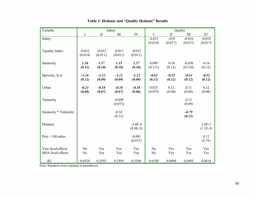
Table 3: Hedonic and “Quality Hedonic” Results
Variable Salary Quality I II III IV I II III IVSalary -0.013 -.018 -0.016 -0.018
(0.014) (0.017) (0.017) (0.017)
Tquality Index -0.012 -0.012 -0.011 -0.012 (0.014) (0.011) (0.011) (0.011)
Sminority 1.30 1.37 1.35 1.37 0.090 -0.16 -0.030 -0.16 (0.11) (0.10) (0.10) (0.10) (0.113) (0.12) (0.124) (0.12)
Spoverty, K-6 -1.16 -1.12 -1.12 -1.12 -0.62 -0.52 -0.51 -0.52 (0.11) (0.09) (0.09) (0.09) (0.11) (0.12) (0.12) (0.12)
Urban -0.21 -0.18 -0.18 -0.18 0.025 0.12 0.11 0.12 (0.08) (0.07) (0.07) (0.06) (0.079) (0.08) (0.08) (0.08)
Tminority -0.058 0.13 (0.073) (0.09)
Sminority * Tminority 0.14 -0.79 (0.12) (0.15)
Distance -3.4E-4 2.0E-3 (8.8E-5) (1.1E-3)
Dist > 100 miles -0.081 0.12 (0.057) (0.70)
Year fixed effects No Yes Yes Yes No Yes Yes Yes MSA fixed effects No Yes Yes Yes No Yes Yes Yes R2 0.0328 0.3593 0.3595 0.3596 0.0189 0.0409 0.0495 0.0410
Note: Standard errors reported in parentheses
50

51
Table 4: Mean Estimates of Parameters in Wage and Quality Equations Monte Carlo Simulations Varying Either the Preference Parameters or Correlations Between Explanatory Variables
values of preference parameters mean estimates of parameters
in wage equation mean estimates of parameters
in quality equation
1β
2β
4β
1z Sρ ,qLρ
1Z Lρ
1γ%
2γ%
3γ%
1τ%
2τ%
3τ%
0.0 0.0
0.0 0.0 0.0 -0.0003 0.24
-0.009 0.19
0.699 1.00
0.004 0.08
-0.002 0.08
0.692 1.00
0.3 0.6 0.0 0.0 0.0
-0.131 0.84
-0.274 0.99
0.732 1.0
0.183 1.0
0.363 1.0
0.609 1.0
Comparison 1: Variation in the preference parameters for 1Z and 2Z
0.6 1.2 0.0 0.0 0.0
-0.215 0.99
-0.447 1.0
0.776 1.0
0.282 1.0
0.564 1.0
0.470 1.0
0.0 0.0 0.0 0.0 0.0
-0.0003 0.24
-0.009 0.19
0.699 1.0
0.004 0.08
-0.002 0.08
0.692 1.0
0.0 0.0 0.0 0.3 0.0
0.165 0.97
-0.011 0.22
0.667 1.0
0.001 0.08
0.001 0.02
0.693 1.0
Comparison 2: Variation in the correlation between 1Z and salary
0.0 0.0 0.0 0.6 0.0
0.380 1.0
-0.011 0.27
0.543 1.0
-0.006 0.04
0.002 0.05
0.696 1.0
0.5 0.5 0.0 0.0 0.0
-0.219 0.98
-0.231 0.99
0.736 1.0
0.302 1.0
0.302 1.0
0.599 1.0
0.5 0.5 -0.5 0.0 0.0
-0.208 0.99
-0.224 0.99
0.719 1.0
0.296 1.0
0.299 1.0
0.590 1.0
0.5 0.5 -1.0 0.0 0.0
-0.195 0.96
-0.211 0.96
0.690 1.0
0.289 1.0
0.292 1.0
0.572 1.0
Comparison 3: Variation in teachers’ distance preference parameter
0.5 0.5 -1.5 0.0 0.0
-0.186 0.95
-0.200 0.97
0.668 1.0
0.284 1.0
0.284 1.0
0.558 1.0
0.5 0.5 -1.0 0.0 0.0
-0.195 0.96
-0.211 0.96
0.690 1.0
0.289 1.0
0.292 1.0
0.572 1.0
0.5 0.5 -1.0 0.0 0.3
-0.211 0.97
-0.207 0.97
0.688 1.0
0.313 1.0
0.286 1.0
0.561 1.0
Comparison 4: Variation in the correlations between teachers’ location and q and between school location and 1Z 0.5 0.5 -1.0 0.0 0.6
-0.261
1.0 -0.197 0.96
0.687 1.0
0.387 1.0
0.271 1.0
0.529 1.0

Appendix A
As noted in Section IV, it is necessary to use simulation to compute values of ( );mtj mtjE z q θ% in
the moment condition ( )| ;mtj mtj mtj mtjt j
q z E z q θ − = % % 0∑∑ and ( );mtj mtjE d q θ% in the moment
conditions ( )| ; 0mtj mtj mtjE d q θ − = % %
mtjt j
q d∑∑ and ( )| ;mtj mtjd E d q θ 0mtj
t j− = ∑∑ % % . Let
( )|mtj mtF z q ;j θ% be the approximation of ( );mtj mtjE z q θ% obtained through simulation; and
( |mtj mtF d q );j θ% the simulator for ( );mtj mtjE d q θ% .
The following two steps summarize our method for calculating these simulated moments.
Step 1: A random number generator generates H sets of independent draws for the random
variables in the model. In each draw, random numbers are generated corresponding to the random
variable(s) in each candidate’s benefit equation for every school alternative. We denote these values in
the hth draw using the notation hjkδ , j = 1,2,…,J and k = 1,2,…,K. Similarly, the hth draw includes
randomly generated values for the random error terms ( hjkω ) in the equations characterizing the
benefits to each employer associated with hiring each candidate. These randomly generated values are
held constant throughout the estimation, as are the observed attributes of candidates and schools. In
the basic models estimated, hjkδ and h
jkω are assumed to be independent and are generated using a
standard-normal random number generator. As discussed in the paper, a model is also estimated with
hjkδ and h
jkω drawn from the student’s t distribution with four degrees of freedom.24 In the other
specification of the error structure employed, school random effects were introduced into the
24 Because the variance of this student’s t distribution equals 2, the random draws were divided by 2 yielding random variables having unit variances, consistent with the normalization maintained throughout our analysis. This transformed yields random variables having a distribution having thicker-tails at the same time there is a higher concentration of values close to the mode of zero, compared to the standard-normal distribution.
52

specification of candidates’ preferences; h h hjk jk kδ η η•= + where h
kη• is a random effect for school k,
which is assumed to be independent of the white-noise random variable hjkη and the measured school
attributes included in the model. Normalizing the variance of hjkδ to be one, the variances of h
kη• and
hjkη are 2σ and 1 2σ− respectively.
)( )θ =
hjk jk
hmtjz% j
( ); ;mtj mtjE z q θ%
(; ;mtj mtjE d q θ%
( )| ;tj mtjz q θ
( )| ;mtj mtjd q θ
Step 2: For a given set of parameter values ( βα , and the random numbers drawn in
Step 1 for a particular error structure, the simulated moments are obtained as follows. The implied
nonstochastic components of utility along with the values of δ and hω for a particular draw (h) are
used to infer the rankings of the candidates and schools. In turn, these rankings are used with the Gale-
Shapley matching algorithm to determine the school-optimal stable matching and the resulting
distribution of teacher and job attributes. In turn, and are recorded for each of the candidates
hired in the h
hmtd%
th simulated outcome for market m during period t. Repeating this step for each of the
draws yields the following approximations of the pertinent expected values.
( ) 1 hmtj mtj mtjH
hF z q zθ = ≈∑% %
( ) )1 hmtj mtj mtjH
hF d q dθ = ≈∑% %
We substitute these expressions into the moment conditions employed to get the simulated moment
conditions summarized in Equations 1 and 2:
amtj mtj mtj mq z Fψ ≡ −% %
bmtj mtj mtjq d Fψ ≡ −% % (1)
( )| ;cmtj mtj mtj mtjd F d qψ θ ≡ −
% %
0
amtjb
m mtj mtjt j t jc
mtj
ψ
ψ ψ ψ
ψ
= = =
∑∑ ∑∑ (2)
53

54
Defining ( )θψ to be a column vector containing the stacked values of 1ψ , 2ψ , … , 5ψ for the five
markets, the method of simulated moment (MSM) estimator is ( ) )((ˆ θψθψθ W = ) W′minθ
arg where
W is a symmetric, positive semidefinite weighting matrix. We employ the identity weighting matrix
and the consistent estimator ( ) ∑ ′=m
mmI )()(minarg~ θψθψθθ
. The asymptotic covariance matrix of
the estimator is θ~ ( ) [ ] ( ) [1 11n HD D D′ ′= + Ω ]1 1D D− −′( )
V D where θ% =
'0
0 θθ
E
∂∂ψ
D and
[ ]ψVarAsy=Ω . ( )mtj
m t jD
ψ θθ
∂=
′∂∑∑∑
%% is used to approximate D. Given our framework, Ω
simplifies to the block diagonal matrix in (3) where we approximate the mth diagonal block using the
Ω
ΩΩ
=
′
′′
=′=Ω
5
2
1
55
22
11
00
0000
00
0000
][
L
MOMM
L
L
L
MOMM
L
L
ψψ
ψψψψ
ψψ
E
EE
E (3)
formula 1 ( ) ( )m mtjt jmn mtjψ θ ψ θ′Ω = ∑∑ % %% .
We use 100 draws of the random errors to calculate the simulators and a combination of
extensive grid searches and the simplex method available in GQOPT to estimate the parameters. We
then use 500 draws of the random errors in the simulations to calculate the derivatives of the moments
needed to compute the standard errors of the point estimates.


![Compensating Teams[1]](https://static.fdocuments.net/doc/165x107/577d27c61a28ab4e1ea4cb06/compensating-teams1.jpg)