Analyzing Reinforcement Learning Benchmarks with RandomWeight Guessing

Declan OllerProvidence, Rhode Island, USA

declanoller@gmail.com

Tobias GlasmachersInstitute for Neural Computation,Ruhr-University Bochum, Germany

tobias.glasmachers@ini.rub.de

Giuseppe CuccueXascale Infolab, University of

Fribourg, Switzerlandgiuseppe.cuccu@unifr.ch

ABSTRACTWe propose a novel method for analyzing and visualizing the com-plexity of standard reinforcement learning (RL) benchmarks basedon score distributions. A large number of policy networks are gener-ated by randomly guessing their parameters, and then evaluated onthe benchmark task; the study of their aggregated results provideinsights into the benchmark complexity. Our method guaranteesobjectivity of evaluation by sidestepping learning altogether: thepolicy network parameters are generated using Random WeightGuessing (RWG), making our method agnostic to (i) the classic RLsetup, (ii) any learning algorithm, and (iii) hyperparameter tuning.We show that this approach isolates the environment complexity,highlights specific types of challenges, and provides a proper foun-dation for the statistical analysis of the task’s difficulty. We testour approach on a variety of classic control benchmarks from theOpenAI Gym, where we show that small untrained networks canprovide a robust baseline for a variety of tasks. The networks gener-ated often show good performance even without gradual learning,incidentally highlighting the triviality of a few popular benchmarks.

KEYWORDSEvolutionary algorithms; learning agent capabilities; machine learn-ingACM Reference Format:Declan Oller, Tobias Glasmachers, and Giuseppe Cuccu. 2020. Analyzing Re-inforcement Learning Benchmarks with Random Weight Guessing. In Proc.of the 19th International Conference on Autonomous Agents and MultiagentSystems (AAMAS 2020), Auckland, New Zealand, May 9–13, 2020, IFAAMAS,9 pages.

1 INTRODUCTIONReports on new Reinforcement Learning (RL) algorithms [18] arefrequently presented with the scores achieved on standard bench-mark environments such as the OpenAI Gym [2]. These environ-ments are chosen for their solvability and widespread use, meaningthat scores for a new algorithm can be compared to methods in theliterature that use the same environments. In many cases howeverwe lack a solid understanding of the actual challenges posed bysuch environments [3]. This limits the comparison to statementsabout general performance, and it precludes insights about specificstrengths and limitations of RL algorithms. As commonly foundin optimization, an ideal RL benchmark suite should offer variable,discriminative difficulty over a representative set of challenges.

Proc. of the 19th International Conference on Autonomous Agents and Multiagent Systems(AAMAS 2020), B. An, N. Yorke-Smith, A. El Fallah Seghrouchni, G. Sukthankar (eds.), May9–13, 2020, Auckland, New Zealand. © 2020 International Foundation for AutonomousAgents and Multiagent Systems (www.ifaamas.org). All rights reserved.

In optimization there exist well-understood challenges such asnon-convexity, non-smoothness, multi-modality, ill-conditioning,noise, high dimensions, and others. They are attributed to certainproblems, hence defining categories, and some of them even serveas numerical (hence quantitative) measures of problem hardness.This work takes a first, major step in building an analogous measureof difficulty for RL tasks, by designing and open sourcing a tool thatallows analysis of existing (and future) benchmarks based on anexternal and unbiased measure of complexity. It is understood thatour proposal is not the only possible measure. In order to capturethe many facets of task difficulty in RL we resist the temptationto capture complexity in a single number. Instead, we leveragethe performance distribution to visualize rich information about RLtasks.

We are concerned with measuring task difficulty in a way that isappropriate for RL, and in particular for direct policy search. Insteadof the optimization-related challenges listed above, we measurehardness in terms of the probability mass in the weight space thatcorresponds to acceptable solutions. It is in this sense that we addressa fundamental problem of RL research. We are not concerned withhow to address specific difficulties with actual learning algorithms,like deep representation learning, exploration strategies, off-policylearning, and the like.

Gauging a benchmark’s complexity though is not a straight-forward task. As most RL environments are typically distributedas black-box software, the only way to interact with them that isguaranteed to be available is through the environment’s controlloop. Exploring such interaction in a meaningful way requires apotentially sophisticated controller. It would be tempting to use anyarbitrary learning approach for this task. Any choice of trainingmethod however would in turn unavoidably bias the analysis, lim-iting the extent and applicability of consequent findings. The onlyviable alternative to maintain objectivity is thus to avoid learningcompletely.

For our analysis, we propose the simplest procedure conceiv-able: (i) direct policy search; (ii) controller models of minimal butincreasing complexity; (iii) parameter selection based on a randomsampling. In practice, this corresponds to selecting a Neural Net-work (NN) controller of minimal size and complexity, selecting itsweights by means of Random Weight Guessing (RWG; [14]), anddirectly using it in the observation-decision-action loop of controlwith the environment of choice. There is no training, no gradientdescent, no classical RL framework, and sampled controllers arecompletely independent from each other. It’s important to empha-size that RWG is not an approach for solving RL problems, but ratheran analysis method that can complement any learning strategy.

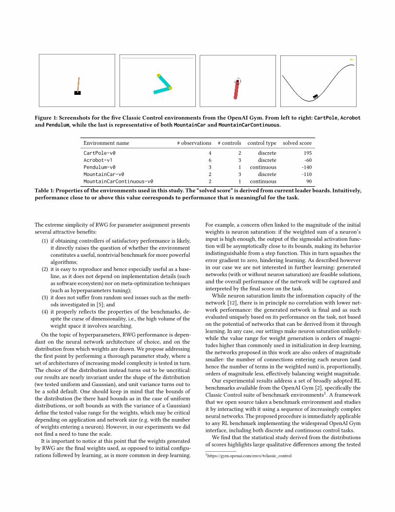
Figure 1: Screenshots for the five Classic Control environments from the OpenAI Gym. From left to right: CartPole, Acrobotand Pendulum, while the last is representative of both MountainCar and MountainCarContinuous.

Environment name # observations # controls control type solved score

CartPole-v0 4 2 discrete 195Acrobot-v1 6 3 discrete -60Pendulum-v0 3 1 continuous -140MountainCar-v0 2 3 discrete -110MountainCarContinuous-v0 2 1 continuous 90

Table 1: Properties of the environments used in this study. The “solved score” is derived from current leader boards. Intuitively,performance close to or above this value corresponds to performance that is meaningful for the task.

The extreme simplicity of RWG for parameter assignment presentsseveral attractive benefits:

(1) if obtaining controllers of satisfactory performance is likely,it directly raises the question of whether the environmentconstitutes a useful, nontrivial benchmark for more powerfulalgorithms;

(2) it is easy to reproduce and hence especially useful as a base-line, as it does not depend on implementation details (suchas software ecosystem) nor on meta-optimization techniques(such as hyperparameters tuning);

(3) it does not suffer from random seed issues such as the meth-ods investigated in [5]; and

(4) it properly reflects the properties of the benchmarks, de-spite the curse of dimensionality, i.e., the high volume of theweight space it involves searching.

On the topic of hyperparameters, RWG performance is depen-dant on the neural network architecture of choice, and on thedistribution from which weights are drawn. We propose addressingthe first point by performing a thorough parameter study, where aset of architectures of increasing model complexity is tested in turn.The choice of the distribution instead turns out to be uncritical:our results are nearly invariant under the shape of the distribution(we tested uniform and Gaussian), and unit variance turns out tobe a solid default. One should keep in mind that the bounds ofthe distribution (be there hard bounds as in the case of uniformdistributions, or soft bounds as with the variance of a Gaussian)define the tested value range for the weights, which may be criticaldepending on application and network size (e.g. with the numberof weights entering a neuron). However, in our experiments we didnot find a need to tune the scale.

It is important to notice at this point that the weights generatedby RWG are the final weights used, as opposed to initial configu-rations followed by learning, as is more common in deep learning.

For example, a concern often linked to the magnitude of the initialweights is neuron saturation: if the weighted sum of a neuron’sinput is high enough, the output of the sigmoidal activation func-tion will be asymptotically close to its bounds, making its behaviorindistinguishable from a step function. This in turn squashes theerror gradient to zero, hindering learning. As described howeverin our case we are not interested in further learning: generatednetworks (with or without neuron saturation) are feasible solutions,and the overall performance of the network will be captured andinterpreted by the final score on the task.

While neuron saturation limits the information capacity of thenetwork [12], there is in principle no correlation with lower net-work performance: the generated network is final and as suchevaluated uniquely based on its performance on the task, not basedon the potential of networks that can be derived from it throughlearning. In any case, our settings make neuron saturation unlikely:while the value range for weight generation is orders of magni-tudes higher than commonly used in initialization in deep learning,the networks proposed in this work are also orders of magnitudesmaller: the number of connections entering each neuron (andhence the number of terms in the weighted sum) is, proportionally,orders of magnitude less, effectively balancing weight magnitude.

Our experimental results address a set of broadly adopted RLbenchmarks available from the OpenAI Gym [2], specifically theClassic Control suite of benchmark environments1. A frameworkthat we open source takes a benchmark environment and studiesit by interacting with it using a sequence of increasingly complexneural networks. The proposed procedure is immediately applicableto any RL benchmark implementing the widespread OpenAI Gyminterface, including both discrete and continuous control tasks.

We find that the statistical study derived from the distributionsof scores highlights large qualitative differences among the tested1https://gym.openai.com/envs/#classic_control

environments. The information made available provides far moredetailed insights than standard aggregated performance scores com-monly reported in the literature.

Related Work. RWG refers to applying the simplistic and usuallynon-competitive optimization technique of pure random search2to the weights of neural networks. To the best of our knowledge itwas first used in [14] for demonstrating that certain widely usedbenchmark problems in sequence learning with recurrent neuralnetworks are trivial. In contrast, we consider RL benchmarks, andour work develops the approach further by turning it into a usefulanalysis methodology for RL environments.

Pure random search was also proposed for tuning the hyper-parameters of learning machines [1], although it is usually lessefficient than Bayesian optimization [7]. However, most Bayesianapproaches start out with an initial design, which can be based ona random sample generated by RWG.

Random weight guessing by itself can be considered a simplisticbaseline method for direct policy search learners such as Neuroevo-lution [4]. In contrast to RWG, Evolution Strategies and similaralgorithms adapt the search distribution online, which turns theminto competitive RL methods [3, 11, 13]. In a direct policy searchcontext, RWG can be thought of as a pure non-local explorationmethod.

It is crucial to distinguish RWG from such methods, since theysometimes come “in disguise”, e.g., using the term random search forelaborate procedures that do actually adapt distribution parametersand hence demonstrate competitive performance on non-trivialtasks [9]. We argue that such algorithms should instead be termedrandomized search, and they are best understood as zeroth ordercousins of stochastic gradient descent (SGD). Although such algo-rithms can be simplistic (as is SGD) they clearly perform iterativelearning, and hence their performance can hardly be consideredunbiased measures of task difficulty.

Understanding the overall complexity of an RL task is usuallyapproached through theoretical analysis, which yields general re-sults, e.g., in terms of regret bounds [6] and convergence guaran-tees [8, 15–17]. That line of work highlights principal strengthsand limitations of RL paradigms, but it is hardly suitable for ana-lyzing and systematically understanding specific challenges posedby complex RL environments. In addition, theoretically promisedresults of RL often break down when parts of the so-called “DeadlyTriad”3 are violated [19]. In particular, we are not aware of anywork that considers widely used benchmarks like the OpenAI Gymcollection of tasks in this perspective. Our study aims to provide apractical tool for such an analysis.

Our Contributions. The above lines of work are mostly concernedwith learning and optimization, as well as with myth busting [14].Here we propose to use RWG for a different purpose, namely forthe analysis of RL tasks. Our contributions are as follows:

2Pure random search is a simplistic optimization technique drawing search pointsindependently from a fixed probability distribution. Its search distribution is memoryfree, but the algorithm keeps track of the best point so far. It can be considered as arandomized variant of exhaustive search without taboo list.3The term refers to combining function approximation, bootstrapping, and off-policylearning.

• We show that RWG is a surprisingly powerful method for theanalysis of RL environments. In particular, the performancedistribution provides information about different solutionregimes, noise, and the minimal sophistication of a NN thatcan act as an effective controller.

• We provide compact and informative visualizations of taskdifficulty that help to identify specific challenges and differ-ences between environments at a single glance.

• Nearly 20 years after the work of Schmidhuber et al. [14]we show that it is still common to (often unwittingly) reportstate-of-the-art results on benchmarks which should ratherbe considered trivial.4

• We provide an open source software framework5 to the com-munity that allows immediate application of our analysis toany environment implementing the OpenAI Gym interface.

The remainder of this paper is organized as follows. In the nextsection we describe in detail how we turn RWG into a methodologyfor the analysis of RL environments. The following section demon-strates its discrimination and explanation power with exemplaryresults on selected OpenAI Gym environments. We close with ourconclusions.

2 ANALYSIS METHODOLOGYIn this section we describe our methodology. Given an RL environ-ment we conduct a fixed series of experiments as follows.

Neural Network Controllers. We construct a series of NN archi-tectures suitable for the task at hand with the following implemen-tation:

• The NN input and output sizes match the dimensionality ofthe environment observation and action spaces, respectively.These numbers are specific to the environment of choice.

• The number of hidden layers and their sizes are specified asan experiment parameter (discussed below).

• All networks use a non-linear tanh activation function.• In environments with a discrete action space, the output istranslated into an action index with the argmax operator.

• For continuous action spaces, each output is scaled to withinthe action boundaries.

• We consider 𝑁architectures = 3 simple connectivity patternsof increasing complexity:– The simplest case of a network without hidden layers,which is also equivalent to a linear model

– A network with a single hidden layer of 4 units– A network with two hidden layers of 4 units eachAlternative architectures were tried without discernible ad-ditional insight, though of course benchmarks of highercomplexity may benefit from larger controller models.

• All networks considered are tested with and without biasinputs to the neurons, which interestingly produces betterperformance in the absence of bias (see Figure 2).

4https://github.com/openai/gym/wiki/Leaderboard5https://github.com/declanoller/rwg-benchmark

Figure 2: Histograms of mean sample scores for 2 hidden layer, 4 hidden unit networks with (top row) and without (bottomrow) bias connections. In all five environments, the probability mass on top-performers generally increases when droppingbias connections. The difference is particularly striking for the MountainCarContinuous and MountainCar environments.

For each of the network architectures we sample 𝑁samples = 104instances by drawing each of their weights i.i.d. from the stan-dard normal distribution N(0, 1), i.e. we draw 𝑁samples weight vec-tors𝑤𝑛 ∈ R𝑑 from the multi-variate standard normal distributionN(0, 𝐼 ), where𝑑 is the number of weights of a network architecture,and 𝐼 ∈ R𝑑×𝑑 denotes the identity matrix. Equivalently, a randommatrix of size 𝑁samples × 𝑑 is drawn from the corresponding multi-variate standard normal distribution.

The Score Tensor. Each of the 𝑁samples networks implements acontroller, which maps observations (input) to actions (output).Each controller is repeatedly tested on the environment’s controlloop for 𝑁episodes independent episodes. Repetition is only neces-sary for environments featuring a stochastic component, as com-monwith random initial conditions. For deterministic environmentswe propose setting 𝑁episodes = 1.

In each episode we record the rewards obtained in each timestep. The total reward (the non-discounted sum of all rewards in theepisode) is assigned as a score. For clarity, the procedure is formallydefined in Algorithm 1.

The resulting score tensor has dimensions𝑁architectures×𝑁samples×𝑁episodes, for 𝑁architectures = 3 network architectures, 𝑁samples =

104 independent networks per architecture, and 𝑁episodes = 20 in-dependent episodes per network. We denote the tensor by 𝑆 , andrefer to the score achieved by network 𝑛 of architecture 𝑎 in the𝑒-th episode as 𝑆𝑎,𝑛,𝑒 .

Algorithm 1 Environment evaluationInitialize environmentCreate array 𝑆 of size 𝑁architectures × 𝑁samples × 𝑁episodesfor 𝑎 = 1, 2, . . . , 𝑁architectures do

Initialize the current NN architecturefor 𝑛 = 1, 2, . . . , 𝑁samples do

Sample NN weights randomly from N(0, 1)for 𝑒 = 1, 2, . . . , 𝑁episodes do

Reset the environmentRun episode with NNStore accrued episode reward in 𝑆𝑎,𝑛,𝑒

A benefit of this search algorithm’s simplicity and the indepen-dence between network architectures, networks, and episodes is

that the algorithm is embarrassingly parallel. Also, our defaultnumbers for 𝑁samples and 𝑁episodes can be adapted based on theavailable computational resources. Running the full evaluation asdescribed above on all five Classic Control environments from theOpenAI Gym (Figure 1) with three architectures took under 20hours on a single machine, using a 32-core Intel(R) Xeon(R) E5-2620 at 2.10GHz, with a RAM utilization below 5GB. Runtimes perarchitecture and environment are shown in Table 2.

It is understood in principle that generating 𝑁samples = 104random networks is not a reasonable learning strategy. The numberis far too large, e.g., for an initial design of a Bayesian optimizationapproach, or as a population size in a neuroevolution algorithm.We want to emphasize that such a large set of samples here serves avery different purpose: we do not aim to optimize the score this way,but instead we aim to draw statistical conclusions about propertiesof the environment.

The Score Distribution. We visualize the score tensor 𝑆 as follows.First of all, each network architecture 𝑎 is treated independently,resulting in series of plots. For each network architecture the scores𝑆𝑎 form an 𝑁samples × 𝑁episodes matrix. From each row of this ma-trix, corresponding to a single network 𝑛, we extract the meanperformance

𝑀𝑎,𝑛 =1

𝑁episodes

𝑁episodes∑𝑒=1

𝑆𝑎,𝑛,𝑒

of the network, as well as its variance

𝑉𝑎,𝑛 =1

𝑁episodes + 1

𝑁episodes∑𝑒=1

(𝑆𝑎,𝑛,𝑒 −𝑀𝑎,𝑛

)2.

A crucial ingredient of the subsequent analysis is that we sort theall networks of the same architecture by their mean score 𝑀𝑎,𝑛 ,and we refer to the position of the network within the sorted listas its rank 𝑅𝑎 (𝑛) (in the rare cases of exact ties of mean scores, thetied samples are left in the order they were originally). Then weaggregate the score matrix in three distinct figures:

(1) A log-scale histogram of𝑀𝑎,𝑛 ;(2) A scatter plot of the individual sample scores 𝑆𝑎,𝑛,𝑒 over their

corresponding 𝑅𝑎 (𝑛) sorted by mean score, with a (naturallymonotonically increasing) curve of their𝑀𝑎,𝑛 overlaid; and

(3) A scatter plot of score variance 𝑉𝑎,𝑛 over mean score𝑀𝑎,𝑛 .

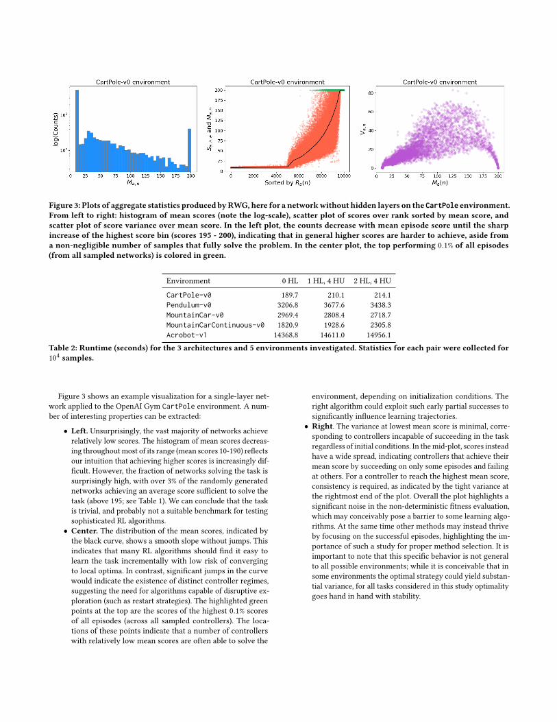
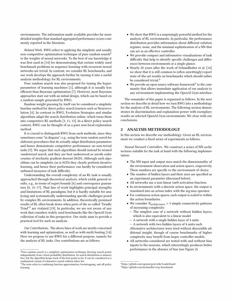
Figure 3: Plots of aggregate statistics produced byRWG, here for a networkwithout hidden layers on the CartPole environment.From left to right: histogram of mean scores (note the log-scale), scatter plot of scores over rank sorted by mean score, andscatter plot of score variance over mean score. In the left plot, the counts decrease with mean episode score until the sharpincrease of the highest score bin (scores 195 - 200), indicating that in general higher scores are harder to achieve, aside froma non-negligible number of samples that fully solve the problem. In the center plot, the top performing 0.1% of all episodes(from all sampled networks) is colored in green.

Environment 0 HL 1 HL, 4 HU 2 HL, 4 HU

CartPole-v0 189.7 210.1 214.1Pendulum-v0 3206.8 3677.6 3438.3MountainCar-v0 2969.4 2808.4 2718.7MountainCarContinuous-v0 1820.9 1928.6 2305.8Acrobot-v1 14368.8 14611.0 14956.1

Table 2: Runtime (seconds) for the 3 architectures and 5 environments investigated. Statistics for each pair were collected for104 samples.

Figure 3 shows an example visualization for a single-layer net-work applied to the OpenAI Gym CartPole environment. A num-ber of interesting properties can be extracted:

• Left. Unsurprisingly, the vast majority of networks achieverelatively low scores. The histogram of mean scores decreas-ing throughoutmost of its range (mean scores 10-190) reflectsour intuition that achieving higher scores is increasingly dif-ficult. However, the fraction of networks solving the task issurprisingly high, with over 3% of the randomly generatednetworks achieving an average score sufficient to solve thetask (above 195; see Table 1). We can conclude that the taskis trivial, and probably not a suitable benchmark for testingsophisticated RL algorithms.

• Center. The distribution of the mean scores, indicated bythe black curve, shows a smooth slope without jumps. Thisindicates that many RL algorithms should find it easy tolearn the task incrementally with low risk of convergingto local optima. In contrast, significant jumps in the curvewould indicate the existence of distinct controller regimes,suggesting the need for algorithms capable of disruptive ex-ploration (such as restart strategies). The highlighted greenpoints at the top are the scores of the highest 0.1% scoresof all episodes (across all sampled controllers). The loca-tions of these points indicate that a number of controllerswith relatively low mean scores are often able to solve the

environment, depending on initialization conditions. Theright algorithm could exploit such early partial successes tosignificantly influence learning trajectories.

• Right. The variance at lowest mean score is minimal, corre-sponding to controllers incapable of succeeding in the taskregardless of initial conditions. In themid-plot, scores insteadhave a wide spread, indicating controllers that achieve theirmean score by succeeding on only some episodes and failingat others. For a controller to reach the highest mean score,consistency is required, as indicated by the tight variance atthe rightmost end of the plot. Overall the plot highlights asignificant noise in the non-deterministic fitness evaluation,which may conceivably pose a barrier to some learning algo-rithms. At the same time other methods may instead thriveby focusing on the successful episodes, highlighting the im-portance of such a study for proper method selection. It isimportant to note that this specific behavior is not generalto all possible environments; while it is conceivable that insome environments the optimal strategy could yield substan-tial variance, for all tasks considered in this study optimalitygoes hand in hand with stability.

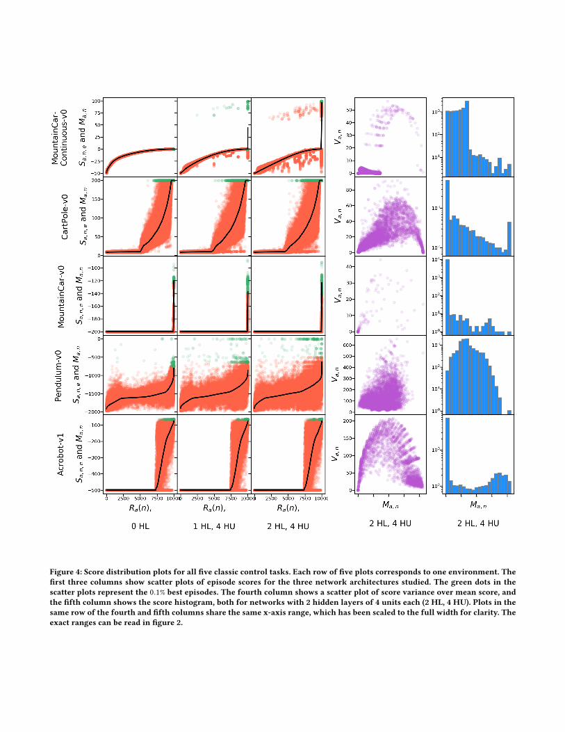
Figure 4: Score distribution plots for all five classic control tasks. Each row of five plots corresponds to one environment. Thefirst three columns show scatter plots of episode scores for the three network architectures studied. The green dots in thescatter plots represent the 0.1% best episodes. The fourth column shows a scatter plot of score variance over mean score, andthe fifth column shows the score histogram, both for networks with 2 hidden layers of 4 units each (2 HL, 4 HU). Plots in thesame row of the fourth and fifth columns share the same x-axis range, which has been scaled to the full width for clarity. Theexact ranges can be read in figure 2.

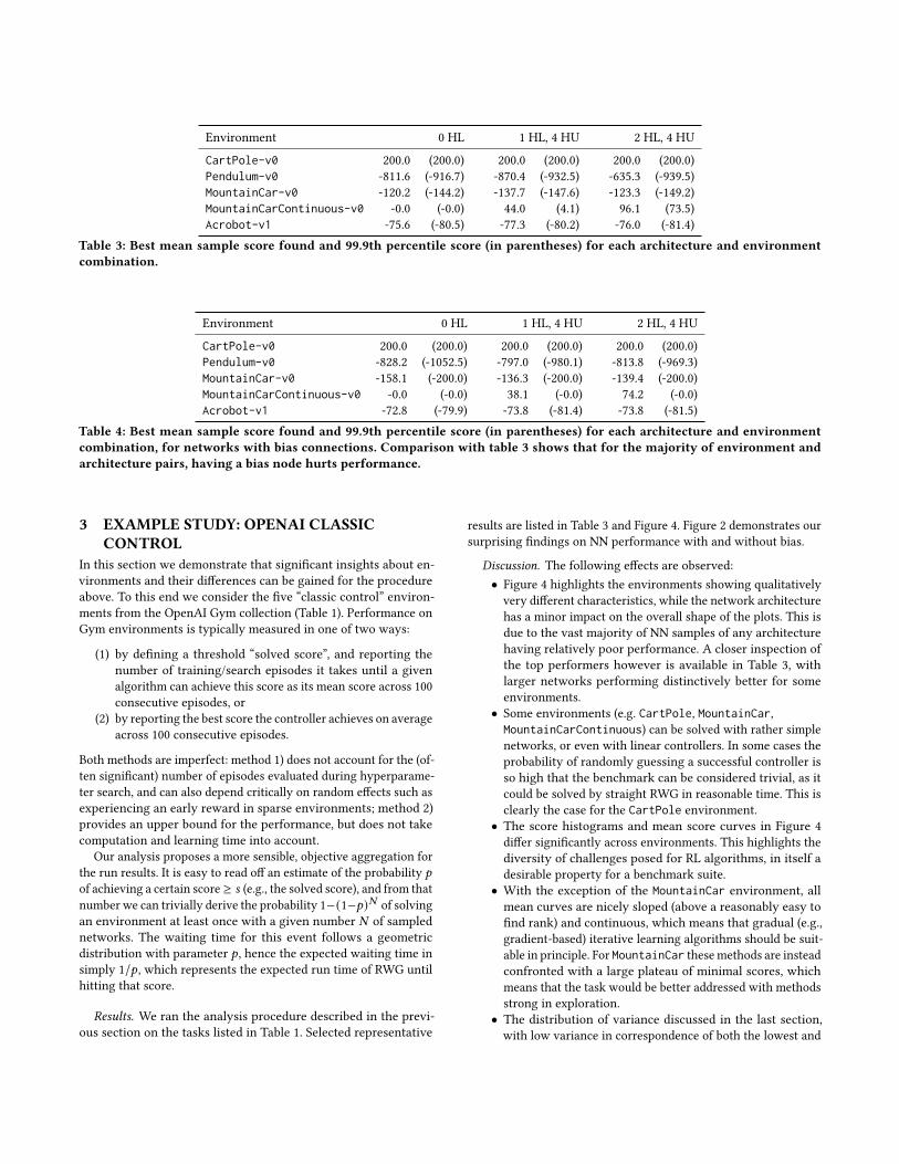
Environment 0 HL 1 HL, 4 HU 2 HL, 4 HU

CartPole-v0 200.0 (200.0) 200.0 (200.0) 200.0 (200.0)Pendulum-v0 -811.6 (-916.7) -870.4 (-932.5) -635.3 (-939.5)MountainCar-v0 -120.2 (-144.2) -137.7 (-147.6) -123.3 (-149.2)MountainCarContinuous-v0 -0.0 (-0.0) 44.0 (4.1) 96.1 (73.5)Acrobot-v1 -75.6 (-80.5) -77.3 (-80.2) -76.0 (-81.4)

Table 3: Best mean sample score found and 99.9th percentile score (in parentheses) for each architecture and environmentcombination.

Environment 0 HL 1 HL, 4 HU 2 HL, 4 HU

CartPole-v0 200.0 (200.0) 200.0 (200.0) 200.0 (200.0)Pendulum-v0 -828.2 (-1052.5) -797.0 (-980.1) -813.8 (-969.3)MountainCar-v0 -158.1 (-200.0) -136.3 (-200.0) -139.4 (-200.0)MountainCarContinuous-v0 -0.0 (-0.0) 38.1 (-0.0) 74.2 (-0.0)Acrobot-v1 -72.8 (-79.9) -73.8 (-81.4) -73.8 (-81.5)

Table 4: Best mean sample score found and 99.9th percentile score (in parentheses) for each architecture and environmentcombination, for networks with bias connections. Comparison with table 3 shows that for the majority of environment andarchitecture pairs, having a bias node hurts performance.

3 EXAMPLE STUDY: OPENAI CLASSICCONTROL

In this section we demonstrate that significant insights about en-vironments and their differences can be gained for the procedureabove. To this end we consider the five “classic control” environ-ments from the OpenAI Gym collection (Table 1). Performance onGym environments is typically measured in one of two ways:

(1) by defining a threshold “solved score”, and reporting thenumber of training/search episodes it takes until a givenalgorithm can achieve this score as its mean score across 100consecutive episodes, or

(2) by reporting the best score the controller achieves on averageacross 100 consecutive episodes.

Both methods are imperfect: method 1) does not account for the (of-ten significant) number of episodes evaluated during hyperparame-ter search, and can also depend critically on random effects such asexperiencing an early reward in sparse environments; method 2)provides an upper bound for the performance, but does not takecomputation and learning time into account.

Our analysis proposes a more sensible, objective aggregation forthe run results. It is easy to read off an estimate of the probability 𝑝of achieving a certain score ≥ 𝑠 (e.g., the solved score), and from thatnumber we can trivially derive the probability 1−(1−𝑝)𝑁 of solvingan environment at least once with a given number 𝑁 of samplednetworks. The waiting time for this event follows a geometricdistribution with parameter 𝑝 , hence the expected waiting time insimply 1/𝑝 , which represents the expected run time of RWG untilhitting that score.

Results. We ran the analysis procedure described in the previ-ous section on the tasks listed in Table 1. Selected representative

results are listed in Table 3 and Figure 4. Figure 2 demonstrates oursurprising findings on NN performance with and without bias.

Discussion. The following effects are observed:• Figure 4 highlights the environments showing qualitativelyvery different characteristics, while the network architecturehas a minor impact on the overall shape of the plots. This isdue to the vast majority of NN samples of any architecturehaving relatively poor performance. A closer inspection ofthe top performers however is available in Table 3, withlarger networks performing distinctively better for someenvironments.

• Some environments (e.g. CartPole, MountainCar,MountainCarContinuous) can be solved with rather simplenetworks, or even with linear controllers. In some cases theprobability of randomly guessing a successful controller isso high that the benchmark can be considered trivial, as itcould be solved by straight RWG in reasonable time. This isclearly the case for the CartPole environment.

• The score histograms and mean score curves in Figure 4differ significantly across environments. This highlights thediversity of challenges posed for RL algorithms, in itself adesirable property for a benchmark suite.

• With the exception of the MountainCar environment, allmean curves are nicely sloped (above a reasonably easy tofind rank) and continuous, which means that gradual (e.g.,gradient-based) iterative learning algorithms should be suit-able in principle. For MountainCar thesemethods are insteadconfronted with a large plateau of minimal scores, whichmeans that the task would be better addressed with methodsstrong in exploration.

• The distribution of variance discussed in the last section,with low variance in correspondence of both the lowest and

highest mean scores, is to be expected as a common pattern.All samples should conceivably fall into one of the follow-ing three categories: 1) never receives reward; 2) rewarddepends on favorable initial condition, but is inconsistent;and 3) reliably achieving good scores, independent of initialconditions. Categories 1 and 3 naturally lead to low variance,as the scores are either all low, or all high.This implies that the score variance is to be expected highestin the range where learning takes place. For the CartPole,Acrobot, and Pendulum tasks the variability covers a hugerange of scores, which makes it difficult to even measureprogress online during learning. We can therefore expectthat despite the fact that learning trajectories with smoothlyincreasing mean scores exist, some types of RL algorithms(like direct policy search) may be expected to suffer sig-nificantly from the high score variance. In contrast, theMountainCarContinuous task is nearly unaffected by noise.In the interesting range it still has a large variance due to thefact that only few controllers solve the task in a few episodes,while the vast majority is caught in a large local optimum.

• It is at first glance surprising that NN controllers without biasterms outperform NNs with bias (Figure 2). We find that thiseffect is systematic across all tested environments, barringnegligible statistical fluctuations. The analogous overviewof results presented in Table 3, but instead for NNs with biasunits, is shown in Table 4.

Our open source reference implementation (in Python) makesit easy to extend the study to other classes of environments, espe-cially if already compatible with the widely adopted OpenAI Gymcontrol interface. Testing a large number of environments overtime would create a broad data base of characterized environments,constituting a strong baseline for the study of existing and newlearning methods.

4 CONCLUSIONEvaluating task complexity in the context of reinforcement learningproblems is a multifaceted and understudied problem. Rather thanaiming at providing a single score of overall complexity, whichwould inevitably remain incomplete, we present a framework toanalyze in depth the complexity of RL tasks. Our analysis usesno learning and does not require any hyperparameter tuning. Weproduce test controllers in a direct policy search fashion usingRandom Weight Guessing, then draw a statistical analysis basedon the complexity of the controllers, their performance on the task,and the distribution of collected reward.

We validate our approach on the set of Classic Control bench-marks from the OpenAI Gym. Due to this limitation of the scopeof our study we consider it only a first step. We nevertheless re-gard this step as an important contribution to a study subject thatdeserves more attention in the future. Our results clearly identifythe distinctive characteristics of each environment, underlying thechallenges that induce their complexity, and pointing at promisingapproaches to address them. Moreover we offer an upper boundon required model complexity. We find RWG to be surprisinglyeffective e.g. in the case of the CartPole problem, pointing at itstriviality.

Future Work. One apparent limitation of RWG regards scalingto large network architectures, which (at first glance) seems topreclude its application to tasks relying on visual input such asAtari games [10]. In future work we will address this widely usedclass of benchmarks by separating feature extraction from the actualcontroller, following [3]. Yet another straightforward extension isto include recurrent NN architectures to better cope with partiallyobservable environments.

A striking open question is how well our analysis predicts theperformance of different classes of algorithms, like temporal differ-ence approaches, policy gradient methods, and direct policy search.Answering this question would have the potential to extend ouranalysis methodology into a veritable recommender system for RLalgorithms.

ACKNOWLEDGMENTSThis work was supported by the Swiss National Science Foundationunder grant number 407540_167320.

REFERENCES[1] James Bergstra and Yoshua Bengio. 2012. Random search for hyper-parameter

optimization. Journal of Machine Learning Research (JMLR) 13 (2012), 281–305.[2] Greg Brockman, Vicki Cheung, Ludwig Pettersson, Jonas Schneider, John

Schulman, Jie Tang, and Wojciech Zaremba. 2016. OpenAI Gym. (2016).arXiv:arXiv:1606.01540

[3] Giuseppe Cuccu, Julian Togelius, and Philippe Cudré-Mauroux. 2019. PlayingAtari with Six Neurons. In Proceedings of the 18th International Conference onAutonomous Agents and MultiAgent Systems. 998–1006.

[4] Christian Igel. 2003. Neuroevolution for reinforcement learning using evolutionstrategies. In The 2003 Congress on Evolutionary Computation, 2003. CEC’03., Vol. 4.IEEE, 2588–2595.

[5] Riashat Islam, Peter Henderson, Maziar Gomrokchi, and Doina Precup. 2017. Re-producibility of benchmarked deep reinforcement learning tasks for continuouscontrol. arXiv preprint arXiv:1708.04133 (2017).

[6] Thomas Jaksch, Ronald Ortner, and Peter Auer. 2010. Near-optimal regret boundsfor reinforcement learning. Journal of Machine Learning Research (JMLR) 11, Apr(2010), 1563–1600.

[7] Donald R Jones, Matthias Schonlau, and William J Welch. 1998. Efficient globaloptimization of expensive black-box functions. Journal of Global optimization 13,4 (1998), 455–492.

[8] Bo Liu, Ji Liu, Mohammad Ghavamzadeh, Sridhar Mahadevan, and Marek Petrik.2015. Finite-Sample Analysis of Proximal Gradient TD Algorithms.. In UAI.504–513.

[9] Horia Mania, Aurelia Guy, and Benjamin Recht. 2018. Simple random searchof static linear policies is competitive for reinforcement learning. In NeuralInformation Processing Systems, Vol. 31.

[10] Volodymyr Mnih, Koray Kavukcuoglu, David Silver, Andrei A Rusu, Joel Veness,Marc G Bellemare, Alex Graves, Martin Riedmiller, Andreas K Fidjeland, GeorgOstrovski, et al. 2015. Human-level control through deep reinforcement learning.Nature 518, 7540 (2015), 529.

[11] Nils Müller and Tobias Glasmachers. 2018. Challenges in high-dimensionalreinforcement learning with evolution strategies. In International Conference onParallel Problem Solving from Nature. Springer, 411–423.

[12] Anna Rakitianskaia and Andries Engelbrecht. 2015. Measuring saturation inneural networks. In 2015 IEEE Symposium Series on Computational Intelligence.IEEE, 1423–1430.

[13] Tim Salimans, Jonathan Ho, Xi Chen, Szymon Sidor, and Ilya Sutskever. 2017.Evolution strategies as a scalable alternative to reinforcement learning. TechnicalReport arXiv:1703.03864. arXiv.org.

[14] Jürgen Schmidhuber, S Hochreiter, and Y Bengio. 2001. Evaluating benchmarkproblems by random guessing. A Field Guide to Dynamical Recurrent Networks,ed. J. Kolen and S. Cremer (2001), 231–235.

[15] John Schulman, Sergey Levine, Pieter Abbeel, Michael Jordan, and Philipp Moritz.2015. Trust region policy optimization. In International conference on machinelearning. 1889–1897.

[16] David Silver, Guy Lever, Nicolas Heess, Thomas Degris, Daan Wierstra, andMartin Riedmiller. 2014. Deterministic policy gradient algorithms. In JMLRconference proceedings, International Conference on Machine Learning, Vol. 32.

[17] Richard S Sutton and Andrew G Barto. 2018. Reinforcement learning: An intro-duction. MIT press.

[18] Richard S Sutton, Andrew G Barto, et al. 1998. Introduction to reinforcementlearning. Vol. 2. MIT press Cambridge.

[19] Hado Van Hasselt, Yotam Doron, Florian Strub, Matteo Hessel, Nicolas Sonnerat,and Joseph Modayil. 2018. Deep reinforcement learning and the deadly triad.

arXiv preprint arXiv:1812.02648 (2018).