Analyzing Diffusion by Analogy with Consolidation · Analyzing Diffusion by Analogy with...

Analyzing Diffusion by Analogy with ConsolidationCharles D. Shackelford1 and Jae-Myung Lee2

Abstract: The analogy between Terzaghi’s governing equation for consolidation and Fick’s governing equation for diffusion �i.e., Fick’ssecond law� is used as the basis for analyzing diffusion of aqueous miscible solutes �e.g., contaminants� in saturated porous media. Basedon this analogy, one-dimensional analytical �closed-form� solutions to the consolidation equation can be transformed into one-dimensionalanalytical solutions to Fick’s second law. The general methodology for transforming the analytical solutions in terms of solute concen-tration, solute mass flux, and cumulative solute mass is presented, and the concepts of degree of diffusion and average degree of diffusionare introduced. Analytical solutions are presented for a variety of initial and boundary conditions. Application of the methodology isillustrated through an example analysis for a problem involving matrix diffusion associated with pump-and-treat remediation. Theexample analysis illustrates the ability to analyze relatively complex problems involving diffusive solute transport based on the analogybetween consolidation and diffusion.

DOI: 10.1061/�ASCE�1090-0241�2005�131:11�1345�

CE Database subject headings: Containment; Diffusion; Models; Soil consolidation; Waste disposal; Waste management.

Introduction

Although the physical process of small-strain consolidation isfundamentally different from the chemical process of diffusion,both processes are governed by the same form of a second-orderpartial differential equation and, therefore, are mathematicallyanalogous. Because of this analogy, analytical �closed-form� so-lutions to Terzaghi’s differential equation describing consolida-tion also represent analytical solutions to Fick’s differentialequation describing diffusion.

The analogy between consolidation and diffusion can facilitatethe analysis of problems in which diffusion is the dominant con-taminant transport process. Such problems typically involve low-permeability ��10−9 m/s�, fine-grained soils �e.g., clay�, and in-clude analyses related to evaluation and design of both engineeredand natural containment facilities for waste disposal, as well asanalyses related to the remediation of existing contaminated soils.Examples of the significance of diffusion in terms of contaminanttransport through engineered barriers include analyses involvingcompacted clay liners �Goodall and Quigley 1977; Crooks andQuigley 1984; Shackelford 1988, 1989, 1990; Toupiol et al. 2002;Willingham et al. 2004�, subaqueous capping layers �Wang et al.1991; Thoma et al. 1993�, geosynthetic clay liners �Lake andRowe 2000; Malusis and Shackelford 2002, 2004�, composite lin-ers �Foose 2002; Edil 2003�, and soil-bentonite vertical cutoff

1Professor, Dept. of Civil Engineering, Colorado State Univ., FortCollins, CO 80523-1372 �corresponding author�. E-mail: [email protected]

2Post-Doctoral Research Assistant, Dept. of Civil Engineering,Colorado State Univ., Fort Collins, CO 80523-1372.

Note. Discussion open until April 1, 2006. Separate discussions mustbe submitted for individual papers. To extend the closing date by onemonth, a written request must be filed with the ASCE Managing Editor.The manuscript for this paper was submitted for review and possiblepublication on June 10, 2004; approved on May 10, 2005. This paper ispart of the Journal of Geotechnical and Geoenvironmental Engineer-ing, Vol. 131, No. 11, November 1, 2005. ©ASCE, ISSN 1090-0241/
2005/11-1345–1359/$25.00.
JOURNAL OF GEOTECHNICAL AND GEOE

walls �Mott and Weber 1991a,b; Devlin and Parker 1996;Rabideau and Khandelwahl 1998�.

Diffusion also has been shown to play a significant role ingoverning contaminant transport through natural containment sys-tems, such as aquicludes and aquitards �e.g., Greenberg et al.1973; Gray and Weber 1984�. In this regard, the process of matrixdiffusion, whereby contaminants diffuse from interconnectedpores into the surrounding intact clay or rock matrix, may be animportant attenuation mechanism when the contaminant transportoccurs through structured clay and rock formations �e.g., Foster1975; Grisak and Pickens 1980; Feenstra et al. 1984; Lever et al.1985; Polak et al. 2002�. For example, the potential significanceof matrix diffusion has been considered in terms of the migrationof pesticides resulting from agricultural practice through fracturedclayey till �Jorgensen and Fredericia 1992; Jorgensen and Foged1994�, the migration of leachate resulting from solid waste land-fills through underlying fractured clayey till �Rowe and Booker1991�, the migration of dense-chlorinated solvents resulting fromindustrial spills and disposal practice through fractured geologicmedia �Parker and McWhorter 1994; Parker et al. 1994, 1996�,and the migration of radionuclides resulting from high-levelradioactive waste disposal through fractured crystalline rocks�Sato 1999�.

In terms of remediation, failure of the pump-and-treat technol-ogy to achieve cleanup goals has been attributed, in part, to theprocess of reverse matrix diffusion resulting in the slow and con-tinuous release of contaminants from the intact clay and rockmatrix into the surrounding, more permeable media, such as frac-tures or aquifer materials �e.g., Mackay and Cherry 1989; Mott1992; Feenstra et al. 1996�. Diffusion also has long been recog-nized as the transport process that controls the potential leachingof contaminants from stabilized or solidified hazardous waste,typically by the addition of pozzolanic materials such as cement,lime, and fly ash �e.g., Nathwani and Phillips 1980�. Finally, dif-fusion may be a significant transport process with respect to con-trolling the rate of delivery of chemical oxidants �e.g., potassiumpermanganate, KMnO4� injected into contaminated low-
permeability media through hydraulic fractures for in situ treat-
NVIRONMENTAL ENGINEERING © ASCE / NOVEMBER 2005 / 1345

ment of chlorinated solvents �Siegrist et al. 1999; Struse et al.2002�.

Selected examples of the use of the analogy between consoli-dation and diffusion occasionally appear in the literature, and theanalogy between diffusion and the conduction of heat is describedin the classic texts by Carslaw and Jaeger �1959� and Crank�1975�. However, the full extent of the analogy between consoli-dation and diffusion has not been developed, and no comprehen-sive treatment of the analogy has appeared in the published lit-erature. Such a comprehensive treatment can be useful in terms ofproviding the practitioner with a rational basis for utilizing exist-ing solutions to Terzaghi’s one-dimensional consolidation equa-tion to solve problems involving the diffusion of aqueousmiscible chemicals �solutes� through porous media.

The overall objective of this paper is to illustrate the method-ology for transforming analytical solutions for small-strain, one-dimensional consolidation of saturated, compressible porousmedia into analytical solutions for one-dimensional liquid-phasediffusion of solutes through saturated porous media. The method-ology includes the relatively standard initial conditions involvingrectangular, triangular, and sinusoidal distributions of excesspore-water pressure as described by Terzaghi �1925� and Taylor�1948�, as well as analyses of nonstandard scenarios, includingtime-dependent boundary conditions and complex initial condi-tions that can be analyzed on the basis of superposition. In addi-tion, analytical solutions for the scenario where diffusive solutemass flux occurs in only one direction due to a constant concen-tration difference across the soil, referred to herein as the unidi-rectional diffusive flux scenario, are presented. The resulting ana-lytical solutions for diffusion are expressed in terms of soluteconcentration, solute mass flux, average degree of diffusion, andcumulative solute mass. The ability to use the extended method-ology to solve relatively complex, albeit only one-dimensional,problems is illustrated via an example problem involving matrixdiffusion associated with pump-and-treat remediation.

General Analogy

Governing Equations

The one-dimensional form of the governing equation describingtransient consolidation of saturated porous media often is referredto as Terzaghi’s consolidation equation, after Karl Terzaghi whofirst derived the equation, and can be written as follows �e.g.,Terzaghi 1925; Taylor 1948; Holtz and Kovacs 1981�:

�ue�z,t��t

= cv�2ue�z,t�

�z2 �1�

where ue�z , t��excess pore-water pressure in the medium �soil�;cv�coefficient of consolidation; z�spatial coordinate; andt�time. The excess pore-water pressure is defined as the differ-ence between the total pore-water pressure �e.g., hydrostatic orsteady state plus excess� at any time, u�z , t�, and the total pore-water pressure after equilibrium has been re-established �e.g., hy-drostatic or steady state� corresponding theoretically to infinitetime, u�z ,��, or ue�z , t�=u�z , t�−u�z ,��. The one-dimensionalform of the differential equation governing diffusion often is re-ferred to as Fick’s second law after Adolf Fick �e.g., Cussler1997�, which may be written for saturated incompressible porous
media as follows �Shackelford and Daniel 1991�:
1346 / JOURNAL OF GEOTECHNICAL AND GEOENVIRONMENTAL ENGIN

�ce�z,t��t

=D*

Rd

�2ce�z,t��z2 = Da

�2ce�z,t��z2 �2�

where ce�z , t��excess solute �mass� concentration in the porewater of the medium; D*�effective diffusion coefficient, definedas the product of the apparent tortuosity factor, �a, and the aque-ous diffusion coefficient, Do, for the chemical species �i.e.,D*=�aDo� in accordance with Shackelford and Daniel �1991�;Rd= retardation factor �Freeze and Cherry 1979�, andDa�apparent, effective diffusion coefficient �Shackelford andDaniel 1991; Grathwohl 1998�. The excess solute concentration isdefined as the difference between the solute concentration in thepore water at any time, c�z , t�, and the solute concentration in thepore water after equilibrium has been re-established correspond-ing theoretically to infinite time, or ce�z , t�=c�z , t�−c�z ,��.

The retardation factor may be defined as the ratio of the totalsolute mass �i.e., solid or sorbed phase plus liquid phase� to thesolute mass in the pore water �i.e., liquid phase� assuming instan-taneous, linear, and reversible sorption, or

Rd =CT�z,t�C�z,t�

=mT�t�m�t�

=MT�t�M�t�

= 1 +�d

nKd �3�

where CT�z , t�, mT�t�, and MT�t��total solute mass per unit totalvolume �i.e., solids plus voids�, the total solute mass per unit area,and the total solute mass, respectively; C�z , t�, m�t�, andM�t��solute mass in the pore water per unit total volume, thesolute mass in the pore water per unit area; and the solute mass inthe pore water, respectively; �d�dry �bulk� density of the me-dium; n�porosity of the medium; and Kd�distribution coefficient�Freeze and Cherry 1979�. In general, Rd�1 �or Kd�0�, wherethe lower bound �i.e., Rd=1 or Kd=0� pertains to nonsorbing sol-utes, and Rd�1 �or Kd�0� corresponds to solutes that are sorbedto the porous medium.

General Analytical Solutions

The general analytical solution for consolidation is derived for aninitial excess pore-water pressure, ue,i��0�, in a consolidatingmedium with freely draining boundaries, or

ue�z,0� = ue,i

ue�0,t� = 0 �4�

ue�H,t� = 0

where H�total thickness of the layer, and the solution based onFourier series analysis performed using Eqs. �1� and �4� is asfollows �e.g., Taylor 1948�:

ue�z,t� = �j=1

� � 2

H�

0

H

ue,i sin� j�z

H�dz�sin� j�z

H�exp�−

j2�2cvt

H2 ��5�

where j�dummy variable taking on integer values. By analogy,the solution to Fick’s second law for a medium initially contain-ing a solute at an excess concentration, ce,i��0�, and surroundedby perfectly flushing boundaries �e.g., clay surrounded by sand�,or

ce�z,0� = ce,i

ce�0,t� = 0 �6�

EERING © ASCE / NOVEMBER 2005

ce�H,t� = 0

is as follows:

ce�z,t� = �j=1

� � 2

H�

0

H

ce,i sin� j�z

H�dz�sin� j�z

H�exp�−

j2�2D*t

RdH2 ��7�

In general, the reduced form of the analytical solution will dependon the initial distribution of excess pore-water pressure, ue,i, in thecase of consolidation, or the initial distribution of excess soluteconcentration, ce,i, in the case of diffusion.

Degree of Diffusion

The total excess solute mass �i.e., solid or sorbed phase plus liq-uid phase� per unit total volume at any depth and at any elapsedtime for a saturated medium, CT�z , t�, can be defined based on Eq.�3� as follows:

CT�z,t� = RdC�z,t� = Rdnce�z,t� �8�

Therefore, the relative amount of total excess solute mass re-moved �or gained� at any depth and at any elapsed time is definedherein as the degree of diffusion, Uz

*, and is given as follows:

Uz* =

CT�z,0� − CT�z,t�CT�z,0� − CT�z,��

=ce�z,0� − ce�z,t�ce�z,0� − ce�z,��

�9�

Note that this definition of Uz* is the same as that for degree of

consolidation, Uz, given by Terzaghi’s theory of consolidationwhen �1� the excess solute concentration, ce�z , t�, is replaced bythe excess pore-water pressure, ue�z , t�, and �2� the excess soluteconcentrations at t=0 and at t=�, or ce�z ,0� and ce�z ,��, respec-tively, are replaced by the excess pore-water pressures at t=0 andat t=�, or ue�z ,0� and ue�z ,��, respectively.

Average Degree of Diffusion

The relative amount of excess solute mass removed �or gained� atany elapsed time is defined herein as the average degree of diffu-sion, U*, and is determined by integrating Eq. �9� with respect todepth as follows:

U* =

�0

H

CT�z,0�dz −�0

H

CT�z,t�dz

�0

H

CT�z,0�dz −�0

H

CT�z,��dz

=

�0

H

ce�z,0�dz −�0

H

ce�z,t�dz

�0

H

ce�z,0�dz −�0

H

ce�z,��dz

�10�

The definition for U* given by Eq. �10� is the same as the defini-tion for the average degree of consolidation, U, from Terzaghi’stheory of consolidation when �1� the excess solute concentration,ce�z , t�, is replaced by the excess pore-water pressure, ue�z , t�, and�2� the excess solute concentrations at t=0 and at t=�, or ce�z ,0�and ce�z ,��, respectively, are replaced by the excess pore-waterpressures at t=0 and at t=�, or ue�z ,0� and ue�z ,��, respectively.

*
As an alternative, U also may be defined as follows:

U* =mT�0� − mT�t�mT�0� − mT��

�11�

The expression for U* given by Eq. �11� is analogous to the defi-nition for U as the consolidation settlement at any time, St, rela-tive to the ultimate consolidation settlement at t=�, Su, orU=St /Su.

Diffusive Excess Solute Mass Flux

The general form of the diffusive excess solute mass flux in soil,Jd, may be written in accordance with Fick’s first law for diffu-sion in soil as follows �Shackelford and Daniel 1991�:

Jd = nD*ic = − nD*�ce�z,t��z

�12�

where ic�solute concentration gradient. Therefore, Jd may be ob-tained at any location within the layer and at any elapsed time bysubstituting the spatial derivative of the analytical solution for theexcess solute concentration, Eq. �7�, for the solute concentrationgradient term in Eq. �12� �e.g., see Shackelford 1990�. Alterna-tively, the diffusive excess solute mass flux can be determinedthrough differentiation of the expression for the excess soluteconcentration �ce�z , t� from Eq. �9�� with respect to depth andsubstituting the resulting expression into Eq. �12� as follows:

Jd = − nD* �

�zce�z,0� + ce�z,�� − ce�z,0��Uz

*�z,t�� 13�

The excess solute mass fluxes at the boundaries of the layer atany elapsed time may be determined by evaluating Eqs. �12� and�13� at z=0 and at z=H. Alternatively, the boundary mass fluxesmay be evaluated through differentiation of the expression for theaverage degree of diffusion �Eq. �11�� as follows:

Jd z=0,H = Jd�0,t� + Jd�H,t�

= �dmT�t�dt

�= �mT�0� − mT��

dU*�t�dt

� �14�

Cumulative Mass

The cumulative excess solute mass removed �or gained� per unitarea at any time via diffusion can be determined through integra-tion of the expression for the boundary mass fluxes �Eq. �14�� asfollows:

�0

t

Jd z=0,Hdt = ��0

t

Jd�0,t�dt� + ��0

t

Jd�H,t�dt�= mT�0� − mT�t�

= mT�0� − mT��U*�t� �15�

Note that Eq. �15� is identical to the absolute value of the numera-*
tor in the definition of U given by Eq. �11�.

Analytical Solutions

Standard Scenarios

The analytical solutions presented herein represent two possiblediffusive flux scenarios as illustrated in Fig. 1, viz., the outwardand the inward flux scenarios. The solution domains for bothscenarios are represented by a thickness H and an infinite arealextent such that diffusion occurs only in the vertical direction.The assumption of an infinite areal extent is applicable for prac-tical situations where the thickness, H, of the domain is suffi-ciently short relative to the horizontal extent of the domain suchthat edge or end effects are insignificant.

The outward diffusive flux scenario is described by solutionsto Eq. �7� for different initial excess solute concentrations, ce,i. Asshown in Fig. 1, a variety of possible initial conditions can berepresented by a constant concentration, co, multiplied by a factor, �i.e., ce,i=co�. In general, is either unity �=1� or somefunction of depth, z= f�z��. The boundary conditions for theoutward diffusive flux scenario are perfectly flushing in that thesolute concentrations in the surrounding medium are maintainedas zero �see Eq. �6��. These boundary conditions may be appli-cable for practical situations when the flow rate through the sur-rounding medium is significantly higher than that through themedium being analyzed, such as in the case of reverse matrixdiffusion from a long, thin contaminated clay lens surrounded bya highly permeable sand or gravel aquifer with lateral groundwa-ter flow. However, an evaluation of the suitability of perfectlyflushing boundary conditions may be required for specific fieldapplications. For example, even if perfectly flushing boundaryconditions are determined to be reasonably accurate relative to thefield scenario, the resulting diffusive mass fluxes may still resultin contaminant concentrations that are in excess of the regulatedmaximum contaminant levels.

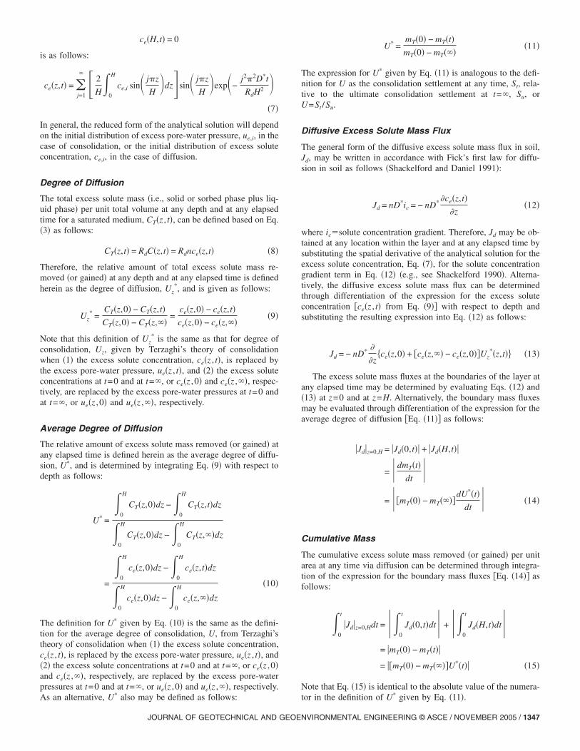
The inward diffusive flux scenario shown in Fig. 1 resultsfrom superposition by subtracting the outward diffusive flux sce-nario from the scenario where both the surrounding medium andthe medium being analyzed are contaminated at a constant con-centration, co, as illustrated schematically in Fig. 2. In this case,the boundary concentrations are maintained constant at co, andthe initial condition is given by �1−�co, where again is either

Fig. 1. Outward and inward diffusive flux scenarios with constantsolute concentration boundary conditions

unity or some function of depth. These boundary conditions are


applicable when the source of contamination surrounding the me-dium can be considered constant, such as in the matrix diffusioncase where contaminants diffuse into a relatively clean clay lensfrom a surrounding contaminated aquifer.

Standard Solutions

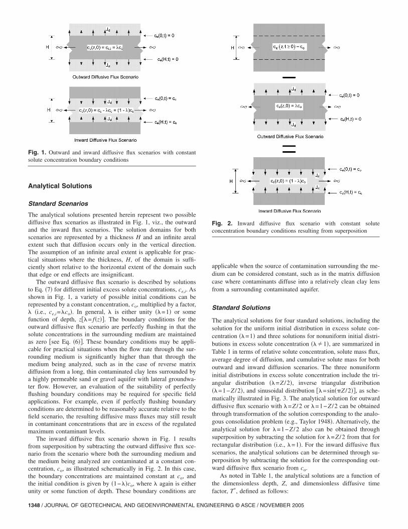
The analytical solutions for four standard solutions, including thesolution for the uniform initial distribution in excess solute con-centration �=1� and three solutions for nonuniform initial distri-butions in excess solute concentration ��1�, are summarized inTable 1 in terms of relative solute concentration, solute mass flux,average degree of diffusion, and cumulative solute mass for bothoutward and inward diffusion scenarios. The three nonuniforminitial distributions in excess solute concentration include the tri-angular distribution �=Z /2�, inverse triangular distribution�=1−Z /2�, and sinusoidal distribution =sin��Z /2��, as sche-matically illustrated in Fig. 3. The analytical solution for outwarddiffusive flux scenario with =Z /2 or =1−Z /2 can be obtainedthrough transformation of the solution corresponding to the analo-gous consolidation problem �e.g., Taylor 1948�. Alternatively, theanalytical solution for =1−Z /2 also can be obtained throughsuperposition by subtracting the solution for =Z /2 from that forrectangular distribution �i.e., =1�. For the inward diffusive fluxscenarios, the analytical solutions can be determined through su-perposition by subtracting the solution for the corresponding out-ward diffusive flux scenario from co.

As noted in Table 1, the analytical solutions are a function ofthe dimensionless depth, Z, and dimensionless diffusive time

*

Fig. 2. Inward diffusive flux scenario with constant soluteconcentration boundary conditions resulting from superposition

factor, T , defined as follows:


able

1.So

lutio

nsfo

rC

onst

ant

Solu

teB

ound

ary

Con

cent

ratio

nsw

ithSt

anda

rdIn

itial

Solu

teC

once

ntra

tion

Dis

trib

utio

ns

iffu

sive

ux cena

rio

Initi

also

lute

conc

entr

atio

ndi

stri

butio

n

Initi

alco

nditi

on�T

*=

0�

Bou

ndar

yco

nditi

ons

Rel

ativ

eso

lute

conc

entr

atio

nc e

�Z,T

* �/c o

Solu

tem

ass

flux

Ave

rage

degr

eeof

diff

usio

n,U

* �T* �

Cum

ulat

ive

solu

tem

assa

Z=

0Z

=2

J d�Z

,T* �

J d�0

,T* �

J d�2

,T* �

utw

ard

�Fig

.3�

a��

Uni

form

�rec

tang

ular

�c o

00

�2/�

��j=

1�

AjC

jDj/

j−

F�

j=1

�B

jCjD

j−

F�

j=1

�C

jDj

−J d

�0,T

* �1

−�4

/�2 ��

j=1

�C

jDj/

j22G

U* �T

* �nw

ard

�Fig

.3�

b��

0c o

c o1

−�2

/��

j=1

�A

jCjD

j/j

F�

j=1

�B

jCjD

jF

�j=

1�

CjD

j−

J d�0

,T* �

Sam

eas

abov

eSa

me

asab

ove

utw

ard

�Fig

.3�

c��

Tri

angu

lar

c oZ

/20

0−

�2/�

��j=

1�

AjC

jEj/

jF

�j=

1�

BjC

jEj

F�

j=1

�C

jEj

F�

j=1

�C

jSa

me

asab

ove

GU

* �T* �

nwar

d�F

ig.

3�d�

�c o

−c o

Z/2

c oc o

1+

�2/�

��j=

1�

AjC

jEj/

j−

F�

j=1

�B

jCjE

j−

F�

j=1

�C

jEj

−F

�j=

1�

Cj

Sam

eas

abov

eSa

me

asab

ove

utw

ard

�Fig

.3�

e��

Inve

rse

tria

ngul

arc o

−c o

Z/2

00

�2/�

��j=

1�

AjC

j/j

−F

�j=

1�

BjC

j−

F�

j=1

�C

j−

F�

j=1

�C

jEj

Sam

eas

abov

eSa

me

asab

ove

nwar

d�F

ig.

3�f�

�c o

Z/2

c oc o

1−

�2/�

��j=

1�

AjC

j/j

F�

j=1

�B

jCj

F�

j=1

�C

jF

�j=

1�

CjE

jSa

me

asab

ove

Sam

eas

abov

e

utw

ard

�Fig

.3�

g��

Sinu

soid

alA

c o0

0A

C−

��/2

�FB

C−

��/2

�FC

−J d

�0,T

* �1

−C

�4/�

�GU

* �T* �

nwar

d�F

ig.

3�h�

�c o

−A

c oc o

c o1

−A

C��

/2�F

BC

��/2

�FC

−J d

�0,T

* �Sa

me

asab

ove

Sam

eas

abov

e

� J d

Z=

0,2d

T* .

Not

atio

n:A

j=si

n�j�

Z/2

�;B

j=co

s�j�

Z/2

�;C

j=ex

p�−

j2 �2 T

*/4

�;D

j=1

−co

s�j�

�=1

−�−

1�j ;

Ej=

cos�

j��=

�−1�

j ;A

=si

n��

Z/2

�;B

=co

s��

Z/2

�;C

=ex

p�−

�2 T

*/4

�;F

=nD

* c o/H

d;G

Hdn

Rdc

o;Z

=z/

Hd;

T*=

D* tR

d−1 H

d−2=

Dat

Hd−

2 .

Z =z

Hd

�16�

T* =D*t

RdHd2 =

Dat

Hd2

where z�actual depth and Hd�maximum diffusive distance. Thedefinition for the dimensionless depth is identical to that for thecase of consolidation where Hd�maximum drainage distance,whereas the definition for the diffusive time factor, T*, is identicalto that for the dimensional consolidation time factor, T, when Da

is replaced by cv.As an example, the solution for the case where =1 is plotted

in terms of the degree of diffusion, Uz*, as a function of Z and T*

in Fig. 4. As indicated in Fig. 4, the upper x axis and curves arealso labeled in terms of Uz and T, respectively, for the case of auniform initial distribution in excess pore-water pressure. Asnoted in Fig. 4, the curves representing the excess solute concen-tration profiles as a function of time �i.e., isoconcentration curves�in the form of Uz

* due to outward diffusion are symmetric aboutthe mid-plane of the medium �Z=1�, which is the same as thesymmetry exhibited in the isochrones resulting from consolida-tion for the analogous case. At any time T*, the gradient in excesssolute concentration at the mid-plane of the profile is zero. There-fore, all of the excess solute in the upper half of the medium�0�Z1� must diffuse out the top boundary �Z=0�, whereas allthe excess solute in the lower half of the medium �1Z�2� mustdiffuse out the lower boundary �Z=2�. As a result, the maximum

Fig. 3. Schematic of basic initial solute concentration distributionsfor both outward and inward diffusive flux scenarios: �a� and �b�uniform; �c� and �d� triangular; �e� and �f� inverse triangular; and �g�and �h� sinusoidal

diffusive distance, Hd, in this case is half the total thickness, H, ofT D fl s O I O I O I O I a =

JOURNAL OF GEOTECHNICAL AND GEOENVIRONMENTAL ENGINEERING © ASCE / NOVEMBER 2005 / 1349

the medium �i.e., H=2Hd�. For this case, note that Jd is less thanzero for 0�Z1 indicating diffusion in the negative �upward�direction, greater than zero for 1Z�2 indicating diffusion inthe positive �downward� direction, and zero for Z=1 indicating nodiffusive transport across the mid-plane of the medium. The sym-metry in isoconcentration profiles also can be utilized for analysisof problems involving a no-flux boundary condition by consider-ing the domain to reside only within either 0�Z�1 or 1�Z�2, such that the total thickness of the medium is the same as themaximum diffusive distance �i.e., H=Hd�. In consolidation, thecase where H=2Hd is referred to as the double-drainage case, andthe case where H=Hd is referred to as the single-drainage case.

Values of U* for the case where =1 are plotted versus T* inFig. 5�a�. Again, since this case is analogous to the standard casein consolidation where there is a uniform initial distribution inexcess pore-water pressure, the upper x axis and right-hand y axisare also labeled in terms of T and U, respectively. In accordancewith Eq. �15�, this temporal distribution in U* can be used todetermine the cumulative excess solute mass removed at any timedue to outward diffusion. In addition, the slope of the relationshipbetween U* and T* shown in Fig. 5�b� can be used to determinethe diffusive mass flux at the boundaries as a function of time inaccordance with Eq. �14�. Finally, although the relationshipsshown in Fig. 5 were formerly developed for the case where=1, these relationships are also applicable for any situationwhere the initial excess concentration profile is linear with depth,as indicated in Table 1.

The maximum diffusive distance, Hd, was previously definedas being equal to half the total thickness of the layer, or H /2, forthe case where both the boundaries transmit mass flux. However,this physical interpretation is valid only for the cases where theisoconcentration profiles are symmetrical about the mid-plane ofthe layer �i.e., uniform and sinusoidal distributions�. While thedefinition of Hd=H /2 still is valid mathematically for the caseswhere the isoconcentration profiles are not symmetrical about themid-plane of the layer, such as for the triangular and inversetriangular distributions, the physical interpretation of Hd as themaximum diffusive distance, of course, is not valid. This samedistinction occurs in consolidation, where Hd is defined as the

Fig. 4. Degree of diffusion for outward �or inward� diffusive fluxscenario with uniform initial solute concentration distribution �T* orT�dimensionless diffusive or consolidation time factor�

maximum drainage distance and is taken mathematically to be


equal to H /2 for the case of a triangular distribution in initialexcess pore-water pressure, even though the isochrone distribu-tion is not symmetrical about the mid-plane of the layer �Lambeand Whitman 1969�. In summary, the maximum drainage or dif-fusive distance, Hd, is half the total thickness, H, of the medium�i.e., H=2Hd� for the double-flux boundary case, and the totalthickness of the medium �i.e., H=Hd� for the single-flux boundarycase, regardless of the initial distribution in excess pore-waterpressure or excess solute concentration distribution.

Nonstandard Boundary Conditions

Time-Dependent Boundary ConditionsOlson �1977� presented the analytical solution for the case ofconsolidation resulting from a single ramp load applied over atime interval, tc, corresponding to the end of construction, with anultimate applied load of qo corresponding to an ultimate excesspore-water pressure, uo �e.g., see Fig. 6�, as follows:

Fig. 5. Average degree of diffusion �a� and rate of diffusion �b� foroutward �or inward� diffusive flux scenario with uniform �ortriangular� initial solute concentration distribution

Fig. 6. Excess pore-water pressure generated with time due to singleramp load


� with Time-Dependent or Constant Boundary Conditions �BCs�

solutece�Z ,T*� /co

Solute mass fluxJd�Z ,T*�

Average degree ofdiffusion U*�T*�

Cumulativesolute massa

Inward

�time-dependent

BCs�

coT* /Tc* �T*�Tc

*� T* /Tc*− �8/�3Tc

*�� j=1� AjDj�1−Cj� / j3 �4F /�2Tc

*�� j=1� BjDj�1−Cj� / j2 T* /Tc

*− �16/�4Tc*�� j=1

� Dj�1−Cj� / j4 2GU*�T*�

co �T*�Tc*� 1− �8/�3Tc

*�� j=1� AjCjDj�Cj

*−1� / j3 �4F /�2Tc*�� j=1

� BjCjDj�Cj*−1� / j2 1− �16/�4Tc

*�� j=1� CjDj�Cj

*−1� / j4 2GU*�T*�

Upward

�constant

BCs�

0 co Z /2+ �2/�� j=1� AjCjEj / j −F /2−F� j=1

� BjCjEj 1− �4/�2�� j=1� CjDj / j2 GT* /2− �4G /�2�� j=1

� Ej�Cj −1� / j2

Downward

�constant

BCs�

co 0 1−Z /2− �2/�� j=1� AjCj / j F /2+F� j=1

� BjCj Same as above Same as above

Upward

�time-dependent 0


*� ZT* /2Tc*+ �8/�3Tc

*�� j=1� AjEj�1−Cj�j−3 −FT* /2Tc

*− �4F /�2Tc*�� j=1

� BjEj�1−Cj�j−2 T* /Tc*− �16/�4Tc

*�� j=1� Dj�1−Cj� / j4 GT*2 /4Tc

*−GT* /3Tc*− �16G /�4Tc

*�� j=1� Ej�1−Cj�j−4

AjCjEj�Cj*−1�j−3 −F /2− �4F /�2Tc

*�� j=1� BjCjEj�Cj

*−1�j−2 1− �16/�4Tc*�� j=1

� CjDj�Cj*−1� / j4 −GTc

* /4+GT* /2−G /3− �16G /�4Tc*�� j=1

� CjEj�Cj*−1�j−4

3Tc*�� j=1

� Aj�1−Cj�j−3 FT* /2Tc*+ �4F /�2Tc

*�� j=1� Bj�1−Cj�j−2

Same as upward for

time-dependent BC

Same as upward for

time-dependent BCj=1� AjCj�Cj

*−1�j−3 F /2+ �4F /�2Tc*�� j=1

� BjCj�Cj*−1�j−2

nward diffusion. Notation: Aj =sin�j�Z /2�; Bj =cos�j�Z /2�; Cj =exp�−j2�2T* /4�; Cj*=exp�j2�2Tc

* /4�; Dj =1− �−1� j; Ej = �−1� j;

d−2.

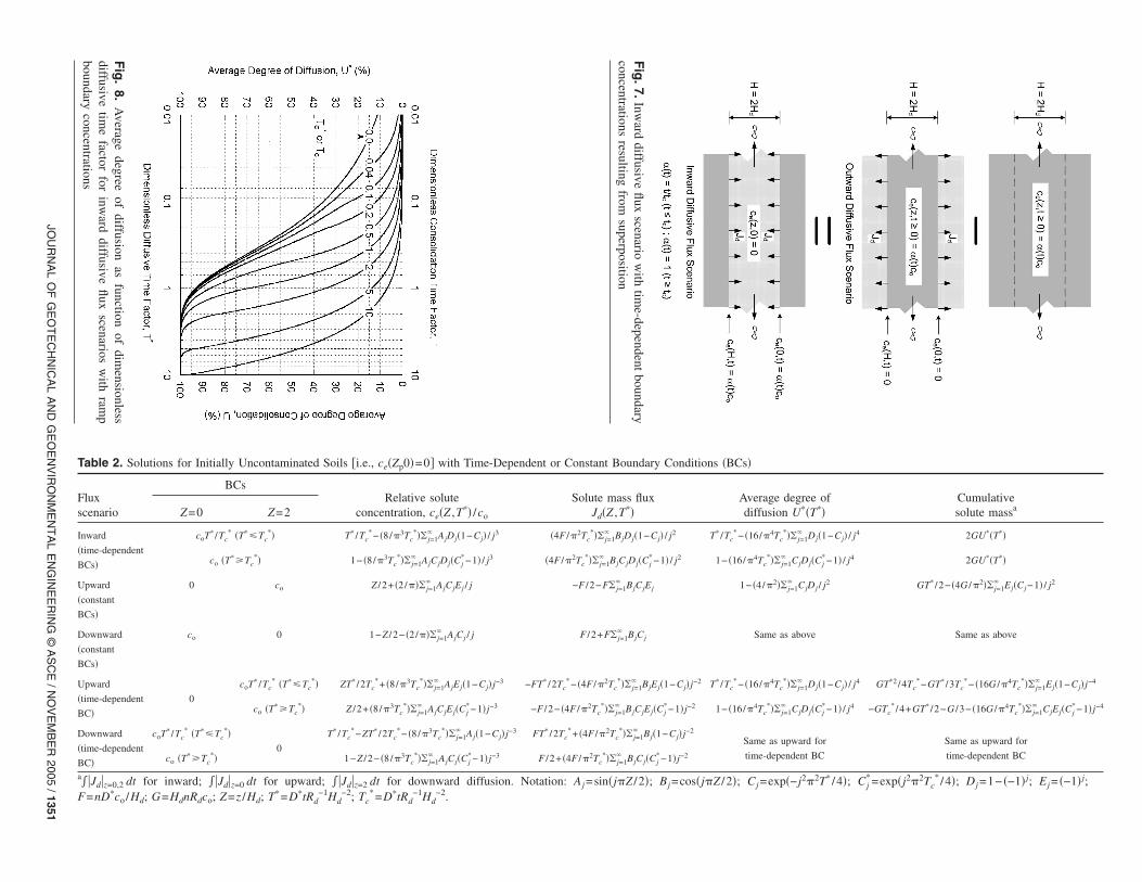
Fig

.7.Inw

arddiffusive

fluxscenario

with

time-dependent

boundaryconcentrations

resultingfrom

superposition

JOU

RN

AL

OF

GE

OT

EC

HN

ICA

LA

ND

GE

OE

NV

IRO

NM

EN

TA

LE

NG

INE

ER

ING

©A

SC

E/N

OV

EM

BE

R2005

/1351

Table 2. Solutions for Initially Uncontaminated Soils �i.e., ce�Zp0�=0

Fluxscenario

BCsRelative

concentration,Z=0 Z=2

Fig

.8.

Average

degreeof

diffusionas

functionof

dimensionless

diffusivetim

efactor

forinw

arddiffusive

fluxscenarios

with

ramp

boundaryconcentrations

BC� co �T*�Tc*� Z /2+ �8/�3Tc

*�� j=1�

Downward

�time-dependent

BC�


*�0

T* /Tc*−ZT* /2Tc

*− �8/�

co �T*�Tc*� 1−Z /2− �8/�3Tc

*��

a� Jd z=0,2 dt for inward; � Jd z=0 dt for upward; � Jd z=2 dt for dowF=nD*co /Hd; G=HdnRdco; Z=z /Hd; T*=D*tRd

−1Hd−2; Tc

*=D*tRd−1H

ue�Z,T� =8uo

�3Tc�j=1

�

1 − cos�j��sin� j�Z

2�

��1 − exp�−j2�2T

4�� ; T � Tc �17a�

ue�Z,T� =8uo

�3Tc�j=1

�


2�exp�−

j2�2T

4�

��exp� j2�2Tc

4� − 1� ; T � Tc �17b�

where Z=z /Hd, T=cvt�Hd�−2, and Tc�dimensionless consolida-tion time factor corresponding to tc or cvtc�Hd�−2. Based on theanalogy between consolidation and diffusion, the analytical solu-tions given by Eqs. �17a� and �17b� can be transformed into ana-lytical solutions for diffusion into an uncontaminated soil layerunder simple time-dependent �ramp� boundary conditions �i.e.,top and bottom� for solute concentration by: �1� invoking theprinciple of superposition as illustrated in Fig. 7; �2� substitutingthe corresponding excess solute concentrations, co and ce for uo

and ue, respectively; and �3� substituting the dimensionless diffu-sive time factors, T* and Tc

*, for T and Tc, respectively. Theresulting solution for the inward diffusive flux scenario with rampboundary conditions is as follows:

ce�Z,T*� =T*

Tc* −

8co

�3Tc*�

j=1

�


2�

��1 − exp�−j2�2T*

4�� ; T* � Tc

* �18a�

ce�Z,T*� = 1 −8co

�3Tc*�

j=1

�


2�exp�−

j2�2T*

4�

��exp� j2�2Tc*

4� − 1� ; T* � Tc

* �18b�

*
where Tc �dimensionless diffusive time factor corresponding to
nario, the boundary solute concentrations are maintained constant


the time, tc, to reach an ultimate, constant boundary concentration�co�, or D*tc�RdHd

2�−1.Based on Eq. �9�, the degree of diffusion, Uz

*, is given asfollows:

Uz* =

ce�Z,T*�co

�19�

Furthermore, the average degree of diffusion, U*, is given as fol-lows:

U* =T*

Tc* −

16

�4Tc*�

j=1

�1 − cos�j��1 − exp�− j2�2T*/4��

j4 ;

T* � Tc* �20a�

U* = 1 −16

�4Tc*

��j=1

�1 − cos�j��exp�− j2�2T*/4�exp�j2�2Tc

*/4� − 1�j4 ;

T* � Tc* �20b�

Note that both definitions of Uz* and U* are directly analogous to

those for degree of consolidation, Uz, and average degree of con-solidation, U, given by Terzaghi’s theory of consolidation. Valuesof U* based on Eq. �10� are plotted versus T* in Fig. 8 as afunction of Tc

*. This expression can be used to determine thecumulative excess solute mass gained at any time due to inwarddiffusion with time-dependent boundary concentrations.

The diffusive excess solute mass flux in soil, Jd, can be deter-mined through differentiation of the expression for the excesssolute concentration ce�Z ,T*�� with respect to depth and substi-tuting the resulting expression into Fick’s first law �Eq. �12�� as
follows:
Jd =4nD*co

�2HdTc*�

j=1

�1 − cos�j��cos�j�Z/2�1 − exp�− j2�2T*/4��

j2 ; T* � Tc* �21a�

Jd =4nD*co

�2HdTc*�

j=1

�1 − cos�j��cos�j�Z/2�exp�− j2�2T*/4�exp�j2�2Tc

*/4� − 1�j2 ; T* � Tc

* �21b�

The analytical solutions for the inward diffusive flux scenariowith ramp boundary conditions in terms of solute concentration,solute mass flux, average degree of diffusion, and cumulative sol-ute mass are summarized in Table 2.

Unidirectional Diffusive Flux ScenariosA diffusive solute mass flux scenario commonly encountered inengineering practice is referred to herein as the unidirectionaldiffusive flux scenario. In the unidirectional diffusive flux sce-

as zero for one boundary and as co for the other boundary. For thisscenario, the solute concentration difference across the soil,�c�=co�, is also constant, and the initial condition is given by�1−�co, where is either unity �=1� or some function ofdepth, z= f�z��. These boundary conditions are applicable whenthe source of contamination at one side of the medium can beconsidered constant, and the other side of the medium is perfectlyflushing in that the solute concentration is maintained as zero.
This situation typically exists in cases where solutes diffuse

through a barrier �e.g., vertical cutoff wall, clay liner� and thenare collected by a collection system or flushed by groundwatermovement �e.g., Rabideau and Khandelwal 1998�.

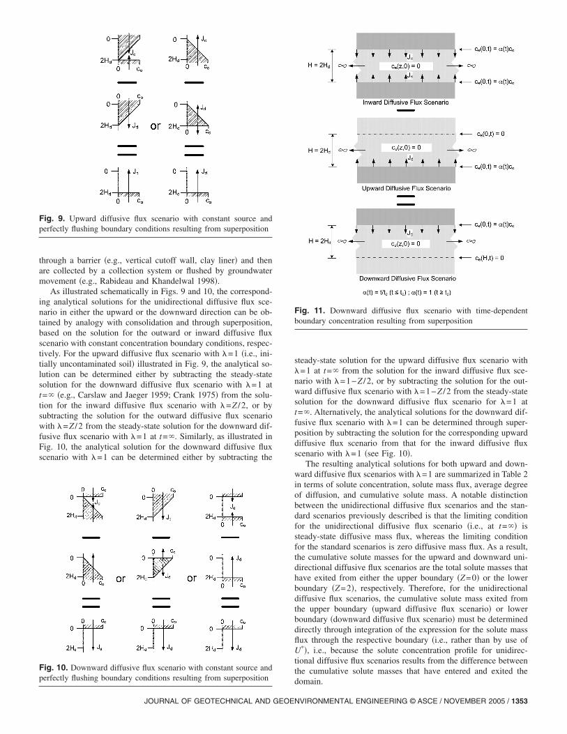
As illustrated schematically in Figs. 9 and 10, the correspond-ing analytical solutions for the unidirectional diffusive flux sce-nario in either the upward or the downward direction can be ob-tained by analogy with consolidation and through superposition,based on the solution for the outward or inward diffusive fluxscenario with constant concentration boundary conditions, respec-tively. For the upward diffusive flux scenario with =1 �i.e., ini-tially uncontaminated soil� illustrated in Fig. 9, the analytical so-lution can be determined either by subtracting the steady-statesolution for the downward diffusive flux scenario with =1 att=� �e.g., Carslaw and Jaeger 1959; Crank 1975� from the solu-tion for the inward diffusive flux scenario with =Z /2, or bysubtracting the solution for the outward diffusive flux scenariowith =Z /2 from the steady-state solution for the downward dif-fusive flux scenario with =1 at t=�. Similarly, as illustrated inFig. 10, the analytical solution for the downward diffusive fluxscenario with =1 can be determined either by subtracting the

Fig. 9. Upward diffusive flux scenario with constant source andperfectly flushing boundary conditions resulting from superposition

Fig. 10. Downward diffusive flux scenario with constant source andperfectly flushing boundary conditions resulting from superposition


steady-state solution for the upward diffusive flux scenario with=1 at t=� from the solution for the inward diffusive flux sce-nario with =1−Z /2, or by subtracting the solution for the out-ward diffusive flux scenario with =1−Z /2 from the steady-statesolution for the downward diffusive flux scenario for =1 att=�. Alternatively, the analytical solutions for the downward dif-fusive flux scenario with =1 can be determined through super-position by subtracting the solution for the corresponding upwarddiffusive flux scenario from that for the inward diffusive fluxscenario with =1 �see Fig. 10�.

The resulting analytical solutions for both upward and down-ward diffusive flux scenarios with =1 are summarized in Table 2in terms of solute concentration, solute mass flux, average degreeof diffusion, and cumulative solute mass. A notable distinctionbetween the unidirectional diffusive flux scenarios and the stan-dard scenarios previously described is that the limiting conditionfor the unidirectional diffusive flux scenario �i.e., at t=�� issteady-state diffusive mass flux, whereas the limiting conditionfor the standard scenarios is zero diffusive mass flux. As a result,the cumulative solute masses for the upward and downward uni-directional diffusive flux scenarios are the total solute masses thathave exited from either the upper boundary �Z=0� or the lowerboundary �Z=2�, respectively. Therefore, for the unidirectionaldiffusive flux scenarios, the cumulative solute mass exited fromthe upper boundary �upward diffusive flux scenario� or lowerboundary �downward diffusive flux scenario� must be determineddirectly through integration of the expression for the solute massflux through the respective boundary �i.e., rather than by use ofU*�, i.e., because the solute concentration profile for unidirec-tional diffusive flux scenarios results from the difference betweenthe cumulative solute masses that have entered and exited the

Fig. 11. Downward diffusive flux scenario with time-dependentboundary concentration resulting from superposition

domain.


Unidirectional Diffusive Flux Scenario with Time-DependentBoundary ConditionThe analytical solutions for the unidirectional diffusive flux sce-narios with a time-dependent solute concentration at one bound-ary and a perfectly flushing condition at the other boundary �i.e.,combinations of ce�0, t�=0 and ce�2Hd , t�=c�t� or ce�0, t�=c�t�and ce�2Hd , t�=0� also can be obtained by introducing the differ-ential excess solute concentration, dci, imposed at the boundarycorresponding to the time, ti. For the upward diffusive flux sce-nario �i.e., ce�0, t�=0 and ce�2Hd , t�=c�t��, the resulting expres-sion is as follows:

ce�z,t� =z

2Hd� dci +

2

��j=1

�cos�j��

jsin� j�z

2Hd�

�� exp�−j2�2D*�t − ti�

4RdHd2 �dci �22�

The analytical solution for downward diffusive flux scenario �i.e.,ce�0, t�=c�t� and ce�2Hd , t�=0� can be determined either by re-placing z on the right-hand side of Eq. �22� with �2Hd−z� orthrough superposition by subtracting the solution correspondingto Eq. �22� from that for an inward diffusive flux scenario withtime-dependent boundary conditions, as illustrated schematicallyin Fig. 11. The analytical solutions for the unidirectional diffusiveflux scenarios with a ramp concentration boundary condition aresummarized in Table 2. Again, the cumulative solute mass pre-sented in Table 2 is the total solute mass exited from the upperboundary �Z=0� for the upward diffusive flux scenario or thelower boundary �Z=2� for the downward diffusive flux scenario.

Nonstandard Initial and Multistage BoundaryConditions

For cases involving more complex, nonstandard initial conditions,such as combinations of more than one standard concentrationdistribution �e.g., rectangular, triangular, and sinusoidal�, the ana-lytical solution for the excess solute concentration can be deter-mined conveniently through the use of superposition �e.g., Taylor1948�, as follows:

ce�z,t� = �i=1

N

ce,i�z,t� �23�

where ce,i�z , t��excess solute concentration for the case i, andN�number of individual cases required for superposition. In ad-dition, for cases involving discontinuous, multistage boundaryconditions, such as combinations of more than one simple bound-ary condition �i.e., constant or single-ramp time-dependentboundary condition�, the solutions for the excess solute concen-tration corresponding to each stage of the time-dependent bound-ary condition can be obtained through superposition of individualsolutions for the corresponding time period in accordance withEq. �23�. Similarly, the diffusive excess solute mass flux in soil,Jd, at any elapsed time also can be determined by superposition ofeach solution for the corresponding initial concentration distribu-tion in the case of nonstandard initial conditions or each solutionfor the corresponding time period in the case of multistage bound-ary conditions.

On the other hand, overall average degree of diffusion, U*, canbe determined by: �1� integrating the expression for the overall
excess solute concentrations �i.e., Eq. �23�� with respect to depth,

or the expression for the overall boundary mass fluxes and �2�using superposition with weighting factors, as follows:

U* =

�0

H

ce�z,0�dz −�0

H

ce�z,t�dz

�0

H

ce�z,0�dz −�0

H

ce�z,��dz

= �i=1

N

Wi

�0

H

ce,i�z,0�dz −�0

H

ce,i�z,t�dz

�0

H


H

ce,i�z,��dz

= �i=1

N

WiUi* �24a�

or

U* =

�0

t

Jd z=0,Hdt

�0

�

Jd z=0,Hdt

= �i=1

N

Wi

�0

t

Jd,i z=0,Hdt

�0

�

Jd,i z=0,Hdt

= �i=1

N

WiUi*

�24b�

where ce�z ,0� and ce�z ,��= excess solute concentrations att=0 and at t=�, respectively; and � Jd z=0,Hdt and� Jd,i z=0,Hdt�cumulative excess solute mass removed �outward�or gained �inward� per unit area for the case of interest and thecase i, respectively; Ui

*= average degree of diffusion for the casei; and Wi�weighting factor for average degree of diffusion forcase i defined as follows:

Wi = ±

�0

H


H

ce,i�z,��dz

�0

H

ce�z,0�dz −�0

H

ce�z,��dz

= ±

�0

�

Jd,i z=0,Hdt

�0

�

Jd z=0,Hdt

�25�

�i=1

N

Wi = 1

where the positive and negative signs represent addition and sub-traction in superposition, respectively, based on the correspondingsuperposition scenario. Eq. �24� can be used to determine theoverall cumulative excess solute mass gained for the inward dif-fusive flux scenarios. However, the overall cumulative solutemass exited for the unidirectional diffusive flux scenarios must bedetermined directly through integration of the overall expressionfor the solute mass flux through the exit boundary.

Differences between Diffusion and Consolidation

Although mathematically similar, the processes of consolidationand diffusion are fundamentally different. Consolidation repre-sents the time-dependent dissipation of excess pore-water pres-sures after application of a load, whereas liquid-phase diffusionrepresents the transport of aqueous miscible chemicals �solutes�due to a gradient in solute concentration �i.e., chemical potential�,
without the requirement for solution flow. Therefore, consolida-

tion is a physical process, whereas diffusion is a chemicalprocess. Some examples of the potential effects of this differenceare elucidated to avoid misinterpretation and misuse of themethodology and/or the analysis of unrealistic situations.

Rates of Two Processes

The rate of consolidation is controlled by the coefficient of con-solidation, cv, which is primarily a function of the hydraulic con-ductivity and the volume compressibility of the porous medium.For nonsorbing solutes �Rd=1�, the rate of diffusion is controlledby the effective diffusion coefficient, D*�=�aDo�, which is a func-tion through �a of the nature and extent of the interconnectedpores, and a function through Do of the absolute mobility of thediffusing solute and the absolute temperature �Shackelford andDaniel 1991�. Typical values for cv range from 1�10−8 to 3.5�10−6 m2/s �Lambe and Whitman 1969�, whereas typical valuesof D* for saturated clays that do not behave as semipermeablemembranes �e.g., see Malusis and Shackelford 2002� range from1�10−10 to 1�10−9 m2/s �Shackelford 1991�. Thus, D* is ap-proximately 2–3 orders of magnitude lower than cv, and accord-ingly, the process of diffusion typically is significantly slowerthan the process of consolidation.

Potential Limitation on Mass Removal

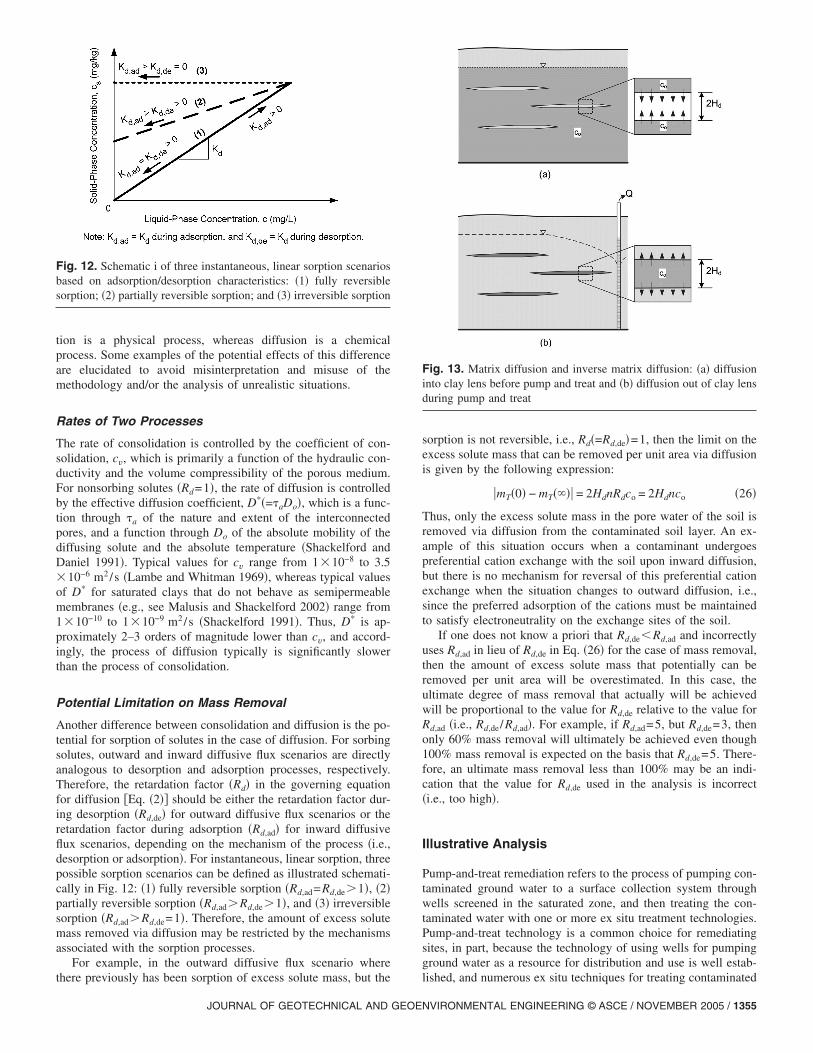
Another difference between consolidation and diffusion is the po-tential for sorption of solutes in the case of diffusion. For sorbingsolutes, outward and inward diffusive flux scenarios are directlyanalogous to desorption and adsorption processes, respectively.Therefore, the retardation factor �Rd� in the governing equationfor diffusion �Eq. �2�� should be either the retardation factor dur-ing desorption �Rd,de� for outward diffusive flux scenarios or theretardation factor during adsorption �Rd,ad� for inward diffusiveflux scenarios, depending on the mechanism of the process �i.e.,desorption or adsorption�. For instantaneous, linear sorption, threepossible sorption scenarios can be defined as illustrated schemati-cally in Fig. 12: �1� fully reversible sorption �Rd,ad=Rd,de�1�, �2�partially reversible sorption �Rd,ad�Rd,de�1�, and �3� irreversiblesorption �Rd,ad�Rd,de=1�. Therefore, the amount of excess solutemass removed via diffusion may be restricted by the mechanismsassociated with the sorption processes.

For example, in the outward diffusive flux scenario where

Fig. 12. Schematic i of three instantaneous, linear sorption scenariosbased on adsorption/desorption characteristics: �1� fully reversiblesorption; �2� partially reversible sorption; and �3� irreversible sorption

there previously has been sorption of excess solute mass, but the


sorption is not reversible, i.e., Rd�=Rd,de�=1, then the limit on theexcess solute mass that can be removed per unit area via diffusionis given by the following expression:

mT�0� − mT�� = 2HdnRdco = 2Hdnco �26�

Thus, only the excess solute mass in the pore water of the soil isremoved via diffusion from the contaminated soil layer. An ex-ample of this situation occurs when a contaminant undergoespreferential cation exchange with the soil upon inward diffusion,but there is no mechanism for reversal of this preferential cationexchange when the situation changes to outward diffusion, i.e.,since the preferred adsorption of the cations must be maintainedto satisfy electroneutrality on the exchange sites of the soil.

If one does not know a priori that Rd,deRd,ad and incorrectlyuses Rd,ad in lieu of Rd,de in Eq. �26� for the case of mass removal,then the amount of excess solute mass that potentially can beremoved per unit area will be overestimated. In this case, theultimate degree of mass removal that actually will be achievedwill be proportional to the value for Rd,de relative to the value forRd,ad �i.e., Rd,de /Rd,ad�. For example, if Rd,ad=5, but Rd,de=3, thenonly 60% mass removal will ultimately be achieved even though100% mass removal is expected on the basis that Rd,de=5. There-fore, an ultimate mass removal less than 100% may be an indi-cation that the value for Rd,de used in the analysis is incorrect�i.e., too high�.

Illustrative Analysis

Pump-and-treat remediation refers to the process of pumping con-taminated ground water to a surface collection system throughwells screened in the saturated zone, and then treating the con-taminated water with one or more ex situ treatment technologies.Pump-and-treat technology is a common choice for remediatingsites, in part, because the technology of using wells for pumpingground water as a resource for distribution and use is well estab-

Fig. 13. Matrix diffusion and inverse matrix diffusion: �a� diffusioninto clay lens before pump and treat and �b� diffusion out of clay lensduring pump and treat

lished, and numerous ex situ techniques for treating contaminated


water already exist �Shackelford and Jefferis 2000�. However,pump-and-treat remediation can be costly due to the need forcontinuous pumping, and the pump-and-treat remediation tech-nology in many cases has not been able to achieve reductions incontaminant concentrations to acceptable regulatory levels �e.g.,Mackay and Cherry 1989; Mott 1992; Feenstra et al. 1996;Shackelford and Jefferis 2000�. This inability of pump-and-treatremediation to achieve regulatory objectives has been attributedto several factors, including the process of reverse matrixdiffusion.

As shown schematically in Fig. 13, the existence of low-permeability zones �e.g., clay lenses� interspersed within higher-permeability formations �e.g., aquifers� results in a process knownas matrix diffusion �e.g., Grisak and Pickens 1980; Feenstra et al.1984; Rowe and Booker 1991; Jorgensen and Fredericia 1992;Jorgensen and Foged 1994; Parker and McWhorter 1994; Parkeret al. 1994, 1996; Sato 1999; Polak et al. 2002�. During initialcontamination of the aquifer, the difference in concentration be-tween the contaminated aquifer and the clay lens results in diffu-sion of contaminants into the porous matrix of the clay lens �Fig.13�a��. Once pumping commences, the higher permeability por-tion of the heterogeneous aquifer is flushed relatively quicklyresulting in a reversal of the concentration gradient and an out-ward diffusive flux of the contaminant �Fig. 13�b��. Since thediffusion process is relatively slow, this reverse matrix diffusioneffect can result in the long-term release of residual contamina-tion such that cleanup goals are not achieved �e.g., Feenstra et al.1996�.

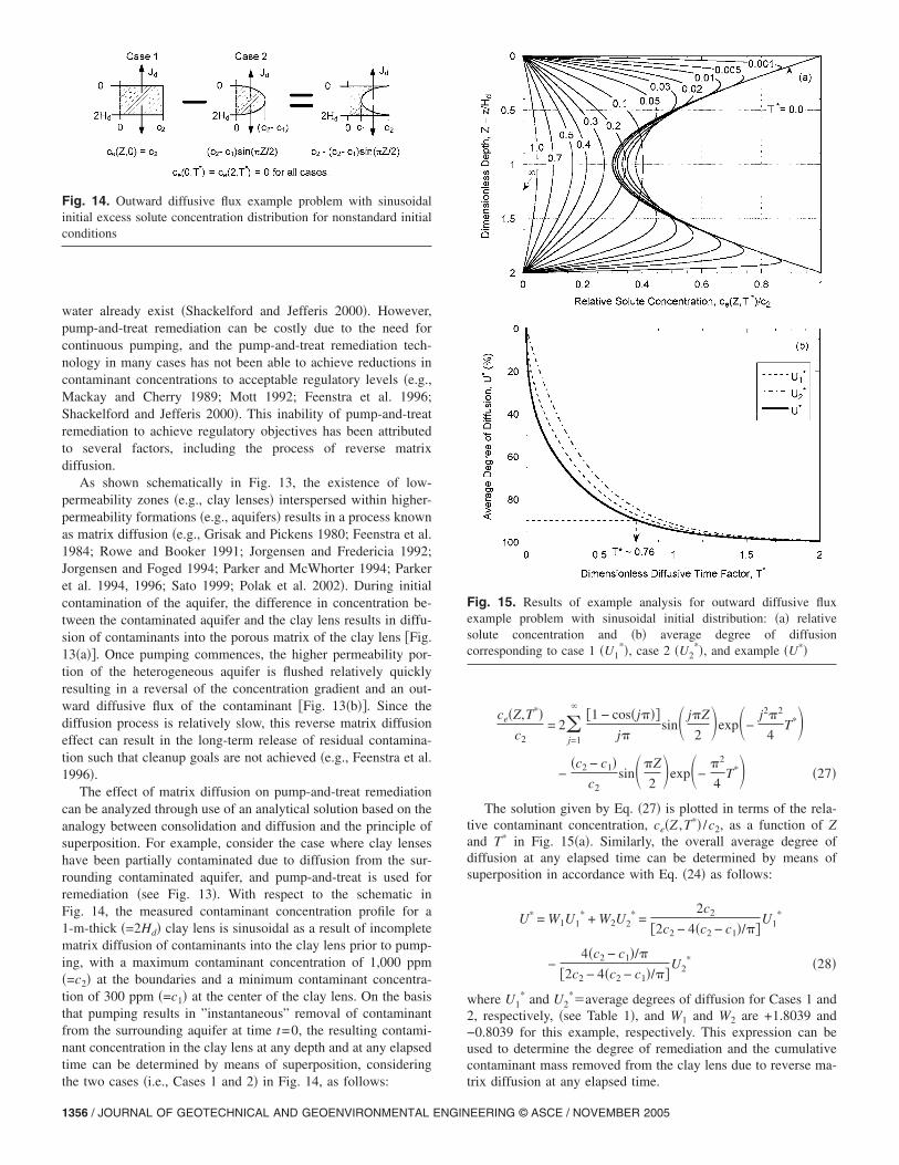
The effect of matrix diffusion on pump-and-treat remediationcan be analyzed through use of an analytical solution based on theanalogy between consolidation and diffusion and the principle ofsuperposition. For example, consider the case where clay lenseshave been partially contaminated due to diffusion from the sur-rounding contaminated aquifer, and pump-and-treat is used forremediation �see Fig. 13�. With respect to the schematic inFig. 14, the measured contaminant concentration profile for a1-m-thick �=2Hd� clay lens is sinusoidal as a result of incompletematrix diffusion of contaminants into the clay lens prior to pump-ing, with a maximum contaminant concentration of 1,000 ppm�=c2� at the boundaries and a minimum contaminant concentra-tion of 300 ppm �=c1� at the center of the clay lens. On the basisthat pumping results in ”instantaneous” removal of contaminantfrom the surrounding aquifer at time t=0, the resulting contami-nant concentration in the clay lens at any depth and at any elapsedtime can be determined by means of superposition, considering

Fig. 14. Outward diffusive flux example problem with sinusoidalinitial excess solute concentration distribution for nonstandard initialconditions

the two cases �i.e., Cases 1 and 2� in Fig. 14, as follows:


ce�Z,T*�c2

= 2�j=1

�1 − cos�j��

j�sin� j�Z

2�exp�−

j2�2

4T*�

−�c2 − c1�

c2sin��Z

2�exp�−

�2

4T*� �27�

The solution given by Eq. �27� is plotted in terms of the rela-tive contaminant concentration, ce�Z ,T*� /c2, as a function of Zand T* in Fig. 15�a�. Similarly, the overall average degree ofdiffusion at any elapsed time can be determined by means ofsuperposition in accordance with Eq. �24� as follows:

U* = W1U1* + W2U2

* =2c2

2c2 − 4�c2 − c1�/��U1

*

−4�c2 − c1�/�

2c2 − 4�c2 − c1�/��U2

* �28�

where U1* and U2

*�average degrees of diffusion for Cases 1 and2, respectively, �see Table 1�, and W1 and W2 are +1.8039 and−0.8039 for this example, respectively. This expression can beused to determine the degree of remediation and the cumulativecontaminant mass removed from the clay lens due to reverse ma-

Fig. 15. Results of example analysis for outward diffusive fluxexample problem with sinusoidal initial distribution: �a� relativesolute concentration and �b� average degree of diffusioncorresponding to case 1 �U1

*�, case 2 �U2*�, and example �U*�

trix diffusion at any elapsed time.


For example, if we assume that the contaminant is trichloro-ethylene �TCE� with Rd of 5.2 and D* of 3.33�10−10 m2/s �e.g.,Parker et al. 1996�, then the degree of remediation att=10 years �or T*= �0.081� after the beginning of pumping isapproximately 0.43 or 43% �=0.32�1.8039−0.18�0.8039�based on U1

* and U2* at T*= �0.081 in Fig. 15�b�. Based on a

porosity, n, of 0.60 for the clay lens and assuming complete re-versibility of the sorbed TCE �i.e., Rd,ad=Rd,de=Rd�, the cumula-tive contaminant mass removed per unit area of the clay lens after10 years of pumping is approximately 750 g/m2 =2HdnRdc2

−2�c2−c1� /��U*�. More importantly, as indicated in Fig. 15�b�, aU* of 90% corresponds to T* of approximately 0.76, which isequivalent to 94 years. Thus, this analysis indicates that close to acentury of pumping will be required to remediate the 1-m-thickclay lense to a level of 90%, which is consistent with the afore-mentioned observations attributing failure of some pump-and-treat systems to reverse matrix diffusion.

Feenstra et al. �1996� present the analysis for a similar sce-nario, but they start from the assumption that the clay lens isinitially completely contaminated such that they do not invoke theuse of superposition. Complete contamination of clay lenseswould be likely only in the case of relatively thin clay lenses andrelatively long durations of aquifer contamination. Otherwise, theclay lenses likely would only be partially contaminated resultingin an initial concentration distribution within the clay lenses thatis sinusoidal �as opposed to uniform� and the need for superposi-tion in the resulting analysis.

Conclusions

Fick’s governing equation for diffusion �i.e., Fick’s second law� ismathematically analogous to Terzaghi’s governing equation forconsolidation. As a result of this mathematical similarity, one-dimensional analytical �closed-form� solutions to Fick’s secondlaw transformed from corresponding one-dimensional analyticalsolutions to the consolidation equation can be used for analyzingdiffusion of aqueous miscible solutes �e.g., contaminants� in satu-rated porous media. The general methodology for transformingthe analytical solutions in terms of solute concentration, solutemass flux, and cumulative solute mass is presented, and the con-cepts of degree of diffusion and average degree of diffusion areintroduced. Analytical solutions for two primary diffusive fluxscenarios, i.e., outward and inward diffusive flux scenarios, arepresented for constant boundary solute concentrations and avariety of initial solute concentration distributions �e.g., uniform,triangular, inverse triangular, and sinusoidal�. For the inward dif-fusive flux scenario, the analytical solutions result from superpo-sition based on the analytical solutions for the corresponding out-ward diffusive flux scenario.

The methodology for transforming one-dimensional analytical�closed-form� solutions to Terzaghi’s governing equation for con-solidation into one-dimensional analytical solutions to Fick’s sec-ond law is extended to cover cases involving nonstandard bound-ary and initial conditions. Analytical solutions for inwarddiffusive flux scenarios are presented for the case of an initiallyuncontaminated soil under simple time-dependent �ramp� bound-ary concentrations. In addition, analytical solutions for an initiallyuncontaminated soil are extended for unidirectional diffusive fluxscenarios �both upward and downward� under conditions of con-stant source and zero exit concentrations as well as the conditionsof simple time-dependent source concentration and zero exit con-
centration. Nonstandard initial conditions and multistage time-

dependent boundary conditions can be handled by superpositionusing weighting factors.

The differences between the physical process of consolidationand the chemical process of diffusion that go beyond the math-ematical analogy are emphasized in terms of the rates of the twoprocesses as well as the potential limitation on mass removal toavoid misinterpretation of results and analyses of unrealisticproblems.

Finally, an example analysis is used to illustrate the effect ofreverse matrix diffusion on the efficiency of contaminant massremoval via pump-and-treat remediation. Results of the illustra-tive analysis are presented in terms of contaminant concentrationand average degree of diffusion. Although the practical applica-tion of the closed-form solutions is inevitably limited by the as-sumptions inherent in the analytical solutions �e.g., homogeneousmedia�, the example analysis illustrates the ability to analyzemore complex problems through the use of superposition.

Notation

The following symbols are used in this paper:C,CT � solute mass in pore water �i.e., liquid-phase�

per unit total volume �solids plus voids� andtotal solute mass �solid plus liquid phase� perunit total volume, respectively;

c,co � solute concentration in pore water andconstant solute concentration in pore water,respectively;

ce,ce,i � excess solute concentration in pore water andinitial excess solute concentration in porewater, respectively;

cv � coefficient of consolidation;D*,Da,Do � effective diffusion coefficient �=�aDo�,

apparent, effective diffusion coefficient�=D* /Rd�, and aqueous diffusion coefficient,respectively;

dti,dui � differential time and differential excesspore-water pressure at time ti, respectively;

H,Hd � total thickness of medium �soil� and maximumdrainage or diffusive distance, respectively;

ic � solute concentration gradient;Jd,Jd,i,Jd,ss � diffusive solute mass flux; diffusive solute

mass flux for case i; and steady-statediffusive solute mass flux, respectively;

j � dummy variable taking on integer values;Kd � distribution coefficient;

Kd,ad,Kd,de � distribution coefficient during adsorption anddesorption, respectively;

M,MT � solute mass in pore water and total solutemass, respectively;

m,mT � solute mass in pore water per unit area andtotal solute mass per unit area, respectively;

N � number of individual cases required forsuperposition;

n � porosity;q,qo � time-dependent load and ultimate applied

load, respectively;Rd � retardation factor;

Rd,ad,Rd,de � retardation factor during adsorption anddesorption, respectively;

St,Su � consolidation settlement at any time and at
t=�, respectively;

T,T*,t � dimensionless consolidation time factor�=cvtHd

−2�, dimensionless diffusive time factor�=D*tRd

−1Hd−2�, and time, respectively;

Tc,Tc*,tc � dimensionless consolidation time factor

�=cvtcHd−2� for tc, dimensionless diffusive time

factor �=D*tcRd−1Hd

−2� for tc, and timecorresponding to end of construction forconsolidation or to reach ultimate soluteconcentration for diffusion, respectively;

U,Uz � average degree of consolidation and degree ofconsolidation, respectively;

U*,Ui*,Uz

* � average degree of diffusion, average degreeof diffusion for case i, and degree of diffusion,respectively;

u,uo,ue,ue,i

� variable excess pore-water pressure, ultimateexcess pore-water pressure; excess pore-waterpressure, and initial excess pore-waterpressure, respectively;

Wi � weighting factor for case i;Z,z � dimensionless depth �=z /Hd� and spatial

coordinate, respectively; � multiplier �1 or f�z��;

�d � dry �bulk� density of medium; and�a � apparent tortuosity factor.

References

Carslaw, H. S., and Jaeger, J. C. �1959�. Conduction of heat in solids, 2ndEd., Oxford University Press, Oxford, U.K.

Crank, J. �1975�. The Mathematics of diffusion, 2nd Ed., Oxford Univer-sity Press, New York.

Crooks, V. E., and Quigley, R. M. �1984�. “Saline leachate migrationthrough clay: A comparative laboratory and field investigation.” Can.Geotech. J., 21, 349–362.

Cussler, E. L. �1997�. Diffusion, mass transfer in fluid systems, 2nd Ed.,Cambridge University Press, New York.

Devlin, J. F., and Parker, B. L. �1996�. “Optimum hydraulic conductivityto limit contaminant flux through cutoff walls.” Ground Water, 34�4�,719–726.

Edil, T. �2003�. ”A review of aqueous-phase VOC transport in modernlandfill liners.” Waste Manage. 23�7�, 561–571.

Feenstra, S., Cherry, J. A., and Parker, B. L. �1996�. “Conceptual modelsfor the behavior of dense non-aqueous phase liquids�DNAPLs� in the subsurface.” Dense chlorinated solvents and otherDNAPLs in groundwater, J. F. Pankow and J. A. Cherry, eds., Chap.2., Waterloo Press, Portland, Ore, 53–88.

Feenstra, S., Cherry, J. A., Sudicky, E. A., and Haq, Z. �1984�. “Matrixdiffusion effects on contaminant migration from an injection well infractured sandstone.” Ground Water, 22�3�, 307–316.

Foose, G. �2002�. ”Transit-time design for diffusion through compositeliners.” J. Geotech. Geoenviron. Eng., 128�7�, 590–601.

Foster, S. S. D. �1975�. “The chalk groundwater tritium anomaly—Apossible explanation.” J. Hydrol., 25�1�, 159–165.

Freeze, R. A., and Cherry, J. A. �1979�. Groundwater, Prentice-Hall,Englewood Cliffs, N.J.

Goodall, D. C., and Quigley, R. M. �1977�. “Pollutant migration from twosanitary landfill sites near Sarnia, Ontario.” Can. Geotech. J., 14,223–236.

Grathwohl, P. �1998�. Diffusion in natural porous media, contaminanttransport, sorption/desorption and dissolution kinetics. KluwerAcademic, Norwell, Mass.

Gray, D. H., and Weber, W. J., Jr. �1984�. “Diffusional transport of haz-
ardous waste leachate across clay barriers.” Proc., 7th Annual

Madison Waste Conf., Madison, Wis., 373–389.Greenberg, J. A., Mitchell, J. K., and Witherspoon, P. A. �1973�.

“Coupled salt and water flows in a groundwater basin.” J. Geophys.Res., 78�27�, 6341–6353.

Grisak, G. E., and Pickens, J. F. �1980�. “Solute transport through frac-tured media: I. The effect of matrix diffusion.” Water Resour. Res.,16�4�, 719–730.

Holtz, R. D., and Kovacs, W. D. �1981�. An introduction to geotechnicalengineering, Prentice-Hall, Englewood Cliffs, N.J.

Jorgensen, P. R., and Foged, N. �1994�. “Pesticide leaching in intactblocks of clayey till.” Proc., 13th International Conf. on Soil Mechan-ics and Foundation Engineering, New Delhi, India, 1661–1664.

Jorgensen, P. R., and Fredericia, J. �1992�. “Migration of nutrients, pes-ticides and heavy metals in fractured clayey till.” Geotechnique,42�2�, 67–77.

Lake, C. B., and Rowe, R. K. �2000�. “Diffusion of sodium and chloridethrough geosynthetic clay liners.” Geotext. Geomembr., 18�2–4�,103–131.

Lambe, T. W., and Whitman, R. V. �1969�. Soil mechanics, Wiley, NewYork.

Lever, D. A., Bradbury, M. H., and Hemingway, S. J. �1985�. “The effectof dead-end porosity on rock-matrix diffusion.” J. Hydrol., 80�1–2�,45–76.

Mackay, D. M., and Cherry, J. A. �1989�. “Groundwater contamination:Pump-and-treat remediation.” Environ. Sci. Technol., 23�6�, 630–636.

Malusis, M. A., and Shackelford, C. D. �2002�. “Coupling effects duringsteady-state solute diffusion through a semipermeable clay mem-brane.” Environ. Sci. Technol., 36�6�, 1312–1319.

Malusis, M. A., and Shackelford, C. D. �2004�. “Predicting solute fluxthrough a clay membrane barrier.” J. Geotech. Geoenviron. Eng.,130�5�, 477–487.

Mott, R. M. �1992�. “Aquifer restoration under CERCLA: New realitiesand old myths.” Environment Reporter, Aug. 28, 1301–1304.

Mott, H. V., and Weber, W. J., Jr. �1991a�. “Diffusion of organic contami-nants through soil-bentonite cut-off barriers.” Res. J. Water Pollut.Control Fed., 63�2�, 166–176.

Mott, H. V., and Weber, W. J., Jr. �1991b�. “Factors influencing organiccontaminant diffusivities in soil-bentonite cut-off barriers.” Environ.Sci. Technol., 25�10�, 1708–1715.

Nathwani, J. S., and Phillips, C. R. �1980�. “Leachability of Ra-226 fromuranium mill tailings consolidated with naturally occurring materialsand/or cement.” Water, Air, Soil Pollut., 14, 389–402.

Olson, R. E. �1977�. “Consolidation under time dependent loading.”J. Geotech. Eng. Div., Am. Soc. Civ. Eng., 103�1�, 55–60.

Parker, B. L., Cherry, J. A., and Gillham, R. W. �1996�. “The effects ofmolecular diffusion on DNAPL behavior in fractured porous media.”Dense chlorinated solvents and other DNAPLs in groundwater,J. F. Pankow and J. A. Cherry, eds., Chap. 12, Waterloo Press, Port-land, Ore., 355–393.

Parker, B. L., Gillham, R. W., and Cherry, J. A. �1994�. “Diffusive dis-appearance of immiscible-phase organic liquids in fractured geologicmedia.” Ground Water, 32�5�, 805–820.

Parker, B. L., and McWhorter, D. B. �1994�. “Diffusive disappearance ofimmiscible-phase organic liquids in fractured porous media: Finitematrix blocks and implications for remediation.” Transport andreactive processes in aquifers, Th. Dracos and F. Stauffer, eds., A. A.Balkema, Rotterdam, The Netherlands, 543–548.

Polak, A., Nativ, R., and Wallach, R. �2002�. “Matrix diffusion in north-ern Negev fractured chalk and its correlation to porosity.” J. Hydrol.,268�1–4�, 203–213.

Rabideau, A., and Khandelwahl, A. �1998�. “Boundary conditions formodeling transport in vertical barriers.” J. Environ. Eng., 124�11�,1135–1139.

Rowe, R. K., and Booker, J. R. �1991�. “Pollutant migration through linerunderlain by fractured soil.” J. Geotech. Eng., 117�12�, 1902–1919.

Sato, H. �1999�. “Matrix diffusion of simple cations, anions, and neutralspecies in fractured crystalline rocks.” Nucl. Technol., 127�2�,
199–211.

Shackelford, C. D. �1988�. “Diffusion as a transport process in fine-grained barrier materials.” Geotech. News, 6�2�, 24–27.

Shackelford, C. D. �1989�. “Diffusion of contaminants through wastecontainment barriers.” Transportation Research Record. 1219, Trans-portation Research Board, Washington, D.C., 169–182.

Shackelford, C. D. �1990�. “Transit-time design of earthen barriers.” Eng.Geol., 29�1�, 79–94.

Shackelford, C. D. �1991�. “Laboratory diffusion testing for wastedisposal—A review.” J. Contam. Hydrol., 7�3�, 177–217.

Shackelford, C. D., and Daniel, D. E. �1991�. “Diffusion in saturated soil.I: Background.” J. Geotech. Eng., 117�3�, 467–484.

Shackelford, C. D., and Jefferis, S. A. �2000�. ”Geoenvironmental engi-neering for in situ remediation.” Proc., International Conf. on Geo-technical and Geoenvironmental Engineering (GeoEng2000),Melbourne, Australia, Vol. 1, Technomic, Lancaster, Pa., 121–185.

Siegrist, R. L., Lowe, K. S., Murdoch, L. C., Case, T. L., and Pickering,D. A. �1999�. “In situ oxidation by fracture emplaced reactive solids.”J. Environ. Eng., 125�5�, 429–440.

Struse, A. M., Siegrist, R. L., Dawson, H. E., and Urynowicz, M. A.
�2002�. “Diffusive transport of permanganate during in situ

oxidation.” J. Environ. Eng., 128�4�, 327–334.Taylor, D. W. �1948�. Fundamentals of soil mechanics, Wiley, New York.Terzaghi, K. �1925�. Erdbaumechanik auf bodenphysikalischer grund-

lage, Franz Deuticke, Leipzig and Wein, Germany.Thoma, G. J., Reible, D. D., Valsaraj, K. T., and Thibodeaux, L. J. �1993�.

“Efficiency of capping contaminated sediments in situ. 2. Mathemat-ics of diffusion–adsorption in the capping layer.” Environ. Sci. Tech-nol., 27�12�, 2412–2419.

Toupiol, C., Willingham, T. W., Valocchi, A. J., Werth, C. J., Krapac, I.G., Stark, T. D., and Daniel, D. E. �2002�. “Long-term tritium trans-port through field-scale compacted soil liner.” J. Geotech. Geoenvi-ron. Eng. 128�8�, 640–650.

Wang, X. Q., Thibodeaux, L. J., Valsaraj, K. T., and Reible, D. D. �1991�.“Efficiency of capping contaminated sediments in situ. 1. Laboratoryscale experiments on diffusion–adsorption in the capping layer.”Environ. Sci. Technol., 25�9�, 1578–1584.

Willingham, T. W., Werth, C. J., Valocchi, A. J., Krapac, I. G., Toupiol,C., Stark, T. D., and Daniel, D. E. �2004�. ”Evaluation of multidimen-sional transport through a field-scale compacted soil liner.” J. Geo-
tech. Geoenviron. Eng. 130�9�, 887–895.

Analyzing Diffusion by Analogy with Consolidation · Analyzing Diffusion by Analogy with...

Documents

Transcript of Analyzing Diffusion by Analogy with Consolidation · Analyzing Diffusion by Analogy with...