
Analyzing Data with Missing Values in Spotfire S+ 8 · 2013-03-13 · Spotfire S+ to support a...
176
Analyzing Data with Missing Values in TIBCO Spotfire S+ ® 8.2 November 2010 TIBCO Software Inc.
Transcript of Analyzing Data with Missing Values in Spotfire S+ 8 · 2013-03-13 · Spotfire S+ to support a...

Analyzing Data with Missing Values in TIBCO Spotfire S+® 8.2
November 2010
TIBCO Software Inc.

Proprietary Notice
TIBCO Software Inc. owns both this software program and its documentation. Both the program and documentation are copyrighted with all rights reserved by TIBCO Software Inc. .
The correct bibliographical reference for this document is:
Schimert, J., Schafer, J.L., Hesterberg, T., Fraley, C., & Clarkson, D.B., Analyzing Data with Missing Values in Spotfire S+ . TIBCO Software Inc.
Printed in the United States.
Copyright Notice Copyright © 2000-2010, TIBCO Software Inc. All rights reserved.
Trademarks S-PLUS and Spotfire S+ are registered trademarks. StatServer, S-PLUS Analytic Server, S+SDK, S+SPATIALSTATS, S+DOX, S+GARCH, and S+WAVELETS are trademarks of TIBCO SoftwareInc. S and New S are trademarks of Lucent Technologies, Inc.; Intel is a registered trademark, and Pentium a trademark, of Intel Corporation; Microsoft, Windows, MS-DOS, and Excel are registered trademarks, and Windows NT is a trademark of Microsoft Corporation. Other brand and product names referred to are trademarks or registered trademarks of their respective owners.

Acknowledgments The Insightful development team for the S+MISSINGDATA library was Jim Schimert, Douglas B. Clarkson, Chris Fraley, and Tim Hesterberg. The Research and Development of the S+MISSINGDATA library was partially supported by Small Business Innovative Research (SBIR) grants 1R43RR0925401, R44CA65147-02, R44CA65147-03.
This work is strongly influenced by Professor Joseph Schafer, who originally devised the iterative simulation algorithms, implemented the EM and simulation algorithms, provided us code, and served as consultant and subcontractor on this project. His book (Schafer, 1997) should be viewed as an essential companion to this software and manual.
Consultants included Gary Donaldson, Donald Rubin, and Alan Zaslavsky. Thanks to Shan Jin for testing, Ken Baldwin for documentation support, and Stephen Kaluzny for help with builds.
iii

Chapter
iv

CONTENTS
Chapter 1 Introduction 1
Overview 2
Imputing Missing Data with S+MISSINGDATA 5
S+MISSINGDATA Features 8
Using S+MISSINGDATA 9
Using This Manual 11
Chapter 2 Background 13
Overview 14
Taxonomy of Missing Data Methods 15
Imputation 17
Model Fitting Algorithms 20
Multiple Imputation Using DA 23
Using the EM and DA Algorithms in Conjunction 25
Chapter 3 Exploring and Preprocessing 27
Overview 28
Exploring Patterns of Missingness 29
Preprocessing Data 35
Chapter 4 Fitting a Missing Data Model 37
Overview 38
Missing Data Models 39
S-PLUS Implementation 48
v

Contents
Chapter 5 Convergence of Data Augmentation Algorithms 55
Overview 56
Parameter Simulation 57
Multiple Imputation 58
Practical Considerations for Missing Data Problems 60
Chapter 6 Imputation 63
Overview 64
Imputing Data 65
The Class of impute Objects 68
Chapter 7 Analyzing Completed Data Sets 73
Overview 74
Analysis Functions 75
Chapter 8 Consolidating Analyses 81
Overview 82
Simple Statistics 83
Inferences 84
Chapter 9 Example 1: The Gaussian Model 93
Overview 94
Exploring Patterns of Missingness 96
Model Fitting 100
Assessing Convergence 105
Analysis Using Parameter Simulation 111
Generating Multiple Imputations Through DA 114
Omitting Cases with Missing Values 119
Summary 120
vi

Contents
Chapter 10 Example 2: The Loglinear Model 123
Overview 124
Exploring Patterns of Missingness 126
Model Fitting 129
Assessing Convergence 133
Generating Multiple Imputations Through DA 140
Analyzing Completed Data Sets 142
Chapter 11 Example 3: The Conditional Gaussian Model 145
Overview 146
Exploring Patterns of Missingness 148
Model Fitting 152
Assessing Convergence 156
Multiple Imputation 158
Analyzing Completed Data Sets 159
Consolidating Inferences 161
Conclusions 163
Bibliography 165
vii

Contents
viii

INTRODUCTION 1Overview 2
Model-Based Approaches 3Model-Based Multiple Imputation 3
Imputing Missing Data with S+MISSINGDATA 5Workflow 7
S+MISSINGDATA Features 8
Using S+MISSINGDATA 9Starting and Quitting S+MISSINGDATA 9Organizing Your Working Data 9Getting Help 10
Using This Manual 11Intended Audience 11Organization 11Typographic Conventions 12
1

Chapter 1 Introduction
g as
e
OVERVIEW
Missing data cripple most routines in statistical packages that typically expect a complete data set (a data set with no missing values). The common practice is to artificially create a complete data set as follows:
• Throw away cases with missing values, or
• Impute (estimate and fill in missing data using some ad hoc method).
The analyst then treats the altered data set as if
• The deleted cases had never been observed, or
• The imputed values had always been observed.
These and other ad hoc methods can lead to misleading inferences because they either throw away or distort information in the data. More principled methods require methodology and computational methods that can be expensive to implement.
The Spotfire S+ library S+MISSINGDATA extends the statistical modelincapabilities of Spotfire S+ to support model–based missing data methods outlined in Little and Rubin (1987). These may be applied more or less routinely to handle a wide variety of missing data problems. The models are fit using a variety of computational tools including:
1. Expectation-Maximization (EM) algorithm (Dempster, Laird, and Rubin (1977)) and extensions (see Rubin (1992) for a review).
2. Data Augmentation (DA) algorithms (Tanner and Wong (1987), Schafer (1991), Schafer (1997)). These are Monte Carlo Markov Chain methods (Gelfand and Smith (1990), Gelman and Rubin(1992), Geyer (1992), Smith and Roberts (1993), Tierney (1991)). One important property is that these DA algorithms also produce proper multiple imputations (Rubin (1987)), which are discussed at length below.
This chapter briefly discusses model–based methods, including multiple imputation. It explains how this software for missing data adds to the collection of Spotfire S+ modeling functions and expands thSpotfire S+ modeling paradigm to incorporate multiple imputation. It
2
Overview
explains the steps you will take in using this software to perform statistical analysis on data with missing values, and organizes the functions and objects by these steps.
Model-Based Approaches
Compared with more ad hoc methods of handling missing data, model–based methods have two advantages: you can display and evaluate model assumptions, and you can estimate the variance of the parameter estimates.
One model–based approach assumes a distribution for the complete data (the missing and observed data together). Intuitively, this model describes the relationships among the variables, and when combined with observed data, can be used to “fill the holes” in the data.
The S+MISSINGDATA library implements a parametric approach instead. The approach assumes a multivariate parametric model with parameter θ for the complete data, possibly with a prior distribution for θ (Little and Rubin (1987) and Schafer (1997)). S+MISSINGDATA implements three models for independent, identically distributed (iid) observations: the Gaussian model for numeric variables, the loglinear model for factor variables, and the conditional Gaussian model for both numeric and factor variables. In some situations, you may want to fit these specific models to your data. In such cases, S+MISSINGDATA provides tools to fit model parameters and perform inference. More commonly, you will want to perform other analyses but must first deal with the missing data. In such cases, you can proceed using multiple imputation.
Model-Based Multiple Imputation
In model-based multiple imputation , a missing data model (as described in the previous section) is used as an imputation model to create M complete data sets. An analysis model is then used to perform M statistical analyses on the complete data sets. The analysis model may require fewer assumptions than the imputation model, or even be entirely different (see Meng (1994) for a discussion of congeniality ). The resultant M analyses are then combined to produce one overall inference.
3

Chapter 1 Introduction
For example, to perform a regression analysis on data containing missing values, you can use the following procedure:
1. Multiply impute missing data under a Gaussian imputation model.
2. Perform a regression analysis on each of the completed data sets.
3. Appropriately combine the results.
Multiple imputation is fairly robust to imputation model mis-specification, especially with small fractions of missingness. This is because the imputation model is applied only to handle the missing part of the data (Ezzati-Rice et al. (1995), Rubin and Schenker (1986), Schafer (1997)).
4

Imputing Missing Data with S+MISSINGDATA
IMPUTING MISSING DATA WITH S+MISSINGDATA
Normally, Spotfire S+ model fitting functions combine the model formula and data to produce a fitted model object, as shown in Figure 1.1. You can then manipulate the fitted model object with inference and diagnostic procedures. For example, you can print, summarize, or plot the model.
Data FrameObject
ModelSpec.
Fitted ModelObject
Fit ModelOptions &Parameters
Figure 1.1: Spotfire S+ modeling functions combine data and models to produce a fittedmodel object.
S+MISSINGDATA extends the statistical modeling capabilities of Spotfire S+ to support a model–based approach to multiple imputation.Multiple imputation can be viewed as a front end procedure resulting in a multi-stage process, as illustrated in Figure 1.2.
5

Chapter 1 Introduction
Data FrameObject (*)
Analysis ModelSpec. (*)
Multiple FittedModel(s) Object
Fit Model(s)Options &Parameters
Impute
ImputedData Frame
ImputationModel Spec.
Figure 1.2: The role of multiple imputation objects and functions in Spotfire S+. The asterisk (*) indicates components that are the same as in Figure 1.1.
Multiple imputation allows you to reach valid inferences by applying familiar analysis techniques and suitably combining the results. Figure 1.2 illustrates this by showing two stages of modeling:
1. Multiply impute missing data using a missing data model.
2. Analyze the resulting complete data sets with respect to an analysis model.
Dealing with the missing data is mostly confined to the imputation phase. Multiple imputation creates M data sets in complete rectangular form that the analysis procedures can accept. The objects that input and output to the analysis functions thus represent M complete data sets. Several S+MISSINGDATA functions manipulate these objects to obtain one inference that incorporates uncertainty due to missing values.
6

Imputing Missing Data with S+MISSINGDATA
Workflow The workflow for using S+MISSINGDATA can be broken down into distinct stages:
• Explore. Look for and understand patterns in the missing data.
• Preprocess. Process the data to create an object that contains information needed by the model fitting algorithms. By creating this object once, calculation can be saved if the model fitting functions are used several times.
• Fit. Fit a missing data model.
For multiple imputation, the additional steps are:
• Impute. Create M complete data sets, starting the imputation algorithm from the parameters of the fitted missing data model.
• Analyze. Analyze the completed data sets with respect to a standard analysis model to produce M fitted analysis objects.
• Consolidate. Combine the M fitted analysis objects to obtain a single inference that incorporates uncertainty due to missing values.
7

Chapter 1 Introduction
S+MISSINGDATA FEATURES
Table 1.1 organizes the objects and functions available in S+MISSINGDATA by the activities specified in the workflow on page 7.
Table 1.1: Objects and functions in the S+MISSINGDATA library, organized by activites in the workflow.
Activity Objects Functions
Explore miss miss
print.miss
summary.miss
plot.miss
Preprocess preGauss
preLoglin
preCgm
preGauss
preLoglin
preCgm
Fit missmodel mdGauss
mdLoglin
mdCgm
(and associated functions)
Impute miVariable, or a data frame consisiting of columns with class "miVariable"
impGauss
impLoglin
impCgm
Analyze miVariable
miList
miApply
miEval
Consolidate miVariable
miList
miMeanSE
miFTest
miChiSquareTest
miLikelihoodTest
8

Using S+MISSINGDATA
A + e
USING S+MISSINGDATA
If you are familiar with Spotfire S+, getting started with S+MISSINGDATis simple. If you have not used Spotfire S+ before, consult the Spotfire SUser’s Guide ; we recommend that you learn more about Spotfire S+ beforproceeding with S+MISSINGDATA.
Starting and Quitting S+MISSINGDATA
To start S+MISSINGDATA, you must first start Spotfire S+ . See the Spotfire S+ User’s Guide for detailed instructions on starting Spotfire S+.
To add the S+MISSINGDATA functions to your Spotfire S+ session, typethe following at the Spotfire S+ command line:
> library(missing)
In Spotfire S+ for Windows, you can also select File � Load Library from the main menu to add S+MISSINGDATA to your session.
If you plan to use S+MISSINGDATA extensively, you may want to customize your Spotfire S+ start-up routine to automatically attach the S+MISSINGDATA library. You can do this by adding the line library(missing) to your .First function. If you do not already have a .First function, you can create one from the Spotfire S+ command line by typing:
> .First <- function() { library(missing) }
Organizing Your Working Data
To help you organize the data you analyze with S+MISSINGDATA, you can create separate directories for individual projects. In this section, we briefly describe how to create project directories in both UNIX and Windows. For a detailed discussion, see the Spotfire S+ User’sGuide .
9

Chapter 1 Introduction
e gs
n
p
UNIX
To create a specific project directory in Spotfire S+ for UNIX, use the CHAPTER utility. To then work in a particular project, simply start Spotfire S+ from that project’s directory. For example, to create and usethe directory missingdir for an S+MISSINGDATA project, type the following commands from the UNIX prompt:
mkdir dir cd dir Splus CHAPTER Splus
In these commands, Splus should be replaced with whatever you type to start Spotfire S+ on your system.
Windows
To create a specific project directory in Spotfire S+ for Windows, use thOpen Spotfire S+ Project dialog. If this dialog does not automaticallyappear when you start Spotfire S+ , choose Options � General Settinfrom the main menu, click the Startup tab, and check the Prompt for project folder box. The next time you launch Spotfire S+, the OpeSpotfire S+ Project dialog appears, in which you can specify a project folder for the duration of your session. If the folder you select does not already exist, Spotfire S+ creates and initializes it for you.
Getting Help S+MISSINGDATA provides help files for virtually all functions included in the library. For example, you can obtain help on the function impGauss by typing the following at the Spotfire S+ command line:
> help(impGauss)
Alternatively, you can use the ? function:
> ?impGauss
In Spotfire S+ for Windows, you can also select Help � Available Hel� missing after loading S+MISSINGDATA into your session. Note that some functions intended for internal use do not have help files.
10

Using This Manual
USING THIS MANUAL
This manual describes how to use the S+MISSINGDATA library and includes detailed descriptions of the principal S+MISSINGDATA functions and objects.
Intended Audience
Like the S+MISSINGDATA library, this book is intended for statisticians, clinical researchers, and other analysts involved in analyzing data with missing values. This book is not meant to be a text book in missing data methods; we refer you to the Bibliography for recommended reading in this area. Schafer (1997) should be viewed as an essential companion to this software and manual.
For users familiar with Spotfire S+, this manual contains all the information most users need to begin making productive use of S+MISSINGDATA. Users who are not familiar with Spotfire S+ should read their Spotfire S+ User’s Guide, which provides complete procedures for basic Spotfire S+ operations, including graphics manipulation, customization, and data input and output. Other useful information can be found in the Spotfire S+ Guide to Statistics. This manual describes how to analyze data using a variety of statistical and mathematical techniques, including classical statistical inference, time series analysis, linear regression, ANOVA models, generalized linear and generalized additive models, loess models, nonlinear regression, and regression and classification trees.
Organization The main body of this book is divided into 11 chapters that guide you step-by-step through the S+MISSINGDATA library.
• Chapter 1 (this chapter) introduces you to S+MISSINGDATA, lists its features, and tells you how to use this manual.
• Chapter 2 briefly gives background information, which may be skimmed at first and revisited as needed.
• Chapters 3 to 8 describe each step in the workflow given on page 7.
• Chapters 9 to 11 provide examples using the functions and objects in S+MISSINGDATA.
11

Chapter 1 Introduction
Typographic Conventions
This book uses the following typographic conventions:
• The italic font is used for emphasis, new terminology, and user-supplied variables in UNIX, DOS, and Spotfire S+ commands.
• The bold font is used for UNIX and DOS commands and filenames. For example:
setenv S_PRINT_ORIENTATION portrait SET SHOME=C:\Spotfire S+
The bold font is also used for components of the Spotfire S+ graphical user interface, such as menus, dialogs, and fields.
• The typewriter font is used for Spotfire S+ code, output, and examples. For example:
> miss(myData)
Displayed Spotfire S+ commands are shown with the default Spotfire S+ prompt > and commands that require more than oneline of input are displayed with the Spotfire S+ continuation prompt +:
> miss(+ myData)
12

BACKGROUND 2Overview 14
Taxonomy of Missing Data Methods 15Omit Cases with Missing Values 15Imputation 15Weighting 15Model–Based Approaches 16
Imputation 17Single Imputation 17Multiple Imputation 17
Model Fitting Algorithms 20Expectation-Maximization (EM) 20Data Augmentation (DA) 21
Multiple Imputation Using DA 23
Using the EM and DA Algorithms in Conjunction 25
13

Chapter 2 Background
OVERVIEW
This chapter discusses background information regarding model–based missing data methods. You may want to skim this chapter at first and return to it when needed as you read the rest of the manual.
To put model–based methods into context, we briefly describe common approaches to handling missing data, with additional details on imputation. Two algorithms, expectation-maximization (EM) and data augmentation (DA), are described for fitting missing data models.
The DA algorithm may be used to produce either multiple imputations or multiple sets of parameter estimates. The average of the parameter estimates may be used as a point estimate; their variability indicates the additional uncertainty due to missing data. Whether you use DA to produce multiple imputations or parameter estimates, assessing convergence is an important practical problem. To address this problem, we discuss simple diagnostic procedures that may be enough to assess convergence in the missing data models described here.
Finally, we describe how the EM and DA algorithms complement each other in analysis.
14

Taxonomy of Missing Data Methods
TAXONOMY OF MISSING DATA METHODS
To put model–based methods into context, it is instructive to first consider a taxonomy of methods for missing data (Little and Rubin (1987)).
Note
The methods discussed here are not mutually exclusive. For example, S+MISSINGDATA provides a model–based approach to multiple imputation.
Omit Cases with Missing Values
Omitting cases with missing values is easy to do and may be satisfactory with small amounts of missing data. However, it can lead to serious biases. This approach is usually not very efficient.
Imputation With imputation methods, you estimate and fill in missing values, then analyze the resulting complete data set by standard methods. To obtain valid inferences, the standard analyses must be modified to account for the differing status of the observed and imputed values.
Single imputation replaces each missing value by a single imputed value. Multiple imputation replaces each missing value by a vector of M 2≥ imputed values, and thereby shares the advantages of single imputation while overcoming its disadvantages. We discuss this in more detail in the section Imputation on page 17.
Weighting Weighting is used mostly for unit missingness , in which the values for all variables in a case are missing. Respondents and non-respondents are grouped together into a relatively small number of classes based on other variables recorded for both respondents and non-respondents. This arises, for example, in survey design variables. The non-respondents are assigned weights of zero, and the weights of the remaining cases are proportionately inflated so that the total weight of the cases within cells is preserved.
15

Chapter 2 Background
Model–Based Approaches
In a model–based approach, you define a model for the missing data and base inferences on the likelihood or posterior distribution under that model. Parameters are estimated by procedures such as maximum likelihood or iterative simulation.
16

Imputation
IMPUTATION
One advantage of imputation over the other methods described in the previous section is that, once the missing values have been imputed, standard analysis methods can be applied to the complete data. Imputation is also advantageous in contexts where the data producer (collector) and consumer (data analyst) are different individuals:
• The producer may have access to information and resources for creating imputations that are not available to the consumer;
• The created set of “official” imputations tends to increase the comparability of analyses of the same data set;
• The possibly substantial effort required to create sensible imputations need be carried out only once.
Single Imputation
Single imputation replaces each missing value in a data set by a single imputed value. While this is a straightforward approach to filling in missing data, it does not provide valid inferences that adjust for observed differences between respondents and non-respondents. In addition, single imputation does not provide standard errors that reflect the reduced sample size, nor does it display sensitivity of inferences to various plausible models for nonresponse.
Multiple Imputation
Multiple imputation replaces each missing value in a data set by a vector of M 2≥ imputed values. It shares the advantages of single imputation while overcoming its disadvantages. If the M imputations are taken from the same model, the resulting M complete data analyses may be combined to create an inference that reflects sampling variability due to the missing values. If the multiple imputations are from more than one missing data model, uncertainty about the correct model is shown by the variation in inferences across the models.
17

Chapter 2 Background
The following are desirable properties for general-purpose imputations (Heitjan and Little (1991)):
• Imputations of missing values should condition on the values of observed variables for that case;
• Imputations of missing values should account for the multivariate nature of the non-response (that is, values are missing on more than one variable) with a general pattern of missing data;
• Imputations should not distort marginal distributions and associations between observed and imputed variables. To achieve this, they should be stochastic and represent values from the predictive distribution of the missing variables, rather than the means.
Commonly used variable–by–variable methods do not meet these requirements (Schafer (1997)). For example, replacing the missing values for a variable by the mean of that variable preserves the sample means, but biases the estimated variances and covariances toward zero. Using predicted values from regression models based on other variables tends to bias the observed correlations away from zero. With complex patterns of missing data, it is nearly impossible to achieve good properties using ad hoc techniques.
Proper multiple imputation reflects evidence about the missing data from all available sources. This is most directly motivated from the Bayesian perspective (Little and Rubin (1987), Schafer et al. (1993)). Let Y Yobs Ymis,( )= denote the complete data, with Yobs and Ymis denoting the observed and missing portions of the data, respectively. Proper multiple imputations reflect evidence about Ymis from: Yobs ,
the complete–data model, and the prior distribution for θ (Schafer (1997)).
For each model considered, the M imputations of Ymis can be most easily conceptualized as M independent draws from the posterior predictive distribution of Ymis given the observed data:
P Ymis Yobs( ) P Ymis Yobs θ,( )P θ Yobs,( ) θd∫= .
18
Imputation
In this equation, P θ Yobs( ) is the posterior density of the parameters
given the observed data. Directly simulating Ymis from P Ymis Yobs( )
is typically difficult. In the section Multiple Imputation Using DA on page 23, we discuss Schafer’s iterative simulation approach that produces multiple imputations (Schafer (1991), Schafer (1997)). Schafer’s algorithms are general–purpose, and can be routinely applied to produce proper multiple imputations in a multivariate setting.
Multiple imputation results in M complete data sets, each of which are analyzed by complete data methods. Results of the M analyses may be combined to yield a single overall inference (Li et al. (1991), Li, Raghunathan, and Rubin (1991), Meng and Rubin (1992)). In addition, exploratory analyses such as graphical displays of the M completed data sets help to informally assess how interesting features of the data are affected by missing data uncertainty. Typically, if the fractions of missing information are moderate, M 3= or M 5= is adequate.
19

Chapter 2 Background
MODEL FITTING ALGORITHMS
In S+MISSINGDATA, you can fit models to your data with missing values using a variety of computational tools. Sometimes the goal is to estimate the parameters of the models themselves, rather than to create multiple imputations. In such cases, the following algorithms are used:
• The expectation-maximization (EM) algorithm (Dempster, Laird, and Rubin (1977)) and extensions (see Rubin (1992) for a review) may be used to maximize either the likelihood function or posterior distribution.
• The data augmentation (DA) algorithm may be used to draw a sample of parameters from the posterior distribution from which further inference is achieved. (References include Tanner and Wong (1987), Schafer (1991), Schafer (1997). DA algorithms are Monte Carlo Markov Chain methods, so see also Gelfand and Smith (1990), Gelman and Rubin (1992), Geyer (1992), Smith and Roberts (1992), Tierney (1991)).
The EM and DA algorithms can also be used in a complementary fashion to create multiple imputations.
In this chapter, we briefly describe the EM and DA algorithms and then discuss how they are used to create multiple imputations. If you are interested in the specifics of the algorithms for particular models, you must work them out on your own. For details, see Little and Rubin (1987) and Schafer (1997); Fraley (1998) describes the Spotfire S+implementation of algorithms for the Gaussian model.
Expectation-Maximization (EM)
The EM algorithm (Dempster, Laird, and Rubin (1977)) is a likelihood-based approach to handling missing data. Let Y Yobs Ymis,( )= be the complete data. Maximizing l θ Y( ) , the log-likelihood of the complete data, may be complicated because of the missing data. Instead, suppose that the best current estimate of the
parameters is θ t( ). We can create (E step) and maximize (M step) with
respect to θ as follows:
Q θ θ t( )( ) l θ Y( )f Ymis Yobs θ t( ),( ) Ymisd∫= .
20

Model Fitting Algorithms
This procedure is iterated until convergence; one of the optimality characteristics of the EM algorithm is that the likelihood increases at each iteration.
For the complete exponential family of distributions, EM iteratively calculates the expected values of the sufficient statistics, then performs the usual maximization for complete data. This is close to the intuitive practice of iteratively imputing missing values, then performing a complete data analysis.
Data Augmentation (DA)
Data augmentation algorithms are Monte Carlo Markov Chain (MCMC) methods. These methods are similar to Monte Carlo methods, which estimate features of an unknown distribution π x( ) by either sampling from that distribution or suitably reweighting samples drawn from some other appropriately chosen distribution. For general and high dimensional distributions, however, Monte Carlo methods are difficult if not impossible to perform. MCMC methods overcome this limitation by constructing a Markov chain with an equilibrium equal to π x( ) and a state space that is easy to sample from. If the chain is run for a long time, simulated values of the chain can be used to summarize features of π x( ) , often through familiar exploratory data analysis tools like the histogram.
Several algorithms have been proposed for constructing chains with specified equilibrium distributions. Some of these algorithms include the Gibbs sampler (Geman and Geman (1984), Ripley (1977), Ripley (1979), Gelfand and Smith (1990), Zeger and Karim (1991)), the data augmentation methods of Tanner and Wong (1987), and sequential imputation (Kong and Wong (1991)). The Gibbs sampler leads to a relatively straightforward implementation, even in situations that are intractable for other approaches. Gibbs sampling succeeds because it reduces the problem to a simpler sequence of problems, each of which deals with one unknown quantity at a time. Each unknown quantity is then sampled from its full conditional distribution.
In missing data problems, both the parameters θ and the missing data Ymis are unknown. Because the joint posterior distribution of θ
and Ymis is typically intractable, we can simulate the posterior iteratively. The algorithm described below (Schafer (1991), Schafer (1997)) is a special case of both the Gibbs sampler and the data augmentation methods of Tanner and Wong (1987).
21

Chapter 2 Background
The posterior distribution is simulated by alternately drawing random values of the missing data and parameters as follows. At iteration t , perform the following steps:
• Imputation step (I-step). Given the current value θ t( ) of the
parameter, draw Ymist 1+( )
from its conditional predictive
distribution P Y[ mis Yobs θ t( ) ], .
• Posterior step (P-step). Given Ymist 1+( )
, draw θ t 1+( ) from its
complete data posterior P θ[ Yobs Ymist 1+( ) ], .
With a sample of independent, identically distributed, incomplete multivariate data, the following is true:
P Y[ mis Yobs θ ], P y[ i mis( ) yi obs( ) θ ],
i 1=
n
∏= .
Here, yi mis( ) and yi obs( ) are the missing and observed parts of the
i th row of data, respectively. Thus, in the I-step above, the missing data are imputed independently for each row.
22

Multiple Imputation Using DA
MULTIPLE IMPUTATION USING DA
Repeating the I-step and P-step described on page 22 using a starting
value θ 0( ) gives the following stochastic sequences:
• The sequence θ( t( ) Ymist( )
, ) t 1 2 …, ,=;{ } has a stationary
distribution of P θ Ymis,[ Yobs ] .
• The subsequence θ t( ) t 1 2 …, ,=;{ } has a stationary
distribution of P θ[ Yobs ] .
• The subsequence Ymist( ) t 1 2 …, ,=;{ } has a stationary
distribution of P Ymis[ Yobs ] .
To produce multiple imputations using data augmentation, you must first ensure that the sequence of parameters and imputations has converged to stationarity. That is, the imputations must be approximately independent draws from P Ymis[ Yobs ] . If
convergence is reached by k iterations, then θ s( ) and Ymis
s( ) are
approximately independent of θ s k+( ) and Ymis
s k+( ) for all s .
Schafer (1997) argues that either
θ t( ) P θ[ Yobs ]∼
or
Ymist( ) P Ymis[ Yobs ]∼
implies that
θ( t s+( ) Ymist s+( )
, ) P θ Ymis,[ Yobs ]∼
for all s 0> . Therefore, to assess convergence in distribution of the sequence, it is sufficient to assess the convergence of either sub-sequence. In practice, however, it is usually easier to monitor
23

Chapter 2 Background
convergence using the parameter subsequence rather than the imputed data subsequence, since parameters are typically of lower dimension than imputations.
Once stationarity is reached, a set of parameter values can be combined with the data to produce a set of Bayesianly proper M M 1>( ) imputations. That is, the imputations are approximately independent realizations of P Ymis Yobs[ ] , the posterior predictive
distribution of the missing data under some complete-data model and prior. Data augmentation simulates values of Ymis that have
P Ymis Yobs[ ] as their stationary distribution.
In practice, M imputations are produced either with one long chain or several parallel chains. Imputations are produced with one long chain by repeating the following steps M times:
1. Run the DA algorithm for k steps.
2. Use the parameter estimates at the last step to impute one set of data.
3. Use the parameter estimates at the last step to start the next run.
Imputations are produced with parallel chains by performing these steps:
1. Supply M sets of parameters to start M separate chains of length k .
2. Save the results of the final I-step in each chain to achieve M imputations.
24

Using the EM and DA Algorithms in Conjunction
USING THE EM AND DA ALGORITHMS IN CONJUNCTION
It is more difficult to monitor convergence of an empirical distribution to an unknown limiting distribution (as in DA) than to monitor the convergence of a sequence of iterates to an unknown maximizing value (as in EM). But since the rate of convergence of both algorithms is governed by the fraction of missing information, Schafer (private communication) has suggested that the number of iterations needed for EM to converge gives a conservative estimate of the number of iterations needed for DA. This suggests that the EM and DA algorithms can be used in a complementary fashion to create multiple imputations, as follows:
1. Use EM to obtain the maximum likelihood estimate (MLE) and the value of the maximized log-likelihood. Note the number of iterations required to converge. Estimate the “worst fraction of missing information” from the EM iterates, which is an eigenvalue and its corresponding eigenvector (Fraley (1999), Schafer (1997)). If convergence is slow and the fraction of missing information is very high, either adopt a more parsimonious model, apply an informative prior distribution, or try to find overdispersed starting values. Otherwise, proceed to Step 2.
2. Perform an experimental run of DA. Start with the MLE obtained in Step 1 and run a single chain for at least ten times the number of steps needed for EM to converge. Save the sequence of parameter estimates produced at each iteration.
3. Assess convergence (see Chapter 5).
4. Create M imputations, either by continuing the DA run and saving every k th imputation (where k is large enough to make the sample values approximately independent), or by starting from M overdispersed starting values and iterating until convergence.
25

Chapter 2 Background
26
EXPLORING AND PREPROCESSING 3
Overview 28
Exploring Patterns of Missingness 29Initial Explorations 29The miss Function 31
Preprocessing Data 35
27
Chapter 3 Exploring and Preprocessing
OVERVIEW
Most data analyses begin by exploring the data, often graphically. When there are missing values in the data, additional tools are necessary to analyze patterns of missingness. In particular, the EM and DA algorithms require initial analysis of the patterns in missing data. To accomplish this, S+MISSINGDATA includes functions that preprocess the data. If you perform this preprocessing once at the beginning of an analysis, it need not be repeated every time you apply EM or DA. As described in Chapter 2, the EM and DA algorithms are often used in a complementary fashion and called several times, so preprocessing can save considerable resources over the course of a large analysis.
In this chapter, we discuss graphical and numerical techniques for discovering patterns in missing data, some of which are implemented in the miss function and its methods. In the final section of this chapter, we discuss model-specific preprocessing functions that compute and return information required by the EM and DA fitting algorithms.
28

Exploring Patterns of Missingness
r
EXPLORING PATTERNS OF MISSINGNESS
There are often patterns to missing values in data. For example, if a patient in a clinical trial misses a follow-up visit, then all data for that follow-up is missing. Similarly, if participants in a marketing survey are randomly given one of two questionnaires containing some overlapping and some disjoint questions, then the results for each participant shows missing values for one of two groups of questions.
It is important to discover patterns in missing data when performing calculations and analysis. For instance, if missingness patterns are monotone (that is, there is an ordering of the variables such that an observation which is missing in one variable is also missing in all later variables), then efficient algorithms can be used for EM estimation as well as for DA (Schafer (1997)). Whether data are monotone (or nearly so) can be discovered by sorting rows and columns by the number of missing values.
Initial Explorations
A variety of Spotfire S+ functions can be used to explore the variables ocases in your data set that have missing values. Existing Spotfire S+ functions include is.na and which.na; both functions indicate which values are missing. Newer functions in the S+MISSINGDATA library include anyMissing and numberMissing. We demonstrate all four of these functions using the built-in health data set, which is available as part of S+MISSINGDATA.
For a single variable, using the functions is straightforward:
> is.na(health$Hyp)[1] T F F T F T F F F T T T F F F T F F F F T F F F F
> which.na(health$Hyp)[1] 1 4 6 10 11 12 16 21
> anyMissing(health$Hyp)[1] T
> numberMissing(health$Hyp)[1] 8
29

Chapter 3 Exploring and Preprocessing
You can also use these functions to explore the variables in a multivariate data set all at once. To do this, combine the output with Spotfire S+ functions such as apply, colSums, and rowSums:
# Apply anyMissing to each of the columns in health.# Variables 2:4 in health have missing values.> apply(health, 2, anyMissing)
Age Hyp BMI Chl F T T T
# Apply which.na to each of the columns in health.# This lists the row numbers of the missing values in # each column.> apply(health, 2, which.na)
$Age:numeric(0)
$Hyp:[1] 1 4 6 10 11 12 16 21
$BMI:[1] 1 3 4 6 10 11 12 16 21
$Chl: [1] 1 4 10 11 12 15 16 20 21 24
The number of missing values by column is given by either of the following commands:
> colSums(is.na(health))
Age Hyp BMI Chl 0 8 9 10
> apply(health, 2, numberMissing)
Age Hyp BMI Chl 0 8 9 10
30

Exploring Patterns of Missingness
The number of missing values by row is given by:
> rowSums(is.na(health))
1 2 3 4 5 6 7 8 9 10 11 12 13 14 15 16 17 18 19 20 21 22 3 0 1 3 0 2 0 0 0 3 3 3 0 0 1 3 0 0 0 1 3 0
23 24 25 0 1 0
The percent missing by column is given by:
> round(100 * colMeans(is.na(health)))
Age Hyp BMI Chl 0 32 36 40
Finally, you can compute the correlations of missingness with:
> round(cor(is.na(health)), 2)
Age Hyp BMI Chl Age NA NA NA NAHyp NA 1.00 0.91 0.67BMI NA 0.91 1.00 0.58Chl NA 0.67 0.58 1.00
The miss Function
The miss function facilitates the discovery of patterns in missing data by grouping together similar variables and observations. The output of the miss function is an object of class "miss". You can use the print, summary, and plot methods to display the information in a miss object.
For example, create a miss object for the built-in health data set and then print it:
> M <- miss(health)> M
Summary of missing values 4 variables, 25 observations, 5 patterns of missing values 3 variables (75%) have at least one missing value 12 observations (48%) have at least one missing valueFor more detailed information use summary(x).
31
Chapter 3 Exploring and Preprocessing
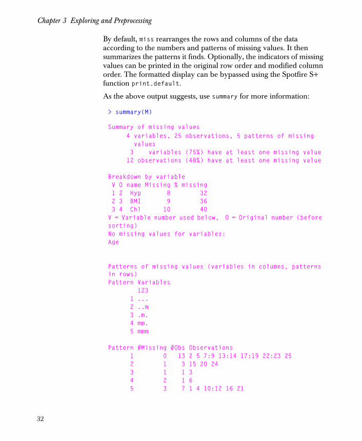
By default, miss rearranges the rows and columns of the data according to the numbers and patterns of missing values. It then summarizes the patterns it finds. Optionally, the indicators of missing values can be printed in the original row order and modified column order. The formatted display can be bypassed using the Spotfire S+ function print.default.
As the above output suggests, use summary for more information:
> summary(M)
Summary of missing values 4 variables, 25 observations, 5 patterns of missing values 3 variables (75%) have at least one missing value 12 observations (48%) have at least one missing value
Breakdown by variable V O name Missing % missing 1 2 Hyp 8 32 2 3 BMI 9 36 3 4 Chl 10 40V = Variable number used below, O = Original number (before sorting)No missing values for variables:Age
Patterns of missing values (variables in columns, patterns in rows)Pattern Variables 123 1 ... 2 ..m 3 .m. 4 mm. 5 mmm
Pattern #Missing #Obs Observations 1 0 13 2 5 7:9 13:14 17:19 22:23 25 2 1 3 15 20 24 3 1 1 3 4 2 1 6 5 3 7 1 4 10:12 16 21
32

Exploring Patterns of Missingness
Patterns of missing values (variables in columns, observations in rows)Obs. Variables 123 1 mmm 2 ... 3 .m.. . .
See Figure 3.1 for the plots that result from the following commands:
# This plot sorts observations to show common patterns.> plot(M)# This plot sorts observations as in the original data.> plot(M, sort.obs = F)
Figure 3.1: Plots of the miss object for the health data set.
Output of plot.miss
25
20
15
10
5
1
Ob
serv
atio
ns
(re
ord
ere
d)
AgeHypBMI Chl
Original order
25
20
15
10
5
1
Ob
serv
atio
ns
AgeHypBMI Chl
33

Chapter 3 Exploring and Preprocessing
If your data set has a missing value code other than NA, you should change it to NA before calling miss. For example, the following command changes all missing values in the vector x as from -9 to NA.
> x[x == -9] <- NA
34

Preprocessing Data
PREPROCESSING DATA
Preprocessing functions in S+MISSINGDATA process a data set to create an object that contains the information needed for the EM and DA model fitting algorithms. Note that the preprocessing functions are model-specific; see Chapter 4 for detailed descriptions of the models mentioned here.
• To fit a Gaussian imputation model, use the preGauss function to preprocess the data. This returns an object of class "preGauss". For example, the following preprocesses the built-in cholesterol data:
> cholesterol.pre <- preGauss(cholesterol)
• To fit a loglinear imputation model, use the preLoglin function to preprocess the data. This returns an object of class "preLoglin". For example, the following preprocesses the built-in crime data:
> crime.pre <- preLoglin(crime, + margins = count ~ Visit.1 : Visit.2)
• To fit a conditional Gaussian imputation model, use the preCgm function to preprocess the data. This returns an object of class "preCgm". For example, the following preprocesses the built-in language data:
> language.pre <- preCgm(language)
For additional details about the preGauss, preLoglin, and preCgm functions, see their on-line help files.
Calling preprocessing functions manually before fitting a missing data model is optional. If preprocessing is not performed once in advance, it is performed automatically as needed. However, this may cause the same processing to be repeated at different stages of your analysis, which consumes your machine’s resources unneccessarily.
35

Chapter 3 Exploring and Preprocessing
36

FITTING A MISSING DATA MODEL 4
Overview 38
Missing Data Models 39The Gaussian Model 39The Loglinear Model 41The Conditional Gaussian Model 44
S-PLUS Implementation 48Fitting a Gaussian Model 49Fitting a Loglinear Model 51Fitting a Conditional Gaussian Model 54
37

Chapter 4 Fitting a Missing Data Model
OVERVIEW
Once you’ve explored the patterns of missingness in your data and preprocessed it for the fitting algorithms, the next step is to fit a model. The model you fit is the distribution assumed for the complete data (the missing and observed data together).
S+MISSINGDATA implements three models for independent, identically distributed (iid) observations: the Gaussian model for numeric variables, the loglinear model for factor variables, and the conditional Gaussian model for both numeric and factor variables. This chapter describes these three models and their associated priors, and then shows how to fit the models using functions in S+MISSINGDATA.
38

Missing Data Models
MISSING DATA MODELS
The Gaussian Model
The Gaussian model handles missing data when all the variables are numeric.
Model
Let Y1 … Yp, , be numeric variables in which values are recorded for
n cases, so that the complete data form an n p× data frame Y . The cases are assumed to be independent and identically distributed multivariate Gaussians with mean μ and covariance Σ .
Prior distribution
In complete data problems, using a normal inverted-Wishart prior distribution leads to a conjugate analysis. The posterior distribution is again normal inverted-Wishart with updated parameters involving the data and prior parameters. In the presence of missing data, though, this family is not conjugate in general. However, using this family of distributions is computationally convenient for the EM and DA model fitting algorithms. This is because both algorithms depend on the complete data problem being tractable; see the section S-PLUS Implementation on page 48. Further details may be found in Schafer (1997).
A normal inverted-Wishart prior distribution means the following. Given Σ , the mean μ is assumed to have a conditional Gaussian distribution:
μ Σ N μ0 τ 1– Σ,( )∼
with known and fixed hyperparameters μ0 and τ 0> . In addition, Σ is assumed to have an inverted-Wishart distribution:
Σ W 1– m Λ,( )∼
with fixed hyperparameters m p≥ and Λ 0> . Schafer (1997) discusses choosing between noninformative , informative , and ridge prior hyperparameters.
39

Chapter 4 Fitting a Missing Data Model
• A noninformative prior is used when little is known about the parameters. This improper prior is the limiting form of the
normal inverted-Wishart as τ 0→ , m 1–→ , and Λ 1– 0→ :
π μ Σ,( ) Σ p 1+( ) 2⁄( )–∝ .
Note that μ does not appear on the right side of this equation; its distribution is assumed to be uniform.
• With an informative prior, you choose reasonable values for the hyperparameters by interpreting them as a summary of the information provided by an imaginary set of data. The value μ0 is the best guess as to what μ is, τ is the number of
imaginary prior observations on which μ0 is based, and
m 1– Λ 1– is the best guess for Σ . The parameter m is the number of imaginary prior degrees of freedom on which
m 1– Λ 1– is based.
• A ridge prior is useful for stabilizing the inference about μ when the sample covariance matrix is singular or nearly so, and little is known a priori about μ or Σ . This can happen, for example, when the data are sparse.
A ridge prior is the limiting form of the normal inverted-Wishart distribution when τ 0→ . Take m ε 0>= and
Λ 1– ε Ψ⋅= , where Ψ is a covariance matrix. For complete
data, the estimate for Σ is a weighted average of Ψ and the sample covariance S . When S is nearly singular, set
Ψ diag S( )= , the matrix with sample variances along the diagonal and zeroes elsewhere. This helps to smooth the calculated variances towards the observed data variances and the correlations towards zero; the smoothing results in something closer to an independence model. The relative sizes of ε and the sample size n determine the degree of smoothing.
40

Missing Data Models
When there are missing data, S is not available. However, set Ψ Diag V( )= in this case, where V is a matrix with diagonal elements that are the sample variances of the observed values for each variable.
The Loglinear Model
The loglinear model handles missing data when all the variables are categorical, or of class "factor".
Models
Let W1 W2 … Wq, , , be factor variables with values recorded for n
cases, so that the complete data form an n q× data frame W . If the cases are independent and identically distributed, the information in W is equivalent to a contingency table with D cells, where D is the number of level combinations:
D djj 1=
q
∏= .
Here, dj is the number of levels for the variable Wj . Some cells in the contingency table are empty because of logical constraints; these are known as structural zeroes .
If the sample size is assumed fixed, the set of D cell frequencies (or counts) has a multinomial distribution. The parameters of the distribution are the D probabilities that a case falls into each of the D cells of the contingency table. If there are no restrictions on the parameters other than that they are true probabilities, then the model is said to be saturated . In many realistic examples, however, the amount of data is insufficient to model such arbitrarily complex associations among the variables.
Loglinear models are a flexible class of models for specifying possible dependencies among variables. The cell probabilities are parameterized as the product of effects for each variable and the associations among variables. The log of the probabilities is therefore linear. Eliminating terms from this decomposition imposes equality constraints on odds ratios in the contingency table. See Bishop, Fienberg, and Holland (1975) or Agresti (1990) for details.
41
Chapter 4 Fitting a Missing Data Model
The implementation of these models in S+MISSINGDATA assumes hierarchical loglinear models. That is, it is assumed that no high-order interaction is present unless all main effects and lower-order interactions involving the same variables are also present.
Other situations
If the levels of the factors in your data are ordered, you may either:
• Pretend that they are approximately normally distributed, or
• Disregard the order. If the immediate goal is to create plausible multiple imputations of missing data, then applying a loglinear model may be reasonable in this case (Schafer, 1997, page 240).
The multinomial model can also be applied in some non-multinomial situations:
• If the distribution of one or more categorical variables is fixed by design, the cell frequencies follow a product-multinomial model. This arises, for example, in variables used to define strata in sample surveys. The multinomial model may still be valid in this situation if the missing values are confined to variables that are not fixed.
• If the total sample size n is random, the multinomial likelihood may lead to valid conditional inferences. This occurs, for example, in Poisson sampling.
Prior distribution
With complete data, using a Dirichlet prior distribution for the saturated model leads to a conjugate analysis. The posterior distribution is again Dirichlet with updated parameters involving the data and prior parameters.
For the loglinear model, Schafer (1997) adopts the constrained Dirichlet as the prior distribution. This has the same functional form as the Dirichlet but requires the parameters to satisfy constraints imposed by a loglinear model. The advantage of this prior is that it forms a conjugate class: the posterior distribution is another constrained Dirichlet with updated parameters. Note, however, that the constrained Dirichlet prior assumes that the given loglinear model is true. This can be assessed by performing goodness-of-fit tests against more general alternative models.
42

Missing Data Models
The parameters are updated in a way that suggests thinking of the prior parameters as imaginary prior counts in the cells of the contingency table. Schafer (1997) gives the form of a Dirichlet distribution and discusses noninformative , flattening , and data-dependent values for the hyperparameters.
• As with Gaussian models, noninformative priors are used when little is known about the parameters. Taking all hyperparameters equal to a common value is a sensible approach when little information is available a priori . Schafer (1997, page 252) argues that any common value between 0 and 1 is potentially noninformative. For the EM algorithm, the uniform prior sets all hyperparameters equal to 1 and leads to a maximum likelihood estimate. Therefore, this is adopted as the default noninformative prior for the EM algorithms. For DA algorithms, the default noninformative prior is arbitrarily established as the Jeffreys prior, in which all hyperparameters are equal to 1 2⁄ .
• The flattening prior is related to the noninformative prior, in that all hyperparameters are set to a common value. The effect is to smooth estimates toward a uniform table in which all cell probabilities are equal. For mode-finding algorithms such as EM, a prior with common value greater than 1 is flattening; for DA, a common value that is greater than 0 is flattening. However, Schafer (1997, page 253) warns that for nonlinear parameters, common prior values close to 0 can cause problems.
A flattening prior is often useful when the contingency table is sparse. In such cases, model parameters may be inestimable or lie on the boundary of the parameter space. A flattening prior can help ensure that the mode is unique and lies in the interior of the parameter space. Since a uniform table implies no relationship between variables, smoothing toward a uniform table is conservative; it does not increase the chance of concluding relationships among variables when they do not exist.
Since flattening priors are used in sparse data situations, care must be taken not to inadvertently smooth the data too much. More specifically, sparse data situations imply that the sample size n is small relative to the number of cells D . If we think of
43

Chapter 4 Fitting a Missing Data Model
the hyperparameters as imaginary prior counts, even small values can result in an effective prior sample size that is greater than the actual sample size.
• A data-dependent prior is used to smooth estimates toward a model of mutual independence among the variables, leaving the marginal distributions unaffected (Fienberg and Holland, 1970, 1973). This is calculated as follows. For each factor Yk ,
estimate the probabilities P Yk ik=( ) of the levels ik from the
completely observed data for that factor. If cell d has the level
combination y1 y2 … yp, , ,( ) , estimate the cell d probability
by
θdˆ P Yk yk=( )
k 1=
p
∏= .
The number of prior observations allocated to cell d is then
given by n0Θˆ
d , where n0 is the desired total number of prior
observations. For the DA algorithm, this is the data-
dependent prior for cell d : αd n0θd= . For EM, add 1 to this
quantity.
In applying any of these priors, Schafer (1997) recommends conducting a sensitivity analysis by applying several priors to see if and how the choice of prior affects inferences. When the goal is to help cure inestimable parameters or estimates on the boundary, Schafer (1997) warns against compromising the integrity of the observed data by adding more prior information than prior beliefs support. Instead, he recommends simplifying the model by eliminating variables or imposing loglinear constraints.
The Conditional Gaussian Model
The conditional Gaussian model (CGM) handles missing data when some of the variables are factors and others are numeric. This arises, for example, in the analysis of covariance and logistic regression with continuous predictors.
44
Missing Data Models
Model
Let W1 W2 … Wp, , , be factor variables and let Z1 Z2 … Zq, , , be
numeric variables in which values are recorded for n cases. Thus, the complete data form an n p q+( )× data frame Y W Z( , )= . The rows are assumed to be:
• Independent and identically distributed, and
• Distributed according to a general location model (Olkin and Tate, 1961), or more descriptively as a conditional Gaussian model.
The conditional Gaussian model is best described in terms of the marginal distribution of W and the conditional distribution of Z given W , as follows. The information in W is equivalent to a contingency table with D cells, where D is the number of level combinations:
D djj 1=
p
∏= .
Here, dj is the number of levels for the factor variable Wj . If the
sample size is assumed fixed, the set of D cell frequencies (or counts) has a multinomial distribution. The parameters of the distribution are the D probabilities that a case falls into each of the D cells of the contingency table.
Given W , the conditional distribution of Z is Gaussian. Each case falls into one of the D cells of the contingency table defined by W . The distribution of the continuous variables for the cases that fall into cell d is conditionally Gaussian with mean μd and covariance Σ .
Note that the means vary from cell to cell, but the covariance matrix is common to all cells. For a single binary factor variable, the CGM is the model that underlies classical discriminant analysis.
Restricted models
The number of parameters in the unrestricted conditional Gaussian model is:
D 1–( ) Dq q q 1+( ) 2⁄+ + .
45

Chapter 4 Fitting a Missing Data Model
.
In this equation, D is the number of cells in the contingency table defined by W and q is the number of numeric variables in Z . Note that D affects not only the number of cell parameters but also the number of mean parameters Dq . The value of D increases quickly with both the number of factor variables and the number of levels in each factor variable. The unrestricted CGM is feasible only when the sample size n is large relative to D . When data are sparse relative to the size of the model, more cells are likely to be empty and the parameters related to the empty cells are inestimable.
The number of parameters can be reduced by restricting the parameter sets in two possible ways:
• Loglinear constraints on the cell probabilities, and
• Multivariate analysis of variance (MANOVA) for the numeric variables Z with effects defined by the factor variables W .
Loglinear constraints are discussed in the section The Loglinear Model on page 41. They are specified in Spotfire S+ functions for the CGM identically to the way they are specified in the loglinear model fitting function. See the section Spotfire S+ Implementation on page 48
The remainder of this discussion focuses on the MANOVA model for the numeric variables Z . First, note that the model for Z given W may be written as a standard multivariate regression:
Z Uμ ε+= ,
where U is an n D× matrix. Each row of U is a dummy variable indicating which cell the case falls into: if case i falls into cell d , the
i th row of U is 1 in position d and 0 elsewhere. The matrix μ is
D q× and has rows that are the means of the cells. The error ε is an n q× matrix whose rows have independent Gaussian distributions
with mean 0 and covariance Σ .
The means μ vary freely among the cells. A restricted model is
obtained by parametrizing μ in terms of a smaller number of
regression coefficients β :
μ Aβ= .
46

Missing Data Models
Here, A is a fixed matrix of dimension D r× and β is r q× . The multivariate regression model now becomes:
Z UAβ ε+=
Taking A to be the D D× identity matrix gives the unrestricted model as a special case.
You can create A as you would a design matrix for a factorial ANOVA (Schafer 1997, page 343). The rows of A correspond to possible level combinations of the factor variables. Columns represent the main effects and possibly interactions. Creating a design matrix is simplified in Spotfire S+ by using formulas and specifying contrasts, as shown in the section Specifying a Restricted Model on page 152.
Prior distribution
The likelihood factors as a product of a multinomial distribution involving W and a conditional Gaussian distribution for Z given W . By applying independent prior distributions for the parameters of each distribution, the parameter sets remain independent in the posterior distribution.
In principal, the same prior distributions discussed in the sections The Gaussian Model on page 39 and The Loglinear Model on page 41 can be used. In practice, however, it may be difficult to quantify prior knowledge about the Gaussian model parameters. A noninformative prior for these parameters is the only option allowed in the Spotfire S+ functions for fitting a CGM.
In sparse data situations, the posterior distribution may be improper or the Gaussian parameters from certain cells may be poorly estimated. Rather than trying to stabilize the inferences through informative priors, Schafer (1997; pages 341, 348) recommends restricting the model. In case of problems, simplify the model by using a design matrix that has fewer columns.
For the multinomial portion of the model, apply a Dirichlet prior distribution. See the section The Loglinear Model on page 41 for details.
47
Chapter 4 Fitting a Missing Data Model
Spotfire S+ IMPLEMENTATION
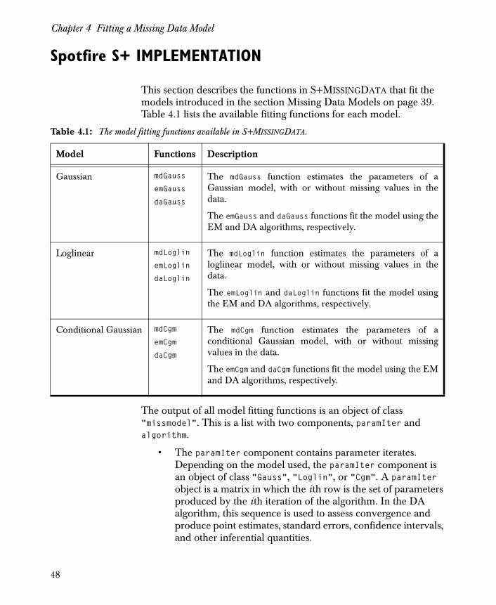
This section describes the functions in S+MISSINGDATA that fit the models introduced in the section Missing Data Models on page 39. Table 4.1 lists the available fitting functions for each model.
Table 4.1: The model fitting functions available in S+MISSINGDATA.
Model Functions Description
Gaussian mdGauss
emGauss
daGauss
The mdGauss function estimates the parameters of a Gaussian model, with or without missing values in the data.
The emGauss and daGauss functions fit the model using the EM and DA algorithms, respectively.
Loglinear mdLoglin
emLoglin
daLoglin
The mdLoglin function estimates the parameters of a loglinear model, with or without missing values in the data.
The emLoglin and daLoglin functions fit the model using the EM and DA algorithms, respectively.
Conditional Gaussian mdCgm
emCgm
daCgm
The mdCgm function estimates the parameters of a conditional Gaussian model, with or without missing values in the data.
The emCgm and daCgm functions fit the model using the EM and DA algorithms, respectively.
The output of all model fitting functions is an object of class "missmodel". This is a list with two components, paramIter and algorithm.
• The paramIter component contains parameter iterates. Depending on the model used, the paramIter component is an object of class "Gauss", "Loglin", or "Cgm". A paramIter object is a matrix in which the i th row is the set of parameters produced by the i th iteration of the algorithm. In the DA algorithm, this sequence is used to assess convergence and produce point estimates, standard errors, confidence intervals, and other inferential quantities.
48
Spotfire S+ Implementation
• The algorithm component contains information about the fitting algorithm that produced the iterates in paramIter. Depending on the algorithm used, the algorithm component is an object of class "em" or "da". An algorithm object describes aspects of the algorithm such as the number of iterations and the value of the objective function (log-likelihood or posterior) at the termination of the algorithm.
All model fitting functions take data as input in the form of a matrix, data frame, preproccessed object (see the section Preprocessing Data on page 35), or another missmodel object.
Fitting a Gaussian Model
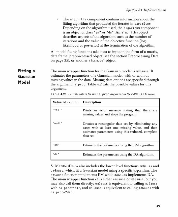
The main wrapper function for the Gaussian model is mdGauss. It estimates the parameters of a Gaussian model, with or without missing values in the data. Missing data options are specified through the argument na.proc; Table 4.2 lists the possible values for this argument.Table 4.2: Possible values for the na.proc argument to the mdGauss function.
Value of na.proc Description
"fail" Prints an error message stating that there are missing values and stops the program.
"omit" Creates a rectangular data set by eliminating any cases with at least one missing value, and then estimates parameters using this reduced, complete data set.
"em" Estimates the parameters using the EM algorithm.
"da" Estimates the parameters using the DA algorithm.
S+MISSINGDATA also includes the lower level functions emGauss and daGauss, which fit a Gaussian model using a specific algorithm. The emGauss function implements EM while daGauss implements DA. The main wrapper function calls either emGauss or daGauss, but you may also call them directly; emGauss is equivalent to calling mdGauss with na.proc="em", and daGauss is equivalent to calling mdGauss with na.proc="da".
49

Chapter 4 Fitting a Missing Data Model
All three functions for fitting the Gaussian model have a prior argument that specifies the hyperparameters of the normal inverted-Wishart distribution. The following are possible values for prior:
• One of the character strings "ml", "noninformative", or "ridge". When prior="ml", no prior is specified and maximum likelihood estimates are produced. Specifying prior="ridge" sets the scale hyperparameter of the inverted-Wishart distribution to a diagonal matrix of observed variances with degrees of freedom equal to 1.
To specify a different scale hyperparameter or different degrees of freedom, use the function dataDepPrior (for “data-dependent prior”). This is a generic function with methods for preGauss and preLoglin objects (see page 35).
• Output from the function priorGauss, which allows you to explicitly supply the hyperparameters. The priorGauss function has the arguments tau, mean, df, and scale. See the on-line help file for more details.
The default value for prior is the noninformative prior. When you give a missmodel object to one of the model fitting functions, the prior used to produce that object is applied instead of the default, unless prior is explicitly set.
Control parameters that influence behavior of the EM or DA algorithms are specified through the control argument, which is governed by algorithm-specific functions. Convergence criteria for EM are specified through the emGauss.control function, while criteria for DA are specified through daGauss.control. For example, convergence occurs in one of three ways for emGauss.control:
• The maximum relative change in the estimates is less than the first element in the tolerance argument. The default value of tolerance[1] is 0.001.
• The relative change in the log–likelihood is less than the second element in the tolerance argument. By default, this criterion is not used.
• A maximum number of iterations is reached, as determined by the maxit argument. The default value is Inf.
50

Spotfire S+ Implementation
These values can be specified directly as a list to the control argument of mdGauss. For example, to change the maxit criterion to 2000 and accept the default values of the other control parameters, use either of the following in a call to mdGauss:
control = emGauss.control(maxit = 2000)
control = list(maxit= 2000)
Fitting a Loglinear Model
The model fitting functions for a loglinear model are analogous to those described for the Gaussian model in the previous section. The wrapper function mdLoglin estimates the parameters of the loglinear model, with or without missing values in the data. Missing data options are specified through the argument na.proc, which has the values described in Table 4.2. The lower level functions emLoglin and daLoglin fit the model using the EM and DA algorithms, respectively; they are equivalent to calling mdLoglin with na.proc="em" and na.proc="da".
The functions mdLoglin, emLoglin, and daLoglin all accept the argument prior, which specifies the hyperparameters of the Dirichlet distribution. The following are possible values for prior:
• One of the character strings "ml", "noninformative", or "data.dependent". When prior="ml", no prior is specified and maximum likelihood estimates are produced. Specifying prior="data.dependent" calls the function dataDepPrior, which is a generic function with methods for preLoglin and preGauss objects (see page 35). For preLoglin objects, you must supply the argument nPriorObs, which is the total number of prior observations; this is referred to as n0 in the
section The Loglinear Model on page 41.
• The output object from the function priorLoglin.
• A vector that explicitly defines the Dirichlet hyperparameters. The length of the vector equals the number of distinct combinations of the variables’ factor levels. The ordering is such that the first variable varies the fastest, then the second variable, and so on. Structural zeroes must be coded as missing values (NAs). If a single numeric value is given to prior, its value is replicated for all cells in the contingency table.
51

Chapter 4 Fitting a Missing Data Model
The default value for prior is the noninformative prior. When you give a missmodel object to one of the model fitting functions, the prior used to produce that object is applied instead of the default, unless prior is explicitly set.
Table 4.3 summarizes values of the cell hyperparameters for different priors. For the data-dependent prior, n0 is the total number of prior
observations and θd is the cell probability estimated under independence using the observed data. Table 4.3: Values of the cell hyperparameters for different priors.
Prior EM Algorithm DA Algorithm
maximum likelihood c 1= c 0=
noninformative c 1= c 1 2⁄=
data-dependent αd 1 n0θd+= αd n0θd=
flattening c 1> c 0>
Control parameters that influence behavior of the EM or DA algorithms are specified through the control argument, which is governed by algorithm-specific functions. Convergence criteria for EM are specified through the emLoglin.control function, while criteria for DA are specified through daLoglin.control. For example, the arguments to daLoglin.control include:
• niter, which sets the number of iterations. The default value is 1.
• seed, which sets the seed required by the random number generator used by the algorithm. The default is .Random.seed.
• save, which specifies the parameter iterates to return as a row in the paramIter component of the missmodel object. You can choose, for example, to throw away some of the early iterates.
52

Spotfire S+ Implementation
Another possibility is to thin the iterates by saving only a subsequence of them. The default behavior throws away the first 10 percent of the iterates.
• monotone, a logical value that determines whether a monotone algorithm is used. A monotone algorithm potentially saves a computation resources and is appropriate when the missingness pattern is (nearly) monotone. By default, monotone=FALSE.
• trace, a logical value that determines whether information is printed during the course of the algorithm. By default, trace=FALSE.
These values can be specified directly as a list to the control argument of mdLoglin. For example, to change the monotone criterion to TRUE and accept the default values of the other control parameters, use either of the following in a call to mdLoglin:
control = daLoglin.control(monotone = T)
control = list(monotone = T)
The loglinear model fitting functions also accept the argument margins, which specifies loglinear constraints (if any). The margins argument refers to the marginal totals to be fit, and can be specified in one of three ways:
• A list of integers representing the variables. For example, margins=list(1:2, 3:4) fits the 1,2 margin (summing over variables 3 and 4) and the 3,4 margin in a four way table. This fits main effects for each variable and the two-way interactions between variables 1 and 2, and 3 and 4.
• A list of the names of the variables. For example, margins=list(c("V1","V2"), c("V3","V4")) also fits the 1,2 margin and the 3,4 margin in a four way table, if the variable names are "V1","V2", "V3", and "V4".
• An S-PLUS formula. For example, margins=~V1:V2 + V3:V4 specifies the same model described in the previous two cases. The argument frequency to mdLoglin may be included as the dependent variable in the formula, as in frequency~V1:V2 + V3:V4.
53

Chapter 4 Fitting a Missing Data Model
If margins is not specified, a saturated model is fit if the data object is a matrix, data frame, or preLoglin object. If the data is a missmodel object, margins defaults to the margins used to fit the missmodel object.
Fitting a Conditional Gaussian Model
The model fitting functions for a conditional Gaussian model are entirely analogous to those described for the Gaussian and loglinear models of the previous sections. The wrapper function mdCgm estimates the parameters of the conditional Gaussian model, with or without missing values in the data. Missing data options are specified through the argument na.proc, which has the values described in Table 4.2. The lower level functions emCgm and daCgm fit the model using the EM and DA algorithms, respectively; they are equivalent to calling mdCgm with na.proc="em" and na.proc="da". Control parameters for the fitting algorithms are specified through the control argument to mdCgm. See the on-line help files for emCgm.control and daCgm.control for details.
Several arguments to these fitting functions behave the same as those for the loglinear model. For details, see the on-line help for mdCgm, emCgm, and daCgm.
54

CONVERGENCE OF DATA AUGMENTATION ALGORITHMS 5
Overview 56
Parameter Simulation 57
Multiple Imputation 58
Practical Considerations for Missing Data Problems 60Starting Values 60S-PLUS Functions 61
55

Chapter 5 Convergence of Data Augmentation Algorithms
OVERVIEW
The goal of Monte Carlo Markov Chain (MCMC) methods is to sample values from a convergent Markov chain in which the limiting distribution is the true joint posterior of quantities of interest. In practice, you need to determine when the algorithm has converged. That is, you must determine when the samples are representative of the stationary distribution of the Markov chain can be used to estimate characteristics of the distribution of interest.
Theoretical convergence rates involve laborious and sophisticated mathematics that must be repeated for each model. In addition, the bounds of such rates can be so loose as to be impractical. Instead, S+MISSINGDATA uses statistical analysis, called convergence diagnostics, on the generated samples to assess convergence. The diagnostics for assessing convergence vary according to the method of inference being used.
This chapter discusses diagnostics used for both parameter simulation and multiple imputation. In conclusion, we discuss practical considerations for missing data problems, including starting values and the implementation of convergence diagnostics in S+MISSINGDATA.
56

Parameter Simulation
PARAMETER SIMULATION
In parameter simulation, the goal is to accurately estimate characteristics of the posterior distribution P θ Yobs[ ] , such as its moments and quantiles. Convergence is given by the law of large numbers and occurs when the sample summaries are sufficiently close to the posterior quantities they estimate.
To reduce bias due to starting values, samples within an initial burn-in period are thrown away. The length of this period varies according to how fast the algorithm converges to the parameters of the target distribution.
To estimate a quantity g g θ( )= of interest such as a point estimate, standard error, interval estimate, or p-value, collect iterates
gk 1+ gk 2+ … gk n+, , , .
Here, k is the burn-in period and n is the Monte Carlo sample size. If
k is large enough to ensure stationarity and n k⁄ is large enough for the law of large numbers to apply, then the sample quantities estimate the corresponding posterior quantities (for example, the posterior mean E g Yobs[ ] ). The burn-in period k should be chosen large
enough to make gk practically independent of g0
. To determine k , Schafer (1997) recommends looking at time series and autocorrelation
function plots of gt{ } .
After convergence, the following should apply:
• Time series plots should not show a trend, nor should iterates k steps apart have more than negligible correlation. See Schafer (1997), page 121 for examples.
• Autocorrelation function (ACF) plots should die out. The sample ACFs should fall within approximate 0.05-level critical values for testing that the ACFs are zero. See Schafer (1997), page 122 for examples.
57
Chapter 5 Convergence of Data Augmentation Algorithms
MULTIPLE IMPUTATION
In multiple imputation, the goal is to generate Bayesianly proper multiple imputations. These are independent realizations of P Ymis Yobs[ ] , the posterior predictive distribution of the missing data
under some complete-data model and prior.
The DA algorithm simulates values of Ymis that have P Ymis Yobs[ ] as
their stationary distribution. In practice, M imputations are produced either with one long chain or several chains. The working notions of convergence differ depending on whether one or several chains are used, as we discuss below. In both cases, however, the main problem is to approximate the burn-in period k . As in parameter simulation, samples within an initial burn-in period are discarded to reduce bias due to starting values.
Note
As discussed in the section Multiple Imputation Using DA on page 23, it is easier to monitor convergence using the parameter sequence rather than the imputed data sequence.
• Single chain. Here, imputations are obtained by subsampling the long chain, taking every k th iterate, for example. The value k must be large enough so that the dependence between imputations is negligible. To determine k , Schafer (1997) recommends looking at time series and ACF plots of scalar functions of θ , the distribution parameter of interest.
• Several chains. Here, imputations are obtained by simulating M independent chains of length k and keeping the last values of Ymis from each chain. The value k must be large enough so that the imputations are independent of the starting values and starting distribution.
For the M chains, at each step t there are M replicate values of the distribution parameter θ . Denote these by θ *:t( ) . If stationarity has been achieved by step t , then θ *:t( ) is an iid
58

Multiple Imputation
sample from P θ Yobs[ ] . To determine k , Schafer (1997) recommends monitoring summaries of the distribution of θ *:t( ) . Some scalar functions of θ to consider are sample moments, quantiles, and density estimates. Presumably, these do not change after stationarity is achieved, although if M is small there is likely to be sampling variability.
59
Chapter 5 Convergence of Data Augmentation Algorithms
PRACTICAL CONSIDERATIONS FOR MISSING DATA PROBLEMS
So far, we have discussed assessing convergence of the DA algorithm in general. Our main goal is to provide tools that work quickly and reliably for the current methods and models used to handle missing data. To quote Schafer (1997) (page 120):
In typical missing-data scenarios addressed by this book, fractions of missing information are moderate and data augmentation algorithms tend to converge quickly. Pathological behavior such as slow convergence or nonexistence of a stationary distribution usually means that the model is too complicated (i.e. has too many parameters) to be supported by the observed data, and the problem should probably be reformulated. For our purposes, the most sensible diagnostics are those that can be implemented quickly and easily, providing an informal but reliable assessment of whether the situation is normal or pathological.
Since the rate of convergence of both the EM and DA algorithms is governed by the fraction of missing information, Schafer (private communication) suggests that the number of iterations needed for EM to converge gives a conservative estimate of the number of iterations needed for DA. Therefore, for missing data applications, it may suffice to use ten times the number of iterations needed for EM to converge and then look at:
1. Time series plots for each parameter (parameter iterates versus iteration number);
2. An autocorrelation plot for each parameter;
3. An autocorrelation plot of the worst linear function , discussed below.
Starting Values The rate of convergence to stationarity for DA partly depends on the starting values or starting distribution. Schafer (1997) recommends using starting values that are near the center of the posterior. For example, use a maximum likelihood estimate or posterior mode obtained from running an EM algorithm.
To facilitate this, objects of class "missmodel" returned by the EM fitting functions emGauss, emLoglin, and emCgm may be used as input to a DA algorithm. For example, the missmodel object returned by
60

Practical Considerations for Missing Data Problems
emLoglin can be used as data input to daLoglin. Similarly, objects of class "missmodel" returned by the wrapper functions mdGauss, mdLoglin, and mdCgm can be given back to the wrapper functions as input. For example, the object created by calling mdLoglin with na.proc="em" can be used as input to mdLoglin again, this time specifying the DA algorithm instead of EM.
For multiple chains, Gelman and Rubin (1992) recommend starting values that are overdispersed (exhibit greater variability) relative to P θ Yobs,[ ] . This results in a conservative estimate of the number of iterations needed to achieve stationarity. It also reduces the chance of being misled if the posterior is so oddly shaped that single runs tend to get stuck in small regions.
In practice, Schafer (1997) recommends using the bootstrap method to obtain an overdispersed starting distribution. For example, repeat the following M times:
1. Draw with replacement n* rows from Yobs to obtain a
bootstrap sample Yobsb
.
2. Calculate θbˆ θ Yobs
b( )= .
If we take n* to be smaller than n , say n* n2---= , then θb tends to be
overdispersed relative to P θ Yobs,[ ] . Care is required, however, since a reduced data set size may lead to problems such as colinearity.
S-PLUS Functions
Several S+MISSINGDATA functions help diagnose convergence of a DA chain. The tsplot and generic plot functions produce univariate time series plots of the parameter iterates. Similarly, acf and daAcfPlot calculate and plot autocorrelation function plots of the parameter iterates. The daAcfPlot function is a simpler version of acf; it avoids the default title and does not calculate cross-correlations.
It can also be useful to plot functions of the parameter iterates. The function worstLinFun calculates the worst linear function of the parameters , which is the inner product of the parameter iterates with the eigenvector returned by worstFraction. Intuitively, this function
61

Chapter 5 Convergence of Data Augmentation Algorithms
has a high rate of missing information and is useful to monitor because the rate of convergence to stationarity depends partly on the fraction of missing information.
62

IMPUTATION 6Overview 64
Imputing Data 65The Gaussian Model 65The Loglinear Model 66The Conditional Gaussian Model 67
The Class of impute Objects 68Extracting Imputations 69Replacing Imputations 70Manipulating impute Objects 70
63

Chapter 6 Imputation
OVERVIEW
As discussed in Chapter 2, the DA algorithm can be used to produce multiple imputations under one of the models discussed in Chapter 4: Gaussian, loglinear, and conditional Gaussian. Applied within the framework of multiple imputation, these models are more widely applicable than would appear at first glance. This is because multiple imputation is fairly robust to model misspecification, especially with small fractions of missing information (Ezzati-Rice et al. (1995), Rubin and Schenker (1986), Schafer (1997)). Multiple imputation under these models thus applies more or less routinely to a wide variety of missing data problems.
This chapter discusses the functions and objects in S+MISSINGDATA that support multiple imputation. The main functions discussed are impGauss, impLoglin, and impCgm, corresponding to each of the models from Chapter 4. All three imputation functions return objects of class "impute", which are designed to store multiple imputations efficiently with the original data. The impute objects work with a variety of utility functions available in S+MISSINGDATA.
In principal, you can generate multiple imputations by using nonparametric procedures, or by using parametric models that are different than the ones provided in S+MISSINGDATA. As long as your custom procedures and models return an object of class "impute", you may use the capabilities described in the next two chapters to perform multiple complete data analyses and consolidate results.
64

Imputing Data
IMPUTING DATA
The following functions for imputing data are available in S+MISSINGDATA:
• The impGauss function produces multiple imputations under the Gaussian model.
• The impLoglin function produces multiple imputations under the loglinear model.
• The impCgm function produces multiple imputations under the conditional Gaussian model.
These functions are generic with methods for preGauss, preLoglin, and preCgm objects, respectively; see the section Preprocessing Data on page 35 for descriptions of these objects. The impGauss, impLoglin, and impCgm functions also have methods for the missmodel objects described in Chapter 4, as well as default methods for matrices and data frames.
All three functions for imputing data return an object of class "impute", which by default is a data frame with columns of class "miVariable". See the section The Class of impute Objects on page 68 for details on miVariable. Alternatively, you can set the argument return.type="matrix" in a call to impGauss, impLoglin, or impCgm. In this case, an miVariable version of a matrix is returned instead of a data frame. The form of the return object usually depends on the whether the original data is a data frame or matrix. Preserving the form of the original data in the impute object makes the commands for subsequent complete data analyses parallel to those used when the data has no missing values.
The form of the starting values, given by the argument start in the impGauss, impLoglin, and impCgm functions, determines how many chains are run. The possible values for start are model-specific, as we discuss below.
The Gaussian Model
For one long chain, the start argument of the impGauss function is a list with two components: a vector that gives the mean and a matrix that gives the covariance matrix.
65

Chapter 6 Imputation
For multiple chains, start may take several forms:
• A list of lists. The inner lists must all have a vector component containing the mean and a matrix component containing the covariance. Each list of parameters starts a separate chain.
• An object of class "Gauss", which is the paramIter component of a missmodel object created by one of the functions mdGauss, emGauss, or daGauss. A Gauss object is a matrix in which each row contains one set of parameter estimates; each row then starts a separate chain. Typically, a Gauss object contains a limited set of iterations, obtained either through subsetting or by specifying the save argument to emGauss.control or daGauss.control.
• A list of Gauss objects. In this case, the last row of each Gauss object starts a separate chain.
The Loglinear Model
For one long chain, the start argument of the impLoglin function is a vector of cell probabilities. The length of start equals the number of distinct combinations of levels in the factor variables. The ordering is such that the first variable varies the fastest, then the second variable, and so on. Starting values should be zero for cells that are structural zeros. For one long chain, you must also supply the argument nimpute, which gives the number of imputations.
For multiple chains, start may take several forms:
• A list with vector components that contain cell probabilities. Each component starts a separate chain.
• An object of class "Loglin", which is the paramIter component of a missmodel object created by one of the functions mdLoglin, emLoglin, or daLoglin. A Loglin object is a matrix in which each row contains one set of cell probabilities; each row then starts a separate chain. Typically, a Loglin object contains a limited set of iterations, obtained either through subsetting or by specifying the save argument to emLoglin.control or daLoglin.control.
• A list of Loglin objects. In this case, the last row of each Loglin object starts a separate chain.
66

Imputing Data
The Conditional Gaussian Model
For one long chain, the start argument of the impCgm function is a list with the following components:
• mu, which is matrix of cell means. Each column in the matrix represents one numeric variable and each row represents a cell. The ordering of the rows is equivalent to the ordering in the pi component.
• sigma, which is a variance-covariance matrix of the numeric variables.
• pi, which is vector of cell probabilities. The length of pi equals the number of distinct combinations of the factor variable levels. The ordering is such that the first variable varies the fastest, then the second variable, and so on. Starting values should be zero for cells that are structural zeros.
For multiple chains, the start argument may take several forms:
• A list of lists. The inner lists must all have a vector component containing the mean, a matrix component containing the covariance, and a vector component containing the cell probabilities. Each list of parameters starts a separate chain.
• An object of class "Cgm", which is the paramIter component of a missmodel object created by one of the functions mdCgm, emCgm, or daCgm. A Cgm object is a matrix in which each row contains one set of parameter estimates; each row then starts a separate chain. Typically, a Cgm object contains a limited set of iterations, obtained either through subsetting or by specifying the save argument to emCgm.control or daCgm.control.
• A list of Cgm objects. In this case, the last row of each Cgm object starts a separate chain.
67

Chapter 6 Imputation
s
s
THE CLASS OF IMPUTE OBJECTS
Calculating and storing multiple imputations involves two types of impute objects: miVariable and miList. An miVariable object has three slots:
• The Data slot contains the original data object, including missing values.
• The whichNA slot is a numeric vector that indicates which positions in the data are missing. The order of whichNA matches the order of the rows in the Imputations slot.
If the original data object is a vector, matrix, or array, whichNA is a vector with each position represented as a single integer. Note that positions are not represented by matrix subscripts. For example, for a matrix with 10 rows and 2 columns that has missing values in positions [2,1] and [3,2], the whichNA slot contains the values 2 and 13. See the Spotfire S+ Programmer’Guide for details on vector subscripts of matrices and arrays.
• The Imputations slot is a data frame that contains the actual imputations. There are as many rows in Imputations as the length of whichNA, and it has M columns. Each column is a variable with the same class and many of the same attributes as the original object.
An miList object is a list of length M with the SV3 class "miList" (see the Spotfire S+ Programmer’s Guide for a general discussion on SV3 versuSV4 classes). It has one component for each set of imputations. Each component contains a complete data object , which is either complete data obtained by filling in missing values using a set of imputations, or the results of an analysis using a single set of complete data. Components of an miList object typically have the same structure; for example, they might all be lm objects.
Any impute object must have names for the imputations. These are the names of the components of the miList list or the column names of the Imputations slot in an miVariable.
Any miVariable object can be converted to a corresponding miList object, though this may result in loss of information. For example, for a categorical variable in which all of the M random imputations are the same for one data value, it is not possible to determine from an
68

The Class of impute Objects
miList that the data value was originally missing. The converse is not always true, however. Only an miList object with components that have the same length, names, attributes, and atomic mode may be converted to an miVariable object. The generic function miVariablePossible determines whether an object can be converted to an miVariable; you may write your own methods for this function.
Generally, miVariable objects should be used for data and miList objects for the results of analyses. Results of analyses that can be treated as data, such as a vector of residuals from a regression, are usually created and stored as miList objects. However, it is possible to convert them to miVariable objects.
Both miList and miVariable objects may be components of a list. In particular, variables in a data frame may be miVariable objects. These types of objects may be contained in an attribute, though this has not been well tested and is not currently recommended. These objects can also be contained in a slot if the definition for the class allows this.
Extracting Imputations
Extracting complete-data objects from an impute object is handled by the miSubscript function. This operation is similar to regular S-PLUS subscripting. In fact, it is implemented using subscripting for miList objects. For example, the command
> miSubscript(x,3) <- miSubscript(y,3)
is equivalent to
> x[[3]] <- y[[3]]
when x and y are both miList objects.
Extraction for miVariable objects involves replacing missing values in the Data slot by a set of imputations, then returning the Data slot as the complete-data object. The miSubscript function performs these steps. For example, suppose crime.imp is an miVariable object. To extract the second set of completed data for crime.imp, type:
> y <- miSubscript(crime.imp, 2)
Extraction for lists (or objects with slots) containing miList and miVariable objects proceeds recursively. Each miList or miVariable component is replaced with the corresponding extracted complete-data object, then the whole list (or object with slots) is returned.
69

Chapter 6 Imputation
Replacing Imputations
The reverse of extraction involves replacing complete-data objects in an impute object. This begins by converting the new object to an miList object, if it was not one already. This holds for ordinary and miVariable objects, as well as for lists or objects with slots containing impute objects. The appropriate component of the miList is then replaced. For example, if x is an impute object, then
> miSubscript(x,2) <- value
converts x to an miList and then replaces the second component.
An ordinary object with no imputations must first be converted to an miList object by replicating the object into each component of a new miList object. This is usually accomplished by calling the as.miList function. For example,
> x <- as.miList(x, + Names = paste("Imputation", 1:5, sep=""))> miSubscript(x,2) <- value
connverts x to an miList with 5 imputations, then replaces the second.
Manipulating impute Objects
The miList and miVariable objects can be created using the miList and miVariable functions, respectively.
To determine the number, names, or existence of imputations, use miReps, miNames, and is.mi functions, respectively. These functions operate recursively, searching for imputations in any list component or slot of an object. The is.miVariable and is.miList existence functions are also useful. The latter has an optional argument recursive; if recursive=TRUE, the is.miList function searches for miList objects recursively.
To convert between the two types of impute objects, use the as.miList and as.miVariable functions. In the latter case, the original object is returned if it is not possible to convert it to an miVariable object.
Use miTrim to simplify an impute object. This replaces miList with miVariable objects wherever possible, and replaces both with ordinary objects if all imputations are identical. The miTrim function also restructures recursive objects so that the imputations are stored at the lowest levels. For example, an miList containing ordinary lists
70

The Class of impute Objects
can be converted to a list of miList objects, provided that this does not result in an object that has a class and contains impute objects where they are not allowed for that particular class.
The miPrint function may be used to print an miVariable or a data frame containing one or more miVariable columns. This provides a formatted printout that shows the imputations more clearly than would otherwise occur with regular printing.
71

Chapter 6 Imputation
72

ANALYZING COMPLETED DATA SETS 7
Overview 74
Analysis Functions 75The miEval Function 75The miApply Function 76Additional Arguments 77Compatibility of miEval and miApply 77
73

Chapter 7 Analyzing Completed Data Sets
OVERVIEW
The process of statistical analysis may involve creating graphics, fitting models, investigating diagnostics, and comparing results. If you use multiple imputation to handle missing values, you still perform a similar sequence of analysis steps. However, you need to perform the steps on several data sets, each of which is completed by filling in the missing values using one set of imputations. Each completed data set gives a different result; the results must then be collected as described in this chapter and combined as described in the next chapter.
The S+MISSINGDATA library provides two functions to facilitate the process of performing analyses and collecting results:
• The miApply function is analogous to S-PLUS functions such as apply and sapply. It is useful when the complete data analysis can be expressed as a function applied to one set of data.
• The miEval function is analogous to the S-PLUS function eval. If the complete data analysis involves more than one set of data or requires an S-PLUS expression, then miEval is the function to use.
In this chapter, we discuss miApply and miEval in detail. Both functions usually produce miList objects in which each component is the result of one complete data analysis.
74
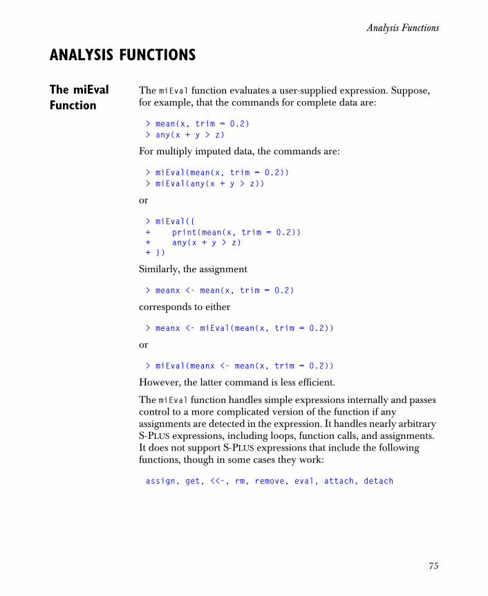
Analysis Functions
ANALYSIS FUNCTIONS
The miEval Function
The miEval function evaluates a user-supplied expression. Suppose, for example, that the commands for complete data are:
> mean(x, trim = 0.2)> any(x + y > z)
For multiply imputed data, the commands are:
> miEval(mean(x, trim = 0.2)) > miEval(any(x + y > z))
or
> miEval({ + print(mean(x, trim = 0.2))+ any(x + y > z) + })
Similarly, the assignment
> meanx <- mean(x, trim = 0.2)
corresponds to either
> meanx <- miEval(mean(x, trim = 0.2))
or
> miEval(meanx <- mean(x, trim = 0.2))
However, the latter command is less efficient.
The miEval function handles simple expressions internally and passes control to a more complicated version of the function if any assignments are detected in the expression. It handles nearly arbitrary S-PLUS expressions, including loops, function calls, and assignments. It does not support S-PLUS expressions that include the following functions, though in some cases they work:
assign, get, <<-, rm, remove, eval, attach, detach
75

Chapter 7 Analyzing Completed Data Sets
The miEval function does not provide support for functions that access data directly, without being passed through the argument list. This becomes a problem when, for example, the function is called by another function. However, miEval has an advantage in this situation: the given expression is evaluated in the calling frame, so that data that would be visible if the expression was evaluated outside of miEval is also visible inside of miEval. If the data is an impute object, the appropriate set of imputations is not extracted. The expression given to miEval can include explicit assignments to frame 1 to handle these situations.
The miApply Function
An alternative to miEval is miApply, which is a member of the apply family of functions. In the simplest call, you provide an impute object, a function, and any additional arguments to be passed to the function; the additional arguments should not contain imputations.
For example, if a complete data set is named x, the following computes its mean:
> meanx <- mean(x, trim = 0.2)
For an impute object x, the corresponding call is:
> meanx <- miApply(x, mean, trim = 0.2)
In some analyses, the impute object is not the first argument to a function. This occurs when you pass an impute object as the data argument to S-PLUS modeling functions (lm(y~x, data=myData), for example). In these cases, miApply can be used in one of two ways.
1. Provide all arguments to the function by name, including formula:
> miApply(myData, lm, formula = y~x)
2. Use a wrapper function:
> miApply(myData, function(data) lm(y~x, data))
Note that miApply cannot be used for expressions; you must use a wrapper function instead. For example, the expression x+y/z becomes the following:
> miApply(list(x=x, y=y, z=z), + function(l) l$x + l$y / l$z))
76

Analysis Functions
You must also use a wrapper function when calling functions that require multiple impute objects. For example, the command
> anova(fit1, fit2)
corresponds to the following:
> miApply(list(fit1=fit1, fit2=fit2), + function(X) anova(X$fit1, X$fit2))
Additional Arguments
Both miEval and miApply have an optional logical argument simplify. If simplify=TRUE and all imputations (components) of the result are identical, then the returned miList is simplified to an ordinary object with a single component.
The miEval function has an optional argument vnames, which is a vector of names for all impute objects used, including assigned objects that will become impute objects. For example, the command
> miEval(lm(y~x, data=myData), vnames = "myData")
specifies that only myData (and not y or x) is an impute object. In this simple example, it is not strictly necessary to specify vnames because miEval contains code to handle modeling functions like lm. If the expression passed to miEval is a call to a function for which one argument is a formula and another has the name data, then variable names in the formula are assumed to refer to columns in the data and not impute objects. This intelligence is limited, however. For example, in the command
> miEval(coef(lm(y~x, data=myData)), vnames = "myData")
it is necessary to specify vnames because the expression is a call to coef, which does not have a formula or a data argument. In general, it is safest to always supply vnames when calling functions that handle their arguments symbolically.
Other optional arguments are described in the help files for the miEval and miApply functions.
Compatibility of miEval and miApply
In most cases, the objects produced by miEval and miApply (when called with analogous expressions) are compatible. When the expressions contain modeling functions such as lm or glm, however, the objects produced by miEval and miApply are slightly different.
77

Chapter 7 Analyzing Completed Data Sets
This is because modeling functions return objects that contain call attributes. We recommend using miEval in these cases because some subsequent analyses will be easier.
For example, suppose m.kyphosis is a data frame similar to the built-in data set kyphosis, but containing variables with multiple imputations. A glm analysis can be performed using either of the following commands:
> m.fit1 <- miApply(m.kyphosis, function(xx) + glm(Kyphosis ~ Age + Start + Number, + family = binomial, data = xx))
> m.fit2 <- miEval(glm(Kyphosis ~ Age + Start + Number,+ family = binomial, data = m.kyphosis))
Both m.fit1 and m.fit2 are miList objects with components that are glm objects. The call attributes for the first components of each are, respectively:
glm(Kyphosis ~ Age + Start + Number, family = binomial, data = xx)
glm(Kyphosis ~ Age + Start + Number, family = binomial, data = miSubscript(m.kyphosis, 1))
Note the differences in the data arguments. The expression miSubscript(m.kyphosis, 1) is valid outside miEval, while xx is simply a dummy name. In fact, the data expression in the call attribute for m.fit2 actually produces the completed data set used in calculating the first component of m.fit2.
Objects produced by miEval can be used by miApply, but the converse is not always true. Indeed, results from miApply cannot always be used easily by miApply. For example, both of the following commands work as expected:
> miApply(m.fit2, predict, type = "terms")> miEval(predict(m.fit2, type = "terms"))
However, the same commands using m.fit1 fail because the data cannot be found. Instead, you must do one of the following:
> miApply(m.fit1, predict, type = "terms",+ X.frame1 = list(xx=m.kyphosis))
78

Analysis Functions
> miEval({ + assign("xx", m.kyphosis, frame = 1)+ predict(m.fit1, type = "terms") + })
This ensures that the appropriate data sets are assigned to frame 1 where they are sure to be found. The first completed data set from m.kyphosis is assigned to frame 1 with the name xx before the first analysis is run, then the second completed data set is assigned there, and so on. Note that replacing the dummy name xx with m.kyphosis when creating m.fit1 would be dangerous, because some code would not know whether to use the original m.kyphosis (which contains multiple imputations) or its completed data sets with the same names. Results could be transparently incorrect.
79

Chapter 7 Analyzing Completed Data Sets
80

CONSOLIDATING ANALYSES 8Overview 82
Simple Statistics 83
Inferences 84Normal and Students-t Inferences 84Chi-Square and F Inferences 86Likelihood Ratio Inferences 90
81

Chapter 8 Consolidating Analyses
OVERVIEW
The final step in an analysis of multiple imputations is consolidating results from all imputations to produce a single result. If the result from a single set of imputations is an estimate with no associated standard error or other inferences, then you can use the miMean function, which computes the average result across imputations. Likewise, the miVar function computes the variance across imputations.
More interesting is the case where you need to combine not only estimates but also standard errors or other inferences. The final result must encompass both the uncertainty associated with individual estimates, such as standard errors for linear regression coefficients, as well as the additional uncertainty due to missing data. The miMeanSE function combines point and variance estimates that are used for inference assuming asymptotic normality (Rubin (1987), Chapter 3) or Students-t (Barnard and Rubin (1999); Hesterberg (1998)). The functions miChiSquareTest, miFTest, and miLikelihoodTest combine
inferences based on χ2 (Li et al. (1991)), F (Hesterberg (1998); Li, Ragunathan, and Rubin (1991)), and likelihood ratio statistics, respectively.
82

Simple Statistics
SIMPLE STATISTICS
S+MISSINGDATA includes two functions for calculating simple statistics across imputation sets. The miMean function calculates the mean across imputation sets and the miVar function calculates the variances:
> miMean(m.coef) > miVar(m.coef)
Both functions return vectors, matrices, or arrays, depending on the shape of the original data. For positions without missing data, the variances across imputations are zero.
83

Chapter 8 Consolidating Analyses
INFERENCES
Normal and Students-t Inferences
Many inferences are based on estimates, standard errors, and approximate normality. The miMeanSE function consolidates both estimates and their standard deviations or standard errors by averaging the estimates and obtaining adjusted standard errors. The rules implemented in miMeanSE are based on those described in Rubin (1987) for combining normal-based inferences, and in Barnard and Rubin (1999) and Hesterberg (1998) for combining Students-t inferences. In this section, we describe the computations underlying miMeanSE.
Let θ be a scalar parameter and θ its estimate with standard
deviation σθ
. Normal-based confidence intervals with no missing
data are of the form θ zα 2⁄ σθ
± , where zα 2⁄ is a quantile of the
normal distribution. With multiple imputations, denote the estimates
and standard errors as θm and σm , for m 1 2 … M, , ,= . The
consolidated estimate is obtained by averaging the individual estimates:
θ 1M----- θm∑= .
The within-imputation variance averages the estimated complete data variances:
σ2 1
M----- σm
2∑= .
The between-imputation variance is the variance of the complete data point estimates:
B 1M 1–-------------- θm θ–( )
2∑= .
Finally, the consolidated variance combines the within and between variances:
σθ2
σ2
1 M 1–+( )B+= .
84

Inferences
Inferences are then based on Students-t quantiles θ tν α 2⁄, σθ± ,
where the degrees of freedom ν reflect the uncertainty in estimating the standard error.
For small sample sizes, where Students-t distributions are used for inferences in the absence of missing data, estimates and standard errors are consolidated as above except that estimated standard errors
Sθ are used in place of standard deviations. Degrees of freedom
combine the degrees of freedom for Sθ as an estimate of σθ and the
additional uncertainty due to multiple imputations. The final degrees of freedom is not greater than what is obtained in the absence of missing data.
As input, miMeanSE accepts the estimates, standard errors, and degrees of freedom computed for each completed data set. Other possible arguments include the degrees of freedom and the sample size. The degrees of freedom should not normally vary across imputations, as this may indicate violations of assumptions. To obtain normal-based inference, let the degrees of freedom be infinite (df=Inf).
For example:
> m.sumfit <- miApply(m.fit, summary) > miMeanSE(m.coef, + se = miEval(m.sumfit$coef[,2]), + df = miEval(m.fit$df, simplify=T), + n = nrow(m.data))
This returns a list containing the consolidated estimates, standard errors, and degrees of freedom. In addition, it returns the relative increase in variance due to nonresponse and the estimated fraction of missing information due to nonresponse.
The miMeanSE function also accepts variance-covariance matrices in place of standard errors. In this situation, it produces adjusted variance-covariance matrices using methods described in Hesterberg (1998). The results differ from those obtained using methods in Rubin (1987) and Schafer (1997). In particular, the square roots of the diagonal elements of the resulting variance-covariance matrix are the same as the standard errors produced above, and results are more stable with small numbers of imputations.
85

Chapter 8 Consolidating Analyses
An example command is:
> miMeanSE(m.coef), + cov = miEval(sumfit$cov.unscaled * sumfit$sigma^2), + df = miEval(m.fit$df, simplify=T), + n = nrow(m.data))
The miMeanSE function handles certain standard data structures automatically. For example, since m.fit is an miList with components that are lm objects, miMeanSE automatically extracts the regression coefficients and their variance-covariance matrices and consolidates them. The above example could have been written more simply as:
> miMeanSE(fit)
This allows you to call miMeanSE without first calculating sumfit and extracting the coefficients, degrees of freedom, and covariance matrices.
Chi-Square and F Inferences
When complete data inferences are based on χ2 or F statistics, there are two cases to consider:
• The estimates and variance-covariance estimates are available from each set of imputations; or
• Only the χ2 or F statistics are available.
In the first case, consolidate the estimates and variance-covariance matrices using miMeanSE and calculate an F statistic using the formula:
θ θ0–( )TΣˆ 1–
θ θ0–( ) df1( )⁄ .
Here, θ is the consolidated estimate, θ0 is the null hypothesis value (or the consolidated version of the estimates obtained under a
composite null hypothesis), Σˆ
is the consolidated variance-covariance
matrix, and df1 is the numerator degrees of freedom. The denominator degrees of freedom are obtained from the output of
miMeanSE. Note that even if complete-data inferences are based on χ2 statistics, the consolidated inferences are based on F statistics because of uncertainty in the variance-covariance estimate.
86

Inferences
For example, suppose we test whether a factor variable with 6 levels is significant in a linear model. This test involves an F test with 5 degrees of freedom (5 contrasts). The null hypothesis is that the coefficients for the 5 contrasts are all zero. First, create an miVariable object from the built-in data set fuel.frame:
# Set the seed for reproducibility.> set.seed(0)> m.fuel.frame <- fuel.frame
# Create missing values in m.fuel.frame.> for(j in c(1:3,5)) + m.fuel.frame[[j]][sample(1:60, 2*j)] <- NA> m.fuel.frame <- RandomImpute(m.fuel.frame)> m.fuel.frame[[4]] <- 100/m.fuel.frame[[3]]
Next, fit the linear model:
> m.fit <- miEval(lm(Fuel ~ Weight + Disp. + Type, + data = m.fuel.frame))
The goal is to test whether the categorical variable Type is significant. The null hypothesis is that all coefficients for the Type variable are zero.
The following commands calculate consolidated estimates and variance-covariance matrices for m.fit:
> m.C <- miMeanSE(m.fit)> coefType <- m.C$est[4:8] > covType <- m.C$cov[4:8, 4:8]> m.F <- coefType %*% solve(covType, coefType)/5
The denominator degrees of freedom vary across dimensions:
> m.C$df[4:8])
Type1 Type2 Type3 Type4 Type5 35.56862 16.85757 28.7291 45.00113 5.512315
Therefore, calculate the p-value conservatively using the smallest degrees of freedom:
> 1-pf(m.F, 5, min(m.C$df[4:8]))[1] 0.3541523
87

Chapter 8 Consolidating Analyses
When only the χ2 or F statistics are available, the functions in S+MISSINGDATA follow Schafer (1997, page 115) and Li et al. (1991), with natural extensions to F statistics. The functions miChiSquareTest
and miFTest accept as input the scalar χ2 or F statistics calculated on each completed data set and the degrees of freedom for the tests. They return the consolidated F statistic, numerator and denominator degrees of freedom, estimated average relative increase in variance due to nonresponse, and approximate p-value corresponding to the F statistic. The p-value should be used for screening only; the actual p-value may be larger or smaller by a factor of two.
For example, we might use the F statistics computed by the anova function to compare linear models with and without a factor variable. To continue the preceding example:
> m.fit2 <- miEval(lm(Fuel ~ Weight + Disp., + data = m.fuel.frame))> m.anov <- miEval(anova(m.fit2, m.fit))> miFTest(x = miEval(m.anov$"F Value"[2]),+ df1 = miEval(m.anov$Df[2]),+ df2 = miEval(m.anov$"Resid. Df"[2]))
$Fstatistic:[1] 0.2926602
$df1:[1] 5
$df2:[1] 5.758413
$r:[1] 0.3130781
$p:[1] 0.9001019
Both procedures fail to reject the null hypothesis that all coefficients for the Type variable are zero. However, note that the p -value obtained by combining F statistics is larger than the p -value based on averaging parameter estimates (obtained earlier). The p -value here is based on a less powerful test.
88

Inferences
To see why, consider a similar problem. Suppose that X1 X2 …Xn, ,
are iid N μ 1,( ) random variables. The null hypothesis H0 is that
μ 0= ; the alternative hypothesis H1 is that μ 0≠ .
• Case 1: The X values are observed. In this case, the test uses
the consolidated estimate X of μ .
• Case 2: Only Yi Xi2
= is observed (these are equivalent to
χ2 test statistics). In this case, the test uses the statistic Yi∑ .
Both procedures give exact tests, where the probability of Type I error is exactly equal to α . However, any single set of data can reach different conclusions. The first procedure, which averages individual parameter estimates, is more powerful.
The next example consolidates chi-square statistics from a loglinear analysis of a contingency table. First, create an impute object from the built-in data set barley:
# Set the seed for reproducibility.> set.seed(0)> m.barley.exposed <- barley.exposed
# Create 10 random missing values.> w <- sample(1:120, 10) > m.barley.exposed[w] <- NA> imputes <- matrix(rpois(40, barley.exposed[w]+0.1), 10)> m.barley.exposed <- miVariable(m.barley.exposed, + data.frame(imputes))
Fit a loglinear model to each completed data set:
> ml <- miApply(m.barley.exposed, loglin, + margin = list(1:2, c(1,3)))
Finally, consolidate the chi-square statistics:
> miChiSquareTest(miApply(ml, "[[", "pearson"),+ df = miApply(ml, "[[", "df"))
89
Chapter 8 Consolidating Analyses
Likelihood Ratio Inferences
The final consolidation function that we discuss in this chapter, miLikelihoodTest, combines likelihood ratio inferences. There are two ways to call this function. The first is
miLikelihoodTest(m.data, FUN, df1, estimates, estimates0,...)
Here, m.data is an miVariable object, and estimates and estimates0 are the maximum likelihood parameter estimates under the alternative and null hypotheses, respectively. The df1 argument is the degrees of freedom for the test, FUN is a function that calculates the likelihood ratio statistic (twice the likelihood ratio) for the data between estimates and estimates0, and ... are additional arguments to FUN.
For example, the following commands illustrate miLikelihoodTest when the parameters are the mean and variance of a normal distribution. The null hypothesis is that the mean is zero:
> x <- rnorm(20) > x[2:5] <- NA > x <- miVariable(x, Imputations = + split(sample(x[-(2:5)], 12, replace=T), rep(1:3,4)))
> estimates <- miEval(c(mean(x), mean((x-mean(x))^2))) > estimates0 <- miEval(c(0, mean(x^2))) > f1 <- function(dat, e1, e0, ...) { + n <- length(dat) + 2*((-n*log(e1[2])/2 - sum((dat-e1[1])^2)/(2*e1[2])) - + (-n*log(e0[2])/2 - sum((dat-e0[1])^2)/(2*e0[2]))) + }
> miLikelihoodTest(x, f1, 1, estimates, estimates0)
The parameter estimates are assumed to be approximately normally distributed and the estimates are averaged in the course of computations. This is not always appropriate. Indeed, if the parameter space is nonconvex, the average of the parameter estimates may lie outside of it. In any case, the procedure is not invariant under transformations of the parameters.
The second way to call miLikelihoodTest is:
miLikelihoodTest(data, FUN, df1, ...)
90

Inferences
Here, the df1 and ... arguments are defined as before, but FUN is a function that calculates parameter estimates internally for both the alternative and null hypotheses and returns the likelihood ratio statistic. Furthermore, the data argument must be such that the completed data sets can be combined into a single large data set using rbind, and FUN must be able to take this large data set as input and compute likelihood ratios. The log-likelihood statistic for the large data set formed by stacking M copies of a single data set should be M times the statistic obtained for the single data set. The procedure followed in this case is invariant under transformations of the parameters.
For example:
> f2 <- function(dat, ...) { + n <- length(dat) + mu0 <- 0 + mu1 <- mean(dat) + var0 <- mean(dat^2) + var1 <- mean((dat-mu1)^2) + 2*((-n*log(var1)/2 - sum((dat-mu1)^2)/(2*var1)) - + (-n*log(var0)/2 - sum((dat-mu0)^2)/(2*var0))) + }
> miLikelihoodTest(x, f2, 1)
In either case, the function returns the likelihood ratio F statistic, numerator and denominator degrees of freedom, and an estimate of the average increase in variance due to missing data.
91

Chapter 8 Consolidating Analyses
92

EXAMPLE 1: THE GAUSSIAN MODEL 9
Overview 94The Cholesterol Data 94
Exploring Patterns of Missingness 96Summarizing and Plotting 96Preprocessing Data 99
Model Fitting 100Fitting a Model Using EM 100Fitting a Model Using DA 103
Assessing Convergence 105Autocorrelation Plots 105Fractions of Missing Information 108Conclusions 110
Analysis Using Parameter Simulation 111
Generating Multiple Imputations Through DA 114
Omitting Cases with Missing Values 119
Summary 120
93

Chapter 9 Example 1: The Gaussian Model
OVERVIEW
This chapter provides detailed examples illustrating the Gaussian model fitting process, in which all variables with missing values are numeric. Chapter 4 briefly describes the Gaussian model, the associated priors, and the functions in S+MISSINGDATA used to fit it. In this chapter, we illustrate the S+MISSINGDATA functions using the cholesterol example from Schafer (1997). Note that the algorithms in S+MISSINGDATA differ from those in Schafer’s book, which involve sweep operators; details are in Fraley (1998).
Multivariate normality is often assumed in analyzing continuous data. It is therefore natural to treat missing data using the same assumptions. The Gaussian model handles missing data even when data sets deviate from normality, however. Some reasons are:
• Transformations of the variables may make normality more tenable.
• If some variables are clearly non-normal but complete, the Gaussian model can be used if the incomplete variables may be modeled as conditionally Gaussian, given a linear function of the complete variables. In this case, inferences must be made about the parameters of the conditional distribution only.
• When used as a model for multiple imputation, the Gaussian model is applied only to the missing part of the data. Multiple imputation inferences are robust to assumptions on the imputation model as long as the fraction of missing information is small.
The Cholesterol Data
Schafer (1997) illustrates the Gaussian model using a data set of 28 patients treated for heart attacks at a Pennsylvania medical center. The original data are given in Table 9.1 of Ryan and Joiner (1994). For each patient, serum-cholesterol levels are measured 2 and 4 days after the attack. For 19 patients, a measurement is also taken 14 days after attack.
The data from the cholesterol study is included in S+MISSINGDATA as the built-in data set cholesterol. It consists of three variables, chol2, chol4, and chol14.
94

Overview
> cholesterol
chol2 chol4 chol14 1 270 218 156 2 236 234 NA 3 210 214 242 4 142 116 NA 5 280 200 NA 6 272 276 256 7 160 146 142 8 220 182 216 9 226 238 24810 242 288 NA11 186 190 16812 266 236 23613 206 244 NA14 318 258 20015 294 240 26416 282 294 NA17 234 220 26418 224 200 NA19 276 220 18820 282 186 18221 360 352 29422 310 202 21423 280 218 NA24 278 248 19825 288 278 NA26 288 248 25627 244 270 28028 236 242 204
For additional details, see the online help file for cholesterol.
The goals of the study are to estimate three parameters:
• Mean cholesterol level at 14 days;
• Average decrease in cholesterol level from data 2 to day 14;
• Percentage decrease in cholesterol level from day 2 to day 14.
We accomplish these goals in this chapter using the EM algorithm, the DA algorithm, and multiple imputation. The latter two techniques provide confidence intervals for each of the estimated parameters.
95

Chapter 9 Example 1: The Gaussian Model
EXPLORING PATTERNS OF MISSINGNESS
Summarizing and Plotting
In this section, we use the miss function and its associated methods to explore the cholesterol data. As discussed in Chapter 3, the miss function is designed to facilitate exploratory data analysis for data sets that include missing values. It creates an object of class "miss", which by default rearranges the rows and columns of the data according to the numbers and patterns of missing values.
To create a miss object from the cholesterol data, type:
> cholesterol.miss <- miss(cholesterol)> cholesterol.miss
Summary of missing values 3 variables, 28 observations, 2 patterns of missing
values 1 variables (33%) have at least one missing value 9 observations (32%) have at least one missing valueFor more detailed information use summary(x)
Note that omitting cases with missing values would throw out nearly a third (32%) of the observations.
Use summary for more detailed information. Here is the annotated output from summary for the cholesterol.miss object:
> summary(cholesterol.miss)
Summary of missing values 3 variables, 28 observations, 2 patterns of missing
values 1 variables (33%) have at least one missing value 9 observations (32%) have at least one missing value
Breakdown by variable V O name Missing % missing 1 3 chol14 9 32V = Variable number used below, O = Original number (before
sorting)No missing values for variables:chol2 chol4
96

Exploring Patterns of Missingness
The three variables in cholesterol are sorted by the number of missing values. The chol14 variable is the only one with missing values, and so it is the only one summarized in the Breakdown by variable section of the output. The chol14 variable is the first variable after reordering, and thus a 1 appears in the V column of the summary. It is the third variable in the original data set, so that a 3 appears in the O column. It has 9 missing values, which is 32% of the data.
Of the 28 rows in the original cholesterol data, there are two distinct patterns of missing values. These are shown in the next section of the output from the summary function:
Patterns of missing values (variables in columns, patternsin rows)
Pattern Variables 1 1 . 2 m
Observed values are displayed with a period and missing values with an m. The output indicates that the first pattern has no missing values while the second pattern has missing values only in variable 1. As we previously noted, the first variable after reordering is chol14.
Each pattern detected by the miss function corresponds to one or more rows in the original data set. The correspondence between rows and patterns is shown in the next section of output from summary:
Pattern #Missing #Obs Observations 1 0 19 1 3 6:9 11:12 14:15 17 19:22 24 26:28 2 1 9 2 4:5 10 13 16 18 23 25
Patterns of missing values (variables in columns, observations in rows)
Obs. Variables 1 1 . 2 m 3 . 4 m 5 m 6 . 7 . 8 .
97

Chapter 9 Example 1: The Gaussian Model
9 . 10 m 11 . 12 . 13 m 14 . 15 . 16 m 17 . 18 m 19 . 20 . 21 . 22 . 23 m 24 . 25 m 26 . 27 . 28 .
You can view an image plot of the cholesterol.miss object by using the plot.miss function. Figure 9.1 displays the plot created by the following command:
> plot(cholesterol.miss)
98
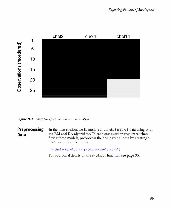
Exploring Patterns of Missingness
Figure 9.1: Image plot of the cholesterol.miss object.
25
20
15
10
5
1
Obs
erva
tions
(re
orde
red)
chol2 chol4 chol14
Preprocessing Data
In the next section, we fit models to the cholesterol data using both the EM and DA algorithms. To save computation resources when fitting these models, preprocess the cholesterol data by creating a preGauss object as follows:
> cholesterol.s <- preGauss(cholesterol)
For additional details on the preGauss function, see page 35.
99

Chapter 9 Example 1: The Gaussian Model
MODEL FITTING
Fitting a Model Using EM
To fit a Gaussian model to the cholesterol data using the EM algorithm, type:
> cholesterol.EM <- mdGauss(cholesterol.s, prior = "ml", + na.proc = "em")
Iterations of EM:Iteration ParChange 1 2.2853 2 0.3018 3 0.1211 4 0.0523 5 0.0233 6 0.0105 7 0.0048 8 0.0022 9 0.0010 10 0.0005
Note that the cholesterol.s object defined in the section Preprocessing Data on page 99 is used here to save computation resources. No prior is specified, and maximum likelihood estimates are therefore produced. Since no starting values are given, the default starting values are the mean and diagonal matrix of variances for the data set of completely observed cases.
The EM algorithm converges by the tenth iteration. The maximum relative change in parameter values and likelihood values is listed above by iteration number in the ParChange column.
The mdGauss function is a wrapper in which you specify the desired algorithm through the na.proc argument. Alternatively, you can call emGauss directly to produce the same model:
> cholesterol.EM <- emGauss(cholesterol.s, prior = "ml")
The paramIter component of the cholesterol.EM object is a matrix in which the rows are the parameter iterates for each iteration. The paramIter matrix is an object of class "Gauss", which enables S+MISSINGDATA to adapt to and format accordingly the different structures of the parameter estimates.
100

Model Fitting
> cholesterol.EM$paramIter
========== iteration = 9 ================Mean chol2 chol4 chol14 253.9286 230.6429 222.2284 Covariance chol2 chol4 chol14 chol2 2194.995 1454.617 835.233 chol4 1454.617 2127.158 1514.498chol14 835.233 1514.498 1950.798========== iteration = 10 ================Mean chol2 chol4 chol14 253.9286 230.6429 222.2329 Covariance chol2 chol4 chol14 chol2 2194.9949 1454.617 835.3333 chol4 1454.6173 2127.158 1515.0270chol14 835.3333 1515.027 1951.5629==========================================
By default, only the last two iterates are saved for the EM algorithm. This can be modified through the argument last to emGauss.control. For example, to save the last four iterates, add the following to the argument list in the original call to emGauss:
control = emGauss.control(last= 4)
The algorithm component of cholesterol.EM is an object of class "em":
> cholesterol.EM$algorithm
final log-likelihood = -307.9951 difference in the log-likelihood (or log posterior density)
= 5.1745e-06 maximum absolute relative change in parameter estimate on
last iteration = 0.0004649684
101

Chapter 9 Example 1: The Gaussian Model
The rate of convergence for the EM algorithm is governed by the fraction of missing information. You can use the worstFraction function with the cholesterol.EM object to compute the worst fraction of missing information and its corresponding eigenvector. See Fraley (1999) for details on the algorithms implemented in worstFraction.
> worstFraction(cholesterol.EM)
$direction:Mean chol2 chol4 chol14 0 0 -0.3081905 Covariance chol2 chol4 chol14 chol2 0 0 0.0000000 chol4 0 0 0.0000000chol14 0 0 0.9050186========================================== $fraction:[1] 0.4265396
Since there are no missing values in either chol2 and chol4, the parameters corresponding to these variables converge in a single step and the fractions of missing information are zero.
To compute the worst fraction of missing information using the power method, type:
> worstFraction(cholesterol.EM, method = "power")
$direction: chol2 chol4 chol14 chol2.chol2 chol2.chol4 chol4.chol4 0 0 -0.4331057 0 0 0
chol2.chol14 chol4.chol14 chol14.chol14 0.002251207 0.90134 0.0007351246
$fraction:[1] 0.4657516
For details on the power argument, see the online help file for worstFraction.Gauss.
102

Model Fitting
Before we calculate the three parameters of interest for the cholesterol study, recall that they are stored in the paramIter component of cholesterol.EM, which is a matrix that contains one row for each iteration. Therefore, each set of parameter estimates is a vector. For a Gaussian model, the most natural form for the parameter estimates is a mean vector and a variance-covariance matrix. To obtain this, set the argument expand=TRUE in the paramIter function as follows:
> cholesterol.EM.ex <- paramIter(cholesterol.EM, + expand = T)
Finally, calculate the parameters of interest with the commands below.
• Mean cholesterol level on day 14:
> cholesterol.EM.ex$mu[3] chol14 222.2329
• Average decrease in cholesterol level from day 2 to day 14:
> dec.2to14 <- cholesterol.EM.ex$mu[1] - + cholesterol.EM.ex$mu[3]> dec.2to14 chol2 31.69567
• Percentage decrease in cholesterol level from day 2 to day 14:
> 100*dec.2to14/cholesterol.EM.ex$mu[1] chol2 12.48212
These estimates are summarized in Table 9.2 on page 120, along with those obtained using data augmentation and multiple imputation.
Fitting a Model Using DA
It is also possible to estimate the three parameters of interest in the cholesterol study via parameter simulation. To accomplish this, it is generally a good idea to start a DA algorithm near the center of the posterior obtained from running an EM algorithm. See the section Using the EM and DA Algorithms in Conjunction on page 25 for additional details.
103

Chapter 9 Example 1: The Gaussian Model
The following command starts from the maximum likelihood estimate computed in the previous section by the EM algorithm. It runs a single chain for 1100 iterations, and then discards the first 100:
> cholesterol.DA <- daGauss(cholesterol.EM, prior = "non", + control = list(save=101:1100))
The paramIter component of the cholesterol.DA object is similar to the one for the cholesterol.EM object, except that more iterates may be saved (as specified by the save argument to daGauss.control). The default is to save about one tenth of the total iterations.
The algorithm component of cholesterol.DA prints as follows:
> cholesterol.DA$algorithm
seed = 13 46 10 7 30 0 6 9 59 60 1 1parameter estimates saved for iterations: 101:1100
104

Assessing Convergence
ASSESSING CONVERGENCE
Autocorrelation Plots
As discussed in the section Practical Considerations for Missing Data Problems on page 60, it may suffice to look at the following to assess convergence of the EM and DA model fitting algorithms:
1. Time series plots for each parameter (parameter iterates versus iteration number);
2. An autocorrelation plot for each parameter;
3. An autocorrelation plot of the worst linear function .
We begin with the plot method for the missmodel class of objects. This method is not typically useful if the EM algorithm has been used. However, it can help diagnose convergence in the case of data augmentation.
By default, the plot method produces time series plots of all variables. In the cholesterol example, there are nine parameters; since there are no missing data in the first two variables, however, the five parameters associated with those variables are not worth monitoring. Instead, set the argument select=T and choose the mean and variance of the third variable:
> plot(cholesterol.DA, select = T)
Figure 9.2 shows the resulting time series.
105

Chapter 9 Example 1: The Gaussian Model
Figure 9.2: Time series plots for parameters that are related to cholesterol measurements on day 14, the only variable in cholesterol with missing values.
Iteration Number
chol
14
200 600 1000
190
210
230
250
Iteration Number
chol
14.c
hol1
4
200 600 1000
2030
4050
60
Next, plot the autocorrelation function for the same parameters.
> daAcfPlot(cholesterol.DA, select = T)
In addition, it is also reasonable to think that parameters of the linear regression of chol14 on both chol2 and chol4 may also have high fractions of missing information. See Figure 9.3 for the ACF plots of all of these parameters.
106

Assessing Convergence
The ACF plots for the parameters of the linear regression are generated by writing several functions. For the intercept, define the following function:
fun30.12 <- function(x) x$mu[3] - x$sigma[3,1:2] %*% solve(x$sigma[1:2,1:2]) %*%
x$mu[1:2]
For the slopes, define the next two functions:
fun31.12 <- function(x)(x$sigma[3,1:2] %*% solve(x$sigma[1:2,1:2]))[1]
fun32.12 <- function(x)(x$sigma[3,1:2] %*% solve(x$sigma[1:2,1:2]))[2]
Finally, define the following for the residual standard deviation:
fun33.12 <- function(x)x$sigma[3,3] - x$sigma[3,1:2] %*%
solve(x$sigma[1:2,1:2]) %*% x$sigma[1:2,3]
As we mention in the section Fitting a Model Using EM on page 100, you can use the paramIter function to obtain the parameters as a list of mean vectors and variance-covariance matrices:
> cholesterol.DA.exp <- paramIter(cholesterol.DA, 1:1000, + expand = T)
We use the cholesterol.DA.exp object to product the ACF plots in Figure 9.3. An example of the code needed to produce the plot for the intercept is:
# ACF plot for intercept.> acf.int <- acf(sapply(cholesterol.DA.exp, fun30.12),+ lag.max = 100, plot= F) > acf.int$series <- "Intercept"> acf.plot(acf.int)
107
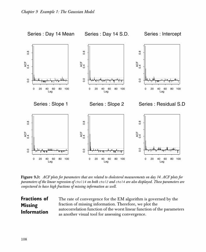
Chapter 9 Example 1: The Gaussian Model
Figure 9.3: ACF plots for parameters that are related to cholesterol measurements on day 14. ACF plots for parameters of the linear regression of chol14 on both chol2 and chol4 are also displayed. These parameters are conjectured to have high fractions of missing information as well.
Lag
AC
F
0 20 40 60 80 100
0.0
0.4
0.8
Series : Day 14 Mean
Lag
AC
F
0 20 40 60 80 100
0.0
0.4
0.8
Series : Day 14 S.D.
Lag
AC
F
0 20 40 60 80 100
0.0
0.4
0.8
Series : Intercept
Lag
AC
F
0 20 40 60 80 100
0.0
0.4
0.8
Series : Slope 1
Lag
AC
F
0 20 40 60 80 100
0.0
0.4
0.8
Series : Slope 2
Lag
AC
F
0 20 40 60 80 100
0.0
0.4
0.8
Series : Residual S.D
Fractions of Missing Information
The rate of convergence for the EM algorithm is governed by the fraction of missing information. Therefore, we plot the autocorrelation function of the worst linear function of the parameters as another visual tool for assessing convergence.
108
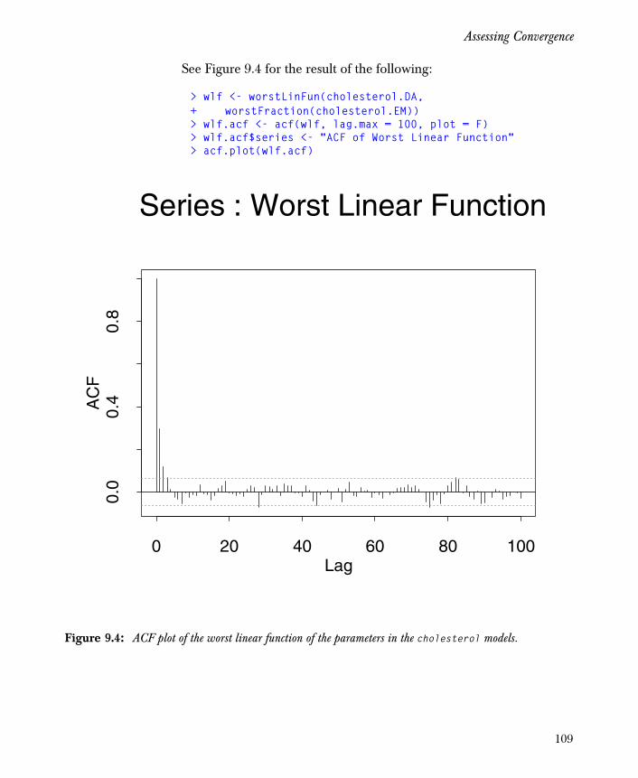
Assessing Convergence
See Figure 9.4 for the result of the following:
> wlf <- worstLinFun(cholesterol.DA, + worstFraction(cholesterol.EM))> wlf.acf <- acf(wlf, lag.max = 100, plot = F)> wlf.acf$series <- "ACF of Worst Linear Function"> acf.plot(wlf.acf)
Figure 9.4: ACF plot of the worst linear function of the parameters in the cholesterol models.
Lag
AC
F
0 20 40 60 80 100
0.0
0.4
0.8
Series : Worst Linear Function
109

Chapter 9 Example 1: The Gaussian Model
Conclusions In summary, the times series plots of this section show no unusual features. Similarly, the ACF plots indicate rapid convergence and negligible correlations by lag 20. Based on this evidence, it seems safe to conclude that the DA algorithm achieves stationarity by 20 iterations. To be safe, discard the first 100 observations:
> cholesterol.DA$paramIter <- + cholesterol.DA$paramIter[-c(1:100),]
110
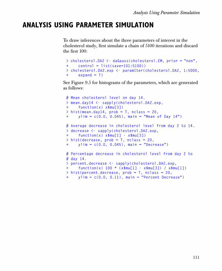
Analysis Using Parameter Simulation
ANALYSIS USING PARAMETER SIMULATION
To draw inferences about the three parameters of interest in the cholesterol study, first simulate a chain of 5100 iterations and discard the first 100:
> cholesterol.DA2 <- daGauss(cholesterol.EM, prior = "non", + control = list(save=101:5100))> cholesterol.DA2.exp <- paramIter(cholesterol.DA2, 1:5000,+ expand = T)
See Figure 9.5 for histograms of the parameters, which are generated as follows:
# Mean cholesterol level on day 14.> mean.day14 <- sapply(cholesterol.DA2.exp, + function(x) x$mu[3])> hist(mean.day14, prob = T, nclass = 20, + ylim = c(0.0, 0.045), main = "Mean of Day 14")
# Average decrease in cholesterol level from day 2 to 14.> decrease <- sapply(cholesterol.DA2.exp,+ function(x) x$mu[1] - x$mu[3])> hist(decrease, prob = T, nclass = 20, + ylim = c(0.0, 0.045), main = "Decrease")
# Percentage decrease in cholesterol level from day 2 to # day 14.> percent.decrease <- sapply(cholesterol.DA2.exp,+ function(x) 100 * (x$mu[1] - x$mu[3]) / x$mu[1])> hist(percent.decrease, prob = T, nclass = 20, + ylim = c(0.0, 0.11), main = "Percent Decrease")
111
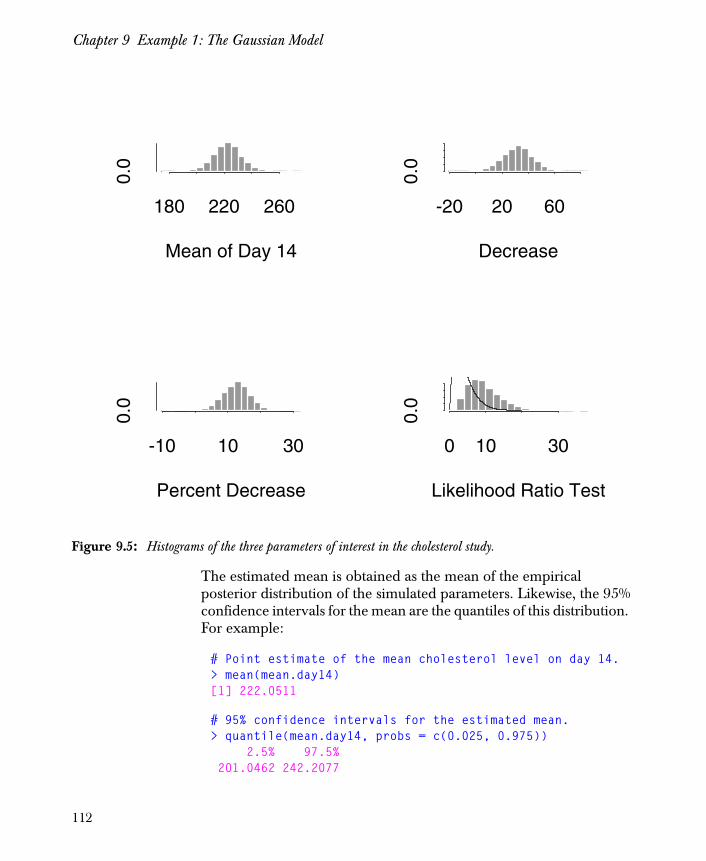
Chapter 9 Example 1: The Gaussian Model
Figure 9.5: Histograms of the three parameters of interest in the cholesterol study.
180 220 260
0.0
Mean of Day 14
-20 20 60
0.0
Decrease
-10 10 30
0.0
Percent Decrease
0 10 30
0.0
Likelihood Ratio Test
The estimated mean is obtained as the mean of the empirical posterior distribution of the simulated parameters. Likewise, the 95% confidence intervals for the mean are the quantiles of this distribution. For example:
# Point estimate of the mean cholesterol level on day 14.> mean(mean.day14)[1] 222.0511
# 95% confidence intervals for the estimated mean.> quantile(mean.day14, probs = c(0.025, 0.975)) 2.5% 97.5% 201.0462 242.2077
112

Analysis Using Parameter Simulation
The estimates and confidence intervals are summarized below in Table 9.1. See Table 9.2 on page 120 to compare these results with those obtained using EM and multiple imputation. Table 9.1: Estimates and confidence intervals given by parameter simulation.
Parameter Estimate Lower Confidence Bound
Upper Confidence Bound
mean 222.05 201.05 242.21
difference 31.87 9.01 54.23
percent decrease
12.48 3.78 20.55
113
Chapter 9 Example 1: The Gaussian Model
GENERATING MULTIPLE IMPUTATIONS THROUGH DA
Data augmentation algorithms can be used to generate multiple imputations. You may produce multiple imputations either by saving imputations from fixed intervals of one long chain or by saving the final imputations of several parallel chains. Gelman and Rubin (1992) recommend starting parallel chains with the initial values from a distribution that is overdispersed relative to the observed data posterior P θ Yobs[ ] . In practice, Schafer (1997) recommends using
the bootstrap, where the bootstrap sample sizes n* are smaller than
the original sample size n (n* n 2⁄= , for example).
The starting values to the impGauss function can be either a Gauss object or a list. The following illustrates using the bootstrap to create a Gauss object:
> start <- matrix(0, 5, 9)> for (i in 1:5)+ start[i,] <- paramIter(emGauss(cholesterol, + subset = sample(1:28, 14, T), prior = "ml"))[1,]> class(start) <- "Gauss"
Alternatively, create a list as follows:
> start <- list()> for (i in 1:5)+ start[[i]] <- paramIter(emGauss(cholesterol, + subset = sample(1:28, 14, T), prior = "ml"))
The diagnostics in the section Assessing Convergence on page 105 indicate that the chain converges to stationarity after 20 iterations. However, computations are inexpensive with this small data set, so we run fifty iterations. In the unlikely event that stationarity is not achieved in fifty iterations, the overdispersed starting values help to reach conservative inferences.
For example, generate five imputations from five parallel chains using the five starting values as follows:
> cholesterol.imp <- impGauss(cholesterol, prior = "non",+ start = start, control = list(niter=50))
114

Generating Multiple Imputations Through DA
To perform inference in this situation, we apply Rubin’s rule for inference using a normal approximation. Schafer (1997, page 196) derives the complete data point estimates and standard errors for each quantity given in the section The Cholesterol Data on page 94. The following is a function that calculate these estimates:
cholesterol.estimates <- function(x) {tmp <- x[,3]mu3 <- mean(tmp)tmp <- x[,1] - x[,3]delta13 <- mean(tmp)tmp <- tmp/mean(x[,1])tau13 <- 100*mean(tmp)c(mean.day14 = mu3, decrease = delta13,
percent.decrease=tau13)}
Next is a function that calculates the standard errors:
cholesterol.se <- function(x) {tmp <- x[,3]mu3 <- mean(tmp)sigma.mu3 <- sqrt(var(tmp)/28)sigma3 <- var(tmp)tmp <- x[,1] - x[,3]delta13 <- mean(tmp)sigma.delta13 <- sqrt(var(tmp)/28)tmp <- tmp/mean(x[,1])tau13 <- 100*mean(tmp)tmp <- x[,1]mu1 <- mean(tmp)sigma1 <- var(tmp)sigma13 <- var(tmp, x[,3])sigma.tau13 <- sqrt((100^2/28)*((mu3^2/mu1^4)*sigma1 -
2*(mu3/mu1^3)*sigma13+(1/mu1^2)*sigma3))c(sigma.mean.day14 = sigma.mu3,
sigma.decrease = sigma.delta13, sigma.percent.decrease = sigma.tau13)
}
You calculate these quantities for each of the completed data sets with the following:
> m.cholesterol.estimates <- + miEval(cholesterol.estimates(cholesterol.imp))
> m.cholesterol.se <- + miEval(cholesterol.se(cholesterol.imp))
115
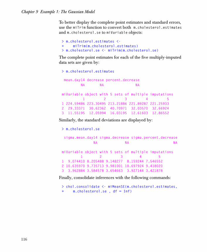
Chapter 9 Example 1: The Gaussian Model
To better display the complete point estimates and standard errors, use the miTrim function to convert both m.cholesterol.estimates and m.cholesterol.se to miVariable objects:
> m.cholesterol.estimates <- + miTrim(m.cholesterol.estimates)> m.cholesterol.se <- miTrim(m.cholesterol.se)
The complete point estimates for each of the five multiply-imputed data sets are given by:
> m.cholesterol.estimates
mean.day14 decrease percent.decrease NA NA NA
miVariable object with 5 sets of multiple imputations 1 2 3 4 5 1 224.59486 223.30495 213.21886 221.89287 221.259332 29.33371 30.62362 40.70971 32.03570 32.669243 11.55195 12.05994 16.03195 12.61603 12.86552
Similarly, the standard deviations are displayed by:
> m.cholesterol.se
sigma.mean.day14 sigma.decrease sigma.percent.decrease NA NA NA
miVariable object with 5 sets of multiple imputations 1 2 3 4 5 1 9.074410 8.205488 9.148277 8.159244 7.5465522 10.635970 9.735713 9.981001 10.697924 9.4180203 3.962884 3.584578 3.654663 3.927144 3.421878
Finally, consolidate inferences with the following commands:
> chol.consolidate <- miMeanSE(m.cholesterol.estimates, + m.cholesterol.se , df = Inf)
116

Generating Multiple Imputations Through DA
> chol.consolidate
$est: mean.day14 decrease percent.decrease 219.9349 33.99365 13.38709
$std.err: sigma.mean.day14 sigma.decrease sigma.percent.decrease 8.950076 10.25067 3.782212
$df: sigma.mean.day14 sigma.decrease sigma.percent.decrease 150.7358 259.3694 199.8662
$m:[1] 5
$r: mean.day14 decrease percent.decrease 0.1946008 0.1417942 0.1647799
$fminf: mean.day14 decrease percent.decrease 0.1737904 0.1308616 0.1499327
Two diagnostics given in this output are:
• r, the relative increase in variance due to nonresponse, and
• fminf, the fraction of missing information.
Point estimates are obtained by accessing the est component of chol.consolidate:
> chol.consolidate$est
mean.day14 decrease percent.decrease 220.8542 33.0744 13.02508
117

Chapter 9 Example 1: The Gaussian Model
Confidence intervals are obtained using t-intervals as follows:
# Lower confidence bounds.> chol.consolidate$est -+ qt(0.975, chol.consolidate$df) * + chol.consolidate$std.err
mean.day14 decrease percent.decrease 201.3565 10.83281 4.711483
# Upper confidence bounds> chol.consolidate$est + + qt(0.975, chol.consolidate$df) * + chol.consolidate$std.err
mean.day14 decrease percent.decrease 240.3519 55.31598 21.33867
118

Omitting Cases with Missing Values
OMITTING CASES WITH MISSING VALUES
It is also interesting to calculate parameter estimates using only complete cases:
> cholesterol.omit <- mdGauss(cholesterol, + na.proc = "omit")
119

Chapter 9 Example 1: The Gaussian Model
SUMMARY
Table 9.2 shows the estimates and confidence intervals obtained for each of the methods for handling missing data. In each cell, the order of the methods is first EM, then DA, and finally multiple imputation. The Estimate column also shows estimates obtained after omitting cases with missing values. Table 9.2: Comparison of answers obtained using EM, DA, multiple imputation, and deleting cases with missing values.
Parameter Estimate Lower Confidence Bound
Upper Confidence Bound
mean 222.23
222.05
220.8542
221.47
NA
201.05
201.36
NA
242.21
240.35
decrease 31.70
31.87
33.07
38
NA
9.01
10.83
NA
54.23
55.32
percent decrease
12.48
12.48
13.03
14.65
NA
3.78
4.71
NA
20.55
21.34
Note that omitting cases with missing values leads to a drastically different estimate for the average decrease in cholesterol level from day 2 to day 14. Thus, there is at least circumstantial evidence that a complete case analysis is misleading. Figure 9.6 shows that the complete cases have a higher average cholesterol level than the incomplete cases, which helps to explain the difference.
120
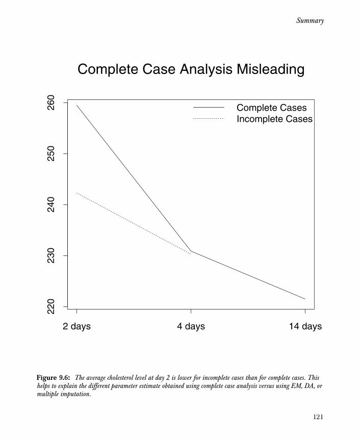
Summary
Figure 9.6: The average cholesterol level at day 2 is lower for incomplete cases than for complete cases. This helps to explain the different parameter estimate obtained using complete case analysis versus using EM, DA, or multiple imputation.
Complete Case Analysis Misleading
2 days 4 days 14 days
220
230
240
250
260
Complete CasesIncomplete Cases
121

Chapter 9 Example 1: The Gaussian Model
122

EXAMPLE 2: THE LOGLINEAR MODEL 10
Overview 124The Crime Data 124
Exploring Patterns of Missingness 126Summarizing and Plotting 126Preprocessing Data 128
Model Fitting 129Fitting a Model Using EM 129Fitting a Model Using DA 130
Assessing Convergence 133Autocorrelation Plots 133Fractions of Missing Information 135Conclusions 136
Generating Multiple Imputations Through DA 140
Analyzing Completed Data Sets 142Analysis Using Multiple Imputation 142
123

Chapter 10 Example 2: The Loglinear Model
OVERVIEW
This chapter provides detailed examples illustrating the loglinear model fitting process, in which all variables with missing values are categorical. Chapter 4 briefly describes both the saturated multinomial model and the loglinear model, as well as the functions in S+MISSINGDATA used to fit them. In this chapter, we illustrate the S+MISSINGDATA functions using the crime example from Schafer (1997). See Schafer’s book for details about this study and descriptions of the algorithms involved.
The Crime Data
Schafer (1997, page 45) illustrates the loglinear model using a data set that represents 641 housing occupants. The original data were obtained through the National Crime Survey conducted by the U.S. Bureau of the Census. Housing occupants were intially asked whether they had been victimized by crimes committed in the previous six months, and then six months later they were asked the same question. A total of 641 occupants responded on at least one of the two occasions.
The data from the crime study is included in S+MISSINGDATA as the built-in data set crime. It consists of two dichotomous variables, Visit.1 and Visit.2, each taking on the values Crime-free or Victim. A third variable provides the number of housing occupants corresponding to each of the combinations:
> crime
Visit.1 Visit.2 count 1 Crime-free Crime-free 392 2 Victim Crime-free 76 3 NA Crime-free 31 4 Crime-free Victim 55 5 Victim Victim 38 6 NA Victim 7 7 Crime-free NA 33 8 Victim NA 9 9 NA NA 115
For additional details, see the online help file for crime.
124

Overview
Note that this data set is in a grouped format. This saves space by representing the data as the unique combinations of values in Visit.1 and Visit.2 with the corresponding frequencies in the count column. Equivalently, the data can be represented in an ungrouped format with the following command. This requires 756 rows instead of 9:
> crime.df <- crime[rep(1:9, crime$count), 1:2]
The goal of the study is to determine whether victimization status in the second period is independent of victimization status in the first period. In this chapter, we explore this question in three ways:
1. Large sample approximation to the distribution of the likelihood ratio test under the null hypothesis of independence. Because of the missing data, an EM algorithm is used to calculate the maximum likelihood parameter estimates.
2. Parameter simulation.
3. Multiple imputation.
125

Chapter 10 Example 2: The Loglinear Model
EXPLORING PATTERNS OF MISSINGNESS
Summarizing and Plotting
In this section, we use the miss function and its associated methods to explore the crime data. As discussed in Chapter 3, the miss function is designed to facilitate exploratory data analysis for data sets that include missing values. Patterns in missing data are reasonably easy to discern for data in a grouped format, such as crime. This is especially true when the data set includes a limited number of factors. Nevertheless, we illustrate the miss function using the ungrouped data set crime.df.
The miss function creates an object of class "miss", which by default rearranges the rows and columns of the data according to the numbers and patterns of missing values. To create a miss object from the crime.df data, type:
> crime.miss <- miss(crime.df) > crime.miss
Summary of missing values 2 variables, 756 observations, 4 patterns of missing
values 2 variables (100%) have at least one missing value 195 observations ( 26%) have at least one missing valueFor more detailed information use summary(x)
The output indicates that both variables in crime.df have missing values. Note that omitting cases with missing values would throw out 26% of the observations.
Use summary for more detailed information. Here is the annotated output from summary for the crime.miss object:
> summary(crime.miss)
Summary of missing values 2 variables, 756 observations, 4 patterns of missing
values 2 variables (100%) have at least one missing value 195 observations ( 26%) have at least one missing value
126

Exploring Patterns of Missingness
Breakdown by variable V O name Missing % missing 1 1 Visit.1 153 20 2 2 Visit.2 157 21V = Variable number used below, O = Original number (before
sorting)
The two variables in crime.df are sorted by the number of missing values. The Visit.1 variable has 153 missing values while Visit.2 has 157. Thus, the first row in the output corresponds to Visit.1. It is the first variable after reordering and is also the first variable in the original data set, and so a 1 appears in both the V and O columns of the summary. Likewise, the second row corresponds to Visit.2, which is the second variable both before and after the reordering.
Of the 756 rows in the original crime.df data, there are four distinct patterns of missing values. These are shown in the next section of the output from the summary function:
Patterns of missing values (variables in columns, patternsin rows)
Pattern Variables 12 1 .. 2 .m 3 m. 4 mm
Observed values are displayed with a period and missing values with an m. The output indicates that the first pattern has no missing values while the second pattern has missing values only in the first variable. As we previously noted, the first variable after reordering is Visit.1. Likewise, the third pattern detected has missing values only in the second variable (Visit.2), and the fourth pattern has missing values in both variables.
Each pattern detected by the miss function corresponds to one or more rows in the original data set. The correspondence between rows and patterns is shown in the next section of output from summary:
Pattern #missing #Obs Observations 1 0 561 1:468 500:592 2 1 42 600:641 3 1 38 469:499 593:599 4 2 115 642:756
127

Chapter 10 Example 2: The Loglinear Model
The observations are contiguous because crime.df is created by stacking patterns in crime.
Preprocessing Data
In the next section, we fit models to the crime data using both the EM and DA algorithms. To save computation resources when fitting these models, preprocess the crime data by creating a preLoglin object as follows:
> crime.s <- preLoglin(crime, + margins = count~Visit.1:Visit.2)
The margins argument identifies the variables so that count is recognized as the response in this call to preLoglin. For additional details, see page 35 and the online help file for preLoglin.
128

Model Fitting
MODEL FITTING
Fitting a Model Using EM
To perform the likelihood ratio test of independence, the likelihood must be maximized twice: once for the saturated model and once under the null hypothesis of independence. Since there are missing values in the crime data set, an EM algorithm is used to maximize the likelihoods. The maximum likelihood estimates (MLEs) under independence are obtained as follows:
> crime.EM.ind <- mdLoglin(crime.s, + margins = ~Visit.1+Visit.2, na.proc = "em", prior = 1)
Iterations of ECM: 1...2.498457, -589.665968278183 2...0.6356901, -575.88481965762 3...0.1355902, -575.224397116118 4...0.02803836, -575.195583085395 5...0.005763061, -575.194355312622 6...0.00118325, -575.194303240237
Note that the crime.s object defined in the section Preprocessing Data on page 128 is used here to save computation resources. The margins argument specifies the independence model. Since no starting values are given, the default values are taken from the uniform table; in this example, each of the four probabilities is equal to 0.25.
The EM algorithm converges by the sixth iteration. The iterations are listed above under the Iterations of ECM heading. The abbreviation ECM stands for “Expectation Conditional Maximization,” which is a type of EM algorithm. See Meng and Rubin (1992) for details.
The mdLoglin function is a wrapper in which you specify the algorithm through the na.proc argument. Alternatively, you can call emLoglin directly to produce the same model:
> crime.EM.ind <- emLoglin(crime.s, + margins = ~Visit.1+Visit.2, prior = 1)
129

Chapter 10 Example 2: The Loglinear Model
Similarly, the MLEs for the saturated model are obtained with either of the following:
> crime.EM.sat <- mdLoglin(crime.s, + margins = ~Visit.1:Visit.2, na.proc = "em", prior = 1)
> crime.EM.sat <- emLoglin(crime.s, + margins = ~Visit.1:Visit.2, prior = 1)
A hierarchical model is assumed, so the formula ~Visit.1:Visit.2 is equivalent to ~Visit.1*Visit.2 in the margins argument.
Asymptotic analysis
The following command calculates the likelihood ratio test statistic for testing independence:
> like.ratio.test <- 2*(+ crime.EM.sat$algorithm$likelihood - + crime.EM.ind$algorithm$likelihood)
The asymptotic p -value is given by:
> 1 - pchisq(like.ratio.test, 1) [1] 4.70321e-07
There is thus strong evidence that victimization status on the two occasions is related.
Fitting a Model Using DA
It is also possible to explore via parameter simulation whether victimization status on the two visits is related; see Schafer (1997, page 252). To accomplish this, it is generally a good idea to start a DA algorithm near the center of the posterior obtained from running an EM algorithm. See the section Using the EM and DA Algorithms in Conjunction on page 25 for additional details.
The following command fits a saturated model using EM under a noninformative prior:
> crime.EM <- mdLoglin(crime.s, + margins = ~Visit.1:Visit.2, + na.proc = "em", prior = "n")
Note that prior="n" is equivalent to prior="noninformative" since partial matching is used. Also equivalent is prior=0.5.
130

Model Fitting
Next, start from crime.EM and run the DA algorithm for 5100 iterations, saving all of them:
> crime.DA <- mdLoglin(crime.EM, na.proc = "da", + control = list(save=1:5100))
The paramIter component of the crime.EM object is a matrix in which the rows are the parameter iterates for each iteration. The paramIter matrix is an object of class "Loglin", which enables S+MISSINGDATA to adapt to and format accordingly the different structures of the parameter estimates.
> crime.EM$paramIter
Visit.1=1;Visit.2=1 Visit.1=2;Visit.2=1 5 0.6969570 0.13584276 0.6970886 0.1357966
Visit.1=1;Visit.2=2 Visit.1=2;Visit.2=2 5 0.09872477 0.068475496 0.09865219 0.06846263
By default, only the last two iterates are saved for the EM algorithm. This can be modified through the argument last to emLoglin.control.
The paramIter component of the crime.DA object is similar to the one for crime.EM, except that more iterates may be saved (as specified by the save argument to daLoglin.control). Here are the first 10 rows:
> crime.DA$paramIter[1:10,]
Visit.1=1;Visit.2=1 Visit.1=2;Visit.2=1 1 0.6745408 0.1479869 2 0.6784437 0.1372391 3 0.6967126 0.1552910 4 0.6997548 0.1312311 5 0.6952653 0.1364643 6 0.6921411 0.1398454 7 0.6676453 0.1529987 8 0.6944598 0.1230416 9 0.6508019 0.156029110 0.6968313 0.1309274
131

Chapter 10 Example 2: The Loglinear Model
Visit.1=1;Visit.2=2 Visit.1=2;Visit.2=2 1 0.08282638 0.09464592 2 0.10567274 0.07864449 3 0.07906126 0.06893515 4 0.10795915 0.06105492 5 0.09763649 0.07063395 6 0.11058398 0.05742950 7 0.11219294 0.06716300 8 0.11210834 0.07039024 9 0.12209065 0.0710782810 0.08831767 0.08392358
The algorithm component of crime.EM is an object of class "em":
> crime.EM$algorithm
final likelihood = -558.8221 difference in the log-likelihood (or log posterior density) = 4.540166e-05 maximum absolute relative change in parameter estimate on last iteration = 0.0007472389
Likewise, the algorithm component of crime.DA is an object of class "da":
> crime.DA$algorithm
seed = 21 14 49 32 43 1 32 22 36 23 28 3parameter estimates saved for iterations: 1:5100
132

Assessing Convergence
ASSESSING CONVERGENCE
Autocorrelation Plots
As discussed in the section Practical Considerations for Missing Data Problems on page 60, it may suffice to look at the following to assess convergence of the EM and DA model fitting algorithms:
1. Time series plots for each parameter (parameter iterates versus iteration number);
2. An autocorrelation plot for each parameter;
3. An autocorrelation plot of the worst linear function.
We begin with the plot method for a missmodel class of objects. This method is not typically useful if the EM algorithm has been used. However, it can help diagnose convergence in the case of data augmentation.
By default, this plot method produces the time series plots of all variables:
> plot(crime.DA)
By setting the argument select=T, you may select specific variables to plot.
Next, plot the autocorrelation function for each parameter:
> daAcfPlot(crime.DA)
Again, by setting the argument select=T, you may produce autocorrelation plots only for selected variables. Figure 10.1 shows the time series and autocorrelation plots for each parameter.
133

Chapter 10 Example 2: The Loglinear Model
Figure 10.1: Plots for the parameters in the crime model. The top row, produced by the plot method for missmodel objects, is a set of time series plots of each parameter versus iteration number. The bottom row, produced by the daAcfPlot function, is a set of ACF plots of each parameter. These suggest that convergence is reached quickly.
Iteration Number
Vis
it.1=
1;V
isit.
2=1
0 2000 5000
0.62
0.66
0.70
0.74
Iteration Number
Vis
it.1=
2;V
isit.
2=1
0 2000 5000
0.10
0.14
0.18
Iteration Number
Vis
it.1=
1;V
isit.
2=2
0 2000 5000
0.08
0.12
Iteration Number
Vis
it.1=
2;V
isit.
2=2
0 2000 5000
0.04
0.06
0.08
0.10
Visit.1=1;Visit.2=1
lag
AC
F
0 40 80
0.0
0.2
0.4
0.6
0.8
1.0
Visit.1=2;Visit.2=1
lag
AC
F
0 40 80
0.0
0.2
0.4
0.6
0.8
1.0
Visit.1=1;Visit.2=2
lag
AC
F
0 40 80
0.0
0.2
0.4
0.6
0.8
1.0
Visit.1=2;Visit.2=2
lag
AC
F
0 40 800.
00.
20.
40.
60.
81.
0
134

Assessing Convergence
Fractions of Missing Information
The rate of convergence for the EM algorithm is governed by the fraction of missing information. To aid in assessing convergence, we monitor a function with high rates of missing information, since convergence is slowest for this type of function. Schafer (1997, pages 129–131) recommends monitoring the worst linear function of θ . To do this, we first use the worstFraction function with the crime.EM object to compute the worst fraction of missing information and its corresponding eigenvector. See Fraley (1999) for details on the algorithms implemented in worstFraction.
> worst.est <- worstFraction(crime.EM, method = "power") > worst.est
$direction: [1] -0.4616784 0.4846614 0.5137191 -0.5367021 $fraction: [1] 0.2642576
Next, calculate the worst linear function of the parameters by combining worst.est with the crime.DA object:
> wlf <- worstLinFun(crime.DA, worst.est)
Finally, plot the autocorrelation function of wlf:
> wlf.acf <- acf(wlf, lag.max = 100, plot = F)> wlf.acf$series <- "Worst Linear Function"> acf.plot(wlf.acf)
135

Chapter 10 Example 2: The Loglinear Model
Figure 10.2: ACF plot of the worst linear function of the parameters in the crime models, with 95% confidence bounds. The correlations for lags 4 and beyond are not significantly different than 0.
Lag
AC
F
0 20 40 60 80 100
0.0
0.2
0.4
0.6
0.8
1.0
Series : Worst Linear Function
Conclusions In summary, all of the diagnostics in this section indicate fast convergence. Moreover, the EM algorithm converged in 6 steps. To be safe, discard the first 100 observations:
> crime.DA$paramIter <- crime.DA$paramIter[-c(1:100), ]
136

Assessing Convergence
In the parameter simulation approach, test independence by looking at the distribution of the odds ratios. See Figure 10.3 for the result of the following commands:
> crime.omega <- apply(crime.DA$paramIter, 1,+ function(x) x[1]*x[4]/(x[2]*x[3])) > hist(crime.omega)
Figure 10.3: Histogram of the simulated odds ratios. This distribution forms the basis of inference using parameter simulation.
2 4 6 8
020
060
010
00
crime.omega
137

Chapter 10 Example 2: The Loglinear Model
The fraction of simulated odds ratios less than 1 gives an approximate p -value for testing independence versus the alternative hypothesis that households victimized in the first period were more likely to be victimized in the second period:
> sum(crime.omega <= 1)/length(crime.omega) [1] 0
This agreement with the asymptotic result is not surprising if we look at the distribution of the likelihood ratio test statistic that compares the MLE with the simulated values. Asymptotically, the posterior distribution is chi-square with 3 degrees of freedom. See Figure 10.4
for the histogram with the χ32
distribution overlaid.
The simulated posterior mean is a point estimate of the odds ratio:
> mean(crime.omega) [1] 3.666283
This compares with the MLE of 3.566756 obtained using the estimates given in the section Fitting a Model Using EM on page 129 to calculate the odds ratio.
The 95% confidence intervals for the odds ratio are given by:
> quantile(crime.omega, probs = c(0.025, 0.975))
2.5% 97.5% 2.211379 5.692615
See table Table 10.1 on page 143 to compare these results with those obtained by other methods.
138

Assessing Convergence
Figure 10.4: Histogram of the likelihood ratio test statistic that compares the MLE with the simulated values.
Asymptotically, this observed data posterior distribution is χ32
. The agreement is good, suggesting good large
sample properties.
0 5 10 15 20
0.0
0.10
0.20
Likelihood Ratio Statistic
139

Chapter 10 Example 2: The Loglinear Model
GENERATING MULTIPLE IMPUTATIONS THROUGH DA
Data augmentation algorithms can be used to generate multiple imputations. For example, to generate ten imputations from one long chain under a saturated model of the crime data, type:
> crime.imp.1chain <- impLoglin(crime.s, nimpute = 10, + prior = "n", start = crime.EM$paramIter[2,], + control = list(niter=100)
Alternatively, type the following to generate 10 independent chains, each starting from the MLE:
> start.crime <- crime.EM$paramIter[rep(2,10), ] > crime.imp <- impLoglin(crime.s, prior = "n", + start = start.crime, control = list(niter=100))
The result of impLoglin is an miList object if the original data is in grouped format; otherwise it is an miVariable object. The case of grouped data is a (rare) situation when the imputed data object is most naturally represented as an miList:
> crime.imp
$I1: Visit.1 Visit.2 frequency1 "Crime-free" "Crime-free" "529"2 " Victim" "Crime-free" "100"3 "Crime-free" " Victim" " 71"4 " Victim" " Victim" " 56" $I2: Visit.1 Visit.2 frequency1 "Crime-free" "Crime-free" "525"2 " Victim" "Crime-free" " 96"3 "Crime-free" " Victim" " 76"4 " Victim" " Victim" " 59"...
140

Generating Multiple Imputations Through DA
$I10: Visit.1 Visit.2 frequency1 "Crime-free" "Crime-free" "517"2 " Victim" "Crime-free" "102"3 "Crime-free" " Victim" " 82"4 " Victim" " Victim" " 55" attr(, "call"):impLoglin.preLoglin(object = crime.s, prior = "n", start = start.crime, control = list(niter = 100))attr(, "seed"): [1] 33 2 58 26 51 3 47 25 42 12 28 1
141

Chapter 10 Example 2: The Loglinear Model
ANALYZING COMPLETED DATA SETS
The miApply function can be used to calculate contingency tables for each of the ten completed data sets as follows:
> crime.col2 <- miApply(crime.imp, function(data, formula) + oldUnclass(crosstabs(formula, data)), + frequency ~ Visit.1+Visit.2)
Instead, you can use miEval as follows:
> crime.col <- miEval(oldUnclass(crosstabs(+ frequency ~ Visit.1+Visit.2, data = crime.imp)), + vnames = "crime.imp")
Note
Any calculation on the result of crosstabs is another object of class "crosstabs", so that the elements of the calculation must be integers. In particular, the odds ratio calculation fails, which is why we must oldUnclass above.
Analysis Using Multiple Imputation
Several functions combine the separate complete data analyses to produce one result that accounts for missing data uncertainty. For the crime example, we test independence by:
• Combining odds ratios. Asymptotically, the log odds ratios are normally distributed. Following rules given by Rubin (1987), the multiple imputation inference is based on a t distribution.
• Combining likelihood ratio tests.
With complete data, the log odds ratio ωlog is asymptotically
normal with mean ωlog and a variance estimated by
1x11------- 1
x12------- 1
x21------- 1
x22-------+ + + ,
where xij is the count for which Visit.1=i and Visit.2=j. See Schafer (1997, section 6.4.2).
142
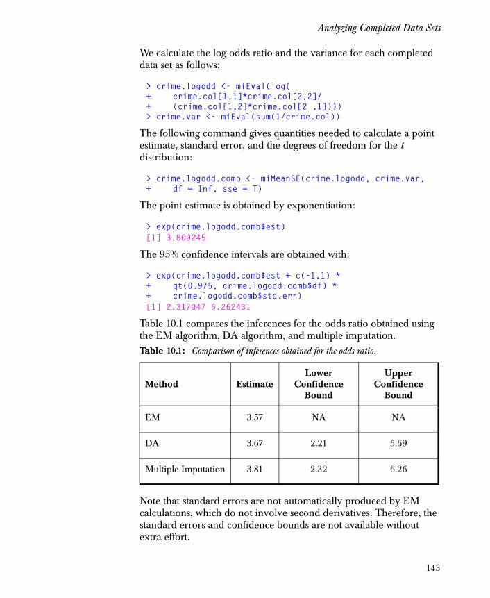
Analyzing Completed Data Sets
We calculate the log odds ratio and the variance for each completed data set as follows:
> crime.logodd <- miEval(log(+ crime.col[1,1]*crime.col[2,2]/+ (crime.col[1,2]*crime.col[2 ,1]))) > crime.var <- miEval(sum(1/crime.col))
The following command gives quantities needed to calculate a point estimate, standard error, and the degrees of freedom for the t distribution:
> crime.logodd.comb <- miMeanSE(crime.logodd, crime.var, + df = Inf, sse = T)
The point estimate is obtained by exponentiation:
> exp(crime.logodd.comb$est) [1] 3.809245
The 95% confidence intervals are obtained with:
> exp(crime.logodd.comb$est + c(-1,1) * + qt(0.975, crime.logodd.comb$df) * + crime.logodd.comb$std.err) [1] 2.317047 6.262431
Table 10.1 compares the inferences for the odds ratio obtained using the EM algorithm, DA algorithm, and multiple imputation. Table 10.1: Comparison of inferences obtained for the odds ratio.
Method EstimateLower
Confidence Bound
Upper Confidence
Bound
EM 3.57 NA NA
DA 3.67 2.21 5.69
Multiple Imputation 3.81 2.32 6.26
Note that standard errors are not automatically produced by EM calculations, which do not involve second derivatives. Therefore, the standard errors and confidence bounds are not available without extra effort.
143

Chapter 10 Example 2: The Loglinear Model
We can also test independence using the likelihood ratio test. The following simple function calculates the test:
likratio.Loglin <- function(data, marginsHa, marginsH0, prior) {
# "data" is a data frame and "frequency" is a column in # "data". This is the form of each component in the miList # object returned by impLoglin when the data is given in # grouped format
missmodel.Ha <- Loglin(data, frequency = frequency, margins = marginsHa, prior = prior)
missmodel.H0 <- Loglin(data, frequency = frequency, margins = marginsH0, prior = prior)
2*(logpost.Loglin(missmodel.Ha) -logpost.Loglin(missmodel.H0))
}
The miLikelihoodTest function uses likratio.Loglin, both to calculate the likelihood ratio test for each completed data set and to combine the tests; see Li et al. (1991).
> crime.lrt <- miLikelihoodTest(crime.imp, likratio.Loglin, 1, marginsHa = ~Visit.1:Visit.2, marginsH0 = ~Visit.1+Visit.2, prior = 0.5)
The p -value of the test for independence is:
> 1 - pf(crime.lrt$Fstat, crime.lrt$df1, crime.lrt$df2) [1] 1.891866e-08
This confirms the likelihood ratio test result obtained using the EM in Fitting a Model Using EM on page 129.
144

EXAMPLE 3: THE CONDITIONAL GAUSSIAN MODEL 11
Overview 146The Foreign Language Data 146
Exploring Patterns of Missingness 148Summarizing and Plotting 148Preprocessing Data 151
Model Fitting 152Specifying a Restricted Model 152Fitting a Model Using EM 153Fitting a Model Using DA 154
Assessing Convergence 156
Multiple Imputation 158
Analyzing Completed Data Sets 159
Consolidating Inferences 161
Conclusions 163
145

Chapter 11 Example 3: The Conditional Gaussian Model
OVERVIEW
This chapter provides detailed examples illustrating the conditional Gaussian model fitting process, in which the variables with missing values are either numeric or categorical. This model arises, for example, in analysis of covariance and logistic regression with continuous predictors. Chapter 4 briefly describes the conditional Gaussian model, the associated priors, and the functions in S+MISSINGDATA used to fit it. In this chapter, we illustrate the S+MISSINGDATA functions using the foreign language example from Schafer (1997). See Schafer (1997) for additional details and algorithm descriptions.
The Foreign Language Data
Schafer (1997) illustrates the conditional Gaussian model using a data set of 279 students enrolled in foreign language courses at the Pennsylvania State University. The original data are given in Raymond and Roberts (1983). For each student, twelve variables were collected, including age and sex. Variables measuring academic achievement in foreign languages were also collected. One such variable, GRD, is the final grade in the foreign language course. Two instruments, the new Foreign Language Attitude Scale (FLAS) and the established Modern Language Aptitude Test (MLAT), are designed to predict success in studying foreign languages. The students’ scores on these standardized tests were also collected and recorded.
The data from the foreign language study is included in S+MISSINGDATA as the built-in data set language. It consists of 12 variables, including GRD, FLAS, and MLAT:
> language
AGE PRI SEX FLAS MLAT SATV SATM ENG HGPA CGPA GRD 1 20-21 3 male 74 32 540 660 58 3.77 3.75 A 2 <20 2 male 69 28 610 760 75 2.18 3.81 A 3 20-21 0 female 81 28 610 560 61 3.19 3.73 A 4 <20 4+ female 89 13 430 470 33 2.21 3.54 B 5 <20 3 male 56 26 630 630 78 3.59 4.00 NA 6 20-21 3 female 95 22 440 580 48 3.25 3.20 A 7 NA NA male 71 NA NA NA NA 2.46 NA NA 8 <20 4+ female 95 NA 560 540 55 2.00 2.77 NA. . .
146

Overview
For additional details, see the help file for language.
The goal of the study is to address the following questions:
• Does the newly developed instrument, FLAS, help predict success in the study of foreign languages?
• How does FLAS compare with a well established instrument like MLAT?
As Schafer (1997) shows, you may use the Gaussian model after recoding some of the factor variables to make the normality assumption more reasonable. To avoid possible loss of information due to recoding, you may also use the conditional Gaussian model.
If there were no missing data, one way of answering the question would be to heuristically gauge the practical importance of the estimated effects by estimating partial correlations . In particular, how does the partial correlation of FLAS with GRD compare with that of MLAT? Since there are missing data, however, we show how to perform the analysis after first multiply imputing missing values under a conditional Gaussian model.
147

Chapter 11 Example 3: The Conditional Gaussian Model
EXPLORING PATTERNS OF MISSINGNESS
Summarizing and Plotting
In this section, we use the miss function and its associated methods to explore the language data. As discussed in Chapter 3, the miss function is designed to facilitate exploratory data analysis for data sets that include missing values. It creates an object of class "miss", which by default rearranges the rows and columns of the data according to the numbers and patterns of missing values.
To create a miss obect from the language data, type:
> language.miss <- miss(language)> language.miss
Summary of missing values 10 variables, 279 observations, 18 patterns of missing
values 10 variables (83%) have at least one missing value 105 observations ( 38%) have at least one missing valueFor more detailed information use summary(x)
Ten of the twelve variables have at least one missing value. Omitting cases with missing values would delete 38% of the observations.
Use summary for more detailed information. Here is the annotated output from summary for language.miss:
> summary(language.miss)
Summary of missing values 10 variables, 279 observations, 18 patterns of missing
values 10 variables (83%) have at least one missing value 105 observations ( 38%) have at least one missing value
Breakdown by variable V O name Missing % missing 1 9 HGPA 1 0 2 3 SEX 1 0 3 1 AGE 11 4 4 2 PRI 11 4 5 6 SATV 34 12 6 7 SATM 34 12 7 10 CGPA 34 12
148

Exploring Patterns of Missingness
8 8 ENG 37 13 9 11 GRD 47 17 10 5 MLAT 49 18V = Variable number used below, O = Original number (before
sorting)No missing values for variables:FLAS LAN
The twelve variables in language are sorted by the number of missing values; neither FLAS nor LAN have any missing values. The HGPA variable has the least number (1) of missing values. Thus, it is the first variable after reordering and a 1 appears in the V column of the summary. It is the ninth variable in the original data set, so that a 9 appears in the O column. Likewise, the MLAT variable has the most number (49) of missing values. It is the last variable after reordering and the fifth variable in the original data set. Thus, a 10 appears in the V column of the output and a 5 appears in the O column.
Of the 279 rows in the original language data, there are 18 distinct patterns of missing values. These are shown in the next section of the output from summary:
Patterns of missing values (variables in columns, patterns in rows)
Pattern Variables 1 1234567890 1 .......... 2 .........m 3 ........m. 4 .......m.. 5 ........mm 6 .......mm. 7 ..mm...... 8 .m......m. 9 ..mm.....m 10 ..mm....m. 11 ....mmmm.. 12 ..mm....mm 13 ....mmmm.m 14 ....mmmmm. 15 m...mmmm.. 16 ....mmmmmm 17 ..mmmmmm.. 18 ..mmmmmmmm
149
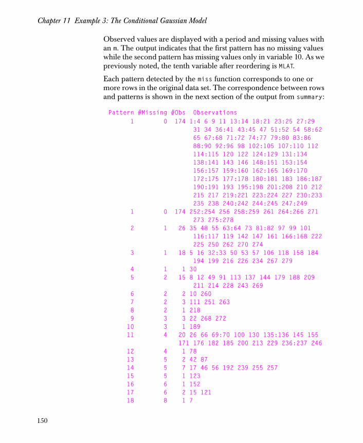
Chapter 11 Example 3: The Conditional Gaussian Model
Observed values are displayed with a period and missing values with an m. The output indicates that the first pattern has no missing values while the second pattern has missing values only in variable 10. As we previously noted, the tenth variable after reordering is MLAT.
Each pattern detected by the miss function corresponds to one or more rows in the original data set. The correspondence between rows and patterns is shown in the next section of the output from summary:
Pattern #Missing #Obs Observations 1 0 174 1:4 6 9 11 13:14 18:21 23:25 27:29 31 34 36:41 43:45 47 51:52 54 58:62 65 67:68 71:72 74:77 79:80 83:86 88:90 92:96 98 102:105 107:110 112 114:115 120 122 124:129 131:134 138:141 143 146 148:151 153:154 156:157 159:160 162:165 169:170 172:175 177:178 180:181 183 186:187 190:191 193 195:198 201:208 210 212 215 217 219:221 223:224 227 230:233 235 238 240:242 244:245 247:249 1 0 174 252:254 256 258:259 261 264:266 271 273 275:278 2 1 26 35 48 55 63:64 73 81:82 97 99 101 116:117 119 142 147 161 166:168 222 225 250 262 270 274 3 1 18 5 16 32:33 50 53 57 106 118 158 184 194 199 216 226 234 267 279 4 1 1 30 5 2 15 8 12 49 91 113 137 144 179 188 209 211 214 228 243 269 6 2 2 10 260 7 2 3 111 251 263 8 2 1 218 9 3 3 22 268 272 10 3 1 189 11 4 20 26 66 69:70 100 130 135:136 145 155 171 176 182 185 200 213 229 236:237 246 12 4 1 78 13 5 2 42 87 14 5 7 17 46 56 192 239 255 257 15 5 1 123 16 6 1 152 17 6 2 15 121 18 8 1 7
150

Exploring Patterns of Missingness
You can view an image plot of the language.miss object by using the plot.miss function. Figure 11.1 displays the plot created by the following command:
> plot(language.miss)
Figure 11.1: Image plot of the language.miss object.
250
200
150
100
50
1
Obs
erva
tions
(re
orde
red) F
LAS
LA
N
HG
PA
SE
X
AG
E
PR
I
SA
TV
SA
TM
CG
PA
EN
G
GR
D
MLA
TPreprocessing Data
In the next section, we fit models to the language data using both the EM and DA algorithms. To save computation resources during the model fitting process, preprocess the language data by creating a preCgm object as follows:
> language.s <- preCgm(language)
The arguments margins and gauss to preCgm identify the factor and numeric variables, respectively. Since language is a data frame and these arguments are not supplied in the above command, all factor variables are modeled by the loglinear part of the model and all numeric variables are modeled by the (conditional) Gaussian part. For additional details, see page 35 and the online help file for preCgm.
151

Chapter 11 Example 3: The Conditional Gaussian Model
MODEL FITTING
Specifying a Restricted Model
The categorical variables in the language data set, AGE, PRI, SEX, GRD, and LAN, have 5, 5, 2, 5, and 4 levels, respectively. Together, they specify a 5 dimensional contingency table with 5 5× 2× 5× 4× 1000= cells. In addition, there are 7 numeric variables in language. An unrestricted model therefore involves 1000 1–( ) 1000 7×( ) 7 7 1+( ) 2⁄×( )+ + 8027= free parameters.
Clearly, an unrestricted model cannot be fit with 279 observations!
Instead, Schafer (1997, page 367) suggests a restricted model in which:
• The table formed by the factor variables is described by a loglinear model with all main effects and two-variable associations.
• The numeric variables are collectively described by a regression with main effects for each factor variable. The eight-column design matrix for this regression includes an intercept, dummy indicators for SEX and LAN, and linear contrasts for AGE, PRI, and GRD.
To compute this restricted model, first specify the formula for a loglinear model with all main effects and two-variable associations:
> margins.form <- ~ LAN + AGE + PRI + SEX + GRD ++ LAN:AGE + LAN:PRI + LAN:SEX + LAN:GRD ++ AGE:PRI + AGE:SEX + AGE:GRD ++ PRI:SEX + PRI:GRD ++ SEX:GRD
Setting the following option ensures that any factor variable appearing in a formula is represented by dummy variables:
> options(contrasts = c("contr.treatment", "contr.poly"))
The linear contrast is specified by:
> lc <- c(-2,-1,0,1,2)
Finally, the formula that produces the appropriate design matrix is:
> design.form <- ~ LAN + SEX + C(AGE,lc,1) + C(PRI,lc,1) + + C(GRD,lc,1)
152

Model Fitting
Note that LAN and SEX are coded by dummy variables while the other factor variables are represented by linear contrasts.
Fitting a Model Using EM
The command below fits the restricted conditional Gaussian model to the language data using the EM algorithm. To ensure a mode in the interior of the parameter space, Schafer (1997, page 369) recommends setting the Dirichlet prior hyperparameter to 1.05:
> language.EM <- emCgm(language.s, margins = margins.form,+ design = design.form, prior = 1.05)
Steps of ECM: 1...2...3...4...5...6...7...8...9...10...11...12...13...14...15...16...17...18...19...20...21...22...23...24...25...26...27...28...29...30...31...32...33...34...35...36...37...38...39...40...41...42...43...44...45...46...47...48...49...50...51...52...53...54...55...56...57...58...59...60...61...62...63...64...65...66...
Note that the language.s object defined in the section Preprocessing Data on page 151 is used to save computation resources. As discussed by Schafer (1997, page 253), the 1.05 prior is an example of a flattening prior, which smooths estimates toward a uniform table. In this example, the equivalent of 0.05 prior observations is added to each cell. Since there are 1000 cells in the contingency table, this gives an effective prior sample size of 50, roughly 18% of the actual sample size.
The paramIter component of the language.EM object is a matrix in which the rows are the parameter iterates for each iteration. The paramIter matrix is an object of class "cgm", which enables S+MISSINGDATA to adapt to and format accordingly the different structures of the parameter estimates.
> language.EM$paramIter
========== iteration = 65 ================meansnumeric matrix: 7 rows, 1000 columns. AGE=1;PRI=1;SEX=1;GRD=1;LAN=1 FLAS 71.694619MLAT 17.126537SATV 467.402216SATM 529.032427
153

Chapter 11 Example 3: The Conditional Gaussian Model
ENG 43.504382HGPA 1.516468CGPA 2.530749
AGE=2;PRI=1;SEX=1;GRD=1;LAN=1 FLAS 70.311911MLAT 15.833215SATV 468.583594SATM 513.125791 ENG 41.335946HGPA 1.563725CGPA 2.417728. . .
The algorithm component of language.EM is an object of class "em":
> language.EM$algorithm
final log-likelihood = -6087.938
difference in the log-likelihood (or log posterior density) = 4.773301e-08
maximum absolute relative change in parameter estimate on last iteration = 0.0009985025
Fitting a Model Using DA
In this section, we use the DA model fitting algorithm on the language data. As discussed in Schafer (1997, page 369), a flattening prior may be undesirable for models of the language data because the AGE and GRD variables have rare levels. Flattening priors can distort the marginal distributions for these variables, leading to too many rare levels in the imputed values. Instead, Schafer recommends using a data dependent prior that smooths toward a table of mutual independence but leaves the marginal distributions unchanged. The hyperparameters are scaled so that they add to 50, giving the same effective prior sample size as used in the previous section for the EM algorithm.
Create such a data dependent prior as follows:
> dataDepend <- dataDepPrior(language.s, nPriorObs = 50,+ algorithm = "da")
154

Model Fitting
The following command starts from the maximum likelihood estimate computed by the EM algorithm and runs the DA algorithm for 1000 iterations, discarding the first 99:
> language.DA <- daCgm(language.EM, prior = dataDepend,+ control = list(niter=1000, save=100:1000))
155

Chapter 11 Example 3: The Conditional Gaussian Model
ASSESSING CONVERGENCE
Since there are 8028 parameters for the language data, it is unreasonable to monitor each of them individually with autocorrelation plots. Instead, we look at the worst linear function of the parameters. The rate of convergence for the EM algorithm is governed by the fraction of missing information. To aid in assessing convergence, we monitor a function with high rates of missing information, since convergence is slowest for this type of function. Schafer (1997, pages 129–131) recommends monitoring the worst linear function of θ .
Warning
When the posterior is non-normal, other functions may converge more slowly. Thus, do not blindly rely on the apparent stationarity of the worst linear function without enlisting other diagnostic techniques.
To compute the worst linear function, we first use the worstFraction function with the language.EM object to compute the worst fraction of missing information and its corresponding eigenvector. See Fraley (1999) for details on the algorithms implemented in worstFraction.
> worst.est <- worstFraction(language.EM, method = "power")> worst.est$fraction[1] 0.8278831
Next, calculate the worst linear function of the parameters by combining worst.est with the language.DA object:
> wlf <- worstLinFun(language.DA, worst.est)
Finally, calculate and plot the autocorrelation function of wlf:
> wlf.acf <- acf(wlf, lag.max = 250, plot = F)> wlf.acf$series <- "Worst Linear Function"> acf.plot(wlf.acf)
156

Assessing Convergence
Figure 11.2: ACF plot of the worst linear function of the parameters in the language models. The autocorrelations seem to die out by iteration 50.
Lag
AC
F
0 50 100 150 200 250
0.0
0.4
0.8
Series : Worst Linear Function
157

Chapter 11 Example 3: The Conditional Gaussian Model
MULTIPLE IMPUTATION
The ACF of the worst linear function in Figure 11.2 suggests convergence by 50 iterations. To be conservative, we save every 250th imputation. The following command generates ten imputations, starting from the last parameter values in the language.DA object:
> language.imp <- impCgm(language.DA, nimpute = 10, + control = list(niter=250))
To extract the second set of imputations, type:
> miSubscript(language.imp, 2)
158

Analyzing Completed Data Sets
ANALYZING COMPLETED DATA SETS
One way to asses the practical importance of the language variables in predicting GRD is to estimate partial correlations. In linear regression, a squared partial correlation measures the proportion of the variance in the response variable explained by a predictor, after accounting for the effects of the other predictors. We can use this fact to compare the partial correlations of the FLAS and MLAT variables with GRD.
A partial correlation r may be calculated from the t -statistic T used for testing the significance of a regression coefficient:
r T2
T2 ν+---------------±= ,
where the sign is chosen to be the sign of T . Moreover, r( )atan is
asymptotically Gaussian with a mean of ρ( )atan and variance
1 ν 1–( )⁄ . We use this fact in the next section to apply Rubin’s rule and consolidate inferences.
The first step in estimating partial correlations is to fit a linear model to each of the ten completed data sets for language:
> m.lm.fit <- miEval(lm(as.numeric(GRD) ~ LAN + + C(AGE, lc, 1) + C(PRI, lc, 1) + + SEX + FLAS + MLAT + SATV + SATM + ENG + HGPA + CGPA, + data = language.imp))mi objects: language.imp
To apply Rubin’s rule, we must calculate the estimate and its standard error for each completed data set. First, calculate the transformed partial correlation for each of the data sets:
> m.atanPartCorr <- miEval({+ tstat <- summary(m.lm.fit)$coef[,"t value"];+ partCorr <- sign(tstat)*sqrt((tstat*tstat)/+ ((tstat*tstat) + 267));+ atan(partCorr)+ })mi variables: tstat partCorr m.lm.fit
159

Chapter 11 Example 3: The Conditional Gaussian Model
The degrees of freedom for each t -statistic is equal to n p– :
> dim(language)[1] - dim(language)[2][1] 267
Therefore, the standard error is equal to
1υ 1–------------ 1
n p– 1–--------------------- 1
266---------= = .
The following commands create an impute object that represents this standard error for each of the ten completed data sets:
> se <- sqrt(1/266)> se.list <- vector("list", 10)> for(i in 1:10)+ se.list[[i]] <- rep(se,14)> m.se <- miList(se.list, paste("I", 1:10, sep=""))
160

Consolidating Inferences
CONSOLIDATING INFERENCES
The following command calculates the consolidated estimate of the transformed partial correlation:
> partCorr <- miMeanSE(m.atanPartCorr, m.se, df = Inf, + n = 279)
Transform back to get the point estimates for the correlations:
> tan(partCorr$est)
(Intercept) LAN2 LAN3 LAN4 C(AGE, lc, 1) -0.007382197 -0.08169879 0.05172681 -0.03863925 0.1044772 C(PRI, lc, 1) SEX FLAS MLAT SATV SATM 0.235524 0.03341574 0.2696982 0.1473144 -0.04067603 0.03491293 ENG HGPA CGPA-0.03602713 0.4290499 0.1888691
The estimated fractions of missing information are:
> partCorr$fminf
(Intercept) LAN2 LAN3 LAN4 C(AGE, lc, 1) 0.5309861 0.1211011 0.07448829 0.8683221 0.3792738 C(PRI, lc, 1) SEX FLAS MLAT SATV 0.1410323 0.2163655 0.3212395 0.4995211 0.2361616 SATM ENG HGPA CGPA0.2208094 0.404194 0.1395629 0.5229428
161

Chapter 11 Example 3: The Conditional Gaussian Model
The 95% confidence intervals using a t distribution are given as follows.
# Lower confidence bound.> tan(partCorr$est + qt(0.025, partCorr$df) * + partCorr$std.err)
(Intercept) LAN2 LAN3 LAN4 C(AGE, lc, 1) -0.1863897 -0.2128767 -0.07338188 -0.4002118 -0.0490225 C(PRI, lc, 1) SEX FLAS MLAT SATV SATM 0.1019368 -0.1028575 0.117741 -0.02479043 -0.1802482 -0.1017438 ENG HGPA CGPA-0.1947592 0.2828887 0.01132832
# Upper confidence bound.> tan(partCorr$est + qt(0.975, partCorr$df) * + partCorr$std.err)
(Intercept) LAN2 LAN3 LAN4 C(AGE, lc, 1) 0.1711535 0.04674426 0.1784716 0.3131192 0.2630067 C(PRI, lc, 1) SEX FLAS MLAT SATV SATM 0.3775806 0.17094 0.4342266 0.3284068 0.09733176 0.1728846
ENG HGPA CGPA0.1209123 0.592527 0.3787023
162

Conclusions
CONCLUSIONS
As Schafer (1997, page 372) indicates, the assumptions underlying the regression model and the normal approximation to the transformed partial correlation do not hold, so the estimated partial correlation coefficients must be interpreted loosely. Yet these estimates indicate that the FLAS variable has the highest partial correlation with GRD except for HGPA. In particular, its partial correlation is higher than that of the well established instrument MLAT.
163

Chapter 11 Example 3: The Conditional Gaussian Model
164

BIBLIOGRAPHY
John Barnard and Donald B. Rubin. Small-sample degrees of freedom wth multiple imputation. Biometrika, 86, Issue 4:948–955, 1999.
Y. M. M. Bishop, S. E. Fienberg, and P. W. Holland. Discrete Multivariate Analysis: Theory and Practice. MIT Press, Cambridge, MA, 1975.
A. P. Dempster, N. M. Laird, and D. B. Rubin. Maximum likelihood estimation from incomplete data via the em algorithm. Journal of the Royal Statistical Society, Series B, 39:1–38, 1977.
T. Ezzati-Rice, W. Johnson, M. Khare, R. J. A. Little, D. B. Rubin, and J. L. Schafer. A simulation study to evaluate the performance of model-based mutiple imputation in nchs health examination surveys. presented at the Annual Research Conference, U. S. Bureau of the Census, March 21, 1995, Washington, D. C., 1995.
C. Fraley. Computation of the em iteration for multivariate normal data with missing values. Internal tech. report, MathSoft, Inc., 1700 Westlake Ave. N., Suite 500, Seattle, WA 98109, 1998.
C. Fraley. On Computing the Largest Fraction of Missing Information for the EM Algorithm and the Worst Linear Function for Data Augmentation. Computational Statistics and Data Analysis, 31(1):13-26, 1999.
A. E. Gelfand and A. F. M. Smith. Sampling–based approaches to calculating marginal densities. Journal of the American Statistical Association, 85, No. 410, 1990.
A. Gelman and D. B. Rubin. Inference from iterative simulation using multiple sequences. Statistical Science, 7, No. 4, 1992.
165

Bibliography
S. Geman and D. Geman. Stochastic relaxation, gibbs distributions, and the bayesian restoration of images. IEEE Transactions on Pattern Analysis and Machine Intelligence, 6:721 – 741, 1984.
C. J. Geyer. Practical markov chain monte carlo. Statistical Science, 7, No. 4, 1992.
D. F. Heitjan and R. J. A. Little. Multiple imputation for the fatal accident reporting system. Applied Statistics, 40, No. 1:13–29, 1991.
Tim C. Hesterberg. Combining multiple imputation t, chi-square, and f inferences. Research Department 75, MathSoft, Inc., 1700 Westlake Ave. N., Suite 500, Seattle, WA 98109, 1998.
A. Kong, J. Liu, and W. H. Wong. Sequential imputations and bayesian missing data problems. Technical report, 1991. University of Chicago Department of Statistics Technical Report 321.
K. H. Li, X. L. Meng, T. E. Raghunathan, and D. B. Rubin. Significance levels from repeated p-values with multiply–imputed data. Statistica Sinica, 1:65–92, 1991.
K. H. Li, T. E. Raghunathan, and D. B. Rubin. Large–sample significance levels from multiply imputed data using moment–based statistics and an f reference distribution. Journal of the American Statistical Association, 86, No. 416:1065–1073, 1991.
K. H. Li, T. E. Raghunathan, and D. B Rubin. Large-sample significance levels from multiply imputed data using moment-based statistics and an f reference distribution. Journal of the American Statistical Association, 86(416):1065–1073, 1991.
R. J. A. Little and D. B. Rubin. Statistical Analysis with Missing Data. John Wiley and Sons, Inc., 1987.
X.-L. Meng. Multiple imputation inferences with uncongenial sources of input. Statistical Science, 9, No. 4:538–573, 1994.
X-L. Meng and D. B. Rubin. Performing likelihood ratio tests with multiply–imputed data sets. Biometrika, 79, No. 1:103–111, 1992.
B. D. Ripley. Modeling spatial patterns (with discussion). Journal of the Royal Statistical Society, Series B, 39:172–212, 1977.
B. D. Ripley. Simulating spatial patterns: dependent samples from a multivariate density. Applied Statistics, 28:109–112, 1979.
166

Bibliography
D. B. Rubin. Multiple Imputation for Nonresponse in Surveys. John Wiley and Sons, Inc., 1987.
D. B. Rubin. Computational aspects of analysing random effects/longitudinal models. Statistics in Medicine, 11:1809–1821, 1992.
D. B. Rubin and N. Schenker. Multiple imputation for interval estimation from simple random samples with ignorable nonresponse. Journal of the American Statistical Association, 81, No. 394:366–374, 1986.
J. L. Schafer. Algorithms for Multiple Imputation and Posterior Simulation from Incomplete Multivariate Data with Ignorable Nonresponse. PhD thesis, Harvard University, 1991.
J.L. Schafer. Analysis of Incomplete Multivariate Data. Chapman and Hall, London, 1997.
J.L. Schafer, M. Khare, and T.M. Ezzati-Rice. Multiple imputation of missing data in NHANES III. In Proceedings of the Bureau of the Census Annual Research Conference, 1993.
A. F. M. Smith and G. O. Roberts. Bayesian computation via the gibbs sampler and related markov chain monte carlo methods. Journal of the Royal Statistical Society, Series B, 55, No. 1, 1992.
M. A. Tanner and W. H. Wong. The calculation of posterior distributions by data augmentation. Journal of the American Statistical Association, 82, No. 398:528 – 550, 1987.
Luke Tierney. Markov chains for exploring posterior distributions. Technical report, 1991. Technical Report No. 560, University of Minnesota School of Statistics.
S. L. Zeger and M. R. Karim. Generalized linear models with random effects: a Gibbs sampling approach. Journal of the American Statistical Association, 86:79–86, 1991.
167

Bibliography
168


![[MI] Multiple Imputation - Stata](https://static.fdocuments.net/doc/165x107/62039c6dda24ad121e4b6a82/mi-multiple-imputation-stata.jpg)