Analyzing Data to Characterize Steps in the Your...
13
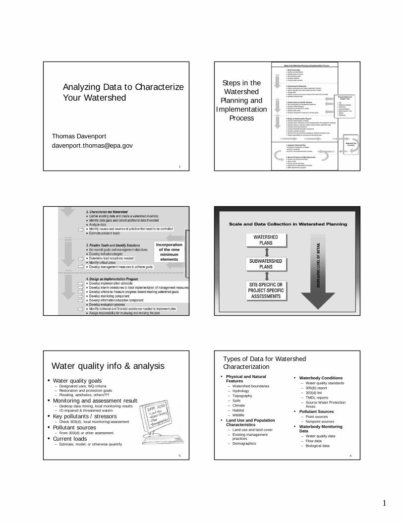
1 1 Analyzing Data to Characterize Your Watershed Thomas Davenport [email protected] 2 Steps in the Watershed Planning and Implementation Process 3 Incorporation of the nine minimum elements 4 5 Water quality info & analysis • Water quality goals – Designated uses, WQ criteria – Restoration and protection goals – Flooding, aesthetics, others??? • Monitoring and assessment results – Desktop data mining, local monitoring results – ID impaired & threatened waters • Key pollutants / stressors – Check 303(d); local monitoring/assessment • Pollutant sources – From 303(d) or other assessment • Current loads – Estimate, model, or otherwise quantify 6 Types of Data for Watershed Characterization • Physical and Natural Features – Watershed boundaries – Hydrology – Topography – Soils – Climate – Habitat – Wildlife • Land Use and Population Characteristics – Land use and land cover – Existing management practices – Demographics • Waterbody Conditions – Water quality standards – 305(b) report – 303(d) list – TMDL reports – Source Water Protection Areas • Pollutant Sources – Point sources – Nonpoint sources • Waterbody Monitoring Data – Water quality data – Flow data – Biological data
Transcript of Analyzing Data to Characterize Steps in the Your...
1
1
Analyzing Data to Characterize Your Watershed
Thomas [email protected]
2
Steps in the Watershed
Planning and Implementation
Process
3
Incorporation of the nine minimum elements
4
5
Water quality info & analysis• Water quality goals
– Designated uses, WQ criteria– Restoration and protection goals– Flooding, aesthetics, others???
• Monitoring and assessment results– Desktop data mining, local monitoring results– ID impaired & threatened waters
• Key pollutants / stressors– Check 303(d); local monitoring/assessment
• Pollutant sources– From 303(d) or other assessment
• Current loads– Estimate, model, or otherwise quantify
6
Types of Data for Watershed Characterization
• Physical and Natural Features – Watershed boundaries– Hydrology– Topography– Soils– Climate– Habitat– Wildlife
• Land Use and Population Characteristics– Land use and land cover– Existing management
practices– Demographics
• Waterbody Conditions– Water quality standards– 305(b) report– 303(d) list– TMDL reports– Source Water Protection
Areas• Pollutant Sources
– Point sources– Nonpoint sources
• Waterbody Monitoring Data– Water quality data– Flow data– Biological data

2
7
Flow data is available from the US Geological
Survey web site at http://waterdata.usgs.gov
/nwis/rt
8
T.C. Stiles, 2001; B.Cleland, 2002
9 10
How can we estimate loads?
11
What is a “load?”• Maybe measured by weight .
. . – Kilograms per day– Pounds per week– Tons per month
• Maybe not . . . – Concentration-based expression of the
“load” (e.g., milligrams per liter)• mg/L x L/day = mg/day [C = m/v]
– # of miles of streambank needing stabilization or vegetation
– # of AFOs requiring nutrient plans– % of urban area to be ‘perforated’
12
Existing loads come from lots of places . . .

3
13
Existing loads come from:
• Point-source discharges (NPDES facilities)– Info is available on the discharges (DMRs, etc.)– Some are steady-flow, others are precip-driven
• Nonpoint sources (polluted runoff)– All are (mostly) precip-driven– Calculating the “wash-off, runoff” load is tough– Literature values can be used to estimate– Modeling gets you closer . . . . do you need it?
• Air / atmospheric deposition– Can be significant in some locations
14
Steady-load: sewage treatment plant discharge via
infrared photography
15
Identification of causes & sources• What “pollutants” are you dealing with?
– Chemical or other stressors or causes of impairment
• How big is the problem for each?• How do you know?
– Did you “measure” them?– Did you estimate? How?
• Where are they coming from?– Can you put the info on a map?
• Can you estimate the % from each source?
16
Data-driven Approaches• Estimate source loads using:
– Monitoring data• Periodic water quality concentrations and flow
gauging data• Facility discharge monitoring reports
– Literature• Loading rates, often by landuse (e.g.,
lbs/acre/year)• Typical facility concentrations and flow
17
Is a Data-driven Approach Appropriate?• Monitoring data
– Does it represent most conditions that occur (low flow, storms, etc.)?
– Are spatial and source variability well-represented?
– Have all parameters of interest been monitored?– Is there a clear path to a management strategy?
18
Load Estimates – Monitoring Data• In simplest terms…
load = flow x concentration• Load duration curves
– Flow-based presentation• Statistical techniques
– Relationships between flow and concentration to “fill in the blanks” when data aren’t available
– Examples include:• Regression approach• FLUX

4
19
Load Duration Curves• Rank daily flow and generate flow duration curve• Multiply water quality concentrations by corresponding flow
values• Flow “curve” represents water quality target
5104
1
10
100
1000
10000
100000
1000000
0% 10% 20% 30% 40% 50% 60% 70% 80% 90% 100%
Observed Flow Exceedence at KAIN18
Tota
l Sus
pend
ed S
olid
s Lo
ad (k
g/da
y)
Allowable Total Suspended Solids Load (kg/day) Observed Total Suspended Solids Load (kg/day)
Observed (Surface Flow > 50%)
20
Load Estimates – Literature• Landuse-specific loading rates (typically annual)
• Multiply loading rate by area:loadall = (arealu1 x loading ratelu1)+ (arealu2 x loading ratelu2) +…
• Generally for landuse or watershed-wide analysis
• Many sources: Lin (2004); Beaulac and Reckhow(1982), etc.
• Use with caution (need correct representation for your local watershed)– Pollution sources
– Climate
– Soils
21
Example Load Estimation Based on Literature Values
22
23
Limitations of Data-driven Approaches
• Monitoring data– Reflect current/historical conditions (limited use
for future predictions)– Insight limited by extent of data (usually water
quality data) • Often not source-specific• May reflect a small range of flow conditions
• Literature– Not reflective of local conditions– Wide variation among literature– Often a “static” value (e.g., annual)
24
Key Points:
• Many tools are available to quantify pollutant loads
• Approach depends on intended use of predictions
• Simplest approaches are data-driven• Watershed modeling is more complex and time-
consuming– provides more insight into spatial and temporal
characteristics– useful for future predictions and evaluation of
management options• One size doesn’t fit all!

5
25
Load assessment is is on ongoing learning process – iterative & creative!
26
Identify candidate practices
27
Identify Opportunities for Implementation• Impervious
analysis
• Political constraints and priorities
• Physical constraints
• Environmental constraints
28
Quantifying Load Reductions to Meet Objectives• Sources of load quantification data
– Watershed modeling/load quantification results (previously described), TMDL reports, etc.
– Source and spatial targets for implementation
Table 5-4. Nutrient and BOD baseline and allocation loads by contributing subwatershed for impaired waters of the Cedar Creek watershed (daily averages based on the 2001-2003 meteorological regime).
BOD TN TP Reach ID/Subwatershed Baseline
(lb/day)TMDL
(lb/day)Percent
ReductionBaseline (lb/day)
TMDL (lb/day)
Percent Reduction
Baseline (lb/day)
TMDL (lb/day)
Percent Reduction
1, Lower Cedar Creek 24.74 14.12 43% 31.49 17.51 44% 1.54 0.85 44% 2, Slaughter Creek 4.44 2.74 38% 4.74 2.74 42% 0.20 0.12 41% 3, Slaughter Creek 15.16 9.03 40% 23.76 13.31 44% 0.87 0.49 43% 4, Slaughter Creek 61.40 35.49 42% 97.83 54.47 44% 3.65 2.05 44% 5, Slaughter Creek 17.54 9.98 43% 30.81 17.09 45% 1.12 0.62 44% 6, Slaughter Creek 34.70 23.42 33% 34.38 20.68 40% 1.28 0.76 40% 7, Slaughter Creek 31.19 18.67 40% 47.92 26.91 44% 1.87 1.04 44% 8, Slaughter Creek 52.48 32.26 39% 77.65 43.68 44% 2.99 1.69 43%
29
9%
11%
13%
15%
17%
19%
21%
23%
$0 $200,000 $400,000 $600,000 $800,000 $1,000,000 $1,200,000Cost ($)
Run
off V
olum
e R
educ
tion
(% fr
om E
xist
ing
Con
ditio
n)
Trad
e-O
ff Cu
rve
Optimal Solution
Initial Run
Identify Optimal SolutionExample of BMP-DSS Multiple Run Output
30
Quantify BMP Options at a Subwatershed or Watershed Scale• Goals
– Quantify selected BMP strategies (i.e., individual BMPs or BMP pairings)• Watershed scale• Local scale
– Compare potential load reductions to target– Determine optimal strategy considering
environmental benefits and $$• Available Tools
– Spreadsheet tools– Watershed/site-scale models

6
31
Prioritizing/targeting BMPs
• Importance of waterbody– Drinking water source, recreational resource
• Magnitude of impairment(s)– Level of effort needed; public interest/attention
• Existing loads (stressors & sources)– Magnitude, spatial variation, clustering
• Ability of BMPs to reduce loads– Sure thing, or a shot in the dark?
• Feasibility of implementation– Willing partners? Public support?
• Additional benefits– Recreational enhancements, demonstration
32
What Tool Should I Select?• Has a model already been used for load
quantification?• What scale is important? • Is an annual load reduction estimate sufficient? • Should individual storms be evaluated?
• Spreadsheet tools– Normally good for annual/overall reductions– Usually at a watershed scale – sometimes at the site
scale• Watershed models
– Allow for continuous/long-term simulation– Often can be used for storm evaluation– Ability to function at all scales – site and watershed
33
Flashiness Index
Even without pollutant load data, can be used to quantify hydrologic impacts of watershed change on hydrologic regime and to evaluate efforts to restore natural flow regimes
34
Examples• Minimize the total volume of surface water runoff that flows
from any specific site during and following development, in order to replicate pre-development hydrology to the maximum extent practicable
• Achieve average annual 85% Total Suspended Solids (TSS) removal for the developed area of a site. Areas designated as open space that are not developed do not require stormwater treatment. All sites must employ Low Impact Development (LID) practices to control and treat runoff from the first inch of rainfall
0
5
10
15
20
25
11:00 AM 12:00 PM 1:00 PM 2:00 PM
Time (hours)St
ream
Flo
w (f
f3 /s
) Developed site hydrograph
BMP influence on hydrograph
35
Clinton River Watershed Site Evaluation Tool
• Evaluate potential benefits of BMPs at the site development scale
• Inputs– Site characteristics– BMP characteristics
• Outputs– Peak discharge– Annual runoff– Pollutant Loads
Nitrogen Rate
Target
0.002.004.006.008.00
10.0012.0014.0016.0018.00
1-yr 24-hr storm
01234567
11:00 AM 12:00 PM 1:00 P
cfs
Post, no BM PsExistingPost, with BM Ps
36
Why a Site Evaluation Tool?• Evaluate flow and water quality impact
of proposed residential and commercial development
• Identify most cost-effective suite of BMPs
• Support decision-making activities– Tool used in combination with other
data/information to make final management decisions at the site scale
– Promote consistency• Help with Phase 2 reporting
requirements

7
37
Example
38
Areal Loading Rates ExistingLanduse
Designwithout BMPs
Designwith BMPs Target
Meets Goal?
Total Nitrogen (lb/ac/yr) 0.66 9.56 7.17 6.00 NO!Total Phosphorus (lb/ac/yr) 0.11 1.53 0.92 1.33 YesSediment (ton/ac/yr) 0.011 0.120 0.018
Site is located in Urban Residential Nutrient ZoneTN loading rate is higher than the buy-down range of 3.6 to 6 lb/ac/yr
Nitrogen Rate
Target
0.00
2.00
4.00
6.00
8.00
10.00
12.00
Phosphorus Rate
Target
0.00
0.50
1.00
1.50
2.00
Sediment Rate
0.000
0.020
0.040
0.060
0.080
0.100
0.120
0.140
39 40
Areal Loading Rates ExistingLanduse
Designwithout BMPs
Designwith BMPs Target
Meets Goal?
Total Nitrogen (lb/ac/yr) 0.66 9.56 3.26 6.00 YesTotal Phosphorus (lb/ac/yr) 0.11 1.53 0.30 1.33 YesSediment (ton/ac/yr) 0.011 0.120 0.001
Site is located in Urban Residential Nutrient ZoneTN loading rate is below the buy-down range of 3.6 to 6 lb/ac/yr
Nitrogen Rate
Target
0.00
2.00
4.00
6.00
8.00
10.00
12.00
Phosphorus Rate
Target
0.00
0.50
1.00
1.50
2.00
Sediment Rate
0.000
0.020
0.040
0.060
0.080
0.100
0.120
0.140
41
Key Points in Quantifying BMP Performance:
• Quantifying potential impacts from BMPs is critical to watershed planning– Provides a guide toward achieving load reduction goal– Informs selection of a management strategy
• Spreadsheet and modeling tools are available– Spreadsheet tools
• Most useful for watershed-scale analysis• Operate on a large time step
– Watershed/site-scale models• Useful for local scale, as well as watershed-scale• Can operate on a short time-step (including individual storms)• Provide a key first step for engineering design
• Again, one size doesn’t fit all!
42
Examples of Different Scenarios to Meet the Same Load Target

8
43
phosphorus load
0
50
100
150
200
250
300
1 2 3 4 5 6 7 8 9 10 11 12
months
kg/d
ay
Typical monitoring program measures water quality at a relatively few points in time, then “connects the dots”.
Note: Total annual load is assumed to be the area under the curve. 44
However:
If storm events aren’t measured, the actual load may be much larger.
phosphorus load
0
50
100
150
200
250
300
1 2 3 4 5 6 7 8 9 10 11 12
months
kg/d
ay
45
dissolved oxygen
0
2
4
68
10
12
14
16
1 2 3 4 5 6 7 8
days
mg
/ lite
r
Many monitoring schemes miss daily variation as well.
Blue dots are typical late afternoon measurements of dissolved oxygen. In many productive systems, however, DO drops to very low values at night.
46
All Samples
0
20
40
60
80
100
4926
35
4926
29
4926
39
4926
38
4926
28
4926
36
4926
26
4926
37
Perc
ent
Total PhosphorusTotal Suspended Solids
Pollution Indicator Exceedence(Total P and TSS)
020406080
100
4926
35
4926
29
4926
39
4926
38
4926
28
4926
36
4926
26
4926
37
Perc
ent
Total PhosphorusTotal Suspended Solids
All Samples
Non Runoff Samples
Comparison of storm event data with non-storm data at 8 different urban stations in Utah
Note difference in percent exceedence of pollutant criteria.
Data from Rieke, Mesner and Gilles, 2005
47
Upstream/downstream monitoring demonstrates impact of BMP very effectively.
Rees Creek TSS load
0
5000
10000
15000
20000
25000
30000
35000
40000
45000
50000
1 2 3 4 5 6 7 8 9
weeks
kg /
day upstream
downstream
48
But… will upstream/downstream monitoring capture all impacts?

9
49
Bear River phosphorus load
0
50
100
150
200
250
300
350
400
1 2 3 4 5 6 7 8 9
weeks
load
(kg/
day)
upstream
downstream
Loading from large feeding operation swamped by the large loads carried by the Bear River.
50
NPS issues: livestock, grazing, feedlots
NPS issues: excessive pasturing along stream
51
Findings: BMP implementations improved overall stream physical habitat conditions.
However:
Spring Creek (with relatively large amounts of BMPs in both upland and riparian) :
improved habitat, temps and fisheries
Joos-Eagle (with very few BMPs installed)
No change in fish or thermal regime
habitat only improved in localized areas.
52
RESULTSCooler water
temperatures in pools and deeper runs
Reduced width-depth ratios compared to unrestored reaches
Rainbow trout numbers increased in restored reaches, while constant or decreasing in unrestoredand control reaches
Trout Counted Each Visit During Study Period
Mean Mean±SE Mean±SD DARKL MCCL1 MCCL2 MCCLR MCCR
SITE
-20
0
20
40
60
80
100
120
140
Num
ber o
f Tro
ut
control before after
53
Findings:
• Fisheries improvement thru riparian bmps alone will only work if the watershed is already in good shape, or if upland bmps are installed.
• A minimum of 30-50% bmp implementation at a watershed scale may be necessary
54

10
55
Cross-Section Locations - Chalk Creek
5000
5050
5100
4825 4875 4925 4975 5025 5075Easting (m)
Nor
thin
g (m
)
left bankfulls 98right bankfulls 98left bankfulls 95right bankfulls 95X-Section G0X-Section G1X-Section G2X-Section G3X-Section G4X-Section G5X-Section G6
G0
G3
G4
G5
Transect Locations at Curtis Property
G2
56
Cross Section - G0
98.5
99.5
100.5
75.000 85.000 95.000
G0 98 G0 95 G0 94qbr est 98 qbr est 95 qbl est 94G0 03 qbr est 03
Cross Section - G1
98.5
99.5
100.5
35.000 45.000 55.000 65.000 75.000
G1 98 G1 95 G1 94qbr est 98 qbr est 95 qbr est 94G1 03 qbr est 03
Surveying demonstrates response of stream width, depth, lateral migration.
In these cross sections, stream has deepened and narrowed at BMP site.
57
1978-1989y = 0.037x + 0.0813R2 = 0.5294, n=75
1990-2003y = 0.0327x + 0.0385R2 = 0.513, n=123
0.0
0.2
0.4
0.6
0.8
1.0
1.2
1.4
0 5 10 15 20 25 30
Discharge (m3 sec -1 )
Tota
l Pho
spho
rus (
mg
L-1)
.
1978-19891990-1999
The reports also utilize monitoring data collected by DWQ. In this example, response was measured as a change in the slope of the TP/discharge relationship.
58
Urbanization
59
OUTCOMESINPUTS OUTPUTS
Activities Participation Short Medium Long
term
Programmaticinvestments
i
EVALUATION
PLANNING
60
25
• Statistics is a vital part of any study design as it isusually the tool used to answer the question.
• The type of statistical method to be used is guided by yourquestion and the design of your study.
• Statistics is a separate course in itself.
• It is the data assumptions inherent in statistical methodsthat drives the development of so many sampling strategies.
• Knowledge of statistics is required to address sample sizeestimates and determine the cost of science-related programs.
Statistics:

11
61
29
• The issue of scale has been referred to as the centralproblem in ecology.
• There is no single correct scale at which to study somethingand the results you get are dependent on the scale you choose.
• A linear change in scale does not necessarily mean a linearchange in the measured value. Scale dependent patterns canbe complex and non-linear.
• How can you select the appropriate scale(s) for a study?
Scale:
62
37
Power Analysis,Effect Size &Sample SizeEstimation:
Power analysis quantifies the relationships between the following:
• Effect Size: The smallest detectable change.
• Variation: The amount of “noise” in the data.
• Confidence: Probability of not making a “false alarm” (Type 1 error).
• Power: Probability of not missing a significant change when it happens(Type 2 error).
• Sample Size: The amount of data you have.
Using Power Analysis, if you have estimates for any 4 of these things,you can solve for the 5th thing.
63
38
ThePowerCurve:
Sam
ple
Pow
er
Sample Size
high
low
small large
A
B
C
not effectiveor efficient
effective butnot efficient
effective andefficient
64
39
Preliminary& Sequential
Sampling:
• Where do you get estimates for power analysis parameters?
• Preliminary Sampling (i.e., pilot projects) occurs before the formalstart of a study. This stage allows for testing of methods, evaluatingeffort, and for collecting power analysis parameters to pin downthe strength of the proposed study.
• Sequential Sampling (i.e., ongoing monitoring) occurs when data areanalyzed during the data collection phase of a project. Sequentialsampling, analysis, and evaluation makes the manager more familiarwith the study and its data and promotes Adaptive Management.
Data collected from preliminary & sequential sampling can often beused in the overall study. People who skip this step often end up wasting money, not saving it.
65
44
Money isAlways
Tight:
• Study design should be carefully considered beforeany investment in monitoring is made.
• No amount of statistical hocus pocus will turn data collected from abad design into useful information.
• Not all designs are complex and not all topics covered today willalways be relevant, but some always will be (e.g., scale, disturbingvariables - bias).
• Most study design problems groups face are common acrossthe country. If you have a problem chances are someone has alreadythought about it.
66
MonitoringSeveral major watershed monitoring projects have reported little or no improvement in water quality after extensive implementation of best management practices (BMPs) in the watershed:
• Uncooperative weather• Improper selection of BMPs• Mistakes in understanding of pollution sources • Poor experimental design• Lag time

12
67
VT NMP Project 1993 - 2001Evaluate effectiveness of livestock exclusion, streambank
protection, and riparian restoration in reducing runoff of nutrients, sediment, and bacteria from agricultural land to surface waters
68
Paired watershed designContinuous dischargeFlow-proportional automated
composite sampling (weekly)Total Phosphorus (TP)Total Kjeldahl Nitrogen (TKN)Total Suspended Solids (TSS)
Bi-weekly grab samplingIndicator bacteria Temp., conductivity, D.O.
Annual biomonitoringMacroinvertebratesHabitatFish
Annual land use/management
69
[TP] -15%[TKN] -12%[TSS] -34%E. coli -29%Temperature -6%TP load -49% -800
kg/yrTKN load -38% -2200
kg/yrTSS load -28% -115,000
kg/yr
RESULTS
Macroinvertebrate IBI improved to meet biocriteriaNo significant change in fish community
70
OR Upper Grande Ronde NMP Project 1995 - 2003
Improve salmonid community through restoration of habitat and stream temperature regime
Document effectiveness of channel restoration on water temperature and salmonid community
71
½ mile
Reintroduced W et Meadow Channel 1997
Diversion 1997
N
McIntyre Road
McCoy Creek Channelized 1968
Meadow Creek Temperature Monitoring Site
Direction of stream flow
New Bridge and Culvert
2001
Reconstructed W et Meadow Channel 2002
MCCM
MCCR
MCCLR
MEADL
MCCL1&2
Before/after channel restoration, with controlContinuous air & water temperature, periodic habitat
assessment, snorkel surveys for fish monitoring
72
Is a Model Necessary? It depends what you want to know…
• What are the loads associated with individual sources?
• Where and when does impairment occur? • Is a particular source or multiple sources
generally causing the problem?• Will management actions result in meeting
water quality standards?• Which combination of management actions will
most effectively meet load targets?• Will future conditions make impairments
worse?• How can future growth be managed to
minimize adverse impacts?Models are used in many areas…TMDLs, stormwater evaluation and design, permitting, hazardous waste remediation,
dredging, coastal planning, watershed management and planning, air studies
Probably Not
Probably

13
73
To model, or not to model . . .
•As these things increase:– Number of pollutants– Complexity of loads/stressors– Uncertainty regarding existing information– Expense involved in addressing problems
• The need for more sophisticated modeling also increases