Analytical Solutions to Blocked LubricationShuangbiao Liu  ( shuangbiaoliu@yahoo.com )

Tribo-Interface Design

Short Report

Keywords: Lubrication, Analytical solutions, Boundary conditions

Posted Date: May 6th, 2021

DOI: https://doi.org/10.21203/rs.3.rs-499984/v1

License: This work is licensed under a Creative Commons Attribution 4.0 International License.  Read Full License

Analytical Solutions to Blocked Lubrication

Shuangbiao Liu

Tribo-Interface Design, 1309 Blue Sky Ct, Peachtree City, GA 30269

shuangbiaoliu@yahoo.com

Abstract

When mixed/boundary lubrication problems are studied, proper boundary conditions are

needed to reflect the local physical reality that occurs between fluid lubrication and solid

contacts. In order to improve understanding of such reality, often in a microscopic scale hidden

from direct observation, simple lubrication problems with zero net exiting flow or blocked

lubrication are identified, and several analytical solutions are derived for the first time based on

one- and two-dimensional Reynolds equations.

Keywords: Lubrication; Analytical solutions; Boundary conditions

1. Introduction

Liu [1] summarizes various boundary conditions that are used together with the Reynolds

equation in the full-film lubrication regime. Due to various design constrains, such as slow

speed or heavy load, mixed lubrication or even boundary lubrication can occur in real life

products. As a result, regions of solid contacts co-exist with regions of fluid lubrication, often in

a microscopic scale hidden from direct observation. Solid contacts not only block flows but also

reduce service life of these products and simulations if available are conducted in order to

properly design such tribological interfaces. The sub-problem with regions of fluid lubrication is

governed by the Reynolds equation together with additional boundary conditions reflecting local

physical reality of solid contact on one side and fluid lubrication on the other side. These

additional boundary conditions are LCBCs in short.

Zhu and Wang [2] reviewed the history and progress of elastohydrodynamic lubrication

(EHL) simulations, including lately significant accomplishments in relatively thin film

deterministic solutions considering real measured roughness in the mixed and boundary

lubrication regimes. Two approaches can be classified:

(1) On one hand, lubrication and solid-contact regions are treated separately with fluid-film

pressure and dry-contact pressure variables, respectively, and these variables are updated in

sequential sweeps of an iteration process. In 1995, Chang [3] studied transient mixed EHL line-

contact problems with a deterministic model. His treatment of “check the film thickness at every

grid point. If the film thickness is smaller than one-thousandth of the central film thickness for

perfect smooth contact, hos, set it to 0.001hos” allows the fluid-film pressure to be obtained from

the Reynolds equation for the entire domain, therefore avoids the LCBCs. Then the solid-contact

pressure is evaluated for grid points with negative gaps, which include deformations only caused

by the fluid-film pressure. Results presented in [3] have non-zero fluid-film pressure values after

the first (counting from the inlet) solid contact region, however this is physically impossible

since lubricant should have been blocked by the first solid contact region and no fluid-film

pressure should occur in the downstream after the solid contact. Jiang et al. [4] presented a

transient mixed EHL model for point-contact problems. Their discretized Reynolds equation has

three left-hand side terms involving three nodal pressures (triples) along the velocity direction

and one right-hand term.

𝛼",$𝑃"&',$ + 𝛽",$𝑃",$ + 𝛾",$𝑃"+',$ = 𝑏",$

Their treatments related to LCBCs can be summarized as following: when the film thickness at a

node (i, j) is less than or equal to zero, (a) the film thickness is set to zero; (b) two coefficients,

𝛼"+',$ and 𝛾"&',$, need to be updated with zero film thickness; and (c) the fluid pressure is set to

the solid-contact pressure.

Zhao et al. [5] simulated circular contacts start up, where the constraints (a) for the fluid-

film lubrication regions are positive film thickness, zero solid-contact pressure, and non negative

fluid-film pressure, (b) for the solid-contact regions are zero film thickness, positive solid-

contact pressure, and zero fluid-film pressure. Deolalikar et al. [6] explicitly applied a no-flow

boundary condition to boundaries where the fluid regions are upstream of the solid-contact

regions.

(2) On the other hand, pressure variables, i.e., old and new pressure arrays during iterations,

cover both lubrication and solid-contact regions, and are updated within the same sweep over

nodes of an iteration process. Zhu and Hu [7] introduced a unified equation system, where

a) regular Reynolds equation for the lubrication regions,

b) truncated Reynolds equations--eliminating Poiseuille terms and a transient term, for solid-

contact regions

Dimensionless film thickness is compared with a fixed small value to decide the truncation in

(b). This approach is practical and has been successfully applied in their subsequent work [8].

Holmes et al. [9] used regular Reynolds equation and the elastic deflection equation in a

differential form to update unknown nodal values of pressure and film thickness. Once a nodal

value of film thickness is negative, it is set to zero and the nodal value of pressure is updated

with the elastic deflection equation only. Li and Kahraman [10], Azam et al. [11], and Wang et

al. [12] utilized the unified equation system of Zhu and Hu [7].

The LCBCs in mixed/boundary EHL problems are microscopic, complex by nature, and

often overlooked in experimental and fundamental studies, so it is important to

understand/formulate them through focused investigations in order to enable physically

meaningful numerical results. Given the situation, it is necessary to first address simpler

lubrication problems under simpler configurations. In this paper, several analytical solutions are

derived for the first time based on one- or two-dimensional Reynolds equations without net

exiting lubricant—blocked lubrication problems. These solutions themselves may be applicable

to special engineering problems or to be used to validate numerical algorithms in the

mixed/boundary lubrication study. Also, they can be exercises for students in the tribology field,

and can help readers to better understand lubrication where flow is blocked locally. In the future

work, reasonable boundary conditions can be introduced to deal with boundaries between fluid

lubrication and solid contacts, and they ultimately allow details closer to reality around solid

contacts to be obtained in lubrication simulations.

2. Analytical Solutions

In the following steady-state lubrication problems, flow through the lubrication area is

intentionally blocked in one direction, in order to gain insights of film pressure involving solid

contacts in mixed lubrication. They are mostly two dimensional problems, but one three

dimensional pad bearing problem is also analytically solved in section 2.5.

For simplicity, density ρ are constant. Also in sections 2.1 to 2.3, and 2.5, lubricant

viscosity η is constant and bodies are rigid. In section 2.4, the Barus viscosity-pressure

relationship is used with an elastic cylinder. Furthermore, referring to Figs. 1-5, it is assumed

that (a) The bottom plate is always flat and horizontal moving along the x axis with a constant

velocity of u, and the top plate is stationary with various shapes; (b) no air has been trapped

inside for all problems; (c) a perfect sealing exists between the rigid block plate and the moving

plate, and (d) there is no slip between lubricant and the plate surfaces. One could use this website

https://www.wolframalpha.com/ or softwares such as mathematica® or Maple ® to help

derivation.

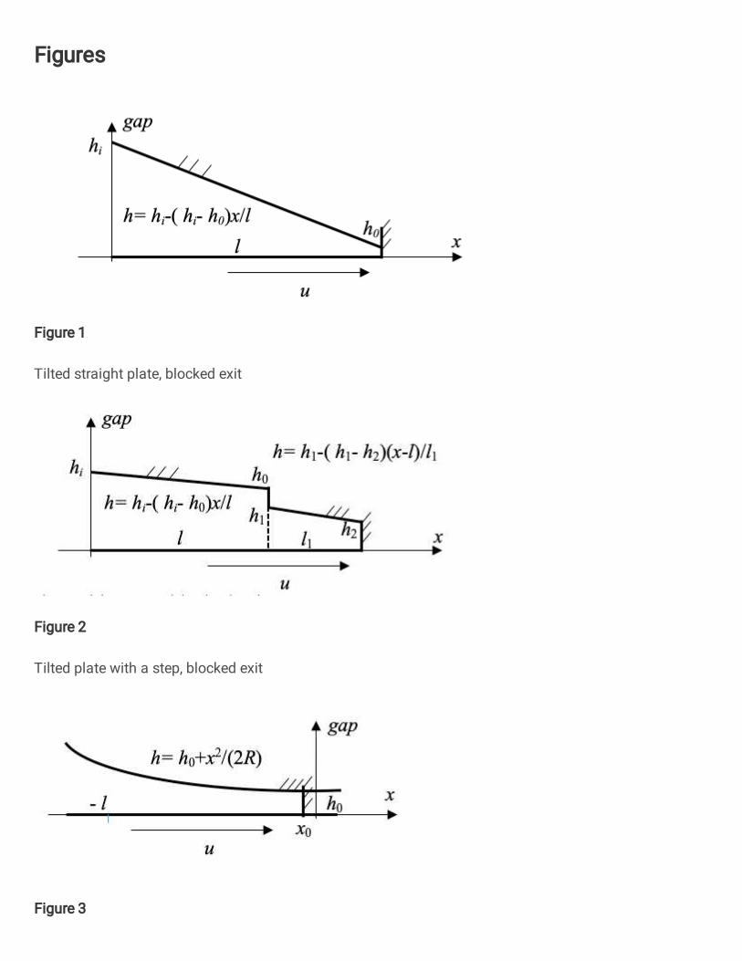
2.1 Straight plate

Problem 1 has a tilted straight plate and a block plate, both of which are rigid surfaces

(see Fig. 1). The gap in the inlet is hi and the gap on the blocked side is h0.

Fig. 1 Tilted straight plate, blocked exit

When steady state cases are considered, the one-dimensional Reynolds equation is

written as

../ 01234 .5./6 = 6𝑢 .(12)./ (1)

After an integration, one can find,

hi

u

h0 h= hi-( hi- h0)x/l

l x

gap

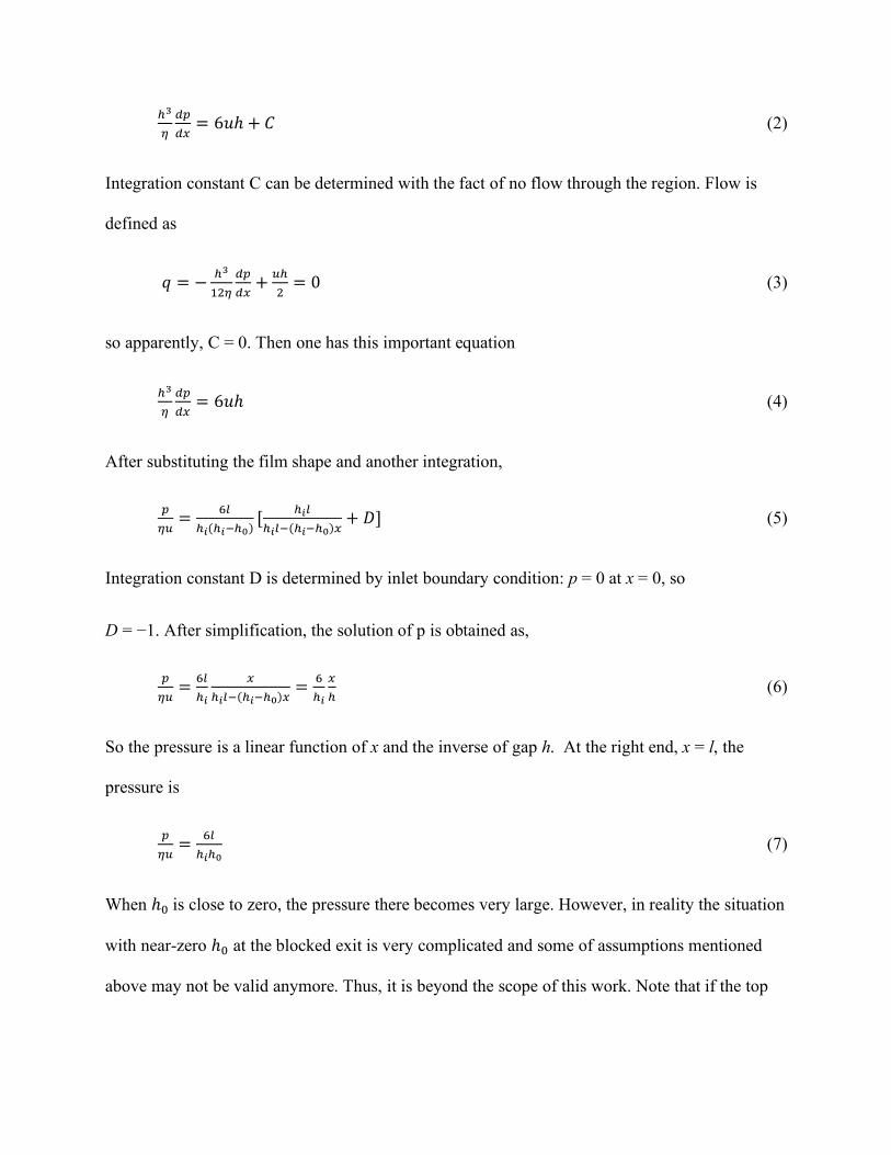
234 .5./ = 6𝑢ℎ + 𝐶 (2)

Integration constant C can be determined with the fact of no flow through the region. Flow is

defined as

𝑞 = − 23'?4 .5./ + @2? = 0 (3)

so apparently, C = 0. Then one has this important equation

234 .5./ = 6𝑢ℎ (4)

After substituting the film shape and another integration,

54@ = BC2D(2D&2E) [ 2DC2DC&(2D&2E)/ + 𝐷] (5)

Integration constant D is determined by inlet boundary condition: p = 0 at x = 0, so

D = −1. After simplification, the solution of p is obtained as,

54@ = BC2D /2DC&(2D&2E)/ = B2D /2 (6)

So the pressure is a linear function of x and the inverse of gap h. At the right end, x = l, the

pressure is

54@ = BC2D2E (7)

When ℎIis close to zero, the pressure there becomes very large. However, in reality the situation

with near-zero ℎI at the blocked exit is very complicated and some of assumptions mentioned

above may not be valid anymore. Thus, it is beyond the scope of this work. Note that if the top

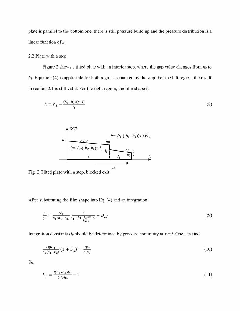
plate is parallel to the bottom one, there is still pressure build up and the pressure distribution is a

linear function of x.

2.2 Plate with a step

Figure 2 shows a tilted plate with an interior step, where the gap value changes from h0 to

h1. Equation (4) is applicable for both regions separated by the step. For the left region, the result

in section 2.1 is still valid. For the right region, the film shape is

ℎ = ℎ' − (2K&2L)(/&C)CK (8)

Fig. 2 Tilted plate with a step, blocked exit

After substituting the film shape into Eq. (4) and an integration,

54@ = BCK2K(2K&2L) ( ''&(MKNML)(ONP)MKPK+𝐷?) (9)

Integration constants 𝐷? should be determined by pressure continuity at x = l. One can find

B4@CK2K(2K&2L) (1 + 𝐷?) = B4@C2D2E (10)

So,

𝐷? = C(2K&2L)2KCK2D2E − 1 (11)

h2

hi

u

h1

l l1 x

h0

h= hi-( hi- h0)x/l

h= h1-( h1- h2)(x-l)/l1

gap

In summary,

54@ = R BC2D /2DC&(2D&2E)/ 𝑥 ≤ 𝑙BCK2K 0 /&C2KCK&(2K&2L)(/&C) + C2KCK2D2E6 𝑥 > 𝑙 (12)

If h1 equals to h0, step disappears, this plate has a point, and this solution is still valid.

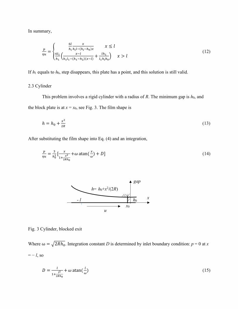
2.3 Cylinder

This problem involves a rigid cylinder with a radius of R. The minimum gap is h0, and

the block plate is at x = x0, see Fig. 3. The film shape is

ℎ = ℎI + /L?W (13)

After substituting the film shape into Eq. (4) and an integration,

54@ = X2EL [ /'+ OLLYME

+𝜔 atan( /) + 𝐷] (14)

Fig. 3 Cylinder, blocked exit

Where ω = `2𝑅ℎI. Integration constant D is determined by inlet boundary condition: p = 0 at x

= − l, so

𝐷 = C'+ PLLYME

+𝜔 atan( C ) (15)

h0

u

h= h0+x2/(2R)

- l x

x0

gap

After simplification, the solution of p is obtained as,

54@ = X2EL [ /+C'+ OLLYME

+𝜔 atan( /)+𝜔 atan( C )] (16)

One can see this solution does not contain x0. If x0 is negative, it has a convergent geometry, so

this solution is valid for the entire length of l. But if x0 is positive, the portion beyond x = 0 is

divergent. Even in this divergent gap, this solution is valid. When x0 = 0, pressure reaches this

value

54@ = X2EL [𝑙 +ωatan( Cc)] (17)

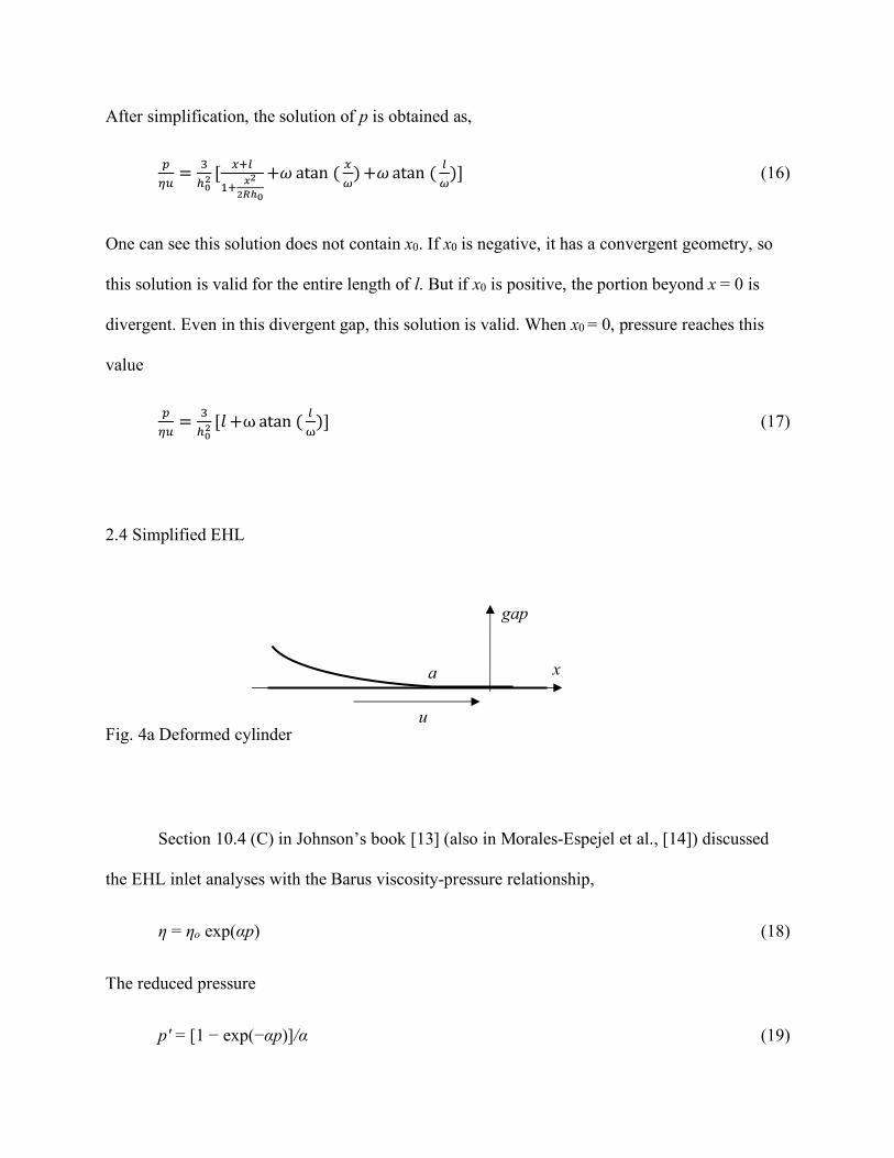
2.4 Simplified EHL

Fig. 4a Deformed cylinder

Section 10.4 (C) in Johnson’s book [13] (also in Morales-Espejel et al., [14]) discussed

the EHL inlet analyses with the Barus viscosity-pressure relationship,

η = ηo exp(αp) (18)

The reduced pressure

p' = [1 − exp(−αp)]/α (19)

u

x a

gap

is applied.

Figure 4a illustrates an elastic cylinder (radius of R) and a rigid plate under a load. The

Hertzian contact width is a. dimensionless coordinate X is defined as x/a. Without considering

the deformation from the fluid pressure, the gap between these two bodies when 𝑋 ≤ −1 can

be expressed as,

ℎ = eL?W [−𝑋√𝑋? − 1 − lnh−𝑋 + √𝑋? − 1i] (20)

In order to facilitate integration, Eq. (20) can be approximated as follows, see Eq. (10.38) of

[13],

Appr. 1: ℎ ≈ eLXW [−2(𝑋 + 1)]'.l (21)

It is found that this approximation is reasonable for −1.5 ≤ 𝑋 ≤ −1 and the exponent of 1.673

has much better approximation for −4 ≤ 𝑋 ≤ −1.5,

Appr. 2: ℎ ≈ eLXW [−2(𝑋 + 1)]'.BoX (22)

Fig. 4b Absolute errors from two approximations of 2R h/a2: with exponents of 1.5 (Solid line)

and 1.673 (Dashed-line)

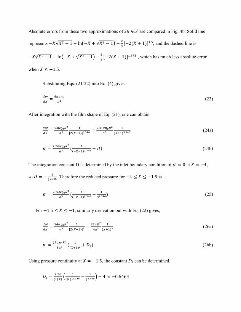
Absolute errors from these two approximations of 2R h/a2 are compared in Fig. 4b. Solid line

represents −𝑋√𝑋? − 1− lnh−𝑋 + √𝑋? − 1i − ?X [−2(𝑋 + 1)]'.l, and the dashed line is

−𝑋√𝑋? − 1 − lnh−𝑋 + √𝑋? − 1i − ?X [−2(𝑋 + 1)]'.BoX , which has much less absolute error

when 𝑋 ≤ −1.5.

Substituting Eqs. (21-22) into Eq. (4) gives,

.5p.q = Be@4E2L (23)

After integration with the film shape of Eq. (21), one can obtain

.5p.q = lr@4EWLe3 '[?(q+')]3.3st = l.X'@4EWLe3 '(q+')3.3st (24a)

𝑝′ = ?.?B@4EWLe3 ( '(&q&')L.3st + 𝐷) (24b)

The integration constant D is determined by the inlet boundary condition of 𝑝′ = 0 at 𝑋 = −4,

so 𝐷 = − 'XL.3st. Therefore the reduced pressure for −4 ≤ 𝑋 ≤ −1.5 is

𝑝′ = ?.?B@4EWLe3 ( '(&q&')L.3st − 'XL.3st) (25)

For −1.5 ≤ 𝑋 ≤ −1, similarly derivation but with Eq. (22) gives,

.5p.q = lr@4EWLe3 '[?(q+')]3 = ?o@WLre3 '(q+')3 (26a)

𝑝′ = ?o@4EWLwe3 ( '(q+')L +𝐷') (26b)

Using pressure continuity at 𝑋 = −1.5, the constant D1 can be determined,

𝐷' = ?.?BX.Xol 0 '(I.l)L.3st − 'XL.3st6 − 4 ≈ −0.6464

Therefore, the reduced pressure for −1.5 ≤ 𝑋 ≤ −1 is

𝑝′ = ?o@4EWLwe3 ( '(q+')L − 0.6464) (27)

The pressure can be found from

𝑝 = − xy('&z5{)z (28)

Example: the value of α is 2.28E-8, R is 20mm, a is 0.1mm, u is 100mm/s, 𝜂I = 0.04247Pa.s.

a) If the maximum pressure inside this wedge is 1E6 Pa,

𝑝′=[1 − exp(−αp)]/α =988686

This pressure is in the region of −4 ≤ 𝑋 ≤ −1.5,

'XL.3st + 𝑝′ e3?.?B@4EWL = 0.333 and 𝑋 = −0.333& KL.3st − 1 = −2.597

X is −2.597.

b) If X is given, one can find the pressure value there. When X = −1.35,

𝑝p = ?o@4EWLwe3 0 '(q+')L − 0.64646 = 43097571

And 𝑝 = − xyh'&z5{iz = 0.1778E9 Pa

Beyond this location, the pressure increases dramatically. Note that when the speed is slower, X

needs to be closer to −1 to reach the same pressure value. If the deformation from the fluid

pressure has to be considered in the calculation, one has to use numerical simulations.

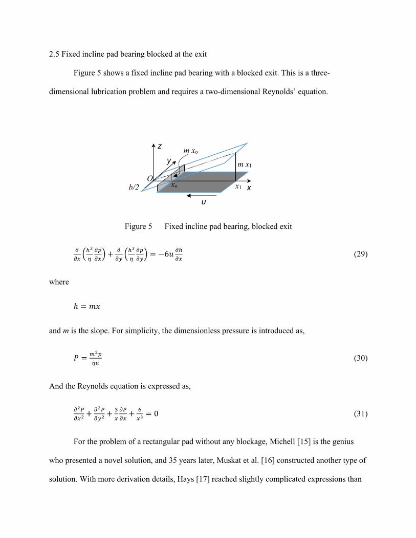
2.5 Fixed incline pad bearing blocked at the exit

Figure 5 shows a fixed incline pad bearing with a blocked exit. This is a three-

dimensional lubrication problem and requires a two-dimensional Reynolds’ equation.

Figure 5 Fixed incline pad bearing, blocked exit

��/ 0234 �5�/6 + ��� 0234 �5��6 = −6𝑢 �2�/ (29)

where

ℎ = 𝑚𝑥

and m is the slope. For simplicity, the dimensionless pressure is introduced as,

𝑃 = �L54@ (30)

And the Reynolds equation is expressed as,

�L��/L + �L���L + X/ ���/ + B/3 = 0 (31)

For the problem of a rectangular pad without any blockage, Michell [15] is the genius

who presented a novel solution, and 35 years later, Muskat et al. [16] constructed another type of

solution. With more derivation details, Hays [17] reached slightly complicated expressions than

O x1

y

x

z

b/2

u

m x1

m xo

xo

what is in Muskat et al. [16]. Liu and Mou [18] derived a general solution which unifies these

two existing groups of analytical solutions, and also showed that Hays’ solution is actually

equivalent to what Muskat et al. derived. The core idea in the work of Muskat et al. [16] and Hay

[17] is that the solution for an infinite sliding pad can eliminate the inhomogeneity of Eq. (29),

then the separation of variable can be used to solve the homogenous PDE. The solution for an

infinite sliding pad, Eq. (6), is the corresponding particular solution, and will be re-written based

on notations in Fig. 5 as,

𝑃 = B/K /K&// (32)

which satisfies the 1D Reynolds equation of �L��/L + X/ ���/ + B/3 = 0. Therefore, the homogenous

equation becomes,

�L��/L + �L���L + X/ ���/ = 0 (33)

One can use separation of variables, and obtain the general solution to the homogenous equation,

which is a linear combination of all possible solutions [18],

𝑃 = (𝑐' + 𝑐?𝑦) 0𝑑' + .L/L6 + (34)

∑ [𝑐'�sinh(𝛼'�𝑦) + 𝑐?�cosh(𝛼'�𝑦)][𝑑'�𝐽'(𝛼'�𝑥) + 𝑑?�𝑌'(𝛼'�𝑥)] 'zK�/���I +

∑ [𝑐X�sinh(𝛼?�𝑦) + 𝑐r�cosh(𝛼?�𝑦)][𝑑X�𝐼'(𝛼?�𝑥) + 𝑑r�𝐾'(𝛼?�𝑥)] 'zL�/���I

where and are the Bessel functions of the first and second kinds, respectively, and

and are the modified Bessel functions of the first and second kinds, respectively. By

)(1 zJ )(1 zY

)(1 zI )(1 zK

selecting their proper values of unknown constants cj, dj, , , and 𝛼$� (i =1…4, j =1 or 2),

one should be able to solve problems with complicated boundary conditions.

Following Muskat et al. [16] and Hay [17] successes, the middle line of Eq. (34) with

Bessel functions will be selected for the problem in Fig. 5, and

𝑈�(𝑥) = 𝐽'(𝛼�𝑥')𝑌'(𝛼�𝑥) − 𝑌'(𝛼�𝑥')𝐽'(𝛼�𝑥) (35)

is defined with x1 the inlet coordinate to satisfy zero pressure boundary condition at x1 since

𝑈�(𝑥') = 0. 𝛼� is used to replace 𝛼'� for simplicity. The origin of the coordinate system in Fig.

5 was deliberately set in the middle of width, so the two boundary conditions are at y = ±𝑏/2

and terms with the “Cosh” function are suitable and selected,

𝑃 = B/K /K&// +∑ B��(/)/ �� ��� (z��)��� (z�¡/?)���' (36)

𝐶� is used to replace 𝐶'� for simplicity. The solution for an infinite sliding pad with a blocked

exit is the corresponding particular solution and is the first term in Eq. (36). The coefficient, 𝛼�

will be determined with the exit boundary condition. Flow equation is expressed as

¢@� = − /? − /3'? ���/ (37)

The derivative involved in the above expression is quite complicate, so a new function is defined

as

𝑊�(𝑥) = 𝐽'(𝛼�𝑥')𝑌?(𝛼�𝑥) − 𝑌'(𝛼�𝑥')𝐽?(𝛼�𝑥) (38)

to satisfy the following derivative,

��/ ¤��(/)/ ¥ = − z�¦�(/)/

inc

ind

Thus,

���/ = ��/ ¤ B/K /K&// +∑ B��(/)/ �� ��� (z��)��� (z�¡/?)���' ¥ = − B/L − ∑ Bz�¦�(/)/ �� ��� (z��)��� (z�¡/?)���'

At the exit, x0, flow is blocked, so

[− /? − /3'? ���/]|/E = 0

One can obtain

𝑊�(𝑥I) = 0 (39a)

Or

𝐽'(𝛼�𝑥')𝑌?(𝛼�𝑥I) − 𝑌'(𝛼�𝑥')𝐽?(𝛼�𝑥I) = 0 (39b)

This equation is used to calculate the coefficient, 𝛼�. Based on the recurrence relations in the

Appendix, the Bessel functions of the order of 2 can be expressed with those of lower orders. So,

one can have the following form,

𝐽'(𝛼�𝑥')[2𝑌'(𝛼�𝑥I) − 𝛼�𝑥I𝑌I(𝛼�𝑥I)] − 𝑌'(𝛼�𝑥')[2𝐽'(𝛼�𝑥I) − 𝛼�𝑥I𝐽I(𝛼�𝑥I)] = 0 (39c)

Introducing two general variables,

𝜏 = 𝑥'/𝑥I

𝛽� = 𝛼�𝑥I

The equation is simplified as

𝐽'(𝛽�𝜏)𝑌?(𝛽�) − 𝑌'(𝛽�𝜏)𝐽?(𝛽�) = 0 (40)

One can see that 𝛽� is solely dependent on the variable 𝜏. The coefficients, 𝛼�, can then be easily

obtained from 𝛽� , i.e., 𝛽�/𝑥I . This equation (39c) is also used in the Appendix to simplify

formulae that are used to determine the other coefficients, 𝐶�.

The remaining boundary conditions are on the two sides, i.e. 𝑃 0𝑥, ¡?6 = 0, and one has

0 = 1 − //K +∑ 𝐶�𝑈�(𝑥)���' (41)

One can use this equation and the orthogonality of Un (see Appendix) to determine the

coefficients, 𝐶�. The method is to multiply 𝑥𝑈�(𝑥)for every term on both sides and then

integrate with respect to x from x0 to x1. Due to orthogonality of Un, terms with 𝑛 ≠ 𝑚 inside the

summation are zero, and only one term with 𝑛 = 𝑚 inside the summation is non-zero (see

Appendix). Denote 𝑆e�¡ = 𝑆e(𝛼�𝑥¡) where S can be J , Y, or H (the Struve function), and a and

b could be 0, 1, or 2. For example, 𝐽'�' = 𝐽'(𝛼�𝑥') or 𝐻I�I = 𝐻I(𝛼�𝑥I). All integrations are

discussed in the Appendix. After simplification, one can found the coefficients of 𝐶� from Eqs.

(A13-A14) as,

𝐶� = ­K�K+®L¯(z�/E­E�E&?­K�E)+L®L®L&(°�OE±)LL= ?²L­K�K+²3¯(z�/E­E�E&?­K�E)+r²r&(²z�/E¯)L (42)

Where are the Struve function of order and Δ = 𝐽'�'𝑌'�I − 𝑌'�'𝐽'�I = 𝑈�(𝑥I). Note that

both sets of coefficients, 𝛼� and 𝐶�, are determined without involving the width, b. In other

words, problems with different widths can use the same sets of these coefficients.

nH n

3. Results and discussion

For the problem in section 2.1, one example is described as: the length of 30mm, inlet

gap of 1mm, and the exit gap of 0.4mm, i.e., l = 30mm, hi = 1mm, and h0 = 0.4mm. The

modified pressure (54@) and gap distributions are shown in Fig. 6 with a label of “line”. For the

problem in section 2.2, the step is 20mm away from the inlet and the heights are 0.7 and 0.5mm,

The modified pressure and gap distributions are shown in Fig. 6 with a label of “step”. The last

case shown in Fig. 6 with a label of “bent” is for a bent plate with the minimum gap of 0.35mm.

One can see there are pressure further built-up inside the divergent gap.

Fig. 6 Three plates and their modified pressure

The example for section 2.3 has a radius R of 20mm, l = 2mm, and h0 = 0.05mm. So ω =`2𝑅ℎI=√2. Figure 7 shows the gap and the modified pressure.

Fig. 7 Cylinder and its modified pressure

For the 3D problem in section 2.5, the parameters l = 30mm, hi = 1mm, and h0 = 0.4mm

are also used. Thus, the coordinates of x0 and x1 are 20 and 50 mm, respectively. m = 0.02 and 𝜏 =/K/E = 2.5. In addition, two widths of the plate are used 20 and 40 mm, i.e., b = 10 and 20mm,

respectively. The solutions of Eq. (45),

𝐽'(𝛽�𝜏)𝑌?(𝛽�) − 𝑌'(𝛽�𝜏)𝐽?(𝛽�) = 0

can be determined by a FORTRAN program or through https://www.wolframalpha.com/ with the

input of,

solve(BesselY(2, x)*BesselJ(1, 2.5*x) - BesselJ(2, x)*BesselY(1, 2.5*x) =0 , x=0 to 20)

and the first 9 positive roots are listed in Table 1. The coefficients of 𝛼� = 𝛽�/𝑥I can be readily

obtained. The same website can calculate the corresponding values of the Struve functions, which

are also listed in Table 1. The values of Δ, Bessel functions, and the coefficients, 𝐶� are listed in

Table 2.

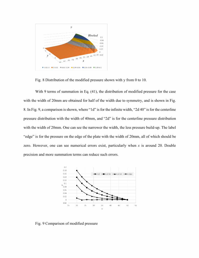
Fig. 8 Distribution of the modified pressure shown with y from 0 to 10.

With 9 terms of summation in Eq. (41), the distribution of modified pressure for the case

with the width of 20mm are obtained for half of the width due to symmetry, and is shown in Fig.

8. In Fig. 9, a comparison is shown, where “1d” is for the infinite width, “2d 40” is for the centerline

pressure distribution with the width of 40mm, and “2d” is for the centerline pressure distribution

with the width of 20mm. One can see the narrower the width, the less pressure build-up. The label

“edge” is for the pressure on the edge of the plate with the width of 20mm, all of which should be

zero. However, one can see numerical errors exist, particularly when x is around 20. Double

precision and more summation terms can reduce such errors.

Fig. 9 Comparison of modified pressure

x

y

Blocked

Solutions of pressure, particularly around the centerline, can be used to validate the boundary

condition treatment of numerical algorithms in the mixed lubrication.

4. Conclusions

Several analytical solutions to lubrication problems with blocked exits have been derived.

They are critical to understand the boundary conditions between solid contact and fluid

lubrication occurring in the mixed/boundary lubrication regimes.

Acknowledgements

The author would acknowledge his family’s financial support during COVID-19, which

make this work possible.

Funding

This research did not receive any specific grant from funding agencies in the public,

commercial, or not-for-profit sectors.

Nomenclature

a = Hertzian contact width in section 2.4 (m)

b = width of the plate in section 2.5 (m)

C, D = integration constants

h = film thickness (m)

h0, hi, h1, h2 = gaps (m)

q = mass flow per unit length (kg/m/s)

p = pressure (Pa)

𝑃 = �L54@ , modified pressure in section 2.5

R = radius (m)

l, l1 = length of a lubrication region (m)

m = slope

u = horizontal velocity of the bottom plate along the x axis (m/s)

F = total force per length (N/m)

x , X = coordinate (m) and its dimensionless value, X = x/a in section 2.4

x0 , x1 = coordinate (m) in section 2.5

α = pressure-viscosity coefficient (Pa-1)

αi, βi, γi, δi = coefficients and right-hand side in the discrete Reynolds equation

αn, βn, Cn = coefficients in the solution of pressure

η = viscosity (Pa·s)

η0 = viscosity at atmospheric pressure (Pa·s)

ρ = density (kg/m3)

Δ = 𝐽'�'𝑌'�I − 𝑌'�'𝐽'�I = 𝐽'(𝛼�𝑥')𝑌'(𝛼�𝑥I) − 𝑌'(𝛼�𝑥')𝐽'(𝛼�𝑥I) 𝜏 = 𝑥'/𝑥I

References

[1] Liu S. On Boundary Conditions in Lubrication with One Dimensional Analytical Solutions.

Tribol Int 2012;48:182–190.

[2] Zhu D, Wang Q. Elastohydrodynamic Lubrication: A Gateway to Interfacial Mechanics -

Review and Prospect. J Tribol 2011;133(4):041001.

[3] Chang L. A Deterministic Model for Line Contact Partial Elastohydrodynamic Lubrication.

Tribol Int 1995;28:75–84.

[4] Jiang X, Hua DY, Cheng HS, Ai X, Lee SC. A Mixed Elastohydrodynamic Lubrication

Model with Asperity Contact. J Tribol 1999;121:481–491.

[5] Zhao JX, Sadeghi F, Hoeprich MH. Analysis of EHL Circular Contact Start Up: Part I—

Mixed Contact Model with Pressure and Film Thickness Results. J Tribol 2001;123:67–74.

[6] Deolalikar N, Sadeghi F, Marble S. Numerical Modeling of Mixed Lubrication and Flash

Temperature in EHL Elliptical Contacts. J Tribol 2008;130:011004-1.

[7] Zhu D, Hu YZ. The Study of Transition from Full Film Elastohydrodynamic to Mixed and

Boundary Lubrication. The Advancing Frontier of Engineering Tribology, Proceedings of the

1999 STLE/ASME H.S. Cheng Tribology Surveillance:150–156.

[8] Hu YZ, Zhu D. A Full Numerical Solution to the Mixed Lubrication in Point Contacts. J

Tribol 2000;122:1-9.

[9] Holmes MJA, Evans HP, Snidle, RW. Analysis of Mixed Lubrication Effects in Simulated

Gear Tooth Contacts. J Tribol 2005;127:61–69.

[10] Li S, Kahraman A. A Mixed EHL Model with Asymmetric Integrated Control Volume

Discretization. Tribol Int 2009;42:1163–1172.

[11] Azam A, Dorgham A, Morina A, Neville A, Wilson M. A simple deterministic

plastoelastohydrodynamic lubrication (PEHL) model in mixed lubrication. Tribol Int

2019;131:520-529.

[12] Wang Y, Dorgham A, Liu Y, Wang C, Wilson M, Neville A, Azam A. An Assessment of

Quantitative Predictions of Deterministic Mixed Lubrication Solvers. J. Tribol, 2021;143(1):

011601.

[13] Johnson KL. Contact Mechanics. Cambridge University Press; 1987.

[14] Morales-Espejel GE, Dumont ML, Lugt PM, Olver AV. A Limiting Solution for the

Dependence of Film Thickness on Velocity in EHL Contacts with Very Thin Films. Tribol

Transactions 2005;48(3):317-327.

[15] Michell AGM. Lubrication of Plane Surfaces. Zeitschrift für Mathematik und Physik, 1905

(Transactions of the Institution of Engineers 1988;12 (3-4):48-62).

[16] Muskat M, Morgan F, Meres MW. The Lubrication of Plane Sliders of Finite Width. J

Applied Physics. 1940;11:208-219.

[17] Hays DF. Plane Sliders of Finite Width. Tribol Transactions, 1958;1 (2):233-240.

[18] Liu S, Mou L. Hydrodynamic Lubrication of Thrust Bearings with Rectangular Fixed-

Incline-Pads. J Tribol, 2012;134 (2):024503

Appendix

A.1 Recurrence relations of Bessel functions

Jn and Yn are the Bessel functions of the first and second kinds, respectively. n is the

order. If S is a representative symbol for these Bessel functions, either Jn or Yn but no mixing,

one has the following relationship,

𝑆�+'(𝑧)+𝑆�&'(𝑧) = ?�µ�(¶)¶ (A.1)

For instance, if n = 1, it is true that

𝑆?(𝑧)+𝑆I(𝑧) = ?µK(¶)¶ (A.2)

One can verify that

𝐽'(𝑧)𝑌I(𝑧) − 𝐽I(𝑧)𝑌'(𝑧) = ?²¶ (A.3)

A.2 Integrals related to Bessel functions

Integrations of multiplications among x and two of these Bessel functions of the first and

second kinds, 𝑆'(𝑥) and𝑇'(𝑥) which can be either 𝐽'(𝑥) or 𝑌'(𝑥), are as follows,

2∫ 𝑆'(𝑥)𝑇'(𝑥)𝑥𝑑𝑥 =𝑥?[𝑆I(𝑥)𝑇I(𝑥) + 𝑆'(𝑥)𝑇'(𝑥)] − 2𝑥𝑆'(𝑥)𝑇I(𝑥) (A.4)

Note if S and T are different functions, the last term can have 2 equivalent options, 𝑆'(𝑥)𝑇I(𝑥) or

𝑆I(𝑥)𝑇'(𝑥).

Also, integrations of multiplications among x and two of these Bessel functions of the

first and second kinds with different variables are as follows,

(𝑎? − 1)∫𝑆'(𝑥)𝑇'(𝑎𝑥)𝑥𝑑𝑥 =𝑥[𝑆I(𝑥)𝑇'(𝑎𝑥) − 𝑎𝑆'(𝑥)𝑇I(𝑎𝑥)] (A.5)

Furthermore,

2∫ 𝑆'(𝑥)𝑥𝑑𝑥 =𝜋𝑥[𝐻I(𝑥)𝑆'(𝑥) − 𝐻'(𝑥)𝑆I(𝑥)] (A.6)

∫ 𝑆'(𝑥)𝑥?𝑑𝑥 =𝑥?𝑆?(𝑥) = −𝑥?𝑆I(𝑥) + 2𝑥𝑆'(𝑥) (A.7)

A.3 Orthogonality of Un

The definition of Un is given in Eq. (40),

𝑈�(𝑥) = 𝐽'(𝛼�𝑥')𝑌'(𝛼�𝑥) − 𝑌'(𝛼�𝑥')𝐽'(𝛼�𝑥) Denote 𝑆e»¡ = 𝑆e(𝛼»𝑥¡) where S can be J and Y, c can be m and n, and a and b are integers, e.g.,

𝐽'�' = 𝐽'(𝛼�𝑥'). The following integrations are of interest,

¼ 𝑥𝑈�(𝑥)𝑈�(𝑥)𝑑𝑥/K/E

= 'z½L ∫ 𝑧[𝐽'�'𝑌'(𝑧) − 𝑌'�'𝐽'(𝑧)][𝐽'�'𝑌'(𝑎𝑧) − 𝑌'�'𝐽'(𝑎𝑧)]𝑑𝑧z½/Kz½/E (A.8)

where 𝑧 = 𝛼�𝑥,𝑎 = 𝛼�/𝛼�.

a. When m n, one can easily use the above integrals, Eq. (A.5) to obtain that

𝛼�? (𝑎? − 1)¼ 𝑥𝑈�(𝑥)𝑈�(𝑥)𝑑𝑥/K/E

= {𝐽'�'𝐽'�'[𝑧𝑌I(𝑧)𝑌'(𝑎𝑧) − 𝑎𝑧𝑌'(𝑧)𝑌I(𝑎𝑧)]

¹

+𝑌'�'𝑌'�'[𝑧𝐽I(𝑧)𝐽'(𝑎𝑧) − 𝑎𝑧𝐽'(𝑧)𝐽I(𝑎𝑧)] −𝐽'�'𝑌'�'[𝑧𝑌I(𝑧)𝐽'(𝑎𝑧) − 𝑎𝑧𝑌'(𝑧)𝐽I(𝑎𝑧)] −𝑌'�'𝐽'�'[𝑧𝐽I(𝑧)𝑌'(𝑎𝑧) − 𝑎𝑧𝐽'(𝑧)𝑌I(𝑎𝑧)]}|z½/Ez½/K ≡ 0 (A.9)

During derivation, boundary conditions at x0 need to be used with 𝛼� and 𝛼�：

𝐽'�'[2𝑌'�I − 𝛼�𝑥I𝑌I�Á] − 𝑌'�'[2𝐽'�I − 𝛼�𝑥I𝐽I�I] = 0 (A.10)

𝐽'�'[2𝑌'�I − 𝛼�𝑥I𝑌I�Á] − 𝑌'�'[2𝐽'�I − 𝛼�𝑥I𝐽I�I] = 0 (A.11)

b. When m = n, one needs the following identities,

𝐽'�"𝑌I�" − 𝐽I�"𝑌'�" = ?²z½/D (A.12)

i can be 0 or 1. With integrals in Eq. (A.4) and Eqs. (A.11-12), it can be shown that,

2𝛼�? ¼ 𝑥𝑈�(𝑥)𝑈�(𝑥)𝑑𝑥/K/E

= ⟨𝐽'�'? 𝑧?[𝑌'?(𝑧) + 𝑌I?(𝑧)] − 2𝐽'�'? 𝑧𝑌I(𝑧)𝑌'(𝑧) −2𝐽'�'𝑌'�'{𝑧?[𝐽I(𝑧)𝑌I(𝑧) + 𝐽'(𝑧)𝑌'(𝑧)] − 2𝑧𝐽'(𝑧)𝑌I(𝑧)} +𝑌'�'? 𝑧?[𝐽'?(𝑧) + 𝐽I?(𝑧)] − 2𝑌'�'? 𝑧𝐽I(𝑧)𝐽'(𝑧)⟩|z½/Ez½/K

= r²L − (𝛼�𝑥I)?Δ? (A.13)

where Δ = 𝐽'�'𝑌'�I − 𝑌'�'𝐽'�I.

A.4 Integration

In order to determine the coefficients of 𝐶�, one has to work out the following

integration,

𝛼�? ∫ 01 − //K6 𝑥𝑈�(𝑥)𝑑𝑥/K/E

= ¼ 𝑧[𝐽'�'𝑌'(𝑧) − 𝑌'�'𝐽'(𝑧)]𝑑𝑧z½/Kz½/E − 1𝑥'𝛼� ¼ 𝑧?[𝐽'�'𝑌'(𝑧) − 𝑌'�'𝐽'(𝑧)]𝑑𝑧z½/K

z½/E

With integrals in Eqs. (A.6-7) and Eqs. (A.11-12), one can find,

𝛼�? ∫ 01 − //K6 𝑥𝑈�(𝑥)𝑑𝑥/K/E = −𝐻'�' + ²? (2𝐻'�I − 𝛼�𝑥I𝐻I�I)Δ + ?² (A.14)

where are the Struve function of order .

nH n

Table 1 Values of coefficients 𝛽�with 𝜏 = 2.5 and their corresponding Struve function results

No. 𝛽� = 𝛼�𝑥I H0(𝛽�) H1(𝛽�) H0(𝛽�𝜏)

1 1.66587424966859 0.76782919939071 0.48821876318662 0.48821876318662

2 3.46654024675250 0.37601360397385 1.08972199199506 1.08972199199506

3 5.44558877655249 -0.22657230036734 0.65110156042030 0.65110156042030

4 7.48347465240147 0.19674126258965 0.38588158606551 0.38588158606551

5 9.54498705593612 0.22794517763496 0.85310481659537 0.85310481659537

6 11.6180079403612 -0.17604478396564 0.67181180541025 0.67181180541025

7 13.6974350624300 0.11741330588462 0.43899940144122 0.43899940144122

8 15.7807779094053 0.17266413295270 0.79431486503444 0.79431486503444

9 17.8666835911315 -0.14927278010559 0.67176218614100 0.67176218614100

Table 2 Values of Bessel functions, Δ functions, and coefficients 𝐶�

No. J1(𝛽�𝜏) Y1(𝛽�𝜏) Δ=𝑈�(𝑥I) Cn

1 -0.126384182 0.374226728 -0.176713193 2.026829781

2 0.271029369 0.019002595 0.107584365 -0.907938617

3 0.061832572 -0.207444222 -0.071688222 0.64467594

4 -0.145289034 -0.113822135 0.052933135 -0.432981319

5 -0.145734404 0.073876444 -0.041762887 0.358690929

6 0.000267714 0.148081195 0.03442302 -0.280510018

7 0.120807429 0.06326472 -0.029252699 0.247211959

8 0.105293443 -0.071089832 0.025421232 -0.207190957

9 -0.01103938 -0.118884304 -0.022471389 0.188438102

Figures

Figure 1

Tilted straight plate, blocked exit

Figure 2

Tilted plate with a step, blocked exit

Figure 3

Cylinder, blocked exit

Figure 4

4a Deformed cylinder. 4b Absolute errors from two approximations of 2R h/a2: with exponents of 1.5(Solid line) and 1.673 (Dashed-line)

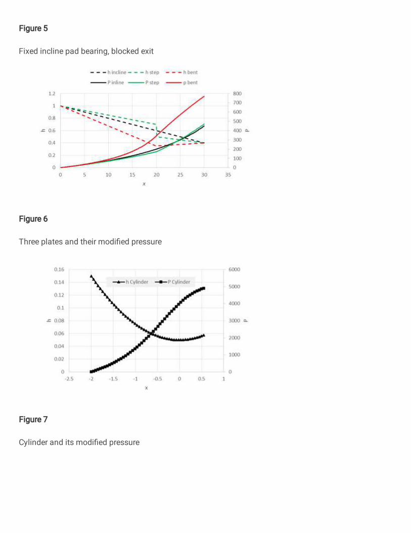
Figure 5

Fixed incline pad bearing, blocked exit

Figure 6

Three plates and their modi�ed pressure

Figure 7

Cylinder and its modi�ed pressure

Figure 8

Distribution of the modi�ed pressure shown with y from 0 to 10.

Figure 9

Comparison of modi�ed pressure