Analytical Solutions of Computer Virus Propagation Model ...

International Journal of Engineering Research and Technology. ISSN 0974-3154, Volume 12, Number 12 (2019), pp. 3006-3017

© International Research Publication House. http://www.irphouse.com

3006

Analytical Solutions of Computer Virus Propagation Model with Anti-virus

Software and Time Dependent Connecting Network in Caputo Fractional

Derivative Sense

T. Korkiatsakul1, S. Koonprasert2 and K. Neamprem3

1 Ph.D., Students, Department of Mathematics, Faculty of Applied Science,

King Mongkut's University of Technology North Bangkok, Bangkok, 10800, Thailand.

2Associate Professor, Department of Mathematics, Faculty of Applied Science,


3Assistant Professor, Department of Mathematics, Faculty of Applied Science,


ORCIDs: 0000-0001-5890-7316 (Korkiatsakul), 0000-0001-5236-033X (Koonprasert)

0000-0003-0930-4943 (Neamprem)

Abstract

Computer viruses and related malware are major problems for

personal and corporate computers and for computer networks.

A common approach to prevent the destructive effects of

viruses on computers is to install anti-virus programs on

individual computers. An alternative approach to prevent the

propagation of viruses in computer networks is to use

mathematical models similar to those developed for

understanding and preventing the spread of epidemics in

human, animal or plant populations. In this paper, we focus on

the fully susceptible, partially susceptible, infectious,

protected (FSSIP) model including Caputo fractional

derivative to study the effect of anti-virus software on

infection in computer networks. We apply the shifted

Chebyshev collocation method to obtain analytical solutions

(series solutions) of the FSSIP model with the virus input into

each group which is time-dependent function due to the

appearance of new viruses and updating of the installed anti-

virus software. This method is simple, efficiency, and accurate

when comparing the numerical results to Runge-Kutta-

Fehlberg method (RKF45) and Cash-Karp method (CK45).

Keywords: Computer viruses, anti-virus programs, Caputo

fractional differential equations, FSSIP model, shifted

Chebyshev collocation method.

I. INTRODUCTION

With the widespread use of the internet, systems running on

networked computers become more vulnerable to digital

threats such as computer viruses, ILOVEYOU, Redcode,

Melissa and Sasser. These threats pose a serious challenge to

information security. Many programmers and anti-virus

software companies currently develop and update anti-virus

programs against the new viruses, but more computer viruses

are continuously created. However, most anti-virus software

currently installed in computers can only offer a temporary

immunity against viruses because of the rapid development of

new viruses and the time lag between the dissemination of the

new virus and the dissemination of updated anti-virus

software. Due to the fact that the development of anti-virus

software often lags behind the appearance of new viruses,

many computers are only partially protected and can be

susceptible to attacks that can cause the loss of millions of

dollars worth of data and loss of productivity. It is therefore

important to understand the way that computer viruses spread

through computer networks and to work out effective defense

measures [1, 2].

In the past several decades, many researchers have used

mathematical models for determining the transmission of

disease as models to study the spread of computer viruses

through computer networks. For example, the SIR classical

epidemic model[3, 4] has been used to develop models for the

spreading and attacking behaviour of computer viruses in

many different phenomena, including virus propagation [1-6],

time delay [2], fuzziness [3], effect of anti-virus software [7,

8], virus immunization [9], vaccination [10], quarantine [11,

12], etc. May et al. [13] studied the dynamical behaviour of

viruses on scale-free networks, and T. Chen et al. [12] studied

the fast quarantining of proactive worms in peer-to-peer (P2P)

computer networks. Z. Wang et al. [14, 15] studied the

robustness of filtering on non-linearities in packet losses,

sensors.

The spread of computer virus phenomenon is unusual and

some computer viruses can spread to ten million computers in

a short time period. These spreads (revolutions) led to use of

mathematical tools based on the derivative and integrals with

integer order, and the differential and difference equations.

Actually, the present moment new spread changes are actually

taking place in modern computer viruses. These changes can

be called a revolution of memory and non-locality. It is

increasingly obvious in computer viruses when their

behaviour may depend on the history of previous changes in

computer viruses. Many researchers try to propose fractional

generalization models which include Riemann–Liouville,

Caputo, Hadamard, Riesz and Grünwald–Letnikov fractional

derivative that improved the computer virus models for

researching processes with memory or history. The suggested

factional models are realized by considering non-integer

fractional order 0 1 instead of positive integer values of . Fractional modelling is a more advantageous approach



3007

which has been used to study the behaviour of diseases or

viruses than the integer derivative model which is local in

nature, while the fractional derivative is global (non-local). In

addition, the fractional derivative is used to increase the

stability region of the system.

In 2014, C.M. A. Pinto and J. A. T. Machado [16] proposed a

fractional model for computer virus propagation which

includes the interaction between computers and removable

devices by numerically simulating the model for distinct

values of the order of the fractional derivative and for two sets

of initial conditions. In 2015, A. H. Handam and A. A.

Freihat [17] modified the epidemiological model for computer

viruses (SAIR) proposed by J. R. C. Piqueira and V. O.

Araujo by fractional derivatives described in the Caputo sense.

In 2016, A. M. A. El-Sayed, A. A. M. Arafa, M. Khalil and A.

Hassan [18] proposed numerical simulations that are used to

show the behaviour of a fractional-order mathematical model

with memory for the propagation of computer virus under

human intervention. In 2017, E. Bonyah, A. Atangana and M.

Khan [19] investigated the analytical solutions of modeling

the spread of computer virus via Caputo fractional derivative

and the Beta‑ derivative solved by the Laplace perturbation

method and the homotopy decomposition technique. In 2018,

J. Singh, D. Kumar, Z. Hammouch and A. Atangana [20]

analyzed a moderate fractional epidemiological model to

describe computer viruses with an arbitrary order derivative

having a non-singular kernel.

Chebyshev method which is a relatively power tool and an

emerging area in mathematical researches is greatly useful for

solving differential equations, fractional differential equations,

integro-differential equations and fractional Volterra integro-

differential equations. The properties of Chebyshev are used

to make the operational matrix which eventually leads to the

coefficient matrix of obtained system. In 2007, G.C.

Malachowski, R.M. Clegg and G.I. Redford [21] proposed

analytic solutions to model exponential and harmonic

functions by using Chebyshev polynomials. In 2015 A. Rivaz,

S. J. Ara and F. Yousef [22] studied two-dimensional

Chebyshev polynomials for solving two-dimensional integro-

differential equations. In 2016, O. B. Arushanyan and S. F.

Zaletkin [23] applied Chebyshev series to approximate

analytic solution of ordinary differential equations. In 2017,

N. Razmjooy and M. Ramezani [24] proposed analytical

solution for optimal control by the second kind Chebyshev

polynomials expansion. Moreover, many mathematical

methods have been proposed for finding analytical solutions

based on transform methods or perturbation methods or

expansions as series of orthogonal functions. The

transformation methods that have been used include Laplace,

Fourier and Mellin transforms [25], the Tau method [26]. The

perturbation methods include the Adomian decomposition

method [27], the variational iteration method [28, 29] and the

Sumudu decomposition method [30]. The methods based on

expansions in orthogonal functions include expansions in

blockpulse functions [31], shifted Chebyshev polynomials

[32], shifted Legendre polynomials [33], Chebyshev wavelets

[34], Legendre wavelets [35] etc.

II. MODEL FORMULATION

In this paper, we propose a fully and partially susceptible,

infectious, protected computer virus propagation model

(FSSIP) in Caputo fractional order- derivative sense, which

was originally studied by B. K. Mishra and S. K. Pandey [36]

(1 )

(1 )

(1 )

.

dSp b SI S dS S P

dt

dSpb S S dS S S I

dt

dIb SI S I dI I I

dt

dPS I dP P

dt

(1)

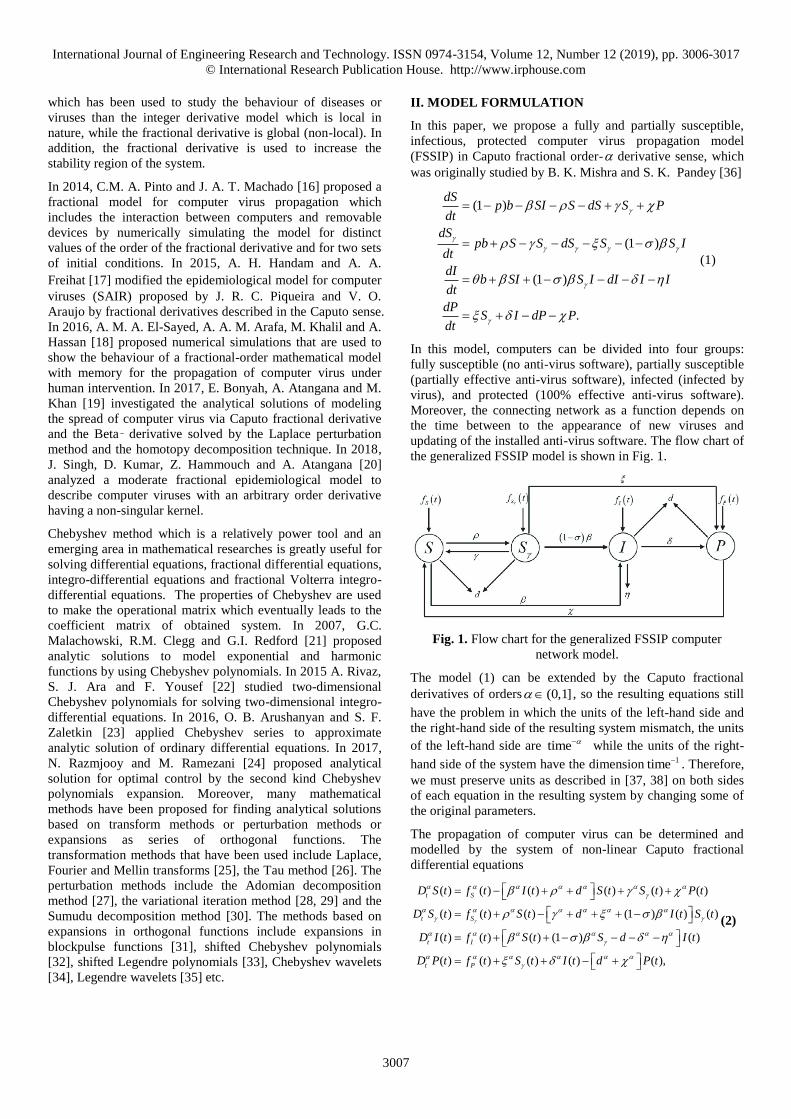
In this model, computers can be divided into four groups:

fully susceptible (no anti-virus software), partially susceptible

(partially effective anti-virus software), infected (infected by

virus), and protected (100% effective anti-virus software).

Moreover, the connecting network as a function depends on

the time between to the appearance of new viruses and

updating of the installed anti-virus software. The flow chart of

the generalized FSSIP model is shown in Fig. 1.

Fig. 1. Flow chart for the generalized FSSIP computer

network model.

The model (1) can be extended by the Caputo fractional

derivatives of orders (0,1] , so the resulting equations still

have the problem in which the units of the left-hand side and

the right-hand side of the resulting system mismatch, the units

of the left-hand side are time while the units of the right-

hand side of the system have the dimension 1time . Therefore,

we must preserve units as described in [37, 38] on both sides

of each equation in the resulting system by changing some of

the original parameters.

The propagation of computer virus can be determined and

modelled by the system of non-linear Caputo fractional

differential equations

( ) ( ) ( ) ( ) ( ) ( )

( ) ( ) ( ) (1 ) ( ) ( )

( ) ( ) ( ) (1 ) ( )

( ) ( ) ( ) ( ) ( ),

t S

t S

t I

t P

D S t f t I t d S t S t P t

D S t f t S t d I t S t

D I t f t S t S d I t

D P t f t S t I t d P t

(2)



3008

with initial conditions (0), (0), (0) and (0),S S I P where ( )tD

is Caputo fractional derivative operator, the value of (0,1]

represents fractional order of Caputo fractional derivative and

the definitions of the variables, parameters, and functions in

the model are given in Table 1.

Table 1. Definitions of parameters and functions in the generalized FSSIP model

Parameter Explanation Units

Sf t Rate of attachment of new fully susceptible S nodes to the network 1minite

( )Sf t

Rate of attachment of new partially susceptible S nodes to the network 1minite

If t Rate of attachment of new infected I nodes to the network 1minite

Pf t Rate of attachment of new fully protected P nodes to the network 1minite

0d Rate at which internal nodes are detached from the network 1minite

0 Rate at which S nodes move to the S group due to installation of anti-virus software 1minite

0 Rate at which S nodes move to the S group due to out-of-date anti-virus software 1minite

0 Rate at which S nodes become infected and move to I group 1minite

0 1 Effectiveness factor of anti-virus software in reducing rate at which S nodes become infected

0 Rate at which S nodes move to P group due to installation of anti-virus software 1minite

0 Rate at which virus is removed from I nodes by anti-virus software and they move to P group 1minite

0 Rate at which I nodes crash due to infection by virus 1minite

0 Rate at which P nodes lose protection and move to S group due to out-of-date anti-virus software 1minite

III. PRELIMINARIES

III.I Caputo fractional Derivative

In this section we introduce some necessary definitions of

Caputo fractional derivative [39].

Definition 1. Let ,n and [ , ]nu C a b . Then the

Caputo fractional derivative of ( )u t is defined by

( )

1

1 ( )( ) ,

( ) ( )

nt

a na

u xD u t dx

n t x

with some properties of Caputo fractional derivatives;

0 is a constant = aD C C (3)

0,

( 1),

(

1 )

aD tt

(4)

where 0 . denotes the largest integer less than

or equal to and is the smallest integer greater than or

equal to .

III.II Existence of solutions for Caputo fractional

differential equation

Theorem 2. Assuming a function f in the initial value

problem of fractional order with (0,1]

0( ) , ( ) , , n

aD u t f t u t u a u u (5)

is continuous and bounded. Then there exists a solution [40].

Theorem 3. The function ( ) [ , ]u t C a b is a solution of the

initial value problem in (5) if and only if it is a solution of the

nonlinear Volterra integral equation

1

( ) 1

00

0

1( ) ( ) ( , ( )) ,

! ( )

km tk

k

tu t u t f u d

k

(6)

where m [40].

III.III Shifted Chebyshev polynomials

Definition 4. Chebyshev polynomials ( )nT s of the first kind

are polynomials in s of degree 0,1,2,3, ,n which are

defined by the relation [41, 42]:

( ) cos( ), where cos( ).nT s n s



3009

This leads to shifted Chebyshev polynomials (of the first kind) *( )nT t of degree n for [0,1]t given by

*( ) ( ) (2 1),n n nT t T s T t

where * *

0 1( ) 1, ( ) 2 1T t T t t and the shifted Chebyshev

polynomials *

1( )nT t

* * *

1 1( ) 2(2 1) ( ) ( ), 1,2,3,n n nT t t T t T t n (7)

The zeros of the shifted Chebyshev polynomials *

1( )NT t are

given by

1 [4( ) 3]

1 cos , 0,1,2, , .2 4( 1)

n

N nt n N

N

(8)

By shifted Chebyshev method, the solution ( )u t can be

expressed in terms of shifted Chebyshev polynomials as

*

0

( ) ( )n n

n

u t a T t

(9)

where the coefficients na are given by

*1

0

00 2

*1

0 2

( ) ( )1,

( ) ( )2, 1 3 2, ,= ,n

n

u t T ta dt

t t

u t T ta dt n

t t

(10)

In practice, the first (N+1)-terms of shifted Chebyshev

polynomials are only considered, so we have an approximate

analytical solution as:

*

0

( ) ( ).N

N

n n

n

u t a T t

(11)

Theorem 5. Let ( )Nu t be approximated by Chebyshev

polynomials as (11) and 0 1 ; then the Caputo fractional

derivative of ( )Nu t is obtained by [43]

( )

,( ( )) ,N n

N k

n n k

n k

D u t a w t

(12)

where ( )

,n kw is given by

2

( )

,

2 ( 1)! ( 1)( 1) .

(2 )!( )! ( 1 )

kn k

n k

n n k kw

k n k k

(13)

III.IV Shifted Chebyshev analytical solution

In the shifted Chebyshev method, the approximate analytical

solution of the FSSIP model can be written as a sum of shifted

Chebyshev polynomials as the form:

(1) * (2) *

0 0

(3) * (4) *

0 0

( ) ( ), ( ) ( ),

( ) ( ), ( ) ( ),

N NN N

n n n n

n n

N NN N

n n n n

n n

S t a T t S t a T t

I t a T t P t a T t

(14)

where the real-numbers ( ) , 1,2,3,4, 0k

na k n N are

unknown coefficients which can be determined later. By

constructing some matrices in (14), we have

( ) * ( ) *

( ) * ( ) *

( ) ( ), ( ) ( ),

( ) ( ), ( ) ( ),

N N

N N

S t t S t t

I t t P t t

1 2

3 4

A T A T

A T A T (15)

where the shifted Chebyshev column vector * * * *

0 1( ) [ ( ) ( ) ... ( )]T

Nt T t T t T tT and the coefficient row

vectors , , ,1 2 3 4

A A A A are defined by

(1) (1) (1) (2) (2) (2)

0 1 0 1

(3) (3) (3) (4) (4) (4)

0 1 0 1

[ ... ], [ ... ],

[ ... ], [ ... ].

N N

N N

a a a a a a

a a a a a a

1 2

3 4

A A

A A(16)

From (7), each term , 1,2,3,...,it i N can be rewritten as the

combination of the shifted Chebyshev functions.

0 *

0

1 1 * *

0 1

2 3 * * *

0 1 2

2 1 *

0

2 ( )

2 (6 4 )

22 ( ), 0 1.

NN N

N k

k

t T

t T T

t T T T

Nt T t t

k

(17)

Define ,( ) [1 ... ]N Tt t tY then it obtains

* * 1( ) ( ), or ( ) ( ),t t t t Y CT T C Y (18)

where the coefficient shifted Chebyshev matrix C is given as

[44]

0

2 1

02 0 0

0

2 22 2 0

,1 0

2

2 22 2

1 0

N N Nk k k

N N

C (19)

and 22 Nk . Therefore, the solutions in (15) can be rewritten

in terms of the product of matrices as

( ) 1 ( ) 1

( ) 1 ( ) 1

( ) ( ), ( ) ( ),

( ) ( ), ( ) ( ).

N N

N N

S t t S t t

I t t P t t

1 2

3 4

A C Y A C Y

A C Y A C Y (20)

Applying the Caputo fractional derivative in (20), we also

construct the operational matrix for the Caputo fractional

derivative of ( )tY as

( ) ( ) ( ),tD t t t

Y B Y

where the Caputo Chebyshev fractional derivative matrix

( )tα

B is given by



3010

0 0 0 0

(2)0 0 0

(2 )

(3)0 0 0( ) .

(3 )

( 1)0 0

)0

( 1

t t

N

N

αB (21)

Now, the Caputo fractional derivatives of each solution are

given by the ( 1) ( 1)N N matrices

( ) 1 ( ) 1

( ) 1 ( ) 1

( ) ( ) ( ), ( ) ( ) ( ),

( ) ( ) ( ), ( ) ( ) ( ).

N N

t t

N N

t t

D S t t t D S t t t

D I t t t D P t t t

1 2

3 4

A C B Y A C B Y

A C B Y A C B Y(22)

Substituting these results into Eq. (2), we have the following

system

1 1 1

1 1 1

1 1 1

1 1

1 1 1

1

( ) ( ) ( ) ( )

( ) ( ) ( ) ( ) ( )

( ) ( ) (1 ) ( ) ( )

( ) ( ) ( ) ( )

( ) ( ) ( ) ( )

(1 ) (

S

S

t t t t

t t d t f t

t t t t

t d t f t

d t t t

t

1 1 3

2 4 1

2 2 3

1 2

3 1 3

2

A C B Y A C Y A C Y

A C Y A C Y A C Y

A C B Y A C Y A C Y

A C Y A C Y

A C Y A C Y A C Y

A C Y1 1

1 1

1 1

) ( ) ( ) ( ) ( )

( ) ( ) ( ) ( )

( ) ( ) ( )

I

P

t t t f t

t t d t

t t f t

3 3

4 4

2 3

A C Y A C B Y

A C B Y A C Y

A C Y A C Y

(23)

with the following initial conditions :

1 1

1 1

(0) (0), (0) (0),

(0) (0), (0) (0),

S S

I P

1 2

3 4

A C Y A C Y

A C Y A C Y (24)

where the matrices , 1,2,3,4i i A in (16),

( ) [1 ... ]N Tt t tY in (18) and the matrix C in (19). The

system in Eq. (23) and initial conditions (24) can be evaluated

at the specific it of the 1N roots

0 1( , , , )Nt t t in Eq. (8).

We next define the ( 1) ( 1)N N matrix , the 1 ( 1)N

matrices ,, , ,S S I PF F F F and an 1 4( 1)N matrix F defined

as follows:

( )

1

( )

1

( )

1

( )

1

( )

1

( ) ( ) ( ) ( ) (

( ) [ (0) ( ) ... ( )],

( ) [ (0), ( ), , ( )],

( ) [ (0), ( ), , ( )],

( ) [ (0), ( ), , ( )],

( ) [ (0), ( ), , ( )],

( ) [ ( ) ( ) ( ) ( =

N

N

N

S S S N

N

S S S N

N

I I I N

N

P P P N

N N N N

S S I P

t t t

t S f t f t

t S f t f t

t I f t f t

t P f t f t

t t t t t

Y Y Y

F

F

F

F

F F F F F) )],N

and we also construct the 4( 1) 4( 1)N N matrices

, ,B C and *T

, ,

B 0 0 00 0 0

0 B 0 00 0 0B

0 0 B 00 0 0

0 0 0 B0 0 0

1 *

1 *

*

1 *

1

= ,

3

3

3

C 0 0 0 T A 0 0 0

0 C 0 0 0 T A 0 0C T

0 0 C 0 0 0 T A 0

0 0 0 C 0 0 0 0

and 1 4( 1)N matrix [ ]1 2 3 4

A A A A A , finally the

system in Eq. (23) can be rewritten in the matrix form as

*

0 1 , A C B T C C F (25)

where I is identity matrix and the matrices 0

and 1

are

given by

0

1

(1 ) (1 ),

( )

( ).

(

(

=)

)

d

d

d

d

I 0 I 0

0 I I 0

0 0 0 0

0 0 0 0

I I 0 0

I I 0 I

0 0 I I

I 0 0 I

Taking transpose, the equation (25) becomes

*

0 1 ,

TT T T T TT T T T

B C C T C A F (26)

which can be solved the matrix TA and then determine the

coefficient matrices , 1,2,3,4i i A in Eq. (16).

IV. SHIFTED CHEBYSHEV APPROXIMATE

ANALYTICAL SOLUTIONS

In this section we applied Shifted Chebyshev method to solve

analytical solutions of the FSSIP model in Eq. (20) with some

fractional orders 0.6,0.8,1 and several types of functions

for connecting network: ( )Sf t , ( )Sf t

, ( )If t , ( )Pf t and

using some parameters in Table 2.

Table 2. Values of parameters used in the numerical

simulations

Parameter Value Parameter Value Parameter Value

b 0.05 p 0.03 d 0.02

0.09 0.07

0

0.03 0 0

0 0.0005 0.5



3011

Case 1. Functions for connecting network are given by

( ) (1 )Sf t p b , ( )Sf t pb

, ( )If t b , ( ) 0Pf t [36]

which mean that the new fully ( )S and partially susceptible

( )S , and infected nodes ( )I connected to the network with

constant rates. Assuming the shifted Chebyshev analytical

solutions ( 6)N of the FSSIP model (2) as

6 6(1) * (2) *

0 0

6 6(3) * (4) *

0 0

( ) ( ), ( ) ( ),

( ) ( ), ( ) ( ).

r r r r

r r

r r r r

r r

S t a T t S t a T t

I t a T t P t a T t

(27)

By shifted Chebyshev method, the zeros of *

6 ( )T t in Eq. (8)

can be calculated as

0 1 2 3

4 5 6

0.0125, 0.1091, 0.2831, 0.5000,

0.7169, 0.8909, 0.9875.

t t t t

t t t

(28)

Calculating 1C in Eqs. (19)–( 21) and the shifted Chebyshev

matrices ( )itY , ( )itB , 0,1, ,6i as

1.0 1.0 1.0 1.0

0.0125 0.1091 0.2831 0.9875

0.0002 0.0119 0.0801 0.9751

,1.9 6 0.0013 0.0227 0.9629

2.5 8 0.0001 0.0064 0.9508

3.0 10 2.0 5 0.0018 0.9389

3.8 12 1.7 6 0.0005 0.9271

e

e

e e

e e

Y

1

0 0 0 0

(2)0 0 0

(2 )

(3)0 0 0( ) ,

(3 )

(7)0 0 0

(7 )

1 0 0 0

1 2 0 0

.1 8 8 0

1 72 840 2048

i it t

αB

C

The symbolic computation of the shifted Chebyshev method

has already developed to compute the coefficients matrices

iA with 1 as

10.1410 15.9771 10.7495 6.4387 1.0234 ,

5.4365 6.9952 2.5502 0.6439 1.0339 ,

10.0527 10.0267 1.5776 0.7105 0.0692 ,

5.3473 0.9537 3.1931 2.2911 0.0880 .

T

T

T

T

1

2

3

4

A

A

A

A

then the shifted Chebyshev approximate analytical solutions

( 6)N which provide a finite series are given by

( ) 2 3 5 4

8 5 10 6

( ) 2 3 5 4

8 5 10 6

( ) 2 3 6 4

( ) 50 3.5049 0.1178 0.0021 2.0 10

9.6575 10 1.8401 10

( ) 10 1.2419 0.0797 0.0018 1.9 10

9.4486 10 1.8590 10

( ) 20 0.1195 0.0126 0.0002 1.8 10

N

N

N

S t t t t t

t t

S t t t t t

t t

I t t t t t

9 5 11 6

( ) 10 2 4 3

7 4 9 5 11 6

7.3821 10 1.2447 10

( ) 6.6521 10 0.5949 0.0102 2.2 10

7.5 10 6.5 10 1.6 10 .

N

t t

P t t t t

t t t

(29)

All graphs of their solutions are shown in Fig 2.

Fig. 2. Shifted Chebyshev solutions with 1 , 00 ,5S

(0) 10,S 0 20,I 00 .P

In Fig. 2, the solution of anti-virus susceptible nodes ( S ) and

protected nodes ( P ) are increasing during short time period

after that decreasing and approaching the equilibrium point

which is an asymptotically stable.



3012

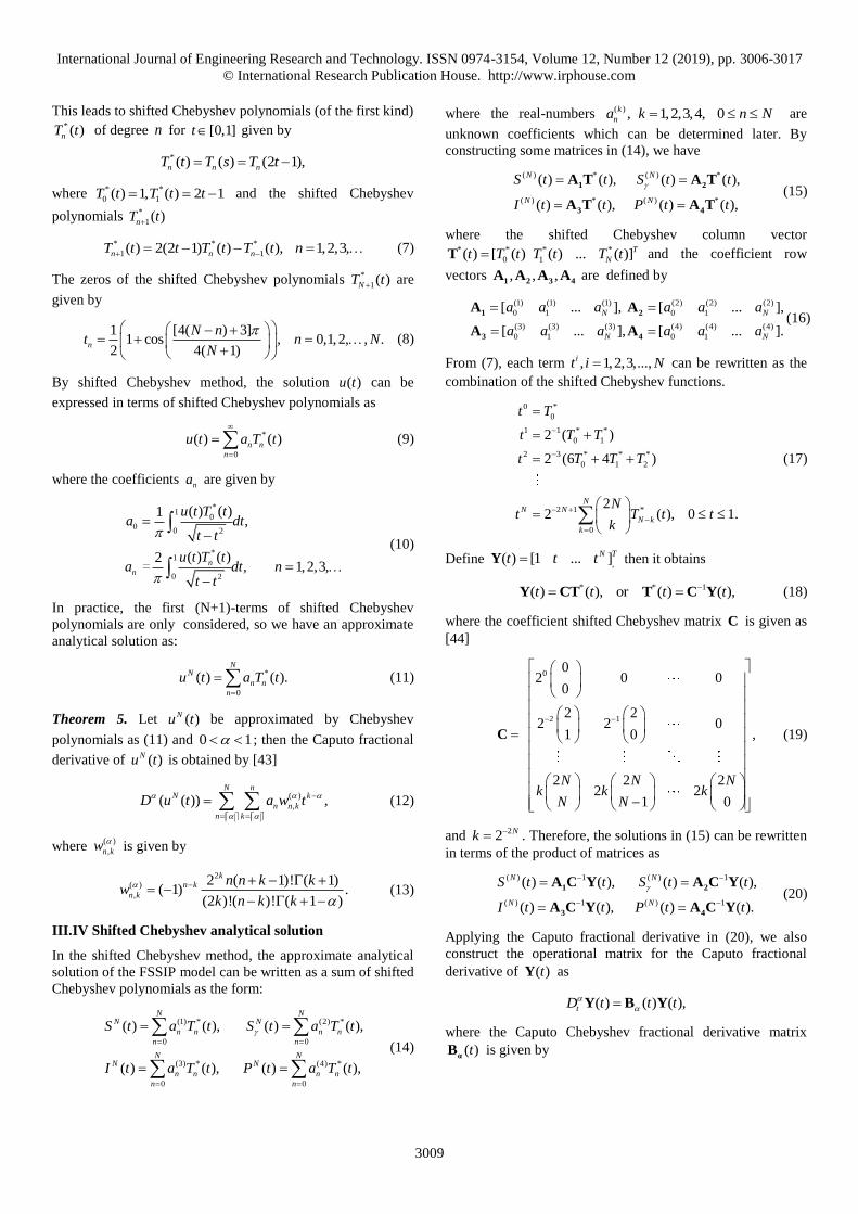
Fig. 3. Shifted Chebyshev solutions for (a) 8,

(b) 15, where 00 ,5S (0) 10,S 0 20,I 00 .P

In Fig. 3, if the function of connecting new infected I nodes

to the network ( ( ) )If t b increases by increasing the value

of 8 and 15. The numerical results show that increasing

the value of will lead to more numbers of computer virus at

infected nodes ( )I t .

The system of non-linear Caputo fractional differential

equations (2) will be used as our model for analysis for order

1 to find equilibrium points of the system. We set

( ), ( ), ( ), ( ) 0t t t tD S t D S t D I t D P t and then solve the obtained

equations for the disease free equilibrium point * * *

0 ( , ,0, ) (0.85869565,0.65652174,0,0.98478261).E S S P

The local stability of 0E determined by modulus of the

eigenvalues are 1 20.019406521, 0.020000001,

3 0.035470131 and 4 0.194529869.

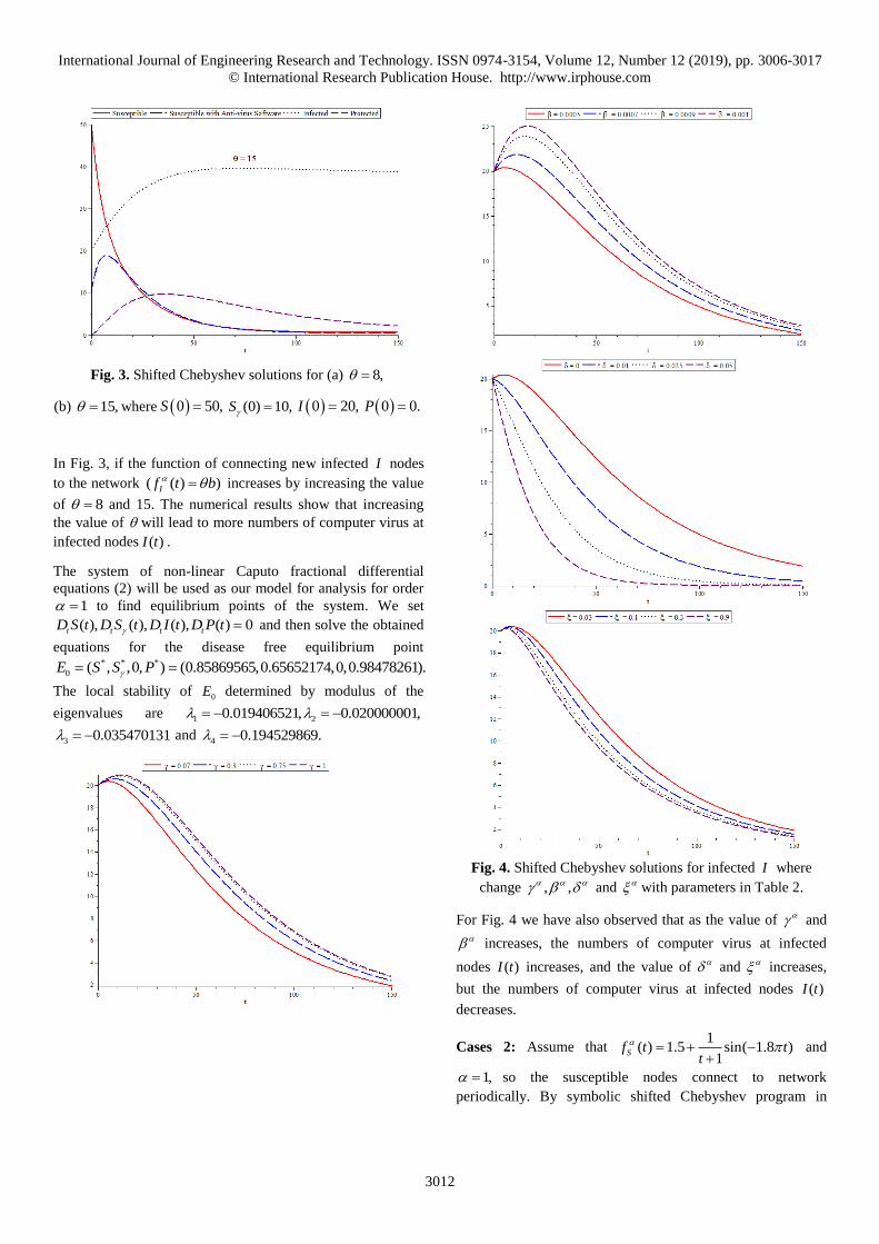
Fig. 4. Shifted Chebyshev solutions for infected I where

change , , and with parameters in Table 2.

For Fig. 4 we have also observed that as the value of and

increases, the numbers of computer virus at infected

nodes ( )I t increases, and the value of and increases,

but the numbers of computer virus at infected nodes ( )I t

decreases.

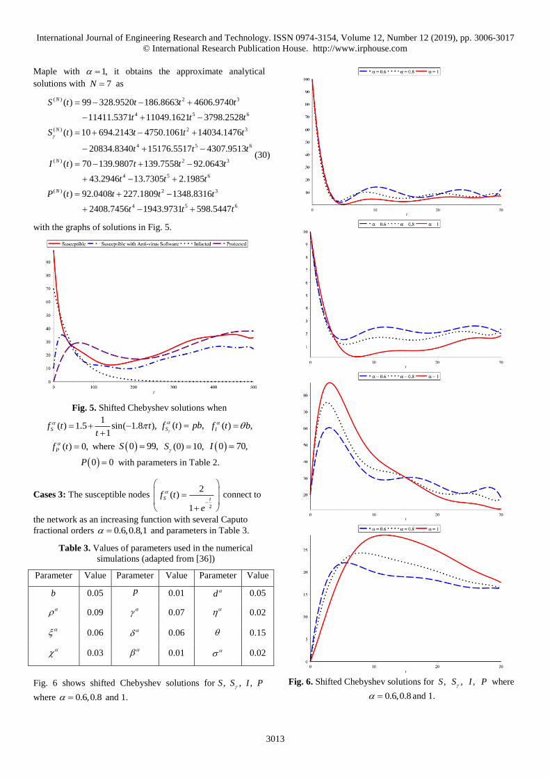
Cases 2: Assume that 1

( ) 1.5 sin( 1.8 )1

Sf t tt

and

1, so the susceptible nodes connect to network

periodically. By symbolic shifted Chebyshev program in



3013

Maple with 1, it obtains the approximate analytical

solutions with 7N as

( ) 2 3

4 5 6

( ) 2 3

4 5 6

( ) 2

( ) 99 328.9520 186.8663 4606.9740

11411.5371 11049.1621 3798.2528

( ) 10 694.2143 4750.1061 14034.1476

20834.8340 15176.5517 4307.9513

( ) 70 139.9807 139.7558 92.

N

N

N

S t t t t

t t t

S t t t t

t t t

I t t t

3

4 5 6

( ) 2 3

4 5 6

0643

43.2946 13.7305 2.1985

( ) 92.0408 227.1809 1348.8316

2408.7456 1943.9731 598.5447

N

t

t t t

P t t t t

t t t

(30)

with the graphs of solutions in Fig. 5.

Fig. 5. Shifted Chebyshev solutions when

1( ) 1.5 sin( 1.8 ),

1Sf t t

t

( ) ,Sf t pb

( ) ,If t b

( ) 0,Pf t where 0 99,S (0) 10,S 0 0,7I

0 0P with parameters in Table 2.

Cases 3: The susceptible nodes

2

2( )

1

S tf t

e

connect to

the network as an increasing function with several Caputo

fractional orders 0.6,0.8,1 and parameters in Table 3.

Table 3. Values of parameters used in the numerical

simulations (adapted from [36])

Parameter Value Parameter Value Parameter Value

b 0.05 p 0.01 d 0.05

0.09 0.07

0.02

0.06 0.06 0.15

0.03 0.01 0.02

Fig. 6 shows shifted Chebyshev solutions for ,S ,S ,I P

where 0.6,0.8 and 1.

Fig. 6. Shifted Chebyshev solutions for ,S ,S ,I P where

0.6,0.8 and 1.



3014

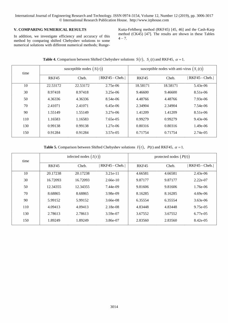
V. COMPARING NUMERICAL RESULTS

In addition, we investigate efficiency and accuracy of this

method by comparing shifted Chebyshev solutions to some

numerical solutions with different numerical methods; Runge-

Kutta-Fehlberg method (RKF45) [45, 46] and the Cash-Karp

method (CK45) [47]. The results are shown in these Tables

4 – 7.

Table 4. Comparison between Shifted Chebyshev solutions ,S t ( )S t and RKF45, 1.

time

susceptible nodes S t susceptible nodes with anti-virus ( )S t

RKF45 Cheb. | RKF45 Cheb. | RKF45 Cheb. | RKF45 Cheb. |

10 22.53172 22.53172 2.75e-06 18.58171 18.58171 5.43e-06

30 8.97418 8.97418 3.25e-06 9.46600 9.46600 8.51e-06

50 4.36336 4.36336 8.54e-06 4.48766 4.48766 7.93e-06

70 2.41071 2.41071 6.45e-06 2.34904 2.34904 7.54e-06

90 1.55149 1.55149 3.27e-06 1.41209 1.41209 8.51e-06

110 1.16583 1.16583 7.65e-05 0.99279 0.99279 9.43e-06

130 0.99138 0.99138 1.27e-06 0.80316 0.80316 1.49e-06

150 0.91284 0.91284 3.57e-05 0.71754 0.71754 2.74e-05

Table 5. Comparison between Shifted Chebyshev solutions ,I t ( )P t and RKF45, 1.

time

infected nodes I t protected nodes ( )P t

RKF45 Cheb. | RKF45 Cheb. | RKF45 Cheb. | RKF45 Cheb. |

10 20.17238 20.17238 3.21e-11 4.66581 4.66581 2.43e-06

30 16.72093 16.72093 2.66e-10 9.87177 9.87177 2.22e-07

50 12.34355 12.34355 7.44e-09 9.81606 9.81606 1.76e-06

70 8.68865 8.68865 3.98e-09 8.16285 8.16285 4.69e-06

90 5.99152 5.99152 3.66e-08 6.35554 6.35554 3.63e-06

110 4.09413 4.09413 2.18e-08 4.83448 4.83448 9.75e-05

130 2.78613 2.78613 3.59e-07 3.67552 3.67552 6.77e-05

150 1.89249 1.89249 3.86e-07 2.83560 2.83560 8.42e-05



3015

Table 6. Comparison between Shifted Chebyshev solutions ,S t ( )S t and CK45, 1.

time

susceptible nodes S t susceptible nodes with anti-virus ( )S t

CK45 Cheb. | CK45 Cheb. | CK45 Cheb. | CK45 Cheb. |

10 22.53172 22.53172 4.02e-06 18.58171 18.58171 5.32e-06

30 8.97418 8.97418 2.10e-06 9.46600 9.46600 1.36e-06

50 4.36336 4.36336 4.32e-07 4.48766 4.48766 3.56e-07

70 2.41071 2.41071 7.43e-06 2.34904 2.34904 5.12e-06

90 1.55149 1.55149 6.57e-06 1.41209 1.41209 5.11e-06

110 1.16583 1.16583 9.11e-05 0.99279 0.99279 4.68e-06

130 0.99138 0.99138 7.54e-06 0.80316 0.80316 6.99e-06

150 0.91284 0.91284 5.53e-05 0.71754 0.71754 3.11e-05

Table 7. Comparison between Shifted Chebyshev solutions ,I t ( )P t and CK45, 1.

time

infected nodes I t protected nodes ( )P t

CK45 Cheb. | CK45 Cheb. | CK45 Cheb. | CK45 Cheb. |

10 20.17238 20.17238 3.45e-10 4.66581 4.66581 1.22e-06

30 16.72093 16.72093 3.18e-10 9.87177 9.87177 3.12e-07

50 12.34355 12.34355 2.75e-09 9.81606 9.81606 6.37e-08

70 8.68865 8.68865 4.31e-08 8.16285 8.16285 2.54e-06

90 5.99152 5.99152 4.87e-08 6.35554 6.35554 3.71e-07

110 4.09413 4.09413 2.69e-07 4.83448 4.83448 4.92e-05

130 2.78613 2.78613 2.54e-07 3.67552 3.67552 5.32e-05

150 1.89249 1.89249 1.86e-07 2.83560 2.83560 5.21e-05

VI. CONCLUSION

Chebyshev method is firstly proposed to provide

approximated analytical solutions of the FSSIP model in

Caputo fractional derivative sense. The method has been

applied to three types of connection, which are based on each

node connecting to the network as a function. Approximate

and analytical solutions of examples are compared. For Case 1,

where each node connects to the network as a constant and

when comparing with present results, it is clear that the results

obtained by the proposed method approaches numerical

solutions which are computed by Runge-Kutta-Fehlberg

method (RKF45) in Table 4 – 5 and Cash-Karp method

(CK45) in Table 6 – 7 with the maximum absolute errors

3.21e -11 and 3.45e-10, respectively. Case 2 presents the

approximated analytical solutions where each node connects

to network as the function 1

1.5 sin( 1.8 ).1

tt

Our method

obtains the solutions in terms of power expansion. Example 3

presents that applications of this method are very simple and

very convenient for solving the Caputo fractional derivative

SSIP model with order 0.6,0.8,1 and the connecting

network as the functions 2

2.

1t

e

The proposed method can

be applied to solve analytical solutions for various fractional

derivatives or other problems.

VII. ACKNOWLEDGEMENT

This research is supported by the Centre of Excellence in

Mathematics, the Commission on Higher Education, Thailand.

This work is also supported by the Department of

Mathematics, Faculty of Applied Science and Graduate

College, King Mongkut's University of Technology North

Bangkok, Thailand.



3016

REFERENCES

[1] N. H. Khanh, N. B. Huy, Stability analysis of a

computer virus propagation model with antidote in

vulnerable system, Acta Mathematica Scientia 36 (1)

(2016) 49–61.

[2] M. Jackson, B. M. Chen-Charpentier, Modeling plant

virus propagation with delays, Journal of

Computational and Applied Mathematics 309

(Supplement C) (2017) 611 – 621.

[3] C. Gan, X. Yang, W. Liu, Q. Zhu, A propagation

model of computer virus with nonlinear vaccination

probability, Communications in Nonlinear Science and

Numerical Simulation 19 (1) (2014) 92 – 100.

[4] Y. Wang, J. Cao, A. Alofi, A. AL-Mazrooei, A. Elaiw,

Revisiting node-based sir models in complex networks

with degree correlations, Physica A: Statistical

Mechanics and its Applications 437 (Supplement C)

(2015) 75 – 88.

[5] I. M. Foppa, A Historical Introduction to Mathematical

Modelling of Infectious Diseases: Seminal Papers in

Epidemiology, Academic Press, 2016.

[6] M. Jackson, B. M. Chen-Charpentier, A model of

biological control of plant virus propagation with

delays, Journal of Computational and Applied

Mathematics 330 (Supplement C) (2018) 855 – 865.

[7] L.-X. Yang, X. Yang, A new epidemic model of

computer viruses, Communications in Nonlinear

Science and Numerical Simulation 19 (6) (2014) 1935

– 1944.

[8] Y. Yao, L. Guo, H. Guo, G. Yu, F. X. Gao, X. J. Tong,

Pulse quarantine strategy of internet worm

propagation: Modelling and analysis, Computers &

Electrical Engineering 38 (5) (2012) 1047 – 1061,

special issue on Recent Advances in Security and

Privacy in Distributed Communications and Image

processing.

[9] L. Chen, D. Wang, An improved acquaintance

immunization strategy for complex network, Journal of

Theoretical Biology 385 (Supplement C) (2015) 58 –

65.

[10] J. Shukla, G. Singh, P. Shukla, A. Tripathi, Modeling

and analysis of the effects of antivirus software on an

infected computer network, Applied Mathematics and

Computation 227 (Supplement C) (2014) 11 – 18.

[11] T. Easton, K. Carlyle, C. Scoglio, Optimizing

quarantine regions through ellipsoidal geographic

networks, Computers & Industrial Engineering 80

(Supplement C) (2015) 145 – 153.

[12] T. Chen, X. S. Zhang, H. Li, X. D. Li, Y. Wu, Fast

quarantining of proactive worms in unstructured P2P

networks, Journal of Network and Computer

Applications 34 (5) (2011) 1648 – 1659, dependable

Multimedia Communications: Systems, Services, and

Applications.

[13] R. M. May, A. L. Lloyd, Infection dynamics on scale-

free networks, Physical Review E 64 (6) (2001)

066112.

[14] Z. Wang, B. Shen, X. Liu, H1 filtering with randomly

occurring sensor saturations and missing

measurements, Automatica 48 (3) (2012) 556–562.

[15] J. Hu, Z. Wang, H. Gao, Probability-guaranteed H1

finite-horizon filtering with sensor saturations, in:

Nonlinear Stochastic Systems with Network-Induced

Phenomena, Springer, 2015, pp. 101–118.

[16] C. Pinto, J. T. Machado, Fractional dynamics of

computer virus propagation, Mathematical Problems in

Engineering 2014.

[17] A. H. Handam, A. A. Freihat, A new analytic numeric

method solution for fractional modified

epidemiological model for computer viruses.,

Applications & Applied Mathematics 10 (2).

[18] A. El-Sayed, A. Arafa, M. Khalil, A. Hassan, A

mathematical model with memory for propagation of

computer virus under human intervention, Progr. Fract.

Differ. Appl 2 (2016) 105–113.

[19] E. Bonyah, A. Atangana, M. A. Khan, Modelling the

spread of computer virus via caputo fractional

derivative and the Beta-derivative, Asia Pacific Journal

on Computational Engineering 4 (1) (2017) 1.

[20] J. Singh, D. Kumar, Z. Hammouch, A. Atangana, A

fractional epidemiological model for computer viruses

pertaining to a new fractional derivative, Applied

Mathematics and Computation 316 (2018) 504–515.

[21] G. C. Malachowski, R. M. Clegg, G. I. Redford,

Analytic solutions to modelling exponential and

harmonic functions using Chebyshev polynomials:

fitting frequency-domain lifetime images with

photobleaching, Journal of microscopy 228 (3) (2007)

282–295.

[22] A. Rivaz, F. Yousefi, S. J. Ara, Two-dimensional

Chebyshev polynomials for solving two-dimensional

integro-differential equations, Cankaya Universitesi

Bilim ve Muhendislik Dergisi 12 (2).

[23] O. B. Arushanyan, S. F. Zaletkin, The use of

Chebyshev series for approximate analytic solution of

ordinary differential equations, Moscow University

Mathematics Bulletin 71 (5) (2016) 212–215.

[24] N. Razmjooy, M. Ramezani, Analytical solution for

optimal control by the second kind Chebyshev

polynomials expansion, Iranian Journal of Science and

Technology, Transactions A: Science 41 (4) (2017)

1017–1026.

[25] S. Kazem, Exact solution of some linear fractional

differential equations by Laplace transform,

International Journal of nonlinear science 16 (1) (2013)

3–11.

[26] T. Allahviranloo, Z. Gouyandeh, A. Armand,

Numerical solutions for fractional differential

equations by Tau-collocation method, Applied

Mathematics and Computation 271 (2015) 979–990.

[27] B. Ibis¸, M. Bayram, Numerical comparison of

methods for solving fractional differential–algebraic

equations (fdaes), Computers & Mathematics with

Applications 62 (8) (2011) 3270–3278.



3017

[28] B. Ibis, M. Bayram, Numerical comparison of methods

for solving fractional differential–algebraic equations

(fdaes), Computers & Mathematics with Applications

62 (8) (2011) 3270–3278.

[29] V. Turut, N. Guzel, On solving partial differential

equations of fractional order by using the variational

iteration method and multivariate Pade

approximations, European Journal of Pure and Applied

Mathematics 6 (2) (2013) 147–171.

[30] K. Al-Khaled, Numerical solution of time-fractional

partial differential equations using Sumudu

decomposition method, Rom. J. Phys 60 (1-2) (2015)

99–110.

[31] S. Mashayekhi, M. Razzaghi, Numerical solution of

nonlinear fractional integro-differential equations by

hybrid functions, Engineering Analysis with Boundary

Elements 56 (2015) 81–89.

[32] S. Nemati, S. Sedaghat, I. Mohammadi, A fast

numerical algorithm based on the second kind

Chebyshev polynomials for fractional integro-

differential equations with weakly singular kernels,

Journal of Computational and Applied Mathematics

308 (2016) 231–242.

[33] M. Pakdaman, A. Ahmadian, S. Effati, S. Salahshour,

D. Baleanu, Solving differential equations of fractional

order using an optimization technique based on

training artificial neural network, Applied Mathematics

and Computation 293 (2017) 81–95.

[34] A. Gupta, S. S. Ray, Numerical treatment for the

solution of fractional fifth-order Sawada–Kotera

equation using second kind Chebyshev wavelet

method, Applied Mathematical Modelling 39 (17)

(2015) 5121–5130.

[35] M. Yi, L. Wang, J. Huang, Legendre wavelets method

for the numerical solution of fractional integro-

differential equations with weakly singular kernel,

Applied Mathematical Modelling 40 (4) (2016) 3422–

3437.

[36] B. K. Mishra, S. K. Pandey, Effect of anti-virus

software on infectious nodes in computer network: a

mathematical model, Physics Letters A 376 (35)

(2012) 2389–2393.

[37] R. Magin, X. Feng, D. Baleanu, Solving the fractional

order Bloch equation, Concepts in Magnetic

Resonance Part A: An Educational Journal 34 (1)

(2009) 16–23.

[38] Y. Cho, I. Kim, D. Sheen, A fractional-order model for

MINMOD millennium, Mathematical biosciences 262

(2015) 36–45.

[39] I. Podlubny, Fractional differential equations: an

introduction to fractional derivatives, fractional

differential equations, to methods of their solution and

some of their applications, Vol. 198, Elsevier, 1998.

[40] K. Diethelm, The analysis of fractional differential

equations: An application-oriented exposition using

differential operators of Caputo type, Springer Science

& Business Media, 2010.

[41] P. J. Davis, Interpolation and approximation, Courier

Corporation, 1975.

[42] J. C. Mason, D. C. Handscomb, Chebyshev

polynomials, CRC Press, 2002.

[43] A. Ali, N. H. M. Ali, On numerical solution of multi-

terms fractional differential equations using shifted

Chebyshev polynomials, International Journal of Pure

and Applied Mathematics 120 (1) (2018) 111–125.

[44] Y. Ozturk, M. Gulsu, Numerical solution of a modified

epidemiological model for computer viruses, Applied

Mathematical Modelling 39 (23) (2015) 7600–7610.

[45] A. Romeo, G. Finocchio, M. Carpentieri, L. Torres, G.

Consolo, B. Azzerboni, A numerical solution of the

magnetization reversal modelling in a permalloy thin

film using fifth order Runge–Kutta method with

adaptive step size control, Physica B: Condensed

Matter 403 (2) (2008) 464–468.

[46] J. H. Mathews, K. D. Fink, et al., Numerical methods

using MATLAB, Vol. 4, Pearson London, UK:, 2004.

[47] K. E. Niemeyer, C.-J. Sung, Accelerating moderately

stiff chemical kinetics in reactive-flow simulations

using gpus, Journal of Computational Physics 256

(2014) 854–871.

Analytical Solutions of Computer Virus Propagation Model ...

Documents

Transcript of Analytical Solutions of Computer Virus Propagation Model ...