1

Analytical Solution of Governing Equations of Triple Coupled Physics of Structural

Mechanics, Diffusion, and Heat Transfer

E. Mahdavia, M. Haghighi-Yazdi

a, M. Baniassadi

a,b*, M.Tehrani

c. S. Ahzi

b,d, J. Jamali

e

a School of Mechanical Engineering, Faculty of Engineering, University of Tehran, P. O. Box 1155-4563, Tehran,

Iran, m.baniassadi@ut.ac.ir, phone: (+98)9181621480 bUniversity of Strasbourg, ICube laboratory-CNRS, 2 Rue Boussingault, 67000 Strasbourg,

CS 10413, F-67412 Illkirch Cedex, France, contact@icube.unistra.fr , phone: +33 (0)3 68 85 45 54 c Department of Mechanical Engineering, University of New Mexico, Albuquerque, NM 87131-0001, USA

mtehrani@unm.edu, Phone: (+1)505.277.6298 dQatar Environment and Energy Research Institute, Hamad Bin Khalifa University, Qatar Foundation, PO Box

5825, Qatar eMechanical Department, Shoushtar Branch, Islamic Azad University, Shoushtar, P.O. BOX 6451741117, Iran

Abstract

Transport pipes have been widely used for their several advantages including their cost-

effectiveness and simplicity of installation. These pipes are constantly in contact with the

flowing fluid and therefore pipe’s material properties may degrade due to the diffusion of the

fluid into the material system. These conditions are exacerbated as a result of high pressure and

temperature of the transported fluid. Therefore, to simulate the behaviour of such pipes, three

interactive phenomena of mechanical stress, heat transfer and mass diffusion need to be

investigated. This study considers the three mechanisms simultaneously and provides an

analytical solution to the corresponding coupled governing equations. The results of this work

are in good agreement with the results of double coupled physics available in the literature and

therefore can be used to predict the material behaviour under complicated environmental

conditions.

Key Words: fully coupled, diffusion, thermomechanical process, analytical solution, constitutive

laws

Symbol Definition

C Concentration

CV Specific heat at constant strain and normalized concentration (J/kg.K)

cg Gas normalized concentration

cp Polymer normalized concentration

D Defined as a function of coefficients ρ, D and kμ (m2/s

2)

D Diffusivity(m2/s

2)

d Linking coefficient of effect of temperature variation (concentration variation)

on the chemical potential

E Young coefficient (Pa)

2

𝑓 Body force per unit of mass (N/kg)

J Heat flux per unite area (J/m2.s)

Jm̅g Relative mass flux of the gas phase (kg/m2s)

Jq̅ Heat flux per unit area (J/ m2s)

K Kinematic energy

kμ Linking of the chemical potential gradient effect on the gas mass flux (kg.s/m3)

kT Represents the thermal gradient effect on the entropy flux (W/m.K2)

Pin Input power from the environment (J)

𝐪 Heat flux (J/s)

r Volume density of heat generated by an outer source (J/m3.s)

s Specific entropy (J/kgK)

Sg Solubility (1/Pa)

T(X, t) Absolute temperature (K)

u Displacement (m)

U Potential energy (J)

v̇ Acceleration (m/s2)

W Work

CTμ Coupling coefficient corresponding to the temperature (kg.s/m3)

𝛂(X, t) Internal state vector

σ Cauchy stress tensor (Pa)

ρ Average density of the mixture (kg/m3)

Ω Free energy

Ω0 Initial energy

λ,μ Lame elastic coefficients

αC Coefficient of mass transfer

αT Coefficient of thermal expansion (1/K)

ν Poisson coefficient

αi(X, t) Internal state variable

μi Mass chemical potential (J/kg) or the ith

species

ti Traction

σij Stress Tensor (Pa)

εij Strain tensor

βij Thermoelastic tensor

βij′ Diffusion tensor

Tij Stress tensor (Pa)

Cijkl Elastic tensor

Tr Trace operator

Γ Area Boundary

3

Ω Volume Boundary

Λ Thermal conductivity (J/m.s.K)

div [∎] Divergence operator

Grad {∎} Gradient operator with respect to the reference

grad {∎} Gradient operator with refers to the current displacement

1. Introduction

Transportation and storing of refined or crude petroleum products including oil and natural

gas have been carried out by pipeline systems and vessels for many years. This method ensures

using a safe means of transporting fluids while providing a cost-effective facility. Gas pipes and

vessels are made from steel coated with anti-corrosion materials or polymer materials that are

usually corrosion resistant. The material system is usually designed to withstand different

irreversible damage mechanisms caused by high temperature and pressurized fluid. Depending

on the fluid-polymer system and operating thermal conditions, damage appears either locally [1]

or in a diffuse way [1]. Because of the contact between fluid and the material system the

phenomenon of diffusion may also occur.

Diffusion can cause gradual degradation in material properties but its effects become more

sever when coupled with mechanical loading and temperature variations. It is known that

coupling between the three physics of diffusion, structural mechanics and heat transfer makes the

prediction of material’s behavior more complicated. Therefore, without having a suitable model,

it is difficult to analyze such problems and determine parameters such as interactions between

the fluid and the material system, procedure of diffusion, and intergranular fracture. To

understand the fully coupled thermal, mechanical and diffusive mechanisms, it is essential to

know constitutive laws and coupling mechanisms between the material and the fluid. The

constitutive equations and interactions can also be described as a function of temperature,

diffusant concentration, and fluid pressure using thermodynamic equations so that the material

behaviour is characterized.

There are various researches in open literature that involve coupled physics using two

different approaches including theoretical and experimental studies. In both methods, a number

of studies include dual coupled physics and some others include triple and quadruple problems.

For instance, in dual coupling studies, Vijalapura and Govindjee [2] proposed a coupled

diffusion-deformation mechanism. Their research focuses on numerical simulation of the

mechanism by using the balance laws to develop partial differential equations and to solve these

nonlinear equations using finite element and finite difference methods. Holalkere et al. [3]

studied moisture and hygrothermal stress evaluated by fracture mechanics and finite element

analysis on polymers. In their study, plastic package delamination was evaluated in order to

obtain moisture sensitivity of plastic encapsulated microcircuits.

Govindjee and Simo [4] worked on coupling which can happen in diffusive-mechanical

problems and later, Busso and Cailletaud [5] mentioned the interactions between mechanics and

4

oxidation. Klopffer and Flaconeche [6] mentioned the diffusion process which is a function of

conce

ntration. This phenomenon happens when a polymer material is plasticized by the penetrant.

Teh et al. [7] described the effect of the coefficient of moisture expansion mismatch. They used

finite element method to study this effect on hygroscopic swelling stress.

Abdel Wahab et al. [8] investigated the behaviour of diffusion in adhesively bonded carbon

fibre polymer composites. The research analyzed a nonlinear transient moisture problem using

finite element model to evaluate moisture concentration as input data in stress analysis. Then, a

comparison was made between analytical solution and the obtained results which indicated the

thinner adhesive layer agrees well with the analytical solutions. Wong et al. [9] discussed finite

element modeling in electronic multi-material packages with definite temperature and humidity

as boundary conditions to solve the coupled diffusion and thermal processes. This simulation

was performed based on experimental results.

Also Yu and Pochiraju [10] studied the coupled phenomena in polymer composite materials

considering temperature-dependent diffusion coefficients. Shirangi et al. [11] proposed another

numerical method to obtain residual moisture content in modeling of components and IC

packages.

Similarly, triple coupled physics were investigated by some authors such as Lin and Tay[12].

They used finite element method to predict delamination occurring in hygroscopic and thermal

stresses in IC packages. Moreover, Yi and Sze [13] described moisture distribution and residual

stress in IC packages which are affected by temperature and moisture. Moreover, Chang et al.

[14] explained moisture diffusion in plastic ball grid array packages while neglecting residual

stresses. A similar study was done by Lahoti et al. [15] to conduct a three dimensional finite

element analysis of flip chip ball grid array packages. Viscoelastic behaviour of polymeric

components was studied by Dudek et al.[16]. Fan and Zhao [17], also proposed sequential

coupled equations including moisture diffusion, heat conduction and material deformation in

encapsulated microelectronics devices. Their study was later extended by Rambert et al. [1] to

develop a fully coupled mechanical-diffusion-thermal model.

There are also some experimental studies such as the works of Briscoe et al.[18, 19], Campion

(1990), and Liatsis [20] which confirm the existence of a strong coupling between mechanical,

thermal and diffusion procedures. Some studies also include both theoretical and experimental

investigations of the coupled physics such as the recent work of Haghighi-Yazdi and Lee-

Sullivan [21].

One of the most complete models studying triple coupled physics has been proposed by

Rambert et al. [1] and includes the effective factors simultaneously. Rambert and collaborators

[1] have suggested a fully coupled mechanical-diffusion-thermal model which was developed

based on finite element analysis. They used a representative volume element (RVE) to illustrate

thermo-diffuso-mechanical behavior of polymers. The considered RVE is the simplest one

including a homogenous mixture of polymer and gas. This RVE is also explained in the

thermodynamics of continuous media with internal variables. Therefore, the material

5

characteristics have constant values. The considered RVE, however, does not include all

sophisticated thermomechanics coupled with diffusion properties. Therefore, Rambert et al. [1]

analyzed the problem in micro-scale, where there exist different kinds of RVE depending on

types of materials and considering how diffusion happens, as follows:

1. Monophasic modeling divided into three categories such as Homogeneous Mixture,

Saturated Porous Medium with an Impermeable Skeleton and Porous Medium with a

Permeable Skeleton. This is suitable for amorphous materials.

2. Biphasic modeling divided into two categories of Unsaturated Porous Medium with an

Impermeable Skeleton and Unsaturated Porous Medium with a permeable Skeleton. This

is suitable for modeling the polymer mechanical behaviour.

Moreover, this RVE is an open system and thus exchanges heat as well as matter with the

surrounding medium. In addition, the material is assumed to be isotropic and is studied in the

framework of small perturbations. Finally, a strong assumption which consists of keeping

constant each RVE characteristic in time and space was made. To analyze this kind of situation

means that thermo-diffuso-mechanical models describing micro and nanoscale are suitable [22].

Rambert and Grandidier [23] and Rambert et al. [1] extended the model further to include

gradient-type elasticity. To the best of the authors’ knowledge, there is no work in open literature

on quadruple coupled physics.

Classical continuum mechanics has usually been employed by most researchers to develop the

coupled physics. However, classical continuum mechanics can only describe bulk materials

without considering surface effect, which can have significant influence on constitutive

equations. Therefore, to consider the effect of surfaces in continuum mechanics, some additional

parameters should be added to the conventional theorems of continuum mechanics. Moreover,

considering surfaces plays a significant role in affecting the properties of the bulk material

exposed to humid environments which cause the initiation of diffusion and subsequent possible

chemical reactions. To analyze the effect of surfaces and obtain constitutive laws, some

investigations [24, 25] have been conducted in different approaches to describe the surface effect

based on Helmholtz energy. This energy is separated into two parts for the surface and the bulk

material to explain their interactions [24, 25]. A number of studies deal with multi-physics and

describe their constitutive equations and material’s responses. Different modeling approaches

have been proposed such as in the work of McBride et al. [22] who proposed a model at the

micro- and nano-scales. This is while some other investigations tried to explain size-dependent

response of materials such as the works of Duan et al.[26], Miller and Shenoy [27],

Mitrushchenkov et al. [28], She and Wang [29], Wei et al.[30], and Yvonnet et al.[31]

Some studies considered material surface effects on the mechanical and thermal descriptions

[32-35]. Gurtin and Murdoch [32] described surface stress in elastic media. They used

kinematics and balance laws for the surface to explain tensorial nature of surface tension. This

research was then extended by adding the thermal effect by Angenent and Gurtin [33].Gurtin and

Struthers [35] employed a novel description of surface effect to show the role of surface

separating distance phases.

6

Daher and Maugin [36] proposed a method to obtain equations for interface in

thermomechanical solid and therefore described complicated situations. Dolbow et al. [37]

mentioned swelling of a hydrogel which deals with finite deformation. Their work was further

extended through considering thermal effects by Ji et al. [38].Yi and Duan [39] described

adsorbate interactions in nanoscale and also explained the mechanical properties of this

phenomenon. Studies such as the work of Steinmann [40] continued further to include nonlinear

continuum thermomechanics, diffusion, and viscoelasticity.

Moreover, the main purpose of such studies is to obtain governing equations to create a

precise model. Therefore, it is required to have a model which is capable of representing three

coupled equations including diffusion, mechanical stress-strain, and thermal effects.

As mentioned earlier, many investigations have been conducted to understand the mechanism

of interaction of a fluid and the material system. There are, however, some restrictions to

problem analysis due to the existence of coupling between mechanical and thermal physics. For

example, Rodier-Renaud [41] proposed isobaric expansion coefficient as a function of

temperature for polyethylene but difficulty in doing tests makes such experimental study

impossible. Cunat [42] considered direct couplings while taking into account specific free energy

and internal dissipation phenomena such as mechanical, thermal and diffusion mechanisms.

Therefore, to model the behaviour of a polymer exposed to a gaseous environment with high

pressure and temperature, the interactions of three physical phenomena should be considered

from modeling point of view. The interactions should include both direct and indirect coupling.

There are usually two kinds of methods employed in the open literature to analyze the

problems involving dual, triple, and quadruple coupled physics: semi-coupled analysis and fully-

coupled analysis. One of the studies which employed the fully-coupled analysis method is the

work of Rambert et al. [1]. However, the studies conducted by these authors are limited to

numerical studies and to the best of our knowledge, there is no work in the open literature

including the analytical solution of fully-coupled problems. Therefore, a complete model is

required which can include simultaneously the effects of the three mechanisms on material

properties and also different interactions. Using mathematical method to solve the triple coupled

equations can also provide a closed-form solution which is preferable to numerical methods.

In this study, an analytical solution to the coupled mechanisms of diffusion, structural

mechanics, and heat transfer is developed. The development of governing equations, which is

based on the model proposed by Rambert et al. [1], is first explained. Next, an attempt is made to

solve the equations analytically using Hankel transforms. The obtained closed-form solution is

then used to investigate the effects of different coupling coefficients.

2. Constitutive law and concepts

To obtain an analytical solution to the full interaction between mechanical, thermal and

diffusion phenomena, some concepts need to be known about constitutive laws. These are

described in many existing works like Fosdick and Tang [43], Gurtin and Murdoch [32], Gurtin

7

and Struthers [35], Steinmann [40]. Below, the two concepts of deformation and internal

variables are briefly described.

2.1.Deformation

As mentined before, it is important to consider the assumptions of both surface and bulk

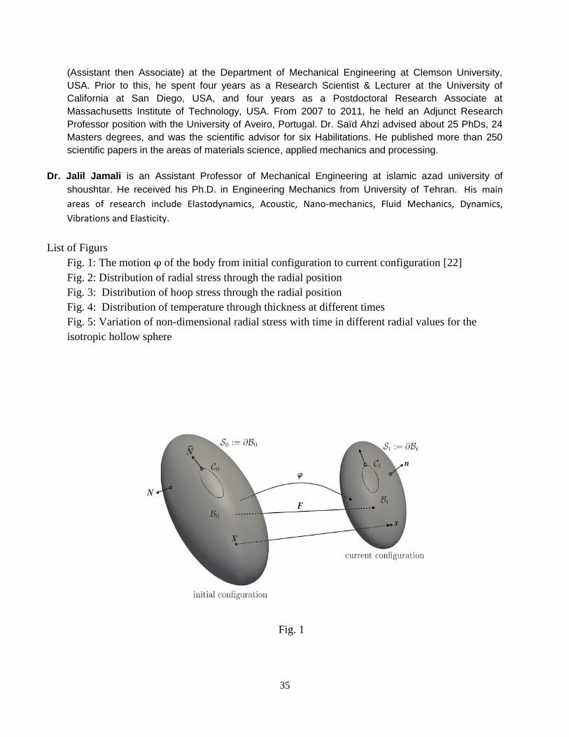
effects in a continuum such as the one shown schematically in Fig. 1[22], which depicts material

particles as point 𝑿 that is related to body 𝑩𝟎. Also, the surface is denoted by 𝑺𝟎 and 𝑵 shows

the unit normal to 𝑺𝟎 (see [22] for further details).

Fig. 1: The motion φ of the body from initial configuration to current configuration [22]

Also, in order to map d𝐗 to dx, the following mapping function is introduced[22, 44]. To define

the mapping as derivative of the motion with respect to the reference placement, they used:

F(X,t) = Grad (X, t) (1)

Where the invertible tangent map F: Tβ0 ⟶ Tβt (that is, the deformation gradient) maps a line

element d𝐗ϵ Tβ0 in the reference configuration to a line element d𝐱 ϵ Tβt in the current

configuration. The notation T{∎} denotes the tangent space to {∎} . Also, Grad {∎} =

∂{∎}/ ∂𝐗 is the gradient operator with respect to the reference placement and grad {∎} =

∂{∎}/ ∂𝐱 refers to the current displacement (as shown in Fig. 1). Therefore, to map other

parameters such as the absolute temperature T(𝐗, t) > 0 , F(X,t) maps Grad𝜃 to grad𝑇 as

follows[22, 44]: TGradT=F gradT (2)

2.2.Internal variables

To include all parameters that may change during mechanical and chemical phenomena, the

introduction of some internal variables are necessary to describe thermomechanical equations.

It is therefore assumed that there exists a function as follows [44]:

i i 1 N=f (T,F,gradT, , ) , i=1 N

(3)

Where 𝛂is the internal state vector,1 2 N= (X,t)=( , , , ) , and the number = (X,t)i i are

the internal state variables. Finding logical relation through thermodynamical conditions

governed by Clausius-Duhem inequality between different parameters in Eq. (3) is important.

3. Coupled Triple phenomena

As mentioned before, Rambert et al. [1] suggested a model that involves triple coupled

physics and Rambert and Grandidier [23] extended this investigation but they did not solve the

equations analytically.

8

Moreover, the RVE was modeled with some characteristics such as RVE being assumed as an

open system which therefore, trades heat as well as matter with the surrounding medium. In

addition, the material was assumed to be isotropic and was studied in the framework of small

perturbations [45]. Finally, they considered a strong assumption by keeping constant each RVE

characteristic with respect to time and space. Fick’s type law dominates diffusion which is driven

by concentration gradients.

Among the diffusion models described by Rambert et al [1], a model was selected that implies

complicated descriptions of the RVE by coupling three phenomena of diffusion, mechanical

behavior and thermal condition. The diffusion model was related to a semi-crystalline polymer as

a porous medium. Some researchers such as Michaels and Bixler [46, 47] proposed diffusion in

this kind of material. Therefore, the mixture framework was chosen to develop the thermo-

diffuso-mechanical model.

4. Equation Development

To model the coupled equations using free and dissipative energy, internal variables

representing the material are introduced according to Eq. (3). Some parameters such as stress,

entropy and chemical potential are thermodynamic forces; and strain, temperature, and

normalized concentration are known as dual variables which are linked by specific free energy.

On the other hand, dissipative energy is employed to connect diffusion to thermal event.

4.1.Multi-physics equations

As mentioned before, there are three coupled equations which involve the mechanical balance

related to stress, heat balance linked with first and second laws of thermodynamics and finally

mass balance related to mass diffusion.

4.1.1 Mechanical Balance

The mechanical balance equation with some assumptions such as neglecting the inertia is

derived from the fundamental principle of dynamics, as follows:

0div f (4)

where 𝛔 is the total Cauchy stress tensor, f is the body force per unit of mass at any point within

the RVE, div [∎] denotes the divergence operator, andρ is average density of the mixture.

4.1.1.1 Derivation of stress equilibrium equations

The equilibrium equation by considering inertia effect is: •

,ij j i if v (5)

For isotropic case, it can be obtained that: 2 2

, 2 2 2 2

2 2 2 2( ) ( )( ) ( )ij j

u u u uu u

r r r r r r r r

(6)

Assuming that changes are in radius direction in a spherical coordinate system and neglecting the

body force, by substituting Eq. (6) into Eq. (5), the reduced constitutive equation of mechanical

stress-strain is obtained:

9

2

2 2

2 2 (3 2 ) (3 2 ) 1( ) 0

( 2 ) ( 2 ) ( 2 )T C g i

u u T Cu S u

r r r r r r

(7)

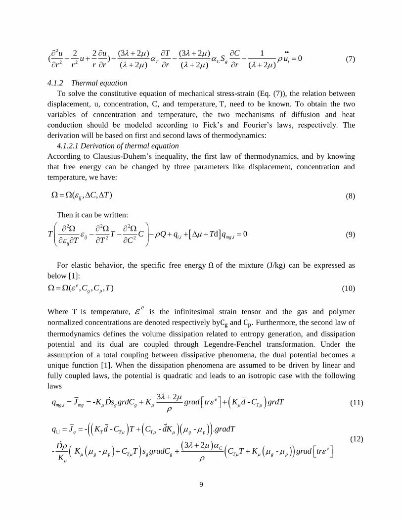
4.1.2 Thermal equation

To solve the constitutive equation of mechanical stress-strain (Eq. (7)), the relation between

displacement, u, concentration, C, and temperature, T, need to be known. To obtain the two

variables of concentration and temperature, the two mechanisms of diffusion and heat

conduction should be modeled according to Fick’s and Fourier’s laws, respectively. The

derivation will be based on first and second laws of thermodynamics:

4.1.2.1 Derivation of thermal equation

According to Clausius-Duhem’s inequality, the first law of thermodynamics, and by knowing

that free energy can be changed by three parameters like displacement, concentration and

temperature, we have:

( , , )ij C T (8)

Then it can be written:

2 2 2

, ,2 2d 0ij i i mg i

ij

T T C Q q T qT T C

(9)

For elastic behavior, the specific free energy Ω of the mixture (J/kg) can be expressed as

below [1]:

( , , , )e

g pC C T (10)

Where T is temperature, e is the infinitesimal strain tensor and the gas and polymer

normalized concentrations are denoted respectively byCg and Cp. Furthermore, the second law of

thermodynamics defines the volume dissipation related to entropy generation, and dissipation

potential and its dual are coupled through Legendre-Fenchel transformation. Under the

assumption of a total coupling between dissipative phenomena, the dual potential becomes a

unique function [1]. When the dissipation phenomena are assumed to be driven by linear and

fully coupled laws, the potential is quadratic and leads to an isotropic case with the following

laws

,

3 2- -e

mg i mg g g Tq J K Ds grdC K grad tr K d C grdT

(11)

, - - - - .

3 2- - -

i i q T T T g p

C e

g p T g g T g p

q J K d C T C dK gradT

DK C T s gradC C T K grad tr

K

(12)

10

Where kμ is linked to the chemical potential gradient effect on the gas mass flux; kT represents

the thermal gradient effect on the entropy flux, and CTμis a coupling coefficient corresponding

to the temperature (chemical potential) gradient effect on the mass (entropy) flux.

Now substituting the above equations into Eq. (9) we can have:

2

2 26 6

22

6

- 2 . . - 2 .

3 2110 - 3 2 2 10 .

3 2 110

3 2

V T T T

ee

g g T g C g

e

C T g g

T

dTC K K d C d T div gradT r K d C d gradT

dt

dD s gradC Ttr D s grad tr gradC

K dt

K grad tr C K d D s Tdiv gradCK

C K d T

612 10 .

3 22 .

e

C T g g

e

T C

div grad tr C K d D s gradC gradTK

C K d grad tr gradT

(13)

4.1.3 Heat equation

4.1.3.1 Derivation of heat equation

Assuming that there are two separate mass balance equations in the bi-component system,

leads to applying the classical balance equation to polymer and gas. For gas diffusion, we have:

.g

g mg

dCs divJ

dt (14)

Obviously, the heat balance equation can be obtained [1]:

3 2 .e

g

V q T g p g

dCdT dC divJ r Ttr Td s

dt dt dt

(15)

Where CV = T(∂S

∂T)εe,Ci

is the specific heat at constant strain and normalized concentration, Jq̅ is

the heat flux per unit area and r is the volume density of heat generated by an external source.

The last term in Eq. (15) corresponds to coupling between temperature variation and gas

diffusion within the polymer material. By substituting the relation proposed by Rambert et al. [1]

forμg −μpin Eq. (15), we have:

11

6 63 2

10 10g C e

g g g

T

dCs D s div gradC K grad tr

dt

C K d div gradT

(16)

5. Analytical solution

To develop a more straight-forward solution to the three coupled physics equations, a

spherical coordinate system is assumed. Therefore, displacement, heat conduction and mass

transfer are only considered in radial direction; i.e., u = u(r, t), T = T(r, t) and C = C(r, t).Also,

separate boundary conditions are employed for each boundary value problem. Cauchy and

Dirichlet boundary conditions have been employed at the inner and outer surfaces. So, initial and

boundary conditions for displacement, temperature and concentration are, respectively, as

follows:

Initial boundary condition for displacement:

1

2

( ,0) ( )

( ,0) ( )

u r F r

u r F r

Boundary conditions for displacement:

1 1( ,0) ( ,0) ( )i iu R k u R B tr

2 2( ,0) ( ,0) ( )o ou R k u R B tr

(17a)

Initial boundary condition for temperature:

3( ,0) ( )T r F r

Boundary conditions for temperature:

1 2( , ) ( ), ( ,0) ( )i oT R t g t T R g t

(17b)

Initial condition for concentration:

4( ,0) ( )C r F r

Boundary conditions for concentration:

1 2( , ) ( ), ( ,0) ( )i oC R t f t C R f t

(17c)

Now, the following new variables are defined:

12

1( , ) ( , )u r t r t

r

(18a)

1( , ) ( , )T r t r t

r

(18b)

1( , ) ( , )C r t r t

r (18c)

By changing the variables in Eqs. (7), (13), and (16) to the newly defined variables above, the

standard format of Hankel’s equation will be obtained:

2

2 2

1 1 21 9 1

4 1 1 2

10

1 2

T

g C

r r r r E r r

sr r

(19)

22 23/ 2

2 2 2 2

2 23/ 2 3/ 2 3/ 2 5/ 2

2

3/ 2

1 1 1 1 1 1

4 4 2

1 1 1 1 1 3.

2 2 4

1 1

2

V

d AC B r r

dt r r r r r r r r rr r

C r r D r E r r rr t r r rr r r

r F rrr

22 2

3/ 2 5/ 2

2 2 2

2 23/ 2 5/ 2 3/ 2 5/ 2

2 2

3/ 2 3/ 2

1 3 1 1 1

4 4

2 1 3 1 3

4 4

1 1 1 1.

2 2

r r Gr r r r r rr r

H r r r rr r r r r rr r

I r r r J rr rr r

23/ 2 5/ 2 3/ 2

2

1 3 1 1.

4 2r r r

r r rr r

(20)

The coefficients in Eq. (20) can be calculated as follows:

2T TA k k d C d 2 TB k d C d 0r

2

6110 gC D s

k

(3 2 ) TD 6 (3 2 )

2 10 c

gE D s

13

2

(3 2 ) cF k

6110T gG C k d D s

k

(3 2 ) c

TH C k d

612 10T gI C k d D s

k

(3 2 )

2 c

TJ C k d

26 6

2 2

2 23/ 2 5/ 2 3/ 2 5/ 2

2 2

2

2 2

(3 2 )1 110 10 .

4

2 1 3 1 3

4 4

1 1

4

C

g g

T

ds D s k r

dt r r r r

r r r rr r r r r rr r

C k dr r r r

(21)

Also, using Eqs. (18a) to (18c) for boundary and initial conditions, the following relations are

obtained:

Initial conditions:

1( ,0) ( )r rF r (22a)

2( ,0) ( )r rF r (22b)

4( ,0) ( )r rF r (22c)

Boundary conditions:

1 1( ,0) ( ,0) ( )i iR k R B tr

2 2( ,0) ( ,0) ( )o oR k R B tr

(23a)

14

1( ,0) ( )i iR R g r

2( ,0) ( )o oR R g r

(23b)

1( ,0) ( )i iR R f r

2( ,0) ( )o oR R f r

(23c)

To solve the triple coupled Equations of (19)-(21), the equations need to be divided into two

parts, as follows:

1 2 (24a)

1 2 (24b)

1 2 (24c)

Then, the triple equations are divided into two parts and resolved into the following boundary

value problems: The boundary value problem represented by Eq. (19) and related boundary and

initial conditions are: 2

21 11 12 2

1 9

4r r r r

(25a)

1 1 1 1( ,0) ( ,0) ( )i iR k R B tr

1 2 1 2( ,0) ( ,0) ( )o oR k R B tr

(25b)

1 1( ,0) ( ,0) 0r r (25c)

And

2

2 22 22 2

1 9 (1 )(1 2 ) (3 2 ) (3 2 )( ) ( ) ( ) 0

4 (1 ) ( 2 ) 2 ( 2 ) 2T g Cs

r r r r E r r r r

(26a)

2 1 2( ,0) ( ,0) 0i iR k Rr

2 2 2( ,0) ( ,0) 0o oR k Rr

(26b)

15

2 1( ,0) ( )r rF r

2 2( ,0) ( )r rF r (26c)

Similarly, the boundary value problem of Eq. (20) and related boundary and initial conditions

are: 2

1 1 112 2

1 1

4

VC d

r r r r dt

(27a)

1 1( , ) ( )i iR t R g t

1 2( , ) ( )o oR t R g t

(27b)

1( ,0) 0r (27c)

And

2

2 2 22 22 2

1 1( , , , )

4

VC dZ r

r r r r dt

(28a)

2 ( , ) 0iR t

2 ( , ) 0oR t (28b)

2 3( ,0) ( )r rF r (28c)

Also the boundary value problem of Eq. (21) and related boundary and initial condit ions are

written as: 2

1 1 112 2

1 1 10

4

d

r r r r D dt

(29a)

1 1( , ) ( )i iR t R f t

1 2( , ) ( )o oR t R f t

(29b)

1( ,0) 0r (29c)

And

(30a)

16

2

2 2 222 2

1 1 1( , , )

4

dZZ r

r r r r D dt

2 ( , ) 0iR t

2 ( , ) 0oR t (30b)

2 4( , ) ( )r t rF r (30c)

Equations (25a), (27a) and (29a) are of Bessel type and can be solved by finite Hankel

transformation [48]. According to boundary conditions for boundary value problems; i.e., Eqs

(25), (27) and (29), the kernels can be written [48]:

1 1.5 1.5 1 1.5

1.5 1.5 1 1.5

( , ) ( ) ( ) ( )

( ) ( ) ( )

n n n n i n i

n n n i n i

dK r J r Y R k Y R

dr

dY r J R k J R

dr

(31a)

2 0.5 0.5 0.5 0.5( , ) ( ) ( ) ( ) ( )m m i m i m mK r J r Y R J R Y r (31b)

3 0.5 0.5 0.5 0.5( , ) ( ) ( ) ( ) ( )p p i p i p pK r J r Y R J R Y r (31c)

λn , ξmand γpare positive roots of the equation below:

1.5 1 1.5 1.5 2 1.5

1.5 2 1.5 1.5 1 1.5

( ) ( ) ( ) ( )

( ) ( ) ( ) ( )

n i n i n o n o

n o n o n i n i

d dY R k Y R J R k J R

dr dr

d dY R k Y R J R k J R

dr dr

(32a)

0.5 0.5 0.5 0.5( ) ( ) ( ) ( ) 0m i m o m o m iJ R Y R J R Y R (32b)

0.5 0.5 0.5 0.5( ) ( ) ( ) ( ) 0p i p o p o p iJ R Y R J R Y R (32c)

Now using Hankel transformation in Eq. (25a), (27a) and (29a), we have:

17

1.5 1 1.52

1 11 2 12 2 2 2

2

1.5 2 1.5

2 ( ) ( )1 1 9 2

( ) ( )4

( ) ( )

n n i n i

n n o n o

dJ R k J R

drB t B t

dr r r rJ R k J R

dr

(33a)

2

0.51 1 11 0 2 12 2

0.5

2 ( )1 1 2( ) ( )

4 ( )

m ii

V V m o

J RdR g t R g t

C r r r r dt C J R

(33b)

20.51 1 1

1 0 2 12 2

0.5

2 ( )1 1 1 2( ) ( )

4 ( )

p i

i

p o

J RdR f t R f t

r r r r D dt J R

(33c)

Now, the following equations are obtained:

2 2 1.5 1 1.5

1

1 2 12 2 22

1.5 2 1.5

2 ( ) ( )( , ) 2

( , ) ( ) ( )

( ) ( )

n n i n i

n nn

n n o n o

dJ R k J R

t drt B t B t

dtJ R k J R

dr

(34a)

2 1 0.51 2 1

0.5

( , ) 2 ( ) 2( , ) ( ) ( )

( )

m m im m o i

V V m o

d t J Rt R g t R g t

C dt C J R

(34b)

1 0.52

1 2 1

0.5

( , ) 2 ( ) 2( , ) ( ) ( )

( )

p p i

p p o i

p o

d t J RD t D R f t R f t

dt J R

(34c)

Using Laplace transformation leads to the following:

1

1 22

2

( )( , )n

n

St L

S

(35a)

18

1

12 2

( )( , )m

m

V

St L

SC

(35b)

1

1 2 2

( )( , )p

p

St L

S D

(35c)

Where

1.5 1 1.5

2 122

1.5 2 1.5

2 ( ) ( )2

( ) ( ) ( )

( ) ( )

n n i n i

n n o n o

dJ R k J R

drt B t B t

dJ R k J R

dr

0.52 1

0.5

2 ( ) 2( ) ( ) ( )

( )

m io i

V m o

J Rt R g t R g t

C J R

0.5

2 1

0.5

2 ( ) 2( ) ( ) ( )

( )

p i

o i

p o

J Rt D R f t R f t

J R

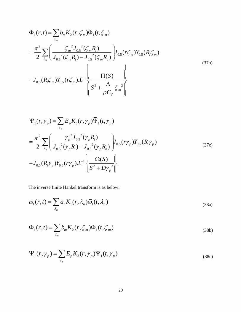
The inverse finite Hankel transform is as below:

19

1

2

1

2

2 2

1.5 2 1.5

2 2

'2 2

2 1.5 1 1.5

2

'2 2

2

1( , )

( , )

( ) ( )

1.51 ( ) ( )

1.51

o

n

i

R

n

R

n n n o n o

n n n i n i

n o

n n

n o

r t

r K r dr

dJ R k J R

dr

dk J R k J R

R dr

dk

R d

1 1

2

1.5 1 1.5

( , ) ( , )

( ) ( )

n n

n i n i

K r t

J R k J Rr

(36a)

2 22

0.51 2 12 2

0.5 0.5

( )( , ) ( , ) ( , )

2 ( ) ( )m

m m im m

m i m o

J Rr t K r t

J R J R

(36b)

2 22

0.5

1 3 12 2

0.5 0.5

( )( , ) ( , ) ( , )

2 ( ) ( )p

p p i

p p

p i p o

J Rr t K r t

J R J R

(36c)

Finally, we have:

1 1 1

1.5 1.5 1 1.5 1.5 1.5 1 1.5

1

22

2

( , ) ( , ) ( , )

( ) ( ) ( ) ( ) ( ) ( ) .

( )

n

n

n n n

n n n n i n i n n n i n i

n

r t a K r t

d da J r Y R k Y R Y r J R k J R

dr dr

SL

S

(37a)

20

1 2 1

2 22

0.50.5 0.52 2

0.5 0.5

1

0.5 0.52 2

( , ) ( , ) ( , )

( )( ) ( )

2 ( ) ( )

( )( ) ( ).

m

n

m m m

m m im i m

m i m o

i m m

m

V

r t b K r t

J RJ r Y R

J R J R

SJ R Y r L

SC

(37b)

1 3 1

2 220.5

0.5 0.52 2

0.5 0.5

1

0.5 0.5 2 2

( , ) ( , ) ( , )

( )( ) ( )

2 ( ) ( )

( )( ) ( ).

p

n

p p p p

p p i

p i p

p i p o

i p p

p

r E K r t

J RJ r Y R

J R J R

SJ R Y r L

S D

(37c)

The inverse finite Hankel transform is as below:

1 1 1( , ) ( , ) ( , )n

n n nr t a K r t

(38a)

1 2 1( , ) ( , ) ( , )m

m m mr t b K r t

(38b)

1 3 1( , ) ( , ) ( , )p

p p p pr E K r t

(38c)

21

Therefore Eqs (25a), (27a) and (29a) are solved which lead, respectively, to Eqs (38a) to

(38c).Next, the solution to Eqs (26a) to (30a) will be developed.

First, the following relations, which can be easily shown to satisfy the boundary conditions

Eqs (26b), (28b) and (30b), are assumed:

2 1( ) ( , )nS t K r (39a)

2 2( ) ( , )mP t K r (39b)

2 3( ) ( , )pX t K r (39c)

S(t) , P(t) and X(t) are unknown time-dependent functions that need to be obtained. By

substituting Eq. (33a) to Eq. (33c) into Eqs (26a), (28a) and (30a), we have:

2

1 12

2 2

12

3 3

1 3 2( ) ( ) ( , ) ( )

2

( , ) ( , ) 1 3 2( )

2 2

( , ) ( , )

2

n

n T m

m m

g C p

p p

S t S t K r b P t

dK r K rs E X t

dr r

dK r K r

dr r

(40a)

2

2( ) ( ) ( , ) , , , , , ,m m m p n

V

P t P t K r WW P S t rC

(40b)

2

3( ) ( ) ( , ) , , , , , ,p p m p nD F t F t K r WWW P S t r (40c)

where:

2

2 3/ 2 5 / 22 2

2 22

( , ) ( , )1 1, , , , , , ( ) ( , ) ( , )

4

m m

m p n m m

d K r dK rWW P S t r P t K r r r K r

C dr drr

2

1 12 2

2 2

( , ) ( , )1 1 1( ) ( , ) ( ) ( , )

2 2

m m

m m

dK r dK rBP t r K r P t r K r

C dr C dr

(41)

22

3 3 / 2

1 3 1

2

3 / 2 5 / 21 1

12

( , )1 1( ( , ( ) ( , ) ( , ) ( )

2

( , ) ( , )1 3( , ) )

4

p

p p p n n

n n

n

dK rI E t X t r K r J a t S t

drr

d K r dK rr r K r

dr drr

2

3 1

1 3 2

3/ 211 1

( , )1 1 1( , ) ( ) ( , ) ( ) ( , ).

2

( , )1 1( , ) ( ) ( , )

2

p

p p p m

nn n n

dK rC E t X t r K r DP t K r

C dr C

dK ra t S t r K r

drr

22 1 21 1

1 12

23 / 21

1 1

22

3 / 2 5 / 21 1

12

2

( , ) ( , )1 3( , ) ( ) ( , ) .

4

( , )1 1 1( , ) ( , ) ( ) .

2

( , ) ( , )1 3( , )

4

1 1( ) ( ,

n n

n n n

n

n n n

n n

n

m

d K r dK rE a t S t r r K r

C dr dr

dK rr K r F r a t S t

dr Cr

d K r dK rr r K r

dr drr

G P t K rC r

2

3 3

1 32 2

2 1

2 2

3 / 2 5 / 2 3 / 21 1 1 1

12 2

( , ) ( , )1 1). ( ) ( , ( , )

4

1( ) ( , ) ( , ) ( ) .

( , ) ( , ) ( , ) ( , )2 1 3 1 3( ( , )

4 4

p p

p p p

m n n

n n n n

n

d K r dK rX t E t K r

dr r dr r

HP t K r a t S tC

d K r dK r d K r dK rr r K r r r

r dr dr r dr drr r

5 / 2

1( , ) )

nK r

2

1 2 1

2 2

1 2 3 / 2 5 / 21 1 1 1

1 12 2

( , , , , , ) ( , ) ( ) ( , ) ( , ) ( ) .

( , ) ( , ) ( , ) ( , )2 3 1 3( , ) ( , )

4 4

m n m m m m n n

n n n n

n n

WWW P A t r z b t P t K r W a t S t

d K r dK r d K r dK rr r K r r r r K r

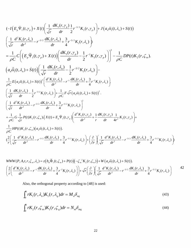
r dr dr r dr drr

42

Also, the orthogonal property according to [48] is used:

1 1( , ) ( , )b

n q n nqa

rK r K r dr M (43)

2 1( , ) ( , )b

m q m mqa

rK r K r dr N (44)

23

3 3( , ) ( , )b

p q p pqa

rK r K r dr O (45)

where δij is the Kronecher delta.

Briefly, we consider the final form of Eq. (34a) to Eq. (34c):

2

1 1( ) ( ) ( ) ( )nm pS t S t AA b P t BB E X t

(46a)

2 2 2

1

2

1 1 1

2 2

1 1 1

1

( ) ( ) ( ) ( ) ( , ) ( ) ( )

, ( ) ( ) ( , ) ( ) ( ) , ( )

, ( ) , ( ) ( ) ( , ) ( )

1( ) ,

m m m P p

V

n n p p n n

n n n n P p

m n n

P t P t N CCP t N DDP t EE E t X t P tC

FF a t S t P t HH E t X t KKP t a t S t

LL a t S t MM a t S t NNP t E t X t

N HP t a tC

( )S t

(46b)

2

1 1( ) ( ) , ( ) , ( )p p m m n nD F t F t O OO b t P t QQ a t S t (46c)

Constant Coefficients are as below:

2 2

12

( , ) ( , )1 3 2( , )

2 2

o

i

Rm m

T nR

n

dK r K rAA rK t dr

M dr r

3 3

12

( , ) ( , )1 3 2( , )

2 2

o

i

RP P

g C nR

n

dK r K rBB S rK t dr

M dr r

2

3/ 2 5 / 22 2

22

( , ) ( , )1 1( , )

4

m m

m

d K r dK rACC r r K r

C dr drr

2

12

2 2

( , ) 1( , ) ( , )

2o

i

R m

R m m

dK rBDD rK r r K r dr

C dr

24

31 3/ 22

2 2 3

( , )( , )1 1 1 1( , ) ( , ) ( , )

2 2o

i

pR m

R m m p

dK rdK rEE rIK r r K r r K r dr

C dr drr

31 3 / 22

2 2 3

2

3 / 2 5 / 21 1

12

( , )( , )1 1 1 1( , ) ( , ) ( , )

2 2

( , ) ( , )1 3( , )

4

o

i

pR m

R m m p

n n

n

dK rdK rFF rJK r r K r r K r

C dr drr

d K r dK rr r K r dr

dr drr

3/ 22 1

1

( , ) ( , )1 1( , )

2o

i

R m n

R n

DK r dK rKK r K r dr

C drr

2

1 2 3/ 21 1 1

1 12

( , ) ( , ) ( , )3 1 1( , ) ( , )

4 2o

i

R n n n

R n n

d K r dK r dK rELL r r K r r K r dr

C dr dr drr

22

3/ 2 5 / 21 1

12

( , ) ( , )1 3( , )

4o

i

R n n

R n

d K r dK rFMM r r r K r dr

C dr drr

2

3 3

2 32 2

( , ) ( , )1 1 1( , ) ( , )

4o

i

p pR

R m p

d K r dK rGNN K r K r dr

C dr r dr rr

2

2 2 3( , ) ( , ) ( , )o

i

R

R m m m pOO Z K r K r rK r dr

2

1 21 1

3 12

2

3 / 2 5 / 21 1

12

( , ) ( , )2 3( , )( ( , )

4

( , ) ( , )1 3( , ) )

4

o

i

R n n

R p n

n n

n

d K r dK rQQ WrK r r r K r

r dr dr

d K r dK rr r r K r dr

r dr drr

Solving the equations above results inS(t), P(t) and X(t) . Then, it is possible to obtain

ω2(r, t), Φ2(r, t) and Ψ2 = (r, t). Now, we have three ordinary equations which should be

solved simultaneously by some mathematical manipulations.

Therefore, we have:

1 1 11 1

1( , ) ( , ) , ( ) ( , )

n n n nn n

u r t a K r t S t K rr

(47a)

2 1 21 1

1( , ) ( , ) , ( ) ( , )

m m m mn n

T r t b K r t P t K rr

(47b)

25

3 1 31 1

1( , ) ( , ) , ( ) ( , )

p p p pn n

C r t E K r t X t K rr

(47c)

Consequently, the triple coupled thermo-diffuse-mechanical equations are solved analytically

using the discussed method. It is a general solution which can be developed for any kind of

boundary condition. It is only sufficient to have the kernel of transformation to obtain the

response of triple coupled boundary value problems.

6. Case Study

In this study the quasi-static thermoelasticity problem of a pressurized sphere is solved

analytically where material properties vary with radial position. The axisymmetric equations of

uncoupled thermoelasticity are:

2

2

20V

CT T dT

r r r dt

(48a)

2

2 2

12 2

1

u u u T

r r r r r

(48b)

Constitutive law states that the relation between stress components, radial displacement

component and temperature is as follows:

1 2 1

1 1 2rr

E du uT

dr r

(49a)

1

1 1 2

E du uT

dr r

(49b)

The analytical solution presented in the previous section was applied to a thick hollow sphere

of the inner radius is 𝑅𝑖 = 1 𝑚 and the outer radius is 𝑅𝑂 = 2 𝑚. Internal pressure exerted in

inner surface of the hollow sphere σi = 100 MPa and it is assumed to be traction free at outer

surface. The thermal boundary conditions are as follows:

, 100i

R t MPa (50a)

, 0O

R t (50b)

The material properties of sphere are shown in Table.1.

Table.1: Material properties of sphere

26

Solving the problem, the results are shown graphically in the following. Distribution of radial

stress through the radial position is shown in Fig.2 for various instances of time. It can be seen

that radial stress decreases with time so that it becomes compressive as time grows up.

Fig. 2: Distribution of radial stress through the radial position

Fig. 3 shows the distribution of hoop stress versus radial position for various instances of

time. It is obvious that as time grows up hoop stress becomes compressive in all positions.

Fig. 3: Distribution of hoop stress through the radial position

Temperature distribution through the thickness of sphere is shown in Fig.4 for four time

instances.

Fig. 4: Distribution of temperature through thickness at different times

27

7. Validation

A spherically isotropic elastic hollow sphere problem is chosen as a case study. The problem

solved is similar to the thermomechanical problem proposed by Hui-ming et al. (2003). For

symmetric problems, only the radial displacement is considered. Material properties are:

6 1200 , 0.3, 10E GPa

K

Also, the boundary and initial conditions are as follows:

Mechanical boundary and initial conditions are:

, , 0rr O rr i

R t R t (51a)

, ( ,0) 0u r t u r (51b)

Thermal boundary and initial conditions are of the following form:

0, , 100

O iT R t T R t K T (52a)

,0 0T r (52b)

Mechanical stress for isotropic material is obtained by:

, ,

, 1 2 1 ,1 1 2

rr

u r t u r tEr t T r t

r r

(53a)

, ,, ,

1 1 2 1 2

u r t u r tE Er t T r t

r r

(53b)

Substituting Eqs (51a) and (51b) into Eq. (53a) results in:

0

, 2 , 1

1 1

i i

i

u R t u R t ET

r R

(54a)

, 2 ,0

1

o o

o

u R t u R t

r R

(54b)

Obviously, the boundary conditions above are of Cauchy type.

On the other hand, using the change of variables according to Eqs (20a), (20b) and (20c), we

have:

0

1, 5 1,

2 1 1

ii

i

i

RR tR t T

r R

(55a)

, 5 1, 0

2 1

o

o

o

R tR t

r R

(55b)

where initial conditions are:

,0 0r (56a)

,0 0r

(56b)

28

Also, a similar procedure is performed for Dirichlet boundary and initial conditions:

,0 0r

0,

i iR t T R

(57a)

0,

o oR t T R (57b)

,0 0r (57c)

Equations (19) and (20) are rewritten for two coupled mechanical and thermal problems, then

the following relations are obtained:

2

2 2

1 1 21 9 10

4 1 1 2T

r r r r E r r

(58)

2

2 2

1 10

4

C

r r r r K t

(59)

To solve the mechanical and thermal equations; i.e. Eqs (57) and (58), Eqs (34a) and (34b)

are, respectively, employed and the following relations are thus obtained:

02

1

1 022

2

2

12

11 2, 1 cos

1

i

i n

n

nn

RT

R tt T

S S

(60)

20

1

1 02

2

2

2, 1

mV

Ki t

C

m i

m

m

V

R T

t R T eK

SC

(61)

Moreover, Eq. (40a) is rewritten for the two coupled physics:

2

( ) ( )n

mS t S t AA b

(62)

Obtaining S(t) from Eq. (46a) leads to:

29

2

1

2

2

2

0

0 2 22 2 2

2 2

2

(0) (0)

( )

22

2

m

m

n

Kt

Ci n

i

m n n nm V n m

m

KsS S b AA S

CS t

S

R T AAKeR T AA Sin t

K KC

C C

22

0 2 2

2

mK

tC

n

i

n n

m

eR T AA Cos t

K

C

(63)

Using Eqs (47a) and (47b), it is possible to obtain ω(r, t) and Φ(r, t) so that we can obtain

u(r, t) and T(r, t), as follows:

2

,,

m

m mb K r

T r tr

(64)

1 1 1

, ( ) ,,

m n m

n n na K r S t K r

u r tr r

(65)

To obtain u(r, t) it is required to solve Eq. (63) for S(t) by applying the boundary conditions:

2

2

2

0

0 2 22 2 2

2 2

2

0 2 22

2

22( ) (

2

m

n m

m

Kt

Ci n

i

m n n nm V n m

Kt

C

i

m n n

m

R T AAKeS t R T AA Sin t

K KC

C C

eR T AA

K

C

nCos t

(66)

Now, the radial stress can be determined using the obtained results for u(r, t) and T(r, t) . The

radial stress can then be normalized in order to be compared with the results presented by Wang

et al.[49]. Normalized radial stress is presented as a function of normalized factors, which are

defined by Wang et al. [49]as:

30

Non-dimensional time:

*1Et

tb a

Non-dimensional radius:

r a

b a

Non-dimensional radial stress:

0

1 2*

rr

rrE T

where inner and outer radii are represented ,respectively, by a and b.

Fig. 5 demonstrates a comparison of non-dimensional radial stress (𝜎𝑟𝑟∗) versus non-dimensional

time (𝑡∗) obtained in this study and those presented by Wang et al. [49]. To better illustrate the

comparison of the results, the values of nondimensional radial stress obtained in this study for

two values of 𝜉 = 0.75, 𝜉 = 0.5 as well as those reported by Wang et al. [49] are tabulated in

Table 1.

Fig. 5: Variation of non-dimensional radial stress with time in different radial values for the isotropic

hollow sphere

Table2: Comparison of nondimensional radial stress for 𝜉 = 0.75, 𝜉 = 0.5

The results in Fig. 5 and Table2 show a good agreement between the solution developed using

the method presented in the current study and the one proposed by Wang et al. [49].

8. Conclusion

The three coupled equations of mechanical stress, heat transfer, and diffusion have been

solved analytically using Hankel tranform. The equations have been derived based on the work

of Rambert et al. [1] and the details of the derivation are given. The closed form solution can

therefore provide a tool for an accurate calculation of the fields of mechanical stress-strain,

temperature and concentration. To validate this solution, the results of this study were compared

against the results of dual coupled thermomechanical physics available in open literature and a

good agreement was observed. For validating the performed solution for the dynamical problem

of thermoelasticity, the problem of an isotropic sphere subjected to a sudden uniform

temperature rise 𝑇0 throughout the sphere is considered. In other words, the entire sphere

experiences a temperature rise of 𝑇0. The presented solution approach of the boundary value

problem provides a closed-form solution, which obviates the need for time-taking numerical

methods or extensive experimental work to analyze the triple coupled mechanisms available in

numerous industrial structures such as gas and oil pipeline systems.

31

References

[1] Rambert, G., Grandidier, J., Cangemi L., and Meimon Y. "A modelling of the coupled

thermodiffuso-elastic linear behaviour. Application to explosive decompression of

polymers", Oil & gas science and technology, 58, pp. 571-591 (2003).

[2] Vijalapura, P. K. and Govindjee S. "Numerical simulation of coupled‐stress case II

diffusion in one dimension", Journal of Polymer Science Part B: Polymer Physics, 41, pp.

2091-2108 (2003).

[3] Holalkere,V., Mirano, S., Kuo, A.-Y., Chen, W.-T., Sumithpibul, C. and Sirinorakul S.

"Evaluation of plastic package delamination via reliability testing and fracture mechanics

approach", 47th

Conf. on Electronic Components and Technology, pp. 430-435 (1997).

[4] Govindjee, S. and Simo, J. C. "Coupled stress-diffusion: Case II", Journal of the

Mechanics and Physics of Solids, 41, pp. 863-887 (1993).

[5] Busso, E. "Oxidation-induced stresses in ceramic-metal interfaces," Le Journal de

Physique IV, 9, pp. Pr9-287-Pr9-296 (1999).

[6] Klopffer, M. and Flaconneche, B. "Transport properdines of gases in polymers:

bibliographic review," Oil & Gas Science and Technology, 56, pp. 223-244 (2001).

[7] Teh L., Teo, M., Anto, E., Wong,C., Mhaisalkar, S., Teo, P. "Moisture-induced failures

of adhesive flip chip interconnects", Components and Packaging Technologies, IEEE

Transactions on, 28, pp. 506-516 (2005).

[8] Wahab, M. A., Ashcroft, I., Crocombe, A. and Shaw, S. "Diffusion of moisture in

adhesively bonded joints", The Journal of Adhesion, 77, pp. 43-80 (2001).

[9] Wong, E., Koh, S., Lee, K. and Rajoo, R. "Advanced moisture diffusion modeling and

characterisation for electronic packaging," 52nd

Conf. on Electronic Components and

Technology, pp. 1297-1303 (2002).

[10] Yu, Y. T. and Pochiraju, K. "Three‐Dimensional Simulation of Moisture Diffusion in

Polymer Composite Materials", Polymer-Plastics Technology and Engineering, 42, pp.

737-756 (2003).

[11] Shirangi, H., Auersperg, J., Koyuncu, M., Walter, H., Müller, W. and Michel, B.

"Characterization of dual-stage moisture diffusion, residual moisture content and

hygroscopic swelling of epoxy molding compounds", Int. Conf. on Thermal, Mechanical

and Multi-Physics Simulation and Experiments in Microelectronics and Micro-Systems,

EuroSimE 2008., pp. 1-8 (2008).

[12] Lin T. and Tay A. "Mechanics of interfacial delamination under hygrothermal stresses

during reflow soldering", 1st Conf. on Electronic Packaging Technology, pp. 163-169

(1997).

[13] Yi, S. and Sze, K. Y. "Finite element analysis of moisture distribution and hygrothermal

stresses in TSOP IC packages," Finite elements in analysis and design, 30, pp. 65-79

(1998).

32

[14] Chang, K.-C., Yeh, M.-K. and Chiang, K.-N. "Hygrothermal stress analysis of a plastic

ball grid array package during solder reflow," Proceedings of the Institution of

Mechanical Engineers, Part C: Journal of Mechanical Engineering Science, 218, pp. 957-

970 (2004).

[15] Lahoti, S. P., Kallolimath, S. C. and Zhou, J. "Finite element analysis of thermo-hygro-

mechanical failure of a flip chip package," 6th

Int. Conf. on Electronic Packaging

Technology, pp. 330-335 (2005).

[16] Dudek, R., Walter, H., Auersperg, J. and Michel, B. "Numerical analysis for thermo-

mechanical reliability of polymers in electronic packaging", 6th

Int. Conf. on in Polymers

and Adhesives in Microelectronics and Photonics, pp. 220-227 (2007).

[17] Fan, X. and Zhao, J.-H. "Moisture diffusion and integrated stress analysis in encapsulated

microelectronics devices", 12th

Int. Conf. on in Thermal, Mechanical and Multi-Physics

Simulation and Experiments in Microelectronics and Microsystems (EuroSimE), pp. 1-8

(2011).

[18] Briscoe, B. and Liatsis,D. "Internal crack symmetry phenomena during gas-induced

rupture of elastomers", Rubber chemistry and technology, 65, pp. 350-373 (1992).

[19] Briscoe, B., Savvas, T. and Kelly, C. "Explosive Decompression Failure of Rubbers: A

Review of the Origins of Pneumatic Stress Induced Rupture in Elastomers", Rubber

chemistry and technology, 67, pp. 384-416 (1994).

[20] Liatsis, D. "Gas induced rupture of elastomers", Imperial College London, London

(1989).

[21] Haghighi-Yazdi, M. and Lee-Sullivan, P. "Modeling of structural mechanics, moisture

diffusion, and heat conduction coupled with physical aging in thin plastic plates", Acta

Mechanica, 225, pp. 929-950 (2014).

[22] McBride, A., Javili, A., Steinmann, P. and Bargmann, S. "Geometrically nonlinear

continuum thermomechanics with surface energies coupled to diffusion", Journal of the

Mechanics and Physics of Solids, 59, pp. 2116-2133 (2011).

[23] Rambert, G. and Grandidier, J.-C. "An approach to the coupled behaviour of polymers

subjected to a thermo-mechanical loading in a gaseous environment", European Journal

of Mechanics-A/Solids, 24, pp. 151-168 (2005).

[24] Gibbs, J. W. "On the equilibrium of heterogeneous substances", American Journal of

Science, pp. 441-458 (1878).

[25] Gibbs, J. W. and Bumstead, H. A. Thermodynamics vol. 1: Longmans, Green and

Company (1906).

[26] Duan, H., Wang, J. and Karihaloo, B. L. "Theory of elasticity at the nanoscale", Advances

in applied mechanics, 42, pp. 1-68 (2009).

[27] Miller, R. E. and Shenoy, V. B. "Size-dependent elastic properties of nanosized structural

elements" Nanotechnology, 11, pp. 139 (2000).

[28] Mitrushchenkov A., Chambaud, G., Yvonnet, J. and He, Q. "Towards an elastic model of

wurtzite AlN nanowires", Nanotechnology, 21, pp. 255-702 (2010).

33

[29] Yang, K., She, G.-W., Wang, H., Ou, X.-M., Zhang, X.-H., Lee, C.-S. "ZnO nanotube

arrays as biosensors for glucose", The Journal of Physical Chemistry C, 113, pp. 20169-

20172 (2009).

[30] Wei, G., Shouwen, Y. and Ganyun, H. "Finite element characterization of the size-

dependent mechanical behaviour in nanosystems", Nanotechnology, 17, pp. 11-18

(2006).

[31] Yvonnet, J., Quang, H. L. and He, Q.-C. "An XFEM/level set approach to modelling

surface/interface effects and to computing the size-dependent effective properties of

nanocomposites", Computational Mechanics, 42, pp. 119-131 (2008).

[32] Gurtin, M. E. and Murdoch, A. I. "A continuum theory of elastic material surfaces,"

Archive for Rational Mechanics and Analysis, 57, pp. 291-323 (1975).

[33] Angenent, S. and Gurtin, M. E. "Multiphase thermomechanics with interfacial structure

2. Evolution of an isothermal interface", Archive for Rational Mechanics and Analysis,

108, pp. 323-391 (1989).

[34] Gurtin, M. E. and Matano, H. "On the structure of equilibrium phase transitions within

the gradient theory of fluids", Quart. Appl. Math, 46, pp. 301-317 (1988).

[35] Gurtin, M. E. and Struthers, A. "Multiphase thermomechanics with interfacial structure,"

Archive for Rational Mechanics and Analysis, 112, pp. 97-160 (1990).

[36] Daher, N. and Maugin, G. "The method of virtual power in continuum mechanics

application to media presenting singular surfaces and interfaces", Acta Mechanica, 60,

pp. 217-240 (1986).

[37] Dolbow, J., Fried, E. and Ji, H. "Chemically induced swelling of hydrogels", Journal of

the Mechanics and Physics of Solids, 52, pp. 51-84 (2004).

[38] Ji B. and Gao, H. "Mechanical properties of nanostructure of biological materials",

Journal of the Mechanics and Physics of Solids, pp. 1963-1990 (2004).

[39] Liu, C.-L., Ho, M.-L., Chen, Y.-C., Hsieh, C.-C., Lin, Y.-C., Wang, Y.-H. "Thiol-

functionalized gold nanodots: two-photon absorption property and imaging in vitro" The

Journal of Physical Chemistry C, 113, pp. 21082-21089 (2009).

[40] Steinmann, P. "On boundary potential energies in deformational and configurational

mechanics", Journal of the Mechanics and Physics of Solids, 56, pp. 772-800 (2008).

[41] RODIER RENAUD, L. "Etude transitiometrique de l'influence de la pression sur les

proprietes thermomecaniques des polymeres. Expansibilite thermique jusqu'a 393 k et

300 mpa de polyethylenes seuls ou en interaction avec le methane," Clermont Ferrand 2,

(1994).

[42] Cunat, C. "A thermodynamic theory of relaxation based on a distribution of non-linear

processes", Journal of Non-Crystalline Solids, 131, pp. 196-199 (1991).

[43] Fosdick R. and Tang, H. "Surface transport in continuum mechanics", Mathematics and

Mechanics of Solids, (2008).

[44] Coleman, B. D. and Gurtin, M. E. "Thermodynamics with internal state variables", The

Journal of Chemical Physics, 47, pp. 597-613 (1967).

34

[45] Coleman, B. D. and Gurtin, M. E. "On the growth and decay of discontinuities in fluids

with internal state variables" (1967).

[46] Michaels, A. S. and Bixler, H. J. "Flow of gases through polyethylene", Journal of

Polymer Science, 50, pp. 413-439 (1961).

[47] Michaels, A. S. and Bixler, H. J. "Solubility of gases in polyethylene," Journal of

Polymer Science, 50, pp. 393-412 (1961).

[48] Sneddon, I. N. "The use of integral transforms", McGraw-Hill Book Company, New

York, 1972.

[49] Ding, H., Wang, H. and Chen,W. "Transient responses in a piezoelectric spherically

isotropic hollow sphere for symmetric problems", Journal of applied mechanics, 70, pp.

436-445 (2003).

Ehsan Mahdavi is a PhD student in the Department of Mechanical Engineering at University of Tehran,

Iran. He received his MSc degree from the Department of Mechanical Engineering at Khaje Nasir

University of Technology. His main areas of research include noncomposite and composite materials,

and viscoelasticity.

Dr Mojtaba Haghighi-Yazdi received his BSc and MSc in the field of Mechanical Engineering from Iran

University of Science and Technology. His MSc thesis focused on fatigue modeling of composite

laminates with stress concentration. He earned his PhD in the field of Mechanical Engineering from

University of Waterloo. His PhD thesis centered around modeling the four-coupled physics available

in hygrothermal aging of a polymer blend. He has joint the University of Tehran as a faculty member

since 2012 and his current research interests include composite materials, mechanical behavior of

polymeric materials, and viscoelasticity.

Dr. Majid Baniassadi is an Assistant Professor at the School of Mechanical Engineering, University of

Tehran, Iran. He holds a PhD in Mechanics of Materials from the University of Strasbourg (2011). He

received his Master’s degree from the University of Tehran (2007) and his undergraduate degree

from Isfahan University of Technology (2004), in Mechanical Engineering. His research interests

include multiscale analysis and micromechanics of heterogeneous materials, numerical methods in

engineering, electron microscopy image processing for microstructure identification.

Dr. Mehran Tehrani is an Assistant Professor of Mechanical Engineering at the University of New

Mexico (UNM). He received his Ph.D. in Engineering Mechanics from Virginia Tech in 2012. He is

currently the director of the Advanced Structural and Energy Materials Laboratory (ASEMlab) at

UNM.

Professor Saïd Ahzi is currently a Research Director of the Materials Science and Engineering group at

Qatar Environment and Energy Research Institute (QEERI) and Professor at the College of Science

& Engineering, Hamad Bin Khalifa University, Qatar Foundation, Qatar. He holds a position as a

Distinguished Professor at the University of Strasbourg (Exceptional Class). He also holds an

Adjunct Professor position with the School of Materials Science and Engineering at Georgia Institute

of Technology, USA. In January 2000, he joined the University of Strasbourg, France, Faculty of

Physics and Engineering, as full Professor. From 1995 to 2000, he held the position of Professor

35

(Assistant then Associate) at the Department of Mechanical Engineering at Clemson University,

USA. Prior to this, he spent four years as a Research Scientist & Lecturer at the University of

California at San Diego, USA, and four years as a Postdoctoral Research Associate at

Massachusetts Institute of Technology, USA. From 2007 to 2011, he held an Adjunct Research

Professor position with the University of Aveiro, Portugal. Dr. Saïd Ahzi advised about 25 PhDs, 24

Masters degrees, and was the scientific advisor for six Habilitations. He published more than 250

scientific papers in the areas of materials science, applied mechanics and processing.

Dr. Jalil Jamali is an Assistant Professor of Mechanical Engineering at islamic azad university of

shoushtar. He received his Ph.D. in Engineering Mechanics from University of Tehran. His main

areas of research include Elastodynamics, Acoustic, Nano-mechanics, Fluid Mechanics, Dynamics,

Vibrations and Elasticity.

List of Figurs

Fig. 1: The motion φ of the body from initial configuration to current configuration [22]

Fig. 2: Distribution of radial stress through the radial position

Fig. 3: Distribution of hoop stress through the radial position

Fig. 4: Distribution of temperature through thickness at different times

Fig. 5: Variation of non-dimensional radial stress with time in different radial values for the

isotropic hollow sphere

Fig. 1

36

Fig. 2

Fig. 3

-200

-150

-100

-50

0

50

1 1.2 1.4 1.6 1.8 2R

adia

l Str

ess

(M

Pa)

Radial Position (m)

t=1000 sec

t=10000 sec

-450

-400

-350

-300

-250

-200

-150

-100

-50

0

50

1 1.2 1.4 1.6 1.8 2

Ho

op

Str

ess

(M

Pa)

Radial Position (m)

t=1000 sec

t=10000 sec

37

Fig. 4

Fig. 5

-20

0

20

40

60

80

100

120

1 1.2 1.4 1.6 1.8 2

Tem

pe

ratu

re

Radial Position (m)

t=10 sec

t=100 sec

t=1000 sec

t=10000 sec

38

List of Tables

Table.1: Material properties of sphere

Table2: Comparison of nondimensional radial stress for 𝜉 = 0.75, 𝜉 = 0.5

Poisson’s ratio Elastic modulus Density Thermal conductivity Specific heat Coefficient of thermal

expansion

ν E (GPa) 𝜌 (kg/m3) Λ (W/mK) CV(J/kg.K) αT (1/K°)

0.3 70 2707 204 903 23×10-6

Table.1

Current

study

Wang et al.

[49] Error %

𝜉 = 0.75

0.25 0.26 0.04

0.2 0.21 0.05

0.18 0.17 0.06

𝜉 = 0.5

0.5 0.45 0.10

0.4 0.4 0.00

0.3 0.31 0.03

Table2