Analytical simulation of nonlinear elastic–plastic averagestress–average strain relationships for un-corroded/both-sidesrandomly corroded steel plates under uniaxial compression

Mohammad Reza Khedmati n, Zorareh Hadj Mohammad Esmaeil NouriDepartment of Marine Technology, Amirkabir University of Technology, Tehran 15914, Iran

a r t i c l e i n f o

Article history:Received 26 August 2012Received in revised form14 October 2014Accepted 14 October 2014Available online 6 November 2014

Keywords:Imperfect steel plateBoth-sides random corrosionUltimate strengthAverage stress–average strain relationshipSimulation

a b s t r a c t

In this paper, an analytical simplified method for derivation of the average stress–average strainrelationship of imperfect steel plates taking into account of both geometric and material nonlinearities ispresented. The method utilizes the theory of elastic large deflection analysis of plates in the elasticregion, and also the theory of rigid-perfectly plastic mechanism analysis of plates in the plastic region.The ultimate strength of the plate is predicted using an empirical formulation. The steel plates may beentirely un-corroded or both-sides randomly corroded. The algorithm can be easily implemented inmethods for evaluation of ship hull girder ultimate strength as well as in the estimation of the ultimatecapacity of offshore structures.

& 2014 Elsevier Ltd. All rights reserved.

1. Introduction

In design of ships and offshore structures, it is essential to ensurethat the structure has sufficient strength to sustain extreme loadingsituations. Such marine structures are mostly assembled of plates andplated elements. Thus, strength of plates and other plated elements iscrucial for the overall structural capacity or in other words for theultimate strength of the whole structure. For a thorough assessmentof a structural design, for understanding possible improvements andto predict the consequences in the event of failure, an approximationof the value of ultimate strength is not sufficient. The completebehaviour, up to collapse and beyond, of the structure has to besimulated to gain insight into causes and effects of a structural failure.

For the analysis of large marine structures, an accurate and efficientapproach is required to obtain results within a reasonable space of thetime. Despite the enormous development in computer technology,elastic-plastic large deflection analyses with conventional finite ele-ment analysis (FEA) are too time-consuming for large structures.Therefore, a simplified method has to be employed to reduce thecomputational time and/or increase the size of the structural parts thatcan be analysed.

For cross sections of ships in bending, methods to obtain themoment-curvature relationship, Fig. 1, considering the collapse of

parts of the cross section have been developed. One of the mostknownmethods is the Smith’s method [1,2], in which the ship cross-section is divided into small elements each of which is composed ofplates without/with stiffener. Average stress–average strain relation-ships of all elements are derived before the analysis of the wholecross-section progresses as follows: curvature is applied incremen-tally about the instantaneous neutral axis, the strain of each elementis calculated, the corresponding stress is taken from the stress–straincurves previously derived, and the corresponding moments is obtai-ned by integration over the cross-section, Fig. 2. FEA is usuallyapplied in order to derive the average stress–average strain relation-ships of plate and stiffened plate elements. Application of FEA inderivation of average stress–average strain relationships of theplated elements in the cross-section of a ship hull girder or anyother box-shape structure would mean spending a considerableamount of cost and time. Therefore, it is felt that there is a need todevelop or propose a simplified method in order to perform suchcalculations. These calculations create a significant step in progres-sive collapse analysis of marine structures.

Analytical method proposed in this paper, is one suitable frame-work for implementing a general approach to collapse analysis, since itleads to the reduction of solution process either in time or in cost.Combining the theory of elastic large deflection analysis with rigid-plastic mechanism analysis, a simple formulation is expressed in orderto derive average stress–average strain relationships of plates. Theaccuracy of the method or formulation is verified against the FEAobtained results. Employing such a formulation, the ultimate strength

Contents lists available at ScienceDirect

journal homepage: www.elsevier.com/locate/tws

Thin-Walled Structures

http://dx.doi.org/10.1016/j.tws.2014.10.0120263-8231/& 2014 Elsevier Ltd. All rights reserved.

n Corresponding author. Tel.: þ98 21 64543113; fax: þ98 21 66412495.E-mail address: khedmati@aut.ac.ir (M. Reza Khedmati).

Thin-Walled Structures 86 (2015) 132–141

evaluation of ships and offshore structures is possible in a very shorttime with reasonable accuracy and cost.

2. General assumptions

The longitudinal stiffening system is usually employed in largeships at their mid-length part, especially in the deck and bottom

structures. If an extreme bending moment acts on a hull girder, themost possible collapse mode may be the overall collapse ofstiffened panel after local collapse of individual plate elementsbetween stiffeners.

The following assumptions are made in the derivation of theaverage stress–average strain relationships of the plate elements:

1. Attached plating between longitudinal stiffeners behaves as anisolated plate.

2. The material is assumed to be elastic-perfectly plastic.

Average stress–average strain relationships of the isolatedplates are derived combining the results of elastic large deflectionanalysis and rigid plastic mechanism analysis.

3. Average stress–average strain relationship of un-corrodedplates

3.1. Welding induced initial deflections

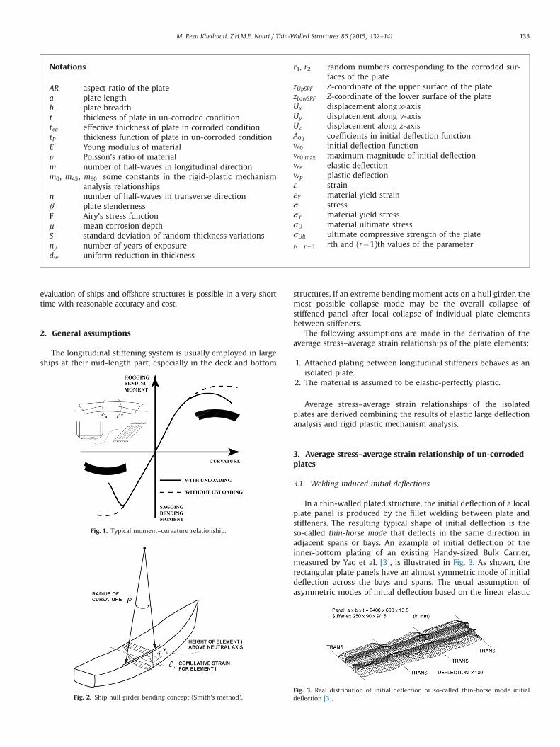
In a thin-walled plated structure, the initial deflection of a localplate panel is produced by the fillet welding between plate andstiffeners. The resulting typical shape of initial deflection is theso-called thin-horse mode that deflects in the same direction inadjacent spans or bays. An example of initial deflection of theinner-bottom plating of an existing Handy-sized Bulk Carrier,measured by Yao et al. [3], is illustrated in Fig. 3. As shown, therectangular plate panels have an almost symmetric mode of initialdeflection across the bays and spans. The usual assumption ofasymmetric modes of initial deflection based on the linear elastic

Notations

AR aspect ratio of the platea plate lengthb plate breadtht thickness of plate in un-corroded conditionteq effective thickness of plate in corroded conditiontP thickness function of plate in un-corroded conditionE Young modulus of materialν Poisson’s ratio of materialm number of half-waves in longitudinal directionm0, m45, m90 some constants in the rigid-plastic mechanism

analysis relationshipsn number of half-waves in transverse directionβ plate slendernessF Airy’s stress functionμ mean corrosion depthS standard deviation of random thickness variationsny number of years of exposuredw uniform reduction in thickness

r1, r2 random numbers corresponding to the corroded sur-faces of the plate

zUpSRF Z-coordinate of the upper surface of the platezLowSRF Z-coordinate of the lower surface of the plateUx displacement along x-axisUy displacement along y-axisUz displacement along z-axisA0ij coefficients in initial deflection functionw0 initial deflection functionw0 max maximum magnitude of initial deflectionwe elastic deflectionwp plastic deflectionε strainεY material yield strainσ stressσY material yield stressσU material ultimate stressσUlt ultimate compressive strength of the plater, r�1 rth and (r�1)th values of the parameter

Fig. 1. Typical moment–curvature relationship.

Fig. 2. Ship hull girder bending concept (Smith’s method).Fig. 3. Real distribution of initial deflection or so-called thin-horse mode initialdeflection [3].

M. Reza Khedmati, Z.H.M.E. Nouri / Thin-Walled Structures 86 (2015) 132–141 133

buckling analysis gives very conservative predictions of the ulti-mate strength [4].

Theoretically, for a plate of length a, breadth b, and thickness t,the initial deflection of a thin-horse mode can be expressed by adouble sinusoidal series as

w0 ¼ ∑1

i ¼ 1∑1

j ¼ 1A0ij sin

iπxa

sinjπyb

ð1Þ

Among the deflection components in the direction of theshorter side of the plate (y-direction), the first term with onehalf-wave has the greatest effect on the initial deflection mode.Thus, a simpler form of the initial deflection equation can bewritten as follows

w0 ¼ ∑1

i ¼ 1A0i sin

iπxa

sinπyb

ð2Þ

Ueda and Yao [5] idealised this mode with another expressionas follows which includes only odd terms

w0 ¼ ∑21

i ¼ 1;3;5;…A0i sin

iπxa

sinπyb

ð3Þ

Later Yao et al. [6], introduced even terms also in this mode,and finally the idealised thin-horse mode of initial deflection tookthe following form

w0 ¼ ∑11

i ¼ 1A0i sin

iπxa

sinπyb

ð4Þ

The initial deflection is herein assumed to be in the idealisedthin-horse mode. The coefficients of this mode (A0i), nondimen-sionalised by plate thickness (t), i.e., A0i=t, are given in Table 1 [6]as functions of plate aspect ratio.

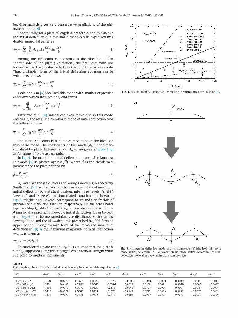
In Fig. 4, the maximum initial deflection measured in Japaneseshipyards [5] is plotted against β2t, where β is the slendernessparameter of the plate defined by

β¼ bt

ffiffiffiffiffiffiσY

E

rð5Þ

σY and E are the yield stress and Young’s modulus, respectively.Smith et al. [7] have categorized their measured data of maximuminitial deflection by statistical analysis into three levels, “slight”,“average” and “severe”, and formulated equations as shown inFig. 4. “slight” and “severe” correspond to 3% and 97% fractals ofprobability distribution function, respectively. On the other hand,Japanese Ship Quality Standard (JSQS) prescribes an upper limit of6 mm for the maximum allowable initial deflection. It can be seenfrom Fig. 4 that the measured data are distributed such that the“average” line and the allowable limit prescribed by JSQS form anupper bound. Taking average level of the measured maximumdeflection in Fig. 4, the maximum magnitude of initial deflection,w0max, is taken as

w0 max ¼ 0:05β2t ð6ÞTo consider the plate continuity, it is assumed that the plate is

simply-supported along its four edges which remain straight whilesubjected to in-plane movements.

Table 1Coefficients of thin-horse mode initial deflection as a function of plate aspect ratio [6].

a/b A01/t A02/t A03/t A04/t A05/t A06/t A07/t A08/t A09/t A010/t A011/t

1oa/bo√2 1.1158 �0.0276 0.1377 0.0025 �0.0123 �0.0009 �0.0043 0.0008 0.0039 �0.0002 �0.0011√2oa/bo√6 1.1421 �0.0457 0.2284 0.0065 0.0326 �0.0022 �0.0109 0.001 �0.0049 �0.0005 0.0027√6oa/bo√12 1.1458 �0.0616 0.3079 0.0229 0.1146 �0.0065 0.0327 0.000 0.000 �0.0015 �0.0074√12oa/bo√20 1.1439 �0.0677 0.3385 0.0316 0.1579 �0.0149 0.0743 0.0059 0.0293 �0.0012 0.0062√20oa/bo√30 1.1271 �0.0697 0.3483 0.0375 0.1787 �0.0199 0.0995 0.0107 0.0537 �0.0051 0.0256

Fig. 4. Maximum initial deflections of rectangular plates measured in ships [5].

Fig. 5. Changes in deflection mode and its magnitude. (a) Idealised thin-horsemode initial deflection. (b) Equivalent stable mode initial deflection. (c) Finaldeflection mode after applying in-plane compression.

M. Reza Khedmati, Z.H.M.E. Nouri / Thin-Walled Structures 86 (2015) 132–141134

The total deflection mode under the action of in-plane long-itudinal compression is assumed to follow as:

w¼ ∑11

i ¼ 1Ai sin

iπxa

sinπyb

ð7Þ

3.2. Stable mode

With the increase of the compressive load above the bucklingload, just one single deflection component among the deflectioncomponents Ai is magnified [6]. Consequently, taking singledeflection modes as follows can approximate the behaviour ofthe plate

w0 ¼ A0m sinmπxa

sinπyb

ð8Þ

and

w¼ Am sinmπxa

sinπyb

ð9Þ

In above equations, m is the number of half-waves in the stabledeflection mode above the plate buckling load, and is determinedas [6]

m¼1 : a=bo1:3k : k�0:7ra=bokþ0:3

(ð10Þ

where a/b is the plate aspect ratio and k is an integer greater than1. Hereafter, A0m and Am are simply denoted as A0 and A,respectively. Fig. 5 exhibits changes in the deflection mode ofthe plate from beginning to the end of simulations.

3.3. Relationship between average stress and deflection

3.3.1. Elastic rangeThe relationship between average stress and deflection in the

elastic range is derived applying the elastic large deflection analysis(ELDA). The differential equation representing the compatibilitycondition of an initially deflected plate is expressed as

∇4F ¼ E∂2w∂x∂y

� �2

�∂2w∂x2

∂2w∂y2

"� ∂2w0

∂x∂y

� �2

þ∂2w0

∂x2∂2w0

∂y2

#ð11Þ

Fig. 6 shows a plate under longitudinal compression σ ¼ σx.Substituting the assumed initial deflection, Eq. (8), and total

deflection, Eq. (9), into Eq. (11), the Airy’s stress function isobtained in the following form

F ¼ EðA2�A20Þ

32α2 cos

2mπxa

�þ 1α2 cos

2πyb

�þσ ð12Þ

where

α¼ amb

ð13Þ

Fig. 6. Rectangular plate under longitudinal compression.

Fig. 7. Plastic mechanisms of plate under compression.

Fig. 8. Schematic representation of the present method for constructing theaverage stress-deflection and average stress–average strain relationships of theplate. (a) Average stress-deflection relationship. (b) Average stress-average stainrelationship.

M. Reza Khedmati, Z.H.M.E. Nouri / Thin-Walled Structures 86 (2015) 132–141 135

Having Airy’s stress function, in-plane stress components areeasily obtained as

σxp ¼ ∂2F∂y2

;σyp ¼ ∂2F∂x2

;σxyp ¼ � ∂2F∂x∂y

ð14Þ

Applying the stress–strain relationships for the plane stressstate, the corresponding in-plane strains are

εxp ¼1Eðσxp�νσypÞ;

εyp ¼1Eðσyp�νσxpÞ;

γxyp ¼2ð1þνÞ

Eτxyp ð15Þ

where ν is Poisson’s ratio. On the other hand, the bending straincomponents are given as

εxb ¼ �z∂2ðw�w0Þ

∂x2;

εyb ¼ �z∂2ðw�w0Þ

∂y2;

γxyb ¼ �2z∂2ðw�w0Þ

∂x∂yð16Þ

While the corresponding bending stress components are

σxb ¼E

1�ν2ðεxbþνεybÞ;

σyb ¼E

1�ν2ðεybþνεxbÞ;

τxyb ¼E

2ð1þνÞγxyb ð17Þ

The principle of virtual work is expressed as

δwi ¼ δwe ð18Þwhere δwi and δwe are the internal and external virtual work donefor a virtual deflection δA, respectively, and are expressed as

δwi ¼Zv½ðσxpþσxbÞðδεxpþδεxbÞþðσypþσybÞðδεypþδεybÞ

þðτxypþτxybÞðδγxypþδγxybÞ�dv ð19Þ

and

δwe ¼ �σbtδu ð20ÞTherefore, the average stress-deflection relationship is obtained

as follows

π2E

16b21α2þα2

� �ðA2�A2

0Þþσcr0 1�A0

A

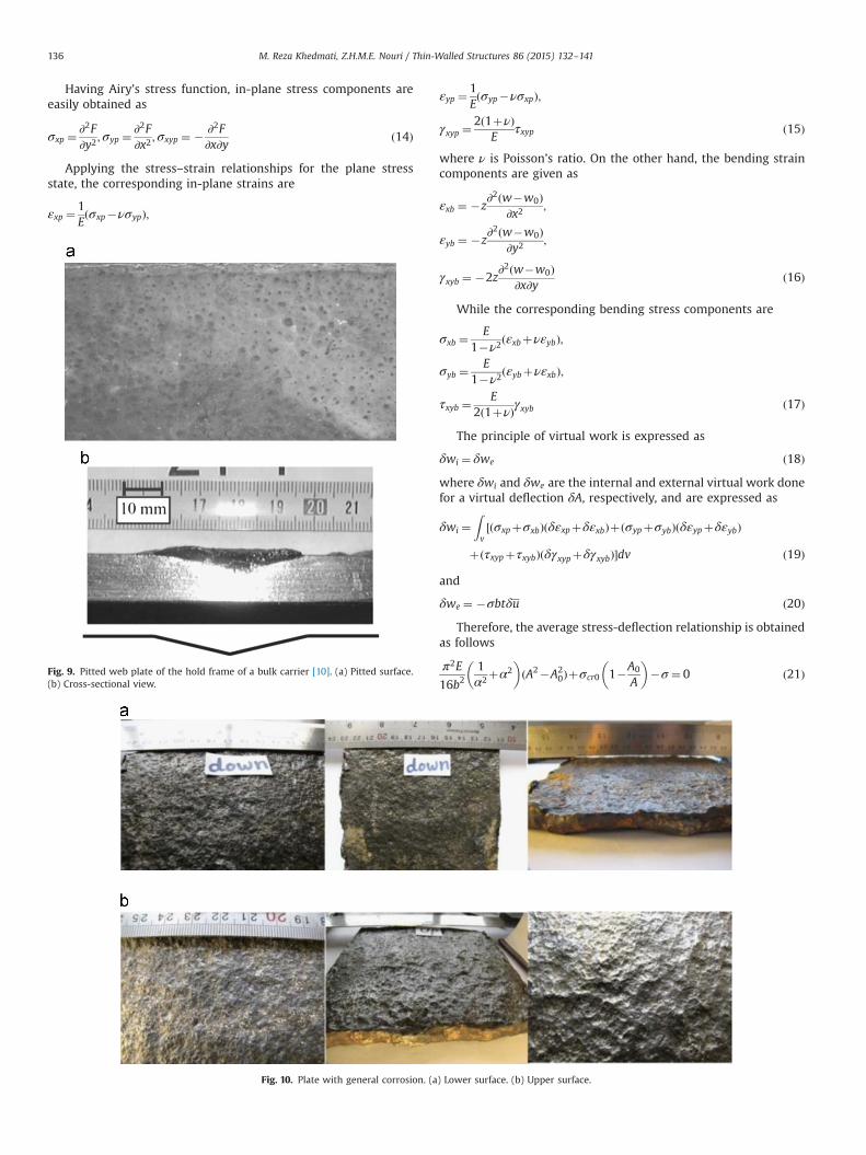
� ��σ ¼ 0 ð21ÞFig. 9. Pitted web plate of the hold frame of a bulk carrier [10]. (a) Pitted surface.

(b) Cross-sectional view.

Fig. 10. Plate with general corrosion. (a) Lower surface. (b) Upper surface.

M. Reza Khedmati, Z.H.M.E. Nouri / Thin-Walled Structures 86 (2015) 132–141136

where

σcr0 ¼π2t2E

12ð1�ν2Þb21αþα

� �2

ð22Þ

σcr0 is buckling strength of a simply-supported rectangular plate.The incremental form of Eq. (21) is

π2E

8b21α2þα2

� �A�ΔAþσcr0

A0

A2

� ��ΔA�Δσ ¼ 0 ð23Þ

where

ΔA¼ Ar�Ar�1 ð24Þ

and

Δσ ¼ σr�σr�1 ð25Þ

3.3.2. Plastic rangeWith the increase in the applied end-shortening displacement,

a plate undergoes buckling and yielding, and then attains itsultimate strength. After the ultimate strength, the compressiveload decreases with the increase of the applied end-shorteningdisplacement and deflection.

The average stress–plastic deflection relationship at the post-ultimate strength region is derived according to the rigid-plasticmechanism analysis (RPMA) assuming rigid-perfectly plasticmaterial. Depending on the plate aspect ratio (a/b), two config-urations of plastic mechanism may exist as illustrated in Fig. 7. Forthese mechanisms, the following relationships between the

average stress and deflection coefficient are derived [8]

m45þð1=α�1Þm90=2¼ ð2=α�1Þσ � A for αr1:0 ð26Þ

m45þðα�1Þm0=2¼ σ � A for α41:0 ð27Þwhere σ ¼ σ=σY ; A¼ A=t and :

m90 ¼ 1�σ2 ð28Þ

m0 ¼ 2m90=ffiffiffiffiffiffiffiffiffiffiffiffiffiffiffiffiffiffiffi1þ3m90

pð29Þ

m45 ¼ 4m90=ffiffiffiffiffiffiffiffiffiffiffiffiffiffiffiffiffiffiffiffiffiffi1þ15m90

pð30Þ

3.4. Relationship between average stress and average strain

3.4.1. Elastic rangeAccording to elastic large deflection analysis, the in-plane

shortening in x-direction will become

u¼ 1b

Z a

0

Z b

0εx�

12

∂w∂x

� �2

� ∂w0

∂x

� �2)(" #

dydx¼ �aEσ�m2π2

8a2ðA2�A2

0Þ

ð31ÞDividing u by the plate length a, average stress–average strain

relationship is derived as follows

ε¼ �1Eσ�m2π2

8a2ðA2�A2

0Þ ð32Þ

And its incremental form would be

Δε¼ �1EΔσ�m2π2

4a2A�ΔA ð33Þ

where

Δε¼ εr�εr�1 ð34Þ

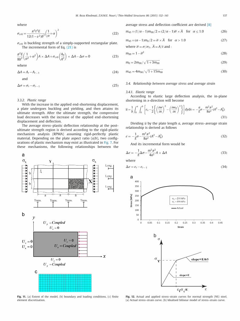
Fig. 11. (a) Extent of the model, (b) boundary and loading conditions, (c) finiteelement discretisation.

Fig. 12. Actual and applied stress–strain curves for normal strength (NS) steel.(a) Actual stress–strain curve. (b) Idealised bilinear model of stress–strain curve.

M. Reza Khedmati, Z.H.M.E. Nouri / Thin-Walled Structures 86 (2015) 132–141 137

3.4.2. Plastic rangeBased on rigid-plastic mechanism analysis, average stress–

average strain relationship is derived as

ε¼ �1Eσ�2m2

a2ðA2�A2

0Þ for αr1:0 ð35Þ

ε¼ �1Eσ�2m2

abðA2�A2

0Þ for α41:0 ð36Þ

Also, the incremental forms of above equations are

Δε¼ �1EΔσ�4m2

a2A�ΔA for αr1:0 ð37Þ

Δε¼ �1EΔσ�4m2

abA�ΔA for α41:0 ð38Þ

3.5. Procedure to obtain the average stress–deflection and averagestress–average strain curves

The procedure to create the average stress–deflection andaverage stress–average strain curves is shown schematically inFig. 8. The following steps are required to be done for obtainingthese relationships

(1) Using Eq. (23) the average stress–deflection curve in the elasticrange is drawn (dashed line in Fig. 8(a)).

Fig. 13. Comparison between simulated average stress–average strain relationships with FEA results for the un-corroded plate (a¼2400 mm, b¼800 mm, made of NS steel).

M. Reza Khedmati, Z.H.M.E. Nouri / Thin-Walled Structures 86 (2015) 132–141138

(2) The average stress–deflection relationship is drawn in theplastic range based on Eqs. (26) and (27) (dotted-dashed linein Fig. 8(a)).

(3) The initial yielding stress level (point A) is determined bychecking the stress state inside plate. A horizontal line AC isdrawn at the initial yielding stress level.

(4) The ultimate compressive strength (σUlt) of the plate isaccurately estimated by the second author’s formula [9] asfollows

σUlt=σY ¼1:0 for βr1:730:1þ1:571=β for β41:73

(ð39Þ

(5) The stress level corresponding to the predicted ultimatestrength is shown in Fig. 8(a) by the line cd. The deflectionat the ultimate strength level for point B is determined byassuming cB=cd as 1/3.

(6) Between points A and B, the deflection is approximated as

w¼weþcB 1�ffiffiffiffiffiffiffiffiffiffiffiffiffiffiffiffiffiffiffiffiffiffiffiffiffiffiffiffiffiffiffiffiffiffiffiffiffiffiffiffiffiffiffiffiffiffiffiffiffiffi1� σ�σAð Þ2= σB�σAð Þ2

q� �ð40Þ

where we is the elastic deflection at the stress level σ.(7) In the same manner, average stress-deflection relationship

between points B and C is determined using the followingequation

w¼wpþBd 1�ffiffiffiffiffiffiffiffiffiffiffiffiffiffiffiffiffiffiffiffiffiffiffiffiffiffiffiffiffiffiffiffiffiffiffiffiffiffiffiffiffiffiffiffiffiffiffiffiffiffi1� σ�σAð Þ2= σB�σAð Þ2

q� �ð41Þ

where wp is the plastic deflection at the stress level σ.(8) In the same manner, the average stress–average strain curve

(Fig. 8(b)) is obtained. To do that, Eq. (33) in the elastic rangeand Eqs. (37) and (38) in the plastic range are applied.

A special computer program was written in Fortran 77 lan-guage in order to implement the explained procedure in anincremental way.

4. Average stress–average strain relationship of both-sidesrandomly corroded plates

Corrosion in marine structures is mainly observed in twodistinct types, namely, general corrosion and localised corrosion.As an example of localised corrosion, reference may be made tothe corrosion of hold frames in way of cargo holds of bulk carrierswhich have coating such as tar epoxy paints, Fig. 9 [10]. Generally,pitting corrosion is defined as an extremely localised corrosiveattack and sites of the corrosive attack are relatively smallcompared to the overall exposed surface [11]. In the case oflocalised corrosion observed on hold frames of bulk carriers, thesites of the corrosive attack, that is, pits are relatively large (up toabout 50 mm in diameter).

General corrosion is the problemwhen the plate elements suchas the hold frames of bulk carriers have no protective coating,Fig. 10. Both surfaces of the plate may be corroded, in a pattern likethe sea waves spectrum, as shown in Fig. 10.

Based on the extensive results obtained by the authors [12,13],strength characteristics of a plate having random corrosion on it'sboth sides can be effectively assessed by considering an equivalentun-corroded plate with the equivalent thickness described by

teq ¼ t�μ�S ð42Þwhere t, μ and S are respectively representing the thickness ofplate in un-corroded condition, mean corrosion depth and stan-dard deviation of random thickness variations. Thus, for a both-sides randomly corroded plate of length a, breadth b and original

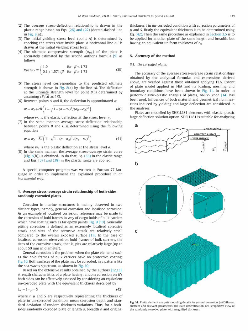
thickness t in un-corroded condition with corrosion parameters ofμ and S, firstly the equivalent thickness is to be determined usingEq. (42). Then the same procedure as explained in Section 3.5 is tobe applied for another plate of the same length and breadth, buthaving an equivalent uniform thickness of teq.

5. Accuracy of the method

5.1. Un-corroded plates

The accuracy of the average stress–average strain relationshipsobtained by the analytical formulas and expressions derivedabove, are verified against those obtained applying FEA. Extentof plate model applied in FEA and its loading, meshing andboundary conditions have been shown in Fig. 11. In order toperform elastic–plastic analysis of plates, ANSYS code [14] hasbeen used. Influences of both material and geometrical nonlinea-rities induced by yielding and large deflection are considered inthe analyses.

Plates are modelled by SHELL181 elements with elastic–plasticlarge deflection solution option. SHELL181 is suitable for analyzing

Fig. 14. Finite element analysis modeling details for general corrosion. (a) Differentsurfaces and relevant parameters. (b) Plate descretisation. (c) Perspective view ofthe randomly corroded plate with magnified thickness.

M. Reza Khedmati, Z.H.M.E. Nouri / Thin-Walled Structures 86 (2015) 132–141 139

thin to moderately-thick shell structures. It is a 4-node elementwith six degrees of freedom at each node: translations in the x, y,and z directions, and rotations about the x, y, and z-axes. SHELL181is well-suited for linear, large rotation, and/or large strain non-linear applications. Change in shell thickness is accounted for innonlinear analyses. In order to obtain reasonable results a numberof sensitivity analyses were carried out to find out the optimummesh density and proper values of nonlinear analysis options. Asample of finite element descretisations is represented in Fig. 11(c),which is relevant to a plate of aspect ratio equal to 3 with 30 and10 numbers of mesh divisions in longitudinal and transversedirections, respectively.

Axial compression was simulated by an imposed displacementin longitudinal direction, applied in small enough increments toensure that the analysis would closely follow the model load–response curve. The material was assumed of normal strength orso-called NS steel type, for which actual and applied stress–straincurves are shown in the Fig. 12. Yield stress (σY), Young’s modulusof elasticity (E) and Poisson’s ratio (ν) of the material wererespectively taken as 235 MPa, 205.8 GPa and 0.3.

It is evident that strain-hardening effect has some influence onthe nonlinear behaviour of plates. The degree of such an influenceis a function of many factors including plate slenderness. In thisstudy, material behaviour for plate was modelled as a bi-linearelastic-plastic manner with strain-hardening rate of E/65, Fig. 12(b). This value of strain-hardening rate was obtained through alarge number of elastic–plastic large deflection analyses made byKhedmati [9]. w0 and w0 max are obtained respectively according toEqs. (4) and (6).

Some comparisons for a range of thin to thick plates are shownin Fig. 13. The plates have a length of 2400 mm, a breadth of

800 mm and a thickness of 10 mm to 20 mm. As can be seen fromthe results, good correlations are observed among them, althoughsome more improvements are to be attempted in the future.

5.2. Both-sides randomly corroded plates

Randomly corroded surfaces were generated for both sides ofthe plate models. A special purpose computer code was written inFORTRAN90 language. Generation of randomly corroded surfaceswas achieved using the features of the DRANDM function ofFORTRAN90. There was one limitation in the generation processand it was standard deviation of the plate thicknesses at differentnodes that was set to 0.23 mm, as investigated by Ohyagi [15].Ohyagi corrosion model is adopted here as

dw ¼ 0:34ny ð43Þwhere ny is the number of years of exposure and dw is the uniformreduction in thickness in millimeters after ny years of exposure.Eq. (43) represents a linear corrosion model and is used here in asan example. It is obvious that the effectiveness of simulationprocedure explained in this paper is independent of the corr-osion model.

Finally the z-coordinate of upper and lower surfaces of theplate can be defined as, Fig. 14(a)

zLowSRF ¼w0�t�dw2

�r1 ; zUpSRF ¼w0þt�dw2

þr2 ð44Þ

where

tp ¼ zUpSRF�zLowSRF ¼ t�dwþr1þr2 ð45Þand also r1 and r2 are the random numbers, corresponding to the

Fig. 15. Comparison between simulated average stress–average strain relationships with FEA results for the corroded plate.

M. Reza Khedmati, Z.H.M.E. Nouri / Thin-Walled Structures 86 (2015) 132–141140

random thickness variation of the plate surfaces, produced byDRANDM function. Again w0 and w0 max are obtained respectivelyaccording to Eqs. (4) and (6).

There are several finite element techniques available to modeluniform corrosion. The easiest way is to reduce the thickness ofthe plate in surface, carry out buckling analysis to get the buckledshape of plate with uniform corrosion and finally to performnonlinear finite element control to get the ultimate strength ofplate by using stress versus strain relationship. Khedmati andKarimi [16] modelled corroded plate with 3-D 20-node structuralsolid element but this method also cannot represent the realsituation and easily tends to fail to converge during nonlinearcontrol based on author’s experience.

Fig. 14(b) represents modelling details in finite element analysis,while Fig. 14(c) shows a magnified view of the plate with surfacessimulating random corrosion. The same elements in ANSYS codewere used in descretisation of the corroded plate models.

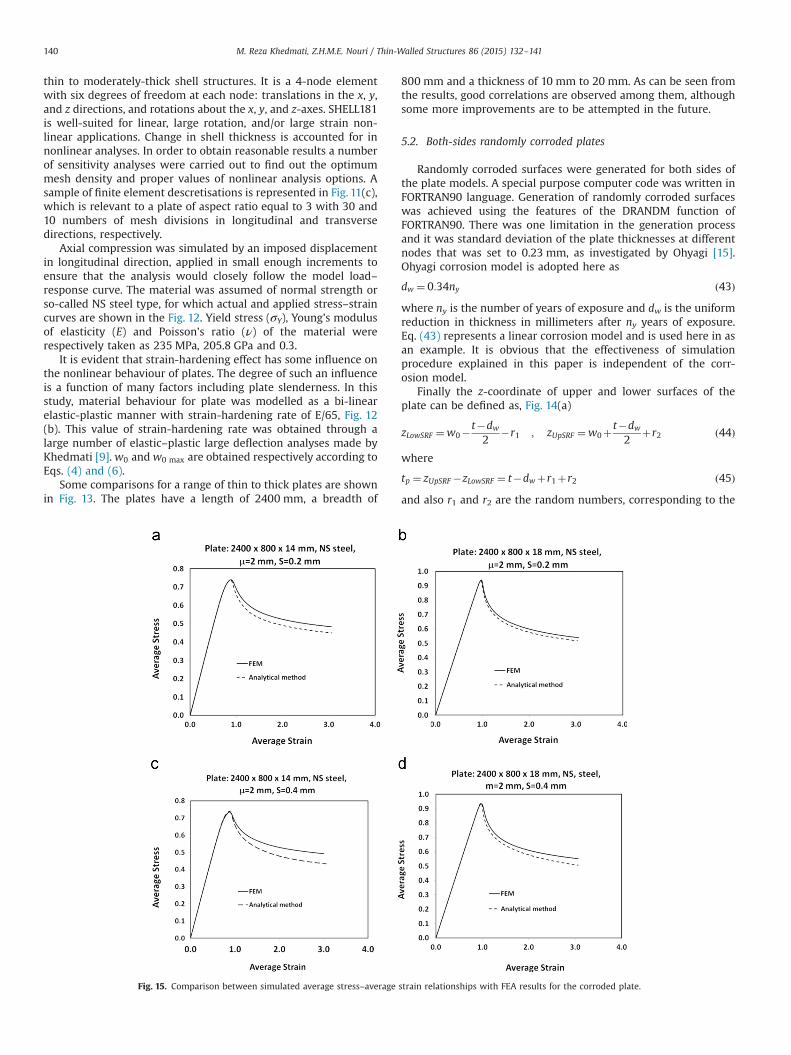
Some comparisons between simulated average stress–averagestrain relationships with FEA results for the corroded plate modelsare shown in Fig. 15. Again good correlation is observed betweentwo groups of FEM results and analytical ones.

6. Conclusions

A simple method for simulation of the average stress–averagestrain relationships of plates under the action of longitudinal axialcompression is developed. The features of the method are:

� The results of elastic large deflection analysis and rigid-plasticmechanism analysis are combined together in derivation of theaverage stress–average strain relationship of the plates. Theinfluences of buckling and plastic deformations are accountedfor in the formulations.

� The procedure is capable of simulating the average stress–average strain relationship for un-corroded as well as both-sides randomly corroded plates.

� The results show that the explained method is a simple andrelatively accurate and can be applied effectively in the ulti-mate strength evaluation of ship hull girders and other box-likestructures.

References

[1] Smith CS. Influence of local compressive failure on ultimate longitudinalstrength of a ship’s hull. Tokyo: PRADS; 1977.

[2] Smith CS. Structural redundancy and damage tolerance in relation to ultimateship hull strength. In: International symposium on the role of design,inspection and redundancy in marine structural reliability, Williamsburg,1983.

[3] Yao T, Fujikubo M, Yanagihara D Varghese B. Influences of welding imperfec-tions on buckling/ultimate strength of ship bottom plating subjected tocombined bi-axial & lateral pressure. In: Thin-walled structures, secondinternational conference on thin-walled structures, Elsevier, 1998:425–432.

[4] Smith CS. Imperfection effects and design tolerances in ships and offshorestructures. Trans Inst Eng Shipbuilders Scotland 1981;124:37–46.

[5] Ueda Y, Yao T. The influence of complex initial deflection on the behaviour andultimate strength of rectangular plates in compression. J Const Steel Res1985;5:265–302.

[6] Yao T, Nikolov PI, Miyagawa Y. Influence of welding imperfections on stiffnessof rectangular plates under thrust. In: Karlsson K, Lindgren LE, Jonsson M,editors. In: Proceedings of IUTAM Sump on mechanical effects of welding.Springer-Verlag; 1992. p. 261–8.

[7] Smith CS, Davidson PC, Chapman JC, Dowling PJ. Strength and stiffness of shipsplating under in-plane compression and tension. Trans RINA 1987;137:277–96.

[8] Okada H, Oshima K, Fukumoto Y. Compressive strength of long rectangularplates under hydrostatic pressure. J Soc Naval Arch Jpn 1979;146:270–80(in Japanese).

[9] Khedmati MR. Ultimate strength of ship structural members and systemsconsidering local pressure effects. (Dr. Eng. dissertation (Supervisors: TetsuyaYao and Masahiko Fujikubo). Grad. School of Eng., Hiroshima University; 2000(Oct.).

[10] Nakai T, Matsushita H, Yamamoto N. Effect of pitting corrosion on local strengthof hold frames of bulk carriers (1st report). Mar Struct 2004;17:403–32.

[11] ASM International Corrosion. ASM Handbook. 2001, Vol. 13.[12] Nouri ZHME. Assessment of effective thickness for practical evaluation of

ultimate strength and post-buckling behaviour of both-sides randomly cor-roded steel plates under uniaxial compression. (Interim progress report of PhDthesis (Supervisor: Mohammad Reza Khedmati). Faculty of Marine Technol-ogy, Amirkabir University of Technology; 2010 (January).

[13] Roshanali MM. Strength of plates with randomly distributed corrosionwastage under uniaxial compression, MSc thesis (Supervisor: MohammadReza Khedmati), Faculty of Marine Technology, Amirkabir University ofTechnology, February 2010.

[14] ANSYS 11.0 reference manual, ANSYS Inc. 2008.[15] Ohyagi M. Statistical survey on wear of ship’s structural members. Tokyo: NK

Technical Bulletin; 1987.[16] Khedmati MR, Karimi AR. Ultimate compressive strength of plate elements

with randomly distributed corrosion wastage. In: Topping BHV, Montero G,Montenegro R, editors. In: Proceeding of the eight international conference oncomputational structural technology. Civil-Comp Press; 2006.

M. Reza Khedmati, Z.H.M.E. Nouri / Thin-Walled Structures 86 (2015) 132–141 141