Analytical Modeling of Cyclic Steam Stimulation Process ...

University of Calgary

PRISM: University of Calgary's Digital Repository

Graduate Studies The Vault: Electronic Theses and Dissertations

2013-12-04

Analytical Modeling of Cyclic Steam Stimulation

Process for a Horizontal Well Configuration

Saripalli, Hari

Saripalli, H. (2013). Analytical Modeling of Cyclic Steam Stimulation Process for a Horizontal Well

Configuration (Unpublished master's thesis). University of Calgary, Calgary, AB.

doi:10.11575/PRISM/24826

http://hdl.handle.net/11023/1173

master thesis

University of Calgary graduate students retain copyright ownership and moral rights for their

thesis. You may use this material in any way that is permitted by the Copyright Act or through

licensing that has been assigned to the document. For uses that are not allowable under

copyright legislation or licensing, you are required to seek permission.

Downloaded from PRISM: https://prism.ucalgary.ca

UNIVERSITY OF CALGARY

Analytical Modeling of Cyclic Steam Stimulation Process for a Horizontal Well

Configuration

by

Hari Kaushik Saripalli

A THESIS

SUBMITTED TO THE FACULTY OF GRADUATE STUDIES

IN PARTIAL FULFILLMENT OF THE REQUIREMENTS FOR

THE DEGREE OF MASTER OF SCIENCE

DEPARTMENT OF CHEMICAL AND PETROLEUM ENGINEERING

CALGARY, ALBERTA

DECEMBER, 2013

© Hari Kaushik Saripalli 2013

i

Abstract

Cyclic steam stimulation is one of the most widely used heavy oil recovery methods.

Steam is injected into a formation at high rates for several weeks through a vertical well.

The well is then shut-in for a certain period of time, which is called “soak” period. Steam

condenses in the formation, thus heating the reservoir rock and fluids around the

wellbore. During this period the oil viscosity is reduced by many times. The heated sand

contains mobile oil, steam and water. The oil and other fluids are expelled out as the sand

face pressure is lowered when the well is put on production. Oil is produced until the oil

rate reaches an economic limit and the cycle is repeated again.

There are many analytical models that predict the performance of a conventional Cyclic

Steam Stimulation process for vertical wells. However, there are only very few models

that are applicable to a horizontal well configuration. The objective of this study is to

model heavy oil production using cyclic steam stimulation with a horizontal well

configuration. Reasonable assumptions were made to simplify the problems to an extent

that they can be solved using analytical or semi-analytical methods. Such analytical or

semi-analytical solutions are required for more advanced understanding of the physical

problem under investigation and validation of more sophisticated numerical models. The

practical value of these solutions lies in the fact that they aid to improve interpretations

and conduct fast sensitivity analysis and fast computations.

In order to predict oil production the governing equations of heat and fluid flow in

cylindrical coordinate need to be solved. Average temperatures in the formation during

the steam injection process are calculated by solving the transient heat transfer equations.

The heat transfer model is then coupled to a fluid in flow model to predict the fluid rates.

The fluid inflow model is a two phase model that takes into account the relative

permeability of oil and water. The developed model is validated with the fine grid

numerical simulation of the problem using STARS® numerical simulator from CMG.

Since, a lot of simplifying assumptions are involved modifications, such as a correction

for the pressure drawn-down and water relative permeability, were made during the

ii

history matching with STARS, in order to get a good match for the fluid rates. These

modifications include altering the relative permeability of water and making an initial

guess of the pressure draw down based on the results from the simulator. The robustness

of the model was tested by comparing the model results with the results from the

numerical simulator by changing various parameters such as: steam injection rates,

reservoir permeability, relative permeability, oil viscosity and reservoir diffusivity.

With some reasonable assumptions, it is seen that the results from the developed model

are very close to the results obtained using STARS numerical simulator from CMG and it

can be concluded that the proposed model captures the essential mechanism of the

process. The model is relatively simple and all the calculations can be performed using a

user friendly spreadsheet in just a few minutes. Currently, the proposed model can be

used to optimize production from a single well. The model can be coupled with an

economic model to optimize steam injection rates and production rates based on the

reservoir properties.

iii

Acknowledgements

First of all, I would like to express my sincere appreciation to my supervisor, Dr. Hassan

Hassanzadeh, for his outstanding support, constant guidance, and encouragement,

throughout the course of this research and my master’s program at the University of

Calgary. It has truly been a great privilege for me to work with him. Without his support

and help, this work would not be accomplished.

I am also grateful to the members of my thesis committee, Dr. Sudarshan A Mehta, Dr.

Brij Maini, and Dr. Abdulmajeed Mohamad, for taking time out of their busy schedule to

read my thesis and for their valuable comments. My gratitude also goes to the

Department of Chemical and Petroleum Engineering at the University of Calgary and

PennWest Exploration for their financial support. I would like to acknowledge Majid

Saeedi, without whom the project would not have been successful.

I am thankful to my friends and fellow graduate students for their support and help during

my research.

Last but most importantly, I thank my parents for the encouragement and continuous

support they have given me all the way.

iv

Table of Contents

Abstract ................................................................................................................................ i

Acknowledgements ............................................................................................................ iii

Table of Contents ............................................................................................................... iv

List of Tables .................................................................................................................... vii

List of Figures .................................................................................................................. viii

Nomenclature ................................................................................................................... xiii

1 INTRODUCTION ....................................................................................................... 1

1.1 Typical Reservoir Properties.................................................................................... 1

1.2 Thermal Recovery Methods ..................................................................................... 2

1.2.1 In situ combustion ................................................................................................ 2

1.2.2 Cyclic steam stimulation ...................................................................................... 3

1.2.3 Wellbore heating .................................................................................................. 5

1.2.4 Steam flooding ..................................................................................................... 5

1.2.5 Hot water flooding ............................................................................................... 5

1.2.6 Steam assisted gravity drainage ........................................................................... 5

1.3 Motivations and Objectives ..................................................................................... 5

1.4 Organization of Thesis ............................................................................................. 6

2 LITERATURE REVIEW ............................................................................................ 8

2.1 Existing CSS and Horizontal Well Models ............................................................. 8

2.1.1 Cyclic steam injection using vertical wells .......................................................... 8

2.1.2 Models for pressure depleted gravity drainage reservoirs ................................. 15

2.1.3 In-flow equations for horizontal wells: .............................................................. 17

2.1.4 Cyclic steam stimulation using horizontal wells ................................................ 20

2.2 Concluding Remarks .............................................................................................. 23

v

3 ANALYTICAL MODELING ................................................................................... 24

3.1 Cyclic Steam Stimulation for Horizontal wells ..................................................... 24

3.1.1 Model assumptions ............................................................................................. 25

3.1.2 Volume of steam zone ........................................................................................ 25

3.1.3 Heat remaining in the reservoir .......................................................................... 26

3.1.4 Average steam zone temperature: ...................................................................... 27

3.1.5 Oil and water viscosities .................................................................................... 34

3.1.6 Fluid saturations and relative permeabilities ...................................................... 34

3.1.7 Fluid- inflow equation ........................................................................................ 35

3.1.8 Flow chart showing important steps in calculations .......................................... 37

3.2 Summary ................................................................................................................ 39

4 VALIDATION OF THE MODEL AND SENSITIVITY ANALYSES ................... 40

4.1 Base Case ............................................................................................................... 40

4.1.1 Input data ............................................................................................................ 40

4.1.2 Relative permeability model .............................................................................. 42

4.1.3 Relative permeability adjustment ....................................................................... 43

4.1.4 Pressure drop model and inflow equation .......................................................... 45

4.2 Sensitivity Analyses ............................................................................................... 49

4.2.1 Grid sensitivity ................................................................................................... 50

4.2.2 Steam injection rates .......................................................................................... 53

4.2.3 Length of horizontal well ................................................................................... 57

4.2.4 Absolute permeability ........................................................................................ 60

4.2.5 Relative permeability of oil and water ............................................................... 65

4.2.6 Thermal diffusivity ............................................................................................. 68

4.2.7 Types of oil viscosity ......................................................................................... 71

4.2.8 Number of cycles ............................................................................................... 73

4.3 Summary ................................................................................................................ 78

vi

5 CONCLUSIONS AND RECOMMENDATIONS .................................................... 79

5.1 Results .................................................................................................................... 79

5.2 Future Work ........................................................................................................... 80

5.2.1 Economic studies................................................................................................ 80

5.2.2 Pressure drop model and water relative permeability adjustment ..................... 80

APPENDIX ....................................................................................................................... 81

REFERENCES ................................................................................................................. 85

vii

List of Tables

Table 1.1: Definitions of heavy oil based on properties ..................................................... 1

Table 3.1 Reservoir parameters and PVT data ................................................................. 32

Table 3.2 Operational parameters ..................................................................................... 33

Table 4.1 Operational parameters ..................................................................................... 40

Table 4.2 Reservoir parameters and PVT data ................................................................. 41

Table 4.3 Viscosity data .................................................................................................... 41

Table 4.4 Model dimensions and grid data ....................................................................... 41

viii

List of Figures

Figure 1.1: A typical cyclic steam injection process .......................................................... 4

Figure 2.1: Plot of F1 versus dimensionless time (after Marx- Langenheim) ................... 10

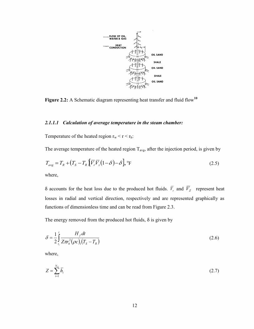
Figure 2.2: A Schematic diagram representing heat transfer and fluid flow .................... 12

Figure 2.3: and versus dimensionless time (after Boberg and Lantz). .................... 13

Figure 2.4 a) Schematic diagram of heated area geometry; b) differential element of the

heated area. ....................................................................................................................... 21

Figure 2.5: Schematic diagram of area of cross section of heated area. .......................... 22

Figure 3.1: Schematic diagram of model .......................................................................... 28

Figure 3.2: A plot of dimensionless temperature of Zone 1 and Zone 2 versus

dimensionless time ............................................................................................................ 31

Figure 3.3: A plot of the average temperature of Zone 1 and Zone 2 versus time ........... 32

Figure 3.4: Volume and radius of steam zone for three cycles ......................................... 33

Figure 3.5: Plot of the average steam zone temperature versus time for three cycles ...... 34

Figure 4.1: Oil and water relative permeabilities .............................................................. 42

Figure 4.2: Water saturations in the heated zone obtained from developed model and

STARS .............................................................................................................................. 43

Figure 4.3: Oil relative permeability obtained from developed model and STARS ........ 44

Figure 4.4: Water relative permeability obtained from developed model and STARS .... 44

Figure 4.5: Comparison of oil production rate, qo, obtained from the model versus

STARS simulator. ............................................................................................................. 47

rV ZV

ix

Figure 4.6: Comparison of cumulative oil production, Qo, from the model versus STARS.

........................................................................................................................................... 47

Figure 4.7: Comparison of water rate, qw, obtained from model versus STARS simulator

........................................................................................................................................... 48

Figure 4.8: Comparison of cumulative water production, Qw, from the model versus

STARS. ............................................................................................................................. 49

Figure 4.9: Plot of oil production rate, qo, versus time for different grid sizes. ............... 51

Figure 4.10: Plot of cumulative oil production, Qo, versus time for different grid sizes. . 51

Figure 4.11: Plot of water production rates, qw, versus time for different grid sizes........ 52

Figure 4.12: Plot of cumulative water production, Qw, versus time for different grid sizes.

........................................................................................................................................... 52

Figure 4.13: Comparison of oil production rates from STARS and model for a steam

injection rate of 1800 bpd. ................................................................................................ 54


injection rate of 2500 bpd. ................................................................................................ 54

Figure 4.15: Comparison of oil rate from STARS and model for steam injection rate of

3000 bpd............................................................................................................................ 55

Figure 4.16: Cumulative oil production versus time for different steam injection rates. . 55

Figure 4.17: Comparison of water production rate from STARS and model for different

steam injection rates. ......................................................................................................... 56

Figure 4.18: Comparison of cumulative water production obtained from STARS and

analytical model for different steam injection rates. ......................................................... 56

Figure 4.19: Comparison of oil rates from STARS and model for a well length of 1000ft.

........................................................................................................................................... 57

x

Figure 4.20: Comparison of oil production rates from STARS and model for a well length

of 1250ft. ........................................................................................................................... 58

Figure 4.21: Cumulative oil production versus time for different lengths of the horizontal

well. ................................................................................................................................... 58


horizontal well lengths. ..................................................................................................... 59

Figure 4.23: Comparison of cumulative water production from STARS and model for

different lengths of horizontal well. .................................................................................. 59

Figure 4.24: Comparison of oil rate from STARS and model for absolute permeability of

150 mD.............................................................................................................................. 60


200 mD.............................................................................................................................. 61

Figure 4.26: Comparison of cumulative oil production versus time from, STARS and

developed model, for different absolute permeability values. .......................................... 61

Figure 4.27: Comparison of water production rate versus time, form STARS and


Figure 4.28: Comparison of cumulative water production versus time, from STARS and


Figure 4.29: Plot of oil production rate, qo, obtained from STARS and analytical model

for a permeability of 1000 mD.......................................................................................... 63

Figure 4.30: Plot of cumulative oil production, Qo, obtained from STARS and analytical

model for a permeability of 1000 mD. .............................................................................. 64

Figure 4.31: Plot of water production rate, Qw, obtained from STARS and analytical

model for a permeability of 1000 mD. .............................................................................. 64

xi

Figure 4.32: Plot of cumulative water production, Qw, obtained from STARS and

analytical model for a permeability of 1000 mD. ............................................................. 65

Figure 4.33: Different types of relative permeability curves versus water saturation. ..... 66

Figure 4.34: Comparison of oil production rate versus time, from STARS and developed

model, for a different relative permeability model. .......................................................... 66

Figure 4.35: Comparison of cumulative oil production versus time, from STARS and

developed model, for different relative permeability curves. ........................................... 67

Figure 4.36: Comparison of water production rate versus time, from STARS and

developed model, for a different relative permeability model. ......................................... 67


developed model, for a different relative permeability model. ......................................... 68

Figure 4.38: Comparison of oil rate versus time, from STARS and developed model, for a

new diffusivity value......................................................................................................... 69

Figure 4.39: Comparison of cumulative oil production versus time, form STARS and

developed model, for a different thermal diffusivity value. ............................................. 69

Figure 4.40: Comparison of water production rates versus time, form STARS and

developed model, for a different thermal diffusivity value. ............................................. 70


developed model, for different thermal diffusivities. ....................................................... 70

Figure 4.42: Comparison of oil rate versus time, from STARS and developed model, for

PennWest oil viscosity. ..................................................................................................... 71


developed model, for different types of oil- viscosity. ..................................................... 72

Figure 4.44: Comparison of water production rate versus time, from STARS and model,

for PennWest oil viscosity. ............................................................................................... 72

xii


developed model, for PennWest oil viscosity. .................................................................. 73


model, for ten cycles. ........................................................................................................ 74


developed model, for ten cycles........................................................................................ 74


developed model, for ten cycles........................................................................................ 75

Figure 4.49: Comparison of cumulative water production versus time, obtained from

STARS and developed model, for ten cycles. .................................................................. 75

Figure 4.50: Plot of cumulative steam oil ratio versus time ............................................. 77

Figure 4.51: Plot of average steam oil ratio versus the number of cycles ........................ 77

xiii

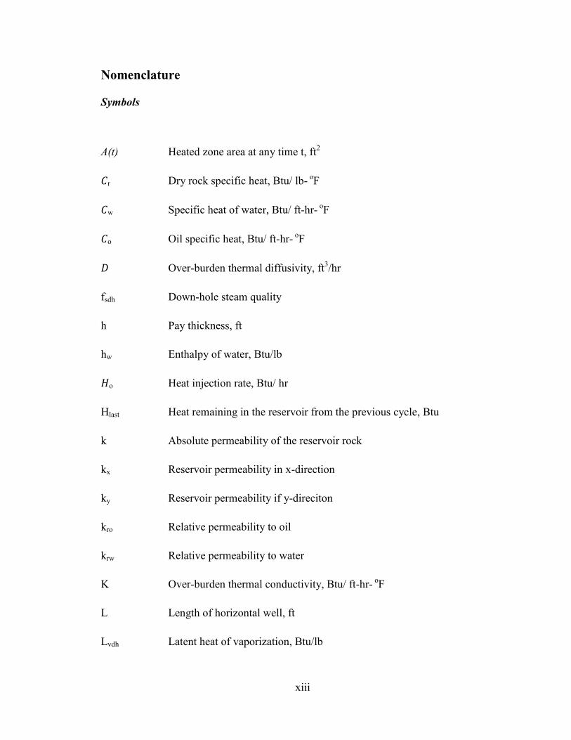
Nomenclature

Symbols

A(t) Heated zone area at any time t, ft2

r Dry rock specific heat, Btu/ lb- oF

w Specific heat of water, Btu/ ft-hr- oF

o Oil specific heat, Btu/ ft-hr- oF

Over-burden thermal diffusivity, ft3/hr

fsdh Down-hole steam quality

h Pay thickness, ft

hw

Enthalpy of water, Btu/lb

o Heat injection rate, Btu/ hr

Hlast Heat remaining in the reservoir from the previous cycle, Btu

k Absolute permeability of the reservoir rock

kx Reservoir permeability in x-direction

ky Reservoir permeability if y-direciton

kro Relative permeability to oil

krw Relative permeability to water

K Over-burden thermal conductivity, Btu/ ft-hr- oF

L Length of horizontal well, ft

Lvdh Latent heat of vaporization, Btu/lb

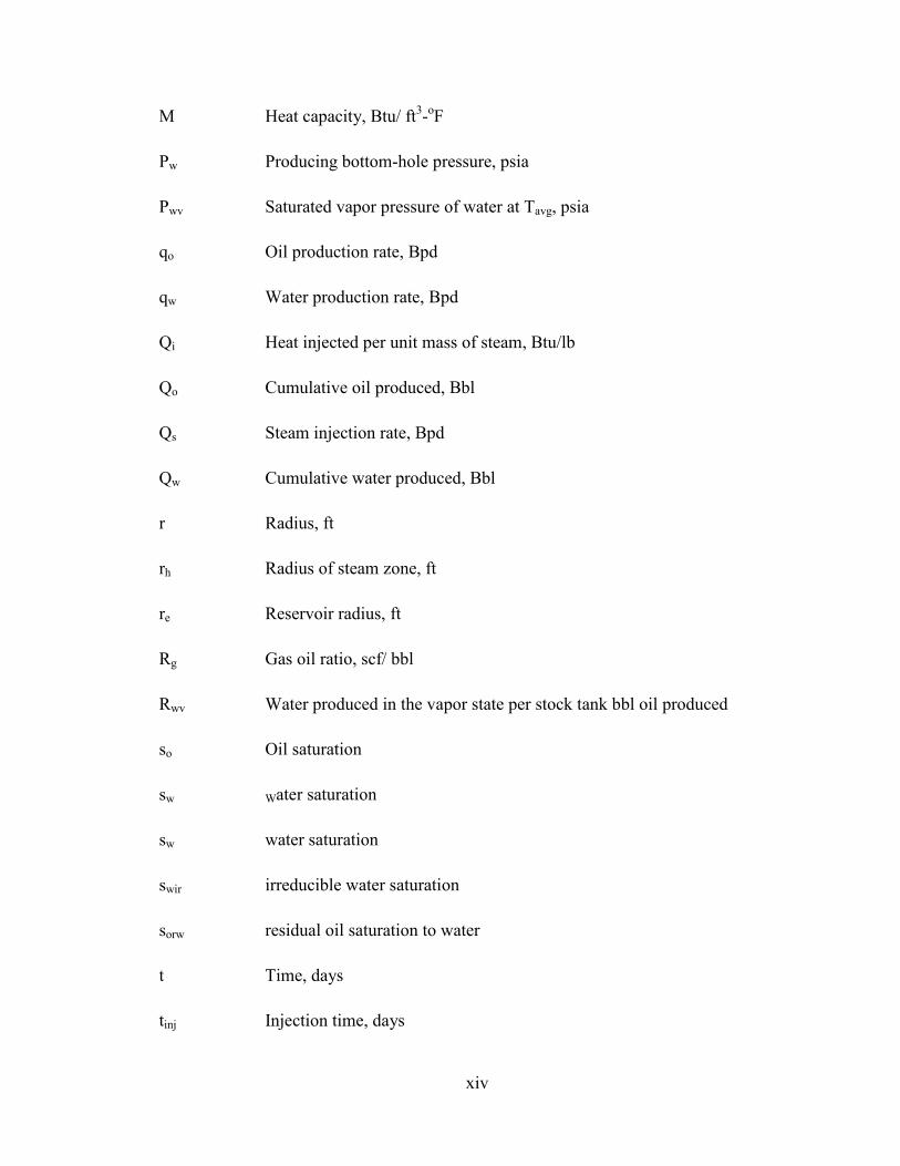
xiv

M Heat capacity, Btu/ ft3-oF

Pw Producing bottom-hole pressure, psia

Pwv Saturated vapor pressure of water at Tavg, psia

qo Oil production rate, Bpd

qw Water production rate, Bpd

Qi Heat injected per unit mass of steam, Btu/lb

Qo Cumulative oil produced, Bbl

Qs Steam injection rate, Bpd

Qw Cumulative water produced, Bbl

r Radius, ft

rh Radius of steam zone, ft

re Reservoir radius, ft

Rg Gas oil ratio, scf/ bbl

Rwv Water produced in the vapor state per stock tank bbl oil produced

so Oil saturation

sw Water saturation

sw water saturation

swir irreducible water saturation

sorw residual oil saturation to water

t Time, days

tinj Injection time, days

xv

T Temperature, oF

TS Steam temperature, oF

TR Reservoir temperature, oF

TAvg Average steam zone temperature, oF

rV Dimensionless heat loss in radial direction

zV Dimensionless heat loss in vertical direction

Vs Volume of steam zone, ft3

Wp Cumulative water produced, Bbl

WIP Water-in-place, Bbl

Reservoir thermal diffusivity, ft2/hr

o Viscosity of oil, cp

ho Viscosity of oil in the heated zone, cp

co Viscosity of oil in the cold zone, cp

w Viscosity of water, cp

wh Visocisty of water in the heated zone, cp

cw Viscosity of water in the cold zone, cp

p Pressure drawdown, psi

Formation porosity

r Rock grain density, lb/ft3

w Water density, lb/ft3

xvi

o Oil density, lb/ft3

w Density of water, lb/ft3

Volumetric heat capacity of the reservoir rock, Btu/ft3-oF

Dimensionless heat loss due to the produced hot fluids

Subscripts

1 Zone 1

2 Zone 2

Avg. Average

h heated zone boundary

o Oil

w Water

R Reservoir

S Steam

tc

1

CHAPTER ONE:

1 Introduction

Heavy oil and oil sands are important hydrocarbon resources that play an important role

in the oil supply of the world, and North America particularly. Oil sands account for one

fourth of the oil production of Canada1. The resource base of heavy oil and oil sands is

much larger than the in-place conventional oil. Conventional oils have an API gravity of

25o

or higher. Heavy oil and oil (tar) sands are petroleum or petroleum-like liquids or

semi-solids occurring in porous formations, mainly sands and also carbonates. The

definitions, according to 1982 UNITAR conference is summarized below:

Table 1.1: Definitions of heavy oil based on properties

Classification Viscosity

(cp at Res. Temp.)

Density at 15oC

(kg/m3)

API Gravity

Heavy Crude 100-10000 943-1000 20-10

Oil Sand Crude

(Bitumen) >10000 1000 <10

1.1 Typical Reservoir Properties

Most of the heavy oil and bitumen occur in shallow (around 1000 m), high permeability

(One to several Darcies), highly porous (30%), and poorly consolidated formations. The

2

oil saturation is generally high (typically greater than 50% pore volume) and the

formation thickness may range from 10 to hundreds of meters1. However, there are some

exceptions as well. For example, in Saskatchewan, 85% of the oil occurs in formations of

less than 3 m thickness. Most heavy oils in California and Venezuela have viscosities in

the range of 1000-2000 m.Pa.s whereas; those in Cold Lake, Alberta is around 100,000

m.Pa.s. The temperatures in the heavy oil reservoirs of Canada are very low, for example,

around 15-20oC at the depths of around 500 m

1.

1.2 Thermal Recovery Methods

Thermal methods aim to reduce the viscosity of oil by application of heat. This can be

achieved by either hot fluid injection or by in- situ combustion. The thermal processes

currently used are briefly reviewed in the following.

1.2.1 In situ combustion

The process is applicable for a wide range of oil gravities. In-situ combustion can be

classified into: i) Forward Dry combustion, ii) Forward Wet Combustion and iii) Reverse

Combustion. Forward dry combustion involves injection of oxygen rich air, ignition

within the oil sand, and propagation of a combustion front through the reservoir. Oil is

displaced by hot gas (nitrogen and carbon dioxide) passing ahead of the combustion front

and by steam obtained from the combustion process and vaporization of the connate

water. Forward wet combustion involves simultaneous injection of air and water.

Theoretically, it should be the most efficient of all thermal drive processes as it has

mechanisms of both a steam drive and dry- combustion drive process. However, in

practice, gravitational forces cause separation of air and water, and the process is very

difficult to control. The challenges of predicting the field performance of air injection

projects using laboratory and numerical modeling has been addressed by Gutierrez et

al.2. They proposed that an optimum design cycle can be obtained by performing

laboratory testing that would help in the design and monitoring of a pilot scale field

operation. The data from pilot operation, as well as laboratory data can be used to history

match and fine tune the analytical models for prediction of the full field operation.

3

In reverse combustion, air flow is counter to the direction of the combustion front. Air is

injected until there is a communication with the procuring wells and then using a

downhole heater to ignite the oil sand around the producing well. The combustion front

burns back towards the injection well. However, this process has been unsuccessful in the

field.

1.2.2 Cyclic steam stimulation

This technique is by far the most popular3 thermal stimulation process and will be

discussed in great detail in this thesis. Steam is injected into a formation at high rates for

several weeks through a vertical well. The well is then shut-in for a certain period of

time, which is called “soak” period. Steam condenses in the formation, thus heating the

reservoir rock and fluids around the wellbore. During this period the oil viscosity is

reduced by many times. The amount of oil produced in a cyclic steam injection process

depends largely on the how much the viscosity of oil is reduced, which is controlled by

the amount of heat that is transferred from the injected steam to the reservoir. The heated

sand contains mobilized oil, steam and water. The oil and other fluids are expelled out as

the sand face pressure is lowered when the well is put on production. Oil is produced

until the well reaches an economic limit and the cycle is repeated again. A typical CSS

process is shown in Figure 1.1

4

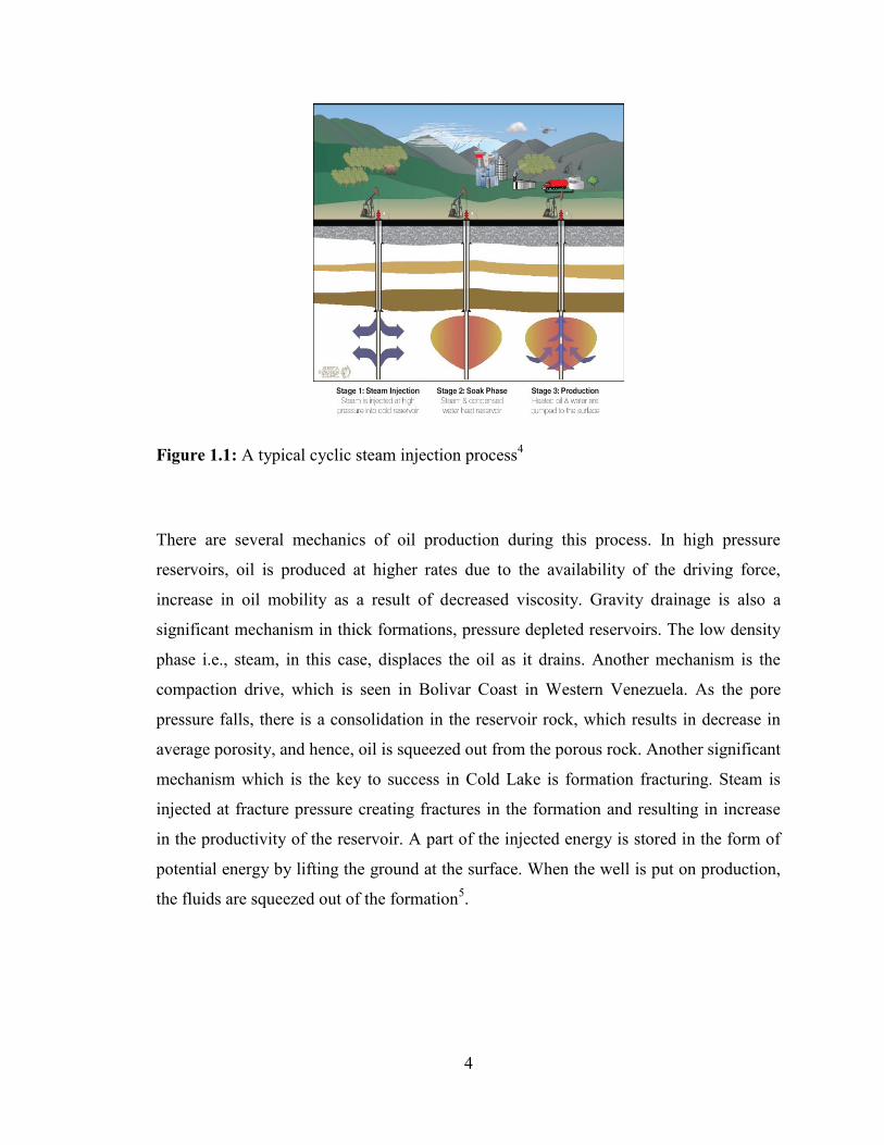
Figure 1.1: A typical cyclic steam injection process4

There are several mechanics of oil production during this process. In high pressure

reservoirs, oil is produced at higher rates due to the availability of the driving force,

increase in oil mobility as a result of decreased viscosity. Gravity drainage is also a

significant mechanism in thick formations, pressure depleted reservoirs. The low density

phase i.e., steam, in this case, displaces the oil as it drains. Another mechanism is the

compaction drive, which is seen in Bolivar Coast in Western Venezuela. As the pore

pressure falls, there is a consolidation in the reservoir rock, which results in decrease in

average porosity, and hence, oil is squeezed out from the porous rock. Another significant

mechanism which is the key to success in Cold Lake is formation fracturing. Steam is

injected at fracture pressure creating fractures in the formation and resulting in increase

in the productivity of the reservoir. A part of the injected energy is stored in the form of

potential energy by lifting the ground at the surface. When the well is put on production,

the fluids are squeezed out of the formation5.

5

1.2.3 Wellbore heating

Down-hole electrical, gas, and steam heaters have been used to improve the mobility of

oil in the near vicinity of the well bore.6 Though steam stimulation offers much deeper

heat penetration and much greater stimulation effect, wellbore heating is sometimes used

for low production rate wells where depth, excessive injection pressure or swelling clays

prevent the application of steam. Well-bore heating techniques have a potential to be used

in the recovery of oil shale, where steam injection is not possible because of extremely

low permeability of the reservoir.

1.2.4 Steam flooding

The main advantage of this multi well pattern type method is its large areal coverage and

high recovery factor (around 50%). However, this method has drawbacks such as high

heat losses and long payout times and high expenditure.1

1.2.5 Hot water flooding

In this method, heat losses in the wellbore and formation cause a large drop in

temperature and is less effective in reducing the oil viscosity. However, this process can

be applied in deep heavy oil reservoirs where steam may not be very successful. Hot

water flooding is used in Kaparuk filed in Alaska.1

1.2.6 Steam assisted gravity drainage

In this process, a pair of horizontal wells is drilled at a certain vertical distance near the

base of the formation. Steam is injected into the upper well. Steam rises up in the

formation and forms a steam chamber that heats the oil at the interface. The steam

chamber grows upwards and laterally, as oil is mobilized and produced, along with

condensed water, is produced from the lower well. This process is sensitive to geology

and extremely effective in highly viscous oil formations1.

1.3 Motivations and Objectives

Traditionally, vertical wells have been utilized in the majority of the cyclic steam

stimulation projects. However, since CSS with vertical well configuration may not be

efficient in thin formations, application of horizontal wells becomes inevitable as the

6

industry is moving toward production from such formations. Horizontal well technology

provides a more efficient access to oil resources that are not recoverable using vertical

wells. In general, horizontal wells have better injectivity, and their productivity is higher

than vertical wells draining the same volume of reservoir. For a given reservoir, a

horizontal well has a higher contact area than a vertical well and hence, the heated zone

around a horizontal well will be larger than that of a vertical well. Hence, cyclic steam

stimulation using horizontal wells can be very useful in thin-heavy oil reservoirs.

Empirical correlations are very helpful to correlate data within a field for predicting the

performance of new wells in that field. Compositional or black-oil thermal reservoir

simulators can be used to predict the performance of cyclic steam stimulation. These

thermal models are based on mass and heat balance equations. Fluid flow is related to

pressure gradient through the concept of relative permeability. In addition, a thermal

model is sensitive to input data such as rock properties, fluid properties and geological

features that are often not known or available. Also, because of the complex nature of the

cyclic steam stimulation process, it could be very difficult and expensive to use thermal

reservoir simulators. Hence, an analytical model of cyclic steam injection might be useful

to describe basic features of reservoir heating and oil production.

Analytical or semi-analytical models with reasonable assumptions need to be developed

to better understand the shape of steam zone during steam injection, to calculate the oil

production rate, and also optimize the process based on process variables studies. The

objective of this study is to develop analytical models that can predict the performance of

a cyclic steam stimulation process for a horizontal well configuration.

1.4 Organization of Thesis

The outline for the remainder of this thesis is as follows:

Chapter 2 reviews the relevant literature on the existing models for a cyclic steam

stimulation process. Heat transfer models as well as fluid in flow models for horizontal

wells are reviewed.

7

Chapter 3 describes the analytical model developed in this study that is able to simulate

heat transfer and fluid flow and outlines the steps to perform the calculations for

predicting oil and water flow rates for a CSS process with a horizontal well

configuration.

Chapter 4 presents the simulation studies of CSS process using the thermal simulator

STARS by CMG. Sensitivity analysis has been performed and the model is validated for

an expected range of parameters. A comparison of the results obtained from the

developed analytical model and results from simulation are presented in this chapter.

Finally, Chapter 5 presents conclusions of this thesis and makes recommendations for

future works.

8

CHAPTER TWO:

2 Literature Review

2.1 Existing CSS and Horizontal Well Models

Existing models can be divided into four categories: i) cyclic steam injection using

vertical wells, ii) models for pressure depleted gravity drainage reservoirs, iii) in-flow

equations for productivity of horizontal wells and iv) cyclic steam injection using

horizontal wells.

2.1.1 Cyclic steam injection using vertical wells

Steam is injected at a fixed rate and a known well-head quality. As the steam enters the

reservoir, there is some heat loss in the wellbore. The amount of heat reaching the

reservoir during the steam injection is essentially a function of the steam injection

temperature and well-bore heat losses. The bottom hole steam quality and pressure can be

predicted from a wellbore model as described by Fontilla and Aziz7. Marx and

Langenheim8 described a method for estimating thermal invasion rates, cumulative

heated area, and theoretical economic limits for sustained hot fluid injection at a constant

rate into an idealized reservoir. Full allowance is made for non-productive reservoir heat

losses. The method is very simplistic and does not require extensive mathematical

calculations.

The heated zone area A(t), at any time t, can be calculated using the method described by

Marx-Langenheim8

(Equation. 2.1).

9

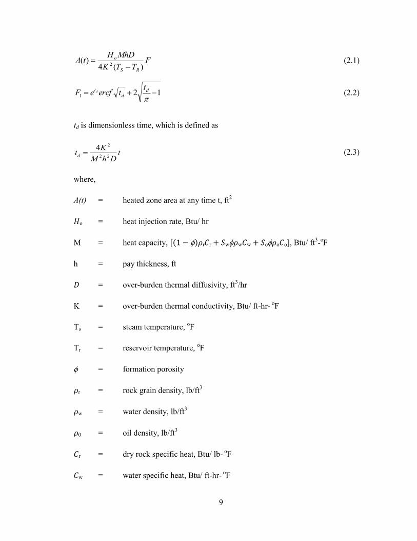
FTTK

MhDHtA

RS

o

)(4)(

2 (2.1)

121 d

d

t ttercfeF d (2.2)

td is dimensionless time, which is defined as

tDhM

Ktd 22

24 (2.3)

where,

A(t) = heated zone area at any time t, ft2

o = heat injection rate, Btu/ hr

M = heat capacity, ( ) r r w w w o o o], Btu/ ft3-oF

h = pay thickness, ft

= over-burden thermal diffusivity, ft3/hr

K = over-burden thermal conductivity, Btu/ ft-hr- oF

Ts = steam temperature, oF

Tr = reservoir temperature, oF

= formation porosity

r = rock grain density, lb/ft3

w = water density, lb/ft3

= oil density, lb/ft3

r = dry rock specific heat, Btu/ lb- oF

w = water specific heat, Btu/ ft-hr- o

F

10

o = oil specific heat, Btu/ ft-hr- oF

o, w = initial oil and water saturations, respectively

t = time since the start of injection, hours

Figure 2.1 shows a plot of F1 vs. td and it can be used to calculate the values of F1.

d √ d √ d

Figure 2.1: Plot of F1 versus dimensionless time (after Marx- Langenheim4)

During the injection period the temperature gradient of the hot zone can be estimated

using Marx and Langenheim’s equation4

rhk

terfceH

dr

dT d

t

od

2

)(2

(2.4)

0.01

0.1

1

10

0.01 0.1 1 10

F1

td

11

The solution for the heated area is based on the fluid flow analogy by Carter9, does not

depend upon the direction of development of the heated area and hence, can be applied

for heat injection in any type of well pattern with any specified swept area. For a vertical

well, assuming a cylindrical heated area, the radius of the heated zone can easily be

calculated using the above equations.

Boberg and Lantz10

developed the first analytical model of cyclic steam stimulation for a

vertical well. They considered the reservoir pressure as the main driving mechanism for

oil production, ignoring the gravity drainage. The steam zone is assumed to propagate

radially outward from the wellbore during the steam injection. Radius of the steam zone

is based on the model developed by Marx and Langenheim8. During the soak and

production period, an average temperature is calculated taking into account the heat

losses in vertical direction (both overburden and under-burden), heat losses in radial

direction (i.e., outlying cold sand) and heat losses of production of hot fluids. A

schematic diagram representing the heat transfer and the fluid flow considered in the

model is shown in Fig. 2.2

It is assumed that oil sands are invaded by steam radially and uniformly. After steam

injection is stopped, the oil sands start to cool down because of conduction, and the

unheated shale and oil sand beyond r>rh begin to warm. To calculate the oil production

rate, an idealized step function temperature distribution in the reservoir is assumed where

the original temperature exists for r> rh and an average elevated temperature exists for r<

rh. The average temperate in the heated sand region is computed as a function of time,

and from the average temperature the oil viscosity is determined, from which oil

production rate can be calculated using a steady state radial flow equations.

12

Figure 2.2: A Schematic diagram representing heat transfer and fluid flow10

2.1.1.1 Calculation of average temperature in the steam chamber:

Temperature of the heated region rw < r < rh:

The average temperature of the heated region Tavg, after the injection period, is given by

1zrRSRavg VVTTTT , oF (2.5)

where,

accounts for the heat loss due to the produced hot fluids. rV and ZV represent heat

losses in radial and vertical direction, respectively and are represented graphically as

functions of dimensionless time and can be read from Figure 2.3.

The energy removed from the produced hot fluids, is given by

t

t RSh

f

iTTcrZ

dtH

1

22

1

(2.6)

where,

SN

i

ihZ1

(2.7)

13

Figure 2.3: and versus dimensionless time (after Boberg and Lantz 6

).

Hf = Rate at which energy is removed from the formation with the produced fluids at time

t, in Btu/D

Hf = qoh(Hog + Hw), Btu/D (2.8)

where,

RAvggggooog TTcRcH .615.5 , Btu/ STB oil

fgwvrfww hRhhWORH 625.5 , Btu/STB oil

Hog = Heat removed from the formation by the produced oil and gas

Hw = Heat removed from the formation by produced water

Rg = GOR, scf/ bbl

Rwv = water produced in the vapor state per stock tank bbl oil produced

0

0.2

0.4

0.6

0.8

1

0.01 0.1 1 10 100 Dimensionless Time

rV ZV

14

w ( w

w w

) g,

Pw = Producing bottom-hole pressure, psia

Pwv = Saturated vapor pressure of water at Tavg, psia

when Pw > Pwv and Rwv < Rw, Rwv = Rw

when Pwv > Pw, and if Rwv calculated is greater than Rw, then Rwv = Rw

The main drawback of this method is that they made an assumption that steady state flow

exists from the start of the production. However, in reality, transient flow prevails at an

early stage, and thus this method predicts the oil production rate, which is less than the

actual production rate. Also, this method is limited to use in reservoirs with relatively

light oil and high primary productivity.

Later, Bensten and Donohue11

developed a model where they used the transient flow

model to calculate oil rate. They assumed that transient flow occurs until the rate

predicted by the steady state model is greater than that predicted by transient model.

Bidner and Kostiria12

proposed a modification to the Bensten and Donohue’s10

model that

consists of numerically solving the diffusivity equation for transient radial flow for

different outer boundary conditions. The reservoir is divided into two concentric

cylinders. The zone extending from the well bore to the heated radius is called the hot

zone. The outer zone, from the heated radius to the drainage radius is called the cold

zone. Temperature during the injection period is calculated using the Marx- Langenheim8

model. Temperature during the soak period and production period is estimated using the

method, as described by Boberg and Lantz10

.

The advantages of this model over the Bensten and Donohue10

model are that: 1)

arbitrary definitions dividing transient and steady state flow are unnecessary; 2) van

E erdingen and Hurst’s13

tables can be avoided; 3) pressure distribution as a function of

radius and time can be found. The main application of this method is to calculate the oil

production for different flowing well conditions (inner boundary conditions) in terms of

the Flowing Bottom Hole Pressure (FBHP); or flow rate as a function of time for

15

different outer boundary conditions (i.e. no flow, constant pressure, and infinite medium).

The pressure variation at the cold/hot interface is calculated at each time step. However,

steady state radial flow solutions are used to calculate the oil production, at each time-

step.

2.1.2 Models for pressure depleted gravity drainage reservoirs

Towson and Boberg14

predicted gravity drainage production rates using a semi-steady

state model developed by Mathews and Leftkovits15

. They used the following equation in

conjugation with the equation used in the Boberg and Lantz6 i.e., radial model to

calculate the qoh and choose the larger of the two values.

2

1ln

)( 22

w

h

o

who

oh

r

r

hhgkq

(2.9)

where,

hh = height of oil column

hw = fluid level in the well

They presented an equation to calculate hh at each time step. They assumed that the

average temperature in the steam zone varied with time and the temperature outside the

steam zone is maintained at the original reservoir temperature.

Seba and Perry16

developed a model addressing gravity drainage phenomenon. They

made some limiting assumptions, such as, constant hot zone radius and temperature and

harmonic decline in oil production, which limits the application of the model to only a

specific set of parameters. The model developed by Kuo et al.17

predicts the production

performance of steam soak process in which oil is produced by gravity drainage. They

found out that the largest improvement in the cumulative oil production is achieved when

the hot zone radius is less than one-quarter of the outer drainage radius. However, this

model does not consider the performance of individual steam-soak cycles.

16

The amount of heat reaching the reservoir depends upon the injection temperature,

injection pressure, surface steam quality and well-bore heat losses. These injection

parameters were not calculated in the previous models7,8,14

. Jones18

presented a simple

cyclic steam model for gravity drainage in pressure depleted heavyoil reservoirs.

Boberg and Lantz6 procedure was used as the basis for the reservoir shape and

temperature calculations versus time. Here, the only driving force assumed is gravity, and

hence, the model tends to calculate lower initial oil rates than observed in the field. They

used some empirical factors to match the measured values.

Butler et al.19

developed an analytical model for gravity-drainage of heavy-oils during in

situ steam heating, the Steam Assisted Gravity Drainage (SAGD) method. In SAGD

pattern, two horizontal wells are used i.e., a horizontal injector above a horizontal

producer. The method described consists of an expanding steam zone as a result of steam

injection into the upper injector and production of oil through the producer below via the

mechanism of gravity-drainage along the steam/oil interface of the expanding steam

chamber. As the oil is removed from the steam chamber, more space is left in the

reservoir for the steam to flow in. The steam chamber thus grows upwards and sideways

such that the steam zone has a shape of an inverted triangle in the vertical cross sectional

view.

Oil flow rate is deri ed starting from Darcy’s law. Heat transfer takes into account the

thermal diffusivity of the reservoir and it is proportional to the square root of the driving

force. In the case of an infinite reservoir, an analytical dimensionless expression is

derived that describes the position of the interface. When the outer boundary of the

reservoir is considered, the position of the interface and the oil rate are calculated

numerically. Oil production rate scales with the square root of the height of the steam

chamber. An equation describing the growth of the steam chamber is also presented. The

method is limited to gravity-drainage and linear flow of heavy oil from horizontal wells.

Gontigo and Aziz20

used a similar approach for radial flow to vertical wells. The

following assumptions were made: 1) steam occupies a conical volume; 2) oil is

mobilized in a thin layer below the steam-oil interface; 3) pseudo-steady state flow inside

the heated zone; 4) the flow potential is a combination of pressure drop and gravity

17

forces; 5) pressure drawdown is based on the steam pressure and the average temperature

in the heated zone. They solved a combined Darcy flow and a heat conduction problem.

Heat remaining in the formation from the previous cycles was included.

The average temperature of the steam zone (Tavg) is calculated using Boberg and Lantz10

model; however, a simple method to calculate the heat losses, using some reasonable

approximations, applicable to conical steam zone shape, was presented. Details on the

calculation of the heat loss parameters can be found in the paper15

. Further details on

calculating the oil and water viscosities, fluid saturations and relative permeabilities are

also presented in the paper.

The model by Gonzito and Aziz20

is easy to use and seems to be an ideal choice for

calculating the well performance under cyclic steam stimulation process. However, a

scaling factor had to be introduced to obtain a good match. The above mentioned gravity

drainage models cannot be used for a horizontal well CSS process because of the

significant difference in the physical mechanism of the process. Though the approach is

essentially the same, a different model will apply for calculating the fluid flow rate.

Hence, we need to review some models to calculate the fluid flow rate in horizontal

wells.

2.1.3 In-flow equations for horizontal wells:

Several models are available in the literature to calculate the steady- state flow rate in

horizontal wells. The steady state analytical solutions assume that pressure at any point in

the reservoir does not change with time. In practice, this may not be true for most

reservoirs but steady state solutions are used widely as they are easy to derive analytically

and the steady state results can be easily verified in a laboratory using physical models.

Borisov21

developed an equation to calculate the steady state oil production for a

horizontal well howe er. Later, using Boriso ’s equation Giger22

and Giger et al.23

presented reservoir engineering aspects of horizontal wells. Renard and Dupuy24

have

also reported a similar solution. These solutions in generalized units are given below:

18

Borisov21

)2/(ln)/()/4(ln

)/(2

weh

oohh

rhLhLr

Bphkq

(2.10)

Giger22

)2/(ln

)2/(

)2/(11ln)/(

)/(22

w

eh

eh

oohh

rhrL

rLhL

BpLkq

(2.11)

Giger, Reiss & Jourdan23

)2/(ln)/(

)2/(

)2/(11ln

)/ln(/

2

w

eh

eh

wevvh

rhLhrL

rL

rrJJ

(2.12)

Renard and Dupuy24

)2/(ln)/()(cosh

121

00 rwhLhXB

pkq h

h

(2.13)

X = 2a/L for ellipsoidal drainage area

a = half of the major axis of drainage ellipse

Joshi25

developed an equation to calculate the productivity of horizontal wells. To

simplify the solution, he reduced the three dimensional problem to two 2-D problems and

the solutions were added to calculate the oil production. An equation to include the

horizontal well eccentricity was also presented. However, a basic assumption on the

Joshi’s inflow equation is that the well bore pressure is constant in the horizontal well.

This assumption neglects the pressure drop in the horizontal well length, which could be

very important26

.

19

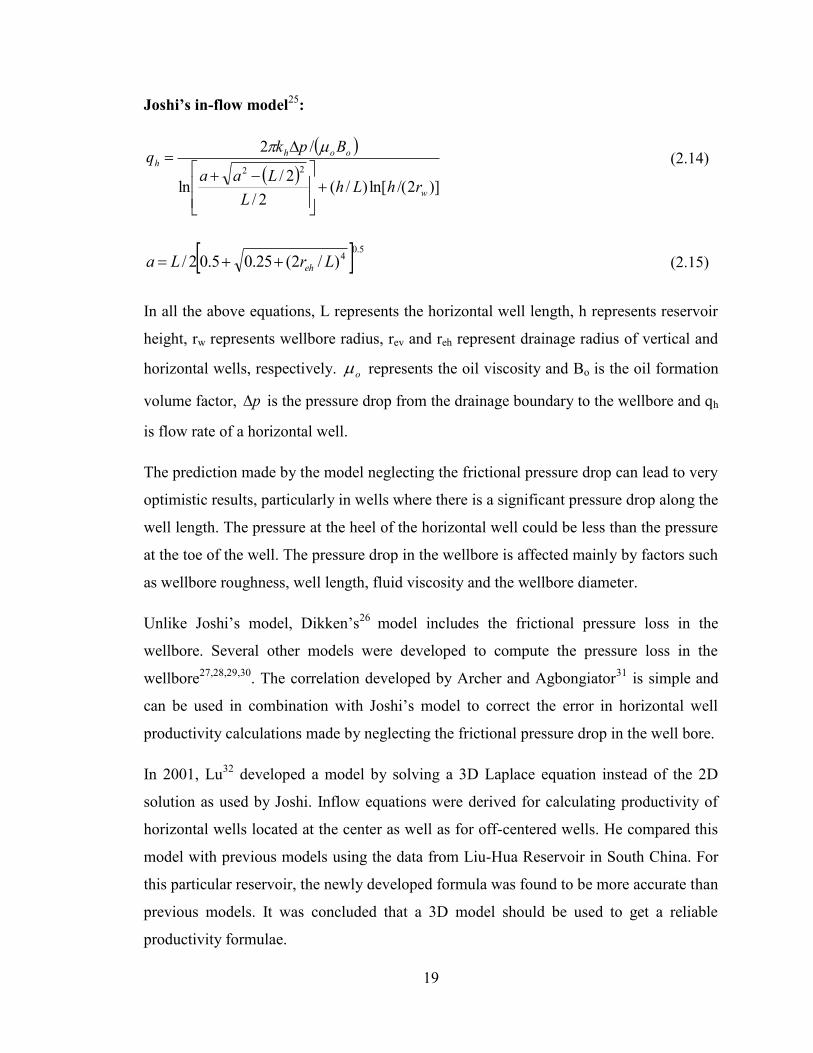
Joshi’s in-flow model25

:

)]2/(ln[)/(

2/

2/ln

/2

22

w

oohh

rhLhL

Laa

Bpkq

(2.14)

5.04)/2(25.05.02/ LrLa eh (2.15)

In all the above equations, L represents the horizontal well length, h represents reservoir

height, rw represents wellbore radius, rev and reh represent drainage radius of vertical and

horizontal wells, respectively. o represents the oil viscosity and Bo is the oil formation

volume factor, p is the pressure drop from the drainage boundary to the wellbore and qh

is flow rate of a horizontal well.

The prediction made by the model neglecting the frictional pressure drop can lead to very

optimistic results, particularly in wells where there is a significant pressure drop along the

well length. The pressure at the heel of the horizontal well could be less than the pressure

at the toe of the well. The pressure drop in the wellbore is affected mainly by factors such

as wellbore roughness, well length, fluid viscosity and the wellbore diameter.

Unlike Joshi’s model, Dikken’s26

model includes the frictional pressure loss in the

wellbore. Several other models were developed to compute the pressure loss in the

wellbore27,28,29,30

. The correlation developed by Archer and Agbongiator31

is simple and

can be used in combination with Joshi’s model to correct the error in horizontal well

productivity calculations made by neglecting the frictional pressure drop in the well bore.

In 2001, Lu32

developed a model by solving a 3D Laplace equation instead of the 2D

solution as used by Joshi. Inflow equations were derived for calculating productivity of

horizontal wells located at the center as well as for off-centered wells. He compared this

model with previous models using the data from Liu-Hua Reservoir in South China. For

this particular reservoir, the newly developed formula was found to be more accurate than

previous models. It was concluded that a 3D model should be used to get a reliable

productivity formulae.

20

2.1.4 Cyclic steam stimulation using horizontal wells

Gravity drainage is a significant mechanism for displacing the heated oil into the

wellbore for a horizontal well CSS process and critically, this mechanism has not been

included in any of the models discussed above.

Gunadi33

developed an analytical model for predicting oil production rates for cyclic

steam stimulation process using horizontal wells, and verified it with experimental

results. The model was divided into two sub-models. The first sub-model is used to

calculate the length and radius of steam zone during injection. The injection period is

divided into a number of equal time steps. The growth in radius of steam zone around

each segment and the length of steam zone is calculated using material balance equations,

Darcy’s law and heat balance equations. The second sub-model calculates the average

temperature and production rates during the soak and injection period. The heat losses to

the formation during the soak period and the heat losses through liquid production are

based on Boberg and Lantz10

method. The liquid production is calculated based on a

slightly modified form of Boberg and Lantz10

method. Liquid production from hot zone

(occupied by steam) and warm zone (not occupied by steam) are calculated separately,

based on relative permeability to oil and water, water saturation, average temperature and

reservoir pressure at each time step.

As verified with the experimental results, this model is more accurate for the horizontal

well at the base of the formation than horizontal well at the center of the reservoir, This

model may underestimate the production rate in the early stages, as it is based on Boberg

and Latz10

method, that considers steady state flow right from the start of production,

whereas, in reality, transient flow conditions prevail in the beginning. Also, this model

does not include gravity drainage effect, which would be very significant mechanism in

the later cycles. Although this model is fairly consistent with the experimental results,

further research should be conducted using a larger physical model to improve the

accuracy of the model.

Diwan and Kovseck34

developed an analytical model assuming that the steam zone

adopts a triangular shape in cross section when it is injected near the bottom of the

21

formation through a horizontal well. Steam heats the colder oil sand near the

condensation front. During production oil drains along the condensation surface by a

combination of gravity and pressure difference into the production well as does steam

condensate. In addition, oil drains through the steam chamber into the production well.

Reduction of oil viscosity as a result of an increase in the temperature greatly improves

the production response. Heat losses were included to the overburden as well as to the

adjacent unheated oil-bearing formation but they neglected the heat losses to the under-

burden. The approach used is similar to Butler et al35

gravity drainage of heavy-oil

reservoirs subjected to steam injection in which the theory was directed to linear flow

from horizontal wells. However, the steam zone shape was assumed to be a prism with

triangular cross section and the horizontal well lies at the bottom edge, as shown in

Figure 2.4 and Figure 2.5.

Figure 2.4 a) Schematic diagram of heated area geometry; b) differential element of the

heated area.27

22

Figure 2.5: Schematic diagram of area of cross section of heated area. 27

Wu et al.36

presented a model to calculate the in-flow performance of a cyclic steam

stimulated horizontal well under the influence of gravity drainage. The mechanisms of

gravity drainage, pressure drawdown and two phase flow were included. The model

couples the reservoir multi-phase flow and the frictional pressure loss in the wellbore.

The basic assumptions that were made are that the reservoir is homogenous and isotropic

with constant permeability and porosity. The horizontal well is approximated as a series

of vertical wells and fluid flow from the reservoir into the wellbore is along the radial

axis. It is further assumed that during the injection period steam forms a chamber in the

shape of a cylinder. The assumption may not be valid if the reservoir is significantly

anisotropic.

Further research should be carried out to determine the shape of the steam chamber to

obtain accurate and reliable results. Also, this model presents an equation for horizontal

well placed at the center of the reservoir. It would be necessary that the well be placed at

the bottom of the reservoir so as to get the maximum advantage of the gravity drainage.

However, it is possible that the placing a well at the bottom of the formation may

increase the heat losses to the under-burden. Hence, it is advisable to place the well in

such a location so as to optimize the heat losses as well as to get the maximum benefit

from the gravity drainage mechanism.

23

2.2 Concluding Remarks

The available models use the Boberg and Lantz model for calculating the average

temperatures in the steam zone. After reviewing the literature it was concluded that a new

analytical model should to be developed that addresses the heat transfer phenomenon for

a horizontal well during thermal recovery processes. The developed model can be

verified by comparing it with direct numerical simulations or field test results, if

available. To test the robustness of the model, sensitivity analysis to various operating

and reservoir parameters should be conducted by testing the model with the parameters

such as steam injection rates, thermal diffusivity, different types of oil (viscosity),

relative permeability of oil and water, the length of the horizontal wellbore etc.

24

CHAPTER THREE:

3 Analytical Modeling

This chapter describes the development of a heat transfer model that is applicable for a

cyclic steam stimulation process for horizontal wells. A radial heat transfer model was

developed to predict the average temperature in the steam zone. To predict the fluid rates,

a modified form of Joshi’s inflow equation is used. The heat transfer model is coupled to

the inflow model. Finally, detailed steps are shown and a flow chart is presented at the

end of this chapter, which outlines the important steps involved in the performance

prediction for a CSS process for horizontal wells.

3.1 Cyclic Steam Stimulation for Horizontal wells

Cyclic steam stimulation involves injection of steam into the formation at high pressure

for several weeks, followed by soak period, and finally production period. The purpose of

this study is to develop a new heat transfer model to predict the average temperatures in

the steam zone during soak and production periods. The heat transfer model takes into

account the heat lost by the steam zone to the adjacent reservoir. Steam zone is defined as

the region that is at the steam temperature. Fluid viscosities are calculated based on the

average steam zone temperatures. The heat transfer model is then coupled with a fluid

flow model to predict the oil and water production rates.

25

3.1.1 Model assumptions

Steam is injected through a horizontal well placed at the centre of the formation. Steam

displaces oil and forms a steam zone. Steam zone is defined as the region that is at the

saturated steam temperature. Steam heats the adjacent colder formation by conduction.

During the production period oil in the steam chamber is driven into the well bore due to

pressure drawdown. Reduction of oil viscosity as a result of increase in temperature

improves the production response significantly.

The main assumptions of the heat transfer model are:

i. The reservoir is initially saturated with oil and water

ii. Steam forms a cylindrical geometry

iii. During the injection period, the steam is considered as a heat source at a constant

temperature, TS.

iv. Heat is transferred from the steam zone to the cold oil zone through conduction

3.1.2 Volume of steam zone

The steam zone is defined as the region that is at the steam temperature, TS. The volume

of steam zone is based on a simple heat balance equation and was proposed by Gonzito

and Aziz (1984)37

:

))(( RSt

lastiwinjs

STTc

HQtQV

(3.1)

where,

sdhvdhRSwi fLTTCQ )( (3.2)

Qs = steam injection rate

tinj = injection time

Qi = heat injected per unit mass of steam

w = density of water

26

tc = volumetric heat capacity of the reservoir rock

Lvdh= latent heat of vaporization

fsdh = downhole steam quality

Hlast= heat remaining in the reservoir from the previous cycle

Specific heat of water is given by38

RS

RwSww

TT

ThThC

)()( (3.3)

Enthalpy of water was calculated using the correlation given by Jones18

and for steam

latent heat correlation of Farouq Ali39

was used:

24.1

10068)(

TThw , T is in

oF (3.4)

38.070594 TSLvdh , T is in

oF (3.5)

Assuming a cylindrical geometry, the radius of the steam zone is calculated by the

equation:

L

Vr S

h

(3.6)

3.1.3 Heat remaining in the reservoir

Initially, the amount of heat in the reservoir is set to zero. For later cycles, the heat

remaining is calculated on the basis of the steam zone volume and the average

temperature at the end of the previous cycle:

))(( RavgtSlast TTcVH (3.7)

27

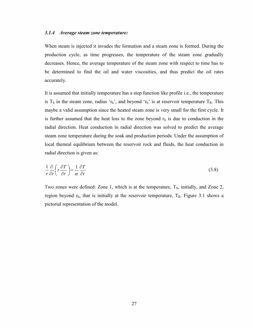
3.1.4 Average steam zone temperature:

When steam is injected it invades the formation and a steam zone is formed. During the

production cycle, as time progresses, the temperature of the steam zone gradually

decreases. Hence, the average temperature of the steam zone with respect to time has to

be determined to find the oil and water viscosities, and thus predict the oil rates

accurately.

It is assumed that initially temperature has a step function like profile i.e., the temperature

is TS in the steam zone, radius ‘rh’, and beyond ‘rh’ is at reser oir temperature TR. This

maybe a valid assumption since the heated steam zone is very small for the first cycle. It

is further assumed that the heat loss to the zone beyond rh is due to conduction in the

radial direction. Heat conduction in radial direction was solved to predict the average

steam zone temperature during the soak and production periods. Under the assumption of

local themral equlibrium between the reservoir rock and fluids, the heat conduction in

radial direction is given as:

t

T

r

Tr

rr

11 (3.8)

Two zones were defined: Zone 1, which is at the temperature, TS, initially, and Zone 2,

region beyond rh, that is initially at the reservoir temperature, TR. Figure 3.1 shows a

pictorial representation of the model.

28

Figure 3.1: Schematic diagram of model

Let T1 and T2 be the temperatures of the Zone1 and Zone 2 at any time, t, respectively.

The initial and boundary conditions are defined as below:

Initial Condition:

T1=Ts at t=0 (3.9)

Here, time t=0 represents the start of soak period when the heated zone is at a

temperature Ts. During the soak period and production period, the steam zone loses heat

due to conduction to the surround formation. The processed is modeled from the start of

the soak period.

The net heat flux at r=0 is zero because of the radial symmetry. The total heat from the

boundary of Zone 1 is equal to the amount of heat absorbed by the Zone 2. It is denoted

by B.C. 2. These are represented mathematically as:

Boundary Conditions:

01

r

T at r=0 (3.10)

t

TcV

r

TkA p

ar

21 . at r= rh (3.11)

29

For solving the PDE, the following dimensional parameters were defined and the

equation is converted into a dimensionless form.

RS

SD

TT

TTT

1

1 (3.12)

RS

SD

TT

TTT

2

2 (3.13)

w

Dr

rr (3.14)

2

w

Dr

tt

(3.15)

RS

RS

DTT

TTT

)0(2 (3.16)

The governing equations in dimensionless form are given by:

D

D

D

D

DD

D

t

T

r

T

rr

T

11

2

1

21

(3.17)

The initial condition (tD=0) in dimensionless form is given by:

01 DT at t=0 (3.18)

The boundary condition at the wellbore, in dimensionless form is given as:

01

D

D

r

T at 0Dr (3.19)

The boundary condition at the interface, r=rh, is given by:

D

Dp

wD

D

t

TVc

rr

TkA

21 ).(

at rd=rdh (3.20)

30

The PDE is solved by using Laplace transform. The equation in Laplace domain is given

below. Detailed derivation is given in Appendix A.

1

1

2

1

2~

~1

~

D

D

D

DD

D Tsr

T

rr

T

(3.21)

The solutions for temperature in Zone 1 and Zone 2, in Laplace domain, are given as:

)0(2

01

11

21)()(

)()(.1

1

2.

~D

DhDh

DhDh

Dh

AvgD TSrQsISrIS

sISrIrQ

srT

(3.22)

)()(

).(.~

01

)0(20

2srQsIsrIs

TsrIQT

DhDh

DDh

D

(3.23)

where,

kAr

VcQ

w

p

.

).( (3.24)

The equations in Laplace domain are inverted to time domain using Gaver-Stehfest40,41

algorithm in MATLAB. The average temperature at any time during the cycle is

calculated by the following equations:

)(.1.1 RSAvgDSAvg TTTTT (3.25)

and,

)(22 RSDS TTTTT (3.26)

Figure 3.2 shows a plot of the dimensionless average temperature of Zone 1 and Zone 2

versus the dimensionless time.

31

Figure 3.2: A plot of dimensionless temperature of Zone 1 and Zone 2 versus

dimensionless time

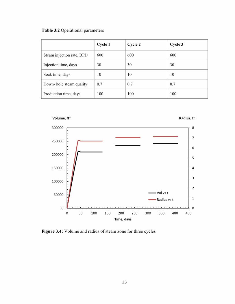
Sample calculations were made for the radius of the steam zone and the average

temperature of the steam zone. The reservoir and operational parameters used for these

calculations are shown in Table 3.1 and Table 3.2. Figure 3.3 shows a plot of the average

temperature in oF) of Zone 1 and Zone 2 versus time (days). The radius of steam zone and

the temperature profile were plotted for three cycles using the operation parameters

described in Table 3.2. Figure 3.4 shows a plot of the volume of steam zone and the

radius of steam zone versus time and the average temperature for three cycles is shown in

Figure 3.5. It can be seen from the plots that initially, at the start of the production period,

the temperature is at steam temperature, TS, and it gradually declines during the

production period.

0

0.1

0.2

0.3

0.4

0.5

0.6

0.7

0.8

0.9

1

0.01 0.1 1 10 100 1000

Td

tD

Td1 vs tD

Td2 vs tD

32

Table 3.1 Reservoir parameters and PVT data

Variable Value

Reservoir porosity 0.2

Well radius (ft) 0.3

Initial reservoir temperature (oF) 115

Saturated steam temperature (oF) 415

Reservoir thermal conductivity (Btu/ft hr. oF) 1

Reservoir thermal diffusivity (ft2/hr) 0.04

Injected steam quality 0.7

Steam injection rate (B/D) 600

API gravity of oil (oAPI) 14

Injection pressure (psi) 300

Pay thickness, ft 80

Specific heat of water, Btu/lboF 1

Figure 3.3: A plot of the average temperature of Zone 1 and Zone 2 versus time

0

50

100

150

200

250

300

350

400

450

0 20 40 60 80 100

Temp, oF

days

T1 vs t

T2 vs t

33

Table 3.2 Operational parameters

Cycle 1 Cycle 2 Cycle 3

Steam injection rate, BPD 600 600 600

Injection time, days 30 30 30

Soak time, days 10 10 10

Down- hole steam quality 0.7 0.7 0.7

Production time, days 100 100 100

Figure 3.4: Volume and radius of steam zone for three cycles

0

1

2

3

4

5

6

7

8

0

50000

100000

150000

200000

250000

300000

0 50 100 150 200 250 300 350 400 450

Radius, ft Volume, ft3

Time, days

Vol vs t

Radius vs t

34

Figure 3.5: Plot of the average steam zone temperature versus time for three cycles

3.1.5 Oil and water viscosities

The oil and water viscosities are calculated using the available correlations given

below18

:

)460/( Tb

o ae (3.27)

14.1

10066.1

Tw (3.28)

3.1.6 Fluid saturations and relative permeabilities

The oil and water relative permeabilities can be calculated using the generalized

equations available for California reservoirs18

, as given by Gomaa:

2** 021467.0002167.0 wwrw SSk (3.29)

2** 13856.0/0808.19416.0 wwro SSk (3.30)

0

50

100

150

200

250

300

350

400

450

0 100 200 300 400 500

Temp, F

days

Cycle 1

Cycle 2

Cycle 3

Injection+Soak

Injection+Soak

Injection+Soak

Production Production Production

35

with,

1rok if 2.0* wS (3.31)

where,

)1/()(*

orwwirwirww SSSSS (3.32)

Sw = water saturation

Swir = irreducible water saturation

Sorw = residual oil saturation to water

Water saturation, Sw, is given by:

WIP

WSSSS P

wiwww (3.33)

After the soak period, it is assumed that the only mobile phase around the well is water.

orww SS 1 (3.34)

3.1.7 Fluid- inflow equation

We assume that pressure drawdown is the main driving force for fluid production and

flow is through the steam chamber. Joshi’s model was used to calculate the productivity

index. The assumed steam zone is cylindrical in nature and hence, the model was

modified for a cylindrical geometry. Joshi's (1988) solution for horizontal well in an

anisotropic reservoir is given by:

fs

whr

hLh

L

Laa

oB

o

px

ky

kh

Hq

2/

2222/

ln/2/

22/2

ln

007078.0

(3.35)

36

where,

kx and ky are the permeability in horizontal and vertical direction respectively

x

y

k

k (3.36)

(3.37)

and, is the distance of the well from mid- height of the formation

For an isotropic reservoir, if we assume that kx= ky and 2a=L (‘2a’ is the major axis of the

ellipse) and the well is located at the center of the formation, then the above equation

reduces to a simple radial flow model:

h

e

c

w

h

hr

r

r

r

pkLq

lnln

007078.0

, Rb/day (3.38)

For two phase oil and water flow, the production rates can be calculated as:

h

eoc

w

hoh

ro

o

r

r

r

r

pLkkq

lnln

007078.0

(3.39)

h

ewc

w

hwh

rw

w

r

r

r

r

pLkkq

lnln

007078.0

(3.40)

5.0

4/5.0

1

4

1

2

1)2/(

ehrL

La

37

3.1.8 Flow chart showing important steps in calculations

An outline is presented in Figure 3.6 that shows important steps in the calculating the

average temperature of the steam zone and predicting the performance of a CSS process.

The main inputs for the model are: reservoir temperature, reservoir properties, fluid

saturations and the cyclic operational parameters. First, the volume (and radius) of the

heated zone geometry are calculated based on the input properties. Second, the average

temperature of the steam zone is calculated using the model developed in the Section

3.1.4. The oil and water viscosities are calculated based in the average temperature of the

steam zone. Oil and water relative permeabilities are calculated from water saturation

based on the correlations discussed in Section 3.1.6. After the end of the soak period, it is

assumed the only mobile phase around the well bore is water. For the first time step, the

water production, WP, is zero. Based on this, the water saturation is calculated and the oil

and water relative permeabilities are calculated using the water saturation, Sw, values.

The oil and water flow rates, for small time steps, are calculated using the modified

Joshi’s equation described in Section 3.1.7. The cumulative oil and water production are

calculated and fluid saturations are updated. The process is repeated until the end of the

cycle and the amount of fluids and heat remaining in the reservoir is calculated at the end

of the cycle. Finally, the same steps are repeated for a new cycle. Details of the

calculations are presented in the following chapter.

38

Figure 3.6: A flow chart outlining important steps in the calculation.

Input reservoir temperature, reservoir properties, fluid saturations and other operational parameters.

Calculate volume of heated zone geometry (radius, thickness and volume)

Calculate the average steam zone temperature and using Tavg calculate oil and water viscosities.

Calculate kro and krw

Calculate the oil and water flow rates for small time steps within the cycle and update fluid saturations.

Calculate the cumulative oil and water production and check against the fluids initially in place. Calculate average temperature at the end of the each time step.

Check to see if additional steps are required to complete the cycle.

Calculate the amount of heat remaining in the reservoir at the end of the cycle

Repeat the steps for a new cycle.

39

3.2 Summary

In this chapter, an analytical model that is applicable for a cyclic steam stimulation

process for horizontal wells has been developed. A radial heat transfer model was

developed to predict the average temperature in the steam zone. The oil and water

viscosities are calculated based on the average steam zone temperature. Correlations for

fluids saturation and relative permeabilities of oil and water are described. To predict the

fluid rates, a modified form of Joshi’s inflow equation is used. Finally, detailed steps are

shown and a flow chart is presented at the end of this chapter which outlines the

important steps involved in the performance prediction for a CSS process for horizontal

wells.

The developed model will be validated using numerical simulation in CMG STARS in

the next chapter. First, a base case will be run and checked if the results from the

simulator match with that of the developed analytical model. Next, sensitivity analyses

will be conducted to test the robustness of the model for a range of operating parameters.

40

CHAPTER FOUR:

4 Validation of the Model and Sensitivity Analyses

The robustness of the developed analytical model is tested for an expected range of

parameters. All the calculations for the analytical model were done using an excel

spreadsheet. The results obtained from the analytical model are compared with the results

obtained from the numerical simulator. The findings are presented in this section.

4.1 Base Case

4.1.1 Input data

The proposed model is validated using numerical simulator from CMG. The operational

parameters and reservoir properties are shown in Table 4.1 and Table 4.2, respectively.

Table 4.1 Operational parameters

Cycle 1 Cycle 2 Cycle 3

Steam injection rate, BPD 3000 3000 3000

Injection time, days 10 10 10

Soak time, days 5 5 5

Down- hole steam quality 0.7 0.7 0.7

Production time, days 200 200 200

41

Table 4.2 Reservoir parameters and PVT data

Variable Value

Reservoir Permeability 100 mD

Reservoir porosity 0.3

Well radius (ft) 0.5

Pay thickness, ft 80

Initial reservoir temperature (oF) 85

Saturated steam temperature (oF) 567

Initial water saturation 0.3

Residual oil saturation to steam 0.4

Reservoir thermal conductivity (Btu/ft hr. oF) 1

Reservoir thermal diffusivity (ft2/hr) 0.04

Injected steam quality 0.7

Steam injection rate (B/D) 3000

API gravity of oil (oAPI) 14

Injection pressure (psi) 1200

Specific heat of water, Btu/lboF 1

Table 4.3 Viscosity data

Temperature, oC Viscosity, mPa.S

30 2710

180 4

Table 4.4 Model dimensions and grid data

Model Dimension 2000ft 200ft 80ft (i, j and k direction respectively)

Number of grids 100 50 20 (i, j and k direction respectively)

42

Aberfeldy field viscosity data, as shown in Table 4.3, was used to calculate oil viscosities

at different temperatures1. Table 4.4 shows the model dimensions and grid data used for

the numerical simulator. Using Andrade’s equation to model the oil iscosity, the

viscosity at any temperature can be obtained by )15.273/(78.5969610596.7 Te

4.1.2 Relative permeability model

In order to compare and validate the model, it is important that the same relative

permeability model is used for both the model and the numerical simulator. First, the

relative permeability curves are generated in STARS and using simple curve fitting, the

analytical expressions for relative permeabilities is obtained as:

8314.4314.19075.25593.1023

wwwro SSSk (4.1)

1837.02245.10408.22

wwrw SSk (4.2)

Figure 4.1 shows a plot of the relative permeabilities of oil and water versus water

saturation.

Figure 4.1: Oil and water relative permeabilities

0

0.1

0.2

0.3

0.4

0.5

0.6

0.7

0.8

0.9

1

0.3 0.4 0.5 0.6 0.7 0.8 0.9 1

Kro

an

d K

rw

Sw

Krw- STARS

Kro- STARS

Krw- Model

Kro-Model

43

4.1.3 Relative permeability adjustment

A comparision of water saturation in the heated zone, oil and water relative permeabilites

obtained from the model and the numerical simulator are shown in Figure 4.2, 4.3 and

4.4, respectively. It can be seen from the plots that there is a slight different in the results

from simulator and the developed model. The difference in the relative permeability of

water is rather significant during the initial stages of the cycle. This resulted in a

mismatch in the water production. Hence, a corrected relative permeability has to be used

to get a good match for the water production between numerical simulator and the model.

The developed fluid flow model is a two phase-oil and water, model. The oil and water

relative permeabilities are calculated using the water saturation obtained by mass balance

in the heated zone. Relative permeabilities of oil and water play a significant role in

determining the actual oil and water production. Hence, it is important to obtain a good

match for the water saturation in the heated zone and, oil and water relative

permeabilities.

Figure 4.2: Water saturations in the heated zone obtained from developed model and

numerical simulator

0.3

0.35

0.4

0.45

0.5

0.55

0.6

0 200 400 600 800

Sw

t, days

STARS- 100x50x20

Model

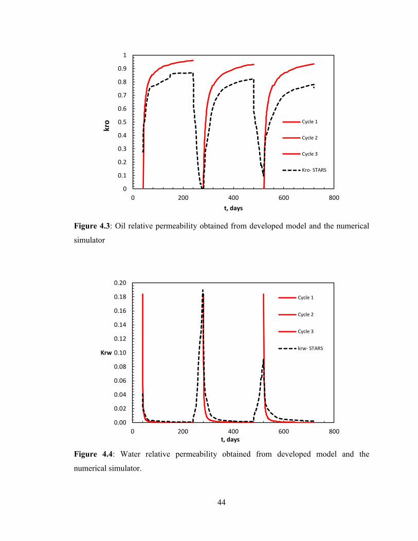
44

Figure 4.3: Oil relative permeability obtained from developed model and the numerical

simulator

Figure 4.4: Water relative permeability obtained from developed model and the

numerical simulator.

0

0.1

0.2

0.3

0.4

0.5

0.6

0.7

0.8

0.9

1

0 200 400 600 800

kro

t, days

Cycle 1

Cycle 2

Cycle 3

Kro- STARS

0.00

0.02

0.04

0.06

0.08

0.10

0.12

0.14

0.16

0.18

0.20

0 200 400 600 800

Krw

t, days

Cycle 1

Cycle 2

Cycle 3

krw- STARS

45

4.1.4 Pressure drop model and inflow equation

The following assumtions are made to obtain a good match with the results from the

numerical simulator:

i. Oil production comes only from the heated zone. Oil rate is calculated using

Equation 4.6 given below. This equation is a modified form of Equation 3.39.

ii. The mass balance is done only in the heated zone. The water saturation obtained

from the mass balance equations is used to calculate the oil relative permeability.

iii. The same relative permeability model as the numerical simulator is used to

calculate the oil relative permeability.

iv. Water production comes from the entire reservoir and is calcualted using

Equation 4.7

v. A modified relative permeability model for water is used in the inflow equation to

obtain a good match with the results from the simulator.

A comparision of oil production rate and cumulative oil production are shown in Figure

4.5 and 4.6, respectively. The three regions correspond to three cycles and the flat zones

in between are the injection and soak intervals. There is no production during injection

and soak interval. Oil production is very high at the early times during the production

cycle as the temperature is high and the viscosity is low. It is assumed that the oil

production comes only from the heated zone and the pressure does not propagate through

the cold, highly viscous oil outside the heated zone.

It should be noted that in calculation of oil produciton rate, the pressure drawdown refers

to pressure difference between the heated zone boundary and the botom-hole pressure of

the well. The pressure at the heated boundary is calculated using the following equations:

Dp

Lkkr

Bqptrp

o

ooo

hw

2.141),( (4.3)

46

where

pD =1

2ln(tD )+0.80907[ ] (4.4)

tD =0.002637kkrwt

jmctrh2

(4.5)

w

hoo

whro

o

r

rB

ppLkkq

ln

)(007078.0

(4.6)

The actual inflow equation that accounts for the production from both the hot zone and

the cold zone is given by Equation 3.39. However, in order to get a match with STARS,

the equation is modified to consider the oil production only from the heated zone and is

given by the above Equation 4.6.

Computational procedure for calculating the pressure at the heated zone boundary, ph,

involves trial and error and is summarized in the following steps:

i) Assume an average value for ph

ii) Calculate the oil and water production rates using the radial flow model

discussed above.

iii) Calculate tD and pD using the equations described above.

iv) Calculate ph using the qo and pD values and check to see if the value for the

first few time steps matches with the assumed value.

v) Repeat the process till a good match is obtained.

47

Figure 4.5: Comparison of oil production rate, qo, obtained from the model versus the


Figure 4.6: Comparison of cumulative oil production, Qo, from the model versus the


0

50

100

150

200

250

300

350

400

450

500

0 200 400 600 800

qo

, bp

d

t, days

STARS- 100x50x20

Qo- Model

0

5000

10000

15000

20000

25000

0 200 400 600 800

Qo

, bb

l

t, days

Cum. Oil- Model

Cum. Oil- STARS

48

It is assumed that water production comes from both the heated zone and the outside

cold zone. The following equation is used to calculate the water production rates:

h

e

wc

w

h

whw

wirww

r

r

r

rB

ppLkkQ

lnln

)(007078.0 *

(4.7)

The water mass balance calculations are all performed using the actual water relative

permeability curve (Equation 4.2). To obtain a good match with the results from the

simulator, a modified relative permeability model is used for water in the inflow

equation. The modified water relative permeability is obtained in history mathing of the

water production rate from the numerical simulator and the developed model. The

modified water relative permeability is only used for calculation of the water production

rate using the inflow Equation 4.7 and is given by:

krw* = (0.0637Sw -0.01827) (4.8)

A comparision of water production rate and cumulative water production are shown in

Fig. 4.7 and 4.8, respectively. The instantaneous water rate is also very high because of

the condensed steam around the well-bore and it delines rapidly at later times.

Figure 4.7: Comparison of water rate, qw, obtained from model versus STARS simulator

0

200

400

600

800

1000

1200

1400

0 200 400 600 800

qw

, bp

d

t, days

STARSQw- Model

49

Figure 4.8: Comparison of cumulative water production, Qw, from the model versus

STARS.

4.2 Sensitivity Analyses

The robustness of the analytical model is tested by comparing the results obtained from

the developed model with the results from the numerical simulator, for an expected range

of parameters. In all sensitivity analyses, the same data as base case is used, except noted

otherwise. The following parameters were considered:

i. Grid Sensitivity

ii. Steam Injection rates

iii. Length of horizontal well

iv. Absolute Permeability

v. Relative permeability of oil and water

vi. Thermal Diffusivity

vii. Types of oil: viscosity

viii. Number of Cycles

0

10000

20000

30000

40000

50000

60000

70000

0 200 400 600 800

Qw

, bb

l

t, days

Cum. Water- STARS

Cum. Water- Model

50

4.2.1 Grid sensitivity

For simulation, a reservoir of dimensions 2000ft 200ft 80ft (i, j, k direction

respectively) is considered. The following four different grid size configurations were

considered and a comparison of results obtained from these configurations is shown in

Figure 4.5, Figure 4.6, Figure 4.7 and Figure 4.8. The horizontal well of length 1500ft is

placed at the center of the reservoir and is produced at a constant bottom-hole pressure of

100 psi.

i. 1005010 (number of grid blocks in i, j, and k direction, respectively)

ii. 1005020

iii. 1005040

iv. 2005020

The three time intervals in the plot of oil production rate versus time shown in Figure 4.5

started with a peak that correspond to three cycles. The flat zones in the cumulative oil

production plot in Figure 4.10 represent the injection and soak intervals. There is no

production during the soak period. The soak interval in a given cycle is followed by the

production interval. At early times in the production interval, the instantaneous oil rate

increases rapidly as shown by the steep gradients in the Figure 4.9, because the oil is hot

and viscosity is very low. At later times, the production of oil decreases as the formation

begins to lose heat, temperature declines and the oil viscosity increases. Similarly, the

water production rate is very high at early times, as shown in Figure 4.11, in the

production interval due to the condensed steam around the wellbore. At later times water

production declines. The flat zones in the cumulative water production plot in Figure

4.12 represent the injection and soak intervals. It can be seen from these plots that the

results for different grid sizes are fairly close to each other and the results are

independent of the grid size configurations. The results for the grid configuration of

1005010 produces erroneous results and slightly under- estimates the fluid production

as there is not enough resolution in the k direction. Based on these results, the simulation

model with a grid size of 1005020 was used for all the validation and sensitivity

studies in the next sections.

51

Figure 4.9: Plot of oil production rate, qo, versus time for different grid sizes.

Figure 4.10: Plot of cumulative oil production, Qo, versus time for different grid sizes.

0

50

100

150

200

250

300

350

400

450

500

0 100 200 300 400 500 600 700 800

qo

, Stb

/ d

ay

t, days

100x50x10

100x50x20

100x50x40

200x50x20

0

5000

10000

15000

20000

25000

0 200 400 600 800

Qo

, Stb

t, Days

Cum. Oil-100x50x10

Cum. Oil- 100x50x20

Cum. Oil- 100x50x40

Cum. OIl- 200x50x20

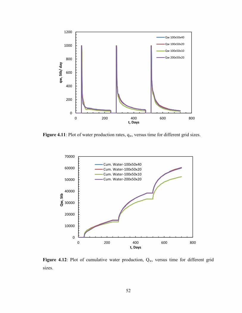
52

Figure 4.11: Plot of water production rates, qw, versus time for different grid sizes.

Figure 4.12: Plot of cumulative water production, Qw, versus time for different grid

sizes.

0

200

400

600

800

1000

1200

0 200 400 600 800

qw

, Stb

/ d

ay

t, Days

Qw 100x50x40

Qw 100x50x20

Qw 100x50x10

Qw 200x50x20

0

10000

20000

30000

40000

50000

60000

70000

0 200 400 600 800

Qw

, Stb

t, Days

Cum. Water-100x50x40Cum. Water-100x50x20

Cum. Water-100x50x10Cum. Water-200x50x20

53

4.2.2 Steam injection rates

This case was run for three different values of steam injection rates: 1800 bpd, 2500 bpd,

and 3000 bpd using the same data used for the base case except for the steam injection

rate. Figures 4.13, 4.14 and 4.15 show the comparison plots of oil production rate versus

time for the results obtained from the developed model and the simulator for different

steam injection rates. It can be seen from the plots that the results from the model and the

numerical simulator are fairly close to each other. Figure 4.16 depicts the cumulative oil

production versus time. As the steam injection rate increases the cumulative oil

production increases as greater amount of heat is injected and a greater amount of

reservoir is heated. However, it can be seen that the increase in oil production is not

proportional to the increase in the steam injection rates. Figure 4.17 shows a plot of the

water production rates obtained from the numerical simulator and the developed

analytical model and it can be seen from the plot that the results are fairly close to each

other. Figure 4.18 shows a plot of cumulative water production obtained from the

simulator and the developed analytical model. The results are fairly close and it can be

seen that as the steam injection rate is increased, water production increases significantly,

as greater amount of heat and water is injected and a greater volume of the reservoir is

contacted.

54


injection rate of 1800 bpd.


injection rate of 2500 bpd.

0

100

200

300

400

500

600

700

800

0 100 200 300 400 500 600 700

qo

, bp

d

t, days

STARS- 1800 bpd

Model 1800 bpd

0

100

200

300

400

500

600

700

800

0 100 200 300 400 500 600 700

qo

, bp

d

t, days

STARS- 2500 bpdModel- 2500 bpd

55

Figure 4.15: Comparison of oil rate from STARS and model for steam injection rate of

3000 bpd.

Figure 4.16: Cumulative oil production versus time for different steam injection rates.

0

100

200

300

400

500

600

700

800

0 100 200 300 400 500 600 700

qo

, bp

d

t, days

STARS- 3000 bpd

Model- 3000 bpd

0

5000

10000

15000

20000

25000

30000

0 100 200 300 400 500 600 700

Qo

, bb

l

t, days

3000- STARS2500- STARS2500- Model3000- Model1800- Model1800- STARS

56


steam injection rates.

Figure 4.18: Comparison of cumulative water production obtained from STARS and

analytical model for different steam injection rates.

0

100

200

300

400

500

600

700

800

900

1000

0 100 200 300 400 500 600 700

qw

, bp

d

t, days

qw: STARS- 1800 bpd

qw: STARS- 2500 bpd

qw: STARS- 3000 bpd

qw: Model- 1800 bpd

qw: Model- 2500 bpd

qw: Model- 3000 bpd

0

10000

20000

30000

40000

50000

60000

70000

80000

0 100 200 300 400 500 600 700

Qw

, bb

l

t, days

Qw: STARS- 1800 bpd

Qw: STARS- 2500 bpd

Qw: STARS- 3000 bpd

Qw: Model- 1800 bpd

Qw: Model- 2500 bpd

Qw: Model- 3000 bpd

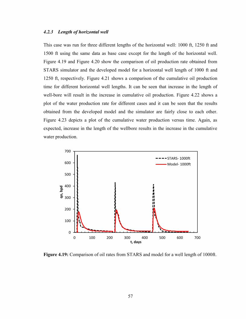
57

4.2.3 Length of horizontal well

This case was run for three different lengths of the horizontal well: 1000 ft, 1250 ft and

1500 ft using the same data as base case except for the length of the horizontal well.

Figure 4.19 and Figure 4.20 show the comparison of oil production rate obtained from

STARS simulator and the developed model for a horizontal well length of 1000 ft and

1250 ft, respectively. Figure 4.21 shows a comparison of the cumulative oil production

time for different horizontal well lengths. It can be seen that increase in the length of

well-bore will result in the increase in cumulative oil production. Figure 4.22 shows a

plot of the water production rate for different cases and it can be seen that the results

obtained from the developed model and the simulator are fairly close to each other.

Figure 4.23 depicts a plot of the cumulative water production versus time. Again, as

expected, increase in the length of the wellbore results in the increase in the cumulative

water production.

Figure 4.19: Comparison of oil rates from STARS and model for a well length of 1000ft.

0

100

200

300

400

500

600

700

0 100 200 300 400 500 600 700

qo

, bp

d

t, days

STARS- 1000ft

Model- 1000ft

58

Figure 4.20: Comparison of oil production rates from STARS and model for a well

length of 1250ft.

Figure 4.21: Cumulative oil production versus time for different lengths of the horizontal

well.

0

100

200

300

400

500

600

700

800

0 100 200 300 400 500 600 700

qo

, bp

d

t, days

STARS- 1250 ft

Model- 1250 ft

0

5000

10000

15000

20000

25000

30000

0 100 200 300 400 500 600 700

Qo

, bb

l

t, days

STARS- 1000 ftModel- 1000ftSTARS- 1500 ftModel- 1500ftModel- 1250ftSTARS- 1250ft

59


horizontal well lengths.

Figure 4.23: Comparison of cumulative water production from STARS and model for

different lengths of horizontal well.

0

200

400

600

800

1000

1200

1400

0 100 200 300 400 500 600 700

qw

, bp

d

t, days

qw: STARS- 1000 ft

qw: STARS- 1250 ft

qw: Model- 1000 ft

qw: Model- 1250 ft

0

10000

20000

30000

40000

50000

60000

70000

80000

90000

0 100 200 300 400 500 600 700

Qw

, bb

l

t, days

Qw: STARS- 1000 ft

Qw: STARS- 1250 ft

Qw: STARS- 1500 ft

Qw: Model- 1000 ft

Qw: Model- 1250 ft

Qw: Model- 1500 ft

60

4.2.4 Absolute permeability

A case was run by changing the absolute permeability of reservoir. Three different

scenarios were considered. One is the base case scenario where the permeability is 100

mD and the other two cases considered 150 mD and 200 mD. The other data used is same

as the base case. Figure 4.24 and Figure 4.25 show the comparison of oil production rate

obtained from the analytical model and the numerical simulator for absolute permeability

values of 150 mD and 200 mD, respectively. Figure 4.26 shows a comparison of the

cumulative oil production time for different absolute permeability values. It can be seen

from the plot that as the permeability of the reservoir increases the cumulative oil

production increases as well. Figure 4.27 shows a plot of the water production rate for

different cases and it can be seen that the results obtained from the developed model and

the simulator are fairly close to each other. Figure 4.28 depicts a plot of the cumulative

water production versus time. Again, as expected, increase in the absolute permeability

results in the increase in the cumulative water production.


150 mD.

0

100

200

300

400

500

600

700

800

0 100 200 300 400 500 600

qw

, bp

d

t, days

STARS: k= 150 md

Model: k= 150 md

61


200 mD.

Figure 4.26: Comparison of cumulative oil production versus time from, STARS and

developed model, for different absolute permeability values.

0

100

200

300

400

500

600

700

800

0 100 200 300 400 500 600

qo

, bp

d

t, days

STARS: k= 200 md

Model: k= 200 md

0

5000

10000

15000

20000

25000

30000

35000

0 100 200 300 400 500 600 700

Qo

, bb

l

t, days

Model- k=150Model-k=100Model-k=200STARS-k=100STARS K=150STARS- k=200

62

Figure 4.27: Comparison of water production rate versus time, form STARS and




The model is tested for a reservoir permeability of 1000 mD. A comparison of the oil

production rate and cumulative oil production, obtained from the numerical simulator and

0

100

200

300

400

500

600

700

800

900

1000

0 200 400 600 800

qw

, bb

l

t, days

qw: STARS- k= 150 mD

qw: STARS- k= 200 mD

qw: Model- k= 150 mD

qw: Model- k= 200 mD

0

20000

40000

60000

80000

100000

120000

0 100 200 300 400 500 600 700

Qw

, bb

l

t, days

Qw: STARS- k= 100 mD



Qw: Model- k= 100 mD



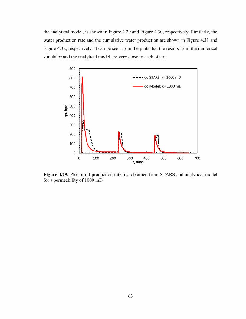
63

the analytical model, is shown in Figure 4.29 and Figure 4.30, respectively. Similarly, the

water production rate and the cumulative water production are shown in Figure 4.31 and

Figure 4.32, respectively. It can be seen from the plots that the results from the numerical

simulator and the analytical model are very close to each other.

Figure 4.29: Plot of oil production rate, qo, obtained from STARS and analytical model

for a permeability of 1000 mD.

0

100

200

300

400

500

600

700

800

900

0 100 200 300 400 500 600 700

qo

, bp

d

t, days

qo STARS: k= 1000 mD

qo Model: k= 1000 mD

64

Figure 4.30: Plot of cumulative oil production, Qo, obtained from STARS and analytical

model for a permeability of 1000 mD.

Figure 4.31: Plot of water production rate, Qw, obtained from STARS and analytical

model for a permeability of 1000 mD.

0

5000

10000

15000

20000

25000

30000

0 100 200 300 400 500 600 700

Qo, b

bl

t, days

Qo STARS: k= 1000 mD

Qo Model: K= 1000 mD

0

200

400

600

800

1000

1200

1400

1600

1800

0 100 200 300 400 500 600 700

qw

, bb

l

t, days

qw STARS: k= 1000 mD

qw Model: k= 1000 mD

65

Figure 4.32: Plot of cumulative water production, Qw, obtained from STARS and

analytical model for a permeability of 1000 mD.

4.2.5 Relative permeability of oil and water

The model was tested for two different relative permeability models, as shown in the

Figure 4.33. Figure 4.34 shows a plot comparing the oil production rate obtained from the

numerical simulator and developed model for the new relative permeability model.

Figure 4.35 shows the cumulative oil production versus time. Similarly, the plots for

water production rate and cumulative water production are shown in Figure 4.36 and

4.37, respectively. Figure 4.35 shows that the cumulative oil production for the base case

is higher than the cumulative oil production obtained from the new relative permeability

curve. On the other hand, it can be seen from the Figure 4.37 that the cumulative water

production from the base case is lower. An explanation for this could be that during the

initial stages of a cycle, when the water saturation is high (1-Sorw), the relative

permeability of water is lower in the base case than compared to the new case. For

example, in base case when Sw= 0.6, the value of krw is about 0.18 and for the new case,

when Sw=0.75 the value of krw is about 0.3. This implies that during the initial the initial

0

20000

40000

60000

80000

100000

120000

0 100 200 300 400 500 600 700

Qw

, bb

l

t, days

Qw STARS: k= 1000 MD

Qw Model: k= 1000 MD

66

stages of the cycle (which accounts for major water production) the water production rate

is higher in the new case than compared to the base case.

Figure 4.33: Different types of relative permeability curves versus water saturation.


model, for a different relative permeability model.

0

0.1

0.2

0.3

0.4

0.5

0.6

0.7

0.8

0.9

1

0 0.2 0.4 0.6 0.8 1

Sw

Kro

Krw

Kro-Base

Krw- Base

0

100

200

300

400

500

600

700

800

0 100 200 300 400 500 600

qo

, bp

d

t, days

STARS: new rel. perm.

Model: new rel. perm.

67


developed model, for different relative permeability curves.


developed model, for a different relative permeability model.

0

5000

10000

15000

20000

25000

30000

0 100 200 300 400 500 600 700

Qo

, bb

l

t, days

STARS- Base Case

Model- Base Case

STARS- New Rel. Perm.

Model- New Rel. Perm.

0

100

200

300

400

500

600

700

800

900

1000

0 100 200 300 400 500 600

qw

, bp

d

t, days

qw: STAS- New Rel. Perm.

qw: Model- New Rel. Perm.

68


developed model, for a different relative permeability model.

4.2.6 Thermal diffusivity

The model was tested for two different thermal diffusivity values of the reservoir:

0.04ft2/hr (base case) and 0.02ft

2/hr. Figure 4.38 shows a comparison of oil production

rate obtained from the numerical simulator and developed model for the new thermal

diffusivity value. Figure 4.39 shows a plot of the cumulative oil production obtained from

the simulator and the model. Similarly, the water production rate and the cumulative

water production are shown in Figure 4.40 and 4.41, respectively. For a rock with high

thermal diffusivity, heat propagates faster because the rock conducts heat quickly relative

to its volumetric heat capacity. Hence, the higher the thermal diffusivity, faster will be

the heat loss to the surrounding during the soak and production period and lower the

production rate. Figure 4.39 and 4.41 show that the cumulative oil and water production

for the base case is lower than the latter case (base case has a higher thermal diffusivity

value).

0

10000

20000

30000

40000

50000

60000

70000

80000

90000

100000

0 100 200 300 400 500 600 700

Qw

, bb

l

t, days

Qw: STARS- New Rel. Perm.

Qw: STARS- Base Case

Qw: Model- Base Case

Qw: Model- New Rel. Perm.

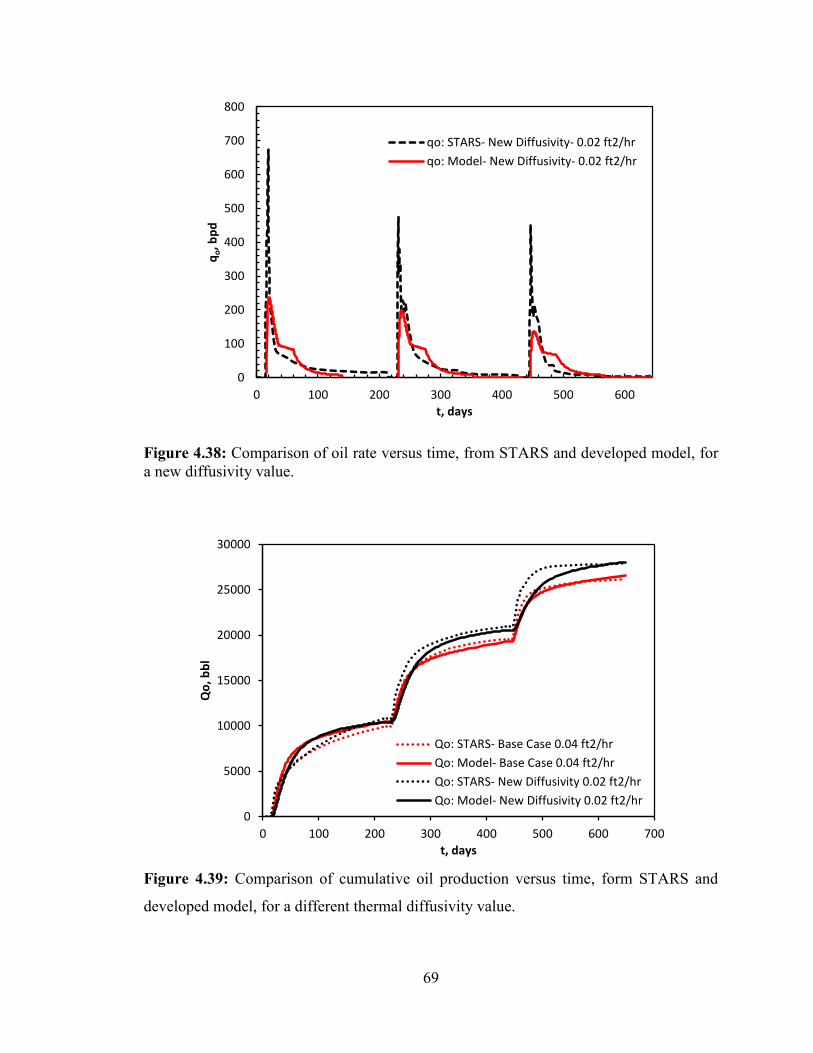
69


a new diffusivity value.

Figure 4.39: Comparison of cumulative oil production versus time, form STARS and

developed model, for a different thermal diffusivity value.

0

100

200

300

400

500

600

700

800

0 100 200 300 400 500 600

qo, b

pd

t, days

qo: STARS- New Diffusivity- 0.02 ft2/hr

qo: Model- New Diffusivity- 0.02 ft2/hr

0

5000

10000

15000

20000

25000

30000

0 100 200 300 400 500 600 700

Qo

, bb

l

t, days

Qo: STARS- Base Case 0.04 ft2/hr

Qo: Model- Base Case 0.04 ft2/hr

Qo: STARS- New Diffusivity 0.02 ft2/hr

Qo: Model- New Diffusivity 0.02 ft2/hr

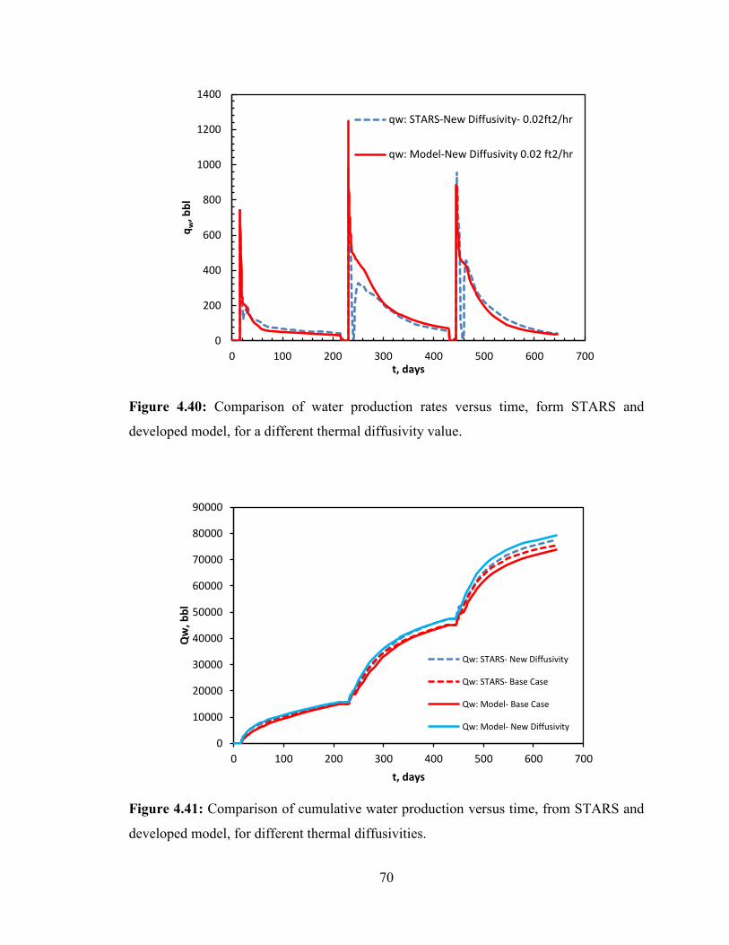
70

Figure 4.40: Comparison of water production rates versus time, form STARS and

developed model, for a different thermal diffusivity value.


developed model, for different thermal diffusivities.

0

200

400

600

800

1000

1200

1400

0 100 200 300 400 500 600 700

qw

, bb

l

t, days

qw: STARS-New Diffusivity- 0.02ft2/hr

qw: Model-New Diffusivity 0.02 ft2/hr

0

10000

20000

30000

40000

50000

60000

70000

80000

90000

0 100 200 300 400 500 600 700

Qw

, bb

l

t, days

Qw: STARS- New Diffusivity



Qw: Model- New Diffusivity

71

4.2.7 Types of oil viscosity

The model was tested for two different type of oil viscosity: base case; and viscosity data

obtained from the research sponsor-PennWest Exploration. Figure 4.42 and Figure 4.44

show the oil and water production rates, respectively, obtained from the developed model

and the simulator. Figure 4.43 shows the comparison of cumulative oil production

obtained from the developed model and the numerical simulator for two different cases

and the results are fairly close to each other. Similarly, the cumulative water production

for both the cases shows an acceptable match, as depicted in Figure 4.45.


PennWest oil viscosity.

0

100

200

300

400

500

600

700

800

0 100 200 300 400 500 600

qo

, bp

d

t, days

STARS: Pennwest Oil

Model: PennWest Oil

72


developed model, for different types of oil- viscosity.

Figure 4.44: Comparison of water production rate versus time, from STARS and model,

for PennWest oil viscosity.

0

5000

10000

15000

20000

25000

30000

35000

40000

45000

0 100 200 300 400 500 600 700

Qo

, bb

l

t, days

STARS- Base Case

Model- Base Case

STARS- PennWest Oil

Model- Pennwest Oil

0

100

200

300

400

500

600

700

800

900

1000

0 100 200 300 400 500 600 700

qw

, bp

d

t, days

qw: STARS- PennWest Oil

qw: Model- PennWest Oil

73


developed model, for PennWest oil viscosity.

4.2.8 Number of cycles

A cyclic steam stimulation process consists of many cycles, typically around 7-10 cycles

or as long as it is economically viable. Hence, it is important to see if the developed

model is able to accurately predict the performance of the process for more than just three

cycles. The model was tested for ten cycles and the results are presented in this section.

Figure 4.46 and Figure 4.47 show the oil production rate and cumulative oil production,

respectively, for ten cycles. Similarly, the water rate and cumulative water production

rate are plotted in Figure 4.48 and Figure 4.49. It can be verified from the plots that the

model is robust to predict the performance for up to ten cycles.

0

10000

20000

30000

40000

50000

60000

70000

80000

0 100 200 300 400 500 600 700

Qw

, bb

l

t, days

Qw: STARS- PennWest Oil



Qw: Model- PennWest Oil

74


model, for ten cycles.


developed model, for ten cycles.

0

100

200

300

400

500

600

700

800

0 500 1000 1500 2000

qo

, bp

d

t, days

STARSAnalytical Model

0

10000

20000

30000

40000

50000

60000

0 500 1000 1500 2000

Qo

, bb

l

t, days

STARSAnalytical Model

75


developed model, for ten cycles.

Figure 4.49: Comparison of cumulative water production versus time, obtained from

STARS and developed model, for ten cycles.

0

100

200

300

400

500

600

700

800

900

1000

0 500 1000 1500 2000 2500

qw

, bp

d

t, days

qw: STARS

qw: Model

0

50000

100000

150000

200000

250000

300000

350000

400000

0 500 1000 1500 2000 2500

Qw

, bb

l

t, days

Qw: STARSQw: Model

76

4.2.8.1 Steam oil ratio

An important index used to evaluate the performance of a cyclic steam stimulation

process is SOR (steam oil ratio). It is defined as the volume of steam required to produce

one unit volume of oil. Hence, the lower the SOR value, the more efficient the process is.

The cumulative steam oil ratio (CSOR) can be calculated as.

o

injs

Q

QCSOR

where,

Qs.inj = the cumulative steam injected, bbl CWE

Qo = the cumulative oil produced, bbl

Typical values of SOR for a cyclic steam stimulation process are in the range of three to

eight. For a ten cycle process, the SOR is plotted and are shown in the Figure 4.50 and

Figure 4.51. Figure 4.50 shows a plot of the cumulative steam oil ratio versus time.

Initially, the SOR value is very high as the cumulative oil production is very low for the

first time step. Figure 4.51 shows a plot of the average values of CSOR with respect to

the number of cycles. It can be seen from the plots that the calculated values of SOR is in

the range of three to six, which is typical of a cyclic steam stimulation process.

77

Figure 4.50: Plot of cumulative steam oil ratio versus time

Figure 4.51: Plot of average steam oil ratio versus the number of cycles

0

2

4

6

8

10

0 500 1000 1500 2000 2500

CSO

R

time, days

CSOR

0

1

2

3

4

5

6

7

8

0 1 2 3 4 5 6 7 8 9 10 11

Avg

. C

SOR

No. of Cycles

Avg. CSOR

78

4.3 Summary

The model is successfully validated and tested by comparing the fluid production (rate

and cumulative production of both oil and water) obtained from the model with the fluid

production obtained from STARS numerical simulator. The following parameters were

considered: steam injection rates, length of the horizontal well, absolute permeability of

the reservoir, relative permeability of oil and water, thermal diffusivity of the formation,

oil with different viscosities, and finally the number of operational cycles.

All the calculations for the analytical model were done using MATLAB and an excel


obtained from STARS numerical simulator. Step by step procedure to calculate the oil

and water rates is presented in the Section 4.1 and detailed sensitivity analyses are

presented in Section 4.2 of this chapter. It is concluded that the model is able to predict

the performance of the CSS process and there is a good match with the results obtained

from the numerical simulator. To obtain a good match for the water production, a

corrected relative permeability of water was used.

79

CHAPTER FIVE:

5 Conclusions and Recommendations

5.1 Results

In this thesis, a radial one dimensional heat transfer model has been developed to predict

the average temperature of the steam zone for a cyclic steam stimulation process with

horizontal well configuration. The oil and water viscosities are calculated based on the

average steam zone temperature. Correlations for fluids saturation and relative

permeabilities of oil and water are described. This heat transfer model is coupled to a

transient radial fluid inflow model that is used to calculate the fluid flow rates. A

modified form of Joshi’s in flow equation is used. Finally, detailed steps for calculations

are shown and a flow chart is presented which outlines the important steps involved in

the performance prediction for a CSS process for horizontal wells.

The developed model is validated using numerical simulation in CMG STARS. First, a

base case is run to checked if the results from the simulator match with that of the

developed analytical model. Next, sensitivity analyses were conducted to test the

robustness of the model for parameters such as: steam injection rates, length of the

horizontal well, absolute permeability of the reservoir, relative permeability of oil and

water, thermal diffusivity of the formation, oil with different viscosities, and finally the

number of operational cycles.

80

All the calculations for the analytical model were done using MATLAB and an Excel


obtained from STARS numerical simulator. To obtain a good match for the water

production, a corrected relative permeability of water is used. It is concluded that, with

reasonable assumptions and using a correction factor for the water relative permeability,

the model is able to predict the performance of the CSS process and there is a good match

with the results obtained from the numerical simulator.

5.2 Future Work

5.2.1 Economic studies

Currently, the developed analytical model for cyclic steam stimulation process for a

horizontal well configuration can be used to optimize production from a single well. The

model has a potential to be coupled with an economic model to optimize steam injection

rates, production rates based on the reservoir properties and conducting economic studies.

5.2.2 Pressure drop model and water relative permeability adjustment

The pressure drop model for predicting the pressure drawdown is based on a trial and

error method. In order to obtain a good match for the oil production with STARS, the

calculation of pressure drawdown requires an initial guess work, based upon the

production data obtained from the numerical simulator and iteration. To match the water

production, some adjustments were made to the water relative permeability curves. This

area needs further investigation in order to minimize the need of matching parameters.

81

APPENDIX

A. Solution for Average Temperature of the Steam Zone (CSS)

Heat conduction in radial direction is given as:

r

T

r

Tr

rr

11 (A.1)

We defined two zones-Zone 1, which is at the temperature, TS, initially, and Zone 2,

region beyond rh, that is at an elevated temperature due to the heat transfer in the steam

injection and soak period, T2(0). Let T1 and T2 be the temperatures of the Zone1 and Zone

2 at any time, t, respectively. The initial and boundary conditions are defined as below:

Initial Condition:

T1=Ts at t=0 (A.2)

The net heat flux at r=0 is zero because of the radial symmetry. The total heat from the

boundary of zone 1 is equal to the amount of heat absorbed by the Zone 2. It is denoted

by B.C. 2. These are represented mathematically below as:

Boundary Conditions:

01

r

T at r=0 (A.3)

t

TcV

r

TkA p

rr h

21 . at r= rh (A.4)

For solving the PDE, the following dimensional parameters were defined and the above

equation is converted into a dimensionless form.

82

Dimensionless Parameters

RS

SD

TT

TTT

1

1 (A.5)

RS

SD

TT

TTT

2

2 (A.6)

w

Dr

rr (A.7)

2

w

Dr

tt

(A.8)

RS

S

DTT

TTT

)0(2

)0(2 (A.9)

Equation in dimensionless form:

D

D

D

D

DD

D

t

T

r

T

rr

T

11

2

1

21

(A.10)

Initial Condition:

01 DT at t=0 (A.11)

B.C. 1:

01

D

D

r

T at 0Dr (A.12)

B.C. 2:

D

Dp

wD

D

t

TVc

rr

TkA

21 ).(

at rd=rdh (A.13)

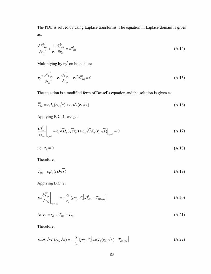
83

The PDE is solved by using Laplace transforms. The equation in Laplace domain is given

as:

11

2

1

2~

~1

~

D

D

D

DD

D Tsr

T

rr

T

(A.14)

Multiplying by rD2 on both sides:

0~

~~

1

21

2

1

22

DD

D

DD

D

DD Tsr

r

Tr

r

Tr (A.15)

The equation is a modified form of Bessel’s equation and the solution is gi en as:

)()(~

02011 srKcsrIcT DDD (A.16)

Applying B.C. 1, we get:

0)()(

~

01211

0

1

D

D

rDD

rD

D srKscrsIscr

T (A.17)

i.e. 02 c (A.18)

Therefore,

)(~

011 srDIcTD (A.19)

Applying B.C. 2:

)0(22

1 ~).(

~

DDp

wrrD

D TTsVcrr

TkA

DaD

(A.20)

At ,DaD rr 12 DD TT (A.21)

Therefore,

)0(20111 )(.).()(. DDap

w

Da TsrIcsVcr

srIsckA

(A.22)

84

Let,

kAr

VcQ

w

p

.

).( (A.23)

The Equation A.22 can be written as:

)0(20111 .)(.)( DDaDa TQsrIQscsrIsc (A.24)

)()(

.

1

)0(2

1srQsIsrIs

TQc

DaoDa

D

(A.25)

From Equations A.19 and A.25, we get:

)()(

).(.~

01

)0(20

1srQsIsrIs

TsrIQT

DaDa

DD

D

(A.26)

The average temperature in Zone-1 can be calculated as:

)1(

~2

~2

1

1

1

Da

rr

r

DDD

AvgDr

drTr

T

DaD

D

(A.27)

)0(2

01

11

21)()(

)()(.1

1

2.

~D

DaDa

DaDa

Da

AvgD TSrQsISrIS

sISrIrQ

srT

(A.28)

Temperature of Zone-2 is given by:

)()(

).(.~~

01

)0(20

12srQsIsrIs

TsrIQTT

DaDa

DDa

rrDD

DaD

(A.29)

85

References

1 Farouq Ali, S.M.: “Practical Hea y Oil Reco ery”, ENCH 6 9 Notes, Uni ersity of

Calgary, 2010.

2 Gutierrez, D., Moore, R.G., Mehta, S.A., and Skoreyko, F.: “The Challenge of

Predicting Field Performance of Air Injection Process Based on Laboratory and

Numerical Modeling”, J.Can.Pet. Tech., March 2009.

3 Boberg, T.C. “Thermal Methods of Oil Reco ery”, John Wiley & Sons, Inc., 988

4 Alvarez, J., and Coates, R., Heavy Oil Recovery; Cyclical Solvent Injection, CSI,

Wednesday, 27 May 2009, Russian Oil and Gas Technologies. 2009.

5 Butler R.M.: “Thermal Reco ery of Oil and Bitumen”, Gra Drain Inc., July 2 8.

6 Schild, A. “A Theory for the Effect of Heating Oil Producing Wells”, Trans. AIME,

210, 1 (1957)

7 Fontanilla, J.P. and Aziz, K.: “Prediction of Bottom-Hole Conditions for Wet Steam

Injection Wells”, J.Can.Pet.Tech., March-April 1982.

8 Marx J.W. and Langenheim R.H.: “Reser oir Heating by Hot Fluid Injection”, Trans.,

Aw (19S9) 216, 312-314.

9 Carter, R.D.: Appendix to “Optimum Fluid Characteristics for Fracture Extension”, by

G.C. Howard and G.R. Fast, Drill. And Prod. Prac., API (1957) 267.

10 Boberg, T.C. and Lantz, R.B.: “Calculation of the Production Rate of a Thermally

Stimulated Well”, J.Pet.Tech., December 1966.

11 Bensten R.G and Donohue, D.A.T.: “A Dynamic Programming Model of the Cyclic

Steam Injection Process,” JPT (Dec 969) 2582- 96; Trans., AIME 246.

12 Bidnr M.S. and Kostilia H.M.: “Analysis of Transient Production of a Thermally

Stimulated Well,” SPE 6997 (Sept. 1989).

86

13

an E erdingen, A.F. and Hurst, W.: “The Applications of Laplace Transformations to

Flow Problems in Reser oirs,” Tran., AIME ( 949) 86, 3 5-24.

14 Towson, D.E. and Boberg, T.C.: “Gra ity Drainage in Thermally Stimulated Wells”, J.

Can. Pet. Tech., (Oct- Dec. 1967) 130-135

15 Matthews, C.S. and Leftko ics, H.C.: “Gra ity Drainage Performance of Depletion-

Type Reser oirs in the Stripper Stage”, Trans., AIME ( 956) 2 7, 265- 274.

16 Seba, R.A. and Perry, G.E.: “A Mathematical Model of Repeated Steam Soaks of

Thick Gra ity Drainage Reser oirs”, J. Pet. Tech. (Jan., 969) 87-94.

17 Kuo, C.H., Shain, S.A., and Phocas, D.M.: “A Gra ity Drainage Model for the Steam

Soak Process”, paper SPE 2329 presented at the 39th

Annual SPE California Fall

Meeting, Bakersfield, California, Nov. 7-8, 1968.

18 Jones, J.: “Cyclic Steam Reser oir Model for Viscous Oil, Pressure-depleted, Gravity-

drainage Reser oirs”, SPE 6544, 47th

Annual California Regional Meeting of the SPE of

AIME, Bakersfield (April 13-15, 1977).

19 Butler, R.M., McNab, G.S., and Lo, H.Y.: “Theoretical Studies on the Gra ity

Drainage of Hea y Oil during in Situ Steam Heating”, presented at the 29th

Can. Chem.

Eng. Conf., Sarnia, Ont., Oct. 1-3, 1979.

20 Aziz, K. and Gontijo J.E.: “A Simple Analytical Model for Simulating Hea y oil

Recovery by Cyclic Steam in Pressure-Depleted Reser oirs”, paper SPE 3 37 presented

at the 59th Annual Technical Conference and Exhibition, Houston (September 16-19,

1984).

21 Boriso , Ju.P.: “Oil Production Using Horizontal and Multiple De iation Wells,”

Nedra Moscow, 1964. Translated by J. Strauss, S.D. Joshi (ed.). Phillips Petroleum Co.,

the R & D Library Translation, Bartlesville, Oklahoma, 1984.

87

22

Giger, F.: “Reduction du nombre de puits par l’utilisation de forages horizontaux,”

Re ue de l’ Institut Francis du Petrole, ol. 38, No. 3, May- June 1983.

23 Giger, F. M., Reiss, L. H., and Jourdan, A.P.: “The reser oir Engineering Aspects of

Horizontal Drilling,” paper SPE 3 24 presented at the SPE59th Annual Technical

Conference and Exhibition, Houston, Texas, Sept. 16-19, 1984.

24 Renard, G. I. and Dupuy, J. M.: “Influence of Formation Damage on the Flow

Efficiency of Horizontal Wells,” paper SPE 94 4 presented at the Formation Damage

Control Symposium, Lafayette, Louisiana, Feb. 22- 23, 1990.

25 Joshi, S.D.: “Augmentation of Well Producti ity with Slant and Horizontal Wells”, J

Pet. Tech. 40 (6): 729- 739; Trans., AIME, 285. SPE- 15375- PA. doi: 10.2118/ 24941-

PA, 1988.

26 Dikken, B.J.: “Pressure Drop in Horizontal Wells and Its Effect on Production

Performance”, J. Pet. Tech. 426- 1433, Nov. 1990

27 Babu, D.K. and Odeh, A.S.: “Producti fity of a Horizontal Well” SPE Res. Eng 4 (4):

417- 421, SPE- 18298- PA

28 Ozkan, E. Haciislamoglu,M. and Ragha an, R.: “The Influence of Pressure Drop

Along the Wellbore on Horizontal Well Producti ity, “SPE 255 2, presented ar the

Production Operations Sumposium, Oklahoma, March 21-23, 1993.

29 No y, R.A.: “Pressure Drops in Horizontal wells: When Can Theory Be Ignored?” Spe

Res. Eng. 29-35, Feb 1995.

30 Ozkan, E, Sarica and Haciislamoglu, M.: “Effect of Conducti ity on Horizontal Well

Pressure Beha ior”, SPE Ad . Tech. Series, Vol. 3. No. , pp. 85- 93, 1995.

31 Archer, R.A., and Agbongiator, E.O.: “Correlation for Frictional Pressure Drop in

Horizontal- Well Inflow- Performance Relationships,” Feb 2 5, SPE production &

Facilities, 21-25.

88

32

Lu, J.: “New Producti ity Formulae of Horizontal Wells”, J. of Can. Pet. Tech, Vol.

40, No. 10, Oct. 2001.

33 Gunadi, B.: “Experimental and Analytical Studies of Cyclic Steam Injection using

Horizontal Wells”, Ph.D Thesis, December 999, Texas A&M Uni ersity.

34 Diwan, U. and Ko scek, A.R.: “An Analytical Model for Simulating Hea y-Oil

Recovery by Cyclic Steam Injection Using Horizontal Wells”, July 999.

35 Butler, R.M. and Stephens, D.J.,: “The Gra ity-drainage of Steam-Heated Heavy-Oil to

Parallel Horizontal Wells”, paper presented at the 3 st Annual Technical Meeting of The

Petroleum Society of CIM in Calgary (May 25-28,1980).

36 Wu, Z., Vasantharajan, S., El-Mandouh, M., Suryanarayana, P.V.: “Inflow

Performance of a Cyclic- Steam- Stimulated Horizontal Well Under the Influence of

Gra ity Drainage”, SPE 275 8, Sept, 2 .

37 Aziz, K. and Gontijo J.E.: “A Simple Analytical Model for Simulating Heavy oil

Recovery by Cyclic Steam in Pressure-Depleted Reser oirs”, paper SPE 3 37 presented

at the 59th Annual Technical Conference and Exhibition, Houston (September 16-19,

1984).

38 Prats, M.: “Thermal Reco ery”, Monograph – Volume 7, SPE of AIME, Henry L.

Doherty Memorial Fund of AIME, 1982.

39 Farouq Ali, S.M.: “Steam Injection Theories- A Unified Approach”, paper SPE 746

presented at the 57th

Annual Fall Technical Conference and Exhibition, Denver, Oct. 9-

12, 1977.

40 Villinger, H., 1985, Solving cylindrical geothermal problems using Gaver-Stehfest

inverse Laplace transform, Geophysics, vol. 50 no. 10 p.1581-1587

41

Stehfest, H., 1970, Algorithm 368: Numerical inversion of Laplace transform,

Communication of the ACM, vol. 13 no. 1 p. 47-49

Analytical Modeling of Cyclic Steam Stimulation Process ...

Documents

Transcript of Analytical Modeling of Cyclic Steam Stimulation Process ...