HAL Id: tel-03269981https://tel.archives-ouvertes.fr/tel-03269981

Submitted on 24 Jun 2021

HAL is a multi-disciplinary open accessarchive for the deposit and dissemination of sci-entific research documents, whether they are pub-lished or not. The documents may come fromteaching and research institutions in France orabroad, or from public or private research centers.

L’archive ouverte pluridisciplinaire HAL, estdestinée au dépôt et à la diffusion de documentsscientifiques de niveau recherche, publiés ou non,émanant des établissements d’enseignement et derecherche français ou étrangers, des laboratoirespublics ou privés.

Analytical methods for the study of the two-bodyproblem, and alternative theories of gravitation.

François Larrouturou

To cite this version:François Larrouturou. Analytical methods for the study of the two-body problem, and alternativetheories of gravitation.. General Relativity and Quantum Cosmology [gr-qc]. Sorbone Université,2021. English. tel-03269981

THÈSE DE DOCTORATDE L’UNIVERSITÉ SORBONNE UNIVERSITÉ

Spécialité : PhysiqueÉcole doctorale nº564: Physique en Île-de-France

réalisée

sous la direction conjointe de Luc BLANCHET & Cédric DEFFAYET

présentée par

François LARROUTUROUpour obtenir le grade de :

DOCTEUR DE L’UNIVERSITÉ SORBONNE UNIVERSITÉ

Sujet de la thèse :

Méthodes analytiquespour l’étude du problème à deux corps,

et des théories alternatives de gravitation

soutenue le 18 juin 2021devant le jury composé de :

Mme. Danièle STEER : RapporteuseM. Clifford M. WILL : RapporteurMme. Marie-Christine ANGONIN : ExaminatriceM. Éric GOURGOULHON : ExaminateurM. Shinji MUKOHYAMA : ExaminateurM. Luc BLANCHET : Directeur de thèseM. Cédric DEFFAYET : Membre invité

Καί με θεὰ πρόφρων ὑπεδέξατο, χεῖρα δὲ χειρί

δεξιτερὴν ἕλεν, ὧδε δ΄ ἔπος φάτο καί με προσηύδα·

ὦ κοῦρ΄ ἀθανάτοισι συνάορος ἡνιόχοισιν,

ἵπποις ταί σε φέρουσιν ἱκάνων ἡμέτερον δῶ

χαῖρ΄, ἐπεὶ οὔτι σε μοῖρα κακὴ προὔπεμπε νέεσθαι

τήνδ΄ ὁδόν ἦ γὰρ ἀπ΄ ἀνθρώπων ἐκτὸς πάτου ἐστίν,

ἀλλὰ θέμις τε δίκη τε. Χρεὼ δέ σε πάντα πυθέσθαι

ἠμὲν Αληθείης εὐκυκλέος ἀτρεμὲς ἦτορ

ἠδὲ βροτῶν δόξας, ταῖς οὐκ ἔνι πίστις ἀληθής.

Et la déesse en toute bienveillance m’accueillit, elle prit ma main droitedans sa main, elle proféra ces paroles en s’adressant à moi :Jeune homme, compagnon d’immortels cochers,qui grâce aux juments qui te portent parviens à notre demeure,bienvenue, car ce n’est pas un mauvais destin qui t’a conduit à prendrecette voie, si loin des hommes qu’elle soit à l’écart du sentier battu,c’est la règle, la justice. Il faut que tu sois instruit de tout,et du cœur sans tremblement de la vérité bien persuasive,et de ce qui paraît aux mortels, où n’est pas de croyance vraie.

Parménide,Sur la nature Frag. I, v. 22–30, trad. B. Cassin.

Acknowledgment

The past three years have been a thrilling and fruitful journey, mostly thanks to all the encountersand discussions they were filled with. All those interactions constituted for me the living proof thatdoing science is a collaborative process. That is why I would like to thank all the people that madethis work possible.

First of foremost, I would like to express my deepest gratitude to both my supervisors, LucBlanchet and Cédric Deffayet. They were patient and inspiring guides in the learning and compre-hension of post-Newtonian and solitonic defects frameworks, but also, and more importantly, in thepractical understanding of the scientific method.

Regarding post-Newtonian theory, I am grateful to Guillaume Faye, for his patience in answeringmy questions, and tireless help with software-related issues; Tanguy Marchand for guiding my firststeps with Mathematica and practical post-Newtonian computations; Sylvain Marsat for his help andvaluable advice; and Quentin Henry, who has been far more a friend than a collaborator during thosethree years we shared inside and outside IAP. The fruitful and inspiring conversations I had withGilles Esposito-Farèse, Eugeny Babichev and Sebastian Garcia-Saenz provided strong motivationand support during my discovery of scalar theories, and I would like to thank them warmly. Iwould also like to thank Stefano Foffa and Riccardo Sturani for introducing me to the EFT languageand techniques, and Guillaume Hébrard and Jean-Philippe Beaulieu for showing me the way to thewonderful world of exoplanets.

Beyond those projects carried out with Luc and Cédric, the freedom they gave me allowed meto pursue other collaborations on my own. I would thus like to express all my gratitude to ShinjiMukohyama and Antonio De Felice, that opened me the doors of the fascinating realm of minimaltheories, and hosted me for two weeks at Yukawa Institute for Theoretical Physics in Kyôto; and toMichele Oliosi and Özgün Mavuk with whom my discoveries were as much focused on science as onKyôto and Naoshima lifestyles.

Those three years were also filled with inspiring scientific exchanges, and I would like to thankLaura Bernard, Giulia Cusin, Giulia Isabella, Éric Gourgoulhon, Otto Hannuksela, Rafael Porto forpost-Newtonian and post-Minkowskian conversations; Shweta Dalal, Gwenaël Boué, Alain Lecavelierdes Étangs and Jordan Philidet for stellar and exoplanetary discussions; Timothy Anson and LucasPinol for cosmological ones; and Catherine de Montety for being my guide through the ideas ofAristotle and Occam.

I am also extremely thankful to Danièle Steer and Clifford M. Will for having accepted to refereethis dissertation, and to Marie-Christine Angonin, Éric Gourgoulhon and Shinji Mukohyama for be-ing part of the thesis jury.

Those three years would have been much more difficult without the help of the efficient supportingstaff of IAP, and I would like to express my gratitude to Valérie Bona, Roselys Rakotomandimby,Isabelle Coursimault, Sandy Artero and Chantal Le Vaillant for their patience and kindness; CarlosCarvalho, Laurent Domisse, Jean Mouette and Lionel Provost for their help with computer and otherrelated issues; Cynthia Tshiela Kuyakula and Pierre Wachel for their unfailing morning smiles andjokes; and Valérie de Lapparent for taking care of the practical issues of PhD students.

iii

One of the strength of IAP is that it is, and managed to remained under the reign of Covid, aplace with a real and exciting “PhD vibe”. I would thus like to thank all the other students withwhom I shared either coffee or beer, Alexandre, Aline, Amaël, Amaury, Amélie, Arno, Clément,David, Doogesh, Émile, Erwan, Étienne, Florian, Jacopo, Julie, Julien, Lukas, Marko, Martin, Nico-las, Oscar, Pierre, Raphaël, Sandrine, Simon, Valentin and Virginia.

I would like to thank all the teachers and professors that gave me a taste for physics and gravi-tation, and especially Xavier Ovido, Jack-Michel Cornil and Gilles Esposito-Farèse, who played eacha major role in the path that led me to this thesis. I would also like to express my deepest gratitudeto my family for their support and help during those years, and notably to my mother for her carefuland valuable proofreading of this dissertation, and to Nathalie for her help with the subtelties of theEnglish language.

And to finish en beauté, I am very grateful to my fiancée, Andréane Bourges, for her infallibleencouragements and priceless support.

iv

Contents

I General Introduction 1I.1 A brief history of gravitation . . . . . . . . . . . . . . . . . . . . . . . . . . . . . . . 1

I.1.1 The pre-Aristotelian conceptions . . . . . . . . . . . . . . . . . . . . . . . . . 1I.1.2 Rise and fall of the Aristotelian models . . . . . . . . . . . . . . . . . . . . . 2I.1.3 The Newtonian theory of gravitation . . . . . . . . . . . . . . . . . . . . . . . 2

I.2 General Relativity as the current theory of gravitation . . . . . . . . . . . . . . . . . 4I.2.1 A geometrical description of the gravitational phenomena . . . . . . . . . . . 4I.2.2 Lovelock’s theorem and theories “beyond” General Relativity . . . . . . . . . 5I.2.3 The brilliant success and darkness of General Relativity . . . . . . . . . . . . 6

I.3 Motivations for this thesis . . . . . . . . . . . . . . . . . . . . . . . . . . . . . . . . . 9I.3.1 Pushing forward our comprehension of General Relativity . . . . . . . . . . . 9I.3.2 Seeking for viable alternative . . . . . . . . . . . . . . . . . . . . . . . . . . . 10I.3.3 Work done in this thesis . . . . . . . . . . . . . . . . . . . . . . . . . . . . . . 10

A The relativistic two-body problem 13

II Introduction to the relativistic two-body problem 15II.1 From the Newtonian to the relativistic problem . . . . . . . . . . . . . . . . . . . . . 15

II.1.1 Revisiting the Newtonian two-body problem . . . . . . . . . . . . . . . . . . . 15II.1.2 The relativistic notion of trajectory . . . . . . . . . . . . . . . . . . . . . . . . 17II.1.3 The relativistic gravitational radiation . . . . . . . . . . . . . . . . . . . . . . 19II.1.4 The relativistic non-linearities . . . . . . . . . . . . . . . . . . . . . . . . . . . 19

II.2 The case of the exoplanet HD 80606b as an illustration . . . . . . . . . . . . . . . . 20II.2.1 HD 80606b, a remarkable exoplanet . . . . . . . . . . . . . . . . . . . . . . . 20II.2.2 Computation of the relativistic effects on the trajectory . . . . . . . . . . . . 22II.2.3 Feasibility of the measure . . . . . . . . . . . . . . . . . . . . . . . . . . . . . 27

II.3 Different approaches to tackle the relativistic problem . . . . . . . . . . . . . . . . . 29II.3.1 Weak-field, slow-motion approaches . . . . . . . . . . . . . . . . . . . . . . . 29II.3.2 Other approaches . . . . . . . . . . . . . . . . . . . . . . . . . . . . . . . . . 31II.3.3 Beyond the point-particle approximation . . . . . . . . . . . . . . . . . . . . . 32

III Conservative sector 33III.1 The tail effects in General Relativity . . . . . . . . . . . . . . . . . . . . . . . . . . . 33III.2 The logarithmic simple tail contributions . . . . . . . . . . . . . . . . . . . . . . . . 35

III.2.1 An effective action for the simple tail terms . . . . . . . . . . . . . . . . . . . 35III.2.2 Contributions to the dynamics . . . . . . . . . . . . . . . . . . . . . . . . . . 37III.2.3 The case of quasi-circular orbits . . . . . . . . . . . . . . . . . . . . . . . . . 39

III.3 Logarithmic contributions in the conserved energy . . . . . . . . . . . . . . . . . . . 39III.3.1 Simple tail contributions . . . . . . . . . . . . . . . . . . . . . . . . . . . . . . 39III.3.2 The relative 3PN logarithmic contributions . . . . . . . . . . . . . . . . . . . 40

v

III.3.3 Discussion on the reliability of the formalism . . . . . . . . . . . . . . . . . . 43III.3.4 Leading logarithm contributions in the conserved energy . . . . . . . . . . . . 44

IV Radiative sector 49IV.1 Towards the gravitational phase at the 4PN accuracy . . . . . . . . . . . . . . . . . . 49IV.2 The Hadamard regularized mass quadrupole . . . . . . . . . . . . . . . . . . . . . . . 51

IV.2.1 The mass quadrupole in d dimensions . . . . . . . . . . . . . . . . . . . . . . 51IV.2.2 Computation of the potentials . . . . . . . . . . . . . . . . . . . . . . . . . . 55IV.2.3 Computation of the surface terms . . . . . . . . . . . . . . . . . . . . . . . . 60IV.2.4 Application of the UV shift and final sum . . . . . . . . . . . . . . . . . . . . 63

IV.3 IR dimensional regularization of the mass quadrupole . . . . . . . . . . . . . . . . . 64IV.3.1 Computation of the different contributions . . . . . . . . . . . . . . . . . . . . 65IV.3.2 Computation of the required potentials in d dimensions . . . . . . . . . . . . 71IV.3.3 The IR regularized mass quadrupole . . . . . . . . . . . . . . . . . . . . . . . 74

IV.4 Dimensional regularization of the radiative quadrupole . . . . . . . . . . . . . . . . . 74IV.4.1 Dimensional regularization of the non-linear interactions . . . . . . . . . . . . 74IV.4.2 Computation of the d-dimensional quadratic interactions . . . . . . . . . . . . 77IV.4.3 The 3PN dimensional corrections to the radiative quadrupole . . . . . . . . . 78IV.4.4 Towards the 4PN dimensional corrections . . . . . . . . . . . . . . . . . . . . 79

B Alternative theories of gravitation 81

V Non-canonical domain walls 83V.1 The canonical domain walls . . . . . . . . . . . . . . . . . . . . . . . . . . . . . . . . 83

V.1.1 Solitonic defects . . . . . . . . . . . . . . . . . . . . . . . . . . . . . . . . . . 83V.1.2 Some generalities about canonical domain walls . . . . . . . . . . . . . . . . . 84V.1.3 An interesting change of variables . . . . . . . . . . . . . . . . . . . . . . . . 85V.1.4 The usual argument sustaining stability . . . . . . . . . . . . . . . . . . . . . 87

V.2 Domain walls in potential-free scalar theories . . . . . . . . . . . . . . . . . . . . . . 88V.2.1 Bypassing the usual argument . . . . . . . . . . . . . . . . . . . . . . . . . . 88V.2.2 General stability requirements . . . . . . . . . . . . . . . . . . . . . . . . . . 88V.2.3 Explicit stability requirements . . . . . . . . . . . . . . . . . . . . . . . . . . 90

V.3 Mimicking canonical domain wall profile . . . . . . . . . . . . . . . . . . . . . . . . . 91V.3.1 The case of mexican hat-like profiles . . . . . . . . . . . . . . . . . . . . . . . 91V.3.2 Apparent singularities . . . . . . . . . . . . . . . . . . . . . . . . . . . . . . . 92V.3.3 Non-perturbative stability considerations . . . . . . . . . . . . . . . . . . . . 94V.3.4 The case of mimickers . . . . . . . . . . . . . . . . . . . . . . . . . . . . . . . 96V.3.5 An extended family of kinks . . . . . . . . . . . . . . . . . . . . . . . . . . . . 97V.3.6 Mimicking other canonical domain wall profiles . . . . . . . . . . . . . . . . . 98

V.4 Towards gravitating non-canonical domain walls . . . . . . . . . . . . . . . . . . . . 99V.4.1 Generalities about gravitating domain walls . . . . . . . . . . . . . . . . . . . 99V.4.2 Practical implementation for the models previously investigated . . . . . . . . 100

VI Minimalism as a guideline to construct alternative theories of gravitation 101VI.1 The principle of minimalism . . . . . . . . . . . . . . . . . . . . . . . . . . . . . . . 101VI.2 Construction of a minimal theory of bigravity . . . . . . . . . . . . . . . . . . . . . . 102

VI.2.1 A brief review of Hassan-Rosen bigravity . . . . . . . . . . . . . . . . . . . . 102VI.2.2 The precursor theory . . . . . . . . . . . . . . . . . . . . . . . . . . . . . . . . 105VI.2.3 A minimal theory of bigravity . . . . . . . . . . . . . . . . . . . . . . . . . . . 109

VI.3 Cosmology of our minimal theory of bigravity . . . . . . . . . . . . . . . . . . . . . . 113

vi

VI.3.1 Cosmological background . . . . . . . . . . . . . . . . . . . . . . . . . . . . . 113VI.3.2 Cosmological perturbations . . . . . . . . . . . . . . . . . . . . . . . . . . . . 115VI.3.3 Gravitational Cherenkov radiation in MTBG . . . . . . . . . . . . . . . . . . 120

VII Testing the strong field regimes of minimal theories 121VII.1 Strong field regime of the minimal theory of massive gravity . . . . . . . . . . . . . . 121

VII.1.1 The minimal theory of massive gravity . . . . . . . . . . . . . . . . . . . . . . 121VII.1.2 Non-rotating black holes and stars . . . . . . . . . . . . . . . . . . . . . . . . 123VII.1.3 Towards rotating solutions . . . . . . . . . . . . . . . . . . . . . . . . . . . . 126

VII.2 Strong field regime of the V CDM model . . . . . . . . . . . . . . . . . . . . . . . . . 131VII.2.1 The model under consideration . . . . . . . . . . . . . . . . . . . . . . . . . . 131VII.2.2 Static solutions . . . . . . . . . . . . . . . . . . . . . . . . . . . . . . . . . . . 134VII.2.3 Time dependent, non-rotating solutions . . . . . . . . . . . . . . . . . . . . . 137VII.2.4 Inclusion of matter . . . . . . . . . . . . . . . . . . . . . . . . . . . . . . . . . 141

Conclusion 143

A Conventions and some technical aspects of General Relativity 147A.1 Conventions . . . . . . . . . . . . . . . . . . . . . . . . . . . . . . . . . . . . . . . . 147

A.1.1 Geometrical conventions . . . . . . . . . . . . . . . . . . . . . . . . . . . . . . 147A.1.2 Dimensional conventions . . . . . . . . . . . . . . . . . . . . . . . . . . . . . . 148A.1.3 Conventions specific to post-Newtonian computations . . . . . . . . . . . . . 148

A.2 General Relativity: Lagrangian formulation . . . . . . . . . . . . . . . . . . . . . . . 149A.3 Arnowitt-Deser-Misner formalism and Hamiltonian analysis of General Relativity . . 150

B Toolkit for post-Minkowskian expansions 153B.1 Recasting Einstein’s field equations . . . . . . . . . . . . . . . . . . . . . . . . . . . . 153B.2 The multipolar-post-Minkowskian iteration scheme . . . . . . . . . . . . . . . . . . . 154

B.2.1 At linear order . . . . . . . . . . . . . . . . . . . . . . . . . . . . . . . . . . . 154B.2.2 Canonical moments . . . . . . . . . . . . . . . . . . . . . . . . . . . . . . . . 156B.2.3 Iteration scheme . . . . . . . . . . . . . . . . . . . . . . . . . . . . . . . . . . 157

B.3 Radiative moments . . . . . . . . . . . . . . . . . . . . . . . . . . . . . . . . . . . . 159

C Lengthy post-Newtonian expressions 161C.1 The 4PN metric in the near zone . . . . . . . . . . . . . . . . . . . . . . . . . . . . . 161C.2 The potentials entering the 4PN metric . . . . . . . . . . . . . . . . . . . . . . . . . 162C.3 The surface terms entering the source quadrupole . . . . . . . . . . . . . . . . . . . . 164C.4 The coordinate shifts applied in the equations of motion . . . . . . . . . . . . . . . . 165

C.4.1 The UV shifts . . . . . . . . . . . . . . . . . . . . . . . . . . . . . . . . . . . 165C.4.2 The IR shift . . . . . . . . . . . . . . . . . . . . . . . . . . . . . . . . . . . . 167

D Explicit dimensional regularization of the radiative quadrupole 169D.1 Iteration of the d-dimensional propagator . . . . . . . . . . . . . . . . . . . . . . . . 169D.2 Dimensional regularization of the metric . . . . . . . . . . . . . . . . . . . . . . . . . 171

D.2.1 Three-dimensional computation . . . . . . . . . . . . . . . . . . . . . . . . . . 172D.2.2 d-dimensional computation . . . . . . . . . . . . . . . . . . . . . . . . . . . . 173D.2.3 Difference in regularization schemes for the non-linear interactions . . . . . . 174

E Résumé en français 177

Bibliography 181

vii

viii

Chapter I

General Introduction

I.1 A brief history of gravitationBefore entering the core subject of this thesis, it appeared essential to briefly review the history

of theories that were built to explain the gravitational phenomena. Indeed, if this work is firmlyanchored in the most up-to-date theory, namely General Relativity, it aims to push it forward, andthereby, to enter a more general motion of building up new ways to understand gravitation. As thismotion began roughly 25 centuries ago, it seemed important to have a look on the path that hasbeen taken.

Note that, due to obvious biases from our part, but also to the lack of written records for somecivilizations (notably precolumbian ones), we will focus on the “western” (ie. circum-Mediterranean)area.

I.1.1 The pre-Aristotelian conceptionsThe first compiled observations of stars and planets that reached us were conducted by the

Mesopotamian civilizations around the second millennium. The astonishing precision they attained(they localized celestial bodies with an arc-minute accuracy) allowed them to predict Moon’s andSun’s eclipses [104]. Nevertheless, they were only “bookkeepers” of the astronomical events: theytranscribed observations with great care, but without using them to build up a unified picture of thesky. The first representation of the cosmos by a théôria (ie. a global vision that explains the worldas a whole) was elalorated by the Greeks thinkers of the “Milesian school” (Thales, Anaximander,...)around the sixth century BC. If Thales or Anaximenes imagined a flat Earth, floating on water orair inside a spherical sky, Anaximander argued that the Earth cannot be supported by anything elsethan itself, and thus has to be spherical. As remarkably described in the work of J.-P. Vernant (seenotably [343, 344]), this revolution in the representation of the world has been the corollary of thebirth of geometry: the Mesopotamian astronomy was an arithmetic one, when the Greek cosmologywas of geometric nature.

Summarizing [344], it is fascinating to note that this fundamental difference can be linked to a notless profound discrepancy in the political organizations. The Mesopotamian system was purely pyra-midal, with the King at the top and a complex system of hierarchical relations in the administration.Conversely, the Greeks were organized in cities, where important decisions were taken by an agora,ie. an assembly of citizen1 gathered in a circular place, the speaker standing in the center. Moreoverthe Greek world experienced a crisis in the seventh century, due to an increasing commercial expan-sion and to the beginning of a monetary economics. The two main outcomes of this crisis were that

1Note that this relative equity was also taking place when the city was led by a king. It can be seen explicitly inthe second song of the Odyssey, where Telemachus, that reigns upon Ithaca, summons the assembly of warriors todiscuss important matters [234].

1

the administration of the cities became a secular matter, and the rise of a political awareness, theGreek citizens taking conscience of themselves as political beings, linked to other citizens2 by equityrelationships. This directly echoes the two main achievements of the Milesian school: demystifyingthe Nature by throwing away divine attributes, and producing a knowledge accessible to everyone,notably by the use of simple and common pictures. In a nutshell, the sixth century realized thetransition from a mythical vision of the world to a geometrical and political global conception of thecosmos. This revolution in the representation of space was a necessary condition, and a prolog tothe astonishing intellectual impetus of the fifth century.

Let us nevertheless note that those global representations are cosmologies, and do not mentionthe sector of gravitation, ie. they do not answer the question of why apples fall.

I.1.2 Rise and fall of the Aristotelian modelsThe first elaborated theory of gravitation per se is given by Aristotle’s works. In his conception,

each object is composed of four elements (earth, water, air and fire), and each of those elements has anatural location, to which it aims (up for the fire, and down for the earth, for instance). The relativeabundance of those elements within the object will determine its natural location. Moreover, thenatural state of any object is to be at rest, within its natural location, and a motion that is not forcedby an eternal external action has to dissipate and thus stops at some point: Aristotle’s conception ofmotion ignores inertia. For example the natural location of a rock is down, as it is mostly composedof earth. When launched upwards, it experiences a “violent” motion (it is propelled by an externalaction) and looses its “strength” till it stops and goes down, following its natural motion, propelled“by itself” [29].

This behavior is only valid in our common world. Indeed Aristotle differentiated the world underthe Moon, that is composed of the four elements, and the world above the Moon, which is thelocation of eternal and harmonious celestial bodies, that follow circular motions (the circle being the“perfect” trajectory, as it is the only one that can be followed with an eternally constant speed).This supra-lunar world is filled by a fifth element [30], as Aristotle’s Universe cannot be empty [28].It is interesting to note that Aristotle’s Universe is finite and composed of spheres, the outermostone being the one where the stars are fixed, and that the center of the Universe is the center of the(spherical) Earth.

At this point one can notice two main obstacles that stood in the way towards a “modern” theoryof gravitation [302]. The first one is that the questions of physics were strongly subordinated to thequestions of metaphysics. For instance the discussion on the falling rock takes places in the broaderframework of a debate about the substance (oυσια), and thus about the being. The second obstacleis the fact that motion was considered as the way an object naturally deploys itself, and thereforedepending of the essence of the object. Due to the discrepancy in essence between the sub- and supra-lunar worlds, the motion of stars and falling apples were thus thought to be different in nature. Nomodern vision of physics could emerge from this discrepancy, that forbids to conceptualize an unified,global gravitational law.

Aristotle astronomical conceptions took their final shape in the famous Ptolemy’s planetary sys-tem. If this system has been questioned during the medieval times, notably by Andalusian thinkersas Averroes [318], it survived until the seminal work of N. Copernicus [128] and the well-knowndevelopment of modern astronomy.

I.1.3 The Newtonian theory of gravitationThe modern approach of gravitation was initiated by the conceptualization of inertia by G. Galilei

and R. Descartes, which designates the resistance of a body to a change in its velocity (it requires2This class of citizens was nevertheless restricted to free men of the city, excluding most of its population.

2

less energy to stop a fly than a truck, even if they move at the same speed: the truck’s inertia isgreater than the fly’s one). This conceptualization of inertia led I. Newton to formulate his first law,also called principle of inertia [293], stating that the “natural” state of an isolated body (ie. withoutexternal forces applied on it) is to propagate in a rectilinear trajectory with a constant speed. Afirst consequence is that it always exists a frame of reference in which this body appears to be atrest (such frames are dubbed inertial or Galilean). This principle is a breakthrough as it impliesthe relativity of the observer’s point of view: being “at rest” is meaningless and thus Aristotle’sconception of the natural state became obsolete. A direct corollary is that the laws of gravitationshould be independent of the inertial frame in which they are written, and thus can only depend onthe acceleration of the body, or on relative quantities with respect to other bodies. This is formalizedin Newton’s second law (also named fundamental principle of dynamics), that states that a bodyresponds to an external force by a change in its acceleration, the proportionality coefficient beingcalled “inertial mass”. Newton’s third law, or action–reaction principle, states that if an object exertsa force on a second one, it will suffer in return a force with the same intensity, but reverse direction.

In addition to those three laws of mechanics, and strongly inspired by J. Kepler’s and R. Hooke’sworks, I. Newton exposed the law of universal gravitation in its Principia [293]. As by the name,this law reconciliates the motion of falling apples with the motion of celestial bodies, by stating thatthey both obey the same underlying physics: the gravitational force exerted by one body on anotherone is attractive and proportional to the product of their respective gravitational masses dividedby the square of their relative distance (the proportionality constant being now called Newton’sconstant). Note that, as expected, this law agrees with the principle of inertia, as it only dependsupon relative distances, that are independent from the frame of observation. A major breakthrough,experimentally due to G. Galilei, has been to identify the inertial and gravitational masses, thatare conceptually different: the inertial mass measures the resistance to a change in speed, whereasthe gravitational mass describes how a body responds to gravitational attraction. This equivalenceprinciple (that has been at the heart of the construction of General Relativity) is currently tested toastonishing precision: one part in ten trillions using torsion pendulum on Earth [347], and one partin a quadrillion using the MICROSCOPE instrument in space [336]. Why this principle holds, andthus those two conceptually different masses are identical, remains a mystery of Nature.

With the three laws of mechanics and the law of universal gravitation, I. Newton has laid in1687 the foundations of the modern physics, that survived in this form until the dawn of the XXth

century. The fame of this “Newtonian gravitation” culminated with the outstanding prediction ofthe existence of the planet Neptune by U. Le Verrier in 1846 [262]. Applying Newtonian celestialmechanics, he guessed that the small irregularities detected in the trajectory of Uranus were due tothe presence of a disturbing body, of which he computed the mass and orbital parameters, indicatingto J. Galle where he had to look at to observe the new planet. Newton’s physics was so triumphantduring the XIXth century that it ended with A. Michelson stating that “future truths of physicalscience are to be looked for in the sixth place of decimals” [283], implying that the era of constructingnew theoretical frameworks was revolved, and that the only way forward in physics would consist inincreasing the accuracy of the measures. Similarly, the XXth century opened with the famous speechof W. Thomson, stating in substance that the future of physics was bright, excepted for two “darkclouds” [334], that turned out to give birth to Quantum Mechanics and General Relativity, drasticallychanging our comprehension of Nature. One of the observational problems was the unexplainedprecession of Mercury’s orbit (see chapter II for a detailed discussion on the precession of celestialbodies). Summing up the identified Newtonian causes for such a periastron advance (influence ofVenus and Jupiter, non-sphericity of the Sun, etc), astronomers did not recover the observed value.Quite naturally, U. Le Verrier tried to reiterate the tour de force of the discovery of Neptune, bypredicting the existence of a small companion to Mercury, that he baptized Vulcain. But thishypothetical planet has never been found, as the explanation for the abnormal periastron advancewas due to a failure of Newtonian physics.

3

In addition to those concrete problems, Newtonian gravitation (as seen by a XXIth centuryphysicist) also suffers from conceptual ambiguities, as the gravitational interaction is instantaneous:by moving your hand, you affect each body in the whole Universe, at once. Moreover it lacks acarrier for the information: to state it roughly, how does the apple “knows” where it has to fall ?

I.2 General Relativity as the current theory of gravitationThe spirit of this section is absolutely not to give a comprehensive view of General Relativity,

as it has already been done (eg. in [285, 348]), and far better done than all what could be temptedin this dissertation. Actually, this section is devoted to highlight some specific features of GeneralRelativity, that will be used in the core of the thesis. The notations that are used, and differenttechnical aspects, are exposed in app. A.

I.2.1 A geometrical description of the gravitational phenomenaGeneral Relativity (GR) depicts the gravitational phenomena as the effects of distortions of the

space-time structure, and is thus a theory of geometrical nature. Given a manifold3 M, with a(at least locally defined) chart of coordinates xµ, the metric gµν , is defined by the square ofthe distance between two infinitesimally nearby points: ds2 ≡ gµν dxµdxν , which is nothing butthe generalization of Pythagoras theorem to non-flat manifolds. This metric encodes the wholelocal geometrical structure, and can be thought as a tensorial field living on the manifold. GeneralRelativity is then simply a theory describing the interactions of the metric with itself, and withthe matter fields4 that live in the manifold. The self-interactions of the metric are governed by theso-called Ricci scalar, which express the curvature of the manifold at each point of it, and involvessecond derivatives of the metric, thus playing the role of a kinetic term in the action. As the mattercontent of the manifold is directly coupled to the metric, it will source such curvature term: thematter bends the space-time. Conversely, the matter will “feel” the space-time curvature, and freelyfalling particles follow geodesics of the manifold, ie. the shorter paths between two points. Let usalso note that the curvature term is highly non-linear in the metric, which leads to remarkable effectsthat will be described in the bulk of this thesis (notably in chapters III and IV). Technical detailstogether with the derivation of the field equations from the action are presented in app. A.2.

A remarkable feature of GR is that it is a “covariant” theory: under a change of coordinates,its components vary in such a way that physical (ie. observable) quantities do not depend on thesystem of coordinates. To state it roughly, the laws of Nature are independent of the observer andof its measure apparatus, which appears to be a reasonable attribute for a gravitational theory. Thisindependence is mathematically translated as an invariance under diffeomorphisms, and is extremelyuseful in practical computation, as physical quantities will be the same whatever the coordinatesystem used to compute them. Thus one can always choose the most suitable coordinate system forthe derivation, without worrying about the final result. We will make great use of this feature in thefollowing.

Another fundamental consequence of this geometrical description is the existence of gravitationalwaves [177, 179]. As usual in field theory, the metric field can oscillate around a fixed backgroundvalue determined by the matter content of the Universe. Those tiny oscillations propagate at thespeed of light, and induce small perturbations in the manifold structure (“ripples in space-time” asusually stated). When passing through matter, they induce extremely small changes of the physicaldistances between two points, but preserve volumes: a rigid circle spanned by such a wave wobbles,but its area remains constant. The oscillations of objects spanned by gravitational waves can be

3Usually of dimension 4, but we will also use manifolds of arbitrary, complex dimensions for regularization purposes.4By “matter”, we encompass all non-gravitational forms of energy: baryons, light, neutrinos, etc.

4

decomposed in two independent motions, called polarizations: the first one, dubbed + polarization,corresponds to elongations in the “top-bottom” and “left-right” directions; the second, × polarization,corresponds to elongations on 45 directions. Those oscillations are depicted in fig. I.1.

Those waves are sourced by any motion that is not symmetrical under spatial rotations, as willbe discussed in details in chapter IV. For instance, when raising your elbow to enjoy some wine, youemit gravitational waves. But such waves are so weak that they cannot have detectable effects (thepreceding example will induce a change of ∼ 10−43 m in the size of your drinking fellows, located1m away from you) and extreme events (such a supernovae, coalescences of compact binaries or thebeginning of the Universe) are needed to produce gravitational radiations that can be detected bycurrent human means.

Note that this geometrical conception clarifies the two conceptual ambiguities of Newtonian grav-itation raised in the previous section: gravitational interaction is not instantaneous, but is carried bygravitational waves that propagate at the speed of light; bodies fall by following the local curvatureof space-time.

Figure I.1: Extreme magnification of the effects of a gravitational wave going through a rigid circle,lying in the (xy) plane. The wave is of frequency ω and propagates along the z direction. The upperpanel shows the effect of the + polarization and the lower one, the × polarization. No deformationsare to be observed in the z direction.

I.2.2 Lovelock’s theorem and theories “beyond” General RelativityThe next feature of GR to be discussed in this section is a powerful uniqueness theorem due

to D. Lovelock [271]. It states that, under a set of six hypothesis, the only possible equations ofmotion in vacuum are those of GR (with a cosmological constant). The hypothesis are that the onlygravitational field is the metric, that the manifold is four-dimensional, that the equations of motionare at most second-order and that the theory is local, invariant under diffeomorphisms and derivesfrom a least-action principle. In addition to be a remarkable property of GR per se, this theorem isextremely useful as it indicates the possible directions to seek for “beyond” GR theory, by breakingone (or more) of the hypothesis. It would be extremely presumptuous to pretend that we can listhere all the attempts that have been made to construct “beyond” GR theories, and we will hereafteronly present a selection of the major steps that led to the current profusion of models.

5

The most explored direction is to break the first hypothesis, ie. adding extra gravitational fields.The simplest configuration, by adding a single scalar field, has been initiated by the seminal works ofP. Jordan, C. Brans and R. Dicke [110, 244] and has known many developments under the name ofscalar-tensor theories. If the scalar sector of Brans and Dicke theory was quite simple, many effortshave been made in finding the most general scalar-tensor theory. Allowing second-order derivativesin the action (but keeping the equations of motion to be second-order), A. Nicolis, R. Rattazziand E. Trincherini constructed the theory of “Galileons” (where the scalar field enjoys a Galileansymmetry) in flat space-time [294]. Those Galileons were then covariantized [163], ie. written ina generic, dynamical space-time, and finally generalized [164, 166] so to obtain the thought-to-bemost general theory leading to second-order equations of motion. As a matter of fact, this theoryhas been shown to be equivalent to the model that G. Horndeski constructed 35 years ago, and thathas been forgotten then [121, 236]. The following development has been to use non-invertible metrictransformations to construct “beyond-Horndeski” theories [208], and even to use higher derivativesin the action, together with degeneracy conditions, to construct even more general scalar-tensortheories [46].

This conceptually simple framework of scalar-tensor theories is in fact extremely powerful, as itencompasses many other models, that are a priori fundamentally different. For example, H. Buchdahlconstructed theories involving an arbitrary function of the Ricci scalar [114], naturally dubbed f(R)theories. Due to their promising possible cosmological applications, those models have received arenewed interest starting from the 80’s [331] and are still actively explored [141]. Interestingly, itcan be shown that, under a particular change of variables, they can be rewritten as a special case ofscalar-tensor theories.

Departing from the scalar-tensor framework, one can construct vector-tensor theories [224, 355],at the cost of creating preferred-frame effects. If less active than the scalar-tensor one, this frame-work is still explored, as proven by the recent work [159]. One can naturally also built tensor-tensor(dubbed bi-gravity) models [221], as we will discuss in more details in chapter VI, or combine every-thing with tensor-vector-scalar proposals [45].

Naturally, all other possible breakings of Lovelock’s hypothesis have been investigated. For ex-ample a five-dimensional theory has been constructed by G. Dvali, G. Gabadadze and M. Por-rati [171], where the matter fields live in a four-dimensional “brane” embedded in a five-dimensionalspace-time. This model was in fact the inspiration of the original Galileon theory, the scalar fieldbeing the bending of the brane. Other examples are given by non-local theories [274, 352, 359],diffeomorphism-breaking ones [31, 160, 189, 237] or emergent theories (that do not derive from aleast-action principle) [320, 342].

I.2.3 The brilliant success and darkness of General RelativityWhen formulated by A. Einstein in its final form [175], General Relativity differentiated itself

from Newtonian gravity by four phenomenological consequences: a relativistic precession of plane-tary perihelia, a relativistic deflection of light by massive bodies, a gravitational redshift effect andthe existence of gravitational radiation. Those four phenomena have been observed and tested toextremely high accuracy level, thus confirming the strong foundations of GR.

The existence of a relativistic precession of the perihelion of Mercury was a prerequisite to any“beyond” Newtonian theory of gravitation, as discussed in sec. I.1.3. The fact that A. Einstein foundthe good value with its theory [174]5 was thus only half a success for GR, as the whole effort intheory-building at this time was aimed at recovering this precise value. On the contrary, predicting

5To be exact, A. Einstein computed the value using the first formulation of its theory, that turned out to beincorrect. But, as this initial theory and GR do not differ in vacuum, he found the good value, even if he was usingthe wrong theory.

6

a relativistic deflection of light by massive bodies was a new feature of the theory, and thus led toa genuine prediction, that was confirmed during the 1919’s Solar eclipse by a collaboration led byA. Eddington [172]. This observation, that rendered GR and thus A. Einstein extremely popular(notably by the symbol of a British astronomer confirming a German theory, six months after theend of the war), was a real confirmation for the young theory. Later on, other genuine GR effectstaking place in the Solar system have been computed and tested, for instance the gravitationalredshift effect, stating that a light ray escaping the gravitational field of a body looses energy, andthus its frequency decreases (it becomes redder). This effect is deeply linked to the fact that clocksmeasure different times, depending on their altitude, which is naturally primordial to take intoaccount for the GPS system. The Earth-induced redshift has been measured in 1959 by R. Poundand G. Rebka [309], and the GR prediction has been recovered. All Solar system-based tests havebeen pushed to an astonishing precision (up to one part in hundred thousand), confirming with highaccuracy the predictions of GR, and putting strong constraints on “beyond” GR theories [182, 354].For a comprehensive review on those post-Newtonian tests, see [353].

As for gravitational radiation, it has first been indirectly detected by monitoring the motion of abinary system of compact objects. Such a system looses energy trough the emission of gravitationalwaves, and thus its orbital period decreases. The Nobel-winning detection of this effect in a system oftwo pulsars [238, 351] was the first of a series of tests of GR in strong-field regimes. The first directdetection of a gravitational wave event took place in 2015 and was performed by the two LIGO(Laser Interferometer Gravitational-Wave Observatory) instruments [3]. The delay of a centurybetween the prediction and observations of gravitational radiation is due to the extreme precisionthat is needed to detect it: the relative change of length induced by the first event, provoked by thecoalescence of two black holes roughly 400 Mpc away from us, was of order 10−21 (which correspondsto detect that the closest star oscillates by the thickness of a human hair). The European detector,Virgo, joined the observation campaign and gravitational radiation emitted by the coalescence of twoneutron stars was detected in 2017 [4], together with an electromagnetic counterpart [5], allowingnotably to localize precisely the event, and thus to conduct stringent tests on the emission andpropagation of gravitational waves [6]. At the time being, a fourth detector, the Japanese KAGRA(KAmioka GRAvitational-wave detector), joined the collaboration and 39 gravitational wave eventshave been confirmed [7, 9]. This catalog of observations have naturally been used to perform testson the emission and propagation of gravitational waves, as well as on the nature of the compactobjects that emit the radiation. Those tests show perfect agreement with the predictions comingfrom GR [10]. Note that gravitational radiation is particularly powerful to constraint the presence ofadditional gravitational degrees of freedom, as those would induce additional polarization modes. Themonitoring of pulsars has put a severe constraint on the presence of scalar fields, as the energy radiatedthrough the additional polarization has to be less than 1% of the total energy radiated away [169, 354](due to the configuration of the detector network, the direct observation of gravitational waves is notyet competitive for such tests [10]6, but the LISA (Laser Interferometer Space Antenna) gravitational-wave detector will be able to perform accurate tests of the presence of additional polarizations [44]).

The gravitational waves that we detect are emitted by binary systems of compact objects and,among the compact objects that exist in the Universe, black holes are also genuine predictions of GR.It is true that the idea of “black holes” also exists in Newtonian gravity, as celestial bodies that aremassive enough so that their escape velocity7 exceeds the speed of light. Such objects were conceivedindependently in 1783 by J. Michell [282] and in 1796 by P.-S. de Laplace [157], but were rapidlydiscarded by the community. But the story is different in GR and K. Schwarzschild noticed as soon

6They can only perform “GR vs only non-GR” polarization tests, but no modern theory contains exclusivelynon-GR polarizations.

7We recall that the escape velocity is the minimal velocity needed to escape from the gravitational influence of acelestial body. If it exceeds the speed of light, even light would be trapped in the vicinity of the body, which wouldthus appear black for observers at infinity.

7

as 1916 [325] that black holes appear quite naturally as vacuum solutions (contrarily to Newtonianblack holes that are tangible bodies) possessing an horizon, ie. a surface that encloses a trapped re-gion, from which no information can escape. This horizon can be formed dynamically, notably by thecollapse of a massive star. Thus, and by definition, one cannot access what is “inside” a black hole,and the only relevant physics is the one that takes place from the horizon up to the spatial infinity.Note that the definition of this horizon can be non-trivial, as will be discussed in chapter VII. Thestatic Schwarzchild solution has rapidly been generalized to bear an electric charge, by H. Reissnerand G. Nordström [297, 313], but its generalization to rotating space-time had to wait for 1963 andthe seminal work of R. Kerr [252]. A very powerful theorem, known under the name of the “no-hairtheorem”, states that black holes in GR only depend on three parameters : mass, spin and electriccharge, and are thus entirely described by Kerr-Newman space-times [292]. This theorem is heavilytested by observing the coalescence of the black hole binaries, as a dependence to another parameterthan the mass and spin would be an indication of some “beyond” GR phenomenology (the electriccharge is irrelevant in an astrophysical context). By definition, black holes cannot be directly ob-served, but there are currently four ways to indirectly detect them: by the gravitational waves theyemit when two of them coalesce; by observing the powerful electromagnetic emissions of the accret-ing matter that surrounds them; by directly observing this accreting matter [16]; or by monitoringthe motion of stars in their vicinity [12]. Note that, excepted for the first technique, one can onlydetect objects with large masses (at least millions of solar masses), and that the direct observation oftheir surroundings (stars and accreting matter) gave excellent agreement with GR predictions [12, 16].

But despite passing all possible tests with flying colors, GR suffers from some “darkness”, ie. yetambiguous gravitational phenomena that can be explained either by non-gravitational ingredients,or by “beyond” GR completions. First of all, the stars living in periphery of the galaxies do notmove accordingly to GR predictions, as observed by A. Bosma, V. Rubin and J. Ford [105, 317].Instead, they behave as if the total mass of the observed stars was only a small fraction of thetotal mass of the galaxy, thus the name of the "missing mass" problem. The usual way to addressthis problem is to postulate the existence of a yet unknown form of matter that will account forthe missing mass by forming large clusters encompassing the galaxies. This new particle has tobe insensitive to electromagnetic forces (otherwise we would have already seen it), and be non-relativistic in order to pass galaxy formation constraints, thus the name “cold dark matter” [58]. Ifthis paradigm is appealing as it naturally explains the missing mass problem, and is a cornerstoneof current physics, there is still no evidence of this new particle, despite decades of tremendoustheoretical and experimental efforts [2, 18, 27].

One can also imagine a population of small primordial black holes populating the galaxies: theywould naturally explain the phenomena as they are massive, but invisible. Sadly this hypothesis hasdifficulties to pass other constraints, such as microlensing or gravitational waves emission [215, 295]:it seems quite unlikely that such objects account for the whole missing mass (but they still canaccount for some fraction of the missing mass).

Another way to address the missing mass problem is to consider that at low energy, the laws ofgravity are not given by GR anymore. For example, in 1983 M. Milgrom found a very simple, butad hoc modification of Newton’s law that accounts for the motion of stars in galaxies [284] (at thoseenergies, GR reduces to Newtonian gravity, up to definitively negligible corrections). This MONDian(for MOdified Newtonian Dynamics) framework is also successful in explaining the Tully-Fischer re-lation [338] (a proportionality relationship between the stellar mass of a galaxy and the speed of itsperipheric stars), yet unexplained by the cold dark matter paradigm. Nevertheless, the MONDianapproach is not yet a consistent theory, but rather a phenomenological paradigm, and many attemptsto embed it within a complete theory have all failed till today [78, 113, 167]. For a comprehensivereview on the MONDian approach, see [185].

8

The second sector of “darkness” is the accelerated expansion of the Universe, that has been firstobserved in 1998 [305, 314] and then monitored by the WMAP [233] and Planck [15] satellites. In-deed this acceleration cannot be explained by the (dark) matter only, there must be an additional“dark” energy that sources it. The simplest way to account for this dark energy is to simply add anad hoc cosmological constant to GR, as first introduced by A. Einstein on very different motivationgrounds [178]. The usual comprehension of such a cosmological constant is to associate it with themean value of the vacuum’s energy (non-vanishing due to natural oscillations of the quantum fieldspopulating the Universe). But this perspective leads to a complication: the observed value of thecosmological constant is 120 orders of magnitude smaller than the computed mean energy of thevacuum [350]. Despite this issue, our current standard model for cosmology consists in a cosmolog-ical constant together with (dark) matter, and thus is dubbed ΛCDM (Λ denotes the cosmologicalconstant, and CDM stands for cold dark matter). See [301] for a review on cosmological constant asthe source of dark energy.

As in the case of dark matter, the standard model is not the only one, and there has been greatefforts in explaining this late-time acceleration of the expansion by means of “beyond” GR theories.A first example is to promote the cosmological constant to a dynamical “dark fluid”, modeled by ascalar field [33, 312] (thus in the class of scalar-tensor theories). Another path has been exploredby the so-called massive gravities, where the metric acquires a mass term [158, 160, 221]. If suchmass term is of order of 10−30 eV/c2 (which is consistent with all current bounds), then it would bea natural explanation for the late-time acceleration. Note that some of those theories also containa degravitation mechanism [158], ie. a machinery that makes the mean energy of vacuum gravitateless than (dark) matter, thus reducing its effects (but none have yet reached the Graal of reducingit by 120 orders of magnitude).

I.3 Motivations for this thesisThose darkness point out that some sectors of the gravitational phenomenology remain mysterious

to us. Even if those mysteries finally turn out to be of non-gravitational nature8 it is vital to keepquestioning our gravitational theory. This questioning has to be dual: an endogenous one, that seeksto deepen our knowledge of GR and to better understand its phenomenological implications; and anexternal one, that aims at building viable and distinguishable alternatives to GR. It is vital for thosetwo inquiries to be carried out together, as only simultaneous progresses on those paths will lead toa better understanding of gravitational phenomena.

This thesis thus aims at following both directions, by deepening our comprehension of the rel-ativistic two-body problem on the one hand; by investigating non-canonical scalar defects and byconstructing and testing “minimal” theories of gravitation, on the other hand.

I.3.1 Pushing forward our comprehension of General RelativityThe first direction that will be explored in this thesis is to aim at deepening our knowledge of

GR. This approach has two main goals: the first one is of epistemological nature and relies on thefact that, despite one century of progress, we still imperfectly master GR (note that the situation inthis regard is quite different from what happened with Newtonian theory, that was well mastered onecentury after its release). Naturally, aiming at going “beyond” GR cannot be done without betterunderstanding it. On this regard, the two-body problem is the perfect toy model: even if it is one ofthe simplest systems in Nature, and is easily solved in Newtonian theory, it remains unsolved in GR.Moreover, the main efforts to solve it rely on perturbative expansions, ie. by expanding physicalquantities with respect to a “small” parameter. But this series is probably an asymptotical one,

8For example, a cold dark matter particle, and a dark fluid accounting for the late-time acceleration of the Universe.

9

meaning that there is no assurance that it does converge towards a finite result [1], thus questioningour own ability to access the whole comprehension of the two-body problem by those means.

The second goal is to have stronger tests, as a better knowledge of GR phenomenology allows tospot more easily deviations from it. In this regard also, the two-body problem offers many advantages.First of all, it is one of the most common systems in Nature, from the falling apple to the coalescenceof two supermassive black holes, passing by the Earth-Moon system. The corollary of this abundanceis that such systems are widely monitored (either by electromagnetic or gravitational radiations) andmany tests have already been performed, as discussed in the previous section. Another advantageis that if some new physics shows up, it is quite likely to appear in the strong-field regimes, eg. byalternatives to black holes (indicating new gravitational physics) or exotic compact stars (indicatingnew states of matter). This new physics will leave faint imprints on the gravitational-wave signals(for example a non-canonical matter in neutron stars will show up at least at the (next)5-to-leadingorder in the gravitational waveform), and we should have a perfect knowledge of GR at those ordersin order to discriminate such new phenomenologies.

As stated by the title of this thesis, we will only focus on analytic methods to iteratively solvethe two-body problem, and will not discuss at all the great achievements of the numerical methodsto solve GR (see eg. [66] and references therein). We will work within the Blanchet-Damour-Iyerformalism that relies on a small-velocity-weak-field expansion: for a binary of speed v ≪ c, total massM and separation r, the small parameter is ϵ ∼ v2/c2 ∼ GM/r/c2 (those two quantities being of thesame order of magnitude for virialized bound systems that will be considered). A post-Newtonianorder (PN order) is then an order in this expansion, so that nPN denotes the order ϵn ∼ (v/c)2n.

I.3.2 Seeking for viable alternativeBut this endogenous questioning of GR has to be accompanied by an outer one, ie. by seeking

viable and distinguishable alternatives. This is naturally vital to perform educated tests of GR. Forexample, instead of looking for generic deviations in the gravitational waveforms, one can constructviable scalar-tensor theories, and subsequently derive the exact imprint that the scalar field wouldyield in the gravitational waveform. In the same spirit, constructing viable “massive” gravities allowsto derive precisely the effect of a mass in the dispersion relation for gravitational waves, and thusto refine the algorithm that searches such deviations from GR predictions. But the construction ofviable alternatives to GR is also important as it reinforces our knowledge of GR itself, by pointing outwhat GR is not. For instance, the first trials to construct a healthy “massive” gravity have revealedthe presence of additional polarization states, one of which is a “ghost”, ie. it interacts wrongly tomatter, and thus renders the theory harmful. Understanding what such dreadful polarization statereally implies, and more importantly, why it does not exist in GR, requires a careful analysis of GR,and it took roughly 40 years to construct a “massive” viable alternative free of this ghost.

I.3.3 Work done in this thesisThe rest of this dissertation is organized so that each chapter presents at least a new result ob-

tained during this thesis.

The first part is devoted to the study of the relativistic two-body problem, within the post-Newtonian-multipolar-post-Minkowskian approximation scheme.

In chapter II, the Newtonian and relativistic two-body problems are introduced and the state-of-the-art methods and results are outlined. Focusing on post-Newtonian treatments, the split betweena conservative and a radiative sector is exposed. To concretely illustrate this rather theoreticaldiscussion, we investigate the case of a peculiar exoplanetary system, HD 80606b, and propose arealizable method to detect relativistic effects in the motion of the exoplanet. Such observation, that

10

will be feasible around 2025, would be the first Solar system-like test of gravitation, performed in adistant stellar system, and thus a strong trial for GR.

The conservative sector of the two-body problem is presented in chapter III, and illustrated bythe high precision (next-to-next-to-next-to-leading order) computation of the non-linear “tail” effectsin the conserved energy. Such computation heavily relies on novel synergies between the traditionalpost-Newtonian formalism and the Effective Field Theory techniques, synergies that appear to be avery promising tool for efficient computations of high accuracy quantities.

Finally, chapter IV deals with the radiative sector, and the ongoing computation of the gravi-tational phase for non-spinning compact binaries, at the 4th post-Newtonian order, which was themain goal of this thesis. Three steps towards such result are presented in details: the derivation ofthe Hadamard regularized source mass quadrupole, its infra-red dimensional regularization and thed-dimensional derivation of the non-linear interactions entering the radiative mass quadrupole. Thetwo last ones are presented here for the first time.

Part B is dedicated to the construction and phenomenological study of some alternative theories.Chapter V focus on scalar theories, and more precisely deals with the existence and stability of

domain-wall solitons. By circumventing the usual topological argument used to prove their stability,a new class of theories supporting stable solitons is constructed. Moreover, we show that thosenon-canonical solitons can perfectly mimic the canonical ones, even at the linear perturbation level.

Chapter VI introduces a recent guideline for building alternative theories of gravitation: theprinciple of minimalism, requiring that the theory only contains the observationally required polar-izations. Following this principle, we present in details the construction of a “minimal theory ofbigravity”, ie. a theory of two interacting metrics, that contains only four polarizations (twice thepolarizations that are present in GR), instead of the usual seven that are present in bigravity the-ories. The cosmological phenomenology of this new theory is derived and its confrontation againstobservations is discussed.

Finally, chapter VII is devoted to another class of tests for alternative theories, by exploringtheir strong-field regimes. Black hole space-times are constructed in two minimal theories and theirphenomenologies, as well as their distinguishability from GR ones, are discussed.

The conventions used within this dissertation, as well as the Hamiltonian formulation of Gen-eral Relativity, are presented in app. A. App. B displays a “post-Minkowskian” toolkit, useful for thediscussions and computations of chapters III and IV. As we will deal with lengthy post-Newtonian ex-pressions, app. C collects those that are too long to appear in the core of the dissertation. The crucialderivation of the d-dimensional non-linear interactions appearing in the radiative mass quadrupole,which is one of the main results obtained during this thesis, is presented in app. D. Finally, app. Eprovides a summary in French of this dissertation.

11

The research work done during this thesis led to the following publications.

On the relativistic two-body problem:

• L. Blanchet, G. Hébrard, FL; Detecting the General Relativistic Orbital Precession of the Exo-planet HD 80606b, A&A 628, A80 (2019). arXiv: 1905.06630 [astro-ph]. [95]

• L. Blanchet, S. Foffa, FL, R. Sturani; Logarithmic tail contributions to the energy function ofcircular compact binaries, Phys. Rev. D 101, 084045 (2020). arXiv: 1912.12359 [gr-qc]. [96]

• T. Marchand, Q. Henry, FL, S. Marsat, G. Faye, L. Blanchet; The mass quadrupole momentof compact binary systems at the fourth post-Newtonian order, CQG 37, 215006 (2020). arXiv:2003.13672 [gr-qc]. [278]

On alternative theories:

• C. Deffayet, FL; Domain walls without a potential, Phys. Rev. D 103, 036010 (2021). arXiv:2009.00404 [hep-th]. [165]

• A. De Felice, FL, S. Mukohyama, M. Oliosi; Minimal Theory of Bigravity: construction andcosmology, JCAP 04, 015 (2021). arXiv: 2012.01073 [gr-qc]. [155]

• A. De Felice, FL, S. Mukohyama, M. Oliosi; Black holes and stars in the minimal theory ofmassive gravity, Phys. Rev. D 98, 104031 (2018). arXiv: 1808.01403 [gr-qc]. [148]

• A. De Felice, A. Doll, FL, S. Mukohyama; Black holes in a type-II minimally modified gravity,JCAP 03, 004 (2021). arXiv: 2010.13067 [gr-qc]. [154]

• A. De Felice, FL, S. Mukohyama, M. Oliosi; On the absence of conformally flat slicings of theKerr spacetime, Phys. Rev. D 100, 124044 (2019). arXiv: 1908.03456 [gr-qc]. [151]

All the computations presented in this dissertation have been implemented with the Mathematicasoftware [358]. The results of chapters VI and VII have been obtain by the use of the xAct pack-age [279]. The post-Newtonian studies of chapters III and IV have been analytically performed byusing the PNComBin library of the xAct package, developed by G. Faye, J. Laidet and S. Marsat,and its d-dimensional extension, ExtendedPNComBin, implemented by T. Marchand.

12

Part A

The relativistic two-body problem

13

Chapter II

Introduction to the relativistic two-bodyproblem

II.1 From the Newtonian to the relativistic problem

II.1.1 Revisiting the Newtonian two-body problemAs an appetizer, we will show that the Newtonian gravitation and the two-body problem are

closely linked. To this purpose, starting from a system composed of two particles and imposing only“natural” requirements on the gravitational interaction, we aim at recovering the Newtonian law.

Let us consider two point-like test particles of masses m1 and m2, interacting via a gravitationalfield Φ12. Using for the moment a generic Galilean reference frame, we denote the positions ofthe masses as yi1 and yi2, their speeds as via ≡ dyia/dt (a = 1, 2), together with r12 = |yi1 − yi2| andni12 = (yi1 −yi2)/r12. As for the specific form of Φ12, we only require that it satisfies usual expectationsfor a gravitational field: fulfilling Newton’s first law, being static, attractive, and vanish when thedistance between the masses becomes infinite. The two first conditions together imply that Φ12 canonly depend on r12, the attractivity condition, that Φ12 is a monotonically increasing function ofr12, and the last one, that Φ12(r12 → ∞) = 0. In addition we will require that the equivalenceprinciple holds, ie. that Φ12 is linear in each of the masses. All those conditions impose to useΦ12 = m1m2 Φ(r12), where Φ does not depend on the masses. The test particles thus obey theLagrangian

L = m1

2 v21 + m2

2 v22 −m1m2 Φ(r12) . (II.1)

Defining the usual variables X i ≡ (m1yi1 + m2y

i2)/(m1 + m2) and xi ≡ yi1 − yi2, together with the

mass parameters M ≡ m1 +m2 and µ ≡ m1m2/M , the Lagrangian is rewritten as

L = M

2 V 2 + µ

2 v2 −MµΦ(r) , (II.2)

where we have denoted r = |xi| together with ni = xi/r and the new speeds obey vi1 = V i +m2/Mvi

and vi2 = V i − m1/Mvi. We thus see that the motion of the two particles can be decomposed intothe motion of the center-of-mass X i and the motion of an effective body of mass µ, immersed in thegravitational field created by a mass M . They obey the equations of motion

dV i

dt = 0 , and dvidt = −M dΦ(r)

dr ni . (II.3)

The center-of-mass, on which no external forces apply, behaves as an isolated body and is at rest,which is nothing but the practical translation of the principle of inertia.1 As the motion of the center-of-mass is trivial, we focus henceforth on the motion of the effective particle of mass µ. Its equation

1As expected this principle is independent of the precise form of the gravitational interaction, Φ, as it embodies abroader framework than just Newtonian gravitational law.

15

of motion indicates that the motion takes place within a plane, spanned by the initial position andvelocity vectors2 and we set zi as a constant unit vector, normal to this plane. Defining as usualthe λi vector so that (ni, λi, zi) forms an orthonormal basis of the Euclidean space, we associate anangular coordinate θ to the λi vector. In this coordinate system, the equation of motion (II.3) takesthe form

dvidt =

(r − rθ2

)ni + d r2θ

dtλi

r= −M dΦ

dr ni , (II.4)

where a dot denotes time derivative. Integrating the projections onto each direction, two conservedquantities arise, corresponding to the usual energy and angular momentum, explicitly given by

E = µ

2 r2 + µ j2

2r2 +MµΦ(r) ≡ µ ε , and J = µ r2 θ ≡ µ j . (II.5)

Using a trick due to J. Binet, we introduce u ≡ 1/r and trade the time dependence for an angularone, so that the energy per unit mass is rewritten as

ε = j2

2

(dudθ

)2

+ u2 + 2φ(u)j2

. (II.6)

where we used the shorthand φ(u) = MΦ(1/r). The first additional requirement that we impose onthe gravitational interaction is that it allows bound orbits to form, as such orbits are to be observedin Nature. From eq. (II.6), we can see that the presence of closed orbits is linked to the well-definitionand existence of positive roots of the quantity

K(u) ≡√

2εj2 − 2φ(u)

j2 − u2 . (II.7)

To be more precise, we need K to be well-defined between two of its strictly positive roots. Togetherwith the initial requirements, this translates into the existence of at least one strictly positive numberu0, such that the gravitational field satisfies the set of conditions

φ(0) = 0 , dφdu < 0 , dφ

du

∣∣∣∣∣u0

= −j2u0 , and d2φ

du2

∣∣∣∣∣u0

> −j2 . (II.8)

Taking as an example a simple power-law φ(u) = φ0 uα, those conditions are met as long as φ0 < 0

and 0 < α < 2: there is thus a large class of theories accommodating bound orbits.Let us require in addition that those closed orbits do not precess. We could impose such non-

precession condition in a strong manner, by requiring a full periodicity of the orbit, u(θ+2π) = u(θ).We will rather enforce non-precession in a weak way, by fixing only the periastron and apastron,allowing the orbits to “breath” between those two points. This amounts to impose that the apastron,origin and periastron are exactly aligned, thus∫ u+

u−dθ(u) = π , or equivalently 1

π

∫ u+

u−

(dθdu

)du = 1

π

∫ u+

u−

duK(u) = 1 , (II.9)

where u− < u+ are two strictly positive roots of K, corresponding respectively to the apastron andperiastron of the orbit. In order to express this integral in a simpler form, we rely on a methodexposed in [19], and define a new variable τ such that 2u = u+ + u− + (u+ − u−) cos τ , which yields

1π

∫ u+

u−

duK(u) = 1

π

∫ π

0

dτ√1 − ∆(τ)

, (II.10)

2Of course, if the initial speed is null or colinear to the initial position, the motion will follow a straight line, whichis of little interest and will not be considered in the following.

16

with

∆(τ) = 2sin2 τ

u+ + u−u+ − u−

cos τ − 4 j−2

u2+ − u2

−

[φ (u+)

2 + φ (u−)2 − φ

(u+ + u−

2 + u+ − u−2 cos τ

)].

(II.11)Inverting this relation yields

φ(u) = −j2

2

u2 + u+u− + (u+ − u)(u− u−)

A2(u)

, (II.12)

where 1π

∫ π0 dτA[u(τ)] = 1 in order to satisfy the condition (II.9). Let us note that, injecting the

function (II.12) in eq. (II.7) evaluated in u+, it comes u+u− = −2ε/j2. As u+ and u− are positiveby definition, this traduces the fact that the energy of a bound system is necessarily negative, asexpected by its conservation and its cancellation at infinity. On the other hand, there is one freedomleft in the u+ and u− coefficients, and we label u+ + u− = 2GM/j2, with G a positive constant.

Note also that the two last conditions of (II.8) are automatically satisfied by the function (II.12)as long as it is regular, ie. as long as A does not vanish. Moreover, as there is a large freedom inthe choice of the function A, it can be taken so that the two first conditions of eq. (II.8) are met.Nevertheless, unless A = 1, the potential contains a contribution −j2u+u−/2 = ε, which violatesthe equivalence principle. Therefore only the solution with A(u) = 1, ie. φ = −Gu, satisfies ourrequirements.

Let us sum up this rather arid discussion. Starting from two gravitationally interacting testbodies, we have only made a few natural assumptions (that the gravitational field obeys Newton’sfirst law and the principle of equivalence, is attractive, static, vanishes at infinity and allows boundorbits to form) and have added a weak condition of non-precession for the bound orbits. With thisminimal set of requirements we have obtained a unique solution for the gravitational field, namely

Φ12 = −Gm1m2

r12, (II.13)

with G a positive constant, and we have unsurprisingly rediscovered Newtonian gravitation. More-over, it is now clear that precession, that plays an important role in the relativistic discussionof sec. II.2, is not a special attribute of GR, but rather a common feature of mostly all non-Newtoniantheories of gravitation.

When switching from Newtonian gravitation to General Relativity, three major discrepanciesshow up, that are to be discussed in the remaining of this section.

II.1.2 The relativistic notion of trajectoryThe first and most important discrepancy between Newtonian and Einstein gravitations is of con-

ceptual nature. As discussed in sec. I.2.1, GR is a geometrical description of gravitational phenomena,and it relies on a unification of space and time into a four-dimensional manifold. Therefore the New-tonian conception of motion (ie. the time evolution of a particle’s position) looses its significance.The relativistic description of motion is encoded in the notion of world-line: a one-dimensional,time-like section of the manifold. There is thus no genuine notion of “time evolution” in GR: whatwe (as observers) consider as all the successive positions of a body are to be considered as a whole.

The second consequence of the geometrical nature of GR is the disappearance of the notion of“gravitational force”. Apples do not fall because they are attracted by Earth via its gravitational field,but because they follow their “natural” trajectories : freely falling bodies are isolated systems. Fortest particles, such “natural” trajectories are the geodesics of the space-time, which are nothing butthe generalizations of the straight lines in the case of curved manifolds. The gravitational attractionmanifests itself via a curvature of the space-time, created by a distribution of energy, which affects

17

the form of the geodesics, and thus the trajectories of particles. This directly applies to the two-body system: the bodies are not interacting via a gravitational force as in Newtonian gravity, butare simply freely falling in the space-time they create. Nevertheless, the exact geodesics of suchspace-times are not yet known exactly, and we have to rely on approximation schemes in order toacquire knowledge on the relativistic two-body problem, as will be presented in more details in thenext sections.

Taking an affine parameterization of the world-line, with parameter λ, the trajectory is thus a one-dimensional, connected, future-oriented ensemble of points xµ(λ), and we can define its tangentialvector field, dubbed four-velocity, uµ ≡ dxµ/dλ. For an isolated test particle, the world-line is definedby the fact that the tangent vector is parallel transported along itself, which reads

uν∇νuµ = d2xµ

dλ2 + Γµρσdxρdλ

dxσdλ = 0 , (II.14)

where we refer to app. A.1 for the definition of the covariant derivative ∇µ and the Christoffelsymbols Γρµν . The whole effects of gravitation are encrypted in Γµρσ, and naturally, beyond the testmass approximation, there is a back reaction of the particle on the geometry. In addition to obeyingthe geodesic equation (II.14), the four-velocity should have a negative norm gµνu

µuν < 0, as we dealwith matter particles.

It is nevertheless extremely convenient to recover the usual Newtonian conception of motion byfoliating the space-time in three-dimensional, space-like hypersurfaces, cf. app. A.3. In this setup,the continuous label of the slice can be used as an obvious time parameter, and one can naturallymimic the time evolution of a particle’s position. Another manner to recover a Newtonian-likeinterpretation of the trajectory is by using an approximation scheme that weakly departs from theNewtonian case. As an example, let us consider the simplest realization of the two-body problem:a spinless test particle in the space-time created by a mass M , sitting at the origin.3 We naturallyneglect the back-reaction of the particle on the geometry, and use a weak-field approximation, ie.focus on large enough radial separations r between the two masses, so that our small parameteris given by ϵ ∼ GM

rc2 ≪ 1. The world-line of the test body xµ = (ct, r, θ, ϕ obeys the geodesicequation (II.14) with the Cristoffel symbols given by the geometry created by a point-particle of massM , namely the Schwarzchild line element [325]. The 0 component of the geodesic equation (II.14)reads

cd2t

dλ2 = O(c ϵ2) , (II.15)

so we can identify the affine parameter λ = t, at leading order, thus recovering the Newtonianinterpretation of the coordinate time being a label tracking the evolution of the particles. Theangular sector of the geodesic equation reads

θ − 2 rθr

− cos θ sin θ φ2 = O(ϵ2) , and φ+ 2(r

r+ θ

tan θ

)φ = O(ϵ2) . (II.16)

At leading order, it is naturally solved by θ = π/2 (ie. restricting the motion to the equatorial plane)and r2φ = j where j is a constant. This constant is naturally the Newtonian conserved angularmomentum per unit mass (II.5) (where θ corresponds to φ). Last, the radial part is then given by

r − j2

r3 + 2GMr2 = O(ϵ2) . (II.17)

Multiplying by mr and integrating, the conservation of energy (II.5) is recovered. Appropriately,the weak-field limit of GR is indeed Newtonian gravitation. The whole point of the approximationschemes that are to be used in this dissertation is to make this analogy persist at higher orders, ie.treating the relativistic problem in a Newtonian fashion.

3To be accurate, we should rather describe the trajectory of this mass M by a four-velocity uµ = (c, 0).

18

II.1.3 The relativistic gravitational radiationThe second difference between Newtonian and Einstein gravitations has deep observational con-

sequences, as it is the existence of gravitational radiation. This radiation can be defined as smalldepartures from flatness at infinity.

Note however that, strictly speaking, the definition of such radiation does not make sense in GR.Indeed, as discussed just above, nothing can radiate in GR: the manifold structure is given at onceand the notions of “time evolution” or “wave propagation” are absolutely meaningless. But whenadopting a Newtonian-like approach by singling out a time parameter (for example in the frameworkof a weak-field approximation scheme), the notion of radiation recovers some sense.

A direct consequence of the existence of such radiation is that energy and angular momentumare carried away from two-body systems. If it is complicated to rigorously define a notion of energyin GR, it is doable when approximation schemes are at play, as will be done in this dissertation. Insuch case, the equations of motion, given by the relativistic extensions of eqs. (II.15)–(II.17), can beseparated in two sectors: a conservative one, given by conserved quantities, and a dissipative sector(also dubbed radiative sector), encoded in fluxes. Both sectors are linked by the so-called flux-balanceequations,

dEdt = −F , and dJ i

dt = −Gi , (II.18)

where E and J i are the relativistic extensions of the Newtonian conserved energy and angular mo-mentum, and F and Gi are their associated fluxes. The second equation indicates that, in general,the relativistic motion is not planar: when J i and Gi are not aligned, the direction of the angularmomentum evolves in time. At the lowest order, the energy and angular momentum fluxes F andGi are vanishing, and we recover the usual Newtonian conservation laws. Note that similar flux-balance equations also exist for the relativistic extensions of the six Newtonian conserved quantitiesassociated with the center-of-mass: its position X i and its linear momentum MV i.

This separation in conservative and dissipative sectors is vital, as both are to be treated verydifferently. The conservative sector is associated with the dynamics of the binary system, as eg.E is composed of the kinetic energy and gravitational binding of the two bodies. Those quantitiesmake sense in the so-called near-zone, ie. the surroundings of the binary. On the other hand, thedissipative sector is linked to the emission of gravitational waves, and the fluxes are computed viasuitable formulas, presented in detail in chapter IV. Such computations are defined in the wave- orradiative-zone, that is simply defined as the exterior of the binary. Those two zones overlap in thematching-zone, where interplays between conservative and dissipative effects occur, as discussed inthe next chapters.

II.1.4 The relativistic non-linearitiesThe last main discrepancy between the two gravitational theories is more technical (but bears

great physical significance): when Newtonian gravitation is a linear theory, GR is a (highly) non-linear one. The former is clear from the two-body equations of motion written in Binet’s variables:d2u/dθ2 + u = GM/j2, which is nothing but a driven linear oscillator. The most straightforwardconsequence of this linearity is that the two-body problem is fully solvable in Newtonian gravitation.Regarding Einstein gravitation, the theory is highly non-linear, as clearly indicated by the geodesicequation (II.14): the world-line of the particle sources the metric, which enters non-linearly in theCristoffel symbols (A.4), that affect the world-line of the particle. Those non-linearities are a strongbridle towards the achievement of non-perturbatively solving the two-body problem.

But in addition to that, those non-linearities yield appealing physical implications, as they en-tail scattering of the gravitational waves. If a gravitational wave scatters off the static monopolarstructure, the effect is called a tail. Indeed an observer located at infinity will see delayed arrivals ofwaves, the signal decaying as a power-law (typically as t−3), thus the name. As for the wave-to-wave

19

scatterings, they are usually dubbed memory effects, as they encode the whole history of the evolu-tion of the binary. Those non-linear interactions in the radiative sector are treated in chapter IV.Such effects also affect the conservative sector, as the backreaction of gravitational waves changesthe dynamics of the binary system. The tail contribution to the conservative sector is the objectof chapter III.

II.2 The case of the exoplanet HD 80606b as an illustrationBefore outlining the state-of-the-art relativistic methods and results in sec. II.3, we present a

simple computation with rewarding observational consequences, that illustrates the strategy of us-ing Newtonian-looking methods to perturbatively solve the two-body problem. Together with L.Blanchet and G. Hébrard, we have studied the binary system formed by the star HD 80606 andthe exoplanet HD 80606b, and have shown in [95] that the lowest-order relativistic effects on suchpeculiar system are detectable and could thus provide a new channel to test GR.

By their conceptual simplicity and abundance in Nature, binary systems have been widely usedto test the predictions of GR and alternative theories, in a large variety of regimes, from the Earth-Moon system [108, 346] to the vicinity of the central black hole of our galaxy [12, 21]. Using stellarbinary systems was proposed in [207], but it is quite complicated to discriminate the relativisticprecession from the Newtonian one due to tidal effects (see eg. [357]). To the best of our knowledge,our proposition is the only one to suggest a complete and realistic test in an exoplanetary system,4and thus the only one allowing to realize a Solar system-like test of GR at a distant location.

II.2.1 HD 80606b, a remarkable exoplanetHD 80606b as the perfect candidate

For a stellar binary system of total mass M , the orbit is well described by a Newtonian one, ie.an ellipse of semi-major axis a and eccentricity e. The relativistic, or “post-Newtonian”, corrections5

to this orbit are of order v2

c2 ∼ GMac2 ≪ 1, where v is the typical velocity of the system, and both

quantities are of the same order of magnitude as we suppose that the bound system is virialized.In such weak-field slow-motion regime, the dominant relativistic effect on the Newtonian orbit is

the precession of the periastron, given by

∆GR = 6π1 − e2

GM

ac2 . (II.19)

Thus in order to have a substantial effect, one needs either a large compactness6 GMac2 or a large eccen-

tricity. In addition, the relativistic precession should be clearly distinguishable from the Newtonianone, that can be caused by tidal effects, a third body, etc. As they are largely stiffer than stars (andso less subject to tidal precession), exoplanets are thus particularly recommended for such detection.In order to detect the effect, one should be able to easily observe the consequences of the precession.If such orbital variation should leave imprints on the radial velocity of the star,7 its detection would

4In the final stage of our study, we found that similar methods have been suggested by [243, 300] and later by [239].Nevertheless those works assume a central transit and only consider the effect of the periastron shift, when we takethe full relativistic effects into account, with a non-vanishing impact parameter. Furthermore they are generic studieswhile we apply our computations to the remarkable case of HD 80606b and explicitly derive an observable quantity.

5As explained in I.3.1, we count perturbative “post-Newtonian” (PN) orders as powers of c−2. Thus the nPNcorrection consists of the c−2n order.

6Obviously if the compactness is too large, ie. if it approaches 1, the system departs from the weak-field regime.However for Solar system values, this corresponds to an orbital separation of a few km, which is naturally unreachable.

7Due to the presence of one or many exoplanets, the star moves around the center-of-mass of the system and thisradial velocity induces an observable periodic Doppler shift in its spectrum. This technique is widely used to detectexoplanets and we let the interested reader refers to the reviews [272, 360].

20

require tremendous efforts in precisely monitoring the spectrum of the star. It would be much easierto observe a (anti-)transiting exoplanet, as the detection of precession-induced modifications of thetransits would be much more perceptible. A similar method, called “transit-timing variation”, isalready used to detect exoplanets, via the precession they induce on a known, transiting planetarycompanion (see [229] for the proposition and [41] for the first detection using such technique).

Among the more that 4700 exoplanets detected (and confirmed) at the time of writing of thisdissertation, 1847 have known eccentricity values, and only four of those exceed 0.9, according to theregularly updated catalog exoplanet.eu [323]. Among those four exoplanets, only HD 80606b has beenobserved (anti-)transiting, and is the only planet with measured mass, radius and inclination. Itseccentricity and the compactness of the binary system are respectively e ≃ 0.934 and GM

ac2 ≃ 2.2·10−8,to be compared eg. to the value for Mercury e ≃ 0.206 and GM

ac2 ≃ 2.6 · 10−8. This leads to therelativistic precession

∆HD 80606bGR ≃ 215 arcsec/century , to be compared with ∆Mercury

GR ≃ 43 arcsec/century . (II.20)

In addition, more than 15 years of radial-velocity monitoring did not provide a hint of any additionalplanetary companion [190, 223]: the exoplanet HD 80606b is thus the perfect candidate for themeasure of the relativistic effects that we plan to conduct.

Detection and characterization of HD 80606b

As many other exoplanets, HD 80606b has been discovered through radial velocity measurements,in 2001 [290]. The relatively long orbital period of the planet, P ≃ 111 days, together with its higheccentricity implied a low probability of the orbital plan to be aligned with the line of sight tothe Earth, and thus less than one chance over a hundred that it would transit. Fortunately, HD80606b was successively discovered to pass behind its parent star [258] and in front of it [288] (seealso [198, 204, 230, 356]), and the first monitoring of a full twelve-hour long transit has been conductedin 2010 [223]. Those observations allowed to derive the planetary radius Rp ≃ 0.98RJup, and theinclination of its orbit i ≃ 89. Together with the sky-projected mass (derived with radial velocities),the inclination provides the mass Mp ≃ 4MJup. The obliquity of the system could also be measuredfrom the Rossiter-McLaughlin anomaly8 observed during transits, which revealed that the orbit ofHD 80606b is prograde but quite inclined [288, 307, 356]: [223] reported an obliquity of λ ≃ 40.

The host star, HD 80606, is a Solar-like star: its radius and mass are similar to the Sun’s oneand it is of the G5 spectral type. In addition, it is part of a binary system, together with HD 80607,located 1200 AU away. For the precise characterization of the stellar system and the associatedaccuracy, we let the interested reader refer to [223].

Other remarkable features of HD 80606b

The favored mechanism for the formation of such a peculiar orbit relies on a “Kozai-Lidov mi-gration” [361], due to the influence of the stellar companion, HD 80607. Such mechanism wasindependently introduced by M. L. Lidov in the case of artificial satellites [266] and Y. Kozai inthe case of asteroids [256], and consists in a specific resonance of the three-body problem. In thecase of HD80606b, the formation of the orbit presumably happened as follows. First, the planetis formed with a small eccentricity (e ≲ 0.1) and a wide orbit (a ≳ 5 AU), the angle between itsorbital plane and the orbital plane of the stellar companion, α, being slightly less that π/2. ThenKozai-Lidov cycles take place, meaning that the orbits of the planet and of the stellar companion

8Due to the Doppler effect, the spectrum of a rotating star is not homogeneous on its apparent surface. Whenthe planet transits, it screens only a part of this surface, which results in a change of the apparent color of the star.Monitoring this effect, dubbed Rossiter-McLaughlin anomaly, gives access to the angle between the orbital plane ofthe planet and the spin orientation of the star. See [337] for more details.

21

enter in resonance, the quantity JKL =√

1 − e2 cosα, being conserved. During those cycles (thatare quite rapid, lasting a few Myrs) eccentricity and relative inclination of the two planes are thusexchanged. In addition, and during those many cycles, the energy of the system is dissipated throughtidal effects, and therefore the orbit of the planet shrinks. Finally the Kozai-Lidov mechanism stopswhen the planet is close enough from its parent star so that the relativistic precession takes overthe influence of the stellar companion. The computation realized in [361] shows that the currentorbital parameters are reached only 1.2 Gyrs after the birth of the planet, and that the Kozai-Lidovmechanism does not occur anymore today. Note that, in order to reach this state, HD 80606b hadto undergo through a much higher eccentricity, e ≃ 0.99 !

For completeness, let us mention two other, disfavored, formation mechanisms for HD 80606b.This first consists in a planet-planet scattering, assuming that HD 80606b has been formed togetherwith a planetary companion, in an unstable configuration. It would then have acquired its higheccentricity during the ejection process of the companion. Nevertheless, [197] has studied morethan a thousand of such unstable systems, and none resulted in eccentricities larger than 0.90: theformation of HD 80606b via this channel is thus unlikely. The second discarded possibility relies ondynamical friction between the planet and the gas disks from which it formed. Such interactionshave been investigated in [212], and were not efficient enough to produce eccentricities above 0.6.

In addition to those fascinating features, HD 80606b is also remarkable by its atmosphere prop-erties. The transiting nature of the planet allows to study its atmospheric composition and, forexample, traces of potassium were found [125]. But the most impressive aspect of this gas giant isthat it grazes its host star: the periastron is only 0.03 AU away from the star, which correspondsto less than 8 times the radius of the star ! The surface temperature of the planet thus increasesfrom ∼ 800 K to ∼ 1500 K within 6 hrs, inducing violent heat shock waves [258]. But this heatingis so prompt that, unlike many “hot Jupiters”, the mass loss of HD 80606b is absolutely negligible:the relative mass loss was estimated in [257] to be at most 3 · 10−4 during the whole lifetime of theplanet.

II.2.2 Computation of the relativistic effects on the trajectoryGeometry of the orbit and transits

As discussed in sec. II.1.3, the position and impulsion of the center-of-mass are conserved, upto 3.5PN order [77]. This accuracy is far from our current concern and we can assume that theyare both perfectly conserved: as in the Newtonian case, we will only focus on the relative motionand thus work in a frame x, y, z with origin at the center of the star. By convention, the observeris in the direction x, while the projected angular momentum of the star lies along the direction z.Hence the plane y, z is the plane of the sky. The orbital plane of the planet X, Y is defined byits inclination I with respect to the plane x, y, and by its longitude Ω with respect to the planex, z, following the conventions described in fig. II.1a.

As depicted in fig. II.1c, the motion of the planet in the orbital plane is parametrized by polarcoordinates (r, φ), where φ denotes the sum of the true anomaly and of ω0, the latter denoting aconstant angle, which can be viewed as defining the initial argument of the periastron at a referencetime. Then the coordinates (x, y, z) of the planet in this frame read (see figs. II.1a and II.1c)

x = r[− cosφ cos Ω + sinφ cos I sin Ω

], (II.21a)

y = r[− cosφ sin Ω − sinφ cos I cos Ω

], (II.21b)

z = r sinφ sin I . (II.21c)

We define the positions of the planet T1, T2, T3, T4 to be respectively the entry in the transit,the start of the full transit, and the exits from the full and partial transits. Similarly the points

22

(a)(b)

(c)(d)

Figure II.1: Geometry of the planetary transit: (a) Motion of the planet with respect to the observer,located at infinity in the x direction. The center of the star is denoted O, P is the periastron atreference time tP , and J⋆ is the angular momentum of the star projected on the plane of the skyy, z. (b) The transit as seen by the observer and the definition of the points Ti; here are onlyshown T1 and T3. (c) The trajectory of the planet and the points Ti (transit) and Ti (eclipse) asseen in the orbital plane X, Y . Up to an angle Ω, the observer is in the direction of X. (d) Viewof the transit from above. The direction (ON) is the line of “nodes”, corresponding to (OX) in (a).

T1, T2, T3, T4 corresponding to the eclipse are shown in fig. II.1c. Since x is the direction of theobserver, the condition for the (partial or complete) transit of the planet is that y2 +z2 ⩽ (R⋆+Rp)2,where R⋆ and Rp are the radius of the star and planet, hence

sin2 I sin2 φ+(cos I cos Ω sinφ+ sin Ω cosφ

)2⩽(R⋆ +Rp

r

)2. (II.22)

Since R⋆+Rp ≪ r at the transits, it is easy to see that this condition can be satisfied when sin I ≪ 1or sinφ ≪ 1, and | cos I cos Ω sinφ + sin Ω cosφ| ≪ 1. With the conventions of fig. II.1a we areinterested in a transit for which φ ≃ π and Ω ≃ 0.9 On the other hand, for an eclipse (or anti-transit), we have φ ≃ 0 and Ω ≃ 0. In an expansion to the first order in R⋆+Rp

r≪ 1, we find that

9For HD 80606b, [223] gives sin Ω ≃ 0.019.

23

the coordinates of the planet during and around the transit are

x ≃ b

sin I

[cot Ω + cos I sinφ

], (II.23a)

y ≃ b

sin I

[1 − sinφ cos I

sin Ω

], (II.23b)

z ≃ b sinφsin Ω , (II.23c)

where the impact parameter b of the planet is the distance between the trajectory of the planetprojected on the plane y, z and the center of the star. Neglecting the bending of the trajectoryduring the transits and eclipses,10 the impact parameter is given by (see fig. II.1b)

b =

r(π) sin Ω sin I (transits Ti) ,

r(0) sin Ω sin I (eclipses Ti) ,(II.24)

where r(π) and r(0) are the values of the radial coordinate of the planet at φ = π and φ = 0, whenthe transit and eclipse occur. The transit and eclipse conditions for the polar coordinates (r, φ) atthe passage of these points read

r sinφ = Y (b) . (II.25)

Given a model r(φ) for the planetary orbit, this determines the true anomaly φ for each of thesepoints, where the vertical coordinate Y (b) is given in terms of the impact parameter b by (seefigs. II.1b and II.1c)

Y (b) =

√(R⋆ +Rp)2 − b2 + b cot I (T1 and T4) ,√(R⋆ −Rp)2 − b2 + b cot I (T2 and T3) ,

−√

(R⋆ −Rp)2 − b2 + b cot I (T3 and T2) ,

−√

(R⋆ +Rp)2 − b2 + b cot I (T4 and T1) .

(II.26)

The cases for which (R⋆±Rp)2 = b2 correspond to the planet just grazing tangentially the star, eitherfrom the exterior or from the interior of the stellar disc. In addition to the entry and exit of the(anti-)transit, Tn and Tn, we compute also the points corresponding to the minimal approachto the center of the star, Tm and Tm, whose transit conditions are obviously (see fig. II.1b)

Y (b) = b cot I (Tm and Tm) . (II.27)

Now that we have clearly stated the geometry of the transits, we need to derive the dynamics ofthe system, in order to solve (II.25), and to deduce the instants ti and ti of passage at each of thesepoints. Note that, since the eclipse will be seen from behind the star, we have to add to the instantsof eclipse a Roemer time delay accounting for the propagation of light at finite velocity c. Thusti −→ ti + ∆tR where

∆tR = r(0) + r(π)c

≃ 2.7 min (for HD 80606b) . (II.28)

10The correction induced by taking into account this effect is of the order of δbb ∼ 1

2(

R⋆

r

)2, so ∼ 10−4 for the transitsand ∼ 10−2 for the anti-transits, in the case of HD 80606b.

24

Post-Newtonian motion of the planet

We will investigate the first relativistic correction to the dynamics of the two-body problem witha Lagrangian method. In [95], we have also used two other methods to derive it (relying on the1PN Hamiltonian in Delaunay-Poincaré variables, and using a quasi-Keplerian representation of themotion [131]), and they gave excellent agreement. Note that the Hamiltonian and the hereafterpresented Lagrangian computations rely on celestial perturbation computational methods, that wereintensively developed during the XIXth century. The “XXth century” piece of the computationconsists only in the explicit form of the perturbation function R defined hereafter.

The Lagrangian of the relative motion of two point masses at the first post-Newtonian order issimply an extension of eq. (II.2) and reads

L1PN = M

2 V 2 + m

2 v2 − GMm

r+mR

(xi, vi

). (II.29)

The 1PN perturbation function reads (see eg. [79])

R(xi, vi

)= 1

2c2

[1 − 3ν

4 v4 + GM

r

(ν r2 + (3 + ν) v2

)− G2M2

r2

], (II.30)

where we have defined the “symmetric mass ratio” ν ≡ m/M = m1m2/(m1 + m2)2 and we recallthat r = dr/dt. The post-Newtonian approximation is well suited to the case of HD 80606b, as|mR/L1PN| ≲ 10−5.

As the non-perturbed orbit is Newtonian, thus elliptic, we are going to use an osculating ellipticorbit, meaning that at each instant of time, we approximate the relativistic motion by an ellipse.Thus we use a Newtonian-looking parametrization of the orbit, which orbital elements, given bya, e, ω, ℓ, I,Ω, are naturally allowed to depend on time. Together with the semi-major axis a,eccentricity e and argument of the periastron ω, we have defined the mean anomaly ℓ = n(t − tP )where n ≡

√GM/a3 and tP is the (time-dependent) instant of passage at periastron. The two angles

defining the orbital plane, I and Ω, are still defined as in fig. II.1a. For each successive ellipse, thoseorbital elements are linked to the usual r, φ coordinates depicted in fig. II.1c by the Keplerianrelations

r = a (1 − e cosψ) , and φ = ω + 2 arctan√1 + e

1 − etanψ

, (II.31)

where the eccentric anomaly ψ is solution of

ψ − e sinψ = ℓ . (II.32)

We are seeking for secular effects, ie. relativistic effects that accumulate over time. Therefore,we can directly apply the usual perturbation equations of celestial mechanics with the perturbationfunction R in the Lagrangian (see eg. [133]). Those equations are explicitly given by [83, 111]

dadt = 2

an

∂R∂ℓ

, (II.33a)

dedt =

√1 − e2

ea2n

[√1 − e2 ∂R

∂ℓ− ∂R∂ω

], (II.33b)

dωdt = 1

a2n

[√1 − e2

e

∂R∂e

− cot I√1 − e2

∂R∂I

], (II.33c)

dℓdt = n− 1

a2n

[2a ∂R

∂a+ 1 − e2

e

∂R∂e

], (II.33d)

dIdt = 1

a2n√

1 − e2 sin I

[cos I ∂R

∂ω− ∂R∂Ω

], (II.33e)

25

dΩdt = 1

a2n√

1 − e2 sin I∂R∂I

. (II.33f)

Note that Kepler’s third law does not hold here, as n ≡√GM/a3 is not equal to the orbital frequency

2π/P . Instead the orbital frequency will be given by averaging eq. (II.33d) for ℓ.As the perturbing function R (II.30) only depends on r, r2 and v2, the only orbital elements

entering it are a, e and ℓ (the latter entering via ψ(e, ℓ), solution of eq. (II.32)). As a direct conse-quence, I and Ω are constant in time: the orbital plane is fixed. This is directly related to the factthat, for a spinless particle, the angular momentum flux Gi is vanishing at 1PN order, see eq. (II.18).

As for the other quantities, we denote the zeroth order constant orbital elements as a0, e0, andsimilarly define n0 =

√GM/a3

0. To first order the equations for a and e can readily be integrated as

a = a0 + 2a0n2

0R , and e = e0 + 1 − e2

0e0a2

0n20

R , (II.34)

where the perturbation function reduces in this case to

R = G2M2

2a20c

2

[1 − 3ν

4 + ν − 4X0

+ 6 + ν

X 20

− ν1 − e2

0X 3

0

], (II.35)

with X0 ≡ 1 − e0 cosψ. Next, the equations for ℓ and ω at first order becomedℓdt = n0 − 3

a20n0

R − 1a2

0n0

[2a0

∂R∂a0

+ 1 − e20

e0

∂R∂e0

], (II.36a)

dωdt =

√1 − e2

0

e0a20n0

∂R∂e0

. (II.36b)

As we are mainly interested in the secular evolution of the orbit,11 we perform the orbital average⟨f⟩ ≡ 1

P

∫ P0 dt f(t) of those equations before integrating them, with P being the orbital period. It is

equivalent to directly average the equations (II.36) or to replace in them the perturbing function Rby its average ⟨R⟩

⟨R⟩ = GMa0n20

8c2

24√1 − e2

0

− 15 + ν

. (II.37)

It finally comes⟨dℓdt

⟩= n0 + GMn0 (ν − 15)

8 a0c2 ≡ n0 (1 + ζ) , and⟨

dωdt

⟩= 3GMn0

a0c2(1 − e20)

≡ n0k , (II.38)

where we have introduced the relativistic precession parameter k (corresponding to the periastronadvance) and the relativistic shift in the orbital period, ζ. Note that for HD 80606b,

k

ζ= −24

(15 − ν)(1 − e20)

≃ −12 , (II.39)

the periastron advance is thus dominant over the shift in orbital period.The relativistic evolution of the impact parameter is simply given by a perturbation of eq. (II.24),

δb = ∓ b0 sinω0

1 ∓ e0 cosω0δω , (II.40)

where b0 is naturally the constant Newtonian value of the impact parameter, and the minus (resp.plus) sign corresponds to a transit (resp. eclipse). Injecting δb in eq. (II.26), one can solve theperturbed conditions for the (anti-)transit (II.25), and thus extract the relativistic modifications ofthe time of (anti-)transits.

11In [95], the computation has been done also for the periodic quantities, and the final results showed excellentagreement with the averaged method that we use here, the two methods differing only by 2% after 33 periods, ie. 10years.

26

Seeking for an observable quantity

When dealing with relativistic corrections, it is of prime importance to study an appropriateobservable quantity. For example, in the case of HD 80606b, despite 15 years of radial velocity data,[190] reported that the relativistic effects were not detectable. They measured the variation of thelongitude of the periastron to be ω = 9 720 ± 11 160 arcsec/century, thus in a non-significant way.This inconclusive result is explained by the insufficient accuracy reached on ω: ± 540 arcsec [223].

As briefly explained in the beginning of sec. II.2.1 and clear from the previous computation, ourmethod does not rely on radial velocities but rather on the variation of the time of transits. Wethus have to construct an appropriate observable quantity with those times and compare it to areference one, quite naturally defined at the first complete observation of the transit, realized inJanuary 2010 [223]. For the N th orbit following the reference one, we defined the post-Newtoniantime corrections

δti(N) ≡ ti(N) − t0,i(N) , and δti(N) ≡ ti(N) − t0,i(N) , (II.41)

where i ∈ (1, 2,m, 3, 4) and the index 0 denotes the Newtonian prediction: t0,i(N) = t0,i(0) + NP0and t0,i(N) = t0,i(0) + NP0, where P0 is the Newtonian period of the orbit, evaluated in January2010. Note that taking the Newtonian predicted times as reference times is merely a convenient trick,as Newtonian orbits do not exist: the “real” motion of the system is obviously the fully relativisticone. But, as P0 is known, it is quite convenient to use those Newtonian orbits as references.

After 10 years (ie. for N = 33), the post-Newtonian time corrections for the transit times are oforder of 170 s. As the measure of Jan. 2020 had an accuracy of 85 s. [223], this indicates that theeffect could be measurable in this way. But such measure relying only on the variation of the entrancetime t1, for instance, would require a extreme precision on the Newtonian period, P0, that is not yetachieved. In order to have a realistic observable quantity, one should eliminate this uncertainty bycomparing durations instead of absolute times. Unfortunately, the relativistic variation of the transittime t4 − t1 is only of order 2 s. after 10 years, and thus seems hardly detectable (as for the eclipse,it is even worse, of the order of 0.2 s). Instead, we propose to monitor the time interval between thepassage at the minimum approach point during an eclipse and the passage at the minimum approachpoint during the following transit:

ttr-ec(N) − ttr-ec(0) = tm(N) − tm(N) −[t0,m(N) − t0,m(N)

]. (II.42)

The important point about this result is that the right-hand side of the equation represents the rela-tivistic prediction, that we have previously computed, while the left-hand side is directly measurable.In fact ttr−ec(0) has been measured [223, 258]

ttr−ec(0) = (5.8491 ± 0.003) days , (II.43)

where the precision is 275 seconds. The relativistic effect becomes of the same order than thisprecision after 49 orbits (corresponding to the transit of December 2024), the time interval betweenthe eclipse and transit being shorter by 271.4 seconds (4.5 minutes) than to the one measured in 2010.Therefore we conclude that, starting from 2025, observational campaigns monitoring the eclipses andtransits of HD 80606b should be able to detect the relativistic effects .

II.2.3 Feasibility of the measureThe observational uncertainty on the ttr−ec(0) measure (± 271 sec) is a combination of the accura-

cies of ± 260 sec [258] and ± 85 sec [223] that were respectively obtained on the mid-points of eclipseand transit, using the IRAC instruments of the Spitzer Space Telescope.

27

Precision of the computation

As for the accuracy of the relativistic computation, one can estimate the effects of the secondpost-Newtonian order to be of relative order 5 · 10−6 [95]. Stopping at the first post-Newtonian orderis thus accurate enough.

The main source of error in the relativistic computation comes from the accuracy of the physicalparameters of the system. In order to estimate their repercussions, we have saturated one-by-onethe uncertainties tabulated in [223], and have re-evaluated our observable quantity after 33 cycles.It appeared clearly that the major uncertainty comes from the measure of the mass of the star: itis known at the 5% level and induces a 5% error on our prediction. Similarly the value of the semi-major axis, known up to 1.7% leads to a 1.7% uncertainty in our result. Note that, as expected, thephysical properties of the planet play a marginal role: the mass of HD 80606b is constrained up to3%, but it impacts our derivation by 10−4 only, as it only enters ν. Note also that using the averagedmethod that we presented in this dissertation yields results that differ by 2% only from the exactmethods used in [95], thus largely under the uncertainty due to the mass of the star. Such convenientaveraging procedure can thus be used without problems. Similarly, neglecting the bending of thetrajectory induces a error under the percent level, thus sub-leading.

Other disturbing effects

As presented in sec. II.2.1, HD 80606b has no known planetary companion. To be more precise,companions with sky-projected masses larger than 0.5MJup and orbital periods shorter than 40 yearsare excluded [190, 223]. In addition, the stellar companion HD 80607 is currently too far away (1200AU) to significantly influence the orbital precession of HD 80606b: we do not expect disturbingeffects from third bodies. To compare with the usual Solar system case, the periastron advance ofMercury is largely dominated by the Newtonian effect of the other planets, mainly Venus and Jupiter:∆planets = 532.3 arcsec/century ≃ 12.4 ∆GR. In this regard the HD 80606 system is much cleanerthan the Solar system.

Besides the possibility that there might be some disturbing third bodies, we have to consider theprecession of the orbit caused by the oblateness of the star, the tidal effects, and the Lense-Thirringeffect. The orbital precession rate due to the quadrupolar deformation J2 of the star is

∆J2 = 3πJ2 R2⋆

a2(1 − e2)2 . (II.44)

Assuming the Solar value J2 ∼ 10−7 we obtain ∆J2/∆GR ∼ 2·10−3 for HD 80606b, which is definitivelynegligible for our purpose. As for the orbital precession induced by the tidal interaction of the planetwith its parent star, it produces a supplementary orbital precession at the rate [183, 243]

∆T = 30π(kpM⋆R

5p

Mp

+ k⋆MpR

5⋆

M⋆

)1 + 3

2e2 + 1

8e4

a5(1 − e2)5 , (II.45)

where kp denotes the Love number of the planet, which is approximately kp ∼ 0.25 for a hotJupiter, and k⋆ that of the star, expected to be approximately k⋆ ∼ 0.01 [243]. We find thatthe first term, due to the tidal deformation of the planet, gives a rather large contribution of about32 arcsec/century, while the second term, due to the deformation of the star, is much smaller, ap-proximately 2 arcsec/century. Hence the tidal interactions represent a non-negligible effect, butnevertheless six times smaller than the GR relativistic precession:

∆T ∼ 34 arcsec/century ≃ 0.16 ∆GR . (II.46)

Hence we conclude that the tidal interactions should be taken into account in the precise data analysisof the transit times aimed at measuring the GR effect. Finally the Lense-Thirring effect, due to the

28

angular momentum J⋆ of the star, induces a precession of the line of nodes with a rate of

dΩdt = 2GJ⋆

c2a3(1 − e2)3/2 , (II.47)

when Mp ≪ M⋆. Considering the extreme case of a spin-orbit alignment and assuming a solar valueJ⋆ ∼ 1042 kg.m2/s, it is negligible as expected: ∆LT/∆GR ∼ 3 · 10−4 arcsec/century. To compare withthe Solar system, those three effects are negligible for Mercury, for which they are on the order of∆J2 ≃ 0.2 arcsec/century, ∆T ≃ 2 · 10−6 arcsec/century, and ∆LT ∼ 2 · 10−3 arcsec/century.

The last possible effect, the modification of the orbit by the mass loss that can happen in hotJupiter systems [106, 263], is absolutely marginal here as the mass losses of HD 80606b are negligi-ble [257], as already advertised.

Practical implementation of the observation

Starting from 2025, an instrument with a perfect accuracy could make the clear detection of therelativistic precession in the HD 80606 system, thus (a priori) confirming GR in a distant stellarsystem.

More realistically, a 12 hour-long observation of the full transit is required to make such detection,which implies necessarily a space-borne instrument. If the 2010 observations were conducted with theSpitzer Space Telescope and its IRAC instruments, this spacecraft has been decommissioned at theend of 2020. Fortunately, at the time of writing of this dissertation, the James Webb Space Telescope(JWST) is planned to be launched in October 2021. Thanks to its NIRCam and MIRI instruments,it would provide an accuracy on ttr−ec a few times better than Spitzer, and thus could detect theeffect (if the mission is not delayed eternally). Naturally other current or future telescopes, suchas TESS, CHEOPS or PLATO, could also sample long-duration transits and perform the measure.However such instruments are smaller and less sensitive than Spitzer or JWST.

Among the telescopes dedicated to the study of exoplanets, the Atmospheric Remote-sensingInfrared Exoplanet Large-survey (ARIEL) instrument, to be launched around 2030, is devoted to thestudy of their atmospheres (see eg. [206]). As HD 80606b has remarkable atmospheric properties, itis already listed as a potential target for ARIEL [173]. It would thus be clever to use this opportunityof performing both observations (atmospheric and relativistic effect) at once. The feasibility of themeasure with the ARIEL spacecraft is thus currently discussed with J.-P. Beaulieu, the coPI of themission, and A. Bocchieri, in charge of simulating the noise of the instrument. The first results givegood hopes that ARIEL would successfully achieve the detection, and that the relativistic effects willbe measured in the HD 80606 system.

II.3 Different approaches to tackle the relativistic problem

II.3.1 Weak-field, slow-motion approachesThe relativistic computation of the previous section relies on a weak-field, slow-motion approxi-

mation, ie. by expanding the equations of motion in terms of the compactness GMrc2 and the square of

the dimensionless speed v2

c2 , both being of the same order of magnitude for virialized bound systems.In addition we have seen that post-Newtonian (PN) effects begin at the formal c−2 order, therefore itis usual to denote the c−2n correction to the Newtonian motion as a “nPN effect”. Such an approachhas been developed as early as 1917, by H. A. Lorentz and J. Droste, in order to tackle the firstrelativistic correction to the N -body problem [270], and rediscovered more than twenty years laterby A. Einstein, L. Infeld and B. Hoffmann [180]. Since those works, it has been extensively appliedto the two-body problem, and has known many developments, to reach extremely high accuracy.

29

The weak-field, slow-motion regime is particularly adequate for bound, virialized binary systems,and is valid during the inspiralling phase (when the two bodies are well enough separated). Thisapproximation naturally fails during the last cycles of the binary, when the velocities of the bodiesbecome comparable to the speed of light. To describe this extreme regime, one has to rely onother frameworks like numerical relativity. Note that resummation methods have been developed topush forward the validity of the expansions, for example the “effective one-body” framework [115].In the following, we intend to outline the modern computational methods that rely on weak-field,slow-motion approximations for spinless point-particles.

Traditional post-Newtonian approaches

Concerning the conservative sector, the state-of-the art is the 4PN approximation.12 This accu-racy has first been reached by an ADM Hamiltonian method [134], together with an action-angle-Delaunay averaging [135], both agreeing with previous partial results [136]. But, quoting their owndevelopers [134], those Hamiltonian-based methods are only «incomplete representations of the two-body conservative dynamics». Indeed they involve an ambiguity parameter, that has to be fixed by acareful matching with the radial potential in the circular limit, that is known by effective one-bodytechniques [61]. This ambiguity parameter is related to the near-zone non-linear tail effect: theconservative dynamics becomes non-local in time at 4PN, which is known since long time [74]. TheHamiltonian methods are unable to properly deal with this time non-locality, and therefore theycannot achieve the complete conservative dynamics from first principles.

Using the Fokker Lagrangian integration technique, a first computation of the conserved dynamicswas also plagued by an ambiguity coming from the tail effect [54]. If such ambiguity parameter couldalso be fixed via a matching to the test mass limit results [55], its genuine derivation has beenachieved [56, 277], yielding the first computation of the conservative sector from first principles. Thephysical quantities finally agreed with the Hamiltonian results [57]. The fact that, conversely tothe Hamiltonian method, this method could deal with the time non-locality is highly non-trivial. Itrelies on the fact that the radiative sector can be treated by using the same (harmonic) coordinatesystem. Thus, computing the tail term with the methods developed for the radiative sector, one canintegrate it in the conservative computation in a natural way.

This method used to compute the radiative sector is the so-called “post-Newtonian-multipolar-post-Minkowskian” (PN-MPM) scheme, that is currently the only one to reach high accuracy. Asadvertised by its name, it combines a post-Newtonian expansion in the near-zone and a post-Minkowkian one (PM, ie. in powers of Newton’s constant G) in the radiative zone. Those twoexpansions have an overlapping region of validity, dubbed matching zone. In this buffer zone, thetwo expansions should obviously agree with each other, which is realized if the PN expansion ofthe multipolar solution agrees with the multipolar expansion of the PN solution. Using overbarsto denote PN expansions, and M for PM ones, this matching requirement can be restated by theelegant equation

M (gµν) = M (gµν) . (II.48)

Using this PN-MPM approach, the waveform and flux are known up to 3.5PN accuracy, see [73]for a review. The 4PN order is currently under investigation, and will be discussed in great detailsin chapter IV. Note that the 4.5PN sector of the gravitational flux is already known [276], as it doesnot rely on the knowledge of the 4PN one, and has been confirmed by the technique of factorizedwaveforms [281].

12Partial 5PN and 6PN results have been obtained [63, 64], but only the 4PN order is fully mastered.

30

Effective field theoretical approach

The effective field theoretical (EFT) approach of the two-body problem has been initiated in2004 [210], and relies on an effective field treatment of the matter sector: the Lagrangian is com-posed of the most general set of operators that are invariant under diffeomorphisms, with unknown“Wilsonian” coefficients that are to be determined by matchings, see eg. [193, 308] for reviews. Thisapproach led to the derivation of the 4PN dynamics in either Lagrangian [194, 196] or Hamilto-nian [98] formulations. Naturally, both those computations are in perfect agreement with the resultsderived by traditional PN methods. As for the radiative sector, the EFT techniques reached the 2PNaccuracy [264], and efforts are currently made to push forward higher precisions.

The EFT community is currently developing “bound-to-boundary” relations [245, 246], as dictio-naries relating observable quantities of unbound systems (like the deflection angle of two scatteringblack holes) to physical quantities of bound systems (like conserved energy or periastron advance),via some well-chosen analytic continuations. (Note that such dictionaries were first introduced in thelanguage of traditional PN methods [68]). Therefore, in addition to direct computations of boundquantities, it is interesting to perform post-Minkowskian expansions for unbound system, ie. releas-ing the small-velocity approximation [247]. In this vein, the conservative dynamics of a binary systemhas been computed at 3PM from an EFT perspective [249], recovering previous results exposed inthe next subsection [48, 49].

In addition, synergies between the traditional PN and EFT communities, such as the one pre-sented in the next chapter, are exciting paths towards novel and efficient computational methods. Ifnot common today, those synergies may play a crucial role in the coming years.

II.3.2 Other approachesOther approaches to tackle the relativistic two-body problem have naturally been developed in

parallel to the weak-field slow motion ones. For instance the non-perturbative, numerical approachhas been initiated during the 70’s [181, 330], at the crossroads between the first efficient computersand vital theoretical breakthroughs, consisting in recasting Einstein’s field equations as a Cauchyproblem (see notably the work of Y. Choquet-Bruhat, eg. [124]). If the first numerical integrationsof the relativistic field equations were not very reliable, this field has known great breakthroughsand became competitive in 2005 [40, 117, 310]. It is yet an extremely active field of research and itsresults are widely used for the detection of gravitational radiation, see eg. [66] for a review.

Another (perturbative) technique to deal with the relativistic two-body problem is the so-called“gravitational self-force” approach. Such method considers a particle of mass m evolving in thespace-time created by a mass M ≫ m, and expands the field equations in terms of the smallquantity m/M , see eg. [42] for a review. At zeroth-order, the motion is simply given by the geodesicsof the Schwarzchild (or Kerr, if spin is included) space-time. The first-order corrections are explicitlyknown up to extremely high post-Newtonian orders: 21.5PN for analytical computations [251] and22PN for numerical integration [200]. The first attempts to push the method towards second-orderencountered strong but unphysical divergences on the world-line of the small object, that are currentlybeing understood and regularized [339]. Note that the future LISA detector is expected to observemany “extreme mass ratio inspirals” events, ie. gravitational waves that are generated by smallbodies orbiting gigantic black holes. The gravitational self-force approach is obviously particularlyindicated to provide templates for such events.

Inspired by the laws of thermodynamics, the first law of black hole mechanics relates the variationsof the mass, spin and surface area of a black hole [43]. In the case of a binary of compact objects,on a circular orbit, a similar law has been found to relate the variations of the total ADM mass,total angular momentum and both individual masses [199, 261]. This “first law of binary point-likeparticle mechanics” has been then generalized to include spins [92], eccentricity [259], non-linear taileffects [82], and finally finite-size effects [311]. Those relations are widely employed when dealing

31

with the two-body problem, and we will explicitly use them in chapter III.The last, but definitively not least, present-day method to address the relativistic two-body

problem is the use of scattering amplitude techniques. Taking a particle-physicist point of view, thescattering of two black holes is not so different from the scattering of two quarks, as both processesare made by the interactions of tensorial particles (gravitons or gluons), in a highly non-linear theory.The similarity is even more striking, as the vertices of the graviton interactions can be extracted fromthose of gluonic interactions: this is the famous “double copy” [47]. Therefore, from the quantumamplitudes involving gluons, one can extract “amplitudes” of the scattering process for two blackholes, and derive observable quantities, such as the conserved energy or angular momentum. Theequivalent of the gluon coupling constant is naturally the strength of the gravitational force, G, andthus those amplitude techniques are formally post-Minkowskian expansions, valid regardless of thevalue of the speed. The last decades saw tremendous efforts to push forward the comprehensionand computations of Quantum Chromodynamics processes, so the computational techniques usedto derive gluonic amplitudes can be mapped to the relativistic problem. This brilliant idea led tothe computation of the dynamics at the third post-Minkowskian order [48, 49], and partial results(the potential contributions) have been achieved at 4PM accuracy [51]. Those computations arenaturally valid for unbound, scattering black holes, but they can lead to results for bound orbitswhen a dictionary such as the one described in the previous section is employed.

In addition to be extremely interesting per se, those methods are vital for the post-Newtoniancomputations, as they derive the same observables (conserved energy, gravitational phase,...) butfor different regimes of validity. Agreement of physical results in the overlapping regions is thus astrong validation of our computations. For instance, we always derive the m1/m2 → 0 limit of apost-Newtonian observable to compare it with the corresponding gravitational self-force result. Fur-thermore, those approaches are usually very powerful in different regions. Combining computationswith different approaches, depending of their strengths, allows to derive high-accuracy quantities ina drastically simpler manner than with a single approach. Such “tutti frutti” method has been usedto derive partial 5 and 6PN results in the conservative sector [63, 64].

II.3.3 Beyond the point-particle approximationJust as in the case of the study of HD 80606b, the work done during this thesis focuses on spinless,

point-particle modelizations of compact objects. Nevertheless, all the above presented frameworksare naturally generalizable to include spins and finite-size effects.

We will not review the tremendous efforts that have been put in including spins and finite-sizeeffects in the two-body problem, but only sample some of the latest results, and let the interestedreader refer to references therein. For the traditional PN computations, the results with spins effectsare gathered in [73], see references therein. A double copy framework including spins has been derived,and applied up to 2PM to the spin-spin coupling [50]. As for the EFT method, the conservative andradiative spin-spin effects at next-to-leading order have also been recently computed [123], and werefound to perfectly agree with previous results.

Regarding finite-size effects, which enter at 5PN, they are known up to 2.5PN [225, 226, 227] and2PM [122, 248] beyond the leading order, those results perfectly agreeing in the overlapping regions,as proven in [227].

32

Chapter III

Conservative sector

The main contributions of this thesis to the post-Newtonian field belong to the radiative sector,and are exposed in the next chapter. As for the contribution to the conservative sector, it consistedin the derivation of the logarithmic “tail” effects, ie. the impact of non-linear radiative processes onthe conservative dynamics. Those computations were pushed to high accuracy, using new synergiesbetween traditional PN and EFT methods. The technical parts of this chapter, presented in sec. III.2and III.3, are thus extensively based on the work done in collaboration with L. Blanchet, S. Foffaand R. Sturani, published in [96].

III.1 The tail effects in General RelativityAs advertised in sec. II.1.4, the non-linear nature of GR yields interesting “tail” effects, that are

known since a long time [103, 335] and were formalized in the multipolar post-Minkowskian context1

in [74, 75].From a phenomenological point of view, the tails can be understood as scatterings of gravita-

tional waves onto the static curvature of the space-time. Those scatterings induce effects in bothconservative and radiative sectors. In the conservative sector, back-reactions of the waves into thebinary modify its motion, and thus naturally change its dynamics. In the radiative sector, wavesthat are scattered back into the observers line of sight will induce a typical power-law decay of thesignal, thus the name of “tails”. The tail effects for an instantaneous burst of gravitational radiationis schematically represented in fig. III.1.

In the multipolar post-Minkowskian language of app. B, the three-dimensional2 linearized metriccan be expressed as

h00(1) = − 4

c2

+∞∑ℓ=0

(−)ℓℓ! ∂L

(1r

ML

), (III.1a)

h0i(1) = 4

c3

+∞∑ℓ=1

(−)ℓℓ!

∂L−1

(1r

M(1)iL−1

)+ ℓ

ℓ+ 1εijk∂jL−1

(1r

SkL−1

), (III.1b)

hij(1) = − 4c4

+∞∑ℓ=2

(−)ℓℓ!

∂L−2

(1r

M(2)ijL−2

)+ 2ℓℓ+ 1∂kL−2

(1rεkl(iS(1)

j)L−2

), (III.1c)

with ML (SL) the mass (current) type canonical multipole moments, numbers in parenthesis denotetime derivatives and the indices L are shorthands for ℓ indices, eg. ∂L ≡ ∂i1i2...iℓ , see app. A.1.3. The

1As tail effects are radiative by nature, we will make extensive use of the radiative machinery in this chapter. Wethus strongly invite the unfamiliar reader to use the post-Minkowskian toolkit of app. B.

2Here and henceforth, the split between space and time has been performed, and we speak about spatial dimensions.In the following, we will use d-dimensional quantities (d being arbitrary) for regularization purposes.

33

Figure III.1: Schematic effects of the scattering of gravitational waves onto the static curvature.In this space-time diagram, time flows from bottom to top, whereas the transverse direction is theradial dimension. In red is the primary propagation of a flash of radiation; some of the tail effectsare represented in blue; in green are the tail-of-tail ones (higher scattering processes are omitted).The black straight line represents the world-line of an observer located at infinity, eg. the LISAinstrument. Both conservative effects (via the back-reactions of the waves into the dynamics of thebinary) and radiative effects (via the delayed arrivals of gravitational radiation) are to be observed.

ℓ = 0 mass moment, M, is simply identified with the conserved ADM mass M . The tails can thusbe understood as the interplay of multipolar moments in the quadratic (and higher) iterations, thatarise when injecting this linear metric in the non-linear source Λµν , as explained in app. B.2.3. Theinteraction M × M is nothing but the PM expansion of the Schwarzschild geometry, and the dipolemoment Mi is naturally vanishing in the center-of-mass. Thus the leading interesting interaction isM × Mij, ie. the interaction of the quadrupolar radiation and the static mass, which is nothing butthe simple tail process. Similarly, the octupolar tail is the interaction M × Mijk, the quadrupolartail-of-tail is given by M × M × Mij, etc, and this is trivially generalized to current type tails. Suchformalism has been developed in the radiative zone, and thus directly applies to the radiative sector.In the waveform, the simple tails appear at 1.5PN order and each iteration is 1.5PN higher than theprecedent. They have been computed (using three-dimensional techniques) up to 4.5PN [276], ie.including the tail-of-tail and tail-of-tail-of-tail contributions.

In the conservative sector, the mathematical emergence and proper treatment of tails is moresubtle, as they arise via the crucial matching of the near zone and far zone solutions. This matchinghas to be dealt with great care by a well chosen and properly regularized homogeneous solutionof the PN-expanded d’Alembertian operator. Understanding how to treat this term was crucial tofix the last ambiguity parameter in the 4PN conserved energy from first principles, see [56, 277].Those simple tails appear thus in the conserved energy starting at the (state-of-the-art) 4PN orderand each iteration is again 1.5PN higher than the precedent. The 1PN corrections to the simpletail contributions have been derived [91, 132, 261], as well as the 2PN corrections, but only in thegravitational self-force limit [62]. The leading tail-of-tail effects (thus entering at 5.5PN in the energy)are also known in the gravitational self-force limit [62].

An extremely interesting feature of those tails is that they are non-local in time. Indeed, at a giveninstant, the binary receives scattered waves from all of its previous emissions, and thus its dynamicsis influenced by its whole history. In the simple case of quasi-circular orbits, this non-locality in time

34

implies that the conserved energy bears logarithmic dependencies in the orbital frequency. In thefollowing of this chapter, we will focus on those tail-induced logarithmic contributions in the energy.As the subtleties linked with the 4PN ambiguity came from the instantaneous sector of the taileffects [56, 277], we can safely neglect them in the following of the chapter. It thus follows that wecan directly do our computation in a three-dimensional space, as there is no need for d-dimensionalregularization schemes.

III.2 The logarithmic simple tail contributions

III.2.1 An effective action for the simple tail termsThe starting point of this computation is an effective action, that was proposed in [195], for all

the non-local simple tails, involving all multipolar contributions ℓ ⩾ 2. This action only considersnon-local terms and can be recognized as being part of the effective action of EFT or equivalently,the Fokker action of traditional PN methods (see eg. eq. (3.18) of [277]). Originally written in thefrequency domain, it reads

Snltail = −

+∞∑ℓ=2

2G2M

c2ℓ+4

∫ +∞

−∞

dk0

2π ln(|k0|ℓ0

)k2ℓ+2

0

[aℓ |IL(k0)|2 + bℓ

c2 |JL(k0)|2], (III.2)

where M is the ADM mass, IL(t) and JL(t) denote the mass and current type source multipolemoments3 with Fourier integrals

IL(k0) =∫ +∞

−∞dt IL(t) eik0t and JL(k0) =

∫ +∞

−∞dt JL(t) eik0t . (III.3)

In traditional PN methods the mass and current multipoles are defined in harmonic coordinates bythe metric (III.1). In (III.2) ℓ0 is an arbitrary energy scale coming from dimensional regularization,defined by the ratio of Newton constants in d and three dimensions, see eq. (A.7). Finally thecoefficients in (III.2) are exactly those which appear in the multipole expansion of the gravitationalwave energy flux [335], namely

aℓ = (ℓ+ 1)(ℓ+ 2)(ℓ− 1)ℓℓ!(2ℓ+ 1)!! , and bℓ = 4ℓ(ℓ+ 2)

(ℓ− 1)(ℓ+ 1)!(2ℓ+ 1)!! . (III.4)

In the time domain, the non-local action (III.2) becomes

Snltail =

+∞∑ℓ=2

G2M

c2ℓ+4

∫ +∞

−∞dt[aℓ I

(ℓ+1)L (t) I(ℓ+1)

L (t) + bℓc2J

(ℓ+1)L (t) J (ℓ+1)

L (t)], (III.5)

where we have defined the non-local pieces

IL(t) ≡∫ +∞

0dτ ln

(τ

τ0

) [I

(1)L (t− τ) − I

(1)L (t+ τ)

], (III.6)

together with the same definition for the functional JL[JL]. Here the scale τ0 is related to ℓ0 bycτ0 ≡ ℓ0 e

−γE , with γE being the Euler constant.4 The expression (III.6) is equivalent to the followingform, involving the Hadamard finite part prescription in terms of the scale τ0,

IL(t) = Pfτ0

∫ +∞

−∞

dt′|t− t′|

IL(t′) , (III.7)

3We recall that they differ from the mass and current type canonical multipole moments ML and SL by 2.5PNcorrections [187].

4For a conservative dynamics, the source moments are time symmetric, IL(−t) = IL(t), and we can check that thedefinition (III.6) is also time symmetric, ie. IL(−t) = IL(t).

35

in terms of which the time-domain action (III.5) takes the elegant form

Snltail =

+∞∑ℓ=2

G2M

c2ℓ+4 Pfτ0

∫∫ dtdt′|t− t′|

[aℓ I

(ℓ+1)L (t)I(ℓ+1)

L (t′) + bℓc2J

(ℓ+1)L (t)J (ℓ+1)

L (t′)]. (III.8)

In the derivation of the 4PN equations of motion, either by Hamiltonian, Lagrangian or EFT meth-ods, it was proved that the unphysical scale ℓ0 (or equivalently τ0) originally present in the tailaction (III.2) disappears from the final total action, and that the distance between the two bodiesplays the role of the cut-off scale in the logarithmic term. Therefore we fix the unphysical scale τ0in eq. (III.8) to be τ0 = r/c, where r is the distance in harmonic coordinates. For a more detailedderivation of the substitution τ0 → r/c, due to the interplay between near and far zone logarithms,we refer the interested reader to Sec. IV of [194].

A proof that the effective action (III.2) indeed describes the dynamics of the non-local tail effectshas been provided in the EFT language in [96] (see also [195]), and relies on the relation sketchedin fig. III.2. This relation states that the logarithmic, non-local part of the tail contributions tothe self-energy Feynman diagram can be directly extracted from to the imaginary part of the “raw”self-energy diagram. A proof relying on traditional PN methods has been sketched in the App. Aof [96], and achieved at the 1PN, 1PM level.

∋ −GM k0

c2

[ 1d− 3 + 2 ln

(|k0|ℓ0

)− i π

]×Im :

Figure III.2: Schematic representation of the relation between the tail self-energy amplitude (whichincludes also a real finite, local term) and the purely imaginary self-energy diagram. The black linesrepresent the two compact objects; the red curly lines, the graviton propagators; and the blue dashedline, the potential interaction sourced by the mass M . The logarithmic term fully determines thenon-local tail action (III.2); the imaginary part relates the tail contribution to the energy flux, whichis proportional via a factor GMk0π to the non-tail radiation flux; finally the UV pole 1/(d − 3)cancels the IR pole coming from near-zone conservative contributions. See [96] and reference therein.

So it is clear that the tail terms yield logarithmic contributions to the energy, but are they the onlyones to contribute ? From the EFT point of view, such logarithmic contributions are associated withUV divergent diagrams in the far zone, their divergence being exactly compensated by an oppositeIR divergence from the near zone, and the logarithmic terms from near and far zones combine togive a ln(k0r) term [194]. As explicitly shown in [195], divergent terms do not appear in leadingorder memory diagrams (eg. ML × ML interactions), which give instantaneous contributions to theself energy. Simultaneously, the “failed” tail diagrams (involving an angular momentum insteadof the mass M at the insertion of the blue dashed line onto the source in fig. III.2) yield onlyinstantaneous contributions. However additional sub-leading logarithmic terms are expected frommixed tail-memory processes, eg. from M × ML × ML interactions, but those appear beyond theaccuracy we intend to reach.

Similarly, in traditional PN methods, all the logarithms are generated by tails propagating inthe far zone, as well as iterated tail-of-tails and sub-leading tail-memory couplings. In turn, thelogarithms in the far zone give rise to logarithms in the near zone, through the matching procedure.Notice that in intermediate steps of the calculation there are other logarithms which appear, butthese are pure gauge and cancel out in gauge invariant quantities. This is the case of the logarithmsat the 3PN order in the equations of motion in harmonic coordinates, which disappear from theinvariant circular energy and angular momentum [73]. In the following we assume (rather thanexplicitly check) that these gauge logarithms properly cancel up to the required PN order.

36

III.2.2 Contributions to the dynamicsIn the action (III.8), the multipole moments IL and JL (and also the mass M) are functionals of

the particles’ positions, velocities, accelerations, etc. We know that the action can be order reducedby means of the equations of motion, and that the variables can be expressed in the center-of-mass frame, so that the action (III.8) is an ordinary action depending on the relative separationxi = yi1 − yi2 and velocity vi = dxi/dt of the two particles. And, as we said, the tail term is obtainedwith τ0 = r/c where r = |xi| is the separation between particles. We denote by m = m1+m2 the totalmass, ν = m1m2/m

2 the symmetric mass ratio and will omit to write explicitly the contributionsdue to current type multipoles, as they are easily restored by (IL, IL, aℓ) → (JL,JL, c

−2bℓ).We vary the action (III.8) with respect to the particles’ relative variables, taking into account

the non-local structure of the action (see [54] for more details). Considering the multipole momentsas functionals of the independent variables xi and vi we get the direct contribution of tails in theacceleration ai = dvi/dt as5

∆aitail = 1mν

+∞∑ℓ=2

G2aℓc2ℓ+4

∂M

∂xiI

(ℓ+1)L I(ℓ+1)

L − ddt

(∂M

∂viI

(ℓ+1)L I(ℓ+1)

L

)

−2M(−)ℓ[∂IL∂xi

I(2ℓ+2)L − d

dt

(∂IL∂vi

I(2ℓ+2)L

)].

(III.9)

Furthermore, at high PN orders, there will be also other tail contributions (not detailed here) comingfrom the replacements of accelerations in lower order terms of the final equations of motion, as wellas coming later from the reduction to quasi circular orbits. From the tail contribution (III.9) inthe acceleration we obtain the corresponding tail contribution in the conserved energy, via the usualmultiplication by mν vi and subsequent integration (see [55] for details)

∆Etail =+∞∑ℓ=2

G2aℓc2ℓ+4

vi∂M

∂viI

(ℓ+1)L I(ℓ+1)

L + 2Mℓ∑

p=1(−)pI(ℓ+1−p)

L I(ℓ+1+p)L

+MI(ℓ+1)L I(ℓ+1)

L − 2(−)ℓMvi∂IL∂vi

I(2ℓ+2)L +M δHℓ

.

(III.10)

Those terms are easily derived, except the last one δHℓ which represents a non trivial correction to beadded in the case of the non-local dynamics, for which the Noetherian conserved energy E actuallydiffers from the value of the non-local Hamiltonian H computed on shell [55]. This term satisfies

dδHℓ

dt = I(ℓ+1)L I(ℓ+2)

L − I(ℓ+2)L I(ℓ+1)

L , (III.11)

which is the generalization of eq. (3.8) of [55] in the case of generic multipole moments. In analogyto similar relations discussed in [69, 195, 209], note that the time average over one period of thisterm is related to the energy flux,

⟨δH⟩ = −2GMc3 F source

GW , (III.12)

where we have naturally denoted δH = ∑ G2Maℓ

c2ℓ+4 δHℓ + identical contribution for the current moments,and where the total (averaged) energy flux associated with the source moments IL and JL reads

F sourceGW =

+∞∑ℓ=2

G

c2ℓ+1

[aℓ I

(ℓ+1)L I

(ℓ+1)L + bℓ

c2J(ℓ+1)L J

(ℓ+1)L

]. (III.13)

5We ignore the variation of the scale τ0 = r/c since this gives an instantaneous term, without logarithms.

37

This result seems to confirm the soundness of the general action (III.8) with the general coef-ficients (III.4) and source moments IL and JL. Nevertheless, and as detailed in the discussionin sec. III.3.3, it appears that we should rectify this formalism at high PN orders.

As presented hereafter, and contrary to the other contributions in (III.10), the term δHℓ will notcontribute to the logarithmic part of the conserved energy when dealing with quasi-circular orbits.

Derivation of the extra contribution in the non-local energy

Let us focus on the extra contribution satisfying eq. (III.11). By recasting the functional (III.7)as

IL(t) = Pfτ0

∫ +∞

−∞

dτ|τ |

IL(t+ τ) , (III.14)

one can perform a formal Taylor expansion when τ → 0. As the kernel 1/|τ | is even, it only suffices toselect even powers of τ in the expansion of IL(t+ τ). This procedure will naturally lead to divergentintegrals (due to the behaviour at τ → ±∞). To cure those divergences, let us modify the kernel byintroducing a regulator e−ϵ|τ |, with an arbitrary parameter ϵ > 0, that will be put to 0 at the endof the computation. Thanks to this regulator, the Hadamard partie finie is no longer needed (theintegrals are now convergent at τ = 0). With this modified kernel, and after some integrations bypart, it comes as a generalization of eq. (3.11) of [55]:

δHℓ =+∞∑n=1

[I

(ℓ+1)L I

(ℓ+2n+1)L − 2

n−2∑s=0

(−)sI(ℓ+s+2)L I

(ℓ+2n−s)L + (−)n

(I

(ℓ+n+1)L

)2]∫ +∞

−∞

dτ e−ϵ|τ ||τ |

τ 2n

(2n)! .

(III.15)To resum the Taylor series, we introduce the Fourier decomposition of the multipoles, following [35],

IL(t) =+∞∑p=−∞

+ℓ∑m=−ℓ

I(p,m)

L ei (p+m k)M , with I

(p,m)L =

∫ 2π

0

dM2π IL e

−i (p+m k)M , (III.16)

where M ≡ ω(t − t0) is the mean anomaly of the binary motion, with ω = 2π/P being the orbitalfrequency, and t0 an instant of reference. The index p corresponds to the usual orbital motion, andthe “magnetic-type” index m, to the relativistic precession (k being defined by the precession ofthe periastron per period, ∆GR = 2πk). The discrete Fourier coefficients (p,m)IL naturally satisfy(−p,−m)IL = (p,m)I

⋆L, with the star denoting the complex conjugation. In the following, we will denote

p ≡ p+m k and thus pIL ≡ (p,m)IL. Separating the constant part p+ q = 0 from the oscillating one,and resuming with respect to n, the equation (III.15) reads

δHℓ = −∑p

(pω)2ℓ+2 | IpL|2

∫ +∞

−∞

dτ e−ϵ|τ ||τ |

pωτ sin (pωτ)

− (−)ℓ2

∑p+q =0

(pqω2

)ℓ+1IpL IqLp− q

p+ qei(p+q)M

∫ +∞

−∞

dτ e−ϵ|τ ||τ |

[cos (pωτ) − cos (qωτ)

].

(III.17)

Using the integration formulas∫ dτ e−ϵ|τ |

|τ |pωτ sin (pωτ) = 2 + O(ϵ) , and

∫ dτ e−ϵ|τ ||τ |

[cos (pωτ) − cos (qωτ)

]= −2 ln

∣∣∣∣∣ pq∣∣∣∣∣+ O(ϵ) ,

(III.18)it finally comes, by setting the regulator ϵ to zero,

δHℓ = −2ω2ℓ+2[∑p

| IpL|2p2ℓ+2 − (−)ℓ

2∑

p+q =0IpL IqLpℓ+1qℓ+1(p− q)

p+ qln∣∣∣∣∣ pq∣∣∣∣∣ ei(p+q)M

]. (III.19)

38

The total contribution in the conserved energy that is due to those extra terms reads

δH =∞∑ℓ=2

G2M aℓc2ℓ+4 δHℓ + (current moments contribution) . (III.20)

Averaging over one period, only the first term in (III.19) survives, and yields

⟨δH⟩ = −2GMc3

+∞∑ℓ=2

G

c2ℓ+1

[aℓ I

(ℓ+1)L I

(ℓ+1)L + bℓ

c2J(ℓ+1)L J

(ℓ+1)L

]. (III.21)

This confirms the previously stated relation (III.12).

III.2.3 The case of quasi-circular orbitsIn order to explicitly compute the tail effects for a binary, we need to specify its whole history,

as the tail integral (III.7) involves an integration on its remote past. From now on, we model theevolution of the binary as a series of shrinking circular orbits in the adiabatic approximation, theso-called “quasi-circular orbits”. Taking circular orbits simplifies drastically the computation, asnon-circular parametrizations usually rely on small-eccentricity developments, and the tail sectorbecomes quite involving (see eg. [135]). The adiabatic approximation implies that the timescale ofthe decrease in radius of those orbits (cause by the energy loss through gravitational radiation) isvery large compared to the orbital period. Therefore in practical computations, one can consideronly one timescale: the orbital period 2π/ω.

When specialized to bound orbits, the tail integrals IL and JL become local (as the time in-tegration can be explicitly performed) and, in the case of quasi circular orbits, they become (seeeg. [54]):

IL = −2IL[ln(r ω

c

)+ γE

], and JL = −2JL

[ln(r ω

c

)+ γE

], (III.22)

where γE denotes the Euler constant and we recall that τ0 = r/c. As we focus on logarithmiccontributions, we can naturally ignore the Euler constant. Hence we obtain the purely logarithmiccontributions in the tail acceleration (III.9) for circular orbits as

∆aitail = − 2mν

+∞∑ℓ=2

G2aℓc2ℓ+4

[∂M

∂xi

(I

(ℓ+1)L

)2− d

dt

(∂M

∂vi

(I

(ℓ+1)L

)2)]

ln(r ω

c

)

− 4mν

+∞∑ℓ=2

G2Maℓ(−)ℓ+1

c2ℓ+4

[∂IL∂xi

I(2ℓ+2)L − d

dt

(∂IL∂vi

I(2ℓ+2)L

)]ln(r ω

c

)+ identical contribution for the current moments .

(III.23)

As for the logarithmic contributions in the conserved energy (III.10), we find for circular orbits

∆Etail = − 2+∞∑ℓ=2

G2aℓc2ℓ+4 v

i∂M

∂vi

(I

(ℓ+1)L

)2ln(r ω

c

)

− 4+∞∑ℓ=2

G2Maℓ(−)ℓ+1

c2ℓ+4

ℓ∑p=1

(−)pI(p)L I

(2ℓ+2−p)L − (−)ℓ

2(I

(ℓ+1)L

)2+ vi

∂IL∂vi

I(2ℓ+2)L

ln(r ω

c

)+ identical contribution for the current moments .

(III.24)We recall that the extra contribution δHℓ in the energy is explicitly given by eq. (III.19) and doesnot contain logarithmic terms for circular orbits.

39

III.3 Logarithmic contributions in the conserved energy

III.3.1 Simple tail contributionsAs an application, we compute logarithmic contributions to the circular energy, as a function

of the orbital frequency, or the equivalent 1PN gauge invariant quantity x ≡ (Gmω/c3)2/3, withm ≡ m1 + m2. Up to now, such contributions have been computed up to 5PN order [91, 132, 261],while at 6PN order only the leading term in the symmetric mass ratio ν ≡ m1m2

m2 is known [62]. Usingthe material displayed in the previous section, the only limitation to compute all the logarithmicterms coming from simple tails is the knowledge of the multipole moments. Given that the state-of-the-art is 3PN for the dominant ℓ = 2 mass quadrupole moment, and that the effect starts at 4PNprecision, we are presently able to provide such terms up to 7PN order.6

As advertised in the previous chapter, the multipole moments have not been computed at thatorder by means of EFT methods, so we rely on the source moments computed by PN-MPM tech-niques. In order to apply the formula of the previous section at 7PN, we have to order-reduce thederivatives of the multipole moments by means of the equations of motion obtained from the non-local formulation, so that the acceleration (III.23) and energy (III.24) are expressed only in termsof r and ω, or equivalently, in terms of x and γ ≡ Gm/(rc2). We then use the expression of theacceleration in the adiabatic approximation, ai = −rω2ni, and express it in terms of the two PNvariables, as ai = −x3c4/(Gmγ)ni. By plugging the values of the multipolar moments, we expressai (which is the sum of the usual acceleration at 3PN order and of the tail contribution (III.23))in terms of γ and x. This yields the relation γ(x) at the required accuracy. The energy (which issimilarly the sum of the usual energy at the 3PN order and of the tail contribution (III.24)) is alsoexpressed in terms of γ and x and, by plugging the previously found γ(x) and selecting only thelogarithmic contributions, it comes

Elnsimple-tail = −mν2

2 x5 ln x[448

15 +(

−498835 − 656

5 ν)x+

(−1967284

8505 + 914782945 ν + 32384

135 ν2)x2

+(16785520373

2338875 − 14243841575 ln

(r

r0

)+(2132

45 π2 − 4116160151030

)ν

−134765415670 ν2 − 289666

1215 ν3)x3 + O

(x4)],

(III.25)where r0 is the unphysical UV regulator which appears in the expression of the 3PN mass quadrupolemoment, see eg. [73]. Such constant is nevertheless just an artefact and as such should disappear fromfinal results. As discussed in the following, this is realized by taking into account the tail-of-tail-of-tailcontributions.

The 4PN and 5PN coefficients, as well as the leading order 6PN coefficient in the test mass limitν → 0, confirm previous findings in the literature [62, 91, 132, 261], while all the remaining ones arederived here for the first time.

III.3.2 The relative 3PN logarithmic contributionsAs the iterated tails appear at relative 1.5PN orders, the result (III.25) does not encompass the

whole logarithmic sector at 7PN: the tail-of-tails and tail-of-tail-of-tails may also contribute.

The tail-of-tail contributions

The simplest iterated tails are the so-called tail-of-tails (or (tail)2) and correspond to the cubicinteractions M×M×ML and M×M×SL. They arise at 5.5PN in the conserved energy (corresponding

6Note that the source and canonical moments are similar at this accuracy. Indeed the source and canonical massquadrupole moments differ by a 3.5PN term, and other moments, by 2.5PN terms, see [187].

40

to 3PN in the asymptotic waveform [70, 209]), which is possible because of the non-locality involved7

(half-integer PN orders are usually associated with dissipation effects). By contrast to the simpletails, or to any (tail)n with n odd, the (tail)2 will not bring any logarithmic dependence in theconserved energy, at least up to 7.5PN order (see [93, 94] for discussions). The effects of the (tail)2

in the redshift variable have been computed using traditional PN methods at the leading order whenν → 0, ie. in the gravitational self-force (GSF) limit [168]. From this quantity, it is possible toextract the contribution of the (tail)2 to the energy function, by using the first law of binary point-like particle mechanics. At the best of our knowledge, this has not been done yet, and only theleading PN order is known [62], thus we present the derivation in the present section.

In the non-spinning case, and for circular orbits, the first law of binary point-like particle me-chanics [199, 261] relates the variation of the total ADM mass M and the total angular momentumJ to the variation of the individual masses m1 and m2 as

δM − ω δJ = z1 δm1 + z2 δm2 , (III.26)

where ω is the circular orbital frequency and z1 and z2 are the gravitational redshift variables.8 Inthe GSF limit, the expressions for those variables is known analytically from usual PN methodsup to 3PN order [90] (the logarithmic coefficients at 4PN and 5PN being added in [91, 261]), fromanalytical GSF methods up to 21.5PN [251] and from numerical ones up to 22PN [200]. Expressedin terms of the 1PN variable x, it reads

z1 =√

1 − 3x+ ν zSF(x) + O(ν2) , (III.27)

where√

1 − 3x is the Schwarzschild redshift in the test mass limit. The tail-of-tails in the GSF partof the redshift variable are known analytically up to the 2PN relative order, and read [93, 94]9

z(tail)2

SF = π x13/2[13696

525 − 3686933675 x− 361209292

3274425 x2 + O(x3)]. (III.28)

Note that these terms represent the full contributions in the redshift variable to these orders, and theyare in agreement with modern analytic SF computations of the redshift up to high PN order [251].

Integrating the first law (III.26), it is possible to express the conserved energy of the test particlein terms of its redshift variable as [260]

E

mν= 1 − 2x√

1 − 3x− 1 + ν ESF(x) + O

(ν2), (III.29)

where the interesting contribution reads

ESF(x) = 12 zSF(x) − x

3 z′SF(x) +

√1 − 3x− 1 + x

67 − 24x

(1 − 3x)3/2 . (III.30)

Plugging the redshift (III.28) in this expression, the energy contribution of the tail-of-tails reads

E(tail)2(x) = −mν x

2

ν π x11/2

[27392315 − 1474772

3675 x− 7224185841403325 x2 + O

(x3)]

+ O(ν2)

. (III.31)

Starting at the 6.5PN order we also expect couplings between the simple tail and memory effects,eg. M × ML × ML, to contribute to the conservative dynamics. However such effects do not enterthe formulas (III.28) and (III.31), as they only affect terms of higher-order in ν.

The leading 5.5PN term of (III.31) was already computed in [62], and shows perfect agreement.Both the 6.5 and 7.5PN sub-leading terms are new contributions.

7The fact that the conservative dynamics contains half-integer PN orders starting at 5.5PN has been discovered inhigh-precison numerical gravitational self-force calculations [328].

8Defined as the redshift experienced by a photon emitted by one of the masses and observed at infinity in thedirection of the angular momentum.

9Note that the quantity used in those references is uT1 = 1/z1 and is expressed in terms of y = x(1 + m1/m2)−2/3,

thus the different numerical coefficients. Here m1 ≪ m2 is the smaller mass orbiting the larger one m2.

41

The tail-of-tail-of-tail contributions

The simple tail contributions displayed in eq. (III.25) are the only logarithmic terms contributingto the observable E(x) up to 6PN order, while at 7PN one should account also for the leading ordertail-of-tail-of-tail or (tail)3 terms, which are expected to cancel out the residual UV regulator r0.

The leading order (tail)3 contribution to the energy, which contains both ln and (ln)2 terms, ispurely quadratic in the mass ratio ν (because the quadrupole is linear in ν at Newtonian order).This means that while the ν-dependent 7PN terms in the square bracket of eq. (III.25) account forthe total logarithmic contributions, this is not true for ν-independent ones, so that we can write the7PN logarithmic sector of the total energy as

Eln7PN(x) = −mν2

2 x8 ln x[cln2

7PN ln x+ cln7PN +

(213245 π2 − 41161601

51030

)ν − 13476541

5670 ν2 − 2896661215 ν3

].

(III.32)

The coefficient cln2

7PN will be computed from first principles in sec. III.3.4. For the moment we justnotice that both cln

7PN and cln2

7PN can be derived from GSF redshift results by proceeding along thesame lines as in the (tail)2 case. Using the results of [235], we find

cln7PN = 85229654387

16372125 − 14243841575

(γE + ln 4

), and cln2

7PN = −3560961575 . (III.33)

This result allows us to predict the leading order (tail)3 contribution as the difference between eq. (III.32)and the 7PN part of eq. (III.25), namely

Eln(tail)3(x) = −mν2

2 x8 ln x

−3560961575 ln x− 108649792

55125 + 14243841575

[ln(r

r0

)− γE − ln 4

]+ O (x)

.

(III.34)

Note that the coefficient of γE in (III.33) is exactly matching the one of ln(r/r0) in eq. (III.25),thus giving an indication that the cancellation of the UV scale by the tail-of-tail-of-tails will bestraightforward, when performed from first principles.

The total logarithmic contributions at the relative 3PN order

In a nutshell, starting from an effective action for the simple tails (III.2) derived by EFT methods,and employing source multipoles moments computed by traditional PN-MPM means, we were ableto derive the logarithmic contributions of simple tails in the conserved energy, up to 7PN order.At this order, the full logarithmic structure receives contributions also from the tail-of-tail-of-tails,whose direct computation has been reserved for future work. Nevertheless we were able to extractthis contribution from gravitational self-force results, and to derive the whole logarithmic sector ofthe conserved energy at 7PN, that can be written as

Eln = −mν2

2 x5 ln x

44815 +

(−4988

35 − 6565 ν

)x+

(−1967284

8505 + 914782945 ν + 32384

135 ν2)x2

+[85229654387

16372125 − 14243841575

(γE + ln 4

)+(2132

45 π2 − 4116160151030

)ν

−134765415670 ν2 − 289666

1215 ν3 − 3560961575 ln x

]x3 + O

(x4)

.

(III.35)

Although it does not contain logarithmic terms, we have also derived the contribution of the tail-of-tails at leading order in the mass ratio, up to 7.5PN order, as presented in eq. (III.31).

42

III.3.3 Discussion on the reliability of the formalismThe fact that our result (III.35) agrees with all the previous computations, that the coefficient

of γE is exactly matching the one of ln(r/r0) in eq. (III.25) and the structure of eq. (III.12) arestrong indications that the framework developed in this section should be accurate. However, afterconsequent discussions with L. Blanchet, S. Foffa, Q. Henry and R. Sturani, and long after thepublication of our work, I came to the conclusion that we applied it in an erroneous manner, butthat the result (III.35) is nevertheless correct. In a nutshell, I am convinced that the formalism shouldbe applied with some kind of radiative moments instead of source ones.10 Note that this would notspoil agreements with the previous computations reported in the literature, as the difference strikesonly at 3PN beyond the leading order, ie. 7PN in the conserved energy, and that our work was thefirst one to reach this accuracy.

When deriving the source quadrupole moment at the 4PN accuracy, we have found out that itsexpression was dependent of the IR regularization scheme employed, as presented in details in the nextchapter. To summarize the discussion of sec. IV.3.3, the transition from the traditional Hadamardregularization to dimensional regularization (imposed by the resolution of the ambiguity) leads to theemergence of a divergence ∝ 1/(d− 3) starting at 3PN order. This pole is exactly compensated by aUV pole coming from the instantaneous part of the d-dimensional tail-of-tails, and thus disappearsin the radiative quadrupole, as noticed as early as 2009 in the EFT language [209]. In this section,we have used IR-Hadamard regularized source moments, and thus did not care about this pole (atthis time, the computation of the IR dimensional regularization of the mass quadrupole was not eveninitiated). But this dependence on regularization schemes points out that the source moments arenot the good quantities to use.

In addition, the vertices of fig. III.2 (that is at the root of the proof of the effective action thatwe used) are to be dressed. From a diagrammatic point of view, it means that all processes withtwo matter and one graviton legs are to be included in the vertices, as schematically representedin fig. III.3. Those additional contributions are simply given by loops involving source moments, ie.tail, memory and other non-linear interplays. From a traditional PN point of view, those non-linearlydressed vertices are simply given by radiative moments.

Figure III.3: Schematic dressing of the vertices of fig. III.2, for the quadrupolar moment. The ellipsisencompasses all higher non-linear interactions, building up to give the radiative moment Uij.

A last indication that the multipoles entering the effective action (III.2) should not be the sourceones is given by the structure of eq. (III.12). The flux (III.13) is the one associated with sourcemoments, but the physical gravitational flux has to be expressed in terms of mass and currentradiative moments UL and VL as

FGW =+∞∑ℓ=2

G

c2ℓ+1

[aℓ U

(1)L U

(1)L + bℓ

c2V(1)L V

(1)L

]. (III.36)

Once those three points are taken in consideration, it becomes less clear that the moments enteringthe action (III.8) are the source (or canonical) ones. Instead, my conjecture is that, in order to

10The confusion has been caused by a misunderstanding between the traditional PN and EFT sides of the collab-oration, that definitively use different languages when coming to the radiative sector. This points out the dramaticnecessity of building bridges between the different communities, as synergies can be extremely powerful, but requirea mutual understanding.

43

properly treat the logarithmic contributions of the simple tails, we should have used the effectiveaction

Snltail =

+∞∑ℓ=2

G2M

c2ℓ+4 Pfτ0

∫∫ dtdt′|t− t′|

[aℓ U

(1)L (t)U (1)

L (t′) + bℓc2 V

(1)L (t)V (1)

L (t′)], (III.37)

where UL and VL the instantaneous parts of the radiative moments. Note that UL and VL arecoordinate dependent, just as IL and JL were, but are independent of the regularization scheme at3PN (and a priori up to at least 4PN), as discussed in the next chapter.

Even if we have not performed the computation with the effective action (III.37), we can guar-antee that using it instead of eq. (III.8) would not change our final result (III.35). Indeed at 3PNaccuracy, the differences between IL and UL are the instantaneous sectors of the 1.5PN tail (togetherwith 2.5PN corrections) and 3PN tail-of-tail contributions. Those will induce a 7PN discrepancyin the energy, involving two ADM masses and two Newtonian quadrupole moments. Therefore thedisagreement will be purely quadratic in the symmetric mass ratio, and will only affect the cln

7PNcoefficient of eq. (III.32). As this coefficient has been computed by means of GSF results, and thusits value (III.33) is independent of the effective action used, we can conclude that using the effectiveaction (III.37) would still yield the final result (III.35). Note that using (III.37) would also yield oddcontributions in the energy, starting at the 5.5PN order. Those have also been computed by meansof GSF results (III.31), and thus the same reasoning applies.

Let us conclude this discussion by some words on the possibility of including the non-local intime parts of UL and VL in the effective action (III.37). This would require to drastically refine themachinery that led to the generic eqs. (III.9) and (III.10), in order to include infinitely nested non-localities. Nevertheless, such task seems doable when truncated at some accuracy (eg. the relative3PN order), and one can naively expect that those nested non-localities are linked to iterated taileffects and contribute as higher powers of logarithms in the energy. It would thus be extremelyinteresting to see if one can recover the whole logarithmic sector (III.35) from first principles byusing the 3PN radiative quadrupole instead of the source ones.

III.3.4 Leading logarithm contributions in the conserved energyWhen computing the logarithmic tail contributions in the energy up to 7PN accuracy, it ap-

peared that we could also straightforwardly derive the dominant logn contributions, that enter at(3n + 1)PN orders. The dominant log and log2 contributions are presented in (III.35) and wererespectively derived by means of the effective action (III.2) and GSF results. As for the higherdominant logn contributions, we have used EFT techniques, deriving from the renormalization group(RG) equations [211].

The renormalization group equations

Setting henceforth c = 1, we start from the RG equation for the total mass-energy M , see eq. (19)of [211] that we copy here:

d lnM(µ)d lnµ = −2G2

5[2I(1)ij I

(5)ij − 2I(2)

ij I(4)ij + I

(3)ij I

(3)ij

], (III.38)

where µ is the renormalization scale, and both the (Bondi11) mass M and quadrupole moment Iijare defined at the scale µ. This equation traduces the leading radiative corrections that are to beincluded into the definition of the mass. It agrees with the traditional PN eq. (4.6) of [57], with

11At the required order, and restricting to the conservative dynamics, the Bondi mass can however be traded forthe usual ADM mass. We thus use a similar notation, M , for both.

44

the obvious replacement r12 → µ since we are only interested in the running with the scale µ. Theangular momentum J i undergoes a similar renormalization, that reads

dJ i(µ)d lnµ = −8G2M

5 εijk[IjlI

(5)kl − I

(1)jl I

(4)kl + I

(2)jl I

(3)kl

], (III.39)

and is the consequence of eq. (4.15a) of [57]. The quadrupole moment itself undergoes a logarithmicrenormalization under the RG flow, which is computable from the singularities in the tail-of-taileffects in the EFT language. The relation between the quadrupole moment Iij at the scale µ andthe same quantity at the scale µ0, is reported by eq. (21) of [211] and reads in the Fourier domain(with Ω the Fourier frequency)

Iij(Ω, µ) = µβI(GMΩ)2Iij(Ω, µ0) , (III.40)

where µ ≡ µ/µ0 and βI = −214105 is the coefficient associated with the logarithmic renormalization of

the mass quadrupole moment [209]. The latter relation can be recast in the time domain as

Iij(t, µ) =+∞∑n=0

1n!(−βIG2M2 ln µ

)nI

(2n)ij (t, µ0) . (III.41)

Let us emphasize that this renormalization of the mass quadrupole is associated with the 3PN IRpole that cancels the UV pole coming from the radiative tail-of-tail term, as presented in the nextchapter, where the constant βI plays an important role.

Short-circuiting eqs. (III.38) and (III.41), one can derive the mass renormalization group flowequation, which reads

d lnM(µ)d ln µ = −2G2

5∑k,p⩾0

(−βIG2M2 ln µ

)k+p

k!p![2I(2k+1)ij I

(2p+5)ij − 2I(2k+2)

ij I(2p+4)ij + I

(2k+3)ij I

(2p+3)ij

](t, µ0) ,

(III.42)and by integrating it, we obtain

ln M(µ)M(µ0)

= −2G2

5∑k,p⩾0

(−βIG2M2

)k+p(ln µ)k+p+1

k!p!(k + p+ 1)[2I(2k+1)ij I

(2p+5)ij − 2I(2k+2)

ij I(2p+4)ij + I

(2k+3)ij I

(2p+3)ij

],

(III.43)in which the quadrupole moment Iij in the right-hand side is defined at the scale µ0. Finally,and for general orbits, we can average the previous result over an orbital period and approximateln M(µ)

M(µ0) ≃ M(µ)M(µ0) − 1 (ie. discarding all terms higher than quadratic in the quadrupole moment), to

obtain [211] ⟨M(µ)M

⟩= 1 −G2

+∞∑n=1

(2 ln µ)nn!

(βIG

2M2)n−1

⟨I(n+2)ij I

(n+2)ij ⟩ , (III.44)

where the brackets denote the time-average and M = M(µ0). Exactly the same procedure appliedto the angular momentum, ie. starting from eq. (III.39) gives similarly

⟨J i(µ)⟩ = ⟨J i(µ0)⟩ − 12G2M

5 εijk+∞∑n=1

(2 ln µ)nn!

(βIG

2M2)n−1

⟨I(n+1)jl I

(n+2)kl ⟩ . (III.45)

Explicit leading lnn contributions

Let us work out the consequences of the two results (III.44) and (III.45) in the case of quasi-circular orbits. In this case, there is no need of averaging and we no longer mention the time-average

45

process. In the case of circular orbits, the combinations appearing in eqs. (III.44) and (III.45) aregiven at leading order by

I(n+2)ij I

(n+2)ij = 22n+3m2ν2 (Gm)n+2

r3n+2 , and εijkI(n+1)jl I

(n+2)kl = 22n+2m2ν2 (Gm)n+1

r3n−1 ω J i , (III.46)

with J i the constant unit vector normal to the orbital plane such that εijkxjvk = r2ω J i, where werecall that j = r2ω is the Newtonian value of the angular momentum per unit mass (II.5). At leadingorder, the relations (III.44) and (III.45) yield

E ≡ M −m = 12mν r

2ω2 − Gm2ν

r− 8mν2γ

2

βI

+∞∑n=1

1n!(8βIγ3 ln v

)n, (III.47a)

J ≡ |J i| = mν r2ω − 485 G

2m3ν2 ω

βIγ

+∞∑n=1

1n!(8βIγ3 ln v

)n. (III.47b)

In eq. (III.47) we have fixed the scale ratio µ to be the relevant one for our purpose, that is theratio between the radiation zone scale µ ≃ λ−1

GW, where the observer is located, and the orbital scaleµ0 ≃ r−1 at which the eqs. (III.46) hold. Hence we can take µ ≃ rω = v, where v is the orbitalvelocity.

Furthermore, we also know that for circular orbits the two invariants E(ω) and J(ω) are notindependent but are linked by the “thermodynamic” relation

dEdω = ω

dJdω , (III.48)

which is the consequence of the first law of binary black hole mechanics (III.26) when the individualmasses do not vary. The three relations (III.47) and (III.48) then permit to determine the orbitalseparation r or equivalently γ, which is defined here in harmonic coordinates, as a function of theorbital frequency:12

γ(x) = x

[1 + 32ν

15

+∞∑n=1

3n− 7n! (4βI)n−1x3n+1(ln x)n

], (III.49)

together with the two invariants E(x) and J(x), that are related to each other by eq. (III.48):

E(x) = −mν x

2

[1 + 64ν

15

+∞∑n=1

6n+ 1n! (4βI)n−1x3n+1(ln x)n

], (III.50a)

J(x) = m2ν√x

[1 − 64ν

15

+∞∑n=1

3n+ 2n! (4βI)n−1x3n+1(ln x)n

]. (III.50b)

Summarizing, we have obtained the leading powers of the logarithms (ln)n in the conserved energyfor circular orbits, which can quite remarkably be explicitly resumed as

Eleading-(ln)n = −8mν2x2

15βI

[(1 + 24βIx3 ln x

)x4βIx

3 − 1], (III.51)

where we recall that βI = −214105 . Similarly, the leading powers of the logarithms (ln)n in the angular

momentum areJleading-(ln)n = −32m2ν2√x

15βI

[(1 + 6βIx3 ln x

)x4βIx

3 − 1]. (III.52)

12This crucial relation γ(x), as well as the angular momentum RG equation, are not discussed in [211]. We findthat working simply with the RG equation (III.44) for the mass-energy does not allow to get the correct result for theinvariant circular energy E(x), eq. (III.50a), for every n.

46

For the linear and quadratic terms, one recovers the coefficients cln4PN = 448

15 and cln2

7PN = −3560961575

displayed in eqs. (III.25) and (III.33). Further comparisons with [251] (see App. B and the electronicarchive Ref. [19] there) show perfect agreement, via the first law of binary dynamics, between thefirst terms of the infinite series (III.50a) and the high accurate self-force results, that is up to n ⩽ 7,ie. up to the 21PN accuracy. This stresses the great consistency between EFT methods predictingthe RG equations (III.44)–(III.45) [209, 211], the traditional PN approach deriving the first law ofbinary mechanics [261], and the state-of-the-art 21.5PN accurate SF calculations [251].

47

48

Chapter IV

Radiative sector

We conclude the part devoted to the study of the two-body system by presenting the contributionof this thesis to the developments of the radiative sector. As advertised in sec. II.3, only the PN-MPMtechniques are currently able to deal with high PN accuracy, and we are relying on such approach tocompute the gravitational waveform up to the 4thPN accuracy. To reach such precision, one cruciallyneeds the knowledge of the properly regularized mass-type radiative quadrupole at the 4PN order,which is the subject of this chapter.

If the procedure and results of sec. IV.2 have been published in [278] (up to a small correctionto the final result, implemented in this dissertation), the computations of secs. IV.3 and IV.4 arepresented here for the first time.

IV.1 Towards the gravitational phase at the 4PN accuracyThe gravitational waveform at infinity, as felt by observers, is given by the radiative metric (B.29).

HTTij = 4G

c2RPTTijab

∑ℓ≥2

1cℓℓ!

NL−2UabL−2

(T − R

c

)− 2ℓc(ℓ+ 1)NcL−2εcd(aVb)dL−2

(T − R

c

)

+ O( 1R2

),

(IV.1)

where PTTijab is the transverse and traceless projector. Due to the interferometric technology they rely

on, the current and planned gravitational wave detectors are more sensible to the phase than to theamplitude of the waves. If the latter can be directly extracted from the radiative moments UL, VL,the former requires the knowledge of their explicit time dependence, which directly follows from themotion of the two bodies. It is thus linked to the conservative sector and cannot be accessed fromthe radiative sector only.

Instead, one has to rely on the flux-balance equations (II.18) to derive the gravitational phase.We define the orbital phase ϕ as usual by dϕ

dt = ω, where ω is the orbital pulsation1 satisfying eg.|vi| = rω. As presented in the previous chapter, the energy for circular orbits is usually expressed interms of the 1PN parameter x ≡ (Gmω/c3)2/3, with m ≡ m1 + m2. Similarly, the flux emitted bybinaries on circular orbits is also to be expressed in terms of x. Therefore the flux-balance equationcan be recast as dE(x)

dt = dEdx

dxdt = −F(x). Taking the reference time t0 as the merger time (or more

realistically, as the time at which the PN approximation breaks down), it comes

ϕ− ϕ0 =∫ t

t0dt ω = − c3

Gm

∫ x

x0dx x3/2

F(x)dE(x)

dx . (IV.2)

1Note that, due to their tensorial nature, gravitational waves have a fundamental pulsation ωGW = 2ω.

49

In the case of Newtonian circular orbits, the energy and flux read [73] E = −mνc2x2 and F = 32c5ν2x5

5G ,with ν ≡ m1m2

m2 . Applying the former integral, it comes ϕ(x) = ϕ0 − x−5/2

32ν . This parametrization interms of x (or equivalently, in terms of ω) is quite convenient for the data analysis of the gravitationalobservations, that monitor the time evolution of the frequency of the signal. At the Newtonianlevel, the flux-balance equation can be expressed in terms of the fundamental frequency of the wavef = ωGW

2π = ωπ

= πc3

Gmx3/2 as

dfdt = 96

5π8/3(Gm)5/3

c5 ν f 11/3 = 965 π

8/3(GMc

c3

)5/3f 11/3 , (IV.3)

where we have defined the “chirp mass” Mc = mν3/5. By using the lower order approximation for thegravitational radiation, only this special combination of the masses is thus measurable. In order toaccess individual masses, and naturally to refine the measure of the parameters of the binary system,one needs to break the degeneracy by including higher orders in eq. (IV.3). The state-of-the-art isthe 3.5PN accuracy [73], and thus the aim is to push the computation of ϕ up to the 4PN order.Obviously in order to reach such precision, we need the expressions of the energy and flux up to4PN. The former is known and has been confirmed by independent methods (cf. sec. II.3.1), so weneed to compute the latter. In terms of radiative moments, the flux is expressed as [335]

F =∑ℓ≥2

G

c2ℓ+1

[aℓ U

(1)L U

(1)L + bℓ

c2 V(1)L V

(1)L

], (IV.4)

where the coefficients are the same as in eq. (III.4), namely

aℓ = (ℓ+ 1)(ℓ+ 2)(ℓ− 1)ℓℓ!(2ℓ+ 1)!! , and bℓ =

(2ℓℓ+ 1

)2

aℓ . (IV.5)

At this point let us emphasize a direct consequence of this formula for high PN orders: the prac-tical computation of the flux is highly dependent on the equations of motion. Indeed the radiativemultipoles involve accelerations and derivatives of the acceleration (either in the expressions of thesource (B.12) and gauge moments (B.20), or in the relation between the radiative and canonicalmoments, as in eq. (B.30)). Therefore, one should lead the investigation of the radiative sector ina manner that is consistent with the conservative one. This can be realized notably by using thesame coordinate system, as done when computing the flux in the PN-MPM procedure: the radiativecoordinates are the same than those used in the Fokker Lagrangian method. This is why this par-ticular method was able to deal with the ambiguities, as both radiative and conservative sectors canbe treated within a common formalism.

Thus the regularization scheme used in the conservative sector should also be used for the deriva-tion of the flux. If the historical regularization scheme was the Hadamard one, UV divergencesappearing at 3PN were too strong to be cured this way. Those are related to the point-particleapproximation, and thus a UV dimensional regularization scheme had to be implemented to yieldthe consistent dynamics at 3PN order [87]. The final results contained a UV pole ∝ 1/(d − 3) thathas been removed by an unphysical coordinate shift. When computing the flux at 3PN, the used ac-celeration was the d-dimensional one, and similarly the residual pole was removed by the exact samecoordinate shift [88]. This was a strong confirmation of the accuracy of the PN-MPM framework.

At the 4PN order, an additional IR dimensional regularization had to be implemented in theequations of motion, to deal with divergences coming from the PN expansion formally extendingto infinity. This IR regularization was part of the resolution of the ambiguities, and similarly aresidual IR pole was removed by means of a coordinate shift. Therefore, we need to perform this IRdimensional regularization when computing the flux, and applying the subsequent coordinate shift.If this succeeds in compensating the remaining poles, it will be a powerful consistency check of themethod used.

50

The dominant contribution to the flux (IV.4) is given by the radiative mass quadrupole Uij.Therefore, in order to compute the flux at 4PN, one needs Uij at the same order, and thus one hasto implement UV and IR regularization schemes when computing it. In practice, this computation(that is currently reaching its completion) has been split in three major steps, corresponding to thethree next sections. First, the source mass quadrupole Iij is computed with the historical Hadamardregularization and a UV regularization scheme is implemented. Second, the IR dimensional regu-larization scheme is applied on Iij. Finally the non-linear interactions are computed and properlyregularized, to yield Uij. Starting by computing Iij with a Hadamard regularization scheme ratherthan directly in d dimensions may seem a loss of time. It is in fact a powerful gain of energy. Indeedthe Hadamard computations are largely simpler to perform than the d-dimensional ones, and thesectors in which both regularization schemes differ are well identified. Therefore, we rarely computequantities in d dimensions, but rather derive and apply formulas to compute the difference betweenthe two regularization schemes, that we add to the Hadamard regularized quantities.

As for the other radiative moments, the difficult computation of the current quadrupole Vij at3PN order, and its proper UV dimensional regularization2 were tackled by Q. Henry, L. Blanchetand G. Faye [228]. The (UV regularized) 3PN mass octupole Uijk has been derived in [188], andchecked (ie. recomputed) by Q. Henry. The other moments are at most 2PN, and thus do not requiredimensional regularization. They are all known at the required PN order, see eg. [73, 89].

IV.2 The Hadamard regularized mass quadrupoleThe first step towards the computation of the 4PN radiative mass quadrupole is the derivation

of the source mass quadrupole, using a UV regularization scheme on top of the Hadamard one. Suchproject was initiated during the PhD thesis of T. Marchand (under the direction of L. Blanchet andin collaboration with G. Faye), and was nearly finished at the end of the thesis. Nevertheless, suchcomputation is extremely involving and errors are quite difficult to track down, so it is customaryto perform a “double-blind” computation: two different persons compute independently the samequantity, and compare their final results. As T. Marchand’s computation of Iij lacked a “double-blind” confirmation, Q. Henry and myself recomputed it at the beginning of our PhD thesis. WhileQ. Henry carried the major part of this unglamorous task, I recomputed the “quadratic potentials”,as presented in sec. IV.2.2, and reapplied the UV shift, as described in sec. IV.2.4. But my maincontribution to this project was to derive the surface terms (see sec. IV.2.3), in a “double-blind”configuration, together with S. Marsat. If the next section presents an overview of the variousmethods used for the 4PN computation of Iij, we will only detail the computations in which Ieffectively took part, and let the interested reader refer to [278] for a more detailed outline of thewhole derivation. Note that we have recently noticed that the Hadamard regularized published massquadrupole misses a small piece. The expressions displayed in eq. (IV.65) are thus more accuratethan the ones published in [278].

IV.2.1 The mass quadrupole in d dimensionsAs we intend to apply a UV dimensional regularization scheme, a d-dimensional generalization

of eq. (B.12a) is required, and reads [88]

IL(t) = d− 12(d− 2)PF

B

∫ ddxℓε0

(r

r0

)BxL Σ[ℓ]−

α(d)ℓ

c2 xiL Σ(1)i[ℓ+1]+

β(d)ℓ

c4 xijL Σ(2)ij[ℓ+2]−

(d− 3)B α(d)ℓ

(d− 1)c2r2 xiLxj Σij[ℓ+1]

,

(IV.6)2Interestingly the Levi-Civita tensors used to define JL in three dimensions, see eq. (B.12b), do not exist in generic

d dimensions. They had to rely on Young tableaux to perform the UV dimensional regularization of Jij .

51

with ℓ0 the d-dimensional length scale (defined by the ratio of gravitational strengths, see (A.7)) andthe parenthesis in exponent indicate time derivatives. The coefficients are given by

α(d)ℓ = 4(d+ 2ℓ− 2)

(d+ ℓ− 2)(d+ 2ℓ) , and β(d)ℓ = 2(d+ 2ℓ− 2)

(d+ ℓ− 1)(d+ ℓ− 2)(d+ 2ℓ+ 2) . (IV.7)

Note the appearance of a fourth term, which is proportional to (d − 3)B and thus plays no role inthis section. Indeed in the UV regime (say for r < R with R some constant scale) the integral isconvergent and thus does not develop poles in 1/B: the finite part kills this contribution. In the IRregime (for r > R), the regularization scheme is three-dimensional, and thus no pole 1/(d − 3) canappear: this contribution vanishes by virtue of the (d− 3) factor.

The source terms are defined by a formal PN expansion of the Landau-Lifschitz pseudo ten-sor (B.5) as They explicitly read

Σ = 2d− 1

(d− 2)τ 00 + τ ii

c2 , Σi = τ 0i

c, and Σij = τ ij , (IV.8)

and thus the overall d-dependent factor in front of IL (IV.6) is such that the source quadrupolereduces to the usual Newtonian-looking expression IL =

∫d3x ρ xL + O(c−2). From those source

densities, we defineΣℓ(x, t) =

∫ 1

−1dz δ(ε)

ℓ (z) Σ(x, t+ zr/c) , (IV.9)

where δ(ε)ℓ (z) is the d-dimensional generalization of δℓ(z) and reads

δ(ε)ℓ (z) ≡

Γ(ℓ+ 3

2 + ε2

)Γ(

12

)Γ(ℓ+ 1 + ε

2

) (1 − z2)ℓ+ ε2 , such that

∫ 1

−1dz δ(ε)

ℓ (z) = 1 . (IV.10)

This allows to use the formal PN expansion

Σ[ℓ](x, t) =∑k≥0

122kk!

Γ(ℓ+ d2)

Γ(ℓ+ d2 + k)

(r

c

∂

∂t

)2k

Σ(x, t) , (IV.11)

which is the one entering the expression of the moments (IV.6).Those source moments involve the stress-energy tensor of the matter distribution T µν through the

Landau-Lifschitz pseudo tensor (B.5), which we now have to specify in the case of a binary system ofcompact objects. For celestial bodies composed of matter (neutron star, white dwarf, etc), we neglectfinite-size effects that arise at 5PN and thus it is quite natural to use a point-particle approximation,ie. modeling the objects by a Dirac distribution with a constant mass ma. As for black holes, themodeling is more subtle as those celestial bodies are vacuum solutions by definition (the “mass” of ablack hole space-time is very different conceptually from the mass of a star). Nevertheless, as we willnot directly probe the vicinity of those objects (in which the PN approximation breaks down), onecan model them as point-“particle” of “mass” given by the Schwarzchild parameter. Therefore we willnot discriminate between the different possible natures of the compact objects, but model them allby Dirac distributions of mass ma localized in ya, ie. an coordinate energy density3 ρ = maδ(x−ya).This non-discrimination can be related to the fact that the space-time generated by a spherical non-rotating star is given by the Schwarzschild metric [65, 242]: far from it, one cannot distinguish a staticblack hole from a perfectly spherical and spinless matter distribution via gravitational interactiononly. The stress-energy tensor associated with two of such objects is given by

T µν = µ1 vµ1 v

ν1 δ

(d)(x − y1) + µ2 vµ2 v

ν2 δ

(d)(x − y2) , (IV.12)3This quantity represents the energy contained in a box of coordinates, and is thus not covariantly conserved.

52

where vµ1 = dyµ1 /dt = (c, vi1) is the coordinate velocity of the particle 1, and δ(d) is the d-dimensionalDirac distribution, see fig. A.1 for our geometrical conventions. In order to account for all PNcorrections, the effective masses entering T µν are given by

µ1(t) = 1√−(g)1

m1√−(gµν)1

vµ1 v

ν1

c2

, (IV.13)

where the index 1 indicates that the metric has to be evaluated at the location x = y1. Theself-gravitating divergences are removed by means of Hadamard regularization up to 2PN, and bydimensional regularization from 3PN order on. It is very useful to define matter currents in a similarguise than the source terms (IV.8)

σ ≡ 2d− 1

(d− 2)T 00 + T ii

c2 , σi ≡ T 0i

c, and σij ≡ T ij . (IV.14)

In the case of compact binary systems they read

σ = µ1 δ(d)(x − y1) + 1 ↔ 2 , (IV.15a)

σi = µ1vi1 δ

(d)(x − y1) + 1 ↔ 2 , (IV.15b)σij = µ1v

i1vj1 δ

(d)(x − y1) + 1 ↔ 2 , (IV.15c)

with the novel effective parameter

µ1 = 2d− 1

(d− 2 + v2

1c2

)µ1 . (IV.16)

Metric parametrization in terms of potentials

As the source moments IL, JL encode the whole physical information of the binary system,the metric to inject in (IV.6) is the PN-expanded metric hµν , valid in the near-zone. This metrichas been naturally computed in order to solve the conservative sector, but we cannot use directlythose results. Indeed in the Fokker Lagrangian method, the computation of the nPN equations ofmotion requires the knowledge of the metric at O(c−n−2), this is the so-called “n+2” method [54].The metric was therefore computed up to the 3PN order. Nevertheless no equivalent of such “n+2”method exists for the computation of the source moments, and thus we need to compute the metricat 4PN order (more precisely we require the knowledge of h00, h0i and hij at respectively 4PN, 3.5PNand 4PN accuracies).

It is convenient to parametrize the metric in terms of potentials [69]. As h00, h0i and hij startrespectively at 1PN, 1.5PN and 2PN orders, we need a relative 3PN knowledge for h00 and relative2PN knowledges for h0i and hij. Parametrizing each order with a new potential, we thus needfour scalar V,K, X, T, three vector Vi, Ri, Yi and three tensor Wij, Zij, Mij potentials.4 Thestructure of the metric at the required order is then given by

h00 = − 2c2

(d− 1)Vd− 2 + 4

c4

[(d− 3)(d− 1)K

(d− 2)2 + . . .

]− 8c6

[(d− 1)Xd− 2 + . . .

]− 32c8

[(d− 1)Td− 2 + . . .

],

(IV.17a)

h0i = − 4c3Vi − 8

c5

[Ri + . . .

]− 16c7

[Yi + . . .

], (IV.17b)

hij = − 4c4

[Wij − W

2 δij

]− 16c6

[Zij − Z

2 δij

]− 32c8

[Mij + . . .

], (IV.17c)

4The hats were introduced to distinguish those potentials from older definitions, that were not involving traces inthe hij component of the metric (IV.17c). For historical reasons, we will retain this notation with hats.

53

where ellipses denote combinations of other potentials, and we have used shorthands for the trace,eg. W ≡ Wii. Note that the potential K is a pure feature of the d-dimensional space and does notenter the three-dimensional metric (but it plays a crucial role in regularization processes). The fullmetric at the required order is presented in app. C.1. The potentials are defined by Einstein’s fieldequations (B.4) in the near zone, and thus obey flat wave equations with sources given by compactsupport terms coming from the matter sector, and products of other potentials, coming from theΛµν source term. The simplest potentials have compact support sources (ie. proportional to Diracdistributions)

V = −4πGσ , Vi = −4πGσi , and K = −4πGV σ . (IV.18)

The other potentials involve non-linear terms, such as the Wij potential obeying

Wij = −4πG(σij − σkk

d− 2 δij)

− 12

(d− 1d− 2

)∂iV ∂jV . (IV.19)

The wave equations governing the ten potentials that we need are presented in app. C.2.

The different types of terms involved in the Hadamard computation

Injecting the metric (IV.17) in the expression (IV.6) for ℓ = 2, and truncating at 4PN order, onegets the expression of the source quadrupole in terms of potentials and matter densities (IV.14). Intheory, a simple integration and regularization process would then allow to get its explicit expressionin terms of the masses, positions and speeds of the two compact objects.

But in practice we do not known the expression of the complicated potentials (such as Mij), assolving the associated wave equations is, to the best of our computational techniques, not feasible.In order to avoid using them, we employ integrations by parts. For example, let us consider a term∫ddxrBxLϕP involving a complicated potential P (with source S, so that P = S) and a simple

one, ϕ (where we have set r0 = 1 as it will play no role here). Defining the superpotentials associatedto ϕ as obeying

∆ΨϕL = xL ϕ , (IV.20)

(note that superpotentials are defined with a Laplacian and not a d’Alembertian), one can integratethe complicated term by parts as∫

ddx rB xLϕP =∫

ddx rBΨϕL∆P + ∂i

(P∂iΨϕ

L − ΨϕL∂iP

)=∫

ddx rB

ΨϕLS + 1

c2 ΨϕL∂

2t P

+∫

d3x rB∂i(P∂iΨϕ

L − ΨϕL∂iP

),

(IV.21)

where we have substituted P by S in the last line. This integration by parts pushes the unknownpotential to a higher PN order, which would usually contribute beyond the aimed accuracy. Thepotential P also enters surface terms (the second integral in the last line of (IV.21)), that only involvean expansion of P at spatial infinity, always computable as detailed in sec. IV.2.3. If such integrationsby parts are very convenient to deal with unknown potentials, they involve the sources of thosepotentials and thus induce extremely long expressions (see eg. eq. (C.5a)). Note that all the requiredsuperpotentials are straightforward to compute, see [94, 278] for the detailed procedure. The (elevenpages long) integrated by parts source quadrupole, given in terms of potentials, superpotentials andmatter densities, is presented in the app. C of [278].

Let us first focus on the Hadamard computation of the source quadrupole, thus taking d = 3.This computation involves three different types of terms: compact support, volume and surface ones.The first type appears when a matter density enters, as eg. in

∫d3x(r/r0)BxLViRiσ. Indeed matter

densities involve Dirac distributions, as clear from eq. (IV.15), and thus one simply needs to evaluate

54

the associated product of potentials (ViRi in our example) in x = y1 and y2. The second, andmost common, type of terms are volume terms, ie. usual Hadamard regularized volume integralsof products of known potentials. The last class of terms, surface integrals, that appear eg. via thedescribed integrations by parts are dealt with in sec. IV.2.3.

Performing the accurate dimensional regularization requires five supplementary types of compu-tations. First, one has to compute the difference between Hadamard and dimensional regularizationsfor compact support and volume terms (as the dimensional regularizations is of UV type, it doesnot affect surface terms). Convenient formulas have been derived and are extensively used. Notethat, in practice, the compact support terms are directly computed in d dimensions. Next, as we usedistributions when defining the potential, we should use distributional derivatives instead of ordinaryones. To remedy this problem, a generalization of the Gel’fand-Shilov formula [205] in d dimensionsis applied. Note that this problem is not specific to the d-dimensional case, and a similar procedureshould be applied in the pure three-dimensional case. Nevertheless, it is easier to apply it directlyin d dimensions, which is why we have not implemented it in three dimensions. The fourth typeof contributions comes from the time derivatives entering eq. (IV.6) and eq. (IV.11): indeed thenon-shifted 3PN acceleration bears a pole 1/ε that combines with the O(ε) order of 1PN terms, togive a non-vanishing 4PN contribution in the d → 3 limit. Finally, the UV shift coming from theequations of motion has to be applied, and should (and did) remove the remaining poles.

IV.2.2 Computation of the potentialsIt appears clearly that the core of the computation of the source moment is the knowledge of the

potentials parametrizing the metric (and some superpotentials). In full generality, those potentialsare derived at the required PN order by applying the Hadamard regularized retarded propagator −1

R .But the odd PN terms are already known and begin at 2.5PN order [86]: their first contributions viaodd-odd couplings are 5PN. Therefore we can focus on even PN terms only, and trade the retardedpropagator for the PN-expanded symmetric one

−1sym =

∑n∈N

(1c

∂

∂t

)2n

∆−n−1 . (IV.22)

The inverse Laplacian operator is given by the usual Hadamard regularized Poisson integral ind dimensions (

∆−1S)

(x) ≡ PFB

− k

4π

∫ddx′

(r′

r0

)BS (x′)

|x − x′|d−2

, (IV.23)

which naturally reduces to the canonical three dimensional Poisson integral for d = 3. The constantk = Γ(d−2

2 )/π d−22 has been defined in app. A.1.2. Note that this prescription for the propagator is

the one compatible with the matching procedure: it automatically selects the accurate homogeneousfunction to satisfy the matching equation (II.48). When applying other propagators, we will have tocorrect the procedure by adding an accurate homogeneous solution, so that the matching equationis fulfilled.

Computation of the linear and cubic potentials

The compact support sources are easily integrated, as the Green function of the Laplace operatoris simply given by

∆−1δ(d)(x − y1) = − k

4π r2−d1 . (IV.24)

The “linear” potentials V , Vi and K are thus easily computed in all space, at any PN order, andautomatically fulfill the matching equation.

55

The only “cubic” potential whose knowledge is required in all space is X, at Newtonian order.It is cubic in the sense that its source (C.4a) involves a non-linearity between a quadratic and alinear potential, via a term Wij∂ijV . How to compute and match such difficult interaction in threedimensions has been understood in [84, 85].

Computation of the quadratic potentials

The remaining of this section deals with the computation of the quadratic potentials Wij at 2PN,Ri and Zij at 1PN, in three dimensions. The previous knowledge of those potentials was respectively1PN and Newtonian orders. We focus on the most involving case, namely the computation of thenon-linear part of Wij at 2PN, that involves all the ingredients required to compute the two otherspotentials. So we seek for the 2PN solution of

W (NL)ij = −∂iV ∂jV , with V = −4πGµ1δ1 + 1 ↔ 2 , (IV.25)

where δ1 ≡ δ(3)(x−y1) and we recall that µ1 is a time-dependent effective mass defined by eq. (IV.16).The iteration of the Poisson integrals straightforwardly yields the 2PN expression for the potentialV as

V = Gµ1

r1+ G

c2 ∂2t

(µ1r1

2

)+ G

c4 ∂4t

(µ1r3

124

)+ 1 ↔ 2 + O(c−6) . (IV.26)

When plugging this expression into the source term of W (NL)ij up to 2PN order, it is convenient to

split it into “self” terms, which are essentially proportional to µ21 or µ2

2, and “interaction” termsproportional to µ1µ2, as

W(NL)ij = W self

ij + W interij + O(c−6) . (IV.27)

Introducing the partial derivatives with respect to the source points a∂i ≡ ∂/∂yia, and using the factthat µ1 and µ2 are just functions of time, the interaction part is expressed in terms of elementarykernel functions g, f, f 12, f 21, h, h12, h21, k as

W1

interij = −G2µ1µ2 ∂1 (i∂2 j)

g − G2

c2

∂2t

[µ1µ2 ∂1 (i∂2 j)

f]

+ 2¨µ1µ2 ∂1 (i∂2 j)f 12 + 4 ˙µ1µ2v

k1 ∂1k(i∂2 j)

f 12

+2µ1µ2ak1 ∂1k(i∂2 j)

f 12 + 2µ1µ2vk1v

l1 ∂1kl(i

∂2 j)f 12

− G2

c4

∂4t

[µ1µ2 ∂1 (i∂2 j)

h]

+ ∂2t

[2¨µ1µ2 ∂1 (i∂2 j)

k21 + 4 ˙µ1µ2vk1 ∂1k(i∂2 j)

k21

+ 2µ1µ2ak1 ∂1k(i∂2 j)

k21 + 2µ1µ2vk1v

l1 ∂1kl(i

∂2 j)k21]

+ µ1µ2am1 a

k2 ∂1m(i∂2 j)k

k + µ1µ2am1 v

k2v

l2 ∂1m(i∂2 j)kl

k + µ1µ2vm1 v

n1a

k2 ∂1mn(i∂2 j)k

k

+ µ1µ2vm1 v

n1 v

k2v

l2 ∂1mn(i∂2 j)kl

k + 2µ1µ2ak1 ∂1k(i∂2 j)

h12 + 8µ1µ2ak1v

l1 ∂1kl(i

∂2 j)h12

+6µ1µ2ak1a

l1 ∂1kl(i

∂2 j)h12 + 12µ1µ2a

k1v

l1vm1 ∂

1klm(i∂2 j)h12 + 2µ1µ2v

k1v

l1vm1 v

n1 ∂1klmn(i∂2 j)

h12,

(IV.28)where dots denote time derivatives, v1,2 are the velocities and a1,2 the accelerations. The kernelfunctions introduced in this term are defined by the Poisson equations they obey:

∆g = 1r1r2

, (IV.29a)

∆f = g , ∆f 12 = r1

2r2, ∆f 21 = r2

2r1, (IV.29b)

∆h = f , ∆h12 = r31

24r2, ∆h21 = r3

224r1

, (IV.29c)

56

∆k = r1r2

4 , ∆k12 = f 21 , ∆k21 = f 12 , (IV.29d)

where the numerical coefficients have been introduced for later convenience, and differ eg. from thoseemployed in the definition of f , f 12 and f 21 in [76].

To the “interaction” term given in eq. (IV.28), one must add the corresponding “self” term,obtained from W inter

ij by performing the limit of source points yi2 → yi1 and replacing µ2 by µ1.However this term becomes divergent when performing the limit yi2 → yi1 and we have to carefullyuse the self-field regularization. With this caveat in mind we have

W1

selfij = lim

y2→y1µ2→µ1

[W1

interij

]. (IV.30)

Naturally, we have to add to (IV.28) and (IV.30) the terms corresponding to 1 ↔ 2.The aim is thus to compute the kernels defined by eq. (IV.29). If g is well-known as the Fock

function [192]g = ln

(r1 + r2 + r12

rc

), (IV.31)

where r12 ≡ |y1 − y2|, and rc is an arbitrary constant, the others are not as famous. As presentedhereafter, we will select the particular solution of the kernels by adapting previous findings in theliterature. Such procedure will yield potentials that do not satisfy the matching condition, and thuswe have to add the accurate homogeneous solution by a matching to the far-zone. A subtle pointis that it is equivalent to match the potentials, or directly the kernels. Choosing the second way ofproceeding, we will have to select the accurate homogeneous functions so that the matching equationis fulfilled (in the case of g, this is equivalent to choosing the accurate constant rc).

Computing the particular solutions

Particular solutions for the Poisson equations (IV.29) have been already used within the Hamil-tonian approach of PN, see eg. the app. A of [241]. The general structure of these solutions isconstituted of two parts: a homogeneous regular solution of the Laplace or iterated Laplace oper-ator, multiplied by the Fock function, and a specific polynomial of r1, r2 and r12. As we seek forparticular solutions, we are free to add a global homogeneous solution, for example by adding anumerical constant to the Fock function. This will not affect the true final solution as the properhomogeneous function will be selected later by the matching procedure. Thus we have chosen to startwith the following particular solutions, that differ from those in app. A of [241] by homogeneoussolutions, and will be denoted with a hat:

g = lnS + 197810 , (IV.32a)

f = 112

[(r2

1 + r22 − r2

12

)(lnS − 73

810

)+ r1r12 + r2r12 − r1r2

], (IV.32b)

h = 1320

[(r4

1 + r42 − r4

12 − 2r212(r2

1 + r22) + 2

3r21r

22

)(lnS − 37

81

)

+ r1r2(r212 − r2

1 − r22) + r12(r1 + r2)(r1r2 − r12) + 4

9r21r

22 + 5

3r12(r31 + r3

2)], (IV.32c)

k = 1120

[(r4

12 − 3r41 − 3r4

2 + 6r21r

22 + 2r2

12(r21 + r2

2))

lnS

+ 2110(r4

1 + r42) − r4

1230 + 3r12(r3

1 + r32) + (r2

1 + r22)(

3r1r2 − 3115r

212

)+ r1r2r

212 − 21

5 r21r

22 − r12(r1 + r2)

(r2

12 − 3r1r2)], (IV.32d)

57

with the shorthand S ≡ r1 + r2 + r12. The functions f 12, h12 and k12 are naturally obtained byexchanging the field point x with the source point y1:

f 12 = f

∣∣∣∣x←→y1

, h12 = h∣∣∣∣x←→y1

, k12 = k∣∣∣∣x←→y1

, (IV.33)

and similarly f 21, h21 and k21 are obtained by exchanging x and y2.It is straightforward to check that the kernel functions (IV.32) and (IV.33) satisfy the constitutive

relations (IV.29) and also, in addition, the relations

∆1f12 = g , ∆1h

12 = f 12 , ∆1k = f 21 , and ∆1k21 = f , (IV.34)

together with the relations obtained from 1 ↔ 2, where ∆1 = ∂1 i∂1 i

. Those extra relations arespecifically true for the homogeneous solutions chosen in eq. (IV.32). All those relations suggest thatthere is an underlying algebra relating those particular kernel functions to higher orders, and thusthat we should be able to compute a particular solution to the general Poisson equation ∆φnm =r2n−1

1 r2m−12 , with (n,m) ∈ N2. This would lead to the knowledge at all even PN orders of the

quadratic potentials Wij, Zij and Ri, up to the possible odd-odd couplings.

Matching procedure

As the particular solutions (IV.32) and (IV.33) have not been derived by using the accuratepropagator (IV.23), they have to be matched to the far-zone by adding the accurate homogeneoussolution. To this purpose, it is more convenient to work with d’Alembertian rather than Poissonequations, hence we resum the kernels into the functions

G ≡ g + 1c2 ∂

2t f + 1

c4 ∂4t h+ O(c−6) , (IV.35a)

F12 ≡ f 12 + 1c2 ∂

2t k

21 + O(c−4) , (IV.35b)

H12 ≡ h12 + O(c−2) , (IV.35c)K ≡ k + O(c−2) , (IV.35d)

that obey

G = 1r1r2

, F12 = r1

2r2, K = r1r2

4 , and H12 = r31

24r2. (IV.36)

Let Ψ = S(x, t) be one of those wave equations, with some non-compact support source S. Thematching equation (II.48) can be worked out to state that the multipolar expansion of the solutionΨ, denoted M(Ψ), should satisfy [73]

M(Ψ) = −1R M(S) − 1

4π

+∞∑ℓ=0

(−)ℓℓ! ∂L

[1r

SL(t− r

c

)], (IV.37)

where the first term is a solution of the multipole expanded wave equation M(Ψ) = M(S), definedby means of the Hadamard regularized retarded propagator, and the second term is a homogeneoussolution constructed out of the multipole moments:

SL(u) = FPB=0

∫d3x

(r

r0

)BxL S(x, u) , (IV.38)

which themselves integrate over the source S. Suppose now that we know a particular solution ofthe wave equation, say Ψ such that Ψ = S. We look for a homogeneous solution Ψhom such that

58

Ψ = Ψ + Ψhom satisfies eqs. (IV.37)–(IV.38). Since the homogeneous solution is directly in the formof a multipole expansion, we obtain the following relation:

Ψhom = M(Ψhom) = −1R M (S) − M

(Ψ)

− 14π

+∞∑ℓ=0

(−)ℓℓ! ∂L

[1r

SL(t− r

c

)]. (IV.39)

The previous recipe (IV.39) completely determines the homogeneous solution, since all the terms inthe right-hand side are computable. In practical computations, we trade the Hadamard regularizedretarded propagators −1

R for symmetric ones (IV.22), as only even PN terms are relevant to ourpurpose.

We have applied this method to determine all the relevant homogeneous solutions in the kernelfunctions g, f , etc. For example, expanding the last term of eq. (IV.39), and identifying the relevantPN orders, it comes

ghom = ∆−1M( 1r1r2

)− M

(g), (IV.40a)

fhom = ∆−2M( 1r1r2

)− M

(f)

+ 14(r Y − niYi

), (IV.40b)

where we have denoted (notice the STF multipole factor xL)

YL ≡ − 12π FP

B=0

∫d3x

(r

r0

)B xLr1r2

= r12

ℓ+ 1

ℓ∑m=0

y⟨M1 y

L−M⟩2 . (IV.41)

We emphasize that, although we introduced the “Poisson” kernels g, f , f 12, etc. for convenience,it is better to consider the “d’Alembertian” kernels (G, F12, etc.) as the fundamental quantities.Indeed, when working with the Poisson kernels, we have to take into account the fact that theHadamard regularization and the inverse Laplacian do not commute, thus for instance

∆−1M (f) = ∆−3M( 1r1r2

), (IV.42)

and the matching procedure in more complicated. Nonetheless, after adding some correction termsaccounting for this non-commutativity, the previous results are recovered. Note however that thenon-commutativity emerges at 2PN order, and only affects the computation of h.

Having matched the particular solutions, one has selected the good prescription for the elementarykernels. The results for g and f are for example

g = ln(r1 + r2 + r12

2r0

)− 1 , (IV.43a)

f =r1r2 n1 · n2

6

[ln(r1 + r2 + r12

2r0

)+ 1

6

]+ r12r1 + r12r2 − r1r2 + 2r n · (y1 + y2) − 3r2

12 , (IV.43b)

where r0 is the usual scale associated with Hadamard regularization. We do not display the otherkernels since their homogeneous solutions are not very enlightening, and we have described thegeneral procedure to obtain them.

In the end, by means of this technique, we have obtained in the whole space (and 3 dimensions) thepotential Wij at 2PN order, as well as the potentials Zij and Ri at 1PN order. Those computationshad two main applications. First it gave the correct value for the 2PN trace value of Wij evaluatedin y1 (such quantity was previously computed by another method, plagued by a subtle issue of non-commutativity of the d’Alembertian and Hadamard regularized retarded propagator). Second, itallowed to avoid the lengthy matching procedure at infinity required for surface terms, as exposedin the next section.

59

IV.2.3 Computation of the surface termsThe surface terms entering the mass quadrupole are classified in two types: the divergence ones,

coming from the integrations by parts (IV.21) and the Laplacian ones. The latter arise from thedouble gradient of a linear potential ϕ (ie. V , Vi or K) and an involving one, P (with source S), as∫

ddx rB xL∂iϕ ∂iP = 12

∫ddx rB

∆(ϕP ) − ϕ∆P − P∆ϕ

= −12

∫ddx rB

ϕS + P∆ϕ

+∫

d3x rB∆ (ϕP ) + O( 1c2

).

(IV.44)

The first term is easy to evaluate as ∆ϕ has a compact support, and thus only the knowledge of P aty1 is required. The so-created surface term involves a Laplacian operator, thus the name. Obviouslythe UV regularization scheme does not apply to such terms, and as such we can restrict ourselves toa three-dimensional computation. The list and expressions of surface terms we had to deal with arepresented in app. C.3.

Integration of the divergence terms

Let us consider a generic divergence term

D = PFB

∫d3x

(r

r0

)B∂iAi , (IV.45)

where Ai is typically a product of potentials, superpotentials and their derivatives. Performing anintegration by parts, it comes

D = PFB

∫d3x ∂i

[(r

r0

)BAi

]− PF

B

∫d3xB

(r

r0

)B nir

Ai . (IV.46)

Using Ostrogradski theorem, the first term reduces to the angular integral of (r/r0)BAini, evaluatedat infinity. Such term vanishes by virtue of Hadamard regularization: B can be chosen so that(r/r0)BAini is asymptotically null, and by analytic continuation in B, the integral vanishes. As forthe second integral, let us split it in two pieces, separated by an arbitrary constant scale R. Forr < R, the smoothness of the metric in the near zone implies that the integrand is regular and thusthe B prefactor kills the integral. On the other hand, for r > R, we multipolarly expand Ai as

M (Ai) =∑p≥p0

1rp

[αi,p (n) + αlog

i,p (n) ln(r

r0

)], (IV.47)

where p0 is a (possibly negative) integer, and we have not included higher powers of logarithms as wehave not encountered them in practical computations, nor the time dependence as it plays no role.Then

D = −PFB

∫ ∞R

d3xB(r

r0

)B nir

M (Ai)

= −PFB

∑p≥p0

B∫

dΩ2

∫ ∞R

drrB+1−p

rB0ni

[αi,p (n) + αlog

i,p (n) ln(r

r0

)]

= PFB

∑p≥p0

B

B + 2 − p

RB+2−p

rB0

∫dΩ2 ni

αi,p (n) + αlogi,p (n) ln

(Rr0

)−

αlogi,p (n)

B + 2 − p

,(IV.48)

where the upper boundary does not contribute by analytic continuation in B and dΩ2 is the volumeelement of the two-sphere. It is clear that only the p = 2 terms survive the Hadamard regularization:

D =∫

dΩ2 ni αi,2(n) . (IV.49)

60

This divergence term thus reduces to a simple angular integral, that does not depend on R nor on r0.In order to practically compute it, one has to extract the r−2 coefficient of the product of potentialsand superpotentials Ai.

Integration of the Laplacian terms

The Laplacian terms are treated in a similar fashion. Let us consider a generic Laplacian term

LL = PFB

∫d3x

(r

r0

)BxL ∆B , (IV.50)

where B is typically a product of potentials and their derivatives, and ℓ is either 2 or 3 in practicalimplementations. Performing two integrations by parts, it comes

LL = PFB

∫d3x

(r

r0

)BxL ∂iB − B ∂i

[(r

r0

)BxL

]+ PF

B

∫d3xB(B + 2ℓ+ 1)

(r

r0

)B xLr2 B , (IV.51)

where we have notably used ∆xL = 0. Using the same argument than for the divergence terms, thefirst integral is vanishing, and the second one can be restricted to r > R. Expanding B as

M (B) =∑p≥p0

1rp

[βp (n) + βlog

p (n) ln(r

r0

)], (IV.52)

where we have dropped the time dependence, it comes

LL = PFB

∫ ∞R

d3xB(B + 2ℓ+ 1)(r

r0

)B xLr2 M (B)

= PFB

∑p≥p0

B(B + 2ℓ+ 1)∫

dΩ2

∫ ∞R

drrB+ℓ−p

rB0nL

[βp (n) + βlog

p (n) ln(r

r0

)]

= −PFB

∑p≥p0

B(B + 2ℓ+ 1)B + 1 + ℓ− p

RB+1+ℓ−p

rB0

∫dΩ2 nL

[βp (n) + βlog

p (n) ln(Rr0

)−

βlogp (n)

B + 1 + ℓ− p

],

(IV.53)where the upper boundary still does not contribute by analytic continuation in B. Only the p = ℓ+1terms contribute, to yield

LL =∫

dΩ2 nL[−(2ℓ+ 1)βℓ+1 (n) + βlog

ℓ+1 (n)]. (IV.54)

As for the divergence terms, the Laplacian ones reduce to simple angular integrals, that do not dependon R nor on r0, and require the knowledge of the r−ℓ−1 coefficients of the product of potentials B.

Development of the potentials at spatial infinity

Once the functions αi,2(n), βℓ+1(n) and βlogℓ+1(n) are known, performing the angular integrals of

eqs. (IV.49) and (IV.54) is direct (all the needed formulas are encoded in the PNComBin libraryof xAct). Therefore, the crucial part of the computation of the surface terms is the knowledgeof the asymptotic value of the potentials (and superpotentials). Most of those are already knownin all space at the required PN order (notably thanks to the machinery developed in sec. IV.2.2),namely V at 3PN, Vi, Wij and Ψ∂abV

ij at 2PN, and Zij, Ri, Ψ∂t∂aVij , Ψ∂aVb

ij and Ψ∂aVijk at 1PN. We thus

straightforwardly5 expand them and their required derivatives up to the proper order in 1/r.5Note that, if this expansion is conceptually simple, it may become cumbersome in practice. For instance, the

expansion of Wij at 2PN at the required O(r−2) order involves ∼ 34 000 terms, and its first derivative, ∼ 100 000.

61

But the main interest of creating surface terms is to deal with unknown potentials, in our case Xat 1PN and T , Yi and Mij at Newtonian order. Obviously the compact support parts of their sourcescan be integrated in whole space, and expanded subsequently. Similarly, the contributions of thedistributional derivatives are to be treated in the same way, as those yield Dirac distributions. Forexample, the source of the X potential (C.4a) contains a contribution of the distributional derivativearising in ∂ijV as

Wij∂ijV = 12Wij∂

ordij V − 4πGµ1

3 W δ1 − 4πGµ1

15c2

(2vi1v

j1 + v2

1δij)Wij δ1 + 1 ↔ 2 + O

( 1c2

), (IV.55)

where ∂ordi is the ordinary derivation in the sense of functions.

The unknown pieces come from the non-linear source terms, and we construct their accurateexpansions at infinity by iterating the propagator on the expanded non-compact sources. Let usconsider a potential P obeying P = S, where the source term S is known in all space.6 Theasymptotic value of the source M(S) is easily derived, and we seek for the multipolar expansionM(P ). This is exactly the situation that we have encountered when dealing with the matching ofthe kernels in the previous section. Indeed, eq. (IV.37) tells us that the multipolar expansion of P isgiven by

M(P ) = −1R M(S) − 1

4π

+∞∑ℓ=0

(−)ℓℓ! ∂L

[1r

SL(t− r

c

)], (IV.56)

where we recall that the particular solution is iterated with the Hadamard regularized retardedpropagator −1

R , and that the homogeneous solution is constructed out of the quantity

SL (u) ≡ PFB

∫d3x

(r

r0

)BxL S(x, u) . (IV.57)

For the potentials required at the Newtonian order, eq. (IV.56) reduces to

M(P ) = ∆−1M(S) − 14π

+∞∑ℓ=0

(−)ℓℓ! SL(t) ∂L

(1r

), (IV.58)

and the first term is computed by use of the so-called Matthieu formulas7 (see app. C of [87])

∆−1[rαnL

]= rα+2nL

(α + 3 + ℓ)(α + 2 − ℓ) , for α ∈ C \ℓ− 2,−ℓ− 3

, (IV.59a)

∆−1[rℓ−2nL

]= 1

2ℓ+ 1

[ln(r

r0

)− 1

2ℓ+ 1

]rℓnL , (IV.59b)

∆−1[nLrℓ+3

]= − 1

2ℓ+ 1

[ln(r

r0

)+ 1

2ℓ+ 1

]nLrℓ+1 . (IV.59c)

For the particular solution of X at 1PN, we naturally truncate −1R = ∆−1 + 1

c2∂2t ∆−2. As the source

term involves also some logarithms ln(r/r0), we use (in the generic case α ∈ C \ ℓ− 2,−ℓ− 3),

∆−1

[ln(r

r0

)rαnL

]= rα+2nL

(α + 3 + ℓ)(α + 2 − ℓ)

[ln(r

r0

)− 2α + 5

(α + 3 + ℓ)(α + 2 − ℓ)

]. (IV.60)

Thanks to the formulas encoded in the PNComBin library, the integration of the three-dimensionalsource terms (IV.57) develops no conceptual problems.

The surface terms presented in app. C.3 have consequently been computed in a “double-blind”fashion, together with S. Marsat, and added to the source quadrupole.

6As the Newtonian value of X is known, this is always the case in our computations.7Note that the name of those useful formulas do not come from a bad spelling of the name of the physicist

É. Mathieu, but from the evangelist [1]: the (α + 3 + ℓ)(α + 2 − ℓ) structure directly echos the verse «for to everyonewho has will be given more, and he will have more than enough; but from the man who has not, even what he haswill be taken away.» [280].

62

IV.2.4 Application of the UV shift and final sumApplication of the shifts

In fact not one, but two UV shifts were applied in the equations of motions: the first wasconstructed to remove the remaining UV poles [55, 56] and the second, merely for convenience [57].The complete expressions of those UV shifts are given in app. C.4.1.

It is of prime importance for the computation of the source quadrupole to use the same coordinatesystem as for the equations of motion. Therefore those two shifts have to be applied to the raw sourcequadrupole and should (and do) remove the remaining poles. Therefore, starting from the computedquadrupole, we have to perform the coordinate change

yi1 → yi1 + δyi1 , and yi2 → yi2 + δyi2 , (IV.61)

where δyi1 is the sum of the two shifts, and can be decomposed as

δyi1 = 1c6

(1ε

Ψi(3,−1) + Ψi

(3,0)

)+ 1c8

(1ε

Ψi(4,−1) + Ψi

(4,0)

). (IV.62)

As δyi1 starts at 3PN, is has to be applied to the d-dimensional 1PN source quadrupole, thatreads

Iij = m1yij1 + m1

c2

d

2(d− 2) v21 y

ij1 − 2(d− 2)

d− 1k Gm2

rd−212

yij1 − 2(d− 1)(d+ 2)d(d+ 4)(d− 2)

ddt[va1 y

aij1

]+ 1

2(d+ 4)d2

dt2[yij1]

+ 1 ↔ 2 + O( 1c2

).

(IV.63)

Note that in this expression the accelerations can be replaced by their on-shell values and thus Iijonly depends on positions and speeds. Obviously we shift the speeds as vi1 → vi1 + dδyi

1dt and similarly

for vi2.Enforcing the UV shifts given in app. C.4.1, the residual UV poles disappear, which is a strong

confirmation of the soundness of the PN-MPM framework.

The Hadamard regularized mass quadrupole at 4PN

Adding all the different contributions yields an expression for the mass quadrupole that is fartoo long to be presented in this dissertation (well simplified, it involves roughly 50 000 terms).Fortunately, reducing Iij to the center-of-mass and expressing it on circular orbits only require theknowledge of the center-of-mass coordinates at 3PN, and the 3PN equations of motion for circularorbits. Those 3PN quantities are naturally insensitive to the 4PN IR dimensional regularizationscheme and thus, even if we have not yet performed the accurate IR regularization, we can presentthis temporary result for circular orbits in the center-of-mass frame. It takes the compact form

IHadij = mν

(Ax⟨ixj⟩ +B

r2

c2 v⟨ivj⟩ + G2m2ν

c5rC x⟨ivj⟩

)+ O

( 1c9

). (IV.64)

For completeness, we have added the time-odd 2.5PN and 3.5PN contributions computed in [187].We have denoted here r = |y1 − y2| the radial separation in harmonic coordinates, and similarly,x = y1 − y2 the relative distance and v = v1 − v2 the relative velocity. The coefficients entering thisexpression are explicitly given by

A = 1 + γ

(− 1

42 − 1314ν

)+ γ2

(− 461

1512 − 183951512 ν − 241

1512ν2)

63

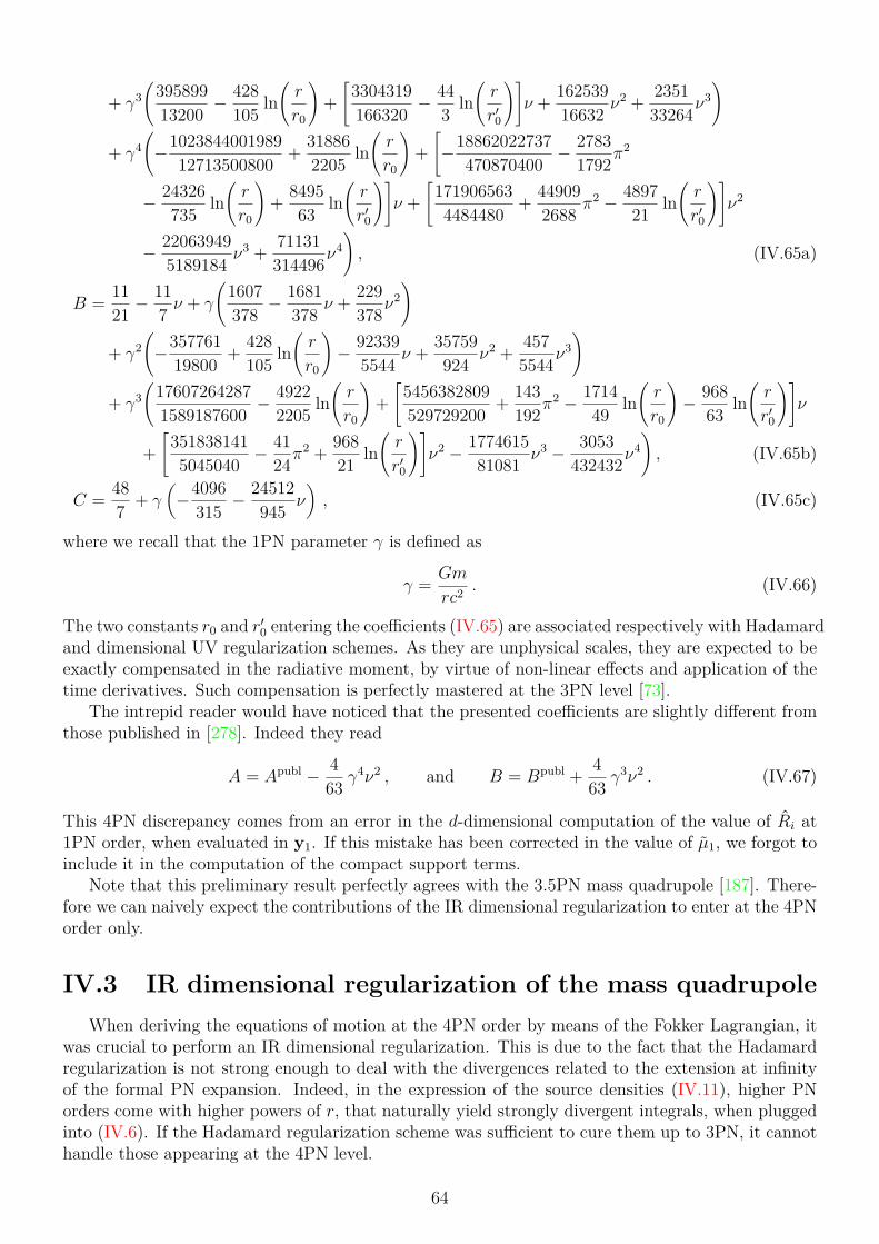
+ γ3(

39589913200 − 428

105 ln(r

r0

)+[

3304319166320 − 44

3 ln(r

r′0

)]ν + 162539

16632 ν2 + 2351

33264ν3)

+ γ4(

−102384400198912713500800 + 31886

2205 ln(r

r0

)+[−18862022737

470870400 − 27831792π

2

− 24326735 ln

(r

r0

)+ 8495

63 ln(r

r′0

)]ν +

[1719065634484480 + 44909

2688 π2 − 4897

21 ln(r

r′0

)]ν2

− 220639495189184 ν

3 + 71131314496ν

4), (IV.65a)

B = 1121 − 11

7 ν + γ

(1607378 − 1681

378 ν + 229378ν

2)

+ γ2(

−35776119800 + 428

105 ln(r

r0

)− 92339

5544 ν + 35759924 ν2 + 457

5544ν3)

+ γ3(

176072642871589187600 − 4922

2205 ln(r

r0

)+[

5456382809529729200 + 143

192π2 − 1714

49 ln(r

r0

)− 968

63 ln(r

r′0

)]ν

+[

3518381415045040 − 41

24π2 + 968

21 ln(r

r′0

)]ν2 − 1774615

81081 ν3 − 3053432432ν

4), (IV.65b)

C = 487 + γ

(−4096

315 − 24512945 ν

), (IV.65c)

where we recall that the 1PN parameter γ is defined as

γ = Gm

rc2 . (IV.66)

The two constants r0 and r′0 entering the coefficients (IV.65) are associated respectively with Hadamardand dimensional UV regularization schemes. As they are unphysical scales, they are expected to beexactly compensated in the radiative moment, by virtue of non-linear effects and application of thetime derivatives. Such compensation is perfectly mastered at the 3PN level [73].

The intrepid reader would have noticed that the presented coefficients are slightly different fromthose published in [278]. Indeed they read

A = Apubl − 463 γ

4ν2 , and B = Bpubl + 463 γ

3ν2 . (IV.67)

This 4PN discrepancy comes from an error in the d-dimensional computation of the value of Ri at1PN order, when evaluated in y1. If this mistake has been corrected in the value of µ1, we forgot toinclude it in the computation of the compact support terms.

Note that this preliminary result perfectly agrees with the 3.5PN mass quadrupole [187]. There-fore we can naively expect the contributions of the IR dimensional regularization to enter at the 4PNorder only.

IV.3 IR dimensional regularization of the mass quadrupoleWhen deriving the equations of motion at the 4PN order by means of the Fokker Lagrangian, it

was crucial to perform an IR dimensional regularization. This is due to the fact that the Hadamardregularization is not strong enough to deal with the divergences related to the extension at infinityof the formal PN expansion. Indeed, in the expression of the source densities (IV.11), higher PNorders come with higher powers of r, that naturally yield strongly divergent integrals, when pluggedinto (IV.6). If the Hadamard regularization scheme was sufficient to cure them up to 3PN, it cannothandle those appearing at the 4PN level.

64

In order to be consistent, and to use the accurate coordinate system, an IR dimensional regular-ization of the source quadrupole is thus required. In practice, we will only compute the differencesbetween the dimensionally regularized IDR

ij and Hadamard regularized IHadij source quadrupoles, and

add it to our previous result for IHadij . This difference of regularization schemes can be decomposed

in five different contributions

DIij ≡ IDRij − IHad

ij = DIVolij + DIComp

ij + DISurfij + Iextra

ij + δχIij , (IV.68)

where DIVolij , DIComp

ij and DISurfij are the differences in the volume, compact support8 and surface

terms, respectively. Iextraij denotes the value of the last piece of eq. (IV.6) (indeed the previous

argument relying on the (d − 3)B factor to discard such contribution does not apply anymore).Finally, δχIij is the contribution of the IR shift χi that has been applied in the equations of motion.

As the Hadamard regularization scheme is crucial to the matching procedure, we do not use apure dimensional regularization scheme, but rather a “mixed” Hadamard-dimensional regularizationscheme. We defined thus the “dimensional regularization” of the integral

∫ddxA(x, t) to be

DR[∫

ddxA(x, t)]

≡ limd→3

PFη

[∫ddx

(r

r0

)ηA(x, t)

], (IV.69)

where r0 is the same IR scale as in the three-dimensional Hadamard regularization, but we havechanged the name of the regulator from B to η to emphasize that the procedure in now taking placein d dimensions. The difference between the two regularization schemes is thus formally given by thecommutator of the finite part and d → 3 limit as

D∫

ddxA(x, t)

≡[limd→3

,PFη

] (∫ddxA(x, t)

)= lim

d→3

PFη

[∫ddx

(r

r0

)ηA(x, t)

]− PF

η

[limd→3

∫ddx

(r

r0

)ηA(x, t)

].

(IV.70)

IV.3.1 Computation of the different contributionsRegularization of the volume terms

Let us consider a volume term of the type

V =∫ ddx

ℓε0

(r

r0

)ηF (x, t) . (IV.71)

The function F (x, t) is a product of (super)-potentials and xL, and we will drop the time dependenceas it will play no role. As we investigate IR regularization schemes, we can restrict the integral tor > R, where R is an arbitrary constant scale, significantly larger than r1 and r2. We will thusexpand F (x) in multipolar series

F (x) =∑p≥p0

q1∑q=q0

ℓqε0rp+qε φp,q(n) =

∑p≥p0

q1∑q=q0

ℓqε0rp+qε

[φp,q(n)ε

+ φ(ε)p,q(n)

], (IV.72)

where p0, q0 and q1 are (possibly negative) integers and we will drop the angular dependencies forconvenience. We have allowed the function F to bear a simple pole 1/ε (as we have checked that nodouble poles appear in volume terms), and thus φp,q does not depend on ε. All higher order in ε arethus contained in φ(ε)

p,q. The three-dimensional limit of F is given by

F 3D(x) =∑p≥p0

r−p[φ3Dp + φlog

p ln(r

ℓ0

)], (IV.73)

8Note that, due to the Dirac distribution they involve, we include the contributions of distributional derivatives inthe class of compact support terms.

65

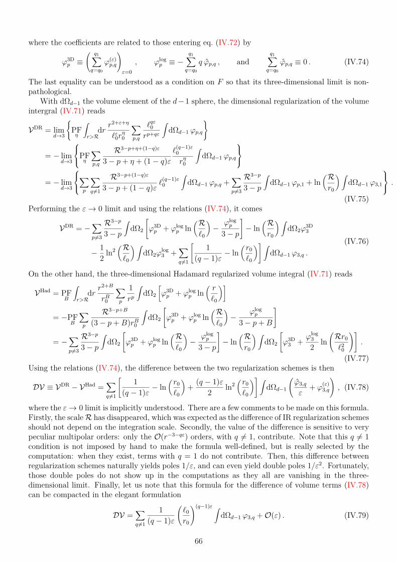
where the coefficients are related to those entering eq. (IV.72) by

φ3Dp ≡

( q1∑q=q0

φ(ε)p,q

)ε=0

, φlogp ≡ −

q1∑q=q0

q φp,q , andq1∑q=q0

φp,q ≡ 0 . (IV.74)

The last equality can be understood as a condition on F so that its three-dimensional limit is non-pathological.

With dΩd−1 the volume element of the d− 1 sphere, the dimensional regularization of the volumeintergral (IV.71) reads

VDR = limd→3

PFη

∫r>R

dr r2+ε+η

ℓε0rη0

∑p,q

ℓqε0rp+qε

∫dΩd−1 φp,q

= − limd→3

PFη

∑p,q

R3−p+η+(1−q)ε

3 − p+ η + (1 − q)εℓ

(q−1)ε0rη0

∫dΩd−1 φp,q

= − lim

d→3

∑p

∑q =1

R3−p+(1−q)ε

3 − p+ (1 − q)ε ℓ(q−1)ε0

∫dΩd−1 φp,q +

∑p =3

R3−p

3 − p

∫dΩd−1 φp,1 + ln

(Rr0

) ∫dΩd−1 φ3,1

.

(IV.75)Performing the ε → 0 limit and using the relations (IV.74), it comes

VDR = −∑p=3

R3−p

3 − p

∫dΩ2

[φ3Dp + φlog

p ln(Rℓ0

)−

φlogp

3 − p

]− ln

(Rr0

) ∫dΩ2φ

3D3

− 12 ln2

(Rℓ0

) ∫dΩ2φ

log3 +

∑q =1

[1

(q − 1)ε − ln(r0

ℓ0

)] ∫dΩd−1 φ3,q .

(IV.76)

On the other hand, the three-dimensional Hadamard regularized volume integral (IV.71) reads

VHad = PFB

∫r>R

dr r2+B

rB0

∑p

1rp

∫dΩ2

[φ3Dp + φlog

p ln(r

ℓ0

)]

= −PFB

∑p

R3−p+B

(3 − p+B)rB0

∫dΩ2

[φ3Dp + φlog

p ln(Rℓ0

)−

φlogp

3 − p+B

]

= −∑p =3

R3−p

3 − p

∫dΩ2

[φ3Dp + φlog

p ln(Rℓ0

)−

φlogp

3 − p

]− ln

(Rr0

) ∫dΩ2

[φ3D

3 + φlog32 ln

(Rr0

ℓ20

)].

(IV.77)Using the relations (IV.74), the difference between the two regularization schemes is then

DV ≡ VDR − VHad =∑q =1

[1

(q − 1)ε − ln(r0

ℓ0

)+ (q − 1)ε

2 ln2(r0

ℓ0

)] ∫dΩd−1

(φ3,q

ε+ φ

(ε)3,q

), (IV.78)

where the ε → 0 limit is implicitly understood. There are a few comments to be made on this formula.Firstly, the scale R has disappeared, which was expected as the difference of IR regularization schemesshould not depend on the integration scale. Secondly, the value of the difference is sensitive to verypeculiar multipolar orders: only the O(r−3−qε) orders, with q = 1, contribute. Note that this q = 1condition is not imposed by hand to make the formula well-defined, but is really selected by thecomputation: when they exist, terms with q = 1 do not contribute. Then, this difference betweenregularization schemes naturally yields poles 1/ε, and can even yield double poles 1/ε2. Fortunately,those double poles do not show up in the computations as they all are vanishing in the three-dimensional limit. Finally, let us note that this formula for the difference of volume terms (IV.78)can be compacted in the elegant formulation

DV =∑q =1

1(q − 1)ε

(ℓ0

r0

)(q−1)ε ∫dΩd−1 φ3,q + O(ε) . (IV.79)

66

Regularization of the compact support terms

An interesting and non-trivial feature of the IR dimensional regularization scheme is that it affectsthe evaluation of the potentials in the location of the particles. This feature is due to the fact thatmost of the potentials have a non-compact source: the non-linear terms extend towards infinity andthus the value of the potential in say y1 is sensitive to the IR regularization process. Naturally thiseffect does not affect the linear potentials, whose sources are proportional to Dirac distributions,and thus sensitive to UV regularization processes only. The IR regularization scheme could thereforeaffect the compact support terms, the contributions of distributional derivatives and the values ofµ1 (IV.13) and µ1 (IV.16), that all involve some potentials evaluated in y1 or y2.

Let us consider a potential P with d-dimensional source S. As in the previous section, weare interested in the IR behaviour of S and hence we will expand it in a multipolar manner. Inpractice, none of the sources we are interested in develop poles (or equivalently, logarithms in threedimensions), so we can safely take

S(x) =∑p≥p0

q1∑q=q0

ℓqε0rp+qε φp,q(n) , (IV.80)

where φp,q has no pole, and we will drop the angular dependencies. The source has a (non-pathological) three-dimensional limit

S3D(x) =∑p≥p0

φ3Dp

rp, with φ3D

p ≡( q1∑q=q0

φp,q

)ε=0

. (IV.81)

Let us first deal with the Newtonian case, ie. compute the difference induced by the change ofIR regularization scheme in the Poisson integral (IV.23) evaluated in y1

PNewt1 =

(∆−1S

)(y1) ≡ PF

η

[− k

4π

∫r′>R

ddx′(r′

r0

)ηS (x′)

|y1 − x′|d−2

], (IV.82)

where we have safely replaced x by y1 in the kernel, as we integrate for r′ > R > r1, and thus arefree from UV divergences. Taylor-expanding the kernel

1|y1 − x′|d−2 =

∑ℓ∈N

2ℓℓ!

Γ(d−2

2 + ℓ)

Γ(d−2

2

) yL1 nLrd−2+ℓ , (IV.83)

the Poisson integral becomes

PNewt1 = PF

η

k4π

∑p,q,ℓ

2ℓℓ!

Γ(d−2

2 + ℓ)

Γ(d−2

2

) R2−p−ℓ+η−qε

2 − p− ℓ+ η − qε

ℓqε0rη0yL1

∫dΩd−1nLφp,q

. (IV.84)

Using the machinery developed for the treatment of volume terms, the difference between bothregularizations turns out to be

DPNewt1 = −

∑ℓ∈N

(2ℓ− 1)!!4πℓ! yL1

∑q =0

[1qε

− ln(r0

ℓ0

)− ln (4πeγE )

2q + 1q

ℓ∑k=1

12k − 1

] ∫dΩd−1nL φ2−ℓ,q ,

(IV.85)where γE is the Euler constant, and naturally DPNewt

2 is obtained under the replacement yL1 → yL2 .Once again, the q = 0 criterion is not an artificial requirement to ensure that the formula is well-defined, but it comes naturally out of the derivation. The main difference with the formula for thevolume terms (IV.79) is the sum over ℓ. Nevertheless, this sum is finite by virtue of the structure ofthe source (IV.80): ℓ is bounded by 2 − p0.

67

But if the potentials T , Yi or Mij enter at Newtonian order in the source quadrupole, all theother potentials enter at higher orders. For those, the accurate propagator is the one in d dimen-sions (IV.125), that will be investigated in great details in sec. IV.4. For our purpose, we can restrictourselves to an integration region r′ > R > r1 and thus safely replace x by y1, so that

P1 =(−1

R S)

(y1) ≡ PFη

[− k

4π

∫r′>R

ddx′|y1 − x′|d−2

(r′

r0

)η ∫ +∞

1dz γ 1−d

2(z)S

(x′, t− z

|y1 − x′|c

)],

(IV.86)where the time-dependence of the source is now crucial, and the z-integration translates the fact thatthis propagator is not localized on the light cone, and involves the kernel

γ 1−d2

(z) ≡ 2√π

Γ(− ε

2

)Γ(

1+ε2

) (z2 − 1)−1− ε

2 . (IV.87)

PN-expanding this propagator in the same fashion than what is presented in sec. IV.4.2, it comes

P1 =(∆−1Seven

)(y1) +

(∆−1Sodd

)(y1) , (IV.88)

where(∆−1A

)(y1) is the Poisson integral (IV.82) and the PN expansion of the source term reads

Seven =∑j∈N

√π

(2j)!Γ(

1+ε2 − j

)Γ(

1+ε2

)Γ(

12 − j

) (r1

c

)2jS(2j)(x, t) , (IV.89a)

Sodd =∑j∈N

(−)jj!

2√π Γ (ε)

Γ(

1+ε2

)Γ(−j − ε

2

)Γ (2j + 2 + ε)

(r1

c

)1+2j+ε ∫ +∞

0dτ τ−εS(2j+2)(x, t− τ) .

(IV.89b)

As expected, the j = 0 term of Seven is exactly given by S. Note that the odd piece, which we willnot consider, appears to be non-local.

Hence for potentials entering at post-Newtonian orders, we can simply apply the Newtonianformula (IV.85), but using the even PN-expanded source (IV.89a), truncated at the accurate order.It turns out that all the non-vanishing corrections are strongly connected. Indeed they obey therelations (naturally valid up to the O(ε0) order only, as the O(ε) corrections do not play any role inthe IR dimensional regularization of the compact support terms)

DW 2PN1 = 4

c2 DZ1PN1 = −2ε

c2 DX1PN1 = 8

3c4 DTNewt1 = −16ε

3c4 DMNewt1 . (IV.90)

Note that only the trace of the Newtonian Mij and the 1PN X develop poles. Note also that onlythe “scalar” sector of the potentials is affected: neither Ri nor Yi receive corrections, and regardingthe tensor potentials Zij and Mij, only their traces are impacted. In addition to those nice relations,the difference itself can be compactly written in terms of the moment of inertia I ≡ m1y

21 +m2y

22, as

DM0PN1 =

(38 − ε

)c2 DX1PN

1 = −G2(m1 +m2)8

[1ε

− 1 − 2 ln(r0

√q

ℓ0

)]I(4) , (IV.91)

where we have defined q ≡ 4πeγE .The regularization induced differences (IV.90) yield corrections in the µ1 and in a few compact

terms, that all enter at 4PN in the source quadrupole, but not in the contributions of the distributionalderivatives.

68

Regularization of the surface terms

Turning now to the surface terms, we will not compute the difference between the two regu-larization schemes, but rather directly compute them in d dimensions and show that they vanish.Therefore their contributions to the difference in regularization schemes will simply be given by

DISurfij = −ISurf,Had

ij . (IV.92)

Considering a surface term of the divergence type

D = PFη

∫ ddxℓε0

(r

r0

)η∂iAi , (IV.93)

we naturally perform the multipolar expansion

Ai(x, t) =∑p≥p0

q1∑q=q0

ℓqε0rp+qε α

ip,q(n, t) , (IV.94)

where the αip,q can develop poles, and we drop the time and angular dependencies. Integrating (IV.93)by parts and dropping the surface integrals that are vanishing by analytic continuation in η, we have

D = PFη

∑p,q

η

2 − p+ η + (1 − q)εR2−p+η+(1−q)ε

rη0 ℓ(1−q)ε0

∫dΩd−1niα

ip,q =

∫dΩd−1ni α

i2,1 . (IV.95)

Similarly, let us consider a surface term of the Laplacian type

LL = PFη

∫ ddxℓε0

(r

r0

)ηxL ∆B . (IV.96)

Once again, we perform the multipolar expansion

B(x, t) =∑p≥p0

q1∑q=q0

ℓqε0rp+qε β

ip,q(n, t) , (IV.97)

allowing the βp,q to develop poles. Integrating (IV.96) by parts and dropping the surface integralsthat are vanishing by analytic continuation in η, we have

LL = −PFη

∑p,q

η(η + 2ℓ+ 1 + ε)ℓ+ 1 − p+ η + (1 − q)ε

Rℓ+1−p+η+(1−q)ε

rη0 ℓ(1−q)ε0

∫dΩd−1nL βp,q

= − (2ℓ+ 1 + ε)∫

dΩd−1nL βℓ+1,1 .

(IV.98)

So the values of the d-dimensional surface terms are extremely simple and only involve termswith q = 1. But all of them have q ≥ 2. Indeed, as can be intuited from their three-dimensionalexpressions (C.7) and (C.8) and confirmed by their d-dimensional expressions displayed in app. Cof [278], all surface terms are products of potentials, superpotentials and their derivatives. It is easyto understand from the Green function (IV.24) that compact support potentials have q = 1. Asnon-compact support potentials are made of products of compact support ones, and as the iterationof Poisson integral does not produces q < 1,9 all potentials have q ≥ 1. A similar argument appliesto the case of superpotentials, and thus the surface terms, composed of products of potentials,superpotentials and their derivatives, cannot contributes to the d-dimensional source quadrupole.

9This can be understood from the Matthieu formula (IV.110), the homogeneous solution to add bearing q = 1, asexplicit by (IV.108).

69

Contribution of the extra term

The argument developed in sec. IV.2.1 to discard the contribution of the extra piece of Iij isobsolete in d-dimensional IR regularization: we have to compute it. Nevertheless, the argumentpreventing contributions for r < R still holds, and thus we can restrict ourselves to an integrationzone r > R, and recast

Iextraij = − 2

c2 PFη

∑k∈N

γ(d)k

(1c

ddt

)2k ∫r>R

ddxℓε0

(r

r0

)ηηr2k xaijxb

r2 Σab , (IV.99)

where we have shortened

γ(d)k ≡ 1

2k k!Γ(d2 + 3

)Γ(d2 + 3 + k

) (d− 3)(d+ 2)d(d− 2)(d+ 4) . (IV.100)

As usual now, we expand the source density Σab as

Σab(x, t) =∑p≥p0

q1∑q=q0

ℓqε0rp+qε σ

abp,q(n, t) , (IV.101)

where the σabp,q contain many orders in c and can develop poles. We will drop the angular and timedependencies, and perform the integration

Iextraij = 2

c2 PFη

∑k,p,q

γ(d)k

(1c

ddt

)2kη R5+2k−p+η+(1−q)ε

5 + 2k − p+ η + (1 − q)εℓ

(q−1)ε0rη0

∫dΩd−1 naijnb σ

abp,q

= 2c2

∑k

γ(d)k

(1c

ddt

)2k [∫dΩd−1 naijnb σ

ab5+2k,1

],

(IV.102)

where the fact that the γ(d)k do not depend on η was crucial. Exactly as in the case of the surface

terms, we see that the finite part procedure selects only the terms with q = 1. But, recalling thatΣij = τij and the definition of the Landau-Lifschitz pseudo tensor (B.5), one can see that the σabp,qare made of two pieces. The first one, coming from the stress-energy tensor T µν , involves Diracdistributions and thus does not enter our computation as we are restricted to r > R. The secondentails the non-linear source term Λµν and thus is composed of products of potentials. As alreadydiscussed, it can not involve q = 1 terms. Therefore, we can conclude that, even in the IR dimensionalregularization scheme, the extra piece does not contribute

Iextraij = 0 . (IV.103)

Contribution of the IR shift

The IR shift χi1,2 used to compensate the remaining poles in the equations of motion [56] is givenin app. C.4.2.10 It starts at the 4PN order, and thus its contribution to the source quadrupole issimply given by

δχIij = 2m1 y⟨i1 χ

j⟩1 + 2m2 y

⟨i2 χ

j⟩2 . (IV.104)

10We thank L. Bernard for providing us the file containing this shift.

70

IV.3.2 Computation of the required potentials in d dimensionsJust as in the case of the three-dimensional Hadamard regularized surface terms, the differ-

ence between Hadamard and dimensional regularizations only involves specific multipolar orders, seeeqs. (IV.79) and (IV.85). Therefore the asymptotic expansions of the d-dimensional potentials arerequired.

The linear potentials V , Vi and K and the superpotentials are known in the whole d-dimensionalspace, thus one has just to expand them in r → ∞.

But the volume terms and the source of the potential involved in compact support terms alsoinclude the quadratic potentials Wij at 1PN, Ri and Zij at Newtonian order, and the cubic potentialX at Newtonian order. If the compact support parts of their sources (and contributions of thedistributional derivatives in the X) can be treated easily,11 none of those potentials are known in alld-dimensional space. We thus have to compute their asymptotic behaviors by iterating the propagatorat infinity, and we will construct such multipolar expansions by adding the accurate homogeneoussolution to a particular one. For a potential P with source S, the generalization of the matchingprocedure (IV.56) in the case of a d-dimensional potential reads [56]

M(P ) = −1R M(S) − 1

4π∑ℓ∈N

(−)ℓℓ! ∂LSL⋆ , (IV.105)

where we will trade −1R for the d-dimensional symmetric propagator, as we are only interested in

even orders. The homogeneous solution is constructed out of the PN expansion of

SL⋆ (t, r) ≡ k

rd−2

∫ +∞

1dz γ 1−d

2(z)

[SL(t− zr

c

)+ SL

(t+ zr

c

)], (IV.106)

withSL(u) ≡ PF

η

∫ddx

(r

r0

)ηxL S(x, u) , (IV.107)

and the γ 1−d2

kernel is defined by eq. (IV.87). Note that SL(u) is the PN-even d-dimensional gen-eralization of eq. (IV.57), but with the main difference of the presence of the z integration, due tothe fact that the propagator does not lie anymore on the light-cone. Performing explicitly the PNexpansion, eq. (IV.105) becomes

M(P ) =∑k∈N

(1c

∂

∂t

)2k

∆−k−1M(S) − 14π d−1

2

∑k,ℓ

(−)ℓℓ!(2k)!

Γ(d2 − 1 − k

)Γ(

12 − k

) 1c2k S(2k)

L (t) ∂Lr2k−1−ε .

(IV.108)

Computing the particular solutions

There is no particular issues with the multipolar development of the sources,12 so computing theparticular solutions

M(P )part ≡∑k∈N

(1c

∂

∂t

)2k

∆−k−1M(S) =∑k∈N

(1c

∂

∂t

)2k

PFη

[∆−k−1

(r

r0

)ηM(S)

], (IV.109)

is easily done by means of iterations of the d-dimensional Matthieu formula [87]

∆−1[rα+η nL

]= rα+2+η nL

(α + d+ η + ℓ)(α + 2 + η − ℓ) . (IV.110)11To the only difficult point that we need to know the value of the Newtonian W evaluated at y1, required to

compute X, see eq. (IV.55).12The source of the X potential involves Wij , which has thus to be computed and matched before deriving X.

71

Homogeneous solutions for the quadratic potentials

Computing the homogeneous solutions is more involving. Indeed, it relies on the source integralSL(u) (IV.107), and thus on the integration of the source in the whole space. For the quadraticpotentials Wij, Ri and Zij, the source is a product of (derivatives) of the linear potentials and thusknown in all space. Therefore, in full generality, we need to integrate products like∫

ddx xLrα1 rβ2 r

γ12 n

K1 n

P2 n

Q12 . (IV.111)

First, by substituting xi = yi1 + r1ni1 and ni2 = (r12n

i12 + r1n

i1)/r2 (cf. fig. A.1), and noticing that

neither yi1, r12 nor ni12 depend on x, we only need to compute integrals such as∫ddx rα1 r

β2 n

L1 . (IV.112)

There are two approaches to compute such integrals. The first one is to express rα1nL1 in terms ofderivatives with respect to yi1, for instance

rα1ni1 = − 1

α + 1 ∂1 i rα+11 , or rα1n

ij1 = 1

α(α + 2) ∂1 ij rα+21 − rα1

αδij . (IV.113)

Those derivatives can be brought outside of the integral and it only remains to use the d-dimensionalRiesz formula [87, 315]

∫ddx rα1 r

β2 = πd/2 Γ

(α+d

2

)Γ(β+d

2

)Γ(−α+β+d

2

)Γ(−α2

)Γ(−β

2

)Γ(α+β+2d

2

) rα+β+d12 . (IV.114)

If this procedure is very convenient for small values of ℓ, it becomes extremely cumbersome when ℓ islarger than 3, as practically implementing the generalizations of eq. (IV.113) is then quite laborious.In addition, this method yields spurious divergences, eg. for α = −d, that have to be dealt with by theintroduction of a new regulator. Therefore, we would like to directly compute integrals as (IV.112),with a “generalized Riesz” procedure. Such computation has been performed by using a methodexposed in app. A.6 of [220], which relies on a projection of n1 onto n12, given by

ni1 = r22 − r2

1 − r212

2r1r12ni12 + ni⊥ , (IV.115)

where ni⊥ is the component of n1 orthogonal to n12. The interest of such projection is that, by usingprolate spheroidal coordinates, one can single the integration of products of ni⊥ out from the totalintegration. As the averages of products of ni⊥ are directly expressed in terms of r1, r2, r12, n12and δij, the complicated integral (IV.112) reduces to a sum of Riesz ones (IV.114), and thus can becomputed. By means of this technique, we were able to match all the required quadratic potentials.13

Homogeneous solution of the X cubic potential

The non-linear part of the source of the cubic X potential (C.4a) can be decomposed intoquadratic and cubic sectors as

X(NL) = Sq + Sc , (IV.116)with

Sq = 2Vi ∂t∂iV + 12

(d− 1d− 2

)V ∂2

t V + d(d− 1)4(d− 2)2 (∂tV )2 − 2∂iVj ∂jVi (IV.117a)

13G. Faye provided an explicit formula to express integrals such as (IV.111). Unfortunately, it was after the practicalcomputations were achieved, so we have not used it.

72

Sc = Wij ∂ijV . (IV.117b)

The integration of the quadratic part is naturally performed by using the “generalized Riesz”procedure described previously. The major difficulty comes from the cubic part, as it involves thepotential Wij in all space in d dimensions. As we need it only at Newtonian level, we could relyon a d-dimensional generalization of the Fock function (IV.43a). The latter has been derived, butonly in an integral form [87], which is of little practical use. Instead, we will employ the method ofsuperpotentials in order to replace Wij by the expression of its source. As superpotentials are definedin a STF guise, cf. eq. (IV.20), we will compute

ScL ≡ PF

η

∫ddx

(r

r0

)ηxL Wij∂ijV , (IV.118)

instead of eq. (IV.107), and un-STFize it at the end of the computation (as it is clear that eq. (IV.107)is symmetrical under its ℓ indices, this simply accounts to putting the traces back). Two integrationsby parts and the use of eq. (C.3a) give

ScL = −4πGPF

η

∫ddx

(r

r0

)η (σij − δij σkk

d− 2

)Ψ∂ijVL − 1

2d− 1d− 2 PF

η

∫ddx

(r

r0

)ηΨ∂ijVL ∂iV ∂jV , (IV.119)

where we have introduced the superpotentials Ψ∂ijVL obeying

∆Ψ∂ijVL = xL ∂ijV . (IV.120)

We have discarded the surface terms coming from the integration by parts, as they bear q > 1 andthus are vanishing. The first integral of (IV.119) has a compact support and is straightforwardlycomputed as we know the value of Ψ∂ijV

L in y1. The second integral can be evaluated by means ofthe “generalized Riesz” procedure, and thus the matching of the X is doable, and has been done.

Consistency checks performed on the potentials

With all those techniques, we can compute and match all the required potentials, and extracttheir asymptotic behaviors. Nevertheless, these computations are heavy14 and some verificationsare thus required. The first and most stringent one is that those computations were performed ina “double-blind” fashion, together with Q. Henry. In addition to that, we investigated the three-dimensional limits of our potentials, and confirmed that they agree with the matched asymptoticexpressions that were used to compute the three-dimensional surface terms. We have also verifiedthat the harmonicity relations ∂µhµν = 0 hold, up to 1PN and to the achievable order in 1/r. At1PN order, those conditions read [278]

∂µhµ0 = d− 1

2(d− 2)∂tV + ∂iVi

+ 1c2

[∂t

(−(d− 1)(d− 3)

(d− 2)2 K + W

2 + (d− 1)2

2(d− 2)2 V2)

+ ∂i

(2Ri + d− 1

d− 2 V Vi)]

, (IV.121a)

∂µhµi =∂tVi + ∂j

(Wij − W

2 δij

)+ 1c2

[∂t

(2Ri + d− 1

d− 2 V Vi)

+ 4 ∂j(Zij − Z

2 δij

)]. (IV.121b)

The cancellation of ∂µhµ0 has been checked exactly at Newtonian order, and up to O(r−6) at 1PNorder. The fact that ∂µhµi vanishes, up to O(r−7) at Newtonian order, and up to O(r−5) at 1PNorder.

14For instance, it took more than 160 CPU hours to match the 1PN Wij up to O(r−4). At this order, it has morethan 10 000 terms, of which ∼ 8 000 come from the homogeneous part.

73

IV.3.3 The IR regularized mass quadrupoleOnce the asymptotic expansions of the potentials are derived, the computation of the difference

of regularization schemes for volume and compact support terms can be implemented by means ofeqs. (IV.79) and (IV.85). This has been done in a “double-blind” fashion, together with Q. Henry.Adding the contribution of the IR shift (IV.104) and removing the Hadamard regularized surfaceterms, the difference of regularization schemes for the source quadrupole reads

DIij = DIVolij + DIComp

ij − ISurf,Hadij + δχIij

= −βIG2M2Q

(2)ij

2c6

[1ε

− 2 ln(r0

√q

ℓ0

)− 246 299

22 470

]+ βI

G2MP⟨iPj⟩c6

[1ε

− 2 ln(r0

√q

ℓ0

)− 252 599

22 470

]

+ 1c8

[1ε

DI4PN,pij + DI4PN

ij

],

(IV.122)where Qij = m1y

ij1 + m2y

ij2 is the Newtonian mass quadrupole, Pi = m1v

i1 + m2v

i2 is the Newtonian

linear momentum (that vanishes in the center-of-mass) and βI = −214105 is the coefficient associated

with the logarithmic renormalization of the mass quadrupole moment [209].Recalling that the Hadamard regularized mass quadrupole (IV.64) agrees with previous results

at the 3PN accuracy [187], this 3PN contribution due to dimensional regularization indicates thatthere is an effect that we have not taken into account. Note that this 3PN pole cannot result froma failure of the application of the IR shift, as χi is a 4PN quantity, and thus cannot generate norremove poles entering at 3PN.

The number associated with this 3PN pole, βI , indicates that the missing effect is given by thetail-of-tails. Indeed those enter at 3PN, and it is known by EFT methods that they bear a UVpole that should cancel the IR pole appearing in the mass quadrupole [209]. Therefore the physicalquantity to regularize is the radiative moment Uij rather than the source one Iij. In addition, itmeans that the IR shift χi should remove the remaining poles in Uij and not in Iij.

IV.4 Dimensional regularization of the radiative quadrupoleIn order to check if our computation of the source quadrupole Iij is correct, and notably if the

crucial IR shift compensates accurately the remaining poles, we should thus compute and regularizethe radiative quadrupole Uij. This dimensional regularization of the radiative quadrupole is currently,and for the first time, under investigation.

IV.4.1 Dimensional regularization of the non-linear interactionsWe first focus on the transition between the canonical and radiative moments. Most of the

pieces required to perform this transition are already known in three dimensions. For instance, theiterated tail contributions have been computed up to 4.5PN order [276]. Therefore, we do not intendto perform a full computation in d dimensions, but rather only to derive and apply formulas thatgive the difference between Hadamard and dimensional regularizations, leaving the computation ofthe three-dimensional missing pieces for future works. Let us also note that we only need to iteratetwice the propagator, as the dominant contribution of the third iteration, the tail-of-tail-of-tail effect,enters at 4.5PN order when we aim to 4PN accuracy. Therefore we only seek for cubic interactions.

Last but not least, the effect to be compensated is local, as clear from eq. (IV.122), whereasthe non-linear interactions reveal non-local features by nature. Fortunately, and as explicitly shownhereafter, those non-local effects will play no role in the change of regularization scheme. From anEFT point of view, this can be related to the relation displayed in fig. III.2: we seek for the local polethat is associated to the non-local piece of the tails (represented by the logarithmic dependence).

74

The computation of the dimensional regularization of those non-linear interactions, and the dif-ference with the usual Hadamard regularized ones, is one of the main achievements of this thesis.The detailed derivation is thus presented in app. D, we only sketch it rapidly hereafter.

Dimensional regularization of the post-Minkowskian metric

The aim is to study the d-dimensional solution of the vacuum Einstein equationshµν = Λµν(x, t) . (IV.123)

As they will play no role, we will henceforth drop space-time indices, and focus on multipolar ones.Therefore our object of study is the wave equation

hL = NL(x, t) , (IV.124)where NL is some source function that will be specified later on. The accurate prescription for thed-dimensional propagator is

hL(x, t) = −k4π

∫ddx′

(r′

r0

)η ∫ +∞

1dzγ 1−d

2(z) NL (x′, t− z|x′ − x|/)

|x′ − x|d−2 , (IV.125)

where the kernel of the z-integration is given by the function

γ 1−d2 −ℓ

(z) = 2√π

Γ(d−2

2 + ℓ)

Γ(

3−d2 − ℓ

) (z2 − 1) 1−d

2 −ℓ , (IV.126)

which is properly normalized for any ℓ ∈ C by analytic continuation as∫ +∞

1dz γ 1−d

2 −ℓ(z) = 1 . (IV.127)

The presence of this kernel accounts for the fact that the propagator is not localized on the lightcone. In fact such a localization only happens in even-dimensional space-times, as can be seen bythe distributional limit of γ 1−d

2 −ℓ(z), see app. C of [56],

γ−1−ℓ(z) =ℓ∑

k=0

2k−ℓ(2ℓ− 1)!!

(2ℓ− k)!(ℓ− k)! δ

(k)(z − 1) , for ℓ ∈ N , (IV.128)

where δ(k) is the kth derivative of the Dirac distribution. Note also the similarities between this kernelγ 1−d

2and the δ(ε)

ℓ functions entering the source terms (IV.10).As we will see in the next section, the source can be recast as

NL(x, t) =∑p≥p0

q1∑q=q0

ℓqε0rp+qε

[ψp,q(t)ε

+ ψp,q(t)]nL , (IV.129)

where the ψp,q coefficients do not depend on ε. As shown in app. D, the only contributions to thedifference of regularization schemes come from the terms with p− ℓ− 3 ∈ 2N and read

DhL = −4(−)ℓℓ! ∂L

k

rd−2

∫ ∞1

dz γ 1−d2

(z)DH(t− zr

c

), (IV.130)

with

DH(t) = −∑q =1

2ℓ−2

q − 1ℓ! (ℓ+ j)!

j! (p+ ℓ− 2)!

1ε

+ ln(ℓq−1

0√q

rq−10

)−

ℓ+j∑k=0

12k + 1

ψ(2j)p,q (t)c2j , (IV.131)

where we have denoted j ≡ (p − ℓ − 3)/2 ∈ N, and we recall our definition q = 4πeγE . Note thatthis contribution is local, as expected. Conversely, contributions coming from the pole terms ψp,qreveal non-local pieces, as displayed in eq. (D.35). Fortunately, none of the poles entering in thesources we deal with satisfies the condition p− ℓ− 3 ∈ 2N and as such, contributes to the differenceof regularization schemes. Therefore this effect is purely local.

75

From the corrections in the metric to the corrections in the moments

Once the contribution of the dimensional regularization scheme in the metric has been established,one should translate it into a contribution in the radiative quadrupole. This is to be done byidentifying it as a non-linear correction to the linear canonical moment, just as the canonical momentswere identified as non-linear completions of the source ones. In d dimensions, the mass canonicalmoments enter the linear metric as

k00(1) = − 4

c2

∑ℓ≥0

(−)ℓℓ! ∂L ML , k0i

(1) = 4c3

∑ℓ≥1

(−)ℓℓ! ∂L−1 M(1)

iL−1 , kij(1) = − 4c4

∑ℓ≥2

(−)ℓℓ! ∂L−2 M(2)

ijL−2 ,

(IV.132)where we have defined the “tilded” versions of the moments as

ML ≡ k

rd−2

∫ ∞1

dzγ 1−d2

(z) ML

(t− zr

c

), (IV.133)

which reduce to the usual moments in the d → 3 limit.The interest of writing the dimensional contribution under the form (IV.130) is now manifest: it

mimics the linearized metric (IV.132), and thus is directly formatted in the appropriate fashion tobe recognized as a non-linear completion of the source moments.

But before any recognition, one has first to remove the divergence, as DhL is divergenceful. Thisis done following a very similar procedure as the three-dimensional one, presented in app. B.2.3(by roughly replacing potentials by their “tilded” versions). Once the metric obeys the de Dondergauge condition, two techniques are possible to recognize the difference in regularization schemes ascorrections to the moments. The brute force one consists in recasting the metric into source andgauge moments, as in the d-dimensional generalization of eq. (B.18)

h00(1) = − 4

c2

∑ℓ≥0

(−)ℓℓ! ∂L

IL + W(1)L

c2 + X (2)L

c4 + YL

c2

,

h0i(1) = 4

c3

∑ℓ≥1

(−)ℓℓ!

∂L−1

I(1)iL−1 + Y(1)

iL−1c2

+ ∂iL

WL + X (1)L

c2

,

hij(1) = − 4c4

∑ℓ≥2

(−)ℓℓ!

∂L−2I(2)ijL−2 + 2∂ijLXL + 2∂L−1(iYj)L−1 + δij ∂L

W(1)L − X (2)

L

c2 − YL

,

(IV.134)where, for the sake of clarity, we have not included the current-type moments, nor the third typeof moments that appears in d-dimensional space-times (see [228]). Identifying the contribution thatbehaves as Iij yields the correction to the source quadrupole.

The second possible way to proceed is to compute the 0i0j components of the linearized Riemanntensor (A.3)

R0i0j = G

2

(∂ijh

00 + 2c∂t∂

(ihj)0 + 1c2 ∂

2t h

ij + ∂ijh

d− 1 − 1c2

δijd− 1 ∂

2t h

)+ O

(h2), (IV.135)

with h = ηµνhµν the four-dimensional trace of the metric perturbation. Indeed, those components are

gauge independent, ie. plugging the metric (IV.134) in eq. (IV.135), the gauge moments disappear

R0i0j = −2Gc2

∑ℓ≥0

(−)ℓℓ!

(d− 2d− 1 ∂ijLIL − 2

c2 ∂L−1(iI(2)j)L−1 + 1

c4 ∂L−2I(4)ijL−2 + 1

c2δijd− 1 ∂LI(2)

L

),

(IV.136)and one can more easily identify the contributions to the IL moments.

76

IV.4.2 Computation of the d-dimensional quadratic interactionsAs we have advertised, the 3PN and 4PN corrections are due to cubic interactions, or 3PM

corrections. Therefore one needs to known the 3PM source of (IV.123), ie. compute the d-dimensional2PM effect, or quadratic interactions. We will present hereafter the computation of the tail effectM × Mij, as it is the most representative quadratic interaction.

The source of the d-dimensional tails is given by the interplay of the ℓ = 0 and ℓ = 2 modes ofthe canonical metric (IV.132). As M = kMr2−d, we have to solve equations of the generic form

hL = NL(x, t) = nL

∫ ∞1

dz γ 1−d2

(z) zk ℓqε0rp+qε F

(t− zr

c

). (IV.137)

If we know the exact prescription to apply, namely the propagator (IV.125), we do not need to useit here. Instead, following [56],15 we can rely on a formal PN expansion as

hL = −1R NL − PF

η

∑p∈N

(−)pp!

∑j∈N

∆−jxP∫

ddx′(r′

r0

)η∂′P

N (2j)L (y, t− zr′/c)

r′d−2

y=x′

, (IV.138)

with

∆−jxL ≡Γ(d2 + ℓ

)Γ(d2 + ℓ+ j

) r2jxL22jj! . (IV.139)

As now usual, we can recognize a particular and a homogeneous solution, the latter being constructedso that the metric satisfies the matching condition (II.48).

The particular solution involves the PN expansion of the source NL. Introducing τ = zr/c andusing the asymptotic development of the γ 1−d

2kernel

γ 1−d2

(z) =z→∞

∑j∈N

(−)jj!

2√π z−2−2j−ε

Γ(−j − ε

2

)Γ(

1+ε2

) , (IV.140)

we can decompose NL into “even” and “odd” sectors, generalizing the results of [56] in the case of anon-vanishing k, as

N evenL =

∑j∈N

Akjr2j+βk−p−qε

c2j+βkF (2j+βk)(t) nL , (IV.141a)

NoddL =

∑j∈N

Bkj

r1+2j−k−p+(1−q)ε

c1+2j−k+ε

∫ ∞0

dτ−ε F (2j+2−k)(t− τ) nL , (IV.141b)

where βk = 0 if k is even and 1 if k is odd. The coefficients that enter those expressions are

Akj ≡ (−)j22j+βkj!

Γ(

12 − j − βk

)Γ(

1+ε2

) Γ(

1−βk−k+ε2 − j

)Γ(

1−βk−k2 − j

) , (IV.142a)

Bkj ≡ (−)k

22jj!2√π Γ (2 − k + ε)

Γ(

1+ε2

)Γ (1 − ε) Γ

(−ε2

) Γ(1 + j + ε

2

)Γ(1 + ε

2

) Γ(1 − k

2 + ε2

)Γ(1 + j − k

2 + ε2

) Γ(

3−k+ε2

)Γ(j + 3−k+ε

2

) . (IV.142b)

The expressions (IV.141), once integrated with the PN-expanded propagator, can (and will) yieldpoles. Fortunately, those poles disappear in the three-dimensional limit by giving logarithmic terms,and thus this limit is non-pathological. Moreover, such poles will not contribute to the difference inregularization schemes in the iterated cubic solution, as already advertised.

15Note that the following computations are generalizations of the results exposed in [56].

77

As for the homogeneous sector, ie. the second part of eq. (IV.138), once well massaged, it comes

hhomL = −1

d+ 2ℓ− 2Γ (qε− η)

Γ (p+ ℓ− 1 + qε− η) Ck,p,qℓ

∑j∈N

∆−jxL∫ ∞

0dττ η−qεF (2j+ℓ+p−1)(t− τ) , (IV.143)

with the coefficients

Ck,p,qℓ ≡

∫ ∞1

dy γ 1−d2 −ℓ

(y)∫ ∞

1dz γ 1−d

2(z) zk(y + z)ℓ−2+p+qε−η , (IV.144)

which are generalizations of the ones introduced in [56] for q = 2, and are derivable by similarmethods to those developed in the app. D of this work.16

Therefore we have access to the knowledge of the PN-expanded d-dimensional quadratic interac-tions (IV.138), which consist in series in powers of 1/r. As we know that only certain contributions(namely those satisfying p − ℓ − 3 ∈ 2N) will contribute to the cubic result (IV.130), we can thusrestrict our computations to the necessary orders only. Injecting those in the cubic source (IV.124),we see in addition that we were allowed to decompose it as in eq. (IV.129).

The only quadratic interaction that does not fall within the presented computation is the memoryMij × Mij that is needed for 4PN corrections. For this interaction, the source term (IV.137) has tobe generalized into

hL = NL(x, t) = nL

∫ ∞1

dy γ 1−d2

(y) ys∫ ∞

1dz γ 1−d

2(z) zk ℓqε0

rp+qε F(t− yr

c

)G(t− zr

c

). (IV.145)

In this case the PN expansions of the sources are naturally given by four terms: “even-even”, “even-odd”, etc. and the homogeneous solution keeps the same structure.

Note that in the case of the sought cubic interactions, performing such PN expansion insteadof the machinery developed in app. D would not have helped. Indeed, putting the result in thecrucial linear metric-looking form (IV.130) would have been definitively more involving. Moreoverwe would have had a potentially extremely large number of terms to study, coming from the iteratedPN-expanded propagator acting on NL.

IV.4.3 The 3PN dimensional corrections to the radiative quadrupoleA dimensional analysis indicates that the only possible interactions entering at 3PN in the ra-

diative quadrupole are the tail-of-tail M × M × Mij and tail-of-“linear memory” M × Mi × Mi. Thedifference between dimensional and Hadamard regularizations of those interactions were thus com-puted by using the machinery developed in this section.

The extraction of the correction to the mass quadrupole from the metric has been performed inboth direct recognition (IV.134) and through the gauge independent components of the linearizedRiemann tensor (IV.136), and they agreed to yield

δMij = βIG2M2M(2)

ij

2c6

[1ε

− 2 ln(r0

√q

ℓ0

)− 246 299

22 470

]−βI

G2MM(1)<iM

(1)j>

c6

[1ε

− 2 ln(r0

√q

ℓ0

)− 252 599

22 470

].

(IV.146)At the Newtonian order, we naturally have Mij = Qij + O(c−2) and M(1)

i = Pi + O(c−2), so thatthis contribution exactly compensates the 3PN sector of DIij (IV.122). This result, and the factthat we recover the tail-of-tail EFT results of [209], are strong confirmations of the soundness ofthe d-dimensional computations we conducted. But it is also a confirmation of the previously led3PN computation, using only an IR Hadamard regularization [88] . Indeed, if the two regularizationschemes yield different results for the source quadrupole, they converge when dealing with the physicalradiative quadrupole. Therefore, both regularization schemes are suitable at 3PN order, as long asthey are consistently implemented.

16Note that our notations differ from those of [56] by the exchange p ↔ k.

78

IV.4.4 Towards the 4PN dimensional correctionsAt the 4PN order, using dimensional arguments, the only possible interactions that can yield

corrections to the radiative quadrupole are the tail-of-memory effects M × Mij × Mij, M × Mi × Mijk,M × Si × Mij and M × Mi × Sij together with the “memory-of-memory” Mi × Mi × Mij. Note thatthe only interactions to exist in the center-of-mass are M × Mij × Mij and M × Si × Mij. Thedimensional regularizations of those contributions are currently under investigation, by using thewhole machinery presented above. One of the main differences with the 3PN case is that the 3PNtail-of-tail M×M×Mij and tail-of-“linear memory” M×Mi×Mi could only contribute as correctionsto the mass quadrupole. The identification was thus quite easy to perform. On the contrary, in the4PN case, the tail-of-memory M × Mij × Mij can eg. contribute to the monopole, quadrupole andℓ = 4 moments, depending on contractions of its indices. In addition, the interactions involving Siand Sij can naturally also contribute as corrections to the current moments. The identification ofthe accurate dimensional regularization effects in the mass moment will thus be more involving.

But in addition to those tail and memory contributions to the radiative quadrupole, the canonicalquadrupole can also receive corrections from dimensional regularization. Indeed at 4PN, the followinginteractions are dimensionally authorized to enter Mij: M ×M ×Gij, M × Iij ×G, M × Ii ×Gi andIi × Ii ×G, where GL stands for one of both gauge moments WL or YL. Note that only the first twotypes of interactions remain when expressed in the center-of-mass, andW is vanishing at leading orderfor circular orbits [187]. If such corrections are too high orders to affect the computation of the tailand memory interactions, they may play a crucial role in the final radiative moments. Fortunately,the machinery developed to deal with the transition from Mij to Uij is directly adaptable to thetransition from Iij to Mij, so we won’t have to develop a novel procedure to deal with such gaugeinteractions in d dimensions.

Nevertheless, it is to note that, once expressed in the center-of-mass, the pole in the 4PN contri-bution of DIij (IV.122) can be expressed in terms of tail-of-memory effects only, as

DI4PN,p,CoMij = G2M

c8

(107 Qa⟨iQ

(4)j⟩a − 12

7 Q(1)a⟨iQ

(3)j⟩a + 6

7 Q(2)a⟨iQ

(2)j⟩a − 2

3 εab⟨iQ(3)j⟩aJb

), (IV.147)

with Qij = m1yij1 + m2y

ij2 the Newtonian mass quadrupole and Ji = ϵijk(m1y

j1vk1 + m2y

j2vk2) the

conserved Newtonian angular momentum. This feature seems to indicate that the pole can becompensated by implementing dimensional regularization only in the transition from canonical toradiative moment, and thus that the gauge moments may not play a significant role. But this is justan intuition and obviously, concrete computations are to be done, and will be performed in a nearfuture.

79

80

Part B

Alternative theories of gravitation

81

Chapter V

Non-canonical domain walls

To begin with the second part of this dissertation, devoted to the study of alternatives to thecanonical gravitational theory, we first discuss a novel proposition for the construction of stablesolitonic defects.

The discussion on the stability of those solitonic defects usually invokes a topological argument,reviewed in sec. V.1.4, based on the vacuum structure of the potential energy of the field. Togetherwith C. Deffayet, we have shown that viable alternatives exist beyond this usual construction, whichare to be presented in this chapter, extensively based on [165]. Note that we do not seek for exhaus-tivity, nor for a classification of those theories: after presenting the general framework we focus on afew examples of such non-canonical defects.

V.1 The canonical domain walls

V.1.1 Solitonic defectsSolitonic defects are static and self-sustained non-trivial configurations of a given field, with

localized energy (ie. their energy must decay “fast enough” in at least one spatial direction), see eg.the textbooks [275, 329, 340, 349].

The first of such defects that was studied is of hydrodynamical origin, and results from thepropagation of self-sustained front waves in rectangular narrow channels. This effect was scientificallydescribed as soon as 1845 by J. Scott-Russell [326], and an accurate theoretical modeling was derivedin 1871 by J. Boussinesq [109]. By solving the hydrodynamical equations, he recovered the relationbetween the speed of the front wave, v, the depth of water ahead of the soliton, H, and the heightof the wave, h:

v2 = g

(H + 3h

2

), (V.1)

that had been observed by J. Scott-Russell and M. Bazin (in this formula g ≃ 9.81 m.s−2 is thestandard gravity). Note that similar (but widely more impressive) effects can happen at river mouths:the tidal bores (mascarets in French). Such front waves are extremely powerful, as the Seine tidalbores could easily reach Rouen, for instance.1

Beyond those hydrodynamical examples, solitons exist and are used in a large variety of domains,ranging from liquid crystals to communications. Focusing on the scope of this thesis, ie. gravita-tional theories, such defects are present in cosmological contexts. Indeed, implementing GR (or analternative theory of gravitation) with non-linear matter fields can lead to self-sustained non-trivialconfigurations. The simplest examples of such scenarios lie within the scalar-tensor framework, brieflyreviewed in sec. I.2.2, and thus we will restrict ourselves to this class of theories.

1As such front waves can be extremely devastating, the rives were adapted to break them. Those events are thusextremely rare nowadays.

83

An interesting formation mechanism for those cosmological defects is through phase transitionsin the early stages of the evolution of our Universe [345]. Let us consider a field whose vacuumconfiguration is unique at high energy, but degenerate at low energy (such as the Higgs field). In thevery early times such field is thus perfectly homogeneous but, when the temperature of the Universehas decreased enough, it has to settle down to one of the possible vacuum configurations. Duringthis phase transition, causally disconnected patches of the Universe have no reason to settle downto the same configuration. Therefore, localized and self-sustained non-vacuum configurations of thefield have to appear at some point: cosmological defects are hence formed.

From an observational point of view, those cosmological solitons are localized sources of en-ergy, and thus should leave detectable imprints on the cosmic microwave background. Those effectshave been investigated by the Planck collaboration, that was able to put bounds on the parameterspace [13]. Moreover, string-shaped cosmological defects would induce polarizations in the cosmicmicrowave background [59, 306, 327]. Current experiments (such as the BICEP3 instrument [250]),or planned ones (eg. the LiteBIRD satellite [222]) are conducted to detect this polarization. Inaddition to those cosmological impacts, defects also emit gravitational radiation. Considering a cos-mological network of solitons, the individual contributions add up to be observed as an unresolvedstochastic background of gravitational radiation [36, 60, 191, 232], which is currently searched for,either by using the pulsar timing array techniques [97, 265] or directly by the LIGO-Virgo-KAGRAcollaboration [11].

V.1.2 Some generalities about canonical domain wallsThe simplest realizations of solitonic defects are the domain walls, that are invariant under

translations in two directions: the energy is localized on a two-dimensional (thick) brane, thus thename. For the sake of simplicity, we will restrict ourselves to those domain wall geometry, and, apartin the last section, turn off the gravitational interaction, working on a Minkowskian space-time. Thegeneralization to gravitating solutions, and to string or monopole configurations, is left for futurestudies.

Before investigating alternatives, let us review the usual domain walls in flat space-time. Thecanonical Lagrangian density for a scalar field ϕ is simply given by

Lcan = X − V (ϕ) , (V.2)

where the Lorentz-invariant kinetic term reads

X ≡ −12 η

µν ∂µϕ ∂νϕ , (V.3)

with ηµν the inverse Minkowskian metric with mostly plus signature.As we seek for domain wall configurations, that are invariant under translations in two spatial

directions, we will restrict ourselves to the study of one-dimensional defects, usually called kinks.Using a 1+1 dimensional space-time instead of a 3+1 dimensional one does not spoil any of ourresults (as long as we work in flat space-time). We denote z the spatial coordinate that remains,write derivatives with respect to z with primes, and time derivatives with dots.

The specific form of the potential V (ϕ) that appears in the Lagrangian (V.2) determines theexistence and shape of possible domain wall configurations. In the canonical case, V must havedegenerate minima, ie. two or more distinct values ϕkmin for which V is minimal. In topologicalterms, the vacuum structure of V has to be non-connected. A kink configuration is then a staticsolution that interpolates between one of those minima at z = −∞, and a distinct one at z = +∞.As the field tends towards a state of minimal energy at both infinities, the energy of the kink is welllocalized. Moreover the decay of such configuration is forbidden as the two extremities of the kinkare “trapped” in their vacuum states: exiting one of those states would require an infinite amountof energy (this rather vague assertion will be formalized in sec. V.1.4).

84

For a profile ϕ(z), the Euler-Lagrange equation for the theory (V.2) can be recast in the form ofa total derivative, yielding the first integral2

ϕ′2

2 − V (ϕ) ≈ J0 , (V.4)

where J0 is a constant. This leads to the very simple differential equation

ϕ′ ≈ ±√

2 (V (ϕ) + J0) . (V.5)

As we seek for kinks, we require that ϕ settles down to some ϕkmin at spatial infinities, and thatϕ′(z = ±∞) = 0. Thus evaluating eq. (V.4) at z = +∞, we see that J0 is nothing but minusthe minimal value of V (which renders eq. (V.5) well-defined for all ϕ). As we have the freedomof shifting the potential, we will only consider potentials that have vanishing minima, ie. we takeJ0 = 0 in the following.

Using a trick originally due to Bogomolny [99], let us write the energy carried by the kink as

Hkin =∫

dz[ϕ′2

2 + V (ϕ)]

=∫

dz[12(ϕ′ ∓

√2V)2

± ϕ′√

2V]. (V.6)

Choosing the sign inside the parenthesis so that the perfect square vanishes by virtue of (V.5), itonly remains

Hkink = ±∫

dzϕ′√

2V = ±∫ ϕ(+∞)

ϕ(−∞)dϕ

√2V . (V.7)

As the energy density vanishes at infinity, it is natural to require that the total energy (V.7) is finite.Two of the usual potentials that accommodate domain walls are the “mexican hat” and “sine-

Gordon” ones, given respectively by3

Vmh = (1 − ϕ2)2

2 , and VsG = 1 − cosϕ . (V.8)

Those two potentials are quite different: the mexican hat potential posses only two vacuum configu-rations, at ϕ = ±1, when the sine-Gordon one has an infinite number of minima, for ϕ = 2πk, k ∈ Z.Integrating (V.5) with J0 = 0, the resulting configurations are given by

ϕmh(z) = ± tanh z , and ϕsG(z) = 2πk ± 4 arctan ez . (V.9)

Those configurations have finite energies, explicitly given by

Hmh = 43 , and HsG = 8 . (V.10)

V.1.3 An interesting change of variablesEq. (V.5) points out a very convenient change of variable: defining ψ as

dψ ≡ dϕ√2V (ϕ)

, (V.11)

2In this chapter, we denote with curly symbols “≈” relations that hold on-shell, ie. when the field and its derivativesare replaced by the configuration that satisfies the equation of motion.

3As we do not seek for exhaustivity, we only consider the most “natural” form of those potentials. Parameters couldnaturally be added, eg. by Vmh = V0 − µ2ϕ2 + λϕ4, but taking such parameters into account changes the discussionin a quantitative rather than a qualitative manner. Similarly, we consider that our domain walls “sit” in the origin(which amounts to integrating out the translationnal zero mode), and we will treat the + and − solutions of (V.5) asbeing the same configuration.

85

the Lagrangian density is factorized as

Lcan = 2(Xψ − 1

2

)V [ϕ(ψ)] , (V.12)

with Xψ being naturally given by replacing ϕ by ψ in eq. (V.3). This form is interesting as it is easyto see that ψ = ±z generates solutions, whatever the shape of the potential V is.

More noteworthy, the quite different mexican hat and sine-Gordon theories (V.8) appear verysimilar when written in the ψ variable

Lmh =(Xψ − 1

2

)cosh−4 ψ , and LsG = 4

(Xψ − 1

2

)cosh−2 ψ . (V.13)

Note that those two Lagrangians appear singular at the ψ = ±∞ points, which is to be expectedas the transformation (V.11) is ill-defined when V vanishes. Note also that the inverse change ofvariable ϕ[ψ] induced by this transformation maps the real line (domain of variation of ψ) to a finiteinterval (bounded by the two vacuum states between which the kink interpolates) which does notrepresent the full range of variation of the ϕ field of the original model, eg. it does not cover thelarge values of ϕ in the mexican hat potential.

Given the similarity between the Lagrangians (V.13), we can easily generalize these canonicalmodels to a larger family

Lk,can = Kcosh2k(ψ)

(Xψ − 1

2

), (V.14)

where K is some positive constant and k a half integer. As discussed, is easy to see that ψ′ = ±1provides a solution of the field equations of the kink type. The energy of such a solution is finite andgiven by

Hk,can = K∫ +∞

−∞

dzcosh2k z

= K Ik , (V.15)

where we have defined Ik as

Ik ≡∫ +∞

−∞

dzcosh2k(z)

=√π Γ(k)

Γ(k + 1/2) for k ≥ 12 . (V.16)

In order to express those theories in the original ϕ variable, let us perform a change of variable ofthe form

ϕ[ψ] =√

K∫ ψ

0

ducoshk u

. (V.17)

When ψ varies over the whole real line, the interval of variation of ϕ is just given by]−√K2 I k

2,√K2 I k

2

[and because the hyperbolic cosine is a positive function, we see that the above defined ϕ[ψ] isinvertible into a ψ[ϕ] on this interval. This change of variable puts the Lagrangian (V.14) in thestandard form (V.2) with the specific potential

V (ϕ) = K2 cosh−2k (ψ[ϕ]) , (V.18)

where, at this stage, V is defined for ϕ ∈]−√K2 I k

2,√K2 I k

2

[. However, it is easy to see that dV/dϕ

vanishes at the ends of this interval (where ψ diverges) allowing to extend the domain of variationof ϕ to the entire real line, either by making V periodic (which is always possible, with period thengiven by

√K I k

2) or by using an analytic extension, possibly non periodic. This later possibility

arises for instance in the case of the canonical mexican hat model, which corresponds to k = 2. Thek = 6 or k = 10 also yield analytical expressions for ψ[ϕ] (however not very enlightening) which inturn result in potentials having similar shapes to the mexican hat one. In turn, the sine-Gordon(k = 1) and the k = 1/2 cases have potentials which are periodic by analytic extension. We showthese potentials in the fig. V.1.

86

Figure V.1: Analytic extensions of the potential V (ϕ) (V.18). The left panel displays the cases k = 2,k = 6 and k = 10, yielding a mexican hat-like profile; the right one, k = 1 and k = 1/2, yielding aperiodic profile.

V.1.4 The usual argument sustaining stabilityThe Hamiltonian of a generic configuration ϕ(t, z) is easily derived from the Lagrangian den-

sity (V.2) and, using the Bogomolny trick, it reads

H(t) =∫

dz[ϕ2

2 + ϕ′2

2 + V (ϕ)]

=∫

dz[ϕ2

2 + 12(ϕ′ ∓

√2V)2

± ϕ′√

2V]. (V.19)

This energy can be decomposed as H(t) = Hkin(t) + Htopo(t) with

Hkin(t) ≡ 12

∫dz[ϕ2 +

(ϕ′ ∓

√2V)2], (V.20a)

Htopo(t) ≡ ±∫

dzϕ′√

2V = ±∫ ϕ(+∞)

ϕ(−∞)dϕ

√2V . (V.20b)

The first term is obviously always positive, thus the energy is always greater than Htopo. The lastterm, which is nothing but Hkink, depends only on the value of ϕ at spatial boundaries, thus it hasbeen dubbed topological. Once again, for a kink configuration, one can choose the sign within theparenthesis accordingly to (V.5) so that Hkin = 0 (we recall that such a solution is static). Thus werecover the result (V.7), namely that all the energy of a kink is contained in a topological contribution.In addition, this provides an elegant proof of the perturbative stability of the kinks: the addition ofa localized perturbation to a kink configuration will not change the topological term, but only adda contribution δHkin. The energy of the perturbed configuration is thus inevitably greater than theenergy of the background one: the kink is stable against perturbations.

The usual argument invoked to prove the non-perturbative stability of the kink relies on theexistence of a “topological charge”. Using the fully antisymmetric Levi-Civita tensor εµν and ageneric smooth function f(ϕ), one can construct a “conserved” current εµν∂νf(ϕ) as, by symmetryconsiderations, ∂µ (εµν∂νf(ϕ)) is trivially vanishing. A convenient choice of f leads to the current

Jµ ≡ εµν∂ν

(∫ ϕ

ϕ(−∞)dφ√

2V (φ)), (V.21)

with associated “charge”Q =

∫dzJ0 = ± Htopo , (V.22)

where the sign directly corresponds to the sign of ϕ′. One can then argue that among the class ofsolutions sharing the same value of the “topological charge” Q, the kink one minimizes the energy.Thus, as long as the charge is conserved, the kink is stable in a non-perturbative way.

87

In order to change the value of its charge, a kink has to be deformed to a configuration withdifferent boundaries. If one considers that this deformation has to be smooth, there exist intermediateconfigurations in which the field at infinities is not in a vacuum state, as the vacuum structure of thepotential is not connected, and thus the total energy of those configurations diverges. Therefore theusual argument supporting the conservation of the charge Q is that it requires an infinite amountof energy to smoothly deform a configuration with a given charge into a configuration with anothercharge.

But one can be reticent to the idea of considering Q as a physical charge, and thus its conservationas a fundamental principle. Indeed the notion of a conserved current usually implies an underlyingsymmetry, as discussed in the work of E. Noether [296]. If the present system enjoys a symmetryunder time redefinition, the associated conserved quantity is already given by the first integral (V.4).Thus the conservation of the current (V.21) is nothing more that a mathematical artifact, and the“conservation of the charge Q” must be dealt with great care.

V.2 Domain walls in potential-free scalar theories

V.2.1 Bypassing the usual argumentThe ambiguity of this concept of “charge”, on which the usual argument to prove the stability

of kinks relies, is a sufficient motivation to seek for alternatives. As this concept is based on thevacuum structure of the potential, a straightforward way to go beyond the argument is to seek fortheories without potentials. But a canonical Lagrangian with no potential simply describes a freefield L = X, and is of no interest as it cannot sustain kink configurations. We thus have to use non-canonical kinetic terms, ie. seeking for theories belonging to the class of Horndeski models [164, 236].For simplicity, we will only consider Lagrangian containing at most first derivatives

L = P (ϕ,X) , (V.23)

leaving the extension to second and higher derivatives for future works. We define a potential-freetheory by requiring that the Lagrangian density is trivially vanishing when the kinetic term is set tozero

P (ϕ, 0) ≡ 0 . (V.24)

Solitonic solutions in theories involving non-canonical kinetic terms have been already studied andare usually dubbed k-defects (see eg. [37, 38, 322, 364] and other references displayed in [165]). Butto our knowledge, none of those works investigate theories that satisfy the condition (V.24): theyeither involve an explicit potential (as in the original paper [37]), or a “hidden” one, as for examplein the DBI-like Lagrangian of [20], L = −[1 +U(ϕ)]

√1 − 2X, that does not vanish when X is set to

vanish.

V.2.2 General stability requirementsFor a static profile ϕ(z), the theory (V.23) admits the first integral4

J ≡ 2XPX − P ≈ −J0 , (V.25)

which is the generalization of eq. (V.4). The conservation of this quantity is equivalent to thecancellation of the equation of motion E ≡ δL/δϕ, as

J ′ = −E ϕ′ . (V.26)4As from now, we denote partial derivatives with a subscript, eg. PX ≡ ∂P (ϕ, X)/∂X.

88

Similarly to what was done in the canonical case, we will only study the solutions with J0 = 0for simplicity. It comes as a natural requirement to impose that the energy of the background isfinite and strictly positive. For a static configuration, the energy density being simply minus theLagrangian one, we require that

H = −∫

dzP = −2∫

dzXPX ∈ ]0,+∞[ , (V.27)

where we have used eq. (V.25) with J0 = 0.Assuming that a background profile has been found, we study its stability by adding a small

perturbation φ(t, z) on top of it. The quadratic Lagrangian for this perturbation reads

δ(2)L = −12[Zµν∂µφ∂νφ+ M2φ2

], (V.28)

where the kinetic matrix and mass terms read

Z00 = −PX , (V.29a)Zzz = JX = 2XPXX + PX , (V.29b)M2 = −Eϕ = Jϕϕ − JϕXϕ

′′ . (V.29c)

In the canonical case (V.2), those quantities are given by Zµν = ηµν and M2 = Vϕϕ. In order toavoid tachyonic instabilities, we require that the determinant of the kinetic matrix is strictly negativeeverywhere5

− Z00 Zzz > 0 . (V.30)As the background is time-independent, one can perform a Fourier decomposition of the pertur-

bation φ(t, z) = ∑k φk(z)eiωkt, where the index k can be discrete or continuous. Each mode then

obeys(Zzzφ′k)

′ −(Z00ω2

k + M2)φk = 0 . (V.31)

This equation is in a Sturm-Liouville form, the modes obey orthogonality relations with the measure−Z00dz [129] ∫

dz(−Z00

)φkφℓ = 0 when k = ℓ . (V.32)

Note that there is always a zero-mode, given by φ0 ∝ ϕ′, which explicitly appears when taking thederivative of the equation of motion

E ′ = (JXϕ′′)′ − (JϕXϕ

′′ − Jϕϕ)ϕ′ = (Zzzϕ′′)′ − M2 ϕ′ ≈ 0 . (V.33)

The condition (V.27) can now be understood also as a normalizability condition for this zero-mode,under the measure −Z00dz, as we recall that for a kink, X = −ϕ′2/2 ∝ −φ2

0. Naturally we have torequire that this massless mode is the lowest lying one, otherwise instabilities would appear. Notethat when the background configuration is proportional to ϕmh or to ϕsG (V.9), this zero mode hasno node, and thus is indeed the lowest lying one.

Moreover, by combining the conditions (V.27) and (V.30) we recover the usual conditions for thetheory to be consistent for arbitrary configurations (see eg. [32, 39, 113] and other references listedin [165]), namely

PX > 0 and 2XPXX + PX > 0 . (V.34)The first condition is necessary to have a bounded by below Hamiltonian, and, together with thesecond, leads to a hyperbolic equation of motion for ϕ.

5We could have weakened this requirement by allowing the determinant to vanish, as long as Z00 < 0, but forsimplicity we will not consider such case.

89

In a nutshell, given a particular theory accommodating a kink configuration (ie. satisfying J ≈ 0),we require that

− Z00 Zzz > 0 , (V.35a)

0 < 2∫

dzZ00X < +∞ , (V.35b)

φ0 ∝ ϕ′ is the lowest lying mode. (V.35c)Note that in the case of the canonical theory (V.2), the kinetic matrix reads Zµν = ηµν , and thus

the condition (V.35a) is satisfied.

V.2.3 Explicit stability requirementsIn order to construct viable alternatives to the usual framework, we will follow a reverse procedure:

we start by choosing a convenient kink configuration ϕ, and aim at constructing a theory admittingit as a solution. The advantages of this procedure are that we are trivially confident that our finaltheory admits a kink solution, and that we can enforce the zero-mode condition (V.35c) from thebeginning, by selecting a kink profile which derivative has no node.

Assuming a well-behaving kink profile ϕ, we denote as f(ϕ) the on-shell value of |ϕ′|, so thatX ≈ −f 2(ϕ)/2. The relation |ϕ′| ≈ f(ϕ) is in some sense the generalization of eq. (V.5). Inaddition, we restrict ourselves to Lagrangians that are analytical in

√−X, ie. theories that can be

power-expanded asP (ϕ,X) =

∑n≥2

αn(ϕ)(−2X)n/2 , (V.36)

where we have set α0(ϕ) = 0 to fulfill the no-potential condition (V.24) and α1(ϕ) = 0 as such termwould not contribute in the equation of motion for static profiles.

No domain walls for P (X) theories

Beginning with the simplest P (X) case, the first integral (V.25) vanishes off-shell and is easilyintegrated as

P (X) = P0√

−2X with P0 ∈ R , (V.37)which does not fall in the class (V.36), and thus will not be considered hereafter.

Separable theories

We then focus on separable theories, i.e. considerP (ϕ,X) = α(ϕ)

∑n≥2

βn (−2X)n/2 , (V.38)

where βnn≥2 is a collection of constant coefficients. In this case, it simply comesJ ≈ α(ϕ)

∑n≥2

βn(n− 1)fn ≈ 0 . (V.39)

Leaving aside the case of a vanishing α which would make the theory trivial, f must be a constant rootof the polynomial equation (V.39), say f0. The conditions (V.35a) and (V.35b) become respectively∑

n≥2nβnf

n0

∑m≥2

m(m− 1)βmfm0

> 0 , (V.40a)

0 < −

∑n≥2

nβnfn0

∫ dz α[ϕ(z)] < +∞ , (V.40b)

imposing that α is regular everywhere and has a finite integral.

90

Non-separable theories

Let finally focus on the most general case (V.36) and define n0 ≥ 2 as the smallest integer n forwhich αn is non-vanishing. We can extract αn0 from the first integral as

αn0 = −∑n>n0

n− 1n0 − 1αn f

n−n0 . (V.41)

Plugging this value in the conditions (V.35a) and (V.35b), they read(−∑n>n0

n− n0

n0 − 1 αnfn

)( ∑m>n0

(m− n0)(m− 1)αmfm)> 0 . (V.42a)

0 <∫

dz(∑n>n0

n− n0

n0 − 1αnfn

)< +∞ . (V.42b)

V.3 Mimicking canonical domain wall profileIn this section we apply the general conditions (V.40) and (V.42) to derive theories accommo-

dating kinks that mimic the canonical ones (V.9).

V.3.1 The case of mexican hat-like profilesLet us start by seeking a mexican hat-like profile ϕmh = ± tanh z. As previously discussed, the

zero mode φ0 ∝ ϕ′ = cosh−2 z has no node, and thus the condition (V.35c) is satisfied. The absolutevalue of ϕ′ is non-constant, and we can express f(ϕ) = 1 − ϕ2. Therefore no separable theory (whenwritten in terms of the ϕ variable) can sustain such profiles and we have to seek a non separabletheory satisfying the conditions (V.42). When decomposing P as in (V.36), we can choose to restrictourselves to even functions αn

αn =∑p∈Z

βn,p2(n− 1)

(1 − ϕ2

)p, (V.43)

where βn,p are some constants (and the factor 2(n− 1) is introduced to simplify the computations).We could have added an odd part as well, however it would drop out of the crucial normalizationcondition (V.42b) and thus we do not need it. Let us further simplify the setting by only consideringa deviation from the canonical Lagrangian, ie. by imposing P = X + O(X3/2), which amounts totake n0 = 2 and α2 = −1/2. Considering only two non-vanishing coefficients βn,p, our ansatz reads

P (ϕ,X) = X + βn,p2(n− 1)

(1 − ϕ2

)p(−2X)n/2 + βm,q

2(m− 1)(1 − ϕ2

)q(−2X)m/2 . (V.44)

In order to get a finite energy, we must have n+ p > 0 and m+ p > 0 so that the integrals∫dzfn+p

and∫dzfm+p converge in equation (V.42b). Next, eq. (V.41) with α2 = −1/2 imposes

βn,p = f 2−n−p − βm,q fm+q−n−p . (V.45)

As f is not a constant, we get

p = 2 − n q = 2 −m and βn,2−n = 1 − βm,2−m , (V.46)

so that we are left with a family of theories parametrized by a single parameter κ ≡ βm,2−m, withLagrangians

Pn,m(ϕ,X) = X + 1 − κ

2(n− 1)(−2X)n/2

(1 − ϕ2)n−2 + κ

2(m− 1)(−2X)m/2

(1 − ϕ2)m−2 . (V.47)

91

The total energy of a kink in such a theory is

H = 23

(n− 2n− 1 + (m− n)κ

(n− 1)(m− 1)

). (V.48)

Hence we get a strictly positive energy provided that

n−m

n− 2 κ < m− 1 . (V.49)

Let us finally check the constraint (V.42a). The coefficients of the kinetic matrix are independent ofz and given by

Z00 = −12

(n− 2n− 1 + (m− n)κ

(n− 1)(m− 1)

)= −3

4H , Zzz = 2 − n+ (n−m)κ2 . (V.50)

As in the canonical case, the mass term depends on z, and reads

M2(z) = (2 − n+ (n−m)κ) (3ϕ(z) − 1) . (V.51)

The positivity of the energy implies that Z00 is strictly negative, so we just have to check that Zzz

is strictly positive, which amounts to1 < n−m

n− 2 κ . (V.52)

Hence, at this point, we have shown that the family of Lagrangians (V.47) does accommodate ahyperbolic tangent configuration ϕ = ± tanh(z) with stable perturbations as long as n and m aretwo distinct integers and together with κ verify the bounds

n > 2 , m > 2 , and 1 < n−m

n− 2 κ < m− 1 . (V.53)

Note in particular that these bounds cannot be satisfied if κ = 0, hence we need at least two nontrivial terms of the form (1 − ϕ2)2−n(−2X)n/2 in the Lagrangian P (ϕ,X). However, more terms areallowed and we could have considered a larger family with Lagrangians of the form

P (ϕ,X) =∑n≥2

κn(1 − ϕ2)2−n(−2X)n/2 , (V.54)

where κn are more than two non vanishing and properly chosen constants (we will later derivethe conditions they must obey). If this family is quite simple, it is not the only one to exhibit suchfeatures, and another one, inspired by the DBI action, is presented in the App. A of [165].

In the following of this section, we will study in more details the family (V.47), before discussingthe generalization of the method to mimic other canonical profiles in sec. V.3.6.

V.3.2 Apparent singularitiesA possible concern with the class of theories (V.47) is its singularity in ϕ = ±1. Let us first

note that this is not a problem for the kink configuration as ϕ = tanh z takes values on ] − 1; 1[and the fact that X decays as (1 − ϕ2)2 allows the energy density and the quadratic Lagrangianfor perturbations (V.28) to remain bounded. Nevertheless if one wants to consider such theories formore generic applications, this singularity may become a real problem.

A simple way to circumvent this singularity is to push it towards infinity, for instance by a changeof variables, using the variable ψ introduced in eq. (V.11) where V is taken to be the mexican hat

92

potential (1 − ϕ2)2/2. Concretely we set ψ = tanh−1 ϕ so that the wall solution reads ψ ≈ z and theLagrangian (V.47) becomes

Pn,m (ψ,Xψ) = 1cosh4 ψ

(Xψ + 1 − κ

2(n− 1) (−2Xψ)n/2 + κ

2(m− 1) (−2Xψ)m/2), (V.55)

Comparing this form with eq. (V.13) we see that the above family of theories and the canonical scalarwith a mexican hat potential belong to the same family of theories, with Lagrangians of the form

L =∑n∈N

κn(−2Xψ)n/2

cosh−4 ψ, (V.56)

where κn are constants. Note that this family also includes the more general class (V.54) whenwritten in terms of ψ variable. One difference between our theories (V.54) and the canonical ones isof course the presence in eq. (V.12) of a pure potential encoded in a non vanishing κ0 above.

But those Lagrangians are still singular, at infinity. If one wishes to extend elegantly the the-ory (V.47) “beyond” the ϕ = ±1 singularity with an everywhere regular theory, a possible change ofvariable to consider is given by

dξ ≡ dϕ(1 − ϕ2)1− 2

m

, (V.57)

where we have considered that m > n (if the converse holds, the argument is similar, under a trivialchange of coefficients). This can be explicitly integrated to yield

ξ(ϕ) = 2F1

[12 , 1 − 2

m; 32;ϕ2

]ϕ , (V.58)

where 2F1(a, b; c;u) is the Gauss hypergeometric function (which is well defined on the unit intervalfor its fourth argument u, and whenever c > a + b, see e.g. [214]). The minima ϕ = ±1 of themexican hat potential are mapped to finite values of the ξ field

ξ± ≡ ξ (ϕ = ±1) = ±√π Γ

(2m

)2 Γ

(12 + 2

m

) . (V.59)

As the mapping (V.57) is (monotonic and hence) one to one between ϕ ∈ [−1, 1] and ξ ∈ [ξ−, ξ+],and that dξ/dϕ diverges in ϕ = ±1, the inverse mapping ϕ(ξ) can be naturally extended to aperiodic everywhere smooth, non singular function, defined on the entire real line and of period 4ξ+.In general, this inverse mapping, even though it exists, does not correspond to a simple function,however, this is not true for m = 4 and m = 8, for which we have respectively

ϕ = sin ξ and ϕ = sin [2am(ξ/2)] , (V.60)

where am is the so-called amplitude of the elliptic integral of the first kind6. Obviously the periodof the first function above is 2π = 2

√πΓ(1/2)/Γ(1), while the period of the second function is

2√πΓ(1/4)/Γ(3/4) ∼ 10.5. Of course this is not the only possibility to extend the inverse function

beyond the points ξ±, however, choosing this way offers an elegant extension of the family of models(which strictly speaking differ from (V.47) where the function (1 −ϕ2)2 is not periodic). It would beinteresting to investigate if this “periodic” extension would allow to find solutions with a non trivialtime dependence interpolating between non adjacent minima, similarly to what is known to exist inthe sine-Gordon model (as discussed briefly at the end of sec. V.3.6).

6We use here the definition of [214] for the elliptic integral of the first kind, ie. F (φ, k) =∫ φ

0dα√

1−k2 sin α.

93

The interest of the change of variable (V.58) appears when writing the Lagrangians (V.47) interms of ξ and Xξ (defined by replacing ϕ by ξ in eq. (V.3))

P (ξ,Xξ) = κ (−2Xξ)m/2

2(m− 1) + 1 − κ

2(n− 1)f [ϕ(ξ)]2(1− nm) (−2Xξ)n/2 + f [ϕ(ξ)]2(1− 2

m)Xξ , (V.61)

where we recall that f(ϕ) = 1 − ϕ2. In this form the Lagrangian is no longer singular at the finitevalues ξ± (corresponding to ϕ = ±1), even though the purely “kinetic” term of ξ has the non standardform ∝ (−Xξ)m/2. The domain wall profile is found to be

ξ(z) = 2F1

[12 , 1 − 2

m,32 , tanh2(z)

]tanh(z) . (V.62)

Those profiles are shown in fig. V.2 for the cases m = 2 (the usual hyperbolic tangent), m = 6 andm = 8.

Figure V.2: Behavior of the domain wall profile ξ(z) (V.62) normalized to its value at infinity fordifferent values of m (m = 2 corresponds to the usual hyperbolic tangent).

V.3.3 Non-perturbative stability considerationsIn this section, we will see what happens to the arguments developed in sec. V.1.4, when applied

to our non-canonical theories. To that end we consider the theory written in the ψ variable, and startwith the general form (V.56) which also encompasses the canonical mexican hat model by allowingn = 0, and restrict it to integer powers of Xψ for simplicity. The energy density H(t, z) of a given(arbitrary) field configuration is easily found to be

H(t, z) = −

∑n∈N

κ2n(ψ′2 − ψ2)n + 2nκ2nψ2(ψ′2 − ψ2)n−1

cosh−4 ψ . (V.63)

In the case of the canonical mexican hat model (recalling that we just have then κ0 = κ2 = −1/2)we find an energy density H(t, z) = (1 + ψ′2 + ψ2)/(2 cosh4 ψ). Using the shorthands

x ≡ ψ′ , and y ≡ ψ , (V.64)

we see that the Bogomolny decomposition (V.19) amounts here to just rewrite the energy densityH = (1+x2+y2)/(2 cosh4 ψ) = [y2 + (x∓ 1)2 ± 2x] /(2 cosh4 ψ) where the two first terms on the righthand side yield the kinetic energy (V.20a) and the last one gives the equivalent of the “topological”charge (V.20b). A nice feature of our non-canonical theories is that a similar decomposition existsin general. Indeed, the Hamiltonian density (V.63) is just Π0(x, y)/(2 cosh4 ψ), with the polynomial

Π0(x, y) ≡ −2∑n∈N

κ2n(x2 − y2)n + 2nκ2ny2(x2 − y2)n−1

. (V.65)

94

In order to have a domain wall with profile ψ = ±z, the coefficient κn must obey the algebraicrelation

Σκ,0 = 2Σκ,1 , with Σκ,k ≡∑n∈N

κ2nnk , (V.66)

where we imply in particular that Σκ,0 = ∑n∈N κ2n (using the convention that 00 = 1). At this stage,

considering the form of Π0, we can notice that the Hamiltonian cannot be bounded by below if thelargest integer n for which κ2n does not vanish, call it nmax, is even. In contrast, if nmax is odd we seethat at large x and y the dominant terms in Π0(x, y) read −2κ2nmax(x2 +(2nmax −1)y2)(x2 −y2)nmax−1

which shows that the Hamiltonian is bounded by below for negative κ2nmax (and finite ψ). In factit can further be shown (see below) that it is possible to find, for specific odd nmax and κ2n, aneverywhere positive Hamiltonian (the Hamitonian vanishing only at (x = 0, y = 0)). Let us nowexpand Π0 around x = ±1 and y = 0 corresponding to the domain wall solution. We find after somesimple manipulations, and taking eq. (V.66) into consideration

Π0(x, y) = ∓2xΣκ,0 + Π((x∓ 1), y2

), (V.67)

where Π(a, b) is a polynomial in a and b which vanishes in (a = 0, b = 0) and starts only at order a2

and b around this point. Thus, and exactly as in the case of the canonical kink, we can decomposeH(t) = Hkin(t) + Htopo(t) with

Hkin(t) =∫

dzΠ((ψ′ ∓ 1), ψ2

)2 cosh4 ψ

, (V.68a)

Htopo(t) = ∓Σκ,0

∫dz ψ′

cosh4 ψ, (V.68b)

where one sees that the last term is a “topological conserved charge” just identical (up to a constantfactor) to the one of the canonical model (V.22). The above decomposition generalizes the one ofBogomolny in our context, and one can check that with the choice of non vanishing κ2n given byκ0 = κ2 = −1/2 we find back exactly the form V.20. As Π vanishes for the kink configuration, wesee that the whole energy of the kink is stored in the topological term only, just as for the canonicalcase. Note however that in contrast to the canonical mexican hat domain wall, no non-canonical kink(ie. whenever κ0 vanishes) can be a global minimum of the energy within the class of configurationswith the same Htopo. Indeed a look at the the behavior of Π0 around (±1, 0), taking into accountthe constraint (V.66), gives

Π0(x, y) = ∓2xΣκ,0 − (x∓ 1)2 (4Σκ,2 − Σκ,0) − y2Σκ,0 + . . . (V.69)

where the ellipsis encapsulates terms that are at least cubic in (x ∓ 1) and y. Thus we see thatΠ = Π0 ± 2xΣκ,0, but Π0 vanishes in (x = 0, y = 0) with first corrections quadratic in x and y.This means that Π has to change sign across (x = 0, y = 0) and must be somewhere negative,preventing the local minimum of Π at x = ±1, y = 0 (where Π vanishes) to be a global minimum.The existence of such a global minimum and of its possible meaning for field configurations is ofcourse an interesting, but difficult, question. In fact the total energy (say in field configurations withfixed Htopo) does not only depends on x and y through Π but also on the value of the field ψ via thedenominator cosh−4 ψ. Hence, even if in some cases a global minimum of Π can be found (eg. for somemodels in the class to be discussed later where the Hamiltonian is bounded by below), the discussionabove shows that Π is strictly negative there. It is not enough to conclude for what concerns theenergy, after the taking into account of the coshψ−4 factor (in contrast, the local minimum of Πfound for the wall configuration is a local minimum of the energy because Π vanishes there). Thoseinteresting issues, which are of course related to the non perturbative decay of our walls, are left fora future work.

95

Nevertheless, the expansion (V.69) shows that the domain wall solutions represent a local mini-mum of the energy in the class of all field configurations having the same Htopo, provided that thequantities Σκ,0 and Σκ,2 verify

4Σκ,2 < Σκ,0 < 0 . (V.70)Setting κ2, κn and κm as in (V.55) for some specific even n and m, we can check that above conditionsare equivalent to the conditions (V.53). Similarly the conditions that the κn coefficients of thefamily (V.54) must obey are nothing but (V.66) and (V.70).

To discuss a more explicit case, let us consider the simplest model in the class (V.55), takingn = 4 and m = 6. Explicitly the Lagrangian of this model reads

P4,6 (ψ,Xψ) = 1cosh4 ψ

(Xψ + 1 − κ

6 (−2Xψ)2 + κ

10 (−2Xψ)3). (V.71)

The bounds (V.53) are satisfied provided that −5 < κ < −1, which corresponds also to the allowedrange for κ given in eq. (V.70). Moreover, in the line of the previous discussion on non-perturbativestability, one can show that restricting further κ to be larger than −(17 + 3

√21)/10 ∼ −3.07 we

get an everywhere positive Hamiltonian density. As further expected, we find in that case that Πvanishes at (x = ±1, y = 0) which is a local minimum of Π, but Π is negative somewhere on they = 0 line in the (x, y) plane and hence (x = ±1, y = 0) is not a global minimum of Π.

V.3.4 The case of mimickersLet us note that the kinetic matrix (V.50) and mass term (V.51) of the perturbations of our kinks

are very similar to the ones of the canonical mexican hat configuration. More precisely, we see that,as Zzz is constant and M2 = Zzz M2

can (the subscript “can” denoting naturally a quantity relatedto the perturbations of the canonical mexican hat kink), a perturbation of our wall obeys the sameequation as a perturbation of the canonical wall

(Zzzcan φ

′k)′ −

(Z00

can ω2k + M2

can

)φk = 0 , (V.72)

where the frequency of each mode is simply given by the canonical one, multiplied by a constantfactor

ω2k ≡ (n− 2)(m− 1) + (m− n)κ

(2 − n+ (n−m)κ) (n− 1)(m− 1) ω2k,can . (V.73)

Thus, by settingκ = n(m− 1)(n− 2)

(n−m)(2 − n+m(n− 1)) , (V.74)

which lies within the bounds (V.53), we get ω2k = ω2

k,can and so the theory has exactly the samespectrum as the canonical one. This corresponds explicitly to the family of Lagrangians

Pmim(ϕ,X) = X + 12(m− n)(2 − n+m(n− 1)

m(m− 2) (−2X)n/2

(1 − ϕ2)n−2 − n(n− 2) (−2X)m/2

(1 − ϕ2)m−2

,(V.75)

which have stable domain walls with profiles identical to the one of the canonical mexican hat, energydensities and kinetic matrices just rescaled by a common factor given by

(n− 2)(m− 2)2(2 − n+m(n− 1)) = 1 − mn

2(mn− (m+ n) + 2) . (V.76)

In this class of models, that we will call here and henceforth mimickers, the simplest ones are obtainedby choosing (n,m) = (4, 6) and κ = −5/4 yielding the Lagrangian

L = X + 3X2

2 (1 − ϕ2)2 + X3

(1 − ϕ2)4 , (V.77)

96

which has a domain wall solution ϕ = ± tanh(z), a Hamiltonian everywhere positive (as seen in theprevious section), and energy density and kinetic matrix just rescaled by a global factor 1/4 withrespect to the canonical ones.

If we can perfectly mimic the phenomenology of the canonical kinks at the quadratic order, canwe push such imitation at higher orders ? The answer is necessarily negative as, within the classof field configurations with fixed boundary conditions, the non-canonical walls are local minima ofthe energy, whereas the canonical ones are global minima. As a consequence, one should be able todistinguish the two by looking at higher order perturbations, as we now show. Up to surface terms,for a generic theory (V.23), the third-order perturbed Lagrangian reads

δ(3)L = − 13![Yµνρ ∂µφ∂νφ∂ρφ− 3Yµνφ∂µφ∂νφ+ Y φ3

], (V.78)

where the different coefficients appearing above are given by

Yµνρ = PXXX ∂µϕ ∂νϕ ∂ρϕ− 3PXX ηµν ∂ρϕ , (V.79a)

Yµν = PXXϕ ∂µϕ ∂νϕ− PXϕ η

µν , (V.79b)Y = −Pϕϕϕ − ∂µ (PXϕϕ ∂µϕ) . (V.79c)

For the canonical model (V.2), only Y = Vϕϕϕ = 12ϕ is non-vanishing. For the Pn,m models, as wellas their subset mimickers, we present some relevant coefficients in the table V.1, with backgroundgiven as usual by ϕ = ± tanh(z). One can notice that for all Pn,m models, Y00 = −2ϕ/3 Y00z

Generic Pn,m Mimicker Pn,m Mimicker P4,6

Y00z −32

(n(n−2)(κ−1)

n−1 − m(m−2)κm−1

)1

1−ϕ2 0 0Yzzz n(n−2)(κ−1)−m(m−2)κ

21

1−ϕ2mn(n−2)(m−2)2(2−n+m(n−1))

11−ϕ2

61−ϕ2

Y00(n(n−2)(κ−1)

n−1 − m(m−2)κm−1

)ϕ

1−ϕ2 0 0Yzz − (n(n− 2)(κ− 1) −m(m− 2)κ) ϕ

1−ϕ2 −mn(n−2)(m−2)(2−n+m(n−1))

ϕ1−ϕ2 − 12ϕ

1−ϕ2

Table V.1: Some relevant coefficients of the cubic vertices for the generic Pn,m Lagrangiansof eq. (V.47), for the subset of mimicker models (V.75), and for the specific choice (n,m) = (4, 6).

and Yzz = −2ϕYzzz. Moreover, for the mimickers, all contributions containing time derivatives ofthe perturbations vanish at cubic order. However, the cubic interactions are found to diverge atlarge z, for which, for the domain wall profile, 1/(1 − ϕ2) as well as ϕ/(1 − ϕ2) diverge. Hence theperturbation theory in the ϕ variable diverges at large z off the wall. Note however, that as we haveshown that the wall is a local minimum of the energy in the class of field configurations with fixedboundary conditions, one expects that there is a range of localized perturbations of the wall which areabsolutely stable. To conclude, we also notice that one cannot mimic our models with a Lagrangianof the form f(X) − V (ϕ) as Yµν would be vanishing. Note also that the generic properties of theperturbations found in this section using the ϕ variable (sound quadratic perturbations, off-the-wallstrong coupling at cubic order) persist when written in terms of the variable ξ (once the quadraticperturbations are properly normalized).

V.3.5 An extended family of kinksIn addition to the hyperbolic tangential kink ϕ = ± tanh z (or ψ = ±z) that has been discussed

until now, our non-canonical theories (V.56) allow for other kink configurations. Indeed a generic

97

theory described by (V.56) falls in the class of separable theories discussed and the expression of itfirst integral is given by (V.39)

J =∑n∈N

κn(n− 1)(−2Xψ)n/2

cosh−4 ψ . (V.80)

Hence we see that we can get a domain wall solution ψ = λz provided that J vanishes and that λverifies (using −2Xψ ≈ λ2) ∑

k∈Nκk(k − 1)|λ|k = 0 . (V.81)

For the canonical theory which has κ0 = κ2 = −1/2, the only roots of such polynomial are givenby λ = ±1, and thus the usual kink is the only possible solution. However, considering non-canonical theories, it is possible that eq. (V.81) has other roots than ±1. Such solutions are extremelyappealing as, if they can coexist with the usual λ = ±1 one, and have a different total energy, non-perturbative decay can happen. For instance, taking the theory (V.71), a second set of roots aregiven by λ = ±1/

√−κ. Nevertheless, for the case of the Lagrangians (V.55) with generic (n,m), it

has been shown in the App. B of [165] that the two sets of solutions cannot be stable simultaneously:the solutions with λ = ±1 can be made stable only at the price of violating the bounds (V.53) on κ(which are in turn necessary for the stability of the solutions with λ = ±1). However, having morethan three terms in the Lagrangian leads to the possibility to have more roots of the equation (V.81)and hence possibly more than one stable kink configuration.

Another possibility to extend the solutions discussed above is to let the walls move. In particular,using the ψ variable and considering for simplicity the models (V.55), it is easy to see that the partof the field equations that do not contain any second derivatives is in full generality proportional(and as a consequence of Lorentz invariance) to

Xψ + 1 − κ

2 (−2Xψ)n/2 + κ

2 (−2Xψ)m/2 , (V.82)

which for a static wall is in turn proportional to the expression of the first integral J . This meansthat any static wall profile extends (including the case λ = ±1) to a boosted solution of the form

ϕβ(t, x) = ± tanh(λz ± βt√1 − β2

), (V.83)

where β < 1 is the dimensionless speed, and where one has −2Xψ = ψ′2 − ψ2 ≈ λ2.

V.3.6 Mimicking other canonical domain wall profilesThe above discussion and construction can easily be extended to other kinds of kink profiles

such as the one of sine-Gordon or more generally the family of models (V.14). Indeed, consideringLagrangians of the form

L =∑n∈N

κn(−2Xψ)n/2

cosh−2k ψ. (V.84)

ψ = λz is a solution as long as λ obeys (V.81) and moreover, the solution with λ = ±1 is stable pro-vided conditions (V.66) and (V.70) hold. Turning back to the original ϕ variable, the correspondingLagrangians are simply given by eq. (V.54), where the powers of (1 − ϕ2) are replaced by powers of|ϕ′|, considered and expressed in terms of ϕ. It is then easy to get the corresponding domain wallprofiles for the ϕ variable. In particular, for k = 1, the Lagrangians

L =∑n≥2

κ2n sin(ϕ/2 − pπ)2−2n(−2X)n with p ∈ Z . (V.85)

98

sustain stable domain wall profiles identical to the one of sine-Gordon model ϕ = 2pπ ± 4 arctan ez,as long as the κ2n obey accurate relations. One feature of the sine-Gordon model is its integrabilityleading in particular to non trivial solutions such as breathers or kink-antikink (see eg. [329]). Itwould be interesting to investigate if remnants of such solutions still exist in the kind of modelsconsidered here.

V.4 Towards gravitating non-canonical domain wallsBefore closing this chapter on non-canonical domain walls, we wish to discuss their possible

gravitating configurations. In this section we will show that unfortunately, one cannot just “turn on”the gravitational interaction in the models considered previously. Further studies are thus requiredto construct gravitating domain walls that are not supported by potentials.

Note that we will not rely on approximations (such as the usual Israel’s thin wall formalism [240]that treats the wall as an infinitesimally thin veil, characterized only by junction conditions at itssurface, or the expansion in curvature performed in [120]), but rather analytically solve the exact setof equations of motion for the scalar field and metric.

V.4.1 Generalities about gravitating domain wallsBy “turning on the gravitational interaction”, we mean promoting the Minkowski metric ηµν to

a dynamical one, gµν , with compatible covariant derivative ∇µ. As two-dimensional metrics are allconformally flat, and thus of no interest for our purpose, we are forced to restore the transversespatial directions (x, y). We thus consider the four-dimensional Lagrangian density

L =√

−gM2

Pl2 R [g] + P (ϕ,X)

, with X ≡ −1

2 gµν∂µϕ ∂νϕ . (V.86)

By a trivial dilatation of P , we set MPl = 1 in the following.A well-known fact is that, for generic configurations, the scalar field can be treated as a perfect

fluid with stress-energy tensor

T µν ≡ −1√−g

(∂L

∂ (∂µϕ) ∂νϕ− L gµν

)= PX ∂

µϕ ∂νϕ+ P gµν . (V.87)

We will notably use such ansatz when dealing with the cosmology of the minimal theory of bigravityin sec. VI.3.2. The equations of motion for the metric and scalar field take the usual form of Einstein’sand continuity equations

Eµν = Rµν − Tµν + gµν2 gαβ Tαβ ≈ 0 , and Eϕ = ∇µT

µν ≈ 0 . (V.88)

Specifying to the case of one-dimensional configurations for the scalar field ϕ(z), we follow [102]to implement an accurate ansatz for the metric. As usual the scalar field settles down to constantvalues at spatial infinities z → ±∞, so, as long as gzz and PX are regular at spatial infinities,Rµν = −P (ϕ±∞, 0) gµν at the boundaries. Note that we cannot arbitrarily set P (ϕ±∞, 0) = 0, as wehave done in the previous sections, as the introduction of a dynamical metric has spoiled the freedomof shifting P . Therefore the metric has in general an asymptotical (anti)-de Sitter behavior, whichinduces the requirement of time dependencies in gµν . As for the invariance of ϕ under translationsalong x and y, they are encoded in the metric by a planar (x, y) symmetry. As all configurations thatwe have considered in the previous section have energy densities that are invariant under z → −z,it seems natural to impose the reflexivity of the metric along the z axis, thus killing gtz. Finally,choosing z to be the proper distance from the wall, we can take

ds2 = −A2(z)dt2 +B2(t, z)(d2x+ d2y

)+ dz2 , (V.89)

99

where A and B are yet arbitrary functions (the would-be time dependence of A can be reabsorbedin a redefinition t → t′(t) that does not spoil any other property of the metric). Note that by takingz to be the proper distance, we recover X = −ϕ′2/2.

But the metric (V.89) can be further simplified by considering combinations of the Einstein’sequations that do not involve the scalar field. Injecting it in the cross term tz of Einstein’s equa-tions (V.88), it comes

Etz = 2(A′

A

B

B− B′

B

)= 0 . (V.90)

As A only depends on z, this imposes B(t, z) = A(z)b(t), with b an arbitrary function of time. Next,the combination

B2

A2 Ett + Ezz = b2 − b b = 0 , (V.91)

leads to b = b20 e

ωt, where b0 and ω are constant. By rescaling (x, y) → b−10 (x, y), the constant b0 can

be set to unity. This gives the final form of the metric

ds2 = A2(z)[−dt2 + eωt

(dx2 + dy2

)]+ dz2 . (V.92)

V.4.2 Practical implementation for the models previously investigatedInjecting the metric (V.92) in the Einstein’s and continuity equations (V.88), they can be com-

bined to yield only two independent combinations: an evolution equation and a constraint one, thatrespectively read

Eevol ≡ A′′

A− ρ+ 3P

6 ≈ 0 , (V.93a)

Econstr ≡(A′

A

)2

− ω2

A2 + ρ ≈ 0 , (V.93b)

where we have introduced the equivalent of the energy density ρ ≡ 2XPX −P , which is nothing butthe covariant version of the first integral (V.25). As the kinetic term simply reduces to X = −ϕ′2/2,we even have the equality ρ = J .

All the models investigated in the previous sections were constructed to satisfy J ≈ 0. Pluggingρ = 0 in eqs. (V.93b) simply yields A(z) = A0 ±ωz, with A0 a constant, and thus eq. (V.93a) impliesP ≈ 0, ie. the metric has a Minkowskian asymptotical behavior. In order to be a solution of thegravitating equations of motion, the domain wall has thus to violate the condition (V.35b). Thereforenone of the models considered in the flat space-time case can be implemented as a gravitating domainwall configuration.

100

Chapter VI

Minimalism as a guideline to constructalternative theories of gravitation

As briefly presented in sec. I.2.2, the landscape of alternative theories of gravitation is quite vast,and the possibilities of constructing frameworks “beyond” General Relativity are multiple. Classifyingall possible alternatives would be a tremendously difficult (if not impossible) task. Therefore whenaiming at constructing new theories, it may help to impose supplementary theoretical requirements,in addition to the breaking of one of Lovelock’s hypothesis.

This chapter introduces one of those additional “aesthetic” guidelines, namely the framework ofminimalism, and presents the construction of one of its explicit realizations, the “minimal theoryof bigravity”, which is one of the main achievements of this thesis. The next chapter discusses thestrong-field regimes of two other minimal theories, by constructing and testing black hole solutions.

VI.1 The principle of minimalismAs discussed in sec. I.2.2, the most explored path to break Lovelock’s hypothesis is by imple-

menting additional degrees of freedom (dofs). Even when starting by breaking another hypothesis,additional dofs can enter the game (eg. in the case of f(R) theories). Those additional modesusually have appealing phenomenological implications (eg. a natural explanation for the late-timeacceleration of the expansion of the Universe, in the case of some scalar-tensor theories and massivegravities). Nevertheless, the gravitational radiation that should betray their presence is still unde-tected (cf. sec. I.2.3). Such additional dofs are therefore convenient ways to address some of ourcurrent problems, but they are not necessary from an observational point of view.

The basis of the minimalistic approach is thus to seek theories that retain the interesting phe-nomenological implications of those additional dofs, but propagate only the minimal number of dofsthat are required by observations. Such approach can be related to the philosophical notion ofOccam’s razor [298], stating1 that «entities should not be multiplied without necessity».

This approach has been initiated in 2015 by the work of A. De Felice and S. Mukohyama [137],who constructed the “minimal theory of massive gravity”, by “minimalizing” the canonical ghost-freemassive gravity [160]. By adding appropriate constraints at the Hamiltonian level, they killed thescalar and vector modes, but retained the interesting cosmological implication of massive gravity,namely a natural explanation of the accelerated expansion of our Universe [137, 138]. Nevertheless,in order to contain a viable cosmology, this theory needs an ad hoc and non-trivial time dependenceof the fiducial metric. In order to bypass this unaesthetic and non-dynamical time evolution, the“minimal theory of massive gravity” has been extended to a “minimal theory of quasidilaton massivegravity” [146, 147, 152], where the time dependence is realized by an additional scalar field.

1In its ontological version, Pluralitas non est ponenda sine necessitate.

101

In addition to this original procedure of “minimalization” of previously existing theories, minimaltheories can also be generated per se, by imposing the sole requirement that they propagate twohealthy tensorial dofs, and are not GR. This approach was initiated in [269] and extended in [119,267, 268, 289], and it became clear that those theories are separable in two classes. The type-Iminimal theories are those that posses an Einstein frame, meaning that they are (at least locally)equivalent to GR in vaccum. Thus a type-I minimal theory only differs from GR by a non canonicalmatter coupling, and all of them can be generated by following the prescription of [23]. On the otherhand, type-II theories are those that lack Einstein frames, and no systematic construction methodis yet known, but some particular examples have been built [25, 140, 153, 289, 363]. Note that theoriginal minimal theory of massive gravity belongs to this second type. In the the following of thisdissertation, we will only study type-II theories.

If all those theories share the interesting feature of a natural explanation for the acceleratedexpansion of our Universe (and some can even mimic the dark matter phenomenology [140]), theycannot be different from GR while propagating only two tensorial dofs, without breaking at leastone of the hypothesis of Lovelock’s theorem (cf. sec. I.2.2). In fact all minimal theories implementa breaking of the invariance under full diffeomorphisms, down to a restricted subset of them. Notehowever that this breaking only happens in the gravitational sector, the induced Lorentz violationsin the matter sector are exclusively due to graviton loops, thus heavily suppressed. Moreover, and formany of the minimal theories (notably all those that are presented in this dissertation), this breakingcan be made extremely weak and only effective at cosmological scales: such theories pass all currentlocal experimental constraints.

The phenomenological tests and successes of the minimal theories are reviewed in the beginningof the next chapter.

VI.2 Construction of a minimal theory of bigravityIn this section we will present the “minimalization” of Hassan-Rosen bigravity (HRBG) [221],

and seek for a “minimal theory of bigravity” (MTBG) propagating only four tensorial dofs (ie. twofor each metric). This task has been achieved in collaboration with A. De Felice, S. Mukohyama andM. Oliosi, and published in [155]. The advantages of minimalizing HRBG are twofold: firstly we willseek to retain its extremely appealing phenomenological features that are to be discussed hereafter(namely a natural dark energy paradigm and oscillations of the gravitons); secondly, by promotingthe fiducial metric to be dynamical, we avoid the ad hoc and unaesthetical time evolution of thefiducial metric, that was necessary in the original minimal theory of massive gravity.

VI.2.1 A brief review of Hassan-Rosen bigravityConstruction of the theory

Hassan-Rosen bigravity [221] is a theory of two interacting dynamical metrics, gµν and fµν . Thekinetic sector of each metric is given by an usual Einstein-Hilbert term, thus the theory in vacuumreads

SHRBG = M2Pl

2

∫d4x

√−gR [g] + α2M2

Pl2

∫d4x

√−fR [f ] − m2M2

Pl2

∫d4xV [g, f ] , (VI.1)

where α is the ratio of Planck masses in both sectors and m is a coupling constant. If not carefullycrafted, the interaction term V will give rise to a ghost scalar dof. In fact, as presented in app. A.3,the Einstein-Hilbert term contains four first-class constraints, with associated Lagrange multipliersgiven by lapse and shifts. Adding a generic potential V [g, f ] does not change the number of dynamicalvariables (that are still given by the spatial metrics and their conjugate momenta) but removes the

102

constraint structure of the Hamiltonian, as there is no reason that the lapses and shifts still enterlinearly. Therefore the metric gµν propagates in general six dofs, among which one has a wrongsign kinetic term2 thus being a ghost, usually called the “Boulware-Deser” (BD) ghost [107]. Inorder to kill this sick dof, one has to choose V so that the Hamiltonian contains either one first-classconstraint, or two second-class constraints.

Seeking for a healthy theory of massive gravity,3 C. de Rham, G. Gabadadze and A. Tolley havederived the accurate structure of the interaction term [160]. This potential only depends on fivecoupling constants βnn=0..4, and the two metrics enter it via the so-called square-root matrix Xµ

ν

defined byXµ

ρXρν ≡ gµλfλν . (VI.2)

Introducing the elementary symmetric polynomials4 en (where the brackets denote the trace opera-tion)

e0 (X) = 1 , (VI.3a)e1 (X) = [X] , (VI.3b)

e2 (X) = 12([X]2 −

[X2]), (VI.3c)

e3 (X) = 13!([X]3 − 3 [X]

[X2]

+ 2[X3]), (VI.3d)

e4 (X) = 14!

([X]4 − 6

[X2]

[X]2 + 3[X2]2

+ 8[X3]

[X] − 6[X4])

, (VI.3e)

the ghost-free, or “dRGT”, interaction term5 reads

VdRGT [g, f ] =√

−g4∑

n=0βn en (X) . (VI.4)

Using the relation√

−f en (X−1) = √−g e4−n (X), we see that VdRGT is symmetrical under the

exchange g ↔ f, βn ↔ β4−n, and thus the whole theory (VI.1) is symmetrical under the exchangeof both metrics together with a relabeling of the constants: the theory has no “preferred metric”,as expected for a bigravity theory in vacuum. Naturally, one of the coupling constants is redundantas it can be reabsorbed in the mass parameter m appearing in (VI.1). For clarity, and to make thef ↔ g symmetry explicit, we will keep it as such (a similar redundancy appears in our minimal theoryand, for the same reason, we will not fix it). The specificity of this interaction term is to contain aparticular combination of lapses and shifts that enters linearly in the Hamiltonian, thus giving birthto a second-class constraint. The time conservation of this constraint induces a secondary constraintand together, they kill the BD ghost.

This bimetric theory contains seven dofs, distributed into a massless graviton (two dofs) and amassive one (five dofs). Note that the mass eigenstates and the kinetic ones are different, leading toan oscillating behavior of the graviton, similar to the usual oscillation of neutrinos [202].

When adding matter to HRBG, the story becomes more involving. The simplest and most naturalimplementation of two matter species, each one being minimally coupled to a metric, is healthy [221].But when coupling a matter field to both metrics, the BD ghost usually reappears, excepted for some

2This can be related to the usual result of field theory stating that a massive spin-2 field has only five polarizations.3In a theory of “massive gravity” only one metric propagates. But in order to build up a mass term, as gµνgµν = 4

cannot yield any mass effects, a second, frozen, metric is required. The action of massive gravity is thus givenby eq. (VI.1) with α = 0, see [158] for more details.

4For a diagonizable matrix A, en(A) is simply given by the sum of n-by-n products of the eigenvalues of A, andthey obey det [Id + λA] =

∑n λnen (A).

5Here and henceforth, we dub “ghost-free” a theory that is free of the BD ghost, but can contain other types ofinstabilities.

103

very specific forms of the couplings [362]. Nevertheless, for a large class of couplings to a compositemetric (that is, a combination of both metrics), the BD ghost appears only out of the range ofvalidity of the theory (ie. beyond the strong-coupling scale) [145, 161, 162, 184, 218], and thus suchcouplings can be considered as relatively healthy.

Note that, once matter is considered, the bimetric theory (VI.1) implemented with the ghost-freepotential (VI.4) has preferred frame effects. Indeed observers couple to only one metric (or to acombination of both metrics), and so the value of the other metric (or the orthogonal combinationof the metrics) plays the role of a “reference metric”, inducing preferred frame effects. This is deeplyrelated to the fact that HRBG is not invariant under the two copies of full diffeomorphisms, but onlyunder joint diffeomorphisms (ie. diffeormorphisms that affect both metrics in the exact same way).In order to restore this invariance, the usual trick is to introduce a set of four scalars, σa, calledStückelberg fields [333], and to replace one of the metrics, say fµν , by

fab → fµν ∂µσa ∂νσ

b . (VI.5)

Under a change of coordinates, the Stückelberg fields behave in such a way that they absorb thevariation of the metric fµν . Therefore the theory becomes invariant under the two copies of diffeo-morphisms, at the cost of introducing new fields.

The cosmology of HRBG

Contrarily to the dRGT massive gravity that lacks stable homogeneous and isotropic cosmolo-gies [130, 142], HRBG contains the usual cosmological configuration. Taking two Friedmann-Lemaître-Robertson-Walker (FLRW) line elements, with respective lapses N and M and scale factors a andb,

ds2g = gµν dxµdxν = −N2(t)dt2 + a2(t)γijdxidxj ,

ds2f = fµν dxµdxν = −M2(t)dt2 + b2(t)γijdxidxj ,

(VI.6)

the Bianchi identity is factorizable as (∂ta

N− ∂tb

M

)B = 0 , (VI.7)

where B is a complicated function of the scale factors and coefficients βn. This factorization indicatesthe presence of two branches of solution [17, 126, 144, 273]. The first one, corresponding to B = 0,gives rise to a natural cosmological constant, proportional to m2. Nevertheless, it is the equivalentof the cosmological solution of the ghost-free massive gravity and, as such, is unstable. As for thesecond branch, defined by ∂ta/N = ∂tb/M , it contains two “dark fluids”, that come as naturalexplanations for the late-time acceleration of the expansion of the Universe. By dark fluid, we meanthat the contribution of the mass sector can be put in the form of a canonical stress-energy tensorfor a perfect fluid. It is thus an unobservable cosmological contribution mimicking a fluid, hencethe name. Such dark fluid can naturally source an accelerated expansion of the Universe. But thisbranch also suffers from a gradient-type instability [127, 255].

A possible way to cure the gradient instabilities is by adequately tune the ratio of Planck massesin such a way that they occur at unobservably early times [17]. Similarly, under a careful choiceof the coefficients βn, the instability of the normal branch can be pushed away from the range ofvalidity of the theory (beyond the strong coupling scale) [143]. Those methods are nevertheless quiteharsh, and we would prefer to have a theory that contains stable cosmological solutions without toomuch tuning of the coupling constants.

Possible extensions of HRBG

A another way to cure those instabilities is by adding a chameleonic scalar field χ [149, 150]. Thisapproach is inspired by the Vainhstein screening mechanism, and considers matter fields minimally

104

coupled to the conformal metric A2(χ)gµν , instead of gµν , in addition to promoting the βn to functionsof χ. The function A(χ) is chosen so that the effective mass of the graviton scales as the energydensity of the medium, and so the behavior of the field depends on its environment, hence thename [253].

Another possible extension of HRBG is given by the “Dipolar Dark Matter” framework, thatattempts to unify the descriptions of dark matter and dark energy phenomenologies within a singletheory [52, 53, 78]. As expected, the modeling of the late-time acceleration of the expansion of theUniverse relies on the cosmology of HRBG, as discussed above (the instability being pushed beyondthe decoupling limit [78]). The dark matter sector is implemented via the MONDian dielectricanalogy [72, 81]. For a non-relativistic body of mass m0 experiencing an acceleration a, the MONDianphenomenological law states that Newton’s law F = m0 a should be modified to

F = m0 µ

(|a|a0

)a , where µ(x ≫ 1) = 1 and µ(x ≪ 1) = x . (VI.8)

The a0 constant is observationally fixed to ∼ 10−10m.s−2 Note that the interpolating function µ hasthe same behavior as the permittivity of a dielectric medium, and thus Newtonian gravity is recoveredfor accelerations greater than a0. Therefore, if one can mimic the gravitational interaction as beingimmersed in a dielectric-like medium, the MONDian phenomenology can be inherently recovered.The point of using a bimetric theory is that it naturally provides a polarization-like mechanism:identifying the particles living in the g-sector as “positive” charges and those coupled to f -sectoras “negative” ones,6 and linking them via a “graviphoton”,7 we have a consistent dielectric analogy.This Dipolar Dark Matter framework thus offers an elegant extension of HRBG that implements alsodark matter phenomenology. But, if this theory and its achievements seem really appealing, a typoin the field equations of its most recent version [78] spoils the whole polarization mechanism [80].

VI.2.2 The precursor theoryThe procedure to “minimalize” a given theory proceeds by two steps: firstly, one builds a pre-

cursor theory that explicitly breaks the full diffeomorphisms invariance. Next, one adds appropriateconstraints to the precursor theory to kill the adequate dofs.

We will build MTBG in vacuum, and discuss the issues related to inclusion of matter at the veryend of sec. VI.2.3.

Building blocks

In order to explicitly break the diffeomorphisms invariance, we write the two metrics in theirADM forms, cf. app. A.3

ds2g = gµν dxµdxν = −N2dt2 + γij

(dxi +N idt

) (dxj +N jdt

),

ds2f = fµν dxµdxν = −M2dt2 + ϕij

(dxi +M idt

) (dxj +M jdt

).

(VI.9)

Note that we could have covariantized our theory by the introduction of four Stückelberg fields σa inthe f -sector. This would be done by promoting the corresponding lapse, shifts and spatial metric to

M = 1√−fµν∂µσ0∂νσ0

, Mi = M2 fµν∂µσ0∂νσ

i , and ϕij = fµν∂µσi∂νσ

j + MiMj

M2 , (VI.10)

6Note that we do not introduce negative masses, but rather a new charge.7Ie. a massless vector field that couples adequately to the two metrics so that the instability lies beyond the

decoupling limit [78].

105

so that eq. (VI.5) holds. Nevertheless, for the sake of simplicity, we will work in the so-called “unitarygauge”, ie. setting the Stückelberg fields as σa ≡ xa, which is sufficient for our purpose: constructingthe theory and deriving its cosmological phenomenology.

Let us introduce the spatial covariant derivatives compatible with γij and ϕij as respectively Di

and Di, and the two extrinsic curvatures

Kij ≡ 12N

(∂tγij − 2D(iNj)

), and Φij ≡ 1

2M(∂tϕij − 2D(iMj)

). (VI.11)

Here and henceforth, we operate the g-related quantities (N i, Kij,...) with γij, and the f -related oneswith ϕij without more precision, the two sectors being well enough separated so that no confusioncan arise.

We will use two usual Einstein-Hilbert terms for the kinetic sector of our theory. As for theinteraction term, we mimic the construction that led to HRBG by defining two square-root matrices,Kpq and Kp

q, inverse to each other, as

KpsKsq = γprϕrq , K s

q K ps = γqrϕ

rp , and KpsK sq = K s

q K ps = δpq . (VI.12)

The non-vanishing elementary symmetric polynomials of the square-root matrix Kpq are given by

e0 (K) = 1 , e1 (K) = [K] , e2 (K) = 12([K]2 −

[K2]), e3 (K) = det [K] , (VI.13)

and similarly for en (K). From those building blocks, we define the action of the precursor theory

Spre = M2Pl

2

∫d4x

√

−gR [g] + α2√

−fR [f ] −m23∑

n=0

[N

√γ c4−nen (K) +M

√ϕ cnen (K)

],

(VI.14)where α is still the ratio between the Planck masses of the two sectors, m and the set cnn=0..4 arecoupling constants. Naturally there is a redundancy as one of the cn can be absorbed in m2, but wewill keep it as it is for simplicity.

This theory is naturally symmetrical under the exchange of both metrics, together with a rela-beling of the constants.

Another construction of the precursor theory

If the construction of the precursor theory (VI.14) by mimicking HRBG could seem somehowarbitrary, there exists another path leading to it. Let us introduce two sets of four-dimensionalvielbeins eAµ and EA

µ (A = 0..3) so that

gµν = ηAB eAµeBν , and fµν = ηAB E

AµE

Bν , (VI.15)

together with their dual basis e µA and E µ

A obeying

e µA e

Bµ = δBA , e µ

A eAν = δµν , E µ

A EBµ = δBA , and E µ

A EAν = δµν . (VI.16)

In such language, the ghost-free interaction term (VI.4) reads [158]

VdRGT [e, E] = εABCD εµνρσ(β0 e

AµeBνeCρeDσ + β1 e

AµeBνeCρE

Dσ + β2 e

AµeBνE

CρE

Dσ

+β3 eAµE

BνE

CρE

Dσ + β4 E

AµE

BνE

CρE

Dσ

),

(VI.17)

where εµνρσ is the four-dimentional totally antisymetric Levi-Civita tensor and the βn coefficientsare linked to the βn of eq. (VI.4) by simple rescalings. Imposing the so-called ADM gauge for thevielbein [137]

eAµ =(

N 0jeIiN

i eIj

), and EA

µ =(

M 0jEI

iMi EI

j

), (VI.18)

106

with the two sets of spatial vielbeins eIi and EIi (I = 1..3), the two metrics take the form (VI.9).

The potential (VI.17) becomes

VdRGT [e, E] = − 2N det[eIj] (

12β0 + 3β1 XII + β2

(X II X

JJ −X J

I XIJ

)+ 3β3 det

[X JI

])− 2M det

[EI

j

] (12β4 + 3β3 Y

II + β2

(Y II Y J

J − Y JI Y I

J

)+ 3β1 det

[Y JI

]),

(VI.19)

where we have introduced the quantities

X JI = e i

I EJi , and Y J

I = E iI e

Ji . (VI.20)

The symmetry of the extrinsic curvature Kij induces the relation δACX BC = δBCX A

C , as shownin [138], and naturally a similar relation holds for Y A

B . Thus the spatial square-root matrices (VI.12)are expressed in terms of the spatial vielbeins as

Kpq = e pI E

Iq , and Kp

q = E pI e

Iq . (VI.21)

It is then easy to see that the matrices X JI and Y J

I play a similar role as the square-root matrices,namely that en(X) = en(K) and similarly en(Y ) = en(K). Defining

(4n

)cn = −24β4−n, we recover the

precusor Lagrangian (VI.14). Therefore the precusor theory is nothing but the usual HRBG gaugedin a specific manner.

Counting the number of dofs propagating in the precursor theory

Once the precursor theory (VI.14) is constructed, one has to investigate how many dofs it propa-gates in order to add the accurate number of constraints. To perform such a counting, we will followthe usual Dirac procedure [170] (presented for GR in app. A.3).

As clear from eq. (VI.14), the lapses enter linearly the mass term, and the shifts do not enter it:the Hamiltonian is thus linear in lapses and shifts. Therefore they can be simply treated as Lagrangemultipliers, and we will not associate conjugate momenta to them. We thus start with a twenty-fourdimensional phase space spanned by the spatial metrics and their conjugate momenta, defined asusual:

πij ≡ δSpre

δ∂tγij= M2

Pl2

√γ(Kij −Kγij

), and σij ≡ δSpre

δ∂tϕij= α2M2

Pl2

√ϕ(Φij − Φϕij

). (VI.22)

A Legendre transformation yields the primary Hamiltonian of the precursor theory

H(1)pre = −

∫d3x

(NR0 +N iRi +MR0 +M iRi

). (VI.23)

Note the striking similarity with the Hamiltonian of GR (A.22): both are linear combinations ofconstraints. In the case of the precursor theory, those constraints read

R0 = RGR0 − m2M2

Pl2

√γH0 , R0 = RGR

0 − m2M2Pl

2√ϕ H0 , (VI.24a)

Ri = 2√γγijDk

(πjk√γ

), Ri = 2

√ϕϕijDk

(σjk√ϕ

), (VI.24b)

H0 =3∑

n=0c4−nen (K) , H0 =

3∑n=0

cnen (K) , (VI.24c)

where RGR0 is directly given by eq. (A.23a) and RGR

0 is given by eq. (A.23a) under the expectedreplacements γij, πij,MPl → ϕij, σij, αMPl. Note that the momentum constraints Ri and Ri areexactly the same as in GR, eq. (A.23b).

107

At this stage, we need to discriminate first-class constraints from second-class ones, by computingthe algebra of Poisson brackets (as explained in app. A.3, we use distributional forms for the con-straints). In order to greatly simplify the algebra, we eliminate Ri in favor of the three combinationsRi ≡ Ri + Ri, that are first-class constraints, as proven in the app. B of [155] (as the detailed com-putation is quite arid and not really enlightening, we will not detail it in this dissertation). Thesethree first-class constraints are generators of the joint spatial diffeomorphisms, under which both theprecursor theory and MTBG are invariant. This point is worth emphasizing, as understanding thatthose constraints are first-class in the precursor theory, and remain first-class when the precursor the-ory is promoted to MTBG (as presented in the next section), was a crucial step towards an accurateconstruction of MTBG. As it is not very enlightening, we will not present the detailed computationof the Poisson brackets in this dissertation, but let the interested reader refer to the app. A of [155].The only non-vanishing Poisson brackets are

R0,Ri ≈ Ai ,R0, R0

≈ B0 ,

R0,Ri

≈ Bi , (VI.25)

where we have introduced (with the shorthands π ≡ γijπij and σ ≡ ϕijσ

ij)

Ai

[ξi]

= m2M2Pl

4

∫d3y

√γ

3∑n=1

c5−n(U i

(n) j + γiqγjp Up(n) q

)Diξ

j − m2M2Pl

2

∫d3y

√γDi

(H0ξ

i),

(VI.26a)

B0 = −m24∑

n=1

[c4−n

(πij − π

2 δij

)U j

(n) i − cnα2

(σij − σ

2 δij

)V j

(n) i

], (VI.26b)

Bi

[ξi]

= m2M2Pl

4

∫d3y

√γ

3∑n=1

c4−n(U i

(n) j + γiqγjp Up(n) q

)Diξ

j , (VI.26c)

where the derivatives of the elementary symmetric polynomials are given by

Up(n) q ≡ ∂en(K)

∂Kqp=

n−1∑ℓ=0

(−)ℓen−1−ℓ(K)(Kℓ)pq, (VI.27)

and similarly for V p(n) q ≡ ∂en(K)

∂Kqp

. The time evolution of the constraints is thus given by

R0 ≡R0, H

(1)pre

≈ −MB0 −

(N i −M i

)Ai , (VI.28a)

˙R0 ≡R0, H

(1)pre

≈ NB0 −

(N i −M i

)Bi , (VI.28b)

Ri ≡Ri, H

(1)pre

≈ NAi +MBi , (VI.28c)

Ri ≡Ri, H

(1)pre

≈ 0 . (VI.28d)

The conservation in time of the constraints imposes that each of the above equations has to vanish.It is easy to see that this system of eight equations is of rank four, as the non-trivial combinationNR0 + M ˙R0 + (N i −M i) Ri trivially vanishes, thus the presence of a fourth first-class constraint,that allows to discard one of the Ri ≈ 0 constraints. As R0 ≈ 0 and ˙R0 ≈ 0 can be used to fix Mand N in terms of N i − M i, the remaining constraints are Ri ∝ (N j − M j)(AiBj − AjBi). Thisgives thus rise to two secondary constraints, that we will denote Cτ=1,2. Note that, as neither Ai norBi depend on the conjugate momenta, the secondary constraints Cτ do not involve πij nor σij. Thesecondary Hamiltonian of the precursor theory is thus given by

H(2)pre = −

∫d3x

[NR0 +MR0 +

(N i −M i

)Ri +M iRi + λτCτ

], (VI.29)

and its constraint algebra is displayed in table VI.1. As it is straightforward to prove by use of Jacobiidentities that the Ri weakly commute with R0,Ri and R0,Ri, the Poisson brackets Ri, Cτ are

108

also vanishing (meaning that the Ri remain first-class). In addition, as Cτ do not contain conjugatemomenta, the Poisson brackets Cτ , Cτ ′ strongly vanish. The time evolution of the secondary set ofconstraints is thus given by

R0 ≡R0, H

(2)pre

≈ −MB0 −

(N i −M i

)Ai − λτ R0, Cτ , (VI.30a)

˙R0 ≡R0, H

(2)pre

≈ NB0 −

(N i −M i

)Bi − λτ

R0, Cτ

, (VI.30b)

Ri ≡Ri, H

(2)pre

≈ NAi +MBi − λτ Ri, Cτ , (VI.30c)

Ri ≡Ri, H

(2)pre

≈ 0 , (VI.30d)

Cτ ≡Cτ , H(2)

pre

≈ N R0, Cτ +M

R0, Cτ

+(N i −M i

)Ri, Cτ , (VI.30e)

where we do not give explicit expressions for the complicated Poisson brackets involving Cτ . Again,all those equations shall weakly vanish, and the combination NR0 +M ˙R0 +(N i −M i) Ri+λτ Cτ ≈ 0indicates the presence of an additional first-class constraint, which allows to discard ˙R0. The threeconditions Ri ≈ 0 can be solved for N and the two λτ . Then R0 ≈ 0 can be solved for M , and theremaining two Cτ ≈ 0, for two of the N i. Thus the system can be solved by itself, there is no needfor tertiary constraints. Note that the freedom in the choice of the remaining N i and the three M i

is naturally related to the four first-class constraints.To sum up, we have four first-class and six second-class constraints, removing a total of fourteen

phase space dofs at each point. As the secondary Hamiltonian contains twenty-six variables (twenty-four from the metrics and their conjugate momenta, and the two Lagrange multipliers λτ ), it containstwelve phase space dofs left at each point. In order to built a minimal theory containing only eightphase space dofs, we still have to eliminate four of them, by introducing appropriate constraints.

↓,→ R0 R0 Ri Ri Cτ

R0 ≈ 0 B0 Ai ≈ 0 ≈ 0

R0 ≈ 0 Bi ≈ 0 ≈ 0

Rj ≈ 0 ≈ 0 ≈ 0

Rj ≈ 0 ≈ 0

Cτ 0

Table VI.1: Final constraint algebra of the precursor theory, including the secondary constraints.The omitted entries are due to the antisymmetric nature of the Poisson brackets.

VI.2.3 A minimal theory of bigravityHamiltonian construction

As advertised, we construct our minimal theory of bigravity at the Hamiltonian level, addingconstraints to the precursor Hamiltonian (VI.23). As the precursor theory propagates twelve phasespace dofs, a natural guess would be that we need to add four constraints to recover eight phasespace propagating dofs

In order to choose the appropriate form for the constraints, we require in addition that MTBGhas the same background equations of motion than HRBG on generic FLRW manifolds. In thiscase, MTBG naturally becomes a stable (its stability will be proven later on) nonlinear completion

109

of HRBG. It turns out that this is achieved by adding a constraint C0 − C0, where the two pieces aredefined as

C0 [ζ] =

RGR0 [ζ] ,−m2M2

Pl2

∫d3x

√ϕH0

, C0 [ζ] =

RGR

0 [ζ] ,−m2M2Pl

2

∫d3x

√γH0

,

(VI.31)and read explicitly

C0 = −m2(πprγrq − π

2 δpq

)U q

p , and C0 = −m2

α2

(σprϕrq − σ

2 δpq

)U q

p , (VI.32)

with the shorthands

Upq ≡ 1

2

3∑n=1

c4−n(Up

(n) q + γprγqsUs(n) r

), and Up

q ≡ 12

3∑n=1

cn(V p

(n) q + ϕprϕqsVs

(n) r

). (VI.33)

Having now stable FLRW backgrounds makes the cosmology of the HRBG-backgrounds appealingonce again. In order to prevent a spoiling of such nice property, any additional constraint shall vanishon homogeneous and isotropic backgrounds.

As we have a priori three more constraints to add, and as the three-dimensional invariance is notbroken in any way in MTBG, we can mimic the pieces (VI.31) and define

Ci[ξi]

=

RGRi

[ξi],−m2M2

Pl2

∫d3x

√ϕH0

, Ci

[ξi]

=

RGRi

[ξi],−m2M2

Pl2

∫d3x

√γH0

.

(VI.34)Those quantities read

Ci = m2M2Pl

2√γDjU j

i , and Ci = m2M2Pl

2√ϕDjU j

i . (VI.35)

The associated constraint is taken as ∝ Ci − βCi, which vanishes on cosmological background byisotropy. We have made an attempt to treat a rather general case, by introducing the parameterβ as an extra possible free parameter of the theory. However, this β-constant will play no role inthe cosmological study of MTBG, and thus its numerical value is not relevant for the present study.Although we were tempted to fix it to unity by symmetry with the C0 − C0 constraint, we havechosen to let it be free, as it may play a role (and so be constrained) in the study of strong gravityregime (eg. for black-hole type solutions). Note also that, just by fixing to three the number of thesevector-like constraints, several other possibilities could have been taken into account, but we had tomake a choice.

At this point we could hope that we have added the accurate number of constraints. Nevertheless,a Hamiltonian analysis shows that the fourth first-class constraint of the precursor theory is degradedto second-class in this theory, removing only one phase space dof. Thus we need a fifth additionalconstraint, that vanishes on cosmological background. By symmetry with the C0 − C0 constraint, wewant to add a constraint looking as C0 + C0. In order to preserve the cosmological background, weplug spatial derivatives on this quantity, finally achieving the Hamiltonian construction of a minimaltheory of bigravity

H = −∫

d3x

NR0 +N iRi +MR0 +M iRi + λ(C0 − C0

)+ λi

(Ci − β Ci

)

+λ[√γγijDij

(C0√γ

)+√ϕϕijDij

(C0√ϕ

)],

(VI.36)

110

where λ, λi, λ is a set of five Lagrange multipliers, β is a free constant and the eight first constraintsR0,Ri, R0, Ri are the same as in eq. (VI.24). Note that the fifth additional constraint is the oneassociated with λ.

As discussed in the previous section, it has been proven in app. B of [155] that the combinationsRi ≡ Ri + Ri , (VI.37)

are still first-class constraints, and this statement holds independently of the value of the constantβ. This is similar to what is happening in usual bigravity [362]. Therefore, starting from twenty-fourphase space variables, the three first-class and the ten second-class constraints remove sixteen phasespace variables: our theory propagates at most four physical degrees of freedom. For readers thatare more familiar with formulations in terms of vielbeins, app. C of [155] presents the constructionof MTBG in this language.

The fact that MTBG only contains the three first-class constraints (VI.37) indicates that itbreaks both temporal copies of the diffeomorphisms, as well as one copy of the spatial ones, retainingonly the invariance under joint spatial diffeomorphisms. Introducing Stückelberg fields as in (VI.10)would restore one copy of the full diffeomorphisms. As such reintroduction was of no interest for ourpurpose, we have not explicitly performed it.

In order to demonstrate that the theory (VI.36) propagates exactly four physical dofs at eachpoint, we should in principle properly check that the algebra of the Poisson brackets is closed, ie.that no secondary constraints are generated by the time conservation of the primary ones. As thisseems quite involving, we do a little detour and investigate the cosmology of MTBG. Indeed, bystudying the linear perturbations that propagate on FLRW backgrounds, we will prove that thetheory propagates at least four dofs, and thus we will conclude that it propagates exactly four dofs.

Lagrangian formulation

From the Hamiltonian (VI.36), it follows that

∂tγij = ∂H

∂πij= 4NM2

Pl√γ

(πij − π

2 γij)

+ 2γk(iDj)Nk +m2

(Up

(iγj)p − 12 Up

pγij

) (λ+ γklDklλ

),

(VI.38a)

∂tϕij = ∂H

∂σij= 4Mα2M2

Pl√ϕ

(σij − σ

2 ϕij)

+ 2ϕk(iDj)Mk − m2

α2

(Up

(iϕj)p − 12 Up

pϕij

) (λ− ϕklDklλ

),

(VI.38b)which can be inverted to give

πij = M2Pl

2√γ

Kij −K γij −m2

(λ+ γklDklλ

)2N U (i

pγj)p

, (VI.39a)

σij = α2M2Pl

2√ϕ

Φij − Φϕij +m2

(λ− ϕklDklλ

)2Mα2 U (i

pϕj)p

. (VI.39b)

Legendre-transforming the Hamiltonian, the Lagrangian density of MTBG finally reads

L = M2Pl

2√

−gR [g] + α2M2Pl

2√

−f R [f ] − m2M2Pl

2

(N

√γH0 +M

√ϕ H0

)− m2M2

Pl2

√γ Up

qDpλq − β

√ϕ Up

qDpλq +

(λ+ γijDijλ

)√γ Up

qKpq −

(λ− ϕijDijλ

)√ϕ Up

qΦpq

+m2

(λ+ γijDijλ

)2

4N√γ

(Up

q − Ukk

2 δpq

)U q

p +m2

(λ− γijDijλ

)2

4Mα2

√ϕ

(Up

q − Ukk

2 δpq

)U q

p

.

(VI.40)

111

We find important at this point to recall that the principle of minimalism is a guideline towardsphenomenological simplicity, which can be very different from computational simplicity, as obviouslyproven by our theory (VI.40).

Some remarks on MTBG

Before discussing the cosmology of MTBG, let us conclude this section by three remarks.Firstly, the choice of the additional constraints in (VI.36) is totally arbitrary, and naturally other

possibilities are allowed: we do not claim to have derived the minimal theory of bigravity, but ratherone minimal theory of bigravity. For example, if the λ and λi constraints have no influence on theFLRW background dynamics, they will affect in general the dynamics of other background solutionsand, at least, the linear perturbations around FLRW space-times. Choices had to be done, and wehave chosen the constraints so that our theory has the same cosmological background as HRBG,and stable linear cosmological perturbations. Needless to say, each inequivalent choice of constraintswould lead to a different minimal theory.

Secondly, as clear from the Lagrangian density (VI.40), the breaking of the invariance underdiffeomorphisms is only due to the interaction term, and thus of order m2. This parameter isnaturally related to the acceleration of the expansion of the Universe (see sec. VI.3.1) and to themass of the graviton (see sec. VI.3.2), so it can be taken of order of the current Hubble parameter.In such a natural setup, the breaking of the temporal diffeomorphism is extremely weak and onlyoccurs at cosmological scales, as advertised at the end of sec. VI.1.

Last but not least, the construction has been performed in vacuum. As discussed in sec. VI.2.1,coupling matter to a bimetric theory can be dangerous if not carefully done, as it can reintroducethe BD ghost. We will not tackle in detail this subtle issue here, but let us emphasize two importantpoints. The first one is that in order to study cosmology, it is enough to implement the simplestsetup consisting of two perfect fluids (or dust components), each one minimally coupled to onemetric. This setup is viable in HRBG and, as proven in the next section, also in MTMG. The secondpoint is that, in HRBG, dubious matter couplings are not linear in the specific combination of lapsesand shifts that removes the BD ghost: the redeeming constraint is no longer present and the BDghost is thus reintroduced. In our theory, the situation is quite different as we do not rely on thisspecific combination, but we introduce constraints by hand. Therefore we expect that, unless beingvery exotic, no matter coupling can spoil any of our constraints, the only danger being a dubiouscoupling that degrades our first-class constraints Ri to second-class. As Ri is associated with thethree-dimensional rotational invariance, this should not happen as long as the matter coupling iscovariant. Therefore we have good clues to guess that no covariant matter couplings can introduceghosts in MTBG, whatever the combination of metrics enters it. Naturally this assertion should becarefully probed by a detailed analysis.

If verified, a direct consequence of this claim is that the Dipolar Dark Matter framework (discussedat the end of sec. VI.2.1) could revive if implemented in MTBG rather than in HRBG. Firstly, the“graviphoton” that couples to the two metrics should be perfectly healthy. Secondly, the failure of thepolarization mechanism in the current version [78] is due to the so-called van Dam–Veltman–Zakharovdiscontinuity [341] (roughly stated, the phenomenology of GR is not recovered in the m → 0 limitof the phenomenology of HRBG). This discontinuity is due to a coupling between the healthy scalarmode and the trace of the stress-energy tensor of matter, coupling that survives in the m → 0limit. As there is no scalar modes in MTBG, the trace of the stress-energy tensor of matter cannotcouple to any dynamical dof, and thus we expect to be free from van Dam–Veltman–Zakharov-likediscontinuities in MTBG. Therefore a Dipolar Dark Matter framework may work if implemented inMTBG, which is currently under investigation.

112

VI.3 Cosmology of our minimal theory of bigravityIn order to check that only four dofs propagate in MTBG, but also to derive its interesting

phenomenological implications, let us study the cosmology of the theory (VI.40), at the backgroundand linear perturbation levels. In this section, we assume that we live in the g-sector and thus, wewill favor g-related observable quantities in the final expressions.

VI.3.1 Cosmological backgroundLet us first consider homogeneous and isotropic background solutions, ie. let us begin with two

flat Friedman-Lemaître-Robertson-Walker (FLRW) line elements

ds2g = −N2(t) dt2 + a2(t) δij dxidxj ,

ds2f = −M2(t) dt2 + b2(t) δij dxidxj ,

(VI.41)

with δij the flat Euclidean three-dimensional metric. We define the two Hubble-Lemaître expansionrates H = a/Na and L = b/Mb, where a dot denotes time derivative. We will also introduce theratios of the scale factors and the ratio of speeds of light in each sector as

X ≡ b

a, and r ≡ M

NX= cfcg. (VI.42)

By virtue of homogeneity of the background, we will consider only time-dependent auxiliary fieldsλ(t), λ(t) and λi(t), so that λ and λi disappear from the action.8 As for the matter, we willconsider two general perfect fluids with barotropic equations of state p(ρ) and p (ρ), minimallycoupled respectively to gµν and fµν . For later convenience, we introduce the combination

Γ1 = c1X 2 + 2c2X + c3 . (VI.43)

The equations of motion E⋆ = 0 for the components of the metric can be put in the usual form

EN = 3H2 − ρ+ ρm + ρaux

M2Pl

, (VI.44a)

EM = 3L2 − ρ+ ρm + ρaux

α2M2Pl

, (VI.44b)

Ea = 2HN

+ 3H2 + p+ pm + paux

M2Pl

, (VI.44c)

Eb = 2LM

+ 3L2 + p+ pm + paux

α2M2Pl

, (VI.44d)

where we have introduced the usual matter energy densities and pressures ρ, ρ, p and p, togetherwith the effective energy densities

ρm = M2Plm

2

2(c1X 3 + 3c2X 2 + 3c3X + c4

), ρm = M2

Plm2

2X 3

(c0X 3 + 3c1X 2 + 3c2X + c3

), (VI.45a)

ρaux = −3m2M2Plλ

2N

(H + m2Γ1λ

8N

)Γ1 , ρaux = 3m2M2

Plλ

2MX 2

(L− m2Γ1λ

8Mα2X 2

)Γ1 , (VI.45b)

and pressures (which detailed expressions are given in eq. (25) of [155]). The two perfect fluids obeytheir respective continuity equations

Egc = ρ+ 3NH (ρ+ p) , and Efc = ˙ρ+ 3ML (ρ+ p) . (VI.46)8The fact that λi disappears from the action is also naturally enforced by the joint requirement of isotropy.

113

All those equations take the same form as in the usual HRBG [143]. For latter convenience, weconstruct two “Bianchi” identities, one for each sector, as

EgB = EN + 3NH (EN − Ea) + EgcM2

Pl, and EfB = EM + 3ML (EM − Eb) + Efc

α2M2Pl. (VI.47)

The equation of motion of the only non-vanishing auxiliary field reads

Eλ =(

Γ1λ

N+ Γ1λ

α2MX+ 4(H − XL)

m2

)Γ1 . (VI.48)

Note the similar structure as the Bianchi identity of HRBG (VI.7), revealing that there exist alsotwo branches of cosmological solutions in MTBG. As we will prove hereafter, those two branchesare the same as the two branches of HRBG cosmology. The “self-accelerating” branch, defined byΓ1 = 0 (and thus a constant X ) is the analogue of the strongly-coupled branch of HRBG (definedby B = 0 in eq. (VI.7)), up to the only important difference that it is now perfectly healthy. Thesecond, “normal”, branch corresponds to the healthy9 branch of HRBG, defined by H = XL.

Self-accelerating branch

In the self-accelerating branch, Γ1 = 0 and thus X is constant, which implies in turn ML = NH.Closing the set of equations of motion (VI.44) and (VI.46) is equivalent to verify that the twoidentities (VI.47) hold. They are proportional to each other and give the condition

3m2H2 (c1X + c2)1 − X 2 r

X rλ = 0 . (VI.49)

As we will see later, in addition to be a severe tuning, strong coupling issues appear when the quantityc1X + c2 is vanishing, so we will keep it non-zero. On the other hand, imposing X 2 r = 1 wouldyield H = L/X which, as X is constant, totally fixes the dynamics of the g-sector with respect tothe f -sector. This would naturally yield an ill-defined cosmology, thus we discard this possibility.Therefore the only possible way to satisfy the Bianchi’s identities is to fix λ = 0.

Defining the two constants

Λ0 = m2

2(c2X 2 + 2c3X + c4

)and Λ0 = m2

2α2c0X 2 + 2c1X + c2

X 2 , (VI.50)

the energies and pressures coming from the mass sector are then

ρm = M2Pl Λ0 , pm = −ρm , ρm = α2M2

Pl Λ0 , pm = −ρm , (VI.51)

so that the mass sector yields a set of two effective cosmological constants, thus the name “self-accelerating” branch. As we will show later on, since MTBG propagates only tensor modes, thisbranch is not strongly coupled any longer, and one can then study its phenomenology.

Normal branch

In the normal branch, recalling that by definition Γ1 = 0, eq. (VI.48) is solved by

λ = 4α2NX 2 r (XL−H)m2Γ1 (1 + α2X 2 r) . (VI.52)

9The self-accelerating and normal branches have also been called “algebraic” and “dynamical”, respectively (forexample in [17]).

114

Injecting this result in the identities (VI.47) and forming the linear combination EgB + X 4 EfB yields

EgB + X 4 EfB = (H − XL) Q = 0 , (VI.53)

where Q is a complicated quantity that has no reason to vanish (or it will be equivalent to add moreconstraints). This relation thus imposes that H − XL, and thus λ, vanish. So in the normal branch,we have

λ = 0 and H = XL . (VI.54)Note here that the previous argument against proportionality between H and L does not hold hereas neither X nor r are constant. The normal sector is thus filled with two effective dark fluids (ρm,pm) and (ρm, pm) that satisfy their respective conservation equations. The equations of state of thoseeffective dark fluids are given by

wm ≡ pmρm

= −1 + c1X 3 + 2c2X 2 + c3Xc1X 3 + 3c2X 2 + 3c3X + c4

(1 − r) , (VI.55a)

wm ≡ pmρm

= −1 + c1X 3 + 2c2X 2 + c3Xc0X 3 + 3c1X 2 + 3c2X + c3

r − 1r

. (VI.55b)

This branch is analogous to the healthy branch of HRBG, defined by H = XL [143]. Moreover,as in HRBG, the evolution of the ratios X and r (and thus of the dark fluids) is totally fixed by thematter content, as

XNX

= (r − 1) H , and 2(m2Γ1

4X1 + α2X 2

α2 −H2)

(r − 1) = ρ+ p

M2Pl

− ρ+ p

α2M2Pl

X 2 r . (VI.56)

VI.3.2 Cosmological perturbationsLet us now study linear cosmological perturbations, on both branches. This study has two aims:

on the one hand, by showing that four gravitational dofs propagate at the linear level, we canconclude that the theory contains exactly 4 gravitational dofs since the Hamiltonian analysis hasalready shown that the number of propagating dofs is at most four at the fully nonlinear level. Onthe other hand, it allows us to investigate the cosmological phenomenology, and possible deviationsfrom canonical GR results.

Let us perturb the gravitational sector as

N = N(t) (1 + η) , M = M(t) (1 + ω) , (VI.57a)Ni = N(t) a2(t) (βi + ∂iβ) , Mi = M(t) b2(t) (θi + ∂iθ) , (VI.57b)γij = a2(t)

[(1 + 2ζ) δij + 2∂ijχ+ 2∂(iχj) + πij

], ϕij = b2(t)

[(1 + 2ξ) δij + 2∂ijτ + 2∂(iτj) + ψij

],

(VI.57c)λ = δλ , λ = δλ , (VI.57d)

λi = δℓi + δij

a2(t) ∂jδℓ , (VI.57e)

where all the perturbation variables are of the same order in perturbation and depend on space andtime, the vector quantities βi, θi, χi, τi, δℓi are divergenceless and the tensor quantities πij, ψijare divergenceless, symmetric and trace-free. We operate indices in both sectors with the flat δijmetric.

As for the matter, we will present the computation with two pure dust components, à la Schutz-Sorkin [112, 324], one in each sector

Sdust = −∫

d4x√

−g [ρ(n) + Jα∂αφ] +√

−f[ρ(n) + Jα∂αφ

], (VI.58)

115

where Jα and Jα are two four-vectors. The dusts are made of particles of individual masses µ0 andµ0 so that the coordinate densities read

ρ = µ0 n , n =√

−gαβJαJβ , (VI.59a)

ρ = µ0 n , n =√

−fαβJαJβ , (VI.59b)

and the four-velocities uα = Jα/n and uα = Jα/n are properly normalized uαuα = uαuα = −1.Varying Sdust with respect to Jα and Jα, it follows that

uα = ∂αφ

µ0, and uα = ∂αφ

µ0. (VI.60)

The dust quantities are perturbed as

J0 = 1Na3 (N0 + j0) , J0 = 1

Mb3

(N0 + j0

), (VI.61a)

J i = 1a3(t)

(ji + δik

a2(t) ∂kj), J i = 1

b3(t)

(ji + δik

b2(t) ∂kj), (VI.61b)

φ = −µ0

∫ t

dτN(τ) − µ0vm , φ = −µ0

∫ t

dτM(τ) − µ0vm , (VI.61c)

where N0 and N0 are constants of integration of the background equations for φ and φ, that representthe comoving number density of particles, as they satisfy n = N0/a

3 and n = N0/b3. We will also

introduce the gauge invariant density contrasts

δm ≡ δρ

ρ+ 3Hvm , and δm ≡ δρ

ρ+ 3Lvm . (VI.62)

Using (VI.59) and (VI.61a), it follows that

δm ≡ j0

N0+ η + 3Hvm , and δm ≡ j0

N0+ ω + 3Lvm . (VI.63)

For a cross-check and as a complementary calculation, we have also made the computation withtwo minimally coupled k-essences

Sk−ess =∫

d4x√

−g P (X) +√

−f Q(Y ), (VI.64)

where

X ≡ −gµν∂µϕ ∂νϕ

2 , and Y ≡ −fµν∂µϕ ∂νϕ

2 . (VI.65)

For this system of matter, the background pressures and energy densities are p = P (X), p = Q(Y ),ρ = 2XPX−P and ρ = 2Y QY −Q. As for the perturbations, the GR no-ghost condition and squaredsound speed are given in the g-sector by

2XPXX + PX > 0 , and c2s = PX

2XPXX + PX, (VI.66)

with similar relations holding in the f -sector.

116

Tensor sector

In both branches, the quadratic action of the tensor sector reads

δ(2) ST = M2Pl

8

∫dtd3xNa3

(πijN

)2−(∂kπija

)2

+ α2X 3M

N

( ψijM

)2

−(∂kψijXa

)2− µ2

T (πij − ψij)2

,

(VI.67)the only difference being the expression of the effective mass

µ2T = m2X 2

2 (c1X + c2) (r − 1) in the self-accelerating branch , (VI.68a)

µ2T = m2X 2

2

[(c1X + c2) r + c2X + c3

X

]in the normal branch . (VI.68b)

As the kinetic terms are the canonical ones, we are automatically free from ghost and gradientinstabilities. In order to avoid tachyonic instabilities, one needs to ensure the positivity of thesquared mass, which does not drastically restrict the parameter space of MTBG. It is clear that thetensor sector propagates four dofs at the linear level. On the phenomenological point of view, werecover the usual bigravity features: the mass eigenstates are different from either g-perturbation orf -perturbation, with the massive eigenstate being hij ∝ πij − ψij. This leads to oscillations of thegravitons during their propagation, and would naturally have observable consequences [144].

Vector sector

In the vector sector, defining Di = χi − τi, Bi = βi − χi/N and similarly Bi = θi − τi/M , thequadratic action can be represented in both branches as

δ(2) SV = M2Pl

4

∫dtd3xNa3

(∂iBj)2 + α2X 3M

N

(∂iBj

)2+ 2a2ρ

M2Pl

(βi + ji

N0

)2+ 2a2X 2ρ

M2Pl r

(θi + ji

N0

)2

−µ2T (∂iDj)2 −m2 (c1X + c2) (1 − βX ) − βΓ1

N∂iDj ∂

iδℓj,

(VI.69)where µ2

T is the squared tensor mass (VI.68). The auxiliary field imposes the constraint Di = 0,which eliminates the whole massive sector, so the action simply reduces to two linked copies of theusual GR vector sector. The phenomenology of the vector sector of MTBG is thus the same as theone of GR, separately in each metric. Moreover this clearly shows that no vector gravitational degreeof freedom is dynamical, as in GR.

Scalar sector in the self-accelerating branch

In the scalar sector of the self-accelerating branch, all auxiliary fields enter linearly in the quadraticaction. As variations with respect to δλ and δλ yield redundant constraints, one has only the tworelations

ζ = ξ , and χ = τ . (VI.70)

Those two conditions suffice to eliminate the whole mass sector, leaving only two copies of the usualGR scalar sector.

In the following, we eliminate the quantities j0 and j0 in favor of the gauge invariant densitycontrasts (VI.63). Moreover, we still have one freedom to fully fix the gauge, and thus we will takeζ = 0. One can then integrate out j and j as

j = −N0(vm + a2β

), and j = −N0

(vm + X 2a2θ

), (VI.71)

117

so that the shift perturbations β and θ enter linearly and allow to express η = ρvm/(2M2PlH) and

ω = ρvm/(2α2M2PlL). At this point χ vanishes by virtues of its own equation of motion and vm and

vm can be integrated out so to give

δ(2)SSsa =

∫dtd3x

Na5ρ

2k2

(δ2m

N2 + 4πGN ρ δ2m

)+ Mb5ρ

2k2

˙δ2m

M2 + 4π GN ρ δ2m

, (VI.72)

where we have naturally defined GN = (8πM2Pl)−1 and GN = (8πα2M2

Pl)−1 the Newton constantsin both sectors. So the no-ghost conditions (ρ > 0 and ρ > 0) and the equations of motion for thedensity contrasts

1N

ddt

(δmN

)+ 2H δm

N− 4πGNρ δm = 0 and 1

M

ddt

˙δmM

+ 2L˙δmM

− 4πGN ρ δm = 0 , (VI.73)

are strictly the same as in GR. It is thus clear that only two dofs propagate in the scalar sector, andthat they can be identified as two matter dofs. Each of the equations (VI.73) reproduces exactly thephenomenology of a dust component in GR.

When using the k-essence ansatz (VI.64), we also recover exactly two copies of the usual GRquadratic action, notably the no-ghost conditions and squared sound speeds are given exactlyby (VI.66). Therefore we can conclude that the phenomenology of the scalar sector of the self-accelerating branch is exactly given by two unrelated copies of GR. Note that, contrary to the fateof the self-accelerating branch of HRBG, the self-accelerating branch of MTBG is perfectly healthy,at least at the level of linear perturbations.

Scalar sector in the normal branch

In the scalar sector of the normal branch, the auxiliary field δℓ enters linearly in the quadraticaction, leading to the constraint

ζ = ξ . (VI.74)As in the self-accelerating branch, we eliminate j0 and j0 in favor of the gauge invariant density

contrasts (VI.63), and still have a remaining gauge freedom, that we use to fix χ = 0. One can thenintegrate out j and j via the same relations as in the self-accelerating branch (VI.71), so that the shiftperturbations β and θ still enter linearly and allow to express η(vm, ζ, δλ, δλ) and ω(vm, ζ, δλ, δλ). Atthis point δλ and δλ enter linearly and can be used to express ζ(δm, δm, vm, vm) and τ(δm, δm, vm, vm).Finally, the fields vm and vm are not dynamical and can be integrated out to give a complicated actionfor δm and δm, that are both dynamical. Thus we can conclude that, also in the normal branch, thescalar sector of the theory propagates only two dofs, which can be identified as two matter dofs.

From a phenomenological point of view, let us take the sub-horizon (large k) limit. At leading korder, the action reads

δ(2)SSnorm =

∫dtd3x

Na5ρ

2k2

(δ2m

N2 + 4πG11 ρ δ2m

)+ Mb5ρ

2k2

˙δ2m

M2 + 4π G22 ρ δ2m

+ Na3b2ρ ρ

k2 π G12 δm δm

,

(VI.75)as the kinetic coupling term ∝ δm

˙δm and the friction term ∝ δm δm − δm˙δm appear at subleading

O(k−4) order. The no-ghost conditions (ρ > 0 and ρ > 0) are the same as in GR. Nevertheless,the phenomenology of the scalar sector is different from the GR one, due to the non-standard massterms. Indeed, the components of the G matrix are given by

G11

GN

= 1 + 8m2 (c1X + c2) X 4H2 (1 − r) + 4m2X 3H2Γ1 +m4 (X 2 + α−2) (r − 2) X 2Γ21 − 6m2H2X 3Γ1 Ωm

[4H2X −m2 (X 2 + α−2) Γ1]2,

(VI.76a)

118

G12

GN

= 16m2H2X 3 (c1X 2 − c3) r − 32m2H2X 4 (c1X + c2) + 4m4X 2 (X 2 + α−2) Γ21 + 24m2H2X 3Γ1 Ωm

α2 [4H2X −m2 (X 2 + α−2) Γ1]2,

(VI.76b)G22

GN

= 1 + 8m2H2X (c2X + c3) r + 4m2H2X (c1X 2 − c3) −m4 (X 2 + α−2) r Γ21 − 6m2H2X Γ1 Ωm

α2 r [4H2X −m2 (X 2 + α−2) Γ1]2,

(VI.76c)

with the g-sector matter density Ωm ≡ ρ/(3M2PlH

2). The relations (VI.56) were used to eliminate ρin favor of the g-observable Ωm.

When using the k-essence ansatz (VI.64), we also recover, at the leading sub-horizon approx-imation, the usual no-ghost conditions and squared sound speeds (VI.66), and a non-standard,non-diagonal mass matrix. It should be noticed that if the dynamics of the background leads to4H2X → m2 (X 2 + α−2) Γ1, then linear perturbation theory would break down, and in this case thesystem needs to be further studied. This possibility was present also in MTMG [138].

When the Hubble constant is notably larger than the mass of the massive graviton, as it is thecase in the early Universe, one can expand the previous relations as

G11

GN

= 1 + m2X2H2

[3c1X 2 + 4c2X + c3

2 −(c1X 2 + c2X

)r − 3Γ1

4 Ωm

]+ O

(m4

H4

), (VI.77a)

G12

GN

= m2XH2α2

[(c1X 2 − c3

)r − 2 X (c1X + c2) + 3Γ1

2 Ωm

]+ O

(m4

H4

), (VI.77b)

G22

GN

= 1 + m2

2H2α2 rX

[c1X 2 − c3

2 + (c2X + c3) r − 3Γ1

4 Ωm

]+ O

(m4

H4

). (VI.77c)

Deviations from the usual phenomenology are thus strongly suppressed. Nevertheless, if one seeksto mimic the late-time acceleration of the Universe by means of the effective dark fluid (VI.55a), itrequires m ∼ H0, so the deviations can be large at the present epoch.

Considering only one dust component, minimally coupled in the g-sector, the action reads

δ(2)SSnorm =

∫dtd3x

Na5ρ

2k2

(δ2m

N2 + 4πGeff ρ δ2m

)+ O

(k−4

). (VI.78)

Once again, the no-ghost condition (ρ > 0) is the same as in GR, and the dust experiences theeffective Newton constant

Geff

GN

= 1 + m2Γ1X 2

4H2X −m2 (X 2 + α−2) Γ1+ 24m2H4X 4 (c1X 2 − c3) Ωm

[4H2X −m2 (X 2 + α−2) Γ1]3

= 1 + m2

4H2

[Γ1X + 3 (c1X 2 − c3) X

2 Ωm

]+ O

(m4

H4

).

(VI.79)

Therefore we find that Geff/GN = 1 + O(1) ×m2M2Pl/ρm. The situation is similar to what happens

in MTMG [138]. The only gravity modes introduced by the theory are tensorial, no extra scalar dofis present, and m is related to the mass of the massive graviton. Then, whenever the mass-energyof the environment, ρm, becomes much larger than m2M2

Pl, we would naturally expect the graviton(sourced by matter fields) to be ultra-relativistic, that Geff/GN → 1, and that dust matter fields inthe dark sector coupled to the f -metric would decouple from the dark matter/baryonic componentsbelonging to our physical sector coupled to the g-metric, at least, as long as linear perturbationtheory is concerned.

Cosmological perturbations in a nutshell

Let us sum up the cosmological phenomenology of MTBG (VI.40). At the background level,we found two branches of solutions that are equivalent to the ones present in HRBG, the only

119

difference being that, in MTBG, they are both perfectly healthy and do not suffer from eitherstrong-coupling issues or the Higuchi ghost.10 In the first (self-accelerating) branch, the mass termproduces two pure cosmological constants, one for each metric, and the phenomenology of the scalarand vector perturbations is the same as in GR. The tensor perturbations acquire an effective massand oscillate, as usual in bigravity theories. It is thus interesting to note that this branch providesthe simplest testing ground for those oscillations [144], massive graviton dark matter [22] as wellas the enhancement mechanism of stochastic gravitational waves [201]. Indeed it perfectly mimicsthe ΛCDM model at the background, scalar and vector perturbative levels, but has a non-canonicaltensor sector.

In the background of the second (normal) branch, the mass term behaves as two dark fluids,with equations of state given by (VI.55). While the vector sector is the same as in GR, the ten-sor perturbations acquire an effective mass and oscillate as in the self-accelerating branch. Moreinterestingly, the scalar perturbations have a non-trivial phenomenology, with an effective Newtonconstant depending on the graviton mass, the background energy density and the scale of perturba-tions. It would be interesting to investigate this branch more deeply, to see how well this modifiedgravitational strength can accommodate the most recent cosmological data.

VI.3.3 Gravitational Cherenkov radiation in MTBGWe finish this chapter by discussing the possible gravitational Cherenkov effect in MTBG. In

fact, as it is clear from the action of tensor perturbations (VI.67), gravitational waves propagatealong light cones, despite the (weak) breaking of temporal diffeomorphism invariance. Therefore,and if r is less than unity, the f -sector gravitational perturbations travel slower than the g-sectorelectromagnetic waves. This would yield a gravitational Cherenkov effect, meaning that ultra-high-energy cosmic rays in the g-sector propagating at speeds greater than cf would loose their energyby emission of coherent f -gravitons. As ultra-high-energy cosmic rays are observed on Earth, thismechanism could be used to put a lower bound on r [287]. However, such an effect has beeninvestigated in detail in HRBG and the bounds on (r,m2) were found to be extremely weak [254].An essential reason for this is that in HRBG, cosmic rays in the g-sector do not couple directly tothe f -metric. Although we have not performed the detailed computation, we expect that a similar(if not the same) conclusion should hold in MTBG. Indeed the enforcement of the ADM vielbeinsand the additional constraints that we use are not tensorial in nature, so it is expected that theywould not significantly impact the computation of the Cherenkov effect. Moreover the quadraticaction of the tensor perturbations (VI.67) takes exactly the same form as the one in [254], and thematter couplings are the same in both works. Therefore we expect that the gravitational Cherenkovradiation would not put stringent bounds on the parameter space of MTBG.

10This Higuchi ghost usually appears in de Sitter space-times when the mass of the graviton is positive and smallerthan

√2H. In such regimes (than are easily reached in the early Universe), the scalar mode acquires a negative norm,

and thus becomes a spurious degree of freedom [231]. As we have no dynamical scalar dof, we are automatically freefrom this instability.

120

Chapter VII

Testing the strong field regimes ofminimal theories

The cosmological phenomenology of minimal theories is usually derived when they are con-structed, as we did in the previous chapter when constructing a minimal theory of bigravity (MTBG).Indeed, deriving the linear cosmological perturbations is an essentially part of the proof that thosetheories propagate the accurate number of dofs. In addition, more specific cosmological predictionshave been investigated for the original minimal theory of massive gravity (MTMG), such as redshiftspace distortions [139], integrated Sachs-Wolfe effects [100] or non-linear dynamics via N -body sim-ulations [219]. Those computations gave noteworthy results as MTMG can achieve better fits withthe current cosmological data than the canonical ΛCDM framework. In addition, the cosmologi-cal phenomenology of type-I models has been investigated and constrained in [23], and some othertype-II theories have been confronted against the Planck data: they also gave better results than thecanonical ΛCDM model [24, 140, 156]. The dispersion relation of gravitational radiation as well asthe dynamics of Bianchi-I types of Universe were also investigated in a specific model [26]. In addi-tion, an inflationary scenario has been implemented in a type-II model, with interesting deviationsfrom the usual paradigm [321].

If very interesting per se, we have to point out that all those results belong to the same typeof tests, namely cosmological ones. In order to have better phenomenological knowledge and obser-vational constraints on minimal theories, it is thus necessary to exit the cosmological realm and tostudy them in others regimes. In this spirit, this chapter is devoted to the short-distance, strong-fieldregimes of two minimal theories: the original MTMG [137] and a type-II theory dubbed V CDM [153].This will be realized by constructing black hole and star space-times in both those specific theories.We emphasize that the presented tests are currently the only ones that have been performed out ofthe cosmological realm for minimal theories.

VII.1 Strong field regime of the minimal theory of massivegravity

VII.1.1 The minimal theory of massive gravityAs discussed in the previous chapter, the minimal theory of massive gravity is the first minimal

theory that has been constructed [137, 138]. The method that has been used to construct it is verysimilar to what we have presented for MTBG in sec. VI.2, but was first achieved in the vielbeinlanguage. This theory is the minimalization of the ghost-free massive gravity, that is given by theaction (VI.1) with α = 0 and the potential (VI.17), and thus contains a dynamical metric gµν anda fiducial (ie. non-dynamical) one, fµν . In contrast to MTBG, the metric fµν is here part of thedefinition of theory and, as such, frozen. Imposing the ADM gauge (VI.18) for the two sets of vielbein

121

gives a precursor theory, propagating three dofs instead of the five present in the original theory. Theunwanted scalar dof is then removed by the addition of appropriate constraints. As expected by theuse of ADM decomposition, the resulting theory breaks the temporal sector of the diffeomorphismsinvariance. Note that, contrary to MTBG, MTMG bears a uniqueness feature: it is the uniqueminimal theory of massive gravity that is invariant under three-dimensional diffeomorphisms.

The building blocks of MTMG are thus two metrics, written in their usual ADM decomposi-tions (VI.9) and a set of four Lagrange multipliers λ, λi. In this section, we use the notationsintroduced in sec. VI.2, to the only exception that the lapse of the fiducial metric is denoted as Nf ,to avoid confusion with the symbol M that will be used as a mass. The fiducial metric fµν onlyenters the theory via its lapse Nf , the square-root matrix Kpq and the matrix ζpq that obey

KprKrq ≡ γpsϕsq , and ζpq ≡ 1

2Nf

ϕps ∂tϕsq . (VII.1)

The action of MTMG is then given by

SMTMG = SEH [gµν ] + Smat [ψmat; gµν ] − M2Plm

2

2

∫d4x

√−gW , (VII.2)

where SEH and Smat are respectively the canonical Einstein-Hilbert kinetic term and the usual actionfor matter fields minimally coupled to the metric gµν . The potential term W is the diffeomorphismsbreaking part of the action1 and explicitly reads

W ≡ Nf

NE + E + Nfλ

N

(F i

jζji − Eζpp + F i

jKjkγik

)+ Nf

NF i

j Djλi −

m2N2fλ

2

4N2

(F i

j −Fp

p

2 δij

)F j

i ,

(VII.3)where we recall that Kij is the extrinsic curvature (VI.11) and Di the covariant derivative compatiblewith γij. The quantities entering W are given by

E ≡3∑

n=0cne3−n (K) , E ≡

4∑n=1

cne4−n (K) , E ≡4∑

n=2cne5−n (K) , (VII.4a)

Fpq ≡ δE

δKqp, Fp

q ≡ δEδKqp

, (VII.4b)

the elementary polynomials being expressed in eq. (VI.13). Note here the striking similarities withthe action of MTBG (VI.40).

Cosmological phenomenology of MTMG

Just as in MTBG, the cosmology of MTMG contains two branches. Taking two FLRW lineelements (VI.6) and homogeneous Lagrange multipliers, the equation of motion (eom) for λ reads(

c3 + 2c2X + c1X 2)

Q = 0 , (VII.5)

where X is again the ratio of the two scale factors, and Q is some complicated expression (theinterested reader will refer to eq. (83) of [138]). Note that the combination c3 + 2c2X + c1X 2 issimply the quantity Γ1 introduced in eq. (VI.43). The “self-accelerating” branch is still given byΓ1 = 0 and has a phenomenology similar to the one of MTBG (excepted for the graviton oscillationsof course): it contains a natural cosmological constant, a tensor sector with a non-vanishing massand the scalar and vector sectors are the same as in GR. On the other hand, in the “normal” branch(given by Q = 0), the mass terms give rise to a dark fluid, the tensor sector is massive and the scalarsector has a different phenomenology than GR, leading to a modified growth of perturbations.

1Thus, if the mass parameter m is chosen to provide a late-time acceleration of the expansion of the Universe, thisbreaking is weak and only occurs at cosmological scales, just as in the case of MTBG.

122

A valuable lemma

Leaving the phenomenology of the strong field regime in the normal branch for future studies, wefocus on the self-accelerating branch only. In this branch the search is heavily simplified by the useof the following lemma, that we derived and exploited together with A. De Felice, S. Mukohyamaand M. Oliosi in [148].

Lemma : Any GR solution that can be written with flat constant-time surfaces is a solution ofthe self-accelerating branch of MTMG, with the additional feature of a bare cosmological constant.

The proof of this lemma is given as follows. A metric with flat constant-time surfaces is writtenas

ds2 = −N2dt2 + a2(t) δFij(dxi +N idt

) (dxj +N jdt

), (VII.6)

where the laspe and shifts are free functions of the four-dimensional coordinates xµ, a(t) is a functionof t corresponding to a scale factor and δFij is a flat three-dimensional metric. Similarly, we use thefiducial metric

fµνdxµdxν = −N2f (t)dt2 + b2(t) δFijdxidxj , (VII.7)

and the Lagrange multipliers are kept in their most general form λ(xµ) and λi(xµ).The eom for λ reveals the same splitting in two branches as in cosmology, and we will work in the

self-accelerating one, where X ≡ b(t)/a(t) is constant. In this branch, the eom for λi are automaticallysatisfied, so one can safely choose the Lagrange multipliers to be equal to their cosmological values,λ = λi = 0. With this choice, the Einstein equations for the metric (VII.6) are

M2Pl

[Gµν + m2

2(c4 + 2c3X + c2X 2

)gµν

]= Tµν , (VII.8)

where Tµν is the usual stress-energy tensor of matter. Thus the Einstein equations are indeed thesame as in GR with an effective cosmological constant

Λeff ≡ m2

2(c4 + 2c3X + c2X 2

). (VII.9)

QED

This lemma uncovers a large class of solutions of MTMG, given by all solutions of GR (witha cosmological constant) of the form (VII.6). Deriving and classifying all those metrics appearsas an unmanageable task, therefore we will adopt a less ambitious approach and, starting froma chosen interesting space-time, we will seek for the appropriate diffeomorphism that puts it inthe form (VII.6). Note that while the chosen examples are all spherically symmetric systems, thisassumption was not made in the lemma.

VII.1.2 Non-rotating black holes and starsLet us first apply this approach to non-rotating black holes, by seeking for the diffeomorphism

that foliates GR black hole space-times in flat constant-time surfaces.The metric of a generic spherically symmetric system can be written as

ds2 = −f(t, r) dt2 + dr2

1 − 2µ(t,r)r

+ r2d2Ω , (VII.10)

where d2Ω is the usual line element on the two-sphere. By a simple change of the time coordinatet → τ + T (τ, r) satisfying (

∂T (τ, r)∂r

)2

= 1f(τ, r)

2µ(τ, r)r − 2µ(τ, r) , (VII.11)

123

the metric (VII.10) can be put in a spatially flat form

ds2 = −N2dτ 2 +[(dr + β dτ)2 + r2d2Ω

], (VII.12)

withN2 = (1 + ∂τT )2 f

(1 + (∂rT )2f

), and β = −∂rT (1 + ∂τT ) f . (VII.13)

Simplest non-rotating black holes

The simplest representation of a non-rotating black hole in GR is given by the Schwarzschild-de Sitter solution in Schwarzschild coordinates, ie. by (VII.10) with µ(t, r) = M − Λr2/6 andf(t, r) = 1 − 2µ(r)/r, with both M and Λ constant. Applying the transformation as in eq. (VII.11)and (VII.13), it simply comes

ds2 = −dτ 2 +dr ±

√2Mr

− Λr2

3 dτ2

+ r2d2Ω . (VII.14)

Going to the pure Schwarzschild solution (ie. taking Λ = 0), this particular form of the metric hasbeen long known and was firstly independently proposed by P. Painlevé [299] and A. Gullstrand[216].

By the lemma, the metric (VII.14) is a solution of MTMG for a flat fiducial metric ϕij = X 2δFijwith X constant and λ = λi = 0, provided that Λ = Λeff. This demonstrates the existence of staticblack holes in MTMG, identical to those in GR.2

Inclusion of matter

Let us now turn to the study of time-dependent non-rotating stars in MTMG, filled with a fluidof density ρ obeying a general barotropic equation of state P (ρ). If such objects are absolutely notlikely to exist, their construction is a first step towards realistic star solutions. More importantly,such solutions allow to test if the addition of matter is harmless or if it introduces instabilities. Asexposed previously, in MTMG two solutions that differ from a temporal diffeomorphism are physicallydistinct, and thus including matter may lead to a coordinate singularity at the center of solutions.As a condition for the regularity of solutions with matter, we require that in the r → 0 limit, theextrinsic curvature remains regular and becomes isotropic. This translates into requesting that theanisotropic part of the extrinsic curvature, Krr −K/3 (where K is the trace of Kij), vanishes at thecenter. For the metric ansatz (VII.12) it is sufficient to show that

limr→0

(∂rβ − β

r

)= 0 . (VII.15)

For this purpose we expand all quantities around r = 0, as

N(τ, r) =∞∑n=0

Nn(τ)rn , β(τ, r) =∞∑n=0

βn(τ)rn , and ρ(τ, r) =∞∑n=0

ρn(τ)rn . (VII.16)

In the lowest order in r, the ττ component of the Einstein equations becomes M2Plβ

20/r

2 = 0, imposingβ0 = 0. Then, taking the next relevant order in r, one finds that the ττ and rr components of the

2More generally, ie. beyond the lemma, λ(r) = λ0 and λi∂i = ±λ0√

2M/r − Λr2/3 ∂r are also allowed, where λ0 isa constant. However, if we require a matching with the cosmological boundary conditions, one has to impose λ0 = 0so that λ = λi = 0.

124

Einstein equations are N20ρ0 = 3M2

Plβ21/2 and N1/N0 = 0, leaving N0 = 0 and N1 = 0. Iterating this

procedure yields β2 = 0 and thus

β(τ, r) = ±N0 r

MPl

√23ρ0 + O(r3) , (VII.17)

in which we have omitted the negligible contribution from the effective cosmological constant term. Itis thus obvious that the condition (VII.15) is satisfied, ie. that the inclusion of matter is harmless andthat we can have healthy time-dependent non-rotating stars in MTMG. Note that our argument doesnot depend on the effective equation of state, and applies to both dynamical and static configurations.

Regular solutions found here include static solutions with matter as a special case. As a concreteand simple example, let us consider the interior Schwarzschild solution, as described for instance in[332]. The solution, after matching to the Schwarzschild solution of mass M at the stellar radius r0,is described by (VII.10) with

µ = M(r

r0

)3, and f =

32

√1 − 2M

r0− 1

2

√1 − 2µ(r)

r

2

, (VII.18)

where we have once again omitted the contribution of the effective cosmological constant as physicallynegligible at scales of order of the stellar radius. After a transformation of the form of eqs. (VII.11)and (VII.13), we recover a spatially flat space-time with

N2 = rf

r − 2µ , and β = ±√

2µfr − 2µ . (VII.19)

Thanks to the lemma, we can claim that this is a solution of MTMG with λ = λi = 0.As for the outer part of the non-rotating stars, just as in GR, they are described by the black

hole solutions (VII.14). This important result allows us to extract the PPN parameters βPPN andγPPN, that are unity, as in GR. Therefore the self-accelerating branch of MTMG passes the mostusual Solar-system tests as successfully as GR does. Nevertheless, a more detailed study wouldbe necessary to obtain all other parameters, and thus to put constraints using the whole range ofSolar-system tests.

Matching black holes to cosmology

The presence of time-dependent solutions with matter allows to construct non-homogeneouscosmological solutions, as discussed in [130] for dRGT massive gravity. Those solutions are goodapproximations of the canonical FLRW Universe for patches larger than the Vainshtein radius. For-tunately, we can go beyond this approximation in MTMG and embed black holes into homogeneousand isotropic cosmological setups, as presented in the following.

Indeed the first result (VII.14) can be extended by noticing that the special form of the metricused in the lemma (VII.6) allows for a non-trivial scale factor a(t). To include non-trivial a(t),one has also to implement a non-trivial scale factor in the fiducial sector as ϕij = b2(t)δFij , so thatthe ratio X ≡ b(t)/a(t) remains constant for an expanding universe (∂ta > 0), as required in theself-accelerating branch. Note that in MTMG this class of solutions is distinct from the genericsolution (VII.12). Indeed, in MTMG in the unitary gauge, due to the breaking of the invarianceunder diffeormorphisms, two solutions related by a temporal diffeomorphism are physically differentand thus the Schwarzschild-de Sitter black hole solution of the form (VII.14) is not equivalent to ablack hole embedded in a de Sitter Universe.

Starting in GR with the Schwarzschild-de Sitter black hole written in Schwarzchild coordinates,the aim is thus to write it in “generalized Painlevé-Gullstrand” coordinates

ds2 = −N(t, r)2dt2 + a2(t)[(dr + β(t, r) dt)2 + r2d2Ω

]. (VII.20)

125

This can be done with a time redefinition of the form of eq. (VII.11) and (VII.13) together withr → a(t)r (the function a(t) being unspecified), to have

N(t, r) = 1, and β(t, r) = ∂ta

ar ±

√2Ma3r

− Λ r2

3 . (VII.21)

Turning to MTMG, we inject the metric (VII.20) in the eoms, taking spherically symmetricansätze for the auxiliary fields as λ = λ(t, r) and λi∂i = λr(t, r) ∂r. This yields

N(t, r) = 1, and β(t, r) = ∂ta

ar ±

√2M(t)a3r

− Λeff r2

3 , (VII.22)

with the time-dependent modified mass function

M(t) = M0 ± m2 (c1X + c2) X2√

3

∫ t

−∞dτ a3(τ)Nf (τ)λ(τ) , (VII.23)

where M0 is a constant and λ(t) an arbitrary function of t. The Lagrange multipliers λ and λr are

λ(t, r) = 0, and λr(t, r) = λ(t)√r(√

3M(t) − Λeff r3) . (VII.24)

Considering a BH or an exterior solution of a star formed from smooth and asymptotically FLRWinitial data with matter, both λ and λr should vanish at spatial infinity to recover their cosmologicalvalues. Also, λr(t, r) should vanish at r = 0 for regularity, at least until a physical singularity formsthere. Thus, considering black holes formed by gravitational collapse, it comes λ(t) = 0 due toregular initial data, meaning that M(t) = M0. In this case the solution (VII.22) in MTMG recoversthe solution (VII.20) in GR, with M0 = M and Λeff = Λ.

Contrary to the solutions found in [130] and [217] for dRGT massive gravity, this solution (withλ = 0) in the M0 → 0 limit is strictly homogeneous and isotropic and is free from strong couplingissues, which seems to be a unique and significant feature of MTMG among massive gravity theories.Indeed, it has been shown that in the canonical massive gravity, no static solution is healthy, althoughthere exist time-dependent non-GR solutions [316].

VII.1.3 Towards rotating solutionsUntil now, we have presented a collection of corollaries to the lemma: (i) spherically symmetric

static solutions in vacuum, (ii) spherically symmetric solutions with matter which are either timedependent or time independent, and (iii) a Schwarzschild-de Sitter solution matched with a de Sitterbackground in the FLRW form. As it appears that most of the detected black holes do spin, the nextstep would naturally be to construct a rotating vacuum solution of MTMG. The most straightforwardway to proceed in MTMG would be by repeating the preceding strategy and finding a change ofcoordinates that puts the Kerr-de Sitter metric in the form (VII.6). Using the lemma we could thusclaim that we have obtained a rotating black hole, solution of MTMG.

Unfortunately a study performed by A. Garat and R. H. Price [203]3 seems to indicate thatsuch change of coordinates does not exist. Starting from a Kerr space-time with spin parameter a,written in Boyer-Lindquist coordinates (t, r, θ, ϕ), they performed a slicing t = F (r, θ, a), requiredconformally flatness for the induced spatial metric, and demonstrated that such requirement wasnot possible to achieve. As our target metric (VII.6) is only a specific case of metrics that haveconformally flat spatial sections, it seems that this is a no-go theorem for the simplest implementation

3Kindly brought to our attention by E. Gourgoulhon.

126

of rotating black holes in MTMG. However their work cannot be directly applied to our case for tworeasons. First they started from the Kerr metric, with vanishing cosmological constant, whereasthe lemma would in general involve a Kerr-de Sitter-like geometry. More importantly they requiredthe spinless limit of the foliation to be given by a constant, thus the foliated Kerr space-time boilsdown to the Schwarzschild metric, written in Schwarzschild coordinates. This restriction reducesdrastically the number of possibilities, and notably forbids to consider spinning completions of thePainlevé-Gullstrand coordinates. As we know that we should seek for a space-time that reduces tothe metric (VII.14) in the spinless limit, we have to extend the work done in [203] to apply it toMTMG.

In a collaboration with A. De Felice, S. Mukohyama and M. Oliosi, we have thus extended [203] fora Kerr geometry, taking the spinless limit F (r, θ, 0) = f0(r) [151]. We had to expand the foliation upto the fifth power in a to prove that conformally flat slicings were indeed not achievable. Nevertheless,due to the fact that we worked with a Kerr geometry, this result does not strictly forbid to use thelemma for constructing Kerr-de Sitter-like solutions of MTMG.

In the following, we will reproduce the computation performed in app. A of [151] that implementsa general coordinate change in the Kerr-de Sitter metric, thus directly answering to the question ofthe usefulness of the lemma for rotating solutions. This method is less subtle than the slicingt = F (r, θ, a), but it has the merit of encompassing all possible options. As we will find out thatno coordinate change can satisfy our requirements, we will finally conclude that the lemma candefinitively not be applied to construct rotating vacuum solutions of MTMG.

The Kerr-de Sitter line element written in Boyer-Lindquist-like coordinates xµ = (t, r, θ, ϕ) reads

gµνdxµdxν = − ∆ − a2ζ sin2 θ

Ξ dt2 + Σ∆

dr2 + Σζ

dθ2 + (r2 + a2)2ζ − a2∆ sin2 θ

Ξ sin2 θdϕ2

− 2a [6Mr − Λ(r2 + a2)Σ]3 Ξ dtdϕ ,

(VII.25)

where Λ is a cosmological constant and

∆ ≡(r2 + a2

)(1 + Λr2

3

)− 2Mr , Σ ≡ r2 + a2 cos2 θ ,

Ξ ≡ Σ(

1 − Λa2

3

)2

, ζ ≡ 1 − Λa2 cos2 θ

3 .

(VII.26)

As expected, in the Λ → 0 limit, eq. (VII.25) reduces to the usual Kerr metric in Boyer-Lindquistcoordinates.

As in the case of non-rotating black holes, we will first aim to achieve purely flat spatial sections.4This is not contradictory with the Kerr-de Sitter geometry, as the metric (VII.25) is static. We willperform a general coordinate change xµ → χµ(a, xν) = (τ, ρ, ϑ, φ) and require that the spatiallyinduced metric is flat

γij ≡ gµνdxµdχi

dxνdχj = δij , (VII.27)

where δij is the usual three-dimensional Euclidean metric in spherical coordinates

δijdχidχj = dρ2 + ρ2 dϑ2 + ρ2 sin2 ϑ dφ2 . (VII.28)

We also require the change of coordinates to be invertible, ie. that the Jacobian of the transformationis non-vanishing

J ≡ det[∂χα

∂xµ

]= 0 . (VII.29)

4Note that the “rotating” Minkowskian metric, ie. written in Born coordinates, has purely flat spatial sections.

127

In the spinless limit a → 0, we naturally already know the result: the Boyer-Lindquist-like coordi-nates reduce to the Schwarzschild-de Sitter ones and thus the transformation to apply is the extendedPainlevé-Gullstrand one that was applied in the previous section to obtain the metric (VII.14)

t = τ +∫ ρ

du

√2uµ(u)

u− 2µ(u) , xi = χi , (VII.30)

where the effective mass is given by µ(r) = M − Λr3/6. Starting from this zeroth-order solution, weexpand the coordinate change in a as

t = τ +∫ ρ

du√

2uµu− 2µ +

∑n≥1

an T (n)(ρ, ϑ, φ) , (VII.31a)

r = ρ+∑n≥1

anR(n)(ρ, ϑ, φ) , (VII.31b)

θ = ϑ+∑n≥1

an Θ(n)(ρ, ϑ, φ) , (VII.31c)

ϕ = φ+∑n≥1

an Φ(n)(ρ, ϑ, φ) . (VII.31d)

Note the absence of temporal dependencies in the functions (T (n), R(n),Θ(n),Φ(n)), as we start from astatic metric and aim for flat constant-time surfaces. We will then solve order by order the equations

Eij ≡ γij − δij =∑n≥1

anE (n)ij = 0 . (VII.32)

Denoting F (n)µ the collection T (n), R(n),Θ(n),Φ(n), one can decompose E (n)

ij = Oij

[F (n)µ

]+ S(n)

ij ,where S(n)

ij is a source term (depending only on F (m)µ with 1 ≤ m ≤ n − 1) and the linear operator

Oij is given by

Oij

[F (n)µ

]=gSdS

µν

∂F (0)ν

∂χi∂

∂χj+ gSdS

µν

∂F (0)ν

∂χj∂

∂χi+ ∂gSdS

νλ

∂xµ∂F (0)

ν

∂χi∂F

(0)λ

∂χj

F (n)µ , (VII.33)

where gSdSµν is the usual Schwarzschild-de Sitter metric. Explicitly, it reads

Oρρ = 2(∂ρA+ 3M + Λρ3

6M − Λρ3A−R

ρ

), (VII.34a)

Oρϑ = ∂ϑA+ ρ2 ∂ρΘ , (VII.34b)Oρφ = ∂φA+ ρ2 sin2 ϑ ∂ρΦ , (VII.34c)

Oϑϑ = 2ρ2(∂ϑΘ + R

ρ

), (VII.34d)

Oϑφ = ρ2(∂φΘ + sin2 ϑ ∂ϑΦ

), (VII.34e)

Oφφ = 2ρ2(∂φΦ + R

ρ+ Θ cotϑ

)sin2 ϑ , (VII.34f)

where we have introduced the ancillary function A(ρ, ϑ, φ) ≡ −√

2µ(ρ)ρ

T (ρ, ϑ, φ) + ρρ−2µ(ρ)R(ρ, ϑ, φ).

At a given order, we have thus to solve a system of coupled linear differential equations: the mostgeneral solution will be given by the sum of a homogeneous solution of the operator Oij and aparticular solution.

128

Homogeneous solution

We first seek a general solution of the operator Oij, defined in (VII.34). Eliminating all butΘ-dependencies in the angular sector gives

12ρ2∂ϑ

(Oϑϑ − Oφφ

sin2 ϑ

)+ ∂φ

(Oϑφ

ρ2 sin2 ϑ

)= ∂ϑ

[sinϑ ∂ϑ

(Θ

sinϑ

)]+ 1

sin2 ϑ∂2φΘ = 0 . (VII.35)

Imposing periodicity in φ and regularity in ϑ, the solution reads

Θ = Θs(ρ) sinϑ+ Θc(ρ) cosϑ sin [φ− φ0(ρ)] , (VII.36)

where Θs, Θc and φ0 are constants (in angular variables) of integration. Plugging this solution backin eqs. (VII.34d), (VII.34e) and (VII.34f) and solving them, it comes

R = −ρΘs(ρ) cosϑ+ ρΘc(ρ) sinϑ sin [φ− φ0(ρ)] , (VII.37a)

Φ = Φ0(ρ) + Θc(ρ)cos [φ− φ0(ρ)]

sinϑ , (VII.37b)

with Φ0 a constant of integration. Then ∂ϑOρφ − ∂φOρϑ = ρ2 sin(2ϑ)∂ρΦ0 = 0 forces Φ0 to beconstant. Injecting those solutions in eqs. (VII.34b) and (VII.34c) yields

A = A0(ρ) + ρ2 cosϑ ∂ρ(

Θs − Θc sin [φ− φ0(ρ)] tanϑ). (VII.38)

with A0 a last constant of integration. Finally eq. (VII.34a) gives

A′0 + ℵ A0

ρ+(ρ2Θ′′s + (2 + ℵ)ρΘ′s + ℵΘs

)cosϑ−

(ρ2Θ′′c + (2 + ℵ)ρΘ′c + ℵ Θc

)sinϑ = 0 , (VII.39)

where we have shortened ℵ = (3M + Λρ3)/(6M − Λρ3) and Θc = Θc(ρ) sin [φ− φ0(ρ)] and denotedwith primes derivatives with respect to ρ. This imposesA0 = −T0

√2µ/ρ, Θs =

(κ1 + κ2

∫du√

2µ/u)/ρ

and Θc = 0, where T0, κ1 and κ2 are constants of integration. Let us point out that in the Λ = 0limit, it simply comes Θs = κ1/ρ+2κ2

√2M/ρ. Turning back to the original variables (ie. expressing

T in terms of A and R), it finally comes

Th = T0 +κ1

√2ρµ

ρ− 2µ + κ2

ρ+√

2ρµρ− 2µ

∫du√

2µu

cosϑ , (VII.40a)

Rh =κ1 + κ2

∫du√

2µu

cosϑ , (VII.40b)

Θh = −1ρ

κ1 + κ2

∫du√

2µu

sinϑ , (VII.40c)

Φh = Φ0 . (VII.40d)

We can easily recognize that T0 and Φ0 are respectively linked to the staticity and axisymmetry ofthe Schwarzschild-de Sitter metric. The two other constants are certainly associated with the tworemaining generators of the group of isometries of the Schwarzschild-de Sitter space-time.

Particular solution at linear order

At the linear order in a, the only non-vanishing source term is S(1)ρφ , leading to

A(1)φ +

ρ2 Φ(1)ρ −

(2µρ

)3/2ρ

ρ− 2µ

sin2 ϑ = 0 , (VII.41)

129

which is easily solved by imposing Φ(1)p =

∫ ρ duu

(2µu

)3/2 1u−2µ . Together with the previously found

homogeneous solution (VII.40), it comes

t = τ + aT0 +∫ ρ

du√

2Mu

u− 2M + a

κ1

√2ρµ

ρ− 2µ + κ2

ρ+√

2ρµρ− 2µ

∫du√

2µu

cosϑ+ O(a2) ,

(VII.42a)

r = ρ+ a

κ1 + κ2

∫du√

2µu

cosϑ+ O(a2) , (VII.42b)

θ = ϑ− a

ρ

κ1 + κ2

∫du√

2µu

sinϑ+ O(a2) , (VII.42c)

ϕ = φ+ aφ0 + a∫ ρdu

u

(2µu

)3/2 1u− 2µ + O(a2) . (VII.42d)

Note that the Jacobian J = 1 + a(κ1 − κ2

√2µρ+ κ2

∫du√

2µu

)cosϑρ

+ O(a2) cannot vanish butin localized points.

Particular solution at quadratic order

At the second order in a, introducing K = κ1 + κ2∫ ρdu√2µ

u, the source term is slightly more

involving

S(2)ρρ = (ρ+ 2µ) cos(2ϑ)

2ρ3 − ρ2 − 20µ2

2ρ3 (ρ− 2µ) − 2Mρ3

ρ2 + 6ρµ− 8µ2

(ρ− 2µ)2 (VII.43a)

−[(

(3M − 2µ)2 (ρ2 − 12ρµ− 12µ2)2µρ (ρ− 2µ) + ρ− 6µ

)ρ cos2 ϑ

(ρ+ 2µ)2 − 1]

K2

ρ2

+ 2√

2µρ3/2

(4µ2 (ρ+ 2µ) + 3Mρ (ρ− 6µ)

2µ (ρ− 2µ)2 cos2 ϑ− 1)κ2K + 2µ− (ρ− 2µ) cos2 ϑ

ρκ2

2 ,

S(2)ρϑ =

[ρ (ρ− 6µ) + 3M (ρ+ 2µ)

ρ (ρ− 2µ)2 K2 − 3M√2ρµ κ2K + κ2

2ρ

]cosϑ sinϑ , (VII.43b)

S(2)ρφ = 2µ

[2µ (ρ+ 2µ) − 3M (3ρ− 2µ)√

2µ ρ3/2 K + (ρ− 2µ)κ2

]cosϑ sin2 ϑ , (VII.43c)

S(2)ϑϑ =

[1 + Λρ2

3 − 2K2]

cos2 ϑ+

κ1 + κ2

∫du√

2µu

− κ2√

2ρµ2

− κ22 ρ

2

sin2 ϑ , (VII.43d)

S(2)ϑφ = 2µ

ρ− 2µ

[√2µρ

K + (ρ+ 2µ)κ2

]sin3 ϑ , (VII.43e)

S(2)φφ =

[1 + Λρ2

3 + 2Mρ

sin2 ϑ−(1 + cos2 ϑ

)K2]

sin2 ϑ . (VII.43f)

We first focus on the angular part. The combination ∂ϑ

(E (2)ϑϑ − E(2)

φφ

sin2 ϑ

)+ 2 ∂φ

(E(2)

ϑφ

sin2 ϑ

)yields

∂ϑ

[sinϑ ∂ϑ

(Θ(2)p

sinϑ

)]+∂2φΘ(2)

p

sin2 ϑ=[1 + 2M

ρ+ Λρ2

3 − 2K2 + 2√

2ρµ κ2K + κ22 ρ (ρ− 2µ)

]sin(2ϑ)

2ρ2 .

(VII.44)

130

This is notably solved by

Θ(2)p = −

[1 + 2M

ρ+ Λρ2

3 − 2K2 + 2√

2ρµ κ2K + κ22 ρ (ρ− 2µ)

]sin(2ϑ)

4ρ2 , (VII.45)

and thus, when injected back in E (2)ϑϑ − E(2)

φφ

sin2 ϑand E (2)

ϑφ , one obtains

Φ(2)p =

[κ2 +

√2µρ

Kρ− 2µ

]2µ cosϑρ2 . (VII.46)

Then E (2)ϑϑ gives

R(2)p =

(M

ρ2 + ρ− 2µ2 κ2

2 +√

2µρκ2K

)cos2 ϑ+

(µ− 2Mρ2 + K2 − 1

2ρ

)sin2 ϑ . (VII.47)

Turning to the radial part of the system, E (2)ρφ gives

A(2)p = 6M κ2 cosϑ sin2 ϑ

2ρ φ+ f2(ρ, ϑ) , (VII.48)

where f2 is the yet unconstrained φ-independent part of A(2)p . Plugged into ∂φE (2)

ρϑ , it imposes thatκ2 = 0. E (2)

ρϑ then yields

f2 =[

3M + ρ

ρ− ρ2 − 2ρµ+ 8µ2 − 3M (ρ+ 2µ)

(ρ+ 2µ)2

]cos(2ϑ)

4ρ . (VII.49)

But then∂ϑE (2)

ρρ = 9M2 sin(2ϑ)2ρ3µ

, (VII.50)

cannot vanish. Thus we conclude that it is impossible to achieve a spatially flat slicing of the Kerr-deSitter space-time beyond linear order in a.

Other attempts to construct rotating black holes in MTMG

If the previous result prevents us to use the lemma for constructing rotating black hole solutionsin MTMG, it naturally does not preclude the existence of such solutions.

A usual trick to generate rotating solutions from static ones is the Newman–Janis algorithm [291].This method relies on a complexification of the non-rotating metric (and hence a doubling of thenumber of coordinates), and then a careful slicing of this higher-dimensional line element to recovera rotating metric. But this algorithm is usually performed in theories that are invariant under thefull set of diffeomorphisms (eg. such as f(R) [118]), and we have failed to implement it in MTMG.

Unfortunately, all other attempts that have been undertaken until now have also miserably failed,5either by trying to build up such a rotating solution from scratch (imposing only that it satisfies thevacuum equations of MTMG and bears a non-vanishing Komar momentum [213]), or by attemptingto find some extension of Painlevé-Gullstrand coordinates (allowing for a small departure from spatialflatness) in which the Kerr-de Sitter metric becomes solution of MTMG.

5To the only exception of taking a ficudical metric whose spatial sector is given by the Kerr-de Sitter one, up toa proportionality constant. The ugliness of such a construction is definitively too repellent for us to consider it as aserious candidate.

131

VII.2 Strong field regime of the VCDM model

VII.2.1 The model under considerationLet us now turn to another minimal theory, belonging to the type-II (ie. it does not admit an

Einstein frame), dubbed V CDM for reasons that will be clear in the following. This theory wasproposed in [153], and albeit it formally contains a metric field gµν , an ancillary scalar field ϕ, aLagrange multiplier λ and a gauge-fixing field λi, it only propagates two tensor dofs, as expected.ADM-decomposing the metric gµν as usual and introducing the extrinsic curvature Kij, the actionthat will be considered is

SV CDM = SEH [gµν ] −M2Pl

∫d4xN

√γ

λ (K + ϕ) + 3λ2

4 + λi∂iϕ

N+ V (ϕ)

+ Smat [ψmat, gµν ] ,

(VII.51)with V (ϕ) a free function and Smat the usual action for matter fields minimally coupled to gµν . Thenot so obvious fact that this theory has no Einstein frame was recently proven [26]. In addition itwas shown in the same study that this theory is equivalent to the cuscuton model, introduced in [14].It is clear that the diffeomorphisms invariance is only broken by the second term. In fact the theoryhappens to be invariant under the so-called foliation-preserving diffeomorphisms

t → τ(t) , xi → χi(t, xi) . (VII.52)

In the next sections, following the work done in collaboration with A. De Felice, A. Doll andS. Mukohyama [154], we will study the strong-field regime of the theory (VII.51), in non-rotating6

configurations. The resulting spherical symmetry allows us to use the ansatz

N = N(t, r) , Nidxi = B(t, r)F (t, r)dr , and γijdxidxj = F (t, r)2dr2 + r2d2Ω , (VII.53)

so that B is the tetrad component of the shift vector and the four-dimensional metric reads

ds2g = −N(t, r)2dt2 + [F (t, r)dr +B(t, r)dt]2 + r2d2Ω , (VII.54)

As for the auxiliary fields, spherical symmetry fixes the ansatz

ϕ = ϕ(t, r) , λ = λ(t, r) , and λi ∂i = λr(t, r) ∂rF (t, r) . (VII.55)

Sketch of the construction of the theory

For completeness, we will sketch the procedure that led to the theory (VII.51), as it is quiteelegant. Starting from GR in vacuum, a cosmological constant is added in a new frame; the theoryis then pulled back to the original frame, where matter is finally included. For a detailed descriptionof the construction, we let the reader refer to [153].

In practice, and as usual when dealing with minimal theories, the construction is performed atthe Hamiltonian level. The starting point is the Hamiltonian of GR in vacuum (A.22)

HEH = −∫

dtd3x(NR0 +N iRi + κπ + κi πi

), (VII.56)

where the four constraints R0,Ri are given in eq. (A.23), and we have included the momentaπ, πi that are conjugated to N,N i, toghether with associated Lagrange multipliers κ, κi. The

6Contrarily to the case of MTMG, we have not yet tried to implement rotation in V CDM.

132

change of frame is realized by a canonical transformation of the variables N,N i, γij to N,Ni,Γijvia the generating functional (where f is an arbitrary function)

F = −∫

d3x

[M2

Pl√

Γ f(πijΓijM2

Pl√

Γ,

πN

M2Pl

√Γ

)+ Niπi

], (VII.57)

ie. the new momenta Π,Πi,Πij and old variables obey

Π = −δFδN

, Πi = − δFδNi

= πi , Πij = − δFδΓij

, (VII.58a)

N = −δFδπ

, N i = −δFδπi

= Ni , γij = − δFδπij

. (VII.58b)

Only the combination ϕ ≡ πijΓij/(M2Pl

√Γ) will play a role at the end of the process. In this new

frame, a cosmological constant term M2PlN

√Γ Λ as well as a gauge-fixing term

√Γλigf ∂iϕ are added.

The former is vital to have a theory that differs from GR, and the latter to ensure that the finaltheory propagates only two dofs. Reversing the transformation, relabeling the Lagrange multipliersand performing a Legendre transformation, it comes

SV CDM,vac = M2Pl

2

∫d4xN

√γ

R [γ] +KijK

ij −K2 − 2λ (K + ϕ) − 3λ2

2 − 2λi∂iϕ

N− 2V (ϕ)

,

(VII.59)where we have defined

V (ϕ) ≡ Λf1 f

3/20

, with f0(ϕ) ≡ ∂f(ϕ, 0)∂ϕ

, and f1(ϕ) ≡ ∂f(ϕ, y)∂y

∣∣∣∣∣y=0

. (VII.60)

Introducing minimally coupled matter in this old frame, we obtain the theory (VII.51).

Cosmological phenomenology

As usual when constructing minimal theories, the cosmological phenomenology of V CDM hasbeen investigated as soon as it was constructed [153]. On a flat FLRW background with Hubblefactor H, the Lagrange multipliers obey

λ = −23 ϕ− 2H , and λi = 0 . (VII.61)

As for the auxiliary field ϕ, it gives rise to a dark fluid entering the usual Friedman equations. Theequation of state of this fluid is determined by the shape of V as

ρϕ ≡ M2Pl

V (ϕ) − ϕdVdϕ + 3

4

(dVdϕ

)2 , and Pϕ ≡ −3

2 (ρ+ P ) d2V

dϕ2 − ρϕ , (VII.62)

where ρ and P are the density and pressure of the usual matter sector. As expected, ϕ is notdynamical but is fixed by the relation

32

dVdϕ − ϕ = 3H . (VII.63)

Instead of determining the evolution of the Universe from the behavior of V (ϕ), one can reversethe problem and, given a background dynamic for the Universe, reconstruct the shape of V (ϕ) thatsources it. The only assumptions that are to be made are that the total stress energy tensor obeys

133

the null energy condition ρ + P > 0, and that the Universe is expanding, ie. H > 0. This ensuresthat ϕ is a steadily increasing function of the number of e-folds N ∝ ln a

dϕdN

= 32ρ+ P

M2PlH

. (VII.64)

In such a case, ϕ(N ) is invertible, and the metric equations allow to express ρ in term of ϕ. So, givena specific background dynamic for the Universe, one can reconstruct the potential V (ϕ) as

V (ϕ) = ϕ2

3 − ρ [N (ϕ)]M2

Pl. (VII.65)

This feature has naturally been applied to the evolution of our Universe, using Planck data, and thereconstructed V (ϕ) gave excellent results [156]. In conclusion, adding a cold dark matter componentin the matter sector, the theory (VII.51) could challenge the current ΛCDM paradigm, thus thename “V CDM”.

A last nice feature of V CDM at cosmological scales is that the gravitational waves propagateat the speed of light, and obey the canonical dispersion relations [26], thus the theory is in perfectagreement with the most up-to-date tests on the propagation of gravitational radiation.

VII.2.2 Static solutionsWe first focus on static configurations in vacuum, ie. implementing the ansatz (VII.53)-(VII.55)

with time-independent quantities. Here and henceforth we denote by E⋆ the equation of motion of thevariable ⋆, and, in this section, we do not write explicitly the radial dependencies, as all quantitiescan depend only on r. With this ansatz, only one gauge-fixing constraint remains, namely

Eλr = −M2Plr

2F ∂rϕ , (VII.66)

thus ϕ = ϕ0 is constant. The non-dynamical fields λ and ϕ obey the equations of motion

Eλ = −3M2Plr

2NF

2

[λ+ 2ϕ0

3 − 23r2NF

∂r(r2B

)], (VII.67a)

Eϕ = M2Pl

[∂r

(r2λr − 2r2B

3

)+ r2NF

(2ϕ0

3 − V ′0

)], (VII.67b)

where we naturally shortened V ′0 = (dV (ϕ)/dϕ)ϕ=ϕ0 . Those equations allow to write λ and λr interms of N , B and F . The equation of motion for the shift B is of the form

EB = −2M2Pl

3rF ∂r

[r4

NF∂r

(B

r

)], (VII.68)

so we can express B = 3κ0r∫ rr0

duNFu−4, where r0 and κ0 are constants of integration. Finally theequations of motion for N and F are solved by

F (r) = N0

N(r) =(

1 − 2µ0

r− Λ0r

2

3 + κ20r4

)−1/2

, (VII.69)

where µ0 is a constant of integration and we have defined Λ0 = V0 − ϕ20/3. The constant N0 can be

set to any positive value by the space-independent time reparametrization, which is a part of thefoliation-preserving diffeomorphisms (VII.52), and it is convenient to set it to unity.

134

So finally, the static and spherically symmetric solutions of our theory are parameterized by fiveconstants µ0, b0, κ0, ϕ0, ℓ0 as

ds2 = − dt2F 2(r) +

[F (r) dr +

(b0r − κ0

r2

)dt]2

+ r2d2Ω , (VII.70a)

ϕ = ϕ0 , λ = 2b0 − 2ϕ0

3 , λi ∂i =[ℓ0

r2 +(V ′0 + 2b0 − 2ϕ0

3

)r

3

]∂rF (r) , (VII.70b)

where F is defined in (VII.69). We have also defined b0 = κ0/r30 and ℓ0 is the constant of integration

associated with the equation of motion for ϕ (VII.67b). When setting b0 and κ0 to zero, this familyof metrics reduces to the usual Schwarzschild-de Sitter ones with mass µ0 and cosmological constantΛ0.

The function F (VII.69) differs from the usual Schwarzschild solution and is obviously divergent.It is thus vital to seek if those apparent divergences are only coordinate ones (as in GR), or pointout physical singularities. In other words, we have to investigate the regularity of the family ofmetrics (VII.70a). Scalars made of the intrinsic and extrinsic curvatures for those metrics are givenby

RijklRijkl = 4Λ20

3 + 24µ20

r6 + 8κ20

r6

(Λ0 − 6µ0

r3 + 9κ20

2r6

), (VII.71a)

RijRij = 4Λ20

3 + 6µ20

r6 + 8κ20

r6

(Λ0 − 3µ0

2r3 + 9κ20

4r6

), (VII.71b)

R = 2Λ0 + 6κ20

r6 , (VII.71c)

KijKij = 3b2

0 + 6κ20

r6 and K = −3b0 . (VII.71d)

They are well-behaved in all space but the origin r = 0: there is no geometrical singularity at thehorizons.

Black hole mass and effective cosmological constant

The family of metrics (VII.70a) describes a set of Einstein space-times, as their associated four-dimensional Ricci tensors read

Rµν =(Λ0 + 3b2

0

)gµν . (VII.72)

This indicates that those space-times bear an effective cosmological constant Λeff = Λ0 + 3b20. More-

over, Birkhoff theorem [65, 242] implies that the four-dimensional metric is locally Schwarzschild-deSitter (Λeff > 0), Schwarzschild (Λeff = 0), or Schwarzschild-AdS (Λeff < 0). In order to determinethe mass of the black hole, let us compute the (generalized) Misner-Sharp mass [116, 286]. For ablock-diagonal, spherically symmetric metric of the form

ds2 = habdxadxb + r2d2Ω , (VII.73)

where habdxadxb is the metric of a two-dimensional space-time spanned by the coordinates xcc=0..1,often called the orbit space, and r is a non-negative function of the coordinates of the orbit space,the (generalized) Misner-Sharp mass M is defined by

hab∂ar∂br = 1 − 2Mr

− Λeff

3 r2 . (VII.74)

Here, hab is the inverse of hab. For the family (VII.70a), a straightforward calculation results in

M = µ0 − κ0b0 . (VII.75)

135

Therefore, the mass and cosmological constant of our Schwarzschild-de Sitter black holes are differentfrom their naive expectation values µ0 and Λ0, respectively.

The fact that κ0 does not enter Λeff can be understood from the fact that this parameter is linkedto a coordinate change. Starting with an usual Schwarzschild-de Sitter space-time with mass µ0

and cosmological constant Λ0, and performing the time redefinition t → t − κ0∫ F 3(r)r2 drκ2

0F2(r)−r4 , the line

element reads

ds2SdS = −

(1 − 2µ0

r− Λ0r

2

3

)dt2 + dr2

1 − 2µ0r

− Λ0r2

3 + κ20r4

− 2κ0

r2dt dr√

1 − 2µ0r

− Λ0r2

3 + κ20r4

+ r2d2Ω ,

(VII.76)which is nothing but the line element (VII.70a) with b0 = 0. As κ0 is only associated to a boost, it isnatural that it does not enter the effective cosmological constant. We nevertheless recall that whilesuch a parameter would be unphysical in GR, this is not the case in the framework of this study: dueto the breaking of temporal diffeomorphisms, two solutions with different κ0 are physically distinct,as the applied time redefinition is space-dependent, and as such does not enter the class (VII.52).

The b0 parameter represents the leftover freedom in space-time slicing. Indeed, as shown in (VII.71),it does not enter Rijkl, but only the extrinsic curvature, when κ0 only enters Rijkl.

Matching to cosmology

In the empty cosmological setup, in general a de Sitter solution in the flat FLRW form is present,as H2 = H2

0 = ρϕ(ϕ0)/(3M2Pl) ≡ Λeff/3 = b2

0 + Λ0/3, which sets the value of b20 [153]. The four-

dimensional metric of the de Sitter solution in the flat slicing is

ds2 = −dt2 + e2H0t(dρ2 + ρ2d2Ω) . (VII.77)

Since the theory enjoys the spatial diffeomorphisms invariance, the metric is physically equivalent to

ds2 = −dt2 + (dr −H0r dt)2 + r2d2Ω , (VII.78)

which is spatially flat and manifestly static. Here, r = eH0tρ.If one requires that the Schwarzschild-de Sitter black holes asymptotically match with this de

Sitter solution, then the intrinsic curvature should vanish at infinity. By means of (VII.71c) it impliesthat Λ0 = 0, and thus V (ϕ0) = ϕ2

0/3. In this case, it is convenient to set limr→∞N = 1 (ie. settingN0 = 1 in eq. (VII.69), as F → 1) by the space-independent time reparametrization, which is a part ofthe foliation-preserving diffeomorphisms (VII.52), so that one can match the metric (VII.70a) to themetric (VII.78) at infinity not only up to the foliation-preserving diffeomorphisms but also explicitly.The matching between the two metrics then requires b0 = −H0 as well. In this same case, theauxiliary fields ϕ and λ are also well matching their cosmological values: ϕ is constant, which agreeswith its homogeneous behavior in cosmology and λ = −2(ϕ + K)/3 (as expected from (VII.61)).Last, but not least, the fields λi should vanish at spatial infinity. As clear from eq. (VII.70b), this isrealized if 2b0 + V ′0 − 2ϕ0/3 = 0, which agrees with (VII.63).

In the above we have imposed the exact matching to the de Sitter solution with the flat FLRWslicing. In a more realistic situation, the boundary condition within the spherically symmetric ansatzshould be modified one way or another to the extent that the would-be mismatch between the cos-mological solution and the black hole solution can be absorbed by physical effects in the intermediateregion (such as deviations from spherical symmetry, the existence of interstellar matter, etc.) or bynon-trivial cosmology (eg. the existence of cold dark matter, baryons, radiation, etc.). Nonetheless,the properties of the black hole solution at astrophysical scales are expected to be insensitive tosuch modifications of the boundary condition as far as there is a large enough hierarchy betweenthe size of the black hole and the scales associated with the physical effects in the intermediate and

136

cosmological scales. For this reason we have considered the idealized situation where the spheri-cally symmetric solution asymptotically matches with the de Sitter (or Minkowski) space-time in thespatially homogeneous and isotropic slicing.

Let us finally note that if one takes the limit b0 → 0 (after matching to the flat FLRW de Sittersolution), then the Schwarzschild-de Sitter solution reduces to the asymptotically flat Schwarzschildsolution.

Summary of static black hole solutions

In a nutshell, the static and spherically symmetric solutions of our theory are given by Schwarzschild-de Sitter space-times (VII.70a)–(VII.69), parameterized by four parameters: the mass M , the effec-tive cosmological constant Λeff, and the two slicing parameters b0 and κ0, linked to the way thespace-time is foliated by constant time hypersurfaces. The two other parameters entering (VII.70a),Λ0 and µ0, are not independent of the parameters mentioned above, and are defined by

µ0 = M + κ0b0 , and Λ0 = Λeff − 3b20 . (VII.79)

Let us emphasize that the effective cosmological constant depends not only on the gravity actionbut also on the way the space-time is foliated by constant-time hypersurfaces, which is a naturalconsequence of the breaking of temporal diffeomorphism. As for the auxiliary sector (VII.70b), itis parameterized by two additional constants: the value of the auxiliary field ϕ, and an integrationconstant entering the gauge-fixing field.

Those solutions are perfectly asymptotically matching the de Sitter solutions found in [153] aslong as V (ϕ0) = ϕ2

0/3 (ie. Λ0 = 0) and b0 = −H0 = ϕ0/3 − V ′0/2. This completely eliminates themismatch between the effective cosmological constant deduced from the solution and that from theaction: the effective cosmological constant agrees with the cosmological value that is determined bythe gravitational action.

Let us conclude the static case with a word on the parameter κ0. Since it is independent fromΛeff and M , it does not affect the covariant properties of the four-dimensional metric. Therefore,as long as the matter action is covariant, no astrophysical processes involving matter can probe thevalue of κ0. The only way to probe it is through gravity, eg. gravitational radiation.

VII.2.3 Time dependent, non-rotating solutionsLet us consider now vacuum time-dependent solutions of V CDM. The gauge-fixing constraint

imposes that ϕ(t, r) = ϕ(t). One can then solve EN for B, and then EB for F to find

F =(

1 − 2µ(t)r

− 13 Λ(t) r2 + κ2(t)

r4

)−1/2

, (VII.80)

where we have fixed F > 0. Here µ(t) and κ(t) are two constants (in r) of integration and we havedefined Λ(t) = V [ϕ(t)] −ϕ2(t)/3. Note the similarity with the static case (VII.69). Then on fixing Fto such a solution, one finds that, on reconsidering EN , one can solve it for N , finding the followingequation7

N = r2 (rB,r −B − rF,t)3κF . (VII.81)

This solution for N is valid unless κ = 0. The case for which κ = 0 turns out to reproduce thestatic case with κ0 = 0, as demonstrated in the appendix of [154], and thus will be discarded here.Appropriate boundary conditions need to be set for the solution so that, for instance, N remains

7In order to avoid confusion with other underscripts, we denote henceforth partial or total derivatives with acomma, as B,r ≡ ∂B/∂r or Λ,ϕ ≡ dΛ/dϕ. A dot denotes a total derivative with respect to time.

137

finite in the wanted coordinate patch (in particular at infinity). These same boundary conditionswill take care of the case 0 < |κ| ≪ 1. At this point, both the equations EN and EB are satisfied, andErr can be used to find

B = b1(t)r2 + r b2(t) + r

6

∫ r

du Ω(t, u)u5 − 1

6r2

∫ r

du Ω(t, u)u2 , (VII.82a)

Ω = −2κϕF 3r3 + F 3 (r6Λ,ϕϕ+ 12κκ) + 3F 2F,t (r6Λ − r4 + 3κ2) + 7r4F,t , (VII.82b)

where the functions b1,2 are free functions which come as constants (in r) of integration for the twointegrals defining the solution for B.

We will now proceed to understand the properties of such a solution. First of all, we get thefollowing relations

R = 2r2 − 2

r2F 2 + 4F,rrF 3 = 2Λ(t) + 6κ2

r6 , (VII.83a)

K = −3r

(B

NF+ κ

r2

), (VII.83b)

KijKij = 3r2

(B

NF+ κ

r2

)2+ 6κ2

r6 (VII.83c)

λ = 2r

(B

NF+ κ

r2

)− 2

3 ϕ , (VII.83d)

λr = ℓ(t)r2 + 1

r2

∫ r

duNFu2[Λ,ϕ + 2

u

(B

NF+ κ

u2

)]. (VII.83e)

Here ℓ(t) is a constant (in r) of integration. As κ = 0, the 3D Ricci scalar only blows up at the originr = 0. In this case we see that a singularity is present at the origin in general, and thus we need ahorizon to make sure that it is not naked.

Coordinate singularity

We first investigate the apparent singularity at r = r0(t), defined by the property

1F (r0)2 = 0 , (VII.84)

which can be formally solved for µ(t) as

µ(t) = r0

2 + κ2

2r30

− 16 Λr3

0 . (VII.85)

Then if we expand F around r0(t), by taking r = r0(t) + ρ with 0 < ρ ≪ r0, it comes

1F 2 = r4

0 − 3κ2 − r60Λ

r50

ρ+ O(ρ2) , (VII.86)

which leads to the condition r40 − 3κ2 − r6

0Λ ≥ 0. It is easy to show that in this case the properdistance,

∫dr F , remains finite around this point. On calculating the limit of several expressions

around the critical point r = r0(t), we find that all the scalars remain finite. We can thus concludethat this point corresponds only to a coordinate singularity and focus henceforth on the presence ofhorizons for this metric. Note the difference with the usual Schwarzschild-de Sitter case in GR, inwhich the critical points that cancel F−2 correspond to the horizons.

138

Trapping horizons and null surfaces

In order to study the presence of horizons for an effective metric defined as in eq. (VII.54)

ds2 = −(N2 −B2) dt2 + 2BF dtdr + F 2dr2 + r2d2Ω , (VII.87)

it is convenient to introduce two future-oriented four-vectors

lµ = 1F

(F,N −B, 0, 0) , and nµ = 1F

(F,−N −B, 0, 0) , (VII.88)

lµ being “outgoing” and nµ, “ingoing.” Those vectors are null and conveniently normalized, namely

nµnµ = 0 , lµlµ = 0 , and nµlµ = −2N2 . (VII.89)

Out of these two light-like vectors, on following eg. [186], we can then build up a projector

πµν = gµν + lµnν + lνnµ

(−nαlα) , (VII.90)

and we can introduce the corresponding expansion scalars, that roughly express the dilatation un-dergone by a box made of photon, in the directions of respectively nµ and lµ,

θin = πµν ∇µnν = − 2rF

(N +B) , and θout = πµν ∇µlν = 2rF

(N −B) . (VII.91)

In terms of the expansion scalars, grr reads

grr = N2 −B2

N2F 2 = −θin θout

4N2 . (VII.92)

We now define rH(t) byB(t, r = rH(t)

)= N

(t, r = rH(t)

), (VII.93)

and SH bySH ≡ r − rH(t) = 0 . (VII.94)

Then the surface SH = 0 with B > 0 and 0 < F < ∞ represents a Marginally Outgoing TrappedSurface (MOTS), as θout = 0 and θin < 0 there, ie. null geodesics pointing towards the center convergeand those pointing outward are at the edge of converging: light rays are marginally trapped. Thissurface represents an apparent horizon as (VII.92) implies grr = 0 on the MOTS.

Instead the surface representing the coordinate singularity S0 ≡ r − r0(t) = 0, with r0 satisfyingF(r = r0(t)

)→ ∞, is then trapped (since both θin and θout are negative). In fact, for this S0 surface,

we find that both N and B/F get the following values

limr→r+

0

N = 2r30

3r3

0 ϕ− 3κr4

0 − r60Λ − 3κ2 , (VII.95a)

limr→r+

0

B

F= −r0

3r6

0 Λ,ϕϕ+ 6r30 µ− 6κ κ

r40 − r6

0Λ − 3κ2 , (VII.95b)

which sets r30ϕ− 3κ ≥ 0, as the denominator is positive by virtue of (VII.86).

The two surfaces S0 = 0 and SH = 0 coincide only if B = N and 1/F → 0. The condi-tions (VII.95b) then impose that r6

0 Λ,ϕϕ + 6r30 µ − 6κ κ = 0, which in turn imposes that r0 (and

thus rH) is constant in time, as can be seen with the help of eq. (VII.85). In this case the expansionscalars are vanishing at the surface, thus the MOTS condition degrades to a marginally trappedsurface (MTS) one. Note that this property is strongly linked to the static case, where N = F−1,thus θin and θout vanish on S0, which is then a MTS.

Otherwise, when the two surfaces are distinct, the continuity of θout implies that r0(t) < rH(t),ie. that the coordinate singularity lies inside the MOTS and is thus hidden for observers living atinfinity.

139

Type of horizons

Let us consider the MOTS, SH = 0, and study whether it is spacelike or not. Since grr vanisheson this surface, we find

gµν∂µSH∂νSH = − r2H

N2 − 2rHNF

, (VII.96)

so that this surface is spacelike if 0 < −rH < 2N/F [t, rH(t)]. Taking the time derivative of eq. (VII.93),we can express rH , and find that SH is spacelike if

0 < B,t −N,t

B,r −N,r

∣∣∣∣∣r=rH

<2NF

∣∣∣∣r=rH

, (VII.97)

and lightlike if one of the inequalities is saturated.As for the coordinate singularity surface S0 = r−r0(t) = 0 (with r0(t) > 0 and F [r = r0(t)] → ∞),

we havegµν∂µS0∂νS0 = − 1

N2

(r0 + B

F

)2+ 1F 2 = 0 . (VII.98)

To obtain the last equality, we need to take the time derivative of eq. (VII.85), and use eq. (VII.95b),which leads to r0 = − limr→r0 B/F , so that S0 = 0 is always a null surface.

A possible violation of the null convergence condition

In GR, the null energy condition for the stress energy tensor of matter and the null convergencecondition for the geometry are equivalent. The latter states that for any future directed null vectorℓµ, Rµνℓ

µℓν ≥ 0. In non-GR gravitational theories, the null energy condition does not necessarilyimplies the null convergence condition. In our theory, we will see below that the null convergencecondition can in principle be violated, even in the absence of matter. For simplicity we study thepossible violation of the null convergence condition on the MOTS (SH = 0) and on the S0 = 0surface.

In our theory, using the “outgoing” null vector (VII.88), we have

Rµνlµlν = 2 (N −B)2

F 2r

(F,rF

+ N,r

N

)+ 4 (N −B)F,t

F 2r+ 2BFr

(B,t

B− N,t

N

). (VII.99)

On the MOTS, on imposing the condition B = N , we simply find

Rµνlµlν = 2

rHF(B,t −N,t)|r=rH

= 2F

rHrH

(N,r −B,r)|r=rH. (VII.100)

Solving the eq. (VII.93) in terms of b2(t) and inserting the solution in eq. (VII.100), we find acomplicated relation which does not need to be non-negative, in principle. Thus the null convergencecondition can be violated in our theory in the absence of matter.

Matching to cosmology

From what we have said in the case of static solution, we match the vacuum time-dependentsolutions with a vacuum FLRW cosmology solution at infinity. In other words, we impose

limr→∞

R = 0 , limr→∞

K = 3H0 , limr→∞

KijKij = 3H20 , lim

r→∞λr = 0 , ϕ = 0 , (VII.101)

where H0 is a positive constant. The last condition comes from the fact that, in vacuum FLRWcosmology, ρϕ has to be constant, see eq. (VII.62). We also demand that the mass of the compactobject be finite. A well-known definition of the mass in an asymptotically de Sitter space-time is the

140

Abbott-Deser mass [8], which is known to be conserved. In spherically symmetric configurations,the Abbott-Deser mass reduces to the r → ∞ limit of the generalized Misner-Sharp mass M definedin eq. (VII.74) with Λeff = 3H2

0 . Therefore, we require that

hab∂ar ∂br = 1 −H20r

2 + O(r−1) . (VII.102)

On demanding the first conditions of (VII.101), we need to impose Λ = 0 (cf. eq. (VII.83a)) so thatwe can set

F =(

1 − 2µ(t)r

+ κ2(t)r4

)−1/2

. (VII.103)

We then demand the second condition of (VII.101) to find b2 = H0(5µ2µ+ 2b1)/(2κ), which ensuresthe third condition as well. So far the free function b1 is left unspecified. In order to simplify theexpressions, we can trade it for n(t), as

b1 ≡ −n(t)κ− 52 µ µ

2 , so that limr→∞

N = n(t) > 0 , (VII.104)

to match a yet undetermined and free behavior at infinity8. In this case b2 = −H0 n(t). The forthcondition then leads to

(2H0 − Λ,ϕ)n = 0 . (VII.105)As n cannot vanish, this reduces to the same condition we have found in the static case, namely2H0 − V,ϕ + 2ϕ/3 = 0. Finally, demanding the finite mass condition (VII.102), one obtains

µ+H0κ = 0 . (VII.106)

After imposing all the above mentioned boundary conditions, the four-dimensional Ricci tensoris shown to be

Rµν = 3H20 gµν . (VII.107)

Therefore, from a GR point of view, the effective four-dimensional metric is locally Schwarzschild(H0 = 0) or Schwarzschild-AdS (H0 = 0), again thanks to the Birkhoff theorem. By using thedefinition (VII.74), we find that the generalized Misner-Sharp mass is

M = µ+H0κ , (VII.108)

which is constant due to the condition (VII.106). Note again the similarity with the static case(VII.75), where H0 = −b0. This is consistent with the fact that the four-dimensional metric is eitherthe Schwarzschild (H0 = 0) or Schwarzschild-AdS (H0 = 0) metric. Therefore, the Abbott-Desermass limr→∞M is constant and finite.

Summary of time-dependent black hole solutions

In the time-dependent case, despite the absence of extra local physical degrees of freedom, thetheory admits non-trivial solutions that are not Einstein spaces in general and that possess regulartrapping and event horizons. Those generic solutions are given by eqs. (VII.80)–(VII.82) and areparametrized by several functions of time. They are in general different from Schwarzschild orSchwarzschild-(A)dS solutions even locally, and can break the null convergence condition despite thefact that they are written in vacuum.

Those exotic solutions become simpler if we require that they should asymptotically approachthe corresponding cosmological solution, (a de Sitter (or Minkowski) space-time in the spatially

8We can eg. choose n = 1 by means of the freedom of the space-independent time reparametrization, which is apart of the foliation-preserving diffeomorphisms (VII.52).

141

homogeneous and isotropic slicing), but in general they still deviate from those in GR, ie. theyare not Einstein spaces in general. Thus, despite the absence of extra physical degrees of freedom,the Birkhoff theorem does not hold in the model under consideration and a spherically symmetricvacuum solution depends not only on the cosmological constant and the mass but also on severalfree functions of the globally defined time coordinate. Those free functions are specified by suitableasymptotic conditions at the spatial infinity or boundary conditions at a finite distance.

However, for those non-GR solutions, the Abbott-Deser mass diverges and thus they do notrepresent compact objects. Such solutions may be interesting as possible large-scale structures inthe Universe but our main focus in the present study is compact objects at astrophysical scales.Requiring that the Abbott-Deser mass be finite eliminates the non-GR time-dependent solutionsand thus only possible solutions in the setup turned out to be Schwarzschild or Schwarzschild-(A)dSones even in the time-dependent case.

VII.2.4 Inclusion of matterAs what was done in MTMG, let us have a word on the inclusion of matter, ie. study non-rotating

stars. So far, we have dealt with solutions which represent black holes in vacuum and we were able tofix some of the free parameters (or functions) of the solutions by their asymptotic behavior at infinity,but some of those remain unconstrained. For example, while the combination (VII.108) is constant,each of µ(t) and κ(t) may depend on time and one of them can be thought as being a free function ofthe solution, still unrestricted. Nonetheless, the theory is free from extra local degrees of freedom andthe functions µ(t) and κ(t) shall be unambiguously determined by matching the boundary conditionand the initial condition of dynamical degrees of freedom. Obviously, if for a black hole solution onecannot impose a boundary condition at r = 0, the situation is different for stars, and we can expectthat by building star solutions and matching them with exterior configurations, we will be able tofix more parameters (or functions).

To model such a non-rotating star, we include a perfect fluid with density ρ and a barotropicequation of state P (ρ).

Exterior solution of static stars

Let us first focus on the static case with B = 0. In this case, the interior metric radial functionF takes the form

F (r) =(

1 + Φ0

r−∫ r dRR2 ρ(R)

rM2Pl

− Λ0 r2

3

)−1/2

, (VII.109)

and we need to set the constant Φ0 = 0 for regularity at the origin. It should be noted that inthis solution no term proportional to r−4 is present,9 so that matter does not source r−4 terms inthe function F (r). Then for this interior solution, we can set at its border, ie. at the radius ofthe star, r = r⋆ defined as ρ(r⋆) = 0, the matching condition with the exterior vacuum metric. Ondoing this, we find that also in the exterior metric, we need to set B = 0, and in particular κ0 = 0.On the other hand, the exterior solution fixes Λ0 = 0 also for the interior solution. Since B = 0also for the exterior solution, this solution represents a static asymptotically flat solution. In otherwords, we reach the conclusion that, on choosing B = 0 for the interior matter static solution, thefour-dimensional metric solution surrounding a spherically symmetric star reduces to the standardSchwarzschild metric of GR.

For the general case B = 0, on the other hand, we were unable to derive an analytic interiorsolution in general. Therefore we cannot use the matching conditions between the interior and

9This is not highly surprising as, in the vacuum case, the r−4 term is proportional to κ0, that arises as an integrationconstant of the equation of motion of B (VII.68). So if one imposes B = 0 from the beginning, there will be no r−4

term in vacuum also.

142

exterior solutions to determine the value of κ0 analytically. Instead, one should set the value of κ0by looking for the numerical interior solution of the star for a given equation of state, after settingappropriate boundary conditions at the origin, and then matching the interior solution to the exteriorsolution. On the other hand, if the solution is to represent a static black hole formed by gravitationalcollapse then κ0 should be obtained by the dynamics of gravitational collapse starting from a regularinitial condition.

The case of time-dependent stars

In the time dependent case, we completely failed to derive an analytic general interior solution,and we will have to rely on a numerical integration of the equations of motion. When doing so, wewill need to impose the boundary conditions which are compatible with the absence of a singularityat the origin. Through the matching conditions at the border of the compact object, these boundaryconditions will in turn affect the exterior solution. On the other hand, the boundary conditionsimposed by cosmology will also affect the interior solution by fixing the free functions which cannotbe set by the boundary conditions at the origin. For example, around the origin, we expect to havein general B = ζ1(t) r+O(r2), where ζ1(t) will be determined by the interplay between the dynamicsof matter and the matching conditions with the exterior solution.

143

144

Conclusion

This PhD thesis was devoted to the study of the gravitational interaction. As exposed in chap-ter I, our current cosmological model, the ΛCDM framework relying on General Relativity, faces twoobservational challenges. Those challenges, the missing mass problem and the current accelerationof the expansion of our Universe, could be explained by non-gravitational physics (eg. a cold darkmatter particle and a dark cosmological fluid), but also by purely gravitational effects. In order todiscriminate between those possible origins, the path to undertake is threefold: we should acquirea better observational knowledge of our Universe; we should deepen our theoretical comprehensionof the current gravitational theory and of its phenomenological implications; and we should con-struct and investigate viable alternatives to the canonical gravitational theory. This thesis aimed atfollowing the two last directions.

In the first part, we have focused on the two-body problem within General Relativity, and theemission of gravitational waves. The study of this problem can yield rewarding observational conse-quences, such as providing the first realistic test of GR in a distant exoplanetary system, as presentedin chapter II. Nevertheless, the main interest of such study is to push forward our theoretical knowl-edge of GR, deep within the realm of high precision computations. In this vein, using synergiesbetween the traditional post-Newtonian methods, Effective Field Theoretical approaches and othercomputational techniques, we have derived in chapter III high accuracy predictions for the logarith-mic contributions of “tail” effects in the conserved energy. Those tail effects are genuine consequencesof the non-linear nature of GR, and their proper treatment is always a subtle issue. The ansatz wehave used is questionable, and its validity for high precision computations is not obvious to me. Nev-ertheless, this shortcoming appears as an exciting opportunity, as it merely indicates that there is agreat deal of discussion and mutual understanding between the two communities, which will certainlylead to promising breakthroughs. The main contribution of this thesis to the two-body problem isthe IR regularizations of the source mass quadrupole and of the non-linear interactions, at the fourthpost-Newtonian order, presented in chapter IV. The investigation of the iterated non-linearities ina d-dimensional space is a premiere, and the preliminary results at the third post-Newtonian ap-proximation, a strong confirmation of the soundness of the methods we employed. Moreover, byrecovering EFT results and translating them in the traditional post-Newtonian language, we haveopened a new space for discussions between the two communities.

The second part of this dissertation has been dedicated to the construction and study of theoriesbeyond the canonical ones. First, a new construction of domain wall configurations has been pre-sented in chapter V. By breaking the hypothesis on which usual arguments sustaining the stabilityof such defects rely, we have built stable kink configurations, that can mimic the canonical ones, atbackground and first order levels. Moreover those configurations are distinguishable from the canon-ical ones (and thus testable) at second order. Turning back to gravitational theories, we have thenpresented the idea of “minimalism”, that can be used as a guideline when constructing alternativesto GR. This concept relies on the observational fact that only tensorial modes are observationallynecessary, and thus proposes to build gravitational theories that contain only those tensorial modes.This idea has been applied by constructing a minimal theory of bigravity in chapter VI, which is oneof the main results of this thesis. The study of its cosmological phenomenology revealed that it isa viable completion of the canonical Hasasn-Rosen bigravity theory at cosmological scales. Finally

145

we have investigated the strong-field regimes of two of those minimal theories in chapter VII, byconstructing non-rotating black hole solutions. We have found out interesting black hole space-timeswith non-trivial time dependences and possible violations of the null convergence condition. Thissecond part thus offered an overview of the different steps that are to be followed when investi-gating alternative frameworks: studying the canonical hypothesis and breaking them, constructingnovel theories, and then deriving and testing their phenomenological implications, notably in thecosmological and strong-field regimes.

Perspectives

If this PhD thesis left many exciting doors wide open, three major directions of future studiesare worth being emphasized.

• The most natural one is inevitably to finish the computation of the radiative sector at thefourth post-Newtonian approximation. All the necessary ingredients are available, apart fromthe radiative quadrupole moment, which is currently under investigation. The proper treatmentof the dimensional regularization of the tail and memory effects is now fully understood, andwill be implemented in a very near future. The last remaining conceptual difficulty is thederivation of the second-order non-linear interplay between gauge and source moments, thatwill be treated for the first time (in either three of d dimensions).

• The second stimulating direction is to deepen synergies with the EFT community, notablyby fully understanding and completing the proper treatment of the high orders tail effects inthe conservative sector. This would naturally open many other doors, as current and futurechallenges of the two-body problem, notably in the radiative sector, would crucially benefitfrom a common understanding.

• A third exciting open door is the derivation of the phenomenological implications of our minimaltheory of bigravity, and the possible deviations from the canonical ones. If we have seen thatthe cosmological phenomenology is appealing, and calls for a deeper analysis, it would alsobe extremely interesting to build rotating black hole and star solutions. The exploration ofthis strong-field regime by the construction and investigation of (yet non-rotating) black holespace-times is currently undertaken, and will be pursued in a near future.

146

Appendices

147

Appendix A

Conventions and some technical aspectsof General Relativity

A.1 ConventionsIn this thesis, we use natural units (where ℏ = c = 1), unless otherwise specified and define the

Planck mass as

MPl ≡√

ℏc8πG , (A.1)

where G ≃ 6.67 · 10−11 m3.k−1.s−2 is the Newton constant. Greek letters denote space-time indices,latin ones denote spatial indices and we naturally use the Einstein summation convention. Wedenote with “≡” a definition relation and with curly symbols (eg. “≈” or “≲”) relations that holdonly on-shell.

A.1.1 Geometrical conventionsWe choose a mostly plus signature for the metric, defining the Minkowki metric as

ηµνdxµdxν ≡ −c2dt2 + δijdxidxj , (A.2)

with δij the Euclidean metric. Subsequently, the Riemann tensor is defined as

R σµνρ = ∂νΓσµρ − ∂µΓσνρ + ΓλµρΓσνλ − ΓλνρΓσµλ , (A.3)

with ∂µ ≡ ∂/∂xµ the partial derivatives and the Christoffel symbols

Γσµν = gσλ

2

(∂µgνλ + ∂νgµλ − ∂λgµν

). (A.4)

The covariant derivative associated with gµν is denoted as ∇µ, and we recall that for a vector V µ

and a one-form Wµ,

∇µVα = ∂µV

α + ΓαµβV β , ∇µWα = ∂µWα − ΓβµαWβ . (A.5)

Symmetrizors and antisymmetrizors are weighted by the usual factorial terms. For example,

A(µν) ≡ 12

(Aµν + Aνµ

), A[µν] ≡ 1

2

(Aµν − Aνµ

),

B(µνρ) ≡ 13!

(Bµνρ +Bµρν +Bνµρ +Bνρµ +Bρµν +Bρνµ

).

(A.6)

149

A.1.2 Dimensional conventionsMost of this dissertation deals with four-dimensional space-times. Nevertheless, in chapter IV we

will also work in a d+1 dimensional manifold, ie. bearing a single time dimension and d spatial ones,d being an arbitrary complex number. For simplicity, we will focus on spatial dimensions, and thusdub “d-dimensional” this d+1-dimensional analysis (and similarly “three-dimensional” the usual four-dimensional space-time). In this d-dimensional copy of General Relativity, the gravitational strengthG is related to the usual Newton constant GN by a new length scale ℓ0 as

G = ℓd−30 GN . (A.7)

We will also extensively use the notations ε ≡ d− 3 and

k ≡Γ(d−2

2

)π

d−22

= 1d− 2

4πΩd−1

, (A.8)

with Γ the usual Euler function and Ωd−1 the volume of the d− 1 Euclidean sphere. The definitionof k was chosen so that it goes to unity in the three-dimensional limit:

k = 1 − ln(4π) + γE2 ε+ O

(ε2), (A.9)

with γE the Euler constant.

A.1.3 Conventions specific to post-Newtonian computationsIn the post-Newtonian and post-Minkowskian analysis led in chapters chapter III and IV, we

focus on two point-particles of mass m1 and m2, located in y1 and y2, respectively. Taking a pointx ≡ r n in the d-dimensional Euclidean space, it is useful to define the vectors r1 ≡ x − y1 = r1 n1and r2 ≡ x − y2 = r2 n2 together with the relative separation of the bodies r12 ≡ y1 − y2 = r12 n12,as presented in fig. A.1. Naturally the n vectors are unit vectors.

Figure A.1: Geometric conventions used in the analysis led in chapter III and chapter IV.

In addition to those geometric conventions, we will use a particular set of shorthands, presentedhereafter. As we employ a flat spatial metric δij, we do not discriminate between covariant andcontravariant spatial indices. Similarly, repeated indices denote trace operation, irrespectively oftheir position : Aii = Aii = Aii ≡ δijAij.

We write multi-index with uppercase shorthands: L ≡ i1i2 . . . iℓ. This allows to stack repeatedvectors or derivatives as for example nK ≡ ni1ni2 . . . nik or ∂L ≡ ∂i1∂i2 . . . ∂iℓ . This notation is

150

straightforwardly extended in many situations, as eg. ∂aL−2 ≡ ∂a∂i1∂i2 . . . ∂iℓ−2 and accounts also forimplicit summation conventions as in ∂LAL.

We make extensive use of symmetric and trace-free (STF) projections, denoted either explicitlyby the shorthands

STFL

[AL] ≡ A⟨L⟩ ≡ AL , (A.10)

or implicitly by directly defining tensors in a STF fashion (eg. all the multipoles of app. B). As statedby the name, a STF quantity is totally symmetric under the exchange of any two of its indices, andvanishing under any contraction of its indices. For example in d-dimensional space-times, the STFprojections of quantities with two and three indices are easily worked out

A⟨ij⟩ = A(ij) − Aaaδijd, and A⟨ijk⟩ = A(ijk) − Aaai δjk

d+ 2 − Aaaj δikd+ 2 − Aaak δij

d+ 2 . (A.11)

A.2 General Relativity: Lagrangian formulationFrom the Riemann tensor (A.3), one can construct the Ricci tensor and scalar by contracting

appropriate indicesRµν = R λ

µλν , R = gµνRµν . (A.12)

The Einstein-Hilbert action is then simply given by [176]

SEH = M2Pl

2

∫d4x

√−gR , (A.13)

the square-root of (minus) the determinant of the metric, √−g, being the canonical measure for

generic manifolds. In addition to this Einstein-Hilbert sector, GR can also contain a cosmologicalconstant, denoted as Λ, and a matter sector, described by a Lagrangian density Lmat [gµν ;ψmat],where ψmat denotes the collection of matter fields (ie. all non-gravitational forms of energy) livingin the manifold. The action for GR finally reads

SGR = M2Pl

2

∫d4x

√−g (R − 2Λ) +

∫d4x

√−gLmat [gµν ;ψmat] . (A.14)

The equations of motion for the metric and matter fields result from the usual least-action prin-ciple

Eµν ≡ 2√−g

δ

δgµν

[M2

Pl2

√−g gαβRαβ −M2

PlΛ√

−g +√

−gLmat

], Emat ≡ δLmat

δψmat. (A.15)

The variation of the measure is given by δ(√−g) = −12√

−g gαβ δgαβ, and the variation of the Riccitensor is obtained by using the Palatini formula

δΓρµν = −gρλ

2

(∇µδgνλ + ∇νδgµλ − ∇λδgµν

), gαβδRαβ = ∇µν

[δgµν − gµνgρλ δg

ρλ], (A.16)

with the perturbation δgµν = −gµαgνβ δgαβ. Injecting it in the action, we see that it gives rise to asurface term, that will not contribute to the equations of motion. Defining the stress-energy tensoras Tµν ≡ − 2√

−gδ(√−gLmat)δgµν , we finally obtain the famous Einstein’s field equations

Eµν = M2Pl

(Rµν − R

2 gµν + Λ gµν)

− Tµν ≈ 0 . (A.17)

151

A.3 Arnowitt-Deser-Misner formalism and Hamiltonian anal-ysis of General Relativity

Any metric gµν can be reshaped in the so-called Arnowitt-Deser-Misner (ADM) form by intro-ducing a lapse function N , a shift vector N i and a spatial metric γij as [34]

gµν dxµdxν = −N2dt2 + γij(N idt+ dxi

) (N jdt+ dxj

). (A.18)

If this decomposition explicitly breaks the temporal diffeomorphism, it retains the spatial ones.Indeed the lapse is a spatial scalar, the shifts constitute a spatial vector, and the spatial metric isnaturally a spatial tensor.

The physical meaning of this “3 + 1” decomposition can be easily understood when the manifoldis foliated by a (infinite) family of space-like hypersurfaces (which is always possible for space-timesthat are considered within this thesis). In this framework, the spatial metric is simply the inducedmetric on the hypersurface, the shift vector is the projection of the coordinate time vector on thehypersurface and the lapse is the normal component of the coordinate time vector. For a compre-hensive review on this decomposition (and its powerful applications in numerical relativity), see [213].

This ADM decomposition is convenient as it singles out the time sector of the metric, which isrequired1 when performing a Hamiltonian analysis. Denoting Di the covariant derivative compatiblewith γij, and introducing the extrinsic curvature

Kij ≡ 12N

(∂tγij − 2D(iNj)

), (A.19)

and its trace K ≡ γijKij, the Gauss-Codazzi relations [213] allow to express the Einstein-Hilbertaction as

SEH = M2Pl

2

∫dtd3xN

√γ(R [γ] +KijK

ij −K2)

=∫

dtd3xLEH . (A.20)

Where R [γ] is obviously the Ricci scalar constructed out of the spatial metric. The lapse and shiftsenter non-dynamically, thus we will not associate conjugate momenta to them, but treat them asancillary variables. As for the spatial metric, its time derivative only enters the extrinsic curvature,thus its conjugate momentum is easily computed as

πij ≡ δLEH

δ(∂tγij)= M2

Pl2

√γ(Kij −K γij

). (A.21)

At this point, we have twelve dynamical phase-space degrees of freedom γij, πij. Constructing theprimary Hamiltonian in the usual way, and discarding surface terms, it comes∫

dtd3xH(1)EH ≡

∫dtd3x

(πij∂tγij − LEH

)= −

∫dtd3x

(NR0 +N iRi

). (A.22)

The primary Hamiltonian is thus a pure constraint, with Lagrange multipliers given by the lapse andshifts. Denoting π ≡ γijπ

ij, the so-called Hamiltonian and momentum constraints are given by

R0 = M2Pl

2√γR [γ] − 2

M2Pl

√γ

(πijπ

ij − π2

2

), (A.23a)

Ri = 2√γ γijDk

(πjk√γ

). (A.23b)

1To be exact, one needs to single out one of the coordinates to perform the Legendre transformation, and we couldhave chosen one of the spatial coordinates. But retaining the invariance under spatial diffeomorphisms is extremelyuseful, and thus we have chosen to single out time.

152

Following the usual Dirac procedure [170], we investigate the nature of those constraints. Forsimplicity, we use “distributional forms” , ie. using well-behaved test functions ζ and ξi that vanishat spatial boundaries, we define

R0 [ζ] ≡∫

d3zR0 ζ(z) , Ri

[ξi]

≡∫

d3zRi ξi(z) . (A.24)

Using Hamilton’s equations of motion, one can show that the time evolution of a constraint C, thatdoes not explicitly depend on time, is given by its Poisson bracket with the Hamiltonian, as

dC [ζ]dt = ∂C [ζ]

∂γij

dγijdt + ∂C [ζ]

∂πijdπijdt =

∫d3y

∂C [ζ]∂γij(y)

∂H(1)EH [χ]

∂πij(y) − ∂C [ζ]∂πij(y)

∂H(1)EH [χ]

∂γij(y)

=C [ζ] , H(1)

EH [χ].

(A.25)

Therefore the constraints can be split in two classes: the first-class constraints have vanishing Poissonbrackets with all other constraints (and thus are automatically conserved in time), and the second-class constraints have non-vanishing Poisson brackets with at least one other constraint.

A first-class constraint removes two phase-space degrees of freedom. Firstly, the algebraic re-lation C = 0 is to be solved for one dynamical variable. Secondly, as its time conservation isautomatically ensured, its associated Lagrange multiplier is not determined, but remains free. Assuch non-dynamical variable enters the equations of motion of the dynamical variables, it can be usedto fix one of them (this behavior is very similar to a gauge choice, and indeed, primary first-classconstraints are associated with gauge freedom [170]). Regarding the second-class constraints, thealgebraic relation C = 0 is still to be solved for one dynamical variable. But enforcing the conserva-tion in time of such constraint dC/dt ≡ 0 can either be solved by fixing one Lagrange multiplier, oryield a secondary constraint. Thus second-class constraints remove only one phase-space degree offreedom each.

For the Hamiltonian (A.22), the Dirac algebra is given by

R0 [ζ] ,R0 [χ] =∫

d3zRi

[ζ∂iχ− χ∂iζ

], (A.26a)

R0 [ζ] ,Ri

[ξi]

= −∫

d3z√γDi

[R0ζξ

i], (A.26b)

Ri

[ξi],Rj

[χj]

=∫

d3zRi

[χjDjξ

i − ξjDjχi], (A.26c)

and thus vanishes on-shell, which means that all constraints are first-class. Therefore there is no needof secondary constraints: the primary Hamiltonian is also the final one. As each first-class constraintfixes two phase-space variables, the number of independent phase-space variables is 12 − 2 × 4 = 4,thus two physical degrees of freedom propagates, corresponding to the usual two gravitational wavepolarizations.

As advertised, primary first-class constraints are usually associated with gauge symmetries. Inthe case of the Einstein-Hilbert Hamiltonian (A.22), the Hamiltonian constraint is associated withthe invariance under boosts, and the momentum constraints with the spatial rotational invariance.

153

154

Appendix B

Toolkit for post-Minkowskian expansions

B.1 Recasting Einstein’s field equationsWe ultimately seek a metric gµν solution of the GR field equations (A.17) with vanishing cosmo-

logical constant, and matter sector given by Lmat. Instead of studying directly gµν , we define theperturbation of the so-called “gothic” metric

hµν ≡√

−g gµν − ηµν , (B.1)

where ηµν is the inverse Minkowskian metric with mostly plus signature, and the results of this sectionare valid also in d-dimensional space. As advertised in the previous appendix, there remains somegauge freedom, so we can impose the de Donder conditions (sometimes also called Henry gauge)

∂µhµν ≡ 0 . (B.2)

The associated coordinate system is usually dubbed “harmonic”. Indeed, considering the coordinatesxµ as a set of scalar functions, it comes

∂νhµν = ∂ν

(√−ggµν − ηµν

)= −

√−ggρσΓµρσ = −

√−ggρσΓνρσ∂νxµ =

√−ggx

µ , (B.3)

where g ≡ gµν∇µ∇ν is the curved space d’Alembertian operator. Therefore in this gauge gxµ = 0:

the coordinates enjoy being homogeneous solutions of the d’Alembertian operator, thus the name“harmonic” coordinate system. The interest of the particular definition (B.1), together with thiscoordinate system, is that the metric field equations are simply recast as

hµν = 16πGc4 τµν , (B.4)

ie. a wave equation with propagator given by the usual flat space d’Alembertian operator ≡ ηµν∂µνand source term involving the Landau-Lifschitz pseudo tensor

τµν ≡ |g|T µν + c4

16πG Λµν , (B.5)

where T µν is the usual stress-energy tensor for matter. The second piece, given by Λµν , is constructedout of the metric only and reads in d dimensions

Λµν = − hαβ∂αβhµν + ∂αh

µβ∂βhνα + 1

2 gµνgαβ∂ρh

ασ∂σhβρ − 2gα(µgρβ∂σh

ν)β∂αhρσ

+ gαβgρσ∂αhµρ∂βh

νσ + 14(2gµαgνβ − gµνgαβ

) (gρσgλτ − 1

d− 1 gρλgστ)∂αh

ρλ∂βhστ .

(B.6)

Note that Λµν is highly non-linear, as expected for GR, but begins at the quadratic order in hµν only.

155

B.2 The multipolar-post-Minkowskian iteration schemeAs advertised by the name, the spirit of post-Minkowskian (PM) computations is to expand

quantities around their Minkowskian vacuum configurations, outside of the distribution of matter.Naturally this expansion performed in the radiation zone has to be carefully matched with thepost-Newtonian expansion performed in the near zone, inside the matter distribution.1 We formallyexpand the perturbation in powers of Newton constant as

hµν ≡∑n≥1

Gn hµν(n) . (B.7)

In addition to this PM expansion, we also decompose each quantity in a multipolar way, ie. weproject them on spherical harmonics. It can be shown (see eg. the formulas displayed in [187]) thatspin-2 weighted spherical harmonics and symmetric trace-free (STF) products of unit vectors nL areequivalent. Therefore we will work for example with

h00(n) =

∑ℓ∈N

AL(n)(r, t) nL , or h0i(n) =

∑ℓ∈N

BiL

(n)(r, t) nL + CL(n)(r, t) niL

. (B.8)

This MPM double formal expansion is to be injected in the vacuum field equations (ie. eq. (B.4)with T µν = 0), that reduce to

hµν = Λµν . (B.9)

The aim of MPM computations is thus to solve such equations, order by order in G and for eachmulitpolarity ℓ, together with the gauge-fixing condition (B.2).

In the rest of this section, we briefly outline the most striking features of this method in three-dimensional spaces, and the generalization to d dimensions is to be worked out in chapter IV. We letinterested readers refer to [73] for a more comprehensive presentation of the MPM framework.

B.2.1 At linear orderInjecting the formal expansion (B.7) in the non-linear source term (B.6), it straightforwardly

appears that Λµν begins at order G2. Therefore the linear piece of the metric, hµν(1), is simply givenby a homogeneous solution of the flat d’Alembertian operator.

Source moments

A homogeneous solution of the flat d’Alembertian operator can be parametrized by a series ofSTF multipolar advanced and retarded waves

Hµν =∑ℓ∈N

∂L

(AµνL (t+ r/c) + Rµν

L (t− r/c)r

), (B.10)

as easily verified by applying the d’Alembertian operator (that obviously commutes with the partialderivatives) on Hµν . Note that the multipolarity is here encoded in the ℓ derivatives (as long as ALis STF, ∂LAL(t± r/c) ∝ A

(ℓ)L (t± r/c) nL). If both advanced and retarded waves are mathematically

allowed, the advanced ones physically correspond to radiation coming from infinity towards thematter system. Therefore it is usual to impose in addition a “no-incoming radiation” condition that,as stated by its name, accounts for discarding the moments Aµν

L .1We will naturally apply this formalism to the two-body problem, but note that the formulas presented in this

appendix hold for any compact support matter distribution.

156

Requiring in addition that the homogeneous solution Hµν obeys the gauge condition (B.2), theten components of Rµν

L can be naturally parametrized by two sets of STF moments IL, JL, as

k00(1) = − 4

c2

∑ℓ≥0

(−)ℓℓ! ∂L

[1rIL

(t− r

c

)],

k0i(1) = 4

c3

∑ℓ≥1

(−)ℓℓ!

∂L−1

[1rI

(1)iL

(t− r

c

)]+ ℓ

ℓ+ 1 ∂aL−1

[1rεabiJbL−1

(t− r

c

)],

kij(1) = − 4c4

∑ℓ≥2

(−)ℓℓ!

∂L−2

[1rI

(2)ijL

(t− r

c

)]+ 2ℓℓ+ 1 ∂aL−2

[1rεab(iJ

(1)j)bL−2

(t− r

c

)],

(B.11)

where εijk is the flat Levi-Civita symbol and parenthesis in exponent denote time derivation. Dueto their apparent parity, IL are called mass moments, and JL are called current moments (they arerespectively analogous to the electric and magnetic moments of electromagnetism).

This expansion has to be matched to the post-Newtonian expansion performed within the source.This matching is the most delicate part of the process and formally reads [71]

IL(u) = PFB

∫d3x

(r

r0

)B ∫ 1

−1dzδℓ(z) xL Σ − 4(2ℓ+ 1)δℓ+1(z)

c2(ℓ+ 1)(2ℓ+ 3) xiLΣ(1)i + 2(2ℓ+ 1)δℓ+2(z) xijL

c4(ℓ+ 1)(ℓ+ 2)(2ℓ+ 5)Σ(2)ij

,

(B.12a)

JL(u) = PFB

∫d3x

(r

r0

)B ∫ 1

−1dz εab⟨iℓ

δℓ(z) xL−1⟩a Σb − (2ℓ+ 1)δℓ+1(z)

c2(ℓ+ 2)(2ℓ+ 3) xL−1⟩acΣ(1)bc

, (B.12b)

where the source densities are evaluated in (x, u+ zr/c) and defined from the PN-expanded compo-nents of the Landau-Lifschitz pseudo tensor (B.5) (an overbar denoting a formal PN expansion)

Σ ≡ τ 00 + δijτij

c2 , Σi ≡ τ 0i

c, and Σij ≡ τ ij . (B.13)

Note the particularity of GR, that is encoded in the definition of those source densities: the momentsdepend naturally on the matter content of the source, but also on the energy contained in the metricfield, via the Λµν piece of the Landau-Lifschitz pseudo tensor. The z-integration involving the kernels

δℓ(z) ≡ (2ℓ+ 1)!!2ℓ+1 ℓ!

(1 − z2

)ℓ, (B.14)

allows to formally define the PN expansion of the moments, as∫ 1

−1dz δℓ(z)A

(x, u+ zr

c

)=∑k∈N

(2ℓ+ 1)!!2k k!(2ℓ+ 2k + 1)!!

(r

c

∂

∂u

)2k

A (x, u) . (B.15)

Note that this expansion is even in c. Last, but definitively not least, the definitions of the multi-poles (B.12) involve the crucial Hadamard partie finie regularization scheme. This is due to the fact,that, plugging the formal expansions (B.15) in eq. (B.12), the integrals are fiercely IR divergent.Those integrals are thus to be computed with a regulator (r/r0)B and evaluated by analytic continu-ation in B ∈ C. At the end of the computation, only the zeroth order of the Laurent series on B is tobe considered (this notably implies that all the poles 1/B are to be discarded). The final expressionof the moments will then inevitably depend on the IR scale r0, but such scale is not physical, and infact r0 has to disappear in the observables (flux, gravitational phase,...).

If the expressions (B.12) are quite massive, they fortunately give back the usual source momentsin the Newtonian limit. In such limit, T 00 = ρ c2 + O(1), T 0i = ρ c vi + O(c−1) and T ij ∼ O(1), withρ the matter density, and vi the speed of the system. Therefore, only Σ = ρ+ O(c−2) will contributeto the dominant order in IL, and Σi = ρvi + O(c−2), to JL. Injecting those expressions in (B.12) , itcomesIL(u) =

∫d3x ρ(x, u)xL+O(c−2) , and JL(u) =

∫d3x ρ(x, u) εab(ixL−1)avb+O(c−2) , (B.16)

which are the usual Newtonian source moments for an arbitrary distribution of matter.

157

Gauge moments

If the linear perturbation (B.11) is indeed a homogeneous solution of the d’Alembertian operator,satisfying the gauge condition (B.2), it is not the most general one. In fact, there remains a freedom inthe coordinate choice, which can be linked to the fact that two physical degrees of freedom propagatein GR, whereas eq. (B.2) only fixes four of the ten components of hµν . Performing the coordinatechange xµ → χµ = xµ +Gξµ, and perturbing eq. (B.1) at 1PM order, it comes

hµν → hµν = hµν + 2∂(µξν) − ηµν ∂αξα , (B.17)

where we naturally raise indices with ηµν . In order not to spoil the de Donder gauge condition, wehave to impose in addition that ξµ = 0. Let us point out that the coordinate transformation ξµ

fixes four additional components of hµν , which is now totally gauged: there is no residual freedom.Therefore the most general solution at linear order is given by

hµν(1) = kµν(1) + ∂µφν(1) + ∂νφµ(1) − ηµν ∂αφα(1) , (B.18)

where the tensorial piece, kµν(1), is naturally given by eq. (B.11), and the linear gauge vector isparametrized by four sets of STF moments WL, XL, YL, ZL as

φ0(1) = 4

c3

∑ℓ≥0

(−)ℓℓ! ∂L

[1rWL

(t− r

c

)], (B.19a)

φi(1) = − 4c4

∑ℓ≥0

(−)ℓℓ! ∂iL

[1rXL

(t− r

c

)]

− 4c4

∑ℓ≥1

(−)ℓℓ!

∂L−1

[1rYiL−1

(t− r

c

)]+ ℓ

ℓ+ 1 ∂aL−1

[1rεabiZbL−1

(t− r

c

)], (B.19b)

where the no-incoming radiation condition accounts for selecting the minus sign in the argumentof the moments. Those moments are naturally dubbed gauge moments, as they only account for agauge transformation. They have also to be carefully matched to the PN expansion of the near zone,and formally read [73]

WL(u) = PFB

∫d3x

(r

r0

)B ∫ 1

−1dz 2ℓ+ 1

(ℓ+ 1)(2ℓ+ 3)

δℓ+1(z) xiL Σi − (2ℓ+ 3) δℓ+2(z)

2c2(ℓ+ 2)(2ℓ+ 5) xijLΣ(1)ij

,

(B.20a)

XL(u) = PFB

∫d3x

(r

r0

)B ∫ 1

−1dz 2ℓ+ 1

2(ℓ+ 1)(ℓ+ 2)(2ℓ+ 5) δℓ+2(z) xijL Σij , (B.20b)

YL(u) = PFB

∫d3x

(r

r0

)B ∫ 1

−1dz

−δℓ(z) xL Σii + 3(2ℓ+ 1) δℓ+1(z)

(ℓ+ 1)(2ℓ+ 3) xiLΣ(1)i

− 2(2ℓ+ 1) δℓ+2(z)c2(ℓ+ 1)(ℓ+ 2)(2ℓ+ 5) xijLΣ(2)

ij

, (B.20c)

ZL(u) = −PFB

∫d3x

(r

r0

)B ∫ 1

−1dz εab⟨ixL−1⟩bc

2ℓ+ 1(ℓ+ 2)(2ℓ+ 3) δℓ+1(z) Σac , (B.20d)

where δℓ(z) is still given by (B.14); the source densities, by (B.13) and are evaluated in (x, u+ zr/c).

B.2.2 Canonical momentsThe linear post-Minkowskian solution is thus parametrized by six sets of moments, given by (B.12)

and (B.20). All those moments naturally enter the source term of eq. (B.9), and thus contribute to

158

higher order iterations, which induces involving computations. Fortunately, it has been shown that,to any order in G, the non-linear metric parametrized by those six sets of moments is equivalent upto a coordinate change to a simpler metric, parametrized only by two sets of moments [73].

At linear order, this simpler metric is given by kµν(1) under the replacement IL, JL → ML, SL,where those new moments are called mass and current canonical moments. As the four gaugemoments parametrize an unphysical linear coordinate transformation, they are absolutely irrelevantat linear order. Therefore the discrepancy between ML, SL and IL, JL starts only at relative1PM (and 2.5PN) order. For example, it comes [187]

Mij = Iij + 4Gc5

[W (2)Iij −W (1)I

(1)ij

]+ O

(G

c7 ; G2

c8

), (B.21a)

Mijk = Iijk + 4Gc5

[W (2)Iijk −W (1)I

(1)ijk + 3I⟨ijY (1)

k⟩

]+ O

(G

c7 ; G2

c8

), (B.21b)

Sij = Jij + 2Gc5

[3J⟨iY (1)

j⟩ − 2J (1)ij W

(1) + εab⟨i(I

(1)j⟩bY

(1)a − I

(3)j⟩bWa − 2Ij⟩bY (2)

a

)]+ O

(G

c7 ; G2

c8

).

(B.21c)

Let us emphasize that those sets of canonical moments are merely mathematical conveniences,and contain exactly the same amount of physical information than the six sets of moments enteringthe linear metric (B.18). It is thus physically equivalent to iterate the linear metric (B.18) or thelinear canonical metric

h00(1),can = − 4

c2

∑ℓ≥0

(−)ℓℓ! ∂L

[1r

ML

(t− r

c

)],

h0i(1),can = 4

c3

∑ℓ≥1

(−)ℓℓ!

∂L−1

[1r

M(1)iL

(t− r

c

)]+ ℓ

ℓ+ 1 ∂aL−1

[1rεabiSbL−1

(t− r

c

)],

hij(1),can = − 4c4

∑ℓ≥2

(−)ℓℓ!

∂L−2

[1r

M(2)ijL

(t− r

c

)]+ 2ℓℓ+ 1 ∂aL−2

[1rεab(iS(1)

j)bL−2

(t− r

c

)],

(B.22)

where the canonical moments ML, SL are non-linear completions of the source moments IL, JL.

B.2.3 Iteration schemeFrom the linear solution (B.22), the higher PM orders of the metric (B.7) are derived by iteratively

solving eq. (B.9). Indeed it is easy to see that the source term Λµν (B.6) expanded up to (n > 1)PMorder only involves the metric perturbations of order m < n, and therefore eq. (B.9) reduces to a flatwave equation with a non-trivial source term.

As the linear order has been expanded in multipolarities, those higher orders can be split betweenthe different interactions they traduce. To illustrate such representation, let us consider only themass monopole M and quadrupole Mij, and so unambiguously separate the linear perturbation ashµν(1) ≡ hµνM + hµνMij

. When plugged into the source term (B.6), it is clear that the 2PM order can beseparated in three contributions: a static one, realized by the quadratic interaction hµνM ×hµνM , a “tail”one, given by the coupling hµνM × hµνMij

and finally a “memory” one, hµνMij× hµνMij

. Naturally, the 2PMsolution will then be easily split into the corresponding static hµνM×M, “tail” hµνM×Mij

and “memory”hµνMij×Mij

interactions. In a similar way, any PM order can be arranged into the different interactions itrepresents. For instance the so-called “tail-of-memory” hµνM×Mij×Mij

will be sourced by the quadraticinteraction of the monopole and memory sectors hµνM × hµνMij×Mij

, the quadratic interplay betweenquadrupole and tail hµνMij

× hµνM×Mijand the cubic interaction of a monopole and two quadrupoles

hµνM × hµνMij× hµνMij

. From a particle-physicist point of view, those interplays are simply representedby scatterings of gravitons with different multipolarities, as sketched in chapter III.

159

Let us consider that we have enough knowledge of the metric perturbations to build up an explicitexpression of the nth PM order source term Λµν

(n)(x, t) for a given interaction. The solution hµν(n) isthus composed of two pieces: a particular solution of (B.9) and a homogeneous solution of theflat d’Alembertian operator. The particular solution is given by the three-dimensional Hadamardregularized retarded propagator

uµν(n)(x, t) ≡ PFB

−1ret

[(r

r0

)BΛµν

(n)

]≡ PF

B

−14π

∫ d3x′

|x − x′|

(r′

r0

)BΛµν

(n)

(x′, t− |x − x′|

c

) . (B.23)

But, if this solution satisfies (B.9) by construction, does it obey the gauge relation (B.2)? If the sourceis divergenceless ∂µΛµν

(n) = 0 (as can be explicitely checked by applying the divergence operator onits expression (B.6)), the presence of the regulator (r/r0)B contributes to the divergence of uµν(n) as

wµ(n) ≡ ∂νuµν(n) = PF

B−1

ret

[B(r

r0

)B nir

Λiµ(n)

]. (B.24)

This term is vanishing only when rB−1niΛiµ(n) does not develop poles ∝ 1/B. In general such poles

appear, and thus the particular solution uµν(n) is not the accurate solution to our problem: we need toadd a homogeneous solution to compensate the divergence. Nevertheless, it is easy to see that thedivergence satisfies wµ(n) = 0 and, as it is a vector, it can be recast2 in terms of four sets of STFmoments

w0(n) =

∑ℓ≥0

∂L

[1rNL

(t− r

c

)], (B.25a)

wi(n) =∑ℓ≥0

∂iL

[1rPL

(t− r

c

)]+∑ℓ≥1

∂L−1

[1rQiL−1

(t− r

c

)]+ ∂aL−1

[1rεabiRbL−1

(t− r

c

)].

(B.25b)

Note the expected similarity with the gauge vector φµ(1) (B.19). So, in order to complete uµν(n) intoan accurate solution hµν(n), one should find a quantity vµν(n) such that vµν(n) = 0 and ∂νv

µν(n) = −wµ(n).

Of course, such quantity will not be unique, as it remains the freedom of an unphysical non-linearcoordinate change, and a convenient choice is

v00(n) = − N (−1)

r− ∂i

N (−1)i −Q

(−2)i + 3Pir

, (B.26a)

v0i(n) = 3P (1)

i −Q(−1)i

r− ∂a

εabiR(−1)b

r

−∑ℓ≥2

∂L−1

(NiL−1

r

), (B.26b)

vij(n) = − δijP

r+∑ℓ≥2

2δij ∂L−1

(PL−1

r

)− 6∂L−2(i

(Pj)L−2

r

)+ ∂L−2

N (1)ijL−2 + 3P (2)

ijL−2 −QijL−2

r

−2∂aL−2

(εab(iRj)bL−2

r

), (B.26c)

where all the moments are naturally evaluated in t − r/c and we have denoted anti-derivativeswith minus signs: A(−1)(u) ≡

∫ u−∞ dτA(τ), which are well-defined as we consider sources that are

stationary in the remote past. The PM solution satisfying the vacuum Einstein equations (B.9) atthe nth PM order while obeying the de Donder gauge condition (B.2) is thus given by

hµν(n) ≡ uµν(n) + vµν(n) . (B.27)2Naturally, in practical computation this divergence is not computed by means of eq. (B.24), but rather by directly

applying partial derivatives on uµν(n).

160

B.3 Radiative momentsThe whole iteration procedure relies on the crucial Hadamard regularization, that inherently

yields logarithmic dependencies in hµν . Indeed such logarithms appear as soon as the quantity to beregularized develops poles in B, as PF

B

[rn+B/Bq

]= rn(ln r)q/q!. Nevertheless, such logarithms are

only artifacts of the harmonic coordinates, as it is known that there exists a coordinate system inwhich the metric is written only in terms of inverse powers of the radial distance, without logarithmicdependencies. Such radiative coordinates are deeply linked with the study of the structure at futurenull infinity, performed in the Bondi-Sachs-Penrose approach [101, 303, 304, 319].

It has been shown in [67] that the MPM procedure can be performed in such radiative coordinatesinstead of the harmonic ones, by defining the coordinate change iteratively. For example the linearpiece of this coordinate change is given by eq. (B.17) with

ξ0 = −2Mc2 ln

(r

rh

), and ξi = 0 , (B.28)

where rh is a new (unphysical) scale associated with this change of coordinates. If the harmoniccoordinates are extremely useful to deal with the processes that generate gravitational radiation, thoseradiative coordinates are particularly indicated for dealing with the observation of this radiation, asthey are defined to be well-behaved at infinity, where observers are located. We will denote thoseradiative coordinates as (T,X), and naturally define the radial distance R ≡ |X| together with theunit vector N = X/R. For the current and planned configurations of the detectors, it is particularlyconvenient to use the traceless and transverse (TT) gauge. The corresponding projector is given byPTTijab ≡ PiaPjb − 1

2PijPab with Pab = δab −NaNb is the projector onto the plane orthogonal to N i. Inthe radiative coordinate systems, one can formally resum the post-Minkowskian expansion and thusdefine the mass and current radiative moments UL and VL as parametrizing the leading 1/R orderof the TT metric [335]

HTTij = 4G

c2RPTTijab

∑ℓ≥2

1cℓℓ!

NL−2UabL−2

(T − R

c

)− 2ℓc(ℓ+ 1)NcL−2εcd(aVb)dL−2

(T − R

c

)

+ O( 1R2

),

(B.29)

As HTTij directly produces the observed gravitational wave signal, the two sets of radiative moments

are thus the only physically relevant ones. The relation between the radiative moments and thesource (or canonical) ones is obtained by performing the iterative coordinate change that led toHTTij . For instance, at the relative 1PM (and 1.5PN) order, it comes

UL(T ) = M(ℓ)L (T ) + 2GM

c3

∫ +∞

0dτM(ℓ)

L (T − τ)[ln(cτ

2rh

)+ 2ℓ2 + 5ℓ+ 4ℓ(ℓ+ 1)(ℓ+ 2) + Hℓ−2

]+ O

(G

c5 ,G2

c6

),

(B.30a)

VL(T ) = S(ℓ)L (T ) + 2GM

c3

∫ +∞

0dτS(ℓ)

L (T − τ)[ln(cτ

2rh

)+ ℓ− 1ℓ(ℓ+ 1) + Hℓ−1

]+ O

(G

c5 ,G2

c6

), (B.30b)

where Hp ≡ ∑pk=1

1k

is the harmonic number. Those 1PM corrections are “tail” contributions, thatcan be separated between a non-local in time sector (the logarithmic one), and an instantaneous one.Similarly the “memory” contributions, starting at 2.5PN, are split into hereditary and instantaneoussectors. Note the presence of the scale associated with the change of coordinates (B.28), rh. Thisunphysical dependency is naturally compensated when expressing the radiative moments in terms ofharmonic coordinates, in order to derive the gravitational phase.

161

162

Appendix C

Lengthy post-Newtonian expressions

C.1 The 4PN metric in the near zoneAs explained in sec. IV.2.1 the knowledge of the near zone, PN-expanded metric hµν is required

at the 4PN order to compute the source mass quadrupole. As h00, h0i and hij start respectively at

1PN, 1.5PN and 2PN orders, we need a relative 3PN knowledge for h00 and relative 2PN knowledgefor h0i and hij. We reproduce here the expression of the near zone metric in terms of potentials, thathas been used [278]

h00 = − 1

c22(d− 1)Vd− 2 + 1

c4

[4(d− 3)(d− 1)K

(d− 2)2 − 2(d− 1)2V 2

(d− 2)2 − 2W]

+ 1c6

[−4(d− 1)3V 3

3(d− 2)3 + 8(d− 3)VaVad− 2 + 8(d− 3)(d− 1)2V K

(d− 2)3 − 4(d− 1)V Wd− 2 − 8(d− 1)X

d− 2 − 8Z]

+ 1c8

[2dWabWab

d− 2 − 2(d− 3)2(d− 1)(−4 + 3d)K2

(d− 2)4 + 32Md− 2 − 32(d− 1)T

d− 2 − 2(d− 1)4V 4

3(d− 2)4 − 2W 2

+ 16(d− 4)RaVad− 2 + 8(d− 3)(d− 1)KW

(d− 2)2 + 8(d− 3)(d− 1)3KV 2

(d− 2)4 − 4(d− 1)2WV 2

(d− 2)2

+16(d− 3)(d− 1)V VaVa(d− 2)2 − 4(d− 1)(−4 + 3d)XV

(d− 2)2 − 16(d− 1)ZVd− 2

]+ O

( 1c10

),

(C.1a)

h0i = − 4

c3Vi + 1c5

[−8Ri − 4(d− 1)ViV

d− 2

]

+ 1c7

[−16Yi + 8(d− 3)(d− 1)ViK

(d− 2)2 − 8(d− 1)RiV

d− 2 − 4(d− 1)2ViV2

(d− 2)2 + 8WiaVa − 8ViW]

+ O( 1c9

),

(C.1b)

hij = 1

c4

[− 4Wij + 2δijW

]+ 1c6

[− 16Zij + 8δijZ

]

+ 1c8

[− 32Mij − 16ViRj − 16RiVj − 8WijW + 8WiaWja

+ δij

− 2(d− 3)2(d− 1)K2

(d− 2)3 + 16RaVa + 2W 2 − 2WabWab − 4(d− 1)V Xd− 2

]+ O

( 1c10

),

(C.1c)

where we have used unambiguous shorthands for the trace, eg. W ≡ Wii.

163

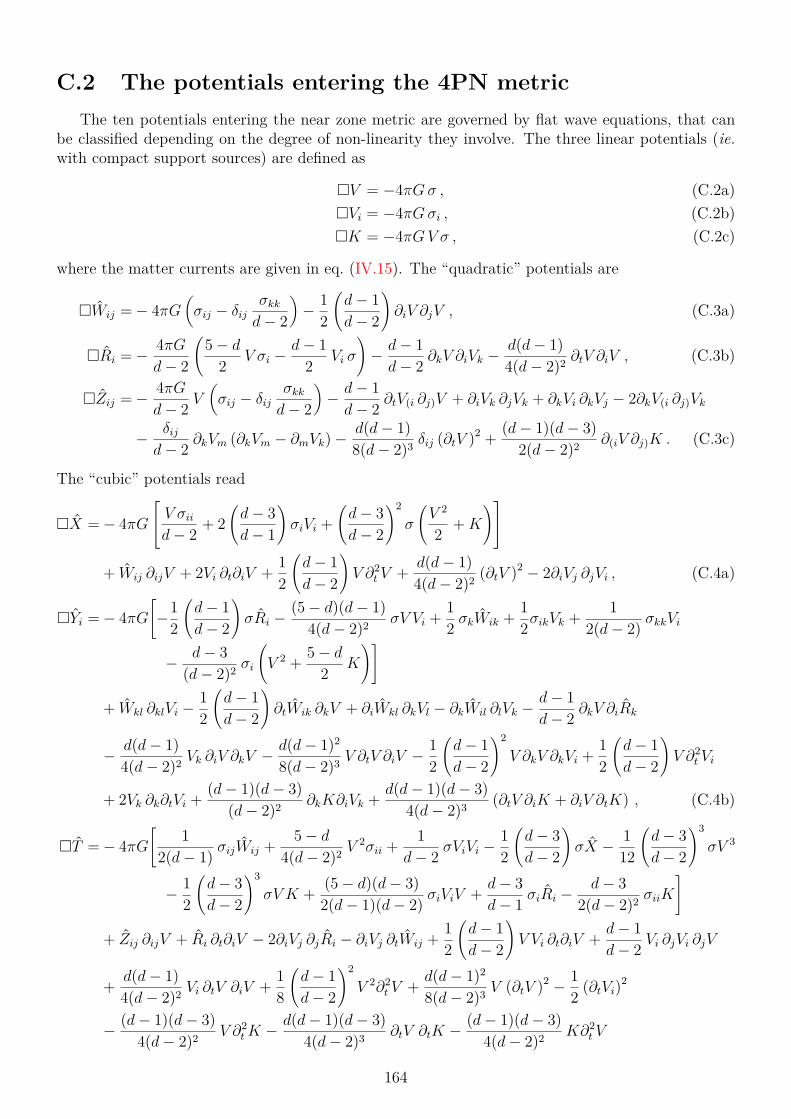
C.2 The potentials entering the 4PN metricThe ten potentials entering the near zone metric are governed by flat wave equations, that can

be classified depending on the degree of non-linearity they involve. The three linear potentials (ie.with compact support sources) are defined as

V = −4πGσ , (C.2a)Vi = −4πGσi , (C.2b)K = −4πGV σ , (C.2c)

where the matter currents are given in eq. (IV.15). The “quadratic” potentials are

Wij = − 4πG(σij − δij

σkkd− 2

)− 1

2

(d− 1d− 2

)∂iV ∂jV , (C.3a)

Ri = − 4πGd− 2

(5 − d

2 V σi − d− 12 Vi σ

)− d− 1d− 2 ∂kV ∂iVk − d(d− 1)

4(d− 2)2 ∂tV ∂iV , (C.3b)

Zij = − 4πGd− 2 V

(σij − δij

σkkd− 2

)− d− 1d− 2 ∂tV(i ∂j)V + ∂iVk ∂jVk + ∂kVi ∂kVj − 2∂kV(i ∂j)Vk

− δijd− 2 ∂kVm (∂kVm − ∂mVk) − d(d− 1)

8(d− 2)3 δij (∂tV )2 + (d− 1)(d− 3)2(d− 2)2 ∂(iV ∂j)K . (C.3c)

The “cubic” potentials read

X = − 4πG V σiid− 2 + 2

(d− 3d− 1

)σiVi +

(d− 3d− 2

)2

σ

(V 2

2 +K

)+ Wij ∂ijV + 2Vi ∂t∂iV + 1

2

(d− 1d− 2

)V ∂2

t V + d(d− 1)4(d− 2)2 (∂tV )2 − 2∂iVj ∂jVi , (C.4a)

Yi = − 4πG[−1

2

(d− 1d− 2

)σRi − (5 − d)(d− 1)

4(d− 2)2 σV Vi + 12 σkWik + 1

2σikVk + 12(d− 2) σkkVi

− d− 3(d− 2)2 σi

(V 2 + 5 − d

2 K

)]

+ Wkl ∂klVi − 12

(d− 1d− 2

)∂tWik ∂kV + ∂iWkl ∂kVl − ∂kWil ∂lVk − d− 1

d− 2 ∂kV ∂iRk

− d(d− 1)4(d− 2)2 Vk ∂iV ∂kV − d(d− 1)2

8(d− 2)3 V ∂tV ∂iV − 12

(d− 1d− 2

)2

V ∂kV ∂kVi + 12

(d− 1d− 2

)V ∂2

t Vi

+ 2Vk ∂k∂tVi + (d− 1)(d− 3)(d− 2)2 ∂kK∂iVk + d(d− 1)(d− 3)

4(d− 2)3 (∂tV ∂iK + ∂iV ∂tK) , (C.4b)

T = − 4πG[

12(d− 1) σijWij + 5 − d

4(d− 2)2 V2σii + 1

d− 2 σViVi − 12

(d− 3d− 2

)σX − 1

12

(d− 3d− 2

)3

σV 3

− 12

(d− 3d− 2

)3

σV K + (5 − d)(d− 3)2(d− 1)(d− 2) σiViV + d− 3

d− 1 σiRi − d− 32(d− 2)2 σiiK

]

+ Zij ∂ijV + Ri ∂t∂iV − 2∂iVj ∂jRi − ∂iVj ∂tWij + 12

(d− 1d− 2

)V Vi ∂t∂iV + d− 1

d− 2 Vi ∂jVi ∂jV

+ d(d− 1)4(d− 2)2 Vi ∂tV ∂iV + 1

8

(d− 1d− 2

)2

V 2∂2t V + d(d− 1)2

8(d− 2)3 V (∂tV )2 − 12 (∂tVi)2

− (d− 1)(d− 3)4(d− 2)2 V ∂2

tK − d(d− 1)(d− 3)4(d− 2)3 ∂tV ∂tK − (d− 1)(d− 3)

4(d− 2)2 K∂2t V

164

− d− 3d− 2 Vi ∂t∂iK − 1

2

(d− 3d− 2

)Wij ∂ijK . (C.4c)

Finally the only “quartic” potential required is governed by

Mij = 4πGδij[−1

2Ra + (d− 4)V V a

2(d− 2)

]σa +

[R(i − (d− 5)V V (i

2(d− 2)

]σj) + 1

8δijW abσab

+(

−(d− 1)V iV j

2(d− 2) + δij[

(d− 3)2(d− 1)KV4(d− 2)3 + (d− 3)2(d− 1)V 3

16(d− 2)3 + (d− 1)VaV a

4(d− 2) + (d− 1)X8(d− 2)

])σ

+ (d− 1)δijV 2σaa8(d− 2)2 − δijW a

aσbb

8(d− 2) +[

(d− 3)K(d− 2)2 − V 2

(d− 2)2

]σij − 1

2Wa(iσj)a

+ 1

2Wab∂b∂aW

ij − 12∂aW

ib∂bW ja − (d− 3)2(d− 1)∂iK∂jK

4(d− 2)3

+ ∂tV(i[−∂tV j) + (d− 3)(d− 1)∂j)K

(d− 2)2

]− 2∂aV (i∂j)Ra + 2∂(iVa∂

j)Ra − (d− 1)∂tR(i∂j)V

d− 2

+ (d− 1)W (ia∂

j)V ∂aV

4(d− 2) − (d− 1)∂(iX∂j)V

2(d− 2) + V (i[

(d− 1)∂aV j)∂aV

d− 2 + (d− 1)∂tV ∂j)V4(d− 2)

]

+ V

[(d− 1)∂2

t Wij

4(d− 2) − (d− 1)2∂tV(i∂j)V

2(d− 2)2

]+ V a

[∂t∂aW

ij − (d− 1)∂aV (i∂j)V

d− 2

]

− 2∂aR(i∂j)Va + ∂tW(ia

[− ∂aV j) + ∂j)V a

]+ ∂bW a(i∂j)Wab − 1

4∂iW ab∂jWab

+ δij(

−(d− 3)(d− 1)d∂tK∂tV8(d− 2)3 − (d− 1)2V 2∂2

t V

16(d− 2)2 + V a

[−1

2∂t∂aWbb − (d− 1)∂tV ∂aV

8(d− 2)

]

− (d− 3)(d− 1)∂tVa∂aK2(d− 2)2 + (d− 1)∂tRa∂

aV

2(d− 2) − 14W

ab∂b∂aWkk + ∂aVb∂

bRa

− (d− 1)Wab∂aV ∂bV

16(d− 2) − 12∂tWab∂

bV a − 14∂bWak∂

kW ab

+ V

[(d− 1)2d(∂tV )2

32(d− 2)3 − (d− 1)V a∂t∂aV

4(d− 2) − (d− 1)∂2t W

aa

8(d− 2)

+ (d− 1)2∂tVa∂aV

4(d− 2)2 − (d− 1)W ab∂b∂aV

8(d− 2) + (d− 1)∂aVb∂bV a

4(d− 2)

]). (C.5a)

165

C.3 The surface terms entering the source quadrupole

The mass quadrupole, once written in terms of potentials and superpotentials as in App. Cof [278], contains the following surface terms

Iij ∋ PFB

∫d3x

(r

r0

)B ∂a

(D2,0aij

c4 +D3,0aij

c6 +D4,0aij

c8

)+ xij∆

(L1,0

c2 + L2,0

c4 + L3,0

c6 + L4,0

c8

)

+ ddt

[PFB

∫d3x

(r

r0

)B ∂a

(D3,1aij

c6 +D4,1aij

c8

)+ xaij∆

(L2,1a

c4 + L3,1a

c6 + L4,1a

c8

)],

(C.6)

with the divergence terms

D2,0aij = 1

πG

(Ψ∂bkVai ∂jWbk − Wbk∂aΨ∂bkV

ij

), (C.7a)

D3,0aij = 4

πG

(Ψ∂tbVai ∂jRb − Rb∂aΨ∂tbV

ij

)+ 4πG

(Ψ∂bkVai ∂jZbk − Zbk∂aΨ∂bkV

ij

)− 8πG

(Ψ∂bVkai ∂kjRb − ∂aΨ∂bVk

ij ∂kRb

), (C.7b)

D4,0aij = 8

πG

(Ψ∂tbVai ∂jYb − Yb∂aΨ∂tbV

ij

)+ 8πG

(Ψ∂bkVai ∂jMbk − Mbk∂aΨ∂bkV

ij

)− 16πG

(Ψ∂bVkai ∂kjYb − ∂aΨ∂bVk

ij ∂kYb), (C.7c)

D3,1aij = 40

21πG(Ψ∂kVaib ∂kjRb − ∂aΨ∂kV

ijb ∂kRb

), (C.7d)

D4,1aij = 80

21πG(Ψ∂kVaib ∂kjYb − ∂aΨ∂kV

ijb ∂kYb), (C.7e)

and the Laplacian ones

L1,0 = − 12πG V 2 , (C.8a)

L2,0 = − 23πG V 3 − 1

2πG V W , (C.8b)

L3,0 = − 23πG V 4 − 1

πGV 2W − 1

4πG W 2 + 12πG WabWab − 4

πGV X − 2

πGV Z , (C.8c)

L4,0 = − 815πG V 5 − 1

2πG V W 2 − 43πG V 3W − 2

πGWX − 2

πG ,W Z + 4

πGWabZab

− 16πG

TV + 8πG

MV , (C.8d)

L2,1a = 10

21πG V Va , (C.8e)

L3,1a = 10

21πG V 2Va + 1021πG VaW − 10

21πG VbWab + 2021πG RaV , (C.8f)

L4,1a = 10

7πG VaVbVb + 2021πG V VaW − 20

21πG V VbWab + 4021πG RaV

2 + 2021πG RaW

− 2021πG RbWab + 40

21πG VaX + 4021πG VaZ − 40

21πG VbZab + 4021πG V Ya . (C.8g)

166

C.4 The coordinate shifts applied in the equations of motion

C.4.1 The UV shiftsWe present here the two UV shifts that have to be applied in the quadrupole. The first, denoted

ξi1,2, was constructed to remove the UV poles in the equations of motion [54]. The second, ηi1,2, wasmainly used for convenience [57]. The shift ξi1 is composed of 3PN and 4PN contributions and isgiven by

ξi1 = 113G2 m2

1c6

[1ε

− 2 ln(q1/2r′0ℓ0

)− 327

1540

]ai1 + 1

c8 ξi1, 4PN . (C.9)

The first term represents the 3PN contribution determined in [87]. Here q = 4πeγE where γE is theEuler constant, r′0 is the (unphysical) length scale associated with the UV dimensional regularizationand a1 is the Newtonian acceleration of the particle 1 in d dimensions. The 4PN term in the shift isconveniently decomposed as

ξi1, 4PN = 1εξi (−1)1, 4PN + ξ

(0,y1)1, 4PNy

i1 + ξ

(0,n12)1, 4PN n

i12 + ξ

(0,v1)1, 4PNv

i1 + ξ

(0,v12)1, 4PN v

i12 , (C.10)

with 1/ε being the UV pole and vi12 = vi1 − vi2. We have

ξi (−1)1, 4PN = G3m2

1m2vi12

r212

(11(n12v12) + 11

3 (n12v1))

+ ni12

[G4

r312

(553 m

31m2 + 22

3 m21m

22 + 4m1m

32

)

+ G3m21m2

r212

(112 (n12v12)2 − 11(n12v12)(n12v1) + 11

2 (n12v1)2 − 223 v

212

)], (C.11a)

ξ(0,y1)1, 4PN = G3(m1 +m2)

m1m2

15r312

([−67 + 48 ln

(r12

r0

)](n12v12)2 +

[17 − 16 ln

(r12

r0

)]v12

2)

+G4(m1 +m2)2m1m2

15r412

[−17 + 16 ln

(r12

r0

)], (C.11b)

ξ(0,n12)1, 4PN = G3m1m

22

1r2

12

([−1753

80 + 725 ln

(r12

r0

)](n12v12)2 +

[175340 + 96

5 ln(r12

r0

)](n12v12)(n12v1)

+[−1753

60 − 645 ln

(r12

r0

)](v12v1) +

[1753120 − 32

5 ln(r12

r0

)]v2

12

)

+ 1r3

12

([−431

10 + 48 ln(r12

r0

)](n12v12)2(n12y1) +

[532 − 144

5 ln(r12

r0

)](n12v12)(v12y1)

+[

6710 − 48

5 ln(r12

r0

)](n12y1)v2

12

)+G3m2

1m2

1r2

12

([−2761

168 − 332 ln

(q1/2r′0ℓ0

)− 11

2 ln(r12

r′0

)](n12v12)2

+[

4367168 + 33 ln

(q1/2r′0ℓ0

)+ 96

5 ln(r12

r0

)+ 11 ln

(r12

r′0

)](n12v12)(n12v1)

+[

7489840 − 33

2 ln(q1/2r′0ℓ0

)− 11

2 ln(r12

r′0

)](n12v1)2 +

[−1753

60 − 645 ln

(r12

r0

)](v12v1)

+[

1753120 + 22 ln

(q1/2r′0ℓ0

)+ 16

5 ln(r12

r0

)]v2

12

)

+ 1r3

12

([−431

10 + 48 ln(r12

r0

)](n12v12)2(n12y1) +

[532 − 144

5 ln(r12

r0

)](n12v12)(v12y1)

167

+[

6710 − 48

5 ln(r12

r0

)](n12y1)v2

12

)+G4m2

1m22

(1r3

12

[−88

3 ln(q1/2r′0ℓ0

)− 16

5 ln(r12

r0

)]+ 1r4

12

[6715 − 32

5 ln(r12

r0

)](n12y1)

)

+G4m31m2

(1r3

12

[−220

3 ln(q1/2r′0ℓ0

)− 32

5 ln(r12

r0

)]+ 1r4

12

[6730 − 16

5 ln(r12

r0

)](n12y1)

)

+G4m1m32

(1r3

12

[−16 ln

(q1/2r′0ℓ0

)+ 16

5 ln(r12

r0

)]+ 1r4

12

[6730 − 16

5 ln(r12

r0

)](n12y1)

),

(C.11c)

ξ(0,v1)1, 4PN = G3

(m2

1m2

r212

[−269

120 + 3215 ln

(r12

r0

)](n12v12) + m1m

22

r212

[−269

120 + 3215 ln

(r12

r0

)](n12v12)

),

(C.11d)

ξ(0,v12)1, 4PN = G3m1m

22

1r2

12

([75548 − 8 ln

(r12

r0

)](n12v12) +

[−1753

60 − 645 ln

(r12

r0

)](n12v1)

)

+ 1r3

12

([532 − 144

5 ln(r12

r0

)](n12v12)(n12y1) +

[−134

15 + 645 ln

(r12

r0

)](v12y1)

)+G3m2

1m2

1r2

12

([231131680 − 33 ln

(q1/2r′0ℓ0

)+ 11

3 ln(r12

r′0

)](n12v12)

+[−2572

105 − 11 ln(q1/2r′0ℓ0

)− 64

5 ln(r12

r0

)− 11

3 ln(r12

r′0

)](n12v1)

)

+ 1r3

12

([532 − 144

5 ln(r12

r0

)](n12v12)(n12y1) +

[−134

15 + 645 ln

(r12

r0

)](v12y1)

) . (C.11e)

The shift ηi1 is more compact. It starts at the 4PN order and is made only of G3 and G4 terms,

η1 = G3

c8 η(3)1, 4PN + G4

c8 η(4)1, 4PN , (C.12)

where

η(3)1, 4PN = v12

r212

(76924 m

21m2(n12v12) + 561

35 m1m22(n12v12)

)(C.13a)

+ n12

r212

[m1m

22

(217191400 (n12v12)2 − 2096

175 v212

)+m2

1m2

(−2119

50 (n12v12)2 + 587692100 v

212

)],

η(4)1, 4PN =

(88612100m

31m2 + 613

350m21m

22 − 5183

2100m1m32

)n12

r312. (C.13b)

Obviously, the shifts ξi2 and ηi2 are obtained from ξi1 and ηi1 by the exchange of the two particles.

168

C.4.2 The IR shiftThe shift used to remove the remaining IR poles in the equations of motion [56] was provided to

us by L. Bernard. It can be decomposed as

χi1 = 1c8

(1εχi (−1)1 + χ

(0,y1)1 yi1 + χ

(0,n12)1 ni12 + χ

(0,v1)1 vi1 + χ

(0,v12)1 vi12

), (C.14)

where

χi (−1)1 =8G4m1m2(m1 +m2)

5r124

[(m1 +m2)(n12y1)ni12 + r12(2m1 −m2)ni12 − m1 +m2

3 yi1

]

− 4G3m1m2 ni12

5r312

[2v2

12 (r12(m1 − 2m2) − 3 (n12y1) (m1 +m2)) − 8r12 (v1v12)

+ (n12v12)2 (30 (n12y1) (m1 +m2) + 9m2r12)

+ 6 (n12v12) (m1 +m2) (2r12 (n12v1) − 3 (y1v12)) (m1 +m2)]

+ 4G3m1m2 vi12

5r123

[8(m1 +m2) (r12 (n12v1) − (y1v12)) + (n12v12) (18 (n12y1) (m1 +m2) + 5m2r12)

]

− 8G3m1m2(m1 +m2) yi115r3

12

[3 (n12v12)2 − v2

12

]− 16G3m1m2 (n12v12) (m1 +m2)

15r212

vi1 , (C.15a)

χ(0,y1)1 =G

4m1m2(m1 +m2)2

75r412

[80 ln

(r2

0 q

ℓ20

)+ 80 ln

(r12

r0

)+ 73

]

+ G3m1m2(m1 +m2)75r3

12

[(n12v12)2

(180 ln

(r2

0 q

ℓ20

)+ 120 ln

(r12

r0

)+ 359

)

− v212

(60 ln

(r2

0 q

ℓ20

)+ 40 ln

(r12

r0

)+ 133

)], (C.15b)

χ(0,n12)1 = − G4m1m2(m1 +m2)

2100r412

[r12

(6720(2m1 −m2)

(ln(r2

0 q

ℓ20

)+ ln

(r12

r0

))+ 8861m1 − 5183m2

)

+ 42 (n12y1) (m1 +m2)(

160 ln(r2

0 q

ℓ20

)+ 160 ln

(r12

r0

)+ 61

)]

+ G3m1m2

4200r312

[2r12v

212

((m1 − 2m2)

(5040 ln

(r2

0 q

ℓ20

)+ 3360 ln

(r12

r0

))− 121916m1 − 37995m2

)

− 84v212 (n12y1) (m1 +m2)

(360 ln

(r2

0 q

ℓ20

)+ 240 ln

(r12

r0

)+ 223

)

+ 2100 (n12v12)2 (n12y1) (m1 +m2)(

72 ln(qr0

2)

+ 48 ln(r12

r0

)+ 35

)+ 3r12 (n12v12)2

(15120m2 ln

(r2

0 q

ℓ20

)+ 10080m2 ln

(r12

r0

)+ 126959m1 + 45908m2

)

+ 21r12 (n12v1) (n12v12) (m1 +m2)(

2880 ln(r2

0 q

ℓ20

)+ 1920 ln

(r12

r0

)− 9661

)

− 252 (n12v12) (y1v12) (m1 +m2)(

360 ln(r2

0 q

ℓ20

)+ 240 ln

(r12

r0

)+ 223

)

− 42r12 (v1v12) (m1 +m2)(

960 ln(r2

0 q

ℓ20

)+ 640 ln

(r12

r0

)− 3007

)],

(C.15c)

169

χ(0,v1)1 =G

3m1m2 (n12v12) (m1 +m2)600r2

12

[960 ln

(r2

0 q

ℓ20

)+ 640 ln

(r12

r0

)+ 2113

], (C.15d)

χ(0,v12)1 = − G3m1m2

4200r312

[5r12 (n12v12)

(5040m2 ln

(r2

0 q

ℓ20

)+ 3360m2 ln

(r12

r0

)+ 55132m1 + 41681m2

)

+ 42r12 (n12v1) (m1 +m2)(

960 ln(r2

0 q

ℓ20

)+ 640 ln

(r12

r0

)− 3007

)

+ 252 (n12v12) (n12y1) (m1 +m2)(

360 ln(r2

0 q

ℓ20

)+ 240 ln

(r12

r0

)+ 223

)

− 366 (y1v12) (m1 +m2)(

120 ln(r2

0 q

ℓ20

)+ 80 ln

(r12

r0

)+ 101

)]. (C.15e)

Obviously, the shift χi2 is obtained from χi1 by the exchange of the two particles.

170

Appendix D

Explicit dimensional regularization of theradiative quadrupole

In this appendix, we present the derivation of the dimensional regularization for the non-linearinteractions in Uij. In order to lighten the expressions that will be displayed, we set c = r0 = ℓ0 = 1.

D.1 Iteration of the d-dimensional propagatorWe aim at solving the d-dimensional wave equation

hL = NL(x, t) = N(r, t) nL . (D.1)

We recall that the accurate prescription for the d-dimensional propagator is given by eq. (IV.125)

hL(x, t) = −k4π

∫ddx′ r′η

∫ +∞

1dzγ 1−d

2(z) NL (x′, t− z|x′ − x|)

|x′ − x|d−2 , (D.2)

withγ 1−d

2 −ℓ(z) = 2

√π

Γ(d−2

2 + ℓ)

Γ(

3−d2 − ℓ

) (z2 − 1) 1−d

2 −ℓ . (D.3)

The strategy to compute the integral (D.2) relies on a split into two integration zones, dependingon whether r′ is larger than r or not. In the first integration zone, for r′ > r, we expand the integrandas

NL (x′, t− z|x′ − x|)|x′ − x|d−2 =

∑p∈N

xP

p! ∂P[NL (x′, t− z|x′ − x|)

|x′ − x|d−2

]x=0

=∑p∈N

(−)pp! xP∂′P

[NL (y, t− zr′)

r′d−2

]y=x′

,

(D.4)and in the second integration zone, defined by r′ < r, we expand it as

NL (x′, t− z|x′ − x|)|x′ − x|d−2 =

∑p∈N

x′P

p! ∂′P

[NL (y, t− z|x′ − x|)

|x′ − x|d−2

]x′=0,y=x′

=∑p∈N

(−)pp! x′P∂P

[NL (x′, t− zr)

rd−2

].

(D.5)Next, injecting those expansions in eq. (D.2), and massaging it notably by using the relations

∑p∈N

(−)pp! xP∂′P =

∑(j,q)∈N2

(−)q r2j+q

22j j!q!Γ(d2 + q

)Γ(d2 + q + j

) nQ ∂′Q∆′j , ∂QA(r) = rqnQ

(1r

ddr

)qA(r) ,

(D.6a)

171

∫ +∞

1dzγ 1−d

2(z)

(1r

ddr

)ℓ [F (t− zr)rd−2

]= (−2)ℓ

Γ(d−2

2 + ℓ)

Γ(

1−d2

) r2−2d−2ℓ∫ +∞

1dzγ d−2

2 −ℓ(z)F (t− zr) ,

(D.6b)

it comes out

hL = −12∑j∈N

nL22jj!

Γ(d−2

2 + ℓ)

Γ(d2 + ℓ+ j

) ∫ +∞

1dzγ 1−d

2 −ℓ(z)

r2−d−ℓ

∫ r

0dλλd−1+2j+ℓ+ηN (2j)(λ, t− zr)

+r2j+ℓ∫ +∞

rdλλ1−ℓ+ηN (2j)(λ, t− zλ)

,

(D.7)

where the separation into two integration zones appears clearly. If already complicated, this expres-sion is not yet satisfactory. Indeed its brute force three-dimensional limit does not directly reduce tothe usual Hadamard non-linear interactions. Therefore we need some more massaging of the integralsbefore studying the differences between regularization schemes.

Using the formal asymptotic expansion

γ 1−d2 −ℓ

(z) =z→∞

∑j∈N

(−)jj!

2√π z−2−2j−2ℓ−ε

Γ(−ℓ− j − ε

2

)Γ(

1+ε2 + ℓ

) , (D.8)

one obtains the expression for the “retarded minus advanced” propagator

∫ ∞1

dz γ 1−d2 −ℓ

(z)[A(t− zr) − A(t+ zr)

]=

2√πΓ

(d2 + ℓ

)Γ (2 − 2ℓ− d)

Γ(d−2

2 + ℓ)

Γ (1 − ε) Γ(− ε

2 − ℓ) ∑j∈N

122jj!

r2j+2ℓ+1+ε

Γ(d2 + ℓ+ j

)×∫ ∞

0dττ−ε

[A(2+2ℓ+2j)(t− τ) − A(2+2ℓ+2j)(t+ τ)

],

(D.9)where r is here a dummy variable. We have used this “retarded minus advanced” form in order todiscard the even sector, irrelevant for our purpose. But we now have to recognize the right-hand sideof eq. (D.9) within the integral (D.7). It is straightforward (in Fourier space) to show that

A(t) =∫ ∞

0dττ−ε [A(t− τ) − A(t+ τ)] ⇒ A(t) = 1

πtan

(πε

2

) ∫ ∞0

dττ ε[A(2)(t− τ) − A(2)(t+ τ)

].

(D.10)Let us now concentrate on only one given multipolar order, ie. write N(r, t) = r−p−qεF (t). Pluggingit, together with the relations (D.9) and (D.10), in the integral (D.7), it finally comes

hL = Γεℓ nLrℓ+1+ε

∫ ∞1

dy γ−1− ε2−ℓ(y)

∫ ∞1

dz γ−1− ε2−ℓ(z)

∫ +∞

−∞dτ ε |τ |ε−1

×∫ r

0dλλ1−ℓ−p−qε+η

[F (−2ℓ−1) (t− yr − zλ+ τ) − F (−2ℓ−1) (t− yr + zλ+ τ)

]+∫ ∞r

dλλ1−ℓ−p−qε+η[F (−2ℓ−1) (t− yr − zλ+ τ) − F (−2ℓ−1) (t+ yr − zλ+ τ)

] ,

(D.11)

where we have compacted the prefactor

Γεℓ ≡ (−)ℓ 22(ℓ−1)

π3/2

Γ(

1−ε2

)Γ(1 + ε

2

) [Γ(ℓ+ 1 + ε

2

)]2, (D.12)

whose three-dimensional limit is simply given by Γ0ℓ = (−)ℓ [(2ℓ− 1)!!]2 /4. Even if not obvious per

se, the three-dimensional limit of the integral (D.11) is naturally defined, and agrees with the usualthree-dimensional propagator. Therefore it is the formulation we will use henceforth.

172

D.2 Dimensional regularization of the metricWe know that the pole compensating the IR pole of the source moment is of UV nature, and thus

should come from the 0 boundary of the integral (D.11). Therefore, the difference between the tworegularization schemes comes only from the sector

hL ≡ Γεℓ nLrℓ+1+ε

∫ ∞1

dy γ−1− ε2−ℓ(y)

∫ ∞1

dz γ−1− ε2−ℓ(z)

∫ +∞

−∞dτ ε |τ |ε−1

×∫ Λ

0dλλ1−ℓ−p−qε+η

[F (−2ℓ−1) (t− yr − zλ+ τ) − F (−2ℓ−1) (t− yr + zλ+ τ)

],

(D.13)

where Λ is an irrelevant cut-off scale that can be safely set to +∞. The aim is then to put thisintegral in a nicer looking form. This is realized by setting

φ(t) ≡ Γεℓ nLrℓ+1+ε

∫ ∞1

dyγ−1− ε2−ℓ(y)

∫ +∞

−∞dτ ε|τ |ε−1F (−2ℓ−1)(t− yr + τ)

= (−)ℓ2ℓ Γεℓ

Γ(

1+ε2

)Γ(ℓ+ 1+ε

2

) ∫ ∞1

dyγ−1− ε2(y)

∫ +∞

−∞dτ ε|τ |ε−1∂L

[F (−2ℓ−1)(t− yr + τ)

rd−2

],

(D.14)

where we have used the relation (D.6b). Defining ρ ≡ λz, it comes

hL =(∫ ∞

1dz zℓ−2+p+qε−η γ−1− ε

2−ℓ(z)) ∫ ∞

0dρ ρ1−ℓ−p−qε+η [φ(t− ρ) − φ(t+ ρ)]

=√π Γ

(3+ℓ−p−qε+ε+η

2

)Γ(ℓ+ 1+ε

2

)Γ(

3−ℓ−p−qε+η2

) (−)ℓ+p+1Γ(qε− η)Γ(p+ ℓ− 1 + qε− η)

×∫ ∞

0dρ ρη−qε

[φ(ℓ+p−1)(t− ρ) + (−)ℓ+pφ(ℓ+p−1)(t+ ρ)

].

(D.15)

The interest of this definition is that the metric perturbation is now written so that it looks like thelinear d-dimensional metric, namely

hL = −4 (−)ℓℓ! ∂L

k

rd−2

∫ ∞1

dzγ−1− ε2(z)H (t− zr)

, (D.16)

where the role of the multipolar moments is played by H, that reads

H(t) ≡ (−)p ℓ!24−ℓπ

1−ε2

Γ(

1−ε2

)Γ(1 + ε

2

) Γ(

3+ℓ−p−qε+ε+η2

)Γ(

3−ℓ−p−qε+η2

) Γ (qε− η)Γ (p+ ℓ− 1 + qε− η)

×∫ +∞

−∞dτ ε|τ |ε−1

∫ +∞

0dρ ρη−qε

[F (p−ℓ−2)(t+ τ − ρ) + (−)ℓ+pF (p−ℓ−2)(t+ τ + ρ)

].

(D.17)

We are thus interested in the difference of regularization schemes of H more than of hL. Thereforewe aim at computing

DH ≡ limε→0

[PFηH]

− PFη

[limε→0

H]. (D.18)

For simplicity, the previous formulas have been obtained by considering only one multipolar orderin (p, q), but naturally the source consists in a summation over many of them. Formally, we candecompose

N(r, t) =∑p,q

r−p−qε φp,q(t) =∑p,q

r−p−qε[ψp,q(t)ε

+ ψp,q(t)], (D.19)

173

where the ψp,q coefficients do not depend on ε. The F (t) function corresponds to one particularφp,q(t). As we have explicitly checked in practical computations, all the considered sources have anon-pathological three-dimensional limit, meaning that

N3D(r, t) = limε→0

N(r, t) =∑p

r−p [φp(t) + φp(t) ln r] = PFϵ

∑p

r−p[φp(t) + φp(t)

rϵ

ϵ

], (D.20)

with ∑q

ψp,q = 0 ,∑q

q ψp,q = −φp and∑q

ψp,q = φp + O(ε) . (D.21)

Note that the rewriting of the logarithms by means of a finite part has been made for practicalcomputational purposes.

D.2.1 Three-dimensional computationIn order to perform the three-dimensional computation with a natural implementation of loga-

rithms, let us identify ϵ with ε in (D.20). The three-dimensional limit thus becomes a finite partoperation on ε, where only the ε associated with a q are to be considered, and one takes q ≡ −1.Therefore the three-dimensional limit is formally given by

limε→0

H = (−)p ℓ!23−ℓ

Γ(

3+ℓ−p+η2

)Γ(

3−ℓ−p+η2

) Γ (−η)Γ (p+ ℓ− 1 − η)

∫ +∞

0dτ τ η

φ(p−ℓ−2)p (t− τ) + (−)ℓ+pφ(p−ℓ−2)

p (t+ τ)

+ln τ + ψ (p+ ℓ− 1 − η) − ψ(−η) +

ψ(

3+ℓ−p+η2

)− ψ

(3−ℓ−p+η

2

)2

×[φ(p−ℓ−2)p (t− τ) + (−)ℓ+pφ(p−ℓ−2)

p (t+ τ)]

,

(D.22)with ψ the digamma function.

To accurately perform the finite part operation on η, we have to distinguish cases following thevalues of p and ℓ. First, for p+ ℓ ≤ 1, it comes

Pfη

(limε→0

H)

=(−)ℓ+1 ℓ!23−ℓ

Γ(

3+ℓ−p2

)Γ(

3−ℓ−p2

) Γ (2 − p− ℓ)

×

[1 − (−)ℓ+p] φ(p−ℓ−3)

p (t) +H1−p−ℓ +

ψ(

3+ℓ−p2

)− ψ

(3−ℓ−p

2

)2

φ(p−ℓ−3)p (t)

+∫ ∞

0dτ ln τ

[φ(p−ℓ−2)p (t− τ) + (−)ℓ+pφ(p−ℓ−2)

p (t+ τ)]

.

(D.23)Then in the case p+ ℓ− 2 ∈ 2N, it reads

Pfη

(limε→0

H)

= (−)p+1 ℓ!23−ℓ

Γ(

3+ℓ−p2

)Γ(

3−ℓ−p2

) 1Γ (p+ ℓ− 1)

∫ ∞0

dτ ln τφ(p−ℓ−2)

p (t− τ) + φ(p−ℓ−2)p (t+ τ)

+Hp+ℓ−2 +

ψ(

3+ℓ−p2

)− ψ

(3−ℓ−p

2

)2 + ln τ

2

[φ(p−ℓ−2)p (t− τ) + φ(p−ℓ−2)

p (t+ τ)] .

(D.24)

174

In the p+ ℓ = 2j + 3 case, with j < ℓ, the finite part reduces to

Pfη

(limε→0

H)

= (−) 1+p−ℓ2 ℓ!

23−ℓ

Γ(

3+ℓ−p2

)Γ(ℓ+p−1

2

)Γ (p+ ℓ− 1)

φ(p−ℓ−3)p (t) +

(Hp+ℓ−2 +

H 1−p+ℓ2

2 −H p+ℓ−3

2

2

)φ(p−ℓ−3)p (t)

+∫ ∞

0dτ ln τ

φ(p−ℓ−2)p (t− τ) − φ(p−ℓ−2)

p (t+ τ)2

.

(D.25)Finally, for p− ℓ− 3 = 2j with j ∈ N, it comes

Pfη

(limε→0

H)

= ℓ!23−ℓ

Γ (ℓ+ j + 1)Γ (j + 1) Γ (2j + 2ℓ+ 2)

2Hφ(2j)

p (t) +∫ ∞

0dτ ln τ

[φ(2j+1)p (t− τ) − φ(2j+1)

p (t+ τ)]

+(

H2 + ψ1(j + ℓ+ 1) − ψ1(j + 1) − 4ψ1(2j + 2ℓ+ 2)4 + π2

6

)φ(2j)p (t)

+∫ ∞

0dτ(

H ln τ + ln2 τ

2

) [φ(2j+1)p (t− τ) − φ(2j+1)

p (t+ τ)]

,

(D.26)where we have shortened the combination of harmonic numbers H ≡ H2j+2ℓ+1 + Hj

2 − Hj+ℓ

2 , and ψ1denotes the trigamma function.

D.2.2 d-dimensional computationFor clarity purposes, we will omit here the summation over the values of q. In this vein, we note

eg. F = ∑q(ψp,q/ε + ψp,q) or qF = ∑

q q(ψp,q/ε + ψp,q). It was verified that no source terms withq = 0 appear in our computation (this fact can be related to the fact that all considered d-dimensionalquantities have at least q = 1). Therefore, as long as p− ℓ− 3 ∈ N, we are protected by a ε and thusthe finite part on η is trivially realized by taking η = 0. Discriminating again on the values of p andℓ, for p+ ℓ ≤ 1, it comes

limε→0

(PfηH)

=(−)ℓ+1 ℓ!23−ℓ

Γ(

3+ℓ−p2

)Γ(

3−ℓ−p2

) Γ (2 − p− ℓ)

×

σ1 + ε

ln q + γE2 − qH1−p−ℓ +

(1 − q)ψ(

3+ℓ−p2

)+ qψ

(3−ℓ−p

2

)2

F (p−ℓ−3)(t)

+ε∫ ∞

0dτ ln τ

[(σ

2 − q)F (p−ℓ−2)(t− τ) −

(σ

2 + (−)ℓ+pq)F (p−ℓ−2)(t+ τ)

],

(D.27)where we have shortened σ ≡ 1 − (−)ℓ+p. By virtue of the relations (D.21), eq. (D.23) is recovered:the two regularization schemes agree.

For p+ ℓ− 2 ∈ 2N, the d-dimensional computation yields

limε→0

(PfηH)

=(−)p+1 ℓ!23−ℓ

Γ(

3+ℓ−p2

)Γ(

3−ℓ−p2

) 1Γ (p+ ℓ− 1)

×∫ ∞

0dτ ln τ

1 + ε

ln q + γE2 − qHp+ℓ−2 +

(1 − q)ψ(

3+ℓ−p2

)+ qψ

(3−ℓ−p

2

)2 − q ln τ

2

×[F (p−ℓ−2)(t− τ) + F (p−ℓ−2)(t+ τ)

]+ε

2

∫ ∞0

dλ ln λ[F (p−ℓ−1)(t− τ − λ) − F (p−ℓ−1)(t− τ − λ)

],

(D.28)

175

so that the three-dimensional result (D.24) is recovered.As for p+ ℓ = 2j + 3, with j < ℓ, it reads

limε→0

(PfηH)

= (−) 1+p−ℓ2 ℓ!

23−ℓ

Γ(

3+ℓ−p2

)Γ(ℓ+p−1

2

)Γ (p+ ℓ− 1)

F (p−ℓ−3)(t)

+ ε

ln q2 − qHp+ℓ−2 +

(1 − q)H 1−p+ℓ2

+ qH p+ℓ−32

2

F (p−ℓ−3)(t)

+ε(1 − q)2

∫ ∞0

dτ ln τ[F (p−ℓ−2)(t− τ) − F (p−ℓ−2)(t+ τ)

].

(D.29)

Once again, the d-dimensional and three-dimensional (D.25) computations yield the same result.Finally for p − ℓ − 3 = 2j with j ∈ N, we separate the d-dimensional result into two pieces: the

first one sums over all q

Pfη

(limε→0

H)

1= ℓ!

23−ℓΓ (ℓ+ j + 1)

Γ (j + 1) Γ (2j + 2ℓ+ 2)

2HF (2j)(t) +

∫ ∞0

dτ ln τ[F (2j+1)(t− τ) − F (2j+1)(t+ τ)

]+ 2ε

[Hj + ln q

2 H − q + 12

(H2 − ψ1(2j + 2ℓ+ 2) + ψ1(1 + ℓ+ j)

4

)

+q − 18 ψ1(1 + j) − q

12π2]F (2j)(t)

− ε∫ ∞

0dτ ln τ

(qH − Hj + ln q

2 + q + 12 ln τ

) [F (2j+1)(t− τ) − F (2j+1)(t+ τ)

]+ε

2

∫∫ ∞0

dτdλ ln τ ln λ[F (2j+2)(t− τ − λ) − 2F (2j+2)(t− τ + λ) + F (2j+2)(t+ τ + λ)

],

(D.30)and, thanks to the conditions (D.21), exactly agrees with the three-dimensional limit (D.26). There-fore the difference in regularization schemes is exactly given by the second contribution, that sumsover q = 1, namely

Pfη

(limε→0

H)

2= ℓ!

23−ℓΓ (ℓ+ j + 1)

Γ (j + 1) Γ (2j + 2ℓ+ 2)∑q =1

1q − 1

2(

−1ε

+ H2j+2ℓ+1 − Hj+ℓ

2 − ln q2

)F (2j)(t)

− ε

H2 +(

H2 − Hj + ln q2

)2

− 2ψ1(2j + 2ℓ+ 2) + ψ1(1 + ℓ+ j)2 + π2

6

F (2j)(t) −ε∫ ∞

0dτ ln2 τ

[F (2j+1)(t− τ) − F (2j+1)(t+ τ)

]+ε

2

∫∫ ∞0

dτdλ ln τ ln λ[F (2j+2)(t− τ − λ) − 2F (2j+2)(t− τ + λ) + F (2j+2)(t+ τ + λ)

].

(D.31)

D.2.3 Difference in regularization schemes for the non-linear interac-tions

The main result of this technical appendix is that for a source

N(r, t) =∑p,q

r−p−qε[ψp,q(t)ε

+ ψp,q(t)], (D.32)

the difference in regularization schemes only comes from the terms that have p = ℓ+3+2j, for j ∈ N.One can separate the contribution coming from the pole from the one coming from the regular sectoras

DH = (DH)reg + (DH)p , (D.33)

176

with

(DH)reg = −∑q =1

2ℓ−2

q − 1ℓ! (ℓ+ j)!

j! (p+ ℓ− 2)!

1ε

+ ln√q −

ℓ+j∑k=0

12k + 1

ψ(2j)p,q (t) , (D.34)

and

(DH)p = −∑q =1

2ℓ−2

q − 1ℓ! (ℓ+ j)!

j! (p+ ℓ− 2)!

1ε2 + ln

√q

ε− 1ε

ℓ+j∑k=0

12k + 1 − Aj,ℓ

ψ(2j)p,q (t)

−∫∫ ∞

0dτdλ ln τ ln λ

ψ(2j+2)p,q (t− τ − λ) − 2ψ(2j+2)

p,q (t− τ + λ) + ψ(2j+2)p,q (t+ τ + λ)

4

,

(D.35)where

Aj,ℓ ≡ H2

2 + 12

(H2 − Hj + ln q

2

)2

− ψ1(2j + 2ℓ+ 2) + ψ1(1 + ℓ+ j)4 + π2

12 . (D.36)

ψ1 is the trigamma function and we recall the shorthand H ≡ H2j+2ℓ+1 + Hj

2 − Hj+ℓ

2 .It is to note that the regular contribution is local, whereas the one coming from the pole bears a

non-local part. Fortunately, in our practical case, there is no poles when p− ℓ− 3 ∈ 2N !

177

178

Appendix E

Résumé en français

La théorie actuellement la plus à même de rendre compte des phénomènes gravitationnels, laRelativité Générale (RG), a été testée dans une variété de régimes sans précédent : depuis lesaccélérations très faibles ressenties par les sondes Pioneer 10 et 11 aux confins du système Solaire,aux voisinages des trous noirs, en passant naturellement par notre mouvement autour du Soleil. Cestests ont tous été concluants, et ont confirmé la fermeté des assises de la RG. Cependant, il resteaujourd’hui au moins deux phénomènes qui n’ont pas d’explication convaincante : la phénoménologiede la matière noire et l’accélération de la dilatation de notre univers. La phénoménologie de la matièrenoire a été postulée pour rendre compte d’anomalies dans le comportement des étoiles en périphériedes galaxies, et se retrouve aujourd’hui à toutes les échelles : depuis les expériences sondant lastructure fondamentale de la matière au CERN jusqu’aux observations des reliques du début del’univers. Cette “matière noire” pourrait être composée d’une (ou de plusieurs) nouvelle particule,qui résiste encore et toujours à l’observateur, ou alors elle pourrait être dûe à une insuffisance de laRG pour décrire la phénoménologie des accélérations extrêmement ténues. De même, l’accélérationde la dilatation de notre univers peut être décrite par une simple “constante cosmologique” ajoutéeaux équations de la RG, par une “énergie sombre” de nature matérielle, ou encore par une complétionde la RG dans le régime des énergies très faibles.

Pour avancer vers une explication convaincante de ces phénomènes, trois voies semblent primor-diales à suivre. La première, que nous ne suivrons pas, consiste naturellement à tendre vers unemeilleure connaissance empirique de notre univers, en raffinant les observations actuelles et en in-ventant de nouveaux modes d’observation. Un effort conséquent est actuellement porté en ce senset de nombreux instruments sont développés et exploités, sur terre, sous terre, dans les profondeursmarines et dans l’espace. Les deux autres voies, plus théoriques, sont celles que nous avons choisiesd’explorer lors de cette thèse. Tout d’abord, et en parallèle de cette nécessité d’affiner notre connais-sance empirique de l’univers, il y a un vrai besoin d’affuter nos prédictions théoriques pour la RG.Ce n’est qu’en comparant les observations à des prédictions robustes que nous serons capables dediscerner de possibles déviations à la RG, qui pourront indiquer dans quelle direction celle-ci a besoind’être dépassée. La troisième et dernière voie consiste à construire et tester des scénarios alternatifsà la RG. Même si les théories exotiques développées ne sont pas forcément de meilleures descriptionsde la nature que la RG, il est toujours intéressant de les explorer pour au moins deux raisons. Lapremière tient à ce que de telles constructions nous renseignent sur la nature même de la RG : enla déconstruisant pour construire une autre théorie, on en expose au grand jour les mécaniques in-ternes. La seconde raison est d’ordre plus pratique: en sachant quelles alternatives sont viables, onpeut réaliser des tests plus affutés en cherchant à isoler un effet particulier, inexistant en RG.

Naturellement ces deux dernières voies (une meilleure connaissance théorique de la RG, et larecherche d’alternatives viables) se doivent d’être suivies en parallèle, et d’être mises en regard l’unede l’autre. C’est dans cet esprit que nous avons abordé cette thèse, dédiée d’une part à l’étude duproblème à deux corps, et de l’autre, à la construction et au test de théories alternatives.

179

Étude du problème à deux corps

Le problème à deux corps est un cadre idéal pour l’étude de la RG. Conceptuellement c’est l’undes systèmes les plus simples que l’on puisse imaginer, puisqu’il n’est composé que de deux corps,liés uniquement par l’interaction gravitationnelle. Empiriquement, on trouve de telles configurationsen abondance dans l’univers, de la pomme qui tombe aux binaires de trous noirs, en passant par lesystème Terre-Lune, ce qui permet de multiplier les régimes d’observation. Mais d’un point de vuethéorique, si le problème à deux corps Newtonien est très simple car linéaire, le problème relativisteexhibe toutes les non-linéarités de la RG, et est donc bien plus ardu. Bien que centenaire, c’est ainsiun champ toujours très actif et dynamique, et de nombreux pans restent à défricher.

Pour simplifier la configuration étudiée, nous allons considérer les deux corps comme des partic-ules ponctuelles, négligeant les effets de rotation et de taille finie. Traiter le problème relativiste àdeux corps tel quel semble une tache impossible avec les techniques actuelles de calcul, nous allonsdonc devoir recourir à des méthodes d’approximation, dites “post-Newtonienne” (PN, qui consiste àconsidérer des corps de faible vitesse) et “post-Minkowskienne” (PM, qui traite des champs faibles).La première approximation traite des caractéristiques des corps (en l’occurrence, leur vitesse), elleest donc valable en zone proche, c’est-à-dire à proximité des-dits corps. Elle sera donc utilisée pourdéduire la structure de l’espace-temps dans cette zone uniquement. La seconde approximation con-sidère des déviations à un espace vide, elle est donc particulièrement adaptée à l’étude de la radiationgravitationnelle, et est valide à l’extérieur de la distribution de matière. Ces deux approches engen-drent deux solutions, chacune dans une zone différente : nous allons donc devoir les associer pourobtenir une unique solution, valable dans tout l’espace-temps. Cette association se fait dans la zonede recouvrement où les deux approximations sont valides, au moyen d’une puissante équation deraccord. Ce formalisme “post-Newtonien-post-Minkowskien-multipolaire” (PN-MPM, de l’anglais),qui consiste à raccorder ces deux approches, est celui que nous utiliserons dans cette thèse. Commela première correction à la dynamique Newtonienne est quadratique en l’inverse de la vitesse de lalumière, il est d’usage de nommer nPN l’ordre c−2n. En revanche le nième ordre PM est tradition-nellement donné par la correction en Gn.

Une première contribution de cette thèse au domaine du problème à deux corps fut le calcul descontributions logarithmiques dues aux effets de sillage (tail effects en anglais) dans l’énergie. Ceseffets sont dûs à la diffusion d’ondes gravitationnelles sur la courbure statique de l’espace-temps crééepar la binaire, et sont donc des phénomènes non-linéaires par essence. En “ricochant” sur la structurestatique du fond, les ondes vont se disperser et certaines vont revenir interagir avec la binaire, cequi va naturellement affecter son mouvement. Ces effets sont par essence non-instantanés puisqu’àun instant donné, les ondes qui interagissent avec la binaire sont celles qui ont été émises dans lepassé de la source. Cette non-localité en temps se traduit par l’apparition de logarithmes en vitessedans l’énergie d’une binaire évoluant sur une orbite circulaire. En exploitant de nouvelles synergiesentre les méthodes PN-MPM, les techniques provenant des théories effectives des champs et celledite “première loi de la dynamique des binaires de trous noirs”, et en collaboration avec L. Blanchet,S. Foffa et R. Sturani, nous avons calculé cette dépendance logarithmique à une précision qui n’avaitpas encore été atteinte (3PN en sus de l’ordre dominant, soit 7PN dans l’énergie). En outre, nousavons tiré profit de l’équation de renormalisation pour extraire une formule analytique donnant, pourchaque puissance du logarithme, la valeur du coefficient dominant. Nous avons naturellement vérifiéque, pour les ordres les plus bas (ie. jusqu’à 21PN), notre formule concorde bien avec les résultatspréexistants.

Si cette première étude fut importante car révélatrice du potentiel encore largement inexplorédes synergies entre ces différentes approches du problème à deux corps, la contribution principale decette thèse réside dans le travail relatif à la génération d’onde. Les générations actuelles et futures dedétecteurs sont bien plus sensibles à l’évolution de la fréquence des ondes qu’à celle de leur amplitude.Il est donc essentiel de connaitre la phase gravitationnelle (ie. la dépendance temporelle de ces

180

ondes) à de très grandes précisions, notamment pour le futur détecteur LISA (Laser InterferometerSpace Antenna). Si l’état de l’art est la précision 3.5PN, le programme visant à déterminer lecomportement à 4PN a été initié il y a plusieurs années et touche à sa fin. Il est important de soulignerqu’actuellement seule la méthode PN-MPM est capable d’atteindre de telles précisions, c’est donccelle que nous implémenterons. Parmi les multiples étapes qui conduisent à l’établissement de la phaseà 4PN, nous nous sommes attachés lors de cette thèse à la détermination du moment quadrupolairede masse. Ce calcul peut se décomposer en trois étapes : le quadrupole source est d’abord évaluéavec une régularisation dimensionnelle1 dans l’UV et une régularisation de Hadamard dans l’IR;ensuite la régularisation dimensionnelle est appliquée dans l’IR; enfin le quadrupole radiatif, c’est-à-dire observable, est déterminé à partir du quadrupole source et de la prise en compte des nombreusesinteractions non-linéaires, qui doivent être évaluées en dimension arbitraire. L’établissement duquadrupole source Hadamard a été achevé par T. Marchand avant le début de cette thèse, maisnous en avons recalculé quelques secteurs avec L. Blanchet et S. Marsat dans l’optique de réaliserdes vérifications en double aveugle, rendues nécessaires par la longueur et la technicité des calculs.Néanmoins l’apport majeur de cette thèse fut l’implémentation de la régularisation dimensionnelledans l’IR pour les quadrupoles source et radiatif, réalisée en collaboration avec Q. Henry, L. Blanchetet G. Faye. Ce procédé de régularisation est vital pour obtenir un quadrupole radiatif physique, c’est-à-dire sans divergences fallacieuses provenant de l’approximation PN étendue hors de son régime devalidité. La régularisation dimensionnelle du quadrupole source a été achevée et satisfait tous lescritères de validité, nous sommes actuellement en train de mettre au point celle du quadrupoleradiatif, en calculant les effets de sillage, de mémoire et leurs itérations.

Un troisième projet fut entrepris lors de cette thèse, et concerne l’établissement d’un test dela RG dans un système exoplanétaire bien particulier, HD 80606b. En effet cette exoplanète a uneexcentricité très élevée et a été observée lors de transits et d’éclipses. Avec L. Blanchet et G. Hébrard,nous avons calculé la prédiction relativiste de la variation du temps écoulé entre une éclipse et letransit suivant, et avons montré qu’elle pourrait être détectable à partir de 2025. Les lancementsprévus des télescopes spatiaux James–Webb et Ariel, à même d’observer précisément les éclipses ettransits d’HD 80606b, nous donnent bon espoir que le test soit effectué (des discussions en ce sensavec J.-P. Beaulieu, coPI d’Ariel sont en cours). À notre connaissance, il s’agit là du premier testréaliste de la RG dans un système stellaire qui ne soit pas le système Solaire.

Étude de théories alternatives

En parallèle de l’étude du problème à deux corps en RG, nous avons aussi considéré des théoriesalternatives. Avec C. Deffayet nous nous sommes intéressés aux défauts topologiques (ou solitons),c’est-à-dire des configurations d’énergie localisées et auto-entretenues, les exemples les plus sensa-tionnels étant les mascarets, remontant l’embouchure des fleuves. Nous nous sommes concentrés surde tels défauts réalisés par des champs scalaires, une configuration qui a notamment d’importantesimplications cosmologiques. L’argument habituel justifiant leur stabilité est topologique, et reposesur la dégénérescence de la structure du vide d’un potentiel. Pour dépasser un tel argument etévaluer sa nécessité, nous avons cherché à construire des défauts non-topologiques, sans potentielmais néanmoins stables, et nous nous sommes restreints à des géométries planaires non-gravitantespar simplicité. Après avoir obtenu des formules générales permettant de construire de tels soli-tons, nous nous sommes concentrés sur une réalisation particulière et avons démontré qu’un certainchoix de paramètres permettait d’imiter exactement les solitons canoniques, aussi bien au niveaudu profil de la solution, qu’au niveau de ses perturbations linéaires. Malheureusement, de telsdéfauts non-topologiques ne peuvent pas être directement solutions de théories cosmologiques carl’implémentation de la gravitation altère trop gravement leurs conditions d’existence.

1Un tel procédé consiste à effectuer les calculs en dimension arbitraire, puis à prendre la limite tridimensionnelle.

181

Conjointement à l’étude de ces défauts non-topologiques, cette thèse s’est attachée à l’étude dethéories alternatives de gravitation dites minimales. La philosophie du minimalisme repose sur leconstat que si l’ajout de degrés de liberté est un moyen pratique de rendre compte de phénomènestels que l’accélération de la dilatation de notre univers, de tels supplétifs ne sont pas nécessairesd’un point de vue empirique. De fait, ni le suivi de binaires de pulsars, ni la détection directe deradiation gravitationnelle ne laisse transparaître de traces de degrés de liberté autres que les deuxpolarisations tensorielles présentes en RG. Une théorie minimale est donc une théorie qui ne propageque des polarisations tensorielles, tout en offrant une phénoménologie sensiblement plus riche quecelle de la RG. Naturellement une telle construction a un coût, et les théories minimales brisentfaiblement l’invariance sous les difféomorphismes temporels, présente en RG. Une telle brisure estnéanmoins peu contraignante car elle n’est effective qu’aux échelles cosmologiques et dans le secteurpurement gravitationnel : ces théories satisfont donc tous les tests habituels, réalisés à des échellesterrestres. La première de ces théories, construite en 2015 par A. De Felice et S. Mukohyama est uneminimalisation de la gravité massive canonique, qui offre une explication naturelle à l’accélération dela dilatation de notre univers. Mais pour pouvoir donner lieu à une cosmologie attrayante, l’un deschamps non-dynamiques de cette théorie minimale de gravité massive doit être muni d’une artificielledépendance en temps.

Un tel artefact étant peu convaincant et encore moins esthétique, nous nous sommes efforcés dele dépasser, en collaboration avec A. De Felice, S. Mukohyama et M. Oliosi. Cela nous a conduit àchercher une théorie minimale de bigravité, c’est-à-dire une théorie faisant apparaître deux métriquesdynamiques, mais seulement quatre polarisations (contrairement aux sept habituellement présentesdans de telles théories de bigravité). En jaugeant la théorie canonique de bigravité, due à S. Hassanet R. Rosen, et en introduisant des contraintes supplémentaires au niveau du Hamiltonien, nousavons réalisé une telle théorie. Une étude de sa phénoménologie cosmologique a révélé qu’elle donnelieu à deux branches de solutions, toutes deux stables (contrairement à la bigravité canonique, dontla cosmologie est instable) et conduisant à des mécanismes naturels d’accélération de la dilatation del’univers. En outre cette théorie conduit à des oscillations et une relation de dispersion non trivialepour les gravitons et, dans l’une des deux branches, la croissance des structures à grande échelle estdifférente de celle de la RG. Toutes ces disparités avec la cosmologie orthodoxe sont naturellementobservables, et pourraient permettre de tester notre théorie.

Outre de tels tests cosmologiques, il est important de sonder la phénoménologie à petite échelle,notamment en explorant les régimes forts par la construction de solutions de trous noirs. C’est ceque nous avons réalisé, en collaboration avec A. De Felice, A. Doll, S. Mukohyama et M. Oliosi,dans deux théories minimales, la théorie initiale de gravité massive et le modèle dit V CDM. Dansla première de ces théories, nous avons démontré un lemme qui relie les solutions de RG ayant dessections spatiales plates à des solutions de la théorie alternative. Ce lemme technique est en faitextrêmement puissant puisque les espaces-temps de la RG représentant des étoiles et des trous noirsstatiques admettent de telles sections spatiales plates, et sont donc directement solutions de la théorieminimale. Le corollaire direct de ce résultat est que cette théorie alternative satisfait la majorité destests réalisés dans le système Solaire aussi bien que la RG, c’est-à-dire avec brio. Nous avons essayéd’implémenter des trous noirs en rotation par un processus similaire, mais avons montré que les trousnoirs en rotation de la RG n’admettent pas de sections spatiales plates, et nous n’avons donc paspu appliquer notre lemme. L’étude du régime de champ fort du modèle V CDM s’est révélée biendifférente. En effet nous avons pu construire des espaces-temps de trou noirs distincts de ceux dela RG, notamment par des phénomènes de non-staticité et une possible violation de la condition deconvergence nulle. De telles disparités avec les trous noirs usuels sont évidemment observables, quece soit lors des effondrements gravitationnels dont ils émergent, par le suivi du mouvement des corpsdans leur voisinage ou par l’émission de radiation gravitationnelle.

182

Bibliography

[1] Discussions with L. Blanchet.

[2] G. Aad et al.; “Search for new phenomena in events with two opposite-charge leptons, jetsand missing transverse momentum in pp collisions at

√s = 13 TeV with the ATLAS detector”;

(2021)arXiv: 2102.01444.

[3] B. P. Abbott et al.; “Observation of Gravitational Waves from a Binary Black Hole Merger”;Phys. Rev. Lett. 116, p. 061102 (2016). arXiv: 1602.03837.

[4] B. P. Abbott et al.; “GW170817: Observation of Gravitational Waves from a Binary NeutronStar Inspiral”; Phys. Rev. Lett. 119, p. 161101 (2017). arXiv: 1710.05832.

[5] B. P. Abbott et al.; “Multi-messenger Observations of a Binary Neutron Star Merger”; Astro-phys. J. Lett. 848, p. L12 (2017). arXiv: 1710.05833.

[6] B. P. Abbott et al.; “Tests of General Relativity with GW170817”; Phys. Rev. Lett. 123, p.011102 (2019). arXiv: 1811.00364.

[7] B. P. Abbott et al.; “GWTC-1: A Gravitational-Wave Transient Catalog of Compact BinaryMergers Observed by LIGO and Virgo during the First and Second Observing Runs”; Phys. Rev.X 9, p. 031040 (2019). arXiv: 1811.12907.

[8] L. F. Abbott & S. Deser; “Stability of gravity with a cosmological constant”; Nuclear PhysicsB 195, pp. 76–96 (1982).

[9] R. Abbott et al.; “GWTC-2: Compact Binary Coalescences Observed by LIGO and VirgoDuring the First Half of the Third Observing Run”; (2020)arXiv: 2010.14527.

[10] R. Abbott et al.; “Tests of General Relativity with Binary Black Holes from the second LIGO-Virgo Gravitational-Wave Transient Catalog”; (2020)arXiv: 2010.14529.

[11] R. Abbott et al.; “Constraints on cosmic strings using data from the third Advanced LIGO-Virgo observing run”; (2021)arXiv: 2101.12248.

[12] R. Abuter et al.; “Detection of the Schwarzschild precession in the orbit of the star S2 near theGalactic centre massive black hole”; Astron. Astrophys. 636, p. L5 (2020). arXiv: 2004.07187.

[13] P. A. R. Ade et al.; “Planck 2013 results. XXV. Searches for cosmic strings and other topologicaldefects”; Astron. Astrophys. 571, p. A25 (2014). arXiv: 1303.5085.

[14] N. Afshordi, D. J. H. Chung & G. Geshnizjani; “Cuscuton: A Causal Field Theory withan Infinite Speed of Sound”; Phys. Rev. D 75, p. 083513 (2007). arXiv: hep-th/0609150.

[15] N. Aghanim et al.; “Planck 2018 results. VI. Cosmological parameters”; Astron. Astrophys.641, p. A6 (2020). arXiv: 1807.06209.

183

[16] K. Akiyama et al.; “First M87 Event Horizon Telescope Results. I. The Shadow of the Super-massive Black Hole”; Astrophys. J. 875, p. L1 (2019). arXiv: 1906.11238.

[17] Y. Akrami, S. F. Hassan, F. Könnig, A. Schmidt-May & A. R. Solomon; “Bimetricgravity is cosmologically viable”; Phys. Lett. B 748, pp. 37–44 (2015). arXiv: 1503.07521.

[18] A. Albert et al.; “Combined search for neutrinos from dark matter self-annihilation in theGalactic Center with ANTARES and IceCube”; Phys. Rev. D 102, p. 082002 (2020). arXiv:2003.06614.

[19] P. Amore & F. M. Fernández; “Exact and approximate expressions for the period of anhar-monic oscillators”; European Journal of Physics 26, pp. 589–601 (2005). arXiv: math-ph/0409034.

[20] M. Andrews, M. Lewandowski, M. Trodden & D. Wesley; “Distinguishing k-defects fromtheir canonical twins”; Phys. Rev. D 82, p. 105006 (2010). arXiv: 1007.3438.

[21] T. Anson, E. Babichev & C. Charmousis; “Deformed black hole in Sagittarius A”;(2021)arXiv: 2103.05490.

[22] K. Aoki & S. Mukohyama; “Massive gravitons as dark matter and gravitational waves”; Phys.Rev. D 94, p. 024001 (2016). arXiv: 1604.06704.

[23] K. Aoki, A. D. Felice, C. Lin, S. Mukohyama & M. Oliosi; “Phenomenology in type-Iminimally modified gravity”; Journal of Cosmology and Astroparticle Physics 2019, p. 017 (2019).arXiv: 1810.01047.

[24] K. Aoki, A. De Felice, S. Mukohyama, K. Noui, M. Oliosi & M. C. Pookkillath;“Minimally modified gravity fitting Planck data better than Λ-CDM”; The European PhysicalJournal C 80 (2020). arXiv: 2005.13972.

[25] K. Aoki, M. A. Gorji & S. Mukohyama; “A consistent theory of D → 4 Einstein-Gauss-Bonnet gravity”; Phys. Lett. B 810, p. 135843 (2020). arXiv: 2005.03859.

[26] K. Aoki, F. Di Filippo & S. Mukohyama; “Non-uniqueness of massless transverse-tracelessgraviton”; (2021)arXiv: 2103.15044.

[27] E. Aprile et al.; “Excess electronic recoil events in XENON1T”; Phys. Rev. D 102, p. 072004(2020). arXiv: 2006.09721.

[28] Aristote; La Physique, Livre IV (Flammarion) (1999); préf. by P. Pellegrin.

[29] Aristote; La Physique, Livre VII (Flammarion) (1999); préf. by P. Pellegrin.

[30] Aristote; Traité du Ciel, Livre I (Flammarion) (2004).

[31] N. Arkani-Hamed, H.-C. Cheng, M. A. Luty & S. Mukohyama; “Ghost condensation anda consistent infrared modification of gravity”; JHEP 05, p. 074 (2004). arXiv: hep-th/0312099.

[32] C. Armendariz-Picon, T. Damour & V. F. Mukhanov; “k - inflation”; Phys. Lett. B 458,pp. 209–218 (1999). arXiv: hep-th/9904075.

[33] C. Armendariz-Picon, V. F. Mukhanov & P. J. Steinhardt; “A Dynamical solution tothe problem of a small cosmological constant and late time cosmic acceleration”; Phys. Rev. Lett.85, pp. 4438–4441 (2000). arXiv: astro-ph/0004134.

[34] R. L. Arnowitt, S. Deser & C. W. Misner; “The Dynamics of general relativity”; Gen. Rel.Grav. 40, pp. 1997–2027 (2008). arXiv: gr-qc/0405109.

184

[35] K. G. Arun, L. Blanchet, B. R. Iyer & M. S. S. Qusailah; “Tail effects in the 3PNgravitational wave energy flux of compact binaries in quasi-elliptical orbits”; Phys. Rev. D 77, p.064034 (2008). arXiv: 0711.0250.

[36] P. Auclair, D. A. Steer & T. Vachaspati; “Particle emission and gravitational radiationfrom cosmic strings: observational constraints”; Phys. Rev. D 101, p. 083511 (2020). arXiv:1911.12066.

[37] E. Babichev; “Global topological k-defects”; Physical Review D 74 (2006). arXiv: hep-th/0608071.

[38] E. Babichev; “Gauge k-vortices”; Phys. Rev. D 77, p. 065021 (2008). arXiv: 0711.0376.

[39] E. Babichev, C. Charmousis, G. Esposito-Farèse & A. Lehébel; “Hamiltonian unbound-edness vs stability with an application to Horndeski theory”; Phys. Rev. D 98, p. 104050 (2018).arXiv: 1803.11444.

[40] J. G. Baker, J. Centrella, D.-I. Choi, M. Koppitz & J. van Meter; “Gravitational waveextraction from an inspiraling configuration of merging black holes”; Phys. Rev. Lett. 96, p. 111102(2006). arXiv: gr-qc/0511103.

[41] S. Ballard et al.; “The Kepler-19 System: A Transiting 2.2 R⊕ Planet and a Second PlanetDetected via Transit Timing Variations”; Astrophys. J. 743, p. 200 (2011). arXiv: 1109.1561.

[42] L. Barack; “Gravitational self force in extreme mass-ratio inspirals”; Class. Quant. Grav. 26,p. 213001 (2009). arXiv: 0908.1664.

[43] J. M. Bardeen, B. Carter & S. W. Hawking; “The Four laws of black hole mechanics”;Commun. Math. Phys. 31, pp. 161–170 (1973).

[44] S. Baumgartner, M. Bernardini, J. R. Canivete Cuissa, H. de Laroussilhe, A. M. W.Mitchell, B. A. Neuenschwander, P. Saha, T. Schaeffer, D. Soyuer & L. Zwick; “To-wards a polarization prediction for LISA via intensity interferometry”; Monthly Notices of theRoyal Astronomical Society 498, pp. 4577–4589 (2020). arXiv: 2008.11538.

[45] J. D. Bekenstein; “Relativistic gravitation theory for the MOND paradigm”; Phys. Rev. D70, p. 083509 (2004). [Erratum: Phys.Rev.D 71, 069901 (2005)]; arXiv: astro-ph/0403694.

[46] J. Ben Achour, M. Crisostomi, K. Koyama, D. Langlois, K. Noui & G. Tasinato;“Degenerate higher order scalar-tensor theories beyond Horndeski up to cubic order”; JHEP 12,p. 100 (2016). arXiv: 1608.08135.

[47] Z. Bern, J. J. M. Carrasco & H. Johansson; “New Relations for Gauge-Theory Ampli-tudes”; Phys. Rev. D 78, p. 085011 (2008). arXiv: 0805.3993.

[48] Z. Bern, C. Cheung, R. Roiban, C.-H. Shen, M. P. Solon & M. Zeng; “Scattering Ampli-tudes and the Conservative Hamiltonian for Binary Systems at Third Post-Minkowskian Order”;Phys. Rev. Lett. 122, p. 201603 (2019). arXiv: 1901.04424.

[49] Z. Bern, C. Cheung, R. Roiban, C.-H. Shen, M. P. Solon & M. Zeng; “Black Hole Bi-nary Dynamics from the Double Copy and Effective Theory”; JHEP 10, p. 206 (2019). arXiv:1908.01493.

[50] Z. Bern, A. Luna, R. Roiban, C.-H. Shen & M. Zeng; “Spinning Black Hole Binary Dy-namics, Scattering Amplitudes and Effective Field Theory”; (2020)arXiv: 2005.03071.

185

[51] Z. Bern, J. Parra-Martinez, R. Roiban, M. S. Ruf, C.-H. Shen, M. P. Solon & M. Zeng;“Scattering Amplitudes and Conservative Binary Dynamics at O(G4)”; (2021)arXiv: 2101.07254.

[52] L. Bernard & L. Blanchet; “Phenomenology of Dark Matter via a Bimetric Extension ofGeneral Relativity”; Phys. Rev. D 91, p. 103536 (2015). arXiv: 1410.7708.

[53] L. Bernard, L. Blanchet & L. Heisenberg; “Bimetric gravity and dark matter”; in “50thRencontres de Moriond on Gravitation: 100 years after GR,” (2015); arXiv: 1507.02802.

[54] L. Bernard, L. Blanchet, A. Bohé, G. Faye & S. Marsat; “Fokker action of nonspinningcompact binaries at the fourth post-Newtonian approximation”; Phys. Rev. D 93, p. 084037 (2016).arXiv: 1512.02876.

[55] L. Bernard, L. Blanchet, A. Bohé, G. Faye & S. Marsat; “Energy and periastron advanceof compact binaries on circular orbits at the fourth post-Newtonian order”; Phys. Rev. D 95, p.044026 (2017). arXiv: 1610.07934.

[56] L. Bernard, L. Blanchet, A. Bohé, G. Faye & S. Marsat; “Dimensional regularizationof the IR divergences in the Fokker action of point-particle binaries at the fourth post-Newtonianorder”; Phys. Rev. D 96, p. 104043 (2017). arXiv: 1706.08480.

[57] L. Bernard, L. Blanchet, G. Faye & T. Marchand; “Center-of-Mass Equations of Motionand Conserved Integrals of Compact Binary Systems at the Fourth Post-Newtonian Order”; Phys.Rev. D 97, p. 044037 (2018). arXiv: 1711.00283.

[58] G. Bertone, D. Hooper & J. Silk; “Particle dark matter: Evidence, candidates and con-straints”; Phys. Rept. 405, pp. 279–390 (2005). arXiv: hep-ph/0404175.

[59] N. Bevis, M. Hindmarsh, M. Kunz & J. Urrestilla; “CMB polarization power spectra con-tributions from a network of cosmic strings”; Phys. Rev. D 76, p. 043005 (2007). arXiv: 0704.3800.

[60] P. Binetruy, A. Bohe, T. Hertog & D. A. Steer; “Gravitational wave signatures from kinkproliferation on cosmic (super-) strings”; Phys. Rev. D 82, p. 126007 (2010). arXiv: 1009.2484.

[61] D. Bini & T. Damour; “Analytical determination of the two-body gravitational interactionpotential at the fourth post-Newtonian approximation”; Phys. Rev. D 87, p. 121501 (2013). arXiv:1305.4884.

[62] D. Bini & T. Damour; “High-order post-Newtonian contributions to the two-body gravitationalinteraction potential from analytical gravitational self-force calculations”; Phys. Rev. D 89, p.064063 (2014). arXiv: 1312.2503.

[63] D. Bini, T. Damour & A. Geralico; “Novel approach to binary dynamics: application to thefifth post-Newtonian level”; Phys. Rev. Lett. 123, p. 231104 (2019). arXiv: 1909.02375.

[64] D. Bini, T. Damour, A. Geralico, S. Laporta & P. Mastrolia; “Gravitational scatteringat the seventh order in G: nonlocal contribution at the sixth post-Newtonian accuracy”; Phys.Rev. D 103, p. 044038 (2021). arXiv: 2012.12918.

[65] G. D. Birkhoff; Relativity and Modern Physics (Harvard University Press) (1923).

[66] N. T. Bishop & L. Rezzolla; “Extraction of Gravitational Waves in Numerical Relativity”;Living Rev. Rel. 19, p. 2 (2016). arXiv: 1606.02532.

[67] L. Blanchet; “Radiative Gravitation Fields in General Relativity II. Asymptotic Behaviourat Future Null Infinity”; Proc. of the Roy. Soc. of London Series A 409, pp. 383–399 (1987).

186

[68] L. Blanchet & G. Schäfer; “Higher order gravitational radiation losses in binary systems”;Mon. Not. Roy. Astron. Soc. 239, p. 845 (1989).

[69] L. Blanchet; “Second post-Newtonian generation of gravitational radiation”; Phys. Rev. D51, pp. 2559–2583 (1995). arXiv: gr-qc/9501030.

[70] L. Blanchet; “Gravitational wave tails of tails”; Class. Quant. Grav. 15, pp. 113–141 (1998).[Erratum: Class.Quant.Grav. 22, 3381 (2005)]; arXiv: gr-qc/9710038.

[71] L. Blanchet; “On the multipole expansion of the gravitational field”; Class. Quant. Grav. 15,pp. 1971–1999 (1998). arXiv: gr-qc/9801101.

[72] L. Blanchet; “Gravitational polarization and the phenomenology of MOND”; Class. Quant.Grav. 24, pp. 3529–3540 (2007). arXiv: astro-ph/0605637.

[73] L. Blanchet; “Gravitational Radiation from Post-Newtonian Sources and Inspiralling Com-pact Binaries”; Living Rev. Rel. 17, p. 2 (2014). arXiv: 1310.1528.

[74] L. Blanchet & T. Damour; “Tail-transported temporal correlations in the dynamics of agravitating system”; Phys. Rev. D 37, pp. 1410–1435 (1988).

[75] L. Blanchet & T. Damour; “Hereditary effects in gravitational radiation”; Phys. Rev. D 46,pp. 4304–4319 (1992).

[76] L. Blanchet & G. Faye; “General relativistic dynamics of compact binaries at the thirdpost-Newtonian order”; Phys. Rev. D 63, p. 062005 (2001). arXiv: gr-qc/0007051.

[77] L. Blanchet & G. Faye; “Flux-balance equations for linear momentum and center-of-massposition of self-gravitating post-Newtonian systems”; Class. Quant. Grav. 36, p. 085003 (2019).arXiv: 1811.08966.

[78] L. Blanchet & L. Heisenberg; “Dipolar Dark Matter as an Effective Field Theory”; Phys.Rev. D 96, p. 083512 (2017). arXiv: 1701.07747.

[79] L. Blanchet & B. R. Iyer; “Third post-Newtonian dynamics of compact binaries: Equa-tions of motion in the center-of-mass frame”; Class. Quant. Grav. 20, p. 755 (2003). arXiv: gr-qc/0209089.

[80] L. Blanchet & F. Larrouturou; unpublished computations.

[81] L. Blanchet & A. Le Tiec; “Model of Dark Matter and Dark Energy Based on GravitationalPolarization”; Phys. Rev. D 78, p. 024031 (2008). arXiv: 0804.3518.

[82] L. Blanchet & A. Le Tiec; “First Law of Compact Binary Mechanics with Gravitational-Wave Tails”; Class. Quant. Grav. 34, p. 164001 (2017). arXiv: 1702.06839.

[83] L. Blanchet & J. Novak; “External field effect of modified Newtonian dynamics in the Solarsystem”; Mon. Not. Roy. Astron. Soc. 412, pp. 2530–2542 (2011). arXiv: 1010.1349.

[84] L. Blanchet, T. Damour & B. R. Iyer; “Gravitational waves from inspiralling compactbinaries: Energy loss and wave form to second post-Newtonian order”; Phys. Rev. D 51, p. 5360(1995). [Erratum: Phys.Rev.D 54, 1860 (1996)]; arXiv: gr-qc/9501029.

[85] L. Blanchet, G. Faye & B. Ponsot; “Gravitational field and equations of motion of compactbinaries to 5/2 post-Newtonian order”; Phys. Rev. D 58, p. 124002 (1998). arXiv: gr-qc/9804079.

187

[86] L. Blanchet, B. R. Iyer & B. Joguet; “Gravitational waves from inspiralling compactbinaries: Energy flux to third post-Newtonian order”; Phys. Rev. D 65, p. 064005 (2002). [Erratum:Phys.Rev.D 71, 129903 (2005)]; arXiv: gr-qc/0105098.

[87] L. Blanchet, T. Damour & G. Esposito-Farese; “Dimensional regularization of the thirdpost-Newtonian dynamics of point particles in harmonic coordinates”; Phys. Rev. D 69, p. 124007(2004). arXiv: gr-qc/0311052.

[88] L. Blanchet, T. Damour, G. Esposito-Farese & B. R. Iyer; “Gravitational radiation frominspiralling compact binaries completed at the third post-Newtonian order”; Phys. Rev. Lett. 93,p. 091101 (2004). arXiv: gr-qc/0406012.

[89] L. Blanchet, G. Faye, B. R. Iyer & S. Sinha; “The Third post-Newtonian gravitationalwave polarisations and associated spherical harmonic modes for inspiralling compact binaries inquasi-circular orbits”; Class. Quant. Grav. 25, p. 165003 (2008). [Erratum: Class.Quant.Grav. 29,239501 (2012)]; arXiv: 0802.1249.

[90] L. Blanchet, S. L. Detweiler, A. Le Tiec & B. F. Whiting; “Post-Newtonian and Numeri-cal Calculations of the Gravitational Self-Force for Circular Orbits in the Schwarzschild Geometry”;Phys. Rev. D 81, p. 064004 (2010). arXiv: 0910.0207.

[91] L. Blanchet, S. L. Detweiler, A. Le Tiec & B. F. Whiting; “High-Order Post-NewtonianFit of the Gravitational Self-Force for Circular Orbits in the Schwarzschild Geometry”; Phys. Rev.D 81, p. 084033 (2010). arXiv: 1002.0726.

[92] L. Blanchet, A. Buonanno & A. Le Tiec; “First law of mechanics for black hole binarieswith spins”; Phys. Rev. D 87, p. 024030 (2013). arXiv: 1211.1060.

[93] L. Blanchet, G. Faye & B. F. Whiting; “Half-integral conservative post-Newtonian approx-imations in the redshift factor of black hole binaries”; Phys. Rev. D 89, p. 064026 (2014). arXiv:1312.2975.

[94] L. Blanchet, G. Faye & B. F. Whiting; “High-order half-integral conservative post-Newtonian coefficients in the redshift factor of black hole binaries”; Phys. Rev. D 90, p. 044017(2014). arXiv: 1405.5151.

[95] L. Blanchet, G. Hébrard & F. Larrouturou; “Detecting the General Relativistic Or-bital Precession of the Exoplanet HD 80606b”; Astron. Astrophys. 628, p. A80 (2019). arXiv:1905.06630.

[96] L. Blanchet, S. Foffa, F. Larrouturou & R. Sturani; “Logarithmic tail contributionsto the energy function of circular compact binaries”; Phys. Rev. D 101, p. 084045 (2020). arXiv:1912.12359.

[97] J. J. Blanco-Pillado, K. D. Olum & J. M. Wachter; “Comparison of cosmic string andsuperstring models to NANOGrav 12.5-year results”; (2021)arXiv: 2102.08194.

[98] J. Blümlein, A. Maier, P. Marquard & G. Schäfer; “Fourth post-Newtonian Hamiltoniandynamics of two-body systems from an effective field theory approach”; Nucl. Phys. B 955, p.115041 (2020). arXiv: 2003.01692.

[99] E. Bogomolny; “Stability of Classical Solutions”; Sov. J. Nucl. Phys. 24, p. 449 (1976).

[100] N. Bolis, A. De Felice & S. Mukohyama; “Integrated Sachs-Wolfe-galaxy cross-correlationbounds on the two branches of the minimal theory of massive gravity”; Phys. Rev. D 98 (2018).arXiv: 1804.01790.

188

[101] H. Bondi, M. G. J. van der Burg & A. W. K. Metzner; “Gravitational Waves in GeneralRelativity. VII. Waves from Axi-Symmetric Isolated Systems”; Proc. of the Roy. Soc. of LondonSeries A 269, pp. 21–52 (1962).

[102] F. Bonjour, C. Charmousis & R. Gregory; “Thick domain wall universes”; Class. Quant.Grav. 16, pp. 2427–2445 (1999). arXiv: gr-qc/9902081.

[103] W. B. Bonnor & M. A. Rotenberg; “Gravitational waves from isolated sources”; Proc. R.Soc. Lond. A 289, pp. 247–274 (1966).

[104] Bordas, sous la direction de R. Caratini; Encyclopédie – 2 – Astronomie (ÉditionsBordas) (1968).

[105] A. Bosma; “21-cm line studies of spiral galaxies. II. The distribution and kinematics of neutralhydrogen in spiral galaxies of various morphological types.” Astron. J. 86, pp. 1825–1846 (1981).

[106] G. Boué, P. Figueira, A. C. M. Correia & N. C. Santos; “Orbital migration induced byanisotropic evaporation. Can hot Jupiters form hot Neptunes?” Astron. Astrophys. 537, p. L3(2012). arXiv: 1109.2805.

[107] D. G. Boulware & S. Deser; “Can Gravitation Have a Finite Range?” Phys. Rev. D 6, pp.3368–3382 (1972).

[108] A. Bourgoin, A. Hees, S. Bouquillon, C. Le Poncin-Lafitte, G. Francou & M. C.Angonin; “Testing Lorentz symmetry with Lunar Laser Ranging”; Phys. Rev. Lett. 117, p.241301 (2016). arXiv: 1607.00294.

[109] J. Boussinesq; “Théorie de l’intumescence liquide, appelée onde solitaire ou de translation, sepropageant dans un canal rectangulaire”; C. R. Acad. Sci. (Paris) 72, pp. 755–759 (1871)https://gallica.bnf.fr/ark:/12148/bpt6k3029x/f759.

[110] C. Brans & R. H. Dicke; “Mach’s Principle and a Relativistic Theory of Gravitation”; Phys.Rev. 124, pp. 925–935 (1961).

[111] D. Brouwer & G. Clemence; Methods of celestial mechanics (Academic Press (New York))(1961).

[112] J. D. Brown; “Action functionals for relativistic perfect fluids”; Class. Quant. Grav. 10, pp.1579–1606 (1993). arXiv: gr-qc/9304026.

[113] J.-P. Bruneton & G. Esposito-Farese; “Field-theoretical formulations of MOND-like grav-ity”; Phys. Rev. D 76, p. 124012 (2007). [Erratum: Phys.Rev.D 76, 129902 (2007)]; arXiv:0705.4043.

[114] H. A. Buchdahl; “Non-Linear Lagrangians and Cosmological Theory”; Monthly Notices ofthe Royal Astronomical Society 150, pp. 1–8 (1970).

[115] A. Buonanno & T. Damour; “Effective one-body approach to general relativistic two-bodydynamics”; Phys. Rev. D 59, p. 084006 (1999). arXiv: gr-qc/9811091.

[116] M. E. Cahill & G. C. McVittie; “Spherical Symmetry and Mass-Energy in General Rela-tivity”; Journal of Mathematical Physics 11, p. 1392 (1970).

[117] M. Campanelli, C. O. Lousto, P. Marronetti & Y. Zlochower; “Accurate evolutionsof orbiting black-hole binaries without excision”; Phys. Rev. Lett. 96, p. 111101 (2006). arXiv:gr-qc/0511048.

189

[118] S. Capozziello, M. De laurentis & A. Stabile; “Axially symmetric solutions in f(R)-gravity”; Class. Quant. Grav. 27, p. 165008 (2010). arXiv: 0912.5286.

[119] R. Carballo-Rubio, F. D. Filippo & S. Liberati; “Minimally modified theories of grav-ity: a playground for testing the uniqueness of general relativity”; Journal of Cosmology andAstroparticle Physics 2018, p. 026 (2018). arXiv: 1802.02537.

[120] B. Carter & R. Gregory; “Curvature corrections to dynamics of domain walls”; Phys. Rev.D 51, pp. 5839–5846 (1995). arXiv: hep-th/9410095.

[121] C. Charmousis, E. J. Copeland, A. Padilla & P. M. Saffin; “General second orderscalar-tensor theory, self tuning, and the Fab Four”; Phys. Rev. Lett. 108, p. 051101 (2012).arXiv: 1106.2000.

[122] C. Cheung & M. P. Solon; “Tidal Effects in the Post-Minkowskian Expansion”; Phys. Rev.Lett. 125, p. 191601 (2020). arXiv: 2006.06665.

[123] G. Cho, B. Pardo & R. A. Porto; “Gravitational radiation from inspiralling compact ob-jects: Spin-spin effects completed at the next-to-leading post-Newtonian order”; (2021)arXiv:2103.14612.

[124] Y. Choquet-Bruhat & R. Geroch; “Global aspects of the Cauchy problem in generalrelativity”; Comm. in Math. Phys. 14, pp. 329–335 (1969).

[125] K. D. Colón, E. B. Ford, S. Redfield, J. J. Fortney, M. Shabram, H. J. Deeg &S. Mahadevan; “Probing potassium in the atmosphere of HD 80606b with tunable filter transitspectrophotometry from the Gran Telescopio Canarias”; Mon. Not. Roy. Astr. Soc. 419, pp. 2233–2250 (2012). arXiv: 1008.4800.

[126] D. Comelli, M. Crisostomi, F. Nesti & L. Pilo; “FRW Cosmology in Ghost Free MassiveGravity”; JHEP 03, p. 067 (2012). [Erratum: JHEP 06, 020 (2012)]; arXiv: 1111.1983.

[127] D. Comelli, M. Crisostomi & L. Pilo; “Perturbations in Massive Gravity Cosmology”;JHEP 06, p. 085 (2012). arXiv: 1202.1986.

[128] N. Copernicus; De revolutionibus orbium cœlestium (J. Petreius ed. (Nürnberg)) (1530).

[129] R. Courant & D. Hilbert; Methods of Mathematical Physics (Interscience (New York))(1953).

[130] G. D’Amico, C. de Rham, S. Dubovsky, G. Gabadadze, D. Pirtskhalava & A. J.Tolley; “Massive Cosmologies”; Phys. Rev. D 84, p. 124046 (2011). arXiv: 1108.5231.

[131] T. Damour & N. Deruelle; “General relativistic celestial mechanics of binary systems. I.The post-Newtonian motion”; Annales Inst. H. Poincaré Phys. Théor. 43, pp. 107–132 (1985)http://www.numdam.org/article/AIHPA_1985__43_1_107_0.pdf.

[132] T. Damour; “Gravitational Self Force in a Schwarzschild Background and the Effective OneBody Formalism”; Phys. Rev. D 81, p. 024017 (2010). arXiv: 0910.5533.

[133] T. Damour & G. Esposito-Farèse; “Testing for preferred frame effects in gravity withartificial earth satellites”; Phys. Rev. D 49, pp. 1693–1706 (1994). arXiv: gr-qc/9311034.

[134] T. Damour, P. Jaranowski & G. Schäfer; “Nonlocal-in-time action for the fourth post-Newtonian conservative dynamics of two-body systems”; Phys. Rev. D 89, p. 064058 (2014). arXiv:1401.4548.

190

[135] T. Damour, P. Jaranowski & G. Schäfer; “Fourth post-Newtonian effective one-bodydynamics”; Phys. Rev. D 91, p. 084024 (2015). arXiv: 1502.07245.

[136] T. Damour, P. Jaranowski & G. Schäfer; “Conservative dynamics of two-body systemsat the fourth post-Newtonian approximation of general relativity”; Phys. Rev. D 93, p. 084014(2016). arXiv: 1601.01283.

[137] A. De Felice & S. Mukohyama; “Minimal theory of massive gravity”; Physics Letters B752, p. 302 (2016). arXiv: 1506.01594.

[138] A. De Felice & S. Mukohyama; “Phenomenology in minimal theory of massive gravity”;JCAP 04, p. 028 (2016). arXiv: 1512.04008.

[139] A. De Felice & S. Mukohyama; “Graviton mass might reduce tension between early andlate time cosmological data”; Phys. Rev. Lett. 118, p. 091104 (2017). arXiv: 1607.03368.

[140] A. De Felice & S. Mukohyama; “Weakening gravity for dark matter in a type-II minimallymodified gravity”; (2020); arXiv: 2011.04188.

[141] A. De Felice & S. Tsujikawa; “f(R) theories”; Living Rev. Rel. 13, p. 3 (2010). arXiv:1002.4928.

[142] A. De Felice, A. E. Gümrükçüoglu & S. Mukohyama; “Massive gravity: nonlinearinstability of the homogeneous and isotropic universe”; Phys. Rev. Lett. 109, p. 171101 (2012).arXiv: 1206.2080.

[143] A. De Felice, A. E. Gümrükçüoğlu, S. Mukohyama, N. Tanahashi & T. Tanaka;“Viable cosmology in bimetric theory”; JCAP 06, p. 037 (2014). arXiv: 1404.0008.

[144] A. De Felice, T. Nakamura & T. Tanaka; “Possible existence of viable models of bi-gravity with detectable graviton oscillations by gravitational wave detectors”; PTEP 2014, p.043E01 (2014). arXiv: 1304.3920.

[145] A. De Felice, A. E. Gümrükçüoğlu, L. Heisenberg & S. Mukohyama; “Matter couplingin partially constrained vielbein formulation of massive gravity”; JCAP 01, p. 003 (2016). arXiv:1509.05978.

[146] A. De Felice, S. Mukohyama & M. Oliosi; “Minimal theory of quasidilaton massive grav-ity”; Phys. Rev. D 96 (2017). arXiv: 1701.01581.

[147] A. De Felice, S. Mukohyama & M. Oliosi; “Horndeski extension of the minimal theory ofquasidilaton massive gravity”; Phys. Rev. D 96 (2017). arXiv: 1709.03108.

[148] A. De Felice, F. Larrouturou, S. Mukohyama & M. Oliosi; “Black holes and stars inthe minimal theory of massive gravity”; Phys. Rev. D 98, p. 104031 (2018). arXiv: 1808.01403.

[149] A. De Felice, S. Mukohyama, M. Oliosi & Y. Watanabe; “Stable cosmology in chameleonbigravity”; Phys. Rev. D 97, p. 024050 (2018). arXiv: 1711.04655.

[150] A. De Felice, S. Mukohyama & J.-P. Uzan; “Extending applicability of bimetric theory:chameleon bigravity”; Gen. Rel. Grav. 50, p. 21 (2018). arXiv: 1702.04490.

[151] A. De Felice, F. Larrouturou, S. Mukohyama & M. Oliosi; “On the absence of confor-mally flat slicings of the Kerr spacetime”; Phys. Rev. D 100, p. 124044 (2019). arXiv: 1908.03456.

191

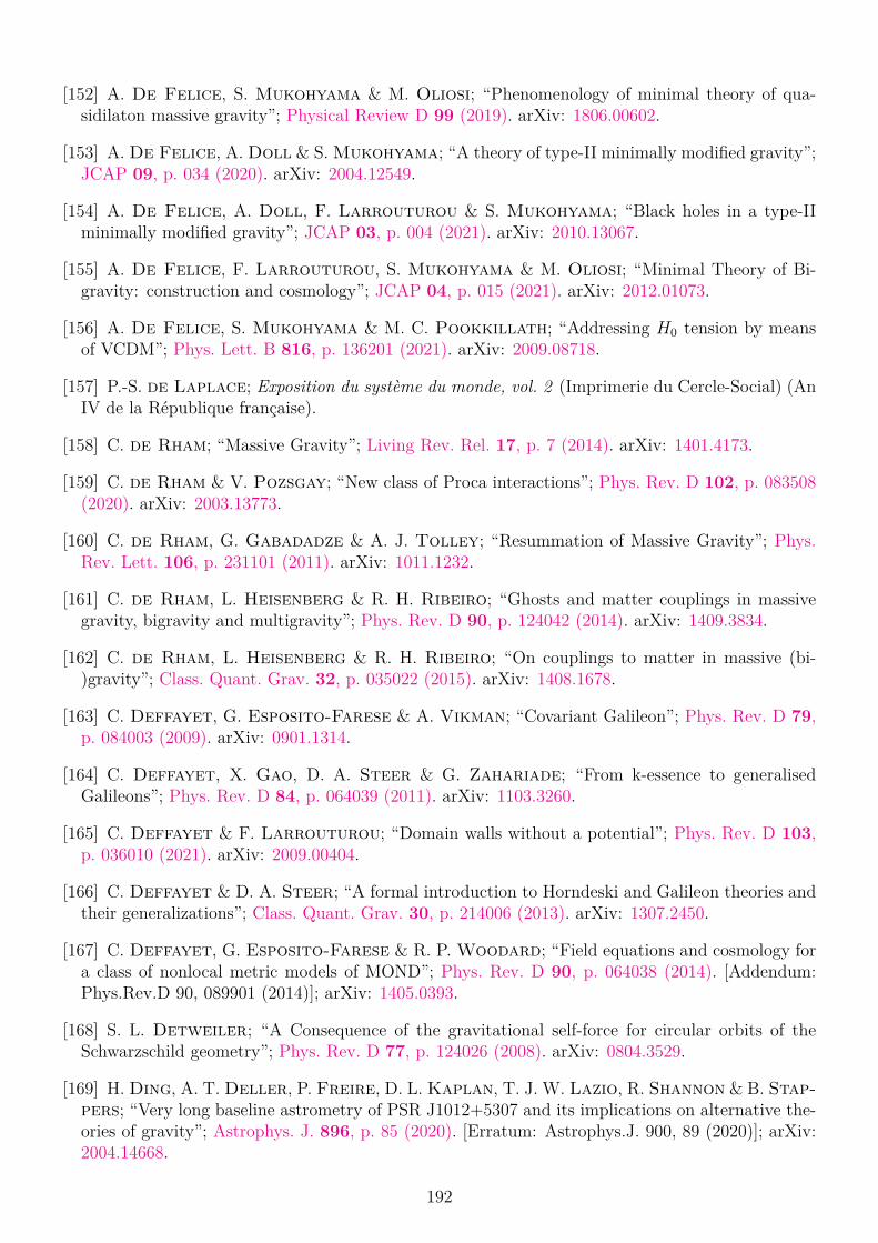
[152] A. De Felice, S. Mukohyama & M. Oliosi; “Phenomenology of minimal theory of qua-sidilaton massive gravity”; Physical Review D 99 (2019). arXiv: 1806.00602.

[153] A. De Felice, A. Doll & S. Mukohyama; “A theory of type-II minimally modified gravity”;JCAP 09, p. 034 (2020). arXiv: 2004.12549.

[154] A. De Felice, A. Doll, F. Larrouturou & S. Mukohyama; “Black holes in a type-IIminimally modified gravity”; JCAP 03, p. 004 (2021). arXiv: 2010.13067.

[155] A. De Felice, F. Larrouturou, S. Mukohyama & M. Oliosi; “Minimal Theory of Bi-gravity: construction and cosmology”; JCAP 04, p. 015 (2021). arXiv: 2012.01073.

[156] A. De Felice, S. Mukohyama & M. C. Pookkillath; “Addressing H0 tension by meansof VCDM”; Phys. Lett. B 816, p. 136201 (2021). arXiv: 2009.08718.

[157] P.-S. de Laplace; Exposition du système du monde, vol. 2 (Imprimerie du Cercle-Social) (AnIV de la République française).

[158] C. de Rham; “Massive Gravity”; Living Rev. Rel. 17, p. 7 (2014). arXiv: 1401.4173.

[159] C. de Rham & V. Pozsgay; “New class of Proca interactions”; Phys. Rev. D 102, p. 083508(2020). arXiv: 2003.13773.

[160] C. de Rham, G. Gabadadze & A. J. Tolley; “Resummation of Massive Gravity”; Phys.Rev. Lett. 106, p. 231101 (2011). arXiv: 1011.1232.

[161] C. de Rham, L. Heisenberg & R. H. Ribeiro; “Ghosts and matter couplings in massivegravity, bigravity and multigravity”; Phys. Rev. D 90, p. 124042 (2014). arXiv: 1409.3834.

[162] C. de Rham, L. Heisenberg & R. H. Ribeiro; “On couplings to matter in massive (bi-)gravity”; Class. Quant. Grav. 32, p. 035022 (2015). arXiv: 1408.1678.

[163] C. Deffayet, G. Esposito-Farese & A. Vikman; “Covariant Galileon”; Phys. Rev. D 79,p. 084003 (2009). arXiv: 0901.1314.

[164] C. Deffayet, X. Gao, D. A. Steer & G. Zahariade; “From k-essence to generalisedGalileons”; Phys. Rev. D 84, p. 064039 (2011). arXiv: 1103.3260.

[165] C. Deffayet & F. Larrouturou; “Domain walls without a potential”; Phys. Rev. D 103,p. 036010 (2021). arXiv: 2009.00404.

[166] C. Deffayet & D. A. Steer; “A formal introduction to Horndeski and Galileon theories andtheir generalizations”; Class. Quant. Grav. 30, p. 214006 (2013). arXiv: 1307.2450.

[167] C. Deffayet, G. Esposito-Farese & R. P. Woodard; “Field equations and cosmology fora class of nonlocal metric models of MOND”; Phys. Rev. D 90, p. 064038 (2014). [Addendum:Phys.Rev.D 90, 089901 (2014)]; arXiv: 1405.0393.

[168] S. L. Detweiler; “A Consequence of the gravitational self-force for circular orbits of theSchwarzschild geometry”; Phys. Rev. D 77, p. 124026 (2008). arXiv: 0804.3529.

[169] H. Ding, A. T. Deller, P. Freire, D. L. Kaplan, T. J. W. Lazio, R. Shannon & B. Stap-pers; “Very long baseline astrometry of PSR J1012+5307 and its implications on alternative the-ories of gravity”; Astrophys. J. 896, p. 85 (2020). [Erratum: Astrophys.J. 900, 89 (2020)]; arXiv:2004.14668.

192

[170] P. A. M. Dirac; Lectures on Quantum Mechanics; Belfer Graduate School of Science, mono-graph series (Dover Publications) (2001); ISBN 9780486417134.

[171] G. R. Dvali, G. Gabadadze & M. Porrati; “4-D gravity on a brane in 5-D Minkowskispace”; Phys. Lett. B 485, pp. 208–214 (2000). arXiv: hep-th/0005016.

[172] F. W. Dyson, A. S. Eddington & C. Davidson; “A Determination of the Deflection of Lightby the Sun’s Gravitational Field, from Observations Made at the Total Eclipse of May 29, 1919”;Philosophical Transactions of the Royal Society of London Series A 220, pp. 291–333 (1920).

[173] B. Edwards, L. Mugnai, G. Tinetti, E. Pascale & S. Sarkar; “An Updated Study ofPotential Targets for Ariel”; Astronom. J. 157, p. 242 (2019). arXiv: 1905.04959.

[174] A. Einstein; “Erklärung der Perihelbewegung des Merkur”; Sitz. der Kön. Preu. Ak. derWiss. pp. 831–839 (1915)https://einstein-annalen.mpiwg-berlin.mpg.de/related_texts/sitzungsberichte.

[175] A. Einstein; “Die Feldgleichungen der Gravitation”; Sitz. der Kön. Preu. Ak. derWiss. pp. 844–847 (1915)https://einstein-annalen.mpiwg-berlin.mpg.de/related_texts/sitzungsberichte.

[176] A. Einstein; “Anhang. Darstellung der Theorie ausgehend von einem Variationsprinzip”; Sitz.der Kön. Preu. Ak. der Wiss. pp. 340–345 (1916)https://einstein-annalen.mpiwg-berlin.mpg.de/related_texts/sitzungsberichte.

[177] A. Einstein; “Näherungsweise Integration der Feldgleichungen der Gravitation”; Sitz. derKön. Preu. Ak. der Wiss. pp. 688–696 (1916)https://einstein-annalen.mpiwg-berlin.mpg.de/related_texts/sitzungsberichte.

[178] A. Einstein; “Kosmologische Betrachtungen zur allgemeinen Relativitätstheorie”; Sitz. derKön. Preu. Ak. der Wiss. pp. 142–152 (1917)https://einstein-annalen.mpiwg-berlin.mpg.de/related_texts/sitzungsberichte.

[179] A. Einstein; “Über Gravitationswellen”; Sitz. der Kön. Preu. Ak. der Wiss.pp. 154–167 (1918)https://einstein-annalen.mpiwg-berlin.mpg.de/related_texts/sitzungsberichte.

[180] A. Einstein, L. Infeld & B. Hoffmann; “The Gravitational Equations and the Problem ofMotion”; Annals of Mathematics 39, pp. 65–100 (1938).

[181] K. Eppley; The numerical evolution of the collision of two black holes; Ph.D. thesis; PrincetonUniversity (1975).

[182] G. Esposito-Farese; “Comparing solar system, binary pulsar, and gravitational wave testsof gravity”; in “34th Rencontres de Moriond: Gravitational Waves and Experimental Gravity,”pp. 475–480 (1999); arXiv: gr-qc/9903058.

[183] D. Fabrycky; “Non-Keplerian dynamics of exoplanets”; Exoplanets, ed. S. Seager p. 217(2010).

[184] A. Falkowski & G. Isabella; “Matter coupling in massive gravity”; JHEP 04, p. 014 (2020).arXiv: 2001.06800.

[185] B. Famaey & S. McGaugh; “Modified Newtonian Dynamics (MOND): Observational Phe-nomenology and Relativistic Extensions”; Living Rev. Rel. 15, p. 10 (2012). arXiv: 1112.3960.

193

[186] V. Faraoni; “Evolving black hole horizons in General Relativity and alternative gravity”;Galaxies 1, pp. 114–179 (2013). arXiv: 1309.4915.

[187] G. Faye, S. Marsat, L. Blanchet & B. R. Iyer; “The third and a half post-Newtoniangravitational wave quadrupole mode for quasi-circular inspiralling compact binaries”; Class. Quant.Grav. 29, p. 175004 (2012). arXiv: 1204.1043.

[188] G. Faye, L. Blanchet & B. R. Iyer; “Non-linear multipole interactions and gravitational-wave octupole modes for inspiralling compact binaries to third-and-a-half post-Newtonian order”;Class. Quant. Grav. 32, p. 045016 (2015). arXiv: 1409.3546.

[189] M. Fierz & W. Pauli; “On Relativistic Wave Equations for Particles of Arbitrary Spin in anElectromagnetic Field”; Proceedings of the Royal Society of London Series A 173, pp. 211–232(1939).

[190] P. Figueira et al.; “Is the activity level of HD 80606 influenced by its eccentric planet?”Astron. Astrophys. 592, p. A143 (2016). arXiv: 1606.05549.

[191] D. G. Figueroa, M. Hindmarsh, J. Lizarraga & J. Urrestilla; “Irreducible backgroundof gravitational waves from a cosmic defect network: update and comparison of numerical tech-niques”; Phys. Rev. D 102, p. 103516 (2020). arXiv: 2007.03337.

[192] V. Fock; Theory of space, time and gravitation (Pergamon (London)) (1959).

[193] S. Foffa & R. Sturani; “Effective field theory methods to model compact binaries”; Class.Quant. Grav. 31, p. 043001 (2014). arXiv: 1309.3474.

[194] S. Foffa & R. Sturani; “Conservative dynamics of binary systems to fourth Post-Newtonianorder in the EFT approach I: Regularized Lagrangian”; Phys. Rev. D 100, p. 024047 (2019). arXiv:1903.05113.

[195] S. Foffa & R. Sturani; “Hereditary terms at next-to-leading order in two-body gravitationaldynamics”; Phys. Rev. D 101, p. 064033 (2020). arXiv: 1907.02869.

[196] S. Foffa, R. A. Porto, I. Rothstein & R. Sturani; “Conservative dynamics of binarysystems to fourth Post-Newtonian order in the EFT approach II: Renormalized Lagrangian”;Phys. Rev. D 100, p. 024048 (2019). arXiv: 1903.05118.

[197] E. B. Ford, M. Havlickova & F. A. Rasio; “Dynamical instabilities in extrasolar planetarysystems containing two giant planets”; Icarus 150, pp. 303–313 (2001). arXiv: astro-ph/0010178.

[198] S. J. Fossey, I. P. Waldmann & D. M. Kipping; “Detection of a transit by the planetarycompanion of HD 80606”; Mon. Not. Roy. Astr. Soc. 396, p. L16 (2009). arXiv: 0902.4616.

[199] J. L. Friedman, K. Uryu & M. Shibata; “Thermodynamics of binary black holes and neutronstars”; Phys. Rev. D 65, p. 064035 (2002). [Erratum: Phys.Rev.D 70, 129904 (2004)]; arXiv: gr-qc/0108070.

[200] R. Fujita; “Gravitational Waves from a Particle in Circular Orbits around a SchwarzschildBlack Hole to the 22nd Post-Newtonian Order”; Prog. Theor. Phys. 128, pp. 971–992 (2012).arXiv: 1211.5535.

[201] T. Fujita, S. Kuroyanagi, S. Mizuno & S. Mukohyama; “Blue-tilted Primordial Gravita-tional Waves from Massive Gravity”; Phys. Lett. B 789, pp. 215–219 (2019). arXiv: 1808.02381.

194

[202] Y. Fukuda et al.; “Evidence for oscillation of atmospheric neutrinos”; Phys. Rev. Lett. 81,pp. 1562–1567 (1998). arXiv: hep-ex/9807003.

[203] A. Garat & R. H. Price; “Nonexistence of conformally flat slices of the Kerr space-time”;Phys. Rev. D 61, p. 124011 (2000). arXiv: gr-qc/0002013.

[204] E. Garcia-Melendo & P. R. McCullough; “Photometric Detection of a Transit of HD80606b”; Astrophys. J. 698, p. 558 (2009). arXiv: 0902.4493.

[205] I. M. Gel’fand & G. E. Shilov; Generalized functions (Academic Press (New York)) (1964).

[206] P. Giacobbe et al.; “Five carbon- and nitrogen-bearing species in a hot giant planet’s atmo-sphere”; Nature 592, pp. 205–208 (2021).

[207] A. Gimenez; “General-relativistic periastron advances in eclipsing binary systems”; Astrophys.J. 405, p. 167 (1985)http://adsabs.harvard.edu/pdf/1985ApJ...297..405G.

[208] J. Gleyzes, D. Langlois, F. Piazza & F. Vernizzi; “Healthy theories beyond Horndeski”;Phys. Rev. Lett. 114, p. 211101 (2015). arXiv: 1404.6495.

[209] W. D. Goldberger & A. Ross; “Gravitational radiative corrections from effective field the-ory”; Phys. Rev. D 81, p. 124015 (2010). arXiv: 0912.4254.

[210] W. D. Goldberger & I. Z. Rothstein; “An Effective field theory of gravity for extendedobjects”; Phys. Rev. D 73, p. 104029 (2006). arXiv: hep-th/0409156.

[211] W. D. Goldberger, A. Ross & I. Z. Rothstein; “Black hole mass dynamics and renormal-ization group evolution”; Phys. Rev. D 89, p. 124033 (2014). arXiv: 1211.6095.

[212] P. Goldreich & R. Sari; “Eccentricity evolution for planets in gaseous disks”; Astrophys. J.585, pp. 1024–1037 (2003). arXiv: astro-ph/0202462.

[213] E. Gourgoulhon; “3+1 formalism and bases of numerical relativity”; (2007)arXiv: gr-qc/0703035.

[214] I. S. Gradshteyn & I. M. Ryzhik; Table of Integrals, Series, and Products (Academic Press)(2000); 6th edition.

[215] A. M. Green & B. J. Kavanagh; “Primordial Black Holes as a dark matter candidate”; J.Phys. G 48, p. 043001 (2021). arXiv: 2007.10722.

[216] A. Gullstrand; “Allgemeine Lösung des statischen Einkörperproblems in der EinsteinschenGravitationstheorie”; Ark. Mat. Astron. Fys. 16, p. 8 (1922).

[217] A. E. Gümrükçüoglu, C. Lin & S. Mukohyama; “Open FRW universes and self-acceleration from nonlinear massive gravity”; JCAP 11, p. 030 (2011). arXiv: 1109.3845.

[218] A. E. Gümrükçüoglu, L. Heisenberg, S. Mukohyama & N. Tanahashi; “Cosmology inbimetric theory with an effective composite coupling to matter”; JCAP 04, p. 008 (2015). arXiv:1501.02790.

[219] R. Hagala, A. De Felice, D. F. Mota & S. Mukohyama; “Nonlinear Dynamics of theMinimal Theory of Massive Gravity”; (2020); arXiv: 2011.14697.

[220] J. Hartung, J. Steinhoff & G. Schafer; “Next-to-next-to-leading order post-Newtonianlinear-in-spin binary Hamiltonians”; Annalen Phys. 525, pp. 359–394 (2013). arXiv: 1302.6723.

195

[221] S. F. Hassan & R. A. Rosen; “Bimetric Gravity from Ghost-free Massive Gravity”; JHEP02, p. 126 (2012). arXiv: 1109.3515.

[222] M. Hazumi et al.; “LiteBIRD: JAXA’s new strategic L-class mission for all-sky surveys ofcosmic microwave background polarization”; Proc. SPIE Int. Soc. Opt. Eng. 11443, p. 114432F(2020). arXiv: 2101.12449.

[223] G. Hébrard et al.; “Observation of the full 12-hour-long transit of the exoplanet HD80606b.Warm-Spitzer photometry and SOPHIE spectroscopy”; Astron. Astrophys. 516, p. A95 (2011).arXiv: 1004.0790.

[224] R. W. Hellings & K. Nordtvedt; “Vector-Metric Theory of Gravity”; Phys. Rev. D 7, pp.3593–3602 (1973).

[225] Q. Henry, G. Faye & L. Blanchet; “Tidal effects in the equations of motion of compactbinary systems to next-to-next-to-leading post-Newtonian order”; Phys. Rev. D 101, p. 064047(2020). arXiv: 1912.01920.

[226] Q. Henry, G. Faye & L. Blanchet; “Tidal effects in the gravitational-wave phase evolutionof compact binary systems to next-to-next-to-leading post-Newtonian order”; Phys. Rev. D 102,p. 044033 (2020). arXiv: 2005.13367.

[227] Q. Henry, G. Faye & L. Blanchet; “Hamiltonian for tidal interactions in compact binarysystems to next-to-next-to-leading post-Newtonian order”; Phys. Rev. D 102, p. 124074 (2020).arXiv: 2009.12332.

[228] Q. Henry, L. Blanchet & G. Faye; “The current-type quadrupole moment andgravitational-wave mode (ℓ,m) = (2, 1) of compact binary systems at the third post-Newtonianorder”; (2021)arXiv: 2105.10876.

[229] J. S. Heyl & B. J. Gladman; “Using long-term transit timing to detect terrestrial planets”;Mon. Not. Roy. Astr. Soc. 377, pp. 1511–1519 (2007). arXiv: astro-ph/0610267.

[230] M. G. Hidas et al.; “An ingress and a complete transit of HD80606 b”; Mon. Not. Roy. Astr.Soc. 406, p. 1146 (2010). arXiv: 1002.1052.

[231] A. Higuchi; “Forbidden Mass Range for Spin-2 Field Theory in De Sitter Space-time”; Nucl.Phys. B 282, pp. 397–436 (1987).

[232] M. B. Hindmarsh, M. Lüben, J. Lumma & M. Pauly; “Phase transitions in the earlyuniverse”; (2020). arXiv: 2008.09136.

[233] G. Hinshaw et al.; “Nine-year Wilkinson Microwave Anisotropy Probe (WMAP) Observations:Cosmological Parameter Results”; A. P. J. S. 208, 19 (2013). arXiv: 1212.5226.

[234] Homère; L’Odyssée, Chant II (La Découverte) (1982); trad. by P. Jaccottet.

[235] S. Hopper, C. Kavanagh & A. C. Ottewill; “Analytic self-force calculations in the post-Newtonian regime: eccentric orbits on a Schwarzschild background”; Phys. Rev. D 93, p. 044010(2016). arXiv: 1512.01556.

[236] G. W. Horndeski; “Second-Order Scalar-Tensor Field Equations in a Four-DimensionalSpace”; International Journal of Theoretical Physics 10, pp. 363–384 (1974).

[237] P. Hořava; “Quantum Gravity at a Lifshitz Point”; Phys. Rev. D 79, p. 084008 (2009). arXiv:0901.3775.

196

[238] R. A. Hulse & J. H. Taylor; “Discovery of a pulsar in a binary system.” Astrophys. J. 195,pp. L51–L53 (1975).

[239] L. Iorio; “Classical and relativistic long-term time variations of some observables for transitingexoplanets”; Mon. Not. Roy. Astr. Soc. 411, p. 167 (2011). arXiv: 1007.2780.

[240] W. Israel; “Thin shells in general relativity”; Nuovo Cimento 44B, p. 1 (1966).

[241] P. Jaranowski & G. Schaefer; “Third post-Newtonian higher order ADM Hamilton dy-namics for two-body point mass systems”; Phys. Rev. D 57, pp. 7274–7291 (1998). [Erratum:Phys.Rev.D 63, 029902 (2001)]; arXiv: gr-qc/9712075.

[242] J. T. Jebsen; “Über die allgemeinen Kugelsymmetrischen Lösungen der Einsteinschen Gravi-tationsgleichungen im Vakuum”; Arkiv for Mat. Astr. och Fys. 15, p. 18 (1921).

[243] A. Jordàn & G. Bakos; “Observability of the general relativistic precession of periastra inexoplanets”; Astrophys. J. 685, p. 543 (2008). arXiv: 0806.0630.

[244] P. Jordan; Schwerkraft und Weltall: Grundlagen der theoretischen Kosmologie. (Braun-schweig) (1952).

[245] G. Kälin & R. A. Porto; “From Boundary Data to Bound States”; JHEP 01, p. 072 (2020).arXiv: 1910.03008.

[246] G. Kälin & R. A. Porto; “From boundary data to bound states. Part II. Scattering angle todynamical invariants (with twist)”; JHEP 02, p. 120 (2020). arXiv: 1911.09130.

[247] G. Kälin & R. A. Porto; “Post-Minkowskian Effective Field Theory for Conservative BinaryDynamics”; JHEP 11, p. 106 (2020). arXiv: 2006.01184.

[248] G. Kälin, Z. Liu & R. A. Porto; “Conservative Tidal Effects in Compact Binary Sys-tems to Next-to-Leading Post-Minkowskian Order”; Phys. Rev. D 102, p. 124025 (2020). arXiv:2008.06047.

[249] G. Kälin, Z. Liu & R. A. Porto; “Conservative Dynamics of Binary Systems to Third Post-Minkowskian Order from the Effective Field Theory Approach”; Phys. Rev. Lett. 125, p. 261103(2020). arXiv: 2007.04977.

[250] J. H. Kang et al.; “2017 upgrade and performance of BICEP3: a 95GHz refracting telescopefor degree-scale CMB polarization”; Proc. SPIE Int. Soc. Opt. Eng. 10708, p. 107082N (2018).arXiv: 1808.00567.

[251] C. Kavanagh, A. C. Ottewill & B. Wardell; “Analytical high-order post-Newtonianexpansions for extreme mass ratio binaries”; Phys. Rev. D 92, p. 084025 (2015). arXiv: 1503.02334.

[252] R. P. Kerr; “Gravitational Field of a Spinning Mass as an Example of Algebraically SpecialMetrics”; Phys. Rev. Lett. 11, pp. 237–238 (1963).

[253] J. Khoury & A. Weltman; “Chameleon fields: Awaiting surprises for tests of gravity inspace”; Phys. Rev. Lett. 93, p. 171104 (2004). arXiv: astro-ph/0309300.

[254] R. Kimura, T. Tanaka, K. Yamamoto & Y. Yamashita; “Constraint on ghost-free bi-gravity from gravitational Cherenkov radiation”; Phys. Rev. D 94, p. 064059 (2016). arXiv:1605.03405.

197

[255] F. Könnig & L. Amendola; “Instability in a minimal bimetric gravity model”; Phys. Rev.D 90, p. 044030 (2014). arXiv: 1402.1988.

[256] Y. Kozai; “Secular perturbations of asteroids with high inclination and eccentricity”; As-tronom. J. 67, pp. 591–598 (1962).

[257] H. Lammer et al.; “Determining the mass loss limit for close-in exoplanets: what can we learnfrom transit observations?” Astron. Astrophys. 506, pp. 399–410 (2009).

[258] G. Laughlin, D. Deming, J. Langton, D. Kasen, S. Vogt, P. Butler, E. Rivera &S. Meschiari; “Rapid heating of the atmosphere of an extrasolar planet”; Nature 457, p. 562(2009).

[259] A. Le Tiec; “First Law of Mechanics for Compact Binaries on Eccentric Orbits”; Phys. Rev.D 92, p. 084021 (2015). arXiv: 1506.05648.

[260] A. Le Tiec, E. Barausse & A. Buonanno; “Gravitational Self-Force Correction to theBinding Energy of Compact Binary Systems”; Phys. Rev. Lett. 108, p. 131103 (2012). arXiv:1111.5609.

[261] A. Le Tiec, L. Blanchet & B. F. Whiting; “The First Law of Binary Black Hole Mechanicsin General Relativity and Post-Newtonian Theory”; Phys. Rev. D 85, p. 064039 (2012). arXiv:1111.5378.

[262] U. Le Verrier; Recherches sur les mouvements de la planète Herschel (Bachelier (Paris))(1846). http://hdl.handle.net/1908/3096.

[263] A. Lecavelier des Étangs; “A diagram for the evaporation status of extrasolar planets”;Astron. Astrophys. 461, p. 1185 (2007). arXiv: astro-ph/0609744.

[264] A. K. Leibovich, N. T. Maia, I. Z. Rothstein & Z. Yang; “Second post-Newtonian orderradiative dynamics of inspiralling compact binaries in the Effective Field Theory approach”; Phys.Rev. D 101, p. 084058 (2020). arXiv: 1912.12546.

[265] S.-L. Li, L. Shao, P. Wu & H. Yu; “NANOGrav Signal from First-Order Confine-ment/Deconfinement Phase Transition in Different QCD Matters”; (2021)arXiv: 2101.08012.

[266] M. L. Lidov; “The evolution of orbits of artificial satellites of planets under the action of grav-itational perturbations of external bodies”; Planetary and Space Science 9, pp. 719–759 (1962).

[267] C. Lin; “The self-consistent matter coupling of a class of minimally modified gravity theories”;Journal of Cosmology and Astroparticle Physics 2019, p. 037 (2019). arXiv: 1811.02467.

[268] C. Lin & Z. Lalak; “Novel matter coupling in Einstein gravity”; (2019)arXiv: 1911.12026.

[269] C. Lin & S. Mukohyama; “A class of minimally modified gravity theories”; Journal of Cos-mology and Astroparticle Physics 2017, p. 033 (2017). arXiv: 1708.03757.

[270] H. A. Lorentz & J. Droste; “The Motion of a System of Bodies under the Influence oftheir Mutual Attraction, According to Einstein’s Theory”; Collected Papers: Volume V (SpringerNetherlands) pp. 330–355 (1917). Trad. of Versl. K. Akad. Wet. Amsterdam. 26, 392, (1917).

[271] D. Lovelock; “The Einstein Tensor and Its Generalizations”; Journal of MathematicalPhysics 12, pp. 498–501 (1971).

198

[272] C. Lovis & D. Fischer; “Radial Velocity Techniques for Exoplanets”; Exoplanets, ed. S.Seager pp. 27–53 (2010).

[273] K.-i. Maeda & M. S. Volkov; “Anisotropic universes in the ghost-free bigravity”; Phys. Rev.D 87, p. 104009 (2013). arXiv: 1302.6198.

[274] M. Maggiore & M. Mancarella; “Nonlocal gravity and dark energy”; Phys. Rev. D 90, p.023005 (2014). arXiv: 1402.0448.

[275] N. Manton & P. Sutcliffe; Topological solitons; Cambridge Monographs on MathematicalPhysics (Cambridge University Press) (2004); ISBN 978-0-511-20783-9.

[276] T. Marchand, L. Blanchet & G. Faye; “Gravitational-wave tail effects to quartic non-linear order”; Class. Quant. Grav. 33, p. 244003 (2016). arXiv: 1607.07601.

[277] T. Marchand, L. Bernard, L. Blanchet & G. Faye; “Ambiguity-Free Completion of theEquations of Motion of Compact Binary Systems at the Fourth Post-Newtonian Order”; Phys.Rev. D 97, p. 044023 (2018). arXiv: 1707.09289.

[278] T. Marchand, Q. Henry, F. Larrouturou, S. Marsat, G. Faye & L. Blanchet; “Themass quadrupole moment of compact binary systems at the fourth post-Newtonian order”; Class.Quant. Grav. 37, p. 215006 (2020). arXiv: 2003.13672.

[279] J. M. Martín-García, A. García-Parrado, A. Stecchina, B. Wardell, C. Pitrou,D. Brizuela, D. Yllanes, G. Faye, L. Stein, R. Portugal & T. Bäckdahl; “xAct: Efficienttensor computer algebra for Mathematica”; (GPL 2002–2012); http://www.xact.es/.

[280] Matthew; Gospel, 25:29 (ed. Jerusalem).

[281] F. Messina & A. Nagar; “Parametrized-4.5PN TaylorF2 approximants and tail effects toquartic nonlinear order from the effective one body formalism”; Phys. Rev. D 95, p. 124001(2017). [Erratum: Phys.Rev.D 96, 049907 (2017)]; arXiv: 1703.08107.

[282] J. Michell; “Letter to Henry Cavendish”; Phil. Trans. of the Roy. Soc. of London 74, pp.35–57 (1784).

[283] A. Michelson; “Some of the Objects and Methods of Physical Science”; University of ChicagoQuaterly Calendar p. 15 (1894).

[284] M. Milgrom; “A modification of the Newtonian dynamics as a possible alternative to thehidden mass hypothesis.” A. P. J. 270, pp. 365–370 (1983).

[285] C. W. Misner, K. S. Thorne & J. A. Wheeler; Gravitation (W. H. Freeman and Company)(1973).

[286] C. W. Misner & D. H. Sharp; “Relativistic Equations for Adiabatic, Spherically SymmetricGravitational Collapse”; Phys. Rev. 136, pp. B571–B576 (1964).

[287] G. D. Moore & A. E. Nelson; “Lower bound on the propagation speed of gravity fromgravitational Cherenkov radiation”; JHEP 09, p. 023 (2001). arXiv: hep-ph/0106220.

[288] C. Moutou et al.; “Photometric and spectroscopic detection of the primary transit of the111-day-period planet HD 80 606 b”; Astron. Astrophys. 498, p. L5 (2009). arXiv: 0902.4457.

[289] S. Mukohyama & K. Noui; “Minimally modified gravity: a Hamiltonian construction”; Jour-nal of Cosmology and Astroparticle Physics 2019, p. 049 (2019). arXiv: 1905.02000.

199

[290] D. Naef et al.; “HD 80606b, a planet on an extremely elongated orbit”; Astron. Astrophys.375, p. L27 (2001). arXiv: astro-ph/0106256.

[291] E. T. Newman & A. I. Janis; “Note on the Kerr Spinning-Particle Metric”; Journal of Math-ematical Physics 6, pp. 915–917 (1965).

[292] E. T. Newman, E. Couch, K. Chinnapared, A. Exton, A. Prakash & R. Torrence;“Metric of a Rotating, Charged Mass”; Journal of Mathematical Physics 6, pp. 918–919 (1965).

[293] I. Newton; Philosophiæ naturalis principia mathematica (1756); trad. by E. du Châtelet.

[294] A. Nicolis, R. Rattazzi & E. Trincherini; “The Galileon as a local modification of gravity”;Phys. Rev. D 79, p. 064036 (2009). arXiv: 0811.2197.

[295] H. Niikura et al.; “Microlensing constraints on primordial black holes with Subaru/HSCAndromeda observations”; Nature Astron. 3, pp. 524–534 (2019). arXiv: 1701.02151.

[296] E. Noether; “Invariante Variationsprobleme”; Nachrichten von der Gesellschaft der Wis-senschaften zu Göttingen 1918, pp. 235–257 (1918)http://eudml.org/doc/59024.

[297] G. Nordström; “On the Energy of the Gravitation field in Einstein’s Theory”; KoninklijkeNederlandse Akademie van Wetenschappen Proceedings Series B Physical Sciences 20, pp. 1238–1245 (1918).

[298] W. Occam; Quatuor libros Sententiarum cum centilogio theologico (1319).

[299] P. Painlevé; “La mécanique classique et la théorie de la relativité”; C. R. Acad. Sci. (Paris)173, pp. 677–680 (1921).

[300] A. Pàl & B. Kocsis; “Periastron precession measurements in transiting extrasolar planetarysystems at the level of general relativity”; Mon. Not. Roy. Astr. Soc. 389, p. 191 (2008). arXiv:0806.0629.

[301] P. J. E. Peebles & B. Ratra; “The Cosmological Constant and Dark Energy”; Rev. Mod.Phys. 75, pp. 559–606 (2003). arXiv: astro-ph/0207347.

[302] P. Pellegrin; Le vocabuaire d’Aristote (Ellipses) (2009).

[303] R. Penrose; “Zero Rest-Mass Fields Including Gravitation: Asymptotic Behaviour”; Proc. ofthe Roy. Soc. of London Series A 284, pp. 159–203 (1965).

[304] R. Penrose; “Asymptotic Properties of Fields and Space-Times”; Phys. Rev. Lett. 10, pp.66–68 (1963).

[305] S. Perlmutter et al.; “Measurements of Ω and Λ from 42 high redshift supernovae”; Astro-phys. J. 517, pp. 565–586 (1999). arXiv: astro-ph/9812133.

[306] L. Pogosian & M. Wyman; “B-modes from cosmic strings”; Phys. Rev. D 77, p. 083509(2008). arXiv: 0711.0747.

[307] F. Pont et al.; “Spin-orbit misalignment in the HD 80606 planetary system”; Astron. Astro-phys. 502, p. 695 (2009). arXiv: 0906.5605.

[308] R. A. Porto; “The effective field theorist’s approach to gravitational dynamics”; Phys. Rept.633, pp. 1–104 (2016). arXiv: 1601.04914.

200

[309] R. V. Pound & G. A. Rebka; “Gravitational Red-Shift in Nuclear Resonance”; PRL 3, pp.439–441 (1959).

[310] F. Pretorius; “Evolution of binary black hole spacetimes”; Phys. Rev. Lett. 95, p. 121101(2005). arXiv: gr-qc/0507014.

[311] P. Ramond & A. Le Tiec; “Multipolar Particles in Helically Symmetric Spacetimes”;(2020)arXiv: 2005.00602.

[312] B. Ratra & P. J. E. Peebles; “Cosmological consequences of a rolling homogeneous scalarfield”; Phys. Rev. D 37, pp. 3406–3427 (1988).

[313] H. Reissner; “Über die Eigengravitation des elektrischen Feldes nach der Einsteinschen The-orie”; Annalen der Physik 355, pp. 106–120 (1916).

[314] A. G. Riess et al.; “Observational evidence from supernovae for an accelerating universe anda cosmological constant”; Astron. J. 116, pp. 1009–1038 (1998). arXiv: astro-ph/9805201.

[315] M. Riesz; “L’intégrale de Riemann-Liouville et le problème de Cauchy”; Acta Mathematica81, pp. 1 – 222 (1949).

[316] R. A. Rosen; “Black Hole Mechanics for Massive Gravitons”; Phys. Rev. D 98, p. 104008(2018). arXiv: 1805.12135.

[317] V. C. Rubin, J. Ford, W. K., N. Thonnard & D. Burstein; “Rotational properties of 23Sbgalaxies.” Astrophys. J. 261, pp. 439–456 (1982).

[318] A. I. Sabra; “The Andalusian revolt against Ptolemaic astronomy: Averroes and al-Bitrûjî”;Transformation and Tradition in the Sciences: Essays in honor of I. Bernard Cohen pp. 133–153(1984).

[319] R. K. Sachs; “Gravitational Waves in General Relativity. VIII. Waves in Asymptotically FlatSpace-Time”; Proc. of the Roy. Soc. of London Series A 270, pp. 103–126 (1962).

[320] A. D. Sakharov; “Vacuum Quantum Fluctuations In Curved Space And The Theory OfGravitation”; Sov. Phys. Dokl. 12, p. 104 (1968).

[321] J. Sangtawee & K. Karwan; “Inflationary model in minimally modified gravity theories”;(2021)arXiv: 2103.11463.

[322] S. Sarangi; “DBI global strings”; JHEP 07, p. 018 (2008). arXiv: 0710.0421.

[323] J. Schneider, C. Dedieu, P. Le Sidaner, R. Savalle & I. Zolotukhin; “Defining andcataloging exoplanets: the exoplanet.eu database”; Astron. Astrophys. 532, p. A79 (2011). arXiv:1106.0586.

[324] B. F. Schutz & R. Sorkin; “Variational aspects of relativistic field theories, with applicationto perfect fluids”; Annals Phys. 107, pp. 1–43 (1977).

[325] K. Schwarzschild; “Über das Gravitationsfeld eines Massenpunktes nach der EinsteinschenTheorie”; Sitz. der Kön. Preu. Ak. der Wiss. pp. 189–196 (1916)https://archive.org/details/sitzungsberichte1916deutsch/page/188/mode/2up?view=theater.

[326] J. Scott-Russell; “Report on Waves: Made to the Meetings of the British Association”;(1845). https://archive.org/details/reportonwavesma00russgoog.

201

[327] U. Seljak, U.-L. Pen & N. Turok; “Polarization of the microwave background in defectmodels”; Phys. Rev. Lett. 79, pp. 1615–1618 (1997). arXiv: astro-ph/9704231.

[328] A. G. Shah, J. L. Friedman & B. F. Whiting; “Finding high-order analytic post-Newtonianparameters from a high-precision numerical self-force calculation”; Phys. Rev. D 89, p. 064042(2014). arXiv: 1312.1952.

[329] Y. M. Shnir; Topological and Non-Topological Solitons in Scalar Field Theories (CambridgeUniversity Press) (2018); ISBN 978-1-108-63625-4.

[330] L. Smarr; “Space-time generated by computes: black holes with gravitational radiation”;Annals of the New York Academy of Sciences 302, pp. 569–604 (1977).

[331] A. A. Starobinsky; “A new type of isotropic cosmological models without singularity”;Physics Letters B 91, pp. 99–102 (1980).

[332] H. Stephani; Relativity: An introduction to special and general relativity (Cambridge Univer-sity Press) (2004).

[333] E. C. G. Stückelberg; “Die Wechselwirkungs Kräfte in der Elektrodynamik und in derFeldtheorie der Kernkräfte”; Helv. Phys. Acta 11, pp. 225–244 (1938).

[334] W. Thomson; “Nineteenth-Century Clouds over the Dynamical Theory of Heat and Light”;Philosophical Magazine and Journal of Science pp. 1–40 (1901)https://www.equipes.lps.u-psud.fr/Montambaux/histoire-physique/Kelvin-1900.pdf.

[335] K. S. Thorne; “Multipole expansions of gravitational radiation”; Rev. Mod. Phys. 52, pp.299–339 (1980).

[336] P. Touboul et al.; “Space test of the Equivalence Principle: first results of the MICROSCOPEmission”; Class. Quant. Grav. 36, p. 225006 (2019). arXiv: 1909.10598.

[337] A. Triaud; “The Rossiter-McLaughlin Effect in Exoplanet Research”; Handbook of Exoplan-ets, ed. H. J. Deeg and J. A. Belmonte (2018). arXiv: 1709.06376.

[338] R. B. Tully, O. de Marseille & J. R. Fisher; “A New Method of Determining Distancesto Galaxies”; in “Bulletin of the American Astronomical Society,” , vol. 7p. 426 (1975).

[339] S. D. Upton & A. Pound; “Second-order gravitational self-force in a highly regular gauge”;(2021)arXiv: 2101.11409.

[340] T. Vachaspati; Kinks and domain walls: An introduction to classical and quantum solitons(Cambridge University Press) (2010); ISBN 978-0-511-24290-8.

[341] H. van Dam & M. Veltmann; “On the mass of the graviton”; Gen. Rel. Grav. 3, pp. 215–220(1972).

[342] E. P. Verlinde; “On the Origin of Gravity and the Laws of Newton”; JHEP 04, p. 029 (2011).arXiv: 1001.0785.

[343] J.-P. Vernant; “Géométrie et astronomie sphérique dans la première cosmologie grecque”; LaPensée 109, pp. 82–92 (1963).

[344] J.-P. Vernant; “Structures géométriques et notions politiques das la cosmologied’Anaximandre”; Eirene. Studia Græca et Latina VII, pp. 5–23 (1968).

202

[345] A. Vilenkin & E. S. Shellard; Cosmic Strings and Other Topological Defects (CambridgeUniversity Press) (2000); ISBN 978-0-521-65476-0.

[346] V. Viswanathan et al.; “Extending Science from Lunar Laser Ranging”; (2020)arXiv:2008.09584.

[347] T. A. Wagner, S. Schlamminger, J. H. Gundlach & E. G. Adelberger; “Torsion-balance tests of the weak equivalence principle”; Class. Quant. Grav. 29, p. 184002 (2012). arXiv:1207.2442.

[348] R. M. Wald; General Relativity (University of Chicago Press) (1984).

[349] E. J. Weinberg; Classical solutions in quantum field theory: Solitons and Instantons in HighEnergy Physics; Cambridge Monographs on Mathematical Physics (Cambridge University Press)(2012); ISBN 978-1-107-43805-7.

[350] S. Weinberg; “The cosmological constant problem”; Rev. Mod. Phys. 61, pp. 1–23 (1989).

[351] J. M. Weisberg & J. H. Taylor; “Relativistic binary pulsar B1913+16: Thirty years ofobservations and analysis”; ASP Conf. Ser. 328, p. 25 (2005)arXiv: astro-ph/0407149.

[352] C. Wetterich; “Effective nonlocal Euclidean gravity”; Gen. Rel. Grav. 30, pp. 159–172(1998). arXiv: gr-qc/9704052.

[353] C. M. Will; Theory and Experiment in Gravitational Physics (Cambridge University Press)(1993).

[354] C. M. Will; “The Confrontation between General Relativity and Experiment”; Living Rev.Rel. 17, p. 4 (2014). arXiv: 1403.7377.

[355] C. M. Will & K. J. Nordtvedt; “Conservation Laws and Preferred Frames in RelativisticGravity. I. Preferred-Frame Theories and an Extended PPN Formalism”; APJ 177, p. 757 (1972).

[356] J. N. Winn et al.; “The Transit Ingress and the Tilted Orbit of the Extraordinarily EccentricExoplanet HD 80606b”; Astrophys. J. 703, p. 2091 (2009). arXiv: 0907.5205.

[357] M. Wolf et al.; “Relativistic apsidal motion in eccentric eclipsing binaries”; Astron. Astrophys.509, p. A18 (2010).

[358] Wolfram Research, Inc.; “Mathematica, Version 12.1”; https://www.wolfram.com/mathematica; Champaign, IL, 2020.

[359] R. P. Woodard; “Nonlocal Models of Cosmic Acceleration”; Found. Phys. 44, pp. 213–233(2014). arXiv: 1401.0254.

[360] J. T. Wright; “Radial Velocities as an Exoplanet Discovery Method”; Handbook of Exoplan-ets, ed. H. J. Deeg and J. A. Belmonte (2018). arXiv: 1707.07983.

[361] Y. Wu & N. Murray; “Planet migration and binary companions: The case of HD 80606b”;Astrophys. J. 589, pp. 605–614 (2003). arXiv: astro-ph/0303010.

[362] Y. Yamashita, A. De Felice & T. Tanaka; “Appearance of Boulware–Deser ghost in bigrav-ity with doubly coupled matter”; Int. J. Mod. Phys. D 23, p. 1443003 (2014). arXiv: 1408.0487.

[363] Z.-B. Yao, M. Oliosi, X. Gao & S. Mukohyama; “Minimally modified gravity with anauxiliary constraint: a Hamiltonian construction”; (2020); arXiv: 2011.00805.

[364] Y. Zhong, R.-Z. Guo, C.-E. Fu & Y.-X. Liu; “Kinks in higher derivative scalar field theory”;Physics Letters B 782, pp. 346–352 (2018). arXiv: 1804.02611.

François LARROUTUROU 18 juin 2021

Méthodes analytiques pour l’étude du problème à deuxcorps, et des théories alternatives de gravitation

Résumé : Le travail effectué durant cette thèse visait à parfaire notre connaissance desphénomènes gravitationnels, en poursuivant deux buts: (i) améliorer notre compréhensiondu problème relativiste à deux corps, (ii) construire et tester des modèles alternatifs.Dans un premier temps, nous avons utilisé une approximation post-Newtonienne (champset vitesses faibles) pour chercher une expression analytique et très précise de la phasedes ondes gravitationnelles. Pour ce faire, nous avons dû implémenter une régularisationdimensionnelle pour le quadrupole de masse, et pour les effets non-linéaires dits de “sillage”et de “mémoire”. En exploitant des synergies communes avec d’autres méthodes, nousavons aussi calculé les contributions logarithmiques qui entrent dans l’énergie conservée,jusqu’à une haute précision. Enfin, nous avons proposé le premier test réaliste de la RGdans un système exoplanétaire.Quant au second but, nous avons étudié des murs de domaine originaux, en proposant unenouvelle classe de défauts non-topologiques. Nous avons prouvé leur stabilité, et montréqu’ils peuvent imiter les défauts canoniques. De plus, nous avons construit et étudié lacosmologie d’une “théorie minimale de bigravité”, basée sur le principe du rasoir d’Occam.Pour finir, nous avons étudié le régime de champs forts de deux théories “minimales” enconstruisant leurs solutions de trous noirs.Mots clés : Problème à deux corps, défauts non-topologiques, théories alternatives

Analytical methods for the study of the two-bodyproblem, and alternative theories of gravitation

Abstract: The work completed during this thesis aimed at pushing forward our knowledgeof gravitational phenomena, by following two directions: (i) deepening our comprehensionof the relativistic two-body problem, (ii) building and testing alternative models.First, we used a post-Newtonian (weak-field and slow motion) approximation to seek an-alytic expressions for the phase of gravitational waves at high accuracy. Two of the mainresults of this thesis are thus the proper dimensional regularization of the mass quadrupole,and of the non-linear “tail” and “memory” effects, appearing in the radiative quadrupole.Using synergies with other approaches, we have also derived the logarithmic tail contri-butions in the conserved energy at high accuracies. Finally, and as a side result, we havealso proposed the first realistic test of GR in an exoplanetary system.As for the second direction, we have investigated non-canonical domain walls by building anew class of non-topological kinks. We have shown that those were stable, and could mimicthe canonical ones. A “minimal theory of bigravity” was also constructed by requiringto avoid observationally unnecessary gravitational polarizations, and its cosmology wasproven stable. Finally, we have investigated the strong-field regime of two of such minimaltheories by deriving their (non-trivial) black hole solutions.Keywords : Two-body problem, non-topological defects, alternatives theories