Analytical approximations of the nonlinear Schrödinger...

Analytical approximations of the nonlinear Schrödinger

equation: applications to optical communications and

information theory

M. Secondini, D. Marsella, E. Forestieri

Nonlinear Evolution Equations and Linear Algebra

September 2%5, 2013, Cagliari, Italy

Supported in part by MIUR under the FIRB project COTONE

© 2013 Scuola Superiore Sant’Anna

Outline

• First, I’ll try to answer the following questions:

– What are typical problems concerning the nonlinear Schrödinger

equation (NLSE) in fiber%optic communication?

– Why the inverse scattering transform (IST) is not employed in this

case?

– Why the split�step Fourier method (SSFM) is widely employed?

– Are there other options?

• Then, I’ll introduce a few concepts from information theory and a

specific problem involving the NLSE.

• Finally, I’ll show how we can (approximately and partially) solve it

by using an approximate analytical solution of the NLSE.


Digital communications in a nutshell

Typical problems

• Transmission techniques: how to map information bits on x(t) ?

• Detection strategies: how to retrieve information bits from y(t) ?

• Performance evaluation: what is the error probability ?

• Information theoretical limits: what is channel capacity (maximum

information rate for reliable transmission) ?

TX Channel RX…101101… …101101…x(t) y(t)

Modulated signals (e.g., the EM field)

What about fiber�optic communications?

• Propagation of the signal through the fiber%optic link is governed by

the nonlinear Schrödinger equation (NLSE)


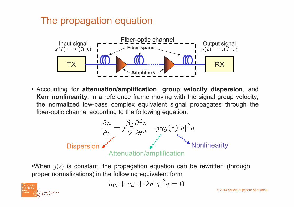
• Accounting for attenuation/amplification, group velocity dispersion, and

Kerr nonlinearity, in a reference frame moving with the signal group velocity,

the normalized low%pass complex equivalent signal propagates through the

fiber%optic channel according to the following equation:

Dispersion Nonlinearity

Attenuation/amplification

TX

Fiber spans

Amplifiers

RX

Fiber%optic channelInput signal Output signal

The propagation equation

•When g(z) is constant, the propagation equation can be rewritten (through

proper normalizations) in the following equivalent form


Deterministic problem

Given the input signal at z=0 and

the evolution equationEvaluate the output signal at z=L

– Information bits mapped on

– Pulse shape p(t)

– Time duration: very long (K~billions), but can be properly truncated to a shorter length T

– Limited bandwidth: P(f)≃0 for |f|>B/2, with B of the order of 1/Ts

Typically:

• β2 and γ are constant or step%wise constant

• g(z): alternating exponential decay and concentrated amplification

• Input signal: pulse amplitude modulation (PAM)

t……


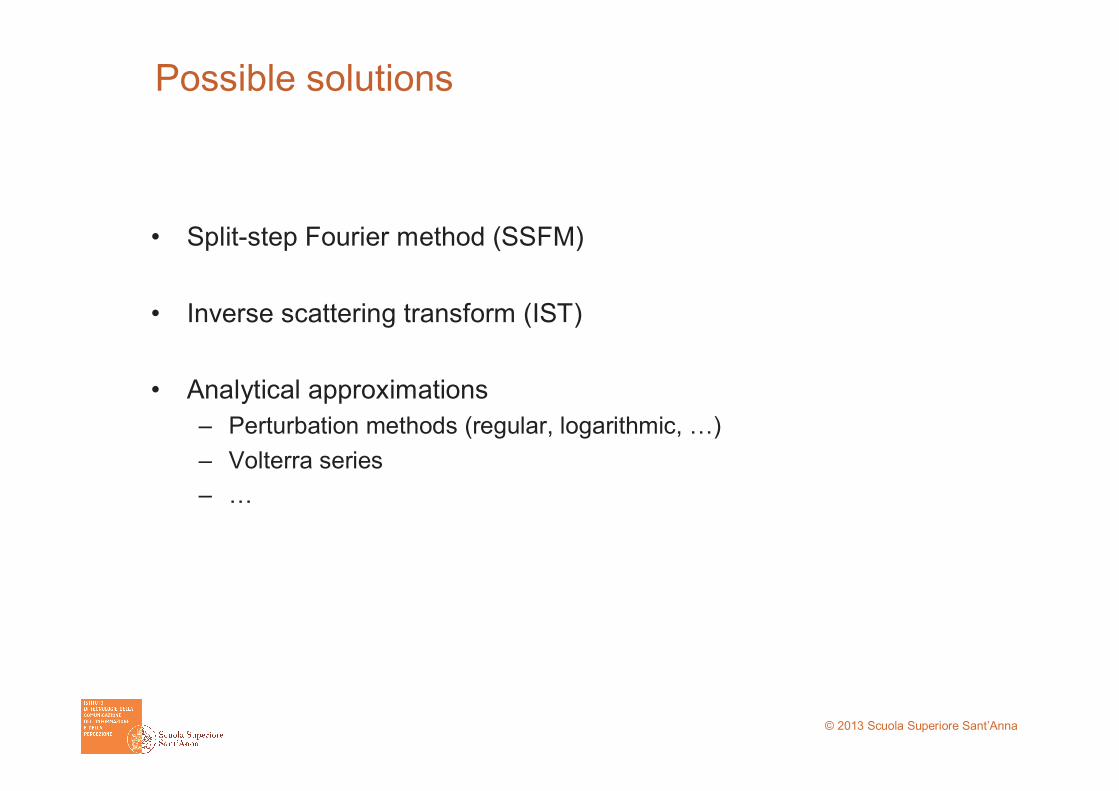
Possible solutions

• Split%step Fourier method (SSFM)

• Inverse scattering transform (IST)

• Analytical approximations

– Perturbation methods (regular, logarithmic, …)

– Volterra series

– …


Why SSFM is hard to beat in this case?

• It works in any practical system

• Its accuracy can be increased at will (by increasing computational

complexity)

• Among known numerical methods, it has the lowest complexity

(for a desired accuracy)

• Both theory and implementation are very simple


• Propagation of a signal of duration T and bandwidth B through a fiber

of length L requires the computation of 2M FFT of size N, where

– N=BT is the total number of signal samples

– M=L/dz is the number of propagation steps, where dz is the step size

• The global error decreases quadratically with the step size dz

� Computational complexity (number of multiplications per output

sample) is

– M: trade off between accuracy and complexity

– N: propagation of a long signal performed by overlap & save, dividing it

into shorter overlapping blocks of duration T≥Tm, where Tm is channel

memory). Typically, N≈4πβ2LB2

SSFM computational complexity


SSFM limitations

• It does not provide a closed�form expression of the output signal

• An even lower computational complexity is desirable


Why IST is not employed in this case?

• The evolution equation is not integrable in the general case, but for specific attenuation/amplification profiles (e.g., g(z) constant)

• Computational complexity of direct and inverse scattering can be very high (and increases much faster than logN per sample)

• IST theory is quite involved for beginners.


What about analytical approximations?

• There are several:

– Regular perturbation (RP), equivalent to Volterra series.

– Logarithmic perturbation (LP), more accurate.

• Typically, they don’t provide significant computational gain with

respect to SSFM for the solution of the deterministic problem

• However, they provide some physical insight and are a valuable

tool for the analysis and design of fiber%optic systems.

� After recalling the RP and LP approximation, I’ll introduce a

modified LP approximation, with a simpler 1st%order term but similar

accuracy, and show its application to a specific problem.


• The NLSE solution is expanded in power series in γ (nonlinearity is a small

additive perturbation of the linear signal)

…

• By substituting it into the NLSE, we obtain:

linear solution

…

1st�order perturbation

is the impulse response in linear regime

Regular perturbation (RP)


• We have proposed the following alternative expansion in γ (nonlinearity is a small

multiplicative perturbation of the linear signal)

LP terms are simply related to RP terms:

same complexity, higher accuracy!

• By substituting it into the NLSE, we obtain:

…

1st�order perturbation

linear solution

…

Logarithmic perturbation (LP)


A simplified (linearized) propagation equation

• Linear Schrödinger equation with time and space varying potential

• Preserves the L2 norm as the original equation.

• u0 evaluated analytically

• Good approximation to the original equation

• Equivalent to the original equation when considering a 1st%order

approximated solution based on RP or LP.

Potential |u|2 of the NLS is replaced by the approximation |u0|2

is the linearly propagated signal (for γ=0)


• Represent input signal through its Fourier transform U(f)

• Solve the propagation equation separately for each frequency component by

using a 1st%order LP approximation

• Recombine all the components at the output (exploit linearity of the equation)

Frequency%resolved logarithmic perturbation

perturbation term

nonlinear interaction efficiency

(for g(z)=1 and β2=const.)


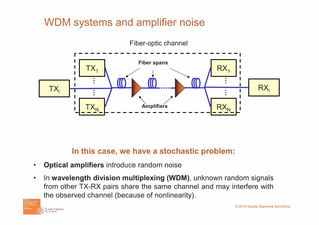
WDM systems and amplifier noise

In this case, we have a stochastic problem:

• Optical amplifiers introduce random noise

• In wavelength division multiplexing (WDM), unknown random signals

from other TX%RX pairs share the same channel and may interfere with

the observed channel (because of nonlinearity).

TXiRXi

TX1

Fiber spans

AmplifiersTXN RXN

…

RX1

…

……

Fiber%optic channel


• NLS equation modified to include cross�phase modulation (XPM) from other

copropagating signals and optical noise:

– Noise ni from i%th amplifier is added at z=zi

– ni: independent complex zero%mean white Gaussian processes with PSD Ni

Typically:

• u(0,t) and w(0,t): PAM signals (at different center frequencies) with i.i.d. symbols

• F(z,t): white Gaussian noise (space and time uncorrelated)

evaluate some output statistic

e.g.,

Given the evolution equation and

the statistical properties of

u(0,t), w(0,t), and F(z,t)

Stochastic problem


Solution methods

• SSFM and Monte Carlo method

• Analytical Approximations and Analysis

• What about inverse scattering transform?


A problem from information theory: channel capacity

Channel capacity

• What is the maximum rate at which information can be reliably transmitted

through the channel?

– Maximum: any modulation, encoding, and decoding is possible

– Reliably: with arbitrarily low error probability

� It depends on channel characteristics. Analytical solutions are available for

a few classes of channels.

TX Channel RX…101101… …101101…x(t) y(t)

Fiber�optic channel

In this case, propagation through the channel is governed by the NLSE and

the problem has not yet been completely solved.


• Mutual information between xxxxN and yyyyN

• Average mutual information rate for ergodic processes

• Capacity: supremum of the mutual information rate taken over all possible

input distributions satisfying some constraints

Mutual information and capacity

ChannelxxxxN yyyyN

Noisy channel coding theorem (Shannon, 1948)

There exist channel codes that make it possible to achieve reliable

communication if the transmission rate is R<C. If R>C, it is not possible to

achieve reliable communication with any code.


Waveform channels

• x(t) and y(t) are expanded into a complete set of orthonormal functions

and represented by the corresponding coefficients

• Shannon’s sampling theorem: a band%limited signal x(t) of bandwidth

B/2 can be represented through its samples taken at rate B

Channelx(t) y(t)

ChannelxxxxN yyyyN


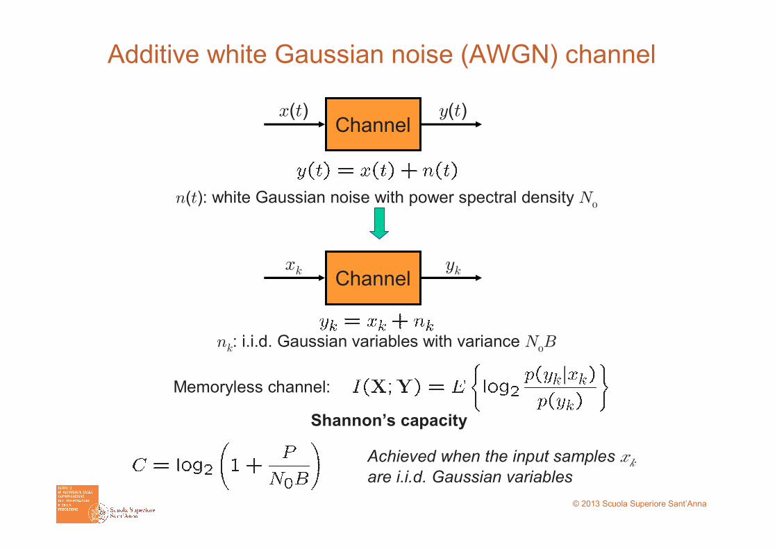
Additive white Gaussian noise (AWGN) channel

Shannon’s capacity

n(t): white Gaussian noise with power spectral density N

Channelx(t) y(t)

Channelxk yk

nk: i.i.d. Gaussian variables with variance NB

Memoryless channel:

Achieved when the input samples xkare i.i.d. Gaussian variables


• Processing theorem:

� Same channel capacity as the AWGN channel

Fiber%optic channel: linear regime (γ=0)

Channelx(t) y(t)

n(t): white Gaussian noise

with power spectral density

AWGN channel!


Fiber%optic channel: XPM+AWGN

~ compensated by processingapproximated as AWGN

Channelx(t) y(t)

approximated by linear propagation

FRLP solution:

XPM term

nonlinear interaction efficiency

(for g(z)=1 and β2=const.)


Fiber%optic channel: XPM+AWGN

Channelxk yk

According to the FRLP model: linear channel with random time%varying

coefficients plus AWGN

� channel coefficients:

We cannot evaluate the exact channel statistics, but we can easily evaluate the input%output covariance matrix for xk and yk


A capacity lower bound: achievable information rate

• Achievable information rate

• Mismatched decoding theorem: it is achievable on the real channel

when using the optimum detector for the auxiliary channel

• Corollary: it is a lower bound to the actual information rate and to

channel capacity

Real channelxxxxN yyyyN

Aux. channelxxxxN yyyyN


Fiber%optic channel: AIR

(for g(z)=1, β2=const.,

Nc interfering channels)

stand. 4th moment (kurtosis)

power

interfering signal w(t)

TXiRXi

TX1Fiber spans

AmplifiersTXN RXN

…

RX1

…

……

x(t) y(t)

• Input distribution: i.i.d. Gaussian

• Auxiliary channel: AWGN channel with same covariance matrix as real channel


Numerical results


Conclusions

• Analytical (approximated) solution of the i.v.p. for the NLSE in fiber%

optic systems are required for:

– Reduce computational complexity w.r.t. SSFM

– Evaluate output statistics

• Solutions must possibly account for attenuation, variable coefficients,

forcing term (noise)

� We have shown an approximated solution and its application to an

information theory problem concerning the fiber%optic channel.

Things to do

• Find numerical methods with lower computational complexity

• Find tighter bounds to channel capacity by

– Using more refined auxiliary channel models

– Looking for the optimum input distribution


References

Part of this work is based on results published in

• E. Forestieri, M. Secondini, “Solving the nonlinear Schrödinger equation,” in Optical

Communication Theory and Techniques, E. Forestieri, Ed. New York: Springer,

2005, pp. 3–11.

• M. Secondini, E. Forestieri, “The nonlinear Schrödinger equation in fiber%optic

systems”, Rivista di Matematica dell’Università di Parma, vol. 8, 2008, pp. 69–97

• M. Secondini, E. Forestieri, “Analytical fiber%optic channel model in the presence of

cross%phase modulation,” IEEE Photonics Technology Letters, vol. 24, no. 22, pp.

2016 –2019, nov.15, 2012.

• M. Secondini, E. Forestieri, G. Prati, “Achievable Information Rate in Nonlinear

WDM Fiber%Optic Systems with Arbitrary Modulation Formats and Dispersion

Maps”, submitted to Journal of Lightwave Technology.

See references therein for a complete bibliography.


emailemail: [email protected]: [email protected]

thank you!thank you!

This work was supported in part by the Italian Ministry for Education,

University and Research (MIUR) under the FIRB project COTONE

Analytical approximations of the nonlinear Schrödinger...

Documents

Transcript of Analytical approximations of the nonlinear Schrödinger...