Analysis of Truss Structures with Uncertainties: From ...rec2016.sd.rub.de/papers/REC2016-FP-11_P....

© 2016 by authors. Printed in Germany.

REC 2016 - P. Longo, N. Maugeri, G. Muscolino and G. Ricciardi

Analysis of Truss Structures with Uncertainties:

From Experimental Data to Analytical Responses

P. Longo1), N. Maugeri1), G. Muscolino2) and G. Ricciardi2) 1) Department of Engineering, University of Messina, Villaggio S. Agata, 98166 Messina, Italy, {plongo,

nmaugeri}@unime.it

2) Department of Engineering and Inter-University Centre of Theoretical and Experimental Dynamics,

University of Messina, Villaggio S. Agata, 98166 Messina, Italy, {gmuscolino, gricciardi}@unime.it

Abstract: This paper deals with the analysis of truss structures with uncertain elastic modulus under

deterministic loads. The uncertain parameters, which characterize the elastic modulus, are determined by

examining the experimental data obtained from tensile tests on several steel bars performed in the

Laboratory of Structures and Materials of the Department of Engineering (University of Messina).

Analyzing the experimental data, both the probabilistic and non-probabilistic models are examined. In the

first case the random uncertainties are completely characterized through the knowledge of the probability

density function, which is determined by applying the maximum entropy approach and compared with

Gaussian model. In the second case the interval model is adopted and the uncertainties are characterized by

the midpoint and deviation values. Finally, in order to compare the propagation of these two models of

uncertainties, the response of a benchmark truss structure is evaluated and the results in terms of

displacements are compared.

Keywords: probabilistic uncertainties, maximum entropy approach, interval analysis, rational series

expansion

1. Introduction

In recent years it has been recognized that the analysis of structural systems should take into account all the

relevant uncertainties present in the analyzed problem. Uncertainties associated with an engineering

problem, due to the different sources, can be divided into two main groups: random uncertainties and

epistemic uncertainties (Elishakoff and Ohsaki, 2010). The random uncertainties are completely

characterized through the knowledge of the full set of its statistics (which could be moments, cumulants or

other derived quantities) or, which is the same, through the knowledge of its probability density function

(PDF). Despite their success, unfortunately the probabilistic approaches give reliable results only when

sufficient experimental data are available to define the PDF of the fluctuating properties. If available

information are fragmentary or incomplete so that only bounds on the magnitude of the uncertain structural

parameters are known, non-probabilistic approaches can be alternatively applied. In the framework of non-

probabilistic approaches the interval model, which stems from interval analysis (see e.g. Moore, 1966;

Moore et al., 2009), may be considered as the most widely used analytical tool among non-probabilistic

179

P. Longo, N. Maugeri, G. Muscolino and G. Ricciardi


methods (Muhanna and Mullen, 2001; Moens and Vandepitte, 2005). According to this approach, the

fluctuating structural parameters are treated as interval numbers inside their lower and upper bounds.

In the framework of probabilistic approaches usually the uncertainties are assumed as stochastic

variables modelled by Gaussian distributions. However, often, this distribution does not reflect the actual

one. As a consequence the numerical results obtained by assuming the Gaussian approximations could be

very far from the effective ones. On the contrary in this paper, starting from data obtained from experiments

on several steel bars performed in the Laboratory of Structures and Materials of the Department of

Engineering (University of Messina), the PDF of elastic modulus of the material is derived by applying the

maximum entropy approach proposed by Alibrandi and Ricciardi (2008). Then the probabilistic response of

a benchmark truss structures is determined once the inverse of the global stochastic stiffness matrix is

evaluated in approximate explicit closed form by applying the recently proposed Rational Series Expansion

(RSE) (Muscolino and Sofi, 2013; Muscolino et al., 2014). So operating a substantial computational savings

over classical Monte Carlo Simulation (MCS) is obtained.

In the framework of interval analysis the midpoint and deviation values of the uncertain elastic modulus

are determined by analyzing experimental data. Then, approximate explicit expressions of the bounds of the

interval nodal displacements of the benchmark truss structures are derived by applying the so-called

Interval Rational Series Expansion (IRSE) (Muscolino and Sofi, 2013; Muscolino et al., 2014) recently

proposed to evaluate the explicit inverse of the global stiffness matrix with interval modifications.

2. Preliminary concepts and definitions

2.1. EQUATIONS GOVERNING THE PROBLEM OF TRUSS STRUCTURES

It is well known that the equilibrium equations of a truss structure with n unconstrained nodal

displacements and m elements, subjected to known static loads, can be written as follows:

; equilibrium equation;

; constitutive equation;

. compatibility equation.

TC Q = f

Q = R q

C U = q

(1a,b,c)

where U is the is the vector, of order n , of nodal displacements; f is the vector, of order n , collecting

the external loads applied at the nodes; Q and q are the vectors , of order m , of internal forces and

deformations respectively; T

C is the n m equilibrium matrix and R is the m m diagonal internal

stiffness matrix. Let us now indicate with j j j jE A L the axial stiffness of the j-th element, where jE ,

jA and jL are the Young elastic modulus, the area and the length of the j-th element, respectively. Let us

assume now that r m elements possess uncertain elastic modulus. Denoting with j the dimensionless

fluctuation of the j-th uncertain elastic modulus around the nominal value, 0, jE , of the j-th element, such

that 0, 1j j jE E , one gets:

180

Analysis of Truss Structures with Uncertainties: From Experimental Data to Analytical Responses


0, 0,1 (1 )j j j j j j jE A L (2)

where 0, 0,j j j jE A L is the nominal value of the axial stiffness of the j-thelement with 1,2, ,j r m .

Then, the internal stiffness matrix ( )R α can be written as:

0 , ,

1

( ) = + , r

T

j E j E j

j

R α R l l (3)

where α is the vector collecting the r uncertain dimensionless fluctuations j , 0R is the diagonal nominal

internal stiffness matrix and ,E jl is a vector of order n with only the j-th element equal to 0, j and the

other ones equal to zero. Notice that the dyadic product , ,

T

E j E jl l gives a change of rank one to the nominal

internal stiffness matrix. After simple substitutions into Eqs. (1) the solving equilibrium equation, in the

framework of the displacement method, can be written as:

( ) ( ) K α U α f (4)

where ( )U α is the vector, of order n , of the unknown nodal displacement depending on uncertainties and

( )K α is the uncertain stiffness matrix which, by means of Eqs. (1), can be written as:

( ) ( )TK α C R α C (5)

Then, according to Eq. (3), the stiffness matrix ( )K α , which possesses r uncertain parameters. can be

rewritten as:

0 0

1

( )r

j j

j

K α K K K K α (6)

where0K is the nominal stiffness matrix and jK is a rank-one matrix defined respectively as:

0 0 ; T T

j j j K C R C K v v (7a,b)

with the vector jv given as:

,

T

j E jv C l (8)

Finally, the solution of Eq. (4) can be formally written as:

1( ) ( )U α K α f (9)

Because of the presence in Eq. (9) of the vector α , collecting the uncertain dimensionless fluctuations

j , the solution of previous equation can be obtained efficiently if explicit expressions of the inverse of the

random stiffness matrix ( )K α are known. To do this, in the next subsection a new series expansion is

described.

181



2.2. EXPLICIT INVERSE OF THE STIFFNESS MATRIX FOR STRUCTURAL SYSTEM WITH RANK-ONE

MODIFICATIONS

In order to derive the explicit expression of the inverse of the stiffness matrix, in this section a recently

proposed series expansion, called Rational Series Expansion (RSE), is described (Muscolino and Sofi,

2013; Muscolino et al., 2014). The RSE has been obtained by properly modifying the Neumann series

expansion in the case of structural systems with more rank-one modifications in the stiffness matrix. So

operating an approximate explicit expression of the inverse of an invertible matrix with r modifications was

derived. In particular, for truss structures, the matrix K α , which collects the rank-r change in the

stiffness matrix, can be written as the superposition of r rank-one matrices as follows:

1

r

T

i i i

i

K α v v (10)

where the vector iv has been defined in Eq. (8). Moreover, since the fluctuating dimensionless

uncertainties are lesser than one, that is 1s , it is possible to evaluate in explicit form the approximate

inverse of stiffness matrix by retaining only the first order term as follows:

1

1 1

0 0

1 1 1+

r rT i

i i i i

i i i id

K α K v v K D (11)

where the following quantities have been introduced:

1 1 1

0 0 0;T T

i i i i i id v K v D K v v K . (12a,b)

Notice that Eq. (11) certainly holds if the following condition is satisfied:

<1.i id (13)

2.3. EXPLICIT MEAN-VALUE VECTOR AND COVARIANCE MATRIX FOR STOCHASTIC UNCERTAINTIES

This section addresses the problem of static analysis of structures in which the uncertainties are modelled as

zero-mean stochastic independent variables i , with assigned Probability Density Function (PDF) ( )

ip x ,

collected in the vector α . In this case the solution of equilibrium equations depend on stochastic variables,

that is:

K α U α f (14)

where the tilde denotes a stochastic quantity. By applying Eq. (11), the inverse of the stochastic matrix

K α can be evaluated as:

1

1 1

0 0

1 1 1+

r rT i

i i i i

i i i id

K α K v v K D (15)

182



where 0K is the stiffness matrix of the nominal system while and i id D have been defined in Eq. (12).

Accordingly, the solution of the set of linear stochastic Eq. (14) can be written in the following

approximate explicit form:

1 1

0

1 1+

ri

i

i i id

U α U K α f K f D f (16)

Finally, since zero-mean stochastic variables i are realistically assumed independent ones, the mean-

value vector and the covariance matrix of the stochastic response vector U can be evaluated, respectively,

as follows:

1

0

1

22

1

E E ;1+

E E E1+ 1+

ri

i

i i i

rT T Ti i

i i

i i i i i

d

d d

U

U U U

U K f D f

UU D f f D

(17a,b)

where E is the stochastic operator defined as:

2 2

E ( ) d ; E ( )d .1+ 1+ 1+ 1+i i

i i

i i i i i i

x xp x x p x x

d x d d x d

(18a,b)

Obviously, if the stochastic variable is defined in a finite interval ,a b the previous relationships can be

rewritten as:

2 2

E ( )d ; E ( )d .1+ 1+ 1+ 1+i i

b b

i i

i i i i i ia a

x xp x x p x x

d xd d x d

(19a,b)

The previous equations provide substantial computational savings over classical MCS method since they

just involve the statistics of the random variables 1+i i id without requiring the inversion of the

global stochastic stiffness matrix. Furthermore, the closed-form expression of the random response in Eq.

(16) enables one to evaluate higher-order statistical moments useful to determine the PDF of the response.

2.4. EXPLICIT BOUNDS OF THE RESPONSE FOR INTERVAL UNCERTAINTIES

Let us consider now the case in which the uncertainties are modelled with uncertain-but-bounded

parameters modeled as interval variables. According to interval analysis, the vector α , of order r, in this

case has to be defined as: , α α α . In the following with the apex I is denoted an interval quantity. The

vector Iα , collects the r uncertain-but-bounded symmetric fluctuations of axial stiffness around their

nominal value and defines a r-dimension bounded convex set-interval vector of real numbers, such that

183



α α α whose i-th element is i

. Without loss of generality it is assumed the midpoint value vector, 0α ,

equals to 0. Then the deviation amplitude vector, α , which collect the fluctuations around the midpoint is

given as:

0

1

2 α 0 α α α α α (20a,b)

where the symbols α and α denote the lower and upper bound vectors respectively. As a consequence of

Eqs. (20), the following relationship holds for the generic interval variable

ˆ I

i i ie (21)

where ˆ 1, 1 1,2, ,I

ie i r is the so-called Extra Unitary Interval (EUI) (Muscolino and Sofi, 2012;

Muscolino and Sofi, 2013).

For deterministic static loads and uncertain-but-bounded parameters, the equilibrium Eq. (5) can be

rewritten as:

( ) ( )I I K u f (22)

It follows that the stiffness matrix ( )IK , depends only on deviation amplitude value of the r uncertain-

but-bounded parameters and according to interval formalism is written as:

0 0

1 1

ˆ ˆr r

I I T I

i i i i i i

i i

e e

K K v v K K (23)

where:

T

i i i i K = v v (24)

The goal is now to find the narrowest interval I

u containing all possible response vectors u , satisfying

the equilibrium Eq. (22), when the vector α assumes all possible values inside the interval vector I

α . The

problem is formally solved as:

1

I I

u K α f (25)

Since in structural engineering the stiffness matrix is regular and it can be assumed that the uncertainties

are not large, so that 1 i i , the inverse interval of the stiffness matrix, by applying the Improved

Interval Analysis (Muscolino and Sofi, 2012), can be determined by the applying so called Interval Rational

Series Expansion (IRSE) (Muscolino and Sofi, 2013; Muscolino and al., 2014) as (see Eq. (11)):

1

11

0 0

1 1

ˆˆ

ˆ1

Ir rI I T i i

i i i i iIi i i i i

ee

e d

K α K v v K D (26)

184



Obviously, the accuracy of Eq. (26), which gives the explicit inverse of a matrix with r fluctuating

parameters, depends on the magnitude of the fluctuations i . Alternatively, Eq. (26) can be rewritten in

the so-called affine form (Muscolino and Sofi, 2013) as:

1

11

0 0 0,

1 1

ˆ ˆr r

I I T I

i i i i i i i i

i i

e a a e

K α K v v K D (27)

where 0, ia and ia are given by:

2

0, 2 20; 0.

1 1

i i ii i

i i i i

da a

d d

(28a,b)

Then the solution of Eq. (22) is given respectively as:

1

1

0 0,

1

ˆr

I I I

i i i i

i

a a e

u K α f K f D f (29)

Due to the monotonicity of the components of the vector ( )Iu α with respect to the generic

i , the

lower and upper bounds of displacements can be evaluated respectively as:

0 0; u u u u u u (30a,b)

where the following vectors are introduced:

1

0 0 0,

1 1

; r r

i i i i

i i

a a

u K f D f u D f (31a,b)

with the symbol which denotes the component wise absolute value.

3. Probability density function derived by experimental data

In the framework of structural engineering usually the uncertainties are assumed as stochastic variables

modelled by Gaussian distributions. However, often, this distribution does not reflect the actual one. As a

consequence the numerical results obtained by assuming the Gaussian approximations could be very far

from the effective ones. To overcome this drawback, in this section, a method to derive the distribution

coherent in some way with the histogram obtained analysing the results of a set of experimental data is

presented. The method is based on the maximum entropy principle proposed by Alibrandi and Ricciardi

(2008), which derived the effective PDF coherent with experimental data in terms of moments.

Let denote with ˆX

p x the approximating PDF of the given random variable X , defined in a finite

interval ,a b , which can be written as superposition of basis PDF ( ) ; ,i

i iXx x h :

( )

1

ˆ ; ,N

i

i i iX Xi

p x p x x h

(32)

185



where the i-th basis PDF ( ) ; ,i

i iXx x h , having unitary area in the interval domain [ , ]a b , depends on the

location xi and bandwidth hi. The location parameters are N points belonging to the domain [ , ]a b , chosen

for sake of simplicity with a constant step 1i ix x x , (with 1,2, , 1i N ). In a similar way it has

been assumed a constant bandwidth parameter ih h q x , a good choice is 2 3q .

The superposition of basis PDF (Eq. (32)) represents a PDF if and only if the coefficients ip satisfy the

following conditions:

1

0 1, 1

1

i

N

i

i

p i N

p

(33)

Equations (32) and (33) show that a generic PDF can be expressed as a linear convex combination of

simpler PDFs, whose coefficients have the meaning of probabilities. In order to evaluate the probabilities

ip , it is useful to rewrite Eq. (32) as follows:

ˆ T

X Xp x x φ p (34)

where (1) (2) ( )

1 2; , , ; , , , ; ,T N

NX X X Xx x x h x x h x x h φ and 1 2, , ,T

Np p pp are vectors of

order N. Multiplying both sides of Eq. (34) by kx (with 0,1,2, ,k M ). and integrating over the domain,

taking into account Eqs. (33), the following system of equations is obtained:

1

T1 p

Mp = μ (35a,b)

where 1 is a unit vector of order N, M is a matrix of order M N , whose elements, kim , are the moments

of order k of the i-th basis PDF ( ) ; ,i

i iXx x h :

( ) ; , db

k i

ki i iXam x x x h x (36)

while μ is a vector of order M collecting the k-th moment derived from experimental data. In the system of

equations (Eq. (35)) the number of moments M gives the data information. Here it is assumed that only the

lower six moments ( 6M ) can be derived with good accuracy from experimental data.

The number N of kernel densities gives the resolution for the recovery of the target PDF Xp x ; as

much as N increases, computational complexity grows; it’s a good choice to select N in the range 20-100,

being generally N lower than the Ns sample data.

To solve the system (Eq. (35)) the Maximum Entropy method is adopted, that leads to find the unique

minimum of the free functional 1 2, , ,ME

MH H , where λi is the i-th Lagrange multiplier, defined

as (Alibrandi and Ricciardi, 2008):

186



1 2 0

1

, , ,M

ME

M k k

k

H H

(37)

where

0 0 1 2

1 1

, , , ln expN M

k

M k i

i k

x

(38)

is the normalization constant, that can be expressed as a function of λ1,λ2,., λM, and

1 1

1 2

1 1

exp

, , ,

exp

N Mk k

i j i

i j

k k MN M

k

j i

i j

x x

x

(39)

The free function 1 2, , ,ME

MH H is convex with respect to the Lagrange multipliers

1 2, , , M and, as a consequence, it has an unique minimum , which can be obtained through a standard

convex optimization algorithm, with a limited number of iterations.

The corresponding coefficients ip can be computed as:

0

1

expM

k

i k i

k

p x

(40)

where the Lagrange multipliers are solution of the Maximum Entropy optimization problem (Alibrandi and

Ricciardi, 2008).

4. Numerical results versus experimental data

Aim of this study is to perform the analysis of truss structures with uncertain Young elastic modulus

under deterministic loads by applying both probabilistic and non-probabilistic approaches. To do this the

Young elastic modulus is determined by several experiments on steel bars performed in the Laboratory of

Structures and Materials of the Department of Engineering (University of Messina). Tensile strength tests,

according to UNI EN ISO 15630-1, were performed on 128 specimens, using universal machine, Galdabini

VB47, Quasar 1200 and elastic modulus was computed by electronic extensometer micron motor (class 0.5

according to UNI EN ISO 9513). The main statistics of experimental data: Coefficient of Variation (CoV),

/ ; skewness coefficient, 3

3, / , and excess kurtosis, 4

4,( / ) 3 , are reported in Table I.

In this section, the described procedure is applied to the benchmark truss structure depicted in Figure 1.

The cross-sectional areas and Young’s moduli of five bars are A1=A2=A3=A4=A5=0.0009 [m2] and

E0,1=E0,2=E0,3=E0,4=E0,5=2.1 106 [N/mm2] respectively. In particular, first, in the framework of probabilistic

approaches, the statistics of the response are evaluated by applying the proposed formulation and compared

187



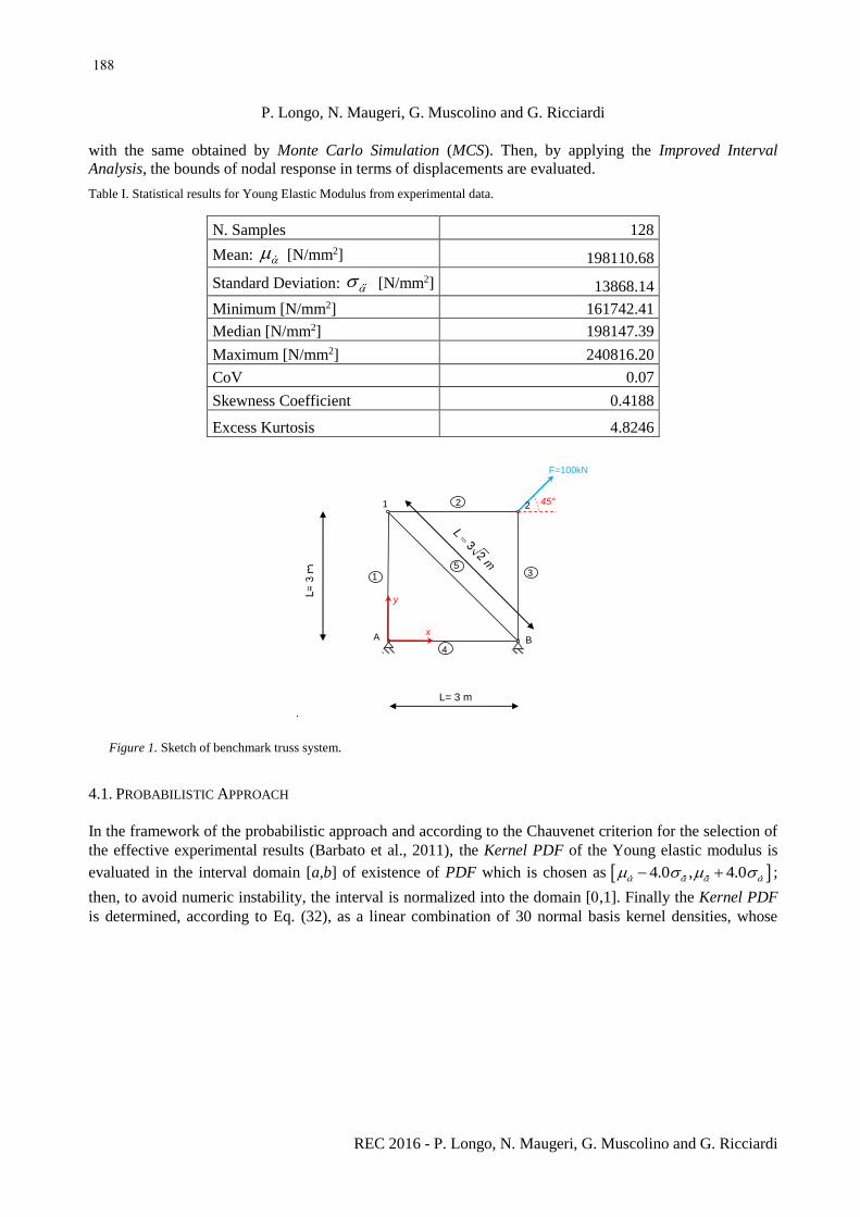
with the same obtained by Monte Carlo Simulation (MCS). Then, by applying the Improved Interval

Analysis, the bounds of nodal response in terms of displacements are evaluated.

Table I. Statistical results for Young Elastic Modulus from experimental data.

N. Samples 128

Mean: [N/mm2] 198110.68

Standard Deviation: [N/mm2] 13868.14

Minimum [N/mm2] 161742.41

Median [N/mm2] 198147.39

Maximum [N/mm2] 240816.20

CoV 0.07

Skewness Coefficient 0.4188

Excess Kurtosis 4.8246

Figure 1. Sketch of benchmark truss system.

4.1. PROBABILISTIC APPROACH

In the framework of the probabilistic approach and according to the Chauvenet criterion for the selection of

the effective experimental results (Barbato et al., 2011), the Kernel PDF of the Young elastic modulus is

evaluated in the interval domain [a,b] of existence of PDF which is chosen as 4.0 , 4.0 ;

then, to avoid numeric instability, the interval is normalized into the domain [,1]. Finally the Kernel PDF

is determined, according to Eq. (32), as a linear combination of 30 normal basis kernel densities, whose

1

A

5

4 B

F=100kN

2 1

3

2

y

x

45°

L= 3 m

188



coefficient pi are computed by Eq. (40) once the Maximum Entropy optimization problem is solved

(Alibrandi and Ricciardi, 2008).

Figure 2. Comparison between Kernel PDF, Gaussian PDF and experimental data.

The Kernel PDF is depicted in Figure 2 together with the histogram of experimental data and the

Gaussian PDF having same mean value and standard deviation of experimental data. Clearly this figure

shows as the Kernel PDF better fits experimental data.

The nominal displacement vector 0

Nu is evaluated as follows :

1

0 0

N u K F (41)

obtaining:

1

1

0

2

2

4.29699

1.12239

5.41939

1.12239

mm

x

yN

x

y

u

u

u

u

u ; (42)

To evaluate in explicit form the first two statistics of the response, the Kernel PDF, to satisfy the

condition (13), has to be normalized into a lesser than 1 domain. This normalization has been performed by

means of the following transformation:

e

(43)

where is the mean value of Kernel PDF. So operating the normalized Kernel PDF of uncertain elastic

modulus, Ep e , represented in Figure 3, lies into the interval domain 0.28,0.28 .

Kernel PDF

Gaussian

PDF

189



Figure 3. Normalized Kernel PDF.

To test the accuracy of proposed method, in Table II are reported the mean values, ru , and the standard

deviations,ru , of displacements of studied structure, evaluated by means of Eqs. (17) and compared with

the ones coming from MCS. In Table II the percentage errors are given, comparing the analytical data with

the results obtained from MCS of 5000, 500 000, 1 000 000 samples. Negligible percentage errors confirm

the accuracy of proposed method, provided a considerable reduction of the computational effort.

Table II. Comparison between stochastic results and Monte Carlo Simulation (Kernel Density).

Parameter

[mm]

analytical MCS 5000 Error [%] MCS

500000

Error [%] MCS 106 Error [%]

µux1 4.31818 4.31884 0.0153 4.31854 0.0083 4.3180 -0.0037

µuy1 1.12793 1.12768 -0.0222 1.12796 0.0027 1.1280 0.0062

µux2 5.44611 5.44564 -0.0086 5.44658 0.0086 5.4468 0.0127

µuy2 1.12793 1.12806 0.0115 1.12774 -0.0168 1.1280 0.0027

σux1 0.23680 0.23715 0.1451 0.23677 -0.0114 0.2369 0.0355

σuy1 0.07893 0.07943 0.6288 0.07876 -0.2174 0.0789 -0.0390

σux2 0.24961 0.25103 0.5669 0.24949 -0.0481 0.2496 0.0024

σuy2 0.07893 0.07801 -1.1898 0.07885 -0.1074 0.0789 0.0152

The same analytical approach has been applied assuming a Gaussian PDF. In Table III the percentage

errors between analytical results and MCS with 1.000.000 samples are reported, confirming the accuracy of

proposed method.

190



Table III. Comparison between stochastic results and Monte Carlo Simulation (Gaussian PDF).

Parameter[mm] analytical MCS106 Error[%]

µux1 4.318

34

4.3182

1

-

0.0030

µuy1 1.127

97

1.1280

7

0.008

9

µux2 5.446

31

5.4460

1

-

0.0055

µuy2 1.127

97

1.1280

2

0.004

4

σux1 0.240

32

0.2405

22

0.085

6

σuy1 0.080

11

0.0801

257

0.025

5

σux2 0.253

32

0.2534

63

0.058

4

σuy2 0.080

11

0.0801

882

0.103

4

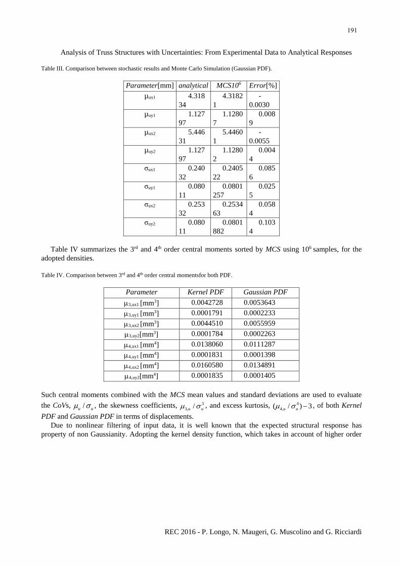
Table IV summarizes the 3rd and 4th order central moments sorted by MCS using 106 samples, for the

adopted densities.

Table IV. Comparison between 3rd and 4th order central momentsfor both PDF.

Parameter Kernel PDF Gaussian PDF

3,ux1 [mm3] 0.0042728 0.0053643

3,uy1 [mm3] 0.0001791 0.0002233

3,ux2 [mm3] 0.0044510 0.0055959

3,uy2[mm3] 0.0001784 0.0002263

4,ux1 [mm4] 0.0138060 0.0111287

4,uy1 [mm4] 0.0001831 0.0001398

4,ux2 [mm4] 0.0160580 0.0134891

4,uy2[mm4] 0.0001835 0.0001405

Such central moments combined with the MCS mean values and standard deviations are used to evaluate

the CoVs, /u u , the skewness coefficients, 3

3, /u u , and excess kurtosis, 4

4,( / ) 3u u , of both Kernel

PDF and Gaussian PDF in terms of displacements.

Due to nonlinear filtering of input data, it is well known that the expected structural response has

property of non Gaussianity. Adopting the kernel density function, which takes in account of higher order

191



statistics of the input data, the structural response statistics of order higher than the second gives results

which are different from the ones sorted by simply assuming the Gaussianity of input data (i.e. taking into

account the input data statistics up to the second order). Such consideration justifies the need to take into

account of input data statistics of higher order to the second, when it is interesting to well catch the non

Gaussian character of structural response.

On the other hand, the non Gaussianity of the response in both cases is highlighted by slightly right-

tailed shape with respect to the mean of responses, as indicated by skewness coefficient, given in Table V

where it is clearly evident that, adopting the Kernel PDF, the sensible higher value of excess kurtosis is

provided.

Table V. C.O.V., skewness coefficients and excess kurtosis of the responses.

Parameter Kernel PDF Gaussian PDF

1 1ux ux 0.055 0.056

1 1uy u 0.070 0.071

2 2ux ux 0.046 0.047

2 2uy uy 0.070 0.071

3

3, 1 1ux ux 0.3214 0.3855

3

3, 1 1uy uy 0.3646 0.4342

3

3, 2 2ux ux 0.2862 0.3437

3

3, 2 2uy uy 0.3625 0.4390

4, 1

4

1

3ux

ux

1.3845 0.3253

4, 1

4

1

3uy

uy

1.7249 0.3909

4, 2

4

2

3ux

ux

1.1361 0.2683

4, 2

4

2

3uy

uy

1.7246 0.3985

4.2. INTERVAL ANALYSIS

It is well known that when the information on experimental data is incomplete or fragmentary, the interval

analysis is a very efficient method to evaluate the propagation of the uncertainties on structural response.

To define the interval of uncertainty, the knowledge of the distribution function is not required but its

bounds only. Furthermore, according to the philosophy of interval analysis, the measured data define an

interval with full confidence that the value is within the interval, and not outside it. That is, it is not a

192



confidence interval or credibility interval. Rather, the interval represents sure bounds of the measurement,

with full degree of confidence on experimental data (Ferson et al., 2007).

The starting point in using a bounded interval to model the measurement uncertainty is to acknowledge

the intrinsic imprecision in measurement. In the studied truss structure, the population of experimental data

is numerous, so that reliable results can be obtained by applying the probabilistic approach, described in the

previous section. The aim of this section, is to compare the results provided by the probabilistic model with

the ones evaluated by applying the Improved Interval Analysis. For this purpose, the first step is to define a

reliable interval of the uncertain elastic modulus. A reasonable choice seems to be a normalized interval

containing all experimental data, i.e. 0.28, 0.28 , which has been chosen for Kernel PDF evaluation. In

Table VI, the chosen values of lower bound (LB), , and upper bound (UB), , as well as the midpoint,

2 , deviation, 2 , and Coefficient of Interval Uncertainty (C.I.U.), , are

reported.

Table VI. Interval parameters for Young Elastic Modulus from experimental data (100% of experimental data).

[N/mm2] 142638.10

[N/mm2] 253583.26

[N/mm2] 198110.68

[N/mm2] 110945.16

. . .C I U 0.28

The corresponding midpoint displacement vector 0u and the lower and the upper bounds of

displacements vectors calculated by Eqs. (30) and (31) are given respectively as:

0

3.35701 5.96811

0.87686

4.23387 7.52701

0.87686

4.66256

1.21788 1.55890mm mm ; mm ;

5.88044

1.21788 1.55890

u u u

The difference between midpoint values and explicit mean value vectors for Kernel PDF and Gaussian

PDF, reported in Table II and Table III, is reported in Table VII.

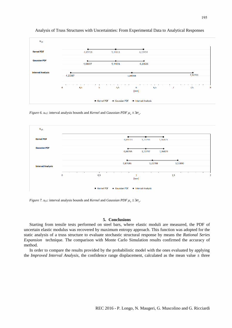
In Figures 4-7 the bounds of interval responses, in terms of displacement, sorted by Improved Interval

Analysis, are compared with the results obtained in terms of confidence range displacements, calculated as

the mean value ± three times standard deviation of stochastic results, coming out by assuming maximum

entropy approach and adopting the normal distribution. These Figures show that for the analysed truss

structure, the confidence range lie into the bounds defined by Interval Analysis, if an interval that includes

all experimental data is chosen.

193



Table VII. Comparison between mean values and midpoint displacements.

Parameter

[mm] 0u Uμ

(Kernel PDF) U

μ

(Gaussian PDF)

Difference [%]

(Kernel PDF)

Difference [%]

(Gaussian PDF)

µux1 4.66256 4.31818 4.31834 7.3861 7.3826

µuy1 1.21788 1.12793 1.12797 7.3858 7.3825

µux2 5.88044 5.44611 5.44631 7.3860 7.3826

µuy2 1.21788 1.12793 1.12797 7.3858 7.3825

Figure 4. ux1: interval analysis bounds and Kernel and Gaussian PDF 3 .u u

Figure 5.uy1: interval analysis bounds and Kernel and Gaussian PDF 3 .u u

194



Figure 6. ux2: interval analysis bounds and Kernel and Gaussian PDF 3 .u u

Figure 7. uy2: interval analysis bounds and Kernel and Gaussian PDF 3 .u u

5. Conclusions

Starting from tensile tests performed on steel bars, where elastic moduli are measured, the PDF of

uncertain elastic modulus was recovered by maximum entropy approach. This function was adopted for the

static analysis of a truss structure to evaluate stochastic structural response by means the Rational Series

Expansion technique. The comparison with Monte Carlo Simulation results confirmed the accuracy of

method.

In order to compare the results provided by the probabilistic model with the ones evaluated by applying

the Improved Interval Analysis, the confidence range displacement, calculated as the mean value ± three

195



times standard deviation of stochastic results, is determined. Then the bounds of the response interval by

applying the Improved Interval Analysis are evaluated. The comparison of two response intervals showed

that the selected confidence range lies into the bounds defined by Interval Analysis if, for the uncertain

elastic modulus, the interval that includes all experimental data is chosen.

References Alibrandi U. and G. Ricciardi. Efficient evaluation of the pdf of a random variable through the kernel density maximum entropy

approach. International Journal for Numerical Methods in Engineering, 75:1511–1548, 2008.

Barbato G., E. M. Barini, G. Genta and R. Levi. Features and performance of some outlier detection methods. Journal of Applied

Statistics, 38:2133–2149, 2011.

Elishakoff I. and M. Ohsaki. Optimization and Anti-optimization of Structures under Uncertainty, Imperial College Press, London,

2010.

Ferson S., V. Kreinovich, J. Hajagos, W. Oberkampf and L. Ginzburg. Experimental Uncertainty Estimation and Statistics for Data

Having Interval Uncertainty. SANDIA REPORT: SAND 2007-0939, 2007.

Moens, D. and D. Vandepitte. A Survey of Non-Probabilistic Uncertainty Treatment in Finite Element Analysis. Computer

Methods in Applied Mechanics and Engineering 194:1527–1555, 2005.

Moore, R. E. Interval Analysis, Prentice-Hall, Englewood Cliffs, 1966.

Moore, R. E., R. B. Kearfott and M. J. Cloud. Introduction to Interval Analysis, SIAM, Philadelphia, USA, 2009.

Muhanna, R. L. and R. L. Mullen. Uncertainty in Mechanics: Problems-Interval-Based Approach. Journal Engineering Mechanics

ASCE 127:557-566, 2001.

Muscolino G. and A. Sofi. Stochastic Analysis of Structures with Uncertain-but-Bounded Parameters via Improved Interval

Analysis. Probabilistic Engineering Mechanics 28:152-163, 2012.

Muscolino, G. and A. Sofi. Bounds for the Stationary Stochastic Response of Truss Structures with Uncertain-but-Bounded

Parameters. Mechanical Systems and Signal Processing 37:163-181, 2013. Muscolino G., R. Santoro and A. Sofi. Explicit frequency response functions of discretized structures with uncertain parameters.

Computer and Structures, 133:64-78, 2014.

196

Analysis of Truss Structures with Uncertainties: From ...rec2016.sd.rub.de/papers/REC2016-FP-11_P....

Documents

Transcript of Analysis of Truss Structures with Uncertainties: From ...rec2016.sd.rub.de/papers/REC2016-FP-11_P....