ANALYSIS OF THE INFLUENCE OF ECONOMIC INDICATORS ON STOCK PRICES USING

MULTIPLE REGRESSION

SYS 302

Spring 2000 Professor Tony Smith

Yale Chang Carl Yeung Chris Yip

1

TABLE OF CONTENTS

I. INTRODUCTION A. Chosen Economic Variables B. Assumptions on the Regression Model

II. ANALYSIS A. Single Regression Models of TCB 500 Against Indicators B. Preliminary Multiple Regression C. Multicollinearity D. Choosing Variables With the Stepwise Regression Model E. Gauss-Markov Assumptions: Heteroscedasticity and Autocorrelation F. Predictive Abilities of the Regression Models

III. CONCLUSION A. Single Regression Discussion B. Multiple Regression Discussion

IV. SUPPLEMENTS

A. Appendix A B. Appendix B

2

I. INTRODUCTION

Every month, anxious investors eagerly await the release of key economic

indicators such as the employment report, CPI, and even housing starts. It is not

uncommon for the Dow Jones Industrial Average and NASDAQ to swing more than a

hundred points when the numbers only slightly miss consensus estimates. Every indicator

is an important measure of some facet of the domestic economy, but do these numbers

really shape the movement of stock prices in the long run? Which indicators yield the

most influence on the equity market? Can a model consisting of these indicators be

constructed to accurately forecast the stock market? And are any single indicators a good

predictor of stock prices? As curious investors ourselves, we developed a statistical

model in an attempt to detect a trend between stock prices and such variables and

evaluated the predictive abilities of the model.

Data was obtained from The Conference Board Economic Indicator Package,

provided by Wharton Research Data Services (WRDS). Monthly time series data was

obtained for stock market prices and a selection of economic indicators over a span of

twenty years, from January 1979 to January 1999. This period was chosen because of the

relative stability of the economy, the nation’s minimal exposure to severe external shock

(i.e. wars), and the comprehensiveness of the data. The stock market index provided by

the Conference Board is the TCB 500 common stock index, which is not commonly

quoted; each data point represents the index’s closing price for the given month. This

index was employed in our analysis because it represents the stock market more fully

than the Dow Jones Industrial Average, which includes only thirty stocks. Furthermore, a

3

comparison of the TCB 500 and the SP500 revealed that the two indices are almost

identical, as the single regression shows below:

SPX By TCB 500 Stock

SPX

0100

300

500600

800900

1100

1300

0 100 300 500 700 900 1100 1300500 Stock

Linear Fit

Linear Fit SPX = 0.05124 + 1.00486 500 Stock

Summary of Fit Rsquare 0.997687 RSquare Adj 0.997678 Root Mean Square Error 12.80636 Mean of Response 370.3486 Observations (or Sum Wgts) 241

A time series graph comparing the two indices is also shown below:

SP 500 vs TCB 500

0

200

400

600

800

1000

1200

1400

time (1979-1999)

TCB 500 SP 500

4

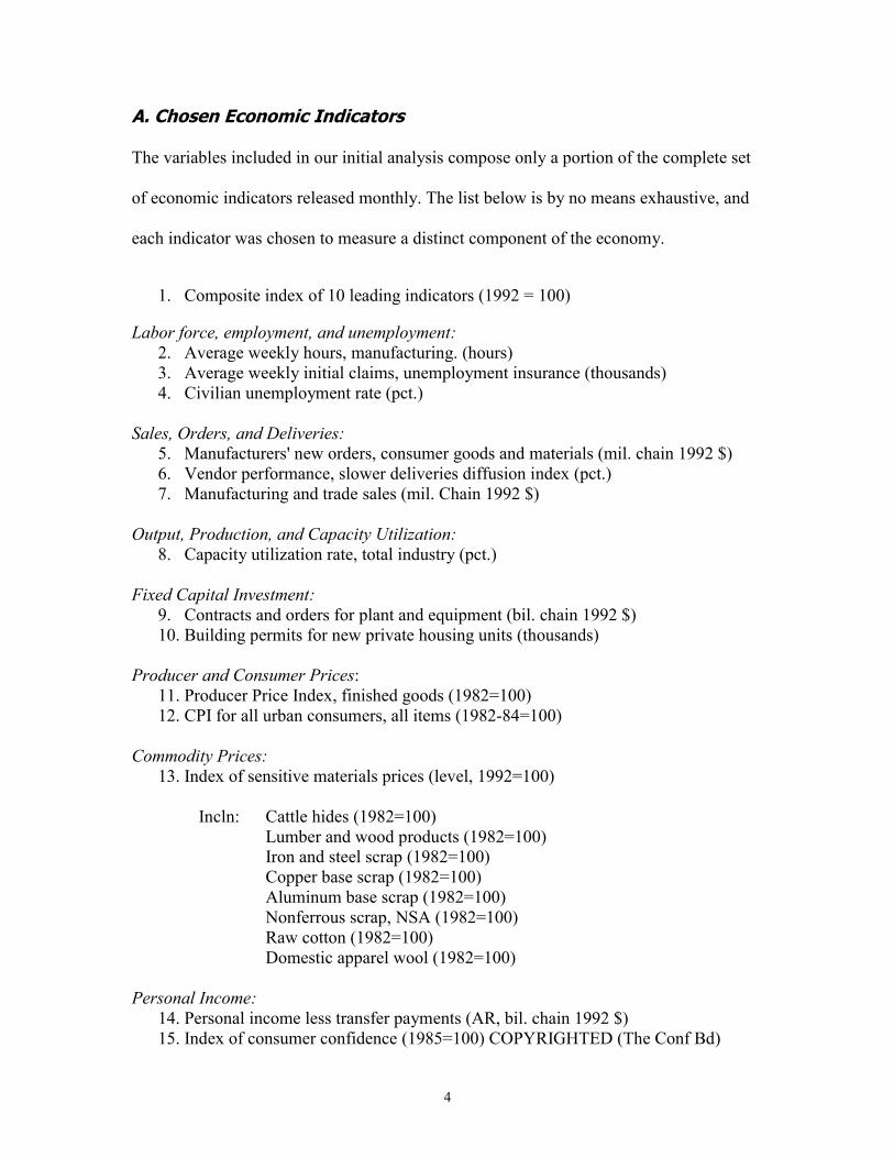
A. Chosen Economic Indicators

The variables included in our initial analysis compose only a portion of the complete set

of economic indicators released monthly. The list below is by no means exhaustive, and

each indicator was chosen to measure a distinct component of the economy.

1. Composite index of 10 leading indicators (1992 = 100)

Labor force, employment, and unemployment: 2. Average weekly hours, manufacturing. (hours) 3. Average weekly initial claims, unemployment insurance (thousands) 4. Civilian unemployment rate (pct.)

Sales, Orders, and Deliveries:

5. Manufacturers' new orders, consumer goods and materials (mil. chain 1992 $) 6. Vendor performance, slower deliveries diffusion index (pct.) 7. Manufacturing and trade sales (mil. Chain 1992 $)

Output, Production, and Capacity Utilization:

8. Capacity utilization rate, total industry (pct.) Fixed Capital Investment:

9. Contracts and orders for plant and equipment (bil. chain 1992 $) 10. Building permits for new private housing units (thousands)

Producer and Consumer Prices:

11. Producer Price Index, finished goods (1982=100) 12. CPI for all urban consumers, all items (1982-84=100)

Commodity Prices:

13. Index of sensitive materials prices (level, 1992=100) Incln: Cattle hides (1982=100) Lumber and wood products (1982=100) Iron and steel scrap (1982=100) Copper base scrap (1982=100)

Aluminum base scrap (1982=100) Nonferrous scrap, NSA (1982=100)

Raw cotton (1982=100) Domestic apparel wool (1982=100)

Personal Income:

14. Personal income less transfer payments (AR, bil. chain 1992 $) 15. Index of consumer confidence (1985=100) COPYRIGHTED (The Conf Bd)

5

16. Index of consumer expectations (1985=100) COPYRIGHTED (The Conf Bd) Money, Credit, Interest Rates, and Stock Prices:

17. Money supply, M2 (bil. chain 1992 $) 18. Interest rate spread, 10-year Treasury bonds less federal funds 19. Federal funds rate, NSA (pct.)

Exports and Imports:

20. Exports, excluding military aid shipments (mil. $) - General imports (mil. $) = Trade Balance

International Comparisions:

21. Exchange value of U.S. dollar, NSA (Mar. 1973=100)

6

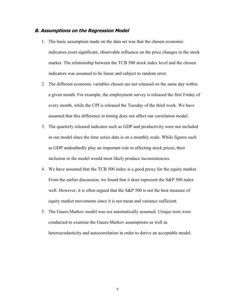
B. Assumptions on the Regression Model

1. The basic assumption made on the data set was that the chosen economic

indicators exert significant, observable influence on the price changes in the stock

market. The relationship between the TCB 500 stock index level and the chosen

indicators was assumed to be linear and subject to random error.

2. The different economic variables chosen are not released on the same day within

a given month. For example, the employment survey is released the first Friday of

every month, while the CPI is released the Tuesday of the third week. We have

assumed that this difference in timing does not affect our correlation model.

3. The quarterly released indicator such as GDP and productivity were not included

in our model since the time series data is on a monthly scale. While figures such

as GDP undoubtedly play an important role in affecting stock prices, their

inclusion in the model would most likely produce inconsistencies.

4. We have assumed that the TCB 500 index is a good proxy for the equity market.

From the earlier discussion, we found that it does represent the S&P 500 index

well. However, it is often argued that the S&P 500 is not the best measure of

equity market movements since it is not mean and variance sufficient.

5. The Gauss-Markov model was not automatically assumed. Unique tests were

conducted to examine the Gauss-Markov assumptions as well as

heteroscedasticity and autocorrelation in order to derive an acceptable model.

7

II. ANALYSIS

A. Single Regression Models of TCB 500 Against Indicators

To begin our study, single regression models of the TCB 500 index were run

against each economic indicator to obtain a graphical interpretation of how well each

variable correlates with the stock market. The regression plots for each indicator are

attached at the end of the report as Appendix A. These plots show that the only indicators

which seem to display a smooth, consistent relationship with the TCB 500 index are the

following: index of ten leading indicators, manufacturing and trade sales, CPI, and

personal income. The polynomial fits of these four variables correlate surprisingly well

with the stock index, with R2 values of at least 0.95 (see Appdendix B). With this

information in mind, we proceeded to perform a preliminary multiple regression.

B. Preliminary Multiple Regression

While single regressions can be limited in their analysis, multiple regression

models simultaneously take into account the effects of each variable. A standard least

squares multiple regression was conducted, plotting the TCB 500 common stock index

against all economic indicators. The results of the multiple regression are shown below:

Response: 500 Stock Summary of Fit

RSquare 0.987224 RSquare Adj 0.985999 Root Mean Square Error 31.25715 Mean of Response 368.508 Observations (or Sum Wgts) 241

Parameter Estimates Term Estimate Std Error t Ratio Prob>|t| Intercept -2845.606 879.1908 -3.24 0.0014 10 Leading Ind 52.003024 13.65247 3.81 0.0002 Avg Wkly Hr -16.89806 11.42545 -1.48 0.1406

8

UE Claims 0.2057853 0.128894 1.60 0.1118 Mfrs New Orders -0.003696 0.001289 -2.87 0.0045 Vendor Prfm -0.738489 0.716969 -1.03 0.3041 Bldg Permit -0.162113 0.024568 -6.60 <.0001 M2 -0.564221 0.106776 -5.28 <.0001 Intrt Rate Spre -18.52264 3.92238 -4.72 <.0001 UE Rate -0.023767 10.1186 -0.00 0.9981 Capacity Util R -18.84474 3.565865 -5.28 <.0001 Mnfr & Trade Sa 0.0046085 0.000586 7.87 <.0001 Cntrct & Orders 0.0024846 0.001011 2.46 0.0148 PPI 3.9181248 3.13577 1.25 0.2128 CPI -17.05578 2.667677 -6.39 <.0001 Comd Prices 0.0406398 0.634698 0.06 0.9490 Pers Inc 0.4029118 0.097376 4.14 <.0001 Cnsmr Conf -3.88931 0.731443 -5.32 <.0001 Cnsmr Expt 3.1739166 0.659718 4.81 <.0001 FF Rate -9.068953 3.771536 -2.40 0.0170 Trade Balance 0.0001526 0.00142 0.11 0.9145 Ex Value USD 1.9144678 0.491674 3.89 0.0001

Effect Test Source Nparm DF Sum of Squares F Ratio Prob>F 10 Leading Ind 1 1 14175.342 14.5089 0.0002 Avg Wkly Hr 1 1 2137.106 2.1874 0.1406 UE Claims 1 1 2490.361 2.5490 0.1118 Mfrs New Orders 1 1 8034.001 8.2231 0.0045 Vendor Prfm 1 1 1036.540 1.0609 0.3041 Bldg Permit 1 1 42538.108 43.5391 <.0001 M2 1 1 27280.134 27.9221 <.0001 Intrt Rate Spre 1 1 21787.388 22.3001 <.0001 UE Rate 1 1 0.005 0.0000 0.9981 Capacity Util R 1 1 27286.563 27.9287 <.0001 Mnfr & Trade Sa 1 1 60460.850 61.8836 <.0001 Cntrct & Orders 1 1 5895.660 6.0344 0.0148 PPI 1 1 1525.340 1.5612 0.2128 CPI 1 1 39936.970 40.8768 <.0001 Comd Prices 1 1 4.006 0.0041 0.9490 Pers Inc 1 1 16726.921 17.1205 <.0001 Cnsmr Conf 1 1 27623.796 28.2738 <.0001 Cnsmr Expt 1 1 22613.772 23.1459 <.0001 FF Rate 1 1 5649.062 5.7820 0.0170 Trade Balance 1 1 11.283 0.0115 0.9145 Ex Value USD 1 1 14812.891 15.1615 0.0001

This model shows an excellent fit, with almost 99% of the variance accounted for

(R2 = 0.987); it appears that the available data is sufficient to describe the movement in

stock prices. Not surprisingly, the four variables that demonstrated high correlation with

the TCB 500 from the earlier single regressions have also produced highly significant p-

values here.

9

On the other hand, not all of the variables are significant, such as the trade

balance, commodity prices, and the unemployment rate, which has a p-value of almost 1!

It seems illogical to claim that what is probably the most closely watched measure of

economic performance by Wall Street and the Fed has practically no effect on stock

prices. It is also strange that the coefficients for CPI and PPI have opposite signs even

though they both measure inflation. Similarly, the unemployment rate and unemployment

claims also have a negative correlation, as well as consumer confidence and consumer

expectations.

C. Multicollinearity

A possible explanation of these discrepancies might be multicollinearity, which

undermines the significance of the individual coefficients. To refine the model, a

correlation plot between the stock index and the economic indicators was drawn to

determine which variables are highly dependent:

Variable 10

Leading Indicies

Avg Wkly Hr

UE Claims

Mfrs New

Orders

Bldg Permit M2

Intrt Rate

Spread

UE Rate

Capacity Util Rate

Mnfr & Trade Sales

Cntrct &

OrdersPPI CPI Pers

Inc Cnsmr Conf

Cnsmr Expt

FF Rate

Trade Balance

Ex Value USD

500 Stock

10 Leading Ind 1 0.8968 -0.7549 0.8954 0.2309 0.9665 0.4231 -0.6713 0.326 0.9075 0.7075 0.8576 0.897 0.9349 0.5724 0.3774 -0.8185 -0.8714 -0.4352 0.8156

Avg Wkly Hr 0.8968 1 -0.812 0.9078 0.2123 0.8006 0.3059 -0.7067 0.5284 0.8699 0.6887 0.7707 0.8261 0.857 0.5383 0.2914 -0.7119 -0.797 -0.4955 0.7468

UE Claims -0.7549 -0.812 1 -0.7392 -0.4653 -0.6496 -0.1116 0.7539 -0.6826 -0.6369 -0.6018 -0.4328 -0.5041 -0.6095 -0.7254 -0.4463 0.4645 0.6852 0.3242 -0.5006

Mfrs New Orders 0.8954 0.9078 -0.7392 1 0.1647 0.8062 0.1685 -0.7852 0.5157 0.9746 0.8769 0.8053 0.878 0.9393 0.6249 0.2774 -0.6625 -0.84 -0.5305 0.9115

Bldg Permit 0.2309 0.2123 -0.4653 0.1647 1 0.0964 0.1002 -0.1259 0.0688 0.0466 0.1329 -0.1604 -0.1047 -0.0072 0.5578 0.5351 -0.13 -0.3827 0.4352 0.0489

M2 0.9665 0.8006 -0.6496 0.8062 0.0964 1 0.4068 -0.6457 0.2577 0.8574 0.6436 0.8492 0.877 0.915 0.4702 0.268 -0.8064 -0.8025 -0.4777 0.7652

Intrt Rate Spread 0.4231 0.3059 -0.1116 0.1685 0.1002 0.4068 1 0.1916 -0.2923 0.1944 -0.1141 0.4303 0.3864 0.2715 -0.1331 0.1745 -0.7336 -0.272 0.0488 0.114

UE Rate -0.6713 -0.7067 0.7539 -0.7852 -0.1259 -0.6457 0.1916 1 -0.8275 -0.7427 -0.8241 -0.4541 -0.5514 -0.7062 -0.6963 -0.1141 0.3413 0.6413 0.5733 -0.6377

Capacity Util Rate 0.326 0.5284 -0.6826 0.5157 0.0688 0.2577 -0.2923 -0.8275 1 0.4024 0.5588 0.1118 0.2052 0.339 0.5033 -0.0114 -0.0743 -0.2785 -0.5108 0.249

Mnfr & Trade Sales 0.9075 0.8699 -0.6369 0.9746 0.0466 0.8574 0.1944 -0.7427 0.4024 1 0.8606 0.8853 0.9428 0.9862 0.5383 0.2104 -0.6957 -0.8368 -0.5596 0.9541

Cntrct & Orders 0.7075 0.6887 -0.6018 0.8769 0.1329 0.6436 -0.1141 -0.8241 0.5588 0.8606 1 0.6052 0.6909 0.809 0.6707 0.1954 -0.4037 -0.7084 -0.4607 0.8572

PPI 0.8576 0.7707 -0.4328 0.8053 -0.1604 0.8492 0.4303 -0.4541 0.1118 0.8853 0.6052 1 0.9872 0.9299 0.2604 0.1755 -0.7474 -0.711 -0.4933 0.8176

CPI 0.897 0.8261 -0.5041 0.878 -0.1047 0.877 0.3864 -0.5514 0.2052 0.9428 0.6909 0.9872 1 0.9707 0.3325 0.1679 -0.7755 -0.7662 -0.5441 0.8765

Pers Inc 0.9349 0.857 -0.6095 0.9393 -0.0072 0.915 0.2715 -0.7062 0.339 0.9862 0.809 0.9299 0.9707 1 0.4912 0.2056 -0.7396 -0.8315 -0.5548 0.9282

Cnsmr Conf 0.5724 0.5383 -0.7254 0.6249 0.5578 0.4702 -0.1331 -0.6963 0.5033 0.5383 0.6707 0.2604 0.3325 0.4912 1 0.7214 -0.1388 -0.6671 -0.0033 0.5157

Cnsmr Expt 0.3774 0.2914 -0.4463 0.2774 0.5351 0.268 0.1745 -0.1141 -0.0114 0.2104 0.1954 0.1755 0.1679 0.2056 0.7214 1 -0.0825 -0.3832 0.3137 0.2276

10

FF Rate -0.8185 -0.7119 0.4645 -0.6625 -0.13 -0.8064 -0.7336 0.3413 -0.0743 -0.6957 -0.4037 -0.7474 -0.7755 -0.7396 -0.1388 -0.0825 1 0.6338 0.4345 -0.6009

Trade Balance -0.8714 -0.797 0.6852 -0.84 -0.3827 -0.8025 -0.272 0.6413 -0.2785 -0.8368 -0.7084 -0.711 -0.7662 -0.8315 -0.6671 -0.3832 0.6338 1 0.2154 -0.7889

Ex Value USD -0.4352 -0.4955 0.3242 -0.5305 0.4352 -0.4777 0.0488 0.5733 -0.5108 -0.5596 -0.4607 -0.4933 -0.5441 -0.5548 -0.0033 0.3137 0.4345 0.2154 1 -0.4427

500 Stock 0.8156 0.7468 -0.5006 0.9115 0.0489 0.7652 0.114 -0.6377 0.249 0.9541 0.8572 0.8176 0.8765 0.9282 0.5157 0.2276 -0.6009 -0.7889 -0.4427 1

From this correlation plot, the composite index of 10 leading indicators shows much

higher correlation with the following individual variables than with the stock index:

Average weekly hours, mfg. (hours) Manufacturers' new orders Manufacturing and trade sales Vendor performance Building permits for new private housing units (thous.) Index of stock prices, 500 common stocks, NSA (1941-43=10) Money supply, M2 (bil. chain 1992 $) Interest rate spread, 10-year Treasury bonds less federal funds

Trade balance Personal savings

PPI CPI

Given the large number of dependent variables with such high correlations, further

economic research was conducted on these indicators; we later discovered that the index

of ten leading indicators actually includes many of the above variables. Most importantly,

the index of leading indicators includes the TCB 500 common stock index. As a result, a

second correlation plot was performed without the index of leading indicators:

Variable 500 Stocks

Avg Wkly Hr

UE Claims

Mfrs New

Orders

Bldg Permit M2

Intrt Rate

Spread

UE Rate

Capacity Util Rate

Mnfr & Trade Sales

Cntrct &

OrdersPPI CPI Pers

Inc Cnsmr Conf

Cnsmr Expt

FF Rate

Trade Balance

Ex Value USD

Vendor Prfm

Comd Prices

500 Stock 1 0.7468 -0.5006 0.9115 0.0489 0.7652 0.114 -0.6377 0.249 0.9541 0.8572 0.8176 0.8765 0.9282 0.5157 0.2276 -0.6009 -0.7889 -0.4427 0.0922 0.5992

Avg Wkly Hr 0.7468 1 -0.812 0.9078 0.2123 0.8006 0.3059 -0.7067 0.5284 0.8699 0.6887 0.7707 0.8261 0.857 0.5383 0.2914 -0.7119 -0.797 -0.4955 0.4503 0.6374

UE Claims -0.5006 -0.812 1 -0.7392 -0.4653 -0.6496 -0.1116 0.7539 -0.6826 -0.6369 -0.6018 -0.4328 -0.5041 -0.6095 -0.7254 -0.4463 0.4645 0.6852 0.3242 -0.575 -0.5003

Mfrs New Orders 0.9115 0.9078 -0.7392 1 0.1647 0.8062 0.1685 -0.7852 0.5157 0.9746 0.8769 0.8053 0.878 0.9393 0.6249 0.2774 -0.6625 -0.84 -0.5305 0.3409 0.7227

Bldg Permit 0.0489 0.2123 -0.4653 0.1647 1 0.0964 0.1002 -0.1259 0.0688 0.0466 0.1329 -0.1604 -0.1047 -0.0072 0.5578 0.5351 -0.13 -0.3827 0.4352 0.4549 -0.208

M2 0.7652 0.8006 -0.6496 0.8062 0.0964 1 0.4068 -0.6457 0.2577 0.8574 0.6436 0.8492 0.877 0.915 0.4702 0.268 -0.8064 -0.8025 -0.4777 0.1857 0.4911

Intrt Rate Spread 0.114 0.3059 -0.1116 0.1685 0.1002 0.4068 1 0.1916 -0.2923 0.1944 -0.1141 0.4303 0.3864 0.2715 -0.1331 0.1745 -0.7336 -0.272 0.0488 0.2906 -0.1127

UE Rate -0.6377 -0.7067 0.7539 -0.7852 -0.1259 -0.6457 0.1916 1 -0.8275 -0.7427 -0.8241 -0.4541 -0.5514 -0.7062 -0.6963 -0.1141 0.3413 0.6413 0.5733 -0.2084 -0.7191

Capacity Util Rate 0.249 0.5284 -0.6826 0.5157 0.0688 0.2577 -0.2923 -0.8275 1 0.4024 0.5588 0.1118 0.2052 0.339 0.5033 -0.0114 -0.0743 -0.2785 -0.5108 0.3459 0.6462

11

Mnfr & Trade Sales

0.9541 0.8699 -0.6369 0.9746 0.0466 0.8574 0.1944 -0.7427 0.4024 1 0.8606 0.8853 0.9428 0.9862 0.5383 0.2104 -0.6957 -0.8368 -0.5596 0.187 0.7112

Cntrct & Orders 0.8572 0.6887 -0.6018 0.8769 0.1329 0.6436 -0.1141 -0.8241 0.5588 0.8606 1 0.6052 0.6909 0.809 0.6707 0.1954 -0.4037 -0.7084 -0.4607 0.1874 0.6949

PPI 0.8176 0.7707 -0.4328 0.8053 -0.1604 0.8492 0.4303 -0.4541 0.1118 0.8853 0.6052 1 0.9872 0.9299 0.2604 0.1755 -0.7474 -0.711 -0.4933 0.0671 0.6231

CPI 0.8765 0.8261 -0.5041 0.878 -0.1047 0.877 0.3864 -0.5514 0.2052 0.9428 0.6909 0.9872 1 0.9707 0.3325 0.1679 -0.7755 -0.7662 -0.5441 0.1159 0.6529

Pers Inc 0.9282 0.857 -0.6095 0.9393 -0.0072 0.915 0.2715 -0.7062 0.339 0.9862 0.809 0.9299 0.9707 1 0.4912 0.2056 -0.7396 -0.8315 -0.5548 0.1453 0.6813

Cnsmr Conf 0.5157 0.5383 -0.7254 0.6249 0.5578 0.4702 -0.1331 -0.6963 0.5033 0.5383 0.6707 0.2604 0.3325 0.4912 1 0.7214 -0.1388 -0.6671 -0.0033 0.3686 0.4724

Cnsmr Expt 0.2276 0.2914 -0.4463 0.2774 0.5351 0.268 0.1745 -0.1141 -0.0114 0.2104 0.1954 0.1755 0.1679 0.2056 0.7214 1 -0.0825 -0.3832 0.3137 0.3991 0.1384

FF Rate -0.6009 -0.7119 0.4645 -0.6625 -0.13 -0.8064 -0.7336 0.3413 -0.0743 -0.6957 -0.4037 -0.7474 -0.7755 -0.7396 -0.1388 -0.0825 1 0.6338 0.4345 -0.2797 -0.2685

Trade Balance -0.7889 -0.797 0.6852 -0.84 -0.3827 -0.8025 -0.272 0.6413 -0.2785 -0.8368 -0.7084 -0.711 -0.7662 -0.8315 -0.6671 -0.3832 0.6338 1 0.2154 -0.3013 -0.4527

Ex Value USD -0.4427 -0.4955 0.3242 -0.5305 0.4352 -0.4777 0.0488 0.5733 -0.5108 -0.5596 -0.4607 -0.4933 -0.5441 -0.5548 -0.0033 0.3137 0.4345 0.2154 1 -0.0591 -0.6624

Vendor Prfm 0.0922 0.4503 -0.575 0.3409 0.4549 0.1857 0.2906 -0.2084 0.3459 0.187 0.1874 0.0671 0.1159 0.1453 0.3686 0.3991 -0.2797 -0.3013 -0.0591 1 0.1372

Comd Prices 0.5992 0.6374 -0.5003 0.7227 -0.2018 0.4911 -0.1127 -0.7191 0.6462 0.7112 0.6949 0.6231 0.6529 0.6813 0.4724 0.1384 -0.2685 -.0.4527 -0.6624 0.1372 1

Based on the above grid, multicollinearity was still found among other variables, as

shown by the highlighted values above. As a result, the following indicators were also

removed: manufacturing new orders, manufacturing and trade sales, personal income,

and PPI. The final correlation plot is shown below:

Variable 500

Stock Avg Wkly

Hr UE

Claims Bldg

Permit M2 Intrt Rate Spread UE Rate Capacity

Util RateCntrct & Orders CPI Cnsmr

Conf Cnsmr Expt

FF Rate

Trade Balance

Ex Value USD

Vendor Prfm

Comd Prices

500 Stock 1 0.7468 -0.5006 0.0489 0.7652 0.114 -0.6377 0.249 0.8572 0.8765 0.5157 0.2276 -0.6009 -0.7889 -0.4427 0.0922 0.5992

Avg Wkly Hr 0.7468 1 -0.812 0.2123 0.8006 0.3059 -0.7067 0.5284 0.6887 0.8261 0.5383 0.2914 -0.7119 -0.797 -0.4955 0.4503 0.6374

UE Claims -0.5006 -0.812 1 -0.4653 -0.6496 -0.1116 0.7539 -0.6826 -0.6018 -0.5041 -0.7254 -0.4463 0.4645 0.6852 0.3242 -0.575 -0.5003

Bldg Permit 0.0489 0.2123 -0.4653 1 0.0964 0.1002 -0.1259 0.0688 0.1329 -0.1047 0.5578 0.5351 -0.13 -0.3827 0.4352 0.4549 -0.208

M2 0.7652 0.8006 -0.6496 0.0964 1 0.4068 -0.6457 0.2577 0.6436 0.877 0.4702 0.268 -0.8064 -0.8025 -0.4777 0.1857 0.4911

Intrt Rate Spread 0.114 0.3059 -0.1116 0.1002 0.4068 1 0.1916 -0.2923 -0.1141 0.3864 -0.1331 0.1745 -0.7336 -0.272 0.0488 0.2906 -0.1127

UE Rate -0.6377 -0.7067 0.7539 -0.1259 -0.6457 0.1916 1 -0.8275 -0.8241 -0.5514 -0.6963 -0.1141 0.3413 0.6413 0.5733 -0.2084 -0.7191

Capacity Util Rate 0.249 0.5284 -0.6826 0.0688 0.2577 -0.2923 -0.8275 1 0.5588 0.2052 0.5033 -0.0114 -0.0743 -0.2785 -0.5108 0.3459 0.6462

Cntrct & Orders 0.8572 0.6887 -0.6018 0.1329 0.6436 -0.1141 -0.8241 0.5588 1 0.6909 0.6707 0.1954 -0.4037 -0.7084 -0.4607 0.1874 0.6949

CPI 0.8765 0.8261 -0.5041 -0.1047 0.877 0.3864 -0.5514 0.2052 0.6909 1 0.3325 0.1679 -0.7755 -0.7662 -0.5441 0.1159 0.6529

Cnsmr Conf 0.5157 0.5383 -0.7254 0.5578 0.4702 -0.1331 -0.6963 0.5033 0.6707 0.3325 1 0.7214 -0.1388 -0.6671 -0.0033 0.3686 0.4724

Cnsmr Expt 0.2276 0.2914 -0.4463 0.5351 0.268 0.1745 -0.1141 -0.0114 0.1954 0.1679 0.7214 1 -0.0825 -0.3832 0.3137 0.3991 0.1384

FF Rate -0.6009 -0.7119 0.4645 -0.13 -0.8064 -0.7336 0.3413 -0.0743 -0.4037 -0.7755 -0.1388 -0.0825 1 0.6338 0.4345 -0.2797 -0.2685

Trade Balance -0.7889 -0.797 0.6852 -0.3827 -0.8025 -0.272 0.6413 -0.2785 -0.7084 -0.7662 -0.6671 -0.3832 0.6338 1 0.2154 -0.3013 -0.4527

Ex Value USD -0.4427 -0.4955 0.3242 0.4352 -0.4777 0.0488 0.5733 -0.5108 -0.4607 -0.5441 -0.0033 0.3137 0.4345 0.2154 1 -0.0591 -0.6624

Vendor Prfm 0.0922 0.4503 -0.575 0.4549 0.1857 0.2906 -0.2084 0.3459 0.1874 0.1159 0.3686 0.3991 -0.2797 -0.3013 -0.0591 1 0.1372

Comd Prices 0.5992 0.6374 -0.5003 -0.208 0.4911 -0.1127 -0.7191 0.6462 0.6949 0.6529 0.4724 0.1384 -0.2685 -0.4527 -0.6624 0.1372 1

12

The table shows that much of the multicollinearity problem has been eliminated

through the removal of five indicators: index of leading indicators, manufacturing new

orders, manufacturing and trade sales, personal income, and PPI. However, it is important

to realize the impossibility of completely removing multicollinearity since all of the

indicators are related in some way through macroeconomic principles. Although the

removal of variables will slightly diminish R2, and hence the predictability of the model,

our objective is to find the best combination of the most significant and influential

independent indicators in the regression model. Although considerable correlation still

exists among certain variables, further removal of variables would prevent a thorough

analysis of the influence of these indicators on the stock market.

D. Choosing Variables With the Stepwise Regression Model

After the filtering of certain variables, a stepwise regression was conducted to further

narrow down the most significant indicators and to yield the highest adjusted R2 value,

indicating highest predictability. The results of the first stepwise regression (Step model

1) are shown below:

Response: 500 Stock

Stepwise Regression Control Prob to Enter 0.250 Prob to Leave 0.250

Direction

Current Estimates SSE DFE MSE RSquare RSquare Adj Cp AIC 884727.99 228 3880.386 0.9472 0.9444 9.256008 2004.185

Lock Entered Parameter Estimate nDF SS "F Ratio" "Prob>F" X X Intercept 2030.66465 1 0 0.000 1.0000 _ X Avg Wkly Hr 28.4736768 1 9987.642 2.574 0.1100 _ _ UE Claims ? 1 39.81886 0.010 0.9196 _ X Bldg Permit -0.083008 1 27995.25 7.215 0.0078 _ X M2 -0.3213083 1 209604.7 54.016 0.0000 _ X Intrt Rate Spread -32.04761 1 147559.4 38.027 0.0000 _ X UE Rate -58.964848 1 43864.13 11.304 0.0009 _ X Capacity Util Rate -29.704393 1 121007.9 31.184 0.0000

13

_ X Cntrct & Orders 0.01546194 1 388882.6 100.218 0.0000 _ X CPI 7.55712093 1 308604.9 79.529 0.0000 _ X Cnsmr Conf 1.37104117 1 7634.109 1.967 0.1621 _ X Cnsmr Expt 1.51430471 1 11304.35 2.913 0.0892 _ X FF Rate -19.827616 1 88482.79 22.803 0.0000 _ _ Trade Balance ? 1 533.1804 0.137 0.7117 _ _ Ex Value USD ? 1 285.0882 0.073 0.7870 _ _ Vendor Prfm ? 1 26.21451 0.007 0.9347 _ X Comd Prices -4.8035508 1 124197.3 32.006 0.0000

Step History

Step Parameter Action "Sig Prob" Seq SS RSquare Cp p 1 CPI Entered 0.0000 12866812 0.7683 746.62 2 2 Cntrct & Orders Entered 0.0000 2028176 0.8894 234.53 3 3 Capacity Util Rate Entered 0.0000 464129.7 0.9171 118.88 4 4 Intrt Rate Spread Entered 0.0001 91356.8 0.9226 97.728 5 5 Avg Wkly Hr Entered 0.0000 104074.3 0.9288 73.348 6 6 Comd Prices Entered 0.0018 48692.8 0.9317 63.005 7 7 M2 Entered 0.0159 28276.16 0.9334 57.838 8 8 UE Rate Entered 0.0000 93389.68 0.9389 36.166 9 9 Cnsmr Expt Entered 0.0010 47220.86 0.9418 26.197 10 10 FF Rate Entered 0.0001 62452.44 0.9455 12.367 11 11 Avg Wkly Hr Removed 0.5487 1431.699 0.9454 10.73 10 12 Bldg Permit Entered 0.0749 12548.41 0.9462 9.549 11 13 Avg Wkly Hr Entered 0.1237 9302.653 0.9467 9.1911 12 14 Cnsmr Conf Entered 0.1621 7634.109 0.9472 9.256 13

The above stepwise regression shows that much of the multicollinearity problem has been

eliminated; for example, the unemployment rate now has a significant p-value, and

consumer confidence and expectation are no longer negatively correlated. However,

average weekly hours, consumer confidence, and consumer expectations are still included

in the model even though they exhibit high p-values. A possible explanation is that their

inclusion in the model contributes to a higher adjusted R2 value. After testing with

various combinations of the variables, the final stepwise regression model (step model 2)

is shown below:

Response: 500 Stock Stepwise Regression Control

Prob to Enter 0.250 Prob to Leave 0.250

Direction

Current Estimates SSE DFE MSE RSquare RSquare Adj Cp AIC 914213.16 231 3957.633 0.9454 0.9433 10.72975 2006.086

Lock Entered Parameter Estimate nDF SS "F Ratio" "Prob>F"

14

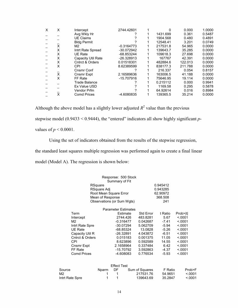
X X Intercept 2744.42601 1 0 0.000 1.0000 _ _ Avg Wkly Hr ? 1 1431.699 0.361 0.5487 _ _ UE Claims ? 1 1904.568 0.480 0.4891 _ _ Bldg Permit ? 1 12548.41 3.201 0.0749 _ X M2 -0.3164773 1 217531.8 54.965 0.0000 _ X Intrt Rate Spread -30.072942 1 139643.7 35.285 0.0000 _ X UE Rate -68.853244 1 109618.3 27.698 0.0000 _ X Capacity Util Rate -26.328913 1 167767 42.391 0.0000 _ X Cntrct & Orders 0.01518301 1 482884.6 122.013 0.0000 _ X CPI 8.62389599 1 838177.3 211.788 0.0000 _ _ Cnsmr Conf ? 1 216.337 0.054 0.8157 _ X Cnsmr Expt 2.16589636 1 163006.5 41.188 0.0000 _ X FF Rate -15.707916 1 75646.95 19.114 0.0000 _ _ Trade Balance ? 1 0.215112 0.000 0.9941 _ _ Ex Value USD ? 1 1169.58 0.295 0.5878 _ _ Vendor Prfm ? 1 64.92614 0.016 0.8984 _ X Comd Prices -4.6080835 1 139365.5 35.214 0.0000

Although the above model has a slightly lower adjusted R2 value than the previous

stepwise model (0.9433 < 0.9444), the “entered” indicators all show highly significant p-

values of p < 0.0001.

Using the set of indicators obtained from the results of the stepwise regression,

the standard least squares multiple regression was performed again to create a final linear

model (Model A). The regression is shown below:

Response: 500 Stock

Summary of Fit RSquare 0.945412 RSquare Adj 0.943285 Root Mean Square Error 62.90972 Mean of Response 368.508 Observations (or Sum Wgts) 241

Parameter Estimates Term Estimate Std Error t Ratio Prob>|t| Intercept 2744.426 483.8281 5.67 <.0001 M2 -0.316477 0.042687 -7.41 <.0001 Intrt Rate Spre -30.07294 5.062709 -5.94 <.0001 UE Rate -68.85324 13.0828 -5.26 <.0001 Capacity Util R -26.32891 4.043872 -6.51 <.0001 Cntrct & Orders 0.015183 0.001375 11.05 <.0001 CPI 8.623896 0.592589 14.55 <.0001 Cnsmr Expt 2.1658964 0.337484 6.42 <.0001 FF Rate -15.70792 3.592863 -4.37 <.0001 Comd Prices -4.608083 0.776534 -5.93 <.0001

Effect Test

Source Nparm DF Sum of Squares F Ratio Prob>F M2 1 1 217531.76 54.9651 <.0001 Intrt Rate Spre 1 1 139643.69 35.2847 <.0001

15

UE Rate 1 1 109618.27 27.6979 <.0001 Capacity Util R 1 1 167767.02 42.3908 <.0001 Cntrct & Orders 1 1 482884.62 122.0135 <.0001 CPI 1 1 838177.30 211.7875 <.0001 Cnsmr Expt 1 1 163006.51 41.1879 <.0001 FF Rate 1 1 75646.95 19.1142 <.0001 Comd Prices 1 1 139365.53 35.2144 <.0001

In this final revised model, the R2 value is 0.9454. Interestingly, three of the four “good”

variables identified from the single regressions have been removed in the refinement

process. Although the R2 value of our refined model is slightly less than the R2 value of

0.987 obtained in our preliminary multiple regression, we can be confident that the final

combination of indicators exhibits high significance, independence, and the most

influence on the TCB 500.

E. Gauss-Markov Assumptions: Heteroscedasticity and Autocorrelation

The Gauss-Markov Assumptions can be stated as follows:

(i) εi ∼ N(0, σ2), i = 1, …, n

(ii) Var (εi) = σ2, i = 1, …, n

(iii) (εi, . . . , εn) mutually independent

If the final least squares model fits the first Gauss-Markov assumption, the

residuals of the model must be normally distributed. A normal quantile plot of the

residuals is shown below:

16

-150

-100

-50

0

50

100

150

200 .01 .05.10 .25 .50 .75 .90.95 .99

-3 -2 -1 0 1 2 3

Normal Quantile

The above plot shows that the residuals are extremely close to being normally distributed;

therefore, the first Gauss-Markov assumption is valid for this regression model.

Next, for the new model to be accepted, possible violations of the constant-

variance assumption must be tested for. The whole model test and the residual plot of the

multiple regression are shown below:

Whole-Model Test

0100

300

500600

800900

1100

1300

-100 100 300 500 700 900 1100 1300500 Stock Predicted

Analysis of Variance Source DF Sum of Squares Mean Square F Ratio Model 9 15833148 1759239 444.5179 Error 231 914213 3958 Prob>F C Total 240 16747362 <.0001

17

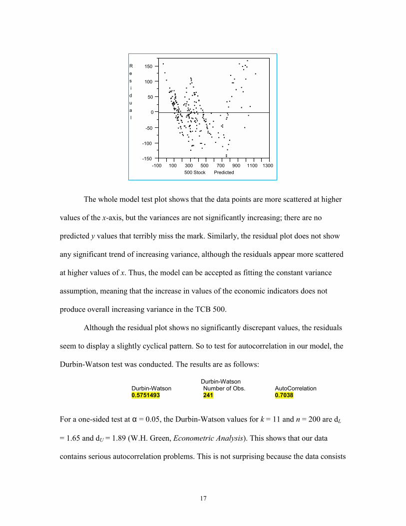
The whole model test plot shows that the data points are more scattered at higher

values of the x-axis, but the variances are not significantly increasing; there are no

predicted y values that terribly miss the mark. Similarly, the residual plot does not show

any significant trend of increasing variance, although the residuals appear more scattered

at higher values of x. Thus, the model can be accepted as fitting the constant variance

assumption, meaning that the increase in values of the economic indicators does not

produce overall increasing variance in the TCB 500.

Although the residual plot shows no significantly discrepant values, the residuals

seem to display a slightly cyclical pattern. So to test for autocorrelation in our model, the

Durbin-Watson test was conducted. The results are as follows:

Durbin-Watson Durbin-Watson Number of Obs. AutoCorrelation

0.5751493 241 0.7038

For a one-sided test at α = 0.05, the Durbin-Watson values for k = 11 and n = 200 are dL

= 1.65 and dU = 1.89 (W.H. Green, Econometric Analysis). This shows that our data

contains serious autocorrelation problems. This is not surprising because the data consists

Residual

-150

-100

-50

0

50

100

150

-100 100 300 500 700 900 1100 1300500 Stock Predicted

18

of time series statistics that include business cycles and economic fluctuations. There are

two alternatives to solving the autocorrelation problem: 1) perform a two-stage

estimation procedure to modify the data by weighted differencing or 2) add additional

variables which can account for the apparent autocorrelation effect. Although the second

alternative is generally a superior approach, all of the x-variables used in our regressions

are economic indicators and therefore unavoidably reflect business fluctuations; if we add

any more of the variables that we eliminated, we would end up with our preliminary

model and still not be able to correct autocorrelation. Therefore, the two-stage estimation

procedure was performed, and the no-intercept regression of the residuals are shown

below:

Response: Residual 500 Stock Summary of Fit

RSquare ? RSquare Adj ? Root Mean Square Error 44.27803 Mean of Response 0.136608 Observations (or Sum Wgts) 240

Parameter Estimates Term Estimate Std Error t Ratio Prob>|t| Intercept Zeroed 0 0 ? ? Lag Residuals 0.6921693 0.04757 14.55 <.0001

Effect Test Source Nparm DF Sum of Squares F Ratio Prob>F Lag Residuals 1 1 415083.08 211.7183 <.0001

The estimate for p-hat is 0.692, as shown in bold.

After transforming the variables, the new data set was used to run the multiple

regression again (Model Atransformed). The final result is shown below:

Response: T. 500 Stock Summary of Fit

RSquare 0.860731 RSquare Adj 0.855281 Root Mean Square Error 32.79234 Mean of Response 117.0965

19

Observations (or Sum Wgts) 240

Parameter Estimates Term Estimate Std Error t Ratio Prob>|t| Intercept 870.58837 133.8725 6.50 <.0001 T.M2 -0.29684 0.054307 -5.47 <.0001 T. Int Rate Spr -21.77922 5.145625 -4.23 <.0001 T. UE Rate -93.16051 11.11445 -8.38 <.0001 T. Cap Util Rat -23.98903 4.057743 -5.91 <.0001 T. Cont & Ords 0.0040738 0.000847 4.81 <.0001 T. CPI 10.046571 0.761136 13.20 <.0001 T. Cons. Expect 1.6722569 0.317441 5.27 <.0001 T. FF Rate -10.81747 4.50438 -2.40 0.0171 T. Comd Prices -3.875311 1.034767 -3.75 0.0002

Effect Test

Source Nparm DF Sum of Squares F Ratio Prob>F T.M2 1 1 32127.99 29.8771 <.0001 T. Int Rate Spr 1 1 19264.29 17.9146 <.0001 T. UE Rate 1 1 75549.69 70.2567 <.0001 T. Cap Util Rat 1 1 37583.84 34.9507 <.0001 T. Cont & Ords 1 1 24857.97 23.1164 <.0001 T. CPI 1 1 187351.23 174.2255 <.0001 T. Cons. Expect 1 1 29841.85 27.7511 <.0001 T. FF Rate 1 1 6201.93 5.7674 0.0171 T. Comd Prices 1 1 15082.48 14.0258 0.0002

Durbin-Watson

Durbin-Watson Number of Obs. AutoCorrelation 0.9526597 240 0.5008

Model A Model Atransformed

0100

300

500600

800900

1100

1300

-100 100 300 500 700 900 1100 1300500 Stock Predicted

T. 500 Stock

0

50

100

150

200

250

300

350

400

450

0 100 200 300 400T. 500 Stock Predicted

20

After the two-stage estimation, the new value of d, 0.953, is still much less than

the critical value, and significant autocorrelation still exists (autocorrelation = 0.5008).

However, a tradeoff must be made between the value of d and R2; while d increased from

0.692 to 0.952, R2 has dropped to 0.861 from 0.954 (Model A) in the transformed

multiple regression. The whole-model test plot of the transformed regression

correspondingly shows that the fit has become poorer. The federal funds rate and

commodity prices also showed a large decrease in their p-values. This estimation

procedure could have been carried out with more lags, but collinearity would start to

become a problem since the lagged residuals are correlated with each other.

The tested model therefore does not satisfy the third Gauss-Markov assumption,

which states that the residual deviations are mutually independent. Because the

autocorrelation problem could not be eliminated to an acceptable extent, this model

would most likely not make an accurate forecasting tool.

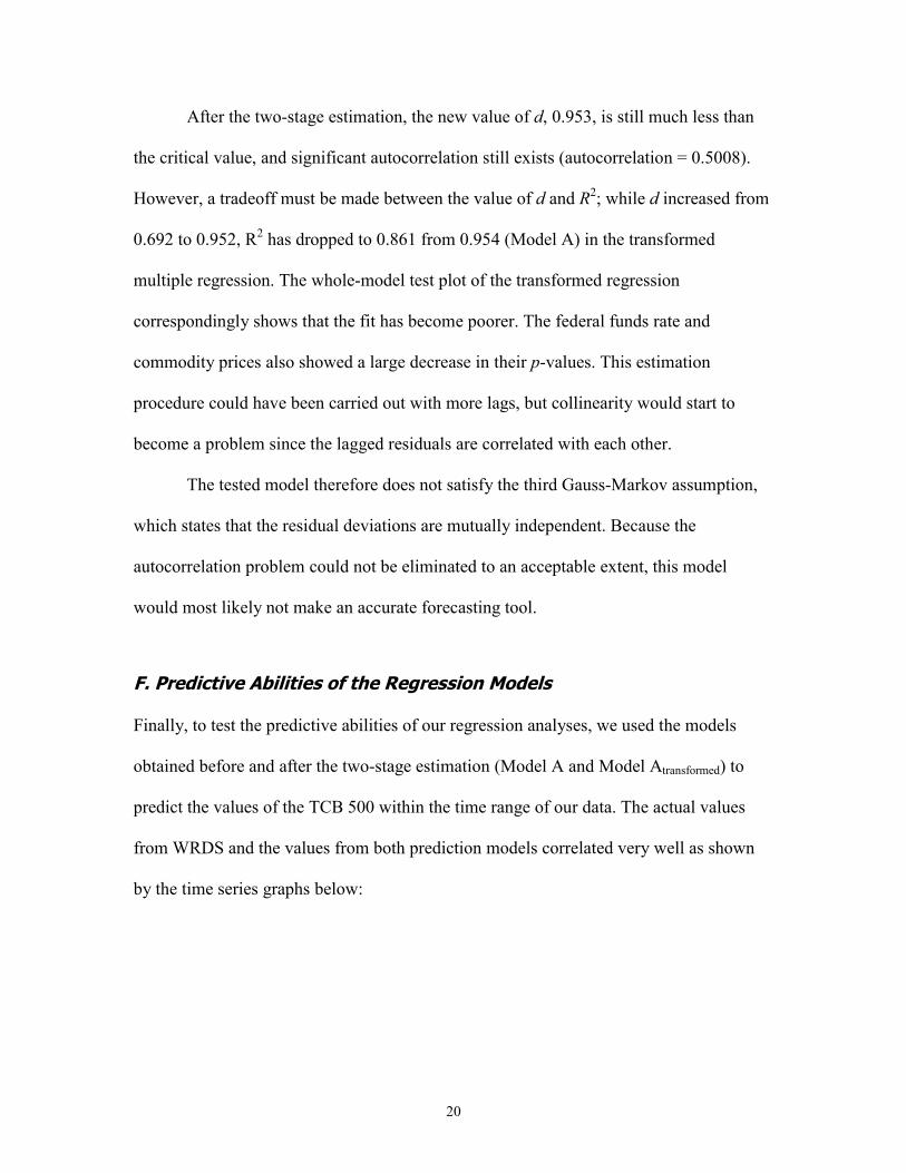
F. Predictive Abilities of the Regression Models

Finally, to test the predictive abilities of our regression analyses, we used the models

obtained before and after the two-stage estimation (Model A and Model Atransformed) to

predict the values of the TCB 500 within the time range of our data. The actual values

from WRDS and the values from both prediction models correlated very well as shown

by the time series graphs below:

21

Predicted TCB 500 VS Actual TCB 500 (1977-1999)

-200

0

200

400

600

800

1000

1200

1400

time (1977-1999)

Predicted TCB 500by modelReal TCB 500

Predicted Transformed TCB500 vs Actual Transformed TCB500 stocks (1977-1999)

-100

0

100

200

300

400

500

time (1977-1999)

Actual TCB 500

Predicted TCB 500

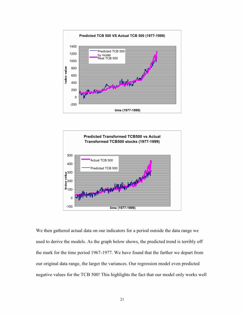
We then gathered actual data on our indicators for a period outside the data range we

used to derive the models. As the graph below shows, the predicted trend is terribly off

the mark for the time period 1967-1977. We have found that the farther we depart from

our original data range, the larger the variances. Our regression model even predicted

negative values for the TCB 500! This highlights the fact that our model only works well

22

within the range of our original data and performs poorly in forecasting data outside this

range.

Model Prediction VS. Real TCB 500 from (1967-1977)

-100

-50

0

50

100

150

200

250

300

350

400

0 20 40 60 80 100 120 140 160

time (1967-1977)

inde

x va

lue

Model Prediction

Real TCB 500 value

23

IV. CONCLUSION

I. Single Regression From our initial single regression plots, the four indicators that demonstrated the

strongest correlation with stock price were the index of ten leading indicators,

manufacturing and trade sales, CPI, and personal income. This result is not surprising: the

leading indicators are a broad measure of the economy and should move in sync with the

stock market; manufacturing and trade sales are a good indicator of overall economic

activity and output, similar to GDP, and therefore should correspond with stock prices;

the CPI measures the price level which generally increases with rising aggregate demand;

and the more income an individual has, the more stocks he/she is likely to buy.

II. Multiple Regression

In the final multiple regression model (model A), the nine remaining economic

indicators were: M2 money supply, interest rate spread, unemployment rate, capacity

utilization rate, manufacturing contracts and orders, CPI, consumer expectations, the

federal funds rate, and commodity prices. All of these indicators were highly significant,

with p < 0.0001, and they accounted for approximately 94.5% of the variance. The model

is shown again below:

Response: 500 Stock Summary of Fit

RSquare 0.945412 RSquare Adj 0.943285 Root Mean Square Error 62.90972 Mean of Response 368.508 Observations (or Sum Wgts) 241

Parameter Estimates Term Estimate Std Error t Ratio Prob>|t| Intercept 2744.426 483.8281 5.67 <.0001 M2 -0.316477 0.042687 -7.41 <.0001

24

Intrt Rate Spre -30.07294 5.062709 -5.94 <.0001 UE Rate -68.85324 13.0828 -5.26 <.0001 Capacity Util R -26.32891 4.043872 -6.51 <.0001 Cntrct & Orders 0.015183 0.001375 11.05 <.0001 CPI 8.623896 0.592589 14.55 <.0001 Cnsmr Expt 2.1658964 0.337484 6.42 <.0001 FF Rate -15.70792 3.592863 -4.37 <.0001 Comd Prices -4.608083 0.776534 -5.93 <.0001

Based on the model, the stock market is negatively correlated with M2, interest

rates, unemployment rate, commodity prices, and capacity utilization rate and positively

correlated with CPI, consumer expectations, and manufacturing contracts and orders.

Stock prices should be inversely related to interest rates because higher rates imply

higher costs of borrowing money, and bonds would appear more attractive. Logically, the

economy would be in a recession given a high unemployment rate, so these two factors

are negatively related. Increases in CPI and consumer expectation generally imply

growing aggregate demand and high confidence in the economy, so they are reasonably

correlated with the stock index in this model. Contracts and orders for plant and

equipment is a measurement of investment in the economy, and therefore correlates

positively with the TCB 500 as well. However, M2 would be expected to correlate

positively with stocks since it includes money market funds. In addition, higher capacity

utilization rates would imply that firms are operating with higher efficiency and output,

and it should have been directly correlated with stocks as well, from an economic

perspective. The variables M2 and CPI should have a direct relationship as well since

money supply growth leads to a proportional rise in the price level; instead, they had

opposite signs.

Since not all of these variables are on the same scale, their coefficients cannot be

compared to evaluate the relative influence of each indicator on the stock index.

However, it was surprising that indicators such as commodity prices were more

25

significant than variables such as the trade balance, which would be assumed to have

bigger importance and more impact on the entire economy.

Multicollinearity was substantial in our preliminary multiple regression since all

the indicators are related according to economic theory; as more variables were

eliminated in the refinement process, the R2 value in our model decreased slightly in

return for more significant p-values and more logical coefficients. In fact, CPI was the

only one of the four “quality” variables from single regression analysis to remain in the

final set of indicators. This was the result of the removal of highly dependent variables.

In addition, those four indicators had good polynomial fits with stock prices, but the

multiple regression was based on linear relationships.

While the TCB 500 stock index was predicted fairly well by our data within the

same time range, it seems futile to attempt to forecast the stock market outside the range

using our set of economic indicators. It is surprising that given all of the measures of

economic performance that we used, a successful prediction model failed to be

developed. This could be partly due to high autocorrelation problems in the model, but

more importantly, it suggests that many other factors contribute to the movement of the

equity market than just the economic indicators.

IV. SUPPLEMENTS:

APPENDIX A: Single Regression Plots, TCB 500 Against All Indicators

APPENDIX B: Polynomial Line Fit For Leading Indicators,

Manufacturing and Trade Sales, CPI, and Personal Income

APPENDIX B

500 Stock By 10 Leading Ind

0100

300

500600

800900

1100

1300

90 10010 Leading Ind

Polynomial Fit degree=6

Polynomial Fit degree=6

500 Stock = 1.561e7 611383 10 Leading Ind + 6226.79 10 Leading Ind^2 + 50.4847 10 Leading Ind^3 1.47785 10 Leading Ind^4 + 0.01071 10 Leading Ind^5 0.00003 10 Leading Ind^6

Summary of Fit RSquare 0.951879 RSquare Adj 0.950645 Root Mean Square Error 58.68599 Mean of Response 368.508 Observations (or Sum Wgts) 241

Analysis of Variance Source DF Sum of Squares Mean Square F Ratio Model 6 15941455 2656909 771.4502 Error 234 805906 3444 Prob>F C Total 240 16747362 <.0001

Parameter Estimates Term Estimate Std Error t Ratio Prob>|t| Intercept 15611913 7426678 2.10 0.0366 10 Leading Ind -611383.1 391548.6 -1.56 0.1198 10 Leading Ind^2 6226.7869 9018.339 0.69 0.4906 10 Leading Ind^3 50.484734 122.3188 0.41 0.6802 10 Leading Ind^4 -1.477852 1.039863 -1.42 0.1566 10 Leading Ind^5 0.0107058 0.005017 2.13 0.0339 10 Leading Ind^6 -0.000026 0.00001 -2.59 0.0103

-200

-100

0

100

200

90 10010 Leading Ind

APPENDIX B

500 Stock By Mnfr & Trade Sales

0100

300

500600

800900

1100

1300

400000 500000 600000 700000 800000Mnfr & Trade Sales

Polynomial Fit degree=6

Polynomial Fit degree=6

500 Stock = -195090 + 2.32132 Mnfr & Trade Sales 0.00001 Mnfr & Trade Sales^2 + 2.9e-11 Mnfr & Trade Sales^3 4e-17 Mnfr & Trade Sales^4 + 2.9e-23 Mnfr & Trade Sales^5 8.9e-30 Mnfr & Trade Sales^6

Summary of Fit RSquare 0.983595 RSquare Adj 0.983174 Root Mean Square Error 34.26507 Mean of Response 368.508 Observations (or Sum Wgts) 241

Analysis of Variance Source DF Sum of Squares Mean Square F Ratio Model 6 16472623 2745437 2338.343 Error 234 274738 1174 Prob>F C Total 240 16747362 <.0001

Parameter Estimates Term Estimate Std Error t Ratio Prob>|t| Intercept -195090.1 113131.5 -1.72 0.0859 Mnfr & Trade Sales 2.321316 1.194856 1.94 0.0532 Mnfr & Trade Sales^2 -0.000011 0.000005 -2.16 0.0317 Mnfr & Trade Sales^3 2.86e-11 1.2e-11 2.38 0.0182 Mnfr & Trade Sales^4 -4.01e-17 1.55e-17 -2.59 0.0101 Mnfr & Trade Sales^5 2.945e-23 1.05e-23 2.80 0.0055 Mnfr & Trade Sales^6 -8.87e-30 2.96e-30 -3.00 0.0030

-100

0

100

400000 500000 600000 700000 800000Mnfr & Trade Sales

APPENDIX B

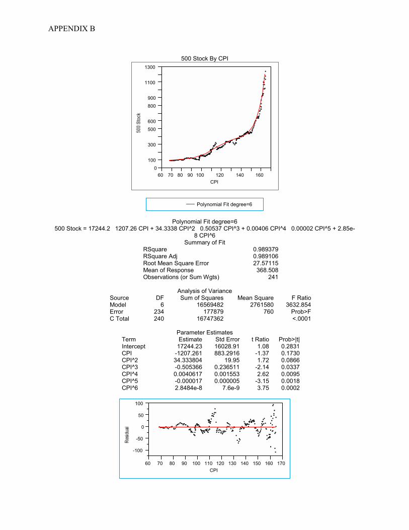
500 Stock By CPI

0100

300

500600

800900

1100

1300

60 70 80 90 100 120 140 160CPI

Polynomial Fit degree=6

Polynomial Fit degree=6

500 Stock = 17244.2 1207.26 CPI + 34.3338 CPI^2 0.50537 CPI^3 + 0.00406 CPI^4 0.00002 CPI^5 + 2.85e-8 CPI^6

Summary of Fit RSquare 0.989379 RSquare Adj 0.989106 Root Mean Square Error 27.57115 Mean of Response 368.508 Observations (or Sum Wgts) 241

Analysis of Variance Source DF Sum of Squares Mean Square F Ratio Model 6 16569482 2761580 3632.854 Error 234 177879 760 Prob>F C Total 240 16747362 <.0001

Parameter Estimates Term Estimate Std Error t Ratio Prob>|t| Intercept 17244.23 16028.91 1.08 0.2831 CPI -1207.261 883.2916 -1.37 0.1730 CPI^2 34.333804 19.95 1.72 0.0866 CPI^3 -0.505366 0.236511 -2.14 0.0337 CPI^4 0.0040617 0.001553 2.62 0.0095 CPI^5 -0.000017 0.000005 -3.15 0.0018 CPI^6 2.8484e-8 7.6e-9 3.75 0.0002

-100

-50

0

50

100

60 70 80 90 100 110 120 130 140 150 160 170CPI

APPENDIX B

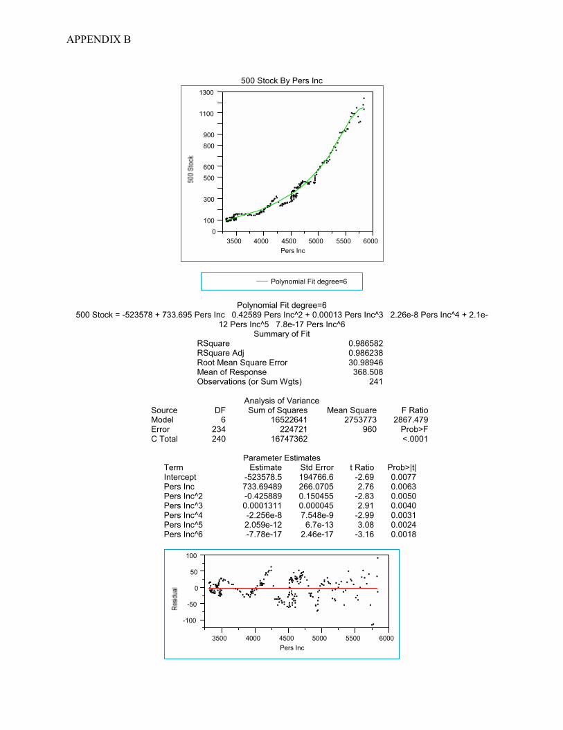
500 Stock By Pers Inc

0100

300

500600

800900

1100

1300

3500 4000 4500 5000 5500 6000Pers Inc

Polynomial Fit degree=6

Polynomial Fit degree=6

500 Stock = -523578 + 733.695 Pers Inc 0.42589 Pers Inc^2 + 0.00013 Pers Inc^3 2.26e-8 Pers Inc^4 + 2.1e-12 Pers Inc^5 7.8e-17 Pers Inc^6

Summary of Fit RSquare 0.986582 RSquare Adj 0.986238 Root Mean Square Error 30.98946 Mean of Response 368.508 Observations (or Sum Wgts) 241

Analysis of Variance Source DF Sum of Squares Mean Square F Ratio Model 6 16522641 2753773 2867.479 Error 234 224721 960 Prob>F C Total 240 16747362 <.0001

Parameter Estimates Term Estimate Std Error t Ratio Prob>|t| Intercept -523578.5 194766.6 -2.69 0.0077 Pers Inc 733.69489 266.0705 2.76 0.0063 Pers Inc^2 -0.425889 0.150455 -2.83 0.0050 Pers Inc^3 0.0001311 0.000045 2.91 0.0040 Pers Inc^4 -2.256e-8 7.548e-9 -2.99 0.0031 Pers Inc^5 2.059e-12 6.7e-13 3.08 0.0024 Pers Inc^6 -7.78e-17 2.46e-17 -3.16 0.0018

-100

-50

0

50

100

3500 4000 4500 5000 5500 6000Pers Inc