ANALYSIS OF THE HUNGARIAN ECONOMY … · ANALYSIS OF THE HUNGARIAN ECONOMY ... PRODUCTIVE...

ANALYSIS OF THE HUNGARIAN ECONOMY

Hungarian Statistical Review, Special number 7. 2002.

PRODUCTIVE EFFICIENCYIN THE HUNGARIAN INDUSTRY*

ÁDÁM REIFF1 – ANDRÁS SUGÁR2 – ÉVA SURÁNYI3

The paper estimates industry-specific stochastic production frontiers for selected Hun-garian manufacturing industries on a rich panel-data set between 1992–1998, then calculatesfirm-specific inefficiency estimates. One of the main findings is that between-industry dif-ferences in average inefficiency can be explained partially by differences in industry con-centrations. Nevertheless, the within-industry differences are best explained by the presenceof foreign owners, and also partially by the region of operation, but not by the exporting ac-tivity of the firms.

KEYWORDS. Stochastic production frontiers; Frontier estimation; Efficiency.

Measuring productivity and efficiency are very important when evaluating produc-tion units, the performance of different industries or that of a whole economy. It enablesus to identify sources of efficiency and productivity differentials, which is essential topolicies designed to improve performance.

The productivity of a production unit is defined as the ratio of its outputs to its inputs(both aggregated in some economically sensible way). Productivity varies due to differ-ences in production technology, differences in the efficiency of the production process,and differences in the environment in which the production occurs. In this paper we areinterested in isolating the efficiency component of productivity.

We define the efficiency of a production unit as the relation of the observed and op-timal values of its inputs and outputs. The comparison can be a ratio of the observed tomaximum possible output obtainable from the given set of inputs, or the ratio of theminimum possible amount of inputs to the observed required to produce the given output.(This is the widely used definition of technical efficiency.)

Until recently analyses have been facing difficulties when trying to determine empiri-cally the potential production of a unit, and the productivity literature ignored the effi

* Our research is funded by the Phare-Ace Research Project entitled ‘The adjustment and financing of Hungarianenterprises’, and was carried out in the Hungarian Ministry of Economic Affairs, Institute for Economic Analysis in 1999. Wegratefully appreciate the inspiration and useful comments of László Mátyás, Jerôme Sgard, and the seminar participants ofseveral project discussions. All the remaining errors are ours.

1 PhD student at the Economics Department of the Central European University, Budapest.2 Head of Department at the Hungarian Energy Office.3 PhD student at the Economics Department of the Central European University, Budapest.

ÁDÁM REIFF – ANDRÁS SUGÁR – ÉVA SURÁNYI46

ciency component. Only with the development of a separate efficiency literature has theproblem of determining productive potential seriously been addressed.

The measurement of technical efficiency is also important, as it enables us to quantifytheoretically predicted differentials in efficiency. Examples include the theories con-necting efficiency with market structure (see Hicks; 1935, Alchian–Kessel; 1962), modelsinvestigating the effects of ownership structure on performance (Alchian; 1965), and thearea of economic regulation (for example, Averch–Johnson (1962) and Bernstein–Feld-man–Schinnar (1990) examine the impact of economic environment and regulation onthe efficiency of the firms). The paper is organized as follows. In the first part we providetheoretical backgrounds for our empirical calculations, from both economic andeconometric points of view, while in the second part we analyze our data set, exploringthe main characteristics of the firms in different branches of industry included in thesample. We also examine the time trends of these relevant variables, together with therepresentativity of our data set. The third part contains the estimates of the productionfunction frontiers for different branches of the Hungarian industry. Our results about pro-duction functions also lets us draw some conclusions about different returns to scale indifferent industries. Next, in the fourth part we analyze sources of inefficiency differen-tials: the influence of export orientation, ownership structure and region of operation onthe efficiency of the firms.

1. THEORETICAL BACKGROUNDS

This section presents the theoretical backgrounds for determining efficiency meas-ures, and the details of our estimation technique.

Definitions and measures of productive efficiency

Productive efficiency has two components. The purely technical, or physical compo-nent refers to the ability to use the inputs of production effectively, by producing as muchoutput as input usage allows, or by using as little input as output production allows. Theallocative, or price component refers to the ability to combine inputs and outputs in opti-mal proportions in the light of prevailing prices. In this paper we only deal with the tech-nical component of productive efficiency.

Koopmans (1951. p. 60) provided a formal definition of technical efficiency: ‘a pro-ducer is technically efficient if an increase in any output requires a reduction in at leastone other output or an increase in at least one input and if a reduction in any input re-quires an increase in at least one other input or a reduction in at least one output.’ Thus atechnically inefficient producer could produce the same outputs with less of at least oneinput, or could use the same inputs to produce more of at least one output.

Debreu (1951) and Farrell (1957) introduced a measure of technical efficiency. Theirmeasure is defined as one minus the maximum equiproportionate reduction in all inputsthat still allow continuous production of given outputs. Therefore, a score of unity indi-cates technical efficiency, a score less than unity indicates technical inefficiency. Theconversion of the Debreu–Farrell measure (that is defined to inputs) to the output expan-sion case is straightforward.

PRODUCTIVE EFFICIENCY 47

Since our technical efficiency measurement is oriented towards output augmentation,we will examine them in that direction. Production technology can be represented with anoutput set:

L(x)={y: (x,y) is feasible}, /1/

where x stands for inputs, and y for output(s). From this we can define the Debreu–Farrelloutput-oriented measure of technical efficiency:

DF0 (x,y) = max {θ: θy Є L(x)}. /2/

This concept will be used in this paper. We note that the Debreu–Farrell measure oftechnical efficiency does not coincide perfectly with Koopmans’ definition of technicalefficiency. Koopmans’ definition requires that the point of production should belong tothe efficient subset-part of a particular isoquant, while the Debreu–Farrell measure onlyrequires that the production point should be on a particular isoquant. Consequently theDebreu–Farrell measure of technical efficiency is necessary, but not sufficient for Koop-mans’ technical efficiency. However, this problem disappears in many econometricanalysis, in which the parametric form of the function used to represent production tech-nology (e.g. Cobb–Douglas) ensures that isoquants and efficient subsets are identical.

The econometric approach to the measurement of productive efficiency:the theory of stochastic production function frontiers

The econometric measurement of productive efficiency is based on the well-knownstochastic production function frontier approach of the efficiency analysis. The stochasticfrontier production function, proposed independently by Aigner, Lovell and Schmidt(1977) and Meeusen and van den Broeck (1977), has been applied and modified in anumber of studies later. The earlier studies involved the estimation of the parameters ofthe stochastic frontier production function and the mean technical efficiency of the firmsin a given industry. It was initially claimed that technical inefficiencies for individualfirms could not be predicted. But later Jondrow et al. (1982) presented two predictors forthe firm effects of individual firms for cross-sectional data, and later panel data estimateswere discovered as well.

To introduce the main idea, let us consider the well-known stochastic productionfunction frontier approach of the efficiency analysis. In the most general setting (Greene;1993) we assume a well-defined, smooth, continuous, continuously differentiable, quasi-concave production function, and we accept that producers are price-takers in their input-markets.

Our starting point is exactly the production function:

� �;i iQ f� x β , /3/

where Q denotes the somehow measured single output, x denotes the vector of inputs, βare parameters and i is used to index the firms.


In most applications, the specification of the function � �f � is either Cobb–Douglas ortranslog production function. These choices are mainly made for convenience, as eitherof these allows us to obtain linear equations in the parameters when taking the logarithmof /3/. Therefore if we introduce lni iy Q� , and from this point we denote by ix the ap-propriately transformed input-vector of /3/, then we can write the logarithm of /3/ as:

Ti i iy � � � � �β x /4/

i i iv u� � � . /5/

Here the i� residual term has two components: irregular events (like weather, unfore-seen fluctuation in the quality of inputs etc.), and the firm’s inefficient production.

The effect of irregular events is captured by the variable iv ,4 and we assume that thiscan affect the actual production in either way; hence iv can be both positive and nega-tive. In particular, it is typical to assume that iv is normally distributed with mean 0 and

variance 2v� . This assumption will be used throughout the paper.

The effect of the firm’s inefficient production is captured by term iu . It is obviousthat inefficiency negatively influences the production, that is why it has a negative sign in/5/. This means that the iu variable itself is assumed to be non-negative.5 As for the rela-tion between the two parts of the compound error term, we will stick to the assumption(when applicable) that iu is independent from iv . The assumptions concerning iu dis-tinguish the different families of models from each other. We can list the following pos-sibilities.

1. We can assume that iu is constant for each observation (firm). This would meanthat iu is deterministic. However, these firm-specific constants can only be estimated ifwe have several observations for each firm. Therefore this approach (often called as fixedeffects approach) can only be used for panel data.6

2. Alternatively, we can assume that iu is stochastic, and the efficiency component ofeach unit can be characterized with the same probability distribution. With these as-sumptions, this approach can be used for both cross-sectional and panel data. (In case ofpanel data set, this is the random effects approach.)

If iu is stochastic, there are other possible choices regarding to its distribution.

4 One of the first attempts to estimate production frontiers was done by Aigner and Chu (1968), but they disregarded thisirregular term; therefore they searched for the deterministic frontier of the production function. This method can be criticizedfrom several aspects (see for example Greene; 1993), moreover it is only a special case of the general model introduced here(namely, when 0v� � ). Therefore further we will not deal with this model.

5 When first describing the stochastic frontier of the production functions, Aigner, Lovell and Schmidt (1977) defined

i i iv u� � � , assuming in the same time that iu is non-positive. Since then our notation became conventional.6 This is easy to see if we consider the following: if iu is constant for all i, then adding it to the constant term of the re-

gression we obtain the ‘firm-specific’ constant terms: one constant term for each firm (observation). This means as many pa-rameters as many observations we have, therefore in cross-sectional data (when we have only one observation for each firm) thenumber of parameters to estimate would be higher than the number of observations.


a) We can assume: iu is half-normally distributed, i.e. it follows a truncated normal dis-tribution (truncated at 0), where the mean of the original normally distributed variable is 0.7

b) More generally, it is possible to assume that iu follows a truncated normal dis-tribution (where the mean of the original variable is � , and truncation is made at 0).

c) It is also a usual assumption that iu is exponentially distributed with parameter � .d) Beckers and Hammond (1987), and Greene (1990) consider the case when iu fol-

lows a gamma-distribution with parameters � �; P� . This is the so-called gamma-normalmodel (the normal term reflecting to the normal distribution of iv ), and it can also be es-timated, but it imposes so much numerical difficulties when computing the estimated pa-rameters that it has been hardly used so far.

In the following, we will first present the estimators for the cross-sectional model, andthen we generalize our results to panel data.

The cross-sectional model. We will insist on the assumption that the iv variables arenormally distributed, and its outcomes are independent. Furthermore, we saw previouslythat when we have a cross sectional model, we can only apply the approach of randomeffects. Therefore iu must be stochastic: we assume that iu follows a truncated normal

distribution; the parameters of the underlying normal distribution are � �2; u� � , and trun-

cation is made at 0.If we wish to determine the density function of our compound error term, v u� � � ,

then we can use the well-known convolution rule (note that u and v are assumed to be in-dependent):

� � � � � �

2 2 2 22 2

1

u v

v u

u u u v v u vu vu

f f t f t dt�

��

� � � � �

� ��

�

.

Here � �.� is the distribution function, � �.� is the cumulative distribution function ofa standard normally distributed variable.

At this point it is a convention in the literature to rewrite the parameters of the model

in the following way: introduce 2 2u v� � � �� and u

v

��

�, or equivalently,

21v

��

� �

, and 21

u��

� �

� �

.

7 An alternative definition for the half-normally distributed variable is the absolute value of a normally distributed variablewith mean 0.


With these parameters

� �2

1

1f � ��

� � � � � � � � � � � � � ��

. /6/

From /6/ the log-likelihood function of model /4/ is /5/ is as follows:

� � � �1

ln ; ; ; ; ln lnN

ii

f N�

� � � � � � � � � ��β�

� � � �2

22

1 1

1 1ln ln 2 ln2 2

N Ni

ii i

NN� �

� � �� , /7/

where N denotes the size of our cross-sectional sample, and Ti i iy� � � � �β x .

The maximum likelihood estimates of this model can be obtained by maximizing thisexpression. Having this result accomplished, we can compute the estimates of the i� -s;denoted by ie . As Jondrow et al. (1982) show, we can infer iu from the estimated i� .Their main idea is that it is possible to determine the conditional cumulative distributionfunction of iu , under the condition that the estimated value of i� happens to be ie :

� � � ��

� � � �

0

0

Pr

iu

u v i

i i i i

u v i

f t f e t dtF u e u u e

f t f e t dt�

�

� � �

�

�

�

. /8/

With this, the conditional density function and the conditional expected value of iucan be written as:

� � � � 20 1

i

ii i i

i

ee

E u e uf u e due

�

� ��

� � ��

� . /9/

Having the maximum likelihood estimates for the parameters, this can be computedfor all i. As Greene (1993) notes, this estimator is unbiased, but inconsistent. (Inconsis-tent, because regardless of N, the variance of it remains non-zero.)

The panel model. Now we turn to the panel model, which can be formulated as

Tit it ity � � � � �β x , /10/

it it iv u� � � . /11/


Here the variables have the same meaning as in equations /4/ and /5/, with the exceptionthat t stands for the time index. We assume that for each firm i, we have iT observations.8

According to /11/, the inefficiency component of any firm is constant over time. If weomitted this assumption, we would have to estimate each firm’s inefficiency componentfor each period, which would lead us back to the cross-sectional case. Furthermore, thisassumption is not unreasonable for our data set, where we have at most seven observa-tions for each firm. As we saw earlier, we can choose among different assumptions re-garding to iu : it can be either deterministic (fixed effects approach) or stochastic (ran-dom effects approach). Now we turn to the analysis of these.

Case 1. Fixed effects model. If iu is deterministic, we can rewrite our model in /10/and /11/ in the following way:

� �T T Tit it it i i it it i it ity v u u v v� � � � � � � � β x β x β x . /12/

We can represent therefore the fixed and non-stochastic inefficiency term with theconstant term of the regression, obtaining firm-specific constant terms. This model is theusual fixed effects panel model, of which the estimation is well-known.

Once we have the estimates for the firm-specific constant terms, we can estimate thefirm-specific inefficiency terms as well. As Gabrielsen (1975) and Greene (1980)showed , in equation /12/ the OLS-estimates for β are consistent, and ˆ ˆmax ii

� � � is also

a consistent estimator for the overall constant term.9 Hence

ˆ ˆ ˆ ˆˆ maxi i i iiu � � �� /13/

can be used for the estimation of the firm-specific inefficiency terms. Therefore, we willhave by construction at least one firm which is producing on its efficiency frontier, the restbeing under it (i.e., having positive inefficiency measure). The advantages and disadvan-tages of this method are summarized by Greene (1993). The advantages are the following.

– Unlike to the random effects model, where the inefficiency term is a part of the er-ror term in the regression and is assumed to be uncorrelated with the inputs in the regres-sion, here it is included in the constant term and no such implicit (and unrealistic) as-sumption is needed.

– We do not have to assume normality; our parameter estimates (with the previouscorrection for the constant term) are consistent in N without assuming normality.

– The firm-specific inefficiency estimates are consistent in iT .

The disadvantages are as follows.

– This method does not allow us to include time-invariant inputs (like capital usage)in the model, as this would be exactly multicollinear with the firm-specific (and also

8 We will see in the following that it is unnecessary to assume that iT is the same for all firms.9 In both cases, consistency is understood as consistency in N, but not as consistency in T.


time-invariant) inefficiency terms, as both of these are constants for each observations ofthe same unit. Furthermore, if we simply omit these inputs from our model, then the ef-fect of these time-invariant inputs will appear in the inefficiency component. The solu-tion can be a random effect model under such circumstances.

Case 2. Random effects model with truncated normal distribution. We again assumethat itv is normally distributed, iu follows a truncated normal distribution, and each re-alizations of u and v are pair-wise independent. Furthermore, different realizations of vare independent also, and this is true for u as well.

When constructing the likelihood function, we have to consider that by /11/, the re-sidual terms � �1 2, , ,

ii i iT� � �� are not independent from each other, while these residual

vectors are independent for different i-s. So what have to be constructed is the jointprobability distribution function for the parameter vectors � �1 2, , ,

ii i iT� � �� ,

1, 2, ,i N� � . As

1 1 2 2, , , ,i ii i i i i i iT iT iv u v u v u� � � � � � � � �� ,

the convolution formula generalizes to:

� � � � � � � � � �1 2 1 2, , ,i ii i iT u v i v i v iTf f t f t f t f t dt

�

��

� � � � � � � � � � ��

� �

� � � � � � � �22 22

1 22 22 2

0

1 1

22

i i iTi

u v

i

t t tt

Tvu

u

e dt

� ��

� ��

� ��

�

�

.

With a similar reparametrization as in the cross-sectional case,

� �1 2, , ,ii i iTf � � � ��

� �2 22

1

12

2

1

2 1

1

1

Tiii

ij ii j i

i

TT

Ti

ijTi ij j

j i i iii

i

Te

T

�

��

�

�

�

� ��

��

�

�

� . /14/

(In the former equation, 2 2

1

1 , ,iT

ui ij i v i u

ji vT

T�

��

�� .) From this the log-

likelihood function and error terms e can easily be computed.


To obtain estimates for the firm-specific inefficiency parameters, the method to fol-low is exactly the same as it was before. Following the procedure by Jondrow et. al(1982), we can determine the conditional cumulative distribution function, the condi-tional distribution function, and the conditional expected value of iu , under the conditionof the observed e-s.

� �

1

11 2 2

1

, , ,1

i

i

i i

T

ijj

Ti i

ijji

i i i iT Ti ii

ijj

i i

e

eE u e e e

Te

�

�

�

� ��

� ��

�

�

�

� . /15/

A very important feature of this estimator is that if iT � , then

� �1 2, , ,ii i i iT iE u e e e e�� , which converges to iu as our maximum likelihood parameter

estimates are consistent.Finally, the consistency of our inefficiency term estimator in iT is true for all estima-

tion methods that estimate the model parameters consistently. So we do not have to usethe maximum likelihood estimator, any method resulting consistent parameter estimateswill be appropriate.

2. THE BASIC CHARACTERISTICSOF THE DATA SET

The data set contains information from the balance sheets and profit and loss accountsof non-financial, profit-oriented corporations between 1992 and 1998. (The 7-year aver-age of the number of employees at the selected enterprises was at least 20.) We wanted toexamine a panel data set in our study, i.e., we only selected enterprises which had thesame code number in each of the seven years. This means that instead of the original4–6000 companies we included only 1839 in our data set. Because of our use of the paneldata our study is relevant for the whole manufacturing and energy sectors.

This sample of course does not represent all the double entry book keeping companiesin Hungary, but it does describe enterprises which are solidly present in, and represent asignificant portion of the Hungarian economy. In order to characterize the weight andstructure of the sample, we collected data from all Hungarian double entry book keeping,non financial companies and compared these with the distribution of some of the keyvariables in our sample, but these figures are not presented in this paper.

In this study we define productivity by using the classic concept of the productionfunction, i.e., we approach it from the point of view of the productivity of production in


puts. For this reason, our most important variables are output, labour and capital. We op-erationalized each variable using several number of measures.

For the output variable, we use: net sales revenues and value added. For the labourvariable we use payments to personnel; average number of employees and for the capitalvariable: tangible assets and depreciation.

In the case of productive efficiency we explored the most important factors which af-fect its variability. These are:

– region, – type of economic activity (industrial classification), – share of export activity, – ownership of the enterprises.

We present the empirical information in two steps. First we analyze changes in thekey variables of the double entry book keeping non financial companies between 1992and 1998, and the productivity (absolute efficiency) of the companies in our sample andits variability. Secondly we use the stochastic production frontier method to analyze rela-tive efficiency and the factors affecting it. Since there is a significant variability acrossindustrial sectors we carried out the analysis for each sector separately. In order to ensurehomogeneity within each group and at the same time to make sure that we have a samplelarge enough, we had to make some compromises.

Price changes between 1992 and 1998

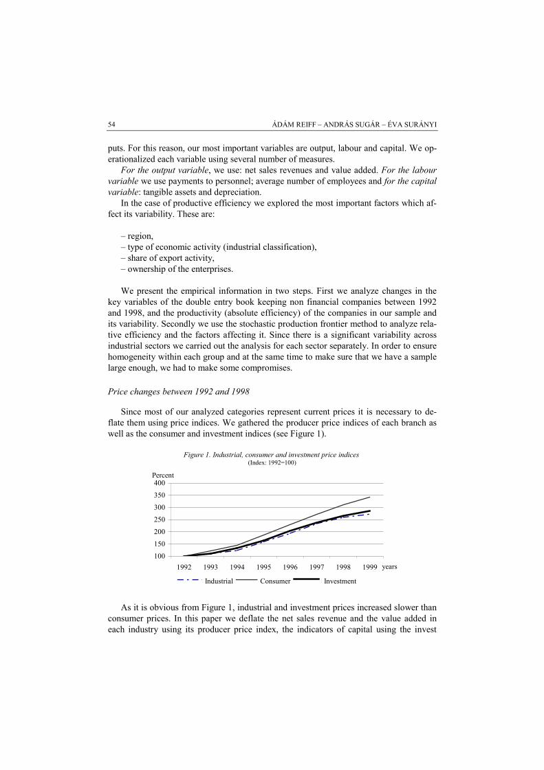
Since most of our analyzed categories represent current prices it is necessary to de-flate them using price indices. We gathered the producer price indices of each branch aswell as the consumer and investment indices (see Figure 1).

Figure 1. Industrial, consumer and investment price indices (Index: 1992=100)

100

150

200

250

300

350

400

1992 1993 1994 1995 1996 1997 1998 1999 years

industry consumer investmentIndustrial Consumer Investment

Percent

As it is obvious from Figure 1, industrial and investment prices increased slower thanconsumer prices. In this paper we deflate the net sales revenue and the value added ineach industry using its producer price index, the indicators of capital using the invest


ment, and the value of personnel payments using the consumer price index. In the case ofthe volume index of the value added it would make sense to use the method of double de-flation, but in Hungary input price indices are not calculated by industry (except in theagriculture). Therefore, we assumed that the companies suffered the same level of priceincreases from both the input and output side.

Time trends in output and ownership structure in the sample

In what follows we only analyze data from our sample of enterprises. First we explorechanges over time in the key variables in each branch, focusing on input and output factorsand the measures of labour and capital productivity. Before analyzing the factors of outputand production, we present the ownership structures of the companies in our sample.

Table 1

The proportion of different types of equities by industries(percent)

1992 1993 1994 1995 1996 1997 1998Industries

year

State ownedFood 36.9 24.9 14.9 10.8 10 1.9 1.3Textile 40.4 32.8 25.7 9.9 8.3 7.7 6.9Paper 37 29.1 23 9.6 6.6 1.3 1.3Chemical 77.1 71.9 61.9 43.1 28.1 16.8 12.1Metal 40.9 20.6 15.4 15.6 13.2 4.7 4.5Machinery 27.8 18 13.1 9.8 7.9 3.6 3.8Furniture 35.3 20.6 16.8 8.9 8.2 3.4 3.3Energy 93 90.1 88 68.7 61.3 53.1 48.1

Total 75.4 67.6 61.8 45.6 38 29.1 25.2

Foreign ownedFood 43.1 56.6 60.5 63.8 63.1 72.2 71.8Textile 26.1 32.5 35.7 47.7 49.5 50.4 49.1Paper 27.1 43.1 43.9 54.5 52.5 60.4 59.5Chemical 14.4 19.8 25.6 43.1 53.6 60.9 63.3Metal 24.2 34.7 36.8 38.1 47 59 60.1Machinery 22.6 50.3 55.6 59.8 65.9 66.6 66.4Furniture 18.6 29.3 32.2 34.7 35.8 36.4 36.7Energy 0.4 0.6 0.6 20.9 27 30.3 41.3

Total 10.7 17.5 20.4 36.3 42.7 48.1 53.9

The proportion of state (and local government) ownership declined to its third, and by1998 it represented a significant part only in the energy sector. Foreign ownership in oursample increased from 10 percent to over 50 percent by 1998. We can observe the high-est rate in the food sector and the lowest in the furniture industry, but it exceeds one-thirdeven here. The two indicators of output are the net sales revenues and the value added.Both indicators have been deflated by the producer price index of each branch so weanalyze the output at 1992 constant prices.


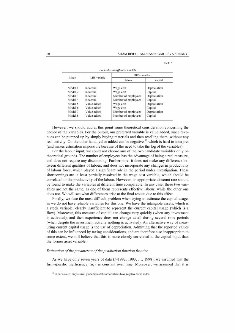
The volume of output roughly doubled according to both indicators during the sevenyears. The value added increased a bit more rapidly and this is particularly true for thechemical and metal industries. In other words, the proportion of material requirementsdecreased in these sectors. The same is true for the energy sector but we have to take intoaccount the fact that in the period under study prices were under state control in the en-ergy sector and especially until 1995 the rise in retail prices remained well below that ofthe input, that is, the deflation of the value added using the producer price index overes-timates its volume. After 1995 (and the privatization of the sector) cost based price set-ting was introduced so this problem is less significant.

Figure 2 displays the volume of the value added by industries. It is clear how the av-erage increase in the share of metal and machinery industries raised their share in theoverall output. The machinery industry produced only 14 percent of the value added in1992, but 25 percent by 1998.

Figure 2. Value added at constant price in 1992–1998 by industries

0

50

100

150

200

250

300

350

400

450

1992 1993 1994 1995 1996 1997 1998

Billion HUF

ENERGY

FURNITURE

MACHINERY

METAL

CHEMICAL

PAPER

TEXTILE

FOOD

Simple productivity indicators

Having characterized both output and inputs using two indicators, we will now de-scribe the productivity of labour and capital using the following variables. For the pro-ductivity of labour: net sales/number of employees, value added/number of employees,net sales/payments to personnel, value added/payments to personnel. For the productivityof capital: net sales/depreciation, value added/depreciation, net sales/tangible assets,value added/tangible assets.

We calculated the changes in the size of these eight indicators at constant prices byindustries, but in Table 2 we only present those that are based on value added.

The labour and capital requirements of the branches vary widely. Our indicators persua-sively demonstrate that the textile and furniture industries are the most labour intensiveones, and the chemical and energy sectors are the least. During the seven years productivityincreased most in the metal production and machinery industries. Examining time trends,

Energy

Furniture

Machinery

Metal

Chemical

Paper

Textile

Food

years


the rate of increase seems relatively smaller (or the rate of decrease larger) comparing withpersonnel payments and with the size of the personnel. This indicates that the relative costof labour increased even in real terms during the seven years under review.

Table 2

Value added indicators1992 1993 1994 1995 1996 1997 1998

Industriesyear

Index:1992=100

Value added/number of employees (thousand HUF/capita)Food 712.7 855 882.5 888.9 918 868.2 867.6 121.7Textile 351.7 407.8 469.2 448 406.5 410.7 442.5 125.8Paper 684 865.9 885.4 807.8 843 1049.1 1086.1 158.8Chemical 1150.4 1550.2 1667.9 1668.4 1508.3 1790.2 1872.5 162.8Metal 254.9 583.3 849.6 963.2 913.5 1009 1119.8 439.3Machinery 423.9 563.5 803.2 939.5 835.3 1153.2 1117.2 263.6Furniture 404.6 499.7 546.5 554.2 545.5 544.6 529 130.7Energy 1187.7 1180.5 1116.1 1197 1175.9 1519.3 1641 138.2

Total 651.4 861.6 980 1012.3 930.5 1123.3 1160.4 178.1

Value added/ payments to personnel (HUF/HUF)Food 1.8 1.7 1.7 1.7 1.8 1.7 1.6 88.9Textile 1.3 1.2 1.4 1.5 1.5 1.3 1.4 107.7Paper 1.4 1.4 1.5 1.5 1.6 1.9 1.9 135.7Chemical 2.1 2.2 2.4 2.4 2.2 2.5 2.4 114.3Metal 1.1 1.1 1.6 1.8 1.7 1.8 1.9 172.7Machinery 0.9 1.1 1.5 1.8 2.3 2.3 2.1 233.3Furniture 1.2 1.4 1.5 1.6 1.6 1.6 1.5 125Energy 2.4 2 1.7 1.9 1.8 2.3 2.3 95.8

Total 1.6 1.6 1.8 1.9 2 2.1 2.1 131.3

Value added/depreciation (HUF/HUF)Food 7.2 7.3 6.8 6.6 6.6 6.2 6.4 88.9Textile 7.1 13.4 15.8 17.4 17.6 15.5 14.2 200Paper 6.8 6.9 4.7 7.1 7.4 8.3 7.9 116.2Chemical 2.5 3.4 4.1 4.9 5.2 5.6 5.9 236Metal 4.9 5.4 8 8.8 8.6 9.3 9.2 187.8Machinery 5.4 6.2 8.2 10 12.5 12.4 12.2 225.9Furniture 10.4 12.9 14.1 13.8 14.5 13.7 13 125Energy 1.9 2.6 3.1 3.1 2.5 3.3 3.5 184.2

Total 3.3 4.3 5.1 5.9 6.1 6.5 6.7 203

Value added/tangible assets (HUF/HUF)Food 0.44 0.54 0.56 0.62 0.69 0.67 0.76 172.7Textile 0.83 1.01 1.28 1.51 1.63 1.47 1.42 171.1Paper 0.45 0.64 0.85 0.84 0.84 1.03 1.03 228.9Chemical 0.26 0.38 0.49 0.56 0.56 0.69 0.69 265.4Metal 0.35 0.47 0.74 0.92 0.92 0.98 1.1 314.3Machinery 0.37 0.55 0.84 1.16 1.49 1.73 1.61 435.1Furniture 0.62 0.96 1.11 1.27 1.35 1.45 1.43 230.6Energy 0.1 0.14 0.16 0.21 0.24 0.34 0.36 360

Total 0.25 0.35 0.45 0.55 0.64 0.75 0.77 308


It is obvious that the productivity of capital is the lowest in the energy sector and in thechemical sector (that is, these are the most capital intensive branches). The dynamics ofchange over time, however, differs quite a bit according to the four indicators, althoughthey all show significant (two- or threefold) increase. At the same time, we can observesome contradicting figures in some of the branches. In most sectors the size of output rela-tive to the value of tangible assets increased more steep than relative to the depreciation.This means that the real value of tangible assets grew slower than the depreciation. Sincewe calculate the value of tangible assets for a given year by adding investments to its valuein the previous year and deducting the depreciation this means that in most branches thevalue of new investments increased slower (or decreased faster) than the depreciation. Ex-ceptional from this trend are textile and clothing industries with reverse situation.

We measured the productivity of both factors of production using four indicators ofeach. We analyzed the covariation of the variables (at the level of the enterprise) usingprincipal component analysis. The four indicators of the productivity of labour move to-gether relatively closely. The first principal component explains 62 percent of the variance.

The correlations between the first principal component and the variables are as fol-lows: the net sales/number of employees is 0.62, the value added/number of employees is0.79, the net sales/payments to personnel is 0.72 and the value added/payments to per-sonnel is 0.81. On the basis of the previous we can approximate the common factor in theindicators of efficiency the best by using the value added/payments to personnel variablebut the value added/number of employees variable is almost as good.

In the case of capital efficiency the first component explains 63 percent of the totalvariance. The correlation coefficients of the variables and the factor are: the netsales/depreciation is 0.77, the value added/depreciation is 0.82, the net sales/tangible as-sets is 0.64 and the value added/tangible assets is 0.70. In this case the variable valueadded/depreciation is the most useful one.

Obviously, the differences in productivity and the factors determining them can notbe described very precisely by using these very simple descriptive statistics, therefore inthe following we will employ more sophisticated statistical methods.

3. ESTIMATING THE INDUSTRY-SPECIFIC PRODUCTION FRONTIERSAND THE FIRM-SPECIFIC INEFFICIENCIES

In this part we describe how we chose the functional form for the production functionand the variables to measure output, labour and capital input, how we estimated the pa-rameters of the production function frontiers, calculated the firm-specific inefficiencies,transformed the data prior to estimation, and the effects of this if any. At last we wouldinterpret the results obtained in this part.

The choice of production function

We assumed that in each industry there is an industry-specific, Cobb–Douglas typeproduction function frontier of the following form:

*0 1 2it it it ity l k v� � �� .


Here � �0 1 2, ,� � � � � denotes the industry-specific parameters of the production

function, * , ,it it ity l k are the logs of the appropriately measured efficient output, labour in-put and capital input variables for firm i at time t, and finally itv is the random distur-bance term affecting firm i’s efficient output at time t. (The distribution of itv is assumedto be normal).

The actual output of firm i at time t equals its efficient output *ity minus the firm-

specific inefficiency, 0iu � :

*0 1 2it it i it it it iy y u l k v u� � � � � � �� . /16/

An alternative assumption could have been that the production function frontier is oftranslog-type (see, for example Greene; 1997). In this case the production function is thefollowing:

* 2 20 1 2 3 4 5it it it it it it it ity l k l k l k v� � � � �� . /17/

It is obvious that this contains the Cobb–Douglas production function as a specialcase (when 3 4 5 0� � � � � � ), and the relevancy of the Cobb–Douglas model can betested.

Indeed, we prepared estimates with this formulation as well for selected industries(containing the most influential machinery), and the results were as follows. The new pa-rameters were jointly significant, indicating that the Cobb–Douglas type productionfunction frontier may not be appropriate; however, the estimated firm-specific inefficien-cies remained practically the same in the two cases (with a correlation coefficient above0.98). Therefore, for the sake of simplicity of exposition, we decided to present the re-sults obtained with Cobb–Douglas production function. We note, however, that obtainingthe full set of results with the more flexible translog production function formulation re-mains for future research (affecting mainly the production function estimates, not thefirm-specific inefficiency estimates).

The choice of variables

For each variable (output, labour, capital) we had two possible choices:

– for output, we used either total sales revenues (in what follows, simply revenues) orvalue added;

– for labour input, we used either wage costs or the number of employees;– for capital input, we used either depreciation or tangible assets.

This gave us eight possibilities for the formulation of our model, summarized in Ta-ble 3. We estimated each possible model, to see whether the extent of the estimated pa-rameters are sensitive to changes in the input variables. A detailed comparison of the re-sults will be provided later.


Table 3

Variables in different modelsRHS variables

Model LHS variablelabour capital

Model 1 Revenue Wage cost DepreciationModel 2 Revenue Wage cost CapitalModel 3 Revenue Number of employees DepreciationModel 4 Revenue Number of employees CapitalModel 5 Value added Wage cost DepreciationModel 6 Value added Wage cost CapitalModel 7 Value added Number of employees DepreciationModel 8 Value added Number of employees Capital

However, we should add at this point some theoretical consideration concerning thechoice of the variables. For the output, our preferred variable is value added, since reve-nues can be pumped up by simply buying materials and then reselling them, without anyreal activity. On the other hand, value added can be negative,10 which is hard to interpret(and makes estimation impossible because of the need to take the log of the variables).

For the labour input, we could not choose any of the two candidate variables only ontheoretical grounds. The number of employees has the advantage of being a real measure,and does not require any discounting. Furthermore, it does not make any difference be-tween different qualities of labour, and does not incorporate any changes in productivityof labour force, which played a significant role in the period under investigation. Theseshortcomings are at least partially resolved in the wage cost variable, which should becorrelated to the productivity of the labour. However, an appropriate discount rate shouldbe found to make the variables at different time comparable. In any case, these two vari-ables are not the same, as one of them represents effective labour, while the other onedoes not. We will see what differences arise at the final results due to this effect.

Finally, we face the most difficult problem when trying to estimate the capital usage,as we do not have reliable variables for this one. We have the intangible assets, which isa stock variable, clearly insufficient to represent the current capital usage (which is aflow). Moreover, this measure of capital can change very quickly (when any investmentis activated), and then experience does not change at all during several time periods(when despite the investment activity nothing is activated). An alternative way of meas-uring current capital usage is the use of depreciation. Admitting that the reported valuesof this can be influenced by taxing considerations, and are therefore also inappropriate tosome extent, we still believe that this is more closely correlated to the capital input thanthe former asset variable.

Estimation of the parameters of the production function frontier

As we have only seven years of data (t=1992, 1993, …, 1998), we assumed that thefirm-specific inefficiency ( )iu is constant over time. Moreover, we assumed that it is

10 In our data set, only a small proportion of the observations have negative value added.


stochastic, with a half-normal distribution among firms in each industry. Finally, we alsoassumed that the inefficiency components are independent from the itv random shocksaffecting the stochastic production frontier.

Under these assumptions the parameters of the model can consistently be estimatedby the random-effects panel model, described previously. Here we repeat the exact for-mulation of the model to be estimated (for each industry separately):

0 1 2it it it it iy l k v u� � � � �� . /18/

A technical note is appropriate here: in /18/, the expected value of the compound distur-bance term it it iv u� � � is non-zero, as 0iu � , and therefore � � 0iE u � . But consider:

� � � �0 1 2it i it it it i iy E u l k v u E u� � � �� , /19/

the same model with a disturbance variable of zero expected value. The standard esti-mated random-effects model parameters will be the parameters of this latter model, so, to

obtain the parameters of our original model, we will have to add � �2

i uE u � �

�

to the

estimated constant parameter. 11 The random-effects estimates of the parameters of thelabour and capital variables � �1 2,� � are consistent estimates of the true parameters inthe initial model.

4. ESTIMATION OF THE FIRM-SPECIFIC INEFFICIENCIES

With consistent estimates of the parameters of the previous model in hand,12 we canprepare estimates of the compound disturbance terms in model /19/:

� � � �0 1 2ˆ ˆ ˆˆ ( ) ( )it it i i it i it ite v u E u y E u l k� � � � � � � � � �� . /20/

If we subtract � �iE u from these estimates, we obtain estimates for the disturbanceterms of our original model:

� � � �0 1 2ˆ ˆ ˆˆ ( ) ( ) ( )it it i it i it i it it ie e E u v u y E u l k E u� � � � � � � � �� . /21/

As demonstrated previously, the estimates of the firm-specific inefficiencies can beobtained by using the formula defined by Jondrow et al. (1982) (see /15/ with 0� � ).

With given observations , 1,...,it ie t T� , and given estimates for u� and v� , we cancalculate the conditional expected value of the firm-specific inefficiencies according to/15/. These will be consistent estimates of the true iu -s.13

11 This formula comes from the assumption that u-s are half-normally distributed among the firms in each industry.12 We made all calculations by LIMDEP; the program code was written by the authors, and available upon request.13 As in our data set the maximum value of T is 7, this is only of theoretical interest here.


Initial data manipulations

The initial transformations that we made prior estimation are the following.

1. We divided our data set into eight industries, investigated in the previous section ofthe paper.

2. From each industry, we excluded all observations that contained implausible in-formation: non-positive net sales revenues, value added, intangible assets, depreciation ,wage costs or number of employees.

3. We also excluded those observations that changed industries during the seven yearobservation period, and this way our industry classification of the firm changed. (For ex-ample, textile industry in our sample contains industries from 17 to 19. If a firm was ini-tially in industry 17, then changed to industry 18, then this firm was not excluded, as itoperated in our classification of textile industry during the entire period. But, if a firmchanged its classification from 17 to say, 29, then those observations with classification29 were excluded from the textile industry, while observations with classification 17could remain there.)

4. We also deflated the variables when it was appropriate.

Table 4 represents the remaining size of our data set after the exclusions.

Table 4

The effect of initial exclusions of the implausible observations

Industries Initial numberof observations

Initial numberof firms

Numberof observation

after exclusions

Number of firmsafter exclusions

Food 1 547 221 1 463 221Textile 2 429 347 2 300 346Paper 1 505 215 1 405 214Chemical 1 652 236 1 589 235Metal 1 694 242 1 581 242Machinery 3 101 443 2 885 441Furniture 679 97 617 95Electric 266 38 255 38

Total 12 873 1 839 12 095 1 832

Summary of the results

The Appendix contains all estimated parameters for the 64 models (8 possible modelsfor 8 industries). We also included the Wald test-statistics considering the hypothesis thatthe production frontier of the industry is of constant returns to scale (i.e., the sum of thetwo reported estimated parameters is 1), and to the significance level of this test-statistics. Our main findings are as follows.

1. The estimated parameters are highly dependent of the variables chosen to measureoutput, labour input and capital input. Sometimes there is a conflict among the alternative


models even in their returns to scale predictions (there are instances when some of themodels indicate increasing, some other models decreasing returns to scale for the sameindustry). This is clearly a discrepancy that not only our parameter estimates are not ro-bust to the choice of the model, but our return to scale estimates are either.

2. However, there is a systematic difference among the parameter estimates and re-turn to scale predictions of different models. The most obvious difference is that replac-ing the wage cost variable to the number of employees variable, the sum of the estimatedparameters systematically reduces. Sometimes this causes that predictions about an in-creasing/constant returns to scale with the wage cost variable (models 1, 2, 5, 6) changeto predictions about constant/decreasing returns to scale with the number of employeesvariable (models 3, 4, 7, 8). The same occurs when replacing the value added variable (inmodels 5, 6, 7, 8) with revenue (models 1, 2, 3, 4). Finally, the incorporation of capitalinstead of depreciation tends to reduce the share of capital relative to the labour (i.e.,smaller estimated parameters are obtained for the capital variable), while the sum of thetwo estimated parameters remains constant.

3. Let us summarize the results for the models containing our preferred dependentvariable, value added (models 5-8).

– For the textile industry, all models predict increasing returns to scale.– For industries of food, furniture and electricity, there is a consensus about the pre-

dictions of constant returns to scale.– For paper and machinery, the prediction of all the models is decreasing returns to

scale. – For the chemical models with wage cost (5, 6) predict increasing, models with

number of employees (7, 8) predict constant returns to scale.– Finally, for the metal industry, models with wage cost (5, 6) predict constant, mod-

els with the number of employees (7, 8) predict decreasing returns to scale.

4. Finally, the relative labour intensiveness of the different industries matches our in-tuition. In our most preferred models, in model 5 and 7, the two industries with the high-est labour shares are textile and furniture, which are clearly the most labour intensive in-dustries. The most capital intensive industry is paper industry, with machinery also beingrelatively capital intensive in both cases.

Inefficiencies in different branches of the industry

From our production function estimates, for each industries we have calculated theaverage firm efficiencies, i.e. the average across firms inefficiency estimates. Differentmodels lead to very similar results, the efficiencies in our two preferred models (5 and 7)are highly correlated (r=0.752). However, there is a systematic difference between thetwo measures: the average inefficiency terms estimated by model 5 (ineff5) are in eachcases less than the model 7 estimations (ineff7); the reason for this was explained earlier.But luckily this does not change relative inefficiency measures, i.e. the order of industrieswith regard to inefficiencies. So both measures lead to the same results. The most effi-ciently operating branches (with the smallest inefficiency terms) are electricity, textile


and paper industry; furniture, chemistry and food are around the average; while there aregreat inefficiencies in metal and machinery industries.

The main aim of the following section is to find some explanations for these differ-ences both among and within different branches. Two possible sources of the between-industry differences are the extent of concentration of the industry and the share of for-eign enterprises.

In the second part we will examine relative efficiencies within the industries: the ef-fects of ownership structure, firm-size, the market share of the enterprises and the regionof operation.

Concentration and inefficiencies

For each industries we calculated an index of the concentration, by calculating theshare of the first 10 percent of the companies in the total value added and revenues (aver-ages over the period).

Table 5

Concentration indices and average inefficiencies in different industries Concentration

value added revenuesIndustries

percent

Ineff7 Ineff5

Food 57.77 57.71 0.5623 0.4377Textile 54.18 60.83 0.4800 0.2794Paper 60.59 63.26 0.6222 0.3539Chemical 82.07 83.59 0.6711 0.4378Metal 68.88 81.31 0.6524 0.5319Machinery 73.51 77.26 0.6798 0.4907Furniture 49.09 50.57 0.5178 0.3557Electric 46.04 64.37 0.3788 0.2177

Note: Ineff7 and ineff5 stand for the estimated inefficiency measures in model 7 and model 5, respectively.

In Table 5 we can see the concentration indices and the average inefficiencies for theindustries under investigation. It is apparent that there is a strong correlation between thetwo types of variables, and this is why we suppose that the higher the concentration is,i.e. the higher the monopolization in a specific industry is, the higher inefficiencies weexpect to occur. In the case of the two variables in the figure, the correlation coefficientbetween them is 0.8905.

The share of foreign enterprises in the sector

The measure of the share of foreign enterprises in the sector can have opposite effectof what we have explained in the previous part; a higher foreign enterprise share in thesector probably refers to higher (international) market competition in the branch. Tomeasure this effect we calculated two foreign enterprise share indices for each industry,


i.e. the proportion of value added and the proportion of net sales revenues of foreign en-terprises relative to all enterprises. We defined foreign owned companies as firms withmore than 25 percent of foreign ownership on average over the period.

Table 6

Foreign share indices and average inefficiencies in different industriesForeign share

value added revenues number of firmsIndustries

percent

Ineff7 Ineff5

Food 76.40 73.74 33.80 0.5623 0.4377Textile 47.78 48.58 30.98 0.4800 0.2794Paper 68.15 72.76 31.73 0.6222 0.3539Chemical 49.61 39.29 50.43 0.6711 0.4378Metal 47.87 48.98 29.24 0.6524 0.5319Machinery 67.26 72.56 32.11 0.6798 0.4907Furniture 39.92 41.47 21.74 0.5178 0.3557Electric 69.21 54.57 28.95 0.3788 0.2177

Total 60.26 56.71 33.86 0.4144 0.6018

The result is ambiguous. When measured with value added, foreign share shows aslight negative correlation with inefficiency terms, just as we would expect, but whenmeasured with revenue the sign of the correlation coefficient turns into positive, thoughthe coefficient is not significant (in neither cases). We can find the explanation for thisphenomenon in Table 6. In the third column we can see the share of foreign enterprises inthe different sectors when this share is measured simply by the number of firms. We caneasily observe that the proportion declines to about the half compared to the previousones, which means that foreign enterprises are usually the ones with higher than the aver-age market share. This is reasonable as we think of the great number of multinationalfirms entering the Hungarian markets. So it seems that foreign enterprise presence notonly means higher international competition but it is also connected with higher concen-tration in the branch,14 which has just the opposite effect on efficiency. The outcome issomehow ambiguous.

The correlation coefficients between the inefficiency terms (ineff7 and ineff5) and theforeign share are –0.06 if it is measured with the value added, 0.18 and 0.16 respectivelyif the share is measured by the revenues.

The effect of ownership structure

In this section we transformed the standardized inefficiency terms into an intervalbetween 0 and 100, therefore zero inefficiency term refers to a firm which is the most ef-ficient, while a hundred indicates the less efficient company.

14 This is justified if we examine the correlation coefficients between the proportion of the foreign firms and theconcentration indices (as defined in Table 5). These are 0.75 and 0.64 (the former refers to the value added based concentrationindex, while the latter is calculated with the revenue based index).


a) State and local government ownership. To examine the effect of state ownershipon productivity we have divided the firms in the sample into four main subgroups:

1. state owned during the whole period (1.1%),2. privatized (state owned in 1992 but mainly private owned in 1998) to Hungarian

investors (10.86%),3. privatized to foreign investors (7.47%),4. private (Hungarian and foreign) owned companies (average private ownership ex-

ceeds 30 percent). This means 74.24 percent of firms in the sample.

Figure 3 shows the average inefficiency terms in the defined subgroups.15 We can seethat private owned firms do outperform state owned ones. We can also conclude that pri-vatization was successful when evaluating efficiencies: privatized firms perform betterthan state owned ones, especially when they are purchased by foreign investors.

Figure 3. Average inefficiencies in state and private owned firms (model7)

0,0

5,0

10,0

15,0

20,0

25,0

State owned Privatized (Hungarianinvestors)

Privatized (Foreigninvestors)

Private ownership

Increasing inefficiencies in the state owned firms can be observed in nearly each indus-tries (see Table 7). There are two interesting exceptions: the food and the metal industry. Inboth cases state owned firms operate nearly as efficiently as private owned, while privat-ized ones seem to be less efficient. This probably refers to the fact that in most cases thestate sells its firms when they operate less efficiently, but especially in the food industrythere are some huge companies that are world wide famous and operate so successfully(even if state owned) that the state do not want to sell them. An alternative explanation ad-dresses the problems that firms just under privatization have to overcome: the costs of reor-ganization can be quite large, and normal operation is reached only after a certain period.

15 Ineffiencies are measured by method 5 (explained in the previous sections).

25.0

20.0

15.0

10.0

5.0

0.0


Another interesting feature is that in electric industry there is a huge difference ac-cording to the effect of the direction of the privatization. Those firms that are sold toHungarian investors are nearly as inefficient as state owned ones, while those that werepurchased by foreign investors have significantly improved their efficiency.

Table 7

Average inefficiencies in different industries and different ownership (method 5)

Industries State owned Privatized toHungarian investors

Privatizedto foreign investors

Private owned

Food 14.2 17.0 15.0 13.9Textile 27.4 18.6 18.6 14.2Paper 16.4 16.4 13.7 14.8Chemical 25.2 17.2 15.2 14.1Metal 14.8 17.9 16.8 13.7Machinery 20.8 17.1 15.1 14.1Furniture – 10.8 23.1 14.3Electric 21.9 21.5 9.9 11.3

Total 19.9 17.2 15.3 14.1

b) Foreign investors. Because of the huge changes in the ownership structure duringthe given period it seemed reasonable to examine the performance of the following sub-groups of companies:16

1. foreign owned (during the whole period) (18.4%),2. privatized to foreign owners (3.5%),3. sold from Hungarian private owners to foreign investors (1.7%),4. private owned (during the whole period) (57.7%),5. state owned (during the whole period) (1.3%).

Figure 4 shows the average inefficiency terms in these subgroups (calculated withmodel 7). We can observe that foreign firms in Hungarian markets overperform even thedomestic private ones, the effect is probably caused by the great inflow of multinationalcompanies into the country.

Although privatization has a negative effect on efficiency among the firms that arepurchased by foreign investors too, probably because of the reorganization costs, wewould expect they will probably catch up after a short transitional period. But again wewould like to note that privatization was successful in terms of improving the efficiencyof their operation relative to state owned ones.

When examining these effects in different branches we can observe some interestingfeatures of the Hungarian industry17 (see Table 8). Parallel to the results of the previous

16 In this case for simplicity ownership was defined according to the ‘dominant’ owner; for example we say an enterprise isstate owned if the share of state among the owners is larger than 50 percent. This way of course some firms will be missingfrom the sample; the valid number of observations is 1062.

17 In this case we could not evaluate state owned firms and those which have been sold from Hungarian to foreign privateowners because of the small number of valid cases.


section we can see again the special case of the food sector, where both private and pri-vatized firms perform worse than the overall average, while state owned ones show greatadvantages.

Figure 4. Average inefficienciesin foreign and Hungarian owned firms

0,0

5,0

10,0

15,0

20,0

25,0

30,0

Foreign owned(during the whole

period)

Privatized toforeign owners

Sold fromHungarian privateowners to foreign

investors

Private owned(during the whole

period)

State owned(during the whole

period)

Table 8

Average inefficiencies in different industries and different ownership

Industries Foreign owned(the whole period)

Privatizedto foreign owners

Private owned(the whole period)

Food 19.0 24.7 22.3Textile 17.8 15.9 22.5Paper 14.8 17.9 24.2Chemical 15.6 19.4 23.6Metal 19.1 17.9 20.7Machinery 18.1 17.6 20.0Furniture 13.1 29.6 19.6Electric 8.3 15.6 8.5

Total 17.2 19.4 21.7

In textile industry we see right the opposite features. Those firms that were privatized toforeign investors are the most efficient ones, while the rest is less efficient. In chemical andfurniture industry foreign firms are especially efficient relative to Hungarian ones, and alsoin metal and machinery branches, but with smaller differences among the two groups offirms. In electric industry we also see some very efficiently operating companies, owned bythe private sector (either Hungarian or foreign), but we must note that in these categoriesthere are only few firms in the sample, so the reliability of this result is quite low.

The effect of the size of the enterprise

It is also interesting to examine whether the size of the company is a good predictorof efficiency differences or not: can small companies catch up with big multinational

30.0

25.0

20.0

15.0

10.0

5.0

0.0


ones? To measure this hypothesis we created three categories of enterprises in thesample:

– small enterprises (the average number of employees is smaller than 100 persons,61.5 percent),

– medium size enterprises (the average number of employees is between 100 and 500persons, 24.7 percent),

– large enterprises (the average number of employees exceeds 500 persons, 8.6 per-cent).

As Table 9 shows, larger enterprises are more efficient (have smaller average ineffi-ciency terms) than smaller and medium ones. Indeed, we found significant negative cor-relation between size and inefficiency.18 It seems that small enterprises cannot be as effi-cient as large multinational firms. The result is quite robust: according to Table 9, wereach the same conclusion in each of the industries. This can have strong implications forpolicy makers.

Table 9

Average inefficiency terms in small, medium and large enterprisesSmall Medium size Large

Industriesenterprises

Food 22.3 18.1 18.9Textile 21.3 20.4 17.7Paper 21.7 18.6 10.8Chemical 22.5 17.4 19.6Metal 21.2 19.3 21.6Machinery 21.1 21.8 16.8Furniture 23.1 17.3 13.5Electric 24.6 23.9 17.0

Average 21.7 19.6 18.0

Region

It is well known that there are huge regional differences in the Hungarian industry.To explore regional differences in the performance of the enterprises we divided thecountry into seven regions: Central Hungary, Central Transdanubia, Western Transda-nubia, Southern Transdanubia, Northern Hungary, Northern Great Plain, SouthernGreat Plain.

Efficiency terms on Figure 5. show that the centralized feature of the country leads tothe relative advantages of the central part compared to some other regions. Transdanubia,especially Central and Western Transdanubia are also nearly as efficient as the centralregion of the country. Nevertheless there are huge inefficiencies in the operation of thefirms in Southern Hungary and the Great Plain.

18 The correlation coefficient is –0.67 in case of inefficiency measured by model 7.


Figure 5. Average inefficiencies in different regions

0,0

5,0

10,0

15,0

20,0

25,0

30,0C

entra

lTr

ansd

anub

ia

Cen

tral

Tran

sdan

ubia

Wes

tern

Tran

sdan

ubia

Sout

hern

Tran

sdan

ubia

Nor

ther

nH

unga

ry

Nor

ther

n G

P

Sout

hern

GP

An alternative method of measuring determinants of inefficiency

To test for the significance of the previously analyzed relations we estimated effi-ciency equations. We regressed firm level efficiency terms against export share, propor-tion of state, foreign and private ownership and regions. Due to size considerations, wecan present only a summary of our main findings.

The first observation is that the choice of the capital variable (depreciation againsttangible assets) does not have much influence on the final results. On the other hand, re-placing the labour input variable of the number of employees with wage costs has dra-matic effects for the final results. Therefore we decided to split our results into two sub-groups: to demonstrate them when the labour input variable is the number of employees,and when it is the wage costs.

To see all the significance relationship at the same time, we constructed ‘significancetables’, where we can see each significant variables for each industries. Table 10 containsthe results when the labour input variable is the number of employees, while Table 11 hasthe same structure, but the labour input variable is the wage costs. In both tables, cells withdark backgrounds represent highly significant variables, while those with light backgroundrefer to weaker relationships (significant at 10 percent, but not significant at 5 percent).

The following conclusions can be drawn from the Tables 10 and 11.

1. The role of exports. The exporting companies do not seem to be more efficient thantheir non-exporting counterparts. The important exception can be found in the case offood industry, where there is a very small number of exporters (20 percent of the firms).These rare companies tend to be more efficient. In other industries, however, it is morecommon for a company to sell its products to foreign markets (in a typical industry theproportion of exporters is approximately 40 percent), then the competition at the domes

Hun

gary

Nor

then

Gre

at P

lain

Sout

hen

Gre

at P

lain

30.0

25.0

20.0

15.0

10.0

5.0

0.0


tic markets among these exporting firms forces their non-exporting competitors to bemore efficient, so that exporting alone is not an efficiency-improving activity. There is aninteresting exception as well: in paper industry, exporting firms tend to be significantlyless efficient. We explained this by industry-specific features: exporting firms are raw-material (like wood, etc.) exporters, while the non-exporter efficient firms (publishingand printing firms) operate mainly on domestic markets.

Table 10

Significance table of the explanatory variables when the labour input variable is the number of employeesDenomination Food Textile Paper Chemical Metal Machinery Furniture Electricity

Export (-) Export 2 (-) Export (+) Export 2 (+) State share (-) State share 2 (-) Privatized Foreign (-) Partly foreign (-) Partly foreign (+) Hungarian private owner (-) Central Transdanubia (+) Western Transdanubia (+) Southern Transdanubia (+) Northern Hungary (+) Northern Great Plain (+) Southhern Great Plain (+)

Table 11

Significance table of the explanatory variables when the labour input variable is the wage costDenomination Food Textile Paper Chemical Metal Machinery Furniture Electricity

Export (-) Export 2 (-) Export (+) Export 2 (+) State share (+) State share 2 (+) Privatized Foreign (-) Partly foreign (-) Partly foreign (+) Hungarian private owner (-) Central Transdanubia (+) Western Transdanubia (+) Southern Transdanubia (+) Northern Hungary (+) Northern Great Plain (+) Southern Great Plain (+)

Note: In Table 10 and 11 the directions of impact on inefficiency are in parenthesis.

2. The role of state ownership. We would expect that firms under public ownership op-erate less efficiently, but this is not justified in our data set. In some cases we saw exactly


the opposite: state owned companies were found to be more efficient. We explained thisphenomenon by the fact that the number of state-owned companies is recently very small,in a typical industry, it is around 10 percent; among these companies there are several stra-tegically important, relatively well-performing companies. (This is especially true for theelectricity sector, where the state was reluctant to sell the big national suppliers.) Though, itis still interesting that we have found inefficiency corresponding to state in only one in-stance (at the chemical industry, when the labour input variable is wage costs). Anothersignificant issue is privatization: we expected that inefficiencies can be explained (at leastto some extent) by the dramatic changes in the ownership structure. But we could not detectany evidence that newly privatized companies were more efficient. This may be explainedby the fact that: first, the observation period is too short to detect any significant change inefficiency for a specific company; second, the majority of private firms gave the controllingrights for the former management and workers, who had limited financial backgrounds forthe necessary investments. (This is especially true for the smaller firms.)

3. The role of foreign ownership. This is the variable that seems to explain the mostsuccessfully the differences in inefficiencies. According to almost all models in all in-dustries under investigation, dominant (above 50 percent) foreign control increases effi-ciency. However, the role of partial foreign ownership is not so obvious. We have foundevidence that it may even reduce efficiency (in metal and machinery).

4. The role of domestic private ownership. Here we observed a very interesting pat-tern of significance: when our labour input variable is the number of employees, Hun-garian private ownership tends to have not a significant effect on efficiency. However,when labour input is measured in wage costs, Hungarian private firms are found to bemuch more efficient. This may be explained by the differences in wage levels amongmultinational and other companies: when we measure efficiency per unit wage costs,those Hungarian firms that pay lower salaries outperform the other ones. This is not true,however, if we consider ‘raw labour’, i.e. efficiency per worker.

5. The role of regional dummies. There is a sharp difference between the two typesof models. When we consider the number of employees, Budapest and the Central re-gion are the most efficient on average. (The estimated regional dummies are almostalways positive, relative to East Hungary, though sometimes insignificant.) Thoughchanging to wage costs as labour input variable, Budapest and the Central region(which is characterized by much higher wage levels) looses its efficiency advantage,and several times it becomes the least efficient region. (In this case the estimated pa-rameters for the regional dummies tend to turn into negative, though remaining mainlyinsignificant.)

CONCLUSION

In this paper we estimated industry-specific production function frontiers and foundthat our estimates are highly dependent on the choice of input and output variables.Based on simple statistical methods, and on theoretical arguments, our preferred outputvariable is value added, and our preferred capital input variable is depreciation. We can-not choose between wage costs and number of employees as a labour input measure, as itinfluences significantly our final results.


The results show that average efficiency is highest in textile, electric and paper in-dustries, while machinery and metal industries are the least efficient on average. We ex-plained the differences by several factors. When examining all industries together, wefound that the highest the concentration is, the highest is the average inefficiency; privateand foreign owned firms generally outperform the rest of the companies. Large compa-nies tend to be more efficient as well and regional differences do not play an importantrole in explaining inefficiency, the western and central region being only slightly moreefficient than eastern firms.

We also tried to explain firm-specific inefficiencies in all industries separately. Ourmain results were that the only variable that could robustly (i.e., independently from themodel setting and the industry under investigation) explain higher efficiency is foreignownership. State owned companies tend to be as efficient as privatized ones. Export-orientation is also a weak indicator of higher efficiency, examined at industry level. Hun-garian private ownership also tends to increase efficiency in those models when the la-bour input is measured as wage costs. Regional dummies gain significance only when thelabour input variable is the number of employees.

APPENDIX

Estimated parameters for different modelsRHS variables

LHS variablelabour capital

Variable coeffi-cient for labour

Variable coeffi-cient for capital

Wald teststatistics

Significancelevel

FoodRevenue Wage cost Depreciation 0.83 0.16 0.64 0.43Revenue Wage cost Capital 0.92 0.06 2.34 0.13Revenue Number of employees Depreciation 0.66 0.31 2.64 0.10Revenue Number of employees Capital 0.81 0.12 9.03 0.00Value added Wage cost Depreciation 0.88 0.13 0.36 0.55Value added Wage cost Capital 0.93 0.08 0.42 0.52Value added Number of employees Depreciation 0.70 0.33 1.60 0.21Value added Number of employees Capital 0.82 0.20 0.70 0.40

TextileRevenue Wage cost Depreciation 0.87 0.16 3.39 0.07Revenue Wage cost Capital 0.93 0.08 1.85 0.17Revenue Number of employees Depreciation 0.68 0.29 3.99 0.05Revenue Number of employees Capital 0.76 0.19 8.87 0.00Value added Wage cost Depreciation 0.99 0.07 46.36 0.00Value added Wage cost Capital 1.04 0.03 41.50 0.00Value added Number of employees Depreciation 0.84 0.24 25.24 0.00Value added Number of employees Capital 0.91 0.15 14.74 0.00

PaperRevenue Wage cost Depreciation 0.59 0.29 54.44 0.00Revenue Wage cost Capital 0.71 0.12 80.05 0.00Revenue Number of employees Depreciation 0.43 0.39 80.67 0.00Revenue Number of employees Capital 0.55 0.15 179.49 0.00Value added Wage cost Depreciation 0.73 0.22 10.93 0.00Value added Wage cost Capital 0.85 0.09 11.32 0.00Value added Number of employees Depreciation 0.49 0.40 25.91 0.00Value added Number of employees Capital 0.62 0.15 80.98 0.00

ChemistryRevenue Wage cost Depreciation 0.77 0.19 8.44 0.00Revenue Wage cost Capital 0.85 0.11 6.07 0.01Revenue Number of employees Depreciation 0.60 0.33 11.53 0.00Revenue Number of employees Capital 0.74 0.18 16.83 0.00Value added Wage cost Depreciation 0.87 0.16 6.60 0.01Value added Wage cost Capital 0.97 0.07 7.59 0.01Value added Number of employees Depreciation 0.62 0.37 0.14 0.71Value added Number of employees Capital 0.80 0.18 1.46 0.23

(Continued on the next page.)

REIFF–SUGÁR–SURÁNYI: PRODUCTIVE EFFICIENCY74

(Continuation.)RHS variables

LHS variablelabour capital

Variable coeffi-cient for labour

Variable coeffi-cient for capital

Wald teststatistics

Significancelevel

MetalRevenue Wage cost Depreciation 0.74 0.24 1.79 0.18Revenue Wage cost Capital 0.85 0.11 4.10 0.04Revenue Number of employees Depreciation 0.50 0.39 40.39 0.00Revenue Number of employees Capital 0.60 0.20 91.17 0.00Value added Wage cost Depreciation 0.89 0.13 0.97 0.33Value added Wage cost Capital 0.97 0.04 0.54 0.46Value added Number of employees Depreciation 0.56 0.34 22.38 0.00Value added Number of employees Capital 0.68 0.17 44.40 0.00

MachineryRevenue Wage cost Depreciation 0.71 0.25 14.33 0.00Revenue Wage cost Capital 0.82 0.13 14.41 0.00Revenue Number of employees Depreciation 0.51 0.37 56.84 0.00Revenue Number of employees Capital 0.67 0.19 80.60 0.00Value added Wage cost Depreciation 0.83 0.15 3.99 0.05Value added Wage cost Capital 0.91 0.07 3.97 0.05Value added Number of employees Depreciation 0.59 0.31 39.14 0.00Value added Number of employees Capital 0.74 0.14 54.08 0.00

FurnitureRevenue Wage cost Depreciation 0.77 0.10 29.93 0.00Revenue Wage cost Capital 0.82 0.04 30.54 0.00Revenue Number of employees Depreciation 0.60 0.23 28.16 0.00Revenue Number of employees Capital 0.68 0.13 31.28 0.00Value added Wage cost Depreciation 0.91 0.09 0.04 0.85Value added Wage cost Capital 0.94 0.05 0.01 0.93Value added Number of employees Depreciation 0.68 0.27 2.35 0.13Value added Number of employees Capital 0.76 0.18 3.11 0.08

EletricityRevenue Wage cost Depreciation 0.39 0.29 101.18 0.00Revenue Wage cost Capital 0.54 0.17 72.39 0.00Revenue Number of employees Depreciation 0.22 0.37 128.61 0.00Revenue Number of employees Capital 0.38 0.19 115.08 0.00Value added Wage cost Depreciation 0.82 0.20 0.92 0.34Value added Wage cost Capital 0.94 0.10 4.22 0.04Value added Number of employees Depreciation 0.63 0.36 0.24 0.63Value added Number of employees Capital 0.85 0.17 0.56 0.46

REFERENCES

AIGNER, D. – CHU, S. (1968): On estimating the industry production function. American Economic Review, No. 58. p. 826–839. AIGNER, D. – LOVELL, K. – SCHMIDT, P. (1977): Formulation and estimation of stochastic frontier production function models. Journal of

Econometrics, Vol. 6. No. 1. p. 21–37.ALCHIAN, A. A. (1965): Some economics of property rights. Il Politico, Vol. 30. No. 4. p. 816–829.ALCHIAN, A. A. – KESSEL, R. A. (1962): Competition, monopoly, and the pursuit of money. In: Aspects of Labour Economics. Princeton

University Press for The National Bureau of Economic Research, Princeton. p.157-175.AVERCH, H. – JOHNSON, L. L. (1962): The behaviour of the firm under regulatory constraint. American Economic Review, Vol. 52. No. 5.

p.1052–1069.BATTESE, G. – COELLI, T. (1988): Prediction of firm-level technical efficiencies with a generalized frontier production function and panel

data. Journal of Econometrics, Vol.38. No. 3. p. 387–399.BECKERS, D. – HAMMOND, C. (1987): A tractable likelihood function for the normal-gamma stochastic frontier model. Economics Letters,

No. 24. p. 33–38.BERNSTEIN, M. A. – FELDMAN, S. L. – SCHINNAR, A. P. (1990): Impact of pollution controls on the productivity of coal-fired power

plants. Energy Economics, Vol. 12. No. 1. p. 11–17.DEBREU, G. (1951): The coefficient of resource utilization. Econometrica, Vol. 19. No. 3. p. 273–292.GABRIELSEN, A. (1975): On estimating efficient production functions. Working Paper, No. A-85, Chr. Michelsen Institute, Bergen, Norway.GREENE, W. (1980): Maximum likelihood estimation of econometric frontier functions. Journal of Econometrics, Vol. 13. No. 1. p. 27–56. GREENE, W. (1990): A gamma-distributed stochastic frontier model. Journal of Econometrics, Vol.46. No. 1–2. p. 141–163.GREENE, W. (1993): The econometric approach to efficiency analysis. In: The measurement of productive efficiency, techniques and ap-

plications. Fried, H. O. – Lovell, C. A. K. – Schmidt, S. S. (ed.) Oxford University Press.GREENE, W. (1997): Econometric Analysis. Prentice-Hall Inc. New Jersey.HICKS, J. R. (1935): The theory of monopoly: A survey. Econometrica, Vol. 3. No. 1. p. 1–20.JONDROW, J. ET AL. (1982): On the estimation of technical inefficiency in the stochastic frontier production function model. Journal of

Econometrics, Vol. 19. No. 2–3. p. 233–238.KOOPMANS, T. C. (1951): An analysis of production as an efficient combination of activities. In: Koopmans, T. C. (ed.) Activity analysis of

production and allocation. Cowles Commission for Research in Economics, John Wiley and Sons, Inc. New York.MEEUSEN, W. – VAN DEN BROECK, J. (1977): Efficiency estimation from Cobb-Douglas production functions with composed error. Inter-

national Economic Review, Vol. 18. No. 2. p. 435–444.SHEPHARD, R.W. (1970): Theory of cost and production functions. Princeton University Press, Princeton.

ANALYSIS OF THE HUNGARIAN ECONOMY … · ANALYSIS OF THE HUNGARIAN ECONOMY ... PRODUCTIVE...

Documents

Transcript of ANALYSIS OF THE HUNGARIAN ECONOMY … · ANALYSIS OF THE HUNGARIAN ECONOMY ... PRODUCTIVE...