Analysis of the Dynamic Interferences between the …...Analysis of the Dynamic Interferences...

Analysis of the Dynamic Interferences between the Stator andRotor of a Refrigeration Compressor Motor

Swen Thompson

Thesis submitted to the Faculty of the Virginia Polytechnic Institute and State University in partialfulfillment of the requirements for the degree of

Master of Sciencein

Mechanical Engineering

Dr. Reginald G. Mitchiner, ChairmanDr. Robert L. WestDr. Alfred L. Wicks

May 7, 1997Blacksburg, VA

Keywords: Refrigeration compressor, electric motor, stator/rotor interference, air gapeccentricity, unbalanced magnetic pull, finite element analysis

Analysis of the Dynamic Interferences between the Stator andRotor of a Refrigeration Compressor Motor

Swen Thompson

(ABSTRACT)

This thesis involves the development and study of a finite element model of a hermetic, single-vane compressor and a single-phase alternating current induction motor assembled in a commonhousing. The manufacturer of this unit is experiencing a high scrap rate due to interference duringoperation between the stator and rotor of the motor. The rotor shaft of the motor is non-typicalbecause of its cantilever design. The finite element model was first subjected to eigenvalueanalysis. This revealed that the interference producing displacements were not the result oftorque application to the rotor at a frequency close to an eigenvalue of the mechanical system.After a review of the literature and discussions with Electrical Engineering Department facultypossessing extensive motor experience, it was surmised that the physical phenomenon causing therotor displacement was unbalanced magnetic pull. This phenomenon occurs in the air gap ofrotating electric machines due to eccentricity in the air gap.

The model was then subjected to simultaneous harmonic force inputs with magnitudes of unity onthe rotor and stator surfaces to simulate the presence of unbalanced magnetic pull. It was foundthat the rotor shaft acts as a cantilever beam while the stator and housing are essentially rigid.The displacements due to these forces were examined and then scaled to develop the motorparameters necessary to produce the radial forces required for stator/rotor interference. Severalrecommendations were then made regarding possible solutions to the interference problem.

iii

Acknowledgements

The author wishes to thank his committee chairman Dr. Reginald G. Mitchiner for his support andguidance in the development of this thesis. The author also wishes to thank professors R.L. Westand A.L. Wicks for their contributions to this project. The author wishes to send his gratitude toDr. Jaime De La Ree Lopez of the Bradley Department of Electrical Engineering for his guidancewith the electrical engineering portions of this project.

The author’s sincerest gratitude goes out to his family for their continued support throughout hisacademic career. Without this support his success would have not been possible.

The author would like to thank Mrs. Jan Riess and Mr. Ben Poe for their help with all of the dayto day problems of graduate school. The author would also like to thank his office mates andfriends for their encouragement during the pursuit of his master’s degree.

iv

Table of Contents

1.0 Introduction ........................................................................................................................12.0 Literature Review ...............................................................................................................23.0 Problem Background ..........................................................................................................4

3.1 Motor/compressor design ..........................................................................................43.2 Interference problem and initial assumptions ..............................................................63.3 Air gap asymmetries and the resulting forces .............................................................6

4.0 Finite element analysis and modeling approach ..............................................................104.1 Overview of the finite element method .....................................................................10

4.1.1 Finite element solution to time dependent problems ................................114.2 Finite element approach ...........................................................................................11

4.2.1 Interference reproduction attempts .........................................................124.3 Geometry simplification ...........................................................................................144.4 Finite element selection ............................................................................................224.5 Boundary conditions, forcing functions and damping ...............................................294.6 Modeling of joint between upper and lower housing ................................................324.7 Use of the Append procedure in assembling the model .............................................32

5.0 Finite element analysis results ..........................................................................................345.1 Finite element model verification .............................................................................34

5.1.1 Rotor/shaft assembly model verification .................................................345.1.2 Housing/stator assembly model verification ............................................37

5.2 Eigenvalue results ....................................................................................................435.3 Displacements due to harmonic force inputs ............................................................44

5.3.1 Displacements due to 29.2 Hz input .......................................................485.3.2 Displacements due to 120 Hz input ........................................................585.3.3 Displacement results due to individual force application .........................65

5.4 Air gap change due to component displacements .....................................................686.0 Conclusions and future investigations .............................................................................70References ...............................................................................................................................72

v

List of Illustrations

Figure 1. Cross-sectional view of compressor as supplied by the manufacturer ............................5Figure 2. Peripheral distribution of unbalanced magnetic pull ......................................................8Figure 3. Isometric view of the compression chamber ...............................................................17Figure 4. Isometric view of the compression chamber, upper support and rotor shaft ................18Figure 5. Isometric view of the stator ........................................................................................19Figure 6. Isometric view of the rotor .........................................................................................20Figure 7. Isometric view of the lower housing ...........................................................................23Figure 8. Isometric view of the upper housing ...........................................................................24Figure 9. Isometric view of the rotor/shaft assembly ..................................................................25Figure 10. Isometric view of the complete housing ....................................................................26Figure 11. Cross-sectional view of the complete assembly .........................................................27Figure 12. Isometric view of the complete assembly ..................................................................28Figure 13. Isometric view of the complete assembly with final finite element mesh ....................30Figure 14. Isometric view of the housing with restraint locations ...............................................31Figure 15. Cross-sectional view of the upper and lower housing interface .................................33Figure 16. Cross-sectional view of the partial lower housing and the stator ...............................39Figure 17. Isometric view of the partitioned partial lower housing .............................................40Figure 18. Isometric view of the partitioned stator ....................................................................41Figure 19. Cross-sectional view of the partial housing/stator assembly with the applied force ....42Figure 20. Locations of the 0°, 90°, 180° and 270° points on the motor ....................................46Figure 21. Orientation of the stator and rotor harmonic force inputs ..........................................47Figure 22. Depiction of stator nodal information interpolation ...................................................48Figure 23. Rotor and Stator X-axis displacements at 0° and 180° due to 29.2 Hz force input ....51Figure 24. Rotor and Stator Y-axis displacements at 0° and 180° due to 29.2 Hz force input ....51Figure 25. Rotor and Stator Z-axis displacements at 0° and 180° due to 29.2 Hz force input .....52Figure 26. Rotor and Stator X-axis displacements at 90° and 270° due to 29.2 Hz force input ..52Figure 27. Rotor and Stator Y-axis displacements at 90° and 270° due to 29.2 Hz force input ..53Figure 28. Rotor and Stator Z-axis displacements at 90° and 270° due to 29.2 Hz force input ...53Figure 29. Exaggerated component displacements in the XY plane due to 29.2 Hz force inputs ..............................................................................................................56Figure 30. Exaggerated component displacements in the YZ plane due to 29.2 Hz force inputs ..............................................................................................................57Figure 31. Rotor and Stator X-axis displacements at 0° and 180° due to 120 Hz force input .....61Figure 32. Rotor and Stator Y-axis displacements at 0° and 180° due to 120 Hz force input .....61Figure 33. Rotor and Stator Z-axis displacements at 0° and 180° due to 120 Hz force input ......62Figure 34. Rotor and Stator X-axis displacements at 90° and 270° due to 120 Hz force input ...62Figure 35. Rotor and Stator Y-axis displacements at 90° and 270° due to 120 Hz force input ...63Figure 36. Rotor and Stator Z-axis displacements at 90° and 270° due to 120 Hz force input ....63Figure 37. Exaggerated component displacements in the XY plane due to 120 Hz

vi

force inputs ..............................................................................................................66Figure 38. Exaggerated component displacements in the YZ plane due to 120 Hz force inputs ..............................................................................................................67

vii

List of Tables

Table 1. Summary of the mesh verification results for the rotor/shaft assembly ..........................37Table 2. Summary of the mesh verification results for the partial housing/stator assembly ..........43Table 3. Eigenvalue results for the various system components .................................................44Table 4. 29.2 Hz Rotor displacement at 0° ................................................................................48Table 5. 29.2 Hz Rotor displacement at 180° ............................................................................49Table 6. 29.2 Hz Rotor displacement at 90° ..............................................................................49Table 7. 29.2 Hz Rotor displacement at 270° ............................................................................49Table 8. 29.2 Hz Stator displacement at 0° ...............................................................................49Table 9. 29.2 Hz Stator displacement at 180° ............................................................................50Table 10. 29.2 Hz Stator displacement at 90° ............................................................................50Table 11. 29.2 Hz Stator displacement at 270° ..........................................................................50Table 12. 120 Hz Rotor displacement at 0° ...............................................................................58Table 13. 120 Hz Rotor displacement at 180° ...........................................................................58Table 14. 120 Hz Rotor displacement at 90° .............................................................................58Table 15. 120 Hz Rotor displacement at 270° ...........................................................................59Table 16. 120 Hz Stator displacement at 0° ...............................................................................59Table 17. 120 Hz Stator displacement at 180° ...........................................................................59Table 18. 120 Hz Stator displacement at 90° .............................................................................59Table 19. 120 Hz Stator displacement at 270° ...……………………………..………..….….....60Table 20. Change in air gap due to component displacement .....................................................68Table 21. Horsepower requirements to produce interference .....................................................69

1

Chapter 1.0 Introduction

Electric motors are essential in today's society. These devices power everything from smallhousehold appliances to large industrial processing equipment, and their potential applicationscontinue to grow. One such application for electric motors is as the power input for refrigerationcompressors. The object of this study is the analysis of such an application. The compressor andmotor in question are employed in a combination unit currently produced by the TecumsehProducts Company for use in applications such as larger office-type water coolers and medium-sized refrigeration units. A high percentage of these motors are experiencing interferenceproblems during running conditions, resulting in a high scrap rate for the manufacturer. Therewere two goals established for this study. The first goal was to model as accurately as practicalthe physical aspects of this unit and to determine the mechanical response of the system due toforce inputs characteristic of those encountered during operating conditions. The second goalwas to use the results of the study to make suggestions to the manufacturer regarding potentialdesign modifications to eliminate the interference problem.

The compressor/motor unit is modeled using the finite element method (FEM). This method wasrequired due to the lack of closed form solutions for the geometry of the compressor components.It was initially known that the interference encountered during operation was a radialdisplacement of the rotor larger than the stator/rotor air gap. It was felt that the ability toreproduce the magnitude of this interference for visual inspection with the software was of primeimportance and much effort was put towards making this possible.

The forcing functions used in predicting the component displacements were typical of thoseresulting from the air gap eccentricity that can occur in an electric motor. The nature of theseforces was determined by other investigators. The true magnitudes of the forcing functions werenot determined. Instead, the magnitude of unity was used for the analysis. This approach yieldeda set of displacements that may be scaled accordingly.

The study is organized into several chapters. Chapter 2 presents the review of the technicalliterature for the study. Chapter 3 presents the background of the motor and the interferenceproblem. Chapter 4 presents the modeling approach used for the FEM analysis, including allsimplifications. Chapter 5 presents the results of the FEM analysis. Chapter 6 presents allconclusions from the study and areas to be considered for future investigations.

2

Chapter 2.0 Literature Review

Much information is available in the technical literature regarding dynamic interferences, whichare commonly referred to as bumping, between the rotor and housing of turbomachinery.However, this information is heavily biased towards such issues as the physics associated with thecomponent contact and the effects of degradation problems such as excessively worn bearings andloose rotor blades. Since the system under study utilizes all new components it was decided thatthese findings were not relevant to this analysis.

Several references exist in the literature dating from the 1910's through the 1960's regarding airgap eccentricity in induction machines and one of its fundamental consequences - unbalancedmagnetic pull (u.m.p.). However, the theories behind many of these references are unclear andproduce no definite conclusions.

In 1974, Rai [1] completed extensive experimental investigations on all aspects of air gapeccentricity in induction motors. These experiments examined both static and dynamiceccentricities on 2-pole motors featuring unslotted, wound and cage rotors. These experimentsconsisted of extensive measurements of eccentricity fields, air gap flux density, unbalancedmagnetic pull, vibratory forces, losses and torque under various operating conditions from no-load to full-load and during starting. In this work it was determined that the following drivingforces of different frequencies can occur in electrical machines

1) Mechanical unbalance producing driving forces at the frequency of rotation.2) Inherent magnetic radial forces at twice line frequency.3) Static eccentricity producing twice line frequency vibratory driving forces.4) Defective rotor winding producing twice slip frequency vibration.5) Dynamic eccentricity producing vibratory forces at rotational speed with a modulation

at twice slip frequency. In addition, small vibratory forces at line frequency and twiceline frequency can occur.

6) Small static eccentricities can produce vibratory forces at line frequency.7) Stator harmonics can produce radial forces at twice-line frequency.8) Certain combinations of harmonics cause vibrations at twice slip frequency.

It was reported that in general, a number of these potential driving forces might exist dependingon the types of asymmetry present.

In 1989 Timar, Fazekas, Kiss, Miklos and Yang produced a text on noise and vibrations inelectrical machines [2]. In the text it was stated that in single-phase asynchronous motorsunbalanced magnetic pull can result in the production of a radial forces at angular frequencies of2f1, 2sf1, 2(1-s)f1, 2(2-s)f1, (3-s)f1 and (1±s)f1 where f1 is the line frequency and s is the slipfrequency of the rotor. Slip frequency is defined as the frequency of the voltages induced in therotor due to relative motion between the stator and rotor fields.

3

In 1994 Ozturk, Balikcioglu, Acikgoz and Bahadir produced a paper on the origins ofelectromagnetic vibrations in series fractional horsepower motors [3]. This paper summarized theworks of Rai, Timar, and others with respect to unbalanced magnetic pull and the resultant forces.In their research the authors used radial forces due to static eccentricity occurring at twice thevoltage supply frequency and radial forces due to dynamic eccentricity occurring at rotationalfrequency. The concept of static and dynamic eccentricities will be discussed in Chapter 2.

The final area explored in the literature was the effect of laminations used in the construction ofthe stator and rotor. In 1979 Girgis and Verma [4] determined that the laminated construction ofstators has virtually no effect on the location of natural frequencies. However, laminations causea significant damping in amplitudes of vibration and thus must be taken into consideration whenperforming stator analysis.

4

Chapter 3.0 Problem background

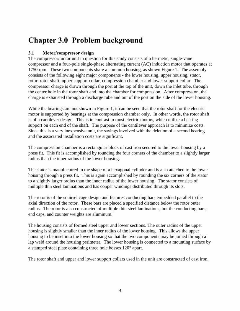
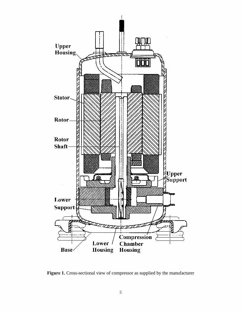
3.1 Motor/compressor designThe compressor/motor unit in question for this study consists of a hermetic, single-vanecompressor and a four-pole single-phase alternating current (AC) induction motor that operates at1750 rpm. These two components share a common housing, as shown Figure 1. The assemblyconsists of the following eight major components - the lower housing, upper housing, stator,rotor, rotor shaft, upper support collar, compression chamber and lower support collar. Thecompressor charge is drawn through the port at the top of the unit, down the inlet tube, throughthe center hole in the rotor shaft and into the chamber for compression. After compression, thecharge is exhausted through a discharge tube and out of the port on the side of the lower housing.

While the bearings are not shown in Figure 1, it can be seen that the rotor shaft for the electricmotor is supported by bearings at the compression chamber only. In other words, the rotor shaftis of a cantilever design. This is in contrast to most electric motors, which utilize a bearingsupport on each end of the shaft. The purpose of the cantilever approach is to minimize costs.Since this is a very inexpensive unit, the savings involved with the deletion of a second bearingand the associated installation costs are significant.

The compression chamber is a rectangular block of cast iron secured to the lower housing by apress fit. This fit is accomplished by rounding the four corners of the chamber to a slightly largerradius than the inner radius of the lower housing.

The stator is manufactured in the shape of a hexagonal cylinder and is also attached to the lowerhousing through a press fit. This is again accomplished by rounding the six corners of the statorto a slightly larger radius than the inner radius of the lower housing. The stator consists ofmultiple thin steel laminations and has copper windings distributed through its slots.

The rotor is of the squirrel cage design and features conducting bars embedded parallel to theaxial direction of the rotor. These bars are placed a specified distance below the rotor outerradius. The rotor is also constructed of multiple thin steel laminations, but the conducting bars,end caps, and counter weights are aluminum.

The housing consists of formed steel upper and lower sections. The outer radius of the upperhousing is slightly smaller than the inner radius of the lower housing. This allows the upperhousing to be inset into the lower housing so that the two components may be joined through alap weld around the housing perimeter. The lower housing is connected to a mounting surface bya stamped steel plate containing three hole bosses 120° apart.

The rotor shaft and upper and lower support collars used in the unit are constructed of cast iron.

5

Figure 1. Cross-sectional view of compressor as supplied by the manufacturer

6

3.2 Interference problem and initial assumptionsAs stated earlier the interference experienced during operation occurs between the stator androtor of the motor. Currently each motor must be tested for this problem as it leaves the assemblyline, and approximately thirty-five percent fail.

At the beginning of this analysis the concept of unbalanced magnetic pull was not known to theauthor. The initial assumption was that the 1750 rpm (29.2 Hz) frequency of the torque appliedto the rotor was close to an eigenvalue of one of the assemblies in the system, thus causingrandom lateral rotor displacements. The most likely culprit in this scenario was thought to be theassembly consisting of the compression chamber, rotor shaft, rotor, and upper and lower supportcollars. If the actual amount of interference between the components could be accuratelydetermined using finite element analysis, appropriate recommendations for modifications could bemade. It was felt that the most likely cure would be to increase the air gap between the stator andthe rotor. There would be a practical limit to an air gap increase, however, as this increase has anegative effect on motor output.

3.3 Air gap asymmetries and the resulting forcesAs stated in Chapter 2 many works have been published regarding air gap asymmetries and theireffects. The discussion of air gap asymmetries and unbalanced magnetic pull presented in thissection is a synopsis of the works of Rai [1] and Timar [2].

The main task in creating electromechanical energy conversion by an asynchronous or inductionmachine is to produce a rotating sinusoidal magnetic field with a pole number 2p in the air gap. Amagnetic flux is induced in the air gap due to current flowing through the conductors in the slots.These slots break up the uniformity of the air gap. Thus, the gap will change periodically as therelative position of the stator and rotor changes. The total magnetizing current of an inductionmachine is supplied from the stator (primary winding), and therefore the air gap is designed to beas small as possible. However, even the smallest deviation of the air gap from the shape of acylindrical sleeve of uniform thickness will result in considerable relative distortion of air gappermeance.

Deviation from a uniform air gap is also highly possible due to tolerances required in themanufacturing process. This non-uniform air gap can result from one or more of the followingmanufacturing flaws:

1) imperfect centering of the rotor in the stator bore,2) non-circular stator bore,3) non-circular rotor and4) bent shaft.

The first two flaws produce a stationary or static eccentricity in the air gap of an electric machine,while the last two flaws produce a rotating or dynamic eccentricity.

7

Regardless of whether the air gap eccentricity is static, dynamic or both, the resulting gap will beat a maximum at one point thus producing a minimum flux and a minimum at one point thusproducing a maximum flux. A non-uniform flux can result in the following adverse effects:

1) flux harmonics2) unbalanced magnetic pull3) noise4) harmonics in the rotor and stator currents5) variation in losses and irregular distribution of heat around the stator bore as a result

of 1) and 4)6) variation in torque as a result of 1) and 4), both during starting and steady state

conditions.

The effect considered for this study is unbalanced magnetic pull.

As stated, the presence of a magnetic flux in the air gap of an electric machine produces anattractive force between the stator and rotor in the direction of the flux. In an induction machinethe sinusoidal flux distribution revolves in the air gap producing a wave of magnetic pull rotatingat twice the frequency of the fundamental field. In a system with a uniform air gap no resultantforce occurs due to symmetry. When eccentricity is present, however, upon energizing of thestator equal but opposite unilateral magnetic forces acting on the stator and rotor are producedthat always act in such a manner as to increase eccentricity. This phenomenon is known asunbalanced magnetic pull (u.m.p.). A graphical representation of the peripheral distribution ofunbalanced magnetic pull on the rotor of a rotating electrical machine from Timar [2] is shown inFigure 2. This figure clearly shows the minimum and maximum magnetic field strengths (g) andthe resulting radial forces. It is obvious that all force terms perpendicular to the eccentricity (e)cancel. This leaves the force terms parallel to the eccentricity (e), which sum to produce aresultant radial force Fresultant. An equal but opposite force situation occurs with the stator.

Due to the sinusoidal distribution of flux around the air gap unbalanced magnetic pull due to staticeccentricity is generally treated as a harmonic, vibratory, radial force between the rotor and statorfor a given operating condition. The frequency of this harmonic force is twice voltage line supplyfrequency for the following reason. As the magnetic field distribution revolves in the air gap of aninduction machine, it passes a given point twice during each cycle of voltage change, once as aflux entering the stator and once as a flux entering the rotor. Since a force of attraction betweenthe stator and rotor occurs regardless of the direction of the flux, the harmonic input must occurat twice the frequency of the applied voltage.

8

Figure 2. Peripheral distribution of unbalanced magnetic pull

Unbalanced magnetic pull can also arise in electrical machines due to the presence of dynamiceccentricity. This form of unbalanced magnetic pull differs in that it rotates at the rotational speedof the rotor, and thus the effects are similar to those encountered with a mechanical unbalance.This situation can be referred to as magnetic unbalance.

The magnitude and distribution of the forces produced due to unbalanced magnetic pull aredependent upon the distribution of magnetic flux in the air gap. These magnitudes are typicallydetermined by using the Maxwell stress tensor method in conjunction with the finite elementmethod to extract the magnetic flux density in the air gap for a series of static rotor positions.The accurate determination of the flux density is a complicated and crucial step in a completeanalysis of an electric motor. Since this phase of the analysis requires a much more extensiveelectrical engineering background than possessed by the author, it was decided to set themagnitude of the u.m.p. based forces to unity. This approach results in a set of displacements thatmay be scaled accordingly upon accurate solution of the flux distribution problem.

9

Ozturk [3] summarized that for analysis purposes the equal but opposite vibratory forces due tounbalanced magnetic pull act upon the stator and rotor of a rotating electric machine. Theseforces occur at twice the electrical supply frequency for static eccentricity and at the rotorrotational frequency for dynamic eccentricity. If the natural frequency of any part or combinationof parts of the mechanical system lies near these forcing frequencies serious vibration problemscan result.

Timar [2] defined the relationship between the amplitude of the tangential forces (torqueproducing forces) and radial forces (i.e., u.m.p. forces) in the air gap as

(3.1)where

p = number of pole pairsλ = order of the rotor space harmonicsδg = geometrical air gapR = outer radius of the rotor.

The order of the rotor space harmonics for a single-phase AC machine is defined as

(3.2)where

g’ = negative gS2 = number of rotor slots

Normally the ratio of tangential to radial force is considerably less than one. Therefore, it isobvious that the radial force magnitude should be much larger than the tangential.

In summary the presence of eccentricity in the air gap of a rotating electric machine causes equalbut opposite harmonic forces of large magnitude at two different forcing frequencies to act uponthe stator and rotor at the point of minimum flux density.

122 +±′= gSgλ

,...2,1,0 ±±=g

Radialg

Tangential FR

pF

λδ=

10

Chapter 4.0 Finite element analysis and modeling approach

4.1 Overview of the finite element methodAccording to Knight [5] the finite element method (FEM) is a numerical method for solving asystem of governing equations over the domain of a physical system. The governing equations forFEM are taken from the field of continuum mechanics and the theory of elasticity. While FEMwas initially developed for performing structural analysis its use has spread to the fields of heattransfer, fluid mechanics, acoustics, electromagnetics and other areas.

The basis of FEM with respect to structural analysis is summarized in the following steps. Thedomain of the solid structure under consideration is subdivided into small domains calledelements. These elements assemble through interconnection of a finite number of points on eachelement called nodes. Within the domain of each element a simple general solution to thegoverning equations is assumed. The specific solution for each element becomes a function ofunknown solution values at the nodes. Application of the general solution form to all theelements results in a finite set of algebraic equations to be solved for the unknown nodal values.This subdivision of the structure allows the formulation of equations for each separate element,which are then combined to obtain the solution for the entire system. The structure response caneither be linear or non-linear. When the response is linear elastic the algebraic equations are linearand are solved with common numerical procedures. Non-linear solutions are not relevant to thisstudy and will therefore not be discussed.

Due to the division of the continuum domain into finite elements, it is necessary to translate thestructure loads and displacement boundary conditions to nodal quantities. Point loads are applieddirectly to nodes while distributed loads are converted to equivalent nodal values. Boundaryconditions such as ground locations are resolved into specified displacements for the specifiednodes.

There are two major sources of error associated with the finite element method. The first sourceof error is the difference between the assumed solution in the element and the exact solution overthe domain of the element. The magnitude of this error depends upon the size of the elements inthe subdivision relative to the solution variation. Most element formulations converge to thecorrect solution as the element size is reduced. The second source of error is the precision of thealgebraic equation solution. This error is a function of the computer accuracy, the algorithm, thenumber of equations and the element subdivision. Thus, accurate and efficient representation ofthe domain of the solid structure is critical.

There are two types of elements available for use in FEM – discrete structural elements andcontinuum elements. Ideally, all structures should be modeled using three-dimensional continuum

11

elements. However, this type of element is the most complicated to mesh and hardware and timeconstraints prohibit its use when other simpler elements will provide adequate solutions.

Structural elements consist of trusses, beams, plates and shells. The formulations of theseelements are based upon their respective structural theories. The structural theories of trusses andbeams are well accepted and thus the FEM solutions based upon these elements are no moreaccurate than those resulting from conventional solutions. Plate and shell elements are very muchdifferent in that the finite element community has yet to agree on formulations for these elementsthat produce completely satisfactory results. Therefore, the analyst must exercise great cautionwhen using these elements and should use all means available for verification of the solution.

Continuum elements are two- and three-dimensional solid elements. The formulation of theseelements is based upon the theory of elasticity. Few closed form solutions exist for two-dimensional continuum problems, and almost none exist for three-dimensional problems, thusmaking FEM invaluable.

4.1.1 Finite element solution to time dependent problemsKnight wrote [5] that when inputting an arbitrary time dependent function to a system orstructure, a transient response analysis must be performed. The solution to this problem taken byfinite element codes is generally one of two types – direct integration or modal superposition.

The integration method involves the direct integration of the system equations afterapproximation by a finite difference in the time domain for the velocity and accelerationcomponents. This approach involves the total set of system equations and must perform manytime steps with a complete solution in each step, thus requiring large computing resources.

The modal superposition method assumes that superposition of the mode shapes corresponding tothe lower natural frequencies adequately represents the dynamic response of the structure. Thecomplete response is found by the summation of correct fractions of the low frequency modeshapes. Mathematically this amounts to a transformation of the equations from node displacementcoordinates to a set of modal coordinates. The transformation changes the set of systemequations consisting of one equation for each degree of freedom in the model to a set of modalequations involving the selected number of mode shapes, thus resulting in fewer equations. Whilethis is an approximation of the total structural response, in most cases it has been shown to besufficiently accurate.

4.2 Finite element approachThe finite element analysis (FEA) for this study was performed using I-DEAS Master Seriesversions 2.1 and 4.0 by the Structural Dynamics Research Corporation (SDRC). Thecomputational hardware used was an IBM RISC 6000 workstation. I-DEAS (Integrated DesignEngineering Analysis software) Master Series is a comprehensive software package composed ofa number of modules or "applications", each of which are subdivided further into "tasks". The

12

different applications included in the software are Design, Drafting, Simulation, Test,Manufacturing, Management, and Geometry Translators.

4.2.1 Interference reproduction attemptsAt this point an overview of the logic used by the I-DEAS software to transfer informationbetween modules is required. In I-DEAS all components are based upon three-dimensional solidmodels. These master solid models or "parts" are constructed in the Master ModelerTM task, andfrom that point the parts serve as the basis for all geometric definitions for all other tasks.

The Master Modeler task contains many capabilities. Included in these are a series of Booleanoperators, which allow geometric comparisons between separate parts. These operators arereferred to as the Cut, Join and Intersect commands. These allow the designer to manipulateparts that share a common volume in three-dimensional space by

1) removing the common volume from one part and thus creating a new part,2) joining the two parts at the common volume and thus creating a new larger part and3) creating a new part which consists only of the common volume between the two

parts,

respectively. The purpose of these Boolean operators is to provide the user with the ability tocheck for static interferences between parts during the design process.

The finite element analysis package in I-DEAS uses a finite element model that is constructedfrom a part created in the Master Modeler task. It is similar to all other FEA codes in that a finiteelement mesh is applied to the part geometry (free mesh, mapped mesh, or a manually createdmesh), the appropriate boundary conditions and forces are applied and the required analysis isperformed (i.e., to determine stress, displacement, temperature, etc.).

It was felt that the most logical approach to the problem at hand would be to create thestator/rotor interference using FEA, and then apply the Intersect command to the deformed finiteelement model to produce the actual interference. The problem with this approach lies with thedistinction made by the software between parts and finite element models. While the finiteelement model is based upon and, therefore, related to the actual part, the two items are in factseparate entities. This system does not allow the use of Boolean operations on a finite elementmodel. This created a major obstacle because all of the information needed was present, but in anunusable form. It also proved to be an obstacle that consumed a large amount of time becauseseveral attempts were made to perform Boolean operations on finite element models before thedistinction made between the two was realized.

The initial thought with respect to interference reproduction was that the required information forreconstruction would be contained in the Simulation Universal Export File. This file contains allinformation pertinent to the finite element model, such as the model name, the type of analysisperformed, the type of mesh applied, the applied boundary conditions, the eigenvalues of the

13

system (if calculated), and so forth. The universal export file was desired because all nodeinformation for the model (i.e., the node numbers and the original coordinates, the nodalconnectivity and the displacements for each node) is also contained in the file. It was felt that thisdata could be used in conjunction with the Boolean operators to produce the desired interference.

The first attempt was to write the universal file for a displaced shape and then import this file intoa new model file. Upon import of this file it was learned that the displaced shape could beimported, but the imported shape was in the form of a finite element model, and no benefits hadbeen realized.

Upon further review of the universal file it was felt that the process of adding the nodaldisplacements to the original locations was causing the inability to use the Boolean operators onthe imported file. Therefore, an external piece of FORTRAN code was developed to retrieve theoriginal node locations and node displacements, sum the two quantities and insert the newlocations into the universal file as the original locations. This process also proved to beineffective because the root of the problem had still not been addressed.

It was at this point that the author realized the true nature of the conflict. The decision was thenmade to regress to the simplest model possible - a one-element cube - and develop a method totransfer a displaced finite element model into a part.

After further study it was realized that the displaced finite element model could possibly bereconstructed using the nodes on the exterior surface of the model and the various constructioncommands in the Master Surfacer and the previously described Master Modeler tasks. Theprimary function of the Master Surfacer task is to allow the designer to create solid models ofobjects with flowing, sculpted surfaces that would be virtually impossible to create with theMaster Modeler. This function is accomplished by either using the solids-based techniques ofsweeping and lofting or by creating surfaces from wireframe geometry and assembling thesesurfaces into a solid part.

The first attempt to reconstruct the displaced model was to draw three-dimensional lines and arcswith the Master Modeler task through the nodes on the surface of the finite element model,therefore, recreating all of the surface features individually. This method proved unsatisfactorybecause of the poor approximation of the displaced shape between the nodes and the largeamount of time required to pick every node on the surface of the finite element model.

The next method attempted was the placing of three-dimensional points through all of the surfacenodes of the finite element model and use of the Surface through Points command in the MasterSurfacer to recreate each individual surface. The individual surfaces could then be fused togetherusing the Stitch Surfaces command to create one part. This method was discarded after the initialtrial due to its inability to accurately follow the contours of the surface.

14

The next seemingly plausible solution was to again place three-dimensional points through all ofthe surface nodes and then to connect all of these points with three-dimensional lines. These linescreated the necessary information to allow use of the Surface by Boundary command in theMaster Surfacer. The intent was to recreate each surface using this command and stitch thesurfaces together to form a part. While this method did produce surfaces that accurately followedthe contour of each original surface, the resulting surfaces were larger than the designatedboundary. An attempt was made to fuse the overlapping surfaces and trim the excess, butstipulations in the program regarding the use of the Stitch Surfaces and the Trim commands madethis path also unfeasible.

It was at this time that the discovery of the Loft command in the Master Surfacer Task was made.This command fits a surface through a series of cross-sections in three-dimensional space. It wasfelt by the author that if the finite element mesh of the rotor was constructed using a mappedmesh scheme with its inherent edge requirements, then a series of wireframes representing cross-sections of the displaced rotor surface could be created with reasonable effort and sufficientaccuracy. These cross-sections could then be lofted together to form the associated surfaces, andin turn, the surfaces could be stitched together to form the required part.

This methodology was applied to the simple model of a concentric shaft and tube where each partwas treated as a cantilever. An inward radial force was applied to the free end of the shaft toproduce a displacement sufficient to cause interference between the shaft and the tube. Thedisplaced finite element model of the shaft was then reconstructed as a part using the loftingprocedure. It was found that the cross-sections could not be constructed based upon a full 360°sweep of the local longitudinal axis of the shaft (i.e., the use of one curve to represent the entirecircumference of the shaft). This was due to the lack of beginning and ending edges of thesurface. However, when the shaft surface was modeled as two halves that could be stitchedtogether (i.e., each half of the total surface was created by performing a 180° sweep of the locallongitudinal axis) the procedure worked as desired. This resulted in a part that could then bemanipulated with Boolean operators.

4.3 Geometry simplificationSeveral simplifications were made when modeling the geometry of the various parts. Thesesimplifications were necessary because of the use of mapped meshing and because of the lack ofaccurate geometric information for some of the components. Had a free mesh been allowable,details such as chamfers and fillets could have been easily modeled, but this was not the case.Since the needed results from the analysis were the natural frequencies and the displacements, thesmall errors induced by ignoring all chamfers, fillets, and countersinks were deemedinconsequential. The mass and stiffness characteristics of the components were kept as accurateas possible in accordance with the given information.

The greatest simplifications were made to the compression chamber, rotor shaft, lower supportand upper support.

15

The lower support was eliminated entirely. This component added nothing to the assembly interms of reducing rotor deflection, but it did add significant mass to the system and thus impactedthe natural frequencies. The deletion of this part was countered by determining its mass andincreasing the density of the compression chamber material by the corresponding amount to resultin the same total mass.

The upper support was modified by1) deleting the flange area and incorporating the mass into the compression chamber housing

material, as was done with the lower support. It can be seen in Figure 1 that the crosssection of the flange area is not only variable, but is also not symmetric about the hubcenterline. This configuration would be virtually impossible to mesh using a mappedmeshing scheme. Therefore, an equivalent constant width cross-section for each half wasfirst calculated and then a final constant width cross-section was calculated from the twosimplified halves. The mass properties of this final constant thickness flange were thenincorporated into the compression chamber housing material by increasing the materialdensity.

2) removing the step in the hub and using the larger of the two hub outer diameters. The hubsection of the upper support was assumed to behave as a cantilever beam. From Rao [6]the transverse stiffness of a cantilever beam is defined as

(4.1)

whereK = stiffnessE = modulus of elasticityI = area moment of inertiaL = beam length

Since the moment of inertia is a function of the hub diameter, I was calculated using bothouter hub diameters. It was found that the ratio of the larger to smaller I values, and thus thestiffness, for the two diameters is 1.61. Since some stiffness was eliminated by ignoring theflange as described in 1) above, it was felt that the use of the stiffer hub section would balancethe overall stiffness of the upper support.

The compression chamber housing was modified in that the open area in the chamber itself andthe discharge opening were not included (i.e., the chamber housing was modeled as solid minusthe center hole for the rotor shaft). These simplifications were made due to the lack of accurateinformation regarding the chamber area and the small amount of mass that was added with respectto the entire system. As stated above the density of the cast iron material for the compressionchamber was increased to account for the eliminated mass of the support collars. The required

3

3

L

EIK =

16

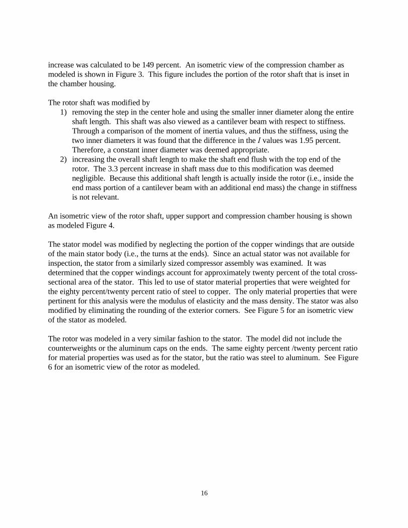
increase was calculated to be 149 percent. An isometric view of the compression chamber asmodeled is shown in Figure 3. This figure includes the portion of the rotor shaft that is inset inthe chamber housing.

The rotor shaft was modified by1) removing the step in the center hole and using the smaller inner diameter along the entire

shaft length. This shaft was also viewed as a cantilever beam with respect to stiffness.Through a comparison of the moment of inertia values, and thus the stiffness, using thetwo inner diameters it was found that the difference in the I values was 1.95 percent.Therefore, a constant inner diameter was deemed appropriate.

2) increasing the overall shaft length to make the shaft end flush with the top end of therotor. The 3.3 percent increase in shaft mass due to this modification was deemednegligible. Because this additional shaft length is actually inside the rotor (i.e., inside theend mass portion of a cantilever beam with an additional end mass) the change in stiffnessis not relevant.

An isometric view of the rotor shaft, upper support and compression chamber housing is shownas modeled Figure 4.

The stator model was modified by neglecting the portion of the copper windings that are outsideof the main stator body (i.e., the turns at the ends). Since an actual stator was not available forinspection, the stator from a similarly sized compressor assembly was examined. It wasdetermined that the copper windings account for approximately twenty percent of the total cross-sectional area of the stator. This led to use of stator material properties that were weighted forthe eighty percent/twenty percent ratio of steel to copper. The only material properties that werepertinent for this analysis were the modulus of elasticity and the mass density. The stator was alsomodified by eliminating the rounding of the exterior corners. See Figure 5 for an isometric viewof the stator as modeled.

The rotor was modeled in a very similar fashion to the stator. The model did not include thecounterweights or the aluminum caps on the ends. The same eighty percent /twenty percent ratiofor material properties was used as for the stator, but the ratio was steel to aluminum. See Figure6 for an isometric view of the rotor as modeled.

17

Figure 3. Isometric view of the compression chamber

18

Figure 4. Isometric view of the compression chamber, upper support and rotor shaft

19

Figure 5. Isometric view of the stator

20

Figure 6. Isometric view of the rotor

21

The compressor/motor housing was modeled in two sections, upper and lower. The crown andknuckle radii for the ends of such a housing are designed according to the requirements fortorispherical flanged and dished heads under internal pressure from the American Society ofMechanical Engineers (ASME) Boiler and Pressure Vessel Code Section VIII, Division 1,Pressure Vessels. The actual equations are available from Chuse [7] and are as follows

(4.2)

wheret = minimum thickness, inP = internal pressure, psiS = allowable stress, psiE = minimum joint efficiency, percentD = inside diameter of head skirt, inL = inside crown radius, inr = knuckle radius, in = 0.06L

However, the only information that was available for constructing the model was a full-scale crosssection of the assembly. Therefore, the inside crown radius L for each end was approximatedfrom the full-scale drawing. This was done using the following theorem for the radius ofcurvature ρ of a line at a point P(x,y) from Swokowski [8]

(4.3)

where the first and second derivatives of y at x are defined using a Newton's central divideddifference interpolating polynomial which consists of the following equations:

(4.4)

( )[ ] 23

21 y

y

′+

′′=ρ

h

yyy ii

211 −+ −

=′

PSEPL

t1.0

885.0

−=

22

(4.5)

whereh = abscissa interval = constantyi = ith ordinate valuey' = first derivative of yiy'' = second derivative of yi

Several values for ρ were calculated for each end of the housing so that a reliable average valuefor the inside crown radius could be determined. The two knuckle radii were then calculated fromthe inner crown radii using the above referenced ASME requirement.

The model for the lower section of the compressor housing was simplified in two ways. The firstmodification was the elimination of the compressor discharge port. The second modification wasthe deletion of the supports or feet and the stamped plate to which these supports are mounted.The restraints that were applied to the housing during the analyses were applied directly to theouter surface of the lower housing at the midpoint of the contact area between the lower housingand the stamped base plate. See Figure 7 for an isometric view of the lower housing as modeled.

The model for the upper section of the compressor housing was simplified greatly in that all of thebosses and holes were ignored and the piece was assumed to have a constant cross-sectionrevolved around the longitudinal axis, just as the lower section. This approach was taken due tothe lack of accurate geometric data available for the upper section and the lack of boundaryconditions to be applied to the section. See Figure 8 for an isometric view of the upper housing asmodeled.

For review isometric views have been included for the complete rotor/shaft assembly and thecomplete housing in Figures 9 and 10, respectively. Additionally, a cross-sectional view of thecomplete compressor assembly as modeled is shown in Figure 11 and an isometric view is shownin Figure 12.

4.4 Finite element selectionAll of the compressor/motor components were modeled using three-dimensional eight node linearhexahedron elements. These components included the compressor housing (upper and lowersections), the stator, the rotor, the rotor shaft, the compression chamber housing and the uppersupport.

211 2

h

yyyy iii −+ +−

=′′

23

Figure 7. Isometric view of the lower housing

24

Figure 8. Isometric view of the upper housing

25

Figure 9. Isometric view of the rotor/shaft assembly

26

Figure 10. Isometric view of the complete housing

27

Figure 11. Cross-sectional view of the complete assembly

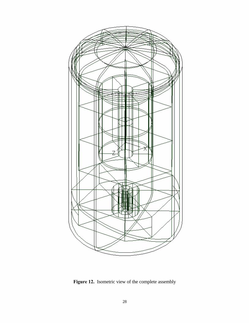
28

Figure 12. Isometric view of the complete assembly

29

The need to reassemble the distorted finite element model into parts dictated the use of thesethree-dimensional solid elements in a mapped mesh on all components except the housing. Thehousing could have theoretically been modeled more efficiently using thin shell elements.However, the use of shell elements would have required constraint equations to be writtenbetween all of the common nodes on the stator, compression chamber housing, and lowerhousing. Due to the large size of the model and the desire to simplify the modeling process asmuch as possible, the decision was made to use the same three-dimensional solid elements on thehousing as well. While it was recognized that the technique would be less efficient and requiremore computational run time, it was felt that the total time required for the alternative would begreater. This decision was not made without first checking for accuracy. The complete can wasinitially modeled by itself using two separate meshes. Each mesh consisted of the same number ofelements and featured the same boundary conditions. The first mesh consisted of three-dimensional solid elements while the second mesh consisted of thin shell elements. It was foundthat the first natural frequency for the two models varied by only 0.52 percent.

The factor of element aspect ratio was also taken into consideration for the decision to use solidelements on the housing. In the I-DEAS software the concept of element aspect ratio isaddressed by calculating the relative distortion and stretch factors for the element, where a valueof 1.0 is a perfect element and values less than 1.0 are less than perfect. Of the 528 solid elementsused to mesh the lower housing the minimum distortion value was 0.80 while the minimum stretchvalue was 0.30. Of the 264 solid elements used to mesh the upper housing the minimumdistortion value was 0.77 while the minimum stretch value was 0.32. It was felt that grosselement distortion is the more significant of the two factors. Therefore, the finite element meshfor the housing did not present problems due to abnormal element aspect ratios. Based upon thisfact and the small variation in eigenvalue reproduction, the decision to use the three-dimensionalsolid elements was deemed justifiable. An isometric view of the complete compressor assemblyincluding the finite element mesh is shown in Figure 13.

4.5 Boundary conditions, forcing functions and dampingAs stated previously the restraint set used for the analyses of these components consisted of threeclamped nodes on the outer surface of the lower housing at 120° radial intervals. Thisconfiguration is shown in Figure 14. Each node was at the midpoint of the contact surfacebetween the lower housing and the stamped base plate assembly. These clamped conditions wereapplied to simulate fastening of the housing base plate to a solid surface by means of threadedfasteners.

The forces applied to the rotor and stator were harmonic inputs at driving frequencies of 29.2 and120 Hz as described previously. On the outer rotor surface a force of magnitude 0.2 lbf in thepositive x-direction was applied to each of the five axial nodes to simulate a unit load. At thecorresponding location of the inner stator surface across the air gap, a force of -.0167 lbf in the x-direction was applied to each of the six axial nodes to simulate an equal but opposite unit load.

30

Figure 13. Isometric view of the complete assembly with final finite element mesh

31

Figure 14. Isometric view of the housing with restraint locations

32

According to Timar [2] the main source of damping in an electrical machine is the friction on thecontact surfaces of the winding and between the core laminations. The amount of dampingpresent is usually derived experimentally with the use of the half-power point method. However,for induction machines, the damping value is normally in the range of 0.01 to 0.04, independent ofthe mode number. On this basis the amount of damping used for all modes in all finite elementmodels for this research was the average value of this range, 0.025.

4.6 Modeling of joint between upper and lower housingAs stated previously the upper and lower housing sections are assembled by inserting the lowerface of the upper housing 1.000 in. into the lower housing and applying a continuous lap weldaround the joint perimeter. This method allows the inset portion of the upper housing to remainfree to deflect. According to Ramani [9] this type of joint is best modeled by connecting the nodesat the weld by rigid elements and letting the inset nodes of the upper housing remain free. Thisarrangement appears to best model the joint with respect to resistance of the joint to housing-sidemotion. In this particular instance the outer diameter of the upper section and the inner diameterof the lower section were modeled as equal. The mapped mesh was dispersed so that a commonnode between the two sections existed only at the weld joint and not along the inset portion of theupper housing. The use of the Append procedure (to be explained in the next section) thenallowed the common nodes to become joined through a rigid link. A cross-sectional view of thisarrangement is shown in Figure 15.

4.7 Use of the Append procedure in assembling the modelAs stated the compression chamber and stator both fasten to the lower housing by means of apressed fit. In many cases this would require that constraint equations be written between thenodes at the chamber/housing and stator/housing interfaces to make the displacements of thesenodes equal. Several attempts were made to follow this procedure for the model at hand, but thecomplexity of the three-dimensional model made this prohibitive. It was discovered that the I-DEAS software contains provisions to link different finite element models into one model. This isknown as appending models. It is best described by imagining two identical finite element meshesof the same part. However, Mesh 1 has a boundary condition applied at Node 1, while Mesh 2has a boundary condition applied at Node 2. If these two models are appended the result will be amodel that has the appropriate boundary conditions applied at Nodes 1 and 2.

This feature is also very useful for constructing finite element models of components that arejoined through a press fit, such as the one under consideration for this analysis. It requires thatthe mesh of each part is planned so that the coincident nodes of the interfering sections will be atthe same location in three-dimensional space. For example, the location of the nodes on the sixaxial edges of the stator outer surface had to be in the same location as those on six imaginaryaxial lines of the lower housing inner surface. When mapped meshing and careful planning areutilized in conjunction with this capability the analyst can model and mesh each part individuallyand then append the separate finite element models into one large model. The Append toolproved to be invaluable in this analysis because it also made the task of assigning the differentmaterial properties to the respective components much easier.

33

Figure 15. Cross-sectional view of the upper and lower housing interface

34

Chapter 5.0 Finite element analysis results

5.1 Finite element model verificationWhile finite element analysis is a powerful tool, its successful application is highly dependent uponthe analyst’s understanding of the finite element method and the associated pitfalls. Therefore, it isalways necessary to validate a finite element model against some other standard. In many cases itis possible to use closed form solutions on simplified geometry for validation. In other cases noform of closed solution may be similar to the actual system. In these instances the only analyticalrecourse is to perform FEA with different models of the same system to assure that convergencehas been reached. The compressor assembly under analysis for this project required both suchapproaches. After examining all of the components involved it was felt that validation of therotor/shaft assembly and the housing/stator assembly would be sufficient.

5.1.1 Rotor/shaft assembly model verificationWhen viewing the cantilever rotor/shaft assembly it can be hypothesized that the compressionchamber is analogous to the fixed base of a cantilever beam. Virtually all displacements will occurin the rotor, the upper support collar and the rotor shaft section above the compression chamber.The combined length of the upper support collar and exposed rotor shaft (1.775 in.) is greaterthan the outside diameters of both the upper support collar (1.110 in.) and the rotor shaft (0.6125in.). Thus, the assembly may be approximated as a cantilever beam with an additional end mass asshown.

From Rao [6] it is known that this is easily treated as the following single degree of freedomspring-mass system

35

with the following equivalent stiffness K and mass M values.

(5.1)

(5.2)

where

E = Modulus of ElasticityI = Area Moment of InertiaL = length of beam

The problem with this approach is that the section modulus EI for the beam must remain constant.The upper support collar introduces a change in I for the system, thus violating this requirement.The decision was made to analyze the beam using I values for the upper support collar I1, therotor shaft I2 and an equivalent I value weighted for I1 and I2.

From Thomson [10] the first natural frequency of a cantilever beam may be found using thefollowing relationship.

3

3

LEI

K equiv =

ENDBEAMequiv MMM += 23.0

36

(5.3)

From Cheng [11] it is known that the static deflection of a cantilever beam due to an in-planeforce perpendicular to the axial direction as shown may be found through the followingrelationships.

(5.4)

(5.5)

31 52.3LM

EI

BEAM

=ω

( )xaEI

PxyAB −= 3

6

2

( )axEI

PayBC −= 3

6

2

37

wherey = displacementP = applied load

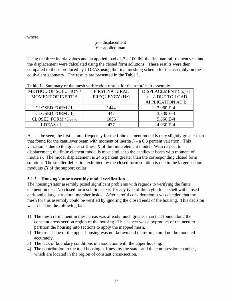
Using the three inertia values and an applied load of P = 100 lbf. the first natural frequency ω1 andthe displacement were calculated using the closed form solutions. These results were thencompared to those produced by I-DEAS using the final meshing scheme for the assembly on theequivalent geometry. The results are presented in the Table 1.

Table 1. Summary of the mesh verification results for the rotor/shaft assemblyMETHOD OF SOLUTION /

MOMENT OF INERTIAFIRST NATURALFREQUENCY (Hz)

DISPLACEMENT (in.) at x = L DUE TO LOADAPPLICATION AT B

CLOSED FORM / I1 1444 3.060 E-4CLOSED FORM / I2 447 3.339 E-3

CLOSED FORM / IEQUIV 1056 5.860 E-4I-DEAS / ITRUE 477 4.030 E-4

As can be seen, the first natural frequency for the finite element model is only slightly greater thanthat found for the cantilever beam with moment of inertia I2 - a 6.3 percent variation. Thisvariation is due to the greater stiffness K of the finite element model. With respect todisplacement, the finite element model is most similar to the cantilever beam with moment ofinertia I1. The model displacement is 24.6 percent greater than the corresponding closed formsolution. The smaller deflection exhibited by the closed form solution is due to the larger sectionmodulus EI of the support collar.

5.1.2 Housing/stator assembly model verificationThe housing/stator assembly posed significant problems with regards to verifying the finiteelement model. No closed form solutions exist for any type of thin cylindrical shell with closedends and a large structural member inside. After careful consideration it was decided that themesh for this assembly could be verified by ignoring the closed ends of the housing. This decisionwas based on the following facts.

1) The mesh refinement in these areas was already much greater than that found along theconstant cross-section region of the housing. This aspect was a byproduct of the need topartition the housing into sections to apply the mapped mesh.

2) The true shape of the upper housing was not known and therefore, could not be modeledaccurately.

3) The lack of boundary conditions in association with the upper housing.4) The contribution to the total housing stiffness by the stator and the compression chamber,

which are located in the region of constant cross-section.

38

5) The short axial distance between the constrained nodes on the lower housing end and thelower face of the compression chamber.

Thus to validate the mesh applied to the stator and housing for the analysis of the complete unit,the housing was treated as a cantilevered cylinder. The length of this cylinder was equal to theaxial distance from the bottom face of the compression chamber to the top face of the stator. Thestator was included, and its upper face was set flush with the free end of the housing. A cross-sectional view of this assembly with the restraint and load locations is shown in Figure 16.

It was initially thought that the stator and housing model could also be treated as a cantileverbeam with an additional end mass. Therefore, displacements and natural frequencies werecalculated using both finite element analysis and the closed form solutions. Upon comparison ofthe results it was realized that this approach was not feasible. The 4.625 in. outer housingdiameter is greater than the 4.275 in. equivalent beam length. Therefore, all assumptions made byconventional beam theory are invalid. The only possible non-numerical solution approach to thisproblem would be the use of the theory of elasticity.

After deliberation, the decision was made to analyze the assembly with several different finiteelement meshes to assure convergence. As stated previously the use of the Append procedureand mapped meshing required that all of the components be partitioned into several sections. Thehousing was partitioned axially and circumferentially, while the stator was partitioned onlycircumferentially. The partitions of the open housing and the stator are shown in Figures 17 and18, respectively. Because varying the housing mesh density in the radial direction wouldintroduce extreme element distortion, it was decided to vary the mesh density along the differentaxial and circumferential partitions. Using the actual mesh densities from the completecompressor model as a baseline, the density in each region was increased by a substantial margin.For each of these mesh densities the first several natural frequencies and the displacements due toa 100 lbf. radial load applied at the free end would be calculated and compared to assureconvergence. A top view of the housing/stator assembly and the applied force is shown in Figure19.

The housing as tested was partitioned axially into three sections – lower, middle and upper (seeFigure 17). The lower section length was equal to the compression chamber thickness, the uppersection length was equal to the stator length and the middle section length was equal to the axialdistance between the compression chamber and stator. The baseline element distribution in theaxial direction was

1) lower section – two elements2) middle section – four elements and3) upper section – five elements.

39

Figure 16. Cross-sectional view of the partial lower housing and stator

40

Figure 17. Isometric view of the partitioned partial lower housing

41

Figure 18. Isometric view of partitioned stator

42

Figure 19. Cross-sectional view of the partial housing/stator assembly with the applied force

43

The housing and stator were each partitioned circumferentially into six sections. The baselineelement distribution in the circumferential direction for the housing was four elements per section.The optimal circumferential element distribution for the stator was determined in separate tests tobe six elements per section. This partitioning scheme provided the commonaxial locations required to append the housing and stator together into a single finite elementmodel.

The mesh variations and the resulting natural frequencies and displacements are shown inTable 2.

Table 2. Summary of the mesh verification results for the partial housing/stator assemblyMESHDENSITY

ωω1

(Hz)ωω2

(Hz)ωω3

(Hz)Ymax

(in.)∆∆ ωω1

(%)∆∆Ymax

(%)

Original 1366.45 1366.45 3081.08 7.90 E-05 0.00 0.00

Lower axial+50%

1364.83 1364.84 3081.33 7.93 E-05 0.12 -0.28

Lower axial+100%

1364.05 1364.05 3081.41 7.94 E-05 0.18 -0.42

Middle axial+25%

1365.88 1365.88 3079.59 7.91 E-05 0.04 -0.08

Middle axial+50%

1365.52 1365.52 3078.62 7.91 E-05 0.07 -0.11

Upper axial+20%

1365.83 1365.83 3077.33 7.91 E-05 0.05 -0.08

Upper axial+40%

1365.38 1365.38 3074.78 7.91 E-05 0.08 -0.14

Circumferential+50%

1360.08 1360.08 3055.62 7.95 E-05 0.47 -0.57

Circumferential+100%

1357.83 1357.83 3048.21 7.96 E-05 0.63 -0.75

As can be seen all differences in the displacement and first natural frequency are less than onepercent. Based upon these results it was decided that the mesh density used in the completeassembly had reached convergence and was fully acceptable.

5.2 Eigenvalue resultsAfter validation of the finite element model the next step was to determine the lower eigenvaluesof the various components. The need to calculate these eigenvalues was twofold. The firstreason was to determine if the operating frequency of the rotor was close to one of the lowernatural frequencies of the system. The second reason was that the ultimate goal of this projectwas to determine the system response to the harmonic force inputs. Since the I-DEAS software

44

uses modal superposition as described in Chapter 4 to solve for cases of systems subjected to theinput of dynamic forces, the solution of the eigenvalue value problem was required.

Eigenvalue analyses were performed on the following combinations of components:1) the rotor/shaft assembly consisting of the compression chamber housing, rotor shaft, upper

support and rotor2) the housing/stator assembly consisting of the upper and lower housings and the stator3) the entire compressor assembly

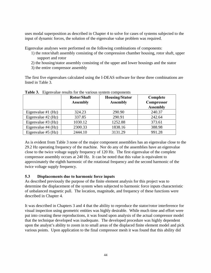
The first five eigenvalues calculated using the I-DEAS software for these three combinations arelisted in Table 3.

Table 3. Eigenvalue results for the various system componentsRotor/ShaftAssembly

Housing/StatorAssembly

CompleteCompressor

AssemblyEigenvalue #1 (Hz) 324.23 290.90 240.37Eigenvalue #2 (Hz) 337.85 290.91 242.64Eigenvalue #3 (Hz) 1030.12 1252.88 373.61Eigenvalue #4 (Hz) 2300.33 1838.16 388.98Eigenvalue #5 (Hz) 2444.10 3131.29 991.28

As is evident from Table 3 none of the major component assemblies has an eigenvalue close to the29.2 Hz operating frequency of the machine. Nor do any of the assemblies have an eigenvalueclose to the twice voltage supply frequency of 120 Hz. The first eigenvalue of the completecompressor assembly occurs at 240 Hz. It can be noted that this value is equivalent toapproximately the eighth harmonic of the rotational frequency and the second harmonic of thetwice voltage supply frequency.

5.3 Displacements due to harmonic force inputsAs described previously the purpose of the finite element analysis for this project was todetermine the displacement of the system when subjected to harmonic force inputs characteristicof unbalanced magnetic pull. The location, magnitude, and frequency of these functions weredescribed in Chapter 4.

It was described in Chapters 3 and 4 that the ability to reproduce the stator/rotor interference forvisual inspection using geometric entities was highly desirable. While much time and effort wereput into creating these reproductions, it was found upon analysis of the actual compressor modelthat the technique developed was inadequate. The developed procedure was highly dependentupon the analyst’s ability to zoom in to small areas of the displaced finite element model and pickvarious points. Upon application to the final compressor mesh it was found that this ability did

45

not exist. At that time it became apparent that two erroneous assumptions were made during thedevelopment of this procedure.

1) It was assumed that the mesh of the compressor model could be made relatively coarseand still maintain accuracy.

2) It was assumed that each displaced component (i.e., the displaced rotor and the displacedstator) could be analyzed individually, thus providing clear access to all of the nodes. Thisassumption was made before it was known that the meshes of the independentcomponents would have to be appended into a final model.

Upon performing the analyses on the final compressor model it was found that the required meshdensity, along with the inability to remove unnecessary objects from the screen, made pickingindividual points on a specific surface virtually impossible.

At this point it was decided to examine specific nodes on the outer rotor surface and inner statorsurface with respect to displacement. These nodes were located at 0, 90, 180 and 270 degreeswhen viewing the compressor assembly from the top just below the upper housing, as seen inFigure 20. The harmonic force inputs to the system were applied at the 0-degree locationperpendicular to the shaft axis as shown in Figure 21. The nodes at these locations wereexamined along the entire length of the rotor and stator surfaces. While this procedure didrequire the task of determining the individual node labels, it proved to be a much more reasonableapproach than picking nodes for surface reproduction. This was because the node labels could bedetermined before the meshes were displaced. Once the node labels were known the analysescould be run and the resulting displacements could be examined in column form through the I-DEAS post-processing capabilities.

As stated there were five nodes dispersed along the axial direction of the rotor and six nodesalong the axial direction of the stator. Since the displacements were examined at the four pointsin the plane perpendicular to the axial direction, twenty and twenty-four points were examined onthe rotor and stator surfaces, respectively, for each applied harmonic force. The six statordisplacements along each axial line were then interpolated to give displacements at five points,thus providing a 1:1 ratio with the rotor surface displacements. A simple schematic depicting thistransition is shown in Figure 22. These global displacements will be listed in tabular form andgraphical form in the following sections. Rather than use the actual node numbers assigned by I-DEAS the nodes will be labeled 1-5 with 1 being at the top or free end of the stator and rotor and5 being at the bottom end. For these analyses the compressor assembly was located in three-dimensional space so that the applied forces occur in the X-direction of the XY-plane. Thus all Z-displacements are perpendicular and out of plane to the applied force.

46

Figure 20. Locations of the 0°, 90°, 180° and 270° points on the motor assembly

47

Figure 21. Orientation of the stator and rotor harmonic force inputs

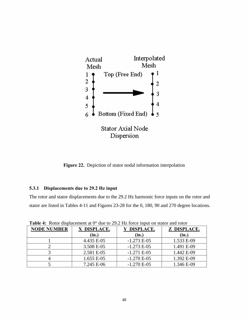
48

Figure 22. Depiction of stator nodal information interpolation

5.3.1 Displacements due to 29.2 Hz input

The rotor and stator displacements due to the 29.2 Hz harmonic force inputs on the rotor and

stator are listed in Tables 4-11 and Figures 23-28 for the 0, 180, 90 and 270 degree locations.

Table 4: Rotor displacement at 0° due to 29.2 Hz force input on stator and rotorNODE NUMBER X–DISPLACE.

(in.)Y–DISPLACE.

(in.)Z–DISPLACE.

(in.)1 4.435 E-05 -1.273 E-05 1.533 E-092 3.508 E-05 -1.273 E-05 1.491 E-093 2.581 E-05 -1.271 E-05 1.442 E-094 1.655 E-05 -1.270 E-05 1.392 E-095 7.245 E-06 -1.270 E-05 1.346 E-09

49


(in.)Y–DISPLACE.

(in.)Z–DISPLACE.

(in.)1 4.435 E-05 1.273 E-05 -9.938 E-102 3.508 E-05 1.273 E-05 -1.034 E-093 2.581 E-05 1.271 E-05 -1.075 E-094 1.655 E-05 1.271 E-05 -1.116 E-095 7.245 E-06 1.270 E-05 -1.132 E-09


(in.)Y–DISPLACE.

(in.)Z–DISPLACE.

(in.)1 4.435 E-05 4.904 E-07 2.961 E-102 3.508 E-05 4.903 E-07 2.016 E-103 2.580 E-05 4.896 E-07 5.367 E-104 1.653 E-05 4.894 E-07 1.174 E-095 7.282 E-06 4.897 E-07 -9.834 E-10


(in.)Y–DISPLACE.

(in.)Z–DISPLACE.

(in.)1 4.435 E-05 4.899 E-07 1.477 E-102 3.508 E-05 4.897 E-07 1.590 E-103 2.580 E-05 4.890 E-07 -2.586 E-104 1.653 E-05 4.888 E-07 -9.775 E-105 7.280 E-06 4.891 E-07 1.092 E-09

Table 8: Stator displacement at 0° due to 29.2 Hz force input on stator and rotorNODE NUMBER X–DISPLACE.

(in.)Y–DISPLACE.

(in.)Z–DISPLACE.

(in.)1 -1.748 E-07 3.835 E-08 1.010 E-112 -1.445 E-07 3.812 E-08 9.522 E-123 -1.148 E-07 3.844 E-08 8.933 E-124 -8.795 E-08 3.934 E-08 8.367 E-125 -6.508 E-08 3.942 E-08 7.803 E-12

50


(in.)Y–DISPLACE.

(in.)Z–DISPLACE.

(in.)1 -1.746 E-07 -3.631 E-08 -7.024 E-122 -1.444 E-07 -3.605 E-08 -7.579 E-123 -1.148 E-07 -3.638 E-08 -8.121 E-124 -8.800 E-08 -3.729 E-08 -8.648 E-125 -6.529 E-08 -3.738 E-08 -9.167 E-12


(in.)Y–DISPLACE.

(in.)Z–DISPLACE.

(in.)1 -1.729 E-07 1.008 E-09 -6.949 E-112 -1.439 E-07 1.002 E-09 -4.363 E-113 -1.139 E-07 1.002 E-09 -1.024 E-114 -8.559 E-08 1.007 E-09 3.905 E-115 -5.995 E-08 1.014 E-09 1.064 E-10


(in.)Y–DISPLACE.

(in.)Z–DISPLACE.

(in.)1 -1.729 E-07 1.007 E-09 7.257 E-112 -1.439 E-07 1.000 E-09 4.560 E-113 -1.139 E-07 1.000 E-09 1.089 E-114 -8.561 E-08 1.005 E-09 -3.914 E-115 -5.997 E-08 1.012 E-09 -1.072 E-10

51

Figure 23. Rotor and Stator X-axis displacements due to 29.2 Hz force input

-5.000E-06

0.000E+00

5.000E-06

1.000E-05

1.500E-05

2.000E-05

2.500E-05

3.000E-05

3.500E-05

4.000E-05

4.500E-05

5.000E-05

1 2 3 4 5

Node Number

Dis

plac

emen

t (in

.)

ROTOR 0 DEGREES

ROTOR 180 DEGREES

STATOR 0 DEGREES

STATOR 180DEGREES

Figure 24. Rotor and Stator Y-axis displacements due to 29.2 Hz force input

-1.500E-05

-1.000E-05

-5.000E-06

0.000E+00

5.000E-06

1.000E-05

1.500E-05

1 2 3 4 5

Node Number

Dis

plac

emen

t (in

.)

ROTOR 0 DEGREES

ROTOR 180 DEGREES

STATOR 0 DEGREES

STATOR 180DEGREES

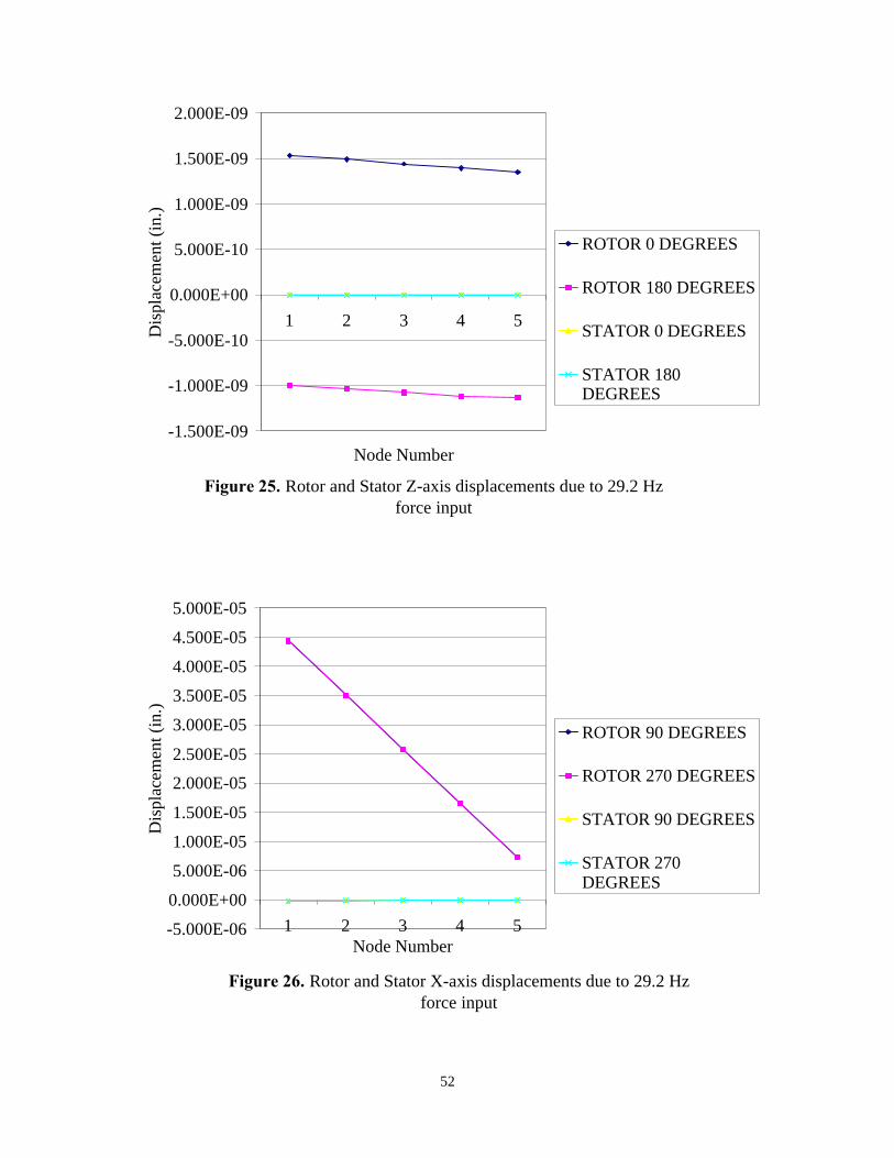
52

Figure 25. Rotor and Stator Z-axis displacements due to 29.2 Hz force input

-1.500E-09

-1.000E-09

-5.000E-10

0.000E+00

5.000E-10

1.000E-09

1.500E-09

2.000E-09

1 2 3 4 5

Node Number

Dis

plac

emen

t (in

.)

ROTOR 0 DEGREES

ROTOR 180 DEGREES

STATOR 0 DEGREES

STATOR 180DEGREES

Figure 26. Rotor and Stator X-axis displacements due to 29.2 Hz force input

-5.000E-06

0.000E+00

5.000E-06

1.000E-05

1.500E-05

2.000E-05

2.500E-05

3.000E-05

3.500E-05

4.000E-05

4.500E-05

5.000E-05

1 2 3 4 5Node Number

Dis

plac

emen

t (in

.)

ROTOR 90 DEGREES

ROTOR 270 DEGREES

STATOR 90 DEGREES

STATOR 270DEGREES

53

Figure 27. Rotor and Stator Y-axis displacements due to 29.2 Hz force input

0.000E+00

1.000E-07

2.000E-07

3.000E-07

4.000E-07

5.000E-07

6.000E-07


Dis

plac

emen

t (in

.)

ROTOR 90 DEGREES

ROTOR 270 DEGREES

STATOR 90 DEGREES

STATOR 270DEGREES

Figure 28. Rotor and Stator Z-axis displacements due to 29.2 Hz force input

-1.500E-09

-1.000E-09

-5.000E-10

0.000E+00

5.000E-10

1.000E-09

1.500E-09

1 2 3 4 5

Node Number

Dis

plac

emen

t (in

.)

ROTOR 90 DEGREES

ROTOR 270 DEGREES

STATOR 90 DEGREES

STATOR 270DEGREES

54

The following facts regarding the rotor displacements can be derived from the data.1) The X-axis displacements at 0°, 180°, 90° and 270° are linear along the rotor length and equal

per node for the four radial locations.2) The Y-axis displacements at 0° and 180° are approximately constant along the rotor length

and are equal in magnitude but opposite in sign, respectively. These displacements are of thesame order of magnitude as the X-axis displacements and thus are substantial. The Y-axisdisplacements at 90° and 270° are approximately constant, equal in magnitude and in sign.These displacements are two orders of magnitude less than the X-axis displacements and thusare negligible.

3) The Z-axis displacements at 0° and 180° are approximately linear along the rotor length.These displacements are four orders of magnitude less than the respective X- and Y- axisdisplacements and therefore may be neglected. The Z-axis displacements at 90° and 270° arenot linear and vary from the average value by 46.5 percent. This variation is due to thetransition in axial cross-section from rotor to rotor shaft at the rotor bottom. However, thesedisplacements are between four and five orders of magnitude less than the respective X-axisdisplacements and therefore may be neglected.

From these facts it can be deduced that due to the application of the 29.2 Hz forcing functions therotor remains cylindrical and thus rigid. Its displacement is essentially two-dimensional in theXY-plane. The rotor is undergoing a clockwise rotation and a translation in the positive X-direction. Thus the rotor shaft behaves as a cantilever beam.

The following facts regarding the stator displacements can be derived from the data.1) The X-axis displacements at 0° and 180° and at 90° and 270° respectively, are approximately

linear. The average X-axis displacement at 0° and 180° is 2.6 percent higher than that at 90°and 270°. This average value is highly biased toward the nodes at the bottom of the stator,where the 0° and 180° displacements are 8 percent higher than the 90° and 270°displacements.

2) The Y-axis displacements at 0° and 180° are approximately constant (less than 1.5 percentaverage deviation). These displacements are of the same order of magnitude as the respectiveX-axis displacements and are therefore significant. The Y-axis displacements at 90° and 270°are also approximately constant (less than 0.5 percent average deviation). These are betweenone and two orders of magnitude smaller than the respective X-axis displacements and aretherefore insignificant.

3) The Z-axis displacements at 0° and 180° are approximately linear and are between four andfive orders of magnitude smaller than the respective X-axis displacements. Thesedisplacements are therefore negligible. The Z-axis displacements at 90° and 270° are not linearand vary from the average value by 63.9 percent. These displacements are three orders ofmagnitude smaller than the respective X-axis displacements and thus are negligible.

In summary the stator displacement due to the 29.2 Hz force inputs is essentially a two-dimensional problem in the XY-plane. The stator is undergoing a counterclockwise rotation and

55

is translating in the negative X-direction. This is similar to the situation encountered with therotor in that the stator and housing are behaving essentially as a cantilever beam. Figures 29 and30 show the I-DEAS output of the component displacements in the XY (in-plane) and YZ (out-of-plane) planes, respectively. The scales of the displacements in these plots have been increasedto 25 percent and 10 percent of the maximum display capability for the XY and YZ planes,respectively, to show the high relative stiffness of the housing/stator assembly in comparison tothe rotor/shaft assembly. Because of this large stiffness differential and the small amount ofdamping used for the system representation, phasing of the displacements between thehousing/stator assembly and the rotor/shaft assembly have been neglected.

56

Figure 29. Exaggerated component displacements in the XY plane due to 29.2 Hz force inputs

57

Figure 30. Exaggerated component displacements in the YZ plane due to 29.2 Hz force inputs

58

5.3.2 Displacements due to 120 Hz inputThe rotor and stator displacements due to the 120 Hz harmonic force inputs on the rotor andstator are listed in Tables 12-19 and Figures 31-36 for the 0, 180, 90 and 270 degree locations.

Table 12: Rotor displacement at 0° due to 120 Hz force input on stator and rotorNODE NUMBER X–DISPLACE.

(in.)Y–DISPLACE.

(in.)Z–DISPLACE.



(in.)Y–DISPLACE.

(in.)Z–DISPLACE.

(in.)1 5.229 E-05 1.481 E-05 -9.159 E-102 4.150 E-05 1.481 E-05 -9.722 E-103 3.072 E-05 1.478 E-05 -1.031 E-094 1.994 E-05 1.478 E-05 -1.088 E-095 9.113 E-06 1.478 E-05 -1.119 E-09


(in.)Y–DISPLACE.

(in.)Z–DISPLACE.

(in.)1 5.229 E-05 5.694 E-07 4.034 E-102 4.150 E-05 5.692 E-07 2.851 E-103 3.070 E-05 5.684 E-07 6.617 E-104 1.991 E-05 5.681 E-07 1.385 E-095 9.155 E-06 5.685 E-07 -1.100 E-09

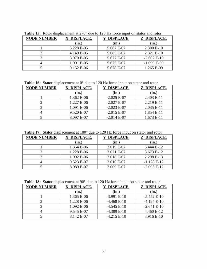
59


(in.)Y–DISPLACE.

(in.)Z–DISPLACE.

(in.)1 5.228 E-05 5.687 E-07 2.300 E-102 4.149 E-05 5.685 E-07 2.321 E-103 3.070 E-05 5.677 E-07 -2.602 E-104 1.991 E-05 5.675 E-07 -1.099 E-095 9.152 E-06 5.678 E-07 1.265 E-09

Table 16: Stator displacement at 0° due to 120 Hz force input on stator and rotorNODE NUMBER X–DISPLACE.

(in.)Y–DISPLACE.

(in.)Z–DISPLACE.



(in.)Y–DISPLACE.

(in.)Z–DISPLACE.

(in.)1 1.364 E-06 2.019 E-07 5.444 E-122 1.228 E-06 2.021 E-07 3.673 E-123 1.092 E-06 2.018 E-07 2.298 E-134 9.523 E-07 2.010 E-07 -1.128 E-125 8.089 E-07 2.009 E-07 -2.095 E-12


(in.)Y–DISPLACE.

(in.)Z–DISPLACE.

(in.)1 1.365 E-06 -3.991 E-10 -5.452 E-102 1.228 E-06 -4.468 E-10 -4.194 E-103 1.092 E-06 -4.545 E-10 -2.641 E-104 9.545 E-07 -4.389 E-10 4.460 E-125 8.142 E-07 -4.215 E-10 3.916 E-10

60


(in.)Y–DISPLACE.

(in.)Z–DISPLACE.

(in.)1 1.365 E-06 -4.040 E-10 5.746 E-102 1.228 E-06 -4.518 E-10 4.451 E-103 1.092 E-06 -4.596 E-10 2.863 E-104 9.545 E-07 -4.440 E-10 1.416 E-115 8.142 E-07 -4.266 E-10 -3.762 E-10

61

Figure 31. Rotor and Stator X-axis displacements due to 120 Hz force input

0.000E+00

1.000E-05

2.000E-05

3.000E-05

4.000E-05

5.000E-05

6.000E-05


Dis

plac

emen

t (in

.)

ROTOR 0 DEGREES

ROTOR 180 DEGREES

STATOR 0 DEGREES

STATOR 180DEGREES

Figure 32. Rotor and Stator Y-axis displacements due to 120 Hz

force input

-2.000E-05

-1.500E-05

-1.000E-05

-5.000E-06

0.000E+00

5.000E-06

1.000E-05

1.500E-05

2.000E-05

1 2 3 4 5

Node Number

Dis

plac

emen

t (in

.) ROTOR 0 DEGREES

ROTOR 180 DEGREES

STATOR 0 DEGREES

STATOR 180DEGREES

62

Figure 33. Rotor and Stator Z-axis displacements due to 120 Hz force input

-1.500E-09

-1.000E-09

-5.000E-10

0.000E+00

5.000E-10

1.000E-09

1.500E-09

2.000E-09

1 2 3 4 5

Node Number

Dis

plac

emen

t (in

.)

ROTOR 0 DEGREES

ROTOR 180 DEGREES

STATOR 0 DEGREES

STATOR 180DEGREES

Figure 34. Rotor and Stator X-axis displacements due to 120 Hz force input

0.000E+00

1.000E-05

2.000E-05

3.000E-05

4.000E-05

5.000E-05

6.000E-05

1 2 3 4 5

Node Number

Dis

plac

emen

ts (

in.)

ROTOR 90 DEGREES

ROTOR 270 DEGREES

STATOR 90 DEGREES

STATOR 270DEGREES

63

Figure 35. Rotor and Stator Y-axis displacements due to 120 Hz force input

-1.000E-07

0.000E+00

1.000E-07

2.000E-07

3.000E-07

4.000E-07

5.000E-07

6.000E-07

1 2 3 4 5

Node Number

Dis

plac

emen

t (in

.)

ROTOR 90 DEGREES

ROTOR 270 DEGREES

STATOR 90 DEGREES

STATOR 270DEGREES

Figure 36. Rotor and Stator Z-axis displacements due to 120 Hz force input

-1.500E-09

-1.000E-09

-5.000E-10

0.000E+00

5.000E-10

1.000E-09

1.500E-09

2.000E-09

1 2 3 4 5

Node Number

Dis

plac

emen

t (in

.)

ROTOR 90 DEGREES

ROTOR 270 DEGREES

STATOR 90 DEGREES

STATOR 270DEGREES

64

The following facts regarding the rotor displacements can be derived from the data.1) The X-axis displacements at 0°, 180°, 90° and 270° are linear along the rotor length and equal

per node for the four radial locations.2) The Y-axis displacements at 0° and 180° are approximately constant along the rotor length

and are equal in magnitude but opposite in sign, respectively. These displacements are of thesame order of magnitude as the X-axis displacements and thus are substantial. The Y-axisdisplacements at 90° and 270° are approximately constant, equal in magnitude and in sign.These displacements are two orders of magnitude less than the X-axis displacements and thusare negligible.

3) The Z-axis displacements at 0° and 180° are approximately linear along the rotor length.These displacements are four orders of magnitude less than the respective X- and Y-axisdisplacements and therefore may be neglected. The Z-axis displacements at 90° and 270° arenot linear and vary from the average value by 46.3 percent. This variation is due to thetransition in axial cross-section from rotor to rotor shaft at the rotor bottom. However,these displacements are between four and five orders of magnitude less than the respective X-axis displacements and therefore may be neglected.

It is obvious that the rotor behaves in virtually an identical manner in response to the 29.2 Hz and120 Hz force inputs. When subjected to the 120 Hz forcing functions the rotor remainscylindrical and thus rigid. Its displacement is essentially two-dimensional in the XY-plane. Therotor undergoes a clockwise rotation and a translation in the positive X-direction. The differencein the reaction characteristics between the two frequencies is that the rotor displacements due tothe 120 Hz forces are greater in all three directions. The maximum X-axis displacement (at thetop of the rotor) is 17.9 percent greater for the 120 Hz input. Consequently, the Y-axisdisplacement at 0° and 180° is 16.3 percent higher for the 120 Hz input.

The following facts regarding the stator displacements can be derived from the data.1) The X-axis displacements at 0° and 180° and at 90° and 270° respectively, are approximately

linear and equal. The X-axis displacements at these four locations are in the positive X-direction. In other words, the stator displacements are in the same direction as the forcesapplied to the rotor surface and opposite to those applied to the stator surface.

2) The Y-axis displacements at 0° and 180° are approximately constant. These displacementsare between zero and one order of magnitude smaller than the respective X-axis displacementsand are thus significant. These displacements also follow the same displacement pattern asthose on the rotor surface. In other words the 0° displacements are negative while the 180°displacements are positive. The Y-axis displacements at 90° and 270° are not constant.However, these are approximately four orders of magnitude smaller than the respective X-axisdisplacements and three orders of magnitude smaller than the Y-axis displacements at 0° and180°. These displacements are therefore insignificant.

3) The Z-axis displacements at 0° and 180° are approximately linear and are between four andfive orders of magnitude smaller than the respective X-axis displacements. Thesedisplacements are therefore negligible. The Z-axis displacements at 90° and 270° are not linear

65

and vary from the average value by 64.7 percent. These displacements are between three andfour orders of magnitude smaller than the respective X-axis displacements and thus arenegligible.

In summary the stator displacement due to the 120 Hz force inputs is essentially a two-dimensional problem in the XY-plane. The difference between these displacements and thoseencountered due to the 29.2 Hz inputs is that the stator and housing are undergoing a clockwiserotation and are translating in the positive X-direction. Thus the stator and housing are displacingin the same manner and direction as the rotor. Figures 37 and 38 show the I-DEAS output of thecomponent displacements in the XY (in-plane) and YZ (out-of-plane) planes, respectively. Thescales of the displacements in these plots have been increased to 25 percent and 10 percent of themaximum display capability for the XY and YZ planes, respectively, to show the high relativestiffness of the housing/stator assembly in comparison to the rotor/shaft assembly. Because of thislarge stiffness differential and the small amount of damping used for the system representation,phasing of the displacements between the housing/stator assembly and the rotor/shaft assemblyhave been neglected. While the effect is not great, careful viewing of Figure 37 shows the netpositive displacement of the stator and housing due to both force inputs.

5.3.3 Displacement results due to individual force applicationAt an initial glance the situation described in Section 5.3.2 directly above seems impossiblebecause an object must displace in the direction of the applied force. To assure that the finiteelement model was behaving correctly analyses were run with the rotor and stator forces appliedindividually rather than simultaneously. To simplify this segment of the analysis a point load wasused on each surface rather than the distributed loads used previously. The moment arm used forthis system was the distance between the upper surface of the compression chamber and the mid-length of the rotor. This is not exactly correct because the compression chamber can not beconsidered true ground. The variation between this moment arm and the true moment arm shouldbe negligible.

The nodal displacement data due to these individual forces can be summarized as follows.1) All X-axis displacements were linear for both rotor and stator for both applied forces. All X-

axis displacements at 0° and 180° were equal in sign and magnitude to those at 90° and 270°.All X-axis displacements were also in the direction of the applied force

2) All Y-axis displacements were analogous to those resulting from simultaneous forceapplication with respect to constant magnitude, linearity and relative order of magnitude.

3) All Z-axis displacements were at least three orders of magnitude smaller than the respectiveX-axis displacements and thus were negligible. With respect to non-linear displacements ofthe rotor and stator surfaces all Z-axis displacements were analogous to those found due tosimultaneous force application.

66

Figure 37. Exaggerated component displacements in the XY plane due to 120 Hz force inputs

67

Figure 38. Exaggerated component displacements in the YZ plane due to 120 Hz force inputs

68

The point to gather from the application of forces individually was that the entire assemblydisplaces, not just the component directly subjected to the force. In other words the applicationof a positive X-force on the rotor surface results in positive X-axis displacements of the rotor andstator. This situation is reversed for the stator force. The negative force input results in statorand rotor displacement in the negative X-direction. This phenomenon can be attributed to theenergy transfer between the stator and rotor through the housing. This fact explains the positivedisplacement of the stator during the application of the simultaneous 120 Hz loads. The truescenario is that the positive stator displacements due to the rotor surface force are greater thanthe negative displacements resulting from the stator surface force. When summed the result is anet positive displacement of the stator.

5.4 Air gap change due to component displacementsAs stated the displacements encountered in the system are two-dimensional. With this in mind thefollowing facts can be deduced for both for the 29.2 Hz and 120 Hz inputs, respectively:

1) the horizontal rotor displacement is dominant,2) the horizontal stator displacement is relatively small but significant and3) the vertical stator displacement is negligible.

Therefore the change in the air gap can be analyzed by summing the X-axis displacements of thetop nodes (Node 1) on the rotor and stator meshes at the 0 degree location and subtracting thisquantity from the original air gap of 0.010 in. The results of this analysis are displayed in Table20. The results due to the simultaneous application of 29.2 Hz and 120 Hz forces are thesuperposition of the two individual results.

Table 20: Change in air gap due to component displacementForcing

Frequency(Hz)

RotorDisplacement

(in.)

StatorDisplacement

(in.)

Air GapChange

(in.)

New Air Gap

(in.)

PercentChange

29.2 4.435 E-5 -1.798 E-7 4.0 E-5 9.96 E-3 0.40120 5.229 E-5 1.385 E-6 5.0 E-5 9.95 E-3 0.50

29.2 and 120 9.664 E-5 1.205 E-6 1.0 E-4 9.90 E-3 1.00

In order to produce an interference the change in the air gap must be 0.010 in . This change istwo orders of magnitude greater than the interference found due to the simultaneous applicationof the 29.2 Hz and 120 Hz unit loads on the stator and rotor surfaces. Therefore, if themagnitudes of the applied forcing functions are increased by two orders of magnitude (a 100 lbfinput on each surface) an interference should result.

According to Shigley and Mitchell [12] the torque applied to a shaft can be found from therelationship

69

(5.6)

whereT = torque (in*lbf)H = horsepowern = shaft speed (rpm)

The shaft torque in an electric motor is equal to the product of the tangential force acting on therotor and the outer radius of the rotor. Using these relationships and those developed in Chapter4 between the radial and tangential forces, it can be said that the following is true:

(5.7)

The exact power rating of the electric motor in question was not known. However, it is believedthat the motor should be rated at approximately 0.5-1.0 horsepower. The above relationship wasused to determine the horsepower rating required to produce an interference. Table 21 lists therequired force magnitudes, scale factors and horsepower requirements.

Table 21. Horsepower requirements to produce interferenceForcing Frequency

(Hz)Radial Force

Magnitude (lbf.)Radial Force Scale

FactorHorsepower

Required29.2 250 2.5 E+2 0.286120 200 2.0 E+2 0.229

29.2 and 120 100 1.0 E+2 0.114

As can be seen, interference between the stator and rotor is possible if the motor produces at least0.29 horsepower. If the motor output is much greater as expected, the radial force requirementfor interference will drop accordingly.

nH

T63000

=

Radialg Fnp

H63000

λδ=

70

Chapter 6.0 Conclusions and future investigations

In conclusion, in this project it was found that the motor under consideration could experienceinterference problems between the stator and rotor if the motor’s output power rating is at least0.29 horsepower. Since this requirement is likely met, recommendations are in order for possiblesolutions to the interference problem.

The first area to examine would be the quality control aspect of the manufacturing process. Asstated initially, the interference problems are occurring on about one-third of the unitsmanufactured. This can lead to the assumption that as certain tolerance levels are approached theeccentricity level that produces interference is realized. It was not known at the onset of thisproject to what extent, if any, stricter quality control measures had been implemented. However,reduction of the amount of eccentricity present in the units through improved quality may be themost cost-effective initial pursuit.

All remaining suggestions deal with the actual design of the unit. For all practical purposes thedisplacements encountered with this system are the bending of the rotor shaft similar to acantilever beam with a transverse load. The two most obvious solutions to this problem are toincrease the stiffness of the shaft or to utilize a support at the free end.

The displacement for a cantilever beam is directly proportional to the magnitude and location ofthe applied load and is inversely proportional to the modulus of elasticity of the material and thearea moment of inertia of the beam. Obviously the current use of cast iron as the shaft materialdoes not provide the necessary stiffness. The substitution of steel for the cast iron would increasethe modulus of elasticity by approximately a factor of two (30.0 Mpsi for steel versus 14.5 Mpsifor non-ductile gray cast iron). This would, in turn, reduce the lateral displacement of the rotorby approximately one-half.

It may be possible to increase the diameter of the rotor shaft and adjust all other geometricparameters accordingly to increase shaft stiffness. This approach appears doubtful when viewingthe cross-section of the actual unit because of the close proximity of the rotor conducting bars tothe rotor inner radius.

The option of redesigning the compressor/motor assembly to include a bearing support at bothends is obviously the most absolute method for correcting the interference problem. Because therotor is located at the end of the shaft inclusion of an additional support would almost guaranteesuccess. However, pursuit of this option would totally defeat the purpose of the cantileverdesign, which was to minimize cost.

Another possible solution would be to retain the cantilever concept but to redesign the geometricparameters of the motor so that the rotor is much larger in diameter but is axially shorter. Thiswould effectively reduce the moment arm of the system and thus the lateral displacements of the

71

rotor. This approach has been taken by other compressor manufacturers such as Sanyo in thepast and has apparently been successful.

Obviously a complete redesign of the unit is a drastic measure. However, because the poweroutput of the motor is not currently known it cannot be discerned whether changing the shaftmaterial to steel will be a sufficient preventative measure. If the motor output is between 0.5 and1.0 horsepower as suspected this approach will not be effective. It can be shown that if a steelshaft is used and the least volatile static eccentricity is present, a motor output of 0.57 horsepowerwould be sufficient to produce interference.

With respect to areas for future investigations, the first item would be to ascertain more preciseinformation regarding the geometric characteristics of the compressor assembly. While the use ofmapped meshing is restrictive with regards to the allowable amount of component detail, severalitems in the current model can be more accurately represented. Another area to examine wouldbe the validity of the assumptions made regarding material properties for the laminated stator androtor.

It was initially desired to reproduce the dynamic air gap so that it could be viewed using thesoftware. Ideally the cylindrical gap would be restructured as a topographical map so that thepeaks and valleys could be easily seen. As was noted the I-DEAS software contains no provisionsfor producing this kind of output. Future development of this area would be of great benefit foranalyzing this and similar problems. This project could be approached in several ways, two ofwhich are:

1) Modify the method attempted for this project to place surfaces through the displacednodes. This approach may prove to be feasible if the ability to pick nodes in a densemesh could be improved. It may also be possible to place different elements inseparate groups during the meshing procedure. This would provide the analyst withthe ability to view displaced nodes on individual surfaces. The potential problem withthis approach is whether it will work in conjunction with the Append command orwhether the group information will be lost during the transfer procedure.

2) Write an external piece of computer code to extract the original node locations andtheir displacements from the Universal File and transfer this data to coordinatesnecessary for a topographical map. These new coordinates could possibly be importedinto I-DEAS and surfaces fitted to emulate the original and displaced cylindricalsurfaces. The new air gap between these surfaces could then be easily inspected.

It would also be wise to perform an experimental modal analysis on an existing assembly tovalidate the finite element analysis results. Experimental analyses on machines consisting ofmultiple components such as the compressor featured here are complicated. However, Timar’stext [2] contains many valuable guidelines regarding experimental modal analysis on rotatingelectric machinery.

72

References

(1) Rai, G.B. 1974. Air Gap Eccentricity in Induction Motors. Thesis. ERA Technology Ltd.Leatherhead, Surrey, England.

(2) Timar, P.L., A. Fazekas, J. Kiss, A. Miklos and S.J. Yang. 1989. Noise and Vibration ofElectrical Machines, Elsevier Science Publishers, Amsterdam, The Netherlands andAkademiai Kiado, Budapest, Hungary.

(3) Ozturk, C.O., A. Balikcioglu, H. Acikgoz and A. Bahadir. 1994. Origins of the Electromagnetic Vibrations in Series Fractional Horsepower Motors. In ISMA Proceedings Vol. 19 – Tools for Noise and Vibration Analysis, 1103-1114.(4) Girgis, R.S. and S.P. Verma. 1979. Resonant Frequencies and Vibration Behaviour of Stators

of Electrical Machines as Effected by Teeth, Windings, Frame and Laminations. IEEEProceedings, 1446-1454.

(5) Knight, C.E. 1993. The Finite Element Method in Mechanical Design. PWS-KENTPublishing Company, Boston, MA USA.

(6) Rao, S.S. 1990. Mechanical Vibrations. 2nd ed. Addison-Wesley Publishing Company,Reading, MA USA.

(7) Chuse, R. and S.M. Eber. 1984. Pressure Vessels – The ASME Code Simplified. 6th ed.McGraw-Hill Book Company, New York, NY USA.

(8) Swokowski, E.W. 1991. Calculus. 5th ed. PWS-KENT Publishing Company, Boston, MAUSA.

(9) Ramani, A. 1993. Finite Element Modeling of a Refrigeration Compressor for NoisePrediction Applications. Thesis. Virginia Polytechnic Institute and State University,Mechanical Engineering Department, Blacksburg, VA.

(10) Thomson, W.T. 1993. Theory of Vibrations with Applications. 4th ed. Prentice Hall,Englewood Cliffs, NJ USA.

(11) Cheng, F.-H. 1986. Applied Strength of Materials. Macmillan Publishing Company, NewYork, NY USA.

(12) Shigley, J.E. and L.D. Mitchell. 1983. Mechanical Engineering Design. 4th ed. McGraw-Hill Book Company, New York, NY USA.

73

Vita

Swen Thompson

Swen Thompson was born on August 26, 1968 in Roanoke, Virginia. He was raised in Roanokeand completed high school there in 1986. In June 1990 he received his Associate of ScienceDegree in Engineering from Virginia Western Community College in Roanoke. In August 1990Mr. Thompson enrolled in the College of Engineering at Virginia Polytechnic Institute and StateUniversity in Blacksburg, Virginia. In May 1994 he successfully completed the requirements for aBachelor of Science Degree in Mechanical Engineering. After working in industry for one yearMr. Thompson returned to the Mechanical Engineering Department at VPI & SU to enroll in thegraduate program.

Mr. Thompson will be completing the requirements for the degree of Master of Science inMechanical Engineering in May 1997. He is looking forward to beginning a career withSchrader-Bridgeport International, Inc. following graduation.

Analysis of the Dynamic Interferences between the …...Analysis of the Dynamic Interferences...

Documents

Transcript of Analysis of the Dynamic Interferences between the …...Analysis of the Dynamic Interferences...