Analysis of the conflict between omission and commission in low ...

www.elsevier.com/locate/rse

Remote Sensing of Environment 91 (2004) 280–292

Analysis of the conflict between omission and commission in low spatial

resolution dichotomic thematic products: The Pareto Boundary

Luigi Boschettia,*, Stephane P. Flasseb, Pietro A. Brivioc

aGlobal Vegetation Monitoring Unit, European Commission, DG Joint Research Centre, Institute for Environment and Sustainability,

via Fermi 1, I-21020 Ispra, VA, ItalybFlasse Consulting, 3 Sycamore Crescent, Maidstone, Kent ME16 0AG, UK

cCNR-Istituto per il Rilevamento Elettromagnetico dell’Ambiente, via Bassini 15, I-20133 Milan, Italy

Received 8 July 2003; received in revised form 26 February 2004; accepted 28 February 2004

Abstract

During the last few years, the remote sensing community has been trying to address the need for global synthesis to support policy makers

on issues such as deforestation or global climate change. Several global thematic products have been derived from large datasets of low-

resolution remotely sensed data, the latter providing the best trade-off between spatial resolution, temporal resolution and cost. However, a

standard procedure for the validation of such products has not been developed yet. This paper proposes a methodology, based on statistical

indices derived from the widely used Error Matrix, to deal with the specific issue of the influence of the low spatial resolution of the dataset

on the accuracy of the end-product, obtained with hard classification approaches. In order to analyse quantitatively the trade-off between

omission and commission errors, we suggest the use of the ‘Pareto Boundary’, a method rooted in economics theory applied to decisions with

multiple conflicting objectives. Starting from a high-resolution reference dataset, it is possible to determine the maximum user and producer’s

accuracy values (i.e. minimum omission and commission errors) that could be attained jointly by a low-resolution map. The method has been

developed for the specific case of dichotomic classifications and it has been adopted in the evaluation of burned area maps derived from

SPOT-VGTwith Landsat ETM+ reference data. The use of the Pareto Boundary can help to understand whether the limited accuracy of a low

spatial resolution map is given by poor performance of the classification algorithm or by the low resolution of the remotely sensed data,

which had been classified.

D 2004 Elsevier Inc. All rights reserved.

Keywords: Omission; Commission; Pareto Boundary

1. Introduction tropical forest maps (Achard et al., 2001, 2002), the Global

Thematic land-cover maps are being increasingly pro-

duced from image classification of remotely sensed data,

which provides consistent and spatially contiguous data

over large areas (Foody, 2002). In the last few years,

global datasets of low spatial resolution data have been

made available to the user community, and consequently

several global thematic maps have been produced, such as

the International Geosphere–Biosphere Project (IGBP)

land-cover map (Loveland et al., 1999), the TRopical

Ecosystem Environment observation by Satellite (TREES)

0034-4257/$ - see front matter D 2004 Elsevier Inc. All rights reserved.

doi:10.1016/j.rse.2004.02.015

* Corresponding author. Tel.: +39-0223699457; fax: +39-0223699599.

E-mail addresses: [email protected] (L. Boschetti),

[email protected] (S.P. Flasse), [email protected]

(P.A. Brivio).

Land Cover 2000 (GLC2000) global scale vegetation map

(Bartholome et al., 2002) or the Global Burned Area 2000

(GBA2000) burned area map (Gregoire et al., 2003;

Tansey et al., in press), the MODIS burned area product

(Justice et al., 2002; Roy et al., 2002) or the GLOBSCAR

multi-year burned area maps (Simon et al., 2004). The

accuracy assessment methods available in the literature

relate mainly to mapping investigations on local to regional

scales and may not be transferable to coarser scales

(Foody, 2002). The development of methods and protocols

for the assessment of products derived from moderate to

low spatial resolution data is still a research topic, and its

need has been recognised as a priority (Chilar, 2000;

Foody 2002; Justice et al., 2000; Mayaux & Lambin,

1995).

Mayaux and Lambin (1995) analysed the effects due to

the spatial aggregation on the estimation of tropical forest

L. Boschetti et al. / Remote Sensing of Environment 91 (2004) 280–292 281

area derived from NOAA-AVHRR. In the analysis of the

relationships between area estimates at a fine and a coarse

resolution, they indicated the Matheron index and the

patch size, both related to the fragmentation of the the-

matic map, as factors influencing the accuracy of the low-

resolution map. More recently, in a systematic analysis of

spatial sampling effects on burnt area mapping, Eva and

Lambin (1998) underlined the impact of the proportion and

spatial pattern of burnt areas at the high spatial resolution

as well as of the detection threshold, on the accuracy of

burned area estimates from low-resolution satellite data.

The study by Smith et al. (2003) on the impact of

landscape characteristics on classification accuracy high-

lighted the impact land-cover heterogeneity and patch size

have on classification accuracy, with the probability of a

correct classification decreasing with decreasing patch size

and increasing heterogeneity.

The comprehensive review of Foody (2002) analyses

several aspects of the background and methods currently in

use within the remote sensing community and recommen-

ded in the research literature. However, no particular men-

tion is given to the problems raised by the accuracy

assessment issues of land-cover mapping of large areas

from coarse spatial resolution satellite data.

The vast majority of the statistical indices, which are

available in the literature for the validation of thematic

maps, are derived from the error matrix (Congalton et al.,

1983; Story & Congalton, 1986); Stehman (1997) provides

a review of these indices. The error matrix is a square matrix

which expresses the number of pixels (i.e. the amount of

land surface) assigned to a particular land-cover class

relative to the actual verified land-cover class. In this article,

the columns of the matrix correspond to the reference data,

assumed as the truth, and the rows correspond to the

classification that is being evaluated. The diagonal elements

of the matrix are the correctly classified pixels; therefore, an

absolutely correct classification will generate a diagonal

matrix.

However, the typical use of the error matrix assumes

that reference data and classified data have the same

spatial resolution, which is often not the case when

evaluating coarse spatial resolution classifications, e.g. data

acquired by sensors such as NOAA-AVHRR, TERRA and

AQUA-MODIS, SPOT-VEGETATION or AATSR on

Envisat. Usually the accuracy assessment or evaluation

process is carried out by using samples of either ground

data and/or higher spatial resolution multispectral data

(such as Landsat-TM or SPOT-HRV). The present work

proposes a methodology to analyse the influence of the

low spatial resolution of the remotely sensed dataset on the

accuracy of the final thematic map products, highlighting

the presence of a trade-off between omission and commis-

sion errors when employing a hard classification scheme.

First the concepts of low-resolution bias and ‘Pareto

Boundary’ are introduced. Then this paper presents how

the latter concept can be used at different stages of the

classification process, and illustrates its application with

some examples.

This work has been developed in the framework of the

Global Burned Area 2000 (GBA2000) initiative (Gregoire

et al., 2003), coordinated by the Global Vegetation Moni-

toring Unit of the European Commission Joint Research

Centre, aimed at the production of monthly burned area

maps at global scale. The maps (http://www.gvm.jrc.it/fire/

gba2000/index.htm) are derived from low spatial resolution

SPOT-VEGETATION data and their accuracy assessment

is conducted mainly by comparison with Landsat ETM

data, using a multi-level accuracy assessment procedure

(Boschetti et al., 2001).

The assessment method described in this paper has been

developed specifically for binary classification products

(e.g. dichotomic classifications where the user is interested

in the accuracy of the mapping of one class versus the

background). Dichotomic classifications are typically used

in the study of land-cover disturbances such as flooding or

fire effects. Burned area maps will be used in this paper as

an illustrative example.

2. Concepts and methods

In the case where a user is interested in the accuracy

assessment of a single class, this class often represents a

relatively small fraction of a thematic map. In the following,

we will refer to generic thematic classes x1 and x2, where

class x1 is the class of interest and x2 is always the

background. The method could be extended to n classes if

the classes are evaluated one at a time, merging all the other

classes into a generic background. Since the mapping of

class x1 is the objective of the dichotomic classification

itself, the assessment must focus on this class of interest. For

this reason, the analysis of the accuracy of low-resolution

thematic products will be conducted from the point of view

of the ‘non-background’ class x1.

The assessment of thematic product is commonly

achieved by comparing it with some samples of reference

data assumed to represent the reality. When evaluating

global products, a significant number of samples of refer-

ence data are required, making the acquisition of ground

truth difficult and unrealistic, hence calling on high spatial

resolution satellite data and their best possible interpreta-

tion. Consequently, the proposed methodology aims at

addressing issues linked to the use of samples of high-

resolution map as reference data for the accuracy assess-

ment of low-resolution products. Like these product assess-

ments, the presented analysis assumes that reference data

represent the reality, i.e. it is free from errors. It has been

recognised that, when comparing any spatial datasets, geo-

location errors between them may affect heavily the accu-

racy indices (Foody, 2002; Plourde & Congalton, 2003;

Thomlinson et al., 1999). For the case of dichotomic

classification, Mayaux and Lambin (1995) proposed a

http:\\www.gvm.jrc.it\fire\gba2000\index.htm

L. Boschetti et al. / Remote Sensing of Environment 91 (2004) 280–292282

method based on the spatial aggregation on larger cells

(boxes of 11�11 low-resolution pixels) but the compen-

sation for misregistration errors is obtained at the cost of a

complete loss of information about the locational accuracy

within the boxes. More recently, Remmel and Perera (2002)

proposed a method based on the comparison of polygons.

However, these methods are not compatible with the use of

the error matrix. The Pareto Boundary is based only on the

reference data and on the pixel size of the low-resolution

data (not on the actual low-resolution map). As a conse-

quence, rather than an issue of misregistration, there is a

sub-pixel uncertainty in the positioning of the low-resolu-

tion grid on the higher resolution data. The impact of this

uncertainty on the Pareto Boundary will be discussed in

Section 3.4 and numerically assessed in the two examples

of Section 3.5.

Finally, it must be noted that the proposed methodology

applies to hard classifiers only; therefore, the techniques

developed for soft classifiers (Binaghi et al., 1999; Foody,

1996) will not be taken into account. A soft classification

scheme could indeed theoretically achieve 100% accuracy

even with mixed pixels, and the computation of the Pareto

Boundary actually involves the hardening of an ideal error-

free soft classification, as explained in detail in Section 3.1.

The discussion of the relative merits and drawbacks of hard

and soft classifiers is not the objective of this paper.

Instead, the proposed methodology is intended as an

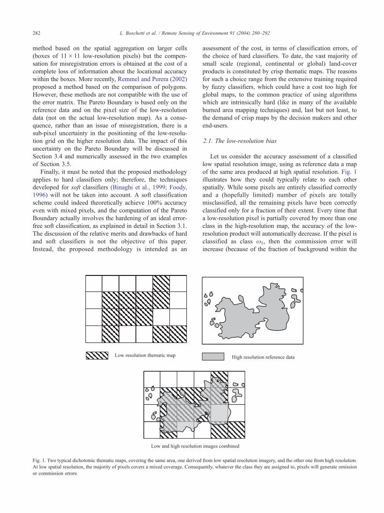
Fig. 1. Two typical dichotomic thematic maps, covering the same area, one derived

At low spatial resolution, the majority of pixels covers a mixed coverage. Consequ

or commission errors.

assessment of the cost, in terms of classification errors, of

the choice of hard classifiers. To date, the vast majority of

small scale (regional, continental or global) land-cover

products is constituted by crisp thematic maps. The reasons

for such a choice range from the extensive training required

by fuzzy classifiers, which could have a cost too high for

global maps, to the common practice of using algorithms

which are intrinsically hard (like in many of the available

burned area mapping techniques) and, last but not least, to

the demand of crisp maps by the decision makers and other

end-users.

2.1. The low-resolution bias

Let us consider the accuracy assessment of a classified

low spatial resolution image, using as reference data a map

of the same area produced at high spatial resolution. Fig. 1

illustrates how they could typically relate to each other

spatially. While some pixels are entirely classified correctly

and a (hopefully limited) number of pixels are totally

misclassified, all the remaining pixels have been correctly

classified only for a fraction of their extent. Every time that

a low-resolution pixel is partially covered by more than one

class in the high-resolution map, the accuracy of the low-

resolution product will automatically decrease. If the pixel is

classified as class x1, then the commission error will

increase (because of the fraction of background within the

from low spatial resolution imagery, and the other one from high resolution.

ently, whatever the class they are assigned to, pixels will generate omission

Table 1

Typical confusion matrix for a dichotomic thematic product

Classified data Reference data

Class x1 Class x2 (background)

Class x1 p11 p12Class x2 (background) p21 p22


pixel), but if it is classified as background x2, then the

omission error increases. A low-resolution pixel covered

exactly by 50% class x1 and 50% class x2 is the extreme

case. Whatever label is assigned to it, omission and com-

mission errors will increase by the same amount.

In the situation exemplified in Fig. 1, it is possible to

identify intuitively, pixel by pixel, whether the error (either

commission or omission) is due to an actual misclassifica-

tion, or whether it is due to mixed coverage of the pixel.

The error matrix does not take into account any of such

‘contextual intuitive’ consideration. It has indeed already

been recognised that the accuracy measures derived from

the error matrix, which assume implicitly that the testing

samples are pure, are often inappropriate for the assessment

of remotely sensed datasets (Binaghi et al., 1999; Foody,

1996, 2002).

It is important to note that the number of low-resolution

pixels with mixed land cover is linked to the intrinsic

characteristic of the features on the ground (i.e. in the

reference data) and it is a function of their shape, size and

fragmentation (Eva & Lambin, 1998; Mayaux & Lambin,

1995; Woodcock & Strahler, 1987). Henceforth we refer to

the inaccuracy introduced by the difference in spatial

resolution between high and low resolution data as the

‘low-resolution bias’.

A quantitative analysis of the impact of this effect on

the accuracy of the low spatial resolution thematic maps

could benefit several phases of the classification process.

Given that the low-resolution bias depends only on the

landscape heterogeneity of the class of interest in the high-

resolution reference data and on the pixel size of the low-

resolution data, an a priori feasibility analysis could be

carried out, using a sample of high-resolution reference

data, for understanding the implications of the use of a low

spatial resolution product, even before embarking in the

classification processing of the low-resolution dataset.

Such a quantitative analysis could also be useful to the

analyst during the assessment of the first results of a

classification algorithm, or when choosing among different

available algorithms because it allows understanding how

much of the error is due to the algorithm (and could be

avoided by using a better one) as well as how much is due

to the spatial characteristics of the low-resolution data

itself.

2.2. Omission and commission errors as conflicting

objectives

The main effect of the low-resolution bias concept

introduced above is that the reduction of the omission

and the reduction of the commission errors become two

partially conflicting objectives. Once all pixels entirely

belonging to either class have been classified, the residual

errors shown by the error matrix cannot be avoided in any

way. Any reduction in commission error will be attained at

the cost of increasing the omission error and vice versa,

because it will imply a change of label of at least one

mixed pixel.

Table 1 is an example of confusion matrix. Diagonal

elements represent the pixels correctly classified, while off-

diagonal elements represent errors, either of commission or

omission (Congalton, 1991). From the error matrix, it is

possible to derive two class specific indices, Commission

Error (Ce) and Omission Error (Oe), which quantify the

classification errors of commission and omission, respec-

tively. For class x1, these are formulated as follows:

Ce ¼ p12

p11 þ p12ð1Þ

Oe ¼ p21

p11 þ p21ð2Þ

The Commission Error Ce of a generic class x1 is the

percentage of pixels classified as class x1 which do not

belong to that class according to the reference data (com-

mission), while the Omission Error Oe is the percentage of

the pixels, belonging to class x1 in the reference data, which

have not been classified as such (omission). Omission and

commission errors make excellent candidate indices to

represent the situation of reducing omission and commis-

sion errors as conflicting objectives. In the following, these

two indices are used in order to model the low-resolution

bias problem as a minimisation problem, i.e. given the

sensor’s spatial resolution, what is the minimum level of

omission and commission errors that any thematic map of

given spatial resolution will have.

It should be noted that Omission Error and Commission

Error are linked to the widely used User’s Accuracy and

Producer’s Accuracy (Congalton & Green, 1999) by the

relations:

Ce ¼ p12

p11 þ p12¼ p12 þ p11 � p11

p11 þ p12¼ 1� p11

p11 þ p12

¼ 1� Ua ð3Þ

Oe ¼ p21

p11 þ p21¼ p21 þ p11 � p11

p11 þ p21¼ 1� p11

p11 þ p21

¼ 1� Pa ð4Þ

2.3. The Pareto optimum

When in the process of developing algorithms for the

creation of thematic products, such as regional, continental


or global burned area maps, it is important to have some

tools to quantify as representatively as possible their per-

formance, independently to the limitation of the actual low

spatial resolution data.

As discussed above, the accuracy indices alone are not

sufficient to evaluate how well a classifier has performed,

because at a certain point, it is not possible to minimise

both omission and commission errors at the same time.

To rank the classification results and to establish when a

thematic map is better than another, we can borrow the

Pareto Boundary of efficient solutions from Economics

Theory, where the so-called ‘Pareto optimum’ (Pareto,

1906) is largely used in the case of decisions with

multiple objectives (Keeney & Raiffa, 1976). According

to Pareto’s definition of efficiency, the optimum allocation

of the resources is attained when it is not possible to

make at least one individual better off while keeping

others as well off as before. ‘Efficiency’ does not imply

any evaluation of the ‘equity’ or ‘fairness’ of the distri-

bution, and that it is possible to find up to an infinity of

efficient solutions.

In our case of image classification, as ranking criterion,

we assume that preference will be given to lower commis-

sion or omission error; i.e. that ceteris paribus a classified

image with lower omission (commission) will be preferred

to one with higher omission (commission). Hence, we can

say that classified image A dominates (Keeney & Raiffa,

1976) classified image B whenever

OeðAÞ < OeðBÞ

CeðAÞ V CeðBÞ

8<: ð5iÞ

or

OeðAÞ V OeðBÞ

CeðAÞ < CeðBÞ:

8<: ð5iiÞ

With these assumptions, we can easily adapt Pareto’s

definition to our case, by saying that a low-resolution

thematic product is Pareto optimal if it is impossible to

find another classification with less commission error (omis-

sion error) with at the most the same omission error

(commission error). The set of Pareto optimal classified

images will dominate any other possible classification and it

is known as the Pareto Boundary (also known as the

Efficient Frontier or the Pareto optimal set).

Adopting the Pareto efficiency approach, it follows

that:

� we are interested only in the ordinal character of the

accuracy indices, not in the cardinal character, e.g. given

three thematic maps A, B and C, with omission error

Oe(A) = 0.2,Oe(B) = 0.3,Oe(C) = 0.6, we are interested in

the relationship that Oe(A) <Oe(B) <Oe(C), regardless of

the actual values of Oe(A), Oe(B) and Oe(C). Any

monotonic function of omission and commission errors

would lead to the same optimal set of classification maps.� no preference structure other than the relationship of

dominance is expressed, i.e. no preference can be

expressed among a set of classification maps if none of

them is dominating any other. Further ranking (Section

3.3) could therefore only be based on the fairness of a

classification (i.e., to what extent it is better to have

omission rather than commission error or omission rather

than commission error) but there can be no fixed rule to

evaluate it. The user needs to specify if there is a greater

cost associated to omission errors than to commission

errors.

As an example of the difference between efficiency and

fairness, let us consider a low-resolution map where there are

no class x1 pure pixels, but many pixels with 99% class x1.

The classification with complete omission (and, of course,

no commission error) of x1 will be an efficient solution,

because to reduce the omission error, a commission error,

even if minimal, must be introduced. At the same time, for

most of the users such a classification will be almost useless,

because class x1 has been completely missed. In this sense,

we will say that for these users, the classification is not fair.

Anyway, while the efficiency of the classification can be

evaluated based only on intrinsic characteristics of the area

mapped (the landscape heterogeneity), the fairness can be

evaluated only from a specific user’s point of view, and when

the user’s preferences are known.

2.4. Defining the set of Pareto-optimal classifications

A set of Pareto-optimal classified images, with the prop-

erties defined in the previous paragraph, could be obtained

starting from the high-resolution reference map (our ‘true’

data). Each optimal classification will have a pair of error

rates (Oe,Ce), that uniquely identify a point in the omission/

commission Oe/Ce={(Oe,Ce)aR�ROea[0,1], Cea[0,1]}

bi-dimensional space (henceforth noted Oe/Ce). The line

joining all these points is the Pareto Boundary related to the

specific high-resolution reference map and to a specific low-

resolution pixel size. As all the points belonging to the Pareto

Boundary represent the error level of efficient classification,

by the definition of efficiency given in the previous para-

graph, it follows that the Pareto Boundary divides the Oe/Ce

in two regions. Any possible low-resolution thematic prod-

ucts can be associated only to the points in the region above

or, at the most, on the Pareto Boundary. The point (0,0), with

neither omission nor commission error, will unfortunately lie

in the unreachable region!

The terms ‘efficient’ or ‘optimal’ will be used as syno-

nyms and will always mean efficient (optimal) under

Pareto’s definition. The Pareto-dominance will be adopted


as the main ranking criterion, i.e., ‘A performs better than B’

is equivalent to say ‘A dominates B’.

3. Using the Pareto Boundary

3.1. Calculating the Pareto Boundary

To create the boundary, we only need to use:

(i) the high-resolution reference map,

(ii) the size of the low-resolution cell (not the actual low-

resolution thematic product).

Fig. 2 exemplifies how it is possible to determine point

by point the Pareto Boundary and to eventually trace it in

the ‘Oe/Ce’ bi-dimensional space. We start by applying the

low-resolution grid to the high-resolution reference map,

assigning to each new low-resolution cell a value corres-

Fig. 2. The procedure for generating a discrete set of points belonging to the P

spatial resolution. (a) A low-resolution grid is overlaid on the high-resolution refe

set of low-resolution products is generated by thresholding the percentage of clas

solutions according to Pareto’s criterion. The map generated with t = 100% will h

map with t = 1% will have no omission (all the mixed pixels are included) but lar

higher the omission. (d) The confusion matrix is produced for each one of these

omission error/commission error space. As all the maps are efficient solutions,

Boundary.

ponding to the percentage of class x1 it covers (Fig. 2a

and b). This new low-resolution cell ‘‘product’’ could be

seen as a sort of ideal soft low-resolution classification.

Defining a threshold t on the percentage of class x1

present within a low-resolution cell, above which it would

be selected as x1, we are actually creating ‘‘ideal-virtual’’

hard classification maps for each threshold value. We

have thus an optimal classification, because it is possible

to reduce the commission error only by raising the

threshold t and consequently increasing the omission

error, and vice-versa. Consequently, a discrete set of t

values covering the range (0, 1] will generate a set of

Pareto-optimal hard classifications (Fig. 2c): omission and

commission error pairs computed for each threshold value

will identify a set of points in Oe/Ce. The line linking

these points will be a discrete approximation of the Pareto

Boundary (Fig. 2d).

More rigorously, once the soft low-resolution map with

low-resolution cell size L has been obtained, commission

areto Boundary, starting from the high-resolution map, for a desired low

rence map. (b) The percentage of class x1 is computed for each cell. (c) A

s x1; threshold t varies in the interval (0, 1]. All of these maps are efficient

ave no commission (no mixed pixels included) but large omission, and the

ge commission; in general, the higher t, the lower the commission and the

maps. Omission error and commission error are derived and plotted in the

the line linking the corresponding points is a discretisation of the Pareto

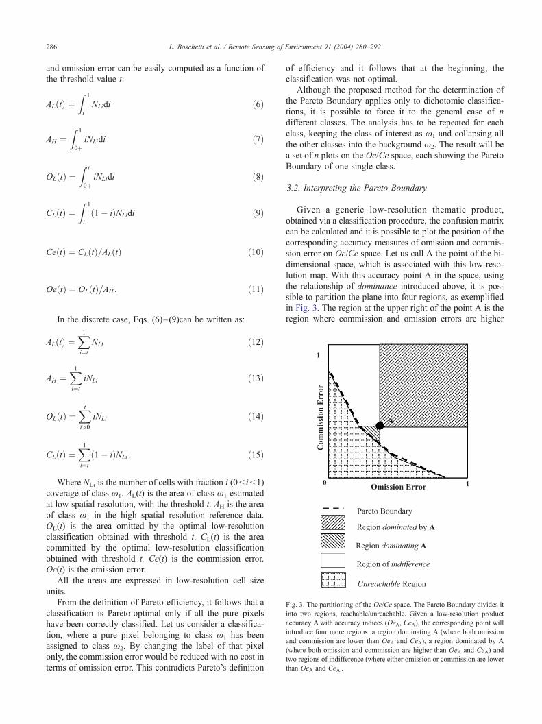
Fig. 3. The partitioning of the Oe/Ce space. The Pareto Boundary divides it

into two regions, reachable/unreachable. Given a low-resolution product

accuracy A with accuracy indices (OeA, CeA), the corresponding point will

introduce four more regions: a region dominating A (where both omission

and commission are lower than OeA and CeA), a region dominated by A

(where both omission and commission are higher than OeA and CeA) and

two regions of indifference (where either omission or commission are lower

than OeA and CeA..


and omission error can be easily computed as a function of

the threshold value t:

ALðtÞ ¼Z 1

t

NLidi ð6Þ

AH ¼Z 1

0þiNLidi ð7Þ

OLðtÞ ¼Z t

0þiNLidi ð8Þ

CLðtÞ ¼Z 1

t

ð1� iÞNLidi ð9Þ

CeðtÞ ¼ CLðtÞ=ALðtÞ ð10Þ

OeðtÞ ¼ OLðtÞ=AH : ð11Þ

In the discrete case, Eqs. (6)–(9)can be written as:

ALðtÞ ¼X1i¼t

NLi ð12Þ

AH ¼X1i¼t

iNLi ð13Þ

OLðtÞ ¼Xt

i>0

iNLi ð14Þ

CLðtÞ ¼X1i¼t

ð1� iÞNLi: ð15Þ

Where NLi is the number of cells with fraction i (0 < i < 1)

coverage of class x1. AL(t) is the area of class x1 estimated

at low spatial resolution, with the threshold t. AH is the area

of class x1 in the high spatial resolution reference data.

OL(t) is the area omitted by the optimal low-resolution

classification obtained with threshold t. CL(t) is the area

committed by the optimal low-resolution classification

obtained with threshold t. Ce(t) is the commission error.

Oe(t) is the omission error.

All the areas are expressed in low-resolution cell size

units.

From the definition of Pareto-efficiency, it follows that a

classification is Pareto-optimal only if all the pure pixels

have been correctly classified. Let us consider a classifica-

tion, where a pure pixel belonging to class x1 has been

assigned to class x2. By changing the label of that pixel

only, the commission error would be reduced with no cost in

terms of omission error. This contradicts Pareto’s definition

of efficiency and it follows that at the beginning, the

classification was not optimal.

Although the proposed method for the determination of

the Pareto Boundary applies only to dichotomic classifica-

tions, it is possible to force it to the general case of n

different classes. The analysis has to be repeated for each

class, keeping the class of interest as x1 and collapsing all

the other classes into the background x2. The result will be

a set of n plots on the Oe/Ce space, each showing the Pareto

Boundary of one single class.

3.2. Interpreting the Pareto Boundary

Given a generic low-resolution thematic product,

obtained via a classification procedure, the confusion matrix

can be calculated and it is possible to plot the position of the

corresponding accuracy measures of omission and commis-

sion error on Oe/Ce space. Let us call A the point of the bi-

dimensional space, which is associated with this low-reso-

lution map. With this accuracy point A in the space, using

the relationship of dominance introduced above, it is pos-

sible to partition the plane into four regions, as exemplified

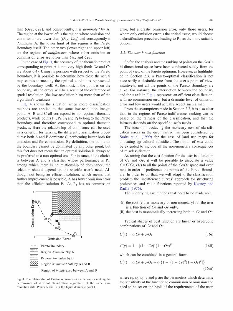
in Fig. 3. The region at the upper right of the point A is the

region where commission and omission errors are higher


than (OeA, CeA), and consequently, it is dominated by A.

The region at the lower left is the region where omission and

commission are lower than (OeA, CeA) and consequently it

dominates A; the lower limit of this region is the Pareto

Boundary itself. The other two (lower right and upper left)

are the regions of indifference, where either omission or

commission error are lower than OeA and CeA.

In the case of Fig. 3, the accuracy of the thematic product

corresponding to point A is not very high (both Oe and Ce

are about 0.4). Using its position with respect to the Pareto

Boundary, it is possible to determine how close the actual

map comes to meeting the optimal conditions represented

by the boundary itself. At the most, if the point is on the

boundary, all the errors will be a result of the difference of

spatial resolution (the low-resolution bias) more than of the

algorithm’s weakness.

Fig. 4 shows the situation when more classification

methods are applied to the same low-resolution image:

points A, B and C all correspond to non-optimal thematic

products, while points P1, P2, P3 and P4 belong to the Pareto

Boundary and therefore correspond to optimal thematic

products. Here the relationship of dominance can be used

as a criterion for ranking the different classification proce-

dures: both A and B dominate C, performing better both for

omission and for commission. By definition, the points on

the boundary cannot be dominated by any other point, but

this fact does not mean that an optimal solution is always to

be preferred to a non-optimal one. For instance, if the choice

is between A and a classifier whose performance is P4,

among which there is no relationship of dominance, the

selection should depend on the specific user’s need. Al-

though not being an efficient solution, which means that

further improvement is possible, A has lower omission error

than the efficient solution P4. As P4 has no commission

Fig. 4. The relationship of Pareto-dominance as a criterion for ranking the

performance of different classification algorithms of the same low-

resolution data. Points A and B in the figure dominate point C.

error, but a drastic omission error, only those users, for

whom only omission error is the critical issue, would choose

a classification procedure leading to P4, as the more suitable

option.

3.3. The user’s cost function

So far, the analysis and the ranking of points on the Oe/Ce

bi-dimensional space have been conducted solely from the

point of view of the Pareto optimum. However, as highlight-

ed in Section 2.3, a Pareto-optimal classification is not

necessarily a desirable one from the user’s point of view:

intuitively, not all the points of the Pareto Boundary are

alike. For instance, the intersection between the boundary

and the x axis in Fig. 4 represents an efficient classification,

with no commission error but a dramatic level of omission

error and few users would actually accept such a map.

From the assumptions made in Section 2.2, it is also clear

that, in the regions of Pareto-indifference, ranking can be

based on the fairness of the classification, and that the

fairness depends on the specific user’s needs.

The idea of introducing the monetary cost of classifi-

cation errors in the error matrix has been considered by

Smits et al. (1999) for the case of land use maps for

allocating agricultural subsidies. The notion of cost could

be extended to include all the non-monetary consequences

of misclassification.

Assuming that the cost function for the user is a function

of Ce and Oe, it will be possible to associate a value

C =C(Ce, Oe) to all the points of the Ce/Oe space and even

rank in order of preference the points of the Pareto Bound-

ary. In order to do that, we will adapt to the classification

problem the ‘indifference curves’ approach for structuring

preferences and value functions reported by Keeney and

Raiffa (1976).

The underlying assumptions that need to be made are:

(i) the cost (either monetary or non-monetary) for the user

is a function of Ce and Oe only,

(ii) the cost is monotonically increasing both in Ce and Oe.

Typical shapes of cost function are linear or hyperbolic

combinations of Ce and Oe:

CðxÞ ¼ c1Ceþ c2Oe ð16iÞ

CðxÞ ¼ 1� ½ð1� CeÞað1� OeÞb ð16iiÞ

which can be combined in a general form:

CðxÞ ¼ c1Ceþ c2Oeþ c3f1� ½ð1� CeÞað1� OeÞbgð16iiiÞ

where c1, c2, c3, a and b are the parameters which determine

the sensitivity of the function to commission or omission and

need to be set on the basis of the requirements of the user.

Fig. 6. Ranking combining the Pareto-dominance and the user’s cost

function. Point P2 of tangency between the Pareto Boundary and the iso-

cost lines is the point with lowest misclassification cost, compatible with

the low-resolution bias. Points A and B are ranked according to the cost

function.


The higher are c1 and a, the more the user is worried by

commission error, the higher are c2 and b, the more the user

would like to avoid omission error. Fig. 5 shows an example

of linear and hyperbolic iso-lines in the Ce/Oe space.

When the user bears a monetary cost for the classification

errors, the cost function can be easily determined; in all the

other cases, there is no way to determine unequivocally the

coefficients or even the general form of the cost function.

Consequently, the whole idea of cost function must be taken

as a way of formalising in a rigorous way an analysis that is

substantially a qualitative one.

Associating the concept of Pareto-Dominance and Pareto

Boundary (Section 2.3) with the cost function defined above,

it is possible to solve the problems of incomplete ranking,

highlighted is Section 3.2, by observing that:

(i) A dominates BZ C(A) < C(B), i.e. whenever A

dominates B, the cost of A is always lower that the

cost of B.

(ii) The criterion of minimum cost can be used for ranking

in the regions of Pareto-indifference.

(iii) In case of Pareto-indifference and equal cost, the point

with the smaller Euclidean distance from the Pareto

Boundary is preferred.

As the Pareto Boundary is a region of indifference (all

the points are efficient, thus by definition not dominated),

the points of the Pareto Boundary can be ranked according

to the associated cost: the point of tangency between the

Boundary and the iso-lines is the ideal point representing the

best achievable result, for the specific user.

Fig. 6 shows an example of complete ranking of the

results of different methods in the Ce/Oe space:

– Point P2 is the point representing the best possible

method for the specific user.

Fig. 5. Example of iso-lines of linear

– A is neither dominating nor dominated by B, therefore,

the ranking is based on the cost function. Because

C(A) <C(B), A should be selected as more respondent to

the requirements of the user.

– The difference C(A)�C(P2) is an index of the margin of

improvement of the classifier.

Lark (1995) introduced the concept that the classification

algorithm can be modified to emphasize whichever is more

important, user’s or producer’s accuracy for a particular

user. Point P2 could be seen as the target of such an

adjustment of the classification method.

and hyperbolic cost functions.

ng of Environment 91 (2004) 280–292 289

3.4. The misregistration issue: A stochastic approach

The Pareto Boundary, being computed from the high-

resolution data alone, is not affected by misregistration

between the low-resolution map and the reference data. As

it requires that the a low-resolution grid is superimposed on

the high-resolution data, there is an uncertainty of F 0.5

low-resolution pixel units both in x and in y directions and

this uncertainty will propagate on the positioning of the

Pareto Boundary points in the Oe/Ce space. Being the

Pareto Boundary, a function of the pattern of class x1 in

the specific images, such an uncertainty cannot be deter-

mined analytically, but needs to be assessed numerically,

generating a random sample of shifts (Dx, Dy) within the

range [� 0.5, 0.5] and computing the variance of the

omission and commission error pair values of all the points

belonging to the Boundary. As a result, the Pareto Boundary

is no longer a deterministic set of points (a line) but

becomes a region of the Oe/Ce space, described by a

probability distribution.

When the Pareto Boundary is used, as described in

Sections 3.2 and 3.3, to evaluate low-resolution classifica-

tion results, the misregistration between low and high-

resolution data is an issue that should be taken into account,

because it will affect the omission and commission error of

the classification (Foody, 2002; Plourde & Congalton, 2003;

Thomlinson et al., 1999). Automated co-registration soft-

ware tools based on correlation algorithms (Baltsavias,

1991; Carmona-Moreno, in press) provide sub-pixels accu-

racy, set aside the case of strongly nonlinear deformations.

The coregistration error could be seen as an uncertainty and,

as it is possible to estimate its variance, it is also possible to

estimate its propagation on the position of the point in Oe/

Ce, using the same numerical procedure adopted for the

points of the Pareto Boundary.

Under the usual assumptions of the error matrix (same

spatial resolution of the datasets, no misregistration errors),

the problem of minimising the classification error is a mono-

dimensional, deterministic one. By taking into account the

low-resolution bias, the problem is still deterministic, but

requires the use of a bi-dimensional space; by taking also

into account the misregistration issue, the problem becomes

a bi-dimensional, stochastic one.

3.5. Examples: Application of the Pareto Boundary to

burned area maps

As discussed in Section 3.1, the Pareto Boundary can be

calculated for any low-resolution pixel size starting from the

high-resolution reference data alone. Images with different

levels of fragmentation will generate different Pareto bound-

aries. In general, the higher the fragmentation, the lower the

accuracy that can be achieved and the higher the proportion

of the Oe/Ce space that is not reachable. This is illustrated in

Fig. 7, where the Pareto Boundary is computed for two

burned area maps derived from Landsat7 ETM data, by

L. Boschetti et al. / Remote Sensi

means of a maximum likelihood supervised classification

(Boschetti et al., 2002; Brivio et al., 2003). The two images,

respectively, scene 179-74 (Fig. 7a and b) acquired over

Namibia on October 31st, 2000, and scene 177-57 (Fig. 7c

and d), acquired on December 2nd, 1999 over Central

African Republic and Democratic Republic of Congo, were

part of the reference dataset used for the accuracy assess-

ment of continental burned area maps obtained from 1-km

spatial resolution SPOT-VGT data. Continental burned area

maps are a situation where relatively frequent mapping is

required over a very large area. The ETM+ scenes used for

the validation of the low-resolution data are a sample, both

in the space and in the time domain, as it would be

impossible (not only because of the cost, but also because

of insufficient data availability) to systematically use high

resolution data for the production of multitemporal global

thematic maps. As explained above, the Pareto Boundary is

calculated for a given low spatial resolution grid, 1 km� 1

km in this example. Fig. 7a and c present the fraction of

observed burned area, in each 1 km� 1 km pixel (what was

referred to as soft classification in Section 3.1 above); and

Fig. 7b and d) the discrete Pareto Boundary. The higher the

number of 1-km pixels with a low percentage of burned

area, the stronger the effect of the low-resolution bias and

the lower the accuracy that can be attained by a low-

resolution classification. The two scenes show a very

different level of heterogeneity. In scene 179-74 (Namibia),

71% of the high-resolution burned pixels fall into low-

resolution cells with a fraction of 50% burned area or more,

while in scene 177-57 (Central Africa), the cells with a

fraction of 50% burned area or more account only for 27%

of the total high-resolution burned pixels. To illustrate the

fragmentation, we use the Matheron index, identified by

Eva and Lambin (1998) as one of the indicators of landscape

fragmentation, which in the case of two classes can be

computed as:

Mðx1Þ ¼px1ffiffiffiffiffiffiffiffiffi

Ax1

p ffiffiffiffiffiffiffiffiAtot

p ð17Þ

where px1 = total perimeter of class x1, Ax1 = area of class

x1, Atot = total area.

The Matheron Index for the Namibia scene is 4.6, while

it is 6.2 for the more fragmented Central Africa scene. The

different level of fragmentation of the two thematic maps is

reflected in the respective Pareto Boundary plots. The

Pareto Boundary of the more fragmented scene of Central

Africa is always above that of the Namibia scene and its

unreachable region in the Oe/Ce space is considerably

larger. As a consequence, the accuracy levels that can be

attained by any burned area map of the region covered by

scene 177-57 are considerably smaller than that of the other

scene. For instance, a classification with Ce = 0.42 and

Oe = 0.43, which could be considered quite a poor perfor-

mance, is in fact on the Pareto Boundary, meaning that such

level of error is entirely due to the low-resolution bias.

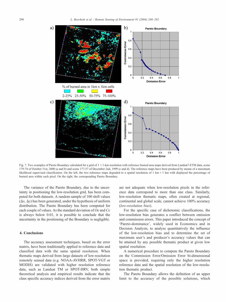
Fig. 7. Two examples of Pareto Boundary calculated for a grid of 1�1-km resolution with reference burned area maps derived from Landsat7-ETM data, scene

179-74 of October 31st, 2000 (a and b) and scene 177-57 of December 2nd, 1999 (c and d). The reference maps have been produced by means of a maximum

likelihood supervised classification. On the left, the two reference maps degraded to a spatial resolution of 1 km� 1 km with displayed the percentage of

burned area within each pixel. On the right, the corresponding Pareto Boundary.


The variance of the Pareto Boundary, due to the uncer-

tainty in positioning the low-resolution grid, has been com-

puted for both datasets. A random sample of 100 shift values

(Dx, Dy) has been generated, under the hypothesis of uniform

distribution. The Pareto Boundary has been computed for

each couple of values. As the standard deviation ofOe andCe

is always below 0.01, it is possible to conclude that the

uncertainty in the positioning of the Boundary is negligible.

4. Conclusions

The accuracy assessment techniques, based on the error

matrix, have been traditionally applied to reference data and

classified data with the same spatial resolution. When

thematic maps derived from large datasets of low-resolution

remotely sensed data (e.g. NOAA-AVHRR, SPOT-VGT or

MODIS) are validated with higher resolution reference

data, such as Landsat TM or SPOT-HRV, both simple

theoretical analysis and empirical results indicate that the

class specific accuracy indices derived from the error matrix

are not adequate when low-resolution pixels in the refer-

ence data correspond to more than one class. Similarly,

low-resolution thematic maps, often created at regional,

continental and global scale, cannot achieve 100% accuracy

(low-resolution bias).

For the specific case of dichotomic classifications, the

low-resolution bias generates a conflict between omission

and commission errors. This paper introduced the concept of

‘Pareto-dominance’, widely used in Economics and in

Decision Analysis, to analyse quantitatively the influence

of the low-resolution bias and to determine the set of

maximum user’s and producer’s accuracy values that can

be attained by any possible thematic product at given low

spatial resolution.

A numerical procedure to compute the Pareto Boundary

on the Commission Error/Omission Error bi-dimensional

space is provided, requiring only the higher resolution

reference data and the spatial resolution of the low-resolu-

tion thematic product.

The Pareto Boundary allows the definition of an upper

limit to the accuracy of the possible solutions, which


delimits a region of unreachable accuracy. All the points of

the line are equally efficient from the point of view of

omission and commission errors, as they represent possible

classifications where all the errors are due solely to the low-

resolution bias. Nonetheless, if the preference function of

the user of the specific map is known, it is possible to derive

from the accuracy figures a cost function that can be

combined with the Pareto Boundary to identify the point

of the boundary which has the lowest cost for the user. This

point of the Commission Error/Omission Error space rep-

resents the accuracy figures of the best map that could be

theoretically achieved, according to the specific user’s

needs. The difference between the cost of such a point

and the cost derived from the accuracy figures of a given

thematic map is an index of the performance of the

classification algorithm adopted.

Being computed only from high-resolution data, the

Pareto Boundary can be easily used as a tool for understand-

ing the implications of the spatial resolution in preliminary

feasibility studies. Using a sample of high-resolution data

over a region of interest, documentation of the low-resolution

bias could help identify the relevance (required accuracy) of a

low-resolution product for the target and region of interest,

even before starting the development of algorithms. In case of

regional or continental scale low-resolution thematic prod-

ucts, the computation of the Pareto Boundary could be

calculated for a selection of sites, in order to characterise

the low-resolution bias for the relevant ecosystems.

The proposed methodology based on the Pareto

Boundary could be also used by the analyst during the

classification process. Typically, after the first phase of

implementation of a classification method and when the

first results are available, the analyst needs to decide

whether the classification is accurate enough, or the

classifier needs to be improved. If a sample of reference

data is available, quantifying the low-resolution bias

allows understanding whether the errors described by

the error matrix could be reduced using a better algorithm,

or are due only to the low-resolution bias and therefore

depend on the intrinsic characteristics of the area mapped.

Furthermore, when more than one method is available and

a choice has to be made, combining the Pareto Boundary

with the analysis of the preferences of the user, it is

possible to rank the methods and to select the one which

corresponds better to the specific user’s needs.

Acknowledgements

The authors would like to acknowledge the contribution

of Marta Maggi, who kindly provided one of the TM

classifications used as examples, and to thank Hugh Eva and

Jean Marie Gregoire of JRC, for the useful comments on the

original manuscript; we are also grateful for the comments

from the anonymous reviewers, which helped to strengthen

and clarify the paper.

The first author is supported by a research fellowship

from the European Commission-Directorate General JRC.

References

Achard, F., Eva, H., & Mayaux, P. (2001). Tropical forest mapping from

coarse spatial resolution satellite data: Production and accuracy as-

sessment issues. International Journal of Remote Sensing, 22(14),

2741–2762.

Achard, F., Eva, H., Stibig, H. J., Mayaux, P., Gallego, J., Richards, T., &

Malingreau, J. P. (2002). Determination of deforestation rates of the

world’s humid tropical forests. Science, 297, 999–1002.

Baltsavias, E. P. (1991). Geometrically constrained multiphoto matching.

Mitteilungen, vol. 49. Zurich: Institute of Geodesy and Photogramme-

try, ETH.

Bartholome, E., Belward, A. S., Achard, F., Bartalev, S., Carmona-Moreno,

C., Eva, H., Fritz, S., Gregoire, J. -M.,Mayaux, P., & Stibig, H. -J. (2002).

GLC 2000-Global Land Cover mapping for the year 2000-Project status

November 2002. Ispra, Italy: Publication of the European Commission,

JRC, EUR 20524 EN.

Binaghi, E., Brivio, P. A., Ghezzi, P., & Rampini, A. (1999). A fuzzy set-

based accuracy assessment of soft classifications. Pattern Recognition

Letters, 20, 935–948.

Boschetti, L., Flasse, S., Jacques de Dixmude, A., & Trigg, S. (2002). A

multitemporal change-detection algorithm for the monitoring of burnt

areas with SPOT-Vegetation data. In L. Bruzzone, & P. Smith (Eds.),

Analysis of multi-temporal remote sensing images (pp. 75–82). Singa-

pore: World Scientific Publishing.

Boschetti, L., Flasse, S., Trigg, S., Brivio, P. A., & Maggi, M. (2001). A

methodology for the validation of low resolution remotely sensed data

products. Proceedings of 5th ASITA conference (Rimini 9–12 October

2001) vol. 1 (pp. 293–298). Asita, Milano.

Brivio, P. A., Maggi, M., Binaghi, E., & Gallo, I. (2003). Mapping

burned surfaces in Sub-Saharan Africa based on multi-temporal neu-

ral classification. International Journal of Remote Sensing, 20,

4003–4016.

Carmona-Moreno, C. (2004). Vegetation L-band processing system. Geo-

metric performance and spatio-temporal stability. International Journal

of Remote Sensing (in press).

Chilar, J. (2000). Land cover mapping of large areas from satellites: Status

and research priorities. International Journal of Remote Sensing, 21,

1093–1114.

Congalton, R. G. (1991). A review of assessing the accuracy of classi-

fications of remotely sensed data. Remote Sensing of Environment, 37,

35–46.

Congalton, R. G., & Green, K. (1999). Assessing the accuracy of remotely

sensed data (p. 137). Florida: CRC Press.

Congalton, R. G., Oderwald, R. G., & Mead, R. A. (1983). Assessing

Landsat classification accuracy using discrete multivariate analysis sta-

tistical techniques. Photogrammetric Engineering and Remote Sensing,

49, 1671–1678.

Eva, H., & Lambin, E. F. (1998). Remote sensing of biomass burning in

tropical regions: Sampling issues and multisensor approach. Remote

Sensing of Environment, 64, 292–315.

Foody, G. M. (1996). Approaches for the production and evaluation of

fuzzy land cover classification from remotely sensed data. International

Journal of Remote Sensing, 17, 1317–1340.

Foody, G. M. (2002). Status of land cover accuracy assessment. Remote

Sensing of Environment, 80, 185–201.

Gregoire, J. -M., Tansey, K., & Silva, J. M. N. (2003). The GBA2000

initiative: Developing a global burned area database from SPOT-VEG-

ETATION imagery. International Journal of Remote Sensing, 24,

1369–1376.

Justice, C., Belward, A., Morisette, J., Lewis, P., Privette, J., & Baret, F.

(2000). Developments in the validation of satellite sensor products for


the study of land surface. International Journal of Remote Sensing,

21(17), 3383–3390.

Justice, C. O., Giglio, L., Korontzi, S., Owens, J., Morisette, J. T., Roy, D.,

Descloitres, J., Alleaume, S., Petitcolin, F., & Kaufman, Y. (2002). The

MODIS fire products. Remote Sensing of Environment, 83, 244–262.

Keeney, R. L., & Raiffa, H. (1976). Decisions with multiple objectives:

Preferences and value tradeoffs. New York: Wiley.

Lark, R. M. (1995). Components of accuracy of maps with special refer-

ence to discriminant analysis on remote sensor data. International Jour-

nal of Remote Sensing, 16(8), 1461–1480.

Loveland, T. R., Zhu, Z., Ohlen, D. O., Brown, J. F., Reed, B. C., & Yang, L.

(1999). An analysis of the IGBP Global Land-Cover characterization

process. Photogrammetric Engineering and Remote Sensing, 65,

1021–1032.

Mayaux, P., & Lambin, E. F. (1995). Estimation of tropical forest area from

coarse spatial resolution data: A two-step correction function for pro-

portional errors due to spatial aggregation. Remote Sensing of Environ-

ment, 53, 1–15.

Pareto, V. (1906). Manuale d’Economia Politica. Milano: Societa Editrice

Libraria.

Plourde, L., & Congalton, R. (2003). Sampling method and sample place-

ment: How do they affect the accuracy of remoltely sensed maps?

Photogrammetric Engineering and Remote Sensing, 69, 289–297.

Remmel, T. K., & Perera, A. H. (2002). Accuracy of discontinuous binary

surfaces: A case study using boreal forest fires. International Journal of

Geographical Information Science, 16, 287–298.

Roy, D., Lewis, P. E., & Justice, C. O. (2002). Burned area mapping using

multi-temporal moderate spatial resolutio data-a bi-directional reflec-

tance model-based expectation approach. Remote Sensing of the Envi-

ronment, 83, 263–286.

Simon, M., Plummer, S., Fierens, F., Hoeltzemann, J. J., & Arino, O.

(2004). Burnt area detection at global scale using ATSR-2: The Globs-

car products and their qualification. Journal of Geophysical Research

(In press).

Smith, J. H., Stehman, S. V., Wickham, J. D., & Yang, W. (2003). Effects

of landscape characteristics on land-cover class accuracy. Remote Sens-

ing of Environment, 84, 342–349.

Smits, P. C., Dellepiane, S. G., & Showengerdt, R. A. (1999). Quality

assessment of image classification algorithms for land-cover mapping:

A review and a proposal for a cost-based approach. International Jour-

nal of Remote Sensing, 20(8), 1461–1486.

Stehman, S. V. (1997). Selecting and interpreting measures of thematic

classification accuracy. Remote Sensing of Environment, 62, 77–89.

Story, M., & Congalton, R. G. (1986). Accuracy assessment: A user’s

perspective. Photogrammetric Engineering and Remote Sensing, 52,

397–399.

Tansey, K., Gregoire, J. -M., Stroppiana, D., Sousa, A., Silva, J. M. N.,

Pereira, J. M. C., Boschetti, L., Maggi, M., Brivio, P. A., Fraser, R.,

Flasse, S., Ershov, D., Binaghi, E., Graetz, D., & Peduzzi, P. (2004).

Vegetation burning in the year 2000: Global burned area estimates

from SPOT VEGETATION data. Journal of Geophysical Research

(In press).

Thomlinson, J. R., Bolstad, P. V., & Cohen, W. B. (1999). Coordinating

methodologies for scaling landcover classifications from site-specific to

global: Steps toward validation global map products. Remote Sensing of

Environment, 70, 16–28.

Woodcock, C., & Strahler, A. (1987). The factor of scale in remote sensing.

Remote Sensing of Environment, 20, 311–332.

Analysis of the conflict between omission and commission in low ...

Documents

Transcript of Analysis of the conflict between omission and commission in low ...