CMIT-2005-259

CMIT Report Number: CMIT–2005–259

Analysis of Hydrostatic Test Water

Final Report for APIA

G. Tjandraatmadja, S. Gould, S. Burn

5 December 2005

CSIRO Manufacturing and Infrastructure Technology ©CSIRO 2005

1

CMIT-2005-259

Circulation: Client (2) Publications Officer, Group Leader, CMIT (2) Authors (4)

This report has been prepared on the basis of information, data and material supplied to us by the Client and on the assumption that such information, data and material is correct and accurate. ©2005 CSIRO The Client may only copy extracts from the Report if it clearly notes on the extract: (a) That it is part of a larger Report; and (b) Where the full Report can be obtained. Mr Stewart Burn CSIRO Manufacture & Infrastructure Technology PO Box 56 Highett, Victoria 3190 Tel: (03) 9252 6032

2

CMIT-2005-259

ACKNOWLEDGEMENTS This report has only been possible with the assistance of a large number of people and companies that graciously volunteered their time, information and resources. The project officers would like to thank the advisory committee: Phil Venton, Max Kimber, Andy Pym, Lynndon Harnell, Graeme Gentles, Wendy Mathieson, Craig Bonar, Peter Thomas, Harry Moss, Lucas Group, Mitchell Pty Ltd, Enertrade, Origin Energy, Santos, Gasnet and many more.

3

CMIT-2005-259

Table of contents EXECUTIVE SUMMARY................................................................................................................................ 12 BACKGROUND ................................................................................................................................................ 14 1 HYDROSTATIC TESTING.................................................................................................................... 16

1.1 PARAMETERS AFFECTING WATER QUALITY........................................................................................ 17 1.1.1 Construction materials................................................................................................................. 17 1.1.2 Pipeline history ............................................................................................................................ 19 1.1.3 Water sources............................................................................................................................... 19 1.1.4 Natural water contaminants......................................................................................................... 19

2 ADDITIVES.............................................................................................................................................. 21 2.1 OXYGEN SCAVENGERS....................................................................................................................... 21 2.2 BIOCIDES ........................................................................................................................................... 22

2.2.1 Target bacteria............................................................................................................................. 23 2.2.2 Biocide categories........................................................................................................................ 24 2.2.3 Toxicity of biocides ...................................................................................................................... 25 2.2.4 Biocide regulation........................................................................................................................ 27 2.2.5 Neutralisation of biocides ............................................................................................................ 28 2.2.6 Technologies for biocide neutralisation....................................................................................... 28

3 REGULATORY REQUIREMENTS...................................................................................................... 31 3.1 BACKGROUND AND OBJECTIVES ........................................................................................................ 31 3.2 WATER DISPOSAL REGULATIONS ....................................................................................................... 31

3.2.1 New South Wales.......................................................................................................................... 32 3.2.2 Northern Territory ....................................................................................................................... 33 3.2.3 South Australia............................................................................................................................. 33 3.2.4 Tasmania...................................................................................................................................... 33 3.2.5 Victoria ........................................................................................................................................ 34 3.2.6 Western Australia......................................................................................................................... 34 3.2.7 Queensland................................................................................................................................... 34 3.2.8 United States of America.............................................................................................................. 35 3.2.9 Major findings.............................................................................................................................. 36

4 EXPERIMENTAL ................................................................................................................................... 37 4.1 SAMPLING LOCATIONS AND CHARACTERISTICS ................................................................................. 37 4.2 WATER SOURCES ............................................................................................................................... 37 4.3 SAMPLE SELECTION ........................................................................................................................... 37 4.4 SAMPLING PROCEDURE...................................................................................................................... 37 4.5 SAMPLE CHARACTERISATION............................................................................................................. 38 4.6 PARAMETER SELECTION .................................................................................................................... 39

4.6.1 Soil properties .............................................................................................................................. 40 4.6.1.1 Sodium adsorption ratio (SAR).......................................................................................................... 40 4.6.1.2 Other ions........................................................................................................................................... 41

4.6.2 Plant growth................................................................................................................................. 41 4.6.2.1 Nitrogenous compounds (Total nitrogen, NO3

-, NH4+) ...................................................................... 41

4.6.2.2 Phosphorus (P) ................................................................................................................................... 41 4.6.2.3 Chloride (Cl) ...................................................................................................................................... 41 4.6.2.4 Copper (Cu)........................................................................................................................................ 42 4.6.2.5 Chromium (Cr)................................................................................................................................... 42 4.6.2.6 Iron (Fe) ............................................................................................................................................. 42 4.6.2.7 Manganese (Mn) ................................................................................................................................ 42 4.6.2.8 Lead (Pb)............................................................................................................................................ 42 4.6.2.9 Sodium (Na)....................................................................................................................................... 43 4.6.2.10 Zinc (Zn) ............................................................................................................................................ 43

4.6.3 Residue analysis ........................................................................................................................... 43 5 ANALYSIS OF HYDROSTATIC TEST WATER................................................................................ 44

4

CMIT-2005-259

5.1 INTRODUCTION .................................................................................................................................. 44 5.2 SOURCE WATER ................................................................................................................................. 44

5.2.1 General characteristics................................................................................................................ 45 5.2.1.1 Water pH............................................................................................................................................ 45 5.2.1.2 Electrical conductivity........................................................................................................................ 45 5.2.1.3 Turbidity and colour........................................................................................................................... 45 5.2.1.4 Dissolved oxygen ............................................................................................................................... 46

5.2.2 Metals........................................................................................................................................... 46 5.2.3 Dissolved salts.............................................................................................................................. 47

5.3 FLUSHING WATER .............................................................................................................................. 48 5.4 DISPOSAL WATER .............................................................................................................................. 49

5.4.1 General characteristics................................................................................................................ 49 5.4.1.1 Water pH............................................................................................................................................ 49 5.4.1.2 Electrical conductivity........................................................................................................................ 50 5.4.1.3 Turbidity ............................................................................................................................................ 50 5.4.1.4 Dissolved oxygen ............................................................................................................................... 50 5.4.1.5 Solids ................................................................................................................................................. 51

5.4.2 Metals........................................................................................................................................... 52 5.4.3 Dissolved salts.............................................................................................................................. 53 5.4.4 Environmental impact .................................................................................................................. 54 5.4.5 Disposal to aquatic ecosystems.................................................................................................... 55

5.4.5.1 Physio–chemical parameters .............................................................................................................. 55 5.4.5.2 Water pH............................................................................................................................................ 55 5.4.5.3 Electrical conductivity........................................................................................................................ 55 5.4.5.4 Turbidity ............................................................................................................................................ 55 5.4.5.5 Metals................................................................................................................................................. 57 5.4.5.6 Salinity ............................................................................................................................................... 58 5.4.5.7 Nutrients............................................................................................................................................. 59 5.4.5.8 ................................................................................................................................. 61 Sulphate (SO4

2-)5.4.6 Disposal to land ecosystems......................................................................................................... 61

5.4.6.1 Physico–chemical parameters ............................................................................................................ 61 5.4.6.2 Metals................................................................................................................................................. 62 5.4.6.3 Salinity on crops................................................................................................................................. 64 5.4.6.4 Sodicity and salinity on soil ............................................................................................................... 65 5.4.6.5 Nutrients............................................................................................................................................. 66

5.4.7 Disposal options........................................................................................................................... 67 5.4.8 Summary ...................................................................................................................................... 69

6 TREATMENT OF DISPOSAL WATER............................................................................................... 71 6.1 PRE–TREATMENT OF PIPELINE AND SOURCE WATER .......................................................................... 71 6.2 TREATMENT OF DISCHARGE WATER................................................................................................... 71

6.2.1 Disposal to land ........................................................................................................................... 72 6.2.2 Hay Bales ..................................................................................................................................... 73 6.2.3 Evaporation Ponds....................................................................................................................... 75 6.2.4 Flotation....................................................................................................................................... 76 6.2.5 Sedimentation............................................................................................................................... 76 6.2.6 Filtration ...................................................................................................................................... 76 6.2.7 Clay .............................................................................................................................................. 77 6.2.8 Aeration/Air stripping .................................................................................................................. 77 6.2.9 Activated carbon .......................................................................................................................... 78 6.2.10 Discharge to a public water treatment facility ........................................................................ 78 6.2.11 Removal by truck ..................................................................................................................... 78 6.2.12 Ultra–violet light oxidation ..................................................................................................... 79 6.2.13 Cost comparison...................................................................................................................... 79 6.2.14 Experimental investigation of treatment alternatives.............................................................. 83

7 FINAL REMARKS .................................................................................................................................. 86 8 OVERALL CONCLUSIONS .................................................................................................................. 87 9 REFERENCES ......................................................................................................................................... 89 APPENDIX 1 – REGULATORY BODIES ..................................................................................................... 93 APPENDIX 2 – OXYGEN SCAVENGERS .................................................................................................... 94

5

CMIT-2005-259

APPENDIX 3 – DATA SUMMARY ................................................................................................................ 95

6

CMIT-2005-259

Table of Tables Table 1 – Hydrostatic test Standards (Fletcher et al. 2003) .................................................... 17 Table 2 – Examples of steel used in pipeline construction (Bluescope Steel 2004a, 2004b,

2004c).............................................................................................................................. 17 Table 3 – Chemical composition of pipeline steel .................................................................. 17 Table 4– Examples of common oxygen scavengers ............................................................... 21 Table 5 – Examples of biocides used in the oil and gas industry (Chen & Chen 1997, Frayne

2001)................................................................................................................................ 24 Table 6 – Toxicity of biocides (Chen & Chen 1997) .............................................................. 26 Table 7 – Persistence of biocides (Chen & Chen 1997).......................................................... 26 Table 8 – Toxicity of biocides combined with oxygen scavengers (Chen & Chen 1997)...... 27 Table 9 – Neutralization of bactericide residuals following three months exposure (Chen &

Chen 1997) ...................................................................................................................... 29 Table 10 – Additives used in hydrostatic testing (Chen & Chen 1997).................................. 30 Table 11– Environment Regulation Authorities in Australia.................................................. 32 Table 12 – Pipeline characteristics.......................................................................................... 37 Table 13 – Summary of parameters analysed in the water samples (APHA 2001) ................ 38 Table 14 – Sampling sites ....................................................................................................... 44 Table 15 – Main characteristics of source waters used in hydrostatic tests ............................ 45 Table 16 – Metal concentration in source waters.................................................................... 47 Table 17 – Inorganic contents in source waters ...................................................................... 47 Table 18 – Flush water characteristics for T10 ....................................................................... 49 Table 19 – Main characteristics of hydrostatic test discharge water....................................... 51 Table 20 – Metal concentration in disposal waters ................................................................. 53 Table 21 – Inorganic contents in disposal waters.................................................................... 54 Table 22– Comparison of characteristics of hydrostatic test waters before and after

hydrostatic test................................................................................................................. 56 Table 23–Ranges of default trigger values for Turbidity (NTU) in Australian ecosystems

(ANZECC/ARMCANZ 2000) ........................................................................................ 56 Table 24 – Trigger values for toxicants at alternate protection levels (ANZECC/ARMCANZ

2000)................................................................................................................................ 57 Table 25 – Comparison of disposal water with guidelines (ANZECC/ARMCANZ 2000).... 58 Table 26 – Trigger values for salinity (ANZECC/ARMCANZ 2000) ................................... 58 Table 27 – Nutrient levels in disposal water ........................................................................... 60 Table 28 – Nutrient trigger values for Australian waters (ANZECC/ARMCANZ 2000) ...... 60 Table 29–Guidelines for irrigation (ANZECC/ARMCANZ 2000) ........................................ 63 Table 30– Comparison of disposal water with irrigation guideline values (ANZECC/

ARMCANZ 2000)........................................................................................................... 63 Table 31 – Estimated load for hydrostatic test disposal water ................................................ 64 Table 32 – Examples of salt tolerance crops (ANZECC/ARMCANZ 2000) ......................... 65 Table 33 – Oxygen scavenger impact on ionic species........................................................... 66 Table 34 – SAR for disposal water ......................................................................................... 66 Table 35 – Recommended guidelines for N and P in irrigation water (ANZECC/ARMCANZ

2000)................................................................................................................................ 67 Table 36– Suitability for disposal of test water into aquatic bodies ....................................... 68 Table 37 – Suitability for use of test water for irrigation........................................................ 68 Table 38 – Treatment requirements for water based on composition ..................................... 72 Table 39 – Methodologies for disposal water treatment ......................................................... 72

7

CMIT-2005-259

Table 40 - Summary of costs in the USA grouped by treatment range (API,1998) ............... 80 Table 41 – Cost estimates for six treatment technologies (API 1998).................................... 81 Table 42 – Advantages and disadvantages for seven treatment technologies (Tallon et al

1992a).............................................................................................................................. 82 Table 43 – Treatment of disposal water .................................................................................. 83 Table 44 –Effect of treatment on water quality....................................................................... 85 Table 45 – Information sources for State regulation............................................................... 93 Table 46 – Chemistry of active compounds in common oxygen scavengers ......................... 94 Table 47 – Data Summary....................................................................................................... 96

8

CMIT-2005-259

Table of Figures Figure 1 – Schematic of hydrostatic test (adapted from Sprester et al. 1986) ........................ 16 Figure 2 – Chemistry of ammonium and sodium bisulphite oxygen scavengers in water

(Baker Petrolite, pers. com 2003).................................................................................... 22 Figure 3 – Examples of residues from disposal water after drying at 105°C for T2, T3, T6 and

T9 replicates. ................................................................................................................... 52 Figure 4 – Sulphate content in disposal waters ....................................................................... 61 Figure 5 – Classification of disposal water based on irrigation water salinity ratings............ 64 Figure 6 – Relationship between SAR and EC of EC water for prediction of structural soil

stability – adapted from ANZECC/ARMCANZ (2000) ................................................. 66 Figure 7 – Spray nozzles used for disposal of hydrostatic test water in Moomba–Sydney

Binerah Downs (Courtesy of Max Kimber, 2004). ......................................................... 73 Figure 8 – Aerial view of hydrostatic test water sprayed in Moomba–Sydney Binerah Downs

(Courtesy of Max Kimber, 2004). ................................................................................... 73 Figure 9–Schematic representation of some hay bale treatment structure on a downward

sloping terrain.................................................................................................................. 74 Figure 10 – Hay bale treatment apparatus (Tallon et al 1992a) .............................................. 75 Figure 11 – Diagram of sedimentation process....................................................................... 76 Figure 12 – Apparatus for hydrostatic test water disposal (Courtesy of Enertrade, 2005) ..... 77 Figure 13 – Cost of treatment technologies (API 1998) ......................................................... 80 Figure 14 – Oxidation of ferrous iron to ferric hydroxide ...................................................... 83 Figure 15 – Water samples before and after settling for 48 hours for T10. ............................ 84

9

CMIT-2005-259

Nomenclature AC Activated carbon

ADWG Australian Drinking Water Guidelines

API American Petroleum Institute

APIA Australian Pipeline Industry Association Inc

ANZGFMWQ Australian and New Zealand Guidelines for Fresh and Marine Water Quality

BBAB bis–bromo acetyl butene

BHAP 2–bromo–4–hydroxyacetophenone

BNS β–bromo–β–nitrostyrene

BTEX benzene, toluene, ethylbenzene, and xylene

DBNPA 2,2 dibromo–3–nitrilopropionamide

CCL Cumulative contaminant loading

C Nominal concentration of scavenger (mg/L)

CO2 Concentration of oxygen (mg/L)

DE Department of Environment (WA)

DEC Department of Environment and Conservation (NSW)

DEM Director of Environmental Management (Tas)

DIPR Department of Infrastructure, Natural Resources and Planning (NSW)

DIPE Department of Infrastructure, Planning and Environment (NT)

DNRM Department of Natural Resources and Mines (Qld)

DO Dissolved oxygen

EC Electrical conductivity

EC50–15 min Effective concentration for 50% reduction in light output from a micro–assay of

marine bacterium after 15 min exposure

EMPCA Environmental Management and Pollution Control Act 1994

EPA Environmental Protection Agency

ERW Electric resistance welding

EU European Union

FIFRA Federal Insecticide, Fungicide and Rodenticide Act 1972

GAB General aerobic bacteria

GMA Gas shielded metal arc

LC50 Lethal concentration of a chemical which causes the death of 50% of test organisms

in a 96hr period

LD50 Lethal dose which causes the death of 50% of a group of test organisms

LTV Long–term trigger value

10

CMIT-2005-259

MAOP Maximum operating pressure

MMA Manual metal arc

MW Molecular weight of scavenger

MWO2 Molecular weight of oxygen

NPDES National Pollutant Discharge Elimination System

Nox Oxides of nitrogen

PHMB poly(hexamethylenebiguanide) hydroxide

ppm parts per million

R Stoichiometric reaction ratio of scavenger to oxygen

SAR Sodium adsorption ratio

SEPP State of Environment Protection Policy (Vic)

SRB Sulphate–reducing bacteria

STV Short-term trigger value

TDS Total dissolved solids

THPS tetrakis(hydroxymethyl)phosphonium sulfate

TN Total nitrogen

TP Total phosphorus

TS Total solids

TSS Total suspended solids

V Volume of scavenger required (L) 2O

Vpipe Total volume of water in pipe (L)

X Percentage of active compound in formulation

11

CMIT-2005-259

Executive Summary This report outlines an investigation conducted by CSIRO on the processes associated with the disposal of hydrostatic test water. The aim of the paper was to review the requirements and practices utilised for the disposal and treatment of hydrostatic test water in the gas pipeline industry, and to assess their environmental impact. The investigation covered the technical and environmental aspects of the supply, treatment and disposal of water used for hydrostatic testing of pipelines. It aimed to establish and document the constraints on the processes and their management; to monitor the effect of dynamic changes in water quality from different sources on the pipeline and the disposal water quality; and to review and benchmark practices used worldwide for water disposal. Finally, it aimed to provide the basis for a chapter in the APIA Code of Environmental Practice on hydrostatic test water sourcing, treatment and disposal. The investigation consisted of:

• A review of the current environmental standards in Australian jurisdictions and a survey of water disposal requirements from regulatory authorities.

• A review of water source quality and impact of untreated water on pipe materials. • Characterisation of pipe materials used in pipeline manufacture. • Inventory of additives incorporated into hydrostatic test water and their impact on

water quality. • Evaluation of hydrostatic test water quality in the field – sampling and analysis of

water, that either contained no additives or contained oxygen scavengers, obtained from 10 hydrostatic tests on new pipelines around Australia.

• Environmental risk assessment for field samples and a review of treatment technologies.

• Verification of a range of disposal methods and practices used by industry in the field including: oxygen scavenger neutralisation by aeration, sediment removal by filtration with geofabric, erosion mitigation with hay bales, final discharge to rivers, farm dams, holding ponds, reuse in another test section, and onto land.

• Conclusions and recommendations. The evaluation of adverse impacts that metal and chemical contaminants present in the hydrostatic water could have on the environment has been the major drivers of this project. The research concluded that for all hydrostatic tests investigated, with the exception of specific pipelines that use ‘source contaminated’ water, the quality of discharge water causes no increase in environmentally hazardous compounds derived from either the pipe, or any treatment made to the water. Note that none of the pipelines investigated used biocides in the treatment process.

Hydrostatic testing does not contribute to the concentration of nutrients (nitrogen, phosphorus, potassium and dissolved ions) in the discharge water. However the discharged water does contain increased turbidity levels (10 to 10,000 times that of the source water) caused mainly by iron–based suspended solids and possibly soil residues, low levels of dissolved oxygen due to oxygen scavenger and increased levels of sodium or ammonium sulphate.

12

CMIT-2005-259

The removal of sediment and the associated decrease in turbidity may be required when disposing to some water courses to reduce the impact of disposal on the water course and to ensure there is no depletion of oxygen levels. Lining of pipelines would avoid mill scale breakdown, residue formation and so remove most pipe related contamination, reducing suspended solids and simplifying turbidity control. Current industry methods to remove solids by sedimentation and/or filtration, to neutralise residual oxygen scavenger and restore dissolved oxygen levels by aeration are effective in raising the quality of disposal water sufficiently for it to be disposed by irrigation, evaporation or into water courses depending on their characteristics. Finally, discharge of hydrostatic water is a one–off event and needs to be considered as such when evaluating its environmental impact and comparing it to data from guidelines. Commonsense is needed for site assessment and in the use of guidelines. In some cases, the quality of disposal water was similar to the source water extracted from a river, but would have been considered beyond range if only compared to Australian and New Zealand Guidelines for Fresh and Marine Water Quality (ANZECC/ARMCANZ 2000). In conclusion, organisations planning hydrostatic testing must plan for water disposal, both in selecting the source water (if possible) and disposal site, and developing a treatment program for the discharge water. Whilst not observed in the case studies, special planning is required when specifying treatment programs for hydrostatic test water containing biocides to deactivate residues prior to discharge to the environment, and when using water that may cause disposal problems (e.g. containing high salinity, presence of sulphate–reducing bacteria, sewerage effluent).

13

CMIT-2005-259

Background Prior to commissioning new pipelines, structural integrity is determined using a hydrostatic pressure test, in which the pipe is filled with water, pressurised above the intended operating pressure and monitored for leaks or pressure loss over a specified time period. Additives such as oxygen scavengers and biocides can be added to the water as a preventative measure to control the risk of potential corrosion and micro–organism growth in the pipe. After hydrostatic testing, the test water can become discoloured and odorous, and after industry practices, such as aeration and other minimal treatment techniques, it is discharged to irrigation or streams. Pipeline developers typically assign the risk of finding and discharging the hydrostatic test water to the pipeline construction contractor. Typically, the contractor does not have the required expertise to satisfy the assessor (often an environmental scientist) that this risk will be properly managed. The test proponent must make a significant effort to obtain approval for the test and disposal of its water, often at a significant cost and risk of schedule delays (Venton 2003). Furthermore, as pipeline construction projects occur infrequently and in different jurisdictions, a different regulatory assessor has responsibility for authorising water supply and disposal for each project. Because pipeline projects are irregular events, it is not unusual for the regulatory assessors to have no experience with the hydrostatic testing process, or of the effect of water disposal on the environment. Whilst practices and methodologies for the disposal of hydrostatic water have been in use for a long time in the industry, documentation of best practices and details of environmental impact assessment in the open literature are limited. Research has been undertaken overseas (by the Gas Research Institute), but this work is not generally available. Unfortunately, there are no codes of practice or standards and generally no documented records of previous hydrostatic tests that are sufficiently detailed to provide guidance to assessors (Venton 2003). Through this research a better understanding of the chemical and biological processes, the interaction between test water, the pipeline and the environment, will be obtained to allow the development of procedures for suitable process management. This will also provide assessors and construction personnel with references for the evaluation and development of optimal disposal methodologies. The aims of the research described in this report were:

• To investigate the technical and environmental aspects of the supply, discharge and disposal of water used for hydrostatic testing of pipelines.

• To establish and document the constraints on the processes and their management. • To monitor the effect of dynamic changes in water quality from different sources on

the pipeline and the disposal water quality, including the determination of contaminants generated in the process and the impact of their disposal on the environment.

• To review practices used worldwide for benchmarking and to investigate procedures commonly used for test water disposal to minimise the risk of adverse impacts on the environment.

14

CMIT-2005-259

• To provide the basis for a chapter in the APIA Code of Environmental Practice on hydrostatic test water sourcing, treatment and disposal.

To achieve these goals, an in–depth study was conducted to examine hydrostatic test water, including the analysis of water sources and additives, and characterisation of water used in 10 hydrostatic tests conducted across the country, and an evaluation of treatment and disposal alternatives.

15

CMIT-2005-259

1 Hydrostatic Testing The safe operation of gas and petroleum pipelines requires rigorous design, construction and verification of the structural integrity. Failure of a pipeline causes not only economic losses, but could also result in catastrophic environmental impact and even loss of life. AS 2885.1:1997 (Amdt 2001): ‘Pipelines – Gas and liquid petroleum – Design and construction’ has adopted the practice of proving the structural integrity of a pipeline prior to approval for service by hydrostatic testing. Field testing is conducted according to AS 2885.5: 2002: ‘Pipelines – Gas and liquid petroleum – Field pressure testing’ to prove strength, followed by an extended test at reduced pressure (depending on the standard requirements) to prove its leak–tightness. The strength test is conducted at a pressure higher than the maximum allowable operating pressure, to detect defects in the pipeline that have the potential to grow to failure when the pipeline is operated at its maximum allowable pressure. Hydrostatic tests are sometimes conducted on pipelines that have been in service for some years to demonstrate a pipeline’s integrity, although this practice is being replaced by in–line inspection procedures. There are proposals in North America, particularly where pipelines are installed in permafrost, to replace the hydrostatic test requirement with an inspection and quality management regime, principally because of the difficulty in managing the hydrostatic test water sourcing and disposal in these areas, together with the risk that the fluid will freeze in the pipeline, causing it to become unserviceable. To date, this remains as a proposal only (Venton 2005). During hydrostatic testing, an internal pressure above the normal pressure is applied to an isolated segment of a pipeline, under no–flow conditions, for a fixed period of time (AS/NZS 2885.5:2002, ASME B31.8:2003, ISO 13623:2000). Pressurisation can be performed using gases such as air, inert gas and natural gas, or liquids such as petroleum products or water. Water is the test medium of choice in most pressure tests for reasons of cost and safety (Tallon & Fillo 1992). A pipeline segment is isolated and filled with water using a high volume pump (Figure 1). After the pipe is filled with water, the pressure is increased to the desired level using a high–pressure pump. This pressure is then held for a preset time to check the integrity of the pipeline (Table 1) (Fletcher et al. 2003).

Temporary end plate

Temporary end plate

Testing water inlet

Section of line to be tested Figure 1 – Schematic of hydrostatic test (adapted from Sprester et al. 1986)

16

CMIT-2005-259

Table 1 – Hydrostatic test Standards (Fletcher et al. 2003)

Standard Organisation Pressure (max. operating pressure)

Pressurisation period

AS 2885.5 Standards Australia/New Zealand Standards 2002

1.25 MAOP (min.) 1.1 MAOP 24 hr

Min. 4 hr (strength test) Min. 24 hr (leak test)

ASME B31.82 American Society of Mechanical Engineers 2004

1.1 MAOP Mini. 2 hr

ISO 13623 International Standards Organisation 2000

1.25 MAOP 1.1 MAOP

Min. 1 hr Min. 8 hr

After the test is completed, the pressure is released and the pipeline dewatered. Pipeline dewatering is accomplished by pushing a ‘pig’ through the line using pressurised air, gas or petroleum liquid. The hydrostatic test process, including filling, testing and depressurising, can range from a few days to a few weeks depending on pipe size and length. The discharged water typically contains the contaminants and particulate matter present in the pipeline (Fillo et al. 1992).

1.1 Parameters affecting water quality

The quality of disposal water from hydrostatic tests is affected by four major sources: a) The quality of the source water. b) The reactions between materials in contact with the test water (e.g. materials used in

the construction of the pipeline, debris from construction). c) Chemicals added to the test water. d) Pipeline operation or previous service.

1.1.1 Construction materials Gas and petroleum pipelines are manufactured from low alloy, high pipe strength carbon steel (Table 2). Examples of the composition of the steel used in some major gas and fuel pipelines are shown in Table 3.

Table 2 – Examples of steel used in pipeline construction (Bluescope Steel 2004a, 2004b, 2004c)

Major pipelines Steel type Tasmania Natural Gas Pipeline API 5L Grades X65 & X70 Roma Looping Line API 5L Grade X80 Yolla Pipeline API 5L Grade X65 SEA Gas Pipeline API 5L Grade X70

Table 3 – Chemical composition of pipeline steel

Composition (max. %) Element X701

T = 7.1 mm X801 pipe

T = 5.1 mm PS56002 PS52002 PS49002 X80 strip1 Weld slag

Fe 97.85 96.89 97.5 97.88 98.35 49.6–77 C 0.080 0.06 0.075 0.08 0.08 0.080 — P 0.015 0.01 — — — 0.014

Mn 1.40 1.3 1.57 1.53 1.13 1.61 3–3.7 Si 0.34 0.41 0.34 0.25 0.29 0.36 — S 0.0040 0.014 0.003 0.005 0.005 0.0020 — Ni 0.023 0.82 — — — 0.02 —

17

CMIT-2005-259

Cr 0.028 0.044 — — — 0.021 — Mo 0.11 0.29 0.28 0.12 0.004 0.30 — Cu 0.014 0.110 0.017 — V <0.003 <0.003 — 0.012 0.069 <0.003 — Al 0.037 0.005 0.038 0.042 0.05 0.032 — Sn <0.0020 0.003 0.006 — Ti 0.022 0.023 0.021 0.02 0.021 0.024 — Nb 0.060 0.011 0.074 0.064 0.056 0.086 — N 0.0047 0.006 0.0081 0.0071 0.0075 0.0012 — Zn — — — — — 0.006 0.01 Ca <0.0005 0.0012 — — — 0.0005 — N 0.0047 0.006 — — — 0.0041 — K — — — — — — 0.01 Na — — — — — — 2.2 Mg — — — — — — 0.8

1CRC 98.62. 2Bluescope Steel (2004) (product description code).

Most pipe used in Australia is manufactured by the electric resistance welding (ERW) process. This process is essentially a forge welding process where the surfaces to be joined are heated by high frequency electricity, and the molten surfaces are forced together in the welding machine. This process does not involve any flux or chemical additions. Large diameter pipe (>DN400) is formed from rolled plate, and welded using a submerged arc process that may use gas or flux shielding. Pipelines are commonly installed with the internal surface being simply the as–rolled finish. The internal surface is covered with a layer of iron oxide (mill scale) formed by oxidation of the high temperature steel during the rolling process. Upon expansion of the pipe walls during the hydrostatic test, the mill scale detaches, releasing metal residues into the disposal water (Naderi et al. 2004). The internal surfaces of some pipelines are treated by grit blasting, and then coated with an epoxy paint to provide the pipe with a smooth surface to improve the flow characteristics of the pipeline. This factory treatment removes all mill scale and leaves a clean painted surface that is not affected by the hydrostatic testing process. Water discharged from internally painted pipe contains much lower levels of suspended solids than pipe that is not internally coated. Field pipeline construction involves joining individual 12 or 18 m long pipes by welding. In Australia the welding process is generally a flux shielded manual metal arc (MMA) welding process, although gas shielded metal arc (GMA) welding processes are sometimes used for large diameter pipelines. The MMA process leaves a small quantity of weld metal and flux splatter on the internal pipe surface adjacent to the weld, deposited during the first welding run (the root run), which makes the initial join between the two pipes. Subsequent welding for most pipes is external, and do not introduce additional contamination to the internal surface of the pipe. The GMA welding process generally does not use weld filler metal that contains a flux, and for projects that use this welding process, internal contamination from the root run is simply weld metal splatter and because the process is automatic, the volume of ‘splatter’ is much reduced when compared with the MMA process.

18

CMIT-2005-259

Internal surface corrosion could potentially form metal residues in the disposal water. However, since steel has a lower carbon and silicon content and fewer impurities than cast iron and ductile iron (about 1% compared to 18%), it undergoes corrosion at a lower rate than other ferrous materials in a given corrosive environment (AWWA–TZW 1996). Corrosion can be generalised or localised. Uniform corrosion is generally caused by numerous short–lived cathodic and anodic sites, and it often results in the formation of a protective film that repairs itself when breached. On the other hand, localised corrosion occurs at points of non–uniformity within the pipe material or water composition adjacent to it, e.g. air pockets. Although corrosion is a potential failure mode, it is unlikely to be significant due to the short residence time of water in the pipeline during hydrostatic testing. In H2O with 8–10 ppm of dissolved O2, if all O2 is used for the conversion of Fe to Fe2O3, a pipeline of 450 mm in diameter would suffer a loss of approximately 0.1 µm of wall thickness. If the corrosion is uniform, the loss is negligible compared with pipe wall thickness manufacturing tolerances. During the construction process residues can accumulate in the pipeline. For example, debris such as soil, metal scrap, paper, plastic, weld flux residues or larger foreign objects can be found. Such debris are generally removed as the pipe is precleaned, pigged and flushed before the hydrostatic test.

1.1.2 Pipeline history Residues can accumulate onto the pipe internal wall depending on the pipeline application and history. In new pipelines there are no major residues other than inorganic particles such as dirt, metal scraps and other debris accumulated during construction. However, for pipelines that have been in service, residues of fluids previously transported can be found, e.g. hydrocarbons and contaminants such as sulphur from oil and gas transport (Tallon et al. 1992a, 1992b).

1.1.3 Water sources Source water affects the characteristics of the disposal water, as it is a major source of micro–organisms, inorganic and organic contaminants. Water for testing is obtained from the closest available water source, including surface water (river, lake, stream or sea), bore water, municipal water supply and sewerage effluent. Consequently, the quality of source water is specific to each test site and can vary significantly with source location.

1.1.4 Natural water contaminants Parameters such as pH, hardness, dissolved oxygen and chloride content can affect the rate of metal oxidation during the period that the test water is in the pipe. Certain bacteria, such as sulphate–reducing bacteria (SRB), often found in soil can induce bio–corrosion of the pipe walls. Microbiological corrosion in ductile iron water pipes of between <100 µm/yr and 1 mm/year have been reported in the literature (De Rose & Parkinson 1985). However, the residence time of water in hydrostatic tests is generally too short to allow any significant corrosion.

19

CMIT-2005-259

Some hydrocarbon pipelines are hydrostatically tested using water derived from gas or oil production wells – these fluids are known to contain SRB and other contaminants, and special biocidal treatments are often added to test water from these sources to control the SRB risk during the test, and during future pipeline operation.

20

CMIT-2005-259

2 Additives Chemical additions are made to hydrostatic test water to minimise the risk of corrosion damage to the pipe during hydrostatic testing. Additives and their degradation by–products are another source of contaminants in hydrostatic test water. For example, in the case of the oxygen scavengers such as ammonium and sodium bisulphite, decomposition leads to the formation of sulphate salt residues and acids. Two main additive groups are commonly added to water as it is introduced into the pipeline:

a) Oxygen scavengers – chemicals that reduce the amount of oxygen available for corrosion of the pipe metal in the water.

b) Biocides (or bactericides) – chemicals that prevent the formation and growth of micro–organisms in water.

The above compounds may be used in combination where necessary.

2.1 Oxygen scavengers

Corrosion is an electrochemical process that requires the presence of dissolved oxygen. Under increasing pressure, the solubility of oxygen and carbon dioxide in water increases, increasing the amount of dissolved oxygen and potentially the corrosion rate. The hydrostatic test process is designed to control the volume of air in a pipe prior to testing. Where the test shows that the residual air volume exceeds the permitted maximum, the pipe must be refilled. During hydrostatic tests the pipeline is sealed and the only oxygen available is limited to the dissolved oxygen contained in the test water, which is often reduced with the use of oxygen scavengers. Oxygen scavengers react with dissolved oxygen, reducing the oxygen available for corrosion reactions in the system. Examples include sodium metabisulphite (Na2S2O5), ammonium bisulphite, sodium sulphite and liquid carbohydrazide (Table 4).

Table 4– Examples of common oxygen scavengers

Active ingredient Example Ammonium bisulphite Baker Petrolite 3–514 OS Sodium sulphite Chemtreat 649L Sodium bisulphite Sodium metabisulphite MAXSO3™, Chemtreat 650 OS Liquid carbonhydrazide

The main reason for the use of oxygen scavengers is to manage the risk of non–uniform corrosion (e.g. at pockets where there is residual air), to reduce the quantity of corrosion product discharged with the test water, and to assist in the expeditious cleaning and dehydrating of the pipeline following the completion of the test. The reactions between oxygen and the most common oxygen scavengers used in hydrostatic tests are shown in Figure 2.

21

CMIT-2005-259

(a) Conversion of sodium metabisulphite to sodium bisulphite:

Na2S2O5 + H2O 2NaHSO3 (b) Reaction for sodium bisulphite

2NaHSO3 + O2 Na2SO4 + H2SO4 (18 ppm NaHSO3: 1 ppm DO) 2NaHSO3 + 2HOCl Na2SO4 + H2SO4 + 2HCl

(c) Reaction for ammonium bisulphite:

2NH4HSO3 + O2 (NH4)2SO4 + H2SO4 (8 ppm NH4HSO3:1 ppm DO) 2NH4HSO3 + 2HOCl (NH4)2SO4 + 2HCl + H2SO4

(d) Reaction for sodium sulphite

2Na2SO3 + O2 2Na2SO4

Figure 2 – Chemistry of ammonium and sodium bisulphite oxygen scavengers in water (Baker Petrolite, pers. com 2003)

Sodium metabisulphite (Na2S2O5) is also used as an antioxidant in food and wine, water treatment, pulp and paper (Solvay 2003). The MSDS lists it as a hazardous substance when used in high concentrations (LD50 = 115 mg/kg when a rat is injected intravenously), but it is not considered dangerous at the concentrations used in test waters, which are usually in the ppm range. Some formulations use a cobalt catalyst to accelerate the reaction. Sodium metabisulphite dissolves in water to form sodium bisulphite (NaHSO3), which is a highly reactive compound to oxygen, as shown in Figure 2(a). Sodium bisulphite and ammonium bisulphite (NH4HSO3) undergo a similar reaction mechanism in the presence of oxygen, resulting in the formation of sulphate salts and acids, as shown in Figure 2(b) and (c). The compounds also react with chlorine in water, a fact that needs to be considered in the dosage calculations when chlorinated mains water is used. Sodium sulphite (Na2SO3) reacts with oxygen to form sodium sulphate. Any unreacted scavenger that remains after the hydrostatic test can be neutralised by promoting contact of the disposal water with air, e.g. via aeration or spraying. The dissolved oxygen (DO) concentration for 100% air–saturated water at sea level is 8.6 mg O2/L at 25°C, increasing to 14.6 mg O2/L at 0°C and decreases as temperature and elevation increase. The maximum concentration of DO normally found in water at ambient temperatures is 8–10 ppm. Figure 2 indicates the approximate dosage required for commercial oxygen scavenger solutions. The effective dosage is usually the stoichiometric quantity, plus a residual to provide for inaccuracies in dispensing the additive, and a residual to absorb any increased oxygen levels that may exist due to air trapped in the pipeline. Commercial oxygen scavengers are generally sold with the active ingredient in dilution, a factor that has to be considered in the dosage calculation.

2.2 Biocides

Biocides are used in oil and gas operations to limit the activity of bacteria that can cause biological corrosion to equipment. In hydrostatic testing, their application is rarely necessary

22

CMIT-2005-259

due to the limited residence time. Elimination of suspended particles, scale and cleaning of the pipe is often sufficient to reduce the potential habitats and bacteria proliferation. Biocides are often applied in service for oil and some gas pipelines to control both chemical and bacterial corrosion from contaminants in the production fluid. The type of biocide selected will depend on:

a) The target bacteria. b) Chemical effectiveness. c) Chemical stability. d) Toxicity, which in general correlates with the antimicrobial performance of the

biocide (Chen & Chen 1997). e) Compatibility with other additives used in the pipe – often combinations of biocides

with oxygen scavengers are used allowing a wider range of effectiveness. f) Reactivity towards other materials or compounds in the pipeline.

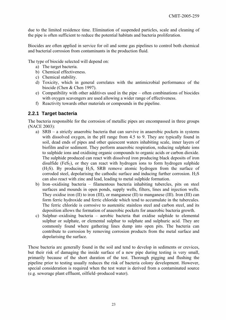
2.2.1 Target bacteria The bacteria responsible for the corrosion of metallic pipes are encompassed in three groups (NACE 2003):

a) SRB – a strictly anaerobic bacteria that can survive in anaerobic pockets in systems with dissolved oxygen, in the pH range from 4.5 to 9. They are typically found in soil, dead ends of pipes and other quiescent waters inhabiting scale, inner layers of biofilm and/or sediment. They perform anaerobic respiration, reducing sulphate ions to sulphide ions and oxidising organic compounds to organic acids or carbon dioxide. The sulphide produced can react with dissolved iron producing black deposits of iron disulfide (FeS2), or they can react with hydrogen ions to form hydrogen sulphide (H2S). By producing H2S, SRB remove atomic hydrogen from the surface of corroded steel, depolarising the cathodic surface and inducing further corrosion. H2S can also react with zinc and lead, leading to metal sulphide formation.

b) Iron–oxidising bacteria – filamentous bacteria inhabiting tubercles, pits on steel surfaces and mounds in open ponds, supply wells, filters, lines and injection wells. They oxidise iron (II) to iron (III), or manganese (II) to manganese (III). Iron (III) can form ferric hydroxide and ferric chloride which tend to accumulate in the tubercules. The ferric chloride is corrosive to austenitic stainless steel and carbon steel, and its deposition allows the formation of anaerobic pockets for anaerobic bacteria growth.

c) Sulphur–oxidising bacteria – aerobic bacteria that oxidise sulphide to elemental sulphur or sulphate, or elemental sulphur to sulphate and sulphuric acid. They are commonly found where gathering lines dump into open pits. The bacteria can contribute to corrosion by removing corrosion products from the metal surface and depolarising the surface.

These bacteria are generally found in the soil and tend to develop in sediments or crevices, but their risk of damaging the inside surface of a new pipe during testing is very small, primarily because of the short duration of the test. Thorough pigging and flushing the pipeline prior to testing usually reduces the risk of bacteria colony development. However, special consideration is required when the test water is derived from a contaminated source (e.g. sewerage plant effluent, oilfield–produced water).

23

CMIT-2005-259

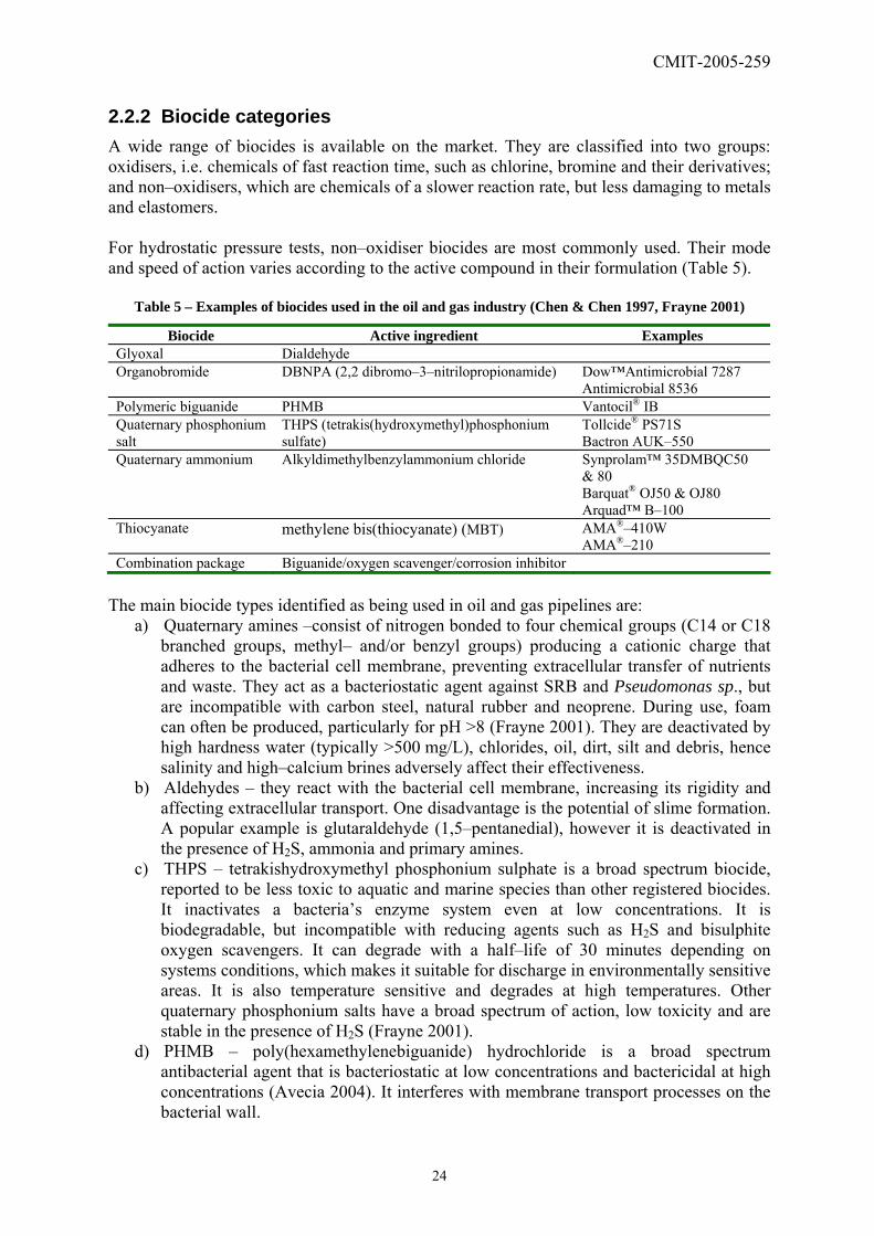
2.2.2 Biocide categories A wide range of biocides is available on the market. They are classified into two groups: oxidisers, i.e. chemicals of fast reaction time, such as chlorine, bromine and their derivatives; and non–oxidisers, which are chemicals of a slower reaction rate, but less damaging to metals and elastomers. For hydrostatic pressure tests, non–oxidiser biocides are most commonly used. Their mode and speed of action varies according to the active compound in their formulation (Table 5).

Table 5 – Examples of biocides used in the oil and gas industry (Chen & Chen 1997, Frayne 2001)

Biocide Active ingredient Examples Glyoxal Dialdehyde Organobromide DBNPA (2,2 dibromo–3–nitrilopropionamide) Dow™Antimicrobial 7287

Antimicrobial 8536 Polymeric biguanide PHMB Vantocil® IB Quaternary phosphonium salt

THPS (tetrakis(hydroxymethyl)phosphonium sulfate)

Tollcide® PS71S Bactron AUK–550

Quaternary ammonium Alkyldimethylbenzylammonium chloride Synprolam™ 35DMBQC50 & 80 Barquat® OJ50 & OJ80 Arquad™ B–100

Thiocyanate methylene bis(thiocyanate) (MBT) AMA®–410W AMA®–210

Combination package Biguanide/oxygen scavenger/corrosion inhibitor The main biocide types identified as being used in oil and gas pipelines are:

a) Quaternary amines –consist of nitrogen bonded to four chemical groups (C14 or C18 branched groups, methyl– and/or benzyl groups) producing a cationic charge that adheres to the bacterial cell membrane, preventing extracellular transfer of nutrients and waste. They act as a bacteriostatic agent against SRB and Pseudomonas sp., but are incompatible with carbon steel, natural rubber and neoprene. During use, foam can often be produced, particularly for pH >8 (Frayne 2001). They are deactivated by high hardness water (typically >500 mg/L), chlorides, oil, dirt, silt and debris, hence salinity and high–calcium brines adversely affect their effectiveness.

b) Aldehydes – they react with the bacterial cell membrane, increasing its rigidity and affecting extracellular transport. One disadvantage is the potential of slime formation. A popular example is glutaraldehyde (1,5–pentanedial), however it is deactivated in the presence of H2S, ammonia and primary amines.

c) THPS – tetrakishydroxymethyl phosphonium sulphate is a broad spectrum biocide, reported to be less toxic to aquatic and marine species than other registered biocides. It inactivates a bacteria’s enzyme system even at low concentrations. It is biodegradable, but incompatible with reducing agents such as H2S and bisulphite oxygen scavengers. It can degrade with a half–life of 30 minutes depending on systems conditions, which makes it suitable for discharge in environmentally sensitive areas. It is also temperature sensitive and degrades at high temperatures. Other quaternary phosphonium salts have a broad spectrum of action, low toxicity and are stable in the presence of H2S (Frayne 2001).

d) PHMB – poly(hexamethylenebiguanide) hydrochloride is a broad spectrum antibacterial agent that is bacteriostatic at low concentrations and bactericidal at high concentrations (Avecia 2004). It interferes with membrane transport processes on the bacterial wall.

24

CMIT-2005-259

e) Guanides – general–purpose biocides, algicides and fungicides, this group includes guanidine and biguanide derivatives. They act by disrupting the bacterial cell wall and cytoplasm. They are usually applied at doses of 20–100 mL/L, at a pH of 6–9.5. Foaming can occur at high dose rates. They precipitate in the presence of strong alkalies, and are more effective in clean environments than in fouled systems.

f) Organobromines – this group includes bis–bromo acetyl butene (BBAB), β–bromo–β–nitrostyrene (BNS), 2–bromo–4–hydroxyacetophenone (BHAP), DBNPA and 2–bromo–2–nitropropane–1,3–diol (Bromopol). BHAP is good for bacterial slime and it is pH independent, but it has a long half–life – 175 to 250 hr (Frayne 2001) requiring treatment prior to discharge. Bromopol is a general–purpose microbiocide, slimicide and aerobic/anaerobic bactericide.

g) DBNPA – 2–2–dibromo–3–nitrilopropionamide is a general–purpose organobromine biocide suitable for high levels of organics and biomass. It has a fast biocidal action (approximately 1 hr), but it is not very effective against algae. It decreases in effectiveness as pH and temperature increase, and it is photodegradable (Frayne 2001). The dose rate is 25–35 mg/L for 5% active material.

Offshore pipelines often incorporate a bactericide (in the sea water) whether needed or not, a practice primarily driven by chemical companies and ‘experience’, rather than by fact. Biocide was eliminated from the treatment of sea water for the offshore section of the Tasmanian Gas Pipeline, because of difficulty in getting approval to discharge the water near the shore. Tests conducted on that residue water provided evidence that the risk of bacterial corrosion during the test period, plus a substantial margin, was low (Venton 2005). The water was treated with an oxygen scavenger to control salt corrosion.

2.2.3 Toxicity of biocides In general the effectiveness of a biocide is correlated to its toxicity to the environment, and so often requires treatment before disposal. Some biocides such as glutaraldehyde and acrolein require less treatment than others like quaternary compounds and amines which are persistent and require extensive treatment before disposal. This limits the types of biocides that can be used in hydrostatic testing when the water is discharged into the environment. Isothiazolone, THPS and glutaraldehyde are the most commonly used biocides (NACE 2003). A comparison of the toxicity of the effective dosage required for SRB elimination as verified by Chen & Chen (1997), is given in Table 6. The data indicates that the concentrations of organobromide, biguanide, quaternary phosphonium, thiocyanate and the combination package required to eliminate SRB were greater than the dose required to kill 50% of fish/shrimp over a 96 hr period (LC50), and hence would be toxic to a marine environment if disposed to sea. The least toxic compound identified in that study was glyoxal, whose active ingredient is dialdehyde. The persistence of biocides from disposal water in the environment is of concern. Evaluation of biocide persistence ( Table 7) by Chen & Chen (1997) indicated that while having the lowest toxicity, Glyoxal was active at three months after application. Biguanide and quaternary phosphonium were observed to still persist at eight months. Analysis of the quaternary phosphonium solution indicated that aging had reduced the content of the active ingredient THPS, but the decomposition process resulted in the formation of toxic intermediates. Whilst still toxic, organobromide and thiocyanate decreased in toxicity after eight months (EC50>50%).

25

CMIT-2005-259

Quaternary ammonium in concentrations greater than 6.25% in water has been verified to be toxic after 48 hr. At higher dilutions, however, it was neutralised after 24 hr exposure in sunlight and air (Slabbert 2003).

Table 6 – Toxicity of biocides (Chen & Chen 1997)

Biocide Fish/shrimp1

LC50–96 hr (ppm)

EC50 15 min2 (ave.) (ppm)

Min. effective concentration against SRB

(ppm)

Min. effective concentration against GAB

(ppm) Glyoxal 760 771 <50 >500 Organobromide 4–9 2.1 <50 250–500 Polymeric biguanide 1–100 5.6 >500 <50 Quaternary phosphonium salt 3–340 44.8 <50 50 Thiocyanate 0.6–2.2 0.2 50 100–250 Combination package 23–110 38.8 >500 >500 Quaternary ammonium (Nilcor C) + MaxSO3

6.6 (Daphnia sp. 48 hr)

1 LC50: concentration lethal to 50% of test organisms in a 96hr period (suppliers in Chen & Chen 1997). 2 EC50–15 min: effective concentration for 50% reduction in light output from a micro–assay of marine bacterium after 15 min exposure (Chen & Chen 1997).

Table 7 – Persistence of biocides (Chen & Chen 1997)

Biocide EC50–5min at 0 h (%)

EC50–5min After 3

months (% conc.)

EC50–5min After 8

months (% conc.)

Residual at 8 months (ppm)

EC50–5min (ppm)

Control (50ppm O/S)

>50 33.6 23.8 – –

Glyoxal 1566–1655 50 ppm >50 36.2 nd – 100 ppm >50 49 nd – 500 ppm >50 >50 nd –

Polymeric biguanide

10.9–11.2

50 ppm 7.7 12.2 6.4 44 (88%) 100 ppm 5.4 5.3 5.4 67 (67%) 500 ppm 1.5 1.5 1.2 270 (54%)

Quaternary phosphonium

81.7–93.7

50 ppm 35.9 39.1 31.2 8 (16%) 100 ppm 34.2 47 24.1 9 (9%) 500 ppm 13.8 21.6 20.6 24 (5%)

Organobromide 2.1–2.3 50 ppm >50 >50 >50 – 100 ppm >50 55 36.4 – 500 ppm 1.1 55.1 46.7 –

Thiocyanate 0.3–0.8 50 ppm 16.2 35.9 >50 – 100 ppm 6.1 25.5 >50 – 500 ppm 3.2 18.9 >50 –

Combination package

46.2–55.3

500 ppm 7.8 >50 nd – nd – not detected

26

CMIT-2005-259

Combinations of certain biocides with oxygen scavengers can enhance or reduce the toxicity compared to the use of either additive alone (Chen & Chen 1997). For example, sulphur–based scavengers are not compatible with DBNPA biocides, causing their inactivation (Chen & Chen 1997). Whilst for other combinations, reactions between degradation by–products need to be determined. Slabbert (2003) evaluated the toxicity of disposal water containing the oxygen scavenger MaxSO3 and the biocide Nilcor C to Daphnia sp. The oxygen scavenger alone was not toxic, but samples with both oxygen scavenger and biocide combined were toxic to the organisms at dilutions down to 12.5% of the original test water. Exposure to air and sunlight resulted in a slight reduction in toxicity compared to the unexposed sample after 24 hr and 48 hr, 83% and 65% reduction respectively. When the additives were combined an increase in lethality was observed after 48 hr (lethality 5% after 24 hr, 35% after 48 hr) (Slabbert 2003), suggesting that some of the degradation by–products might result in toxic compounds. The compatibility of the biocides with oxygen scavengers was also tested for quaternary phosphonium, biguanide, organobromide and thiocyanate based biocides (Chen & Chen 1997). The addition of an oxygen scavenger (50 ppm carbonhydrazide or ammonium bisulphite) reduced the effectiveness of organobromide, whilst enhancing the action of quaternary phosphonium, thiocyanate and polymeric biguanide (Table 8).

Table 8 – Toxicity of biocides combined with oxygen scavengers (Chen & Chen 1997)

Toxicity (light loss gamma–5 min) Solution Biocide alone Biocide + ammonium

bisulphite Biocide +

carbonhydrazide Seawater – 2.3 0.10 Polymeric biguanide (10ppm)

8.01 95 –

Quaternary phosphonium (50ppm)

0.38 1.54 –

Organobromide (2.5ppm)

5.54 – 0.58

Thiocyanate (1ppm) 1.41 – 1.83

2.2.4 Biocide regulation In the USA biocides used by the oil and gas industry are regulated by the US Environmental Protection Agency (EPA) under the Federal Insecticide, Fungicide and Rodenticide Act 1972 (FIFRA). Biocides need to be approved and tested before use, and permits are issued to regulate discharges from hydrostatic tests, establishing effluent limits, prohibitions, reporting requirements etc. Treatment and discharge limits are specified by the National Pollutant Discharge Elimination System (NPDES). In the European Union (EU), chemicals are classified according to Directive 67/548/EEC (Europa 2005). Manufacturers are required to classify and package their chemicals according to the relevant laws. Relevant authorities in the member states are notified when new products are introduced, and the importer/manufacturer needs to provide a technical report on the product and testing procedures. Biocidal products and their active compounds are covered in the Biocidal Products Directive 98/8/EU, however, each member state is responsible for its implementation and regulation in its own territory.

27

CMIT-2005-259

In Australia, biocide use requires approval from the regulatory body in each state or territory, e.g. EPA. If biocides are present, the test water has to be treated and the biocide neutralised before disposal.

2.2.5 Neutralisation of biocides As all biocides are toxic to the aquatic environment they all need to be neutralised before release. The most practical approach to biocide use is to choose an effective additive and then use physical or chemical methods to detoxify the biocide–treated water prior to discharge (Chen & Chen 1997). Often the detoxification procedures reported in the literature or recommended by the chemical suppliers require weeks for significant detoxification to occur, rather than the hours or minutes desired in field operations. As such, direct disposal into the environment is not possible and the construction of holding tanks or additional facilities for biocide neutralisation is required (Chen & Chen 1997).

2.2.6 Technologies for biocide neutralisation Chen & Chen (1997) investigated methodologies for reducing quaternary phosphonium, organobromide, thiocyanate and biguanide toxicity using a laboratory micro–assay of sea water and bioluminescent marine bacterium (Vibrio fischeri) at 20 °C. A range of treatments were tested in the laboratory for those biocides using 10 mL aliquots (Table 9). The range of treatments and their effects were:

• Dilution did not neutralise biocides, it simply reduced their concentration. The major disadvantage is that it requires large volumes of water to achieve any reduction in toxicity. As verified by Chen & Chen (1997), the reduction in biocide toxicity to acceptable levels occurred only after dilution with sea water by a factor of 50 or greater.

• Aeration for 1 hr at ambient temperature had a slight effect on toxicity, i.e. 28%

reduction for biguanide, 23% reduction for organobromide, 13% reduction for thiocyanate, but no effect on the toxicity of quaternary phosphonium.

• Exposure to sunlight for 1 hr had a slight effect on toxicity for biguanide,

organobromide and thiocyanate, reducing it by 52%, 10% and 15% respectively, but it had no effect on quaternary phosphonium.

• Increasing the pH to 9 increased the toxic effect of all solutions. Further increasing

the pH to 10 was effective in reducing the toxicity of quaternary phosphonium and biguanide. On the other hand, it increased the toxicity of the other solutions and it is also toxic to micro-organisms in seawater.

• Filtration with a glass fibre filter caused a slight increase of toxicity for the biocide

solutions.

• Sand filtration followed by glass fibre filtration was effective for reducing the toxicity of biguanide, but it had no significant effect on the other additives.

28

CMIT-2005-259

29

• Activated carbon filtration followed by glass fibre filtration appears to be the most promising of all the detoxification methods evaluated reducing the toxicity of all four samples by >85% (Chen & Chen 1997).

• The use of an oxidising agent such as chlorine has been proposed as a potential

method for removal of biocide residuals. However the water remains toxic following chlorine treatment due to chlorine residues and/or by–products produced during oxidation (Chen & Chen 1997). Chlorine residues could be reduced by filtering the water through a carbon filter.

Neutralisation is strongly dependent on the individual biocide. In many cases, the impact of the degradation by–products needs to be characterised to determine an appropriate treatment. For example, the use of chlorine and its derivatives for neutralisation is generally not recommended due to the toxicity of the reagent and its residues. Table 9 shows that the most effective method for neutralisation of quaternary phosphonium, biguanide, organobromides and thiocyanates was treatment with activated carbon and glass fibre (Chen & Chen 1997). This is also a highly effective method for removal of hydrocarbons and aromatic compounds (eg. benzene, toluene, ethylbenzene, xylene). Other methods advocated in the literature and also seen in Table 9 included raising pH, aeration, exposure to sunlight (good for Cl2 removal) and hydrolysis, but these are likely to require extended time periods for neutralisation, most likely a period of days and weeks before significant reduction can occur (Chen & Chen 1997).

Table 9 – Neutralization of bactericide residuals following three months exposure (Chen & Chen 1997)

Additive Sea water

(light loss in gamma – 5

min values1)

Sea water with quaternary

phosphonium

Sea water with

Biguanide

Sea water with Organobromide

Sea water with

Thiocyanate

Concentration – 50 ppm 50 ppm 500 ppm 250 ppm No treatment (light loss in gamma – 5 min values)

0 0.68 9.76 1.22 1.09

Light loss effect after three months exposure compared to untreated sample2 (%)

Dilution – x50 x50 x50 x50 Aeration 0 +3 –28 –23 –13 Sunlight 0 +3 –52 –10 –15 pH 9 0.55 +55 +1024 +14 –6 pH 10 2.88 0 0 +202 +881 Filtration <0.05 +4.4 +84.3 +10.6 + 2.8 AC/filtration <0.05 –93 –98.7 –85.1 –96.4 Sand/filtration 0.07 +5.8 –90.4 +15.6 –12 Chlorine –0.5 ppm 1.04 +5.8 +82.4 +20.5 +11807 Chlorine 1 ppm 44.0 +13.2 +133 +38.5 +3807 Chlorine 2 ppm 94.0 +29.4 +376 +122 +8542

1 The higher the value, the higher the toxicity. 2 Positive values indicate increase, negative values indicate reduction in toxicity compared to the untreated samples.

Table 10 is a summary of common additives used and their characteristics.

CMIT-2005-259

30

Table 10 – Additives used in hydrostatic testing (Chen & Chen 1997)

Substance Formula Use LD50 (mg/Kg) Human toxicity Min effectiveconcentration

against bacteria (ppm)

Sodium metabisulphite/ Sodium bisulphite

Na2S2O5/ NaHSO3

Oxygen scavengers, antimicrobial agents for foodstuff and wine, chlorine removal in potable water (max. 15 mg/L)

1540 (rats) 100–200 (rainbow trout) (96 hr) 200 (golden orfe) (48 hr)

Limited reports of allergy, limited human and environmental toxicological data, 660 mg/L Na2S2O5 has no effect on rats

–

Glyoxal (ethanedial)

C2H2O2 Biocide, oxygen scavenger, paper, textile and industrial resins, Copolymers, dye intermediates, pesticides, pharmaceuticals, photographic chemicals, corrosion inhibitors

EC50–5>50% LC50 750 mg/L–96 hr (fish/shrimp)

>500 (GAB)<50 (SRB)

Nilcor C Biocide 6.6 (Daphnia sp.)(48 hr) 3.8 (Daphnia sp.)(48 hr) (after use)

Quaternary phosphonium

(CH2OH)4P–X where X = anion

Biocide 3–340 (96 hr) (fish/shrimp) 50 (GAB) <50 (SRB)

Biguanide (chlorhexidine)

Biocide EC50–5 12.2–1.5%1–100 (96 hr) (Fish/shrimp) Fish LC50 (96 hr) (mg/L): 0.0013 Daphnia sp. magna EC50 (48hr) (mg/L): 0.25Toxicity to fish: LC50(96 hr) 1.3 µg/L Toxicity invertebrate: LC50(48 hr) 0.5 µg/L

Skin irritation 1.5 mg/3d–I–mild

<50(GAB) <50(SRB)

Organobromide Biocide 4–9 (96 hr) fish/shrimp 250–500 (GAB) <50 (SRB)

Thiocyanate Biocide 0.6–2.2 (96 hr) 100–250 (GAB) 50 (SRB)

1 Baker Petrolite (pers. com 2003) 2 GAB – general aerobic bacteria

CMIT-2005-259

3 Regulatory Requirements

3.1 Background and objectives

The disposal of hydrostatic test water requires a license or permit from the relevant regulatory agency. However, obtaining such permits can be a complex process, as the approval procedure can require the involvement of multiple government agencies and often the responsibility for regulating the disposal of test water is unclear. A survey was conducted among State regulatory agencies in Australia to determine the regulatory requirements and/or guidelines applicable for the disposal of hydrostatic test water. This section outlines the results of these enquiries. Information was also sought detailing procedures or legislation for hydrostatic test water treatment and disposal.

3.2 Water disposal regulations

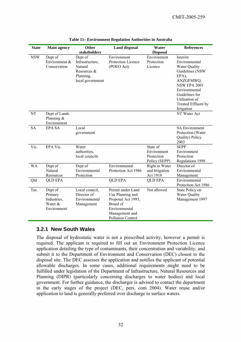
The reference document for the management of water quality in Australia and New Zealand is the Australian and New Zealand Guidelines for Fresh and Marine Water Quality (ANZGFMWQ) (ANZECC/ARMCANZ 2000), which is part of the National Water Quality Management Strategy. The document provides a management framework, principles and guidelines for protecting water resources based on impact minimisation, and a hazard and risk assessment approach. Although the document does not have specific guidelines for hydrostatic test water disposal, it features management and assessment guidelines for water in aquatic systems and also for primary industries. Water disposal is regulated by State authorities according to the ANZGFMWQ or state-specific legislation, as outlined in Table 11. The processes and requirements that need to be followed are further explained in the Appendix showing the correspondence with authorities (DIPE 2004).

31

CMIT-2005-259

Table 11– Environment Regulation Authorities in Australia

State Main agency Other stakeholders

Land disposal Water Disposal

References

NSW Dept of Environment & Conservation

Dept of Infrastructure, Natural Resources & Planning, local government

Environment Protection Licence (POEO Act)

Environment Protection Licence

Interim Environmental Water Quality Guidelines (NSW EPA), ANZGFMWQ, NSW EPA 2001 Environmental Guidelines for Utilisation of Treated Effluent by Irrigation

NT Dept of Lands Planning & Environment

NT Water Act

SA EPA SA Local government

SA Environment Protection (Water Quality) Policy 2003

Vic. EPA Vic. Water authorities, local councils

State of Environment Protection Policy (SEPP)

SEPP Environment Protection Regulations 1998

WA Dept of Natural Resources

Dept of Environmental Protection

Environmental Protection Act 1986

Right in Water and Irrigation Act 1918

Director of Environmental Management

Qld QLD EPA QLD EPA QLD EPA Environmental Protection Act 1986

Tas. Dept of Primary Industries, Water & Environment

Local council, Director of Environmental Management

Permit under Land Use Planning and Proposal Act 1993, Board of Environmental Management and Pollution Control

Not allowed State Policy on Water Quality Management 1997

3.2.1 New South Wales The disposal of hydrostatic water is not a prescribed activity, however a permit is required. The applicant is required to fill out an Environment Protection Licence application detailing the type of contaminants, their concentration and variability, and submit it to the Department of Environment and Conservation (DEC) closest to the disposal site. The DEC assesses the application and notifies the applicant of potential allowable discharges. In some cases, additional requirements might need to be fulfilled under legislation of the Department of Infrastructure, Natural Resources and Planning (DIPR) (particularly concerning discharges to water bodies) and local government. For further guidance, the discharger is advised to contact the department in the early stages of the project (DEC, pers. com 2004). Water reuse and/or application to land is generally preferred over discharge to surface waters.

32

CMIT-2005-259

3.2.2 Northern Territory Management, protection and use of water resources fall under the NT Water Act, administered by the Department of Infrastructure, Planning and Environment (DIPE) (DIPE 2004). The disposal of hydrostatic test water requires a licence from the Regulatory Services of the Office of Environment and Heritage (DIPE 2004). The licence stipulates the quantity and quality of water being discharged and may require:

• Development of Environmental Management plans. • Water management plans. • Structured monitoring programs.

3.2.3 South Australia The discharge of hydrostatic test water falls under the SA Environment Protection Act 1993. The Act determines that an environmental authorisation is required before undertaking certain prescribed activities, as outlined in Schedule 1 of the Act. Whilst hydrostatic test water is not considered as a prescribed waste stream under the Act, this requirement is generally enforced. Permits for disposal are administered by the EPA SA. The proponent has to submit an application outlining the disposal characteristics, location and details for assessment by the EPA. Further requirements such as risk assessments are likely to be required to determine the impact of disposal (N. Sison EPA SA pers. com 2004).

3.2.4 Tasmania Tasmania has no legislative requirements for hydrostatic test water disposal, however historically the applicant has to apply to the local council for a permit under the Land Use Planning and Proposal Act 1993. If there are environmental concerns, the Director of Environmental Management (DEM) can request a ‘Development Proposal’ and an ‘Environmental Management Plan’ for assessment by the Board of Environmental Management and Pollution Control, which also stipulates the conditions of discharge under the Environmental Management and Pollution Control Act 1994 (EMPCA). Standards for disposal water quality prior to discharge are determined according to the framework from the State Policy on Water Quality Management 1997. In enquiries to the DEM, reference was made to their previous experience with the Duke/Alinta pipeline construction. In that case, the permit required that a management plan be approved by the DEM prior to disposal. The following requirements were specified in the plan:

• Prevention of erosion and/or sediment movement. • No entry of the disposal water into a watercourse. • Any discharge (flush water and hydrostatic test water) must be conducted and

contained within an approved irrigation area. • Passage through geotextile fabric required for removal of suspended solids. • Discharge must occur in a manner non–detrimental to vegetation, pastures or

crops (K. Bull DPIWE pers. Com 2004).

33

CMIT-2005-259

Further information can be obtained from the Department of Primary Industries, Water and Environment in Tasmania.

3.2.5 Victoria EPA Victoria is responsible for the approval and monitoring of waste discharge in the Sate. The applicant needs to contact the regional EPA office with a submission on the location of testing, nature, discharge proposal and an environmental impact assessment. After discussion with the EPA, an environmental management plan is submitted. The discharge of hydrostatic test water falls under the Environment Protection Act 1970 and policies such as the State Environment Protection Policy (Waters of Victoria). If the disposal water contains any prescribed wastes, e.g. biocides and phytopharmaceuticals, it has to be managed as prescribed waste under the Environment Regulations 1998. The EPA Vic. advocates a hierarchy of disposal management to minimise the impact on the environment: avoid, reuse and recycle, recover, treat, contain and discharge. If discharge is the only option, the order of preference is discharge to sewers (in consultation with a water authority), discharge to land (with the approval of landowner) and discharge to water. Discharge to water and land requires the development of a risk management framework to prevent adverse impacts to the environment. Environmental quality objectives for water environments are outlined in the State of Environment Protection Policy (Waters of Victoria) and schedules (L. Horshell EPA Vic pers. Com 2004).

3.2.6 Western Australia The Department of Environment (DE) oversees the Environmental Protection Act 1986, and the Rights in Water and Irrigation Act 1918. The management of disposal waters occurs via regional decision making, rather than specifications, codes and subsequent applications for permits from a central office. According to the DE, ‘For a proponent wanting to release hydrostatic testing water to the environment, common sense should prevail in the first instance. If a proponent has concerns about release of hydrostatic testing water, then they need to contact one of our Regional Offices and the DE will be able to advise accordingly after examination of the specific situation that is presented to them. The regional office will refer the matter to the central Perth office if they don't have sufficient technical expertise to make a proper environmental assessment of the specific request’ (P. Byrnes DE pers. com 2004).

3.2.7 Queensland The Department of Natural Resources and Mines (DNRM) was the licensing agent until 2004. Currently the EPA is responsible for administering Queensland’s Environmental Protection Act 1994, including hydrostatic test water disposal, and is also responsible for issuing pipeline licenses. Queensland has no set State–wide guidelines for hydrostatic test water quality and its disposal, however specific water quality guidelines have been developed for a number of rivers and ecosystems.

34

CMIT-2005-259

Revision of the Qld Water Quality Guidelines was taking place at the time this report was written. Each disposal application is evaluated based on its merits. If biocides and other additives such as oxygen scavengers are used, the EPA generally recommends aeration to be conducted upon disposal. For disposal onto land, sediment control and erosion avoidance is recommended, as is containment into evaporation ponds and, if salts or hydrocarbons are present, clean-up procedures might be required. Discharge to water bodies will require more rigorous logistics and planning, and also more severe monitoring depending on the location of disposal and the sensitivity of the ecosystems (S. McFayden DNRM pers. com 2004). Sourcing of water generally requires approval from the DNRM, unless the water resource is controlled by a commercial entity (Mathieson, W., Enertrade, pers. com 2005).

3.2.8 United States of America The USA has a long history of hydrostatic testing of gas and oil pipelines. Periodic hydrostatic testing of operating pipelines to demonstrate their ongoing fitness for service is used in the USA partly as a result of a number of in-service failures resulting from undetected corrosion. Water discharged from tests on in-service pipelines contains an increased the range of contaminants compared to new pipelines. A survey conducted by the American Petroleum Institute determined that surface water bodies, river/streams and lakes/ponds were the most common places for the disposal of the testing water, accounting for 71% of tests (Tallon & Fillo, 1992). In the south-west, test waters were most often released into stock ponds for treatment, even when the discharge waters contain high concentrations of organic compounds from in-service pipelines (Eiceman et al 1983) The US Department of Transportation regulates hydrostatic testing procedures at a national level. However, the discharge of hydrostatic test water is regulated at the state level, under the National Pollutant Discharge Elimination System (NPDES) (Tallon & Fillo, 1992). Hence, each state is responsible for its own regulations for disposal of hydrostatic test water. A permit is required for hydrostatic testing of new and old pipelines and subsequent water disposal. In a survey of 21 American States with significant pipeline lengths, all required regulatory approval before discharge (Bruderly et al. 1992). The type of permit required varied from State to State among the 21 surveyed:

• Full NPDES – was required in less than 50% of the states for discharges to all surface waters.

• Simplified NPDES – was required under specific conditions for six states. • Blanket permits – were applied for the rest of the USA. The US study showed

that stipulation of blanket parameters was not always relevant to the pipe contents, nor to the ecosystem in which disposal took place. Parameters such as pH, oil and grease content, total suspended solids and flow were the most commonly monitored parameters in such permits.

35

CMIT-2005-259

• Other permit types such as general permits, short–term permits and letters of authorisation were issued for smaller volume discharges.

Permits were mandatory for discharge into surface waters in all US States, but an evaluation was often performed on a case–by–case basis to evaluate the suitability of other locations of discharge: public-owned treatment works, evaporation ponds, retention ponds, groundwater and injection wells. Often permits apply for lined ponds or injection wells (Tallon & Fillo 1992). Requirements for sampling and water quality analysis varied from State to State. In some cases, water quality had to be determined for discharge water and for fill water. A third of the States surveyed had State specific water quality parameters for discharge water. Some established specific effluent requirements based on water quality standards and site characteristics, others adopted a general water quality criteria, such as ‘no visible sheen’ (oil and grease) and erosion avoidance. Fifteen States specified monitoring of discharge water quality. Twelve specified identical water quality requirements for new and existing pipelines.

3.2.9 Major findings Regulated procedures for water disposal and water quality requirements were not uniform between states. In Australia, NSW, Qld and Tas. have clear assessment procedures to evaluate the quality of hydrostatic test water disposal. Most of the regulatory bodies, e.g. EPA Vic., DEC NSW, EPA Qld use a risk assessment framework for the evaluation of discharge on a case–by–case basis. In SA and WA, the jurisdiction and regulation of hydrostatic test water disposal was not as clearly defined, and requirements are evaluated on a case–by–case basis. EPA SA is responsible for monitoring urban water disposal, and in WA the responsibility is allocated to the regulatory authority closest to the disposal location. In discussions with the regulators in each State, the personnel who had familiarity with the process from previous experience were able to advise how the water was generally treated, and had a clearer idea of its potential impact. In most cases, a risk assessment framework requires the evaluation of water quality parameters to determine its impact on the environment. A number of States have water quality descriptors for specific or limited ecosystems. Victoria and Tasmania have the greatest number of ecosystems already characterised. The preference in Tas, Vic. and NSW is for disposal onto land. In the case of Tas, this is done to minimise impact to waterways and in Vic. and NSW to facilitate beneficial water reuse.

36

CMIT-2005-259

4 Experimental

4.1 Sampling locations and characteristics

Ten hydrostatic test sites were sampled in this study. The test sites covered six new pipelines and were representative of typical tests conducted on new infrastructure in Australia. The characteristics of the test sites are shown in Table 12. The pipelines covered a number of states and different regulatory requirements. Tests T2 and T3 were conducted in two sections of the same pipeline ‘B’, whilst tests T4 - T7 were conducted on sections of the same pipeline ‘C’.

Table 12 – Pipeline characteristics

Pipeline A B C D E F Test section T1 T2 T3 T4 T5 T6 T7 T8 T9 T10 Material 5LX42 5LX65 5LX70 5LX70 5LX70 5LX70 5LX70 X60ERW X70 X70 Section length (km)

0.072 34 30 77 106 37 22 80 12 87

Diameter (mm) 154 333 282 323.9 323.9 323.9 273.1 250 305 305 Surface/ Volume ratio

26.0 12.0 14.2 12.3 12.3 12.3 14.6 16.0 13 13

Internal lining No No No No No No No No No No Volume of test water (m3)

35 2970 1880 6345 8735 3050 1290 3930 875 6348

Jurisdiction Vic. Vic. Vic. Qld Qld Qld Qld WA Vic. Qld

4.2 Water sources

The water used for filling the test sections came from a range of sources including town mains, rivers and, in one case, from a previous hydrostatic test in an adjacent pipe section.

4.3 Sample selection

Samples of water were collected from: • Source water. • Source water after the addition of additives and prior to filling of the pipe. • The point of discharge of the test water after completion of the hydrostatic test

(disposal water). At test sites T2 and T10 samples of the pre-test flush water were also collected for determination of the initial flush characteristics. Analysis of sample variability was conducted by comparing the sample concentration at the beginning, middle and end of the discharge period.

4.4 Sampling procedure

Water samples were collected as grab samples from the sources and discharge of the pipes. Water was allowed to flow for at least 5 min before sample collection. Samples were collected in polyethylene bottles containing suitable additives for sample

37

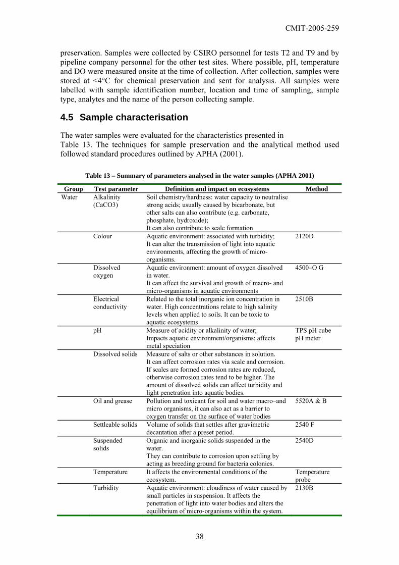
CMIT-2005-259

preservation. Samples were collected by CSIRO personnel for tests T2 and T9 and by pipeline company personnel for the other test sites. Where possible, pH, temperature and DO were measured onsite at the time of collection. After collection, samples were stored at <4°C for chemical preservation and sent for analysis. All samples were labelled with sample identification number, location and time of sampling, sample type, analytes and the name of the person collecting sample.

4.5 Sample characterisation

The water samples were evaluated for the characteristics presented in Table 13. The techniques for sample preservation and the analytical method used followed standard procedures outlined by APHA (2001).

Table 13 – Summary of parameters analysed in the water samples (APHA 2001)

Group Test parameter Definition and impact on ecosystems Method Water Alkalinity

(CaCO3) Soil chemistry/hardness: water capacity to neutralise strong acids; usually caused by bicarbonate, but other salts can also contribute (e.g. carbonate, phosphate, hydroxide); It can also contribute to scale formation

Colour Aquatic environment: associated with turbidity; It can alter the transmission of light into aquatic environments, affecting the growth of micro-organisms.

2120D

Dissolved oxygen

Aquatic environment: amount of oxygen dissolved in water. It can affect the survival and growth of macro- and micro-organisms in aquatic environments

4500–O G

Electrical conductivity

Related to the total inorganic ion concentration in water. High concentrations relate to high salinity levels when applied to soils. It can be toxic to aquatic ecosystems

2510B

pH Measure of acidity or alkalinity of water; Impacts aquatic environment/organisms; affects metal speciation

TPS pH cube pH meter

Dissolved solids Measure of salts or other substances in solution. It can affect corrosion rates via scale and corrosion. If scales are formed corrosion rates are reduced, otherwise corrosion rates tend to be higher. The amount of dissolved solids can affect turbidity and light penetration into aquatic bodies.

Oil and grease Pollution and toxicant for soil and water macro–and micro organisms, it can also act as a barrier to oxygen transfer on the surface of water bodies

5520A & B

Settleable solids Volume of solids that settles after gravimetric decantation after a preset period.

2540 F

Suspended solids

Organic and inorganic solids suspended in the water. They can contribute to corrosion upon settling by acting as breeding ground for bacteria colonies.

2540D

Temperature It affects the environmental conditions of the ecosystem.

Temperature probe

Turbidity Aquatic environment: cloudiness of water caused by small particles in suspension. It affects the penetration of light into water bodies and alters the equilibrium of micro-organisms within the system.

2130B

38

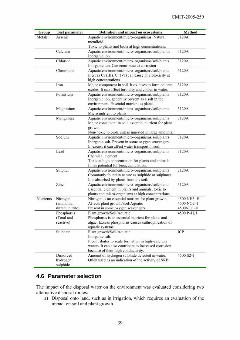
CMIT-2005-259

Group Test parameter Definition and impact on ecosystems Method Metals Arsenic Aquatic environment/micro–organisms. Natural

metalloid. Toxic to plants and biota at high concentrations.

3120A

Calcium Aquatic environment/micro–organisms/soil/plants. Inorganic ion.

3120A

Chloride Aquatic environment/micro–organisms/soil/plants Inorganic ion. Can contribute to corrosion

3120A

Chromium Aquatic environment/micro–organisms/soil/plants Inert as Cr (III). Cr (VI) can cause phytotoxicity at high concentrations.

3120A

Iron Major component in soil. It oxidises to form colored oxides. It can affect turbidity and colour in water.

3120A

Potassium Aquatic environment/micro–organisms/soil/plants Inorganic ion, generally present as a salt in the environment. Essential nutrient to plants.

3120A

Magnesium Aquatic environment/micro–organisms/soil/plants Micro nutrient to plants

3120A

Manganese Aquatic environment/micro–organisms/soil/plants Major constituent in soil, essential nutrient for plant growth. Non- toxic to biota unless ingested in large amounts.

3120A

Sodium Aquatic environment/micro–organisms/soil/plants Inorganic salt. Present in some oxygen scavengers. In excess it can affect water transport in soil.

3120A

Lead Aquatic environment/micro–organisms/soil/plants Chemical element. Toxic at high concentration for plants and animals. It has potential for bioaccumulation.

3120A

Sulphur Aquatic environment/micro–organisms/soil/plants Commonly found in nature as sulphide or sulphates. It is absorbed by plants from the soil.

3120A

Zinc Aquatic environment/micro–organisms/soil/plants Essential element in plants and animals, toxic to plants and micro-organisms at high concentrations.

3120A

Nutrients Nitrogen (ammonia, nitrate, nitrite)

Nitrogen is an essential nutrient for plant growth. Affects plant growth/Soil/Aquatic Present in some oxygen scavengers.

4500 NH3–H 4500 NO2–I 4500NO3–H

Phosphorus (Total and reactive)

Plant growth/Soil/Aquatic Phosphorus is an essential nutrient for plants and algae. Excess phosphorus causes euthrophication of aquatic systems.

4500 P–H, I

Sulphate Plant growth/Soil/Aquatic Inorganic salt. It contributes to scale formation in high–calcium waters. It can also contribute to increased corrosion because of their high conductivity.

ICP

Dissolved hydrogen sulphide

Amount of hydrogen sulphide detected in water. Often used as an indication of the activity of SRB.

4500 S2–I

4.6 Parameter selection

The impact of the disposal water on the environment was evaluated considering two alternative disposal routes:

a) Disposal onto land, such as in irrigation, which requires an evaluation of the impact on soil and plant growth.

39

CMIT-2005-259

b) Disposal into surface water bodies, such as rivers, lakes and ponds, a more sensitive route, requires evaluating the impact on the aquatic ecosystem.

The samples were analysed for a range of parameters related to source water quality, materials and the chemicals used or generated in the pipeline (e.g. corrosion products) that could impact land and surface water ecosystems.

The parameters that affect terrestrial and aquatic ecosystems are generally similar, however aquatic ecosystems are generally more sensitive to contaminant loads. In terrestrial ecosystems, the passage of water through the soil attenuates the contaminant load before it reaches plant roots. The parameters analysed belong to one of four groups:

a) Common water characteristics-: these are characteristics that influence the action and availability of other species in the environment, e.g. metal speciation. They are often classified as indirect stressors. This group includes pH, temperature, dissolved oxygen, salinity (electrical conductivity and sodium adsorption ratio), turbidity and colour.

b) Plant and soil parameters-: characteristics that affect soil and plant development. Some parameters act as direct toxicants to plant growth (e.g. some metals at certain concentrations), whilst other parameters are nutrients for plant development (e.g. N, P, K and metals in small concentrations).

c) Surface water stressors-: parameters that can act as chronic or acute toxicants to water ecosystems, e.g. metal concentration.

d) Anthropogenic substances such as pesticides and hydrocarbon derivatives were not analysed as no reported sources or potential exposure to such parameters was observed in the new pipelines. However, some samples were evaluated to determine if oil and grease were present.

4.6.1 Soil properties The two major water parameters that affect soil properties are the salts content and the sodium absorption ratio (SAR). A high salt content in water can increase salinity and hence affect the growth and productivity of plants and/or crops, whilst the sodium adsorption ratio is an indication of sodicity, which can affect the soil’s water conductivity and compaction (ANZECC/ARMCANZ 2000). The combined effect of both parameters needs to be considered in the impact assessment.

4.6.1.1 Sodium adsorption ratio (SAR) The SAR of water used in irrigation gives an indication of potential sodicity problems that could develop in the soil. Sodium salts (Na+) act as coagulants or flocculants of soil particles, and when the ratio of sodium to calcium and magnesium ions in the soil is high, it can lead to sodicity and contribute to soil salinity.

40

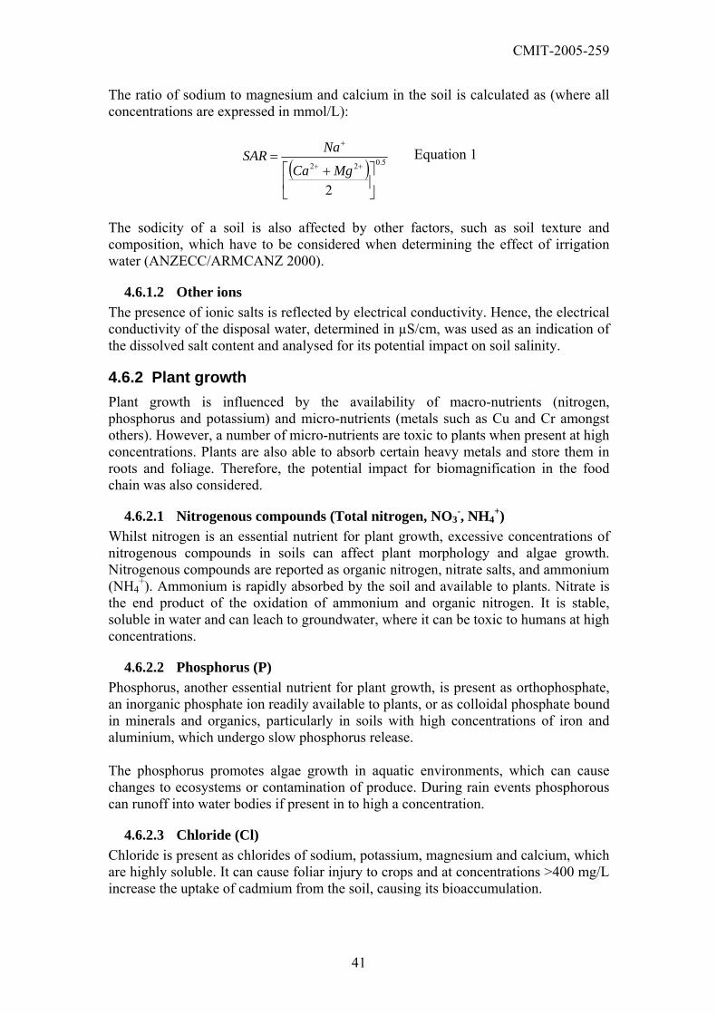
CMIT-2005-259

The ratio of sodium to magnesium and calcium in the soil is calculated as (where all concentrations are expressed in mmol/L):

( ) 5.022

2 ⎥⎦

⎤⎢⎣

⎡ +=

++

+

MgCa

NaSAR Equation 1

The sodicity of a soil is also affected by other factors, such as soil texture and composition, which have to be considered when determining the effect of irrigation water (ANZECC/ARMCANZ 2000).

4.6.1.2 Other ions The presence of ionic salts is reflected by electrical conductivity. Hence, the electrical conductivity of the disposal water, determined in µS/cm, was used as an indication of the dissolved salt content and analysed for its potential impact on soil salinity.

4.6.2 Plant growth Plant growth is influenced by the availability of macro-nutrients (nitrogen, phosphorus and potassium) and micro-nutrients (metals such as Cu and Cr amongst others). However, a number of micro-nutrients are toxic to plants when present at high concentrations. Plants are also able to absorb certain heavy metals and store them in roots and foliage. Therefore, the potential impact for biomagnification in the food chain was also considered.

4.6.2.1 Nitrogenous compounds (Total nitrogen, NO3-, NH4

+) Whilst nitrogen is an essential nutrient for plant growth, excessive concentrations of nitrogenous compounds in soils can affect plant morphology and algae growth. Nitrogenous compounds are reported as organic nitrogen, nitrate salts, and ammonium (NH4

+). Ammonium is rapidly absorbed by the soil and available to plants. Nitrate is the end product of the oxidation of ammonium and organic nitrogen. It is stable, soluble in water and can leach to groundwater, where it can be toxic to humans at high concentrations.

4.6.2.2 Phosphorus (P) Phosphorus, another essential nutrient for plant growth, is present as orthophosphate, an inorganic phosphate ion readily available to plants, or as colloidal phosphate bound in minerals and organics, particularly in soils with high concentrations of iron and aluminium, which undergo slow phosphorus release. The phosphorus promotes algae growth in aquatic environments, which can cause changes to ecosystems or contamination of produce. During rain events phosphorous can runoff into water bodies if present in to high a concentration.

4.6.2.3 Chloride (Cl) Chloride is present as chlorides of sodium, potassium, magnesium and calcium, which are highly soluble. It can cause foliar injury to crops and at concentrations >400 mg/L increase the uptake of cadmium from the soil, causing its bioaccumulation.

41

CMIT-2005-259

4.6.2.4 Copper (Cu) Copper is a plant nutrient essential in small concentrations for the production of plant enzymes. It is present in Australian soils at concentrations ranging from 0.4 to 412 mg/kg, and is toxic in nutrient solutions ranging from 0.1 to 1.0 mg/L.

4.6.2.5 Chromium (Cr) Chromium does not appear to be an essential nutrient for plants. It can be present as Chromium (III) (Cr3+) or Chromium VI (Cr6+). Cr3+ forms immobile complexes in the soil and is inoffensive, whilst Cr6+ is mobile and available to plants. The toxicity limits for Cr6+ range between 5 and 500 mg/kg depending on plant and soil type. Evidence to date indicates that Cr6+ generally remains in the root zone of plants. There are indications that some phytotoxicity might occur at concentrations between 1 and 10 mg/L, however agricultural soil conditions tend to promote reduction of Cr6+ to Cr3+ and there is insufficient evidence to confirm if Cr6+ is available to plants upon irrigation.

4.6.2.6 Iron (Fe) Iron is an essential micro–nutrient used by plants in the production of chlorophyll. It is the fourth most abundant element in the earth’s crust. Soils generally contain 1–5% total iron. Iron is present as silicate minerals, iron oxides and hydroxides, which are not readily available for plant use and need to be transformed by microbial activity. Iron can be present as ferrous iron (Fe2+) or ferric iron (Fe3+) depending on the soil aeration and pH conditions. Ferrous iron is more soluble and available to plants than ferric iron oxides and hydroxides. Alkaline soils (pH >7.4) favour the formation of ferric compounds reducing their availability to plants. Upon aeration ferrous iron oxidises to ferric iron. However, ferric and hydroxide iron can be reduced to ferrous iron under water logged conditions by microbial activity. Precipitated iron can bind the essential nutrients P and molybdenum (Mo) making them unavailable to plants. There are no reports confirming negative effects due to direct application of iron on plants (ANZECC/ARMCANZ 2000), however long-term values have been set based on the potential of iron precipitation on foliage during irrigation, and the potential for damage or blockage of irrigation equipment during application by spraying.

4.6.2.7 Manganese (Mn) Manganese is a major soil constituent. It is essential for plant growth, nitrogen metabolism and chlorophyll synthesis. Its availability is controlled by pH and oxidation–reduction reactions in the soil. A lower pH and reducing conditions increase its availability to plants. It is toxic to plants at concentrations >0.75 mg/L.

4.6.2.8 Lead (Pb) Lead is retained by most soils, particularly in the top soil, reducing its availability to plants (ANZECC/ARMCANZ 2000). While it is mainly toxic to higher organisms, actual toxicity depends on the type of animal, the form of lead and the rate of ingestion, phytotoxicity has been observed at nutrient solutions of 10 mg/L.

42

CMIT-2005-259

4.6.2.9 Sodium (Na) Sodium is beneficial to plant growth in minute quantities, but high levels can cause leaf burn and defoliation, and poor soil physical conditions limiting plant growth and deficiency in Ca and Mg through reduced availability and imbalance with Na.

4.6.2.10 Zinc (Zn) Zinc is an essential nutrient that is readily available in acidic soil conditions (pH <6). It is toxic at concentrations >4–6.5 mg/L depending on the plant type.

4.6.3 Residue analysis An analysis of the particulate matter was performed on the residues of some of the samples using X–ray diffraction to determine the composition of the inorganic sediments formed during hydrostatic testing.

43

CMIT-2005-259

5 Analysis of Hydrostatic Test Water

5.1 Introduction

The preservation of the environment on the disposal of hydrostatic test waters is the major concern for regulatory authorities. Regulation and licensing procedures require risk analysis and impact minimisation studies to be conducted prior to each disposal. This section evaluates the characteristics of the water used in hydrostatic tests conducted throughout Australia, and analyses its impact on the environment.

5.2 Source water

The water used for filling the pipes in the case studies came from a range of sources including:

a) Town mains for T1, T2, T7 and T8. Town water often contains a small concentration of chlorine to prevent bacterial growth in the pipelines (<0.6 mg/L).

b) Rivers for T4, T5, T7 and T9 - composition varied from location to location. c) T3 reused water from a previous hydrostatic test in an adjacent section, T2. d) Bore water for T10 - bore and groundwater can sometimes contain higher

levels of dissolved ions or salts, Fe2+, 3+, H2S and SO42- than other water

sources.

Table 14 – Sampling sites

Test site Source water State T1 Mains Vic. T2 Mains Vic. T3 Reused Vic. T4 River Qld T5 River Qld T6 River Qld T7 Mains Qld T8 Mains WA T9 River Vic. T10 Bore Qld

44

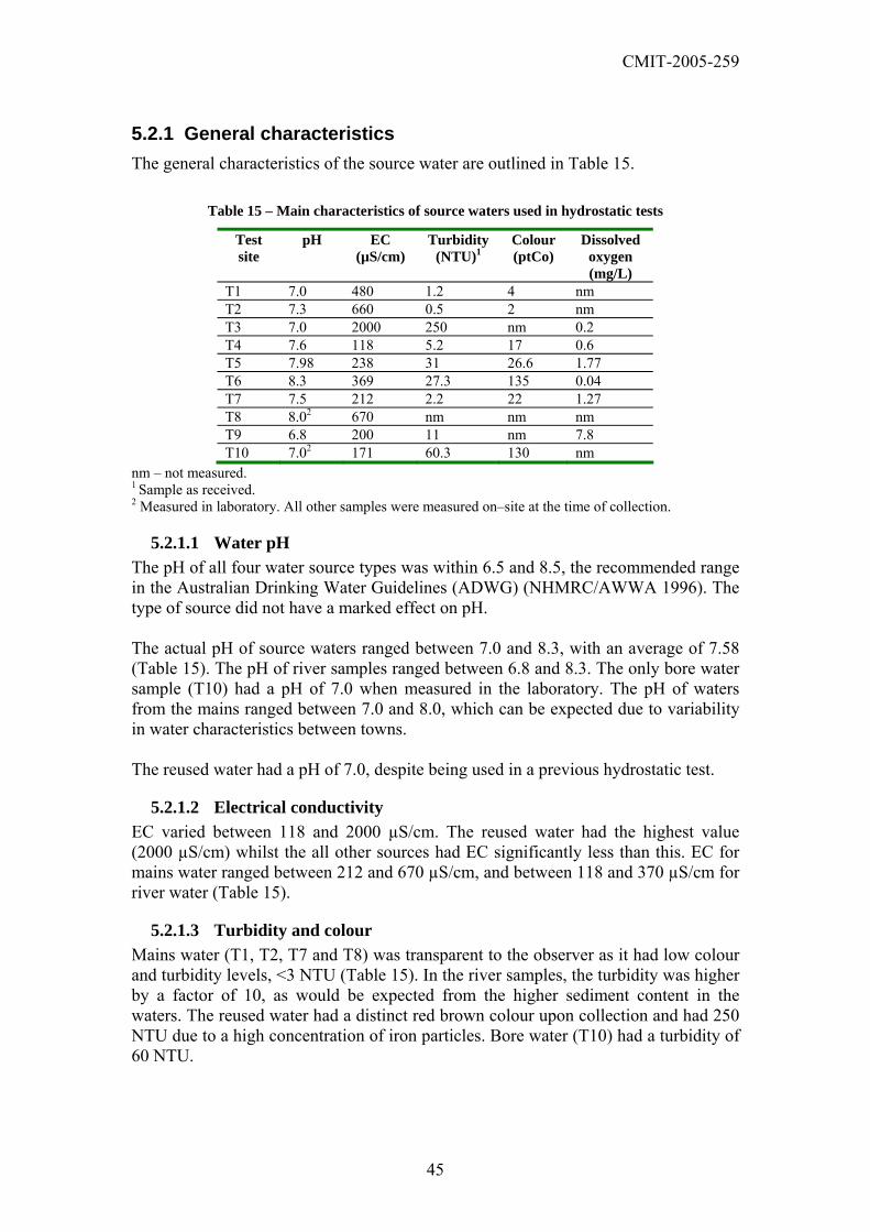
CMIT-2005-259

5.2.1 General characteristics The general characteristics of the source water are outlined in Table 15.

Table 15 – Main characteristics of source waters used in hydrostatic tests

Test site

pH EC (µS/cm)

Turbidity (NTU)1

Colour (ptCo)

Dissolved oxygen (mg/L)

T1 7.0 480 1.2 4 nm T2 7.3 660 0.5 2 nm T3 7.0 2000 250 nm 0.2 T4 7.6 118 5.2 17 0.6 T5 7.98 238 31 26.6 1.77 T6 8.3 369 27.3 135 0.04 T7 7.5 212 2.2 22 1.27 T8 8.02 670 nm nm nm T9 6.8 200 11 nm 7.8 T10 7.02 171 60.3 130 nm

nm – not measured. 1 Sample as received. 2 Measured in laboratory. All other samples were measured on–site at the time of collection.

5.2.1.1 Water pH The pH of all four water source types was within 6.5 and 8.5, the recommended range in the Australian Drinking Water Guidelines (ADWG) (NHMRC/AWWA 1996). The type of source did not have a marked effect on pH. The actual pH of source waters ranged between 7.0 and 8.3, with an average of 7.58 (Table 15). The pH of river samples ranged between 6.8 and 8.3. The only bore water sample (T10) had a pH of 7.0 when measured in the laboratory. The pH of waters from the mains ranged between 7.0 and 8.0, which can be expected due to variability in water characteristics between towns. The reused water had a pH of 7.0, despite being used in a previous hydrostatic test.

5.2.1.2 Electrical conductivity EC varied between 118 and 2000 µS/cm. The reused water had the highest value (2000 µS/cm) whilst the all other sources had EC significantly less than this. EC for mains water ranged between 212 and 670 µS/cm, and between 118 and 370 µS/cm for river water (Table 15).

5.2.1.3 Turbidity and colour Mains water (T1, T2, T7 and T8) was transparent to the observer as it had low colour and turbidity levels, <3 NTU (Table 15). In the river samples, the turbidity was higher by a factor of 10, as would be expected from the higher sediment content in the waters. The reused water had a distinct red brown colour upon collection and had 250 NTU due to a high concentration of iron particles. Bore water (T10) had a turbidity of 60 NTU.

45

CMIT-2005-259

5.2.1.4 Dissolved oxygen DO levels were measured in 6 of the 10 samples (Table 15). The measured values were low (<2 mg/L) and would have been expected to decrease further after the addition of an oxygen scavenger. Natural water sources such as groundwater often have low DO levels. Low DO can favour the growth of anaerobic micro-organisms. Sample T9 had a DO level of 7.8 mg/L. The higher DO level was caused by turbulent discharge of the water into a holding tank after being transport from the river.

5.2.2 Metals Water from natural sources contains a variety of naturally occurring metals, which are often removed during water treatment. The concentrations of arsenic (Ar), cadmium (Cd), Cr and Pb were below detection limits in the water samples analysed (Table 16). Whilst the most abundant metals detected in the source waters were Zn, Cu, Mn and Fe. The highest metal concentration in the source water was Fe, which is a common element in soil and also commonly found in mains water due to corrosion. Mn, also commonly found in soil, was the second most abundant metal (0.009–4.3 mg/L), followed by Zn, whose concentration varied between the different sources (≤0.08 mg/L). Cu levels were 0.23 mg/L for bore water, 0.1 mg/L for the reused water and <0.04 mg/L for all other samples. Overall, the metals content in water was <1 mg/L for the majority of the elements tested, with the exception of Fe, which was present at concentrations ranging up to 2.6 mg/L for the town and river samples, 4 mg/L for bore water and 150 mg/L for the reused water. The metals content was the highest in the reused water, particularly for Fe (150 mg/L), Mn (4.3 mg/L) and Cu (0.10 mg/L) compared to the other sources. This is caused by the accumulation of metal residues from the previous hydrostatic test. River water had Mn concentrations an order of magnitude higher than mains water in two of the four cases, however the concentration of other metals were comparable between the two source types. The metal content was within health guidelines for the ADWG for all samples, with the exception of Mn in the reused water. The high Fe content would also have resulted in a metallic taste in the reused water. Differences between the metal concentrations in the river, mains water, bore and reused sources were expected. In particular, the reuse water was expected to have a higher metal content than the other sources as it contained sediments from the previous test section.

46

CMIT-2005-259

Table 16 – Metal concentration in source waters

Metal concentration (mg/L) Test site Ar Cd Cr Pb Zn Cu Mn Fe

T1 nm nm nm nm nm nm nm nm T2 <0.001 <0.0002 <0.02 <0.01 0.016 0.037 0.009 <0.05 T3 <0.001 nm <0.02 <0.01 0.027 0.10 4.3 150 T4 nm nm <0.02 <0.01 0.08 <0.01 0.02 2.6 T5 nm nm <0.02 <0.01 0.05 <0.01 0.27 1.7 T6 nm nm <0.02 <0.01 <0.01 0.01 0.30 1.2 T7 nm nm <0.02 <0.01 <0.01 0.01 0.05 1.2 T8 nm nm nm nm nm nm nm <0.05 T9 nm <0.02 <0.05 <0.01 <0.01 0.01 0.03 1.9 T10 nm <0.02 <0.05 <0.01 0.1 0.23 0.04 4 ADWG 0.007 0.002 0.05 0.01 – 2 0.5 –

nm – not measured.

5.2.3 Dissolved salts The inorganic content of the source water varied widely between samples and did not show any trends in regards to source type (Table 17):

• Sulphate (SO42–) levels detected were <50 mg/L, except for the reused water

(630 mg/L). • Ca concentration was <37 mg/L. • Mg concentration was <20 mg/L. • Potassium (K) concentration was <15 mg/L. • Na concentration ranged between 9 and 71 mg/L. • Total nitrogen (TN) was <3.2 mg/L, except for the reused water (110 mg/L). • Total phosphorus (TP) was <0.07 mg/L.

The reused water had significantly higher concentrations of TN and SO4

2- than the other samples, which was attributed to residues from the oxygen scavenger ammonium bisulphite used in the preceding hydrostatic test.

Table 17 – Inorganic contents in source waters

Concentration (mg/L) Test site Ca K Mg Na TN TP SO4 CaCO3

T1 nm nm nm nm 0.935 nm 2 nm T2 21 nm 13 nm nm nm 49 100 T3 9.4 1.1 4.5 19.0 1101 0.032 630 nm T4 10 nm 5.5 8.9 0.72 0.02 14 nm T5 32.2 15 9.8 32.8 0.18 0.07 2 nm T6 36.3 4.1 10.8 36.0 0.10 0.03 3 nm T7 10.8 5.9 7 32.0 <0.03 0.03 18 nm T8 31 2.4 19 71 3.22 nm 19 <1 T9 4.5 1.7 5.7 23 0.079 0.04 6 nm T10 4.9 4 3 24 0.022 <0.01 2 nm

nm - not measured 1 Water contained ammonium bisulphite oxygen scavenger from the previous test section. 2 Nitrate concentration only.

47

CMIT-2005-259

5.3 Flushing water

Prior to hydrostatic testing each test section was pigged, scrubbed, cleaned and flushed. An analysis was conducted on the water used for the flushing and cleaning for one of the test sites to evaluate its composition. The flush water removes the majority of the debris (e.g. dirt, sand, earth) and residues present in the pipeline and, as such, was expected to present a larger concentration of contaminants. The water characteristics for five samples obtained at different stages during flushing prior to test T10 are shown in Table 18. As expected, the flush water was dirtier than the source and disposal waters. The average measurement of flush water parameters compared to the disposal water was significantly higher: EC +45%, turbidity +241%, SO4

2– +208%, sulphur +425%, Fe +121%, Mn +3.9%) Ca (+136%), Zn +30%, nitrite +150%) ammonia +20.3%, total phosphorus (TP) +660%, Ca +51.2%, Na +96.7% and K +79.8%. Analysis of the metal composition in the residue indicated that soluble Mn, total Mn, soluble Zn and soluble Cd were present at 2.35%, 1.20%, 0.21% and 0.08% of the Fe concentration, respectively, in both the flush and the disposal water. Metals such as Cr, Cu and Pb did not vary significantly between the two samples, suggesting that the removal of these elements is related to the removal of oxidised metallic compounds on the pipe wall. The higher concentration of ions (Ca, Cl, Na, K) may be caused by the presence of soil, sand and similar residues. Overall, flush water is expected to have more contaminants than source and disposal water, however the volume of water used is usually smaller as cleaning generally uses a slug of water between pigs and as such, can be more easily managed. Often, the site for the disposal of the flush water is not the same as the site for the disposal as the hydrostatic test water.

48

CMIT-2005-259

Table 18 – Flush water characteristics for T10

Parameter Sample Source Flush 1 Flush 2 Flush 3 Flush 4 Flush 5 Flush Average

EC(µS/cm @ 25°C)

171 591 224 169 308 389 336.2

SAR 4.19 13.7 2.6 4.5 10.7 3.6 7.0 Turbidity (NTU)

60.3 434 3875 948 446 200 1180

Colour (ptCo) 130 1180 1575 515 1275 1250 1159 SO4

2– (mg/L) 2 68 13 2 25 <1 21.8 Sulphur (mg/L)

<1 19 <1 147 3 <1 <42.5

Ammonia (mg/L)

<0.010 0.52 0.01 <0.010 0.464 0.061 0.21

NO3– (mg/L) <0.010 <0.010 <0.010 <0.010 0.012 <0.010 <0.213

Total P <0.010 <0.04 0.2 0.1 0.65 0.58 0.304 Reactive P <0.010 <0.010 <0.010 <0.010 <0.010 <0.010 <0.010 Ca (mg/L) 4.9 13.7 13.6 5.3 5.7 7.6 9.2 Cd (mg/L) <0.02 0.1 0.28 <0.02 0.13 0.06 0.02 Cl (mg/L) 20 90 <15 <15 <15 20 31 Co (mg/L) <0.01 0.02 0.03 <0.01 0.03 0.01 0.02 Cr (mg/L) <0.05 <0.05 <0.05 <0.05 <0.05 <0.05 <0.05 Cu (mg/L) 0.23 0.19 0.18 0.03 0.15 0.11 0.13 Fe (soluble) (mg/L)

4 97 206 25 81 150 111.8

Fe (total) (mg/L)

6 421 943 39 483 246 426.4

K (mg/L) 4 17 3 4 5 4 6.6 Mg (mg/L) 3 3 7 3 1 4 3.6 Mn (mg/L) 0.04 3 3.8 0.7 2.32 3.26 2.6 Mn (total) (mg/L)

0.04 5.2 8.0 0.9 6.46 3.25 4.75

Na (mg/L) 24 108.0 24.0 26.0 53.0 25.0 47.2 Pb (mg/L) <0.01 0.01 0.02 <0.01 <0.01 <0.01 <0.01 Zn (mg/L) 0.1 0.5 0.2 0.2 0.1 0.3 0.26

5.4 Disposal water

The main factors that determine the composition of disposal waters are the characteristics of the source water, any additives, any residues contained not removed during flushing and reactions occurring within the pipe during testing, such as corrosion.

5.4.1 General characteristics The main characteristics of the disposal waters are outlined in Table 19.

5.4.1.1 Water pH The pH of the disposal water ranged between 7.0 and 8.2, which was within the range of pH seen for the source waters (6.8 - 8.3), indicating that pH is not significantly affected by hydrostatic testing.

49

CMIT-2005-259

Overall the pH values of the disposal water were within the recommended range in the ADWG (NHMRC/AWWA 1996) and the pH variation range of Australian aquatic ecosystems (ANZECC/ARMCANZ 2000), i.e. 6.5 and 8.5. However, if disposal is to a water body, it is recommended that verification of specific site characteristics be performed, as in many sites there are specific pH requirements. Additionally, water stored in ponds, dams or via other means where water is stagnant for long periods of time tends to undergo changes in due to exchange of CO2 with the atmosphere, and pH needs to be verified before disposal.

5.4.1.2 Electrical conductivity EC of the disposal water varied between 164 and 2000 µS/cm. The highest value, 2000 µS/cm, was for sample T2. The other waters had an EC ranging between 164 and 830 µS/cm, including the reused water. The EC value was not directly correlated to oxygen scavenger addition.

5.4.1.3 Turbidity After hydrostatic testing, the turbidity of all samples increased to levels that could be detected by eye (>5NTU) (Table 19). The reused water represented the most severe case. It had initially been red brown (250 NTU) after one hydrostatic test and became dark brown (4100 NTU) after the second test.

5.4.1.4 Dissolved oxygen DO levels were measured in 6 of the 10 samples (Table 19). The DO at disposal was low (<1 mg/L), with the exception of sample T7, which had a DO of 6.5 mg/L. Sample T9 collected at the exit of the line had an initial DO of 0 mg/L, but after aeration the DO increased to 4.6 mg/L. The recommended DO values are usually >80–90% of saturation or approximately 6 mg/L depending on conditions (ANZECC/ARMCANZ 2000), so the low DO levels in the disposal water would have needed to be increased if the water were to be disposed into an aquatic environment. Insufficient DO in water bodies can lead to asphyxiation of fauna.

50

CMIT-2005-259

Table 19 – Main characteristics of hydrostatic test discharge water

Test site

Oxygen scavenger

pH EC (µS/cm)

Turbidity (NTU)1

Var (%)

Colour (ptCo)

Dissolved oxygen (mg/L)

TS (mg/L)

T1 No 7.0 830 850 70,730 nm nm nm T2 Yes 7.01 2000 250 49,900 nm 0.21 nm T3 Yes 7.45 780 4100 1,540 nm – 520 T4 Yes 7.22 164 14 169 10 0.22 nm T5 Yes 7.29 380 32 3.2 8 0.95 500 T6 No 8.21 229 2000 7,226 19 0.07 116 T7 No 7.65 241 62.1 2,736 19 6.5 nm T8 Yes 7.8 710 nm – nm nm nm T9 Yes 7.05 491 29.8 171 0 (4.6)2 nm T10 No nm 231 346 473 1270 nm nm 1 Sample as received. 2 Sample was aerated in a tank after leaving pipe, as sample exited the pipe DO was 0 mg/L, after aeration it was 4.6 mg/L.

5.4.1.5 Solids The total solids (TS) after drying at 105°C for samples T2, T3, T6 and T9 are shown in Figure 3. The appearance of the solids differed for each of the samples shown, with variations in colour and texture. The residues from samples T4 - T7 (which were part of the same pipeline) were similar in appearance with a red colouration. The mass of residue recovered after drying varied between 33 and 520 mg/L, being 520 mg/L for T3 (reuse water), 500 mg/L for T5, 117 mg/L for T6 and 33 mg/L for T9. The solids from samples T2 and T3 were identified as iron oxides and salts. T2 consisted of goethite (FeOOH), chalcopyrite (CuFeS2), ferro–gedrite (Fe5Al4Si6O22(OH)2), bernalite Fe(OH)3 and salammoniac (NH4Cl). T3 consisted of iron oxide (Fe2O3), magnetite (Fe3O4), halite (NaCl), salammoniac and quartz (SiO2). Elemental analysis determined that Fe was the major element at 30% w/w, the other elements were present as follows: Na 8.4%, Ca 0.67%, Mg 0.40%, Si 0.10%, aluminium 0.10%, Zn 0.02% and Cu <0.05%.

51

CMIT-2005-259

5ToTh AbTa CTn Cs Ca Pd Z< Mh

T2 T3 T6

Figure 3 – Examples of residues from disposal water after drying at 105°C for T2, T3, T6 and T9 replicates.

.4.2 Metals he metals contents in the disposal water are shown in Table 20. The concentrations f Ar, Cd and Cr were below detection limits in all samples. Cu was detected in T8, 9 and T10, and Pb was detected in T1 and T2. Zn, Mn and Fe were present at the ighest concentrations.

r levels detected in the source and disposal waters for samples T2 and T3 were elow the detection limit, indicating no significant variation occurred during testing. his is expected as Ar occurs mainly due to the water source. This parameter was not nalysed for the other disposal samples.

d was below detection limits in the source water and the disposal water in sample 9, however it was present at 0.05 mg /L in sample T10. However, as neither the steel or the additives contained Cd, it was not measured for the other samples.

r was below detection limits for samples T4 through T10 and was detected in amples T1, T2 and T3 at ≤0.01 mg/L.

u was below detection limit of 0.05 mg/L in most samples and was detected at pproximately 0.10 mg/L in samples T2 and T10.

b was present in samples T1 and T2 in concentrations <0.05 mg/L. Pb was below etection limits in all other samples (Table 20).

n in the disposal water had less than 0.25 mg/L, with concentrations ranging from 0.05 to 0.25 mg/L with an average of 0.10 mg/L.

n was detected at concentrations between 0.05 and 12 mg/L. Samples T2 and T3 ad the highest Mn contents of 4.3 mg/L and 12 mg/L respectively.

52

CMIT-2005-259

Fe was the most abundant element detected, and was present at concentrations ranging between 8 and 820 mg/L for most samples, the only exception was T8 which was below detection limits. The content of Fe and Mn was the highest for the sample T3 which had been used in two hydrostatic tests, compared to the other samples. Note that Fe and Mn are the most abundant elements present in steel (Table 3).

Table 20 – Metal concentration in disposal waters

Metal concentration (mg/L) Test site

Oxygen scavenger

Ar Cd Cr Cu Pb Zn Mn Fe T1 No nm nm 0.002 nm 0.046 0.10 0.43 36 T2 Yes <0.001 nm 0.002 0.1 0.002 0.027 4.3 150 T3 Yes <0.001 nm 0.01 nm <0.01 0.08 12 820 T4 Yes nm nm <0.02 nm <0.01 0.25 0.43 19.9 T5 Yes nm nm <0.02 <0.01 <0.01 0.06 0.68 20.8 T6 No nm nm <0.02 <0.01 <0.01 0.14 1.64 120 T7 No nm nm <0.02 <0.01 <0.01 0.04 0.35 19.6 T8 Yes nm nm <0.05 <0.05 <0.05 <0.05 0.05 <0.05 T9 Yes nm <0.02 <0.05 <0.02 <0.01 0.115 0.245 8.7 T10 No nm 0.05 <0.05 0.09 <0.01 0.2 2.51 103

nm – not measured.

5.4.3 Dissolved salts The results in Table 21 indicate that the inorganic content was influenced by the water characteristics of each individual source and by any additives used. The sulphate (SO4

2–) content at disposal was similar to that of the source waters for tests T1, T7 and T10, as they did not contain an oxygen scavenger, SO4

2– content remained <23 mg/L. Samples with oxygen scavenger experienced a significant increase in SO4

2– content. SO42– content were the highest in samples T2, T3, T8 and

T9 being 630, 120, 120 and 140 mg/L respectively. The disposal waters from samples T2 and T3 had the highest concentration of Total Nitrogen (TN). These cases were the only ones that used the oxygen scavenger ammonium bisulphite, which forms (NH4)2SO4 upon oxidation. The concentration of Na was higher at disposal for the samples that used sodium based oxygen scavengers (T4, T5, T8 and T9). In conclusion, the contaminants in the discharged water for new pipelines are a combination of the contaminants present in the source water and contaminants added by oxidised steel, rust/mill scale, traces of weld flux and chemical additives. Note that in-service pipelines that are subject to retest are contaminated with substances deposited on the internal surfaces during service, often hydrocarbon and sulphur compounds, and as such require special consideration is needed when considering disposal.

53

CMIT-2005-259

Table 21 – Inorganic contents in disposal waters

Concentration (mg/L) Test site

Oxygen scavenger

SO42– TN Na Ca Mg P K CaCO3

T1 No 7 0.935 nm 6.0 1.8 0.031 nm nm T2 NH4HSO3 630 110 19 9.4 4.5 0.0321 1.1 100 T32 NH4HSO3 120 27.0 nm nm nm 0.0251 nm nm T4 Na2S2O5 43 0.23 16.8 10.4 5.7 0.03 nm nm T5 Na2S2O5 69 0.323 47.7 32.2 9.6 0.13 16 nm T6 No 23 0.12 34.3 17.7 5.9 0.18 15 nm T7 No 22 <0.01 31.8 10.4 5 0.09 5 nm T8 Na2S2O5 120 0.39 99 13.0 19 0.08 2.2 <1 T9 Na2SO3 140.5 0.327 83 5.1 5.2 0.034 2.5 nm T10 No <1 <0.010 24 6.1 3.7 <0.010 3.7 nm nm – not measured. 1 Reactive phosphorus only. 2 Water contained oxygen scavenger, ammonium bisulphite, used in previous section. 3 Nitrate concentration only.

5.4.4 Environmental impact The impact of discharge water on the environment is dictated by a complex combination of factors, including water composition, physical and chemical properties, the rate of application, the site of application and the robustness of the receiving ecosystem. Land ecosystems are generally more robust than water ecosystems, however, discharge to water ecosystems is sometimes preferred to maintain environmental flow. The key indicators of physical and chemical stressors in an environment are:

• nutrients. • DO, • turbidity, • suspended particulate matter, • salinity, • temperature, • optical properties, and • environmental flows.

54

CMIT-2005-259

55

5.4.5 Disposal to aquatic ecosystems

5.4.5.1 Physio–chemical parameters The main characteristics of the discharge waters are outlined in Table 19.

5.4.5.2 Water pH Overall the pH of the disposal waters were between 6.5 and 8.5, the recommended range in the ADWG ((NHMRC/AWWA 1996)) and the pH range of Australian aquatic ecosystems (ANZECC/ARMCANZ 2000) (Table 22). However, if disposal is to a water body, it is recommended that verification of specific site characteristics be performed, as in many sites there are specific pH requirements. Additionally, water stored in ponds, dams or via other means where water is stagnant for long periods of time tends to undergo changes in due to exchange of CO2 with the atmosphere, and pH needs to be verified before disposal.

5.4.5.3 Electrical conductivity EC for the disposal water varied between 164 and 2000 µS/cm. The highest value, 2000 µS/cm, was for sample T2. The other waters had an EC ranging between 164 and 830 µS/cm. The EC values were comparable to those of the source waters for most samples (Table 22).

5.4.5.4 Turbidity The turbidity in the disposal waters was markedly higher than in the source waters (Table 22). Turbidity increased by more than 1000% after most tests. The values were larger than the average range of turbidity values encountered in the different regions of Australian water systems (Table 23). However, for a specific ecosystem, guidelines need to be stipulated based on the water flow, seasonality and stress level of the specific receiving point. Some individual rivers have turbidity levels much higher than those specified in the average values. If a large volume of high turbidity water is discharged into an aquatic system, a significant reduction in light transmission could occur, reducing photosynthesis in the ecosystem. The extent of this impact would depend on the volume discharged and the mixing potential of the specific aquatic body in absorbing the load. High turbidity indicates the need for further evaluation of the receiving ecosystem and the potential adoption of impact minimisation strategies for its reduction, such as filtration, settling and/or the adoption of suitable management techniques to ensure smaller shock loads, such as allowance for mixing zones and control of discharge rates.

CMIT-2005-259

56

Table 22– Comparison of characteristics of hydrostatic test waters before and after hydrostatic test

Test site

Source pH

Disposal pH

Source EC

(µS/cm)

Disposal EC

(µS/cm)

Source Turbidity

(NTU)1

Disposal Turbidity

(NTU)1

Turbidity increase

(%)

Source Colour (ptCo)

Disposal Colour (ptCo)

Source Dissolved

oxygen (mg/L)

Disposal Dissolved

oxygen (mg/L)

Disposal TSS

(mg/L)

T1 7.0 7.0 480 830 1.2 850 70,730 4 nm nm nm nmT2 7.3 7.01 660 2000 0.5 250 49,900 2 nm nm 0.21 nmT3 7.01 7.45 2000 780 250 4100 1,540 nm nm 0.2 – 520T4 7.62 7.22 118 164 5.2 142 169 17 10 0.6 0.22 nmT5 7.98 7.29 238 380 31 32 3.2 26.6 8 1.77 0.95 500T6 8.28 8.21 369 229 27.3 2000 7,226 135 19 0.04 0.07 116T7 7.5 7.65 212 241 2.19 62.1 2,736 22 19 1.27 6.5 nmT8 8.0 7.8 670 710 nm nm – nm nm nm nm nmT9 6.8 7.05 200 491 11 29.8 171 nm nm nm nm nmT10 nm nm 171 231 60 346 476 130 1270 nm nm nm

nm – not measured 1 Samples measured as received.

Table 23–Ranges of default trigger values for Turbidity (NTU) in Australian ecosystems (ANZECC/ARMCANZ 2000)

Ecosystem type South east South west Tropical South central Vic, NSW, ACT, south–east Qld and Tas Southern WA Northern WA, northern QLD and NT Low rainfall areas in SA

Upland River 2–25 10–20 2–15 1–50 Lowland River 6–50 10–20 2–15 1–50 Lakes and reservoirs 1–20 10–100 2–200 1–100 Estuarine and marine 0.5–10 1–2 1–20 0.5–10 Wetlands – – 2–200 1–100

CMIT-2005-259

5.4.5.5 Metals Aquatic ecosystems have a higher sensitivity to stressors than land ecosystems. The ANZGFMWQ (ANZECC/ARMCANZ 2000) sets guideline values for major toxicant groups, as shown in Table 24, however a number of those values are below the detection limits of current analytical equipment. Determination of the toxicity of the water would require evaluation of the water characteristics, application method and the characteristics of the receiving site. As an illustration of the potential impact, the ANZGFMWQ has been used for comparison in this report, however state and local regulatory authorities often have more site specific guidelines that take precedence over the ANZGFMWQ.

Table 24 – Trigger values for toxicants at alternate protection levels (ANZECC/ARMCANZ 2000)

Chemical Trigger values for freshwater (mg/L)

Trigger values for marine water (mg/L)

Level of protection Level of protection Metals 99% 95% 90% 80% 99% 95% 90% 80%

Arsenic (III) 0.001 0.024 0.094 0.360 ID ID ID ID Arsenic (V) 0.0008 0.013 0.042 0.140 ID ID ID ID Cadmium 0.0006 0.0002 0.0004 0.0008 0.0007 0.0055 0.014 0.036 Chromium (III) ID ID ID ID 0.0077 0.0274 0.0486 0.0906 Chromium (VI) 0.00001 0.001 0.006 0.040 0.00014 0.0044 0.020 0.085 Copper 0.001 0.0014 0.0018 0.0025 0.0003 0.0013 0.003 0.008 Iron ID ID ID ID ID ID ID ID Lead 0.001 0.0034 0.0056 0.0094 0.0022 0.0044 0.0066 0.012 Manganese 1.200 1.900 2.500 3.600 ID ID ID ID Zinc 0.0024 0.0080 0.015 0.031 0.007 0.015 0.023 0.043

Non–metallic Inorganics Ammonia 0.320 0.900 1.430 2.300 0.500 0.910 1.200 1.700 Chlorine 0.0004 0.003 0.006 0.013 ID ID ID ID Nitrate 0.017 0.70 3.40 17.0 ID ID ID ID Hydrogen sulphide

0.0005 0.001 0.0015 0.0026 ID ID ID ID

ID – insufficient data

Table 24 shows the trigger values and protection levels as recommended in ANZGFMWQ. Compared to the values in Table 24, the metals concentration in the disposal water would allow:

a) For Ar, 99% protection of freshwater species. b) For Cd, T10 was over all established trigger values. However the trigger

values are all below the analytical detection limits. c) For Cr, ≥80% protection of freshwater species. d) For Cu, T2 and T10 exceeded all established trigger values. However the

trigger values are all below the analytical detection limits. e) For Pb, T2 ≥95% protection of freshwater species. T1 exceed all established

trigger values. All other samples had concentrations below detection limits, however the trigger values are all below the analytical detection limits.

f) For Zn, ≥80% protection of freshwater species for sample T2. g) For Mn, ≥95% protection of freshwater species, with the exception of samples

T 2, T3 and T10.

57

CMIT-2005-259

h) For Fe there are no guideline values, however at the concentrations recorded the optical properties could be affected.

Table 25 compares the disposal water concentrations with the guidelines. The trigger concentration of Cu and Zn were higher than the guideline values for most samples, however the metal concentrations in source waters were also higher than the 99% protection values in the guideline values. Hence, it would be necessary to investigate other water characteristics to determine their impact and their bioavailability.

Table 25 – Comparison of disposal water with guidelines (ANZECC/ARMCANZ 2000)

Metal concentration (mg/L) (level of protection %)

Tes

t site

Oxy

gen

scav

enge

r

Ar Cd Cr

Cu Fe Mn Pb Zn

T1 No nm nm 0.002 (90) nm 36 0.43 (99) 0.046 0.10 T2 Yes <0.001 (99) nm 0.002 (90) 0.1 150 4.3 0.002 (95) 0.027 (80) T3 Yes <0.001 (99) nm 0.01 (80) nm 820 12 <0.01 (80) 0.08 T4 Yes nm nm <0.02 (80) nm 19.9 0.43 (99) <0.01 (80) 0.25 T5 Yes nm nm <0.02 (80) <0.01 20.8 0.68 (99) <0.01 (80) 0.06 T6 No nm nm <0.02 (80) <0.01 120 1.64 (95) <0.01 (80) 0.14 T7 No nm nm <0.02 (80) <0.01 19.6 0.35 (99) <0.01 (80) 0.04 T8 Yes nm nm <0.05 (80) <0.05 <0.05 0.05 (99) <0.05 (80) <0.05 T9 Yes nm <0.02 <0.05 (80) <0.02 8.7 0.25 (99) <0.01 (80) 0.115 T10 No nm 0.05 <0.05 (80) 0.09 103 2.51 <0.01 (80) 0.2

Green – within guideline limits Yellow – Concentration higher than the guideline value stipulated for 80% level of protection.

5.4.5.6 Salinity The impact of water salinity is dependent on the salinity tolerance of a specific aquatic ecosystem. The EC values of the disposal water ranged between 164 and 2000 µS/cm (Table 22). EC for the tests conducted in Victoria (T1, T2, T3 and T9) ranged between 491 and 2000 µS/cm, in Western Australia T8 was 710 µS/cm and in Queensland T4 - T7 and T10 ranged between 164 and 380 µS/cm. To illustrate the variability in salinity for Australian water bodies, Table 26 shows the range of trigger values applicable to each of the major aquatic ecosystems. Depending on the discharge location, the salinity levels of the receiving body can be lower or higher than the trigger value displayed in Table 26. Disposal water with values higher than the trigger value would require evaluation of site-specific conditions.

Table 26 – Trigger values for salinity (ANZECC/ARMCANZ 2000)

EC (µS/cm) South east South west Tropical South central Ecosystem type Vic, NSW, ACT,

south–east Qld and Tas

Southern WA

Northern WA, northern Qld

and NT

Low rainfall areas in SA

Upland river 30–350 120–300 20–250 – Lowland river 125–2200 120–300 20–250 100–5000 Lakes & reservoirs

20–30 300–1500 90–900 300–1000

Wetlands – 300–1500 90–900 300–1000

58

CMIT-2005-259

59

5.4.5.7 Nutrients Nitrogen and phosphorus levels affect algae growth in aquatic ecosystems and plant growth in land ecosystems. Comparisons of nitrogen and phosphorus concentrations from disposal samples in Table 27 with average trigger values in Table 28 suggest that:

• Total nitrogen (TN) (max 110 mg/L, min. <0.010 mg/L) most samples were below trigger limits and suitable for discharge in south-east, south-west, tropical and south central ecosystems, with the exception of T2, T3 and T8 in some cases. Low rainfall areas were the least sensitive to higher loads. A similar pattern was observed with ammonium, but with levels of T2, T3, and T8 higher than the trigger values.

• NOx (oxides of nitrogen) (max. 0.905 mg/L., min <0.020 mg/L) sample T1 exceeded the trigger values in all locations, while T2, T3, T5 and T9 exceeded the trigger values for most locations.

• Total phosphorus (TP) (max. 0.180 mg/L, min. 0.030 mg/L) - samples were over the trigger values for most aquatic ecosystems in south-east, south-west and tropical Australia. Discharge to lowland rivers, estuaries and marine environments could have had excessive TP depending on the location and type of ecosystem.

The majority of the disposal waters were over the trigger values, however these values are estimates for slightly disturbed systems only, the final impact being dependent on specific ecosystem characteristics such as background pollution. For the samples analysed, the source waters’ nutrient content was also higher than the trigger values outlined in Table 28. The major variation was observed for samples T2 and T3, to which the oxygen scavenger ammonium bisulphite had been added. Whilst the concentration of phosphorus, TP, nitrogen, TN and NOx were higher than the majority of the trigger values for aquatic ecosystems, they were similar to their respective source waters, including rivers. This highlights the impact that the characteristics of each individual disposal site can have on the disposal options, and that the sensitivity of an ecosystem to disposal water depends on the physical, chemical and biological characteristics of each ecosystem, and conditions such as climate and level of disturbance.

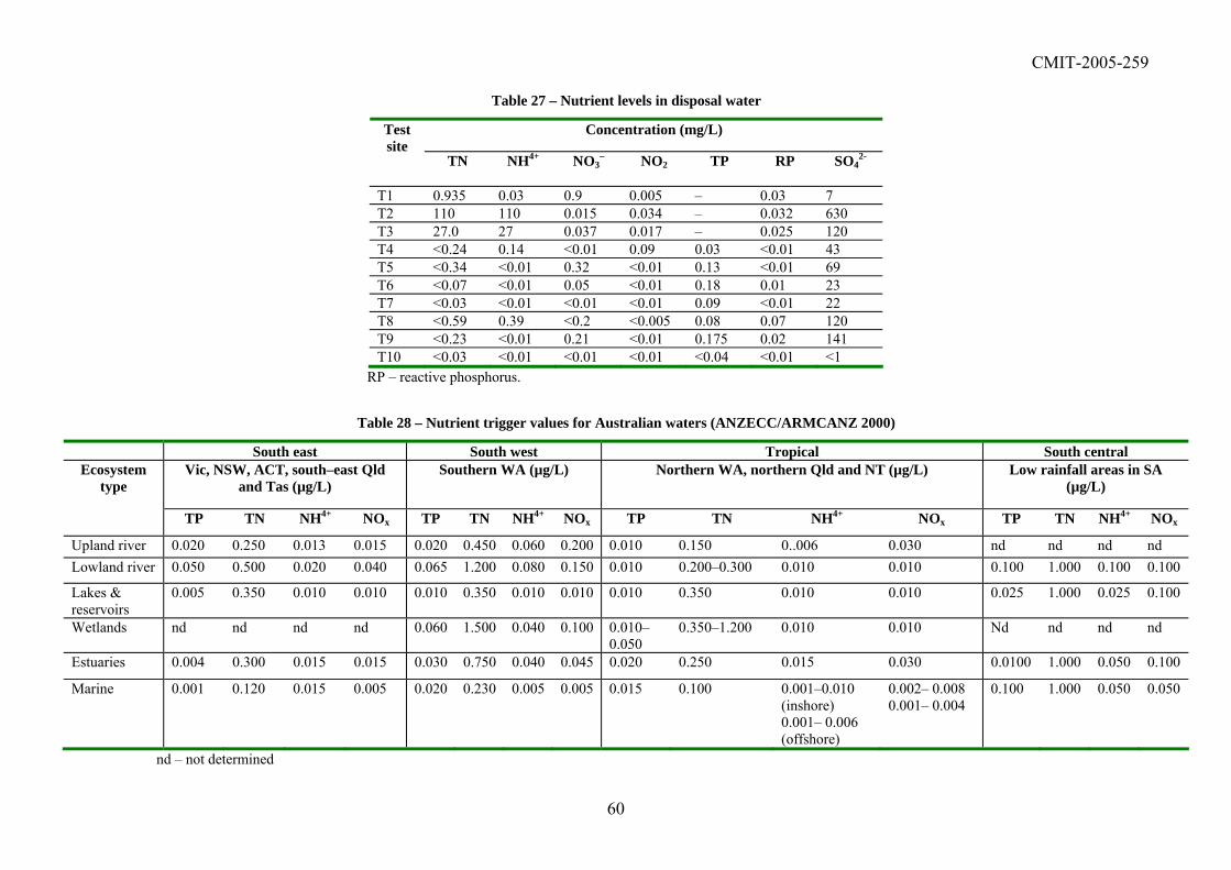
CMIT-2005-259

60

Table 27 – Nutrient levels in disposal water

Concentration (mg/L) Test site

TN

NH4+ NO3– NO2 TP RP

SO4

2-

T1 0.935 0.03 0.9 0.005 – 0.03 7T2 110 110 0.015 0.034 – 0.032 630T3 27.0 27 0.037 0.017 – 0.025 120T4 <0.24 0.14 <0.01 0.09 0.03 <0.01 43T5 <0.34 <0.01 0.32 <0.01 0.13 <0.01 69T6 <0.07 <0.01 0.05 <0.01 0.18 0.01 23T7 <0.03 <0.01 <0.01 <0.01 0.09 <0.01 22T8 <0.59 0.39 <0.2 <0.005 0.08 0.07 120T9 <0.23 <0.01 0.21 <0.01 0.175 0.02 141T10 <0.03 <0.01 <0.01 <0.01 <0.04 <0.01 <1

RP – reactive phosphorus.

Table 28 – Nutrient trigger values for Australian waters (ANZECC/ARMCANZ 2000)

South east South west Tropical South central Vic, NSW, ACT, south–east Qld

and Tas (µg/L) Southern WA (µg/L) Northern WA, northern Qld and NT (µg/L) Low rainfall areas in SA

(µg/L) Ecosystem

type

TP TN NH4+ NOx TP TN NH4+ NOx TP TN NH4+ NOx TP TN NH4+ NOx

Upland river 0.020 0.250 0.013 0.015 0.020 0.450 0.060 0.200 0.010 0.150 0..006 0.030 nd nd nd ndLowland river 0.050 0.500 0.020 0.040 0.065 1.200 0.080 0.150 0.010 0.200–0.300 0.010 0.010 0.100 1.000 0.100 0.100

Lakes & reservoirs

0.005 0.350 0.010 0.010 0.010 0.350 0.010 0.010 0.010 0.350 0.010 0.010 0.025 1.000 0.025 0.100

Wetlands nd nd nd nd 0.060 1.500 0.040 0.100 0.010–0.050

0.350–1.200 0.010 0.010 Nd nd nd nd

Estuaries 0.004 0.300 0.015 0.015 0.030 0.750 0.040 0.045 0.020 0.250 0.015 0.030 0.0100 1.000 0.050 0.100

Marine 0.001 0.120 0.015 0.005 0.020 0.230 0.005 0.005 0.015 0.100 0.001–0.010(inshore) 0.001– 0.006 (offshore)

0.002– 0.008 0.001– 0.004

0.100 1.000 0.050 0.050

nd – not determined

CMIT-2005-259

5.4.5.8 Sulphate (SO42-)

The use of oxygen scavengers such as ammonium or sodium bisulphite generates sulphate residues. There are currently no prescribed guidelines for sulphate concentration in irrigation and aquatic ecosystems however, a limit of 400 mg/L applies to recreation waters (ANZECC/ARMCANZ 2000). With the exception of T2, the disposal waters had a much lower sulphate content (<120 mg/L) Table 21) (Figure 4).

0

100

200

300

400

500

600

700

T1 T2 T3 T4 T5 T6 T7 T8 T9 T10

Test site

[SO

4-2] (

mg/

L) Limit for Recreational Waters

Figure 4 – Sulphate content in disposal waters

Water from town mains and rivers with no oxygen scavenger (T1, T6, and T7) had a lower sulphate content than samples containing oxygen scavengers. The bore water (T10) had a lower sulphate concentration than all samples.

5.4.6 Disposal to land ecosystems Disposal of hydrostatic test water to land can occur in farms, paddocks or native conservation areas. As there are no specific concentration guidelines for hydrostatic test waters, the guideline values for irrigation waters were used as a benchmark.

5.4.6.1 Physico–chemical parameters The physico–chemical parameters in the disposal water do not restrict their application onto land (Table 19). Based on pH and DO, the disposal water could be used for irrigation, however the high turbidity and particulate content in the water would have to be addressed, as it could cause clogging of irrigation equipment and result in run off of particulate matter into nearby water streams during rain events.

61

CMIT-2005-259

5.4.6.2 Metals When water is used for irrigation, the impact of the contaminants is reduced as water is transported through the soil and further absorbed by the roots of plants. The soil conditions affect the speciation of the contaminants and their availability to plants and, as a result, the allowable contaminant values can be higher than for aquatic ecosystems. The guideline values for irrigation are the long–term trigger value (LTV), the short–term trigger value (STV) and cumulative contaminant loading (CCL). These guidelines were developed to reduce the build up of contaminants on surface soils and to avoid direct toxicity to crops (ANZECC/ARMCANZ 2000). The values are based on the assumptions that:

• The annual application of water is 1000 mm. • Inorganic contaminants are retained in the top 150 mm of soil. • Irrigation occurs on an annual basis for a maximum of 100 years. • The soil bulk density is 1300 kg/m3.

LTV is the maximum concentration of contaminant that can be allowed in the irrigation water based on 100 years irrigation under the loading conditions previously mentioned. STV is the maximum concentration of contaminant that can be allowed in the irrigation water based on 20 years irrigation assuming the same maximum annual irrigation loading to soil as the LTV. However, the most significant guideline value for disposal of test waters is CCL. CCL is the maximum cumulative contaminant loading that can be added to the soil, above which a site specific risk assessment has to be undertaken to continue application. The CCL calculation also considers the background contaminant load already present in Australian agricultural soils. It is expressed in kg/ha, which is equivalent to kg/10,000 m2.

Based on the guideline values for metals, the disposal waters were suitable for irrigation provided the Fe content is reduced (Table 29 and Table 30), and for sample T3 further evaluation would be required for Mn bioavailability. The STV value for Fe was set to avoid phytotoxicity of plants, whilst the LTV value was set to minimise blemishes on plant foliage during irrigation, and blockage of irrigation equipment.

62

CMIT-2005-259

Table 29–Guidelines for irrigation (ANZECC/ARMCANZ 2000)

Chemical LTV (mg/L) STV (mg/L) CCL (kg/ha) CCL (kg/m2)

Phytotoxicity in solution (mg/L)

Background uncontaminated

soil (mg/kg) Ar 0.1 2.0 20 0.002 >0.5 5 Cd 0.01 0.05 2 0.0002 0.1–1 0.05–0.10 Ch (VI) 0.1 1.0 nd nd – – Cu 0.2 5.0 140 0.014 0.1–1.0 0.4–412 Fe 0.2 10 nd nd – – Pb 2.0 5.0 260 0.026 250–500 mg/kg

(soil) 10 mg/L solution

–

Mn 0.2 10 nd nd >0.7 mg/L – Zn 2.0 5.0 300 0.03 0.4–6.5 – N 5 25–125 – – – – P 0.05 0.8–12 – – – –

nd – Not determined Table 30– Comparison of disposal water with irrigation guideline values (ANZECC/ARMCANZ

2000)

Metal concentration (mg/L) Test site

Oxygen scavenger Ar Cr Cu Fe Mn Pb Zn

T1 No nm 0.002 nm 36 0.43 0.046 0.10 T2 Yes <0.001 0.002 0.1 150 4.3 0.002 0.027 T3 Yes <0.001 0.01 nm 820 12 <0.01 0.08 T4 Yes nm <0.02 nm 19.9 0.43 <0.01 0.25 T5 Yes nm <0.02 <0.01 20.8 0.68 <0.01 0.06 T6 No nm <0.02 <0.01 120 1.64 <0.01 0.14 T7 No nm <0.02 <0.01 19.6 0.35 <0.01 0.04 T8 Yes nm <0.05 <0.05 <0.05 0.05 <0.05 <0.05 T9 Yes nm <0.05 <0.02 8.7 0.25 <0.01 0.11 T10 No nm <0.05 0.09 103 2.51 <0.01 0.2 nm – not measured. Green – within guideline STV. Yellow – Concentration higher than the STV and LTV guideline value. Hydrostatic test water is usually not applied in the same manner as irrigation water, instead occurring as a single load over a short time period. Table 31 compares the total contaminant load (assuming all the water is disposed at once) with the CCL. The load of the metal contaminant was less than 1kg for most metals analysed, with the exception of Fe and Mn, and hence would not be a concern if disposed over a suitable area. For instance if the water was sprayed over a (20 x 20) m2 area, the contaminant values observed in the disposal water would be lower than the maximum allowable concentration estimated from CCL as shown in

63

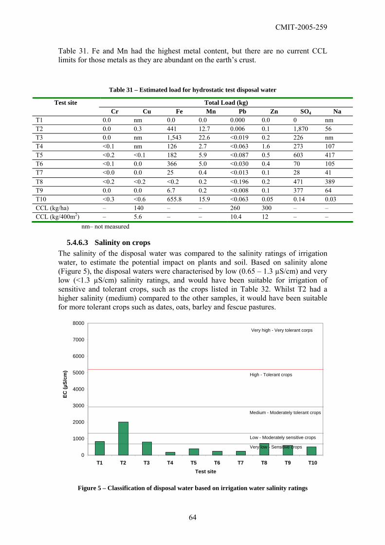
CMIT-2005-259

Table 31. Fe and Mn had the highest metal content, but there are no current CCL limits for those metals as they are abundant on the earth’s crust.

Table 31 – Estimated load for hydrostatic test disposal water

Total Load (kg) Test site Cr Cu Fe Mn Pb Zn SO4 Na

T1 0.0 nm 0.0 0.0 0.000 0.0 0 nm T2 0.0 0.3 441 12.7 0.006 0.1 1,870 56 T3 0.0 nm 1,543 22.6 <0.019 0.2 226 nm T4 <0.1 nm 126 2.7 <0.063 1.6 273 107 T5 <0.2 <0.1 182 5.9 <0.087 0.5 603 417 T6 <0.1 0.0 366 5.0 <0.030 0.4 70 105 T7 <0.0 0.0 25 0.4 <0.013 0.1 28 41 T8 <0.2 <0.2 <0.2 0.2 <0.196 0.2 471 389 T9 0.0 0.0 6.7 0.2 <0.008 0.1 377 64 T10 <0.3 <0.6 655.8 15.9 <0.063 0.05 0.14 0.03 CCL (kg/ha) – 140 – – 260 300 – – CCL (kg/400m2) – 5.6 – – 10.4 12 – –

nm– not measured

5.4.6.3 Salinity on crops The salinity of the disposal water was compared to the salinity ratings of irrigation water, to estimate the potential impact on plants and soil. Based on salinity alone (Figure 5), the disposal waters were characterised by low (0.65 – 1.3 µS/cm) and very low (<1.3 µS/cm) salinity ratings, and would have been suitable for irrigation of sensitive and tolerant crops, such as the crops listed in Table 32. Whilst T2 had a higher salinity (medium) compared to the other samples, it would have been suitable for more tolerant crops such as dates, oats, barley and fescue pastures.

0

1000

2000

3000

4000

5000

6000

7000

8000

T1 T2 T3 T4 T5 T6 T7 T8 T9 T10 Test site

EC (µ

S/cm

)

Very high - Very tolerant corps

High - Tolerant crops

Medium - Moderately tolerant crops

Low - Moderately sensitive crops Very low - Sensitive crops

Figure 5 – Classification of disposal water based on irrigation water salinity ratings

64

CMIT-2005-259

Table 32 – Examples of salt tolerance crops (ANZECC/ARMCANZ 2000)

Crop Common name Salinity threshold (EC µS/cm)

Apple 1000 Avocado 1300

Fruits

Dates 4000 Phasey bean, Murray 800 Corn 1700 Oats 5000

Grain

Barley (grain) 8000 Corn, forage 1800 Fescue 3900

Pasture

Barley (hay) 6000

5.4.6.4 Sodicity and salinity on soil High levels of sodium ions (Na+) in irrigation water can increase soil salinity and lead to sodicity problems in the soil. Sodicity occurs when the soil contains a high proportion of Na+ relative to other cations in the soil or water. Na+ is an exchangeable cation that acts as a dispersant. Sodium salts in soil can act as a coagulant or flocculant of soil particles making the soil more susceptible to erosion, restricting water entry and reducing water conductivity, causing salts to concentrate on the upper layers of the soil profile. The use of sodium based oxygen scavengers increases the sodium content in the disposal water as seen in Table 33. Estimates of sodicity levels in irrigation water can be calculated using the sodium adsorption ratio (SAR). In Table 34 the SAR was determined for all samples except T1 and ranged between 1.8 and 8.7. The overall impact depends on the disposal water composition and the soil characteristics (texture, clay content, structure, water holding capacity, conductivity, leaching factor, pH, etc.) The relationship between SAR and EC can give an indication of the impact of the disposal water on soil (Figure 6). Structural soil problems could develop if water of similar characteristics as samples T6 (SAR 2.54, 229 µS/cm), T7 (SAR 2.86, 241 µS/cm), T9 (SAR 8.7, 491 µS/cm) and T10 (SAR 2.71, 231 µS/cm) were used for continuous irrigation. A similar effect would have been observed for the source water of most of these samples (SAR 2.84, 212 µS/cm), (SAR 2.4, 200 µS/cm) and (SAR 2.97, 171 µS/cm) for T7, T9 and T10 respectively. Only sample T2 was identified as not affecting the soils structure, indicating the need for site specific evaluation in most cases. There should be noted that SAR guidelines assume frequent irrigation over a number of years, whilst, the case of hydrostatic test water disposal occurs as a single event.

65

CMIT-2005-259

Table 33 – Oxygen scavenger impact on ionic species

Test site T4 T5 T6 T7 T8 T9 T10 ∆Na 15.2 14.9 –1.7 –0.2 28 60 –1 ∆Ca 0.4 0 –18.6 –0.4 –18 0.6 1 ∆Mg 0 –0.2 –4.9 0 0 –0.5 0 O/S Na2S2O5 Na2S2O5 – – Na2S2O5 Na2SO3 –

Table 34 – SAR for disposal water

Test site T2 T4 T5 T6 T7 T8 T9 T10 SARsource – 1.47 1.83 1.90 2.84 3.49 2.4 2.97 SARdisposal 1.8 1.46 2.67 2.54 2.86 5.76 8.7 2.71 O/S NH4HSO3 Na2S2O5 Na2S2O5 – – Na2S2O5 Na2SO3 –

0

5

10

15

20

25

30

100 1000 10000

EC (µS/m)

SAR Source

Disposal

stable soil structure

depends onsoil properties and rainfall

soil structuralproblems likely

Figure 6 – Relationship between SAR and EC of EC water for prediction of structural soil

stability – adapted from ANZECC/ARMCANZ (2000)

5.4.6.5 Nutrients Nitrogen affects plants maturation and is essential, particularly during the early stages of plant growth. However, excess nitrogen leaches into groundwater or enter surface water bodies in run–off. Recommended limits based on health guidelines prescribe <50 mg/L NO3

- for infants, and <3 mg/L nitrite in drinking water (NHMRC/AWWA 1996). The LTV for nitrogen was set to ensure that there is no decrease in crop yield during flowering and fruiting stages (ANZECC/ARMCANZ 2000), the STV was set based

66

CMIT-2005-259

on suitable nitrogen levels for drinking groundwater and surface water. Nitrogen is more easily absorbed by plants when present as nitrate and/or ammonium. The total nitrogen concentrations found in disposal water (Table 27) were lower than the STV guidelines shown in Table 35. The concentrations in T2 and T3 were the highest, 110 mg/L and 27 mg/L respectively. These high values were essentially due to high ammonia concentration, requiring site specific assessment. The concentrations of the other disposal samples were <1 mg/L.

Table 35 – Recommended guidelines for N and P in irrigation water (ANZECC/ARMCANZ 2000).

Element LTV (mg/L) STV (mg/L) N 5 25–1251 P 0.05 0.8–12

The threshold for phosphorus concentrations is set at >0.05 mg/L (Foy & Withers 1995 in ANZECC/ARMCANZ 2000) at such levels it starts to affect sensitive streams and lakes. The P is adsorbed in the soil and made available for plant growth, but its environmental impact varies with soil retention and absorption condition, plant uptake, previous application of fertiliser and other ecosystem characteristics. The concentration of P in all the disposal waters was below the recommended STV guideline values and should be safe for use in irrigation.

5.4.7 Disposal options Disposal to aquatic systems requires assessment of the individual characteristics of each disposal site. The trigger values used for comparison in this study were based on average quality estimates for slightly disturbed systems, however the robustness of a specific ecosystem and the true impact of water disposal depend on the individual ecosystem characteristics such as background pollution, water level and seasonality. The discrepancy between site-specific systems and tabled values from guidelines were also highlighted by the nutrient content of the source waters being higher than the trigger values outlined in Table 28. The suitability of test waters to be disposed to aquatic systems is shown in Table 36. The major factor requiring consideration is the high turbidity caused by mill scale release, which can be treated by simple methods. On the other hand, pre–cleaning of the pipeline can have a significant effect on the water quality, as observed for T8 whose source and disposal waters were very similar and had a very low metal content, attributed to thorough pre–cleaning of the pipe with metal scrubbing pigs. In some cases, the allowable nutrient and DO levels may also have required further investigation of the receiving stream/lake/river, but these can generally be managed by selecting appropriate disposal methods. Disposal via irrigation onto land would also have been a suitable and more robust management technique (Table 37). For these tests DO correction would not be

67

CMIT-2005-259

required and the nutrient levels were too low to pose a risk to plant growth. The dissolved salts and ion contents in the disposal water were generally suitable for irrigation of moderately sensitive crops and their impact on soil salinity in some cases was low, however consideration of the specific soil properties at the disposal sites would be recommended. In regards to metal content, the major issue was the high iron concentration which could cause spotting of leaves on crops and blockage of irrigation equipment if used continuously. However this could be reduced by filtration or settling of the residues.

Table 36– Suitability for disposal of test water into aquatic bodies

Disposal water characteristics Test site pH DO EC NTU SO4 Cu Cr Fe Pb Mn Zn TN TP NOx NH4T1 nd Rec nd 90% <80% 99% <80% T2 nd Rec <80% 90% 95% <80% 80% T3 Rec nd 80% 80% <80% <80% T4 Rec <80% 80% 80% 99% <80% T5 Rec <80% 80% <80% 99% <80% T6 Rec <80% 80% <80% 95% <80% T7 Rec <80% 80% <80% 99% <80% T8 nd nd Rec <80% 80% <80% 99% <80% T9 nd Rec <80% 80% T10 nd Rec <80% 80%

Green – Within guidelines; Red – Does not fulfil guidelines, requires further investigation Yellow – Within guidelines depending on ecosystem characteristics, requires further investigation. White – No recommended guidelines. nd –not determined.

Table 37 – Suitability for use of test water for irrigation

Disposal water characteristics Test site pH DO EC NTU SO4 Cu Cr Fe Pb Mn Zn TN TP NOx NH4 SAR

T1 VL nd Rec nd nd T2 M nd Rec nd T3 L nd Rec nd nd T4 VL nd Rec nd T5 VL nd Rec nd T6 VL nd Rec nd T7 VL nd Rec nd T8 L nd Rec nd T9 VL nd Rec nd T10 VL nd Rec nd

Green – Within guidelines; Red – Does not fulfil guidelines, requires further investigation Yellow – Within guidelines depending on ecosystem characteristics, requires further investigation. White – No recommended guidelines. nd –not determined. Changes to water quality during hydrostatic testing can only occur if substances are introduced into the pipe, via the fill water and its additives; if residues on the pipe walls, such as mill scale, breakdown, or if reactions within the pipe occur, such as formation of by–products from the oxygen scavenger reaction.

68

CMIT-2005-259

The tests indicated that oxygen scavenger concentrations (when used) were sufficient to suppress DO in the pipe, and the excess was reactive after the conclusion of the test period. The selection of additives also affects water composition, as test waters will contain the by–products from the oxygen depletion reaction. The major by–products of oxygen scavenger decomposition were sulphate, sodium sulphate and acids, but these were present only in low concentrations (ppm range). Oxygen scavenger by–products and low DO can be neutralised by aeration of the water, however use of biocides, which is becoming less common, would require inactivation by a specific treatment. A large number of disposal water properties are dictated by the original properties of the source water, such as nutrient content, salinity and the concentration of certain metals and ions (B, Ar, Cd, Co, Ca, Mg, Cl). Residues in the pipe are also generated from reactions with the pipe material. Mill scale breakdown was the main factor responsible for the increase of metal residues in the water. For the field tests analysed, the method used for disposal of the water included:

• Discharge to rivers. • Discharge to farm dams. • Holding ponds for reuse by other industry. • Reuse in another test section. • Land disposal.

Aeration was used for oxygen scavenger neutralisation and oxygenation, geofabric filtration was used for sediment removal and hay barriers for erosion mitigation when deemed suitable for each case.

5.4.8 Summary Samples of disposal water for the 10 test sites were analysed for water quality and compared with general guidelines for irrigation and aquatic ecosystems to illustrate their potential impact on the environment. The study focused on newly constructed onshore pipelines that were tested either with water alone or with water and an oxygen scavenger. Water was sourced from rivers, municipal town supply or bore and from a previous test. None of the samples tested contained biocides. This study has elucidated that:

1. The major contributor to the characteristics of the disposal water was the quality of the source water.

2. Turbidity increase due to iron compounds was the principal change verified after the test. It was not a significant risk to land or marine ecosystems and can be readily managed, but it needs to be considered and in some cases managed to avoid a reduction in light transmission and any detrimental impact to aquatic life.

3. Dissolved oxygen in the disposal water was low, and needed to be increased upon disposal to aquatic systems.

69

CMIT-2005-259

4. Excess oxygen scavenger is readily deactivated by aeration, and the water is readily re–oxygenated by the same method.

5. The oxygen scavenger contributes to Na (depending on the type of scavenger used), sulphate and to the overall total dissolved salts (TDS) levels – The quantity of scavenger should be designed based on the stoichiometric quantity plus a small residual – excessive addition does not improve corrosion control, but does increase TDS;

6. Pipe manufacture and pipeline construction do not introduce significant levels of plant or aquatic nutrients into the hydrostatic test water;

7. The concentration of Zn, Cu and Mn was higher than the trigger values for aquatic systems in some of the samples, warranting further investigation of the ecosystem tolerance and site specific conditions of any waterway used for disposal.

8. If the source water is heavily contaminated, or if the water must be treated with biocide the conclusions from this testing are not relevant, and project specific testing is required to determine the contaminant level and the treatment process.

9. In regards to disposal options, land or aquatic disposal can be pursued. The robustness of the receiving ecosystem and the compatibility between the disposal water characteristics and the disposal site are the main factors that need to be considered.

The analysis conducted is not an absolute assessment as the impact depends on the specific characteristics of the receiving ecosystem, its degree of disturbance and the disposal strategy. The present assessment does not consider many of the mitigation factors encountered in actual situations, such as speciation of metals into immobile species and hence it illustrates a potential worst case scenario.

70

CMIT-2005-259

6 Treatment of Disposal Water

6.1 Pre–treatment of pipeline and source water

Pre–treatment reduces the contaminant levels of the outlet stream by reducing the contaminant levels in the source water and/or in the inside of the pipe. By removing residues and debris which could have accumulated during construction, sites that can harbour bacteria are reduced and significant reduction in the amount of sediment collected during the disposal of water can be achieved. A number of pre–treatment options can be employed. Pigging and an initial flush or pre–clean are the most common pre–treatment techniques adopted prior to hydrostatic testing.

• Pigging Pigging consists of pushing a pig through the pipeline with air or natural gas before filling with test water. Various types of pigs such as squeegee, brush, or wire may be used individually or in combination in single or multiple passes (API 1998). Pigging assists in the removal of debris, dirt and even mill scale from the inside of the pipe surface. Tallon et al (1992b) estimated that pre–pigging with direct discharge to land would cost US$1.82/gallon for a 10,000 gallon discharge down to US$0.04/gallon for discharges of 1,000,000 gallons.

• Pre–cleaning/flushing A relatively small volume of water or cleaning solution is placed between two pigs and forced with natural gas or another fluid along the length of the pipe. This pre–cleaning technique is intended to collect the majority of the debris, condensate and/or benzene, toluene, ethylbenzene, and xylene (BTEX), deposited in the line during construction or operation (Tallon et al 1992b). Test section T8 was pre–cleaned with power brush pigs and air cleaning before filling resulting in very low metal residues in the discharge water (Hickling 2004).

• Inlet Filters Filtering of source water and/or supporting the inlet hose above the sediment layer in the water can be a valuable practice for reducing inlet contaminants, and hence outlet contaminants, particularly if the water source has a high level of suspended solids (Tallon 2002)(API 1998). Filtration of source water for removal of particulate matter larger than 50µm diameter to <80 mg/L is commonly practiced by companies such as Santos (Santos 2002).

6.2 Treatment of discharge water

Hydrostatic test disposal water can contain a large range of residues: additives, dirt, lunch boxes, rags and metal scrap added involuntarily as a result of pipeline construction, contaminants from previous pipeline operation (oil or gas residues) and those generated due to reactions within the pipe (e.g. by–products from oxygen scavenger decomposition).

71

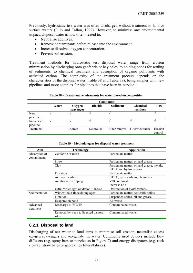
CMIT-2005-259

Previously, hydrostatic test water was often discharged without treatment to land or surface waters (Fillo and Tallon, 1992). However, to minimise any environmental impact, disposal water is now often treated to:

• Neutralise additives. • Remove contaminants before release into the environment. • Increase dissolved oxygen concentration. • Prevent soil erosion.

Treatment methods for hydrostatic test disposal water range from erosion minimisation by discharging onto geofabric or hay bales, to holding ponds for settling of sediments, to chemical treatment and absorption of organic pollutants with activated carbon. The complexity of the treatment process depends on the characteristics of the disposal water (Table 38 and Table 39), being simpler with new pipelines and more complex for pipelines that have been in–service.

Table 38 – Treatment requirements for water based on composition

Compound Water Oxygen

scavenger Biocide Sediment Chemical

residues Flow

New pipeline

√ √ √ √ √

In–Service pipeline

√ √ √ √ √ √

Treatment Aerate Neutralise Filter/remove Filter/neutralise Erosion control

Table 39 – Methodologies for disposal water treatment

Aim Technology Application Absorption of contaminants

Geofabric or mesh Particulate matter

Straw Particulate matter, oil and grease Clay Particulate matter, oil and grease, metals,

BTEX and hydrocarbons. Filtration Particulate matter Activated carbon BTEX, hydrocarbons, chemicals Aeration/air stripping VOC removal

Increase DO Ultra–violet light oxidation + H2O2 Destruction of hydrocarbons Sedimentation With/without flocculating agent Particulate matter, settleable solids Flotation Suspended solids, oil and grease Evaporation pond All waste. Advanced treatment

Discharge to WWTP Contaminated waste.

Removal by truck to licensed disposal sites

Contaminated waste.

6.2.1 Disposal to land Discharging of test water to land aims to minimise soil erosion, neutralise excess oxygen scavengers and oxygenate the water. Commonly used devices include flow diffusers (e.g. spray bars or nozzles as in Figure 7) and energy dissipaters (e.g. rock rip–rap, straw bales or geotextiles filters/fabrics).

72

CMIT-2005-259

Figure 7 – Spray nozzles used for disposal of hydrostatic test water in Moomba–Sydney Binerah

Downs (Courtesy of Max Kimber, 2004).

Figure 8 – Aerial view of hydrostatic test water sprayed in Moomba–Sydney Binerah Downs

(Courtesy of Max Kimber, 2004).

6.2.2 Hay Bales A survey conducted by American Petroleum Institute (Tallon et al 1992b) found that hay bales were the most used filter treatment for water from new pipelines in the USA. Directing the water stream into a hay wall (Figure 9) or a circular or rectangular hay pen (Figure 10) minimises soil erosion (Williams, 1995), oxygenates water and assists in the removal of suspended solids and particulate matter, but it is not suitable for removal of organic volatiles (Tallon et al 1992a).

73

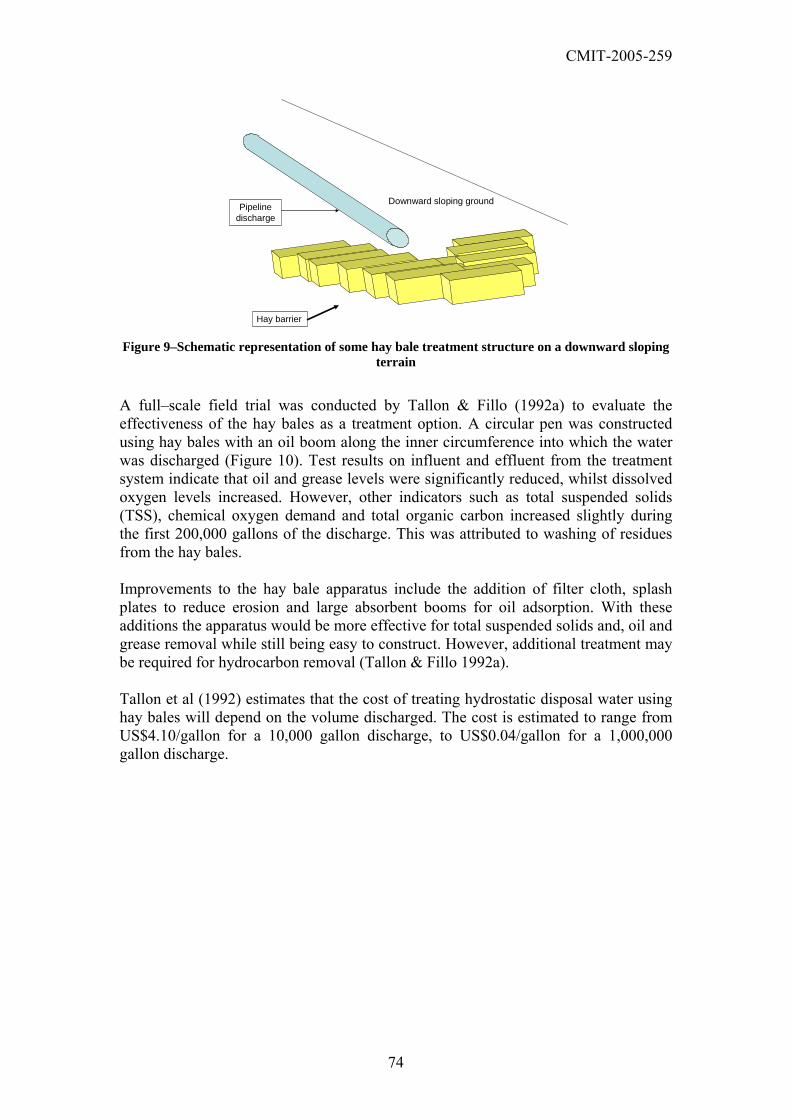
CMIT-2005-259

Hay barrier

Pipeline discharge

Downward sloping ground

Figure 9–Schematic representation of some hay bale treatment structure on a downward sloping terrain

A full–scale field trial was conducted by Tallon & Fillo (1992a) to evaluate the effectiveness of the hay bales as a treatment option. A circular pen was constructed using hay bales with an oil boom along the inner circumference into which the water was discharged (Figure 10). Test results on influent and effluent from the treatment system indicate that oil and grease levels were significantly reduced, whilst dissolved oxygen levels increased. However, other indicators such as total suspended solids (TSS), chemical oxygen demand and total organic carbon increased slightly during the first 200,000 gallons of the discharge. This was attributed to washing of residues from the hay bales. Improvements to the hay bale apparatus include the addition of filter cloth, splash plates to reduce erosion and large absorbent booms for oil adsorption. With these additions the apparatus would be more effective for total suspended solids and, oil and grease removal while still being easy to construct. However, additional treatment may be required for hydrocarbon removal (Tallon & Fillo 1992a). Tallon et al (1992) estimates that the cost of treating hydrostatic disposal water using hay bales will depend on the volume discharged. The cost is estimated to range from US$4.10/gallon for a 10,000 gallon discharge, to US$0.04/gallon for a 1,000,000 gallon discharge.

74

CMIT-2005-259

Figure 10 – Hay bale treatment apparatus (Tallon et al 1992a)

6.2.3 Evaporation Ponds Spent test water can be discharged into evaporation ponds or farm dams. The water then evaporates leaving behind the non–volatile contaminants. A liner is used to prevent migration of the water into the surrounding soil and it also acts as a collection tool for the sludge which remains after evaporation. The liner and sludge are removed and disposed of (Williams 1995). Tallon estimated that this method of disposal/treatment would cost US$2.61/gallon for a 10,000 gallon discharge, US$0.74/gallon for a 100,000 gallon discharge. However, this method was most impractical for discharges of 1,000,000 gallons which would require in excess of 1 year for evaporation to occur (Tallon et al 1992a). In Australia, water reuse is generally preferred over simple evaporation.

75

CMIT-2005-259

6.2.4 Flotation Flotation can be a useful method of removing suspended solids and, emulsified oil and grease. The air bubbles produced attach to suspended particles imparting buoyancy and floating them to the top, where they can be removed by skimming. Removal rates of up to 97% for TSS and, oil and grease can be achieved. This can be increased with the use of flocculating and coagulating agents. However, flotation is not effective for the removal of organic contaminants and VOC’s, and has a high capital cost (Table 41) (API 1998).

6.2.5 Sedimentation After discharge, hydrostatic test disposal water is allowed to rest in a pond or tank to allow suspended components to settle at the bottom of the tank (Figure 11). This can be achieved in one of two modes:

a) Gravity sedimentation (without flocculating agent) – Gravity sedimentation requires significant intervals of time for sedimentation to occur. (Tallon et al 1992). Analytical results indicated that sedimentation without a flocculating agent requires settling times greater than 24h to achieve a reasonable level of suspended solids removal.

b) Gravity sedimentation with a flocculating agent – Gravity sedimentation using either alum (aluminium sulphate) or ferric chloride was able to remove suspended material and iron to levels near detection limits (Tallon et al 1992a). Optimum floc formation pH levels for alum and ferric chloride were between 6, 8 to 9 and 7 to 8 respectively. At optimum pH levels, high removal efficiencies for TSS and iron were achieved at flocculating agent concentrations in the order of 50 mg/L in 30 min. As flocs settle they also remove some hydrocarbons, oil and grease. The sediment residue needs to be disposed of afterwards.

Disposal water

Settled sediment

Pond or tank

Figure 11 – Diagram of sedimentation process.

6.2.6 Filtration Hydrostatic test water can be treated by straining or filtering through geofabric for particulate removal or using a pressure filter container. The bag filters can be operated in series or parallel to handle a variety of flow rates and water quality levels. The filters contain a canister that holds a fibre sock (Tallon et al 1992a). Socks are able to filter a range of particle sizes and specialised absorbent socks are also able to remove oil and grease from the stream (Williams 1995). Filters are labour intensive as they require periodic cleaning for sludge removal. Also the high flow rates required for efficient discharge will require often multiple filter streams (Tallon et al 1992a). An

76

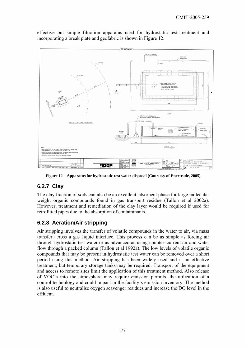
CMIT-2005-259

effective but simple filtration apparatus used for hydrostatic test treatment and incorporating a break plate and geofabric is shown in Figure 12.

Figure 12 – Apparatus for hydrostatic test water disposal (Courtesy of Enertrade, 2005)

6.2.7 Clay The clay fraction of soils can also be an excellent adsorbent phase for large molecular weight organic compounds found in gas transport residue (Tallon et al 2002a). However, treatment and remediation of the clay layer would be required if used for retrofitted pipes due to the absorption of contaminants.

6.2.8 Aeration/Air stripping Air stripping involves the transfer of volatile compounds in the water to air, via mass transfer across a gas–liquid interface. This process can be as simple as forcing air through hydrostatic test water or as advanced as using counter–current air and water flow through a packed column (Tallon et al 1992a). The low levels of volatile organic compounds that may be present in hydrostatic test water can be removed over a short period using this method. Air stripping has been widely used and is an effective treatment, but temporary storage tanks may be required. Transport of the equipment and access to remote sites limit the application of this treatment method. Also release of VOC’s into the atmosphere may require emission permits, the utilization of a control technology and could impact in the facility’s emission inventory. The method is also useful to neutralise oxygen scavenger residues and increase the DO level in the effluent.

77

CMIT-2005-259

Tallon estimated that spray aeration to land would cost US$3.04/gallon for a 10,000 gallon discharge and US$0.14/gallon for discharges of 1,000,000 gallons (Tallon et al 1992a).

6.2.9 Activated carbon Activated carbon is a relatively inert, highly porous material, which adsorbs organic compounds via physical attractive forces. This method is particularly effective for removal of organic molecules such as benzene, xylene and toluene that are generally more adsorbable than inorganic molecules due to their non–polar nature, low solubility in water (Naderi and Moayed 2004, Oil and Gas 1995). This methodology is primarily used for treatment of disposal water from recommissioned pipes due to the effectiveness in removing hydrocarbons, BTEX, but it is also effective for removal of biocide residues (Chen & Chen 1997). An American survey established that that activated carbon was the single most utilized treatment technology for existing pipelines, used during 30.5% of the hydrostatic tests on existing lines in the USA (Tallon et al 1992a). Activated carbon adsorption requires pumping the hydrostatic test water through one or more parallel columns packed with activated carbon (Tallon et al 1992a). An oil/water separator is typically installed in front of the packed column to remove free oil from the test water. While the effectiveness of this treatment is very good, multiple columns are often needed to provide the desired flow rate for discharge and/or temporary storage tanks may be required. Access to and transportation of the treatment apparatus may prove difficult depending on the location of the discharge (Tallon et al 1992a). Tallon et al states that the cost of treating spent test water using carbon adsorption depends on the discharge volume (1992a). The cost is estimated to range from US$3.61/gallon for a 10,000 gallon discharge, to US$0.13/gallon for a 1,000,000 gallon discharge.

6.2.10 Discharge to a public water treatment facility Discharge to a public water treatment facility is often a desirable option for highly contaminated water from retrofitted pipes, or for high salinity water. However, this may not always be logistically possible, due to remote location or if the volume of discharge water exceeds the capacity of the facility. Generally, wastewater treatment facilities are designed for biological waste and if the disposal water contains biocide, pre–treatment may be required before entry into the plant to prevent disruption to biological processes (Williams 1995).

6.2.11 Removal by truck This is an expensive practice in which spent hydrostatic test water is stored in polyethylene lined ponds and then transported by truck to a licensed disposal site. This method of disposal is generally only applied when necessary, i.e. for water with biocides or heavily contaminated water from testing of retrofitted pipelines (Tallon et al 1992a).

78

CMIT-2005-259

The economic feasibility of this method varies with wastewater characteristics and volume. Tallon estimated that this method of disposal/treatment was the cheapest of all methods investigated for small volumes, costing US$1.01/gallon for a 10,000 gallon discharge. However, Tallon also reported that this method was the most expensive for discharges of 1,000,000 gallons, at US$0.35/gallon.

6.2.12 Ultra–violet light oxidation In this method, dissolved organic compounds are oxidized by exposure to high intensity UV light in the presence of hydrogen peroxide. The combination promotes rapid breakdown into CO2 and H2O. An advantage of this system is that there are typically no hazardous air emissions. However this technique requires prior removal of suspended solids etc and is prone to scale fouling of the lamps. In general, this technique is impractical for the liquid pipeline industry (Tallon et al 1992a)

6.2.13 Cost comparison Figure 13 and Table 40 shows costs for an unspecified range of treatment technologies for new and existing pipelines. Table 41 gives additional cost estimates for six of the above treatment technologies. Table 42 identifies the positive and negative aspects of seven of the treatment technologies described above. For in–service pipelines that carried hydrocarbon or BTEX the most promising techniques are pigging and pre–cleaning, activated carbon adsorption, hay bales or a combination of these options. Where practicable and when dealing with retrofitted pipelines, reuse of test water for multiple tests will minimize the volume of water that needs to be treated and improve removal effectiveness. Recycled test water could be reused indefinitely while there is an ongoing need. While water quality diminishes over time with reuse, this should not be a problem if (upon discharge) the water is properly treated. However, multiple tests will place added constraints on disposal and an assessment will be required to determine if the lower water requirements and the cost of treatment at disposal are advantageous.

79

CMIT-2005-259

Figure 13 – Cost of treatment technologies (API 1998)

Table 40 - Summary of costs in the USA grouped by treatment range (API,1998)

Pipe ID Treatment technology No. tests

Range of volume discharged

(m3)

Cost per gallon

(US cents)

Weighted average cost

for group (US$/m3)

New A

Hay bales, Filter screens, Not reported, Tank pre-cleaning

8 0.25 -25,915 <1 0.42

Existing B

Discharge to refinery WWTP or other indirect industrial discharge, Hay bales, Carbon adsorption, Tank separation, No treatment, Tank Separation

28 48.21 – 63,595 <1 0.92

Existing C Carbon adsorption, air stripping, carbon adsorption and air stripping, not reported 19 734.52 - 120,830 1 to < 5

6.23

Existing D Carbon adsorption, Carbon adsorption with hay bales 7 1431- 9062 5 to <10 16.70

Existing E Carbon adsorption 9 4.54 -159 10 to <25 37.51 Existing F Carbon adsorption 2 238 -3180 25 to <50 90.80

80

CMIT-2005-259

81

Table 41 – Cost estimates for six treatment technologies (API 1998)

Summary of Capital/operating Cost Estimates For Treatment Technologies

(See page 5-5 of API 1998 for assumptions made in developing cost estimates)

Capital Operating Estimates (¢/gal) Pre-Pigging and Pre-Cleaning

100,000 Gallons US$6,300 US$5,948 12.25 1,000,000 Gallons US$6,300 US$5,948 1.22 10,00,000 Gallons US$7,715 US$11,175 0.18

Hay Bales/HRT System

100,000 Gallons US$10,080 US$25 10.11 1,000,000 Gallons US$11942 US$250 1.22 10,00,000 Gallons US$11942 US$250 0.122

Carbon Adsorption

100,000 Gallons US$78,831 US$544 79.38 1,000,000 Gallons US$78,855 US$702 7.96 10,00,000 Gallons US$281,258 US$1,790 2.83

Air Stripping

100,000 Gallons US$96,860 US$540 97.40 1,000,000 Gallons US$144,395 US$540 14.50 10,00,000 Gallons US$144,395 US$1,890 1.46

Dissolved Air Flotation

100,000 Gallons US$286,884 US$529 287.00 1,000,000 Gallons US$286,884 US$529 28.70 10,00,000 Gallons US$286,884 US$5,908 2.93

Ultra Violet Oxidation

100,000 Gallons US$423,976 US$544 424.00 1,000,000 Gallons US$423,976 US$540 42.40 10,00,000 Gallons US$423,976 US$8,976 4.33

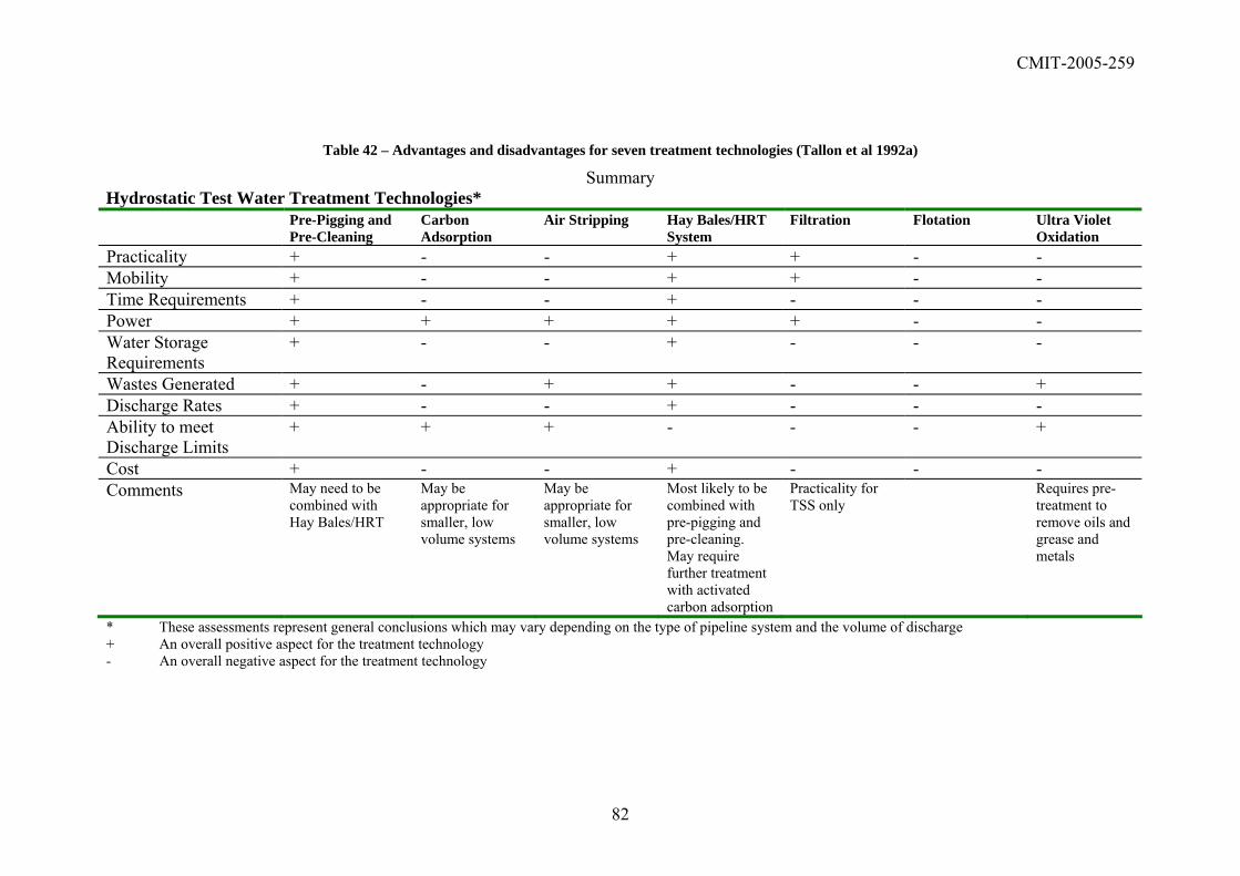
CMIT-2005-259

82

Table 42 – Advantages and disadvantages for seven treatment technologies (Tallon et al 1992a)

Summary Hydrostatic Test Water Treatment Technologies* Pre-Pigging and

Pre-Cleaning Carbon Adsorption

Air Stripping Hay Bales/HRT System

Filtration Flotation Ultra Violet Oxidation

Practicality + - - + + - - Mobility + - - + + - - Time Requirements + - - + - - - Power + + + + + - -Water Storage Requirements

+ - - + - - -

Wastes Generated + - + + - - +Discharge Rates + - - + - - -Ability to meet Discharge Limits

+ - - + + + -

Cost + - - + - - - Comments May need to be

combined with Hay Bales/HRT

May be appropriate for smaller, low volume systems

May be appropriate for smaller, low volume systems

Most likely to be combined with pre-pigging and pre-cleaning. May require further treatment with activated carbon adsorption

Practicality for TSS only

Requires pre-treatment to remove oils and grease and metals

* These assessments represent general conclusions which may vary depending on the type of pipeline system and the volume of discharge + An overall positive aspect for the treatment technology - An overall negative aspect for the treatment technology

CMIT-2005-259

6.2.14 Experimental investigation of treatment alternatives Selection of the treatment methodology depends on the characteristics of the hydrostatic test water, requirements of the disposal permit and the alternatives available onsite. The discharge water from each tests site evaluated was treated as shown in Table 43.

Table 43 – Treatment of disposal water

Test site Treatment T1 Discharge onto land (low volume of water). T2 Water pumped to a holding tank for reuse in the next test section. T3 Water untreated and discharged to a holding pond for future treatment. T4 Water filtered with geofabric and returned to source river. T5 Water filtered with geofabric and returned to source river. T6 Water filtered with geofabric and returned to source river. T7 Water filtered with geofabric and returned to source river. T8 Water aerated and discharged to a holding pond. T9 Water aerated and retained in farm dam. T10 Water untreated and discharged to a holding pond.

Samples of disposal water were treated in the laboratory to evaluate the effectiveness of common treatment methods. Samples were subjected to treatment by the following techniques:

a) Aeration A sample of the discharge water from test T9 was aerated in the lab for 1 hour to analyse the resultant increase in DO. Sample T9 consisted of river water and oxygen scavenger Chemtreat 649L, added at a ratio of 1.5:1000 v/v (active ingredient sodium sulphite approximately 0.15–0.45 kg/1000 L or sufficient to react with 17–50 ppmO2) (Appendix 1). Air was delivered via a hose to the bottom of a 500 mL beaker with 500 mL hydrostatic test water for 1h. DO was checked before and after treatment to ensure effective to neutralisation of any unreacted oxygen scavenger. The initial DO after a 10 day hydrostatic test was 0 mg/L, but after aeration DO increased to 4.6 mg/L. The 100% saturation level for DO at the test temperature of 20°C is approximately 9 mg/L. Aeration (exposure to oxygen) is also an effective method to remove iron from water. Ferrous iron (Fe2+) is soluble in water, however it oxidises in presence of oxygen to form ferric iron (Fe3+) which complexes and settles as ferric hydroxide (Figure 14). Oxidation of ferrous iron to ferric iron.

4Fe2+(aq) + O2(g) + 4H+

(aq) ---> 4Fe3+(aq) + 2H2O(l)

Formation of ferric hydroxide from ferric iron.

4Fe3+(aq) + 12 H2O(l) ---> 4Fe(OH)3(s) + 12H+

(aq)

Figure 14 – Oxidation of ferrous iron to ferric hydroxide

83

CMIT-2005-259

84

b) Settling for 1, 24 and 48 hr

Samples of disposal water were allowed to settle for periods of 1 hr, 24 hr and 48 hr resulted in separation of the coloured residues to the bottom of the flask and a clearer supernatant on the surface. By allowing samples to settle the turbidity and colour improved over periods > 24 hr for all of the samples received (Figure 15). Alteration of pH did not result in any significant reduction in the time taken for settling to occur. Settling periods of approximately 12–24 hr were required.

Figure 15 – Water samples before and after settling for 48 hours for T10.

c) Filtration

Filtration was performed with GF–A filter paper (pore diameter 1.6 µm). Filtra sample from T9 removed sediment and particles from the sample including the iron originally detected in the initial sample.

d) Acidification and filtration The filtrate from (c) was acidified with HNO3 to pH <3 and refiltereconcentration of dissolved iron in the final filtrate was below detection limits (Table 44). However disposal of the water would not be allowed with pH <6 ( Table 44), requiring neutralisation. The laboratory sample was neutraliseNaOH. Double filtration and alteration of pH aided in the removal of iron compoundsmg/L) but the solution would have required further pH correction before dCorrection of pH with NaOH increases the amount of dissolved salts in the swhilst addition of lime increased the volume of sludge that had to be removeddisposal.

e) Addition of flocculant (Ca(OH)2) The addition of Ca(OH)2 raise’s solution pH and promotes the formation of floiron particles, promoting their sedimentation. This method resulted inflocculation and sedimentation, however it tripled the volume of sludge compsettling of the residue without any additives. Additionally, as the method raisesof the water pH monitoring and potentially neutralisation may be requireddischarge.

Flush Flush Flush Flush Flush Disposal Disposal Disposal

Source

ation of 77% of

d. The

d with

(Fe <1 isposal. olution before

cs with rapid ared to the pH before

CMIT-2005-259

Table 44 –Effect of treatment on water quality

Treatment Parameter untreated Filtration Filtration + acid

+ filtration + NaOH

Filter Residue (mg/L) – 33.3 1.6 – pH 6.50 7.78 2.93 7.16 S (mg/L) 4.00 5.00 4.00 4.00 Fe (mg/L) (in soln) 8.60 3.00 <1 <1 Mn (mg/L) 0.30 0.12 0.24 0.21 Cd (mg/L) <0.02 <0.02 <0.02 <0.02 Co (mg/L) <0.01 <0.01 <0.01 <0.01 Cu (mg/L) <0.02 0.09 1.13 0.89 Cr (mg/L) <0.05 <0.05 <0.05 <0.05 Pb (mg/L) <0.01 <0.01 0.01 <0.01 Zn (mg/L) 0.07 <0.1 0.60 0.40 Ca (mg/L) 4.80 5.40 6.30 5.30 Cl (mg/L) 50.00 80.00 70.00 70.00 Mg (mg/L) 5.60 6.00 7.00 6.00 Na (mg/L) 26.00 34.00 32.00 57.00 K (mg/L) 1.90 3.00 4.00 5.00

In summary, for elimination of unreacted oxygen scavenger, aeration is a simple and effective method as observed in the field. Aeration also assists in the removal of ferrous iron as it oxidises it to ferric iron which is a solid. Whilst the colour of the disposal water varied among the tests, the residues in the samples tended to settle between 24 and 48 hr. The residue was composed mainly of iron salts. The remaining solution was clearer and less turbid than the original samples. Filtration was effective for the removal of particulate matter. However, large volumes of contaminants will cause clogging and loss of performance requiring frequent maintenance and replacement of filters. More complex filtration systems such as ion exchange have also been reported to be effective for removal of ferrous compounds but they are more costly. The addition of Ca(OH)2 as a flocculant resulted in rapid removal and settling of sediment, but the method produces a high volume of sludge that also requires disposal.

85

CMIT-2005-259

7 Final remarks Disposal water from ten hydrostatic pressure tests on new steel pipelines conducted in Australia were analysed for metal contaminants, salts, nutrients and other species which might have a detrimental environmental impact upon disposal. Source waters prior to and after the incorporation of additives were also analysed. The following conclusions were made:

a) Source water is the main source of nutrients (NOX, NH4+ and P), metals such as Ar, Cd, Co, Mn, I, inorganic salts, sand/soil and ionic species such as SO4

2-, Cl, Ca, Mg.

b) Fe, Mn and Zn were the most abundant elements detected. These metal residues enter the water during hydrostatic testing primarily through breakdown of mill scale.

c) Residues from oxygen scavengers contributed to an increase in salts of sulphur, ammonia or sodium, depending on the formulation of the scavenger;

d) Disposal water was free of oil and grease. This was expected as these were new pipelines.

e) Pre–cleaning of the pipe removed mill scale and sediment in the pipe, reducing the amount of debris collected during disposal.

The principal factor that determined the quality of the disposal waters was the quality of the source water. The characteristics of source waters generally varied independently of source type. However;

a) Mains water had less colour and turbidity than the natural sources (rivers and bore well), but showed no other distinguishing features.

b) The reused water had the greatest concentration of metal residues and total nitrogen. This was expected as it contained the metal and oxygen scavenger residues from a previous hydrostatic test.

The quality of the disposal waters was verified to be:

a) Within water quality guidelines for pH. b) Often of low dissolved oxygen. This was easily corrected by aeration or

spraying of the water. c) Low in nutrients. d) Variable salt content. T2 displayed a particularly high EC value. e) Low heavy metal content, mostly below detection limits. The heavy metal

content was mainly attributed to the source water. Heavy metal contribution from the pipe material was not significant.

f) The major metal detected was iron in the form of various oxides and hydroxides. These can be removed by aeration and sedimentation.

g) Highly turbid, but sediments tended to settle after 24h improving the colour and reducing turbidity significantly.

86

CMIT-2005-259

8 Overall conclusions The research described in this report aimed to:

a) To investigate the technical and environmental aspects of supply, discharge and disposal of water used for hydrostatic testing of pipelines;

b) To establish and document the constraints on the process and their management;

c) To monitor the effect of different water sources and changes to water quality during testing on disposal water quality and its impact on the environment.

d) To review practices used worldwide for benchmarking and investigate procedures commonly used for test water disposal to minimise the risk of adverse impacts to the environment.

e) To provide the basis for a chapter in the APIA Code of Environmental Practice on hydrostatic test water sourcing, treatment and disposal.

The research has shown that:

f) Discharged water contains contaminants that may require treatment prior to disposal;

g) For new pipelines disposal water contaminants are mainly due to mill scale breakdown e.g. iron oxides and traces of manganese and copper. Unreacted additives and their reaction products e.g. inorganic salts when oxygen scavengers are used.

h) The contaminant levels in the disposal water were generally not toxic.

i) For most new pipelines and most water sources treatment is required to lower turbidity and to raise DO levels.

j) Organisations planning hydrostatic testing must plan the water disposal, both in the selection of the source water (if possible), and developing a treatment program for the water prior to disposal.

k) Care is necessary to develop a minimum treatment program.

l) The characteristics of the disposal site play a large role in determining the treatment required.

m) Lining of pipelines would avoid mill scale breakdown, residue formation and so remove most pipe related contamination, reducing suspended solids and simplifying turbidity control

n) In–service pipelines require more specific treatment programs for residues from the compounds previously transported. However hydrostatic testing of in–service pipelines is not common in Australia. Documented management strategies for the treatment of such disposal waters exist in the industry and literature.

87

CMIT-2005-259

o) Special planning is required when specifying treatment programs that require biocide, and when selecting water sources that in themselves present a disposal problem (high salinity, SRB presence, sewerage effluent, etc).

p) Discharge of hydrostatic water is a one–off event and needs to be considered as such when evaluating its environmental impact and comparing to data from guidelines.

88

CMIT-2005-259

9 References American Petroleum Institute (1997), Pressure Testing of Liquid Petroleum Pipelines, American Petroleum Institute Recommended Practice 1110. (API, 1997) American Petroleum Institute, (1998), Hydrostatic Test Water Treatment and Disposal Options for Liquid Pipeline Systems, American Petroleum Institute Publication 1157, prepared by R.A.Bausell, B.Wendrow and B.I. Schmidt. (API 1998) American Society of Mechanical Engineers (2004) ASME B31.8–2003 Gas Transmission and Distribution Piping Systems ANZECC/ARMCANZ (2000) Australian and New Zealand Guidelines for Fresh and Marine Water Quality (2000), http://www.ea.gov.au/water/quality/nwqms/index.html. APHA (2001) Standard Methods for the Examination of Water and Wastewater, APHA/AWWA/WEF, USA. AWWA–TZW (1996) Internal Corrosion of Water Distribution Systems, American Waterworks Association Research foundation and DVGW–Technologiezentrum Wasser, 2nd Edition, Denver, USA. Australian Pipeline Industry Association Inc., (unknown), Code of environmental practice – onshore pipelines, Australian pipeline industry association inc. (APIA, unknown) Avecia, (2004), Vantocil technical brief, http://www.avecia.com/biocides. Baker Petrolite (2003), personal communication. British Standards Institution (2003), BS EN 14161:2003 – Petroleum and natural gas industries– Pipeline transportation systems. Bluescope Steel (2004a) http://www.bluescopesteel.com.au/au/index.cfm/objectID.3A958FE5–7619–4878–908AA654D70450BC (Tasmania Natural Gas Pipeline). Bluescope Steel (2004b) http://www.bluescopesteel.com.au/au/index.cfm/objectID.FF4C72FB–OC51–472E–8CB451FF7E63136D (Eastern Gas Pipeline), Bluescope Steel. Bluescope Steel (2004c) http://www.bluescopesteel.com.au/au/index.cfm/objectID.6139CF8D–7A93_45DA–B2B48E308F9463 (Roma Looping X80 Pipeline). Bruderly, L.M., Halapin, T.A. and Fillo, J.P. (1992) Report No. GRI–92/0126.2: Regulations associated with the hydrostatic testing of natural gas pipelines, volume 2, US Department of Commerce – National Technical Information Service.

89

CMIT-2005-259

Chen, E.Y. and Chen R.B., (1997), Wet Lay–Up Fluid: Can it be both corrosion preventive and environmentally friendly?, Proceedings of the SPE/EPA Exploration & Production Environmental Conference, pp. 83–92. DE (2004), WA Department of Environment, Mr.P.Byrnes, personal communication. DEC (2004), Department of Environment and Conservation NSW, personal communication. DIPE (2004) Department of Infrastructure, Planning and Environment, www.ipe.nt.gov.au. DNRM (2004), Department of Natural Resources and Mines, Ms. S.McFadyen, personal communication. DPIWE (2004), Department of Primary Industries, Water and Environment, Ms.K.Bull, personal communication. De Rose, P.J. and Parkinson, R.W. (1985) Corrosion and Protection of Ductile Iron Pipe, Proceedings from the 6th International conference on the internal and external protection of pipes, Nice, France, Nov., 249. Eiceman, G.A., Leasure, C.S., Baker, B.D., (1983), Characterization of Discharge Water from Hydrostatic Testing of Natural Gas Pipelines Using High Resolution Gas Chromatography/Mass Spectrometry, Intern. J. Environ. Anal. Chem. Vol 16, pp. 149–160. EPA SA (2004), Ms.N. Sison, personal communication. EPA Vic (2004), Ms.L. Horshell, personal communication. Europa (2005) European Commission Directive 67/548/EEC, http://europa.eu.int/comm/environment/dansub/main67_548/index_en.htm,. Fillo, J.P. and Tallon, J.T., (1992), Regulation, analysis and treatment of hydrostatic test water from natural gas pipelines, Oper. Sect. Proc. – American Gas Association. ISO 10802, 1992. Ductile iron pipelines – Hydrostatic testing after installation. (ISO, 1992) Fletcher L., Venton P., Kimber M., Haddow I., Bilston K., Australian Standard AS2885: A modern Standard for design, construction, welding, operation and maintenance of high integrity petroleum pipelines, International Conference on the Application and Evaluation of High–Grade Pipelines in Hostile Environments Hotel Pacifico, Yokohama, JAPAN November 7–8, 2002 [also presented to the Joint Technical Meeting in Berlin 20–22 May 2003] Frayne, C. (2001) The selection and application of nonoxidising biocides for cooling water systems, The Analyst, Spring 2001, Association of Water Technologies. Hickling, W. (2004) Personal communication.

90

CMIT-2005-259

International Standard Organisation (2000) ISO 13623 :2000 : Petroleum and natural gas industries – Pipeline transportation systems. Kimber, Max (2004) personal communication. Mathieson, W. (2005), Enertrade, personal communication. Miles, L.W., (1984), New Innovations in Hydrostatic Pipeline Testing, 12th International pipeline technology exhibition and conference, pp. 53–56. NACE (2003) Proposed NACE Technical committee report: Selection, application, and evaluation of biocides in the oil and gas industry, NAACE International. Draft report, p.2–3. Naderi, R., Attar, M.M. and Moayed, M.H. (2004) EIS examination of mill scale on mild steel with polyster–epoxy powder coating, Progress in Organic Coatings, 50, 162–165. NHMRC/AWWA - National Health and Medical Research Council, Australian Water and Wastewater Association (1996), Australian Drinking Water Guidelines – Summary (1996). (Oil and Gas, 1995) Pipeline treats hydrostatic test water on site with carbon adsorption, Oil and Gas Journal. Santos (2002), Guidelines for selection and treatment of water in pipelinbe Operations, Santos Pty Ltd. Slabbert, J.L. (2003) Test Report No. 0239: Toxicity evaluation on water used for the chemical treatment of water pipes, Toxicity Testing Laboratory, CSIR. Solway (2003) MSDS No. sodmeta–1003 Sodium metabisulphite material safety datasheet, http://www.solvaychemicals.us/pdf/Sodium_Metabisulphite/SODMETA.pdf Sprester, F.R., Candena, F., Fingleton, D.J., (1986), Characterization and treatment of spent hydrostatic test water in the natural gas industry, Proceedings of the 41st Industrial Waste Conference, pp. 488–496. (Sprenster et al., 1986) Standards Australia/New Zealand Standards (2002) AS/NZS 2885.5 Pipelines–Gas and liquid petroleum – Field pressure testing Tallon, J.T. and Fillo, J.P. (1992) Report No. GRI–92/0126.1: Regulation, characterisation and treatment of discharge waters from hydrostatic testing of Natural gas pipelines: Executive summary, Volume 1, US Department of Commerce – National Technical Information Service.

91

CMIT-2005-259

Tallon, J.T., Lee–Ryan, P.B., Volpi, K.A., Fillo, J.P. (1992a), Treatment of discharge water from hydrostatic testing of natural gas pipelines, Volume 4, Topical Report, US Department of Commerce – National Technical Information Service. Tallon, J.T., Myerski, F.J., Mesing, G.E. and Fillo, J.P. (1992b) Report No.GRI–92/0126.3: Characterization of discharge Waters from Natural Gas Pipeline hydrostatic Testing Operations, Volume 3, Topical Report, US Department of Commerce – National Technical Information Service. Williams, M., (1995), Meeting Hydrostatic Test Water Discharge Permits, Proc. American Gas Assoc., Operating Section, pp. 448–460.(Williams 1995) Venton, P (2003) Research Project Proposal, personal communication.

92

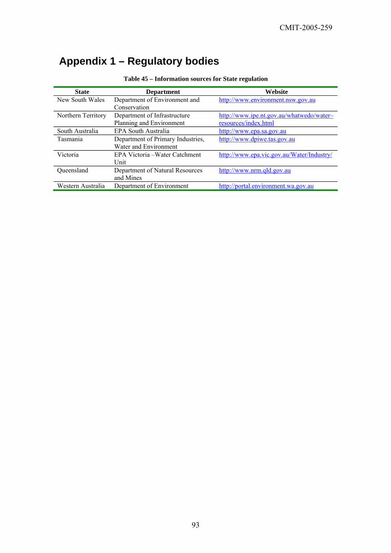
CMIT-2005-259

Appendix 1 – Regulatory bodies Table 45 – Information sources for State regulation

State Department Website New South Wales Department of Environment and

Conservation http://www.environment.nsw.gov.au

Northern Territory Department of Infrastructure Planning and Environment

http://www.ipe.nt.gov.au/whatwedo/water–resources/index.html

South Australia EPA South Australia http://www.epa.sa.gov.au Tasmania Department of Primary Industries,

Water and Environment http://www.dpiwe.tas.gov.au

Victoria EPA Victoria –Water Catchment Unit

http://www.epa.vic.gov.au/Water/Industry/

Queensland Department of Natural Resources and Mines

http://www.nrm.qld.gov.au

Western Australia Department of Environment http://portal.environment.wa.gov.au

93

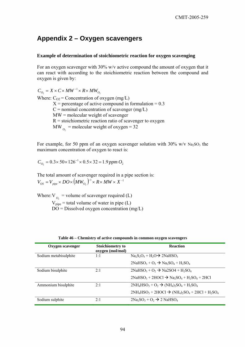
CMIT-2005-259

Appendix 2 – Oxygen scavengers Example of determination of stoichiometric reaction for oxygen scavenging For an oxygen scavenger with 30% w/v active compound the amount of oxygen that it can react with according to the stoichiometric reaction between the compound and oxygen is given by:

Where: CO2 = Concentration of oxygen (mg/L) X = percentage of active compound in formulation = 0.3 C = nominal concentration of scavenger (mg/L) MW = molecular weight of scavenger R = stoichiometric reaction ratio of scavenger to oxygen MW = molecular weight of oxygen = 32

For example, for 50 ppm of an oxygen scavenger solution with 30% w/v Na2SO3 the maximum concentration of oxygen to react is:

The total amount of scavenger required in a pipe section is:

22

1OO MWRMWCXC ××××= −

2O

21 9.1325.0126503.0

2OppmCO =××××= −

( ) 112

−− ×××××= XMWRMWDOVV OpipeOS Where: V = volume of scavenger required (L)

Vpipe = total volume of water in pipe (L) DO = Dissolved oxygen concentration (mg/L)

Table 46 – Chemistry of active compounds in common oxygen scavengers

Oxygen scavenger Stoichiometry to oxygen (mol/mol)

Reaction

2O

Sodium metabisulphite 1:1 Na2S2O5 + H2O 2NaHSO3

2NaHSO3 + O2 Na2SO4 + H2SO4

Sodium bisulphite

2:1 2NaHSO3 + O2 Na2SO4 + H2SO4

2NaHSO3 + 2HOCl Na2SO4 + H2SO4 + 2HCl

Ammonium bisulphite 2:1 2NH4HSO3 + O2 (NH4)2SO4 + H2SO4

2NH4HSO3 + 2HOCl (NH4)2SO4 + 2HCl + H2SO4

Sodium sulphite 2:1 2Na2SO3 + O2 2 NaHSO4

94

CMIT-2005-259

95

Appendix 3 – Data summary

CMIT-2005-259

Table 47 – Data Summary

Pipeline A B C D E F Section T1 T2 T3 T4 T5 T6 T7 T8 T9 T9C1 T10

Steel 5LX42 5LX65 5LX65 5LX70 5LX70 5LX70 5LX70 X60 ERW 5LX70 5LX70 5LX70 ID (mm) 154.08 333.4 282.6 323.9 323.9 323.9 273.1 250 185.4 5.08 304.8 L (km) 0.072 34 30 77 106 37 22 80 12 12 87 Source Main Main Reuse River 1 River 2 River 2 Main Reuse River River Bore O/S (ppm) 0 200 40 100 100 0 0 150 450 450 0 Biocide (ppm) 0 0 0 0 0 0 0 0 0 0 0 Other – – Aerate – – – – – Aerate Aerate – Internal Surface (m2)

34.85 36,612 26,634 78,352 107,862 37,650 18,875 62,832 10,759 191 83,307

Vol (m3) 1.34 2,968 1,882 6,345 8,734 3,049 1,289 3,927 768 0.24 6,348 S/V 26 12 14.2 12.3 12.3 12.3 14.6 16 14 787 13.1 Source characteristics pH (on–site)

– 5.9 7.01 7.62 7.98 – – 8 6.8 6.8 –

With O/S – – 6.89 6.43 7.01 – – 7.7 9.05 9.05 – EC (µS/cm) 480 660 2000 117.8 238 369 212 670 200.3 200.3 171 Turbidity 0 (NTU)2

1.2 0.5 250 5.2 31 27.3 2.2 – 11 11 60.3

Turbidity 1 (NTU)3

– – 0.9 5.6 9.4 1.45 – – – 35.6 –

Ca (mg/L) – – 9.4 10 32.2 36.3 10.8 31 4.5 4.5 4.9 Cl (mg/L) – 120 – – – – – 66 50.4 50.4 20 Mg (mg/L) – 13 4.5 5.5 9.8 10.8 5 19 5.7 5.7 3 Na (mg/L) – 85 19 8.9 32.8 36 32 71 23 23 24 TDS (mg/L) – – – – – – – 430 – – – HCO3 (mg/L) – – – – – – – 240 – – – 1 T9C was the control line along the major pipeline E. 2 As received. 3 After 1h settling.

96

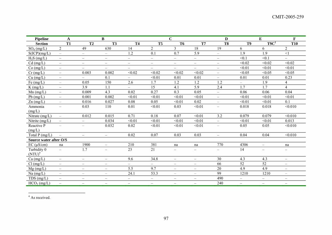
CMIT-2005-259

Pipeline A B C D E F Section T1 T2 T3 T4 T5 T6 T7 T8 T9 T9C1 T10

SO4 (mg/L) 2 49 630 14 2 3 18 19 6 6 2 S(ICP)(mg/L) – – – 1.2 0.1 0.7 5.9 – 1.9 1.9 <1 H2S (mg/L) – – – – – – – – <0.1 <0.1 – Cd (mg/L) – – – – – – – – <0.02 <0.02 <0.02 Co (mg/L) – – – – – – – – <0.01 <0.01 <0.01 Cr (mg/L) – 0.003 0.002 <0.02 <0.02 <0.02 <0.02 – <0.05 <0.05 <0.05 Cu (mg/L) – – 0.1 – <0.01 0.01 0.01 – 0.01 0.01 0.23 Fe (mg/L) – 0.05 150 2.6 1.7 1.2 1.2 1.2 – 1.9 4 K (mg/L) – 3.9 1.1 – 15 4.1 5.9 2.4 1.7 1.7 4 Mn (mg/L) – 0.009 4.3 0.02 0.27 0.3 0.05 – 0.06 0.06 0.04 Pb (mg/L) – 0.001 0.002 <0.01 <0.01 <0.01 <0.01 – <0.01 <0.01 <0.01 Zn (mg/L) – 0.016 0.027 0.08 0.05 <0.01 0.02 – <0.01 <0.01 0.1 Ammonia (mg/L)

– 0.03 110 0.01 <0.01 0.03 <0.01 – 0.018 0.018 <0.010

Nitrate (mg/L) – 0.012 0.015 0.71 0.18 0.07 <0.01 3.2 0.079 0.079 <0.010 Nitrite (mg/L) – – 0.034 <0.01 <0.01 <0.01 <0.01 – <0.01 <0.01 0.013 Reactive P (mg/L)

– – 0.032 0.02 <0.01 <0.01 <0.01 – 0.05 0.05 <0.010

Total P (mg/L) – – – 0.02 0.07 0.03 0.03 – 0.04 0.04 <0.010 Source water after O/S EC (µS/cm) na 1900 – 210 381 na na 770 4306 – na Turbidity 0 (NTU)4

– 1.7 – 23 21 – – – 14 – –

Ca (mg/L) – – – 9.6 34.8 – – 30 4.3 4.3 – Cl (mg/L) – – – – – – – 66 52 52 – Mg (mg/L) – – – 5.5 9.7 – – 20 4.9 4.9 – Na (mg/L) – – – 24.1 53.3 – – 99 1210 1210 – TDS (mg/L) – – – – – – – 490 – – – HCO3 (mg/L) – – – – – – – 240 – – –

4 As received.

97

CMIT-2005-259

Pipeline A B C D E F Section T1 T2 T3 T4 T5 T6 T7 T8 T9 T9C1 T10

SO4 (mg/L) – 420 – 114 78 – – 120 15200 – – S(ICP)(mg/L) – – – 20.4 26.7 – – – 7660 – – H2S (mg/L) – – – – <0.1 – – – <0.1 – – Cd (mg/L) – – – – – – – – <0.02 <0.02 – Co (mg/L) – – – – – – – – <0.01 <0.01 – Cr (mg/L) – 0.001 – <0.02 <0.02 – – – <0.05 <0.05 – Cu (mg/L) – – – – <0.01 – – – 0.01 0.01 – Fe (mg/L) – 1.3 – 3.1 1.2 – – – 2.3 2.3 – K (mg/L) – – – – 15 – – – 6.1 6.1 – Mn (mg/L) – 0.017 – 0.03 0.25 – – – 0.06 0.06 – Pb (mg/L) – 0.001 – <0.01 <0.01 – – – <0.01 <0.01 – Zn (mg/L) – 0.19 – 0.15 0.09 – – – 0.15 0.15 – Ammonia (mg/L)

– 59 – 0.01 <0.01 – – – 0.024 0.024 –

Nitrate (mg/L) – 0.012 – 0.65 0.03 – – – 0.011 0.011 – Nitrite (mg/L) – 0.005 – 0.01 <0.01 – – – 0.064 0.064 – Reactive P (mg/L)

– 0.026 – 0.04 <0.01 – – – 0.019 0.019 –

Total P (mg/L) – – – 0.04 0.12 – – – 0.03 0.03 – After Hydrostatic test pH (on–site)

– 7.01 7.45 7.22 7.29 8.21 7.65 7.80 7.04 6 –

EC (µS/cm) 830 2000 780 163.7 380.5 229.2 241 710 490.8 578.3 231.3 Turbidity 0 (NTU)5

850 250 4100 14 32 2000 62.1 – 29.8 – 346

Turbidity 1 6(NTU)

– – – 2.36 6.3 760 5.55 – – – 410

Turbidity F – – – 0.55 1.7 2 0.2 – – – 0.46

5 As received. 6 After 1h settling.

98

CMIT-2005-259

Pipeline A B C D E F Section T1 T2 T3 T4 T5 T6 T7 T8 T9 T9C1 T10

(NTU)7

Ca (mg/L) – 9.4 – 10.4 32.2 17.7 10.4 13 5.1 4.7 6.07 Cl (mg/L) – – – – – – – 66 50 45 <15 Mg (mg/L) – 4.5 – 5.7 9.6 5.9 5 19 5.2 4 3.67 Na (mg/L) – 19 – 16.8 47.7 34.3 31.8 99 83 109 24 TDS (mg/L) – – – – – – – 450 – – – HCO3 (mg/L) – – – – – – – 240 – – – SO4 (mg/L) 7 630 120 43 69 23 22 120 140.5 289 <1 S(ICP)(mg/L) – – – 12.2 24.5 5.7 6.1 – 51 71 <1 H2S (mg/L) – – – – <0.1 – – – <0.1 <0.1 – Cd (mg/L) – – – – – – – <0.02 <0.02 <0.02 0.05 Co (mg/L) – – – – – – – – <0.01 <0.01 <0.01 Cr (mg/L) 0.002 0.002 0.01 <0.02 <0.02 <0.02 <0.02 <0.05 <0.05 <0.05 <0.05 Cu (mg/L) – 0.1 – <0.01 <0.01 <0.01 0.01 <0.05 <0.05 <0.05 0.09 Fe (mg/L) 36 150 820 1.7 20.8 120 19.6 <0.05 8.7 30 103.3 K (mg/L) – 1.1 – – 16 15 5 2.2 2.45 2.4 3.67 Mn (mg/L) 0.43 4.3 12 0.27 0.68 1.64 0.35 0.05 0.25 0.23 2.51 Pb (mg/L) 0.046 0.002 <0.01 <0.01 <0.01 <0.01 <0.01 <0.01 <0.01 <0.01 <0.01 Zn (mg/L) 0.1 0.027 0.08 0.25 0.06 0.14 0.04 <0.05 0.035 0.11 0.2 Ammonia (mg/L)

0.03 110 27 0.14 <0.01 0.07 <0.01 0.39 <0.22 <0.01 <0.010

Nitrate (mg/L) 0.9 0.015 0.037 <0.01 0.18 0.32 0.05 <0.01 0.21 0.11 <0.010 Nitrite (mg/L) 0.005 0.034 0.017 0.09 <0.01 <0.01 <0.01 <0.005 <0.01 <0.01 <0.010 Reactive P (mg/L)

– 0.032 0.025 0.03 <0.01 0.01 <0.01 0.07 0.017 0.026 <0.010

Total P (mg/L) – – – 0.03 0.13 0.18 0.09 0.079 0.175 0.12 <0.04 Oil & grease (mg/L)

– – – – <5 – – – <5 <5 –

Total solids – – 520 – 500 116.5 – – – – –

7 Filter with 0.45µm diameter pore.

99

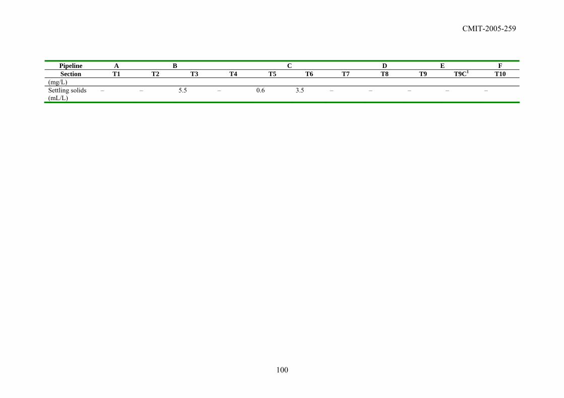
CMIT-2005-259

Pipeline A B C D E F Section T1 T2 T3 T4 T5 T6 T7 T8 T9 T9C1 T10

(mg/L) Settling solids (mL/L)

– – 5.5 – 0.6 3.5 – – – – –

100