Analysis of single fiber pushout test of fiber reinforced composite with a nonhomogeneous interphase
87
University of South Florida Scholar Commons Graduate eses and Dissertations Graduate School 2009 Analysis of single fiber pushout test of fiber reinforced composite with a nonhomogeneous interphase Sri Harsha Garapati University of South Florida Follow this and additional works at: hp://scholarcommons.usf.edu/etd Part of the American Studies Commons is esis is brought to you for free and open access by the Graduate School at Scholar Commons. It has been accepted for inclusion in Graduate eses and Dissertations by an authorized administrator of Scholar Commons. For more information, please contact [email protected]. Scholar Commons Citation Garapati, Sri Harsha, "Analysis of single fiber pushout test of fiber reinforced composite with a nonhomogeneous interphase" (2009). Graduate eses and Dissertations. hp://scholarcommons.usf.edu/etd/1981
Transcript of Analysis of single fiber pushout test of fiber reinforced composite with a nonhomogeneous interphase

University of South FloridaScholar Commons
Graduate Theses and Dissertations Graduate School
2009
Analysis of single fiber pushout test of fiberreinforced composite with a nonhomogeneousinterphaseSri Harsha GarapatiUniversity of South Florida
Follow this and additional works at: http://scholarcommons.usf.edu/etd
Part of the American Studies Commons
This Thesis is brought to you for free and open access by the Graduate School at Scholar Commons. It has been accepted for inclusion in GraduateTheses and Dissertations by an authorized administrator of Scholar Commons. For more information, please contact [email protected].
Scholar Commons CitationGarapati, Sri Harsha, "Analysis of single fiber pushout test of fiber reinforced composite with a nonhomogeneous interphase" (2009).Graduate Theses and Dissertations.http://scholarcommons.usf.edu/etd/1981

Analysis of Single Fiber Pushout Test of Fiber Reinforced Composite with a Nonhomogeneous Interphase
by
Sri Harsha Garapati
A thesis submitted in partial fulfillment of the requirements for the degree of
Master of Science in Mechanical Engineering Department of Mechanical Engineering
College of Engineering University of South Florida
Major Professor: Autar Kaw, Ph.D. Glen Besterfield, Ph.D.
Craig Lusk, Ph.D.
Date of Approval: March 24, 2009
Keywords: Pushout Test, Nonhomogeneous Interphase, Interfacial Stresses, ANSYS, Design of Experiments, Composite
© Copyright 2009, Sri Harsha Garapati
1

2
DEDICATION
This thesis dedicated to my parents, who took care with all their love, supported
and believed in me. To my professor Dr. Autar K. Kaw, who guided, instructed and
inspired me in the graduate school.

i
ACKNOWLEDGEMENTS
I wish to acknowledge the gracious support of many people for their contributions
towards this work both directly and indirectly. Firstly, I thank my advisor Dr. Autar Kaw
who patiently guided me through all phases of this work. He is a true role model, and a
best professor I have ever seen. I am deeply indebted to him for financial support, and for
the academic resources he provided. The time and effort of Dr. Glen Besterfield and Dr.
Craig Lusk as committee members is greatly appreciated.
I would like to thank my parents, Nagabhushanam and Padmavathi for their
support, suggestions and invaluable encouragement that have always made me a better
man and have indirectly prepared me to tackle challenges that I came across. Without my
parents support and encouragement, I never would have made it this far.
Additionally, I would like to thank all my friends, especially from the research
group Luke Snyder and John Daly for having always motivated and accompanied me
throughout the challenges of research. Without their help, this thesis would have been
much more difficult.
This work has been supported in part through the University of South Florida.

TABLE OF CONTENTS
TABLE OF CONTENTS..................................................................................................... i
LIST OF TABLES.............................................................................................................. v
LIST OF FIGURES ........................................................................................................... vi
LIST OF EQUATIONS ...................................................................................................... x
ABSTRACT…................................................................................................................. xiv
CHAPTER 1 LITERATURE REVIEW ........................................................................... 1
1.1 Introduction................................................................................................. 1
1.2 Analytical Modeling ................................................................................... 3
1.2.1 Interphase Layer Model .................................................................. 3
1.2.2 Cohesive Zone Model ..................................................................... 4
1.2.3 Spring Layer Model ........................................................................ 4
1.3 Shear Lag Analysis ..................................................................................... 4
1.4 Finite Element Modeling ............................................................................ 6
1.4.1 3-D finite Element Model ............................................................... 6
1.4.2 Axisymmetric Model ...................................................................... 6
1.4.3 Axisymmetric Model with Friction Elements................................. 7
i

1.5 Boundary Element Method (BEM)............................................................. 9
1.6 Functionally Graded (FG) Coating ........................................................... 10
1.7 Nonhomogeneous Interphase.................................................................... 10
1.8 Comparison Between Multi and Single Fiber Pushout Test..................... 11
1.9 Present Work............................................................................................. 12
CHAPTER 2 FORMULATION ..................................................................................... 14
2.1 Finite Element Modeling .......................................................................... 14
2.1.1 Geometry....................................................................................... 14
2.2 Meshing the Geometry.............................................................................. 15
2.2.1 PLANE182.................................................................................... 16
2.3 Modeling the Bonded Contact in the Composite...................................... 17
2.4 Properties .................................................................................................. 18
2.4.1 Fiber and Matrix ........................................................................... 18
2.4.2 Interphase...................................................................................... 19
2.4.3 Composite ..................................................................................... 21
2.4.3.1 Axial Properties ............................................................. 21
2.4.3.2 Tangential Properties ..................................................... 22
2.4.3.3 Radial Properties............................................................ 24
2.5 Continuity Conditions............................................................................... 25
2.5.1 Fiber-Interphase ............................................................................ 25
2.5.2 Sub Layers of Interphase .............................................................. 26
ii

2.5.3 Interphase-Matrix.......................................................................... 27
2.5.4 Matrix-Composite ......................................................................... 28
2.6 Boundary Conditions ................................................................................ 29
2.6.1 Boundary Condition -1 (BC-1) ..................................................... 29
2.6.2 Boundary Condition-2 (BC-2) ...................................................... 30
2.7 Loading ..................................................................................................... 31
2.7.1 Spherical Indenter ......................................................................... 31
2.7.1.1 Radius of Contact........................................................... 32
2.7.2 Uniform Pressure Loading............................................................ 34
2.7.3 Flat Indenter .................................................................................. 35
2.8 Factors for Sensitivity Analyses ............................................................... 36
2.8.1 Type of Indenter............................................................................ 36
2.8.2 Fiber Volume Fraction.................................................................. 36
2.8.3 Thickness of Interphase to Radius of Fiber Ratio (TIRFR).......... 37
2.8.4 Type of Interphase ........................................................................ 37
2.8.5 Boundary Conditions .................................................................... 38
2.9 Responses for Sensitivity Analyses .......................................................... 38
2.9.1 Load to Contact Depth Ratio (LCDR) .......................................... 38
2.9.2 Normalized Maximum Interfacial Radial Stress (NMIRS) .......... 38
2.9.3 Normalized Maximum Interfacial Shear Stress (NMISS) ............ 39
2.10 Modeling the Contact between the Fiber and the Indenter ....................... 40
CHAPTER 3 VALIDATION OF MODEL .................................................................... 41
iii

3.1 Spherical Indenter ..................................................................................... 41
3.1.1 Contact Between the Indenter and Fiber....................................... 41
3.1.2 Bonded Contact Between the Interfaces ....................................... 43
3.2 Uniform Pressure Indenter........................................................................ 44
3.2.1 Contact Between the Indenter and Fiber....................................... 44
3.2.2 Bonded Contact Between the Interfaces ....................................... 46
3.3 Flat Indenter .............................................................................................. 46
3.3.1 Contact Between the Indenter and Fiber....................................... 46
3.3.2 Bonded Contact Between the Interfaces ....................................... 48
3.4 Validation with Huang SLA and Finite Element Model .......................... 48
3.5 Validation Using Interfacial Stresses........................................................ 50
3.5.1 Validation Using Interfacial Radial Stress.................................... 50
3.5.2 Validation Using Interfacial Shear Stress ..................................... 52
CHAPTER 4 RESULTS AND CONCLUSIONS .......................................................... 55
4.1 Responses for the Sensitivity Analyses .................................................... 57
4.1.1 Load to Contact Depth Ratio (LCDR) .......................................... 57
4.1.2 Normalized Maximum Interfacial Radial Stress (NMIRS) .......... 58
4.1.3 Normalized Maximum Interfacial Shear Stress (NMISS) ............ 61
4.2 Conclusions............................................................................................... 64
REFERENCES ................................................................................................................. 66
iv
LIST OF TABLES
Table 1 Young’s Modulus and Poisson's Ratio of Fiber and Matrix........................ 19
Table 2 Values of Different Levels of the Factors.................................................... 56
Table 3 Percentage Contribution of Factors to Load to Contact Depth Ratio .......... 58
Table 4 Percentage Contribution of Factors to NMIRS............................................ 61
Table 5 Percentage Contribution of Factors to Normalized Interfacial
Maximum Shear Stress ................................................................................ 64
v
LIST OF FIGURES
Figure 1 Schematic Diagram of a Pushout Test of a Composite.................................. 2
Figure 2 Schematic Diagram of the Fiber-Interphase-Matrix-Composite
Model ........................................................................................................... 15
Figure 3 Meshed Model of Composite with Nonhomogeneous Interphase............... 16
Figure 4 Structure of PLANE182............................................................................... 17
Figure 5 Contact and Target Elements at the Interfaces ............................................ 18
Figure 6 Composite with BC-1 .................................................................................. 30
Figure 7 Schematic Diagram of Spherical Indenter Loading..................................... 32
Figure 8 Contact between the Fiber and the Indenter ................................................ 33
Figure 9 Schematic Diagram Illustrating Uniform Pressure Loading........................ 35
Figure 10 Schematic Diagram of Flat Indenter Loading.............................................. 36
Figure 11 Finite Element Model of Composite with Spherical Indenter ..................... 40
vi

Figure 12 Typical Distribution of Normalized Axial Stress Along the
Normalized Radial Distance from the Center of the Fiber for
Spherical Indenter ........................................................................................ 42
Figure 13 Typical Distribution of Normalized Axial Displacement Along the
Normalized Radial Distance from the Center of the Fiber for
Spherical Indenter ........................................................................................ 42
Figure 14 Typical Distribution of Normalized Axial Stress Along the
Normalized Radial Distance from the Center of the Fiber for
Uniform Pressure Indenter........................................................................... 44
Figure 15 Typical Distribution of Normalized Axial Displacement Along the
Normalized Radial Distance from the Center of the Fiber for
Uniform Pressure Indenter........................................................................... 45
Figure 16 Typical Distribution of Normalized Axial Stress Along the
Normalized Radial Distance from the Center of the Fiber for Flat
Indenter ........................................................................................................ 47
Figure 17 Typical Distribution of Normalized Axial Displacement Along the
Normalized Radial Distance from the Center of the Fiber for Flat
Indenter ........................................................................................................ 47
Figure 18 Typical Distribution of Normalized Interfacial Radial Stress Along
the Normalized Length of the Fiber............................................................. 51
vii
Figure 19 Typical Distribution of Normalized Interfacial Radial Displacement
Along the Normalized Length of the Fiber.................................................. 52
Figure 20 Typical Distribution of Normalized Interfacial Shear Stress Along
the Normalized Length of the Fiber............................................................. 53
Figure 21 Typical Distribution of Normalized Interfacial Axial Displacement
Along the Normalized Length of the Fiber.................................................. 54
Figure 22 Normalized LCDR as a Function of Type of Indenter. ............................... 57
Figure 23 Normalized Maximum Interfacial Radial Stress as a Function of
Fiber Volume Fraction for Uniform Pressure Indenter, Linear Type
of Interphase, and TIRFR=1/20. .................................................................. 59
Figure 24 Normalized Maximum Interfacial Radial Stress as a Function of
Fiber Volume Fraction for Spherical Indenter Loading, Linear Type
of Interphase, and BC-1 ............................................................................... 60
Figure 25 Normalized Maximum Interfacial Radial Stress as a Function of
Fiber Volume Fraction for Flat Indenter Loading, TIRFR=1/20, and
BC-2............................................................................................................. 60
Figure 26 Normalized Maximum Interfacial Shear Stress as a Function of Fiber
Volume Fraction for Uniform Indenter, Linear Type of Interphase,
and TIRFR=1/20 .......................................................................................... 62
viii
Figure 27 Normalized Maximum Interfacial Shear Stress as a Function of Fiber
Volume Fraction for Spherical Indenter Loading, Linear Type of
Interphase, and BC-1 ................................................................................... 62
Figure 28 Normalized Maximum Interfacial Shear Stress as a Function of Fiber
Volume Fraction for Flat Indenter Loading, TIRFR=1/20, and BC-2......... 63
ix
LIST OF EQUATIONS
Equation 1 Force Balance Equation to Calculate the Friction Stress at the
Interface [1].................................................................................................... 5
Equation 2 Exponential Variation of Young's Modulus along the Radial
Thickness of Interphase ............................................................................... 19
Equation 3 Exponential Variation of Poisson's Ratio along the Radial Thickness
of Interphase................................................................................................. 19
Equation 4 Linear Variation of Young's Modulus along the Thickness of the
Interphase..................................................................................................... 20
Equation 5 Linear Variation of Poisson's Ratio along the Thickness of the
Interphase..................................................................................................... 20
Equation 6 Poisson's Ratio of the jth layer of Interphase................................................ 20
Equation 7 Young's Modulus of the jth Layer of the Interphase..................................... 20
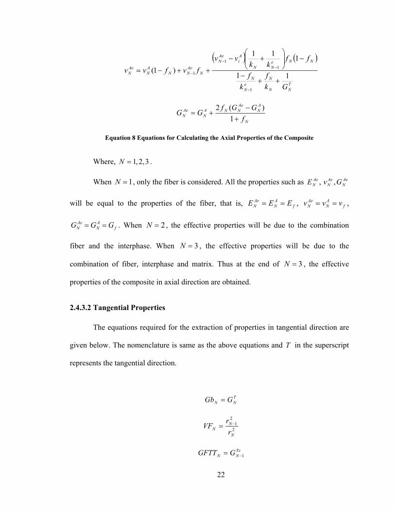
Equation 8 Equations for Calculating the Axial Properties of the Composite............... 22
Equation 9 Equations for Calculating the Tangential Properties ................................... 24
x

Equation 10 Radial Stress Continuity in Fiber-Interphase Interface................................ 25
Equation 11 Shear Stress Continuity in Fiber-Interphase Interface ................................. 25
Equation 12 Radial Displacement Continuity in Fiber-Interphase Interface ................... 25
Equation 13 Axial Displacement Continuity in Fiber-Interphase Interface..................... 25
Equation 14 Radial Stress Continuity at the Interface of jth and j+1th Sublayer of
Interphase..................................................................................................... 26
Equation 15 Shear Stress Continuity at the Interface of jth and j+1th Sublayer of
Interphase..................................................................................................... 26
Equation 16 Radial Displacement Continuity at the Interface of jth and j+1th
Sublayer of Interphase ................................................................................. 26
Equation 17 Axial Displacement Continuity at the Interface of jth and j+1th
Sublayer of Interphase ................................................................................. 26
Equation 18 Radial Stress Continuity at Interphase-Matrix Interface ............................. 27
Equation 19 Shear Stress Continuity at Interphase-Matrix Interface............................... 27
Equation 20 Radial Displacement Continuity at Interphase-Matrix Interface ................. 27
Equation 21 Axial Displacement Continuity at Interphase-Matrix Interface................... 27
Equation 22 Radial Stress Continuity at Matrix-Composite Interface............................. 28
Equation 23 Shear Stress Continuity at Matrix-Composite Interface .............................. 28
xi
Equation 24 Radial Displacement Continuity at Matrix-Composite Interface ................ 28
Equation 25 Shear Displacement Continuity at Matrix-Composite Interface.................. 28
Equation 26 Axisymmetric Condition.............................................................................. 29
Equation 27 Matrix Constrained in its Axial Direction at its Bottom End ...................... 29
Equation 28 Composite Constrained in its Axial Direction at its Bottom End................ 29
Equation 29 Radial Stressfree Condition at the Radial Edge of the Composite .............. 29
Equation 30 Shear Stressfree Condition at the Radial Edge of the Composite................ 30
Equation 31 Radial Displacement Constrained at the Radial Edge of the Matrix ........... 30
Equation 32 Axial Displacement Constrained along the Radial Edge of the Matrix....... 30
Equation 33 Pressure Applied on the Spherical Indenter................................................. 31
Equation 34 Fischer-Cripps Equation to Calculate the Contact Radius........................... 33
Equation 35 Uniform Pressure Applied on the Fiber ....................................................... 34
Equation 36 Fiber Volume Fraction................................................................................. 37
Equation 37 Load to Contact Depth Ratio ....................................................................... 38
Equation 38 Normalized Maximum Radial Stress at the Fiber-Interphase Interface....... 39
Equation 39 Normalized Maximum Shear Stress at the Fiber-Interphase Interface........ 39
xii

Equation 40 Total Load on the Fiber using the Axial Stress Data on the Top of
the Fiber ....................................................................................................... 43
Equation 41 Total Load Applied on the Fiber through Spherical Indenter...................... 43
Equation 42 Load Applied on the Fiber through Uniform/Flat indenter ......................... 45
Equation 43 Loading Condition for Huang Model .......................................................... 49
Equation 44 LCDR from Huang's Shear Lag Model ....................................................... 49
Equation 45 Intermediate Parameters to be Calculated for LCDR using Huang's
Model ........................................................................................................... 49
Equation 46 Force in Radial Direction from the Interfacial Radial Stress ....................... 51
Equation 47 Axial Force Applied on the Fiber from the Interfacial Shear Stress ............ 53
xiii

Analysis of Single Fiber Pushout Test of Fiber Reinforced Composite with a Nonhomogeneous Interphase
Sri Harsha Garapati
ABSTRACT
Fiber pushout test models are developed for a fiber-matrix-composite with a
nonhomogeneous interphase. Using design of experiments, the effects of geometry,
loading and material parameters on critical parameters of the pushout test such as the
load-displacement curve and maximum interfacial shear and normal stresses are studied.
The sensitivity analysis shows that initial load displacement curve is dependent only on
the indenter type and not on parameters such as fiber volume fraction, interphase type,
thickness of interphase, and boundary conditions. In contrast, interfacial shear stresses
are not sensitive to indenter type, while the interfacial radial stresses are mainly sensitive
to fiber volume fraction and the boundary conditions.
xiv

CHAPTER 1 LITERATURE REVIEW
1.1 Introduction
In a fiber-matrix composite, the material immediately surrounding the fiber called
the interphase can be different from the bulk matrix. The interphase is a very thin layer
formed between the fiber and matrix due to chemical reaction between them or may be
intentionally introduced to improve the properties of composite. Interphase properties
have a significant effect on the overall structural integrity of the composite. This
importance of the interphase has led researchers to carry numerous experimental
characterizations and micro mechanical analysis of the interphase subjected to different
loading conditions [2].
The pushout test is one of the experimental techniques used for finding the
interphase properties where the fiber is pushed with an indenter (spherical/flat/cubical,
etc). The indentation process starts by applying the load and gradually increasing the load
to a maximum value. The displacement of the fiber is continuously measured as the load
is increased. Similarly, displacement of the fiber is recorded during the unloading of the
specimen. Now by drawing a loading / unloading curve, the interphase properties can be
found [2]. The two important interphase properties are coefficient of friction of fiber-
matrix interphase and the residual radial stress in the interface. Several methods are
implemented to extract these two properties of the interphase.
1

Figure 1 Schematic Diagram of a Pushout Test of a Composite.
The pushout specimen is prepared by slicing the composite normal to fiber
direction and is placed on platform with a hole (Figure 1). The radius of the hole of the
platform is slightly larger than the radius of the fiber in the specimen. An indenter is used
to apply load on the fiber. The load applied is gradually increased and simultaneously
displacements are noted. Usually the indenter radius is about 60-90% of the fiber radius
[1].
Fiber pushout test is regarded as the most important widely used experimental
technique because of the relative simplicity of preparing the specimen and conducting the
experiment. But the pushout process has certain limitations and they include the
following.
1. The values obtained for shear strength and frictional shear stress are average
values.
2. Fiber may damage during the loading.
3. Indenter failure may also occur.
2
1.2 Analytical Modeling
The above limitations of the fiber pushout test created a demand to model it either
analytically or numerically. Kerans and Parthasarathy [3] developed an analytical model
which gives the fiber-end displacement for an applied stress. Hsueh [4, 5] showed that
by averaging interfacial shear stress and Poisson’s effect along the sliding length, the
predictions are surprisingly accurate. Lara-Curzio and Ferber [6] developed a
methodology to determine the interfacial properties of brittle matrix composites using the
models developed by Kerans and Parthasarathy [3] and Hsueh [4, 5]. Lara-Curzio and
Ferber [6] also discussed data analyses techniques by comparing the models developed
by Kerans and Parthasarathy [3] and Hsueh [4, 5].
The most difficult part of modeling the pushout test is modeling the interface.
There are three methods used for modeling the interface. They are
1. Interphase layers model
2. Cohesive zone model
3. Spring layers model
1.2.1 Interphase Layer Model
Interphase layer model considers that interphase is a distinct layer with a specified
thickness. This layer is placed between the fiber and the matrix. Interphase layer model is
very complicated as it requires numerous parameters to completely describe the behavior
of the interface. Also the failure of the interface is difficult to ascertain [7].
3
1.2.2 Cohesive Zone Model
In this model the interface is treated as a separate material with its own
constitutive relationship. This model is relatively simpler than the interphase layer
modeling. This model uses only energy based criterion [7].
1.2.3 Spring Layer Model
This is the simplest of all the models. The interface is modeled using spring
elements with certain stiffness. The spring zone model uses both stress-based and energy-
based criteria [7].
1.3 Shear Lag Analysis
Shear-lag theory was first proposed for modeling the pushout test by Shetty [8].
His model predicted the exponential decrease of interfacial shear stress along the fiber
length. This result is similar to the ones obtained from finite element analysis[9]. His
theory also provided a basis for determining coefficient of friction and interfacial residual
stress. He also proposed frictional stress due to sliding could be over estimated if the
transverse expansion of fibers is not taken into account.
Shear-lag theory is widely used for analytical based mechanics to evaluate fiber-
matrix interface properties. According to this theory, the interphase is assumed to be a
thin layer surrounding the fiber. It is also assumed that this thin layer of interface has a
constant stiffness [2].
The pushout force-displacement plot from the test is regressed to a theoretical
model for determining the coefficient of friction and residual radial stress in the fiber-
matrix interface. By experimentally performing the pushout the force ( ) required to F
4

pushout the fibers is found. From the force balance equation, the friction stress near the
interface can be calculated as.
Equation 1 Force Balance Equation to Calculate the Friction Stress at the Interface [1].
In the Equation 1, is the fiber radius, fr L is the length of the fiber and rzσ is the
shear stress along the fiber-matrix interface [1]. But this assumption is only valid when
the coefficient of friction is very small or the length of the specimen is very small. This
assumption is not valid for all the cases because it assumes that the shear stress is uniform
through the length. But actually when the fiber is pushed by the indenter, the fiber is in
compression and it expands in the transverse direction due to Poisson’s effect. As the
fiber expands in transverse direction, it exerts force on the interface which increases the
normal stress on the interface and in turn the frictional stress at the interface. If the
Poisson’s effect is not taken into account, the sliding frictional stress can be
overestimated. Due to Poisson’s effect, the frictional shear stress is nonlinear in nature
along the length of embedded fiber [1]. Some of the important assumptions in SLA are
1. Coulomb friction law is assumed at the interface.
2. Residual radial compression due to thermal coefficients mismatch between the
fiber and matrix is assumed [1, 7, 10-12].
Using these assumptions the experimental data collected is regressed to find the
mechanical properties of the interface. Huang et al. [2] verified the accuracy of analytical
solution based on shear-lag assumptions by a finite element method. The analytical
model failed to capture the values at the top surface due to free edge effects, but in the
rzf LrF σπ2=
5

interior region the finite element results and analytical results are very close to each
other.
1.4 Finite Element Modeling
1.4.1 3-D finite Element Model
Mital and Chamis [13] developed a 3-D finite element model consisting of nine
fibers. All the nine fibers were unidirectional and were arranged in three-by-three unit
cell order. Their finite element model consisted of an interphase between the fiber and the
matrix, and the interphase thickness was taken as 6.8% of the fiber diameter. The
material properties of the interphase were assumed to be same as the matrix properties
except for its shear modulus. Very low shear modulus of the interphase was assumed to
linearize the simulation up to push through load of the fiber. This procedure was used to
predict the fiber push through load at any temperature and helped in determining the
average interfacial shear strength.
1.4.2 Axisymmetric Model
Shirazi-Adl [14-16] and Forcione [15] conducted finite element stress analysis of
a pushout test using an axisymmetric finite element model with two concentric cylinders
with a common interface. The model was meshed with bilinear quadrilateral elements.
They studied the effects of material properties and boundary conditions on interfacial
shear stress. The three cases of material properties they used for their study were
1. Harder material inside
2. Identical materials
3. Softer material inside.
6

They used four different boundary conditions for their study
1. Outer cylinder is constrained axially at the bottom
2. Outer cylinder is fixed at the bottom
3. Outer surface area of outer cylinder is constrained radially
4. Outer cylinder is fixed in all directions.
They considered both axial compression and axial torque loads for this study, and
observed that the shear stress at the interface is almost constant for material property of
type-1 and boundary conditions 3 and 4. For the same material property type and the
boundary conditions 1 and 2, the interfacial shear stress varied along the length and the
maximum value is found at the bottom. Interfacial radial stresses for material property of
type-1 and boundary condition 4 were of very small magnitude and compressive. For
boundary conditions 1 and 3, the interfacial radial stress was found to have very large
values of tensile stress at the bottom and at the top.
1.4.3 Axisymmetric Model with Friction Elements
Yuan et al. [7] modeled the single fiber pushout test as an axisymmetric
cylindrical model. The SiC fiber and titanium matrix were modeled using isoparametric
4-noded quadrilateral elements. The interface between the fiber and matrix was modeled
using contact-friction and spring elements. The interface was modeled using the spring
elements because the analyses was carried based on the stress based criterion [7]. The
procedure was modulated into two steps as given below.
First, cooling the matrix from high temperature to room temperature was modeled
in finite element analyses by using a thermal load. Residual stresses were induced due to
the mismatch in the coefficient of thermal expansion. Also, we should note that we
7

should have same displacement in the matrix and fiber at the interface through out the
length of the specimen. The radial displacement at the center of fiber is zero.
In the second step, pushing the fiber out of the specimen with a flat indenter was
simulated. In numerical analyses, prescribed displacement was added to the punch until
the fiber was completely pushed out from the specimen. The boundary condition of axial
displacement being zero along the supported end was applied. Duplicate nodes were
created on both fiber and matrix ends. With the use of these duplicate nodes, fiber matrix
bonding was simulated by connecting the duplicate nodes with spring elements. In this
analysis, the interface failure was based upon shear stress criterion, that is, when the
interfacial shear stress was larger than the critical shear stress value, debonding was
assumed to initiate. When the interface debonded completely, frictional sliding could be
observed. Coulomb’s law was applied for modeling the frictional sliding. Property
variation with temperature was included in the analyses.
The results obtained from the numerical analyses [7] were that the residual
stresses are symmetric and the shear stresses are asymmetric relative to the center of the
specimen.
The shear stress vs. length of the specimen was plotted. From the plot it was
observed that shear stress was positive (as per the coordinate system used in his study) at
the loading end, and then slowly decreases and changes to negative stress as we go
towards the compressive end.
When a compressive load is applied on the loading end, the load induces
compressive stress in the specimen. Thus by superimposing the shear stress due to
compressive loading on the shear stress due to cooling, we observe the shear stress
8

decrease at the loading end and increase at the supporting end and reach the critical shear
stress value. This provides the support for fiber debonding starting from the supported
ends.
Load displacement curves were plotted. The load displacement curve was linear
up to maximum load after which the load decreased dramatically. This was due to
complete debonding of the fiber from the matrix.
The shear stress obtained from the peak load in the pushout test in not the exact
actual shear stress but it provides a reference value. In this way, numerical analyses are
helpful in evaluating the interfacial shear strength.
1.5 Boundary Element Method (BEM)
Ye and Kaw [1] modeled the pushout test using an axisymmetric model with fiber
as a solid cylinder and the matrix is modeled as a hollow cylinder. The study concluded
the following.
Maximum pushout force is independent of indenter radius, type of indenter and
radius of hole.
The interfacial stresses remain constant along the length of the specimen except at
the top and bottom surfaces. This conclusion from BEM was in agreement with the shear-
lag model proposed by Shetty [8]).
The coefficient of friction extracted from BEM differed by 15% from the value
that was obtained from shear-lag model of Shetty [8].
9
1.6 Functionally Graded (FG) Coating
Functionally graded coatings offer an improvement of 35 % after heat treatment
and 70% before heat treatment on composite fracture [17]. Hence FG coatings are widely
used in variety of fields where composite materials are used. SiC monofilaments in Ti
based matrix are widely used in aerospace applications. Haque and Choy [17] coated SiC
monofilaments with a FG TiC based coating (SiCf/C/ (Ti,C)/Ti) using a close field un-
balanced magnetron sputtering. The coated fibers were placed in Ti matrix using isostatic
pressing [17]. Carbon layer within the graded system was weakly bonded to the fiber
before the heat treatment. This was the reason for easy debonding of the fiber from the
matrix. After heat treatment, the interfacial shear strength was observed to have
increased. The percentage of increase depended up on the fiber/matrix and FG type of
coating. For the above mentioned SiC fiber and Ti matrix, the increase in interfacial
strength was around 146%. This increase in interfacial shear strength was due to the
formation of brittle titanium silicide or a ternary compound of SiC/C interface, which
resulted in better bonding. For the FG coated layers, a reaction layer was found adhered
to the fiber during the pushout test after heat treatment. The remaining layers were found
adhered to the matrix itself. The pushout tests were analyzed with scanning electron
microscopy (SEM) which was equipped with both secondary and back scattered electron
analysis mode, which helped in identifying the region of failure.
1.7 Nonhomogeneous Interphase
The interphase region might have multiple regions of chemically distinct region
[18]. Interphase is important in mechanics of composites. Jayaram et al. [19, 20]
reviewed the elastic and thermal effects of interphases, while Chamis [21] and Argon
10

[22] studied the effects of fracture toughness of composites with interphase. Fracture
mechanics models with nonhomogeneous interphases have been developed by Delale and
Erdogan [23], Erdogan [24], Kaw [25]. In these studies, the elastic moduli of the
interphase was assumed to vary exponentially along the radial thickness. Bechel and Kaw
[26] modeled the interphase, with elastic moduli varying as an aribitary piecewise
continuous function along its radial thickness.
Indentation model for thin layer-substrate geometry with an interphase were
developed by Chalasani et al. [27]. The interphase was modeled either as a
nonhomogeneous layer or as a homogeneous layer. The analysis based on design of
experiments (DOE) [28] was carried and it was found that contact depth is not sensitive
to the type of interphase. Critical interfacial stresses differed significantly for film to
substrate elastic moduli ratios greater than 25. It was also found that interphase thickness
and film to substrate Young’s moduli ratio had the most impact on the critical interfacial
stresses. The variation of elastic moduli in the interphase and indenter radius had the least
impact [27].
This study was carried on thin (film) layer-substrate geometry and in this study
nonhomogeneous interphase was modeled between the film and the substrate. This study
laid the foundation for the present work, single fiber pushout test with a nonhomogeneous
interphase. In the present study the nonhomogeneous interphase is modeled between the
fiber and the matrix.
1.8 Comparison Between Multi and Single Fiber Pushout Test
Till now we confined the total discussion to single fiber pushout test only. Let us
now discuss the multi-fiber pushout test and compare it with the single fiber push out test.
11

Single and multi-fiber pushout tests were carried out on Nicalon/glass (Corning 1723)
composite to examine the interfacial properties by Jero et al. [3]. A mμ10 flat probe was
used in single fiber pushout test to push the fiber out of the matrix where as in multi-fiber
pushout test mμ100 flat probe was used [3]. The loading and unloading curve was
obtained in both the cases. The experimental observation of various fibers with the above
mentioned two processes resulted in the following conclusions [3].
1. It was only possible to push fibers from thinnest of the multi-fiber specimens
(0.53 mm). In thicker samples (0.95 and 1.70), fibers were crushed before complete
debonding.
2. Single fiber pushout tests were easy to conduct where as multi-fiber tests were
difficult.
3. The data obtained from the multi-fiber test was more scattered when compared
to single fiber.
4. Multi-fiber pushout test effectively magnified fiber/matrix roughness mismatch
and compressive stress due to Poisson’s expansion.
1.9 Present Work
In this study, I am studying the pushout test differently from the previous studies
as follows.
First, most studies neglect the presence of a separate interface layer called the
interphase. These separate layers may be either created due to the normal processing of
a composite or by intention to develop a composite with better properties. Haque and
Choy [17] proved experimentally that SiC/Ti composites with interphases offer an
improvement on composite fracture of 35-70% and an increase in the interfacial strength
12

of around 146%. Since the characterization of the fiber-matrix interface is dependent on
the results obtained from a pushout test, we have developed a model for the test that not
only incorporates the interphase but also one which can be nonhomogeneous.
Second, I wanted to study the effect of various parameters on the results of the
test. I wanted to quantitatively answer the question of how do the type of indenter,
boundary conditions of the specimen, fiber volume fraction, thickness of interphase to
fiber radius ratio, and type of interphase model effect the load-displacement curve and the
critical interfacial stresses as these are the parameters that characterize the most of the
intrinsic mechanical properties of the fiber-matrix interface.
I accomplish these two objectives by first developing a finite element analysis
model that is capable of incorporating these parameters, and then using a design of
experiments (DOE) study to develop clear conclusions from a parametric study.
13

CHAPTER 2 FORMULATION
2.1 Finite Element Modeling
The finite element program of ANSYS 11.0 [9] was used for conducting
simulations in this study. ANSYS [9] is chosen because it has the capability of solving
nonlinear contact problems.
For this study axisymmetric half space of the indentation model is developed
instead of 3D indentation model because axisymmetric model takes relatively much less
time than the 3D model. Chudoba et al. [29], conducted a study using spherical
indentation of both 3D model and the axisymmetric model and the results deviated by
less than 0.1% from Hertzian theory (ANSYS [9]) for a homogeneous half space.
2.1.1 Geometry
An axisymmetric finite element model of homogeneous fiber surrounded by a
homogeneous matrix separated by a nonhomogeneous interphase and the whole fiber-
interphase-matrix surrounded by a composite is modeled. The geometry of the problem is
shown in Figure 2. The model consists of homogeneous fiber, nonhomogeneous
interphase, homogeneous matrix and composite of infinite length and finite radius of
and respectively. Young’s modulus and Poisson’s ratio vary arbitrarily along
the width of nonhomogeneous interphase where as, they are constant in the homogeneous
fiber, matrix and composite part of the model.
mif rrr ,, cr
14

F I MC
fr
ir
mr
cr
Figure 2 Schematic Diagram of the Fiber-Interphase-Matrix-Composite Model
2.2 Meshing the Geometry
An axisymmetric model is developed in ANSYS [9] with homogeneous fiber-
matrix and composite properties. The nonhomogeneous interphase is modeled with
nonhomogeneous properties between the fiber and the matrix. The nonhomogeneous
interphase is modeled as series of sub homogeneous layers. The model is meshed with
4 node iso-parametric elements (PLANE182). The mesh on the top surface of the fiber
(region of indentation) and at the interfaces of the fiber, interphase, matrix, and
composite is refined several times to catch the stresses and displacements on the top of
the fiber when load is applied and to simulate the perfect bonded contact between the
n
15

fiber, interphase, matrix and composite. The meshed finite element model is shown in
Figure 3.
Figure 3 Meshed Model of Composite with Nonhomogeneous Interphase
2.2.1 PLANE182
PLANE182 is a 2-D structural element in ANSYS [9] element library. It could be
used for plane stress, plane strain and axisymmetric problems. It is defined by four nodes
having two degrees of freedom at each node (translation in X and Y directions). The
element has plasticity, hyperelasticity, stress stiffening, large deflection, and large strain
capabilities. It also has mixed formulation capability for simulating deformations of
nearly incompressible elastoplastic materials, and fully incompressible hyperelastic
materials.
16

Figure 4 Structure of PLANE182
2.3 Modeling the Bonded Contact in the Composite
The contact between the fiber and interphase, sublayers of interphase, interphase
and matrix and matrix, and composite is modeled as a bonded contact using contact
elements (CONTA 171 and TARGET 169) in ANSYS [9] element library. The interfaces
in the finite element model are to be modeled as bonded contact to satisy the continuity
equation mentioned in Section 2.5.
17

Figure 5 Contact and Target Elements at the Interfaces
In Figure 5, the violet pink color elements are the contact elements and the
elements shown in yellow color are the target elements at various interfaces in the
composite model.
2.4 Properties
2.4.1 Fiber and Matrix
For this study, a glass/epoxy composite is chosen. The Young’s modulus and
Poisson’s ratio for the glass fiber and epoxy matrix are taken from the data available in
the literature. The Young’s modulus and Poisson’s ratio of the glass fiber and epoxy
matrix are given in Table 1.
18

Table 1 Young’s Modulus and Poisson's Ratio of Fiber and Matrix
Material Elastic modulus (GPa ) Poisson’s ratio
Glass fiber 72.6 0.2
Epoxy matrix 2.4 0.3
2.4.2 Interphase
The properties of the interphase are calculated assuming the elastic moduli are
varying exponentially or linearly through the radial thickness. If the properties are
varying exponentially, then along the radial thickness of the interphase Young’s modulus
and Poisson’s ratio are given by
ifbr rrraerE ≤≤= ,)(
Equation 2 Exponential Variation of Young's Modulus along the Radial Thickness of Interphase
ifdr rrrcer ≤≤= ,)(ν
Equation 3 Exponential Variation of Poisson's Ratio along the Radial Thickness of Interphase
where , , and are found using the Young’s modulus and Poisson’s ratios
at the edges of the layer
a b c d
( )if rrrr == , .
If the properties are varying linearly, then along the radial thickness of the
interphase Young’s modulus and Poisson’s ratio are given by
19

if rrrbrarE ≤≤+= ,)(
Equation 4 Linear Variation of Young's Modulus along the Thickness of the Interphase
if rrrdrcr ≤≤+= ,)(ν
Equation 5 Linear Variation of Poisson's Ratio along the Thickness of the Interphase
where, , , and are found using the Young’s modulus and Poisson’s ratios
at the edges of the layer
a b c d
( )if rrrr == , .
Poisson’s ratio and the Young’s modulus at the edges of sub-layers are given by
)()1()(
)(
)1(
)(
jiji
r
rji rr
drrji
ji
−=
−
∫−
ν
ν
Equation 6 Poisson's Ratio of the jth layer of Interphase
)()1()(
)(
)1(
)(
jiji
r
rji rr
dxrE
E
ji
ji
−=
−
∫−
Equation 7 Young's Modulus of the jth Layer of the Interphase
Where, )( jiν =Poisson’s ratio of sublayer of the interphase, =Young’s
modulus of sublayer of the interphase,
thj )( jiE
thj nnj ,1,...,2,1 −= , subscript for the
interphase.
=i
Note that when , 1=j fji rr =− )1( . Also when nj = , . iji rr =− )1(
20

2.4.3 Composite
The properties of the composite were obtained by applying Sutcu’s recursive
concentric cylinder model [30].
2.4.3.1 Axial Properties
The equations used to calculate the axial properties of composite by using
recursive cylinder model are given below. In the equations, in the subscript represent
the number of the concentric cylinder (example:
N
1=N represent innermost cylinder, that
is, fiber), e in the superscript represent the effective property and A in the superscript
represent the axial direction (example: represent Young’s modulus,
Poison’s ratio and shear modulus, respectively in axial direction considering
concentric cylinders and represent the Young’s modulus, Poison’s ratio and
shear modulus, respectively in axial direction of the cylinder).
AeN
AeN
AeN GvE ,,
N
AN
AN
AN GvE ,,
thN
2
1⎟⎟⎠
⎞⎜⎜⎝
⎛= −
N
NN r
rf
( )AN
AN
AN
N EGG
k−
=3
2
ANn
AeNNA EfEfE )1(1 −+= −
NTNNN
TN
eN
NTNN
eNN
TN
eNNe
N fGkfGkfGkkfGkk
k)()1)((
)()1)((
1
11
++−+++−+
=−
−−
TNN
NeN
N
NNAN
AeN
AAeN
Gkf
kf
ffvvEE
11)1()(4
1
21
++−
−−+=
−
−
21
( ) ( )
TNN
NeN
N
NNeNN
Ai
AeN
NAeNN
AN
AeN
Gkf
kf
ffkk
vvfvfvv
11
111
)1(
1
11
1
++−
−⎟⎟⎠
⎞⎜⎜⎝
⎛+−
++−=
−
−−
−
N
AN
AeNNA
NAeN f
GGfGG
+−
+=1
)(2
Equation 8 Equations for Calculating the Axial Properties of the Composite
Where, . 3,2,1=N
When , only the fiber is considered. All the properties such as
will be equal to the properties of the fiber, that is, , ,
. When , the effective properties will be due to the combination
fiber and the interphase. When
1=N AeN
AeN
AeN GvE ,,
fAN
AeN EEE == f
AN
AeN vvv ==
fAN
AeN GGG == 2=N
3=N , the effective properties will be due to the
combination of fiber, interphase and matrix. Thus at the end of , the effective
properties of the composite in axial direction are obtained.
3=N
2.4.3.2 Tangential Properties
The equations required for the extraction of properties in tangential direction are
given below. The nomenclature is same as the above equations and T in the superscript
represents the tangential direction.
TNN GGb =
2
21
N
NN r
rVF −=
TeNN GGFTT 1−=
22

2
21
2
N
NNN r
rrVb −−
=
NN kkb =
TNN vvb =
TeNN vvFTT =
N
NN Gb
GFTT=γ
NN vb
b4311
−=
NN vFTT
b43
12−
=
( )( )NN
NNNN b
bba
2121
1×+×−
=γγ
11
2−
+=
N
NNN
ba
γγ
N
N
NN
NNN
GbVb
GbGFTT
VFGbMG
21
2+
−
+=
( )( )( )( ) ⎟⎟
⎠
⎞⎜⎜⎝
⎛××−−×+
××−×+×+= 223
223
13211131211
2NNNNNNN
NNNNNNNNNN bVbVFVFaVFa
bVbVFVFbaVFaGbPG
222 NNTe
NPGMG
G+
=
( )AeN
AeN
eN
N Evk
M2
* 41
×+=
( )TeNN
eN
TeN
eNTe
N GMkGk
E×+
×= *
4
23

( )( )Te
NNeN
TeNN
eNTe
N GMkGMk
v×+×−
= *
*
Equation 9 Equations for Calculating the Tangential Properties
where
3,2,1=N .
When , only fiber is considered. All the properties such as
will be equal to the properties of the fiber, that is, , ,
.
1=N TeN
TeN
TeN GvE ,,
fTN
TeN EEE == f
TN
TeN vvv ==
fTN
TeN GGG ==
Note that when , 1=N 01=−N , then all the values of the terms with 1−N in
subscript are zero.
When , the effective properties will be due to the combination fiber and the
interphase. When , the effective properties will be due to the combination of fiber,
interphase and matrix. Thus at the end of
2=N
3=N
3=N , the effective properties of the composite
in tangential direction are obtained.
2.4.3.3 Radial Properties
As the composite material used for this study is assumed to be transversely
isotropic, the properties of the composite are same in tangential and radial directions.
Hence, the properties of the composite in the polar coordinate system are
obtained.
24

2.5 Continuity Conditions
2.5.1 Fiber-Interphase
The continuity conditions at interface between fiber and interphase for bonded
contact are given by [27].
lzzrzr firf
fr ≤≤= 0),,(),( σσ
Equation 10 Radial Stress Continuity in Fiber-Interphase Interface
lzzrzr firzf
frz ≤≤= 0),,(),( σσ
Equation 11 Shear Stress Continuity in Fiber-Interphase Interface
lzzruzru firf
fr ≤≤= 0),,(),(
Equation 12 Radial Displacement Continuity in Fiber-Interphase Interface
lzzruzru fizf
fz ≤≤= 0),,(),(
Equation 13 Axial Displacement Continuity in Fiber-Interphase Interface
where, = radial stress at the interface of fiber and interphase in the
fiber, = radial stress at the interface of fiber and interphase in the interphase,
= shear stress at the interface of fiber and interphase in the fiber, =
shear stress at the interface of fiber and interphase in the interphase, = radial
displacement at the interface of fiber and interphase in the fiber, = radial
displacement at the interface of fiber and interphase in the interphase, = axial
),( zrff
rσ
),( zrfirσ
),( zrff
rzσ ),( zrfirzσ
),( zru ff
r
),( zru fir
),( zru ffz
25

displacement at the interface of fiber and interphase in the fiber, = axial
displacement at the interface of fiber and interphase in the interphase.
),( zru fiz
2.5.2 Sub Layers of Interphase
The continuity conditions at sub-layer interfaces of interphase ( ijij hr = or
, where 0)1( =+jir 1,2,...,3,2,1 −−= nnj ) are given by
lzzrzr jiji
rjiji
r ≤≤= ++ 0),,(),( )1(
)1()(
)( σσ
Equation 14 Radial Stress Continuity at the Interface of jth and j+1th Sublayer of Interphase
lzzrzr jiji
rzjiji
rz ≤≤= ++ 0),,(),( )1(
)1()(
)( σσ
Equation 15 Shear Stress Continuity at the Interface of jth and j+1th Sublayer of Interphase
lzzruzru jiji
rjiji
r ≤≤= ++ 0),,(),( )1(
)1()(
)(
Equation 16 Radial Displacement Continuity at the Interface of jth and j+1th Sublayer of Interphase
lzzruzru jiji
zjiji
z ≤≤= ++ 0),,(),( )1(
)1()(
)(
Equation 17 Axial Displacement Continuity at the Interface of jth and j+1th Sublayer of Interphase
where, = radial stress at the interface of sublayer in the
interphase, = shear stress at the interface of sublayer in the interphase,
= radial displacement at the interface of sublayer in the interphase,
= axial displacement at the interface of sublayer in the interphase.
),( )()( zr ji
jirσ thj
),( )()( zr ji
jirzσ thj
),( )()( zru ji
jir
thj
),( )()( zru ji
jiz
thj
26

2.5.3 Interphase-Matrix
The continuity conditions at interface between interphase and matrix are given by
lzzrzr imri
ir ≤≤= 0),,(),( σσ
Equation 18 Radial Stress Continuity at Interphase-Matrix Interface
lzzrzr imrzi
irz ≤≤= 0),,(),( σσ
Equation 19 Shear Stress Continuity at Interphase-Matrix Interface
lzzruzru imri
ir ≤≤= 0),,(),(
Equation 20 Radial Displacement Continuity at Interphase-Matrix Interface
lzzruzru imzi
iz ≤≤= 0),,(),(
Equation 21 Axial Displacement Continuity at Interphase-Matrix Interface
where, = radial stress at the interface of interphase and matrix in the
interphase, = radial stress at the interface of interphase and matrix in the
matrix, = shear stress interface of interphase and matrix in the interphase,
= shear stress at the interface of interphase and matrix in the matrix,
radial displacement at the interface of interphase and matrix in the interphase,
= radial displacement at the interface of interphase and matrix in the matrix,
= axial displacement at the interface of interphase and matrix in the interphase,
= axial displacement at the interface of interphase and matrix in the matrix.
),( zriirσ
),( zrimrσ
),( zriirzσ
),( zrmmrzσ
=),( zru iir
),( zru imr
),( zru iiz
),( zru imz
27

2.5.4 Matrix-Composite
The continuity conditions at interface between matrix and composite are given by
lzzrzr mcrm
mr ≤≤= 0),,(),( σσ
Equation 22 Radial Stress Continuity at Matrix-Composite Interface
lzzrzr mcrzm
mrz ≤≤= 0),,(),( σσ
Equation 23 Shear Stress Continuity at Matrix-Composite Interface
lzzruzru mcrm
mr ≤≤= 0),,(),(
Equation 24 Radial Displacement Continuity at Matrix-Composite Interface
lzzruzru mczm
mz ≤≤= 0),,(),(
Equation 25 Shear Displacement Continuity at Matrix-Composite Interface
where, = radial stress at the interface of matrix and composite in the
matrix, = radial stress at the interface of matrix and composite in the
composite, = shear stress at the interface of matrix and composite in the
matrix, = shear stress at the interface of matrix and composite in the
composite, = radial displacement at the interface of matrix and composite in
the matrix, = radial displacement at the interface of matrix and composite in
the composite, = axial displacement at the interface of matrix and composite in
the matrix, = axial displacement at the interface of matrix and composite in the
composite.
),( zrmmrσ
),( zrmcrσ
),( zrmmrzσ
),( zrmcrzσ
),( zru mmr
),( zru mcr
),( zru mmz
),( zru mcz
28
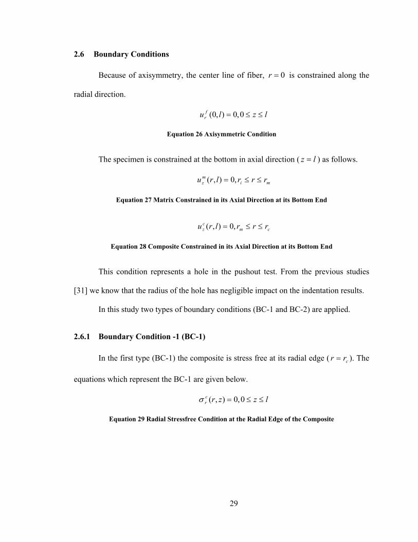
2.6 Boundary Conditions
Because of axisymmetry, the center line of fiber, 0=r is constrained along the
radial direction.
lzlu fr ≤≤= 0,0),0(
Equation 26 Axisymmetric Condition
The specimen is constrained at the bottom in axial direction ( ) as follows. lz =
mimz rrrlru ≤≤= ,0),(
Equation 27 Matrix Constrained in its Axial Direction at its Bottom End
cmcz rrrlru ≤≤= ,0),(
Equation 28 Composite Constrained in its Axial Direction at its Bottom End
This condition represents a hole in the pushout test. From the previous studies
[31] we know that the radius of the hole has negligible impact on the indentation results.
In this study two types of boundary conditions (BC-1 and BC-2) are applied.
2.6.1 Boundary Condition -1 (BC-1)
In the first type (BC-1) the composite is stress free at its radial edge ( crr = ). The
equations which represent the BC-1 are given below.
lzzrcr ≤≤= 0,0),(σ
Equation 29 Radial Stressfree Condition at the Radial Edge of the Composite
29

lzzrcrz ≤≤= 0,0),(σ
Equation 30 Shear Stressfree Condition at the Radial Edge of the Composite
Figure 6 Composite with BC-1
2.6.2 Boundary Condition-2 (BC-2)
In the second type of boundary condition (BC-2), the matrix is constrained at its
radial edge ( ) [2]. mrr =
lzzru mmr ≤≤= 0,0),(
Equation 31 Radial Displacement Constrained at the Radial Edge of the Matrix
lzzru mmz ≤≤= 0,0),(
Equation 32 Axial Displacement Constrained along the Radial Edge of the Matrix
This boundary condition is modeled by assuming the composite as a rigid body by
assigning the Young’s modulus of composite as 100 times the Young’s modulus of the
fiber and the Poisson’s ratio as 0.48.
30
2.7 Loading
Three types of indenter loads are applied – load due to a spherical indenter, a flat
indenter and a uniform pressure.
2.7.1 Spherical Indenter
The spherical indenter is modeled as a quarter (model is axisymmetric) rigid
sphere by assigning its Young’s modulus as 100 times that of the fiber and its Poisson’s
ratio as 0.48.
A constant load, is applied to the fiber via pressure, on the top plane of the
spherical indenter (see
P sp
Figure 7),
2RPps π
=
Equation 33 Pressure Applied on the Spherical Indenter
where,
=R radius of the spherical indenter.
31

F I MC
sP
R
Figure 7 Schematic Diagram of Spherical Indenter Loading
2.7.1.1 Radius of Contact
Many initial trial runs in ANSYS [9] using spherical indenter loading with various
combinations of the factors (boundary conditions of the specimen, fiber volume fraction,
thickness of interphase to fiber radius ratio, and type of interphase model) show that the
contact area does not vary by more than 1%. The contact radius is found by checking the
contact status of the contact and target elements on the top surface of the fiber near the
contact area.
32

Figure 8 Contact between the Fiber and the Indenter
Hence, the contact area between the indenter and fiber depends only on the elastic
moduli of the fiber and the indenter. It was also noted that the radius, a of the contact
area between the fiber and the spherical indenter was within 1% of what Fischer-Cripps,
et al. [32] calculated using the following formulas.
3/1
34
⎟⎟⎠
⎞⎜⎜⎝
⎛=
fEKPRa
⎥⎦
⎤⎢⎣
⎡−+−= )1()1(
169 22
inin
ff E
EK νν
Equation 34 Fischer-Cripps Equation to Calculate the Contact Radius
33

Where, = Young’s modulus of fiber, fE fν = Poisson’s ratio of fiber, =
Young’s modulus of indenter,
inE
inν = Poisson’s ratio of indenter.
Note that the above equations are for the case of a spherical indentor loaded on a
homogeneous half-plane.
2.7.2 Uniform Pressure Loading
The case of the uniform pressure indenter is only a hypothetical indenter and is
considered in this study only because some studies [2] model the indentation as a uniform
pressure. The uniform pressure loading is applied on the fiber over a finite length. The
value of the length over which this uniform pressure is applied is equal to the value of
contact radius, a found from the spherical indenter loading case. The uniform pressure
( ) is calculated using the formula given below. up
2aPpu π
=
Equation 35 Uniform Pressure Applied on the Fiber
34

F I MC
uP
a
Figure 9 Schematic Diagram Illustrating Uniform Pressure Loading
2.7.3 Flat Indenter
The flat indenter is modeled as a cylinder with a circular cross-section of radius,
on the fiber. Like the spherical indenter, the flat indenter is treated as rigid and its
elastic moduli are chosen to be same as that of the spherical indenter. A uniform pressure
is applied on the top plane of the flat indenter.
a
up
35
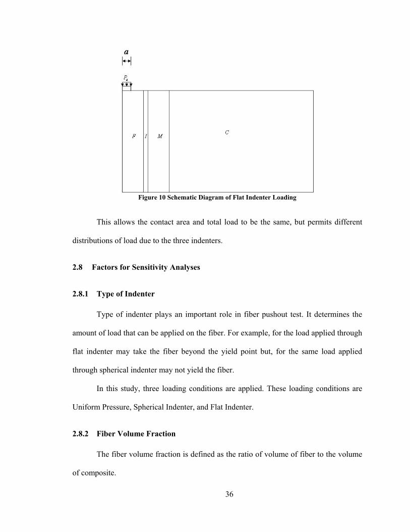
Figure 10 Schematic Diagram of Flat Indenter Loading
This allows the contact area and total load to be the same, but permits different
distributions of load due to the three indenters.
2.8 Factors for Sensitivity Analyses
2.8.1 Type of Indenter
Type of indenter plays an important role in fiber pushout test. It determines the
amount of load that can be applied on the fiber. For example, for the load applied through
flat indenter may take the fiber beyond the yield point but, for the same load applied
through spherical indenter may not yield the fiber.
In this study, three loading conditions are applied. These loading conditions are
Uniform Pressure, Spherical Indenter, and Flat Indenter.
2.8.2 Fiber Volume Fraction
The fiber volume fraction is defined as the ratio of volume of fiber to the volume
of composite.
36
2
2
m
f
rr
FVF =
Equation 36 Fiber Volume Fraction
Fiber volume fraction plays an important role in determining the elastic moduli of
the composite [33].
2.8.3 Thickness of Interphase to Radius of Fiber Ratio (TIRFR)
It is the ratio of thickness of the interphase layer present between fiber and matrix
to radius of the fiber.
Functionally graded coatings offer an improvement of 35 % after heat treatment
and 70% before heat treatment on composite fracture [17]. The increase in interfacial
toughness is dependent on type of fiber/matrix, type of coating, and the thickness of
coating (thickness of interphase). This is the reason for considering this as a factor in this
study.
For this study, we use TIRFR values of 1/10, 1/15 and 1/20.
2.8.4 Type of Interphase
As discussed in the Section 2.8.3, coatings improve the interfacial toughness to
large extent. The extent of increase of the interfacial toughness depends on the type of
coating. The coatings may be homogeneous or nonhomogeneous. Also the extent of
nonhomogenity (variation of elastic moduli) depends up on the type of coating.
The type of interphase is in this study defined by how the elastic moduli vary
along the radial thickness of the interphase. The nonhomogenity is described either by a
linear or exponential variation of the Young’s modulus and Poisson’s ratio.
37

2.8.5 Boundary Conditions
Boundary conditions influence the interfacial stresses. Galbraith et al. [10]
carried the pushout test and found that the interfacial stresses can be reduced to great
extent by keeping a layer on the back face of the specimen.
Two kinds of boundary conditions are applied in our study. One considers the
composite as stress-free at its radial edge (BC-1), and other one constrains the matrix at
its radial edge (BC-2).
2.9 Responses for Sensitivity Analyses
2.9.1 Load to Contact Depth Ratio (LCDR)
We used load to contact depth ratio (LCDR) as a response for this study because
the LCDR is the measure of interphase properties such as shear modulus [2]. The
equation for LCDR is given by Equation 37. Note that it is not a nondimensional number.
δPLCDR =
Equation 37 Load to Contact Depth Ratio
Where, P = Load applied, δ = Displacement at the top (contact depth).
2.9.2 Normalized Maximum Interfacial Radial Stress (NMIRS)
The NMIRS is defined as the nondimensional ratio of the maximum tensile
interfacial radial stress ( max),( zrfirσ ) to the average stress applied over the contact area,
that is,
38

lz
aP
zrNMIRS f
ir ≤≤= 0,
),(
2
max
π
σ
Equation 38 Normalized Maximum Radial Stress at the Fiber-Interphase Interface
NMIRS is taken as a response for this study because when the fiber is loaded, the
crack initiation is observed at the back face of the specimen when the interfacial tensile
radial stress exceeds the bond strength [10, 34-37].
In this study, the maximum interfacial tensile radial stress is taken as the
interfacial tensile radial stresses cause fiber debonding from the matrix.
2.9.3 Normalized Maximum Interfacial Shear Stress (NMISS)
The NMISS is defined as the nondimensional ratio of the magnitude of maximum
interfacial shear stress ( max),( zrfirzσ ) to the average stress applied over the contact area,
that is,
lz
aP
zrNMISS f
irz ≤≤= 0,
),(
2
max
π
σ
Equation 39 Normalized Maximum Shear Stress at the Fiber-Interphase Interface
In this study, the absolute value of the maximum interfacial shear stress is taken
because positive or negative direction of the shear stress is completely dependent on the
coordinate axes chosen.
39
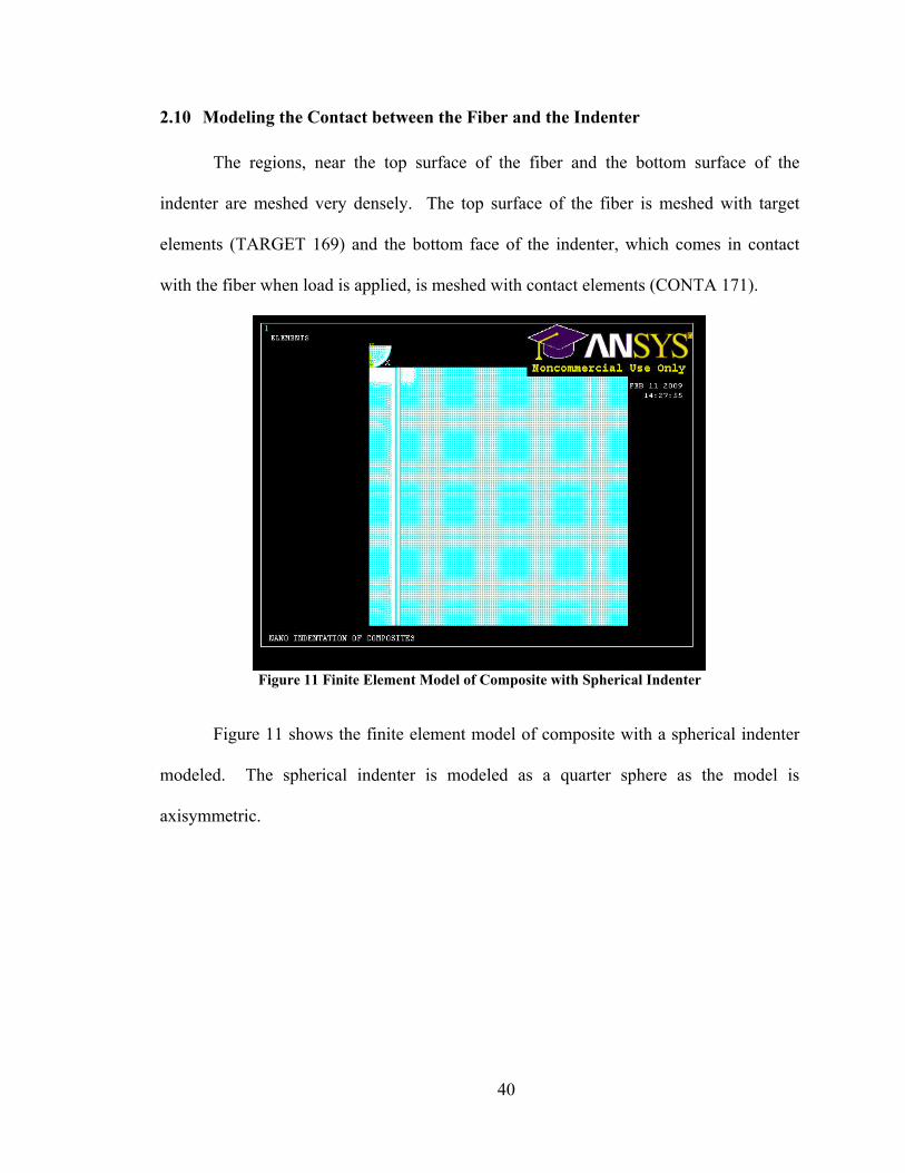
2.10 Modeling the Contact between the Fiber and the Indenter
The regions, near the top surface of the fiber and the bottom surface of the
indenter are meshed very densely. The top surface of the fiber is meshed with target
elements (TARGET 169) and the bottom face of the indenter, which comes in contact
with the fiber when load is applied, is meshed with contact elements (CONTA 171).
Figure 11 Finite Element Model of Composite with Spherical Indenter
Figure 11 shows the finite element model of composite with a spherical indenter
modeled. The spherical indenter is modeled as a quarter sphere as the model is
axisymmetric.
40

CHAPTER 3 VALIDATION OF MODEL
Initially a homogeneous half space meshed with PLANE182 elements and loaded
by an axisymmetric pressure loading is examined.
The stresses and displacements in the finite element model show good agreement
with the classical Terezawa’s [38] solution for a semi-infinite medium of homogeneous
half space with an axisymmetric arbitrary pressure loading.
Before starting the ANSYS [9] runs for all the combinations of factors, several
checks are performed to ensure the accuracy of the model. Accuracy of the model is
checked for each indenter loading case as follows.
3.1 Spherical Indenter
Spherical indenter loading is applied on the fiber by applying a pressure, on
the top plane of the spherical indenter (see
sp
Figure 7). Radius of contact, is obtained by
checking the contact status of the contact elements in ANSYS [9].
a
3.1.1 Contact Between the Indenter and Fiber
Using an APDL code, all the nodal information of the nodes (node number,
location of node, displacements, all stress components, and all elastic strains) on the top
surface of the fiber and whose x -coordinate (radial distance from the center of the fiber)
is less than 1.5 times the contact radius are written to a text file. Now using a MATLAB
41

[39] program, this file is analyzed, and each and every nodal data is read into an array
inside MATLAB. Axial displacement and axial stresses are cubic spline interpolated with
respect to the radial distance from the center of the fiber. After the spline interpolation,
the axial stress and displacements are plotted against the radial distance from the center
of the fiber. (Note: All the nodes are taken on the top surface, so the -coordinate would
be zero for all the nodes).
y
Figure 12 Typical Distribution of Normalized Axial Stress Along the Normalized Radial
Distance from the Center of the Fiber for Spherical Indenter
Figure 13 Typical Distribution of Normalized Axial Displacement Along the Normalized
Radial Distance from the Center of the Fiber for Spherical Indenter
Figure 12 and Figure 13, both the axes are normalized. The axial stress is
normalized with the pressure applied for the uniform pressure indenter (see Equation 35).
The radial distance and the axial displacements are normalized with the contact radius.
42

From Figure 12, it can be clearly seen that the axial stress is distributed parabolically in
the contact area. The axial stress suddenly becomes near-zero value after passing the
contact radius. It is also observed that the contact radius found in ANSYS [9] by
checking the contact status of the contact elements is equal to the contact radius extracted
from MATLAB program. Also the load applied on the fiber is calculated using
MATLAB program from the axial stress data available.
∫=a
zmatlab rdrP0
2πσ
Equation 40 Total Load on the Fiber using the Axial Stress Data on the Top of the Fiber
Total load applied on the spherical indenter is calculated using
)()( 2RpP s π=
Equation 41 Total Load Applied on the Fiber through Spherical Indenter
It is observed that the loads, P and differ by less than 1%. This verifies our
contact between the fiber and indenter as the load applied is obtained back by integrating
the axial stresses over the contact area.
matlabP
3.1.2 Bonded Contact Between the Interfaces
Using an APDL code, displacement, shear stress in radial-axial plane, and the
radial stresses of the nodes at the interfaces of the fiber-interphase, sublayers of
interphase, interphase-matrix and matrix-composite are written to text files. By analyzing
the text files using a MATLAB program, it is found that the displacements and stresses of
the nodes of either side of the interface differ by less than 1%. This validates the bonded
contact between the interfaces in the model.
43

3.2 Uniform Pressure Indenter
Uniform pressure indenter loading is applied on the fiber by applying a uniform
pressure, on the top plane of the fiber (see up Figure 9).
3.2.1 Contact Between the Indenter and Fiber
Using an APDL code, all the nodal information of the nodes (node number,
location of node, displacements, all stress components, and all elastic strains) on the top
surface of the fiber and whose x -coordinate (radial distance from the center of the fiber)
is less than 1.5 times the contact radius are written to a text file. Now using MATLAB
program, this file is analyzed and each and every nodal data is read into an array inside
MATLAB. Now axial displacement and axial stresses are cubic spline interpolated with
respect to radial distance from the center of the fiber. After the spline interpolation, the
axial stress and displacements are plotted against the radial distance from the center of
the fiber.
Figure 14 Typical Distribution of Normalized Axial Stress Along the Normalized Radial
Distance from the Center of the Fiber for Uniform Pressure Indenter
44

Figure 15 Typical Distribution of Normalized Axial Displacement Along the Normalized
Radial Distance from the Center of the Fiber for Uniform Pressure Indenter
Figure 14 and Figure 15, both the axes are normalized. The axial stress is
normalized with the pressure applied over the uniform pressure indenter. The radial
distance and the axial displacements are normalized with the contact radius. From the
Figure 14, it can be clearly seen that the axial stress is uniform in the contact area and is
equal to and decreases immediately to a very low value after the contact radius. It is
also observed that the contact radius found in ANSYS [9] by checking the contact status
of the contact elements is equal to the contact radius extracted from MATLAB. Also the
load applied on the fiber is calculated using MATLAB program from the axial stress data
available using
up
Equation 40 .
Total load applied on the fiber using uniform pressure indenter is calculated using
the following formula.
)()( 2apP u π=
Equation 42 Load Applied on the Fiber through Uniform/Flat indenter
45

It is observed that the loads, and differ by less than 1%. This verifies our
contact between the fiber and indenter as the load applied is obtained back by integrating
the axial stresses over the contact area.
P matlabP
3.2.2 Bonded Contact Between the Interfaces
Using an APDL code, displacement, shear stress in radial-axial plane, and the
radial stresses of the nodes at the interfaces of the fiber-interphase, sublayers of
interphase, interphase-matrix and matrix-composite are written to text files. By analyzing
the text files using a MATLAB program, it is found that the displacements and stresses of
the nodes of either side of the interface differ by less than 1%. This validates the bonded
contact between the interfaces in the model.
3.3 Flat Indenter
Flat indenter loading is applied on the fiber by applying a pressure, on the top
plane of the flat indenter (see
up
Figure 10).
3.3.1 Contact Between the Indenter and Fiber
Using an APDL code, all the nodal information of the nodes (node number,
location of node, displacements, all stress components, and all elastic strains) on the top
surface of the fiber and whose x -coordinate (radial distance from the center of the fiber)
is less than 1.5 times the contact radius are written to a text file. Now using MATLAB
program, this file is analyzed and each and every nodal data is read into an array inside
MATLAB. Now axial displacement and axial stresses are cubic spline interpolated with
respect to radial distance from the center of the fiber. After the spline interpolation, the
46

axial stress and displacements are plotted against the radial distance from the center of
the fiber.
Figure 16 Typical Distribution of Normalized Axial Stress Along the Normalized Radial
Distance from the Center of the Fiber for Flat Indenter
Figure 17 Typical Distribution of Normalized Axial Displacement Along the Normalized
Radial Distance from the Center of the Fiber for Flat Indenter
Figure 16 and Figure 17, both the axes are normalized. The axial stress is
normalized with the pressure applied over the uniform pressure indenter. The radial
distance and the axial displacements are normalized with the contact radius. From Figure
17, the axial displacement is clearly uniform in the contact area and decreases
47

immediately after the radius of contact. Also from Figure 16, it can be clearly observed
that the axial stress increases through the contact radius, and reaches a maximum value at
the contact radius. Beyond the contact radius, it drops to a very low value. It is also
observed the contact radius found in ANSYS [9] by checking the contact status of the
contact elements is equal to the contact radius extracted from MATLAB. Also the load
applied on the fiber is calculated using the MATLAB program from the axial stress data
available using Equation 40.
Total load applied on the fiber using the flat indenter is calculated using Equation
42.
It is observed that the loads, and differ by less than 1%. This verifies our
contact between the fiber and indenter as the load applied is obtained back by integrating
the axial stresses over the contact area.
P matlabP
3.3.2 Bonded Contact Between the Interfaces
Using an APDL code, displacement, shear stress in radial-axial plane, and the
radial stresses of the nodes at the interfaces of the fiber-interphase, sublayers of
interphase, interphase-matrix and matrix-composite are written to text files. By analyzing
the text files using MATLAB program, it is found that the displacements and stresses of
the nodes of either side of the interface differ by less than 1%. This validates the bonded
contact between the interfaces in the model.
3.4 Validation with Huang SLA and Finite Element Model
Huang et al. [2] verified the accuracy of an analytical solution based on shear-lag
assumptions by a finite element method model, and concluded that their shear-lag model
48
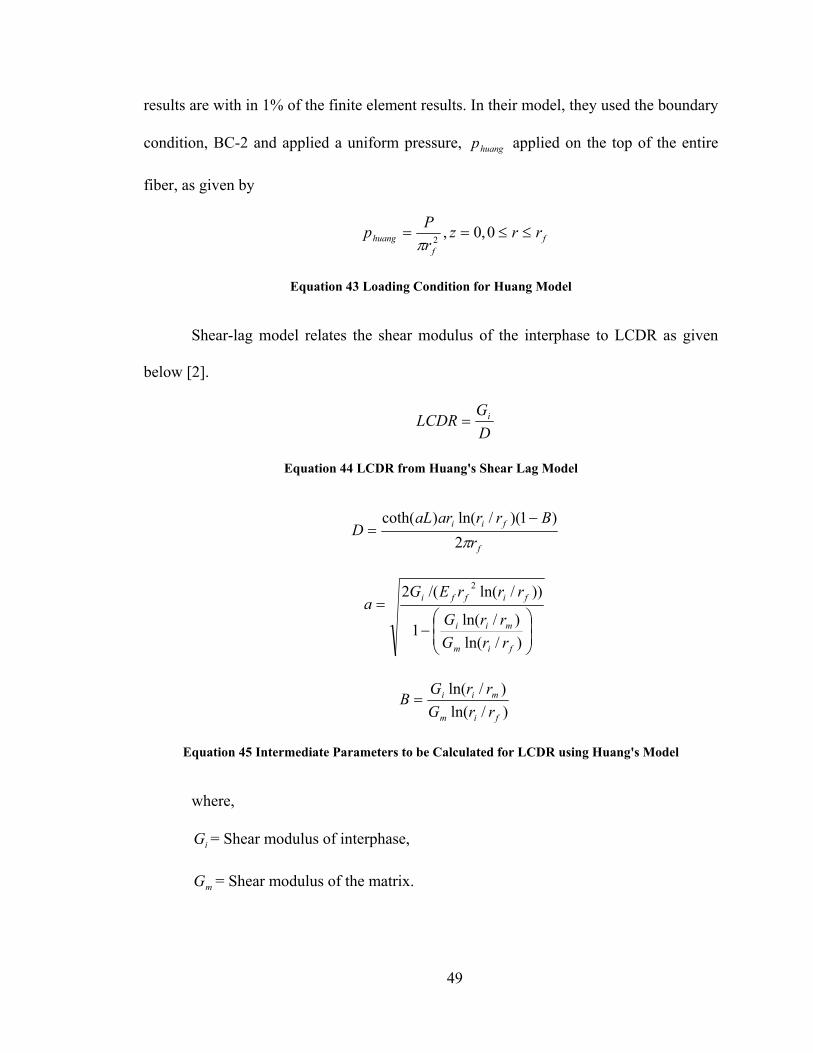
results are with in 1% of the finite element results. In their model, they used the boundary
condition, BC-2 and applied a uniform pressure, applied on the top of the entire
fiber, as given by
huangp
ff
huang rrzrPp ≤≤== 0,0,2π
Equation 43 Loading Condition for Huang Model
Shear-lag model relates the shear modulus of the interphase to LCDR as given
below [2].
DG
LCDR i=
Equation 44 LCDR from Huang's Shear Lag Model
f
fii
rBrraraL
Dπ2
)1)(/ln()coth( −=
⎟⎟⎠
⎞⎜⎜⎝
⎛−
=
)/ln()/ln(
1
))/ln(/(2 2
fim
mii
fiffi
rrGrrG
rrrEGa
)/ln()/ln(
fim
mii
rrGrrG
B =
Equation 45 Intermediate Parameters to be Calculated for LCDR using Huang's Model
where,
iG = Shear modulus of interphase,
mG = Shear modulus of the matrix.
49

Huang et al. [2] found that the values obtained by the Equation 44 are within 1%
of the finite element model. We verified this with our own finite element model by
applying the same boundary conditions and load as Huang, et al. [2]. The results were
within 2% of Huang’s [2] model. However, Huang’s [2] FEM model makes many
assumptions such as
1. Uniform loading over the fiber radius (when actually load is only applied only
over a small area).
2. Homogeneous interphase (when actually interphase may be nonhomogeneous).
3. Constrained matrix along the radial edge (when actually it is surrounded by a
cylinder with composite properties).
Only the first of the above three assumptions is quantitatively critical. Loading by
spherical indenters occurs only over a very small area of the fiber. Approximating this
loading as distributed throughout the fiber can underestimate the shear modulus of the
interphase by the order as much as 1000.
3.5 Validation Using Interfacial Stresses
In this validation, interfacial stresses are observed when load is applied.
3.5.1 Validation Using Interfacial Radial Stress
The interfacial radial stress is very large and compressive at the top end,
decreases, and almost stays constant (near zero value) along the length of the fiber and
changes to a positive value (tensile) as it reaches the bottom end of the composite. This
distribution of interfacial radial stress is in agreement with the BEM [1].
50

Figure 18 Typical Distribution of Normalized Interfacial Radial Stress Along the
Normalized Length of the Fiber
In the Figure 18, the interfacial radial stress is normalized with the pressure
applied on uniform indenter. The length of the fiber is normalized with the fiber radius.
Integrating the radial stress along the radial surface area of the fiber gives the force
applied on the fiber in radial direction. As there is no force applied in the radial direction
the value comes out to be zero.
020
=∫L
irf dzr σπ
Equation 46 Force in Radial Direction from the Interfacial Radial Stress
51

Figure 19 Typical Distribution of Normalized Interfacial Radial Displacement Along the
Normalized Length of the Fiber
In Figure 19, the interfacial radial displacement is highly negative at the top face
(loading end), then along the length of the fiber increases gradually and changes to a
positive value. It becomes a near zero value at the back face of the fiber.
3.5.2 Validation Using Interfacial Shear Stress
It is also observed the interfacial shear stress is very small (near zero) at the top
face of the fiber and increases to certain length of the fiber and again gradually decreases
along the length of the fiber and reaches a near zero value at the bottom end of the fiber.
52

Figure 20 Typical Distribution of Normalized Interfacial Shear Stress Along the Normalized
Length of the Fiber
In the Figure 20, the interfacial shear stress is normalized with the pressure
applied on the uniform indenter. The length of the fiber is normalized with the fiber
radius. Integrating the shear stress along the radial surface area of the fiber gives the axial
load applied on the fiber.
∫=L
irzf dzrP
0
2 σπ
Equation 47 Axial Force Applied on the Fiber from the Interfacial Shear Stress
53

Figure 21 Typical Distribution of Normalized Interfacial Axial Displacement Along the
Normalized Length of the Fiber
In Figure 21, the interfacial axial displacement is highly negative at the top face
(loading end), and then along the length of the fiber increases gradually. The maximum
negative axial displacement is found at the top face (loading end) and the minimum is
found at the back face. The interfacial axial displacement is negative throughout the fiber
length.
54

CHAPTER 4 RESULTS AND CONCLUSIONS
This study uses a formal Design of Experiments (DOE) [27] analysis to quantify
the effects on parameters
1. LCDR,
2. NMIRS,
3. NMISS,
due to the parameters
1. Type of indenter,
2. Fiber volume fraction,
3. Thickness of interphase,
4. Type of interphase, and
5. Boundary conditions.
For this purpose we designed experiments using mixed level full factorial design.
The five factors chosen for the mixed level full factorial design and their levels are shown
in Table 2.
55
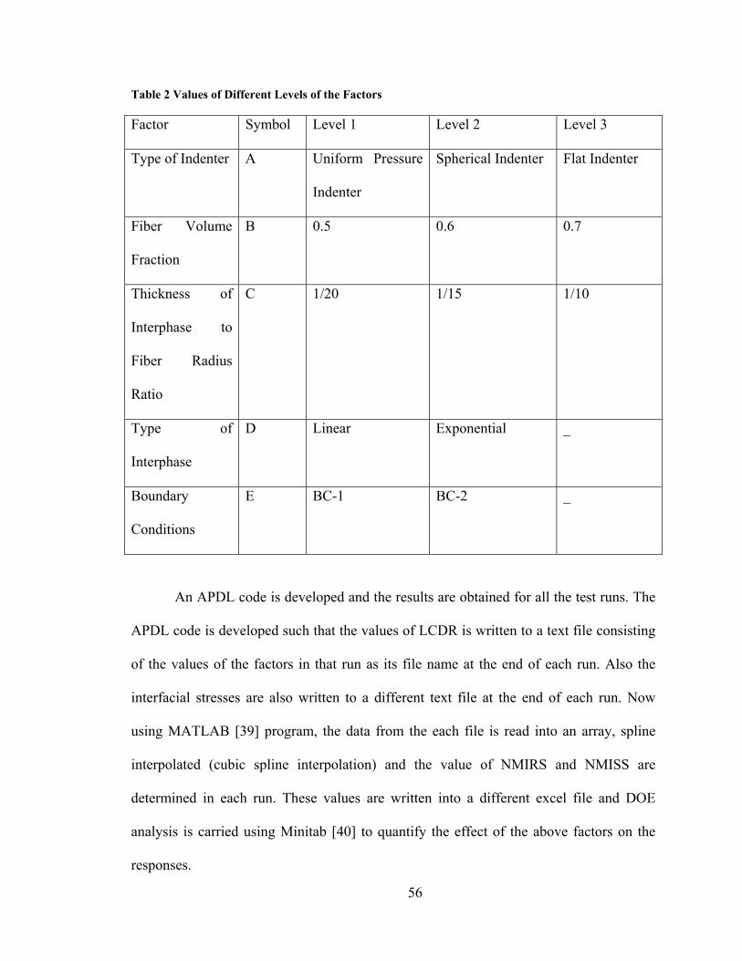
Table 2 Values of Different Levels of the Factors
Factor Symbol Level 1 Level 2 Level 3
Type of Indenter A Uniform Pressure
Indenter
Spherical Indenter Flat Indenter
Fiber Volume
Fraction
B 0.5 0.6 0.7
Thickness of
Interphase to
Fiber Radius
Ratio
C 1/20 1/15 1/10
Type of
Interphase
D Linear Exponential _
Boundary
Conditions
E BC-1 BC-2 _
An APDL code is developed and the results are obtained for all the test runs. The
APDL code is developed such that the values of LCDR is written to a text file consisting
of the values of the factors in that run as its file name at the end of each run. Also the
interfacial stresses are also written to a different text file at the end of each run. Now
using MATLAB [39] program, the data from the each file is read into an array, spline
interpolated (cubic spline interpolation) and the value of NMIRS and NMISS are
determined in each run. These values are written into a different excel file and DOE
analysis is carried using Minitab [40] to quantify the effect of the above factors on the
responses.
56

4.1 Responses for the Sensitivity Analyses
4.1.1 Load to Contact Depth Ratio (LCDR)
Figure 22 shows the normalized load to contact depth ratio for different indenters.
The normalization is done with respect to the load to contact depth ratio of the spherical
indenter. Figure 22 show that, the flat indenter gives the higher LCDR value for the same
load. This also shows that the LCDR can differ by as much as 20 to 50% between the
types of indenter.
0.8
1
1.2
1.4
1.6
uniform spherical flat
Type of Indenter
Nor
mal
ized
Loa
d to
con
tact
dep
th ra
tio
Figure 22 Normalized LCDR as a Function of Type of Indenter.
Table 3 shows that only the type of indenter has the significant effect on LCDR.
All other factors have near-zero effect on load to contact depth ratio (LCDR).
57

Table 3 Percentage Contribution of Factors to Load to Contact Depth Ratio
SOURCE PERCENTAGE
CONTRIBUTION
A 99.9
(A= Type of Indenter, B= Fiber Volume Fraction, C= Thickness of Interphase to
Fiber Radius Ratio, D= Type of Interphase, E=Boundary Conditions)
4.1.2 Normalized Maximum Interfacial Radial Stress (NMIRS)
When indenter load is applied on the fiber, interfacial radial stress at the top face
is found to be compressive and it is found to be tensile at the back face of the specimen
(see Figure 18). The NMIRS used in this study is the maximum tensile interfacial radial
stress obtained from the back face of the specimen.
Figure 23, Figure 24, and Figure 25 show typical parametric curves for the
normalized maximum interfacial radial stress as a function of the fiber volume fraction
for different boundary conditions, interphase thickness, and type of interphase
respectively.
58

Figure 23 Normalized Maximum Interfacial Radial Stress as a Function of Fiber Volume
Fraction for Uniform Pressure Indenter, Linear Type of Interphase, and TIRFR=1/20.
In the pushout test, both interfacial radial and hoop stresses are dependent on the
specimen configuration. Figure 23 shows that, the value of NMIRS for BC-1 is higher
than that for BC-2. For the boundary condition, BC-2, the radial edge of matrix is totally
constrained, and hence the bulging that occurs when the load is applied on the fiber is
reduced greatly as compared to the boundary condition, BC-1, where the radial edge of
the composite is free [10]. This resulted in the lower value of NMIRS for BC-2. Figure
23 show that, the NMIRS differ as much as by 48% with boundary conditions for higher
fiber volume fraction and differ as much as by 115% for lower fiber volume fraction.
59
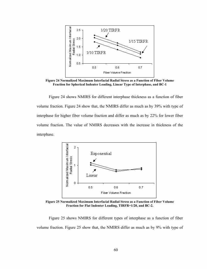
Figure 24 Normalized Maximum Interfacial Radial Stress as a Function of Fiber Volume
Fraction for Spherical Indenter Loading, Linear Type of Interphase, and BC-1
Figure 24 shows NMIRS for different interphase thickness as a function of fiber
volume fraction. Figure 24 show that, the NMIRS differ as much as by 39% with type of
interphase for higher fiber volume fraction and differ as much as by 22% for lower fiber
volume fraction. The value of NMIRS decreases with the increase in thickness of the
interphase.
Figure 25 Normalized Maximum Interfacial Radial Stress as a Function of Fiber Volume
Fraction for Flat Indenter Loading, TIRFR=1/20, and BC-2.
Figure 25 shows NMIRS for different types of interphase as a function of fiber
volume fraction. Figure 25 show that, the NMIRS differ as much as by 9% with type of
60

interphase for higher fiber volume fraction and differ as much as by 11% for lower fiber
volume fraction.
Table 4 shows that the normalized maximum interfacial radial stress is sensitive
to boundary conditions (57%), fiber volume fraction (20%), combined effect of fiber
volume fraction and boundary conditions (15%), thickness of interphase (3%), and type
of interphase (1%). What is more evident is that the normalized maximum radial stress at
the interface is not sensitive to the type of indenter.
Table 4 Percentage Contribution of Factors to NMIRS
SOURCE PERCENTAGE CONTRIBUTION
B 19.88
C 3.23
D 1.21
E 57.45
B*E 14.73
C*E 1.20
(A= Type of Indenter, B= Fiber Volume Fraction, C= Thickness of Interphase to
Fiber Radius Ratio, D= Type of Interphase, E=Boundary Conditions)
4.1.3 Normalized Maximum Interfacial Shear Stress (NMISS)
Figure 26 shows typical parametric curves for the normalized maximum
interfacial shear stress as a function of the fiber volume fraction for the two different
boundary conditions. Figure 26 also shows that the value of NMISS increases with
increase of fiber volume fraction.
61

Figure 26 Normalized Maximum Interfacial Shear Stress as a Function of Fiber Volume
Fraction for Uniform Indenter, Linear Type of Interphase, and TIRFR=1/20
Figure 26 show that, the NMISS differs as much as by 12% with type of
interphase for higher fiber volume fraction, and differs as much as by 14% for lower fiber
volume fraction.
Figure 27 Normalized Maximum Interfacial Shear Stress as a Function of Fiber Volume
Fraction for Spherical Indenter Loading, Linear Type of Interphase, and BC-1
Figure 27 show that the NMISS differs by as much as 16% with type of
interphase for higher fiber volume fraction and differs as much as by 20% for lower fiber
volume fraction. The NMISS value increases with the thickness of the interphase.
62

Figure 28 Normalized Maximum Interfacial Shear Stress as a Function of Fiber Volume
Fraction for Flat Indenter Loading, TIRFR=1/20, and BC-2.
Figure 28 shows NMISS for different types of interphase as a function of fiber
volume fraction. Figure 28 show that the NMISS differs as much as by 8% with type of
interphase for higher fiber volume fraction and differs as much as by 9% for lower fiber
volume fraction.
Table 5 shows that the normalized maximum interfacial shear stress is mainly
sensitive to fiber volume fraction (30%), boundary conditions (27%), thickness of
interphase (23%), and the type of interphase (18%). What is more evident is that the
normalized maximum shear stress at the interface is also not sensitive to the type of
indenter.
63
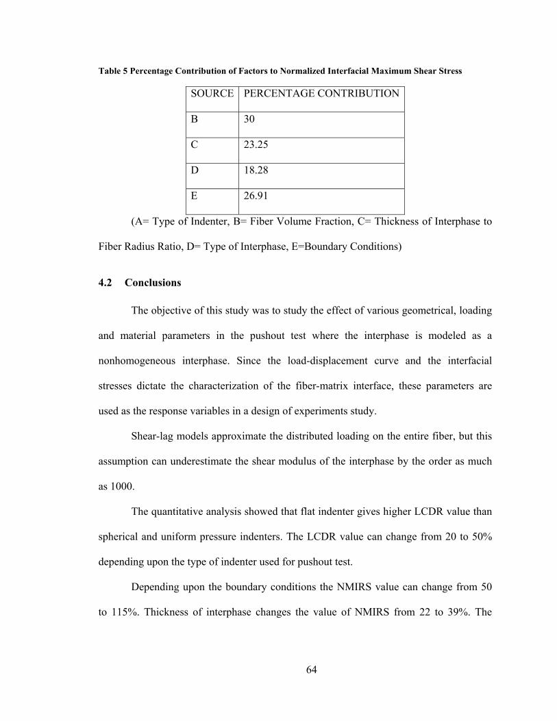
Table 5 Percentage Contribution of Factors to Normalized Interfacial Maximum Shear Stress
SOURCE PERCENTAGE CONTRIBUTION
B 30
C 23.25
D 18.28
E 26.91
(A= Type of Indenter, B= Fiber Volume Fraction, C= Thickness of Interphase to
Fiber Radius Ratio, D= Type of Interphase, E=Boundary Conditions)
4.2 Conclusions
The objective of this study was to study the effect of various geometrical, loading
and material parameters in the pushout test where the interphase is modeled as a
nonhomogeneous interphase. Since the load-displacement curve and the interfacial
stresses dictate the characterization of the fiber-matrix interface, these parameters are
used as the response variables in a design of experiments study.
Shear-lag models approximate the distributed loading on the entire fiber, but this
assumption can underestimate the shear modulus of the interphase by the order as much
as 1000.
The quantitative analysis showed that flat indenter gives higher LCDR value than
spherical and uniform pressure indenters. The LCDR value can change from 20 to 50%
depending upon the type of indenter used for pushout test.
Depending upon the boundary conditions the NMIRS value can change from 50
to 115%. Thickness of interphase changes the value of NMIRS from 22 to 39%. The
64
interfacial radial stress decreases with the increase in thickness. Also the type of
interphase can change the NMIRS value from 9 to 11%.
NMISS value can change up to 14% depending upon the boundary conditions.
Thickness of the interphase changes the NMISS value up to 20%. The interfacial shear
stress increases with the increase in fiber volume fraction, irrespective of the other
parameters.
The sensitivity analysis showed that load to contact depth ratio is dependent only
on the indenter type, while the interfacial radial stresses are not sensitive to indenter type.
The interfacial shear stresses are mainly sensitive to fiber volume fraction, boundary
conditions, thickness of interphase, and type of interphase.
65

REFERENCES
[1] Ye, J., and Kaw, A. K., 1999, "Determination of Mechanical Properties of Fiber-Matrix Interface from Pushout Test," Theoretical and Applied Fracture Mechanics, 32(1) pp. 15.
[2] Huang, X., Foley, M. E., Bogetti, T. A., 7-9 September,2005, "Mechanics of the Fiber-Matrix Interphase Push-Out Test," A Reprint from the Proceedings of the American Society for Composites 20th Annual Technical Conference, .
[3] Jero, P. D., Parthasarathy, T. A., and Kerans, R. J., 1993, "Comparison of Single and Multi-Fiber Pushout Techniques," Ceramic Engineering and Science Proceedings, 14(7) pp. 147.
[4] Chun-Hway, H., 1993, "Evaluation of Interfacial Properties of Fiber-Reinforced Ceramic Composites using a Mechanical Properties Microprobe," Journal of the American Ceramic Society, 76(12) pp. 3041.
[5] Chun-Hway, H., 1989, "Some Considerations of Evaluation of Interfacial Frictional Stress from the Indentation Technique for Fiber-Reinforced Ceramic Composites," Journal of Materials Science Letters, 8(6) pp. 739.
[6] Lara-Curzio, E., and Ferber, M. K., 1994, "Methodology for the Determination of the Interfacial Properties of Brittle Matrix Composites," Journal of Materials Science, 29(23) pp. 6152.
[7] Yuan, M. N., Yang, Y. Q., Ma, Z. J., 2007, "Analysis of Interfacial Behavior in Titanium Matrix Composites by using the Finite Element Method (SCS-6/Ti55)," Scripta Materialia, 56(6) pp. 533.
[8] Shetty, D. K., 1988, "Shear-Lag Analysis of Fiber Push-Out (Indentation) Tests for Estimating Interfacial Friction Stress in Ceramic-Matrix Composites," Journal of the American Ceramic Society, 71(2) pp. C107.
[9] ANSYS, 2009, "ANSYS 11.0," 11.0.
[10] Galbraith, J. M., Rhyne, E. P., Koss, D. A., 1993, "Fiber Pushout and Interfacial Shear in Metal-Matrix Composites," JOM, 45(3) pp. 34.
66

[11] Lin, G., Geubelle, P. H., and Sottos, N. R., 2001, "Simulation of Fiber Debonding with Friction in a Model Composite Pushout Test," International Journal of Solids and Structures, 38(46) pp. 8547.
[12] Xing, Y. M., Tanaka, Y., Kishimoto, S., 2003, "Determining Interfacial Thermal Residual Stress in SiC/Ti-15-3 Composites," Scripta Materialia, 48(6) pp. 701.
[13] Mital, S. K., and Chamis, C. C., 1991, "Fiber Pushout Test. A Three-Dimensional Finite Element Computational Simulation," Journal of Composites Technology Research, 13(1) pp. 14.
[14] Shirazi-Adl, A., 1992, "Finite Element Stress Analysis of a Push-Out Test., 1. Fixed Interface using Stress Compatible Elements," Journal of Biomechanical Engineering, 114(1) pp. 111.
[15] Shirazi-Adl, A., and Forcione, A., 1992, "Finite Element Stress Analysis of a Push-Out Test. II. Free Interface with Nonlinear Friction Properties," Journal of Biomechanical Engineering, 114(2) pp. 155.
[16] Shirazi-Adl, A., 1990, "Stress Continuous Finite Element Formulation. Application to Biomechanics of a Push-Out Test with Attached Interface," American Society of Mechanical Engineers, Bioengineering Division (Publication) BED, 17pp. 311.
[17] Haque, S., and Choy, K. L., 2000, "Push-Out Testing of SiC Monofilaments with a TiC Based Functionally Graded Coating," Journal of Materials Science, 35(17) pp. 4225.
[18] Drzal, L. T., 1986, "Interphase in Epoxy Composites." Advances in Polymer Science, 75pp. 1.
[19] Jayaraman, K., Reifsnider, K.,L., and Swain, R.,E., 1993, "Elastic and Thermal Effects in the Interphase. I. Comments on Characterization Methods," Journal of Composites Technology Research, 15(1) pp. 3.
[20] Jayaraman, K., Reifsnider, K.,L., and Swain, R.,E., 1993, "Elastic and Thermal Effects in the Interphase. II. Comments on Modeling Studies," Journal of Composites Technology Research, 15(1) pp. 14.
[21] Chamis, C.C., 1974, "Mechanics of load transfer at the interface." Springer-Verlag, pp. 31.
[22] Argon, A.,S., Gupta, V., Landis,H.,S., 1989, "Intrinsic Toughness of Interfaces," Materials Science Engineering A: Structural Materials: Properties, Microstructure and Processing, 107(1) pp. 41.
67

[23] Delale, F., and Erdogan, F., 1988, "On the Mechanical Modeling of the Interfacial Region in Bonded Half-Planes." Journal of Applied Mechanics, 55(2) pp. 317.
[24] Erdogan, F., 1995, "Fracture Mechanics of Functionally Graded Materials," Composites Engineering, 5(7) pp. 753.
[25] Kaw, A. K., Selvarathinam, A.,S., and Besterfield, G. H., 1992, "Comparison of Interphase Models for a Crack in Fiber Reinforced Composite," Theoretical and Applied Fracture Mechanics, 17(2) pp. 133.
[26] Bechel, V. T., and Kaw, A. K., 1994, "Fracture Mechanics of Composites with Nonhomogeneous Interphases and Nondilute Fiber Volume Fractions," International Journal of Solids and Structures, 31(15) pp. 2053.
[27] Chalasani, P., Kaw, A., Daly, J., 2007, "Effect of Geometrical and Material Parameters in Nanoindentation of Layered Materials with an Interphase," International Journal of Solids and Structures, 44(16) pp. 5380.
[28] Montgomery, D.C., 2001, "Design and analysis of experiments," John Wiley & Sons, Inc., New York, .
[29] Chudoba, T., Schwarzer, N., Linss, V., 2004, "Determination of Mechanical Properties of Graded Coatings using Nanoindentation," Thin Solid Films, 469pp. 239.
[30] Sutcu, M., 1992, "Recursive Concentric Cylinder Model for Composites Containing Coated Fibers," International Journal of Solids and Structures, 29(2) pp. 197.
[31] Trimula, S., Madanaraj, H., Kaw, A. K., 1996, "Effect of Extrinsic and Intrinsic Factors on an Indentation Test," International Journal of Solids and Structures, 33(24) pp. 3497.
[32] Fischer-Cripps, A. C., 1999, "The Hertzian Contact Surface," Journal of Materials Science, 34(1) pp. 129.
[33] Kaw, A.K., 2005, "Mechanics of Composite Materials, Second Edition," CRC Press, Boca Raton, New York, pp. 496.
[34] Kakisawa, H., Honda, K., and Kagawa, Y., 2000, "Effect of Wear on Interface Frictional Resistance in Fiber-Reinforced Composite: Model Experimental," Materials Science Engineering. A, Structural Materials, 284(1) pp. 226.
[35] Kakisawa, H., and Kagawa, Y., 1999, "New Approach for Interface Sliding Shear Resistance in Al2O3 Fiber-Reinforced Al2O3 Matrix Composite," Ceramic Engineering and Science Proceedings, 20(3) pp. 435.
68

[36] Pochiraju, K. V., Tandon, G. P., and Pagano, N. J., 2001, "Analyses of Single Fiber Pushout Considering Interfacial Friction and Adhesion," Journal of the Mechanics and Physics of Solids, 49(10) pp. 2307.
[37] Dollar, A., Steif, P. S., Wang, Y. C., 1993, "Analyses of the Fiber Push-Out Test," International Journal of Solids and Structures, 30(10) pp. 1313.
[38] Sneddon, I. N., 1951, "Fourier Transforms," McGraw-Hill, New York, .
[39] MATLAB, 2007, "MATLAB 2007," 7.3.0.267.
[40] Mathews, P.G., 2004, "Design of experiments with minitab," ASQ Quality Press, Milwaukee, WI., .
69