Analysis of Satellite Constellations for the Continuous ...
25
Analysis of Satellite Constellations for the Continuous Coverage of Ground Regions Guangming Dai, a Xiaoyu Chen. b and Maocai Wang, c China University of Geosciences, Wuhan CO 430074, China Elena Fernández, d Technical University of Catalonia, Barcelona, CO 08034, Spain Tuan Nam Nguyen, e and Gerhard Reinelt, f Heidelberg University, Heidelberg, CO 69120, Germany This paper studies the problem of analyzing multisatellite constellations with respect to their coverage capacity of areas on Earth’s surface. The geometric configuration of constellation projection points on Earth’s surface is investigated. A geometric subdi- vision approach is described, and the coverage target area belonging to each satellite and its maximum circle radius are defined and calculated. Accordingly, the target area can be decomposed into subregions, and thus the multisatellite coverage problem is decomposed into a one-satellite coverage problem. An accurate and effective solution method is proposed that solves both continuous and discontinuous coverage problems for any type of ground area. In addition, a procedure for calculating satellite orbital parameters is also proposed. The performance of our approach is analyzed using the Globalstar system as an example, and it is shown that it compares favorably with the classical grid-point technique and the longitude method. a Prof. Dr., School of Computer Science, [email protected]. b Ph.D., School of Computer Science, [email protected]. (Corresponding author) c Ass.Prof. Dr., School of Computer Science, [email protected]. d Prof. Dr., Statistics and Operations Research Department, [email protected]. e Dr., Institute of Computer Science, [email protected]. f Prof. Dr., Institute of Computer Science, [email protected].
Transcript of Analysis of Satellite Constellations for the Continuous ...

Analysis of Satellite Constellations for the
Continuous Coverage of Ground Regions
Guangming Dai,a Xiaoyu Chen.b and Maocai Wang,c
China University of Geosciences, Wuhan CO 430074, China
Elena Fernández,d
Technical University of Catalonia, Barcelona, CO 08034, Spain
Tuan Nam Nguyen,e and Gerhard Reinelt,f
Heidelberg University, Heidelberg, CO 69120, Germany
This paper studies the problem of analyzing multisatellite constellations with respect
to their coverage capacity of areas on Earth’s surface. The geometric configuration of
constellation projection points on Earth’s surface is investigated. A geometric subdi-
vision approach is described, and the coverage target area belonging to each satellite
and its maximum circle radius are defined and calculated. Accordingly, the target area
can be decomposed into subregions, and thus the multisatellite coverage problem is
decomposed into a one-satellite coverage problem. An accurate and effective solution
method is proposed that solves both continuous and discontinuous coverage problems
for any type of ground area. In addition, a procedure for calculating satellite orbital
parameters is also proposed. The performance of our approach is analyzed using the
Globalstar system as an example, and it is shown that it compares favorably with the
classical grid-point technique and the longitude method.
a Prof. Dr., School of Computer Science, [email protected] Ph.D., School of Computer Science, [email protected]. (Corresponding author)c Ass.Prof. Dr., School of Computer Science, [email protected] Prof. Dr., Statistics and Operations Research Department, [email protected] Dr., Institute of Computer Science, [email protected] Prof. Dr., Institute of Computer Science, [email protected].

Nomenclature
Oe = Earth’s center
Re = Earth’s radius
S = the satellite
C = the satellites constellation
H = orbital altitude
P,P’ = point on Earth’s surface
γmin = minimum elevation angle
α = coverage angle
d = coverage spherical radius
r = spherical circumcircle radius
O = the finite set in some metric space M with distance function d
V R(Oi) = the Voronoi region associated with the point Oi
V D(O) = the Voronoi diagram of O
DT (O) = the Delaunay triangulation of O
Θ(P, α) = spherical circle with the center point P (θ, ϕ) and radius α
θ, ϕ = the longitude and latitude angle
M(P ) = coordination rotation matrix in R3×3
Ru(α) = the rotation with angle α around the u-axis
β = the orientation angle
g(β) = one-to-one mapping from β to a unique point
h(Θ′) = projection function from a spherical h(Θ′) to the yz-plane
f = mapping an orientation angle to a point on the spherical circle
Ω = target area
Ωi = the coverage target area of Si
∂Ωi = the boundary of coverage target area Ωi
rmax(i) = maximum circle radius of Si
Fi = the coverage feature point set of Si
2

I. Introduction
SATELLITES find numerous applications in communication, navigation, imaging, and remote
sensing [1, 2]. The requirements for data accuracy and real-time observations become more and
more extensive as the need for Earth’s observation data continuously increases [3]. To satisfy these
demands systems of multiple satellites have to be designed and their performance has to be analyzed.
Earth observation from remote satellites and data transmission between satellites and facilities
are both related to satellite coverage. In general, satellite coverage problems arise when a target
area on the Earth’s surface must be visible to one or more satellites. In principle, there are two
main types of coverage problems. One class assumes that the parameters of the satellites is fixed
and studies their coverage capacity measured in terms of the percentage of the target area which is
covered (visible). The second class of problems refers to the determination of the positions of the
satellites (i.e., their constellation or configuration) including satellites orbital parameters in order
to achieve a maximum coverage. Special variants arise in both settings if full coverage of the target
area is requested and an accurate determination of the achieved coverage is necessary with respect
to a variety of coverage areas. Furthermore, because satellites are moving and covering areas are
subject to change, in practice these problems must be extended to account for varying constellations
within given time intervals, also denoted reconstruction periods.
Most methods in coverage analysis are based on the visibility of a subset of points of the given
target area [4]. Hence, an accurate coverage of such points becomes a prerequisite, given that
the performance of satellite constellations significantly depends on the precision with which such
points are covered. Recent research on coverage analysis often resorts to simulation or analytical
methods. Such methods exhibit a low computational efficiency and little reliability of the results.
Thus alternative methods are needed for large target areas when high accuracy is required.
In this paper we present a method to obtain the coverage target area and coverage capacity
for each satellite of a constellation. The method is based on a geometric subdivision of the target
area obtained from the spherical Voronoi diagram and its associated Delaunay triangulation. Our
geometric subdivision method also allows to compute directly the satellites orbital parameters when
full coverage is imposed. From the coverage areas obtained for a fixed time point, the full coverage
3

and the continuous coverage capacity can be efficiently and accurately computed in the desired
reconstruction period. Overall, the constellation design process improves significantly. Furthermore,
our method is very versatile as it solves discontinuous and continuous coverage problems for any
type of target areas.
This paper is organized as follows. Section II reviews some related literature and Section III in-
troduces the main concepts related to satellite coverage of a ground region. In Section IV we review
the properties of two classical geometric structures and define the orientation angle. Section V de-
fines the coverage target area belonging to a single satellite, and presents a computational approach
for the analysis of the continuous coverage area associated with multi-satellites. In section VI we
give a method for the computation of orbital parameters when full coverage is imposed. The results
assessing the correctness and the efficiency of the proposed methods using the Globalstar system as
an example are presented in Section VII [5], where we also compare the performance of our approach
with two popular coverage methods. The paper ends in Section VIII with a summary and some
conclusions.
II. Literature Review
In 1970, Walker [6] studied circular orbital patterns and particular constellation configurations
for the continuous coverage of global regions, ensuring that every point on the Earth’s surface is
always visible from at least one satellite, under the constraint of the minimum elevation angle.
Crossley and Williams [7] proposed simulated annealing and genetic algorithms for the same prob-
lem. Asvial et al. [8] addressed the design of constellation configurations taking into account the
total number of satellites and their altitudes, the angle shift between satellites, the angle between
planes, and the inclination angle. Multi-objective evolutionary algorithms, dealing with the discrete
and nonlinear characteristics of the metrics, have been developed for the design of satellite constella-
tions for regional coverage by Ferringer and Spencer [9] and by Wang et al. [10]. Ferringer et al. [11]
proposed two parallel multi-objective evolutionary algorithmic frameworks (master-slave and island
approach) for the same problem, which approximate the true Pareto frontier.
One challenge when applying evolutionary algorithms to constellation design is how to incorpo-
rate suitably satellite kinematical features and constellation coverage characteristics relevant to the
4

optimization process. Given that satellite orbitals are determined by six parameters which need to
be repeatedly coded and updated, large computing times and memory space are usually required.
Thus, when addressing constellation design, it seems more suitable to only consider a few satellites
together with coverage requirements for a series of point-targets.
From a methodological point of view, recent research on Earth coverage analysis can be classified
as numerical simulation or analytical methods. Currently, the grid-point technique is the most
commonly used method for satellite coverage analysis in several applications [12–14]. This technique
was first introduced in early 1973 by Morrison [15] for the percentage satellite coverage on the
Earth’s surface, and for the statistical analysis of the full coverage of a region for a system with
sixteen synchronous satellites. For the evaluation of the satellite coverage capacity Jiang et al. [16]
computed the percentage coverage of a ground region by a constellation at any time by (i) dividing
the target area into a number of discrete grids according to certain rules, and (ii) taking the
satellite’s coverage capacity to the center of each grid as the coverage capacity for the entire grid
area. Mortari et al. [17] applied the Flower constellation theory to the maximization of the global
coverage and the network connectivity via inter-satellite links. On the other hand, Casten et al. [18]
modeled the Earth’s surface as a series of longitudinal strips and investigated the cumulative coverage
problem by determining the exact latitude intervals that must be observed at each time instant. The
accuracy of the method only depends on the choice of the time step and the number of strips that are
used for instantaneous coverage computations. More recently, Xu and Huang [19] proposed a new
algorithm for the design of revisited orbitals in satellite coverage. In particular, they analyzed the
global coverage performance and the relationship between the coverage percentage and the orbital
altitude by mapping every orbit pass into its ascending and descending nodes on different latitude
circles, and by evaluating the performance at different altitudes. For the constraint on the elevation
angle, Ulybyshev et al. [20] and Seyedi et al. [21] proposed statistical methods for the computation
of satellite coverage times and service areas, based on the analysis of satellites coverage capacity
to each latitude. Such procedures eliminate the errors of traditional techniques, due to points with
discrete values in the latitude direction.
The Rosette Constellation [22] was proposed by Ballard in the 1980s based on a concept different
5

from numerical simulation. This method presents better constellation coverage properties, which
are analyzed in terms of the largest coverage circle range between anywhere on the Earth’s surface
and the nearest subpoint of the satellite. In [23, 24] authors introduce specific methods implemented
for particular cases of discontinuous coverage analysis. they are still associated with the calculat-
ing procedure with a priori selected classes of orbital structures or the particular character of the
Earth surface coverage type. Mozhaev [25] analyzed the kinematics of the specific inter-satellites
constellation and studied a single continuous global coverage problem using symmetry group the-
ory. Ulybyshev [4] defined a function for the (full or partial) coverage capacity of a satellite for a
geographical region, which uses as parameters the right ascension of ascending node (RAAN) and
the latitude. In [26, 27] the same author introduced a geometric pattern, named coverage belt, and
developed a new method for the analysis of maximum revisiting times to a specified latitude in dis-
continuous coverage satellite constellations. Razoumny [28] analysed and investigated the satellite
constellation design for Earth discontinuous coverage based on the geometry analytic solutions for
latitude coverage by single satellite. Mohammadi [29] introduced the concept of the best coverage
region for the receiving stations from a low Earth orbit (LEO) remote sensing satellite. He proposed
a construction method guaranteeing the requirements of the receiving stations, based on the analysis
of the variation of the satellite’s altitude for the coverage areas obtained under different minimum
elevation angle constraints. In this approach, the best coverage region is defined as the coverage
area of the satellite. Sengupta et al. [30] proposed a semi-analytical technique for the study of the
coverage of LEO satellites. They expressed the coverage area of a satellite as a function of orbital
elements, and obtained accurate results using numerical integration methods. The above-mentioned
simulation methods are usually time-consuming and of low accuracy. Analytical methods are only
used for the continuous coverage analysis of a single satellite and regular target areas (e.g., a single
point, a latitude or longitude line, or the global region). They are used for analyzing the coverage
performance of a single satellite and are exact over time only if the orbital parameters are analyz-
able, but they are not suitable for calculating the coverage capacity of satellite constellations for
any specified ground areas.
6
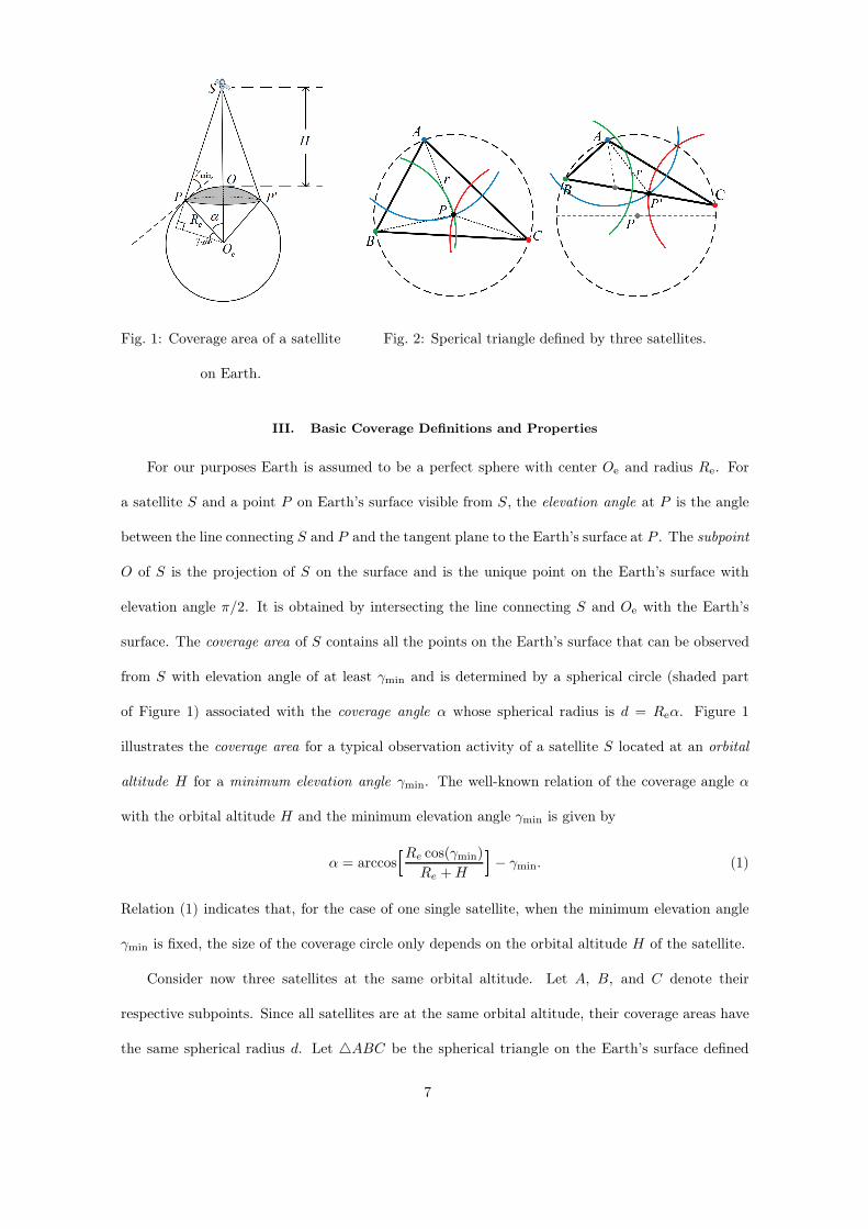
Fig. 1: Coverage area of a satellite
on Earth.
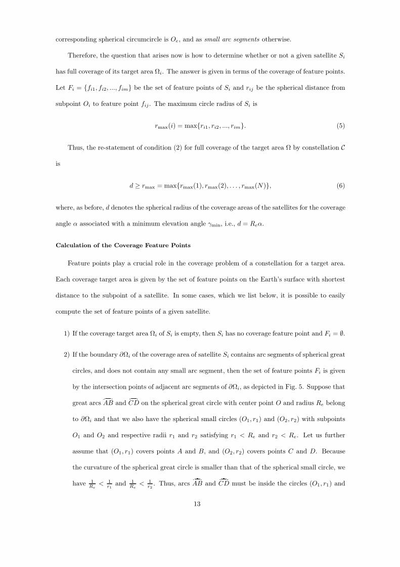
Fig. 2: Sperical triangle defined by three satellites.
III. Basic Coverage Definitions and Properties
For our purposes Earth is assumed to be a perfect sphere with center Oe and radius Re. For
a satellite S and a point P on Earth’s surface visible from S, the elevation angle at P is the angle
between the line connecting S and P and the tangent plane to the Earth’s surface at P . The subpoint
O of S is the projection of S on the surface and is the unique point on the Earth’s surface with
elevation angle π/2. It is obtained by intersecting the line connecting S and Oe with the Earth’s
surface. The coverage area of S contains all the points on the Earth’s surface that can be observed
from S with elevation angle of at least γmin and is determined by a spherical circle (shaded part
of Figure 1) associated with the coverage angle α whose spherical radius is d = Reα. Figure 1
illustrates the coverage area for a typical observation activity of a satellite S located at an orbital
altitude H for a minimum elevation angle γmin. The well-known relation of the coverage angle α
with the orbital altitude H and the minimum elevation angle γmin is given by
α = arccoshRe cos(γmin)
Re +H
i− γmin. (1)
Relation (1) indicates that, for the case of one single satellite, when the minimum elevation angle
γmin is fixed, the size of the coverage circle only depends on the orbital altitude H of the satellite.
Consider now three satellites at the same orbital altitude. Let A, B, and C denote their
respective subpoints. Since all satellites are at the same orbital altitude, their coverage areas have
the same spherical radius d. Let ABC be the spherical triangle on the Earth’s surface defined
7

by these points and let P and r be, respectively, the center and radius of the spherical circumcircle
of ABC. Furthermore let P ′ denote the point in ABC that minimizes the maximum of the
distances to A,B, and C. Note that when P ′ ∈ ABC, then P ′ coincides with P . Otherwise P ′ is
a point in the perimeter of ABC. The two cases are illustrated in Figure 2, where the coverage
areas of satellites A,B, and C intersecting ABC are delimited by the blue, green and red arcs,
respectively. The exact definition and generation approach will be given below.
Thus, in order to have full coverage of ABC with the three satellites it is enough to ensure
that the point P ′ is covered, i.e., that d ≥ r.
This condition can be extended to the case of a constellation consisting of multiple satellites
in circular orbit at the same orbital altitude. Suppose that the Earth’s surface can be divided into
several adjacent spherical triangles (with pairwise disjoint interiors) by connecting the subpoints of
the satellites according to certain rules (see Section IV). Then, only the points P ′
i and the maximum
distance ri of each spherical triangle must be computed, and if the coverage radius d of the satellites
satisfies
d ≥ maxr1, r2, . . . , rN, (2)
then this proves that the constellation covers the surface of the Earth completely.
Note that the coverage radius d is a technical parameter of a satellite. This parameter is
denoted as coverage angle θ introduced in [20]. However, the Earth-central angle ϑ that is defined
in the first covering function of [20] considered for the arbitrary points of a given latitude, whereas
the maximum circle radius r of a satellite that is defined and computed based on two geometric
structures (see Section V) is the maximum spherical distance between its subpoint and any point
in its coverage target area. This kind of analysis will be extended to any type of coverage areas
on Earth’s surface, provided that it can be divided into several adjacent spherical convex polygons
(according to certain rules). Also in such cases it will be easy to determine whether or not the
constellation can completely cover the ground area. Moreover, if condition (2) holds for a given
constellation at any time of a given reconstruction period, then the constellation fulfills the single
continuous coverage property for the given ground area.
8

IV. Spherical Geometric Subdivision
A. Voronoi Diagrams and Delaunay Triangulations
The Voronoi diagram and the Delaunay triangulation are two classical geometric structures
in computational geometry [31, 32], which produce partitions of a given region or set of points
in a metric space. Because of their interesting properties they are widely used in various areas
such as multispectral sensor image processing. Moreover, the closest point property of Delaunay
triangulations is iteratively used in several graph matching and image registration methods, like the
ones proposed by Zhao et al. [33].
The general definition of a Voronoi diagram is as follows. Let O = O1, O2, . . . , On be a finite
set of points (set of generators) in some metric space M with distance function d. The Voronoi
region associated with the point Oi is the set VR(Oi) = O ∈ M | d(O,Oi) ≤ d(O,Oj), for j =
1, . . . , N, j 6= i, i.e., the set of points for which Oi is closest among the generators. The set of all N
Voronoi regions is called the Voronoi diagram VD(O) of O. It gives a partition of M into polygons
with mutually disjoint interiors.
For a given Voronoi diagram of O the corresponding Delaunay triangulation DT (O) of O is
obtained if two points in O are connected by a shortest line if and only if their corresponding
Voronoi regions have a nonempty intersection. Under appropriate conditions which are usually
satisfied, two Voronoi regions do not intersect at all or intersect in more than one point and DT (O)
has 3N −6 edges defining 2N−4 triangles covering the space M (where triangles can only intersect
in lines) [22]. The Delaunay triangulation thus also provides a partition of M (into triangles with
mutually disjoint interiors).
Both concepts are dual to each other. It is also possible to first compute the Voronoi dia-
grams directly and then obtain the Delaunay triangulation. There are many efficient algorithms for
computing either of the two and we do not elaborate on them here [34–37].
In our application we have a constellation of N satellites C = S1, S2, ..., SN and we consider
Voronoi diagram and Delaunay triangulation for the set O = O1, O2, ..., ON of their respective
subpoints. So the metric space is the surface of the Earth and distances are spherical distances.
Accordingly, we speak about the spherical Voronoi diagram and the spherical Delaunay triangulation
9

of O. Note that that Voronoi regions are (spherical) convex polygons. Now, every point on Earth’s
surface belongs to a unique Voronoi region, a unique Delaunay triangle respectively (except for the
case that a point is on a line of the Voronoi diagram or the Delaunay triangulation). So both VD(O)
and DT (O) can be used to partition Earth’s surface. For an example see Figure 4.
It should be noted that on the sphere there are no infinite Voronoi regions and that VD(O) can
be obtained from DT (O) by connecting the circumcircle centers of its triangles following certain
rules. And no point of O is in the interior of the circumcircle of any spherical triangle of DT (O).
In this paper, we compute the Delaunay triangulation basically using the approach of [34] and
then generate the Voronoi diagram from it. By subdividing the target area into several adjacent
convex polygons, the constellation coverage problem can be decomposed into a set of single satellite
coverage problems.
B. Orientation Angle
Consider a spherical circle Θ(P, α) with center point P (θ, ϕ) and radius α, where θ and ϕ are
the longitude and latitude of P , respectively. Let us rotate the coordinates such that in the new
coordinate system, the x-axis passes through the center P ′ of the rotated spherical circle. The
coordinate rotation matrix is
P ′ = M(P ) = Ry(−ϕ)Rz(θ), (3)
where M ∈ R3×3 with
Rz(θ) =
26666664 cos(θ) − sin(θ) 0
sin(θ) cos(θ) 0
0 0 1
37777775 and Ry(−ϕ) =
26666664 cos(ϕ) 0 − sin(ϕ)
0 1 0
sin(ϕ) 0 cos(ϕ)
37777775 .
Figure 3 gives an illustration of the spherical circle Θ′ after the rotation M(Θ) = M(Q) | Q ∈ Θ,
where now the x-axis passes through the center P ′ = (0, 0) of the rotated spherical circle.
The orientation angle with respect to P ′ of any point in the rotated spherical circle is denoted
by β. It is clear that the orientation angle of any point Q′ = (x, y, z), x 6= 0, in the rotated spherical
circle is
β = arctanzy
. (4)
10

Fig. 3: Orientation angle
computation using projection.
Fig. 4: Construction of coverage area for a constellation
There is a natural mapping, which we denote h, that projects the spherical circle Θ′ onto the yz-
plane. Since there exists a one-to-one mapping g that assigns to each orientation angle β ∈ [0, 2π) a
unique point in h(Θ′), it is clear that the projection h(Θ′) is a circle on the yz-plane. Hence, g maps
an angle β ∈ [0, 2π) to g(β) = (0, cosβ, sinβ). The inverse projection f mapping an orientation angle
to a point on the original spherical circle Θ maps β ∈ [0, 2π) to M−1(cosα, sinα cosβ, sinα sinβ),
where M−1 denotes the inverse of the rotation mapping (3). Note that f can also be expressed as
f = M−1 h−1 g.
V. Constellation Coverage Analysis
A key issue for the design of satellite orbits and for the evaluation of the performance of constel-
lations is the accurate computation and analysis of the coverage for a given target area Ω. This topic
is addressed in this section where we give some definitions relating the Voronoi diagram computed
for a constellation C = S1, S2, ..., SN of N satellites to its coverage properties. First we focus on
one satellite Si and later extend the concepts to the full constellation. As before, we denote by
O = O1, O2, ..., ON the set of subpoints of the constellation.
1) The coverage target area Ωi of Si is the intersection of the Voronoi regiond VR(Oi) and the
target area Ω. If Ω is a polygon, then Ωi is also a polygon. Its vertices are all the vertices
of VR(Oi) in the target area plus some "new" vertices generated by the intersection of the
boundary of VR(Oi) with the spherical arcs that define Ω.
11

2) The maximum circle radius of Si is the maximum spherical distance between Oi and any point
in its coverage target area Ωi.
3) A coverage feature point of Si is any point on the boundary of Ωi that potentially could be
of maximum distance to Oi. The set of feature points of Si is denoted by Fi. Indeed Fi
contains all the vertices of Ωi. Furthermore, when some of the lines that define Ω are small
arcs, then Fi may contain additional points, corresponding to the properties and intersection
characteristics of small arcs.
From the above definitions it follows that for any point in Ωi, 1 ≤ i ≤ N , the subpoint Oi is
a nearest subpoint among all subpoints of the satellites. Furthermore, all the coverage target areas
only intersect in boundary points, as they are defined as subsets of Voronoi regions.
A. Construction of the Coverage Target Area
The coverage area of one satellite can be studied directly according to equation (1). Suppose now
that the target area Ω must be covered by a constellation C = S1, S2, ..., SN. In order to obtain
the coverage area of C we compute the Voronoi diagram for the subpoints O = O1, O2, ..., ON
and the coverage target areas Ωi together with the feature points Fi. As an example see Figure 4
giving the Voronoi diagram and Delaunay triangulation for the Walker constellation [6] with the
configuration parameters (T/P/F ) = (48/8/1) and orbital inclination Incl = 52.
Full coverage of a target area Ω is attained by a constellation if each satellite has full coverage
of its coverage target area Ωi. When some Si does not have full coverage of Ωi, then no other
satellite can cover any point in the uncovered part of Ωi. In this case, the constellation cannot
totally cover Ω.
As a consequence of the above analysis, after the Voronoi diagram of O has been obtained, the
constellation full coverage problem for a target area Ω is equivalent to a series of N independent
coverage problems, each of them restricted to its own target area Ωi. The region Ωi = VR(Oi)∩Ω,
is a spherical polygon. The boundary ∂Ωi is composed of several spherical great and small arc
segments, which are generated according to the intersection of VR(Oi) with Ω, and the orientation
angle of the feature point. The spherical arc is denoted as great arc segments if the center of the
12
corresponding spherical circumcircle is Oe, and as small arc segments otherwise.
Therefore, the question that arises now is how to determine whether or not a given satellite Si
has full coverage of its target area Ωi. The answer is given in terms of the coverage of feature points.
Let Fi = fi1, fi2, ..., fim be the set of feature points of Si and rij be the spherical distance from
subpoint Oi to feature point fij . The maximum circle radius of Si is
rmax(i) = maxri1, ri2, ..., rim. (5)
Thus, the re-statement of condition (2) for full coverage of the target area Ω by constellation C
is
d ≥ rmax = maxrmax(1), rmax(2), . . . , rmax(N), (6)
where, as before, d denotes the spherical radius of the coverage areas of the satellites for the coverage
angle α associated with a minimum elevation angle γmin, i.e., d = Reα.
Calculation of the Coverage Feature Points
Feature points play a crucial role in the coverage problem of a constellation for a target area.
Each coverage target area is given by the set of feature points on the Earth’s surface with shortest
distance to the subpoint of a satellite. In some cases, which we list below, it is possible to easily
compute the set of feature points of a given satellite.
1) If the coverage target area Ωi of Si is empty, then Si has no coverage feature point and Fi = ∅.
2) If the boundary ∂Ωi of the coverage area of satellite Si contains arc segments of spherical great
circles, and does not contain any small arc segment, then the set of feature points Fi is given
by the intersection points of adjacent arc segments of ∂Ωi, as depicted in Fig. 5. Suppose that
great arcs ÷AB and ÷CD on the spherical great circle with center point O and radius Re belong
to ∂Ωi and that we also have the spherical small circles (O1, r1) and (O2, r2) with subpoints
O1 and O2 and respective radii r1 and r2 satisfying r1 < Re and r2 < Re. Let us further
assume that (O1, r1) covers points A and B, and (O2, r2) covers points C and D. Because
the curvature of the spherical great circle is smaller than that of the spherical small circle, we
have 1
Re
< 1
r1and 1
Re
< 1
r2. Thus, arcs ÷AB and ÷CD must be inside the circles (O1, r1) and
13

Fig. 5: Subdivision of target area only with
great arcs (like global target area and
spherical polygon area).
(a) Great arcs intersection. (b) Small arcs intersection.
Fig. 6: Spherical arcs intersections.
(O2, r2), respectively. It is obvious that the point of maximum distance to center point O1,
among all the points on arc ÷AB, is either A or B. The same holds with C and D for arc ÷CD
relative to O2 (see Figure 6a).
3) If the boundary ∂Ωi of the coverage area belonging to satellite Si contains a small arc segmentΘ, then, in addition to the points defined in the above item, we add to Fi the intersection
points of the adjacent small arc segments, as depicted in Figure 7.
Suppose now that small arcs ÷AB, ÷CD, and ÷EF on a spherical small circle (O, r) belong to
∂Ωi. Let us also assume that there is another spherical small circle (O′, r′), where O′ is the
subpoint and r′ < Re (see Figure 6b). When the distance between O′ and O is greater than
or equal to r, then all of the points on the small arc ÷AB are inside (O′, r′), provided that
the spherical small circle (O′, r′) covers both A and B (see (O1, r1) in Figure 6b). Otherwise,
two different cases may arise. In the first case we have that 1
r≤ 1
r′(see spherical small circle
(O2, r2) in Figure 6b). Then, full coverage of the small arc ÷CD is implied by coverage of both
C and D. In the second case 1
r> 1
r′(see spherical small circle (O3, r3) in Figure 6b). Then,
neither E nor F are of longest distance to O′ among the points on ÷EF . Now, to obtain such a
maximum distance point, we connect O3 with O and extend this arc to a spherical great circle,
which intersects with the spherical small circle (O, r) in points P and Q. Indeed it can be
shown that the point of maximum distance to O3 is either P or Q, provided that they are on
14

Fig. 7: Subdivision of target area with small
arcs (like latitude target area and spherical
circle target area).
Fig. 8: Satellite coverage in the ECI reference
frame.
arc ÷EF . Such a maximum distance point also becomes one of the feature points of subpoint
O3.
B. Continuous Coverage Analysis of Constellations
The analysis of full coverage of a target area Ω by a constellation C at a fixed time point
performed above can be easily extended to study the continuous coverage of Ω by C over a given
reconstruction period. Indeed, the necessary and sufficient condition that guarantees that C offers
continuous full coverage for Ω throughout the given reconstruction period is that (6) holds at any
time of the reconstruction period. Hence, for this analysis we will discretize the reconstruction
period and check the condition at each time point of the discretized reconstruction period.
Observe, that the position of each satellite changes as time varies, as it moves through different
points of its orbit. Hence the subpoint of each satellite also depends on the time t, and accordingly
on the set of subpoints Ot = Ot1, Ot
2, . . . , Ot
N. That is, for a given minimum elevation angle γmin,
the coverage angle αt obtained with expression equation (1) together with the associated spherical
radius dt = Reαt, depend on t. This means that, in order to check whether or not condition (6)
holds at any time of the reconstruction period, the construction must be repeated for each time point
of the reconstruction period, including the procedure for obtaining the Voronoi diagram, the target
areas of the different satellites, and their feature points. Hence, the condition that guarantees full
coverage for Ω throughout the reconstruction period is dt = Reαt ≥ rtmax, for all t in the discretized
reconstruction period.
15

VI. Satellite Orbital Parameters Calculation
In the previous sections we have seen that the spherical geometric subdivision based on Voronoi
diagrams allows to address the continuous full coverage problem, i.e., the problem of determining
whether or not a given configuration for a satellite constellation provides continuous full coverage
for a given target area.
As we see below, the proposed geometric subdivision can also be used to address the problem
of finding a constellation of N satellites that provides full coverage for a given target area. As
it is known, there are several orbital parameters that define the properties of a constellation of
satellites. Eccentricity and perigee are typically fixed in the design of circular orbital parameters, so
they need not be computed. Moreover, the initial values of the RAAN and Mean Anomaly are not
considered to be important in the continuous coverage problem, so they can be distributed evenly.
On the other hand, it is well-known that Walker’s configuration [6] produces constellations with
good symmetry and stability properties. Hence for the design of a constellation for the continuous
coverage problem, we will follow Walker’s configuration and assume that satellites are distributed in
a uniform way. As a result, only the length of the semi-major axis (altitude h) and the inclination
angle Incl offer some freedom of choice for orbital design.Below, we show how to obtain these
parameters. For our analysis we recall that, for any two satellites in the constellation, the relative
motion trajectory in space changes periodically. Therefore, the values of orbital inclination and
maximum coverage circle radius, satisfying continuous coverage to target, change continuously in
the constellation reconstruction period.
A. Calculation of Orbital Altitude
As we have seen, in order to obtain continuous full coverage for the target area in the recon-
struction period, condition (6) must hold at any time. That is, for a given minimum elevation angle
γmin, at each time instant t of the reconstruction period, the spherical radius dt = Reαt associated
with the coverage angle αt obtained with equation (1) must be such that condition (6) holds.
Next we explain how to analytically compute a value for the altitude of the satellites in the
constellation that guarantees the above condition. For each time point t we obtain the set of
subpoints Ot and the Voronoi diagram of the satellites constellation. Then, for each satellite Si ∈ S,
16

we compute its set of feature points F ti , the spherical distances rtij from the subpoints to their feature
points, and its circle radius value rtmax
(i). Finally we compute the maximum circle radius for the
constellation rtmax
= maxrtmax
(i) | 1 ≤ i ≤ N.
Since condition (6) holds when dt = Reαt ≥ rtmax for all t, we compute the maximum radius
rmax = maxrtmax
| t ∈ T . Then, we take as spherical radius d = maxdt | t ∈ T , associated with
the coverage angle d = maxαt | t ∈ T = rmax/Re.
From equation (1) we obtain
h =Re cos(γmin)
cos( rmax
Re
+ γmin)−Re (7)
as altitude for the satellites in the constellation.
B. Calculation of Orbital Inclination
It is well-known that the optimal orbital inclination corresponds to the minimum value of the
maximum coverage circle radius in the constellation reconstruction period.
Suppose that the coverage target area is located in the latitude region [φl, φu]. The maximum
latitude value of a point in the target area is φmax = max|φl|, |φu|. Therefore, for the full coverage
of the target area, the satellite must cover the point with maximum latitude φmax. Using (1), the
minimum orbital inclination, for a given orbital altitude ht and minimum observation elevation
angle γmin, is given by
Incltmin = maxφmax − αt, 0. (8)
Figure 8 illustrates the satellite coverage of the Earth’s surface in the Earth-centered inertial (ECI)
reference frame. It reflects the coverage status when the satellite passes through the highest and
lowest points in the ECI frame.
VII. Computational Experiments
In this section we analyze the Globalstar mobile satellite system, designed by Loral and Qual-
comm of America, with the geometric subdivision method proposed in this paper. This system is a
Walker constellation with configuration parameters (T/P/F ) = (48/8/1). Note that in this notation
T denotes the total number of satellites and not the reconstruction time period. The satellite orbital
17

Fig. 9: Spherical subdivision for the Globalstar
system.
Fig. 10: Maximum coverage circle radius with
orbital inclination angle over time.
inclination is Incl = 52 and the altitude is h = 1414 km. It provides single continuous full coverage
of the latitude region [S70,N70] with a minimum coverage elevation angle γmin = 10 [5]. In our
study we use a discretized reconstruction period of 142.6 s.
A. Subdivision
Because of the symmetry property of Walker constellations we only need to analyze the coverage
capacity of the Globalstar system for the latitude region [0,N70]. The construction of the Voronoi
diagram at t =2015-01-01 00:00:00 is shown in Figure 9, where every convex polygon in the graph
corresponds to the coverage area of a satellite.
B. Coverage Calculation
1. Analysis of System Configuration Parameters
We re-optimize the orbital inclination according to (8) under the assumption that all other
parameters are given and fixed. Then, we use (6) to calculate the value of the coverage circle radius,
satisfying the continuous full coverage of the latitude region. The results are given in Figure 10.
It illustrates the variation of the maximum coverage circle radius relative to the orbital inclination
angle at different times of the reconstruction period when full coverage is imposed.
The results of the computations of the minimum elevation angle corresponding to the maximum
coverage circle radius that satisfies the coverage demand are depicted in Figure 11. Figure 11a
illustrates the variation of the minimum elevation angle with respect to the orbital inclination
18

(a) Minimum elevation angle with respect to orbital
inclination over time (full coverage).
(b) Minimum elevation angle with respect to orbital
inclination (full coverage).
Fig. 11: Variation of the minimum elevation angle relative to orbital inclination.
angle, at different times under the full coverage constraint. Figure 11b shows the variation of the
minimum elevation angle with respect to the orbital inclination under the constraint of continuous
full coverage. From the above results we can conclude the following.
1) In order to satisfy the continuous full coverage of the latitude region under the constraint
of minimum elevation angle γmin = 10, the satellite orbital inclination is in the range
[52.224, 55.094]. So with the original system configuration parameter Incl = 52 the latitude
region [S70,N70] cannot be covered completely.
2) Figures 10 and 11 give optimal inclination values. It can be seen that the maximum coverage
circle radius is rmax = 25.586 and the minimum elevation angle is γ = 10.935, while the
orbital inclination is Incl = 53.24.
Therefore, the configuration (T/P/F ) = (48/8/1) with inclination Incl = 53.24 can be regarded
as the best constellation configuration parameters given the continuous full coverage requirements
for the latitude region. In this context the minimum orbital altitude value is h = 1347.679 km.
Suppose now that all the constellation parameters are constant. Figure 12 gives the maximum
coverage gap of the constellation for different latitude regions. The x-axis represents time in the
constellation reconstruction period and the y-axis gives the upper bound values of the latitude
regions [0, y] in the graph. The shaded area indicates coverage gap intervals in different latitude
regions. For example, the coverage gap interval during the reconstruction period for the latitude
19

Fig. 12: Maximum coverage gap of constellation
in different latitude regions.
Fig. 13: Minimum elevation angle with different
latitude regions imposing continuous full
coverage.
region [0,N70.3] is [t1, t2].
Further results are presented in Figure 13 on the former basis giving the variation of the mini-
mum elevation angle for different latitude regions under the constraint of continuous full coverage.
The x-axis represents the upper bound value [0, x] of the latitude regions. The y-axis represents
the minimum elevation angle under the constraint of continuous full coverage. It is clear that the
original constellation configuration parameters can only offer single continuous full coverage for the
latitude region [S69.81,N69.81] or less.
2. Efficiency Analysis
For the same target area [0,N70] of the latitude region we compared the computational
efficiency of our new coverage method with the classical grid-point technique and the longitude
strip method. For the analyzed data, the computing time needed by our method is only 20 ms and
does not change with the constellation and the type and size of coverage area. The computational
results for the grid-point technique and the longitude strip method are depicted in Figure 14. The
x-axis indicates the partition precision, given as the number of longitude strips or grid-points in
1 km on Earth’s surface. The y-axis shows the instantanous coverage computing time for the
latitude region with the Globalstar system. Given that the grid-point technique and the longitude
strip method are both numerical simulation methods, their major drawback is that results with
20

Fig. 14: Coverage computation times in relation to the partition precision.
high accuracy can only be obtained with a considerable increase in computing times and memory
requirements.
The computations show that the optimal system parameters obtained with our method are
basically the same as the original parameters produced by the Globalstar system.
VIII. Conclusions
In this paper we have proposed a new method based on spherical geometric subdivision for the
analysis of the continuous coverage of satellites and the calculation of satellite orbital parameters for
the full coverage problem. The proposed method is exact for fixed time t and works on any type of
coverage target areas. Though only approximate in the constellation reconstruction period, it is also
very effective for evaluating a series of further meaningful performance indices for the continuous
and the discontinuous coverage problem. (Note the exception, that when computing the spherical
Delaunay subdivision not all subpoints must be located in the same semi-spherical surface since,
otherwise, the subdivision is invalid.)
The new proposed method also produces analytical solutions as well as the range for each
parameter value so as to satisfy the coverage requirements. The satellite orbital parameters can
be obtained directly from the maximum coverage circle radii. Moreover, optimal satellite orbital
inclinations and altitudes can be obtained according to the original design objectives. Experimental
results also indicate that traditional methods based on grid-point division or longitude strip partition
are usually unsuitable for very large regions under high accuracy requirements.
21

Summarizing, the decision space for an optimal constellation design is reduced considerably,
and the constellation design process improves significantly.
Acknowledgments
This work was supported by National Natural Science Foundation of China under Grant No.
41571403 and No. 61472375.
References
[1] Rainer, S., Klaus, B., and Marco, D. E. "Small Satellites for Global Coverage: Potential and Limits,"
ISPRS Journal of Photogrammetry and Remote Sensing, Vol. 65, No. 6, Sep. 2010, pp. 492–504.
[2] Sandau, R., "Status and Trends of Small Satellite Missions for Earth Observation," Acta Astronautica,
Vol. 71, No. 1, Jan. 2010, pp. 1–12.
[3] Zhao, Z.Y., Cai, Y. W., Zhao, Y. B., and Li, Y. "Research on Small Satellite Formation Scheme for
Earth Observation Task," Proceedings of the 2015 International Conference on Automation, Mechanical
Control and Computational Engineering, Atlantis Press, Paris, France, April 2015, pp. 1678–1683.
[4] Y. Ulybyshev, "Satellite Constellation Design for Complex Coverage," AIAA Journal of Spacecraft and
Rockets, Vol. 45, No. 4, Jul. 2008, pp. 843–849.
[5] Crowe, K. E. and Raines, R. A. "A Model to Describe the Distribution of Transmission Path Elevation
Angles to the Iridium and Globalstar Satellite Systems," IEEE Communications Letters, Vol. 3, No. 8,
Aug. 1999, pp. 242–244.
[6] Walker, J. G. "Circular Orbit Patterns Providing Continuous Whole Earth Coverage," Royal Aircraft
Establishment, U.K., Technique Report 70211, Nov. 1970.
[7] Crossley, W. A. and Williams, E. A. "Simulated Annealing and Genetic Algorithm Approaches for
Discontinuous Coverage Satellite Constellation Design," Engineering Optimization, Vol. 32, No. 3, 2000,
pp. 353–371.
[8] Asvial, M., Tafazolli, R., and Evans, B. G. "Satellite Constellation Design and Radio Resource Man-
agement using Genetic Algorithm," IEE Proceedings-Communications, Vol. 151, No. 3, 6 Jul. 2004, pp.
204–209.
[9] Ferringer, M. P., and Spencer, D. B. "Satellite Constellation Design Tradeoffs using Multiple-Objective
Evolutionary Computation," AIAA Journal of Spacecraft and Rockets, Vol. 43, No. 6, Nov. 2006, pp.
1404–1411.
22

[10] Wang, L., Wang, Y., Chen, K., and Zhang, H. "Optimization of Regional Coverage Reconnaissance
Satellite Constellation by NSGA-II Algorithm," Proceedings of the 2008 IEEE International Conference
on Information and Automation, IEEE, Piscataway, New Jersey, USA, Jun. 2008, pp. 1111–1116.
[11] Ferringer, M. P., Clifton, R. S., and Thompson, T. G. "Efficient and Accurate Evolutionary Multi-
Objective Optimization Paradigms for Satellite Constellation Design," AIAA Journal of Spacecraft and
Rockets, Vol. 44, No. 3, May. 2007, pp. 682–691.
[12] Jiang, Y., Zhang, G., Li, G., Xie, Z., and Yang, S. "Study on Orthogonal IGSO Global Communication
Satellite Constellation," IEEE 6th International ICST Conference on Communications and Networking
in China (CHINACOM), Aug. 2011, pp. 1064–1068.
[13] Ma, D. M., Hong, Z. C., Lee, T. H., and Chang, B. J. "Design of a Micro-Satellite Constellation for
Communication," Acta Astronautica, Vol. 82, No. 1, Jan. 2013, pp. 54–59.
[14] Lluch, I., and Golkar, A. "Satellite-to-Satellite Coverage Optimization Approach for Opportunistic
Inter-Satellite Links," IEEE Aerospace Conference, IEEE, Piscataway New Yersey, USA, Mar. 2014,
pp. 1–13.
[15] Morrison, J. J. "A System of Sixteen Synchronous Satellites for Worldwide Navigation and Surveil-
lance," Technical Department of Transportation Federal Aviation Administration Systems Research and
Development Service, Washington D. C., Mar. 1973.
[16] Jiang, Y., Yang, S., Zhang, G., and Li, G. "Coverage Performances Analysis on Combined-GEO-IGSO
Satellite Constellation," Journal of Electronics (China), Vol. 28, No. 2, Mar. 2011, pp. 228–234.
[17] Mortari, D., Sanctis, M. D., and Lucente, M. "Design of Flower Constellations for Telecommunication
Services," Proceedings of the IEEE, Vol. 99, No. 11, Jul. 2011, pp. 2008–2019.
[18] Casten, R. G., and Gross, R. P. "Satellite Cumulative Earth Coverage," AIAA Astrodynamics Specialist
Conference, Univelt, San Diego, California, USA, Vol. 1, Aug. 1981.
[19] Xu, M., and Huang, L. "An Analytic Algorithm for Global Coverage of the Revisiting Orbit and its
Application to the CFOSAT Satellite," Astrophysics and Space Science, Vol. 352, No. 2, Aug. 2014, pp.
497–502.
[20] Ulybyshev, Y. "Geometric Analysis of Low-Earth-Orbit Satellite Communication Systems: Covering
Functions," AIAA Journal of Spacecraft and Rockets, Vol. 37, No. 3, May. 2000, pp. 385–391.
[21] Seyedi, Y. and Safavi, S. M. "On the Analysis of Random Coverage Time in Mobile LEO Satellite
Communications," IEEE Communications Letters, Vol. 16, No. 5, 23 Mar. 2012, pp. 612–615.
[22] Ballard, A. H. "Rosette constellation of earth satellite," IEEE Transaction on Aerospace and Electronic
Systems, Vol 16, No. 5, Sep. 1980, pp. 656–673.
23

[23] Sarno, S., Graziano, M.D., and DÉrrico, M., "Polar Constellations Design for Discontinuous Coverage,"
Acta Astronautica, Vol. 127, Oct. 2016, pp. 367–374.
[24] Li, T., Xiang, J., Wang, Z., and Zhang, Y., "Circular Revisit Orbits Design for Responsive Mission over
a Single Target", Acta Astronaut, Vol. 127, Oct. 2016, pp. 219–225.
[25] Mozhaev, G. V. "Capabilities of Kinematically Regular Satellite Systems with Symmetry Groups of
the Second Type in the Problem of Continuous Single Coverage of the Earth," Cosmic Research, Vol.
43, No. 3, May. 2005, pp. 205–212.
[26] Ulybyshev, Y. "Geometric Analysis and Design Method for Discontinuous Coverage Satellite Constel-
lations," AIAA Journal of Guidance, Control, and Dynamics, Vol. 37, No. 4, 5 Feb. 2014, pp. 549–557.
[27] Ulybyshev, Y.P., "A General Analysis Method for Discontinuous Coverage Satellite Constellations,"
AIAA Journal of Guidance, Control, and Dynamics, Vol. 38, No. 12, Aug. 2015, pp. 2475–2482.
[28] Razoumny, Y.N., "Fundamentals of the Route Theory for Satellite Constellation Design for Earth
Discontinuous Coverage. Part1: Analytic Emulation of the Earth Coverage," Acta Astronautica, Vol.
128, July. 2016, pp. 722–740.
[29] Mohammadi, L. "Determination of the Best Coverage Area for Receiver Stations of LEO Remote
Sensing Satellites," Proceedings of the 2008 3rd International Conference on Information and Commu-
nication Technologies: From Theory to Applications, IEEE, Piscataway, New Jersay, April 2008, pp.
1–4.
[30] Sengupta, P., Vadali, R. S., and Alfriend, T. K. "Satellite Orbit Design and Maintenance for Terrestrial
Coverage," AIAA Journal of Spacecraft and Rockets, Vol. 47, No. 1, Jan. 2010, pp. 177–187.
[31] Devillers, O. "Delaunay Triangulation and Randomized Constructions," Springer Encyclopedia of Al-
gorithms, Springer US, Oct. 2014, pp. 1–7.
[32] Okabe, A., Boots, B., Sugihara. K., and Chui, S. N. "Spatial Tessellations: Concepts and Applications
of Voronoi Diagrams," John Wiley and Sons, Vol. 501, 2009, pp. 46–105.
[33] Zhao, M., An, B., Wu, Y., Chen, B., and Sun, S. "A Robust Delaunay Triangulation Matching for
Multispectral/Multidate Remote Sensing Image Registration," IEEE Geoscience and Remote Sensing
Letters, Vol. 12, No. 4, Apr. 2015, pp. 711–715.
[34] Zhou, L., Huang, D., Li, C., and Zhou, D., "Algorithm for GPS Network Construction Based on
Spherical Delaunay Triangulated Irregular Network," Journal of Southwest Jiaotong University, Vol.
42, No. 3, Jun. 2007, pp. 380-383.
[35] Jacobsen, D. W., Gunzburger, M., Ringler, T., Burkardt, J., and Peterson, J. "Parallel Algorithms for
Planar and Spherical Delaunay Construction with an Application to Centroidal Voronoi Tessellations,"
24

Geoscientific Model Development, Vol. 6, No. 4, 6 Dev. 2013, pp. 1353–1365.
[36] Yan, D. M., Wang, W., Levy, B. and Liu, Y. "Efficient Computation of Clipped Voronoi Diagram for
Mesh Generation," Computer-Aided Design, Vol. 45, No. 4, Apr. 2013, pp. 843–852.
[37] Peterka, T., Morozov, D. and Phillips, C. "High-Performance Computation of Distributed-Memory
Parallel 3D Voronoi and Delaunay Tessellation," Proceedings of the International Conference for High
Performance Computing, Networking, Storage and Analysis, IEEE, Piscatawaay, New Jersey, USA,
Nov. 2014, pp. 997–1007.
25