1

ANALYSIS OF RETINOTOPIC MAPS IN EXTRASTRIATE CORTEX

Martin I. Sereno, Colin T. McDonald, and John M. Allman

Cognitive ScienceUniversity of California, San DiegoLa Jolla, CA 92093-0515andDivision of Biology 216-76California Institute of TechnologyPasadena, CA 92115

Published as: Sereno, M.I., C.T. McDonald, and J.M. Allman (1994) Analysis of retinotopic maps in extrastriate cortex. Cerebral Cortex 4:601-620.

AbstractTwo new techniques for analyzing retinotopic maps—arrow diagrams and visual field sign maps—are

demonstrated with a large electrophysiological mapping data sets from owl monkey extrastriate visual cortex. An arrow diagram (vectors indicating receptive field centers placed at cortical coordinates) provides a more compact and understandable representation of retinotopy than does a standard receptive field chart (accompanied by a penetration map) or a double contour map (e.g., isoeccentricity and isopolar angle as a function of cortical x-y coordinates). None of these three representational techniques, however, make separate areas easily visible, especially in data sets containing numerous areas with partial, distorted representations of the visual hemifield. Therefore, we computed visual field sign maps (non-mirror-image versus mirror-image visual field representation) from the angle between the direction of the cortical gradient in receptive field eccentricity and the cortical gradient in receptive field angle for each small region of the cortex. Visual field sign is a local measure invariant to cortical map orientation and distortion but also to choice of receptive field coordinate system. To estimate the gradients, we first interpolated the eccentricity and polar angle data onto regular grids using a distance-weighted smoothing algorithm. The visual field sign technique provides a more objective method for using retinotopy to outline multiple visual areas. In order to accurately relate these arrow and visual field sign maps to architectonic features visualized in the stained, flattened cortex, we also developed a deformable template algorithm for warping the photograph-derived penetration map using the final observed location of a set of marking lesions.

IntroductionOver half of the neocortex in primates consists of visual areas, many of which are retinotopically

organized (reviews: Sereno and Allman, 1991; Kaas and Krubitzer, 1991; Felleman and Van Essen, 1991). The region of cortex involved, however, is large, and there is substantial variability among species and among individual animals of a species. Even well-defined areas like primary visual cortex (V1) and the

2

middle temporal areas (MT) show variability in their location, shape, size, appearance (see, e.g., Tootell et al., 1985 and Fiorani et al., 1989, on MT in New World monkeys). Since the majority of visual areas are not graced with the convenient suite of easily distinguishable features that characterize V1 and MT (e.g., prominent myeloarchitectonic borders, nearly complete, not-too-distorted, topological maps of the hemiretina), it has proved quite difficult to convincingly define their boundaries. Several different naming schemes have persisted for a number of the areas beyond V1, V2, and MT.

Visual areas in the cortex are ideally defined on the basis of converging criteria (Allman and Kaas, 1971, 1974, 1975, 1976; Van Essen, 1985). These include visuotopic organization, architectonic features, connection patterns, and physiological properties. It is virtually impossible, however, to obtain detailed information about all of these criteria for multiple visual areas in a single animal. In the following set of papers, we have focussed on the first two criteria—visuotopy and architectonics. By concentrating on obtaining large numbers of recording sites in each animal, we have been able to much more clearly delineate the complex and variable mosaic of visual areas in primate dorsal, lateral, and ventral extrastriate cortex.

In the present paper, we begin by describing our techniques for recording visual receptive fields from a large number of locations in each animal. In the process of analyzing these large data sets, it became clear that the standard technique for illustrating retinotopy—a numbered penetration site chart with correspondingly numbered receptive field charts—was much too unwieldy to handle multiple, partial visual field representations involving hundreds of sites. We needed to find a tractable way to view the entire data set for single animal, not the least, to avoid the temptation to extract the small portions of the data set that can often be found to support a simple story.

We describe two new methods for representing large retinotopic mapping data sets in an interpretable way—arrow diagrams and visual field sign maps. We first illustrate conventional numbered receptive field/penetration plots and then show how arrow (vector field) diagrams make it possible to view the same data set much more compactly and understandably. Second, we describe a deterministic distance-weighted algorithm for interpolating receptive field eccentricity, angle, and diameter data onto regular grids so that we can generate isoeccentricity, isopolar angle, and isodiameter contour plots. Third, we describe how to make a visual field sign map (local mirror-image or non-mirror-image transformation of the visual field) from the interpolated isoeccentricity and isopolar angle grids. This technique brings out relations that are often subtle in an arrow diagram and completely opaque in a raw receptive field plot. Finally, we develop an iterative algorithm for warping an x-y penetration map derived from a recording photograph onto the stained, physically flattened cortex using marker lesions. This allows us to more accurately align our mapping data with anatomical landmarks.

The overall picture of retinotopy in primate extrastriate visual cortex that we arrived at was substantially more complex than we had anticipated. The second companion paper (Sereno, McDonald, O’Dell, and Allman, forthcoming) uses the techniques developed here to analyze retinotopy and architectonic features of dorsolateral extrastriate cortical areas in the owl monkey. A detailed discussion of the 600+ point case illustrated here is contained in that paper. The third companion paper (Sereno, McDonald, and Allman, in preparation) examines ventrolateral extrastriate areas in the owl monkey. Portions of this work have been presented in abstract form (Sereno et al., 1986; 1987; 1993).Materials and Methods

The analytical techniques described in this paper were developed in the course of a long series of chronic and acute electrophysiological mapping experiments on anesthetized owl monkeys (Aotus trivirgatus). They will be demonstrated on a single, extensive acute mapping experiment, which is

3

described below. Our chronic mapping procedures and variations in our acute procedures are described in the companion papers.Acute Mapping Experiment Procedures

The animal was deeply anesthetized and a large craniotomy made. A rod cemented to the skull using several small stainless steel bone screws and Grip dental acrylic cement under full aseptic conditions to allow the animal’s head to be fixed without pressure points. The animal was positioned for recording in the natural crouched resting posture of the owl monkey in a specially designed monkey chair (owl monkeys lack ischial callosities and cannot sit comfortably for extended periods on a standard macaque monkey chair). The animal was tilted somewhat to keep the surface of the cortex close to horizontal. The dura was retracted and the cortex was covered with a pool of warm sterile silicone oil. The vascular pattern of the exposed cortex was then photographed. The animal’s body temperature monitored with a rectal probe and maintained with a warm water pad, and the animal was given 5% dextrose in saline intravenously to prevent dehydration. Care was taken to express urine accumulated in the bladder. Anesthesia was maintained with additional doses of ketamine (3-5 mg/kg/hr i.m., or as needed to suppress muscular or heart rate response to stimuli). The depth of anesthesia of the unparalyzed animal was monitored continuously by the person manipulating the electrode. Triflupromazine was given initially (3-6 mg/kg i.m.) and afterward in smaller doses at 10-15 hour intervals (2 mg/kg i.m.) because of its longer resident time. Triflupromazine potentiates the effects of ketamine. The animal monocularly viewed a translucent, dimly back-lit plastic hemisphere 28.5 cm in diameter (one degree of visual angle equals 5 mm along hemisphere surface) that was centered on the open contralateral eye.

A stepping motor microdrive was positioned in the x-y plane with a manual micromanipulator while observing the brain surface through a dissecting microscope. Each electrode penetration was first marked on the enlarged photograph (20×) of the vascular pattern on the cortical surface with the electrode tip touching the pial surface. A glass-coated platinum-iridium microelectrode with 10-40 µm tip exposures was then driven perpendicularly into the cortex with the stepping motor microdrive (designed by Herb Adams, California Institute of Technology) to depths of approximately 700 µm. Up to 25 penetrations per mm2 were made in regions where receptive field position changed rapidly. The x-y location of a recording site as marked on the cortical surface photograph is subject to small errors due to difficulties in triangulating from blood vessel landmarks in the microscope image. However, since the smallest vessels on the pial surface are typically separated by only 100-200 µm, location errors were probably restricted to within a 50 µm radius of the true location in the x-y plane. With these techniques, it was possible to record more than 600 receptive fields in one very long session (90 hours). Small electrophysiological lesions (10-20 µA for 10 seconds) were made before the end of the experiment to identify individual recording sites.Visual Stimulation

The cornea was anesthetized with a long acting local anesthetic (0.7% dibucaine HCl dissolved in contact lens wetting solution). The pupil was dilated with Cyclogyl (1%). A thin ring machined to the contours of the large owl monkey eye was then cemented to the margin of the anesthetized cornea with a small drop (~10 µL) of Histoacryl cyanoacrylate tissue cement. An appropriate contact lens was placed over the cornea (the diameter of the ring was slightly larger than the contact) to prevent drying during the course of the experiment and to bring the eye into focus. This technique provides excellent stability because of the large size of the owl monkey eye and the poor mechanical advantage of the posteriorly inserting eye muscles in this nocturnal animal. Paralysis is thus avoided making it easier to monitor and maintain the anesthetic state of the animal.

4

At the beginning of the experiment, the blind spot and four other widely separated retinal blood vessel landmarks were plotted on the plastic hemisphere by backprojecting their images with an ophthalmoscope. These landmarks were checked repeatedly during the experiment. Gaze remained fixed to within the accuracy of our backpojection technique (≅ 1 degree) for the duration of the 90 hour experiment. Many points around the circumference of each receptive field were tested to carefully determine their extent using backprojected light and dark spots, bars, and texture patterns while listening to an audio monitor. We plotted the position of the response field for single neurons or small clusters of neurons. The hemisphere was dimly lit to avoid spurious responses due to light scatter. Receptive fields and retinal landmarks were copied onto tracing paper made into a hemisphere by small, taped radial folds after every 30-50 had been plotted so that we could clear the plastic hemisphere to avoid confusion.Histology and Cortical Flatmounts

At the end of the experiment, the animal was deeply anesthetized with Nembutal (100 mg/kg i.v.) and perfused through the heart with buffered saline. We immediately removed the unfixed brain and physically flattened the cortex (Tootell et al., 1985; Olavarria and van Sluyters, 1985) by gently dissecting away the white matter with dry Q-tips. In the later stages of this process, the cortex was supported, pial surface down, on moist filter paper. A cut in the fundus of the calcarine sulcus and two smaller cuts in the cortex at the anterior ends of the Sylvian sulcus and the superior temporal sulcus were made to allow the cortex to lie flat. It was held in fixative without sucrose between large glass slides under a small weight for several hours (sucrose tends to cause the tissue to slip out from in between the slides). The tissue was kept free floating in fixative overnight, and then soaked in 30% sucrose solution the following day.

The flattened cortex was sectioned in one piece parallel to cortical laminae at 50 µm on a large freezing microtome stage. A built-up block of ice was first shaved flat with the microtome knife. The flattened cortex was held on the underside of a moistened glass slide and then attached, pial surface down, to the cut ice surface with a thin coat of Tissue Tek compound. Overly rapid initial freezing of the tissue can trap pockets of air in between the ice and the tissue. During sectioning, the knife often lifts these regions from the block, destroying them as it cuts deeply into the tissue. To avoid this, the block temperature was first raised to approximately -15 °C; this provides 5-10 seconds to exclude air bubbles by pressing and tapping on the overlying slide while the tissue freezes. With technique, it was often possible to recover every section, including the most superficial, which contains mainly blood vessels. By aligning this section with deeper sections using radial blood vessels, it was possible to draw additional correspondences between the stained tissue and the penetration photograph. Every section was stained using the Gallyas technique after drying mounted sections in air for two days (longer delays result in light, irregular staining).Digitization of Cortical Sites and Receptive Fields

Electrophysiological lesions made during the course of the experiment were first located in individual sections. A properly scaled and warped (see Results below) copy of the surface penetration map was then superimposed on photographs and drawings of the flattened and stained sections using the marker lesions.

We found that receptive fields at all levels in extrastriate cortex are generally much better approximated by an ellipse than a circle or rectangle. Therefore, a total of seven numbers were obtained for each named receptive field: the location of the recording site on the cortex (x,y) (obtained as described above), and then the eccentricity (r) and angle (θ) of the receptive field center relative to the center of gaze, and the length (l), width (w), and angle (φ) of the receptive field ellipse (see Fig. 1). The receptive field coordinates were digitized by placing individual hemispherical paper data sheets back onto a spherical polar coordinate system drawn onto the plastic hemisphere. The center of gaze was placed at the ’North Pole’ of

5

the spherical polar coordinate system, in contrast to the ‘equatorial’ location of the center of gaze in the scheme of Tusa et al. (1978). Placing the center of gaze at the North Pole results—after the hemifield has been flattened (see below)—in a polar coordinate system (cf. Allman and Kaas, 1971). By contrast, an equatorial center of gaze results, after flattening, in a curvilinear coordinate systems that approximates a 2-D Cartesian coordinate system near the center of gaze. Polar coordinates (r, θ) are more natural for describing primate retinotopy than Cartesian coordinates (x, y) since magnification factor (plotted in the visual field) is approximately rotationally symmetric around the center of gaze.

Computer programs (available from the authors on request and by anonymous ftp—see below) converted the receptive field data files (ASCII tables) into five kinds of Postscript files: receptive field charts, numbered penetration charts, arrow diagrams, interpolated isoeccentricity-isopolarangle-isodiameter maps, and visual field sign maps. For cases that were flatmounted, a deformable template algorithm was first used to stretch the x-y locations taken from the photographed penetration map according to the final location of lesions, generating a sixth kind of PostScript file illustrating stages in the deformation of the starting grid. These PostScript files were directly pasted into Adobe Illustrator on the NeXT computer and annotated to make the Figures.

For convenience, the angle of the receptive field center is measured in a clockwise direction starting from the left horizontal meridian (the angle of the ellipse is treated similarly); thus a receptive field in the upper left visual quadrant will have an angle between 0 and 90 degrees, while a receptive field in the lower left visual quadrant will have an angle between 0 and -90 degrees (see Fig. 1).ResultsReceptive Field Charts

A numbered receptive field chart (in visual hemifield coordinates) accompanied by a correspondingly numbered penetration chart (in cortical surface coordinates) is the most straightforward way to illustrate the retinotopic organization of visual cortex. Since we plotted and digitized receptive fields on a spherical surface, there is unavoidable distortion when representing them on a flattened visual hemifield. The flat

Figure 1. Seven receptive field parameters. The location of the recording site is measured from the penetration photograph (x,y), the center of the receptive field is defined by its eccentricity and angle (r,θ), and the receptive field shape is parameterized by the length, width, and angle of the best-fitting ellipse (l,w,φ). An arrow diagram (see Figs. 5,6) is constructed by placing a scaled copy of the arrow from the center of gaze to the receptive field center (thick arrow) at the x-y position on the cortex from which that receptive field was recorded. A receptive field on the horizontal meridian of the left hemifield is conventionally labeled with an angle of 0 degrees.

(x,y)

Visual Field Visual Cortex

receptivefield

w

l

φ

θr

6

hemifield chart we use represents radial distances (from the center of gaze) faithfully, but stretches distances in a circumferential direction as one moves away from the center of gaze; it is as if the hemisphere has been flattened by introducing innumerable cuts radiating from the center of gaze point (while keeping the vertical meridian straight). The circumferential stretching inherent in the flattened coordinate system ranges from no distortion at the center of gaze up to a linear magnification of π/2 (~1.57×) at 90 degrees eccentricity. Each receptive field was therefore ’flat-corrected’ on the planar visual field map by stretching it in a circumferential direction as a function of its eccentricity. Receptive field overlap is represented faithfully with this system, but the areas of peripheral receptive fields appear larger than they actually are (see Fig. 2).

True receptive field dimensions were used for isodiameter contour plots.For small numbers of receptive fields (10-40) all recorded from a single area with small receptive

fields and an undistorted map (like V1), the simplest way to examine and present the data is to draw the receptive fields (or their centers) on a hemifield chart, and then number the receptive fields so that they can be matched up with similarly numbered penetration points on a drawing of the brain. Visuotopy can be displayed more intuitively in a such receptive field chart through the use of overlapping and shading. The sequence of receptive fields from a track across a visual area can be indicated by the pattern of overlapping of opaque receptive field ellipses while several different parallel tracks across an area can be distinguished by different shades, obviating the need to continually refer to a penetration chart (see Fig. 2, which shows three recording tracks across the dorsolateral posterior visual area, DLp).

Unfortunately, these simple procedures become completely unwieldy when there are many (100-600) receptive fields, when the receptive fields are large, and when several different representations of the visual

file: OM88inj-DLp-noflatnot flat-corrected +45

+30

+15

-15

-30

-45

32

33

34

1

23

4

1718

1920

21

O.D.

Flat-corrected Not Flat-corrected(true overlap) (true area)

file: OM88inj-DLpflat-corrected +45

+30

+15

-15

-30

-45

32

33

34

1

23

4

1718

1920

21

O.D.

Figure 2. Receptive field plots from three penetration rows across the posterior dorsolateral area, DLp. Receptive fields are digitized on a hemisphere but illustrated on a flattened representation of the hemifield. Receptive fields can be drawn to preserve their true areas (left) or be drawn ’flat-corrected’ to preserve their true overlap and accurately represent their boundaries relative to the flattened hemifield (right). The transformation of the visual field shown here preserves distances in the radial direction (eccentricity) but results in a magnification of distances in a circumferential direction that gradually increases with eccentricity (reaching π/2 at 90˚ eccentricity). Subsequently, we illustrate flat-corrected receptive fields (but use actual receptive field areas for calculating magnification factors). The sequence of penetrations in a row is illustrated implicitly here by the overlapping of opaque receptive fields, while the three parallel rows of penetrations across the cortex are indicated by differently shading the receptive

7

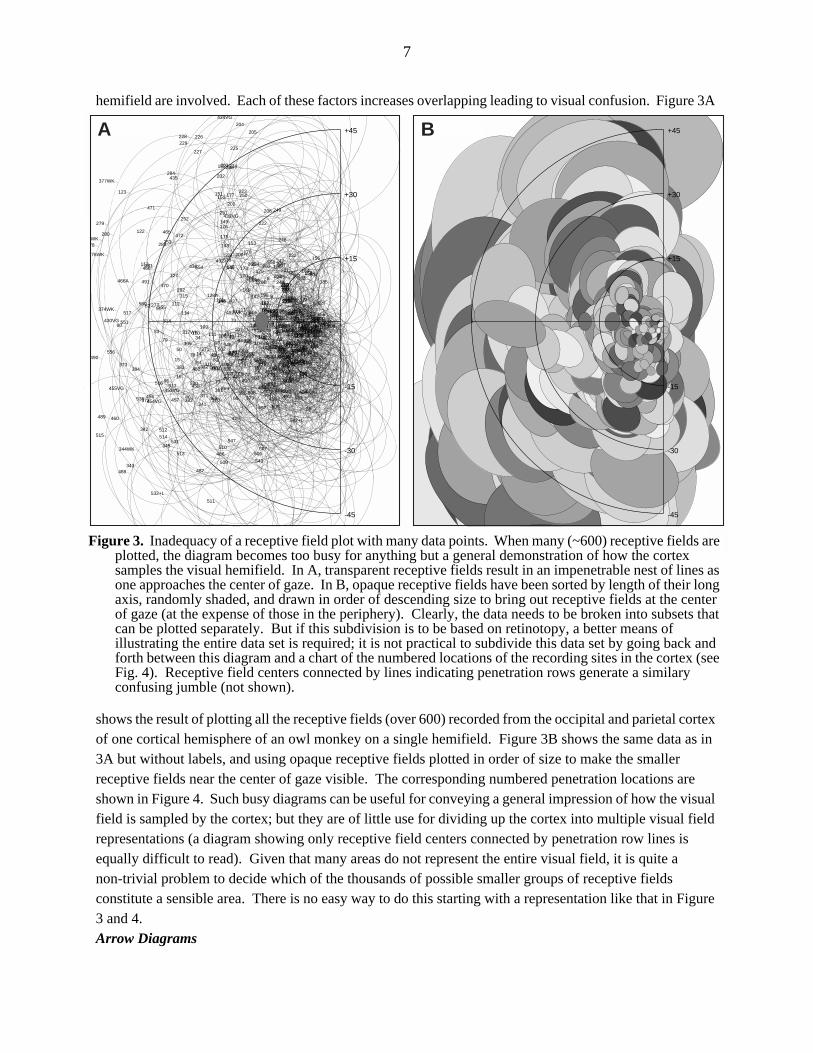
hemifield are involved. Each of these factors increases overlapping leading to visual confusion. Figure 3A

shows the result of plotting all the receptive fields (over 600) recorded from the occipital and parietal cortex of one cortical hemisphere of an owl monkey on a single hemifield. Figure 3B shows the same data as in 3A but without labels, and using opaque receptive fields plotted in order of size to make the smaller receptive fields near the center of gaze visible. The corresponding numbered penetration locations are shown in Figure 4. Such busy diagrams can be useful for conveying a general impression of how the visual field is sampled by the cortex; but they are of little use for dividing up the cortex into multiple visual field representations (a diagram showing only receptive field centers connected by penetration row lines is equally difficult to read). Given that many areas do not represent the entire visual field, it is quite a non-trivial problem to decide which of the thousands of possible smaller groups of receptive fields constitute a sensible area. There is no easy way to do this starting with a representation like that in Figure 3 and 4.Arrow Diagrams

file: OM90-sortflat-corrected +45

+30

+15

-15

-30

-45

Bfile: OM90flat-corrected +45

+30

+15

-15

-30

-45

12

3

45

6

7

8

9

1011

1213

1415

16 17

18

1920

21

22

23

24

2527

28

29

30

31

3233

34

3536

3738

3940 41

42

43

44

45

46

474849

50

5152

53

54 55

56

5758

59

60

61

6263

6465

6667

6869

707172

73

7475

76

77

78

79

80

8182

83 8485

86

87

8889

9091

92

93VG

94VG95

96

97WK

100101102VG103VG

104VG105

106

107108

109110 111

112

113

114

115

116 117118

119

120

121

122

123

125

127

128A

128B

129A

129B130

131132133134135

136137

138

139

140141

142

143

144145

146147

148

149

150151

152

153

154155

156

157158159

160161+L

162163164

165

166

167168

169

170

171172

173

174

175

176

177

178

179180

181182183

184

185

187188189190

191192

193194195196

197

198

199

200+L

201

202

203

204

205

206

207

211212

213

214

215

216217

218219

220

221

222

223

224

225

226

227

228229

230

232

234235

236237

238

239240

241242243

244245

246247

248

249

250

251252

253

255256257+L

258

259260261

262

263264265

266

267

268

269

270271

272273

274275276

277

278

279

280

281

282

283

284

287288289290291

292

293294295

296

297

298299

300301

302

303304

305

306

307

308

309

310

311312

313

314

315

317WK 319320321

322323

324

325326

327

328329

330331332

333334

335

336

337338339

340

341

342

343

344WK345

350351352353

354

355

356

359

360

361

362

363

364

365

366

367368369

370371

372

373

374WK

376WK

377WK

379380

381

382

383384

408409410411412

413414

415

416417

418

419

420

421422 423424425

426427

428

429

430VG

431

432

433VG

434VG

435

436

437

440

441

442

443444

445

446447

448

449450

451452

453VG

454VG

455VG

456457

458

459

460

461 462

463

464

465

466A

468

470

471

472

473

474

475

476477

478479

480481

482

483484485

486

487488

489

490

491

492WK

494

495

496

497

498

499

500

501

502

503504

505

506507

508

509

510

511

512

513

514515

516

517

518519

520

522

523

527

528

529

530

531

532+L

534

535

536

537

538

541

542+L

543

544

547

548

551

552

554

555

556

558

559

560

B.S.

A

Figure 3. Inadequacy of a receptive field plot with many data points. When many (~600) receptive fields are plotted, the diagram becomes too busy for anything but a general demonstration of how the cortex samples the visual hemifield. In A, transparent receptive fields result in an impenetrable nest of lines as one approaches the center of gaze. In B, opaque receptive fields have been sorted by length of their long axis, randomly shaded, and drawn in order of descending size to bring out receptive fields at the center of gaze (at the expense of those in the periphery). Clearly, the data needs to be broken into subsets that can be plotted separately. But if this subdivision is to be based on retinotopy, a better means of illustrating the entire data set is required; it is not practical to subdivide this data set by going back and forth between this diagram and a chart of the numbered locations of the recording sites in the cortex (see Fig. 4). Receptive field centers connected by lines indicating penetration rows generate a similary confusing jumble (not shown).

8

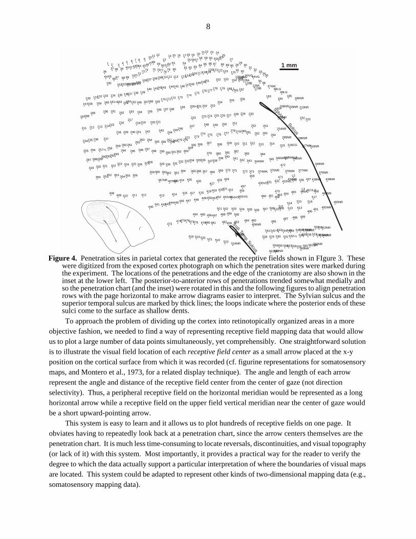
To approach the problem of dividing up the cortex into retinotopically organized areas in a more objective fashion, we needed to find a way of representing receptive field mapping data that would allow us to plot a large number of data points simultaneously, yet comprehensibly. One straightforward solution is to illustrate the visual field location of each receptive field center as a small arrow placed at the x-y position on the cortical surface from which it was recorded (cf. figurine representations for somatosensory maps, and Montero et al., 1973, for a related display technique). The angle and length of each arrow represent the angle and distance of the receptive field center from the center of gaze (not direction selectivity). Thus, a peripheral receptive field on the horizontal meridian would be represented as a long horizontal arrow while a receptive field on the upper field vertical meridian near the center of gaze would be a short upward-pointing arrow.

This system is easy to learn and it allows us to plot hundreds of receptive fields on one page. It obviates having to repeatedly look back at a penetration chart, since the arrow centers themselves are the penetration chart. It is much less time-consuming to locate reversals, discontinuities, and visual topography (or lack of it) with this system. Most importantly, it provides a practical way for the reader to verify the degree to which the data actually support a particular interpretation of where the boundaries of visual maps are located. This system could be adapted to represent other kinds of two-dimensional mapping data (e.g., somatosensory mapping data).

1 mm

SylvianSulcus

Sup. Temp. Sulcus

1 2 34 5 6 7 8 9

1011 12

1314 15 16 17 18 19 20 2122 23 24

2527

2829

3031

3233

3435

3637 38 39 4041424344 4546

474849 505152 53 54

55 565758 59 60 616263

64 656667 68 69 707172

7374 75 76777879 80 81 82 83 84 85 86 87 88 89 90

91 9293VG94VG

9596

97WK98LG

99LG

100 101102VG103VG104VG105106107 108109110111 112 113114115116117118119

120121122123 125

126LG127128A

128B129A

129B

130 131132 133 134 135 136137 138 139140 141142143 144145 146 147148 149150151 152 153 154 155

156

157158 159 160 161+L162 163164165 166 167168 169170171172 173

174175

176 177178 179 180 181182

183184

185186NR

187188189 190 191 192 193 194 195

196 197 198199 200+L201 202 203

204205 206

207208NR209NR 210NR

211 212 213 214215216

217218219 220 221

222 223 224 225 226 227 228 229 230231NR 232 233

234235 236 237

238 239 240 241 242 243244

245246247 248 249 250 251

252 253254NR

255 256 257+L 258259 260 261

262263 264

265 266267268269270 271

272 273274 275 276 277

278279280281 282 283284

285NR 286NR

287 288289290291292293

294 295 296 297298 299 300 301302 303

304305 306 307 308 309 310 311 312 313 314

315 316CG 317WK318NR

319 320 321 322323 324 325 326 327328

329 330 331332 333334 335336 337338

339 340341 342 343 344WK

345 346WKLF347WKLF348NR

349NR

350 351352 353 354355 356359360 361362 363

364 365366 367 368 369 370 371 372 373 374WK 375NR 376WK 377WK378NR

379 380 381 382383 384

387NR

388NR

406NR

407NR

408409 410 411 412 413 414 415 416417

418419 420421 422

423 424 425 426427

428 429430VG431 432 433VG

434VG435 436 437 438NR 439NR

440441 442443444445446 447 448 449450451452 453VG454VG455VG

456

457

458

459

460 461 462463 464 465 466A467A-F468

469NR470

471

472

473474475476477478 479480 481 482 483 484 485 486

487 488 489

490491

492WK

493NR

494 495 496497 498 499 500

501 502 503 504 505 506 507 508 509510511 512513

514515 516

517

518 519 520 521 522 523 524NR

527528 529 530 531 532+L 534535536 537538539NR540NR

541542+L543544545546 547548549NR550NR551552553NR

554555 556557558559 560 561NR562NR

563NR564NR565NR

L1

L2

L3

Figure 4. Penetration sites in parietal cortex that generated the receptive fields shown in FIgure 3. These were digitized from the exposed cortex photograph on which the penetration sites were marked during the experiment. The locations of the penetrations and the edge of the craniotomy are also shown in the inset at the lower left. The posterior-to-anterior rows of penetrations trended somewhat medially and so the penetration chart (and the inset) were rotated in this and the following figures to align penetration rows with the page horizontal to make arrow diagrams easier to interpret. The Sylvian sulcus and the superior temporal sulcus are marked by thick lines; the loops indicate where the posterior ends of these sulci come to the surface as shallow dents.

9

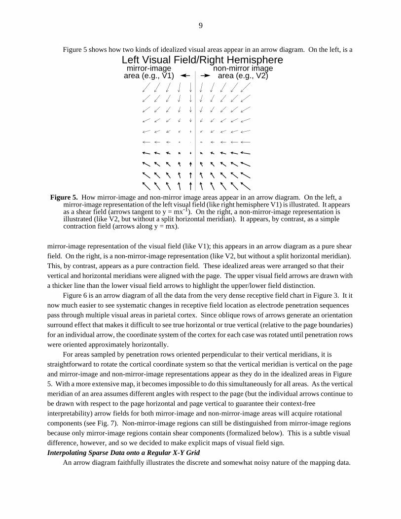
Figure 5 shows how two kinds of idealized visual areas appear in an arrow diagram. On the left, is a

mirror-image representation of the visual field (like V1); this appears in an arrow diagram as a pure shear field. On the right, is a non-mirror-image representation (like V2, but without a split horizontal meridian). This, by contrast, appears as a pure contraction field. These idealized areas were arranged so that their vertical and horizontal meridians were aligned with the page. The upper visual field arrows are drawn with a thicker line than the lower visual field arrows to highlight the upper/lower field distinction.

Figure 6 is an arrow diagram of all the data from the very dense receptive field chart in Figure 3. It it now much easier to see systematic changes in receptive field location as electrode penetration sequences pass through multiple visual areas in parietal cortex. Since oblique rows of arrows generate an orientation surround effect that makes it difficult to see true horizontal or true vertical (relative to the page boundaries) for an individual arrow, the coordinate system of the cortex for each case was rotated until penetration rows were oriented approximately horizontally.

For areas sampled by penetration rows oriented perpendicular to their vertical meridians, it is straightforward to rotate the cortical coordinate system so that the vertical meridian is vertical on the page and mirror-image and non-mirror-image representations appear as they do in the idealized areas in Figure 5. With a more extensive map, it becomes impossible to do this simultaneously for all areas. As the vertical meridian of an area assumes different angles with respect to the page (but the individual arrows continue to be drawn with respect to the page horizontal and page vertical to guarantee their context-free interpretability) arrow fields for both mirror-image and non-mirror-image areas will acquire rotational components (see Fig. 7). Non-mirror-image regions can still be distinguished from mirror-image regions because only mirror-image regions contain shear components (formalized below). This is a subtle visual difference, however, and so we decided to make explicit maps of visual field sign.Interpolating Sparse Data onto a Regular X-Y Grid

An arrow diagram faithfully illustrates the discrete and somewhat noisy nature of the mapping data.

non-mirror imagearea (e.g., V2)

Left Visual Field/Right Hemispheremirror-image

area (e.g., V1)

Figure 5. How mirror-image and non-mirror image areas appear in an arrow diagram. On the left, a mirror-image representation of the left visual field (like right hemisphere V1) is illustrated. It appears as a shear field (arrows tangent to y = mx-1). On the right, a non-mirror-image representation is illustrated (like V2, but without a split horizontal meridian). It appears, by contrast, as a simple contraction field (arrows along y = mx).

10

However, there is also a need for maps interpolated onto a uniform grid. These can then be contoured and used to estimate local visual field sign (see below). Since there are two main coordinates of retinotopy at each point in the cortex (eccentricity, r, and angle, θ), we need to superimpose two contour plots to illustrate retinotopy. A third coordinate is the receptive field diameter, d, which can be used to estimate the degree to which a particular region of the cortex smears an image. We used a distance-weighted smoothing method to interpolate the scattered r, θ, and d data onto uniform x-y grids (Lancaster and Salkauskas, 1986; Zipser and Andersen, 1988). The interpolated value ζj at the jth grid point was the distance-weighted sum of the values, zi, of all of the surrounding N data points, scaled by the sum of the weights

(1)

where the weight for the ith data point, w(rij), was an exponential function of the distance rij (in mm) between the ith data point and the jth grid point:

1 mm

SylvianSulcus

Sup. Temp. Sulcus

Figure 6. An arrow diagram can compactly illustrate retinotopy for many data points. The same data plotted in Figure 3 and 4 as a receptive field plot is shown here as an arrow diagram. In addition to illustrating the position of every receptive field shown in Figure 3, this diagram illustrates the relative position of every cortical recording site (the center of each arrow). As in Figure 4 and subsequent illustrations, the coordinate system of the cortex has been rotated so that the penetration rows are horizontal on the page to make it easier to see the absolute angle of each arrow.

ζj

zi w rij( )i

N

∑

w rij( )i

N

∑=

11

(2)

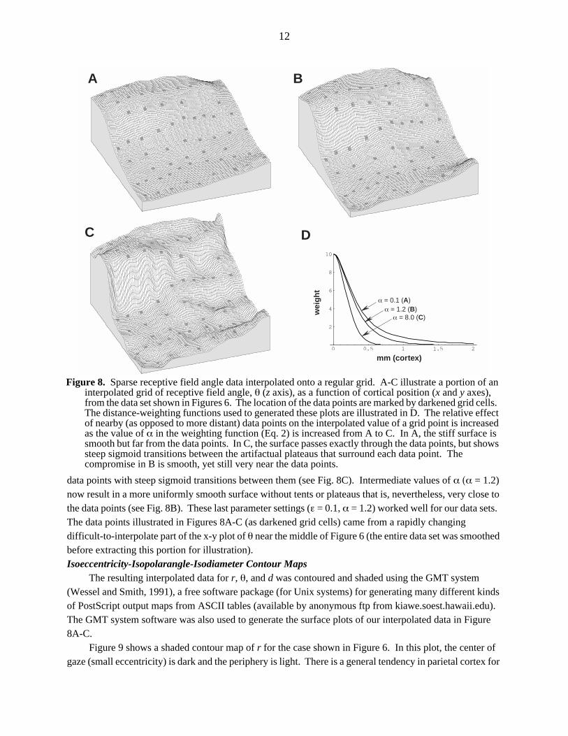
The weight function has a maximum at r = 0, that is, when a grid point lies exactly on a data point. This maximum height is set by the value of ε (wmax = ε−1 so wmax → ∞ as ε → 0). With small values of ε (ε < 0.01), the weight function is tall enough to constrain the surface to pass exactly through the data points. The value of α adjusts the shape of the fall-off of the weight function with distance; larger values of α more strongly emphasize the effect of nearby data points. Figure 8D shows a plot of the weight function w(r) for three different values of α with ε held constant (ε = 0.1).

With small values of both ε (ε ≤ 0.01) and α (α ≤ 0.1), Equation 1 generates a tent-like surface, held up by data point ’poles’ (this resembles a minimum-surface-tension smoothing, which can be approximated by iteratively setting non-data points to the average of their neigbors). As the value of α is increased (with ε held constant), the surface is more influenced by nearby data points, eventually resulting in broad plateaus surrounding each data point with steep sigmoid transitions between them. However, with small values of ε, it was difficult to find an intermediate value of α that was satisfactory for the entire data set; plateaus began appearing in some parts of the data set while other parts still had tents. By making ε somewhat larger (ε = 0.01 → ε = 0.1), the height of the weight function is reduced, which makes the interpolated surface stiffer; it was then possible to find a better compromise at intermediate values of α. Small values of α (α = 0.1) now result in a very smooth surface, but one that is too far from the data points (see Fig. 8A). Large values of α (α = 8.0) emphasize nearby data points and result as before in plateaus passing exactly through

map rotated90 degrees

map rotated60 degrees

map rotated0 degrees

map rotated30 degrees

Figure 7. Difficulty of extracting visual field sign from an arrow diagram. When the vertical meridian of a cortical visual area is not oriented vertically on the page, rotational components are added to both non-mirror-image and mirror-image representations (since the arrows are always drawn relative to the page coordinate system to guarantee their context free interpretability). Since vertical meridians of real cortical areas are often not parallel to each other, and since penetration rows are often not orthogonal to vertical meridians, it can be quite difficult to distinguish these two kinds of maps.

w r( ) e αr2− r2 ε+( )⁄=

12

data points with steep sigmoid transitions between them (see Fig. 8C). Intermediate values of α (α = 1.2) now result in a more uniformly smooth surface without tents or plateaus that is, nevertheless, very close to the data points (see Fig. 8B). These last parameter settings (ε = 0.1, α = 1.2) worked well for our data sets. The data points illustrated in Figures 8A-C (as darkened grid cells) came from a rapidly changing difficult-to-interpolate part of the x-y plot of θ near the middle of Figure 6 (the entire data set was smoothed before extracting this portion for illustration).Isoeccentricity-Isopolarangle-Isodiameter Contour Maps

The resulting interpolated data for r, θ, and d was contoured and shaded using the GMT system (Wessel and Smith, 1991), a free software package (for Unix systems) for generating many different kinds of PostScript output maps from ASCII tables (available by anonymous ftp from kiawe.soest.hawaii.edu). The GMT system software was also used to generate the surface plots of our interpolated data in Figure 8A-C.

Figure 9 shows a shaded contour map of r for the case shown in Figure 6. In this plot, the center of gaze (small eccentricity) is dark and the periphery is light. There is a general tendency in parietal cortex for

0 0.5 1 1.5 2

2

4

6

8

10

A

C

B

D

mm (cortex)

wei

gh

t

α = 0.1 (A)α = 1.2 (B)

α = 8.0 (C)

Figure 8. Sparse receptive field angle data interpolated onto a regular grid. A-C illustrate a portion of an interpolated grid of receptive field angle, θ (z axis), as a function of cortical position (x and y axes), from the data set shown in Figures 6. The location of the data points are marked by darkened grid cells. The distance-weighting functions used to generated these plots are illustrated in D. The relative effect of nearby (as opposed to more distant) data points on the interpolated value of a grid point is increased as the value of α in the weighting function (Eq. 2) is increased from A to C. In A, the stiff surface is smooth but far from the data points. In C, the surface passes exactly through the data points, but shows steep sigmoid transitions between the artifactual plateaus that surround each data point. The compromise in B is smooth, yet still very near the data points.

13

eccentricity to increase as one moves rostrally, although there are several pockets of small eccentricity rostrally. Figure 10 shows a shaded contour map of θ, also for the case from Figure 6, where the lower field vertical meridian (-90 degrees) is dark, the horizontal meridian (0 degrees) is gray, and the upper field vertical meridian (+90 degrees) is light. The picture of θ is quite complex; there are a number of representations of the horizontal meridian (marked by thick dashed lines) as well as the upper and lower field vertical meridians.

A map of cortical retinotopy would be obtained by superimposing the two maps from Figures 9 and

10. When the data set contains multiple, distorted representations, however, it can be exceedingly difficult to read such a map. There are two superimposed set of contours, each with their own labels, and there is no easy way to shade both of them at the same time (to help indicate the direction in which each set of contours is increasing). The fundamental problem with a double contour plot is that individual re-representations of the visual field do not stand out in any way. Boundaries between visual areas appear on double contour

10

10

10

10

2020

20

2

20

30

30

30

30

30

30

40

40

40

40

50

1 mm

MT

DLa

DLi

DLp

V2

Figure 9. Shaded contour map of interpolated receptive field eccentricity (r) for data from Figure 6. Central to peripheral visual fields are shaded dark to light. There is an overall tendency for eccentricity to increase as one moves both medially and anteriorly in occipitoparietal cortex. However, there are several pockets of center of gaze representations at the anterior and medial extremes of parietal cortex. The location of the recording sites are shown by the small dots and the marker lesions by the large dots.

14

plots only as a change in the angle at which the r and θ contours intersect. The difficulty in reading these maps prompted us to look for a better way of representing the data. We turned to a map shaded by local visual field sign (non-mirror-image versus mirror-image); the double contour map was retained underneath for reference.Visual Field Sign Maps

For each small portion of a retinotopic cortical map, one can calculate the sign of the visual field representation—that is, whether it is a non-mirror-image or mirror-image representation of the retina (when viewed from the cortical surface). The visual field sign can be determined from the (clockwise) angle, λ, between the direction of the gradient in eccentricity, , and the direction of the gradient in angle, (see Fig. 11) (the gradients are locally perpendicular to the contour lines and point uphill). An angle

0

0

00

0

-80

-60

-60

-60

-60

-60

-60

-60

-40

-40

-40

-40

-40

-40

40

-20

-20

-20

-20

-20

-20

-20

20

2020

20

20

20

40

40

40

40

60

60

60

80

1 mm

MT

DLa

DLi

DLp

V2

Figure 10. Shaded contour map of receptive field polar angle (θ) for data from Figure 6. The horizontal meridian is shown in bold dashed lines, upper field isopolar angle lines are shown as thin dashed lines, and lower field contour lines are shown as thin dotted lines. The lower field vertical meridian is shaded black, the horizontal meridian is gray, and the upper field vertical meridian is white. The most prominent feature is a long finger of upper field representation (light) extending almost to the center of gaze representation of V2. The vertical meridian representation of MT is visible as a dark patch at the lower right. There is a second (dark) lower field vertical meridian representation in between MT and the finger of upper field representation, and a third in the anterior medial part of parietal cortex at the upper right.

r∇ θ∇

15

between the gradient directions of π/2 signifies an undistorted (conformal) non-mirror-image representation while an angle of 3π/2 signifies an undistorted mirror-image representation. Intermediate angles signify different degrees of non-orthogonality (non-conformality) of the visual field representation with singularities at 0 and π, where visual field regions would be mapped to lines of indeterminate visual field sign. A map of visual field sign is produced by distinguishing λ between 0 and π from λ between π and 2π. The local gradient directions in the r and θ maps are estimated from finite differences in the x and y directions on the two interpolated maps.

Visual field sign has several attractive properties as a local measure of cortical organization. First, since it is a relative measure, it is invariant to the orientation of the retinotopic map on the cortex (see Fig. 11). Second, and somewhat less obviously, visual field sign is invariant to rigid transformations of the

receptive field coordinate system (as would be produced, for example, by sliding and/or rotating a sheet of spherical paper containing receptive fields over the surface of the plastic hemisphere coordinate system). This is again because of the fact that visual field sign is a relative measure; the r and θ gradient directions are both changed in the same way by such a transformation. Thus, the analysis is completely insensitive to the placement of the center of gaze, the vertical meridian, and so on. The only requirement is that the receptive fields all be digitized using the same (arbitrary) coordinate system.

Figure 12 (top row of plots) illustrates the technique applied to an idealized pair of adjoining visual areas (like those shown in Figure 5) and a more realistic, randomly jittered pair of areas sampled at a density typical of our experiments (bottom row of plots). In both rows, the starting data is shown in the arrow diagrams at the far left. Eccentricity, r, and angle, θ, of each of these data sets were then interpolated onto regular grids using the distance-weighting function used in Figure 8B. The resulting r and θ grids were contoured and shaded in the middle two panels. The r and θ grids were then combined to make visual field sign maps at the far right (the two contour plots are also superimposed for reference), where

Figure 11. The local visual field sign is determined by measuring the (clockwise) angle, λ, between the eccentricity gradient (direction of ), and the receptive field polar angle gradient (direction of ). An angle of approximately 90 degrees (0 < λ < π) signifies a non-mirror-image mapping of the contralateral (left) hemifield while an angle of approximately 270 degrees (π < λ < 2π degrees) signifies a mirror-image mapping of the same hemifield. This is a robust, relative local measure capable of distinguishing non-mirror-image from mirror-image regions that is invariant to rotation and distortion of local map regions. Visual field sign is also invariant to receptive field coordinate transformations; to compute it, only the relative position of receptive fields must be known.

r∇ θ∇

-

+

λ

-

+

∆

r

∆

r

Non-mirror-imageleft hemifield map

(λ ≈ π/2)

Mirror-imageleft hemifield map

(λ ≈ 3π/2)

∆

r

∆

r

∆

θ ∆

θ

λ

∆

θ ∆

θ

∆

θ∆

r∆

r∆

rλ λ

16

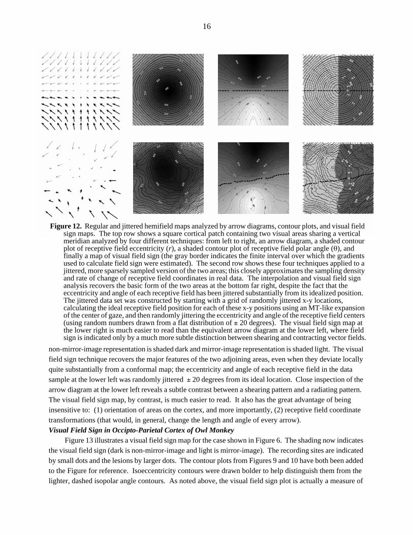
non-mirror-image representation is shaded dark and mirror-image representation is shaded light. The visual field sign technique recovers the major features of the two adjoining areas, even when they deviate locally quite substantially from a conformal map; the eccentricity and angle of each receptive field in the data sample at the lower left was randomly jittered ± 20 degrees from its ideal location. Close inspection of the arrow diagram at the lower left reveals a subtle contrast between a shearing pattern and a radiating pattern. The visual field sign map, by contrast, is much easier to read. It also has the great advantage of being insensitive to: (1) orientation of areas on the cortex, and more importantly, (2) receptive field coordinate transformations (that would, in general, change the length and angle of every arrow).Visual Field Sign in Occipto-Parietal Cortex of Owl Monkey

Figure 13 illustrates a visual field sign map for the case shown in Figure 6. The shading now indicates the visual field sign (dark is non-mirror-image and light is mirror-image). The recording sites are indicated by small dots and the lesions by larger dots. The contour plots from Figures 9 and 10 have both been added to the Figure for reference. Isoeccentricity contours were drawn bolder to help distinguish them from the lighter, dashed isopolar angle contours. As noted above, the visual field sign plot is actually a measure of

00

-60

-60

-40-40

-20

-20

20

20

404060

60

10

20

20

20

30

30

30

30

30

40

40

40

40

40

40

0

0

-60

-60

-40

-40

-20-20

20

20

40

40

40

60

60

8080

20

20

20

20

30

30

30

30

30

30

40

40

40

50

0

0

-60

-60

-40

-40-20

-20

20

20

40

40

40

60

60

8080

20

20

20

20

30

30

30

30

30

30

40

40

40

50

00

-60

-60

-40-40

-20

-20

20

20

404060

60

10

20

20

20

30

30

30

30

30

40

40

40

40

40

40

Figure 12. Regular and jittered hemifield maps analyzed by arrow diagrams, contour plots, and visual field sign maps. The top row shows a square cortical patch containing two visual areas sharing a vertical meridian analyzed by four different techniques: from left to right, an arrow diagram, a shaded contour plot of receptive field eccentricity (r), a shaded contour plot of receptive field polar angle (θ), and finally a map of visual field sign (the gray border indicates the finite interval over which the gradients used to calculate field sign were estimated). The second row shows these four techniques applied to a jittered, more sparsely sampled version of the two areas; this closely approximates the sampling density and rate of change of receptive field coordinates in real data. The interpolation and visual field sign analysis recovers the basic form of the two areas at the bottom far right, despite the fact that the eccentricity and angle of each receptive field has been jittered substantially from its idealized position. The jittered data set was constructed by starting with a grid of randomly jittered x-y locations, calculating the ideal receptive field position for each of these x-y positions using an MT-like expansion of the center of gaze, and then randomly jittering the eccentricity and angle of the receptive field centers (using random numbers drawn from a flat distribution of ± 20 degrees). The visual field sign map at the lower right is much easier to read than the equivalent arrow diagram at the lower left, where field sign is indicated only by a much more subtle distinction between shearing and contracting vector fields.

17

the local relation between the two contour maps (angle between the steepest uphill directions). This relation, however, is very difficult to extract without the explicit shading.

0

0

00

0

-80

-60

-60

-60

-60

-60

-60

-60

-40

-40

-40

-40

-40

-40

40

-20

-20

-20

-20

-20

-20

-20

20

2020

20

20

20

40

40

40

40

60

60

60

80

10

10

10

10

20

20

20

20

30

30

30

30

30

30

40

40

40

40

50

1 mm

MT

DLa

DLi

DLp

V2

Figure 13. Double contour map with superimposed visual field sign map based on data from Figure 6. The shading now indicates the visual field sign (dark is non-mirror-image and light is mirror-image). As before, the location of the recording sites are shown by the small dots and the marker lesions by the large dots. The isoeccentricity contours were drawn in bolder solid lines to help distinguish them from the lighter, dashed (upper field) and dotted (lower field) isopolar angle contours. The visual field sign plot emphasizes the local relation between the two contour maps that is very difficult to extract without explicit shading.

The complexity of the maps in parietal cortex was unexpected. There are many local islands of differing visual field sign once one moves away from V2 and MT. The anterior V2 border (horizontal meridian) appears diagonally at the upper left. V2 was adjoined anteriorly, and unexpectedly, by an upper visual field representation with the same visual field sign as V2 (non-mirror-image = dark). Continuing toward the lower left (anteriorly in the cortex), there is an area of mirror-image visual field sign (light) at the center of the illustration containing upper and lower fields (DLp, dorsolateral posterior area). Just below this is a sinuous region of non-mirror-image representation (dark) containing only the lower visual field (DLi, dorsolateral intermediate area). Below this are several discontinuous patches of lower field, mirror-image (light) representation (DLa, dorsolateral anterior area). Finally, the medial border of MT and small portions of the MT horizontal meridian appear at the bottom middle right (dark). At the far right, near where the horizontal meridian makes an almost complete loop, are a series of small patches of alternating visual field sign containing both upper and lower visual fields (anterior parietal visual areas—not labeled).

18

The complexity of the map in parietal cortex was unexpected. The linear border of an almost conformally mapped V2 (note the almost orthogonal relation between the r and θ contours) appears at the upper left, while the medial border of MT is just visible at the lower right. In between these areas there are many local islands of differing visual field sign. It is possible to make out several sinuous strips of reversed visual field sign that correspond to the multiple areas DLp, DLi, and DLa identified (Sereno et al., 1987) within the region originally named DL by Allman and Kaas (1974). There is, however, an unexpected patch of upper visual field with the same visual field sign as DLp attached directly to lower field DLp. In addition, there appears to be a distinct region of upper field representation just posterior to DLp and anterior to the lower visual field representation in V2 with the same visual field sign as V2. There are also several small areas directly medial to MT. The complexity of the picture is at odds with the usual summary diagrams (see Sereno et al., forthcoming, for detailed discussion of the implications of this case).

We tested the effects of changing the distance-weighted smoothing coefficients, ε and α, on the visual field sign map shown in Figure 13. The overall pattern of visual field sign, but also the position of the visual field sign transitions was quite stable to changes in these parameters, breaking down only when the interpolated surfaces were extremely stiff (smooth), excessively tented, or strongly locally influenced (plateaus with sigmoid transitions). With overly stiff interpolations, smaller pockets of reversed visual field sign were lost. With excessively tented smoothings, artifactual visual field sign reversals appeared around the tents at each data point. With strongly locally influenced smoothings, visual field sign boundaries were artifactually squared up because penetrations were sometimes made in rows. These smoothing artifacts were virtually eliminated with appropriate choices of ε and α.Difficulty of Obtaining Visual Field Sign from Connectional Data

It should be noted that it is very difficult to obtain visual field sign maps from cortico-cortical connectional data when visual areas are: (1) small, (2) variable, (3) have distorted representations of the retina, and (4) have borders that are not architectonically apparent, and (5) have split horizontal meridian representations. These, unfortunately, are characteristics of most visual areas beyond V1. A single injection only establishes that there are connections between areas. If the injection is near an areal border, a single labeled focus may actually represent two labeled areas joined by a congruent border. There are additional complications if the injection encroaches on a horizontal meridian representation since this may result in two foci appearing in a single target area if the target area’s horizontal meridian is split (actually, since horizontal meridians often form congruent borders with adjacent areas, each of the two foci would likely represent two areas).

Two nearby injections in a single area (away from the horizontal meridian representation) establish retinotopy (but do not distinguish visual field sign) if the target label can be positively identified to be within one area. With an undistorted map, three nearby non-colinear injections would suffice to determine the visual field sign of a target area (cf. Montero, 1993, who made three distinguishable non-colinear injections in rat V1). However, given that extrastriate areas are often quite distorted, it can be difficult to determine the field sign using three points, or even whether or not the points are colinear. Figure 14, for example, schematically illustrates three labeled foci in two differently distorted areas that would, in the absence of other information, erroneously suggest that the areas have different visual field signs. Four distinguishable, nearby injections all within one area, all avoiding the horizontal and vertical meridians would therefore typically be required to unambiguously establish the visual field sign of the target map. There are no published cases of this kind, even for injections into V1. Thus, it can be quite hazardous to draw specific conclusions about the macroscopic retinotopic organization of extrastriate cortical areas from current

19

anatomical data. Of course, anatomical data provides a great deal of additional information about the spread of local connections, the laminar identity of source and target projections, and the fine tangential structure of the projections that is much more difficult to obtain using physiological recording techniques (see e.g., Felleman and Van Essen, 1991; Kisvarday and Eysel, 1992; Salin et al., 1992; Lund et al., 1993).Warping the Penetration Map to Superimpose it on the Flattened, Stained Cortex

In our acute experiments, the cortex is photographed at the start of the experiment and then penetrations are marked on the photograph using blood vessels as landmarks, as described above. The x-y location of the penetrations are digitized from the photograph and can be used to make arrow diagrams, isoeccentricity/isopolar angle maps, and visual field sign maps. The resulting maps, however, must then be related to the stained, flattened cortex using marker lesions. If the flattening process only involved global scaling (expansion/contraction) and rotation, it would be a simple matter to superimpose the photograph-derived penetration maps on the stained cortex. The physical flattening process, however, involves local expansions, rotations, and shears. Therefore, we devised a deformable template technique to stretch the x-y photographic penetration map according to final location of lesion control points in the stained tissue.

The technique works by establishing a mesh with square cells and then moving each of the vertices of the mesh so as to minimize a local energy function, Ei. The value of E for the ith vertex is calculated from marker lesion errors and from distances to, and angles between, the neighboring N vertices (N = 4 except for corner and edge points):

(3)

The energy function is constructed from four terms: (1) a data term, which measures the distance, ∆ddata, between the current mesh position of the lesion (starting mesh position is taken from the recording

1

3

1

2

32

3

12

Visual Fieldretinotopic locationof three injections

Cortical Areasspurious indication of

opposite visual field sign

Figure 14. Difficulty of determining visual field sign with tracer injections alone. The visual field location of three distinguishable tracer injections are illustrated at the left. The label in two differently-distorted cortical areas with the same visual field sign are shown at the right. In the absence of other information, a plot of the distribution of the three tracers would spuriously suggest that the two areas have opposite visual field sign (i.e., the triangle formed by injections 1, 2, and 3 is reversed in the two areas). Differently distorted areas, of course, would cause similar problems with injections closer to isoeccentricity lines. For injections with realistic separations, one therefore typically requires four, mutually distinguishable injections, all avoiding the vertical and horizontal meridians, to determine the visual field sign of an area anatomically.

Ei ddata∆ ρ1N

dj dinit−j 1=

N

∑3

β1N

dj dave−j 1=

N

∑3

γ1N

θj π 2⁄−j 1=

N

∑3

+ + +=

20

photograph) and the target position of the lesion on the flattened brain (this term is set to zero for all but data vertices), (2) an initial distance term, which measures deviations of the current distances to neighboring vertices, dj, from their starting length, dinit, (3) an average distance term, which measures deviations of the current distances to neighboring vertices from the current average distance to neighboring vertices, dave, (4) and a conformality term, which measures deviations of the angles, θj, between successive pairs of neighboring vertices from π/2. This interpolation problem is more difficult than that of interpolating receptive field data; and this technique effectively builds in more comprehensive prior assumptions.

The energy function is minimized by estimating its gradient by finite differences. At each iteration, the energy for every vertex is calculated for small deviations, δ, in the x and y directions; each vertex is then moved δ in the direction of minimum energy. For δ = 25-100 µm and a starting intervertex distance (mesh cell size) of about 1 mm, the mesh generally settled after about several hundred (randomly shuffled) updates of each vertex. The coefficients on the terms in the energy function, ρ, β, and γ, were set to emphasize average distance and orthogonality over initial distance. This generates mesh deformations that closely resemble the deformations observed in the physical flattening process as the cortical tissue is lightly compressed between slides prior to fixation. To speed convergence, we included a momentum term (which incorporates a portion of the previous move into the current move). As the mesh settles, the first order data term dominates, forcing the lesions to lie exactly at their flattend brain positions, which simplifies the final overlay. The final locations of the penetration points are calculated by bilinear interpolation using the final location of the four mesh vertices that were nearest each penetration point in the undeformed mesh.

A deformed mesh calculated using 8 identified lesion points is illustrated in Figure 15. The stretching process is illustrated by drawing the final mesh on a bold rectangle, which illustrates the initial borders of the mesh, and by drawing a line between the initial location of each of the ~600 penetrations (small open dot) and their final, stretched location (small filled dot). The initial and starting positions of the lesions are indicated by medium-sized open and filled dots, and lines. Finally, the initial and target locations of the mesh points nearest the lesions (which are used to calculate the data term) are shown as large, and slightly larger open circles. The stretched x-y locations were used to make the isoeccentricity, isopolar angle maps, and visual field sign maps so that they could be accurately superimposed on stained flatmounts. The final mesh appears deceptively undistorted. Close inspection of the starting and ending positions of the lesions and recording sites, however, reveals a complex pattern of local movement across the cortex that would be poorly approximated by global scaling, rotation, and shear. Our technique also works in instances where flattening-induced deformations are more severe and more anisotropic (see Sereno et al., forthcoming).Discussion

Multiple retinotopic maps characterize the tangential organization of most of the visual half of neocortex in primates. Physiological mapping experiments are a crucial tool for defining visual areas. No other technique offers as detailed a window on the organization of extrastriate cortex in single animals. The ability to examine the organization of visual areas within a single animal is particularly important given the large amount of variability that exists between animals of the same species.

In the course of collecting and attempting to analyze large retinotopic mapping data sets from owl monkey extrastriate cortex, it became quite clear that current methods for representing this kind of data were inadequate. In this paper, we have presented several analytic techniques—arrow diagrams and visual field sign maps—that make it possible to more objectively parcel visual cortex into different areas on the basis of retinotopy. These techniques could be extended to other modalities characterized by two dimensional receptotopic maps (e.g., somatosensory cortex). We postpone detailed discussion of the individual areas

21

revealed in the case illustrated in detail here to our two companion papers (Sereno, McDonald, O’Dell, and Allman, forthcoming; Sereno, McDonald, and Allman, in preparation).Definition of a Visual Area

Most recent reviews of reviews of the organization of visual areas (e.g., Krubitzer and Kaas, 1991; Sereno and Allman, 1991; Felleman and Van Essen, 1991) illustrate all areal boundaries as uniform dark lines. Though this make the maps easier to read, it has a strong tendency to downplay the substantial differences in the degree to which the various boundaries are supported by converging data from retinotopic organization, architectonic features, connections patterns, and physiological properties. Some visual areas have boundaries that are well-defined and concordant for all of these criteria. For example, primary visual cortex, area V1, in primates (and other mammals), contains a fine-grained, relatively undistorted map of the entire contralateral visual hemifield. The electrophysiologically defined borders of this map coincide exactly with a very clear architectonic and connection-defined border.

Figure 15. Deformed mesh calculated using 8 identified lesion points (data from Figure 6). The bold rectangle illustrates the initial borders of the mesh. Thin lines are drawn between the initial location of each of the ~600 penetrations (small open dots) and the final, stretched location (small filled dots). The initial and starting positions of the marker lesions are indicated by medium-sized open and filled dots, and lines. Finally, the initial and target locations of the mesh points nearest the lesions (which are what are actually used to calculate the data term) are shown as large, and slightly larger open circles, and lines. Close examination of the starting and final penetration pairs in different parts of the diagram reveals a complex pattern of local distortion that cannot be closely approximated by global rotation and scaling.

22

Most of the 25 or so other visual areas are not as easy to delimit. There are complications even with areas V2 and MT. V2 seems to contain 3 intercalated representations of the hemifield in at least the thick, thin, and interstripes (Rosa et al., 1988; Van Essen et al., 1990). In MT, there is a sudden reduction in myelination in the representation of the visual field periphery in both owl monkeys and macaque monkeys that does not seem to have electrophysiological or retinotopic correlates (e.g., visual field re-representations) (Allman and Kaas, 1971; Gattass and Gross, 1981; Desimone and Ungerleider, 1986). In spite of these difficulties, however, there is good agreement between different methods on the location of substantial portions of the borders of V2 and MT.

Unfortunately, it is much more difficult to unambiguously define the borders of the remaining (large majority!) of visual areas beyond V2 and MT in extrastriate cortex. There are a number of reasons for this. First, the architectonic borders of these areas are generally much less distinct than those of V1, V2, and MT. Second, these areas often contain only partial maps of the visual hemifield or even partial maps of one visual quadrant. Third, the maps are more distorted than those in V1 and MT. Fourth, responses in these other areas are often more leisurely and more susceptible to anesthetic than responses in V1, V2, and MT. Fifth, receptive fields are generally larger, and therefore take longer to map. Finally, the areas themselves are much smaller. These considerations demand a rigorous approach.Quantitative Retinotopic Maps

Double contour maps have often been presented in analyses of retinotopy (Allman and Kaas, 1971; Wagor et al., 1980; Desimone and Ungerleider, 1986; Fioriani et al., 1989; Rosa et al., 1993). Yet these have rarely been explicitly derived by quantitatively interpolating and contouring the data from an individual case. For example, the extensive mapping studies of Tusa, Palmer, and Rosenquist (Tusa et al., 1978; Palmer et al, 1978; Tusa et al., 1979; Tusa and Palmer, 1980) present a considerable amount of the raw mapping data (electrode penetration tracks illustrated on sections with correspondingly numbered receptive field charts) along with summary double contour maps. It would be interesting to see quantitatively interpolated, double contour maps for individual cases showing the location of the data points. To be sure, generating quantitative contour maps is more difficult in cats (and macaque monkeys) than in owl monkeys because of the extensive gyrification of the cortex. A more rigorous approach would have to begin with a computational flattening of the cortex (see e.g., Schwartz, 1990; Dale and Sereno, 1993) prior to interpolating and contouring the receptive field data. In another set of extensive studies of retinotopy in primate extrastriate cortex, sometimes only one coordinate of retinotopy (eccentricity) was contoured (Gattass et al., 1988; Rosa et al., 1988).

The non-iterative distance-weighted interpolation/smoothing technique presented here provides a robust and straightforward way to interpolate sparse retinotopic mapping data onto a regular x-y grid once the cortex has been flattened. These grids (of r and θ) can then be quantitatively contoured. Existing data from areas with obvious architectonic borders suggests that extrastriate areas vary considerably in size, shape, and location. The cytochrome oxidase-stained flatmounts illustrated by Tootell et al. (1985), for example, show that the surface area of area MT probably varies by almost a factor of two in animals with similar body sizes. Rigorous interpolation and contouring of mapping data is a crucial step in better understanding how the remaining majority of visual areas with much less well defined architectonic borders are organized.

Maunsell and Van Essen (1987) presented a quantitative technique for interpolating sparse receptive field data from a single area (MT) onto a regular grid. Each grid cell for r (or θ) was set to the average of the linearly interpolated r (or θ) value along lines between all pairs of data points up to 3 mm apart that

23

passed through that grid cell. Their technique (with lines <= 3 mm) produces a much stiffer surface globally than our distance-weighted technique does (with ε = 0.1, α = 1.2) since it effectively gives equal weight to points that lie within a 6 mm circle (cf. Fig 8). However, since it smooths much more over local retinotopic details such as minima and maxima in r and θ, which are often important for defining areal boundaries, it is less suited to interpolating data sets containing several small visual areas. In addition, though globally stiffer, the Maunsell and Van Essen technique produces surfaces that are locally much less smooth (since a point contributing to one grid cell may often not contribute to the neighboring grid cell); these discontinuities (which are exacerbated by reducing the maximum line length) lead to artifacts when there is a need to estimate derivatives (gradients).Better Representations of Retinotopy

Our large data sets made it necessary to find more intuitive methods for representing retinotopy. In particular, the standard technique of numbered receptive field plots with correspondingly numbered penetration charts proved to be completely unwieldy. Receptive field plots are useful once the data has been divided into areas; but we needed to find another way of representing the data prior to dividing it up. The number of possible subdivisions becomes very large when there are several hundred recording sites.

We presented two complementary techniques—arrow diagrams and visual field sign maps—that make it easier to visually parse cortical retinotopic maps. Arrow diagrams are made by placing a small arrow whose length and angle represent the location of the receptive field center at the cortical x-y location of the site from which it was recorded. With this technique, it is possible to look at all of the raw data from one animal at once. This makes it much easier to look for receptive field reversals, and to examine the degree to which retinotopy is systematic. It is also possible to distinguish whether an area has a non-mirror-image representation of the hemifield (like V2) or a mirror-image representation (like V1); non-mirror-image regions have a radiating pattern while mirror-image regions have a shearing pattern (see Fig. 5). Reversals are much easier to mark on an arrow diagram than on a penetration chart because one does not have to look up numbers on a crowded receptive field chart. Once areal boundaries have been marked, it is a much simpler task for the reader to verify the extent to which the data supports a particular subdivision of the cortex.

One problem with arrow diagrams is that re-representations of parts of the visual field sometimes do not stand out clearly. Systematic changes in arrow direction (receptive field sequence reversals) signifying areal borders can be subtle when these changes are not parallel to penetration rows. A related problem is that it can be quite difficult to distinguish non-mirror-image representations from mirror-image representations when the borders of areas are not oriented vertically on the page; this is because tilting an area adds rotational components to the radiating and shearing patterns that characterize these two types of areas (this is in turn because the arrows themselves must always be drawn with respect to the page to give them context-free interpretability). These difficulties prompted us to look for a more explicit way to mark cortical retinotopic maps for visual field sign.

By plotting the angle between the gradients in receptive field eccentricity and receptive field angle (after interpolating them onto a regular x-y grid), it is possible to shade a double contour map with the visual field sign—that is, whether the local retinotopic map is a non-mirror-image representation or a mirror-image representation. This brings out a relation between the two sets of contours that is equivalent to the radiating/shearing distinction in the arrow diagrams. The best defined interareal boundaries in the cortex—such as the boundary between V1 and V2—are characterized by a sharp transition in visual field sign. By estimating the value of the visual field sign at each point in the cortex, it is possible to color in entire areas.

24

Once we have quantitatively interpolated and contoured a data set and calculated a local visual field sign map, summary diagrams can be made using traditional vertical and horizontal meridian symbols (rows of circles and thick dashes). It is important to point out that these symbols may be somewhat misleading, however, since many of the visual field sign transitions occur at some distance from the vertical and horizontal meridians (see e.g., Gattass et al., 1988).Using Visual Field Sign to Define Cortical Areas

The traditional definition of a visual area on the basis of retinotopy was that an area contained a retinotopic map. As more detailed experiments were carried out, it became clear that many areas did not have a map of the entire visual hemifield. Many areas were found to have incomplete representations of the visual field. Investigators turned to other locally measurable properties of the cortex to help divide it up into distinct areas. For example, Van Essen and his colleagues (review: Van Essen, 1985) have argued, on the basis of contrasts in responsiveness to color and direction of motion, that the complementary lower and upper visual field representations in V3 and VP were in fact different areas, each containing a representation of only one visual quadrant.

We propose that visual field sign (non-mirror-image versus mirror image) is another useful locally defined property of a visual area (alongside architectonic, connectional, and physiological criteria) that can be used to divide up the visual cortex into different regions. Thus, just as an area can be defined by a spatially contiguous region of cortex containing an abundance of motion-sensitive neurons or a pattern of dense myelination, it can also be defined as a contiguous region of the cortex with a certain visual field sign. There may, of course, be reasons to distinguish adjoining region of the cortex that have the same visual field sign, just as we might distinguish areas that share the similar patterns of myelination or similar cellular response properties, if there are other criteria on which those subareas differ sharply.

It may well be enlightening to re-analyze several of the more complete published retinotopic mapping cases in primates and cats mentioned previously using quantitatively derived visual field sign maps. This procedure has recently been used to analyze the results of retinotopic mapping experiments on visual areas in the California ground squirrel (Sereno et al., 1991); there is substantial agreement with between the visual field sign maps and a number of subtle but repeatable features visible in myelin-stained flatmounts (unpublished observations).Visual Field Sign Is Invariant to Receptive Field Coordinate Transformations

The definition of visual field sign (Fig. 11) as a relative measure ensures that it is invariant to the orientation of a visual area on the cortex. Somewhat more subtly, however, visual field sign is also invariant to transformations of the receptive field coordinate system (since such transformations affect the gradients used to calculate visual field sign in the same way). This makes it possible to use retinotopy to precisely define cortical borders without having to know the exact placement of the center of gaze or the placement of the horizontal and vertical meridians in the visual field. The vertical and horizontal meridians, in particular, are difficult to define, since they have no corresponding retinal landmark and since the border between many extrastriate areas appears to lie at some distance from the vertical or horizontal meridian (see Gattass et al., 1988). The only requirement for using this technique is that relative position of all receptive fields be known.Implications of the Complex Pattern of Visual Field Sign

The boundaries between non-mirror-image and mirror-image representations revealed in these studies are quite intricate—much more so than is usually illustrated in summary diagrams of cortical areas. We would like to suggest that the complex pattern of visual field sign may reflect the actual shape of visual areas

25

in extrastriate cortex. At first glance, it would appear that existing data from other techniques such as anatomical tracer studies, architectonics, and studies of physiological properties argues against such complexity. On closer examination, however, it is difficult to support this claim.

Connectional studies can illustrate the target areas of a cortical region as well as laminar details of interareal connections; but these studies invariably sample the connectivity of only a small number of points in the multiple visual maps of any one animal, making it difficult to draw firm conclusions about the overall shape of the borders between areas. Second, architectonic studies have the potential to give a more global, yet fine-grained picture of the cortex. Unfortunately, most extrastriate areas are not easily visible using current techniques for staining the cortex. Even in a flatmount, it is very difficult to definitively divide up the cortex beyond V1, V2, and MT on architectonic bases alone. Certainly, it is often possible to find subtle architectonic features that correlate with areal boundaries determined by mapping. But it is very difficult to rule out the existence of sinuous areal borders on architectonic data alone; there is of course, no way to even determine if an area is even visual by examining its architectonic features. Some recent anatomical studies have actually independently suggested that several extrastriate areas may have quite tortuous borders (Kaas and Morel, 1993). Finally, physiological properties are much more time consuming to examine than retinotopy. As a result, it is very rare that enough locations have been sampled to allow definitive statements about the 2-D form of areal boundaries on the basis of physiological response properties.Is Retinotopy in Extrastriate Visual Cortex Really Continuous?

By interpolating the data for r and θ onto a regular grid, we are implicitly making the assumption that nearby points on the cortex represent nearby points on the visual field. This implies that individual cortical retinotopic maps are internally continuous mappings of portions of the hemiretina. But such an interpolation also implies that the boundaries between areas are continuous—that is, that there are no true ’incongruent’ borders between areas (cf. Allman and Kaas, 1975). We now feel that this is a reasonable assumption. When recording from penetrations perpendicular to the cortical surface, one often sees jumps in the location of the receptive field as the electrode is moved to a nearby location. However, whenever there has been time to record at an intermediate point, we have virtually always found an intermediate receptive field. More convincingly, we have very rarely observed large jumps in receptive field centers (a large jump being one that results in a completely non-overlapping receptive field) in thousands of tangential penetrations through extrastriate areas, where we have almost invariably mapped a new receptive field every 50 to 100 µm of electrode travel.

Note that the continuity of retinotopy is perfectly consistent with there being a mosaic of partial representations of the visual hemifield as well as the existence discontinuities in the representation of the hemifield. The continuity of retinotopy only states that nearby points in the cortex represent nearby points in the visual field. The converse is not implied—that is, nearby points in the visual field can be (and are) represented by widely separated points in the cortex. For example, the horizontal meridian representation in area V2 is split so that visual field locations just above and below the horizontal meridian are represented quite far from each other in the cortex; but this is perfectly consistent with there being no discontinuity in receptive field r and θ as one moves the electrode across the horizontal meridian representation of V2 into the adjoining areas.

This observation may be a natural consequence of the ubiquity of local (albeit patchy) excitatory connections in the cortex (Kisvarday and Eysel, 1992; Lund et al., 1993) coupled with the tendency for nearby points in the visual field to be stimulated in a similar way by extended objects and flow fields in the

26

environment. In the context of a correlation-based synaptic modification rule, both of these factors would favor a situation where nearby cortical regions represent nearby points in the visual field (see, e.g., Linsker, 1989; Zhang et al., 1993). That discontinuities are allowed with respect to the visual field but not with respect to the cortex may reflect the overall stronger enforcement of local correlations in the cortex (presumably the result of local connections) when compared to correlations between activity in nearby parts of the retina generated by looking at the visual world.Comparisons With the Somatosensory System

It is intriguing to compare the patterns of receptotopy in the visual and somatosensory systems. There are a number of similarities but also an instructive difference. In somatosensory cortex many nearby cortical locations do in fact represent nearby points on the sensory surface. However, in a number of instances, nearby cortical locations clearly represent disparate points on the sensory surface, in contrast to what we claimed was universally the case in visual cortex. For example, there are often sharp discontinuities in somatosensory cortex at the borders between different body parts; as one crosses from one digit representation into the adjoining digit representation, receptive fields suddenly jump to the next digit without any overlap (Merzenich et al., 1978). Similar discontinuities appear at the boundary between the representation of the arm and the face. This may reflect the reduced tendency for continuity of stimulation in the somatosensory system when compared to the visual system. The mechanical continuity of the receptor surface (skin) of one finger ensures much greater correlation between stimulation of nearby parts of the finger—upon grasping an object, for example—than between parts of two different fingers (Allard et al., 1991; Grajski et al., 1990). In the visual cortex, by contrast, nearby points in different regions of the retina are on a more equal footing with respect to the chance of being stimulated in a correlated fashion by the visual world. The systematic differences in co-activation of different skin patches may more strongly influence local circuit connections in the somatosensory cortex—for example, by introducing discontinuities into the meshwork of excitatory local circuit connections.

Our visual field sign technique could be adapted to distinguishing cortical areas in the somatosensory system. There, we would distinguish body surface sign—that is, non-mirror-image versus mirror-image representation of the body surface. Since there is only local continuity of somatotopy, the interpolation process would have to be modified to permit somatotopic domains (for example, individual finger representations) to be smoothed independently. A quantitative approach to this might begin by first roughly estimating cortical gradients in both coordinates of body surface position using the shortest distance measured along the surface of the skin between receptive fields recorded at nearby cortical sites (somatosensory geodesics). Elongated discontinuities could be marked by ‘line processes’ where cortical gradients went above a threshold (cf. Koch et al., 1986). The two dimensions of somatotopy (parameterized within each domain) could be then interpolated within each domain, more accurate gradients recalculated, and finally local body surface sign determined by measuring the angle between the gradient directions.Techniques for Flat-Mounted Tissue

We and others have found that subtle tangential architectonic features are much better seen in flat mounted cortical tissue sectioned parallel to the cortical laminae. The physical flattening process, however, subjects the tissue to small but unavoidable local warping. We could not avoid addressing this issue because we needed to relate a penetration map taken from a photograph to the stained flatmounts. When there are only a few recording sites at or near marking lesions, it is an easy matter to locate them in a flatmount. This is not practical, however, with hundreds of recording sites and a large flatmount. The deformable template algorithm we presented allows us to quantitatively warp the photographically derived penetration maps to

27

fit the final flatmounted location of a set of marker lesions in a automatic way. This technique would also be useful for accurately mapping optical recording data onto flatmounts. It would only be necessary to make a set of marks visible in both the optical recording images as well as the flatmounts (e.g., small lesions marked with small ink spots).

NotesWe thank Mark O’Dell and EveLynn McGuinness for help with experiments, and Miriam Rusch and

Kristi Wilson for animal care. Correspondence should be addressed to Martin I. Sereno, Cognitive Science 0515, University of California at San Diego, La Jolla, CA, 92093.

ReferencesAllard, T, S.A. Clark, W.M. Jenkins, and M.M. Merzenich (1991) Reorganization of somatosensory area

3b representations in adult owl monkeys after digital syndactyly. Journal of Neurophysiology 66:1048-1058.

Albright, T.D. and R. Desimone (1987) Local precision of visuotopic organization in the middle temporal area (MT) of the macaque. Experimental Brain Research 65:582-592.

Allman, J.M. and J.H. Kaas (1971) The representation of the visual field in the caudal third of the middle temporal gyrus of the owl monkey (Aotus trivirgatus). Brain Research 31:85-105.

Allman, J.M. and J.H. Kaas (1974) A crescent-shaped area surrounding the middle temporal area (MT) in the owl monkey (Aotus trivirgatus). Brain Research 81:199-213.

Allman, J.M. and J.H. Kaas (1975) The dorsomedial cortical visual area: a third tier visual area in the occipital lobe of the owl monkey (Aotus trivirgatus). Brain Research 100:473-487.

Allman, J.M. and J.H. Kaas (1976) Representation of the visual field on the medial wall of occipital-parietal cortex in the owl monkey. Science 191:572-575.

Dale, A.M. and M.I. Sereno (1993) Improved localization of cortical activity by combining EEG and MEG with MRI cortical surface reconstruction: A linear approach. Journal of Cognitive Neuroscience 5:162-176.

Desimone, R. and L.G. Ungerleider (1986) Multiple visual areas in the caudal superior temporal sulcus of the macaque. Journal of Comparative Neurology 248:164-189.

Fiorani, M., R. Gattass, M.G.P. Rosa, and A.P.B. Sousa (1989) Visual area MT in the Cebus monkey: location, visuotopic organization, and variability. Journal of Comparative Neurology 287:98-118.

Felleman, D. and D.C. Van Essen (1991) Distributed hierarchical processing in primate visual cortex. Cerebral Cortex 1:1-47.

Gallyas, R. (1979) Silver staining of myelin by means of physical development. Neurological Research 1:203-209.

Gattass, R. and C.G. Gross (1981) Visual topography of the striate projection zone in the posterior temporal sulcus (MT) of the macaque. Journal of Neurophysiology 46:621-637.

Gattass, R., A.P.B. Sousa, and C.G. Gross (1988) Visuotopic organization and extent of V3 and V4 of the macaque. Journal of Neuroscience 8:1831-1845.

Grajski, K.A. and M.M. Merzenich (1990) Hebb-type dynamics is sufficient to account for the inverse magnification rule in cortical somatotopy. Neural Computation 2:71-84.

Kaas, J.H., and L.A. Krubitzer (1991) The organization of extrastriate visual cortex. In B. Dreher and S.R. Robinson (eds.), Neuroanatomy of Visual Pathways and their Retinotopic Organization, Vol 3, Vision and Visual Dysfunction. J. Cronly-Dillon (gen. ed.). London: Macmillan, pp. 302-359.

Kaas, J.H., and A. Morel (1993) Connections of visual areas of the upper temporal lobe of owl monkey: the MT crescent and dorsal and ventral subdivisions of FST. Journal of Neuroscience 13:534-546.

Kisvarday, Z.F., and U.T. Eysel (1992) Cellular organization of reciprocal patchy networks in layer III of cat visual cortex (area 17). Neuroscience 46:275-286.

28

Koch, C., J. Marroquin, A. Yuille (1986) Analog "neuronal" networks in early vision. Proceedings of the National Academy of Sciences 83:4263-4267.

Lancaster, P. and K. Salkauskas (1986) Curve and Surface Fitting. London: Academic Press.Linsker, R. (1989) How to generate ordered maps by maximizing the mutual information between inputs

and output signals. Neural Computation 1:402-411.Lund, J.S., T. Yoshioka, and J.B. Levitt (1993) Comparison of intrinsic connectivity in different areas of

macaque monkey cerebral cortex. Cerebral Cortex 3:148-162.Maunsell J.H.R. and D.C. Van Essen (1987) Topographic organization of the middle temporal visual area

in the macaque monkey: representational biases and the relationship to callosal connections and myeloarchitectonic boundaries. Journal of Comparative Neurology 266:535-555.

Merzenich, M.M., J.H. Kaas, M. Sur, and C.-S. Lin (1978) Double representation of the body surface within cytoarchitectonic areas 3b and 1 in "S-I" in the owl monkey. Journal of Comparative Neurology 181:41-74.

Montero, V.M. (1993) Retinotopy of cortical connections between the striate cortex and extrastriate visual areas in the rat. Experimental Brain Research 94:1-15.

Olavarria, J. and R.C. Van Sluyters (1985) Unfolding and flattening the cortex of gyrencephalic brains. Journal of Neuroscience Methods 15:191-202.

Palmer, L.A., A.C. Rosenquist, and R.J. Tusa (1978) The retinotopic organization of lateral suprasylvian visual areas in the cat. Journal of Comparative Neurology 177:237-256.

Rosa, M.P.G., A.P.B. Sousa, and R. Gattass (1988) Representation of the visual field in the second visual area in the Cebus monkey. Journal of Comparative Neurology 275:326-345.

Rosa, M.P.G., L.M. Schmid, L.A. Krubitzer, and J. Pettigrew (1993) Retinotopic organization of the primary visual cortex of flying foxes (Pteropus poliocephalus and Pteropus scapulatus). Journal of Comparative Neurology 335:55-72.

Schwartz, E.L. (1990) Computer-aided neuroanatomy of macaque visual cortex. In E.L. Schwartz (ed.), Computational Neuroscience. MIT Press, pp. 295-315.

Sereno, M.I., C.T. McDonald, and J.M. Allman (1986) Organization of extrastriate cortex in the owl monkey. Society for Neuroscience, Abstracts 12:1181.

Sereno, M.I., C.T. McDonald, and J.M. Allman (1987) Multiple visual areas between V2 and MT in the owl monkey. Society for Neuroscience, Abstracts 13:625.

Sereno, M.I. and J.M. Allman (1991) Cortical visual areas in mammals. In A. Leventhal (ed.), The Neural Basis of Visual Function, Vol 4, Vision and Visual Dysfunction. J. Cronly-Dillon (gen. ed.). London: Macmillan, pp. 160-172.

Sereno, M.I., H.R. Rodman, and H.J. Karten (1991) Organization of visual cortex in the California ground squirrel. Society for Neuroscience, Abstracts 17:844.

Sereno, M.I., C.T. MacDonald, and J.M. Allman (in preparation) Retinotopic organization of ventrolateral extrastriate cortex in owl monkeys.

Sereno, M.I., C.T. MacDonald, M. O'Dell, J.M. Allman (1993) Analysis of retinotopy in owl monkey extrastriate cortex by visual fieldsign. Society for Neuroscience, Abstracts 19.

Sereno, M.I., C.T. MacDonald, M. O'Dell, J.M. Allman (forthcoming) Retinotopic organization of dorsolateral extrastriate cortex in owl monkeys (manuscript).

Tootell, R.B.H., S.L. Hamilton, and M.S. Silverman (1985) Topography of cytochrome oxidase activity in owl monkey cortex. Journal of Neuroscience 5:2786-2800.

Tusa, R.J. and L.A. Palmer (1980) Retinotopic organization of areas 20 and 21 in the cat. Journal of Comparative Neurology 193:147-164.

Tusa, R.J., L.A. Palmer, and A.C. Rosenquist (1978) The retinotopic organization of area 17 (striate cortex) in the cat. Journal of Comparative Neurology 177:213-236.

Tusa, R.J., A.C. Rosenquist, and L.A. Palmer (1979) Retinotopic organization of areas 18 and 19 in the cat. Journal of Comparative Neurology 185:657-678.

Van Essen, D.C. (1985) Functional organization of primate visual cortex. In E.G. Jones and A. Peters (eds.),

29

Cerebral Cortex, Volume 3. Plenum Press, pp. 259-329.Van Essen, D.C., D.J. Felleman, E.A. DeYoe, J. Olavarria, and J. Knierim (1990) Modular and hierarchical

organization of extrastriate visual cortex in the macaque monkey. Cold Spring Harbor Symposia on Quantitative Biology 55:679-96.

Wessel, P. and W.H.F. Smith (1991) Free software helps map and display data. EOS Transactions, American Geophysical Union 72:441-446.

Zhang, K.E., M.I. Sereno, and M.E. Sereno (1993) Emergence of position-independent detectors of sense of rotation and dilation with Hebbian learning: an analysis. Neural Computation 5:597-612.

Zipser, D, and R.A Andersen (1988) The role of the teacher in learning-based models of parietal area 7a. Brain Research Bulletin 21:505-12.