
Analysis of Real Time EEG Signals - DiVA portal716809/FULLTEXT01.pdfThe advancement of EEG...
53
Master Thesis Analysis of Real Time EEG Signals Author: Sangeetha Munian Sivakumaran Sivalingam Vinoth Jayaraman Supervisor: Sven Nordebo Date: 12-05-2014 Subject: Electrical Engineering Level: Masters Course code: 5ED06E
Transcript of Analysis of Real Time EEG Signals - DiVA portal716809/FULLTEXT01.pdfThe advancement of EEG...

Master Thesis
Analysis of Real Time
EEG Signals
Author: Sangeetha Munian
Sivakumaran Sivalingam
Vinoth Jayaraman
Supervisor: Sven Nordebo
Date: 12-05-2014
Subject: Electrical Engineering
Level: Masters
Course code: 5ED06E

Abstract
The recent evolution in multidisciplinary fields of Engineering, neuroscience, microelec-tronics, bioengineering and neurophysiology have reduced the gap between human andmachine intelligence. Many methods and algorithms have been developed for analysisand classification of bio signals, 1 or 2-dimensional, in time or frequency distribution.The integration of signal processing with the electronic devices serves as a major root forthe development of various biomedical applications. There are many ongoing researchin this area to constantly improvise and build an efficient human- robotic system.
Electroencephalography (EEG) technology is an efficient way of recording electrical ac-tivity of the brain. The advancement of EEG technology in biomedical application helpsin diagnosing various brain disorders as tumors, seizures, Alzheimer’s disease, epilepsyand other malfunctions in human brain.
The main objective of our thesis deals with acquiring and pre-processing of real timeEEG signals using a single dry electrode placed on the forehead. The raw EEG signalsare transmitted in a wireless mode (Bluetooth) to the local acquisition server and storedin the computer. Various machine learning techniques are preferred to classify EEGsignals precisely. Different algorithms are built for analysing various signal processingtechniques to process the signals. These results can be further used for the developmentof better Brain-computer interface systems.
Keywords: Signal processing, biomedical, bio signal, EEG, pre-processing.

Acknowledgements
We would like to thank our supervisor prof. Sven Nordebo for his valuable inputs, sug-gestions and guidance to complete our thesis successfully. We thank the governing bodyof Linnaeus University, Vaxjo for the beautiful, clean environment and lab facilities pro-vided to us. Thanks to our solid academic training, today we can write hundreds ofwords on virtually any topic without any problem.
Thanks to our beloved friends and family members in Vaxjo, Oskarshamn and in Indiafor their moral support by giving us words of fine encouragement.
ii

Contents
Abstract i
Acknowledgements ii
Contents iii
List of Figures v
Abbreviations vi
Symbols viii
1 Introduction: The overall Picture 11.1 WHAT is the purpose of the project? . . . . . . . . . . . . . . . . . . . . 11.2 WHY EEG signals are used? . . . . . . . . . . . . . . . . . . . . . . . . . 21.3 HOW EEG signals are analyzed? . . . . . . . . . . . . . . . . . . . . . . 21.4 Brain-Computer Interfaces . . . . . . . . . . . . . . . . . . . . . . . . . . 2
2 EEG Technology: Biological Background 52.1 Human Brain . . . . . . . . . . . . . . . . . . . . . . . . . . . . . . . . . . 52.2 Electroencephalography(EEG) . . . . . . . . . . . . . . . . . . . . . . . . 6
2.2.1 How and Why Brain Activity Is Measured . . . . . . . . . . . . . . 72.2.2 Brain Activity Patterns . . . . . . . . . . . . . . . . . . . . . . . . 8
2.3 Real Time Application of EEG Technology . . . . . . . . . . . . . . . . . 102.3.1 Event Potential . . . . . . . . . . . . . . . . . . . . . . . . . . . . . 102.3.2 Neurofeedback Training . . . . . . . . . . . . . . . . . . . . . . . . 11
3 Preprocessing of EEG signals 133.1 Referencing . . . . . . . . . . . . . . . . . . . . . . . . . . . . . . . . . . . 133.2 Simple Temporal and spatial Filters . . . . . . . . . . . . . . . . . . . . . 14
3.2.1 Temporal Filters . . . . . . . . . . . . . . . . . . . . . . . . . . . . 143.2.2 Spatial Filters . . . . . . . . . . . . . . . . . . . . . . . . . . . . . . 15
3.2.2.1 Surface Laplacian Filtering . . . . . . . . . . . . . . . . . 173.2.3 Advanced Filters . . . . . . . . . . . . . . . . . . . . . . . . . . . . 18
3.2.3.1 Independent Component Analysis (ICA) . . . . . . . . . 18
4 Feature Extraction 194.1 Temporal methods . . . . . . . . . . . . . . . . . . . . . . . . . . . . . . . 20
iii

Contents iv
4.1.1 EEG signal amplitude . . . . . . . . . . . . . . . . . . . . . . . . . 204.1.2 Autoregressive parameters . . . . . . . . . . . . . . . . . . . . . . . 204.1.3 Hjorth parameters . . . . . . . . . . . . . . . . . . . . . . . . . . . 20
4.2 Frequential methods . . . . . . . . . . . . . . . . . . . . . . . . . . . . . . 214.2.1 Power spectral density features . . . . . . . . . . . . . . . . . . . . 214.2.2 Band power features . . . . . . . . . . . . . . . . . . . . . . . . . . 22
4.3 Time-frequency representations . . . . . . . . . . . . . . . . . . . . . . . . 224.3.1 Short-time Fourier transform . . . . . . . . . . . . . . . . . . . . . 224.3.2 Wavelet transform . . . . . . . . . . . . . . . . . . . . . . . . . . . 23
5 Classification of EEG signals 245.1 Linear classifiers . . . . . . . . . . . . . . . . . . . . . . . . . . . . . . . . 24
5.1.1 Linear discriminant Analysis . . . . . . . . . . . . . . . . . . . . . 255.1.2 Support Vector Machine . . . . . . . . . . . . . . . . . . . . . . . . 25
5.2 Neural Networks . . . . . . . . . . . . . . . . . . . . . . . . . . . . . . . . 265.2.1 MultiLayer Perceptron . . . . . . . . . . . . . . . . . . . . . . . . . 26
5.3 Nonlinear Bayesian classifiers . . . . . . . . . . . . . . . . . . . . . . . . . 275.3.1 Bayes quadratic . . . . . . . . . . . . . . . . . . . . . . . . . . . . . 275.3.2 Hidden Markov Model . . . . . . . . . . . . . . . . . . . . . . . . . 27
5.4 Nearest Neighbor classifiers . . . . . . . . . . . . . . . . . . . . . . . . . . 285.4.1 K-Nearest Neighbor(KNN) . . . . . . . . . . . . . . . . . . . . . . 28
6 Algorithm for a simple BCI system 296.1 Main components . . . . . . . . . . . . . . . . . . . . . . . . . . . . . . . . 296.2 Data Acquisition . . . . . . . . . . . . . . . . . . . . . . . . . . . . . . . . 316.3 Data labelling . . . . . . . . . . . . . . . . . . . . . . . . . . . . . . . . . . 33
7 Conclusion 357.1 Further Enhancement and Ideas . . . . . . . . . . . . . . . . . . . . . . . 38

List of Figures
1.1 Overall BCI system . . . . . . . . . . . . . . . . . . . . . . . . . . . . . . . 3
2.1 Structure of a single neuron . . . . . . . . . . . . . . . . . . . . . . . . . . 52.2 Basic structure of brain . . . . . . . . . . . . . . . . . . . . . . . . . . . . 62.3 Artistic illustration of a single neuron and its synapses. . . . . . . . . . . 72.4 Conventional 1020 EEG system for positioning 21 electrodes . . . . . . . . 82.5 EEG headset utilized in this project . . . . . . . . . . . . . . . . . . . . . 82.6 EEG signals over time . . . . . . . . . . . . . . . . . . . . . . . . . . . . . 92.7 Neurofeedback principle . . . . . . . . . . . . . . . . . . . . . . . . . . . . 11
3.1 Temporal filtered signals distributed over time . . . . . . . . . . . . . . . 153.2 Spatial filtered EEG signals over time . . . . . . . . . . . . . . . . . . . . 16
4.1 Raw EEG signal and their power spectral display . . . . . . . . . . . . . . 214.2 time-frequency representation of signal and their power spectral display . 22
5.1 Picture depicting separation of the ”red diamonds” and ”green stars” bya hyperplane . . . . . . . . . . . . . . . . . . . . . . . . . . . . . . . . . . 25
5.2 SVM finds the optimal hyperplane . . . . . . . . . . . . . . . . . . . . . . 255.3 MLP architecture . . . . . . . . . . . . . . . . . . . . . . . . . . . . . . . 26
6.1 First part of the algorithm to collect EEG data . . . . . . . . . . . . . . . 326.2 Left arrow shown to the user . . . . . . . . . . . . . . . . . . . . . . . . . 326.3 Right arrow shown to the user . . . . . . . . . . . . . . . . . . . . . . . . 336.4 Second part of the algorithm for controlling an external application . . . . 33
7.1 Real Time signals with eye blink . . . . . . . . . . . . . . . . . . . . . . . 367.2 Topographical view of signals . . . . . . . . . . . . . . . . . . . . . . . . . 36
v

Abbreviations
EEG Electro EncephaloGram
BCI Brain ComputerInterface
MATLAB MATrix LABoratory
LABVIEW LABoratory Virtual Instrument Engineering Workbench
ADHD Attention Deficit Hyperactivity Disorder
EP Evoked Potential
ERP Event Related Potential
ICA Independent Component Analysis
CSP Common Spatial Patterns
PCA Principal Component Analysis
CSSD Common Subspace Spatial Decomposition
CSD Current Source Density
DFT Discrete Fourier Transform
FIR Finite Impulse Response
IIR Infinite Impulse Response
SSVEP Steady State Visual Evoked Potential
CAR Common Average Reference
SL Surface Laplacian
AR Auto Regressive
PSD Power Spectral Density
STFT Short Time Fourier Transform
LDA Linear Discriminant Analysis
RFLDA Regularized Fishers Linear Discriminant Analysis
SVM Support Vector Machine
NN Neural Network
vi

Abbreviations vii
MLP Multi Layer Perceptron
LVQ Learning Vector Quantization
FIRNN Finite Impulse Response Neural Network
TDNN Time Delay Neural Network
HMM Hidden Markov Model
GMM Gaussian Mixture Model
KNN K Nearest Neighbor

Symbols
V volt
Na+ Sodium ion
K+ Potassium ion
Hz Hertz
α Alpha
β Beta
γ Gamma
θ Theta
viii

Chapter 1
Introduction: The overall Picture
This chapter projects the overall review by defining its what, why and how. It shows the
project incitement and idea. Finally, an overall picture of the report structure is given.
1.1 WHAT is the purpose of the project?
The main drive of this thesis, is to examine and travel around
the possibilities that stays within Brain-Computer Interface do-
main, using user friendly gear that have come into public market
recently. The motivating force for using electroencephalography
technology, method of recording electrical impulse of brain us-
ing electrodes from the scalp (explained in chapter 3) is Bain
Machine Interface (BCI) system. The main focus have been
about developing applications in a medical context, helping par-
alyzed or disabled patients to interact with the external world,
by mapping brain signals to human cognitive and/or sensory
motor functions [1].
More specifically, this project focuses on acquiring and pre-processing of real time brain
signals utilizing a single dry electrode positioned on left side of forehead. The raw
EEG signals are transmitted in a wireless mode (Bluetooth) to the local acquisition
server and stored in the computer. Various machine learning techniques are preferred to
1

Introduction: The overall Picture 2
classify EEG signals precisely. Different algorithms are built for analysing various signal
processing techniques to process the signals. These results can be further used for the
development of better Brain-computer interface systems.
1.2 WHY EEG signals are used?
Electroencephalography (EEG), records and measure electrical activity of the brain
which is the main essence of this project. The Human brain is the most complex part
of the whole body. It generates different kind of mind waves in different mental states.
These waves helps in better understanding of the human activities, for example hand or
leg movement, eye blink etc. Brain waves have fascinated many researchers. There have
been continuous improvement in the development of human machine interaction system
with the help of EEG signals.
1.3 HOW EEG signals are analyzed?
The Brain signals are captured using a single electrode sensor placed on the forehead.
They are connected to a computer via wireless mode. There are many software used
and evolved recently for analyzing real time EEG signals. Most used software’s among
them are MATLAB, Openvibe, Labview and Bioelectromagnetism.
The tool used in this thesis is Openvibe, which is an open source software. The Openvibe
platform has many unique features which will help you to develop BCI applications.
They have easy scripting, powerful signal processing techniques, multi-platform and
support Brain Computer Interface applications. This software helps in analyzing EEG
signals.
1.4 Brain-Computer Interfaces
Building an BCI system needs multidisciplinary specialisations such as signal process-
ing, computer science, neurophysiology. Indeed, in order to use a BCI, two phases are
generally required: 1) an offline training phase which calibrates the system and 2) an

Introduction: The overall Picture 3
online phase which uses the BCI to recognize mental states and translates them into
commands for a computer [2]. An online BCI requires to follow a closed-loop process,
generally composed of six steps: brain activity measurement, pre-processing, feature
extraction, classification, translation into a command and feedback [3].
The whole structure of BCI is summarized in the below diagram. They define the most
important steps in an online BCI. Before operating such a BCI, offline calibration is
done.
Figure 1.1: Overall BCI system
• Measurement of brain activity: this step consists in using various types of
sensors in order to obtain signals reflecting the user’s brain activity [4]. In this
thesis, we focus on EEG technology.
• Preprocessing: this step consists in cleaning and de-noising input data in order
to enhance the relevant information embedded in the signals [4].
• Feature extraction: feature extraction aims at describing the signals by a few
relevant values called “features” [4].
• Classification: the classification step assigns a class to a set of features extracted
from the signals [5]. This class corresponds to the kind of mental state identified.
This step can also be denoted as “feature translation” [5].

Introduction: The overall Picture 4
• External application: once the mental state is identified, a command is associ-
ated to this mental state in order to control a given application such as a speller
(text editor) or a robot [6].
In the below chapters, a clear description on each process is given.

Chapter 2
EEG Technology: Biological
Background
For better understanding of the readers, the basic structure, function of the brain and
the EEG Technology is explained under this section.
2.1 Human Brain
The Brain is the most wonderful creation in human body. It is made of large number of
neuron network which are interconnected to each other and help to produce electrical
impulse in and out of the brain. It is approximately made of 100 billion of neurons.
Figure 2.1: Structure of a single neuron
A neuron has a cell body (or Soma), many dendrites and a long axon which carries the
electrical impulse away from the cell body. They are of many types. The function of
each neuron is dependent on its structure. It helps in controlling the behaviour, body
5

EEG Technology: Biological Background 6
movements and various other aspects of human body coordinating with central nervous
system.
The brain has three main parts: Cerebrum, Cerebellum and brain stem. Cerebrum is
the largest section of the brain. Cerebral cortex is the outermost layer of gray matter
making up the superficial aspect of cerebrum. Cerebrum is responsible for problem solv-
ing, thinking, movements and feeling. Cerebellum controls coordination and balance.
Brain stem controls autonomous functions such as heart rate, breathing, digestion and
blood pressure. There are four major lobes in the Brain. They are Frontal, Parietal,
Occipital and Temporal lobe.
Figure 2.2: Basic structure of brain
2.2 Electroencephalography(EEG)
This section explains the brain activity which is the root of EEG analysis. It also gives
an overview of total EEG technology.

EEG Technology: Biological Background 7
2.2.1 How and Why Brain Activity Is Measured
Figure 2.3: Artistic illustration of a single neuron and its synapses.
The brain waves have always been an interesting area for many researches. Electroen-
cephalography is the measure of electrical activity of the neurons. Around 80 years ago,
Hans Berger, a German scientist discovered electroencephalography (EEG). They help
in identifying epileptic seizures, brain dead, tumors, sleep disorders, depth of anesthesia
in patients, states of deep sleep and many other important functions.
There are two general approaches for measuring the electrical activity of the brain. They
are invasive and non-invasive. In an invasive method, the electrodes are physically im-
planted inside the human brain. They require surgical procedures and are not generally
recommended. In an non- invasive method, electrodes are placed on the surface of the
skin to measure the electrical potential generated by the muscle neurons. They are safe
and painless. Both the methods give different views and allow us to visualize the brain
and to monitor what occurs.
In EEG, brain-related electrical potentials are recorded from the scalp. The electrodes
are held in position on the scalp with special pastes and their diameter typically range
from 0.4 to 1 cm. Electrodes, made of conducting material such as silver are used to read
this electrical impulse. The brain signals vary from 30 V to 100 V. These signals are
weak and has to be amplified. When the brain neurons communicate with each other,
they give rise to current which in general termed as action potential. In medical terms,
action potential occurs when there is a discharge due to fast opening and closing of Na+
and K+ ion channels in the neuron membrane. If the membrane depolarize to some

EEG Technology: Biological Background 8
threshold, the neuron will ”fire”. Tracking these discharges over time reveals the brain
activity [7].
Figure 2.4: Conventional 1020 EEG system for positioning 21 electrodes
In this project, a single dry electrode is used for analysis of EEG signals. They collect
signals from a single point on the forehead, namely FP1 as shown in the below picture.
Figure 2.5: EEG headset utilized in this project
2.2.2 Brain Activity Patterns
The Brain waves can be classified using their frequency, amplitude, shape and the posi-
tion of electrodes on the scalp. The EEG applications focus on a relatively narrow band,
EEG Technology: Biological Background 9
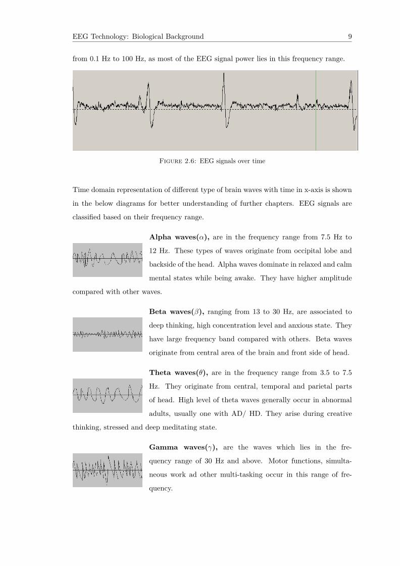
from 0.1 Hz to 100 Hz, as most of the EEG signal power lies in this frequency range.
Figure 2.6: EEG signals over time
Time domain representation of different type of brain waves with time in x-axis is shown
in the below diagrams for better understanding of further chapters. EEG signals are
classified based on their frequency range.
Alpha waves(α), are in the frequency range from 7.5 Hz to
12 Hz. These types of waves originate from occipital lobe and
backside of the head. Alpha waves dominate in relaxed and calm
mental states while being awake. They have higher amplitude
compared with other waves.
Beta waves(β), ranging from 13 to 30 Hz, are associated to
deep thinking, high concentration level and anxious state. They
have large frequency band compared with others. Beta waves
originate from central area of the brain and front side of head.
Theta waves(θ), are in the frequency range from 3.5 to 7.5
Hz. They originate from central, temporal and parietal parts
of head. High level of theta waves generally occur in abnormal
adults, usually one with AD/ HD. They arise during creative
thinking, stressed and deep meditating state.
Gamma waves(γ), are the waves which lies in the fre-
quency range of 30 Hz and above. Motor functions, simulta-
neous work ad other multi-tasking occur in this range of fre-
quency.

EEG Technology: Biological Background 10
Delta waves, are in the frequency range from 0.5 to 3.5 Hz.
They are the slowest waves compared to others. Delta waves
generally occur in deep sleep and sometimes when awake. They
also occur in coma mental state. More of delta waves in awake
state is considered to be a serious phenomenon.
MU is associated with motor activities, and is also found in the alpha wave frequency
range, but where the maximum amplitude is recorded over motor cortex. So it basically
triggers when there is an actual movement or there is an intent to move [1].
2.3 Real Time Application of EEG Technology
The most commonly practised application of EEG is to monitor and study EEG records
manually, to look for, or to understand brain disorders and various damages, such as
epileptic seizures, AD/ HD, tumors and so on. Moreover, EEG is a device used in
healthcare sectors for monitoring patients brains and declare dead when no activity is
monitored.
The study of brain waves and how they relate to different mental states, have led to
number of alternative methods and beliefs on how to manipulate these waves. For
instance, in order to become e.g more relaxed, focused and smarter, you can buy music
that plays in specific Hertzes that promise to do just that [7]. An important information
gained from this is that you should allow your kids listen to Mozart in their period of
growth, enjoying the effects mentioned. Besides this somewhat regarded pseudoscience,
there have been a lot of interesting studies of mental states and how they are effected
[8].
2.3.1 Event Potential
EEG wave respond to the external as well as internal stimuli, like flash light, a tone or
skipping. This is called Evoked Potential (EP), or Event Related Potentials (ERP). One
of the well known ERP is P300.

EEG Technology: Biological Background 11
2.3.2 Neurofeedback Training
Self-regulative abilities to do this comes by getting real-time visual and/or auditory
feedback, and is like Operant conditioning. With frequent training, long termed effect
is possible [8]. The electrical activity of the brain is picked by the electrodes located
on the scalp. An amplifier is used to boost the signals before being fed to a computer.
The EEG signals are identified and processed into feedback before being fed to the user.
Using Fourier transform, the signals can be classified based on frequency bands. Their
factors can then be used to calculate a ratio, for instance β/θ (Leins, Goth, Hinterberger,
Klinger, & Strehl, 2007) [9]. The feedback is obtained from the height of ratio bar graph
displayed on a monitor. The below diagram depicts a simple Neurofeedback principle.
Figure 2.7: Neurofeedback principle
EEG helps in diagnosing AD/HD. AD/ HD people have slow waves and is very difficult
for them to manage concentration and behaviour. More of beta and less of theta activity
is required to reduce inattention.
Preprocessing, feature extraction and classification of EEG signals are briefly explained
in the following chapters. These three BCI modules could be combined into a single
and more general, higher level module, collectively called as “EEG processing”. In any
BCI design, EEG processing plays a vital role as it is involved in developing a command
for BCI application. A wide range of research is going on for the betterment of EEG
processing in order to develop efficient BCI system.

EEG Technology: Biological Background 12
One can keenly observe that the boundaries amongst the “pre-processing”, “feature
extraction” and “classification” are not hard and sometimes the boundaries may even
appear as indistinct. Thus, in certain applications pre-processing and feature extraction
modules are united into a single algorithm, and the classification part can be missing
or reduced to its simplest form where it is not so important. In general, it is very
important to study these three in separate since they play different roles and have
different objectives [10].

Chapter 3
Preprocessing of EEG signals
In order to perform feature extraction and classification from brain waves, it is essential
to pre-process the raw brain waves for increasing the signal to noise ratio and enhance
the relevant information entrenched in the EEG signal. Certainly, electrical activity of
the eyes or of the muscles or high frequency noise from electrical net (50 Hz in Sweden)
affects the EEG signal and makes them noisy [2]. The electrical activity of the mus-
cle or eyes causes more disturbances as they have large amplitude when compared to
EEG signal. One must be very careful while removing these noise from EEG signals;
accidentally it may happen to remove the necessary information entrenched. Likewise,
the remarkable part is removing the signals aroused due to background brain activity
irrelevant to the signals of our interest [2].
To achieve the goal of pre-processing, EEG signals need to be measured using proper
referencing and filtered using simple temporal & spatial filters or advanced filters like
Independent Component Analysis (ICA), Common Spatial Patterns (CSP), Principal
Component Analysis (PCA), Common Subspace Spatial Decomposition (CSSD), etc.,
3.1 Referencing
According to Hagemann et al., the differences between results of different studies are
partly due to the differences in referencing [11]. In general, EEG signals are acquired
13

Preprocessing of EEG signals 14
from various electrodes placed in different positions on the cortex or scalp. The am-
plitude of the brain signal from a particular electrode is relatively measured, may be
in reference with the amplitude of another electrode placed in some other position of
the scalp or cortex [10]. Therefore, the result will be a mixture of brain activity at the
given position, brain activity at the reference position and noise. Hence, the reference
electrode must be placed in a way that the brain activity in that position is negligible or
almost zero. In general, the nose, mastoids and earlobes are used as the reference site.
The most commonly used referencing methods are as follows:
• Common reference: This is the widely used referencing technique in BCI design.
In this method, only one common reference point is used for all the electrode and
the reference point will be far from all the electrodes [10].
• Average reference: In this technique, average of the brain activity measured at
all electrodes is subtracted. The basic principle of this method is, at any particular
time the sum of the brain activity as a whole will be zero. Though, certain elec-
trode’s activities when it has comparatively low density and the activities of the
electrodes at lower part of head is not taken into account, causes some practical
issues. [12]
• Current source density (CSD): The current source density technique is nothing
but ”the rate of change of current flowing into and through the scalp” [10]. By
Laplacian computing the sum of differences between a particular electrode and its
neighbors give CSD estimation. The actual problem with this estimation of CSD
is valid only if the electrodes are in a 2-D plane and placed at equal distance.
3.2 Simple Temporal and spatial Filters
Simple temporal or spatial filters are widely used in most of the BCI designs to improve
the EEG signal quality by de-noising them.
3.2.1 Temporal Filters
Band-pass or low-pass filters are the commonly used temporal filters which filter out a
very high or low frequency bands leaving behind the particular frequency band in which

Preprocessing of EEG signals 15
we are interested. For example, a BCI design uses motor and Sensorimotor rhythms,
the signal in frequency band of 8-30 Hz is band-pass filtered since the signal relevant to
motor and Sensorimotor actions present only in those range [2]. Noise due to external
influence like electrical net interference (50 Hz in Sweden) and electrode polarization are
removed using temporal filtering. Filtering is commonly done by using Discrete Fourier
Transform (DFT) or Finite Impulse Response (FIR) or Infinite Impulse Response (IIR)
filters.
Figure 3.1: Temporal filtered signals distributed over time
3.2.2 Spatial Filters
Primary cortex of the brain is responsible for motor movements. Interest in high -
frequency electroencephalographic (EEG) rhythms (above 20 Hz) has intensified since
the recognition of the involvement of high-frequency beta (15-25 Hz) and gamma (>25
Hz) rhythms in cognitive processing [13, 14, 15]. They are generally used for pattern
recognition, especially for imagined motor activities such as leg or hand movements. The
recognition is easier if the patterns are obtained from a broad frequency band rather
than from only the combined α − β bands [16]. These results are in agreement with
Pfurtscheller and coworkers’ recent observation in which the optimal band selection for
the detection of motor- related mental tasks is the band from 8 to 30 Hz [17].

Preprocessing of EEG signals 16
Figure 3.2: Spatial filtered EEG signals over time
In general, it is well-known that motor imagery causes decrease (ERD: Event-Related
Desynchronization) or increase (ERS: Event-Related Synchronization) of Electroen-
cephalogram (EEG) potentials in the (8-12 Hz) and (13-28 Hz) rhythms over the sensory
motor cortex [18]. Each body limb is associated with the respective region of the brain
[19], but finding a class-discriminative spatial filter has been of great interest in the BCI
community [20, 21, 22] as the volume conduction effect of EEG [23].
For example, when building a BCI design based on Steady State Visual Evoked Poten-
tial (SSVEP), we need the brain signals only from the electrodes (O1 & O2) located in
the visual region (Occipital Lobe) which contains the brain signals of our interest [24].
Similarly for a BCI design based on feet or hand motor imagery movement, the relevant
brain signals are present only in the motor or Sensorimotor cortex region. Hence, the
spatially filtered brain signals from the electrodes (C4 & C3) located on right and left
motor cortex is sufficient for this particular BCI design [2].
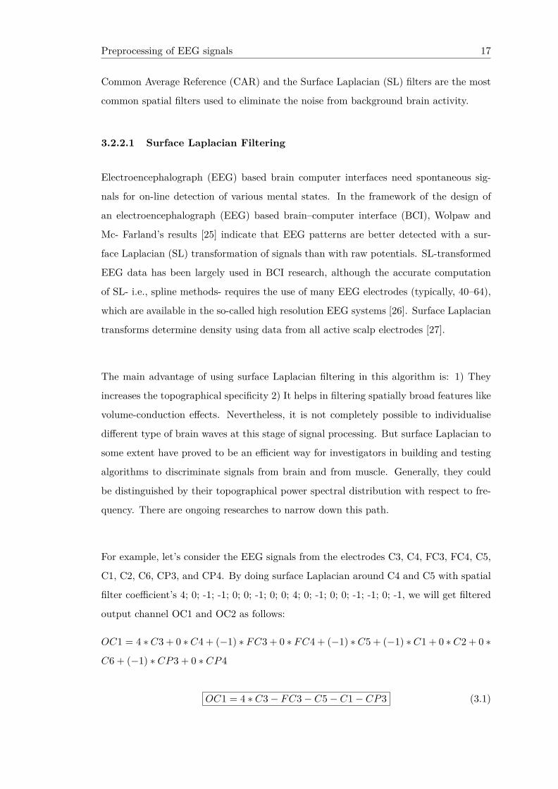
Preprocessing of EEG signals 17
Common Average Reference (CAR) and the Surface Laplacian (SL) filters are the most
common spatial filters used to eliminate the noise from background brain activity.
3.2.2.1 Surface Laplacian Filtering
Electroencephalograph (EEG) based brain computer interfaces need spontaneous sig-
nals for on-line detection of various mental states. In the framework of the design of
an electroencephalograph (EEG) based brain–computer interface (BCI), Wolpaw and
Mc- Farland’s results [25] indicate that EEG patterns are better detected with a sur-
face Laplacian (SL) transformation of signals than with raw potentials. SL-transformed
EEG data has been largely used in BCI research, although the accurate computation
of SL- i.e., spline methods- requires the use of many EEG electrodes (typically, 40–64),
which are available in the so-called high resolution EEG systems [26]. Surface Laplacian
transforms determine density using data from all active scalp electrodes [27].
The main advantage of using surface Laplacian filtering in this algorithm is: 1) They
increases the topographical specificity 2) It helps in filtering spatially broad features like
volume-conduction effects. Nevertheless, it is not completely possible to individualise
different type of brain waves at this stage of signal processing. But surface Laplacian to
some extent have proved to be an efficient way for investigators in building and testing
algorithms to discriminate signals from brain and from muscle. Generally, they could
be distinguished by their topographical power spectral distribution with respect to fre-
quency. There are ongoing researches to narrow down this path.
For example, let’s consider the EEG signals from the electrodes C3, C4, FC3, FC4, C5,
C1, C2, C6, CP3, and CP4. By doing surface Laplacian around C4 and C5 with spatial
filter coefficient’s 4; 0; -1; -1; 0; 0; -1; 0; 0; 4; 0; -1; 0; 0; -1; -1; 0; -1, we will get filtered
output channel OC1 and OC2 as follows:
OC1 = 4 ∗C3 + 0 ∗C4 + (−1) ∗ FC3 + 0 ∗ FC4 + (−1) ∗C5 + (−1) ∗C1 + 0 ∗C2 + 0 ∗
C6 + (−1) ∗ CP3 + 0 ∗ CP4
OC1 = 4 ∗ C3− FC3− C5− C1− CP3 (3.1)

Preprocessing of EEG signals 18
OC2 = 0 ∗C3 + 4 ∗C4 + 0 ∗ FC3 + (−1) ∗ FC4 + 0 ∗C5 + 0 ∗C1 + (−1) ∗C2 + (−1) ∗
C6 + 0 ∗ CP3 + (−1) ∗ CP4
OC2 = 4 ∗ C4− FC4− C2− C6− CP4 (3.2)
3.2.3 Advanced Filters
Unlike the above described simple temporal and spatial filter, there are some advanced
filtering techniques used in the pre-processing of EEG signals which is described in the
below section.
3.2.3.1 Independent Component Analysis (ICA)
ICA is used when the EEG signals of our interest and noise like background brain
activities signals has comparable amplitudes. In other words, the ICA is used when the
brain signals ‘m′ (measured using many electrodes) are resulting from unknown linear
mixing of several sources -‘s’.
m = As (3.3)
where ‘m′ is the matrix of measurements, with electrodes in row and time sample in
column; ‘s′ is the source matrix, with source in row and time sample in column; and ‘A’
is unknown mixing matrix which represents the linear mixing. The ICA to determine
an estimate s of s without knowing A is given by the following equation:
s = Wm (3.4)
where ‘W ′ is the de-mixing matrix. By comparing equation 3.3 and 3.4, one can say
W = A−1, with the problem being ‘A′ is unknown. “To solve this problem, ICA assumes
that the sources -‘s′ is statistically independent, which has been revealed as being a
reasonable hypothesis for numerous problems” [2]. In recent years, many ICA algorithms
have been proposed and proved in the field of EEG signal processing for BCI design.

Chapter 4
Feature Extraction
Acquisition of large amount of data is obtained by measuring electrical activity of the
brain through EEG leads. Moreover, the number of electrodes used for recording EEG
signals generally vary from 1 to 256 and with a sampling frequency varying from 100
Hz to 1000 Hz. ”Features ” are the values which defines some relevant properties of
the acquired signals. They are generally summed up into a vector named as ”feature
vector”. Hence, feature extraction is an operation which converts one or several signals
into a feature vector.
Determining and obtaining required features from EEG signals is an important step.
The classification algorithm, which uses feature extracted from EEG signals will have
problem if the information extracted is not relevant and do not describe the bio-signals
involved, i.e., the mental state of the user.
There are many extraction techniques which were proposed and studied. These tech-
niques can be divided in three main groups, which are: 1) the methods that exploit the
temporal information embedded in the signals [28, 29, 30, 31, 32]. 2) the methods that
exploit the Frequential information [33, 34, 35, 36, 37]. 3) the hybrid methods, based
on time-frequency representations, which exploit both the temporal and Frequential
information [38,39].
19

Feature Extraction 20
4.1 Temporal methods
Temporal variations of the acquired signals are used in temporal methods. They are
specifically adapted to define Neurophysiological signals in a better manner. In this
method, we can find the amplitude, auto-regressive parameters or Hjorth parameters
for EEG signals.
4.1.1 EEG signal amplitude
The amplitude of raw EEG signals is obtained from different electrodes placed in various
locations of the brain. They are preprocessed and aggregated into a single vector before
being fed to a classification algorithm. In those case, pre-processing methods such as
sub-sampling and spatial filtering is used to reduce the EEG signals.
4.1.2 Autoregressive parameters
AutoRegressive (AR) methods assume that a signal X(t), measured at time t, can be
modeled as a weighted sum of the values of this signal at previous time steps, to which
we can add a noise term Et (generally a Gaussian white noise):
X(t) = a1X(t− 1) + a2X(t− 2) + . . . . .+ apX(t− p) + Et (4.1)
where the weights ai are the auto-regressive parameters which are generally used as
features for Brain-Computer Interface [38, 39].
4.1.3 Hjorth parameters
Hjorth parameters defines the temporal dynamics of a signal X(t), by using three mea-
sures that are the mobility, the activity and the complexity [40].

Feature Extraction 21
4.2 Frequential methods
EEG signals are made by a set of specific brain waves. The amplitude of these waves
changes with the brain waves while doing any mental task such as motor imagery or
other cognitive tasks. The brain waves generated are generally synchronized with the
stimulus frequency. Hence, it becomes essential to extract Frequential information from
brain signals. There are two main techniques, namely power spectral density and band
power features.
Figure 4.1: Raw EEG signal and their power spectral display
4.2.1 Power spectral density features
Power Spectral Density (PSD) features, defines the distribution of the power of a signal in
frequency domain. PSD features is generally evaluated by taking square of the Fourier
transform of a signal or by evaluating the Fourier transform of the Autocorrelation
function of a signal. They are the most used features in the development of BCI and
served as one of the efficient way to identify large number of Neurophysiological signals.

Feature Extraction 22
4.2.2 Band power features
Band power features, describes band-pass filtering a signal in a given frequency range,
squaring them and finally averaging the signal values over a given time window. The
normal distribution of the signal can be obtained by taking log transform of the val-
ues. These features have been successfully used for the classification of motor imagery
movements.
4.3 Time-frequency representations
Figure 4.2: time-frequency representation of signal and their power spectral display
These methods are based on time-frequency representations such as the short-time
Fourier transform or wavelets, and extracted information from the signals that are both
Frequential or temporal. The main advantage of these is that they can identify sudden
temporal fluctuations of the signals, while still holding Frequential information.
4.3.1 Short-time Fourier transform
The input signal is first multiplied by a given windowing function w over a short time
period, provided w is non-zero. Taking Fourier transform of this windowed signal gives
the Short-Time Fourier Transform (STFT). The STFT of X(n,w) of a signal x(n) is
given by,

Feature Extraction 23
X(n,w) =+∞∑
n=∞x(n)w(n)e−jωn (4.2)
The main drawback of this method is that analysis window with a fixed size, leads to
a similar temporal as well as Frequential resolution in all frequency ranges. Wavelet
analysis tries to overcome this drawback.
4.3.2 Wavelet transform
Wavelet transform, similar to Fourier transform decomposes a signal onto a basis of
functions. This basis of functions consists of wavelets Φab. Each one being a scaled and
translated version of the same wavelet Φ, where Φ is the mother wavelet:
Φab(t) = 1√a
Φ( t− ba
) (4.3)
The wavelet transform Wx(s, u) of a signal x is given by:
Wx(s, u) =∫ +∞
−∞x(t)Φu,s(t) dt (4.4)
where s and u are the scaling and translating factor of the signal x(t). The wavelet
transform makes it possible to analyze a signal in different scales simultaneously. This
serves as the main advantage of wavelet transform. Adding to that, the level of resolu-
tion depends on the scale. Various kinds of wavelets have been used for BCI, such as
Daubechies wavelets [41, 42], Coiflet wavelets [43], Morlet wavelets [44], bi-scale wavelets
[45] or Mexican hat wavelets [46]. They all made it possible to reach very promising
results.
Even though we have various feature extraction methods for BCI, it is difficult to identify
the most efficient ones due to a lack of comparisons. To reach a good performance, it
is important to extract a small number of features which represents subject- related
information. It is necessary to extract the required features precisely to build a more
efficient BCI.

Chapter 5
Classification of EEG signals
This chapter describes next key step for identifying Neurophysiological signals adapted
by many researchers in the way of development of BCI technology. One can achieve this
by either regression algorithms or classification algorithms.
The aim of the classification step is to automatically assign a class to the feature vector
extracted from the former step. This class defines the mental task. This class is generally
used by the BCI user and represents the type of mental task performed by the user.
Classification is attained using algorithms known as ”classifiers”. Classifiers are smart
enough to identify the class of a feature vector using training sets. The classifiers are
divided into five major categories. They are namely, linear classifiers, neural networks,
non linear Bayesian classifiers, nearest neighbor classifiers and classifier combinations
[2].
5.1 Linear classifiers
Linear classifiers are characteristic algorithms that use linear functions to differentiate
classes. They are the most widely used classifiers in BCI applications. They are two
important Linear classifiers, namely, Linear Discriminant Analysis (LDA) and Support
Vector Machines (SVM).
24

Classification of EEG signals 25
5.1.1 Linear discriminant Analysis
LDA also known as Fisher’s linear discriminant, main purpose of LDA is to employ hy-
perplanes to distinguish the data representing various classes. For a problem consisting
of two-class, the class of a feature vector relays on which side of the hyperplane the
vector is.
Figure 5.1: Picture depicting separation of the ”red diamonds” and ”green stars” bya hyperplane
This technique has very less mathematical calculations which makes it suitable for on-
line BCI systems. They are simple to use and generally provides good results. The
main drawback of LDA is their poor results on complex nonlinear EEG signals. In a
regularized Fisher’s LDA (RFLDA), a regularization parameter C is introduced. This
parameter can penalize classification errors that tend to occur on training set. The
resulting can accommodate outliers. They are less used than LDA for BCI applications.
5.1.2 Support Vector Machine
This classifier also uses a discriminant hyperplane to identify different classes.
Figure 5.2: SVM finds the optimal hyperplane

Classification of EEG signals 26
An SVM, similar to RFLDA has a regularization parameter C that enables space to
outliers and allows errors on the training set. The SVM using linear decision boundaries
is known as linear SVM. Nonlinear decision boundaries are created with a little bit of
complexity, using ”kernel trick”. Kernel function, denoted by K(x, y), maps the data to
another region of much higher dimensionality.
The kernel generally used is the Gaussian or Radial Basis Function (RBF) kernel, which
is given by:
K(x, y) = exp(−‖x− y‖2
2σ2 ) (5.1)
Its corresponding SVM is known as Gaussian SVM or RBF SVM. The major advantage
in SVM classifier is that they have good generalization properties.
5.2 Neural Networks
Neural Networks (NN) is an assembly of several artificial neurons which enables to
produce nonlinear decision boundaries [47]. This section at first defines the most widely
used NN for BCI, which is the MultiLayer Perceptron (MLP).
5.2.1 MultiLayer Perceptron
Figure 5.3: MLP architecture

Classification of EEG signals 27
An MLP is composed of several layers of neurons: an input layer, possibly one or several
hidden layers, and an output layer [48]. The input of each neuron is connected to the
output of the previous neuron’s layer. The class of the input feature vector is determined
by the neurons of the output layer.
Any continuous functions can be approximated by the NN and the MLP, when com-
posed of enough neurons and layers. NN are flexible classifiers which can classify any
number of classes. MLP is the most famous NN utilized in classification. A Perceptron
is a MLP without hidden layers.
There are many other NN classifier used in the field of BCI such as Gaussian classifier,
Learning Vector Quantization (LVQ) Neural Network, Fuzzy ARTMAP Neural Network,
Dynamic Neural Networks like Finite Impulse Response Neural Network (FIRNN), the
Time-Delay Neural Network (TDNN) or the Gamma Dynamic Neural Network.
5.3 Nonlinear Bayesian classifiers
There are two Bayesian classifiers, namely Bayes quadratic and Hidden Markov Model
(HMM). They generate nonlinear decision boundaries. They are not as popular as linear
or Neural Network classifiers among BCI applications.
5.3.1 Bayes quadratic
Bayesian classification aims at assigning to a feature vector the class it belongs to with
the highest probability [49, 50]. The Bayes rule is used to compute the so-called a
Posteriori probability that a feature vector has of belonging to a given class [50].
5.3.2 Hidden Markov Model
Hidden Markov Models (HMM) are popular dynamic classifiers in the field of speech
recognition [51]. An HMM is a kind of probabilistic automaton that can provide the
probability of observing a given sequence of feature vectors [51]. Each state of the

Classification of EEG signals 28
automaton can Modelize the probability of observing a given feature vector. For BCI,
these probabilities usually are Gaussian Mixture Models (GMM) [40].
5.4 Nearest Neighbor classifiers
These classifiers are very simple. A feature vector is assigned to a class with respective
to its nearest neighbour(s). The neighbour can be a feature vector or a class prototype.
5.4.1 K-Nearest Neighbor(KNN)
This is the most basic and simple classification ever known. This type of classifier is
generally used when there is no or very little knowledge about the EEG data. They
bypass the probability density problem.

Chapter 6
Algorithm for a simple BCI
system
After a clear study on the behavior and the techniques involved in processing a EEG
signal, the knowledge is now going to be used in creating an algorithm for extracting
the features and making them as inputs to different applications.
Before moving further, let us first have an overview of the main component boxes utilized
in this algorithm.
6.1 Main components
1. Wireless EEG Headset: This is the main com-
ponent for this whole project being into action. They
are wearable like regular headphones. This helps in col-
lecting EEG data from a person using a single dry elec-
trode placed on the forehead. It also contains another
dry electrode which is connected to the left ear for refer-
ence.
29

Algorithm for a simple BCI system 30
2. Acquisition Client: they help in acquiring EEG data and
distributing it into the algorithm. The output from the acquisi-
tion client can be stimulations, signals, experiment information
and localized channel data.
3. Generic Reader: they are used to store data in a format
which is feasible for the box to read. They can read any data or
file saved with the Generic stream writer box. The files saved
likewise will have a variable number of streams.
4. Generic Writer: This box dumps any stream of data into
a binary file. They can have many number of input depending
on the number of streams.
5. Identity: they help in duplicating output based on its in-
put. They may have many inputs of various types. Each input
has a corresponding output which is of the same type as in-
put.
6. Channel Selector: The channels of interest are selected
using channel selector. They can be selected either by channel
name or index starting from 0. Besides, the channels can also
be rejected instead of being selected.
7. Surface Laplacian: they help in discrimination of two sort
of brain signals. They are constructed, such that, the variance of
signals is minimum for one situation and maximum for the other.
This can be used for discriminating signals of two commonly
performed tasks, for instance movement of left versus right hand.
8. Temporal Filter: they are used to filter the input signal
into a particular range. The plugin used in temporal filter allows
the selection of the class of filter ( Butterworth, Chebychev,
Yule- Walker), the frequency band and also the kind of filter (
low pass , band pass, band loop).

Algorithm for a simple BCI system 31
9. Time Based Epoching: Time based Epoching use the
interval to control overlap of epochs. They generate ’epochs’,
i.e. signal ’segments’ where length is configurable, as is the time
offset between two consecutive epochs. Both input and output are of the same type
’signal’. They are generally needed for other signal processing boxes when the size of
data blocks is not significant enough.
10. Stimulation Based Epoching: The stimulation based
Epoching is same as Time based Epoching. The only difference
is that it generates epochs when a stimulation is received. For
instance, it is possible to start offset of a signal a few hundreds of milliseconds after the
event or few milliseconds before the event.
11. Feature Aggregator: They aggregate the features re-
ceived as inputs into a feature vector. This can be used for
classification.
12. Classifier Trainer: they collect the feature vectors and
label them depending on the input they arrive on. A training
process is triggered when a particular stimulation occurs. The
best example for classifier trainer is the one which is used in BCI
pipelines to classify cerebral activity states.
Being understood the main components used in this algorithm, let us now take a closer
look into it. The main concept of this algorithm is to acquire the signals and process
them in a machine training method. EEG signals of a subject thinking about lifting
his right and left arm are going to be evaluated in this algorithm. There are two set of
operations before getting the final output.
6.2 Data Acquisition
EEG data sets for the Motor Imagery must be acquired from healthy person. This can
be done with people who have very less or no idea about the EEG techniques.

Algorithm for a simple BCI system 32
Figure 6.1: First part of the algorithm to collect EEG data
A exercise will be given to a subject in which random Left and Right arrows will be
shown in a random design. Every time while the arrow is shown in the screen, subject
have to think about lifting the corresponding arm.
Figure 6.2: Left arrow shown to the user
A LUA stimulator will be used in this part of the algorithm to organize the right and
left arrows shown in the screen. The timing for each arrow to be shown and the time
between showing each arrow is specified. After each arrow is shown on the screen, 4
seconds from that point EEG data will be recorded. This is to know that at which point
of time subject was thinking about the movements. The data is recorded in a file using
a generic stream writer.

Algorithm for a simple BCI system 33
Figure 6.3: Right arrow shown to the user
Figure 6.4: Second part of the algorithm for controlling an external application
6.3 Data labelling
The recorded data from the above section is used for further processing. As it is a diffi-
cult task to perform mathematical calculations on real time EEG signals, the first step
in this process is to remove the signal to noise ratio. This can be done using a temporal
filter or by using a reference channel. The filtered data is later sent to a surface Lapla-
cian filter which is configured to produce two output channels from all the electrodes,

Algorithm for a simple BCI system 34
in order to represent one on the right and one on the left. The processing of the signals
from this part is carried out in two processing chains.
The output from the surface Laplacian will be stimulation based Epoched. This Epoching
is configured in a way to remove the signal sets when subject was shown the left and
right arrows. On the left processing chain, the stimulation Epoching time is set to the
time when left arrows were shown. On the right, the time is set to the same time when
right arrows were shown. Further, time based Epoching is done. In this Epoching, the
signals are being split in 1s segments with overlap between consecutive segments. This
leaves behind a bunch of Epoched signals.
The Epoched signals are filtered using a band pass filter to restrict them between 8 to 24
Hz band. Digital signal processing is done by squaring the Epoched signals to increase
its amplitude and the average of all epochs is collected. The signal after averaging is
sent to the feature aggregator which converts these data into a feature vector. The right
and left hand movement vectors will be processed along with the raw stored signal by
the classifier trainer which specifically recognizes the right and left hand movements
from the stored signal and saves it in a separate file. This file is used in the next stage
of signal processing.i.e., connecting it to control an external application such as robotic
arm etc.

Chapter 7
Conclusion
This report presents an complete overview on EEG Technology, different processes in-
volved in classification of EEG signals and an algorithm to represent a simple Brain-
Computer Interface system that allow users to control an external application such as
robotic arm with their brain waves. The brain signals were acquired using a single
electrode placed on the forehead. EEG signals from the user are sent to the computer
via Bluetooth. Various operations were performed on the collected EEG signals. For
example filtering, Epoching, simple DSP and signal averaging. This information is used
as input to a LDA classifier that is trained to classify two different mental tasks. Later,
this classification is used to control the movements (left and right movement).
The major challenge and time-consumption in the project was testing the wireless head-
set with the use of real-time EEG input. The first step was to implement all the com-
ponents of the system and make them interact with each other, then enable the system
to recognize eye blinks in the incoming EEG signal samples.
35

Conclusion 36
Figure 7.1: Real Time signals with eye blink
Figure 7.2: Topographical view of signals

Conclusion 37
Regarding the research questions, the following conclusions are made from the project
findings:
RQ1: How could a single electrode placed on the forehead compensate a grid
of electrodes places across the scalp?
The single dry electrode placed on the forehead can replace a grid of, or several elec-
trodes is highly impossible. There are no papers of previous research or studies where
single electrode have been used. The knowledge and experience from this study, is that
mental tasks which are comparatively safe to classify did not happen. However, there
can be other reasons besides single electrode, but at least it suggest that single electrode
is not sufficient
RQ2: What are the advantages and limitations of single electrode headset?
The major limitation that was insightful with the single electrode headset was the static
electrode location. It can be moved to a certain level, but not ample to get it away
from the forehead. Also, one or two extra electrodes would have been great. Headset,
featuring 14 electrodes would be the suggested option for this upgrade. It is a bit more
expensive than single electrode headset. The limitation with the electrode position
is that it is heavily influenced by eye blink and facial changes. However, the main
requirement of dry electrode is placement of them in an area where there is no hair and
subsequently forehead is a place where many people do not have hair.

Bibliography 38
7.1 Further Enhancement and Ideas
There are two main proposal for constant work with the system presented in this report.
1) Further development of the algorithm, improving signal processing, classification pro-
cedures and feature extensions.
This algorithm could be further build to control a remote application. A system build
with signals from more number of electrodes would have high precision in classification
of the signals. They are of great help for the physically impaired people, who would
want to play a video game or drive a car. They could do this with the advancement in
BCI technology just by imagining about it.
2) Use the current algorithm as a root for larger scale investigations with people, to do
EEG surveys and monitoring studies.
• More validations : More number of verifications can be run over a period of
time, to see if it is feasible to improve the control of system using brain waves.
The aim and drive should be to surpass the need for the eye states, and rely on
mental tasks only.
• Research classification possibilities: Describe new experiments to discover if
there are other mental efforts that can be used for classification in the system.
This could be turning, mental speech or specific recall.
• Research placement possibilities: Dismantle, if possible, the arm on the brain-
wave headset which clamps the electrode and find another placement for it. Check
the possibility if those placements are suited for solving the classification tasks at
hand. The troublesome part is that there can be no hair between the scalp and
dry electrode

Bibliography[1] Bernier, R., Dawson, G., Webb, S., & Murias, M. (2007, August). EEG mu rhythm
and imitation impairments in individuals with autism spectrum disorder. Brain and
cognition, 64(3), 228–37.
[2] Fabien Lotte. Study of Electroencephalographic Signal Processing and Classification
Techniques towards the use of Brain-Computer Interfaces in Virtual Reality Applica-
tions. The National Institute of Applied Sciences of Rennes, 2008.
[3] S.G. Mason and G.E. Birch. A general framework for brain-computer interface design.
IEEE Transactions on Neural Systems and Rehabilitation Engineering, 11(1):70–85,
2003.
[4] A. Bashashati, M. Fatourechi, R. K. Ward, and G. E. Birch. A survey of signal pro-
cessing algorithms in brain-computer interfaces based on electrical brain signals. Journal
of Neural engineering, 4(2):R35–57, 2007.
[5] S.G. Mason and G.E. Birch. A general framework for brain-computer interface design.
IEEE Transactions on Neural Systems and Rehabilitation Engineering, 11(1):70–85,
2003.
[6] A. Kubler, V.K. Mushahwar, L.R. Hochberg, and J.P. Donoghue. BCI meeting 2005-
workshop on clinical issues and applications. IEEE Transactions on Neural Systems and
Rehabilitation Engineering, 14(2):131–134, 2006.
[7] Erik Andreas Larsen. (June, 2011) Classification of EEG signals in Brain-Computer
Interface System.
[8] Braverman, E. (1990). Brain mapping: a short guide to interpretation, philoso-
phy and future. Journal of Orthomolecular Medicine, 5(4), 189–197. Available from
http://orthomolecular.org/library/jom/1990/pdf/1990-v05n04-p189.pdf.
[9] Plass-Oude Bos, D., Reuderink, B., Laar, B. L. A. van de, G urk ok, H., M uhl, C.,
Poel, M., et al. (2010, October). Human-Computer Interaction for BCI Games: Usabil-
ity and User Experience. In A. Sourin (Ed.), Proceedings of the international conference
on cyberworlds 2010, singapore (pp. 277–281). Los Alamitos: IEEE Computer Society
39

Bibliography 40
Press. http://eprints.eemcs.utwente.nl/18057/.
[10] Tarik Al-ani1, 2 and Dalila Trad1, 3. Signal Processing and Classification Ap-
proaches for Brain-computer Interface.
[11] Hagemann D, Naumann E, Thayer JF. The quest for the EEG reference revisited:
a glance from brain asymmetry research.Psychophysiology, 38(5): 847-857, 2001.
[12] Joseph Dien. Issues in the application of the average reference: Review, cri-
tiques, and recommendations. Behavior Research Methods. Instruments, & Computers,
30(10):34-43, 1998.
[13] F. Aoki, E. E. Fetz, L. Shupe, E. Lettich, and G. A. Ojemann, “Increased gam-
marange activity in human sensorimotor cortex during performance of visuomotor tasks,”
Clin. Neurophysiol., vol. 110, no. 3, pp. 524–537, Mar. 1999.
[14] O.Bertrand and C.Tallon-Baudry, “Oscillatory gamma activity in humans: A pos-
sible role for object representation,” Int. J. Psychophysiol., vol. 38, no. 3, pp. 211–223,
Dec. 2000.
[15] A. K. Engel, P. Konig, A. K. Kreiter, T. B. Schillen, andW. Singer, “Temporal
coding in the visual cortex: New vistas on integration in the nervous system,” Trends
Neurosci., vol. 15, no. 6, pp. 218–226, Jun. 1992.
[16] F. Babiloni, F. Cincotti, L. Lazzarini, J. Millan, J. Mourino, M. Varsta, J. Heikko-
nen, L. Bianchi, and M. G. Marciani, Linear Classification of Low-Resolution EEG
Patterns Produced by Imagined Hand Movements. In Proceedings of the IEEE, volume
8, pages 186– 188, Jun. 2000.
[17] J. Muller-Gerking, G. Pfurtscheller, and H. Flyvbjerg, “Designing optimal spatial
filters for single-trial EEG classification in a movement task,” Clin. Neurophysiol., vol.
110, pp. 787–98, 1999.
[18] G. Pfurtscheller and C. Neuper, “Motor Imagery and Direct Brain- Computer Com-
munication,” Proceedings of the IEEE, Vol. 89, No. 7, pp. 1123-1134, 2001.
[19] H. Ehrsson, S. Geyer, and E. Naito, “Imagery of Voluntary Movement of Fingers,
Toes, and Tongue Activates Corresponding Body-Part- Specific Motor Representations,”
Journal of Neurophysiology, Vol. 90, No. 5, pp. 3304-3316, 2003.
[20] D. McFarland, L. McCane, S. David, and J.Wolpaw, “Spatial Filter Selection for
EEG-Based Communication,” Electroencephalography and Clinical Neurophysiology,
Vol. 103, No. 3, pp. 386-394, 1997.
[21] J. Muller-Gerking, G. Pfurtscheller, and H. Flyvbjerg, “Designing Optimal Spatial

Bibliography 41
Filters for Single-Trial EEG Classification in a Movement Task,” Clinical Neurophysiol-
ogy, Vol. 110, No. 5, pp. 787- 798, 1999.
[22] C. Brunner, M. Naeem, R. Leeb, B. Graimann, and G. Pfurtscheller, “Spatial Fil-
tering and Selection of Optimized Components in Four Class Motor Imagery EEG Data
Using Independent Components Analysis,” Pattern Recognition Letters, Vol. 28, No. 8,
pp. 957-964, 2007.
[23] G. Pfurtscheller and A. Berghold, “Patterns of Cortical Activation during Planning
of Voluntary Movement,” Electroencephalography and Clinical Neurophysiology, vol.
72, No. 3, pp. 250-258, 1989.
[24] Muller, S.M.T. , et al., ”SSVEP-BCI implementation for 37- 40 Hz frequency range”
, 33rd Annual International Conference of the IEEE Engineering in Medicine and Biol-
ogy Society, 2011.
[25] D. J. McFarland, L. M. McCane, S. V. David, and J. R. Wolpaw, “Spatial filter
selection for EEG-based communication,” Electroencephalogr. Clin. Neurophysiol., vol.
103, pp. 386–94, 1997.
[26] F. Perrin, J. Pernier, O. Bertrand, and J. F. Echallier, “Spherical spline for poten-
tial and current density mapping,” Electroenceph. Clin. Neurophysiol., vol. 72, pp.
184–187, 1989.
[27] P. L. Nunez and R. Srinivasan, Electric Fields of the Brain: The Neurophysics of
EEG. London, U.K.: Oxford Univ. Press, 2006.
[28] W.D. Penny and S.J. Roberts. EEG-based communication via dynamic neural net-
work models. In Proceedings of International Joint Conference on Neural Networks,
1999.
[29] C. W. Anderson, E. A. Stolz, and S. Shamsunder. Multivariate autoregressive mod-
els for classification of spontaneous electroencephalographic signals during mental tasks.
IEEE Transactions on Biomedical Engineering, 45:277–286, 1998.
[30] M. Kaper, P. Meinicke, U. Grossekathoefer, T. Lingner, and H. Ritter. BCI compe-
tition 2003–data set IIb: support vector machines for the P300 speller paradigm. IEEE
Transactions on Biomedical Engineering, 51(6):1073– 1076, 2004.
[31] A. Rakotomamonjy, V. Guigue, G. Mallet, and V. Alvarado. Ensemble of SVMs for
improving brain computer interface P300 speller performances. In International Con-
ference on Artificial Neural Networks, 2005.
[32] G. Pfurtscheller and C. Neuper. Motor imagery and direct brain-computer commu-
nication. proceedings of the IEEE, 89(7):1123–1134, 2001.

Bibliography 42
[33] R. Palaniappan. Brain computer interface design using band powers extracted dur-
ing mental tasks. In Proceedings of the 2nd International IEEE EMBS Conference on
Neural Engineering, 2005.
[34] J. del R. Millan, J. Mourino, F. Cincotti, F. Babiloni, M. Varsta, and J. Heikkonen.
Local neural classifier for EEG-based recognition of mental tasks. In IEEE-INNS-ENNS
International Joint Conference on Neural Networks, 2000.
[35] S. Rezaei, K. Tavakolian, A. M. Nasrabadi, and S. K. Setarehdan. Different classifi-
cation techniques considering brain computer interface applications. Journal of Neural
Engineering, 3:139–144, 2006.
[36] M. Besserve, L. Garnero, and J.Martinerie. Cross-spectral discriminant analy-
sis (CSDA) for the classification of brain computer interfaces. In 3rd International
IEEE/EMBS Conference on Neural Engineering, 2007. CNE ’07, pages 375–378, 2007.
[37] M. Fatourechi, A. Bashashati, R. Ward, and G. Birch. A hybrid genetic algorithm
approach for improving the performance of the LF-ASD brain computer interface. In
Proc. Int. Conf. Acoust. Speech Signal Process. (ICASSP), volume 5, pages 345–348,
2004.
[38] V. Bostanov. BCI competition 2003–data sets Ib and IIb: feature extraction from
event-related brain potentials with the continuous wavelet transform and the t-value
scalogram. IEEE Transactions on Biomedical Engineering, 51(6):1057–1061, 2004.
[39] T.Wang, J. Deng, and B. He. Classifying EEG-based motor imagery tasks by means
of time-frequency synthesized spatial patterns. Clinical Neurophysiology, 115(12):2744–2753,
2004.
[40] B. Obermeier, C. Guger, C. Neuper, and G. Pfurtscheller. Hidden markov models
for online classification of single trial EEG. Pattern recognition letters, pages 1299–1309,
2001.
[41] M. Varsta, J. Heikkonen, J. R. Millan, and J. Mourino. Evaluating the performance
of three feature sets for brain-computer interfaces with an early stopping MLP commit-
tee. In Proceedings. 15th International Conference on Pattern Recognition, 2000.
[42] P.S. Hammon and V.R. de Sa. Preprocessing and meta-classification for braincom-
puter interfaces. IEEE Transactions on Biomedical Engineering, 54(3):518–525, 2007.
[43] Y.P.A. Yong, N.J. Hurley, and G.C.M. Silvestre. Single-trial EEG classification for
brain-computer interfaces using wavelet decomposition. In European Signal Processing
Conference, EUSIPCO 2005, 2005.
[44] S. Lemm, C. Schafer, and G. Curio. BCI competition 2003–data set III: probabilistic

Bibliography 43
modeling of sensorimotor mu rhythms for classification of imaginary hand movements.
IEEE Transactions on Biomedical Engineering, 51(6):1077–1080, 2004.
[45] S. G. Mason and G. E. Birch. A brain-controlled switch for asynchronous control
applications. IEEE Transactions on Biomedical Engineering, 47(10):1297–1307, 2000.
[46] V. Bostanov. BCI competition 2003–data sets Ib and IIb: feature extraction from
event-related brain potentials with the continuous wavelet transform and the t-value
scalogram. IEEE Transactions on Biomedical Engineering, 51(6):1057–1061, 2004.
[47] C. J. C. Burges. A tutorial on support vector machines for pattern recognition.
Knowledge Discovery and Data Mining, 2:121–167, 1998.
[48] C. M. Bishop. Neural Networks for Pattern Recognition. Oxford University Press,
1996.
[49] R. O. Duda, P. E. Hart, and D. G. Stork. Pattern Recognition, second edition.
WILEY-INTERSCIENCE, 2001.
[50] K. Fukunaga. Statistical Pattern Recognition, second edition. ACADEMIC PRESS,
INC, 1990.
[51] L. R. Rabiner. A tutorial on hidden markov models and selected applications in
speech recognition. In Proceedings of the IEEE, volume 77, pages 257– 286, 1989.

Faculty of Technology
SE-391 82 Kalmar | SE-351 95 Växjö
Phone +46 (0)772-28 80 00 [email protected]
Lnu.se/faculty-of-technology?l=en


![Chromosome banding analysis of cells from fine-needle ... · diagnosing soft tissue and bone tumors [1]. Both needle techniques are in most cases easy to perform, cost effective and](https://static.fdocuments.net/doc/165x107/5e62717311566d4f17382932/chromosome-banding-analysis-of-cells-from-fine-needle-diagnosing-soft-tissue.jpg)