Analysis of ﬂow and heat transfer in porous media imbedded ...vafai/Publications/new/PDF...

International Journal of Heat and Mass Transfer 47 (2004) 1889–1905

www.elsevier.com/locate/ijhmt

Analysis of flow and heat transfer in porous mediaimbedded inside various-shaped ducts

A. Haji-Sheikh a,*, K. Vafai b

a Department of Mechanical and Aerospace Engineering, The University of Texas at Arlington, 500 West First Street, Arlington,

TX 76019-0023, USAb Department of Mechanical Engineering, University of California, Riverside, CA 92521-0425, USA

Received 23 July 2003; received in revised form 20 October 2003

Abstract

Heat transfer to a fluid passing through a channel filled with porous materials is the subject of this investigation. It

includes the derivation of the temperature solutions in channels having different cross sectional geometries. Primarily,

consideration is given to a modified Graetz problem in parallel plate channels and circular tubes. This presentation

includes numerical features of the exact series solution for these two ducts using the Brinkman’s model. The results are

compared to results from another numerical study based on the method of weighted residuals. Moreover, as a test case,

the method of weighted residuals provided flow and heat transfer in elliptical passages. The results include the com-

putation of heat transfer to fluid flowing through elliptical passages with different aspect ratios.

� 2003 Elsevier Ltd. All rights reserved.

1. Introduction

In many applications, the Darcy’s law is inapplicable

where the fluids flow in porous media bounded by an

impermeable boundary. For these cases, the study of

convective heat transfer should include inertia and

boundary effects. A number of recent studies incorpo-

rated these effects by using the general flow model

known as the Brinkman–Forschheimer-extended Darcy

model. For example, Kaviany [1] used the Brinkman-

extended Darcy model to obtain a numerical solution of

laminar flow in a porous channel bounded by isothermal

parallel plates. Vafai and Kim [2], using this model,

studied forced convection for thermally fully developed

flow between flat plates while Amiri and Vafai [3] re-

ported a numerical study on the thermally developing

condition. Also, for flow in parallel plate channels, Lee

and Vafai [4] used a two-equation model to study the

effect of local thermal non-equilibrium condition. Ala-

* Corresponding author. Tel.: +1-817-272-2010; fax: +1-817-

272-2952.

E-mail address: [email protected] (A. Haji-Sheikh).

0017-9310/$ - see front matter � 2003 Elsevier Ltd. All rights reserv

doi:10.1016/j.ijheatmasstransfer.2003.09.030

zmi and Vafai [5] extended the earlier work by investi-

gating different porous media transport models.

An extensive study of flow in porous media is avail-

able in [6–8]. Angirasa [9] discusses the history of

development of transport equations in porous media

and finite difference simulations. Nield et al. [10] pre-

sented the effect of local thermal non-equilibrium on

thermally developing forced convection in a porous

medium. These references are valuable in this investi-

gation of the accuracy and utility of the exact series

solution presented here. The exact series solution re-

quires the computation of a set of eigenvalues and the

numerical computation of certain eigenvalues can be-

come a formidable task. In practice, using, e.g., a 32 bit-

processor, it may not be possible to compute a large

number of eigenvalues. To verify the accuracy of the

series solution, the use of an alternative method of

analysis becomes necessary. The closed-form solution

that uses the method of weighted residuals is selected. It

provides solutions with comparable accuracy over an

extended range of variables. For a finite number of

eigenvalues, the method of weighted residuals provides

results with comparable accuracy at larger values of

the axial coordinate. Because it is based on varia-

tional calculus and the minimization principle, it yields

ed.

mail to: [email protected]

Nomenclature

A area, m2

A matrix

Am, ai coefficients

a elliptical duct dimension, m

aij elements of matrix A

Bm coefficient

B matrix

b elliptical duct dimension, m

bij elements of matrix B

C duct contour, m

cn coefficients

cp specific heat, J/kgK

D matrix

Da Darcy number, K=L2c

Dh hydraulic diameter, m

dmj elements of matrix D

dn coefficients

F pressure coefficient

f Moody friction factor

h heat transfer coefficient, W/m2 K�hh average heat transfer coefficient, W/m2 K

i, j indices

K permeability, m2

k effective thermal conductivity

Lc characteristic length

M le=lN matrix dimension

NuD Nusselt numbed hDe=km, n indices

P matrix having elements pmi

Pe Peclet number, qcpLcU=kp pressure, Pa

pmi elements of matrix P

r radial coordinate

ro pipe radius, m

S volumetric heat source, W/m3

T temperature, K

Ti temperature at x ¼ 0, K

Tw wall temperature, K

u velocity, m/s

�uu �uu ¼ lu=ðUL2cÞ

U average velocity, m/s

U average value of �uux axial coordinate, m

�xx x=ðPeHÞ or �xx ¼ x=ðPeroÞy, z coordinates, m

Greek symbols

b coefficient, Eqs. (16b) or (46a)

U �op=oxkm eigenvalues

l viscosity coefficient, N s/m2

h ðT � TwÞ=ðTi � TwÞl fluid viscosity

le effective viscosity, N s/m2

w coefficient, Eq. (16a) or (46b)

n dimensionless coordinate

q density, kg/m3

g y=H or r=rox parameter,

ffiffiffiffiffiffiffiffiffiffiffiMDa

p

1890 A. Haji-Sheikh, K. Vafai / International Journal of Heat and Mass Transfer 47 (2004) 1889–1905

significantly higher accuracy near the thermal entrance

region. In addition, standard-computing packages can

produce all eigenvalues with ease instead of getting them

one at a time.

In summary, the presentation in this paper begins by

providing the exact mathematical solution for heat

transfer in the entrance region of a parallel plate chan-

nel. The procedure is then extended to compute similar

parameters in a circular duct. Here, the eigenfunctions

for both cases are obtained analytically. Later, an

alternative solution technique that uses the method of

weighted residuals [11] is used to reproduce the infor-

mation gathered for parallel plate channels and circular

ducts. A unique feature of this method is its ability to

accommodate flow passages having various cross sec-

tional profiles. To demonstrate the utility of this alter-

native solution method, information concerning

developing heat transfer in the entrance region of vari-

ous elliptical ducts is also reported here.

2. General formulation of velocity and temperature

Heat transfer to a fully developed flow though a

porous media confined within an impermeable wall is of

interest in this study. This paper considers heat transfer

in parallel plate channels, circular pipes, and elliptical

passages in the absence of any volumetric heat source

and axial heat conduction. The Brinkman momentum

equation for a fully developed flow is

ler2u� lKu� op

ox¼ 0: ð1Þ

Here, fluid flows in the direction of x and the Laplace

operator takes different forms depending on the shape

of the passages. The energy equation in its reduced form

is

uoTox

¼ kqcp

r2T þ 1

qcpS; ð2Þ

A. Haji-Sheikh, K. Vafai / International Journal of Heat and Mass Transfer 47 (2004) 1889–1905 1891

where S is the classical volumetric heat source that

includes the contribution of frictional heating. Various

theories concerning the form of S are in Nield et al.

[12,13]. For the three specific cases presented in this

study, it is assumed that there is no frictional heating,

S ¼ 0. Eqs. (1) and (2) in conjunction with the given

wall and entrance conditions provide velocity and tem-

perature fields. The energy balance on a differential

fluid element produces the relation hCðTw � TbÞ ¼qUAðdTb=dxÞ where U is the average velocity, C is the

contour of the duct, A is the passage area, Tw is the

constant wall temperature, and Tb ¼ TbðxÞ is the local

bulk or mean temperature of the fluid defined as

Tb ¼1

A

ZA

uU

� �T dA: ð3Þ

Let Lc be a characteristic length selected depending

the shape of a passage and U to designate the average

fluid velocity in the passage. As an example, for a cir-

cular pipe, Lc ¼ ro where ro is the pipe radius. This

produces the working relation for computing the

dimensionless local heat transfer coefficient hLc=k as

hLc

k¼ A

C

� �dTbð�xxÞ=d�xxTw � Tbð�xxÞ

" #

¼ � A

C

� �dhbð�xxÞ=d�xx

hbð�xxÞ

" #; ð4aÞ

where �xx ¼ x=ðPeLcÞ, Pe ¼ qcpLcU=k, A ¼ A=L2c , C ¼

C=Lc, and assuming Tbð0Þ ¼ Ti to be a constant makes

hbðxÞ ¼ ½Tbð�xxÞ � Tw�=ðTi � TwÞ. This equation yields the

standard definition of the Nusselt number NuD ¼ hDh=k,based on the hydraulic diameter Dh ¼ 4A=C, as

hDh

k¼ � D2

h

4L2c

� �dhbð�xxÞ=d�xx

hbð�xxÞ

" #: ð4bÞ

Using the definition of the average heat transfer

coefficient,

�hh ¼ 1

x

Z x

0

hdx; ð5aÞ

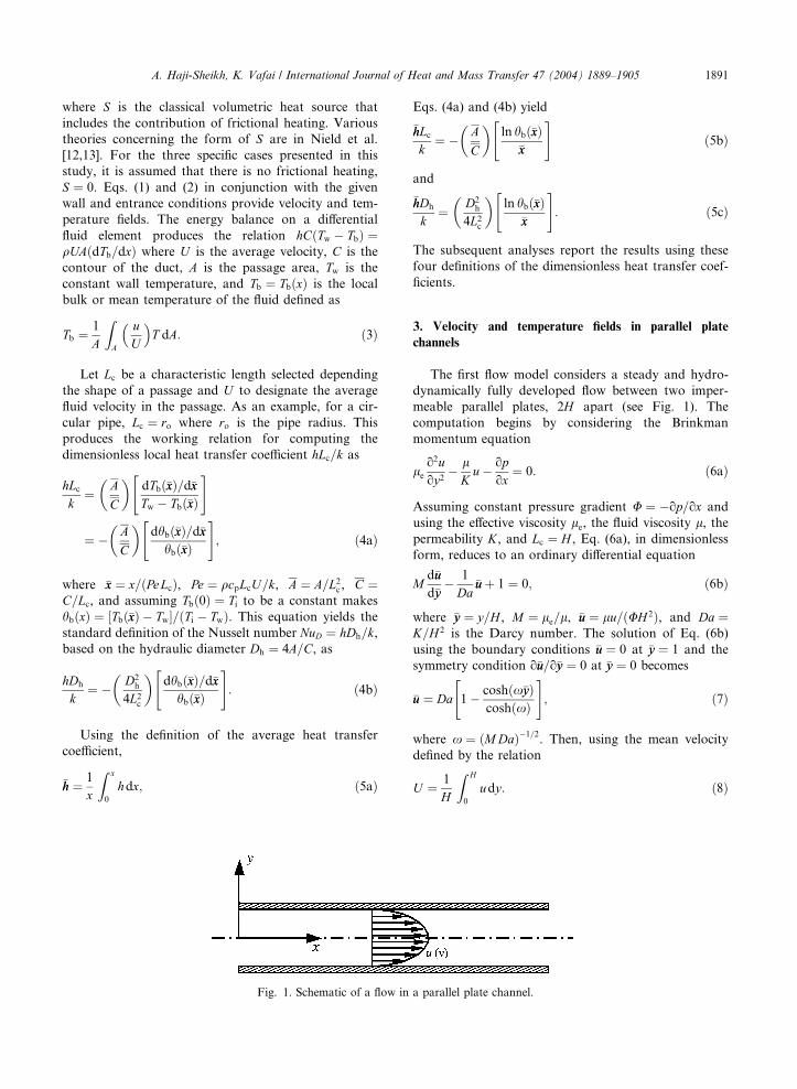
Fig. 1. Schematic of a flow in

Eqs. (4a) and (4b) yield

�hhLc

k¼ � A

C

� �ln hbð�xxÞ

�xx

" #ð5bÞ

and

�hhDh

k¼ D2

h

4L2c

� �ln hbð�xxÞ

�xx

" #: ð5cÞ

The subsequent analyses report the results using these

four definitions of the dimensionless heat transfer coef-

ficients.

3. Velocity and temperature fields in parallel plate

channels

The first flow model considers a steady and hydro-

dynamically fully developed flow between two imper-

meable parallel plates, 2H apart (see Fig. 1). The

computation begins by considering the Brinkman

momentum equation

le

o2uoy2

� lKu� op

ox¼ 0: ð6aÞ

Assuming constant pressure gradient U ¼ �op=ox and

using the effective viscosity le, the fluid viscosity l, thepermeability K, and Lc ¼ H , Eq. (6a), in dimensionless

form, reduces to an ordinary differential equation

Md�uud�yy

� 1

Da�uuþ 1 ¼ 0; ð6bÞ

where �yy ¼ y=H , M ¼ le=l, �uu ¼ lu=ðUH 2Þ, and Da ¼K=H 2 is the Darcy number. The solution of Eq. (6b)

using the boundary conditions �uu ¼ 0 at �yy ¼ 1 and the

symmetry condition o�uu=o�yy ¼ 0 at �yy ¼ 0 becomes

�uu ¼ Da 1

"� coshðx�yyÞ

coshðxÞ

#; ð7Þ

where x ¼ ðMDaÞ�1=2. Then, using the mean velocity

defined by the relation

U ¼ 1

H

Z H

0

udy: ð8Þ

a parallel plate channel.


Eq. (7) leads to a relation for the reduced mean

velocity U as,

U ¼ Da½1� tanhðxÞ=x�; ð9aÞ

and therefore

uU

¼ �uu

U¼ x

x� tanhðxÞ 1

"� coshðx�yyÞ

coshðxÞ

#: ð9bÞ

The definition of the average velocity U ¼ lU=ðUH 2Þleads to a relation for the friction factor

f ¼ �ðop=oxÞDh

qU 2=2¼ 2

U

1

ReD

Dh

H

� �2

¼ FReD

; ð10Þ

where F ¼ ð2=UÞðDh=HÞ2. Moreover, Eq. (8) provides

the value of U once the function �uu replaces u in the

integrand.

The temperature distribution assuming local thermal

equilibrium is obtainable from the energy equation

uoTox

¼ kqcp

o2Toy2

: ð11aÞ

Introducing the Peclet number Pe ¼ qcpHU=k where Uis the mean velocity in the duct, and dimensionless

�xx ¼ x=ðPeHÞ, the energy equation (Eq. (11)) reduces to

uU

oho�xx

¼ d2hd�yy2

; ð11bÞ

where h is the dimensionless temperature h ¼ ðT � TwÞ=ðTi � TwÞ. In this formulation, it is assumed that the inlet

temperature Ti and the wall temperature Tw have con-

stant values.

The solution of the partial differential Eq. (11b) is

obtainable using the method of separation of variables;

that is, let hð�xx;�yyÞ ¼ X ð�xxÞY ð�yyÞ. The substitution of this

functional for h in Eq. (11b) yields

uU

X 0

X¼ Y 00

Yð12Þ

leading to two ordinary differential equations

X 0ð�xxÞ þ k2X ð�xxÞ ¼ 0 ð13aÞ

and

Y 00ð�yyÞ þ k2uU

� �Y ð�yyÞ ¼ 0: ð13bÞ

The parameter k is the eigenvalue in this eigenvalue

problem that produces the temperature solution

h ¼X1m¼1

BmYmð�yyÞe�k2m�xx; ð14Þ

where the term e�k2m�xx in Eq. (14) is the solution of Eq.

(13a) once the parameter k is replaced by km. However,

the solution of Eq. (13b) remains as the major task for

this investigation and it is presented in the following

sections.

Following substitution for u=U , Eq. (13b) takes the

following form:

Y 00ð�yyÞ þ k2x

x� tanhðxÞ 1

"(� coshðx�yyÞ

coshðxÞ

#)Y ð�yyÞ ¼ 0:

ð15Þ

Next, consideration is given to the exact and numerical

solutions of this ordinary differential equation. For

simplicity of this presentation, let

w ¼ k2=xx� tanhðxÞ ð16aÞ

and

b ¼ 1

coshðxÞ ; ð16bÞ

then Eq. (15) reduces to

Y 00ð�yyÞ þ x2w½1� b coshðx�yyÞ�Y ð�yyÞ ¼ 0: ð17Þ

This differential equation has the form of a modified

Mathieu differential equation whose solution is associ-

ated with the modified Mathieu Function [14]. Various

classical solutions of the Mathieu differential equation

are in [14,15]. However, the plus sign instead of a minus

sign in Eq. (17) makes its solution more demanding than

the classical modified Mathieu Function. Since this is a

special Mathieu differential equation, it is best to de-

scribe the method of solution for this special case.

Among a few possible solutions, two different solutions

are presented here.

First solution: For convenience of algebra, the

abbreviated form of this ordinary differential equation is

Y 00 þ x2w½1� b coshðx�yyÞ�Y ¼ 0; ð18Þ

where w ¼ ðk2=xÞ=½x� tanhðxÞ� and b ¼ 1= coshðxÞ.The boundary conditions require having a symmetric

condition at y ¼ 0 and Y ¼ 0 at y ¼ H or �yy ¼ 1; they are

Y 0ð0Þ ¼ Y ð1Þ ¼ 0. For convenience of algebra, using a

new independent variable g ¼ coshðx�yyÞ � 1, one obtains

dYd�yy

¼ dYdg

dgd�yy

¼ dYdg

½x sinhðx�yyÞ� ð19Þ

and

d2Yd�yy2

¼ d2Ydg2

½x sinhðx�yyÞ�2 þ dYdg

½x2 coshðx�yyÞ�

¼ x2 sinh2ðx�yyÞd2Ydg2

þ x2 coshðx�yyÞdYdg

¼ x2½ðgþ 1Þ2 � 1� d2Ydg2

þ x2ð1þ gÞ dYdg

: ð20Þ


Following appropriate substitution, the resulting differ-

ential equation is

ðg2 þ 2gÞ d2Ydg2

þ ðgþ 1ÞdYdg

þ wð1� b� bgÞY ¼ 0: ð21Þ

It is interesting to note that the boundary conditions

dY =dy ¼ 0 when y ¼ 0 or g ¼ 0 is automatically satis-

fied regardless of the value of dY =dg. The solution

of this differential equation is a hypergeometric func-

tion and two different solutions are in the following

sections.

To obtain this solution by a standard technique, let

Y ðgÞ ¼X1n¼0

cngn; ð22aÞ

and then differentiate to get

dY ðgÞdg

¼X1n¼0

cnngn�1 for n > 0 ð22bÞ

and

d2Y ðgÞdg2

¼X1n¼0

cnnðn� 1Þgn�2 for n > 1: ð22cÞ

The substitution for Y ðgÞ and its derivatives in the dif-

ferential equation (Eq. (21)) produces

X1n¼2

cnnðn� 1Þðgn þ 2gn�1Þ þX1n¼1

cnnðgn þ gn�1Þ

þX1n¼0

cnw½ð1� bÞgn � bgnþ1� ¼ 0: ð23Þ

The examination of Eq. (22) shows that c0 is a con-

stant since Y ð0Þ 6¼ 0. This leads to the condition that

dY =dg 6¼ 0 when g ¼ 0 or c1 6¼ 0. Therefore, in the

above equation, the terms that contain the parameter g0

take the following form:

c1 � 1 � g0 þ c0wð1� bÞg0 ¼ 0 ð24aÞ

which makes c1 þ c0wð1� bÞ ¼ 0 or c1 ¼ �c0wð1� bÞ.Next, the examination of the coefficients that multiply

by g1 shows that

½4c2 þ c1 þ 2c2 þ c1wð1� bÞ � c0wb�g1 ¼ 0: ð24bÞ

This procedure is to be repeated for g values with

exponents 2; 3; . . . and so on. In general, the examina-

tion of the coefficients that multiply gn�1 leads to the

relation

½ðn� 1Þðn� 2Þcn�1 þ 2nðn� 1Þcn þ ðn� 1Þcn�1

þ ncn þ wð1� bÞcn�1 � wbcn�2�gn�1 ¼ 0: ð24cÞ

Since g 6¼ 0, then the solution for cn is

cn ¼ � n2 � 2n� nþ 2þ n� 1þ wð1� bÞ2n2 � 2n� n

cn�1

þ wb2n2 � 2n� n

cn�2

¼ �ðn� 1Þ2 þ wð1� bÞnð2n� 1Þ cn�1 þ

wbnð2n� 1Þ cn�2: ð24dÞ

In summary, the solution can be rewritten as

Y ð�yyÞ ¼ 1þX1n¼1

cn coshðx�yyÞh

� 1in: ð25Þ

In this formulation, c0 ¼ 1 is selected arbitrarily, then

c1 ¼ �c0wð1� bÞ and the recursive relation (24d) pro-

vide the remaining coefficients cn for nP 2. It should

be noted that there are other possible variations of

this solution, e.g., g ¼ b coshðxyÞ, g ¼ ½1� coshðx�yyÞ�=coshðxÞ with 06 g6 1.

Second solution: As an alternative solution of this

ordinary differential equation (Eq. (18)) let

Y ðgÞ ¼X1n¼0

cngn; ð26Þ

using a different independent variable g ¼ �yy. Moreover,

Eqs. (22b) and (22c) provide the first and second

derivatives for Y ðgÞ in Eq. (26). Following substitution

in the differential equation (Eq. (18)) and, after remov-

ing the zero terms, one obtains

X1n¼2

cnnðn� 1Þgn�2 þ x2w½1� b coshðxgÞ�X1n¼0

cngn ¼ 0:

ð27Þ

After substituting for

b coshðxgÞ ¼X1i¼0

aigi; ð28aÞ

where

ai ¼bi! ðxÞ

iwhen i is even;

0 when i is even:

�ð28bÞ

In Eq. (27), it can be written as

X1n¼2

cnnðn� 1Þgn�2 þ x2wX1n¼0

cngn � x2wX1n¼0

dngn ¼ 0;

ð29aÞ

where

dn ¼Xnj¼0

cjan�j: ð29bÞ

The term that includes g0 suggests c0 ¼ constant ¼ 1

whereas the terms that include g1 require c1 ¼ 0 because

of symmetry at y ¼ 0. Accordingly, all the terms with


odd power vanish in this solution. The values of other

constants are obtainable from the recursive relation

cnþ2 ¼ � x2wðcn � dnÞðnþ 2Þ2 � ðnþ 2Þ

: ð30Þ

Since the terms with odd power vanish, the working

relations are rearranged as

Y ðgÞ ¼X1n¼0

cng2n; ð31aÞ

c0 ¼ 1 and cn ¼ �x2wðcn�1 � dn�1Þ4n2 � 2n

for nP 1:

ð31bÞAlso, Eq. (29a) is rearranged to take the form

b coshðxgÞ ¼X1i¼0

bð2iÞ! ðxgÞ

2i: ð32aÞ

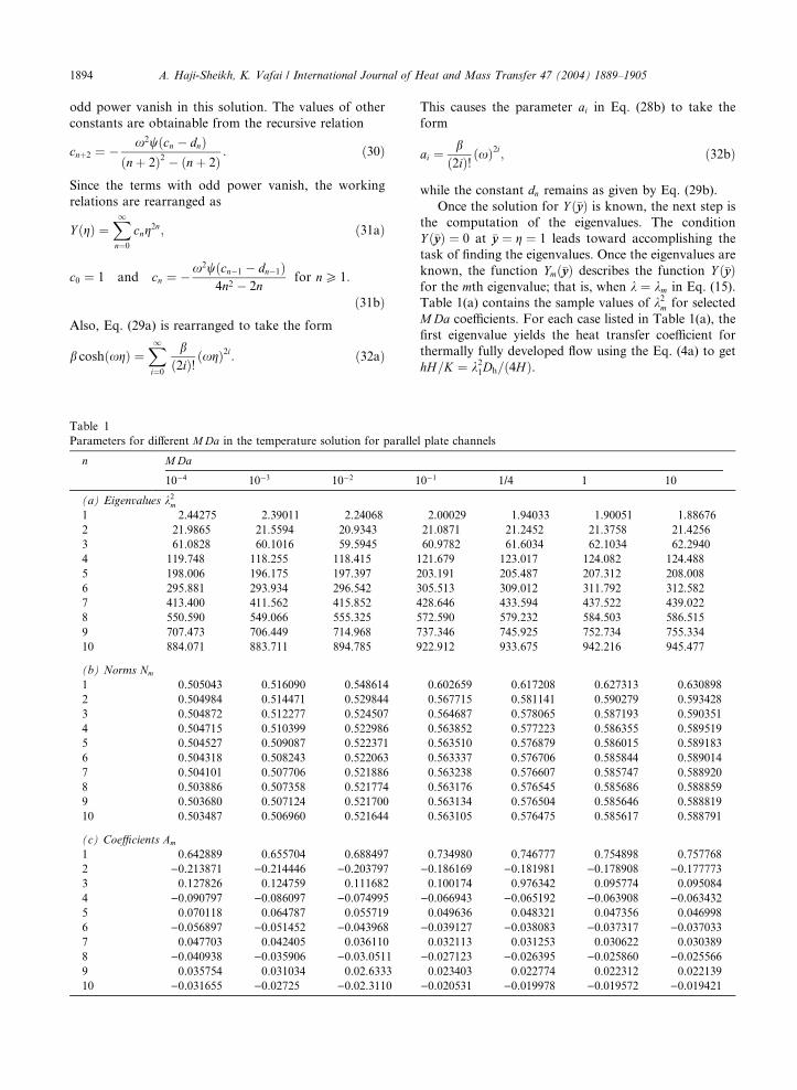
Table 1

Parameters for different MDa in the temperature solution for paralle

n M Da

10�4 10�3 10�2 1

(a) Eigenvalues k2m1 2.44275 2.39011 2.24068

2 21.9865 21.5594 20.9343

3 61.0828 60.1016 59.5945

4 119.748 118.255 118.415 1

5 198.006 196.175 197.397 2

6 295.881 293.934 296.542 3

7 413.400 411.562 415.852 4

8 550.590 549.066 555.325 5

9 707.473 706.449 714.968 7

10 884.071 883.711 894.785 9

(b) Norms Nm

1 0.505043 0.516090 0.548614

2 0.504984 0.514471 0.529844

3 0.504872 0.512277 0.524507

4 0.504715 0.510399 0.522986

5 0.504527 0.509087 0.522371

6 0.504318 0.508243 0.522063

7 0.504101 0.507706 0.521886

8 0.503886 0.507358 0.521774

9 0.503680 0.507124 0.521700

10 0.503487 0.506960 0.521644

(c) Coefficients Am

1 0.642889 0.655704 0.688497

2 )0.213871 )0.214446 )0.2037973 0.127826 0.124759 0.111682

4 )0.090797 )0.086097 )0.0749955 0.070118 0.064787 0.055719

6 )0.056897 )0.051452 )0.0439687 0.047703 0.042405 0.036110

8 )0.040938 )0.035906 )0.03.05119 0.035754 0.031034 0.02.6333

10 )0.031655 )0.02725 )0.02.3110

This causes the parameter ai in Eq. (28b) to take the

form

ai ¼b

ð2iÞ! ðxÞ2i; ð32bÞ

while the constant dn remains as given by Eq. (29b).

Once the solution for Y ð�yyÞ is known, the next step is

the computation of the eigenvalues. The condition

Y ð�yyÞ ¼ 0 at �yy ¼ g ¼ 1 leads toward accomplishing the

task of finding the eigenvalues. Once the eigenvalues are

known, the function Ymð�yyÞ describes the function Y ð�yyÞfor the mth eigenvalue; that is, when k ¼ km in Eq. (15).

Table 1(a) contains the sample values of k2m for selected

MDa coefficients. For each case listed in Table 1(a), the

first eigenvalue yields the heat transfer coefficient for

thermally fully developed flow using the Eq. (4a) to get

hH=K ¼ k21Dh=ð4HÞ.

l plate channels

0�1 1/4 1 10

2.00029 1.94033 1.90051 1.88676

21.0871 21.2452 21.3758 21.4256

60.9782 61.6034 62.1034 62.2940

21.679 123.017 124.082 124.488

03.191 205.487 207.312 208.008

05.513 309.012 311.792 312.582

28.646 433.594 437.522 439.022

72.590 579.232 584.503 586.515

37.346 745.925 752.734 755.334

22.912 933.675 942.216 945.477

0.602659 0.617208 0.627313 0.630898

0.567715 0.581141 0.590279 0.593428

0.564687 0.578065 0.587193 0.590351

0.563852 0.577223 0.586355 0.589519

0.563510 0.576879 0.586015 0.589183

0.563337 0.576706 0.585844 0.589014

0.563238 0.576607 0.585747 0.588920

0.563176 0.576545 0.585686 0.588859

0.563134 0.576504 0.585646 0.588819

0.563105 0.576475 0.585617 0.588791

0.734980 0.746777 0.754898 0.757768

)0.186169 )0.181981 )0.178908 )0.1777730.100174 0.976342 0.095774 0.095084

)0.066943 )0.065192 )0.063908 )0.0634320.049636 0.048321 0.047356 0.046998

)0.039127 )0.038083 )0.037317 )0.0370330.032113 0.031253 0.030622 0.030389

)0.027123 )0.026395 )0.025860 )0.0255660.023403 0.022774 0.022312 0.022139

)0.020531 )0.019978 )0.019572 )0.019421

Fig. 2. Heat transfer coefficient in a parallel plate channel for

different MDa coefficients: (a) local and (b) average.


Following the computation of the eigenvalues, the

thermal condition at the entrance location provides the

constants Bm in Eq. (14). The use of a constant tem-

perature at �xx ¼ 0; that is, hð0;�yyÞ ¼ 1, greatly simplifies

the determination of Bm. As an intermediate step, it is

necessary to utilize the orthogonality conditionZ 1

0

uU

� �Ymð�yyÞYnð�yyÞd�yy ¼

0 when n 6¼ m;Nm when n 6¼ m;

�ð33aÞ

and a Graetz-solution type of analysis provides the

norm

Nm ¼Z 1

0

uU

� �½Ymð�yyÞ�2 d�yy

¼ 1

2km

oYmð�yyÞo�yy

" #�yy¼1

oYmð�yyÞokm

" #�yy¼1

: ð33bÞ

Also, the utilization of the orthogonality condition leads

toward the determination of the integral that reduces to

Am ¼Z 1

0

uU

� �Ymð�yyÞd�yy ¼ � 1

k2m

oYmð�yyÞo�yy

" #�yy¼1

ð33cÞ

when integrating Eq. (13b) over �yy. These forms of Eqs.

(33b) and (33c) remain the same for any u=U function.

Finally, the use of the initial condition and orthogo-

nality condition yield the coefficient Bm as

Bm ¼ Am

Nm¼ � 2

km

� �oYmð�yyÞokm

" #,�yy¼1

: ð34Þ

Table 1(b) is prepared to show a sample value of

the computed norm Nm for the same MDa values

appearing in Table 1(a). Moreover, Table 1(c) is prepared

to demonstrate corresponding computed values of coeffi-

cient Am. All entries listed in these tables have accurate

figures. Finally, the temperature solution is obtainable

after substituting for Bm from Eq. (34) in Eq. (14).

To avoid redundancy, a presentation of the temper-

ature solution will appear later. The main objective of

this study is the computation of local and average heat

transfer coefficients. For parallel plate channels, Lc is

selected as H and then Eq. (4a) provides the local

dimensionless heat transfer coefficient. Fig. 2(a) shows

the computed local dimensionless heat transfer coeffi-

cient hH=k plotted versus �xx ¼ x=ðPeHÞ using 35–50 ei-

genvalues depending on the value ofMDa. The data in a

log–log plot show near linear behavior as �xx goes towardzero. A mixed symbolic and numerical computation was

used to accomplish this task. The computation of ei-

genvalues when m is large becomes demanding. Using

Mathematica [16], a mixed symbolic and numerical

procedure with a high degree of precision was written to

perform the task of finding these eigenvalues. Next, the

dimensionless average heat transfer coefficient �hhH=k (seeEq. (5b)) is plotted versus �xx in Fig. 2(b). Because a rel-

atively small number of eigenvalues was used, a second

method of solution is employed in order to verify the

accuracy of the results; this comparison is discussed in a

separate section.

4. Velocity and temperature fields in circular pipes

Consideration is given to heat transfer to a fluid

passing through a porous medium bounded by an

impermeable circular wall (see Fig. 3). The procedure to

obtain a temperature solution is similar to that described

for the parallel plate channel. The second method used

earlier is modified here. In cylindrical coordinates, the

momentum equation is

le

o2uor2

�þ 1

rouor

�� lKu� op

ox¼ 0; ð35Þ

where r is the local radial coordinate and x is the axial

coordinate (Fig. 3). If the pipe radius is designated by ro

Fig. 3. Schematic of a flow in a circular pipe.


and Lc ¼ ro, the dimensionless quantities defined for

flow in parallel plate channels are repeated after some

modifications; the modified quantities are: Lc ¼ ro,�rr ¼ r=ro, �uu ¼ lu=ðUr2oÞ, Da ¼ K=r2o, and x ¼ ðMDaÞ�1=2

.

Then, the momentum equation reduces to

Md2�uud�rr2

þ 1

�rrd�uud�rr

!� uDa

þ 1 ¼ 0: ð36Þ

Using the boundary condition �uu ¼ 0 at �rr ¼ 1 and the

condition o�uu=o�rr ¼ 0 at �rr ¼ 0, the solution becomes

�uu ¼ Da 1

"� I0ðx�yyÞ

I0ðxÞ

#; ð37Þ

where, as before, x ¼ ðMDaÞ�1=2. Here, the mean

velocity defined by the relation

U ¼ 2

r2o

Z ro

0

urdr; ð38Þ

and the velocity profile take the form

uU

¼ �uu

U¼ xI0ðxÞ

xI0ðxÞ � 2I1ðxÞ1

"� I0ðx�rrÞ

I0ðxÞ

#: ð39Þ

Using the computed values of U ¼ Da½1� ð2=xÞI1ðxÞ=I0ðxÞ�, the relation

f ¼ �ðop=oxÞDh

qU 2=2¼ 2

U

1

ReD

Dh

ro

� �2

ð40Þ

provides the pipe pressure drop.

The steady-state form of the energy equation in

cylindrical coordinates is

uoTox

¼ kqcp

o2Tor2

�þ 1

roTor

�: ð41Þ

Defining the dimensionless temperature h ¼ ðT � TwÞ=ðTi � TwÞ where Ti is the inlet temperature and Tw is the

wall temperature, one obtains

uU

oho�xx

¼ o2ho�rr2

þ 1

�rroho�rr

; ð42Þ

where �xx ¼ x=ðPeroÞ and Pe ¼ qcproU=k. As before, sep-

arating the variables, hð�xx;�rrÞ ¼ X ð�xxÞRð�rrÞ leads to solution

of two ordinary differential equations,

X 0ð�xxÞ þ k2X ð�xxÞ ¼ 0 ð43aÞ

and

R00ð�rrÞ þ 1

�rrR0ð�rrÞ þ k2

uU

� �Rð�rrÞ ¼ 0: ð43bÞ

The major task remaining is to find the exact value of

Rð�rrÞ and its verification by comparing it with the

numerically obtained data. The parameter k in Eq. (43b)

serves as the eigenvalue. The final temperature solution,

after the computation of eigenvalues, is

h ¼X1m¼1

BmRmð�rrÞe�k2m�xx: ð44Þ

Eq. (43b) following substitution for u=U takes the

following form:

R00ð�rrÞ þ 1

�rrR0ð�rrÞ þ k2

xI0ðxÞxI0ðxÞ � 2I1ðxÞ

(

� 1

"� I0ðx�rrÞ

I0ðxÞ

#)Rð�rrÞ ¼ 0: ð45Þ

Using the abbreviations

b ¼ 1=I0ðxÞ ð46aÞ

and

w ¼ I0ðxÞxI0ðxÞ � 2I1ðxÞ

k2

x; ð46bÞ

in the following analysis, Eq. (45) is rewritten as

R00ð�rrÞ þ 1

�rrR0ð�rrÞ þ x2w 1

h� bI0ðx�rrÞ

iRð�rrÞ ¼ 0: ð46cÞ

Eq. (46c) is subject to the boundary conditions R0ð0Þ ¼Rð1Þ ¼ 0. Similar to the previous case, one can select

g ¼ I0ðxrÞ � 1; however, this selection did not produce

sufficient simplification to warrant its implementation.

Therefore, a direct derivation of a series solution will

follow.

Solution: To obtain this solution, let g ¼ �rr and then

set

RðgÞ ¼X1n¼0

cngn ð47Þ


then

dRðgÞdg

¼X1n¼0

cnngn�1 for n > 0 ð48aÞ

and

d2RðgÞdg2

¼X1n¼0

cnnðn� 1Þgn�2 for n > 1: ð48bÞ

After removing the zero terms in Eqs. (48a) and (48b),

the substitution RðgÞ and its derivatives in Eq. (46c)

yields

X1n¼2

cnnðn� 1Þgn þX1n¼1

cnngn þ ðxgÞ2w

� ½1� bI0ðxgÞ�X1n¼0

cngn ¼ 0: ð49Þ

Table 2

Parameter for different MDa in the temperature solution for circular

n MDa

10�4 10�3 10�2 1

(a) Eigenvalues k2m1 5.66823 5.42732 4.78988

2 29.8685 28.6766 26.2350

3 73.4184 70.7493 65.8977

4 136.346 131.874 123.858 1

5 218.676 212.181 200.120 1

6 320.434 311.724 294.682 2

7 441.649 430.523 407.545 3

8 582.344 568.584 538.711 4

9 742.543 725.907 688.177 6

10 922.266 902.508 855.946 7

(b) Norms Nm

1 0.137487 0.143488 0.159961

2 0.0590511 0.0613218 0.0655328

3 0.0375695 0.0387828 0.0409746

4 0.0275390 0.0282878 0.0298015

5 0.0217298 0.0222421 0.0234160

6 0.0179401 0.0183201 0.0192840

7 0.0152729 0.0155728 0.0163915

8 0.0132940 0.0135417 0.0142535

9 0.0117676 0.0119793 0.0126089

10 0.0105547 0.0107401 0.0113046

(c) Coefficients Am

1 0.220128 0.228737 0.248854

2 )0.062696 )0.063753 )0.0623333 0.031764 0.031356 0.029049

4 )0.019841 )0.019012 )0.0171905 0.013818 0.012901 0.0115313

6 )0.010287 )0.0094039 )0.00835527 0.0080122 0.0072030 0.0063781

8 )0.0064475 )0.0057215 )0.00505559 0.0053188 0.0046725 0.0041228

10 )0.0044743 )0.0039015 )0.0034376

After substituting for

bI0ðxgÞ ¼X1i¼0

aigi; ð50Þ

Eq. (49) can be written as

X1n¼2

cnnðn� 1Þgn þX1n¼1

cnngn þ x2wX1n¼0

cngnþ2

� x2wX1n¼0

dngnþ2 ¼ 0; ð51aÞ

where

dn ¼Xnj¼0

cjan�j: ð51bÞ

The term that includes g0 suggests c0 ¼ constant ¼ 1

whereas the terms that include g1 require c1 ¼ 0.

pipes

0�1 1/4 1 10

3.96224 3.79632 3.69438 3.66064

23.4011 22.8066 22.4400 22.3186

59.5023 58.1222 57.2731 56.9925

12.269 109.743 108.191 107.679

81.701 177.669 175.192 174.375

67.798 261.898 258.275 257.081

70.559 362.430 357.440 355.796

89.984 479.260 472.688 470.520

26.074 612.405 604.017 601.253

78.829 761.847 751.427 747.994

0.179869 0.18408 0.1868201 0.187759

0.0720243 0.0736315 0.0746558 0.0750002

0.0450105 0.0460102 0.0466463 0.0468598

0.0327336 0.0334597 0.0339215 0.0340765

0.0257188 0.0262891 0.0266516 0.0267733

0.0211800 0.0216495 0.0219480 0.0220482

0.0180029 0.0184019 0.0186557 0.0187450

0.0156547 0.0160019 0.0162181 0.0163021

0.0138483 0.0141553 0.0143504 0.0144238

0.0124158 0.0126909 0.0128659 0.0129250

0.269514 0.273661 0.276348 0.277268

)0.060905 )0.060710 )0.060557 )0.0604980.027938 0.027775 0.027654 0.027609

)0.016449 )0.016338 )0.016257 )0.0162270.011009 0.010931 0.010873 0.010852

)0.0079669 )0.007908 )0.0078656 )0.00784970.0060771 0.0060316 0.0059984 0.0059881

)0.0048145 )0.0047783 )0.0047514 )0.00473890.0039249 0.0038949 0.0038730 0.0038683

)0.0032718 )0.0032466 )0.0032282 )0.0032212


Accordingly, all the terms with odd power vanish in the

solution. The values of other constants are obtainable

from the recursive relation

cnþ2 ¼ �x2wðcn þ dnÞðnþ 2Þ2

: ð52Þ

Since the terms with odd power vanish, the working

equation may be rewritten as

RðgÞ ¼X1n¼0

cng2n; ð53aÞ

c0 ¼ 1; cn ¼ �x2wðcn�1 � dn�1Þ4n2

for nP 1: ð53bÞ

Moreover, the relation

bI0ðxgÞ ¼X1i¼0

b

ði!Þ2xg2

� �2ið54aÞ

makes

ai ¼b

ði!Þ2x2

� �2i; ð54bÞ

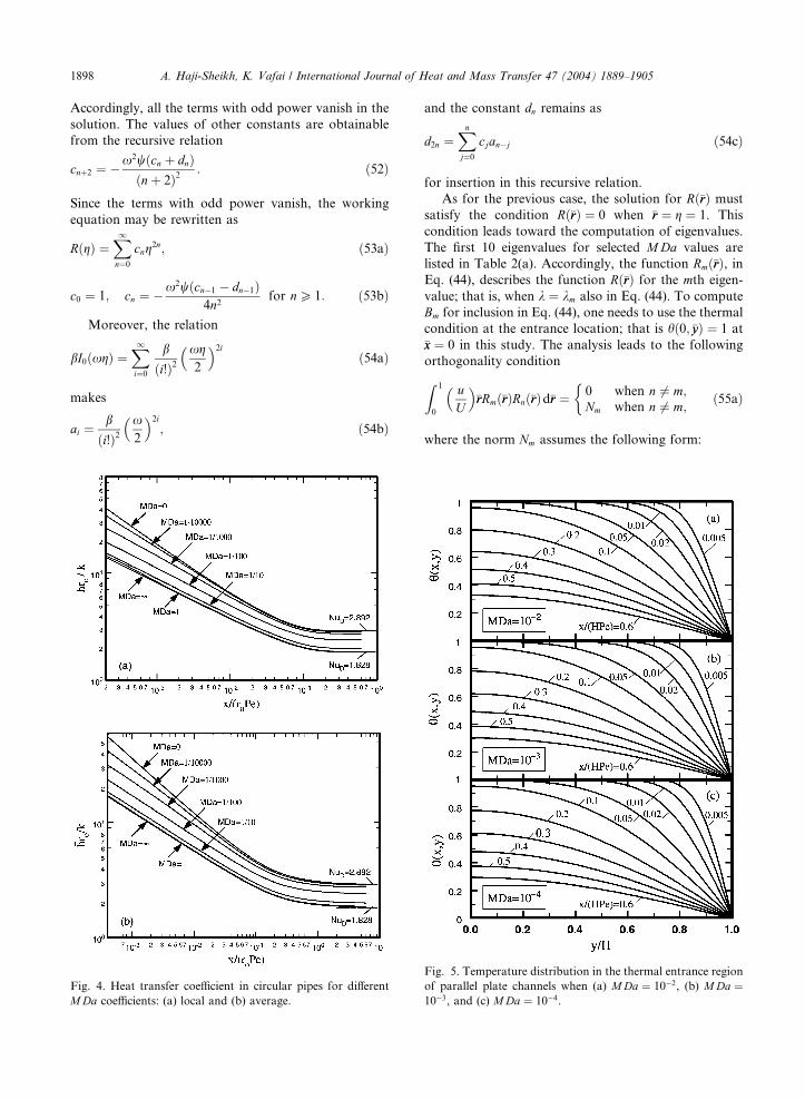
Fig. 4. Heat transfer coefficient in circular pipes for different

MDa coefficients: (a) local and (b) average.

and the constant dn remains as

d2n ¼Xnj¼0

cjan�j ð54cÞ

for insertion in this recursive relation.

As for the previous case, the solution for Rð�rrÞ must

satisfy the condition Rð�rrÞ ¼ 0 when �rr ¼ g ¼ 1. This

condition leads toward the computation of eigenvalues.

The first 10 eigenvalues for selected MDa values are

listed in Table 2(a). Accordingly, the function Rmð�rrÞ, inEq. (44), describes the function Rð�rrÞ for the mth eigen-

value; that is, when k ¼ km also in Eq. (44). To compute

Bm for inclusion in Eq. (44), one needs to use the thermal

condition at the entrance location; that is hð0; �yyÞ ¼ 1 at

�xx ¼ 0 in this study. The analysis leads to the following

orthogonality conditionZ 1

0

uU

� ��rrRmð�rrÞRnð�rrÞd�rr ¼

0 when n 6¼ m;Nm when n 6¼ m;

�ð55aÞ

where the norm Nm assumes the following form:

Fig. 5. Temperature distribution in the thermal entrance region

of parallel plate channels when (a) MDa ¼ 10�2, (b) MDa ¼10�3, and (c) MDa ¼ 10�4.


Nm ¼Z 1

0

uU

� ��rr½Rmð�rrÞ�2 d�rr

¼ 1

2km

oRmð�rrÞo�rr

" #�rr¼1

oRmð�rrÞokm

" #�rr¼1

; ð55bÞ

and the determination of coefficient Am followed by

integrating Eq. (43b) after replacing k with km and Rwith Rm yields

Am ¼Z 1

0

uU

� ��rrRmð�rrÞd�rr ¼ � 1

k2m

oRmð�rrÞo�rr

" #�rr¼1

: ð55cÞ

Finally, the coefficients Bm for inclusion in Eq. (44) is

Bm ¼ Am

Nm¼ � 2

km

� �oRmð�rrÞokm

" #�rr¼1

:

,ð56Þ

Table 2(b) is prepared to show the computed norms Nm

corresponding to the eigenvalues listed in Table 2(a). To

facilitate the computation of Bm from Eq. (56) for

inclusion in Eq. (44), Table 2(c) contains the coefficients

Am computed using Eq. (55c).

For circular pipes, ro replaces Lc in Eqs. (4a) and (5b)

and they can be used to compute fluid temperature (Eq.

(44)); a temperature solution presentation will appear

later. Subsequently, the computed bulk temperature

leads toward the determination of heat transfer coeffi-

cients. Fig. 4(a) shows the computed dimensionless local

heat transfer coefficient hro=k plotted versus �xx using 50

eigenvalues in a Graetz-type solution. As in the previous

case, the data, in a log–log plot, show near linear

behavior as �xx goes toward zero. Fig. 4(b) shows the

dimensionless average heat transfer coefficient �hhro=kplotted versus �xx. These data are also to be compared with

data obtained using an alternative method of solution.

The temperature solution, using the aforementioned

exact analysis provided accurate results when x is rela-

tively large. However, it became a cumbersome task to

evaluate all needed eigenvalues for any arbitrarily se-

lected MDa at extremely small values of �xx. Because the

computer capacity limits the needed number of eigen-

values, an alternative method of analysis is the subject of

the following studies.

Fig. 6. Temperature distribution in the thermal entrance region

of circular pipes when (a) MDa ¼ 10�2, (b) MDa ¼ 10�3, and

(c) MDa ¼ 10�4.

5. An alternative method of solution

As stated earlier, it is difficult to obtain many ei-

genvalues using the exact analysis. This is due to round-

off errors caused by the finiteness of machine capacity

and computational speed. Therefore, for a finite number

of eigenvalues, it is best to optimize the solution using

variational calculus. This type of analysis leads to a

Green’s function solution method that uses the weigh-

ted residuals technique. The temperature solution is

similar to that for transient heat conduction in Beck et al.

[11, Chapter 10] when the axial coordinate x replaces

time t.The method of solution presented here equally ap-

plies to ducts described earlier and it can be extended to

accommodate the ducts having various cross section

shapes. As significant advantages, the computation of

eigenvalues is automatic, and the computation of other

coefficients is also automatic. In this technique, for

preselected M eigenvalues, the proposed solution is a

modification of Eq. (14), that is,

h ¼X1m¼1

BmWmð�yyÞe�k2m�xx; ð57aÞ

where

WmðgÞ ¼XNj¼1

dmjfjðgÞ; ð57bÞ

and the function fjðgÞ are selected so that they satisfy the

homogeneous boundary conditions along the surface of

the ducts; that is,

fjðgÞ ¼ ð1� g2Þg2ðj�1Þ: ð57cÞ


For a parallel plate channel WmðgÞ stands for YmðgÞ andfor a circular pipe WmðgÞ stands for RmðgÞ. The

remaining steps apply equally to both cases with minor

modifications to be identified later.

As described in Beck et al. [11], the next task is the

computation of eigenvalues k2m and the coefficients dmj inEq. (57b). The computation begins by finding the ele-

ments of two matrices, A and B,

aij ¼Z 1

0

fiðgÞr2fjðgÞJ dg ð58aÞ

and

bij ¼Z 1

0

qcpuU

� �fiðgÞfjðgÞJ dg: ð58bÞ

The parameter J in Eqs. (58a) and (58b) is the Jacobian;

J ¼ 1 for parallel plate channels and J ¼ g is for circular

ducts. This analysis leads to an eigenvalue problem [11]

ðAþ k2BÞd ¼ 0; ð59aÞ

that can be rewritten as

ðB�1Aþ k2IÞd ¼ 0: ð59bÞ

Table 3

Comparison of computed data for parallel plate channels

MDa ðx=DhÞReDPr

½NuD�Exa ½NuD�WRb

10�2 10�4 38.074 38.074

5 · 10�4 21.634 21.634

10�3 17.053 17.053

5 · 10�3 10.516 10.516

10�2 9.3025 9.3025

5 · 10�2 8.9626 8.9626

10�1 8.9626 8.9626

0.5 8.9626 8.9626

10�3 10�4 48.638 48.637

5 · 10�4 25.806 25.806

10�3 19.672 19.672

5 · 10�3 11.377 11.377

10�2 9.9424 9.9424

5 · 10�2 9.5605 9.5605

10�1 9.5605 9.5605

0.5 9.5605 9.5605

10�4 10�4 56.280 56.271

5 · 10�4 27.624 27.623

10�3 20.587 20.587

5 · 10�3 11.625 11.625

10�2 10.149 10.149

5 · 10�2 9.7710 9.7710

10�1 9.7710 9.7710

0.5 9.7710 9.7710

aNusselt number from exact analysis.bNusselt number using method of weighted residuals.

The symbolic software Mathematica was used to

produce the elements of matrices A and B and subse-

quently the eigenvalues k2m and the corresponding coef-

ficients dmj embedded within the eigenvectors d. The

basic Mathematica statements to accomplish this task,

when using Eqs. (58a) and (58b) for a parallel plate

channel, are

fi ¼ (1-x^2) * x^(2*i-2);

fj ¼ (1-x^2) * x^(2*j-2);

oper ¼ Simplify[fi*(D[D[fj,x],x])];

amat ¼ Table[Integrate[oper, {x,0,1}], {i,1,m},

{j,1,m}];

bmat ¼ Table[Integrate[cap*u*fi*fj/uav, {x,0,1}],

{i,1,m}, {j,1,m}];

eigv ¼ N[Eigenvalues[-Inverse[bmat].amat]];

dvect ¼ Eigenvectors[-Inverse[bmat].amat];

In the computer code above, x stands for g,amat¼A, bmat¼B, uav¼U , cap¼ qcp, while eigv is a

vector containing the eigenvalues and dvect contains the

eigenvectors within its rows. The remaining parameters

are the same as those presented earlier in the text and in

the nomenclature. The eigenvectors in Mathematica

appear as the rows of a matrix to be designated as D.

½NuD�Exa ½NuD�WRb ½hb�Exact

58.383 58.383 0.97692

33.275 33.275 0.93562

26.127 26.127 0.90077

15.249 15.249 0.73714

12.502 12.502 0.60648

9.6932 9.6932 0.14390

9.3279 9.3279 0.2397· 10�1

9.0356 9.0356 0.1418· 10�7

77.477 77.479 0.96948

42.049 42.048 0.91934

32.143 32.143 0.87935

17.529 17.529 0.70427

14.001 14.001 0.57118

10.474 10.474 0.12311

10.017 10.017 0.1819· 10�1

9.6518 9.6518 0.4136· 10�8

96.297 96.319 0.96221

48.570 48.572 0.90743

36.036 36.037 0.86576

18.630 18.630 0.68894

14.661 14.661 0.55630

10.773 10.773 0.11594

10.272 10.272 0.1643· 10�1

9.8712 9.8712 0.2667· 10�8


One can show that the eigenfunctions WmðgÞ are

orthogonal; however with matrices B and D in hand, the

coefficients Bm for inclusion in Eq. (14) are obtainable

from the relation [11, Eq. (10.53)],

Bm ¼XNi¼1

pmi

Z 1

0

qcpuU

� �fiðgÞdg: ð60Þ

The parameters pmi in Eq. (60) are the elements of a

matrix

P ¼ ½ðD � BÞT��1; ð61Þ

that is, the matrices D multiplied by matrix B and the

resulting matrix is transposed and then inverted. Fol-

lowing computation of D and P, the Green’s function is

readily available to include the effect of frictional heating

(see Beck et al. [11, p. 308]). This task can be performed

conveniently using Mathematica [16]. This numerical

computation of temperature can be extended to passages

Fig. 7. Comparison of the local heat transfer coefficient ob-

tained by two methods in a parallel plate channel for different

MDa coefficients: (a) local and (b) average.

having various shapes, e.g., triangular ducts, etc. The

needed modifications are described in Refs. [11,17]. It

should be stated that both the exact values of velocity

and a computed velocity using the classical Galerkin

method [17] were used and the results show insignificant

difference in the temperature data.

6. Numerical results

As a first test of these two solution methods, the

temperature distribution in parallel plate channels are

presented in Fig. 5. The data show the temperature field

in the entrance region under the conditions (a) when

MDa ¼ 10�2, (b) when MDa ¼ 10�3, and (c) when

MDa ¼ 10�4. The data show a slight increase in the

slope at the wall as MDa decrease. Fig. 6 repeats the

presentation of temperature fields for flow in circular

pipes and the temperature in the entrance region are for

Fig. 8. Comparison of the local heat transfer coefficient ob-

tained by two methods in a circular pipe for different MDacoefficients: (a) local and (b) average.


the conditions (a) when MDa ¼ 10�2, (b) when

MDa ¼ 10�3, and (c) when MDa ¼ 10�4. The tempera-

ture fields plotted in Figs. 5 and 6 have noticeably dif-

ferent distribution patterns.

Following the computation of temperature, the next

task is to compute local and average heat transfer

coefficients for fluid flowing through parallel plate ducts

and circular pipes within the range of 10�66

ðx=DhÞ=ðReDPrÞ < 1 where Dh ¼ 4A=C, ReD ¼ qUDh=l,and Pr ¼ lcp=k. As many as 50 eigenvalues did not

provide results with sufficient accuracy using the exact

analysis; however, 40 eigenvalues did yield relatively

accurate results using this alternative solution. The data

in Table 3 show excellent agreement between computed

Table 4

Comparison of computed data for cylindrical pipes

MDa ðx=DhÞReDPr

½NuD�Exa ½NuD�WRb

10�2 5 · 10�4 17.447 17.447

10�3 13.645 13.645

5 · 10�3 7.8710 7.8710

10�2 6.3810 6.3810

5 · 10�2 4.8349 4.8349

10�1 4.7905 4.7905

0.5 4.7899 4.7899

1 4.7899 4.7899

10�3 5 · 10�4 22.272 22.251

10�3 17.010 17.002

5 · 10�3 9.2264 9.2255

10�2 7.3122 7.3119

5 · 10�2 5.4677 5.4677

10�1 5.4277 5.4277

0.5 5.4273 5.4273

1 5.4273 5.4273

10�4 5 · 10�4 25.650 25.647

10�3 18.942 18.941

5 · 10�3 9.7254 9.7253

10�2 7.6266 7.6265

5 · 10�2 5.7043 5.7043

10�1 5.6685 5.6685

0.5 5.6682 5.6682

1 5.6682 5.6682

aNusselt number from exact analysis.bNusselt number using method of weighted residuals.

Fig. 9. Schematic of a flow

local heat transfer coefficients within a small range of the

dimensionless axial coordinate (see Columns 2 and 3).

Also, these two completely different methods of solution

yield the average heat transfer coefficients in Columns 5

and 6 that are in excellent agreement. For a larger range

of the dimensionless axial coordinate, Fig. 7 is prepared

to demonstrate graphically the agreement between these

two solution methods. Fig. 7(a) shows the local heat

transfer coefficient for flow between two parallel plates

filled with porous materials. The solid lines in Fig. 7(a)

are obtained using this alternative analysis using 40 ei-

genvalues. The graph shows the local Nusselt number

NuD ¼ hDh=k ¼ 4hH=k, for various MDa values, plotted

versusffiffiffiffiffiffiffiffiffiffiffiffiffiffiffiffiffiffiffiffiffiffiffiffiffiffiffiffiffiffiffiffiðx=DhÞ=ðReDPrÞ

p¼

ffiffiffiffiffiffiffiffiffiffi�xx=16

p. The solid lines in

½NuD�Exa ½NuD�WRb ½hb�Exact

26.938 26.938 0.94755

21.093 21.093 0.91909

11.999 11.999 0.78665

9.4985 9.4985 0.68390

6.0584 6.0584 0.29770

5.4293 5.4293 0.11398

4.9178 4.9178 0.5351· 10�4

4.8538 4.8538 0.3699· 10�8

35.482 35.541 0.93149

27.354 27.377 0.89636

14.828 14.830 0.74338

11.464 11.465 0.63221

6.9970 6.9972 0.24674

6.2165 6.2166 0.8319· 10�1

5.5852 5.5852 0.1409· 10�4

5.5062 5.5062 0.2721· 10�9

43.943 43.951 0.91587

32.842 32.845 0.87690

16.628 16.628 0.71709

12.556 12.556 0.60518

7.4093 7.4093 0.22721

6.5425 6.5425 0.7302· 10�1

5.8431 5.8431 0.8409· 10�5

5.7557 5.7557 0.1003· 10�9

in an elliptical duct.


Fig. 7(b) show the average Nusselt number, NuD ¼�hhDh=k ¼ 4�hhH=k, plotted versus

ffiffiffiffiffiffiffiffiffiffiffiffiffiffiffiffiffiffiffiffiffiffiffiffiffiffiffiffiffiffiffiffiðx=DhÞ=ðReDPrÞ

p¼ffiffiffiffiffiffiffiffiffiffi

�xx=16p

. The solid lines in Fig. 7(b) show similar char-

acteristics to those in Fig. 7(a). At lower values of �xx, theslope in Fig. 7(b) is nearly linear and it is similar to that

in Fig. 7(a); however, the Nusselt number values are

higher as expected. The discrete circular symbols, in Fig.

7(a) and (b), are from the exact analysis using 50 ei-

genvalues. These two sets of data agree well at larger

values of x. However, the discrete data exhibit a sudden

departure from a near linear form at their lowest plotted

values of the dimensionless axial coordinate. This phe-

nomenon appears when the number of eigenvalues is

insufficient. As a remedy, the space partitioning similar

to time partitioning [11] can be effective.

For flow in circular ducts filled with porous materials,

the solid lines in Fig. 8(a) show the computed local heat

transfer coefficients for various MDa values. For a cir-

cular pipe, the Nusselt number NuD ¼ hDh=k ¼ 2hro=k is

plotted versusffiffiffiffiffiffiffiffiffiffiffiffiffiffiffiffiffiffiffiffiffiffiffiffiffiffiffiffiffiffiffiffiðx=DhÞ=ðReDPrÞ

p. As in the previous case,

the data properly approach the limiting values: unob-

Fig. 10. Local heat transfer coefficient in elliptical ducts for

differentMDa values: (a) when b=a ¼ 0:75, (b) when b=a ¼ 0:50,

and (c) when b=a ¼ 0:25.

structed tube flowwhenMDa ! 1 and that for slug flow

when MDa ! 0. The data in this figure clearly indicate

that the first eigenvalue in Table 2(a) directly represents

the fully developed Nusselt number for various MDavalues. The average Nusselt number is plotted, using solid

lines, in Fig. 8(b). They show the variation of the average

Nusselt number NuD ¼ �hhDh=k ¼ 2�hhro=k as a function offfiffiffiffiffiffiffiffiffiffiffiffiffiffiffiffiffiffiffiffiffiffiffiffiffiffiffiffiffiffiffiffiðx=DhÞ=ðReDPrÞ

p¼

ffiffiffiffiffiffiffi�xx=4

p. The circular symbols in Fig.

8(a) and (b) represent exact analysis using 50 eigenvalues.

The data in Fig. 8(b) show trends similar to the data in

Fig. 8(a) except they have higher values. A numerical

comparison for these two solutions is Table 4. The entries

in this table show that both solution methods agree well,

except at very small values of x.

7. Discussion

For comparison, the symbols in Fig. 2(a) and (b) are

the data plotted in Fig. 7(a) and (b), respectively. Simi-

larly, the discrete data in Fig. 8(a) and (b) are taken

Fig. 11. Average heat transfer coefficient in elliptical ducts for

differentMDa values: (a) when b=a ¼ 0:75, (b) when b=a ¼ 0:50,

and (c) when b=a ¼ 0:25.


from Fig. 4(a) and (b) also to verify their accuracy.

Certainly, the agreement between data obtained using

these two solution methods is satisfactory. The numer-

ical evaluation of the coefficients in the exact analysis

often requires large computer word length depending on

the number of eigenvalues sought. The same state of

affairs was encountered using this alternative solution

based on the method of weighted residuals. However, in

this alternative solution, the computer computes all ei-

genvalues and needed coefficients directly and auto-

matically. This is significant when the process needs to

be repeated for various MDa values.

Analogous to the classical diffusion equation, one

can use space partitioning in order to reduce the re-

quired number of eigenvalues once a solution at and

near x ¼ 0 is available. Such a study is beyond the scope

of this paper. In the absence of a solution at small x, thenear linear behavior of data is significant. Because, as an

approximation, this line can be extended toward x ¼ 0 in

order to estimate the heat transfer coefficient at x valuesmuch smaller than those reported here.

As stated earlier, this alternative solution based on

the method of weighted residuals, can be used to solve

Table 5

Pressure coefficient and the Nusselt number under fully developed co

b=a (Dh=a) MDa MU k

1/4 (0.732441) 0 0

1/10,000 0.00009457

1/1000 0.0008316

1/100 0.005161

1/10 0.01231

1 0.01442

1 0.01471

1/2 (1.29705) 0 0

1/10,000 0.00009691

1/1000 0.0009045

1/100 0.007131

1/10 0.03026

1 0.04688

1 0.05000

3/4 (1.70557) 0 0

1/10,000 0.00009762

1/1000 0.0009272

1/100 0.007793

1/10 0.04162

1 0.08039

1 0.090000

1 (2) 0 0

1/10,000 0.0000980

1/1000 0.0009378

1/100 0.008103

1/10 0.04806

1 0.1072

1 0.1250

for temperature field and heat transfer coefficients in

ducts having other shape, e.g., triangular passages. To

demonstrate this, consideration is given to a fluid flow in

an elliptical duct filled with porous materials. The walls

of the duct are impermeable and satisfy equation

y2=a2 þ z2=b2 ¼ 1; the coordinates and parameters a and

b are depicted in Fig. 9. Assuming the wall to have a

uniform temperature, the temperature solution is com-

puted after inserting Bm from Eq. (60) in Eq. (57a). For

this application, the needed modifications are the selec-

tion of a new set of basis functions and modified inte-

grations to compute elements of matrices A, B, and

coefficients Bm. For a suitable and complete set of basis

functions, equation

fjðy; zÞ ¼ ð1� y2=a2 � z 2=b2Þy2ðmj�1Þz2ðnj�1Þ ð62Þ

with appropriate values for mj ¼ 1; 2; . . . and nj ¼ 1;2; . . . is used.

The computations are performed for three different

aspect ratios: b=a ¼ 0:75, 0.50, and 0.25; the computed

local heat transfer coefficients are in Fig. 10(a)–(c),

respectively. In these figures, the values of NuD ¼

ndition for flow in elliptic passages

21 F =M NuD (x ! 1)

46.72 1 6.267

44.22 11,350 5.931

39.62 1290 5.314

32.62 207.9 4.375

28.99 87.16 3.888

28.36 74.41 3.804

28.28 72.96 3.793

14.27 1 6.000

13.83 34,720 5.817

12.95 3720 5.447

10.99 471.8 4.622

9.332 111.2 3.925

8.947 71.77 3.763

8.897 67.29 3.742

8.014 1 5.828

7.824 59,600 5.690

7.440 6275 5.411

6.467 746.6 4.703

5.392 139.8 3.921

5.095 72.37 3.705

5.055 64.64 3.676

5.783 1 5.783

5.668 81,624 5.668

5.438 8531 5.438

4.790 987.3 4.790

3.962 166.5 3.962

3.661 74.61 3.661

3.657 64.00 3.657


hDh=kare plotted versusffiffiffiffiffiffiffiffiffiffiffiffiffiffiffiffiffiffiffiffiffiffiffiffiffiffiffiffiffiffiffiffiðx=DhÞ=ðReDPrÞ

p. Moreover,

the average heat transfer coefficient is computed using

Eq. (5c) and plotted in Fig. 11(a)–(c) also for b=a ¼ 0:75,0.50, and 0.25. The data are well behaved and show the

same trends as those for circular passages.

Table 5 is prepared to provide information concern-

ing limits of certain parameters. It contains the value

of U ¼ lU=ðUH 2Þ and the first eigenvalue k21 for selec-

ted MDa coefficients and for b=a ¼ 1=4, 1/2, 3/4, and 1.

These U and k21 values provide the Moody-type fric-

tion factor and the Nusselt number under hydrody-

namically and thermally fully developed condition. For

this reason, the pressure coefficient F ¼ 2ðDh=LeÞ2=Uthat yields f ¼ F =ReD and NuD for fully developed

condition are also available in Table 5. The data for

b=a ¼ 1 are included to demonstrate the asymptotic

behavior of the solution. When b=a ¼ 1, the results are

those given for a circular pipe; however, when a ! 1the data differs from those given for a parallel plate

channel.

8. Conclusion

The data presented here are taken from solutions of

the Graetz-type problem for different flow passages.

Accurate evaluation of the thermally developing tem-

perature in the passages is a demanding task. Indeed the

effect of the porosity further complicates the numerical

evaluations. The alternative analysis, presented here,

improves numerical accuracy when x becomes small.

There are two unique features that should be mentioned

here. First, this alternative procedure equally applies to

passages having various shapes. Second, one can write

the solution in more generalized Green’s function solu-

tion form to accommodate the effect of frictional heating

using the procedure described earlier.

References

[1] M. Kaviany, Laminar flow through a porous channel

bounded by isothermal parallel plates, Int. J. Heat Mass

Transfer 28 (4) (1985) 851–858.

[2] K. Vafai, S. Kim, Forced convection in a channel filled

with porous medium: an exact solution, ASME J. Heat

Transfer 111 (4) (1989) 1103–1106.

[3] A. Amiri, K. Vafai, Analysis of dispersion effects and non-

thermal equilibrium, non-Darcian, variable porosity

incompressible flow through porous media, Int. J. Heat

Mass Transfer 37 (6) (1994) 939–954.

[4] D.-Y. Lee, K. Vafai, Analytical characterization and

conceptual assessment of solid and fluid temperature

differentials in porous media, Int. J. Heat Mass Transfer

42 (3) (1999) 423–435.

[5] B. Alazmi, K. Vafai, Analysis of variants within the porous

media transport models, ASME J. Heat Transfer 122 (2)

(2000) 303–326.

[6] D.A. Nield, A. Bejan, Convection in Porous Media, second

ed., Springer-Verlag, New York, 1999.

[7] K. Kaviany, Principles of Heat Transfer in Porous Media,

Springer-Verlag, New York, 1991.

[8] K. Vafai (Ed.), Handbook of Porous Media, Marcel

Dekker, New York, 2000.

[9] D. Angirasa, Forced convective heat transfer in metallic

fibrous materials, ASME J. Heat Transfer 124 (4) (2002)

739–745.

[10] D.A. Nield, A.V. Kuznetsov, M. Xiong, Effect of local

thermal non-equilibrium on thermally developing forced

convection in a porous medium, Int. J. Heat Mass Transfer

45 (25) (2002) 4949–4955.

[11] J.V. Beck, K.D. Cole, A. Haji-Sheikh, B. Litkouhi, Heat

Conduction Using Green’s Functions, Hemisphere, Wash-

ington, DC, 1992.

[12] D.A. Nield, A.V. Kuznetsov, M. Xiong, Thermally devel-

oping forced convection in a porous medium: parallel plate

channel with walls at uniform temperature, with axial

conduction and viscous dissipation effects, Int. J. Heat

Mass Transfer 46 (4) (2003) 643–651.

[13] D.A. Nield, A.V. Kuznetsov, M. Xiong, Thermally devel-

oping forced convection in a porous medium: circular ducts

with walls at constant temperature, with longitudinal

conduction and viscous dissipation effects, Transport

Porous Media 53 (3) (2003) 331–345.

[14] N.W. McLachlan, Theory and Application of Mathieu

Functions, Dover, New York, 1964.

[15] I.S. Gradshteyn, I.M. Ryzhik, Table of Integrals, Series,

and Products, Academic Press, New York, 1980.

[16] S. Wolfram, The Mathematica Book, fourth ed., Cam-

bridge University Press, Cambridge, UK, 1999.

[17] L.V. Kantorovich, V.I. Krylov, Approximate Methods of

Higher Analysis, Wiley, New York, 1960.

Analysis of ﬂow and heat transfer in porous media imbedded ...vafai/Publications/new/PDF...

Documents

Transcript of Analysis of ﬂow and heat transfer in porous media imbedded ...vafai/Publications/new/PDF...