Analysis of Multi-National Underwriting Cycles in Property

Analysis of Multi-National Underwriting Cycles in Property-LiabilityInsurance

Chao-Chun Leng1 and Ursina B. Meier2

this version: 30 August 2002

Abstract

We use the loss ratio series of Switzerland, Germany, USA, and Japan, and test for possible

structural changes. The results show that all four countries have breaks in different years. This

result leads to the hypothesis that the factors affecting underwriting cycles are country-specific

factors, such as economic environment and regulations, instead of global/international effects.

Although financial theory and insurance pricing theory suggest that the loss ratio series should be

cointegrated with the interest rate series, the empirical results do not support the theories at all

time.

Keywords: Underwriting cycles, property-liability insurance, structural changes

JEL codes: C5, D4, G2, L1

1 Graduated from Temple University. E-mail: [email protected]. Phone number: +1 416-944-2270

2 Brunnmattstrasse 69, CH-3007 Bern, Switzerland. E-mail: [email protected], phone: +41 31 371 57 18.

Introduction

Insurance industry is drawing attention again. The terrorist attacks of September 11 last

year showed once more, how difficult it must be for insurers to calculate expected loss payments

to determine the premiums needed not to incur company losses. Following the attacks, premiums

have gone up 20 to 30 percent for the fourth quarter of 2001 (Insurance Information Institute,

2001, Council of Insurance Agents and Brokers, 2001). This event pushed the insurance market

further into the “hard market” after many years in the “soft market” . In a hard market, premiums

for insurance go up, insurers limit their policy renewals, new policies are diff icult to get, and

available policies have higher deductible and lower policy limit . In other words, the affordabili ty

and availabili ty of insurance become an issue for consumers. The soft market is the opposite of

the hard market. Consumers may benefit from the soft market, but insolvency of insurance

companies creates externaliti es, which becomes a society problem. Like business cycles,

underwriting cycles have been studied by regulators, consumers, and insurers in order to predict

future underwriting results and decrease fluctuations of underwriting results.

A wide range of studies about underwriting cycles is based on several different theories.

Venezian (1985) shows that underwriting results followed an AR(2) process due to the rate-

making procedures adopted by insurers. Cummins and Outrevill e (C&O, 1987) show that data

reporting, accounting, and regulatory lags (delay) cause the second order of autoregression even

under the assumption that the insurers are rational. They conclude that underwriting cycles exist

internationally with cycle lengths of six to eight years. Two later studies, Lamm-Tennant and

Weiss (1997), and Chen, Wong, and Lee (1999), followed C&O’s method and confirmed the

results. Doherty and Kang (1988) use demand and supply to explain underwriting cycles. Gron

(1994) and Winter (1988) use the theory of capacity constraints. Niehaus and Terry (1993) were

2

the first to use VAR analysis for underwriting cycles. Fung, Lai, Patterson, and Witt (1998) test

all the existing theories for underwriting cycles by VAR and found that no single theory can

explain underwriting cycles completely. Leng (2000) used longer data period and more recent

data and found that combined ratio of P/L insurance industry for the United States has a break in

1981. Before the break, combined ratio was stationary and followed an AR(2) process. After

the break, combined ratio is not stationary but behaves as the financial theory predicted for a

competitive market. International data have not previously been analyzed in this way. Meier

(2001) also suggests there is a break in 1981 in the US data. By using more recent data, she

showed that underwriting cycles for four countries have either longer cycle lengths than those

from C&O, 1987, or no cycles at all anymore.

Underwriting results from four countries, Switzerland, Germany, USA, and Japan, are

studied in this paper. C&O, 1987 brought underwriting cycles to an international level.

However, some questions that arose from studies using more recent data, such as the changes of

the coefficients and explaining power of the AR(2) process, and the cycle lengths, need to be

answered. If all of these four countries have underwriting cycles as C&O 1987 indicated, is

there any change in the cycles after C&O’s study? Does each country have its own distinct

pattern? Or, are the phase and oscill ation of the underwriting cycle for one country similar to

those of other countries? Meier (2001) shows that AR(2) processes do not have the same

explaining power as C&O had since the adjusted R2s are lower, the coefficients of the second lag

are not significant in four countries, and the cycle lengths are much longer. The possible causes

of these changes should be studied further. Therefore, additional tests are imposed to check for

possible breaks. A break implies the potential for changes in the nature of “ the cycle”. We

3

should explore whether international data have breaks, and if there are breaks, how the

fluctuations of underwriting profit behave before and after the breaks.

The remainder of the paper is arranged as follows. In the next section, some background

information about these four countries’ property-liabili ty insurance industry is given. Following

that is the data section with data sources, characteristics of the loss ratio series for each country,

and a comparison of the loss ratio series among the four countries. Then follows a hypotheses

section for the testing procedures for each hypothesis. The results section shows test results for

our hypotheses. In the discussion section, we mention the possible explanations for the results.

In the further analysis section, results from extended tests for issues addressed in discussion

section are reported. The paper closes with the conclusions.

Background Information

1. Switzerland:

1.1 Organizational Form/Ownership Structure

Most insurance companies in Switzerland are stock companies.

1.2 Distribution System

In Switzerland, insurance is usually sold directly by the insurance companies. However,

there also exist independent agents who handle their customers’ insurance portfolios. In recent

years, some collaboration between insurance companies and banks emerged. There is a growing

market for independent agents and there are several independent evaluators of insurance policies.

1.3 Entry-Exit Barriers and Competitiveness in the Industry

The Swiss insurance market is quite regulated. The profit margin is limited and there are

also strict rules on solvency requirements. In recent years, there were several take-overs and the

4

market got more concentrated.

2. Germany:

The German insurance market is organized very similar to the Swiss one. However, the

German market also follows regulations imposed by the European Union.


The main ownership structure of German insurance companies is stock ownership.


The distribution system is similar as in Switzerland: most insurance policies are sold

directly by the insurance companies. However, there also exist agents who sell i nsurance policies

for different companies, especially if the single companies do not offer all li nes of business that a

customer needs.


Due to the regulation on the profit margin, it is quite hard for new companies to enter the

market. Also, the market is getting more and more concentrated.

3. United States


There are four kinds of ownership structures for insurance companies in the United

States. They are stocks, mutuals, reciprocals, and Lloyds. The two most common ownership

forms are: one is stocks, which is the standard form, and the other is mutuals, which are like

cooperatives. Mayers and Smith (1988) have performed a detailed analysis to show that even

though stock insurers face the separation of managerial, ownership/risk bearing, and

customer/policyholder functions, they specialize in each function and lower costs. This result

can be seen from the wide range of lines and low geographical concentration in stock insurers’

5

business. On the other hand, mutual insurers combined three functions to eliminate the agency

problem. But, they have to compensate the cost of management by writing standard business,

which requires less management discretion.

In recent years, some major mutual life insurers demutualized. In property-liability

insurance, this tendency is not seen.


There are three distribution channels: brokerage, independent/American agency system,

and direct writing system.1 Among these systems, the independent agency and the direct writing

system are dominant in the market. The independent agency system allows the agents sell

insurance policies from different insurers and the agency owns the client lists. The direct writing

system only allows the agents sell insurance from a single insurance company. Historically, the

independent agency system and brokers were the dominant sales systems. After World War II,

direct writers started gaining market shares by selling policies with lower rates, especially in

personal lines of business. Since the independent agency system is more costly, it has been seen

as less efficient (Joskow, 1973, Cummins and VanDerhei, 1979). But the fact that the

independent agency system continues to exist shows that effects other than a low price, such as

service and quality, are important to consumers as well.


The insurance market has long been seen as a competitive one with a large number of

companies and low concentration. Since the capital requirement is moderate, entry barriers have

been considered as not very high. However, the distribution system may play a role as an entry

barrier. The entry barrier is low when a new entrant chooses the distribution system through the

1 Sometimes, the direct writing system is listed separately as exclusive agency and direct sale system.

6

American Agency System. If a new insurer wants to get into the insurance market through the

direct writing system, it has to pay a large amount of advertisement in order to make consumers

aware of its existence, which becomes an entry barrier.

4. Japan


There are four kinds of insurance companies in Japan. They are the horizontal (financial)

keiretsu system, the vertical keiretsu system, independent companies, and foreign companies.

Financial keiretsu and vertical keiretsu systems dominate this industry. A financial keiretsu has a

commercial bank, a trust bank, a life insurance company, and a non-life insurance company. A

vertical keiretsu is usually related to a large industrial company, e.g. Toyota or Hitachi. The

relationship is a long-term one between contractor and subcontractors. Usually, a keiretsu

insurer insures its own keiretsu members.


The Japanese non-life insurance distribution systems are direct sale and the independent

agency system. The brokerage system just started when the New Insurance Business Law was

effectuated in 1996. In Japan, selling insurance is labor intensive because insurers hire many

part time sales people to sell their products. The independent agents represent almost all insurers

but, unlike the independent agents in the United States, the agents do not own their client list.

Generally speaking, the commission is comparably higher in Japan than in the U.S. Combining

high commissions with labor-intensive selling technique, Japanese non-life insurers operate with

high underwriting expenses. In order to account for their high expense ratio, as we point out

later, Japanese insurers operate with the lowest loss ratio among the four countries in our study.


7

The total number of non-li fe insurance companies in Japan was only 54 in 1995. The top

four companies, which are all financial keiretsu, have about half of the market share. Therefore,

the Japanese non-li fe insurance market can be classified as an oligopoly. Due to regulations, all

insurers follow a price schedule and sell standard policies, which are highly controlled by the

government. There was no price competition until the New Insurance Business Law in 1996.

This cartel price system puts insurers in a very stable underwriting operation environment.2 Due

to the lack of product differentiation and price competition, Japanese insurers compete by

recruiting and maintaining more sales people and by offering more service, which increases

underwriting expenses.

Data

For insurance data we use direct premiums written, incurred losses, and internal capital3

from the Bundesamt für Privatversicherungen for Switzerland and from Swiss Re for the other

countries. As macroeconomic data, we use GDP, CPI, and interest rate from the International

Financial Statistics Yearbook, OECD, and from the Bank of International Settlement. GDP is

local currency without inflation adjusted. The base year of CPI is 1995. Interest rate is

Government bond Yield, which is a long-term interest rate for either 10 or 20 years. The data

period for premium written and incurred losses for Switzerland and the US is from 1955 to 1997,

for Germany from 1955 to 19914, and for Japan from 1968 to 1997. For internal capital, the data

2 This explains why only one insurance company went insolvent since World War II. The company gone bankruptis Nissan Life in 1997.

3 Internal capital = paid-in internal capital + reserve allocation + balance carried forward to the next financial year.

4 Due to the German reunification in 1989, data for former West Germany is available up to 1991 only.

8

period are 1974 to 1997, 1975 to 1987, 1967 to 1997, and 1974 to 1989 for Switzerland,

Germany, the US, and Japan, respectively.

Figure 1 shows the loss ratios5 of the four countries. We can see the cyclical patterns and

the level of the loss ratio series from this figure: Switzerland and Germany exhibit very similar

cyclical patterns. However, the loss ratio of Germany is about 8 to 10 percentage points higher

than that of Switzerland. The patterns for the loss ratio series of USA and Japan are very

different from each other, as well as from those of the two European countries. Table 1 shows

the correlation coefficients of the loss ratios among the four countries. Germany and

Switzerland are highly correlated and both of them are correlated with US. Japan, however, is

negatively correlated with the other three countries. This implies that the underwriting results

for Japanese insurers move into other directions than the ones for the other three countries. This

result confirms that international operation has a diversification effect to lower the fluctuation of

the underwriting results.

Table 1. Correlation Coefficients of Loss Ratios among Four CountriesCHLR DLR JPLR USLR

CHLR 1 0.8905 -0.1934 0.6391DLR 1 -0.3150 0.5646JPLR 1 -0.4059USLR 1

5 Some ratios often used in the insurance literature need to be mentioned. (1) Pure loss ratio is the ratio of incurredlosses to premiums earned. (2) Loss ratio (LR) is the ratio of incurred losses plus loss adjustment expenses topremiums earned. (3) Combined ratio (CR) is loss ratio plus expense ratio (ER). Expense ratio is the ratio ofunderwriting expenses to premiums written. Combined ratio is often used to show insurers’ underwriting results. IfCR > 100%, insurers suffer underwriting losses and vice versa. Due to the data limitation, the variable we use inthis paper is the ratio of incurred losses to premium written. We call it l oss ratio throughout the paper.

9

Figure 1. The Comparison of Loss Ratios from Four Countries

20

30

40

50

60

70

80

90

LR

1955 1960 1965 1970 1975 1980 1985 1990 1995 2000 Year

Switzerland Germany USA Japan

Two situations may cause high correlation of loss ratio series among different countries.

The first situation is that the insurance markets in these countries are closely tied. The second

situation is that their economies are closely tied. The first situation can be seen after the

September 11th attack. US insurers suffer huge losses, but a large portion of the losses is covered

by reinsurance. Most reinsurers are European companies. Therefore, we expect to see that the

loss ratio series between European countries and the U.S. are highly correlated.6 An example for

the second situation is an economic tie between Switzerland and Germany. When one decides to

change economic policies, such as increasing interest rate, the other is likely to follow. This

dynamic movement between the two countries can be seen from the correlation of

macroeconomic variables, such as interest rate, GDP, and CPI.

Table 2 shows the correlation coefficients of interest rates among the four countries.

Germany and Switzerland again have the highest correlation coefficient, and Switzerland and the

6 However, the other side of argument can be made as well. For example, there was a liability crisis in the US in1984 to 1985, but the loss ratios of Germany and Switzerland did not have a peak.

10

U.S. have the lowest one. This shows that economies of European countries have closer ties

with each other than with either that of the US or Japan.

Table 2. Correlation Coefficients of Interest Rates among Four CountriesCHI DI JPI USI

CHI 1 0.7877 0.5555 0.1174DI 1 0.7485 0.4855JPI 1 0.4828USI 1

Further analysis is needed to find out whether insurance market tie or economy tie cause

highly correlated underwriting results between two countries.

What concerns the level of the loss ratio, the U.S. has the highest loss ratio and Japan has

the lowest one. However, this doesn’ t imply that insurers in the U.S. have the lowest operating

profit since we don’ t have the data for underwriting expenses and investment income, which are

very different among the countries due to regulatory and economic environments.7

Hypotheses

Hypothesis One: The loss ratio follows an AR(2) process

Venezian (1985) and C&O (1987) show that underwriting losses/profits follow a second

order autoregressive model.8 We would like to see whether this is still t rue by using more recent

data. If this hypothesis is true, that is, if the AR(2) process for the loss ratio has significant

7 In 1995, combined ratios for Switzerland, Germany, United States, and Japan are 1.07, 0.99, 1.07, 0.96,respectively. In the same year, expense ratios for these countries are 0.34, 0.27, 0.30, and 0.46. As we mentionedearlier, the Japanese distribution system causes higher underwriting expenses.

8 C&O, 1987, include a time trend in AR(2) process to adjust the downward trend of underwriting expenses.

11

coefficients and high a R2, then we find cycle lengths and compare them with previous studies.

If this hypothesis is not true, we go on to the next hypothesis.

Hypothesis Two: The loss ratio series are stationary.

The autocorrelation function (ACF), partial autocorrelation function (PACF), and

Augmented Dickey-Fuller (ADF) test are used to check whether the loss ratio series are

stationary. If this hypothesis is true, we should use vector autoregressive (VAR) process and

impulse-response function to determine the relationship between the loss ratio and

macroeconomic variables. If the loss ratio series are not stationary, we should check whether

these series have breaks because a break in a series may cause rejection of stationarity.

Hypothesis Three: The loss ratio series do not have breaks.

Chow test and switching regression are used to test for breaks. If this hypothesis is true,

we use the first difference of loss ratio series to run AR(2).9 If the loss ratio has a break, we look

for the year of the break for each country.

Hypothesis Four: Loss ratio and interest rate are cointegrated before and after the break.

From Capital Asset Pricing Model (CAPM, Fairley, 1979, Hill and Modigliani, 1981),

insurance policy is treated such as that an insurer borrows a lump sum from its policyholder and

returns a certain amount of payment if the insured event happens during the insured time period.

In other words, an insurance policy is a debt-like contract. Underwriting return ( ur ) should be:

( )fmufu rrrr −+−= β (1)

where fr is the risk free rate, and ( )fm rr − is the market risk premium.

9 We should take the first difference of LR when it is a difference-stationary (DS) process. LR series is not a trend-stationary (TS) process because LR cannot go up or down unlimited. Nelson and Plosser (1982), and Stock andWatson (1988) discuss these two processes in detail.

12

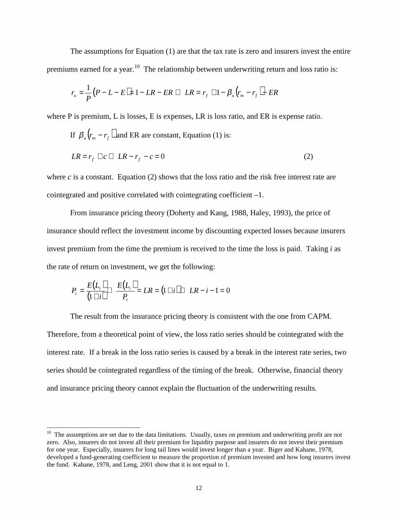
The assumptions for Equation (1) are that the tax rate is zero and insurers invest the entire

premiums earned for a year.10 The relationship between underwriting return and loss ratio is:

( ) ERLRELPP

ru −−=−−= 11 ( ) ERrrrLR fmuf −−−+=⇒ β1

where P is premium, L is losses, E is expenses, LR is loss ratio, and ER is expense ratio.

If ( )fmu rr −β and ER are constant, Equation (1) is:

0=−−⇒+= crLRcrLR ff (2)

where c is a constant. Equation (2) shows that the loss ratio and the risk free interest rate are

cointegrated and positive correlated with cointegrating coeff icient –1.

From insurance pricing theory (Doherty and Kang, 1988, Haley, 1993), the price of

insurance should reflect the investment income by discounting expected losses because insurers

invest premium from the time the premium is received to the time the loss is paid. Taking i as

the rate of return on investment, we get the following:

( )( )

( ) ( ) 0111

=−−⇒+==⇒+

= iLRiLRP

LE

i

LEP

t

ttt

The result from the insurance pricing theory is consistent with the one from CAPM.

Therefore, from a theoretical point of view, the loss ratio series should be cointegrated with the

interest rate. If a break in the loss ratio series is caused by a break in the interest rate series, two

series should be cointegrated regardless of the timing of the break. Otherwise, financial theory

and insurance pricing theory cannot explain the fluctuation of the underwriting results.

10 The assumptions are set due to the data limitations. Usually, taxes on premium and underwriting profit are notzero. Also, insurers do not invest all their premium for liquidity purpose and insurers do not invest their premiumfor one year. Especially, insurers for long tail l ines would invest longer than a year. Biger and Kahane, 1978,developed a fund-generating coefficient to measure the proportion of premium invested and how long insurers investthe fund. Kahane, 1978, and Leng, 2001 show that it is not equal to 1.

13

Results

1. AR(2) Process with and without a Time Trend

Tables 3 and 4 are the results of AR(2) processes for the loss ratio series with and without

a time trend. The coefficients of the second lag for AR(2) are not significant at the 5 percent

level with or without time trend for all countries.

Table 3. Loss Ratio Following an AR(2) Process Without Time TrendC AR(1) AR(2)

Coef t Coef t Coef tAdj. R2 F

Switzerland 57.4168 17.4238 0.8819 5.4372 -0.0050 -0.0322 0.7861 74.4986

Germany 70.5213 45.1453 0.7581 4.0438 -0.0716 -0.4210 0.5436 18.8645

USA 75.1603 19.7725 0.9780 5.9147 -0.1180 -0.7461 0.7825 72.9573

Japan 41.3424 14.5318 1.0443 5.7243 -0.2686 -1.4580 0.6784 32.6405

** is for 1 percent significant level, and * for 5 percent significant level.

Table 4. Loss Ratio Following an AR(2) Process With Time TrendC AR(1) AR(2) T

Coef t Coef t Coef t Coef tAdj. R2

Switzerland 47.6111 29.8029 0.7463 4.6598 -0.2177 -1.2993 0.3588 5.6851 0.8138

Germany 65.9844 29.7951 0.6948 3.6755 -0.2016 -1.0642 0.2351 2.0732 0.5607

USA 63.8226 24.8090 0.8598 5.0761 -0.2912 -1.6693 0.4574 4.3960 0.7989

Japan 49.5896 15.9702 0.9181 5.0706 -0.3457 -1.9558 -0.4592 -2.9314 0.7159

** is for 1 percent significant level , and * for 5 percent significant level .

2. Autocorrelation Function (ACF) and Partial Autocorrelation Function (PACF)

Figure 2 shows the ACF and PACF for Switzerland.11 The figure suggests that this series

is not stationary since the ACF decays slowly and the PACF is significant at one lag only.

3. Augmented Dickey-Fuller (ADF) Test

11 The ACF and PACF for the other three countries are similar as the ones for Switzerland. They are available onrequest from the authors.

14

We check whether the loss ratio series have unit roots by applying the ADF test.12 From

Table 5, we conclude to accept the null hypothesis that this series has a unit root. The results of

the ADF test are confirmed by the ones from the ACF and PACF.

Table 5. ADF Test for Loss Ratio

Switzerland Germany US JapanLR(-1) -0.1231 -0.3135 -0.1399 -0.2244

t-Statistic -1.6936 -2.7178 -1.9303 -2.0509

MacKinnon criti cal value is –2.9339 for 5 percent level.

Figure 2. ACF and PACF of the Loss Ratio for Switzerland

-1 -0.8 -0.6 -0.4 -0.2

0 0.2 0.4 0.6 0.8

1

1 3 5 7 9 11 13 15 17 19

ACF

-1 -0.8 -0.6 -0.4 -0.2

0 0.2 0.4 0.6 0.8

1

1 3 5 7 9 11 13 15 17 19

PACF

The dashed lines are plus and minus 2 standard deviations.

4. Chow Test and Switching Regression13

The methods we use to check for structural changes are the Chow test and Switching

Regression. Appendix A shows the steps for the Switching regression. The results are reported

as the F-statistic for the Chow Test and the Log Likelihood Ratio (LLR) for the switching

regression in Table 6. Figure 3 is the plot of the LLR for Switzerland. It shows that the

structural change happened gradually and reached the highest LLR in 1975.

12 The number of lags for the lagged difference term in the test is determined by the Akaike Information Criterion(AIC) and the Schwarz Bayesian Information Criterion (BIC). In our case, one lag is included.13 Judge, Griffiths, Hill , Lütkepohl, and Lee (1985) describe the method of switching regression, which seeks toidentify the switching point or year of structural change. Brown, Durbin, and Evans (1975) call this methodQuandt’s log-likelihood ratio technique because it was originally developed by Quandt (1958).

15

Figure 3. Log Likelihood Ratios from Switching Regressions for Switzerland

0

3

6

9

12

15 LL

R

1960 1965 1970 1975 1980 1985 1990 1995 Year

The dashed line is the 5% significant level.

We found that Germany also has a break in 1975, US has a break in 1986, and Japan has

a break in 1985. From Figure 1, the loss ratio of Switzerland was consistently lower than 55

percent before 1975 but higher than 55 percent after 1975. For Germany, its loss ratio is volatile

in the first sub-period and lower than 70 percent, but it is above 70 percent in the second sub-

period. The Japanese loss ratio is above 40 percent in the first period but lower than that in the

second period. Using combined ratio, Leng(2000) found a break for the US in 1981. Obviously,

the years of breaks are different for the combined ratio and for the loss ratio in the US because

the expense ratio is not constant. However, combined ratio is more suitable for studying

structural change rather than the loss ratio to reflect the fluctuation of the underwriting results.

Unfortunately, underwriting expenses are only available for the US data. Different variables

with different years of break in the US helps us to be aware of the possible bias from the use of

the loss ratio as a variable in the analysis for the other countries.

16

Table 6. The Results from Chow Test and Switching RegressionSwitzerland Germany US-LR Japan

F-statistic LLR F-statistic LLR F-statistic LLR F-statistic LLR

1960 0.4038 1.3951 0.6231 2.13321961 0.2821 0.9796 0.6797 2.32171962 0.7216 2.4607 0.8090 2.74891963 0.6949 2.3721 0.8558 2.90241964 0.3303 1.1445 0.5422 1.86241965 0.5285 1.8164 0.4229 1.45981966 0.9325 3.1527 0.4441 1.53191967 1.5233 5.0315 0.9203 3.11301968 1.2206 4.0797 0.7644 2.60201969 1.5448 5.0983 0.6883 2.35021970 1.8103 5.9140 0.8980 3.1725 0.6129 2.0994 1.8854 6.32261971 0.7954 2.7042 0.3413 1.2444 0.8648 2.9318 2.2699 7.46771972 1.6835 5.5266 1.5674 5.3427 1.6044 5.2829 1.8319 6.16011973 1.9637 6.3781 0.9241 3.2602 2.2334 7.1813 1.2670 4.38771974 4.8762** 14.3180** 1.6857 5.7110 2.0809 6.7292 1.0753 3.76241975 4.9980** 14.6187** 2.4210 7.9064** 1.1673 3.9096 1.7553 5.92551976 1.4836 4.9079 2.1613 7.1487 1.1934 3.9931 1.6773 5.68511977 3.5371* 10.8570* 1.6392 5.5667 1.3329 4.4353 1.9714 6.58261978 2.4211 7.7315 1.8212 6.1272 2.5279 8.0411* 2.0570 6.83891979 2.8543 8.9730* 0.7425 2.6460 3.0213* 9.4421* 2.0816 6.91231980 2.8495 8.9595* 1.0871 3.8011 2.6457 8.3798* 2.0425 6.79571981 2.8717 9.0223* 0.8162 2.8967 2.8616 8.9937* 2.1531 7.12431982 2.7764 8.7526* 0.5442 1.9612 2.8646 9.0022* 2.7120 8.7341*1983 2.5352 8.0622* 0.4497 1.6292 2.4170 7.7195 3.7040* 11.4002**1984 2.5388 8.0724* 0.5006 1.8084 2.3232 7.4455 4.0146* 12.1900**1985 1.4785 4.8921 0.4943 1.7863 2.6860 8.4953* 4.1556* 12.5420**1986 1.5292 5.0500 0.6721 2.4045 4.0817* 12.3001** 3.6948* 11.3766**1987 1.4654 4.8511 0.5330 1.9220 2.5980 8.2430* 1.9464 6.50731988 1.5789 5.2040 0.4573 1.6560 3.0800* 9.6055* 1.9169 6.41831989 1.9268 6.2669 2.8740* 9.0287* 1.2504 4.33391990 2.5233 8.0277* 2.7712 8.7379* 2.0069 6.68911991 1.6298 5.3614 3.4398* 10.5939* 4.5257* 13.4473**1992 0.6806 2.3248 3.4562* 10.6385* 1.8046 6.07661993 0.3811 1.3178 4.1916* 12.5851** 0.0717 0.26571994 0.3852 1.3317 0.8429 2.8601 0.1478 0.5451

1995 0.9841 3.3203 0.5116 1.7595 0.1109 0.4099

17

Discussion

The break in the loss ratio for Switzerland and Germany is in 1975, which coincides with

a serious recession in these two countries. The pattern of the loss ratio series seems to support

the hypothesis that this recession may have caused the structural change. If the recession did

cause the break in the insurance industry, the loss ratios should be cointegrated with GDP or/and

CPI for the whole period regardless of the time of the break. If the cause of the break is due to

the change of regulations or competitiveness in the property-liabili ty insurance industry, the

relationship between loss ratio and interest rate should change after the break. This may be the

explanation for the break for the US since regulations changed from bureau rating to competitive

pricing and competition in the property-liabili ty insurance market forced insurers to reflect

investment income into the rate-making process during the end of the 70s to the beginning of the

80s.14 It is also possible that the liabili ty crisis from 1984 to 1985 effected underwriting

standards for insurers. If this is the case, the break should only affect the liabili ty part of

business. However, most lines of business include both property and liabilit y parts and they are

diff icult to separate. Based on the available data, the loss ratio should be cointegrated with the

ratio of premium to surplus, which is used to measure the insurers’ risk taking behavior. 15

In Japan, the loss ratio does not behave as the other three countries’ loss ratios: its loss

ratio goes down after the break. Therefore, the cause of the break in Japan must be different

from the ones for the other countries. In 1980, savings-type insurance policies started to become

popular in the Japanese non-li fe insurance market. From 1985 to 1994, it reached a share of

14 Self-insurance and captives are the alternatives for insurance. Insurers use price competition and reflectinvestment income into premium to decrease consumers switching to alternative methods. However, self-insuranceand captives gain their popularity when the insurance market becomes a hard market.

15 The premium to surplus ratio is one of the tests used in the Insurance Regulatory Information System (IRIS) topredict insurers’ financial strength to prevent insolvency. If an insurer has a premium to surplus ratio of more than3, which is considered that the insurer is engaged in a high risk underwriting practice, the insurer fails this test.

18

about 30 to 45 percent of the non-li fe insurance premium. The premium for savings-type

insurance contains risk premium and savings, which accounts for more than 90 percent of the

premium. If no covered incident occurred during the policy period, insurers refund the savings

portion of the premium and guarantee the payment of interest to the policyholder after the policy

matures. If a covered incident occurred, the claims are determined by the policy agreement.

Since internal capital includes a savings portion of the premium, internal capital should increase

more than the loss ratio when the savings type insurance became popular. Therefore, if the

popularity of the savings-type insurance caused the break in Japan, the relationship between loss

ratio and internal capital should change. Another thing worth mentioning is that, due to the

regulatory requirements, the US insurers invest the majority of assets in bonds which makes the

interest rate important to their underwriting results. On the other hand, Japanese insurers invest

much more of their assets in stocks, loans, and real estate. Therefore, economy condition should

have more effect on insurers’ income than the interest rate does.16

Further Analysis

In this section, we test for the possible reasons for the cause of the break for each

country. For Switzerland, the loss ratio series is not stationary before the break, but stationary

after the break. Also, the loss ratio after the break follows an AR(2) process.17 Interestingly, the

interest rate also has a break in 1975. Cointegration analysis shows that loss ratio and interest

rate after the break are cointegrated. This implies that the break is most likely caused by

regulation changes. The loss ratio is also cointegrated with GDP, but this relationship changed

16 In 1995, US insurers invested 60.7% of their assets in bonds. Japanese insurers, on the other hand, invest only18% of their assets in bonds.17 LR = 59.91 + 0.78 * LR(t-1) – 0.43 * LR(t-2) with 0.4 R2, and cycle length is 4.8. All the coefficients aresignificant and in the theoretical range proposed by C&O, 1987.

19

with the break. It seems that the condition of the economic recession did have an impact on the

insurance industry.

For Germany, the loss ratio is cointegrated with the interest rate only after the break with

cointegrating coeff icient close to –1, which is what insurance pricing theory suggests.

For the US, the loss ratio is neither cointegrated with interest rate nor with the premium

to surplus ratio. This may be caused by the small sample in the second period. However, the

loss ratio is cointegrated with internal capital, what supports the capacity theory. Looking at the

relationship between premium written and internal capital, we find that internal capital for the

second period is twice as high as the one for the first period for the same amount of premium.

This seems to be the result of regulatory requirements.

For Japan, the cointegrating relationship between the loss ratio and GDP changed due to

the break18 and the one between loss ratio and interest rate only exists before the break. This is

possibly the joint effect of the economic situation and regulations.

Conclusions

Previous studies for underwriting cycles in property-liabili ty insurance show that

underwriting profit follows an AR(2) process. Leng (2000) shows that the combined ratio for the

United States has a break in 1981. Meier (2001) also suggested a break in 1981 in the US data.

In our paper, we look into the special characteristics of property-liabili ty insurance

markets for the four countries, Switzerland, USA, Germany and Japan, and their loss ratio series.

We find that the insurance markets of Switzerland and Germany are closely tied, but they are not

tied to the US and Japan. Also, Japanese loss ratio series is negatively correlated with the series

18 Before the break, loss ratio and GDP move into opposite directions, but after the break, two variables move intothe same direction.

20

of the other three countries. This shows that the underwriting cycle in Japan has a different

phase than the cycles in the other countries. Therefore, international operation has a

diversification effect which can be used to reduce the fluctuation of underwriting results.

The loss ratio series from the four countries are neither stationary nor stable. Testing for

possible structural changes, we find that all four countries have breaks, but in different years.

For Switzerland and Germany, the break is in 1975. For Japan and the US, the breaks are in

1985 and 1986, respectively. This shows that even though underwriting cycles are an

international phenomenon, they are not caused by the same international/global effect. More

likely, the structural changes in these countries are caused by the economic environment and

regulation in each country.

From financial theory and insurance pricing theory, the loss ratio and the interest rate

series should be cointegrated. However, empirically the two series are not cointegrated at the 5

percent level. This is interesting for future research on possible explanations for the

contradiction between theory and empirical results.

21

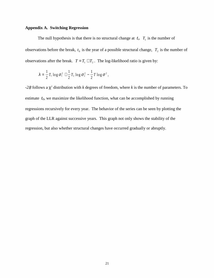
Appendix A. Switching Regression

The null hypothesis is that there is no structural change at t0. 1T is the number of

observations before the break, 0t is the year of a possible structural change, 2T is the number of

observations after the break. 21 TTT += . The log-likelihood ratio is given by:

λ σ σ σ= + −1

2

1

2

1

21 12

2 22 2T T Tlog log log ,

-28 follows a χ2 distribution with k degrees of freedom, where k is the number of parameters. To

estimate t0, we maximize the likelihood function, what can be accomplished by running

regressions recursively for every year. The behavior of the series can be seen by plotting the

graph of the LLR against successive years. This graph not only shows the stability of the

regression, but also whether structural changes have occurred gradually or abruptly.

22

References

Balke, N., 1991, Modeling Trend in Macroeconomics Time Series, Economic Review, FederalReserve Bank of Dallas, May, pp. 19-33.

Banerjee, A., J. Dolado, G. W. Galbraith, and D. F. Hendry, 1993, Co-integration, Error-Correction and the Econometric Analysis of Non-Stationary Data, Oxford UniversityPress.

Banerjee, A., R. L. Lumsdaine, and J. H. Stock, 1992, Recursive and Sequential Tests of theUnit-Root and Trend-Break Hypotheses: Theory and International Evidence, Journal ofBusiness and Economic Statistics, Vol.10, pp.271- 288.

Biger N. and Y. Kahane, 1978, Risk Considerations in Insurance ratemaking, Journal of Riskand Insurance, Vol. 45, pp. 121-132.

Box, G., and G. Jenkins, 1970, Time Series Analysis: Forecasting and Control, Holden-Day, Inc.

Brown, R. L., J. Durbin, J. M. Evans, 1975, Techniques for Testing the Constancy of RegressionRelationships Over Time, Journal of Royal Statistical Society, Series B, Vol. 37, pp. 149-172.

Charemza, W. W. and D. F. Deadman, 1997, New Directions in Econometric Practice: Generalto Specific Modelling, Cointegration and Vector Autoregression, Edward ElgarPublishing Limited.

Chen, R., K. Wong, and H. Lee, 1999, Underwriting Cycles in Asian, Journal of Risk andInsurance, Vol. 66, pp. 29-47.

Cummins, D., 1988, Risk-Based Premiums for Insurance Guaranty Funds, Journal of Finance,Vol. 43, pp. 823-839.

Cummins, D. and F. Outreville, 1987, An International Analysis of Underwriting Cycles inProperty-Liability Insurance, Journal of Risk and Insurance, Vol. 54, pp. 246-262.

Diebold, F., and M. Nerlove, 1990, Unit Roots in Economic Time Series: A Selective Survey, inThomas Fomby and George Rhodes, eds. Advances in Econometrics, Vol. 8, pp. 3-69,JAI Press Inc.

Doherty, N., and H. Kang, 1988, Interest Rates and Insurance Price Cycles, Journal of Bankingand Finance, Vol. 12, pp., 199-214.

Fairley, W. B., 1979, Investment Income and Profit Margins in Property-Liability Insurance:Theory and Empirical Results, Bell Journal of Economics, Vol. 10, pp. 192-210.

Fama, E. F., and M. C. Jensen, 1983a, Agency Problems and Residual Claims, Journal of Law

23

and Economics, Vol. 26, pp. 327-349.

Fama, E. F., and M. C. Jensen, 1983b, Separation of Ownership and Control, Journal of Law andEconomics, Vol. 26, pp. 301-325.

Fields, J., and E. C. Venezian, 1989, Profit Cycles in Property-Liabili ty Insurance: ADesegregated Approach, Journal of Risk and Insurance, Vol. 56, pp. 312-319.

Fung, H. G., G. C. Lai, G. A. Patterson, and R. C. Witt, 1998, Underwriting Cycles in Propertyand Liabili ty Insurance: An Empirical Analysis of Industry and By-Line Data, Journal ofRisk and Insurance, Vol. 65, pp. 539-562.

Grace, M., and J. Hotchkiss, 1995, External impacts on the Property/Liabilit y Insurance Cycle,Journal of Risk and Insurance, Vol. 62, pp. 738-754.

Greene, Willi am, 1993, Econometric Analysis, second edition, Macmillan Inc.

Gron, A., 1994, Capacity Constraints in Property-Casualty Insurance Markets, Rand Journal ofEconomics, Vol. 25, pp. 110-127.

Gujarati, D., 1995, Basic Econometrics, third edition, McGraw-Hill Inc.

Haley, J., 1993, A Cointegration Analysis of the Relationship Between Underwriting Marginsand Interest Rate: 1930-1989, Journal of Risk and Insurance, Vol. 60, pp. 480-493.

Haley, J., 1995, A By-Line Cointegration Analysis of Underwriting Margins and Interest Ratesin the Property-Liabili ty Insurance Industry, Journal of Risk and Insurance, Vol. 62, pp.755-63.

Hamilton, J. D., 1994, Time Series Analysis, Princeton University Press, Princeton, NJ.

Hammond, J. D., E. R. Melander, and N. Shilli ng, 1976, Risk, Return, and the CapitalMarket: The Insurer Case, Journal of Financial and Quantitative Analysis, Vol.11,pp.115-131.

Harrington, S., and T. Yu, 2000, Do Underwriting Margins Have Unit Roots?, paper presented inthe ARIA conference, Baltimore, MA.

Hartwig, R. P., 2002, The Long Shadow of September 11: Terrorism and Its Impacts onInsurance and Reinsurance Markets, presentation fromwww.iii .org/media/hottopics/insurance/sept11.

Hill , R. D., 1979, Profit Regulation in Property-Liabili ty Insurance, Bell Journal of Economics,Vol. 10, pp. 172-191.

Hill , R. D., and Modigliani, F., 1981, “The Massachusetts Model of Profit Regulation in Nonli fe

24

Insurance: An Appraisal and Extensions,” manuscript presented at the 1982Massachusetts automobile hearings, reprinted in Fair Rate of Return in Property-LiabilityInsurance, J. D. Cummins and S. A. Harrington (editors), Kluwer-Nijhoff, Boston, 1986.

Judge G. G., W. E. Griff iths, R. C. Hill , H. Lutkepohl, and T. Lee, 1985, The Theory andPractice of Econometrics, second edition, John Wiley and Sons, Inc.

King, R., C. Plosser, J. Stock, and M. Watson, 1991, Stochastic Trend and EconomicFluctuations, The American Economic Review, Vol. 81, pp. 819-841.

Kraus, A., and S. A. Ross, 1980, The Determination of Fair Profits for the Property-LiabilityInsurance Firm, MRR Inc.

Kraus, A., and S. A. Ross, 1982, The Determination of Fair Profits for the Property-Liabili tyInsurance Firm, Journal of Finance, Vol. 37, pp.1015-1028.

Lai, G. C., and R. Witt, 1992, Changed Insurer Expectations: An Insurance Economics View ofthe Commercial Liabili ty Insurance Crisis, Journal of Insurance Regulation, Vol. 10, pp.342-383.

Lamm-Tennant, J., and M. Weiss, 1997, International Insurance Cycles: RationalExpectations/Institutional Intervention, Journal of Risk and Insurance, Vol. 64, pp. 415-439.

Leng, Chao-Chun, 2000. “Underwriting Cycles: Stationarity and Stabili ty,” presented at theAnnual Meeting of the American Risk and Insurance Association, Baltimore, MD.

Leng, Chao-Chun, 2001. An Examination of the Fluctuations in Underwriting Profits ofProperty-Liability Insurers, Ph.D. dissertation, Temple University, Philadelphia, PA.

Leng, C. 2000, M. Powers, and E. Venezian, 2002, Did Regulation Change competitiveness inProperty-Liabili ty Insurance?, Journal of Insurance Regulation, forthcoming.

Meier, Ursina B. (2001): Underwriting Cycles in Property-Liabili ty Insurance: Do they (still )exist? mimeo

Myers, D., and C. W. Smith, Jr., 1988, Ownership Structure Across Lines of Property-CasualtyInsurance, Journal of Law and Economics, Vol. 31, pp. 351-378.

Myers S. C. and R. A. Cohn, 1981, A Discounted Cash Flow Approach to Property-Liabili tyInsurance Rate Regulation, manuscript presented at the 1982 Massachusetts automobilehearings, reprinted in Fair Rate of Return in Property-Liability Insurance, J. D. Cumminsand S. A. Harrington (editors), Kluwer-Nijhoff , Boston, 1986.

Nelson, C., and C. Plosser, 1982, Trends and Random Walks in Macroeconomic Time Series,Journal of Monetary Economics, Vol. 10, pp. 139-162.

25

Niehaus, G., and A. Terry, 1993, Evidence on the Time Series Properties of Insurance Premiumsand Causes of the Underwriting Cycle: New Support for the Capital Market ImperfectionHypothesis, Journal of Risk and Insurance, Vol. 60, pp. 466-479.

Perron, P., 1989, The Great Crash, the Oil Shock and the Unit Root Hypothesis, Econometrica,Vol. 57, pp. 1361-1401.

Poirier, D. J., 1976, The Econometrics of Structural Change: with Special Emphasis on SplineFunctions, North-Holland Publishing Company.

Quandt, R. E., 1958, The Estimation of the Parameters of a linear Regression System Obeyingtwo Separate Regimes, Journal of American Statistical Association, Vol. 53, pp. 873-880.

Quirin, D. G., and W. R. Waters, 1975, Market Efficiency and the Cost of Capital: The StrangeCase of Fire and Casualty Companies, Journal of Finance, Vol. 30, pp. 427-450.

Schmidt, P., 1990, Dickey Fuller Tests With Drift, in Thomas Fomby and George Rhodes, Eds.Advances in Econometrics, Vol. 8, pp. 161-200, JAI Press Inc.

Slater, C. M. and C. J. Strawser, editors, 1999, Business Statistics of the United States, (5thEdition), Bernan Press, Lanham, MD.

Stock, J., and M. Watson, 1988, Variable Trends in Economic Time Series, Journal of EconomicPerspectives, Vol. 2, pp. 147-174.

Venezian, E., 1969, The Effects of Changing Capital Levels on Insurance Stockholder’s Returnand Risk, in Studies on the Profitability, Industrial Structure, Finance, and Solvency ofthe Property and Liability Insurance Industry, Arthur D. Little, Inc., Cambridge, MA.

Venezian, E., 1985, Ratemaking Methods and Profit Cycles in Property and Liabili ty Insurance,Journal of Risk and Insurance, Vol. 52, pp. 477-500.

Wei, W., 1990, Time Series Analysis: Univariate and Multivariate Methods, Addison-WesleyPub, Redwood City, CA.

Winter, R., 1988, The Liabili ty Crisis and the Dynamics of Competitive Insurance Market, YaleJournal on Regulation, Vol. 5, pp. 455-499.

Winter, R., 1991, Solvency Regulation and the Property-Liabili ty “ Insurance Cycle”, EconomicInquiry, Vol. 29, pp. 458-471.

Zivot, E., and D. W. K. Andrews, 1992, Further Evidence on the Great Crash, the Oil PriceShock, and the Unit Root Hypothesis, Journal of Business and Economic Statistics, Vol.10, pp. 251-270.

Analysis of Multi-National Underwriting Cycles in Property

Documents

Transcript of Analysis of Multi-National Underwriting Cycles in Property