Automated Iris Recognition Technology & Iris Biometric System

TUM Department of Civil, Geo and Environmental Engineering
Chair of Computational Modeling and Simulation
Prof. Dr.-Ing. Andre Borrmann
Analysis of Methods for Automated Symbol
Recognition in Technical Drawings
Deian Stoitchkov
Bachelorthesis
for the Bachelor of Science Course Civil Engineering
Author: Deian Stoitchkov
Student ID:
Supervision: Prof. Dr.-Ing. Andre Borrmann
Simon Vilgertshofer, M.Sc.
Date of Issue: 14. November 2017
Date of Submission: 14. April 2018

Abstract
Even in today’s modern world, in which almost everything is digitized, many technical draw-
ings are still only available in paper form. The main reason for this is that most of the
infrastructure we see was built before the widespread availability of computers. Many of
these drawings are now being digitized so as to be used by modern computer programs.
Much of the digitization process of a technical drawing consists of recognizing and locating
different symbols which is often a difficult and time-consuming task. Therefore, this work
aims to find a method of automating the process and drastically reducing the processing time.
This work begins with some basic computer vision techniques that can be very accurate,
but only under certain conditions. Next, a more complex and versatile method of machine
learning is proposed (Cascade Classifiers), which can be used in a multitude of situations.
However, the Cascade Classifiers method still faces difficulties if a simple symbol with too few
features needs to be recognized. Therefore, another technique is proposed that uses artificial
neural networks to find symbols in large technical drawings. This method includes training
that requires a powerful graphics processing unit (GPU), but shows very promising results.
Ultimately, a graphical user interface (GUI) is created for the program which enables simple
operations without in-depth programming knowledge.

Zusammenfassung
Auch in der heutigen modernen Welt, in der fast alles digitalisiert ist, gibt es viele tech-
nische Zeichnungen nur noch in Papierform. Der Hauptgrund dafur ist, dass der großte
Teil der Infrastruktur, die wir sehen, vor der weit verbreiteten Verfugbarkeit von Computern
aufgebaut wurde. Viele dieser Zeichnungen werden jetzt digitalisiert, um von modernen Com-
puterprogrammen verwendet zu werden. Ein großer Teil des Digitalisierungsprozesses einer
technischen Zeichnung besteht darin, verschiedene Symbole zu erkennen und zu lokalisieren,
was oft eine schwierige und zeitraubende Aufgabe ist. Ziel dieser Arbeit ist es daher, eine
Methode zu finden, den Prozess zu automatisieren und die Bearbeitungszeit drastisch zu re-
duzieren.
Diese Arbeit beginnt mit einigen grundlegenden Computer-Vision-Techniken, die sehr genau
sein konnen, aber nur unter bestimmten Bedingungen. Als nachstes wird eine komplexere
und vielseitigere Methode des maschinellen Lernens vorgeschlagen (Cascade Classifiers), die
in einer Vielzahl von Situationen eingesetzt werden kann. Die Cascade Classifiers Methode
hat jedoch immer noch Schwierigkeiten, wenn ein einfaches Symbol mit zu wenigen Merk-
malen erkannt werden soll. Daher wird eine andere Technik vorgeschlagen, die kunstliche
neuronale Netzwerke verwendet, um Symbole in großen technischen Zeichnungen zu finden.
Diese Methode beinhaltet ein Training, das einen leistungsfahigen Grafikprozessor (GPU)
erfordert, aber sehr vielversprechende Ergebnisse zeigt. Schließlich wird eine grafische Be-
nutzeroberflache (GUI) fur das Programm erstellt, die einfache Operationen ohne tiefere
Programmierkenntnisse ermoglicht.

1
Contents
1 Introduction 2
2 OpenCV and Python 3
2.1 Template Matching . . . . . . . . . . . . . . . . . . . . . . . . . . . . . . . . . 3
2.1.1 Theory . . . . . . . . . . . . . . . . . . . . . . . . . . . . . . . . . . . 4
2.1.2 Implementation and results . . . . . . . . . . . . . . . . . . . . . . . . 5
2.1.3 Improvements . . . . . . . . . . . . . . . . . . . . . . . . . . . . . . . . 9
2.1.4 Limitation . . . . . . . . . . . . . . . . . . . . . . . . . . . . . . . . . . 13
2.2 Contours . . . . . . . . . . . . . . . . . . . . . . . . . . . . . . . . . . . . . . 14
2.2.1 Theory . . . . . . . . . . . . . . . . . . . . . . . . . . . . . . . . . . . 14
2.2.2 Implementation and results . . . . . . . . . . . . . . . . . . . . . . . . 18
2.2.3 Limitation . . . . . . . . . . . . . . . . . . . . . . . . . . . . . . . . . . 23
2.3 Cascade Classifiers . . . . . . . . . . . . . . . . . . . . . . . . . . . . . . . . . 24
2.3.1 Theory . . . . . . . . . . . . . . . . . . . . . . . . . . . . . . . . . . . 24
2.3.2 Implementation and results . . . . . . . . . . . . . . . . . . . . . . . . 26
2.3.3 Limitation . . . . . . . . . . . . . . . . . . . . . . . . . . . . . . . . . . 32
3 Neural networks with Keras and TensorFlow 33
3.1 The theory behind Convolutional Neural Network . . . . . . . . . . . . . . . . 34
3.2 Implementation and Results . . . . . . . . . . . . . . . . . . . . . . . . . . . . 38
3.3 Limitations . . . . . . . . . . . . . . . . . . . . . . . . . . . . . . . . . . . . . 45
4 Practical implementation with graphical user interface 46
4.1 Windows Presentation Foundation and Emgu CV for Template Matching . . 47
4.2 Python and Tkinter for Neural Networks . . . . . . . . . . . . . . . . . . . . . 48
5 Conclusion 50

2
Chapter 1
Introduction
With the help of modern day computer programs, planning and construction has become a
simpler and often faster process. To use these helpful programs, most of the data is being
digitized. However, digitizing old technical drawings can be a very tedious task as many
different symbols have to be manually recognized and located. This work aims to find the
best technique to automate the process of manually searching for symbols.
Symbol recognition is a well-known challenge yet few techniques have been proposed. In
Weber et al. (2012) a template matching operator HMTAIO (Hit-or-Miss Transform Adapted
to Information Overlapping) is described. ”The advantage of our approach compared to
correlation methods is its robustness to occlusion and overlapping. Moreover, our method is
enough robust to be applied on real documents unlike the majority of previous ones”. The
results show a very good spotting rate of 98-100% even with a variety of symbols. Another
technique is proposed in Luqman et al. (2009) which represents symbols by their graph based
signatures. ”A graphic symbol is vectorized and is converted to an attributed relational
graph, which is used for computing a feature vector for the symbol”. Again, this method
shows a very high recognition rate and is rotation and scale invariant. Different symbol
spotting methods are also described in Rusinol et al. (2006) and Nayef et al. (2012).
However, this work is not based on these techniques. First, some basic computer vision tech-
niques will be tested, followed by more sophisticated methods with artificial neural networks,
none of which can be found in the previously mentioned papers. In the second chapter, some
useful functions of the computer vision library OpenCV will be used to find symbols in tech-
nical drawings. In the first two sections, techniques are proposed which don’t require training
and can be implemented with speed and efficiency but only work under certain conditions.
In the third section, a more complex and versatile method is described which shows good
results but still can’t be used for specific symbols. The last technique proposed in this work,
which uses artificial neural networks, shows very promising results under many circumstances
and has almost no implementational limits.

3
Chapter 2
OpenCV and Python
OpenCV is an open source computer vision library. The open source license for OpenCV
means it is free for both academic and commercial use. It is written in C++ and can also be
used in Python, Java and MATLAB. There are wrappers for different languages such as C#,
Perl and Ruby. With over 500 built-in functions, OpenCV makes challenging tasks easy and
fast to program. Therefore, OpenCV is the choice for building a symbol detection program.
In this chapter, different methods and functions from the OpenCV library will be used. Some
of the most important ones are Template Matching, Contours and Haar Cascade methods.
They are all easily accessible and therefore fast to implement.
Python is a high-level programming language that makes writing programs easier with fewer
lines of code and has better code readability, which makes it perfect for non-professional
programmers. For these reasons, it is the natural choice for programming and testing the
methods described above.
2.1 Template Matching
The descriptions in this chapter are based on the explanations in Kaehler et al. (2016). Also,
some online sources of information were used such as OpenCV (3.4.0) and OpenCV (2.4).
Template Matching is a method for searching and localization of a template image in a
larger image. This is made by sliding the template image over the input (larger) image
and comparing them at every position. In this case, the term ”sliding” means moving the
patch (template image) one pixel at a time - left to right, up and down. There are different
comparison methods implemented in OpenCV, which will be explained in the next section.

2.1. TEMPLATE MATCHING 4
2.1.1 Theory
The result of the Template Matching method is a grayscale (also known as black-and-white
or monochrome) image, where each pixel shows how much of the surroundings of that pixel
match the template. The output image is a size of (W-w+1, H-h+1), where W and H are
the width and the height of the input image, w and h are the width and the height of the
template image. It is important to note, that the output image is smaller than the input
image. There are 3 different matching methods in OpenCV and for each one of them there
is a normalized version. The normalized versions improve the matching by different lighting
conditions as explained in Rodgers et al. (1988). The matching methods in OpenCV are
listed below:
- Square Difference Matching Method: TM SQDIFF
The squared differences are matched, as a result a perfect match will be 0 and a poor
match will be a large number.
R(x, y) =∑x′,y′
(T (x′, y′)− I(x+ x′, y + y′))2 (2.1)
- Normalized Square Difference Matching Method: TM SQDIFF NORMED
A perfect match is again 0, but a perfect mismatch will be 1.
R(x, y) =
∑x′,y′ (T (x′, y′)− I(x+ x′, y + y′))2√∑
x′,y′ (T (x′, y′)2 ·∑
x′,y′ I(x+ x′, y + y′)2(2.2)
- Correlation Matching Method: TM CCORR
The match is made by a multiplication, resulting in a big number for a good match and
0 for a complete mismatch.
R(x, y) =∑x′,y′
(T (x′, y′) · I(x+ x′, y + y′)) (2.3)
- Normalized Cross-Correlation Matching Method: TM CCORR NORMED
A complete mismatch with this method will be again 0, but a perfect match will be 1.
R(x, y) =
∑x′,y′ (T (x′, y′) · I(x+ x′, y + y′))√∑
x′,y′ (T (x′, y′)2 ·∑
x′,y′ I(x+ x′, y + y′)2(2.4)
- Correlation Coefficient Matching Method: TM CCOEFF
The result of this method will be a large positive number for a good match and a large
2.1. TEMPLATE MATCHING 5
negative number for a poor match.
R(x, y) =∑x′,y′
(T ′(x′, y′) · I ′(x+ x′, y + y′)) (2.5)
- Normalized Correlation Coefficient Matching Method: TM CCOEFF NORMED
A perfect match will be 1 and a perfect mismatch -1.
R(x, y) =
∑x′,y′ (T ′(x′, y′) · I ′(x+ x′, y + y′))√∑
x′,y′ (T ′(x′, y′)2 ·∑
x′,y′ I′(x+ x′, y + y′)2
(2.6)
where T is the template image, I is the input image, R is the result image and
T ′(x′, y′) = T (x′, y′)− 1/(w · h) ·∑x′′,y′′
T (x′′, y′′)
I ′(x+ x′, y + y′) = I(x+ x′, y + y′)− 1/(w · h) ·∑x′′,y′′
I(x+ x′′, y + y′′).
After testing all of the methods explained above, the methods ”TM SQDIFF NORMED” and
”TM CCOEFF NORMED” were found to be the most accurate and therefore will be used
in the next section. Both methods performed well by finding most symbols while keeping the
false positives low (explained in more detail further in this chapter).
2.1.2 Implementation and results
The code in Listing 2.1 below will be explained through the whole section and will not be
referenced further.
1 . . .
2 img co lo r = cv2 . imread ( ’ input1 . png ’ )
3 img gray = cv2 . cvtColor ( img co lor , cv2 .COLOR BGR2GRAY)
4
5 template = cv2 . imread ( ’ template . png ’ )
6 temp gray = cv2 . cvtColor ( template , cv2 .COLOR BGR2GRAY)
7
8 r e s = cv2 . matchTemplate ( img gray , temp gray , cv2 .TM SQDIFF NORMED)
9
10 thre sho ld = 0 .2
11 l o c = np . where ( r e s <= thre sho ld )
12
13 f i l e = open ( ’ r e s u l t s . txt ’ , ’w’ )
14 h ,w = temp gray . shape
2.1. TEMPLATE MATCHING 6
15 num = 0 ;
16
17 f o r x , y in z ip ( l o c [ 1 ] , l o c [ 0 ] ) :
18
19 num=num+1;
20
21 cv2 . r e c t a n g l e ( img co lor , (x , y ) , ( x+w, y+h) , (0 , 0 , 255) , (2 ) )
22
23 x cen t e r = i n t ( x+w/2)
24 y cen t e r = i n t ( y+h/2)
25
26 text = ’ Match No. : ’+ s t r (num)+’−>x−coo rd ina t e s : ’+ s t r ( x c en t e r ) + ’ , y−coo rd ina t e s : ’+ s t r ( y c en t e r ) +’\n ’
27 f i l e . wr i t e ( t ex t )
28
29 f i l e . c l o s e ( )
30 . . .
Listing 2.1: Program code
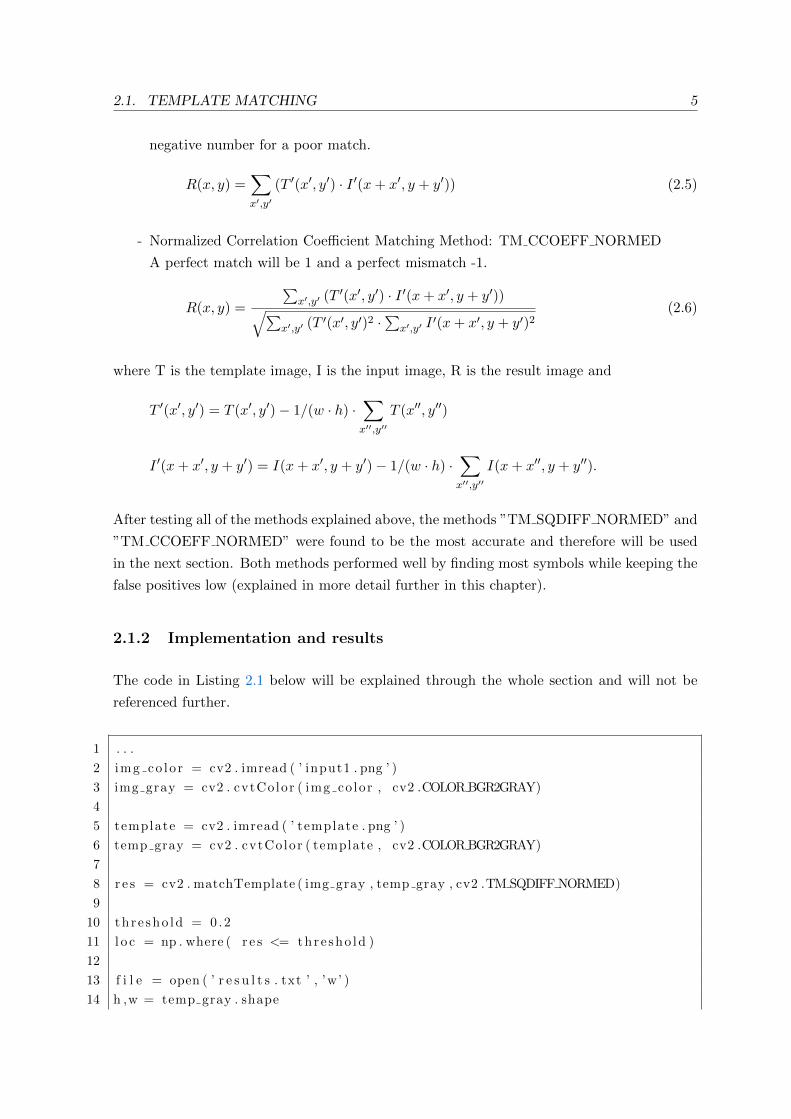
In this section, the Template matching method will be used on a given image with the help
of the OpenCV library. A part of a telecommunication technical drawing will be used as an
input image, which is shown in Figure 2.1. A small cut from the input image of the exact
symbol has been chosen as a template image - Figure 2.2.
Figure 2.1: Input image

2.1. TEMPLATE MATCHING 7
Figure 2.2: Template image
In order to be accessed, the OpenCV and NumPy packages are imported into the program
at the beginning. The NumPy library has powerful and easy to use functions to operate
with arrays. This is very important for this task as every image is basically an array, which
describes the pixels of the image.
The next step is to read the images from the source with the function ”cv2.imread”. The
function loads an image from the specified file and returns a 3-channel color image (line 2).
The colored image is then converted to a grayscale image with the ”cv2.cvtColor” function,
which uses the cv2.COLOR BGR2GRAY method (line 3). This makes the search for the
symbol faster and more accurate. The same steps are then taken for the template image
(lines 5 and 6).
On the next line (line 8) the function ”cv2.matchTemplate” is called with the comparison
method TM SQDIFF NORMED (Equation 2.2). The result is a black-and-white image,
where the brightest locations indicate the highest matches. They are marked with red circles
in Figure 2.3. With the method used, the result image has values between 0 and 1, where 0
will be a perfect match and 1 a complete mismatch.
Figure 2.3: Result image

2.1. TEMPLATE MATCHING 8
As all of the images are represented as arrays, they could be easily accessed and transformed
with the help of the NumPy library. The function ”np.where” is used to find the locations
of the highest matches in the result image (lines 10 and 11). Next, a threshold has to be
set, below which the result will be assumed as a correct match. In this case, the threshold
is set to 0.2, which means that all the elements of the array that have a value below 0.2 are
assumed to be a proper match. Because 0 is a perfect match and 1 is a complete mismatch,
this means that all the results with higher than 80% match will be accepted as a correct
match. All of the correct matches are then stored in an array called ”loc”. The x-coordinates
of the matches are stored in loc[1] and the y-coordinates in loc[0] respectively.
The next step is to iterate through all of the correct matches, where ”x” and ”y” are the
coordinates of the upper left corner of a given match. The size of the template image is
required to draw a rectangle around every correct match. It can be found with the help of
the function ”shape” as shown in (line 14). The function returns the height and the width
of the given image, in this case the template image. A rectangle can be then drawn over
the input image with the help of the function ”cv2.rectangle” (line 21). It is important to
note that a new image will not be created, but instead the original image will be replaced.
For this function 5 arguments are required. The first is the input image, the second is the
upper-left corner of the rectangle, the third is the bottom-right corner, the fourth is the color
of the rectangle in a BGR (Blue-Green-Red) color space and the fifth is the thickness of the
lines that make up the rectangle.
A text file containing all the matches with the corresponding coordinates will be created in
addition to the drawn rectangles. The text file will be saved in the directory of the program
with the name ”results.txt”. The built-in function in Python ”open” opens a file with the
given name or if the file doesn’t exist it creates one (line 13). The center point of every match
is then calculated (lines 23 and 24). Ultimately, a string is created with the corresponding
number and coordinates of a match and is saved in the text file with the function ”write”
(lines 26 and 27). At the end, the text file has to be closed (line 29).
To evaluate the Template Matching method, the time elapsed will be measured. For this,
the function ”datetime.now” from the library datetime will be used. Firstly, the function is
called and the exact current time is noted. At the end of the program the difference between
the start time and the current time is calculated and displayed to the user. The input image
with the drawn rectangles on it is then shown to the user in a resizable window with the help
of the functions ”cv2.namedWindow” and ”cv2.imshow”.
The final result can be seen in Figure 2.4. The image shown is the same as the input image
but with red rectangles marking where matches have been found. The program has found
the correct matches in just 0.09 sec. For an input image with a size of 1721x927 pixels this
is notably fast. The problem is that, although only three rectangles are drawn in the result

2.1. TEMPLATE MATCHING 9
image, the list in the result text file is longer with most of the matches having almost the
same coordinates. A simple solution to this problem will be described in the next section.
Figure 2.4: Final result
2.1.3 Improvements
In this section, Listing 2.2 will be explained and will not be referenced further.
1 . . .
2 x o ld = −2
3 y o ld = −2
4
5 f o r x , y in z ip ( l o c [ 1 ] , l o c [ 0 ] ) :
6
7 i f ( x != x o ld+1 and y != y o ld+1 and x != x o ld+2 and y != y o ld +2) :
8
9 r o i = img gray [ y : y+h , x : x+w]
10
11 r e s 2 = cv2 . matchTemplate ( ro i , temp gray , cv2 .TM CCOEFF NORMED)
12
13 , max val , , = cv2 . minMaxLoc( r e s 2 )
14
15 i f max val >= 0 . 2 7 :

2.1. TEMPLATE MATCHING 10
16
17 num=num+1;
18
19 cv2 . r e c t a n g l e ( img co lor , (x , y ) , ( x+w, y+h) , (0 , 0 , 255) , (2 ) )
20
21 . . .
Listing 2.2: Updated program code
As shown in the previous section the method finds more matches than the actual number of
matches. After analyzing the result text file it can be seen that the coordinates of most of
the matches are very close to one another. This is because the Template Matching method
finds the same symbol multiple times with slightly different coordinates. For this reason, the
code shown in Listing 2.1 will be modified and the redundant matches removed.
Every match will be checked whether it differs from the last match with at least two pixels
in x- and y-direction (line 11). If this condition is false, the match will not be considered
as a result. The ”x old” and ”y old” are set to -2, so that the condition of the if statement
is always true for the first match (lines 2 and 3). As a result there are only three correct
matches, which can be seen in Listing 2.3. However, this will work only if there are no actual
matches with the same x- or y-coordinates.
1 Match No.:0−>x−coo rd ina t e s : 1489 , y−coo rd ina t e s :549
2 Match No.:1−>x−coo rd ina t e s : 846 , y−coo rd ina t e s :552
3 Match No.:2−>x−coo rd ina t e s : 218 , y−coo rd ina t e s :560
Listing 2.3: result.txt
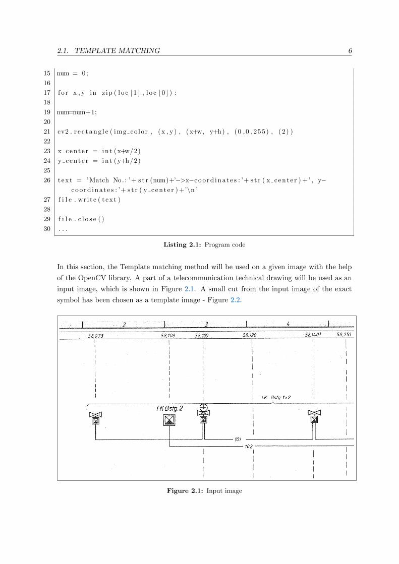
Another improvement of the code in Listing 2.1 is to eliminate some of the false positives.
False positives are objects incorrectly characterized as a match. In the example in the previous
chapter there are no false positives because the threshold value was carefully selected. For
example, if the threshold value is set to 0.251 instead of 0.2, there will be 38 matches, instead
of only 3 (Figure 2.5). It is very often not possible to adjust the threshold value so that there
are no false positives.
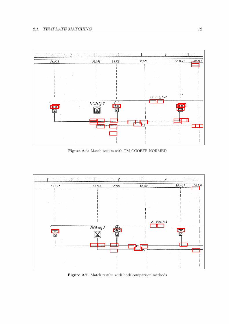
The different comparison methods in OpenCV (Equations 2.1-2.6) deliver slightly differ-
ent false positives. When the same program (Listing 2.1) is tested, but this time with
TM CCOEFF NORMED, it delivers different false positives (Figure 2.6). With this compar-
ison method the result image has values between -1 and 1, where 1 is a perfect match and
-1 is a perfect mismatch. The threshold value is then chosen so that there are again exactly
38 matches - the same amount as with the TM SQDIFF NORMED - comparison method.
It will then be compared between the first 38 matches from both methods. As a result many
of the false positives are different, whereas the correct matches are still the same.
2.1. TEMPLATE MATCHING 11
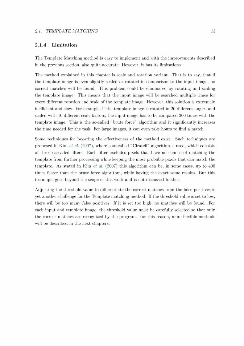
The different false positives can be eliminated when both methods are combined and used
together in the same program. First the ”cv2.matchTemplate” function with the comparison
method TM SQDIFF NORMED (Equation 2.2) is called. A region of interest (ROI) is then
cut from the input image for every match that satisfies the conditions explained above. The
ROI has the same size as the template image and the location of a given match (line 9).
The ”cv2.matchTemplate” function is then called again, but this time not for the input
image, but instead for the ROI and the template image. This time the comparison method
TM CCOEFF NORMED (Equation 2.6) is used (line 11). As explained in the previous
section, all images are stored as arrays. The function ”cv2.minMaxLoc” is then used, which
finds the global minimum and maximum in an array. In this case only the maximum is
relevant (line 13). A threshold value is then again chosen that helps to categorize the matches
as correct or not (line 15).
There are fewer false positives when the same threshold values are chosen for both comparison
methods, which can be clearly seen in Figure 2.7. This shows that with using two comparison
methods, instead of only one, the amount of false positives could be reduced. In this case,
the program was executed for just 0.1 seconds, which is almost identical if only one method
is used. This is because the second method is used only for the ROI instead of the whole
image and thus barely affects the speed of the program.
Figure 2.5: Match results with TM SQDIFF NORMED
2.1. TEMPLATE MATCHING 12
Figure 2.6: Match results with TM CCOEFF NORMED
Figure 2.7: Match results with both comparison methods
2.1. TEMPLATE MATCHING 13
2.1.4 Limitation
The Template Matching method is easy to implement and with the improvements described
in the previous section, also quite accurate. However, it has its limitations.
The method explained in this chapter is scale and rotation variant. That is to say, that if
the template image is even slightly scaled or rotated in comparison to the input image, no
correct matches will be found. This problem could be eliminated by rotating and scaling
the template image. This means that the input image will be searched multiple times for
every different rotation and scale of the template image. However, this solution is extremely
inefficient and slow. For example, if the template image is rotated in 20 different angles and
scaled with 10 different scale factors, the input image has to be compared 200 times with the
template image. This is the so-called ”brute force” algorithm and it significantly increases
the time needed for the task. For large images, it can even take hours to find a match.
Some techniques for boosting the effectiveness of the method exist. Such techniques are
proposed in Kim et al. (2007), where a so-called ”Ciratefi” algorithm is used, which consists
of three cascaded filters. Each filter excludes pixels that have no chance of matching the
template from further processing while keeping the most probable pixels that can match the
template. As stated in Kim et al. (2007) this algorithm can be, in some cases, up to 400
times faster than the brute force algorithm, while having the exact same results. But this
technique goes beyond the scope of this work and is not discussed further.
Adjusting the threshold value to differentiate the correct matches from the false positives is
yet another challenge for the Template matching method. If the threshold value is set to low,
there will be too many false positives. If it is set too high, no matches will be found. For
each input and template image, the threshold value must be carefully selected so that only
the correct matches are recognized by the program. For this reason, more flexible methods
will be described in the next chapters.

2.2. CONTOURS 14
2.2 Contours
The explanations and examples in this chapter are inspired by Kaehler et al. (2016) and
OpenCV (3.4.0).
”Contours can be explained simply as a curve joining all the continuous points (along the
boundary), having the same color or intensity. The contours are a useful tool for shape
analysis and object detection and recognition” (OpenCV, 3.3.1). For the given image in
Figure 2.8 - left there are two contours shown with red and green lines in Figure 2.8 - right,
one around the rectangle and one around the triangle. As it can be seen in the example, a
contour lies on the border between the black and the white spaces and thus it represents the
form of a given shape.
Figure 2.8: Contours
2.2.1 Theory
The contours in Figure 2.8 - right were found with the help of the function ”cv2.findContours”.
It is important to understand how the different contours relate to one another. For this
purpose the concept of a contour tree will be explained, which was first proposed by G.
Reeb and further developed in Bajaj et al. (1997) and Kreveld et al. (1997). A contour tree
contains the relationship between contours and is important when doing a comparison.
In Figure 2.9, gray regions are positioned on a white background, where every region has a
different shape. The contours of the shapes can be seen as red and green lines around the
shapes. The red lines are labeled cX and the green lines hX, where c stands for ”contour”, h
stands for ”hole” and X is some number (Kaehler et al., 2016). The red lines represent the
exterior boundaries of a given shape. The green lines can be seen as the interior boundary of
the shape or as the exterior boundary of the white space in it. In the example above (Figure
2.8) the red lines represent the outer boundary of the rectangle and the green lines represent
the outer boundary of the ”hole” in the rectangle.

2.2. CONTOURS 15
Figure 2.9: Contour tree
The contour tree contains the hierarchy between the contours or how they relate to one
another. In OpenCV, the hierarchy is stored in an array with one entry for each con-
tour. Each entry contains an array of four elements, each indicating the connected
contours with the current one. There are four possible ways to represent a hierarchy
in OpenCV - ”cv2.RETR EXTERNAL”, ”cv2.RETR LIST”, ”cv2.RETR CCOMP” and
”cv2.RETR TREE”. In this work only the ”cv2.RETR TREE” type of hierarchy will be
discussed and further explained, since it is best structured and therefore easiest to use. It
retrieves all the contours and creates a graph like the one shown in Figure 2.10 - right, where
each node is a contour connected by edges with the corresponding contours.
For the given contours in Figure 2.9 the resulting contour tree is shown in Figure 2.10 - right.
Every number in the contour tree corresponds to the id of a given contour. The corresponding
ids of the contours are shown in Figure 2.10 - left. When a contour is inside another contour,
it can be seen as a child contour. In the contour tree, every child is below its parent. For
example, the contours with id-1 and id-2 are the children of the contour 0 and contour 2 is
the parent of the contour 4. In OpenCV, these relationships are stored in an array with four
values - [Next, Previous, First Child, Parent] (OpenCV, 3.4.0). ”Next” represents the next
contour at the same hierarchical level. For example, the next contour of contour 1 will be
contour 2. Contour 2 has no ”next” contour, but it has a ”previous” contour, which in this
case is contour 1. ”First child” stand for the first contour that lies in the given contour. The
”first child” contour with id 6 will be the contour 8. ”Parent” represent the contour in which
the given contour lies. For contour 9, that would be contour 6. An example hierarchical

2.2. CONTOURS 16
array for contour 2 will look like this : [-1, 1, 4, 0], where -1 denotes that there is no such
relationship.
Figure 2.10: Contour tree with cv2.RETR TREE
Next, a ”contour moment” will be explained. The explanation formulation is aided by Kaehler
et al. (2016) and Kmiec (2011). Contour moments have been widely used in computer vision
for a long time. With image moments two contours can be compared with one another and
thus the similarities between them can be found. A moment is a characteristic of a given
contour calculated by summing over the pixels of that contour. The (p,q) moment of an
image is defined as:
mp,q =∑x,y
I(x, y) · xp · yq (2.7)
Here the moment mp,q is the sum over all the pixels in the object. P is the x-order and q is
the y-order. Order means the power to which the corresponding component is taken in the
sum. If p and q are both equal to 0, then the m0,0 moment is the length of the contour in
pixels (Bradski et al., 2008).
The problem of the moments explained above is that they are not invariant to translation,
rotation or scaling. Therefore, the concept of the Hu invariant moments will be explained
next. Introduced first in Hu (1962), these moments are invariant to scale, rotation and
translation by combining the different normalized central moments. First, a central moment
will be explained. It is invariant under translation and is defined as follows:
µp,q =∑x,y
I(x, y) · (x− x)p · (y − y)q (2.8)
where:
x =m10
m00and y =
m01
m00
2.2. CONTOURS 17
Next, a normalized central moment is not only a translation invariant but also a scale invari-
ant. The normalized central moments achieve scale invariance by factoring out the overall
size of the object and are defined with the following formula:
νp,q =µp,q
m00( p+q+2
2 )(2.9)
Finally, the Hu invariant moments are combinations of the normalized central moments. They
are defined as follows:
h1 = ν20 + ν02 (2.10)
h2 = (ν20 + ν02)2 + 4 · ν211 (2.11)
h3 = (ν30 − 3 · ν12)2 + (3 · ν21 − ν03)2 (2.12)
h4 = (ν30 + ν12)2 + (ν21 − ν03) (2.13)
h5 = (ν30 − 3 · ν12) · (ν30 + ν12) · ((ν30 + ν12)2 − 3 · (ν21 + ν03)
2)+
(3 · ν21 − ν03) · (ν21 + ν03) · (3 · (ν30 + ν12)− (ν21 + ν03))(2.14)
h6 = (ν20 − ν02) · ((ν30 + ν12)2 − (ν21 + ν03)
2)
+4 · ν11 · (ν30 + ν12) · (ν21 + ν03)(2.15)
h7 = (3 · ν21 − ν03) · (ν30 + ν12) · ((ν30 + ν12)2 − 3 · (ν21 + ν03)
2)−
(ν30 − 3 · ν12) · (ν21 + ν03) · (3 · (ν30 + ν12)2 − (ν21 + ν03)
2)(2.16)
By combining the different normalized central moments invariant functions are created, which
represent different aspects of the image with scale, rotation and translation invariance. ”The
first one, h1, is analogous to the moment of inertia around the image’s centroid, where the
pixels’ intensities are analogous to physical density. The last one, h7, is skew invariant, which
enables it to distinguish mirror images of otherwise identical images” (Wikipedia).
In OpenCV, the Hu invariant moments can be easily computed with the help of the function
”cv2.HuMoments”, which will be shown in the next section. The contours found can be then
compared with ”cv2.matchShapes”, which returns a number showing the similarity between
two contours. If the number is small, there is a good match between the contours. There are
three types of comparison methods, which can be used with the ”cv2.matchShapes”-function.
They are defined as follows (Kaehler et al., 2016):
2.2. CONTOURS 18
- cv2.CONTOURS MATCH I1
I1(A,B) =∑
i=1...7
1
ηAi− 1
ηBi| (2.17)
- cv2.CONTOURS MATCH I2
I2(A,B) =∑
i=1...7
|ηAi − ηBi | (2.18)
- cv2.CONTOURS MATCH I3
I3(A,B) =∑
i=1...7
|ηAi − ηBiηAi
| (2.19)
where ηAi and ηBi are defined with the following equations:
ηAi = sign(hAi ) · log(hAi ) and ηBi = sign(hBi ) · log(hBi )
and hAi and hBi are the Hu invariant moments of given images A and B. From these matching
methods it can be seen that the result is the sum of the differences between the 7 Hu invariant
moments (Equations 2.10 to 2.16). If the differences are small, the two objects that are
compared are similar to one another.
The methods explained in this chapter will be demonstrated next with an example. After
testing, the results have shown that the comparison method ”cv2.CONTOURS MATCH I1”
works best and will therefore be used.
2.2.2 Implementation and results
The methods explained in the previous section will now be tested. For this purpose, a
template image will be searched in a bigger image. It is important to note that the template
image is not a part of the larger image, but rather a completely different image, in which the
symbol in question looks like some of the symbols in the big image. It is also important that
the template image has a different size and is rotated in comparison to the symbols in the
big image. Such a template image would not work with the method explained in chapter 2.1.
As a template image for this example the image in Figure 2.12 will be used. The bigger image
or the input image can be seen in Figure 2.11.
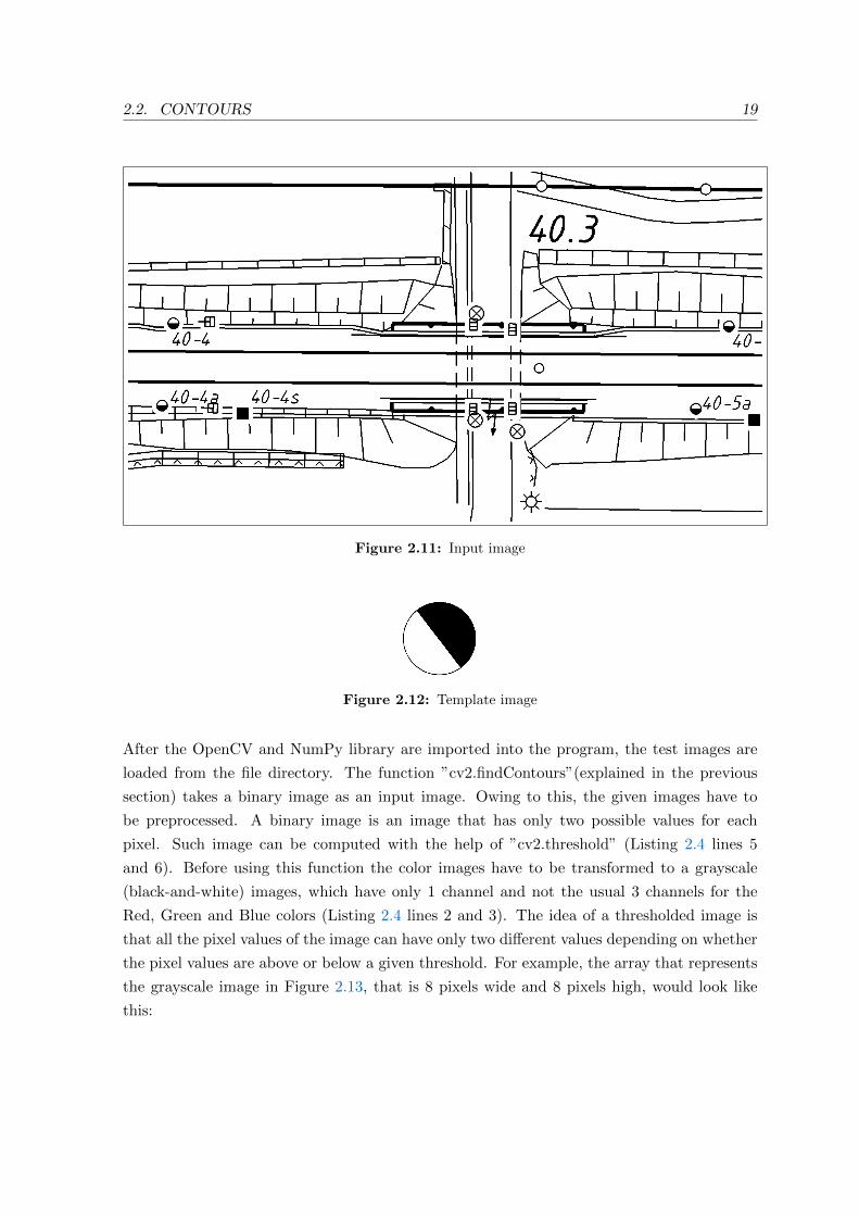
2.2. CONTOURS 19
Figure 2.11: Input image
Figure 2.12: Template image
After the OpenCV and NumPy library are imported into the program, the test images are
loaded from the file directory. The function ”cv2.findContours”(explained in the previous
section) takes a binary image as an input image. Owing to this, the given images have to
be preprocessed. A binary image is an image that has only two possible values for each
pixel. Such image can be computed with the help of ”cv2.threshold” (Listing 2.4 lines 5
and 6). Before using this function the color images have to be transformed to a grayscale
(black-and-white) images, which have only 1 channel and not the usual 3 channels for the
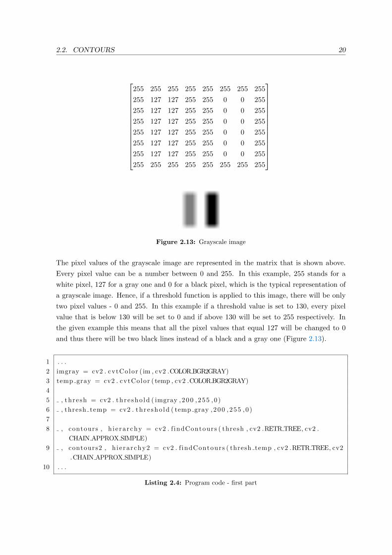
Red, Green and Blue colors (Listing 2.4 lines 2 and 3). The idea of a thresholded image is
that all the pixel values of the image can have only two different values depending on whether
the pixel values are above or below a given threshold. For example, the array that represents
the grayscale image in Figure 2.13, that is 8 pixels wide and 8 pixels high, would look like
this:
2.2. CONTOURS 20
255 255 255 255 255 255 255 255
255 127 127 255 255 0 0 255
255 127 127 255 255 0 0 255
255 127 127 255 255 0 0 255
255 127 127 255 255 0 0 255
255 127 127 255 255 0 0 255
255 127 127 255 255 0 0 255
255 255 255 255 255 255 255 255
Figure 2.13: Grayscale image
The pixel values of the grayscale image are represented in the matrix that is shown above.
Every pixel value can be a number between 0 and 255. In this example, 255 stands for a
white pixel, 127 for a gray one and 0 for a black pixel, which is the typical representation of
a grayscale image. Hence, if a threshold function is applied to this image, there will be only
two pixel values - 0 and 255. In this example if a threshold value is set to 130, every pixel
value that is below 130 will be set to 0 and if above 130 will be set to 255 respectively. In
the given example this means that all the pixel values that equal 127 will be changed to 0
and thus there will be two black lines instead of a black and a gray one (Figure 2.13).
1 . . .
2 imgray = cv2 . cvtColor ( im , cv2 .COLOR BGR2GRAY)
3 temp gray = cv2 . cvtColor ( temp , cv2 .COLOR BGR2GRAY)
4
5 , thresh = cv2 . th r e sho ld ( imgray , 200 , 255 , 0 )
6 , thresh temp = cv2 . th r e sho ld ( temp gray , 200 , 255 , 0 )
7
8 , contours , h i e ra r chy = cv2 . f indContours ( thresh , cv2 .RETR TREE, cv2 .
CHAIN APPROX SIMPLE)
9 , contours2 , h i e ra rchy2 = cv2 . f indContours ( thresh temp , cv2 .RETR TREE, cv2
.CHAIN APPROX SIMPLE)
10 . . .
Listing 2.4: Program code - first part

2.2. CONTOURS 21
After the preprocessing step is finished, the function ”cv2.findContours” is called for both the
template image and the input image. It returns the contours in the images and the hierarchy
between them (Listing 2.4, lines 8 and 9). The hierarchy is represented as a contour tree as
explained in the previous Section 2.2.
Listing 2.5 will be used for the next explanation and will not be further referenced.
The next step is to compare every contour from the input image with the outer contour
from the template image. This is made with the function ”cv2.matchShapes”. The function
returns the differences between the Hu invariant moments of two contours (explained in the
previous section 2.2). It is important to highlight that the first contour in an image is the
border of the image. The second contour actually describes the first contour of an object
in the given image and will be therefore compared (line 3). If the differences are small, the
contours are similar to one another. The next step is to set a threshold value for the result
from ”cv2.matchShapes”. In the example, it is set to 0.1, which means that if the result is
below 0.1, it will be accepted that the contours are similar to one another. If the template
object has a child contour (explained in the previous section 2.2), it will be compared, in
addition to the outer contour for better accuracy. For the given template image (Figure 2.12)
the outer contour is the boundary of the circle and the child contour is the boundary of the
white semicircle, that lies within the circle. To check whether a particular contour has a child
contour, it is controlled whether the template image has more than 2 contours and whether
the parent id of the following contour is equal to the id of the given contour (line 6). As it was
previously explained, the fourth element of the hierarchy array of a given contour denotes
the parent of this contour.
The child contours are then compared again with the function ”cv2.matchShapes” and a new
threshold value is set once more to 0.1 (lines 8 and 10). If all the conditions mentioned above
are met, the shape found in the input image is accepted as a good match and the contour
around it is drawn in red (lines 11-13). However, if the template shape has no child contours,
which means it is a filled shape without ”holes” in it, it is accepted as a semi-good match
and is drawn again, but in a different color (lines 17-19).
The result for the given input image (Figure 2.11) and template image (Figure 2.12) can
be seen in Figure 2.14. The method explained in this chapter has accurately found every
matching symbol in the input image, although the template image is rotated and scaled
compared to the symbols in the input image.

2.2. CONTOURS 22
Figure 2.14: Result
1 . . .
2 f o r i in range (1 , l en ( contours ) ) :
3 r e t = cv2 . matchShapes ( contours [ i ] , contours2 [ 1 ] , cv2 .CONTOURS MATCH I1
, 0 )
4
5 i f ret <0.1 :
6 i f ( l en ( contours2 ) >2 and h i e ra r chy [ 0 ] [ i + 1 ] [ 3 ] == i ) :
7
8 r e t2 = cv2 . matchShapes ( contours [ i +1] , contours2 [ 2 ] , cv2 .
CONTOURS MATCH I1, 0 )
9
10 i f ret2 <0.1 :
11 p r i n t ( ’ Good match . Match No . : ’ , num)
12 cnt = contours [ i ]
13 cv2 . drawContours ( im , [ cnt ] , 0 , ( 0 , 0 , 255 ) , 6)
14 num = num + 1
15
16 e l i f ( l en ( contours2 ) <=2) :
17 p r i n t ( ’ Semi−good match . No . : ’ , num)
18 cnt = contours [ i ]
19 cv2 . drawContours ( im , [ cnt ] , 0 , ( 0 , 255 ,0 ) , 6)
20 num = num + 1
21 . . .
Listing 2.5: Program code - second part

2.2. CONTOURS 23
2.2.3 Limitation
As seen in the previous section, template symbols in a bigger image can be found with a
relatively high degree of accuracy with the help of contours. This method is a scale and
rotation invariant, which is sometimes very important, and which the method in Chapter 2.1
fails to achieve. Unfortunately, it comes with a few limitations.
The method described in this chapter works only if the searched symbol is not somehow
crossed or even ”touched” by another symbol or a line. For example, it won’t work if the
template image (Figure 2.12) is modified and a rectangle lies directly next to the shape
already given (Figure 2.15 - left). In this case, the outer contour will be around both the
circle and the rectangle and the shapes cannot be differentiated from one another.
Moreover, if the shape in Figure 2.12 is not closed (an example can be seen in Figure 2.15 -
right), it also won’t work, because the outer contour can no longer be differentiated from the
inner contour. Hence, there will be only one contour, which does not match the contours in
Figure 2.12.
Figure 2.15: Examples, for which the method won’t work
Another disadvantage of this method is that a threshold value for the matching result has to
be set. Similarly, as with the method explained in Chapter 2.1, if the threshold value is set
too low, there will be no matches found and if set too high, more than the actual amount
of matches will be found. However, this method is pretty accurate if the template symbol
has not only an outer contour but a child contour as well and is less common to return false
positives.
2.3. CASCADE CLASSIFIERS 24
2.3 Cascade Classifiers
This chapter explains a Haar feature-based cascade classifier and how to train it in OpenCV.
It is a method for object detection, which was first proposed in Viola et al. (2001). It was
originally used for face detection, but it can be used for many types of objects.
A cascade classifier is a machine learning method in which the information computed in a
given classifier is used for the next classifier and becomes more complex at each stage. A
machine learning is referred to the ability of a computer to learn and improve without being
explicitly programmed.
2.3.1 Theory
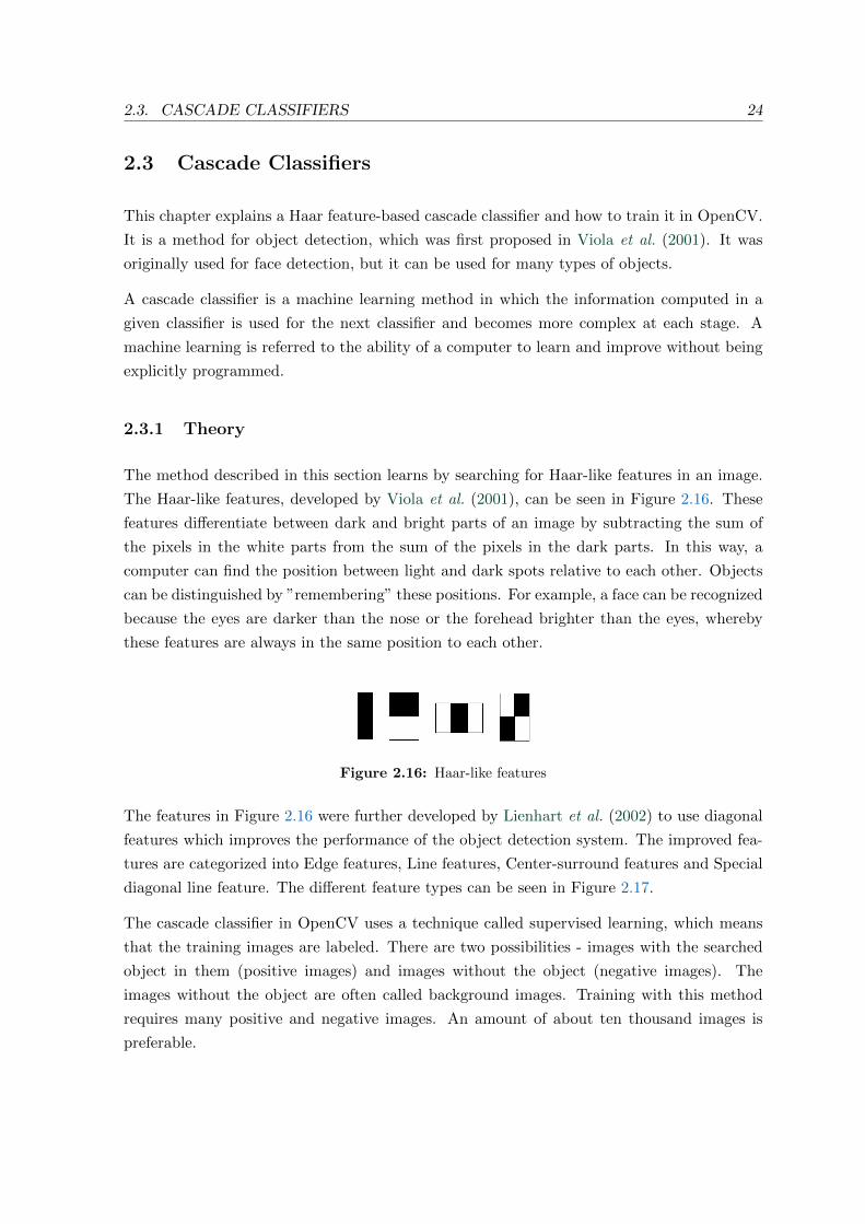
The method described in this section learns by searching for Haar-like features in an image.
The Haar-like features, developed by Viola et al. (2001), can be seen in Figure 2.16. These
features differentiate between dark and bright parts of an image by subtracting the sum of
the pixels in the white parts from the sum of the pixels in the dark parts. In this way, a
computer can find the position between light and dark spots relative to each other. Objects
can be distinguished by ”remembering” these positions. For example, a face can be recognized
because the eyes are darker than the nose or the forehead brighter than the eyes, whereby
these features are always in the same position to each other.
Figure 2.16: Haar-like features
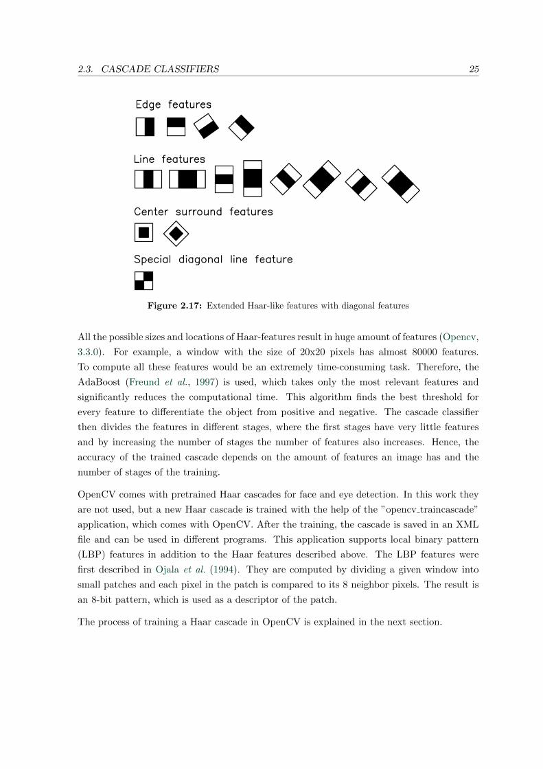
The features in Figure 2.16 were further developed by Lienhart et al. (2002) to use diagonal
features which improves the performance of the object detection system. The improved fea-
tures are categorized into Edge features, Line features, Center-surround features and Special
diagonal line feature. The different feature types can be seen in Figure 2.17.
The cascade classifier in OpenCV uses a technique called supervised learning, which means
that the training images are labeled. There are two possibilities - images with the searched
object in them (positive images) and images without the object (negative images). The
images without the object are often called background images. Training with this method
requires many positive and negative images. An amount of about ten thousand images is
preferable.
2.3. CASCADE CLASSIFIERS 25
Figure 2.17: Extended Haar-like features with diagonal features
All the possible sizes and locations of Haar-features result in huge amount of features (Opencv,
3.3.0). For example, a window with the size of 20x20 pixels has almost 80000 features.
To compute all these features would be an extremely time-consuming task. Therefore, the
AdaBoost (Freund et al., 1997) is used, which takes only the most relevant features and
significantly reduces the computational time. This algorithm finds the best threshold for
every feature to differentiate the object from positive and negative. The cascade classifier
then divides the features in different stages, where the first stages have very little features
and by increasing the number of stages the number of features also increases. Hence, the
accuracy of the trained cascade depends on the amount of features an image has and the
number of stages of the training.
OpenCV comes with pretrained Haar cascades for face and eye detection. In this work they
are not used, but a new Haar cascade is trained with the help of the ”opencv traincascade”
application, which comes with OpenCV. After the training, the cascade is saved in an XML
file and can be used in different programs. This application supports local binary pattern
(LBP) features in addition to the Haar features described above. The LBP features were
first described in Ojala et al. (1994). They are computed by dividing a given window into
small patches and each pixel in the patch is compared to its 8 neighbor pixels. The result is
an 8-bit pattern, which is used as a descriptor of the patch.
The process of training a Haar cascade in OpenCV is explained in the next section.

2.3. CASCADE CLASSIFIERS 26
2.3.2 Implementation and results
This section was made possible by the excellent explanation in Kinsley (2016).
The first step to train a Haar cascade in OpenCV is to collect background images. A back-
ground or negative image is an image without the object for which the cascade is trained.
In this section, the image in Figure 2.18 is used as such an object. It is a part of a larger
image, shown in Figure 2.1. Any image that does not contain this symbol can be used as a
background image.
Figure 2.18: Symbol for the training
Ideally, the training would work best if the background images consist of different colors,
brightness and scenes. In this case the symbol is searched in different technical drawings, so
it is best if the background images are all different technical drawings, without the symbol in
Figure 2.18 being displayed. Thousands of background images are required for the cascade
to be accurate. Therefore, they are not collected individually, but only three large technical
drawings are used, which are then cut into a thousand smaller images and stored in a folder
called ”Background” (Listing 2.6). For this example, the background images will have a size
of 100x100 pixels. As a result, there are 11888 background images, which will be further used
for the training.
1 . . .
2 h , w = img . shape
3
4 num = 1 ;
5
6 f o r i in range (1 ,w−200 ,60) :
7 f o r j in range (1 , h−200 ,60) :
8
9 r o i = img [ j : j +200 , i : i +200]
10 r e s i z e d = cv2 . r e s i z e ( ro i , ( 1 0 0 , 1 0 0 ) )
11 name = ’ Background / ’ + s t r (num) + ’ . png ’
12 cv2 . imwrite (name , r e s i z e d )
13 num = num+1
14 . . .
Listing 2.6: cut image.py

2.3. CASCADE CLASSIFIERS 27
The next step is to create a text file in which the directory path and the name of each
background image are stored. For this purpose, all the names of the images from the folder
”Background” are read and saved on a different line in a text file with the name ”bagr.txt”
(Listing 2.7).
1 . . .
2 f o r img in os . l i s t d i r ( ’ Background ’ ) :
3 t ex t = ’ Background/’+img+’\n ’
4 with open ( ’ bagr . txt ’ , ’ a ’ ) as f i l e :
5 f i l e . wr i t e ( t ex t )
6 . . .
Listing 2.7: text bagr.py
After creating the background images and saving the directory path of each one in a text file,
the positive images will be created. For the cascade to be accurate, thousands of positive
images are required (in addition to the thousands of negative images), making the process
of finding them highly impractical. Therefore, the positive images will be created with the
help of the negative images. The OpenCV application ”opencv createsamples” is used for
this purpose. This application places the given symbol on each background image in dif-
ferent positions and scales so that positive images are created from the negative ones. The
”opencv createsamples” application can be accessed from the Command Prompt in Windows
OS or from the Terminal in Mac OS. In this case, it is executed from the Command Prompt
in Windows OS with the following code:
opencv createsamples −img symbol . png −bg bagr . txt − i n f o P o s i t i v e /pos . l s t
−pngoutput P o s i t i v e −maxxangle 0 . 3 −maxyangle 0 . 3 −maxzangle 0 . 3 −num
11888
Listing 2.8: opencv createsamples
where:
- ”-img symbol.png” denotes the image file of the symbol for which the cascade will be
trained. In this image there should only be the symbol and no background. In this case,
the image contains just the symbol in Figure 2.18 with a size of 50x50 pixels, making
it smaller than the background images.
- ”-bg bagr.txt” stands for the text file in which the directory path and the name of every
positive image are described. This is required for the program to find the images and
access them.

2.3. CASCADE CLASSIFIERS 28
- ”-info Positive/pos.lst” creates a file in the ”Positive” folder with the extension ”.lst”
in which the position of every symbol in the positive image is described (this will be
explained further in the coming paragraphs).
- ”-pngoutput Positive” defines where the positive images will be stored. In this case, in
a folder with the name ”Positive”.
- ”-maxxangle 0.3 -maxyangle 0.3 -maxzangle 0.3” denotes how much the given symbol
will be rotated around the x-, y- and z-axis. The angles are in radians. The given
symbol is randomly rotated and placed over the negative images.
- ”- num 11888” stands for how many positive images are to be created. In this case,
there are 11888 background images and the same amount of positive images will be
created.
As already explained, the ”pos.lst” file contains the position of each symbol in the image.
In Listing 2.9, it can be seen precisely how the file is structured. The name of each positive
image is written at the first place on every line. The second place indicates how many of the
specified symbols can be seen in the image. In this case, there is always only one symbol for
a positive image. Next the x- and y-coordinates of the upper left corner of the symbol in the
image are displayed. The last two numbers of each line represent the width and height of the
symbol that distinguishes them since the symbol is scaled randomly for each positive image.
1 . . .
2 0113 0011 0049 0041 0041 . jpg 1 11 49 41 41
3 0114 0018 0021 0062 0062 . jpg 1 18 21 62 62
4 0115 0008 0015 0024 0024 . jpg 1 8 15 24 24
5 0116 0021 0023 0043 0043 . jpg 1 21 23 43 43
6 . . .
Listing 2.9: Few lines from ”pos.lst”
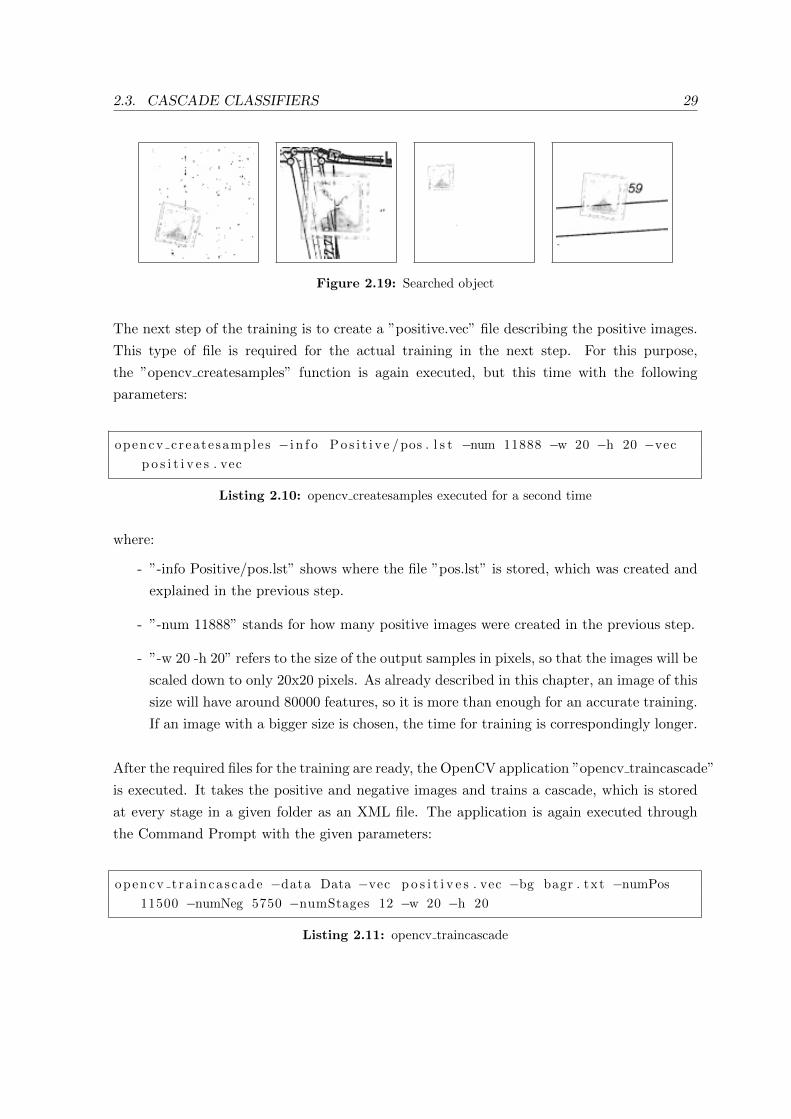
After execution of the program, 11888 positive images are generated. The resulting positive
images are the same as the background images, but with the given symbol placed randomly
above them. Four of the positive images are shown in Figure 2.19, each one of them corre-
sponding to one of the descriptions in 2.9. As it can be seen, the given symbol was randomly
placed over the background images with a different rotation, scale, and position.
2.3. CASCADE CLASSIFIERS 29
Figure 2.19: Searched object
The next step of the training is to create a ”positive.vec” file describing the positive images.
This type of file is required for the actual training in the next step. For this purpose,
the ”opencv createsamples” function is again executed, but this time with the following
parameters:
opencv createsamples − i n f o P o s i t i v e /pos . l s t −num 11888 −w 20 −h 20 −vec
p o s i t i v e s . vec
Listing 2.10: opencv createsamples executed for a second time
where:
- ”-info Positive/pos.lst” shows where the file ”pos.lst” is stored, which was created and
explained in the previous step.
- ”-num 11888” stands for how many positive images were created in the previous step.
- ”-w 20 -h 20” refers to the size of the output samples in pixels, so that the images will be
scaled down to only 20x20 pixels. As already described in this chapter, an image of this
size will have around 80000 features, so it is more than enough for an accurate training.
If an image with a bigger size is chosen, the time for training is correspondingly longer.
After the required files for the training are ready, the OpenCV application ”opencv traincascade”
is executed. It takes the positive and negative images and trains a cascade, which is stored
at every stage in a given folder as an XML file. The application is again executed through
the Command Prompt with the given parameters:
opencv t ra inca scade −data Data −vec p o s i t i v e s . vec −bg bagr . txt −numPos
11500 −numNeg 5750 −numStages 12 −w 20 −h 20
Listing 2.11: opencv traincascade

2.3. CASCADE CLASSIFIERS 30
where:
- ”-data Data” indicates where the computed cascade will be stored. In this case that
would be in a folder called ”Data”. It is important to note that after each level of
training an XML file is created and at the end a large XML file containing all levels.
- ”-vec positives.vec” shows where the file ”positives.vec” is stored, in which the infor-
mation about the positive images is saved.
- ”-bg bagr.txt” shows where the text file ”bagr.txt” is stored, in which the information
about the negative or background images is saved.
- ”-numPos 11500 -numNeg 5750” denotes the number of positive and negative images
which will be considered by the training. 11500 of the 11888 positive images are used
because at every stage the training requires more images and thus a few hundred of the
positive images are left as a buffer. Only half of the positive images will be used for
the negative images.
- ”-numStages 12” stands for how many stages the training will go through before it is
considered trained. The training often does not reach all the stages (if given too many),
because it is ready before reaching the final stages, but again a buffer is left.
- ”-w 20 -h 20” denotes the size of the output samples in pixels as described in the
previous step.
The learning process for the given example takes between one and two hours, depending on
the machine being used. After the cascade has been trained, it is saved in an XML file.
This file can then be opened with the help of the OpenCV function ”cv2.CascadeClassifier”
(Listing 2.12, line 2). After the cascade has been read, the symbol can be searched in a
given image. For this purpose the function ”detectMultiScale” is used to search the symbol
in different sizes (Listing 2.12, line 4). This function takes as a first parameter the image in
which the symbol will be detected. The second parameter is a scale factor which specifies
how much the image size is reduced at each scale. Hence, a small scale factor will result in
a more accurate result but is computationally more expensive. The third parameter of the
function denotes how many neighbors each candidate object should have. The result of the
function is an array containing the x and y coordinates and the width and height of each
object found. A rectangle is then drawn around every object that has been found (Listing
2.12, lines 6 and 7).

2.3. CASCADE CLASSIFIERS 31
1 . . .
2 cascade = cv2 . C a s c a d e C l a s s i f i e r ( ’ t r a i n e d c a s c a d e . xml ’ )
3
4 r e s = cascade . de t e c tMu l t iS ca l e ( gray img , 1 . 2 , 5 )
5
6 f o r (x , y ,w, h) in r e s :
7 cv2 . r e c t a n g l e ( img , (x , y ) , ( x+w, y+h) , ( 0 , 0 , 255 ) , 4)
8 . . .
Listing 2.12: cascade.py
The trained cascade is then tested with the image shown in figure 2.1. As a result, all symbols
for which the cascade was trained are correctly recognized with the precise location and size
(Figure 2.20).
Figure 2.20: Result from the trained cascade
The method described in this chapter is not only accurate for the given symbol, but also
very efficient and therefore very fast after training the cascade. Therefore, it can be used not
only for still images but also for videos. Furthermore, after the parameters in the function
”detectMultiScale” have been correctly selected, the cascade works for a variety of image
sizes and types, without any further adjustments. This method is therefore very useful when
searching for the same symbol in many different technical drawings. However, it is not
preferable to find many different symbols, as the time for training is relatively long and the
techniques described in the previous chapters may be a better choice.
2.3. CASCADE CLASSIFIERS 32
2.3.3 Limitation
The method described in this chapter is very efficient and very accurate under many condi-
tions. However, there are some disadvantages.
First and foremost is that the cascade has to be trained, which is a time-consuming task
and many parameters have to be correctly chosen making the process more difficult. In most
cases, the training for a symbol, like the one in Figure 2.18, takes no longer than 2 hours
because it doesn’t require many features (described in section 2.3) to be accurate. However,
if an object like a face or a car is to be found, it would take much longer to train.
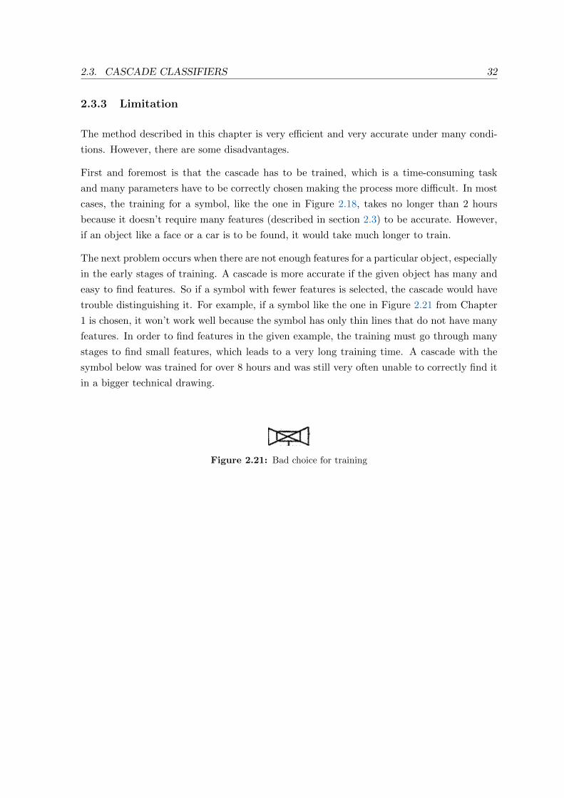
The next problem occurs when there are not enough features for a particular object, especially
in the early stages of training. A cascade is more accurate if the given object has many and
easy to find features. So if a symbol with fewer features is selected, the cascade would have
trouble distinguishing it. For example, if a symbol like the one in Figure 2.21 from Chapter
1 is chosen, it won’t work well because the symbol has only thin lines that do not have many
features. In order to find features in the given example, the training must go through many
stages to find small features, which leads to a very long training time. A cascade with the
symbol below was trained for over 8 hours and was still very often unable to correctly find it
in a bigger technical drawing.
Figure 2.21: Bad choice for training

33
Chapter 3
Neural networks with Keras and
TensorFlow
As shown in the previous chapter, symbol recognition is a challenging task and each of the
explained methods is somehow limited and only works under certain conditions. Therefore,
yet another approach for object detection will be tested in this chapter - convolutional neural
networks.
Neural networks (NN) have led to huge progress over the last few years in areas such as
image, text and speech recognition. A neural network is a form of machine learning, or more
precisely deep learning, in which the computer ”learns” from given data. For the sake of
this work, a convolutional neural network (CNN or ConvNets) will be used, which helps the
training process especially with images.
The Keras library is used to build a CNN. Keras is a high-level programming language that
makes it possible to create complex programs with fewer lines of code. This helps to build
CNNs quickly so that less time is required for coding and more time is left for testing, which is
important for building an accurate neural network. However, Keras does not process the NN
alone. It is just a front-end layer written in Python that uses either TensorFlow (developed
by the Google Brain team) or Theano (developed at the Universite de Montreal) libraries to
build the neural network. Both libraries can be implemented similarly, but the TensorFlow
library will be used because Google offers excellent learning tools, making it easier to start
building a neural network.

3.1. THE THEORY BEHIND CONVOLUTIONAL NEURAL NETWORK 34
3.1 The theory behind Convolutional Neural Network
Deep learning is a vast topic, which goes beyond the scope of this work. For this reason, only
the essential parts of a CNN will be explained without going into mathematical detail.
Convolutional neural networks are a type of neural networks that are very effective in image
recognition. One of the first CNN is called LeNet5 (LeCun, 1998), which has started an
era of state-of-the-art artificial intelligence. Unfortunately, the computers did not have the
processing power at that time to make significant progress in this area of machine learning,
but in recent years computers have become more powerful than ever, and better NNs are
trained every day (Culurciello, 2017).
CNNs are so effective for image recognition because they use filters to detect patterns (or
features) in an image. For example, a pattern can be a horizontal or a vertical line. Different
locations of the image are searched for these features and a value is saved, representing how
well every pattern matches the image in a given location (Rohrer, 2017). This is called
filtering and will be explained next with the help of Figure 3.1 and Figure 3.2.
Figure 3.1 shows two different features (or filters), both of which have a size of 3x3 pixels.
A feature representing a vertical line is displayed on the left, while a feature denoting a
horizontal line is shown on the right. The actual filtering is made by sliding the feature over
a bigger image (Figure 3.2) and comparing it against a small patch from the large image,
whereby the patch always has the same size as the feature.
Figure 3.1: Filters
Each filter pixel is multiplied with the corresponding patch pixel from the image and the
results are added up. For example, if the feature which represents a vertical line (Figure 3.1
- left) is compared with the part of the image that is marked by a red rectangle in Figure
3.2, the result would be 3. There are 6 pixels with the same value (-1) and 3 pixels that have
different values (-1 and 1). All the pixels with the same values are added together, the rest
is subtracted from the sum, resulting in the number 3. This result is then divided by the
number of pixels in the feature, which in this case is 9. For the given example above, the
final result would be 0.33 (3 divided by 9). If the same feature (Figure 3.1 - left) is compared
with the patch, drawn in blue (Figure 3.2), the result will be 1 after it has been divided by
the number of pixels. This means that there is a perfect match between the two. The same
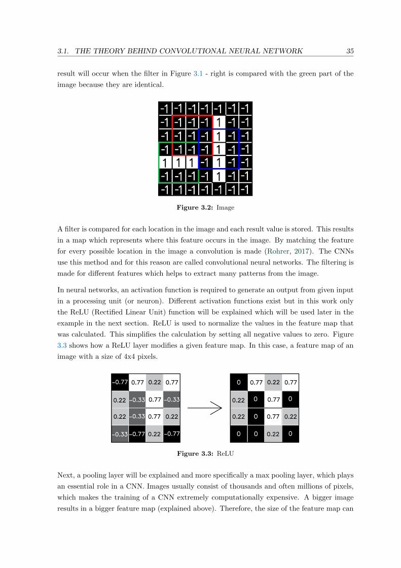
3.1. THE THEORY BEHIND CONVOLUTIONAL NEURAL NETWORK 35
result will occur when the filter in Figure 3.1 - right is compared with the green part of the
image because they are identical.
Figure 3.2: Image
A filter is compared for each location in the image and each result value is stored. This results
in a map which represents where this feature occurs in the image. By matching the feature
for every possible location in the image a convolution is made (Rohrer, 2017). The CNNs
use this method and for this reason are called convolutional neural networks. The filtering is
made for different features which helps to extract many patterns from the image.
In neural networks, an activation function is required to generate an output from given input
in a processing unit (or neuron). Different activation functions exist but in this work only
the ReLU (Rectified Linear Unit) function will be explained which will be used later in the
example in the next section. ReLU is used to normalize the values in the feature map that
was calculated. This simplifies the calculation by setting all negative values to zero. Figure
3.3 shows how a ReLU layer modifies a given feature map. In this case, a feature map of an
image with a size of 4x4 pixels.
Figure 3.3: ReLU
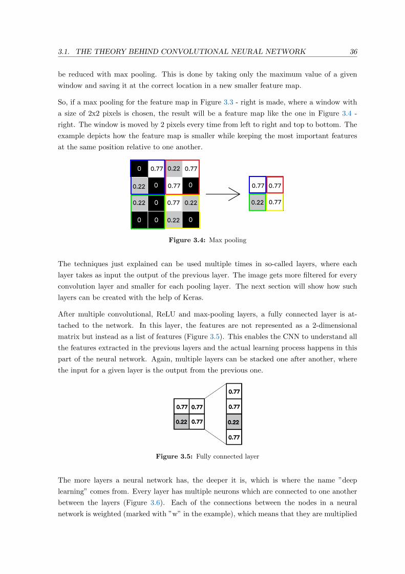
Next, a pooling layer will be explained and more specifically a max pooling layer, which plays
an essential role in a CNN. Images usually consist of thousands and often millions of pixels,
which makes the training of a CNN extremely computationally expensive. A bigger image
results in a bigger feature map (explained above). Therefore, the size of the feature map can
3.1. THE THEORY BEHIND CONVOLUTIONAL NEURAL NETWORK 36
be reduced with max pooling. This is done by taking only the maximum value of a given
window and saving it at the correct location in a new smaller feature map.
So, if a max pooling for the feature map in Figure 3.3 - right is made, where a window with
a size of 2x2 pixels is chosen, the result will be a feature map like the one in Figure 3.4 -
right. The window is moved by 2 pixels every time from left to right and top to bottom. The
example depicts how the feature map is smaller while keeping the most important features
at the same position relative to one another.
Figure 3.4: Max pooling
The techniques just explained can be used multiple times in so-called layers, where each
layer takes as input the output of the previous layer. The image gets more filtered for every
convolution layer and smaller for each pooling layer. The next section will show how such
layers can be created with the help of Keras.
After multiple convolutional, ReLU and max-pooling layers, a fully connected layer is at-
tached to the network. In this layer, the features are not represented as a 2-dimensional
matrix but instead as a list of features (Figure 3.5). This enables the CNN to understand all
the features extracted in the previous layers and the actual learning process happens in this
part of the neural network. Again, multiple layers can be stacked one after another, where
the input for a given layer is the output from the previous one.
Figure 3.5: Fully connected layer
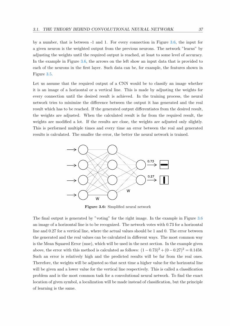
The more layers a neural network has, the deeper it is, which is where the name ”deep
learning” comes from. Every layer has multiple neurons which are connected to one another
between the layers (Figure 3.6). Each of the connections between the nodes in a neural
network is weighted (marked with ”w” in the example), which means that they are multiplied
3.1. THE THEORY BEHIND CONVOLUTIONAL NEURAL NETWORK 37
by a number, that is between -1 and 1. For every connection in Figure 3.6, the input for
a given neuron is the weighted output from the previous neurons. The network ”learns” by
adjusting the weights until the required output is reached, at least to some level of accuracy.
In the example in Figure 3.6, the arrows on the left show an input data that is provided to
each of the neurons in the first layer. Such data can be, for example, the features shown in
Figure 3.5.
Let us assume that the required output of a CNN would be to classify an image whether
it is an image of a horizontal or a vertical line. This is made by adjusting the weights for
every connection until the desired result is achieved. In the training process, the neural
network tries to minimize the difference between the output it has generated and the real
result which has to be reached. If the generated output differentiates from the desired result,
the weights are adjusted. When the calculated result is far from the required result, the
weights are modified a lot. If the results are close, the weights are adjusted only slightly.
This is performed multiple times and every time an error between the real and generated
results is calculated. The smaller the error, the better the neural network is trained.
Figure 3.6: Simplified neural network
The final output is generated by ”voting” for the right image. In the example in Figure 3.6
an image of a horizontal line is to be recognized. The network votes with 0.73 for a horizontal
line and 0.27 for a vertical line, where the actual values should be 1 and 0. The error between
the generated and the real values can be calculated in different ways. The most common way
is the Mean Squared Error (mse), which will be used in the next section. In the example given
above, the error with this method is calculated as follows: (1− 0.73)2 + (0− 0.27)2 = 0.1458.
Such an error is relatively high and the predicted results will be far from the real ones.
Therefore, the weights will be adjusted so that next time a higher value for the horizontal line
will be given and a lower value for the vertical line respectively. This is called a classification
problem and is the most common task for a convolutional neural network. To find the exact
location of given symbol, a localization will be made instead of classification, but the principle
of learning is the same.
3.2. IMPLEMENTATION AND RESULTS 38
The explanation in this section is simplified and does not go into mathematical details. Many
sources of information for a detailed description of a convolutional neural network exist. An
excellent explanation can be found in Karpathy et al..
3.2 Implementation and Results
In this section, a convolutional neural network will be created and trained with Keras (using
the TensorFlow backend) and Python. It will be a simple neural network which can be
trained using almost any modern computer and doesn’t require high-end computer hardware.
Therefore, the CNN can be trained relatively fast but some accuracy will be lost.
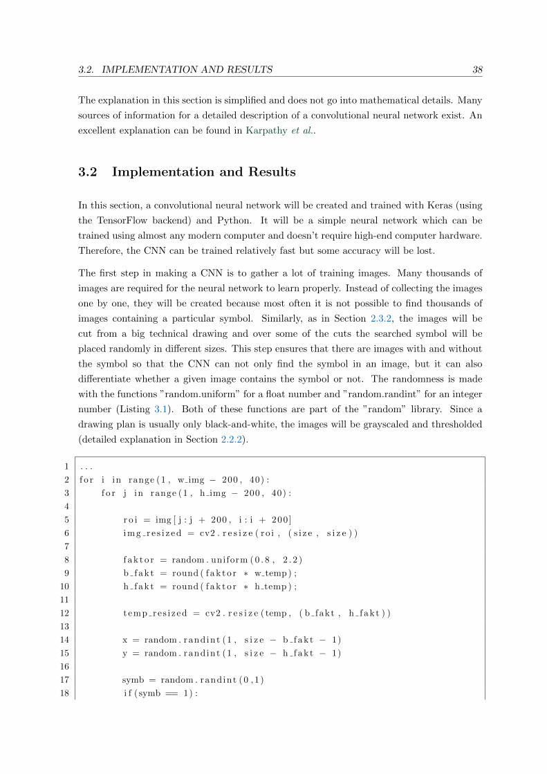
The first step in making a CNN is to gather a lot of training images. Many thousands of
images are required for the neural network to learn properly. Instead of collecting the images
one by one, they will be created because most often it is not possible to find thousands of
images containing a particular symbol. Similarly, as in Section 2.3.2, the images will be
cut from a big technical drawing and over some of the cuts the searched symbol will be
placed randomly in different sizes. This step ensures that there are images with and without
the symbol so that the CNN can not only find the symbol in an image, but it can also
differentiate whether a given image contains the symbol or not. The randomness is made
with the functions ”random.uniform” for a float number and ”random.randint” for an integer
number (Listing 3.1). Both of these functions are part of the ”random” library. Since a
drawing plan is usually only black-and-white, the images will be grayscaled and thresholded
(detailed explanation in Section 2.2.2).
1 . . .
2 f o r i in range (1 , w img − 200 , 40) :
3 f o r j in range (1 , h img − 200 , 40) :
4
5 r o i = img [ j : j + 200 , i : i + 200 ]
6 i m g r e s i z e d = cv2 . r e s i z e ( ro i , ( s i z e , s i z e ) )
7
8 f a k t o r = random . uniform ( 0 . 8 , 2 . 2 )
9 b f ak t = round ( f a k t o r ∗ w temp ) ;
10 h f ak t = round ( f a k t o r ∗ h temp ) ;
11
12 temp res i z ed = cv2 . r e s i z e ( temp , ( b fakt , h f ak t ) )
13
14 x = random . rand int (1 , s i z e − b fak t − 1)
15 y = random . rand int (1 , s i z e − h fak t − 1)
16
17 symb = random . rand int (0 , 1 )
18 i f ( symb == 1) :

3.2. IMPLEMENTATION AND RESULTS 39
19 i m g r e s i z e d [ y : y + temp res i z ed . shape [ 0 ] , x : x + temp res i z ed .
shape [ 1 ] ] = temp res i z ed
20 , img thresh = cv2 . th r e sho ld ( img re s i z ed , 130 , 255 , cv2 .
THRESH BINARY)
21 . . .
Listing 3.1: Preparing the data for training - part 1
The generated images will be saved in an array with a size of: (number images, w size image,
h size image), which contains the pixel values of all the images (Listing 3.2, line 2). The
location of the symbol in every image is saved in another array with a size of: (number images,
4), where the number 4 stands for the x- and y-coordinates and the width and the height
of the symbol in each image. If the variable ”symb” equals 1, the symbol is placed over the
image and if not, the image won’t contain the symbol (”symb” was randomly generated in
Listing 3.1, line 17). The coordinates and size of the symbol are stored in the array if the
image contains it, and negative values are stored if no symbol is displayed on the image. All
values are divided by the size of the image so that they are only between -1 and 1, which
helps the CNN learn easier (Listing 3.2, lines 4-7).
1 . . .
2 img array [ num pic ] = img thresh
3
4 i f ( symb == 1) :
5 p o s s i z e [ num pic ] = [ x/ s i z e , y/ s i z e , b f ak t / s i z e , h f ak t / s i z e ]
6 e l s e :
7 p o s s i z e [ num pic ] = [−50/ s i z e , −50/ s i z e , −50/ s i z e , −50/ s i z e ]
8 . . .
Listing 3.2: Preparing the data for training - part2
A CNN always expects to become an array of images as an input. The array has to be sized
as follows: (number images, w size image, h size image, number channels). Therefore, a new
dimension to the existing array with images (”img array” in Listing 3.2) will be created
which denotes how many channels each image has. This can be made with the function
”np.expand dims” from the NumPy library (Listing 3.3, line 2). The next step is to divide
the images into train and test images (Listing 3.3, lines 7-11). The input array contains all
images and the output array contains the positions of the symbols in the images. For training
90% of the images will be used and for testing - 10%. The testing images will be used as a
validation data in the training process.
1 . . .
2 img array = np . expand dims ( img array , 4)
3
4 input = img array

3.2. IMPLEMENTATION AND RESULTS 40
5 output = p o s s i z e
6
7 c o e f f = i n t ( 0 . 1 ∗ cuts )
8 t r a i n i n p u t = input [ c o e f f : ]
9 t e s t i n p u t = input [ : c o e f f ]
10 t r a in ou tput = output [ c o e f f : ]
11 t e s t o u t p u t = output [ : c o e f f ]
12 . . .
Listing 3.3: Preparing the data for training - part 3
After the input and output data has been created, the convolutional neural network will be
designed and trained (Listing 3.4). The designing process is very important for building an
accurate CNN. Designing the architecture of a neural network means choosing the number
of layers and how these layers are ordered.
In this case (Listing 3.4, lines 3-18) the CNN will have four convolutional layers, four pool-
ing layers and five fully-connected layers (explained in the previous Section 3.1). All the
convolution and fully-connected layers have ReLU as an activation function. The input size
of the neural network is passed to the first layer of the network (Listing 3.4, Line 3). The
input shape is of size (w size image, h size image, 1), where the number 1 stands for how
many channels the image has. In this case, only grayscaled (more specifically thresholded)
images are passed to the CNN, which means that the images have only one channel. All the
convolutional layers have a filter (or kernel) size of 2x2 pixels. The number of filters varies
for each of these layers, where the first one has 20 filters, the second one 40 and so on. The
number of filters doubles after every pooling layer. The size of the image gets smaller after
every pooling layer, so adding more filters to a smaller image result in approximately the
same amount of computations. The first layer has only 20 filters, which is not ideal, but a
small amount of filters reduces the training time.
After the feature extraction is ready, a ”Flatten” layer is added. This layer transforms the
multidimensional features to a list of features (shown in Figure 3.5). In Listing 3.4 on line
13, a ”Dropout” layer is added which prevents the neural network from overfitting. ”The
key idea is to randomly drop units (along with their connections) from the neural network
during training. This prevents units from co-adapting too much” (Srivastava, 2014). Five
fully-connected layers are then attached to the network, where each layer has a different
quantity of nodes (or neurons). The first one has 300, the second 200, the third 100, the
fourth 50 and the last one has 25 nodes (Listing 3.4 lines 14-18). The number of nodes was
again chosen for better time efficiency by the training process, sacrificing some accuracy.
The network should predict the x- and y-coordinates and the width and the height of the
symbol in each image. Therefore, the last layer in the network has four nodes for each one
of these values (3.4 line 19). The predicted values should be linear values. Meaning that

3.2. IMPLEMENTATION AND RESULTS 41
no ReLU activation function will be used, but instead the last layer is left with the default
activation function, which is a linear activation function. It is important to note that all of
the predicted values will be between -1 and 1, because the train output data also has values
only between -1 and 1.
After the architecture of the convolutional neural network is designed, the training process
can begin. First, the neural network is compiled (Listing 3.4, line 22) where for a loss function
the mean squared error (mse) is chosen, which was explained in the previous section. A loss
function calculates the difference between the generated output and the target output. After
testing, the best results were acquired with the ”RMSprop”-optimizer and will therefore be
used. The actual training is made with the function ”model.fit” (Listing 3.4, line 23). The
first two parameters in this function are the training images and the expected output for each
of the images respectively. They are stored in the arrays ”train input” and ”train output”.
During the training process the neural network will pass multiple times over the training
data, each time becoming more accurate. In the given example, 30 passes across the entire
training data will be made. These are called epochs. The test images, which are 10% of all
generated images, will be given as a validation data. These images don’t play any role in
the training, instead they are used for measuring how well the network is trained after each
epoch. On the one hand, if the epochs are too few the neural network won’t be able to make
accurate predictions. On the other hand, if too many epochs are made the network will be
slower to train and can cause overfitting problems. To make the training data random, the
images will be shuffled before being passed to the neural network which can further improve
the accuracy. The last parameter in ”model.fit” denotes that more detailed information will
be printed during the training process. About
After the training process is finished, the neural network is saved to a file which can be used
in multiple programs (Listing 3.4, line 25). The file has an extension of ”h5”, which is a data
file saved in the Hierarchical Data Format (HDF) and contains multidimensional arrays.
1 . . .
2 model = Sequent i a l ( [
3 Convolution2D (20 , ( 2 , 2 ) , input shape=( s i z e , s i z e , 1 ) , a c t i v a t i o n =’
re lu ’ ) ,
4 MaxPooling2D ( p o o l s i z e =(2 , 2) ) ,
5 Convolution2D (40 , 2 , 2 , a c t i v a t i o n =’ re lu ’ ) ,
6 MaxPooling2D ( p o o l s i z e =(2 , 2) ) ,
7 Convolution2D (80 , 2 , 2 , a c t i v a t i o n =’ re lu ’ ) ,
8 MaxPooling2D ( p o o l s i z e =(2 , 2) ) ,
9 Convolution2D (160 , 2 , 2 , a c t i v a t i o n =’ re lu ’ ) ,
10 MaxPooling2D ( p o o l s i z e =(2 , 2) ) ,
11
12 Flat ten ( ) ,

3.2. IMPLEMENTATION AND RESULTS 42
13 Dropout ( 0 . 2 5 ) ,
14 Dense (300 , a c t i v a t i o n =’ re lu ’ ) ,
15 Dense (200 , a c t i v a t i o n =’ re lu ’ ) ,
16 Dense (100 , a c t i v a t i o n =’ re lu ’ ) ,
17 Dense (50 , a c t i v a t i o n =’ re lu ’ ) ,
18 Dense (25 , a c t i v a t i o n =’ re lu ’ ) ,
19 Dense (4 )
20 ] )
21
22 model . compi le ( ’ rmsprop ’ , ’mse ’ )
23 model . f i t ( t r a in input , t ra in output , epochs =30, s h u f f l e=True ,
v a l i d a t i o n d a t a =( t e s t i n p u t , t e s t o u t p u t ) , verbose =2)
24
25 model . save (” saved cnn . h5 ”)
26 . . .
Listing 3.4: Designing and training the CNN
After the training is finished, the CNN has to be tested. The trained CNN can be loaded
in a new program and predictions can be made for a given array of images. The input data
for the trained network has to have the same size as the input data used for training the
network. This includes the number of channels for every image. The predicted results will be
between -1 and 1. They should be multiplied by the size of the images before being further
used so that the actual location of the symbol in pixels is acquired (Listing 3.5).
1 . . .
2 model = load model (” saved cnn . h5 ”)
3
4 pred i c t ed output = model . p r e d i c t ( t e s t i n p u t )
5 pred i c t ed = pred i c t ed output ∗ s i z e
6 . . .
Listing 3.5: Using the trained CNN
The generated images for testing are cut from a different image than the one used for training.
This ensures that the neural network hasn’t seen these images during training. The accuracy
is then measured in two ways. The first measures how accurately the trained network can
predict whether the symbol is in the image or not. Further to this will be measured how
well the CNN finds the exact position of the symbol in the image by calculating the overlap
between the predicted and the real bounding boxes of the symbols, which is called Intersection
Over Union (explained in Rieke (2017)). As a result, the trained neural network was able
to detect if the searched symbol is on the image with an accuracy of above 95% which is an
excellent result. The predicted location of the symbol, on the other hand, strongly depends

3.2. IMPLEMENTATION AND RESULTS 43
on the size of the symbol and the size of the image. The testing CNN was trained with images
with a size of 120x120 pixels (for the symbol in Figure 2.18), therefore the test images should
have the same size. With this size of the images, the neural network could predict the exact
location of the symbol with a 75-85% accuracy, again depending on the size of the symbol.
In this case, 100% would be a perfect match for the x- and y-coordinates, as well as the
width and the height of the symbol in a given image. Thus 80% is a relatively good match.
For testing over ten thousand generated images were used, so the results should represent
the real accuracy of the CNN quite good. Figure 3.7 shows some examples of how well the
network can predict the location of the symbol (marked by red rectangles), even when it is
relatively hard to spot. It is important to note that the network was trained in such a way
that a maximum of one symbol should be on every image.
Figure 3.7: Detected symbols
The predictions shown above were made with a simple convolutional neural network and
relatively few training images. The accuracy can be increased if a more complex network is
used, but this would require a very powerful graphics processing unit (GPU). The size of the
images is pretty small but usually a CNN is not trained with images bigger than 250x250
pixels. However, they can be used in bigger images by resizing the bigger image or by cutting
it into small parts and using the trained CNN for every part of the image. YOLO (You Only
Look Once), for example, is an algorithm for fast object detection, which can be even used
in videos with high frame rates (Redmon, 2016).
In the previous Chapter 2.3.3, the method used could not recognize a symbol like the one in
Figure 2.21. Meaning that a CNN for the same symbol will be trained. After training, the
neural network was tested once more with thousands of images. The accuracy of prediction
for this symbol was surprisingly close to the results for the symbol mentioned above. This
shows that the CNN was able to recognize the same symbol which wasn’t recognized by the
cascade method from the previous chapter. Henceforth, a convolutional neural network can
be used in a variety of cases, for which a Haar-cascade can’t be used.
Next, the trained CNNs will be tested on a real data. For testing purposes, an image shown
in Figure 3.8 will be used, containing both of the symbols for which a neural network was
trained.

3.2. IMPLEMENTATION AND RESULTS 44
Figure 3.8: Image for testing the trained CNN
To test the CNN, the big image must be cut in small ROIs (regions of interest, explained in
the previous chapter) and for each ROI the trained neural network will predict the location
of the symbol if one is present. The coordinates of the predictions will be in local coordinates
for the given ROI. Therefore, they have to be transformed into global coordinates. The image
must be also thresholded because the neural network expects such an image (explained earlier
in this section).
Figure 3.9: Result using two different CNNs
3.3. LIMITATIONS 45
The result can be seen in Figure 3.9 where the predictions for each symbol are marked with
different colors. The trained neural networks have correctly predicted the position and the
size of each symbol, in most cases with a very high accuracy. There are often multiple pre-
dictions for a single symbol because the ROIs overlap and thus the same symbol occurs in
different ROIs. This problem could be easily eliminated in the majority of situations (simple
solution was shown in chapter 2.1.3).
3.3 Limitations
A convolutional neural network can accurately detect symbols as shown above. The used
CNN is a very simple and could be trained from almost any modern computer. However, it
won’t recognize any symbols in certain situations.
If two symbols are very close to one another, the neural network won’t be able to recognize
both because it was trained to predict only one symbol at a time. Meaning that if there is
more than one symbol in a single ROI, they won’t be recognized correctly. Nevertheless, a
more complex neural network can be trained which would be able to identify multiple symbols
at a time. This, however, would require a more powerful GPU and a longer training period.
Furthermore, the method with the ROIs described above, isn’t very efficient and is relatively
slow, but it was created only for testing the accuracy of the CNNs in real technical drawings
and can be further modified.
The biggest challenge to train an accurate convolutional neural network is to have a powerful
enough GPU but even then a, complex CNN can require many hours or even days to train.
This is a huge drawback, but once correctly designed and trained, a CNN can be very accurate
and can be used in a variety of situations.

46
Chapter 4
Practical implementation with
graphical user interface
In the previous chapters, various methods have been proposed for finding symbols in tech-
nical drawings. A graphical user interface (GUI) will be created for some of these methods.
Programming skills are required to use a program without a GUI, which makes it unpractical
in many situations. Therefore, a graphical user interface will be created for easier operation
using the Template Matching method and Neural networks, which were already programmed
and explained in the previous chapters.
A GUI for the Template Matching method will be made using Windows Presentation Foun-
dation (WPF). WPF is a graphical system developed by Microsoft for building Windows
desktop application. Applications with WPF are programmed in the integrated development
environment (IDE), called Microsoft Visual Studio, with the programming language C#. To
use the OpenCV library in C#, which is normally used in C++ or Python, the ”Emgu CV”
is used. Emgu CV is a cross-platform wrapper to the OpenCV library that allows OpenCV
functions to be called from C#.
As explained in the previous chapter, Keras with TensorFlow backend is used to design,
build and test a neural network. Unfortunately, Keras cannot be used in WPF to build a
GUI because it can’t be used with C#. The ”Tkinter” library in Python is used for this
purpose. Tkinter comes included with the standard Python distributions and is the Python
standard GUI. Tkinter is not as easy to create a complex GUI as WPF, but it has the
advantage of building cross-platform applications, while WPF is only suitable for Windows
applications.
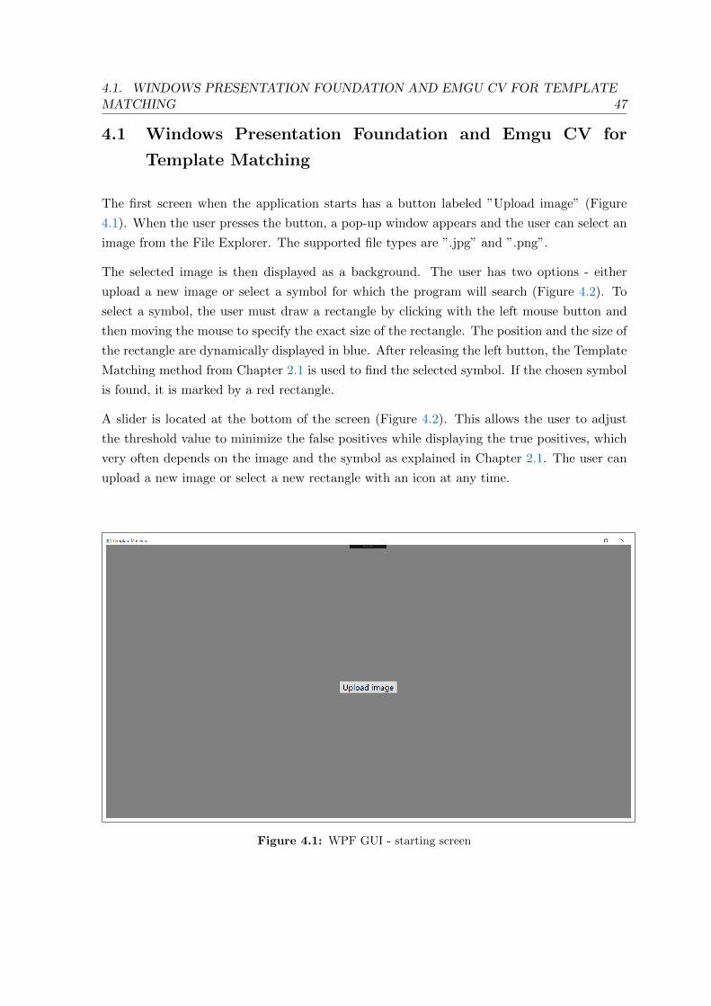
4.1. WINDOWS PRESENTATION FOUNDATION AND EMGU CV FOR TEMPLATEMATCHING 47
4.1 Windows Presentation Foundation and Emgu CV for
Template Matching
The first screen when the application starts has a button labeled ”Upload image” (Figure
4.1). When the user presses the button, a pop-up window appears and the user can select an
image from the File Explorer. The supported file types are ”.jpg” and ”.png”.
The selected image is then displayed as a background. The user has two options - either
upload a new image or select a symbol for which the program will search (Figure 4.2). To
select a symbol, the user must draw a rectangle by clicking with the left mouse button and
then moving the mouse to specify the exact size of the rectangle. The position and the size of
the rectangle are dynamically displayed in blue. After releasing the left button, the Template
Matching method from Chapter 2.1 is used to find the selected symbol. If the chosen symbol
is found, it is marked by a red rectangle.
A slider is located at the bottom of the screen (Figure 4.2). This allows the user to adjust
the threshold value to minimize the false positives while displaying the true positives, which
very often depends on the image and the symbol as explained in Chapter 2.1. The user can
upload a new image or select a new rectangle with an icon at any time.
Figure 4.1: WPF GUI - starting screen
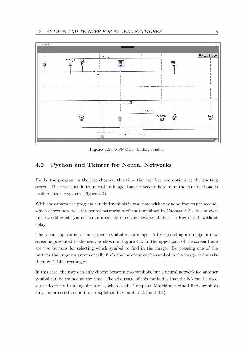
4.2. PYTHON AND TKINTER FOR NEURAL NETWORKS 48
Figure 4.2: WPF GUI - finding symbol
4.2 Python and Tkinter for Neural Networks
Unlike the program in the last chapter, this time the user has two options at the starting
screen. The first is again to upload an image, but the second is to start the camera if one is
available to the system (Figure 4.3).
With the camera the program can find symbols in real time with very good frames per second,
which shows how well the neural networks perform (explained in Chapter 3.2). It can even
find two different symbols simultaneously (the same two symbols as in Figure 3.9) without
delay.
The second option is to find a given symbol in an image. After uploading an image, a new
screen is presented to the user, as shown in Figure 4.4. In the upper part of the screen there
are two buttons for selecting which symbol to find in the image. By pressing one of the
buttons the program automatically finds the locations of the symbol in the image and marks
them with blue rectangles.
In this case, the user can only choose between two symbols, but a neural network for another
symbol can be trained at any time. The advantage of this method is that the NN can be used
very effectively in many situations, whereas the Template Matching method finds symbols
only under certain conditions (explained in Chapters 2.1 and 3.2).
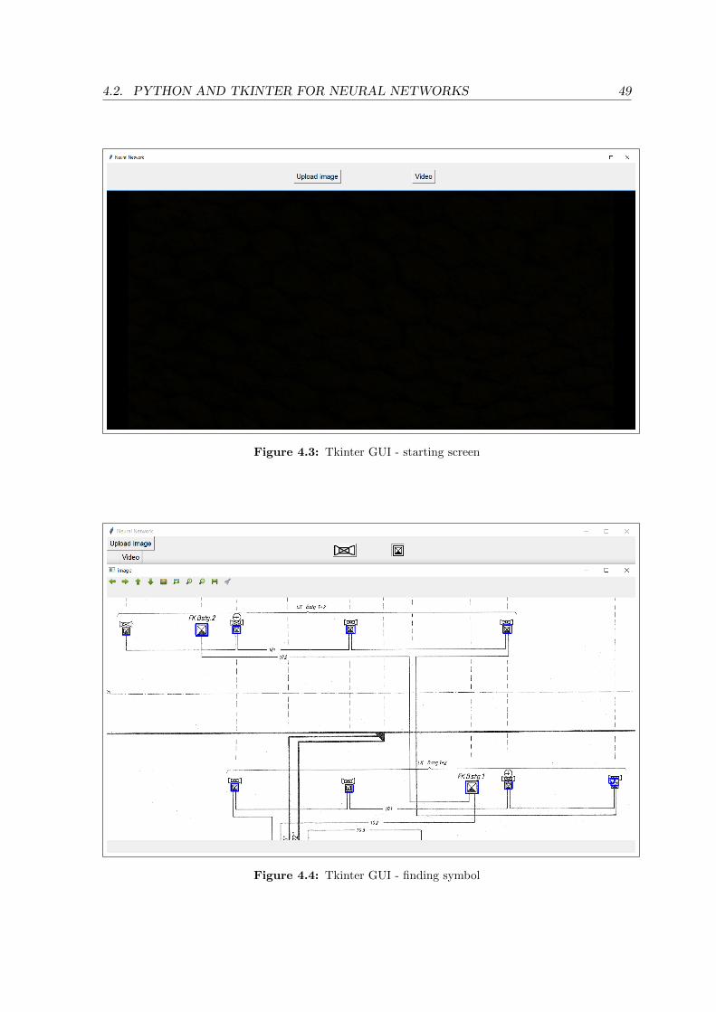
4.2. PYTHON AND TKINTER FOR NEURAL NETWORKS 49
Figure 4.3: Tkinter GUI - starting screen
Figure 4.4: Tkinter GUI - finding symbol

50
Chapter 5
Conclusion
In this work, different approaches for finding symbols in technical drawings have been pro-
posed. An overview of the differences between these methods can be seen in the table below.
Figure 5.1: Overview
The first two techniques require no training and can be implemented almost instantly with
very promising results under certain conditions. The main disadvantage of the Template
matching method is that it is not rotation and scale invariant, meaning that it can only find
symbols with the same size and orientation. This problem can be eliminated by rotating and
scaling the template image multiple times. However, this is an inefficient and slow solution.
Alternatively, the second method is scale and rotation invariant, which is an advantageous
factor. Nevertheless, it remains unusable in select situations. For example, the symbol won’t
be recognized if it is connected to another symbol or crossed by a line, which is often the case
in technical drawings. Another disadvantage of this technique is that it works most optimally

51
only if the symbol is in a closed shape, as explained in Chapter 2.2.3. In addition, both of
these methods require a precisely adjusted threshold value so as to simultaneously keep the
false positives low and not lose true positives.
The third method (Cascade classifiers) is rotation and scale invariant and can be used in many
situations where the other two techniques fail. However, the Cascade classifiers method
requires training, which is a time-consuming task and many variables must be carefully
tuned for an accurate training. Although this technique works under many conditions it
fails to differentiate a given symbol if it has too few features, as described in Chapter 2.3.3.
Furthermore, a threshold value has to be carefully adjusted in order to achieve good results.
The last technique proposed in this work uses convolutional neural networks to find symbols
in technical drawings. In addition to being scale and rotation invariant, this method requires
no threshold value to be adjusted. The sole disadvantage of this technique is that a neural
network (NN) must be trained before being used. The training requires a powerful GPU and
a vast quantity of image data, whereas a simple NN can be trained quickly, as described in
Chapter 3.2.
The convolutional neural network, which was designed in this work, is a very simple NN
and shows promise for optimization. One option would be to add the possibility for the NN
to find more than one symbol in a single ROI (explained in Chapter 3.3). Furthermore, the
proposed algorithm for implementing the neural network in big images is inefficient and offers
room for improvement. Another upgrade would be to make the NN more complex, and thus
more accurate, but this would require a significantly more powerful GPU.

BIBLIOGRAPHY 52
Bibliography
Jonathan Weber and Salvatore Tabbone. Symbol spotting for technical documents : An effi-
cient template-Matching approach. 21st International Conference on Pattern Recognition
(ICPR 2012) November 11-15, 2012.
Muhammad Muzzamil Luqman, Thierry Brouard and Jean-Yves Ramel. Graphic Symbol
Recognition using Graph Based Signature and Bayesian Network Classifier. 10th Interna-
tional Conference on Document Analysis and Recognition (ICDAR) July 26-29, 2009.
Marcal Rusinol and Josep Llados. Symbol Spotting in Technical Drawings Using Vectorial
Signatures. In: Liu W., Llados J. (eds) Graphics Recognition. Ten Years Review and Future
Perspectives. GREC 2005. Lecture Notes in Computer Science, vol 3926. Springer, Berlin,
Heidelberg, 2006.
Nibal Nayef, Muhammad Zeshan Afzal and Thomas M. Breuel. Learning Feature Weights of
Symbols, with Application to Symbol Spotting. 21st International Conference on Pattern
Recognition (ICPR 2012) November 11-15, 2012.
Adrian Kaehler and Gary Bradski. Learning OpenCV 3: computer vision in C++ with the
OpenCV library. O’Reilly Media, 2016.
OpenCV (3.4.0): Open Source Computer Vision. Template Matching
https://docs.opencv.org/trunk/d4/dc6/tutorial py template matching.html
Accessed on: 2018-01-18
OpenCV (2.4): OpenCV 2.4.13.5 documentation. Template Matching
https://docs.opencv.org/2.4/doc/tutorials/imgproc/histograms/
template matching/template matching.html
Accessed on: 2018-01-18
Joseph Lee Rodgers and W. Alan Nicewander Thirteen ways to look at the Correlation
Coefficient. The American Statistician, Vol. 42, pp. 59-66, 1988.
Hae Yong Kim and Sidnei Alves de Araujo. Grayscale Template-Matching Invariant to
Rotation, Scale, Translation, Brightness and Contrast. Mery D., Rueda L. (eds) Advances

BIBLIOGRAPHY 53
in Image and Video Technology. PSIVT 2007. Lecture Notes in Computer Science, vol
4872. Springer, Berlin, Heidelberg, 2007.
OpenCV (3.4.0): Open Source Computer Vision. Contours Hierarchy
https://docs.opencv.org/trunk/d9/d8b/tutorial py contours hierarchy.html
Accessed on: 2018-01-23
OpenCV (3.3.1): Open Source Computer Vision. Contours : Getting Started
https://docs.opencv.org/3.3.1/d4/d73/tutorial py contours begin.html
Accessed on: 2018-01-25
Chandrajit L. Bajaj, Valerio Pascucci and Daniel R. Shikore. The contour spectrum. Pro-
ceedings of the 8th conference on Visualization 1997 pp. 167-ff, 1997.
Marc van Kreveld, Rene van Oostrum, Chandrajit Bajaj, Valerio Pascucci and Dan Schikore.
Contour trees and small seed sets for isosurface traversal. Proceedings of the thirteenth
annual symposium on Computational geometry pp. 212-220, 1997.
Marcin Kmiec. New Optical Character Recognition Method Based on Hu Invariant Moments
and Weighted Voting. Journal of applied computer science, Vol. 19, pp. 33-50, 2011.
Gary Bradski and Adrian Kaehler. Learning OpenCV: computer vision with the OpenCV
library. O’Reilly Media, 2008.
Wikipedia: The Free Encyclopedia. Image moment.
https://en.wikipedia.org/wiki/Image moment
Accessed on: 2018-01-27.
Ming-Kuei Hu. Visual pattern recognition by moment invariants. IRE Transactions on In-
formation Theory, Vol.8(2), pp.179-187, 1962.
P. Viola and M. Jones. Rapid Object Detection using a Boosted Cascade of Simple Features.
Computer Vision and Pattern Recognition, 2001. CVPR 2001. Proceedings of the 2001
IEEE Computer Society Conference on, 2001.
Rainer Lienhart and Jochen Maydt. An Extended Set of Haar-like Features for Rapid Object
Detection. Proceedings 2002 International Conference on Image Proceedings. Vol. 1. IEEE,
2002.
OpenCV (3.3.0): Open Source Computer Vision. Face Detection using Haar Cascades
https://docs.opencv.org/3.3.0/d7/d8b/tutorial py face detection.html
Accessed on: 2018-01-29.
Yoav Freund and Robert E. Schapire A decision-theoretic generalization of on-line learning
and an application to boosting. Journal of Computer and System Sciences, Vol. 55(1),
pp.119-139, 1997.
BIBLIOGRAPHY 54
T. Ojala, M. Pietikainen and D. Harwood. Performance evaluation of texture measures with
classification based on Kullback discrimination of distributions. Pattern Recognition, 1994.
Harrison Kinsley. Creating your own Haar Cascade OpenCV Python Tutorial.
https://pythonprogramming.net/haar-cascade-object-detection-python-opencv-tutorial/
Accessed on: 2018-01-25.
Eugenio Culurciello. Neural Network Architectures
https://towardsdatascience.com/neural-network-architectures-156e5bad51ba
Accessed on: 2018-02-03.
Brandon Rohrer. How do Convolutional Neural Networks work?
http://brohrer.github.io/how convolutional neural networks work.html
Accessed on: 2018-02-04.
Johannes Rieke. Object detection with neural networks - a simple tutorial using keras.
https://towardsdatascience.com/object-detection-with-neural-networks-a4e2c46b4491
Accessed on: 2018-02-06.
Yann LeCun, Leon Bottou, Yoshua Bengio and Patrick Haffner. Gradient-based learning
applied to document recognition. Proceedings of the IEEE. 86 (11): 2278-2324, 1998.
Andrej Karpathy, Justin Johnson. CS231n Convolutional Neural Networks for Visual Recog-
nition.
http://cs231n.github.io/convolutional-networks/
Accessed on: 2018-02-08.
Nitish Srivastava, Geoffrey Hinton, Alex Krizhevsky, Ilya Sutskever, Ruslan Salakhutdinov.
Dropout: a simple way to prevent neural networks from overfitting. Journal of Machine
Learning Research 15: 1929-1958, 2014.
Joseph Redmon, Santosh Divvala, Ross Girshick, Ali Farhadi. You only look once: Unified,
real-time object detection. Proceedings of the IEEE conference on computer vision and
pattern recognition, pp. 779-788, 2016.

Declaration of Originality
With this statement I declare, that I have independently completed this Bachelor’s thesis.
The thoughts taken directly or indirectly from external sources are properly marked as such.
This thesis was not previously submitted to another academic institution and has also not
yet been published.
Munchen, 14. April 2018
Deian Stoitchkov