Analysis of liquid metal MHD flow in multiple adjacent ducts using

Fusion Engineering and Design 13 (1991) 363-380 363 North-Holland

Analysis of liquid metal MHD flow in multiple adjacent ducts using an iterative method to solve the core flow equations

K.A. M c C a r t h y a n d M . A . A b d o u

University of California, Los Angeles, 6288 Boelter Hall, Los Angeles, CA 90024-1597, USA

Submitted 1990; accepted July 1990 Handling Editor: R.W. Conn

A computationally fast and efficient method for analyzing MHD flow at high Hartmann number and interaction parameter is presented and used to analyze a multiple duct geometry. This type of geometry is of practical interest in fusion applications. Because the Hartmann number and interaction parameter are generally large in fusion applications, the inertial and viscous terms in the Navier-Stokes equation can often be neglected in the core flow region, making this equation linear. In addition, because the magnetic fields in a fusion reactor vary slowly and the magnetic Reynolds number is small, the induced magnetic field can be neglected. The resulting equations representing core flow have certain characteristics which make it possible to reduce them to two dimensional without losing the three dimensional characteristics.

The method which has been developed is an "iterative" method. A velocity profile is assumed, then Ohm's law and the current conservation equation are combined and used to solve for the potential distribution in a plane in the fluid, and in a surface in the duct wall. The potential variation along magnetic field lines is checked, and if necessary, the velocities are adjusted. This procedure is repeated until the potentials along field lines vary to within a specified error.

The analysis of the multiple duct geometry shows the importance of global effects. The results of two basic cases are presented. In the first, the average velocity in each duct is the same, but the wall conductance ratios of the walls perpendicular to the magnetic field vary from duct to duct. The total pressure drop in the electrically connected ducts was greater than or equal to the total pressure drop in the same ducts electrically isolated. In addition, the velocity profile in the ducts can be significantly affected by the presence of neighboring ducts. In the second case, the wall conductance ratios are the same for each duct, but the average velocity varies from duct to duct. The overall pressure drop is the same as if the ducts were electrically isolated, but the velocity profile and side layer flow rate can be very different from the electrically isolated case.

1. Introduction

The self-cooled liquid metal blanket is a prime candidate for use in a fusion reactor. While lithium-con- taining liquid metals have good heat transfer and tri- t ium breeding characteristics, their flow is affected by the presence of a magnetic field. These magnetohydrodynamic (MHD) effects have a significant impact on the fluid flow, and therefore affect heat transfer, mass transfer, and the pressure drop.

The M H D pressure drop is a particularly important aspect of M H D flow. Limiting the pumping power is necessary for economic reasons, but more importantly, a large pressure drop results in large stress in the coolant duct walls. This stress may be accommodated by increasing the thickness of the duct walls. However, if the walls are conducting, this increases the M H D

pressure drop. It is important to be able to calculate the pressure drop for each proposed blanket design. Ad- ditionally, it is important to be able to calculate the heat transfer in a blanket.

Numerical solution of the full set of equations would give the most accurate solution for any situation. How- ever, this is particularly difficult to do, because at parameters characteristic of the fusion reactor, the viscous and inertial terms in the Navier-Stokes equation are many orders of magni tude smaller than the other terms. A numerical solution of the full set of equations for fully developed flow was done by Tillack et al. [1], but it is also important to understand developing flows. Two dimensional numerical analyses of developing M H D flow have been done (see for example Abdou et al. [2]), but the applicability of these analysis is limited because developing M H D flows are three dimensional.

0 9 2 0 o 3 7 9 6 / 9 1 / $ 0 3 . 5 0 © 1991 - E l sev ie r Sc ience Pub l i she r s B.V. ( N o r t h - H o l l a n d )

364 K.A. McCarthy, M.A. A bdou / Analysis of liquid metal MHD flow

A three dimensional numerical analysis of flow in a varying magnetic field and flow in a sudden expansion has been carried out by Kim [3], but the codes are computer time intensive and are limited to Hartmann numbers on the order of one hundred. For some geometries such as abrupt expansions, solution of the full set of MHD equations is warranted. There are cases however, when certain terms can be neglected in the Navier-Stokes equation and Amp4re's Law, making the MHD equations linear and eliminating the difficulties associated with their numerical solution. When the magnetic field is high enough, viscous and inertial terms can often be neglected without a significant impact on the calculation of the core flow variables. (The core is the region in MHD flow where viscous and inertial forces are generally negligible, and the pressure gradient is balanced by the electromagnetic body force.) In addition, if the induced magnetic field is negligible with respect to the applied magnetic field, the magnetic field can be assumed known. This is valid for slowly varying fields if the magnetic Reynolds number (the ratio of induced to applied magnetic field) is small, and in a fusion reactor, the magnetic fields are slowly varying. After making the simplifications implied by these as- sumptions, the set of MHD equations can be solved numerically without the problems inherent in the solution of the full set of equations.

The set of equations resulting from the approximations mentioned above could be solved in a three dimensional domain, but certain characteristics of the equations can be exploited. Because the variation of the flow variables along magnetic field lines can be de- termined, the equations can be reduced to two dimensions. Two such methods of solving these equations have been explored, based on work done by Kulikovskii [4]. One is a "direct integration" method where the equations are integrated along magnetic field lines. The resulting equations are then solved subject to the correct boundary conditions. This method has been applied to various geometries such as circular ducts (see for example Reed et al. [5] through Tillack [7]) and rectangular ducts (see for example Reed et al. [5] and Picologlou et al. [8]). In theory, this method is applicable to any problem; however, in certain complicated geometries, the equations become quite unwieldy due to necessary coordinate system transformations. An alternative method based on work done by Madarame and Tokoh [9,10] has been developed which avoids these complica- tions. It is an iterative method - the full set of equations is not solved simultaneously. A velocity profile is assumed and the equations are solved in a plane in the fluid and in a surface of the duct wall. The potentials in

the wall and fluid are compared along magnetic field lines, and if they do not vary in a specified way. the velocity is modified. This process is repeated until the correct solution is found. Because the duct wall and the plane in the fluid are meshed directly, no transformations are necessary as in the direct integration method. In addition, since the full set of equations is not integrated and combined, the equations being solved are not as complex as those derived in the direct integration method. For this reason, the iterative method should be more convenient than the direct integration method when applied to problems with complicated geometries.

2. Solution approach

In this section, background information leading up to the choice of the solution approach is given. The analytic formulation of the equations is presented, and the numerical scheme is described.

2.1. Analytic formulation

The equations describing steady-state, incom- pressible MHD flow are (see for example Shercliff [11]):

Ov" W v = - U p + i x B + ~V'2v, (1)

j = o ( - v,~ + v x n ) , (2)

v - n = o, ( 3 )

V X B = ~t0j, (4)

v.v=O, (5)

v,.j=o, (6)

where O is the fluid density, v is velocity, p is pressure, j is current density, B is the magnetic field, /~ is the kinematic viscosity, o is electrical conductivity, O is electric field potential, and /~0 is the free space permeability. These equations can be made dimensionless by setting v* = v / v , B * = B / B o, j * = j / o f vB o, O* = $/avBo, and p* = p / o f vB2a. In these relationships, the starred quantities are dimensionless, v is the bulk velocity, B 0 is the maximum magnetic field, and a is a characteristic length. All length variables are normalized using a.

The dimensionless MHD equations are (dropping the stars):

N - i v • Wv = - Wp +J X B + M-2tTzv, (7)

• O,.w n ) , ( 8 ) .t = ~ S / ( - v',t, + v x

K.A. McCarthy, M.A. Abdou / Analysis of liquid metal MHD flow 365

V.B=O, (9)

v × B = R ~ j , (10)

V.v=O, (11)

v . j = 0 , (12)

where N is the interaction parameter, N = oBZa/pv, M is the Hartmann number, M = Ba~/-~/ix, the subscripts f and w refer to the fluid and wall, respectively, and R m is the magnetic Reynolds number, Rm=lXoooa. The interaction parameter is the ratio of magnetic forces to inertial forces, the Hartmann number squared is the ratio of magnetic forces to viscous forces, and the magnetic Reynolds number is the ratio of the induced magnetic field to the applied magnetic field.

At high M and N, MHD flow is made up of distinct regions: the core flow, boundary layers, and free shear layers. In the core, viscous and inertial forces are generally negligible, so the pressure gradient is balanced by magnetic forces. In a fusion reactor it is envisioned that M and N may be as large as 106. This introduces additional complexity into the solution of the MHD equations. Besides being nonlinear, the inertial and viscous terms in the Navier-Stokes equation, equation (7), can be orders of magnitude smaller than the other terms. This makes the numerical solution of the full set of MHD equations very difficult as is explained by Ramos and Winowich [12]. However, at such high M and N, certain approximations can often be made that greatly simplify the solution.

If the following is assumed: (1) viscous forces are negligible ( M ~ oo), (2) inertial forces are negligible (N ~ oo), (3) the induced magnetic field is negligible (R m ~ 0),

then the dimensionless equations governing steady, in- ertialess, inviscid MHD flow are:

v p = j x S , (13)

j = °f'w ( - V e p + v X B ) , (14) fff

v . i = 0, ( 1 5 )

V ' v = 0, (16)

where the subscripts f and w refer to the fluid and wall respectively, and B is the divergence-free, known applied magnetic field. The flow is treated as if made up entirely of core flow. The boundary layers are assumed to have a negligible effect on the core flow. This is usually a valid assumption as long as there is a component of magnetic field perpendicular to the duct wall. In certain situations, however, the boundary layers are important. For example, in nonconducting ducts, the

Hartmann boundary layers (boundary layers with a magnetic field component perpendicular to them) carry all the returning current. For this type of problem, it is necessary to use a matching condition between the core and the boundary layer (see for example Hua and Walker [13]). When the walls are conducting however, the amount of current in the Hartmann layers is negligible. In circular ducts with transverse magnetic fields, this is violated only at a point, so all boundary layers can be neglected. In a rectangular duct with one wall parallel to the magnetic field, there is a side wall boundary layer and the influence it has on the flow cannot be neglected. The core flow method can still be applied with special treatment of side wall boundary layers.

Equations (13)-(16) could be solved in a three dimensional domain, but there are certain characteristics of the equations that can be taken advantage of which enable one to solve the equations on a two dimensional surface. It is important to notice that eq. (13) shows that the pressure does not vary along magnetic field lines. Additionally, it can be shown by taking the curl of the Navier-Stokes equation that the components of the current density perpendicular to magnetic field lines (hereafter referred to as perpendicular components) do not vary along field lines. Expressions for the variation of the perpendicular components of velocity and parallel components of current density and velocity can be derived by taking the curl of Ohm's law. For a Carte- sian coordinate system:

= f d l ( v , , x j . + v ' . x j,, ) / B ,

BVl I# I I - V l IV I IB = v..L V'.L B + V . j .L ,

B V j t I - j l i V t i B = j . V j_B,

where 1 is taken along a field line.

(17)

(18) (19)

Once the core variables are known on one surface, they can be calculated in the entire domain. Solving the equations in two dimensions enables one to find the three dimensional solution. This makes the numerical solution much more tractable, both in terms of computer time and code complexity. In making this sim- plification, the three dimensional aspects of the solution are not lost.

2. 2. Numerical scheme

An iterative technique has been developed to solve the core flow equations. A velocity distribution is guessed, then the equations (with the potential as the unknown variable) are solved in a plane in the fluid and

366 K.A. McCarthy, M.A. A bdou /Ana l y s i s of liquid metal M H D flow

in a surface in the duct wall. There is a computational grid in the plane in the fluid, and in the duct wall. It is not necessary to transform the wall equations into the fluid coordinate system or vice versa, as is sometimes necessary in the direct integration method. When the equations and boundary conditions have been satisfied in the entire domain of the duct, the problem has been solved.

In the domain of the fluid, the core flow equations are given by eqs. (13)-(16). Combining eqs. (14) and (15) yields:

v'zq~f = V" ( v X B) . (20)

In order to solve this equation on a two dimensional surface, parallel derivatives of the fluid potential must be put in terms of perpendicular components. This can be done by using eq. (19).

If all of the core current returns through the walls (as opposed to some of the current returning though boundary layers), then in the domain of the wall, Ohm's law and current conservation are used without any modifications. (If there are side layers, and their resis- tance is low enough, a significant fraction of current will return through the boundary layer. This can be approximated in geometries with certain symmetries as is done in McCarthy [14] and Tillack and McCarthy [15], for example):

- °w Vrw4,w, (21) J w - - - - fff

~Tw " lw = - 3 j f J O n , (22)

where n is a unit normal pointing from the wall to the fluid and the gradients are taken in the surface of the wall (the gradients do not contain a component normal to the wall). The wall is assumed to be thin enough so that the potential variation through the thickness of the wall is negligible. Equation (22) can then be integrated across the wall to obtain (for constant wall conductivity):

(V" . j w ) t w = - i f . n , (23)

where tw is the wall thickness normalized with respect to a.

Equations (21) and (23) can be combined, resulting in the following equation:

(/) lTZq)w = h . n , (24)

where (I) is the wall conductance ratio, (/)= Owtw/Oea. Equation (24) is known as the thin-wall boundary condition.

Once the two dimensional potential distribution in the fluid and wall has been calculated for a given velocity field, it is necessary to determine whether the equations have been satisfied in the entire domain of the problem. The criterion for determining this is based on the variation of the potential along field lines. The parallel component of Ohm's law is integrated along a magnetic field line:

f ; Z d l ~ / f = q S f , 2 - ~fq = - f/f2d0f!,, (25)

where jf, is found from equation (19). Integration of this equation results in an expression for the variation of the potential along magnetic field lines.

The potentials in the fluid and wall are compared along field lines. Because the potential jump across Hartmann layers is negligible at high Hartmann numbers, the potential in the fluid is equal to the potential in the wall at the fluid-wall interface. If the potentials do not meet this criterion to within a specified error, it is necessary to adjust the velocities. This is done using the following equation:

. . . . . ld ( ~q~w ~(])f ) (26) Uaxia I - - Oaxia I - - K at 3t wall '

where t is the transverse direction, which is perpendicular to the field and the axial direction, and ~ is an underrelaxation parameter, 0 < K < 1. The value of K depends on the wall conductance ratio: the lower (/) is, the lower r must be.

If the correct velocities have already been found, the potential gradient at the wall will be equal to the potential gradient in the fluid evaluated at the wall. In other words, the potentials vary correctly along magnetic field lines. However, if the potential gradients are not equal, the velocity must be adjusted in order to adjust the potential gradients. If the potential gradient in the wall is larger than the potential gradient in the fluid at the wall, the axial velocity must be decreased in order to decrease the current density in the fluid, which decreases the amount of current going into the wall, thus decreasing the potential gradient in the wall.

The axial velocity calculated in this manner will not necessarily satisfy global mass conservation. The velocity must be normalized such that the flow in the boundary layers plus the flow in the core is equal to the total input flow. When the magnetic field is parallel to a wall at more than one point (such as with a rectangular duct with one wall parallel to the magnetic field), the layers at the fluid-wall interface can carry a large fraction of the flow. These layers are called side layers. For


the case of circular ducts, the amount of fluid in the boundary layers is negligible.

The equation used to normalize the velocities is:

ffd..o.,.l+ffda~,v..,.~l=constant, (27)

where a is the cross sectional area of the duct and asl is the cross sectional area of the side layer. The second term in eq. (27) is necessary only when the magnetic field is parallel to a wall at more than a point.

Using Ohm's law and neglecting O(~) terms, Fig. 2. Geometry and coordinate system for circular duct.

f f das,,,a,,ial,sl = f d',a,o, (28)

where AO is the potential jump across the side layer. The potential jump across the side layer is the difference between the potential at the wall and the potential in the fluid adjacent to the wall. These potentials are calculated so the side layer flow rate can be de- termined.

The transverse component of velocity must also be calculated. An expression for this velocity component

Assume Velocities

I_ Calculate Potential Distribution in Fluid and Wall

No I Adjust Velocities

Fig. 1. Flowchart showing iterative solution procedure.

can be found by integrating eq. (16) along a magnetic field line:

f d t ( v - , 0 = 0, (29)

where the parallel component of velocity is found using eq. (18). This results in an equation that relates the transverse velocity component to the axial velocity component, and which satisfies local mass conservation. Because the parallel component has been integrated out, this equation can be solved on a two dimensional surface.

After calculating a new velocity distribution, the potential in the fluid and wall is calculated again. This process is repeated until the criterion based on the potential variation along field lines is satisfied.

To summarize the process, Ohm's law and the current conservation equation are used to calculate the potential distribution in a plane in the fluid, and in a surface in the wall. The Navier-Stokes equation is used to determine whether the potential variation along magnetic field lines is correct. If necessary, a new axial velocity is calculated using Ohm's law, and the mass conservation equation is used to normalize the new axial velocity. Figure 1 gives a summary of the iterative procedure.

3. Representative examples of benchmarking results

The iterative method described in the previous section has been used to analyze flow in various geometries (see McCarthy [14], and McCarthy et al. [16]). Because there are no exact analytic solutions for developing MHD flow with which to compare the present model, benchmarking to experimental results from the Argonne Liquid Metal Experiment (ALEX) (see Reed et al. [5] and Picologlou et al. [8]) was done for rectangular and circular ducts. Representative results of the benchmark-

368 K.A. McCarthy, M.A. A bdou /Ana ly s i s of liquid metal M H D flow

1.2

1.0 0.8 0,6 0.4 0.2 0 . 0 , I

- 0 - 5 0 5

X Fig. 3. Magnetic field variation at the exit of ALEX [17].

i

0

ing are presented here. Further benchmarking results can be found in McCarthy [14] and McCarthy et al. [161.

In ANL' s circular duct experiment (Reed et al. [5]), the duct had a wall conductance ratio of 0.026. In the results presented, M = 6000 and N = 10000. Measure- ments of potentials, velocities, and pressures were taken in regions of constant magnetic field and in the exit region of the magnet where the field strength decreases to zero.

The circular duct geometry and coordinate system are shown in Fig. 2 and the shape of the magnetic field at the exit region of the magnet is given in Fig. 3. Figures 4 and 5 show model results of the axial pressure gradient near the duct wall and the velocity profile on the z = 0 plane near x = 0 compared with experimental results from ALEX. The bump in the measured pressure gradient is less pronounced than the model predicts. This is because the pressure gradient in the experiment is actually a pressure difference measured over a dis-

0.03

x 0.02 ~ E ~ l _ 7Z3

7ZJ

0.01

0.00 I Mod:l Results I i ~ . _ _ _ m, - 0 - 5 0 5 0

X Fig. 4. Present model prediction of axial pressure gradient at y = - 1 compared with experimental results measured in ALEX

[17] circular duct with variable transverse magnetic field.

o %

-- - M0del,Results /

0 I [ I

1 0 Y

Fig. 5. Present model prediction of velocity profile around x = 0 compared with experimental results measured in ALEX

[17] circular duct with variable transverse magnetic field,

tance of 152 mm. This has the effect of flattening out the bump. In addition, the measured pressures include the pressure drop through the duct wall (the pressure taps are on the outside of the wall) so they are expected to be slightly lower than the values predicted with the model• Overall, there is good agreement between the model and the experimental results.

4. Application of method to multiple duct geometry

The multiple duct geometry (see fig. 6) is assumed to be symmetric about the y = 0 plane, and the ducts are arranged such that a field line intersecting one duct, intersects all ducts•

Because the solution is not necessarily symmetric about the z = z~, i plane (where zc. ~ is the value of z at the centerline of duct i), JL~ ( z = zc, i) may not be zero even in fully developed flow. In order to express the

j s S" y

r I x

! z

/ t . _ _ .

B = B(x ) z

Fig. 6. Multiple duct geometry.

K.A. McCarthy, M.A. Abdou / Analysis of liquid metal MHD frow 369

X

I I I I I I

I . . “._. I

I + t *i+l 1 5

‘c,i

Fig. 7. Reference figure for derivation of the current density at the center of the ith duct.

equations for the walls parallel to the z = 0 plane in

terms of x and y, an expression for jrr,i (z = z,,~) must be derived. If the equation for the potential variation

along field lines, eq. (25), is evaluated twice, once using

Zl = G,, and zr = zi, then using z, = z,+r and z2 = z,,, (see fig. 7), and the second equation is subtracted from the first, an expression for jr,,, (z = z,,~) results:

jf,,, = zi+l -z~

1 aB. --- 2B axlfx.r(Z~+l +zi-2zc,i). (30)

The z component of the current density in the ith duct can now be written:

jf,,, (z) = $ gjfx,i [z-(qq

+ HZi) - cp(Z,,l) z,+1 - zi

(31)

Using this expression in the potential equations where necessary, the potential equation for the fluid, the walls parallel to the z = 0 plane, and the walls at y = - 1 respectively, can be written:

(32)

~ZE[jfx,i_I(T+!)-jfx,,(~)]

+ &VW,,-1 - &v,,, + ew,,i+1 - +w,,

z, - zj-_l zi+1 - zi

= @_ a24v,z ; a’+w l(ax2 ayZ’ i

(33)

Notice that eq. (34) assumes that all the currents return in the side wall (I%-“~ s as,,)_ Because there is no symmetry about the x-y plane through the centerline of each duct, it is not possible to account for the currents

returning in the side layer using the method of past

analyses (see McCarthy [14]). The boundary conditions used to solve the potential

equations are:

Qf,i(O&L, Y, zc,i) ax =O, (35)

a+ssw,i(O&Lt - 1, z) =.

ax (36)

a&JO&L, Y, z,) =o ax (37)

+f.j(Xt O, zc,i) =O, (38)

&,,i(x, O, z,) =O, (39)

Gf,iCx, - 1, z,,,) = hv,i+l(xt - lt zi+l)(z8 -zc,i)

zi - z,+1

_ hv,.iCx* - l, zz)(zi+l - zc,i)

zi - zi+l

L,(x, - 1, zi)tsw -jwz,i--1(x, - 1, zi)tsw

-jwy.,(x, - 1, Zi)tw,j =O. (41)

Equations (35)-(37) specify fully developed (or symmetry) conditions, eqs. (38)-(39) are due to symmetry about the y = 0 plane, eq. (40) comes from the variation of the potentials along field lines, and eq. (41) implies current is conserved at the comers of the duct.

370 K.A. McCarthy, M.A. Abdou /Analysis of liquid metal MHD flow

The variation of the potentials along field lines is given by:

~fA( x ' Y, Zca)

= [ + w . i + l ( x , Y, Zi+l)(Zi--Zc,i) -+w.iCx, y, z , ) ( z , + , - z c , , ) ] / [ z i - z , + , ]

1 3B 2 B aX jfx'i(X' y' zc'')

Z 2 X [ ~ , , - Zc. , (z,+ , + z,) + z i+ , z , ] . (42)

The equation for updating the axial velocities is:

. . . . v o l d ( O ~ P f ~ i O ~ f , i ) (43) G.i - x , , - x ~ y 3y ~=~., '

where Cf*i is ~f,i(z¢,,) in eq. (42). The variation of the velocities along field lines is:

1 3B Ojfx, i v,,,( z ) = ~x,,( z = ~ , , ) + 2B 2 3x 3y

X[(Z2--Zff i ) --(Z-- Zc,t)(Zi+I-]- Zi) ] 1 ( z - z ~ , ; ) a

+ B z ,+ ,Cz -, ~- / [~w . , -~ - . , , , / + , ] , (44)

a a / l a B VY , '(z)=vy. '(zc, ' ) 2B a x ~ B 3-xxJfx,'J

I (45)

The normalization of the new axial velocity must include the flow in the side layer:

After applying the boundary condition Gj(zi&zi+l) = 0 (zero mass flux into the wall), an expression for the

y component of velocity can be derived using eq. (29):

3X + ' Oy 2B 3 ~ ] -~y'

X 6 - ~¢" + z~'i(z' + z'+l )

1 3 B 3 + r / x / x l B 2 ax ay t*tz;)-¢tz;+')l

( Z i~ Zi+l Zc,i ) 2

X " = O. (48) Z i -- Zi+ 1

The potential distribution is found, then the potential variation along field lines is checked. Notice that the variation is checked in each duct separately. In other words, the fluid potentials in duct 1 are checked, based on the value of the potentials in walls z~ and z 2. As a result, the pressure drop in each duct can be different. If the boundary condition required is equal pressure drops through each duct, the analysis would have to be altered. One way to handle it would be to have one duct splitting into many, then joining into one. Therefore, because the pressure is constant along field lines in each duct, at the axial position where the duct splits into many ducts, the pressure is constant along a field line, and the same is true at the axial position where the ducts go into one duct. In order for the pressure at the inlet and outlet of each separate duct to be the same for each duct, the axial pressure drop in each duct must be the same.

f~0 fz,+ dz d y G,i + f i l f f ' dz(q~sw,i _ qff,i) = constant" l ~1 I t + l

(46)

After carrying out the integration with respect to z, eq. (46) becomes:

01dy ( 1 3B Ojfx,, f_ Vx,i(z = Z c , ) ( z ~ - z,+,) + 2 " ~ ax ay

\

[ z L , - z ~, - 3(z,+,z~ + z , z 2 , ) × 6

} 1 -z},,(~i-z,+,) +~c,,(~,+~,+,) B

x [ z'+z'+'2 ] ~7a (~,, ) - z¢,i] - q~w,i+l) = constant.

(47)

5. Results of analysis of multiple duct geometry

The complexity of multiple duct flow makes it difficult to generalize conclusions. The results in this section are presented as an example of the type of phenom- ena which can occur.

There are no multiple duct experimental results with which to benchmark the multiple duct problems that are analyzed here, where the pressure drop across each individual duct can be different. The core flow method was developed for geometries such as these that are difficult to use in an experiment and difficult to model with the direct method. Benchmarking of the model in simpler geometries gives assurance that the method yields good results, so application to a more complicated geometry can be done with an increased level of confidence. In addition, the multiple duct code can


" " 2 t 4 - - ~ 2 t '

B l

y

- [_? t

y

I Lz t t

1 1

y

L: t

Fig. 8. A multiple duct assembly and the corresponding isolated duct equivalent.

be checked by analyzing a multiple duct geometry that is made up of several single ducts as shown in fig. 8. Each duct in the multiple duct assembly should have results identical to the single duct because the current density in the duct walls of the multiple duct assembly is the same as in the single duct problem.

The multiple duct geometry was chosen as a step in moving towards evaluating the flow tailoring blanket shown in fig. 9 (Picologlou [18]). The expansions and contractions together with the different wall conductance ratios skew the fluid towards the first wall of the reactor. In this research, the multiple duct geometry analyzed has straight ducts, but global effects can be present even with straight ducts.

5.1. Ducts without symmetry about the z = 0 plane

The multiple duct code was written so that any number of adjacent ducts can be analyzed. Each duct can have a different average velocity, and the walls perpendicular to the magnetic field can have different wall conductance ratios. In order to determine what global effects are present, comparisons are made between ducts electrically connected, and ducts electrically isolated. Fig. 9. Flow tailoring blanket [18].


When ducts no longer have symmetry about the z = 0 plane, as when the walls perpendicular to the magnetic field have different thicknesses, there is a noticeable effect on the core variables. If the two walls are identical, when flow is fully developed, the velocity profile in the core is flat. If one wall is thicker than the other, the velocity is lower near the center of the duct. and higher near the sides. Figure 10 shows an example of this type of geometry, and the resulting velocity profile and potential variation. The results presented are for a = b. The walls perpendicular to the magnetic field have very different wall conductance ratios. The wall at z = b / a is one hundred times thicker than the wall at z = - b / a ; the wall conductance ratios are 1.0 and 0.01 respectively, and the side wall conductance ratio is 0,06. A graph in fig. 10 shows the velocity profile which is a result of this combination of wall conductance ratios, and the other graph shows the potential distribution in the y direction. The potential no longer increases linearly as in the symmetric problem. The shape of the velocity profile and potential distribution is due to the fact that there are currents in the z direction in the fluid which are a function of y, even in fully developed flow.

(When the field is constant, these currents are constant along z). At y = 0 , there can be no z current in the fluid, due to symmetry. Here, the potential is constant along the magnetic field line. Because the walls have different thicknesses, the potential is not constant along field lines for other values of v. As y gets larger, the potential difference between the wall at z = b / a and the wall at z = - b / a will become greater. Thus, the z current in the fluid, which is constant along field lines. will vary. in the y direction. This affects the fluid potential, and thus the velocity profile. In order to keep the .j,. currents constant along y (which is necessary to satisfy the governing equations), the potential and velocity distribution must assume the shape shown in fig. 10.

5.2. Multiple duet results Constant magnetic f ie ld

In order to determine what global effects are present, two types of analyses were done. In the first, the average velocity in each duct was the same, while the wall conductance ratios were different. In the second, the average velocity in each duct was different, but the wall

_B

q~ = 0.01 -,.., ? f

1.0

w

= 0.06

"d

!

0.6 0.4 0.2 0.0 *0.2 -0.4 -0.6

3

"--~'~ 2 L _~ 1

0 -1

J 0 y

Fig. 10. Duct without symmetry about the z = 0 plane, and the resulting potential distribution and velocity profile in fully developed flow.


B m

\ • = O.Ol

3

\ • = 0.02

\ • = 0.06

• = 1.0 , \ \

0=2.0

1 i

Fig. 11. Duct assembly and wall conductance ratios for multiple duct analysis; each duct has an average velocity of 1.

0.28

"5 o

>

0.26'

0.24

........... Duct I, electrically isolated

Duct I, electrically connected

i

0

Y Fig. 12. Velocity profile in duct I of fig. 11 and corresponding

isolated duct, fully developed flow.

conductance ratios were the same. (When the wall conductance ratios in multiple duct assemblies are said to be the same, what is meant is that if each duct were isolated, they would have equal wall conductance ratios. Thus, in a multiple duct assembly, shared walls must be twice as thick as non-shared walls perpendicular to the magnetic field.) The examples presented here are for three adjacent ducts. The code was tested for up to seven ducts, but using three ducts illustrates the effects adequately, and more simply. The computational grid had 10 nodes in the x direction, 20 nodes in the y direction, and 40 nodes per duct in the z direction.

In the first case, the duct assembly was as shown in fig. 11. Each duct has an average velocity of 1, an aspect ratio of 1, and a length of 1 side-length (because the flow is fully developed, the length of the duct is not important). The value of r used in updating the velocities, eq. (43), was 0.8. Ten iterations were required for convergence. The same problem was analyzed with the three ducts electrically isolated. The resulting pressure drop and percentage of flow in the side layer for each duct is given in table 1. The velocity profiles in the electrically isolated ducts are compared with the corre-

Table 1 Pressure drop and percentage of flow in the side layer for duct assembly shown in fig. 11, and corresponding isolate ducts, fully developed flow

Pressure drop % flow in side layer

electrically electrically electrically electrically connected isolated connected isolated

Duct I 1.45e-! 1.46e-1 73 74 Duct 2 8.06e-2 8.00e-2 41 40 Duct 3 2.04e-2 1.06e-2 10 5

........... Duct 2, electrically isolated

~>~ 2 i ~ Duct 2, electrically connected i

> 1

" . oO I

0 i

1 0

Y Fig. 13. Velocity profile in duct 2 of fig. 11 and corresponding


3 ! ........... Duct 3, electrlcalIy isolated i

/

~ '

> 1

o i

- 0



sponding velocity profiles in the electrically connected ducts in figs. 12-14. The shapes of the velocity profiles can be understood by examining the current density jy.

374 K.A. McCartl~v, M.A. AI3dou / Analysis of liquid metal MHD flow

0.28 0.00

70 ~D

• -0 .04

, - o . o 8 7,

:> --0.12 c_ . . . . . . . . . . . . . . . . . . . . . . . . . . . . .

¢ 0

-0.16

0.24 - 0 2 0 -1 0

Y Fig. 15. Velocity profile and current density in duct 1 isolated

of fig. 11.

The velocity profile and current density for duct 1 isolated is shown in fig. 15. The current density is constant along y, therefore the j × B body force is constant along y producing a flat velocity profile. The velocity profile and current density for duct 1 connected is shown in fig. 16, The current density is lower near v = 0, therefore the body force is lower in that region, and the velocity is higher. The body force is higher near the duct walls, so the velocity in this region is lower. As can be seen from the table and graphs, the duct that is affected the most is duct 3, whose walls have the lowest wall conductance ratio. The velocity profile in duct 3 electrically connected is very similar to duct 2, electrically isolated. This is because there are currents in the z direction when the duct is connected because the potentials in the wall shared by ducts 2 and 3 are affected by the currents in duct 2. As a result, when connected with duct 2, the flow in duct 3 behaves as though one wall has a much greater conductivity than the other• The

o

0.28 -0 .0184

/

°~

c -0.0185

-0 0186 ( -9

0.26

• . s s

0 2 4 , *'~-r" , -O.O 187 -1 0

Y

Fig, 16. Velocity profile and current density in duct 1 connected of fig. l..

13

f

f qb = 0.06

~'X 2 \ /

q~ = 0.12

Y

/ 1

Fig. 17. Duct assembly and wall conductance ratios for multi- pie duct analysis; average velocities in ducts 1, 2, and 3 are 0.5,

1.0, and 1.5, respectively.

pressure drop in each duct is also affected by the presence of the other ducts. The pressure drop in the duct with the highest wall conductance ratios, duct 1, is decreased slightly by the presence of the ducts with lower wall conductance ratios. The pressure drop in duct 2 increases slightly, and the pressure drop in duct 3 increases by about 92%. Overall, the pressure drop increases about 4%. An increase in pressure drop (or no change at all) when ducts are electrically connected was observed for all the cases run, the percent increase depending on the combinat ion of wall conductance ratios.

The effect of varying the average velocities in the ducts was observed by looking at adjacent ducts with wall conductance ratios of 0.06, a = b, and average velocities in ducts 1-3 of 0.5, 1.0, and 1.5 respectively (see fig. 17). Table 2 gives the pressure drop and percentage of flow in the side layer for each duct, and figs. 18-19 show the velocity profiles in ducts I and 3. The velocity profile in duct 2 is the same whether the ducts are connected or isolated. This is because the effects of

Table 2 Pressure drop and percentage of flow in the side layer for duct assembly shown in fig. 17, and corresponding isolated ducts, fully developed flow

Pressure drop % flow in side layer

electrically electrically electrically electrically connected isolated connected isolated

Duct 1 2.20e-3 2.41e-2 2 24 Duct 2 4.82e-2 4.82e-2 24 24 Duct 3 9.43e-2 7.23e-2 32 24


0.6.

0 , 5 '

G 0,4, o

>

0.3'

Duct I, electrically connected

0.2 i

- 0

Y

Fig. 18. Velocity profile in duct 1 of fig. 17 and corresponding isolated duct, fully developed flow.

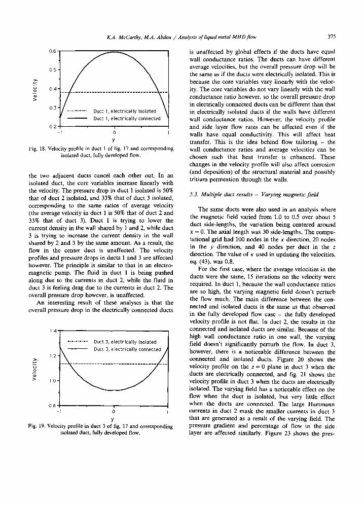
the two adjacent ducts cancel each other out. In an isolated duct, the core variables increase linearly with the velocity. The pressure drop in duct 1 isolated is 50% that of duct 2 isolated, and 33% that of duct 3 isolated, corresponding to the same ratios of average velocity (the average velocity in duct 1 is 50% that of duct 2 and 33% that of duct 3). Duct 1 is trying to lower the current density in the wall shared by 1 and 2, while duct 3 is trying to increase the current density in the wall shared by 2 and 3 by the same amount. As a result, the flow in the center duct is unaffected. The velocity profiles and pressure drops in ducts 1 and 3 are affected however. The principle is similar to that in an electromagnetic pump. The fluid in duct 1 is being pushed along due to the currents in duct 2, while the fluid in duct 3 is feeling drag due to the currents in duct 2. The overall pressure drop however, is unaffected.

An interesting result of these analyses is that the overall pressure drop in the electrically connected ducts

1.4

. . . . . . . . . . . Duct 3, e l e c t r i c a l l y I so la ted

o

> I,o

0.8 -~ o



is unaffected by global effects if the ducts have equal wall conductance ratios. The ducts can have different average velocities, but the overall pressure drop will be the same as if the ducts were electrically isolated. This is because the core variables vary linearly with the velocity. The core variables do not vary linearly with the wall conductance ratio however, so the overall pressure drop in electrically connected ducts can be different than that in electrically isolated ducts if the walls have different wall conductance ratios. However, the velocity profile and side layer flow rates can be affected even if the walls have equal conductivity. This will affect heat transfer. This is the idea behind flow tailoring - the wall conductance ratios and average velocities can be chosen such that heat transfer is enhanced. These changes in the velocity profile will also affect corrosion (and deposition) of the structural material and possibly tritium permeation through the walls.

5.3. Multiple duct results - Varying magnetic fieM

The same ducts were also used in an analysis where the magnetic field varied from 1.0 to 0.5 over about 5 duct side-lengths, the variation being centered around x = 0. The axial length was 30 side-lengths. The computational grid had 100 nodes in the x direction, 20 nodes in the y direction, and 40 nodes per duct in the z direction. The value of K used in updating the velocities, eq. (43), was 0.8.

For the first case, where the average velocities in the ducts were the same, 15 iterations on the velocity were required. In duct 1, because the wall conductance ratios are so high, the varying magnetic field doesn't perturb the flow much. The main difference between the connected and isolated ducts is the same as that observed in the fully developed flow case - the fully developed velocity profile is not fiat. In duct 2, the results in the connected and isolated ducts are similar. Because of the high wall conductance ratio in one wall, the varying field doesn't significantly perturb the flow. In duct 3, however, there is a noticeable difference between the connected and isolated ducts. Figure 20 shows the velocity profile on the z---0 plane in duct 3 when the ducts are electrically connected, and fig. 21 shows the velocity profile in duct 3 when the ducts are electrically isolated. The varying field has a noticeable effect on the flow when the duct is isolated, but very little effect when the ducts are connected. The large Hartmann currents in duct 2 mask the smaller currents in duct 3 that are generated as a result of the varying field. The pressure gradient and percentage of flow in the side layer are affected similarly. Figure 23 shows the pres-


'~ iOt p05ili° - o

Fig. 20. Axial velocity on the z = 0 plane in duct 3 of fig. 11, electrically connected, varying magnetic field.

sure gradient for the electrically connected case, while fig. 24 shows the pressure gradient for the electrically isolated case, and fig. 22 compares the percentage of flow in the side layers. The overall pressure drop in the electrically connected ducts is 3.9% higher, practically the same as the fully developed flow case.

When the same magnetic field variation was used for adjacent ducts with equal wall conductance ratios but different average velocities, the following results were obtained. As in the fully developed flow case, the flow in duct 2 was the same whether the ducts were electrically isolated or connected. In ducts I and 3, the flow

O~

7 '

U

Fig. 21. Axial velocity on the z = 0 plane in duct 3 of fig. 11, electrically isolated, varying magnetic field.


- J

c

O

,'7

t ~

L

rl

12

10-

8 ¸

6-

Duct 3, electrically connected

........... Duct 3, electrically isolated

/ ' \ - \

-15 -5 5 15

Axlal Posltlon

Fig. 22. Percentage of flow in side layers, duct 3 of fig. 11, electrically connected and isolated, varying magnetic field.

field was affected similarly to the constant magnetic field case, and the effect of the varying magnetic field is as pronounced in the electrically connected ducts as in the electrically isolated ducts. Figure 25 shows the velocity profile on the z = 0 plane in duct 3 for the electrically connected case, fig. 26 for the electrically isolated case. While the effect of the varying field ap- pears more pronounced in the electrically isolated case, the magnitude of the change in the velocity due to the varying magnetic field is similar. The same is true for the percentage of flow in the side layer, which is shown in fig. 27. The overall pressure drop in the electrically connected ducts is the same as for the electrically isolated ducts. As in the fully developed flow case, because

the core variables increase linearly with the velocity, the overall pressure drop is not affected.

6. Discussion

Global effects can have a large effect on the flow field. In order to understand the flow in a set of electrically connected ducts, it has been shown to be necessary to evaluate the electrically connected ducts, because electrically isolated results can be misleading. Global effects can have an impact on the flow variables, and therefore they are important in evaluating heat transfer, the pressure drop, corrosion of structural materials and tritium permeation from the fluid through the walls.

The results of this analysis are particularly important to liquid metal blanket design work. Liquid metal blanket designs can be very complex, with many paths for global currents. It is possible that some global effects would introduce a prohibitively large pressure drop or an unacceptable velocity profile. It is important to look at a blanket design carefully to identify possible global current paths.

In this research, the flow in each duct was assumed to be adjusted independently from the flow in adjacent ducts. If the ducts were joined by manifolds at each end, the flow would redistribute such that there would be the same pressure drop across each duct. Thus if different ducts have different wall conductance ratios such as in one of the cases presented here, the core

0-

I

| !

Fig. 23. Pressure gradient on the z = 0 plane in duct 3 of fig. 11, electrically connected, varying magnetic field.

378 K.A. McCarthy, M.A, Abdou / Analysis of liquid metal MHD flow

U

Fig. 24. Pressure gradient on the z = 0 plane in duct 3 of fig. 11, electrically isolated, varying magnetic field.

variables would be affected by this flow redistribution. In the duct assembly shown in fig. 11, more fluid would go through ducts 2 and 3, while less would go through duct 1. This would have an effect on heat transfer and the pressure drop.

Flow redistribution could be included in the code in different ways. One way would be to analyze the prob-

lem without flow redistribution, then to adjust the average velocity in each duct based on the pressure drop in each duct, then repeat the analysis. This process could be repeated until the pressure drop across each duct is the same. This process could take a lot of computer time, however, so it probably would not be optimal. A second method would be to analyze a single duct which

~t " 0

Fig. 25. Axial velocity on the z = 0 plane in duct 3 of fig. 17, electrically connected.

K.A. McCarthy, M.A. Abdou / Analysis of liquid metal MHD flow

[

• " t ~ . ¢ .

y ~.2 0

Fig. 26. Axial velocity on the z = 0 plane in duct 3 of fig. 17, electrically isolated.

379

splits into many ducts, then goes back to a single duct. A third method would be to force the pressure along field lines at the inlet and outlet of the multiple duct assembly to be constant through the whole duct assembly, and allow flow redistribution each time the velocities are normalized. The flow redistribution could be based on the ratio of y currents in each duct to the total amount of y currents.

The work presented here dealt entirely with straight ducts. Multiple duct geometries may contain ducts with bends and/or changes in cross section. These geometries should also be understood.

Further investigation of global effects is necessary. The results presented here show that the flow in each

_c

o

ta_

o

ta .

Fig. 27.

34

3 2 '

30 ' Duct 3, e l ec t r i ca l l y connected

. . . . . . . . . . . Duct 3, e lec t r i ca l l y Isolated

2 8 '

26 ' / ' ~ ,

24

A x i a l P o s i t i o n

Percentage of flow in side layers, duct 3 of fig. 17, electrically connected and isolated.

duct can be affected by neighboring ducts. The velocity profiles and percentage of flow in the side layers were shown to be significantly affected by neighboring ducts in certain situations. This is an important consideration when analyzing heat transfer. The total pressure drop in electrically connected ducts was greater than or equal to the total pressure drop in electrically isolated ducts, the difference depending on the wall conductance ratios.

Nomenclature

B magnetic field, f subscript referring to fluid, j current density, M Hartmann number, t) unit normal, N interaction parameter, p pressure, R m magnetic Reynolds number, t w wall thickness, v velocity, w subscript referring to wall, # kinematic viscosity, ix0 free space permeability, p fluid density, o electrical conductivity,

electric field potential, wall conductance ratio.

380 K.A. McCarthy, M.A. Abdou / Analysis of liquid metal MHD flow

References

[1] M. Tillack, A. Ying, and M. Hashizume, The effect of magnetic field alignment on heat transfer in liquid metal blanket channels, UCLA-FNT-41 (March 23, 1989).

[2] M.A. Abdou et al, Modeling, analysis and experiments for fusion nuclear technology, Fusion Nuclear Technol. 6 No. 1 (1988) 3.

[3] C.N. Kim, Development of a numerical method for full solution of magnetohydrodynamic flows and application to fusion blankets, Ph.D. Dissertation, University of Cali- fornia, Los Angeles (1989).

[4] A.G. Kulikovskii, Slow steady flows of a conducting fluid at large Hartmann numbers, Fluid Dynamics 3(2) (1968) 1.

[5] C.B. Reed, B.F. Picologlou, T.Q. Hua, and J.S. Walker, ALEX results - a comparison of measurements from a round and a rectangular duct with 3-D code predictions, presented at the IEEE 12th Symposium on Fusion En- gineering, October 1987.

[6] M.S. Tillack, Core flow solution of the liquid metal MHD equations in a variable-radius pipe, UCLA-ENG-87-27 (July 1987).

[7] M.S. Tillack, Core flow solution in a circular pipe with variable field having both transverse and axial components, UCLA Informal Technical Memo (December 11, 1987).

[8] Basil Picologlou et al., Experimental investigations of MHD flow tailoring for first wall coolant channels of self-cooled blankets, presented at the Eighth Topical Meeting on the Technology of Fusion Energy, Salt Lake City, Utah, October 9-13, 1988.

[9] H. Madarame and H. Tokoh, Development of computer

code for analyzing liquid metal MHD flow in fusion reactor blankets (I), Nucl. Science and Technol. 25(3) (March 1988) 233.

[10] H. Madarame and H. Tokoh, Development of computer code for analyzing liquid metal MHD flow in fusion reactor blankets (II), Nucl. Science and Technol. 25(4) (April 1988) 323.

[11] J.A. Shercliff, A Textbook of Magnetohydrodynamics (Pergamon Press, Oxford, 1965).

[12] J.l. Ramos and N.S. Winowich, Magnetohydrodynamic channel flow study, Physics of Fluids 29(4) (1986) 992.

[13] T.Q. Hua and J.S. Walker, Three dimensional MHD flow in insulating circular ducts in non-uniform transverse magnetic fields, to appear in Int'l Journal of Eng. Scien- ces.

[14] K.A. McCarthy, Analysis of liquid metal MHD flow using a core flow approximation with applications to calculating the pressure drop in geometric elements of fusion reactor blankets, Ph.D. Dissertation, University of California, Los Angeles (1989).

[15] M.S. Tillack and K.A. McCarthy, Flow quantity in side layers for MHD flow in conducting rectangular ducts, UCLA Report, UCLA-IFNT-89-01 (March 22, 1989).

[16] K.A. McCarthy, M.S. Tillack and M.A. Abdou, Analysis of liquid metal MHD flow using an iterative method to solve the core flow equations, Fusion Engrg. Des. 8 (1989) 257.

[17] B.F. Picologlou, C.B. Reed, and P.V. Dauzvardis, Experi- mental and analytical investigation of magnetohydrodynamic flows near the entrance to a strong magnetic field, Fusion Technol. 10 (November 1986) 860.

[18] Basil Picologlou, private communication, Argonne Na- tional Laboratory (May 1987).

Analysis of liquid metal MHD flow in multiple adjacent ducts using

Documents

Transcript of Analysis of liquid metal MHD flow in multiple adjacent ducts using