Analysis of Image Compression Methods Based On

Transform and Fractal Coding

Archana Deshlahra

Analysis of Image Compression Methods Based On

Transform and Fractal Coding

A Thesis Submitted in partial fulfillment

for the award degree Of

Master of Technology

In

Electronics & Communication Engineering

“Electronics & Instrumentation” Specialization

by

Archana Deshlahra (211EC3306)

Under the supervision of

Prof. Ajit Kumar Sahoo

Department of Electronic & Communication Engineering National Institute of Technology, Rourkela.

May- 2013

i | P a g e

National Institute Of Technology, Rourkela

Certificate

This is to certify that the thesis entitled, ―Analysis of Image Compression Methods Based

On Transform and Fractal Coding” submitted by Archana Deshlahra to the Department of

Electronic & Communication Engineering, National Institute Of Technology, Rourkela, India,

during the academic session 2012-2013 for the award of the degree of Master of Technology in

“Electronics & Instrumentation” specialization, is a bona-fide record of work carried by him

under my supervision and guidance. The thesis has fulfilled all the requirements as per the

regulations of this institute and in our opinion reached the standard for submission.

Place: Rourkela, India Prof. Ajit Kumar Sahoo

Date: NIT,Rourkela -769008 (India)

ii | P a g e

Declaration

I, Archana Deshlahra, declare that:

1. The work contained in this report is original and has been done by me under the guidance of

my supervisor Prof. Ajit Kumar Sahoo

2. The work has not been submitted to any other Institute for any degree or diploma.

3. I have followed the guidelines provided by the institute in preparing the report.

4. I have conformed to the norms and guidelines given in the Ethical Code of Conduct of the

Institute.

5. Whenever I have used materials (data, theoretical analysis, figures and text) from other

sources, I have given due credit to them by citing them in the text of the report and giving their

details in the references.

Department of Electronics & Communication Engineering

NIT, Rourkela, Archana Deshlahra

Rourkela-769008

iii | P a g e

Acknowledgement

I avail this opportunity to extend my hearty indebtedness to my guide Prof. A.K.Sahoo,

Department of Electronics and Communication Engineering, for their valuable guidance,

constant encouragement and kind help at different stages for the execution of this work.

I also express our sincere gratitude to Dr. S. Meher, Head of the Department, Electronics

and Communication Engineering, for providing valuable departmental facilities.

My special thanks to Mr. Deepak Singh (Phd. Scholar) ,Mr. Sanand (Phd. Scholar), Mr.

Nihar (Phd. Scholar), Bijay, Ripan , Sonia for their help and valuable suggestions. I would like

to give special thanks to Sanu, Harsu di, G.S. Shirnewar those helped and supported me

throughout my research work. I must thank Mr. Saubhagya (Phd. Scholar) , Mrs. Hunny

Mehrotra (Phd. Scholar) for their support and help.

I sincerely thank to all my friends, Research scholars of ECE Department, M.Tech

(E&I) students and all academic and non-teaching staffs in NIT Rourkela who helped me. I

would like to thank all those who made my stay in Rourkela an unforgettable and rewarding

experience.

Finally, I dedicate this thesis to my family: my dear father, my dearest mother who

supported me morally despite the distance that separates us. I thank them from the bottom of my

heart for their motivation, inspiration, love they always give me. Without their support nothing

would have been possible. I am greatly indebted to them for everything that I am.

ARCHANA DESHLAHRA

iv | P a g e

Abstract

Image compression is process to remove the redundant information from the image so

that only essential information can be stored to reduce the storage size, transmission bandwidth

and transmission time. The essential information is extracted by various transforms techniques

such that it can be reconstructed without losing quality and information of the image. In this

thesis work comparative analysis of image compression is done by four transform method,

which are Discrete Cosine Transform (DCT), Discrete Wavelet Transform( DWT) & Hybrid

(DCT+DWT) Transform and fractal coding. MATLAB programs were written for each of the

above method and concluded based on the results obtained that hybrid DWT-DCT algorithm

performs much better than the standalone JPEG-based DCT, DWT algorithms in terms of peak

signal to noise ratio (PSNR), as well as visual perception at higher compression ratio. The

popular JPEG standard is widely used in digital cameras and web –based image delivery. The

wavelet transform, which is part of the new JPEG 2000 standard, claims to minimize some of the

visually distracting artifacts that can appear in JPEG images. For one thing, it uses much larger

blocks- selectable, but typically1024 x 1024 pixels – for compression, rather than the 8 X 8 pixel

blocks used in the original JPEG method, which often produced visible boundaries. Fractal

compression has also shown promise and claims to be able to enlarge images by inserting

―realistic‖ detail beyond the resolution limit of the original. Each method is discussed in the

thesis.

v | P a g e

Contents

Declaration ...................................................................................................................................ii Acknowledgement …................................................................................................................... iii

Abstract ...................................................................................................................................... iv

Contents ........................................................................................................................................ v

List of Figures .........................................................................................................................viii

Chapter 1

Image Compression ..................................................................................................................... 1

1.1. Introduction .............................................................................................................................1

1.2 Data Compression Model......................................................................................................... 2

1.2.1 Advantages of Data Compression .............................................................................2

1.2.2 Disadvantages of Data Compression ........................................................................ 4

1.3 Image Compression Based on Entropy..................................................................................... 5

1.3.1 Lossless compression................................................................................................ 6

1.3.2 Lossy compression................................................................................................... 6

1.4 Objective of thesis……………................................................................................................ 7

1.5 Thesis Structure………………................................................................................................ 7

Chapter 2

Image Representation and Transform Coding ......................................................................... 8

2.1 Image …………..…………….................................................................................................. 8

2.2 Redundancy .............................................................................................................................12

2.2.1 Coding redundancy...................................................................................................13

2.2.2 lnterpixel redundancy…........................................................................................... 13

2.2.3 Psychovisual redundancy .........................................................................................13

2.3 Coding…………..……………................................................................................................14

2.3.1 Pixel coding ……….................................................................................................14

2.3.2 Predictive coding……..............................................................................................14

2.3.3 Transform coding……..............................................................................................15

2.4 Transform-based Image Compression.....................................................................................16

2.4.1 Linear Transform..................................................................................................... 17

2.4.2 Quantizer..................................................................................................................17

2.4.2.1 Scalar Quantization....................................................................................18

2.4.2.2 Vector Quantization...................................................................................18

2.4.2.3 Predictive Quantization..............................................................................19

2.4.3 Entropy Encoding.....................................................................................................19

2.5 Discrete Cosine Transform......................................................................................................19

2.5.1 Coding scheme.........................................................................................................20

2.5.1.1 Compression procedure.............................................................................20

2.5.1.2 Decompression procedure..........................................................................22

vi | P a g e

2.5.2 Properties of DCT.....................................................................................................26

2.5.2.1 Decorrelation..............................................................................................26

2.5.2.2 Separability ...............................................................................................26

2.5.2.3 Energy Compaction...................................................................................26

2.5.2.4 Symmetry...................................................................................................28

2.5.2.5 Orthogonality.............................................................................................29

2.5.3 Limitations of DCT..................................................................................................29

2.5.3.1 Blocking artifacts.......................................................................................30

2.5.3.2 False contouring: …..................................................................................30

2.6 Discrete Wavelet Transform (DWT) ...................................................................................31

2.6.1 Multiresolution Concept and Analysis.....................................................................31

2.6.2 Decimator and interpolator.......................................................................................31

2.6.3 Filter bank ................................................................................................................32

2.6.3.1 Analysis bank ..........................................................................................32

2.6.3.2 Synthesis bank..........................................................................................34

2.6.4 Coding scheme.........................................................................................................36

2.6.4.1 Compression procedure............................................................................36

2.6.4.2 Decompression procedure........................................................................36

2.7 Hybrid (DCT+ DWT) Transform………............................................................................37

2.7.1 Coding scheme.........................................................................................................38

2.7.1.1Compression procedure.............................................................................38

2.7.1.2 Decompression procedure........................................................................38

2.8 Fractal Image Compression...................................................................................................40

2.8.1 Baseline Fractal Coding…………............................................................................40

2.8.2 Procedure of proposed speed up encoding................................................................41

2.8.3 Procedure for decoding method ................................................................................42

2.8.4 Advantages and Disadvantages .................................................................................42

2.9 Conclusion ..............................................................................................................................44

Chapter 3

Performance Measurement Parameters....................................................................................45

3.1 Objective evaluation parameters. ............................................................................................45

3.1.1 Mean Square Error (MSE) .........................................................................................45

3.1.2 Peak Signal to Noise Ratio (PSNR) ...........................................................................46

3.1.3 Compression ratio (CR) ...............................................................................................47

3.2 Subjective evaluation parameter..............................................................................................48

3.3 Conclusion ..............................................................................................................................48

vii | P a g e

Chapter 4

Performance Evaluation and Simulation Results.....................................................................50

4.1 Simulation tool.........................................................................................................................50

4.2 Simulation Results...................................................................................................................50

4.3 Conclusion ..............................................................................................................................53

Chapter 5

Conclusion and Future work...................................................................................................55

Reference.....................................................................................................................................57

viii | P a g e

List of Figures

Fig 1.1 Aspect ratio.........................................................................................................................1

Fig 1.2 A data compression model................................................................................................. 4

Fig 2.1 Digital representation of an image.....................................................................................10

Fig 2.2 Block diagram of the color image compression algorithm. ..............................................11

Fig 2.3 Lena image representation ................................................................................................11

Fig 2.4 Block diagram of a DPCM system. ..................................................................................14

Fig 2.5 Block diagram of transform based image coder .............................................................. 16

Fig 2.6 Quantization effect. ..........................................................................................................18

Fig 2.7 JPEG Quantization table .................................................................................................. 21

Fig 2.8 Zigzag ordering for DCT coefficients ............................................................................ 21

Fig 2.9 Flow chart of compression technique .............................................................................. 23

Fig 2.10 Flow chart of decompression technique ........................................................................ 24

Fig 2.11 A random value input data matrix.................................................................................. 24

Fig 2.12 Transformed coefficients after DCT of the random value input data matrix ................ 25

Fig 2.13 Quantized coefficients ................................................................................................... 25

Fig 2.14 Reconstructed output data ............................................................................................. 25

Fig 2.15 Computation of 2-D DCT using Separability property. ................................................ 26

Fig 2.16 DCT of different Images ................................................................................................ 28

Fig 2.17 Illustration of compression using DCT.......................................................................... 30

Fig 2.18 Illustration of compression using DCT.......................................................................... 30

Fig 2.19 Decimator or down sampler........................................................................................... 32

Fig 2.20 Interpolator or up sampler ............................................................................................. 32

Fig 2.21 Filter bank....................................................................................................................... 32

Fig 2.22 Finer scale and coarser scale wavelet coefficients......................................................... 33

Fig 2.23. Block diagram of 1-D forward DWT............................................................................ 33

Fig 2.24 Block diagram of 2-D forward DWT ............................................................................ 34

Fig 2.25 Block diagram of 2 dimensional inverse DWT ............................................................ 34

Fig 2.26 Illustration of 2 dimensional DWT for an image ‗Lena‘ …........................................... 37

Fig 2.27 Compression technique using Hybrid transform .......................................................... 39

ix | P a g e

Fig 2.28 Decompression technique using Hybrid transform ....................................................... 39

Fig 2.29 Fractal coding algorithm................................................................................................. 41

Fig 3.30 A different approach for Fractal coding.........................................................................43

Fig 3.1 Original, reconstructed image using DCT, DWT, Hybrid DWT-DCT …...................... 45

Fig 3.2 CR comparison ................................................................................................................ 46

Fig 4.1 Comparison of visual image quality of reconstructed image for DCT, DWT AND Hybrid

(DCT+DWT) for test images . .................................................................................................... 49

Fig 4.2 Comparison of visual image quality of reconstructed image from the proposed method at

different threshold value. ............................................................................................................ 49

1 | P a g e

Chapter 1

Introduction

1.1 Image Compression

The increasing demand for multimedia content such as digital images and video has led

to great interest in research into compression techniques. The development of higher quality and

less expensive image acquisition devices has produced steady increases in both image size and

resolution, and a greater consequent for the design of efficient compression systems [1].

Although storage capacity and transfer bandwidth has grown accordingly in recent years, many

applications still require compression.

In general, this thesis investigates still image compression in the transform domain.

Multidimensional, multispectral and volumetric digital images are the main topics for analysis.

The main objective is to design a compression system suitable for processing, storage and

transmission, as well as providing acceptable computational complexity suitable for practical

implementation. The basic rule of compression is to reduce the numbers of bits needed to

represent an image. In a computer an image is represented as an array of numbers, integers to be

more specific, that is called a ―digital image‖. The image array is usually two dimensional (2D),

If it is black and white (BW) and three dimensional (3D) if it is colour image [3]. Digital image

compression algorithms exploit the redundancy in an image so that it can be represented using a

smaller number of bits while still maintaining acceptable visual quality. Factors related to the

need for image compression include:

The large storage requirements for multimedia data

Low power devices such as handheld phones have small storage capacity

Network bandwidths currently available for transmission

The effect of computational complexity on practical implementation.

In the array each number represents an intensity value at a particular location in the image and is

called as a picture element or pixel. Pixel values are usually positive integers and can range

between 0 to 255. This means that each pixel of a BW image occupies 1byte in a computer

2 | P a g e

memory. In other words , we say that the image has a grayscale resolution of 8 bits per pixel

(bpp) . On the other hand , a colour image has a triplet of values for each pixel one each for the

red, green and blue primary colours. Hence, it will need 3 bytes of storage space for each pixel.

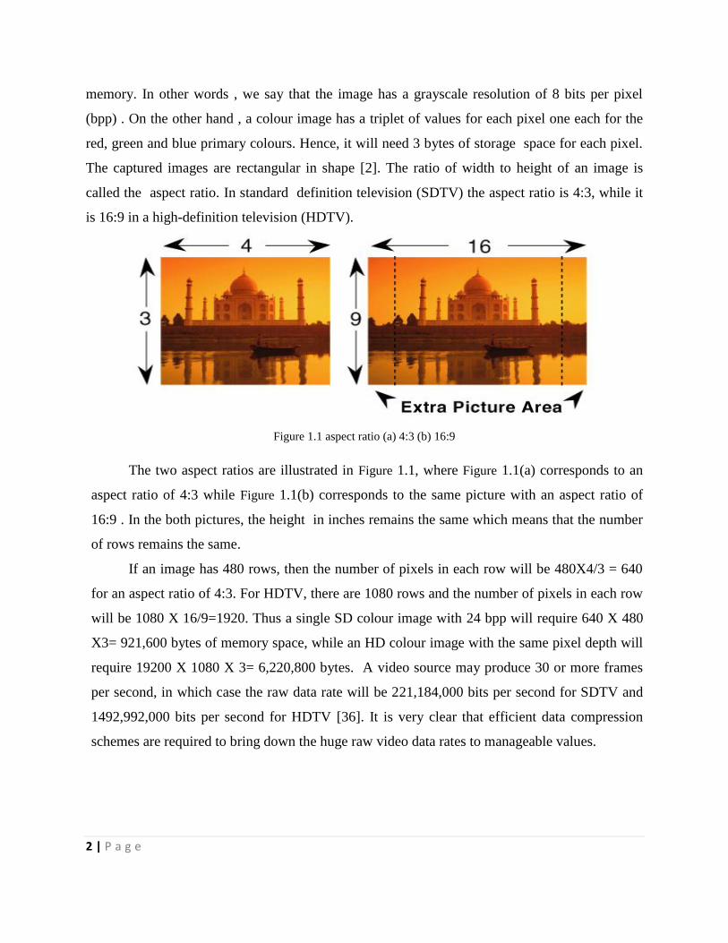
The captured images are rectangular in shape [2]. The ratio of width to height of an image is

called the aspect ratio. In standard definition television (SDTV) the aspect ratio is 4:3, while it

is 16:9 in a high-definition television (HDTV).

Figure 1.1 aspect ratio (a) 4:3 (b) 16:9

The two aspect ratios are illustrated in Figure 1.1, where Figure 1.1(a) corresponds to an

aspect ratio of 4:3 while Figure 1.1(b) corresponds to the same picture with an aspect ratio of

16:9 . In the both pictures, the height in inches remains the same which means that the number

of rows remains the same.

If an image has 480 rows, then the number of pixels in each row will be 480X4/3 = 640

for an aspect ratio of 4:3. For HDTV, there are 1080 rows and the number of pixels in each row

will be 1080 X 16/9=1920. Thus a single SD colour image with 24 bpp will require 640 X 480

X3= 921,600 bytes of memory space, while an HD colour image with the same pixel depth will

require 19200 X 1080 X 3= 6,220,800 bytes. A video source may produce 30 or more frames

per second, in which case the raw data rate will be 221,184,000 bits per second for SDTV and

1492,992,000 bits per second for HDTV [36]. It is very clear that efficient data compression

schemes are required to bring down the huge raw video data rates to manageable values.

3 | P a g e

1.2 Data Compression Model

A data compression system mainly consists of three major steps and that are removal or

reduction in data redundancy, reduction in entropy, and entropy encoding. A typical data

compression system can be labeled using the block diagram shown in Figure 1.2 It is performed

in steps such as image transformation, quantization and entropy coding. JPEG is one of the most

used image compression standard which uses discrete cosine transform (DCT) to transform the

image from spatial to frequency domain [2]. An image contains low visual information in its

high frequencies for which heavy quantization can be done in order to reduce the size in the

transformed representation. Entropy coding follows to further reduce the redundancy in the

transformed and quantized image data.

1.2.1 Advantages of Data Compression

The main advantage of compression is that it reduces the data storage requirements. It also offers

an attractive approach to reduce the communication cost in transmitting high volumes of data

over long-haul links via higher effective utilization of the available bandwidth in the data links.

This significantly aids in reducing the cost of communication due to the data rate reduction. Due

to the data rate reduction, data compression also increases the quality of multimedia presentation

through limited-bandwidth communication channels, Because of the reduced data rate. Offered

by the compression techniques, computer network and Internet usage is becoming more and

more image and graphic friendly, rather than being just data and text-centric phenomena. In

short, high-performance compression has created new opportunities of creative applications such

as digital library, digital archiving, video teleconferencing, telemedicine and digital

entertainment to name a few. There are many other secondary advantages in data compression.

For Example it has great implications in database access. Data compression may enhance the

database performance because more compressed records can be packed in a given buffer space in

a traditional computer implementation. This potentially increases the probability that a record

being searched will be found in the main memory. Data security can also be greatly enhanced by

encrypting the decoding parameters and transmitting them separately from the compressed

database files to restrict access of proprietary information. An extra level of security can be

4 | P a g e

achieved by making the compression and decompression processes totally transparent to

unauthorized users. The rate of input-output operations in a computing device can be greatly

increased due to shorter representation of data. Data compression obviously reduces the cost of

backup and recovery of data in computer systems by storing the backup of large database files in

compressed form. The advantages of data compression will enable more multimedia applications

with reduced cost.

Figure 1.2 A data compression model.

1.2.2 Disadvantages of Data Compression

Data compression has some disadvantages too, depending on the application area and

sensitivity of the data. For example, the extra overhead incurred by encoding and decoding

processes is one of the most serious drawbacks of data compression, which discourages its usage

in some areas. This extra overhead is usually required in order to uniquely identify or interpret

the compressed data. Data compression generally reduces the reliability of the data records [1].

For example, a single bit error in compressed code will cause the decoder to misinterpret all

5 | P a g e

subsequent bits, producing incorrect data. Transmission of very sensitive compressed data (e.g.,

medical information) through a noisy communication channel (such as wireless media) is risky

because the burst errors introduced by the noisy channel can destroy the transmitted data.

Another problem of data compression is the disruption of data properties, since the compressed

data is different from the original data.

In many hardware and systems implementations, the extra complexity added by data

compression can increase the system‘s cost and reduce the system‘s efficiency, especially in the

areas of applications that require very low-power VLSI implementation [3].

1.3 Image Compression Based on Entropy

The principle of digital image compression based on ―information theory‖. Image

compression uses the concept of ‗Entropy‘ to measure the amount of information that a source

produces. The amount of information produced by a source is defined as its entropy. For each

symbol, there is a product of the symbol probability and its logarithm. The entropy is a negative

summation of the products of all the symbols in a given symbol set.

Compression algorithms are methods that reduce the number of symbols used to

represent source information, therefore reducing the amount of space needed to store the source

information or the amount of time necessary to transmit it for a given channel capacity. The

mapping from source symbols into fewer target symbols is referred to as ‗compression‘. The

transformation from the ‗target symbols‘ back into the source symbols representing a close

approximation form of the original information is called ‗decompression‘ [38]. Compression

system consist of two steps, sampling and quantization of a signal. The choice of compression

algorithm involves several conflicting considerations. These include degree of compression

required, and the speed of operation. Obviously if one is attempting to run programs direct from

their compressed state, decompression speed is paramount. The other consideration is size of

compressed file versus quality of decompressed image. Compression is also known as encoding

process and decompression is known as decoding process [30]. Digital data compression

algorithms can be classified into two categories-

1. Lossless compression

2. Lossy compression

6 | P a g e

1.3.1 Lossless compression

In lossless image compression algorithm, the original data can be recovered exactly from

the compressed data. It is used generally for discrete data such as text, computer generated data,

and certain kinds of image and video information. Lossless compression can achieve only a

modest amount of compression of the data and hence it is not useful for sufficiently high

compression ratios. GIF, Zip file format, and Tiff image format are popular examples of a

lossless compression [30, 3]. Huffman Encoding and LZW are two examples of lossless

compression algorithms. There are times when such methods of compression are unnecessarily

exact.

In other words, 'Lossless' compression works by reducing the redundancy in the data.

The decompressed data is an exact copy of the original, with no loss of data.

1.3.2 Lossy compression

Lossy compression techniques refer to the loss of information when data is compressed.

As a result of this distortion, must higher compression ratios are possible as compared to the

lossless compression in reconstruction of the image. 'Lossy' compression sacrifices exact

reproduction of data for better compression. It both removes redundancy and creates an

approximation of the original.

The JPEG standard is currently the most popular method of lossy compression. The

degree of closeness is measured by distortion that can be defined by the amount of information

lost. Some example of lossless compression techniques are :‗CCITT T.6‘, Zip file format, and

Tiff image format. JPEG Baseline and JPEG 2000 is a example of lossy compression algorithm.

The three main criteria in the design of a lossy image compression algorithm are desired bit rate

or compression ratio, acceptable distortion, and restriction on coding and decoding time[30].

While different algorithms produce different type of distortion, the acceptability of which is

often application dependent, there is clearly an increase in distortion with decreasing bit rate.

Obviously, a lossy compression is really only suitable for graphics or sound data, where

an exact reproduction is not necessary. Lossy compression techniques are more suitable for

images, as much of the detail in an image can be discarded without greatly changing the

7 | P a g e

appearance of the image. In practice, very fine details are lost in image compression. Though

image size is drastically reduced.

1.4 Objective of thesis

Image compression plays very important role in storing and transferring images

efficiently. With the evolution of electronic devices like Digital Cameras, Smart phones,

biometric applications, the requirement of storing images in less memory is becoming necessary.

Using different compression methods the requirement of less memory storage and efficient

transmission can be fulfilled. At the same time it should be considered that, the compression

technique must be able to reconstruct the image with low loss or without loss as compared to

original image. The objective of the thesis is to study such compression techniques and validate

the results using MATLAB programming. This thesis also aims the comparative study of various

image compression techniques and it also provides the motivations behind choosing different

compression techniques.

1.5 Thesis Structure

Chapter 2 starts with introduction of an Image and its representation in different domains.

It also presents commonly used transform techniques for the image compression. The Discrete

Cosine Transform (DCT), the Discrete Wavelets Transform (DWT), the Hybrid (DCT+DWT)

Transform and Fractal images compression technique have been described. The algorithm for

implementation these techniques using MATLAB also explained in this chapter. The advantage

and disadvantage of all these algorithms are also included in this chapter.

Chapter 3 explains the various performance measurement parameters for comparing the

compression techniques. Based on parameters explained in this chapter the analysis among the

compression techniques is done. Also the subjective and objective analysis can be done using

these parameters. The quality of reconstructed image is validating.

The simulation results and the comparisons are presented in Chapter 4. In addition, the

fast fractal encoding algorithm is also compared with the already discussed and developed

schemes.

Finally Chapter 5 provides conclusion to this thesis along with future work related to this

area.

8 | P a g e

Chapter 2

Image Representation and Transform Coding

2.1 Image

An image is the two dimensional (2-D) picture that gives appearance to a subject usually

a physical object or a person. It is digitally represented by a rectangular matrix of dots arranged

in rows and columns, or in other words, ―An image may be defined as a two dimensional

function f(x, y), where x and y are spatial (plane) co-ordinates. The amplitude of ‗f‘ at any pair

of co-ordinate (x, y) is called the intensity or gray level of the image at that point‖ [3].

When (x ,y) and amplitude values of ‗f‘ are all finite, discrete quantities, we call the image is a

―DIGITAL IMAGE‖. A Digital image is an array of a number of picture elements called pixels.

Each pixel is represented by a real number or a set of real numbers in limited number of bits.

Based on the accuracy of the representation, we can classify image into three categories-

1. Black and White images

2. Grayscale images

3. Colour images

For Black and White images, each pixel is represented by one bit. These images are also

called as bi-level, binary, or bi-tonal images. In Grayscale images, each pixel is represented by

a luminance or say intensity level. For pictorial images, gray scale images are represented by 256

gray levels or 8 bits [21]. In Bit planes, grayscale images can be transformed into a sequence of

binary images by breaking them up into their bit-planes. If we consider the grey value of each

pixel of an 8-bit image as an 8-bit binary word, then the 0th bit plane consists of the last bit of

each grey value. Since this bit has the least effect in terms of the magnitude of the value, it is

called the least significant bit, and the plane consisting of those bits the least significant bit

plane. Similarly the 7th bit plane consists of the first bit in each value. This bit has the greatest

effect in terms of the magnitude of the value, so it is called the most significant bit, and the

plane consisting of those bits the most significant bit plane. In color images each pixel can be

represented by luminance and chrominance components [10]. Color images can also be

9 | P a g e

represented in an alternative system which is also known as different color space. Some

examples of popular colour spaces are RGB, CIELAB, HSV, YIQ and YUV. Since human visual

system (HVS) are less sensitive to colour images than to luminance or brightness, RGB space

has the advantage of providing equal luminance to human vision. YIQ color spaces separate

grayscale information from colour data. This enables the same signal to be used for black and

white settings. YIQ component are luminance(Y), hue (I) and saturation (Q). Grayscale

information is expressed as luminance (Y), and colour information as chrominance, which is

both hue (I) and saturation (Q). YCbCr is another colour space that has widely been used for

digital video. Here, luminance information is stored as a single component (Y), and chrominance

information is stored as two colour-difference components (Cb) and (Cr). Cb represents the

difference between the blue component and a reference value, whereas Cr represents the

difference between the red component and a reference value. Another type of colour space is

CMYK which is used in colour printers. The primaries in this colour space are cyan (C), magenta

(M), yellow (Y) and black (K). Resolution in an image refers to the capability to represent the

finer details [2]. The RGB color space is a linear, additive, device-dependent color space. Each

value is usually represented as unsigned integers in the range from 0 to 255, giving a total color

depth of 3 x 8 = 24 bits[42]. Different color examples are shown in Table 2.1.

Table 2.1: RGB color examples

MPEG standard use luminance Y and two chrominance CB and CR to represent color.

Figure 2.1 shows the standard image ‗Einstein‘. The size of the row (M) and column (N) gives

the size (or resolution) of M X N image. A small block (8 X 8) of the image is indicated at the

lower right corner in the form of matrix. Each element in the matrix represents the dots of the

image. Each dot represents the pixel value at that position [41].

10 | P a g e

Figure 2.1. Digital representation of an image

Intensity I in RGB model is calculated by

I= 0.3R +0.59G+0.11B (2.1)

This is the same method used for calculating the Y value when converting from RGB to

YCBCR. RGB images are converted into more suitable YCBCR color format using the

following equations.

Y = 0.299 R + 0.587 G + 0.114 B (2.2)

CB = −0.169 R − 0.331 G + 0.500 B = 0.564 (B – Y) (2.3)

CR = 0.500 R − 0.419 G − 0.081 B = 0.713 (R − Y) (2.4)

Where Y represents a monochrome compatible luminance component, and CB, CR represent

chrominance components containing color information. Most of image/video coding standards

adopt YCBCR color format as an input image signal [41]. Figure 1.3 shows a block diagram of

the color space conversion. Each of the three components (Y, Cb, and Cr) is input to the coder.

The PSNR is measured for each compressed component (Yout, Cbout, and Crout) just as we do

for gray scale images.

11 | P a g e

Figure 2.2: Block diagram of the color image compression algorithm.

The three output components are reassembled to form a reconstructed 24-bit color image

(Imageout). It is shown in Figure 2.3[42]

Figure 2.3: (a) Lena image represented in the YCbCr color space. (b) Luminance component.

(c) Chrominance-red component. (d) Chrominance-blue component.

12 | P a g e

Note that the weights have a total sum of 1. This color conversion has the desirable

property of packing most of the signal energy into Y and significantly less energy into the

chrominance components [3].

2.2 Redundancy

Redundancy different amount of data might be used. If the same information can be

represented using different amounts of data, and the representations that require more data than

actual information, is referred as data redundancy. In other words, Number of bits required to

represent the information in an image can be minimized by removing the redundancy present in

it [41]. Data redundancy is of central issue in digital image compression. If n1 and n2 denote the

number of information carrying units in original and compressed image respectively, then the

compression ratio CR can be defined as

CR=n1/n2; (2.5)

And relative data redundancy RD of the original image can be defined as

RD=1-1/CR (2.6)

Three possibilities arise here:

(1) If n1=n2, then CR=1 and hence RD=0 which implies that original image do not contain any

redundancy between the pixels.

(2) If n1>>n1, then CR→∞ and hence RD>1 which implies considerable amount of redundancy

in the original image.

(3) If n1<<n2, then CR>0 and hence RD→-∞ which indicates that the compressed image

contains more data than original image.

There are three kinds of redundancies that may present in the image and video.

I. Coding redundancy

II. lnterpixel redundancy

III. Psychovisual redundancy

13 | P a g e

2.2.1 Coding redundancy

If the gray levels of an image are coded in a way that uses more code symbol than

absolutely necessary to represent each gray level, the resulting image is said to be code

redundancy.

In coding redundancy we assign equal number of bits for symbols of high probability

and less probability. It is better to assign fewer bits for more probable gray level and assign more

bits for less probable gray level, which will provide image compression. This method is called as

―variable length coding‖. Coding redundancy would not provide the correlation between the

pixels [37].

2.2.2 lnterpixel redundancy

In most of the images because of the value of any given pixel can be reasonably predicted

from the value of its neighbors, the information carried by individual pixel is relatively small.

That‘s why we call this type of redundancy as a interpixel redundancy. In order to reduce the

interpixel redundancy in an image is that to cade the difference between the successive pixels

and send it to the decoder side. This type of transformation is generally reversible and called

―mapping‖.

2.2.3 Psychovisual redundancy

Certain information‘s has less relative importance than other information in normal visual

processing. This information is said to be psychovisually redundancy. Its elimination is possible

only because the information itself is not essential for normal visual processing.

The elimination of psychovisual redundant data results in a loss of quantitative

information. It is commonly referred to as ―quantization‖.

14 | P a g e

2.3 Coding

Various coding techniques are used to facilitate compression. Here are pixel coding,

predictive coding and transform coding will be discussed [10]:

2.3.1 Pixel coding

In this type of coding, each pixel in the image is coded separately. The pixel values that

occurs most frequently are assigned shorter code words (i.e. fewer bits), and those pixel values

that are more fare (i.e. less probable) are assigned longer codes. That makes the average code

word length decrease.

2.3.2 Predictive coding

As images are highly correlated from sample to sample, predictive coding technique is

relatively simple to implement [42]. Predictive coding predicts the present values of the sample

based on the past values and only encodes and transmits the difference between the predicted and

the sample value. Differential pulse code modulation (DPCM) is an example of a frequently used

predictive coding.

The DPCM system consists of two blocks as shown in Figure 2.4. The function of the

predictor is to obtain an estimate of the current sample based on the reconstructed values of the

past sample. The difference between this estimate, or prediction, and the actual value is

quantized, encoded, and transmitted to the receiver [17].

Figure 2.4 Block diagram of a DPCM system.

15 | P a g e

The decoder generates an estimate identical to the encoder, which is then added on to

generate the reconstructed value. The requirement that the prediction algorithm use only the

reconstructed values is to ensure that the prediction at both the encoder and the decoder are

identical. The reconstructed values used by the predictor, and the prediction algorithm, are

dependent on the nature of the data being encoded.

2.3.3 Transform coding

In transform coding, an image is transformed from one domain (usually spatial or

temporal) to a different type of representation, using some well –known transform. Then the

transformed values are coded and thus provide greater data compression. In this thesis,

transforms are orthogonal so that the mapping is unique and reversible. As a result, the energy is

preserved in the transform domain that is the sum of the squares of the transformed sequence is

the same as the sum of the squares of the original sequence. Thus, the image can be completely

recovered by the inverse transform.

Transform coding (TC), is an efficient coding scheme based on utilization of interpixel

correlation. Transform coding uses frequency domain, in which the encoding system initially

converting the pixels in space domain into frequency domain via transformation function. Thus

producing a set of spectral coefficients, which are then suitably coded and transmitted [41].

The transform operation itself does not achieve any compression. It aims at decorrelating

the original data and compacting a large fraction of the signal energy into a relatively small set of

transform coefficients (energy packing property). In this way, many coefficients can be discarded

after quantization and prior to encoding. Most practical transform coding systems are based on

DCT of types II which provides good compromise between energy packing ability and

computational complexity. The energy packing property of DCT is superior to that of any other

unitary transform [45]. Transforms that redistribute or pack the most information into the fewest

coefficients provide the best sub-image approximations and, consequently, the smallest

reconstruction errors. In Transform coding, the main idea is that if the transformed version of a

signal is less correlated compared with the original signal, then quantizing and encoding the

transformed signal may lead to data compression. At the receiver, the encoded data are decoded

and transformed back to reconstruct the signal.

16 | P a g e

The purpose of the transform is to remove interpixel redundancy (or de-correlate)

from the original image representation. The image data is transformed to a new representation

where average values of transformed data are smaller than the original form. This way the

compression is achieved. The higher the correlation among the image pixels, the better is the

compression ratio achieved. There are various methods of transformations being used for data

compression as follows [42]:

i. Karhunen-Loeve Transform (KLT)

ii. Discrete Fourier Transform (DFT)

iii. Discrete Sine Transform (DST)

iv. Walsh Hadamard Transform (WHT)

v. Discrete Cosine Transform (DCT)

vi. Discrete Wavelet Transform (DWT)

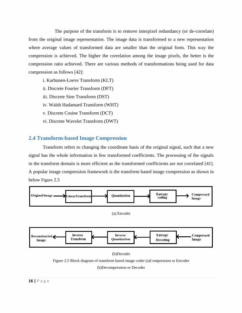
2.4 Transform-based Image Compression

Transform refers to changing the coordinate basis of the original signal, such that a new

signal has the whole information in few transformed coefficients. The processing of the signals

in the transform domain is more efficient as the transformed coefficients are not correlated [41].

A popular image compression framework is the transform based image compression as shown in

below Figure 2.5

(a) Encoder

(b)Decoder

Figure 2.5 Block diagram of transform based image coder (a)Compression or Encoder

(b)Decompression or Decoder

17 | P a g e

The first step in the encoder is to apply a linear transform to remove redundancy in the

data, followed by quantizing the transform coefficients, and finally entropy coding then we get

the quantized outputs. After the encoded input image is transmitted over the channel, the decoder

reverse all the operations that are applied in the encoder side and tries to reconstruct a decoded

image as close as to the original image [9].

2.4.1 Linear Transform

In the encoder side, the first step is to transform the image from the spatial domain to the

transformed domain (where the image information is represented in a more compact form) using

some known transforms like Discrete Fourier Transform(DFT), Discrete Cosine

Transform(DCT), Discrete Wavelet Transform(DWT), Fractal Transforms and many more.

Compression of the original image is not easy, as the energy can be concentrated in the

low frequency part of the transform domain. For conservation of energy from the spatial domain

to the transformed domain, it is necessary for the transform to be orthogonal. Here, in this thesis

Discrete Cosine Transform (DCT), Discrete Wavelet Transform (DWT), Hybrid Transform

(DCT-DWT), Fractal Transforms are implemented due to their superior energy compaction and

correspondence with human visual system [9]. An ideal image transform should retain the

following two properties. These are:

(a) Maximum energy compaction

(b) Less computational complexity

2.4.2 Quantizer

Quantizer is a key component in the transform compression framework that introduces

non-linearity in the system. It maps the transformed digital image to a discrete set of levels or

discrete number.it is a lossy compression technique as it introduces an error in the image

compression process [21]. It converts sequence of floating point numbers to sequence of

integers. In other words, ―If the data symbols are real numbers, quantization may round each to

the nearest integer. If the data symbols are large numbers, quantization may convert them to

small numbers‖. Small numbers take less space than large ones. On the other hand, small

numbers convey less information than large ones, which is why quantization produces lossy

compression. Quantization is a simple approach to lossy compression [17]. It is a many-to-one

18 | P a g e

mapping and therefore it is irreversible. The effect of Quantization can be seen in the below

Figure 2.6

Figure 2.6 Quantization effect.

Inverse quantization step restores original coefficients but with round-off error. Quantizers are of

three type, based on their working principle:

2.4.2.1 Scalar Quantization

Scalar Quantization is the simplest quantization because each input is treated separately in

producing the output. In other words, ―If the data symbols are numbers, then each is quantized to

another number in a process referred to as scalar quantization‖. Many image compression

methods are lossy, but scalar quantization is not suitable for image compression because it

creates annoying artifacts in the decompressed image. Scalar quantization produces lossy

compression, but it makes easy to control the trade-off between compression performance and

the amount of data loss [9]. Applications of scalar quantization are limited to cases where much

loss can be tolerated.

2.4.2.2 Vector Quantization

In vector quantization, the input samples are clubbed together in groups called vectors,

and then processed to give the output. If each data symbol is a vector, then vector quantization

converts a data symbol to another vector. The idea of representing groups of samples rather than

19 | P a g e

individual samples is the main concept of vector quantization. Vector quantization is based on

the fact that adjacent data symbols in image and audio files are correlated [9].

2.4.2.3 Predictive Quantization

The quantization of the difference between the predicted value and the past samples is

called predictive quantization.

A good quantizer is one, which represents the original signal with minimum loss or

distortion.

2.4.3 Entropy Encoding

After quantization of the transformed values, entropy encoder further compresses the

quantized values to give additional compression. It is a lossless compression and is also

reversible. In the entropy encoding, the idea is to find a reversible mapping to the quantized

values such that the average number of bits or symbols is minimized. The basic principle of

entropy encoding is that we assign short codes to the letters appearing frequently whereas long

codes are assigned to the letters appearing less frequently. The two popular entropy- coding

methods are Huffman coding and Arithmetic coding [31].

2.5 Discrete Cosine Transform

DCT is an orthogonal transform, the Discrete Cosine Transform (DCT) attempts to

decorrelate the image data. After decorrelation each transform coefficient can be encoded

independently without losing compression efficiency.

The DCT transforms a signal from a spatial representation into a frequency

representation. The DCT represent an image as a sum of sinusoids of varying magnitudes and

frequencies. DCT has the property that, for a typical image most of the visually significant

information about an image is concentrated in just few coefficients of DCT. After the

computation of DCT coefficients, they are normalized according to a quantization table with

different scales provided by the JPEG standard computed by psycho visual evidence. Selection

of quantization table affects the entropy and compression ratio. The value of quantization is

inversely proportional to quality of reconstructed image, better mean square error and better

compression ratio [42]. In a lossy compression technique, during a step called Quantization, the

20 | P a g e

less important frequencies are discarded, and then the most important frequencies that remain are

used to retrieve the image in decomposition process. After quantization, quantized coefficients

are rearranged in a zigzag order for further compressed by an efficient lossy coding algorithm .

DCT has many advantages:

(1) It has the ability to pack most information in fewest coefficients.

(2) It minimizes the block like appearance called blocking artifact that results when

boundaries between sub-images become visible [36].

An image is represented as a two dimensional matrix, 2-D DCT is used to compute the

DCT Coefficients of an image. The 2-D DCT for an NXN input sequence can be defined as

follows [5]:

D (i,j) =

√ ( ) ( )∑ ∑ ( ) (

( )

) (

( )

)

(2.7)

Where, P(x, y) is an input matrix image NxN, (x, y) are the coordinate of matrix elements and (i,

j) are the coordinate of coefficients, and

C (u) ={

√

} (2.8)

The reconstructed image is computed by using the inverse DCT (IDCT) according to

P(x,y) =

√ ∑ ∑ ( ) ( ) ( ) (

( )

) (

( )

)

(2.9)

The pixels of black and white image are ranged from 0 to 255, where 0 corresponds to a

pure black and 255 corresponds to a pure white. As DCT is designed to work on pixel values

ranging from -128 to 127, the original block is leveled off by 128 from every entry [21]. Step by

step procedure of getting compressed image using DCT and getting reconstructed image from

compressed image is explained in the next sections.

2.5.1 Coding scheme

2.5.1.1 Compression procedure

First the whole image is loaded to the encoder side, then we do RGB to GRAY conversion

after that whole image is divided into small NXN blocks (here N corresponds to 8) then working

from left to right, top to bottom the DCT is applied to each block. Each block‘s elements are

21 | P a g e

compressed through Quantization means dividing by some specific 8X8 matrix called Qmatrix and

rounding to the nearest integer value as shown in Eq 2.10

( ) ( ( )

( )) (2.10)

This Qmatrix is decided by the user to keep in mind that it gives Quality levels ranging

from 1 to 100, where 1 gives the poor image Quality and highest compression ratio while 100

gives best Quality of decompressed image and lowest compression ratio. The standard Qmatrix can

be shown as

Figure 2.7. JPEG Quantization table

We choose Qmatrix, with a Quality level of 50, Q50matrix gives both high compression and

excellent decompressed image. By using Q10 we get significantly more number of 0‘s as

compared to Q90. After Quantization, all of the quantized coefficients are ordered into the

―zigzag‖ sequence. The zigzag can be done in the below manner as shown in the Figure 2.9;

22 | P a g e

Figure 2.8 Zig-zag ordering for DCT coefficients

Now encoding is done and transmitted to the receiver side in the form of one dimensional

array. This transmitted sequence saves in the text format. The array of compressed blocks that

constitute the image is stored in a drastically reduced amount of space. Further compression can

be achieved by applying appropriate scaling factor [21]. In order to reconstruct the output data,

the rescaling and the de-quantization should be performed as given in Eq. (2.11).

( ) ( ) ( ) (2.11)

The de-quantized matrix is then transformed back using the 2-D inverse-DCT [35]. The

equation for the 2-D inverse DCT transform is given in the above mentioned Eq. (2.12)

P(x,y) =

√ ∑ ∑ ( ) ( ) ( ) (

( )

) (

( )

)

(2.12)

The complete procedure of compression an image using DCT is explained in Figure 2.7 through

a flowchart [41].

2.5.1.2 Decompression procedure

To reconstruct the image, receiver decodes the quantized DCT coefficients and computes

the inverse two dimensional DCT (IDCT) of each block, then puts the blocks back together into

a single image in same manner as we done in previously. The dequantization is achieved by

multiplying each element of the received data by corresponding element in the quantization

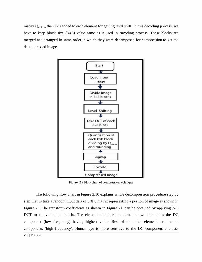
23 | P a g e

matrix Qmatrix, then 128 added to each element for getting level shift. In this decoding process, we

have to keep block size (8X8) value same as it used in encoding process. These blocks are

merged and arranged in same order in which they were decomposed for compression to get the

decompressed image.

Figure. 2.9 Flow chart of compression technique

The following flow chart in Figure 2.10 explains whole decompression procedure step by

step. Let us take a random input data of 8 X 8 matrix representing a portion of image as shown in

Figure 2.5 The transform coefficients as shown in Figure 2.6 can be obtained by applying 2-D

DCT to a given input matrix. The element at upper left corner shown in bold is the DC

component (low frequency) having highest value. Rest of the other elements are the ac

components (high frequency). Human eye is more sensitive to the DC component and less

24 | P a g e

sensitive to AC component. Hence, the AC component can be neglected in order to achieve

higher compression- by passing the transformed data through the quantizer.

Figure 2.10. Flow chart of decompression technique

Figure 2.11 A random value input data matrix

25 | P a g e

Figure 2.12 Transformed coefficients after DCT of the random value input data matrix

The JPEG quantization table is shown in Figure 2.8. The corresponding value after

quantization is as shown in Figure 2.13. We can see that more than 70 percent of the coefficients

are quantized to zero.

Figure 2.13 Quantized coefficients

Figure 2.14 Reconstructed output data

Further compression can be achieved by the use of scaling factor (SF) to the quantized

coefficients. The reconstructed data after inverse transformation is illustrated in Figure 2.14.

There is a small deviation between the input data and output data due to the quantization.

26 | P a g e

2.5.2 Properties of DCT

There are some properties of the DCT which are of particular value to image processing

applications [31].

2.5.2.1 Decorrelation

The principle advantage of image transformation is the removal of redundancy between

neighboring pixels. This leads to uncorrelated transform coefficients which can be encoded

independently. DCT exhibits excellent decorrelation properties.

2.5.2.2 Separability

The DCT transform equation 2.7 can be expressed as,

D (i,j) =

√ ( ) ( )∑ ∑ ( ) (

( )

) (

( )

)

for i, j = 0,1,2,…,N −1.

This property, known as ‗Separability‘, has the principle advantage that D (i, j) can be

computed in two steps by successive 1-D operations on rows and columns of an image. This idea

is graphically illustrated in Figure 2.15. The arguments presented can be identically applied for

the inverse DCT computation.

Figure 2.15 Computation of 2-D DCT using separability property.

2.5.2.3 Energy Compaction

Effectiveness of a transformation scheme can be directly evaluated by its ability to pack

input data into as few coefficients as possible. This allows the quantizer to discard coefficients

27 | P a g e

with relatively small amplitudes without introducing visual falsification in the reconstructed

image. DCT exhibits excellent energy compaction for highly correlated images.

(a) Saturn and its DCT

(b) Circuit and its DCT

(c)Baboon and its DCT

28 | P a g e

(d) sine wave and its DCT

Figure2.16. (a) Saturn and its DCT; (b) Circuit and its DCT; (c) Baboon and its DCT;

(d) sine wave and its DCT

A closer look at Figure 2.16 reveals that it comprises of four broad image classes. Figure

2.16 (a) contain large areas of slowly varying intensities. These images can be classified as low

frequency images with low spatial details. A DCT operation on these images provides very good

energy compaction in the low frequency region of the transformed image.

Figure 2.16(b) contains a number of edges (i.e., sharp intensity variations) and therefore

can be classified as a high frequency image with low spatial content. However, the image data

exhibits high correlation which is exploited by the DCT algorithm to provide good energy

compaction. Figure 2.16 (c) and is image with progressively high frequency and spatial content.

Consequently, the transform coefficients are spread over low and high frequencies. Figure

2.16(d) shows periodicity therefore the DCT contains impulses with amplitudes proportional to

the weight of a particular frequency in the original waveform. The other (relatively insignificant)

harmonics of the sine wave can also be observed by closer examination of its DCT image.

Hence, from the preceding discussion it can be inferred that DCT extracts excellent

energy compaction for correlated images. Studies have shown that the energy compaction

performance of DCT approaches optimality as image correlation approaches one i.e., DCT

provides (almost) optimal decorrelation for such images.

29 | P a g e

2.5.2.4 Symmetry

In the above Equation (2.7), at the row and column operations reveals that these

operations are functionally identical. Such a transformation is called a symmetric transformation.

A separable and symmetric transform can be expressed in the form.

T = APA (2.13)

where A is an N ×N symmetric transformation matrix with entries a (i, j ) given by

(2.14)

and f is the N ×N image matrix. This is an extremely useful property since it implies that the

transformation matrix can be precomputed offline and then applied to the image thereby

providing orders of magnitude improvement in computation efficiency [41].

2.5.2.5 Orthogonality

In order to extend ideas presented in the preceding section, let us denote the inverse

transformation of as

(2.15)

As discussed previously, DCT basis functions are orthogonal. Thus, the inverse

transformation matrix of A is equal to its transpose i.e. . Therefore, and in addition

to its decorrelation characteristics, this property renders some reduction in the pre-computation

complexity [42].

2.5.3 Limitations of DCT

For the lower compression ratio, the distortion is unnoticed by human visual perception.

In order to achieve higher compression it is required to apply quantization followed by scaling to

the transformed coefficient. For such higher compression ratio DCT has following two

limitations.

30 | P a g e

2.5.3.1 Blocking artifacts:

Blocking artifacts is a distortion that appears due to heavy compression and appears as

abnormally large pixel blocks. For the higher compression ratio, the perceptible ―blocking

artifacts‖ across the block boundaries cannot be neglected [48]. The example of appearance of

blocking artifact due to high compression is shown in Figure2.17.

Figure 2.17. Illustration of compression using DCT: (a) Original Image CR at (b) 88%, (c) 96%

2.5.3.2 False contouring:

The false contouring occurs when smoothly graded area of an image is distorted by an

deviation that looks like a contour map for specific images having gradually shaded areas [5].

Figure 2.18 Illustration of compression using DCT: (a) Original Image CR at (b) 87 %, (c) 97%

The main cause of the false contouring effect is the heavy quantization of the transform

coefficients [46]. An example of false contouring can be observed in Figure 2.18.

31 | P a g e

2.6 Discrete Wavelet Transform (DWT)

Wavelets are a mathematical tool for changing the coordinate system in which we

represent the signal to another domain that is best suited for compression. Wavelet based coding

is more robust under transmission and decoding errors. Due to their inherent multiresolution

nature, they are suitable for applications where scalability and tolerable degradation are

important [4].

Wavelets are tool for decomposing signals such as images, into a hierarchy of increasing

resolutions. The more resolution layers, the more detailed features of the image are shown. They

are localized waves that drop to zero. They come from iteration of filters together with rescaling.

Wavelet produces a natural multi resolution of every image, including the all-important edges.

The output from the low pass channel is useful compression. Wavelet has an unconditional basis

as a result the size of the wavelet coefficients drop off rapidly. The wavelet expansion

coefficients represent a local component thereby making it easier to interpret. Wavelets are

adjustable and hence can be designed to suit the individual applications. Its generation and

calculation of DWT is well suited to the digital computer [41]. They are only multiplications and

additions in the calculations of wavelets, which are basic to a digital computer.

2.6.1 Multiresolution Concept and Analysis

The multi resolution concept is designed to represent signals, where a single event will be

decomposed into finer and finer details. A signal is represented by a coarse approximation and

finer details. The coarse and the detail subspaces are orthogonal to each other.by applying

successive approximation recursively the space of the input signal can be spanned by spaces of

successive details at all resolutions [6].

2.6.2 Decimator and interpolator

Decimator and interpolator are two operations concerned with the sampling rate.

Decimator or down sampler lowers the sampling rate whereas interpolator or the up-sampler

32 | P a g e

raises the sampling rate [5]. The down sampler takes a signal x(n) and down samples by a factor

of two. It is shown in Figure 2.19

Figure 2.19 Decimator or down sampler

Similarly, the up-sampler takes a signal and up samples by a factor of two so as to increase the

number of samples. It means to insert zeros between the terms of the original sequence.

Figure 2.20 Interpolator or up sampler

The input sequence is stretched to twice its original length and zeros are inserted. It can be seen

in Figure 2.20.

2.6.3 Filter bank

Filter bank is a set of filters. It consists of analysis bank and synthesis bank. In this thesis

two channel filter bank is considered.it is shown in Figure 2.21 [6]

Figure 2.21 Filter bank

2.6.3.1 Analysis bank

The analysis bank has two filters: a low pass and a high pass. They separate the input

signal into frequency bands. When the input signal (image) is first passed through the analysis

filters, it decomposes the signal into four bands. They are given as LL, HL, LH, AND HH. This

33 | P a g e

is the first level of the decomposition and it represents the finer scale of the expansion

coefficients [11]. It is shown in Figure 2.22

Figure 2.22 Finer scale and coarser scale wavelet coefficients

The DWT represents an image as a sum of wavelet functions, known as wavelets, with

different location and scale. It represents the data into a set of high pass (detail) and low pass

(approximate) coefficients. The input data is passed through set of low pass and high pass filters.

used . The output of high pass and low pass filters are down sampled by 2. The output from low

pass filter is an approximate coefficient and the output from the high pass filter is a detail

coefficient. This procedure is one dimensional (1-D) DWT and Figure 2.23 shows the schematics

of this method.

Figure 2.23. Block diagram of 1-D forward DWT

The two filters double the number of coefficients but the decimator halves it. It implies

that there is a possibility of getting the original image back. The aliasing occurring in the higher

34 | P a g e

scale can be cancelled by using the signal from the lower level [11]. This is the idea behind the

perfect reconstruction filter bank.

Figure 2.24. Block diagram of 2-D forward DWT

Repeating the splitting, filtering and decimation on the scaling coefficients is called

iterating the filter bank.it is illustrated in Figure 2.24 in 2-D DWT. In case of 2-D DWT, the input

data is passed through set of both low pass and high pass filter in two directions, both rows and

columns. The outputs are then down sampled by 2 in each direction as in case of 1-D DWT [53].

As shown in Figure 2.22, output is obtained in set of four coefficients LL, HL, LH and HH. The

first alphabet represents the transform in row whereas the second alphabet represents transform

in column. The alphabet L means low pass signal and H means high pass signal. LH signal is a

low pass signal in row and a high pass in column. Hence, LH signal contain horizontal elements.

Similarly, HL and HH contains vertical and diagonal elements, respectively.

2.6.3.2 Synthesis bank

It is the inverse of the analysis bank. In digital signal processing there was decimation

and filtering in the synthesis bank [11].

35 | P a g e

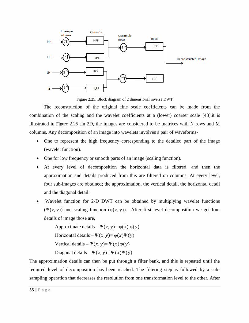
Figure 2.25. Block diagram of 2 dimensional inverse DWT

The reconstruction of the original fine scale coefficients can be made from the

combination of the scaling and the wavelet coefficients at a (lower) coarser scale [48].it is

illustrated in Figure 2.25 .In 2D, the images are considered to be matrices with N rows and M

columns. Any decomposition of an image into wavelets involves a pair of waveforms-

One to represent the high frequency corresponding to the detailed part of the image

(wavelet function).

One for low frequency or smooth parts of an image (scaling function).

At every level of decomposition the horizontal data is filtered, and then the

approximation and details produced from this are filtered on columns. At every level,

four sub-images are obtained; the approximation, the vertical detail, the horizontal detail

and the diagonal detail.

Wavelet function for 2-D DWT can be obtained by multiplying wavelet functions

( ( )) and scaling function (φ( )). After first level decomposition we get four

details of image those are,

Approximate details – ( )= φ( ) φ( )

Horizontal details – ( )= φ( ) ( )

Vertical details – ( )= ( ) ( )

Diagonal details – ( )= ( ) ( )

The approximation details can then be put through a filter bank, and this is repeated until the

required level of decomposition has been reached. The filtering step is followed by a sub-

sampling operation that decreases the resolution from one transformation level to the other. After

36 | P a g e

applying the 2-D filler bank at a given level n, the detail coefficients are output, while the whole

filter bank is applied again upon the approximation image until the desired maximum resolution

is achieved. Figure 2.26(b) shows wavelet filter decomposition. The sub-bands are labelled by

using the following notations [12].

LLn represents the approximation image nth

level of decomposition, resulting from low-

pass filtering in the vertical and horizontal both directions.

LHn represents the horizontal details at nth

level of decomposition and obtained from

horizontal low-pass filtering and vertical high-pass filtering.

HLn represents the extracted vertical details/edges , at nth

level of decomposition and

obtained from vertical low-pass filtering and horizontal high-pass filtering.

HHn represents the diagonal details at nth

level of decomposition and obtained from

high-pass filtering in both directions [33].

2.6.4Coding scheme

2.6.4.1 Compression procedure

Original image is passed through HPF and LPF by applying filter first on each row.

Output of the both image resulting from LPF and HPF is considered as L1 and H1 and they are

combine into A1, where A1= [L1, H1]. Then A1 is down sampled by 2. Again A1 is passed

through HPF and LPF by applying filter now on each column. Output of the above step is

supposed to L2 and H2 and they are combined to get A2, where A2=*

+. Now, A2 is down

sampled by 2 to get compressed image [53]. We get this compressed image by using one level of

decomposition, to get more compressed image i.e. to get more compression ratio we need to

follow above steps more number of times depending on number of decomposition level required

[51]. First level of decomposition gives four detailed version of an image those are shown in

Figure 2.20(a) and (b).

2.6.4.2 Decompression procedure

Extract LPF and HPF images from compressed image by simply taking upper half rectangle

of matrix is LPF image and down half rectangle is HPF image. Then both images are up sampled

by2. Now take the summation of both images into one image called B1.Then again extract LPF

image and HPF image by dividing vertically [50]. Two halves obtained are filtered through LPF

37 | P a g e

and HPF, summation of these halves gives the reconstructed image on each block of 32x32

block, by applying 2 D-DWT, four details are produced. Out of four sub band details,

approximation detail/sub band is further transformed again by 2 D-DWT which gives another

four sub-band of 16x16 blocks. Above step is followed to decompose the 16x16 block of

approximated detail to get new set of four sub band/ details of size 8x8. The level of

decomposition is depend on size processing block obtained initially, i.e. here we are dividing

image initially into size of 32x32, hence the level of decomposition is 2 [46]. After getting four

blocks of size 8x8, we use the approximated details for computation of discrete cosine transform

coefficients. These coefficients are then quantize and send for coding [41]. The DWT algorithm

is typically more memory intensive and time consuming compared to a DCT based coder like

JPEG. Despite this, DWT offers benefits such as :

Allowing image multiresolution representation

Allowing progressive transmission / rate scalability

Higher efficiency in term of quality of compressed image and compression ratio.

(a) (b)

(c) (d)

Figure 2.26. Illustration of 2 dimensional DWT for an image ‗Lena‘

38 | P a g e

2.7 HYBRID (DCT+ DWT) TRANSFORM

In section 2.5 and 2.8 we presented two different ways of achieving the goals of image

compression, which have some advantages and disadvantages, in this section we are proposing a

transform technique that will exploit advantages of DCT and DWT, to get compressed image.

Hybrid DCT-DWT transformation gives more compression ratio compared to JPEG and

JPEG2000, preserving most of the image information and create good quality of reconstructed

image. Hybrid (DCT+DWT) Transform reduces blocking artifacts, false contouring and ringing

effect.[39].

2.7.1 Coding scheme

2.7.1.1Compression procedure

The input image is first converted to gray image from colour image, after this whole

image is divided into size of 32x32 pixels blocks. Then 2D-DWT applied on each block of

32x32 blocks, by applying 2 D-DWT, four details are produced. Out of four sub band details,

approximation detail/sub band is further transformed again by 2 D-DWT which gives another

four sub-band of 16x16 blocks [52]. Above step is followed to decompose the 16x16 block of

approximated detail to get new set of four sub band/ details of size 8x8. The level of

decomposition is depend on size processing block obtained initially, i.e. here we are dividing

image initially into size of 32x32, hence the level of decomposition is 2. After getting four

blocks of size 8x8, we use the approximated details for computation of discrete cosine transform

coefficients. These coefficients are then quantize and send for coding. The complete coding

scheme is explained in Figure 2.27.

2.7.1.2 Decompression procedure

At receiver side, we decode the quantized DCT coefficients and compute the inverse

two dimensional DCT (IDCT) of each block. Then block is dequantized. Further we take inverse

wavelet transform of the dequantized block. Since the level of decomposition while compressing

was two, we take inverse wavelet transform two times to get the same block size i.e. 32x32. This

procedure followed for each block received. When all received blocks are converted to 32x32 by

39 | P a g e

following decompression procedure, explained above. We arrange all blocks to get reconstructed

image. The complete decoding procedure is explained in Figure 2.28. The hybrid DWT-DCT

algorithm has better performance as compared to stand alone DWT and DCT in terms of Peak

Signal to Noise Ratio (PSNR) and Compression Ratio (CR). In standalone DCT, the entire

image/frame is divided into 8X8 block in order to apply 8 point DCT [40].

Figure 2.27 Compression technique using Hybrid transform

Figure 2.28 Decompression technique using Hybrid transform

40 | P a g e

Whereas, in case of hybrid algorithm, image/frame is first divided into 32X32 blocks and

two level of DWT is performed for these 32X32 block image. The output after the two level of

DWT becomes 8X8 and hence the 8 point DCT is applied for that 8X8 output. This difference in

block size causes the blocking artifacts in case of standalone DCT. The contouring effect of DCT

has also been reduced by using proposed hybrid DWT-DCT algorithm.

2.8 Fractal Image Compression

Fractal coding is a new method of image compression. The main principle of the fractal

transform coding is based on the hypothesis that the image redundancies can be efficiently

exploited by means of block self-affine transformations. By removing the redundancy related to

self-similarity in an image. Fractal image compression can achieve a higher compression ratio

with high decoding quality. Fractal coding has the advantage such as resolution independence

and fast decoding as compare to other image compression methods. So fractal image

compression is a promising technique that has great potential to improve the efficiency of image

storage and image transmission [43].

2.8.1 Baseline Fractal Coding

Fractal image coding is based on partition iterated function system (PIFS),in which an

original input image is partitioned into a set of non-overlapping sub-blocks, called range block

(R) that cover up the whole image. The size of every range block is N X N. At the same time, the

original image is also partitioned into a set of other overlapping sub-blocks, called domain

blocks (D), which size is always twice the size of range blocks. The domain blocks are allowed

to be overlapping and need not cover the whole image [26]. Secondly, each of the domain blocks

is contracted by pixel averaging or down sampling to match the size of the range block. Next,

eight symmetrical transformations (rotations and flips) are applied to all contracted domain

blocks to bring out an extended domain pool, which denoted as ̂ For each range block, we

search the domain pool to get the best matched domain block D with a contractive affine

transformation. The problem with fractal coding is the highly computational complexity in the

encoding process [29].

41 | P a g e

Figure2.29 Fractal coding algorithm

Most of the encoding time is spent on the best matching search between range blocks and

numerous domain blocks ( ̂) so that the fractal encoding is a time consuming process, which

limits the algorithm to practical application greatly. In order to solve this problem, lots of

researches were done earlier to speed up the block matching process. Most of these

improvements tried to restrict the search space of the domain block pool in order to reduce the

computation requirements of the best matching search, hence speeding up the fractal image

encoding procession [28].

2.8.2 Procedure of a different speed up encoding method

The different fast fractal encoding method use the variance and mean value to exclude

the searching of those domain blocks whose characteristics are inconsistent to the range block.

By reducing the computational complexity of RMSE and simplified transformation to find out

the best matched domain block would be useful [24].

The steps of the proposed algorithm are given as follows:

42 | P a g e

Partition the original image into non-overlapping range blocks(R) and overlapping

domain blocks (D).

By doing, down sampling we contract the size of the domain block to the size of the

range block and it is noted as ̂

Now, calculate the variance of range and domain blocks by the equation below. The

variance of block I is defined as,

Var (I) = √,

(∑

) (

(∑ )

)

-

(2.16)

Where n is the size of the block and Xi is the pixel value of the range blocks.

For each range block (R), select those domain blocks that can meet the criterion

of | ( ) ( ̂)| . Then classify those selected ̂ by the individual

mean value.

By using simplified transformation analysis and reduced RMSE to find the best matched

domain block and its transformation. Then, store this position of searched domain block

and mapped transformation.

Repeat the above steps for all other range blocks until all the range blocks are processed.

In the above method, according to variance difference between Var (R) and Var ( ̂), the

range blocks are classified. Then both range and domain blocks are classified into a number of

classes according to mean value. The searched domain blocks for every range block are not all

domain blocks now. The proposed method only searches the domain blocks whose mean value

classes are the same or adjacent as the class of range block to reduce the searching time [41]. The

reduction of search domain blocks decreases the decoded quality. However, searching time

decreases melodramatically.

2.8.3 Procedure for decoding method

To decompress an image, the compressor first allocates two memory buffers of equal size,

with arbitrary initial content. The iterations then begin, with buffer 1 the range image and buffer

2 the domain image. The domain image is partitioned into domain regions as specified in the FIF

file. For each domain region, its associated range region is located in the range image. Then the

43 | P a g e

Figure 3.30 A different approach for Fractal coding

corresponding affine map is applied to the content of the range region, pulling the content

toward the map's attractor. Since each of the affine maps is contractive, the range region is

contracted by the transformation. This is the reason that the range regions are required to be

larger than the domain regions during compression.

For the next iteration, the roles of the domain image and range image are switched. The

process of mapping the range regions (now in buffer 2) to their respective domain regions (in

buffer 1) is repeated, using the prescribed affine transformations. Then the entire step is repeated

again and again, with the content of buffer 1 mapped to buffer 2, then vice versa. At every step,

the content is pulled ever closer to the attractor of the IFS which forms a collage of the original

image [27]. Eventually the differences between the two images become very small, and the

content of the first buffer is the output decompressed image.

44 | P a g e

2.8.4 Advantages and Disadvantages

Fractal image compression has the following advantages:

Fast decoding process

High compression ratio

Low performance device

Resolution independence

It can be digitally scaled to any resolution when decoded.

Image compressed in terms of self-similarity rather than pixel resolution

Lower transmission time

Disadvantage of fractal image compression

Long encoding time

Image quality

2.9 Conclusion

The algorithms for compression and decompression for various Image compressions

methods such as DCT, DWT, Hybrid, Fractals are discussed in this chapter. DCT requires less

computational resources and can achieve the energy compaction property. However, for the

higher compression ratio it introduces the blocking artifacts and the false contouring effects

while image reconstruction. DWT is the only techniques which has capacity of multi resolution

compression. However, it requires higher computational complexity as compared to other

techniques. Hence, in order to benefit from each other, hybrid DWT-DCT algorithm has been

discussed for the image compression in this chapter. Conventional Fractal method circumvents

the drawbacks of DCT, DWT, Hybrid (DCT+DWT), but it requires more computational time. A

different approach for image compression using fractals is also discussed which uses the mean

and variance of range and domain blocks. This approach speeds up the encoding time by

reducing the number range- domain comparison with remarkable amount. Each method can be

well suited with different images based on the user requirements.

45 | P a g e

Chapter 3

Performance Measurement Parameters

In this work prominence were given on the amount of compression used and how good

the reconstructed image be similar to the original. Analysis was done on the basis of the amount

of distortion, which was calculated using important distortion measures: mean square error

(MSE), peak signal-to-noise ratio (PSNR) measured in decibels (dB) and compression ratio (CR)

measures were used as performance indicators. Image having same PSNR value may have

different perceptual quality. The quality of reconstructed images can be evaluated in terms of

objective measure and subjective measure. In objective evaluation, statistical properties are

considered whereas, in subjective evaluation, viewers see and investigate image directly to

determine the image quality. A good compression algorithm would reconstruct the image with

low MSE and high PSNR [46]. Performance measurement parameters are described in the

following sub-sections.

3.1 Objective evaluation parameters.

3.1.1 Mean Square Error (MSE)

The MSE is the cumulative squared error between the compressed and the original image.

A lower value of MSE means lesser error, and it has the inverse relation with PSNR. Mean

square error is a criterion for an estimator: the choice is the one that minimizes the sum of

squared errors due to bias and due to variance. In general, it is the average of the square of the

difference between the desired response and the actual system output. As a loss function MSE is

also called squared error loss [41]. MSE measures the average of the square of the ‗error‘. The

MSE is the second moment of the error, and thus incorporates both the variance of the estimator

and its bias. For an unbiased estimator, the MSE is the variance. In an analogy to standard

deviation, taking the square root of MSE yields the root mean squared error or RMSE [43]. For

an unbiased estimator, the RMSE is the square root of the variance, known as the standard error.

46 | P a g e

MSE=

∑ ∑ [ ( ) ( )]

(3.1)

Where, I(x, y) is the original image and I‘(x, y) is the reconstructed image and m, n are the

dimensions of the image. Lower the value of MSE, the lower the error and better picture quality

[49].

3.1.2 Peak Signal to Noise Ratio (PSNR)

PSNR is a measure of the peak error. Many signals have very wide dynamic range,

because of that reason PSNR is usually expressed in terms of the logarithmic decibel scale in

(dB). Normally, a higher value of PSNR is good because it means that the ratio of signal to noise

is higher [1]. Here, a signal represents original image and noise represents the error in

reconstruction. It is the ratio between the maximum possible power of a signal and the power of

the corrupting noise [9]. PSNR decreases as the compression ratio increases for an image. The

PSNR is defined as:

PSNR=10*log10,

- = 20*log10,

√ - (3.2)

PSNR is computed by measuring the pixel difference between the original image and

compressed image [53]. Values for PSNR range between infinity for identical images, to 0 for

images that have no commonality.

(a) Original image (b) PSNR = 25.98 dB

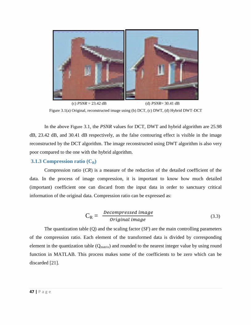
47 | P a g e

(c) PSNR = 23.42 dB (d) PSNR= 30.41 dB

Figure 3.1(a) Original, reconstructed image using (b) DCT, (c) DWT, (d) Hybrid DWT-DCT

In the above Figure 3.1, the PSNR values for DCT, DWT and hybrid algorithm are 25.98

dB, 23.42 dB, and 30.41 dB respectively, as the false contouring effect is visible in the image

reconstructed by the DCT algorithm. The image reconstructed using DWT algorithm is also very

poor compared to the one with the hybrid algorithm.

3.1.3 Compression ratio (CR)

Compression ratio (CR) is a measure of the reduction of the detailed coefficient of the

data. In the process of image compression, it is important to know how much detailed

(important) coefficient one can discard from the input data in order to sanctuary critical

information of the original data. Compression ratio can be expressed as:

CR =

(3.3)

The quantization table (Q) and the scaling factor (SF) are the main controlling parameters

of the compression ratio. Each element of the transformed data is divided by corresponding

element in the quantization table (Qmatrix) and rounded to the nearest integer value by using round

function in MATLAB. This process makes some of the coefficients to be zero which can be

discarded [21].

48 | P a g e

(a) Original image (b) CR=78.32% (c) CR =89.28%

Figure 3.2 CR comparison (a) original image and (b), (c) reconstructed image with different compression ratio.

In order to achieve higher compression ratio, the quantizer output is then divided by some

scalar constant (SF) and rounded to nearest integer value. This process yields more zero

coefficients which can be discarded during compression [54].

The CR can be varied to get different image quality. The more the details coefficients are

discarded, the higher the CR can be achieved. Higher compression ratio means lower

reconstruction quality of the image. Compression ratio comparison can be seen in the above

Figure 3.2 .We can see that at higher compression ratio we get blurred image as compare to the

image that have less compression ratio.

3.2 Subjective evaluation parameter

The visual perception of the reconstructed image is essential. In some cases the objective

quality assessment does not give proper information about the quality of the reconstructed image.

In such scenarios, it is important to analyze the reconstructed image using subjective analysis

that means by human perceptual system [41]. When the subjective measure is considered,

viewers focus on the difference between reconstructed and original image and correlates the

differences.

49 | P a g e

3.3 Conclusion

In this chapter, the objective and subjective evaluation parameter generally used for

image compression analysis has been presented. For the objective evaluation PSNR, CR and

variance have been discussed. The lower value of MSE indicates better picture quality. There is

an inverse relationship between MSE and PSNR. Hence, the larger PSNR value gives the better

image quality. Compression ratio indicates the efficiency of compression technique, more the

compression ratio, less memory space required. Hence, more compression ratio is always

desirable without trade off in image quality.

50 | P a g e

Chapter 4

Performance Evaluation and Simulation Results

This chapter evaluates the performance of the various image compression algorithms.

The studied algorithms are applied on several types of images: natural images, benchmark

images such that the performance of proposed algorithm can be verified for various applications.

These benchmark images are the standard image generally used for the image processing

applications and are obtained from. The results of the meticulous simulation for all images and

are presented in this section. The results are compared with the JPEG-based DCT, DWT, Hybrid

(DCT-DWT) algorithms and using Fractals.

4.1 Simulation tool

The algorithms were implemented in MATLAB simulation tool. For the DWT and DCT,

MATLAB functions ―dwt2‖ and ―dct2‖ has been considered, respectively. The evaluation

parameters (PSNR, CR, MSE and Variance), sub-sampling, quantization and scaling routines

were manually programmed in MATLAB. The proposed algorithm is compared with DCT,

DWT and Hybrid (DCT-DWT) algorithms.

4.2 Simulation Results

Results are tabulated in table 4.1. The results are obtained for images of sizes 128x128

and 512x512. Original and reconstructed images are also shown in Figure 4.1. It can be seen

from table 4.1, the compression ratio CR is high for Hybrid transform as compare to standalone

transforms. DWT comprises between compression ratio and quality of reconstructed image, it

adds speckle noise to the image for improvement in the reconstructed image. Hence DWT

technique is useful in medical applications. DCT gives lesser compression ratio but it is

computationally efficient compared to other techniques.

51 | P a g e

Table4.1 comparative analysis

The proposed fractal encoding is simulated by using several images of size 512 X 512 and 128X 128 with 256 gray levels. The conventional algorithm uses non-overlapping 8 x 8 range blocks and overlapping 16 X16 domain blocks and full exhaustive search. For the purpose of comparison the size of range blocks and

Domain blocks are has to be same that means 8 X 8. The threshold value has to be set for

different images and it is user defined. For the image of ‗Lena‘, we set the threshold value 1800

and 1900.

Image Image

Size

Technique used Compression Ratio MSE PSNR

Image 1

(jas.jpg)

128x128

DCT 2.6122 4.342 49.4436

DWT 3.2365 4.165 50.3181

Hybrid 10.2989 44.148 31.6817

512x512

DCT 26.5462 0.9732 48.2488

DWT 30.237 6.1613 40.2341

Hybrid 52.539 113.2097 27.5920

Image 2

(lena.jp

g)

128x128

DCT 2.3690 0.0676 59.8335

DWT 2.9231 1.9067 45.3279

Hybrid 9.6481 35.0658 32.6820

512x512

DCT 24.5156 2.8152 43.6357

DWT 29.8172 29.3150 33.4599

Hybrid 49.7381 122.4307 27.2519

52 | P a g e

Figure. 4.1 Comparison of visual image quality of reconstructed image for DCT, DWT AND HYBRID

(DCT+DWT) for test images.

Thus, analyze the difference between the decoded images. As we can see the quality of

decoded image at different threshold level in the below Figure 4.2.

(a) Original image (b) Decoded image at threshold (c ) Decoded image at threshold

Value 1800 Value 1900

Figure. 4.2 Comparison of visual image quality of reconstructed image from the proposed method at different

threshold value

53 | P a g e

When we implement the coding of fractal wavelet compression technique without the threshold

value in MATLAB then we got the Peak signal to noise ratio is 39.4201 which is good but we

got the encoding time very high that is 128.1167(approx. more than 2 min) and the decoding

time is 17.052 sec which is quite low then encoding time. If we set the particular threshold value

which is 1800 then we got the peak signal to noise ratio 25.9846 and encoding time is 27.529 sec

which is very low as compare to previous scheme and the decoding time is 16.4702 sec which is

little small then the previous scheme. Now further if we change the threshold value from 1800

To 1900 then we analyze the major change again in encoding time. At this threshold value the

encoding time obtained is very low i.e. 4.891 sec which is quite low. But there is no change in

the PSNR value and decoding time is very near to the previous stage. So we can say that on the

second value of threshold we obtain the best result if we concern only with encoding and

decoding time. The below table 4.2 shows comparison of the schemes i.e. ( existed and proposed

one).

Table 4.2 Comparative analysis of existed and proposed encoding approach

4.3 Conclusion

Based on the comprehensive simulation results presented above for images it can be seen

that the hybrid DWT-DCT algorithm outperforms the JPEG based DCT and DWT algorithms.

Especially, the hybrid algorithm performs better for the images that consist of detailed view,

bright colours, and gradients. Hence, it can be implemented for compressing natural and medical

images. It is observed that in case of the DWT algorithm, the reconstructed images seem to be

the worst, whereas for the DCT, it is affected by artifacts and false contouring effects. However,

for the same CR, the hybrid algorithm consistently has higher PSNR and better reconstruction

54 | P a g e

quality. It is also able to reduce the false contouring effect and artifacts for images. Fractal

encoding is computationally very expensive and hence it requires large time for encoding

process. In spite of many advancements, computational and time requirements of encoding part

is a still remains the main drawback of fractal image compression. Besides these drawbacks,

fractal technique provides more compression ratio, resolution independency; the iteration

function system provides a better quality in the images.

55 | P a g e

Chapter 5

Conclusion and Future work

5.1 Conclusion

In this thesis analysis of various Image compression techniques for different images is

done based on parameters, compression ratio(CR), mean square error (MSE), peak signal to

noise ratio (PSNR). Our simulation results from chapter 4 shows that we can achieve higher

compression ratio using Hybrid technique but loss of information is more. DWT gives better

compression ratio without losing more information of image. Pitfall of DWT is, it requires more

processing power. DCT overcomes this disadvantage since it needs less processing power, but it

gives less compression ratio. DCT based standard JPEG uses blocks of image, but there are still

correlation exits across blocks. Block boundaries are noticeable in some cases. Blocking artifacts

can be seen at low bit rates. In wavelet, there is no need to divide the image. More robust under

transmission errors. It facilitates progressive transmission of the image (scalability). Hybrid

transform gives higher compression ratio but for getting that clarity of the image is partially trade

off. It is more suitable for regular applications as it is having a good compression ratio along

with preserving most of the information.

On the other hand Fractal Image Compression gives a great improvement on the

encoding and decoding time. A weakness of the proposed design is the use of fixed size blocks

for the range and domain images. There are regions in images that are more difficult to code than

others .Therefore; there should be a mechanism to adapt the block size (R, D) depending on the

mean and variance calculated when coding the block. This type of compression can be applied in

Medical Imaging, where doctors need to focus on image details, and in Surveillance Systems,

when trying to get a clear picture of the intruder or the cause of the alarm. This is a clear

advantage over the Discrete Cosine Transform Algorithms such as that used in JPEG.

56 | P a g e

5.2 Future Work

The result in this thesis provides a strong foundation for future work for the hardware

design. All of the analysis presented in this thesis work involved exhaustive simulations. The

algorithm can be realized in hardware implementation as a future work. It can also be a good

option for the image processor of the wireless capsule endoscopic system. The research work has

been analyzed for high compression ratio. Further research can be performed to relax high

compression ratio constraint. This work has been constrained only for the removal of the spatial

redundancy by compression of still images.

57 | P a g e

References

[1] A. Jain, ―Fundamentals of Digital Image Processing‖ Prentice-Hall, 1989.

[2] K. Rao and J. Hwang, ―Techniques and Standards for Image, Video and Audio Coding‖,

Prentice-Hall, 1996

[3] W. Penebaker and J. Mitchell, ―JPEG Still Image Data Compression Standard‖, Van

Nostrand, 1993.

[4] I. Daubechies, ―Ten Lectures on Wavelets‖, SIAM, 1992.

[5] E. Whittaker, ―On the Functions which are Represented by the Expansions of Interpolation

Theory,‖ Proc. Royal Soc., Edinburgh, Section A 35, pp. 181-194, 1915.

[6] P. Vaidyanathan, ―Multirate Systems and Fitler Banks‖, Prentice-Hall, 1993.

[7] D. LeGall and A. Tabatabai, ―Subband Coding of Digital Images Using Symmetric Short

Kernel Filters and Arithmetic Coding Techniques,‖ Proc. ICASSP, IEEE, pp. 761-765, 1988.

[8] D. Huffman, ―A Method for the Construction of Minimum Redundancy Codes,‖ Proc. IRE,

pp. 1098-1101, 1952.

[9] S. Mallat and F. Falzon, ―Understanding Image Transform Codes,‖ IEEE Trans. Im. Proc.,

submitted, 1997.

[10] A. Oppenheim and R. Schafer, ―Discrete-Time Signal Processing‖, Prentice-Hall, 1989

[11] Mark J. T. Smith and Steven L. Eddins. ―Analysis/synthesis techniques for subband image

coding‖ IEEE Trans. Acoust., Speech, Signal Process., pp. 1446–1456, August 1990

[12] M. Antonini et al, ―Image Coding Using Wavelet Transform,‖ IEEE Trans.Image Proc.,

pp. 205-220, April, 1992

[13] A. Gersho and R. Gray, ―Vector Quantization and Signal Compression‖, Kluwer, 1992.

[14] A. Lewis and G. Knowles, ―Image Compression Using the 2-D Wavelet Transform,‖

IEEE Trans. Image Proc., pp. 244-250, April. 1992.

[15] J. Villasenor et al, ―Wavelet Filter Evaluation for Image Compression,‖ IEEE Trans. Image

Proc., August, 1995.

[16] S. Mallat, ―A theory for multiresolution signal decomposition: The wavelet

representation‖, IEEE Trans. Pattern Anal. Machine Intell. vol. 11 pp. 674-693, July 1989

58 | P a g e

[17] G. K. Wallace, ―The JPEG Still Picture Compression Standard‖, Conference of

the ACM, vol. 34, pp. 30-44, April 1991.

[18] J. W. Woods ed. ―Subband Image Coding‖, Kluwer Academic Publishers, Boston, MA.

1991.

[19] A. Lewis and G. Knowles, ―Image compression using the 2-D wavelet transforms,‖

IEEE Trans. Image Processing, vol. 1, pp. 244-250, April 1992

[20] R. L. Joshi, H. Jafarkhani, J. H. Kasner, T. R. Fisher, N. Farvardin, M. W. Marcellin, and

R. H. Bamberger, ―Comparison of different methods of classification in subband coding of

images,‖ submitted to IEEE Trans. Image Processing, 1995.

[21] Rao, K.R. and Yip, P., ―Discrete Cosine Transform‖ ,Academic Press, New York,

1990

[22] Barnsley, M.F., ―Fractals Everywhere‖, Academic Press, Boston, 1988.

[23] Falconer, K., ―Fractal Geometry Mathematical Foundations and Applications‖, John Wiley

& Sons, New York, 1990.

[24] Barnsley, M.F. and Sloan, A.D., ―A better way to compress images‖, pp. 215–223, 1988.

[25] Jacquin, A.E., ―A Fractal Theory of Iterated Markov Operators with Applications

to Digital Image Coding‖, Ph.D. thesis, Georgia Institute of Technology, August 1989.

[26] Fisher, Y., ―Fractal image compression‖, SIGGRAPH‘92, course notes.

[27] Jacquin, A.E., ―A novel fractal block-coding technique for digital images‖, ICASSP‘90, pp.

2225–2228, Albuquerque, NM, 1990.

[28] Jang, J. and Rajala, S.A., ―Segmentation-based image coding using fractals and the human

visual system‖, ICASSP‘90, pp. 1957–1960, Albuquerque, NM, 1990

[29] Walach, E. and Karnin, E., ―A fractal based approach to image compression‖, ICASSP‘86,

pp. 529–532.

[30] ISO/IEC WD15444-1, JPEG 2000 — ―Lossless and lossy compression of continuous-tone

and bi-level still images‖, ISO, Dec. 1999.

[31] Nikolay Ponomarenko, Vladimir Lukin, Karen Egiazarian, Jaakko Astola ―DCT Based High

Quality Image Compression‖

59 | P a g e

[32] Averbuch A., Lazar Danny and Israeli Moshe, ―Image Compression using WT and

Multiresolution Decomposition‖, IEEE Trans. On Image Processing. Vol. 5, No. 1 (1996) , Jan

31

[33] R. R. Coifman, Y. Meyer, and M. V. Wickerhauser. ―Wavelet analysis and signal

processing In Wavelets and their Applications‖, pp. 153—178. Jones and Bartlett, Boston MA,

1992.

[34] Furht, B. (1998) ―Image Presentation and Compression‖, chap. 8. CRC Press, Inc., 1st edn.

[35] Richardson, I. E. (2002) ―Video Codec Design: Developing Image and Video Compression

Systems‖. John Wiley & Sons, Inc.

[36] Salomon, D. (2004) Data Compression: ―The Complete Reference‖ third edn.

[37] Wang, Z., Bovik, A., Sheikh, H., and Simoncelli, E. (2004) Image quality assessment: from

error visibility to structural similarity. Image Processing, IEEE Transactions

[38] W. Penebaker and J. Mitchell, JPEG Still Image Data Compression Standard, Van

Nostrand, 1993.

[39] T.-H. Yu and S. K. Mitra, ―Wavelet based hybrid image coding scheme,‖ in Proc. IEEE Int

Circuits and Systems Symp, vol. 1, 1997, pp. 377–380.

[40] R. Singh, V. Kumar, and H. K. Verma, ―DWT-DCT hybrid scheme for medical image

compression,‖ Medical Engineering and Technology, vol. 31, pp. 109–122, 2007.

[41] Gonzalez, R. and Eugene, R. ―Digital image processing‖, 2008

[42] Thyagarajan, S.K. ―Still image and video compression with Matlab‖, 2007.

[43] E. Jacquin, ―Image coding based on a fractal theory of processing‖, vol. 1, pp. 18–30, jan.

1992.

[44] Y. Fischer, O. Peitgen, H. Jurgens, and D. Saupe, ―A discussion of fractal image

compression, in chaos and fractals‖, eds. New York: springer-verlag, 1992

[45] Yun Q. Shi and Huifang Sun. ―Image and Video Compression for Multimedia Engineering:

Fundamentals, Algorithms, and Standards‖. CRC Press LLC, Boca Raton FL, first edition, 2000

[46] P. N. Topiwala, “Wavelet image and video compression” Kluwer Academic, 1998.

[47] Muhammad Azhar Iqbal, Dr Muhammad Younus Javed, Usman Qayyum, ―Curvelet-based

Image Compression with SPIHT‖, IEEE computer society. International Conference on

Convergence Information Technology, 2007.

60 | P a g e

[48] M. Ghanbari "Standard Codecs: Image Compression to Advanced Video Coding" Institution

Electrical Engineers, ISBN: 0852967101, 2003

[49] Chuanwei Sun 1Quanbin Li, Jingao Liu ―The Study of Digital Image Compression Based

on Wavelets‖, ICALIP2010

[50.] Kencabeen and Peter Gent, "Image Compression and the Descrete Cosine Transform "Math

45,College of the Redwoods

[51] Anoop Mathew and Bensiker Raja Singh D, ―Image Compression using Lifting based

DWT‖, International Journal of computers, Information Technology and Engineering, Jan-June

2009.

[52] E. Elharar, Adrian Stern, OferHadar,“A Hybrid Compression Method for Integral Images

Using Discrete Wavelet Transform and Discrete Cosine Transform”, Member, IEEE, and

Bahram Javidi, Fellow, IEEE

[53] Sriram. B, Thiyagarajans. S, ―Hybrid Transformation technique for image

compression‖,Journal of theoretical and applied information technology, 31st July 2012 Vol. 41

No.2

[54] Z. Wang, A. C. Bovik, H. R. Sheikh and E. P. Simoncelli, Image quality assessment: From

error visibility to structural similarity, IEEE Trans. on Image Processing, vol. 13, no. 4, pp. 600-

612, Apr. 2004.