ANALYSIS OF FUNCTIONAL NEAR INFRARED SPECTROSCOPY SIGNALS...

ANALYSIS OF FUNCTIONAL NEAR INFRARED SPECTROSCOPY SIGNALS

by

Ceyhun Burak Akgül

B.S., Electrical and Electronics Engineering, Boğaziçi University, 2002

Submitted to the Institute for Graduate Studies in

Science and Engineering in partial fulfillment of

the requirements for the degree of

Master of Science

Graduate Program in Electrical and Electronics Engineering

Boğaziçi University

2004

ii

ANALYSIS OF FUNCTIONAL NEAR INFRARED SPECTROSCOPY SIGNALS

APPROVED BY:

Prof. Bülent Sankur .....................................

(Thesis Supervisor)

Assoc. Prof. Aydın Akan .....................................

Assist. Prof. Ata Akın .....................................

Prof. Tamer Demiralp .....................................

Assoc. Prof. Yasemin Kahya .....................................

DATE OF APPROVAL:

iii

To My Family To Lumina Mea

iv

ACKNOWLEDGEMENTS

I am grateful to Prof. Bülent Sankur for not only being my thesis supervisor but also

for his wisdom he never kept away from me. We share the credits equally for having

brought such a work to light. One should regret a lot, if he or she didn’t get the chance to

acquaint with his academic and intellectual knowledge.

I would like to thank Dr. Ata Akın for introducing me to cognitive neuroscience and

for constantly encouraging me throughout the thesis work. His ability to bridge the gaps

between signal processing and the physiology of the human brain have made this work

sound and strong.

I would like to thank my mother, my father and my sister thousands of times for

everything. I hope I deserve to claim their name.

I would like to thank one last person, for she always was and will be with me.

v

ABSTRACT

ANALYSIS OF

FUNCTIONAL NEAR INFRARED SPECTROSCOPY SIGNALS

In recent years, positron emission tomography (PET) and functional magnetic

resonance imaging (fMRI) have facilitated the monitoring of the human brain non-

invasively, during functional activity. Nevertheless, the use of these systems remain

limited since they are expensive, they cannot provide sufficient temporal detail and they

are not very comfortable for the patient or the volunteer whose brain is monitored.

Functional near infrared spectroscopy (fNIRS), on the other hand, is an emerging non-

invasive modality which may be a remedy for the failures of the existing technologies.

However, properly designed data analysis schemes for fNIRS have been missing. In this

M.S. thesis, we intend to introduce a collection of signal processing methods in order to

treat fNIRS data acquired during functional activity of the human brain. Along extensive

hypothesis tests that characterized the statistical properties of the empirical data, we have

described the signals in the time-frequency plane and partitioned the signal spectrum into

several dissimilar subbands using an hierarchical clustering procedure. The proposed

subband partitioning scheme is original and can easily be applied to signals other than

fNIRS. In addition to these, we have adapted two different exploratory data analysis tools,

namely, independent component analysis (ICA) and waveform clustering, to fNIRS short-

time signals in order to learn generic cognitive activity-related waveforms, which are the

counterparts of the brain hemodynamic response in fMRI. The periodicity analysis of the

signals in the 30-250 mHz range validates that fNIRS measures indeed functional cognitive

activity. Furthermore, as extensive ICA and waveform clustering experiments put into

evidence, cognitive activity measured by fNIRS, reveals itself in a way very similar to the

one measured by fMRI. These findings indicate that, in the near future, fNIRS shall play a

more important role in explaining cognitive activity of the human brain.

vi

ÖZET

YAKIN KIZILÖTESİ SPEKTROSKOPİ İŞARETLERİNİN ANALİZİ

Geçtiğimiz yıllarda, pozitron yayınımı tomografisi (PET) ve işlevsel manyetik

rezonans görüntüleme (fMRI), insan beyninin işlevsel etkinlik sırasında gözlenmesini

kolaylaştırmıştır. Yine de, pahalı olmaları, yeterince zamansal çözünürlük

sağlayamamaları ve beyni gözlenen hasta ya da gönüllü için yeterince rahat olmamaları

nedeniyle bu sistemlerin kullanımı sınırlı kalmıştır. Diğer yandan, işlevsel yakın kızılötesi

spektroskopi (fNIRS), varolan teknolojilerin yetersizliklerine çözüm olabilecek bir yöntem

olarak ortaya çıkmaktadır. Ne var ki, fNIRS için tasarlanmış veri analizi yöntemlerinin

eksikliği çekilmektedir. Bu yüksek lisans tezinde, insan beyninin işlevsel etkinliği sırasında

alınan fNIRS verilerine yönelik bir işaret işleme yöntemleri bütününün ortaya çıkarılması

amaçlanmaktadır. Deneysel verilerin istatistiksel özelliklerini nitelendirmek için yapılan

kapsamlı testlerin yanı sıra, işaretler zaman-frekans düzleminde betimlenmiş ve işaret

spektrumu, sıradüzensel topaklandırma kullanılarak, birbirlerinden farklı altbantlara

bölünmüştür. Önerilen alt bantlara ayırma yöntemi özgündür ve fNIRS işaretlerinden farklı

işaretlere de kolaylıkla uygulanabilir. Bunlara ek olarak, fMRI yöntemindeki beyin

hemodinamik yanıtının karşılığı olan bilişsel etkinlik-ilişkili dalga biçimlerini öğrenmek

için, bağımsız bileşenler analizi (BBA) ve dalga biçimi topaklandırma gibi iki ayrı

açınsayıcı veri analizi aracı kısa-zamanlı fNIRS işaretlerine uygulanmıştır. İşaretlerin 30-

250 mHz frekans aralığındaki dönemlilik analizi, fNIRS’nin gerçekten de işlevsel etkinliği

ölçtüğünü geçerlemektedir. Bununla birlikte, kapsamlı BBA ve dalga biçimi topaklandırma

deneylerinin ortaya koyduğu üzere, fNIRS tarafından ölçülen bilişsel etkinlik, fMRI’de

ölçülene çok benzer bir şekilde ortaya çıkmaktadır. Bu bulgular, fNIRS yönteminin yakın

bir gelecekte insan beyninin bilişsel etkinliğinin açıklanmasında şu andakinden daha

önemli bir rol oynayacağını göstermektedir.

vii

TABLE OF CONTENTS

ACKNOWLEDGEMENTS ........................................................................................ iv

ABSTRACT................................................................................................................. v

ÖZET........................................................................................................................... vi

LIST OF FIGURES..................................................................................................... ix

LIST OF TABLES ..................................................................................................... xii

LIST OF SYMBOLS / ABBREVIATIONS............................................................. xiv

1. INTRODUCTION................................................................................................... 1

1.1. Functional Neuroimaging Techniques ............................................................ 2

1.2. Functional Near Infrared Spectroscopy........................................................... 3

1.3. Motivation behind fNIRS Study...................................................................... 6

1.4. Scope of the Thesis.......................................................................................... 8

2. STATISTICAL CHARACTERIZATION ............................................................ 10

2.1. The fNIRS Device and Data.......................................................................... 10

2.1.1. Cognitive Protocol ............................................................................ 11

2.1.2. Preprocessing of fNIRS Measurements ............................................ 12

2.2.3. Nomenclature of the Dataset............................................................. 15

2.2. Statistical Characterization............................................................................ 15

2.2.1. Stationarity of fNIRS-HbO2 Signals................................................. 15

2.2.2. Gaussianity Tests for fNIRS-HbO2 Signals ...................................... 19

3. TIME-FREQUENCY CHARACTERIZATION .................................................. 25

3.1. The Typical fNIRS-HbO2 Spectrum ............................................................. 26

3.2. Selection of Relevant Frequency Bands........................................................ 29

3.3. Evidence of Cognitive Activity in fNIRS-HbO2 Signals .............................. 35

4. FUNCTIONAL ACTIVITY ESTIMATION ........................................................ 50

4.1. Independent Component Analysis Approach................................................ 51

4.2. Clustering Approach...................................................................................... 53

4.3. Preliminaries for the Experiments ................................................................. 54

4.3.1. Formation of the Datasets ................................................................. 54

4.3.2. Ranking the Estimated Vectors......................................................... 56

4.4. Results of the Independent Component Analysis Approach......................... 57

viii

4.5. Results of the Clustering Approach............................................................... 63

4.6. Comparison of ICA and Clustering Approaches........................................... 72

5. CONCLUSIONS ................................................................................................... 75

5.1. Ensemble of fNIRS Signals as a Random Process........................................ 75

5.2. Relevant Spectral Bands of fNIRS Signals ................................................... 76

5.3. Cognitive Activity-Related Waveform Extraction........................................ 78

5.4. Future Prospects ............................................................................................ 79

5.4.1 Process Characterization.................................................................... 79

5.4.2. Alternative Methods for Functional Activity Estimation .................. 80

5.5. Remarks on the Experimental Protocols and Measurements ........................ 82

APPENDIX A: STATISTICAL TOOLS.................................................................. 84

A.1. Hypothesis Testing ....................................................................................... 84

A.2. Run Test for Stationarity .............................................................................. 85

A.3. Gaussianity Tests.......................................................................................... 87

A.3.1. Kolmogorov-Smirnov Test .............................................................. 87

A.3.2. Jarque-Bera Test .............................................................................. 87

A.3.3. Hinich’s Gaussianity Test for Time-series....................................... 88

A.4. Fisher’s Method for Combining Independent Tests ..................................... 89

APPENDIX B: CLUSTERING ................................................................................ 91

B.1. Similarity Measures ...................................................................................... 91

B.2. Clustering Criteria ........................................................................................ 93

B.3. Clustering Algorithms .................................................................................. 94

APPENDIX C: INDEPENDENT COMPONENT ANALYSIS............................... 96

C.1. Description of the Independent Component Analysis .................................. 96

C.2. Applications of the Independent Component Analysis ................................ 98

C.3. The FastICA Algorithm................................................................................ 98

C.3.1. Preprocessing ................................................................................... 99

C.3.2. FastICA for Estimating One Independent Component .................... 99

C.3.3. FastICA for Estimating Multiple Components .............................. 100

REFERENCES......................................................................................................... 101

ix

LIST OF FIGURES

Figure 1.1. (a) The principle of near infared spectroscopy

(b) Light absorption spectra of HbR and HbO2 in the near infrared

range ....................................................................................................... 3

Figure 1.2. A fMRI activity map that results from an experiment involving hand

movement: areas active during right hand movement (green) and areas

active during left hand movement (red) ................................................. 7

Figure 2.1. Source-detector configuration on the brain probe and nomenclature of

photodetectors......................................................................................... 11

Figure 2.2. Optical density and hemoglobin component signals .............................. 14

Figure 2.3. Hemoglobin component signals with trend and after trend removal ..... 14

Figure 2.4. Profiles of the statistics for a typical HbO2 signal up to fourth order .... 17

Figure 2.5. Normal plots for data from different distributions, vertical axes are

read as probability (in log-scale), horizontal axes as data...................... 20

Figure 3.1. 3D normalized intensity graph (top) and intensity level diagram for

the TFR of a typical fNIRS-HbO2 signal (bottom) ................................ 28

Figure 3.2. A typical dendrogram: the horizontal axis indexes the initial bands,

vertical axis indicates pairwise cluster distances.................................... 32

Figure 3.3. The centered Gamma function (left) and its Fourier spectrum

magnitude (right), note that high frequency lobes are due to removing

the DC-value of the signal ...................................................................... 34

x

Figure 3.4. (a) Simulated quasi-periodic sequence of cognitive activity waveforms

(b) White noise sequence (SNR = 10 dB);

(c) An actual A-band signal

(d) Superposition of the signals (a), (b) and (c)

(e) Band-pass filtered version of (d) in the BC-band ............................ 38

Figure 3.5 Periodicity index profiles for simulated data without prefiltering

(solid line) and with prefiltering (dotted line), after local maxima

selection and thresholding ...................................................................... 39

Figure 3.6. Periodicity index profiles of two fNIRS-HbO2 signal with (dotted line)

and without (solid line) prefiltering........................................................ 40

Figure 3.7. Plot of )(kPsubjects with inter-quartile range bars at data points .............. 44

Figure 3.8. Plot of )(d jP etectors with inter-quartile range bars at data points ............. 44

Figure 3.9. Error bar plots of scores vs. detectors with std. dev. bars at data points

(top), scatter plots of periodicities vs. detectors (bottom) for Subject 1 45









xi

Figure 4.1. Four basis vectors estimated from dataset 4leftmidX − using ICA .............. 58

Figure 4.2. Best-fitting ICA basis vectors for (H1)-type datasets shown subject-by-

subject..................................................................................................... 62

Figure 4.3. Best-fitting ICA basis vectors for (H1)-type datasets shown quadruple

-by-quadruple. ........................................................................................ 62

Figure 4.4. (a) Best-fitting ICA basis vectors for (H2)-type datasets

(b) Best-fitting ICA basis vectors for (H3)-type datasets...................... 63

Figure 4.5. A noisy fNIRS-HbO2 signal segment (vector) and its corresponding

cubic B-spline approximations for various values of n .......................... 64

Figure 4.6. JQoC -curves averaged over (H1)-type datasets (top left), over

(H2)-type datasets (top right), over (H3)-type datasets (bottom left),

over all datasets (bottom right)............................................................... 66

Figure 4.7. Best-fitting centroidal waveforms for (H1)-type datasets, subject-by-

subject..................................................................................................... 71

Figure 4.8. Best-fitting centroidal waveforms for (H1)-type datasets, quadruple-

by-quadruple........................................................................................... 71

Figure 4.9. (a) Best-fitting centroidal waveforms for (H2)-type datasets

(b) Best-fitting cluster centroids for (H3)-type datasets......................... 72

Figure 4.10. (a) Best-fitting ICA basis vectors for (H2)-type datasets

(b) Best-fitting ICA basis vectors for (H3)-type datasets

(c) Best-fitting centroidal waveforms for (H2)-type datasets

(d) Best-fitting centroidal waveforms for (H3)-type datasets ................ 74

Figure B.1. A sample dendrogram of 8 data points .................................................. 95

xii

LIST OF TABLES

Table 2.1. Indices of rejected photodetectors .......................................................... 13

Table 2.2. Run test results for short-time HbO2 frames .......................................... 18

Table 2.3. Results of Kolmogorov-Smirnov tests ................................................... 23

Table 2.4. Results of Jarque-Bera tests.................................................................... 24

Table 2.5. Results of Hinich’s tests ......................................................................... 24

Table 3.1. Parameters of the TFR (sampling rate Fs=1700 mHz) ........................... 27

Table 3.2. Candidate frequency bands (out of 216 cases) ....................................... 33

Table 3.3. Possible spectrum partitionings and their significances ......................... 33

Table 3.4. Canonical frequency bands of fNIRS signals......................................... 33

Table 3.5. Responsive photodetectors such that Sin > Sout ....................................... 43

Table 4.1. Subjects/photodetectors considered in cognitive activity estimation..... 55

Table 4.2. Possible forms of datasets ...................................................................... 55

Table 4.3. Parameters in ICA experiments.............................................................. 58

Table 4.4. Correlation coefficients between best-fitting ICA basis vectors and

corresponding Gamma models for (H1)-type datasets .......................... 60

xiii

Table 4.5. Time-constants of Gamma models to best-fitting ICA basis vectors for

(H1)-type datasets................................................................................... 60


corresponding Gamma models, best-fitting time-constants for (H2)

and (H3)-type datasets ............................................................................ 60

Table 4.7. Parameters in clustering experiments ..................................................... 66

Table 4.8. Number of cluster members for (H1)-type datasets ............................... 67

Table 4.9. Quality of clustering values for (H1)-type datasets................................ 67

Table 4.10. Number of cluster members for (H2) and (H3)-type datasets ................ 68

Table 4.11. Quality of clustering values for (H2) and (H3)-type datasets ................ 68

Table 4.12. Correlation coefficients between best-fitting cluster centroids and

corresponding Gamma models for (H1)-type datasets .......................... 69

Table 4.13. Time-constants of Gamma models to best-fitting cluster centroids

for (H1)-type datasets ............................................................................. 70


corresponding Gamma models, best-fitting time-constants for (H2)

and (H3)-type datasets ............................................................................ 70

Table B.1. Several definitions for within-clusters distance )( cQS and between-

cluster distance ),( lc QQd ..................................................................... 93

xiv

LIST OF SYMBOLS / ABBREVIATIONS

A Mixing matrix

ia ith column of the mixing matrix A or the ith ICA basis vector

),( ftBn Power spectral density at the nth frequency band as a function of time t

C Concentration -first use

C Number of clusters -second use

inC Count of the periodicities inside the expected range

outC Count of the periodicities outside the expected range

),( lc QQd Distance between clusters Qc and Ql

E Weighted energy of the signal )(tx

sF Sampling frequency

h Vector notation of h(t)

oh Optimal Gamma fit

)(th Brain hemodynamic response modeled as Gamma function

0H Null hypothesis

1H Alternative hypothesis

)(λLI Transmitted light intensity at wavelength λ

)(tI n Signal power at the nth frequency band as a function of time t

)(tI Total signal power as a function of time t

0I Weighted energy of the signal )(0 tx

)(0 λI Incident light intensity at wavelength λ

)(CJ QoC Quality of clustering index as a function of the number of clusters C

)( 01 PJ Least-square periodicity estimation functional as a function of period 0P

)(λK Pathlength correction factor as a function wavelength λ

L Length of the path that the light travels in the brain tissue

m Dimensionality of the vectors x

n Dimensionality of the vectors s, dimensionality of the vectors y or

the number of estimated ICA basis vectors

xv

)(λOD Optical density at wavelength λ

p False alarm probability of the hypothesis test

P Fishers’s combined test-statistic

)(d jP etectors Mean inside periodicity for the jth subject averaged over photodetectors

)(kPsubjects Mean inside periodicity for the kth photodetector averaged over subjects

0P̂ Period estimate

Q Set of clusters

cq Centroid of the cluster Qc

cQ cth Cluster

Qm Set of centroidal relative power time-series for the the mth signal

Rm Set of relative power time-series for the mth signal mnR )(tRm

n in vector form

)(tRmn Time-series of the relative power for the nth band of the mth signal

)(tRn Time-series of the relative power at the nth frequency band

s Independent component vector

inS Cumulative score of the periodicities inside the expected range

)(0

0ts j

k HbO2 signal from subject j0, photodetector k0

outS Cumulative score of the periodicities outside the expected range

)( cQS Within-cluster distance for cluster Qc

)(ts A generic HbO2 signal

),( fS τ Short-time Fourier transform of a HbO2 signal

T Estimated delay in response to target stimulus

sT Sampling period

x A generic m-dimensional data vector consisting of sequential HbO2 samples

X A generic dataset that consists of multiple realizations of x 0jX All the vectors from 0jΓ

0

0

jkX All the vectors from signal )(0

0ts j

k

)(0

0ij

kx A HbO2 vector from the signal )(0

0ts j

k , target location i

xvi

0jleftX All the vectors from left photodetectors of subject j0

0jleftmidX − All the vectors from mid-left photodetectors of subject j0

0jrightmidX − All the vectors from mid-right photodetectors of subject j0

0jrightX All the vectors from right photodetectors of subject j0

0kX All the vectors from 0kΓ

)(tx Filtered version of a generic HbO2 signal

)(0 tx Periodic component of the signal )(tx

Y Cubic B-spline representation of X

)(iy Cubic B-spline representation of x(i)

α Significance level of the hypothesis test

γ Critical value of the hypothesis test

Γ All the HbO2 signals in the dataset 0jΓ All the HbO2 signals from a given subject j0

0kΓ All the HbO2 signals from a given photodetector k0

f∆ Frequency sampling of the time-frequency representation

[ ]Hb∆ Change in the concentration of deoxygenated hemoglobin

[ ]2HbO∆ Change in the concentration of oxygenated hemoglobin

t∆ Time resolution of the time-frequency representation

)(λε Absorption coefficient as a function of wavelength λ

κ Kurtosis (time or ensemble average)

λ Wavelength -first use

λ Regularization parameter -second use

µ Mean (time or ensemble average)

ξ An hypothesis test-statistic

pqρ Averaged normalized correlation coefficient between the bands p and q

2σ Variance (time or ensemble average)

τ Skewness (time or ensemble average) -first use

τ Time-constant of the Gamma function -second use

xvii

BHR Brain Hemodynamic Response

BOLD Blood Oxygen Level Dependent

cdf cumulative distribution function

CLT Central Limit Theorem

DFT Discrete Fourier Transform

ecdf empirical cumulative distribution function

ECM Expectation Conditional Maximization

EEG Electroencephalogram

fMRI Functional Magnetic Resonance Imaging

fNIRS Functional Near Infrared Spectroscopy

HbO2 Oxygenated Hemoglobin

HbR Deoxygenated Hemoglobin

HF High Frequency

J-B Jarque-Bera

ICA Independent Component Analysis

i.i.d. independent identically distributed

ITI Inter-Target Interval

K-S Kolmogorov-Smirnov

LF Low Frequency

LSPE Least-Square Periodicity Estimation

MSE Mean-Squared Error

PCA Principal Component Analysis

PET Positron Emission Tomography

SOM Self-Organizing Map

STFT Short-Time Fourier Transform

TCDS Transcranial Doppler Sonography

TFR Time-Frequency Representation

VLF Very Low Frequency

WFT Windowed Fourier Transform

1

1. INTRODUCTION

Cognitive neuroscience is the study of the human mind which is able to perfom a

variety of tasks including simple ones such as perceiving a color and much more

sophisticated ones as learning, recall and love. Rather than being reserved as a singular

discipline, cognitive neuroscience borrows questions from pyschology, psychiatry,

linguistics or arts and tries to answer them. The abstract concept of mind links to physical

reality by the organ we call brain. The latter is maybe the most complex system we know.

Its capabilities as well as its disfunctions have consequences which are scaled by its

complexity for both the individual and the society.

Excluding studies in special subject populations such as neurological patients and

children with developmental disoders, cognitive neuroscientists use computer-based

experimental procedures in healthy adult volunteers in order to explore the brain responses

to a variety of stimulated cognitive tasks [1]. The advents of positron emission tomography

(PET) and functional magnetic resonance imaging (fMRI) boosted the interest in cognitive

neuroscience since people in the field can now collect data associated with the human brain

function [2]. PET and fMRI together constitute established functional neuroimaging

modalities. They greatly facilitated studies in localizing various brain areas responsible of

attention, perception, language processing and generation, memory mechanisms and

emotions [3]. A recent technique in the field is the functional near infrared spectroscopy

(fNIRS) which has its own advantages and disadvantages compared to PET or fMRI and

yet is in the process of clinical validation [2, 4, 5]. Nevertheless, fNIRS is a promising

brain monitoring modality and constitutes the source of this thesis. The current work

attempts to propose a general framework in treating fNIRS data from a signal processing

perspective.

In this introductory chapter, the two functional neuroimaging techniques PET and

fMRI are briefly reviewed (Section 1.1) and essential ideas and motivation behind fNIRS

study is exposed (Sections 1.2 and 1.3). The final section of this chapter is devoted to what

is covered in the thesis report.

2

1.1. Functional Neuroimaging Techniques

PET and fMRI are classified as indirect methods in assessing the human brain

function since they rely on some hemodynamic changes, such as the changes in cerebral

blood flow, cerebral blood volume or availability of oxygen, which are consequent to

neuronal activity. They are both non-invasive in that the recordings are done through the

intact human scalp.

PET uses different isotopes to determine the physiological parameters of cerebral

blood flow and cerebral blood volume. It has the advantage of allowing the calibration of

the physiological variables in terms of absolute physical quantities such as metabolic rates

in milligram of a substance consumed per minute per unit volume of tissue. The main

disadvantage is reliance on radioactivity [3].

The way fMRI monitors changes in local brain activity is by measuring signals that

depend on the differential magnetic properties of oxygenated and deoxygenated

hemoglobin, termed as the blood oxygen level dependent (BOLD) signal. The latter gives a

measure of changes in oxygen availability [3]. Since magnetic resonance images reveal

excellent anatomical detail, particularly of soft tissues, it is possible to generate functional

activity maps with good spatial resolution through the assessment of the BOLD signal.

How do we relate the physiological quantities measured by PET or fMRI with the

brain function or specifically to say with the neuronal activity? The answer lies in the

energy metabolism of the brain. In simple terms, the latter requires a steady supply of

oxygen that metabolizes glucose to provide energy. The demand for glucose and oxygen

by neuronal tissues, which may be more pronounced in a particular brain region due to a

particular cognitive task at a particular time, is responded by the increase in cerebral blood

flow to this localized brain region. Similarly, another good indicator of oxygen availability

is the quantity of hemoglobin which is the physiological component responsible of oxygen

transport. Accordingly, these hemodynamic changes, i.e., the changes in cerebral blood

volume, cerebral blood flow, deoxyhemoglobin (HbR) or oxyhemoglobin (HbO2), enable

us to measure the functional brain activity indirectly.

3

1.2. Functional Near Infrared Spectroscopy

Functional near infrared spectroscopy is the assessment of physiological changes

associated with brain activity by exploiting the optical properties of the brain tissue. Near

infrared light in the range of 650-950 nm can pass through the skull and reach the cerebral

cortex up to a depth of 3 cm (see Figure 1.1 (a)) [2, 6]. It is weakly absorbed by the tissue

and at variable amounts by HbR and HbO2 depending on the concentration levels of these

agents. Basically due to the significant difference in the near infrared light absorption

spectra of HbR and HbO2 (see Figure 1.1 (b)), it is possible to compute the changes in their

concentration levels using the intensity of detected light.

The concentrations of HbR and HbO2 can be computed using the modified Beer-

Lambert law [4, 5]. Consider an ideal setting where the concentration of a light absorbing

component in a non-absorbing medium is C. The incident light, with intensity I0 and

wavelength λ, travels a distance L in this medium. The ordinary Beer-Lambert law yields

the intensity IL of the transmitted light as a function of the wavelength λ by

CL

L eII )(0

λε−= (1.1)

(a) (b)

Figure 1.1. (a) The principle of near infared spectroscopy (b) Light absorption spectra of

HbR and HbO2 in the near infrared range [From http://www.hitachimed.com/products/optical_measurement.asp]

4

where ε(λ) is the absorption coefficient of the component at wavelength λ. If we somehow

are able to measure the optical density of the medium at wavelength λ during the process,

we can then compute the concentration C of the absorbing component by using the

following relation

CLIIOD L )()log()( 0 λελ == (1.2)

where OD(λ) is the measured optical density. In case there are multiple absorbing

components, the relation (1.2) can be exploited using light at multiple wavelengths. This

observation leads to the application of modified Beer-Lambert law in order to measure the

change in the concentrations of two absorbing physiological components HbR and HbO2

present in the brain tissue which is a nearly non-absorbing medium as far as considered

wavelengths lie within the near-infrared range. Suppose that we have measured the optical

densities of a particular brain region at wavelengths λ1 and λ2. Neglecting the amount of

the light absorbed by components other than HbR and HbO2, (1.2) can be generalized one

step further into

[ ] [ ]{ } )( )()( )( 12111 2λλελελ KHbOHbOD HbOHb ∆+∆= (1.3)

[ ] [ ]{ } )( )()( )( 22222 2λλελελ KHbOHbOD HbOHb ∆+∆= (1.4)

In the expressions (1.3)-(1.4), [ ]Hb∆ and [ ]2HbO∆ denote the changes in the

concentrations of HbR and HbO2 with respect to their initial levels and K(λi), i = 1, 2 is a

factor that depends on the mean free pathlength traveled by the light at wavelength λi, note

that it is a common practice to assume K(λi) = K for i = 1, 2. Solving these equations for

[ ]Hb∆ and [ ]2HbO∆ , we get

[ ]

−

−=∆

)()(

)()(

)()()(

)(

2

121

22

11

2

2

2

2

λελε

λελε

λλελε

λ

HbO

HbOHbHb

HbO

HbO

K

ODODHb (1.5)

5

[ ]

−

−=∆

)()(

)()(

)()()(

)(

2

121

22

11

2

22 λελε

λελε

λλελε

λ

Hb

HbHbOHbO

Hb

Hb

K

ODODHbO (1.6)

Once the changes in the concentrations of HbR and HbO2 are determined, other

quantities of physiological relevance, such as total blood volume change [ ]BV∆ and

oxygenation [ ]2O∆ , can be deduced through the following equations

[ ] [ ] [ ]2HbOHbBV ∆+∆=∆ (1.7)

[ ] [ ] [ ]HbHbOO ∆−∆=∆ 22 (1.8)

A typical fNIRS device consists of light sources and photodetectors together with

additional units: a transmitter circuit that controls the timing and intensity of light sources,

a receiver circuit that collects reflected light from tissues and sends it to the control unit

which is responsible of the synchronized operation of the whole system. Three distinct

fNIRS measurement methods are available: continuous wave, frequency domain and time-

resolved. Continuous wave fNIRS devices, in particular, are prefered for neuroimaging

/brain monitoring studies [2].

The continuous wave principle is relatively simple. Each source brightens a

particular brain region by emitting light at (at least two) different wavelengths, e.g. 730 nm

and 850 nm, on a timely basis. Reflected photons are integrated at corresponding

photodetectors that convert the received light intensity into electrical signals out of which

optical density signals are derived. Using two such signals, known absorption coefficients

and the pathlength factor K, [ ]Hb∆ and [ ]2HbO∆ time-series can be calculated through

equations (1.5) and (1.6).

6

1.3. Motivation behind fNIRS Study

In order to rationalize the use of the fNIRS technique in neuroimaging applications,

we certainly have to refer to its similarities with the fMRI. Driving point is based on the

observation that both modality, although in much different ways, measure a correlate of

oxygen availability in a particular brain region. It is an established fact that a reduction in

HbR concentration increases the BOLD signal of fMRI [7]. On the other hand, using the

modified Beer-Lambert law, one can obtain the changes in the concentrations of HbR and

HbO2 from raw fNIRS measurements. Hence it would not be unwise to conjecture that

there should exist some correlation between the hemoglobin signals (HbR and HbO2)

obtained using fNIRS and the fMRI-BOLD signal if we were able to perform simultaneous

recordings in both modality. Hopefully, this conjecture turns out to be a truth demonstrated

in a recent study [8], i.e., simultaneous BOLD and fNIRS recordings do exhibit strong

correlations indeed. Accordingly, the problems associated with the analysis of fNIRS time-

series happen to be very similar to those encountered in fMRI.

Let us now turn our attention to computer aided experiments during which the brain

of a human subject is monitored by an fMRI device. The objective of such an experiment

consists of measuring the BOLD responses in each of the 3D brain volumes, or voxels,

fMRI. The human subject is supposed to respond to a series of stimuli which is carefully

designed in order to study a particular brain system (e.g. memory, language, vision) [9].

The measured BOLD responses are localized, i.e., associated with a particular voxel, and

hence can be used to generate functional activity maps of the human brain as shown in

Figure 1.2 [10]. Quantification of BOLD responses is formalized under the name of

activity detection since the end goal is to retrieve information concerning neuronal activity

stimulated by cognitive or behavioural tasks [11]. Activity detection constitutes one of the

two major problems in fMRI data analysis and is strongly related to the other, namely the

estimation of the brain hemodynamic response (BHR) function.

The most basic assumption in fMRI data analysis is that there should be some

correlation between sensory stimulus, usually called stimulus paradigm or onsets, and the

acquired fMRI time-series. At the early stages, the fMRI problem was solely defined as to

7

Figure 1.2. A fMRI activity map that results from an experiment involving hand

movement: areas active during right hand movement (green) and areas active during left

hand movement (red) [From http://www.imt.liu.se/mi/Research/fMRI/]

detect significant activation regions assuming a linear system modeling “the neural

channel” which delays and disperses the sensory input [10], i.e., the latter is reflected to

fMRI-BOLD response after being reshaped by the BHR function which stands for the

impulse response of “the neural channel”. This assertion follows from neurovascular

coupling according to which hemodynamic events, such as the BOLD response, have time

scales of several seconds whereas neuronal events, which are fired by sensory stimuli,

happen in a few milliseconds [9]. Excluding the most recent studies [9, 14-16], researchers

assumed a fixed form for the BHR with a few parameters to set, such as Gaussian and

Gamma filters [10, 12, 13]. However, the relation between neuronal activity and the BOLD

response is not completely characterized and still remains as a research topic [17-19].

Accordingly, accurate estimation of the BHR function should be considered as a first step

for accurate activity detection. Within the last few years indeed, BHR function estimation

has received particular interest in fMRI data analysis [9, 15, 16].

Having stated the two major problems in fMRI data analysis, namely (i) activation

detection and (ii) BHR estimation, we can now reconsider them in view of fNIRS. Diffuse

optical methods, e.g. fNIRS, yields measurements that have poorer spatial resolution (3 cm

at minimum) than fMRI [2]. However they, at least potentially, can provide higher

temporal detail in the investigation of physiological rythms hence they are expected to be

8

more advantageous than fMRI in BHR function estimation. In addition, the fact that

physiological components such as HbR, HbO2, blood volume and oxygenation are readily

obtained from raw fNIRS measurements constitutes a quality that can be used to

understand better the baseline physiology. On the other hand, while poor spatial resolution

of fNIRS leads to localization problems, an additional shortcoming happens to be the

lacking of accurate computation schemes for hemoglobin concentrations. The latter

inconvenience is due to many simplifications, including those in photon diffusion models

and tissue geometries, which are considered in deriving the modified Beer-Lambert law.

Hopefully, simultaneous fMRI-BOLD and fNIRS recordings have the potential to

overcome both limitations [8].

There is a wide variety of fNIRS instruments currently in use for commercial and

research purposes [2]. Although their specifications differ to some extent, they all rely on

the principles described in previous sections. On-going fNIRS research is concentrated on

hardware development and system characterization. However, a unified framework in

treating fNIRS data from a signal processing perspective is still lacking in contrast to the

abundant literature in fMRI data analysis. In order to introduce the fNIRS technique,

maybe not as an alternative but a useful complement to fMRI, to the service of the clinical

neuroscientist, development of signal processing techniques proper to fNIRS is

compulsory. In this view, this thesis aims to fill in the gaps and to motivate further research

in fNIRS data analysis.

1.4. Scope of the Thesis

The subsequent chapters in this report is devoted to an understanding of fNIRS

signals. Issues such as statistical and spectral characterizations as well as activity

estimation are visited. The present work is indebted a lot, in many respects, to fMRI data

analysis but only from a conceptual viewpoint.

In Chapter 2, we provide specifications on the fNIRS device and acquired data as

well as the details of the cognitive protocol. We treat statistical characterization by means

of stationarity and Gaussianity tests.

9

Chapter 3 is reserved for time-frequency characterization where an original spectral

band selection methodology is proposed. Using the results of band selection and prior

knowledge on the data acquisition protocol, we expose evidences on the presence of

cognitive activity in fNIRS signals.

Chapter 4 deals with the non-parametric estimation of cognitive activity-related

fNIRS waveforms, i.e., the counterpart of BHR function estimation in fMRI. We consider

two approaches, namely independent component analysis and clustering. The former has

been proven to be a powerful methodology in applications where very little prior

information on the data is available. It has been successfully applied to separate EEG and

fMRI sources. In the second clustering approach, we represent waveforms with B-spline

coefficients and cluster them to identify the functional behaviours in the data.

In the concluding Chapter 5, we discuss the findings of the thesis and future

prospects.

10

2. STATISTICAL CHARACTERIZATION

In this chapter, we intend to present the characterization of fNIRS data in statistical

terms. In particular, we address the following questions:

(i) How are data acquired? Can we use any domain knowledge to handle the data?

(ii) Does the signal result from a stationary process? If not, can we divide the signal into

short-time segments, so that at least some weaker stationarity criteria are satisfied

such as wide-sense stationarity?

(iii) Is the signal process Gaussian? If not, what can one say about its distribution?

The following sections treat these questions separately in order to provide a

statistical characterization of fNIRS signals.

2.1. The fNIRS Device and Data

Functional NIRS data are collected by a system developed at Dr. Britton Chance's

laboratory at University of Pennsylvania. The system houses a probe with four three-

wavelength light emitting diodes and 12 photodetectors.

The probe is placed on the forehead and a sports bandage is used to secure it on its

place and eliminate background light leakage. Functional NIRS measurements are taken

from four quadruples of photodetectors, i.e., 16 in total, which are equidistantly placed on

the forehead during a cognitive (e.g. target categorization) task (see Figure 2.1). At the

center of every quadruple, there is a source that emits light at three different wavelengths

of 730 nm, 805 nm and 850 nm.

11

Figure 2.1. Source-detector configuration on the brain probe and nomenclature of

photodetectors

2.1.1. Cognitive Protocol

Target categorization or “oddball task” is a simple discrimination task in which

subjects are presented with two stimuli or classes of stimuli in a Bernoulli sequence in the

center of the screen. The probability of one stimulus is less than the other (e.g., 20 per cent

of trials for the “target” or “oddball” stimulus, versus 80 per cent of trials for the “typical”

or “context” stimulus); the participants have to press a button when they see the less

frequent of the two events. Stimulus categories are varied, beginning with the letters

“XXXXX” versus the letters “OOOOO”. 1024 stimuli are presented 1500 ms apart (total

time, 25 minutes); a target is presented on 64 trials, with a minimum of 12 context stimuli

in between to allow for the hemodynamic response to settle [20]. The subjects are asked to

press the left button on a mouse when they see “OOOOO” and right button when they see

the target “XXXXX”. This timing parameter is used as the behavioural reaction parameter

tracking the performance of the subjects. Five male subjects with an age range of 22-50 are

recruited for the preliminary test. We have the following additional specifications for target

stimuli.

12

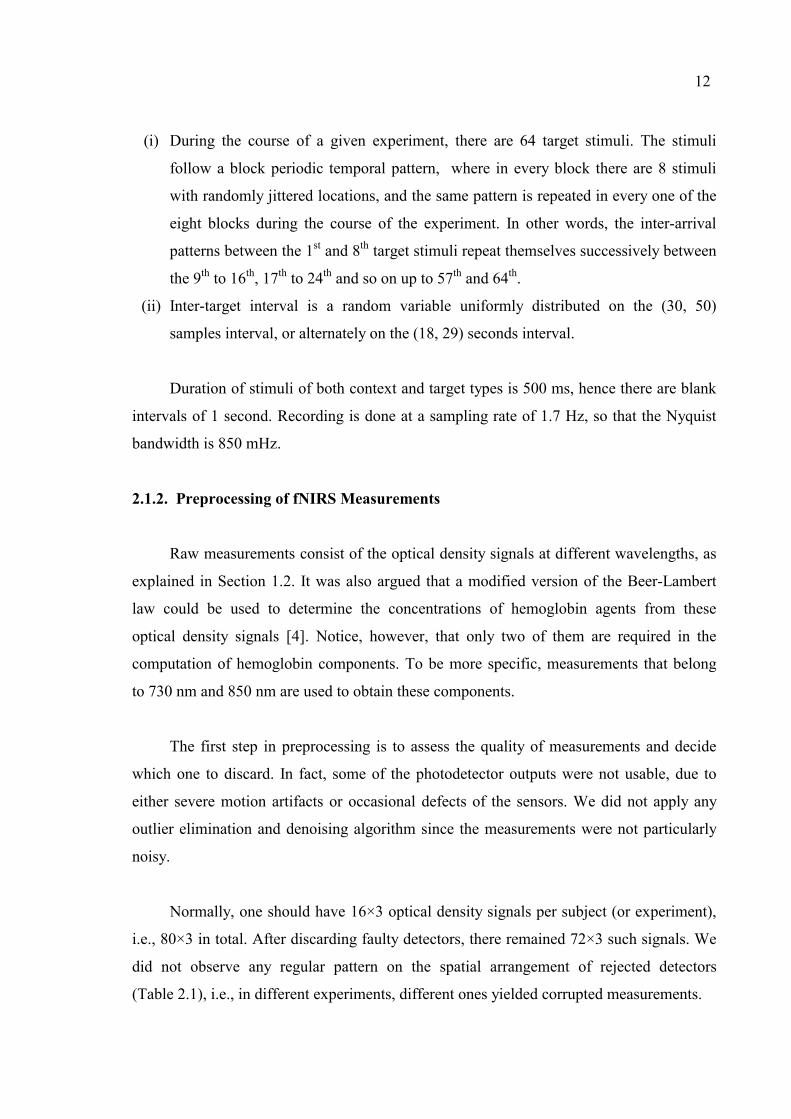
(i) During the course of a given experiment, there are 64 target stimuli. The stimuli

follow a block periodic temporal pattern, where in every block there are 8 stimuli

with randomly jittered locations, and the same pattern is repeated in every one of the

eight blocks during the course of the experiment. In other words, the inter-arrival

patterns between the 1st and 8th target stimuli repeat themselves successively between

the 9th to 16th, 17th to 24th and so on up to 57th and 64th.

(ii) Inter-target interval is a random variable uniformly distributed on the (30, 50)

samples interval, or alternately on the (18, 29) seconds interval.

Duration of stimuli of both context and target types is 500 ms, hence there are blank

intervals of 1 second. Recording is done at a sampling rate of 1.7 Hz, so that the Nyquist

bandwidth is 850 mHz.

2.1.2. Preprocessing of fNIRS Measurements

Raw measurements consist of the optical density signals at different wavelengths, as

explained in Section 1.2. It was also argued that a modified version of the Beer-Lambert

law could be used to determine the concentrations of hemoglobin agents from these

optical density signals [4]. Notice, however, that only two of them are required in the

computation of hemoglobin components. To be more specific, measurements that belong

to 730 nm and 850 nm are used to obtain these components.

The first step in preprocessing is to assess the quality of measurements and decide

which one to discard. In fact, some of the photodetector outputs were not usable, due to

either severe motion artifacts or occasional defects of the sensors. We did not apply any

outlier elimination and denoising algorithm since the measurements were not particularly

noisy.

Normally, one should have 16×3 optical density signals per subject (or experiment),

i.e., 80×3 in total. After discarding faulty detectors, there remained 72×3 such signals. We

did not observe any regular pattern on the spatial arrangement of rejected detectors

(Table 2.1), i.e., in different experiments, different ones yielded corrupted measurements.

13

Table 2.1. Indices of rejected photodetectors

Subject

Index Alias Indices of rejected photodetectors

1 AA005 9 2 GY002 1 to 4 3 KI003 1, 13 and 16 4 KP001 -none- 5 MJ007 -none-

A few comments are in order on the graphical depiction of primary signal sources

(optical density signals) and the secondary signal sources, that is, the physiological

components, such as HbR and HbO2. From Figure 2.2, one can see that the optical density

signals as well as hemoglobin component signals exhibit a very slow trend. These trends

have an antagonistic behaviour for HbR and HbO2, that is a rise in the HbR level

correspond to a fall in the HbO2. This observation is compatible with the brain

hemodynamics and already reported in [4]. Furthermore, this trend is actually a nuisance

quantity from the perspective of measuring cognitive activity and should be removed for

all practical purposes. The trend removal is performed by a simple moving average

filtering: a frame of support 500 samples (corresponding to 4.9 minutes of data) is slided

continuously over the time-series and the mean value of the samples inside the frame is

subtracted from the actual value at the frame position. Such a scheme effectively blocks

the slow signal (below 3 mHz) which is responsible of the trend (Figure 2.3). In summary,

preprocessing fNIRS time-series involves the following.

(i) Discarding signals from defective photodetectors (see Table 2.1.).

(ii) Computation of the hemoglobin component signals by applying the modified Beer-

Lambert law on the optical density signals that correspond to 730 nm and 850 nm

wavelength.

(iii) Trend removal by moving average filtering.

One might ask which hemoglobin component should be used for further analyses.

The study on simultaneous recordings of fMRI-BOLD and fNIRS [8] demonstrates that the

changes in oxygenated hemoglobin and the simultaneously acquired BOLD exhibit the

14

Figure 2.2. Optical density and hemoglobin component signals

Figure 2.3. Hemoglobin component signals with trend and after trend removal

15

strongest correlation compared with other components such as deoxygenated hemoglobin

and total hemoglobin. In this work, motivated by the fMRI studies, we consider henceforth

oxygenated hemoglobin, i.e., HbO2 signals.

2.2.3. Nomenclature of the Dataset

Each HbO2 signal in the data set can be refered by two indices: the subject index and

the index of the phodetector from which it is obtained. Denoting a HbO2 signal by s(t), the

following notation is adopted.

)(0

0ts j

k : HbO2 signal from subject j0, photodetector k0.

{ }fixed ,1 )( 000 jKkts j

kj ≤≤=Γ : All the signals from a given subject j0.

{ }fixed ,1 )( 000kJjts j

kk ≤≤=Γ : All the signals from a given photodetector k0.

{ } k

K

k

jJ

j

jk JjKkts Γ∪=Γ∪=≤≤≤≤=Γ

== 111 ,1 )( : All the signals in the dataset from

any photodetector or subject.

j = 1,..., j0 ,..., J (total number of subjects J is 5)

k = 1,..., k0 ,..., K (total number of photodetectors for a given subject K is 16)

Recall that some of the photodetectors are not usable (as tabulated in Table 2.1),

hence although the detector index runs from one to 16, we obviously skip over the

defective ones.

2.2. Statistical Characterization

This section deals with the statistical characterization of the fNIRS-HbO2 signals in

terms of stationarity and Gaussianity (see Appendix A, for details of the statistical tools).

2.2.1. Stationarity of fNIRS-HbO2 Signals

Stationarity of a process in the strict sense stands for the time-invariance of the nth

order joint probability distribution of the process samples. However, from a practical point

16

of view, it is usually very difficult and not necessary to prove strict-sense stationarity. A

common practice is to use a graphical depiction of the moving time-average estimates of

the central moments up to order four. The less pronounced are the time variations in these

moments, the more there is ad hoc evidence about the stationarity of the underlying

process. For instance, we say that the signal satisfies the wide-sense stationarity criteria,

whenever the mean and the variance do not change over time. Furthermore, if it is known

that the signal is from a Gaussian process, this implies strict-sense stationarity. Note that

hereafter stationarity will refer to wide-sense stationarity unless otherwise stated.

In the case the process cannot be proven to be stationary, one still would be

interested in the stationarity of the short-time signal segments. Short-time stationarity can

also be investigated with graphical techniques [21]. In Figure 2.4, variation of the central

moments up to order four are shown for a representative HbO2 signal. Accordingly,

N-sample segments are extracted from the signal with 75 per cent overlap and the

moments are computed. We choose two segment lengths, N = 200 and N = 400 samples,

corresponding, respectively, to two minutes and four minutes of data. Notice that, the

skewness τ is a measure of the symmetricity of the underlying distribution. For symmetric

distributions, such as the Gaussian, it vanishes. On the other hand, the kurtosis κ measures

the “tailedness” of the underlying distribution. For random samples with κ > 0, the

underlying distribution is heavy-tailed and said to be super-Gaussian; for those with κ < 0

the underlying distribution turns out to have flat tails and it is referred as sub-Gaussian. As

the context implies, Gaussian distribution is the limiting case and has zero kurtosis. The

time-average estimates of these moments, for an N-sample fNIRS-HbO2 segment with first

and last time indices t1 and t2 such that t2- t1+1 = N, can be computed as

(i) Mean ∑=

=2

1

)(1 t

ttts

Nµ

(ii) Variance [ ]∑=

−=2

1

22 )(1 t

ttts

Nµσ

(iii) Skewness [ ]∑=

−=2

1

33 )(1 t

ttts

Nµ

στ

17

(iv) Kurtosis1 [ ] 3)(1 2

1

44 −−= ∑

=

t

ttts

Nµ

σκ

It is known that an accurate estimation of skewness and kurtosis requires relatively

large number of samples, and they are also very sensitive to outliers. Furthermore, the

signal samples are not necessarily identically distributed, hence the estimates for skewness

and kurtosis kurtosis should be interpreted with caution.

From Figure 2.4, we see that the signal fails to be stationary in the long run, however

over short intervals there are intervals of stationarity in the wide sense. We notice these

quiet regions in the first 500 and last 1000 samples of the record, while in the central

regions all moments vary. These observations suggest that HbO2 signals are globally non-

stationary, but also would allow for short-time processing under the assumption of

stationarity.

Figure 2.4. Profiles of the statistics for a typical HbO2 signal up to fourth order

1 The expression stands actually for the normalized kurtosis and in statistical texts it is defined without the additive constant.

18

Table 2.2. Run test results for short-time HbO2 frames

(out of 3600 records, significance level α = 0.01)

Test statistic ξ

Frame length

N

Number of times the stationarity hypothesis

is retained Mean Std. Dev.

The range of ξ for the stationarity hypothesis

to be retained

400 1 39 28 177-224 200 19 22 16 84-117 100 82 14 9 39-62 50 326 9 6 17-34 30 793 7 4 9-22

We can show the non-stationary behaviour of the HbO2 signals more formally, using

statistical tests. The run test is a non-parametric, distribution-free test which is suitable for

this purpose [22], based on counting the number of sign reversals around the median of a

signal. This test compares a statistic ξ, which is one plus the number of sign reversals

around the median, against tabulated values and returns a binary answer on the stationarity

of the tested signal: either retain the stationarity hypothesis or reject it. For the sake of

generality, N-sample frames from each of the signals in the fNIRS-HbO2 dataset are

randomly selected. The number of frames per signal is set to 50, yielding 72×50 = 3600

records to test. The number of samples per frame N takes the values of 400, 200, 100, 50

and 30. In Table 2.2 is shown the number of frames marked as stationarity in the run test

for each selection of N. The significance level α of the tests is set to 0.01. Table 2.2 also

shows that HbO2 signals, definitely, are non-stationary unless short observation window is

chosen. The mean test statistic ξ (decimal parts are removed) becomes close to the

expected range only for small values of N (e.g. 30 and 50), hence for short-time analyses,

one can choose frame lengths in the order of 30 and 50 samples.

We observe in Figure 2.4, that skewness is not zero and that kurtosis is not directly

proportional to the variance. These imply that the fNIRS-HbO2 process is non-Gaussian. In

the next subsection, the non-Gaussianity of HbO2 signals is established by means of

rigorous statistical hypothesis testing.

19

2.2.2. Gaussianity Tests for fNIRS-HbO2 Signals

There are many simple yet powerful Gaussianity (or normality) tests in the statistics

literature [23]. They generally assume independent identically distributed (i.i.d.) samples,

hence they are not particularly suited for testing time-series for Gaussianity due to the

correlatedness of the signal samples. Under the milder condition of whiteness, that is, we

assume that samples are uncorrelated, but not independent, these tests can be used for

establishing the Gaussianity (or non-Gaussianity) of the time-series with lower statistical

accuracy. However, time-series are uncorrelated albeit neither. That is we cannot obtain

uncorrelated samples by sequentially sampling the signals. One idea to get over these

problems may be to sample the signals at random locations, instead of sequential sampling,

so that correlation between samples vanishes. In the sequel, the Kolmogorov-Smirnov (K-

S) test, and the Jarque-Bera (J-B) test are used following the above ideas [23, 24]. On the

other hand, Gaussianity tests dedicated for time-series data do exist, like Hinich’s

bispectrum based test [25]. However, this approach requires the signal to be stationary.

In what follows, the results of both the K-S test, the J-B test and the Hinich test are

presented. However, we first visit some graphical techniques in order to get more inside on

the shape of the underlying distribution.

A very useful graphical tool is the normal probability plot [26], where an empirical

cumulative distribution function (cdf) is plotted along with the theoretical Gaussian

(normal) cdf (see Figure 2.5). What is special with this graph is that the Gaussian cdf plots

linearly with a slope of one in the log-scale. The distance between the tick marks on the

ordinate axis matches the distance between the quantiles of a normal distribution. The

quantiles are close together near the median (probability of one half) and stretch out

symmetrically moving away from the median. Any deviation of the empirical cdf from

linearity is indicative of non-Gaussian behaviour. The top row in Figure 2.5 show test

cases of sample cdf’s of Gaussian and exponential distributions. We see that samples (blue

data points) from the exponential distribution deviates curvilinearly from the straight line

of Gaussian cdf in red. The bottom row of Figure 2.5 illustrates two cases of the sample

cdf plots of actual HbO2 data. In Figure 2.5 (c) we see a collection of samples that results

20

Figure 2.5. Normal plots for data from different distributions, vertical axes are read as

probability (in log-scale), horizontal axes as data

in a good fit to the normal line, whereas in Figure 2.5 (d) deviations from normality

(especially at the tails) are clear. The latter collection has indeed a positive kurtosis (≈

5.14), i.e., it’s heavy tailed. Note that both collections are obtained from the same HbO2

signal but at different random locations sufficiently distanced to guarantee

uncorrelatedness.

After this sample illustration, we need to test over a much large number of

collections, each of which should contain a large number of signal samples in its turn, and

then apply a combined test statistic in order to reject or retain the Gaussianity assumption.

In the following results, consider the signal sets jΓ , the ensemble of all the HbO2 signals,

that is recordings from all detectors, from subject j, j = 1,..., J with J = 5. As was given in

Table 2.1, the number of signals Kj differs from subject to subject. For each subject j, we

(a) (b)

(c) (d)

21

collect records of 500 samples at random, but pairwise distant locations. 500 samples are

enough for accurate estimates. We get 10Kj for Gaussianity test. Furthermore, we also test

the whole dataset Γ, which contains ∑=

=

5

110

J

jjK records, independently.

Tables 2.3 and 2.4 present the K-S and J-B tests for normality of HbO2 signal

samples respectively. Let’s briefly introduce the K-S and J-B tests (more details are given

in Appendix A). Let H0 stand for the Gaussianity hypothesis, and let the values ξks and ξjb

represent the test statistics used in the K-S and J-B tests. For testing a single record, the K-

S test proceeds as follows

If ξks > γks , accept H1: non-Gaussian

If ξks < γks , accept H0: Gaussian

where γks is set at a level such that the probability of falsely rejecting the Gaussian

hypothesis (false alarm probability) α is, say, 0.05. The value of α is said to be the

significance level of the test. Similarly, the J-B test can be formulated as

If ξjb > γjb , accept H1: non-Gaussian

If ξjb < γjb , accept H0: Gaussian

where γjb is set at a level such that the probability of falsely rejecting the Gaussian

hypothesis α is, say, 0.05. Equivalently, these two tests can be performed using computed

false alarm probability pks for K-S test and pjb for J-B test as described below.

If pks (or pjb) < α , accept H1: non-Gaussian

If pks (or pjb) > α , accept H0: Gaussian

In order to combine test results of individual records in the signal set jΓ , following

Fisher’s ideas [27], the combined test statistic P, for both K-S and J-B tests, can be

computed using

∑ −−=i

ipP 21log2 (2.1)

22

where pi denotes the computed false alarm probability of ith test (on the ith record) and the

summation runs up to the total number of records in the signal set. The combined test

statistic Pks (or Pjb) is a chi-square random variable with 2×(the number of individual tests)

degrees of freedom. The value of Pks (or Pjb) can be used to determine whether to reject or

accept H0, i.e., if the value of the chi-square cdf at Pks (or Pjb) is too high, accept H0; else

reject it (see Appendix A for more details on Fisher’s combined test). Based on the results

of Tables 2.3 and 2.4, we see that the J-B test has a more pronounced tendency to reject H0

than the K-S test. The number of cases the K-S test rejected H0 is less than the J-B test

does; consequently, the significance level achieved by the latter is much smaller than the

one achieved by the former for all the individual signal sets jΓ and the whole dataset Γ. In

conclusion, we can safely reject H0 hypothesis for fNIRS-HbO2 signals, since the

probability of rejecting H0 when it is indeed true is extremely low in general (except may

be for 2Γ where H0 can be accepted at significance level 0.05 since the combined test

yielded a significance of 0.02 for K-S test). In Table 2.4, we also show the mean and

standard deviations of sample estimates of skewness τ and of kurtosis κ. We note that the

underlying HbO2 distribution can be considered as symmetric (mean skewness is around

zero) with tails heavier than the Gaussian distribution (mean kurtosis is significantly

positive).

Finally, let’s turn to Hinich’s bispectrum based Gaussianity test which is applicable

for time-series. The test is based on the fact that signals from a Gaussian process have zero

bispectrum. Hence if we can compute a test statistic ξhin that measures how much sample

estimate of the signal bispectrum deviates from zero, we can establish whether the signal

comes from a Gaussian process or not. In Hinich’s test also, the test statistic ξhin is

accompanied with a computed probability phin of the risk in rejecting H0. As usual, if phin

exceeds α, one can deduce that it is risky to reject H0 and the Gaussianity of the signal is

retained. As described previously, false alarm probabilities phin can be used to compute the

combined test statistic Phin which will be effective for testing the Gaussianity of all the

records together. Note that in Hinich’s test, there is no need for random sampling since it is

purely designed for correlated time-series. However, stationarity of the records is

necessary, i.e., the size of the individual records should be small. Accordingly, we collect

50 records of 30 sequential samples from each signal. This yields jK50 cases to test for an

23

individual signal set jΓ , ∑=

=

5

150

J

jjK cases for the whole dataset Γ. The results are shown in

Table 2.5 (significance level α of the individual tests is set to 0.05 again).

Individual Hinich’s tests demonstrate that a majority of short-time fNIRS-HbO2

segments fail to come from a Gaussian process. In the overall, the Gaussianity assumption

is rejected with practically no risk. These results are compatible with those of K-S and J-B

tests. The unique but fundamental conclusion of this subsection is that fNIRS-HbO2 signals

are non-Gaussian.

Table 2.3. Results of Kolmogorov-Smirnov tests

Signal Set

1Γ 2Γ 3Γ 4Γ 5Γ Γ Number of

records 150 120 130 160 160 720

Number of times

H0 retained 72 99 81 84 33 398

Number of times

H0 rejected 78 21 49 76 127 322

Mean 0.08 0.05 0.06 0.06 0.10 0.07 ξks Std. Dev. 0.05 0.01 0.03 0.02 0.07 0.04

γks at α = 0.05 0.06 0.06 0.06 0.06 0.06 0.06

Pks 161.2 196.36 138.60 121.90 44.22 696.81

Result of the combined

tests (based on Pks)

Reject H0 at significance

10-11


0.02


10-10


10-25


10-79


10-67

24

Table 2.4. Results of Jarque-Bera tests

Signal Set


records 150 120 130 160 160 720

Number of times

H0 retained 44 43 20 24 4 143

Number of times

H0 rejected 106 77 110 136 156 577

Mean -0.14 0.14 0.06 -0.34 0.05 0.00 τ Std. Dev. 1.57 0.56 1.18 0.33 4.86 2.21

Mean 3.86 1.34 3.51 0.48 33.75 8.17 κ Std. Dev. 12.26 2.34 5.35 0.84 74.14 33.70

Mean 3578.60 176.00 952.51 37.59 137793.41 25111.52 ξjb Std. Dev. 17276.14 824.60 2581.39 50.67 407016.03 180234.45

γjb at α = 0.05 5.99 5.99 5.99 5.99 5.99 5.99

Pjb 86.00 75.81 38.75 35.79 4.78 253.96

Result of the combined tests (based on Pjb)


10-36


10-25


10-60


10-91


10-225


10-286

Table 2.5. Results of Hinich’s tests

Signal Set


records 750 600 650 800 800 3600

Number of times

H0 retained 236 238 297 468 359 1583

Number of times

H0 rejected 514 362 353 332 441 2017

Mean 0.15 0.19 0.25 0.26 0.23 0.22 phin

Std. Dev. 0.27 0.30 0.34 0.31 0.32 0.31

Phin 450.36 482.44 483.54 939.01 717.77 3008.51

Result of the combined tests (based on Phin)


10-165


10-83


10-103


10-43


10-88


0

25

3. TIME-FREQUENCY CHARACTERIZATION

In this chapter, we analyze the fNIRS-HbO2 signals in the time-frequency plane. We

think that several physiological events are measured by fNIRS and each of them is

associated with a particular frequency band of the HbO2 signal. Identification of such

bands can provide us with some general guidelines in distinguishing between the baseline

and cognitive activity.

Spectral analysis of physiological signals are important in that the oscillatory

dynamics in physiological systems are considered to reflect the degree of functionality.

Presence of such dynamics have been observed especially in the brain by neuroimaging

experts. Specifically, electroencephalogram (EEG) signals are analyzed by decomposing

them into several predetermined frequency bands corresponding to different physiological

activities [28]. As Başar and co-workers argue about the oscillatory dynamics in EEG:

“With respect to the brain, resonance is defined as the ability of brain networks to facilitate

(or activate) electrical transmission within determined frequency bands, when an external

sensory stimulation signal is applied to the brain” [29]. Efforts for characterizing the

components in signal spectra have usually aimed to provide a physiological

correspondence to the peaks or the energy bands. EEG literature is well developed in the

field of frequency analysis owing mostly to its early discovery dating back to 1900’s. On

the contrary, new comers in the field of neuroimaging such as fMRI, PET, transcranial

doppler sonography (TCDS) and fNIRS finally have still not received their share of

attention from the signal processing experts. Although several studies have proposed

association mechanisms between spectral ranges and physiological activities, there is no

consensus on the exact division of spectrum into bands of clinical importance.

Several researchers have decided to investigate the fMRI, PET and TCDS spectra in

search of bands that can elucidate the underlying physiological dynamics where specific

spectral peaks or bands are assumed to be related to a specific task [30]. The general view

is that while some of the oscillatory dynamics occur independent of the task and are

distributed over distinct spectral bands uncorrelated with other physiological activities (e.g.

breathing, heartbeat etc.), others can be directly affected by psychological or pathological

26

conditions (or vice versa) that exhibit themselves as a shift in performance [31]. A subset

of such studies investigate the coupling mechanisms between cerebral energy metabolism

and cerebrovascular dynamics (namely neurovascular coupling).

In this chapter, we first try to do an explorative study of the typical fNIRS-HbO2

spectrum. We then present an original frequency subband partitioning methodology. The

proposed subbanding scheme is general and can be applied to signals other than fNIRS-

HbO2. Finally, we prove that fNIRS measures cognitive activity, and that constitutes one of

the major contributions of this work.

3.1. The Typical fNIRS-HbO2 Spectrum

A time-frequency representation (TFR) of a non-stationary signal is especially useful

in visualizing the evolution of the spectral content through time. This can for instance be

achieved by the short time Fourier transform (STFT) or windowed Fourier transform

(WFT) as defined below

dtetwtsfS ftj πττ 2)()(),( −∞

∞−∫ −= (3.1)

where s(t) denotes the fNIRS signal of interest and wD(t) is a window of finite support D.

The STFT in (3.1) is actually computed using the discrete Fourier transform (DFT), so

that the TFR is discrete in both time and frequency, respectively, with time resolution ∆t

and frequency sampling interval ∆f. A TFR is warranted since the signals are non-

stationary and also because the aim is to capture and characterize local events, like

cognitive activity in the course of the fNIRS process. The windowing wD(t) guarantees the

local nature of the spectral analysis and its support is chosen so that within that D interval

the process can be considered to be at least wide-sense stationary. To control spectral

leakage and peak resolution, the window shape should be judiciously chosen [32]. Table

3.1 gives the parameters used in the TFR analysis. One should see that the frequency

resolution is given by the effective window length, hence it is of the order of 50 mHz,

while the one mHz frequency sampling rate ∆f is obtained by padding the windowed time

series with zeroes.

27

Table 3.1. Parameters of the TFR (sampling rate Fs=1700 mHz)

Parameter

Value Comment

Window type Hamming

Hamming window has good sidelobe suppression.

Window length D 36 samples ≈ 21 s

An interval of such length can be considered as “stationary”.

Time resolution ∆t 9 samples ≈ 5.3 s

This guarantees at least four samples per chosen window length, which provides adequate temporal resolution.

Frequency sampling ∆f 1 mHz

This is set in order to have sufficient number of samples in the bands as narrow as 10 mHz.

A 3D-graph or the contours of the TFR of a time-series alone would provide us some

qualitative information about the spectral content. Figures 3.1 (a) and (b) consist of such

graphs obtained from a fNIRS-HbO2 signal. Observing these, one may conclude that the

time-series is essentially low-pass (main spectral content<100 mHz), that no significant

events at all in the range of 200-700 mHz exist and there is some activity pattern between

700-850 mHz. Hence without objective measures, inferences we can make from a TFR

remain limited. The TFR should further be exploited by deriving some quantifiable

magnitudes as Blanco et al. suggested [28]. The relative power profile per band is such an

objective measure and will be defined next. Let’s consider a set of frequency intervals

),( ,, hnln ff , n = 1,..., N that partitions the frequency axis into subbands, which are not

necessarily equal. Then the evolutionary power spectral density within the nth frequency

band at the instant t is defined as

),(),(),( ftSftSftBn∗= in ),( ,, hnln fff ∈ (3.2)

where fn,l and fn,h denote, respectively, the lower and upper limits of the band. The

total power in the respective band as a function of time can now be calculated by

28

Figure 3.1. 3D normalized intensity graph (top) and intensity level diagram for the TFR of

a typical fNIRS-HbO2 signal (bottom)

29

∫=hn

ln

f

fnn dfftBtI

,

,

),()( (3.3)

Similarly the total instantaneous power in the whole frequency spectrum I(t) is

defined as

∫=Nyquistf

n dfftBtI0

),()( (3.4)

where, in our case, the integration goes from 0 to 850 mHz. Finally, the relative power

profile in the nth band as a function of time becomes

)()()(

tItItR n

n = (3.5)

The relative power profile per band reflects the temporal evolution of the relative

power in each band. It can be conjectured that the dissimilarity in the evolution of the

relative power profiles is indicative of the relevance or redundancy of the bands. More

explicitly, two bands are considered similar if their Rn(t) responses are close to each other;

conversely, dissimilar bands that have different time evolution of the power profile, Rn(t)

are considered to provide different information. In the following section, the relative power

profile will be used as a feature in the systematic partitioning of fNIRS-HbO2 spectrum

into non-overlapping subbands.

3.2. Selection of Relevant Frequency Bands

Starting with a fine partitioning of the frequency spectrum, one can group narrow

bands similar in their evolutionary energy profiles, Rn(t), into wider bands that hopefully

capture significant signal information. In what follows, let’s consider an initial partitioning

of the frequency spectrum into 25 narrow bands of width 10 mHz and a wide high

frequency band covering the 250-850 mHz range, 26 bands in total. All higher frequency

bands are lumped into one 250-850 band as there is very little power in this frequency

30

range and the signals lacked a definitive structure. In fact, this wide band contains only

nine per cent of the total average power.

Since there are many relative power time-series from different bands and

detectors/subjects, the following notation is adopted

)(tRmn : time-series of the relative power for the nth band of the mth fNIRS signal

Thus the subscript n denotes the frequency band of interest, where n=1,...,N=26. For

251 ≤≤ n , the nth band covers the frequency range [(n-1)×10, n×10)] mHz, while for

n=26, the band covers the 250-850 mHz range. On the other hand, the superscript m points

to one of the m = 1,…, M=72 time series in the dataset Γ, note that ∑=

=

=5

1

J

jjKM . Recall that

these time series were obtained from the 16 detectors of the five subjects, after some

pruning (see Table 2.1). Thus the superscript m refers simply to the mth measurement. The

time index t runs with the lags of ∆t = 9 samples, t = 1,..., T. It will be convenient to

express the whole time series TttR mn ,...,1 ),( = in vector notation as m

nR . The T-

dimensional mnR vector denotes the time series of the mth detector/subject in the nth

frequency band. Notice that we have a total of N×M = 26×72 such mnR vectors, each

detector being expanded onto 26 bands, and conversely, there are 72 representative time

series for each band.

We practically search for the formation of the informative bands by a clustering

procedure. In fact, a scheme based on agglomerative clustering2 followed by majority

voting can be used as described below. After obtaining the N relative power profiles per

band of each measurement m, the set of N subbands Rm={ } Nnmn ,...,1 =R are grouped into C

subbands Qm={ } CcmcQ ,...,1 = . Specifically the 26 initially chosen subbands from any

detector/subject are clustered into C = 3 subbands. This target number of clusters is

decided for in order to allow a possibly very low frequency band, a high frequency band

and potentially a single “interesting” mid-band.

2 For a brief summary of clustering and agglomerative approaches in particular, see Appendix B.

31

There are two important aspects in an agglomerative clustering algorithm: the metric

used to compute distances and the closeness criterion between vectors. Here the following

are adopted

(i) One-minus-the-normalized correlation coefficient as the distance metric:

mq

mp

mq

mpm

qmpd

RRRR

RR.,

1),(⟩⟨

−= (3.6)

where ⟩⟨.,. stands for the inner product of two vectors and . for the Euclidean

norm. The vectors involved in the computation are made zero-mean by subtracting

their mean value.

(ii) Single linkage criterion as the closeness criterion, according to which the pair of

bands (p,q) for which ),( mq

mpd RR is minimum should be merged.

The end product of clustering the Rm set is a dendrogram Dm, an hierarchical tree that

helps us to visualize cluster relationships. An example is shown in Figure 3.2. The

dendrogram for the mth measurement Dm is pruned in order to get the clustered set Qm. This

is accomplished by simply obtaining the cutset of the dendrogram that yields the target

number of C clusters. In other words, the dendrogram is cut at a distance value of the

ordinate to yield the desired number of clusters, e.g., at 0.15 as shown in Figure 3.2.

Within each one of the C clusters, the merged bands are similar to each other according to

the chosen correlation coefficient metric, while across clusters they are dissimilar. The

leaves of the dendrogram, that is the singleton clusters, which correspond to the initial

bands, become thus grouped into C = 3 larger bands. Once the agglomerative clustering is

accomplished we obtain M dendrograms, one for each measurement. To extract a single set

of subbands from the M clusters, a voting scheme is resorted to. At this stage there are in

the overall M×C = 72×3 = 216 frequency bands with differing bandwidths, out of which

we try to determine the most frequently occurring ones. Therefore these 216 band patterns

should be ranked based on their frequency of occurrence. To make this point clear, let’s

consider again the sample dendrogram in Figure 3.2, which results in the following

subbands: {0-30, 30-40, 40-850}. We determine how many times each of these subband

formations were generated by clustering of all the Rm measurements, each occurrence

32

Figure 3.2. A typical dendrogram: the horizontal axis indexes the initial bands, vertical

axis indicates pairwise cluster distances.

counting as a vote. Selecting the subband patterns that have received the highest number of

votes (frequency of occurrence), we achieve a “canonical” partitioning of fNIRS frequency

spectrum, where the resulting bands are non-overlapping and exhaustively cover the

frequency interval 0-850 mHz.

As a result of band clustering and voting, nine candidate bands that shared 216 votes

are obtained as shown in Table 3.2. A couple of partitionings that collectively covers the

spectrum is possible (see Table 3.3). The spectrum partitioning that gets the highest

number of votes happen to be the following sequence of bands: 0-30 mHz, 30-40 mHz, 40-

250 mHz and 250-850 mHz. They receive in all 142 votes, i.e. 65.7 per cent of the total.

We hence can argue that this partitioning is reliable in characterizing the fNIRS spectrum

in terms of energy percentage profiles. Hereafter we call them as “canonical frequency

bands” and denote them by letters as shown in Table 3.4.

33

Table 3.2. Candidate frequency bands (out of 216 cases)

Bands (mHz) Number of votes

250-850 44 0-30 35 0-40 35

40-250 35 30-40 28

40-850 28 30-250 7

0-50 2 50-250 2

Table 3.3. Possible spectrum partitionings and their significances

Spectrum partitioning Votes Percentage

0-30 mHz, 30-40 mHz, 40-250 mHz, 250-850 mHz 142 65.7 % 0-40 mHz, 40-250 mHz, 250-850 mHz 114 52.8 % 0-30 mHz, 30-250 mHz, 250-850 mHz 86 39.8 %

0-40 mHz, 40-850 mHz 63 29.2 % 0-50 mHz, 50-250 mHz, 250-850 mHz 48 22.2 %

Table 3.4. Canonical frequency bands of fNIRS signals

Physiological interpretation of the canonical bands: In several studies, three main

frequency bands of interest have been identified for cerebral hemodynamics: a very low

frequency (VLF, 8-33 mHz), a low frequency (LF, 100 mHz) and a high frequency

component (HF, 250 mHz) definitely in synchrony with breathing rate [33]. Similarly, it

can be conjectured that each of the canonical bands is associated to one or more of the

physiological activities that are assessed by hemoglobin concentrations. The very-low

frequency band, namely the A-band, is responsible for the slow signal or the baseline signal

that is thought to be reflecting the very slow vasomotor fluctuations. In fact, reports on the

frequency content of such fluctuations have identified this signal as being the phasic

dilation and contractions of the small regulating arteries. According to Kuo et al. “these

Bands

(mHz)

0 -30

A

30-40

B

40-250

C

250-850 >>

D

Votes 35 28 35 44

34

vasomotor waves produce fluctuations in cerebral blood volume, which are eventually

reflected in the intracranial pressure” [33]. As a matter of fact, it can be thought that this

band is independent of the stimulated cognitive activity. Based on the observation that

typical brain hemodynamic response model functions, e.g. the centered Gamma function

(Figure 3.3), exhibit significant spectral activity in the 30-50 mHz range, the very narrow

B-band should be related to task-related cognitive activity of the subject. The larger C-band

is also assumed to carry cognitive activity related information, most probably due to the

periodicity of the target stimuli sequence. Moreover, vasomotion and breathing rate are

two physiological facts that are responsible for the emerging of the C-band. Finally, the

high frequency D-band reflects some weak high frequency fluctuations and confines the

aliased part of the heart rate signal (~1.1 Hz).

Figure 3.3. The centered Gamma function (left) and its Fourier spectrum magnitude

(right), note that high frequency lobes are due to removing the DC-value of the signal

Although the canonical bands are dissimilar in terms of the chosen metric, there

certainly remain some residual correlations. Hence, a quantification of the similarities

between relative power profiles at these bands would be instructive. In order to track this

purpose, the following is evaluated

∑=

=

⟩⟨=

72

1 .,1 M

mmq

mp

mq

mp

pq M RRRR

ρ (3.7)

35

where { }DCBAqp ,,,, ∈ and mqR is as defined previously, again the vectors in the

computation of the inner-product are made zero-mean. The averaged normalized

correlation coefficients pqρ take the values given in the matrix form below

[ ]

−−−−

−−−−

=

129.054.051.029.0145.094.054.045.0150.051.094.050.01

DCBA

DCBA

pqρ .

We can observe that there exists is a strong negative correlation (correlation

coefficient of minus 0.94) between the A-band and C-band in terms of their relative power

profiles. In other words an accumulation of power in one band (say A) causes a depletion

of the power in the other band (D), and vice versa. One can envision the time series )(tRmA

and )(tRmC being almost “antipodal” signals.

3.3. Evidence of Cognitive Activity in fNIRS-HbO2 Signals

Since the cognitive stimuli are quasi-periodic, with inter-target intervals uniformly

distributed between 18-29 seconds, we can expect some sort of periodic behavior in the

signal portions that are related to cognitive activity. The frequency bands where more

distinctly such periodic response emerges can be said to better reflect cognitive activity or

the “brain hemodynamic response”. Recall that the brain displays continuous activity

patterns even in the absence of any cognitive task. The cognitive activity waveforms, if

any, will be in general immersed in some baseline activity waveforms. In fact, experiments

show that cognitive activity responses are very difficult to discern by observing the

waveforms in the full-band signals. It follows that classical Fourier spectrum and peak

picking techniques are not suitable for hunting these responses and more sophisticated

statistical methods must be invoked to detect and estimate these hidden periodicities.

Thus we turn now to the time-domain signals corresponding to the fNIRS canonical

bands, and investigate the time series in the bands { }DCBA ,,, for the existence of a

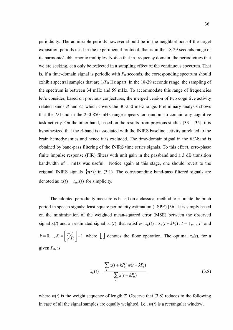
36

periodicity. The admissible periods however should be in the neighborhood of the target

exposition periods used in the experimental protocol, that is in the 18-29 seconds range or

its harmonic/subharmonic multiples. Notice that in frequency domain, the periodicities that

we are seeking, can only be reflected in a sampling effect of the continuous spectrum. That

is, if a time-domain signal is periodic with P0 seconds, the corresponding spectrum should

exhibit spectral samples that are 1/P0 Hz apart. In the 18-29 seconds range, the sampling of

the spectrum is between 34 mHz and 59 mHz. To accommodate this range of frequencies

let’s consider, based on previous conjectures, the merged version of two cognitive activity

related bands B and C, which covers the 30-250 mHz range. Preliminary analysis shows

that the D-band in the 250-850 mHz range appears too random to contain any cognitive

task activity. On the other hand, based on the results from previous studies [33]- [35], it is

hypothesized that the A-band is associated with the fNIRS baseline activity unrelated to the

brain hemodynamics and hence it is excluded. The time-domain signal in the BC-band is

obtained by band-pass filtering of the fNIRS time series signals. To this effect, zero-phase

finite impulse response (FIR) filters with unit gain in the passband and a 3 dB transition

bandwidth of 1 mHz was useful. Notice again at this stage, one should revert to the

original fNIRS signals { })(ts in (3.1). The corresponding band-pass filtered signals are

denoted as )()( tstx BC= for simplicity.

The adopted periodicity measure is based on a classical method to estimate the pitch

period in speech signals: least-square periodicity estimation (LSPE) [36]. It is simply based

on the minimization of the weighted mean-squared error (MSE) between the observed

signal x(t) and an estimated signal )(0 tx that satisfies )()( 000 kPtxtx += , t = 1,..., T and

1 ,...,00−

== PTKk where ⋅ denotes the floor operation. The optimal x0(t), for a

given P0, is

∑∑

+

++=

k

k

kPtx

kPtwkPtxtx

)(

)()()(

0

00

0 (3.8)

where w(t) is the weight sequence of length T. Observe that (3.8) reduces to the following

in case of all the signal samples are equally weighted, i.e., w(t) is a rectangular window,

37

∑ +=k

kPtxK

tx )(1)( 00 (3.9)

It has been argued that the weight sequence should be selected so that it gets the

maximum value of unity at the center of its support and so that it decays smoothly down to

zero towards the extremes since the periodicity deviates more heavily at the extremes than

at the center. It has originally been shown that P0 that minimizes the weighted MSE is

equivalently the one that maximizes

EIPJ 0

00 )( = (3.10)

where I0 stands for the weighted energy of the estimate x0(t) and E for the weighted energy

of the original signal x(t). The unbiased version of (3.10) yields the J1-index, which is

expressed as

1

1001 )(

IEIIPJ

−−= (3.11)

where ∑∑ +=

tk

kPtwtwtxPI

)()()()(0

22

01 . Note that the LSPE with J1-index is also called as the

pseudo-maximum likelihood estimation of periodicities [36].

Using (3.11), one should for look for the value of 0P̂ that maximizes the )( 01 PJ

functional and this value is taken as the dominant period in the signal provided the

periodicity index )( 01 PJ is sufficiently high. In fact, the index function can be interpreted

as a confidence score that becomes one for a truly periodic signal. Since some maximizing

value of 0P̂ can always be found, for this estimate to correspond to a genuine periodicity,

the confidence score should exceed a threshold. In the case of fNIRS-HbO2, the allowed

range of 0P̂ is between Pmin and Pmax, as infered from the experimental protocol, in which

38

Figure 3.4. (a) Simulated quasi-periodic sequence of cognitive activity waveforms; (b)

White noise sequence (SNR = 10 dB); (c) An actual A-band signal; (d) Superposition of

the signals (a), (b) and (c); (e) Band-pass filtered version of (d) in the BC-band

J1( 0P̂ ) values are computed. Let’s note that, since the cognitive stimuli are not exactly

periodic and since furthermore the cognitive activity signals are heavily embedded in

baseline signals, we should not expect the J1( 0P̂ ) scores to be too high, and hence heavy

thresholding should be avoided. Furthermore, cognitive activity is not expected to be fired

just after the target onset, that is, variable amounts of delay may obscure periodicities, if

any, of the cognitive activity waveforms. In order to illustrate the viability of the LSPE

algorithm, we may resort to a simulated data sequence, as shown in Figure 3.4, that

consists of the superposition of a hypothetical cognitive activity waveform train embedded

in white noise (so that the signal-to-noise ratio is 10 dB) with an actual signal from A-band.

The cognitive activity waveform is modeled as the centered Gamma function which is

frequently used in fMRI data analysis [10]. The average periodicity of cognitive activity

39

waveforms is set to 40 samples with a random jitter between (-10,10) samples in order to

simulate the experimental protocol.

Two cases can be considered prior to the application of the LSPE. In the first case,

unfiltered HbO2 signal (e.g. signal (d) in Figure 3.4) is input to the algorithm; in the

second case, in order illustrate the justifiability of prefiltering in the BC-band, the

prefiltered version takes the role of input (e.g. signal (e) in Figure 3.4). The periodicity

index profiles within the (20,60) samples range with and without filtering the synthesized

signal, are shown in Figure 3.5. In both cases, the LSPE estimate coincides with the

jittered theoretical periodicity of 40 samples, a fact that illustrates the ability of LSPE in

tracking jittered periodicities in presence of noise and even additive interference. Using the

prior knowledge that the A-band does not contain pitch-period like periodicity information,

we can get much higher index (or confidence) values by prefiltering the signal in the

approptiate band which is the BC-band.

Figure 3.5 Periodicity index profiles for simulated data without prefiltering (solid line) and

with prefiltering (dotted line), after local maxima selection and thresholding

On the other hand, the situation with real data is exemplified with two cases as

shown in Figure 3.6. In the first case, prefiltering results in a slight increase in the J1-index

value without considerably affecting the value of the detected perodicity (see Figure 3.6

(a), the second plot below is obtained after local maxima selection and thresholding). In the

second case where without prefiltering no periodicity can be detected with a high

confidence, we observe that a periodicity value, with a much better confidence, emerges

within the expected range (see Figure 3.6 (b)).

40

Figure 3.6. (a) Periodicity index profiles of a fNIRS-HbO2 signal with (dotted line) and

without (solid line) prefiltering

Figure 3.6. (continued) (b) Periodicity index profiles of another fNIRS-HbO2 signal with

(dotted line) and without (solid line) prefiltering

41

In order to process the real fNIRS-HbO2 data, it would be wise to proceed as follows.

Since the experimental protocol consists of eight identical sessions in succession, the LSPE

algorithm can be run session by session, by considering each of the eight time segments of

the signal x(t), t = 1,..., T separately. Let’s denote each session by the superscript

l = 1,…, 8 so that { })(tx l stands for the lth experimental segment of the 30-250 mHz band-

pass filtered fNIRS signal from some subject/detector. The session-wise processing of the

fNIRS signals helps also to mitigate the non-stationarity. In fact, one can view the signal

portions in different sessions as independent realizations of the target-categorization

experiment. We now summarize the steps involved in looking for periodicities of HbO2

signals below.

(i) The periodicity range in which we look for periodicities is (20, 60) samples.

(ii) We look for local maxima of the )ˆ( 01 PJ function, where once a peak is found no

further peak is searched within a neighborhood of (-3, 3) samples.

(iii) We set a threshold of 0.1 on the periodicity belief value )ˆ( 01 PJ .

(iv) For each signal portion, we let the algorithm return the periodicity estimate with the

largest J1-index.

Those 0̂P values that fall within the (30, 50) samples interval are thought to belong

to the single-trial cognitive activity sequence in the experiment. Those falling outside are

considered as fortuitous values, indicative of the fact that detector is not capturing properly

any cognitive activity signal. Since there are 8 time segments )(tx l per detector, each

)(tx signal returns eight period estimates, 8 ,...,1 ,ˆ0 =lP l along with their confidence

scores. Accumulating separately the scores of the periodicities falling, respectively, inside

and outside the expected range, the cumulative score of inside periodicities Sin and the

count of inside periodicities Cin for a given detector and subject can be defined as

∑=

=8

1001 )ˆ()ˆ(

l

llin PPJS δ (3.12)

42

∑=

=8

10 )ˆ(

l

lin PC δ (3.13)

with

=range expected theoutside is ˆ if0

range expected theinside is ˆ if1)ˆ(0

00 l

ll

PPPδ (3.14)

where l=1,…,8 is the session index. Corresponding expressions for the outside

periodicities Sout and Cout are defined similarly. Furthermore, in order to investigate inter-

subject and inter-detector variations of periodicities, two additional quantities are

computed: periodicities falling in the proper range averaged over all subjects for a given

photodetector, denoted as )(kPsubjects , k = 1,…, 16 and inside periodicity averaged over all

photodetectors for a given subject, denoted as )(d jP etectors , j = 1,…, 5. The error bar plots

corresponding to these two quantities, )(kPsubjects , k = 1,…, 16 and )(d jP etectors , j = 1,…, 5

are displayed in Figures 3.7 and 3.8. The bar plots of the scores Sin and Sout, and the scatter

plots of the inside and outside periodicities with respect to the photodetector number for

different subjects are shown in Figures 3.9-3.13. Several conclusions can be drawn from

these results.

(i) The averaged estimated periodicity values match the expected value of P0 = 40,

whether the average is computed over detectors or subjects, as illustrated in Figures

3.7-3.8.

(ii) For any detector or subject there is significant dispersion of estimated periodicity

values. The large spread, of the order of 10 per cent in each sense, may be due to the

jitter of target instances, to the presence of remaining baseline activity, and to the

limited observation interval containing at most eight target stimuli.

(iii) The above described method can be used to classify detectors (or optodes) as

responsive of cognitive activity periodicity and the non-responsive ones, that is,

those detectors that do not show any evidence of periodicity within the expected

range. The discrimination method is based on the not-in-the-range periodicity score

Sout, as illustrated in Figures 3.9-3.13. The reason why some detectors do not yield

conjectured periodicity can be due to the lateralization effect for that subject or

simply corrupted measurements. One argument that support lateralization conjecture

43

is that groups of adjacent detectors all succeed or fail. For example, for Subject 1,

detectors 3-12 are “good” (detector 9 was not working though), while detectors 1-2

and 13-15 are “bad” (see Table 3.5 where the indices of responsive photodetectors

are shown). One other reason could be due to the location of the optodes with respect

to the light sources. Since the source-detector distribution determines the volume of

brain being sampled, millimeter range shifts and alignments in the probe will result

in a significant change in the brain volume being monitored. Finally, the corruption

observed could be due to the skin effects (larger arteries on the skin surface right

underneath the optode) dominating the signal.

(iv) There are also marked differences between subjects. For example, Subjects 1, 3 and

4 (especially Subject 4) yields high periodicity scores consistent across all of his/her

detectors, while Subjects 2 and 5 are dubious (see Figures 3.9-3.13). Although inter-

subject variation is always expected in such studies, there is no standard procedure to

isolate corrupted data from statistical analysis for fNIRS signals. The periodicity

analysis method provided in this work might be used as a rule of thumb in

identifying the corrupted data or the patient that is not cooperating.

The results of the previous subsection together with those of the current one are

significant in two aspects. First, the bands of interest in fNIRS-HbO2 are observed to be

localized in the lower part of the spectrum (<250 mHz). The selected canonical bands have

a considerable frequency of occurrence hence they are reliable in time-frequency

characterization. Second, periodicity detection experiments have exposed that fNIRS

indeed measures cognitive activity and prefiltering in the BC-band is exceptionally useful.

Furthermore, the proposed scheme would be useful in assessing the quality of the

measurements.

Table 3.5. Responsive photodetectors such that Sin > Sout

Subject Photodetector quadruples

Index Alias left (1-4)

mid-left (5-8)

mid-right (9-12)

right (13-16)

1 AA005 3 and 4 5 to 8 (all) 10, 11 and 12 16 2 GY002 -not any- 8 9,11 and 12 13 to 16 (all) 3 KI003 4 5 to 8 (all) 9 to 12 (all) 15 and 16 4 KP001 1 to 4 (all) 5 to 8 (all) 9, 11 and 12 13 to 16 (all) 5 MJ007 1 to 4 (all) 5 and 7 9, 11 and 12 13 to 16 (all)

44

Figure 3.7. Plot of )(kPsubjects with inter-quartile range bars at data points

Figure 3.8. Plot of )(d jP etectors with inter-quartile range bars at data points

Perio

dici

ty (s

ampl

es)

Periodicity (averaged over subjects) vs. Photodetectors

Photodetector index

Periodicity (averaged over detectors) vs. Subjects

Perio

dici

ty (s

ampl

es)

Subject index

45

Figure 3.9. Error bar plots of scores vs. detectors with std. dev. bars at data points (top),

scatter plots of periodicities vs. detectors (bottom) for Subject 1

46



47



48



49



50

4. FUNCTIONAL ACTIVITY ESTIMATION

The purpose of this chapter is to introduce and discuss algorithms for the extraction

of waveforms associated with cognitive activity. We consider short-time fNIRS segments

(of length m), which consist of the m samples right after the subjects are presented with the

target stimuli. We adopt the following notation.

i = 1, .., I=64 (total number of targets per experiment I is 64)

j = 1,..., j0 ,..., J=5 (total number of subjects J is 5)

k = 1,..., k0 ,..., K=16 (total number of photodetectors for a given subject K is 16)

x : A generic m-dimensional data vector that consists of sequential HbO2 samples.

X : A generic dataset that consists of multiple realizations of x.

)(0

0ij

kx : A HbO2 vector from the signal )(0

0ts j

k , target location i.

{ } fixed fixed, ,1 )( 000

0

0

0kjIiiX j

kj

k ≤≤= x : All the vectors from signal )(0

0ts j

k .

{ }fixed ,1 ,1 )( 000 jKkIiiX j

kj ≤≤≤≤= x : All the vectors from 0jΓ .

{ }fixed ,1 ,1 )( 000kJjIiiX j

kk ≤≤≤≤= x : All the vectors from 0kΓ .

004

1

jkk

jleft XX

=∪= : All the vectors from left photodetectors of subject j0.

008

5

jkk

jleftmid XX

=− ∪= : All the vectors from mid-left photodetectors of subject j0.

0012

9

jkk

jrightmid XX

=− ∪= : All the vectors from mid-right photodetectors of subject j0.

0016

13

jkk

jright XX

=∪= : All the vectors from right photodetectors of subject j0.

Recall for some values of the index k, the corresponding signal is omitted due to the

fact that the measurement is corrupted.

51

It was noted before that the fNIRS signals exhibit properties similar to fMRI-BOLD

signals recorded during functional brain activation, since both modalities measure,

although in different ways, hemoglobin agents. It is also assumed that a typical fNIRS

segment includes the following.

(i) Cognitive activity related component: “brain hemodynamic response”

(ii) Baseline physiological component

(iii) Higher frequency components

(iv) Noise, movement artifacts

We use independent component analysis (ICA) and clustering as exploratory tools to

find out “interesting” waveforms in a generic dataset X [37, 38]. The former decomposes a

signal into statistically independent components whereas the latter searches for most

commonly occuring “interesting” waveforms (some of which can be associated with

cognitive activity), in a multidimensional feature space. In Sections 4.1 and 4.2, both

approaches are described in the fNIRS-HbO2 setting. In Section 4.3, we introduce the

preliminaries concerning the experiments. In Sections 4.4 and 4.5, we present the results of

ICA and clustering experiments, respectively. The final section discusses the evaluation

and comparison of these investigations.

4.1. Independent Component Analysis Approach

Independent component analysis (ICA) can be interpreted as finding a suitable basis

for multivariate data (for a brief summary of independent component analysis, see

Appendix C). Accordingly, ICA is similar to principal component analysis (PCA) where

the basis vectors are ranked in terms of the data variance they account for. In contrast, ICA

uses higher order statistical information to find a suitable basis in such a way to maximize

statistical independence between projections onto different basis vectors. In formal terms,

let x be an m-dimensional random observation vector, we then want to find a linear

transformation A so that

Asx = (4.1)

52

where the components si and sj (of the transformed vector s) are statistically “as

independent as possible”, mnjinjni ≤≠== and that so ,...,1 ; ,...,1 . The matrix A is the

so-called m×n mixing matrix and the n-dimensional vector s is the vector of independent

components. We are only given a multivariate dataset { } ,...,1 )( IiiX == x that consists

of I realizations of the random vector x. The columns of the matrix A are said to form an

ICA basis that is suitable for representing the observations in the sense explained above.

Let’s rewrite (4.1) in the following form

nn

n

n sss

s

ss

aaaaaax +++=

= 2211

2

1

21 (4.2)

Thus, the data vector x is decomposed as a linear combination of the columns of A,

where the weights si are the independent components. From this perspective, ICA can be

very useful in discovering the underlying nature of many physical phenomena, where

observations result from combinations of unrelated or independent activities. However,

there are two ambiguities in ICA, which may be annoying for some applications [37]. First,

ICA does not provide a natural ordering of the independent components or equivalently of

the basis vectors. This is in contrast to PCA where the basis vectors are ordered as a

function of data variance they explain. Second, independent components can be estimated

up to the sign, that is, we should also consider the negative versions of the estimated

components.

It is reasonable to assume, much as in the fMRI studies, that the components (i)-(iv)

of fNIRS cited above are mutually independent and that they are linearly combined. This

makes the problem suitable for ICA. Accordingly, the basis vectors estimated by ICA will

correspond to one or more of the above components. Since observations consist of short-

time segments sampled just after the target onsets, it is highly likely that one can estimate a

cognitive activity related waveform or the “brain hemodynamic response” in one of the

columns of the mixing matrix A. The FastICA3 algorithm is used for that purpose. As a

3 See Appendix C.

53

common practice, dimensionality is reduced from m to n by PCA, then the observation

vectors with reduced dimensions are whitened, and finally the basis that is spanned by the

columns of A is estimated by maximizing an objective function that “measures”

independence. In addition, we remove the ambiguity in the estimated basis vectors, by

using a brain hemodynamic response model, traditionally adopted in fMRI analyses, such

as the Gamma function.

4.2. Clustering Approach

Another exploratory tool for discovering interesting waveforms related to cognitive

activity is clustering the fNIRS signal segments. Clustering4 is the generic name for the

methods that help us to partition a multidimensional dataset into a set of clusters

Q { } ,...,1 , CcQ cc == q where cq is the centroid of the cluster Qc. That is, each

observation in the dataset is assigned to one of the clusters Qc represented by its centroid

cq . In this way, we are able to label the observations and furthermore summarize the data

variabilities in terms of cluster centroids.

The fNIRS segments, sampled just after the target presentation, can be clustered to

find out typical waveforms that reflect the cognitive activity. To this purpose, we may use

the original fNIRS-HbO2 segments x directly as input to a clustering algorithm or we may

first extract some features. The feature extraction may help in removing noise and

redundancy from the raw data. For example, the B-spline approximation is useful in

putting into evidence the functional nature of the data and in eliminating irrelevant high-

frequency fluctuations, noise and artifacts [39]. B-spline approximation is also known to

have superb summarizing property for the waveforms by just using a few coefficients.

With these ideas in mind, for all the vectors )(ix of dimensionality m in a given dataset X,

the corresponding B-spline approximation coefficients )(iy of dimensionality mn ≤ are

computed. Afterwards, the B-spline feature set { } 1 )( IiiY ≤≤= y is input to the

clustering algorithm in order to learn the set of clusters Q. Here again, an agglomerative

clustering approach is adopted, in other words, we start with a set of clusters where each

)(iy is a singleton cluster, and then group them step by step as described in Appendix B. 4 See Appendix B.

54

For the distance metric, we consider the one-minus-the-normalized correlation coefficient

which is defined by

[ ])(.)()(),(

1)(),(jijijid

yyyyyy ⟩⟨−= (4.3)

where the vectors y(i) and y(j) are made zero-mean by subtracting the mean value of their

components. For the closeness criterion, we adopt the average linkage which states that the

pair of clusters with minimum average distance between their members should be merged

at each step. The dendrogram D of the vectors )(iy is then pruned in order to get the C-

cluster set Q. We hope eventually to identify one (or more) of the C-cluster centroids cq as

cognitive activity related, based possibly on its resemblance to Gamma function. It may

turn out that none of the centroids resembles the sought after waveform. This can be due to

the fact that the dataset does not contain any cognitive activity related waveform or that the

sparse evidence is submerged in some heavy baseline activity.

4.3. Preliminaries for the Experiments

In this section, we discuss two issues: formation of the datasets and ranking the

estimated basis vectors.

4.3.1. Formation of the Datasets

We had obseved in Chapter 3 that some of the subjects/photodetectors were more

responsive to cognitive activity as measured by fNIRS, as compared to others where the

evidence of protocol-induced periodicity was dubious. Specifically, Subjects 1,3 and 4 had

yielded higher scores of periodicity in the admissible interval of (30, 50) samples and that

the qualified photodetectors followed a more or less regular spatial pattern. Accordingly,

we will pay more attention to the subjects/photodetectors in the formation of the datasets

and discard those with low periodicity scores (those with dubious evidence of cognitive

activity), which are Subjects 2 and 5. For convenience, we replicate Table 3.5, Subjects 2

and 5 omitted, in the sequel.

55

Table 4.1. Subjects/photodetectors considered in cognitive activity estimation


No. Alias left (1-4)

mid-left (5-8)

mid-right (9-12)

right (13-16)

1 AA005 3 and 4 5 to 8 (all) 10, 11 and 12 16 3 KI003 4 5 to 8 (all) 9 to 12 (all) 15 and 16 4 KP001 1 to 4 (all) 5 to 8 (all) 9, 11 and 12 13 to 16 (all)

Some guidelines to build a dataset for cognitive activity estimation are as follows.

(H1) Single subject, single quadruple case. Both inter-subject and inter-quadruple

variations are important, hence each photodetector quadruple of a given subject

should be treated separately.

(H2) All detectors case. We must explore inter-subject variation by grouping together the

signals from all photodetectors in forming the dataset of a given subject.

(H3) All subjects case. We explore inter-quadruple variation by grouping together the

signals from all subjects in forming the dataset of a given quadruple.

According to the guidelines (H1)-(H3), several different datasets can be formed as

given in Table 4.2.

Table 4.2. Possible forms of datasets


Index left (1-4)

mid-left (5-8)

mid-right (9-12)

right (13-16)

all (1-16)

1 (H1): 1leftX (H1): 1

leftmidX − (H1): 1rightmidX − (H1): 1

rightX (H2): 1X

3 (H1): 3leftX (H1): 3


rightX (H2): 3X

4 (H1): 4leftX (H1): 4


rightX (H2): 4X

1,3 and 4 (H3): leftX (H3): leftmidX − (H3): rightmidX − (H3): rightX

Note that in grouping detectors and/or subjects, we only consider the pruned ones. To

explicate Table 4.2., consider for example leftX . It is the union of individual datasets 0jleftX ,

j0 = 1,…,5. Although after some pruning Subjects 2 and 5 are excluded, let leftleft XX ≡4,3,1 .

Similarly, 1X stands for the union of individual datasets 10kX , k0 = 1,…, 16, with

56

uninformative photodetectors duly discarded, either due to the fact that they provided no

measurements at all or that they yielded in-range periodicity scores lower than out-of-range

periodicity scores. 1X happens practically to be the union of responsive photodetectors of

Subject 1 (the same applies to 3X and 4X ). It is also worth noting that (H2)-type and

(H3)-type datasets are large in the number of fNIRS-HbO2 vectors as compared to (H1)-

type datasets.

Another important issue is the selection of the dimensionality m of fNIRS-HbO2

vectors x, that is, the number of samples after the stimulus. A natural choice for m would

be the mean inter-target interval (ITI), which is 40 samples. This setting of m is compatible

with both theoretical ITI of stimuli sequence and the estimated periodicities of Chapter 3.

For both explorations, i.e., ICA and clustering, the training waveform vectors will consist

of 40 HbO2 samples following each target instance.

4.3.2. Ranking the Estimated Vectors

In order to associate ICA basis vectors and/or clustering centroids to some cognitive

activity, we require the supervision of an expert or a golden standard. Unfortunately, there

is no such a deus-ex-machina, there is even no consensus on the functional form of

cognitive activity. Therefore, we refer to a common practice used in fMRI data analysis.

We rank the estimated vectors, using a known brain hemodynamic response function

model. The Gamma function is one such model defined as

<≥−=

−−

TtTteTtAth

Tt

for 0for )()(

)(2 τ

(4.4)

where τ is the time-constant that characterizes the response, A is the gain and T is the

delay in responding to the target stimulus. The sampled version of this waveform will be

denoted by the m-dimensional vector h with components hl sampled at time instances t=0,

Ts , ..., (l-1)Ts ,..., (m-1)Ts where Ts is the sampling period. The candidate vectors are

ranked based on their matching degree to the waveform in (4.4), after that the parameters

A, T and τ are estimated. Let z be some estimated m-dimensional vector (either by ICA or

57

clustering) with components zl, l = 1,..., m. The parameters A, T and τ are estimated by a

mean squared error procedure

[ ]∑=

−m

lll

TATAhz

1

2

,,),,(argmin τ

τ (4.5)

Notice that, A is allowed to take negative values as well to account for the ambiguous

sign of the ICA basis vectors. Furthermore the range of values for the remaining

parameters, namely T and τ , is constrained. The delay T is constrained to be between zero

and a reasonable upper bound, say ~2-3 secs. The time constant τ is constrained to be in

the range of (1, 4) seconds. Constrained minimization of (4.5) can be solved by routines

readily available in scientific packages (e.g. the Optimization Toolbox in Matlab 6.5).

Once the optimum model ho is found, the estimated vectors z can be ranked based on their

correlation with ho. The higher is the correlation value of a vector z with ho, the more

likely that the response is deemed to be a cognitive activity related waveform.

4.4. Results of the Independent Component Analysis Approach

As discussed in Section 4.1, most ICA algorithms demand dimensionality reduction

of data which can be realized by PCA. Thus, after eigendecomposition of the data, only

those n projections of multivariate data with the highest variance are kept, so that

effectively, the m-dimensional vector x is transformed into a vector of smaller dimension

n<m. The subspace dimension n is selected based on proportion of data variance (PoV).

When PoV was set to 90 per cent for the fNIRS-HbO2 vectors n was found to be 4. This

subspace projection simplifies the data and removes the high frequency fluctuations and

other irrelevant components. Furthermore, n sets an upper limit to the number of

independent components or basis vectors that can be estimated by the algorithm. Four basis

vectors are also plausible since one can expect one or two cognitive activity related basis

vector(s) and the rest to represent the baseline activity. The parameters in the ICA

approach are shown in Table 4.3.

58

Table 4.3. Parameters in ICA experiments

Parameter Value (or range)

Dimensionality of input vectors m 40 Reduced dimension n 4

Number of basis vectors n 4 Range for delay T (0,3) seconds or (0,5) samples

Range for time constant τ (1,4)

To illustrate the case in point, let’s consider an (H1)-type dataset, namely 4leftmidX − ,

which consists of 256 vectors from mid-left photodetectors of Subject 4 (alias: KP001). In

Figure 4.1, the estimated basis vectors are shown in blue curves (red curves correspond to

the Gamma functions fit to basis vectors, thick black bars mark the estimated delay). At the

top-left, the basis vector that best fits the model function (with a correlation value of 0.90)

is displayed. Other basis vectors, in decreasing order, are displayed in the rest of the figure.

We believe that an fMRI expert would rank these waveforms in much the same way as

given by the correlation measure. In fact the low-ranking waveforms are not at all suited

for cognitive activity representation and they must arise from the baseline activity.

Figure 4.1. Four basis vectors estimated from dataset 4leftmidX − using ICA

59

Table 4.4 summarizes the quality of fit for basis vectors estimated from (H1)-type

datasets. We report only the correlation coefficients of the best-fitting vectors. In all cases,

the correlation coefficient is on the order of 0.9, suggesting that ICA yielded indeed

conjectured type of cognitive activity waveforms. The estimated time-constants of Gamma

functions, as a by-product, may be of particular interest for computational neuroscientists

(see Table 4.5).

In Table 4.6, we give, for (H2) and (H3)-type datasets, the correlation scores between

the best-fitting basis vectors and corresponding Gamma models as well as the estimated

time-constants. Note that correlation scores have slightly decreased for larger datasets (i.e.

H(2) and (H3)-type). Let’s comment and raise questions based on the results given in

Tables 4.4-4.6.

(i) For Subjects 1 (alias: AA005) and 3 (alias: KI003), all quadruples yield Gamma fits

with close time-constants. The mean time-constant for datasets 1leftX to 1

rightX is

1.26 (see Table 4.5). Interestingly, the time-constant for the (H2)-type dataset 1X

(which is the union of 1leftX to 1

rightX ) is 1.44 (see Table 4.6). Similarly, the mean

time-constant for datasets 3leftX to 3

rightX is 2.15, while the time-constant for the (H2)-

type dataset 3X (which is the union of 3leftX to 3

rightX ) is 2.20. That is, inter-

quadruple variations, in terms of time-constants, for these subjects are not

pronounced. Can one practically use the same individual model for all quadruples of

these subjects?

(ii) For Subject 4 (alias: KP001) inter-quadruple variations are more pronounced.

(iii) Inter-subject variations do exist based on the observation that the same quadruple of

different subjects yielded in general different time-constants, except maybe the mid-

left quadruple (to see this, consider each column of Table 3.5 individually).

(iv) The time-constants obtained for Subject 1 is clearly lower than those of Subjects 3

and 4. One can notice that mid-left and mid-right quadruples of these subjects

respond similarly to each other.

60


corresponding Gamma models for (H1)-type datasets



mid-left (5-8)

mid-right (9-12)

right (13-16)

Mean

Std. Dev.

1 AA005 0.96 0.93 0.91 0.94 0.93 0.02 3 KI003 0.88 0.89 0.96 0.91 0.91 0.04 4 KP001 0.93 0.90 0.90 0.90 0.91 0.01

Mean 0.92 0.91 0.92 0.92 Std. Dev. 0.04 0.02 0.03 0.02

Table 4.5. Time-constants of Gamma models to best-fitting ICA basis vectors

for (H1)-type datasets



mid-left (5-8)

mid-right (9-12)

right (13-16)

Mean

Std. Dev.

1 AA005 1.22 1.28 1.37 1.17 1.26 0.08 3 KI003 2.27 1.72 2.60 2.03 2.15 0.37 4 KP001 3.27 1.91 2.44 1.41 2.26 0.80

Mean 2.25 1.64 2.14 1.54 Std. Dev. 1.03 0.32 0.67 0.44


corresponding Gamma models, best-fitting time-constants for (H2) and (H3)-type datasets

Dataset

(H2)-type (H3)-type

1X 3X 4X leftX leftmidX − rightmidX − rightX

Correlation 0.88 0.95 0.89 0.93 0.91 0.77 0.91

Time-constant 1.44 2.20 1.38 1.3569 4 1.5162 4

61

Remind ourselves that Gamma time-constant is but one of the aspects of data and

that one can still glean more information from a visual investigation of the best-fitting

basis vectors. Figs 4.2 and 4.3 are two different ways of looking at the plots of best-fitting

ICA basis vectors for (H1)-type datasets. Figure 4.2 displays them on a subject-by-subject

basis in order to evaluate inter-quadruple variations. One can see that, per quadruple, the

time responses are essentially similar and stable over subjects. Subject 4 (alias: KP001),

presents only the slight exception in that its left quadruple responds with a larger time-

constant. Figure 4.3 also shows that, on a subject-by-subject comparison, all of the

quadruples of Subject 1 responds in a very distinct way compared with Subjects 3 and 4.

The mid-left quadruples of the latter respond similarly as well as their mid-right

quadruples.

Figures 4.4 (a) and (b) exhibit the best-fitting ICA waveforms for (H2) and (H3)-type

datasets, respectively. Figures 4.4 (a) illustrates inter-subject variation, notice for example

Subject 1 has a more agile response compared to the others while Subject 3 has the most

sluggish one. Actually, Subjects 3 and 4 have similar responses in selected quadruples, i.e.,

middle ones, while the ensemble of all their quadruples is considered, they appear

different. In Figure 4.4 (b), we wanted to bring forward inter-quadruple dissimilarities. It

can be seen that all quadruples have distinct responses. The idea of merging all subjects

into one dataset may not be a good idea after all as inter-subject variations will be a

nuisance factor when observing inter-detector variations. Therefore, Figure 4.4 (b) should

be interpreted with caution, as it shows quadruple responses “averaged” over subjects.

In summary, ICA proves to be a viable scheme in extracting cognitive activity

related waveforms, whether observed per detector group or whether averaged over all

subjects or detectors.

62

Figure 4.2. Best-fitting ICA basis vectors for (H1)-type datasets shown subject-by-subject.

Figure 4.3. Best-fitting ICA basis vectors for (H1)-type datasets shown quadruple-by-

quadruple.

63

(a) (b)

Figure 4.4. (a) Best-fitting ICA basis vectors for (H2)-type datasets (b) Best-fitting ICA

basis vectors for (H3)-type datasets

4.5. Results of the Clustering Approach

In this section, we discuss the results of clustering the fNIRS-HbO2 waveforms.

Waveform clustering algorithms in the literature first obtain a parametric representation of

the waveform and then cluster this parameter vector [39]. B-spline approximation has been

successfully applied to represent the functional nature of waveforms. Therefore, we

approximate the fNIRS-HbO2 signals by B-splines, in other words we project the signals

on the space spanned by compactly supported, orthonormal B-spline basis functions. To

this effect, Unser’s algorithm for cubic B-splines on regular grids is simple yet efficient,

and implemented by a series of down/upsampling and linear filtering operations [40].

Since the algorithm demands a regular grid, the dimensionality m of the data vectors x and

the dimensionality n of the feature vectors are constrained. For optimal results on the

boundaries, the relation m = D(n-1)+1, where D is an integer downsampling factor, should

be satisfied. If we take for data dimension m = 41 instead of m = 40, the feasible reduced

dimensions become { }5 ,6 ,9 ,11 ,21∈n for { }10 ,8 ,5 ,4 ,2∈D , in that order. Figure 4.5

illustrates the waveform approximation for each D. The noisy curve (dotted line) stands for

a typical fNIRS-HbO2 segment, out which we hope to extract functional (or cognitive

activity related) part. One can see that the selections of n = 21 or n = 11 do not provide

sufficient smoothing and that the most plausible are obtained by setting n = 6 and n = 5

(with n = 9 we have somewhat a mediocre result). Since there is no considerable difference

64

Figure 4.5. A noisy fNIRS-HbO2 signal segment (vector) and its corresponding cubic B-

spline approximations for various values of n

between setting n = 6 or n = 5, we choose n = 5 cubic B-spline approximation coefficients

for explaining m = 41 dimensional vectors x.

The second critical choice is the number of clusters C. A “good” clustering is said to

be the one in which within cluster distances are minimized and between cluster distances

are maximized [41], with minimum possible number of clusters. There are several cluster

validity indices based on this idea in the multivariate data analysis literature, [42]-[44]. In

this work, we consider a heuristic criterion function to determine the number of clusters C.

The criterion function is expressed as

CQQd

QSCJ C

c

C

clllc

C

cc

QoC )1(),(

)()(

1 ,1

1 λλ −+=∑ ∑

∑

= ≠=

= (4.6)

65

where )( cQS stands for within-cluster distance of cluster Qc and ),( lc QQd denotes the

distance between clusters Qc and Ql.5 The second term in the right-hand side of (4.6) is a

penalty terms that precludes indefinite growth of the number of clusters. From this

perspective, (4.6) has the flavour of the minimum description length criterion and is

compatible with William of Occam’s assertion: “Among the many possible explanations,

the simplest one has the highest generalization ability.”. The regularization parameter λ can

be manually set and depends on the amount of importance we want to associate to

description parsimony or cluster scatter. In the sequel, λ is set as high as 0.95 since cluster

scatter is much more important as an issue than a small number of clusters.

In order to minimize (4.6), for each (H1)-type dataset (there are 12 of them), the

clustering algorithm is run for C = 2,…, 10 and (4.6) is evaluated. The same procedure is

repeated for (H2) and (H3)- type datasets (for (H2)-type there are three datasets, for (H3)

there are 4). This yielded nine different clusterings (since there are nine different choices

for C), i.e., nine quality of clustering value JQoC per dataset. The clustering performance

curves which consist of the JQoC values averaged within each category are shown in Figure

4.6. For completeness, JQoC -curve averaged over all possible 19 datasets is also provided.

Due to the lack of data, we could not perform validation tests for generalization purposes.

The results here are tuned to the training data and it remains to be seen whether they are

valid for any other realizations (of these types of datasets). Figure 4.6 suggests that a

setting of C = 4 or C = 5 is satisfactory. In the sequel, we take C = 5 since we observe that

it sometimes gives better results than the choice of C = 4. Table 4.7 summarizes the

parameters used in clustering experiments.

Tables 4.8 to 4.11 display the major findings of clustering experiments. The

number of members per cluster gives an idea about how the input vectors (B-spline

coefficient vectors y) are distributed over the estimated clusters (see Table 4.8 for (H1)-

type datasets and see Table 4.10 for (H2) and (H3)-type datasets). The vectors are more or

less evenly distributed, i.e., there are no over-populated or under-populated cluster s.

Interestingly, the centroids of the largest clusters (in terms of the number of members)

need not always be the best-fitting one. In other words, the population assigned to the

centroid represented by the best Gamma approximation ranked low, e.g., fourth or fifth, 5 See Appendix B for explicit definitions of these quantities.

66

Figure 4.6. JQoC -curves averaged over (H1)-type datasets (top left), over (H2)-type

datasets (top right), over (H3)-type datasets (bottom left), over all datasets (bottom right).

Table 4.7. Parameters in clustering experiments

Parameter Value (or range)

Dimensionality of input vectors m 41 Reduced dimension n 5 Number of clusters C 5

Distance metric One-minus-the-normalized correlation coefficient Closeness criterion Average linkage Range for delay T (0,3) seconds or (0,5) samples

Range for time constant τ (1,4)

especially in the (H2) and (H3)-type datasets. Thus not all the input waveforms following a

stimulus can be expected to reflect the hemodynamic behaviour. Instead, the interference

from the baseline may be more pronounced, or the subject may have not even responded to

the corresponding target. On the other hand, in terms of cluster quality, all datasets yield

equivalent results. Tables 4.9 and 4.11 indicate that, at C = 5, the value of the clustering

67

index JQoC becomes 0.34 for almost all cases. This fact was already illustrated in Figure

4.6.

Table 4.8. Number of cluster members for (H1)-type datasets

Cluster Dataset

Q1 Q2 Q3 Q4 Q5

Total number of

samples 1leftX 37 36 23 19 13 128 1

leftnidX − 81 63 55 50 7 256 1

rightmidX − 65 59 33 28 7 192 1rightX 20 19 9 8 8 64 3leftX 19 19 13 11 2 64 3

leftnidX − 100 46 46 44 20 256 3

rightmidX − 80 68 53 28 27 256 3rightX 48 46 20 8 6 128 4leftX 88 58 41 40 29 256 4

leftnidX − 98 64 44 27 23 256 4

rightmidX − 69 50 44 16 13 192 4rightX 67 59 55 44 31 256

Shaded rows correspond to centroids that are best-fitting in terms of the correlation with corresponding Gamma fits

Table 4.9. Quality of clustering values for (H1)-type datasets



mid-left (5-8)

mid-right (9-12)

right (13-16)

Mean

Std. Dev.

1 AA005 0.34 0.33 0.34 0.32 0.33 0.01 3 KI003 0.34 0.34 0.34 0.33 0.34 0.00 4 KP001 0.35 0.33 0.34 0.35 0.34 0.01

Mean 0.34 0.33 0.34 0.33 Std. Dev. 0.00 0.00 0.00 0.01

68

Table 4.10. Number of cluster members for (H2) and (H3)-type datasets

Cluster Dataset

Q1 Q2 Q3 Q4 Q5

Total number of

samples 1X 198 169 149 106 18 640 3X 277 219 127 44 37 704 (H2)-type 4X 245 212 183 175 145 960

leftX 139 99 77 73 60 448

leftnidX − 260 237 143 75 53 768

rightmidX − 205 185 109 87 54 640 (H3)-type

rightX 141 106 73 71 57 448

Shaded rows correspond to centroids that are best-fitting in terms of the correlation with corresponding Gamma fits

Table 4.11. Quality of clustering values for (H2) and (H3)-type datasets

Dataset

(H2)-type (H3)-type


JQoC-value 0.34 0.34 0.35 0.35 0.35 0.35 0.34

In Tables 4.12-4.14, we give the correlation scores of the best-fitting waveforms with

corresponding Gamma models and the estimated time-constants. Observations are in the

sequel.

(i) In general, correlation scores for (H1)-type small datasets are not too high and they

fluctuate. For instance, we see that for left and mid-right photodetectors of Subject 3

(alias: KI003) in Table 4.12, the correlation score become as low as 0.69.

(ii) The most consistent quadruple in terms of the time-constants is the mid-right one,

however correlation values (~0.82) for corresponding datasets jrightmidX − , j = 1, 3, 4

are mediocre.

(iii) The most consistent subject in terms of the time-constants is Subject 3 (alias:

KP001). Interestingly, left and mid-right quadruples have proven to give better

correlation values (~0.97) than those of the remainder for this subject (~0.81).

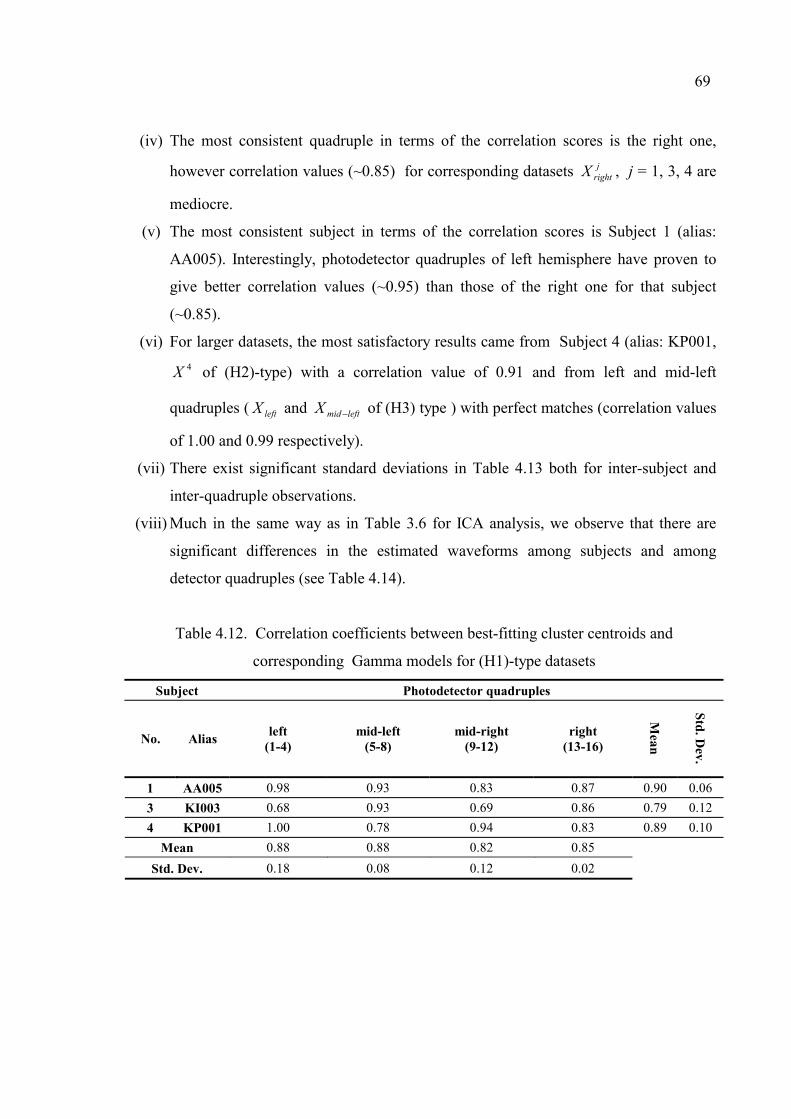
69

(iv) The most consistent quadruple in terms of the correlation scores is the right one,

however correlation values (~0.85) for corresponding datasets jrightX , j = 1, 3, 4 are

mediocre.

(v) The most consistent subject in terms of the correlation scores is Subject 1 (alias:

AA005). Interestingly, photodetector quadruples of left hemisphere have proven to

give better correlation values (~0.95) than those of the right one for that subject

(~0.85).

(vi) For larger datasets, the most satisfactory results came from Subject 4 (alias: KP001, 4X of (H2)-type) with a correlation value of 0.91 and from left and mid-left

quadruples ( leftX and leftmidX − of (H3) type ) with perfect matches (correlation values

of 1.00 and 0.99 respectively).

(vii) There exist significant standard deviations in Table 4.13 both for inter-subject and

inter-quadruple observations.

(viii) Much in the same way as in Table 3.6 for ICA analysis, we observe that there are

significant differences in the estimated waveforms among subjects and among

detector quadruples (see Table 4.14).


corresponding Gamma models for (H1)-type datasets



mid-left (5-8)

mid-right (9-12)

right (13-16)

Mean

Std. Dev.

1 AA005 0.98 0.93 0.83 0.87 0.90 0.06 3 KI003 0.68 0.93 0.69 0.86 0.79 0.12 4 KP001 1.00 0.78 0.94 0.83 0.89 0.10

Mean 0.88 0.88 0.82 0.85 Std. Dev. 0.18 0.08 0.12 0.02

70

Table 4.13. Time-constants of Gamma models to best-fitting cluster centroids

for (H1)-type datasets



mid-left (5-8)

mid-right (9-12)

right (13-16)

Mean

Std. Dev.

1 AA005 2.93 1.41 1.57 3.51 2.35 1.03 3 KI003 1.20 1.49 1.40 2.60 1.67 0.63 4 KP001 2.11 1.88 1.60 1.39 1.75 0.31

Mean 2.08 1.59 1.52 2.50 Std. Dev. 0.86 0.25 0.11 1.06


corresponding Gamma models, best-fitting time-constants for (H2) and (H3)-type datasets

Dataset

(H2)-type (H3)-type


Correlation 0.87 0.75 0.91 1.00 0.99 0.71 0.85

Time-constant 3.52 1.79 2.95 2.34 1.97 1.11 4.00

Let’s turn now our attention to graphical results depicted in Figures 4.7-4.9. Similar

to the presentation of ICA results in Figures 4.2-4.4, Figures 4.7 and 4.8 display the best-

fitting centroidal waveforms on a subject-by-subject basis and on a quadruple-by-

quadruple basis. One can observe that on some centroidal waveforms, there exists a second

rise, resulting in a two-bump appearance. This wave shape cannot be easily modeled by the

single bump Gamma function, which explains the low correlations in Tables 4.12 and 4.14.

It’s disputable whether these waveforms are indeed related to any cognitive activity.

In summary, for (H1)-type datasets, one can state that Subject 4 (alias: KP001) and

mid-left quadruple prove to be the most responsive among subjects and among quadruples,

respectively. This fact can also be verified from Figures 4.9 (a) and (b) where (H2)-type

dataset and (H3)-type dataset results are displayed.

71

Figure 4.7. Best-fitting centroidal waveforms for (H1)-type datasets, subject-by-subject

Figure 4.8. Best-fitting centroidal waveforms for (H1)-type datasets, quadruple-by-

quadruple

72

(a) (b)

Figure 4.9. (a) Best-fitting centroidal waveforms for (H2)-type datasets (b) Best-fitting

cluster centroids for (H3)-type datasets

4.6. Comparison of ICA and Clustering Approaches

Both ICA and clustering approaches were used on a comparative basis to extract

cognitive activity related waveforms. They differ, although they mutually confirm each

other, in the following aspects

(i) In ICA, we decompose the data into its purportedly statistically independent

components. Based on its similarity to the model waveform, we have associated one

of the basis vectors to the cognitive activity. Other basis vectors were thought to

model the baseline which was considered as a confounding component. Notice again

that under the linearity assumption, the baseline and brain hemodynamics are

additively combined. Since there is no evidence that contradicts neither linearity nor

the independence assumption, we accept ICA as a plausible model.

(ii) In clustering, there is no underlying transformation model but we simply group data

directly. We assume that the sought after hemodynamic response is not a rare event,

but it occurs sufficiently often. In other words, it should not be eclipsed by the

baseline, high frequency fluctations or other unwanted components. B-spline

approximation can be a remedy for removing high frequency fluctuations or artifacts.

Even combined with this property of B-spline approximation, clustering is not as

efficient as ICA in distinguishing between the functional activity, the baseline and

other physiological components (such as breathing and vasomotion) since those

components have very close spectral ranges of dominance. Recall that the

73

conjectured A-band of the baseline and the B and C-bands of cognitive activity were

neighboring in the fNIRS spectrum and most probably they interfere with each other

(that’s why simple linear filtering is not considered). On the other hand, it’s easier to

interpret the outcome of clustering compared to ICA outcome as we are searching

commonalities of directly observed waveforms. Once a valid centroidal waveform is

determined, the target instances of the population associated with this waveform

qualify as those instances the subject better reflects cognitive activity.

In the sequel, we present a comparison of the ICA and clustering approaches. Let’s

concentrate the best-fitting ICA basis vectors and centroidal waveforms obtained from

(H2) and (H3)-type datasets. Figures 4.10 (a) and (b) display ICA basis vectors for (H2)

and (H3)-type datasets, Figures 4.10 (c) and (d) do the same thing for estimated cluster

centroids. Let’s itemize the observations for clarity.

(i) Similarity of responses of Subject 3 (alias: KI003) and Subject 4 (alias: KP001) is

observed in both ICA basis vectors and cluster centroids (Figures 4.10 (a) and (c)).

(ii) While the response of Subject 1 (alias: AA005), as estimated by ICA, has a small

time-constant, in contrast, the one estimated by clustering is sluggish (Figures 4.10

(a) and (c)). Note that individual quadruple responses of this subject, as estimated by

ICA (see Figure 4.2), were very similar (with a low standard deviation of the

estimated time-constants of the Gamma fits), hence we should rely more on ICA

results for this case.

(iii) ICA yielded all different quadruple responses (Figure 4.10 (b)). On the other hand

for the clustering case, with the exception of the right quadruple, the other three

quadruple responses are quite similar (Figure 4.10 (b)). At this stage, we cannot

decide in favour of one or the other approach.

(iv) It is comforting to know that the right quadruple responses, as estimated by ICA and

clustering (Figures 4.10 (b) and (d), black curves), are virtually identical.

In conclusion, we have been able to extract cognitive activity-related waveforms

from fNIRS-HbO2 time-series. In this effort, the guideline has been the degree of match

with the model waveform of the Gamma function. We have found ICA to be more

74

satisfactory than clustering in terms of the consistency of its results. These observations

and conclusions, however, need to be corroborated by a clinical neuroscientist.

(a) (b)

(c) (d)

Figure 4.10. (a) Best-fitting ICA basis vectors for (H2)-type datasets, (b) Best-fitting ICA

basis vectors for (H3)-type datasets, (c) Best-fitting centroidal waveforms for (H2)-type

datasets and (d) Best-fitting centroidal waveforms for (H3)-type datasets

75

5. CONCLUSIONS

Let’s recall that the thesis aimed to develop a signal processing framework for fNIRS

signals recorded during functional brain activation. In the following, we present the main

conclusion drawn from this research.

5.1. Ensemble of fNIRS Signals as a Random Process

In Chapter 2, we have explored two aspects of the fNIRS as a random process,

namely the stationarity and the underlying distribution.

(i) Stationarity: Run tests have shown that we cannot easily reject the stationarity

assumption for fNIRS-HBO2 signal frames of length 30 to 50 samples, i.e., 18 to 29

secs of data. Assuming ergodicity at least per subject, the short-time stationarity

legitimizes the estimation of signal attributes such as autocorrelation, power spectral

density, etc. from a signal recorded within such intervals. Fortunately, this range

coincides with the target presentation intervals of the cognitive protocol (which also

vary from 30 to 50 samples). We have used this domain-specific knowledge in

assuming that single-trial cognitive activity-related waveforms are confined within

(30,50) samples interval. Therefore, we feel justified in using signal processing

techniques under the assumption of stationarity. On the other hand, the long-term

non-stationarity of fNIRS signals is mostly due to the baseline which is responsible

of the trend. It’s known that even in resting state, the hemoglobin and

oxyhemoglobin concentrations in the brain change over time [45]. During task-

related cognitive activity, the subject’s hemodynamic responses are superimposed on

the baseline, which in ensemble result in a non-stationary process.

(ii) Gaussianity: We performed three different Gaussianity tests on fNIRS-HbO2 signals.

The conclusion of all these, namely Kolmogorov-Smirnov test, Jarque-Bera test and

Hinich test, was common so that HbO2 signals are non-Gaussian. The implication is

two-fold.

76

The linear minimum mean-squared error (MSE) estimators will not be globally

optimal, in extracting cognitive activity-related waveforms.

The use of ICA in chapter 4 is plausible. ICA can be achieved under the

assumption that all, but except one, sources which linearly combine to yield the

observations, are non-Gaussian. Since the observed signals are non-Gaussian,

the sources cannot be “more” Gaussian than the observations by Central limit

theorem (CLT).

Furthermore, as skewness and kurtosis analyses have put into evidence, the

distribution of detrended HbO2 samples is symmetric with heavy tails. This suggests

that Gaussian mixtures are not suitable for modeling the distribution.

5.2. Relevant Spectral Bands of fNIRS Signals

In Chapter 3, we investigated canonical bands that purportedly corresponded to the

cognitive activity.

(i) The short-time spectrum revealed that fNIRS signals have their main spectral content

below 0.1 Hz. Furthermore, we have observed a peaking at around 0.7-0.85 Hz range

as the aliased part of the heartbeat signal, compatibly with the cardiac frequency

range, i.e, 0.6-1.2 Hz [45]. Otherwise, the whole fNIRS spectrogram was too

promiscous in localizing temporal events such as the responses to cognitive task

stimuli.

(ii) Canonical bands: We have developed a method to parse the signal spectrum into

canonical subbands that, we think, can faithfully be associated to different

physiological components, such as the baseline, the task-related activity or others

such as the breathing effect and the cardiac pulsations. The subbanding scheme uses

dissimilarity between relative power profiles per band of the signal. We note that the

proposed subband partitioning methodology is general and can be utilized for a

similar analysis of any set of signals. For fNIRS signals recorded during functional

brain activation, we found the following.

77

A-band: 0-30 mHz. We conjecture that this band corresponds to the baseline

signal, or at least some part of it, which is independent of task-related cognitive

activity.

B-band: 30-40 mHz. The centered Gamma function, which is a commonly used

brain hemodynamic response model in fMRI, has its spectral peak in this

frequency interval. We believe that the fundamental frequency of task-related

events in fNIRS lies in the B-band.

C-band: 40-250 mHz. The relatively larger C-band is also assumed to carry

task-related information due to the periodicity of target stimuli induced by

cognitive protocol. Moreover, it overlaps with the respiratory-frequency range

(100-500 mHz) [45] and is hypothesized to include vasomotion.

D-band: 250-850 mHz. This band contains a very small proportion of the total

signal power and is definitely uncorrelated with cognitive activity. Notice that

since the upper limit is set by the Nyquist sampling theorem, it only contains

the aliased part of the heartbeat signal.

Notice that fMRI experiments carried over subjects at the resting state, have shown

that the baseline activity is observed up to 100 mHz [45]. Thus, at least in fMRI, the

baseline extends over our A-band, B-band and lower one third of the C-band.

Accordingly, interference from the baseline, although less pronounced, should

coexist with other components cited above at the B and C-bands.

(iii) Evidence of cognitive activity: We have validated our conjecture on the protocol-

induced periodicity. Some of the fNIRS-HbO2 signals exhibit the target quasi-

periodicity. The observability of such periodicity was instrumented in classifying

photodetectors/subjects as responsive and non-responsive to cognitive stimuli. The

algorithm we have used was the least-square periodicity estimation method which

implicitly assumes the stationarity of the signal being analyzed. Notice that the

(30,50) samples stationarity range established by the run tests couldn’t carry such a

periodicity information, since the sought-after periods were in that range. In order to

mitigate the problems associated to non-stationarity, we have first prefiltered the

signals in the BC-band, as a common practice in statistical signal processing since

many signals may look stationary after trend removal [22]. Stationarity was not

actually the major concern in prefiltering but a useful side-benefit. Based on our

78

conjectures on the canonical bands, prefiltering had the effect of removing the

baseline component significantly and putting the protocol-induced periodicity into

evidence. A second precaution concerning stationarity was using signal sessions that

include 8 targets at most. Since target exposition patterns were identical for such

sessions (there are 8 of them per experiment), we have been able to collect enough

evidence to decide for the responsiveness or non-responsiveness of a signal from a

specific photodetector/subject pair. In conclusion, we have observed that the mean

periodicity estimated from qualified pairs matches the mean inter-target interval

length of 40 samples.

5.3. Cognitive Activity-Related Waveform Extraction

With the goal of identifying the brain hemodynamic response waveform to a single

cognitive stimulus, we explored two non-parametric methods: ICA and clustering. Both of

these methods are exploratory. The outcomes of the non-parametric schemes were

benchmarked against the model waveform, that is the parametric fit to the Gamma

waveform was tested. Based on the results, we concluded the following.

(i) Inter-subject and inter-quadruple-of-detectors variations exist.

(ii) In terms of the conformance to Gamma function model, waveforms estimated by

ICA are more plausible to be cognitive-activity related than those estimated by

clustering.

(iii) ICA decomposition yields not only the cognitive activity-related waveform, but also

others that can potentially be used to model the baseline interference.

(iv) The brain hemodynamic response can be more flexibly parametrized as compared to

Gamma model which relegates all the characteristics to a single parameter. Instead,

B-spline coefficients represent the global waveform while preserving locality

property.

(v) A final interesting alternative could be the ICA of B-spline coefficients for cognitive

activity-related waveform extraction.

79

5.4. Future Prospects

Several future research topics can be proposed, as presented in the sequel.

5.4.1 Process Characterization

We emphasize the following issues.

(i) Distribution of fNIRS data: As established in Chapter 2 and pointed out in

Section 5.1 as well, fNIRS signals do not arise from a Gaussian process.

Furthermore, the unimodality of the samples precludes Gaussian mixture

modeling. A future work may concentrate on the density estimation of HbO2

signal samples either in a non-parametric way (e.g. by a kernel or K-nearest

neighbor estimator) [38] or using a parametric heavy-tailed distribution model

[37]. Such a study would not only complete the statistical characterization of

fNIRS signals but it would also provide preliminaries for Bayesian estimation

of the cognitive activity-related waveforms.

(ii) Alternative time-frequency features: In Chapter 3, we have prefered the relative

power profile per band as an objective measure of the time-frequency

representation. Blanco et al. suggested other objective measures such as the

series of the mean weight frequency, the main peak frequency and the

monofrequency deviation in the analysis of EEG signals [28]. An exploration

of the variations of these quantities over time, at the canonical bands we

determined, may be pursued in order to maximize the benefits of the time-

frequency analysis.

(iii) Alternative subband partitioning scheme: The motivation behind wavelet

packet analysis of EEG signals [46] is very similar to the one behind our

subbanding methodology. The wavelet packet analysis may be implemented

for fNIRS signals to see whether the results of both methods mutually confirm

each other.

80

5.4.2. Alternative Methods for Functional Activity Estimation

The following issues can be addressed for the extraction of the cognitive activity

related waveforms.

(i) Fuzzy clustering of B-spline coefficients can potentially improve waveform

classification [38]. In real applications there is often no sharp boundaries between

clusters. Hence one risks of artificially assigning data into some clusters in crisp

clustering. In contrast to the latter, the assignments in fuzzy clustering are

accompanied with membership degrees that vary from zero to one. Such an approach

may be useful in classifying the responses of a subject in a more flexible way and in

associating a confidence to the estimated cognitive activity-related waveform.

(ii) The self-organizing map (SOM) can be another clustering-based approach [47]. A

SOM is a 1D or 2D array of vectors that are equivalent to cluster centroids. In the

SOM, the centroids are configured in such a way that neighboring centroids on the

grid are similar to each other whereas the farther away ones are dissimilar. This

property of the SOM may be exploited in order to observe cognitive activity

variations. The dot-product SOM algorithm, in particular, should be considered in

the first place since it relies on a correlation metric, like in our agglomerative

scheme, to evaluate correspondences.

(iii) Bayesian modeling:One of the most up-to-date approaches in the non-parametric

estimation of the brain hemodynamic response (BHR) function in fMRI is due to

Ciuciu et al. [9]. A reduced form of the generative data model, suitable for single-

trial events, can be described as

kkk vCdhy ++= (5.1)

[ ]Tmtttk kkkyyy 11 ,,, −++=y : the observed BOLD sequence (vector) of length m in

response to the kth target stimulus at instance tk.

[ ]Tmhhh 110 ,,, −=h is the unknowm BHR vector of length m.

81

= QccC ,,1 is a set of orthonormal basis functions [ ]Tmq cc ,,0=c that can

model the low-frequency components, i.e., the baseline.

[ ]TkQkkk ddd ,,2,1 ,,,=d : vector of unknown weighting coefficients of the basis

functions at the arrival of the kth target stimulus.

[ ]Tmtttk kkkvvv 11 ,,, −++=v : the term that stands for unwanted random physiological

fluctuations and measurement noise after the arrival of the kth target stimulus.

They treated the model (5.1), and its general form which is suitable for multitask

cognitive protocols, in a Bayesian formalism and estimated BHR functions, that are

validated for both real and synthetic data, using expectation conditional

maximization (ECM) algorithm [48]. The very same approach can be adopted in

fNIRS for the extraction of cognitive activity-related waveforms by modeling prior

information on the brain hemodynamics and the baseline measured by fNIRS, in

order .

(iv) Dynamic Bayesian modeling: The model (5.1) is time-invariant in that it imposes a

fixed vector h for every trial of the cognitive stimulus, as the methods of Chapter 4 in

this report implicitly assumed. On the other hand, (5.1) can be extended to a

dynamical model using a state-space approach as described below.

kkkk

kkk kkvCdhy

whΓh++=

++=+ ),1(1 (5.2)

where ),1( kk +Γ is the state-transition matrix that should cope with the

dependencies between successive responses and kw is a disturbance vector. From

this viewpoint, the estimation of the cognitive activity-related waveforms (or the

BHR) based on (5.2) constitute a further research topic that should consider the

extended Kalman Filtering concepts [49], such as Markov chain Monte Carlo

methods or particle filtering [50], in the fNIRS setting.

82

(v) Non-linear neurovascular coupling: A majority of the BHR estimation schemes in

fMRI commonly assume linearity between neuronal activity and BOLD response.

However, the true underlying mechanism, i.e., the neurovascular coupling, is not

completely understood and characterized [9]. Linearity is often retained for its

simplicity. In the fMRI literature, there exists a couple of attempts in non-linear

modeling of neurovascular coupling through support vector machines [51], [52].

Based on these ideas, (5.1), or equivalently the second equation in (5.2), extend to

kkk f vCdhXy ++= )( (5.3)

where X stands for the binary stimuli matrix as a mean of expressing neuronal

activity in mathematical formalism and )(⋅f is a non-linear function of X. Notice

that in (5.3), the model is still linear in h, but X undergoes a non-linear

transformation. Multilayer perceptrons, which can learn any non-linear function in

theory [38], can be constructed in conjunction with the ideas proposed in items (iii)

and (iv) above as a further prospect in fNIRS.

5.5. Remarks on the Experimental Protocols and Measurements

In this final section, we would like to discuss two important aspects of cognitive

experiments in the context of fNIRS.

(i) Simultaneous fMRI-fNIRS measurements: There is a necessity to simultaneously

acquire fMRI and fNIRS data during functional brain activity. For the time being,

cognitive activity-related waveform extraction in fNIRS, due to its low spatial

resolution, cannot find its true running track unless it is accompanied with

simultaneous fMRI data. To clarify, using fNIRS one cannot obtain fine detail brain

activity maps, although the brain hemodynamic response can be more accurately

estimated by fNIRS thanks to its higher temporal detail. Research in optimizing

spatial photosensor-array geometry is a relatively new field in diffuse optical

methods [2] and localization of externally recorded signals in fNIRS is still very

difficult [8]. Another argument in favor of simultaneous use of fNIRS and fMRI is

the lacking of reliable quantification schemes for Hb and HbO2 concentrations, as

83

reported in [8]. Once such recordings from both modality are acquired

simultaneously, the fNIRS waveforms can be utilized for generating more reliable

fMRI activation maps.

(ii) Design of experimental protocols: In stimulus design of even-related fMRI

experiments, two dichotomies exist: randomized vs. block designs. The former

consists of impulsive train of target stimuli with random arrivals and it can possibly

be interleaved with a series of more frequent context stimuli. The cognitive protocol

of the present work is an example to randomized designs. On the other hand, in block

designs, the stimuli sequence can be described as a series of rectangular waves. In a

recent study [53], it has been argued that “randomized designs offer maximum

estimation efficiency but poor detection power, while block designs offer good

detection power at the cost of minimum estimation efficiency.”. Since activation

detection in fNIRS cannot be an issue unless devices that can provide more spatial

detail are implemented, randomized event-related designs should be considered in

the first place for maximum estimation efficiency in fNIRS experiments.

84

APPENDIX A: STATISTICAL TOOLS

We made use of [22-27, 38] in preparing the material presented in this part.

A.1. Hypothesis Testing

Statistical hypothesis testing provides a formal way to decide if the results of an

experiment are significant or accidental. Consider a record of samples that consist of n

measurements (samples). Suppose futher that we want to determine whether these

measurements come from a known distribution f0 (whose parameters are fully specified) or

not. Initially, we hypothesize that f0 is indeed the underlying distribution of the samples;

this is called the null hypothesis and denoted as H0. The alternative hypothesis, i.e., that the

samples are not drawn from f0, is denoted as H1. We now state the problem as deciding

whether to accept or reject H0.

At this point, we assume that we will accept H0, if a test-statistic ξ, computed from

the available n samples, is below some critical value γ; otherwise we will accept H1. That

is

. fromdrawn are samples:accept , If. fromdrawn not are samples:accept , If

00

01

fHfH

γξγξ

<>

(A.1)

We can make two kinds of error

False Alarm (Type I error): Reject H0 (accept H1) when H0 is true.

False Miss (Type II error): Reject H1 (accept H0) when H1 is true.

The probability of false alarm PFA is expressed as

{ }0Pr HPFA γξ ≥= (A.2)

85

The hypothesis test can equivalently be performed by the following statements

. fromdrawn are samples:)accept risky to isit (accept , If. fromdrawn not are samples:accept , If

010

01

fHHPFAfHPFA

αα

><

(A.3)

where α is said to be the significance level of the test. As the context implies, there is a

one-to-one correspondence between the significance level α and the critical value γ. In

order to compute (A.2), we must know the distribution of the test-statistic ξ or simply its

percentage points (critical values at corresponding significance levels). Usually, we set the

significance level to 0.05 or 0.01 and use a statistical table to find out the corresponding

critical value. Afterwards we compare the test-statistic against the critical value and decide

whether to accept of reject H0 as descibed above. If we require the explicit knowledge of

the PFA, we can read it from the graph of the cumulative distribution function (cdf) of the

test-statistic. Suppose we read pξ at ξ from the graph of its cdf for some test: if the test is

significant in the upper tail PFA=1- pξ, or otherwise, if it is significant in the lower tail

PFA= pξ.

The use of hypothesis testing is certainly not limited to test whether the

measurements are drawn from a known distribution or not. Some of hypothesis testing

examples are: (i) There is no signal in the present interval, (ii) The short-time signal is

stationary, (iii) There is neuronal activation in a particular brain region at a particular time,

(iv) Smoking does not kill, (v) Team A will defeat Team B in the next match, etc.

A.2. Run Test for Stationarity

Run test can detect a monotonic trend in a time series x(t), t=1,..., 2N, by evaluating

the number of runs in a time-series derived from x(t). A “run” is defined as a sequence of

identical observations that is followed or preceded by a different observation or no

observation at all. To this effect, we first evaluate the median mx of the observations and

derive the series y(t) as

x

x

mtxtymtxty

≥=<=

)( if1)()( if0)(

(A.4)

86

Then we compute the number of runs in y(t), that is the number of consecutive

observations where the signal exceeds the median level and similarly the number of

consecutive observations where the signal remains below the median level. If x(t) is a

stationary random process, the number of runs R is a random variable with

12)1(

1

2

−−

=

+=

NNN

N

R

R

σ

µ (A.5)

where Rµ and 2Rσ denote the mean and variance of R, respectively. An observed number

of runs significantly different from N+1 is indicative of non-stationarity because of the

possible presence of a trend in x(t). Using the run distribution with parameter N, that is

−=

−−

−−

=

−−

==

12 ,...,5,3,2

23

2

1

21

2

1

2

2 ,...,4,2,2

12

1

2

)(

2

Nn

NN

nN

nN

Nn

NN

nN

nRP (A.6)

we determine whether the signal x(t) is stationary or not by hypothesis testing.

87

A.3. Gaussianity Tests

A.3.1. Kolmogorov-Smirnov Test

The Kolmogorov-Smirnov test (K-S test) is a general purpose test based on

comparing the empirical cumulative distribution function (ecdf) of the available samples

with the theoretical cdf of the distribution that the test is carried for. It is defined as

.on distributi specified thefollownot does variableRandom :.on distributi specified thefollows variableRandom :

1

0

F(x)XHF(x)XH

(A.7)

The K-S test-statistic ξks is defined as

)()(max tet

N

tks xFxF −=ξ (A.8)

where Fe(xt) is the ecdf of observations xt, t = 1,..., N. The KS-test can be utilized for

testing observations for Gaussianity (normality). Since F(x) should be completely

specified, we first make the observations zero-mean, unit-variance and then we compute

Fe(x). We evaluate (A.8) using the standard normal cdf in place of F(x) and the ecdf Fe(x).

Once ξks is obtained, the rules of hypothesis testing can be applied to decide for normality

using tabulated critical values of the K-S test-statistic distribution. Note that this test

requires independent identically distributed (i.i.d.) data.

A.3.2. Jarque-Bera Test

The Jarque-Bera (J-B) test is a normality test that uses third and fourth order central

moments based on the fact these vanish for normal random variables. The J-B test-statistic

ξjb is a function of the sample estimates of the skewness and of the kurtosis denoted by τ̂

and κ̂ , respectively.

+=

4ˆ

ˆ6

22 κτξ N

jb (A.9)

88

∑=

−=N

ttx

N 1

33 )ˆ(

ˆ1ˆ µσ

τ (A.10)

3)ˆ(ˆ1ˆ

1

44 −−= ∑

=

N

ttx

Nµ

σκ (A.11)

where µ̂ and 2σ̂ are the sample estimates of the mean and the variance of the observations

xt, t = 1,..., N. The limiting distribution, for i.i.d data, of the J-B test-statistic ξjb is 22χ , i.e.,

Chi-square with two degrees of freedom. Again it is a simple matter to calculate (A.9)-

(A.11) and apply hypothesis testing concepts using the fact that 22χξ →jb . However, the

results are only accurate for sufficiently large N and i.i.d. data since the estimates of higher

order moments can be biased for small N and correlated data.

A.3.3. Hinich’s Gaussianity Test for Time-series

The above described tests assume i.i.d data and are not suitable for time-series unless

one collects data samples at random distant locations. Hinich’s bispectrum-based test is

purely designed for correlated time-series. In theory, signals that result from Gaussian

processes have zero third and higher-order cumulants and this knowledge can be exploited

for determining the underlying process of the signal. However in practice, sample

estimates of cumulants do not strictly vanish. Thus, one needs a test to determine whether

or not estimated quantities are significantly different from zero in the statistical sense. For

a linear non-Gaussian process X(t), the following identity holds

[ ] 2/12121

21

)()()(),(

ffSfSfSffS

xxx

xx

+= constant or zero (A.12)

The left-hand side of (A.12) is the bicoherence of the random process {X(t)}. In

particular, the numerator term ),( 21 ffS xx is the bispectrum and )( fSx is the power

spectral density, f1 and f2 being frequency variables. Again, sample estimates of the

bicoherence will not be constant, and we need a test to determine whether the non-

89

constancy is statistically significant. Hinich developed a test which determines whether a

given signal is non-Gaussian as

Gaussian.not is process thei.e., ,bispectrum zero-non has )( :Gaussian. is process thei.e., ,bispectrum zero has )( :

1

0

tXHtXH

(A.13)

Accordingly the test is based on whether the ratio in (A.12) differs significantly from

zero or not. Hinich’s test statistic ξhin is the sum of the squared bicoherence values over the

principal domain of the bispectrum, and is Chi-square distributed. The test can be

performed either by using ξhin and (A.1) or the computed probability of false alarm phin and

(A.3) at the desired significance level α.

A.4. Fisher’s Method for Combining Independent Tests

Fisher’s method can be used for combining independent tests for several records

based on computed false alarm probabilities, also called p-values, of individual tests.

Suppose K tests are made of null hypotheses KiH i ,...,1 ,0 = each of which states the ecdf of

the samples of the ith record, Ntx it ,...,1 , = , is greater than the standard normal cdf. Let H0

be the composite hypothesis that all iH 0 are true, that is, if anyone is false then we must

reject H0. Suppose further that each test returned pi as its significance level, i.e., the

probability of rejecting iH 0 when it is indeed true. Furthermore, when iH 0 is true, pi is a

uniform random variable in the interval (0, 1). Hence we obtain a record of K samples with

uniform distributions if all iH 0 together, or equivalently the composite hypothesis H0,

holds. In such a situation, any deviation from uniformity would be sufficient for rejecting

the composite hypothesis H0, i.e., the normality of all records. For instance, the

Kolmogorov-Smirnov test can be used for detecting deviations of p-values from

uniformity. On the other hand, Fisher developed a test-statistic, denoted by P1, that can

easily be computed in terms of p-values and be directly used for rejecting or accepting H0

∑−=K

iipP )log(21 (A.14)

90

where log(.) stands for the natural logarithm. P1 combines one-tail component statistics pi,

each of which are the significance levels of the tests, that determine whether the ecdf is

greater than the standard normal cdf, or not in our working example. P1 itself is significant

at the upper tail of its limiting distribution. In the literature, there exist other versions of

statistics of this type, which combines two tail component statistics, each of which tests

whether the ecdf is equal to the theoretical cdf, or not. One such statistic which is

significant at the lower tail of its limiting distribution is defined as

∑ −−=K

iipP 21log22 (A.15)

The limiting distributions of both P1 and P2 are 22Kχ , hence a Chi-square test, with

appropriate degrees of freedom, i.e., 2K, suffices for combining the individual test results.

91

APPENDIX B: CLUSTERING

In exploratory data analysis as well as in pattern recognition, discovering the

underlying distribution of multivariate data in the multidimensional space is of particular

importance. A clustering procedure is a non-parametric method that gives dominant modes

of the multivariate data in terms of clusters or groups of data points that possess strong

internal similarities. In formal terms, clustering partitions a multivariate dataset

X { }Ntt ,...,1 == x into a set of clusters Q { } ,...,1 , CcQ cc == q where cq is the centroid

of the cluster Qc. To this effect, often a criterion or a set of criteria is to be satisfied for a

set of clusters Q. Two major issues are of concern in clustering

(i) The way we measure similarity between data samples,

(ii) The aspects of the clusters that lead to a natural grouping of the data.

Note that we made use of [38,41] in preparing the material presented in this

appendix.

B.1. Similarity Measures

Similarity measures addresses the item-(i) above. The most natural way to measure

similarity between two samples is to evaluate the distance between them. A suitable

distance metric satisfies

Non-negativity: 0),( ≥yxd

Reflexivity: yxyx =⇔≥ 0),(d

Symmetry: ),(),( xyyx dd =

Triangle Equality: ),(),(),( zxzyyx ddd ≤+

Note that it is possible to transfom a similarity measure into a distance metric so that

it gains the above cited properties. Some of the distance metrics and similarity measures

that are widely used in clustering are in the sequel.

92

Minkowski metric cm

k

ckk yxd

1

1),(

−= ∑

=

yx , where 1≥c is the selective

parameter. The Minkowski metric is equivalently called as Lc-metric. Notice that for

c = 2, the Minkowski metric evalautes to the familiar Euclidean distance. For c = 1, it

can be recognized as Manhattan or city block distance that accounts for the sum of

the absolute distances along each of the m coordinate axes. In some cases, the

distances along a single axis is much more important than in all of the remainder.

kk

m

kyxL −=

=∞ 1max is evaluated in such situations.

Mahalanobis distance )()(),( 1 myΣmxyx −−= −Td involves data-dependent terms

as the mean vector m and the covariance matrix Σ of the observations

{ }Ntt ,...,1 =x for which x and y are two generic instances. The Mahalanobis

distance is invariant under dilations, translations and rotations in the m-dimensional

space.

Cosine of the angle yxyxyx

),(

T

s = , where ⋅ stands for the Euclidean distance. In

case the cosine of the angle is a meaningful measure of similarity, we can use

),(1),( yxyx sd −= as a distance metric for clustering, ),( yxd can be called as one-

minus-the-cosine-of-the-angle. In some situations, it would be more appropriate to

treat the observations as sequences of values (e.g., when the components of the

vectors are consecutive samples of a short-time signal), rather than as vectors, by

subtracting the mean value of their components from each of the vectors, i.e., for x,

∑=

−=m

iiknewk x

mxx

1,

1 for k = 1,..., m and similarly for y, before computing s(x,y). The

resulting similarity measure is called as the normalized correlation coefficient, and

the distance metric derived from it as one-minus-the-normalized-correlation-

coefficient in a way compatible with the signal processing literature.

93

B.2. Clustering Criteria

The choice of the distance metric is one of the issues in clustering, the aspects of data

that we exploit for grouping constitute another. An optimal clustering is generally defined

as the one that minimizes within-cluster and maximizes between-clusters distances.

However, such distances need to be defined to get several different criterion functions. In

Table B.1, many possibilities are displayed.

Table B.1. Several definitions

for within-clusters distance )( cQS and between-cluster distance ),( lc QQd

Within-cluster distance )( cQS

average distance ∑′

′−−

=ii

ii

cca NN

S,)1(

1 xx

nearest neighbor distance ∑ ′′ −=

i

iii

cnn N

S xxmin1

centroid distance ∑ −=i

ci

cc N

S qx1

Between-cluster distance ),( lc QQd

single linkage jijisd xx −== ,min

complete linkage jijisd xx −== ,max

average linkage ∑ −=ji

ji

lca NN

d,

1 xx

centroid linkage lcced qq −=

cQ and lQ : two clusters with centroids cq and lcl ≠ ,q , respectively

jjQiiQ ljj

cii ′≠∈′≠∈ ′′ ,, ; ,, xxxx

cN and lN : the number of samples in clusters cQ and lQ , respectively

The distance norm ⋅ can be chosen as one of the metrics presented in B.1 or others

that are not given here, according to the specific application. Notice that the combination

of within-cluster distance, between-clusters distance and the distance metric to form a

criterion function should be carried with caution since an inappropriate combination can

cause misinterpretation of the data. In summary, a criterion J is implicitly expressed as

94

[ ]CQQdQSfJ lcc ),,(),(= (B.1)

where clusters ofnumber total theis and with ,...,1, ClcClc ≠= . The parameter C appears

in (A.1) in order to optimize J with minimum possible number of clusters.

B.3. Clustering Algorithms

Clustering algorithms are dichotomized in the way they make the partitioning: (i)

partitive approaches and hierarchical approaches. The former divide a dataset into a,

usually prescribed, number of clusters C. In a partitive algorithm, initially one should

choose a criterion function to optimize, determine the number of clusters C, determine

assignment (for data vectors) and update (for centroids) rules as dictated by the chosen

criterion. The pseudo-code is as follows.

(1) Initialize the cluster centroids cq .

(2) Assign each of the data vectors to one of the clusters cQ

using the assignment rules.

(3) Update the cluster centroids cq using the update rules.

(4) Stop if the partitioning is unchanged (or the criterion

function is optimized); otherwise return to step (3).

Hierarchical clustering algorithms can be further subdivided to divisive and

agglomerative schemes. The latter is more commonly used and can be implemented by the

following steps.

(1) Initialize: Assign each vector to its own cluster.

(2) Compute distances between all clusters (according to chosen

metric and between-clusters distance).

(3) Merge the two clusters that are closest to ecah other.

(4) Return to step (2) until there is only one cluster left.

95

By executing the above steps, we obtain an hierarchical tree, or a dendrogram, that

holds correspondences between the data vectors. The dendrogram can be utilized in

interpreting the underlying structure of the data. Exploiting the dendrogram tree to finalize

the clustering procedure, is another issue.

In Figure B.1, a sample dendrogram is shown along with three of the plausible cuts.

Consider, for instance, the one that results in four clusters. To identify the clusters, we

look, on each branch, for the next node below the cut. Accordingly, we get the node B as a

singleton cluster, the leaves of the node C as the second cluster, the leaves of the node D as

the third and finally the leaves of the node E as the fourth. In short, each node stands for a

cluster whose members are the leaves of that node. The height of the nodes is proportional

to the distance between its childs, i.e., the clusters that are merged at that level. For

instance, the height of the node A is proportional to the distance between the clusters

denoted by the nodes B and C. Observe that the cut need not to be straight. Although there

exist sophisticated methods that give cuts at different levels; usually, the dendrogram is

pruned at a fixed level to yield the desired number of clusters C.

2 clusters

4 clusters

3 clusters

Figure B.1. A sample dendrogram of 8 data points.

A

B

C D E

96

APPENDIX C: INDEPENDENT COMPONENT ANALYSIS

We made use of [37, 38] in preparing the material presented in this part.

C.1. Description of the Independent Component Analysis

Independent component analysis (ICA) seeks directions of multivariate data that are

mutually most independent. It is formalized by the following general definition.

ICA of a random vector x consists of finding a linear transform s=Wx so that

the components si are as independent as possible, in the sense of maximizing

some function F(s) that measures independence.

If the dimensionality m of the observation vectors x matches the number of

independent components n (i.e., dimensionality of the independent components vector s),

the relation s = Wx can be inverted as x = As. The matrix A is said to be the mixing

matrix, reciprocally the matrix W as the demixing matrix. The naming of these matrices

follows from the classical example of ICA, where two people speaks in a room

simultaneously and you record their speech with two microphones that, ideally, capture but

only the mixture of their voices. You have two time signals x1(t) and x2(t) as measured by

the two microphones. Can you recover the individual speech of both of these people, i.e.,

the source signals s1(t) and s2(t), by just making use of the observed signals x1(t) and x2(t)?

Using ICA, the answer is yes, if certain conditions are fulfilled. In the general case of m

observed mixtures xj(t) and n sources si(t), these conditions are stated as follows

(i) The instances of each of the observed mixtures xj(t), t = 1,...,T must be independent

identically distributed (i.i.d) in time.

(ii) All the indepenent components si, with the possible exception of one component,

must be non-Gaussian.

(iii) The number of observed of observed mixtures m must be as large as the number of

independent components n, i.e., nm ≥ .

(iv) The matrix A must be of full column rank.

97

However, even if the above cited conditions are fulfilled, there are two ambiguities in

identifying the columns of the mixing matrix A.

(i) The columns of A can be estimated up to a multiplicative constant. That is, we

cannot recover the original intensity of the sources neither their sign.

(ii) The columns of A can be estimated up to a permutation. Hence ICA does not provide

an ordering of the independent components.

Two elements are fundamental in solving the ICA problem: an objective function

that measures independence (or a quantity negatively related to independence) and an

optimization algorithm that maximizes (or minimizes) the objective function. Among the

basic ICA methods, one can cite

ICA by maximizing non-Gaussianity. Non-Gaussianity is related to

independence by the Central Limit Theorem which basically states that the sum

of i.i.d. random variables has the Gaussian distribution in the limiting case.

Intuitively to say, if the generative linear mixture model holds for a set of

observed mixtures, they must be “more” Gaussian than the underlying sources.

Hence, ICA can be achieved equivalently by maximizing non-Gaussianity

between the sources to be estimated. Kurtosis and negentropy-based methods

exploit this knowledge.

ICA by maximum likelihood estimation. It is possible to solve the ICA

problem by classical maximum likelihood methods in case the distributions of

the sources are of certain specific form with some parameters to be determined.

These methods treat the problem in a semi-parametric way.

ICA by minimization of mutual information. Mutual information is a natural

measure of dependence between random variables, that vanishes if and only if

the random variables are statistically independent. As a result, the minimization

of mutual information constitutes another approach for solving the ICA

problem.

In addition to these, in the literature, there exist other basic ICA methods that use

higher-order cumulant information and concepts of non-linear decorrelation.

98

C.2. Applications of the Independent Component Analysis

The applications of ICA are certainly not limited to the working example of the

previous section, which may be generalized under the name of blind source separation.

Blind deconvolution is another signal processing problem that ICA methods have been

found to work successfully in some cases. Furthermore, ICA has received a considerable

interest in especially image feature extraction, as an alternative to classical principal

component analysis (PCA). Low-level features of natural image data, extracted by ICA,

have been shown to correspond closely to those observed in primary visual cortex. Texture

analysis, biometric pattern recognition, image compression and watermarking constitute

those applications that make use of ICA image features.

On the other hand, ICA is, first of all, an exploratory data analysis tool that can be

benefited in applications where little prior knowledge about the underlying physical

phenomena is available. Areas like astrophysics, biomedical signal processing, economics

and social sciences possess a great deal of such applications.

C.3. The FastICA Algorithm

FastICA is a fast fixed-point ICA algorithm which is based on the maximization of a

negentropy approximation. Specifically, FastICA maximizes the following objective

function for finding one independent component

{ } { }[ ]2)()()( vGEGEJ TT −≈ zwzw (C.1)

where, z is the preprocessed version of the observed vector x, w is one of the

columns of the mixing matrix W, v is a standard normal random variable and G is

practically any non-quadratic function. Note that, E{.} is computed by sample estimates.

The following choices for G has been found to be very useful for robust approximations of

negentropy

)2/exp()( and coshlog)( 221 uuGuuG −−== (C.2)

99

The FastICA algorithm consists of a preprocessing and an optimization step details

of which are given next.

C.3.1. Preprocessing

Preprocessing involves centering and whitening.

Centering. We make the observed vectors zero-mean by subtracting the mean

vector of the observations.

{ }xxx E−=~ (C.3)

Whitening. We transform x~ to z so that the covariance matrix of the latter becomes

identity, i.e., { } Izz =TE . This can be achieved by first eigendecomposing

{ } TTE EDExx =~~ where E is the orthogonal matrix of eigenvectors and D is the

diagonal matrix of eigenvalues of { }TE xx~~ . Then,

xEEDz ~2/1 T−= (C.4)

Note that in case one would like to estimate fewer independent components than the

observations such that nm ≥ ; only n columns, which are significant in terms of the

eigenvalues, of the the transformation matrix TEEDV 2/1−= are involved in the

computation of (C.4).

C.3.2. FastICA for Estimating One Independent Component

The FastICA algorithm can then be performed by the following procedure.

(1) Choose an initial random vector w.

(2) { } { }wzwzwzw )()( TT GEGE ′′−′←

(3) www ←

100

(4) If not converged, return to step (2).

where ⋅ denotes the Euclidean norm, GG ′′′ and are the first and second derivatives of G

in which place one of the functions in (C.2) can be utilized.

C.3.3. FastICA for Estimating Multiple Components

In order to estimate several independent components, the above procedure should be

repeated as many times as the number of independent components we want to estimate. To

preclude convergence to the same maxima, the vectors w1,..., wn should be decorrelated at

each step. This can be achieved in two ways.

Deflation-based decorrelation. Let w1,..., wp be estimated by the above procedure,

to remove the projections of w1,..., wp from the next estimated vectors wp, we

perform the following

111

1111

+++

=+++

←

−← ∑

ppp

p

jjj

Tppp

www

wwwww (C.5)

Symmetric decorrelation. Decorrelation can equivalently be achieved in a

simultaneous manner by

WWWW 2/1)( −← T (C.6)

where W is the demixing matrix, as estimated at some step of the iterative procedure.

101

REFERENCES

1. Raichle, M. E., “Behind The Scenes of Functional Brain Imaging: A Historical and

Physiological Perspective”, Proc. Natl. Acad. Sci., Vol. 95, pp. 765-772, 1998.

2. Emir, U. E., System Characterization for a Fast Optical Imager, M.S. Thesis, Boğaziçi

University, 2003.

3. Frackowiak, R., P. J. Magistretti, R. Shulman, J. Altman and M. Adams (editors),

Neuroenergetics: Relevance for Functional Brain Imaging, Human Frontier Science

Program, Strasbourg, 2001.

4. Villringer, A. and B. Chance, “Non-Invasive Optical Spectroscopy and Imaging of

Human Brain Function”, Trends in Neuroscience, Vol. 20, pp. 4435-4442, 1997.

5. Strangman, G., D. Boas and J. Sutton, “Non-invasive Neuroimaging using Near-

Infrared Light”, Society of Biological Psychiatry, Vol. 17, pp. 679-693, 2002.

6. Schmidt, F. E. W., Development of a Time-Resolved Optical Tomography System for

Neonatal Brain Imaging, Ph.D. thesis, University College London, 1999.

7. Boynton, G. M., S. A. Engel, G. H. Glover and D. J. Heeger, “Linear Systems Analysis

of Functional Magnetic Resonance Imaging in Human V1”, The Journal of

Neuroscience, Vol. 16, pp. 4207-4221, 1996.

8. Strangman, G., J. P. Culver, J. H. Thompson and D. A. Boas, “A Quantitative

Comparison of Simultaneous BOLD fMRI and NIRS Recordings during Functional

Brain Activation”, NeuroImage, Vol. 17, pp. 719-731, 2002.

9. Ciuciu, P., J-B. Poline, G. Marrelec, J. Idier, C. Pallier and H. Benali, “Unsupervised

Robust Non-Parametric Estimation of the Hemodynamic Response Function for any

102

fMRI Experiment”, IEEE Trans. On Medical Imaging, Vol. 22, No. 10, pp. 1235-1251,

October 2003.

10. Friston, K. J., A. P. Holmes, K. J. Worsley, J-P. Poline, C. D. Frith and R. S. J.

Frackowiak, “Statistical Parametric Maps in Functional Imaging: A General Linear

Approach”, Human Brain Mapping, Vol. 2, pp. 189-210, 1995.

11. Bandettini, P. A., A. Jesmanowicz, E. C. Wong and J. S. Hyde, “Processing Strategies

for Time-Course Data Sets in Functional MRI of the Human Brain”, Magn. Reson.

Med., Vol. 30, pp. 161-173, 1993.

12. Friston, K. J., P. Jezzard and R. Turner, “The Analysis of Functional MRI Time-

Series”, Human Brain Mapping, Vol. 1, pp. 153-171, 1995.

13. Worsley, K. J. and K. J. Friston, “Analysis Of fMRI Time-Series Revisited–Again”,

NeuroImage, Vol. 2, pp. 173-181, 1995.

14. Glover, G. H., “Deconvolution of Impulse Response in Event-Related BOLD fMRI”,

NeuroImage, Vol. 9, pp. 416-429, 1999.

15. Goutte, C., F. A. Nielsen and L. K. Hansen, “Modeling the Haemodynamic Response

in fMRI using Smooth FIR Filters”, IEEE Trans. On Medical Imaging, Vol. 19, pp.

1188-1201, 2000.

16. Marrelec, G., H. Benali, P. Ciuciu, M. Pélégrini-Issac and J-B. Poline, “Robust

Bayesian Estimation of the Hemodynamic Response Function in Event-Related BOLD

fMRI Using Basic Physiological Information”, Human Brain Mapping, Vol. 19, pp. 1-

17, 2003.

17. Ogawa, S., T. Lee, A. Kay and D. Tank, “Brain Magnetic Resonance Imaging with

Contrast Dependent on Blood Oxygenation”, Proc. Natl. Acad. Sci. USA, Vol. 87, no.

24, pp. 9868-9872, 1990.

103

18. Buxton, R. and L. Frank, “A Model for the Coupling between Cerebral Blood Flow and

Oxygen Metabolism during Neural Stimulation”, J. Cereb. Blood Flow Metab., Vol.

17, No. 1, pp. 64-72, 1997.

19. Logothetis, N. K., J. Pauls, M. Augath, T. Trinath and A. Oeltermann,

“Neurophysiological Investigation of the Basis of the fMRI Signal”, Nature, Vol. 412,

No. 6843, pp. 150-157, July 2001.

20. McCarthy, G., M. Luby, J. Gore and P. Goldman-Rakic, “Infrequent Events

Transiently Activate Human Prefrontal and Pparietal Cortex as Measured by Functional

MRI”, J. Neurophysiology, Vol. 77, pp. 1630-1634, 1997.

21. Blanco, S., H. Garcia, R. Q. Quiroga, L. Romanelli and O. A. Rosso, “Stationarity of

the EEG Series”, IEEE Engineering in Medicine and Biology Magazine, Vol. 14, pp.

395-399, 1995.

22. Shanmugan, K. S. and A. M. Breipohl, Random Signals: Detection, Estimation and

Data Analysis, John Wiley & Sons, 1988.

23. D’Agostino, R. B., “Tests for the Normal Distribution”, in R. B. D’Agostino and M. A.

Stephens (eds.), Goodness of Fit Techniques, pp. 367-419, Marcel Dekker, New York,

1986.

24. Bai, J. and S. Ng, “Tests for Skewness, Kurtosis and Normality for Time-series Data”,

Boston College Working Papers in Economics, 501, June 2001.

25. Hinich, M. J., “Testing for Gaussianity and Linearity of a Stationary Time-Series”,

Journal of Time-Series Analysis, Vol. 3, pp. 169-176, 1982.

26. D’Agostino, R. B., “Graphical Analysis”, in R. B. D’Agostino and M. A. Stephens

(eds.), Goodness of Fit Techniques, pp. 7-62, Marcel Dekker, New York, 1986.

104

27. Stephens, M. A., “Tests for the Uniform Distribution”, in R. B. D’Agostino and M. A.

Stephens (eds.), Goodness of Fit Techniques, pp. 357-360, Marcel Dekker, New York,

1986.

28. Blanco, S., R. Q. Quiroga, O. A. Rosso and S. Kochen, “Time-Frequency Analysis of

Electroencephalogram Series”, Physical Review E , Vol. 51, pp. 2624-2631, March

1995.

29. Başar, E., T. Demiralp, M. Schurmann, C. Başar-Eroğlu and A. Ademoğlu,

“Oscillatory Brain Dynamics, Wavelet Analysis and Cognition”, Brain and Language,

Vol. 66, pp. 146-183, 1999.

30. Obrig, H., M. Neufang, R. Wenzel, M. Kohl, J. Steinbrink, K. Einhaupl and A.

Villringer, “Spontaneous Low Frequency Oscillations of Cerebral Hemodynamics and

Metabolism in Human Adults”, NeuroImage, Vol. 12, pp. 623-639, 2000.

31. Kim, D. and K. Uğurbil, “Bridging the Gap between Neuroimaging and Neuronal

Physiology”, Image Anal. Stereol., Vol. 21, pp. 97-105, 2002.

32. Stoica, P. and R. L. Moses, Introduction to Spectral Analysis, p. 43, Prentice Hall,

Upple-Saddle River, New Jersey, 1997.

33. Kuo, T., C. Chern, W. Sheng, W. Wong and H. Hu, “Frequency Domain Analysis of

Cerebral Blood Flow Velocity and its Correlation with Arterial Blood Pressure”, J.

Cereb. Blood Flow Metab., Vol. 18, pp. 311-318, 1998.

34. Giller, A. C., M. R. Hatab and A. M. Giller, “Oscillations in Cerebral Blood Flow

Detected with a Transcranial Doppler Index”, J. Cereb. Blood Flow Metab., Vol. 19,

pp. 452-459, 1999.

35. Hu, H., T. Kuo, W. Wong, Y. Luk, C. Chern, L. Hsu and W. Sheng, “Transfer Function

Analysis of Cerebral Hemodynamics in Patients with Carotid Stenosis”, J. Cereb.

Blood Flow Metab., Vol. 19, pp. 460-465, 1999.

105

36. Friedman, D.H., “Pseudo-Maximum-Likelihood Speech Pitch Extraction”, IEEE

Trans. on ASSP, Vol. 25, pp. 213-221, 1977.

37. Hyvärinen, A., J. Karhunen and E. Oja, Independent Component Analysis, John Wiley

& Sons, 2001.

38. Duda, R. O., P. E. Hart and D. G. Stork, Pattern Classification, John Wiley & Sons,

2001.

39. Ferraty, F. and P. Vieu, “Curves Discrimination: a Nonparametric Functional

Approach”, Computational Statistics and Data Analysis, Vol. 44, pp. 161-173, 2003.

40. Unser, M., A. Aldroubi and M. Eden, “B-Spline Signal Processing: Part II-Efficient

Design and Applications”, IEEE Trans. on Signal Processing, Vol. 41, pp. 834-848,

February 1993.

41. Vesanto, J. and E. Alhoniemi, “Clustering of the Self-Organizing Map”, IEEE

Transactions on Neural Networks, Vol. 11, pp. 586-600, 2000.

42. Davies, D. L. and D. W. Bouldin, “A Cluster Separation Measure”, IEEE Trans. on

Pattern Analysis Machine Intelligence, vol. PAMI-1, pp. 224-227, April 1979.

43. Bezdek, J. C. , “Some New Indexes of Cluster Validity”, IEEE Trans. on Syst., Man,

Cybernetics, Part B, Vol. 28, pp. 301-315, 1998.

44. Milligan, G. W. and M. C. Cooper, “An Examination of Procedures for Determining

the Number of Clusters in a Data Set”, Psychometrika, Vol. 50, pp. 159-179, June

1985.

45. Cordes, D., V. M. Haughton, K. Arfanakis, J. D. Carew, P. A. Turski, C. H. Moritz, M.

A. Quigley and M. E. Meyerand, “Frequencies Contributing to Functional Connectivity

106

in the Cerebral Cortex in Resting-State Data”, Am. J. Neuroradiology, Vol. 22, pp.

1326-1333, 2001.

46. Blanco, S., A. Figliola, R. Q. Quiroga, O. A. Rosso and E. Serrano, “Time-Frequency

Analysis of Electroencephalogram Series. III. Wavelet Packets and Information Cost

Function”, Physical Review E , Vol. 57, pp. 932-940, January 1998.

47. Kohonen, T., Self-Organizing Maps, Springer-Verlag, Berlin, 1995.

48. Meng, X-L. and D. B. Rubin, “Maximum Likelihood Estimation via the ECM

Algorithm: A General Framework”, Biometrika, Vol. 80, pp. 267-278, 1993.

49. Haykin, S., Adaptive Filter Theory, Prentice Hall, Upple-Saddle River, New Jersey,

2002.

50. Djuric, P. M., J. H. Katecha, J. Zhang, Y. Huang, T. Ghirmai, M. Bugallo and J.

Miguez, “Particle Filtering”, IEEE Signal Processing Magazine, Vol. 20, pp. 19-38,

September 2003.

51. Wang, Y. M. , R. T. Schultz, R. T. Constable and L. H. Staib, “Nonlinear Estimation

and Modeling of fMRI Data using Spatio-Temporal Support Vector Regression”,

Information Processing in Medical Imaging, pp. 647 - 659, Ambleside, UK, July 2003.

52. Wang, Y. M., R. T. Schultz, R. T. Constable and L. H. Staib, “A Unified Framework

for Nonlinear Analysis of Functional MRI Data using Support Vector Regression”,

Human Brain Mapping, New York, USA, June 2003.

53. Liu, T. T., L. R. Frank, E. C. Wong and R. B. Buxton, “Detection Power, Estimation

Efficiency and Predictability in Event-Related fMRI”, NeuroImage, Vol. 13, pp. 759-

773, 2001.

ANALYSIS OF FUNCTIONAL NEAR INFRARED SPECTROSCOPY SIGNALS...

Documents

Transcript of ANALYSIS OF FUNCTIONAL NEAR INFRARED SPECTROSCOPY SIGNALS...