
Analysis of Financial Credit Risk Using Machine Learning
73
ANALYSIS OF FINANCIAL CREDIT RISK USING MACHINE LEARNING Jacky C. K. Chow Aston University Birmingham, United Kingdom This dissertation is submitted for the degree of Master of Business Administration April 2017
Transcript of Analysis of Financial Credit Risk Using Machine Learning

ANALYSIS OF FINANCIAL CREDIT RISK
USING MACHINE LEARNING
Jacky C. K. Chow
Aston University
Birmingham, United Kingdom
This dissertation is submitted for the degree of Master of Business Administration
April 2017

ii
To my courageous, wise, and loving mother
Thank you for your patience and time in teaching and taking care of me
Thank you for giving up everything for me
Thank you for all your prayers
Your unconditional love and encouragements made me who I am
I will miss you forever, rest in peace

iii
DECLARATION
I declare that I have personally prepared this report and that it has not in whole or in part
been submitted for any other degree or qualification. Nor has it appeared in whole or in
part in any textbook, journal or any other document previously published or produced
for any purpose. The work described here is my own, carried out personally unless
otherwise stated. All sources of information, including quotations, are acknowledged by
means of reference, both in the final reference section, and at the point where they occur
in the text.

iv
ABSTRACT
Corporate insolvency can have a devastating effect on the economy. With an increasing
number of companies making expansion overseas to capitalize on foreign resources, a
multinational corporate bankruptcy can disrupt the world’s financial ecosystem.
Corporations do not fail instantaneously; objective measures and rigorous analysis of
qualitative (e.g. brand) and quantitative (e.g. econometric factors) data can help identify
a company’s financial risk. Gathering and storage of data about a corporation has
become less difficult with recent advancements in communication and information
technologies. The remaining challenge lies in mining relevant information about a
company’s health hidden under the vast amounts of data, and using it to forecast
insolvency so that managers and stakeholders have time to react. In recent years,
machine learning has become a popular field in big data analytics because of its success
in learning complicated models. Methods such as support vector machines, adaptive
boosting, artificial neural networks, and Gaussian processes can be used for recognizing
patterns in the data (with a high degree of accuracy) that may not be apparent to human
analysts. This thesis studied corporate bankruptcy of manufacturing companies in Korea
and Poland using experts’ opinions and financial measures, respectively. Using publicly
available datasets, several machine learning methods were applied to learn the
relationship between the company’s current state and its fate in the near future. Results
showed that predictions with accuracy greater than 95% were achievable using any
machine learning technique when informative features like experts’ assessment were
used. However, when using purely financial factors to predict whether or not a company
will go bankrupt, the correlation is not as strong. More features are required to better
describe the data, but this results in a higher dimensional problem where the thousands
of published companies’ data are insufficient to populate this space with high enough
density. Due to this “curse of dimensionality”, flexible nonlinear models tend to over-fit
to the training samples and thus fail to generalize to unseen data. For the high-
dimensional Polish bankruptcy dataset, simpler models such as logistic regression could
forecast a company’s bankruptcy one year into the future with 66.4% accuracy.

v
ACKNOWLEDGEMENTS
Thank you, Alison, Angela, Bahar, Brigitte, Daniel, Hiro, Karen, Kirit, Malcolm, Matt,
Nathan, and Uwe for everything you have taught me about business management.
Thank you Adekola, Conor, Farhan, and Omar for all the thought provoking
discussions. I enjoyed working with all of you over the years.
Thank you Henk and Jeroen for supporting my endeavour of broadening my knowledge
by pursuing a business degree.
Thank you Alex, Angelo, Andrea, Arun, Daniela, Elisa, Elise, Flavia, Giovanni,
Ignazio, Jan, Job, Laura, Laurens, Luca, Matteo, Niek, and Victoria for making my time
in Europe less lonely and full of joy.
Thank you Ajeesh, Bailey, Bryan, Colin, Jason, Karen, Kate, Kathie, Kris, Kristi, Louis,
Mark, Matt, Michael, Michelle, Monica, Trista, Suzanne, and Terra for making me feel
positive and look forward to being at work every day.
Thank you K’dee for proof-reading this thesis and being supportive all the time.
Thank you Marie Skłodowska-Curie Actions for funding this research.
The data analysed in this thesis has been provided by the University of California,
Irvine. Lichman, M. (2013). UCI Machine Learning Repository
[http://archive.ics.uci.edu/ml]. Irvine, CA: University of California, School of
Information and Computer Science.

vi
CONTENTS
1 INTRODUCTION ........................................................................................................ 1
2 BACKGROUND .......................................................................................................... 4
2.1 CORPORATE BANKRUPTCY ....................................................................................... 4
2.2 MACHINE LEARNING MODELS FOR FINANCIAL DISTRESS PREDICTION .................... 5
2.2.1 Linear Regression and Logistic Regression .................................................... 8
2.2.2 K-Dimensional Tree ....................................................................................... 10
2.2.3 Support Vector Machine ................................................................................ 12
2.2.4 Decision Trees ............................................................................................... 14
2.2.5 AdaBoost ........................................................................................................ 15
2.2.6 Artificial Neural Network .............................................................................. 16
2.2.7 Gaussian Processes ....................................................................................... 17
3 OBJECTIVES ............................................................................................................ 19
4 METHODOLOGY..................................................................................................... 20
4.1 PRE-PROCESSING ................................................................................................... 21
4.2 DIMENSIONALITY REDUCTION ............................................................................... 22
4.3 LEARNING FROM DATA AND MODEL SELECTION ................................................... 24
4.4 ACCURACY ASSESSMENT ....................................................................................... 26
5 RESULTS AND ANALYSIS..................................................................................... 31
5.1 DATASET 1: KOREAN CORPORATE BANKRUPTCY .................................................. 31
5.1.1 Visualization of the Data ............................................................................... 31
5.1.2 Binary Classification ..................................................................................... 33
5.2 DATASET 2: POLISH CORPORATE BANKRUPTCY ..................................................... 45
5.2.1 Visualization of the Data ............................................................................... 45
5.2.2 Binary Classification ..................................................................................... 47
6 CONCLUSION AND RECOMMENDATIONS ..................................................... 51
7 REFERENCES ........................................................................................................... 53
8 APPENDICES ............................................................................................................ 58

vii
LIST OF TABLES
TABLE 1: QUALITY CONTROL OF VARIOUS MACHINE LEARNING METHODS ON THE KOREAN
BANKRUPTY DATASET WHEN COMBINED WITH DIFFERENT DIMENSIONALITY
REDUCTION TECHNIQUES .......................................................................................... 40
TABLE 2: WEIGHTS OF THE ORIGINAL SIX-DIMENSIONAL QUALITATIVE FEATURES ON THE
PROJECTED TWO-DIMENSIONAL PRINCIPAL COMPONENTS ........................................ 43
TABLE 3: QUALITY CONTROL OF DIFFERENT MACHINE LEARNING METHODS ON THE
POLISH BANKRUPTCY DATASET ................................................................................ 50
viii
LIST OF FIGURES
FIGURE 1: OVERVIEW OF A TYPICAL MACHINE LEARNING PIPELINE ................................... 6
FIGURE 2: SHAPE OF A SIGMOID FUNCTION ...................................................................... 10
FIGURE 3: GRAPHICAL REPRESENTATION OF A 2D K-D TREE. THE LEFT SIDE SHOWS THE
SPATIAL PARTITIONING (WITH HYPERPLANES ℓ1, ℓ2, … ℓ9 DRAWN) AND THE RIGHT
SIDE SHOWS THE CORRESPONDING TREE STRUCTURE. (BERG, CHEONG, KREVELD, &
OVERMARS, 2008) ................................................................................................... 11
FIGURE 4: BINARY SEPARATION OF O AND X USING SVM IN 2D. THE BLUE DASHED LINES
INDICATE POTENTIAL DECISION BOUNDARIES WITH ZERO TRAINING ERRORS (I.E. NO
LABELS ARE LOCATED ON THE WRONG SIDE OF THE LINE) AND THE PURPLE SOLID
LINE SHOWS THE SVM DECISION BOUNDARY. .......................................................... 12
FIGURE 5: DECISION TREE USING ONE LEVEL FOR BINARY CLASSIFICATION ..................... 15
FIGURE 6: STRUCTURE OF A FULLY CONNECTED TWO-LAYER ARTIFICIAL NEURAL
NETWORK ................................................................................................................. 17
FIGURE 7: TUNING OF THE REGULARIZATION PARAMETER OF A SVM USING CROSS-
VALIDATION SCORES. THE SOLID-LINE SHOWS THE MEAN OF A 10-FOLD CROSS-
VALIDATION AND THE DASHED LINES SHOW THE STANDARD DEVIATION. ................. 26
FIGURE 8: INVERSE RELATION BETWEEN PRECISION AND RECALL .................................... 28
FIGURE 9: ROC CURVE OF A CLASSIFIER SHOWN IN SOLID-LINE AND RANDOM GUESSES
SHOWN IN DASH-LINE ............................................................................................... 29
FIGURE 10: CONFUSION MATRIX OF A BINARY CLASSIFIER NORMALIZED BETWEEN ZERO
AND ONE .................................................................................................................. 30
FIGURE 11: TWO-DIMENSIONAL VISUALIZATION OF THE KOREAN BANKRUPTY DATASET 32
FIGURE 12: THREE-DIMENSIONAL VISUALIZATION OF THE KOREAN BANKRUPTY DATASET
................................................................................................................................. 33
FIGURE 13: DECISION BOUNDARY AND CONFUSION MATRIX OF DIFFERENT CLASSIFERS ON
PCA TRANSFORMED FEATURES ................................................................................ 35
FIGURE 14: DECISION BOUNDARY AND CONFUSION MATRIX OF DIFFERENT CLASSIFERS ON
LDA TRANSFORMED FEATURES ............................................................................... 36

ix
FIGURE 15: DECISION BOUNDARY AND CONFUSION MATRIX OF DIFFERENT CLASSIFERS ON
ISOMAP TRANSFORMED FEATURES ........................................................................ 38
FIGURE 16: DECISION BOUNDARY AND CONFUSION MATRIX OF DIFFERENT CLASSIFERS ON
KERNEL PCA TRANSFORMED FEATURES .................................................................. 39
FIGURE 17: TRAINED DECISION TREE ON THE ISOMAP TRANSFORMED FEATURES IN TWO-
DIMENSIONAL SPACE ................................................................................................ 42
FIGURE 18: TRAINED DECISION TREE ON THE RAW FEATURES .......................................... 44
FIGURE 19: THREE-DIMENSIONAL VISUALIZATION OF THE POLISH BANKRUPTY DATASET 46
FIGURE 20: THE ACCUMULATED PERCENTAGE OF VARIANCE IN THE PRINCIPAL
COMPONENTS ........................................................................................................... 46
FIGURE 21: ROC CURVE AND CONFUSION MATRIX FROM APPLYING DIFFERENT MACHINE
LEARNING METHODS ON THE POLISH BANKRUPTCY DATASET .................................. 48

x
LIST OF ABBREVIATIONS AND ACRONYMS
AdaBoost Adaptive Boosting
ANN Artificial Neural Network
AUC Area Under Curve
Bagging Bootstrap Aggregating
BLUE Best Linear Unbiased Estimate
CV Cross-Validation
GP Gaussian Processes
ISOMAP Isometric Feature Mapping
K-D Tree K-Dimensional Tree
LDA Linear Discriminate Analysis
MLE Maximum Likelihood Estimate
PCA Principal Component Analysis
ROC Receiver Operating Characteristic
SVM Support Vector Machine

xi
LIST OF APPENDICES
APPENDIX 1: KOREAN BANKRUPTCY DATASET FEATURES .............................................. 59
APPENDIX 2: POLISH BANKRUPTCY DATASET FEATURES ................................................ 60


Chapter 1: Introduction
Jacky C. K. Chow - February 2018 1
1 INTRODUCTION
This is the century of data. Harvard Business Review recently published an article
which named Data Scientist the “sexiest job” of the 21st century (Davenport & Patil,
2012). With big data about consumers, marketing, operations, accounting, economics,
etc. already widely available to most corporations, the last piece of the puzzle appears to
be extracting valuable information that can be interpreted by humans, using techniques
such as data-mining or machine learning. Corporations are already restructuring their
company strategies to reap the benefits from machine learning. A survey done by the
Accenture Institute for High Performance indicated that more than 40% of large
corporations are already using machine learning to boost their marketing and they can
attribute approximately 38% of their sales improvement to machine learning. In
addition, 76% of these corporations believe that machine learning will be a key
component of their future sales growth (James Wilson, Mulani, & Alter, 2016).
The applications of machine learning to business are broad; aside from targeted sales
and market segmentation, it can be used for inventory optimization based on demand
forecasting, personalized customer service and customer segmentation, and many more
(Chen, Chiang, & Storey, 2012). The domain that will be studied extensively in this
thesis is financial credit risk assessment. Terminology such as credit rating/scoring,
bankruptcy prediction, and corporate financial distress forecast will be used
interchangeably and together they will be referred to as “financial credit risk
assessment” (Chen, Ribeiro, & Chen, 2016). The reason for such simplification is that
(from a probabilistic machine learning perspective) all these problems can be cast into a

Analysis of Financial Credit Risk Using Machine Learning
2 Jacky C. K. Chow - February 2018
binary classification problem in the final stage, e.g. Will this company be bankrupt by
next quarter? Answer: Yes or No.
Bankruptcy prediction dates back more than two centuries where most assessments
were done qualitatively (Bellovary, Giacomino, & Akers, 2007; Li & Miu, 2010; de
Andrés, Landajo, & Lorca, 2012). It was not until the 20th century that more
quantitative (and less subjective) techniques became popular; some examples include
the seminal univariate analysis work of Beaver (Beaver, 1966) and multiple
discriminant analysis work of Altman in the 1960s (Altman, 1968). Their work
demonstrated the ability to predict a company’s failure up to five years in advance. Such
information is an asset not only to creditors, auditors, stockholders, senior management,
etc. because it can have a direct effect on them, but also to many other stakeholders such
as suppliers and employees (Wilson & Sharda, 1994).
To understand the significance and possible impacts of corporate bankruptcy on the rest
of society, it is worthwhile to revisit the largest bankruptcy in world history, Lehman
Brothers Holdings Inc. Caused by social irresponsibility in management and triggered
by their exposure to the subprime mortgage crisis in the United States, on September
15, 2008, the fourth largest investment bank in the United States declared bankruptcy
(Williams, 2010). The global economy went from bad to worse. Almost six million jobs
were lost (the U.S. unemployment rate doubled), Dow Jones industrial average dropped
5000 points, and an estimated $14 trillion of wealth was destroyed (Shell, 2009). On the
same day that Lehman Brothers declared bankruptcy, The European Central Bank and
The Bank of England in London injected more than $50 billion into the market to calm
the world economy (Ellis, 2008). American Broadcasting Company (ABC) News
described it as a “financial tsunami” and even compared it to the Great Depression in
the 1930s. To many people, this event may have seemed sudden, but such financial
disaster did not happen overnight; there were patterns in the data months (even years)
prior to this incident that most people failed to recognize (Demyanyk & Hasan, 2010).
A reliable financial distress forecasting system could have identified financial issues
and challenges prior to the actual bankruptcy. Such a system would be beneficial to
companies in various industries worldwide, as company failures are certainly not
exclusive to the American economy.

Chapter 1: Introduction
Jacky C. K. Chow - February 2018 3
As stated in a recent business article from Forbes: “Machine learning is redefining the
enterprise in 2016” (Columbus, 2016). Therefore, it is critical for business managers,
banks, investors, and other stakeholders to develop an understanding and intuition about
how these algorithms can be beneficial to their decision-making process. This thesis
will investigate the value and limitations of machine learning techniques for businesses,
with a focus on financial credit risk assessment. Popular machine learning techniques
such as logistic regression, support vector machines, decision trees, AdaBoost, artificial
neural networks, and Gaussian processes will be explored. The efficacy of such tools for
expressing business well-being and improving business performance will be analysed.

Analysis of Financial Credit Risk Using Machine Learning
4 Jacky C. K. Chow - February 2018
2 BACKGROUND
2.1 Corporate Bankruptcy
Between the years 2012 and 2016, an average of 32 176 bankruptcies have been filed
annually by businesses in the U.S. alone (United States Courts, 2016). In the European
Union, there are approximately 200 000 corporate bankruptcy filings every year
(Mańko, 2013). Some scholars have argued that this is a natural process of a free-market
economy (White, 1989). As competition arises, companies will be forced to optimize
their operations to increase efficiency and maximize their output given their resources.
This will continue until a market equilibrium is achieved where supply and demand are
balanced. During this process, companies that are inferior compared to their competitors
will be eliminated and bankruptcy can be seen as a filter to remove economic
inefficiencies from the market.
In the U.S., most corporations will file for bankruptcy under either Chapter 7
(liquidation) or Chapter 11 (reorganization) in Title 11 of the United States Bankruptcy
Code. In the case of liquidation, a trustee will be appointed to sell all the company’s
assets in order to pay off the debt. Since the total liabilities will usually exceed the total
assets at this stage of the business, debt holders will be paid back based on the absolute
priority rule. Essentially, the most risk averse investors, who agreed to the least amount
of monetary return even during the peak performance periods of the company will be
repaid first, and this will go down different tiers of investors until the money runs out.
For example, the secured creditors are paid before shareholders (Newton, 2003). Most
companies will only file for liquidation as a last resort; if possible, companies would

Chapter 2: Background
Jacky C. K. Chow - February 2018 5
prefer to restructure their business’s assets and debts under Chapter 11. Although this
allows the business owners to continue operating their business, a committee will be
working closely with the owners and managers to turn the business around. Some
business decisions can only be made if the court believes it is in the interest of the
creditors. By this point it is difficult for a company to become profitable once again, but
there have been exceptions (e.g. General Motors and United Airlines). Also,
reorganization is not always possible. Companies need to be able to demonstrate that
their assets are worth significantly more if they stay in operation than if they were
simply sold.
In today’s global economy, it is common for businesses to operate across geographic
boundaries. Corporate bankruptcy becomes a lot more complicated when a company is
operating in multiple countries under different jurisdictions. The brief overview of
corporate bankruptcy described above is specific to the United States. The legal system
around bankruptcy can vary wildly between countries and this can result in duplicate
prosecution claims, increased administrative cost, race to file, inefficiency in capital
allocation, and many more complications if not administered properly (Guzman, 1999).
Scholars have continued to debate between universalism and territorialism when it
comes to insolvency of international businesses (Tung, 2001). Under the universalism
perspective, the bankruptcy should follow the law of the business’s home country and
all the creditors should be paid accordingly without filing numerous claims. However,
this is mostly an idealistic policy. In reality, countries are typically unwilling to transfer
capital over to another country’s economy at the expense of their domestic investors.
Not to mention it is challenging to enforce foreign law in domestic disputes. What has
emerged is the territorial regime where everyone scavenges for themselves. There have
been active collaborations between some countries to address this issue of cross-border
insolvency; for instance, the Nordic Bankruptcy Convention governs international
corporate bankruptcy in Scandinavia.
2.2 Machine Learning Models for Financial Distress Prediction
An unbiased objective prediction of a company’s probability of going bankrupt can be a
useful management tool. Numerous methods have been proposed for bankruptcy
prediction. Some review papers have attempted to categorize them into statistical
Analysis of Financial Credit Risk Using Machine Learning
6 Jacky C. K. Chow - February 2018
methods, intelligent systems, data mining, and machine learning techniques. However,
the boundaries between these disciplines are slowly vanishing; statistical methods like
logistic regression and intelligent systems such as support vector machines are now
taught in almost every machine learning course. Therefore, all these data-driven
learning methods for continuous and discrete outputs will simply be considered as
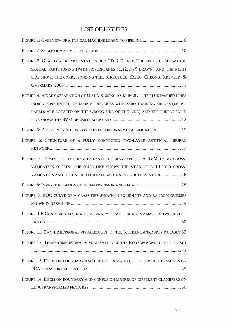
machine learning techniques. In general, the machine learning pipeline consists of pre-
processing (e.g. standardization and centroid reduction), dimensionality reduction (e.g.
principal component analysis), training (e.g. learning parameters), model-selection (e.g.
validation), and testing (e.g. accuracy assessment of the predictions) (Murphy, 2012), as
illustrated in Figure 1.
Figure 1: Overview of a typical machine learning pipeline
Before looking at the state-of-the-art methods in this field, it is helpful to look at the
developments and progression in the past. Qi (2013) presented a concise history of
machine learning for corporate bankruptcy prediction, highlighting some major research
initiatives in the past 50 years. Since the work of Beaver and Altman in the 1960s, an
increasing interest in quantitative assessment of financial credit risk can be observed. In
the 1970s, methods such as ordinary least squares regression (Meyer & Pifer, 1970),
discriminant analysis (Deakin, 1972), and logistic regression (Martin, 1977) were
deployed for bankruptcy classification tasks. Variations of discriminant analysis also
soared above univariate analysis in terms of performance due to its ability to account for
correlation between variables. During this time, Altman was already able to achieve
classification accuracy above 95% one period before bankruptcy and above 70% three
periods before bankruptcy (Haldeman, Altman, & Narayanan, 1977). By the 1980s,
logit analysis (Ohlson, 1980), factor analysis (West, 1985), and other similar methods
were introduced to the field of bankruptcy prediction. In the 1990s, the community saw

Chapter 2: Background
Jacky C. K. Chow - February 2018 7
Altman’s original Z-score method being extended to private firms, non-manufacturers,
and firms in emerging markets (Altman, 1995). On one hand this indicated the
applicability of the same machine learning method to different markets, but on the other
hand it highlighted the fact that the probability distributions coming from different
markets are unique, making it difficult to generalize the training results beyond the
market being studied. For example, applying an accurate prediction model trained on
American steel industry business data to the European apparel market will likely result
in high classification error.
By the 2000s, Bayesian methods had been adopted to combine financial ratios and
maturity schedule factors (Philosophov, Batten, & Philosophov, 2007). In the 2010s,
features beyond financial ratios (such as accounting-based measures, equity prices, firm
characteristics, industry expectations, macroeconomic indicators, and agents’ opinions)
were used for prediction (Altman, Fargher, & Kalotay, 2011; Li, Lee, Zhou, & Sun,
2011). The growing number of features being used in the model was likely a result of
the limited expressiveness of financial ratios on the complex system of financial
distress. Measuring financial ratios is not equivalent to observing “real market
characteristics”; these hidden variables need to be inferred from indirect measurements.
Including more features typically paints a better picture of the actual business situation,
but it does come at a price. Not only can it be expensive and cumbersome to collect that
information (if not impossible due to confidentiality), it turns bankruptcy prediction into
a high-dimensional classification problem. This increases the complexity of utilizing
machine learning methods effectively as they need to combat the curse of
dimensionality. The number of features under consideration in relevant articles usually
ranges from 1 to 57 (du Jardin, 2009). With these challenges, novel solutions have also
surfaced in recent years. These include various modifications of artificial neural
networks such as probabilistic neural network (Yang, Platt, & Platt, 1999) and self-
organizing maps (Kaski, Sinkkonen, & Peltonen, 2001). Other modern day alternative
solutions include decision trees (Li, Sun, & Wu, 2010), case-based reasoning (Li & Sun,
2011), support vector machines (Trustorff, Konrad, & Leker, 2011), soft computing
(Demyanyk & Hasan, 2010), genetic algorithms (Davalos, Gritta, & Adrangi, 2007),
AdaBoost (Sun, Jia, & Li, 2011), and Gaussian process (Peña, Martínez, & Abudu,
2011).
Analysis of Financial Credit Risk Using Machine Learning
8 Jacky C. K. Chow - February 2018
It is not the intention of this thesis to review all state-of-the-art machine learning
methods. Instead, the fundamental principles of a subset of popular modern day
machine learning methods relevant to bankruptcy prediction will be explained in the
following subsections.
2.2.1 Linear Regression and Logistic Regression
Least-squares regression/estimation/adjustment is one of the most popular mathematical
tools in statistics, engineering, and econometrics. Given a set of N observations �⃗� (a.k.a.
the dependent variable or regressand) and some feature map Φ⃗⃗⃗⃗ of explanatory variables
�⃗� (a.k.a. regressor), the best set of weights, �⃗⃗⃗�, that minimizes the square residual errors
(i.e. L2-norm) can be calculated. The objective function for such linear models can be
expressed mathematically by Equation 1. It can further be shown that this gives the Best
Linear Unbiased Estimate (BLUE) of the unknown weights (Förstner & Wrobel, 2016).
If the residuals, 𝑒, follow a Gaussian probability distribution, then the least-squares
solution can be proved to coincide with the Maximum Likelihood Estimate (MLE)
(Bishop, 2006).
wxywxyee
T
w
T
w
)()(minmin
1
The choice of a linear model is generally not prohibitive for two reasons: first, many
important business problems can be expressed using a linear relationship after some
feature mapping, and second, complex nonlinear models can be linearized using a first-
order Taylor series expansion. For instance, a linear model can be used to answer
questions like what is the expected price of detached houses in Calgary (i.e. �⃗�) given
data such as age of house, lot size, number of bedrooms, and number of bathrooms (i.e.
�⃗� )? Given a set of training data N that is greater than or equal to the number of
unknowns M, the optimal weights in Equation 1 can be estimated using Equation 2.
yxxxw T )()()(
1
2

Chapter 2: Background
Jacky C. K. Chow - February 2018 9
If a complex nonlinear functional model is used, the problem can still be linearized
locally using a first-order Taylor series expansion. The only difference is that Equation
2 will need to be applied multiple times, starting at some good initial approximation of
the weights. This yields what is commonly known as the Gauss-Newton update in an
iterative least-squares scheme for solving nonlinear problems (Nocedal & Wright,
2006).
Linear regression takes continuous inputs (e.g. recent years’ Du Pont Ratio, profit
margin, efficiency ratio, acid-test ratio, cash ratio, debt ratio, earnings per share, etc.)
and outputs a continuous variable (e.g. next year’s expected profit). This can already be
useful for forecasting a company’s financial distress. If the predicted profit is a large
negative number and there is not enough cash flow to cover the deficit, it is likely that
the company will go bankrupt. However, this requires an intelligent and experienced
agent to decide what that threshold is for a particular company; i.e. how low does the
predicted profit need to be to declare a financial crisis? Instead of a human expert, a
computer can be trained to set that threshold automatically by supplying the artificial
agent with many binary labels (e.g. 0 if the company did not file for bankruptcy and 1 if
the company did) as the dependent variable �⃗�. In this case, the linear regression model
needs to be modified to accommodate for his discrete output.
Previously, �⃗� was assumed to follow a Gaussian distribution; but now since it can only
take on a value of zero or one, it follows a Bernoulli distribution instead. Furthermore,
the linear combination of the input variables needs to be restricted between zero and one
hundred percent to make it a probability, which can be achieved using a sigmoid/logit
function (Equation 3); the shape of a sigmoid function is shown in Figure 2. After these
modifications, this mathematical formulation is often known as logistic regression or
logit regression, Equation 4 (Murphy, 2012). This is an example of a discrete choice
model in economics (Train, 2004). When used to make a prediction, the output is now
binary: in the near future, either the company will declare bankruptcy or not. This
makes the interpretation of the results simple enough that even non-experts in finances
(e.g. human resources managers and IT managers) can easily understand. Such a
financial distress forecast is more than just a bankruptcy predictor for investors. It can
also be used by managers to monitor the health of their business. This feedback can help

Analysis of Financial Credit Risk Using Machine Learning
10 Jacky C. K. Chow - February 2018
steer business strategies away from insolvency and increase the probability of
profitability.
Figure 2: Shape of a sigmoid function
1
e
esigm
3
N
i
i
T
iw
xwy1
exp1logmin
4
Equation 4 does not have a simple close-form solution like linear regression, instead
numerical optimization techniques like gradient descent, Newton’s method, or the
Levenberg-Marquardt algorithm can be utilized to learn the weights (Nocedal & Wright,
2006).
2.2.2 K-Dimensional Tree
K-Dimensional (K-D) Trees are one of the most popular nearest neighbour
classification algorithms. In low dimensions D, (i.e. D < 20; in other words when only a
handful of financial factors are used for bankruptcy prediction), a K-D Tree can be a
very efficient algorithm even when training the classifier with a large number of
companies (N > million). The main reason for such efficiency lies in its binary tree
structure, which sub-divides the company data as being above or below a hyperplane
defined by the median in all dimensions (Figure 3). Another nice property of the K-D
Tree model is that it is a non-generalizing method (i.e. it simply memorizes all the
previous examples without learning any parameters) and consequently can handle any

Chapter 2: Background
Jacky C. K. Chow - February 2018 11
probability distribution and nonlinearity in the model. Most of the computational efforts
of this method lie in the construction of the tree structure. Once the search tree has been
set up based on the training samples, classifying a new company as either bankrupt or
not is just a matter of retrieving its k-nearest neighbours and using a majority voting
scheme to decide on the label. Intuitively this makes sense: if most companies with
similar financial factors are not going bankrupt, then it is most likely that this new
company under investigation will also not go bankrupt, and vice versa.
The most commonly used distance metric for measuring the closeness between two
companies is the Euclidean norm. Compared to a brute force approach of finding the k-
nearest neighbours, a K-D Tree can reduce the computation complexity from O(DN2) to
O(log(N)). However, this reduction is only achievable when dimension D is sufficiently
low; in very high dimensional space, the efficiency of a K-D Tree diminishes due to the
curse of dimensionality. Even though a K-D Tree does not learn any parameters, it still
has a parameter that needs to be tuned: the number of neighbours ‘k’ to search. A larger
‘k’ can usually reduce the effect of random noise, but the boundaries become less
distinct. A smaller ‘k’ can decrease the bias at the expense of increasing the variance.
Hence, choosing ‘k’ is effectively balancing the bias-variance dilemma/trade-off.
Figure 3: Graphical representation of a 2D K-D tree. The left side shows the spatial
partitioning (with hyperplanes ℓ1, ℓ2, … ℓ9 drawn) and the right side shows the
corresponding tree structure. (Berg, Cheong, Kreveld, & Overmars, 2008)

Analysis of Financial Credit Risk Using Machine Learning
12 Jacky C. K. Chow - February 2018
2.2.3 Support Vector Machine
Among the various Kernel Machines, support vector machine (SVM) is one of the most
widely used for classification tasks. The mathematical formulation can be quite
involved, but from a geometric point of view it can be quite simple to visualize and
explain. When there are two linearly separable classes (O and X) in a two-dimensional
feature space, there can be many different solutions that all yield good accuracy (or
similarly, minimum errors) on the training data (Figure 4). The SVM solution matches
what an intelligent human agent would naturally choose as the decision boundary, i.e.
the one that is the farthest away from either cluster (shown in purple). This makes the
decision made by SVM more robust against errors (both random and systematic). For
example, some financial ratios such as the debt-to-equity ratio rely on subjective
valuations of intangible assets by accountants, which are error-prone.
Figure 4: Binary separation of O and X using SVM in 2D. The blue dashed lines
indicate potential decision boundaries with zero training errors (i.e. no labels are
located on the wrong side of the line) and the purple solid line shows the SVM decision
boundary.
This concept of choosing the decision boundary with the largest margin is one of the
distinguishing characteristic of SVM. Compared to logistic regression, which is more
concerned with maximizing the probability of the two classes, SVM concentrates on
maximizing the separation between the support vectors and therefore the classification

Chapter 2: Background
Jacky C. K. Chow - February 2018 13
accuracy (i.e. minimizing the generalization error). Since only the support vectors (a
subset of training points closest to the boundary) have a significant impact on the
decision boundary, the solution can be considered sparse and full knowledge of the
posteriori/class probabilities is not necessary; this improves the efficiency of the
algorithm.
For SVM to learn from the training data, the primal problem given in Equation 5 is
often converted to its equivalent dual problem, provided in Equation 6. In this case, the
labels �⃗� are {-1, 1} instead of {0, 1} as in the logistic regression formulation. Although
the dual problem appears to be more complicated than the primal problem, there are
many advantages that reduce the complexity of this formulation. When the dimension of
the input feature space (D) is much greater than the number of training points (N), the
dual problem only needs to estimate N number of 𝛼 instead of D number of 𝑤. Even
though this is not usually the case (i.e. N is typically greater than D), only the support
vectors will have a non-zero 𝛼, therefore it can still be more efficient. Furthermore,
Φ(𝑥𝑖)𝑇Φ(𝑥𝑗) can be kernelized into 𝐾(𝑥𝑖, 𝑥𝑗) and calculated directly, which bypasses
the need to explicitly solve for Φ(𝑥). Finally, because this formulation of the objective
function is convex, a globally optimal solution can always be determined (i.e. the
algorithm would not converge to a local optimum). Note that C in the equations is a
hyper-parameter that sets the degree of regularization. This allows some “slack” in the
model in cases where there are outliers and the two classes are not perfectly separable.
When C is large, a hard and narrow margin is obtained between the two classes, while a
small C returns a soft and wide margin.
N
i
i
T
i
T
wbxwyCww
1,0maxmin
5
jk
k
T
jkjkj
i
i xxyyi
2
1max
0
0
0..
i
ii
i
y
iCts
6

Analysis of Financial Credit Risk Using Machine Learning
14 Jacky C. K. Chow - February 2018
2.2.4 Decision Trees
Similar to a K-D Tree, a Decision Tree has a binary tree structure and a decision-
making logic that is easy to interpret. It is a supervised machine learning algorithm
which is considered non-parametric (even though the thresholds at each node are being
learned as parameters) because the size of the tree can grow to adapt to the complexity
of the classification problem (Alpaydin, 2010). Starting with a single node where all the
training data reside, the data are split into two nodes by asking a binary “if-and-else”
question. For instance, if the company’s net profit in the previous quarter is below a
million dollars step to the left, else step to the right. After this split, the purity of the
class labels in both nodes should have improved, meaning most of the financially
healthy companies are together in one node while the companies at a high risk of
insolvency are in the other node (Figure 5). However, sometimes the reduction in
entropy is not immediate at the current binary decision, but a few nodes later (Bishop,
2006). These “if-and-else” questions are continuously being asked for each input
feature, resulting in the growing of the tree. Once the purity at the leaf nodes satisfy
some quality measures such as the Gini index and/or cross-entropy, this branching
process can stop, and pruning can be performed to simplify the tree by trimming and
merging less informative nodes (i.e. remove questions that did not provide significantly
new insights).
When training is done and a new company has been classified by this decision tree, an
analyst or manager can trace all the questions answered by this company’s features (e.g.
financial ratios) to potentially pinpoint the strengths and weaknesses of this company
which resulted in it being assigned to a particular group. For example, if the company is
labelled as being a candidate for insolvency, traversing through the nodes of this
company might indicate their gearing ratio is too high for their business. Unlike black-
box machine learning techniques such as Artificial Neural Network, a decision tree can
provide an easy to understand explanation for its reasoning/decision. Unfortunately, the
binary decisions being localized (axis aligned) to a single feature also has its
disadvantage: since the features are orthogonal to each other in feature space, a
straightforward linear decision boundary at 45 degrees would require many nodes.

Chapter 2: Background
Jacky C. K. Chow - February 2018 15
Figure 5: Decision tree using one level for binary classification
2.2.5 AdaBoost
Motivated by the idea that a committee can make a better judgement than a single
individual, adaptive boosting (AdaBoost) is a technique where decisions of many weak
learners (e.g. decision trees with only one or two levels) are combined to form a
consensus that mimics a strong learner (Freund & Schapire, 1997). This has some
resemblance to the method of Bootstrap Aggregating (a.k.a. bagging) in machine
learning, where the variation in decisions from different committee members are left to
chance by only submitting a subset of randomly drawn training samples with
replacement to the various weak learners. The individual decisions are later combined to
form the final decision. But bagging and boosting are two very different methods. In
AdaBoost, the first base classifier uses a uniform weight for all training samples. All
subsequent weak learners use the previous classifier’s error as weights, where the
weights of the improperly labelled points are increased. If these points are mislabelled
again in training their weights will be increased even more for subsequent weak learner,
otherwise their weights are decreased.
To put things into context, imagine a team in the human resources department deciding
whether to employ an applicant or not. In the case of bagging, each employee will see
slightly different information about the applicant (e.g. employee A might be able to see
their volunteering experience and education background, and employee B might see
their volunteering experience and work experience). The team members will
independently come up with their recommendation, and the committee’s final hiring
decision would reflect all individual team members’ decision. In the case of AdaBoost,

Analysis of Financial Credit Risk Using Machine Learning
16 Jacky C. K. Chow - February 2018
employee A would look at the complete résumé and make recommendations. These
recommendations will then be forwarded to employee B, who will make
recommendations based on the full résumé and employee A’s decisions. By the time the
reports have circulated around the committee, the entire teams’ feedback would have
been incorporated into the final hiring decision.
2.2.6 Artificial Neural Network
As the name suggests, neural networks are inspired by the human brain. Individual
neurons in our brains make simple decisions and yet together they control our complex
motor functions, cognitive abilities, etc. The individual neurons can be mathematically
approximated by logistic regression, and therefore an artificial neural network (ANN)
can be thought of as multiple layers of connected logistic regression classifiers. Figure 6
illustrates the typical structure of a two-layer neural network known as the Multi-Layer
Perceptron. An ANN with this architecture can already be considered a universal
approximator, having the capability/flexibility to model any continuous functions. With
modern day computers, the trend is to have more hidden units and hidden layers, giving
it a deep network architecture. Although an interconnected network with many edges
and nodes can be daunting at first, when broken down into its fundamental building
blocks an ANN is just calculating the weighted sum of several input features. If this
value is larger than a threshold, the activation function “fires” (i.e. returns a value of one
instead of zero).

Chapter 2: Background
Jacky C. K. Chow - February 2018 17
Figure 6: Structure of a fully connected two-layer artificial neural network
ANN share similarities with a lot of the other machine learning algorithms already
discussed. For example, it combines many simple decisions into a complex nonlinear
decision boundary. However, unlike SVM (which is convex), ANN is sensitive to the
initial parameters and can often get trapped in a local minimum. But one noteworthy
benefit of ANN is that it supports sequential learning; this means the ANN can
continuously update itself as new data becomes available over time without having to
re-train the entire model from scratch like SVM and K-D tree. This attribute of ANN
can be critical in stock market forecasting. Also, ANN can be faster than SVM because
the model is generally more compact.
2.2.7 Gaussian Processes
Gaussian process is an interesting machine learning method that has been gaining
popularity in bankruptcy prediction in recent years. One of the main reasons why it was
not widely adopted in the past is because of its high learning complexity (Equation 7),
which is O(N3). But with modern day computers and improved numerical
approximations, this bottleneck is slowly disappearing. Not only is Gaussian process a

Analysis of Financial Credit Risk Using Machine Learning
18 Jacky C. K. Chow - February 2018
Bayesian non-parametric regression and classification technique (meaning it can be
infinitely flexible to fit any data without over-fitting), it assigns proper probability
measures to all outputs. Furthermore, it is comparable to a single layer neural network
with an infinite number of neurons when used with a specific kernel (Equation 8)
(Rasmussen & Williams, 2006). The ability to not over-fit is related to the principle of
Occam’s razor being natively built into the maximum likelihood formulation of GP. As
training and model selection can be done simultaneously, the decision boundary can be
as complex as the data allow but no further. Perhaps the biggest advantage of GP for
bankruptcy forecasting is the ability to give a probabilistic confidence level of the
prediction. For instance, if both companies A and B are being classified as candidates
for insolvency with a 51% and 99% probability, respectively, then we can further say
company A is in a better shape than company B and is only a borderline bankruptcy
candidate, whereas company B has a very high likelihood of declaring bankruptcy.
21
21
1
1
log),(loglog2
1
log,2
1min
iiii
N
i
ii
T
wysigmxKwysigmI
wysigmwxKw
7
''2121
'2sin
2)',( 1
xxxx
xxxxK
TT
T
8

Chapter 3: Objectives
Jacky C. K. Chow - February 2018 19
3 OBJECTIVES
The aim of this thesis is to diagnose the financial health of businesses using machine
learning algorithms. A detailed study of using several data-driven models to forecast
corporate bankruptcy (firm default) was conducted. Both qualitative assessments from
financial experts and quantitative econometric factors will be considered for training
models for predicting financial credit risk.

Analysis of Financial Credit Risk Using Machine Learning
20 Jacky C. K. Chow - February 2018
4 METHODOLOGY
To ease comparison of the applied machine learning method to other techniques, as well
as to allow validation by other researchers, secondary data was used in this project. Two
publicly available datasets from the Machine Learning Repository hosted by the Center
for Machine Learning and Intelligent Systems at the University of California, Irvine,
were processed.
The first dataset (denoted as Dataset 1) contains 250 records of six qualitative measures
of different companies from loan experts with about nine years of experience. Note in
the original paper by Kim & Han (2003), they used a genetic algorithm to forecast
bankruptcy of 772 manufacturing and service companies in Korea and only 250 of those
records have been shared. The following six qualitative measures were established by
one of the largest Korean banks (Kim & Han, 2003):
• Industrial Risk
• Management Risk
• Financial Flexibility
• Credibility
• Competitiveness
• Operating Risk

Chapter 4: Methodology
Jacky C. K. Chow - February 2018 21
More details about these measures are provided in Appendix 1. Basically, industrial risk
measures the health and future potential of the industry, management risk measures the
organizational structure and managers’ capabilities, financial flexibility is a measure of
the company’s cashflow, credibility is a measure of the company reputation and credit
scores, competitiveness is a measure of the company’s market position and competitive
advantages, and operating risk is a measure of its efficiency in production. As presented
in the original paper, the authors’ proposed genetic algorithm method resulted in a
classification accuracy of 94%. They also compared it to two other data-mining
techniques, namely induction learning and neural networks, and reported an accuracy of
89.7% and 90.3%, respectively.
In contrast, the second dataset (denoted as Dataset 2) contains 5910 instances of 64
quantitative attributes from Polish manufacturing companies between the years 2000-
2012, with some still operating companies being evaluated between 2007-2013 (Zięba,
Tomczakb, & Tomczaka, 2016). 5500 of those companies did not declare bankruptcy,
while the remaining 410 filed for insolvency after one year. Most of the quantitative
attributes are financial ratios and econometric indicators as found in majority of existing
literature. A complete list of those attributes can be found in Appendix 2.
The methods for analysing these two datasets are similar and will be explained below.
Note that the difference in the quality of results between Dataset 1 and Dataset 2 can be
attributed to factors such as different geographic location, different dataset size,
different features, and different quality of data.
4.1 Pre-Processing
The range of possible values for various input features can vary drastically. For
example, gross margin defined by Equation 9 will always be less than one (i.e. below
100%) due to normalization, whereas some financial measures like working capital can
theoretically take on any real value (i.e. negative infinity to positive infinity). To
complicate the situation further, some scholars have proposed including additional
features such as corporate governance structures and management practices in the
prediction model (Aziz & Dar, 2006), which can have any arbitrary scale. Having huge
variations in scales across dimensions leads to several issues in machine learning, such

Analysis of Financial Credit Risk Using Machine Learning
22 Jacky C. K. Chow - February 2018
as a higher chance for numerical instability and saturation (i.e. a situation where some
features dominate and mask the importance of some other feature(s) due to sheer
magnitude).
𝐆𝒓𝒐𝒔𝒔 𝑴𝒂𝒓𝒈𝒊𝒏 =𝑻𝒐𝒕𝒂𝒍 𝑹𝒆𝒗𝒆𝒏𝒖𝒆 − 𝑪𝒐𝒔𝒕 𝒐𝒇 𝑮𝒐𝒐𝒅𝒔 𝑺𝒐𝒍𝒅
𝑻𝒐𝒕𝒂𝒍 𝑹𝒆𝒗𝒆𝒏𝒖𝒆 9
One possible solution is to standardize each feature such that all have zero mean and
unit variance. To achieve this, the average can simply be subtracted from every training
sample and then divided by its standard deviation (Equation 10); however, if the
variance of a particular feature is very small (i.e. close to zero), then this division may
have numerical issues. An alternative is to simply scale the data to be between a
minimum (min𝑑𝑒𝑠𝑖𝑟𝑒𝑑) and maximum (max𝑑𝑒𝑠𝑖𝑟𝑒𝑑) value of choice: for instance, zero
and one (Equation 11).
x
ii
xxz
10
desireddesireddesiredi
ixx
xxz minminmax
minmax
min
11
4.2 Dimensionality Reduction
Classification with only one, two, or even three dimensional features is generally
intuitive, because the classification boundary and training data can be visualized.
Unfortunately, financial distress information resides in a higher dimensional feature
space. In other words, only analysing three financial ratios is insufficient to provide a
clear separation between successful companies and companies that will likely
experience bankruptcy in the future. In high dimensional feature space, such as the 64-
dimensional Polish bankruptcy dataset, it becomes difficult for humans to “see” what is

Chapter 4: Methodology
Jacky C. K. Chow - February 2018 23
happening. However, many mathematical tools exist to reduce the dimensionality of the
data; not only can this potentially provide a means to perceive high dimensional data, it
also reduces the complexity of the problem, and can reduce some of the noise in the
data.
One popular method for linear dimensionality reduction is Principal Component
Analysis (PCA). It performs a transformation/projection that maximizes the variance
along each orthogonal axis (equivalent to minimizing the loss of information) by
reducing the correlation between features (Hotelling, 1933). This makes sense because
even though the dimensions of many machine learning problems are high, the
interesting characteristics typically lie in a lower dimensional manifold. For example,
researchers have proposed adding macroeconomic measures to the existing financial
ratios for financial distress prediction. As a company’s operation is inevitably affected
by the macro environment, part of its effect is already reflected in the company’s
financial performance; therefore, when macroeconomic features are included, the
information they provide is not totally independent from the other features. Another
example is the similarities of some financial ratios. Upon close examination of the
Polish bankruptcy features, one would identify that some ratios like feature 4 (i.e.
current assets divided by current liabilities) and feature 55 (i.e. current assets minus
current liabilities) are closely related. A simple dimensionality reduction scheme is to
manually eliminate some features that are less descriptive, but this can become tedious,
subjective, and gives rise to an “all or nothing” situation (sometimes correlated features
can still improve the discriminative ability of the classifier). PCA combines features in
such a way that a lower dimensional representation still retains most of the information.
One noticeable drawback of PCA is that a clear financial interpretation of the feature
space might be lost; each new feature after PCA is a linear projection of many features
(e.g. financial ratios).
Mathematically the PCA solution can be obtained in different ways, one of which is by
Eigen decomposition. The magnitude of the eigenvalue can be used as an indication of
the information content. If the eigenvalues are sorted in descending order then typically
most information is captured in the direction of the first few eigenvectors. The last few

Analysis of Financial Credit Risk Using Machine Learning
24 Jacky C. K. Chow - February 2018
eigenvalues would be close to zero and the elimination of these last few projected
features would result in only a small loss of information.
PCA is an unsupervised method for dimensionality reduction. However, if the training
data contains labels, it can be advantageous to include that information when projecting
the data into a lower dimensional subspace. After all, besides reducing the complexity
of the following machine learning algorithms by working in a lower dimensional
subspace, one of the objectives of this projection should be to maximize the separation
between the different classes. One of the methods to achieve this is the Linear
Discriminate Analysis (LDA). Class labels are required, thus LDA can be considered a
supervised version of PCA.
Both PCA and LDA perform a linear projection. When the projection is nonlinear we
can estimate the geodesic distance along the manifold and apply multi-dimensional
scaling. This method is known as Isometric Feature Mapping (ISOMAP). ISOMAP is
an unsupervised dimensionality reduction method that can handle the nonlinearities at
the expense of more computation efforts. An alternative to this approach is to apply the
“kernel trick” adopted in SVM to PCA; this yields a method known as Kernel PCA. If
the kernel is chosen to be nonlinear (e.g. a radial basis kernel), then the projection will
be nonlinear.
4.3 Learning from Data and Model Selection
Different machine learning algorithms have different methods of constructing a model
of the real world using the provided data. For instance, a K-D tree learns from the data
by partitioning the data and forming a binary tree structure for fast query, while a
logistic regression learns by estimating some weight parameters in an optimization
framework where some likelihood function is being maximized. In general, this learning
from data can either be parametric or non-parametric. Parametric methods will learn
some unknown parameters of a model and forget about the data (e.g. logistic
regression), while non-parametric methods like GP will have to store all the training
data. But even if the method is non-parametric, there will still be some optional tuning
Chapter 4: Methodology
Jacky C. K. Chow - February 2018 25
for optimal performance. Most machine learning methods presented have some hyper-
parameters which are used to change the behaviour of the models. For example, in a GP
classifier with a radial basis function kernel, the length needs to be set. This parameter
controls the neighbourhood size when forming the decision boundary. In general, there
are three ways of selecting the “best” model: (1) manual tuning by an expert, (2) cross-
validation (CV), and (3) Bayesian statistics.
In the first case, a machine learning or econometrics expert would change a hyper-
parameter, re-train the model, and analyse the results until a satisfactory solution is
achieved. This can be time-consuming and subjective.
An automatic method is to do cross-validation either using a validation dataset or the k-
fold scheme. Unless there is an abundance of datasets, doing k-fold cross-validation is
typically a better choice because the same data used for training can be used for model
selection. In k-fold cross-validation the training dataset is randomly clustered into ‘k’
groups. Group one is used as the validation dataset while all the remaining data is used
for training. This process is then repeated with group 2 acting as the validation dataset
and all other data is used for training. K-fold cross-validation terminates when all ‘k’
groups had a chance to play the role of a validation dataset. At this point, the model
with the highest score or the average of all k-folds can be used to select the best model.
For example, this strategy can be used to tune the softness of the margin in SVM, i.e.
the ‘C’ hyper-parameter can be set using cross-validation. Figure 7 shows the cross-
validation score for various choices of ‘C’. For this dataset, a hard margin appears to
deliver a higher mean score, with the highest CV score around a C value of 12.

Analysis of Financial Credit Risk Using Machine Learning
26 Jacky C. K. Chow - February 2018
Figure 7: Tuning of the regularization parameter of a SVM using cross-validation
scores. The solid-line shows the mean of a 10-fold cross-validation and the dashed lines
show the standard deviation.
If the machine learning model is probabilistic like Gaussian Mixture Models, then a
prior distribution can be assigned to find the optimal hyper-parameters. This is similar
to a regularizer that sets the optimal model complexity to prevent over-fitting. One of
the benefits of this approach is that model selection and training can happen
simultaneously. At every iteration during numeric optimization, the hyper-parameters
are updated to improve the posteriori distribution. However, not all machine learning
methods are probabilistic, such as SVM and K-D tree. Therefore, to have a unified
framework for model tuning, cross-validation will be used when comparing different
models.
4.4 Accuracy Assessment
The machine learning models described in Section 2.2 can have very different
characteristics and behaviour, making it difficult to judge which model is performing
better. Therefore, a consistent set of tools applicable for assessing the performance of
any machine learning model is important. Some of the most popular quality control
measures in machine learning are defined below.
The most popular quality assessment method is the accuracy score: given a sample with
ground truth classes/labels, the predicted labels from a trained model are compared to
Chapter 4: Methodology
Jacky C. K. Chow - February 2018 27
the reference labels (Equation 12). Care must be taken to ensure this testing dataset was
never exposed in any of the pre-processing or training stages in the machine learning
pipeline. Also, the testing set should have the same probability distribution as the
training set. This can be achieved by randomly choosing a subset of points from the
original dataset (e.g. 70% use for training, and 30% used for testing). This single scalar
value indicates how well a machine learning algorithm can label companies in a non-
recoverable financial crisis as bankrupt and financially healthy companies as not
bankrupt.
𝐚𝒄𝒄𝒖𝒓𝒂𝒄𝒚 =𝟏
𝑵∑ 𝜹(𝒚𝒊
𝒑𝒓𝒆𝒅− 𝒚𝒊
𝒕𝒓𝒖𝒆)
𝑵
𝒊
where 𝜹(𝒙 = 𝟎) = 𝟏 and 𝜹(𝒙 ≠ 𝟎) = 𝟎
12
Besides the accuracy score, another set of metrics commonly used for quality control in
machine learning is the precision, recall, and F1 score. Precision is a measure of how
well the algorithm can find true positives (Equation 13). In the case of this thesis, it can
be translated into how well the model can predict a company as bankrupt when it is
actually going bankrupt. For example, a precision of 100% means that corporations
flagged as bankrupt will surely experience bankruptcy in the future with great certainty.
Another closely related concept to precision is recall, defined in Equation 14. Recall is a
measure of how reliable can the classifier identify all true positive samples. For
instance, a recall of 50% would indicate that half the bankruptcy candidates have been
found while the other half of bankruptcy facing firms were missed by the classifier.
Ideally, a good classifier should maximize both precision and recall, unfortunately in
reality precision and recall is often a trade-off an econometrics expert would have to
make while training the model. As shown in Figure 8, as the recall increases (x-axis),
the precision decreases (y-axis), and vice versa. If the objective of the prediction is to
highlight all companies susceptible to bankruptcy for further screening by a financial
officer then a high recall would be desirable at the expense of a lower precision, because
the financial officer can then manually remove the false positives. However, if the
objective is to automatically reject all loan applications from companies that are near
bankruptcy to avoid wasting the bank’s resources to perform a more thorough interview
and assessment, then a high precision (lower recall rate) might be more suitable. F1

Analysis of Financial Credit Risk Using Machine Learning
28 Jacky C. K. Chow - February 2018
score is defined as the weighted harmonic mean of precision and recall. It is a single
number that further aids the decision making process of model comparison. A perfect
model would have a F1 score of 100%, which corresponds to 100% precision and 100%
recall. Thus, in general a high F1 score is preferred.
𝐩𝒓𝒆𝒄𝒊𝒔𝒊𝒐𝒏 =
𝒕𝒓𝒖𝒆 𝒑𝒐𝒔𝒊𝒕𝒊𝒗𝒆𝒔
𝒕𝒓𝒖𝒆 𝒑𝒐𝒔𝒊𝒕𝒊𝒗𝒆𝒔 + 𝒇𝒂𝒍𝒔𝒆 𝒑𝒐𝒔𝒊𝒕𝒊𝒗𝒆𝒔
13
𝐫𝒆𝒄𝒂𝒍𝒍 =
𝒕𝒓𝒖𝒆 𝒑𝒐𝒔𝒊𝒕𝒊𝒗𝒆𝒔
𝒕𝒓𝒖𝒆 𝒑𝒐𝒔𝒊𝒕𝒊𝒗𝒆𝒔 + 𝒇𝒂𝒍𝒔𝒆 𝒏𝒆𝒈𝒂𝒕𝒊𝒗𝒆𝒔
14
𝐅𝟏 𝒔𝒄𝒐𝒓𝒆 =
𝟐 × 𝒑𝒓𝒆𝒄𝒊𝒔𝒊𝒐𝒏 × 𝒓𝒆𝒄𝒂𝒍𝒍
𝒑𝒓𝒆𝒄𝒊𝒔𝒊𝒐𝒏 + 𝒓𝒆𝒄𝒂𝒍𝒍
15
Figure 8: Inverse relation between precision and recall
Another way to visualize and select the trade-off between precision and recall is to
analyse the Receiver Operating Characteristic (ROC) curve (Figure 9). Depending on
the threshold value chosen given a boundary curve, the true positive rate and false
positive rate can be manipulated. However, because they are correlated, a low threshold

Chapter 4: Methodology
Jacky C. K. Chow - February 2018 29
value will not only ensure a high positive rate, it will also give a high false positive rate.
Therefore the optimal threshold value is typically in the top left-hand corner of the
curve where the true positive rate is much higher than the false positive rate. To
compare different models using this approach, the area under the ROC curve can be
calculated. The closer the area is to one, the better the discriminant power of the
classifier.
Figure 9: ROC curve of a classifier shown in solid-line and random guesses shown in
dash-line
The relationship between true positives, false positives, false negatives, and true
negatives can be summarized more thoroughly in a simple confusion matrix as well
(Figure 10). This gives the probability of the four scenarios in a binary classification
problem in an easy to visualize manner. In this figure, the true positive rate is 96.6%,
false positive rate is 3.4%, false negative rate is 4.8%, and the true negative rate is
95.2%.

Analysis of Financial Credit Risk Using Machine Learning
30 Jacky C. K. Chow - February 2018
Figure 10: Confusion matrix of a binary classifier normalized between zero and one

Chapter 5: Results and Analysis
Jacky C. K. Chow - February 2018 31
5 RESULTS AND ANALYSIS
For both Dataset 1 and Dataset 2, appropriate pre-processing steps have been taken to
ensure all the features are scaled between negative one and positive one. In order to
have ground truth data for assessing the accuracy of various classification models the
datasets have been split into 80% training and 20% testing. The 20% of testing data is
never used in any of the machine learning steps except in the final accuracy assessment
stage. In using this method, the possibility of over-fitting and introducing personal bias
when choosing model parameters can be reduced.
5.1 Dataset 1: Korean Corporate Bankruptcy
5.1.1 Visualization of the Data
Human beings’ visual cortex are incapable of understanding six-dimensional space,
therefore to be able to recognize patterns in the data visually the features need to be
projected onto a lower-dimensional sub-space; the most intuitive sub-space being two-
dimensional (Figure 11) and three-dimensional (Figure 12). Note, the data that has been
labelled bankrupt is denoted in orange and non-bankrupt data is denoted in purple. It
can be perceived that all four dimensionality reduction techniques are able to separate
the two clusters well. In particular, the post-projection data using PCA, LDA, and
Kernel PCA are linearly separable. Although a clear boundary between bankruptcy and
non-bankruptcy samples can be perceived from the ISOMAP results, the separation
boundary is nonlinear. Based on visual assessment, a significant benefit of using three

Analysis of Financial Credit Risk Using Machine Learning
32 Jacky C. K. Chow - February 2018
features instead of two features cannot be perceived. Therefore, the two-dimensional
sub-space will be chosen for simplicity and better visualization of the classification
results. To better understand the impact of the different dimensionality reduction
methods, various classifiers will be applied to the four two-dimensional datasets.
Figure 11: Two-dimensional visualization of the Korean bankrupty dataset

Chapter 5: Results and Analysis
Jacky C. K. Chow - February 2018 33
Figure 12: Three-dimensional visualization of the Korean bankrupty dataset
5.1.2 Binary Classification
Figures 13, 14, 15, and 16 illustrates the decision boundaries computed using different
machine learning models on the PCA, LDA, ISOMAP, and Kernel PCA projected
training and testing datasets, respectively. In the last column of these figures, their
corresponding confusion matrix is also provided to showcase its classification accuracy
as well as Type-I and Type-II errors. In the linearly separable sub-spaces (i.e. Figures
13, 14, and 16), logistic regression, decision tree, and AdaBoost are all able to learn a
simple linear boundary. In this case, AdaBoost which is built from decision stumps (as
described in Section 2.2.5) gives the same result as the decision tree classifier. The
irregular decision boundaries from K-D tree, and curved boundaries from SVM, ANN,
GP delivers similar level of classification accuracy, but it can be argued that it is more
complex than necessary in this case.
In the ISOMAP projection scenario (Figure 15), where the data are not linearly
separable in a two-dimensional space, the nonlinear classifiers outperformed logistic
regression. Decision tree and AdaBoost in this case is capable of automatically learning
the fact that a linear decision boundary is insufficient and separates the two-classes
using different nonlinear boundaries.

Analysis of Financial Credit Risk Using Machine Learning
34 Jacky C. K. Chow - February 2018

Chapter 5: Results and Analysis
Jacky C. K. Chow - February 2018 35
Figure 13: Decision boundary and confusion matrix of different classifers on PCA
transformed features

Analysis of Financial Credit Risk Using Machine Learning
36 Jacky C. K. Chow - February 2018
Figure 14: Decision boundary and confusion matrix of different classifers on LDA
transformed features

Chapter 5: Results and Analysis
Jacky C. K. Chow - February 2018 37

Analysis of Financial Credit Risk Using Machine Learning
38 Jacky C. K. Chow - February 2018
Figure 15: Decision boundary and confusion matrix of different classifers on ISOMAP
transformed features

Chapter 5: Results and Analysis
Jacky C. K. Chow - February 2018 39
Figure 16: Decision boundary and confusion matrix of different classifers on Kernel
PCA transformed features
Studying the above confusion matrices reveal that Type-II error (i.e. a company is likely
to experience bankruptcy but failed to be detected because it appears “healthy”) is more
predominant than Type-I error (i.e. flagged company as going bankrupt when in fact it
is not). From the perspective of the bank or other loan officers this is unfavourable.
Lending money to a company that eventually goes bankrupt can cost the bank more
capital than if it foregoes the interest rates on a loan. What most of the classifiers tested
above is extremely good at is predicting a company as not going bankrupt when in fact
they are financially stable.
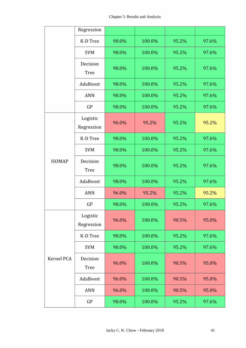
Table 1 summarizes the classification accuracy, precision, recall and F1 score for the
various binary classification methods using different dimensionality reduction
mechanisms. Since the raw input features are discrete (i.e. qualitative measures

Analysis of Financial Credit Risk Using Machine Learning
40 Jacky C. K. Chow - February 2018
converted to numerical values), the compute quality measures from the different
scenarios are quantized and can be grouped by colours. Green indicates the best
performance in that quality measure, yellow is average, and red indicates the worst
relative performance. Regardless of the dimensionality reduction method and
classification model, the results from all the cases are similar. This suggests that the
results are not highly sensitive to the exact model used. Based on Table 1, LDA is the
preferred dimensionality reduction method for this dataset because the two-classes are
well-separated enough that all classification models, linear or nonlinear, performed
equally well, delivering a consistent set of results. Using LDA, the simplest linear
separator, namely logistic regression is preferred. In this dataset an overall classification
error of 2.0% is achieved. The precision is 100%; reaffirming the fact that if a company
is identified as a candidate for insolvency they are almost guaranteed to go bankrupt.
While the recall rate of 95.2% suggest that about 5% of the companies experiencing
financial distress with pass under the radar and loan officers relying purely on this
system for making their decisions will make an error about 5% of the time, which is
typically still too high for a bank or financial institution.
Table 1: Quality control of various machine learning methods on the Korean bankrupty
dataset when combined with different dimensionality reduction techniques
Accuracy Precision Recall F1 Score
PCA
Logistic
Regression 98.0% 100.0% 95.2% 97.6%
K-D Tree 98.0% 100.0% 95.2% 97.6%
SVM 98.0% 100.0% 95.2% 97.6%
Decision
Tree 96.0% 100.0% 90.5% 95.0%
AdaBoost 96.0% 100.0% 90.5% 95.0%
ANN 98.0% 100.0% 95.2% 97.6%
GP 98.0% 100.0% 95.2% 97.6%
LDA Logistic 98.0% 100.0% 95.2% 97.6%
Chapter 5: Results and Analysis
Jacky C. K. Chow - February 2018 41
Regression
K-D Tree 98.0% 100.0% 95.2% 97.6%
SVM 98.0% 100.0% 95.2% 97.6%
Decision
Tree 98.0% 100.0% 95.2% 97.6%
AdaBoost 98.0% 100.0% 95.2% 97.6%
ANN 98.0% 100.0% 95.2% 97.6%
GP 98.0% 100.0% 95.2% 97.6%
ISOMAP
Logistic
Regression 96.0% 95.2% 95.2% 95.2%
K-D Tree 98.0% 100.0% 95.2% 97.6%
SVM 98.0% 100.0% 95.2% 97.6%
Decision
Tree 98.0% 100.0% 95.2% 97.6%
AdaBoost 98.0% 100.0% 95.2% 97.6%
ANN 96.0% 95.2% 95.2% 95.2%
GP 98.0% 100.0% 95.2% 97.6%
Kernel PCA
Logistic
Regression 96.0% 100.0% 90.5% 95.0%
K-D Tree 98.0% 100.0% 95.2% 97.6%
SVM 98.0% 100.0% 95.2% 97.6%
Decision
Tree 96.0% 100.0% 90.5% 95.0%
AdaBoost 96.0% 100.0% 90.5% 95.0%
ANN 96.0% 100.0% 90.5% 95.0%
GP 98.0% 100.0% 95.2% 97.6%

Analysis of Financial Credit Risk Using Machine Learning
42 Jacky C. K. Chow - February 2018
Different classifiers have different strengths. To analyse the insolvency situation in this
Korean market further, the decision tree model is used. As mentioned in Section 2.2.4,
one of the benefits of using decision trees is the transparency it provides when tracing
back the decision-making process. Take the ISOMAP projected 2D features as an
example, after the training is complete, the decision tree can be visualized as shown in
Figure 17. Beginning at the first node on the top with 200 samples and a Gini index of
0.49, if the 2nd component from the projected features is less than -0.33 traverse to the
left branch, else traverse to the right branch. This process repeats until the Gini index is
zero at a node, where each node is either going to be classified as bankrupt or not
bankrupt. As one can imagine, typically the more features and the more complicated the
decision boundary the larger the tree structure, therefore the more difficult for a human
analyst to interpret the results.
Figure 17: Trained decision tree on the ISOMAP transformed features in two-
dimensional space
Although using dimensionality reduction can typically reduce the complexity of the
problem, the physical meaning of the feature space is also partly lost due to the

Chapter 5: Results and Analysis
Jacky C. K. Chow - February 2018 43
projection, for instance the 1st and 2nd component does not have much meaning to a
financial expert. One possible solution is to study the projection function and indirectly
relate the tree structure to the originally measured features. For example, when using
PCA the weights for each feature contributing to the projection can be extracted from
the eigenvectors. For this particular Korean dataset the weights for the first and second
component are given in Table 2. It can be observed that the 1st component is dominated
by the financial flexibility, credibility, and competitiveness of the firm, and the 2nd
component is mostly expressing the industrial risk, management risk, and operating risk
of the firm.
Table 2: Weights of the original six-dimensional qualitative features on the projected
two-dimensional principal components
Industrial
Risk
Management
Risk
Financial
Flexibility Credibility Competitiveness
Operating
Risk
1st
Component 0.231 0.320 0.466 0.472 0.585 0.250
2nd
Component -0.582 -0.307 0.268 0.284 0.214 -0.607
Alternatively, the decision tree classifier can be applied to the original six-dimensional
dataset to directly learn the relationship between each qualitative measure and the
likelihood of the company experiencing financial distress (Figure 18). In this specific
case, the resulting tree structure is relatively simple (it is deeper but less wide than the
tree in Figure 17). From Figure 18, it can be seen that only four of the six qualitative
measures mattered for this particular training set. More specifically, in the order of
importance they are competitiveness, credibility, financial flexibility, and industrial risk.
Stepping through this decision tree in detail, the following can be said about these two
hundred Korean manufacturing and service companies:
1. The firm’s competitiveness has the strongest impact on insolvency. If the
company receives a negative competitive score it will likely go bankrupt
regardless of its score in other attributes.
2. If the firm has an average or high competitive level and good credibility, then
this firm will unlikely face bankruptcy.

Analysis of Financial Credit Risk Using Machine Learning
44 Jacky C. K. Chow - February 2018
3. But if this competitive firm has poor credibility then it better be financially
flexible or be in an industry where the industrial risk is low for them to stay
afloat.
Figure 18: Trained decision tree on the raw features
Compared to the original authors’ results (Kim & Han, 2003), the presented solution in
this thesis showed better classification accuracy. In Kim and Han (2003), the overall
binary classification accuracy of their genetic algorithm, inductive learning, and neural
network are reported to be 94.0%, 89.7%, and 90.3%, respectively. In this thesis, better
classification accuracy (i.e. 98%) is achieved using various classification models. This
improvement can be attributed to the smaller sample size (in reference to the original
paper) and the use of dimensionality reduction techniques. In the article from Kim and
Han (2003), all their data mining technique are applied to the original feature space,
which as demonstrated in this thesis, contains noise and irrelevant information for
bankruptcy prediction. Therefore, it is reasonable to eliminate some dimensions in the
dataset that are less informative to reduce the complexity of the problem.

Chapter 5: Results and Analysis
Jacky C. K. Chow - February 2018 45
5.2 Dataset 2: Polish Corporate Bankruptcy
5.2.1 Visualization of the Data
Following the same approach as 5.1.1 the quantitative financial factors are first scaled to
be between -1.0 and +1.0. Unlike Dataset 1, Dataset 2 is incomplete in the sense that
there are missing attributes for some companies. Instead of simply removing these
entries entirely from the dataset, their missing values are imputed from the remaining
companies as the median. This way the number of samples remains the same and the
imputed features will have little influence on the decision boundary (Jereza, et al.,
2010). Furthermore, there are significantly more data that are labelled as “not bankrupt”
(the ratio of not bankrupt to bankrupt companies in this database is 13:1). This class
imbalance can have a significant impact on some classification algorithms. Therefore
the features labelled as “bankrupt” are up-sampled using the Synthetic Minority Over-
sampling Technique (Chawla, Bowyer, Hall, & Kegelmeyer, 2002).
Dataset 2 with quantitative financial measures is more complex than Dataset 1, using
the same dimensionality reduction methods for mapping features into three-dimensional
space revealed that the bankrupt and non-bankrupt companies are very similar in a low
dimensional space (Figure 19). Therefore, a visual assessment of the classification
boundary is not possible and the assessment has to be based on other numerical
techniques.

Analysis of Financial Credit Risk Using Machine Learning
46 Jacky C. K. Chow - February 2018
Figure 19: Three-dimensional visualization of the Polish bankrupty dataset
To choose a suitable number of components without visualizing the point distribution
the PCA components can be plotted in descending order of information content as
shown in Figure 20. Visually, 50% of the variance can be summarized by the first
couple components. Principal components 31 to 64 together accounts for only 1% of
variance in the data and is assumed to be highly contaminated by noise. Therefore, the
various classification algorithms is applied to only the 30 largest principal components,
which should capture 99% of the information while reducing the dimensionality of the
problem by more than half.
Figure 20: The accumulated percentage of variance in the principal components
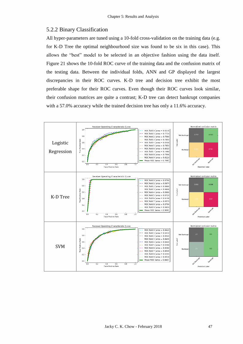
Chapter 5: Results and Analysis
Jacky C. K. Chow - February 2018 47
5.2.2 Binary Classification
All hyper-parameters are tuned using a 10-fold cross-validation on the training data (e.g.
for K-D Tree the optimal neighbourhood size was found to be six in this case). This
allows the “best” model to be selected in an objective fashion using the data itself.
Figure 21 shows the 10-fold ROC curve of the training data and the confusion matrix of
the testing data. Between the individual folds, ANN and GP displayed the largest
discrepancies in their ROC curves. K-D tree and decision tree exhibit the most
preferable shape for their ROC curves. Even though their ROC curves look similar,
their confusion matrices are quite a contrast; K-D tree can detect bankrupt companies
with a 57.0% accuracy while the trained decision tree has only a 11.6% accuracy.
Logistic
Regression
K-D Tree
SVM

Analysis of Financial Credit Risk Using Machine Learning
48 Jacky C. K. Chow - February 2018
Decision
Tree
AdaBoost
ANN
GP
Figure 21: ROC curve and confusion matrix from applying different machine learning
methods on the Polish bankruptcy dataset
Quality control measures of the different machine learning models are summarized in
Table 3. Besides accuracy, precision, recall, and F1 score, the mean area under a ROC
curve (AUC) is also reported to allow for easier comparison with the results from the
original article by Zięba et al. (2016). Some classifiers like logistic regression and SVM
are also tested in Zięba et al. (2016), and overall the mean AUC obtained in this thesis is
comparable. For instance, the AUC for logistic regression reported in this thesis is
79.9% while in the original article it is 63.2%. Considering that the classifier is the

Chapter 5: Results and Analysis
Jacky C. K. Chow - February 2018 49
same, the improvement in the performance can likely be attributed to the data scaling,
dimensionality reduction, and model selection steps.
Not only are the AUC scores in this thesis similar to the original article, the highest
AUC of 96.9% exceeded all the methods reported in Zięba et al. (2016). But it should
be noted that AUC alone is insufficient to describe the actual performance of the
classifier. Many classifiers in Table 3 have a high AUC (i.e. greater than 90%) but their
accuracy, precision, recall, and F1 score can vary significantly. For instance, AdaBoost
has a higher AUC than ANN (91.8% compared to 81.0%), but ANN exhibits better
accuracy, precision, recall, and F1 score. When analysing all the quality measures
together it can be seen that the nonlinear classifiers tend to have less consistent
measures. For example, SVM reported good AUC and accuracy (i.e. 84.3% and 92.6%,
respectively) but the precision, recall, and F1 score is practically zero because the
classifier is predicting all data as belonging to the non-bankrupt class as indicated by the
confusion matrix. This is likely a result of the curse of dimensionality where these
higher-order nonlinear classifiers are over-fitting due to the limited amount of training
data for such a high dimensional problem. Typically, with increasing number of features
(i.e. dimensions) there needs to be an exponential growth in the number of data to
maintain the same density (Verleysen & François, 2005). Although through
dimensionality reduction the number of features are significantly reduced compared to
the original paper, 5000 data points for a 30-dimensional space is still rather low.
After analysing other quality control factors it appears that due to the limited amount of
data and the high number of features, simpler classifiers such as K-D tree and logistic
regression (despite having the lowest AUC among the classifiers tested, it has a better
average quality control measure) are actually able to generalize better to new data than
more sophisticated machine learning algorithms. On the test data, their performances
are comparable, with logistic regression performing slightly better and require
significantly less storage to make faster predictions. Thus, it is the preferred machine
learning model for this dataset because is it well balanced.

Analysis of Financial Credit Risk Using Machine Learning
50 Jacky C. K. Chow - February 2018
Table 3: Quality control of different machine learning methods on the Polish
bankruptcy dataset
Accuracy Precision Recall F1 Score AUC
Logistic
Regression 66.4% 70.4% 59.4% 64.4% 79.9%
K-D Tree 62.9% 66.1% 57.0% 61.2% 96.9%
SVM 92.6% 0.0% 0.0% 0.0% 84.3%
Decision
Tree 51.5% 65.4% 11.6% 19.7% 96.1%
AdaBoost 91.8% 14.3% 2.3% 4.0% 91.8%
ANN 92.4% 38.5% 5.7% 10.0% 81.0%
GP 92.6% 0.0 0.0 0.0 82.1%

Chapter 6: Conclusion and Recommendations
Jacky C. K. Chow - February 2018 51
6 CONCLUSION AND
RECOMMENDATIONS
Business intelligence is a rapidly evolving field carrying tremendous potential for
improving efficiency and competitiveness of corporations across the globe. Data mining
and machine learning are useful tools in this field that can extract valueable information
from big data to aid business strategies. This thesis investigated the adoption of several
popular modern day machine learning algorithms for forecasting business failures, i.e.
corporate bankruptcy. This information can help governments, investors, managers, and
other stakeholders make intelligent economic decisions to avoid financial losses.
Two very different datasets of companies in the manufacturing sector were analysed and
compared to other researchers’ results. The first dataset uses six qualitative measures to
describe the business situation for companies in Korea. The second dataset uses 64
quantitative financial features for assessing the likelihood of corporate insolvency in
Poland. Results from this thesis indicated that all machine learning algorithms applied
to Dataset 1 yielded superior performance when compared to Dataset 2. This can be
attributed to the fact that these handcrafted features from experts’ advice are more
expressive than financial ratios. Despite only asking the financial experts six multiple
choice questions about each company, the collected data showed a more distinct
separation between the two classes. Actually, the decision tree classifier only required

Analysis of Financial Credit Risk Using Machine Learning
52 Jacky C. K. Chow - February 2018
four out of the six questions to detect companies with high chances of insolvency with
better than 90% accuracy. This suggested that in the future, fewer questions can be
asked, collected, and stored. The informativeness of these qualitative measures is
advantageous because even after projecting the data onto a lower dimensional subspace
for visualization a clear separation between the two clusters can still be perceived,
making it more intuitive to optimize, compare, and analyse the classification methods.
In Dataset 2, even with 64 financial ratios and an order of magnitude more data, it was
difficult for the machine learning algorithms to classify companies as going to bankrupt
or not with robustness. However, collecting experts’ advice is quite expensive compared
to using financial ratios that are readily available in most companies’ balance sheets and
income statements. Considering that collecting a large number of financial ratios is
typically less expensive than capturing experts’ opinions, it is recommended that more
data to be collected for training the classifier to combat the curse of dimensionality and
lack of expressiveness of individual features. Quality control should also be based on
multiple performance measures rather than relying on a single score. As demonstrated
in this thesis, when analysing and comparing machine learning techniques using a single
quality control metric, the conclusion can easily be biased.
In general, machine learning is a powerful toolbox for financial analysts to make
predictions and discover patterns in the data with rigour. Many different models and
validation techniques exist to aid data mining and decision making. It is difficult to
determine if any machine learning technique is superior to others. In fact, as a data
scientist and/or financial expert, it is perhaps more beneficial to harvest the strengths of
different methods and combine them to make better business judgements.

Chapter 7: References
Jacky C. K. Chow - February 2018 53
7 REFERENCES
Alpaydin, E. (2010). Introduction to Machine Learning. 2nd Edition. Cambridge,
United States: MIT Press.
Aziz, M., & Dar, H. (2006). Predicting corporate bankruptcy: Where we stand?
Corporate Governance, 6(1), 18-33.
Beaver, W. (1966). Financial ratios as predictors of failure. Journal of Accounting
Research, 4, 71-111.
Bellovary, J., Giacomino, D., & Akers, M. (2007). A review of bankruptcy prediction
studies: 1930 to present. Journal of Financial Education, 33, 87-114.
Berg, M., Cheong, O., Kreveld, M., & Overmars, M. (2008). Computational Geometry
(3rd ed.). Springer-Verlag Berlin Heidelberg.
Bishop, C. (2006). Pattern Recognition and Machine Learning. New York, United
States: Springer.
Chawla, N., Bowyer, K., Hall, L., & Kegelmeyer, W. (2002). SMOTE: Synthetic
Minority Over-sampling Technique. Journal of Artificial Intelligence Research,
16, 321-357.
Chen, H., Chiang, R., & Storey, V. (2012). Business intelligence and analytics: From
big data to big impact. MIS Quarterly: Special Issue on Business Intelligence
Research, 36(4), 1165-1188.
Chen, N., Ribeiro, B., & Chen, A. (2016). Financial credit risk assessment: a recent
review. Artificial Intelligence Review, 45(1), 1-23.
Analysis of Financial Credit Risk Using Machine Learning
54 Jacky C. K. Chow - February 2018
Columbus, L. (2016). Machine learning is redefining the enterprise in 2016. New York
City, United States: Forbes.
Davalos, S., Gritta, R., & Adrangi, B. (2007). Deriving rules for forecasting air carrier
financial stress and insolvency: A genetic algorithm approach. Journal of the
Transportation Research Forum, 46(2), 40-54.
Davenport, T., & Patil, D. (2012). Data scientist: The sexiest job of the 21st century.
Watertown, United States: Harvard Business Review: October.
de Andrés, J., Landajo, M., & Lorca, P. (2012). Bankruptcy prediction models based on
multinorm analysis: An alternative to accounting ratios. Knowledge-Based
Systems, 30, 67-77.
Deakin, E. (1972). A discriminant analysis of predictors of business failure. Journal of
Accounting Research, 10(1), 167-179.
Demyanyk, Y., & Hasan, I. (2010). Financial crises and bank failures: A review of
prediction methods. Omega, 38, 315-324.
du Jardin, P. (2009). Bankruptcy prediction models: How to choose the most relevant
variables? Bankers, Markets & Investors, 98, 39-46.
Ellis, D. (2008). Lehman Brothers collapse stuns global markets. Atlanta, United
Stateds: Cable News Network (CNN).
Förstner, W., & Wrobel, B. (2016). Photogrammetric Computer Vision. Cham,
Switzerland: Springer International Publishing.
Freund, Y., & Schapire, R. (1997). A decision-theoretic generalization of on-line
learning and an application to boosting. Journal of Computer and System
Sciences, 55(1), 119-139.
Guzman, A. (1999). International bankruptcy: In defense of universalism. Retrieved
from Berkeley Law Scholarship Repository:
http://scholarship.law.berkeley.edu/facpubs/1758
Haldeman, R., Altman, E., & Narayanan, P. (1977). Zeta analysis: A new model to
identify bankruptcy risk of corporations. Journal of Banking and Finance, 1, 29-
35.
Hotelling, H. (1933). Analysis of a complex of statistical variables into principal
components. Journal of Educational Psychology, 24, 417-441.

Chapter 7: References
Jacky C. K. Chow - February 2018 55
James Wilson, H., Mulani, N., & Alter, A. (2016). Sales gets a machine-learning
makeover. Cambridge, United States: MIT Sloan Management Review.
Jereza, J., Molinab, I., García-Laencinac, P., Albad, E., Ribellesd, N., Martíne, M., &
Francoa, L. (2010). Missing data imputation using statistical and machine
learning methods in a real breast cancer problem. Artificial Intelligence in
Medicine, 50(2), 105–115.
Kaski, S., Sinkkonen, J., & Peltonen, J. (2001). Bankruptcy analysis with self-
organizing maps in learning metrics. IEEE Transactions on Neural Networks,
12(4), 936-947.
Kim, M., & Han, I. (2003). The discovery of experts’ decision rules from qualitative
bankruptcy data using genetic algorithms. Expert Systems with Applications, 25,
637-646.
Li, M., & Miu, P. (2010). A hybrid bankruptcy prediction model with dynamic loadings
on accounting-ratio-based and market-based information: A binary quantile
regression approach. Empirical Finance, 17, 818-833.
Mańko, R. (2013, February 21). Cross-border insolvency law in the EU. Retrieved from
European Parliament:
http://www.europarl.europa.eu/RegData/bibliotheque/briefing/2013/130476/LD
M_BRI(2013)130476_REV1_EN.pdf
Martin, D. (1977). Early warning of banking failure. Journal of Banking and Finance,
7, 249-276.
Meyer, P., & Pifer, H. (1970). Prediction of bank failures. The Journal of Finance,
25(4), 853-868.
Murphy, K. (2012). Machine Learning: A Probabilistic Perspective . Cambridge,
United States: MIT Press.
Newton, G. (2003). Corporate Bankruptcy: Tools, Strategies, and Alternatives. New
York, United States of America: Wiley.
Nocedal, J., & Wright, S. (2006). Numerical Optimization . 2nd Edition. New York,
United States: Springer.
Ohlson, J. (1980). Financial ratios and the probabilistic prediction of bankruptcy.
Journal of Accounting Research, 18(1), 109-131.

Analysis of Financial Credit Risk Using Machine Learning
56 Jacky C. K. Chow - February 2018
Peña, T., Martínez, S., & Abudu, B. (2011). Bankruptcy prediction: A comparison of
some statistical and machine learning technique. Computational Methods in
Economic Dynamics, 13, 109-131.
Philosophov, L., Batten, J., & Philosophov, V. (2007). Predicting the event and time
horizon of bankruptcy using financial ratios and the maturity schedule of long-
term debt. EFA 2005 Moscow Meetings Paper.
Rasmussen, C., & Williams, C. (2006). Gaussian Processes for Machine Learning.
Cambridge, United States: The MIT Press.
Shell, A. (2009). Lehman Bros. collapse triggered economic turmoil. New York City,
United States: American Broadcasting Company (ABC).
Sun, J., Jia, M., & Li, H. (2011). AdaBoost ensemble for financial distress prediction:
An empirical comparison with data from chinese listed companies. Expert
Systems with Applications, 38(8), 9305-9312.
Train, K. (2004). Discrete Choice Methods with Simulation. Cambridge, United
Kingdom: Cambridge University Press.
Trustorff, J., Konrad, P., & Leker, J. (2011). Credit risk prediction using support vector
machines. Review of Quantitative Finance and Accounting, 36(4), 565-581.
Tung, F. (2001). Is international bankruptcy possible? Michigan Journal of
International Law, 23(1), 31-101.
United States Courts. (2016, July 27). June 2016 Bankruptcy Filings Down 6.9 Percent.
Retrieved from http://www.uscourts.gov/news/2016/07/27/june-2016-
bankruptcy-filings-down-69-percent
Verleysen, M., & François, D. (2005). The curse of dimensionality in data mining and
time series prediction. 8th International Workshop on Artificial Neural Networks
(pp. 758-770). Barcelona, Spain: Lecture Notes in Computer Science.
West, R. (1985). A factor analytic approach to bank condition. Journal of Banking and
Finance, 9, 253-266.
White, M. (1989). The Corporate Bankruptcy Decision. The Journal of Economic
Perspectives, 3(2), 129-151.
Chapter 7: References
Jacky C. K. Chow - February 2018 57
Williams, M. (2010). Uncontrolled risk: Lessons of Lehman Brothers and how systemic
risk can still bring down the world financial system. New York City, United
States: McGraw-Hill Education.
Wilson, R., & Sharda, R. (1994). Bankruptcy prediction using neural networks.
Decision Support Systems, 11, 545-557.
Yang, Z., Platt, M., & Platt, H. (1999). Probabilistic neural networks in bankruptcy
prediction. Journal of Business Research, 44(2), 67-74.
Zięba, M., Tomczakb, S., & Tomczaka, J. (2016). Ensemble boosted trees with
synthetic features generation in application to bankruptcy prediction. Expert
Systems with Applications, 58, 93-101.
Analysis of Financial Credit Risk Using Machine Learning
58 Jacky C. K. Chow - February 2018
8 APPENDICES
APPENDIX 1: KOREAN BANKRUPTCY DATASET FEATURES .............................................. 59
APPENDIX 2: POLISH BANKRUPTCY DATASET FEATURES ................................................ 60

Chapter 8: Appendices
Jacky C. K. Chow - February 2018 59
APPENDIX 1: KOREAN BANKRUPTCY DATASET FEATURES
The following is a detailed description of the six qualitative features from the Korean
bankruptcy dataset:
Risk Factor Risk Component
Industry Risk
Government policies and International agreements
Cyclicality
Degree of competition
The price and stability of market supply
The size and growth of market demand
The sensitivity to changes in macroeconomic factors
Domestic and international competitive power
Product Life Cycle
IR
Management Risk
Ability and competence of management
Stability of management
The relationship between management/owner
Human resources management
Growth process/business performance
Short and long term business planning, achievement and
feasibility
Financial Flexibility Direct financing
Indirect financing
Other financing (affiliates, owner, third parties)
Credibility Credit history
The reliability of information
The relationship with financial institutes
Competitiveness Market position
The level of core capacities
Differentiated strategy
Operating Risk
The stability and diversity of procurement
The stability of transaction
The efficiency of production
The prospects for demand for product and service
Sales diversification
Sales price and settlement condition
Collection of A/R
Effectiveness of sale network

Analysis of Financial Credit Risk Using Machine Learning
60 Jacky C. K. Chow - February 2018
APPENDIX 2: POLISH BANKRUPTCY DATASET FEATURES
The following is a complete list of the 64 quantitative features from the Polish
bankruptcy dataset:
1 net profit / total assets
2 total liabilities / total assets
3 working capital / total assets
4 current assets / short-term liabilities
5 [(cash + short-term securities + receivables - short-term liabilities) / (operating
expenses - depreciation)] * 365
6 retained earnings / total assets
7 EBIT / total assets
8 book value of equity / total liabilities
9 sales / total assets
10 equity / total assets
11 (gross profit + extraordinary items + financial expenses) / total assets
12 gross profit / short-term liabilities
13 (gross profit + depreciation) / sales
14 (gross profit + interest) / total assets
15 (total liabilities * 365) / (gross profit + depreciation)
16 (gross profit + depreciation) / total liabilities
17 total assets / total liabilities
18 gross profit / total assets
19 gross profit / sales
20 (inventory * 365) / sales
21 sales (n) / sales (n-1)
22 profit on operating activities / total assets
23 net profit / sales
24 gross profit (in 3 years) / total assets
25 (equity - share capital) / total assets
26 (net profit + depreciation) / total liabilities
27 profit on operating activities / financial expenses
28 working capital / fixed assets
29 logarithm of total assets
30 (total liabilities - cash) / sales
31 (gross profit + interest) / sales
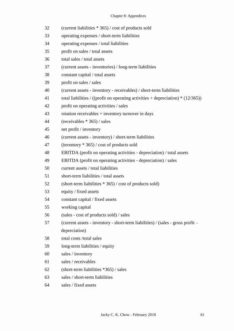
Chapter 8: Appendices
Jacky C. K. Chow - February 2018 61
32 (current liabilities * 365) / cost of products sold
33 operating expenses / short-term liabilities
34 operating expenses / total liabilities
35 profit on sales / total assets
36 total sales / total assets
37 (current assets - inventories) / long-term liabilities
38 constant capital / total assets
39 profit on sales / sales
40 (current assets - inventory - receivables) / short-term liabilities
41 total liabilities / ((profit on operating activities + depreciation) * (12/365))
42 profit on operating activities / sales
43 rotation receivables + inventory turnover in days
44 (receivables * 365) / sales
45 net profit / inventory
46 (current assets - inventory) / short-term liabilities
47 (inventory * 365) / cost of products sold
48 EBITDA (profit on operating activities - depreciation) / total assets
49 EBITDA (profit on operating activities - depreciation) / sales
50 current assets / total liabilities
51 short-term liabilities / total assets
52 (short-term liabilities * 365) / cost of products sold)
53 equity / fixed assets
54 constant capital / fixed assets
55 working capital
56 (sales - cost of products sold) / sales
57 (current assets - inventory - short-term liabilities) / (sales - gross profit –
depreciation)
58 total costs /total sales
59 long-term liabilities / equity
60 sales / inventory
61 sales / receivables
62 (short-term liabilities *365) / sales
63 sales / short-term liabilities
64 sales / fixed assets