Analysis of farm-to-retail maize marketing

margins in Zambia

Olipa Zulu-Mbata, Thomas S. Jayne, Johann F. Kirsten

Invited paper presented at the 5th International Conference of the African Association of

Agricultural Economists, September 23-26, 2016, Addis Ababa, Ethiopia

Copyright 2016 by [authors]. All rights reserved. Readers may make verbatim copies of this

document for non-commercial purposes by any means, provided that this copyright notice

appears on all such copies.

1

Analysis of farm-to-retail maize marketing margins in

Zambia

Olipa Zulu-Mbataa, Thomas S. Jayne

b, Johann F. Kirsten

a

aDepartment of Agricultural Economics, Extension and Rural Development, University of

Pretoria, South Africa.

bDepartment of Agricultural, Food and Resource Economics, Justin S. Morrill Hall of

Agriculture, 446 West Circle Drive, East Lansing, MI 48824, United States

ABSTRACT

Marketing margin analysis has usually been used to examine the behaviour and competitiveness

of markets and the share of a retail commodity price accruing to farmers. Most studies

examining marketing margins have typically considered margins to vary either spatially or

temporally; with little attempt to understand how or why marketing margins may vary across

households holding both space and time constant, even though inter-household variability has

been observed in most rural maize marketing areas. This article determines the relative

importance of spatial, temporal, and household-specific factors in the maize prices received by

farmers in Zambia and in the associated farm-to-retail marketing margin under the assembly

trader channel. We find that spatial factors account for the largest source of explained variation

(72%) in the maize marketing margin and farm-gate prices obtained by farmers followed by

temporal factors (16.7%). Household-specific factors account for the smallest source of

explained variation (11.3%) in marketing margins, with marital status, kinship ties to the chief or

village elders, and access to price information being the most important. Wide inter-household

variation in farm-gate prices within the same locality and month suggest the importance of

unobserved household-specific factors. These results hence indicate that the prices that maize

farmers in Zambia obtain are not fully exogenous to farmers as often assumed. Programs that

generate and improve farmers’ access to timely market information can raise prices that farmers

obtain, while improved road infrastructure in areas where marketing margins are high could

significantly improve farm-gate prices.

Keywords: Marketing Margin, Maize, Traders, Zambia

2

3

1. Introduction

Most studies of rural grain markets in Africa typically regard farmers as price takers, suggesting

that both farm-gate prices and farm-to-retail marketing margins are exogenous to the farmer.

Farm-gate prices are perceived to reflect market conditions in the particular village and time of

sale, while farm-to-retail marketing margins are the difference between this exogenous farm-gate

price and the retail price in the nearest market centre (Wohlgenant, 2001). The margin itself can

of course vary across space and time according to traders’ transport and storage costs and the

degree of non-competitive behaviour in these markets, but these are still exogenous to the

farmer. We find that this characterization of marketing margins and farm-gate prices is

inconsistent with anecdotal evidence in survey data suggesting the existence of wide variability

in farm-gate prices among farmers in the same villages and time of sale. We therefore posit that

household-specific factors (e.g. those correlated with negotiation ability or an understanding of

how markets operate) may be important in explaining variations in prices received by farmers

and hence the farm/retail price spreads commonly analysed in agricultural economics.

While many staple food marketing studies have been carried out in Africa (e.g. Vigne and

Darroch, 2010; Dessalegn et al, 1998; Truab and Jayne, 2008), few studies have examined how

or why marketing margins of staple grains may vary across farm households. Most have

confined their focus to simply measuring the margin between the various stages in the maize

value chain (e.g., Kirimi et al 2011; Sitko and Jayne, 2014) or examining the factors influencing

marketing margins over time (e.g. Traub and Jayne, 2008). Most studies analysing marketing

margins use market-level price data, enabling the measurement of factors associated with spatial

and temporal variation in these margins, but not among transactions carried out at a particular

time and location. Consequently, relatively little attention has been devoted to understanding

how or why marketing margins may vary across households, holding both space and time

constant, even though inter-household variability has been observed in many household-level

analyses of rural market behaviour (Sitko and Jayne, 2014; Yamano and Arai, 2010; Jayne et al,

2010). Understanding the reasons why marketing margins may vary across households in the

same locality and time frame may allow analysts to identify policy and programmatic options for

raising the prices that smallholder farmers receive for their surplus production. Different sources

of variation in marketing margins would call for different policy actions to improve market

access and efficiency for farmers. A review of literature shows that no study to our knowledge

has tried to decompose the marketing margin into temporal, spatial and household-specific

factors.

Therefore, this study identifies the extent to which marketing margins and farm-gate prices

received by smallholder farmers in Zambia are indeed exogenous. We examine three specific

issues: 1) the difference between the retail price and the farm-gate price offered to small-scale

farmers in their villages, and decomposes this farm-to-retail marketing margin into spatial,

temporal, and household-specific factors; 2) underlying sources of variation in the size of the

4

household-specific marketing margins and the degree to which each factor affects the size of the

marketing margin; and 3) the implications of these findings for policy actions to promote

farmers’ incomes from participation in maize markets. The remainder of this article, looks at

prior studies that have been done on marketing margins, provides a description of the data

sources and research methods used in our study, presents the main findings of the analysis, and

concludes with a summary of main findings and possible government actions to raise

smallholders’ incomes from surplus grain production.

2. A Review of Prior Marketing Margin Studies

Food marketing margin analysis has been of interest to researchers and policy makers for a long

time. Marketing margins provide an indication of market structure, performance and efficiency

(Myers, et al., 2010). For commodities that do not undergo processing until after the consumer

purchases it, the farm-retail margin indicates whether producers are getting an increasing or

declining share over time of the total retail price of the commodity. Wider margins mean that

farmers obtain a smaller share of the retail price. Margins are influenced by a number of factors,

primarily shifts in retail demand, farm supply, the costs of transformation across time, space and

form (e.g., transport and storage costs, processing costs in many cases, transaction costs

associated with exchange, the quality of products and risk associated with the transactions) and

potentially non-competitive behaviour in the markets (Wohlgenant, 2001).

A number of empirical studies have analysed marketing margins (retail-price spreads) in

developing countries based on the types of variables mentioned above (Wohlgenant and Mullen,

1987). Other studies have examined the role of policies and potential non-competitive behaviour

in determining the size of the margin. Studies by Traub and Jayne, (2008) and Vigne and

Darroch (2010) have used marketing margin analysis to determine the size of the maize meal

margins in South Africa, finding that the maize meal margins had been rising along the years.

The degree of risk through prices or yield uncertainty has also been shown to affect the

marketing margin (Brorsen, 1985). The marketing margin is also affected by temporal and

spatial factors (Carambas, 2005; Wohlgenant, 2001). Minten and Kyle, (1999) in their study in

the former Zaire, examined how the producer-wholesale price margin of various foods was

affected by distance and road quality. This study found that distance and bad roads increased the

size of the marketing margins. They also found substantial regional price variation and relative

price variations. This price variation and variation in margins across regions and villages has also

been observed in other areas. Apart from regional and seasonal variations in prices, inter-

household variations have also been found in the maize margins in Malawi, Kenya and Zambia

(Sitko and Jayne, 2014; Yamano and Arai, 2010; Jayne et al., 2010). This then raises an

interesting question of whether marketing margins are affected by household or individual

factors. Some recent studies have looked at characteristics of the market participants and how

5

these factors might affect the size of the marketing margin; these factors include age, level of

education, marital status, gender and the family size (Yamano and Arai, 2010).

Other studies have looked at the differences in the marketing margins across different marketing

channels. They have found that marketing margins tend to vary across different market channels.

Therefore, the type of channel the farmer chooses to utilize affects the size of the marketing

margin and in fact, the price the farmer obtains for their produce (Sitko and Jayne, 2014)

From our review of the literature, we conclude that most marketing margin studies of food

commodities have mainly focused on spatial and temporal factors. This stems from the notion

that market participants are price takers, hence their characteristics should have little to do with

price determination and indeed margin size. However, variations in the size of the marketing

margins have been observed at the household level, holding time and space constant, thus an

enquiry of this variation may produce useful insights. Few studies have examined whether

household-specific factors affect the size of the farm-gate price and marketing margin, and none

have tried to decompose the size of marketing margins into spatial, temporal vs. household-level

components. It is from this gap in the literature that this study is motivated to examine the

magnitude of inter-household variability in marketing margins versus spatial and temporal

differences.

3. Data and Methods

The study used nationally-representative cross-sectional household data collected in the 2012

Rural Agricultural Livelihoods Survey (RALS12) by Zambia’s Central Statistical office (CSO)

and the Indaba Agricultural Policy Research Institute (IAPRI). The data covers a 12 month

period, from May 2011 to April 2012. For the purpose of this article, only households that sold

their maize to assembly traders were considered. Assembly traders constituted the second main

transaction channel apart from FRA, chosen by smallholder maize sellers in this year (17.2% of

total maize transactions). The sample was also restricted to areas where maize trade flowed from

the farm to the retail centre (surplus areas). This restriction is important as marketing margin

analysis should be based on observations where the flow of grain is from the farm to the retail

and hence where the retail prices are higher than the farm-gate price. We excluded observations

in rural areas where maize purchases exceeded sales (imply reverse trade flows into those rural

areas), as including them would downwardly bias the measurement of the marketing margin.

Marketing margin analysis is valid if it only includes observations where the flow of grain is

from the farm to the retail centre (lower price to higher price). This exclusion brought our

sample size to 579 households. Farm-gate prices reported by maize selling households in a

particular month was matched to monthly retail price data at the nearest district town (collected

by the Central Statistics Office) in the same period to construct monthly farm-to-retail marketing

margins.

6

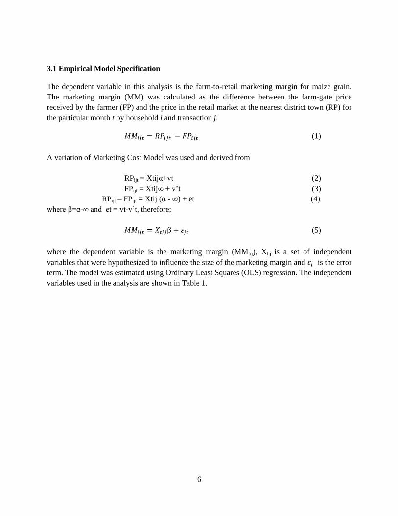
3.1 Empirical Model Specification

The dependent variable in this analysis is the farm-to-retail marketing margin for maize grain.

The marketing margin (MM) was calculated as the difference between the farm-gate price

received by the farmer (FP) and the price in the retail market at the nearest district town (RP) for

the particular month t by household i and transaction j:

𝑀𝑀𝑖𝑗𝑡 = 𝑅𝑃𝑖𝑗𝑡 − 𝐹𝑃𝑖𝑗𝑡 (1)

A variation of Marketing Cost Model was used and derived from

RPijt = Xtijα+vt (2)

FPijt = Xtij∞ + v’t (3)

RPijt – FPijt = Xtij (α - ∞) + et (4)

where β=α-∞ and et = vt-v’t, therefore;

𝑀𝑀𝑖𝑗𝑡 = 𝑋𝑡𝑖𝑗β + 𝜀𝑗𝑡 (5)

where the dependent variable is the marketing margin (MMtij), Xtij is a set of independent

variables that were hypothesized to influence the size of the marketing margin and 𝜀𝑡 is the error

term. The model was estimated using Ordinary Least Squares (OLS) regression. The independent

variables used in the analysis are shown in Table 1.

7

Table 1. Independent variables used

Variables

Spatial Variables

District Dummies

Temporal Variables

Month Dummies

Household Variables

Age Of Household Head In Years

Sex of the household head (1= Male, 2= Female)

Household heads education

Primary Education (1= attended, 0= otherwise)

Secondary Education (1= attended, 0=otherwise)

Tertiary Education (1=attended, 0=otherwise)

Marital status of household head

Never Married (1= Yes, 0=No)

Divorced (1= Yes, 0=No)

Widowed (1= Yes, 0=No)

Separated (1= Yes, 0=No)

Number Of Household Members

Farm size of household (Hectares)

Productive Assets of the household (ZWK)

Household head Kinship Ties Dummy, 1=Yes 0=No

Number Of Traders Entering A Village

Distance To Nearest Boma (Km)

Distance To Nearest Road (Km)

Transport Cost Of Transporting A Kg Of Grain To District Sale point

Access to Price Information (1=Yes, 0=No)

4. Bivariate relationships

Table 2 shows the descriptive results. The mean marketing margins for the farmers that used the

assembly trader channel was found to be ZMK1195.703 (USD0.04) per kg of maize sold, which

entails that in general farmers obtained a lower price at the farm-gate than if they would have

sold at the same period at the nearest district retail market in the same month. However, selling

at the retail market would have necessitated farmers to organize transport from the farm-gate to

the retail market, which may or may not have involved greater costs that the marketing margin.

1 The marketing margin and the farm-gate and retail prices are reported in the old Zambian kwacha (ZMK) before

the currency was rebased by 1000 in January 2013 to the new Zambia Kwacha (ZMW)

8

We note that roughly 10% of the farmers had negative marketing margins; these farmers

managed to obtain a higher price at the farm-gate compared to the price they would have

obtained had they sold at the retail market during that month. The mean farm-gate price was

found to be ZMK 822.74 (USD 0.16) per kg of maize sold and the mean retail price was ZMK

1018.44 (USD 0.20) per kg of maize sold. The farm-gate price as a percentage of the retail price

was found to be 80.78%. More than 80% of the farmers had access to price information. This

shows that price information is readily available to farmers, even in remote areas.

The distance and time travelled to the nearest retail centre give an indication of the ease of

accessing markets. The mean distance to the nearest retail district town (Boma)2 was found to be

about 46 kilometres and the average distance from the villages to the nearest tarred road was 26

kilometres. Even with these distances, it was found that most of the farmers did not travel long

distances to sell their produce. About 75% of the farmers sold their maize produce at the farm

gate. For those that did travel to sell to assembly traders, their average distance was 4.5km per

maize sale transaction thus the farmers in this case might not have problems with regard to

market access as is normally believed to be the case with rural smallholder farmers in Africa.

These findings are similar to those found by Chamberlin and Jayne (2013), who found that the

distance travelled from the farm to the point of sale, was zero for over 70% of a nationwide

sample of Kenyan farmers selling maize to private traders. Hence, it can be noted that traders

offer a much-needed service by obviating the need to organize transport services that the farmers

would otherwise need to pay for themselves if they have to travel to the nearest retail town to

sale their maize. Thus, for 75% of the farmers in this nationally-representative sample of

Zambian farmers the transport costs are borne directly by the trader, which the trader recovers by

offering a lower price to farmers than at the district town. About 25% of the farmers incurred

some transport costs themselves. We can therefore hypothesize that the greater the distance that

farmers travel on their own to sell their maize, the higher the farm-gate price should be and the

lower the marketing margin should be. The average transport cost for the farmers that

transported the maize grain for sale was found to be ZMK863.35 per 50kg bag of maize grain.

We found that the average number of traders that entered the different villages to purchase maize

grain directly from the farmers was seven. This indicates a reasonable level of competitiveness in

the village grain market. The findings are also in line with those by Chapoto and Jayne, (2011)

and Sitko and Jayne, (2014), who found that the mean number of traders in each village during

the marketing season was 9 and 10 respectively.

2 BOMA, or British Overseas Management Area was a term coined during the colonial period for the district town

capital but it continues to be used in Zambia today.

9

Table 2: Descriptive Statistics

Variable Name Description of Variable Mean Distribution of Variables

p10 p25 p50 p75 p90

Dependent variables Dependent variables

Market Margin Market Margin (Zambian kwacha, ZMK)** 195.703 -102.30 39.22 181.45 360.09 480.82

Farm-gate Price Farm-gate Price (ZMK) 822.735 545.455 626.087 800.00 995.025 1111.111

Explanatory

variables Explanatory variables

Age Age of Household head (years) 44.833 28 34 41 55 65

Sex Sex of household head (=1 if male, 2 female) 1.187 - - - - -

Education level of

household head Education level of household head

dedulev1 Primary Education Dummy(attended=1, 0 otherwise) 0.549 - - - - -

dedulev2 Secondary Education Dummy(attended=1,0 otherwise 0.273 - - - - -

dedulev3 Tertiary Education Dummy(attended=1, 0 otherwise) 0.050 - - - - -

dedulev4 No Education Dummy 0.128 - - - - -

Household size Number of household members 5.907 3 4 6 8 9

Dkinties Household Kinship ties dummy,1=yes 0=no 0.484 - - - - -

Farm size Farm size (Ha) 4.042 1 1.715 2.835 5.188 8.91

Prodasst All household Assets (million ZMK) 24.9 0.5 1.02 2.92 10.4 27.8

Traders Number of Traders Entering a Village 6.877 0 2 5 9 15

Distance boma Distance to nearest Boma (Km) 46.019 10 20 35 62 98

Distance road Distance to nearest tarred road (Km) 26.602 1 5 20 40 65

Transport cost Cost of transporting a kg of maize to sale point (ZMK) 17.611 0 0 0 0 86.96

Price information Access to price information-agric commodity( 1=yes) 1.128 - - - - -

Month Month of Maize Sale 7.699 - - - - -

Retail Price Retail Price Per Kg (ZMK) 1018.438 717.647 941.1765 1038.647 1176.471 1176.471

Source: Authors computations from RALS 2012 ** 1 USD = 6240 ZMK in 2012.

10

We also examine how farm-gate prices and marketing margins vary according to farmers’ socio-

demographic characteristics. Table 3 shows that male farmers obtain a higher farm-gate price

than female farmers, but they also tend to incur higher marketing margins than female farmers.

The higher farm-gate price conforms to most studies, as males are believed to be better

negotiators and tend to have more price information than females. Farmers who were less than

30 years obtained higher farm-gate prices followed by those farmers that were between the ages

of 50-70 years. The farmers above 70 years fetched the lowest farm-gate price. We will examine

in the next section whether these bivariate relationships hold after controlling for other observed

factors.

Table 3: Maize Farm-Gate Price and Marketing Margin by Sex, Age and Education Level.

Variable Observations

Farm-Gate

Price

(ZMK)

Farm-gate price

minus median farm-

gate price at ward

level

Marketing

Margin

(ZMK)

Gender

Male 471 823.03 4.95 196.80

(224.05) (147.87) (244.97)

Female 108 821.43 -0.14 190.93

(190.22) (160.48) (217.68)

Age in years

18-30 107 847.60 5.38 157.74

(226.69) (157.33) (242.46)

30-50 286 828.16 2.87 196.56

(213.31) (144.88) (240.90)

50-70 154 817.09 10.79 220.43

(216.41) (158.30) (233.30)

>70 32 718.33 -23.14 195.99

(216.65) (134.79) (249.67)

Education Level

Primary 318 801.25 5.02 204.96

(227.51) (161.89) (247.66)

Secondary 158 855.88 3.82 168.07

(216.65) (133.66) (237.34)

Tertiary 29 878.96 37.07 228.53

(182.42) (93.35) (247.15)

No Education 74 822.25 -12.96 202.06

(179.16) (149.16) (206.07)

Source: Authors computations from RALS 2012, (Numbers in parentheses are standard errors)

11

The level of education of the farmer is expected to affect the size of the farm-gate price and the

marketing margin in that, the more educated the farmer is, the more likely they are to make

informed decisions and obtain better farm-gate prices. This was shown to be the case, as the

farmers with tertiary education obtained higher farm-gate prices (ZMK878.96) than the farmers

with lower levels of education. The farmers with no formal education on the other hand fetched a

lower farm-gate price than the prevailing median farm-gate price at ward level.

4.1 Spatial and Temporal Price Variation

Prices that farmers receive at the farm-gate, as well as the retail price, normally vary from one

region to another according to supply and demand conditions as well as transport costs to major

demand centres. Minten and Kyle (1999) for example, states that “the presence or absence of

road infrastructure is perceived to be one of the main determinants of spatial price variation

observed in African grain markets”. After decomposing the data into temporal and spatial

aspects, Table 4 shows how the marketing margins vary by province, with Southern Province

having the lowest marketing margin (ZMK66.02). Farmers in this province obtained a farm-gate

price that is closer to the retail price in the nearest town/retail centre. Eastern province on the

other hand had the highest margin (ZMK268.95). These differences in marketing margins per

province indicate the spatial price differences that are observed due to differences in marketing

access conditions as well as other factors, such as price information that farmer’s in the different

provinces have access to and the road conditions.

Table 4: Maize Marketing Margin by Province and District

Province Observations Marketing Margin (ZMK)

Central 109 189.29

Copperbelt 47 192.89

Eastern 165 268.95

Luapula 34 264.97

Lusaka 19 225.32

Muchinga 13 151.77

Northern 74 208.82

North Western 48 73.64

Southern 63 66.02

Western 7 118.07

Source: Authors computations from RALS 2012

Apart from spatial price variation, prices tend to also vary over time. Food grains and other types

of food products are likely to exhibit seasonal price variations, due to variations in food

availability and supply. In Zambia, the maize marketing season starts a month or so after the

harvest in May/June, reaches a peak in the June/August period, and tapers off noticeably in the

12

February/April period just before the next harvest. During the main maize marketing season of

June/August, large quantities of maize grain are offloaded onto the market and a decline in retail

prices is observed (Table 5 below). Retail prices are lowest in the months of June and July, with

June having the largest quantity of maize sold in the season.

Table 5: Monthly Maize Prices, Quantity Sold and Marketing Margin

Month3 Observations

Mean

Number of

Sales

Transactions

per

Household

Farm-

gate

Price

(ZMK)

Retail

Price

(ZMK)

Quantity Sold

for all

transactions

(Kg)

Marketing

Margin

(ZMK)

2011

May 19 1.16 696.93 1052.10 549.76 355.18

June 66 1.18 709.99 908.56 1671.68 198.58

July 93 1.24 772.86 929.46 995.36 156.59

August 174 1.34 837.68 1004.45 1329.05 166.77

September 61 1.46 869.56 992.93 749.11 123.37

October 69 1.42 868.70 1119.81 901.32 251.10

November 30 1.93 845.21 1164.22 522.18 319.01

December 24 1.58 908.43 1091.91 522.94 183.49

2012

January 24 1.71 930.52 1185.46 734.13 254.94

February 15 2.40 868.34 1100.00 889.33 231.66

March 3 2.67 811.59 1176.47 345.00 364.88

April 1 2.00 695.65 1058.82 287.50 363.17

Source: Authors computations from RALS 2012

The marketing margin also varies from month to month, with September having the lowest

marketing margin and March and April having the highest marketing margins.

4.2 Inter-Household Price Variation

Price variations are evident in terms of spatial and temporal variations. Theses price variations

are expected as geographical differences bring about differences in market infrastructure and

facilities, such as access to roads, which in turn affect the cost of transportation and thus

affecting the prices differently depending on the area. Seasonal differences affect the grain

availability and in turn affect the price. However, even within the same time period and in the

3 The data was collected from May 2011 to April 2012, therefore the months in this table are reported in this order

13

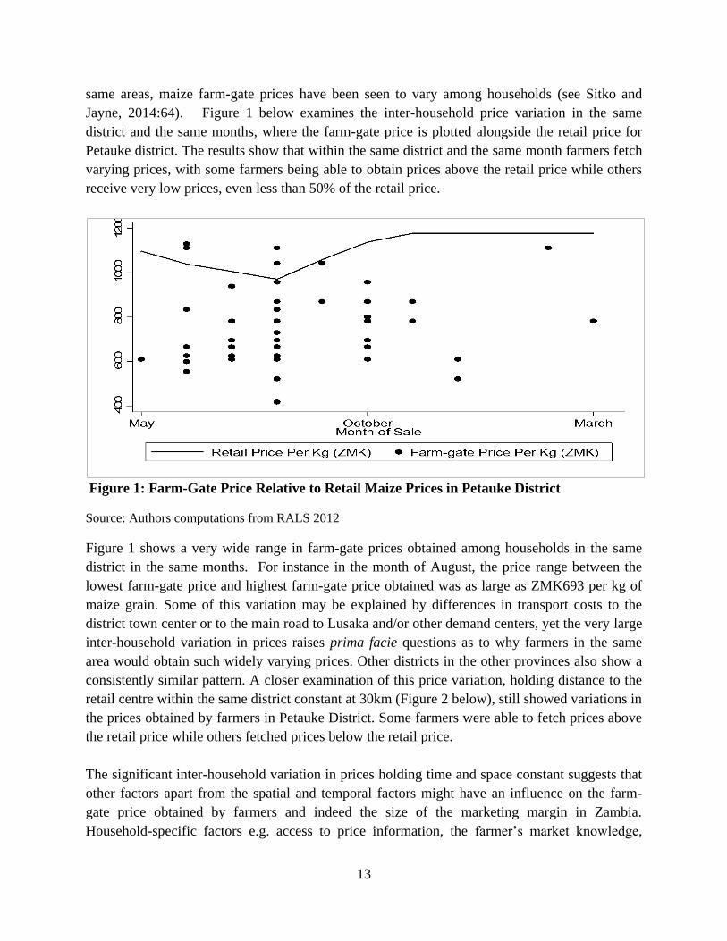
same areas, maize farm-gate prices have been seen to vary among households (see Sitko and

Jayne, 2014:64). Figure 1 below examines the inter-household price variation in the same

district and the same months, where the farm-gate price is plotted alongside the retail price for

Petauke district. The results show that within the same district and the same month farmers fetch

varying prices, with some farmers being able to obtain prices above the retail price while others

receive very low prices, even less than 50% of the retail price.

Figure 1: Farm-Gate Price Relative to Retail Maize Prices in Petauke District

Source: Authors computations from RALS 2012

Figure 1 shows a very wide range in farm-gate prices obtained among households in the same

district in the same months. For instance in the month of August, the price range between the

lowest farm-gate price and highest farm-gate price obtained was as large as ZMK693 per kg of

maize grain. Some of this variation may be explained by differences in transport costs to the

district town center or to the main road to Lusaka and/or other demand centers, yet the very large

inter-household variation in prices raises prima facie questions as to why farmers in the same

area would obtain such widely varying prices. Other districts in the other provinces also show a

consistently similar pattern. A closer examination of this price variation, holding distance to the

retail centre within the same district constant at 30km (Figure 2 below), still showed variations in

the prices obtained by farmers in Petauke District. Some farmers were able to fetch prices above

the retail price while others fetched prices below the retail price.

The significant inter-household variation in prices holding time and space constant suggests that

other factors apart from the spatial and temporal factors might have an influence on the farm-

gate price obtained by farmers and indeed the size of the marketing margin in Zambia.

Household-specific factors e.g. access to price information, the farmer’s market knowledge,

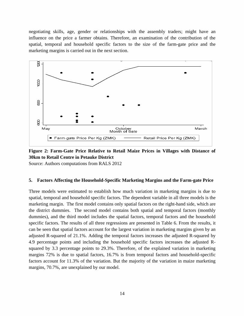
14

negotiating skills, age, gender or relationships with the assembly traders; might have an

influence on the price a farmer obtains. Therefore, an examination of the contribution of the

spatial, temporal and household specific factors to the size of the farm-gate price and the

marketing margins is carried out in the next section.

Figure 2: Farm-Gate Price Relative to Retail Maize Prices in Villages with Distance of

30km to Retail Centre in Petauke District

Source: Authors computations from RALS 2012

5. Factors Affecting the Household-Specific Marketing Margins and the Farm-gate Price

Three models were estimated to establish how much variation in marketing margins is due to

spatial, temporal and household specific factors. The dependent variable in all three models is the

marketing margin. The first model contains only spatial factors on the right-hand side, which are

the district dummies. The second model contains both spatial and temporal factors (monthly

dummies), and the third model includes the spatial factors, temporal factors and the household

specific factors. The results of all three regressions are presented in Table 6. From the results, it

can be seen that spatial factors account for the largest variation in marketing margins given by an

adjusted R-squared of 21.1%. Adding the temporal factors increases the adjusted R-squared by

4.9 percentage points and including the household specific factors increases the adjusted R-

squared by 3.3 percentage points to 29.3%. Therefore, of the explained variation in marketing

margins 72% is due to spatial factors, 16.7% is from temporal factors and household-specific

factors account for 11.3% of the variation. But the majority of the variation in maize marketing

margins, 70.7%, are unexplained by our model.

15

These results show that apart from the usual expected spatial and temporal factors, marketing

margins are also affected by household-specific factors, even though the contribution of the

observed household factors presented are relatively small compared to the other factors. The

household specific factors that were found to be statistically significant in affecting the size of

the marketing margin are marital status, kinship ties, cost of transporting grain and access to

price information.

Table 6: Maize Marketing Margin Regression Results

Variables

Regression 1 Regression 2 Regression 3

Age Of Household Head In Years -0.174

(0.781)

Sex (1= Male, 2= Female) -21.06

(44.52)

Primary Education (1= attended, 0= otherwise) -15.35

(33.15)

Secondary Education (1= attended, 0=otherwise) -34.64

(36.98)

Tertiary Education (1=attended, 0=otherwise) -0.653

(74.43)

Never Married (1= Yes, 0=No) -262.8**

(109.5)

Divorced (1= Yes, 0=No) -78.05

(64.91)

Widowed (1= Yes, 0=No) -30.56

(50.31)

Separated (1= Yes, 0=No) -9.907

(73.99)

Number Of Household Members -1.296

(4.549)

Farm size 0.349

(3.509)

Productive Assets (ZWK) 4.19e-07

(3.10e-07)

Kinship Ties Dummy, 1=Yes 0=No 88.26***

(27.36)

Number Of Traders Entering A Village 0.252

(1.875)

Distance To Nearest Boma (Km) -0.0158

(0.585)

16

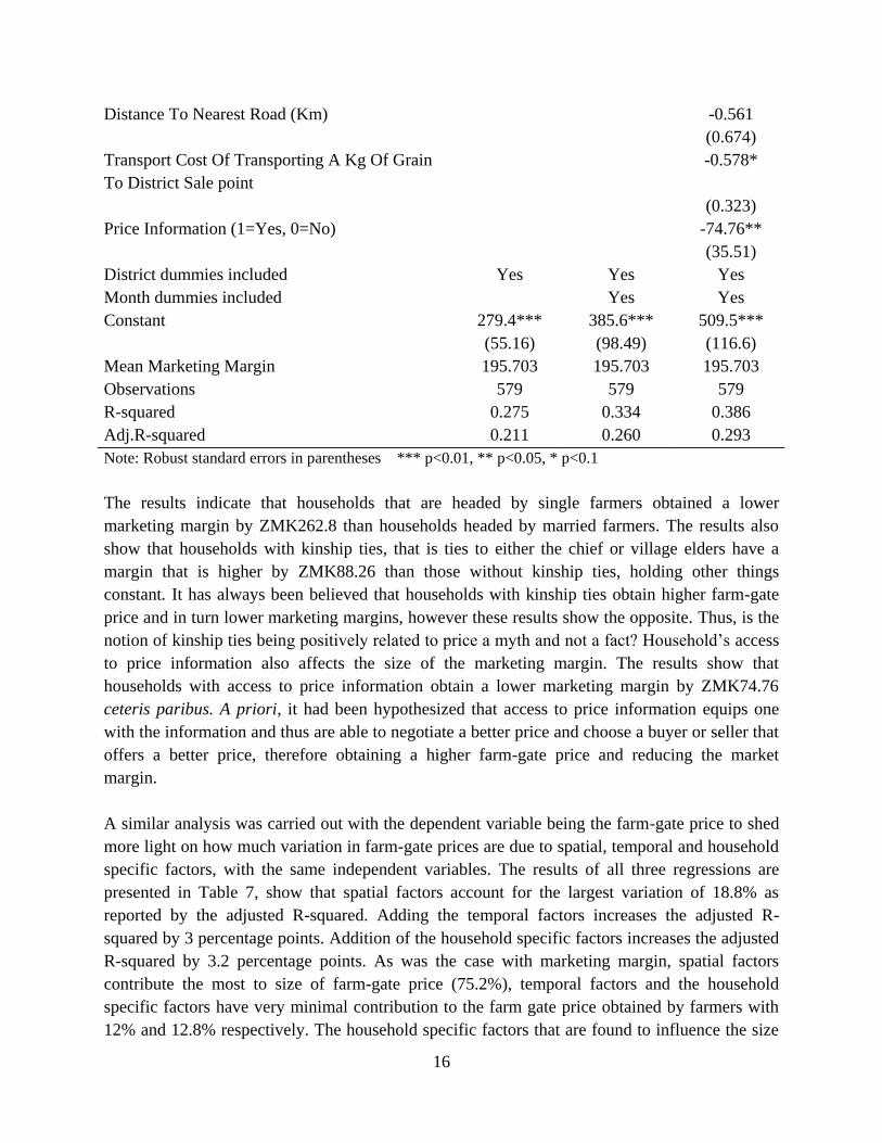
Distance To Nearest Road (Km) -0.561

(0.674)

Transport Cost Of Transporting A Kg Of Grain

To District Sale point

-0.578*

(0.323)

Price Information (1=Yes, 0=No) -74.76**

(35.51)

District dummies included Yes Yes Yes

Month dummies included Yes Yes

Constant 279.4*** 385.6*** 509.5***

(55.16) (98.49) (116.6)

Mean Marketing Margin 195.703 195.703 195.703

Observations 579 579 579

R-squared 0.275 0.334 0.386

Adj.R-squared 0.211 0.260 0.293

Note: Robust standard errors in parentheses *** p<0.01, ** p<0.05, * p<0.1

The results indicate that households that are headed by single farmers obtained a lower

marketing margin by ZMK262.8 than households headed by married farmers. The results also

show that households with kinship ties, that is ties to either the chief or village elders have a

margin that is higher by ZMK88.26 than those without kinship ties, holding other things

constant. It has always been believed that households with kinship ties obtain higher farm-gate

price and in turn lower marketing margins, however these results show the opposite. Thus, is the

notion of kinship ties being positively related to price a myth and not a fact? Household’s access

to price information also affects the size of the marketing margin. The results show that

households with access to price information obtain a lower marketing margin by ZMK74.76

ceteris paribus. A priori, it had been hypothesized that access to price information equips one

with the information and thus are able to negotiate a better price and choose a buyer or seller that

offers a better price, therefore obtaining a higher farm-gate price and reducing the market

margin.

A similar analysis was carried out with the dependent variable being the farm-gate price to shed

more light on how much variation in farm-gate prices are due to spatial, temporal and household

specific factors, with the same independent variables. The results of all three regressions are

presented in Table 7, show that spatial factors account for the largest variation of 18.8% as

reported by the adjusted R-squared. Adding the temporal factors increases the adjusted R-

squared by 3 percentage points. Addition of the household specific factors increases the adjusted

R-squared by 3.2 percentage points. As was the case with marketing margin, spatial factors

contribute the most to size of farm-gate price (75.2%), temporal factors and the household

specific factors have very minimal contribution to the farm gate price obtained by farmers with

12% and 12.8% respectively. The household specific factors that are found to influence the size

17

of the farm-gate price are level of education, access to price information and kinship ties.

Farmers who have attained secondary education have a higher farm-gate price of ZMK61.79

than those with no formal education. The farmers with access to price information receive a

higher farm-gate price of ZMK68.05 and the households with kinship ties receive a lower farm-

gate price by ZMK70.94.

Table 7: Maize Farm-Gate Price Regression Results

Variables Regression 1 Regression 2 Regression 3

Retail Price Per Kg (ZMK) 0.118

(0.106)

Age Of Household Head In Years -0.233

(0.714)

Sex (1= Male, 2= Female) -0.118

(43.71)

Primary (1= attended, 0=otherwise) 19.27

(31.96)

Secondary(1=attended,0=otherwise) 61.79*

(35.34)

Tertiary(1= attended, 0=otherwise) 70.87

(70.27)

Never Married (1= Yes, 0=No) 181.7

(117.7)

Divorced (1= Yes, 0=No) 54.20

(62.22)

Widowed (1= Yes, 0=No) 14.87

(47.21)

Separated (1= Yes, 0=No) 32.46

(64.20)

Number Of Household Members -0.438

(4.288)

Farm size -1.699

(3.308)

Productive Assets (ZMK) -4.31e-07

(2.76e-07)

Kinship Ties Dummy,1=Yes 0=No -70.94***

(26.88)

Number Of Traders Entering A Village 0.0714

(1.837)

Distance To Nearest Boma (Km) 0.311

(0.537)

18

Distance To Nearest Road (Km) 0.244

(0.594)

Transport Cost Of Transporting A Kg Of

Grain To District Sale point

0.453

(0.306)

Price Information(1=Yes, 0=No) 68.05**

(33.70)

District dummies included Yes Yes Yes

Month dummies included Yes Yes

Constant 805.9*** 836.2*** 599.5***

(41.23) (75.67) (166.4)

Mean Farm-gate Price 822.735 822.735 822.735

Observations 579 579 579

R-squared 0.254 0.296 0.350

Adj.R-squared 0.188 0.218 0.250

Note: Robust standard errors in parentheses *** p<0.01, ** p<0.05, * p<0.1

This article focuses on the marketing margin of the household that sold to assembly traders.

However, a further examination of all households selling maize through other market channels

shows that households that sold using the assembly trader channel have the highest marketing

margin as compared to the other market channels (Table 8, below). This is expected as the

assembly traders incur a large cost by following the farmers to their farm-gates, thus the mark-up

price is larger so that they are able to break even. Households that used the cooperative market

channel had the lowest marketing margin, as the farm-gate price they obtained was higher than

the retail price in the nearest market.

Table 8: Farm-gate Price, Retail Price and Marketing Margin by Private Trader Market

Channel

Market Channel Observations

Farm-

gate Price

(ZMK)

Retail

Price

(ZMK)

Marketing

Margin

(ZMK)

Assembly Trader 579 822.74 1018.44 195.7

Large scale trader 88 905.91 983.78 77.87

Retailer / Marketeer 189 948.65 1054.89 106.24

Cooperative (not destined for FRA) 9 1156.02 1000 -156.02

Directly to miller/processor 45 879.9 996.06 116.16

To miller/processor through an agent 38 1000.92 955.27 -45.66

Source: Authors computations from RALS 2012

19

6. Conclusions and Policy Implications

The study has shown that spatial factors account for the largest source of variation in the

marketing margin and farm-gate prices obtained by farmers. The wide variation in marketing

margins observed in different districts show that the price farmers obtain differs from one area to

another, and this is mostly based on the distance to the retail centre. Temporal factors account for

a minimal variation in the marketing margin and the price obtained by farmers. During months of

grain availability, which is from June to August, the farm-gate prices are lower and in times of

low grain availability, the farm-gate prices are higher. Thus, seasonality plays a role in the farm-

gate price and the marketing margins obtained by farmers. These variations in farm-gate prices

are also evident in the same villages and holding time constant as shown.

We find that household-specific factors do have an effect on the farm-gate price and the size of

the marketing margin, but their influence is less important than the spatial factors and slightly

less important than the temporal factors. The household factors that were found to significantly

affect the size of the maize marketing margin were marital status, kinship ties to either the chief

or village elders, and access to price information. However, our models explained roughly 29

percent of the variation in the marketing margins.

Therefore, these results indicate that the prices that maize farmers in Zambia obtain might not be

exogenous of the farmer characteristics and attributes. The individual farmer attributes influence

the price they obtain at the farm-gate and hence it can be said that maize farmers in Zambia are

not necessarily price takers. Hence, it can be noted that the large marketing margins observed do

not necessarily mean farmer exploitation and the small marketing margins do not mean market

competiveness, but these might mean that farmers have different attributes and these attributes

affect the prices that they are able to obtain.

With spatial factors accounting for the largest source of price variation, and the farmers in

villages further away from the central retail centres fetching lower prices than those near the

retail centres. Therefore, in order to help reduce price variation among farmers and raise maize

prices received by the farmers in Zambia, policies aimed at improving infrastructure to better

link rural villages to urban markets ought to be implemented. Rather than trying to engage in

markets in an effort to overcome perceived private trader exploitation, the government and

donors need to help farmers better engage in the existing market channels. As it has been seen

that the type of channel a farmer uses, will influence the price they obtain. Helping farmers have

access to both these existing channels should be a priority and equipping farmers with timely

price information. Having access to price information has been found to be a significant factor in

determining the price a farmer will obtain. Farmers that have access to reliable and timely price

information are in a better position to engage in the market and are able to negotiate better prices

than those farmers without access to price information.

20

Seasonality and time of sale play a big role in the maize price obtained by farmers as temporal

factors account for the second largest source of variation in maize grain prices. To help reduce

maize price variation and improve the prices received by farmers, the Zambian government and

other private sector participants, need to assist smallholder farmers in ensuring they are able to

market grain at the times when it is most profitable and this can be achieved by investing in

storage facilities that farmers can use for instance warehouses. Farmers are unable to take

advantage of higher prices in off-season times due to lack of storage facilities.

21

REFERENCES

Brorsen, B., 1985. Marketing Margin in Rice Uncertainity. American Journal of Agricultural

Economics, Volume 67, pp. 521-28.

Carambas, M., 2005. Analysis of Marketing Margins in Eco-Labeled Products, Center for

Developmemnt Research, University of Bonn: Available at

http://ageconsearch.umn.edu/bitstream/24600/1/pp05ca06.pdf

Chamberlin, J. & Jayne, T. S., 2013. Unpacking the Meaning of 'Market Access': Evidence from Rural

Kenya. World Development 41: 245-264.

Chapoto, A. & Jayne, T., 2011. Zambian Farmers' Access to Maize Markets, Lusaka, Zambia: Indaba

Agricultral Policy Reserach Institute.

Dessalegn, G., Jayne, T. S. & Shaffer, J. D., 1998. Market Structure, Conduct and Perfomance:

Constraints on Perfomance of Ethopian Grain Markets, Addis Ababa: Grain Market Research

Project. Available at http://fsg.afre.msu.edu/Ethiopia/wp8.pdf

Jayne, T., Sitko, N., Ricker-Gilbert, J. & Mangisoni, J., 2010. Malawi’s Maize Marketing System,

Malawi: Available at http://fsg.afre.msu.edu/malawi/Malawi_maize_markets_Report_to-DFID-

SOAS.pdf

Kirimi, L. et al., 2011. A Farm Gate-To-Consumer Value Chain Analysis of Kenya’s Maize Marketing

System, Michgan, USA: MSU International Development. Available at

http://fsg.afre.msu.edu/papers/idwp111.pdf

Minten, B. & Kyle, S., 1999. The effect of distance and road quality on food collection, marketing

margins, and traders’ wages: evidence from the former Zaire. Journal of Development

Economics 60:467-495.

Myers, R. J., Sexton, R. J. & Tomek, W. G., 2010. A Century of Research on Agricultural Markets.

American Journal of Agricultural Econmics, 92(2):376-402.

Sitko, N. J. & Jayne, T. S., 2014. Exploitative Briefcase Businessmen, Parasites, and Other Myths and

Legends: Assembly Traders and the Performance of Maize Markets in Eastern and Southern

Africa. World Development 54: 56-67.

Truab, L. & Jayne, T., 2008. The effects of price deregulation on maize marketing margins in South

Africa. Food Policy 3:224-236.

Vigne, W. & Darroch, M., 2010. Determinants of the Maize Board-Miller Marketing Margn in South

Africa: 1977-1993. Agrekon: Agricultural Economics Research, Policy abd Practice in South

Africa 35(4):295-300.

22

Wohlgenant, M. K., 2001. Marketing Margins: Empirical Analysis. Handbook of Agricultural

Economics 1:933-970.

Wohlgenant, M. & Mullen, J., 1987. Modelling the Farm-Retail Price Spread for Beef. Western Journal

of Agricutural Economics, 12:119-125.

Yamano, T. & Arai, A., 2010. The Maize Farm-Market Price Spread in Kenya and Uganda, Tokyo,

Japan. GRIPS Policy Research Institute. Available at http://www.grips.ac.jp/r-center/wp-

content/uploads/10-25.pdf