Analysis of Economic Data with Multiscale

Spatio-Temporal Models

Marco A. R. Ferreira (University of Missouri - Columbia)

Adelmo Bertolde (Federal University of Espırito Santo, Brazil)

Scott Holan (University of Missouri, Columbia)

Outline

Motivation

Introduction

Multiscale factorization

Exploratory Multiscale Data Analysis

The multiscale spatio-temporal model

Empirical Bayes estimation

Posterior exploration

Agricultural Production in Espırito Santo

Conclusions

Outline

Motivation

Introduction

Multiscale factorization

Exploratory Multiscale Data Analysis

The multiscale spatio-temporal model

Empirical Bayes estimation

Posterior exploration

Agricultural Production in Espırito Santo

Conclusions

Motivation Introduction Factorization Exploratory Analysis Model EB estimation MCMC Application Conclusions

Espırito Santo: Log of agriculture production per county

Observed - 1990 Estimated -1990

Gaussian Multiscale Spatio-temporal Models Marco A. R. Ferreira

Motivation Introduction Factorization Exploratory Analysis Model EB estimation MCMC Application Conclusions

Espırito Santo: Log of agriculture production per county

Observed - 1993 Estimated - 1993

Gaussian Multiscale Spatio-temporal Models Marco A. R. Ferreira

Motivation Introduction Factorization Exploratory Analysis Model EB estimation MCMC Application Conclusions

Espırito Santo: Log of agriculture production per county

Observed - 1996 Estimated - 1996

Gaussian Multiscale Spatio-temporal Models Marco A. R. Ferreira

Motivation Introduction Factorization Exploratory Analysis Model EB estimation MCMC Application Conclusions

Espırito Santo: Log of agriculture production per county

Observed - 1999 Estimated - 1999

Gaussian Multiscale Spatio-temporal Models Marco A. R. Ferreira

Motivation Introduction Factorization Exploratory Analysis Model EB estimation MCMC Application Conclusions

Espırito Santo: Log of agriculture production per county

Observed - 2002 Estimated - 2002

Gaussian Multiscale Spatio-temporal Models Marco A. R. Ferreira

Motivation Introduction Factorization Exploratory Analysis Model EB estimation MCMC Application Conclusions

Espırito Santo: Log of agriculture production per county

Observed - 2005 Estimated - 2005

Gaussian Multiscale Spatio-temporal Models Marco A. R. Ferreira

Outline

Motivation

Introduction

Multiscale factorization

Exploratory Multiscale Data Analysis

The multiscale spatio-temporal model

Empirical Bayes estimation

Posterior exploration

Agricultural Production in Espırito Santo

Conclusions

Motivation Introduction Factorization Exploratory Analysis Model EB estimation MCMC Application Conclusions

Some background

Many processes of interest are naturally spatio-temporal.

Frequently, quantities related to these processes are availableas areal data.

These processes may often be considered at several differentlevels of spatial resolution.

Related work on dynamic spatio-temporal multiscalemodeling: Berliner, Wikle and Milliff (1999), Johannesson,Cressie and Huang (2007).

Gaussian Multiscale Spatio-temporal Models Marco A. R. Ferreira

Motivation Introduction Factorization Exploratory Analysis Model EB estimation MCMC Application Conclusions

Data Structure

Here, the region of interest is divided in geographic subregions orblocks, and the data may be averages or sums over thesesubregions.

Each state in Brazil is divided into counties, microregions andmacroregions; counties are then grouped into microregions, whichare then grouped into macroregions, according to theirsocioeconomic similarity. Thus, our analysis considers three levelsof resolution: county, microregion, and macroregion.

Gaussian Multiscale Spatio-temporal Models Marco A. R. Ferreira

Motivation Introduction Factorization Exploratory Analysis Model EB estimation MCMC Application Conclusions

Geopolitical organization

(a) (b) (c)

Figure: Geopolitical organization of Espırito Santo State by (a) counties,(b) microregions, and (c) macroregions.

Gaussian Multiscale Spatio-temporal Models Marco A. R. Ferreira

Outline

Motivation

Introduction

Multiscale factorization

Exploratory Multiscale Data Analysis

The multiscale spatio-temporal model

Empirical Bayes estimation

Posterior exploration

Agricultural Production in Espırito Santo

Conclusions

Motivation Introduction Factorization Exploratory Analysis Model EB estimation MCMC Application Conclusions

Multiscale factorization

At each time point we decompose the data into empiricalmultiscale coefficients using the spatial multiscale modelingframework of Kolaczyk and Huang (2001). See also Chapter 9 ofFerreira and Lee (2007).

Interest lies in agricultural production observed at the county level,which we assume is the Lth level of resolution (i.e. the finest levelof resolution), on a partition of a domain S ⊂ R

2.

For the j th county, let yLj , µLj = E (yLj ), and σ2Lj = V (yLj)

respectively denote agricultural production, its latent expectedvalue and variance.

Gaussian Multiscale Spatio-temporal Models Marco A. R. Ferreira

Motivation Introduction Factorization Exploratory Analysis Model EB estimation MCMC Application Conclusions

Let Dlj be the set of descendants of subregion (l , j).The aggregated measurements at the l th level of resolution arerecursively defined by

ylj =∑

(l+1,j ′)∈Dlj

yl+1,j ′ .

Analogously, the aggregated mean process is defined by

µlj =∑

(l+1,j ′)∈Dlj

µl+1,j ′ .

Assuming conditional independence,

σ2lj =

∑

(l+1,j ′)∈Dlj

σ2l+1,j ′ .

Gaussian Multiscale Spatio-temporal Models Marco A. R. Ferreira

Motivation Introduction Factorization Exploratory Analysis Model EB estimation MCMC Application Conclusions

Then

yDlj

∣

∣

∣ylj ,µL,σ

2L ∼ N(ν ljylj + θlj ,Ωlj),

with

ν lj = σ2Dlj/σ2

lj ,

θlj = µDlj− ν ljµlj ,

and

Ωlj = ΣDlj− σ−2

ljσ2

Dlj

(

σ2Dlj

)

′

.

Gaussian Multiscale Spatio-temporal Models Marco A. R. Ferreira

Motivation Introduction Factorization Exploratory Analysis Model EB estimation MCMC Application Conclusions

Consider

θelj = yDlj

− ν ljylj ,

which is an empirical estimate of θlj .

Then

θelj |ylj ,µL,σ

2L ∼ N(θlj ,Ωlj),

which is a singular Gaussian distribution (Anderson, 1984).

Gaussian Multiscale Spatio-temporal Models Marco A. R. Ferreira

Outline

Motivation

Introduction

Multiscale factorization

Exploratory Multiscale Data Analysis

The multiscale spatio-temporal model

Empirical Bayes estimation

Posterior exploration

Agricultural Production in Espırito Santo

Conclusions

Motivation Introduction Factorization Exploratory Analysis Model EB estimation MCMC Application Conclusions

Exploratory Multiscale Data Analysis

Macroregion 1 Disaggregated Empiricaltotal by microregion multiscale coefficient

1990 1995 2000 2005

020

040

060

080

0

year

1990 1995 2000 2005

020

040

060

080

0

year

Micro−region 1Micro−region 2Micro−region 3Micro−region 4Micro−region 5

1990 1995 2000 2005

−300

−200

−100

010

020

030

0

year

Micro−region 1Micro−region 2Micro−region 3Micro−region 4Micro−region 5

Espırito Santo: Agriculture production of Macroregion 1.

Gaussian Multiscale Spatio-temporal Models Marco A. R. Ferreira

Motivation Introduction Factorization Exploratory Analysis Model EB estimation MCMC Application Conclusions

Macroregion 2 Disaggregated Empiricaltotal by microregion multiscale coefficient

1990 1995 2000 2005

020

040

060

080

0

year

1990 1995 2000 2005

020

040

060

080

0

year

Micro−region 6Micro−region 7

1990 1995 2000 2005

−300

−200

−100

010

020

030

0

year

Micro−region 6Micro−region 7

Espırito Santo: Agriculture production of Macroregion 2.

Gaussian Multiscale Spatio-temporal Models Marco A. R. Ferreira

Motivation Introduction Factorization Exploratory Analysis Model EB estimation MCMC Application Conclusions

Macroregion 3 Disaggregated Empiricaltotal by microregion multiscale coefficient

1990 1995 2000 2005

020

040

060

080

0

year

1990 1995 2000 2005

020

040

060

080

0

year

Micro−region 8Micro−region 9Micro−region 10

1990 1995 2000 2005

−300

−200

−100

010

020

030

0

year

Micro−region 8Micro−region 9Micro−region 10

Espırito Santo: Agriculture production of Macroregion 3.

Gaussian Multiscale Spatio-temporal Models Marco A. R. Ferreira

Motivation Introduction Factorization Exploratory Analysis Model EB estimation MCMC Application Conclusions

Macroregion 4 Disaggregated Empiricaltotal by microregion multiscale coefficient

1990 1995 2000 2005

020

040

060

080

0

year

1990 1995 2000 2005

020

040

060

080

0

year

Micro−region 11Micro−region 12

1990 1995 2000 2005

−300

−200

−100

010

020

030

0

year

Micro−region 11Micro−region 12

Espırito Santo: Agriculture production of Macroregion 4.

Gaussian Multiscale Spatio-temporal Models Marco A. R. Ferreira

Outline

Motivation

Introduction

Multiscale factorization

Exploratory Multiscale Data Analysis

The multiscale spatio-temporal model

Empirical Bayes estimation

Posterior exploration

Agricultural Production in Espırito Santo

Conclusions

Motivation Introduction Factorization Exploratory Analysis Model EB estimation MCMC Application Conclusions

The multiscale spatio-temporal model

Observation equation:

ytL = µtL + vtL, vtL ∼ N(0,ΣL)

where

ΣL = diag(σ2L1, . . . , σ

2LnL

).

Multiscale decomposition of the observation equation:

yt1k | µt1k ∼ N(µt1k , σ21k)

θetlj | θtlj ∼ N(θtlj ,Ωlj)

Gaussian Multiscale Spatio-temporal Models Marco A. R. Ferreira

Motivation Introduction Factorization Exploratory Analysis Model EB estimation MCMC Application Conclusions

System equations:

µt1k = µt−1,1k + wt1k , wt1k ∼ N(0, ξkσ21k)

θtlj = θt−1,lj + ωtlj , ωtlj ∼ N(0, ψljΩlj)

Gaussian Multiscale Spatio-temporal Models Marco A. R. Ferreira

Motivation Introduction Factorization Exploratory Analysis Model EB estimation MCMC Application Conclusions

Priors

µ01k |D0 ∼ N(m01k , c01kσ21k),

θ0lj |D0 ∼ N(m0lj ,C0ljΩlj),

ξk ∼ IG (0.5τk , 0.5κk ),

ψlj ∼ IG (0.5lj , 0.5ςlj ),

Gaussian Multiscale Spatio-temporal Models Marco A. R. Ferreira

Outline

Motivation

Introduction

Multiscale factorization

Exploratory Multiscale Data Analysis

The multiscale spatio-temporal model

Empirical Bayes estimation

Posterior exploration

Agricultural Production in Espırito Santo

Conclusions

Motivation Introduction Factorization Exploratory Analysis Model EB estimation MCMC Application Conclusions

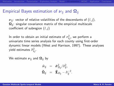
Empirical Bayes estimation of ν lj and Ωlj

ν lj : vector of relative volatilities of the descendants of (l , j),Ωlj : singular covariance matrix of the empirical multiscalecoefficient of subregion (l , j)

In order to obtain an initial estimate of σ2Lj , we perform a

univariate time series analysis for each county using first-orderdynamic linear models (West and Harrison, 1997). These analysesyield estimates σ2

Lj .

We estimate ν lj and Ωlj by

ν lj = σ2Dlj/σ2

lj ,

Ωlj = ΣDlj− σ−2

lj .

Gaussian Multiscale Spatio-temporal Models Marco A. R. Ferreira

Outline

Motivation

Introduction

Multiscale factorization

Exploratory Multiscale Data Analysis

The multiscale spatio-temporal model

Empirical Bayes estimation

Posterior exploration

Agricultural Production in Espırito Santo

Conclusions

Motivation Introduction Factorization Exploratory Analysis Model EB estimation MCMC Application Conclusions

Posterior exploration

Let

θ•lj = (θ′

0lj , . . . ,θ′

Tlj)′,

θt•j = (θ′

t1j , . . . ,θ′

tLj )′,

θ••• = (θ′

•11, . . . ,θ′

•1n1,θ′

•21, . . . ,θ′

•2n2, . . . ,θ′

•L1, . . . ,θ′

•LnL)′,

with analogous definitions for the other quantities in the model.

It can be shown that, given σ2•, ξ•, and ψ••, the vectors

µ•11, . . . ,µ•1n1

, θ•11, . . . ,θ•1n1 , . . . ,θ•L1, . . . ,θ•LnL, are

conditionally independent a posteriori.

Gaussian Multiscale Spatio-temporal Models Marco A. R. Ferreira

Motivation Introduction Factorization Exploratory Analysis Model EB estimation MCMC Application Conclusions

Gibbs sampler

µ•1k : Forward Filter Backward Sampler (FFBS) (Carter and

Kohn, 1994; Fruhwirth-Schnatter,1994).

ξk |µ•1k , σ21k ,DT ∼ IG (0.5τ∗k , 0.5κ

∗

k ) , where τ∗k = τk + T and

κ∗k = κk + σ−21k

∑Tt=1(µt1k − µt−1,1k)2.

ψlj |θ•lj ,DT ∼ IG (0.5∗lj , 0.5ς∗

lj ), where ∗lj = lj + T (mlj − 1)

and ς∗lj = ςlj +∑T

t=1(θtlj − θt−1,lj)′Ω−

lj (θtlj − θt−1,lj), where

Ω−

lj is a generalized inverse of Ωlj .

θ•lj : Singular FFBS.

Gaussian Multiscale Spatio-temporal Models Marco A. R. Ferreira

Motivation Introduction Factorization Exploratory Analysis Model EB estimation MCMC Application Conclusions

Singular FFBS

1. Use the Kalman filter to obtain the mean and covariancematrix of f (θ1lj |σ

2, ψlj ,D1), . . . , f (θTlj |σ2, ψlj ,DT ):

posterior at t − 1: θt−1,lj |Dt−1 ∼ N (mt−1,lj ,Ct−1,ljΩlj) ; prior at t: θtlj |Dt−1 ∼ N (atlj ,RtljΩlj) , where atlj = mt−1,lj

and Rtlj = Ct−1,lj + ψlj ; posterior at t: θtlj |Dt ∼ N (mtlj ,CtljΩlj) , where

Ctlj = (1 + R−1tlj )−1 and mtlj = Ctlj

(

θetlj + R−1

tlj atlj

)

.

2. Simulate θTlj from θTlj |σ2, ψlj ,DT ∼ N(mTlj ,CTljΩlj).

3. Recursively simulate θtlj , t = T − 1, . . . , 0, from

θtlj |θt+1,lj , . . . ,θTlj ,DT ≡ θtlj |θt+1,lj ,Dt ∼ N(htlj ,HtljΩlj),

where Htlj =(

C−1tlj + ψ−1

lj

)

−1and

htlj = Htlj

(

C−1tlj mtlj + ψ−1

lj θt+1,lj

)

.

Gaussian Multiscale Spatio-temporal Models Marco A. R. Ferreira

Motivation Introduction Factorization Exploratory Analysis Model EB estimation MCMC Application Conclusions

Reconstruction of the latent mean process

One of the main interests of any multiscale analysis is theestimation of the latent mean process at each scale of resolution.

From the g th draw from the posterior distribution, we canrecursively compute the corresponding latent mean process at eachlevel of resolution using the equation

µ(g)t,Dlj

= θ(g)tlj + νtljµ

(g)tlj ,

proceeding from the coarsest to the finest resolution level.

With these draws, we can then compute the posterior mean,standard deviation and credible intervals for the latent meanprocess.

Gaussian Multiscale Spatio-temporal Models Marco A. R. Ferreira

Outline

Motivation

Introduction

Multiscale factorization

Exploratory Multiscale Data Analysis

The multiscale spatio-temporal model

Empirical Bayes estimation

Posterior exploration

Agricultural Production in Espırito Santo

Conclusions

Motivation Introduction Factorization Exploratory Analysis Model EB estimation MCMC Application Conclusions

Marginal posterior densities for the signal-to-noise ratio ξk

0.0 0.2 0.4 0.6 0.8 1.0 0.0 0.2 0.4 0.6 0.8 1.0

ξ1 ξ2

0.0 0.2 0.4 0.6 0.8 1.0 0.0 0.2 0.4 0.6 0.8 1.0

ξ3 ξ4

Gaussian Multiscale Spatio-temporal Models Marco A. R. Ferreira

Motivation Introduction Factorization Exploratory Analysis Model EB estimation MCMC Application Conclusions

Marginal posterior densities for the signal-to-noise ratio ψ1j

0.0 0.2 0.4 0.6 0.8 1.0 0.0 0.2 0.4 0.6 0.8 1.0

ψ11 ψ12

0.0 0.2 0.4 0.6 0.8 1.0 0.0 0.2 0.4 0.6 0.8 1.0

ψ13 ψ14

Gaussian Multiscale Spatio-temporal Models Marco A. R. Ferreira

Motivation Introduction Factorization Exploratory Analysis Model EB estimation MCMC Application Conclusions

Mean process at coarse level

1990 1995 2000 2005

020

040

060

080

0

year

1990 1995 2000 2005

020

040

060

080

0

year

µt11 µt12

1990 1995 2000 2005

020

040

060

080

0

year

1990 1995 2000 2005

020

040

060

080

0

year

µt13 µt14

Gaussian Multiscale Spatio-temporal Models Marco A. R. Ferreira

Motivation Introduction Factorization Exploratory Analysis Model EB estimation MCMC Application Conclusions

Multiscale coefficient for Macroregion 1

1990 1995 2000 2005

−300

−200

−100

010

0

year

1990 1995 2000 2005

−300

−200

−100

010

0

year

1990 1995 2000 2005

−300

−200

−100

010

0

year

θt111 θt112 θt113

1990 1995 2000 2005

−300

−200

−100

010

0

year

1990 1995 2000 2005

−300

−200

−100

010

0

year

θt114 θt115

Gaussian Multiscale Spatio-temporal Models Marco A. R. Ferreira

Motivation Introduction Factorization Exploratory Analysis Model EB estimation MCMC Application Conclusions

Observed agriculture production and estimated mean

1993 1997 2001 2005

Observed

Estimated

Gaussian Multiscale Spatio-temporal Models Marco A. R. Ferreira

Outline

Motivation

Introduction

Multiscale factorization

Exploratory Multiscale Data Analysis

The multiscale spatio-temporal model

Empirical Bayes estimation

Posterior exploration

Agricultural Production in Espırito Santo

Conclusions

Motivation Introduction Factorization Exploratory Analysis Model EB estimation MCMC Application Conclusions

Conclusions

New multiscale spatio-temporal model for areal data.

Dynamic multiscale coefficients.

Efficient Bayesian estimation.

Potential to be used with massive datasets.

Gaussian Multiscale Spatio-temporal Models Marco A. R. Ferreira