ANALYSIS OF CONCRETE JOINT MOVEMENTS AND SEASONAL THERMAL …

ANALYSIS OF CONCRETE JOINT MOVEMENTS AND SEASONAL THERMAL STRESSES AT THE CHIANG KAI-SHEK

INTERNATIONAL AIRPORT

Chia-pei CHOU Professor Department of Civil Engineering National Taiwan University No.1 Sec.4 Roosevelt Rd., Taipei, 106 Taiwan R.O.C. Fax: +886-2-2363-9990 E-mail: [email protected]

Hsiang-Jen CHENG Graduated Research Assistant Department of Civil Engineering National Taiwan University No.1 Sec.4 Roosevelt Rd., Taipei, 106 Taiwan R.O.C. Fax: +886-2-2363-9990 E-mail: [email protected]

Abstract: Optical fiber sensors for measuring concrete joint movements were embedded in the concrete slabs during the reconstruction of primary taxiway at Chiang Kai-Shek International Airport since Jan. 2002. Field data have been collected regularly for the first 13 days of concrete curing, and continuously 48 hours per month on a monthly basis. Readings of the sensor 7 demonstrate the joint movements with seasonal temperature changes. It is found that the induced crack occurred four days after joint saw cut and the initial crack width is about 0.29 mm. Concrete slabs shrink during the curing time, mainly due to the drying shrinkage. Joint movement becomes more sensitive to air temperature around two weeks after curing. The slab moves toward joint when air temperature increases from January to June, and backward to its center line from September to January. The measured average moving rate is 0.035 mm per Celsius degree for a 7 m long slab. Due to the limited space at joint, slabs stayed at the closest condition for almost four months, from June to September, with the maximum horizontal compressive stress of 41 kg per square centimeter (586 psi). A prediction model of the readings of joint movement sensor is derived in this study, and the joint movements can be predicted by two regression equations with an average error percentage of 5.8%. Key Words: Optical Fiber Sensors, Joint Movements, Slab Horizontal Thermal Stress 1. OPTICAL FIBER SENSORS INSTALLATION

Pavement joint movements and thermal stresses with seasonal and daily temperature variation are always one of the interesting topics in rigid pavement studies. In order to obtain the actual joint movement along with seasonal temperature changes, optical fibers were installed in the middle of concrete slabs during the re-construction process of some slabs at the taxiway N1 of Chiang Kai-Shek (CKS) International Airport in Taiwan in January 2002. Taxiway N1 is the primary taxiway which serves 42 % of the departure aircrafts and 18% of the arriving aircrafts, approximate 26000 and 11100 operations annually each. Seven optical fiber sensors were embedded, in addition to the other 92 static and dynamic sensors, in four instrumented slabs. The 99 sensors are embedded in slabs #3, #5, #6, and #7. Slab #6 is the main instrumented slab that includes most of the sensors (Figure 1). The embedded sensors include two types of static sensors, thermal and optical fiber sensors, and three types of dynamic sensors, H-bar strain gauges, gear position gauges, and dowel bar strain gauges. All data have been collected since January, 2002. The main objectives of this paper are to analyze the joint movements and stresses throughout the seasons and develop the prediction model of joint movements at different environmental conditions.

Journal of the Eastern Asia Society for Transportation Studies, Vol. 6, pp. 1217 - 1230, 2005

1217

1

2

3

4

5

6

7

8

Runway 05-235

6

7

5S1

6S1

6H2

5S2

6S2

6T2

6H4

6T21~6T27

6H416H43

6H41V6H43V

6H216H23

6H36H316H33

6T16T11~6T17

6H56H516H53

6H51V6H53V

6H66H616H63

6H61V6H63V

6S3

7S3

6H7

7H97H917H93

7H91V7H93V

6S4

7S4

6H8

7H10

7H11

6H816H83

6H81V6H83V

7H1017H103

7H101V7H103V

7H1117H113

7H111V7H113V

6H716H726H73

6H71V6H72V6H73V

Data acquisition system

1. Dowel-bar Strain gage2. H-bar strain gage3. Temperature sensors4. Position gages5. Optical Fiber sensors

Sensor QuantityCode

number

H-bar strain gage 26H2H-bar strain gage 43H1

H-bar strain gage 26H3






Dowel-bar Strain gage4S1 Dowel-bar Strain gage4S2

Dowel-bar Strain gage 4S4Dowel-bar Strain gage 4S3

Temperature sensors 76T1Temperature sensors 76T2

Position gages 20

3H13H113H13

3H11V3H13V

1

2

3

95 cm

98cm88.5cm

31.5cm30.5cm

74.5cm

72.5cm

67.5cm

67.5cm

72.5cm

3.2m

Figure 1. Layout of The Instrument Sensors at CKS Airport.

Optical fiber has been widely used for data transmission for the recent years. Optical fiber sensors are developed for strain measurement in many civil engineering projects. In this project, Smartec SOFO single deformation sensors are used to measure concrete movement due to environmental changes. The resolution of SOFO optical fiber sensor is 2 x 10-3 mm, and each sensor has one active part and one passive part. The active part is 50 cm long, and it is pre-strained for 0.5 %, i.e. 2.5 mm, in this project. This will allow one optical fiber sensor to measure 1% (5 mm) expansion and 0.5 % (2.5 mm) shrinkage of concrete. The passive part can be as long as the project needs and it is only used for data transmission. The susceptive temperature ranges for active and passive parts are -50℃ to +110℃ and -40℃ to +80℃, respectively. Figure 2 illustrates the sketch of optical fiber sensors layout. They are lined up in the longitudinal direction at the middle of concrete slabs that are 7 m long and 6 m wide. Among the in-situ joint movement field data at 16 LTPP seasonal sites, Lee and Stoffels also figured that two-thirds of the investigated joint movements were statistically identical at different slab locations (Lee et al. 2001).

Each SOFO optical fiber sensor is loosely tied to the rebar racks that are designed to support the sensors. Sensor 1 starts at the center point of slab #6 and directs to slab #7. Sensors are lined up with a 5 cm gap between two adjacent ones, so the total length of the first six sensors is around 325 cm. The function of each sensor is to measure the total movement of concrete for the specified 50 cm except the 7th sensor. Sensor 7 is across the joint of slab #6 and slab #7, and about 16 cm down from the slab surface. The major function of sensor 7 is to measure the joint movement between these two slabs. Poblete et al. showed that joint opening at the surface is different from joint opening at the bottom. The temperature gradient is the major affecting factor(Poblete et al.1988). However, Pittman noted that the transverse crack width in the upper half of the core is statistically equal to the lower half of the core(Pittman et


1218

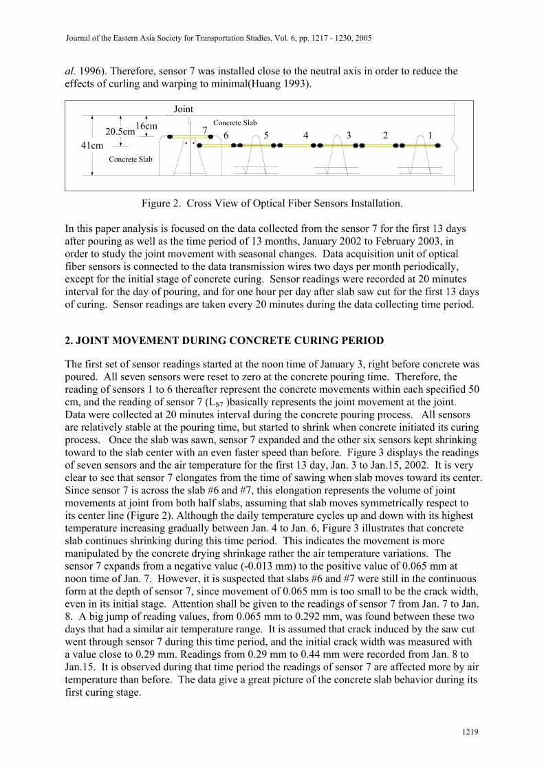
al. 1996). Therefore, sensor 7 was installed close to the neutral axis in order to reduce the effects of curling and warping to minimal(Huang 1993).

Joint

41cm1234567

Concrete Slab

Concrete Slab16cm20.5cm

Figure 2. Cross View of Optical Fiber Sensors Installation.

In this paper analysis is focused on the data collected from the sensor 7 for the first 13 days after pouring as well as the time period of 13 months, January 2002 to February 2003, in order to study the joint movement with seasonal changes. Data acquisition unit of optical fiber sensors is connected to the data transmission wires two days per month periodically, except for the initial stage of concrete curing. Sensor readings were recorded at 20 minutes interval for the day of pouring, and for one hour per day after slab saw cut for the first 13 days of curing. Sensor readings are taken every 20 minutes during the data collecting time period.

2. JOINT MOVEMENT DURING CONCRETE CURING PERIOD

The first set of sensor readings started at the noon time of January 3, right before concrete was poured. All seven sensors were reset to zero at the concrete pouring time. Therefore, the reading of sensors 1 to 6 thereafter represent the concrete movements within each specified 50 cm, and the reading of sensor 7 (LS7 )basically represents the joint movement at the joint. Data were collected at 20 minutes interval during the concrete pouring process. All sensors are relatively stable at the pouring time, but started to shrink when concrete initiated its curing process. Once the slab was sawn, sensor 7 expanded and the other six sensors kept shrinking toward to the slab center with an even faster speed than before. Figure 3 displays the readings of seven sensors and the air temperature for the first 13 day, Jan. 3 to Jan.15, 2002. It is very clear to see that sensor 7 elongates from the time of sawing when slab moves toward its center. Since sensor 7 is across the slab #6 and #7, this elongation represents the volume of joint movements at joint from both half slabs, assuming that slab moves symmetrically respect to its center line (Figure 2). Although the daily temperature cycles up and down with its highest temperature increasing gradually between Jan. 4 to Jan. 6, Figure 3 illustrates that concrete slab continues shrinking during this time period. This indicates the movement is more manipulated by the concrete drying shrinkage rather the air temperature variations. The sensor 7 expands from a negative value (-0.013 mm) to the positive value of 0.065 mm at noon time of Jan. 7. However, it is suspected that slabs #6 and #7 were still in the continuous form at the depth of sensor 7, since movement of 0.065 mm is too small to be the crack width, even in its initial stage. Attention shall be given to the readings of sensor 7 from Jan. 7 to Jan. 8. A big jump of reading values, from 0.065 mm to 0.292 mm, was found between these two days that had a similar air temperature range. It is assumed that crack induced by the saw cut went through sensor 7 during this time period, and the initial crack width was measured with a value close to 0.29 mm. Readings from 0.29 mm to 0.44 mm were recorded from Jan. 8 to Jan.15. It is observed during that time period the readings of sensor 7 are affected more by air temperature than before. The data give a great picture of the concrete slab behavior during its first curing stage.


1219

-0.15

-0.1

-0.05

0

0.05

0.1

0.15

0.2

0.25

0.3

0.35

0.4

0.45

0.5

1/3 1/4 1/5 1/6 1/7 1/8 1/9 1/10 1/11 1/12 1/13 1/14 1/15

Rea

ding

s of s

enso

rs (m

m)

0

3

6

9

12

15

18

21

24

27

30

33

36

39

Tem

pera

ture

(℃)

sensor1 sensor2sensor3 sensor4sensor5 sensor6sensor7 air temperature

Crack occured

Joint saw cut

Pouring

Figure 3. Readings of Sensors & Air Temperatures for the First Thirteen Days of Concrete

Slab Curing.

However, due to the unavailability of data logger for a period of time the records of sensor data were discontinued and did not restart until February. And the data of optical fiber sensors were recorded for continuous 48 hours per month since then.

3. JOINT MOVEMENTS ALONG WITH SEASONAL TEMPERATURE

VARIATIONS

From either theoretical analysis or field observations, it is known that concrete slab moves toward its center when temperature drops, and expands to the joint at high temperature condition. Data collected from the CKS airport experiment field fully coincide with the phenomena. However, the self weight of concrete slab and the friction force between slab and subbase layer also have great resistance to the slab horizontal movement. Figure 4 is the plot of sensor #7 at February and March, 2002. It is clear to observe that readings of sensor increase, i.e. slab contracts, when air temperature drops in the night, and decrease during the day time. However, there exists a 3 hours time lag around between air temperature and sensor reading. In other words, sensor reaches its shortest length about 3 hours after air temperature approaches its peak. This is due to the thermal transmission characteristics of concrete material since the sensor #7 is placed around 16 cm deep from the slab surface. It should be also noted that the air temperature is mostly below 25 oC during these two months. This relatively low air temperature usually gives concrete slabs more freedom to move at joints than that of the high temperature season as shown in Figures 5 and 6.


1220

0.2500

0.3000

0.3500

0.4000

0.4500

0.5000

0.5500

0.6000

0.6500

0.7000

0.7500

0.8000

0.8500

0.9000

0.9500

1.0000

1.0500

1.1000

1.1500

1.2000

1.2500

2/20

11:

00

2/20

14:

20

2/20

17:

40

2/20

21:

00

2/21

00:

20

2/21

03:

40

2/21

07:

00

2/21

10:

40

2/21

14:

00

2/21

17:

20

2/21

20:

40

2/22

00:

00

2/22

03:

20

2/22

06:

40

2/22

10:

00

3/25

12:

30

3/25

17:

30

3/25

22:

30

3/26

03:

30

3/26

08:

30

3/26

13:

30

3/26

18:

30

3/26

23:

30

3/27

04:

30

3/27

09:

30

Rea

ding

s of

sen

sor7

(mm

)

8.00

11.00

14.00

17.00

20.00

23.00

26.00

29.00

32.00

35.00

38.00

Tem

pera

ture

(℃)

sensor7

air temperatureFeb Mar

Figure 4. Readings of Sensor 7 & Air Temperatures in February & March, 2002.

0.2500

0.3000

0.3500

0.4000

0.4500

0.5000

0.5500

0.6000

0.6500

0.7000

0.7500

0.8000

0.8500

0.9000

0.9500

1.0000

1.0500

1.1000

1.1500

1.2000

1.2500

4/30

11:

05

4/30

15:

05

4/30

19:

05

4/30

23:

05

5/1

03:0

5

5/1

07:0

5

5/1

11:0

5

5/1

15:0

5

5/1

19:0

5

5/1

23:0

5

5/2

03:0

5

5/2

07:0

5

5/29

01:

00

5/29

05:

00

5/29

09:

00

5/30

01:

00

5/30

05:

00

5/30

09:

00

5/30

01:

00

5/30

05:

00

5/30

09:

00

5/31

01:

00

5/31

05:

00

5/31

09:

00

Time

Rea

ding

s of s

enso

r7(m

m)

8

10

12

14

16

18

20

22

24

26

28

30

32

34

36

Tem

pera

ture

(℃)

sensor7

air temperature Apr 02 May 02

Figure 5 Readings of Sensor 7 & Air Temperatures in April & May, 2002


1221

0.2500

0.3000

0.3500

0.4000

0.4500

0.5000

0.5500

0.6000

0.6500

0.7000

0.7500

0.8000

0.8500

0.9000

0.9500

1.0000

1.0500

1.1000

1.1500

1.2000

1.2500

6/26

11:

30

6/26

02:

30

6/26

05:

30

6/26

08:

30

6/26

11:

30

6/27

02:

30

6/27

05:

30

6/27

08:

30

6/27

11:

30

6/27

02:

30

6/27

05:

30

6/27

08:

30

6/27

11:

30

6/28

02:

30

6/28

05:

30

6/28

08:

30

8/20

12:

40

8/20

15:

40

8/20

18:

40

8/20

21:

40

8/21

00:

40

8/21

03:

40

8/21

06:

40

8/21

09:

40

9/10

12:

30

9/10

17:

30

9/10

22:

00

9/11

02:

30

9/11

07:

00

9/11

11:

30

9/11

16:

00

9/11

20:

30

9/12

01:

00

9/12

05:

30

9/12

10:

00

9/12

14:

30

Time

Rea

ding

s of s

enso

r7(m

m)

8

11

14

17

20

23

26

29

32

35

38

Tem

pera

ture

(℃)

sensor7

air temperature

Jun 02 Aug 02 Sep 02

Figure 6. Readings of Sensor 7 & Air Temperatures in June, August & September, 2002.

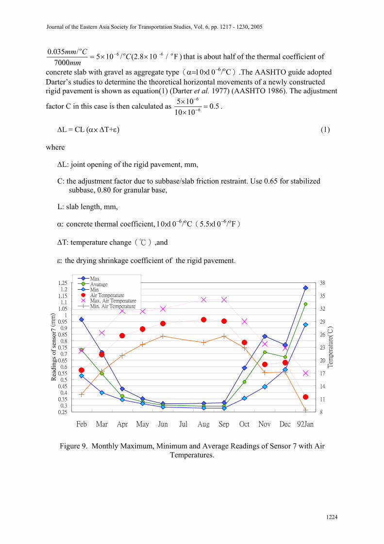
Figure 5 is the graph of sensor data for April and May, 2002. The readings of sensor 7 become less sensitive to the air temperature than before. This phenomenon can be observed even more clearly in Figure 6 which has a rather smooth line when the movements of sensor 7 are almost zero. Readings of sensor 7 of Oct. and Nov., 2002 are shown in Figure 7 while Figure 8 illustrates the data of Dec. 2002 and Jan.2003. It can be seen that the joint movements are more sensitive to air temperature again. From Figure 9, it is also noted that the readings of sensor 7 are decreasing gradually from 0.964 mm (Feb. 2002) to 0.287 mm (June 2002) with the increase of air temperature. The average decreasing rate is 0.034 mm per oC. However, the sensor 7 reaches its shortest length in September. And the decreasing rate slows down significantly from June to September with an average decreasing rate of 0.005 mm per oC of air temperature increasing. The decreasing rate of sensor 7 in the hot seasons is much less than that in the cool seasons due to the limit space for slab expansion. This is mainly because that the concrete slabs were constructed and sawn in January, a relative low temperature season. The slabs were at their shortest condition during that time. The joint saw cut is only at the top one-fourth depth of slab; therefore, the gap down at the joint middle depth was mainly created by the initial crack width plus slab shrinkage during it curing stage. This gap is usually not wide enough for slabs to expand in hot days. From Figure 9 it is observed that the gap of joint is almost closed between June to September while readings of sensor 7 are around 0.28 ±0.01 mm. These readings of sensor 7 coincide the initial crack width measured at the crack occurrence as mentioned earlier in this paper. Since there is not enough space for slab to expand between June and September, it is expected that the slabs have large compressive stresses during these months.


1222

0.2500

0.3000

0.3500

0.4000

0.4500

0.5000

0.5500

0.6000

0.6500

0.7000

0.7500

0.8000

0.8500

0.9000

0.9500

1.0000

1.0500

1.1000

1.1500

1.2000

1.2500

10/9

12:

30

10/9

17:

00

10/9

21:

30

10/1

0 02

:00

10/1

0 06

:30

10/1

0 11

:00

10/1

0 15

:30

10/1

0 20

:00

10/1

1 00

:30

10/1

1 05

:00

10/1

1 09

:30

11/1

5 15

:30

11/1

5 20

:00

11/1

6 00

:30

11/1

6 05

:00

11/1

6 09

:30

11/1

6 14

:00

11/1

6 18

:30

11/1

6 23

:00

11/1

7 03

:30

11/1

7 08

:00

11/1

7 12

:30

Time

Rea

ding

s of

sen

sor7

(mm

)

8.00

11.00

14.00

17.00

20.00

23.00

26.00

29.00

32.00

35.00

38.00

Tem

pera

ture

(℃)

sensor7

air temperature

Oct 02 Nov 02

Figure 7. Readings of Sensor 7 & Air Temperatures in October & November, 2002.

0.2500

0.3000

0.3500

0.4000

0.4500

0.5000

0.5500

0.6000

0.6500

0.7000

0.7500

0.8000

0.8500

0.9000

0.9500

1.0000

1.0500

1.1000

1.1500

1.2000

1.2500

12/1

8 01

:00

12/1

8 05

:30

12/1

8 10

:00

12/1

8 14

:30

12/1

8 19

:00

12/1

8 23

:30

12/1

9 04

:00

12/1

9 08

:30

12/1

9 13

:00

12/1

9 17

:30

12/1

9 22

:00

12/2

0 02

:30

12/2

0 07

:00

1/27

19:

30

1/28

00:

00

1/28

04:

30

1/28

09:

00

1/28

13:

30

1/28

18:

00

1/28

22:

30

1/29

03:

00

1/29

07:

30

1/29

12:

00

1/29

16:

30

Time

Rea

ding

s of

sen

sor7

(mm

)

8.00

11.00

14.00

17.00

20.00

23.00

26.00

29.00

32.00

35.00

38.00

Tem

pera

ture

(℃)

sensor7

air temperature

Dec 02 Jan 03

Figure 8. Readings of Sensor 7 & Air Temperatures in December 2002& January 2003.

From Figure 9, it is also noted that the readings of sensor 7 are increasing gradually from 0.276 mm (Sep. 2002) to 1.209 mm (Jan. 2003) with the air temperature decreasing. The average elongation rate of sensor 7 is 0.036 mm per oC. This increasing rate is very close to the previous decreasing rate of sensor 7. It is assumed that the mean value of the two, i.e. 0.035 mm per oC, reflects the actual movement rate of a 7 m slab in the realistic condition under all the combined restrains, such as friction resistance between slab and subbase layer and slab self weight.

If we divide the elongation rate by the slab length, i.e. 7000 mm, we can obtain the realistic (partially restrained) expansion/ shrinkage rate as


1223

) F / 10 (2.8/1057000

/035.0 o6-o6o

××= − Cmm

Cmm that is about half of the thermal coefficient of

concrete slab with gravel as aggregate type（α=10×10−6/οC）.The AASHTO guide adopted Darter’s studies to determine the theoretical horizontal movements of a newly constructed rigid pavement is shown as equation(1) (Darter et al. 1977) (AASHTO 1986). The adjustment

factor C in this case is then calculated as 5.01010105

6

6

=××

−

−

.

∆L = CL (α× ∆T+ε) (1)

where

∆L: joint opening of the rigid pavement, mm,

C: the adjustment factor due to subbase/slab friction restraint. Use 0.65 for stabilized subbase, 0.80 for granular base,

L: slab length, mm,

α: concrete thermal coefficient, 10×10−6/οC（5.5×10−6/οF）

∆T: temperature change（℃）,and

ε: the drying shrinkage coefficient of the rigid pavement.

0.250.3

0.350.4

0.450.5

0.550.6

0.650.7

0.750.8

0.850.9

0.951

1.051.1

1.151.2

1.25

Feb Mar Apr May Jun Jul Aug Sep Oct Nov Dec 92Jan

Rea

ding

s of s

enso

r7 (m

m)

8

11

14

17

20

23

26

29

32

35

38

Tem

pera

ture

(℃)

MaxAvarageMinAir TemperatureMax. Air TemperatureMin. Air Temperature

Figure 9. Monthly Maximum, Minimum and Average Readings of Sensor 7 with Air

Temperatures.


1224

4. PREDICTION MODELS FOR JOINT MOVEMENT

In this study, prediction model is developed for sensor 7 in order to estimate the slab horizontal movement at any time of any day. A total number of 1234 field data points of sensor 7 collected from February 2002 to January 2003 are utilized in this study to derive an appropriate prediction model for estimating the joint movement. In Chillicothe, Ohio case, Bodocsi et al. noted that slabs are freely moving with temperature (Bodocsi et al. 1993). Some previous studies also showed that there exists a good linear relationship between joint movement and temperature (Lee et al. 2001)(Morian et al. 1999). Morian et al. showed that pavement temperature not only well correlates with the air temperature but also has a significant influence on joint movement (Morian et al. 1999). Therefore, in this study air temperature was selected as the independent variable in the prediction model for predicting the joint movement in this study and it indeed showed a great result. Furthermore, it is noted that there exists a time lag between the air temperature and the slab temperature along the depth (Chou 2003). Equation(2) shows the time lag in hours for various depths of CKS Int’l airport concrete slab (Chou 2003).

ti = 0.2181×D + 0.1937

0

2

4

6

8

10

0 10 20 30 40Depth (cm)

t i (h

our)

Figure 10. Relationship between the Time Lag of the Temperature Reading along the Depth

and the Air Temperature. ti = 0.2181 Di ＋0.1937 R2 =0.985 (2)

where,

ti : time lag in hours at depth Di ,(cm).

Based on the observed data, several independent variables have been applied to the prediction model. The result showed that air temperature which is three hours before the prediction time has the highest correlation to the readings of sensor 7. This result coincides with the findings from Equation 2 and Figure10, since sensor 7 was installed at the 16cm-deep of a 41cm-thick slab. Time lag at this depth is around three hours. In other words, slab temperature at the depth of sensor 7 is affected by air temperature that is three hours earlier.

However, it has been noted from Figures 4, 7 and 8 that joint movements are more related to the delayed air temperature than that at their measured time. It is also noted that the characteristics of joint movement at low temperature seasons, Figures 4, 7, and 8, are different from that at high temperature season, Figures 5 and 6. Table 1 shows the maximum, minimum, difference, and average readings of sensor 7 as well as air temperatures of each month. It is clear to observe that the difference values of sensor 7 between April to September, 2002 are all within 0.1 mm which is much less than that of other months, although the temperature differences of these six months are very similar to others. This observation, again, coincides with the previous findings that joint movement is much more restricted in the


1225

high temperature seasons. It was indicated from previous studies that moisture variation also affects the joint movement. However, in this study temperature is the only independent variable due to the lack of moisture gauge in this study. Therefore, it is decided to separate the 1234 data points into two groups for derive the prediction equations. These two groups are as following:

(1) Data points that are collected between January - March and October - December.

L’S7 = 1.58 – 0.047 x DL3 R2 = 0.903 (3)

(2) Data points that were collected between April and September.

L’S7 = 0.819 – 0.005 x DL3 – 0.013 x AVG48 R2 = 0.811 (4)

where,

L’S7 : estimated reading of sensor 7, mm

DL3 : air temperature at the time that three hours before the prediction of sensor reading, oC

AVG48: average value of air temperatures 48 hours before the prediction of sensor reading, oC

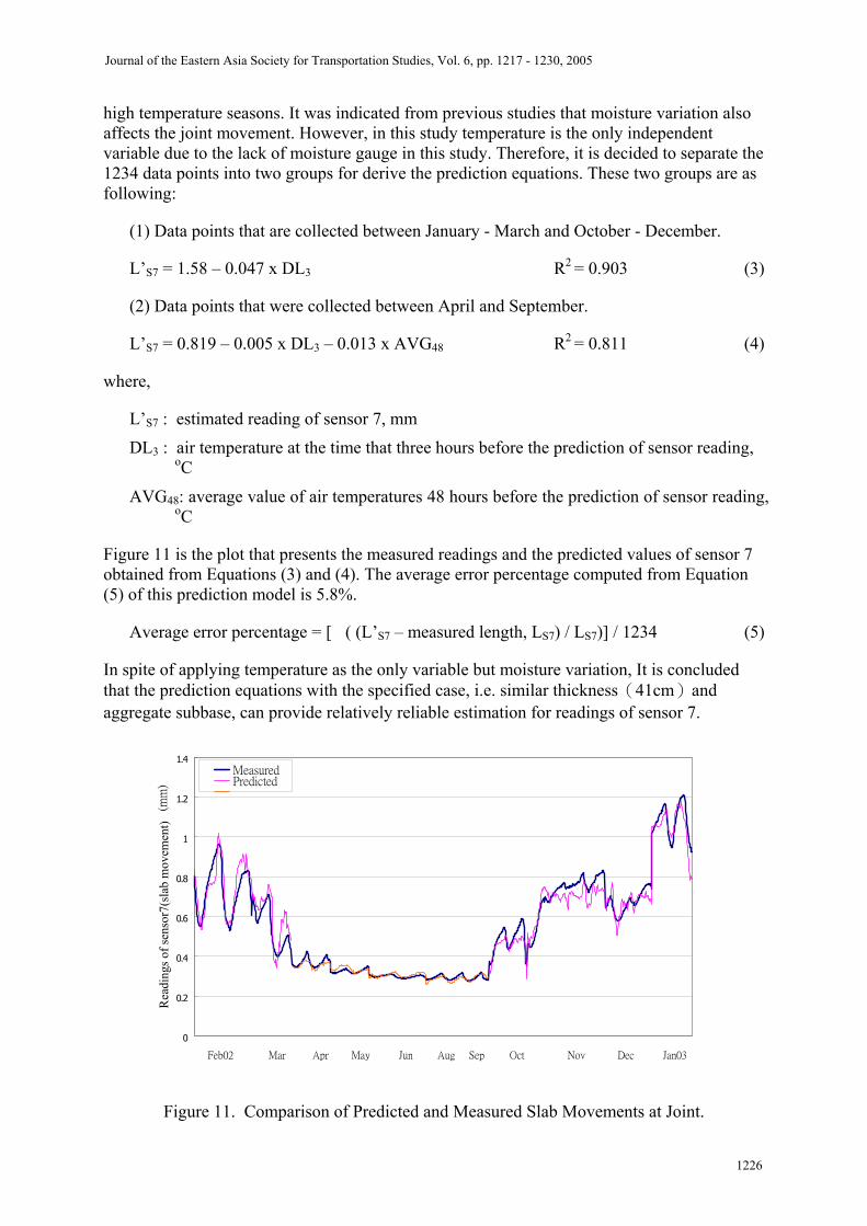
Figure 11 is the plot that presents the measured readings and the predicted values of sensor 7 obtained from Equations (3) and (4). The average error percentage computed from Equation (5) of this prediction model is 5.8%.

Average error percentage = [�( (L’S7 – measured length, LS7) / LS7)] / 1234 (5)

In spite of applying temperature as the only variable but moisture variation, It is concluded that the prediction equations with the specified case, i.e. similar thickness（41cm）and aggregate subbase, can provide relatively reliable estimation for readings of sensor 7.

0

0.2

0.4

0.6

0.8

1

1.2

1.4

Feb02 Mar Apr May Jun Aug Sep Oct Nov Dec Jan03

Rea

ding

s of s

enso

r7(s

lab

mov

emen

t) (

mm

)

MeasuredPredicted

Figure 11. Comparison of Predicted and Measured Slab Movements at Joint.


1226

Table 1. The Maximum, Minimum, Difference, and Average Readings of Sensor 7 as well as Air Temperatures of Each Month.

02Feb Mar Apr May Jun Jul Aug Sep Oct Nov Dec 03Jan

Maximum 0.964 0.710 0.427 0.350 0.313 N/A 0.315 0.321 0.590 0.833 0.767 1.209

Minimum 0.528 0.397 0.343 0.314 0.287 N/A 0.281 0.276 0.355 0.444 0.577 0.924

Difference 0.436 0.313 0.085 0.036 0.026 N/A 0.035 0.045 0.234 0.390 0.190 0.285

Sensor7 (mm)

Average 0.731 0.545 0.371 0.326 0.300 N/A 0.295 0.293 0.481 0.711 0.673 1.083

Maximum 22.2 26.3 31.4 31.3 31.9 33.0 34.0 34.0 29.0 23.7 22.8 17.0

Minimum 12.0 17.4 21.0 23.6 25.5 24.8 24.1 25.5 22.8 17.1 17.2 8.4

Difference 10.2 8.9 10.4 7.7 6.4 8.2 9.9 8.5 6.2 6.6 5.6 8.6

Air Temp. (℃)

Average 17.7 21.3 25.7 27.2 28.5 28.9 29.4 29.0 24.1 19.0 19.4 11.4 5. SLAB THERMAL STRESSES DUE TO TEMPERATURE VARIATIONS

Theoretically, if the slab is at completely free condition（C=1） and concrete moisture shrinkage is considered separately, the joint movements in Equation 1 can be computed as ∆LT = L (α x ∆T ). However, actual joint movement, ∆L, is different from the theoretical joint movement, �LT, because of partially restrained condition. Thus, the restrained strain is calculated as （(∆LT − ∆L ) /L）, and restrained stress can be computed by Equation 6.

σ = ((∆LT − ∆L ) /L) x E (6)

Where

∆LT: theoretical joint movement due to temperature change, mm

∆L: actual joint movements, mm

L: slab length, m (in)

E: Young’s modulus, kg/ cm2 (psi)

α: concrete thermal coefficient,

σ: thermal stresses of concrete slab due to the temperature variations under partially restrained condition (negative value as compression and positive value for tension), kg/ cm2 (pounds/ in2)

In this study it is assumed that α is around 10 x 10 -6 / oC (5.5 x10 -6 / oF) for concrete with gravel aggregates. However, if we use the measured joint movement, LS7, to compute the actual horizontal strain of concrete slab as Equation 7, the critical thermal stresses that occur at the maximum temperature variations can be obtained.


1227

σ = ((α x ∆T) - LS7 / L) x E (7)

Where

�T: the temperature difference between the time of placement to the time at analyzing point, oC (oF)

σ, α, ∆T, LS7 , L, and E are all defined as above

For the computed result, compressive stress should occur at the interior slab while tensile stress occurs at the both ends. Figure 12 displays the computed maximum, minimum, and average slab thermal stresses from February, 2002 to January, 2003. The calculated result might be treated as the possibly extreme value of thermal stress that may occur in this specific test field. It is glad to know that the thermal stress of experimental concrete slabs are in compression at most of the time of the year, since concrete material has a rather high compressive strength, say 455 kg/cm2 (6500 psi) at 28 days in this study, comparing with its tensile strength. The maximum compressive stress occurs in September, and the value is 41 kg/ cm2 (586 psi). It is also noted that slab has tensile stresses in cold days, but the value is relatively low, 9 kg/ cm2 (130 psi) comparing with its tensile strength, 49 kg/ cm2 (710 psi). However, it shall be kept in mind that thermal stresses of concrete slabs will be in tension at most of the time if concrete slabs are constructed in the hot days. It is always considered as a better construction plan if the concrete construction can be scheduled in the relative cool temperature seasons.

7.739.08

-9.03 -9.17

-41.28

-56.00

-42.00

-28.00

-14.00

0.00

14.00

28.00

Feb02 Mar Apr May Jun Jul Aug Sep Oct Nov Dec Jan03

Str

ess(

kg/c

m2 )

-800

-600

-400

-200

0

200

400

Str

ess(

psi)

Max. Slab Thermall StressAverage Slab Thermal StressMin. Slab Thermal Stress

(kg/cm 2)

(kg/cm 2)

(kg/cm 2)

(kg/cm 2)

(kg/cm 2)

Com

pres

sion

Tens

ion

Figure 12. Maximum, Minimum and Average Concrete Slab Thermal Stresses From

February 2002 to January 2003. 6. CONCLUSIONS

This paper presents the application of optical fiber sensors on the measurement of joint movements. A total number of seven sensors were embedded in two concrete slabs of 41 cm thick and 7m long with sensor 7 across a joint in January 2002. Strain data during the early concrete curing stage and joint movements for the first 13 months after construction have been collected and analyzed in this study. The following conclusions are drawn.


1228

1. Concrete shrinks right after the pouring time, and the shrinking speed is even faster after joint saw cut. The induced crack does not occur until four days later in this study and the initial crack width is measured as 0.29 mm. At the early stage of curing, drying shrinkage dominates the joint movements.

2. Concrete slabs expand/ contract at an average rate of 0.034 - 0.036 mm per oC with air temperature changes at relatively low temperature seasons, around January to April and October to December. The realistic expansion/ shrinkage rate is computed as 5 x 10 -6/ oC (2.5 x 10 -6/ oF) that is about half of the assumed thermal coefficient of gravel aggregates.

3. Due to the limited space at joint, slabs reach the closest condition for almost four months (June to September ) with the minimum gap around 0.28 – 0.29 mm, just same as the measured initial crack width.

4. Two regression equations are derived for predicting the readings of sensor 7 (joint movements). The average percentage of error is computed as 5.8 %.

5. Thermal stresses of the experimental concrete slabs are calculated. The maximum compressive stress occurs in September 2002 with 41 kg/ cm2 (586 psi), and the maximum tensile stress is 9 kg/ cm2 (130 psi) in January 2003.

ACKNOWLEDGEMENTS

The Department of Civil Engineering of National Taiwan University would like to express the great appreciation to CKS Int’l Airport for their financial and physical support.

REFERENCES

American Association of State Highway Transportation Officials(AASHTO) AASHTO Guide for Design of Pavement Structures 1986, Washington, D.C.

Andrew Bodocsi, Issam A. Minkarah, and Rajagopal S. Arudi (1993) Analysis of Horizontal Movements of Joints and Cracks in Portland Cement Concrete Pavements, Transportation Research Record 1392, 43-52.

Chia-pei Chou (2003), Concrete Slab Monitoring and Analysis for Chiang Kai-Shek International Airport, Research Report, Civil Aviation Administration, Taiwan.

Darter M. I., and Barenberg E. J. (1977) Design of zero maintenance plain concrete pavement, vol. II-Design Manual, FHWA-RD-77-112, Federal Highway Administration, Washington, DC.

Yang H. Huang (1993) Pavement Analysis And Design, New Jersey, Prentice-Hall.

Seung Woo Lee and Shelly M. Stoffels (2001) Analysis of In Situ Horizontal Joint Movements in Rigdid Pavements, Transportation Research Record 1778, 9-16.


1229

Dennis A. Morian, Nadarajah Suhahar, and Shelley Stoffels (1999) Evaluation of Rigid Pavement Joint Seal Movement, Transportation Research Record 1684, 25-32.

David W. Pittman (1996) Factors Affecting Joint Efficiency of Roller-Compacted Concrete Pavement Joints and Cracks, Transportation Research Record 1525, 10-20.

M. Poblete, R. Salsilli, R. Valenzuela, A. Bull, and P. Spratz (1988) Field Evaluation of Thermal Deformations in Undoweled PCC Pavement Slabs, Transportation Research Record 1207, 217-228.


1230

ANALYSIS OF CONCRETE JOINT MOVEMENTS AND SEASONAL THERMAL …

Documents

Transcript of ANALYSIS OF CONCRETE JOINT MOVEMENTS AND SEASONAL THERMAL …