Analysis of Composite Materials—vucoe.drbriansullivan.com/...Analysis-of-Composites... ·...

Z. Hashin Nathan Cummings Professor

of Mechanics of Solids, Department of Solid Mechanics,

Materials and Structures, Tel Aviv University,

Tel Aviv, Israel Fellow AS ME

Analysis of Composite Materials— A Survey The purpose of the present survey is to review the analysis of composite materials

from the applied mechanics and engineering science point of view. The subjects under consideration will be analysis of the following properties of various kinds of composite materials: elasticity, thermal expansion, moisture swelling, viscoelasticity, conductivity (which includes, by mathematical analogy, dielectrics, magnetics, and diffusion) static strength, and fatigue failure.

"Where order in variety we see And where, though all things differ, all agree'

Alexander Pope

1 Introduction Composite materials consist of two or more different

materials that form regions large enough to be regarded as continua and which are usually firmly bonded together at the interface. Many natural and artificial materials are of this nature, such as: reinforced rubber, filled polymers, mortar and concrete, alloys, porous and cracked media, aligned and chopped fiber composites, polycrystalline aggregates (metals), etc.

Analytical determination of the properties of composite materials originates with some of the most illustrious names in science. J. C. Maxwell in 1873 and Lord Rayleigh in 1892 computed the effective conductivity of composites consisting of a matrix and certain distributions of spherical particles (see Part 6). Analysis of mechanical properties apparently originated with a famous paper by Albert Einstein in 1906 in which he computed the effective viscosity of a fluid containing a small amount of rigid spherical particles. Until about 1960, work was primarily concerned with macroscopically isotropic composites, in particular, matrix/particle composites and also polycrystalline aggregates. During this period the primary motivation was scientific. While the composite materials investigated were of technological importance, a technology of composite materials did not as yet exist. Such a technology began to emerge about 1960 with the advent of modern fiber composites consisting of very stiff and strong aligned fibers (glass, boron, carbon, graphite) in a polymeric matrix and later also in a light weight metal matrix.

The engineering significance of reliable analysis of

Contributed by the Applied Mechanics Division for publication in the JOURNAL OF APPLIED MECHANICS.

Discussion on this paper should be addressed to the Editorial Department, ASME, United Engineering Center, 345 East 47th Street, New York, N.Y. 10017, and will be accepted until two months after final publication of the paper itself in the JOURNAL OF APPLIED MECHANICS. Manuscript received by ASME Applied Mechanics Division, February, 1983.

properties is quite different for particulate composites and for fiber composites. For the former, such capability is desirable, while for the latter it is crucial. The reason is that the range of realizable properties and the ability to control the internal geometry are quite different in the two cases. For example: the effective Young's modulus of an isotropic composite consisting of matrix and very much stiffer and stronger spherical type particles will depend primarily on volume fractions and can be increased in practice only up to about four-five times the matrix modulus. The strength of such a composite is only of the order of the matrix strength and may even be lower. The effect of stiffening and strengthening increases if particles have elongated shapes but at the price of lowering the maximum attainable particle volume fraction.

A unidirectional fiber composite is highly anisotropic and therefore has many more stiffness and strength parameters than a particulate composite. Stiffness and strength in the fiber direction are of fiber value order, and thus very high. Stiffnesses and strengths transverse to the fiber direction are of matrix order, similar to those of a particulate composite, and thus much lower. Carbon and graphite are themselves significantly anisotropic, their elastic properties being defined by five numbers instead of the usual two for an isotropic material. Furthermore, matrix properties may be strongly influenced by environmental changes such as heating, cooling, and moisture absorption. All of this creates an enormous variety of properties, of much wider range than for a particulate composite.

The generally low values of stiffness and strength transversely to the fibers provide the motivation for laminate construction consisting of thin unidirectional layers with different reinforcement directions. The laminates are formed into laminated structures. The layer thicknesses, fiber directions, choice of fibers, and matrix are at the designers disposal and should, ideally, be chosen from the point of view of optimization of an important quantity such as weight or price. The design of such structures is an integrated process leading from constituents to structure in the sequence:

Journal of Applied Mechanics SEPTEMBER 1983, Vol. 50/481

Copyright © 1983 by ASMEDownloaded 18 Feb 2010 to 153.104.2.21. Redistribution subject to ASME license or copyright; see http://www.asme.org/terms/Terms_Use.cfm

FIBERS AND MATRIX - UNIDIRECTIONAL COMPOSITE - LAMINATE - LAMINATED STRUCTURE.

Traditionally, material properties have been obtained by experiment and material improvement has been achieved empirically and qualitatively. The structural designer had at his disposal a limited number of material options provided by the materials developer. This situation is entirely different for fiber composite structures. The only constituents that are materials in the traditional sense are fibers and matrix. Everything following in the sequence, including the unidirectional material, is of such immense variety that analysis, rather than experimentation, is the practical procedure to obtain properties. Thus, the relevant methods are those of applied mechanics rather than those of materials science.

The purpose of the present survey is to present analysis of composite materials from the applied mechanics and engineering science point of view, and thus as a subject that is based on principles and rational methods and not on empiricism and speculation. The subjects under consideration will be analysis of the following properties of various kinds of composite materials: elasticity, thermal expansion, moisture swelling, viscoelasticity, conductivity (which includes, by mathematical analogy, dielectrics, magnetics, and diffusion) static strength, and fatigue failure. Relevant comprehensive literature expositions are Hashin [1] and Christensen [2] which will be referred to frequently. Important subject omissions are elastodynamic behavior and plasticity, this for reasons of space limitation. Surveys of these subjects may be found in [2]. Analysis of laminates is not included since this is a well understood subject and it has been described in several textbooks, except for the problem of laminate failure which will be briefly discussed.

2 General Considerations

There are two kinds of information that determine the properties of a composite material: the internal phase geometry, i.e., the phase interface geometry and the physical properties of the phases, i.e., their constitutive relations. Of these, the former is far more difficult to classify than the latter. In reality the internal geometry of every composite material is to a certain extent random. In a general two phase material (for reasons of simplicity the discussion will be concerned with two phases. The case of more phases will only be considered as needed) the phase regions are of arbitrary unspecified shapes. When one phase is in the form of particles embedded in the second matrix phase the material is called a particulate composite. The internal geometry may be three or two dimensional. The latter case implies cylindrical specimens where each cross section has the same plane geometry. If nothing else is specified this is called a. fibrous material, which is the two-dimensional case of a general two phase material. The two-dimensional analogue of a particulate composite is a fiber composite, the particles being aligned cylinders.

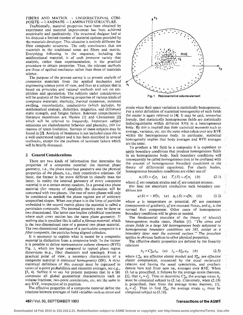
It is necessary to explain what is meant by a composite material in distinction from a composite body. In the former it is possible to define representative volume elements (RVE) Fig. 1, which are large compared to typical phase region dimensions (e.g., fiber diameters and spacings). From a practical point of view, a necessary characteristic of a composite material is statistical homogeneity (SH). A strict statistical definition of this concept must be expressed in terms of n-point probabilities and ensemble averages, see e.g., [3, 4]. Suffice it to say for present purposes that in a SH composite all global geometrical characteristics such as volume fractions, two-point correlations, etc. are the same in any RVE, irrespective of its position.

The effective properties of a composite material define the relations between averages of field variables such as stress and

Fig. 1 Representative volume element

strain when their space variation is statistically homogeneous. For a strict definition of statistical homogeneity of such fields the reader is again referred to [4]. It may be said, somewhat loosely, that statistically homogeneous fields are statistically indistinguishable within different RVE in a heterogeneous body. By this is implied that their statistical moments such as average, variance, etc. are the same when taken over any RVE within the heterogeneous body. In particular, statistical homogeneity implies that body averages and RVE averages are the same.

To produce a SH field in a composite it is expedient to apply boundary conditions that produce homogeneous fields in an homogeneous body. Such boundary conditions will consequently be called homogeneous (not to be confused with the concept of homogeneous boundary conditions in the theory of differential equations). For elastic bodies, homogeneous boundary conditions are either one of

Ui{S)=e%Xj (a) Ti{S)=4nj (b) (2.1) where e$ are constant strains and cr°- are constant stresses.

For heat (of electrical) conduction such boundary conditions are

*>(S) =-//?*,- (a) qn(S)=q»ini (b) (2.2)

where <p is temperature or potential, Hj are constants (components of gradient), q° are constant fluxes, and q„ is the normal flux component. Other cases of homogeneous boundary conditions will be given as needed.

The fundamental postulate of the theory of (elastic) heterogeneous media states, Hashin [1]: "The stress and strain fields in a large SH heterogeneous body subjected to homogeneous boundary conditions are SH, except in a boundary layer near the external surface." The postulate applies in obvious fashion to other physical properties.

The effective elastic properties are defined by the linearity relations

ou = CfJkieki (a) eij = Stjkrok, (b) (2.3) where C,*w are effective elastic moduli and S*Jki are effective elastic compliances, connected by the usual reciprocity relation and having the usual symmetries, and overbars denote here and from now on, averages over RVE. When (2.1a) is prescribed, it follows by the average strain theorem, [1], that ey = ey. Thus to determine Cfjk, the average stress ay must be computed subject to (2.1a). Conversely, when (2.lb) is prescribed, then from the average stress theorem, [1], ay — ay. Thus to find Syk/ the average strain ly must be computed subject to (2.1b).

482/Vol. 50, SEPTEMBER 1983 Transactions of the ASME

Downloaded 18 Feb 2010 to 153.104.2.21. Redistribution subject to ASME license or copyright; see http://www.asme.org/terms/Terms_Use.cfm

Everything is analogous for conductivity. The effective conductivity tensor jtj and the effective resistivity tensor p,* are defined by

q, = rtHj H,=p*qj (2.4)

where H, = — <ph The tensors /nj and pfj are reciprocal and are determined analogously to effective elastic properties. The averages Ht and qs are given by Iff and q<j in (2.2) from conductivity average theorems, [1].

The computation of effective properties in terms of averages will be called the direct approach. In general it requires determination of the appropriate fields in the phases as defined by the field equations, interface continuity conditions, and external homogeneous boundary conditions, in order to compute the required averages. The interface conditions are, for solid mechanics,

«J1) = «P>; 7T> = 7 p on Sl2 (2.5)

and for conductivity

^ ) = v 0 ) ; qM=q«> on Sl2 (2.6)

It follows that effective physical properties are in general functions of all the details of the constituent interface geometry. Actual direct computation is an extremely difficult problem, primarily because of the necessity to satisfy (2.5) or (2.6), and it must be restricted to simple models not only because of mathematical difficulties but also because the actual details of the interface geometry are never known.

An alternative definition of effective physical properties can be given in terms of energy expressions. This is based on the average theorem of virtual work, [1], which when specialized to heterogeneous elastic bodies with homogeneous boundary conditions states

U*=^C*ulcleuSklV=W*V (a)

(2.7)

U'=^StJuauaklV=WV (6)

where t/e is strain energy, U" is stress energy (this replaces the expression strain energy in terms of stresses), Kis the volume, W is elastic energy per unit volume RVE, equation (2.7a) is associated with (2. la), and {2.1b) is associated with {2Ab).

Similarly for conduction with homogeneous boundary conditions

QH=l-tfjHiHJV (a)

(2.8)

Q,= \plqiqJV (b)

where Q is \/2\qj(\)Hi{x)dV, are associated with (2.2 a,b), respectively.

It is of interest to note that in the early stages of the theory of composite materials, effective elastic moduli were defined in terms of energy by expressions of type (2.7), following Einstein's pioneering paper on viscosity of dilute suspensions, [5]. The equivalence of the average and energy definitions of effective elastic moduli (2.3) and (2.7) was apparently only recognized in 1963, independently, by Hill [6] and by Hashin [3], On the other hand, early work on effective conductivity employed the average definition (2.4).

The primary importance of (2.8) is in that such energy expressions can be bounded from above and below by ex-tremum principles. Bounding requires construction of admissible fields that are much easier to construct than actual solutions. By judicious choice of boundary conditions, energy expressions can be expressed in terms of a single property, e.g., effective elastic modulus. Bounding of strain energy yields an upper bound on effective modulus. Bounding of stress energy yields an upper bound on the effective com

pliance, and thus on the reciprocal of the effective modulus, and consequently a lower bound on the effective modulus. Similar considerations apply for conduction.

Everything said so far has merely been concerned with effective properties. In the context of homogeneous media the analogous subject would be homogeneous material properties, which are of course measured in the laboratory using specimens with internal homogeneous fields. Indeed equations (2.3), (2.4), (2.7), and (2.8) have completely analogous homogeneous material counterparts in terms of field quantities "at a point." The question that now arises is: what is a suitable macrodescription of a heterogeneous material body when it is subjected to arbitrary boundary conditions and thus the internal fields are no longer statistically homogeneous? It is instructive to recall how this problem is resolved in the case of "homogeneous" continua. It is always assumed that such continua retain their properties regardless of specimen size, thus also for infinitesimal elements. This permits establishment of field equations in terms of field derivatives. However, all real materials have microstructure. Metals, for example, are actually polycrystalline aggregates and are thus heterogeneous materials. Therefore the differential element of the theory of elasticity is in reality a RVE, which is composed of a sufficiently large number of crystals, and whose effective elastic moduli are the elastic moduli of the theory of elasticity. Since the RVE is not infinitesimal it emerges that the classical theory of elasticity is an approximation that results in a macrodescription of a polycrystalline aggregate when the RVE size is "sufficiently small" in relation to the body dimensions.

The simplest point of view would be to adopt the same approximation for a composite material body. This would imply that the classical field equations of elasticity, conductivity, or other are assumed valid for the composite material body with effective properties replacing the usual homogeneous properties. Such an approach may be called the classical approximation and will now be discussed within the frame of more general theory. It is first necessary to define appropriate field variables for construction of field equations which are to describe a composite material as some equivalent continuum. The usual choice is moving averages over RVE or ensemble averages. A moving average of a function, e.g., displacement, is defined as

«,-(x) = —jw/ (x ,x ' ) c fo ' (2.9)

where x is a position vector to a reference point in the RVE (e.g., centroid) defining its location, x\ is a local coordinate system originating at x (Fig. 1) and the integration is over RVE.

The moving average concept is tied to the concept of geometrical scaling of a composite material which is indispensable for its representation as some equivalent continuum. The typical dimensions of phase regions, e.g., particle diameters, single crystal dimensions, are defined as the MICRO scale. The dimensions of the RVE are defined as the MINI scale and the dimensions of the composite material body as the MACRO scale. The equivalent continuum is a meaningful representation of a heterogeneous body only if

MICRO < < MINI < < MACRO (2.10)

This will be referred to as the MMMprinciple. Displacements w/(x,x'), strains e,y(x,x'), and stresses a-j(x,x) within the phases are called microvariables while moving averages should by the same token be called minivariables. Accordingly computation of effective physical properties on the basis of phase geometry is frequently called micromechanics. It has been suggested that analysis of a composite as if it were



some continuum, thus in terms of minivariables, should be called minimechanics, [7].

It is easily shown that moving averaging and differentiation are commutative (see e.g., [1]). Thus for example

This leads at once to the conclusion that

7lMrJ) = eiJ{x) (2.12)

Another point of view is based on the ensemble average. This average is based on the concept of an ensemble of composite specimens that have certain common characteristics such as: phase properties, phase volume fractions, and certain statistical moments of spatial variation of properties. The ensemble average of w,- is defined by

. n = N

<K,->(x)= - £ K , - „ ( X ) (2.14)

where there are TV members of the ensemble. The operations of ensemble averaging and differentiation are commutative. Therefore (2.12) and (2.13) are also valid for ensemble averages; see e.g. [4],

In the case of SH fields, the moving average and the ensemble average are constants. It is also quite evident that they are equal, which is known as an ergodic hypothesis. The fundamental problem is the relation between moving averages or ensemble averages of statistically nonhomogeneous stress and strain. It is remarkable that the answer to this question has been given for both kinds of averages almost at the same time and that the relations are the same (Beran and McCoy [8]-ensemble average, Levin [9]-moving average), thus

&,y(x)=JLJw(x,x')ew(x')c/x' (2.15)

This important result shows that space variable averages are defined by what is called today a nonlocal theory. It is, however, not a practical result since the two point tensor L* depends on phase properties and phase geometry in unknown fashion. For similar developments for conductivity of heterogeneous media see Beran, [10].

It is of interest to note that multipolar or strain gradient theories are special cases of nonlocal theory. This is seen from series expansion around x, [8], from which it follows that (2.15) can be approximated by

^ij = C*jk/eM+D*ijk/m^k/,m+E*jkim„ek/y,„„+ . . . (2.16)

If only the first term in the right side of (2.16) is retained then

W = C5„£-H(x) (2-17) which implies that variable averages are related just as constant averages in (2.3). The relations (2.11)—(2.13), and (2.17) are equivalent to classical elasticity equations where the displacements are moving or ensemble averages and the elastic properties are effective. Therefore, equation (2.17) is the essence of the classical approximation for heterogeneous media introduced in the foregoing. Classical approximations for other kinds of physical behavior are defined analogously. On the basis of accumulated experience with composite materials and heterogeneous media it appears that this simplest approximation is adequate for most engineering problems. The situation is different for dynamic problems with very high frequencies of vibration, thus very small wavelengths, and for very high stress and strain gradients, e.g., at crack tips.

This survey will be almost exclusively concerned with classical effective properties that define the classical ap

proximation. The following discussions of analytical treatments will be divided, if possible, into three categories: (a) direct approach, (T>) variational approach, and (c) approximations. Direct approach implies exact calculation of effective properties for some geometrical model of a composite material. The value of such results obviously depends on the realism of the model used but the number of choices that permit exact analysis is not large. Exact analysis implies that the microfields that are averaged satisfy the phase governing differential equations, the phase interface conditions, and the external boundary conditions on the composite. However, the latter need not be satisfied precisely but only in a suitable average sense (recall the boundary layer in the fundamental postulate of the theory of heterogeneous media). It frequently happens that effective properties computed for a certain model agree well with experimental data although the details of phase geometry of the model and the tested specimen are different. From this it should not be concluded that the model microfields are in similar agreement with specimen microfields, because effective properties are defined in terms of averages and functions that have the same averages can be very different in detail.

The variational approach is in a certain sense more powerful than the direct approach since it leads to bounds on effective properties when exact calculation is not possible. In particular, it is the only approach that can give results for irregular phase geometry in terms of partial information. The practical importance of the bounds obtained depends on their proximity.

Approximations are by their nature of unlimited variety. The most primitive approach is to postulate "semiempirical" expressions without the benefit of a model or theory. Such expressions will inevitably contain an undetermined parameter to be fitted to the experimental data. However, other experimental data will generally require a different value of the parameter and so measurement of the effective property has been replaced by measurement of a parameter, for no good reason. In more sophisticated and sometimes very ingenious versions, models of composite materials are analyzed on the basis of assumptions that are in principle incorrect, with the hope that the error introduced is not large. Only this kind of approximations will be discussed in the present survey and it will be endeavored to point out their relations to exact procedures. While approximations are unavoidable and often very valuable in the development of a complex subject of practical importance they should always be viewed with caution and should never displace available exact results.

3 Elastic Properties

3.1 Statistically Isotropic Composites

3.1.1 Introduction. A composite is statistically isotropic when its effective stress strain relation is independent of the choice of coordinate system. Important cases are: random mixture of two phases, matrix containing spherical type particles or randomly oriented elongated particles (e.g., short fibers), porous media, etc. It is of interest to note that a polycrystalline aggregate with randomly oriented crystals is a statistically isotropic composite with an infinite number of anisotropic phases. This will be discussed in Section 3.1.5. It follows just as for homogeneous elastic materials that in the isotropic case (2.3) reduce to the usual forms

&v = \*ekk6u + 2G*iu (3.1.1)

or

a=3K*e (a) su = 2G*eu (b) (3.1.2)

where K* = effective bulk modulus; G* = effective shear modulus; &, e = isotropic part of average stress, strain; and

484/ Vol. 50, SEPTEMBER 1983 Transactions of the ASME


Sjj,ey = deviatoric part of average stress, strain. Other effective elastic properties such as E* and c* are defined in the usual way. All of the interrelations of isotropic elastic moduli remain valid for effective elastic moduli.

3.1.2 Direct Approach. for two phase composites elementary relations

Central to the direct approach with isotropic phases are the

*P> K*=Kl+(K2-K{)—v2 (a)

G* = GX+(G2-G,)-P(?)

(3.1.3)

(*)

(no sum on ij in (b)), where 1, 2 indicate the phases, e(2) and e®are averages of e(x) and e,y(x) over phase 2, and v is volume fraction. The averages e and e„ are induced by homogeneous boundary conditions of type (2.1a)

Ui(S)=eXj or ui(S)=eijxj (3.1.4)

which arise from the decomposition e,j• = e5y+ £y. Relations of type (3.1.3) can also be written in terms of stress averages over one phase, see e.g., [1, 6].

The simplest case is dilute concentration of spherical or ellipsoidal particles of material 2 in matrix 1. The definition of "dilute" is that the state of strain in any one particle in the composite body under homogeneous boundary conditions is not affected by all the other particles. Thus the strain is that of a single particle in an infinite body and this happens to be uniform for an ellipsoid with far field homogeneous strain, Eshelby [11]. Thus for spherical particles it follows very simply from spherical particle strain expressions and (3.1.3) that

3K, + 4G,

3A-2+4G,

G* = G j + ( G 2 - G , ) 5(3*,+4G,)

9 ^ + 8 0 , +6i(A", +2G1)G2 /G1

(«)

(b)

(3.1.5)

given independently in [11-13]. Here 1 indicates matrix, 2 = spherical particles, and c = v2<<\. Results for randomly oriented ellipsoidal particles were given in [11]. The special cases of elongated ellipsoids (short fibers) and platelets have been discussed in [2].

Dilute concentration results may be viewed as the first two terms of a power series in particle volume fraction c. In this representation an effective property M* may be written as

M* = l+axc+a2c

2 + . . . (3.1.6)

Dilute concentration results such as (3.1.5) determine the coefficient ax. Evaluation of a2 as a much more difficult problem which has been resolved by Batchelor and Green [15] for identical rigid spheres embedded in incompressible elastic matrix (in the context of their treatment of effective viscosity of a rigid spheres suspension). Chen and Acrivos [14] have extended the analysis to the considerably more difficult case of any linear isotropic elastic spheres and matrix. The analyses require proper summation of the effects of all sphere doublets and unlike ax, ct2 depends on particle statistics. For randomly and isotropically distributed identical rigid spheres in incompressible matrix the analysis of [15] provides the estimate a2 = 5.2 ±0.3 while according to [14] a2 =5.01 in this case.

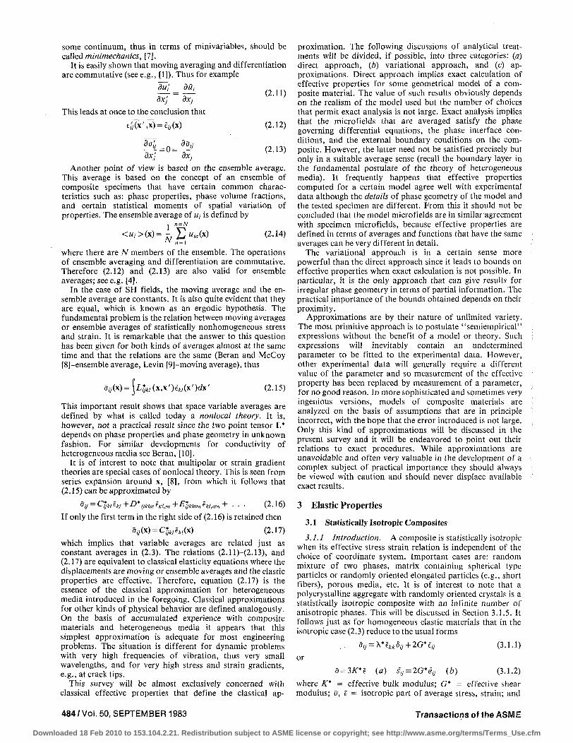
The case of finite concentration of spherical particles is an extremely difficult problem since computation of effective moduli requires a detailed elastic field analysis subject to interface continuity conditions (2.5) on all spherical surfaces. It appears that only one rigorous treatment for a special

Fig. 2 Composite spheres assemblage; composite cylinders assemblage

arrangement of spheres called the composite spheres assemblage is available and this only for the effective bulk modulus. A composite sphere is defined by an isotropic sphere 2 enclosed in an isotropic concentric shell 1, Fig. 2. If the external boundary r=b is subjected to purely radial displacement ur(b)= e°b, the radial stress on the boundary is written arr (b) = 3K*e° where K* follows from the analysis of this elementary, radially symmetric, elasticity problem and is a function of core and shell elastic moduli and of alb. It is seen that to an external observer the composite sphere behaves just as a homogeneous sphere of radius b with bulk modulus K*. If a homogeneous isotropic body with bulk modulus K* is subjected to homogeneous isotropic strain e°8y, the displacement and traction on any internal spherical surface with radius b are purely radial and are precisely those on the composite sphere boundary given in the foregoing. It follows that such a sphere can be replaced by the composite sphere without perturbing the homogeneous isotropic state of stress and strain in the body. Therefore such replacements can be performed again and again with composite spheres of different sizes as long as the spheres all have the same A'* which is certaiflly the case if in all composite spheres the ratio alb and the constituent properties are the same. It may be rigorously shown that if the body is filled out with composite spheres, which diminish to infinitesimal size, then in the limit as the remaining volume goes to zero the effective bulk modulus of this composite material converges to the bulk modulus K*. This model is called the composite spheres assemblage, Fig. 2. Its bulk modulus is given, Hashin [16], by

K*=KX+(K2-KX)

= Kl +

(3A", +Ad)v2

3K2 + 4G1-3(K2-K1)V2

v2

l/(K2-K1) + 3vi/(3Kl+4Gl)

where 1 indicates matrix and 2 indicates particles. The result (3.1.7) is easily generalized to the case of hollow spheres, reference [17], which is of practical importance for hollow microsphere reinforcement.

The basis for the results established so far is special internal geometry which permits exact analysis. Another class of exact solutions is based on special relations among the constituent properties. One of these cases is a two-phase material of arbitrary phase geometry where the shear moduli of the two phases are equal. In this case (3.1.7) is the exact solution for this case, Hill [6].



Another case is a weakly inhomogeneous medium which is defined by small deviation of local space variable moduli from their averages. Then, for any number of phases,

_ K^R+KT^ (3'L8)

where A"2 is the variance of K, Molyneux and Beran [18], which for two phases is given by (K2 -K\)2vxu2. Then (3.1.8) can be interpreted as the beginning of a series expansion in (K2-K,)/K.

Finally, the isotropic version of (2.15) and (2.16) will be briefly discussed. In the case of statistical isotropy the two-point tensor L,*w appearing in (2.15) is statistically isotropic. Even in this simplest case this tensor is expressed in terms of six scalars which are unknown function of r= l x - x ' I, of the phase geometry and the phase properties. This should be contrasted with (3.1.2) which require only two material constants. It has been shown, reference [8], that in the isotropic version of (2.16) D*jklm vanish and the stress-strain relation reduces to that of first strain gradient theory, requiring classical elastic moduli K*, G*, and two effective material length parameters, /, and l2. The latter have been computed, Beran and McCoy [8], for weakly non-homogeneous media in terms of two-point correlations of the space variable local elastic moduli. It appears that this is the only calculation of higher order elastic constants of heterogeneous media available in the literature.

3,1.3 Variational Bounding. When a composite material is statistically isotropic, the strain and stress energies (2.7) can be expressed in terms of (3.1.2) in the convenient forms

W 1 ;W*£2+2G*eiJeij)

1 (3.1.9)

W = - ( ct/K* + SySy /2G*)

Appropriate homogeneous boundary conditions to obtain energy expressions with K* only are

«,• (S) = eXi T, (S) = an-, (3.1.10)

To obtain energy expressions with G* only

ui(S)=eIJXj Ti(S)=s-unj (3.1.11)

In the following, lower and upper bounds on some effective property M* will be denoted M(*_) ,M(*+) implying that

A*?., <M* <M?+ ) (3.1.12)

For arbitrary internal phase geometry with isotropic phases the extremum principles of minimum potential and minimum complementary energy have been used with admissible linear displacement fields or with admissible constant stress to obtain the elementary bounds, Paul [19]

/f(*_) = [ E i ; „ / ^ ] - 1 = - ^ - (a)

(3.1.13)

KU) = m„v„=K (b)

Gf-) = [E«),/GJ1]-1 = - ^ - (a)

(3.1.14)

G('+) = EG„t;„ = G (b)

where n labels the phases. Averages such as K and G are (unfortunately) sometimes called "rules of mixture." It follows from the usual relation of Young's modulus E to K and G that

E?± 9K?±)G; ( ± ) u ( ± )

(±r 3^*±) + G*±) (3.1.15)

for any bounds on K* and G*. Similar bounds for effective Poisson's ratio v* cannot be established.

For most applications, the bounds (3.1.13) and (3.1.14) are not close enough. Improved bounds for arbitrary statistically isotropic phase geometry have been derived, Hashin and Shtrikman [20], on the basis of new variational principles in terms of the elastic polarization tensor established in [21]. For two-phase media these results are:

K(~) Ki + i/^x2-K1) + 3v,/(3Kl+4Gl) {a)

(3.1.16)

K*+) =K2 +

Gf-) = G,

l/(Ki-K2) + 3v2/QK2+4G2) (b)

Vl

l/iGi-GO + bv^Kt +2Gi)/5G]{.'iKl+AGl)

G(*+) = G2

+ V\

(1/(G, - G2) + 6v2(K2 + 2G2)/5G2(3K2 + 4G2)

when

K, <K7 G, <G2

(a)

(3.1.17)

(*)

(3.1.18) Bounds for any number of isotropic phases were also given in [20].

The original derivation of the bounds, reference [20], included some mathematical liberties. These were first removed in [22] by application of Fourier transform methods. Walpole [23] elegantly rederived the bounds by Green's function and potential methods using the classical extremum principles with the polarization concept in a manner indicated by Hill, reference [24]. He also generalized the bounds by removal of the restriction (3.1.18). Other elegant and interesting derivations and generalizations were given by Korringa [25], Willis [26, 27], Kroner [28], who introduced the notion of odd and even order bounds ((3.1.13) and (3.1.14) are first (odd) order and (3.1.16) and (3.1.17) are second (even) order), and Wu and McCullough [29].

Comparison of (3.1.16a) with (3.1.7) reveals the remarkable fact that they are the same. Since (3.1.7) is an exact result and since (3.1.16a) is a general lower bound in terms of phase volume fraction, it follows that (3.1.16a) is the best possible lower bound in terms of volume fractions. Similarly, (3.1.16b) is the best possible upper bound since it is at once interpreted as an exact result for a composite spheres assemblage with particles 1 of volume fraction vx and matrix 2. It has never been shown that (3.1.17) are also best possible in terms of volume fractions but they well may be. The bounds are generally in good agreement with experimental data. A recent particularly careful experimental investigation is given in [30] also citing other experimental investigations.

The bounds are of practical value for phase stiffness mutual ratios up to about 10. They obviously cannot provide good estimates for extreme phase stiffness ratios such as one rigid phase or an empty phase (porous medium). Since the only geometrical information entering is volume fractions, the bounds cannot distinguish between phases in the form of matrix or particles. Evidently, of two composites with same phases and volume fractions, one having very stiff matrix and the other very stiff particles - the first is much stiffer than the second, but both of them must obey the same bounds. Thus in the extreme case of one infinitely rigid phase, the upper bounds become infinite while in the other extreme case of an empty phase the lower bounds vanish.

486/VOI. 50, SEPTEMBER 1983 Transactions of the ASME


To improve the bounds it is necessary to incorporate additional geometrical information. One way of doing this is in terms of higher order statistical information. The volume fractions of a statistically homogeneous material can be interpreted as one-point probabilities. Therefore it is plausible to try to incorporate additional geometrical information in terms of two-point, three-point . . . probabilities. This can be done in terms of the classical extremum principles, reference [4], or in terms of the polarization principles [27, 28], which have been used to derive (3.1.16) and (3.1.17). Kroner [34] has given results for so-called "perfectly disordered" materials, defined as composites in which properties of a phase are not correlated with properties of adjacent phases and thus the two-point probabilities become delta functions. This however, is not a realistic concept since it implies that phase regions are points or that the microscale in the MMM principle has been lost. For discussion of various statistical bounds derived see [4,31, 32]. For discussion of the pertinent Russian literature see [33].

The improvement of bounds in terms of statistical information poses some intrinsic problems. Experimental determination of the required probability functions is an involved and time-consuming task and it is certainly easier to determine the effective moduli experimentally. Furthermore, the ususal multipoint probability functions cannot in general distinguish between matrix and particle phases. Therefore, they are not very useful for the case of one phase much stiffer than the other because the bounds will be far apart for the same reasons given previously in relation to bounds (3.1.16) and (3.1.17).

A different way to obtain improved bounds is to abandon general phase geometry and to construct bounds for a specific model. A case in point is the effective shear modulus of the composite spheres assemblage model discussed in the foregoing in the bulk modulus context. Since a sheared composite sphere does not behave as some equivalent homogeneous sphere, the replacement scheme employed for effective bulk modulus fails. However, solutions for a sheared composite sphere can be interpreted as admissible fields for the principles of minimum potential and minimum complementary energy. This gives the following upper bound for the case of particles stiffer than matrix, Hashin [16, 87].

??+,= G,[l + l / ( 7 - \) + A(l - c ) - c ( l -c2/3)/(Bc1/3 +Q + QJ

where c is particle volume fraction and

1=G2/GX

A 2 ( 4 - 5 . , )

(3.1.19)

B=

15(1-1-,)

10(1 - Vl) (7 - 10e2)(7 + 5 . , ) - T ( 7 - 10i>,)(7 + 5e2)

21 4(7-Wv2) + y(l + 5v2)

10 C=~{l-\QVl){\-Vx)

while the lower bound remains (3.1.17a). These bounds are much more restrictive than (3.1.17) (of course, at the price of very special geometry) and are close even for high particle/matrix stiffness ratio. The bounds coincide for small c (to yield (3.1.56)) and also for c very close to 1.

3.1.4 Approximations. A well-known approximation for effective properties of particulate composites is the so-called Self Consistent Scheme (SCS). It is best discussed in terms of the relations (3.1.3) and in this sense it is a method to estimate the particle phase strain average. A typical particle is assumed to have spherical or ellipsoidal shape. In the most commonly used version of the method it is assumed that any

(a ) (b)

Fig. 3 Self-consistent scheme; (a) first version, and (b) generalized version

particle is embedded in a homogeneous body which has the unknown properties K* and G* and is subject to boundary conditions of type (3.1.4) at infinity, Fig. 3(a). This defines a boundary value problem which can be solved for an arbitrary ellipsoidal particle, Eshelby [11], resulting in uniform strain in the particle that is a function of K* and G*. Inserting the average particle strain into (3.1.3) results in two simultaneous algebraic equations for K* and G*. It appears that the method originates with Bruggeman [120] in the context of conductivity (see Section 6.4) who named it effective medium theory. We shall call this the first version of the SCS. There is, however, no compelling reason to embed the particle directly in the effective medium. We may imagine the particle to be embedded in a matrix shell which is embedded in the effective medium. We shall call this the generalized SCS. Obviously, the mathematics is now more difficult since it is necessary to solve a three-phase inclusion boundary value problem to obtain the particle strain. For this reason the generalized version has been carried out only for spherical surrounded by concentric spherical matrix shell.

The first version has been applied for spherical particles by Budiansky [35] and by Hill [36]. The final results as given by the latter are

v. • + •

Vi

K*-K2 K"-K,

+ v2

3K*+4G*

6(K*+2G*) (3.1.20)

G*-G2 ' G*-G{ 5G*OK*+4G*)

The method has been extended to randomly oriented ellipsoidal particles by Wu [37].

The essential problem with this simple method is that it violates the MMM principle. The inclusion boundary value problem defines variable elastic fields in the equivalent body. As has been explained in Part 2, the treatment of such a case requires micro, mini, and macroscales. In the simplest version, named the classical approximation, classical elasticity formulations can be used to obtain moving averages (or ensemble averages), thus minivariables. The solution of the particle boundary value problem in the SCS version requires satisfaction of displacement and traction continuity condition at particle-equivalent body interface. Thus micro-variables (particle) are equated to minivariables (effective material) which is clearly meaningless, since the latter are averages of the former. Such a procedure would only be permissible for a particle whose size is of RVE order. To put it figuratively: the SCS assumes that a tree sees the forest - but a tree sees only other trees.

It may be shown that K* and G* as defined by (3.1.20) are always between the bounds (3.1.16) and (3.1.17). If plotted as functions of particle volume fraction they are tangent to the lower bounds at v2 = 0 and tangent to the upper bounds at v2 = 1. For particles much stiffer than matrix, equation (3.1.20) overestimates the effective moduli while for particles much more compliant than matrix, the effective moduli are



underestimated. Indeed, for rigid particles (3.1.20) predicts infinite effective moduli for y2=0.50 and for voids-zero effective moduli for v2 =0.50. These results are unreasonable. Furthermore, equation (3.1.20) are invariant to phase property interchange while a particulate composite must certainly be strongly biased to such interchange since stiff matrix defines a much stiffer composite than stiff particles. It must be concluded that this version of the SCS should be considered with caution. But it should be noted that there are cases when no other method is available, e.g., short randomly oriented fibers which can be represented as elongated prolate spheroids, or platelets, which can be regarded as flat oblate spheroids and are thus special cases of the treatment in [37].

In the generalized version a composite sphere consisting of a particle with radius a and a concentric matrix shell with radius b is embedded in the effective medium, Fig. 3(b). The ratio t) = a/b is now an unknown parameter which (arbitrarily) was assigned the value 1 in the first version. In most work with the generalized version it was assumed that rj3 = v2

implying that volume fractions in the composite sphere are the same as in the composite. The first attempt appears to be due to Kerner [38] who made a number of unnecessary assumptions, obtained the correct result for K* and an incorrect result for G*. Interestingly enough, the result for K* is the same as the composite spheres assemblage result (3.1.9). (The mathematical reasons for this are known but unpublished.) He obtained for G* the lower bound (3.1.1 la) but this result is incorrect since he made the assumption that in the three phase boundary value problem, Fig. 3, in shear, the state of strain in the particle is a uniform shear. Another incorrect analysis to obtain G* was given by Van der Poel [39], who employed an inadmissible elasticity solution for the matrix shell. The correct solution for G* was given by Smith [40] and an improved version by Christensen and Lo [41]. It is a complicated implicit result but is easily evaluated numerically. It is interesting to note that this G* result is in between the shear modulus bounds for the composite spheres assemblage, (3.1.17a) and (3.1.19), and tangent to the bounds at both extremities of particle volume concentration v2 = 0,1.

The generalized SCS appears to be a more realistic approximation than the first SCS version since the matrix shell mitigates the problem of satisfaction of interface conditions and results are no longer unbiased to phase interchange. Intuitively, it appears that in any embedding approximation the best results will be achieved when a typical "building block" of the composite material will be embedded. An element consisting of particle and surrounding matrix is such a building block but a particle is obviously not. However, the choice of TJ for a spherical composite element is not obvious. For G*, Christensen and Lo [41] have interpreted the result as an approximate value for the composite spheres assemblage where of course T/3 = v2 • The case of arbitrary ?/ has been considered in [42], in the context of conductivity, and it has been shown that the range v2 < r/3 < 1 defines a family of nonintersecting curves which densely cover the region between the composite spheres assemblage result or best possible lower bound and the first SCS version.

A method that is related in spirit to the SCS is the so-called differential scheme, Boucher [43], McLaughlin [44]. It appears that this method also was first conceived by Bruggeman (see Section 6.4). It is essentially assumed that addition of a small amount of particles to a composite will increase the effective modulus by a dilute concentration-type expression with current effective modulus M*(v2) replacing matrix modulus. This approximation again assumes that particles see an effective material and thus also violates the MMM principle.

In many composites of interest the particles are very elongated and can thus not be approximated by spheres. A case in point is randomly oriented fibers in a matrix, a

material that is of significant modern technological importance and is called a chopped fiber composite. A reasonable approximate treatment for very long fibers is due to Christensen and Waals [45]. It essentially consists of orientation averaging of the effective properties of a randomly oriented composite cylinder. The results are actually upper bounds and are in reasonably good agreement with experimental data. If the fibers are short the only result available is the SCS treatment in [37], but this will probably considerably overestimate effective moduli for such large stiffness ratios as encountered for glass/polymer systems.

3.1.5 Polycrystalline Aggregates. Metals consist of irregularly shaped anisotropic crystalline grains whose principal crystallographic axes are mostly randomly oriented in space. Consequently, the material is statistically isotropic. If the elastic moduli of all single crystals are referred to one fixed system of axes the polycrystalline aggregate (PA) is described as a composite with an infinite number of anisotropic phases, each phase being defined by orientation of crystallographic axes of its member crystalline grains.

The problem of determination of the effective elastic moduli of a PA is one of long standing. Voigt [46] has analyzed the problem by assuming uniform strain in all crystals and Reuss [47], by assuming uniform stress in all crystals. Hill [48], in a pioneering paper, has shown on the basis of the classical extremum principles of elasticity, that the results are upper and lower bounds, respectively. To the writer's knowledge this paper has initiated the notion of bounding of effective moduli. These so-called Voigt and Reuss bounds are the analogues of (3.1.13) and (3.1.14).

Hashin and Shtrikman [49] have employed their variational principles [21] to develop a method for bounding of PA effective moduli and gave explicit results for cubic crystals. These are a considerable improvement of the Voigt-Reuss-Hill bounds. The method has been employed by Peselnick and Meister [50], Watt [51], and Watt and Peselnick [52], to construct bounds for hexagonal, triclinic, tetragonal, and monoclinic crystals. Hashin [53] has given bounds for a PA consisting of two different kinds of cubic crystals. It has been argued [4, p. 229], that the derivation of the bounds by this method implies the assumption that a certain integral vanishes. It has been shown in [53] that this assumption does not enter if the grains are "equiaxed" i.e., have no preferred dimension. Furthermore, Walpole's [54] elegant rederivation of the bounds based on Green's functions and potential theory also reaffirms the rigorous validity of the bounds.

Hershey [55] and Kroner [56] have used the self-consistent scheme with the assumption that a single crystal can be approximated by an anisotropic sphere embedded in the effective isotropic medium. This is the first SCS version and obviously the only one applicable in this case. Here the single crystal is the typical building block.

3.2 Fiber Composites

3.2.1 General. The composite material under consideration consists of aligned parallel fibers which are embedded in a matrix. Material specimens are generally cylindrical with fibers in generator direction x}, Fig. 4. The phase geometry is defined by any transverse plane cut and is thus two-dimensional. The material is in a certain sense the two-dimensional analogue of a particulate composite. A more general two-dimensional material is a fibrous composite where the phases have cylindrical shape but are not necessarily in the form of matrix and fibers. This is the two-dimensional analogue of the general two-phase material. The most commonly used fibers are glass, carbon, and graphite. Their cross-sectional diameters are of the order of 0.01 mm and they are randomly located in the transverse plane. The composite is consequently statistically transversely isotropic which implies



^* Xp Fig. 4 Unidirectional fiber composite

that the effective stress strain-relations are invariant with respect to any rotation of the x2, and x3 axes about Xi. Such stress-strain relations are well known and may be written as

ff11=n*e,l+/*e22 + /*e33

a22=l*en+(k* + G*T)e22+(k*-G*r)e21 (3.2.1)

a3i=l*en+{k*-G*T)e22+(k* + G*T)e33

an=2G*Ltn a2}=2G*Te2i an=2G*Len (3.2.2)

e„ =

622 —

e)3 :

°u vL "L

EI

"*. EI

E£

« i

<t\

Et

+

-

L>22

^7.2

E*r

El

"IT 3 3

y*

<733

Ef- 33

™ +E*T

(3.2.3)

where

k* = transverse bulk modulus, G? = transverse shear modulus, G* = longitudinal shear modulus, E*L = longitudinal Young's modulus, Ef = transverse Young's modulus, v*L = longitudinal Poisson's ratio, v*T = transverse Poisson's ratio.

There are five independent effective elastic moduli and there are thus interrelations among the ones appearing in (3.2.1)-(3.2.3), see [1,58]. Two of these are:

E*T

2(1 + v*T) (a)

(3.2.4)

4/Ef = \/G*T+l/k*+4v*L2/E*L (b)

It has been shown in a general sense [1], that for isotropic or transversely isotropic constituents all effective property computations are defined by two-dimensional elasticity problems; antiplane strain for G* and generalized plane strain for all others.

Hill [57], has shown that for any two-phase fibrous cylinder the effective properties n*, /*, k*, E*L, and v*L are interconnected. Two of such relations are:

E1=E+ 4 ( e 2 - " i ) 2

\k k") (l/k2-l/kl)1 \k k*

\/k2-\/k, \k k*)

(3.2.5)

Here an overbar denotes averages in the sense E = E 1Ui+E 2u 2 . The relations are valid for isotropic and for transversely isotropic phases. They imply that a two-phase transversely isotropic fibrous material has only three independent effective elastic properties.

3.2.2 Direct Approach. To compute the effective elastic moduli it is best to proceed as follows: homogeneous boundary conditions (2.1a) are imposed on a fiber-reinforced cylinder with e22 = e33 = e°, all others vanish. Then from (3.2.1) CT22 = ff33 =2k*e°. Once k* has been computed E£ and v*L are known from (3.2.5) and /* and n* follow from moduli interrelations. To compute G*T, equation (2.1«) are applied with e23 # 0 , all others vanish. This defines Gf- by ff23 = 2Gf-e23

and it is required to solve a shearing plane strain boundary value problem. Similarly, G*L is defined by aX2=2G*Le\2 when e°l2 is the only nonvanishing average strain and the boundary value problem that must be solved is now antiplane.

For purposes of computation, some model of a fiber composite must be assumed. It appears that the only models for which exact analyses are available are the composite cylinder assemblage (CCA) for which simple closed-form analytical results are available and periodic arrays of identical fibers which must, however, be analyzed numerically. The CCA model is the two-dimensional analogue of the composite spheres assemblage model, Section 3.1.2., Fig. 2. The basic element is a long composite cylinder consisting of inner circular fiber and outer concentric matrix shell. For certain kinds of boundary deformations or loadings the composite cylinder is externally indistinguishable from some homogeneous transversely isotropic cylinder. Such boundary conditions are: radial displacement and stress in the transverse plane, uniform extension in axial direction, and uniform longitudinal shearing displacement and traction on the boundary. This, however, is not so for boundary conditions equivalent to transverse shear or to transverse uniaxial stress. It follows that a composite cylinder can be replaced by an equivalent homogeneous cylinder with regard to elastic properties £,* E*, v*L, n*, I*, and G* but not with regard to properties Gf, Ef and v*T. The CCA is constructed by filling out a homogeneous transversely isotropic cylinder of arbitrary transverse section with composite cylinders of different radii in which the fiber volume fraction and constituent properties are the same. It can then be shown that, in the limit, k*, E I , c£, n*, /*, and G* of the assemblage are those of one composite cylinder. For details see [1], In view of what has been said in the foregoing it is sufficient to determine k* and G* and all others of the preceding group follow. Results of interest are

k* = kdk2 + G\)Vi +k2(ki+Gl)v2

(k2 + Gl)vl + (kl+G1)v2

(3.2.6)

= * , + •

E I = E i y , + E 2 i ; 2 +

\/{k2-ki) + vl/(k^ +G, )

4 ( " 2 - " i ) 2 ^ 2

vt = ViVl +V2V2 +

vl/k2 + v2/kl + I /G1

(v2-vl)(\/kl-l/k2)viv2

G*L = G

v1/k2 + v2/kl +1 /G,

G, i ; 1 +G 2 ( l+! ; 2 )

= G,+

G , ( l + t;2) + G 2 y,

v2

(3.2.7)

(3.2.8)

(3.2.9)

\/(G2-Gx) + vl/2Gl

where 1 is matrix and 2 is fibers. These results were first given by Hashin and Rosen [58], with (3.2.7) and (3.2.8) in different more complicated form. The method is easily extended to

Journal of Applied Mechanics SEPTEMBER 1983, Vol. 50 / 489


hollow fibers [1, 58]. It is of interest to note that for the usual case of fibers which are considerably stiffer than the matrix the third term in the right side of (3.2.10) is negligible which leads to the well-known result

E£=E ,u , +E2v2 (3.2.10)

This can be derived by elementary means and is also rigorously true for any fiber (or fibrous) geometry if Poisson's ratios of phases are equal.

The effective properties Gf-, Ef, and v*T can unfortunately not be derived by such a simple method and expressions are not available. However, close bounds have been established as will be discussed in the following.

Most of numerical analyses of effective elastic properties have been carried out for square or hexagonal periodic arrays of identical circular fibers, mostly by finite element and by finite different methods; see e.g., references [59-61]. The boundary conditions on a typical repeating element of the array can be established by symmetry considerations and thus the numerical analysis can be confined to a single repeating element. Effective properties are then found by numerical averaging. It should be pointed out that the square array is not a suitable model for glass, carbon, and graphite fibers since the model is not transversely isotropic but tetragonal. The square array is conceivably applicable to boron/aluminum composites in which fibers are arranged in patterns that resemble such arrays. It is, however, not applicable to any type of boron tapes or prepregs. The reason is that these are thin unidirectionally reinforced layers whose thickness is of the order of the diameter of one boron fiber and can therefore not be considered composite materials (remember the MMM principle).

The hexagonal array is a more suitable model since it is transversely isotropic. (All elastic materials of hexagonal symmetry are also transversely isotropic, see e.g., Love [62].) Comparison of effective elastic moduli results for hexagonal arrays with the CCA results (3.2.6)-(3.2.9) reveals the remarkable fact that they are numerically extremely close, up to fiber volume fractions of 70 percent [1], to all practical purposes. Such a remarkable agreement between two entirely different models leads one to the speculation that as long as the fibers are circular and are not in contact the actual locations of fibers and their diameter variations do not have significant effect on the effective moduli. If this is so the simple results (3.2.6)-(3.2.9) should apply for all such fiber composites.

The results discussed so far are for isotropic fibers and matrix. However, carbon and graphite fibers are very anisotropic. This anisotropy is due to the rope-like microstructure of these fibers which are composed of long ribbons of graphite crystallites. Since the microstructure is axially symmetric these fibers have transversely isotropic properties. Their stress strain relations are thus of form (3.2.1)-(3.2.3) with elastic properties k, GT, GL, EL, ET, vL, vT. A simple scheme to transform results and analysis procedures for isotropic fibers and matrix into corresponding results and procedures for transversely isotropic fibers (and matr ix-if desired) has been given in [1, 63]. This is here summarized

Isotropic Transversely Effective Phase Isotropic Property Modulus Replacement

k=\+G k G Gj

k\G*T,E*T,v*T E GT(3-GT/k) (3.2.11)

v - (1 - GT/k)

~G~l G G~L (3.2.12)

490/Vol. 50, SEPTEMBER 1983

E* and v*L can now be obtained from (3.2.5) where v and k of fibers must be interpreted as vL and k of transversely isotropic fibers.

3.2.3 Variational Bounding. The development of variational bounding methods for fiber composites has many similarities to such development for statistically isotropic composites. The classical principles of minimum potential and complementary energy in conjunction with linear admissible displacement fields and constant stress fields easily yield Voigt and Reuss type bounds, the analogues of (3.1.13) and (3.1.14), for all of the effective moduli, Hill [57], see also [1]. These bounds are, however, not of practical value for the fiber composites used in practice. It has proved possible to established closer bounds in terms of volume fractions only. These bounds happen to be also CCA effective moduli expressions. In order to present them there is introduced for (3.2.6)-(3.2.9) the notation k*(\,2), E£(l,2), v*(l,2), G*L{\,2) where 1,2 denote the phases. In addition denote

Gf(l,2)

1 l / ( G 2 - G , ) + yi(A:i +2G,)/2G,(A:i+Gi) Then all lower bounds are given by k*(\,2), E2(l,2) etc. and all upper bounds are given by £*(2,1), E£(2,l) etc. (However, c*(l,2) and vt(2,l) may be either lower or upper. See [1,57] for criteria). All of the bounds except for Gf are at once recognized to be best possible in terms of volume fractions since they coincide with exact results for the CCA model. The bounds are the fibrous material counterpart of the bounds (3.1.16) and (3.1.17). Bounds for k*, E*L, and v*L have been given by Hill [57] and bounds for k*, G*T, and G*L by Hashin [22]. The bounds are easily transformed to apply for transversely isotropic fibers by use of (3.2.11) and (3.2.12). Details are given in [63].

With respect to practical significance of the bounds, it is noted that E* bounds are always extremely close, thus demonstrating that (3.2.10) is valid for any fiber composite or fibrous material. The v*L bounds are useful estimates (about 15 percent margin). The margin between the other bounds depends strongly on fiber/matrix stiffness ratio. For glass/polymer and boron/polymer composites the bounds are too far apart. For carbon, graphite/polymer they are close enough to be regarded as results (for arbitrary fiber geometry!) [63].

It will be recalled that G*T of the CCA model could not be obtained by a direct approach. However, it can be bounded by use of the classical extremum principles of elasticity. Admissible fields are displacements and stresses in a sheared composite cylinder. Details are given in [1,58]. The results will be written for transversely isotropic fibers 2 and for isotropic matrix 1. In view of (3.2.11), equation (3.2.13) becomes

l > 2

GT-(1,2) = G1 + T 7 ( G n _ G i ) + „ i ( A . i + G l ) / 2G 1 (A: 1 +G 1 )

Then

G*r(_,=G*r(l,2)

G ->=4 1 + 7^TrS^ (3-2-15) when

G\>Gn kx<k2.

G* -cUl (1+fi>2 "j n » ll p-v2[l+3fiv\/ca>l-Pi)]) (3.2.16)

G* r (_,=GKl,2)

when

G^Gn kx>k2.

Transactions of the ASME


Here

« = (0i -702) / ( l + 7 & ) P= (7 + /3iV(7- 1)

0, =1/(3-41-,) (52=*2/(ft2+2G72) (3.2.17)

7 = G 7 2 / G l

The bounds (3.2.15) are applicable for fiber composites with fibers stiffer than matrix, thus all composites with polymeric matrix. The bounds (3.2.16) are applicable for the case of matrix stiffer than fibers, and thus for all cases of carbon and graphite fibers in aluminum or other metallic matrix (note that while EL of carbon and graphite fibers is larger than E of aluminum, the fiber moduli k and GT are smaller than those of aluminum).

Bounds on Ef are simply obtained from (3.2.4b) as follows:

4 1 1 4u*L2

= + — + — — (3.2.18) r(±) un±) K ^L

3.2.4 Approximations. Different methods of approximation of varying degrees of sophistication have been devised over the years to determine the effective elastic properties of fiber composites. For the case of continuous fibers the exact methods discussed in Sections 3.2.2 and 3.2.3 are of sufficient accuracy and reliability to render such approximations obsolete. The purpose of the present discussion is to assess the status of some approximations that are still being used, in relation to the exact results given.

The self-consistent scheme (SCS) can be readily applied to fiber composites, similarly to its application to two-phase particulate composites. In the first version a circular fiber is regarded as being embedded directly in the equivalent transversely isotropic material. This yields algebraic equations for determination of all five effective moduli, Hill [64]. The results are in between the arbitrary phase geometry bounds tangent to the lower bounds (upper bounds) at fiber volume fraction zero (one). The results considerably overestimate the actual effective modup. The first SCS version has also been applied to the case of unidirectional short fibers by considering them as elongated ellipsoids [65]. In the generalized version a composite cylinder in which fiber and matrix volume fractions are those of the composite is embedded in the equivalent transversely isotropic material. This has been done by Hermans [66] for the case •q2 = (a/b)1 = v2 and is the analogue of Kerners approach [38], see Section 3.1.4. The results for k*, E*, v*L, and G* are precisely the exact CCA results (3.2.9)-(3.2.12) (this was not noted by Hermans). The G*T expression obtained is the lower bound (3.2.17) but this result is incorrect [1, 2], since not all of the fiber/matrix and continuity conditions are satisfied by the analysis. It is curiously the same mistake made by Kerner in analysis of G* of a particulate composite. The correct result for G*T in this context has been given by Christensen and Lo [2, 41]. It is algebraically lengthy but easily amenable to numerical evaluation. The case of unspecified t] has been discussed in [1].

A method in which fiber/matrix interface conditions are approximately satisfied (in a force resultant sense) has been devised by Aboudi [173] and has been employed for analysis of aligned short fiber composites, assuming square fiber cross sections.

In some engineering circles, semiempirical so-called "Halpin-Tsai equations" [67], are sometimes used. These consist of the weighted average (3.2.10) for E* (this is universally accepted), a similar weighted average for v*L (this is not a good approximation), the CCA result (3.2.9) for G*, the lower bound (3.2.13) for Gf (taken from Hermans' paper, discussed above) and an empirical expression for EJ-. There seems to be no obvious reason for adopting such an approach.

3.3 Cracked Materials. An interesting and important

heterogeneous medium is an elastic body containing many cracks. This heterogeneous material is unlike any discussed before since the empty phase comprising the cracks has zero volume fraction. The stiffness reduction produced by the cracks is due to the stress singularities at the crack tips. Because of these the stress energy for prescribed surface fractions is increased by a finite amount relative to the stress energy of the body without cracks. Thus the cracks increase the compliances and therefore decrease the stiffnesses.

It may be shown that when a cracked elastic body is subjected to boundary condition (2.1£>), the effective elastic compliances Sfjk/ are defined by

Sfkl akl ~ ^ijkl akl + Ifij (3.3.1)

I f 7i/=2^E]5m(["/J"; + [«y]'»/)^

where Syw are matrix compliances, [«,-] are displacement jumps across the crack faces, and the summation extends over all cracks. The matrix compliances S^, may be isotropic or anisotropic. The symmetry of Sfjkl is defined by crack arrangement. Thus for randomly oriented cracks in an isotropic matrix the effective compliance tensor is isotropic while for cracks aligned in one direction it is orthotropic. In the former case (3.3.1) reduce to

1 _ 1 2

(3.3.2)

JL - 1 A G* ~ G+~olyi2

An alternative important definition of effective compliances is provided by the energy relation

U° = U°0 + LAUm (3.3.3)

where

u°=\s*jkrfJJllv (3.3.4)

and AC/,,, is the energy increase due to the mth crack in the presence of all others. This quantity can be expressed in terms of the crack stress intensity factor(s) (SIF), if known. In the case of isolated cracks this is a useful procedure since the SIF are simple known expressions. In the case of interacting cracks, however, the SIF become unknown functions of the mth crack length and of the entire crack geometry and At/,,,, in the presence of other cracks, must be found in terms of an integral of growing wth crack length, a somewhat hopeless undertaking.

The simplest case is small density which is the analogue of dilute concentration discussed in the foregoing. It is assumed that the SIF and displacement jumps of each are given accurately by those of one crack in an infinite medium. The problem then becomes very simple. All results involve the crack density parameter a which is given by

- Laf„ plane cracks

a = \ (3.3.5)

-Lamb2„ elliptical cracks

where a,„ is half crack length and A the area of the plane specimen in the former case, while a,„, bm are the axes of the elliptical crack and V the volume in the latter case. All small crack density results are of the form



Sfjki — Syiti + aYijkt (3.3.6)

where Yijk, depend on matrix properties and crack geometry. The first low crack density result given appears to be due to Bristow [68] who considered the case of randomly oriented line cracks. Walsh [69] computed the effective moduli for small density of randomly oriented elliptical cracks. Aligned circular cracks in an isotropic body were treated by Piau [70] in terms of long wave scattering (this is an unduly complicated method. The static method outlined in the foregoing is much simpler and gives the same results). Results for aligned line cracks in orthotropic bodies were given by Gottesman [71, 72]. The only exact direct result for arbitrary crack density appears to be due to Delameter, Herrmann, and Barnett [73] who computed the elastic properties of a sheet containing a periodic rectangular array of identical line cracks by an analytical/numerical procedure.

The self-consistent scheme approximation is readily adaptable to the present problem. The energy change due to any one crack is estimated by assuming that the crack is situated in the effective medium. The results are then given by (3.3.6) replacing in the TiJkl functions matrix compliances by effective compliances. The SCS generally underestimates the stiffness of cracked materials. The SCS has been applied to the case of randomly oriented elliptical cracks by Budiansky and O'Connell [74] and to the case of circular cracks aligned in planes by Hoenig [75]. An SCS treatment for a plane orthotropic body with line cracks distributed parallel to the two axes of orthotropy has been given in [76].

Variational methods to obtain bounds have been recently initiated. Willis [77] has obtained bounds for the compliances of a material containing aligned penny-shaped cracks which are identical to the small density results for that case. Gottesman [71] and Gottesman, Hashin, and Brull [72] have employed the classical variational principles to obtain bounds in terms of admissible fields which are elasticity solutions for subregions of the cracked body, each containing one crack.

This concludes the discussion of elastic behavior. There are many important aspects that could not be included here. For excellent recent expositions see Willis [27], which also includes wave propagation, McCoy [30], which emphasizes statistical treatment, and Walpole [78]. See also Watt [177].

4 Thermal Expansion and Moisture Swelling

4.1 General. The effective thermal expansion coefficients of a composite material are defined similarly to those of a homogeneous material. A large composite material body with no load on the boundary is subjected to uniform temperature rise <p. It may be trivially shown, from steady state heat conduction, that if <p = const, on the boundary, this is also true throughout the composite. The resulting average strains are then expressed as

e„ = a*uV (4.1.1)

and afj are defined as the effective thermal expansion coefficients. Since the body is not loaded the average stresses vanish but not the microstresses. For further general discussion of the subject see [1].

The fundamental result in theory of thermal expansion of two-phase composites is due to Levin [79] and extended by Rosen and Hashin [82] to generally anisotropic composites and phases in the forms.

afj = &„ + («g> - aff)Pklrs (S*sij - SrsiJ) (4.1.2)

= a«)+ (ag> - a®)Pklrs (S?sij -S®,)

where

Here a,-, and Sijkl are the averages of the composites' thermal expansion coefficients and compliances, respectively, and Im

is the fourth-rank symmetric unit tensor. The result (4.1.2) uniquely determines a j in terms of phase properties and effective compliances Sfjkl for the most general kind of thermoelastic two-phase composite. It has been derived by application of the theorem of virtual work. The derivation is restricted to the case of two phases.

For temperature dependence, equation (4.1.2) remains valid with all temperature dependent properties taken at final temperature (secant properties).

An interesting general result is obtained for a porous or cracked body. If the matrix is given the index 1 then

a* = „(!) (4.1.3)

for any pore or crack geometry. This may be deduced from (4.1.2) and also simply from first principles.

The case of moisture swelling is very similar. Moisture absorption is characterized by the specific moisture concentration c which is the moisture absorbed by unit mass of the material. In a homogeneous anisotropic body the stress-free moisture-swelling strains are given by

e</ = / V (4-1.4)

where j3y are the swelling coefficients. If the body is isotropic (3,y = )35,y. If there are, in addition, mechanical strains produced by stresses, the simplest assumption is to superpose them on the swelling strains thus obtaining the complete analogue of uncoupled thermoelasticity. The analogy extends to all governing equations with atj replaced by (3,-,. In composites there are certain differences between thermal expansion and moisture swelling. When the boundary of a composite is subjected to a constant humidity environment moisture will seep in through the boundary until a steady state of constant c is achieved but this will take much longer (days) than for temperature where steady state is achieved after very short time. Furthermore, in most applications, one is concerned with a polymeric matrix that absorbs moisture, containing particles or fibers that do not. Thus these particles or fibers act as insulators and their swelling coefficients are zero. It follows from (4.1.2) that the effective swelling coefficients ft*, are given by

05 = ft<j> - 0WPklrs (S?siJ - S $ ) (4.1.5)

whefe 1 indicates absorbing phase. Finally it is noted that expressions for effective specific

heats c*, at constant volume, and Cp, at constant pressure, for two-phase materials have been obtained in [82]. To practical purposes they are given by the volume fraction-weighted averages of the corresponding phase specific heats.

4.2 Statistically Isotropic Composites. For a two-phase material with isotropic phases all tensors in (4.1.3) become isotropic. This leads to the simple result

or* = a, + • a 2 - a ,

1/K-, - \/K \\/K*-VKx) (4.2.1)

where K* is the effective bulk modulus and Kx and K2 are the phase bulk moduli. This fundamental result has been given in [79] and also, independently, in [80-82]. Introducing the exact composite spheres assemblage result (3.1.7) into (4.2.1) it follows that for that model

= «j f I +ot2v2 + 4(K2-K1)(a2~a1)G1v]v2 (4.2.2)

-* klrs \^rstj ^rsij) ~ *\, W

3KiK2+4G1(K1vl+K2v2)

Arbitrary phase geometry bounds for a* which are best possible are easily established. The key to the procedure is the result (3.1.13a) from which it follows that (4.2.1) is a monotonic function of K*, thus replacement of K* by a bound in (4.2.1) produces a bound on a*. Introducing the

492 / Vol. 50, SEPTEMBER 1983 Transactions of the ASME


bounds (3.1.16) into (4.2.1) and denoting the result (4.2.2) as a*(l,2) yields the best possible bounds

a*( l ,2)<a*<a*(2, l ) (4.2.3)

when

( t f 2 -A- , ) («2 -« i )<0 (fl) Kt<K2; G^KG^b) (4.2.4)

Most materials obey (4.2.4a). If, however, this inequality reverses then the bounds (4.2.3) also reverse.

All results are applicable to moisture swelling. (3* is obtained by setting a2 =0 and replacing a, by (3,, the swelling coefficient of the absorbent phase.

4.3 Fiber Composites. A statistically transversely isotropic fiber composite has two expansion coefficients, a* in fiber direction and a f transverse to the fibers. If fibers and matrix are isotropic it follows from (4.1.3) that

«*=«! +

ar = ct[ +

a2-1/K-,

- « i r 3(1-2,4) _ j _ -i - l/K, L E*L Kt\

3 3(l-2i£K 1 0 ( 2 - a i

1/K-, - \/K L2k* i] These results were implicitly given in [79] and explicitly in [82]. A detailed derivation is given in [1].

To obtain the thermal expansion coefficients for the CCA model the results (3.2.9)-(3.2.11) are introduced into (4.3.1). For numerical treatment the numerical results for effective moduli are introduced into (4.3.1). (Unfortunately, expensive numerical analyses of effective thermal expansion coefficients, ignoring (4.3.1), still persist.) The results (4.3.1) also apply to aligned short fiber composites in terms of their effective elastic properties. They are also easily generalized to transversely isotropic phases, [63], thus for carbon and graphite fibers.

Moisture swelling is of particular importance for fiber composites. Again the results are obtained by setting a2 =0 and al=/3l. This yields from (4.3.1) the longitudinal and transverse swelling coefficients PI and /3f.

4.4 Approximations. In view of the unique relations (4.1.3), (4.2.1), and (4.3.1) between effective thermal expansion coefficients and effective elastic properties approximate treatments to obtain the former are redundant and should be confined to effective elastic properties.

5 Viscoelastic Properties

5.1 General. Study of viscoelastic behavior of composite materials is of interest primarily because of the considerable number of composites that have a polymeric matrix. This is the case for most fiber composites, the most common polymer being epoxy for unidirectional fiber composites, polyimide for elevated temperature applications, and polyesters for chopped fiber composites. Because of the time-dependent properties of the polymer the composite will also exhibit time dependence. This implies that deformations grow (creep), stresses relax in time, and amplitudes of vibration are attenuated. The significance of such effects is magnified at elevated temperatures. For a review article on the subject see [83]. A comprehensive detailed treatment emphasizing fiber composites is contained in [1],

Analysis of properties of viscoelastic composites is closely related to analysis of elastic composites. When a viscoelastic composite is subjected to homogeneous boundary conditions Ui(S) = efjXjHU) or T,(S) = (PuitjH(t), where H(t) is the Heaviside step function, the average strains are e^H(t) in the former case and the average stresses are <j°jH(t) in the latter case. It follows from linearity that in these cases

°u(t)=C*Jkl(t)e%

eij(t)=S*jkl(t)o0

kl (5.1.1)

Then C*Jkl{t) is defined as the effective relaxation moduli tensor and SfJkl(t) is the effective creep compliance tensor. These relations assume the usual hereditary form of viscoelastic stress-strain relations when strain and stress averages are general time functions. When the composite is statistically isotropic the effective stress-strain relations reduce to the usual isotropic forms in terms of effective bulk relaxation modulus K* (t),,shear relaxation modulus G*(t), bulk creep compliance I*(t), and shear creep compliance J*(t).

If the problem of determination of internal fields in a viscoelastic composite subjected to homogeneous boundary conditions is formulated and the Laplace Transform (LT) is applied to all equations, the LT problem is entirely analogous to the corresponding problem of an elastic composite. Elastic phase moduli Cijk, are replaced by transform domain (TD) moduli pCijkl (p) where p is the transform variable and lower denotes LT. There then emerges a correspondence principle for quasi-static properties of viscoelastic composites, Hashin, [84]: "The effective TD moduli/compliances of a viscoelastic composite are obtained by replacement of phase elastic moduli by corresponding phase TD moduli in the expressions for effective elastic moduli/compliances of an elastic composite with identical phase geometry." In symbols: let expressions for effective elastic properties be written

Ct,u=FnUVCV,*CV>, ,{g}]

SJW=/^[eC<»,*C<2> {*)] (5.1.2)

where, the left e superscript denotes elastic property, EC( '")

denote phase elastic moduli, and [g} denotes geometry. Then

pC?Jkl(p)=Fukl\pCW(p), pC^ip), . . . ,{g}]

pStjkl(p)=fiJkl[pC^ip), pC^(p), . . . ,{g)] (5.1.3)

Equations (5.1.3) reduce the determination of quasi-static effective elastic properties to LT inversion, provided that expressions for effective elastic properties are known. It should be noted that in the present context the presence of an elastic phase in the composite implies that its properties are left unchanged in the replacement scheme (the TD moduli of an elastic material are its elastic moduli).

It has been shown [85, 1] that the values of effective viscoelastic properties at times 0, oo are given by the simple scheme

C?jkl(l) = FiJkl[CV(.l), C<2>(°„), . . . ,{*}]

SS«(S.)=/««[C ( 1 )(S,), c<2>(°„) [g]] (5.1.4)

which implies that initial (final) values of effective relaxation moduli and creep compliances are determined by associated effective elastic moduli and compliances in terms of initial (final) values of viscoelastic phase properties. It has been argued [83], that relations of type (5.1.9) could be used to approximate effective viscoelastic properties for the whole time range, but such "quasi-elastic" approximation must be regarded with caution.

Relaxation moduli and creep compliances are necessary information for quasi-static analysis of viscoelastic materials. In the important case of steady state vibrations another set of viscoelastic properties called complex moduli are indispensable. For homogeneous viscoelastic materials the complex moduli are defined by the coefficients of linear relations between stress and strain amplitudes in steady state vibrations; see e.g., Christensen [86]. For composite materials the analogous definition is in terms of linear relations between



averages of stress and strain amplitudes. This raises a problem, for the spatial variation of stress and strain in a composite material in a state of vibration can never be SH since oscillatory stress and strain in homogeneous bodies can never be spatially uniform. In the simplest approach a classical approximation of type (2.17) is adopted. Then the effective complex moduli are defined for sinusoidally space variable average (moving or ensemble) strain and stress as follows: If

eu (x,f) = £(,- (x)e"*< au (x,t) = au (x)e" (5.1.5)

Then

°ij(x) = Cfjld{LU))ekl(x) £,y(x) = S5w(ta))ffW(x) (5.1.6)

where C,*w and S,*w are effective complex moduli and compliances, respectively, t = V ^ l , and co is the frequency of vibration. For statistical isotropy (5.1.6) reduce to

~a=3K*(u1}):e s'u = 2G*(pw)eu (5.1.7)

where the stress and strain amplitude are the usual isotropic and deviatoric parts. It is customary to separate complex moduli into real and imaginary parts. Thus

(5.1.8) G(iw) = G*'(w) + iG*"(w)

Loss tangents are defined by

tan5% =K*"/K*' tan% = G*"/G*' (5.1.9)

All of (5.1.5)-(5.1.9) are analogous to corresponding relations for homogeneous materials, thus for viscoelastic phases of a composite material.

The effective complex moduli are related to effective elastic moduli by the correspondence principle for complex moduli of composites, Hashin [87]: "The effective complex moduli (compliances) of a viscoelastic composite are obtained by replacement of phase elastic moduli by corresponding phase complex moduli in the expressions for the effective elastic moduli (compliances) of a composite with identical phase geometry." In symbols

Q H ( » ) = F S « [ C ( 1 ) ( W ) , C<2>(tco), . . . ,{g)]

S8HM=/J,*/[C (1>O«), C<2>M ,(g)]

where the functions on the right sides are the same as in (5.1.4) and C(I)(u<>), C(2)(tco), . . . denote the phase complex moduli.

The evaluation of (5.1.10) can be greatly simplified when the phase loss tangents are small, which is usually the case [1, 87]. In this event

Q«(c J)=F^ /[C<1) '(o J),C(2»'M, . . . ,{g}]

S^/(«)=/w /[C<1>'(«),ce>'(w) , . . • ,[g)]

(5.1.10)

(5.1.11)

while imaginary parts are given in terms of derivatives of (5.1.11) with respect to the components of real parts of phase complex moduli, [87]. Examples will be given in the following.

Viscoelastic properties of polymers are strongly temperature dependent and thus also the effective viscoelastic properties of composites with polymeric constituents (generally the matrix). It has been pointed out by Schapery [83], that the results given here can be modified for temperature dependence by means of a correspondence principle when the composite consists of a thermorheologically simple phase and an elastic phase. It is also possible to obtain thermoviscoelastic expansion coefficients in this case [83]. This method fails, however, for composites consisting of thermorheologically simple phases with different time shifts.

5.2. Statistically Isotropic Composites

5.2.1 Direct Approach. The most important case is a

viscoelastic matrix containing elastic particles. It can mostly be assumed that the matrix is viscoelastic in shear only and thus has an elastic bulk modulus K{, shear relaxation modulus Gx(t), and shear creep compliance J\(t). Available elastic results can be converted into corresponding viscoelastic results. As an example for various approaches the expression for elastic bulk modulus of the composite spheres assemblage is considered to obtain K*(t) of the corresponding viscoelastic case. According to (5.1.3), (3.1.7) converts into [84]:

pK*(p)=Kl+(K2-Ks) [3A-,+4pG,(p)]j;2

3^2+4pG,(p)-3(Ar2-A-,)w2

(5.2.1)

If Gx(t) is known only numerically (5.2.1) can be converted into an integral equation in the time domain that must be solved numerically for K*(t). One possibility to obtain analytical solutions is to represent the shear stress-strain relation of the matrix by a suitable spring-dashpot model whose differential equation is

P(D)su = Q(D)eu D= — (5.2.2)

where P and Q are polynomials in D. Simple examples are the Maxwell model and "standard solids." It follows from LT of (5.2.2) that

pG(p)=Q(p)/2P(p) (5.2.3)

Introducing this into (5.2.1) the result can be inverted to obtain K*(t). Finally, the theorems (5.1.4) can be utilized to obtain K*(0) and K*(oo). The former is merely the elastic result (3.1.7) with G^O) and the latter becomes upon assuming very small Gt (oo)

K*(°°) = (vl/K1+V2/K2yl (5.2.4)

which interestingly is the lower bound (3.1.13a). For the extreme cases of rigid particles (5.2.1) can be inverted in general fashion for the whole time domain

**«)=[*, + j G,(0i>2]/»,

for cavities

[' rv)=\i/3K1 + -ji (0^2_p

(5.2.5)

(5.2.6)

Such simple results are of course exceptional. The case of shear is much more difficult since an exact

result for G* of an elastic particulate composite for the entire range of volume fractions is not available. The dilute concentration result (3.1.5b) can be transformed to viscoelasticity but this is only of academic interest. There is one general result for incompressible viscoelastic matrix containing either rigid particles or voids. It has been shown [84] that in these cases

G*(t) =Jl(t)

G , ( 0 J*(t)

eG* = * (5.2.7)

where the extreme right is the ratio between effective elastic shear modulus and matrix shear modulus for same composite with elastic incompressible matrix containing rigid particles or voids.

Effective complex moduli are easily obtained by utilization of (5.1.10). Assuming again elastic particles 2 and matrix 1 viscoelastic in shear only (5.1.10) reduce to

K*{iu)=FK[KuGl(M),K2G2;ig)]

G*(iw)=FG[Kl,Gl(M),K2,G2,ig}] where FK and FG denote expressions for effective elastic moduli. Define the matrix loss tangent by

tan8 = Gr(«))/Gi(co) (5.2.9)

It has been shown [87], that for small tan<5 (smaller than 0.1,

(5.2.8)



which is usually the case) (5.2.8) can be accurately approximated by

G"(o1)=FG[Kl,G{(o>),K2,G2,lg}]

G*"(w) = G?dFG/dG[

with a similar approximation for K*. The relations (5.2.8) are easily applied to (3.1.7) to obtain the complex bulk modulus for the CCA model. Details are given in [1]. For complex shear modulus of viscoelastic matrix with rigid particles or voids

G * ( K O ) / G I M = I/-

which implies

G*'(co) = ^Gi'(«)

G*"(w) = ^GKw) (5.2.11) tanSG* = tan5G]

where ip is given by (5.2.7). Thus the shear loss tangent of viscoelastic incompressible matrix is not changed by rigid particles or voids.

5.2.3 Variational Bounding. Unfortunately the variational bounding methods that are so powerful for elastic composites are only of limited usefulness for viscoelastic composites. In view of the mathematical analogy between elasticity problems and Laplace transformed quasi-static viscoelastic problems, all bounds on effective elastic moduli convert into bounds on Laplace Transforms of effective viscoelastic properties. However, a bound on Laplace Transform does not convert into a bound on the transformed function.

One special situation where elastic property bounds are easily converted is a viscoelastic incompressible matrix with rigid particles or voids, discussed in the foregoing (5.2.7). Suppose that in the elastic case, bounds are defined by

It follows that

^ G ^ O s G ' M ^ + j G i W (5-2.12)

Another special situation is for times 0, oo when in view of (5.1.4) all elasticity bounds convert into bounds in terms of viscoelastic properties at times 0, oo.

Bounding methods for effective complex moduli have been given by Christensen [88] and Roscoe [89, 90]. Of special interest are the general relations between effective moduli and effective complex moduli bounds derived in [90]. However, because of the complicated relations between real and imaginary parts of complex moduli and compliances such bounds are only rarely of practical value. In the case of small loss tangents, which is the usual situation in practice, it follows from the reasoning leading to (5.1.11) that all effective elastic moduli bounds convert in bounds for real parts of effective complex moduli by replacing phase moduli in elasticity bound expressions by corresponding real parts of phase complex moduli. The situation for bounds on imaginary parts is more complicated. Such bounds can be established by methods used for the analogous problem of lossy dielectrics; see Section 6.3.

5.2.4 Approximations. In view of the correspondence principles, any approximation for an effective elastic modulus can be interpreted as an approximation for the LT of an effective relaxation modulus or for an effective complex modulus. In the first case inversion into the time domain is required, which may be very difficult. It is also quite possible that the inversion will aggravate the inaccuracies introduced by the approximation. In the second case the separation into real and imaginary parts may introduce additional approximations.

Laws and McLaughlin [91] have used the first version of the SCS to estimate viscoelastic properties of a particulate composite based on a time domain analysis. It would seem preferable to use the generalized SCS version. The required analysis for shear modulus would of course be very difficult and it appears that no attempt in this direction has been made.

An important viscoelastic composite is a chopped fiber composite, e.g., glass fibers in polymeric matrix. As has been mentioned before, the only available analytical approach for effective modulus is the first version of the SCS [37].

5.3 Fiber Composites. The case of interest is a unidirectional fiber composite consisting of viscoelastic matrix and elastic fibers. The effective stress-strain relaxation type relations are described by the viscoelastic hereditary analogue of (3.2.1) and (3.2.2) in terms of relaxation moduli n*(t), l*{t), k*(t), G*L(t), and G*T(t). This defines time-dependent stress in terms of given strain history. For creep, thus time-dependent strain in terms of given stress history, it is necessary to use the viscoelastic analogue of the elastic strain-stress relations (3.2.3) in terms of creep compliances et(t),e*T(t),cl(t),c*T(t),g*L(t), and g*T{t) which are the viscoelastic analogues of the elastic compliances 1/E£, 1/Ef, -vl/El, -v*T/E*T, \/G*L and 1/Gf, respectively. All of the interrelations between elastic properties now apply in transform space and thus become quite complicated in the time domain.

Results and methods discussed in Sections 5.1. and 5.2 are all applicable to fiber composites. In the direct approach the CCA results (3.2.6)-(3.2.9), if necessary modified for anisotropic fibers, can be interpreted as Laplace Transforms of effective viscoelastic properties. Assuming matrix viscoelastic in shear, only elastic matrix properties G,, kx, and i>! are replaced by pGl and by

v, (p) =(3tf, -IpG.VlOK, +pGi)

Some simple results obtained in this fashion are

E! (0=E, ( f l i> i+E 2 i ; 2 e*L{t)=ei{t)v1+v2/E2 (5.3.2)

where E,(0 and e^O are matrix Young's relaxation modulus and creep compliance, respectively. Since E 2 > > E ! ( 0 the time-dependent part of these expressions is generally negligible and thus for practical purposes the fiber composite is elastic in fiber direction.

For fibers with shear modulus infinitely larger than matrix shear modulus (not carbon, graphite)

l + l > 9 1 — V-, 01 = 0,(1)- gW)=g1(t)- (5.3.3)

1 - l>2 1 + V2

where gt (t) is matrix shear creep compliance. Other results are not as simple. For detailed analysis see [1].

Some important general conclusions are that the time dependence of n*(t), l*(t), k*(t), and c*L(t) is weak. Such results may be conveniently obtained by using the final and initial value theorems (5.1.4). The situation with respect to G*T(t),g*T{t), E*T(t), "fU), and cf(t) is much more complicated since only bounds are available for their elastic counterparts. If elastic bounds are close, any of them that is analytically sufficiently simple can be regarded as an approximate result and utilized with the correspondence principle to (it is hoped) obtain the corresponding viscoelastic results. This is the situation for carbon or graphite reinforced polymers where the bounds on Gf and Ej- are extremely close, [63].

6 Conduction

6.1 General. The subject under consideration is steady state conduction through a composite material to be



charaterized by an effective conductivity tensor. General aspects of the problem have already been discussed in Part 2. While the present discussion will be in the context of thermal conduction it should be realized that the problems of thermal conduction, electrostatics, magnetostatics, and diffusion are mathematically analogous. Therefore everything said applies to all of these. A list of analogous quantities is given in the following.

Jeffrey [94] on the basis of the Batchelor-Green method [15] and by McCoy and Beran [95]. For randomly distributed identical spheres the analysis of [94] gives a2 as a function of Hi/pi. The largest value of a2 isa2(.<x) = 4.5l.

The composite spheres assemblage (CSA) model is easily analyzed for conductivity, [96]. The result is

't* = " I + T 7 ? ^TTTTTT (6"2'3)

1/(^2 - m ) + y,/3/J. Physical Subject

thermal conduction

electrical conduction electrostatics

magnetostatics

diffusion

<P

temperature

potential

potential

potential

concentration

H = - V v i

gradient

intensity

intensity

intensity

gradient

M

thermal conductivity electrical conductivity permittivity

magnetic permeability diffusivity

q

heat flux

current density electric induction magnetic induction

The subject of diffusion is of particular current interest for composite materials in the context of moisture absorption.

It is helpful to realize that there is a strong conceptual relation between the problems of effective elastic properties and of effective conductivity. Every theorem and result in one area has its counterpart in the other. The conceptual relation between elasticity and conduction is summarized in the following table:

«; = «y = atJ = T, =

Cijkl =

Sijkl =

Elasticity

displacement strain stress traction elastic moduli compliances rigid phase empty phase

<P

q„

Conduction

temperature gradient flux normal flux component conductivities resistivities superconductor insulator

All of the methods, models, and results for elastic composites have their conductivity counterparts. The mathematics of the conductivity problems is considerably simpler than that of the elasticity problems since vectors take the place of second rank tensors and the scalar Laplace equation takes the place of the vectorial elasticity displacement equations.

6.2 Statistically Isotropic Composites

6.2.1 Direct Approach. When the composite is statistically isotropic the effective conductivity and resistivity tensors appearing in (2.4) assume the form

li*U = H*8v P!J = P*SU / i V = l (6.2.1)

Let a two-phase composite material body be subjected to the homogeneous boundary condition (2.2a). Then LL* can be expressed in the form

H* = HI + (fi2 - A*i )(^}2)/^?)^2 ( n o s u m o n 0 (6.2.2)

which is the counterpart of (3.1.3). An analogous definition can be given in terms of flux averages, see e.g., reference [42],

Equation (6.2.2) is the basis for dilute concentration results for ellipsoidal or spherical particles 2 embedded in a matrix 1. The temperature gradient in an ellipsoidal inclusion when the far temperature field is linear is uniform and is a function of ellipsoidal axes, ji, and /x2 and orientation of the ellipsoid. Thus (6.2.2) is easily evaluated for randomly oriented ellipsoids by suitable averaging. The special case of spherical particles appears to be, historically, the first exact solution for an effective property of a composite material, Maxwell [92]. For discussion of various dilute concentration results see [93].

The problem of determination of the second term in a concentration expansion of type (3.1.6) has been treated by

Another model which has been treated is a cubical array of equal spheres in matrix, Rayleigh [97], refined by Meredith and Tobias [98], McPhedran and McKenzie [99], and Bergman, [100]. It is interesting to note that the results for this model and for the CSA (6.2.3) are numerically very close, up to 40 percent particle volume fractions [101], where they begin to diverge. (Note that a cubical array is isotropic for conductivity but not for elasticity.) This divergence is easily understood since in the cubical array, particle volume fractions cannot exceed 52 pecent, i.e., close packing, while in the CSA model 100 percent volume fraction of particles is theoretically possible. Up to 40 percent volume fraction the results agree very well with experimental data [101]. It may be recalled that a similar situation has been encountered with respect to fiber composite elastic moduli for hexagonal array and composite cylinder assemblage results. As in that case it may be conjectured that the effective conductivity of a statistically isotropic particle composite depends primarily on volume fractions and only insignificantly on the statistics of sphere size and locations as long as the spheres are "not close."

The statistical approach for conductivity in particular and for heterogeneous media in general originates with a pioneering paper by Brown [102] in which it was shown that ix* for a two phase medium is given by the series.

^ . . - I ( £ ^ ) ' . , ^ ( i . , H - ^ 1^2

+ vU ')ra + (6.2.4)

where X is a complicated integral involving three and two-point probability functions of the phase geometry. It is seen that the first two terms define the case of weak inhomogeneity. This has been directly derived by Beran and Molyneux [103], on the basis of statistical field analysis of the weakly inhomogeneous case. For further aspects of statistical analysis see Beran [4, 104].

6.2.2 Variational Bounding. The basis for variational bounding of conductivity is the definition (2.8) of conductivity which for statistically isotropic composites assumes the form

Qh l •^'HfitV Qq=~miV

2LI* (6.2.5)

Application of the classical variational principles for steady state conductivity (these are the counterparts of the principles of minimum potential and complementary energies of elasticity) in conjunction with linear admissible temperature



or constant admissible fluxes easily yields the elementary bounds

1 - < / * * < / * (6.2.6) V-

These were first derived by Wiener [105] by very complex methods.

Improved bounds in terms of volume fractions have been derived by Hashin and Shtrikman [96], on the basis of variational principles involving the polarization vector. These bounds are:

v2 M (-) =/^i + 777 r- 7z— (a)

1/0*2 - / x , ) + y , /3 / i , (6.2.7)

V\ M*(+)=ft>+ 777 r- 77— (b)

l / ( / i , - / z 2 ) + y 2 / 3^ 2

It is seen that (6.2.7a) is the same as the CSA result (6.2.3) and therefore (6.2.76) coincides with a CSA result where the particles are of material 1 and the matrix of material 2. Therefore the bounds (6.2.7) are best possible in terms of volume fractions and their improvement requires additional geometric information. Bounds have also been given in [96] for any number of phases. It is of interest to note that if the bounds (6.2.7) are expanded in series such as (6.2.4) the first two terms are identically equal to the first two terms of (6.2.4). An interesting derivation of the bounds (6.2.7) has been given by Bergman [ 106].

Various bounds in terms of additional statistical information have been derived. For discussion see [32, 104], Prager [107] has shown that a known value for effective conductivity can be used to obtain better bounds than (6.2.7) for another two-phase material with the same phase geometry but different phase properties.

The bounds (6.2.7) are not useful when one of the phases is highly conducting relative to the other. Unfortunately, all of the improved bounds in terms of higher order statistical information such as three-point correlations do not provide a practical answer to this problem because the statistical information is more difficult to measure than the effective property. Even such improved bounds are not close enough since statistical description in terms of the usual n-point probabilities or correlations cannot dectect which phase is matrix and which phase is particles. This topological distinction is, however, of primary importance for the case under consideration.

If a random two-phase composite contains a small amount of highly conducting phase 2 the chances are that this will be in the form of particles. Then n* will be governed by the poorly conducting matrix 1 and will be close to the lower bound. If the relative volume of phase 2 is increased it will at some volume fraction start to form a continuous skeleton and thus ix* will increase dramatically, almost discontinuously, and will become close to the upper bound. This phenomenon is called percolation and its initiation is called percolation threshold. Discussion of this important phenomenon is not within the scope of the present survey. For literature and discussion see, e.g., reference [108],

6.3 Anisotropic and Fiber Composites. For a transversely isotropic fiber composite the conductivity effective constitutive relations (2.4) assume the form

ql=li*LHl q2=fj,*TH2 q3 = n$H3 (6.3.1)

where xx is fiber direction, JX*L is effective longitudinal conductivity, and nr is effective transverse conductivity.

It is easily shown, e.g., reference [42], that

IJ.i = ixlv]+ii2v2 (6.3.2)

for any cylindrical fibrous phase geometry. The problem of fi*T determination requires the solution of a plane potential problem with interface conditions (2.6) in the transverse plane and plane homogeneous boundary conditions of type (2.2). Examination of the governing equations reveals that this problem is entirely analogous to the longitudinal shearing problem which must be solved to determine the longitudinal shear modulus G*, Section 3.2.5. This may be called the longitudinal shearing-transverse conduction analogy. It follows that [1], if

Gt=F(GuG2,{g}) (6.3.3)

then

rt=F(pltlt2,ig}) (6-3.4) where {g} denotes interface geometry. This analogy is also valid for numerical analysis results as has been noted for the case of square arrays of circular fibers by Springer and Tsai [109]. It then follows [1, 110] from (3.2.9) that for the composite cylinder assemblage model

/*?• = /*! + 777 "L n (6-3 '5)

l / ( /*2~ Ml) + Vi/2lXl

Keller [111] has shown that for a periodic fiber composite with two axes of symmetry (e.g., a rectangular array of circular fibers) the two effective conductivities in the principal transverse directions obey a simple relation. For the case of a square array with equal conductivity /xj- in these two directions this relation assumes the form

M7-(Ml>M2)A'7'0*2.Ml) = /ilM2 (6.3.6)

If /^j. is insensitive to interchange of phase 1 with phase 2 this yields the simple result

nf = V/x7/̂ 2 (6.3.7)

Some geometries for which (6.3.7) is valid are alternating patterns of equal squares (checkerboard) and regular hexagons. Keller stated that (6.3.7) is also valid for statistically transversely isotropic fibrous material of random geometry which is insensitive to phase interchange. Such a situation occurs for completely random mixtures of cylindrical phases of 0.50 volume fraction each. Keller's conjecture was proved by Mendelson [112]. However, all of these results are not of much practical value for fiber composites.

The longitudinal shearing-transverse conductivity analogy implies that all shear modulus bounds convert directly into transverse conductivity bounds. It follows that the best possible bounds transform into similar bounds for any transversely isotropic fibrous material. Thus [1, 110]

(6.3.8)

^ < + > ^ 2 + i 7 o ^ y w 2 ^ If the phases are transversely isotropic, ^ and JX2 are their transverse conductivities.

Bounds on /xf in terms of statistical information (three-point correlation functions) were given by Beran and Silnutzer [113] and Hori and Yonezawa [114]. Prager type bounds (in terms of known conductivity for certain specified values of phase conductivities) by Schulgasser [115, 116] who also discussed statistical bounds. Bounds for transversely isotropic composites consisting of matrix with aligned spheroidal particles or circular cracks have been derived by Willis [26].

6.4 Lossy Dielectrics. When a lossy dielectric is subjected to sinusoidally alternating potential the induction and intensity vectors are not in phase. If the phase induction is He1"' and the intensity is eml then these are related by

V = ji(io>)H (6.4.1)



where

Ji(ioj) = ^'(o)) —t/x"(u) (6.4.2)

It is seen by comparison with viscoelastic vibrations, Section 5.1, that (6.4.2) is the analogue of the complex modulus. Here it' is called the dielectric constant, \>." which is customarily taken as negative-the loss factor, while the loss tangent is defined by

tanfi = /*"/>' (6.4.3)

A composite material consisting of lossy dielectric phases has an effective complex dielectric constant or permittivity

A*(iw) = /i*'(co)-i/i*"(w) (6.4.4)

which relates average induction amplitude to average intensity amplitude. It follows just as in viscoelasticity that if the permittivity for nonlossy phases is

?=F{jLuVat . . . {g}) (6.4.5)

then the complex permittivity is

£*( iu)=F[£iM,i&2M. . . . {g}] (6.4.6)

where [g] denotes the phase geometry. This is the complete analogue of the complex moduli correspondence principle (5.1.10) and permits conversion of any effective permittivity result into a complex permittivity result. If the phase loss tangents are small, equation (6.4.6) converts into

li"(u)=Flpi(a),ni(u), . . . (g)] (a)

dF dF <6-4-7)

d/x, d i t 2

All of these results have been given by Schulgasser and Hashin [117]. It follows for example that the CSA result (6.2.3) converts at once into a corresponding result for n*' while it*" must be found in terms of the derivatives of (6.2.3) with respect to JX[ and ^ •

The bounds (6.2.7) convert into best possible bounds for /x*' for any statistically isotropic two-phase geometry. The situation with respect to it*" bounds is much more complicated. Such bounds have been derived in [117] for small loss tangent. Bounds for /x*' and n*" without this simplification have also been derived by Milton [118] and Bergman [119],

6.5 Approximations. Many approximations have been derived over the years. For comprehensive discussion see Boettcher [93] and Landauer [108]. The CSA result (6.2.3) has been derived as an approximation by a number of scientists in the 19th Century, Mossotti in 1850, Clausius in 1879, Lorentz in 1868, and Lorenz in 1880. For historical details see [108]. The self-consistent scheme has been applied in the versions discussed in Section 3.1.4. In the first version, in which a sphere is directly embedded in the effective medium, by Bruggeman [120]. This is sometimes called symmetric effective medium theory in the conductivity context. The result is

±l^Vl + J^ZJ^V2=o (6.5.1) l*l+2lt M2+2/X*

This appears to be the initiation of the SCS to composite materials. Similar results have been obtained by Landauer [121].

The generalized SCS with Jj3 = y2 (see Section 3.1.4) has been applied by Kerner [122] with some unnecessary assumptions. The result is again (6.2.3). The case of arbitrary 7] has been investigated by Hashin [42]. It was shown that rj is restricted to the range i>2 < r/3 < 1 and that the results corresponding to this range define a family of nonintersecting curves that densely cover the region between (6.1.7a) and (6.4.1). It is not clear which member of this family of SCS results is to be preferred.

The differential scheme discussed in Section 3.1.4. has been applied to the present problem by Bruggeman [120] and this appears to be the origination of the method.

7 Failure

7.1 Introduction. The problem of the analysis of failure of composite materials is by an order of magnitude more difficult than the problem of physical property prediction which has been discussed until now. When a composite specimen is subjected to increasing load and/or temperature, microfailures will develop at some stage. These may be in the form of matrix cracks, fiber ruptures, interface separation, and local plastification. As loading continues they will multiply and ultimately merge to produce catastrophic failure. The failure process described cannot be followed analytically since: (a) knowledge of microfailure criteria is incomplete; (b) the stresses and strains that produce microfailures cannot be analytically obtained since they are strongly dependent on the details of microstructure, which are not known; and (c) even if a model of microstructure is assumed, stress analysis in the presence of interacting microfailures is a prohibitively difficult problem. While the problem of microfield determination also arises in property analysis, its implications are different in that context since effective properties are relations between averages and thus errors in details are not necessarily significant. Furthermore, the powerful variational bounding method, which can be applied with incomplete definition of microstructure, is not available for the failure problem.

In spite of these difficulties, much valuable work has been done in failure prediction but the treatment must necessarily be qualitative rather than quantitative, in a "strength of materials" rather than "theory of elasticity" spirit. The present discussion will not in any sense aim at reviewing the immense existing body of literature but will emphasize available analytical ideas and guidelines. Almost everything said is concerned with fiber composites. Static and fatigue failure of unidirectional fiber composites are discussed from the point of view that they are the building blocks of laminates. Finally, static and fatigue failure of laminates are discussed in one Section.

7.2 Static Failure: One Stress Component. In "homogeneous" materials it is customary to determine failure when only one stress component, e.g., uniaxial stress, is active, experimentally, and to construct failure criteria for combined stress in terms of one-dimensional ultimate stresses. An excellent review of the subject has been given by Paul [123], A similar point of view may be adopted for composite materials and this will be discussed in the next section. In this section we consider the important subject of the relation of one-dimensional average ultimate failure stresses to the microstructure and to the constituent properties.

Very little analytical work has been done for the case of statistically isotropic composites, e.g., a matrix reinforced with particles. The analytical difficulties are quite staggering since it is first necessary to obtain the stress fields, which by itself is an intractable problem, and to utilize these to draw conclusions about progressive and ultimate failure. In the case when the matrix can be regarded as ideally plastic and the particles as rigid, limit analysis methods are, in principle, applicable. However, the construction of nontrivial admissible stress or velocity fields is an extremely difficult problem. Drucker [124] has shown that when it is possible to pass a principal shear plane without intersecting particles through the matrix, a highly theoretical state of affairs, the limit load is equal to that of a specimen without particles. It may also be easily shown that when there is no such geometrical restriction the matrix limit load is a lower bound



on the composite limit load. For a porous material Hashin [110] has shown that limit stress for uniaxial stress or shear stress is bounded from above by a0(\ -c) where a0 is matrix limit stress and c is the pores volume fraction. The result for shear is analogous.

Experimental evidence shows that reinforcement of a compliant and weak matrix with stiff and strong "equiaxed" particles does not materially improve the strength and may even decrease it. Substantial increase in strength is obtained when the particles are elongated and randomly oriented. An important example is a chopped fiber or whisker-reinforced composite. However, any reliable analytical treatment of strength does not appear to be available.

In the case of a unidirectional fiber composite the following failure stresses are of interest: at = tensile strength in fiber direction, al = compressive strength in fiber direction, af = tensile strength transverse to fibers, of = compressive strength transverse to fibers, TL = longitudinal shear strength (<j12 or <713), and TT = transverse shear strength (ff23)-

A great deal of work has been done in the context of at-The oldest approach consists of the assertion

°L=°LfVf+OmVm (7.2.1)

where aLj is fiber tensile strength, am is matrix tensile strength, and vj and vm are the volume fractions. This would be rigorously correct if fibers and matrix reached their respective failure stresses simultaneously and the Poisson's ratios of the two constituents were equal. The last requirement is practically unimportant and the first one is numerically unimportant if aL/> >om. The failure mode for which (7.2.1) is applicable is a more or less plane transverse fracture of a tension specimen. For further discussion and results in this context see Kelly [125].

The most stringent underlying condition (7.2.1) is the tacit assumption that aLf is a fixed definite number. However, fiber strengths are often considerably scattered and are also functions of fiber length. A well-known analysis of tensile strength taking this into account has been given by Rosen [126]. The failure mechanism underlying this work is progressive random fiber ruptures. The strength of the broken parts is modified since the length has changed. In addition, the buildup of shear stress at a broken end diminishes fiber longitudinal stress in the shear region thus further reducing fiber-effective length. A fiber's carrying capacity is exhausted when its length has diminished to the point where it cannot transfer appreciable longitudinal stress (at which point it acts essentially as a particle). The failure mode consists of cumulative rupture of fibers resulting in a jagged and irregular fracture surface. This approach to predict tensile strength in fiber direction has been extended and further developed in numerous papers, Rosen and Zweben [127, 128], Hedgepeth and Van Dyke [129], and in particular, the statistical analyses by Phoenix [130, 131] and associates.

The failure mode in compression in fiber direction essentially consists of fiber buckling within the matrix. This has been experimentally verified and an approximate two-dimensional analysis to determine this buckling load has been given by Rosen [132] and Schuerch [133]. The result is

aZ=G„,{\-vf) (7.2.2)

where G„, is isotropic matrix shear modulus. Whatever results are available for longitudinal strength are

made possible by the simple cylindrical geometry of fibers and matrix. In the case of transverse strength the situation is as difficult as for a particulate composite since the internal stress fields are unattainable. Attempts to represent the composite by a periodic array and to draw conclusions from the stress fields in this case do not appear useful since the actual stress fields will have vastly different local peaks. Limit analysis methods have been employed by Hashin [134] to repeat

Drucker's argument that when a shear plane can be passed through the matrix without cutting fibers the limit stress is equal to the matrix limit stress. Bounds on limit shear stresses have been obtained by Shu and Rosen [135] and by McLaughlin [136-138]. All of these results are not of much practical value for they apply only to ideally plastic matrix and rigid fibers. The only fiber composite for which this has any relevance is boron/aluminum. Graphite and carbon fibers are transversely much less stiff than aluminum, and polymers are certainly not ideally plastic. Experience shows that the transverse tensile and shear strengths are of the order of matrix strength and quite lower than this in the case of carbon and graphite/aluminum. For review articles on the problems discussed here see Rosen [139], Chamis [140], and Phoenix [131].

7.3 Static Failure: Combined Stress. Unidirectional fiber composites are primarily utilized in the form of laminates consisting of differently oriented parallel layers or laminae. The simplest state of stress in any lamina is plane. At laminate free edges the internal state of stress is generally three dimensional. It is therefore necessary to establish failure criteria for combined states of stress. It is generally assumed that the failure criterion can be expressed in terms of average stress components. It is in principle possible to use failure criteria in terms of strains but this is less convenient and this subject will not be considered here. For discussion, see Wu [141].

It is generally assumed that failure criteria are quadratic polynomials in stress. It should be emphasized that this is an assumption of convenience and curve fitting nature, although the quadratic nature of stress energy has led to attempts of physical interpretation of the quadratic approximation. The coefficients in the stress polynomial must be determined in terms of simple failure information, preferably single-component ultimate stresses. In one of the first contributions to the subject Tsai [142] assumed that Hill's [143] yield criterion for orthotropic plastic materials could be used as a failure criterion. Hoffman [144] added linear terms for the purpose of accounting for different tensile and compressive ultimate stresses. The problem with these criteria is that they imply that isotropic stress cannot produce failure which is incorrect for an anisotropic material. This was corrected by Tsai and Wu [145] who represented the failure criterion of any anisotropic material as a general quadratic in the stresses

Fijki °v °ki + Ftj a ij = 1 (7.3.1)

where Fjjkl and Fu are coefficients to be determined. Similar criteria have been proposed in the Russian literature; see e.g, Wu [141]. It is customary to abbreviate the coefficient indices according to the scheme 11 = 1, 22 = 2, 33 = 3, 13=4, 23=5, and 12 = 6. If the indices denote the material axes of a fiber composite with xy in fiber direction, terms with odd powers in shear stresses must be rejected since the material is insensitive to change of sign of shear stress. For transverse isotropy the surviving coefficients are

Fn = \/atal F^Vot-UoZ

F22=Fn = l/afaf F2=Fi = l/of—l/o:f

F44=F66 = l/rl F5i = \/r\ <7-3-2>

F23 =2/' OJOJ — \/T\

and Fx2 • This coefficient must be found from a biaxial failure experiment involving an and a22. Since, however, the material has different strengths in tension and compression there are four different failure pairs au , a22 and therefore Fn

has four different values F?2 + , F&~ , Ff2

+ , and F{~2 ~~ . This contradicts the basic assumption underlying (7.3.1) that the failure criterion can be described by a single continuous polynomial. Another problem with (7.3.1) is that it does not

Journal of Applied Mechanics SEPTEMBER 1983, Vol. 50 / 499


predict the failure mode of the composite. For further discussion of these aspects see [146].

These problems can be avoided if the different failure modes of the fiber composite and the primary stresses contributing to them are identified and each mode is modeled separately by a quadratic. The principal modes are: tensile fiber mode described by fiber rupture; compressive fiber mode described by fiber buckling; tensile matrix mode described by plane failure surface parallel to fibers with °22 + ff33 > 0 a n d compressive matrix mode with a22 + <r33 <0 . Experimental evidence for some of these modes, obtained with off-axis specimens of various composites has been described in [147-149]. Quadratic failure criteria corresponding to these various modes are, Hashin [146]:

Tensile Fiber Mode

( f f„ /<tf ) 2 +(o? 2 +o? 3 )Ai=l ffi,>0 (7.3.3)

Compressive Fiber Mode

an = -aZ an <0 (7.3.4)

Tensile Matrix Mode ff22 + <?33 > 0

(<r22 + ff33)2/<r?2 + (°23 - 022°n)/rT+ (oh + °hVT2L = 1 (7-3.5)

Compressive Matrix Mode

^22 + ^33 < 0

(ff22 + a33)[(fff/2rr)2 - l]/af+ («r22 + (T33)

2/4T*~

+ (a222 - °22°n)/Tr+ (ffn + <AiVA = 1 (7-3.6)

Denoting the left sides of the four failure criteria by Ft{a) failure for a given stress state is identified by the one for which F,-(o)=l while for the remaining ones Fj{a)<\. This procedure also identifies the failure mode of the composite which is of significant importance for design considerations and finite element analysis of progressing structural failure.

There is much need for critical comparative experimental examination of the various failure criteria proposed. A significant problem is the incorporation of scatter of test data into the failure criteria. A tentative approach to this problem has been proposed in [150].

7.4 Fatigue Failure of Unidirectional Fiber Composites. The subject of concern is failure of unidirectional fiber composites under cyclic average stress. Any such cyclic stress component is characterized by the maximum amplitude ajj, the minimum amplitude a-,, and the cycling frequency. Alternatively, it is customary to use the quantities: mean stress a)" = 1 /2(ff2

/ + a},),alternating stress og- = \/2(a\ —a)j), and stress ratio R = afj/ajj. Tensile-tensile cycling is characterized by 0 < i ? < l , tensile-compressive by R<1, and compressive-compressive by R > 1. Cycling at maximum amplitude which is smaller than the static ultimate stress will produce failure after N cycles, generally called fatigue lifetime. The lifetime is a function of the two amplitudes and of the frequency. It is however frequently a weak function of the latter for a range of frequencies of practical interest and therefore this effect will be disregarded.

In the basic case of constant amplitude cycling the plot of lifetime N, generally plotted as log N, versus maximum stress amplitude is known as the S-N curve. Because of the large scatter, /Vis a random variable for any given stress amplitude. The probability distribution function of N may be described by the log-normal or by the Weibull distribution. The elementary S-N curve is described in terms of the mean or the median of log N. More sophisticated, P-S-N curves, are defined parametrically in terms of probability of failure. Since the unidirectional fiber composite is anisotropic there are different S-N curves in different directions. In analogy with static failure stresses defined in Section 7.2 one may

define the S-N curves aL(R,N), aT(R,N), TL(R,N), and TT(R,N) as basic fatigue failure information. The problem of predicting such S-N curves on the basis of microstructural progressive failure is exceedingly difficult, much more so than the corresponding static failure problem, and therefore no attempt will be made to discuss whatever scant literature there is available on this subject.

The two major problems in analysis of fatigue failure of unidirectional fiber composites are:

1. Establishment of fatigue failure criteria for combined cyclic stress.

2. Prediction of lifetime under variable amplitude cycling.

The first problem is of particular significance for fiber composites since they are generally used as laminates; see Section 7.3. The second problem is known as the cumulative damage problem and has been the subject of much investigation in the context of metals. It is of great practical importance since cyclic loadings in practice are generally of variable amplitude.

Development of failure criteria for cyclic combined stress is quite similar to treatment for static failure criteria. In the general case of three-dimensional cyclic stress there are the 12 stress amplitudes ajj and ajj. In the event that the stresses do not cycle in phase there are also in addition five mutual phase lags. A failure criterion is defined as a functional relationship of these 17 variables that produces failure after a specified number of cycles N. This defines a family of failure criteria with parameter TV. For discussion see [150]. Here we shall be concerned only with the simple but practically important case when all stresses cycle in phase and all R ratios of the stress components are the same. Then the failure criteria family becomes

F(ajJ,R,N)=l (7.4.1)

where a,-, implies maximum amplitude. For R = 1 or for 7V=0, equation (7.4.1) reduces to the static failure criterion.

Fatigue failure testing of off-axis coupons reveals that in tensile-tensile fatigue there are two distinct failure modes, {a) fiber mode defined by fiber rupture, and (ft) matrix mode delivered by a sudden crack along fibers. This phenomenon has been described by Hashin and Rotem [147] for glass/epoxy. The same failure modes occur for graphite/epoxy, Awerbuch and Hahn, [151]. The situation for tensile-compressive and compressive-compressive cycling is less understood; see e.g., reference [150] for discussion. The metal fatigue phenomenon of slow propagation of one dominant crack does not occur in unidirectional fiber composites. In the fiber mode, failure occurs after accumulation of many microcracks or other flaws producing an irregular rupture surface. In the matrix mode, one crack propagates instantaneously along the fibers producing a plane fracture surface [147, 151]. The failure modes described are of phenomenological nature. A discussion of failure modes in terms of micromechanisms has been given by Talreja [152].

Adopting again the point of view that fiber and matrix modes should be modeled separately, exploiting the transverse isotropy of the unidirectional composite, and using a quadratic approximation, it has been shown, Hashin [150], that for fully reversed cycling, R = - 1, the failure criteria are:

Fiber Mode

(a11/ffL)2+(a22 + a?3)/T! = l (7.4.2)

Matrix Mode

[(̂ 22 + a33)/aT]2 + ( 4 , - (T22<r33)/T2r + (a2

2 + a23)/Ti = 1 (7.4.3)

where aL = aL(-\, TV), oT = oT(- \,N), TL=TL(-1,N), and TT = r r ( - 1,7V) are the S-N relations for fully reversed cycling of stress in fiber direction, stress normal to fiber direction,



longitudinal and transverse shear stress, respectively, and xx is fiber direction. In the important case of plane cyclic stress in the xxx2 plane, which is appropriate for a fiber composite lamina, equations (7.4.2) and (7.4.3) reduce to

Fiber Mode

Matrix Mode

{a21/aTf + {an/TLf = 1

When the cycling also has mean stress, additional coefficients appear in the failure criteria which must be determined by test data for two combined cyclic stresses. However, the results (7.4.4) are in reasonable agreement with tensile-tensile off-axis test data, R = 0.1, reference [147].

There is much need for systematic experimental work to investigate failure modes in tensile-compressive and compressive-compressive cycling. Unfortunately, most of experimental work is concerned with laminates. A very significant problem is the large scatter of fatigue test data. The failure criteria discussed in the foregoing as well as all others used in the literature are of deterministic nature. It is customary to interpret them in a mean sense but there is no firm foundation for this assumption. A fatigue failure criterion should predict probability of failure or at least-means and variances of failure loads. A tentative approach to this problem has been outlined in [150].

Next the cumulative damage problem is considered. The goal is to predict lifetime under specified cyclic loading program. Since such lifetime is a random variable the problem is of statistical nature. In spite of the large amount of work

done for metals the problem is still unresolved in that case. Much less is known in the case of fiber composites. There have been two major approaches for metals. In the first, test data information for simple cyclic loading, such as S-N data, are used to predict lifetimes for complicated cyclic loadings. The most well-known result in this context is the simple Palmgren-Miner rule, which is, however, unreliable. In the second approach it is attempted to predict the growth of a single dominant crack under cyclic loading program. This approach is not applicable to unidirectional fiber composites since, as has been explained previously, slow growth of one dominant crack does not occur.

Most of fiber composite work within the first approach has been based on the concept of residual strength degradation. This concept also called "wearout" appears to have been introduced to composites by Halpin and associates; see, e.g., reference [153]. The residual strength <rr(n) is defined as static strength after n elapsed cycles. It is obviously a monotonically decreasing function of n and is chosen as the damage parameter. Fatigue failure is assumed to occur when ar(n) becomes equal to the maximum stress amplitude. A recent paper by Yang and Jones [154] gives a statistical treatment for two-stage cyclic loading in terms of this approach which is in reasonable agreement with some of the test data obtained in [155] and also contains a summary of previous work. The main difficulties with this interesting approach are: (a) it requires a statistical functional relationship of ar not only of n but also of previous cyclic loading history, and (Jb) in many cases ar degradation until failure is insignificant. (This has been sometimes called "sudden death.")

Another possible approach is a general cumulative damage theory proposed by Hashin and Rotem [156] which has recently been generalized to a statistical theory [157]. In this approach damage due to a cyclic loading program is characterized by the residual lifetime under subsequent constant amplitude cycling.

In conclusion it should be pointed out that the problems of failure criterion and cumulative damage which have been

discussed separately are in reality inseparable since the state of stress in a lamina within a laminate is at least plane and therefore cumulative damage theory under combined stress is required.

There is obvious need for systematic experimental work for unidirectional composites. Unfortunately, most of experimental investigation has been done for laminates thus introducing major additional complexity as will become apparent in the next section.

7.5 Failure of Laminates. In conclusion, the important problem of laminate failure under static or cyclic loading will be briefly discussed. A fiber composite laminate consists of thin, parallel, unidirectionally reinforced layers, often called laminae, which are firmly bonded together. The heterogeneity is produced by the different fiber orientations of the layers. Additional heterogeneity may be introduced when the laminate consist of different composites, in which case the laminate is called hybrid. It is usually assumed that the laminae can be represented as homogeneous anisotropic with the effective properties of the unidirectional material. The analysis of elastic and other physical properties of laminates in terms of lamina properties is well understood and is not incorporated in this survey.

Unfortunately, however, analytical determination of static or fatigue failure characteristics of laminates is a very difficult problem which cannot be considered resolved at the present time. The simplest case is a symmetric laminate (the midplane is a geometrical and material plane of symmetry) which is loaded by membrane forces in its plane. In this case the laminae are in states of plane stress while at the edges, however, the state of stress is three dimensional and certain of its components may be singular. For such laminates consisting of polymer fiber composites, under static or cyclic load, there are two major failure processes: (1) The intralaminarprocess: intralaminar cracks accumulate in fiber or in matrix modes. In the former case the cracks are short, rupturing fibers and debonding fiber matrix interfaces and are randomly located. In the latter case cracks run parallel to fibers from edge to edge. Reifsnider [158] has shown experimentally the occurrence of periodic matrix-mode crack patterns (named Characteristic Damage States) and has given a simple analytical method to predict such crack patterns. (2) The interlaminar process: the high edge stresses, interlaminar shear, and tension open up an interlaminar edge crack which may split the laminate. For static load this is a short-time phenomenon while for cyclic load the interlaminar crack may grow slowly with cycling, not unlike a metal fatigue crack. Interaction between these two processes occurs to some extent. Adjacent intralaminar cracks may produce interlaminar debonding and interlaminar cracks may branch out to become intralaminar. For further discussion of such effects see Reifsnider et al. [159].

Analytical prediction is concerned with initiation, development, and termination of the failure process. The most common approach for prediction of initiation of the intralaminar process is to obtain the plane stress fields in the laminae, away from the edges, by conventional methods of linear elastic laminate stress analysis. Laminae nonlinearity may also be incorporated, Hahn [160] for nonlinearity in shear only, Hashin et al. [161] for nonlinear interaction of shear and transverse stress. The failure criteria for unidirectional material discussed in the foregoing are then examined for all laminae stresses and initial failure is characterized by first compliance with a failure criterion. This defines the failed lamina and its failure mode. Such an approach has been employed by Rotem and Hashin [162] for fatigue failure of angle plies. Not surprisingly, the predicted fatigue strength is often less than the experimental result. This



and other aspects of fatigue of laminates have also been discussed in a survey article by Hahn, reference [163].

Analysis of failure in terms of intralaminar crack accumulation by fracture mechanics methods (assuming that it is legitimate to consider the cracks as if in homogeneous anisotropic laminae) appears to be too difficult an undertaking at the present time. Consequently, the approach generally adopted is to represent lamina damage accumulation in terms of in situ stiffness reduction. This produces redistribution of laminae stresses. New initial failure may be predicted until the load-carrying capacity of the laminate is exhausted. The most primitive approach is to assume that lamina fiber-mode failure implies zero stiffness in fiber direction and lamina matrix-mode failure implies zero transverse and shear stiffness. Ultimate failure is mostly identified with fiber-mode failure of primary load-carrying laminae. This approach is sometimes called the Ply Discount Method and may also be applied to the case of cyclic load in terms of laminae S-N curves and the fatigue failure criteria (7.4.4).

The prediction capability of this procedure evidently depends on the accuracy of lamina stiffness-reduction evaluation. One approach is to determine in situ stiffness reduction analytically in terms of crack patterns. This is an important subject in the stage of development. Another approach is to determine such stiffness reduction in terms of measurement of laminate stiffness reduction via the known relations between laminae and laminate stiffnesses; see e.g., O'Brien and Reifsnider [164], Rotem [165]. But the crucial question regarding both approaches is: to what extent is lamina damage accumulation independent of the laminate stacking sequence, or at least of the fiber orientation of its immediate neighboring laminae? While a definitive answer to this question does not seem available at this time it is of interest to note that fatigue failure prediction of laminates based on the experimental stiffness reduction method, Rotem [165], is in good agreement with test data.

The source of interlaminar failure is a theoretically singular state of edge stress, i.e., a very high state of stress of unknown magnitude. The prediction of interlaminar crack opening is thus a fracture mechanics problem the solution to which requires: (1) the mathematical nature of the edge singularity; (2) a criterion of crack criticality for static load; and (3) a crack growth law for cyclic load. With respect to (1), the first edge stress analysis was performed, numerically, by Pipes and Pagano [166] and many others have followed. See a recent review article by Soni and Pagano [167]. The possibility of edge stress singularity had already been surmised in [166] but numerical methods cannot uncover it. The analytical nature of edge singularities and of boundary layer edge fields has been established by Wang and Choi for mechanically loaded laminates [168] and for moisture swelling of laminates [169]. Problems (2) and (3) must be considered unresolved at the present time. Consequently edge delamination studies have frequently been based on application of failure criteria to edge stresses averaged over a small distance from the edge, Herakovich [170, 171].

This concludes the brief discussion of laminate failure. A recent comprehensive survey has been given by Rosen [172]. The present underlying point of view is that laminate failure must be understood in terms of failure of laminae. To descend to the fiber/matrix scale will result in hopeless difficulties. On the other hand, to explore laminate strength in terms of laminate coupon testing is an equally hopeless undertaking since from this point of view laminates are an infinite set of materials.

Conclusion

This survey has been written with the aim of presenting

analysis of mechanical and materials as a discipline within the engineering sciences. Several important subjects have not been covered. One of these is plasticity of composite materials which is of particular importance in the context of metal matrix fiber composites. Much work on this subject has been done by Dvorak and associates and a brief survey has been given in [2]. See also recent analyses by Min [175] and Aboudi [176]. A related problem is plasticity of a poly crystalline aggregate which has received repeated attention, in particular by Budiansky and Wu, Hill, Hutchinson and Lin. The older literature has been discussed in [3]. A second important subject is dynamic behavior and wave propagation in composites. There exists a considerable literature on the subject in the contexts of particulate composites and layered media which by itself would require a substantial survey effort. Recent surveys have been given in [27, 174].

The subjects of strength and failure of composite materials are of special nature. Engineering design requirements have motivated an immense literature much of which is confined to unpublished reports. At the same time the problems are of such difficulty that an analytical definition and/or solution has not been achieved in many cases and therefore much of the available work is of semiempirical nature. The many important problems that require analytical solution continue to be a primary challenge in composite materials research.

Acknowledgment

Support by Naval Air Systems Command, Washington D.C. and Office of Naval Research, Arlington Va. under contract N00014-78-C-0544 is gratefully acknowledged.

References

1 Hashin, Z., Theory of Fiber Reinforced Materials, NASA CR-1974, 1972.

2 Christensen, R. M., Mechanics of Composite Materials, Wiley-Interscience, New York, 1979.

3 Hashin, Z., "Theory of Mechanical Behavior of Heterogeneous Media," Applied Mechanics Reviews, Vol. 17,1964, pp. 1-9.

4 Beran, M. J., Statistical Continuum Theories, Wiley, New York, 1968. 5 Einstein, A., "Eine Neue Bestimmung der Molekiildimensionen,"

Annalen der Physik, Vol. 19, 1906, pp. 289-306, Vol. 34, 1911, pp. 591-592 (errata). English translation in Investigations on the Theory of Brownian Motion, Dover, 1956, pp. 36-62.

6 Hill, R., "Elastic Properties of Reinforced Solids: Some Theoretical Principles," Journal of the Mechanics and Physics of Solids, Vol. 11, 1963, pp. 357-372.

7 Herrmann, G., in an oral presentation in 1967 of Herrmann, G., and Achenbach, J. D., "Wave Propagation in Laminated and Fiber-Reinforced Composites," in Mechanics of Composite Materials, Pergamon Press, 1970, pp.337-360.

8 Beran, M. J., and McCoy, J. J., "Mean Field Variations in a Statistical Sample of Heterogeneous Linearly Elastic Solids," International Journal of Solids and Structures, Vol. 6,1970, pp. 1035-1054.

9 Levin, V. M., "The Relation Between Mathematical Expectation of Stress and Strain Tensors in Elastic MicroheterogeneQus Media," Prikladnaya Matematika y Mekhanika (English translation from Russian), Vol. 35, 1971, pp.694-701.

10 Beran, M. J., "Application of Statistical Theories for the Determination of Thermal, Electrical and Magnetic Properties of Heterogeneous Materials," in Composite Materials, Vol. 2, Sendeckyj, G. P., ed., Academic Press, New York, 1974, pp. 209-249.

11 Eshelby, J. D., "The Determination of the Field of an Ellipsoidal Inclusion and Related Problems," Proceedings of the Royal Society, London, VolM, No. 241, 1957, pp. 376-396.

12 Dewey, J. M., "The Elastic Constants of Materials Loaded With Non-rigid Fillers," Journal of Applied Physics, Vol. 18, 1947, pp. 578-581.

13 Hashin, Z., "The Moduli of an Elastic Solid Containing Spherical Particles of Another Elastic Material," in Nonhomogeneity in Elasticity and Plasticity, Olszak, W. ed., Pergamon Press, 1959, pp. 463-478.

14 Chen, H. S., and Acrivos, A., "The Effective Elastic Moduli of Composite Materials Containing Spherical Particles at Non-Dilute Concentrations,'.' International Journal of Solids and Structures, Vol. 14, 1978, pp. 349-364.

15 Batchelor, G. K., and Green, J. T., "The Determination of the Bulk Stress in a Suspension of Spherical Particles to Order c 2 , " Journal of Fluid Mechanics, Vol. 56, 1972, pp. 401-427.

16 Hashin, Z., "The Elastic Moduli of Heterogeneous Materials," ASME JOURNAL OF APPLIED MECHANICS, Vol. 29, 1962, pp. 143-150.



17 Lee, K. J., and Westmann, R. A., "Elastic Properties of Hollow-Sphere-Reinforced Composites," Journal of Composite Materials, Vol. 4, 1970, pp.242-253.

18 Molyneux, J., andBeran, M. J., "Statistical Properties of the Stress and Strain Fields in a Medium With Small Random Variations in Elastic Coefficients," Journal of Mathematics and Mechanics, Vol. 14,1965, pp. 337-352.

19 Paul, B., "Prediction of Elastic Constants of Multiphase Materials," Transactions of the ASME, Vol. 218, 1960, pp. 36-41.

20 Hashin, Z., and Shtrikman, S., "A Variational Approach to the Theory of the Elastic Behaviour of Multiphase Materials," Journal of the Mechanics and Physics of Solids, Vol. 11, 1963, pp. 127-140.

21 Hashin, Z., and Shtrikman, S., "On Some Variational Principles in Anisotropic and Nonhomogeneous and Elasticity," Journal of the Mechanics and Physics of Solids, Vol. 10, 1962, pp. 335-342.

22 Hashin, Z., "On Elastic Behaviour of Fibre Reinforced Materials of Arbitrary Transverse Phase Geometry," Journal of Mechanics and Physics of Solids, Vol. 13, 1965, pp. 119-134.

23 Walpole, L. J., "On Bounds for the Overall Elastic Moduli of Inhomogeneous Systems—I," Journal of the Mechanics and Physics of Solids, Vol. 14, 1966, pp. 151-162.

24 Hill, R., "New Derivations of Some Elastic Extremum Principles," in Progress in Applied Mechanics, Prager Anniversary Volume, Macmillan, New York, 1963, pp. 91-106.

25 Korringa, J., "Theory of Elastic Constants of Heterogeneous Media," Journal of Mathematics and Physics, Vol. 14, 1973, pp. 509-513.

26 Willis, J. R., "Bounds and Self-Consistent Estimates for the Overall Moduli of Anisotropic Composites," Journal of the Mechanics and Physics of Solids, Vol. 25, 1977, pp. 185-202.

27 Willis, J. R., "Variational and Related Methods for the Overall Properties of Composites," in Advances in Applied Mechanics, Vol. 21, Yih, C.S.,ed., Academic Press, New York, 1981, pp. 1-78.

28 Kroner, E., "Bounds for Effective Elastic Moduli of Disordered Materials," Journal of the Mechanics and Physics of Solids, Vol. 25, 1977, pp. 137-155.

29 Wu, C. T. D., and McCullough, R. L., "Constitutive Relationships for Heterogeneous Materials," in Developments in Composite Materials, Holister, G. S.,ed., 1977, pp. 119-187.

30 Watt, P. J., and O'Connell, R. J., "An Experimental Investigation of the Hashin-Shtrikman Bounds on Two-Phase Aggregate Elastic Properties," Physics of the Earth and Planetary Interiors, Vol. 21,1980, pp. 359-370.

31 McCoy, J. J., "Macroscopic Response of Continua With Random Microstructures," in Mechanics Today, Vol. 6, Nemat-Nasser, S., ed., Pergamon Press, 1981, pp. 1-40.

32 Milton, G. W., "Bounds on the Elastic and Transport Properties of Two-Component Composites," Journal of the Mechanics and Physics of Solids, Vol. 30, 1982, pp. 177-191.

33 Sendeckyj, G. P., "Elastic Behavior of Composites," in Composite Materials, Vol. 2, Sendeckyj, G. P., ed., Academic Press, New York, 1974, pp. 45-83.

34 Kroner, E., "Elastic Moduli of Perfectly Disordered Materials," Journal of the Mechanics and Physics of Solids, Vol. 15, 1967, pp. 319-329.

35 Budiansky, B., "On the Elastic Moduli of Some Heterogeneous Materials," Journal of the Mechanics and Physics of Solids, Vol. 13, 1965, pp. 223-227.

36 Hill, R., "A Self Consistent Mechanics of Composite Materials," Journal of the Mechanics and Physics of Solids, Vol. 13, 1965, pp. 213-222.

37 Wu, T. T., "The Effect of Inclusion Shape on the Elastic Moduli of a Two-Phase Material," International Journal of Solids and Structures, Vol. 2, 1966, pp. 1-8.

38 Kerner, E. H., "The Elastic and Thermoelastic Properties of Composite Media," Proceedings of the Physical Society, Vol. B 69, 1956, pp. 807-808.

39 Van der Poel, C , "On the Rheology of Concentrated Suspensions," RheologicaActa, Vol. 1, 1958, pp. 198-205.

40 Smith, J. C , "Correction and Extension of Van der Poel's Method for Calculating the Shear Modulus of a Particulate Composite," Journal of Research of the National Bureau of Standards, Vol. 78,4, 1974, pp. 355-362.

41 Christensen, R. M., and Lo, K. H., "Solutions for Effective Shear Properties in Three Phase Sphere and Cylinder Models," Journal of the Mechanics and Physics of Solids, Vol. 27, 1979, pp. 315-330.

42 Hashin, Z., "Assessment of the Self Consistent Scheme Approximation: Conductivity of Particulate Composites," Journal of Composite Materials, Vol. 2, 1968, pp. 284-300.

43 Boucher, S., "On the Effective Moduli of Isotropic Two-Phase Elastic Composites," Journal of Composite Materials, Vol. 8,1974, pp. 82-89.

44 Mclaughlin, R., "A Study of the Differential Scheme for Composite Materials," International Journal of Engineering Science, Vol. 15, 1977, pp. 237-244.

45 Christensen, R. M., and Waals, F. M., "Effective Stiffness of Randomly Oriented Fiber-Reinforced Composites," Journal of Composite Materials, Vol. 6, 1972, pp. 518-532.

46 Voigt, W., Lehrbuch derKristallphysik, Teubner, Berlin, 1910. 47 Reuss, A., "Berechnung der Fliessgrense von Mischkristallen auf Grund

der Plastizitatsbedingung fur Einkristalle," Zeitschrift fur Angewandte Mathematik undMechanik, Vol. 9, 1929, pp. 49-58.

48 Hill, R., "The Elastic Behaviour of a Crystalline Aggregate," Proceedings of the Physical Society, London, VolM65, 1952, pp. 349-354.

49 Hashin, Z., and Shtrikman, S., "A Variational Approach to the Theory

of the Elastic Behaviour of Polycrystals," Journal of the Mechanics and Physics of Solids, Vol. 10, 1962, pp. 343-352.

50 Peselnick, L., and Meister, R., "Variational Method for Determining Effective Moduli of Polycrystals: (A) Hexagonal Symmetry, {B) Trigonal Symmetry," Journal of Applied Physics, Vol. 36, 1965, pp. 2879-2884; also, Vol. 37, 1966, pp. 4121-4125.

51 Watt, P. J., "Hashin-Shtrikman Bounds on the Effective Elastic Moduli of Polycrystals With Orthorhombic Symmetry," Journal of Applied Physics, Vol. 50, 1979, pp. 6290-6295; " . . . with Monoclinic Symmetry," Vol. 51, 1980, pp ;1520-1524.

52 Watt, P. J., and Peselnick, L., "Clarification of the Hashin-Shtrikman Bounds on the Effective Elastic Moduli of Polycrystals With Hexagonal, Trigonal and Tetragonal Symmetries," Journal of Applied Physics, Vol. 51, 1980, pp. 1525-1531.

53 Hashin, Z., "Elasticity of Random Media," Transactions of the Society of Rheology, Vol. 9, 1965, pp. 381-406.

54 Walpole, L. J., "On Bounds for the Overall Elastic Moduli of Inhomogeneous Systems—II,'' Journal of the Mechanics and Physics of Solids, Vol. 14, 1966, pp. 289-301.

55 Hershey, A. V., "The Elasticity of an Isotropic Aggregate of Anisotropic Cubic Crystals," ASME JOURNAL OF APPLIED MECHANICS, Vol. 21,1954, pp.236-240.

56 Kroner, E., "Berechnung der Elastischen Konstanten des Vielkristalls aus den Konstanten des Einkristalls," Zeitschrift fur Physik, Vol. 151, 1958, pp.504-518.

57 Hill, R., "Theory of Mechanical Properties of Fibre-Strengthened Materials—I. Elastic Behaviour," Journal of the Mechanics and Physics of Solids, Vol. 12, 1964, pp. 199-212.

58 Hashin, Z., and Rosen, B. W., "The Elastic Moduli of Fiber-Reinforced Materials," ASME JOURNAL OF APPLIED MECHANICS, Vol. 31, 1964, pp.

223-232. 59 Pickett, G., and Johnson, M. W., "Analytical Procedures for

Predicting the Mechanical Properties of Fiber Reinforced Composites," AFML-TR-65-2200, Air Force Materials Laboratory, Wright Patterson AFB, 1965.

60 Adams, D. F., Doner, D. R., and Thomas, R. L., "Mechanical Behavior of Fiber Reinforced Composite Materials," AFML-TR-67-96, Air Force Materials Laboratory, Wright-Patterson AFB, 1967 (See also Journal of Composite Materials, Vol. 1, 1967, pp. 4-17, pp. 152-165.

61 Chen, C. H., and Cheng, S., "Mechanical Properties of Fiber Reinforced Composites," Journal of Composite Materials, Vol. 1,1967, pp. 30-41.

62 Love, A. E. H., A Mathematical Treatise on the Theory of Elasticity, Dover, 1944.

63 Hashin, Z., "Analysis of Properties of Fiber Composites With Anisotropic Constituents," ASME JOURNAL OF APPLIED MECHANICS, Vol. 46, 1979, pp.543-550.

64 Hill, R., "Theory of Mechanical Properties of Fibre-Strengthened Materials—III. Self-Consistent Model," Journal of the Mechanics and Physics of Solids, Vol. 13, 1965, pp. 189-198.

65 Chu, T. W., Nomura, S., and Taya, M., "A Self Consistent Approach to the Elastic Stiffness of Short-Fiber Composites," Journal of Composite Materials, Vol. 14, 1980, pp. 178-188.

66 Hermans, J. J., "The Elastic Properties of Fiber Reinforced Materials When the Fibers are Aligned," Proceedings Koninklijke Nederlandse Akademie van Wetenschappen, Series B, Vol. 70, 1967, pp. 1-9.

67 Ashton, J. E., Halpin, J. C , and Petit, P. H., Primer on Composite Materials, Chapter 5, Technomic, 1969.

68 Bristow, J. R., "Microcracks and the Static and Dynamic Elastic Constants of Annealed and Heavily Cold-Worked Metals," British Journal of Applied Physics, Vol. 11, 1960, pp. 81-85.

69 Walsh, J. B., "The Effect of Cracks on the Compressibility of Rock," Journal of Geophysical Research, Vol. 70, 1965, pp. 381-389, "The Effect of Cracks on the Uniaxial Elastic Compression of Rocks," ibid, pp. 399-411. "The Effect of Cracks in Rocks on Poisson's Ratio," ibid, pp. 5249-5257.

70 Piau, M., "Crack Induced Anisotropy and Scattering in Stressed Rocks: Effective Moduli and Attenuation," International Journal of Engineering Science, Vol. 18, 1980, pp. 549-568.

71 Gottesman, T., "Effective Elastic Moduli of Cracked Materials," Ph.D. Dissertation, Tel-Aviv University, 1980.

72 Gottesman, T., Hashin, Z., and Brull, M. A., "Effective Elastic Moduli of Cracked Fiber Composites," in Advances in Composite Materials, Proc. ICCM3, Bunsell et al. eds., Pergamon Press, 1980, pp. 749-758.

73 Delameter, W. R., Herrmann G., and Barnett, D. M., "Weakening of an Elastic Solid by a Rectangular Array of Cracks," ASME JOURNAL OF A P PLIED MECHANICS, Vol. 42, 1975, pp. 74-80, Erratum, ibid, Vol. 44, 1977, p. 190.

74 Budiansky, B., and O'Connell, R. J., "Elastic Moduli of a Cracked Solid," International Journal of Solids and Structures, Vol. 12, 1976, pp. 81-97.

75 Hoenig, A., "Elastic Moduli of a Non-Randomly Cracked Body," International Journal of Solids and Structures, Vol. 15, 1979, pp. 137-154.

76 Hashin, Z., and Derby, E. A., "Evaluation of the Non-Linear Stress Strain Behavior of Sheet Molding Compounds," TFR 6301/1010. 1979, Materials Sciences Corp.

77 Willis, J. R., "A Polarization Approach to the Scattering of Elastic Waves. II. Multiple Scattering from Inclusions," Journal of Mechanics and Physics of Solids, Vol. 28, 1980, pp. 307-327.



78 Walpole, L. J., "Elastic Behaviour of Composite Materials: Theoretical Foundations," in Advances in Applied Mechanics, Vol. 21, Yih, C. S., ed., Academic Press, New York, 1981, pp. 169-242.

79 Levin, V. M., "On the Coefficients of Thermal Expansion of Heterogeneous Materials," Mekhanika Tverdogo Tela, Vol. 1, 1967, pp. 88-94, English translation—Mechanics of Solids, Vol. 2, 1967, pp. 58-61.

80 Rosen, B. W., "Thermal Expansion Coefficients of Composite Materials, "Ph .D . Dissertation, University of Pennsylvania, 1968.

81 Schapery, R. A., "Thermal Expansion Coefficients of* Composite Materials Based on Energy Principles," Journal of Composite Materials, Vol. 2, 1968, pp. 380-404.

82 Rosen, B. W., and Hashin, Z., "Effective Thermal Expansion Coefficients and Specific Heats of Composite Materials," International Journal of Engineering Science, Vol. 8, 1970, pp. 157-173.

83 Schapery, R. A., "Viscoelastic Behavior and Analysis of Composite Materials," in Composite Materials, Vol. 2, Sendeckyj, G. P., ed., Academic Press, New York, 1974, pp. 84-168.

84 Hashin, Z., "Viscoelastic Behavior of Heterogeneous Media," ASME JOURNAL OF APPLIED MECHANICS, Vol. 32,1965, pp. 630-636.

85 Hashin, Z., "Viscoelastic Fiber Reinforced Materials," AIAA Journal, Vol. 4, 1966, pp. 1411-1417.

86 Christensen, R. M., Theory of Viscoelasticity, Academic Press, New York, 1971.

87 Hashin, Z., "Complex Moduli of Viscoelastic Composites: I. General Theory and Application to Participate Composites," International Journal of Solids and Structures, Vol. 6, 1970, pp. 539-552. " I I . Fiber Reinforced Materials," ibid., Vol. 6, 1970, pp. 797-807.

88 Christensen, R. M., "Viscoelastic Properties of Heterogeneous Media," Journal of the Mechanics and Physics of Solids, Vol. 17,1969, pp. 23-41.

89 Roscoe, R., "Bounds for the Real and Imaginary Parts of the Dynamic Moduli of Composite Viscoelastic System," Journal of the Mechanics and Physics of Solids, Vol. 17, 1969, 17-22.

90 Roscoe, R., "Improved Bounds for Real and Imaginary Parts of Complex Moduli of Isotropic Viscoelastic Composites," Journal of the Mechanics and Physics of Solids, Vol. 20,1972, pp. 91-99.

91 Laws, N., and McLaughlin, R., "Self-Consistent Estimates for the Viscoelastic Creep Compliances of Composite Materials," Proceedings of the Royal Society, London, Series ,4, Vol. 359, pp. 251-273.

92 Maxwell, J. C , Treatise on Electricity and Magnetism, 1st Ed., Clarendon Press, Oxford, 1873, p. 365.

93 Boettcher, C. J. F., Theory of Electric Polarization, Elsevier, 1952. 94 Jeffrey, D. J., "Conduction Through a Random Suspension of

Spheres," Proceedings of the Royal Society, London, Series A, Vol. 335, 1973, pp. 355-367.

95 McCoy, J. J., and Beran, M. J., "On the Effective Thermal Conductivity of a Random Suspension of Spheres," International Journal of Engineering Science, Vol. 104,1976, pp. 7-18.

96 Hashin, Z., and Shtrikman, S., "A Variational Approach to the Theory of the Effective Magnetic Permeability of Multiphase Materials," Journal of Applied Physics, Vol. 33,1962, pp. 1514-1517.

97 Lord Rayleigh, "On the Influence of Obstacles Arranged in Rectangular Order Upon the Properties of a Medium," Philosophical Magazine, Vol. 34, 1892, pp.481-502.

98 Meredith, R. E., and Tobias, C. W., "Resistance to Potential Flow Through a Cubical Array of Spheres," Journal of Applied Physics, Vol. 31, 1960, pp. 1270-1275.

99 McPhedran, R. C.andMcKenzie, D. R., "The Conductivity of Lattices of Spheres. I. The Simple Cubic Lattice," Proceedings of the Royal Society, London, Series A, Vol. 359, 1978, pp. 45-63.

100 Bergman, D. J., "The Dielectric Constant of a Simple Cubic Array of Spheres," Journal of Applied Physics, Vol. C 12,1979, pp. 4947-

101 Hashin, Z., "Rapporteurs Report," Proceedings of the 1975 International Conference on Composite Materials, Metallurgical Society of AIME, 1976, pp. 472-483.

102 Brown, W. F., "Solid Mixture Permittivities," Journal of Chemical Physics, Vol. 23, 1955, pp. 1514-1517.

103 Beran, M. J., and Molyneux, J., "Statistical Properties of the Electric Field in a Medium With Small Random Variations in Permittivity," IINuovo Cimento, Vol. 30, 1963, pp. 1406-1422.

104 Beran, M. J., "Application of Statistical Theories for the Determination of Thermal, Electrical and Magnetic Properties of Heterogeneous Materials," in Mechanics of Composite Materials, Vol. 2, of Composite Materials, Academic Press, New York, 1974, pp. 209-249.

105 Wiener, O., Abhandlungen der Mathematisch—Physischen Klasse der Koniglichen Sachsischen Gesellschaft der Wissenschaften, Vol. 32, 1912, p. 509.

106 Bergman, D. J., "The Dielectric Constant of a Composite Material—A Problem in Classical Physics," Physics Reports (Section C of Physics Letters), Vol. 43, 1978, pp. 377-407.

107 Prager, S., "Improved Variational Bounds on Some Bulk Properties of a Two-Phase, Random Medium," Journal of Chemical Physics, Vol. 50, 1969, pp.4305-4312.

108 Landauer, R., "Electrical Conductivity in Inhomogeneous Media," in Electrical, Transport and Optical Properties of Inhomogeneous Media, American Institute of Physics, 1978, pp. 2-43.

109 Springer, G. S., and Tsai, S. W., "Thermal Conductivities of

Unidirectional Materials," Journal of Composite Materials, Vol. 1, 1967, pp. 166-173.

110 Hashin, Z., "Theory of Composite Materials," in Mechanics of Composite Materials, Pergamon Press, 1970, pp. 201-242.

111 Keller, J. B., "A Theorem on the Conductivity of a Composite Medium," Journal of Mathematical Physics, Vol. 5, 1964, pp. 548-549.

112 Mendelson, K. S., "A Theorem on the Conductivity of Two-Dimensional Heterogeneous Medium," Journal of Applied Physics, Vol. 46, 1975, pp.917-918.

113 Beran, M. J., and Silnutzer, N., "Effective Electrical, Thermal and Magnetic Properties of Fiber Reinforced Materials," Journal of Composite Materials, Vol. 5, 1971, pp. 246-249.

114 Hori, M., and Yonezawa, F., "Statistical Theory of Effective Electrical, Thermal and Magnetic Properties of Random Heterogeneous Materials. V. One and Two-Dimensional Systems," Journal of Mathematical Physics, Vol. 16, 1975, pp. 365-377.

115 Schulgasser, K., "On the Conductivity of Fiber Reinforced Materials," Journal of Mathematical Physics, Vol. 17, 1976, pp. 382-387.

116 Schulgasser, K., "Concerning the Effective Transverse Conductivity of a Two-Dimensional Two-Phase Material," International Journal of Heal and Mass Transfer, Vol. 20, 1977, pp. 1273-1280.

117 Schulgasser, K., and Hashin, Z., "Bounds for Effective Permittivities of Lossy Dielectric Composites," Journal of Applied Physics, Vol. 47, 1975, pp. 424-427.

118 Milton, G. W., "Bounds on the Complex Dielectric Constant of a Composite Material," Applied Physics Letters, Vol. 37,1980, pp. 300-302.

119 Bergman, D. J., "Exactly Solvable Microscopic Geometries and Rigorous Bounds for the Complex Dielectric Constant of a Two-Component Composite Material," Physical Review Letters, Vol. 44, 1980, pp. 1285-1287.

120 Bruggeman, D. A. G., "Berechnung verschiedener physikalischer Konstanten von heterogenen Substanzen. I. Dielektrizitatskonstanten und Leitfahigkeiten der Mischkorper aus isotropen Substanzen," Annalen der Physik, Vol. 24,1935, pp. 636-679.

121 Landauer, R., "Electrical Resistance of Binary Mixtures," Journal of Applied Physics, Vol. 23, 1952, pp. 779-784.

122 Kerner, E. H., "The Electrical Conductivity of Composite Media," Proceedings of the Physical Society, Vol. B69, 1956, pp. 802-807.

123 Paul, B., "Macroscopic Criteria for Plastic Flow and Brittle Fracture," in Fracture, Liebowitz, H., ed., Vol. Ill, Chapter 4, Academic Press, New York, 1968.

124 Drucker, D. C , "On Minimum Weight Design and Strength of Nonhomogeneous Plastic Bodies," in Nonhomogeneity in Elasticity and Plasticity, Olszak, W., ed., Pergamon Press, 1959, pp. 139-

125 Kelly, A., Strong Solids, Clarendon Press, Oxford, 1966. 126 Rosen, B. W., "Tensile Failure of Fibrous Composites," Journal of the

AIAA, Vol. 2, 1964, pp. 1985-1991. 127 Zweben, C , and Rosen, B. W., "A Statistical Theory of Material

Strength With Application to Composite Materials," Journal of the Mechanics and Physics of Solids, Vol. 18, 1970, pp. 180-206.

128 Rosen, B. W., and Zweben, C. H., "Tensile Failure Criteria for Fiber Composite Materials,'' NASA CR-2057, Aug. 1972.

129 Hedgepeth, J. M., and Van Dyke, P., "Local Stress Concentrations in Imperfect Filamentary Composite Materials," Journal of Composite Materials, Vol. 1, 1967, pp. 294-309.

130 Harlow, D. G., and Phoenix, S. L., "The Chain-of-Bundles Probability Model for the Strength of Fibrous Materials, I. Analysis and Conjectures," Journal of Composite Materials, Vol. 12, 1978, pp. 195-214. "II . A Numerical Study of Convergence, "ibid, Vol. 12, 1978, pp. 314-334.

131 Phoenix, S. L., "Statistical Aspects of Failure of Fibrous Materials," in Composite Materials: Testing and Design, STP674 ASTM, 1979, pp. 455-483.

132 Rosen, B. W., "Mechanics of Composite Strengthening," in Fiber Composite Materials, American Society for Metals, 1965.

133 Schuerch, H., "Prediction of Compressive Strength in Uniaxial Fiber-Metal Matrix Composites," Journal of AIAA, Vol. 4, 1966, 102-106.

134 Hashin, Z., "Transverse Strength" in Dow, N.F., and Rosen, B. W., "Evaluation of Filament Reinforced Composites for Aerospace Structural Applications," NASA CR-207, 1965, pp. 36-43.

135 Shu, L, S., and Rosen, B. W., "Strength of Fiber Reinforced Composites by Limit Analysis Method," Journal of Composite Materials, Vol. 1, 1967, pp.366-381.

136 McLaughlin, P. V., "Limit Behavior of Fibrous Materials," International Journal of Solids and Structures, Vol. 6, 1970, pp. 1357-1376.

137 McLaughlin, P. V., "Plastic Limit Behavior and Failure of Filament Reinforced Materials," International Journal of Solids and Structures, Vol. 8, 1972, pp.1299-1318.

138 Majumdar, S., and McLaughlin, P. V., "Upper Bounds to In-Plane Shear Strength of Unidirectional Fiber Composites," ASME JOURNAL OF APPLIED MECHANICS, Vol. 40,1973, pp. 824-825.

139 Rosen, B. W., "Strength of Uniaxial Fibrous Composites," in Mechanics of Composite Materials, Pergamon Press, 1970, pp. 621-651.

140 Chamis, C. C , "Micromechanics Strength Theories," in Fracture and Fatigue, Vol. 5 of Composite Materials, Academic Press, New York, 1974, pp. 93-151.

141 Wu, E. M., "Phenomenological Anisotropic Failure Criterion," in Mechanics of Composite Materials, Vol. 2 of Composite Materials, Academic Press, New York, 1974, pp. 353-431.



142 Tsai, S. W., "Strength Characteristics of Composite Materials," NASA CR-224, 1965.

143 Hill, R., "A Theory of the Yielding and Plastic Flow of Anisotropic Materials," Proceedings of the Royal Society, London, Series A, Vol. 193, 1948, pp.281-290.

144 Hoffman, O., "The Brittle Strength of Orthotropic Materials," Journal of Composite Materials, Vol. 1, 1967, pp. 200-206.

145 Tsai, S. W., and Wu, E. M., "A General Theory of Strength for Anisotropic Materials," Journal of Composite Materials, Vol. 5, 1971, pp. 58-81.

146 Hashin, Z., "Failure Criteria for Unidirectional Fiber Composites," ASME JOURNAL OF APPLIED MECHANICS, Vol. 47, 1980, pp. 329-334.

147 Hashin, Z., and Rotem, A., "A Fatigue Failure Criterion for Fiber-Reinforced Materials," Journal of Composite Materials, Vol. 7, 1973, pp. 448-464.

148 Pipes, R. B., and Cole, B. W., "On the Off-Axis Strength Test for Anisotropic Materials," Journal of Composite Materials, Vol. 7, 1973, pp. 246-256.

149 Kim, R. Y., "On the Off-Axis and Angle-Ply Strength of Composites," in Test Methods and Design Allowables for Fibrous Composites, ASTM, STP 734, 1981, pp.281-337.

150 Hashin, Z., "Fatigue Failure Criteria for Undirectional Fiber Composites," ASME JOURNAL OF APPLIED MECHANICS, Vol. 48, 1981, pp. 846-852.

151 Awerbuch, J., and Hahn, H. T., "Off-Axis Fatigue of Graphite/Epoxy Composite," in Fatigue of Fibrous Composite Materials, ASTM, STP 723, 1981, pp.243-273.

152 Talreja, R., "Fatigue of Composite Materials: Damage Mechanisms and Fatigue-Life Diagrams," Proceedings of the Royal Society, London, Series A, Vol. 378, 1981, pp. 461-475.

153 Halpin, J. C , Jerina, K. L., and Johnson, T. A., "Characterization of Composites for the Purpose of Reliability Evaluation," in Analysis of the Test Methods for High Modulus Fibers and Composites, ASTM, STP 521, 1973, pp. 5-64.

154 Yang, J. N., and Jones, D. L., "Load Sequence Effects on the Fatigue of Unnotched Composite Materials," in Fatigue of Fibrous Composite Materials, ASTM, STP 723, 1981, pp. 213-231.

155 Broutman, L. J., and Sahu, S., "A New Theory to Predict Cumulative Fatigue Damage in Fiberglass Reinforced Plastics," in Composite Materials: Testing and Design, ASTM, STP 497, 1972,pp. 170-188.

156 Hashin, Z., and Rotem, A., "A Cumulative Damage Theory of Fatigue Failure," Materials Science and Engineering, Vol. 34, 1978, pp. 147-160.

157 Hashin, Z., "Statistical Cumulative Damage Theory for Fatigue Life Prediction," ASME JOURNAL OF APPLIED MECHANICS, in press.

158 Reifsnider, K. L., "Some Fundamental Aspects of Damage in Composite Laminates," Proceedings 14th Annual Meeting of Society of Engineering Science, Bethlehem, Pa., 1977, pp. 373-384.

159 Reifsnider, K. L., Henneke, E. G., Stinchcomb, N. W., and Duke, J. C , "Damage Mechanics and NDE of Composite Laminates," in Mechanics of Composite Materials: Recent Advances, Proceedings IUTAM Symposium on Mechanics of Composite Materials, Hashin, Z., and Herakovich, C. T., eds., Pergamon Press, 1983.

160 Hahn, H. T., "Nonlinear Behavior of Laminated Composites," Journal of Composite Materials, Vol. 7, 1973, pp. 257-271.

161 Hashin, Z., Bagchi, D., and Rosen, B. W., "Non-Linear Behavior of Fiber Composite Laminates," NASA CR-2313, 1974.

162 Rotem, A., and Hashin, Z., "Fatigue Failure of Angle Ply Laminates," AIAA Journal, Vol. 14, 1976, pp. 868-872.

163 Hahn, H. T., "Fatigue Behavior and Life Prediction of Composite Laminates," in Composite Materials: Testing and Design, ASTM, STP 674, 1979, pp.383-417.

164 O'Brien, T. K., and Reifsnider, K. L., "Fatigue Damage Evaluation Through Stiffness Measurements in Boron-Epoxy Laminates," Journal of Composite Materials, Vol. 15, 1981, pp. 55-70.

165 Rotem, A., "Fatigue Failure Mechanism of Composite Laminates," in Mechanics of Composite Materials: Recent Advances, Proceedings IUTAM Symposium on Mechanics of Composite Materials, Hashin, Z., and Herakovich, C.T. , eds., Pergamon Press, 1983.

166 Pipes, R. B., and Pagano, N. J., "Interlaminar Stresses in Composite Laminates Under Uniform Axial Extension," Journal ofComposite Materials, Vol. 4, 1970, pp. 538-548.

167 Soni, S. R., and Pagano, N. J., "Elastic Response of Composite Laminates," in Mechanics of Composite Materials: Recent Advances. Proceedings IUTAM Symposium on Mechanics of Composite Materials, Hashin, Z., and Herakovich, C. T., eds., Pergamon Press, 1983.

168 Wang, S. S., and Choi, I., "Boundary Layer Effects in Composite Laminates," ASME JOURNAL OF APPLIED MECHANICS, Vol. 49, 1982, "Part 1-Free-Edge Singularities," pp. 541-548, "Part 2—Free-Edge Solutions and Basic Characteristics," pp. 549-560.

169 Wang, S. S., and Choi, I., "Influence of Fiber Orientation and Ply Thickness on Hygroscopic Boundary—Layer Stresses in Angle-Ply Composite Laminates," Journal of Composite Materials, Vol. 16, 1982, pp. 244-258.

170 Herakovich, C. T., Nagarkar, A., and O'Brien, D. A., "Failure Analysis of Composite Laminates With Free Edges," in Modern Developments in Composite Materials and Structures, ASME, 1979, pp. 53-66.

171 Herakovich, C. T., "On the Relationship Between Engineering Properties and Delamination of Composite Materials," Journal of Composite Materials, Vol. 15, 1981, pp. 336-348.

172 Rosen, B. W., "Failure of Fiber Composite Laminates," in Mechanics of Composite Materials: Recent Advances, Proceedings IUTAM Symposium on Mechanics of Composite Materials, Hashin, Z., and Herakovich, C. T., eds., Pergamon Press, 1983.

173 Aboudi, J., "The Effective Moduli of Short-Fiber Composites," International Journal of Solids and Structures, in press, 1983.

174 Kennett, B. L. N., "Elastic Wave Propagation in Stratified Media," in Advances in Applied Mathematics, Vol. 21, Yih, C. S., ed., Academic Press, New York, 1981, pp. 80-167.

175 Min, B. K., "A Plane Stress Formulation for Elastic Plastic Deformation of Unidirectional Composites," Journal of the Mechanics and Physics of Solids, Vol. 29, 1981, p. 327-352.

176 Aboudi, J., "Effective Behavior of Inelastic Fiber-Reinforced Composites," International Journal of Engineering Sciences, in press.

177 Watt, P. J., "The Elastic Properties of Composite Materials," Reviews of Geophysics and Space Physics, Vol. 14, 1976, pp. 541-563.



Analysis of Composite Materials—vucoe.drbriansullivan.com/...Analysis-of-Composites... ·...

Documents

Transcript of Analysis of Composite Materials—vucoe.drbriansullivan.com/...Analysis-of-Composites... ·...