Analysis of Cenapred’s Rainfall-Runoff methodology for the ... · Jamapa, Nautla, Panuco,...

Analysis of Cenapred’s Rainfall-Runoff

methodology for the estimation of

streamflow values in the Central Region of

Veracruz, Mexico

GIS in Water Resources

Final Term Project Carlos Galdeano Alexandres Fall 2012

Contents

1. Project Scope .............................................................................................................................. 1

2. Background ................................................................................................................................. 2

2.1. Region ......................................................................................................................................................... 2 2.2. Maps of Location ......................................................................................................................................... 2

3. Methodology ............................................................................................................................... 4

3.1 Streamflow Stations Methodology (Frequency Analysis) .............................................................................. 4 3.2 GIS Streamflow Stations watersheds and slope ........................................................................................... 7 3.3 Cenapred’s Rainfall-Runoff Methodology ................................................................................................... 10

4. Results .......................................................................................................................................12

4.1 Streamflow Stations Range ........................................................................................................................ 12 4.2 Cenapred’s Methodology Results ............................................................................................................... 13

5. Conclusions ..............................................................................................................................14

6. References ................................................................................................................................16

1

Cenapred's Rainfall-Runoff Methodology

VS

Frequency analysis methods

Cenapred's Method valid

for the Central Region of Veracruz?

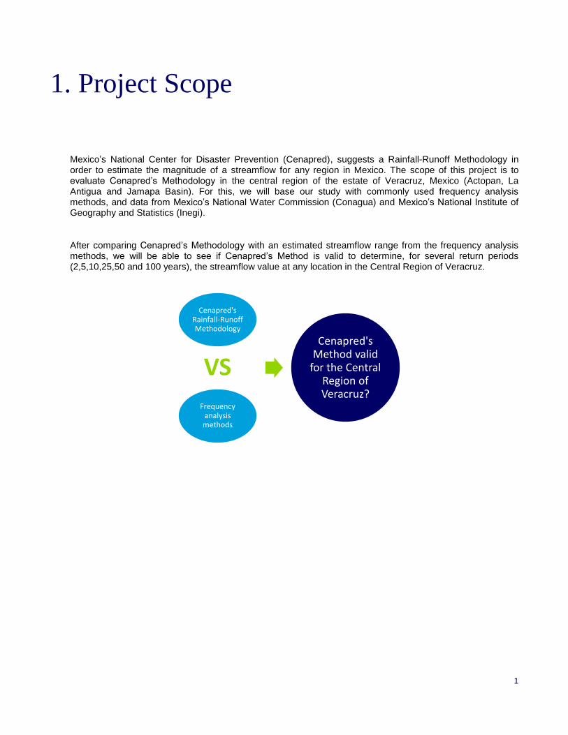
1. Project Scope

Mexico’s National Center for Disaster Prevention (Cenapred), suggests a Rainfall-Runoff Methodology in order to estimate the magnitude of a streamflow for any region in Mexico. The scope of this project is to evaluate Cenapred’s Methodology in the central region of the estate of Veracruz, Mexico (Actopan, La Antigua and Jamapa Basin). For this, we will base our study with commonly used frequency analysis methods, and data from Mexico’s National Water Commission (Conagua) and Mexico’s National Institute of Geography and Statistics (Inegi).

After comparing Cenapred’s Methodology with an estimated streamflow range from the frequency analysis methods, we will be able to see if Cenapred’s Method is valid to determine, for several return periods (2,5,10,25,50 and 100 years), the streamflow value at any location in the Central Region of Veracruz.

2

2. Background

2.1. Region

The state of Veracruz is located at the eastern of Mexico. The state is a crescent-shaped strip of land wedged between the Sierra Madre Oriental to the west and the Gulf of Mexico to the east. Its total area is 78,815 km2 (30,430.6 sq mi), accounting for about 3.7% of Mexico’s total territory. It stretches about 650 km (403.9 mi) north to south, but its width varies from between 212 km (131.7 mi) to 36 km (22.4 mi), with an average of about 100 km (62.1 mi) in width. Veracruz shares common borders with the states of Tamaulipas (to the north), Oaxaca and Chiapas (to the south), Tabasco (to the southeast), and Puebla, Hidalgo, and San Luis Potosí (on the west). Veracruz has 690 km (428.7 mi) of coastline with the Gulf of Mexico.

Approximately 35% of Mexico’s water supply is found in Veracruz. More than 40 rivers and tributaries provide water for irrigation and hydroelectric power; they also carry rich silt down from the eroding highlands, which are deposited in the valleys and coastal areas. All of the rivers and streams that cross the state begin in the Sierra Madre Oriental or in the Central Meseta, following east to the Gulf of Mexico. The more important rivers in the state are the Actopan, Acuatempan, Blanco, Cazones, Coatzacoalcos, La Antigua, Hueyapan, Jamapa, Nautla, Panuco, Papaloapan, Tecolutla, Tonalá Tuxpan, Tonalá, Tuxpan, and the Xoloapa. Two of Mexico’s most polluted rivers are the Coatzacaolacos and the Blanco. Much of the pollution comes from industrial sources, but the discharge of sewerage and uncontrolled garbage disposal are also major contributors. The state has very few waste water treatment plants, with only 10 of the waste water being treated before discharge.

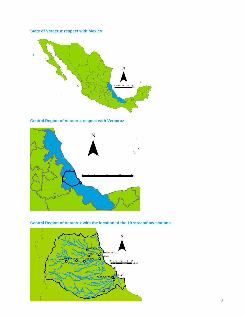
2.2. Maps of Location Mexico respect with United States of America

3

State of Veracruz respect with Mexico

Central Region of Veracruz respect with Veracruz

Central Region of Veracruz with the location of the 10 streamflow stations

4

3. Methodology

3.1 Streamflow Stations Methodology (Frequency Analysis)

To see if the Rainfall-Runoff Methodology proposed by Cenapred is effective, is important to obtain a range in which we can evaluate if the estimated streamflow from this method could be consider as valid. The approximation used to find this range was based on Conagua’s data (mean annual data of the 10 streamflow stations from 1950-2006), and by using the Extreme Value Type 1 (EV1) distribution. The EV1 assist us to get the magnitude of the streamflow and the standard error (for return periods T= 2, 5, 10, 25, 50, and 100 years).

The EV1 distribution is given by:

( ) ( )

Where (scale) and (location) are the parameters of the distribution calculated by the Method of Moments (MOM):

Where Standard Deviation of the data

Mean of the data

The procedure to estimate the magnitude of the streamflow, by using the data of each streamflow station with the EV1 distribution is as follows:

1. Check if the EV1 distribution fits.

In this project, we used the Xc2 test and/or the Probability Plot Correlation Coefficients test (PPCC).

a) Xc2 Goodness of fit test

Hypothesis 0: The distribution fits the data Hypothesis 1: The distribution doesn’t fit Computational steps:

i. Divide the observations in classes (equal length or equal probability)

Check if EV1 fits for all the streamflow stations

Estimate Xt for all return periods in each streamflow station

Upper and Lower range for each Xt

5

ii. Compute the observed and expected number of observation in each class

Test statistic: ∑

( )

Where: number of classes

Observed in class i Expected in class i

iii. Decision rule: Reject Hypothesis 0 if

Where: from chi square table Haan (2002)

Significance level (in this case 5%)

Number of parameter obtained (For EV1 2 parameters; and )

b) The Probability Plot Correlation Coefficients (PPCC test) is a test that uses correlation between observed values and the corresponding fitted quantities ( expected).

Hypothesis 0: The observations are drawn from the fitted distribution Hypothesis 1: The observations are not drawn from the fitted distribution Computational steps: i. Rank the observations from largest to lowest value

ii. Get the probability of exceedance ( ). As we fitted the EV1 distribution, we use the Gringorten expression:

Where Rank number

Total number of observations

iii. Get expected ( ) from the probability of non exceedance ( ). For EV1 is given by:

( )

( ( ))

Where and Parameters obtained by Method of Moments (MOM) Compute the test statistic:

∑( )( )

√∑( ) ∑( )

Where Mean of the series Mean of he data

iv. Decision rule: Reject Hypothesis0 if

Where From table 18.3.3 of Stedinger, Vogel, Foufoula-Georgiou (Chapter 18)

Significance level (in this case 5%)

Total number of observations

6

2. In this particular case, since the distribution fitted in all cases, we get the magnitude of the streamflow ( ) of a given frequency for several return periods by using the formula for the EV1 distribution.

1

ln ( ln (1

1

))

Where: and Parameters obtained by Method of Moments (MOM)

Return Period (2, 5, 10, 25, 50, and 100 years)

Once having for each streamflow station, we calculated the Standard Error ( ( )) for EV1 (MOM)

( )

√

Where: parameter obtained from Table 8.4 of Kite’s (1977)

Number or years of data Standard Deviation of data

3. We obtained the upper (

) and lower ( ) values for magnintude of the streamflow ( ).

( ) 1 2

( ) 1

2

Where: 1

2

Obtained from the normal table

Significance level, in this case was used as 10%







7

3.2 GIS Streamflow Stations watersheds and slope

3.2.1 Watersheds

In order to follow Cenapred’s Methodology, we need to establish the corresponding watersheds that are related to each streamflow station. For this, we followed the steps listed below using certain GIS tools.

1. From the Digital Elevation Model (DEM), remove the pits (GIS Tool Fill).

2. After removing the pits, we are able to get the flow direction of the basin (GIS Tool Flow Direction).

8

3. With the flow direction, we can estimate the flow accumulation (GIS Tool Flow Accumulation). The result of this tool assists us to adjust the site locations to the exact location of the flow.

4. Having the exact locations of flow for every streamflow station, and the flow direction, we are able to find the watershed of each station (GIS Tool Watershed)

5. After getting the raster of the watersheds, we convert it to polygons (GIS Tool Raster to Polygon). The attribute table of the watersheds includes the area of the corresponding watershed for the streamflow station. From this table, we estimated the area of influence for each streamflow station.

9

3.2.2 Slope

To obtain the slope in each watershed, we followed the next procedure.

1. Estimate the slope from the Digital Elevation Model (GIS Tool Slope)

2. As the values in the previous step are given in percentage (%), we divide them by 100 (GIS Tool Raster Calculator).

3. For obtaining the slope in each watershed, we use the zonal statistic tool to obtain the slope value of the watersheds (GIS Tool Zonal statistic). From the zonal statistic table, shown below, we estimate the weighted mean for the corresponding watershed taking into consideration the upstream values.

10

3.2.3 Length of the upstream for each watershed

Having the watersheds for each streamflow stations, we can get the length of the main stream for each station (upstream length; in meters). This length ( ) is needed for Cenapred’s Rainfall-Runoff Methodology.

3.3 Cenapred’s Rainfall-Runoff Methodology This methodology helps us to estimate the streamflow in the same location of the streamflow stations. The steps for this methodology are as follows.

1. Select 15 precipitation stations in the basin we are analyzing.

2. With the average daily data and following the same procedure as for (described in 3.1), we estimate

the magnitude of the precipitation with a return period of two years ( , in mm).

3. Obtain the precipitation value for duration of 1 ( ) and 24 (

) hours for several return periods (T= 2, 5, 10, 25, 50, and 100 years).

( ( ) )( )

Where Duration in minutes (1hour=60 min; 24 hours=1,440 min)

Return period in years

Is given by the expression (in mm)

Where Value between 0.1 (dry) and 0.8 (humid). In this region, the coefficient is 0.4. The daily magnitude calculated for a return period of 2 years (step 2 of 3.3)

4. For this step, we made a tool for GIS (Precipitation Values Tool) that assists us by following the next

procedure:

Estimate and

mean for each watershed of the streamflow stations (delineated in step 4 of 3.2.1) for all the return periods.

a) Interpolate (GIS Tool Empirical Bayesian Kriging) the precipitation values ( and

) obtained in step 3 of 3.3.2.

b) Compute the precipitation mean values ( and

) for each watershed (GIS tool zonal statistics).

1. Select Precipitation

Stations

2. Magnitude of precipitation with return period T=2

years (EV1)

3. Precipitation for a duration of 1 and 24

hours for T = 2, 5, 10, 25, 50, 100

4. Precipitation for a duration of 1 and 24

hours en each watershed

5. Runoff coefficient

6. Streamflow value from precipitation data at the same

location of streamflow stations

11

5. To calculate the runoff coefficient ( ), the procedure is as follows

a) From the soil map of the region, obtained from Mexico’s authorities (INEGI), and the book of Breña and Jacobo (2006), we get the value of the coefficient for each type of soil in the region. This coefficient has to be between 0 and 1 depending of the type and use of the soil.

b) With a tool we adapted (Soil Values Tool); we estimate the mean runoff coefficient for each watershed (GIS tool zonal statistics).

6. Finally, to be able to compute the streamflow from the precipitation data at each streamflow station, we made a GIS tool (Compute Flow Rates Tool) that follows the next procedure:

a) From and

mean values for each watershed, calculate the precipitation with duration equal to the time of concentration in the watersheds for all the return periods.

( ( ))

Where: Time of concentration in each watershed, given by:

Where: Upstream length for each station, obtained in 3.2.3 (meters)

Slope calculated in 3.2.2 (dimensionless)

b) Compute the intensity ( ) in each watershed for all the return periods. The intensity is the amount of precipitation water per unit of time.

c) Estimate the Flow rates for all the return periods

Where Area of influence (km2) for each streamflow station (upstream)

12

4. Results

4.1 Streamflow Stations Range Actopan River Streamflow Stations

Actopan II Streamflow Station (No. 28030)

Magnitude Freq. Analysis XT

Lower

m3/s

XT

upper

m3/s

XT2years = 16.687 m3/s 15.957 17.417

XT5years = 19.894 m3/s 18.604 21.184

XT10years = 22.018 m3/s 20.250 23.785

XT25years = 24.700 m3/s 22.285 27.116

XT50years = 26.691 m3/s 23.803 29.579

XT100years = 28.666 m3/s 25.294 32.039

Idolos Streamflow Station (No. 28111)


Lower

m3/s

XT

upper

m3/s

XT2years = 4.269 m3/s 3.875 4.663

XT5years = 5.788 m3/s 5.085 6.491

XT10years = 6.794 m3/s 5.828 7.760

XT25years = 8.065 m3/s 6.598 9.532

XT50years = 9.008 m3/s 7.426 10.590

XT100years = 9.944 m3/s 8.095 11.792

El Naranjillo Streamflow Station (No. 28108


Lower

m3/s

XT upper

m3/s

XT2years = 14.052 m3/s 12.775 15.330

XT5years = 19.091 m3/s 16.816 21.366

XT10years = 22.427 m3/s 19.301 25.552

XT25years = 26.642 m3/s 22.463 30.820

XT50years = 29.768 m3/s 24.652 34.885

XT100years = 32.872 m3/s 26.896 38.849

La Antigua River Streamflow Stations

Amatitla II Streamflow Station (No. 28133)


Lower

m3/s

XT

upper

m3/s

XT2years = 24.137 m3/s 22.875 25.400

XT5years = 28.893 m3/s 26.636 31.150

XT10years = 32.042 m3/s 28.938 35.145

XT25years = 36.020 m3/s 31.771 40.269

XT50years = 38.972 m3/s 33.886 44.057

XT100years = 41.901 m3/s 35.960 47.843

Jalcomulco Streamflow Station (No. 28134)


Lower

m3/s

XT

upper

m3/s

XT2years = 48.132 m3/s 46.022 50.242

XT5years = 56.178 m3/s 52.409 59.948

XT10years = 61.506 m3/s 56.323 66.688

XT25years = 68.237 m3/s 60.830 75.644

XT50years = 73.230 m3/s 64.741 81.720

XT100years = 78.187 m3/s 68.269 88.106

12

Carrizal Streamflow Station (No. 28125)


Lower

m3/s

XT

upper

m3/s

XT2years = 44.480 m3/s 41.786 47.174

XT5years = 54.508 m3/s 49.686 59.329

XT10years = 61.147 m3/s 54.514 67.779

XT25years = 69.535 m3/s 60.662 78.409

XT50years = 75.759 m3/s 64.889 86.629

XT100years = 81.936 m3/s 69.235 94.636

Cardel Streamflow Station (No. 28003)


Lower

m3/s

XT

upper

m3/s

XT2years = 53.686 m3/s 50.895 56.477

XT5years = 65.841 m3/s 60.906 70.775

XT10years = 73.888 m3/s 67.124 80.652

XT25years = 84.056 m3/s 75.024 93.089

XT50years = 91.599 m3/s 80.545 102.653

XT100years = 99.087 m3/s 86.179 111.995

Jamapa River Streamflow Stations

El Tejar Streamflow Station (No. 28040)


Lower

m3/s

XT

upper

m3/s

XT2years = 16.907 m3/s 15.618 18.196

XT5years = 22.520 m3/s 20.241 24.799

XT10years = 26.237 m3/s 23.113 29.361

XT25years = 30.933 m3/s 26.761 35.105

XT50years = 34.417 m3/s 29.312 39.522

XT100years = 37.875 m3/s 31.913 43.837

Paso del Toro Streamflow Station (No. 28039)


Lower

m3/s

XT

upper

m3/s

XT2years = 39.717 m3/s 37.359 42.074

XT5years = 49.015 m3/s 44.816 53.213

XT10years = 55.171 m3/s 49.403 60.938

XT25years = 62.949 m3/s 55.238 70.659

XT50years = 68.719 m3/s 59.277 78.161

XT100years = 74.447 m3/s 63.417 85.476

Capulines Streamflow Station (No. 28069)


Lower

m3/s

XT

upper

m3/s

XT2years = 39.979 m3/s 34.897 45.062

XT5years = 61.508 m3/s 52.505 70.511

XT10years = 75.763 m3/s 63.413 88.112

XT25years = 93.773 m3/s 77.306 110.239

XT50years = 107.134 m3/s 86.943 127.324

XT100years = 120.396 m3/s 96.816 143.976

13

4.2 Cenapred’s Methodology Results Actopan River Streamflow Stations

Streamflow from Cenapred's Methodology

Return Period

Actopan II m

3/s

El Naranjillo

m3/s

Idolos m

3/s

T =2 years 32.391 32.786 18.690

T =5 years 42.752 43.273 24.668

T =10 years 50.590 51.207 29.191

T =25 years 60.951 61.694 35.169

T =50 years 68.789 69.627 39.692

T =100 years 76.627 77.561 44.214

La Antigua River Streamflow Stations


Return Period

Cardel m

3/s

Carrizal m

3/s

Amatitla II m

3/s

Jalcomulco m

3/s

T =2 years 44.881 41.335 22.594 46.176

T =5 years 59.237 54.556 29.821 60.946

T =10 years 70.097 64.558 35.288 72.119

T =25 years 84.453 77.780 42.515 86.889

T =50 years 95.313 87.782 47.982 98.062

T =100 years 106.172 97.783 53.449 109.236

Jamapa River Streamflow Stations


Return Period

Paso del Toro

m3/s

El Tejar m

3/s

Capulines m

3/s

T =2 years 20.626 28.589 28.140

T =5 years 27.223 37.734 37.141

T =10 years 32.214 44.652 43.950

T =25 years 38.812 53.797 52.951

T =50 years 43.803 60.714 59.760

T =100 years 48.794 67.632 66.569

14

5. Conclusions

Actopan River

In the Actopan River, the values estimated with Cenapred’s methodology are much higher than the range obtained from the Frequency Analysis. For this, is important to reconsider the values used for the Runoff coefficient in order to state if this method is valid or not in this area of the central region of Veracruz.

La Antigua River

0.000

20.000

40.000

60.000

80.000

100.000

T = 2 T = 5 T = 10 T = 25 T = 50 T = 100

Str

ea

mflo

w

m3

/s

Return Period

Actopan II No. 28030

Streamflow(Cenapred)

0.000

10.000

20.000

30.000

40.000

50.000

60.000

T = 2 T = 5 T = 10 T = 25 T = 50 T = 100

Str

ea

mflo

w

m3

/s

Return Period

Amatlitla II No. 28133


0.000

10.000

20.000

30.000

40.000

50.000

T = 2 T = 5 T = 10 T = 25 T = 50 T = 100

Str

ea

mflo

w

m3

/s

Return Period

Idolos No. 28111


0.000

20.000

40.000

60.000

80.000

100.000

T = 2 T = 5 T = 10 T = 25 T = 50 T = 100

Str

ea

mflo

w

m3

/s

Return Period

El Naranjillo No. 28108


0.000

20.000

40.000

60.000

80.000

100.000

120.000

T = 2 T = 5 T = 10 T = 25 T = 50 T = 100

Str

ea

mflo

w

m3

/s

Return Period

Jalcomulco No. 28134


15

0.000

10.000

20.000

30.000

40.000

50.000

60.000

70.000

80.000

T = 2 T = 5 T = 10 T = 25 T = 50 T = 100

Str

ea

mflo

w

m3

/s

Return Period

El Tejar No. 28040


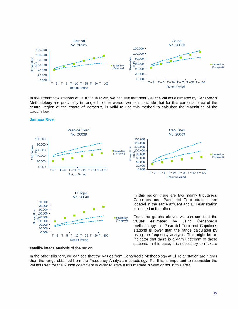
In the streamflow stations of La Antigua River, we can see that nearly all the values estimated by Cenapred’s Methodology are practically in range. In other words, we can conclude that for this particular area of the central region of the estate of Veracruz, is valid to use this method to calculate the magnitude of the streamflow.

Jamapa River

In this region there are two mainly tributaries. Capulines and Paso del Toro stations are located in the same affluent and El Tejar station is located in the other.

From the graphs above, we can see that the values estimated by using Cenapred’s methodology in Paso del Toro and Capulines stations is lower than the range calculated by using the frequency analysis. This might be an indicator that there is a dam upstream of these stations. In this case, it is necessary to make a

satellite image analysis of the region.

In the other tributary, we can see that the values from Cenapred’s Methodology at El Tejar station are higher than the range obtained from the Frequency Analysis methodology. For this, is important to reconsider the values used for the Runoff coefficient in order to state if this method is valid or not in this area.

0.000

20.000

40.000

60.000

80.000

100.000

120.000

T = 2 T = 5 T = 10 T = 25 T = 50 T = 100

Str

ea

mflo

w

m3

/s

Return Period

Carrizal No. 28125


0.000

20.000

40.000

60.000

80.000

100.000

T = 2 T = 5 T = 10 T = 25 T = 50 T = 100

Str

ea

mflo

w

m3

/s

Return Period

Paso del ToroI No. 28039


0.000

20.000

40.000

60.000

80.000

100.000

120.000

140.000

160.000

T = 2 T = 5 T = 10 T = 25 T = 50 T = 100

Str

ea

mflo

w

m3

/s

Return Period

Capulines No. 28069


0.000

20.000

40.000

60.000

80.000

100.000

120.000

T = 2 T = 5 T = 10 T = 25 T = 50 T = 100

Str

ea

mflo

w

m3

/s

Return Period

Cardel No. 28003


16

6. References

Kite, G. W., Frequency and Risk Analyses in Hydrology, Water Resources Publications, Fort Collins,

CO, 1977.

Haan, C. T., Statistical Methods in Hydrology, Iowa State Press, Ames, 1974 (First edition), 2002 (Second edition)

Stedinger, J.R, Vogel, R., Foufoula-Georgiou, E., Frequency Analysis of Extreme Events, Chapter 18

Salas Salinas, M.A, Metodología para la Elaboración de Mapas de Riesgo por Inundaciones en

Zonas Urbanas, Centro Nacional de Prevención de Desastres y Secretaria de Gobernación, July 2011

Breña Puyol, A.F., Jacobo Villa M.A, Principios y Fundamentos de la Hidrología Superficial

Universidad Autónoma Metropolitana, 2006

Comisión Nacional del Agua (CONAGUA)

Instituto Nacional de Estadística y Geografía (INEGI)

Analysis of Cenapred’s Rainfall-Runoff methodology for the ... · Jamapa, Nautla, Panuco,...

Documents

Transcript of Analysis of Cenapred’s Rainfall-Runoff methodology for the ... · Jamapa, Nautla, Panuco,...