Analysis of Algorithms

These slides are a modified version of the slides used by Prof. Eltabakh

in his offering of CS2223 in D term 2013

Analysis of Algorithms

• Correctness Analysis:

An algorithm is correct if under all valid inputs it produces the correct output

• Efficiency (Complexity) Analysis:

We want the algorithm to make best use of– Space (storage)– Time (how long it take to run, number of

instructions executed, …)

Time and Space Complexity

• Time– Executing instructions take time– How fast does the algorithm run?– What affects its runtime?

• Space– Data structures take space– What kind of data structures can be used?– How does the choice of data structure affect

the runtime?

Time vs. Space

Very often, we can trade space for time:

For example: maintain a collection of students with SSN

– Use an array of a billion elements and have immediate access (better time)

– Use an array of 110 elements and have to search (better space)

Joe Smith

000-00-0000 000-00-0001 … 555-55-5555 … 999-99-9999

Name: Joe SmithSSN: 555-55-5555

1 … 97 … 110

The Right Balance

The best solution uses a reasonable mix of space and time.

– Select effective data structures to represent your data model.

– Utilize efficient methods on these data structures.

Measuring the Growth of Work

While it is possible to measure the work done by an algorithm for a given set of input, we need a way to:

– Measure the rate of growth of an algorithm based upon the size of the input

– Compare algorithms to determine which is better for the situation

For example, compare performance of sorting algorithms on different input array conditions at:

http://www.sorting-algorithms.com/

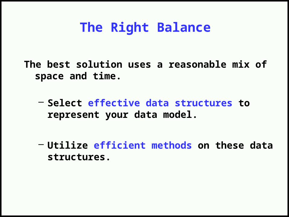
Worst-Case Analysis

• Worst case running time– Obtain bound on largest possible running time

of algorithm on input of a given size N

– Generally captures efficiency in practice

7

We will focus on the Worst-Case when analyzing algorithms

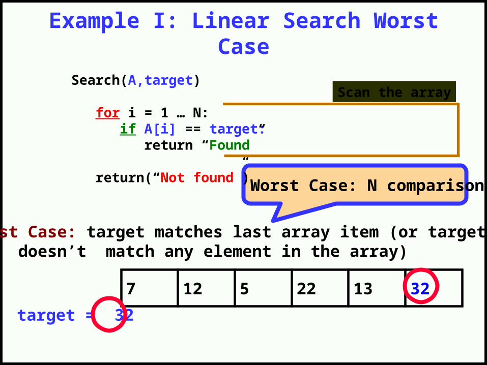
Example I: Linear Search Worst Case

Worst Case: target matches last array item (or targetdoesn’t match any element in the array)

7 12 5 22 13 32

target = 32

Worst Case: N comparisons

Search(A,target)

for i = 1 … N:if A[i] == target:

return “Found”

return(“Not found”)

Scan the array

Example II: Binary Search Worst Case

Worst Case: divide until reach one item, or no match,

How many comparisons??

def BinarySearch(A, first, last, target):middle <- (first + last) / 2

if first > last:return false

if A[middle] = target:return true

if target< A[middle]:return BinarySearch(A, first, middle–1, target)

else:return BinarySearch(A, middle+1, last, target)

Example II: Binary Search Worst Case

• With each comparison we throw away ½ of the list

N

N/2

N/4

N/8

1

………… 1 comparison

………… 1 comparison

………… 1 comparison

………… 1 comparison

………… 1 comparison

.

.

.Worst Case: Number of Steps is: Log2N

Total number of comparisons in the worst case: Log2 N

In General

• Assume the initial problem size is N

• If you reduce the problem size in each step by factor k– Then, the max steps to reach size 1 LogkN

• If in each step the amount of work done is α– Then, the total amount of work is (α LogkN)

In Binary Search- Factor k = 2, then we have Log2N- In each step, we do one comparison (1)- Total : Log2N

Example III: Insertion Sort Worst Case

Worst Case: Input array is sorted in reverse order

In each iteration i , we do i comparisons.Total : N(N-1) comparisons

Sum of the # of comparisons over all iterations

Order Of Growth

Log N N 2NN2 N3 N!

Logarithmic

Polynomial Exponential

More efficientLess efficient (infeasible for large N)

Why It Matters

• For small input size (N) It does not matter• For large input size (N) it makes all the difference

14

Order of Growth

Worst-Case Polynomial-Time

• By convention, we say that an algorithm is efficient if its running time is polynomial.

• Justification: It really works in practice!

– Although 6.02 1023 N20 is technically polynomial time, such a runtime would be prohibitive. But in practice, the poly-time algorithms that people develop almost always have low constants and low exponents.

– Even N2 with very large N is infeasible

Input size N objects

Introducing Big O

• Allows us to evaluate algorithms by providing us with an upper bound of the complexity (e.g., runtime, space) of the algorithm

• Has a precise mathematical definition

• Helps us group algorithms into families

LB

Size of Input

• In analyzing rate of growth based upon size of input, we’ll use a variable for each factor in the input size that affects the performance of the algorithm– N is most commonly used …

Examples:– A linked list of N elements– A 2D array of N x M elements– 2 Lists of size N and M elements– A Binary Search Tree of N elements

Formal Definition

For a given function g(n),

O(g(n)) is defined to be the following set of functions:

O(g(n)) = {f(n): there exist positive constants c and n0

such that

0 f(n) cg(n) for all n n0}

note that f(n) belongs to O(g(n)) if there is a constant multiple of g(n) that is an asymptotic upper bound of f(n)

Visual O() Meaning

f(n)

cg(n)

n0

f(n) = O(g(n))

Size of input

Wo

rk d

on

e

Our Algorithm

Upper BoundAsymptotic

Runtime of

Simplifying O() Answers

We say 3n2 + 2 = O(n2) drop constants!

because we can show that there is a n0 and a c such that:

0 3n2 + 2 cn2 for n n0

i.e. take c = 4 and n0 = 2 yields:

0 3n2 + 2 4n2 for all n 2

Notation “abuse”: it should be 3n2 + 2 belongs to O(n2)

Correct but Meaningless

You could say

3n2 + 2 = O(n6) or 3n2 + 2 = O(n7)

But this is like answering:• What is the world’s record for running one mile?

– Less than 3 days.• How long does it take to drive from here to Chicago?

– Less than 11 years.

O (n2) is a tighter asymptotic

upper bound

Analyzing Algorithm Complexity

• Now that we know the formal definition of the O() notation (and what it means intuitively)…

• We can determine the complexity of an algorithm:

1. Construct a function T(n)

T(n): time (e.g., number of operations) taken by the algorithm on an input of size n

2. Find g(n), an asymptotic upper bound g(n)

of T(N). That is, T(n) = O(g(n))we aim for as tight upper bound g(n) as we can find

This works also for space complexity analysis:S(n) = space taken by the algorithm on input size n

Comparing Algorithms

• Now that we know the formal definition of the O() notation (and what it means intuitively)…

• We can compare different algorithms that solve the same problem:

1. Determine the O(.) for the time complexity of each algorithm

2. Compare them and see which has “better” performance

Comparing Asymptotic Growth

N

log N

N2

1

Size of input

Wo

rk d

on

e

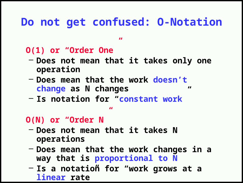
Do not get confused: O-Notation

O(1) or “Order One”– Does not mean that it takes only one operation

– Does mean that the work doesn’t change as N

changes– Is notation for “constant work”

O(N) or “Order N”– Does not mean that it takes N operations– Does mean that the work changes in a way

that is proportional to N– Is a notation for “work grows at a linear rate”

Modular Analysis

• Algorithms typically consist of a sequence of logical steps/sections/modules

• We need a way to analyze these more complex algorithms…

• It’s easy – analyze the sections and then combine them

Example: Insert in a Sorted Linked List

• Insert an element into an ordered list of length N

1. Find the right location

2. Create a new node and add it to the list

17 38 142head //

Inserting 75

Step 1: find the location = O(N)

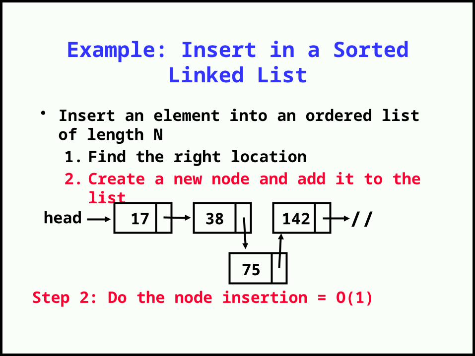
Example: Insert in a Sorted Linked List

• Insert an element into an ordered list of length N

1. Find the right location

2. Create a new node and add it to the list

17 38 142head //

Step 2: Do the node insertion = O(1)

75

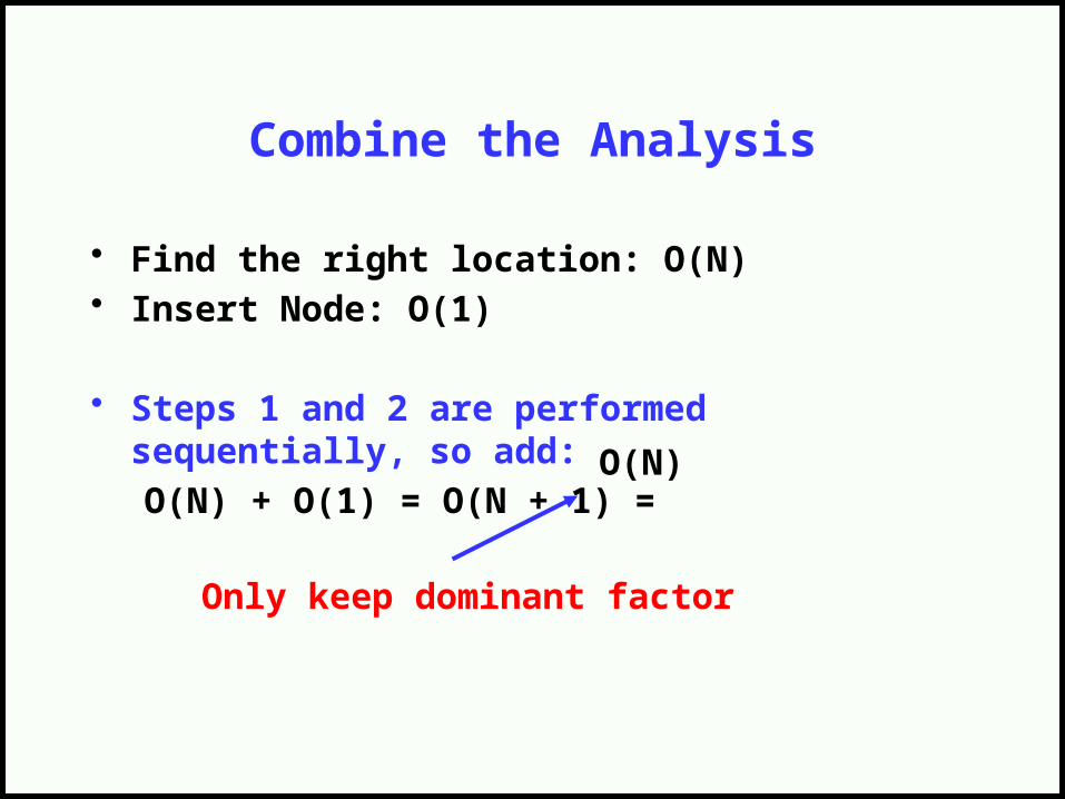
Combine the Analysis

• Find the right location: O(N)• Insert Node: O(1)

• Steps 1 and 2 are performed sequentially, so add:

O(N) + O(1) = O(N + 1) =

Only keep dominant factor

O(N)

Example: Search a 2D ArraySearch an unsorted 2D array of size NxM (row, then column)

– Traverse all rows– For each row, examine all the cells (changing columns)

Row

Column

12345

1 2 3 4 5 6 7 8 9 10

O(N)

Example: Search a 2D ArraySearch an unsorted 2D array of size NxM (row, then column)

– Traverse all rows– For each row, examine all the cells (changing columns)

Row

Column

12345

1 2 3 4 5 6 7 8 9 10

O(M)

Combine the Analysis

• Traverse rows = O(N)– Examine all cells in row = O(M)

• Embedded (i.e., nested loops) so multiply:

O(N) x O(M) = O(N*M)

Sequential Steps

• If steps appear sequentially (one after another), then add their respective O().

loop. . .endlooploop. . .endloop

N

M

O(N + M)

Embedded Steps

• If steps appear embedded (one inside another), then multiply their respective O().

loop loop . . . endloopendloop

M N O(N*M)

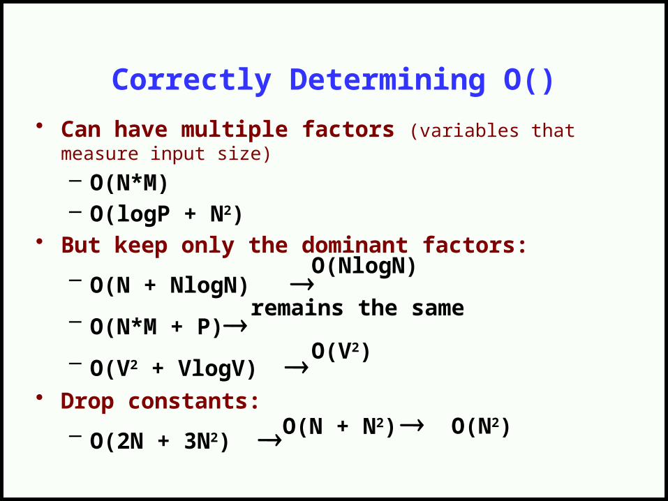
Correctly Determining O()

• Can have multiple factors (variables that measure input size)

– O(N*M)– O(logP + N2)

• But keep only the dominant factors:

– O(N + NlogN)

– O(N*M + P)

– O(V2 + VlogV) • Drop constants:

– O(2N + 3N2)

O(NlogN)

remains the same

O(V2)

O(N2)O(N + N2)

Summary

• We use O() notation to analyze the rate at which the work done (or space used by) an algorithm grows with respect to the size of the input.

• O() provides asymptotic upper bounds

(nicely focusing on asymptotic rate of growth, only keeping dominant terms and dropping non-dominant terms and constants)