ANALYSIS AND DESIGN OF GATEWAY DIVERSITY SYSTEMS …
74
TRABAJO FIN DE GRADO GRADO EN INGENIERÍA DE TECNOLOGÍAS Y SERVICIOS DE TELECOMUNICACIÓN ANALYSIS AND DESIGN OF GATEWAY DIVERSITY SYSTEMS FOR VERY HIGH THROUGHPUT SATELLITES (VHTS) MICHEL MASSANET GINARD 2018
Transcript of ANALYSIS AND DESIGN OF GATEWAY DIVERSITY SYSTEMS …

TRABAJO FIN DE GRADO
GRADO EN INGENIERÍA DE TECNOLOGÍAS Y SERVICIOS DE TELECOMUNICACIÓN
ANALYSIS AND DESIGN OF GATEWAY DIVERSITY SYSTEMS FOR VERY HIGH THROUGHPUT
SATELLITES (VHTS)
MICHEL MASSANET GINARD
2018


TRABAJO FIN DE GRADO
Título: ANALYSIS AND DESIGN OF GATEWAY DIVERSITY
SYSTEMS FOR VERY HIGH THROUGPUT SATELLIES
(VHTS).
Autor: D. Michel Massanet Ginard
Tutor: D. Ramón Martínez Rodríguez-Osorio.
Ponente:
Departamento: Departamento de Señales, Sistemas y
Radiocomunicaciones.
TRIBUNAL:
Presidente: D.
Vocal: D.
Secretario: D.
Suplente: D.
Fecha de lectura:
Calificación:


UNIVERSIDAD POLITÉCNICA DE MADRID
ESCUELA TÉCNICA SUPERIOR
DE INGENIEROS DE TELECOMUNICACIÓN
TRABAJO FIN DE GRADO
GRADO EN INGENIERÍA DE TECNOLOGÍAS Y SERVICIOS DE TELECOMUNICACIÓN
ANALYSIS AND DESIGN OF GATEWAY DIVERSITY SYSTEMS FOR VERY HIGH
THROUGHPUT SATELLITES (VHTS)
MICHEL MASSANET GINARD
2018


Resumen
En la actualidad, se estima que en 2020 la demanda de tráfico a través satélite será de 1 Tbps y
que será satisfecha gracias a una nueva generación de satélites llamada Very High Throughput
Satellites (VHTS). Para satisfacer esta demanda, es necesario el uso de bandas de frecuencia
superiores como la banda Q/V debido a sus mayores anchos de banda. Sin embargo, el uso de
frecuencias altas conlleva efectos severos de atenuación por lluvia en las comunicaciones por
satélite. Para evitar el desvanecimiento por lluvia, las estaciones base hacen uso de sistemas de
diversidad por gateway que consiste en la separación y decorrelación espacial entre gateways.
La creación de diversidad por gateway es posible gracias al uso de las estadísticas de atenuación
diferencial por lluvia que pueden extraerse de la Rec. ITU-R P.1815-1. Además, cuando se
produce un evento de lluvia estos sistemas inteligentes distribuyen el ancho de banda entre
gateways de forma óptima para mantener operativo el sistema. Por ello, el empleo de las series
temporales de atenuación por lluvia obtenidas mediante la Rec. ITU-R P.1853-1 es crucial para
el conocimiento de la dinámica del canal y para estudiar los eventos de transferencia de ancho
de banda entre gateways.
En este trabajo se presenta una herramienta que implementa el uso de las estadísticas de
atenuación diferencial por lluvia para el diseño de sistemas de diversidad por gateway. En este
documento se describe su implementación mediante la explicación de su estructura y
funcionamiento. Posteriormente se presentan resultados de casos de estudios de sistemas reales
donde se busca analizar y estudiar la variación de las estadísticas de atenuación diferencial por
lluvia según parámetros como la localización geográfica o frecuencia entre otros. El estudio se
realiza por medio de la observación de contornos de probabilidad de corte y se debate la
importancia de cambios en los contornos debido a la influencia de ciertos parámetros de interés.
Junto a la herramienta de diseño, se incluye una herramienta que permite analizar los eventos de
transferencia de ancho de banda que se producen en los sistemas de diversidad por gateway.
Esto se consigue gracias al uso de las series temporales de atenuación por lluvia cuyo
procedimiento de extracción y uso para obtener los eventos de switch se describen en este
documento. También se presentan resultados justificados de estudios donde se busca observar
como varían los eventos de switch con la variación de la localización geográfica y tamaño de las
antenas. De los resultados de ambas herramientas se han sacado conclusiones sobre factores a
tener en cuenta a la hora de establecer diversidad por gateway.
Finalmente junto a estas herramientas y sus resultados se incluye la redacción de un artículo
sobre el diseño de diversidad por gateway para VHTS y algunos resultados que sintetizan
algunas de las ideas más importantes de este documento. El artículo ha sido aceptado en el
XXXIII Simposium Nacional de la Unión Científica Internacional de Radio, URSI 2018.
Palabras clave
VHTS, GW, diversidad, análisis, sistema, lluvia, atenuación, diferencial, estadísticas, series
temporales, nivel, contorno, diseño, ITU, corte, probabilidad, transferencia.

Summary
Currently, it is estimated that the traffic demand through satellites will be 1 Tbps by 2020 and it
will be satisfied thanks to a new generation of satellites named Very High Throughput Satellites
(VHTS). In order to satisfy this demand, the use of higher frequency bands such as Q/V band is
necessary due to their greater bandwidth. However, the use of high frequency bands entails
severe effect of rain attenuation in satellite communications. To prevent from rain fade, ground
stations make use of gateway diversity systems which consist of the separation and spatial
decorrelation between gateways. The creation of gateway diversity is possible thanks to the use
of differential rain attenuation statistics which are extracted from Rec. ITU-R P-1815-1. In
addition, when a rain event takes place, these smart systems distribute ideally the bandwidth
between gateways in order to maintain operationally the system. To do this, the use of the rain
attenuation time series obtained from Rec. ITU-R P.1853-1 is crucial to know the dynamics of
the channel and to study the transfer events of bandwidth between gateways.
In this project, a tool which implements the use of differential rain attenuation statistics for
designing gateway diversity systems is presented. This document describes its implementation
through the explanation of its structure and functioning. Afterwards, results from real systems
cases of study are presented where the purpose is to analyze and study the variation of
differential rain attenuation statistics according to parameters such as geographic location or
frequency among others. The studies are carried out through the observation of outage
probability contours and the discussion of the importance of changes on the contours due to the
influence of some interest parameters.
Along with the design tool, a tool that permits analyze the transfer events of bandwidth
produced in gateway diversity systems is included. This is reached thanks to the use of rain
attenuation time series whose extraction procedure and their use to get the switch events are
described in this document. Justified results from studies are also presented where the aim is to
observe how the switch events vary with the modification of geographic location and antenna‟s
size. From the results from both tools, conclusions about factors to be taken into account in the
establishment of gateway diversity have been drawn.
Finally, together with these tools and their results, the writing of a paper about the design of
gateway diversity for VHTS and some results that summarize some of the main ideas from these
documents is included. This paper has been accepted in the XXXIII Simposium Nacional de la
Unión Científica Internacional de Radio, URSI 2018.
Keywords
VHTS, GW, diversity, analysis, system, rain, attenuation, differential, statistics, time series,
contour, level, design, ITU, outage, probability, switch.

Index
1 Introduction ................................................................................................................. 1
1.1 Satellite evolution to future VHTS ................................................................................. 1
1.2 Motivation ..................................................................................................................... 3
1.3 Objectives and scope .................................................................................................... 5
1.4 Work plan ...................................................................................................................... 5
1.5 Structure ........................................................................................................................ 6
2 ITU-R Recommendations .............................................................................................. 7
2.1 ITU-R P.1815-1 ............................................................................................................... 7
2.2 ITU-R P.1853-1 ............................................................................................................. 10
3 Design of Gateway diversity (Design tool) ................................................................... 12
3.1 Designer Interface ....................................................................................................... 12
3.1.1 Input and output parameters .............................................................................. 12
3.1.2 Functioning .......................................................................................................... 13
3.1.3 Structure .............................................................................................................. 15
3.2 Contour Plot Interface ................................................................................................. 18
3.2.1 Input and output parameters .............................................................................. 18
3.2.2 Functioning .......................................................................................................... 19
3.2.3 Structure .............................................................................................................. 20
3.3 Results ......................................................................................................................... 20
3.3.1 Site variation ....................................................................................................... 21
3.3.2 Frequency variation ............................................................................................. 27
3.3.3 Elevation angle variation ..................................................................................... 29
3.3.4 Attenuation thresholds variation ........................................................................ 32
3.3.5 Annual or worst-month statistics ........................................................................ 34
4 Analysis of switched bandwidth (Analysis tool) ........................................................... 36
4.1 Input and output parameters...................................................................................... 36
4.2 Functioning .................................................................................................................. 37
4.3 Structure ...................................................................................................................... 38
4.4 Graphs results of interest ............................................................................................ 38
4.4.1 Rain attenuation time series, C/N and bandwidth variation .............................. 39
4.4.2 Rain attenuation time series histogram .............................................................. 40
4.4.3 Rain attenuation CDF .......................................................................................... 40
4.4.4 Events of switched bandwidth ............................................................................ 41
4.4.5 Events of switched bandwidth histogram ........................................................... 42

4.5 Results ......................................................................................................................... 43
4.5.1 Site variation ....................................................................................................... 44
4.5.2 Antenna’s size variation ...................................................................................... 47
5 Conclusions and future research lines ......................................................................... 49
5.1 Conclusions ................................................................................................................. 49
5.2 Future research lines ................................................................................................... 50
6 Bibliography ............................................................................................................... 51
7 Annexes ..................................................................................................................... 53
7.1 Annex 1: Paper accepted in URSI 2018 Congress ........................................................ 53
7.2 Annex 2: Impact of the TFG ......................................................................................... 54
7.3 Annex 3: Economic budget .......................................................................................... 55
7.4 Annex 4: Scripts of the simulator ................................................................................ 57

Index of figures
Fig. 1. Satellite orbits. ............................................................................................................................................ 1 Fig. 2. Rain attenuation vs. availability (logarithmic scale) from section 2.2.1.1 of Rec. ITU-R P.618-13 [9] ..... 3 Fig. 3. Eutelsat ground segment of KA-SAT [Skylogic]. ...................................................................................... 4 Fig. 4. Site diversity in GW systems ...................................................................................................................... 4 Fig. 5. Gantt chart .................................................................................................................................................. 6 Fig. 6. GW diversity............................................................................................................................................... 8 Fig. 7. Variation of with distance and frequency for = =16dB in site 1 (Madrid) and site 2 (direction to
Valencia), with Hispasat-30W. .................................................................................................................................... 10 Fig. 8. Synthesis‟ procedure of rain attenuation time series ................................................................................. 10 Fig. 9. Example of of rain attenuation time series in Q/V band (50 GHz) in Madrid with KA-SAT. .......... 11 Fig. 10. Designer Interface ..................................................................................................................................... 12 Fig. 11. Scheme of the parameters that define the circular grid ............................................................................. 14 Fig. 12. Support tool to calculate the attenuation thresholds .................................................................................. 15 Fig. 13. Procedure of design .................................................................................................................................. 15 Fig. 14. Diagram of the main function scripts in the design procedure .................................................................. 16 Fig. 15. Input and output parameters of differentialRainAtten1815 ....................................................................... 16 Fig. 16. Cooperation among function scripts to calculate ................................................................................ 18 Fig. 17. Procedure of interpolation ........................................................................................................................ 18 Fig. 18. Contour Plot Interface ............................................................................................................................... 19 Fig. 19. Procedure of plotting contours of a designed system ................................................................................ 20 Fig. 20. Diagram with the functions of the Contour Plot Interface. ....................................................................... 20 Fig. 21. Annual contour levels in Arganda del Rey in Q/V band with longSat=9ºE. ...................................... 23 Fig. 22. Annual contour levels in The Pyrenees in Q/V band with longSat= 9ºE. .......................................... 24 Fig. 23. Annual contour levels in Rambouillet in Q/V band with longSat= 9ºE. ............................................ 25 Fig. 24. Annual contour levels in Lurín in Q/V band with longSat= 61ºW. ................................................... 26 Fig. 25. Annual contour levels in Orlando in Q/V band with longSat= 61ºW. ............................................... 27 Fig. 26. Annual contour levels in Arganda del Rey in W band with longSat= 9ºE. ........................................ 28 Fig. 27. Annual contour levels in Orlando in Ka-band with longSat= 61ºW. ................................................. 29 Fig. 28. Annual contour levels in Arganda del Rey in Q/V band with longSat= 30ºW. ................................. 30 Fig. 29. Annual contour levels in Lurín in Q/V band with longSat= 69.9ºW. ................................................ 31 Fig. 30. Annual contour levels in Rambouillet in Q/V band with longSat= 9ºE ( = =19 dB) .................. 32 Fig. 31. Annual contour levels in Arganda del Rey in Q/V band with longSat=9ºE ( = =10 dB) ............ 33 Fig. 32. Worst-month contour levels in Arganda del Rey in Q/V band with longSat=9ºE. ............................ 35 Fig. 33. BW Analysis Interface .............................................................................................................................. 36 Fig. 34. Procedure of simulation in analysis tool ................................................................................................... 37 Fig. 35. Scheme of the scripts of the analysis tool ................................................................................................. 38 Fig. 36. Example of rain attenuation time series, C/N and BW variation in the BW Analysis Interface. .............. 39 Fig. 37. Example of histogram of the rain attenuation time series synthetized for duration of one year. ............... 40 Fig. 38. Example of cumulative distribution function ............................................................................................ 41 Fig. 39. Example of events of BW switching in a synthesis of one year in BW Analysis Interface. ..................... 42 Fig. 40. Example of histogram of the switched BW. ............................................................................................. 43 Fig. 41. Switch events in Arganda del Rey with minTimeEvent =15 s. .................................................................. 45 Fig. 42. Histogram of switch events in Arganda del Rey with minTimeEvent =15 s. ............................................ 45 Fig. 43. Histogram of switch events in Arganda del Rey with minTimeEvent =5 s. .............................................. 46 Fig. 44. Rain attenuation time series histogram in Orlando ................................................................................... 47 Fig. 45. Rain attenuation time series histogram in Arganda del Rey ..................................................................... 47 Fig. 46. BW events histogram in Arganda del Rey with reduced antennas ............................................................ 47

Index of tables
TABLE I. EXAMPLES OF HTS ............................................................................................................................ 2 TABLE II. ITU RECOMMENDATIONS USED BY THE SYSTEM MODELS ................................................... 7 TABLE III. FUNCTIONS CALLED INTERNALLY IN differentalRainAtten1815 .............................................. 17 TABLE IV. LEGEND OF LEVELS ................................................................................................................ 21 TABLE V. PLACES OF STUDY .......................................................................................................................... 22 TABLE VI. LEVELS IN Q/V BAND IN ORLANDO ..................................................................................... 26 TABLE VII. ORBITAL POSITIONS OF INTEREST AND THEIR ELEVATION ANGLES ............................... 30 TABLE VIII. LEVELS IN WORST-MONTH SIMULATION .......................................................................... 35 TABLE IX. FIXED INPUT PARAMETERS IN THE ANALYSIS OF BANDWIDTH ........................................ 43 TABLE X. RESULTS OF THE STUDY CASES .................................................................................................. 48 TABLE XI. DISTRIBUTION OF WORK HOURS ................................................................................................ 55 TABLE XII. ECONOMICAL BUDGET .................................................................................................................. 56 TABLE XIII. FUNCTION SCRIPTS USED IN THE SIMULATOR ....................................................................... 57

1. Introduction
1
1 INTRODUCTION
1.1 SATELLITE EVOLUTION TO FUTURE VHTS
The most common satellites for telecommunications are the geostationary (GEO) satellites which
are located in a geostationary orbit, approximately 36000 km above the Earth‟s equator. There are
other types of satellites which are not GEO such as those which are in a Low-Earth-Orbit (LEO) or
a Medium-Earth-Orbit (MEO) and their orbit radiuses are lower than the GEO. A lower distance
means a lower illumination zone, however their signals are stronger (less free space losses). The
usefulness of a greater illumination led us opt the GEO satellites and we will center on them. The
GEO satellites are in the Equator plan and that implies to be synchronous with the rotation of the
Earth. Rotating at the same time that the Earth does provokes that the illumination spot beams of
the satellite are fixed. This gives the advantage to create satellite communication systems for
television broadcasting, defense and intelligence applications, voice and data transmissions,
internet services, etc. In Fig. 1 the mentioned types of satellite orbits are illustrated.
Fig. 1. Satellite orbits.
The history of artificial satellites basically started with Sputnik, the first artificial earth satellite
launched in 1957. With the passage of time the quantity of data transmitted through satellites has
raised rapidly. The first proposal of geostationary satellites was made by the British science fiction
writer, Arthur C. Clarke [1]. His idea would make come true with the first GEO satellite called
Syncom. It and the immediate ones had the capacity of 40 two-way voice circuits [2]. Afterwards,
Early Bird (Intelsat I), the first commercial communications satellite, appeared in April 1965. It
was operated by INTELSAT and it could provide 240 circuits between the United States and one
point in Europe (almost 10 times the capacity of submarine telephone for one-tenth the price) [3].
INTELSATs I through IV-A provided a succession of ever-larger spin-stabilized spacecraft. In
seven years, four generations of satellites were launched and placed in commercial operation.
Capacity increased from 240 telephone circuits and 1 television channel in INTELSAT I, through
1200 circuits in INTELSAT III, to 6000 telephone circuits (12 TV channels) in INTELSAT IV
(1970) which has a 500 MHz bandwidth. The following INTELSAT V was the first satellite which
could work in two different frequencies (K-band and C-band) and use of Time Division Multiple
Access (TDMA).
In only 5 years, the satellite industry and their provided services had increased rapidly. Afterwards,
the satellite industry developed as fast as the terrestrial technologies were developing. It was not
until the decade of 1970 where the first broadcast satellite services (BSS) would appear.
INMARSAT was the promoter of mobile satellite communications in 1980. The following years
would be a great advance in satellite communications: the use of higher bands such as L-band, S-
band and C-band started, the International Telecommunications Union (ITU) created standardized
bands for different communications applications, the number of spot beams increased and new

1. Introduction
2
technologies like Inter Satellite Links (ILSs) were created. These will cause the increase of data
rates in satellite links in addition to other causes such as the use of new multiplex techniques (such
as Code-Division Multiple Access (CDMA)) and the capabilities of efficient multiple frequency
reuse through cross-polarization and spot beam separation techniques [3].
At the same time, the Earth stations were changing to cooperate with the new satellites. The
number of Earth stations and antennas rose and their sizes changed. At the beginning the antennas
used to have 30 meters of diameter in UHF. With the passage of time the use of higher frequencies
led to apertures smaller than 12 meters.
The described evolution justifies how in fifty years the satellite communications have developed to
the current situation. Nowadays there are 2000 artificial satellites in Earth‟s orbit. Among them
could be differentiated: Global Navigation Satellite Systems (GNSS), remote sensing satellites,
experimental or scientific satellites and communication satellites (SatComs). The last ones will be
of our interest in this document.
Nowadays the most common SatComs provide services such as: satellite internet, Voice over
Internet Protocol (VoIP), Standard-Definition Television (SDTV), High-Definition Television
(HDTV) or Video on demand (VOD). They operate with Ka and Ku-bands transponders. The use
of higher frequency bands is directly related to high data speeds, and thanks to that some satellites
have achieved capacities up to 50 Gbit/s. These bit rates are distributed among many users. As a
reference, a typical coded and compressed call needs only 10.8 Kbit/s and, on average, an internet
user uses 1 Mbit/s. The efficiency and the techniques used for getting higher bit rates per user allow
provide high quality video broadcasting and other useful uses. However, since some years, the
globalization of technologies and the increase of user data demand have carried to the necessity of
more efficient satellites and with more capacity.
Here it is where High Throughput Satellites (HTS) take an important role the. By definition, HTS
is a classification for communications satellites that provide at least twice, though usually by a
factor of 20 or more, the total throughput of a classic Fixed Satellite Service (FSS) for the same
spectrum [4]. They have a system of radiant multi-spot beams which irradiate to reduced coverage
zones (hundreds or dozens of kilometers) where it is concentrated a high quantity of bandwidth,
therefore, high data rates. They take advantage of frequency reuse, fade mitigation techniques
(FMT) and the usage of multiple spot beams to reduce the cost per bit. Thanks to these advantages
they can provide data rates up to 100 Gbit/s. In TABLE I, there are some examples of HTS and
their total capacities [4], [5]:
TABLE I. EXAMPLES OF HTS
Satellite Longitude Data rate [Gbit/s]
KA-SAT 9ºE 70
ViaSat-1 115.1ºW 140
ViaSat-2 69.9ºW 300
EchoStar XVII 107.1ºW 100
Although these are huge capacities, it seems not be enough. It is estimated that the next generation
of satellites will require a capacity of one Terabit per second (1000 Gbit/s) by 2020 [6]. Current
HTS are not able to accomplish the expected future demand of modern information societies for
growing data rates and ubiquitous coverage. Thus, a new generation of satellites is developing to
achieve data rates next to 1 Tbit/s which will be named as Very High Throughput Satellites
(VHTS). These new satellites will play an important role in the development of the future 5G
networks due to they will support multi-gigabit per second data rates for enhanced mobile
broadband, they will support the implementation of enhanced mobile data offloading and future
machine-to-machine (Internet of Things) communications.

1. Introduction
3
1.2 MOTIVATION
Beside a powerful space segment, a VHTS system also requires an appropriate high-performance
ground system. In these ground systems, gateway diversity strategies need to be taking into account
and the reasons are explained below.
The necessity of getting higher capacity rates implies the movement of the feeder link (even the
user link) from the current Ku-band (12/18 GHz) and Ka-band (20/30 GHz) to Q/V band (40/50
GHz) or W band (70/80 GHz). Ka bands system are allowed to use a limited spectrum of 2 GHz [7]
where as in the Q/V bands systems the bandwidths are up to 5 GHz [8]. Moreover, the spectrums of
Q/V or W bands are also less occupied and because of being higher frequencies, the generation of
large number of narrow spot beams increase. Thus, this seems to be the solution, nevertheless the
great disadvantage of using higher frequencies is the severe attenuation during rain precipitation
events which affects system availability.
Rain attenuation affects severely to frequencies above 11 GHz, being the main fade cause in
satellite communications. In the feeder link, common rain attenuation values come on to 20 dB in
Ka Band (30 GHz) and to 38 dB in Q/V Band (50 GHz) when an availability of 99.99% and a rain
fall rate ( ) of 25 mm/h are required. The consequences are even worst when is above 30
mm/h. In Fig. 2 the variation of rain attenuation with frequency and rain fall rate is represented. In
addition, other atmospheric phenomenon such as gases could severely affect in specific frequency
bands.
Fig. 2. Rain attenuation vs. availability (logarithmic scale) from section 2.2.1.1 of Rec. ITU-R P.618-13 [9]
Transmission techniques like Adaptive Coding and Modulation (ACM) used in DVB-S2 and DVB-
S2X and dynamic uplink power control are only able to compensate a few decibels and seem not
being enough to make up rain fade. Therefore, HTS and future VHTS systems have the necessity of
using ground stations formed by smart Gateway (GW) systems which allow overcome the effect of
rain attenuation. Here it is introduced the concept of smart GW systems. Smart gateway systems
are designed to be available even in the worst propagation conditions. They also analyze the
propagation conditions to act in the most efficient, energetic and economic way.
A very used technique in smart GW systems is site diversity. Space diversity or site diversity is a
term used to describe the utilization of two (or more) geographically separated ground terminals in
a space communications link [10]. So in this case, we will use site diversity via gateway diversity
systems and therefore in smart systems.
Typically, the smart gateway diversity scheme employs a number of active GWs sites (N) and a
reduced number of spare (backup) GW sites (P). This is commonly known as N+P diversity ([11]
and [12]). Each N active station illuminates a different spot beam and the additional stations P are
directly related with one or two active GW. This means that pair active-backup GWs illuminates
the same spot beam. This is an important fact to design GW diversity. In Fig. 3 the distribution of
the active GWs for operating with different spot beams of KA-SAT is illustrated.

1. Introduction
4
Fig. 3. Eutelsat ground segment of KA-SAT [Skylogic].
In practice, GW diversity stations are formed by two GWs, which are interconnected via terrestrial
link (usually optical fiber) to form an agile routing of the feeder link data to combat fades due to
propagation conditions in one GW (specially rain fade). The distance between sites could be from a
dozens to hundreds of kilometers. The unique restriction is that both GWs are in the spot beam
illumination zone to avoid changes in the communication payload.
Thus, in order to overtake rain fade, GW diversity is the key solution provided that the distance
between the main site (active GW) and the other site (backup GW) is larger than the rain cell size
(uncorrelated rain events). In Fig. 4 the common phenomenon of an N+P (1+1) scenario and
usefulness of GW diversity is illustrated.
Fig. 4. Site diversity in GW systems

1. Introduction
5
1.3 OBJECTIVES AND SCOPE
Once discussed what it is searched and what problems result in, the main objective is being able to
design and analyze GW diversity systems to overcome the rain effects, to guarantee high data rates
and high availability for VHTS, and to be economically efficient and feasible. Therefore, the main
question is: What distance is needed between GWs to accomplish a required availability? How
should the system act when one GW enters into an outage state? The answers are not easy. There
are lots of parameters which influence: frequency, place, distance, etc. Furthermore, more distance
could mean more latency and more economic impact. At first sight, in Fig. 2 it is observed that
some parameters such as varies the rain attenuation depending on the studied sites. This gives
us a reason to believe on the necessity of a simulation tool to study anywhere. Therefore, it is
needed a tool to study all the factors that influence in the spatial decorrelation between sites to
establish GW diversity efficiently. There have been proposed a large number of models such as in
[6], [13], [14] and [15] to achieve GW diversity or to get smart GW systems. In our model, we
propose that the solution is the use and the implementation of the recommendation ITU-R P.1815-1
to design GW diversity and the implementation of the recommendation ITU-R P.1853-1 to analyze
the switch and migrating traffic of bandwidth between GWs.
The first recommendation predicts the joint differential rain attenuation statistics between a satellite
and two locations on the Earth surface. Our objective will be the implementation of this
recommendation in a simulator which permits design GW diversity systems anywhere for system
parameters of interest. This will let achieve site diversity, therefore getting high capacities and very
low outage times. The second recommendation synthesizes time series of rain attenuation for
terrestrial or Earth-space paths which permit analyze the variation of rain attenuation with time and
then, the switched bandwidth between two designed GWs to minimize the cost of operation and to
maintain the system available. Even this second recommendation will be useful to make a first
study about the possible impact in the transfer events of bandwidth when a backup GW is added to
a system with a single GW.
The main objective is to create a simulator to design and analyze GW diversity systems for VHTS
and discuss the obtained results to conclude the importance and the implication of some parameters
in the design and functioning of GW diversity systems.
1.4 WORK PLAN
The work plan has followed gradual steps. First of all, it has been necessary learning about basic
Matlab commands and about the use of the Map toolbox. Our tool is based on the Rec. 1815-1 of
the ITU-R so the second step was looking at this recommendation and planning what requires to be
programmed. Also making a scheme helped to see the recommendations that must be implemented.
The implementation of some recommendations was accompanied by tests and validations with the
examples and data validations that the ITU gives in [16].
Once the base is structured and validated, the next step was modeling the ITU-R P.1815-1 and
linking some parameters with the other scripts. Without validation examples of the ITU, testing the
variation with distance, frequency and other influential parameters was enough to observe that the
results were coherent. Then, we wrote a paper about this implementation for the XXXIII
Simposium Nacional de la Unión Científica Internacional de Radio, URSI 2018 Congress at the
same time that the implementation was adapted to an easy to handle interface.
In the same way we have proceeded in the creation of the analysis of bandwidth tool. The
recommendations haven been reused from the design tool and the modelling of the ITU-R P.1853-1
was provided by the ITU in [16]. The implementation has been proved with the variation of
different parameters and then a graphical interface to make easier the use of the implementation has
been made. Finally, simultaneously with the creation of the analysis tool, we started to write this
document.

1. Introduction
6
This procedure is captured by Fig. 5:
Fig. 5. Gantt chart
1.5 STRUCTURE
The remainder of document is organized as follows. Section 2 reviews the system models that are
going to be implemented: the recommendations ITU-R P.1815-1 and ITU-R P.1853-1. In section 3
the main topic is the design tool whose structure, operation and contents are explained. At the final
of this section, results of simulations with this tool are discussed. In the following section, section
4, the analysis tool is developed within its structure, utility and content. This development includes
similar features to section 3. In the same way, at the final of section 4 some simulations and results
have been discussed to see the utility of this tool. The conclusions and future research lines are
stated in section 5. Finally, section 7 includes the annexes where highlights the paper written by
Michel Massanet Ginard and Ramon Martinez Rodríguez-Osorio sent and accepted in the XXXIII
Simposium Nacional de la Unión Científica Internacional de Radio, URSI 2018 Congress. In
addition, section 7 contains additional information to support the body of this document and the
economic, social and environmental impacts and an economic budget of the development of this
TFG (Trabajo de Fin de Grado).

2. ITU-R Recommendations
7
2 ITU-R RECOMMENDATIONS
The simulator is based on the implementation of two recommendations which will define the
design and the analysis model (system models). On the one hand, the recommendation ITU-R
P.1815-1 will be used for calculating the differential rain attenuation statistics and then used for
know where it is possible to achieve the probabilities of occurrence of interest and then establishing
the backup GW there. On the other hand, the recommendation ITU-R P.1853-1 is very helpful to
calculate the time series of rain attenuation in order to know the dynamics of the channel and then
predict how it is going to distribute the bandwidth between two GWs in an already designed
system.
2.1 ITU-R P.1815-1
The ITU-R considers the necessity of having an appropriate technique to predict differential
attenuation due to rain between satellite paths from a single satellite to multiple locations on the
Earth surface. Taking this into account, the ITU-R provides in the Recommendation P.1815-1 a
method to predict the differential rain attenuation on satellite paths between a single satellite and
multiple locations on the surface of the Earth [17]. This model was already included in section
2.2.4.1 of the Recommendation ITU-R P.618-13 [9].
The use of this recommendation is valid for frequencies up to 55 GHz, elevation angles above 10º
and site separations between 0 and at least 250 km. In the calculation of the joint differential rain
attenuation statistics, the Rec. ITU-R P.1815-1 makes use of other recommendations which
basically calculate statistic parameters of interest (TABLE II). The terminology used in this table
will be followed through the entire document. The method also considers the temporal
characteristics of rain cell size and movement of rain cells, among others. It can be obtained either
annual or worst-month differential rain attenuation statistics. The optional calculation of worst-
month statistics implicates the use of the Rec. ITU-R P.841-5 [18]. This fact has to be taken into
account depending on what types of results want to be obtained. This election affects the
calculation procedure of the differential rain statistics.
TABLE II. ITU RECOMMENDATIONS USED BY THE SYSTEM MODELS
ITU-R P. Parameter Units
618-13 Long-term rain attenuation statistic dB
837-7 Rain fall rate statistics mm/h
837-7 Annual probability of rain %
838-3 Specific attenuation dB/km
839-4 Rain height km
841-5 Conversion of annual statistics to
worst-month statistics %
1144-9 Bilinear and bi-cubic interpolations
1510-1 Monthly mean surface temperature K
1511-1 Height above mean sea level km
The geometry scheme of our situation is shown in Fig. 6, where and are the rain attenuations
on path 1 and path 2, respectively.

2. ITU-R Recommendations
8
Fig. 6. GW diversity
We are going to denote the differential rain attenuation statistics as . This statistic is defined as
the joint probability (%) that the attenuation on the path to the first site is greater than and the
attenuation on the path to the second site is greater than . The differential rain attenuation
statistics are obtained using Eq. (1) where is the joint probability that it is raining at both sites
and is the conditional joint probability that the attenuations exceed and , respectively,
given that it is raining at both sites:
( ) (1)
and are complementary bivariate normal distributions with correlations and , given by:
where:
and
where:
(2)
(3)
(4)
(5)
2. ITU-R Recommendations
9
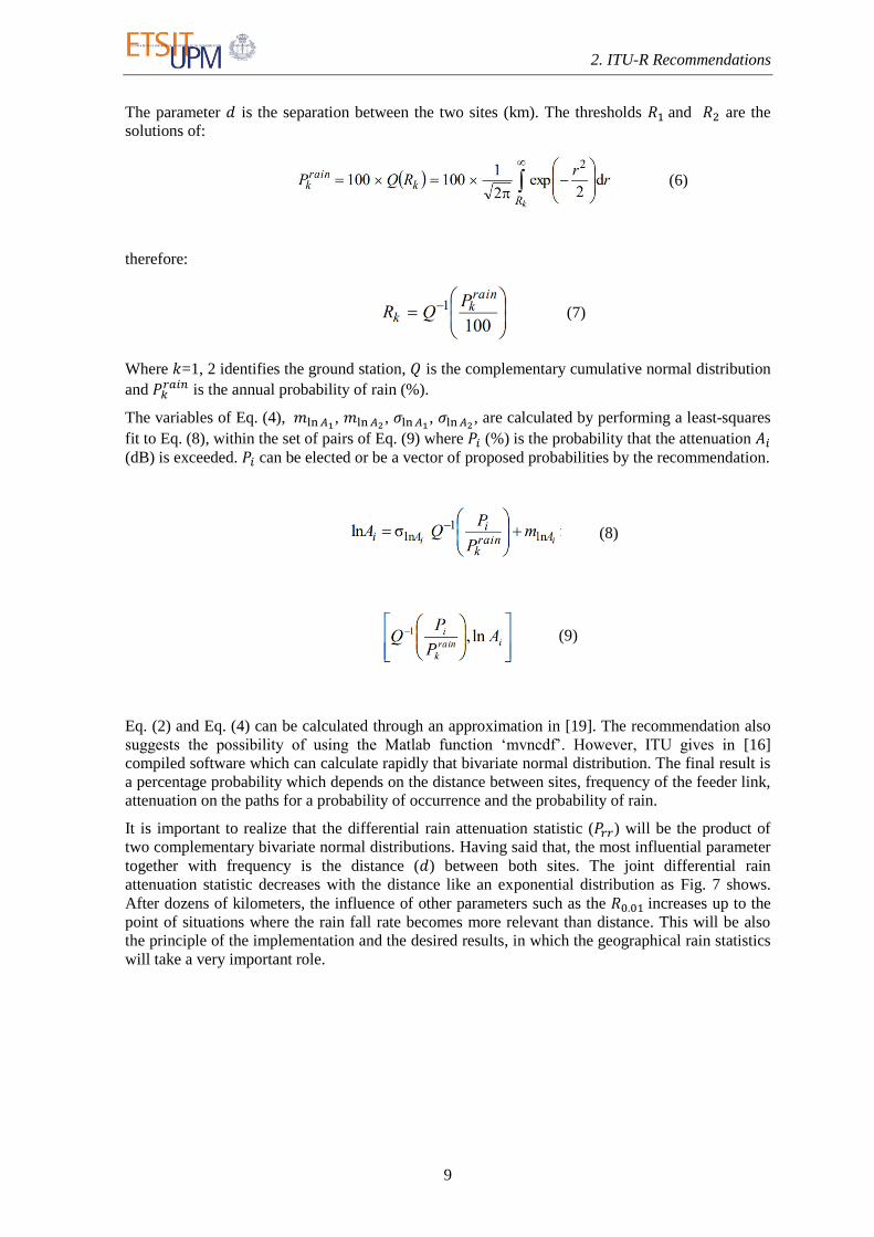
The parameter is the separation between the two sites (km). The thresholds and are the
solutions of:
therefore:
Where =1, 2 identifies the ground station, is the complementary cumulative normal distribution
and is the annual probability of rain (%).
The variables of Eq. (4), ,
, ,
, are calculated by performing a least-squares
fit to Eq. (8), within the set of pairs of Eq. (9) where (%) is the probability that the attenuation
(dB) is exceeded. can be elected or be a vector of proposed probabilities by the recommendation.
Eq. (2) and Eq. (4) can be calculated through an approximation in [19]. The recommendation also
suggests the possibility of using the Matlab function „mvncdf‟. However, ITU gives in [16]
compiled software which can calculate rapidly that bivariate normal distribution. The final result is
a percentage probability which depends on the distance between sites, frequency of the feeder link,
attenuation on the paths for a probability of occurrence and the probability of rain.
It is important to realize that the differential rain attenuation statistic ( ) will be the product of
two complementary bivariate normal distributions. Having said that, the most influential parameter
together with frequency is the distance ( ) between both sites. The joint differential rain
attenuation statistic decreases with the distance like an exponential distribution as Fig. 7 shows.
After dozens of kilometers, the influence of other parameters such as the increases up to the
point of situations where the rain fall rate becomes more relevant than distance. This will be also
the principle of the implementation and the desired results, in which the geographical rain statistics
will take a very important role.
(6)
(7)
(8)
(9)

2. ITU-R Recommendations
10
Fig. 7. Variation of with distance and frequency for = =16dB in site 1 (Madrid) and site 2 (direction to Valencia), with Hispasat-30W.
2.2 ITU-R P.1853-1
The ITU-R recommends having appropriate methods to simulate the time dynamics of the
propagation channel in order to plan proper terrestrial and Earth-space systems. Due to that, the
ITU gives in the recommendation P-1853-1 methods to synthesize the time series of rain
attenuation for terrestrial or Earth-space paths, the times series of scintillation for terrestrial or
Earth-space paths and the time series of total tropospheric attenuation and tropospheric scintillation
for Earth-space paths [20].
As mentioned before, rain attenuation is the main problem of GW systems so our study is going to
center on the synthesis of rain time series of rain attenuation for Earth-space paths which we will
name as ( ). This method is valid for frequencies between 4 GHz and 55 GHz and elevation
angles between 5º and 90º. In the calculation of the rain attenuation time series the
recommendation makes use of other recommendations which are the same as the stated in TABLE
II except the use of the recommendation ITU-R P.841-5. The time series are calculated following
Annex 1 of [20] and method is described below:
The recommendation describes that ( ) is synthesized with a white Gaussian noise which is low-
pass filtered, transformed from a normal distribution to log-normal distribution in memoryless non-
linearity and calibrated to match the desired attenuation statistics. This procedure is shown in Fig.
8:
Fig. 8. Synthesis‟ procedure of rain attenuation time series

2. ITU-R Recommendations
11
In Fig. 8:
is the parameter that describes the time dynamics ( ) and it is fixed as
.
and are, respectively, the mean and the standard deviation of the log-normal rain
attenuation distribution. The procedure of getting these parameters is the same to the
method used in ITU-R P.1815-1 to calculate ,
, ,
. But in this
case, the set of pairs is given by Eq. (10) and and are calculated by performing a
least-squares fit to Eq. (11).
(
)
is defined in Eq. (12) where is the annual probability of rain (%) and it
can be calculated through the recommendation ITU-R P.837-7.
(
)
( ) is calculated with the synthesis step-by-step of ( ) where =1, 2, 3… and is the
time interval between samples. For each , ( ) is synthesized with a noise time series
( ) with zero mean and unit variance at a sampling period, , of 1s. Then, the noise is filtered
in recursive low-pass filter, computed on the memoryless non-linear device and calibrated
with . The result is a synthesized time series where the first 200000 samples must be
discarded because of the filter transient.
Finally, with Fig. 9 we want to show an example of how rain attenuation time series synthetized
vary in a synthesis of one year:
Fig. 9. Example of of rain attenuation time series in Q/V band (50 GHz) in Madrid with KA-SAT.
(10)
(12)
(11)
3. Design of Gateway diversity (Design tool)
12
3 DESIGN OF GATEWAY DIVERSITY (DESIGN TOOL)
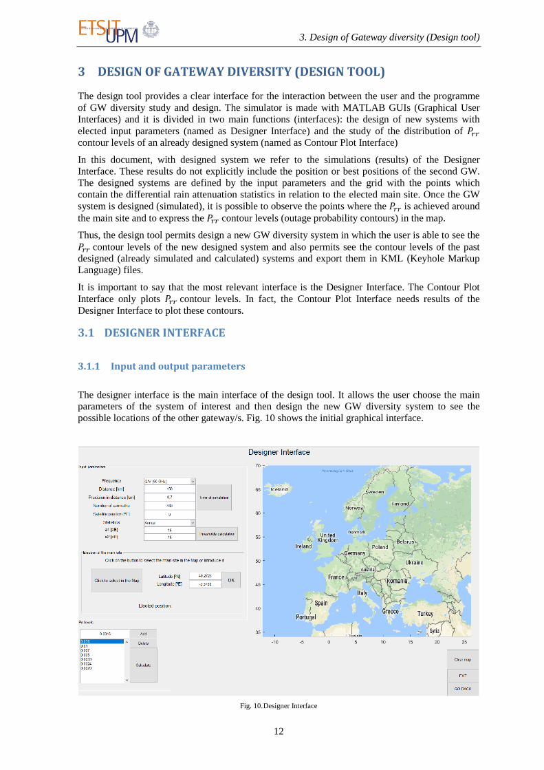
The design tool provides a clear interface for the interaction between the user and the programme
of GW diversity study and design. The simulator is made with MATLAB GUIs (Graphical User
Interfaces) and it is divided in two main functions (interfaces): the design of new systems with
elected input parameters (named as Designer Interface) and the study of the distribution of
contour levels of an already designed system (named as Contour Plot Interface)
In this document, with designed system we refer to the simulations (results) of the Designer
Interface. These results do not explicitly include the position or best positions of the second GW.
The designed systems are defined by the input parameters and the grid with the points which
contain the differential rain attenuation statistics in relation to the elected main site. Once the GW
system is designed (simulated), it is possible to observe the points where the is achieved around
the main site and to express the contour levels (outage probability contours) in the map.
Thus, the design tool permits design a new GW diversity system in which the user is able to see the
contour levels of the new designed system and also permits see the contour levels of the past
designed (already simulated and calculated) systems and export them in KML (Keyhole Markup
Language) files.
It is important to say that the most relevant interface is the Designer Interface. The Contour Plot
Interface only plots contour levels. In fact, the Contour Plot Interface needs results of the
Designer Interface to plot these contours.
3.1 DESIGNER INTERFACE
3.1.1 Input and output parameters
The designer interface is the main interface of the design tool. It allows the user choose the main
parameters of the system of interest and then design the new GW diversity system to see the
possible locations of the other gateway/s. Fig. 10 shows the initial graphical interface.
Fig. 10. Designer Interface

3. Design of Gateway diversity (Design tool)
13
The interface is structured with the following input and output parameters:
Inputs
Frequency band (f): the simulator studies three different bands in the feeder link: Ka-
Band (30 GHz), Q/V band (50 GHz) and W-Band (80 GHz). If these bands are not of
interest, other frequencies can be introduced too.
Maximum distance ( ) [km]: it determines the maximum radius of the circular grid
where the statistics are calculated. The maximum radius could be also defined by the
illumination zone of the spot beam which illuminates the main GW.
Precision in distance ( ) [km]: it establishes the separation in distance between points in
the same azimuth of the grid.
Number of azimuths ( ): it determinates the number of azimuths of the circular grid.
Satellite position (longSat) [ºE]: it is considered the use of geosynchronous satellites. This
parameter defines the longitude position of the satellite. This value may be the position of a
current HTS.
Statistics (p): they can be either annual statistics or worst-month statistics. This parameter
establishes the desired type of statistics.
Attenuation thresholds ( and ): they are definite by the margin that the system can
permit to accomplish a required carrier-to-noise ratio (C/N).
levels: the panel of levels permits select the outage probability of the contours that
are going to be printed in the Map. These will mark the outage or the availability of our
system.
Main site (lat and long) [ºE]: the coordinates of the main site are introduced manually in
the interface or clicking in the Map.
Outputs
Contours: the plot in the Map of Google Maps of the geographical positions where the
levels (outage probabilities) are achieved.
data: the script automatically creates a *.mat file with the values and their
geographical coordinates of the calculated grid ( ).
KML Files (Optional): once the simulation has finished, it is possible to get a *.zip file
with the KML files with the coordinates of the input levels.
3.1.2 Functioning
The interface is very user-friendly. The user introduces the input parameters of interest and when
the button „Calculate‟ is clicked, the main function calculates the joint probability ( ) in the
points of a thin grid specified by the inputs (see explanation below) around the main GW (main
site). Once the grid is created, the simulator finds the coordinate positions of the places where the
searched joint probabilities ( levels) are achieved. Then, the simulator prints that positions
creating contour levels in the Map which will let decide the possible locations of the other
gateway/s. Finally, the simulator exports the data of the grid and offers the possibility of
obtaining the KML files of the contour levels. In the following points, explanations about the
meaning and influence of some parameters are detailed:
The circular grid
Regarding the circular grid (or polar grid), as it has been said before, the main function calculates
the differential rain attenuation statistics ( ) in the points of a circular grid (specified by the
inputs) around the main GW (main site) when the user clicks on the button „Calculate‟. The
drawing of this grid is showed in Fig. 11. This grid is formed by three matrixes:

3. Design of Gateway diversity (Design tool)
14
. The last two indicate the coordinates of the points and the first
one the value of in those points.
should be elected as the radius of the illumination zone of the spot beam which the main GW
illuminates; in Ka-band could be approximated as 200-300 km and in Q/V band as 100-150
km.
It is important to mention that the precision in distance ( ) begins to be applied since certain
distance (11 km). Before 11 km, the grid is already fixed with a high precision in distance ( ). The reason is the high variation of with short distances as it has been seen in Fig. 7.
Therefore, to appreciate these changes, the precision on the first kilometers is high and fixed. In
addition, the precision ( , and ) will affect the time of simulation. It is recommended
good precision values to appreciate the real variation of the levels such as the default given
values. The Designer Interface offers a utility of interest to see how much time could last
approximately the simulation (through button „Time of calculation‟). The approximation is based
on a mean of time that consumes the calculation of the in one point (254 ms). Then, the time of
simulation will be proportional to the number of points that form the grid. This approximation has
been made with a laptop with 8GB of RAM and an Intel Core i5-4210H CPU.
Fig. 11. Scheme of the parameters that define the circular grid
Attenuation thresholds
As it is stated in Eq. (1), the attenuation thresholds ( and ) must be elected depending on the
expected attenuations. The thresholds should be the fade margin that the system can allow in order
to continue working correctly and without outage. If the user does not know which value should
introduce, the simulator contains a tool to calculate the thresholds according to a link budget (see
Fig. 12). This tool can be found clicking on the button „Thresholds Calculation‟ and the proposed
values are defined by a real HTS feeder link budget based on [11]. Thus, once elected the
attenuation thresholds in function of the margin, the calculated shows the probability of the
margin being exceeded simultaneously at both sites. This means that with that probability, the
system will not work, due to in both sites the margin will be exceeded simultaneously. We should
elect the levels as the probability that our system is going to be in outage, or equivalently, the
availability of the system.

3. Design of Gateway diversity (Design tool)
15
Fig. 12. Support tool to calculate the attenuation thresholds
The Map
When the grid is already calculated, the introduced levels will be plotted in the Map. The used
Map is an API of Google Maps which needs internet connection. This API is clearer than the Maps
of the Map toolbox and permits select among different sights: road map, satellite, terrain, hybrid,
etc. We have preferred the road map to appreciate better the highways, towns and surrounding
cities.
The initial map is Europe. We have chosen Europe because of the possibility of studying real
ground stations that currently operate satellites which provide services to Europe (KA-SAT,
HISPASAT satellites or others). However, the user has the freedom to select a place of study in
anywhere of the world. Additionally, beside the Map a color legend is included with the Main Site
and the values of the contour levels.
If a level is not achieved in any point, the interface will remove it from the list of levels and
will show a message advertising that there are not points with that probability. Therefore, the Map,
the legend, the data and the KML files will not contain the non-achieved level. To improve
the design of new systems, the button „Clear Map‟ is very helpful to clear the results plotted in the
Map and to prepare the interface for a new simulation.
3.1.3 Structure
In this sub-section it is going to explain how the simulator is internally made (the Designer
Interface). As it has been previously explained, the process followed by the script is showed below:
Fig. 13. Procedure of design
This procedure implies calls among function scripts and the pass of parameters between functions.
The name‟s functions will be written in italics. The majority of interactions among functions occur
in the MATLAB GUI of the Designer Interface. The Designer Interface coordinates the pass of
data to the function scripts. The general scheme of the process of design is showed in Fig. 14 where
the function scripts will be detailed and described in the following lines.

3. Design of Gateway diversity (Design tool)
16
Fig. 14. Diagram of the main function scripts in the design procedure
GridCalculation
This function script prepares the grid. Firstly, it loads the digital maps (mesh grids) that will be
necessary in the calculation of the differential rain attenuation statistics in
differentialRainAtten1815. Secondly, it takes the inputs showed in Fig. 14 and with , and
it calculates the radius of the rings of the polar grid. As seen before, each ring will have
number of points. The script is going to calculate the in the points of each ring in an iteration
loop. To do this, it passes to the function differentialRainAtten1815 the inputs showed in Fig. 15,
where is the radius of the ring. Finally, the script puts the points and the of the points of
each ring in 3 matrixes that will form the polar grid of interest ( ).
Fig. 15. Input and output parameters of differentialRainAtten1815
Before passing the outputs to PrrLevelsPlot, it is applied a filter to eliminate the samples which
belong to sea positions. This is easily made with the help of the Map Toolbox to load the contours
of coasts and with the use of the function „inpolygon‟.

3. Design of Gateway diversity (Design tool)
17
PrrLevelsPlot
The script receives the circular grid calculated in GridCalculation. For each level passed from
the Designer Interface, it searches the first point in each azimuth that accomplishes the level.
This means that the selected point will be the first point where the probability is less or equal than
the probability searched. We are not able to do a linear-interpolation between two points to find the
point where a level is exactly achieved because the differential rain attenuation statistics does
not follow a linear function. In fact, the in the middle of two points not necessarily must have
an intermediate value between them due to the dependence on the rain statistics of the particular
point.
It could occur that in various azimuths there were not probabilities less or equal than the searched
and in this case the script would introduce a NaN value in those points to avoid plotting.
differentialRainAtten1815
It is the implementation of the recommendation ITU-R P.1815-1 described in section 2.1 and it is
the main function script of this interface. As it has been explained above, this function calculates
the in the points of a ring of number of azimuths. This is made possible thanks to the
iteration of each azimuth of the ring, that is, each point of the ring. The implementation of this
recommendation does not allow calculate a vector of at the same time because the integral used
in the compiled file given by the ITU [16], which calculates the bivariate normal distributions (Eq.
(2) and (4)), does not allow an input vector of values.
As described in section 2.1, this recommendation makes use of other recommendations (see
TABLE II). These other recommendations have been implemented too, due to they are totally
necessary to study adequately a place of interest. Internally, the differentialRainAtten1815 makes
directly calls to the functions stated in TABLE III.
TABLE III. FUNCTIONS CALLED INTERNALLY IN differentalRainAtten1815
Parameter Name of the function
attfunc618
rainfallRate837
earthheight1511
bivnor
attworstmonth841
Probably the process of obtaining of is the most relevant and which most implies the
cooperation among recommendations. Fig. 16 shows all the implementations of the
recommendations that are needed in the calculation of . The arrows‟ direction indicates in which
function they are called or to which function provide.

3. Design of Gateway diversity (Design tool)
18
Fig. 16. Cooperation among function scripts to calculate
As been said before in the specification of GridCalculation, it loads the digital maps (mesh grids)
that are necessary for the calculation of some parameters. These digital maps take importance now,
in the calculation of .
The ITU gives in some recommendations the values of the parameters in a grid of points (digital
maps). The problem emerges when the point of study is not on the points given in the digital maps.
In these cases (the vast majority), the solution is to perform a bi-linear or bi-cubic interpolation
using respectively the four or sixteen surrounding grid points as the recommendation ITU-R
P.1144-9 describes in [21]. Each recommendation imposes which interpolation is needed. In our
parameters of interest, a bi-linear interpolation will be necessary in the calculation of , , ,
and a bi-cubic interpolation in the calculation of .
The calculation of a parameter of interest X in a point defined by its latitude and longitude, with a
grid (digital map) formed by Grid of X, Grid of latitudes and Grid of longitudes follows the
diagram exposed in Fig. 17.
Fig. 17. Procedure of interpolation
The role of searching the nearest points is performed by the function scripts nearLatitudes and
nearLongitudes whereas the roles of carrying out the bi-linear and bi-cubic interpolations are
executed respectively by the function scripts bilinearinterp and bicubicinterp.
3.2 CONTOUR PLOT INTERFACE
3.2.1 Input and output parameters
The Contour Plot Interface is an extra interface of the design tool. It only allows the user observe
how the contour levels vary in an already system designed with the Designer Interface. This is

3. Design of Gateway diversity (Design tool)
19
possible thanks to the file *.mat saved automatically in the Designer Interface. It is important to
mention that this interface is already implemented in the Designer Interface to plot the contour
levels once the grid has been calculated. The objective of the Contour Plot Interface is to
recalculate the contours of our interest from past simulations. Fig. 18 shows its graphical interface
with some contours from a loaded simulation file.
Fig. 18. Contour Plot Interface
Inputs
data: the script needs a *.mat file with the values and their geographical
coordinates of a circular grid ( ). This file is created by the
Design Interface in its simulations.
New levels: the panel of „New levels‟ permits select the values of the contours of
the differential rain attenuation statistics of interest.
Outputs
Contours: the plot in the Map of Google Maps of the geographical positions where the
New levels are achieved.
KML Files (Optional): once the simulation has finished, it is possible to get a *.zip file
with the KML files with the coordinates of the stored contours.
3.2.2 Functioning
Firstly, it must be introduced a file with the data which includes the circular grid of a system
designed by the Design Interface. Secondly, the user can choose the levels of interest using the
panel „New levels‟. Finally, when the user clicks on the button „Calculate‟, the simulator
searches in the loaded grid the coordinate positions of the places where the searched joint
probabilities (New levels) are achieved. Then, the simulator prints those positions creating
contour levels in the Map. The second step can be repeated to add new levels. The interface
also gives the possibility of deleting a contour level of the Map that appears in the panel

3. Design of Gateway diversity (Design tool)
20
„Already contours‟. With these features, the user is able to plot and remove contours in order to
see which probabilities can be achieved in our designed system.
In addition, this interface of the design tool also gives the option of clearing the Map and exporting
the calculated contour levels in KML files.
3.2.3 Structure
The functioning of the Contour Plot Interface follows the procedure exposed in Fig. 19.
Fig. 19. Procedure of plotting contours of a designed system.
Once a file with the grid is introduced, the functioning of the interface is an iterative process where
the user can either delete or introduce new levels. Likewise Designer Interface, it gives the
possibility to export the „Already contours‟ in KML files.
The Contour Plot Interface only uses one function script as shows Fig. 20. This function was
already mentioned and explained in the description of the function scripts of the Design Interface.
Fig. 20. Diagram with the functions of the Contour Plot Interface.
3.3 RESULTS
Once the design tool is finished, it gives us the freedom to observe visually how different input
parameters modify the contour levels with regard to size and shape.
The results of the following sections are cases of study made in different geographical places, with
different frequencies, satellite positions and type of statistics. Although the simulations are centered
in Europe, the use of places outside of Europe will be necessary to observe extreme climatic
variations. The simulations have lasted 7 hours on average with a laptop with 8GB of RAM and an
Intel Core i5-4210H CPU.

3. Design of Gateway diversity (Design tool)
21
Regarding the selected input parameters, the attenuation thresholds ( and ) will mark the
availability of a system which only has one GW. The election of the thresholds will be reasonable
for a real case of study and with the use of the section 2.2.1.1 of Rec. ITU-R P. 618-13 [9], they
will be translated to an availability (or to an outage probability) that will be a reference to compare
with the levels which will mark the new availability of the system with two GWs. In all sub-
sections (expect in 3.3.5) annual statistics are considered. The precision of the grid is similar in the
majority of cases, however in some studies could be different to appreciate properly the results and
the variations. The orbital positions (of satellites) studied could be not occupied by satellites
working in our frequency bands of interest. The orbital positions will be elected to see the effect of
the elevation angle as if a satellite would be working at that frequency. The maximum radius of
study is marked by the illumination zone of the spot beam which depends on the working
frequency. The approximated values of will be respectively for Ka, Q/V and W bands: 250,
150 and 100 km. This approximation takes into account circular illumination zones and this could
not be enough accurate because the illumination zones depend on the elevation angle to the
satellite. However, the approximation is more precise when the place of study is near to the
Equator. In the following results, when we refer generally to Ka, Q/V and W bands, we mean
frequencies of 30, 50 and 80 GHz respectively.
Although the simulator presents the results in a version of Google Maps directly in the simulator,
the results will be presented through Google My Maps. We make this decision because in My
Maps the quality and the clarity of the map are better. The way of exporting the contour levels
is through KML files that the Designer and Contour Plot Interface are able to provide. These files
are directly imported as a layer in the application of Google My Maps and changed the color and
width to observe properly results.
To present the contours, we will follow the legend showed in TABLE IV. This color legend will be
followed in all study cases except situations where the outage probabilities of interest are not in
TABLE IV (Orlando in 3.3.1 and Arganda del Rey in 3.3.5). In these cases, an individual legend
will be specified.
It is important to mention that in each case only the levels of interest will be plotted. It is
possible that in some cases not all the levels will be presented (because they will not be as
relevant as others) or not achieved due to the limiting maximum radius ( ) or the sea presence
which will filter the grid thanks to sea contours.
TABLE IV. LEGEND OF LEVELS
( ) Color
0.04
0.01
0.005
0.0024
0.001
0.0005
0.0003
0.0001
3.3.1 Site variation
Site variation is the primary factor of interest. The idea of studying whatever geographical place
and the surrounding places on the Map is the main objective of this simulator. The cause is that
some parameters such as , , , the elevation angle to the satellite, and therefore the and

3. Design of Gateway diversity (Design tool)
22
highly depend on the point of interest. So establishing the main GW in different places will led
us to observe how the same contour levels vary in each place and then, that the distance to
settle the backup GW will change from one place to another.
In order to appreciate this, in the following sub-sections five cases of study are presented where the
parameters mentioned above will modify the contour levels in each case. In the five cases, the
main site input is different. The common parameters are: frequency (50 GHz (Q/V band)) and
= =16 dB. In these studies, the attenuation thresholds ( and ) have a value of 16 dB. They
are in the order of a reasonable value of a margin in the feeder link with a bandwidth of 250 MHz
and an EIRP of 74.1 dBW (including or not the additional dBs of Uplink Power Control). In a case
of study with only one GW, this margin of 16 dB can be translated to an availability (or time in
which the system works correctly) according to section 2.2.1.1 in Rec. ITU-R P.618-13 [9].
The locations of study of interest and their coordinates are stated in TABLE V.
TABLE V. PLACES OF STUDY
Location Latitude Longitude
Arganda del Rey (Eastern Madrid) 40.2723ºN 3.3788ºW
The Pyrenees (Southern France) 43.099ºN 0.6ºE
Rambouillet (Northern France) 48.5495 ºN 1.7820ºE
Lurín (Peru) 12.2852 ºS 76.8469ºW
Florida (Orlando) 28.258ºN 81.6697ºW
The satellite position will be elected as a reference position where a satellite currently provides
services to the locations of study. Therefore, we have chosen that the European studies will be
associated with a longSat=9ºE (currently KA-SAT) and the American studies will be simulated
with longSat=61ºW (currently AMAZONAS H61W-satellites)
Arganda del Rey
The first study is centered in the Hispasat Satellite Control Center, located in Arganda del Rey. In
this location, Eutelsat and Hispasat have active GWs that operate with KA-SAT and HISPASAT
satellites respectively. In this place, we are going to settle the main site (main GW). With this study
we can simulate a realistic case of study because the main site is a current ground station, and the
other input parameters are very realistic values for operating with HTS or future VHTS. According
to Rec. ITU-R P. 618-13, a margin of 16 dB with one GW is translated to an outage of 0.08 %
(availability = 99.92 %). The new outage probability with two GWs will be the of the contour
levels. In this place, the in the main GW is 24.91 mm/h and the annual probability of rain
( ) is 3.36 %. Next to the main GW, we can expect that parameters such as or are
not going to vary too much because the surrounding region maintains a Mediterranean climate with
high similarity. Therefore, we can foresee that the contours could vary less than other cases.
Fig. 21 shows the simulation for this case of study. The point in the center is where the main GW is
established. The hypothesis is confirmed: the studied area has similar values in and ,
and that is why the first contours seem to be partially circular. The non-regularity is more relevant
in the lowest contour values (the furthest ones from the main GW). As a first sight, the contour of
the first level (0.04 %) is practically invisible because this contour is very near to the main GW.
The distance to the first contour is 2.48 km (constant). Even using a high precision, as was
mentioned in the functioning of the Design Interface (see section 3.1.2), the influence of distance is
extremely high and the contours are totally or practically circular in the first kilometers.

3. Design of Gateway diversity (Design tool)
23
Fig. 21. Annual contour levels in Arganda del Rey in Q/V band with longSat=9ºE.
With lower levels, we can observe the implication of rain parameters to form non-regular
contours. For example if we focus in the pink contour (0.0005 %), we are able to see that the
variation of the contour with distance is higher, being the nearest point to the main GW of 69.6 km
(to the East) and the furthest point 123 km (to the West). This high difference can be explained
using parameters such as and . In the nearest point is 27.0227 mm/h and
=4.9 %, whereas in the furthest point the values of and are respectively: 31.86 mm/h
and 7.3874 %. We know that higher probabilities of rain and higher rain fall rates imply higher
attenuations on the satellite path so owing to the exposed values in the furthest point, it is needed
more distance to achieve the same probability.
Finally, it is observed that the lowest contour level (0.0003 %) is divided in 5 segments. The non-
plotted contour segments would be achieved if the maximum radius of study would be greater. The
limit imposed by the illumination of the spot beam could be extended and the final area of study
would be limited by the real illumination zone of the spot beam. This fact is not included in the
objectives of this project, but the final surface of study could be filtered by its real illumination
zone (external modification of data). These first results justify the necessity of the design tool to
see the contour levels and knowing where it can be established a second GW with the outage
probability of interest.
The Pyrenees
On the second case study, we center our study in the south of France (in The Pyrenees, close to the
border with Spain) where the =31.87 mm/h and =7.8 %. Comparing with previous
simulation, the difference among these values gives us an intuition to think that in France it is
going to need more distance to achieve the same differential rain attenuation statistics. Moreover,
the presence of The Pyrenees let us think that there will be more irregularities than in Madrid.
Fig. 22 illustrates the simulation in the Pyrenees where the irregular contours are totally expected.
The distance to the first contour is 8.45 km on average (higher than the previous 2.48 km in
Arganda del Rey). The contours are oval shaped, being shorter the distances in the Pyrenees than in
the North. On average, the Pyrenees have =32 mm/h and =8.81%, while in the north of

3. Design of Gateway diversity (Design tool)
24
the site =30.5 mm/h and =4.80 %. Taking this into account, it rains more in the
Pyrenees, therefore the distance of the contours in the Pyrenees should be larger. Nevertheless, in
this case the height above the sea level ( ) has a decisive influence. In this case, The Pyrenees (to
the South) have higher than the locations to the North. Higher altitudes imply lower rain heights
( ) and according to the influence of over the rain attenuation on the path to the satellite, less
implies less rain attenuation. Therefore, we have found a case of study where the height above
the sea level has more influence on the differential rain attenuation statistics than parameters such
as or .
Fig. 22. Annual contour levels in The Pyrenees in Q/V band with longSat= 9ºE.
Once again, the design tool has very valuable information about how can we design the GW
diversity system. In this case, the altitude of the GW location is fundamental, so we could think that
the better choice is to settle the second GW on the nearest point in a contour level of interest,
but it should be also considered if building a ground station at the top of a mountain is
economically possible. The user must find a balance between closeness and economical
availability.
Rambouillet
Rambouillet is a small city located in the northern France where there is one of the Eutelsat GWs
which operate with KA-SAT (see Fig. 3). In the same way that Arganda del Rey, we have the
opportunity of studying a real case of study. In this location, if there were only one active GW,
where could we establish a backup GW to achieve GW diversity in the feeder link to KA-SAT and
with which outage probability? The answer of this hypothesis of study is showed in Fig. 23.

3. Design of Gateway diversity (Design tool)
25
Fig. 23. Annual contour levels in Rambouillet in Q/V band with longSat= 9ºE.
At first sight, we realize that whereas in Fig. 21 and Fig. 22 the pink (0.0005 %) and black (0.0003
%) contours have been closed, in Rambouillet that contours are not achieved. The , , and
have similar values to the other two studies. The factor that justifies this fact seems to be the
elevation angle. When the point of interest has greater latitude, the elevation angle to the satellite
increases. This growth means a greater attenuation on the path to the satellite and therefore higher
differential rain attenuation statistics. In this case, the main site and its surrounding places have
greater latitude than Arganda del Rey or The Pyrenees.
The plot is again useful because we can see that places such as in the Paris city center it is not
available to build a ground station although the distance to the same level is shorter than other
locations.
Lurín
Lurín is a small city next to Lima. It has a ground station which operates with AMAZONAS
satellites. It is strategically established because in this region the rain fall rate and the annual
probability of rain are, on average, 10.63 mm/h and 0.5 % respectively. They are very poor values
and imply very low rain attenuations. According to the Rec. ITU-R P.618-13, the availability with
only one GW with a margin of 16 dB is 99.9893 % (outage of 0.0107 %). If we establish a backup
GW, the outage probability could be even lower (Fig. 24).
We have not plotted the first contour levels (0.04, 0.01 and 0.005 %) because they are achieved too
close and do not give relevant information. In fact, the contour 0.04 % is a point. The outage
probability of a system with only one GW is already lower than 0.04 %, so it has not sense to
establish a second GW in the same point that main GW because the outage probability with only
one GW is even lower.
The influence of the sea to limit the contours is easily observed. Low contour levels are
achieved very close to the main site and their variation is extreme. The reason is that the rain
statistics are very low and the dependence with distance disappears when the differential rain
attenuation statistics are very low. Then, any variation of rain statistics might provoke high changes
on the contours. In addition, some probabilities are achieved in the same locations. This can be
explained with the search method of the contours (see PrrLevelsPlot in section 3.2.1). For example,
in Fig. 24 to the north, the black (0.0003%) and the pink (0.0005%) contours have common points.

3. Design of Gateway diversity (Design tool)
26
This is because in some azimuths the probability can change from 0.00055 % in one point to
0.00029 % in the next point and the first point where both probabilities are less or equal is
common.
Fig. 24. Annual contour levels in Lurín in Q/V band with longSat= 61ºW.
With this example, we have showed the variation of levels in locations with low rain statistics.
In this case, the implementation of GW diversity is not as necessary as others but can improve the
availability of the system thanks to the very low outage probabilities that are achieved close to the
main GW (0.0001 % is achieved 15.2 km from the main site in the nearest point).
Orlando
In this case we are in front of an extreme study case. The city of Orlando belongs to the U.S. state
of Florida. Orlando, and in general the Florida‟s peninsula, has a humid subtropical climate. This
climate is caused primarily by its low elevation. In this region, the rain fall rates vary around 67
mm/h, being one of the rainiest locations in U.S. Moreover, the rain height has a high value, being
on average 4.5 km.
Although the probability of rain has common values (around 4 %), the high value of and
will provoke high levels of rain attenuation and therefore the differential rain attenuation
statistics will rise to values that have nothing to do with the levels discussed in previous studies
(TABLE IV). Hence we are forced to define a new legend with higher levers (TABLE VI)
because the exposed ones at the beginning of this sub-section are practically unachievable.
TABLE VI. LEVELS IN Q/V BAND IN ORLANDO
( ) Color
0.5

3. Design of Gateway diversity (Design tool)
27
0.3
0.1
0.07
0.04
The following picture (Fig. 25) shows the simulation made in Florida. Some contours are limited
by the sea and the irregularity tell us that the majority of locations are at the sea level ( ) and
the rain fall rate value oscillate from 65 to 72 mm/h.
Fig. 25. Annual contour levels in Orlando in Q/V band with longSat= 61ºW.
The study of the Florida‟s peninsula has been useful to see an extreme situation of rain attenuation.
The probabilities of the contours achieved inside the radius of study are too high to establish
ground stations with two GWs for feeding a VHTS. Any engineer knows that this place is
unfeasible to accomplish high availabilities in the system. However, if due to specific reasons a
GW diversity system in a place with extreme rain precipitations is required, the study of lower
frequency bands such as Ka-band should be considered. This issue is what will be covered in sub-
section 3.3.2.
3.3.2 Frequency variation
In this sub-section, we are going to study the variation of the outage probability contours with
frequency.
If we consider that in studies showed before some levels have been achieved relatively near to
the main GW, we could establish the second GW even further from the main site. As seen in Fig. 7
in section 2.1, the differential rain attenuation statistics rise if the frequency of the system
increases. Thus, the same contour levels will be achieved further for higher frequency bands.

3. Design of Gateway diversity (Design tool)
28
With this election, the capacity of the system could be even higher thanks to the use of higher
frequencies such as W band.
Our first study will center on the increase of frequency (to W band) to get higher data rates
provided that the levels are also achieved in the new frequency. We will center this study in the
Hispasat Satellite Control Center (Arganda del Rey) with W band. The second study has to do with
the sense of designing GW diversity systems in locations with extreme rain precipitations. In these
cases, the use of lower frequency bands such as Ka-band should be considered. We will center this
case of study with the example of Orlando.
The unique parameter of change will be the frequency, being the longitude of the satellite the same
than in the previous cases (in Arganda del Rey 9ºE and in Orlando 61ºW). The attenuation
thresholds have been elected with the same values that in the study of site variation ( = =16
dB). These thresholds could change with the change of frequency if we extract them from a link
budget (because of the change in the free space losses). This change is around 3 dB, so we consider
that the Uplink power control deals with the variation of the link budget with frequency.
The contour levels that are going to be printed follow the legend previously described in
TABLE IV.
W band (Arganda del Rey)
In comparison with the study in Q/V band (Fig. 21), the study in W band (Fig. 26) only shows four
levels: 0.04, 0.01, 0.005 and 0.0024 %. The contours are limited by the radius of study which is
100 km in W band. The contours lose the circular shape with the increase of frequency and the
distance to the nearest point in each contour level increases (13.68 km more for the purple
contour (0.04 %) and 42.1 km more for the green contour (0.0024 %)).
Fig. 26. Annual contour levels in Arganda del Rey in W band with longSat= 9ºE.
With the limit of the maximum radius of study, the lower differential rain attenuation statistic that
it is possible to achieve is 0.0024 %. It means an outage probability of 0.0024 % that is translated
to an availability of 99.9976 % which is reasonable value. So we have justified that in some study
cases where the contour levels are nearer than other cases, it is possible to increase the
frequency in order to achieve higher data rates while the availability continues being valid.

3. Design of Gateway diversity (Design tool)
29
Ka band (Orlando)
According to the results of the differential rain attenuation statistics in Orlando with Q/V band (Fig.
25) the conclusions are clear: the design of GW diversity with Q/V band in locations with extreme
precipitations is unfeasible. If it is not possible finding places with lower rain precipitations, we
offer the solution of using lower frequency bands such as Ka-band. This solution is against future
VHTS as we commented in section 1.1, but it could be considered in situations where there is no
other option.
So we are going to consider studying the design of GW diversity in Orlando but with Ka-band.
With this study we expect to achieve lower levels than in the case with Q/V band based on the
first intuition made in Fig. 7. The satellite position continues being 61ºW, the color legend follows
TABLE IV and the results of the simulations are showed in Fig. 27.
Fig. 27. Annual contour levels in Orlando in Ka-band with longSat= 61ºW.
The results have nothing to do with the results in Q/V band. The levels which are achieved are:
0.04 % (purple), 0.01 % (red), 0.005 % (blue) and 0.0024 % (green). These values are more
reasonable and support the utility in designing GW diversity in the Florida‟s peninsula. In Q/V
band the value 0.04 % was achieved at 148 km from the main GW and now in Ka-band this value
is achieved at a distance of 20 km from the main GW. The difference is 128 km with the change of
frequency band.
With these results we conclude that the modification of the frequency band is useful to improve the
capacity of the system or to achieve lower outage probabilities. The considered cases of study may
not be as realistic as others. The reasons are that Ka-band contradicts the idea of using Q/V or W
bands to achieve the aim of 1 Tbps and that technology is not prepared for adapting the satellite
systems to work with frequencies in W band. However the proposal of modifying the frequency is
helpful to consider the study of differential rain attenuation statistics in sub-bands of a realistic
frequency band such as Q/V.
3.3.3 Elevation angle variation
The previous results have compared their differences without changing the position of the satellite
which is involved in the design of the GW diversity systems. As said before, the studied orbital

3. Design of Gateway diversity (Design tool)
30
positions could be not occupied by satellites working in the frequency bands of interest. However,
it is expected that in future those satellites will be replaced by others with our frequencies of
interest. In TABLE VII, orbital positions with current situations of interest are showed.
TABLE VII. ORBITAL POSITIONS OF INTEREST AND THEIR ELEVATION ANGLES
Satellite and Main site Orbital position Elevation angle
KA-SAT and Arganda del Rey 9ºE 41.717º
HISPASAT 30W and Arganda del Rey 30ºW 36º
AMAZONAS and Lurín 61ºW 66.61º
ViaSat-2 and Lurín 69.9ºW 73.45º
We have discussed the variation of differential rain attenuation statistics with site and frequency.
Those studies have been developed with satellites in 9ºE and 61ºW. Now, we are going to pick up
some example discussed before and to compare them with new studies where the unique variation
is the orbital position. This change influences on the elevation angle to the satellite, and therefore
on the rain attenuation. So we expect that with lower elevation angles, the contour levels will be
achieved further. The aim of this sub-section is to study the variation of the differential rain
attenuation statistics with the elevation angle to the satellite.
The frequency band is considered Q/V and the attenuation thresholds 16 dB. The contour levels
follow again the legend stated in TABLE IV.
Arganda del Rey (longSat= 30ºW)
We discussed the design of GW diversity in Arganda del Rey because the active GWs of KA-SAT
and HISPASAT satellites are settled there. The study showed in Fig. 21 was designed with an
orbital position of 9ºE. Now we can consider assessing the simulation with longSat= 30ºW.
According to TABLE VII, the elevation angle from the Hispasat control center with a satellite in
9ºE is 41.717º whereas with a satellite in 30ºW is 36º. We can expect that the differential rain
attenuation statistics are going to be worse using a satellite position of 30ºW.
Fig. 28. Annual contour levels in Arganda del Rey in Q/V band with longSat= 30ºW.
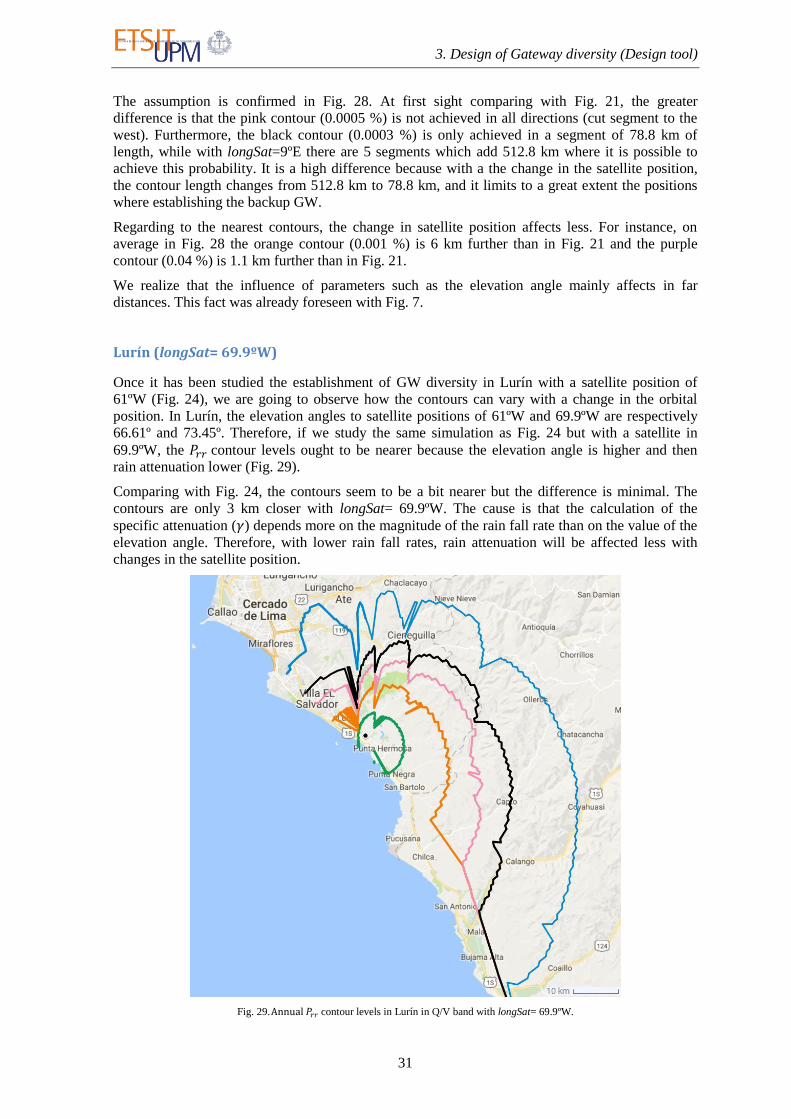
3. Design of Gateway diversity (Design tool)
31
The assumption is confirmed in Fig. 28. At first sight comparing with Fig. 21, the greater
difference is that the pink contour (0.0005 %) is not achieved in all directions (cut segment to the
west). Furthermore, the black contour (0.0003 %) is only achieved in a segment of 78.8 km of
length, while with longSat=9ºE there are 5 segments which add 512.8 km where it is possible to
achieve this probability. It is a high difference because with a the change in the satellite position,
the contour length changes from 512.8 km to 78.8 km, and it limits to a great extent the positions
where establishing the backup GW.
Regarding to the nearest contours, the change in satellite position affects less. For instance, on
average in Fig. 28 the orange contour (0.001 %) is 6 km further than in Fig. 21 and the purple
contour (0.04 %) is 1.1 km further than in Fig. 21.
We realize that the influence of parameters such as the elevation angle mainly affects in far
distances. This fact was already foreseen with Fig. 7.
Lurín (longSat= 69.9ºW)
Once it has been studied the establishment of GW diversity in Lurín with a satellite position of
61ºW (Fig. 24), we are going to observe how the contours can vary with a change in the orbital
position. In Lurín, the elevation angles to satellite positions of 61ºW and 69.9ºW are respectively
66.61º and 73.45º. Therefore, if we study the same simulation as Fig. 24 but with a satellite in
69.9ºW, the contour levels ought to be nearer because the elevation angle is higher and then
rain attenuation lower (Fig. 29).
Comparing with Fig. 24, the contours seem to be a bit nearer but the difference is minimal. The
contours are only 3 km closer with longSat= 69.9ºW. The cause is that the calculation of the
specific attenuation ( ) depends more on the magnitude of the rain fall rate than on the value of the
elevation angle. Therefore, with lower rain fall rates, rain attenuation will be affected less with
changes in the satellite position.
Fig. 29. Annual contour levels in Lurín in Q/V band with longSat= 69.9ºW.

3. Design of Gateway diversity (Design tool)
32
3.3.4 Attenuation thresholds variation
Up to now, the results have used attenuation thresholds of 16 dB in the calculation of the . As
said before, these thresholds should be elected as the link margin between the Carrier-to-noise ratio
in clear sky and the required Carrier-to-noise. The value of this margin affects directly to the value
of the calculation of . If the thresholds rise, the probability of simultaneous exceeded rain
attenuations at both sites decreases. If the thresholds decrease, the joint probability of simultaneous
exceeded rain attenuations at both sites rises. Thus, the position of the contour levels directly
depends on the values of these thresholds. If changing the satellite position or the frequency is not
enough to achieve an outage probability in the radius of study, a solution could be changing the
attenuation thresholds.
If we want to get higher thresholds, it is necessary to change some parameters in the link budget.
The options could be: raising the transmitted power or reducing the transmitted bandwidth or the
required Carrier-to-noise ratio. Even it may be considered changing the antennas‟ size. There is not
one unique solution. The efficient solution might be combining all the options. In order to calculate
the link budget and its margin, the interface includes a tool to calculate the link budget and its
margin as explained in section 3.1.2.
In the same way, when levels are achieved sufficiently nearby, we can improve the use of
resources with the consequences of a bit more remote contour levels. The improvement of
resources implies the increase of transmitted bandwidth, improving the quality of the system,
saving energy through transmitting less power or reducing the antenna‟s diameter.
These two particular cases are going to be discussed through the study in Rambouillet and Arganda
del Rey with respectively higher and lower attenuation thresholds. The work frequency band
continues being Q/V band and the satellite position 9ºE. The levels of interest will follow the
legend showed in TABLE IV.
Rambouillet ( = =19 dB)
With higher attenuation thresholds we expect to decrease the differential rain attenuation statistics
and the nearest contour levels. The simulation made with = =16 dB in Rambouillet (Fig.
23) the pink (0.0005 %) and black (0.0003 %) contours were not achieved, and now with
= =19 dB are managed (Fig. 30). The increase of 3 dB in the attenuation thresholds can be
achieved increasing the uplink power or decreasing the quality of the system. In this case,
increasing the gain of the antenna in 3dB (making the antennas 41% bigger) may be the worst
option, because the economic costs would be enormous.
Fig. 30. Annual contour levels in Rambouillet in Q/V band with longSat= 9ºE ( = =19 dB)

3. Design of Gateway diversity (Design tool)
33
The differences are obvious comparing both simulations: the same contour levels are nearer and
the pink and black contours are achieved with attenuation thresholds of 19 dB. Even the orange
contour (0.001 %) is totally close whereas before no.
Arganda del Rey ( = =10 dB)
If we consider that the contour levels obtained in Fig. 21 are sufficiently close to the main GW,
we can move the contour levels farther with the advantage of saving resources such as power.
In Fig. 21 the attenuation thresholds have been elected with a value of 16 dB. So now we can
reduce the margin in the link budget in a factor of 6 dB (for example saving 3 dB of transmitted
power and raising 3 dB the required C/N). But now a very valuable parameter to reduce must be
the antennas„ dimension. Reducing the aperture size would decrease the EIRP of the GW and for
example if the antennas were 29.29 % smaller, the EIRP would be reduced in 3 dB.
Now, the calculated differential rain attenuation statistics will be the joint probability that the
attenuation on the path to the first site is greater than dB and the attenuation on the path to the
second site is greater than dB. The results are worst and the contours have distanced from the
main GW (Fig. 31).
Fig. 31. Annual contour levels in Arganda del Rey in Q/V band with longSat=9ºE ( = =10 dB)
We notice that only four levels are achieved: 0.04 % (purple), 0.01 % (red), 0.005 % (blue) and
0.0024 % (green). The other contours of the legend do not appear because the radius of study limits
its presence. If we consider that an outage ( level) of 0.0024 % is a reasonable value for the GW
diversity system, we must establish the second GW in the green contour where the minimum
distance to the main GW is 102 km. In the case of = =16 dB (Fig. 21), the minimum distance
to achieve an outage probability of 0.0024 % is 37.2 km. It is about 64.8 km more to achieve the
same probability. This is a good example to understand the agreement that the designer has to
contemplate between distance (delay and economic investment) and economizing the system
resources.

3. Design of Gateway diversity (Design tool)
34
In addition, a great similarity to the study made in W band (Fig. 26) is observed. Differential rain
attenuation statistics increase with a similar performance with frequency and attenuation
thresholds. In practice, these two parameters are associated because when the frequency raises, the
carrier-to-noise in clear sky decreases and therefore the margin. Although the Uplink power control
tries to compensate this fact, a change in frequency tends to change the attenuation thresholds.
3.3.5 Annual or worst-month statistics
The ITU-R defines in the Rec. ITU-R P.581-2 [22] that the fraction of time during which a
preselected threshold is exceeded in the worst month of a year is referred to as “the annual worst-
month time fraction of excess”. It also states that the worst month of a year for a preselected
threshold for any performance degrading mechanism, is that month in a period of twelve
consecutive calendar months, during which the threshold is exceeded for the longest time.
All the results discussed above are results of annual differential rain attenuation statistics. As
explained in section 2.1, the differential rain attenuation statistics can be either annual or worst-
month statistics and the difference is the use of the Rec. ITU-R P.841 [18]. This recommendation
changes the probabilities (%) maintaining the values when it is performed the least-squares fit
to Eq. (8).
The implementation of Rec. ITU-R P.841 is done through the function script attworstmonth841.
The conversion from annual statistics to worst-month statistics highly depends of two parameters
according to Annex 1 of [18]: and . We have elected these values for rain effects in slant path
attenuation in a global planning purpose ( and ). Worst-month statistics are
calculated through Eq. (13) and Eq. (14) where is the annual time percentage of excess.
Thus, with the ITU definition about the worst month, we foresee that the worst-month differential
rain attenuation statistics will be higher than the annual ones. In order to appreciate an example of
worst-month statistics, we are going to discuss the same simulation in Fig. 21 (Arganda del Rey)
but with worst-month statistics (Fig. 32). Owing to the statistics are going to be higher, we are
forced to establish a new legend with higher levels in order to observe properly this increase
(TABLE VIII).
(14)
(13)

3. Design of Gateway diversity (Design tool)
35
TABLE VIII. LEVELS IN WORST-MONTH SIMULATION
( ) Color
0.1
0.04
0.02
0.01
0.007
0.005
Although the levels have increased for the same locations, the contours have similar shape to
the ones in Fig. 21. The reason is that the change in the type of statistics does not modify the
performance of the rain attenuation. Despite the fact that the annual differential rain attenuation
statistics are not directly transformed, the change is like a conversion which acts when the
frequency, the satellite position and the attenuation thresholds have already influenced.
Fig. 32. Worst-month contour levels in Arganda del Rey in Q/V band with longSat=9ºE.
The blue contour (0.1 %) of Fig. 32 is 13.4 km distant from the main site. In the annual statistics
simulation (Fig. 21) in a distance of 13.4 km distant from the main site a probability near to 0.01 %
is achieved. This means a transformation in a factor close to 10. It is not a fixed factor but could be
stated as a reference in the transformation from annual to worst-month differential rain attenuation
statistics.
With this example we want to show that the design of GW diversity depends significantly on the
type of statistics and that the election must be taken by the designer.

4. Analysis of switched bandwidth (Analysis tool)
36
4 ANALYSIS OF SWITCHED BANDWIDTH (ANALYSIS TOOL)
The planning and the design of smart GW diversity systems require the ability to synthesize the
time dynamics of the propagation channel. This information may be required to design fade
mitigation techniques such as, AMC, transmit power control or switched bandwidth between two
or more GWs. This last technique has a great relevance in GW diversity and permits keep the
system available when one GW outages. Furthermore, the control of switched bandwidth helps
transfer only the needed bandwidth to minimize the cost operations.
The analysis of switched bandwidth may also help an engineer consider if creating GW diversity in
a location is profitable depending on the number of switches in a year. A great number of switches
implies more energy consume or a greater process of automation. Therefore it is also important to
analyze the switches of bandwidth between GWs before designing GW diversity systems.
Once we have clear that the time dynamics of the propagation channel is needed and that the main
fade cause of the feeder link is rain attenuation, smart GW systems need an accuracy method to
synthesize the time series of rain attenuation for Earth-space paths. In order to obtain these time
series, Rec. ITU-R P.1853-1 is able to synthesize times series of rain attenuation between others.
The procedure to get the time series of rain attenuation has been explained in section 2.2 and its
implementation to analyze the switched bandwidth is going to be described in this section together
with the discussion of some results.
The analysis tool only has one interface that will be named as BW Analysis Interface. As said
before, the main objective is analyzing the switches of bandwidth between two GWs and this is the
origin of the interface‟s name. Although the use of this tool is thought to be used when a GW
diversity system is already designed, the tool may also be used before the design as has been
commented before.
4.1 INPUT AND OUTPUT PARAMETERS
The analysis tool is composed by a unique interface (Fig. 33) whose visualization output is selected
with a Pop-up-menu.
Fig. 33. BW Analysis Interface

4. Analysis of switched bandwidth (Analysis tool)
37
Inputs
EIRP [dBW]: the Equivalent Isotropic Radiated Power of the main GW.
G/T [dB/K]: it establishes the parameters G/T of the satellite involved in the study.
Frequency band (f): the simulator studies three different bands in the feeder link: Ka-
Band (30 GHz), Q/V band (50 GHz) and W-Band (80 GHz). If these bands are not of
interest, other frequencies can be introduced too.
Latitude (lat) [ºN] and Longitude (long) [ºE]: they determinate the position of the
location of interest (main GW site).
Bandwidth ( ) [MHz]: it marks the quantity of total bandwidth transmitted
initially by the main GW.
Satellite position (longSat) [ºE]: the use of geosynchronous satellites is considered. This
parameter defines the longitude position of the satellite. This value may be the position of a
current HTS.
Required C/N [dB]: it decides the minimum C/N that the system supports to achieve the
desired quality (Bit or Frame Error Rate).
Duration [s]: it determinates the duration of the rain attenuation time series.
Minimal duration of events (minTimeEvent) [s]: it fixes the minimum duration of a fade
event to consider the switch of bandwidth. If the fade event is under this limit, switching
bandwidth to the backup GW is very inefficient.
Outputs
C/N clear sky [dB]: it is the carrier-to-noise ratio without rain attenuation.
Margin [dB]: the difference between the C/N clear sky and the required C/N.
Rain attenuation time series, C/N and BW variation (graph): in this graph it is showed
the synthesized rain attenuation time series, its effect on the C/N of the link budget and the
BW that ought to be transferred to the second GW to maintain the C/N over the required
C/N.
Rain attenuation time series histogram (graph): it shows the histogram of the
synthesized rain attenuation time series
Rain attenuation time series cumulative distribution function (graph): it is the plot of
the cumulative distribution function of the time series.
Events of switched bandwidth (graph): it contains the BW and the duration of events in
which it is necessary to switch to the second GW.
Switched bandwidth histogram (graph): it plots the histogram of the BW switch events.
4.2 FUNCTIONING
The user must select the system parameters of interest. This includes the values of the link budget,
the location of the main GW, the duration of the time series and minimum duration of events. Then
the simulator calculates the rain attenuation time series with them. Finally, it calculates and
presents all the output parameters showed before. To select the graph of interest (among the five
possibilities), there is a pop-up-menu which permits what graph see and buttons to interact with the
graphs. Fig. 34 summarizes the steps of the simulation procedures in the analysis tool:
Fig. 34. Procedure of simulation in analysis tool

4. Analysis of switched bandwidth (Analysis tool)
38
4.3 STRUCTURE
As explained before, the analysis tool has only one interface. The interface internally interacts and
makes calls among function scripts to calculate the output parameters. With Fig. 35, we want to
show how is made the analysis part of the simulator and the scripts which are involved in the
analysis simulations.
Fig. 35. Scheme of the scripts of the analysis tool
Regarding to the implementation of the Rec. ITU-R P.618-13 (attfunc618), it involves the use of
other recommendations whose diagram and functioning has been already explained in section 3.1.3
(see Fig. 16).
The most relevant function script is the implementation of the Rec. ITU-R P.1853-1
(rainTimeSeries1853ITU) explained in section 2.2. This script function is the responsible for
synthesizing the rain attenuation time series for the desired system. This script has been obtained
from the software implementations that ITU gives in [16]. This implementation needs the input
parameters showed in Fig. 35 where is the sample rate (1 second) and duration is the duration of
the generated time series. The parameter ccdf (%) is the set of exceedance probabilities used for
calculating (dB). These parameters are, respectively, and in Eq. (10). We have chosen
the suggested set of time percentages, ccdf= [0.01, 0.02, 0.03, 0.05, 0.1, 0.2, 0.3, 0.5, 1, 2, 3, 5, 10].
The Rec. ITU-R P.1853-1 gives the method to obtain the rain attenuation time series for
frequencies below 55 GHz. However the simulator gives the option of studying frequencies above
55 GHz such as W band. The recommendation does not assure the correct synthesis of the time
series for those frequencies, but the user has the choice to observe a possible approximation of the
time series at those frequencies.
4.4 GRAPHS RESULTS OF INTEREST
When the time series of rain attenuation is calculated, the simulator operates with it and finally
presents five graphs of interest in which the switched bandwidth highlights. This sub-section is
going to review the presented information, its utility and how it has been obtained.
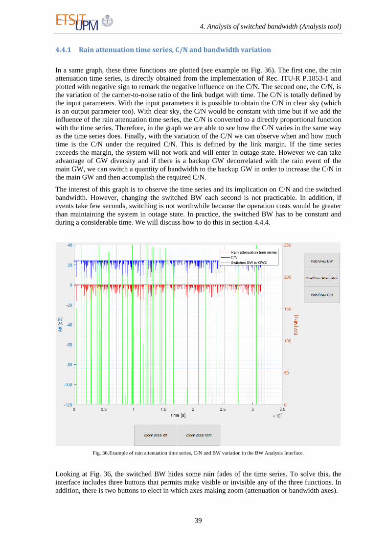
4. Analysis of switched bandwidth (Analysis tool)
39
4.4.1 Rain attenuation time series, C/N and bandwidth variation
In a same graph, these three functions are plotted (see example on Fig. 36). The first one, the rain
attenuation time series, is directly obtained from the implementation of Rec. ITU-R P.1853-1 and
plotted with negative sign to remark the negative influence on the C/N. The second one, the C/N, is
the variation of the carrier-to-noise ratio of the link budget with time. The C/N is totally defined by
the input parameters. With the input parameters it is possible to obtain the C/N in clear sky (which
is an output parameter too). With clear sky, the C/N would be constant with time but if we add the
influence of the rain attenuation time series, the C/N is converted to a directly proportional function
with the time series. Therefore, in the graph we are able to see how the C/N varies in the same way
as the time series does. Finally, with the variation of the C/N we can observe when and how much
time is the C/N under the required C/N. This is defined by the link margin. If the time series
exceeds the margin, the system will not work and will enter in outage state. However we can take
advantage of GW diversity and if there is a backup GW decorrelated with the rain event of the
main GW, we can switch a quantity of bandwidth to the backup GW in order to increase the C/N in
the main GW and then accomplish the required C/N.
The interest of this graph is to observe the time series and its implication on C/N and the switched
bandwidth. However, changing the switched BW each second is not practicable. In addition, if
events take few seconds, switching is not worthwhile because the operation costs would be greater
than maintaining the system in outage state. In practice, the switched BW has to be constant and
during a considerable time. We will discuss how to do this in section 4.4.4.
Fig. 36. Example of rain attenuation time series, C/N and BW variation in the BW Analysis Interface.
Looking at Fig. 36, the switched BW hides some rain fades of the time series. To solve this, the
interface includes three buttons that permits make visible or invisible any of the three functions. In
addition, there is two buttons to elect in which axes making zoom (attenuation or bandwidth axes).

4. Analysis of switched bandwidth (Analysis tool)
40
4.4.2 Rain attenuation time series histogram
Once the time series are synthesized, it may be interesting to observe how much time the different
rain attenuations occur, that is, which occurrence percentage of time has each rain attenuation
value. In order to get it, we make use of a histogram normalized with the total number of
observations to get the probabilities of occurrence of each attenuation value. If the time series is
synthetized for a long time (tending to infinite and using narrow bins), the histogram shows a very
similar function to the graph of probability of occurrence vs. rain attenuation which can be
extracted from Rec. ITU-R P.618-13. The problem is that Rec. P.618-13 is able to study rain
attenuation in the range of occurrence probabilities from 5% to 0.001% (see section 2.2.1.1 in [9])
and the histogram of the time series contains probabilities of occurrence lower than 0.001 %.
An example of a histogram of the time series of rain attenuation made in Arganda del Rey in Q/V
with a satellite in 9º (elevation of 41.717º) is displayed in Fig. 37:
Fig. 37. Example of histogram of the rain attenuation time series synthetized for duration of one year.
4.4.3 Rain attenuation CDF
Taking into account that the annual probability of rain has generally low values, we know that
during the majority of time, the time series will have values near to 0. In fact, if we make zoom in
Fig. 37 for an attenuation value of 0 dB, the probability is very close to 1. Thus, we want to know
with which probability the rain attenuation will be less than or equal to the margin of the system.
This might be extracted from the cumulative distribution function (CDF) and it is truly an
interesting result of the simulation in the analysis tool. In Fig. 38 an example of the CDF made in
Q/V band in Arganda del Rey with longSat=9ºE for a duration of one year is showed.

4. Analysis of switched bandwidth (Analysis tool)
41
Fig. 38. Example of cumulative distribution function
4.4.4 Events of switched bandwidth
With the fourth plot we arrive to the most important output information. As seen in section 4.4.1,
with the knowledge of the time series, the C/N and the margin, we are able to know how much BW
must transfer the main GW to the backup GW in order to maintain the system available. But we
have arrived to the conclusion that the fade events of few seconds with constant modification of the
switched BW are impracticable. The switched BW must be constant and for a considerable
duration.
Hence, we must choose a criterion of decision to establish the constant BW that is going to be
switched in a rain event higher than the margin. It is not a trivial decision and other options can be
also considered. We have elected that the fade events are those where the rain attenuation is higher
than the margin. This includes from the moment where the rain event is over the margin to the time
where the rain event falls under the margin. In order to know how much bandwidth is necessary to
transfer, the mean of the rain attenuation in an event is calculated ( ). With the mean, we are
able to resolve Eq. (15) and Eq. (16) where is the new bandwidth of the main GW, are the
basic space losses (including gases), is the Boltzmann constant and is the switched
bandwidth to the spare GW.
(
)
[
This approximation can be used to analyze how many events are and how much time they last. The
described method takes into account the mean of the rain attenuation on a rain event. During this
event there are rain attenuations under and over the mean, so in some cases the BW could be
enough and in other cases it could be less.
With regard to the minimum time for considering an event of switch (minTimeEvent), it is
introduced as an input parameter and the proposed value is 15 seconds.
Depending on the minTimeEvent elected, the percentage of switched BW with respect to the real
time of switching (extracted from the graph explained in section 4.4.1) will change. This
percentage is defined as Eq. (17) shows. The 100 % of effective switching time is achieved when
(15)
(16)

4. Analysis of switched bandwidth (Analysis tool)
42
even rain events of 1 second are considered. An event of 1 second is which last two samples. In
addition to the outage probability of the GW diversity system ( ), it is important to take into
account the effectiveness on the switching of BW.
In Fig. 39 an example of events of switch is showed. The graph includes the mean of the BW
switched. This parameter may be important to know on average, how much BW is transferred.
Together with the plot, the number of events, the total switching time and the percentage of
effective switching are given in order to have other values of the switch events.
Fig. 39. Example of events of BW switching in a synthesis of one year in BW Analysis Interface.
The events of switched BW do not include when they occur or how much time there is among
events. This information can be extracted from the C/N variation showed in the first graph (section
4.4.1).
4.4.5 Events of switched bandwidth histogram
In the same way that in the time series of rain attenuation, we are able to see which probability of
occurrence has each value of switched bandwidth events (see example in Fig. 40). It is necessary to
use the obtained events of switching (section 4.4.4). The presented histogram is normalized with
the total number of observations (getting the probability of occurrence).
(17)

4. Analysis of switched bandwidth (Analysis tool)
43
Fig. 40. Example of histogram of the switched BW.
4.5 RESULTS
It has been explained how this part of the simulator works and the possible results that is able to
provide to the user. Now we want to discuss the influence of some parameters in the results
extracted from analysis tool. Our interest is centered in the transfer of bandwidth from the main
GW to the backup GW because is one of the most important parameters of study in smart GW
systems. This transfer is a direct consequence of the synthetized rain attenuation time series, so we
are not going to present or discuss how the time series vary depending on changes the input
parameters. However, the histogram or CDF of the time series may be used in order to explain
some phenomenon.
The Rec. ITU-R P.1853-1 gives the method to obtain the rain attenuation time series for
frequencies below 55 GHz. For that reason, we are not going to study frequency bands above 55
GHz, but the use of the recommendation could be interesting for W band despite the fact that the
recommendation does not guarantee its proper functioning.
The most influential parameters are those which define the link budget and the switch events. The
link budget is defined by the majority of the inputs mentioned in section 4.1. Despite the fact that
frequency and satellite position directly influence on the link budget and the time series, they will
be considered constant in all the cases of study. and G/T are considered constant too and
values of real HTS link budget [11]. The required C/N is defined as 12 dB which is a reasonable
value to operate in the feeder link with approximately a spectral efficiency of 3.077 bits/symbol
and a MODCOD 16APSK 7/9 [20].The duration of the synthetized time series is one year being a
realistic parameter to observe properly the events of switch. All the fixed input parameters are
defined in TABLE IX.
TABLE IX. FIXED INPUT PARAMETERS IN THE ANALYSIS OF BANDWIDTH
Parameter Value Units
Frequency 50 GHz
G/T 25 dB/K
Satellite position Arganda del Rey 9 ºE
Orlando 61 ºW
BWinput 250 MHz

4. Analysis of switched bandwidth (Analysis tool)
44
Required C/N 12 dB
Duration of time series 31536000 s
After all, the importance lies on the variation of the link budget and therefore the margin. If the link
margin comes down, there will be more fade events. If the margin goes up, the number of events
decreases.
The unique non-fixed parameters are the EIRP and the latitude and longitude of the site. The first
one includes the transmitted power and the antenna‟s gain. The second ones, the latitude and the
longitude of the main site, will not affect significantly to the margin but they may alter the time
series of rain attenuation due to the difference of rain statistics in each location. Thus, with the
location‟s variation of the main GW and the EIRP of the link budget the margin and the time series
will change and therefore the events of switched BW. This will be the principle of the results that
we are going to search. The main importance belongs to the possible modification of the antennas‟
size modifying the EIRP. This factor is very valuable because if the antenna‟s size reduced, the cost
of the infrastructure would extremely decrease. Additionally, the minimal duration of the fade
events will be also modified in order to see how the number of event changes and the percentage of
effectiveness in switching.
The time series of rain attenuation are time dynamics of the propagation channel, in order words,
they show how much and how the channel varies because it is important to know the depth of the
fading and its duration. This will help in the process of switching to decide a hysteresis. The results
of simulations with the same input parameters present different results (because of being time
dynamics), but on average, the variations and the behavior of the channel are quite similar. We
expect different plots of the rain attenuation time series and the switched BW, but the histograms
and the probabilities of occurrence tend to be the same.
4.5.1 Site variation
In this sub-section, the interest resides on the variation of the switched BW depending on the
location of study. Likewise differential rain attenuation statistics, rain attenuation time series
depend on geographic and rain statistics such as the , or . As explained in section
3.1.3, these parameters depend on the latitude and the longitude of the site and they are usually
calculated with digital maps through a bi-linear or bi-cubic interpolation. We have already seen
their influence on the and now we are going to study their influence on the time series.
The unique input parameter of variation is location. The other parameters are specified in TABLE
IX, expect the EIRP and minTimeEvent. On the one hand, the EIRP is defined as 74.1 dBW. These
74.1 dBW are divided in 4.1 dBW for the transmitted power and 70 dB for the antenna‟s gain (with
a realistic antenna‟s diameter of 9.1 meters and 50 GHz [24]). Having defined all the parameters of
the link budget and taking into account that the required C/N is 12 dB, the GW diversity systems of
study will have a margin by 12.2 dB (depending on the location) to work with only one GW. If this
margin is overcome, the transfer of bandwidth to the spare GW will be mandatory. On the other
hand, minTimeEvent will be defined in each case of study according to the interest of discussing the
implication of defining these parameters. The geographical coordinates of the sites of study are
stated in TABLE V.
Arganda del Rey
The first study is done in the Hispasat control center in Arganda del Rey. It is supposed that a GW
diversity system has been designed or it is being discussed the creation of GW diversity with
dependence on how the channel affects the number and duration of events of switch.
Firstly, minTimeEvent is defined as 15 seconds. The results of the switch events and their
histogram are displayed respectively in Fig. 41 and Fig. 42. Observing them, we realize that there
are events very close to 250 MHz but they do not become that quantity.
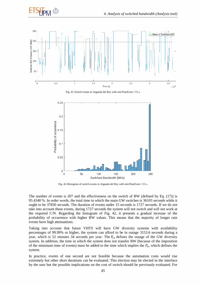
4. Analysis of switched bandwidth (Analysis tool)
45
Fig. 41. Switch events in Arganda del Rey with minTimeEvent =15 s.
Fig. 42. Histogram of switch events in Arganda del Rey with minTimeEvent =15 s.
The number of events is 207 and the effectiveness on the switch of BW (defined by Eq. (17)) is
95.4348 %. In order words, the total time in which the main GW switches is 36103 seconds while it
ought to be 37830 seconds. The duration of events under 15 seconds is 1727 seconds. If we do not
take into account these events, during 1727 seconds the system will not switch and will not work at
the required C/N. Regarding the histogram of Fig. 42, it presents a gradual increase of the
probability of occurrence with higher BW values. This means that the majority of longer rain
events have high attenuations.
Taking into account that future VHTS will have GW diversity systems with availability
percentages of 99.99% or higher, the system can afford to be in outage 3153.6 seconds during a
year, which is 52 minutes 34 seconds per year. The defines the outage of the GW diversity
system. In addition, the time in which the system does not transfer BW (because of the imposition
of the minimum time of events) must be added to the time which implies the which defines the
system.
In practice, events of one second are not feasible because the automation costs would rise
extremely but other short durations can be evaluated. This election may be elected in the interface
by the user but the possible implications on the cost of switch should be previously evaluated. For

4. Analysis of switched bandwidth (Analysis tool)
46
example, considering until rain events of 5 seconds, the number of events rises considerably. The
disadvantages are that the costs in switching rise due to a greater level of events. Nevertheless, the
advantage is the improvement on the availability of the system, because only events shorter than 5
seconds are not taken into account. The key factor in that looking at Fig. 42, events of lower BW
tend to occur less so if we take into account shorter duration of events, the values of bandwidth of
the new considered events will be low.
If we consider minTimeEvent=5 seconds, the results are the followings: the mean of switched BW
has decreased a little because, as explained before, the new introduced events have low BW levels.
The number of events has increased (456 now, 207 before). As a consequence, the percentage of
effectiveness is now 98.4457% (727 seconds in a year). This is a very useful example of how the
considered duration of events can increase the effectiveness and the number of events.
This effect on the change of the mean and value of the events that before we were not taking into
account can be observed through the histogram of events in Fig. 43. Comparing with the histogram
of minTimeEvent =15 s (Fig. 42), the new simulation presents a bit more percentage on the lower
BW values.
Fig. 43. Histogram of switch events in Arganda del Rey with minTimeEvent =5 s.
Orlando
In order to appreciate the effect of site variation, the other study is centered in Orlando where we
have already discussed the particular case of the differential rain attenuation statistics. If we
observe the discussion made in section 3.3 with this location, the conclusions are that in Orlando
the effect of rain is extremely high due to its rain fall rate (next to 70 mm/h). The effect of this
parameter must influence to the rain attenuation time series increasing the number of rain fades and
therefore the time of switch.
In this case, a value of minTimeEvent =5 s (or lower) is absolutely needed because in Orlando it
rains a lot and there are lots of short rain events. A high percentage of effectiveness is needed in
order to face the enormous effect of rain attenuation.
The simulation in Orlando with minTimeEvent =5 s gives the following results. The number of
events is 1622, the time in switching is 178188 seconds and the efficacy is 98.5422 %. The mean of
switched BW is higher than 200 MHz. What we realize is that if the time in which the margin is
exceeded by the rain attenuation rises, the events of BW tend to have higher value. In this
simulation, there are more events of BW values close to 250 MHz (the maximum). Even there are
events in which the BW transferred is 250 MHz. These events are produced by extreme rain events
where the system needs to transfer all the BW because even with 0 Hz of BW, the C/N in the main
GW is under the required one. In Orlando, the rain attenuation time series reach values of 600 dB.

4. Analysis of switched bandwidth (Analysis tool)
47
In order to justify the increase of events in relation to Arganda del Rey, in Fig. 44 and Fig. 45 we
make use of the rain attenuation time series histogram to compare the time series in Orlando and
Arganda del Rey.
Fig. 44. Rain attenuation time series histogram in Orlando
Fig. 45. Rain attenuation time series histogram in Arganda del Rey
4.5.2 Antenna’s size variation
We have arrived to the conclusion that the most interesting alteration is reducing the antenna‟s
diameter because it could provide high economic advantages. However, it carries the disadvantage
of decrease in the antenna‟s gain and therefore, the EIRP and the margin. Reducing the margin
entails more fade events because it is more probably that the rain attenuation exceeds the margin
than maintaining the margin. Our option is reducing the antenna‟s gain in 3 dB. Reducing the gain
of the antenna in 3 dB implies reducing the antenna‟s diameter a 29.29 %, whereas increasing the
gain in 3 dB implies the increase of its diameter a 41.4 %. So the new diameter is 29.29 % smaller,
that is, 6.44 meters. Thus, the new EIRP has a value of 71.1 dBW. Now we want to observe in
which proportion the events of BW change.
The consequences are directly observed in its histogram of events (Fig. 46). The number of events
with lower BW value rises and the probabilities of occurrence of events are more distributed
among all the values, so the mean of switching BW reduces (more close to 150 MHz). The cause is
that the reduced margin permits the existence of lower fade events which did not take place before
because the margin was over them.
Fig. 46. BW events histogram in Arganda del Rey with reduced antennas.

4. Analysis of switched bandwidth (Analysis tool)
48
The advantage of reducing the diameter of the antennas implies the disadvantage of raising the
number of fade events. The designer of the system should consider if it is better saving costs in the
infrastructure or saving cost in the procedure of transferring bandwidth in each event.
In practice, the switch of BW is discretized by the bandwidth of the carriers of the payload. This
fact could be introduced in the consideration of the quantity of switched bandwidth, discretizing to
feasible values of the carriers.
In TABLE X, these last results of the antenna‟s size variation and the comparison with the other
studies are showed:
TABLE X. RESULTS OF THE STUDY CASES
Location
Antenna’s
diameter
[m]
minTimeEvent Number
of events
Percentage of
effectiveness in
switching [%]
Total
switching
achieved
(250 MHz)
Arganda del
Rey
9.1 15 207 95.4348 No
5 456 98.4457 No
6.44 15 329 94.3905 No
Orlando 9.1 5 1622 98.5422 Yes

5. Conclusions and future research lines
49
5 CONCLUSIONS AND FUTURE RESEARCH LINES
5.1 CONCLUSIONS
The objectives of this project were clear: the creation of a simulator which permits design real GW
diversity systems to operate with VHTS and analyze the switched bandwidth in order to evaluate
the number of fade events in a smart GW system and then reconsider some parameters or
performance of the system.
With these objectives in mind, the assignment was the development of a simulator which
implements the Rec. ITU-R P.1815-1 and the Rec. ITU-R P.1853-1 in order to get the differential
rain attenuation statistics and synthetize the rain attenuation time series respectively. These two
parameters would allow us to create GW diversity and to analyze the switch of BW between two
GWs.
The implementation of these recommendations and its use for their respective purposes led us to
implement other recommendations to prevent the external calculation of secondary parameters.
Also, the creation of a graphical user interface in Matlab was considered a necessity to make easier
the interaction between the user and the simulator. The final result is a simulator easy to handle and
very useful to design and analyze GW diversity systems for future VHTS.
On the one hand, the tool to design GW diversity has been the more developed one. The necessity
of design GW diversity was translated into an interface which permits calculate and visualize
contours of outage probabilities in a Map for the GW diversity system parameters of interest. The
implementation of the design tool and its theoretical behavior have been proved by simulations
which changed some input parameters in order to study its implication in the contours of outage
probability. Their results have been reviewed and explanations to the presented results have been
discussed. The results have followed the expected performance of the differential rain attenuation
statistics and they have proved the validity and the utility of the tool to establish GW diversity in
different sites. The most interesting results show the importance of rain statistics on the and the
possibility of achieving low outage probabilities for distances which are located in the same feeder
beam without affecting the satellite payload.
On the other hand, the analysis tool has been implemented to analyze the implementation of GW
diversity and to study the events of switch between two GWs. The main objective of this tool was
synthesizing the rain attenuation time series and obtaining relevant information associated to the
influence of the time series on the events of switch. This objective has been reached and on the
created interface the user is able to study the rain attenuation time series and its effect on the switch
of BW. The tool has been tested with cases of study to analyze the possible effect of changes on
parameters of the system to improve the use of resources such as the antenna‟s diameter reduction
which certainly is the most interesting study as it affects system cost. The results have been the
expected ones and have demonstrated validity of using the times series of rain attenuation to
analyze the number of events which requires a bandwidth switch, their probability of occurrence
and the implication in considering a minimum duration of events.
At the same time that the simulator was being developed, a paper with the first results of the design
of GW diversity for VHTS has been written (see Annex 1 in 7.1). The paper has been peer
reviewed and accepted by the URSI 2018 Congress. This fact let us think that the topic developed
and its results are significantly useful and give reasons to believe the importance and interest of the
project.
Thus, finally the objectives of this project have been reached successfully. GW diversity has been
proposed as the solution to resolve the severe effect of rain attenuation and to satisfy the demand
that future VHTS operating in Q/V and W bands will require. The presented models in this
document and their implementations to design and analyze GW diversity systems have showed
their validity, utility and the implication in the development of 5G networks through VHTS.

5. Conclusions and future research lines
50
5.2 FUTURE RESEARCH LINES
In addition to the tasks and work developed in this project, some tasks emerge related to the
improvement of the study of GW diversity. Therefore we expect to carry out the following tasks in
the near future:
-The optimization of the code which involves the implementation in the MATLAB scripts in order
to accelerate the time implicated in the calculation of the differential rain attenuations statistics.
This could permit design and study GW diversity systems quicker.
-The creation of a cost function which is able to elect the optimal position of the backup GW in a
series of contour levels for the design of GW diversity systems depending on variables such as
distance and . The cost function should consider the system cost.
-Studying other parameters of interest which could alter the outage probability contours in specific
studies.
-Improving the graphical interfaces of the design and analysis tools in terms of esthetics and
usability. It is also considered the possibility of generating a web based application.
-Writing an extended paper which includes the most relevant results of the design of GW diversity
and the analysis of switched bandwidth to be presented to the 13th European Conference on
Antennas and Propagation (EuCAP 2019), to the 24th Ka and Broadband Communications
Conference or to the 36th International Communications Satellite Systems Conference (ICSSC).
Research journals such as IEEE Communication Letters or IET Communications are also
considered to submit the extended results.
-Considering the adaptation of new accurate transmission techniques to design and analyze GW
diversity for future Ultra High Throughput Satellites (UHTS).

6. Bibliography
51
6 BIBLIOGRAPHY
[1] W. Pritchard, “The history and future of commercial satellite communications”, IEEE
Communications Magazine, vol.22, no. 5, pp. 23-27, May 1984.
[2] M. Schwartz, “History of communications”, IEEE Communications Magazine, vol.63, no.
8, pp. 26-31, March 2010.
[3] D.M. O‟Neal, “Commercial communications satellites: history and highlights”, Microwave
Symposium Digest, 1999 IEEE MTT-S International, pp. 1919-1921, 1999.
[4] R. Mehrotra, “Regulation of Global Broadband Satellite Communications”, September
2011 [Online]. Available: http://www.itu.int/ITU-
D/treg/Events/Seminars/GSR/GSR11/documents/BBReport_BroadbandSatelliteRegulation
-E.pdf.
[5] L. Castejón, M. S. Castañer, R. Martínez, “Conectividad de banda ancha mediante satélites
de nueva generación”, Centro de Estudios de Telecomunicaciones de América Latina
(cet.la), September 2016.
[6] A. Kyrgiazos, B. Evans, P. Thompson, “Gateway Diversity scheme for a Future Broadband
Satellite System”, 6th Advanced Satellite Multimedia Systems Conference (ASMS) and 12
th
Signal Processing for Space Communications Workshop (SPSC), pp. 363-370, 2012.
[7] A. Ghranjik, B. Shankar, “Multiple Gateway Transmit Diversity in Q/V Band Feeder
Links”, IEEE Transactions on Communications, vol.63, no. 3, pp. 916-926, March 2015.
[8] O. Vidal, G. Verelst, J. Lacan, E. Alberty, J. Radzik, M. Bousquet, “Next generation high
throughput satellite system”, Proc. IEEE 1st AESS ESTEL, pp. 1-7, 2012.
[9] I.-R- P.618-13, “Propagation data and prediction methods required for the design of Earth-
space telecommunication systems”, 2017. [Online]. Available: https://www.itu.int/rec/R-
REC-P.618-13-201712-I/es.
[10] L. J. Ippolito Jr., Satellite Communications Systems Engineering, John Wiley & Sons Ltd:
2008.
[11] F. Massaro, M. Bergmann, R. Campo, M. Thiebaut, D. V. Finocchiaro, A. Arcidiacono,
“Q/V-LIFT Project: Using the Q/V Band Aldo Paraboni Demonstration Payload for
Validating Future Satellite Systems”, 23rd
Ka and Broadband Communications
Conference, 2017.
[12] M. Bergmann, F. Massaro, R. Campo, V. Soumpholphakdy, G. Bigel, R. Vitalone, D. V.
Finocchiaro, A. Arcidiacono, “Q/V-band feeder links and flexible bandwidth assignment in
future very high throughput satellite (VHTS) communication systems”, 23rd
Ka and
Broadband Communications Conference, 2017.
[13] J. D. Kanellopoulos, S. N. Livieratos, “Analysis of the interference due to differential rain
attenuation induced by an adjacent terrestrial microwave system on a double-site diversity
Earth-space system”, Radio Science, vol.35, no. 6, pp. 1399-1416, November-December
2000.
[14] J. D. Kanellopoulos and V. A. Houdzoumis, “A model for the prediction of differential rain
attenuation on adjacent Earth-space propagation paths”, Radio Science, vol.25, no. 5, pp.
853-864, September-October 1990.
[15] T. Rossi, F. Maggio, M. De Sanctis, M. Ruggieri, “System Analysis of Smart Gateways
Techniques Applied to Q/V-band High Throughput Satellites”, IEEE Aerospace
Conference, pp. 1-10, March 2014.
[16] ITU-R, “Software, Data and Validation examples for ionospheric and tropospheric radio
wave propagation and radio noise”. [Online]. Available: https://www.itu.int/en/ITU-
R/study-groups/rsg3/Pages/iono-tropo-spheric.aspx
[17] I.-R- P.1815-1, “Differential rain attenuation”, 2009. [Online]. Available:
https://www.itu.int/rec/R-REC-P.1815-1-200910-I/.
[18] I.-R- P.841-5 “Conversion of annual statistics to worst-month statistics”, 2016. [Online].
Available: https://www.itu.int/rec/R-REC-P.841-5-201609-I/en.
[19] Z. Drezner, G.O. Wesolowsky, “On the Computation of the Bivariate Normal Integral”,
Journal of Statistical Computation and Simulation, vol.35, pp. 101-107, 1989.
[20] I.-R- P.1853-1 “Tropospheric attenuation time series synthesis”, 2012. [Online]. Available:
https://www.itu.int/rec/R-REC-P.1853-1-201202-I/en.

6. Bibliography
52
[21] I.-R- P.1144-9, “Guide to the application of the propagation methods of
Radiocommunication Study Group 3”, 2017. [Online]. Available:
https://www.itu.int/rec/R-REC-P.1144-9-201712-I/en.
[22] I.-R- P.581-2, “The concept of “worst month””, 1990. [Online]. Available:
https://www.itu.int/rec/R-REC-P.581-2-199006-I/en
[23] ETSI-TR 102 376-2, “Digital Video Broadcasting (DVB); Implementation guidelines for
the second generation system for Broadcasting, Interactive Services, News Gathering and
other broadband satellite applications; Part 2: S2 Extensions (DVB-S2X)”, 2015. [Online].
Available:
http://www.etsi.org/deliver/etsi_tr/102300_102399/10237602/01.01.01_60/tr_10237602v0
10101p.pdf.
[24] Viasat, “9.1 Meter Ka-band Broadband Gateway Earth Station Antenna”. [Online].
Available: https://www.viasat.com/sites/default/files/media/documents/9.1m_ka-
band_earth_station_017_web.pdf

7. Annexes
53
7 ANNEXES
7.1 ANNEX 1: PAPER ACCEPTED IN URSI 2018 CONGRESS
Here it is presented the paper written by Michel Massanet Ginard and Ramón Martínez Rodríguez-
Osorio and accepted in the XXXIII Simposium Nacional de la Unión Científica Internacional de
Radio, URSI 2018 Congress.
The paper is structured as follows: an introduction to justify the necessity of GW diversity in
VHTS, the description of the model (Rec. ITU-R P.1815-1) which follows the design of GW
diversity, the description of the implementation and the functioning of the simulator and the
discussion of some results of study cases together with the most relevant conclusions.
The paper has some differences with the current simulator and the information given in this
document because it was written before having the simulator totally developed due to the periods
that the congress imposed. This Congress will take place on September 2018, in Granada.
The following 4 pages show the written paper:

Design of Gateway diversity systems for
Very High Throughput Satellites (VHTS)
Michel Massanet Ginard, Ramón Martínez Rodríguez-Osorio
[email protected], [email protected]
ETSI Telecomunicación, Universidad Politécnica de Madrid. Avda. Complutense 30, 28040 Madrid.
Abstract- Due to the increase of demand in broadband satellite services, future Very High Throughput Satellites will approach to capacities next to 1 Tbps by 2020. In order to
achieve this, smart gateway (GW) systems will be necessary and gateway diversity is going to be essential. This paper reviews an implementation method of GW diversity in
satellite ground stations in order to mitigate rain fade which affects in a several way to satellite communications at Q/V and higher frequency bands. To reach high availability and
capacity, smart gateway diversity makes use of the ITU-R P.1815-1 which predicts the joint differential rain attenuation statistics between a satellite and two locations on the Earth
surface. The obtained results show visually the importance of geography in designing GW diversity systems and give a useful tool to know where to place the other GW depending
on the availability required and the system parameters.
I. INTRODUCTION
In the last few years, demand of broadband communication
services using communication satellites has drastically raised
and it is expected to continue increasing due to the deployment
of 5G networks. Since 2010, high-throughput satellites (HTS)
are essential to achieve high capacities. HTS take advantage
of frequency reuse, fade mitigation techniques (FMT) and the
usage of multiple spot beams to reduce the cost per bit
regardless the spectrum band selected [1]. Nowadays they are
able to provide data rates over 100 Gb/s. For instance, the KA-
SAT has achieved more than 70 Gb/s, the ViaSat-1 levels of
140 Gb/s and the recent ViaSat-2 has reached 300 Gb/s [2].
Despite being enormous quantities, it is thought that
broadband data rates will arrive to 1 Terabit/s by 2020 [3].
This will force satellite to achieve higher data rates, in the next
generation of HTS called Very High Throughput Satellites.
Currently, Ku-band (12/18 GHz) and Ka-band (20/30
GHz) are the most used bands in satellite communications. Ka
bands systems are allowed to use a limited spectrum of 2 GHz
[4]. Nevertheless, in order to accomplish future capacity rates,
the solution is to move the feeder link (even the user link) to
Q/V band (40/50 GHz) where the bandwidths are up to 5 GHz
[1]. Even the translation to W-band (70/80 GHz) should be
considered for future satellite communications. The spectrum
of Q/V bands also is less occupied and because of being higher
frequencies, the generation of large number of narrow spot
beams increase. However, the great disadvantage of using
higher frequencies is the severe precipitation attenuation
which affects system availability.
Rain attenuation affects severely to frequencies above 11
GHz, being the main fade cause in satellite communications.
In the feeder link, common rain attenuation rates come on to
20 dB in Ka Band (30 GHz) and to 30 dB in Q/V Band when
it is required 99,99% availability and there is a rainfall rate
(𝑅0.01) of 25 mm/h. Even these rates rise to 50 dB in Q/V Band
when 𝑅0.01 is above 30 mm/h.
In order to overtake rain fade, a key solution is the
implementation of diversity in smart gateway systems. One
fact that smart gateways take advantage of is site diversity.
Space diversity or site diversity is a term used to describe the
utilization of two (or more) geographically separate ground
terminals in a space communications link [5]. This let
overcome the effects of rain attenuation provoked by a rain
cell, provided that the distance between the main site and the
other site is larger than the rain cell size. Fig. 1 illustrates this
phenomenon.
This strategy followed by GW systems, gives the
possibility to implement control/switching algorithms in the
GW system making use of a terrestrial fiber network. The
optimum distance between the main and other site highly
depends on the geographical features of the sites, in addition
to other factors.
Fig. 1. Site diversity in GW systems
Thus, in a gateway diversity system, the main aim is to
know where to establish the second gateway. To overcome
this, the Rec. ITU-R P.1815-1 is very useful due to permits
predicting the joint probability (%) that the attenuation
thresholds on the satellite path to the first site and to the second
site are simultaneously exceeded.
In other words, the study of differential rain attenuation
will be the key to achieve high availability percentages even
using high frequencies such as Q/V bands in the feeder link
and will give an opportunity for designing smart GWs.
This paper proposes a scheme of a smart GW system based
on gateway diversity which makes use of the Rec. ITU-R
P.1815-1 and provides a simulation tool to analyze and design
GW diversity systems wherever place.
II. SYSTEM MODEL
A large number of models to achieve and control gateway
diversity have been proposed. In [4], [6], [7] and [8], authors
state some models applied to get smart gateways systems or to

face differential rain attenuation. This paper will review a
model based on the Rec. ITU-R P.1815. It makes use of other
recommendations which basically calculate rain statistic
parameters (Table I). The differential rain attenuation method
also considers the temporal characteristics of rain cell size and
movement of rain cells. The use of this recommendation is
approved for frequencies up to 55 GHz, elevation angles
above 10º and site separations between 0 and at least 250 km
[9]. The method can obtain either annual or worst-month
differential attenuation statistics. The optional obtainment of
worst-month statistics implicates the use of the Rec. ITU-R
P.841. This fact has to be taken into account depending on
what types of results want to be obtained.
TABLE I. ITU RECOMMENDATIONS USED BY THE MODEL
ITU-R P. Parameters
618-13 𝐴𝑃 Long-term rain attenuation statistic
837-7 𝑅0.01 Rain fall rate statistics
838-3 𝛾𝑅 Specific attenuation
839-4 ℎ𝑟 Rain height
841-5 𝑝𝑤 Conversion of annual statistics to worst-
month statistics
1144-9 Bilinear and bi-cubic interpolations
1510-1 𝑇𝑖𝑖 Monthly mean surface temperature
1511-1 ℎ𝑠 Height above mean sea level
The joint probability of exceeded attenuations at both sites
(𝑃𝑟𝑟) is obtained using Eq. (1) where 𝑃𝑟 is the joint probability
that it is raining at both sites and 𝑃𝑎 is the conditional joint
probability that the attenuations exceed 𝑎1 and 𝑎2,
respectively, given that it is raining at both sites:
𝑃𝑟𝑟 = 𝑃𝑟(𝐴1 ≥ 𝑎1, 𝐴2 ≥ 𝑎2) = 100 × 𝑃𝑟 × 𝑃𝑎 % (1)
𝑃𝑟 and 𝑃𝑎 are complementary bivariate normal
distributions that can be calculated through an approximation
in [10]. The recommendation also suggests the possibility of
using the Matlab function ‘mvncdf’. However, ITU gives in
[11] a compiled software which can calculate rapidly that
bivariate normal distribution. The final result is a percentage
probability which depends on the distance between sites,
frequency of the feeder link, attenuation on the paths for a
probability of occurrence and the probability of rain.
The most influential parameter together with frequency is
the distance (d) between both sites. The joint differential rain
attenuation statistic decreases with the distance like an
exponential distribution as it can be seen in Fig. 2.
Fig. 2. A variation example of 𝑃𝑟𝑟 with distance and frequency for exceeded
attenuations of 14 dB in site 1 (Madrid) and site 2 (direction to Valencia),
with Hispasat-30W.
After dozens of kilometers, the influence of other
parameters such as the rain fall rate (𝑅0.01) increases up to the
point of situations where the rain fall rate becomes more
relevant than distance. This will be also the principle of the
implementation and the results that we are going to search, in
which the geographical rain statistics will take a very important
role.
III. IMPLEMENTATION OF THE SIMULATOR
The implementation is done through a Matlab simulator
which is able to plot contour levels of the joint differential rain
attenuation statistics in a coordinate Map. The Map is clicked
in the position where it is wanted to settle the main GW. Then,
the script calculates the joint probability in the points of a thin
grid around the main GW and it finds the coordinate positions
of the points where the searched joint probabilities are
achieved. Then, the simulator prints that positions creating
contour levels in the Map which will let decide the possible
locations of the other gateways.
As it is stated in (1), the attenuation thresholds (𝑎1 and 𝑎2)
must be elected depending on the expected attenuations. The
thresholds should be the fade margin that the system can allow
in order to continue working correctly and without outage.
Thus, once elected the attenuation thresholds in function of the
margin, the calculated 𝑃𝑟𝑟 shows the probability of the margin
being exceeded simultaneously at both sites. This means that
with that probability, the system will not work, due to in both
sites the margin will be exceeded simultaneously. We should
elect the 𝑃𝑟𝑟 levels as the probability that our system is going
to be in outage, or equivalently, the availability of the system.
The script is structured with the following inputs and
outputs:
A. Inputs
• Attenuation thresholds (𝒂𝟏 and 𝒂𝟐): they are
definite by the margin that the system can permit to
accomplish a required carrier-to-noise ratio (C/N).
• Frequency band (f): the simulator studies three
different bands in the feeder link: Ka-Band (20/30
GHz), Q/V band (40/50 GHz) and W-Band (70/80
GHz).
• Satellite: the election of different satellites is related
to their orbital positions. In this study, we consider
positions of HTS such as KA-SAT or HISPASAT
30W-T. Also the studies can be done with ALPHA-
SAT which already works in experimental
communications with Q/V bands.
• Maximum radius of study (𝑹𝐦𝐚𝐱 ) [km]: it
determinates the maximum radius of the circular grid
where the statistics are calculated. The maximum
radius could be also defined by the illumination zone
of the spot beam which illuminates the main GW.
• 𝑷𝒓𝒓 levels: indicate the probability of the contours
that are going to be printed in the Map. These will
mark the outage or the availability of our system.
• Main site: the coordinates of the main site are
introduced clicking in the Map.
B. Outputs
• Contours: the printed coordinates of the locations
where it is achieved the thresholds and are printed in
the Map.

IV. RESULTS
The following results are consequence of particular cases
of study. We are going to center our study to appreciate the
variation of the same outages (𝑃𝑟𝑟) calculated with different
parameters such as geography, frequency or satellite location.
In all cases, it is going to consider an enough radius of study to
appreciate the 𝑃𝑟𝑟 levels searched, whose values are in order
from highest to lowest: 0.036 (purple), 0.01 (red), 0.007 (blue),
0.005 (green), 0.0033 (orange) and 0.0024 (black). The
attenuation thresholds (𝑎1 and 𝑎2) have been elected with a
value of 16 dB, which is a reasonable value of a margin
required in the feeder link with a bandwidth of 225 MHz. It is
important to mention that the orbital positions studied could be
not occupied by satellites working in our frequency bands of
interest. The orbital positions will be elected to see the effect
of the elevation angle.
In order to have a reference value of availability of a single
GW, a fade margin of 16 dB in Madrid in Q/V Band is traduced
to an availability (or time in which the systems works
correctly) about 99.92% according to Rec. ITU-R P. 618 [12].
A. Geographical variation
It is going to see the influence of the geographical statistics
in the determination of the contour levels of the 𝑃𝑟𝑟 previously
mentioned. We have elected two main sites of study whose
coordinates can be seen in Table III. In those positions, it will
be placed the main GW and, with the same inputs (Table IV),
it will be calculated the places where the probabilities searched
are achieved.
TABLE III
PLACES OF STUDY
Location Latitude
[ºN]
Longitude
[ºE]
Arganda del Rey (western Madrid) 40.2723 -3.3788
The Pyrenees (southern France) 43.099 0.6
The first study is centered in the HISPASAT Satellite
Control Center, located in Arganda del Rey. In this place, the
𝑅0.01 in the main GW is 24.91 mm/h and the annual probability
of rain (𝑃𝑜) is 3.36 %. On the second place, we center our study
in the south of France (in The Pyrenees, close to the border
with Spain) where the 𝑅0.01=31.87 mm/h and 𝑃𝑜=7.8%.
Apparently, the difference among these values gives us an
intuition to think that in France it is going to need more
distance to achieve the same 𝑃𝑟𝑟 . There, the presence of The
Pyrenees let us think that there will be more irregularities than
in Madrid. The value of the rain fall rate and the annual
probability of raining will support some explanations of why
in some directions it is needed more distance for the same 𝑃𝑟𝑟 .
TABLE IV
COMMON INPUTS PARAMETERS
𝑎1 and 𝑎2 16 dB
Frequency Q/V Band (40/50 GHz)
Satellite location 9º East
𝑅max 300 km
Fig. 3 shows the simulation made next to Madrid. The point
in the center is where it is established the main GW (in all
figures will be like this). The area studied has similar values in
𝑅0.01 and 𝑃𝑜, that is why the contours seem to be partially
circular. The non-regularity is more relevant in the lowest
contour values. The distance to the first contour is 3.01 km
(constant). In the lower contour level (0.0024), the variation
with distance is higher, being the nearest point to the main GW
of 37.2 km and the furthest point 42.2 km.
Fig. 3. 𝑃𝑟𝑟 Contour levels in Arganda del Rey in Q/V band and a satellite in
9ºE.
Fig. 4 illustrates the simulation in France. Here, the
irregular contours are totally expected. The distance to the first
contour is 9.5 km on average (higher than the previous 3.01 km
in Madrid). The contours are oval shaped, being shorter the
distances in the Pyrenees than in the north. On average, the
Pyrenees have 𝑅0.01=32 mm/h and 𝑃𝑜=8.81%, while in the
north of the site 𝑅0.01=30.5 mm/h and 𝑃𝑜=4.80%. Taking this
into account, it rains more in the Pyrenees, therefore the
distances in the Pyrenees should be largest; nevertheless, in
this case the height above the sea level (ℎ𝑠) has a decisive
influence. The rain attenuation is lower for higher locations
(like the Pyrenees), due to a lower ℎ𝑟 on the satellite path.
Therefore, in this case the altitude of the GW location
influences more than 𝑅0.01 and 𝑃𝑜.
Fig. 4. 𝑃𝑟𝑟 Contour levels in southern France in Q/V band and a satellite in
9ºE.
B. Frequency variation
Once studied two particular places, it is going to study
the variation with frequency for the same place, in this
case, Madrid. Fig. 3 displays the simulation in Q/V band.
In a new simulation, we increase the frequency until W-
band (maintaining the same inputs). In this band, it is much
easier to overcome 16 dB of attenuation in rain periods
(availability=99.8% [12]). Therefore, we can expect that
the separation between GWs is going to be largest and the
rain and geographical statistics will influence more in W-
band. That is what displays Fig. 5. The same contour levels
are further from the main GW than in the Q/V study (Fig.
3). Prr=0.036 is achieved with d=18 km, and Prr=0.0024
is achieved in locations with distances between GWs from
78.4 km (𝑅0.01=27.48 mm/h, 𝑃𝑜=5.48 %, ℎ𝑠=1.4 km) to 218

km (𝑅0.01=33.75 mm/h, 𝑃𝑜=6.99 %, ℎ𝑠=0.5 km). There is
difference of 139.6 km for two different positions to place
the second GW. The reasons are clear. Observing that, in
the largest point it rains more and it has more attenuation
due to a lower ℎ𝑠, that point needs more distance to achieve
the same 𝑃𝑟𝑟.
Fig. 5. 𝑃𝑟𝑟 Contour levels in Arganda del Rey in W-band and with a satellite
in 9ºE.
C. Satellite variation
Finally, in Fig. 6 it is presented a new study in France,
where the unique difference with Fig. 4 is the orbital position
of the satellite. In this new case, the link is with a satellite
located at 30ºW. With this change, the attenuation on the
feeder link rises 3.7 dB due to having a lower elevation angle.
Therefore, the probability of exceed the thresholds rises, so the
distance for the same 𝑃𝑟𝑟 will be greater, as Fig.6 illustrates.
Fig. 6. 𝑃𝑟𝑟 Contour levels in southern France in Q/V band and with a
satellite in 30ºW.
V. CONCLUSIONS
The model proposed and its results have demonstrated the
utility of the simulator to establish GW diversity systems in
different sites and the importance of studying the 𝑃𝑟𝑟 with
parameters such as frequency, distance and satellite position.
These results show the great utility of using the Rec. ITU-R
P.1815 to achieve availabilities next to 99.998 % with
separation between GWs which depends of the factors studied.
Furthermore, in the majority of cases and probabilities studied,
the diversity GWs are located in the same feeder beam so that
does not affect the satellite payload.
In future lines, we have considered the two following
steps. On the one hand, analyzing the switching bandwidth
when the rain attenuation is above the fade margin on the main
GW. This gives the possibility to balance the amount of
bandwidth depending on the rain conditions. On the other
hand, the design tool would be complete with an optimization
function which could give the optimum position for a 𝑃𝑟𝑟 level
as a function of two costs: distance and availability.
ACKNOWLEDGEMENTS
Authors would like to acknowledge the Spanish
Government, Ministry of Economy, National Program of
Research, Development and Innovation for the support of this
publication in the projects ENABLING-5G “ENABLING
INNOVATIVE RADIO TECHNOLOGIES FOR 5G
NETWORKS” (project number TEC2014-55735-C3-1-R)
and FUTURE-RADIO "Radio systems and technologies for
high capacity terrestrial and satellite communications in an
hyperconnected world" (project number TEC2017-85529-C3-
1-R).
REFERENCES
[1] O. Vidal, G. Verelst, J. Lacan, E. Alberty, J. Radzik, M. Bousquet, “Next generation high throughput satellite system”, Proc. IEEE 1st AESS
ESTEL, pp. 1-7, 2012.
[2] L. Castejón, M. S. Castañer, R. Martínez, “Conectividad de banda ancha mediante satélites de nueva generación”, Centro de Estudios de
Telecomunicaciones de América Latina (cet.la), September 2016. [3] A. Kyrgiazos, B. Evans, P. Thompson, “Gateway Diversity scheme for a
Future Broadband Satellite System”, 6th Advanced Satellite Multimedia
Systems Conference (ASMS) and 12th Signal Processing for Space Communications Workshop (SPSC), pp. 363-370, 2012.
[4] A. Ghranjik, B. Shankar, “Multiple Gateway Transmit Diversity in Q/V
Band Feeder Links”, IEEE Transactions on Communications, vol.63, no. 3, pp. 916-926, March 2015.
[5] L. J. Ippolito Jr., Satellite Communications Systems Engineering, John
Wiley & Sons Ltd: 2008. [6] J. D. Kanellopoulos, S. N. Livieratos, “Analysis of the interference due
to differential rain attenuation induced by an adjacent terrestrial
microwave system on a double-site diversity Earth-space system”, Radio Science, vol.35, no. 6, pp. 1399-1416, November-December 2000.
[7] J. D. Kanellopoulos and V. A. Houdzoumis, “A model for the prediction
of differential rain attenuation on adjacent Earth-space propagation paths”, Radio Science, vol.25, no. 5, pp. 853-864, September-October
1990.
[8] T. Rossi, F. Maggio, M. De Sanctis, M. Ruggieri, “System Analysis of Smart Gateways Techniques Applied to Q/V-band High Throughput
Satellites”, IEEE Aerospace Conference, pp. 1-10, March 2014.
[9] I.-R- P.1815-1 “Differential rain attenuation”, 2009. [Online]. Available: https://www.itu.int/rec/R-REC-P.1815-1-200910-I/
[10] Z. Drezner, G.O. Wesolowsky, “On the Computation of the Bivariate
Normal Integral”, Journal of Statistical Computation and Simulation, vol.35, pp. 101-107, 1989.
[11] ITU-R, “Complementary bivariate normal distribution”. [Online].
Available: https://www.itu.int/en/ITU-R/study-groups/rsg3/Pages/iono-tropo-spheric.aspx
[12] I.-R- P.618-12 “Propagation data and prediction methods required for the
design of Earth-space telecommunication systems”, 2017. [Online]. Available: https://www.itu.int/rec/R-REC-P.618-13-201712-I/

7. Annexes
54
7.2 ANNEX 2: IMPACT OF THE TFG
Now, the possible impact with the realization of this TFG in different areas is discussed. As seen
before, we have discussed the use of GW diversity for VHTS in order to achieve high data rates
and high availabilities. The successful application of GW diversity would reach lots of goals where
the most relevant topic is the implication of this TFG in the development of 5G networks and its
social impact. This topic and other implications are divided in the following fields:
Environmental impact: the analysis tool is the perfect way to study the possible switched
bandwidth; therefore it is useful to reduce the energetic consumption implicated in the
transfer of bandwidth. In addition, in this document it is also stated the possible necessity
of a backup GW in a ground station. This could lead to build a ground infrastructure to
connect two GWs and also the installation of the antennas and their components (typically
in a free-of-interference area). The construction of new telecommunication infrastructures
has an impact in the environment, although it could improve the communication networks.
Social and economic impacts: social and economic impacts are directly related.
From a business point of view, companies such as ViaSat or Eutelsat could be interested in
this simulator due to the improvement in terms of availability with the establishment of
GW diversity. Other collectives such as departments related to propagation techniques (for
example the Radiation Group of the SSR department (Señales y Sistemas de
Radiocomunicaciones)) could be also interested in this project to support some researches
about satellite communications. This interest will be greater in future when there are
satellites working at frequency bands such as Q/V and W bands where the implementation
of GW diversity will be a requirement (expected by 2020 as stated in section 1.1). The
implementation of GW diversity implies an extra cost in the required infrastructure.
Nevertheless, the consequences of the implementation are economical profits for the
companies because higher availability and feasible data services would provoke the
satisfaction of their customers and an increase in the number of consumers. In addition, the
maintenance of ground segments would be lower thanks to the analysis tool because the
switched bandwidth could be automatized.
From the customer point of view, they would be indirectly beneficiary. The mentioned
benefits to the companies are consequence of the satisfaction of customers. They would get
higher data rates and the satellite system could provide almost all the consumers‟ demand.
From a professional point of view, the main impact is the contribution to develop 5G
networks. Making possible the effectiveness of VHTS makes come true the implementation
of enhanced mobile data offloading through satellite communications taking advantage of
the non-necessity of very low latencies. This could help to reduce the volume of data sent
by wire with multi-gigabit per second data rates.
Ethic and professional responsibility: we are talking about a simulator that may be useful
now but it will be more useful when VHTS and UHTS come true. The design of GW
diversity systems does not go against the regulation and the rules of ground segment and
satellite communications. In fact, we have demonstrated methods and results that use
efficiently the resources.
To sum up, this project is linked with the improvement of the new technologies to satisfy the future
internet demand and the possibility of operating with more effective satellites. Therefore, the
explained reasons support the predominant positive impact of the topic developed in this TFG.

7. Annexes
55
7.3 ANNEX 3: ECONOMIC BUDGET
In section 1.4, we have seen the tasks and the work plan that has been followed. Fig. 5 has
displayed the distribution of the tasks during time from the beginning (1st of December) to the end
(31st of May). The distribution of hours for each task is developed in TABLE XI in addition to the
spent hours in tutorials.
TABLE XI. DISTRIBUTION OF WORK HOURS
Task Hours
Tutorials 30
Learning about Matlab 10
Implementation of necessary recommendations 40
Test and validation of recommendations 15
Implementation of Rec. 1815-1 15
Development of the Design tool 80
Paper URSI 35
Simulations and results 40
Writing the technical document 50
Development of the Analysis tool 30
Preparation of the presentation 10
TOTAL 355
With this distribution, it has been made an economic budget taking into account the hours and the
means in the development of the simulator. The budget is based on the used hardware and software
and other necessary factors that have helped during the realization of this TFG.
It has been supposed that my laptop has been used the 95% of the whole time. This means a use of
337.25 hours. The total cost of the laptop is 1000€ and it is considered a useful life of 7 years
where it is estimated an use of 4 hours per day, that is, 10220 hours of useful life. The price of the
electricity is considered as 0.103 €/kWh and the feed power of the laptop is 90 Watts.
Regarding to the use of transports to make effective the proper realization of this TFG, it is
estimated a consumption of the 10% related to the use of my public transport pass which costs 20 €
per month.
If this work would have been remunerated through a job in a company, we could estimate an
expense of 16.82 € per hour taking into account an annual salary of 27000 € (which is a reasonable
quantity for an engineer of telecommunications in technical projects), the employer‟s social
security contribution (30% of the annual salary) and a contract of 40 hours per week.
During the realization of this TFG, three main tools have been used: MATLAB, Microsoft Word
and Microsoft PowerPoint, all of them are free thanks to the licenses of the UPM. Regarding to
other hardware necessities, it has not considered any material use or cost except the use of my
tutor‟s computer for some long-lasting intensive simulations.
And finally, with the successful acceptance of the paper related to this TFG, the registration cost is
325 €. The acceptance involves the presence of the authors in the Congress which will take place in
Granada. The costs of sleeping, eating and transport are supposed reduced prices for a stay of three
days.

7. Annexes
56
The economical budget it is presented in the following table:
TABLE XII. ECONOMICAL BUDGET
Electricity 3.12 €
Laptop's amortization 32.99 €
Public Transport 12 €
Informatics tools 0 €
URSI 2018 registration 325 €
URSI 2018 food provision 105 €
URSI 2018 transport 50 €
URSI 2018 lodging 150 €
Salary 5971.1 €
TOTAL 6649.21 €

7. Annexes
57
7.4 ANNEX 4: SCRIPTS OF THE SIMULATOR
Here all the scripts used in the design and analysis tool are named and described.
TABLE XIII. FUNCTION SCRIPTS USED IN THE SIMULATOR
Parameters
of
calculation
Units Name of the function Use
dB attfunc618 It calculates the long-term rain attenuation
statistics in the point of interest.
mm/h,
% rainfallRate837
It calculates the annual probability of rain
and the rain fall rate exceeded in the point of
interest for a given annual probability of
exceedance.
- - bicubicinterp
It performs the bi-cubic interpolation of a
point of interest with the 16 surrounding
points
- - bilinearinterp
It performs the bi-linear interpolation of a
point of interest with the 4 surrounding
points
dB/k
m raingam838
It calculates the specific attenuation for rain
from a rain fall rate.
km rainheight839 It calculates the rain height in a point of
interest.
% attworstmonth841
It performs the conversion of annual
percentage of excess into worst-month
percentage of excess.
,
dB, s rainTimeSeries1853IT
U
It synthetizes the rain attenuation time
series.
K Tii1510 It calculates the annual or the monthly mean
surface temperature for a point of interest.
- bivnor It calculates a complementary bivariate
normal distribution.
km earthheight1511
It provides the topographical height above
mean sea level in a point of interest on the
surface of the Earth.
- - nearArray
It provides the value and the position of the
first element of a given array that is less or
equal than a given value.
- - nearLatitudes
It gives the elected number of the nearest
latitudes to given latitude in a grid of
latitudes.
- - nearLongitudes
It gives the elected number of the nearest
longitudes to a given longitude in a grid of
longitudes.
%
differentialRainAtten18
15
It calculates the differential rain attenuation
statistics ( ) in a ring of points.
- - InitialInterface
It is the initial graphical interface which
permits elect between the design and the
analysis tool.
- - SelectDesign It is the graphical interface that permits elect
either the DesignerInterface or the
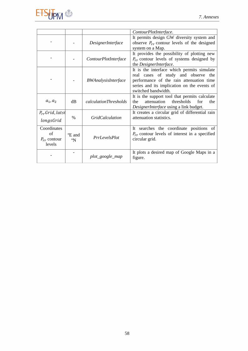
7. Annexes
58
ContourPlotInterface.
- - DesignerInterface
It permits design GW diversity system and
observe contour levels of the designed
system on a Map.
- - ContourPlotInterface
It provides the possibility of plotting new
contour levels of systems designed by
the DesignerInterface.
- - BWAnalysisInterface
It is the interface which permits simulate
real cases of study and observe the
performance of the rain attenuation time
series and its implication on the events of
switched bandwidth.
dB calculationThresholds
It is the support tool that permits calculate
the attenuation thresholds for the
DesignerInterface using a link budget.
% GridCalculation
It creates a circular grid of differential rain
attenuation statistics.
Coordinates
of
contour
levels
ºE and
ºN PrrLevelsPlot
It searches the coordinate positions of
contour levels of interest in a specified
circular grid.
- -
plot_google_map It plots a desired map of Google Maps in a
figure.